arX

iv:1

105.

3364

v1 [

nlin

.PS]

17

May

201

1

ON THE EXISTENCE OF SOLITARY TRAVELING WAVES FOR

GENERALIZED HERTZIAN CHAINS

ATANAS STEFANOV AND PANAYOTIS KEVREKIDIS

Abstract. We consider the question of existence of “bell-shaped” (i.e. non-increasingfor x > 0 and non-decreasing for x < 0) traveling waves for the strain variable of thegeneralized Hertzian model describing, in the special case of a p = 3/2 exponent, thedynamics of a granular chain. The proof of existence of such waves is based on theEnglish and Pego [Proceedings of the AMS 133, 1763 (2005)] formulation of the problem.More specifically, we construct an appropriate energy functional, for which we show thatthe constrained minimization problem over bell-shaped entries has a solution. We alsoprovide an alternative proof of the Friesecke-Wattis result [Comm. Math. Phys 161, 394(1994)], by using the same approach (but where the minimization is not constrained overbell-shaped curves). We briefly discuss and illustrate numerically the implications on thedoubly exponential decay properties of the waves, as well as touch upon the modificationsof these properties in the presence of a finite precompression force in the model.

1. Introduction

Localized modes on nonlinear lattices have been a topic of wide theoretical and exper-imental investigation in a wide range of areas over the past two decades. This can beseen, e.g., in the recent general review [1], as well as inferred from the topical reviews innonlinear optics [2], atomic physics [3] and biophysics [4] where relevant discussions havebeen given of the theory and corresponding applications.

One of the areas in which the theoretical analysis has been especially successful indescribing experimental data and providing insights has been that of granular crystals [5].These consist of closely-packed chains of elastically interacting particles, typically accordingto the so-called Hertz contact law. The broad interest in this area has emerged due to thewealth of available material types/sizes (for which the Hertzian interactions are applicable)and the ability to tune the dynamic response of the crystals to encompass linear, weaklynonlinear, and strongly nonlinear regimes [5, 6, 7, 8]. This type of flexibility renders thesecrystals perfect candidates for many engeenering applications, including shock and energyabsorbing layers [9, 10, 11, 12], actuating devices [13], and sound scramblers [14, 15]. It

Date: May 18, 2011.2000 Mathematics Subject Classification. 37L60, 35C15, 35Q51.Key words and phrases. Solitary Waves; Granular Chains; Nonlinear Lattices; Traveling Waves; Calcu-

lus of Variations.Stefanov’s research is supported in part by nsf-dms 0908802. Kevrekidis is supported by NSF-DMS-

0806762, NSF-CMMI-1000337, as well as by the Alexander von Humboldt Foundation and the AlexanderS. Onassis Public Benefit Foundation (RZG 003/2010-2011). Kevrekidis is grateful to Dr. G. Theocharisfor numerous discussions on this theme and to Prof. Chiara Daraio for stimulating his interest on thissubject.

1

2 ATANAS STEFANOV AND PANAYOTIS KEVREKIDIS

should also be noted that another aspect of such systems that is of particular appeal istheir potential (and controllable) heterogeneity which gives rise to the potential not onlyfor modified solitary wave excitations [16], but also for discrete breather ones [17].

Another motivation for looking at waves in such lattices stems from FPU type problems[18, 19]. In the prototypical FPU context, it has been rigorously proved that travelingwaves exist which can be controllably approximated (in the appropriate weakly supersoniclimit) by solitary waves of the Korteweg-de Vries equation [20]. However, in more stronglynonlinear regimes, compact-like excitations have been argued to exist [5, 6, 8] (see also [21]for breather type excitations) and have even been computed numerically through iterativeschemes [22, 23], but have not been rigorously proved to exist in the general case. In thework of [24], the special Hertzian case was adapted appropriately to fit the assumptionsof the variational-methods’ based proof of the traveling wave existence theorem of [25] inorder to establish these solutions. However the proof does not give information on thewave profile.

Our aim herein is to provide a reformulation and illustration of existence of “bell-shaped”traveling waves in generalized Hertzian lattices. Our work is based on the iterative schemesthat have been previously presented in [23, 22] for the computation of traveling waves insuch chains of the form:

vn = [vn−1 − vn]p+ − [vn − vn+1]

p+.(1)

Here vn denotes the displacement of the n-th bead from its equilibrium position. Thespecial case of Hertzian contacts is for p = 3/2, but we consider here the general case ofnonlinear interactions with p > 1. Notice that the “+” subscript in the equations indicatesthat that the quantity in the bracket is only evaluated if positive, while it is set to 0,if negative (reflecting in the latter case the absence of contact between the beads). Theconstruction of the traveling waves and the derivation of their monotonicity properties willbe based on the strain variant of the equation for un = vn−1 − vn such that:

un = [un+1]p+ − 2[un]

p+ + [un−1]

p+,(2)

Our presentation will proceed as follows. In section 2, we will give a preliminary math-ematical formulation to the problem, briefly illustrate its numerical solution and some ofits consequences. Then, we will proceed in section 3 to state and prove our main result.Some technical aspects of the problem will be relegated to the appendices of section 4.

2. Preliminaries and Numerical Results

When seeking traveling wave solutions of the form un = u(x) ≡ u(n− ct), we are led tothe advance-delay equation (setting c = 1)

(3) u′′(x) = up(x+ 1)− 2up(x) + up(x− 1). x ∈ R1

where u is a smooth and positive function, with the desired monotonicity involving decayin (0,∞) and increase in (−∞, 0).

SOLITARY WAVES FOR HERTZIAN CHAINS 3

2.1. Fourier transform and Sobolev spaces. We introduce the Fourier transform andits inverse via

f(ξ) =

∫ ∞

−∞

f(x)e−2πixξdx

f(x) =

∫ ∞

−∞

f(ξ)e2πixξdξ

As is well-known, the second derivative operator ∂2x has a simple representation via theFourier transform, namely

d2

dx2f(ξ) = −4π2ξ2f(ξ).

For every s ≥ 0, we may define (− d2

dx2)sf(ξ) = (4π2ξ2)sf(ξ) and the Sobolev spaces W s,p

via‖f‖W s,p = ‖f‖L2 + ‖(−∆)s/2f‖Lp.

We will also consider the operator

∆discf(x) = f(x+ 1)− 2f(x) + f(x− 1)

on the space of L2(R1) functions. Using Fourier transform, we may write

∆discf(x) =

∫ ∞

−∞

f(ξ)(e2πiξ + e−2πiξ − 2)e2πixξdξ = −4

∫ ∞

−∞

sin2(πξ)f(ξ)e2πixξdξ.

In other words, ∆disc is given by the symbol −4 sin2(πξ), that is

(4) ∆discf(ξ) = −4 sin2(πξ)f(ξ).

2.2. The English-Pego formulation. We may rewrite the equation (3) in the form

(5) u′′(x) = ∆disc[up](x)

Taking Fourier transform on both sides of this (and using (4)), allows us to write−4π2ξ2u(ξ) = −4 sin2(πξ)up(ξ) or

(6) u(ξ) =sin2(πξ)

π2ξ2up(ξ)

Equivalently, taking Λ : Λ(ξ) = sin2(πξ)π2ξ2

,

u(x) = Λ ∗ up(x) =

∫ ∞

−∞

Λ(x− y)up(y)dy =: M[up].(7)

In other words, we have introduced the convolution operator M with kernel Λ(·). It iseasy to compute that Λ(x) = (1− |x|)+ or

Λ(x) =

1− |x| |x| ≤ 1,0 |x| > 1.

Note that we have the following formula for the convolution Λ ∗ f

(8) Mf = Λ ∗ f(x) =

∫ x+1

x−1

(1− |x− y|)f(y)dy.

4 ATANAS STEFANOV AND PANAYOTIS KEVREKIDIS

2.3. Numerical computations and other consequences of the English-Pego for-

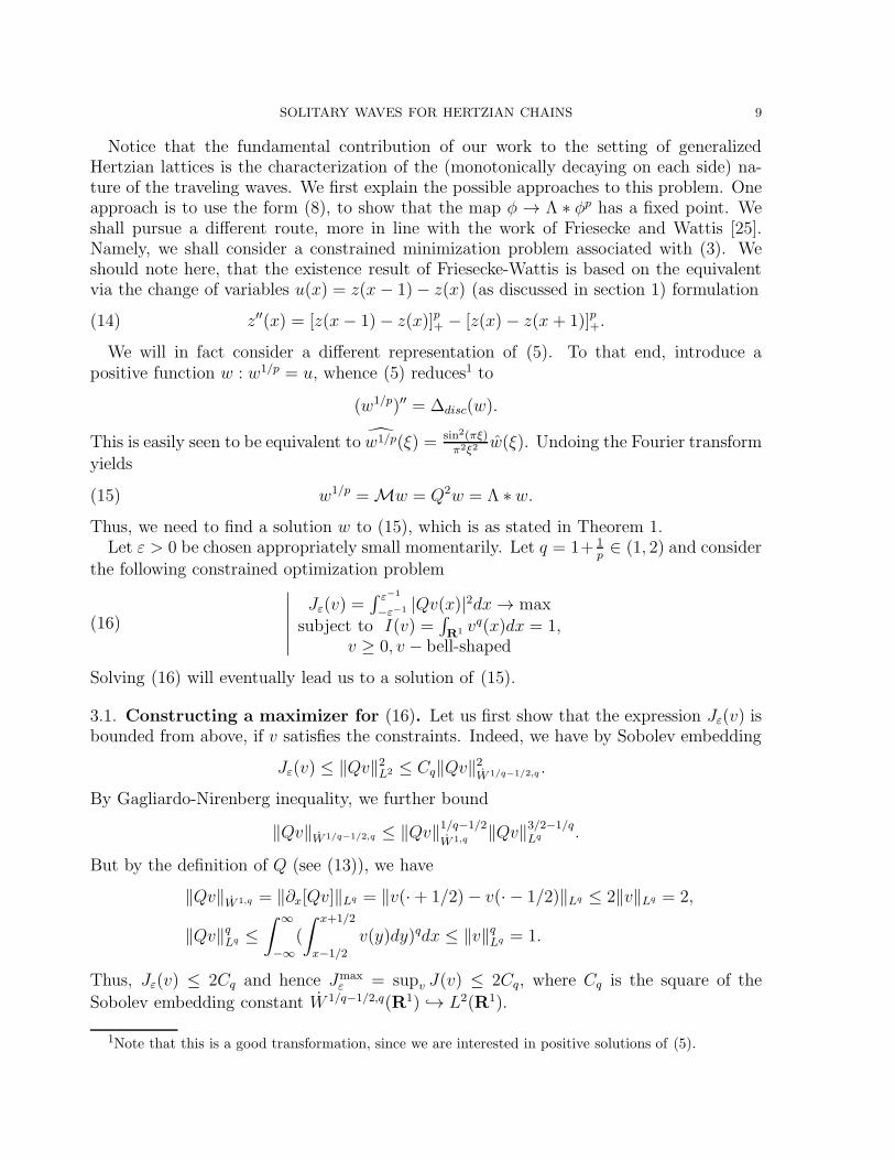
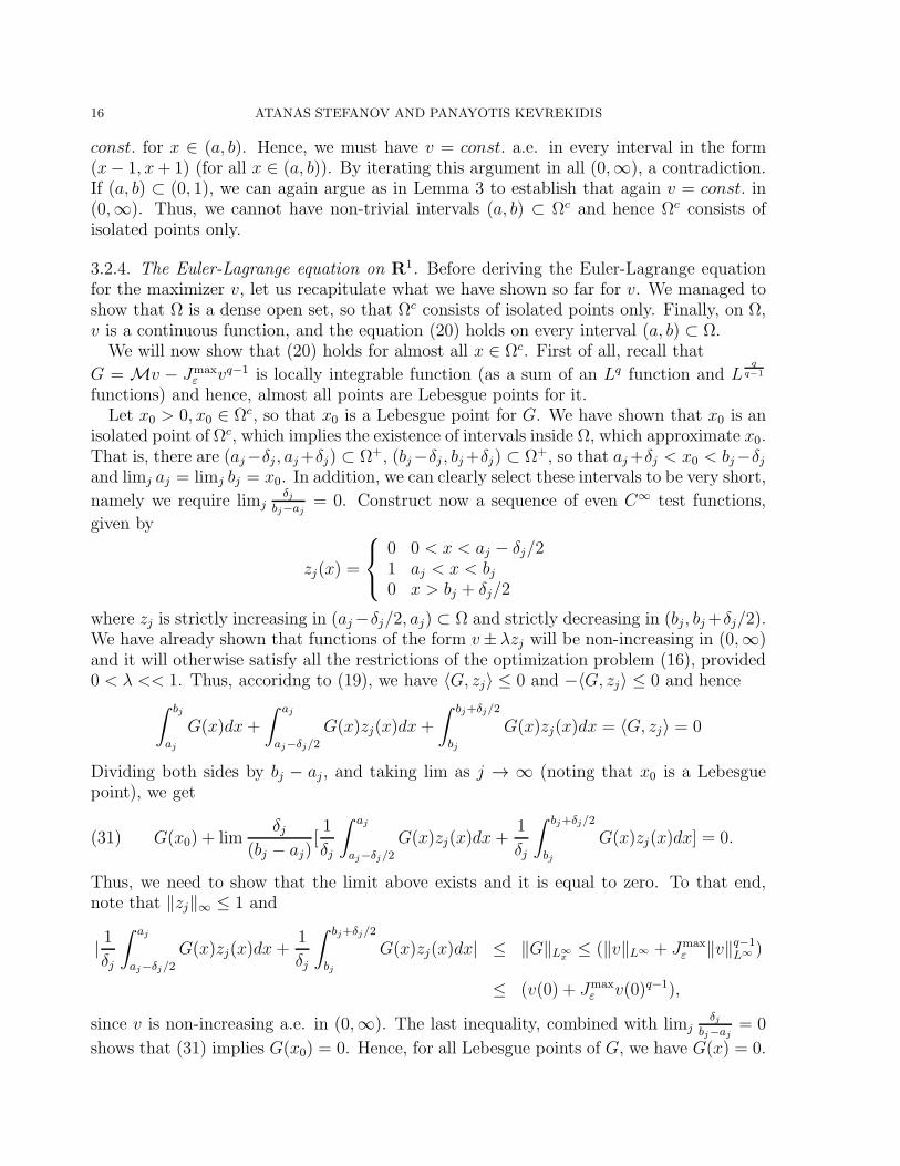
mulation. For reasons of completeness and in order to appreciate the form of (suitablynormalized) solutions of Eq. (7), in Fig. 1, we used this equation as a numerical schemeand proceed to iterate it until convergence. The figure illustrates the converged profile φof the solution and its corresponding momentum φt = −cφx (for c = 1). The results ofthese computations are shown for different values of p (in order to yield a sense of thep−dependence of the solution, namely for p = 3/2 (the Hertzian case), p = 2 and p = 3(the FPU-motivated cases, in that they are the purely nonlinear analogs of α- and β-FPUrespectively) and finally p = 10 (as a large-p case representative). The figure shows thesolutions’ profile and corresponding momenta, as well as the semi-logarithmic form of theprofile, so as to clearly illustrate the doubly exponential nature of the decay (see below).Notice that as p increases, the decay becomes increasingly steeper.

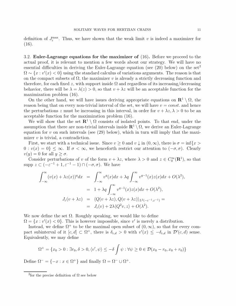
To corroborate the exact nature of such traveling wave solutions, once the solutionwas obtained, then the “lattice ordinates” of both the solution and its time derivativewere extracted and inserted as initial conditions for the dynamical evolution of Eq. (2).The results of the relevant time integration (using an explicit fourth-order Runge-Kuttascheme) are shown in Fig. 2. It can be straightforwardly observed that excellent agreementis obtained with the expectation of a genuinely traveling (without radiation) solution witha speed of c = 1, so that its center of mass moves according to x = ct (the solid line inthe figure). This confirms the usefulness of the method (independently of the nonlinearityexponent p, as long as p > 1) in producing accurate traveling solutions for this dynamicalsystem.

If the convergence to such a nontrivial profile is established (as we will establish itin section 3 with the proper monotonicity properties based on our modified variationalformulation), there is an important immediate conclusion about the decay properties ofsuch a profile. In particular,

u(x+ 1) =

∫ 1

−1

Λ(y)up(x+ 1− y)dy ≤ up(x) ⇒ u(x+ n) ≤ u(x)pn

,(9)

Hence, as was originally discussed in [26] and then more rigorously considered in [22] (seealso [23]), the solutions of Fig. 1 feature a doubly exponential decay. This very fast decay(and nearly compact shape) of the pulses can be clearly discerned in the semi-logarithmicplots of the figure.

As a slight aside to the present considerations, we should mention that a physicallyrelevant variant of the problem consists of the presence of a finite precompression force F0

at the end of the chain [5, 6]. In that case, the model of interest becomes (in the strainformulation and with F0 = δp0)

un = [δ0 + un+1]p+ − 2[δ0 + un]

p+ + [δ0 + un−1]

p+,(10)

The case of δ0 = 0 constitutes the so-called sonic vacuum [5], while that of finite δ0features a finite speed of sound (and allows the existence and propagation of linear spectrumexcitations). It is worthy then to notice that for δ0 6= 0, the above decay estimate ismodified as:

u(x+ 1) ∼ δp−10 u(x) ⇒ u(x) ∼ δp−1

0 exp(n log r(x0))(11)

SOLITARY WAVES FOR HERTZIAN CHAINS 5

−5 0 5−2

−1

0

1

2

φ , φ

t

n−5 0 5

10−50

100

n

φ

−5 0 5−2

−1

0

1

2

φ , φ

t

n−5 0 5

10−50

100

φ

n

−5 0 5−2

−1

0

1

2

φ , φ

t

n−5 0 5

10−50

100

φ

n

−5 0 5−2

−1

0

1

2

φ , φ

t

n−5 0 5

10−50

100

φ

n

Figure 1. Each one of the panels illustrates the numerically exact (up to aprescribed tolerance which we set here to 10−8) solution profile of the iterativescheme, as renormalized for use in Eq. (2). The solid (blue) line illustratesthe spatial form of the solution and the dashed (red) line the correspondingmomentum (for speed c = 1). The circles and stars denote respectivelythe ordinates of the lattice nodes (extracted for use in Eq. (2). The insetillustrates the profile in a semilog to highlight the doubly exponential natureof the decay (notice also the steepening as p increases). The top left panelis for p = 3/2, the top right for p = 2, the bottom left for p = 3 and finallythe bottom right for p = 10.

Namely, the solutions are no longer doubly exponentially localized but rather feature an ex-ponential tail (and are progressively closer to regular solitary waves). This can be thoughtof as a “compacton to soliton” transition that is worth exploring further (although thecase of δ0 6= 0 will not be considered further herein).

2.4. Some facts and definitions regarding distributions. We now turn to severaldefinitions, which will be useful in the sequel. Our space of test functions will be thefollowing. For V ⊂ R1 - an open set, let D(V ) = C∞

0 (V ) be the set of all C∞ functionswith compact support, contained inside V . We equip this with the usual topology of a

6 ATANAS STEFANOV AND PANAYOTIS KEVREKIDIS

t

n

0 5 10 15 20 25 30

−10

0

10

20

30 0

0.5

1

n

t

0 5 10 15 20 25 30

−10

0

10

20

30 0

0.2

0.4

0.6

0.8

1

1.2n

t

0 5 10 15 20 25 30

−10

0

10

20

30 0

0.2

0.4

0.6

0.8

1

1.2

t

n

0 5 10 15 20 25 30

−10

0

10

20

30 0

0.2

0.4

0.6

0.8

1

Figure 2. Result of direct integration of Eq. (2), with rn(0) and rn(0) asseeded from the iteration scheme’s convergent profile. The solid line in eachcase illustrates the trajectory of x = ct (for c = 1) to which the solutionscorrespond. One can notice for all values of p (p = 3/2: top left; p = 2: topright; p = 3 bottom left and p = 10 bottom right) the agreement with theexpectation of a genuinely traveling (non-radiating) waveform of c = 1.

Frechet space, generated by a family of seminorms pN(f) = supx∈Vn∑N

α=1 |∂αx f(x)|, where

Vnn is some fixed nested family of compact sets, so that ∪nVn = V . The distributionsover this space of functions, which we denote by D′(V ), is its dual space, namely allcontinuous linear functionals over D(V ). The derivatives of such distributions are definedin the usual way 〈h′, ψ〉 := −〈h, ψ′〉. One may also define a convolution of a distributionh ∈ D(R1) with a given C∞ function χ, by 〈h ∗ χ, ψ〉 := 〈h, ψ ∗ χ(−·)〉.

We say that two distributions are in the relation h1 ≤ h2 in D′(V ) sense, if for allψ ∈ D(V ), ψ ≥ 0, we have 〈h1, ψ〉 ≤ 〈h2, ψ〉. In particular,

Definition 1. We say that a distribution h is non-increasing (non-decreasing) over a setV , if h′ ≤ 0 (h′ ≥ 0) in D′(V ) sense.

SOLITARY WAVES FOR HERTZIAN CHAINS 7

Of course, if h happens to have a locally integrable derivative h′ on an interval, then thenotion of non-increasing function coincides with the standard (pointwise) notion by thefundamental theorem of calculus. More generally, we have the following

Lemma 1. Suppose that h is a locally integrable function in (a, b) and it satisfies h′ ≥ 0(h′ ≤ 0) in D′(a, b) sense. Then, h is almost everywhere (a.e.) non-decreasing (non-increasing, respectively) function on (a, b). That is, for almost all pairs x < y, h(x) ≤ h(y)(h(x) ≥ h(y) respectively).

Proof. It is well-known by the Lebesgue differentiation theorem that for a locally integrable

function h, one has h(x) = limδ→01δ

∫ x+δx

h(y)dy a.e. All such points x are called Lebesguepoints for h. Denote this full measure set by L. We will show that for all a < c1 < c2 < b :c1, c2 ∈ L, we have h(c1) ≤ h(c2). Indeed, let δ > 0 be so that δ < min(c2−c1, c1−a, b−c2).Define a function ψ,

ψ =

0 x < c1 − δx− (c1 − δ) c1 − δ < x ≤ c1δ c1 < x ≤ c2c2 + δ − x c2 < x ≤ c2 + δ0 c2 + δ ≤ x.

Clearly ψ ≥ 0 is not smooth, but is continuous and it can be approximated well by testfunctions. Moreover ψ′ = 1 on (c1 − δ, c1), ψ

′(x) = −1 on (c2, c2 + δ) and zero otherwise.Since 0 ≤ 〈h′, ψ〉 = −〈h, ψ′〉 (and these are well-defined quantities), we obtain

〈h, ψ′〉 =

∫ c1

c1−δ

h(y)dy −

∫ c2+δ

c2

h(y)dy ≤ 0.

This is true for all δ > 0, which are sufficiently small. Thus, dividing by δ > 0 and takinglimit as δ → 0+ (and taking into account that both c1, c2 are Lebesgue points), we concludethat h(c1) ≤ h(c2).

We find the following trick useful, which allows us to reduce non-increasing/non-decreasingdistrubutions to non-increasing/non-decreasing functions.

More precisely, let us fix a positive even C∞0 function Φ, so that supp Φ ⊂ (−1, 1) and∫

Φ(x)dx = 1. Let Φδ(x) := 1δΦ(x

δ) and define hδ = h ∗ Φδ. The following lemma has a

standard proof.

Lemma 2. Let h be a non-increasing (non-decreasing) distribution. Then for every δ >0, hδ is a C∞ function, which is non-increasing (non-decreasing respectively). Moreoverhδ → h in the sense of distributions.

Next

Definition 2. We say that a distribution h ∈ D′(R1) is bell-shaped, if h is non-decreasing

in D′(−∞, 0) and h is non-increasing in D′(0,∞).

In the sequel, we need the following technical result.

Lemma 3. Suppose that f is an even distribution, so that f is non-increasing in D′(0,∞)and non-decreasing in D′(−∞, 0). Then Λ ∗ f is non-increasing in (0,∞) and non-decreasing in (−∞, 0).

8 ATANAS STEFANOV AND PANAYOTIS KEVREKIDIS

Assume that g is non-increasing in D′(a,∞) for some a ∈ R1. Then Λ ∗ g(x) is non-increasing in (a + 1,∞).

Assume that h is non-decreasing in (−∞, a). Then, Λ∗h is non-decreasing in (−∞, a−1).

Proof. By Lemma 2, it suffices to consider functions instead of ditributions with the saidproperties. We have the following computation for the derivative of the function Λ ∗ g

(12) (Λ ∗ g)′(x) =

∫ x+1

x

g(y)dy −

∫ x

x−1

g(y)dy

which follows by differentiating (8).It is immediate from (12) that the claims for the functions Λ ∗ g and Λ ∗ h hold true.

Regarding Λ ∗ f , it is clear that Λ ∗ f is non-increasing in (1,∞) and non-decreasing in(−∞,−1). Thus, we need to show that for x ∈ (0, 1), (Λ ∗ g)′(x) ≤ 0 and for x ∈ (−1, 0),(Λ ∗ g)′(x) ≥ 0. We only verify this for x ∈ (0, 1), since the other inequality follows in asimilar manner. Indeed, using f(x) = f(−x),

(Λ ∗ f)′(x) =

∫ x+1

x

f(y)dy −

∫ x

x−1

f(y)dy =

∫ x+1

x

f(y)dy − (

∫ x

0

f(y)dy +

∫ 1−x

0

f(y)dy).

Since f is non-increasing in (0,∞),∫ x

0

f(y)dy ≥

∫ x

0

f(y + x)dy =

∫ 2x

x

f(y)dy,

∫ 1−x

0

f(y)dy ≥

∫ 1−x

0

f(y + 2x)dy =

∫ x+1

2x

f(y)dy

Going back to the expression for (Λ ∗ f)′(x), this implies (Λ ∗ f)′(x) ≤ 0, which was theclaim.

We will also need the following multiplier in our considerations

Qf(ξ) =sin(πξ)

πξf(ξ).

It is actually easy to see that since χ[− 1

2, 12](ξ) =

sin(πξ)πξ

, we have also the representation

(13) Qf(x) =

∫ x+1/2

x−1/2

f(y)dy.

Noted that by our definition of the operator M, we have M = Q2.

3. Statement and Proof of the Main Result

Theorem 1. The equation (3) has a positive solution u, so that

• u is even,• u is bell-shaped,• u ∈ H∞(R1)

SOLITARY WAVES FOR HERTZIAN CHAINS 9

Notice that the fundamental contribution of our work to the setting of generalizedHertzian lattices is the characterization of the (monotonically decaying on each side) na-ture of the traveling waves. We first explain the possible approaches to this problem. Oneapproach is to use the form (8), to show that the map φ → Λ ∗ φp has a fixed point. Weshall pursue a different route, more in line with the work of Friesecke and Wattis [25].Namely, we shall consider a constrained minimization problem associated with (3). Weshould note here, that the existence result of Friesecke-Wattis is based on the equivalentvia the change of variables u(x) = z(x− 1)− z(x) (as discussed in section 1) formulation

(14) z′′(x) = [z(x− 1)− z(x)]p+ − [z(x)− z(x+ 1)]p+.

We will in fact consider a different representation of (5). To that end, introduce apositive function w : w1/p = u, whence (5) reduces1 to

(w1/p)′′ = ∆disc(w).

This is easily seen to be equivalent to w1/p(ξ) = sin2(πξ)π2ξ2

w(ξ). Undoing the Fourier transformyields

(15) w1/p = Mw = Q2w = Λ ∗ w.

Thus, we need to find a solution w to (15), which is as stated in Theorem 1.Let ε > 0 be chosen appropriately small momentarily. Let q = 1+ 1

p∈ (1, 2) and consider

the following constrained optimization problem

(16)

∣∣∣∣∣∣

Jε(v) =∫ ε−1

−ε−1 |Qv(x)|2dx→ max

subject to I(v) =∫R1 v

q(x)dx = 1,v ≥ 0, v − bell-shaped

Solving (16) will eventually lead us to a solution of (15).

3.1. Constructing a maximizer for (16). Let us first show that the expression Jε(v) isbounded from above, if v satisfies the constraints. Indeed, we have by Sobolev embedding

Jε(v) ≤ ‖Qv‖2L2 ≤ Cq‖Qv‖2W 1/q−1/2,q .

By Gagliardo-Nirenberg inequality, we further bound

‖Qv‖W 1/q−1/2,q ≤ ‖Qv‖1/q−1/2

W 1,q ‖Qv‖3/2−1/qLq .

But by the definition of Q (see (13)), we have

‖Qv‖W 1,q = ‖∂x[Qv]‖Lq = ‖v(·+ 1/2)− v(· − 1/2)‖Lq ≤ 2‖v‖Lq = 2,

‖Qv‖qLq ≤

∫ ∞

−∞

(

∫ x+1/2

x−1/2

v(y)dy)qdx ≤ ‖v‖qLq = 1.

Thus, Jε(v) ≤ 2Cq and hence Jmaxε = supv J(v) ≤ 2Cq, where Cq is the square of the

Sobolev embedding constant W 1/q−1/2,q(R1) → L2(R1).

1Note that this is a good transformation, since we are interested in positive solutions of (5).

10 ATANAS STEFANOV AND PANAYOTIS KEVREKIDIS

We will now select ε0 so small that Jmaxε = supv J(v) (which we have just shown exists)

is positive for all 0 < ε < ε0. Indeed, take v0(x) = cqe−x2, so that cqq

∫∞

−∞e−qx

2

dx = 1.Thus, the function v0 satisfies the constraints and therefore

Jmaxε ≥ J(v0) = c2q

∫ ε−1

−ε−1

|

∫ x+1/2

x−1/2

e−2y2dy|2dx.

Clearly, as ε→ 0, we have that the right hand side converges to

c2q∫∞

−∞|∫ x+1/2

x−1/2e−2y2dy|2dx > 0. Thus, there exists ε0, so that for all ε ∈ (0, ε0), J

maxε > 0.

In fact, we can select the ε0, so that

(17) Jmaxε ≥

c2q2

∫ ∞

−∞

|

∫ x+1/2

x−1/2

e−2y2dy|2dx,

whenever ε < ε0. For the rest of this section, fix ε < ε0. Construct a maximizing sequencevn ∈ Lq(R1) : ‖vn‖Lq = 1, so that Jε(v

n) → Jmaxε . Namely, we take vn satisfying the

constraints, so that Jε(vn) > Jmax

ε − 1n. We only consider n large enough, so that 1

n< Jmax

ε ,in which case Jε(v

n) > 0.By the compactness of the unit ball of Lq in the weak topology, we may take a weak

Lq limit v = limn vn. Clearly, weak limits preserve the property that v is even and that vis a bell-shaped function. We now need to show that v satisfies the constraint ‖v‖Lq = 1,which is non-trivial since norms are in general only lower semicontinuous with respect toweak limits (and hence, we can only guarantee ‖v‖Lq ≤ 1).

We show now that, there exists a subsequence nkk so that

(18) limk

∫ ε−1

−ε−1

|Qvnk(x)|2dx =

∫ ε−1

−ε−1

|Qv(x)|2dx

Indeed, we check that

‖Qvn‖W 1,q = ‖∂x[Qvn]‖Lq + ‖Qvn‖Lq = ‖vn(·+ 1/2)− vn(· − 1/2)‖Lq + ‖Qvn‖Lq

≤ C‖vn‖Lq = C

Thus, by the compactness of the embedding W 1,q(R1) ⋐ L2(−ε−1, ε−1) we conclude thatthere is a subsequence nkk and z ∈ L2, so that ‖Qvnk − z‖L2 → 0. By uniqueness ofweak limits, (note that Qvnk Qv), it follows that z = Qv and hence (18).

Clearly now

Jmaxε = lim sup

kJε(v

nk) = lim supk

(

∫ ε−1

−ε−1

|Qvnk(x)|2dx) = (

∫ ε−1

−ε−1

|Qv(x)|2dx) = Jε(v).

On the other hand, ‖v‖Lq ≤ 1, by the lower semicontinuity of ‖ · ‖Lq with respect toweak limits, but clearly v 6= 0, since Jε(v) = Jmax

ε > 0. We will show that in fact‖v‖Lq = 1. Indeed, assume the opposite 0 < ρ = ‖v‖Lq < 1 and consider the functionv/ρ : ‖v/ρ‖Lq = 1. Observe that

Jε(v

ρ) = Jε(v)ρ

−2 = Jmaxε ρ−2 > Jmax

ε .

Thus, ‖v‖Lq = 1 (otherwise, we get a contradiction with the constrained maximizationproblem (16)). This implies that Jε(v) = Jmax

ε , otherwise, we get a contradiction with the

SOLITARY WAVES FOR HERTZIAN CHAINS 11

definition of Jmaxε . Thus, we have shown that the weak limit v is indeed a maximizer for

(16).

3.2. Euler-Lagrange equations for the maximizer of (16). Before we proceed to theactual proof, it is relevant to mention a few words about our strategy. We will have noessential difficulties in deriving the Euler-Lagrange equation (see (20) below) on the set2

Ω ∼ x : v′(x) < 0 using the standard calculus of variations arguments. The reason is thaton the compact subsets of Ω, the maximizer v is already a strictly decreasing function andtherefore, for each fixed z, with support inside Ω and regardless of its increasing/decreasingbehavior, there will be λ = λ(z) > 0, so that v + λz will be an acceptable function for themaximization problem (16).

On the other hand, we will have issues deriving appropriate equations on R1 \ Ω, thereason being that on every non-trivial interval of the set, we will have v = const. and hencethe perturbations z must be increasing in this interval, in order for v + λz, λ > 0 to be anacceptable function for the maximization problem (16).

We will show that the set R1 \ Ω consists of isolated points. To that end, under theassumption that there are non-trivial intervals inside R1 \Ω, we derive an Euler-Lagrangeequation for v on such intervals (see (29) below), which in turn will imply that the maxi-mizer v is trivial, a contradiction.

First, we start with a technical issue. Since v ≥ 0 and v ↓ in (0,∞), there is σ = infx >0 : v(x) = 0 ≤ ∞. If σ < ∞, we henceforth restrict our attention to (−σ, σ). Clearlyv(y) = 0 for all y ≥ σ.

Consider perturbations of v of the form v + λz, where λ > 0 and z ∈ C∞0 (R1), so that

supp z ⊂ (−ε−1 + 1, ε−1 − 1) ∩ (−σ, σ). We have

∫ ∞

−∞

(v(x) + λz(x))qdx =

∫ ∞

−∞

vq(x)dx+ λq

∫ ∞

−∞

vq−1(x)z(x)dx+O(λ2),

= 1 + λq

∫ ∞

−∞

vq−1(x)z(x)dx+O(λ2),

Jε(v + λz) = 〈Q(v + λz), Q(v + λz)〉L2(−ε−1,ε−1) =

= Jε(v) + 2λ〈Q2v, z〉+O(λ2).

We now define the set Ω. Roughly speaking, we would like to defineΩ = x : v′(x) < 0. This is however impossible, since v′ is merely a distribution.

Instead, we define Ω+ to be the maximal open subset of (0,∞), so that for every com-pact subinterval of it [c, d] ⊂ Ω+, there is δc,d > 0 with v′(x) ≤ −δc,d in D′(c, d) sense.Equivalently, we may define

Ω+ = x0 > 0 : ∃r0, δ > 0, 〈v′, ψ〉 ≤ −δ

∫ψ : ∀ψ ≥ 0 ∈ D(x0 − r0, x0 + r0)

Define Ω− = −x : x ∈ Ω+ and finally Ω = Ω− ∪ Ω+.

2for the precise definition of Ω see below

12 ATANAS STEFANOV AND PANAYOTIS KEVREKIDIS

3.2.1. Euler-Lagrange on Ω. Due to our requirement for bell-shaped test functions in (16),we need to impose extra restrictions on the function z. To that end, note that Ω is anopen set and fix an interval [a, b] ⊂ Ω. By the definition of Ω and compactness, it is clearthat there exists δ = δa,b, so that v′ ≤ −δ in D′(a, b) sense.

Fix a function z ∈ C∞0 (a, b). Clearly, for each such z, there exists λ0 = λ0(z, δa,b), so

that for all 0 < λ < λ0, (v + λz)/‖v + λz‖Lq satisfy all constraints. That is, we do notneed to restrict over z in terms of positivity or bell-shapedness3. Thus, we have that forall 0 < λ < λ0(z),

Jε

(v + λz

‖v + λz‖Lq

)=

Jε(v + λz)

‖v + λz‖2Lq

=Jmaxε + 2λ〈Mv, z〉+O(λ2)

(1 + λq∫∞

−∞vq−1(x)z(x)dx+O(λ2))2/q

=

=Jmaxε + 2λ〈Mv, z〉+O(λ2)

1 + 2λ∫∞

−∞vq−1(x)z(x)dx+O(λ2)

=

= Jmaxε + 2λ(〈Mv, z〉 − Jmax

ε 〈vq−1, z〉) +O(λ2)

Since Jε

(v+λz

‖v+λz‖Lq

)≤ Jmax

ε , we conclude that for all z ∈ C∞0 (a, b)

(19) 〈Mv − Jmaxε vq−1, z〉 ≤ 0.

Since there are no rectrictions on z (other than compact support), it follows that〈Mv − Jmax

ε vq−1, z〉 = 0 and hence

(20) Mv − Jmaxε vq−1 = 0,

in the D′(a, b) sense. This is the Euler-Lagrange equation that we were looking for. Notethat according to our derivation, it holds in the compact subsets of Ω. Note that from

here, we obtain v =(

1Jmaxε

Mv) 1

q−1

, which is smooth. These could be iterated further to

show that v ∈ C∞ on open sets (a, b), whenever [a, b] ⊂ Ω.

3.2.2. Euler-Lagrange over non-trivial intervals of Ωc. Our goal will be to show that suchnon-trivial intervals do not exist. To that end, we will first assume that they do exist andthen, we will be able to derive an Euler-Lagrange equation on them, which will then leadto a contradiction. Take such an interval, say [a0, a1] ⊂ Ωc, 0 ≤ a0 < a1.

Claim: v = const. in D′[a0, a1] sense, i.e. v is constant on connected components4 ofΩc.

Proof. To prove that, assume the opposite, namely that v is not a constant in D′(a0, a1).Thus (since we know v′ ≤ 0), there exists a test function 0 ≤ ψ0 ∈ D(a0, a1), so that〈v′, ψ0〉 = −α < 0. For some small κ ∈ (0, 1), the set Vκ = x ∈ (a0, a1) : ψ0(x) > κwill be nonempty and open. Take an interval (a0, a1) ⊂ Vκ, so that a1 − a0 < 1. Take anarbitrary function ψ ∈ D(a0, a1), so that 0 ≤ ψ(y) < κ for y ∈ (a0, a1). It follows that

3which will be the case in the Section 3.2.2 below4But it may be a different constant on a different component

SOLITARY WAVES FOR HERTZIAN CHAINS 13

ψ(y) < κ < ψ0(y) and hence 〈v′, ψ〉 ≤ 〈v′, ψ0〉 = −α < 0. Also∫ψ(y)dy ≤ κ(a1 − a0) < 1,

whence

(21) 〈v′, ψ〉 ≤ −α < −α

∫ψ(y)dy,

for all ψ ∈ D′(a0, a1), with 0 ≤ ψ < κ. One can now extend (21) to hold for all 0 ≤ ψ ∈D′(a0, a1). Hence, (a0, a1) ⊂ Ω in contradiction with (a0, a1) ⊂ (a0, a1) ⊂ Ωc.

Now that we have established that v is a.e. constant on any non-trivial interval (a0, a1) ⊂Ωc, we will derive the Euler-Lagrange equation for (16) on it. We will consider first thecase a0 > 0, the other case will be considered separately.Case I: a0 > 0To fix the ideas, we consider first the case when the interval [a0, a1] is isolated from therest of Ωc, that is, there exists r > 0, so that (a0 − r, a0) ⊂ Ω and (a1, a1 + r) ⊂ Ω.

Fix θ > 0 be so small that (a0 − θ, a0), (a1, a1 + θ) ⊂ Ω. Consider a test functionz ∈ C∞

0 (a0 − θ, a1 + θ).Clearly, since v = const on (a0, a1), we need to require that the function z′ ≤ 0 on (a0, a1),

in order for v + λz to be bell-shaped function5 (recall λ > 0). Denote

(22) G(x) = Mv − Jmaxε vq−1.

Since v = const. a.e. on (a0, a1), G is a continuous function on (a0, a1). Following theapproach of the previous section, we derive the equation (19), which in the new notationsays that

(23) 〈G, z〉 ≤ 0,

for all z, so that v + λz is an admissible entry for (16). We will show that (23) implies∫ b

a0

G(x)dx ≤ 0(24)

∫ a1

b

G(x)dx ≥ 0.(25)

for all b ∈ (a0, a1). Applying (24) for b = a1− and (25) for b = a0+ and taking limits,yields

∫ a1a0G(x)dx = 0.

Claim: From (24) and (25), one can infer that G = 0 on (a0, a1).

Proof. By the definition of G, the fact that v = const. and Lemma 3, we conclude that Gis non-increasing and continuous function on (a0, a1). Now, we have several cases. If there

exists a b ∈ (a0, a1), so that∫ ba0G(x)dx < 0 and

∫ a1bG(x)dx > 0, then by continuity, there

will be b0 ∈ (a0, b), so that G(b0) < 0 and b1 ∈ (b, a1), so that G(b1) > 0, a contradictionwith the fact that G is non-increasing. Otherwise, for all b ∈ (a0, a1), we have that either∫ ba0G(x)dx = 0 or

∫ a1bG(x)dx = 0. But since

∫ a1a0G(x)dx = 0,

∫ a1

b

G(x)dx =

∫ a1

a0

G(x)dx−

∫ b

a0

G(x)dx = −

∫ b

a0

G(x)dx.

5so that it is acceptable entry for the minimization problem (16)

14 ATANAS STEFANOV AND PANAYOTIS KEVREKIDIS

Thus,∫ ba0G(x)dx = 0 for all b ∈ (a0, a1). Thus, for any b0, b1 ∈ (a0, a1), we get

∫ b1b0G(x)dx =∫ b1

a0G(x)dx−

∫ b0a0G(x)dx = 0 and hence G(x) ≡ 0 in (a0, a1).

Thus, the Euler-Lagrange equation is in the form G(x) = 0 for x ∈ (a0, a1) or

(26) Mv − Jmaxε vq−1 = 0,

if we can show (24) and (25).We show only (24), the proof of (25) is similar. Fix b : a0 < b < a1. For all 0 < δ << 1,

introduce an even test function, which for x > 0 is given by

zδ(x) =

0 0 < x < a0 − 2δ1 a0 − δ < x < b+ δ0 x > b+ 2δ

so that zδ ∈ C∞, zδ is strictly increasing in (a0 − 2δ, a0 − δ) and zδ is strictly decreasing in(b+ δ, b+ 2δ).

Note that v + λzδ is acceptable for the maximization problem (16) for6 0 < λ < λδ.According to (23), 〈G, zδ〉 ≤ 0. Hence

∫ b

a0

G(x)dx = lim supδ→0

∫ b+2δ

a0−2δ

G(x)zδ(x)dx ≤ 0,

which is (24).The general case, in which [a0, a1] is not isolated from Ωc (i.e. there is no r > 0, so that

(a0 − r, a0) ∪ (a1, a1 + r) ⊂ Ω) is treated in the same way. Indeed, this was needed only inthe very last step, in the construction of the function zδ. But clearly, one can carry out asimilar construction of zδ, if one has a sequence of intervals Iδj = (cδj−δj , cδj) ⊂ Ω, cδj < a0,so that lim cδj = a0. Similarly, for the proof of (25), one needs a sequence of intervalsJδj = (dδj , dδj + δj) ⊂ Ω, dδj > a1, so that lim dδj = a1.

Finally, it remains to observe that every non-trivial interval of Ωc is contained in [a0, a1] ⊆Ωc with the property dist(a0,Ω) = 0 = dist(a1,Ω) and hence, we can carry the construc-tions of zδ and hence the validity of (24) and (25) follows. We then derive (26) on everysuch interval (a0, a1).Case II: a0 = 0This case is similar to the previous one. We again assume that there exists r > 0, so that(−a1 − r,−a1)∪ (a1, a1 + r) ⊂ Ω, the general case being reduced to this one by argumentssimilar to those in the case a0 > 0.

Again, G is even, we have that v = const. on the interval (−a1, a1) and G is non-increasing in (0, a1). We will show that for every b ∈ (0, a1), we have

∫ a1

b

G(x)dx ≥ 0,(27)

∫ b

0

G(x)dx ≤ 0(28)

6Here even though zδ is increasing in (a0 − 2δ, a0 − δ), this is acceptable since (a0 − 2δ, a0− δ) ⊂ Ω andhence, we have no restrictions over the test functions, as long as λδ << 1

SOLITARY WAVES FOR HERTZIAN CHAINS 15

Let us first prove that assuming (27) and (28), one must have G = 0. Indeed, if we apply(27) for b→ 0+ and (28) for b → a1−, we see that

∫ a10G(x)dx = 0.

Again, if we assume that∫ b0G(x)dx = 0 for all b ∈ (0, a1), we again conclude by the

continuity of G that G(x) = 0 : 0 ≤ x ≤ a1. If one has∫ b00G(x)dx < 0 for some

b0 ∈ (0, a1), we have that∫ a1b0G(x)dx > 0 (since

∫ a10G(x)dx = 0) and hence, G cannot be

non-increasing function (as in Case I), a contradiction. Thus G(x) = 0 in (0, a1).Thus, it remains to show (27) and (28). Fix b > 0 and let 0 < δ << 1. For (28), select

zδ(x) =

0 x < −b− 2δ1 −b− δ < x < b+ δ0 x > b+ 2δ

and zδ is C∞, even and increasing in (−b − 2δ,−b − δ) and decreasing in (b + δ, b + 2δ).Clearly, for λ > 0, v + λzδ is admissible for (16), for some small λ > 0. Thus, applying(23) for this zδ and passing to appropriate limits as δ → 0+, we obtain, as above

2

∫ b

0

G(x)dx =

∫ b

−b

G(x)dx = lim infδ→0+

∫G(x)zδ(x)dx ≤ 0.

For (27), we construct zδ to be an even function, so that

zδ(x) =

0 x < b− 2δ−1 b− δ < x < a1 + δ0 x > a1 + 2δ

Now, we require that zδ is decreasing in (b−2δ, b−δ) and it is increasing from (a1+δ, a1+2δ).Note that zδ is still acceptable as a perturbation - in the sense that v+λzδ is non-increasingin (0,∞) for all λ = λ(δ) > 0 small enough (for this, recall that (a1 + δ, a1 + 2δ) ⊂ Ω andhence, there exists σ(δ), so that v′ < −σ in D′(a1 + δ, a1 + 2δ) sense). We have again

−

∫ a1

b

G(x)dx = lim supδ→0+

∫G(x)zδ(x)dx ≤ 0.

Thus, we have established (27) and (28) and thus the Euler-Lagrange equation

(29) 0 = G(x) = Mv − Jmaxε vq−1.

3.2.3. The set Ωc consists of isolated points only. We will now show that if an equationlike (29) holds in a non-trivial interval, say (a, b) and v is a bell-shaped, locally integrablefunction, which is constant on (a, b), then v(x) = const. a.e. on R1 (which would be acontradiction).

Indeed, Mv is in fact a differentiable function on (a, b), which is non-increasing on(0,∞), according to Lemma 3. Thus, taking a derivative of (29) (and taking into accountthat v = const on (a, b)) leads to

(30) 0 = (Mv)′(x) =

∫ x+1

x

v(y)dy −

∫ x

x−1

v(y)dy.

for all x ∈ (a, b).If b > 1, we see that since v is non-increasing in (0,∞) (by Lemma 1), it follows that

x →∫ x+1

xv(y)dy is non-increasing and continuous. By (30), it follows that

∫ x+1

xv(y)dy =

16 ATANAS STEFANOV AND PANAYOTIS KEVREKIDIS

const. for x ∈ (a, b). Hence, we must have v = const. a.e. in every interval in the form(x− 1, x+ 1) (for all x ∈ (a, b)). By iterating this argument in all (0,∞), a contradiction.If (a, b) ⊂ (0, 1), we can again argue as in Lemma 3 to establish that again v = const. in(0,∞). Thus, we cannot have non-trivial intervals (a, b) ⊂ Ωc and hence Ωc consists ofisolated points only.

3.2.4. The Euler-Lagrange equation on R1. Before deriving the Euler-Lagrange equationfor the maximizer v, let us recapitulate what we have shown so far for v. We managed toshow that Ω is a dense open set, so that Ωc consists of isolated points only. Finally, on Ω,v is a continuous function, and the equation (20) holds on every interval (a, b) ⊂ Ω.

We will now show that (20) holds for almost all x ∈ Ωc. First of all, recall that

G = Mv − Jmaxε vq−1 is locally integrable function (as a sum of an Lq function and L

qq−1

functions) and hence, almost all points are Lebesgue points for it.Let x0 > 0, x0 ∈ Ωc, so that x0 is a Lebesgue point for G. We have shown that x0 is an

isolated point of Ωc, which implies the existence of intervals inside Ω, which approximate x0.That is, there are (aj−δj , aj+δj) ⊂ Ω+, (bj−δj , bj+δj) ⊂ Ω+, so that aj+δj < x0 < bj−δjand limj aj = limj bj = x0. In addition, we can clearly select these intervals to be very short,

namely we require limjδj

bj−aj= 0. Construct now a sequence of even C∞ test functions,

given by

zj(x) =

0 0 < x < aj − δj/21 aj < x < bj0 x > bj + δj/2

where zj is strictly increasing in (aj−δj/2, aj) ⊂ Ω and strictly decreasing in (bj , bj+δj/2).We have already shown that functions of the form v± λzj will be non-increasing in (0,∞)and it will otherwise satisfy all the restrictions of the optimization problem (16), provided0 < λ << 1. Thus, accoridng to (19), we have 〈G, zj〉 ≤ 0 and −〈G, zj〉 ≤ 0 and hence

∫ bj

aj

G(x)dx+

∫ aj

aj−δj/2

G(x)zj(x)dx+

∫ bj+δj/2

bj

G(x)zj(x)dx = 〈G, zj〉 = 0

Dividing both sides by bj − aj, and taking lim as j → ∞ (noting that x0 is a Lebesguepoint), we get

(31) G(x0) + limδj

(bj − aj)[1

δj

∫ aj

aj−δj/2

G(x)zj(x)dx+1

δj

∫ bj+δj/2

bj

G(x)zj(x)dx] = 0.

Thus, we need to show that the limit above exists and it is equal to zero. To that end,note that ‖zj‖∞ ≤ 1 and

|1

δj

∫ aj

aj−δj/2

G(x)zj(x)dx+1

δj

∫ bj+δj/2

bj

G(x)zj(x)dx| ≤ ‖G‖L∞

x≤ (‖v‖L∞ + Jmax

ε ‖v‖q−1L∞ )

≤ (v(0) + Jmaxε v(0)q−1),

since v is non-increasing a.e. in (0,∞). The last inequality, combined with limjδj

bj−aj= 0

shows that (31) implies G(x0) = 0. Hence, for all Lebesgue points of G, we have G(x) = 0.

SOLITARY WAVES FOR HERTZIAN CHAINS 17

Thus,

(32) Mv − Jmaxε vq−1 = 0 a.e.

3.3. Taking a limit as ε → 0: Constructing a solution to (5). From (32),

(33) Mvε − Jmaxε vq−1

ε = 0,

which is satisfied a.e. and also inD′(0, ε−1−1) sense. From it, we learn that vε isH4(0, ε−1−

1) and consequently, by iterating this argument, H∞(0, ε−1 − 1) =⋂∞s=1H

s(0, ε−1 − 1)function. Recall also that by construction ‖vε‖Lq(R1) = 1 and there exists ε0 > 0, so thatinfε<ε0 J

maxε > 0, see (17). We will now take several consecutive subsequences of ε→ 0, in

order to ensure that the limit satisfies (5).First, take εn → 0+, so that limn J

maxεn = lim supε→0 J

maxε := J0 > 0. Second, out of this

constructed sequence εn, take a subsequence, say εnk, so that vεnk

v in a weak Lq sense,for some v ≥ 0, v ∈ Lq. This is possible, by the sequential compactness of the unit ballin the weak Lq topology7. By the uniqueness of weak limits (by eventually taking further

subsequence), we also get vq−1εnk

k vq−1 in weak L

qq−1 sense. We also have Mvεnk

Mv in

the weak Lq topology, since for every test function ψ ∈ C∞0 , we have by the self-adjointness

of M and M : Lr → Lr, 1 ≤ r ≤ ∞,

〈Mvεnk, ψ〉 = 〈vεnk

,Mψ〉 →k 〈v,Mψ〉 = 〈Mv, ψ〉.

Thirdly, we show that the limiting function v is non-zero. To that end, it will suffice toestablish that

(34) lim infε→0+

‖vε‖Lq(−ε−1,ε−1) > 0.

Assuming that (34) is false, we will reach a contradiction. Indeed, let δj → 0+ be asequence so that limj ‖vδj‖Lq(−δ−1

j ,δ−1

j ) = 0. Thus,

Jmaxδj

= Jδj(vδj ) ≤

∫ δ−1

j

−δ−1

j

|Qvδj (x)|2dx =

∫ δ−1

j

−δ−1

j

|

∫ x+1/2

x−1/2

vδj (y)dy|2dx.

We now use a refined version of the Gagliardo-Nirenberg estimate that we have used before.∫ δ−1

j

−δ−1

j

|

∫ x+1/2

x−1/2

vδj (y)dy|2dx =

∫ δ−1

j

−δ−1

j

|

∫ x+1/2

x−1/2

vδj (y)χ(−δ−1

j −1,δ−1

j +1)dy|2dx ≤

≤ ‖Q[vδjχ(−δ−1

j −1,δ−1

j +1)]‖2L2

and hence

‖Q[vδjχ(−δ−1

j −1,δ−1

j +1)]‖L2 ≤ ‖Q[vδjχ(−δ−1

j −1,δ−1

j +1)]‖1/q−1/2

W 1,q ‖Q[vδjχ(−δ−1

j −1,δ−1

j +1)]]‖3/2−1/qLq .

While a simple differentiation shows that on one hand,

‖Q[vδjχ(−δ−1

j −1,δ−1

j +1)]‖W 1,q ≤ 2‖vδj‖Lq = 2,

7But again, this argument, so far, does not guarantee that v 6= 0

18 ATANAS STEFANOV AND PANAYOTIS KEVREKIDIS

we also have by Cauchy-Schwartz

‖Q[vδjχ(−δ−1

j −1,δ−1

j +1)]‖qLq ≤

∫ ∞

−∞

(

∫ x+1/2

x−1/2

vδj (y)χ(−δ−1

j −1,δ−1

j +1)(y)dy)qdx ≤

≤

∫ δ−1

j +1

−δ−1

j −1

vqδj (y)dy ≤ 2‖vδj‖q

Lq(−δ−1

j ,δ−1

j )→ 0.

The last inequality here follows by the fact that vδj is non-increasing in (0,∞) and therefore∫ δ−1

j +1

δ−1

j

vqδj (y)dy ≤∫ δ−1

j

0 vqδj (y)dy, if δ−1j ≥ 1, which we have assumed anyway. Thus, we will

have proved that

lim infj

Jmaxδj

≤ 0,

which is in contradiction with (17). Thus, we have established (34).We are now ready to take a limit as ε → 0 in (33). Indeed, take (33) for ε = εnk

, k =1, 2, . . .. Fix a test function ψ ∈ C∞

0 . There exists k0, so that for k ≥ kψ, supp ψ ⊂ (0, ε−1nk).

Thus, for k ≥ kψ, we get8

〈Mvεnk, ψ〉 − Jmax

εnk〈vq−1εnk

, ψ〉 = 0.

Take a limit as k → ∞. By our constructions, we have that Jmaxεnk

〈vq−1εnk

, ψ〉 → J0〈vq−1, ψ〉,

since Jmaxεnk

→ J0, 〈vq−1εnk

, ψ〉 → 〈vq−1, ψ〉 by the weak Lq

q−1 convergence.

We also have 〈Mvεnk, ψ〉 = 〈vεnk

,Mψ〉 →k 〈v,Mψ〉 = 〈Mv, ψ〉. Thus, we have estab-lished the desired identity

(35) Mv − J0vq−1 = 0

valid for all x > 0. By the symmetry, it is also valid for x < 0. It is clear that v is nowinfinitely smooth9 function on (0,∞). Recall though, that for Theorem 1 we needed tosolve Mw − wq−1 = 0. One can easily construct w, based on the solution v of (35). More

precisely, if we take w := J− 1

2−q

0 v, then w will satisfy (15). Theorem 1 is proved.

4. An alternative proof of the Friesecke-Wattis theorem

We quickly indicate how our ideas can be turned into a new proof of the Friesecke-Wattis theorem. Specifically, as we saw in the previous section, it is clear that if we arejust interested in the existence of traveling waves for (5) (but not in bell-shaped solutions),it is a good idea to consider following constrained maximization problem (compare to (16))

(36)

∣∣∣∣∣Jε(v) =

∫ ε−1

−ε−1 |Qv(x)|2dx→ max

subject to v ≥ 0; I(v) =∫R1 v

q(x)dx = 1.

First off, the arguments in Section 3.1 apply unchanged (by just skipping the bell-shapednessof v) to prove that (36) has a maximizer, say v.

8by testing (33), which is valid on the support of ψ9starting with v ∈ Lq(R1), it is easy to conclude that Mv is smooth, which in turn implies that

v ∈ C1(R1) etc.

SOLITARY WAVES FOR HERTZIAN CHAINS 19

Following the argument of Section 3.2 and more specifically, the following identities

‖v + λz‖qLq = ‖v‖qLq + λq〈vq−1, z〉 +O(λ2)

Jε(v + λz) = Jε(v) + 2λ〈Q2v, z〉+O(λ2),

Jε

(v + λz

‖v + λz‖Lq

)= Jmax

ε + 2λ(〈Mv, z〉 − Jmaxε 〈vq−1, z〉) +O(λ2) ≤ Jε(v),

which were established there, it follows that

〈Mv − Jmaxε vq−1, z〉 ≤ 0

for all test functions10 z. It follows that v satisfies

Mv − Jmaxε vq−1 = 0.

This of course produces a family vε : supp vε ⊂ (−ε−1 − 1, ε−1 + 1), which easily can beshown to converge11 (after an eventual subsequence) to a v : supp v ⊂ R1, which solves

Mv − J0vq−1 = 0.

Setting w := J− 1

2−q

0 v again provides a solution to w1/p = Mw as is required by (15).

References

[1] S. Flach and A. Gorbach, Phys. Rep. 467, 1 (2008).[2] F. Lederer, G.I. Stegeman, D.N. Christodoulides, G. Assanto, M. Segev and Y. Silberberg, Phys.

Rep. 463, 1 (2008).[3] O. Morsch and M. Oberthaler, Rev. Mod. Phys. 78, 179 (2006).[4] M. Peyrard, Nonlinearity 17, R1 (2004).[5] V. F. Nesterenko, Dynamics of Heterogeneous Materials (Springer-Verlag, New York, NY, 2001).[6] S. Sen, J. Hong, J. Bang, E. Avalos, and R. Doney, Phys. Rep. 462, 21 (2008).[7] C. Daraio, V. F. Nesterenko, E. B. Herbold, and S. Jin, Phys. Rev. E. 73, 026610 (2006).[8] C. Coste, E. Falcon, and S. Fauve, Phys. Rev. E. 56, 6104 (1997)[9] C. Daraio, V. F. Nesterenko, E. B. Herbold, and S. Jin, Phys. Rev. Lett. 96, 058002 (2006).[10] J. Hong, Phys. Rev. Lett. 94, 108001 (2005).[11] F. Fraternali, M. A. Porter, and C. Daraio, Mech. Adv. Mat. Struct., in press (arXiv:0802.1451).[12] R. Doney and S. Sen, Phys. Rev. Lett. 97, 155502 (2006).[13] D. Khatri, C. Daraio, and P. Rizzo, SPIE 6934, 69340U (2008).[14] C. Daraio, V. F. Nesterenko, E. B. Herbold, and S. Jin, Phys. Rev. E 72, 016603 (2005).[15] V. F. Nesterenko, C. Daraio, E. B. Herbold, and S. Jin, Phys. Rev. Lett. 95, 158702 (2005).[16] M.A. Porter, C. Daraio, E.B. Herbold, I. Szelengowicz and P.G. Kevrekidis, Phys. Rev. E 77, 015601

(2008); M.A. Porter, C. Daraio, I. Szelengowicz, E.B. Herbold and P.G. Kevrekidis, Phys. D 238,666 (2009).

[17] N. Boechler, G. Theocharis, S. Job, P. G. Kevrekidis, M.A. Porter, and C. Daraio Phys. Rev. Lett.104, 244302 (2010); G. Theocharis, N. Boechler, P.G. Kevrekidis, S. Job, M.A. Porter, and C. DaraioPhys. Rev. E 82, 056604 (2010).

[18] E. Fermi, J. Pasta, S. Ulam, Los Alamos National Laboratory report LA-1940 (1955).[19] D.K. Campbell, P. Rosenau and G.M. Zaslavsky, Chaos 15, 015101 (2005).[20] G. Friesecke and R.L. Pego, Nonlinearity 12, 1601 (1999); ibid. 15, 1343 (2002); ibid. 17, 207 (2004);

ibid. 17, 2229 (2004).

10Note that here, there is no restriction whatsoever on the increasing/decreasing character of z, due tothe nature of (36)

11following the methods of Section 3.3

20 ATANAS STEFANOV AND PANAYOTIS KEVREKIDIS

[21] M. Eleftheriou, B. Dey and G.P. Tsironis, Phys. Rev. E 62, 7540 (2000); B. Dey, M. Eleftheriou, S.Flach and G.P. Tsironis, Phys. Rev. E 65, 017601 (2002).

[22] J.M. English and R.L. Pego, Proceedings of the AMS 133, 1763 (2005).[23] K. Ahnert and A. Pikovsky, Phys. Rev. E 79, 026209 (2009).[24] R.S. MacKay, Phys. Lett. A 251, 191 (1999).[25] G. Friesecke and J.A.D. Wattis, Comm. Math. Phys. 161, 391 (1994).[26] A. Chatterjee, Phys. Rev. E 59, 5912 (1998).[27] J. Frohlich, E. H. Lieb, M. Loss, Stability of Coulomb systems with magnetic fields. I. The one-

electron atom. Comm. Math. Phys. 104 (1986), no. 2, p. 251–270.[28] P. Karageorgis, P.J. McKenna, Existence of ground states for fourth order wave equations, preprint,

available at http://arxiv.org/abs/1004.2775[29] E. H. Lieb, On the lowest eigenvalue of the Laplacian for the intersection of two domains. Invent.

Math. 74 (1983), no. 3, p. 441–448.[30] W. Rudin, Functional Analysis, Second Edition, 1991.

Atanas Stefanov, Department of Mathematics, University of Kansas, 1460 Jayhawk

Blvd, Lawrence, KS 66045–7523

Panayotis Kevrekidis, Lederle Graduate Research Tower, Department of Mathematics

and Statistics, University of Massachusetts, Amherst, MA 01003

E-mail address : stefanov@math.ku.eduE-mail address : kevrekid@math.umass.edu