1

UNIVERSITY OF KHARTOUM

FACULTY OF ENGINEERING

DEPARTMENT OF SURVEYING

ON THE ESTABLISHMENT OF A PRECISE GPS NETWORK IN

KHARTOUM STATE

A THESIS SUBMITTED IN PARTIAL FULFILLMENT OF THE REQUIREMENTS

FOR THE BACHELOR OF SCIENCE (HONOUR) IN SURVEYING

ENGINEERING

Prepared by:

Rashad Abdelrahman Khalil

Mudathir Awadelgeed Mohammed

Musa Mukhtar Lammaldean

Supervised by:

Dr. Awadelgeed Mohammed Awadelgeed

Dr. Gamal Hassan Seedahmed

September 2014

2

3

TO OUR PARENTS

4

5

Acknowledgements

Our sincere and heartfelt gratitude goes to our supervisors Dr. Awadeljeed Mohammed Awadeljeed and

Dr. Gamal Seedahmed for their guidance and relentless support throughout the course of this project;

we can never repay their debt nor thank them enough.

We’d also like to thank the Sudanese Surveying Authority for providing us with the GPS equipments, and

especially Lieutenant Colonel Abu Alhassan Ali and First Class Lieutenant Ahmed Abdul-Lateef for their

tireless support and unparalleled patience throughout the planning, field work and post-processing

stages of this project.

Special thanks to our colleagues Mohanad Zain-AlAbideen, Mohammed Najm-Aldeen and Ahmed

Mubarak for their help with the logistics during the field works.

6

7

Abstract

Geodetic networks are the foundations upon which all terrestrial surveying applications are

built, the importance of their reliability cannot be over stressed.

In this graduate project, a geodetic network was established linking Khartoum, Khartoum North

and Omdurman, using satellite-based, static, relative positioning techniques and it was

referenced to a single control station of the International Terrestrial Reference Frame (ITRF

2005).

The network was established using redundant observations which formed an over determined

system, the most probable values of the coordinates were estimated using the methods of least

squares, the accuracies were assessed and the reliability of the network was determined within

the 95% confidence level.

8

9

Contents Acknowledgements ...................................................................................................................................... 5

Abstract ........................................................................................................................................................ 7

1 Introduction ........................................................................................................................................ 11

1.1 Motivation .................................................................................................................................. 11

1.2 Problem Definition and Objectives ............................................................................................ 11

1.3 Overview of the Chapters .......................................................................................................... 12

2 Literature Review ............................................................................................................................... 13

2.1 Overview of GPS ......................................................................................................................... 13

2.2 The GPS Signal ............................................................................................................................ 14

2.3 Reference Coordinate Systems .................................................................................................. 15

2.4 Fundamentals of Satellite Positioning ....................................................................................... 19

2.5 Observation Techniques ............................................................................................................ 21

2.6 GPS Networks ............................................................................................................................. 25

2.7 Sources of Errors in Satellite Surveys ........................................................................................ 27

2.8 The Theory of Errors in Observations and the Method of Least Squares ................................ 29

3 Methodology ...................................................................................................................................... 33

3.1 Planning and Performing Static Survey ..................................................................................... 33

3.2 Data processing .......................................................................................................................... 36

3.3 Network Pre-Adjustment Data Analyses ................................................................................... 37

4 Mathematical Model for Least Squares Adjustment of GPS Network ............................................. 39

5 Results ................................................................................................................................................. 45

6 Discussion and Conclusion ................................................................................................................. 55

References .................................................................................................................................................. 57

Appendix – The Results of the GPS Data Processing ................................................................................. 59

10

11

Chapter 1

1 Introduction

This chapter gives an overview of the general objectives as well as a brief description of the

content of the thesis.

1.1 Motivation

The importance of geodetic work is recognized by all civilized nations, each of which maintains

an extensive organization for this purpose, the knowledge thus gained of the Earth and its

surface has been of great benefit to humanity, from the early Egyptians who used control

points to monitor the water levels of the Nile and gazed at the heavens to determine directions

to modern day civilizations who still need control points for the same ancient reasons plus a

myriad of other modern day applications.

During the past century, technology advanced exponentially and with it grew humanity’s need

and demand for precision and accuracy. The advent of GPS technology propelled Geomatics

into a new era, characterized by speed, precision, and efficiency. The advances in computer

technology particularly in the fields of programming languages and computational capabilities

meant that larger sets of data could be analyzed and more complicated and accurate

mathematical models could be applied. Today we gaze at the heavens again, albeit in a

different way, as satellite-based positioning methods became the standard in establishing new

geodetic networks as well as updating, linking and intensifying existing ones.

1.2 Problem Definition and Objectives

The geodetic networks of Sudan were established using methods of theodolite triangulations

and EDM trilateration and were adjusted using traditional (arbitrary) methods. Sudan’s

embrace of GPS technology has been shy to say the least and no comprehensive attempts have

been made to update, integrate, and intensify existing networks using satellite-based

12

positioning techniques, and even when these techniques are used, networks are rarely if ever

rigorously adjusted, and thus coordinated values are given with no statement of accuracy or

reliability other than the formal standard errors of the vector computations given by the

software, which are generally optimistic by a factor of three to ten times and need to be scaled

to arrive at a true estimate of the network errors (Hofmann-Wellenhof et al. 2001). It is in this

light that we undertook this project to establish a GPS network from a single control station

(ITRF 2005), using static relative positioning technique and single baseline processing,

incorporating new stations as well as existing control stations from different networks and

applying a comprehensive Least Square Estimation to compute the most probable values of the

coordinates.

1.3 Overview of the Chapters

This thesis consists of six chapters, including this chapter (introduction)

In the second chapter (Literature Review), a literature review of the topics of interest to this

thesis is presented. The fundamentals of GPS and the principles of Least Square estimation and

its justifications are discussed.

Chapter three (Methodology) is concerned with the methodology; it gives a detailed description

of the planning, the field procedures and the equipments used, as well as the processing

software, the data processing methods and the network pre-adjustment data analyses

methods.

Chapter four (Mathematical model) outlines the mathematical models used, namely, the

Parametric (Observation) Equation and the Condition Equation methods of least squares

estimation, and the transformation equations between geodetic (curvilinear) and space

rectangular coordinates.

Chapter five (Results) the results of the least squares estimations are tabulated in this chapter,

presented in both curvilinear and space rectangular coordinates accompanied by various

measures of accuracy, the results of the network pre-adjustment data analyses are also

presented in this chapter.

Chapter six (Discussion and Conclusions) the overall results are summarized and discussed in

this chapter, conclusions are drawn and suggestions for future works are presented.

13

Chapter 2

2 Literature Review

2.1 Overview of GPS

During the 1970s, a new and unique approach to surveying, the global positioning system (GPS),

emerged. This system, which grew out of the space program, relies upon signals transmitted

from satellites for its operation. It has resulted from research and development paid for by the

United State’s Department of Defense (DoD) to produce a system for global navigation and

guidance. More recently other countries have developed their own systems. Thus, the entire

scope of satellite systems used in positioning is now referred to as global navigation satellite

systems (GNSS). These systems provide precise timing and positioning information anywhere on

the Earth with high reliability and low cost. The systems can be operated day or night, rain or

shine, and do not require cleared lines of sight between survey stations. This represents a

revolutionary departure from conventional surveying procedures, which rely on observed

angles and distances for determining point positions.

The global positioning system can be arbitrarily broken into three parts:

- The space segment consists nominally of 24 satellites operating in six orbital planes

spaced at 60° intervals around the equator. Four additional satellites are held in reserve as

spares. The orbital planes are inclined to the equator at 55°.

14

(a) (b)

Figure ‎2.1: (a) A GPS Satellite & (b) The GPS constellation

This configuration provides 24-h satellite coverage between the latitudes of 80°N and 80°S.

The satellites travel in near-circular orbits that have a mean altitude of 20,200 km above the

Earth and an orbital period of 12 sidereal hours. The individual satellites are normally

identified by their PseudoRandom Noise (PRN) number, but can also be identified by their

satellite vehicle number (SVN) or orbital position.

- The control segment consists of monitoring stations which monitor the signals and track the

positions of the satellites over time. The initial GPS monitoring stations are at Colorado

Springs, and on the islands of Hawaii, Ascension, Diego Garcia, and Kwajalein. The tracking

information is relayed to the master control station in the Consolidated Space Operations

Center (CSOC) located at Schriever Air Force base in Colorado Springs. The master control

station uses this data to make precise, near-future predictions of the satellite orbits, and

their clock correction parameters. This information is uploaded to the satellites, and in turn,

transmitted by them as part of their broadcast message to be used by receivers to predict

satellite positions and their clock biases (systematic errors).

- The user segment consists essentially of a portable receiver/processor with power supply

and an omnidirezctional antenna. The processor is basically a microcomputer containing all

the software for processing the field data. The user segment in GPS consists of two

categories of receivers that are classified by their access to two services that the system

provides. These services are referred to as the Standard Position Service (SPS) and the

Precise Positioning Service (PPS).

2.2 The GPS Signal

As the GPS satellites are orbiting, each continually broadcasts a unique signal on the two

carrier frequencies. The carriers, which are transmitted in the L band of microwave radio

15

frequencies, are identified as the L1 signal with a frequency of 1575.42 MHz and the L2 signal at

a frequency of 1227.60 MHz.

Much like a radio station broadcasts, several different types of information (messages) are

modulated upon these carrier waves using a phase modulation technique. Some of the

information included in the broadcast message is the almanac, broadcast ephemeris, satellite

clock correction coefficients, ionospheric correction coefficients, and satellite condition (also

termed satellite health).

In order for receivers to independently determine the ground positions of the stations they

occupy in real time, it was necessary to devise a system for accurate measurement of signal

travel time from satellite to receiver. In GPS, this was accomplished by modulating the carriers

with pseudorandom noise (PRN) codes. The PRN codes consist of unique sequences of binary

values (zeros and ones) that appear to be random but, in fact, are generated according to a

special mathematical algorithm using devices known as tapped feedback shift registers. Each

satellite transmits two different PRN codes. The L1 signal is modulated with the precise code, or

P code, and also with the coarse/acquisition code, or C/A code. The L2 signal was modulated

only with the P code. Each satellite broadcasts a unique set of codes known as GOLD codes that

allow receivers to identify the origins of received signals. This identification is important when

tracking several different satellites simultaneously.

The C/A code has a frequency of 1.023 MHz and a wavelength of about 300 m and it is

accessible to all users. The P code, with a frequency of 10.23 MHz and a wavelength of about 30

m, is 10 times more accurate for positioning than the C/A code.

To meet military requirements, the P code is encrypted with a W code to derive the Y code.

This Y code can only be read with receivers that have the proper cryptographic keys. This

encryption process is known as anti-spoofing (A-S). Its purpose is to deny access to the signal by

potential enemies who could deliberately modify and retransmit it with the intention of

“spoofing” unwary friendly users.

2.3 Reference Coordinate Systems

In determining the positions of points on Earth from satellite observations, three different

reference coordinate systems are important. The following subsections describe these three

coordinate systems.

The Satellite Reference Coordinate System

Once a satellite is launched into orbit, its movement thereafter within that orbit is governed

primarily by the Earth’s gravitational force. However, there are a number of other lesser factors

involved including the gravitational forces exerted by the sun and moon, as well as forces due

16

to solar radiation. Because of movements of the Earth, sun, and moon with respect to each

other, and because of variations in solar radiation, these forces are not uniform and hence

satellite movements vary somewhat from their ideal paths. Ignoring all forces except the

Earth’s gravitational pull, a satellite’s idealized orbit is elliptical, and has one of its two foci at G,

the Earth’s mass center. The figure below illustrates a satellite reference coordinate system,

. The perigee and apogee points are where the satellite is closest to, and farthest

away from G, respectively, in its orbit. The line of apsides joins these two points, passes through

the two foci, and is the reference axis . The origin of the satellite coordinate system is at G;

the axis is in the mean orbital plane; and is perpendicular to this plane. Values of

coordinates represent departures of the satellite from its mean orbital plane, and normally are

very small. A satellite at position S1 would have coordinates , & , as shown in Figure 2.2.

For any instant of time, the satellite’s position in its orbit can be calculated from its orbital

parameters, which are part of the broadcast ephemeris.

Figure ‎2.2: Satellite Reference Coordinate System.

The Geocentric Coordinate System

Because the objective of satellite surveys is to locate points on the surface of the Earth, it is

necessary to have a so-called terrestrial frame of reference, which enables relating points

physically to the Earth. The frame of reference used for this is the geocentric coordinate system

. This three-dimensional rectangular coordinate system has its origin at the mass

center of the Earth. Its axis passes through the Greenwich meridian in the plane of the

equator, and its axis coincides with the Conventional Terrestrial Pole (CTP).

To make the conversion from the satellite reference coordinate system to the geocentric

system, four angular parameters are required which define the relationship between the

17

satellite’s orbital coordinate system and key reference planes and lines on the Earth. These

parameters are (1) the inclination angle, (2) the argument of perigee, ω, (3) the right

ascension of the ascending node, Ω, and (4) the Greenwich hour angle of the vernal equinox.

These parameters are known in real time for each satellite based upon predictive mathematical

modeling of the orbits. Where higher accuracy is needed, satellite coordinates in the geocentric

system for specific epochs of time are determined from observations at the tracking stations

and distributed in precise ephemerides.

Figure ‎2.3: Parameters involved in transforming from the satellite reference coordinate system to the geocentric coordinate system.

The Geodetic Coordinate System

Although the positions of points in a satellite survey are computed in the geocentric coordinate

system described in the preceding subsection, in that form they are inconvenient for use by

surveyors (geomatics engineers). This is the case for three reasons: (1) with their origin at the

Earth’s center, geocentric coordinates are typically extremely large values, (2) with the X-Y

plane in the plane of the equator, the axes are unrelated to the conventional directions of

north-south or east-west on the surface of the Earth, and (3) geocentric coordinates give no

indication about relative elevations between points. For these reasons, the geocentric

18

coordinates are converted to geodetic coordinates of latitude (ø), longitude (λ) and height (h)

so that reported point positions become more meaningful and convenient for users.

Figure ‎2.4: The geodetic and geocentric coordinate systems.

Conversions from geocentric to geodetic coordinates, and vice versa are readily made. From

the figure it can be shown that geocentric coordinates of point P can be computed from its

geodetic coordinates using the following equations:

Where

19

In the above Equations & are the geocentric coordinates of any point , and the term

is the eccentricity of the reference ellipsoid. The is the radius in the prime vertical of the

ellipsoid at point , and is the semimajor axis of the ellipsoid. In the previous equations the

north latitudes are considered positive and south latitudes negative. Similarly, east longitudes

are considered positive and west longitudes negative. The reverse transformation are provided

in the methodology chapter.

2.4 Fundamentals of Satellite Positioning

In concept, the GPS observable are ranges from receivers located on ground stations of

unknown locations to orbiting GPS satellites whose positions are known precisely. These ranges

are deduced from measured time or phase differences based on a comparison between

received signals and receiver generated signals. Unlike the terrestrial electronic distance

measurements, GPS uses the ‘’one way concepts’’ where two clocks are used, namely one in

the satellite and the other in the receiver. The satellite have atomic clock which is more

accurate than the quartz crystal clock that is used in the receiver. Thus, the ranges are biased

by satellite and receiver clock error and, consequently, they are denoted as pseudoranges. With

one range known, the receiver would lie on a sphere. If the range were determined from two

satellites, the results would be two intersecting spheres. The intersection of two spheres is a

circle. Thus, two ranges from two satellites would place the receiver somewhere on this circle.

Now if the range for a third satellite is added, this range would add an additional sphere, which

when intersected with one of the other two spheres would produce another circle of

intersection. The intersection of two circles would leave only two possible locations for the

position of the receiver. A “seed position” is used to quickly eliminate one of these two

intersections. With the introduction of a fourth satellite range, the receiver clock bias can be

mathematically determined. Algebraically, the system of equations used to solve for the

position of the receiver and clock bias are:

Where the observed range from receiver A to satellites at epoch (time) t,

the

geometric range, c the speed of light in a vacuum, the receiver clock bias, and the

satellite clock bias, which can be modeled using the coefficients supplied in the broadcast

message.

20

The accuracy of the position determined using a single receiver essentially is affected by the

following factors:

- accuracy of each satellite position,

- accuracy of pseudorange measurement,

- geometry of the observed satellites.

Positioning by time measurements:

In this method the distance between the satellite and receiver determine via observing

precisely the time it takes transmitted signals to travel from satellites to ground receivers. This

is done by determining changes in the PRN codes that occur during the time it takes signals to

travel from the satellite transmitter to the antenna of the receiver. Then from the known

frequency of the PRN codes, very precise travel times are determined. With the velocity and

travel times of the signals known, the corresponding distances to the satellites can then be

calculated from equation below:

Where is the elapsed time for the wave to travel from the satellite to the receiver, the rest of

the symbols are as defined previously.

Positioning by phase difference measurements:

Better accuracy in measuring ranges to satellites can be obtained by observing phase-shifts of

the satellite signals that occurs from the instant it is transmitted by the satellite until it is

received at the ground station. This procedure yields the fractional cycle of the signal from

satellite to receiver, it does not account for the number of full wavelengths or cycles that

occurred as the signal traveled between the satellite and receiver. This number is called the

integer ambiguity or simply ambiguity. There are different techniques used to determine the

ambiguity. All of these techniques require that additional observations be obtained. One such

technique is on-the-fly technique. Once the ambiguity is determined, the mathematical model

for carrier phase-shift, corrected for clock biases, is

where for any particular epoch in time, , is the carrier phase-shift measurement

between satellite and receiver at epoch (time) t, the frequency of the broadcast signal

generated by satellite , the clock bias for satellite j, λ the wavelength of the signal,

the range between receiver and satellite ,

the integer ambiguity of the signal

from satellite to receiver , and the receiver clock bias.

21

2.5 Observation Techniques

The selection of the observation technique in a GPS survey depends upon the particular

requirements of the project; the desired accuracy especially plays a dominant role.

Point positioning

When using a signal receiver, only point positioning with code pseudoranges makes sense. The

concept of the point positioning is simple, it is trilateration in space. For point positioning, GPS

provides two level of service; (1) the Standard Positioning Service (SPS) with access for civilian

users and (2) the Precise Positioning Service (PPS) with access for authorized users. For the

SPS, only the C / A - code is available and the achievable real-time accuracies are about 10 m at

95% probability level. The PPS has access to both codes and accuracies down to the meter

level can be obtained.

As GPS is essentially a military product, the US Department of Defense has retained the facility

to reduce the accuracy of the system by interfering with the satellite clocks and the ephemeris

of the satellite but it was turned off at midnight on May 1, 2000. This is known as Selective

Availability (SA) of the Standard Positioning Service (SPS).

Differential GPS

The degradation of the point positioning accuracy by SA has led to the development of

Differential GPS (DGPS). This technique is based on the use of two (or more) receivers, where

one (stationary) reference or based receiver is located at a known point and the position of the

(mostly moving) remote receiver is to be determined. At least four common satellites must be

tracked simultaneously at both site. The known position reference receiver is used to calculate

corrections to the GPS derived position or to the observed pseudoranges. These correction are

then transmitted via telemetry (i.e., controlled radio link) to the roving receiver and allow the

computation of the rover position with far more accuracy than the single-point positioning

mode. An alternative to the navigation mode is the surveillance mode, where the remote

receiver broadcasts the raw observation data to the (fixed) monitor station where the correct

position of the rover is computed.

The fundamental assumption in Differential GPS (DGPS) is that the errors within the area of

survey would be identical. This assumption is acceptable for most engineering surveying where

the areas involved are small compared with the distance to the satellites. Where the area of

survey becomes extensive this argument may not hold and a slightly different approach is used

called Wide Area Differential GPS.

Using C/A - code ranges, accuracies at the 1 – 5 m level can be routinely achieved. To obtain

the submeter level, phase smoothed code ranges or high performance C/A - code receivers

must be used. An even higher accuracy level can be reached by the use of carrier phases.

22

Relative positioning

The most precise positions are currently obtained using relative positioning techniques. Similar

to both DGPS, this method removes most errors by utilizing the differences in either the code

or carrier phase ranges. The objective of relative positioning is to obtain the coordinates of a

point relative to another point. This can be mathematically expressed as

where , are the geocentric coordinates at the base station A, ( are the

geocentric coordinates at the unknown station B, and , are the computed baseline

vector components. Relative positioning involves the use of two or more receivers

simultaneously observing pseudoranges at the endpoints of lines. Simultaneity implies that the

receivers are collecting observations at the same time and at the same epoch rate. This rate

depends on the purpose of the survey and its final desired accuracy.

Figure ‎2.5: Computed baseline vector components.

If simultaneous observations have been collected, different linear combinations of the

equations can be produced, and in the process certain errors can be eliminated as described in

the subsections that follow.

23

Single Differencing

Single differencing involves subtracting two simultaneous observations made to one satellite

from two points. This difference eliminates the satellite clock bias and much of the

ionospheric and tropospheric refraction from the solution. It would also eliminate the effects

of SA if it were turned on.

Double Differencing

Double differencing involves taking the difference of two single differences obtained from

two satellites j and k. The procedure eliminates the receiver clock bias.

Triple Differencing

The triple difference involves taking the difference between two double differences obtained

for two different epochs of time. This difference removes the integer ambiguity from the

phase equation, leaving only the differences in the phase-shift observations and the

geometric ranges. The importance of employing the triple difference equation in the solution

is that by removing the integer ambiguities, the solution becomes immune to cycle slips.

Today’s processing software rarely, if ever, uses triple differencing since the integer

ambiguities are resolved using more advanced on-the-fly techniques.

o Static Relative Positioning

For highest accuracy, for example geodetic control surveys, static surveying procedures are

used. In this procedure, two (or more) receivers are employed. The process begins with one

receiver (called the base receiver) being located on an existing control station, while the

remaining receivers (called the roving receivers) occupy stations with unknown coordinates.

For the first observing session, simultaneous observations are made from all stations to four

or more satellites for a time period depend on the baseline length. Except for one, all the

receivers can be moved upon completion of the first session. The remaining receiver now

serves as the base station for the next observation session. It can be selected from any of the

receivers used in the first observation session. Upon completion of the second session, the

process is repeated until all stations are occupied, and the observed baselines form

geometrically closed figures. For checking purposes some repeat baseline observations should

be made during the surveying process. The typical epoch rate in static survey is 15 sec. After

all observations are completed, data are transferred to a computer for post-processing.

Relative accuracies with static relative positioning are about (3 to 5 mm + 1 ppm). Typical

durations for observing sessions using this technique, with both single- and dual-frequency

receivers, are shown in Table2.1.

24

Method of the survey Single frequency Dual frequency

Static 30 min + 3 min/km 20 min + 2 min/km

Rapid static 20 min + 2 min/km 10 min + 1 min/km

Table 2.1

Apart from establishing high precision control networks, it is used in control densification, measuring plate movement in crustal dynamics and oil rig monitoring.

o Rapid Static Relative Positioning

This procedure is similar to static surveying, except that one receiver always remains on a

control station while the other(s) are moved progressively from one unknown point to the

next. An observing session is conducted for each point, but the sessions are shorter than for

the static method. Table 2.1 also shows the suggested session lengths for single- and dual-

frequency receivers. The rapid static procedure is suitable for observing baselines up to 20 km

in length under good observation conditions. Rapid static relative positioning can also yield

accuracies on the order of about (3 to 5 mm + 1 ppm). However, to achieve these

accuracies, optimal satellite configurations and favorable ionospheric conditions must exist.

This method is ideal for small control surveys. As with static surveys, all receivers should be

set to collect data at the same epoch rate. Typically the epoch rate is set to 5 sec with this

method.

o Pseudokinematic relative positioning

This procedure is also known as the intermittent or reoccupation method, and like the other

static methods requires a minimum of two receivers. In pseudokinematic surveying, the base

receiver always stays on a control station, while the rover goes to each point of unknown

position. Two relatively short observation sessions (around 5 min each in duration) are

conducted with the rover on each station. The time lapse between the first session at a

station, and the repeat session, should be about an hour. This produces an increase in the

geometric strength of the observations due to the change in satellite geometry that occurs

over the time period. The main advantage of the pseudokinematic method is that for a given

observation time more sites can be occupied than with conventional static surveying. The

main weakness is the necessity of the revisiting the site. During the movement from one site

to another, the receiver can be turned off. Pseudokinematic surveys are most appropriately

used where the points to be surveyed are along a road, and rapid movement from one site to

another can be readily accomplished. Some projects for which pseudokinematic surveys may

be appropriate include alignment surveys, photo-control surveys, lower-order control

surveys, and mining surveys. Using dual frequency data gives values comparable with the

rapid static technique. Due to the method of changing the receiver/satellite geometry, it can

25

be used with cheaper single-frequency receivers (although extended measuring times are

recommended) and a poorer satellite constellation.

o Kinematic Surveys

As the name implies, during kinematic surveys one receiver, the rover, can be in continuous

motion. This is the most productive of the survey methods but is also the least accurate. The

kinematic technique requires the resolution of the phase ambiguities before starting the

survey as well as lock must be maintained on four or more satellites throughout the entire

survey. The accuracy of a kinematic survey is typically in the range of (1 to 2 cm + 2 ppm).

This accuracy is sufficient for many types of surveys and thus is the most common method of

surveying. Kinematic methods are applicable for any type of survey that requires many points

to be located, which makes it very appropriate for most topographic and construction

surveys. It is also excellent for dynamic surveying, that is, where the observation station is in

motion. The range of a kinematic survey is typically limited to the broadcast range of the base

radio. However, real-time networks have made kinematic surveys possible over large regions.

2.6 GPS Networks

There are two basic types of GPS networks: (1) radial and (2) closed geometric figures.

o Radial surveys:

Radial (or cartwheel) surveys are performed by placing one receiver at a fixed site, and

measuring lines from this fixed site to receivers placed at other locations. A typical radial survey

configuration is shown in figure (2.6). There is no geometric consideration for planning this type

of survey except that points in close proximity should be connected by direct observation.

In general, kinematic surveys are radial mode, and many pseudokinematic surveys are

performed in the radial mode. Each point established by the radial method is a ‘’no check’’

position since there is only one determination of the coordinates and there is no geometric

check on the position. An appropriate use of radial surveys might be to establish photo-control

and to provide positions for wells or geological features.

26

Figure ‎2.6: Radial survey.

o Network survey:

GPS surveys performed by static (and pseudokinematic) methods where accuracy is a primary

consideration require that observation be performed in a systematic manner and that closed

geometric figures be formed to provide closed loops. Figure (2.7) shows a typical scheme

consisting of 18 points to be determined. The preferred observation scheme is to occupy

adjacent points consecutively and traverse around the figure using the leapfrog traversing

technique.

When national datum coordinates and elevations are desired for points in a scheme, tie to

existing control must be made.

27

Figure ‎2.7: Static network design.

2.7 Sources of Errors in Satellite Surveys

As is the case in any project, observations are subject to instrumental, natural, and personal

errors. These are summarized in the following subsections.

Instrumental Errors

Clock Bias: both the receiver and satellite clocks are subject to errors. The satellite clock bias

can be modeled by applying coefficients that are part of the broadcast message. The

receiver clock bias can be treated as an unknown and computed. They can be

mathematically removed using differencing techniques for all forms of relative positioning.

Setup Errors: As with all work involving tripods, the equipment must be in good adjustment

Careful attention should be paid to maintaining tripods that provide solid setups, and

tribrachs with optical plummets that will center the antennas over the monuments. In

GNSS work, tribrach adapters are often used that allow the rotation of the antenna

without removing it from the tribrach. If these adapters are used, they should be inspected

for looseness or “play” on a regular basis. Because of the many possible errors that can

occur when using a standard tripod, special fixed-height tripods and rods are often used.

The fixed-height rods can be set up using either a bipod or tripod with a rod on the point.

They typically are set to a height of precisely 2 m from the antenna reference point (ARP).

Nonparallelism of the Antennas: Pseudoranges are observed from the phase center of the

satellite antenna to the phase center of the receiver antenna. The phase center of the

28

antenna may not be the geometric center of the antenna. Each antenna must be calibrated

to determine the phase center offsets for both the L1 and L2 bands. For antennas, with

phase center offsets, the antennas are aligned in the same direction. Generally, they are

aligned according to local magnetic north using a compass.

Receiver Noise: When working properly, the electronics of the receiver will operate within a

specified tolerance. Within this tolerance, small variations occur in the generation and

processing of the signals that can eventually translate into errors in the pseudorange and

carrier-phase observations. Since these errors are not predictable, they are considered as

part of the random errors in the system. However, periodic calibration checks and tests of

receiver electronics should be made to verify that they are working within acceptable

tolerances.

Natural Errors

Refraction: Refraction due to the transit of the signal through the atmosphere plays a crucial

role in delaying the signal from the satellites. The size of the error can vary from 0 to 10 m.

Dual-frequency receivers can mathematically model and remove this error. With single-

frequency receivers, this error must be modeled. For surveys involving small areas using

relative positioning methods, the majority of this error will be removed by differencing.

Since high solar activity affects the amount of refraction in the ionosphere, it is best to

avoid these periods.

Relativity: GNSS satellites orbit the Earth in approximately 12 h. The speed of the satellites

causes their atomic clocks to slow down according to the theories of relativity. The master

control station computes corrections for relativity and applies these to the clocks in the

satellites.

Multipathing: Multipathing occurs when the signal emitted by the satellite arrives at the

receiver after following more than one path. It is generally caused by reflective surfaces

near the receiver. Multipathing can become so great that it will cause the receiver to lose

lock on the signal. Many manufacturers use signal filters to reduce the problems of

multipathing. However, these filters will not eliminate all occurrences of multipathing, and

are susceptible to signals that have been reflected an even number of times. Thus, the best

approach to reducing this problem is to avoid setups near reflective surfaces. Reflective

surfaces include flat surfaces such as the sides of building, vehicles, water, and chain link

fences.

Personal Errors

Tripod Miscentering: This error will directly affect the final accuracy of the coordinates. To

minimize it, check the setup carefully before data collection begins and again after it is

completed.

29

2.8 The Theory of Errors in Observations and the Method of Least Squares

All measurements, no matter how carefully executed, will contain error, and so the true value of a measurement is never known. It follows from this that if the true value is never known, the true error can never be known and the position of a point known only with a certain level of uncertainty. In surveying observations a distinction is made between mistakes, systematic error and random errors.

- Mistakes are observer blunders caused by carelessness and sloppy field procedures, they cannot be estimated but they can be detected and the observation can either be repeated or eliminated (if redundant observations are available).

- Systematic errors (biases) can be constant or variable throughout an operation and are generally attributable to known circumstances comprising the observation system and environment. Systematic errors, in the main, conform to mathematical and physical laws; thus appropriate corrections can be modeled, computed and applied to reduce their effect.

- Random Errors are those variates which remain after all other errors have been removed. They are beyond the control of the observer and result from human and instrument limitations.

The Least Squares Adjustment of observations (or rather the estimation of their most probable values) is concerned with treating random errors and is statistically justified for that purpose. It is worth noting that random errors include errors propagated through the mathematical models for computing systematic error corrections such as errors in temperature and atmospheric pressure measurements. Characteristics of Random Errors Random errors are generally small and there is no procedure that will compensate for or reduce any one single error. The size and sign of any random error is quite unpredictable. Although the behavior of any one observation is unpredictable the behavior of a group of random errors is predictable and the larger the group the more predictable is its behavior. It has been found that random errors are normally distributed around a most probable value and they follow the general laws of probability stated below

Small residuals (errors) occur more often than large ones; that is, they are more probable.

Large errors happen infrequently and are therefore less probable.

Positive and negative errors of the same size happen with equal frequency.

30

The Method of Least Squares

The method of least squares provides the most rigorous and statistically thorough estimation of the unknown parameters. The least squares estimates are defined as those which minimize a specified quadratic form of the weighted residuals. Thus, the fundamental condition of the least squares method is

Where is the vector of residuals and is the weight matrix. Historic Background The first theoretical analysis of the method was by Laplace (1812), who essentially showed that least square estimates were the maximum likelihood estimates, and justified the method so long as the observations were independent and normally distributed. A different approach was taken by Gauss (1821), who was the first to show the minimum variance property of the least square solution and justified it without recourse to the normal distribution. Markov wrote extensively on Gauss’s ideas and highlighted the importance of the minimum variance property which later became known as the Gauss-Markov theorem. Aitken (1934), using matrix algebra notation, extended the Gauss-Markov theorem to the case of correlated observations. Properties Below are some of the statistical properties of estimates computed by the least squares method and it will be seen that, from a number of different statistical points of view, the least squares estimate can be described as the “best estimate”.

The least square estimate is unbiased, i.e. on average the least squares solution is equal to the true solution.

The least squares process yields an estimate with a covariance matrix that has a smaller trace (i.e. smaller sum of variances) than any other linear unbiased estimate.

The variance of a quantity derived from a least square estimate is less than the variance of a quantity computed from any other linear unbiased estimate. Hence if we compute a distance from the least squares estimate of some coordinates, then that distance will have a smaller variance than a similar distance computed from any other unbiased estimate of the coordinates.

Assuming the observational errors are normally distributed, the least squares estimate maximizes the probability density function of the observational errors, and it is thus the maximum likelihood estimate.

Other notable properties of the least squares method are

It provides a unique solution to a given problem, unlike other arbitrary methods which yield a number of solutions depending on the subjective choice of the surveyor.

31

It enables all observations to be simultaneously included in an adjustment, and each observation can be weighted according to its estimated precision.

The method leads to an easy quantitative assessment of the quality, e.g. via the covariance matrix of the estimates.

It is a general method that can be applied to any problem.

These compelling arguments, coupled with the computational simplicity and programmability of the mathematical model have made the method indispensable in modern surveying (geomatics) for assessing compliance of surveys with modern standards such as the FGCS standards and specifications for GNSS Relative Positioning and the ALTA-ACSM Land Title Survey Standards. Computational Procedures

There are two classical approaches to solving least squares problems

o The Parametric Method

This method makes use of observation equations where observables are expressed as a function of the parameters, in the general form

Where is the vector of the true observation and is the vector of true parameters. To satisfy this relation, actual observations need to be corrected or "adjusted". The mathematical model is provided in (chapter 4). The parametric method is readily programmable and easy to compute using computational software.

o The Condition Method

This method utilizes condition equations, which express properties that the observations should satisfy. The general form of a condition equation is

Actual observations are generally biased by a number of errors and therefore do not satisfy this condition. A vector of misclosures can be computed using the actual observation as

The adjustment aims at computing the vector of corrections to the observations such that the corrected observations satisfy both, the least squares condition and

32

33

Chapter 3

3 Methodology

3.1 Planning and Performing Static Survey

Existing Control Station

The control station used to reference and adjust this network is an International Terrestrial

Reference Frame station (ITRF 2005) hereafter denoted by “A0”, located in the Ministry of

Urban Planning. A permit to use the station was acquired from the Sudanese Surveying

Authority together with its coordinates.

Selection of the New Station Locations

Seven existing monuments were provided by the Dam Implementation Unit (DIU) as physical

monuments i.e. no precise coordinates were given. The locations of the monuments as plotted

on a Google Earth map can be seen in (Figure 3.1)

Upon site visits, following the acquisition of the Google Earth coordinates of the monuments,

four out of the seven monuments were deemed inappropriate and one was not found.

1- FC01 located at the junction of Al Ghaba Ave and the Railway line, the monument was

eliminated due to the heavy traffic and its close proximity to the road out of fear for

equipment safety and multipath errors.

2- PU31 was not found.

3- PU32 located in the northwestern corner of a mosque, the monument was eliminated

due to the presence of a telecommunication tower in the very same corner of the

mosque.

34

Figure ‎3.1: Location of DIU Monuments and A0.

4- PU33 located near a metal kiosk and around two meters east of a building. It was

eliminated due to obstruction and fear of multipath errors.

5- PU35 located in the southwestern corner of a mosque, it was found to be obstructed by

dense overhead vegetation.

After the elimination of the five monuments, three new monuments were constructed NP1,2 and

3 and a fourth monument belonging to the Military Surveying Unit hereafter denoted by “MS1”

was incorporated into the network making the final number of monuments six plus the control

station.

1- NP1 was constructed in place of PU31 (The DIU monument that was not found)

2- NP2 was constructed on the rooftop of a building not far from PU35.

3- NP3 was constructed southwest of FC01 away from the traffic.

4- PU34 was admitted into the network in spite of its proximity to a school wall, seeing that

the wall is around 1.5m tall and obstruction can be avoided by mounting the antenna

high and setting the cutoff angle at 10o

5- PU36 was admitted into the network with the same precautions made for PU34.

6- MS1 a pillar monument, provided by the Military Surveying Unit was admitted into the

network.

35

Figure ‎3.2: Distribution of network monuments.

Equipments

The GPS equipments used in the surveying of the network were provided by the Sudanese

Surveying Authority. Three units were used, two Leica GPS900 and one Leica GPS1200 all

operating on the L1 and L2 frequencies.

Session Planning and Field Work

The observation sessions were designed such that

1- Each of the baselines connecting the six points to A0 would be observed once.

2- Each of the baselines forming the external shape of the network would be observed at

least once.

3- Each point is incorporated into two different baseline observations at least.

4- All of the above conditions are met without the incorporation of trivial baseline

observations.

36

The personnel involved in the field work were divided into three teams and two cars were

procured for the transportation of personnel and equipment. To save time, the movements of

two teams were minimized such that one car would be sufficient for their service. The

observation time for each session was calculated; the transportation routes were determined

for each car using Google Earth maps and finally the observation day was set. The session

configurations can be seen in (Table 3.1)

Session No Observation

Time

Team_1 Team_2 Team_3

1 0:55 A0 MS1 PU34

2 0:55 A0 NP1 PU36

3 0:45 A0 NP2 NP3

4 0:35 PU36 PU34 NP3

5 0:45 PU34 MS1 NP2

6 0:40 PU34 NP1 NP2

7 0:45 MS1 NP1 NP2

Table 3.1: Sessions configurations.

Atmospheric data for the observation date, together with satellite availability charts, sky plots

and DOP charts were acquired from http://www.trimble.com/GNSSPlanningOnline/#/Settings ,

a site log was designed and each team was provided with copies.

3.2 Data processing

The software package, Leica Geo Office Combined v7 was used in the post processing of the

GPS data. For each session, the two predetermined nontrivial baseline observations were

processed using a single baseline solution and broadcast ephemeris. The baseline results,

consisting of baseline components (ΔX, ΔY and ΔZ), the standard deviation of each component

and the cofactor matrix elements for each baseline were exported to an excel sheet. The trivial

baselines for each session were processed and exported separately to be used for Network Pre-

Adjustment Data Analyses, and finally the point (position) results for the entire sessions

including the trivial baseline components were exported to an excel sheet such that for every

37

session there is a point processed twice, once as a nontrivial baseline component and another

as a trivial baseline component. The result of data processing is given in the Appendix.

3.3 Network Pre-Adjustment Data Analyses

Analysis of Repeated Baseline Measurements

A number of baselines were observed more than once throughout the sessions, these repeated

observations were compared in terms of absolute differences and part per million ratios (ppm).

The results can be seen in Table 5.1.

Analysis of Loop Closures

A loop closure analysis was performed for a number of loops, all nontrivial baselines were part

of at least one loop, and the misclosures were calculated in terms of absolute error vectors and

ppm ratios. The results are given in Table 5.3.

The loop closure analysis, together with the repeated baseline measurements analysis revealed

certain inconsistencies pertaining to the seventh session. The seventh session was repeated

and the results of the loop closure analysis after the repetition of the seventh session can be

seen in Table 5.4.

Computations Software

All the pre-adjustment analysis and adjustment computations were performed using MATLAB

R2010a software. The network was adjusted using both, the Parametric (Observation) Equation

model and the Condition Equation model.

38

39

Chapter 4

4 Mathematical Model for Least Squares Adjustment of GPS Network

Parametric Equation Method:

For line , an observation equation can be written for each baseline component observed as

In general, any group of observation equations may be represented in matrix form as

Where

. . . Matrix of coefficients for the unknowns (design matrix)

. . . Vector of unknowns

. . . Vector of observations

. . . Vector of residuals

By introducing in addition the definitions

. . . A priori variance

. . . Covariance matrix of observations

. . . Weight matrix of observations

The cofactor matrix of observation is

40

And

The solution of this system becomes unique by the least square principle .

The application of this minimum principle on the observation equations above leads to the

normal equation

With the solution

The matrix equation for calculating residuals after adjustment is

The reference variance can be computed as

Where is the number of degrees of freedom in an adjustment, which usually equals the

number of observations minus the number of unknowns.

The covariance matrix of the adjusted quantities is

From which Standard deviations of the individual adjusted quantities can be computed as

Where

. . . Standard deviation of the th adjusted unknown

. . . Diagonal element in the th row and th column of the covariance matrix .

Condition Equation Method:

The condition equation model is

Where

. . . Vector of adjusted observations

41

. . . Vector function of equations

. . . Degree of freedom

If denotes the vector of observations, then the residuals are defined by

From that we can rewrite the mathematical model as

By using the first-order of Taylor series expansion around the known point of expansion ,

giving

With

The unique solution is obtained by introducing a vector of Lagrange multipliers, , and

minimizing the function

Where

. . . Weight matrix of observations

The expression for residuals followed from minimizing the function is

Substituting the previous equation in , we obtain the solution for Lagrange multiplier:

Then, the residuals can be obtain from

The adjusted observations vector follow from

42

The covariance matrix of the adjusted observations is

With

Where

. . . Identity matrix with dimension

The adjusted coordinates of the point can compute from

Where . . . Coordinates of the point

. . . Adjusted components of the baseline .

The covariance matrix of the point can be computed from:

With

43

The corresponding ellipsoidal coordinates can be calculated using the following steps:

Step 1: Compute as

Step 2: Compute the longitude as

Step 3: Calculate approximate latitude ,

Step 4: Calculate the approximate radius of the prime vertical , using from step 3,

Step 5: Calculate an improved value for the latitude from

Step 6: Repeat the computations of steps 4 and 5 until the change in between iterations

becomes negligible. This final value, is the latitude of the station .

Step 7: Use the following formulas to compute the geodetic height of the station . For

latitudes less than 45°, use

For latitudes greater than 45° use the formula

Where

& . . . Geocentric coordinates of any point

. . . Eccentricity of the reference ellipsoid

. . . Semimajor axis of the ellipsoid

44

The covariance matrix of these ellipsoidal coordinates can be calculated from:

Where

. . . Covariance matrix of the geodetic coordinates of point

. . . Covariance matrix of the Cartesian coordinates of point

. . . Jacobian matrix which is given by

Where

45

Chapter 5

5 Results

The results of the computational procedures outlined in the previous chapter as well as the

network pre-adjustment data analyses results are presented here. The most probable values of

the coordinate were computed using the parametric and condition methods of least squares

estimation, the results were identical.

Network Pre-adjustment Data Analysis Results

This section presents the results of the data analyses (outlined in section 3.3) prior to the

application of the least squares estimation.

o Analysis of Repeated Baseline Measurements

Tables 5.1 and 5.2 show the results of the repeated baseline measurements analysis, before

and after the repetition of the seventh session, respectively.

From To Difference in

ΔX

Difference in

ΔY

Difference in

ΔZ

ppm

(ΔX)

ppm

(ΔY)

ppm

(ΔZ)

PU34 NP2 0.0027 0.0016 0.0120 0.29 0.17 1.29

PU34 MS1 0.0314 0.0139 0.0023 3.06 1.35 0.22

NP1 NP2 0.0299 0.0056 0.0130 6.7358 1.2615 2.9286

MS1 NP2 0.1019 0.0608 0.0093 9.9248 5.9218 0.9058

Table 5.1

From To Difference

in ΔX Difference

in ΔY Difference

in ΔZ ppm

(ΔX)

ppm

(ΔY)

ppm

(ΔZ)

NP1 NP2 0.0246 0.0240 0.0138 5.54 5.40 3.10

MS1 NP2 0.0236 0.0057 0.0138 2.29 0.55 1.34

Table 5.2

46

o Loop Closures Analysis

The results of the loop closure analysis before and after the repetition of the seventh session

are given in tables 5.3 and 5.4, respectively.

Loop Misclosure

in X

Misclosure

in Y

Misclosure

in Z

Length of

misclosure

ppm

A0_MS1_PU34_A0 -0.0261 -0.0109 -0.0008 0.0282 1.02

A0_NP1_NP2_A0 -0.0013 -0.0316 0.0054 0.0320 1.52

A0_PU36_PU34_A0 0.0332 0.0292 0.0075 0.0448 3.14

A0_PU36_NP3_A0 0.0229 -0.0013 0.0159 0.0279 2.17

A0_PU34_NP1_A0 0.0180 0.0524 0.0184 0.0583 2.65

A0_PU34_NP2_A0 0.0123 0.0130 0.0287 0.0338 1.59

NP1_NP2_PU34_NP1 0.0044 0.0078 -0.0049 0.0102 0.46

MS1_NP1_NP2_MS1 0.0310 -0.0040 0.0124 0.0336 1.63

A0_MS1_NP1_A0 -0.0862 -0.0319 0.0236 0.0948 3.41

A0_MS1_NP2_A0 -0.1185 -0.0595 0.0166 0.1336 4.34

PU34_MS1_NP1_PU34 -0.0781 -0.0734 0.0060 0.1073 4.37

PU34_MS1_NP2_PU34 -0.1047 -0.0616 -0.0113 0.1220 4.10

A0_PU34_MS1_NP1_A0 -0.0601 -0.0210 0.0244 0.0681 2.30

PU34_MS1_NP1_NP2_PU34 -0.0737 -0.0656 0.0011 0.0986 3.31

A0_PU34_MS1_NP2_A0 -0.0924 -0.0486 0.0174 0.1058 3.25

A0_NP3_PU36_PU34_A0 0.0103 0.0305 -0.0084 0.0332 2.07

A0_PU34_NP1_NP2_A0 0.0167 0.0208 0.0238 0.0357 1.43

A0_NP3_PU36_PU34_MS1_NP1_NP2_A0 -0.0511 -0.0221 0.0214 0.0596 1.50

Table 5.3

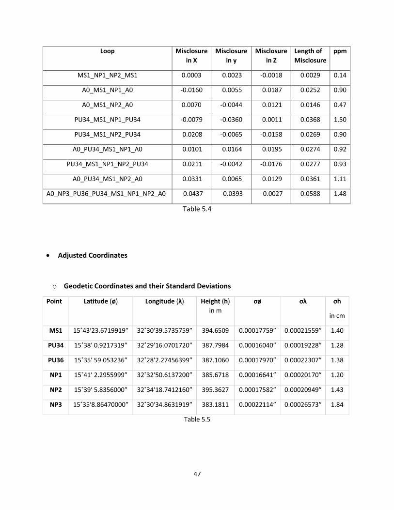
47

Loop Misclosure

in X

Misclosure

in y

Misclosure

in Z

Length of

Misclosure

ppm

MS1_NP1_NP2_MS1 0.0003 0.0023 -0.0018 0.0029 0.14

A0_MS1_NP1_A0 -0.0160 0.0055 0.0187 0.0252 0.90

A0_MS1_NP2_A0 0.0070 -0.0044 0.0121 0.0146 0.47

PU34_MS1_NP1_PU34 -0.0079 -0.0360 0.0011 0.0368 1.50

PU34_MS1_NP2_PU34 0.0208 -0.0065 -0.0158 0.0269 0.90

A0_PU34_MS1_NP1_A0 0.0101 0.0164 0.0195 0.0274 0.92

PU34_MS1_NP1_NP2_PU34 0.0211 -0.0042 -0.0176 0.0277 0.93

A0_PU34_MS1_NP2_A0 0.0331 0.0065 0.0129 0.0361 1.11

A0_NP3_PU36_PU34_MS1_NP1_NP2_A0 0.0437 0.0393 0.0027 0.0588 1.48

Table 5.4

Adjusted Coordinates

o Geodetic Coordinates and their Standard Deviations

Point Latitude (ø) Longitude (λ) Height (h)

in m

σø σλ σh

in cm

MS1 15˚43ʹ23.6719919ʺ 32˚30ʹ39.5735759ʺ 394.6509 0.00017759ʺ 0.00021559ʺ 1.40

PU34 15˚38ʹ 0.9217319ʺ 32˚29ʹ16.0701720ʺ 387.7984 0.00016040ʺ 0.00019228ʺ 1.28

PU36 15˚35ʹ 59.053236ʺ 32˚28ʹ2.27456399ʺ 387.1060 0.00017970ʺ 0.00022307ʺ 1.38

NP1 15˚41ʹ 2.2955999ʺ 32˚32ʹ50.6137200ʺ 385.6718 0.00016641ʺ 0.00020170ʺ 1.20

NP2 15˚39ʹ 5.8356000ʺ 32˚34ʹ18.7412160ʺ 395.3627 0.00017582ʺ 0.00020949ʺ 1.43

NP3 15˚35ʹ8.86470000ʺ 32˚30ʹ34.8631919ʺ 383.1811 0.00022114ʺ 0.00026573ʺ 1.84

Table 5.5

48

Standard deviation

Min Max Mean R.M.S

σø 0.5 0.7 0.55 0.55

σλ 0.6 0.8 0.66 0.67

σh 1.2 1.8 1.41 1.42

Table 5.6

Station E95 of ø (cm) E95 of λ (cm) E95 of h (cm)

MS1 1.07 1.30 2.76

PU34 0.97 1.16 2.51

PU36 1.08 1.35 2.71

NP1 1.01 1.22 2.36

NP2 1.06 1.27 2.80

NP3 1.34 1.61 3.61

Table 5.7: Accuracy standard at 95% confidence level

o Cartesian Coordinates and their Standard Deviations

Table 5.8

Station X Y Z σx σy σz

MS1 5178944.7038 3300748.7160 1717375.0713 0.0131 0.0115 0.0071

PU34 5182536.4811 3300088.3405 1707821.1833 0.0119 0.0104 0.0064

PU36 5184567.1029 3298774.9710 1704213.1367 0.0135 0.0108 0.0067

NP1 5177830.9228 3304666.4067 1713189.0183 0.0116 0.0097 0.0065

NP2 5177241.1116 3307403.8565 1709744.7172 0.0136 0.0112 0.0068

NP3 5182471.8686 3302830.2985 1702726.1106 0.0182 0.0135 0.0085

49

Standard

deviation

Min Max Mean R.M.S

σx 0.0116 0.0182 0.0136 0.0138

σy 0.0097 0.0135 0.0112 0.0112

σz 0.0064 0.0085 0.0069 0.0070

Table 5.9

Station E95 of X (cm) E95 of Y (cm) E95 of Z (cm)

MS1 2.56 2.25 1.39

PU34 2.33 2.03 1.25

PU36 2.64 2.11 1.31

NP1 2.27 1.90 1.27

NP2 2.66 2.19 1.33

NP3 3.56 2.64 1.66

Table 5.10: Accuracy standard at 95% confidence level

50

Figure ‎5.1: Error ellipse of the adjusted coordinates (X,Y).

The error ellipses shown on figure 5.1 were calculated for the coordinates, the

orientation angles are given with respect to the X axis.

51

Most Probable Values of the Baseline Vectors and their Components

From To ΔX ΔY ΔZ Vector Length

A0 MS1 -2515.18534 -2532.03835 12381.77323 12885.87148

A0 PU35 1076.592 -3192.41393 2827.88517 4398.578358

A0 NP2 -3628.96633 1385.65231 8195.72021 9069.689008

A0 PU37 3107.21385 -4505.78338 -780.16142 5528.608651

A0 NP2 -4218.77755 4123.10208 4751.41905 7574.565187

A0 NP3 1011.97952 -450.45593 -2267.18748 2523.321653

PU36 NP3 -2095.23433 4055.32746 -1487.02606 4800.722259

PU32 PU30 -2030.62185 1313.36945 3608.04659 4343.542863

PU34 NP3 -5295.36954 7315.51601 1923.53389 9233.509392

PU34 MS2 -3591.77734 660.37558 9553.88806 10228.08572

NP1 PU35 4705.55833 -4578.06624 -5367.83504 8480.248977

NP3 NP4 -589.81122 2737.44977 -3444.30116 4438.999775

NP1 MS2 1113.78099 -3917.69066 4186.05302 5840.534914

NP3 NP4 -589.81122 2737.44977 -3444.30116 4438.999775

Table 5.11

Residuals

The residuals are tabulated in Table 5.11, their frequency distributions are plotted against a

normal distribution curve in Figure 5.2.

From To VX VY VZ

A0 MS1 0.00846 0.00015 -0.00637

A0 PU34 -0.00810 -0.00913 -0.00823

A0 NP1 -0.00123 0.01621 0.00671

A0 PU36 -0.01735 -0.01368 -0.00762

A0 NP2 0.00775 0.00048 0.00815

A0 NP3 0.00272 -0.00863 0.00372

52

PU36 NP3 -0.00283 0.00636 -0.00456

PU36 PU34 -0.02395 -0.02465 -0.00811

PU34 NP2 0.00356 -0.00339 -0.01231

PU34 MS1 -0.00954 -0.00162 0.00106

NP1 PU34 0.01113 0.02706 0.00346

NP1 NP2 0.01028 0.01587 -0.00396

NP1 MS1 -0.00631 -0.01056 0.00562

NP1 NP2 -0.01432 -0.00813 0.00984

Table 5.12

Figure ‎5.2: Frequency distribution of residuals.

53

54

55

Chapter 6

6 Discussion and Conclusion

The most probable values of the geodetic coordinates are given in table 5.5 and their accuracies

within the 95% level are given in table 5.7. The highest accuracies are those of station PU34

whose standard deviations are 0.49 cm (E95 = 0.97 cm) and 0.59 cm (E95 =1.16 cm) in latitude

and longitude respectively, the lowest are those of station NP3 whose standard deviations are

0.68 cm (E95 = 1.34 cm) and 0.82 cm (E95 = 1.61 cm) in latitude and longitude respectively. The

mean standard deviations are 0.55cm and 0.66cm in latitude and longitude respectively.

Ellipsoidal height accuracies range from 1.20 cm (E95 = 2.36 cm) in station NP1 to 1.84 cm (E95 =

3.62 cm) in station NP3 with a mean value of 1.42cm.

Station NP3 has the lowest accuracy, in both horizontal and vertical components; this is

attributed to low redundancy (Ghilani and Wolf 2008) as the station was only occupied twice.

The highest accuracies were achieved in stations PU34 and NP1; these are attributed to high

redundancy in the case of PU34 which was occupied four times and the complete lack of

obstruction (Ghilani and Wolf 2008) around NP1.

The most probable values of the Cartesian coordinates are given in table 5.8 and their

accuracies within the 95% level are given in table 5.10, a general look at the tables reveals that

the Z-coordinates have the highest accuracies ranging from 1.25 cm (PU34) to 1.67 cm (NP3) and

a mean of 1.35cm followed by Y-coordinates ranging from 1.90cm (NP1) to 2.65cm (NP3) with a

mean of 2.19cm and finally the X-coordinates ranging from 2.27 cm (NP1) to 3.57 cm (NP3) with

a mean of 2.66cm all at the 95% level.

The residuals are given in table 5.12 and their frequency distributions are plotted against a

normal distribution curve on figure 5.2. The residuals in the ΔZ components of the baselines

exhibit the least variance.

In comparison with traditional methods of EDM and Theodolite based triangulations, satellite-

based positioning techniques are decidedly faster and more accurate, furthermore the

equipment are relatively easier to handle and do not require much technical experience. In this

light, we recommend the upgrade of the National Network of Control Monuments using

56

satellite-based relative positioning techniques preferably with GNSS receivers and the

application of a comprehensive Least Squares Estimation.

Outlook

As mentioned earlier, the observations were made using GPS receivers, and the data was

processed using a single baseline solution and broadcast ephemerides, furthermore the

observations were referenced to one control station. The accuracy of the network could be

improved by incorporating more than one reference station and using Global Navigation

Satellite Systems (GNSS) receivers operating on all available constellations; an increased

number of satellites would decrease the DOP values and increase observations, these factors

would generally benefit accuracy (Hofmann-Wellenhof et al. 2008) and further improvement

can be achieved by using precise ephemerides based on observed satellite orbital parameters

rather than broadcast ephemerides based on predicted orbital parameters (Seeber 2003) and

increasing the observation session time (Ghilani and Wolf 2008).

Recommendations, Further Studies and Projects Suggestions:

The formal standard errors of the vector computations given by the software are

optimistic by a factor of three to ten, therefore they do not give a true estimate of the

positioning error, and thus, they should never be used as an indicator of accuracy. The

true estimates of the errors can be computed after adjusting the network using the

method of least squares.

As mentioned earlier, the data acquired from the observation sessions were processed

using a single baseline solution, we recommend a comparison study employing a

multipoint solution preferably on the same data.

The flattening and orientation of the error ellipses indicates a directional-based error

source, we recommend a study on the nature of this error source.

We recommend a study of the relationship between WGS84 and Adindan datums to

establish the transformation parameters.

We recommend the establishment of an integrated Land Information System (LIS)

incorporating the monuments of the various agencies together with all street based

services such as kiosks and telecommunication towers. The construction of a

telecommunication tower near the DIU station PU32 indicates lack of coordination, it is

our belief that a comprehensive LIS would be of great service.

57

References

1. B. Holfmann-Wellenhof, H. Lichtenegger & J. Collins. Global Positioning System: Theory and practice, 5th ed. Published by Springer-Verlag Wien New York. 2001

2. Alfred Leick. GPS SATELLITE SURVEYING, 2th ed. U.S.A & Canada. Published by John Wiley & Sons, Inc. 1995

3. Charles D. Ghilani, Paul R. wolf. ADJUSTMENT COMPUTATIONS: Spatial Data Analysis, 4th ed. U.S.A & Canada. Published by John Wiley & Sons, Inc. 2006

4. Charles D. Ghilani, Paul R. Wolf. Elementary surveying: an introduction to geomatics,

13th ed. Published by Pearson Education, Inc. 2012

5. W. Schofield and M. Breach. Engineering Surveying, 6th ed. U.K. Published by Elsevier

Ltd. 2007

6. Paul A. Cross. Working Paper No (6): Advanced least squares applied to position fixing. University of East London: School of Surveying. 1994

7. Guochang Xu. GPS Theory, Algorithms and Applications, 2th ed. Berlin, Heidelberg & New York. Published by Springer-Verlag. 2007

8. Principle and Practice of GPS Surveying. 1999. Accessible at: http://www.gmat.unsw.edu.au/snap

9. James M. Anderson & Edward M. Mikhail. Surveying: Theory and Practice, 7th ed. U.S.A. The McGraw-Hill Companies, Inc. 1998

58

10. Günter Seeber. Satellite Geodesy, 2th ed. Berlin. Published by Walter de Gruyter GmbH & Co. KG. 2003.

11. Edward L Ingram 1st ed. New York. Published by McGrow-Hill Book Company, Inc. 1911

59

Appendix – The Results of the GPS Data Processing

Q3

3

4E-

07

4.8

E-0

7

4.9

E-0

7

2

.4E-

07

2.3

E-0

7

2.3

E-0

7

3

.6E-

07

3.4

E-0

7

3.5

E-0

7

3

.3E-

07

3.5

E-0

7

3.5

E-0

7

2

.6E-

07

2.6

E-0

7

2.7

E-0

7

1

.63

E-0

6

1.4

4E-

06

1.3

3E-

06

3

.2E-

07

3.2

E-0

7

3.2

E-0

7

Q2

3

4.4

E-0

7

5.9

E-0

7

6.2

E-0

7

1

E-0

7

9E-

08

9E-

08

3

E-0

7

2.8

E-0

7

2.9

E-0

7

1

.9E-

07

2.1

E-0

7

2.1

E-0

7

3

.8E-

07

3.8

E-0

7

3.8

E-0

7

1

.37

E-0

6

1.1

8E-

06

1.1

2E-

06

1

.9E-

07

1.9

E-0

7

1.9

E-0

7

Q2

2

9.1

E-0

7

1.2

4E-

06

1.3

E-0

6

6

.7E-

07

6.8

E-0

7

6.8

E-0

7

9

.7E-

07

9.3

E-0

7

9.7

E-0

7

6

.8E-

07

7.1

E-0

7

7.1

E-0

7

2

.1E-

06

2.1

E-0

6

2.1

3E-

06

1

.77

E-0

6

1.5

6E-

06

1.5

7E-

06

6

.4E-

07

6.3

E-0

7

6.4

E-0

7

Q1

3

4.5

E-0

7

5.6

E-0

7

5.9

E-0

7

2

.4E-

07

2.2

E-0

7

2.2

E-0

7

4

.8E-

07

4.5

E-0

7

4.7

E-0

7

3

.5E-

07

3.7

E-0

7

3.7

E-0

7

4

.4E-

07

4.4

E-0

7

4.5

E-0

7

1

.42

E-0

6

1.2

3E-

06

1.1

5E-

06

3

.5E-

07

3.4

E-0

7

3.5

E-0

7

Q1

2

7.1

E-0

7

9.6

E-0

7

1.0

2E-

06

5

E-0

7

5E-

07

5E-

07

9

.8E-

07

9.5

E-0

7

9.8

E-0

7

6

.9E-

07

7.3

E-0

7

7.3

E-0

7

2

.18

E-0

6

2.1

8E-

06

2.2

1E-

06

1

.43

E-0

6

1.2

5E-

06

1.2

1E-

06

5

.5E-

07

5.5

E-0

7

5.5

E-0

7

Q1

1

1.0

2E-

06

1.2

2E-

06

1.2

9E-

06

9

.2E-

07

9

.1E-

07

9E-

07

1

.78

E-0

6

1.7

E-0

6

1.7

9E-

06

1

.32

E-0

6

1.3

8E-

06

1.3

8E-

06

2

.67

E-0

6

2.6

6E-

06

2.7

1E-

06

1

.9E-

06

1.7

E-0

6

1.6

6E-

06

1

.01

E-0

6

9.9

E-0

7

1.0

E-0

6

ΔZ

12

38

1.7

79

6

28

27

.89

34

-95

53

.88

47

8

19

5.7

13

5

-78

0.1

53

8

-89

75

.86

52

-2

26

7.1

91

2

47

51

.41

09

-70

18

.59

8

-1

48

7.0

21

5

36

08

.05

47

50

95

.07

68

1

92

3.5

46

2

95

53

.88

7

76

30

.34

28

-5

36

7.8

38

5

-34

44

.29

72

-19

23

.53

42

4

18

6.0

47

4

-34

44

.31

1

-76

30

.35

66

ΔY

-2

53

2.0

38

5

-31

92

.40

48

-66

0.3

63

3

1

38

5.6

36

1

-45

05

.76

97

-58

91

.40

43

-4

50

.44

73

41

23

.10

16

-45

73

.54

4

4

05

5.3

21

1

13

13

.39

41

-27

41

.92

61

7

31

5.5

19

4

66

0.3

77

2

-66

55

.14

14

-4

57

8.0

93

3

27

37

.43

39

-73

15

.52

1

-3

91

7.6

80

1

27

37

.45

79

66

55

.13

57

ΔX

-2

51

5.1

93

8

10

76

.60

01

35

91

.79

92

-3

62

8.9

65

1

31

07

.23

12

67

36

.19

77

1

01

1.9

76

8

-42

18

.78

53

52

30

.77

07

-2

09

5.2

31

5

-20

30

.59

79

64

.63

42

-5

29

5.3

73

1

-35

91

.76

78

17

03

.60

81

4

70

5.5

47

2

-58

9.8

21

5

52

95

.37

58

1

11

3.7

87

3

-58

9.7

96

9

-17

03

.58

45

RO

VER

MS1

PU

34

PU

34

N

P1

PU

36

PU

36

N

P3

NP

2

NP

3

N

P3

PU

34

PU

34

N

P2

MS1

MS1

PU

34

NP

2

PU

34

M

S1

NP

2

NP

2

BA

SE

A0

A0

MS1

A

0

A0

NP

1

A

0

A0

NP

2

P

U3

6

PU

36

NP

3

P

U3

4

PU

34

NP

2

N

P1

NP

1

NP

2

N

P1

NP

1

MS1

SESS

ION

NO

.

1 2 3 4 5 6 7

60

The above table containing the output of the GPS data processing; for each session the first two baselines are selected to be as nontrivial baselines while the third baseline is trivial, and that is demonstrated in the figure below where the nontrivial baselines of each session are drawn in unique colors.