On the effect of a central vortex on a stretched magnetic flux tube

J. Fluid Mech. (1997), vol. 339, pp. 121–142. Printed in the United Kingdom

c© 1997 Cambridge University Press

121

On the effect of a central vortex on a stretchedmagnetic flux tube

By K O N R A D B A J E R† AND H. K. M O F F A T TDepartment of Applied Mathematics and Theoretical Physics, University of Cambridge,

Silver Street, Cambridge CB3 9EW, UK

(Received 8 March 1996 and in revised form 6 February 1997)

Experiments and numerical simulations of fully developed turbulence reveal theexistence of elongated vortices whose length is of the order of the integral scale ofturbulence while the diameter is somewhere between the Kolmogorov scale and theTaylor microscale. These vortices are embedded in quasi-irrotational background flowwhose straining action counteracts viscous decay and determines their cross-sectionalshape. In the present paper we analyse the effect of a stretched vortex of thiskind on a uni-directional magnetic flux tube aligned with vorticity in an electricallyconducting fluid. When the magnetic Prandtl number is large, Pm & 1, the field isconcentrated in a flux tube which, like the vortex itself, has elliptical cross-sectioninclined at 45◦ to the principal axes of strain. We focus on the limit Pm � 1 whenthe magnetic flux tube has radial extent much larger than that of the vortex, whichappears like a point vortex as regards its action on the flux tube. We find thesteady-state solution valid in the entire plane outside the vortex core. The solutionshows that the magnetic field has a logarithmic spiral component and no definiteorientation of the inner contours. Such magnetized vortices may be expected to existin MHD turbulence with weak magnetic field where the field shows a tendency toalign itself with vorticity. Magnetized vortices may also be expected to exist on thesolar surface near the corners of convection cells where downwelling swirling flowtends to concentrate the magnetic field.

1. IntroductionVortex tubes, subjected to the action of a locally uniform straining motion and to

the effect of viscous diffusion, were identified half a century ago (Burgers 1948) asa key ingredient of turbulent flow. The idea that at least the dissipative scales ofturbulence might be well represented by a random distribution of vortex tubes and/orsheets was pursued by Townsend (1951) (see Batchelor 1953, §7.4), and has receivedmuch impetus from the frequent detection of concentrated vortices both in directnumerical simulation (DNS) of turbulence (see, for example, Vincent & Meneguzzi1991; She, Jackson & Orszag 1990; Jimenez et al. 1993), and in experiments onturbulence in liquids seeded with small bubbles (Douady, Couder & Brachet 1991;Cadot, Douady & Couder 1995; Villermaux, Sixou & Gagne 1995). A high-Reynolds-number asymptotic theory of vortices subjected to the non-axisymmetric strain

U ∗ = (αx∗, βy∗, γz∗) , α+ β + γ = 0 , α 6 β 6 γ (1.1)

† On leave from the Institute of Geophysics, University of Warsaw, Poland.

122 K. Bajer and H. K. Moffatt

(where an asterisk denotes dimensional variables) has been developed by Moffatt,Kida & Ohkitani (1994, hereafter referred to as MKO94), and this explains certainfeatures of the dissipation fields observed in such vortices in DNS (Kida & Ohkitani1992). A parallel theory of two-dimensional unsteady vortices subjected to two-dimensional strain (Jimenez, Moffatt & Vasco 1996) explains the structure of thevortices that emerge in freely decaying two-dimensional turbulence (McWilliams1984), and provides a new handle on the dynamics of the asymptotic (t → ∞)high-Reynolds-number evolution.

The success of these approaches encourages an extension of the basic ideas tomagnetohydrodynamic (MHD) turbulence, for which magnetic field B∗, as well asvorticity ω∗, is subject to the orienting and intensifying effects of any local strainfield. The powerful (though admittedly incomplete) analogy between B∗ and ω∗ in theturbulence context was first exploited by Batchelor (1950) (see Moffatt 1978, §3.2); theanalogy has been pursued for the problem of stretched ‘vortex/magnetic flux tubes’or ‘magnetic sinew’ by Bajer (1995) who argues the case for simultaneous alignmentof B∗ and ω∗ along the axis Oz∗ of greatest positive rate of strain. These fields aresubject to different diffusivities – kinematic viscosity ν in the case of vorticity, andmagnetic diffusivity η in the case of magnetic field; this means that for positive strainrate γ, the viscous and magnetic diffusion length scales δv and δm are different:

δv = (ν/γ)1/2 , δm = (η/γ)1/2 . (1.2)

We shall suppose in the present paper that the magnetic Prandtl number is small:

Pm = ν/η = (δv/δm)2 � 1 (1.3)

and we shall focus attention on the structure of the magnetic field on scales r∗ � δv ,at which the additional velocity field is essentially that due to a point vortex (see(1.13) below).

We shall suppose that the circulation associated with this vortex is Γ (> 0), andthat the magnetic flux is Φ(> 0), and that both Γ and Φ are finite. We may thenadopt dimensionless variables

r = r∗/δm , ψ = ψ∗/Γ , ω = ω∗δ2m/Γ , B = B∗δ2

m/Φ (1.4)

and, under the assumption of aligned fields,

ω = ω(r, θ)z , B = B(r, θ)z , (1.5a , b)

where z is a unit vector in the direction Oz. The vorticity and magnetic inductionequations then reduce in polar coordinates (cf. MKO94) to the similar form

1

r

∂(ψ,ω)

∂(r, θ)= −εm(L0 + λL1)ω , (1.6)

1

r

∂(ψ, B)

∂(r, θ)= −εm(L0 + λL1)B , (1.7)

where

L0 = 1 + 12r∂

∂r+ ∇2 , (1.8a)

L0 = 1 + 12r∂

∂r+ Pm∇2 , (1.8b)

L1 = ( 12

cos 2θ)r∂

∂r− ( 1

2sin 2θ)

∂

∂θ, (1.8c)

Magnetic flux tube with a central vortex 123

and

εm = η/Γ , λ =α− βα+ β

. (1.9)

The (non-negative) parameter λ is a measure of the non-axisymmetry of the strainfield (1.1); usually we are concerned with the range 0 6 λ < 1; occasionally howeverwe shall discuss the situation λ > 1 (equivalently β > 0). The parameter εm is thereciprocal of a magnetic Reynolds number

Rm = ε−1m = Γ/η . (1.10)

We first present an asymptotic theory for large Rm,

Rm � 1 , i.e. εm � 1 , (1.11)

and then consider the situation when εm increases to values of order unity and greater.Note that the Lorentz force associated with the magnetic field (1.5b) is irrotational,

and therefore makes no contribution to the vorticity equation (1.6) (although it doeshave an effect on the pressure field). This means that (1.6) is the same as in MKO94,(but with δm instead of δv used for non-dimensionalization). For ε = εmPm � 1, and

for r � P−1/2m , the asymptotic solution of (1.6) obtained by MKO94 has the form

ψ(r, θ) = − 1

2πln r + C

εmλP2m

r2sin 2θ + O

(λε2

mP4m

r4

)(1.12)

where C = −17.472 . . .. Hence, provided Pm � 1 as assumed here, we have indeed

ψ(r, θ) ∼ − 1

2πln r (r � P 1/2

m ) (1.13)

and (1.7) then becomes

− 1

2πr2

∂B

∂θ= −εm(L0 + λL1)B . (1.14)

This linear equation, deceptively simple in form, is investigated in the followingsections of the paper. We require a solution which satisfies the (normalized) fluxcondition ∫ ∞

0

∫ 2π

0

B(r, θ)rdrdθ = 1, (1.15)

and boundary conditions that B(r, θ) behaves ‘reasonably’ (despite the presence ofthe vortex) as r → 0, i.e.

B(r, θ) = O(1) as r → 0 , (1.16)

and that B settles down to the unique (up to a constant b) solution of (1.14) thatobtains in the far field where the effect of the vortex is negligible, i.e.

B(r, θ) ∼ b exp

(αx∗

2

+ βy∗2

η

)= b exp

(− 1

4r2(1 + λ cos 2θ)

)= be−r

2/4(

1− λ 14r2 cos 2θ + 1

2λ2(

14r2)2

cos2 2θ + . . .). (1.17)

Here, we see the need for the assumption λ < 1 (i.e. β < 0).The total velocity field with which we are concerned is that due to the uniform strain

(1.1) plus that due to the point vortex (1.13); the dimensionless (r, θ, z) components


2

1

0

–1

–2–2 –1 0 1 2

(c)2

1

0

–1

–2–2 –1 0 1 2

(d )

2

1

0

–1

–2–2 –1 0 1 2

(a)2

1

0

–1

–2–2 –1 0 1 2

(b)

Figure 1. The projections of the streamlines of the flow (1.18) on the (x, y) plane with (a) λ = 0;

(b) λ = 0.3; (c) λ = 0.6; (d) λ = 0.9. The scaled radius is rε1/2m .

of this total velocity field are

ur = − 12εmr(1 + λ cos 2θ) , uθ =

1

2πr+ 1

2εmλr sin 2θ , uz = εmz . (1.18)

Note that the scale (πεm(1 − λ))−1/2 represents the distance from the origin at whichthe vortex and the strain field have comparable intensities. For r � (πεm(1− λ))−1/2,the vortex dominates, while for r � (πεm(1 − λ))−1/2, the strain dominates. Figure 1shows the projection of the streamlines of the velocity field (1.18) on any planez = const. for various values of λ; note the increasingly strong convergence towardsthe axis Oy as λ increases from zero. The scale of the magnetic flux tube is O(1)in the dimensionless units adopted; hence when εm � 1, the flux tube is confinedto the region where the vortex dominates; this induces a strong ‘axisymmetrization’of the flux tube as we shall see; nevertheless all departures from axisymmetry areinduced by the strain field and controlled by a complex interaction of strain, vortexand magnetic diffusion even in the region where r = O(1).

We conclude this introductory section with a plan of the paper. In §2, we recall theasymptotic high-Rm (or low-εm) theory of Bajer (1995) which is a natural extension ofthe approach of MKO94. This predicts elliptic structure for the curves B(r, θ) = const.with principal axes at 45o inclination to the principal axes of strain (Ox,Oy). The


asymptotic expansion appears to be valid for r = O(1) but fails for r = O(R−1/2m ) and

in particular fails to satisfy the outer boundary condition (1.17). In §3, we seek torectify this failing by numerical means. The computed solution does reveal roughlyelliptic contours, but the orientation of these contours shows damped oscillations asr → 0 which are not present in the asymptotic solution.

This puzzling behaviour is explained in §4 where we develop an expansion inpowers of λ yielding a solution valid uniformly for all r and matching the outersolution (1.17). The expansion reveals a non-analytic part with spiral level contoursand validates the numerical results of §3. In order to investigate the convergence ofboth the asymptotic expansion and the λ-expansion as well as explain the differencebetween them we derive a family of series solutions in powers of r. The details aregiven in Appendix A. In §5 we summarize the results.

2. Asymptotic theory for Rm � 1As in MKO94, we may seek an asymptotic solution of (1.14) for εm � 1 in the

form

B = B0 + εmB1 + ε2mB2 + . . . . (2.1)

At leading order, ∂B0/∂θ = 0, so that B0 = B0(r), and at higher orders

1

2πr2

∂Bn

∂θ= (L0 + λL1)Bn−1 (n = 1, 2, 3, . . .) . (2.2)

Integrating the n = 1 equation over θ (from zero to 2π) gives the solvability condition

L0B0(r) = 0 (2.3)

with unique solution (satisfying (1.14) and (1.15))

B0(r) = (4π)−1e−r2/4 . (2.4)

Equation (2.2) (with n = 1) then integrates to give

B1(r, θ) = − 116λr4e−r

2/4 sin 2θ , (2.5)

the arbitrary additive function of r being eliminated by application of the solvabilitycondition at order ε2

m.Similarly, we may proceed to higher levels, obtaining successively B2(r, θ), B3(r, θ),

B4(r, θ), . . .; thus we find

B2(r, θ) = −λπr4e−r2/4[2(r2 − 6) cos 2θ + λr2(r2 − 4) cos 4θ

], (2.6)

B3(r, θ) = 2λπ2r4e−r2/4[(

(3r4 − 44r2 + 72) + λ2r4(r4 − 28r2 + 80))

sin 2θ

+ λr2(2r4 − 29r2 + 44) sin 4θ + 13λ2r4(r4 − 12r2 + 16) sin 6θ

], (2.7)

B4(r, θ) = λπ3r4e−r2/4[(

8(3r6 − 78r4 + 388r2 − 216)

+ 4λ2r6(5r4 − 225r2 + 2244))

cos 2θ

+(4λr2(4r6 − 111r4 + 593r2 − 364)

+ 83λ3r6(r6 − 48r4 + 496r2 − 832)

)cos 4θ

+ 49λ2r4(9r6 − 243r4 + 1244r2 − 752) cos 6θ

+ 13λ3r6(r6 − 24r4 + 112r2 − 64) cos 8θ

], (2.8)

and so on. Here λ = λ/16.


Note that in Bn, the largest power of r is r4n and this appears in conjunction witha factor λn; thus, for example, for λ = O(1) and r � 1,

B2(r, θ) ∼ −πλ2r8e−r2/4 cos 4θ , (2.9a)

B3(r, θ) ∼ 23π2λ3r12e−r

2/4(3 sin 2θ + sin 4θ) , (2.9b)

B4(r, θ) ∼ 13π3λ4r16e−r

2/4(8 cos 4θ + cos 8θ) . (2.9c)

The ordering of the terms of (2.1) is thus consistent only if r . Rε where

Rε = O(εmλ)−1/4 . (2.10)

To order εm, for r = O(1) the contours B0 + εmB1 = const. are ellipses inclined atan angle 45o to the principal axes of strain. The manner in which these contoursrotate and deform as r increases from O(1) to O(Rε) is not apparent from the aboveexpansion.

Note finally that the coefficient of terms involving sin 2θ or cos 2θ in (2.5) and (2.6)are of order r4 for small r, while the coefficient of cos 4θ in (2.6) is of order r6 forsmall r. This type of behaviour persists at higher order: the coefficients of terms incos 2nθ or sin 2nθ are O(r2(n+1)) for small r.

3. Uniformly valid solutionThe above asymptotic solution has to be regarded at best as an inner solution

which must be matched in some way to a solution that satisfies the outer boundarycondition (1.17). Let us seek a solution in the form of a Fourier series

B(r, θ) =

∞∑n=−∞

bn(r)ei2nθ, (3.1)

where, for reality of B,

b−n(r) = b∗n(r) , (3.2)

the star now representing the complex conjugate. Only terms proportional to ei2nθ

occur in (3.1) from the structure of equation (1.14). Substitution in this equationyields a set of coupled linear differential equations:

b′′n +

(1

r+ 1

2r

)b′n +

(1− 4n2

r2

)bn + 1

2λ [(n+ 1)bn+1 − (n− 1)bn−1]

= − 14λr(b′n−1 + b′n+1

)+

in

πεmr2bn (n = 0,±1,±2, . . .). (3.3)

We must apply boundary conditions for this set of equations for both r → 0 andr → ∞. Noting the comment at the end of §2, the appropriate conditions for r → 0are evidently

b0(r) ∼ (4π)−1 , bn(r) ∼ r2(n+1) (n > 1) as r → 0 . (3.4)

For r →∞, the Fourier coefficients are given from (1.17) by

bn(r) ∼b

2π

∫ 2π

0

e−r2(1+λ cos 2θ)/4e−i2nθdθ

= 2(−1)nb e−r2/4In(

14λr2), (3.5)

where In(ξ) is a modified Bessel function (Gradshtein & Ryzhik 1994) whose asymp-


totic behaviour for n fixed and ξ →∞ is

In(ξ) ∼ (2πξ)−1/2eξ . (3.6)

Hence, for fixed n,

bn(r) ∼23/2(−1)nb e−r

2/4

(2πλr2)1/2eλr

2/4 =

(8

πλ

)1/2

(−1)nbr−1e−(1−λ)r2/4. (3.7)

Therefore, when r is large all Fourier coefficients have the same magnitude for n upto about 1

4λr2, beyond which a different asymptotic behaviour of In becomes valid

and |bn| decreases with n.In order to solve (3.3) numerically we must impose the boundary condition (3.5)

at some finite radius r = R. The asymptotic behaviour of bn(r) shows that the largerwe choose R the bigger the number of Fourier modes we have to take into account.However, we must not choose R too small. It must be in the region where the straindominates and (1.17) is valid, which means R & L = (πεm(1−λ))−1/2 (cf. 1.18). TakingR = L we can estimate the number of Fourier modes needed:

N ≈ 14λL2 = λ [4π(1− λ)εm]−1 . (3.8)

We solve numerically equations (3.3) using the deferred correction technique (NAGroutine D02 GBF) forN = 20 modes with the condition (3.4) imposed at r = r0 = 10−5

and (3.5) at r = R = 10.The resulting contours of B and the corresponding contours of the (non-dimen-

sional) ohmic dissipation,

Dm =1

2

(∂Bi

∂xj− ∂Bj

∂xi

)(∂Bi

∂xj− ∂Bj

∂xi

), (3.9)

are plotted in figures 2–4.They do not depend on the precise values of r0, R or N. The contours of B have

a maximum at the origin and for smaller values of εm, e.g. εm = 0.01 and εm = 0.05,they seem to be elliptical with 45◦ inclination, as predicted by the expansion (2.1);farther out they rotate back towards the axes of strain to match the outer solution(1.17).

The contours of the ohmic dissipation Dm show similar change of orientation, butare strongly dipolar with a minimum at the origin (this minimum is to be expectedbecause the current associated with a field given by (3.1) and (3.4) is zero at r = 0).The line joining the maxima of Dm is inclined to the axis of weaker strain at anangle α(εm). For small εm the angle α(εm) is close to 45◦ and the contours approachthose obtained from the expansion (2.1) (cf. Bajer 1995). For larger values of εm, i.e.εm = 0.1 and εm = 1.0, they do not seem to have the diagonal orientation.

The asymptotic behaviour bn ∼ r2(n+1) as r → 0 implies that the shape of the innercontours is determined by

b0(r) + 2bR1 (r) cos 2θ − 2bI1(r) sin 2θ ≈ const , (3.10)

where the superscripts denote the real and imaginary parts. The expansion (2.1)predicts (see (2.5) and (2.6))

b0(r) = 14π−1

(1− 1

4r2 + 1

32r4 . . .

), (3.11a)

bR1 (r) = 38λε2

mπr4 + O(ε4

m), (3.11b)

bI1(r) = 132λεmr

4 + O(ε3m), (3.11c)


5

0

–5–5 0 5

(d )

x

y

5

0

–5–5 0 5

x

5

0

–5–5 0 5

(c )

y

5

0

–5–5 0 5

5

0

–5–5 0 5

(b)

y

Figure 2. Contours of the magnetic field B (left column) and of the ohmic dissipation Dm (rightcolumn) with λ = 0.5 and (a) εm = 1.0; (b) εm = 0.1; (c) εm = 0.05; (d) εm = 0.01.

and so, since |bI1| � |bR1 | as r → 0, the inner contours have elliptical shape inclined at45◦ to the principal axes of strain.

In figure 5 we show a scaled logarithmic plot of 2bR1 as obtained from a numericalsolution. When εm is smaller than a certain threshold value ε0 somewhere between0.01 and 0.02 the function 2bR1 (r)/r4 oscillates, but converges to 3

8λε2

mπ as r → 0


4

0

–4

–4 0 4

(d )

x

y

4

0

–4

–4 0 4x

4

0

–4

–4 0 4

(c)

y

4

0

–4

–4 0 4

4

0

–4

–4 0 4

(b)

y

4

0

–4

–4 0 4

4

0

–4

–4 0 4

(a)

y

4

0

–4

–4 0 4


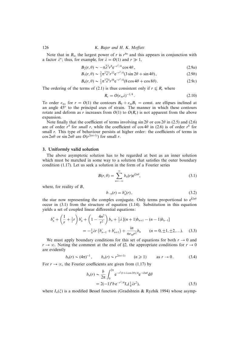
(figure 5a). However, when εm > ε0 the function bR1 (r) looks very different. It seemsto have an infinite number of zeros accumulating at r = 0 (figure 5b). The magnitudeof bR1 (r) decreases like rp, but the computed value of p (when εm = 0.02) appears tobe p = 3.19 . . . instead of p = 4 as in (3.11).

This gives rise to an apparent inconsistency. The computed solution shows different


8

0

–4

–5 0 5

(d )

x

y

8

0

–4

–10 0 5x

4

–8

–10 10 10

4

–8

–5

8

0

–4

–5 0 5

(c )

y

8

0

–4

–10 0 5

4

–8

–10 10 10

4

–8

–5

8

0

–4

–5 0 5

(b)

y

8

0

–4

–10 0 5

4

–8

–10 10 10

4

–8

–5

8

0

–4

–5 0 5

(a)

y

8

0

–4

–10 0 5

4

–8

–10 10 10

4

–8

–5


small-r behaviour from what we assumed (conditions (3.4)) when calculating it. Wehave tried different boundary conditions at r0, for example bn(r0) = 0, and find thesame oscillatory behaviour with the same phase, amplitude and value of p. Changingthe value of r0 we find that the boundary condition affects the solution only in asmall neighbourhood of r0. Hence the oscillations seen in figure 5(b) are not relatedto the conditions adopted at r0.


20

10

5

–4 –2 0

(a)15

–5–6 2

0

(×10–5)15

5

0

–8 –6 0

(b)10

–10

–10 2

–5

(×10–4)

–15–4 –2

Figure 5. 2b1(r)/rp versus ln r from a numerical solution of (3.3)–(3.5) (solid line) and from theexpansion in powers of λ (dashed line) (see §4) with N = 10, λ = 0.7 and (a) p = 4, εm = 0.01; (b)p = 3.19, εm = 0.02.

We cannot decide a priori on the grounds of the numerical solution alone whetherthe oscillatory behaviour is or is not a result of truncation of the system (3.3).Truncating at n = 1 we obtain two coupled linear equations for b0 and b1 which canbe manipulated to give a single fifth-order equation for b0 (see Appendix A),

w4b′′′′′0 + (3w4 + 6w3)b′′′′0 + [(K + 2)w4 + 16w3 + 5w2]b′′′0+[Kw4 + (5K + 9)w3 + 12w2 − w]b′′0 + [(3K + 1)w3 + (3K + 6)w2 − 2w + 1 + σ2]b′0+[2w2 − w + 1 + σ2]b0 = 0, (3.12)

where K = 1− 12λ2, w = 1

4r2 is a new variable and

σ = (4πεm)−1 . (3.13)

From any solution b0(r) we can easily calculate the corresponding b1(r) satisfying thetruncated system. There are two solutions finite at r = 0:

b10(w) = 1− w + 1

2w2 − 1

6

[1 +

3λ2

9 + σ2

]w3 + O(w4), (3.14a)

b11(w) =

12λ

3− iσw2 + O(w3); (3.14b)

b20 = wδ [1 + O(w)] , (3.14c)

b21 = − 1

2λwδ−1

[1

δ− 1

2δ − 1w + O(w2)

]; (3.14d)

where δ = 1 + (1 + iσ)1/2. The general solution of (3.12) finite at r = 0 is a linearcombination of these two solutions, so the behaviour of b1(r) as r → 0 depends on thevalue of δ. When δR−1 < 2, which corresponds to εm > ε0 = (16π

√3)−1 = 0.01148 . . . ,

we have

b1(r) ∼ r2(δ−1) = r2(δR−1) cos(2δI ln r + φ0), (3.15)

φ0 being an arbitrary phase. This is the behaviour observed in figure 5(b). Notethat when εm = 0.02, 2(δR − 1) ≈ 3.1945 . . . , very near the value 3.19 obtained in thecomputation. However, we do not know the asymptotic behaviour of these solutionsfor r → ∞. The numerical results alone cannot rule out the possibility that thesesolutions are physically unacceptable as r →∞. If they decrease rapidly with r it maybe necessary to impose the outer boundary condition at very large r = R in order to


filter out the unphysical solutions, i.e. those which do not satisfy (1.17). As explainedearlier, this requires a prohibitively large number of Fourier modes.

We show in Appendix A that there are in fact no solutions of (3.12) which satisfy(3.7). This could suggest that the oscillatory behaviour is purely the result of truncationand might disappear when the unphysical solutions are properly filtered out. However,in §4 we develop an expansion in powers of λ which yields a spatially uniform solutionand explains the oscillatory behaviour. It has a non-analytic component which is notcaptured by the asymptotic theory of §2. Near the origin this part vanishes in the limitεm → 0, but as εm increases it becomes more prominent and causes the oscillatorybehaviour of the non-axisymmetric Fourier modes, just as seen in figure 5(b).

4. Expansion in powers of λ

Let us first rewrite (1.14) in the new coordinates w = 14r2, θ = 2θ:

σ

w

∂B

∂θ= [L0 + λL1]B, (4.1)

where now

L0 = 1 + w∂

∂w+ w

(∂2

∂w2+

1

w

∂

∂w+

1

w2

∂2

∂θ2

), (4.2a)

L1 = cos θw∂

∂w− sin θ

∂

∂θ. (4.2b)

When λ = 0 the Burgers solution takes a particularly simple form:

B0 = e−w, (4.3)

where, in order to simplify the notation, we now take the total non-dimensional fluxto be Φ = 4π. With λ = 0 the equation (4.1) also has a family of non-axisymmetricsolutions given by

BN(w, θ) = wβNe−weiNθ/2FN(w), βN = 12N(1 + 2iσ/N)1/2 , (4.4)

where N = 1, 2, 3, . . . , and the FN are Kummer functions satisfying (Abramovitz &Stegun 1965, §13.1)

wF ′′N + (2βN + 1− w)F ′N − βNFN = 0. (4.5)

These generalize the solutions obtained by Galloway & Zheligovsky (1994) for thepure flux tube problem without a central vortex (i.e. with σ = 0). The solutions (4.4)have the following asymptotic behaviour:

BN(w, θ) ∼ eiNθwβN as w → 0, (4.6a)

BN(w, θ) ∼ eiNθw−1 as w →∞. (4.6b)

The complex power of w in (4.6a) means that the level contours near the originare logarithmic spirals (see figure 6a in Appendix A). The solutions are linearlyindependent and have finite magnetic energy, but |BN | is not integrable. They havesectors of infinite magnetic flux and cannot be the asymptotic states of the time-dependent problem with finite initial flux. However, Galloway & Zheligovsky (1994)point out that solutions of this kind can play a role in direct numerical simulation ofthe magnetohydrodynamic turbulence.

In Appendix B we analyse the structure of the corresponding family of solutions


of (4.1) when λ 6= 0. These cannot be written in closed form, rather they are given aspower series in w which makes it difficult to analyse their asymptotic behaviour forw →∞. Rather unexpectedly, they shed light on the nature of the expansion (2.1).

When λ = 0 all except one solution of (4.4) have non-analytic spiral behaviournear the origin. The physically acceptable one (satisfying (1.17)) is the only exception.When λ is perturbed away from zero there are, in principle, two possible ways in whichthe family of solutions can be modified. Either the solution satisfying (1.17) is slightlychanged, but is still analytic at r = 0 and thus exceptional, or all solutions are ‘mixed’together and the one satisfying (1.17) acquires a non-analytic spiral component.

We will now show the latter to be true by deriving an expansion in powers of λ:

B(w, θ) = B0(w) + λB1(w, θ) + λ2B2(w, θ) + . . . . (4.7)

Clearly

B0 = e−w, (4.8)

and the first-order term B1 can be written as

B1(w, θ) = Re(H(w)eiθ), (4.9)

where the complex function H(w) satisfies the following inhomogeneous linear equa-tion:

w2H ′′ + w(w + 1)H ′ + [w − (1 + iσ)]H = w2e−w. (4.10)

Solutions of the homogeneous equation are

H1(w) = wαe−wM(α, 2α+ 1, w), H2(w) = wαe−wU(α, 2α+ 1, w), (4.11)

where α = δ − 1 = (1 + iσ)1/2 and M and U are Kummer’s functions (Abramovitz &Stegun 1965, §13.1). H1(w) and H2(w) have the following series expansions convergentfor all values of w:

H1(w) = wα∞∑n=0

Cnαw

n, H2(w) = C+wα

∞∑n=0

Cnαw

n − C−w−α∞∑n=0

Cn−αw

n, (4.12)

with

Cnα =

Γ (2α+ 1)

Γ (α)

n∑k=0

(−1)n−k

k!(n− k)!Γ (α+ k)

Γ (2α+ k + 1), (4.13a)

C± = π [sin π(2α+ 1)Γ (∓α)Γ (±2α+ 1)]−1 = ±Γ (∓2α)/Γ (∓α) . (4.13b)

The solutions have the following asymptotic expansions for large w:

H1(w) ∼ Γ (2α+ 1)

Γ (α)w−1

(S−1∑n=0

Rnw−n + O(w−S )

)

+Γ (2α+ 1)

Γ (α+ 1)eiπαe−w

(R−1∑n=0

Anw−n + O(w−R)

), (4.14)

H2(w) ∼ e−w

(R−1∑n=0

Anw−n + O(w−R)

), (4.15)

where

An =Γ (n+ α)Γ (n− α)

Γ (α)Γ (−α)(−1)n

n!, Rn = (−1)n(n+ 1)α−2An+1. (4.16)


By means of a Green’s function, we construct the unique solution of (4.10) which isfinite at w = 0 and falls off exponentially when w →∞:

H(w) = − Γ (α)

Γ (2α+ 1)

(H2(w)

∫ w

0

ξH1(ξ) dξ +H1(w)

∫ ∞w

ξH2(ξ) dξ

). (4.17)

The series expansion can be obtained from (4.12):

H(w) = w2

∞∑n=0

Wnα w

n − Ic(α)wα∞∑n=0

Cnαw

n, (4.18)

where

Wnα = − 1

2α

n∑k=0

CkαC

n−k−α[(k + α+ 2)−1 − (n− k − α+ 2)−1

],

Ic(α) =Γ (α)

Γ (2α+ 1)limA→0

(∫ ∞A

ξH2(ξ) dξ − C−A2−α∞∑n=0

Cn−α(n− α+ 2)−1An

).

The expression in brackets becomes independent of A when A→ 0, so the limit existsand Ic(α) is finite. When Re(α) < 2 we have (Gradshtein & Ryzhik 1994, §7.621.6)

Ic(α) =Γ (α)

Γ (2α+ 1)

∫ ∞0

ξH2(ξ) dξ =Γ (α)Γ (2 + α)Γ (2− α)

Γ (2α+ 1)6= 0. (4.19)

Hence the solution contains a non-analytic component (at least when Re(α) < 2). All

orders B1, B2, . . . of the expansion (4.7) include terms proportional to ei2θ , but B1

dominates as r → 0. Hence, for small r we have (see (3.1), (4.9))

b1(r) ≈ 12H( 1

4r2). (4.20)

In figure 5 we compare 2bR1 (r) computed from the system (3.3) with HR obtainedfrom (4.17) and find excellent agreement (over the whole range 10−5 < r < 10),which proves that the accumulating zeros of bR1 are not the result of imperfectcomputations. It follows that the boundary conditions (3.4) for bn(r) derived fromthe high-Rm expansion (2.1) are in fact incorrect, but they have negligible influenceon the numerical solution. The expansion (2.1) misses the non-analytic part of the

solution because it is proportional to ( 12r)2α and Re(α) ∼ ε−1/2

m for small εm, so for anyfixed r < 2 the non-analytic term disappears in the limit εm → 0.

The inner contours of B1 are logarithmic spirals and those of B0 + λB1 haveelliptical shape, but the orientation continuously changes when r → 0. The axes ofthe ellipses lie on a logarithmic spiral, so they do not have definite orientation asr → 0.

Working out the asymptotic series for H(w) when w → ∞ is straightforward buttedious. The result is

H(w) ∼ −we−w + iσ lnw e−w∑n=0

Anw−n − e−w

∑n=0

Vnw−n, (4.21)

where Vn can be calculated from (4.4) and (4.5). The leading term of B1 is therefore

B1 = Re(H(w)eiθ) ∼ −we−w cos θ, (4.22)

the same as in (1.17).Comparing (4.8) and (4.22) it may seem that the expansion (4.7) is valid only when


λw . 1. In Appendix B we argue that (4.7) is in fact a convergent series for all valuesof λ and any fixed r, as is the Taylor series (in powers of λ) of the matching outersolution (1.17).Thus we have obtained a uniformly valid solution of (1.14) satisfying(1.17).

In Appendix B, we also explain the difference between (2.1) and (4.7) in greaterdetail. We find an analytic (in r) solution which is approximated by (2.1) and a familyof non-analytic solutions, analogous to (4.4), which must be added to make a uniquesolution satisfying (1.17). The expansion (4.7) approximates this unique solution.

In practice convergence of (4.7) is not a useful property. When w is large manyterms are needed to obtain a reasonable approximation. It is possible to calculatehigher orders, but the results become increasingly more difficult to analyse. Hence,we are rather interested in the region of the (λ, εm)-space where just the first order,B0 + λB1, is a good approximation. The condition is |λB1| � |B0| which meansr � 2λ−1/2 (see (4.8), (4.21)). The approximation will be uniform, provided the radiusabove which the outer solution is valid, i.e. r ∼ (πεm(1 − λ))−1/2 (see 1.18), is muchsmaller than 2λ−1/2. We obtain the condition for B0 +λB1 to be a good approximationin the entire plane:

λ� 4πεm1 + 4πεm

< 1 . (4.23)

We may conclude that the expansion (4.7), although convergent for all values of λ, isuseful only when λ is small.

When λ > 1 we still have a solution, but the matching outer solution (1.17) isunphysical. In fact the problem has no localized steady solution. The streamlinesof the flow projected onto the (x, y)-plane have a separatrix and the magnetic fluxcontinuously ‘leaks’ across the separatrix and is advected away from the origin in aprocess similar to vortex stripping (Legras & Dritschel 1993). Due to its uniformityin r the λ-expansion shows clearly the disappearance of the steady solution for λ > 1.It is not the case with the asymptotic theory of §2.

In an interesting way the expansion (4.7) leads to conclusions about convergenceof (2.1). From (4.18) we notice that H(w) regarded as function of Rm has singularitiesin the plane of complex Rm where the denominators of the coefficients Wn

α have zeros.They are all located on the imaginary axis and their position is given by

j − α+ 2 = 0; j = 0, 1, 2, . . . , (4.24)

or in terms of Rm,

Rm = −i4π(j2 + 4j + 3). (4.25)

The singularities extend to infinity, i.e. there are singularities with arbitrary largeabsolute value. Hence, the expansion of the function H(w) in powers of εm = Rm

−1

is an asymptotic series with zero radius of convergence and the same applies to theexpansion (2.1).

The singularity which is closest to the origin in the plane of complex Rm correspondsto j = 0 or Rm = −12iπ. When Rm � 1 a solution to (1.14)–(1.17) can be soughtin the form of a series in powers of Rm. Such series would have finite radius ofconvergence R0

m determined by the nearest singularity. At O(λ) we obtain an upperbound R0

m = 12π, but higher orders bring more singularities. In Appendix B we arguethat the singularities have an accumulation point at Rm = −8iπ, thus giving R0

m = 8π.A low-Reynolds-number theory of this kind was derived by Robinson & Saffman

(1984) for the stretched vortex problem. They found no evidence of the radius ofconvergence being finite. The existence of singularities and their location is an open


problem. It is possible that they are a consequence of the singular flow due to apoint vortex in our present problem and that they do not appear in the problemconsidered by Robinson & Saffman. However, a more likely explanation is that theirexistence was obscured by the double expansion both in Reynolds number and in theparameter λ.

5. SummaryIn this paper we have analysed a rectilinear magnetic sinew strained by non-

axisymmetric irrotational ambient flow. A large-Rm expansion was developed byBajer (1995) for two regimes: RΓ � 1, Pm & 1; and Pm � 1. The value of Pm in thesolar convection zone varies from 10−5 at the base of the photosphere to 102 deeperdown (Priest 1982, §1.3.1), so both regimes are of potential interest.

Here we considered in detail the regime when Pm = Rm/RΓ � 1 The vortex wasapproximated by a line vortex which corresponds to taking the limit Pm → 0 andneglecting non-axisymmetric terms in the multipole expansion of the velocity.

The expansion (2.1) does not match the linear outer solution. In order to bridgethe gap between the two we calculated numerically a uniformly valid solution. Whenεm exceeds a certain threshold value the computed asymptotic behaviour as r → 0of the higher Fourier modes differs essentially from that predicted by the high-Rmexpansion. They have an infinite number of zeros accumulating at r = 0, a signatureof spiral behaviour.

The main result of the paper is the proof that the computations are quantitativelycorrect and the high-Rm expansion has a rather subtle deficiency, difficult to predictin advance, which becomes prominent when Rm is below a certain threshold. The firstindication came from the analysis of the severely truncated system including onlytwo Fourier modes. It reproduced the computational results and gave an accuratethreshold value Rm ≈ 87 (corresponding to εm = 0.01148), but the solutions hadwrong behaviour for r →∞. In a special case, λ = 0, we have found an infinite family(4.4) of solutions which are oscillatory near the origin, but they are all excluded bythe boundary condition (1.17).

The decisive argument showing that this is not the case when λ > 0 came from theexpansion in powers of λ which yielded a solution valid uniformly in r and satisfyingthe boundary condition (1.17). The solution validates the numerical results and revealsa non-analytic spiral part which was missing from the large-Rm expansion (2.1). Thisspiral ingredient is present however large Rm may be, but it becomes weaker as Rmincreases relative to the non-oscillatory ingredient.

It is difficult to carry out the procedure to orders higher than O(λ), so its practicaluse is limited to small values of λ, but it reveals the nature of the uniformly validsolution. It appears to be a combination of solutions BN , analogous to (4.4), thedetails of which are given in Appendix B. When expanded in powers of εm thesesolutions yield divergent asymptotic series. The series corresponding to B0 appearsto be identical with (2.1).

The λ-expansion, together with the matching outer solution (1.17), provide acomplete solution to our problem. It shows that the spiral component is indeedpresent in the steady state. This is different from the unsteady algebraic spiralscontinuously developing in two-dimensional (Gilbert 1988) and three-dimensional(Lundgren 1982) turbulence.

We expect the magnetic sinews considered here to be prominent features in anyphysical situation where the magnetic field is weak and passive enough not to prevent


the formation of the coherent vortices. By analogy with the small-scale structures ofturbulence such magnetic sinews are likely to feature in weak-field MHD turbulence.Numerical simulations of Brandenburg and others (see Brandenburg 1994) showalignment of B and ω in some regions and magnetic flux tubes are seen (Brandenburg,Procaccia & Segel 1995), but the magnetic sinews still remain to be properly identified.

We thank Andrew Gilbert and Steve Tobias for helpful comments. This work wassupported by PPARC grant no J27974.

Appendix A. Truncated systemHere we derive the equation (3.12) and analyse the asymptotic behaviour of its

solutions for r → 0 as well as r →∞.Let us consider the lowest non-trivial truncation of (3.3) retaining only b0 and b1.

Using the variable w = 14r2 we obtain two equations:

wb0 + (w + 1)b0 + b0 + λ(bR1 + wbR1 ) = 0, (A 1a)

wb1 + (w + 1)b1 + (1− (1 + iσ)w−1)b1 + 12λwb0 = 0. (A 1b)

We integrate (A 1a) once, assuming b0 to be finite at w = 0, and write separately thereal and imaginary parts of (A 1b),

b0 + b0 + λbR1 = 0, (A 2a)

wbI1 + (w + 1)bI1 + (1− w−1)bI1 − σw−1bR1 = 0, (A 2b)

wbR1 + (w + 1)bR1 + (1− w−1)bR1 + σw−1bI1 + 12λwb0 = 0. (A 2c)

From (A 2a) we have bR1 = −λ−1(b0 + b0) and then (A 2c) gives bI1 in terms of b0 andits derivatives. Substituting for bR1 and bI1 in (A 2b) we obtain equation (3.12).

We look for a series solution of (3.12),

b0(w) = wδ∞∑n=0

Anwn, (A 3)

and obtain two solutions finite at w = 0, (3.14a) and (3.14c). Then the correspondingfunctions b1(w) can easily be calculated from (A 1b).

The solution (3.14c, d) has b1(w) bigger than b0(w) as w → 0, contrary to theassumption underlying the truncated system. However, the general solution of (3.12)is a combination of (3.14a, b) and (3.14c, d), so it has the correct ordering, i.e.b1/b0 → 0 as w → 0.

In figure 6(a) we show the inner contours of the solution (3.14c, d) for εm = 0.2, asgiven by

Re(wδ−1ei2θ

)= wδ

R−1 sin(δI lnw + 2(θ − θ0)

)= const, (A 4)

where θ0 is an arbitrary phase. The contours are ‘tongues’ divided by four separatriceswhich are logarithmic spirals given by

θ − θ0 = − 12δI lnw +Ψ, Ψ = 0, 1

2π, π, 3

2π. (A 5)

In figure 6(b) we show the inner contours of the sum of both solutions (3.14). Anylinear combination can be reduced to such a sum by an appropriate scaling of w. Thecontours are given by

w + Re(wδ−1ei2θ

)= wδ

R−1

sin(δI lnw + 2(θ − θ0)

)= const. (A 6)


2

–1

–1 10

(a)

1

–2 2

0

–2

0.8

–0.4

–0.5 0.50

(b)

0.4

–1.0 1.0

0

–0.8

Figure 6. Contours of the leading term of the solution (3.13). (a) Solution (3.13c, d) for εm = 0.2.The radial coordinate is stretched by a transformation w → w3 to emphasize the spiral structure;(b) linear combination of both solutions (3.13) for εm = 0.015. Dashed lines mark the separatrices.

Near the origin they are closed quasi-elliptical curves. The endpoints of the axes ofthe elipses lie on a logarithmic spiral

δI lnw + 2(θ − θ0) = π/2, (A 7)

so the contours do not have definite orientation in the limit w → 0 as they had in thesolution (2.4)–(2.8).

The two solutions (3.14) have finite flux, energy and dissipation for small r, so theyare physically acceptable near the origin. Systematic analysis of (3.12) (see Ince 1956,§§17.5–6, 18.21) shows that there are five solutions with the following asymptoticbehaviour for large w:

w−2, w−2/(2−λ2), w−2 exp(−w), w±λ/2(√

2∓λ) exp[(−1± λ/√

2)w]. (A 8)

None of these matches the outer solution (1.17). Hence, the w → ∞ asymptoticbehaviour will be modified as the truncation order is increased and thus the asymptoticbehaviour as w → 0 could be modified as well. However, in §4 we have shown thatthe non-analytic spiral part of the solution remains.

Appendix B. Expansion in powers of rWe seek solutions of (4.1) in the form of a series in powers of w = 1

4r2,

B(w, θ) = wβ∞∑n=0

Bn(θ)wn. (B 1)

Both β and Bn are complex numbers, so taking the real part of the right-hand sideof the equation is implicitly understood. Substituting in (4.1) we obtain a differentialrecurrence relation

B′′n − σB′n + (n+ β)2Bn = λ sin θ B′n−1 − (n+ β)Bn−1 − λ(n+ β − 1) cos θ Bn−1. (B 2)

When n = 0 this is an indicial equation

B′′0 − σB′0 + β2B0 = 0, B0(θ + 4π) = B0(θ), (B 3)


which gives a family of solutions for the index β,

β = βN = 12N(1 + 2iσ/N

)1/2, (B 4a)

B0 = BN0 = const× eiNθ/2; N = 0, 1, 1, . . . . (B 4b)

We can now solve (B 2) by taking

BNn (θ) =

n∑k=−n

bNn,k exp[i(k + 12N)θ], (B 5)

and obtain a recurrence relation for the coefficients bNn,k ,[(n+ βN)2 − ( 1

2N + k)2 − iσ( 1

2N + k)

]bNn,k

= 12λ[( 1

2N+k)− (n+βN)]bNn−1,k−1− (n+βN)bNn−1,k− 1

2λ[( 1

2N + k)+(n+βN)]bNn−1,k+1.

(B 6)

Thus we have a family of solutions,

BN(w, θ) = wβN∞∑n=0

[n∑

k=−n

bNn,k exp(i( 12N + k)θ)

]wn, (B 7)

where bN0,0 are arbitrary and bNn,k are given by (B 6).

The contours of the (real part) of BN near the origin are logarithmic spirals (except

when N = 0). In particular, in B2(w, θ) we find the same behaviour we had in thetruncated system. The solution N = 0 is real and, up to a constant factor, it takes theform:

B0(r, θ) = 1− 14r2 +

(3λ

9 + σ2cos 2θ + 1

2− σλ

9 + σ2sin 2θ

)116r4 . . . . (B 8)

When we expand the coefficients of r4 in powers of εm we find that for small εm (B 8)is the same as the expansion (2.1). We will show later that (B 8) is a convergent seriesat least when

r <(π(λ+ 1

2)εm)−1/2

. (B 9)

Hence, we have a solution of (1.14) valid for any value of εm and convergent for

r . ε1/2m which seems to be the same as (2.1) when εm is small.

From (B 8) we can see that B0 regarded as a function of εm has a singularity atσ = ±3i, or εm = ±(12πi)−1. From the recursion relation (B 6) we can easily calculateall singularities of B0. First we notice that b0

n,n = b0n,−n = 0. Second, the coefficients

b0n,k have factors

(n2 − k2 − iσk)−1, −n+ 1 6 k 6 n− 1 , (B 10)

so they have singularities at

σ = ±i(n2 − k2)/k , k = ±1,±2, . . . ,±(n− 1) . (B 11)

These singularities lie outside a circle |σ| = 2 on which they have an accumulationpoint at σ = ±2i, but they extend to infinity, as their absolute value has no upperbound. It means that the expansion of B0 in powers of εm, apparently identical with(2.1), is an asymptotic series with zero radius of convergence. The fact that the disc|σ| 6 2 contains no singularities tells us that a low -Rm expansion of B0, i.e. one inpowers of Rm, converges for Rm < 8π.


The λ-expansion of §4 shows that the solution of (1.14) satisfying (1.17) is acombination of the series solutions BN(w, θ) with different N. The O(λ) term revealsB0(w, θ) and B2(w, θ). Higher orders in λ presumably bring in solutions with higherN. All the series solutions are analytical functions of λ, so we may expect theircombination to be analytical too. Hence, the series (4.7) is convergent for all valuesof λ.

The solution B0 determines the shape of the inner contours of B(r, θ), providedRe(β2) > 2 which means σ > 4

√3 or εm < 0.011 . . . . Equation (B 8) tells us that these

contours have quasi-elliptical shape inclined at an angle α for which we obtain anexplicit formula:

tan 2α = − 16σ = −(24πεm)−1. (B 12)

Clearly α→ 45◦ as εm → 0, as predicted by the asymptotic expansion (2.1).Finally we derive the estimate (B 9) for the radius of convergence of (B 8). When

N = 0 the recurrence relation (B 6) gives an inequality:

|bn,k| 6∣∣∣∣ λ(k − n)n2 − k2 − iσk

∣∣∣∣ |bn−1,k−1|+∣∣∣ n

n2 − k2 − iσk

∣∣∣ |bn−1,k|+∣∣∣∣ λ(k + n)

n2 − k2 − iσk

∣∣∣∣ |bn−1,k+1| ,

(B 13)where, to simplify notation, we drop the superscript 0. Now we take a sum over k,

Sn =

n∑k=−n

|bn,k| 6n−1∑

k=−n+1

(| 1

2λ(k + 1− n)|

|n2 − (k + 1)2 − iσ(k + 1)| +n

|n2 − k2 − iσk|

+| 1

2λ(k − 1 + n)|

|n2 − (k − 1)2 + iσ(k − 1)|

)|bn−1,k| , (B 14)

and use simple estimates,

| 12λ(k ± 1∓ n)| 6 λn for n > 0 , (B 15a)

|n2 − k2 − iσk| > nσ for n > 12(1 + σ2) , (B 15b)

where −n 6 k 6 n. Hence, we have

Sn 62λ+ 1

σSn−1 for n > 1

2(1 + σ2). (B 16)

This implies convergence of (B 7) when w < σ/(2λ + 1) which is the lower bound(B 9).

Similar analysis of convergence can be carried out for other series solutions BN

with N > 0. The lower bounds for the radii of convergence are

RN > 2|2βN −N − iσ|1/2(2λ+ 1)1/2. (B 17)

Having only the lower bounds we cannot tell whether the series are convergent forlarge r. We have analysed them using Domb–Sykes plots (Hinch 1991, p. 145). Theyseem to converge for all values of r, but their asymptotic behaviour could not beconfidently determined.

However, each series solution (B 7) provides accurate conditions for all Fouriermodes as r → 0, so the system (3.3) can be solved numerically as an initial valueproblem. We show a sample of the results for N = 2 in figure 7. Such a solution isnot ‘contaminated’ by any outer boundary condition. It shows that for large r thesolutions (B 7) have an algebraic behaviour,

B(r, θ) ∼ r−p(θ). (B 18)


0

40

(a)10

–2 2

5

–5

–10

–15–4 6 8 10 12

ln (w)

ln (B)0

0

(b)10

–5

5

–5

–20

–15

–10 5 10

ln (w)

ln (B)

–10

15

Figure 7. Plots of ln(B2(w, θ = 0)) versus lnw obtained by solving an initial value problem for(3.3). (a ) λ = 0, εm = 0.01, dashed line corresponds to B2(w, 0) ∼ w−1; (b) λ = 0.1, εm = 0.1, dashedline corresponds to B2(w, 0) ∼ w−0.9.

When λ = 0 we obtain p(θ) = 1 (see figure 7a), in agreement with (4.6b). When λ > 0we find p(θ) < 1 for some values of θ (figure 7b), so the solutions (B 7) have sectors ofinfinite flux. The physically acceptable solution of (4.1) is a combination of the seriessolutions (B 7). The coefficients of this combination can, in principle, be determinedfrom the λ-expansion.

REFERENCES

Abramowitz, M. & Stegun, I. A. 1965 Handbook of Mathematical Functions. Dover.

Bajer, K. 1995 High Reynolds number vortices with magnetic field in non-axisymmetric strain. InSmall-Scale Structures in Three-Dimensional Hydro and Magnetohydrodynamic Turbulence (ed.M. Meneguzzi, A. Pouquet & P. L. Sulem). Lecture Notes in Physics, vol. 462, pp. 255–264.Springer.

Batchelor, G. K. 1950 On the spontaneous magnetic field in a conducting liquid in turbulentmotion. Proc. R. Soc. Lond. A 201, 405–416.

Batchelor, G. K. 1953 The Theory of Homogeneous Turbulence. Cambridge University Press.

Brandenburg, A. 1994 Solar dynamos: computational background. In Lectures on Solar andPlanetary Dynamos (ed. M. R. E. Proctor & A. D. Gilbert), pp. 117–159. Cambridge UniversityPress.

Brandenburg, A., Procaccia, I. & Segel, D. 1995 The size and dynamics of magnetic fluxstructures in magnetohydrodynamic turbulence. Phys. Plasmas 2, 1148–1156.

Burgers, J. M. 1948 A mathematical model illustrating the theory of turbulence. Adv. Appl. Mech.1, 171–199.

Cadot, O., Douady S. & Couder, Y. 1995 Characterisations of the low pressure filaments in a 3Dturbulent shear flow. Phys. Fluids 7, 630–646.

Douady, S., Couder, Y. & Brachet, M. E. 1991 Direct observation of the intermittency of intensevorticity filaments in turbulence. Phys. Rev. Lett. 67, 983–986.

Galloway, D. J. & Zheligovsky, V. A. 1994 On a class of non-axisymmetric flux rope solutionsto the electromagnetic induction equation. Geophys. Astrophys. Fluid Dyn. 76, 253–264.

Gilbert, A. D. 1988 Spiral structures and spectra in two-dimensional turbulence. J. Fluid Mech.193, 475–497.

Gradshtein, I. S. & Ryzhik, I. M. 1994 Table of Integrals, Series, and Products, 5th Edn. AcademicPress.

Hinch, E. J. 1991 Perturbation Methods. Cambridge University Press.

Ince, E. L. 1956 Ordinary Differential Equations. Dover.

Jimenez, J., Moffatt, H. K. & Vasco, C. 1996 The structure of the vortices in freely decayingtwo-dimensional turbulence. J. Fluid Mech. 313, 209–222.

Jimenez, J., Wray, A. A., Saffman, P. G. & Rogallo, R. S. 1993 The structure of intense vorticityin homogeneous isotropic turbulence. J. Fluid Mech. 255, 65–90.


Kida, S. & Ohkitani, K. 1992 Spatio-temporal intermittency and instability of a forced turbulence.Phys. Fluids A 4, 1018–1027.

Legras, B. & Dritschel, D. 1993 Vortex stripping and the generation of high vorticity gradientsin two-dimensional flows. Appl. Sci. Res. 51, 445–455.

Lundgren, T. S. 1982 Strained spiral vortex model for turbulent fine structure. Phys. Fluids 25,2193–2203.

McWilliams, J. C. 1984 The emergence of isolated coherent vortices in turbulent flow. J. FluidMech. 146, 21–43.

Moffatt, H. K. 1978 Magnetic Field Generation in Electrically Conducting Fluids. Cambridge Uni-versity Press.

Moffatt, H. K., Kida, S. & Ohkitani, K. 1994 Stretched vortices – the sinews of turbulence; large-Reynolds-number asymptotics. J. Fluid Mech. 259, 241–264 (referred to herein as MKO94).

Priest, E. R. 1982 Solar Magnetohydrodynamics. Reidel.

Robinson, A. C. & Saffman, P. G. 1984 Stability and structure of stretched vortices. Stud. Appl.Maths 70, 163–181.

She, Z.-S., Jackson, E. & Orszag, S. A. 1990 Intermittent vortex structures in homogeneousisotropic turbulence. Nature 344, 226–228.

Townsend, A. A. 1951 On the fine-scale structure of turbulence. Proc. R. Soc. Lond. A 208, 534–542.

Villermaux, E., Sixou, B. & Gagne, Y. 1995 Intense vortical structures in grid-generated turbulence.Phys. Fluids 7, 2008–2013.

Vincent, A. & Meneguzzi, M. 1991 The spatial structure and statistical properties of homogeneousturbulence. J. Fluid Mech. 225, 1–25.

On the effect of a central vortex on a stretched magnetic flux tube

Documents

Transcript of On the effect of a central vortex on a stretched magnetic flux tube