Vortex ropes in draft tube of a laboratory Kaplan hydroturbine at low

load: An experimental and LES scrutiny of RANS and DES

computational models

A. Minakov1,2, D. Platonov1,2, I. Litvinov2, S. Shtork2, K Hanjalić2,3

1Siberian Federal University, Krasnoyarsk, Russia, tov-andrey@yandex.ru 2Novosibirsk State University, Novosibirsk, Russia, platonov-08@yandex.ru 3Delft University of Technology, Chem. Eng. Dept., k.hanjalic@tudelft.nl

Abstract – We performed numerical simulation complemented by experiments of flow in a 60:1 scaled-down

laboratory model of a Kaplan hydroturbine at a part load of about 40% nominal flowrate, using two eddy-

viscosity- (EVM) and a Reynolds stress (RSM) RANS models (realizable k-, k- SST, LRR) and detached-

eddy-simulations (DES), all on 2M (million) and 6M grid cells, as well as large-eddy simulations (LES) on 6M

and 19.3M grids. Unlike the linear EVMs, the RSM, DES (on 2M grid), and LES (on 6M grid) reproduced well

the mean velocity components, the rsm of their fluctuations and pressure pulsations in the diffusor draft tube.

Despite relatively coarse meshes and insufficient resolution of the near-wall region, LES, DES and RSM also

reproduced well the intrinsic flow unsteadiness and the dominant flow structures, all capturing a twin-rope

pattern and the associated pressure pulsations in the draft tube. The EVM URANS on 2M grid could not

maintain unsteady solution, but did so on a finer grid of 6 M, resulting in improved mean-flow patterns, but still

failing to capture the twin-helix structures and the associated pressure pulsations.

Keywords: hydroturbine draft tubes, vortex ropes, pressure pulsation, LES, RANS and DES models.

1. Introduction

The common hydraulic turbomachinery have long reached a mature stage of development and

at design conditions they usually perform with high efficiency and reliability. However, at

part loads and in transient regimes the stability of the system can seriously be impaired

leading to a decrease in efficiency, mechanical damage, fatigue and system failure. The

intrinsic unsteadiness at suboptimal conditions leads often to vortex breakdown and

precessing helical vortices in form of a single or twin rope behind the impeller, which cause

intense flow pulsations and vibrations of the turbine structure that pose serious threat to the

system reliability and safety. These issues have long been in focus of the experimental

research complemented by some simplified analytics, but a full account of the three-

dimensional time dynamics has remained to a large extent beyond the reach of even most

advanced laser-based measurements and diagnostics techniques. Computer simulations have

been seen as a potential tool for capturing the subtleties of the development of instabilities and

associated vortical and turbulence structures. Such information can be obtained by direct and

large-eddy simulations (DNS, LES) over a range of important scales. However, the accuracy

of DNS and LES depends much on the numerical resolution. For complex configurations the

Reynolds-averaged Navier-Stokes (RANS) approach, being computationally less demanding,

has been considered as a more rational option for industrial purposes. However, because if its

empirical contents, the RANS have not been regarded as a trustful research tool, and

moreover, their credibility depends much on the choice of the turbulence model to close the

time- or ensemble-averaged conservation equations.

brought to you by COREView metadata, citation and similar papers at core.ac.uk

provided by Siberian Federal University Digital Repository

Despite the extensive literature (e.g. Doerfler [1], Alligne et al. [2], comprehensive

experimental data for hydroturbines are still scarce, apart from mean velocity and second-

moment turbulence statistics measured at selected locations in laboratory models of some

popular turbine types [3.4]. On the other hand, there are still many open questions regarding

the numerical simulation of flows in turbines of realistic configuration and practical

relevance. Because of typically very high Re numbers, DNS and even LES, requiring

enormous numerical mesh and computer resources, are usually beyond the reach of designers,

but also of many researchers, leaving the URANS or hybrid RANS/LES as the only viable

routes. Here the first challenge is related to selecting the appropriate RANS model that can

reproduce satisfactorily the unsteady flow and the dynamics of at least the dominant large-

scale vortex structures subjected to strong swirls, curvature and adverse pressure gradients in

complex geometric shapes. The popular linear eddy-viscosity modes (k-ε, k-ω, and their many

“improved” variants) lack on sufficient physics and have shown to perform poorly in

describing such flows.

We report here on simulation of flow in a scaled-down model of Kaplan turbine at a part

load using several RANS models, a DES (detached-eddy simulations) and LES. The models

were benchmarked against the experimental data (partly reported by Minakov et al. 2014), as

well as against the present reference LES, run on a fine grid with 19.3 million cells. We

discuss the flow patterns and vortical structure in the turbine draft tube (DT) and its impact on

flow stability and pressure pulsations, especially at part loads characterized by unsteady twin

helix ropes.

2. Flow configuration and the experiment

An experimental study was performed on an open aerodynamic stand. The flow configuration

considered is a 60:1 scaled-down laboratory model mimicking the draft tube of an LMZ

(Leningrad Metal Industry) Kaplan turbine from a hydropower plant, operating at a low load

with a volumetric flowrate of 19 l/s (68.4 m3/h, about 39% of the nominal capacity)

corresponding to Re=89.000, at a head of 1.67 m and rotating speed of 2273 rpm. The

laboratory turbine actually does not look precisely like the typical Kaplan turbine, but

nevertheless it was designed to generate the same inflow conditions into the draft tube as in

the full scale prototype. Namely, as demonstrated in [5-7], the conditions in a real turbine set-

up could be achieved in an experiment without having to replicate precisely the full geometry

of the complete real turbine system (spiral chamber, stay vanes and guide vanes, rotor). What

matters for studying the draft tube flow dynamics is the inflow velocity and turbulence field

distribution after a real turbine, entering the draft tube. These have been created using a set of

two rows of blades, designed by LMZ to generate the draft tube inlet conditions that

corresponds to a real Kaplan turbine. To this effect one of the rows was set still and functions

as a guide vane of the turbine (with a uniform fluid inflow at a volumetric flowrate Q). The

second row forcedly rotates with frequency f and is an analogue to the turbine impeller. Thus,

by controlling the two parameters Q and f it is possible to experimentally simulate the modes

of the turbine generator load.

Air supply in the draft tube model was carried out using a high performance air blower

with a maximum flowrate Qmax=550 m3/h and pressure excess of ΔP=0.4 bar. Air flowrate

was controlled by an ultrasonic flowmeter "IRVIS-Ultra" and frequency converter of the

blower with feedback. For capturing the LDA signal the air flow was seeded with tracers

produced by a standard-type generator of the paraffin oil aerosol with a mean particle

diameter of 1-3 μm.

Figure 1 provides a photo and a schematic of the experimental turbine model. The air

flow with tracers was supplied to an axisymmetric chamber through six bends. To suppress

the influence of the bends and align the airflow entering the guide vanes, two honeycombs

and a profiled nozzle were used. The air flows through the cascade of blades and enters the

draft tube cone. The draft tube model and a pair of blade rows "guide vanes - impeller" were

provided by the company LMZ [8] and manufactured using the technology of 3D printing.

Servo drive SPSh10-3410 ensured precise setting of rotation frequency of the impeller in the

range from 0 to 3000 rpm. The control of the experiment was ensured by a computer. Using

the original software it was possible to maintain the present flow regime with an accuracy of

1.5 and 0.5% respectively for the flowrate and the impeller rotation frequency.

The experiments included measurements of velocity fields in the conical part of the draft

tube using a system of two-component LDA “LAD-06i”, as well as of pressure pulsations

with special acoustic sensors. The acoustic sensors are based on high precision microphones

attached with tiny tips for capturing pressure pulsations at the local points [9]. Two of these

sensors were used to conduct point-to-point measurements [9]. The perturbation mode that

corresponds to the precessing vortex core was identified by analyzing the signal from the

sensors located in diametrically opposite angular positions. Note that the possibility of using

well-proven acoustic technology is another advantage of using air as the working medium.

(a) (b)

Fig.1. A photo of the experimental setup (a), and a schematic of the test section (b)

Pressure fluctuations were recorded using a microphone Bruel&Kjaer Type 2250, which

was set half-way along the draft tube cone flush with the wall (4.5 cm below the swirler), Fig.

2. The signals from the microphones were digitized by an analog-to-digital converter L-card

E-440. The experiments were conducted at a fixed impeller rotation frequency f=2432 rpm

and a flowrate, changeable in the range from Q=65 to 216 m3/h with a step of 0.4 m3/h. At

each point, the signal detected by the acoustic sensors was digitized for 5 seconds with a

sampling rate of 2 kHz.

The LDA measurements of the axial and tangential fluid velocity components were

performed at a cross-section in the draft-tube cone located at 3 mm below the cowl of the

swirler, Fig. 2.

Fig.2. Locations of the LDA measuring cross section and of the microphone mounted in the

casing.

3. The models and numerical details

3.1 Turbulence models considered

Flows in hydroturbine systems are characterized by several features which pose a challenge to

the RANS models. The flows in the guide vanes and the rotating impeller are dominated by

the bounding wall – blades and housing, and a strong favourable pressure gradient which for

the design operating conditions (no flow separation) can be handled reasonably well with a

well-tuned wall-integration (WIN) model that (for the runner) accounts properly for the

rotation effects. Accurate predictions of the blade-tip leakage, the follow-up vortical wakes

and flow separation on blades at part loads, require more advanced, anisotropy-accounting

RANS models. The phenomena in a draft tube are different. Here the flow is governed by a

strong swirl and a bluff-body recirculation zone behind the impeller hub, which is usually

reinforced by the negative pressure due to the swirl. The 90 degree bend encountered in elbow

draft tubes, with a subsequent circular-to-rectangular change of the cross-section further

modify the flow especially at part loads creating very complex vortical patterns with

additional recirculation and secondary flows. On the other hand, the walls are smooth, and

despite a strong elbow curvature, the wall-adjacent azimuthal fluid velocity and turbulence

seem to follow reasonably well the common wall scaling so that computations seem

manageable by the common wall-integration schemes or, according to some publications,

even with using the standard wall-function approach. The apparent success of relatively

standard wall treatment could in part be explained by strong radial pressure gradients and by

inviscid interactions that diminish the wall effects as well as the role of the employed

turbulence model on the dominant vortical structures and the consequent mean flow pattern.

The above brief overview of some major phenomena encountered in hydromachinery

illustrate the importance of choosing the proper RANS model, which depends on which

phenomena are in the focus of the computations. As stated above, our focus is on the draft

tube and, specifically, on the strong and coherent swirling structures, primarily the precessing

vortex cores and especially on the undesirable twin-ropes and the associated strong pressure

pulsations at part loads. The linear eddy-viscosity (LEVM) turbulence models, widely spread

in engineering calculations, are known to describe poorly most features listed above.

Nevertheless, we tested some popular models, all validated against a well-resolved dynamic

LES, aimed at scrutinizing the ability of various models to capture the above mentioned

specific structures and pressure oscillation in the considered draft-tube model.

The computations here reported were performed with the ANSYS-FLUENT code

(version 14.5) using the built-in two popular eddy-viscosity (k--SST and the realizable k- ),

a Re-stress model (Launder-Reece and Rodi, LRR, with the linear pressure strain and wall-

echo terms), and a DES (based on the k SST Menter’s model). In parallel, for reference,

LES with the WALE subgrid-scale viscosity model was carried out on finer grids.

The high-Re-number realizable k- model and the basic RSM were solved using the

standard wall functions. A test with the enhanced wall treatment and the non-equilibrium wall

function available in the FLUENT code produced no significant differences in the results. For

the k SST we used the enhanced-wall-treatment ω-equation model (EWT-ω).

A specific issue in the computer simulation of hydraulic turbines is the treatment of the

rotating impeller and the rotor-stator interaction. Several approaches can be found in the

literature, i.e. dynamic, sliding and moving grid methods, and those based on a moving

reference frame. The latter is the most common and the simplest way to model the runner

rotation. It assumes that the runner is fixed and the equations are solved in a rotating reference

frame. This formulation is often referred to as the "frozen rotor" approach. In this paper, the

modelling of the runner rotation was performed in the rotated reference frame for the runner

zone. The obtained results are then rotated with the runner rotation speed and as such imposed

as the inflow field as the inlet into the draft tube. The earlier test calculations proved that this

approach is credible for describing the integral flow characteristics including the dominant

flow pulsations [4,10,11]. A comparison with the computationally more demanding method

using sliding meshes showed that for this type flows with a focus on draft tube dynamics the

results are almost the same.

The computations were performed using the finite-volume method on structured grids.

The coupling of the velocity and pressure fields for incompressible flow was ensured using

the SIMPLE-C procedure. For the URANS models the convective terms in all equation were

discretized by a second-order upwind scheme, whereas the second-order central difference

scheme was used for LES and DES (in the LES region). The time derivatives were

approximated by an implicit second-order scheme. The time step was set from the condition

CFL<2, but in the bulk of the draft tube the CFL number was less than 1.0. Some peaks

exceeding the value of 2.0 appeared close to the guide-vane and impeller blades. The statistics

was gathered for each run during about 20 sec of real time.

3.2 Computational domain, boundary conditions and grids

The computational domain included all the elements constituting the turbine system (guide

vane, impeller and draft tube) except for the intake channel (Fig.1). Since the intake channel

was not considered in the calculations, the boundary conditions were set at the inlet to the

turbine guide vanes by imposing a fixed flowrate measured in the experiment. As the LES

method requires initial time-dependent forcing mimicking turbulence, random velocity

fluctuations were imposed at the inlet, generated by the method proposed in [12].

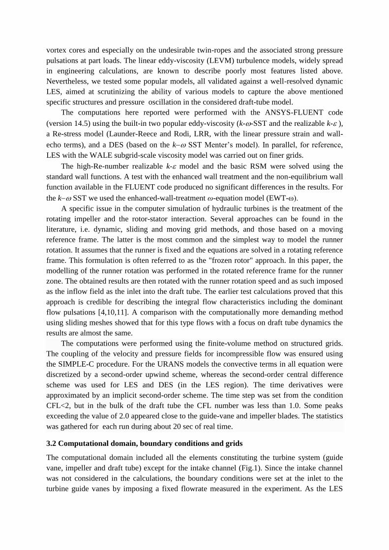
The computations have been carried out using structured grids with the total number of 2, 6

and to 19.3 M (million) nodes for the whole domain. The grid was clustered around the

impeller blades, guide vanes and the draft tube walls (Fig. 3). The average distance of the

wall-nearest grid nodes normalized by the wall units, 1y , for the 2M grid was 9, for the 6M

grid 1.25 and for the 19.3M grid it was 1.05. The corresponding minimum and maximum

values are given in Table 1, together with the proportion of the wall surface bounding the

computational domain where 1y exceeds 2.0. As seen, for the coarse grid of 2M cells, this

portion is 85%, thus disqualifying this grid for the LES. For the 6M grid, the maximum value

of y+ was 23, and the minimum 0.02 with the wall-surface area for which 1y exceeds 2 being

23% of the entire surface. Likewise, for the 19.3M grid, the maximum1y is 4.1, the minimum

0.003. And the wall-area proportion where y exceeds 2, is only 8%, confirming a sufficient

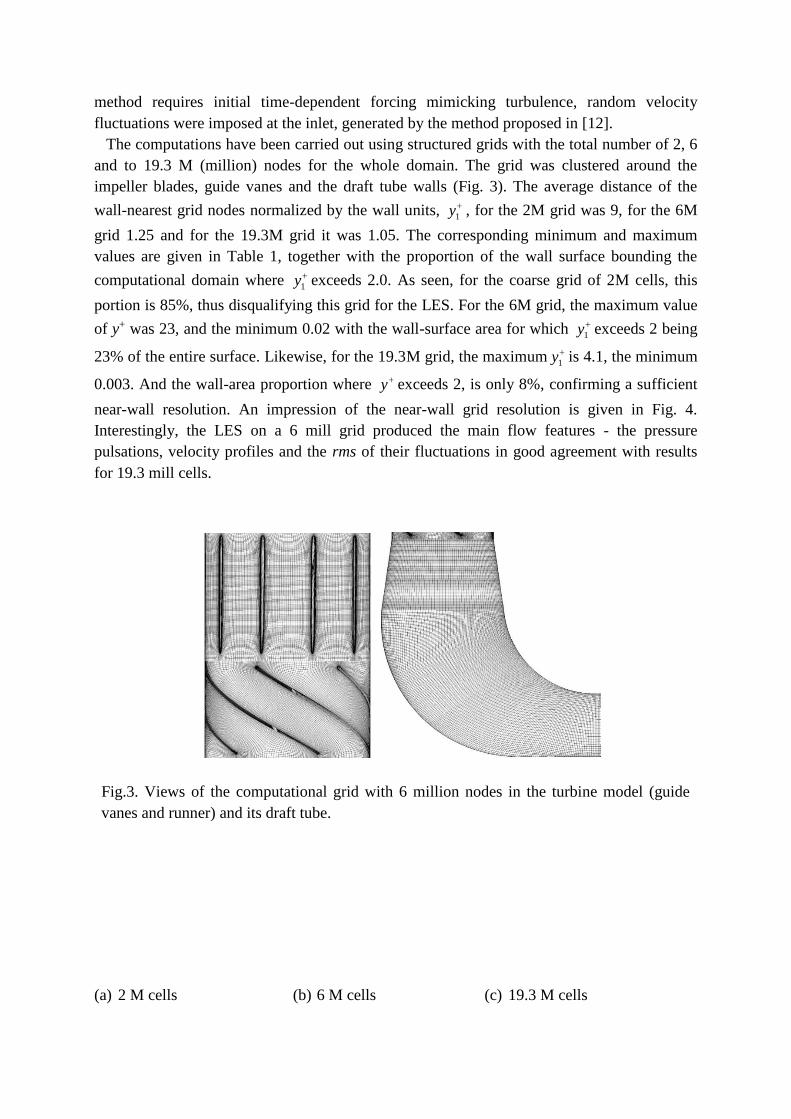
near-wall resolution. An impression of the near-wall grid resolution is given in Fig. 4.

Interestingly, the LES on a 6 mill grid produced the main flow features - the pressure

pulsations, velocity profiles and the rms of their fluctuations in good agreement with results

for 19.3 mill cells.

Fig.3. Views of the computational grid with 6 million nodes in the turbine model (guide

vanes and runner) and its draft tube.

(a) 2 M cells (b) 6 M cells (c) 19.3 M cells

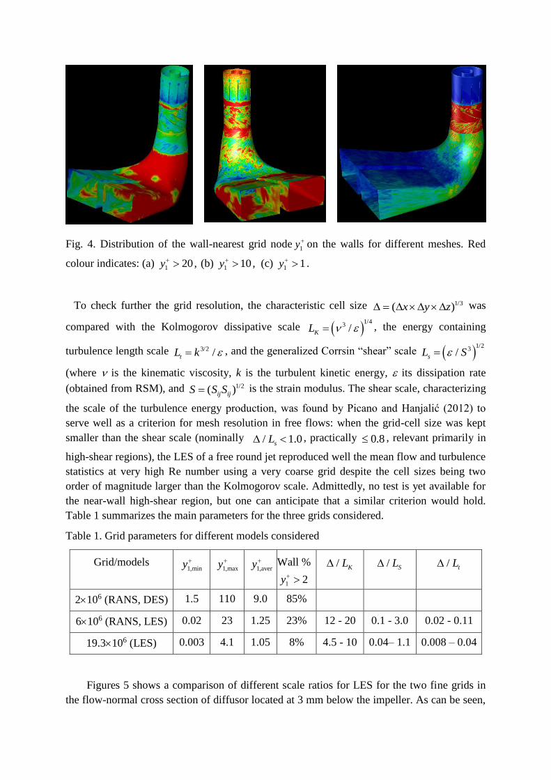
Fig. 4. Distribution of the wall-nearest grid node1y on the walls for different meshes. Red

colour indicates: (a) 1 20y , (b)

1 10y , (c) 1 1y .

To check further the grid resolution, the characteristic cell size 1/3( )x y z was

compared with the Kolmogorov dissipative scale 1/4

3 /KL , the energy containing

turbulence length scale 3/2 /tL k , and the generalized Corrsin “shear” scale 1/2

3/sL S

(where is the kinematic viscosity, k is the turbulent kinetic energy, its dissipation rate

(obtained from RSM), and 1/2( )ij ijS S S is the strain modulus. The shear scale, characterizing

the scale of the turbulence energy production, was found by Picano and Hanjalić (2012) to

serve well as a criterion for mesh resolution in free flows: when the grid-cell size was kept

smaller than the shear scale (nominally / 1.0sL , practically 0.8 , relevant primarily in

high-shear regions), the LES of a free round jet reproduced well the mean flow and turbulence

statistics at very high Re number using a very coarse grid despite the cell sizes being two

order of magnitude larger than the Kolmogorov scale. Admittedly, no test is yet available for

the near-wall high-shear region, but one can anticipate that a similar criterion would hold.

Table 1 summarizes the main parameters for the three grids considered.

Table 1. Grid parameters for different models considered

Grid/models 1,miny

1,maxy

1,avery

Wall %

1 2y

/ KL / SL / tL

2106 (RANS, DES) 1.5 110 9.0 85%

6106 (RANS, LES) 0.02 23 1.25 23% 12 - 20 0.1 - 3.0 0.02 - 0.11

19.3106 (LES) 0.003 4.1 1.05 8% 4.5 - 10 0.04– 1.1 0.008 – 0.04

Figures 5 shows a comparison of different scale ratios for LES for the two fine grids in

the flow-normal cross section of diffusor located at 3 mm below the impeller. As can be seen,

for the grid 6M the ratio / KL of around 15 to 20, whereas for the grid with 19.3M cells

/ KL is less everywhere than 10, except for some sharp peaks very close to the walls in both

cases. Interestingly, the cell-size to shear-scale ration / SL for both grids is below 1.0,

except in the core region for the 6M grid, and of course very close to the wall for both

meshes. This is in agreement with the findings in [15], which shows that the LES method can

return satisfactory predictions when / SL is less than 1.0.

Fig. 5 Grid size compared with turbulence length scales in the middle plane of the horizontal

draft-tube cross- section for 6 M grid (left) and 19.3 M grid (right). Top (red curve) KL L

(Kolmogorov scale), middle (black) sL L (shear scale), bottom (blue) tL L (energy-

containing scale).

3.3 Reference large eddy-simulations: experimental verification

The here reported LES were aimed first to establish more comprehensive reference data

beyond what is available from the experiment, but also to test the LES grid sensitivity,

especially its performance on relatively coarse meshes that do not satisfy the common LES

grid resolution criteria, with a view of possible application to real-scale hydromachinery.

Surprisingly, the mean velocity profiles obtained with LES on very different grids, 6M and

19.3M shown in Fig. 6 (top) agree very well in between and also with the experiments. A

difference appears in the spectra, but primarily at high wave numbers, which apparently does

not affect mush the mean flow characteristics, Fig. 6 (bottom). The successful LES

reproduction of the main flow features in the flow considered using a relatively coarse mesh

of 6 million nodes can be explained by the fact that flow is dominated by the large coherent

spiralling vortex (ropes), and thus not much affected by the unresolved the small-scale

motion. Another explanation can be traced in grid optimization made to satisfy the shear-scale

criterion, / 1SL , congruent with the similar finding for LES of a free round jet reported in

[15].

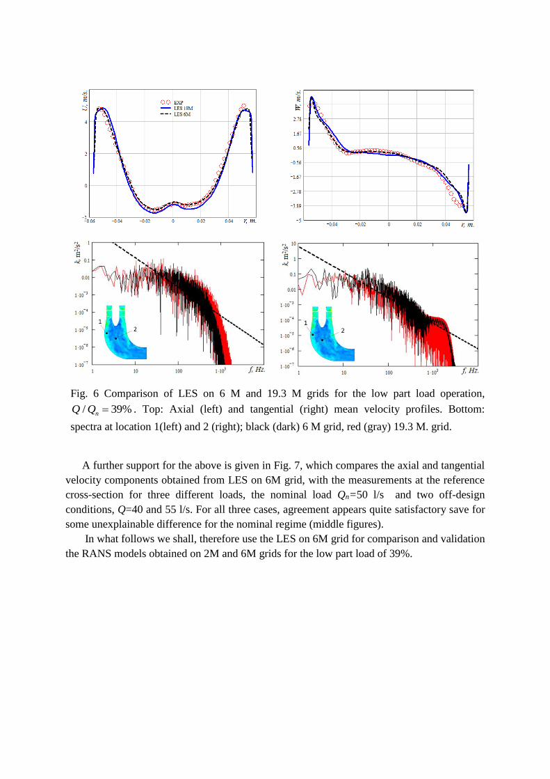
Fig. 6 Comparison of LES on 6 M and 19.3 M grids for the low part load operation,

/ 39%nQ Q . Top: Axial (left) and tangential (right) mean velocity profiles. Bottom:

spectra at location 1(left) and 2 (right); black (dark) 6 M grid, red (gray) 19.3 M. grid.

A further support for the above is given in Fig. 7, which compares the axial and tangential

velocity components obtained from LES on 6M grid, with the measurements at the reference

cross-section for three different loads, the nominal load Qn=50 l/s and two off-design

conditions, Q=40 and 55 l/s. For all three cases, agreement appears quite satisfactory save for

some unexplainable difference for the nominal regime (middle figures).

In what follows we shall, therefore use the LES on 6M grid for comparison and validation

the RANS models obtained on 2M and 6M grids for the low part load of 39%.

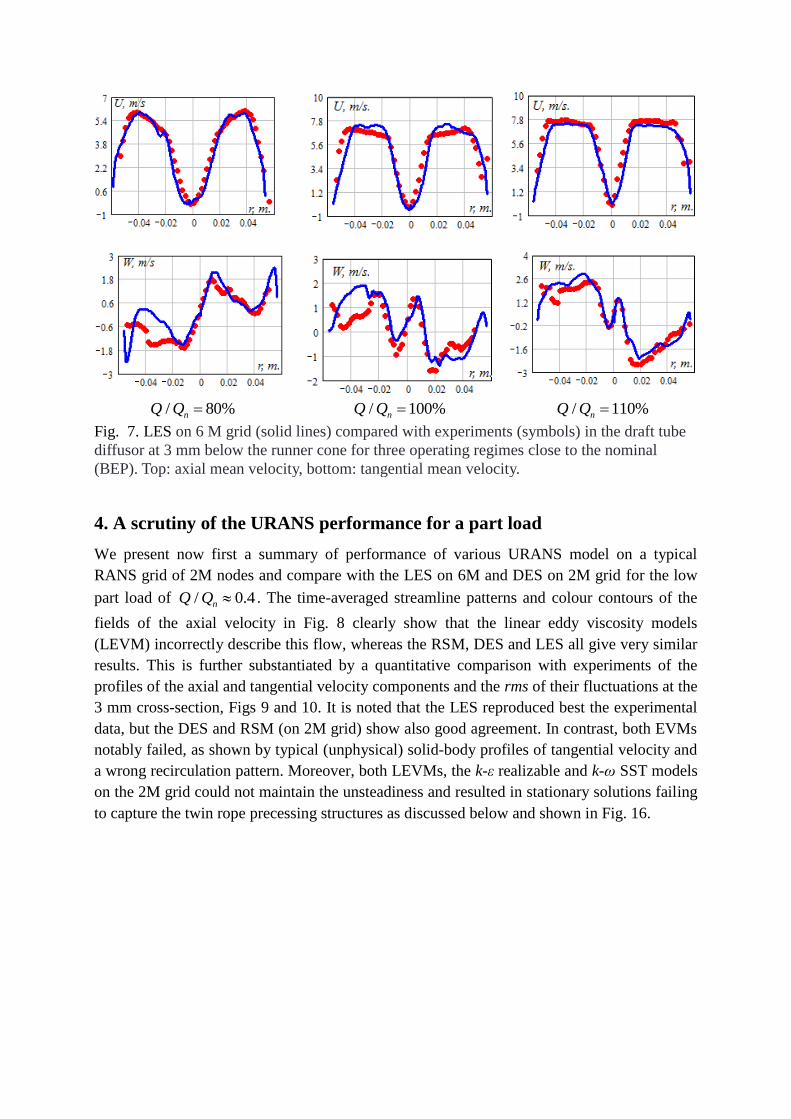
/ 80%nQ Q / 100%nQ Q / 110%nQ Q

Fig. 7. LES on 6 M grid (solid lines) compared with experiments (symbols) in the draft tube

diffusor at 3 mm below the runner cone for three operating regimes close to the nominal

(BEP). Top: axial mean velocity, bottom: tangential mean velocity.

4. A scrutiny of the URANS performance for a part load

We present now first a summary of performance of various URANS model on a typical

RANS grid of 2M nodes and compare with the LES on 6M and DES on 2M grid for the low

part load of / 0.4nQ Q . The time-averaged streamline patterns and colour contours of the

fields of the axial velocity in Fig. 8 clearly show that the linear eddy viscosity models

(LEVM) incorrectly describe this flow, whereas the RSM, DES and LES all give very similar

results. This is further substantiated by a quantitative comparison with experiments of the

profiles of the axial and tangential velocity components and the rms of their fluctuations at the

3 mm cross-section, Figs 9 and 10. It is noted that the LES reproduced best the experimental

data, but the DES and RSM (on 2M grid) show also good agreement. In contrast, both EVMs

notably failed, as shown by typical (unphysical) solid-body profiles of tangential velocity and

a wrong recirculation pattern. Moreover, both LEVMs, the k-ε realizable and k-ω SST models

on the 2M grid could not maintain the unsteadiness and resulted in stationary solutions failing

to capture the twin rope precessing structures as discussed below and shown in Fig. 16.

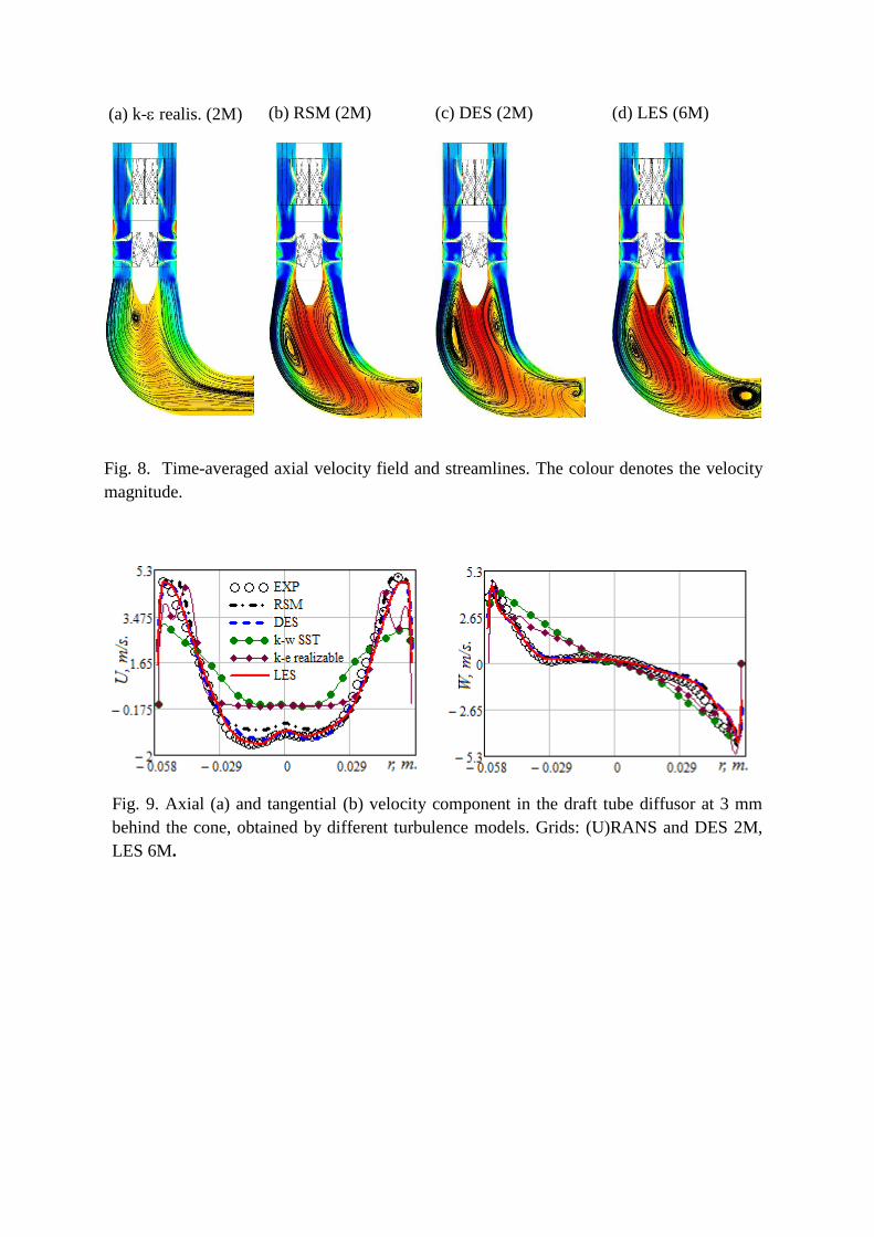
(a) k- realis. (2M) (b) RSM (2M) (c) DES (2M) (d) LES (6M)

Fig. 8. Time-averaged axial velocity field and streamlines. The colour denotes the velocity

magnitude.

Fig. 9. Axial (a) and tangential (b) velocity component in the draft tube diffusor at 3 mm

behind the cone, obtained by different turbulence models. Grids: (U)RANS and DES 2M,

LES 6M.

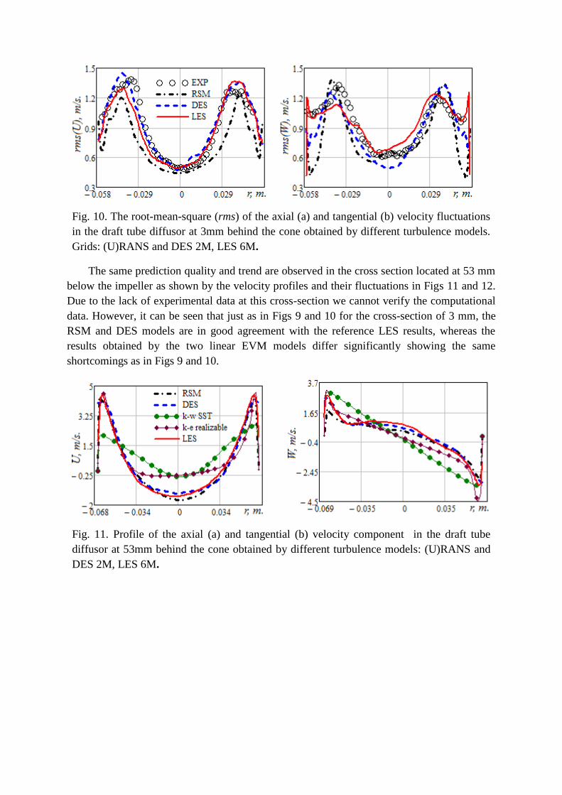
Fig. 10. The root-mean-square (rms) of the axial (a) and tangential (b) velocity fluctuations

in the draft tube diffusor at 3mm behind the cone obtained by different turbulence models.

Grids: (U)RANS and DES 2M, LES 6M.

The same prediction quality and trend are observed in the cross section located at 53 mm

below the impeller as shown by the velocity profiles and their fluctuations in Figs 11 and 12.

Due to the lack of experimental data at this cross-section we cannot verify the computational

data. However, it can be seen that just as in Figs 9 and 10 for the cross-section of 3 mm, the

RSM and DES models are in good agreement with the reference LES results, whereas the

results obtained by the two linear EVM models differ significantly showing the same

shortcomings as in Figs 9 and 10.

Fig. 11. Profile of the axial (a) and tangential (b) velocity component in the draft tube

diffusor at 53mm behind the cone obtained by different turbulence models: (U)RANS and

DES 2M, LES 6M.

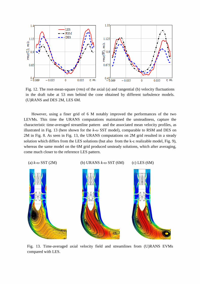
Fig. 12. The root-mean-square (rms) of the axial (a) and tangential (b) velocity fluctuations

in the draft tube at 53 mm behind the cone obtained by different turbulence models.

(U)RANS and DES 2M, LES 6M.

However, using a finer grid of 6 M notably improved the performances of the two

LEVMs. This time the URANS computations maintained the unsteadiness, capture the

characteristic time-averaged streamline pattern and the associated mean velocity profiles, as

illustrated in Fig. 13 (here shown for the k-ω SST model), comparable to RSM and DES on

2M in Fig. 8. As seen in Fig. 13, the URANS computations on 2M grid resulted in a steady

solution which differs from the LES solutions (but also from the k- realizable model, Fig. 9),

whereas the same model on the 6M grid produced unsteady solutions, which after averaging,

come much closer to the reference LES pattern.

(a) k-ω SST (2M) (b) URANS k-ω SST (6M) (c) LES (6M)

Fig. 13. Time-averaged axial velocity field and streamlines from (U)RANS EVMs

compared with LES.

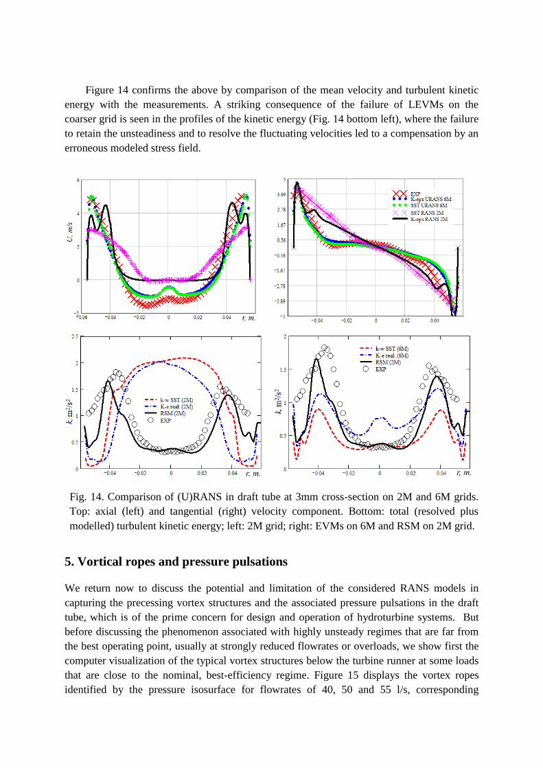
Figure 14 confirms the above by comparison of the mean velocity and turbulent kinetic

energy with the measurements. A striking consequence of the failure of LEVMs on the

coarser grid is seen in the profiles of the kinetic energy (Fig. 14 bottom left), where the failure

to retain the unsteadiness and to resolve the fluctuating velocities led to a compensation by an

erroneous modeled stress field.

Fig. 14. Comparison of (U)RANS in draft tube at 3mm cross-section on 2M and 6M grids.

Top: axial (left) and tangential (right) velocity component. Bottom: total (resolved plus

modelled) turbulent kinetic energy; left: 2M grid; right: EVMs on 6M and RSM on 2M grid.

5. Vortical ropes and pressure pulsations

We return now to discuss the potential and limitation of the considered RANS models in

capturing the precessing vortex structures and the associated pressure pulsations in the draft

tube, which is of the prime concern for design and operation of hydroturbine systems. But

before discussing the phenomenon associated with highly unsteady regimes that are far from

the best operating point, usually at strongly reduced flowrates or overloads, we show first the

computer visualization of the typical vortex structures below the turbine runner at some loads

that are close to the nominal, best-efficiency regime. Figure 15 displays the vortex ropes

identified by the pressure isosurface for flowrates of 40, 50 and 55 l/s, corresponding

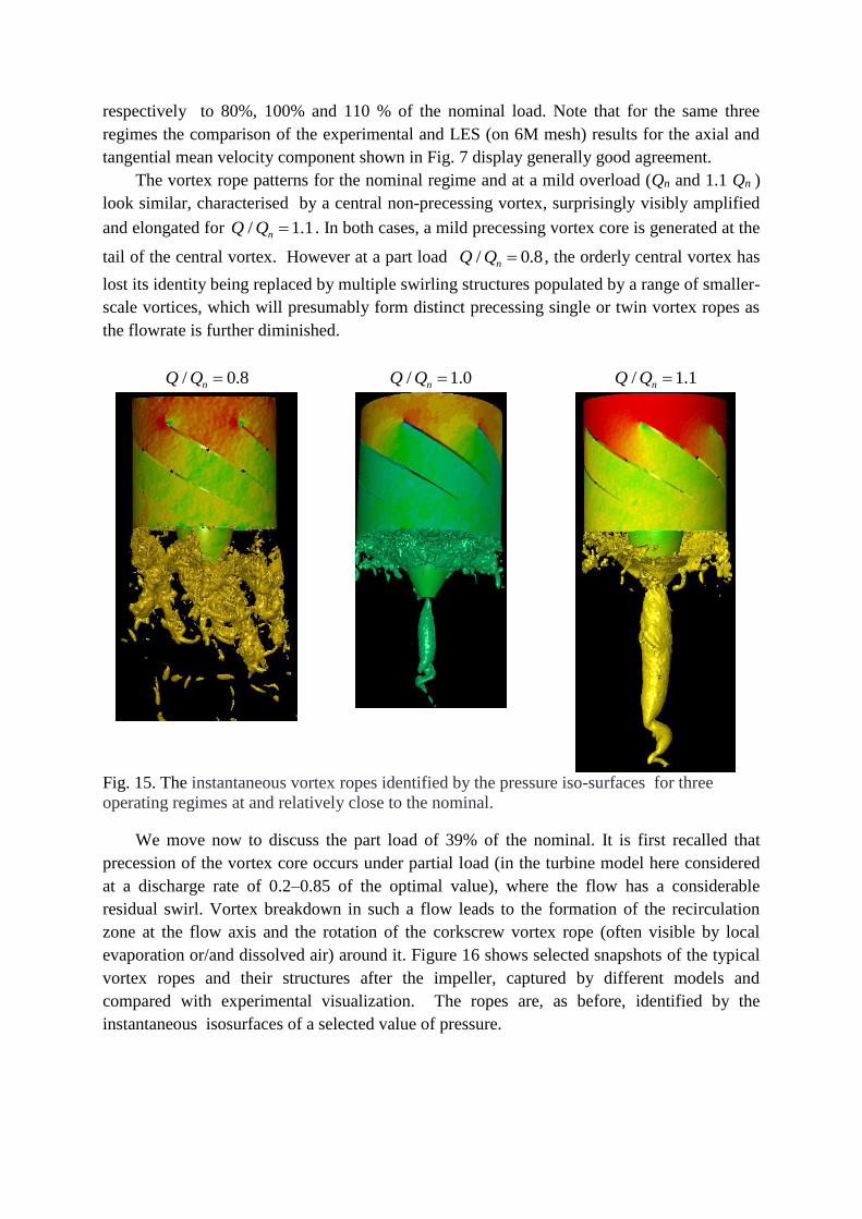
respectively to 80%, 100% and 110 % of the nominal load. Note that for the same three

regimes the comparison of the experimental and LES (on 6M mesh) results for the axial and

tangential mean velocity component shown in Fig. 7 display generally good agreement.

The vortex rope patterns for the nominal regime and at a mild overload (Qn and 1.1 Qn )

look similar, characterised by a central non-precessing vortex, surprisingly visibly amplified

and elongated for / 1.1nQ Q . In both cases, a mild precessing vortex core is generated at the

tail of the central vortex. However at a part load / 0.8nQ Q , the orderly central vortex has

lost its identity being replaced by multiple swirling structures populated by a range of smaller-

scale vortices, which will presumably form distinct precessing single or twin vortex ropes as

the flowrate is further diminished.

/ 0.8nQ Q / 1.0nQ Q / 1.1nQ Q

Fig. 15. The instantaneous vortex ropes identified by the pressure iso-surfaces for three

operating regimes at and relatively close to the nominal.

We move now to discuss the part load of 39% of the nominal. It is first recalled that

precession of the vortex core occurs under partial load (in the turbine model here considered

at a discharge rate of 0.2–0.85 of the optimal value), where the flow has a considerable

residual swirl. Vortex breakdown in such a flow leads to the formation of the recirculation

zone at the flow axis and the rotation of the corkscrew vortex rope (often visible by local

evaporation or/and dissolved air) around it. Figure 16 shows selected snapshots of the typical

vortex ropes and their structures after the impeller, captured by different models and

compared with experimental visualization. The ropes are, as before, identified by the

instantaneous isosurfaces of a selected value of pressure.

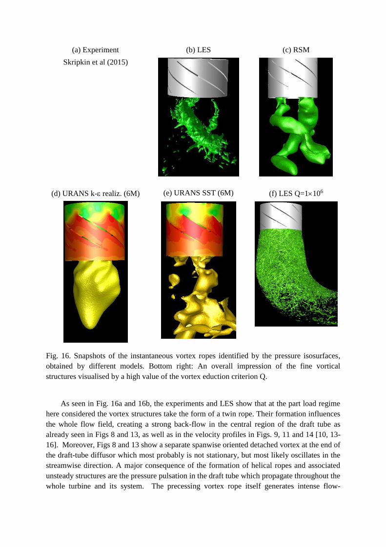
(a) Experiment (b) LES (c) RSM

Skripkin et al (2015)

(d) URANS k- realiz. (6M) (e) URANS SST (6M) (f) LES Q=1106

Fig. 16. Snapshots of the instantaneous vortex ropes identified by the pressure isosurfaces,

obtained by different models. Bottom right: An overall impression of the fine vortical

structures visualised by a high value of the vortex eduction criterion Q.

As seen in Fig. 16a and 16b, the experiments and LES show that at the part load regime

here considered the vortex structures take the form of a twin rope. Their formation influences

the whole flow field, creating a strong back-flow in the central region of the draft tube as

already seen in Figs 8 and 13, as well as in the velocity profiles in Figs. 9, 11 and 14 [10, 13-

16]. Moreover, Figs 8 and 13 show a separate spanwise oriented detached vortex at the end of

the draft-tube diffusor which most probably is not stationary, but most likely oscillates in the

streamwise direction. A major consequence of the formation of helical ropes and associated

unsteady structures are the pressure pulsation in the draft tube which propagate throughout the

whole turbine and its system. The precessing vortex rope itself generates intense flow-

induced pulsations, which pose a serious threat to the reliability and safety of operation of

hydraulic turbine equipment. Pressure pulsations lead to vibrations of the turbine structure

that can lead to damage, especially in the case of resonance. Pressure pulsations, generated by

vortex ropes may also affect cavitation processes.

It is interesting that the Re-stress LRR model captures well the phenomenon, albeit with

smoothed fine-scale structures, Fig. 16c. However, despite maintaining the unsteadiness and

reproducing reasonably well the man velocity components and their rms (Figs 13 and 14),

none of the tested LEVM URANS even on the 6M grid, reproduced the twin-rope vortical

pattern, as revealed in Figs 16d and 16e! The k-ε realizable model gives one thick vortex

showing little if any precessing, Fig.16d, and the SST model gives only a hint at possible

double vortex initiation, but with only one, irregularly shaped structure with no indication of a

spiralling helical pattern. Likewise, although the unsteady LEVM solutions capture some

transient pressure pulsation, the intensity and the character are not in accord with the

experiments or LES.

For practice, whether design or operation, it is vital to know the characteristic

parameters of the pressure pulsations, primarily their intensity (especially the maximum

amplitudes) and frequency. Since for the evaluation of these parameters the industry relies

now more and more on the CFD computations, using most often licenced CFD codes , it is

essential to know a priori which of the model and method can be relied upon to deliver these

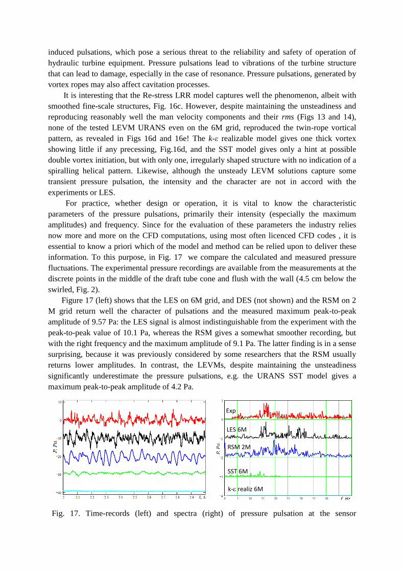
information. To this purpose, in Fig. 17 we compare the calculated and measured pressure

fluctuations. The experimental pressure recordings are available from the measurements at the

discrete points in the middle of the draft tube cone and flush with the wall (4.5 cm below the

swirled, Fig. 2).

Figure 17 (left) shows that the LES on 6M grid, and DES (not shown) and the RSM on 2

M grid return well the character of pulsations and the measured maximum peak-to-peak

amplitude of 9.57 Pa: the LES signal is almost indistinguishable from the experiment with the

peak-to-peak value of 10.1 Pa, whereas the RSM gives a somewhat smoother recording, but

with the right frequency and the maximum amplitude of 9.1 Pa. The latter finding is in a sense

surprising, because it was previously considered by some researchers that the RSM usually

returns lower amplitudes. In contrast, the LEVMs, despite maintaining the unsteadiness

significantly underestimate the pressure pulsations, e.g. the URANS SST model gives a

maximum peak-to-peak amplitude of 4.2 Pa.

Fig. 17. Time-records (left) and spectra (right) of pressure pulsation at the sensor

Exp

LES 6M

RSM 2M

k- realiz 6M

SST 6M

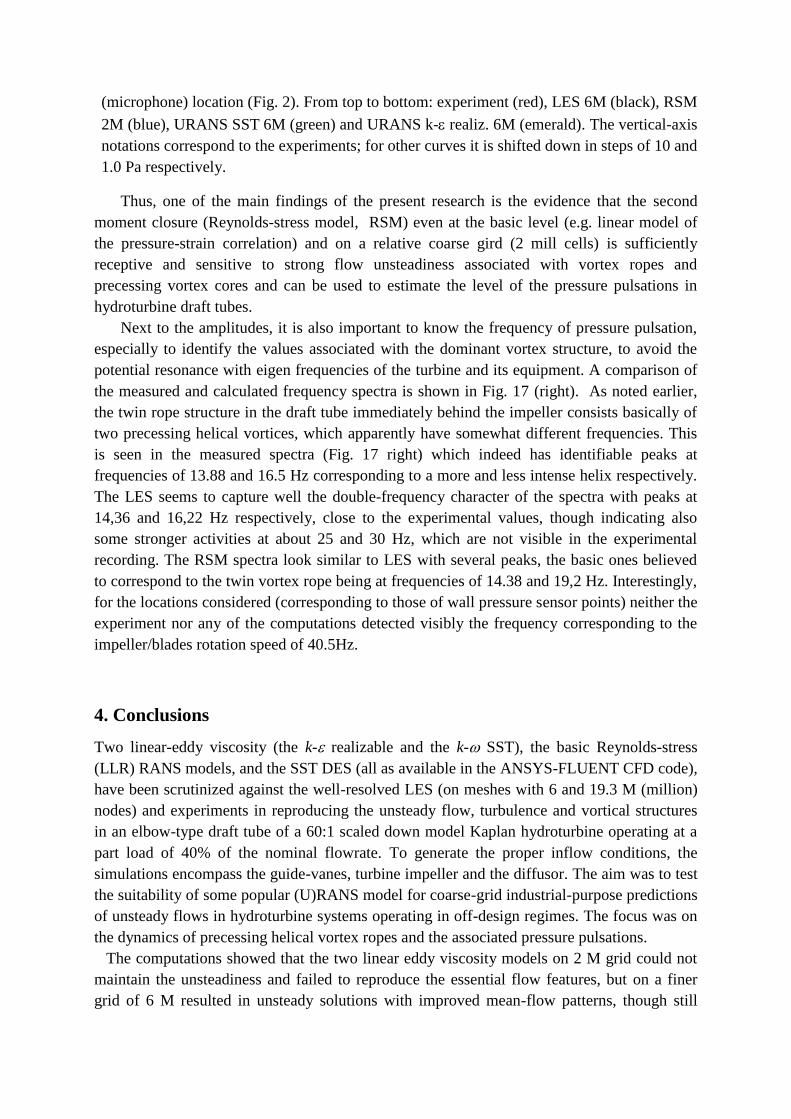
(microphone) location (Fig. 2). From top to bottom: experiment (red), LES 6M (black), RSM

2M (blue), URANS SST 6M (green) and URANS k- realiz. 6M (emerald). The vertical-axis

notations correspond to the experiments; for other curves it is shifted down in steps of 10 and

1.0 Pa respectively.

Thus, one of the main findings of the present research is the evidence that the second

moment closure (Reynolds-stress model, RSM) even at the basic level (e.g. linear model of

the pressure-strain correlation) and on a relative coarse gird (2 mill cells) is sufficiently

receptive and sensitive to strong flow unsteadiness associated with vortex ropes and

precessing vortex cores and can be used to estimate the level of the pressure pulsations in

hydroturbine draft tubes.

Next to the amplitudes, it is also important to know the frequency of pressure pulsation,

especially to identify the values associated with the dominant vortex structure, to avoid the

potential resonance with eigen frequencies of the turbine and its equipment. A comparison of

the measured and calculated frequency spectra is shown in Fig. 17 (right). As noted earlier,

the twin rope structure in the draft tube immediately behind the impeller consists basically of

two precessing helical vortices, which apparently have somewhat different frequencies. This

is seen in the measured spectra (Fig. 17 right) which indeed has identifiable peaks at

frequencies of 13.88 and 16.5 Hz corresponding to a more and less intense helix respectively.

The LES seems to capture well the double-frequency character of the spectra with peaks at

14,36 and 16,22 Hz respectively, close to the experimental values, though indicating also

some stronger activities at about 25 and 30 Hz, which are not visible in the experimental

recording. The RSM spectra look similar to LES with several peaks, the basic ones believed

to correspond to the twin vortex rope being at frequencies of 14.38 and 19,2 Hz. Interestingly,

for the locations considered (corresponding to those of wall pressure sensor points) neither the

experiment nor any of the computations detected visibly the frequency corresponding to the

impeller/blades rotation speed of 40.5Hz.

4. Conclusions

Two linear-eddy viscosity (the k- realizable and the k- SST), the basic Reynolds-stress

(LLR) RANS models, and the SST DES (all as available in the ANSYS-FLUENT CFD code),

have been scrutinized against the well-resolved LES (on meshes with 6 and 19.3 M (million)

nodes) and experiments in reproducing the unsteady flow, turbulence and vortical structures

in an elbow-type draft tube of a 60:1 scaled down model Kaplan hydroturbine operating at a

part load of 40% of the nominal flowrate. To generate the proper inflow conditions, the

simulations encompass the guide-vanes, turbine impeller and the diffusor. The aim was to test

the suitability of some popular (U)RANS model for coarse-grid industrial-purpose predictions

of unsteady flows in hydroturbine systems operating in off-design regimes. The focus was on

the dynamics of precessing helical vortex ropes and the associated pressure pulsations.

The computations showed that the two linear eddy viscosity models on 2 M grid could not

maintain the unsteadiness and failed to reproduce the essential flow features, but on a finer

grid of 6 M resulted in unsteady solutions with improved mean-flow patterns, though still

failing to capture the twin-helix structures and the pressure pulsations. In contrast, the second-

moment closure (Re-stress) model on the same 2M mesh recovers well both the mean velocity

field, the rms of its fluctuations, as well as the specific helical double rope structure in accord

with experiments and LES. Similar performance is returned by DES.

It was also shown that the LES on a 6M and 19.3 M grids performed similarly. This, to

some extent surprising finding, is attributed to the fact that the cell size was optimized to be

smaller than the Corrsin shear scale, while resolving the fine scales proved not to be essential

for the flow dominated by strong large-scale coherent vortical structures.

5. Acknowledgements.

This work was supported by the Russian Science Foundation (grant №14-29-00203).

References

1. Doerfler P. System dynamics of the Francis turbine half load surge. 1982, Proc. IAHR

Symp. on Hydraulic Machinery and Systems, Amsterdam, Netherlands.

2. Alligne S., Maruzewski P., Dinh T., Wang B., Fedorov A., Iosfin J. and Avellan F., 2010,

Prediction of a Francis turbine prototype full load instability from investigations on the

reduced scale model. Proc. IAHR Symp. on Hydraulic Machinery and Systems, Timisoara,

Romania.

3. Cervantes M.J., Engstrom T.F., Gustavsson L.H., 2005, Proc. The third IAHR/

ERCOFTAC workshop on draft tube flows Turbine 99. Sweden, Porjus,. 193 p.

4. Minakov, A.V. Sentyabov, D.V. Platonov, A.A. Dekterev, A.A. Gavrilov, 2014,

Numerical modeling of flow in the Francis-99 turbine with Reynolds stress model and

detached eddy simulation method. Journal of Physics: Conference Series Volume 579,

doi:10.1088/1742-6596/579/1/012004.

5. Bosioc Alin, Tanasa Constantin, Susan-Resiga Romeo, Muntean Sebastian. 2D LDV

Measurements of Swirling Flow in a Simplified Draft Tube, Conf. Model. Fluid Flow. -

2009.

6. Chen Chang-Kun, Nicolet Christophe, Yonezawa Koichi, Farhat Mohamed, Avellan

Francois, Miyazawa Kazuyoshi, Tsujimoto Yoshinobu. Experimental Study and

Numerical Simulation of Cavity Oscillation in a Diffuser with Swirling Flow, Int. J. Fluid

Mach. Syst. Korean Fluid Machinery Association, - 2010. - Vol. 3, № 1. - P. 80–90.

7. Susan-Resiga Romeo, Muntean Sebastian, Tanasa Constantin, Bosioc Alin.

Hydrodynamic Design and Analysis of a Swirling Flow Generator // Proc. 4th Ger. –

Rom. Work. Turbomach. Hydrodyn. (GRoWTH), June 12-15, 2008, Stuttgart, Ger.

8. Kuibin P.A., Litvinov I.V., Sonin V.I., Ustimenko A.S., Shtork S.I. Modelling inlet flow in

draft tube for different regimes of hydro turbine operation // Vestnik Novosibirsk State

University. Series: Physics., 2016, in press

9. Litvinov I. V., Shtork S.I., Kuibin P.A., Alekseenko S. V., Hanjalic K., 2013,

Experimental study and analytical reconstruction of precessing vortex in a tangential

swirler, Int. J. Heat Fluid Flow 42: 251–264.

10. Minakov, A.V., Platonov, D.V., Dekterev, A.A., Sentyabov, A.V., Zakharov, A.V., 2015,.

The numerical simulation of low frequency pressure pulsations in the high-head Francis

turbine. Computers & Fluids. 111: 197–205.

11. Minakov, A.V., Platonov, D.V., Dekterev, A.A., Sentyabov, A.V., Zakharov, A.V., 2015,

The analysis of unsteady flow structure and low frequency pressure pulsations in the high-

head Francis turbines. Int. J. Heat and Fluid Flow 53: 183–194.

12. Smirnov, R., Shi, S., Celik, I., 2001, Random flow generation technique for large-eddy

simulations and particle-dynamics modeling, J. Fluids Engineering. 123: 359–371.

13. Shtork S.I., Cala C.E., Fernandes E.C., 2007, Experimental characterization of rotating

flow field in a model vortex burner, Exp. Therm. Fluid Sci. 31: 779–788.

14. Nicoud, F. and Ducros, F., 1999, Subgrid-Scale Stress Modelling Based on the Square of

the Velocity Gradient Tensor. Flow, Turbulence and Combustion, 62(3). 183–200.

15. Picano, S. and Hanjalić, K., 2012, Leray-α regularization of the Smagorinsky-closed

filtered equations for turbulent jets at high Reynolds numbers, Flow, Turbulence and

Combustion, 89: 627–650.

16. Skripkin, D.G., Tsoy, MA. Shtork, S.I. and Hanjalic, K. Comparative analysis of twin

vortex ropes in laboratory models if two hydroturbine draft tubes. (under consideration for

publication in J. Hydraulic Research).

17. Minakov, A., Platonov, D., Litvinov, I., and Hanjalić, K., 2015, Computer simulation of

flow at part load in a laboratory model of a Kaplan hydroturbine by RANS, DES and LES.

In: Hanjalić et al (Eds), Turbulence, Heat and Mass Transfer 8, Begell House Inc., New

York, 849-853.