1133Bull. Pol. Ac.: Tech. 67(6) 2019

BULLETIN OF THE POLISH ACADEMY OF SCIENCES TECHNICAL SCIENCES, Vol. 67, No. 6, 2019DOI: 10.24425/bpasts.2019.130888

Abstract. The paper concerns the engineering design of guide vane and runner blades of hydraulic turbines using the inverse problem on the basis of the definition of a velocity hodograph, which is based on Wu’s theory [1, 2]. The design concerns the low-head double-regulated axial Kaplan turbine model characterized by a very high specific speed. The three-dimensional surfaces of turbine blades are based on meridional geometry that is determined in advance and, additionally, the distribution of streamlines must also be defined. The principles of the method applied for the hydraulic turbine and related to its conservation equations are also presented. The conservation equations are written in a cur-vilinear coordinate system, which adjusts to streamlines by means of the Christoffel symbols. This leads to significant simplification of the computations and generates fast results of three-dimensional blade surfaces. Then, the solution can be found using the method of characteristics. To assess usefulness of the design and robustness of the method, numerical and experimental investigations in a wide range of operations were carried out. Afterwards, the so-called shell characteristics were determined by means of experiments, which allowed to evaluate the method for application to the low-head (1.5 m) Kaplan hydraulic turbine model with the kinematic specific speed (»260). The numerical and experimental results show the successful usage of the method and it can be concluded that it will be useful in designing other types of Kaplan and Francis turbine blades with different specific speeds.

Key words: inverse method, hydraulic turbine blade design, low-head Kaplan turbine, curvilinear coordinate system, Christoffel symbols.

Engineering design of low-head Kaplan hydraulic turbine blades using the inverse problem method

Z. KRZEMIANOWSKI*The Szewalski Institute of Fluid-Flow Machinery of the Polish Academy of Sciences, J. Fiszera 14, 80-231 Gdańsk, Poland

such cases, CFD is a very powerful tool to evaluate off-design machine operation. Additionally, it helps eliminate significant mistakes in the design process.

Over the years, a number of activities in the application of the inverse problem to turbomachinery have been performed, caused inter alia by the significant development of computers. A vast amount of research regarding the issue of the design process for turbomachines with incompressible and compressible flows was published in the past 4 decades. The improvements proposed through the years for turbomachinery (gas turbines, compres-sors, pumps) by as part of inverse design introduced extensive development and progress of its performance [3–8]. Relating to hydraulic machines, in many papers researchers presented the advantages of two-dimensional and a three-dimensional inverse problem applications to pumps and hydraulic turbines and their operational optimization [9–14]. An approach to the optimization of losses and cavitation number in the axial flow turbine runner can also be found in papers [15, 16]. The common availability of the CFD commercial codes provided for the possibility of an interactive aided inverse design process of hydraulic machines. It still remains faster and less time-consuming than designing by means of analyzing with the use of the CFD alone. For instance, interaction with the CFD allows for eliminating/reducing the secondary flows [17, 18] or reducing the area of pressure below the vapor pressure, which means decreasing intensity of the cav-itation phenomenon [19] and/or estimating the hydrodynamic and suction performance [20]. Generally, mutual interaction of the inverse problem and CFD calculations leads to improving operational parameters, especially the efficiency of hydraulic machines and anti-cavitation performance. However, in some cases in which a fast technical design is required, particularly in the case of small low-cost low-head hydraulic turbines, CFD

1. Introduction

The design of rotating machines including hydraulic turbines and pumps is difficult and requires a comprehensive approach in order to achieve high efficiency and avoid the cavitation phenomenon. This is due to the phenomena occurring in flow passage, which are described by non-linear equations that have to be solved to obtain the flow field. The use of iterative way of designing by means of CFD methods now significantly improves this process and allows for peer numerical analysis of phenomena such as: secondary flows, cavitation prediction, etc. However, on the other hand, the use of CFD is often related to the time-consuming process of determining blade geometry (often, the design of such geometry must be relatively quick for a customer) because direct design (problem) introduces the difficulty of determining the direction of changes leading to the improvement of the blade design due to the complicated three-dimensional nature of the flow through the machine. Then, as an alternative, the inverse problem blade design (deter-mination of the skeleton blade surface) may be helpful, which is significantly faster than the blade design using the direct problem. Obviously, it constitutes good practice to use CFD analysis because the inverse problem design provides the blade geometry at one point of operation, which is supposed to be the best efficiency point (BEP). In fact, it may happen that it works well at this point but the efficiency may rapidly decrease in its vicinity (i.e. by changing the flow rate or/and head). In

*e-mail: krzemian@imp.gda.pl

Manuscript submitted 2019-01-25, revised 2019-03-26, initially accepted for publication 2019-04-19, published in December 2019

THERMODYNAMICS AND MECHANICAL ENGINEERING

1134

Z. Krzemianowski

Bull. Pol. Ac.: Tech. 67(6) 2019

cannot be used because of too long time required. In such cases design by means of an inverse problem is indispensable.

Generally, inverse problems in hydrodynamics are based on potential flow models [21–24] or the flow models using Euler’s equation [7, 25], in which slip condition is imposed at the walls. Models containing viscosity (non-slip condition), i.e. using the Navier-Stokes equation [8, 26], can already be encountered.

The goal of the current work is to design a blade cascade (double-adjustable turbine) by means of the inverse problem method using hodograph theory. The principles of theory are derived from the fundamental works of Wu [1, 2], which are based on the concept of two surfaces called S1 (streamline sur-faces) and S2 (blade surfaces). Generally, this inverse method is suitable for a wide range of subtypes of turbomachines. The basics of this method in application to the design of the Kaplan hydraulic turbine guide vane and runner blades with the very high kinematic specific speed nsq = »260 are presented. This quantity is extremely important for the engineering design pro-cess of hydraulic turbines because it determines their meridio-nal shape and is defined as follows (note: this is not a non-di-mensional quantity):

2

hydraulic machines and anti-cavitation performance. However, in some cases in which a fast technical design is required, particularly in the case of small low-cost low-head hydraulic turbines, CFD cannot be used because of too long time required. In such cases the design by means of an inverse problem is indispensable.

Generally, inverse problems in hydrodynamics are based on potential flow models [21–24] or the flow models using the Euler’s equation [7, 25], in which slip condition at the walls is imposed. Models containing viscosity (non-slip condition), i.e., using the Navier-Stokes equation [8, 26] can already be encountered.

The goal of the current work is to design blade cascade (double-adjustable turbine) by means of the inverse problem method using a hodograph theory. The principles of theory are derived from the fundamental works of Wu [1, 2], which are based on the concept of two surfaces called S1 (streamline surfaces) and S2 (blade surfaces). Generally, this inverse method is suitable for a wide range of subtypes of turbomachines. The basics of this method in application to the design of the Kaplan hydraulic turbine guide vane and runner blades with the very high kinematic specific speed nsq = ~260 are presented. This quantity in engineering design process of hydraulic turbines is extremely important, because it determines their meridional shape and is defined as follows (note: this is not a non-dimensional quantity):

𝑛𝑛𝑠𝑠𝑠𝑠 = 𝑛𝑛 𝑄𝑄0.5

𝐻𝐻0.75 (1)

where n is the rotational speed [rpm], Q is the volumetric flow rate [m3/s], and H is the head [m].

2. Theoretical background

2.1. The principles. The flow through the rotating machine is fully three-dimensional due to the phenomena occurring in the flow (secondary flows, blade vortices, pressure pulsations on the blades and in the draft tube). However, with well-posed boundary conditions, in the case of hydraulic machinery such as hydraulic turbines (particularly low-head), fast engineering methods containing significant simplifications may be considered to be sufficient for engineering purposes to achieve good results of the design.

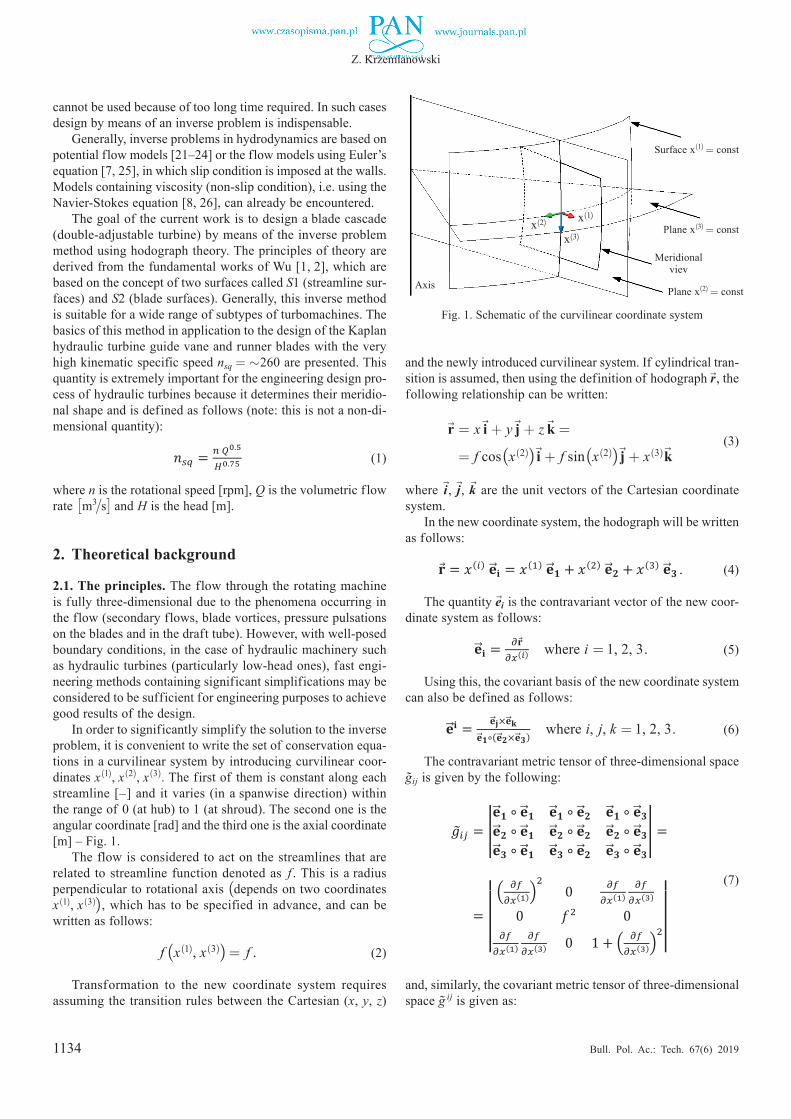
In order to significantly simplify the solution to the inverse problem, it is convenient to write the set of conservations equations in a curvilinear system by introducing curvilinear coordinates 𝑥𝑥(1), 𝑥𝑥(2), 𝑥𝑥(3). First of them is constant along each streamline [-] and it varies (in a spanwise direction) within the range of 0 (at hub) to 1 (at shroud). Second one is the angular coordinate [rad] and third one is the axial coordinate [m] – Figure 1.

Fig. 1. Schematic of the curvilinear coordinate system.

Transformation to the new coordinate system requires

assuming the transition rules between the Cartesian (x, y, z) and the newly introduced curvilinear system. If a cylindrical transition is assumed, then using definition of a hodograph �⃗�𝒓 , the following relationship can be written:

𝐫𝐫 = 𝑥𝑥 𝐢𝐢 + 𝑦𝑦 𝐣𝐣 + 𝑧𝑧 𝐤𝐤 =

= |𝑟𝑟| cos(𝑥𝑥(2))𝐢𝐢 + |𝑟𝑟| sin(𝑥𝑥(2))𝐣𝐣 + 𝑥𝑥(3)𝐤𝐤 (2)

where 𝒊𝒊,⃗⃗ 𝒋𝒋,⃗⃗ 𝒌𝒌 ⃗⃗ ⃗ are the unit vectors of the Cartesian coordinate system.

The hodograph must be dependent on the coordinates operating in a meridional plane, i.e. 𝑥𝑥(1), 𝑥𝑥(3). Since the flow is considered to act on the streamlines, so it is related to streamline function, denoted as f, which has to be specified in advance. In such a case the hodograph, which is the radius can be written as follows:

|𝑟𝑟| = 𝑟𝑟 (𝑥𝑥(1), 𝑥𝑥(3)) ≡ 𝑓𝑓 (𝑥𝑥(1), 𝑥𝑥(3)) = 𝑓𝑓 (3)

In the new coordinate system, the hodograph will be written as follows:

𝐫𝐫 = 𝑥𝑥(𝑖𝑖) �⃗�𝐞 𝐢𝐢 = 𝑥𝑥(1) �⃗�𝐞 𝟏𝟏 + 𝑥𝑥(2) �⃗�𝐞 𝟐𝟐 + 𝑥𝑥(3) �⃗�𝐞 𝟑𝟑 (4)

The quantity �⃗�𝒆 𝒊𝒊 is contravariant vector of the new coordinate system as follows:

�⃗�𝐞 𝐢𝐢 = 𝜕𝜕𝐫𝐫 𝜕𝜕𝑥𝑥(𝑖𝑖) where i = 1, 2, 3 (5)

Using this, covariant basis of the new coordinate system can also be defined as follows:

�⃗�𝐞 𝐢𝐢 = �⃗�𝐞 𝐣𝐣×�⃗�𝐞 𝐤𝐤�⃗�𝐞 𝟏𝟏∘(�⃗�𝐞 𝟐𝟐×�⃗�𝐞 𝟑𝟑) where i, j, k = 1, 2, 3 (6)

The contravariant metric tensor of three-dimensional space �̃�𝑔𝑖𝑖𝑖𝑖 is given:

(1)

where n is the rotational speed [rpm], Q is the volumetric f low rate

£m3/s¤ and H is the head [m].

2. Theoretical background

2.1. The principles. The flow through the rotating machine is fully three-dimensional due to the phenomena occurring in the flow (secondary flows, blade vortices, pressure pulsations on the blades and in the draft tube). However, with well-posed boundary conditions, in the case of hydraulic machinery such as hydraulic turbines (particularly low-head ones), fast engi-neering methods containing significant simplifications may be considered to be sufficient for engineering purposes to achieve good results of the design.

In order to significantly simplify the solution to the inverse problem, it is convenient to write the set of conservation equa-tions in a curvilinear system by introducing curvilinear coor-dinates x(1), x(2), x(3). The first of them is constant along each streamline [–] and it varies (in a spanwise direction) within the range of 0 (at hub) to 1 (at shroud). The second one is the angular coordinate [rad] and the third one is the axial coordinate [m] – Fig. 1.

The flow is considered to act on the streamlines that are related to streamline function denoted as f . This is a radius perpendicular to rotational axis (depends on two coordinates x(1), x(3)), which has to be specified in advance, and can be written as follows:

f (x(1), x(3)) =  f . (2)

Transformation to the new coordinate system requires assuming the transition rules between the Cartesian (x, y, z)

and the newly introduced curvilinear system. If cylindrical tran-sition is assumed, then using the definition of hodograph r→, the following relationship can be written:

r→ = x  i

→ + y  j

→  + z  k

→ = 

r→ = f cos(x(2)) i→ + f sin(x(2)) j

→  + x(3) k

→ (3)

where  i→,  j

→,  k

→ are the unit vectors of the Cartesian coordinate

system.In the new coordinate system, the hodograph will be written

as follows:

2

hydraulic machines and anti-cavitation performance. However, in some cases in which a fast technical design is required, particularly in the case of small low-cost low-head hydraulic turbines, CFD cannot be used because of too long time required. In such cases the design by means of an inverse problem is indispensable.

Generally, inverse problems in hydrodynamics are based on potential flow models [21–24] or the flow models using the Euler’s equation [7, 25], in which slip condition at the walls is imposed. Models containing viscosity (non-slip condition), i.e., using the Navier-Stokes equation [8, 26] can already be encountered.

The goal of the current work is to design blade cascade (double-adjustable turbine) by means of the inverse problem method using a hodograph theory. The principles of theory are derived from the fundamental works of Wu [1, 2], which are based on the concept of two surfaces called S1 (streamline surfaces) and S2 (blade surfaces). Generally, this inverse method is suitable for a wide range of subtypes of turbomachines. The basics of this method in application to the design of the Kaplan hydraulic turbine guide vane and runner blades with the very high kinematic specific speed nsq = ~260 are presented. This quantity in engineering design process of hydraulic turbines is extremely important, because it determines their meridional shape and is defined as follows (note: this is not a non-dimensional quantity):

𝑛𝑛𝑠𝑠𝑠𝑠 = 𝑛𝑛 𝑄𝑄0.5

𝐻𝐻0.75 (1)

where n is the rotational speed [rpm], Q is the volumetric flow rate [m3/s], and H is the head [m].

2. Theoretical background

2.1. The principles. The flow through the rotating machine is fully three-dimensional due to the phenomena occurring in the flow (secondary flows, blade vortices, pressure pulsations on the blades and in the draft tube). However, with well-posed boundary conditions, in the case of hydraulic machinery such as hydraulic turbines (particularly low-head), fast engineering methods containing significant simplifications may be considered to be sufficient for engineering purposes to achieve good results of the design.

In order to significantly simplify the solution to the inverse problem, it is convenient to write the set of conservations equations in a curvilinear system by introducing curvilinear coordinates 𝑥𝑥(1), 𝑥𝑥(2), 𝑥𝑥(3). First of them is constant along each streamline [-] and it varies (in a spanwise direction) within the range of 0 (at hub) to 1 (at shroud). Second one is the angular coordinate [rad] and third one is the axial coordinate [m] – Figure 1.

Fig. 1. Schematic of the curvilinear coordinate system.

Transformation to the new coordinate system requires

assuming the transition rules between the Cartesian (x, y, z) and the newly introduced curvilinear system. If a cylindrical transition is assumed, then using definition of a hodograph �⃗�𝒓 , the following relationship can be written:

𝐫𝐫 = 𝑥𝑥 𝐢𝐢 + 𝑦𝑦 𝐣𝐣 + 𝑧𝑧 𝐤𝐤 =

= |𝑟𝑟| cos(𝑥𝑥(2))𝐢𝐢 + |𝑟𝑟| sin(𝑥𝑥(2))𝐣𝐣 + 𝑥𝑥(3)𝐤𝐤 (2)

where 𝒊𝒊,⃗⃗ 𝒋𝒋,⃗⃗ 𝒌𝒌 ⃗⃗ ⃗ are the unit vectors of the Cartesian coordinate system.

The hodograph must be dependent on the coordinates operating in a meridional plane, i.e. 𝑥𝑥(1), 𝑥𝑥(3). Since the flow is considered to act on the streamlines, so it is related to streamline function, denoted as f, which has to be specified in advance. In such a case the hodograph, which is the radius can be written as follows:

|𝑟𝑟| = 𝑟𝑟 (𝑥𝑥(1), 𝑥𝑥(3)) ≡ 𝑓𝑓 (𝑥𝑥(1), 𝑥𝑥(3)) = 𝑓𝑓 (3)

In the new coordinate system, the hodograph will be written as follows:

𝐫𝐫 = 𝑥𝑥(𝑖𝑖) �⃗�𝐞 𝐢𝐢 = 𝑥𝑥(1) �⃗�𝐞 𝟏𝟏 + 𝑥𝑥(2) �⃗�𝐞 𝟐𝟐 + 𝑥𝑥(3) �⃗�𝐞 𝟑𝟑 (4)

The quantity �⃗�𝒆 𝒊𝒊 is contravariant vector of the new coordinate system as follows:

�⃗�𝐞 𝐢𝐢 = 𝜕𝜕𝐫𝐫 𝜕𝜕𝑥𝑥(𝑖𝑖) where i = 1, 2, 3 (5)

Using this, covariant basis of the new coordinate system can also be defined as follows:

�⃗�𝐞 𝐢𝐢 = �⃗�𝐞 𝐣𝐣×�⃗�𝐞 𝐤𝐤�⃗�𝐞 𝟏𝟏∘(�⃗�𝐞 𝟐𝟐×�⃗�𝐞 𝟑𝟑) where i, j, k = 1, 2, 3 (6)

The contravariant metric tensor of three-dimensional space �̃�𝑔𝑖𝑖𝑖𝑖 is given:

. (4)

The quantity e→i is the contravariant vector of the new coor-dinate system as follows:

2

hydraulic machines and anti-cavitation performance. However, in some cases in which a fast technical design is required, particularly in the case of small low-cost low-head hydraulic turbines, CFD cannot be used because of too long time required. In such cases the design by means of an inverse problem is indispensable.

Generally, inverse problems in hydrodynamics are based on potential flow models [21–24] or the flow models using the Euler’s equation [7, 25], in which slip condition at the walls is imposed. Models containing viscosity (non-slip condition), i.e., using the Navier-Stokes equation [8, 26] can already be encountered.

The goal of the current work is to design blade cascade (double-adjustable turbine) by means of the inverse problem method using a hodograph theory. The principles of theory are derived from the fundamental works of Wu [1, 2], which are based on the concept of two surfaces called S1 (streamline surfaces) and S2 (blade surfaces). Generally, this inverse method is suitable for a wide range of subtypes of turbomachines. The basics of this method in application to the design of the Kaplan hydraulic turbine guide vane and runner blades with the very high kinematic specific speed nsq = ~260 are presented. This quantity in engineering design process of hydraulic turbines is extremely important, because it determines their meridional shape and is defined as follows (note: this is not a non-dimensional quantity):

𝑛𝑛𝑠𝑠𝑠𝑠 = 𝑛𝑛 𝑄𝑄0.5

𝐻𝐻0.75 (1)

where n is the rotational speed [rpm], Q is the volumetric flow rate [m3/s], and H is the head [m].

2. Theoretical background

2.1. The principles. The flow through the rotating machine is fully three-dimensional due to the phenomena occurring in the flow (secondary flows, blade vortices, pressure pulsations on the blades and in the draft tube). However, with well-posed boundary conditions, in the case of hydraulic machinery such as hydraulic turbines (particularly low-head), fast engineering methods containing significant simplifications may be considered to be sufficient for engineering purposes to achieve good results of the design.

In order to significantly simplify the solution to the inverse problem, it is convenient to write the set of conservations equations in a curvilinear system by introducing curvilinear coordinates 𝑥𝑥(1), 𝑥𝑥(2), 𝑥𝑥(3). First of them is constant along each streamline [-] and it varies (in a spanwise direction) within the range of 0 (at hub) to 1 (at shroud). Second one is the angular coordinate [rad] and third one is the axial coordinate [m] – Figure 1.

Fig. 1. Schematic of the curvilinear coordinate system.

Transformation to the new coordinate system requires

assuming the transition rules between the Cartesian (x, y, z) and the newly introduced curvilinear system. If a cylindrical transition is assumed, then using definition of a hodograph �⃗�𝒓 , the following relationship can be written:

𝐫𝐫 = 𝑥𝑥 𝐢𝐢 + 𝑦𝑦 𝐣𝐣 + 𝑧𝑧 𝐤𝐤 =

= |𝑟𝑟| cos(𝑥𝑥(2))𝐢𝐢 + |𝑟𝑟| sin(𝑥𝑥(2))𝐣𝐣 + 𝑥𝑥(3)𝐤𝐤 (2)

where 𝒊𝒊,⃗⃗ 𝒋𝒋,⃗⃗ 𝒌𝒌 ⃗⃗ ⃗ are the unit vectors of the Cartesian coordinate system.

The hodograph must be dependent on the coordinates operating in a meridional plane, i.e. 𝑥𝑥(1), 𝑥𝑥(3). Since the flow is considered to act on the streamlines, so it is related to streamline function, denoted as f, which has to be specified in advance. In such a case the hodograph, which is the radius can be written as follows:

|𝑟𝑟| = 𝑟𝑟 (𝑥𝑥(1), 𝑥𝑥(3)) ≡ 𝑓𝑓 (𝑥𝑥(1), 𝑥𝑥(3)) = 𝑓𝑓 (3)

In the new coordinate system, the hodograph will be written as follows:

𝐫𝐫 = 𝑥𝑥(𝑖𝑖) �⃗�𝐞 𝐢𝐢 = 𝑥𝑥(1) �⃗�𝐞 𝟏𝟏 + 𝑥𝑥(2) �⃗�𝐞 𝟐𝟐 + 𝑥𝑥(3) �⃗�𝐞 𝟑𝟑 (4)

The quantity �⃗�𝒆 𝒊𝒊 is contravariant vector of the new coordinate system as follows:

�⃗�𝐞 𝐢𝐢 = 𝜕𝜕𝐫𝐫 𝜕𝜕𝑥𝑥(𝑖𝑖) where i = 1, 2, 3 (5)

Using this, covariant basis of the new coordinate system can also be defined as follows:

�⃗�𝐞 𝐢𝐢 = �⃗�𝐞 𝐣𝐣×�⃗�𝐞 𝐤𝐤�⃗�𝐞 𝟏𝟏∘(�⃗�𝐞 𝟐𝟐×�⃗�𝐞 𝟑𝟑) where i, j, k = 1, 2, 3 (6)

The contravariant metric tensor of three-dimensional space �̃�𝑔𝑖𝑖𝑖𝑖 is given:

  where i = 1, 2, 3. (5)

Using this, the covariant basis of the new coordinate system can also be defined as follows:

2

hydraulic machines and anti-cavitation performance. However, in some cases in which a fast technical design is required, particularly in the case of small low-cost low-head hydraulic turbines, CFD cannot be used because of too long time required. In such cases the design by means of an inverse problem is indispensable.

Generally, inverse problems in hydrodynamics are based on potential flow models [21–24] or the flow models using the Euler’s equation [7, 25], in which slip condition at the walls is imposed. Models containing viscosity (non-slip condition), i.e., using the Navier-Stokes equation [8, 26] can already be encountered.

The goal of the current work is to design blade cascade (double-adjustable turbine) by means of the inverse problem method using a hodograph theory. The principles of theory are derived from the fundamental works of Wu [1, 2], which are based on the concept of two surfaces called S1 (streamline surfaces) and S2 (blade surfaces). Generally, this inverse method is suitable for a wide range of subtypes of turbomachines. The basics of this method in application to the design of the Kaplan hydraulic turbine guide vane and runner blades with the very high kinematic specific speed nsq = ~260 are presented. This quantity in engineering design process of hydraulic turbines is extremely important, because it determines their meridional shape and is defined as follows (note: this is not a non-dimensional quantity):

𝑛𝑛𝑠𝑠𝑠𝑠 = 𝑛𝑛 𝑄𝑄0.5

𝐻𝐻0.75 (1)

where n is the rotational speed [rpm], Q is the volumetric flow rate [m3/s], and H is the head [m].

2. Theoretical background

2.1. The principles. The flow through the rotating machine is fully three-dimensional due to the phenomena occurring in the flow (secondary flows, blade vortices, pressure pulsations on the blades and in the draft tube). However, with well-posed boundary conditions, in the case of hydraulic machinery such as hydraulic turbines (particularly low-head), fast engineering methods containing significant simplifications may be considered to be sufficient for engineering purposes to achieve good results of the design.

In order to significantly simplify the solution to the inverse problem, it is convenient to write the set of conservations equations in a curvilinear system by introducing curvilinear coordinates 𝑥𝑥(1), 𝑥𝑥(2), 𝑥𝑥(3). First of them is constant along each streamline [-] and it varies (in a spanwise direction) within the range of 0 (at hub) to 1 (at shroud). Second one is the angular coordinate [rad] and third one is the axial coordinate [m] – Figure 1.

Fig. 1. Schematic of the curvilinear coordinate system.

Transformation to the new coordinate system requires

assuming the transition rules between the Cartesian (x, y, z) and the newly introduced curvilinear system. If a cylindrical transition is assumed, then using definition of a hodograph �⃗�𝒓 , the following relationship can be written:

𝐫𝐫 = 𝑥𝑥 𝐢𝐢 + 𝑦𝑦 𝐣𝐣 + 𝑧𝑧 𝐤𝐤 =

= |𝑟𝑟| cos(𝑥𝑥(2))𝐢𝐢 + |𝑟𝑟| sin(𝑥𝑥(2))𝐣𝐣 + 𝑥𝑥(3)𝐤𝐤 (2)

where 𝒊𝒊,⃗⃗ 𝒋𝒋,⃗⃗ 𝒌𝒌 ⃗⃗ ⃗ are the unit vectors of the Cartesian coordinate system.

The hodograph must be dependent on the coordinates operating in a meridional plane, i.e. 𝑥𝑥(1), 𝑥𝑥(3). Since the flow is considered to act on the streamlines, so it is related to streamline function, denoted as f, which has to be specified in advance. In such a case the hodograph, which is the radius can be written as follows:

|𝑟𝑟| = 𝑟𝑟 (𝑥𝑥(1), 𝑥𝑥(3)) ≡ 𝑓𝑓 (𝑥𝑥(1), 𝑥𝑥(3)) = 𝑓𝑓 (3)

In the new coordinate system, the hodograph will be written as follows:

𝐫𝐫 = 𝑥𝑥(𝑖𝑖) �⃗�𝐞 𝐢𝐢 = 𝑥𝑥(1) �⃗�𝐞 𝟏𝟏 + 𝑥𝑥(2) �⃗�𝐞 𝟐𝟐 + 𝑥𝑥(3) �⃗�𝐞 𝟑𝟑 (4)

The quantity �⃗�𝒆 𝒊𝒊 is contravariant vector of the new coordinate system as follows:

�⃗�𝐞 𝐢𝐢 = 𝜕𝜕𝐫𝐫 𝜕𝜕𝑥𝑥(𝑖𝑖) where i = 1, 2, 3 (5)

Using this, covariant basis of the new coordinate system can also be defined as follows:

�⃗�𝐞 𝐢𝐢 = �⃗�𝐞 𝐣𝐣×�⃗�𝐞 𝐤𝐤�⃗�𝐞 𝟏𝟏∘(�⃗�𝐞 𝟐𝟐×�⃗�𝐞 𝟑𝟑) where i, j, k = 1, 2, 3 (6)

The contravariant metric tensor of three-dimensional space �̃�𝑔𝑖𝑖𝑖𝑖 is given:

  where i, j, k = 1, 2, 3. (6)

The contravariant metric tensor of three-dimensional space g̃ij is given by the following:

3

�̃�𝑔𝑖𝑖𝑖𝑖 = |�⃗�𝐞 𝟏𝟏 ∘ �⃗�𝐞 𝟏𝟏 �⃗�𝐞 𝟏𝟏 ∘ �⃗�𝐞 𝟐𝟐 �⃗�𝐞 𝟏𝟏 ∘ �⃗�𝐞 𝟑𝟑�⃗�𝐞 𝟐𝟐 ∘ �⃗�𝐞 𝟏𝟏 �⃗�𝐞 𝟐𝟐 ∘ �⃗�𝐞 𝟐𝟐 �⃗�𝐞 𝟐𝟐 ∘ �⃗�𝐞 𝟑𝟑�⃗�𝐞 𝟑𝟑 ∘ �⃗�𝐞 𝟏𝟏 �⃗�𝐞 𝟑𝟑 ∘ �⃗�𝐞 𝟐𝟐 �⃗�𝐞 𝟑𝟑 ∘ �⃗�𝐞 𝟑𝟑

| =

= ||( 𝜕𝜕𝜕𝜕𝜕𝜕𝑥𝑥(1))

20 𝜕𝜕𝜕𝜕

𝜕𝜕𝑥𝑥(1)𝜕𝜕𝜕𝜕𝜕𝜕𝑥𝑥(3)

0 𝑓𝑓2 0𝜕𝜕𝜕𝜕𝜕𝜕𝑥𝑥(1)

𝜕𝜕𝜕𝜕𝜕𝜕𝑥𝑥(3) 0 1 + ( 𝜕𝜕𝜕𝜕

𝜕𝜕𝑥𝑥(3))2|| (7)

and similarly, the covariant metric tensor of three-dimensional space �̃�𝑔𝑖𝑖𝑖𝑖 is given:

�̃�𝑔𝑖𝑖𝑖𝑖 = |�⃗�𝐞 𝟏𝟏 ∘ �⃗�𝐞 𝟏𝟏 �⃗�𝐞 𝟏𝟏 ∘ �⃗�𝐞 𝟐𝟐 �⃗�𝐞 𝟏𝟏 ∘ �⃗�𝐞 𝟑𝟑�⃗�𝐞 𝟐𝟐 ∘ �⃗�𝐞 𝟏𝟏 �⃗�𝐞 𝟐𝟐 ∘ �⃗�𝐞 𝟐𝟐 �⃗�𝐞 𝟐𝟐 ∘ �⃗�𝐞 𝟑𝟑�⃗�𝐞 𝟑𝟑 ∘ �⃗�𝐞 𝟏𝟏 �⃗�𝐞 𝟑𝟑 ∘ �⃗�𝐞 𝟐𝟐 �⃗�𝐞 𝟑𝟑 ∘ �⃗�𝐞 𝟑𝟑

| =

=|

|1+( 𝜕𝜕𝜕𝜕

𝜕𝜕𝑥𝑥(3))2

( 𝜕𝜕𝜕𝜕𝜕𝜕𝑥𝑥(1)

)2 0 −

𝜕𝜕𝜕𝜕𝜕𝜕𝑥𝑥(3)𝜕𝜕𝜕𝜕𝜕𝜕𝑥𝑥(1)

0 1𝜕𝜕2 0

−𝜕𝜕𝜕𝜕𝜕𝜕𝑥𝑥(3)𝜕𝜕𝜕𝜕𝜕𝜕𝑥𝑥(1)

0 1|

| (8)

The velocity field may be written in the following form:

�⃗⃗�𝐔 = 𝑈𝑈(𝑖𝑖)�⃗�𝐞 𝐢𝐢 = 𝑈𝑈(𝑖𝑖)�⃗�𝐞 𝐢𝐢 = 𝑈𝑈𝑥𝑥(𝑖𝑖)𝐥𝐥 𝐢𝐢 (9)

where 𝑈𝑈(𝑖𝑖) are the contravariant components of velocity vector, 𝑈𝑈(𝑖𝑖) are the covariant components of velocity vector, and 𝑈𝑈𝑥𝑥(𝑖𝑖) are the physical components of velocity vector related to physical base 𝒍𝒍 𝒊𝒊.

In further part of the paper, only the contravariant and physical components of velocity vector will be used. The relationship between the contravariant and physical bases is as follows:

𝑈𝑈𝑥𝑥(𝑖𝑖) = 𝑈𝑈(𝑖𝑖)√�̃�𝑔𝑖𝑖𝑖𝑖 (10)

Therefore, the velocity components will be, respectively:

𝑈𝑈𝑥𝑥(1) = 𝑈𝑈(1)√�̃�𝑔11 = 𝑈𝑈(1) |𝜕𝜕𝜕𝜕𝜕𝜕𝑥𝑥(1)| ≡ 0 (11)

𝑈𝑈𝑥𝑥(2) = 𝑈𝑈(2)√�̃�𝑔22 = 𝑈𝑈(2)|𝑓𝑓| = 𝑈𝑈(2)𝑓𝑓 ≠ 0 (12)

𝑈𝑈𝑥𝑥(3) = 𝑈𝑈(3)√�̃�𝑔33 = 𝑈𝑈(3)√1 + (𝜕𝜕𝜕𝜕𝜕𝜕𝑥𝑥(3))

2≠ 0 (13)

The 𝑈𝑈(1) component (and respectively 𝑈𝑈𝑥𝑥(1) as well) is identically equal to zero because it is related to the 𝑥𝑥(1) coordinate (the velocity vector is tangent to a streamline).

The other velocities mean: 𝑈𝑈(2) is the angular velocity, 𝑈𝑈𝑥𝑥(2) is the tangential velocity, 𝑈𝑈(3) is the axial velocity, and 𝑈𝑈𝑥𝑥(3) is the meridional velocity (resultant velocity of axial and radial velocities).

Let us introduce the so-called Christoffel symbols of the Second Kind [27, 28], denoted as 𝛤𝛤𝑖𝑖,𝑖𝑖𝑘𝑘 , that allow transforming the conservation equations from the Cartesian to the new coordinate system. They can be obtained after carrying out the following scalar multiplication:

�⃗�𝐞 𝐤𝐤 ∘ 𝑑𝑑�⃗�𝐞 𝐣𝐣 = �⃗�𝐞 𝐤𝐤 ∘ 𝑑𝑑 (𝜕𝜕𝐫𝐫 𝜕𝜕𝑥𝑥(𝑗𝑗)) = �⃗�𝐞

𝐤𝐤 ∘ 𝜕𝜕2𝐫𝐫 𝜕𝜕𝑥𝑥(𝑗𝑗)𝜕𝜕𝑥𝑥(𝑖𝑖)⏟ 𝛤𝛤𝑖𝑖,𝑗𝑗𝑘𝑘

𝑑𝑑𝑥𝑥(𝑖𝑖) =

= 𝛤𝛤𝑖𝑖,𝑖𝑖𝑘𝑘 𝑑𝑑𝑥𝑥(𝑖𝑖) (14)

The individual values of the Christoffel symbols form a three-dimensional matrix with 27 components (3 x 3 x 3 = 27) and take the form shown in Appendix.

The formula for the differentiation of velocity related to contravariant coordinates is:

(𝑑𝑑𝑑𝑑)𝑘𝑘

𝑑𝑑𝑥𝑥(𝑖𝑖) =𝜕𝜕𝑑𝑑(𝑘𝑘)

𝜕𝜕𝑥𝑥(𝑖𝑖) + 𝛤𝛤𝑖𝑖,𝑖𝑖𝑘𝑘𝑈𝑈(𝑖𝑖) = 𝛻𝛻𝑖𝑖𝑈𝑈(𝑘𝑘) where 𝛻𝛻𝑖𝑖 =

𝜕𝜕𝜕𝜕𝑥𝑥(𝑖𝑖) (15)

If i = k, then the formula for the divergence of velocity is obtained:

𝛻𝛻𝑖𝑖𝑈𝑈(𝑖𝑖) =𝜕𝜕𝑑𝑑(𝑖𝑖)

𝜕𝜕𝑥𝑥(𝑖𝑖) + 𝛤𝛤𝑖𝑖,𝑖𝑖𝑖𝑖 𝑈𝑈(𝑖𝑖) (16)

Hence, in the presented case, it can be written:

𝐝𝐝𝐢𝐢𝐝𝐝�⃗⃗�𝐔 = 𝜕𝜕𝑑𝑑(3)

𝜕𝜕𝑥𝑥(3) + 𝛤𝛤1,31 𝑈𝑈(3) + 𝛤𝛤2,32 𝑈𝑈(3) (17)

The gradient of any scalar function S in a curvilinear system is as follows:

𝐬𝐬 = 𝐠𝐠𝐫𝐫𝐠𝐠𝐝𝐝 𝑆𝑆 = 𝛁𝛁𝐢𝐢 �⃗�𝐞 𝐢𝐢 𝑆𝑆 = 𝑠𝑠(𝑖𝑖) �⃗�𝐞 𝐢𝐢 = 𝑠𝑠(𝑖𝑖) �⃗�𝐞 𝐢𝐢 (18)

in which:

𝑠𝑠(𝑖𝑖) = 𝑠𝑠(𝑖𝑖) �̃�𝑔𝑖𝑖𝑖𝑖 (19)

and in which:

𝑠𝑠(𝑖𝑖) =𝜕𝜕

𝜕𝜕𝑥𝑥(𝑗𝑗) 𝑆𝑆 (20)

The substantial derivative of velocity will be:

𝑑𝑑�⃗⃗�𝐔

𝑑𝑑𝑑𝑑 =𝜕𝜕�⃗⃗�𝐔 𝜕𝜕𝑑𝑑 + �⃗⃗�𝐔 ∘ 𝐠𝐠𝐫𝐫𝐠𝐠𝐝𝐝 �⃗⃗�𝐔 =

𝜕𝜕𝑑𝑑(𝑘𝑘)

𝜕𝜕𝑑𝑑 �⃗�𝐞 𝐤𝐤 + 𝑈𝑈(𝑖𝑖) 𝛻𝛻𝑖𝑖 𝑈𝑈(𝑘𝑘) �⃗�𝐞 𝐤𝐤 =

= 𝑈𝑈(𝑖𝑖) (𝜕𝜕𝑑𝑑(𝑘𝑘)

𝜕𝜕𝑥𝑥(𝑖𝑖) + 𝛤𝛤𝑖𝑖,𝑖𝑖𝑘𝑘𝑈𝑈(𝑖𝑖)) �⃗�𝐞 𝐤𝐤 (21)

3

�̃�𝑔𝑖𝑖𝑖𝑖 = |�⃗�𝐞 𝟏𝟏 ∘ �⃗�𝐞 𝟏𝟏 �⃗�𝐞 𝟏𝟏 ∘ �⃗�𝐞 𝟐𝟐 �⃗�𝐞 𝟏𝟏 ∘ �⃗�𝐞 𝟑𝟑�⃗�𝐞 𝟐𝟐 ∘ �⃗�𝐞 𝟏𝟏 �⃗�𝐞 𝟐𝟐 ∘ �⃗�𝐞 𝟐𝟐 �⃗�𝐞 𝟐𝟐 ∘ �⃗�𝐞 𝟑𝟑�⃗�𝐞 𝟑𝟑 ∘ �⃗�𝐞 𝟏𝟏 �⃗�𝐞 𝟑𝟑 ∘ �⃗�𝐞 𝟐𝟐 �⃗�𝐞 𝟑𝟑 ∘ �⃗�𝐞 𝟑𝟑

| =

= ||( 𝜕𝜕𝜕𝜕𝜕𝜕𝑥𝑥(1))

20 𝜕𝜕𝜕𝜕

𝜕𝜕𝑥𝑥(1)𝜕𝜕𝜕𝜕𝜕𝜕𝑥𝑥(3)

0 𝑓𝑓2 0𝜕𝜕𝜕𝜕𝜕𝜕𝑥𝑥(1)

𝜕𝜕𝜕𝜕𝜕𝜕𝑥𝑥(3) 0 1 + ( 𝜕𝜕𝜕𝜕

𝜕𝜕𝑥𝑥(3))2|| (7)

and similarly, the covariant metric tensor of three-dimensional space �̃�𝑔𝑖𝑖𝑖𝑖 is given:

�̃�𝑔𝑖𝑖𝑖𝑖 = |�⃗�𝐞 𝟏𝟏 ∘ �⃗�𝐞 𝟏𝟏 �⃗�𝐞 𝟏𝟏 ∘ �⃗�𝐞 𝟐𝟐 �⃗�𝐞 𝟏𝟏 ∘ �⃗�𝐞 𝟑𝟑�⃗�𝐞 𝟐𝟐 ∘ �⃗�𝐞 𝟏𝟏 �⃗�𝐞 𝟐𝟐 ∘ �⃗�𝐞 𝟐𝟐 �⃗�𝐞 𝟐𝟐 ∘ �⃗�𝐞 𝟑𝟑�⃗�𝐞 𝟑𝟑 ∘ �⃗�𝐞 𝟏𝟏 �⃗�𝐞 𝟑𝟑 ∘ �⃗�𝐞 𝟐𝟐 �⃗�𝐞 𝟑𝟑 ∘ �⃗�𝐞 𝟑𝟑

| =

=|

|1+( 𝜕𝜕𝜕𝜕

𝜕𝜕𝑥𝑥(3))2

( 𝜕𝜕𝜕𝜕𝜕𝜕𝑥𝑥(1)

)2 0 −

𝜕𝜕𝜕𝜕𝜕𝜕𝑥𝑥(3)𝜕𝜕𝜕𝜕𝜕𝜕𝑥𝑥(1)

0 1𝜕𝜕2 0

−𝜕𝜕𝜕𝜕𝜕𝜕𝑥𝑥(3)𝜕𝜕𝜕𝜕𝜕𝜕𝑥𝑥(1)

0 1|

| (8)

The velocity field may be written in the following form:

�⃗⃗�𝐔 = 𝑈𝑈(𝑖𝑖)�⃗�𝐞 𝐢𝐢 = 𝑈𝑈(𝑖𝑖)�⃗�𝐞 𝐢𝐢 = 𝑈𝑈𝑥𝑥(𝑖𝑖)𝐥𝐥 𝐢𝐢 (9)

where 𝑈𝑈(𝑖𝑖) are the contravariant components of velocity vector, 𝑈𝑈(𝑖𝑖) are the covariant components of velocity vector, and 𝑈𝑈𝑥𝑥(𝑖𝑖) are the physical components of velocity vector related to physical base 𝒍𝒍 𝒊𝒊.

In further part of the paper, only the contravariant and physical components of velocity vector will be used. The relationship between the contravariant and physical bases is as follows:

𝑈𝑈𝑥𝑥(𝑖𝑖) = 𝑈𝑈(𝑖𝑖)√�̃�𝑔𝑖𝑖𝑖𝑖 (10)

Therefore, the velocity components will be, respectively:

𝑈𝑈𝑥𝑥(1) = 𝑈𝑈(1)√�̃�𝑔11 = 𝑈𝑈(1) |𝜕𝜕𝜕𝜕𝜕𝜕𝑥𝑥(1)| ≡ 0 (11)

𝑈𝑈𝑥𝑥(2) = 𝑈𝑈(2)√�̃�𝑔22 = 𝑈𝑈(2)|𝑓𝑓| = 𝑈𝑈(2)𝑓𝑓 ≠ 0 (12)

𝑈𝑈𝑥𝑥(3) = 𝑈𝑈(3)√�̃�𝑔33 = 𝑈𝑈(3)√1 + (𝜕𝜕𝜕𝜕𝜕𝜕𝑥𝑥(3))

2≠ 0 (13)

The 𝑈𝑈(1) component (and respectively 𝑈𝑈𝑥𝑥(1) as well) is identically equal to zero because it is related to the 𝑥𝑥(1) coordinate (the velocity vector is tangent to a streamline).

The other velocities mean: 𝑈𝑈(2) is the angular velocity, 𝑈𝑈𝑥𝑥(2) is the tangential velocity, 𝑈𝑈(3) is the axial velocity, and 𝑈𝑈𝑥𝑥(3) is the meridional velocity (resultant velocity of axial and radial velocities).

Let us introduce the so-called Christoffel symbols of the Second Kind [27, 28], denoted as 𝛤𝛤𝑖𝑖,𝑖𝑖𝑘𝑘 , that allow transforming the conservation equations from the Cartesian to the new coordinate system. They can be obtained after carrying out the following scalar multiplication:

�⃗�𝐞 𝐤𝐤 ∘ 𝑑𝑑�⃗�𝐞 𝐣𝐣 = �⃗�𝐞 𝐤𝐤 ∘ 𝑑𝑑 (𝜕𝜕𝐫𝐫 𝜕𝜕𝑥𝑥(𝑗𝑗)) = �⃗�𝐞

𝐤𝐤 ∘ 𝜕𝜕2𝐫𝐫 𝜕𝜕𝑥𝑥(𝑗𝑗)𝜕𝜕𝑥𝑥(𝑖𝑖)⏟ 𝛤𝛤𝑖𝑖,𝑗𝑗𝑘𝑘

𝑑𝑑𝑥𝑥(𝑖𝑖) =

= 𝛤𝛤𝑖𝑖,𝑖𝑖𝑘𝑘 𝑑𝑑𝑥𝑥(𝑖𝑖) (14)

The individual values of the Christoffel symbols form a three-dimensional matrix with 27 components (3 x 3 x 3 = 27) and take the form shown in Appendix.

The formula for the differentiation of velocity related to contravariant coordinates is:

(𝑑𝑑𝑑𝑑)𝑘𝑘

𝑑𝑑𝑥𝑥(𝑖𝑖) =𝜕𝜕𝑑𝑑(𝑘𝑘)

𝜕𝜕𝑥𝑥(𝑖𝑖) + 𝛤𝛤𝑖𝑖,𝑖𝑖𝑘𝑘𝑈𝑈(𝑖𝑖) = 𝛻𝛻𝑖𝑖𝑈𝑈(𝑘𝑘) where 𝛻𝛻𝑖𝑖 =

𝜕𝜕𝜕𝜕𝑥𝑥(𝑖𝑖) (15)

If i = k, then the formula for the divergence of velocity is obtained:

𝛻𝛻𝑖𝑖𝑈𝑈(𝑖𝑖) =𝜕𝜕𝑑𝑑(𝑖𝑖)

𝜕𝜕𝑥𝑥(𝑖𝑖) + 𝛤𝛤𝑖𝑖,𝑖𝑖𝑖𝑖 𝑈𝑈(𝑖𝑖) (16)

Hence, in the presented case, it can be written:

𝐝𝐝𝐢𝐢𝐝𝐝�⃗⃗�𝐔 = 𝜕𝜕𝑑𝑑(3)

𝜕𝜕𝑥𝑥(3) + 𝛤𝛤1,31 𝑈𝑈(3) + 𝛤𝛤2,32 𝑈𝑈(3) (17)

The gradient of any scalar function S in a curvilinear system is as follows:

𝐬𝐬 = 𝐠𝐠𝐫𝐫𝐠𝐠𝐝𝐝 𝑆𝑆 = 𝛁𝛁𝐢𝐢 �⃗�𝐞 𝐢𝐢 𝑆𝑆 = 𝑠𝑠(𝑖𝑖) �⃗�𝐞 𝐢𝐢 = 𝑠𝑠(𝑖𝑖) �⃗�𝐞 𝐢𝐢 (18)

in which:

𝑠𝑠(𝑖𝑖) = 𝑠𝑠(𝑖𝑖) �̃�𝑔𝑖𝑖𝑖𝑖 (19)

and in which:

𝑠𝑠(𝑖𝑖) =𝜕𝜕

𝜕𝜕𝑥𝑥(𝑗𝑗) 𝑆𝑆 (20)

The substantial derivative of velocity will be:

𝑑𝑑�⃗⃗�𝐔

𝑑𝑑𝑑𝑑 =𝜕𝜕�⃗⃗�𝐔 𝜕𝜕𝑑𝑑 + �⃗⃗�𝐔 ∘ 𝐠𝐠𝐫𝐫𝐠𝐠𝐝𝐝 �⃗⃗�𝐔 =

𝜕𝜕𝑑𝑑(𝑘𝑘)

𝜕𝜕𝑑𝑑 �⃗�𝐞 𝐤𝐤 + 𝑈𝑈(𝑖𝑖) 𝛻𝛻𝑖𝑖 𝑈𝑈(𝑘𝑘) �⃗�𝐞 𝐤𝐤 =

= 𝑈𝑈(𝑖𝑖) (𝜕𝜕𝑑𝑑(𝑘𝑘)

𝜕𝜕𝑥𝑥(𝑖𝑖) + 𝛤𝛤𝑖𝑖,𝑖𝑖𝑘𝑘𝑈𝑈(𝑖𝑖)) �⃗�𝐞 𝐤𝐤 (21)

(7)

and, similarly, the covariant metric tensor of three-dimensional space g̃ ij is given as:

Fig. 1. Schematic of the curvilinear coordinate system

Surface x(1) = const

Plane x(3) = constx(2) x(1)

x(3)

Plane x(2) = constAxis

Meridional viev

1135

Engineering design of low-head Kaplan hydraulic turbine blades using the inverse problem method

Bull. Pol. Ac.: Tech. 67(6) 2019

3

�̃�𝑔𝑖𝑖𝑖𝑖 = |�⃗�𝐞 𝟏𝟏 ∘ �⃗�𝐞 𝟏𝟏 �⃗�𝐞 𝟏𝟏 ∘ �⃗�𝐞 𝟐𝟐 �⃗�𝐞 𝟏𝟏 ∘ �⃗�𝐞 𝟑𝟑�⃗�𝐞 𝟐𝟐 ∘ �⃗�𝐞 𝟏𝟏 �⃗�𝐞 𝟐𝟐 ∘ �⃗�𝐞 𝟐𝟐 �⃗�𝐞 𝟐𝟐 ∘ �⃗�𝐞 𝟑𝟑�⃗�𝐞 𝟑𝟑 ∘ �⃗�𝐞 𝟏𝟏 �⃗�𝐞 𝟑𝟑 ∘ �⃗�𝐞 𝟐𝟐 �⃗�𝐞 𝟑𝟑 ∘ �⃗�𝐞 𝟑𝟑

| =

= ||( 𝜕𝜕𝜕𝜕𝜕𝜕𝑥𝑥(1))

20 𝜕𝜕𝜕𝜕

𝜕𝜕𝑥𝑥(1)𝜕𝜕𝜕𝜕𝜕𝜕𝑥𝑥(3)

0 𝑓𝑓2 0𝜕𝜕𝜕𝜕𝜕𝜕𝑥𝑥(1)

𝜕𝜕𝜕𝜕𝜕𝜕𝑥𝑥(3) 0 1 + ( 𝜕𝜕𝜕𝜕

𝜕𝜕𝑥𝑥(3))2|| (7)

and similarly, the covariant metric tensor of three-dimensional space �̃�𝑔𝑖𝑖𝑖𝑖 is given:

�̃�𝑔𝑖𝑖𝑖𝑖 = |�⃗�𝐞 𝟏𝟏 ∘ �⃗�𝐞 𝟏𝟏 �⃗�𝐞 𝟏𝟏 ∘ �⃗�𝐞 𝟐𝟐 �⃗�𝐞 𝟏𝟏 ∘ �⃗�𝐞 𝟑𝟑�⃗�𝐞 𝟐𝟐 ∘ �⃗�𝐞 𝟏𝟏 �⃗�𝐞 𝟐𝟐 ∘ �⃗�𝐞 𝟐𝟐 �⃗�𝐞 𝟐𝟐 ∘ �⃗�𝐞 𝟑𝟑�⃗�𝐞 𝟑𝟑 ∘ �⃗�𝐞 𝟏𝟏 �⃗�𝐞 𝟑𝟑 ∘ �⃗�𝐞 𝟐𝟐 �⃗�𝐞 𝟑𝟑 ∘ �⃗�𝐞 𝟑𝟑

| =

=|

|1+( 𝜕𝜕𝜕𝜕

𝜕𝜕𝑥𝑥(3))2

( 𝜕𝜕𝜕𝜕𝜕𝜕𝑥𝑥(1)

)2 0 −

𝜕𝜕𝜕𝜕𝜕𝜕𝑥𝑥(3)𝜕𝜕𝜕𝜕𝜕𝜕𝑥𝑥(1)

0 1𝜕𝜕2 0

−𝜕𝜕𝜕𝜕𝜕𝜕𝑥𝑥(3)𝜕𝜕𝜕𝜕𝜕𝜕𝑥𝑥(1)

0 1|

| (8)

The velocity field may be written in the following form:

�⃗⃗�𝐔 = 𝑈𝑈(𝑖𝑖)�⃗�𝐞 𝐢𝐢 = 𝑈𝑈(𝑖𝑖)�⃗�𝐞 𝐢𝐢 = 𝑈𝑈𝑥𝑥(𝑖𝑖)𝐥𝐥 𝐢𝐢 (9)

where 𝑈𝑈(𝑖𝑖) are the contravariant components of velocity vector, 𝑈𝑈(𝑖𝑖) are the covariant components of velocity vector, and 𝑈𝑈𝑥𝑥(𝑖𝑖) are the physical components of velocity vector related to physical base 𝒍𝒍 𝒊𝒊.

In further part of the paper, only the contravariant and physical components of velocity vector will be used. The relationship between the contravariant and physical bases is as follows:

𝑈𝑈𝑥𝑥(𝑖𝑖) = 𝑈𝑈(𝑖𝑖)√�̃�𝑔𝑖𝑖𝑖𝑖 (10)

Therefore, the velocity components will be, respectively:

𝑈𝑈𝑥𝑥(1) = 𝑈𝑈(1)√�̃�𝑔11 = 𝑈𝑈(1) |𝜕𝜕𝜕𝜕𝜕𝜕𝑥𝑥(1)| ≡ 0 (11)

𝑈𝑈𝑥𝑥(2) = 𝑈𝑈(2)√�̃�𝑔22 = 𝑈𝑈(2)|𝑓𝑓| = 𝑈𝑈(2)𝑓𝑓 ≠ 0 (12)

𝑈𝑈𝑥𝑥(3) = 𝑈𝑈(3)√�̃�𝑔33 = 𝑈𝑈(3)√1 + (𝜕𝜕𝜕𝜕𝜕𝜕𝑥𝑥(3))

2≠ 0 (13)

The 𝑈𝑈(1) component (and respectively 𝑈𝑈𝑥𝑥(1) as well) is identically equal to zero because it is related to the 𝑥𝑥(1) coordinate (the velocity vector is tangent to a streamline).

The other velocities mean: 𝑈𝑈(2) is the angular velocity, 𝑈𝑈𝑥𝑥(2) is the tangential velocity, 𝑈𝑈(3) is the axial velocity, and 𝑈𝑈𝑥𝑥(3) is the meridional velocity (resultant velocity of axial and radial velocities).

Let us introduce the so-called Christoffel symbols of the Second Kind [27, 28], denoted as 𝛤𝛤𝑖𝑖,𝑖𝑖𝑘𝑘 , that allow transforming the conservation equations from the Cartesian to the new coordinate system. They can be obtained after carrying out the following scalar multiplication:

�⃗�𝐞 𝐤𝐤 ∘ 𝑑𝑑�⃗�𝐞 𝐣𝐣 = �⃗�𝐞 𝐤𝐤 ∘ 𝑑𝑑 (𝜕𝜕𝐫𝐫 𝜕𝜕𝑥𝑥(𝑗𝑗)) = �⃗�𝐞

𝐤𝐤 ∘ 𝜕𝜕2𝐫𝐫 𝜕𝜕𝑥𝑥(𝑗𝑗)𝜕𝜕𝑥𝑥(𝑖𝑖)⏟ 𝛤𝛤𝑖𝑖,𝑗𝑗𝑘𝑘

𝑑𝑑𝑥𝑥(𝑖𝑖) =

= 𝛤𝛤𝑖𝑖,𝑖𝑖𝑘𝑘 𝑑𝑑𝑥𝑥(𝑖𝑖) (14)

The individual values of the Christoffel symbols form a three-dimensional matrix with 27 components (3 x 3 x 3 = 27) and take the form shown in Appendix.

The formula for the differentiation of velocity related to contravariant coordinates is:

(𝑑𝑑𝑑𝑑)𝑘𝑘

𝑑𝑑𝑥𝑥(𝑖𝑖) =𝜕𝜕𝑑𝑑(𝑘𝑘)

𝜕𝜕𝑥𝑥(𝑖𝑖) + 𝛤𝛤𝑖𝑖,𝑖𝑖𝑘𝑘𝑈𝑈(𝑖𝑖) = 𝛻𝛻𝑖𝑖𝑈𝑈(𝑘𝑘) where 𝛻𝛻𝑖𝑖 =

𝜕𝜕𝜕𝜕𝑥𝑥(𝑖𝑖) (15)

If i = k, then the formula for the divergence of velocity is obtained:

𝛻𝛻𝑖𝑖𝑈𝑈(𝑖𝑖) =𝜕𝜕𝑑𝑑(𝑖𝑖)

𝜕𝜕𝑥𝑥(𝑖𝑖) + 𝛤𝛤𝑖𝑖,𝑖𝑖𝑖𝑖 𝑈𝑈(𝑖𝑖) (16)

Hence, in the presented case, it can be written:

𝐝𝐝𝐢𝐢𝐝𝐝�⃗⃗�𝐔 = 𝜕𝜕𝑑𝑑(3)

𝜕𝜕𝑥𝑥(3) + 𝛤𝛤1,31 𝑈𝑈(3) + 𝛤𝛤2,32 𝑈𝑈(3) (17)

The gradient of any scalar function S in a curvilinear system is as follows:

𝐬𝐬 = 𝐠𝐠𝐫𝐫𝐠𝐠𝐝𝐝 𝑆𝑆 = 𝛁𝛁𝐢𝐢 �⃗�𝐞 𝐢𝐢 𝑆𝑆 = 𝑠𝑠(𝑖𝑖) �⃗�𝐞 𝐢𝐢 = 𝑠𝑠(𝑖𝑖) �⃗�𝐞 𝐢𝐢 (18)

in which:

𝑠𝑠(𝑖𝑖) = 𝑠𝑠(𝑖𝑖) �̃�𝑔𝑖𝑖𝑖𝑖 (19)

and in which:

𝑠𝑠(𝑖𝑖) =𝜕𝜕

𝜕𝜕𝑥𝑥(𝑗𝑗) 𝑆𝑆 (20)

The substantial derivative of velocity will be:

𝑑𝑑�⃗⃗�𝐔

𝑑𝑑𝑑𝑑 =𝜕𝜕�⃗⃗�𝐔 𝜕𝜕𝑑𝑑 + �⃗⃗�𝐔 ∘ 𝐠𝐠𝐫𝐫𝐠𝐠𝐝𝐝 �⃗⃗�𝐔 =

𝜕𝜕𝑑𝑑(𝑘𝑘)

𝜕𝜕𝑑𝑑 �⃗�𝐞 𝐤𝐤 + 𝑈𝑈(𝑖𝑖) 𝛻𝛻𝑖𝑖 𝑈𝑈(𝑘𝑘) �⃗�𝐞 𝐤𝐤 =

= 𝑈𝑈(𝑖𝑖) (𝜕𝜕𝑑𝑑(𝑘𝑘)

𝜕𝜕𝑥𝑥(𝑖𝑖) + 𝛤𝛤𝑖𝑖,𝑖𝑖𝑘𝑘𝑈𝑈(𝑖𝑖)) �⃗�𝐞 𝐤𝐤 (21)

3

�̃�𝑔𝑖𝑖𝑖𝑖 = |�⃗�𝐞 𝟏𝟏 ∘ �⃗�𝐞 𝟏𝟏 �⃗�𝐞 𝟏𝟏 ∘ �⃗�𝐞 𝟐𝟐 �⃗�𝐞 𝟏𝟏 ∘ �⃗�𝐞 𝟑𝟑�⃗�𝐞 𝟐𝟐 ∘ �⃗�𝐞 𝟏𝟏 �⃗�𝐞 𝟐𝟐 ∘ �⃗�𝐞 𝟐𝟐 �⃗�𝐞 𝟐𝟐 ∘ �⃗�𝐞 𝟑𝟑�⃗�𝐞 𝟑𝟑 ∘ �⃗�𝐞 𝟏𝟏 �⃗�𝐞 𝟑𝟑 ∘ �⃗�𝐞 𝟐𝟐 �⃗�𝐞 𝟑𝟑 ∘ �⃗�𝐞 𝟑𝟑

| =

= ||( 𝜕𝜕𝜕𝜕𝜕𝜕𝑥𝑥(1))

20 𝜕𝜕𝜕𝜕

𝜕𝜕𝑥𝑥(1)𝜕𝜕𝜕𝜕𝜕𝜕𝑥𝑥(3)

0 𝑓𝑓2 0𝜕𝜕𝜕𝜕𝜕𝜕𝑥𝑥(1)

𝜕𝜕𝜕𝜕𝜕𝜕𝑥𝑥(3) 0 1 + ( 𝜕𝜕𝜕𝜕

𝜕𝜕𝑥𝑥(3))2|| (7)

and similarly, the covariant metric tensor of three-dimensional space �̃�𝑔𝑖𝑖𝑖𝑖 is given:

�̃�𝑔𝑖𝑖𝑖𝑖 = |�⃗�𝐞 𝟏𝟏 ∘ �⃗�𝐞 𝟏𝟏 �⃗�𝐞 𝟏𝟏 ∘ �⃗�𝐞 𝟐𝟐 �⃗�𝐞 𝟏𝟏 ∘ �⃗�𝐞 𝟑𝟑�⃗�𝐞 𝟐𝟐 ∘ �⃗�𝐞 𝟏𝟏 �⃗�𝐞 𝟐𝟐 ∘ �⃗�𝐞 𝟐𝟐 �⃗�𝐞 𝟐𝟐 ∘ �⃗�𝐞 𝟑𝟑�⃗�𝐞 𝟑𝟑 ∘ �⃗�𝐞 𝟏𝟏 �⃗�𝐞 𝟑𝟑 ∘ �⃗�𝐞 𝟐𝟐 �⃗�𝐞 𝟑𝟑 ∘ �⃗�𝐞 𝟑𝟑

| =

=|

|1+( 𝜕𝜕𝜕𝜕

𝜕𝜕𝑥𝑥(3))2

( 𝜕𝜕𝜕𝜕𝜕𝜕𝑥𝑥(1)

)2 0 −

𝜕𝜕𝜕𝜕𝜕𝜕𝑥𝑥(3)𝜕𝜕𝜕𝜕𝜕𝜕𝑥𝑥(1)

0 1𝜕𝜕2 0

−𝜕𝜕𝜕𝜕𝜕𝜕𝑥𝑥(3)𝜕𝜕𝜕𝜕𝜕𝜕𝑥𝑥(1)

0 1|

| (8)

The velocity field may be written in the following form:

�⃗⃗�𝐔 = 𝑈𝑈(𝑖𝑖)�⃗�𝐞 𝐢𝐢 = 𝑈𝑈(𝑖𝑖)�⃗�𝐞 𝐢𝐢 = 𝑈𝑈𝑥𝑥(𝑖𝑖)𝐥𝐥 𝐢𝐢 (9)

where 𝑈𝑈(𝑖𝑖) are the contravariant components of velocity vector, 𝑈𝑈(𝑖𝑖) are the covariant components of velocity vector, and 𝑈𝑈𝑥𝑥(𝑖𝑖) are the physical components of velocity vector related to physical base 𝒍𝒍 𝒊𝒊.

In further part of the paper, only the contravariant and physical components of velocity vector will be used. The relationship between the contravariant and physical bases is as follows:

𝑈𝑈𝑥𝑥(𝑖𝑖) = 𝑈𝑈(𝑖𝑖)√�̃�𝑔𝑖𝑖𝑖𝑖 (10)

Therefore, the velocity components will be, respectively:

𝑈𝑈𝑥𝑥(1) = 𝑈𝑈(1)√�̃�𝑔11 = 𝑈𝑈(1) |𝜕𝜕𝜕𝜕𝜕𝜕𝑥𝑥(1)| ≡ 0 (11)

𝑈𝑈𝑥𝑥(2) = 𝑈𝑈(2)√�̃�𝑔22 = 𝑈𝑈(2)|𝑓𝑓| = 𝑈𝑈(2)𝑓𝑓 ≠ 0 (12)

𝑈𝑈𝑥𝑥(3) = 𝑈𝑈(3)√�̃�𝑔33 = 𝑈𝑈(3)√1 + (𝜕𝜕𝜕𝜕𝜕𝜕𝑥𝑥(3))

2≠ 0 (13)

The 𝑈𝑈(1) component (and respectively 𝑈𝑈𝑥𝑥(1) as well) is identically equal to zero because it is related to the 𝑥𝑥(1) coordinate (the velocity vector is tangent to a streamline).

The other velocities mean: 𝑈𝑈(2) is the angular velocity, 𝑈𝑈𝑥𝑥(2) is the tangential velocity, 𝑈𝑈(3) is the axial velocity, and 𝑈𝑈𝑥𝑥(3) is the meridional velocity (resultant velocity of axial and radial velocities).

Let us introduce the so-called Christoffel symbols of the Second Kind [27, 28], denoted as 𝛤𝛤𝑖𝑖,𝑖𝑖𝑘𝑘 , that allow transforming the conservation equations from the Cartesian to the new coordinate system. They can be obtained after carrying out the following scalar multiplication:

�⃗�𝐞 𝐤𝐤 ∘ 𝑑𝑑�⃗�𝐞 𝐣𝐣 = �⃗�𝐞 𝐤𝐤 ∘ 𝑑𝑑 (𝜕𝜕𝐫𝐫 𝜕𝜕𝑥𝑥(𝑗𝑗)) = �⃗�𝐞

𝐤𝐤 ∘ 𝜕𝜕2𝐫𝐫 𝜕𝜕𝑥𝑥(𝑗𝑗)𝜕𝜕𝑥𝑥(𝑖𝑖)⏟ 𝛤𝛤𝑖𝑖,𝑗𝑗𝑘𝑘

𝑑𝑑𝑥𝑥(𝑖𝑖) =

= 𝛤𝛤𝑖𝑖,𝑖𝑖𝑘𝑘 𝑑𝑑𝑥𝑥(𝑖𝑖) (14)

The individual values of the Christoffel symbols form a three-dimensional matrix with 27 components (3 x 3 x 3 = 27) and take the form shown in Appendix.

The formula for the differentiation of velocity related to contravariant coordinates is:

(𝑑𝑑𝑑𝑑)𝑘𝑘

𝑑𝑑𝑥𝑥(𝑖𝑖) =𝜕𝜕𝑑𝑑(𝑘𝑘)

𝜕𝜕𝑥𝑥(𝑖𝑖) + 𝛤𝛤𝑖𝑖,𝑖𝑖𝑘𝑘𝑈𝑈(𝑖𝑖) = 𝛻𝛻𝑖𝑖𝑈𝑈(𝑘𝑘) where 𝛻𝛻𝑖𝑖 =

𝜕𝜕𝜕𝜕𝑥𝑥(𝑖𝑖) (15)

If i = k, then the formula for the divergence of velocity is obtained:

𝛻𝛻𝑖𝑖𝑈𝑈(𝑖𝑖) =𝜕𝜕𝑑𝑑(𝑖𝑖)

𝜕𝜕𝑥𝑥(𝑖𝑖) + 𝛤𝛤𝑖𝑖,𝑖𝑖𝑖𝑖 𝑈𝑈(𝑖𝑖) (16)

Hence, in the presented case, it can be written:

𝐝𝐝𝐢𝐢𝐝𝐝�⃗⃗�𝐔 = 𝜕𝜕𝑑𝑑(3)

𝜕𝜕𝑥𝑥(3) + 𝛤𝛤1,31 𝑈𝑈(3) + 𝛤𝛤2,32 𝑈𝑈(3) (17)

The gradient of any scalar function S in a curvilinear system is as follows:

𝐬𝐬 = 𝐠𝐠𝐫𝐫𝐠𝐠𝐝𝐝 𝑆𝑆 = 𝛁𝛁𝐢𝐢 �⃗�𝐞 𝐢𝐢 𝑆𝑆 = 𝑠𝑠(𝑖𝑖) �⃗�𝐞 𝐢𝐢 = 𝑠𝑠(𝑖𝑖) �⃗�𝐞 𝐢𝐢 (18)

in which:

𝑠𝑠(𝑖𝑖) = 𝑠𝑠(𝑖𝑖) �̃�𝑔𝑖𝑖𝑖𝑖 (19)

and in which:

𝑠𝑠(𝑖𝑖) =𝜕𝜕

𝜕𝜕𝑥𝑥(𝑗𝑗) 𝑆𝑆 (20)

The substantial derivative of velocity will be:

𝑑𝑑�⃗⃗�𝐔

𝑑𝑑𝑑𝑑 =𝜕𝜕�⃗⃗�𝐔 𝜕𝜕𝑑𝑑 + �⃗⃗�𝐔 ∘ 𝐠𝐠𝐫𝐫𝐠𝐠𝐝𝐝 �⃗⃗�𝐔 =

𝜕𝜕𝑑𝑑(𝑘𝑘)

𝜕𝜕𝑑𝑑 �⃗�𝐞 𝐤𝐤 + 𝑈𝑈(𝑖𝑖) 𝛻𝛻𝑖𝑖 𝑈𝑈(𝑘𝑘) �⃗�𝐞 𝐤𝐤 =

= 𝑈𝑈(𝑖𝑖) (𝜕𝜕𝑑𝑑(𝑘𝑘)

𝜕𝜕𝑥𝑥(𝑖𝑖) + 𝛤𝛤𝑖𝑖,𝑖𝑖𝑘𝑘𝑈𝑈(𝑖𝑖)) �⃗�𝐞 𝐤𝐤 (21)

.

(8)

The velocity field may be written in the following form:

3

�̃�𝑔𝑖𝑖𝑖𝑖 = |�⃗�𝐞 𝟏𝟏 ∘ �⃗�𝐞 𝟏𝟏 �⃗�𝐞 𝟏𝟏 ∘ �⃗�𝐞 𝟐𝟐 �⃗�𝐞 𝟏𝟏 ∘ �⃗�𝐞 𝟑𝟑�⃗�𝐞 𝟐𝟐 ∘ �⃗�𝐞 𝟏𝟏 �⃗�𝐞 𝟐𝟐 ∘ �⃗�𝐞 𝟐𝟐 �⃗�𝐞 𝟐𝟐 ∘ �⃗�𝐞 𝟑𝟑�⃗�𝐞 𝟑𝟑 ∘ �⃗�𝐞 𝟏𝟏 �⃗�𝐞 𝟑𝟑 ∘ �⃗�𝐞 𝟐𝟐 �⃗�𝐞 𝟑𝟑 ∘ �⃗�𝐞 𝟑𝟑

| =

= ||( 𝜕𝜕𝜕𝜕𝜕𝜕𝑥𝑥(1))

20 𝜕𝜕𝜕𝜕

𝜕𝜕𝑥𝑥(1)𝜕𝜕𝜕𝜕𝜕𝜕𝑥𝑥(3)

0 𝑓𝑓2 0𝜕𝜕𝜕𝜕𝜕𝜕𝑥𝑥(1)

𝜕𝜕𝜕𝜕𝜕𝜕𝑥𝑥(3) 0 1 + ( 𝜕𝜕𝜕𝜕

𝜕𝜕𝑥𝑥(3))2|| (7)

and similarly, the covariant metric tensor of three-dimensional space �̃�𝑔𝑖𝑖𝑖𝑖 is given:

�̃�𝑔𝑖𝑖𝑖𝑖 = |�⃗�𝐞 𝟏𝟏 ∘ �⃗�𝐞 𝟏𝟏 �⃗�𝐞 𝟏𝟏 ∘ �⃗�𝐞 𝟐𝟐 �⃗�𝐞 𝟏𝟏 ∘ �⃗�𝐞 𝟑𝟑�⃗�𝐞 𝟐𝟐 ∘ �⃗�𝐞 𝟏𝟏 �⃗�𝐞 𝟐𝟐 ∘ �⃗�𝐞 𝟐𝟐 �⃗�𝐞 𝟐𝟐 ∘ �⃗�𝐞 𝟑𝟑�⃗�𝐞 𝟑𝟑 ∘ �⃗�𝐞 𝟏𝟏 �⃗�𝐞 𝟑𝟑 ∘ �⃗�𝐞 𝟐𝟐 �⃗�𝐞 𝟑𝟑 ∘ �⃗�𝐞 𝟑𝟑

| =

=|

|1+( 𝜕𝜕𝜕𝜕

𝜕𝜕𝑥𝑥(3))2

( 𝜕𝜕𝜕𝜕𝜕𝜕𝑥𝑥(1)

)2 0 −

𝜕𝜕𝜕𝜕𝜕𝜕𝑥𝑥(3)𝜕𝜕𝜕𝜕𝜕𝜕𝑥𝑥(1)

0 1𝜕𝜕2 0

−𝜕𝜕𝜕𝜕𝜕𝜕𝑥𝑥(3)𝜕𝜕𝜕𝜕𝜕𝜕𝑥𝑥(1)

0 1|

| (8)

The velocity field may be written in the following form:

�⃗⃗�𝐔 = 𝑈𝑈(𝑖𝑖)�⃗�𝐞 𝐢𝐢 = 𝑈𝑈(𝑖𝑖)�⃗�𝐞 𝐢𝐢 = 𝑈𝑈𝑥𝑥(𝑖𝑖)𝐥𝐥 𝐢𝐢 (9)

where 𝑈𝑈(𝑖𝑖) are the contravariant components of velocity vector, 𝑈𝑈(𝑖𝑖) are the covariant components of velocity vector, and 𝑈𝑈𝑥𝑥(𝑖𝑖) are the physical components of velocity vector related to physical base 𝒍𝒍 𝒊𝒊.

In further part of the paper, only the contravariant and physical components of velocity vector will be used. The relationship between the contravariant and physical bases is as follows:

𝑈𝑈𝑥𝑥(𝑖𝑖) = 𝑈𝑈(𝑖𝑖)√�̃�𝑔𝑖𝑖𝑖𝑖 (10)

Therefore, the velocity components will be, respectively:

𝑈𝑈𝑥𝑥(1) = 𝑈𝑈(1)√�̃�𝑔11 = 𝑈𝑈(1) |𝜕𝜕𝜕𝜕𝜕𝜕𝑥𝑥(1)| ≡ 0 (11)

𝑈𝑈𝑥𝑥(2) = 𝑈𝑈(2)√�̃�𝑔22 = 𝑈𝑈(2)|𝑓𝑓| = 𝑈𝑈(2)𝑓𝑓 ≠ 0 (12)

𝑈𝑈𝑥𝑥(3) = 𝑈𝑈(3)√�̃�𝑔33 = 𝑈𝑈(3)√1 + (𝜕𝜕𝜕𝜕𝜕𝜕𝑥𝑥(3))

2≠ 0 (13)

The 𝑈𝑈(1) component (and respectively 𝑈𝑈𝑥𝑥(1) as well) is identically equal to zero because it is related to the 𝑥𝑥(1) coordinate (the velocity vector is tangent to a streamline).

The other velocities mean: 𝑈𝑈(2) is the angular velocity, 𝑈𝑈𝑥𝑥(2) is the tangential velocity, 𝑈𝑈(3) is the axial velocity, and 𝑈𝑈𝑥𝑥(3) is the meridional velocity (resultant velocity of axial and radial velocities).

Let us introduce the so-called Christoffel symbols of the Second Kind [27, 28], denoted as 𝛤𝛤𝑖𝑖,𝑖𝑖𝑘𝑘 , that allow transforming the conservation equations from the Cartesian to the new coordinate system. They can be obtained after carrying out the following scalar multiplication:

�⃗�𝐞 𝐤𝐤 ∘ 𝑑𝑑�⃗�𝐞 𝐣𝐣 = �⃗�𝐞 𝐤𝐤 ∘ 𝑑𝑑 (𝜕𝜕𝐫𝐫 𝜕𝜕𝑥𝑥(𝑗𝑗)) = �⃗�𝐞

𝐤𝐤 ∘ 𝜕𝜕2𝐫𝐫 𝜕𝜕𝑥𝑥(𝑗𝑗)𝜕𝜕𝑥𝑥(𝑖𝑖)⏟ 𝛤𝛤𝑖𝑖,𝑗𝑗𝑘𝑘

𝑑𝑑𝑥𝑥(𝑖𝑖) =

= 𝛤𝛤𝑖𝑖,𝑖𝑖𝑘𝑘 𝑑𝑑𝑥𝑥(𝑖𝑖) (14)

The individual values of the Christoffel symbols form a three-dimensional matrix with 27 components (3 x 3 x 3 = 27) and take the form shown in Appendix.

The formula for the differentiation of velocity related to contravariant coordinates is:

(𝑑𝑑𝑑𝑑)𝑘𝑘

𝑑𝑑𝑥𝑥(𝑖𝑖) =𝜕𝜕𝑑𝑑(𝑘𝑘)

𝜕𝜕𝑥𝑥(𝑖𝑖) + 𝛤𝛤𝑖𝑖,𝑖𝑖𝑘𝑘𝑈𝑈(𝑖𝑖) = 𝛻𝛻𝑖𝑖𝑈𝑈(𝑘𝑘) where 𝛻𝛻𝑖𝑖 =

𝜕𝜕𝜕𝜕𝑥𝑥(𝑖𝑖) (15)

If i = k, then the formula for the divergence of velocity is obtained:

𝛻𝛻𝑖𝑖𝑈𝑈(𝑖𝑖) =𝜕𝜕𝑑𝑑(𝑖𝑖)

𝜕𝜕𝑥𝑥(𝑖𝑖) + 𝛤𝛤𝑖𝑖,𝑖𝑖𝑖𝑖 𝑈𝑈(𝑖𝑖) (16)

Hence, in the presented case, it can be written:

𝐝𝐝𝐢𝐢𝐝𝐝�⃗⃗�𝐔 = 𝜕𝜕𝑑𝑑(3)

𝜕𝜕𝑥𝑥(3) + 𝛤𝛤1,31 𝑈𝑈(3) + 𝛤𝛤2,32 𝑈𝑈(3) (17)

The gradient of any scalar function S in a curvilinear system is as follows:

𝐬𝐬 = 𝐠𝐠𝐫𝐫𝐠𝐠𝐝𝐝 𝑆𝑆 = 𝛁𝛁𝐢𝐢 �⃗�𝐞 𝐢𝐢 𝑆𝑆 = 𝑠𝑠(𝑖𝑖) �⃗�𝐞 𝐢𝐢 = 𝑠𝑠(𝑖𝑖) �⃗�𝐞 𝐢𝐢 (18)

in which:

𝑠𝑠(𝑖𝑖) = 𝑠𝑠(𝑖𝑖) �̃�𝑔𝑖𝑖𝑖𝑖 (19)

and in which:

𝑠𝑠(𝑖𝑖) =𝜕𝜕

𝜕𝜕𝑥𝑥(𝑗𝑗) 𝑆𝑆 (20)

The substantial derivative of velocity will be:

𝑑𝑑�⃗⃗�𝐔

𝑑𝑑𝑑𝑑 =𝜕𝜕�⃗⃗�𝐔 𝜕𝜕𝑑𝑑 + �⃗⃗�𝐔 ∘ 𝐠𝐠𝐫𝐫𝐠𝐠𝐝𝐝 �⃗⃗�𝐔 =

𝜕𝜕𝑑𝑑(𝑘𝑘)

𝜕𝜕𝑑𝑑 �⃗�𝐞 𝐤𝐤 + 𝑈𝑈(𝑖𝑖) 𝛻𝛻𝑖𝑖 𝑈𝑈(𝑘𝑘) �⃗�𝐞 𝐤𝐤 =

= 𝑈𝑈(𝑖𝑖) (𝜕𝜕𝑑𝑑(𝑘𝑘)

𝜕𝜕𝑥𝑥(𝑖𝑖) + 𝛤𝛤𝑖𝑖,𝑖𝑖𝑘𝑘𝑈𝑈(𝑖𝑖)) �⃗�𝐞 𝐤𝐤 (21)

(9)

where U (i) are the contravariant components of the velocity vector, U(i) are the covariant components of the velocity vector and Ux(i) are the physical components of the velocity vector related to physical base l

→i.

In the further part of the paper, only the contravariant and physical components of the velocity vector will be used. The relationship between the contravariant and physical bases is as follows:

3

�̃�𝑔𝑖𝑖𝑖𝑖 = |�⃗�𝐞 𝟏𝟏 ∘ �⃗�𝐞 𝟏𝟏 �⃗�𝐞 𝟏𝟏 ∘ �⃗�𝐞 𝟐𝟐 �⃗�𝐞 𝟏𝟏 ∘ �⃗�𝐞 𝟑𝟑�⃗�𝐞 𝟐𝟐 ∘ �⃗�𝐞 𝟏𝟏 �⃗�𝐞 𝟐𝟐 ∘ �⃗�𝐞 𝟐𝟐 �⃗�𝐞 𝟐𝟐 ∘ �⃗�𝐞 𝟑𝟑�⃗�𝐞 𝟑𝟑 ∘ �⃗�𝐞 𝟏𝟏 �⃗�𝐞 𝟑𝟑 ∘ �⃗�𝐞 𝟐𝟐 �⃗�𝐞 𝟑𝟑 ∘ �⃗�𝐞 𝟑𝟑

| =

= ||( 𝜕𝜕𝜕𝜕𝜕𝜕𝑥𝑥(1))

20 𝜕𝜕𝜕𝜕

𝜕𝜕𝑥𝑥(1)𝜕𝜕𝜕𝜕𝜕𝜕𝑥𝑥(3)

0 𝑓𝑓2 0𝜕𝜕𝜕𝜕𝜕𝜕𝑥𝑥(1)

𝜕𝜕𝜕𝜕𝜕𝜕𝑥𝑥(3) 0 1 + ( 𝜕𝜕𝜕𝜕

𝜕𝜕𝑥𝑥(3))2|| (7)

and similarly, the covariant metric tensor of three-dimensional space �̃�𝑔𝑖𝑖𝑖𝑖 is given:

�̃�𝑔𝑖𝑖𝑖𝑖 = |�⃗�𝐞 𝟏𝟏 ∘ �⃗�𝐞 𝟏𝟏 �⃗�𝐞 𝟏𝟏 ∘ �⃗�𝐞 𝟐𝟐 �⃗�𝐞 𝟏𝟏 ∘ �⃗�𝐞 𝟑𝟑�⃗�𝐞 𝟐𝟐 ∘ �⃗�𝐞 𝟏𝟏 �⃗�𝐞 𝟐𝟐 ∘ �⃗�𝐞 𝟐𝟐 �⃗�𝐞 𝟐𝟐 ∘ �⃗�𝐞 𝟑𝟑�⃗�𝐞 𝟑𝟑 ∘ �⃗�𝐞 𝟏𝟏 �⃗�𝐞 𝟑𝟑 ∘ �⃗�𝐞 𝟐𝟐 �⃗�𝐞 𝟑𝟑 ∘ �⃗�𝐞 𝟑𝟑

| =

=|

|1+( 𝜕𝜕𝜕𝜕

𝜕𝜕𝑥𝑥(3))2

( 𝜕𝜕𝜕𝜕𝜕𝜕𝑥𝑥(1)

)2 0 −

𝜕𝜕𝜕𝜕𝜕𝜕𝑥𝑥(3)𝜕𝜕𝜕𝜕𝜕𝜕𝑥𝑥(1)

0 1𝜕𝜕2 0

−𝜕𝜕𝜕𝜕𝜕𝜕𝑥𝑥(3)𝜕𝜕𝜕𝜕𝜕𝜕𝑥𝑥(1)

0 1|

| (8)

The velocity field may be written in the following form:

�⃗⃗�𝐔 = 𝑈𝑈(𝑖𝑖)�⃗�𝐞 𝐢𝐢 = 𝑈𝑈(𝑖𝑖)�⃗�𝐞 𝐢𝐢 = 𝑈𝑈𝑥𝑥(𝑖𝑖)𝐥𝐥 𝐢𝐢 (9)

where 𝑈𝑈(𝑖𝑖) are the contravariant components of velocity vector, 𝑈𝑈(𝑖𝑖) are the covariant components of velocity vector, and 𝑈𝑈𝑥𝑥(𝑖𝑖) are the physical components of velocity vector related to physical base 𝒍𝒍 𝒊𝒊.

In further part of the paper, only the contravariant and physical components of velocity vector will be used. The relationship between the contravariant and physical bases is as follows:

𝑈𝑈𝑥𝑥(𝑖𝑖) = 𝑈𝑈(𝑖𝑖)√�̃�𝑔𝑖𝑖𝑖𝑖 (10)

Therefore, the velocity components will be, respectively:

𝑈𝑈𝑥𝑥(1) = 𝑈𝑈(1)√�̃�𝑔11 = 𝑈𝑈(1) |𝜕𝜕𝜕𝜕𝜕𝜕𝑥𝑥(1)| ≡ 0 (11)

𝑈𝑈𝑥𝑥(2) = 𝑈𝑈(2)√�̃�𝑔22 = 𝑈𝑈(2)|𝑓𝑓| = 𝑈𝑈(2)𝑓𝑓 ≠ 0 (12)

𝑈𝑈𝑥𝑥(3) = 𝑈𝑈(3)√�̃�𝑔33 = 𝑈𝑈(3)√1 + (𝜕𝜕𝜕𝜕𝜕𝜕𝑥𝑥(3))

2≠ 0 (13)

The 𝑈𝑈(1) component (and respectively 𝑈𝑈𝑥𝑥(1) as well) is identically equal to zero because it is related to the 𝑥𝑥(1) coordinate (the velocity vector is tangent to a streamline).

The other velocities mean: 𝑈𝑈(2) is the angular velocity, 𝑈𝑈𝑥𝑥(2) is the tangential velocity, 𝑈𝑈(3) is the axial velocity, and 𝑈𝑈𝑥𝑥(3) is the meridional velocity (resultant velocity of axial and radial velocities).

Let us introduce the so-called Christoffel symbols of the Second Kind [27, 28], denoted as 𝛤𝛤𝑖𝑖,𝑖𝑖𝑘𝑘 , that allow transforming the conservation equations from the Cartesian to the new coordinate system. They can be obtained after carrying out the following scalar multiplication:

�⃗�𝐞 𝐤𝐤 ∘ 𝑑𝑑�⃗�𝐞 𝐣𝐣 = �⃗�𝐞 𝐤𝐤 ∘ 𝑑𝑑 (𝜕𝜕𝐫𝐫 𝜕𝜕𝑥𝑥(𝑗𝑗)) = �⃗�𝐞

𝐤𝐤 ∘ 𝜕𝜕2𝐫𝐫 𝜕𝜕𝑥𝑥(𝑗𝑗)𝜕𝜕𝑥𝑥(𝑖𝑖)⏟ 𝛤𝛤𝑖𝑖,𝑗𝑗𝑘𝑘

𝑑𝑑𝑥𝑥(𝑖𝑖) =

= 𝛤𝛤𝑖𝑖,𝑖𝑖𝑘𝑘 𝑑𝑑𝑥𝑥(𝑖𝑖) (14)

The individual values of the Christoffel symbols form a three-dimensional matrix with 27 components (3 x 3 x 3 = 27) and take the form shown in Appendix.

The formula for the differentiation of velocity related to contravariant coordinates is:

(𝑑𝑑𝑑𝑑)𝑘𝑘

𝑑𝑑𝑥𝑥(𝑖𝑖) =𝜕𝜕𝑑𝑑(𝑘𝑘)

𝜕𝜕𝑥𝑥(𝑖𝑖) + 𝛤𝛤𝑖𝑖,𝑖𝑖𝑘𝑘𝑈𝑈(𝑖𝑖) = 𝛻𝛻𝑖𝑖𝑈𝑈(𝑘𝑘) where 𝛻𝛻𝑖𝑖 =

𝜕𝜕𝜕𝜕𝑥𝑥(𝑖𝑖) (15)

If i = k, then the formula for the divergence of velocity is obtained:

𝛻𝛻𝑖𝑖𝑈𝑈(𝑖𝑖) =𝜕𝜕𝑑𝑑(𝑖𝑖)

𝜕𝜕𝑥𝑥(𝑖𝑖) + 𝛤𝛤𝑖𝑖,𝑖𝑖𝑖𝑖 𝑈𝑈(𝑖𝑖) (16)

Hence, in the presented case, it can be written:

𝐝𝐝𝐢𝐢𝐝𝐝�⃗⃗�𝐔 = 𝜕𝜕𝑑𝑑(3)

𝜕𝜕𝑥𝑥(3) + 𝛤𝛤1,31 𝑈𝑈(3) + 𝛤𝛤2,32 𝑈𝑈(3) (17)

The gradient of any scalar function S in a curvilinear system is as follows:

𝐬𝐬 = 𝐠𝐠𝐫𝐫𝐠𝐠𝐝𝐝 𝑆𝑆 = 𝛁𝛁𝐢𝐢 �⃗�𝐞 𝐢𝐢 𝑆𝑆 = 𝑠𝑠(𝑖𝑖) �⃗�𝐞 𝐢𝐢 = 𝑠𝑠(𝑖𝑖) �⃗�𝐞 𝐢𝐢 (18)

in which:

𝑠𝑠(𝑖𝑖) = 𝑠𝑠(𝑖𝑖) �̃�𝑔𝑖𝑖𝑖𝑖 (19)

and in which:

𝑠𝑠(𝑖𝑖) =𝜕𝜕

𝜕𝜕𝑥𝑥(𝑗𝑗) 𝑆𝑆 (20)

The substantial derivative of velocity will be:

𝑑𝑑�⃗⃗�𝐔

𝑑𝑑𝑑𝑑 =𝜕𝜕�⃗⃗�𝐔 𝜕𝜕𝑑𝑑 + �⃗⃗�𝐔 ∘ 𝐠𝐠𝐫𝐫𝐠𝐠𝐝𝐝 �⃗⃗�𝐔 =

𝜕𝜕𝑑𝑑(𝑘𝑘)

𝜕𝜕𝑑𝑑 �⃗�𝐞 𝐤𝐤 + 𝑈𝑈(𝑖𝑖) 𝛻𝛻𝑖𝑖 𝑈𝑈(𝑘𝑘) �⃗�𝐞 𝐤𝐤 =

= 𝑈𝑈(𝑖𝑖) (𝜕𝜕𝑑𝑑(𝑘𝑘)

𝜕𝜕𝑥𝑥(𝑖𝑖) + 𝛤𝛤𝑖𝑖,𝑖𝑖𝑘𝑘𝑈𝑈(𝑖𝑖)) �⃗�𝐞 𝐤𝐤 (21)

. (10)

Therefore, the velocity components will be, respectively:

3

�̃�𝑔𝑖𝑖𝑖𝑖 = |�⃗�𝐞 𝟏𝟏 ∘ �⃗�𝐞 𝟏𝟏 �⃗�𝐞 𝟏𝟏 ∘ �⃗�𝐞 𝟐𝟐 �⃗�𝐞 𝟏𝟏 ∘ �⃗�𝐞 𝟑𝟑�⃗�𝐞 𝟐𝟐 ∘ �⃗�𝐞 𝟏𝟏 �⃗�𝐞 𝟐𝟐 ∘ �⃗�𝐞 𝟐𝟐 �⃗�𝐞 𝟐𝟐 ∘ �⃗�𝐞 𝟑𝟑�⃗�𝐞 𝟑𝟑 ∘ �⃗�𝐞 𝟏𝟏 �⃗�𝐞 𝟑𝟑 ∘ �⃗�𝐞 𝟐𝟐 �⃗�𝐞 𝟑𝟑 ∘ �⃗�𝐞 𝟑𝟑

| =

= ||( 𝜕𝜕𝜕𝜕𝜕𝜕𝑥𝑥(1))

20 𝜕𝜕𝜕𝜕

𝜕𝜕𝑥𝑥(1)𝜕𝜕𝜕𝜕𝜕𝜕𝑥𝑥(3)

0 𝑓𝑓2 0𝜕𝜕𝜕𝜕𝜕𝜕𝑥𝑥(1)

𝜕𝜕𝜕𝜕𝜕𝜕𝑥𝑥(3) 0 1 + ( 𝜕𝜕𝜕𝜕

𝜕𝜕𝑥𝑥(3))2|| (7)

and similarly, the covariant metric tensor of three-dimensional space �̃�𝑔𝑖𝑖𝑖𝑖 is given:

�̃�𝑔𝑖𝑖𝑖𝑖 = |�⃗�𝐞 𝟏𝟏 ∘ �⃗�𝐞 𝟏𝟏 �⃗�𝐞 𝟏𝟏 ∘ �⃗�𝐞 𝟐𝟐 �⃗�𝐞 𝟏𝟏 ∘ �⃗�𝐞 𝟑𝟑�⃗�𝐞 𝟐𝟐 ∘ �⃗�𝐞 𝟏𝟏 �⃗�𝐞 𝟐𝟐 ∘ �⃗�𝐞 𝟐𝟐 �⃗�𝐞 𝟐𝟐 ∘ �⃗�𝐞 𝟑𝟑�⃗�𝐞 𝟑𝟑 ∘ �⃗�𝐞 𝟏𝟏 �⃗�𝐞 𝟑𝟑 ∘ �⃗�𝐞 𝟐𝟐 �⃗�𝐞 𝟑𝟑 ∘ �⃗�𝐞 𝟑𝟑

| =

=|

|1+( 𝜕𝜕𝜕𝜕

𝜕𝜕𝑥𝑥(3))2

( 𝜕𝜕𝜕𝜕𝜕𝜕𝑥𝑥(1)

)2 0 −

𝜕𝜕𝜕𝜕𝜕𝜕𝑥𝑥(3)𝜕𝜕𝜕𝜕𝜕𝜕𝑥𝑥(1)

0 1𝜕𝜕2 0

−𝜕𝜕𝜕𝜕𝜕𝜕𝑥𝑥(3)𝜕𝜕𝜕𝜕𝜕𝜕𝑥𝑥(1)

0 1|

| (8)

The velocity field may be written in the following form:

�⃗⃗�𝐔 = 𝑈𝑈(𝑖𝑖)�⃗�𝐞 𝐢𝐢 = 𝑈𝑈(𝑖𝑖)�⃗�𝐞 𝐢𝐢 = 𝑈𝑈𝑥𝑥(𝑖𝑖)𝐥𝐥 𝐢𝐢 (9)

where 𝑈𝑈(𝑖𝑖) are the contravariant components of velocity vector, 𝑈𝑈(𝑖𝑖) are the covariant components of velocity vector, and 𝑈𝑈𝑥𝑥(𝑖𝑖) are the physical components of velocity vector related to physical base 𝒍𝒍 𝒊𝒊.

In further part of the paper, only the contravariant and physical components of velocity vector will be used. The relationship between the contravariant and physical bases is as follows:

𝑈𝑈𝑥𝑥(𝑖𝑖) = 𝑈𝑈(𝑖𝑖)√�̃�𝑔𝑖𝑖𝑖𝑖 (10)

Therefore, the velocity components will be, respectively:

𝑈𝑈𝑥𝑥(1) = 𝑈𝑈(1)√�̃�𝑔11 = 𝑈𝑈(1) |𝜕𝜕𝜕𝜕𝜕𝜕𝑥𝑥(1)| ≡ 0 (11)

𝑈𝑈𝑥𝑥(2) = 𝑈𝑈(2)√�̃�𝑔22 = 𝑈𝑈(2)|𝑓𝑓| = 𝑈𝑈(2)𝑓𝑓 ≠ 0 (12)

𝑈𝑈𝑥𝑥(3) = 𝑈𝑈(3)√�̃�𝑔33 = 𝑈𝑈(3)√1 + (𝜕𝜕𝜕𝜕𝜕𝜕𝑥𝑥(3))

2≠ 0 (13)

The 𝑈𝑈(1) component (and respectively 𝑈𝑈𝑥𝑥(1) as well) is identically equal to zero because it is related to the 𝑥𝑥(1) coordinate (the velocity vector is tangent to a streamline).

The other velocities mean: 𝑈𝑈(2) is the angular velocity, 𝑈𝑈𝑥𝑥(2) is the tangential velocity, 𝑈𝑈(3) is the axial velocity, and 𝑈𝑈𝑥𝑥(3) is the meridional velocity (resultant velocity of axial and radial velocities).

Let us introduce the so-called Christoffel symbols of the Second Kind [27, 28], denoted as 𝛤𝛤𝑖𝑖,𝑖𝑖𝑘𝑘 , that allow transforming the conservation equations from the Cartesian to the new coordinate system. They can be obtained after carrying out the following scalar multiplication:

�⃗�𝐞 𝐤𝐤 ∘ 𝑑𝑑�⃗�𝐞 𝐣𝐣 = �⃗�𝐞 𝐤𝐤 ∘ 𝑑𝑑 (𝜕𝜕𝐫𝐫 𝜕𝜕𝑥𝑥(𝑗𝑗)) = �⃗�𝐞

𝐤𝐤 ∘ 𝜕𝜕2𝐫𝐫 𝜕𝜕𝑥𝑥(𝑗𝑗)𝜕𝜕𝑥𝑥(𝑖𝑖)⏟ 𝛤𝛤𝑖𝑖,𝑗𝑗𝑘𝑘

𝑑𝑑𝑥𝑥(𝑖𝑖) =

= 𝛤𝛤𝑖𝑖,𝑖𝑖𝑘𝑘 𝑑𝑑𝑥𝑥(𝑖𝑖) (14)

The individual values of the Christoffel symbols form a three-dimensional matrix with 27 components (3 x 3 x 3 = 27) and take the form shown in Appendix.

The formula for the differentiation of velocity related to contravariant coordinates is:

(𝑑𝑑𝑑𝑑)𝑘𝑘

𝑑𝑑𝑥𝑥(𝑖𝑖) =𝜕𝜕𝑑𝑑(𝑘𝑘)

𝜕𝜕𝑥𝑥(𝑖𝑖) + 𝛤𝛤𝑖𝑖,𝑖𝑖𝑘𝑘𝑈𝑈(𝑖𝑖) = 𝛻𝛻𝑖𝑖𝑈𝑈(𝑘𝑘) where 𝛻𝛻𝑖𝑖 =

𝜕𝜕𝜕𝜕𝑥𝑥(𝑖𝑖) (15)

If i = k, then the formula for the divergence of velocity is obtained:

𝛻𝛻𝑖𝑖𝑈𝑈(𝑖𝑖) =𝜕𝜕𝑑𝑑(𝑖𝑖)

𝜕𝜕𝑥𝑥(𝑖𝑖) + 𝛤𝛤𝑖𝑖,𝑖𝑖𝑖𝑖 𝑈𝑈(𝑖𝑖) (16)

Hence, in the presented case, it can be written:

𝐝𝐝𝐢𝐢𝐝𝐝�⃗⃗�𝐔 = 𝜕𝜕𝑑𝑑(3)

𝜕𝜕𝑥𝑥(3) + 𝛤𝛤1,31 𝑈𝑈(3) + 𝛤𝛤2,32 𝑈𝑈(3) (17)

The gradient of any scalar function S in a curvilinear system is as follows:

𝐬𝐬 = 𝐠𝐠𝐫𝐫𝐠𝐠𝐝𝐝 𝑆𝑆 = 𝛁𝛁𝐢𝐢 �⃗�𝐞 𝐢𝐢 𝑆𝑆 = 𝑠𝑠(𝑖𝑖) �⃗�𝐞 𝐢𝐢 = 𝑠𝑠(𝑖𝑖) �⃗�𝐞 𝐢𝐢 (18)

in which:

𝑠𝑠(𝑖𝑖) = 𝑠𝑠(𝑖𝑖) �̃�𝑔𝑖𝑖𝑖𝑖 (19)

and in which:

𝑠𝑠(𝑖𝑖) =𝜕𝜕

𝜕𝜕𝑥𝑥(𝑗𝑗) 𝑆𝑆 (20)

The substantial derivative of velocity will be:

𝑑𝑑�⃗⃗�𝐔

𝑑𝑑𝑑𝑑 =𝜕𝜕�⃗⃗�𝐔 𝜕𝜕𝑑𝑑 + �⃗⃗�𝐔 ∘ 𝐠𝐠𝐫𝐫𝐠𝐠𝐝𝐝 �⃗⃗�𝐔 =

𝜕𝜕𝑑𝑑(𝑘𝑘)

𝜕𝜕𝑑𝑑 �⃗�𝐞 𝐤𝐤 + 𝑈𝑈(𝑖𝑖) 𝛻𝛻𝑖𝑖 𝑈𝑈(𝑘𝑘) �⃗�𝐞 𝐤𝐤 =

= 𝑈𝑈(𝑖𝑖) (𝜕𝜕𝑑𝑑(𝑘𝑘)

𝜕𝜕𝑥𝑥(𝑖𝑖) + 𝛤𝛤𝑖𝑖,𝑖𝑖𝑘𝑘𝑈𝑈(𝑖𝑖)) �⃗�𝐞 𝐤𝐤 (21)

(11)

3

�̃�𝑔𝑖𝑖𝑖𝑖 = |�⃗�𝐞 𝟏𝟏 ∘ �⃗�𝐞 𝟏𝟏 �⃗�𝐞 𝟏𝟏 ∘ �⃗�𝐞 𝟐𝟐 �⃗�𝐞 𝟏𝟏 ∘ �⃗�𝐞 𝟑𝟑�⃗�𝐞 𝟐𝟐 ∘ �⃗�𝐞 𝟏𝟏 �⃗�𝐞 𝟐𝟐 ∘ �⃗�𝐞 𝟐𝟐 �⃗�𝐞 𝟐𝟐 ∘ �⃗�𝐞 𝟑𝟑�⃗�𝐞 𝟑𝟑 ∘ �⃗�𝐞 𝟏𝟏 �⃗�𝐞 𝟑𝟑 ∘ �⃗�𝐞 𝟐𝟐 �⃗�𝐞 𝟑𝟑 ∘ �⃗�𝐞 𝟑𝟑

| =

= ||( 𝜕𝜕𝜕𝜕𝜕𝜕𝑥𝑥(1))

20 𝜕𝜕𝜕𝜕

𝜕𝜕𝑥𝑥(1)𝜕𝜕𝜕𝜕𝜕𝜕𝑥𝑥(3)

0 𝑓𝑓2 0𝜕𝜕𝜕𝜕𝜕𝜕𝑥𝑥(1)

𝜕𝜕𝜕𝜕𝜕𝜕𝑥𝑥(3) 0 1 + ( 𝜕𝜕𝜕𝜕

𝜕𝜕𝑥𝑥(3))2|| (7)

and similarly, the covariant metric tensor of three-dimensional space �̃�𝑔𝑖𝑖𝑖𝑖 is given:

�̃�𝑔𝑖𝑖𝑖𝑖 = |�⃗�𝐞 𝟏𝟏 ∘ �⃗�𝐞 𝟏𝟏 �⃗�𝐞 𝟏𝟏 ∘ �⃗�𝐞 𝟐𝟐 �⃗�𝐞 𝟏𝟏 ∘ �⃗�𝐞 𝟑𝟑�⃗�𝐞 𝟐𝟐 ∘ �⃗�𝐞 𝟏𝟏 �⃗�𝐞 𝟐𝟐 ∘ �⃗�𝐞 𝟐𝟐 �⃗�𝐞 𝟐𝟐 ∘ �⃗�𝐞 𝟑𝟑�⃗�𝐞 𝟑𝟑 ∘ �⃗�𝐞 𝟏𝟏 �⃗�𝐞 𝟑𝟑 ∘ �⃗�𝐞 𝟐𝟐 �⃗�𝐞 𝟑𝟑 ∘ �⃗�𝐞 𝟑𝟑

| =

=|

|1+( 𝜕𝜕𝜕𝜕

𝜕𝜕𝑥𝑥(3))2

( 𝜕𝜕𝜕𝜕𝜕𝜕𝑥𝑥(1)

)2 0 −

𝜕𝜕𝜕𝜕𝜕𝜕𝑥𝑥(3)𝜕𝜕𝜕𝜕𝜕𝜕𝑥𝑥(1)

0 1𝜕𝜕2 0

−𝜕𝜕𝜕𝜕𝜕𝜕𝑥𝑥(3)𝜕𝜕𝜕𝜕𝜕𝜕𝑥𝑥(1)

0 1|

| (8)

The velocity field may be written in the following form:

�⃗⃗�𝐔 = 𝑈𝑈(𝑖𝑖)�⃗�𝐞 𝐢𝐢 = 𝑈𝑈(𝑖𝑖)�⃗�𝐞 𝐢𝐢 = 𝑈𝑈𝑥𝑥(𝑖𝑖)𝐥𝐥 𝐢𝐢 (9)

where 𝑈𝑈(𝑖𝑖) are the contravariant components of velocity vector, 𝑈𝑈(𝑖𝑖) are the covariant components of velocity vector, and 𝑈𝑈𝑥𝑥(𝑖𝑖) are the physical components of velocity vector related to physical base 𝒍𝒍 𝒊𝒊.

In further part of the paper, only the contravariant and physical components of velocity vector will be used. The relationship between the contravariant and physical bases is as follows:

𝑈𝑈𝑥𝑥(𝑖𝑖) = 𝑈𝑈(𝑖𝑖)√�̃�𝑔𝑖𝑖𝑖𝑖 (10)

Therefore, the velocity components will be, respectively:

𝑈𝑈𝑥𝑥(1) = 𝑈𝑈(1)√�̃�𝑔11 = 𝑈𝑈(1) |𝜕𝜕𝜕𝜕𝜕𝜕𝑥𝑥(1)| ≡ 0 (11)

𝑈𝑈𝑥𝑥(2) = 𝑈𝑈(2)√�̃�𝑔22 = 𝑈𝑈(2)|𝑓𝑓| = 𝑈𝑈(2)𝑓𝑓 ≠ 0 (12)

𝑈𝑈𝑥𝑥(3) = 𝑈𝑈(3)√�̃�𝑔33 = 𝑈𝑈(3)√1 + (𝜕𝜕𝜕𝜕𝜕𝜕𝑥𝑥(3))

2≠ 0 (13)

The 𝑈𝑈(1) component (and respectively 𝑈𝑈𝑥𝑥(1) as well) is identically equal to zero because it is related to the 𝑥𝑥(1) coordinate (the velocity vector is tangent to a streamline).

The other velocities mean: 𝑈𝑈(2) is the angular velocity, 𝑈𝑈𝑥𝑥(2) is the tangential velocity, 𝑈𝑈(3) is the axial velocity, and 𝑈𝑈𝑥𝑥(3) is the meridional velocity (resultant velocity of axial and radial velocities).

Let us introduce the so-called Christoffel symbols of the Second Kind [27, 28], denoted as 𝛤𝛤𝑖𝑖,𝑖𝑖𝑘𝑘 , that allow transforming the conservation equations from the Cartesian to the new coordinate system. They can be obtained after carrying out the following scalar multiplication:

�⃗�𝐞 𝐤𝐤 ∘ 𝑑𝑑�⃗�𝐞 𝐣𝐣 = �⃗�𝐞 𝐤𝐤 ∘ 𝑑𝑑 (𝜕𝜕𝐫𝐫 𝜕𝜕𝑥𝑥(𝑗𝑗)) = �⃗�𝐞

𝐤𝐤 ∘ 𝜕𝜕2𝐫𝐫 𝜕𝜕𝑥𝑥(𝑗𝑗)𝜕𝜕𝑥𝑥(𝑖𝑖)⏟ 𝛤𝛤𝑖𝑖,𝑗𝑗𝑘𝑘

𝑑𝑑𝑥𝑥(𝑖𝑖) =

= 𝛤𝛤𝑖𝑖,𝑖𝑖𝑘𝑘 𝑑𝑑𝑥𝑥(𝑖𝑖) (14)

The individual values of the Christoffel symbols form a three-dimensional matrix with 27 components (3 x 3 x 3 = 27) and take the form shown in Appendix.

The formula for the differentiation of velocity related to contravariant coordinates is:

(𝑑𝑑𝑑𝑑)𝑘𝑘

𝑑𝑑𝑥𝑥(𝑖𝑖) =𝜕𝜕𝑑𝑑(𝑘𝑘)

𝜕𝜕𝑥𝑥(𝑖𝑖) + 𝛤𝛤𝑖𝑖,𝑖𝑖𝑘𝑘𝑈𝑈(𝑖𝑖) = 𝛻𝛻𝑖𝑖𝑈𝑈(𝑘𝑘) where 𝛻𝛻𝑖𝑖 =

𝜕𝜕𝜕𝜕𝑥𝑥(𝑖𝑖) (15)

If i = k, then the formula for the divergence of velocity is obtained:

𝛻𝛻𝑖𝑖𝑈𝑈(𝑖𝑖) =𝜕𝜕𝑑𝑑(𝑖𝑖)

𝜕𝜕𝑥𝑥(𝑖𝑖) + 𝛤𝛤𝑖𝑖,𝑖𝑖𝑖𝑖 𝑈𝑈(𝑖𝑖) (16)

Hence, in the presented case, it can be written:

𝐝𝐝𝐢𝐢𝐝𝐝�⃗⃗�𝐔 = 𝜕𝜕𝑑𝑑(3)

𝜕𝜕𝑥𝑥(3) + 𝛤𝛤1,31 𝑈𝑈(3) + 𝛤𝛤2,32 𝑈𝑈(3) (17)

The gradient of any scalar function S in a curvilinear system is as follows:

𝐬𝐬 = 𝐠𝐠𝐫𝐫𝐠𝐠𝐝𝐝 𝑆𝑆 = 𝛁𝛁𝐢𝐢 �⃗�𝐞 𝐢𝐢 𝑆𝑆 = 𝑠𝑠(𝑖𝑖) �⃗�𝐞 𝐢𝐢 = 𝑠𝑠(𝑖𝑖) �⃗�𝐞 𝐢𝐢 (18)

in which:

𝑠𝑠(𝑖𝑖) = 𝑠𝑠(𝑖𝑖) �̃�𝑔𝑖𝑖𝑖𝑖 (19)

and in which:

𝑠𝑠(𝑖𝑖) =𝜕𝜕

𝜕𝜕𝑥𝑥(𝑗𝑗) 𝑆𝑆 (20)

The substantial derivative of velocity will be:

𝑑𝑑�⃗⃗�𝐔

𝑑𝑑𝑑𝑑 =𝜕𝜕�⃗⃗�𝐔 𝜕𝜕𝑑𝑑 + �⃗⃗�𝐔 ∘ 𝐠𝐠𝐫𝐫𝐠𝐠𝐝𝐝 �⃗⃗�𝐔 =

𝜕𝜕𝑑𝑑(𝑘𝑘)

𝜕𝜕𝑑𝑑 �⃗�𝐞 𝐤𝐤 + 𝑈𝑈(𝑖𝑖) 𝛻𝛻𝑖𝑖 𝑈𝑈(𝑘𝑘) �⃗�𝐞 𝐤𝐤 =

= 𝑈𝑈(𝑖𝑖) (𝜕𝜕𝑑𝑑(𝑘𝑘)

𝜕𝜕𝑥𝑥(𝑖𝑖) + 𝛤𝛤𝑖𝑖,𝑖𝑖𝑘𝑘𝑈𝑈(𝑖𝑖)) �⃗�𝐞 𝐤𝐤 (21)

(12)

3

�̃�𝑔𝑖𝑖𝑖𝑖 = |�⃗�𝐞 𝟏𝟏 ∘ �⃗�𝐞 𝟏𝟏 �⃗�𝐞 𝟏𝟏 ∘ �⃗�𝐞 𝟐𝟐 �⃗�𝐞 𝟏𝟏 ∘ �⃗�𝐞 𝟑𝟑�⃗�𝐞 𝟐𝟐 ∘ �⃗�𝐞 𝟏𝟏 �⃗�𝐞 𝟐𝟐 ∘ �⃗�𝐞 𝟐𝟐 �⃗�𝐞 𝟐𝟐 ∘ �⃗�𝐞 𝟑𝟑�⃗�𝐞 𝟑𝟑 ∘ �⃗�𝐞 𝟏𝟏 �⃗�𝐞 𝟑𝟑 ∘ �⃗�𝐞 𝟐𝟐 �⃗�𝐞 𝟑𝟑 ∘ �⃗�𝐞 𝟑𝟑

| =

= ||( 𝜕𝜕𝜕𝜕𝜕𝜕𝑥𝑥(1))

20 𝜕𝜕𝜕𝜕

𝜕𝜕𝑥𝑥(1)𝜕𝜕𝜕𝜕𝜕𝜕𝑥𝑥(3)

0 𝑓𝑓2 0𝜕𝜕𝜕𝜕𝜕𝜕𝑥𝑥(1)

𝜕𝜕𝜕𝜕𝜕𝜕𝑥𝑥(3) 0 1 + ( 𝜕𝜕𝜕𝜕

𝜕𝜕𝑥𝑥(3))2|| (7)

and similarly, the covariant metric tensor of three-dimensional space �̃�𝑔𝑖𝑖𝑖𝑖 is given:

�̃�𝑔𝑖𝑖𝑖𝑖 = |�⃗�𝐞 𝟏𝟏 ∘ �⃗�𝐞 𝟏𝟏 �⃗�𝐞 𝟏𝟏 ∘ �⃗�𝐞 𝟐𝟐 �⃗�𝐞 𝟏𝟏 ∘ �⃗�𝐞 𝟑𝟑�⃗�𝐞 𝟐𝟐 ∘ �⃗�𝐞 𝟏𝟏 �⃗�𝐞 𝟐𝟐 ∘ �⃗�𝐞 𝟐𝟐 �⃗�𝐞 𝟐𝟐 ∘ �⃗�𝐞 𝟑𝟑�⃗�𝐞 𝟑𝟑 ∘ �⃗�𝐞 𝟏𝟏 �⃗�𝐞 𝟑𝟑 ∘ �⃗�𝐞 𝟐𝟐 �⃗�𝐞 𝟑𝟑 ∘ �⃗�𝐞 𝟑𝟑

| =

=|

|1+( 𝜕𝜕𝜕𝜕

𝜕𝜕𝑥𝑥(3))2

( 𝜕𝜕𝜕𝜕𝜕𝜕𝑥𝑥(1)

)2 0 −

𝜕𝜕𝜕𝜕𝜕𝜕𝑥𝑥(3)𝜕𝜕𝜕𝜕𝜕𝜕𝑥𝑥(1)

0 1𝜕𝜕2 0

−𝜕𝜕𝜕𝜕𝜕𝜕𝑥𝑥(3)𝜕𝜕𝜕𝜕𝜕𝜕𝑥𝑥(1)

0 1|

| (8)

The velocity field may be written in the following form:

�⃗⃗�𝐔 = 𝑈𝑈(𝑖𝑖)�⃗�𝐞 𝐢𝐢 = 𝑈𝑈(𝑖𝑖)�⃗�𝐞 𝐢𝐢 = 𝑈𝑈𝑥𝑥(𝑖𝑖)𝐥𝐥 𝐢𝐢 (9)

where 𝑈𝑈(𝑖𝑖) are the contravariant components of velocity vector, 𝑈𝑈(𝑖𝑖) are the covariant components of velocity vector, and 𝑈𝑈𝑥𝑥(𝑖𝑖) are the physical components of velocity vector related to physical base 𝒍𝒍 𝒊𝒊.

In further part of the paper, only the contravariant and physical components of velocity vector will be used. The relationship between the contravariant and physical bases is as follows:

𝑈𝑈𝑥𝑥(𝑖𝑖) = 𝑈𝑈(𝑖𝑖)√�̃�𝑔𝑖𝑖𝑖𝑖 (10)

Therefore, the velocity components will be, respectively:

𝑈𝑈𝑥𝑥(1) = 𝑈𝑈(1)√�̃�𝑔11 = 𝑈𝑈(1) |𝜕𝜕𝜕𝜕𝜕𝜕𝑥𝑥(1)| ≡ 0 (11)

𝑈𝑈𝑥𝑥(2) = 𝑈𝑈(2)√�̃�𝑔22 = 𝑈𝑈(2)|𝑓𝑓| = 𝑈𝑈(2)𝑓𝑓 ≠ 0 (12)

𝑈𝑈𝑥𝑥(3) = 𝑈𝑈(3)√�̃�𝑔33 = 𝑈𝑈(3)√1 + (𝜕𝜕𝜕𝜕𝜕𝜕𝑥𝑥(3))

2≠ 0 (13)

The 𝑈𝑈(1) component (and respectively 𝑈𝑈𝑥𝑥(1) as well) is identically equal to zero because it is related to the 𝑥𝑥(1) coordinate (the velocity vector is tangent to a streamline).

The other velocities mean: 𝑈𝑈(2) is the angular velocity, 𝑈𝑈𝑥𝑥(2) is the tangential velocity, 𝑈𝑈(3) is the axial velocity, and 𝑈𝑈𝑥𝑥(3) is the meridional velocity (resultant velocity of axial and radial velocities).

Let us introduce the so-called Christoffel symbols of the Second Kind [27, 28], denoted as 𝛤𝛤𝑖𝑖,𝑖𝑖𝑘𝑘 , that allow transforming the conservation equations from the Cartesian to the new coordinate system. They can be obtained after carrying out the following scalar multiplication:

�⃗�𝐞 𝐤𝐤 ∘ 𝑑𝑑�⃗�𝐞 𝐣𝐣 = �⃗�𝐞 𝐤𝐤 ∘ 𝑑𝑑 (𝜕𝜕𝐫𝐫 𝜕𝜕𝑥𝑥(𝑗𝑗)) = �⃗�𝐞

𝐤𝐤 ∘ 𝜕𝜕2𝐫𝐫 𝜕𝜕𝑥𝑥(𝑗𝑗)𝜕𝜕𝑥𝑥(𝑖𝑖)⏟ 𝛤𝛤𝑖𝑖,𝑗𝑗𝑘𝑘

𝑑𝑑𝑥𝑥(𝑖𝑖) =

= 𝛤𝛤𝑖𝑖,𝑖𝑖𝑘𝑘 𝑑𝑑𝑥𝑥(𝑖𝑖) (14)

The individual values of the Christoffel symbols form a three-dimensional matrix with 27 components (3 x 3 x 3 = 27) and take the form shown in Appendix.

The formula for the differentiation of velocity related to contravariant coordinates is:

(𝑑𝑑𝑑𝑑)𝑘𝑘

𝑑𝑑𝑥𝑥(𝑖𝑖) =𝜕𝜕𝑑𝑑(𝑘𝑘)

𝜕𝜕𝑥𝑥(𝑖𝑖) + 𝛤𝛤𝑖𝑖,𝑖𝑖𝑘𝑘𝑈𝑈(𝑖𝑖) = 𝛻𝛻𝑖𝑖𝑈𝑈(𝑘𝑘) where 𝛻𝛻𝑖𝑖 =

𝜕𝜕𝜕𝜕𝑥𝑥(𝑖𝑖) (15)

If i = k, then the formula for the divergence of velocity is obtained:

𝛻𝛻𝑖𝑖𝑈𝑈(𝑖𝑖) =𝜕𝜕𝑑𝑑(𝑖𝑖)

𝜕𝜕𝑥𝑥(𝑖𝑖) + 𝛤𝛤𝑖𝑖,𝑖𝑖𝑖𝑖 𝑈𝑈(𝑖𝑖) (16)

Hence, in the presented case, it can be written:

𝐝𝐝𝐢𝐢𝐝𝐝�⃗⃗�𝐔 = 𝜕𝜕𝑑𝑑(3)

𝜕𝜕𝑥𝑥(3) + 𝛤𝛤1,31 𝑈𝑈(3) + 𝛤𝛤2,32 𝑈𝑈(3) (17)

The gradient of any scalar function S in a curvilinear system is as follows:

𝐬𝐬 = 𝐠𝐠𝐫𝐫𝐠𝐠𝐝𝐝 𝑆𝑆 = 𝛁𝛁𝐢𝐢 �⃗�𝐞 𝐢𝐢 𝑆𝑆 = 𝑠𝑠(𝑖𝑖) �⃗�𝐞 𝐢𝐢 = 𝑠𝑠(𝑖𝑖) �⃗�𝐞 𝐢𝐢 (18)

in which:

𝑠𝑠(𝑖𝑖) = 𝑠𝑠(𝑖𝑖) �̃�𝑔𝑖𝑖𝑖𝑖 (19)

and in which:

𝑠𝑠(𝑖𝑖) =𝜕𝜕

𝜕𝜕𝑥𝑥(𝑗𝑗) 𝑆𝑆 (20)

The substantial derivative of velocity will be:

𝑑𝑑�⃗⃗�𝐔

𝑑𝑑𝑑𝑑 =𝜕𝜕�⃗⃗�𝐔 𝜕𝜕𝑑𝑑 + �⃗⃗�𝐔 ∘ 𝐠𝐠𝐫𝐫𝐠𝐠𝐝𝐝 �⃗⃗�𝐔 =

𝜕𝜕𝑑𝑑(𝑘𝑘)

𝜕𝜕𝑑𝑑 �⃗�𝐞 𝐤𝐤 + 𝑈𝑈(𝑖𝑖) 𝛻𝛻𝑖𝑖 𝑈𝑈(𝑘𝑘) �⃗�𝐞 𝐤𝐤 =

= 𝑈𝑈(𝑖𝑖) (𝜕𝜕𝑑𝑑(𝑘𝑘)

𝜕𝜕𝑥𝑥(𝑖𝑖) + 𝛤𝛤𝑖𝑖,𝑖𝑖𝑘𝑘𝑈𝑈(𝑖𝑖)) �⃗�𝐞 𝐤𝐤 (21)

. (13)

The U (1) component (and, respectively, Ux(1) as well) is iden-tically equal to zero because it is related to the x(1) coordinate (the velocity vector is tangent to a streamline). The other veloc-ities mean the following: U (2) is the angular velocity, Ux(2) is the tangential velocity, U (3) is the axial velocity and Ux(3) is the meridional velocity (resultant velocity of axial and radial velocities).

Let us introduce the so-called Christoffel symbols of the second kind [27, 28], denoted as Γi, jk , that allow for transform-ing the conservation equations from the Cartesian to the new coordinate system. They can be obtained after carrying out the following scalar multiplication:

3

�̃�𝑔𝑖𝑖𝑖𝑖 = |�⃗�𝐞 𝟏𝟏 ∘ �⃗�𝐞 𝟏𝟏 �⃗�𝐞 𝟏𝟏 ∘ �⃗�𝐞 𝟐𝟐 �⃗�𝐞 𝟏𝟏 ∘ �⃗�𝐞 𝟑𝟑�⃗�𝐞 𝟐𝟐 ∘ �⃗�𝐞 𝟏𝟏 �⃗�𝐞 𝟐𝟐 ∘ �⃗�𝐞 𝟐𝟐 �⃗�𝐞 𝟐𝟐 ∘ �⃗�𝐞 𝟑𝟑�⃗�𝐞 𝟑𝟑 ∘ �⃗�𝐞 𝟏𝟏 �⃗�𝐞 𝟑𝟑 ∘ �⃗�𝐞 𝟐𝟐 �⃗�𝐞 𝟑𝟑 ∘ �⃗�𝐞 𝟑𝟑

| =

= ||( 𝜕𝜕𝜕𝜕𝜕𝜕𝑥𝑥(1))

20 𝜕𝜕𝜕𝜕

𝜕𝜕𝑥𝑥(1)𝜕𝜕𝜕𝜕𝜕𝜕𝑥𝑥(3)

0 𝑓𝑓2 0𝜕𝜕𝜕𝜕𝜕𝜕𝑥𝑥(1)

𝜕𝜕𝜕𝜕𝜕𝜕𝑥𝑥(3) 0 1 + ( 𝜕𝜕𝜕𝜕

𝜕𝜕𝑥𝑥(3))2|| (7)

and similarly, the covariant metric tensor of three-dimensional space �̃�𝑔𝑖𝑖𝑖𝑖 is given:

�̃�𝑔𝑖𝑖𝑖𝑖 = |�⃗�𝐞 𝟏𝟏 ∘ �⃗�𝐞 𝟏𝟏 �⃗�𝐞 𝟏𝟏 ∘ �⃗�𝐞 𝟐𝟐 �⃗�𝐞 𝟏𝟏 ∘ �⃗�𝐞 𝟑𝟑�⃗�𝐞 𝟐𝟐 ∘ �⃗�𝐞 𝟏𝟏 �⃗�𝐞 𝟐𝟐 ∘ �⃗�𝐞 𝟐𝟐 �⃗�𝐞 𝟐𝟐 ∘ �⃗�𝐞 𝟑𝟑�⃗�𝐞 𝟑𝟑 ∘ �⃗�𝐞 𝟏𝟏 �⃗�𝐞 𝟑𝟑 ∘ �⃗�𝐞 𝟐𝟐 �⃗�𝐞 𝟑𝟑 ∘ �⃗�𝐞 𝟑𝟑

| =

=|

|1+( 𝜕𝜕𝜕𝜕

𝜕𝜕𝑥𝑥(3))2

( 𝜕𝜕𝜕𝜕𝜕𝜕𝑥𝑥(1)

)2 0 −

𝜕𝜕𝜕𝜕𝜕𝜕𝑥𝑥(3)𝜕𝜕𝜕𝜕𝜕𝜕𝑥𝑥(1)

0 1𝜕𝜕2 0

−𝜕𝜕𝜕𝜕𝜕𝜕𝑥𝑥(3)𝜕𝜕𝜕𝜕𝜕𝜕𝑥𝑥(1)

0 1|

| (8)

The velocity field may be written in the following form:

�⃗⃗�𝐔 = 𝑈𝑈(𝑖𝑖)�⃗�𝐞 𝐢𝐢 = 𝑈𝑈(𝑖𝑖)�⃗�𝐞 𝐢𝐢 = 𝑈𝑈𝑥𝑥(𝑖𝑖)𝐥𝐥 𝐢𝐢 (9)

where 𝑈𝑈(𝑖𝑖) are the contravariant components of velocity vector, 𝑈𝑈(𝑖𝑖) are the covariant components of velocity vector, and 𝑈𝑈𝑥𝑥(𝑖𝑖) are the physical components of velocity vector related to physical base 𝒍𝒍 𝒊𝒊.

In further part of the paper, only the contravariant and physical components of velocity vector will be used. The relationship between the contravariant and physical bases is as follows:

𝑈𝑈𝑥𝑥(𝑖𝑖) = 𝑈𝑈(𝑖𝑖)√�̃�𝑔𝑖𝑖𝑖𝑖 (10)

Therefore, the velocity components will be, respectively:

𝑈𝑈𝑥𝑥(1) = 𝑈𝑈(1)√�̃�𝑔11 = 𝑈𝑈(1) |𝜕𝜕𝜕𝜕𝜕𝜕𝑥𝑥(1)| ≡ 0 (11)

𝑈𝑈𝑥𝑥(2) = 𝑈𝑈(2)√�̃�𝑔22 = 𝑈𝑈(2)|𝑓𝑓| = 𝑈𝑈(2)𝑓𝑓 ≠ 0 (12)

𝑈𝑈𝑥𝑥(3) = 𝑈𝑈(3)√�̃�𝑔33 = 𝑈𝑈(3)√1 + (𝜕𝜕𝜕𝜕𝜕𝜕𝑥𝑥(3))

2≠ 0 (13)

The 𝑈𝑈(1) component (and respectively 𝑈𝑈𝑥𝑥(1) as well) is identically equal to zero because it is related to the 𝑥𝑥(1) coordinate (the velocity vector is tangent to a streamline).

The other velocities mean: 𝑈𝑈(2) is the angular velocity, 𝑈𝑈𝑥𝑥(2) is the tangential velocity, 𝑈𝑈(3) is the axial velocity, and 𝑈𝑈𝑥𝑥(3) is the meridional velocity (resultant velocity of axial and radial velocities).

Let us introduce the so-called Christoffel symbols of the Second Kind [27, 28], denoted as 𝛤𝛤𝑖𝑖,𝑖𝑖𝑘𝑘 , that allow transforming the conservation equations from the Cartesian to the new coordinate system. They can be obtained after carrying out the following scalar multiplication:

�⃗�𝐞 𝐤𝐤 ∘ 𝑑𝑑�⃗�𝐞 𝐣𝐣 = �⃗�𝐞 𝐤𝐤 ∘ 𝑑𝑑 (𝜕𝜕𝐫𝐫 𝜕𝜕𝑥𝑥(𝑗𝑗)) = �⃗�𝐞

𝐤𝐤 ∘ 𝜕𝜕2𝐫𝐫 𝜕𝜕𝑥𝑥(𝑗𝑗)𝜕𝜕𝑥𝑥(𝑖𝑖)⏟ 𝛤𝛤𝑖𝑖,𝑗𝑗𝑘𝑘

𝑑𝑑𝑥𝑥(𝑖𝑖) =

= 𝛤𝛤𝑖𝑖,𝑖𝑖𝑘𝑘 𝑑𝑑𝑥𝑥(𝑖𝑖) (14)

The individual values of the Christoffel symbols form a three-dimensional matrix with 27 components (3 x 3 x 3 = 27) and take the form shown in Appendix.

The formula for the differentiation of velocity related to contravariant coordinates is:

(𝑑𝑑𝑑𝑑)𝑘𝑘

𝑑𝑑𝑥𝑥(𝑖𝑖) =𝜕𝜕𝑑𝑑(𝑘𝑘)

𝜕𝜕𝑥𝑥(𝑖𝑖) + 𝛤𝛤𝑖𝑖,𝑖𝑖𝑘𝑘𝑈𝑈(𝑖𝑖) = 𝛻𝛻𝑖𝑖𝑈𝑈(𝑘𝑘) where 𝛻𝛻𝑖𝑖 =

𝜕𝜕𝜕𝜕𝑥𝑥(𝑖𝑖) (15)

If i = k, then the formula for the divergence of velocity is obtained:

𝛻𝛻𝑖𝑖𝑈𝑈(𝑖𝑖) =𝜕𝜕𝑑𝑑(𝑖𝑖)

𝜕𝜕𝑥𝑥(𝑖𝑖) + 𝛤𝛤𝑖𝑖,𝑖𝑖𝑖𝑖 𝑈𝑈(𝑖𝑖) (16)

Hence, in the presented case, it can be written:

𝐝𝐝𝐢𝐢𝐝𝐝�⃗⃗�𝐔 = 𝜕𝜕𝑑𝑑(3)

𝜕𝜕𝑥𝑥(3) + 𝛤𝛤1,31 𝑈𝑈(3) + 𝛤𝛤2,32 𝑈𝑈(3) (17)

The gradient of any scalar function S in a curvilinear system is as follows:

𝐬𝐬 = 𝐠𝐠𝐫𝐫𝐠𝐠𝐝𝐝 𝑆𝑆 = 𝛁𝛁𝐢𝐢 �⃗�𝐞 𝐢𝐢 𝑆𝑆 = 𝑠𝑠(𝑖𝑖) �⃗�𝐞 𝐢𝐢 = 𝑠𝑠(𝑖𝑖) �⃗�𝐞 𝐢𝐢 (18)

in which:

𝑠𝑠(𝑖𝑖) = 𝑠𝑠(𝑖𝑖) �̃�𝑔𝑖𝑖𝑖𝑖 (19)

and in which:

𝑠𝑠(𝑖𝑖) =𝜕𝜕

𝜕𝜕𝑥𝑥(𝑗𝑗) 𝑆𝑆 (20)

The substantial derivative of velocity will be:

𝑑𝑑�⃗⃗�𝐔

𝑑𝑑𝑑𝑑 =𝜕𝜕�⃗⃗�𝐔 𝜕𝜕𝑑𝑑 + �⃗⃗�𝐔 ∘ 𝐠𝐠𝐫𝐫𝐠𝐠𝐝𝐝 �⃗⃗�𝐔 =

𝜕𝜕𝑑𝑑(𝑘𝑘)

𝜕𝜕𝑑𝑑 �⃗�𝐞 𝐤𝐤 + 𝑈𝑈(𝑖𝑖) 𝛻𝛻𝑖𝑖 𝑈𝑈(𝑘𝑘) �⃗�𝐞 𝐤𝐤 =

= 𝑈𝑈(𝑖𝑖) (𝜕𝜕𝑑𝑑(𝑘𝑘)

𝜕𝜕𝑥𝑥(𝑖𝑖) + 𝛤𝛤𝑖𝑖,𝑖𝑖𝑘𝑘𝑈𝑈(𝑖𝑖)) �⃗�𝐞 𝐤𝐤 (21)

3

�̃�𝑔𝑖𝑖𝑖𝑖 = |�⃗�𝐞 𝟏𝟏 ∘ �⃗�𝐞 𝟏𝟏 �⃗�𝐞 𝟏𝟏 ∘ �⃗�𝐞 𝟐𝟐 �⃗�𝐞 𝟏𝟏 ∘ �⃗�𝐞 𝟑𝟑�⃗�𝐞 𝟐𝟐 ∘ �⃗�𝐞 𝟏𝟏 �⃗�𝐞 𝟐𝟐 ∘ �⃗�𝐞 𝟐𝟐 �⃗�𝐞 𝟐𝟐 ∘ �⃗�𝐞 𝟑𝟑�⃗�𝐞 𝟑𝟑 ∘ �⃗�𝐞 𝟏𝟏 �⃗�𝐞 𝟑𝟑 ∘ �⃗�𝐞 𝟐𝟐 �⃗�𝐞 𝟑𝟑 ∘ �⃗�𝐞 𝟑𝟑

| =

= ||( 𝜕𝜕𝜕𝜕𝜕𝜕𝑥𝑥(1))

20 𝜕𝜕𝜕𝜕

𝜕𝜕𝑥𝑥(1)𝜕𝜕𝜕𝜕𝜕𝜕𝑥𝑥(3)

0 𝑓𝑓2 0𝜕𝜕𝜕𝜕𝜕𝜕𝑥𝑥(1)

𝜕𝜕𝜕𝜕𝜕𝜕𝑥𝑥(3) 0 1 + ( 𝜕𝜕𝜕𝜕

𝜕𝜕𝑥𝑥(3))2|| (7)

and similarly, the covariant metric tensor of three-dimensional space �̃�𝑔𝑖𝑖𝑖𝑖 is given:

�̃�𝑔𝑖𝑖𝑖𝑖 = |�⃗�𝐞 𝟏𝟏 ∘ �⃗�𝐞 𝟏𝟏 �⃗�𝐞 𝟏𝟏 ∘ �⃗�𝐞 𝟐𝟐 �⃗�𝐞 𝟏𝟏 ∘ �⃗�𝐞 𝟑𝟑�⃗�𝐞 𝟐𝟐 ∘ �⃗�𝐞 𝟏𝟏 �⃗�𝐞 𝟐𝟐 ∘ �⃗�𝐞 𝟐𝟐 �⃗�𝐞 𝟐𝟐 ∘ �⃗�𝐞 𝟑𝟑�⃗�𝐞 𝟑𝟑 ∘ �⃗�𝐞 𝟏𝟏 �⃗�𝐞 𝟑𝟑 ∘ �⃗�𝐞 𝟐𝟐 �⃗�𝐞 𝟑𝟑 ∘ �⃗�𝐞 𝟑𝟑

| =

=|

|1+( 𝜕𝜕𝜕𝜕

𝜕𝜕𝑥𝑥(3))2

( 𝜕𝜕𝜕𝜕𝜕𝜕𝑥𝑥(1)

)2 0 −

𝜕𝜕𝜕𝜕𝜕𝜕𝑥𝑥(3)𝜕𝜕𝜕𝜕𝜕𝜕𝑥𝑥(1)

0 1𝜕𝜕2 0

−𝜕𝜕𝜕𝜕𝜕𝜕𝑥𝑥(3)𝜕𝜕𝜕𝜕𝜕𝜕𝑥𝑥(1)

0 1|

| (8)

The velocity field may be written in the following form:

�⃗⃗�𝐔 = 𝑈𝑈(𝑖𝑖)�⃗�𝐞 𝐢𝐢 = 𝑈𝑈(𝑖𝑖)�⃗�𝐞 𝐢𝐢 = 𝑈𝑈𝑥𝑥(𝑖𝑖)𝐥𝐥 𝐢𝐢 (9)

where 𝑈𝑈(𝑖𝑖) are the contravariant components of velocity vector, 𝑈𝑈(𝑖𝑖) are the covariant components of velocity vector, and 𝑈𝑈𝑥𝑥(𝑖𝑖) are the physical components of velocity vector related to physical base 𝒍𝒍 𝒊𝒊.

In further part of the paper, only the contravariant and physical components of velocity vector will be used. The relationship between the contravariant and physical bases is as follows:

𝑈𝑈𝑥𝑥(𝑖𝑖) = 𝑈𝑈(𝑖𝑖)√�̃�𝑔𝑖𝑖𝑖𝑖 (10)

Therefore, the velocity components will be, respectively:

𝑈𝑈𝑥𝑥(1) = 𝑈𝑈(1)√�̃�𝑔11 = 𝑈𝑈(1) |𝜕𝜕𝜕𝜕𝜕𝜕𝑥𝑥(1)| ≡ 0 (11)

𝑈𝑈𝑥𝑥(2) = 𝑈𝑈(2)√�̃�𝑔22 = 𝑈𝑈(2)|𝑓𝑓| = 𝑈𝑈(2)𝑓𝑓 ≠ 0 (12)

𝑈𝑈𝑥𝑥(3) = 𝑈𝑈(3)√�̃�𝑔33 = 𝑈𝑈(3)√1 + (𝜕𝜕𝜕𝜕𝜕𝜕𝑥𝑥(3))

2≠ 0 (13)

The 𝑈𝑈(1) component (and respectively 𝑈𝑈𝑥𝑥(1) as well) is identically equal to zero because it is related to the 𝑥𝑥(1) coordinate (the velocity vector is tangent to a streamline).

The other velocities mean: 𝑈𝑈(2) is the angular velocity, 𝑈𝑈𝑥𝑥(2) is the tangential velocity, 𝑈𝑈(3) is the axial velocity, and 𝑈𝑈𝑥𝑥(3) is the meridional velocity (resultant velocity of axial and radial velocities).

Let us introduce the so-called Christoffel symbols of the Second Kind [27, 28], denoted as 𝛤𝛤𝑖𝑖,𝑖𝑖𝑘𝑘 , that allow transforming the conservation equations from the Cartesian to the new coordinate system. They can be obtained after carrying out the following scalar multiplication:

�⃗�𝐞 𝐤𝐤 ∘ 𝑑𝑑�⃗�𝐞 𝐣𝐣 = �⃗�𝐞 𝐤𝐤 ∘ 𝑑𝑑 (𝜕𝜕𝐫𝐫 𝜕𝜕𝑥𝑥(𝑗𝑗)) = �⃗�𝐞

𝐤𝐤 ∘ 𝜕𝜕2𝐫𝐫 𝜕𝜕𝑥𝑥(𝑗𝑗)𝜕𝜕𝑥𝑥(𝑖𝑖)⏟ 𝛤𝛤𝑖𝑖,𝑗𝑗𝑘𝑘

𝑑𝑑𝑥𝑥(𝑖𝑖) =

= 𝛤𝛤𝑖𝑖,𝑖𝑖𝑘𝑘 𝑑𝑑𝑥𝑥(𝑖𝑖) (14)

The individual values of the Christoffel symbols form a three-dimensional matrix with 27 components (3 x 3 x 3 = 27) and take the form shown in Appendix.

The formula for the differentiation of velocity related to contravariant coordinates is:

(𝑑𝑑𝑑𝑑)𝑘𝑘

𝑑𝑑𝑥𝑥(𝑖𝑖) =𝜕𝜕𝑑𝑑(𝑘𝑘)

𝜕𝜕𝑥𝑥(𝑖𝑖) + 𝛤𝛤𝑖𝑖,𝑖𝑖𝑘𝑘𝑈𝑈(𝑖𝑖) = 𝛻𝛻𝑖𝑖𝑈𝑈(𝑘𝑘) where 𝛻𝛻𝑖𝑖 =

𝜕𝜕𝜕𝜕𝑥𝑥(𝑖𝑖) (15)

If i = k, then the formula for the divergence of velocity is obtained:

𝛻𝛻𝑖𝑖𝑈𝑈(𝑖𝑖) =𝜕𝜕𝑑𝑑(𝑖𝑖)

𝜕𝜕𝑥𝑥(𝑖𝑖) + 𝛤𝛤𝑖𝑖,𝑖𝑖𝑖𝑖 𝑈𝑈(𝑖𝑖) (16)

Hence, in the presented case, it can be written:

𝐝𝐝𝐢𝐢𝐝𝐝�⃗⃗�𝐔 = 𝜕𝜕𝑑𝑑(3)

𝜕𝜕𝑥𝑥(3) + 𝛤𝛤1,31 𝑈𝑈(3) + 𝛤𝛤2,32 𝑈𝑈(3) (17)

The gradient of any scalar function S in a curvilinear system is as follows:

𝐬𝐬 = 𝐠𝐠𝐫𝐫𝐠𝐠𝐝𝐝 𝑆𝑆 = 𝛁𝛁𝐢𝐢 �⃗�𝐞 𝐢𝐢 𝑆𝑆 = 𝑠𝑠(𝑖𝑖) �⃗�𝐞 𝐢𝐢 = 𝑠𝑠(𝑖𝑖) �⃗�𝐞 𝐢𝐢 (18)

in which:

𝑠𝑠(𝑖𝑖) = 𝑠𝑠(𝑖𝑖) �̃�𝑔𝑖𝑖𝑖𝑖 (19)

and in which:

𝑠𝑠(𝑖𝑖) =𝜕𝜕

𝜕𝜕𝑥𝑥(𝑗𝑗) 𝑆𝑆 (20)

The substantial derivative of velocity will be:

𝑑𝑑�⃗⃗�𝐔

𝑑𝑑𝑑𝑑 =𝜕𝜕�⃗⃗�𝐔 𝜕𝜕𝑑𝑑 + �⃗⃗�𝐔 ∘ 𝐠𝐠𝐫𝐫𝐠𝐠𝐝𝐝 �⃗⃗�𝐔 =

𝜕𝜕𝑑𝑑(𝑘𝑘)

𝜕𝜕𝑑𝑑 �⃗�𝐞 𝐤𝐤 + 𝑈𝑈(𝑖𝑖) 𝛻𝛻𝑖𝑖 𝑈𝑈(𝑘𝑘) �⃗�𝐞 𝐤𝐤 =

= 𝑈𝑈(𝑖𝑖) (𝜕𝜕𝑑𝑑(𝑘𝑘)

𝜕𝜕𝑥𝑥(𝑖𝑖) + 𝛤𝛤𝑖𝑖,𝑖𝑖𝑘𝑘𝑈𝑈(𝑖𝑖)) �⃗�𝐞 𝐤𝐤 (21)

.

(14)

The individual values of the Christoffel symbols form a three-dimensional matrix with 27 components (3£3£3 = 27) and take the form shown in the Appendix.

The formula for the differentiation of velocity related to contravariant coordinates is:

3

�̃�𝑔𝑖𝑖𝑖𝑖 = |�⃗�𝐞 𝟏𝟏 ∘ �⃗�𝐞 𝟏𝟏 �⃗�𝐞 𝟏𝟏 ∘ �⃗�𝐞 𝟐𝟐 �⃗�𝐞 𝟏𝟏 ∘ �⃗�𝐞 𝟑𝟑�⃗�𝐞 𝟐𝟐 ∘ �⃗�𝐞 𝟏𝟏 �⃗�𝐞 𝟐𝟐 ∘ �⃗�𝐞 𝟐𝟐 �⃗�𝐞 𝟐𝟐 ∘ �⃗�𝐞 𝟑𝟑�⃗�𝐞 𝟑𝟑 ∘ �⃗�𝐞 𝟏𝟏 �⃗�𝐞 𝟑𝟑 ∘ �⃗�𝐞 𝟐𝟐 �⃗�𝐞 𝟑𝟑 ∘ �⃗�𝐞 𝟑𝟑

| =

= ||( 𝜕𝜕𝜕𝜕𝜕𝜕𝑥𝑥(1))

20 𝜕𝜕𝜕𝜕

𝜕𝜕𝑥𝑥(1)𝜕𝜕𝜕𝜕𝜕𝜕𝑥𝑥(3)

0 𝑓𝑓2 0𝜕𝜕𝜕𝜕𝜕𝜕𝑥𝑥(1)

𝜕𝜕𝜕𝜕𝜕𝜕𝑥𝑥(3) 0 1 + ( 𝜕𝜕𝜕𝜕

𝜕𝜕𝑥𝑥(3))2|| (7)

and similarly, the covariant metric tensor of three-dimensional space �̃�𝑔𝑖𝑖𝑖𝑖 is given:

�̃�𝑔𝑖𝑖𝑖𝑖 = |�⃗�𝐞 𝟏𝟏 ∘ �⃗�𝐞 𝟏𝟏 �⃗�𝐞 𝟏𝟏 ∘ �⃗�𝐞 𝟐𝟐 �⃗�𝐞 𝟏𝟏 ∘ �⃗�𝐞 𝟑𝟑�⃗�𝐞 𝟐𝟐 ∘ �⃗�𝐞 𝟏𝟏 �⃗�𝐞 𝟐𝟐 ∘ �⃗�𝐞 𝟐𝟐 �⃗�𝐞 𝟐𝟐 ∘ �⃗�𝐞 𝟑𝟑�⃗�𝐞 𝟑𝟑 ∘ �⃗�𝐞 𝟏𝟏 �⃗�𝐞 𝟑𝟑 ∘ �⃗�𝐞 𝟐𝟐 �⃗�𝐞 𝟑𝟑 ∘ �⃗�𝐞 𝟑𝟑

| =

=|

|1+( 𝜕𝜕𝜕𝜕

𝜕𝜕𝑥𝑥(3))2

( 𝜕𝜕𝜕𝜕𝜕𝜕𝑥𝑥(1)

)2 0 −

𝜕𝜕𝜕𝜕𝜕𝜕𝑥𝑥(3)𝜕𝜕𝜕𝜕𝜕𝜕𝑥𝑥(1)

0 1𝜕𝜕2 0

−𝜕𝜕𝜕𝜕𝜕𝜕𝑥𝑥(3)𝜕𝜕𝜕𝜕𝜕𝜕𝑥𝑥(1)

0 1|

| (8)

The velocity field may be written in the following form:

�⃗⃗�𝐔 = 𝑈𝑈(𝑖𝑖)�⃗�𝐞 𝐢𝐢 = 𝑈𝑈(𝑖𝑖)�⃗�𝐞 𝐢𝐢 = 𝑈𝑈𝑥𝑥(𝑖𝑖)𝐥𝐥 𝐢𝐢 (9)

where 𝑈𝑈(𝑖𝑖) are the contravariant components of velocity vector, 𝑈𝑈(𝑖𝑖) are the covariant components of velocity vector, and 𝑈𝑈𝑥𝑥(𝑖𝑖) are the physical components of velocity vector related to physical base 𝒍𝒍 𝒊𝒊.

In further part of the paper, only the contravariant and physical components of velocity vector will be used. The relationship between the contravariant and physical bases is as follows:

𝑈𝑈𝑥𝑥(𝑖𝑖) = 𝑈𝑈(𝑖𝑖)√�̃�𝑔𝑖𝑖𝑖𝑖 (10)

Therefore, the velocity components will be, respectively:

𝑈𝑈𝑥𝑥(1) = 𝑈𝑈(1)√�̃�𝑔11 = 𝑈𝑈(1) |𝜕𝜕𝜕𝜕𝜕𝜕𝑥𝑥(1)| ≡ 0 (11)

𝑈𝑈𝑥𝑥(2) = 𝑈𝑈(2)√�̃�𝑔22 = 𝑈𝑈(2)|𝑓𝑓| = 𝑈𝑈(2)𝑓𝑓 ≠ 0 (12)

𝑈𝑈𝑥𝑥(3) = 𝑈𝑈(3)√�̃�𝑔33 = 𝑈𝑈(3)√1 + (𝜕𝜕𝜕𝜕𝜕𝜕𝑥𝑥(3))

2≠ 0 (13)

The 𝑈𝑈(1) component (and respectively 𝑈𝑈𝑥𝑥(1) as well) is identically equal to zero because it is related to the 𝑥𝑥(1) coordinate (the velocity vector is tangent to a streamline).

The other velocities mean: 𝑈𝑈(2) is the angular velocity, 𝑈𝑈𝑥𝑥(2) is the tangential velocity, 𝑈𝑈(3) is the axial velocity, and 𝑈𝑈𝑥𝑥(3) is the meridional velocity (resultant velocity of axial and radial velocities).

Let us introduce the so-called Christoffel symbols of the Second Kind [27, 28], denoted as 𝛤𝛤𝑖𝑖,𝑖𝑖𝑘𝑘 , that allow transforming the conservation equations from the Cartesian to the new coordinate system. They can be obtained after carrying out the following scalar multiplication:

�⃗�𝐞 𝐤𝐤 ∘ 𝑑𝑑�⃗�𝐞 𝐣𝐣 = �⃗�𝐞 𝐤𝐤 ∘ 𝑑𝑑 (𝜕𝜕𝐫𝐫 𝜕𝜕𝑥𝑥(𝑗𝑗)) = �⃗�𝐞

𝐤𝐤 ∘ 𝜕𝜕2𝐫𝐫 𝜕𝜕𝑥𝑥(𝑗𝑗)𝜕𝜕𝑥𝑥(𝑖𝑖)⏟ 𝛤𝛤𝑖𝑖,𝑗𝑗𝑘𝑘

𝑑𝑑𝑥𝑥(𝑖𝑖) =

= 𝛤𝛤𝑖𝑖,𝑖𝑖𝑘𝑘 𝑑𝑑𝑥𝑥(𝑖𝑖) (14)

The individual values of the Christoffel symbols form a three-dimensional matrix with 27 components (3 x 3 x 3 = 27) and take the form shown in Appendix.

The formula for the differentiation of velocity related to contravariant coordinates is:

(𝑑𝑑𝑑𝑑)𝑘𝑘

𝑑𝑑𝑥𝑥(𝑖𝑖) =𝜕𝜕𝑑𝑑(𝑘𝑘)

𝜕𝜕𝑥𝑥(𝑖𝑖) + 𝛤𝛤𝑖𝑖,𝑖𝑖𝑘𝑘𝑈𝑈(𝑖𝑖) = 𝛻𝛻𝑖𝑖𝑈𝑈(𝑘𝑘) where 𝛻𝛻𝑖𝑖 =

𝜕𝜕𝜕𝜕𝑥𝑥(𝑖𝑖) (15)

If i = k, then the formula for the divergence of velocity is obtained:

𝛻𝛻𝑖𝑖𝑈𝑈(𝑖𝑖) =𝜕𝜕𝑑𝑑(𝑖𝑖)

𝜕𝜕𝑥𝑥(𝑖𝑖) + 𝛤𝛤𝑖𝑖,𝑖𝑖𝑖𝑖 𝑈𝑈(𝑖𝑖) (16)

Hence, in the presented case, it can be written:

𝐝𝐝𝐢𝐢𝐝𝐝�⃗⃗�𝐔 = 𝜕𝜕𝑑𝑑(3)

𝜕𝜕𝑥𝑥(3) + 𝛤𝛤1,31 𝑈𝑈(3) + 𝛤𝛤2,32 𝑈𝑈(3) (17)

The gradient of any scalar function S in a curvilinear system is as follows:

𝐬𝐬 = 𝐠𝐠𝐫𝐫𝐠𝐠𝐝𝐝 𝑆𝑆 = 𝛁𝛁𝐢𝐢 �⃗�𝐞 𝐢𝐢 𝑆𝑆 = 𝑠𝑠(𝑖𝑖) �⃗�𝐞 𝐢𝐢 = 𝑠𝑠(𝑖𝑖) �⃗�𝐞 𝐢𝐢 (18)

in which:

𝑠𝑠(𝑖𝑖) = 𝑠𝑠(𝑖𝑖) �̃�𝑔𝑖𝑖𝑖𝑖 (19)

and in which:

𝑠𝑠(𝑖𝑖) =𝜕𝜕

𝜕𝜕𝑥𝑥(𝑗𝑗) 𝑆𝑆 (20)

The substantial derivative of velocity will be:

𝑑𝑑�⃗⃗�𝐔

𝑑𝑑𝑑𝑑 =𝜕𝜕�⃗⃗�𝐔 𝜕𝜕𝑑𝑑 + �⃗⃗�𝐔 ∘ 𝐠𝐠𝐫𝐫𝐠𝐠𝐝𝐝 �⃗⃗�𝐔 =

𝜕𝜕𝑑𝑑(𝑘𝑘)

𝜕𝜕𝑑𝑑 �⃗�𝐞 𝐤𝐤 + 𝑈𝑈(𝑖𝑖) 𝛻𝛻𝑖𝑖 𝑈𝑈(𝑘𝑘) �⃗�𝐞 𝐤𝐤 =

= 𝑈𝑈(𝑖𝑖) (𝜕𝜕𝑑𝑑(𝑘𝑘)

𝜕𝜕𝑥𝑥(𝑖𝑖) + 𝛤𝛤𝑖𝑖,𝑖𝑖𝑘𝑘𝑈𝑈(𝑖𝑖)) �⃗�𝐞 𝐤𝐤 (21)

. (15)

If i = k, then the formula for the divergence of velocity is obtained:

3

�̃�𝑔𝑖𝑖𝑖𝑖 = |�⃗�𝐞 𝟏𝟏 ∘ �⃗�𝐞 𝟏𝟏 �⃗�𝐞 𝟏𝟏 ∘ �⃗�𝐞 𝟐𝟐 �⃗�𝐞 𝟏𝟏 ∘ �⃗�𝐞 𝟑𝟑�⃗�𝐞 𝟐𝟐 ∘ �⃗�𝐞 𝟏𝟏 �⃗�𝐞 𝟐𝟐 ∘ �⃗�𝐞 𝟐𝟐 �⃗�𝐞 𝟐𝟐 ∘ �⃗�𝐞 𝟑𝟑�⃗�𝐞 𝟑𝟑 ∘ �⃗�𝐞 𝟏𝟏 �⃗�𝐞 𝟑𝟑 ∘ �⃗�𝐞 𝟐𝟐 �⃗�𝐞 𝟑𝟑 ∘ �⃗�𝐞 𝟑𝟑

| =

= ||( 𝜕𝜕𝜕𝜕𝜕𝜕𝑥𝑥(1))

20 𝜕𝜕𝜕𝜕

𝜕𝜕𝑥𝑥(1)𝜕𝜕𝜕𝜕𝜕𝜕𝑥𝑥(3)

0 𝑓𝑓2 0𝜕𝜕𝜕𝜕𝜕𝜕𝑥𝑥(1)

𝜕𝜕𝜕𝜕𝜕𝜕𝑥𝑥(3) 0 1 + ( 𝜕𝜕𝜕𝜕

𝜕𝜕𝑥𝑥(3))2|| (7)

and similarly, the covariant metric tensor of three-dimensional space �̃�𝑔𝑖𝑖𝑖𝑖 is given:

�̃�𝑔𝑖𝑖𝑖𝑖 = |�⃗�𝐞 𝟏𝟏 ∘ �⃗�𝐞 𝟏𝟏 �⃗�𝐞 𝟏𝟏 ∘ �⃗�𝐞 𝟐𝟐 �⃗�𝐞 𝟏𝟏 ∘ �⃗�𝐞 𝟑𝟑�⃗�𝐞 𝟐𝟐 ∘ �⃗�𝐞 𝟏𝟏 �⃗�𝐞 𝟐𝟐 ∘ �⃗�𝐞 𝟐𝟐 �⃗�𝐞 𝟐𝟐 ∘ �⃗�𝐞 𝟑𝟑�⃗�𝐞 𝟑𝟑 ∘ �⃗�𝐞 𝟏𝟏 �⃗�𝐞 𝟑𝟑 ∘ �⃗�𝐞 𝟐𝟐 �⃗�𝐞 𝟑𝟑 ∘ �⃗�𝐞 𝟑𝟑

| =

=|

|1+( 𝜕𝜕𝜕𝜕

𝜕𝜕𝑥𝑥(3))2

( 𝜕𝜕𝜕𝜕𝜕𝜕𝑥𝑥(1)

)2 0 −

𝜕𝜕𝜕𝜕𝜕𝜕𝑥𝑥(3)𝜕𝜕𝜕𝜕𝜕𝜕𝑥𝑥(1)

0 1𝜕𝜕2 0

−𝜕𝜕𝜕𝜕𝜕𝜕𝑥𝑥(3)𝜕𝜕𝜕𝜕𝜕𝜕𝑥𝑥(1)

0 1|

| (8)

The velocity field may be written in the following form:

�⃗⃗�𝐔 = 𝑈𝑈(𝑖𝑖)�⃗�𝐞 𝐢𝐢 = 𝑈𝑈(𝑖𝑖)�⃗�𝐞 𝐢𝐢 = 𝑈𝑈𝑥𝑥(𝑖𝑖)𝐥𝐥 𝐢𝐢 (9)

where 𝑈𝑈(𝑖𝑖) are the contravariant components of velocity vector, 𝑈𝑈(𝑖𝑖) are the covariant components of velocity vector, and 𝑈𝑈𝑥𝑥(𝑖𝑖) are the physical components of velocity vector related to physical base 𝒍𝒍 𝒊𝒊.

In further part of the paper, only the contravariant and physical components of velocity vector will be used. The relationship between the contravariant and physical bases is as follows:

𝑈𝑈𝑥𝑥(𝑖𝑖) = 𝑈𝑈(𝑖𝑖)√�̃�𝑔𝑖𝑖𝑖𝑖 (10)

Therefore, the velocity components will be, respectively:

𝑈𝑈𝑥𝑥(1) = 𝑈𝑈(1)√�̃�𝑔11 = 𝑈𝑈(1) |𝜕𝜕𝜕𝜕𝜕𝜕𝑥𝑥(1)| ≡ 0 (11)

𝑈𝑈𝑥𝑥(2) = 𝑈𝑈(2)√�̃�𝑔22 = 𝑈𝑈(2)|𝑓𝑓| = 𝑈𝑈(2)𝑓𝑓 ≠ 0 (12)

𝑈𝑈𝑥𝑥(3) = 𝑈𝑈(3)√�̃�𝑔33 = 𝑈𝑈(3)√1 + (𝜕𝜕𝜕𝜕𝜕𝜕𝑥𝑥(3))

2≠ 0 (13)

The 𝑈𝑈(1) component (and respectively 𝑈𝑈𝑥𝑥(1) as well) is identically equal to zero because it is related to the 𝑥𝑥(1) coordinate (the velocity vector is tangent to a streamline).

The other velocities mean: 𝑈𝑈(2) is the angular velocity, 𝑈𝑈𝑥𝑥(2) is the tangential velocity, 𝑈𝑈(3) is the axial velocity, and 𝑈𝑈𝑥𝑥(3) is the meridional velocity (resultant velocity of axial and radial velocities).

Let us introduce the so-called Christoffel symbols of the Second Kind [27, 28], denoted as 𝛤𝛤𝑖𝑖,𝑖𝑖𝑘𝑘 , that allow transforming the conservation equations from the Cartesian to the new coordinate system. They can be obtained after carrying out the following scalar multiplication:

�⃗�𝐞 𝐤𝐤 ∘ 𝑑𝑑�⃗�𝐞 𝐣𝐣 = �⃗�𝐞 𝐤𝐤 ∘ 𝑑𝑑 (𝜕𝜕𝐫𝐫 𝜕𝜕𝑥𝑥(𝑗𝑗)) = �⃗�𝐞

𝐤𝐤 ∘ 𝜕𝜕2𝐫𝐫 𝜕𝜕𝑥𝑥(𝑗𝑗)𝜕𝜕𝑥𝑥(𝑖𝑖)⏟ 𝛤𝛤𝑖𝑖,𝑗𝑗𝑘𝑘

𝑑𝑑𝑥𝑥(𝑖𝑖) =

= 𝛤𝛤𝑖𝑖,𝑖𝑖𝑘𝑘 𝑑𝑑𝑥𝑥(𝑖𝑖) (14)

The individual values of the Christoffel symbols form a three-dimensional matrix with 27 components (3 x 3 x 3 = 27) and take the form shown in Appendix.

The formula for the differentiation of velocity related to contravariant coordinates is:

(𝑑𝑑𝑑𝑑)𝑘𝑘

𝑑𝑑𝑥𝑥(𝑖𝑖) =𝜕𝜕𝑑𝑑(𝑘𝑘)

𝜕𝜕𝑥𝑥(𝑖𝑖) + 𝛤𝛤𝑖𝑖,𝑖𝑖𝑘𝑘𝑈𝑈(𝑖𝑖) = 𝛻𝛻𝑖𝑖𝑈𝑈(𝑘𝑘) where 𝛻𝛻𝑖𝑖 =

𝜕𝜕𝜕𝜕𝑥𝑥(𝑖𝑖) (15)

If i = k, then the formula for the divergence of velocity is obtained:

𝛻𝛻𝑖𝑖𝑈𝑈(𝑖𝑖) =𝜕𝜕𝑑𝑑(𝑖𝑖)

𝜕𝜕𝑥𝑥(𝑖𝑖) + 𝛤𝛤𝑖𝑖,𝑖𝑖𝑖𝑖 𝑈𝑈(𝑖𝑖) (16)

Hence, in the presented case, it can be written:

𝐝𝐝𝐢𝐢𝐝𝐝�⃗⃗�𝐔 = 𝜕𝜕𝑑𝑑(3)

𝜕𝜕𝑥𝑥(3) + 𝛤𝛤1,31 𝑈𝑈(3) + 𝛤𝛤2,32 𝑈𝑈(3) (17)

The gradient of any scalar function S in a curvilinear system is as follows:

𝐬𝐬 = 𝐠𝐠𝐫𝐫𝐠𝐠𝐝𝐝 𝑆𝑆 = 𝛁𝛁𝐢𝐢 �⃗�𝐞 𝐢𝐢 𝑆𝑆 = 𝑠𝑠(𝑖𝑖) �⃗�𝐞 𝐢𝐢 = 𝑠𝑠(𝑖𝑖) �⃗�𝐞 𝐢𝐢 (18)

in which:

𝑠𝑠(𝑖𝑖) = 𝑠𝑠(𝑖𝑖) �̃�𝑔𝑖𝑖𝑖𝑖 (19)

and in which:

𝑠𝑠(𝑖𝑖) =𝜕𝜕

𝜕𝜕𝑥𝑥(𝑗𝑗) 𝑆𝑆 (20)

The substantial derivative of velocity will be:

𝑑𝑑�⃗⃗�𝐔

𝑑𝑑𝑑𝑑 =𝜕𝜕�⃗⃗�𝐔 𝜕𝜕𝑑𝑑 + �⃗⃗�𝐔 ∘ 𝐠𝐠𝐫𝐫𝐠𝐠𝐝𝐝 �⃗⃗�𝐔 =

𝜕𝜕𝑑𝑑(𝑘𝑘)

𝜕𝜕𝑑𝑑 �⃗�𝐞 𝐤𝐤 + 𝑈𝑈(𝑖𝑖) 𝛻𝛻𝑖𝑖 𝑈𝑈(𝑘𝑘) �⃗�𝐞 𝐤𝐤 =

= 𝑈𝑈(𝑖𝑖) (𝜕𝜕𝑑𝑑(𝑘𝑘)

𝜕𝜕𝑥𝑥(𝑖𝑖) + 𝛤𝛤𝑖𝑖,𝑖𝑖𝑘𝑘𝑈𝑈(𝑖𝑖)) �⃗�𝐞 𝐤𝐤 (21)

. (16)

Hence, in the presented case, it can be written as follows:

3

�̃�𝑔𝑖𝑖𝑖𝑖 = |�⃗�𝐞 𝟏𝟏 ∘ �⃗�𝐞 𝟏𝟏 �⃗�𝐞 𝟏𝟏 ∘ �⃗�𝐞 𝟐𝟐 �⃗�𝐞 𝟏𝟏 ∘ �⃗�𝐞 𝟑𝟑�⃗�𝐞 𝟐𝟐 ∘ �⃗�𝐞 𝟏𝟏 �⃗�𝐞 𝟐𝟐 ∘ �⃗�𝐞 𝟐𝟐 �⃗�𝐞 𝟐𝟐 ∘ �⃗�𝐞 𝟑𝟑�⃗�𝐞 𝟑𝟑 ∘ �⃗�𝐞 𝟏𝟏 �⃗�𝐞 𝟑𝟑 ∘ �⃗�𝐞 𝟐𝟐 �⃗�𝐞 𝟑𝟑 ∘ �⃗�𝐞 𝟑𝟑

| =

= ||( 𝜕𝜕𝜕𝜕𝜕𝜕𝑥𝑥(1))

20 𝜕𝜕𝜕𝜕

𝜕𝜕𝑥𝑥(1)𝜕𝜕𝜕𝜕𝜕𝜕𝑥𝑥(3)

0 𝑓𝑓2 0𝜕𝜕𝜕𝜕𝜕𝜕𝑥𝑥(1)

𝜕𝜕𝜕𝜕𝜕𝜕𝑥𝑥(3) 0 1 + ( 𝜕𝜕𝜕𝜕

𝜕𝜕𝑥𝑥(3))2|| (7)

and similarly, the covariant metric tensor of three-dimensional space �̃�𝑔𝑖𝑖𝑖𝑖 is given:

�̃�𝑔𝑖𝑖𝑖𝑖 = |�⃗�𝐞 𝟏𝟏 ∘ �⃗�𝐞 𝟏𝟏 �⃗�𝐞 𝟏𝟏 ∘ �⃗�𝐞 𝟐𝟐 �⃗�𝐞 𝟏𝟏 ∘ �⃗�𝐞 𝟑𝟑�⃗�𝐞 𝟐𝟐 ∘ �⃗�𝐞 𝟏𝟏 �⃗�𝐞 𝟐𝟐 ∘ �⃗�𝐞 𝟐𝟐 �⃗�𝐞 𝟐𝟐 ∘ �⃗�𝐞 𝟑𝟑�⃗�𝐞 𝟑𝟑 ∘ �⃗�𝐞 𝟏𝟏 �⃗�𝐞 𝟑𝟑 ∘ �⃗�𝐞 𝟐𝟐 �⃗�𝐞 𝟑𝟑 ∘ �⃗�𝐞 𝟑𝟑

| =

=|

|1+( 𝜕𝜕𝜕𝜕

𝜕𝜕𝑥𝑥(3))2

( 𝜕𝜕𝜕𝜕𝜕𝜕𝑥𝑥(1)

)2 0 −

𝜕𝜕𝜕𝜕𝜕𝜕𝑥𝑥(3)𝜕𝜕𝜕𝜕𝜕𝜕𝑥𝑥(1)

0 1𝜕𝜕2 0

−𝜕𝜕𝜕𝜕𝜕𝜕𝑥𝑥(3)𝜕𝜕𝜕𝜕𝜕𝜕𝑥𝑥(1)

0 1|

| (8)

The velocity field may be written in the following form:

�⃗⃗�𝐔 = 𝑈𝑈(𝑖𝑖)�⃗�𝐞 𝐢𝐢 = 𝑈𝑈(𝑖𝑖)�⃗�𝐞 𝐢𝐢 = 𝑈𝑈𝑥𝑥(𝑖𝑖)𝐥𝐥 𝐢𝐢 (9)

where 𝑈𝑈(𝑖𝑖) are the contravariant components of velocity vector, 𝑈𝑈(𝑖𝑖) are the covariant components of velocity vector, and 𝑈𝑈𝑥𝑥(𝑖𝑖) are the physical components of velocity vector related to physical base 𝒍𝒍 𝒊𝒊.

In further part of the paper, only the contravariant and physical components of velocity vector will be used. The relationship between the contravariant and physical bases is as follows:

𝑈𝑈𝑥𝑥(𝑖𝑖) = 𝑈𝑈(𝑖𝑖)√�̃�𝑔𝑖𝑖𝑖𝑖 (10)

Therefore, the velocity components will be, respectively:

𝑈𝑈𝑥𝑥(1) = 𝑈𝑈(1)√�̃�𝑔11 = 𝑈𝑈(1) |𝜕𝜕𝜕𝜕𝜕𝜕𝑥𝑥(1)| ≡ 0 (11)

𝑈𝑈𝑥𝑥(2) = 𝑈𝑈(2)√�̃�𝑔22 = 𝑈𝑈(2)|𝑓𝑓| = 𝑈𝑈(2)𝑓𝑓 ≠ 0 (12)

𝑈𝑈𝑥𝑥(3) = 𝑈𝑈(3)√�̃�𝑔33 = 𝑈𝑈(3)√1 + (𝜕𝜕𝜕𝜕𝜕𝜕𝑥𝑥(3))

2≠ 0 (13)

The 𝑈𝑈(1) component (and respectively 𝑈𝑈𝑥𝑥(1) as well) is identically equal to zero because it is related to the 𝑥𝑥(1) coordinate (the velocity vector is tangent to a streamline).

The other velocities mean: 𝑈𝑈(2) is the angular velocity, 𝑈𝑈𝑥𝑥(2) is the tangential velocity, 𝑈𝑈(3) is the axial velocity, and 𝑈𝑈𝑥𝑥(3) is the meridional velocity (resultant velocity of axial and radial velocities).

Let us introduce the so-called Christoffel symbols of the Second Kind [27, 28], denoted as 𝛤𝛤𝑖𝑖,𝑖𝑖𝑘𝑘 , that allow transforming the conservation equations from the Cartesian to the new coordinate system. They can be obtained after carrying out the following scalar multiplication:

�⃗�𝐞 𝐤𝐤 ∘ 𝑑𝑑�⃗�𝐞 𝐣𝐣 = �⃗�𝐞 𝐤𝐤 ∘ 𝑑𝑑 (𝜕𝜕𝐫𝐫 𝜕𝜕𝑥𝑥(𝑗𝑗)) = �⃗�𝐞

𝐤𝐤 ∘ 𝜕𝜕2𝐫𝐫 𝜕𝜕𝑥𝑥(𝑗𝑗)𝜕𝜕𝑥𝑥(𝑖𝑖)⏟ 𝛤𝛤𝑖𝑖,𝑗𝑗𝑘𝑘

𝑑𝑑𝑥𝑥(𝑖𝑖) =

= 𝛤𝛤𝑖𝑖,𝑖𝑖𝑘𝑘 𝑑𝑑𝑥𝑥(𝑖𝑖) (14)

The individual values of the Christoffel symbols form a three-dimensional matrix with 27 components (3 x 3 x 3 = 27) and take the form shown in Appendix.

The formula for the differentiation of velocity related to contravariant coordinates is:

(𝑑𝑑𝑑𝑑)𝑘𝑘

𝑑𝑑𝑥𝑥(𝑖𝑖) =𝜕𝜕𝑑𝑑(𝑘𝑘)

𝜕𝜕𝑥𝑥(𝑖𝑖) + 𝛤𝛤𝑖𝑖,𝑖𝑖𝑘𝑘𝑈𝑈(𝑖𝑖) = 𝛻𝛻𝑖𝑖𝑈𝑈(𝑘𝑘) where 𝛻𝛻𝑖𝑖 =

𝜕𝜕𝜕𝜕𝑥𝑥(𝑖𝑖) (15)

If i = k, then the formula for the divergence of velocity is obtained:

𝛻𝛻𝑖𝑖𝑈𝑈(𝑖𝑖) =𝜕𝜕𝑑𝑑(𝑖𝑖)

𝜕𝜕𝑥𝑥(𝑖𝑖) + 𝛤𝛤𝑖𝑖,𝑖𝑖𝑖𝑖 𝑈𝑈(𝑖𝑖) (16)

Hence, in the presented case, it can be written:

𝐝𝐝𝐢𝐢𝐝𝐝�⃗⃗�𝐔 = 𝜕𝜕𝑑𝑑(3)

𝜕𝜕𝑥𝑥(3) + 𝛤𝛤1,31 𝑈𝑈(3) + 𝛤𝛤2,32 𝑈𝑈(3) (17)

The gradient of any scalar function S in a curvilinear system is as follows:

𝐬𝐬 = 𝐠𝐠𝐫𝐫𝐠𝐠𝐝𝐝 𝑆𝑆 = 𝛁𝛁𝐢𝐢 �⃗�𝐞 𝐢𝐢 𝑆𝑆 = 𝑠𝑠(𝑖𝑖) �⃗�𝐞 𝐢𝐢 = 𝑠𝑠(𝑖𝑖) �⃗�𝐞 𝐢𝐢 (18)

in which:

𝑠𝑠(𝑖𝑖) = 𝑠𝑠(𝑖𝑖) �̃�𝑔𝑖𝑖𝑖𝑖 (19)

and in which:

𝑠𝑠(𝑖𝑖) =𝜕𝜕

𝜕𝜕𝑥𝑥(𝑗𝑗) 𝑆𝑆 (20)

The substantial derivative of velocity will be:

𝑑𝑑�⃗⃗�𝐔

𝑑𝑑𝑑𝑑 =𝜕𝜕�⃗⃗�𝐔 𝜕𝜕𝑑𝑑 + �⃗⃗�𝐔 ∘ 𝐠𝐠𝐫𝐫𝐠𝐠𝐝𝐝 �⃗⃗�𝐔 =

𝜕𝜕𝑑𝑑(𝑘𝑘)

𝜕𝜕𝑑𝑑 �⃗�𝐞 𝐤𝐤 + 𝑈𝑈(𝑖𝑖) 𝛻𝛻𝑖𝑖 𝑈𝑈(𝑘𝑘) �⃗�𝐞 𝐤𝐤 =

= 𝑈𝑈(𝑖𝑖) (𝜕𝜕𝑑𝑑(𝑘𝑘)

𝜕𝜕𝑥𝑥(𝑖𝑖) + 𝛤𝛤𝑖𝑖,𝑖𝑖𝑘𝑘𝑈𝑈(𝑖𝑖)) �⃗�𝐞 𝐤𝐤 (21)

. (17)

The gradient of any scalar function S in a curvilinear system is as follows:

3

�̃�𝑔𝑖𝑖𝑖𝑖 = |�⃗�𝐞 𝟏𝟏 ∘ �⃗�𝐞 𝟏𝟏 �⃗�𝐞 𝟏𝟏 ∘ �⃗�𝐞 𝟐𝟐 �⃗�𝐞 𝟏𝟏 ∘ �⃗�𝐞 𝟑𝟑�⃗�𝐞 𝟐𝟐 ∘ �⃗�𝐞 𝟏𝟏 �⃗�𝐞 𝟐𝟐 ∘ �⃗�𝐞 𝟐𝟐 �⃗�𝐞 𝟐𝟐 ∘ �⃗�𝐞 𝟑𝟑�⃗�𝐞 𝟑𝟑 ∘ �⃗�𝐞 𝟏𝟏 �⃗�𝐞 𝟑𝟑 ∘ �⃗�𝐞 𝟐𝟐 �⃗�𝐞 𝟑𝟑 ∘ �⃗�𝐞 𝟑𝟑

| =

= ||( 𝜕𝜕𝜕𝜕𝜕𝜕𝑥𝑥(1))

20 𝜕𝜕𝜕𝜕

𝜕𝜕𝑥𝑥(1)𝜕𝜕𝜕𝜕𝜕𝜕𝑥𝑥(3)

0 𝑓𝑓2 0𝜕𝜕𝜕𝜕𝜕𝜕𝑥𝑥(1)

𝜕𝜕𝜕𝜕𝜕𝜕𝑥𝑥(3) 0 1 + ( 𝜕𝜕𝜕𝜕

𝜕𝜕𝑥𝑥(3))2|| (7)

and similarly, the covariant metric tensor of three-dimensional space �̃�𝑔𝑖𝑖𝑖𝑖 is given:

�̃�𝑔𝑖𝑖𝑖𝑖 = |�⃗�𝐞 𝟏𝟏 ∘ �⃗�𝐞 𝟏𝟏 �⃗�𝐞 𝟏𝟏 ∘ �⃗�𝐞 𝟐𝟐 �⃗�𝐞 𝟏𝟏 ∘ �⃗�𝐞 𝟑𝟑�⃗�𝐞 𝟐𝟐 ∘ �⃗�𝐞 𝟏𝟏 �⃗�𝐞 𝟐𝟐 ∘ �⃗�𝐞 𝟐𝟐 �⃗�𝐞 𝟐𝟐 ∘ �⃗�𝐞 𝟑𝟑�⃗�𝐞 𝟑𝟑 ∘ �⃗�𝐞 𝟏𝟏 �⃗�𝐞 𝟑𝟑 ∘ �⃗�𝐞 𝟐𝟐 �⃗�𝐞 𝟑𝟑 ∘ �⃗�𝐞 𝟑𝟑

| =

=|

|1+( 𝜕𝜕𝜕𝜕

𝜕𝜕𝑥𝑥(3))2

( 𝜕𝜕𝜕𝜕𝜕𝜕𝑥𝑥(1)

)2 0 −

𝜕𝜕𝜕𝜕𝜕𝜕𝑥𝑥(3)𝜕𝜕𝜕𝜕𝜕𝜕𝑥𝑥(1)

0 1𝜕𝜕2 0

−𝜕𝜕𝜕𝜕𝜕𝜕𝑥𝑥(3)𝜕𝜕𝜕𝜕𝜕𝜕𝑥𝑥(1)

0 1|

| (8)

The velocity field may be written in the following form:

�⃗⃗�𝐔 = 𝑈𝑈(𝑖𝑖)�⃗�𝐞 𝐢𝐢 = 𝑈𝑈(𝑖𝑖)�⃗�𝐞 𝐢𝐢 = 𝑈𝑈𝑥𝑥(𝑖𝑖)𝐥𝐥 𝐢𝐢 (9)

where 𝑈𝑈(𝑖𝑖) are the contravariant components of velocity vector, 𝑈𝑈(𝑖𝑖) are the covariant components of velocity vector, and 𝑈𝑈𝑥𝑥(𝑖𝑖) are the physical components of velocity vector related to physical base 𝒍𝒍 𝒊𝒊.

In further part of the paper, only the contravariant and physical components of velocity vector will be used. The relationship between the contravariant and physical bases is as follows:

𝑈𝑈𝑥𝑥(𝑖𝑖) = 𝑈𝑈(𝑖𝑖)√�̃�𝑔𝑖𝑖𝑖𝑖 (10)

Therefore, the velocity components will be, respectively:

𝑈𝑈𝑥𝑥(1) = 𝑈𝑈(1)√�̃�𝑔11 = 𝑈𝑈(1) |𝜕𝜕𝜕𝜕𝜕𝜕𝑥𝑥(1)| ≡ 0 (11)

𝑈𝑈𝑥𝑥(2) = 𝑈𝑈(2)√�̃�𝑔22 = 𝑈𝑈(2)|𝑓𝑓| = 𝑈𝑈(2)𝑓𝑓 ≠ 0 (12)

𝑈𝑈𝑥𝑥(3) = 𝑈𝑈(3)√�̃�𝑔33 = 𝑈𝑈(3)√1 + (𝜕𝜕𝜕𝜕𝜕𝜕𝑥𝑥(3))

2≠ 0 (13)

The 𝑈𝑈(1) component (and respectively 𝑈𝑈𝑥𝑥(1) as well) is identically equal to zero because it is related to the 𝑥𝑥(1) coordinate (the velocity vector is tangent to a streamline).

The other velocities mean: 𝑈𝑈(2) is the angular velocity, 𝑈𝑈𝑥𝑥(2) is the tangential velocity, 𝑈𝑈(3) is the axial velocity, and 𝑈𝑈𝑥𝑥(3) is the meridional velocity (resultant velocity of axial and radial velocities).

Let us introduce the so-called Christoffel symbols of the Second Kind [27, 28], denoted as 𝛤𝛤𝑖𝑖,𝑖𝑖𝑘𝑘 , that allow transforming the conservation equations from the Cartesian to the new coordinate system. They can be obtained after carrying out the following scalar multiplication:

�⃗�𝐞 𝐤𝐤 ∘ 𝑑𝑑�⃗�𝐞 𝐣𝐣 = �⃗�𝐞 𝐤𝐤 ∘ 𝑑𝑑 (𝜕𝜕𝐫𝐫 𝜕𝜕𝑥𝑥(𝑗𝑗)) = �⃗�𝐞

𝐤𝐤 ∘ 𝜕𝜕2𝐫𝐫 𝜕𝜕𝑥𝑥(𝑗𝑗)𝜕𝜕𝑥𝑥(𝑖𝑖)⏟ 𝛤𝛤𝑖𝑖,𝑗𝑗𝑘𝑘

𝑑𝑑𝑥𝑥(𝑖𝑖) =

= 𝛤𝛤𝑖𝑖,𝑖𝑖𝑘𝑘 𝑑𝑑𝑥𝑥(𝑖𝑖) (14)

The individual values of the Christoffel symbols form a three-dimensional matrix with 27 components (3 x 3 x 3 = 27) and take the form shown in Appendix.

The formula for the differentiation of velocity related to contravariant coordinates is:

(𝑑𝑑𝑑𝑑)𝑘𝑘

𝑑𝑑𝑥𝑥(𝑖𝑖) =𝜕𝜕𝑑𝑑(𝑘𝑘)

𝜕𝜕𝑥𝑥(𝑖𝑖) + 𝛤𝛤𝑖𝑖,𝑖𝑖𝑘𝑘𝑈𝑈(𝑖𝑖) = 𝛻𝛻𝑖𝑖𝑈𝑈(𝑘𝑘) where 𝛻𝛻𝑖𝑖 =

𝜕𝜕𝜕𝜕𝑥𝑥(𝑖𝑖) (15)

If i = k, then the formula for the divergence of velocity is obtained:

𝛻𝛻𝑖𝑖𝑈𝑈(𝑖𝑖) =𝜕𝜕𝑑𝑑(𝑖𝑖)

𝜕𝜕𝑥𝑥(𝑖𝑖) + 𝛤𝛤𝑖𝑖,𝑖𝑖𝑖𝑖 𝑈𝑈(𝑖𝑖) (16)

Hence, in the presented case, it can be written:

𝐝𝐝𝐢𝐢𝐝𝐝�⃗⃗�𝐔 = 𝜕𝜕𝑑𝑑(3)

𝜕𝜕𝑥𝑥(3) + 𝛤𝛤1,31 𝑈𝑈(3) + 𝛤𝛤2,32 𝑈𝑈(3) (17)

The gradient of any scalar function S in a curvilinear system is as follows:

𝐬𝐬 = 𝐠𝐠𝐫𝐫𝐠𝐠𝐝𝐝 𝑆𝑆 = 𝛁𝛁𝐢𝐢 �⃗�𝐞 𝐢𝐢 𝑆𝑆 = 𝑠𝑠(𝑖𝑖) �⃗�𝐞 𝐢𝐢 = 𝑠𝑠(𝑖𝑖) �⃗�𝐞 𝐢𝐢 (18)

in which:

𝑠𝑠(𝑖𝑖) = 𝑠𝑠(𝑖𝑖) �̃�𝑔𝑖𝑖𝑖𝑖 (19)

and in which:

𝑠𝑠(𝑖𝑖) =𝜕𝜕

𝜕𝜕𝑥𝑥(𝑗𝑗) 𝑆𝑆 (20)

The substantial derivative of velocity will be:

𝑑𝑑�⃗⃗�𝐔

𝑑𝑑𝑑𝑑 =𝜕𝜕�⃗⃗�𝐔 𝜕𝜕𝑑𝑑 + �⃗⃗�𝐔 ∘ 𝐠𝐠𝐫𝐫𝐠𝐠𝐝𝐝 �⃗⃗�𝐔 =

𝜕𝜕𝑑𝑑(𝑘𝑘)

𝜕𝜕𝑑𝑑 �⃗�𝐞 𝐤𝐤 + 𝑈𝑈(𝑖𝑖) 𝛻𝛻𝑖𝑖 𝑈𝑈(𝑘𝑘) �⃗�𝐞 𝐤𝐤 =

= 𝑈𝑈(𝑖𝑖) (𝜕𝜕𝑑𝑑(𝑘𝑘)

𝜕𝜕𝑥𝑥(𝑖𝑖) + 𝛤𝛤𝑖𝑖,𝑖𝑖𝑘𝑘𝑈𝑈(𝑖𝑖)) �⃗�𝐞 𝐤𝐤 (21)

(18)

in which:

3

�̃�𝑔𝑖𝑖𝑖𝑖 = |�⃗�𝐞 𝟏𝟏 ∘ �⃗�𝐞 𝟏𝟏 �⃗�𝐞 𝟏𝟏 ∘ �⃗�𝐞 𝟐𝟐 �⃗�𝐞 𝟏𝟏 ∘ �⃗�𝐞 𝟑𝟑�⃗�𝐞 𝟐𝟐 ∘ �⃗�𝐞 𝟏𝟏 �⃗�𝐞 𝟐𝟐 ∘ �⃗�𝐞 𝟐𝟐 �⃗�𝐞 𝟐𝟐 ∘ �⃗�𝐞 𝟑𝟑�⃗�𝐞 𝟑𝟑 ∘ �⃗�𝐞 𝟏𝟏 �⃗�𝐞 𝟑𝟑 ∘ �⃗�𝐞 𝟐𝟐 �⃗�𝐞 𝟑𝟑 ∘ �⃗�𝐞 𝟑𝟑

| =

= ||( 𝜕𝜕𝜕𝜕𝜕𝜕𝑥𝑥(1))

20 𝜕𝜕𝜕𝜕

𝜕𝜕𝑥𝑥(1)𝜕𝜕𝜕𝜕𝜕𝜕𝑥𝑥(3)

0 𝑓𝑓2 0𝜕𝜕𝜕𝜕𝜕𝜕𝑥𝑥(1)

𝜕𝜕𝜕𝜕𝜕𝜕𝑥𝑥(3) 0 1 + ( 𝜕𝜕𝜕𝜕

𝜕𝜕𝑥𝑥(3))2|| (7)

and similarly, the covariant metric tensor of three-dimensional space �̃�𝑔𝑖𝑖𝑖𝑖 is given:

�̃�𝑔𝑖𝑖𝑖𝑖 = |�⃗�𝐞 𝟏𝟏 ∘ �⃗�𝐞 𝟏𝟏 �⃗�𝐞 𝟏𝟏 ∘ �⃗�𝐞 𝟐𝟐 �⃗�𝐞 𝟏𝟏 ∘ �⃗�𝐞 𝟑𝟑�⃗�𝐞 𝟐𝟐 ∘ �⃗�𝐞 𝟏𝟏 �⃗�𝐞 𝟐𝟐 ∘ �⃗�𝐞 𝟐𝟐 �⃗�𝐞 𝟐𝟐 ∘ �⃗�𝐞 𝟑𝟑�⃗�𝐞 𝟑𝟑 ∘ �⃗�𝐞 𝟏𝟏 �⃗�𝐞 𝟑𝟑 ∘ �⃗�𝐞 𝟐𝟐 �⃗�𝐞 𝟑𝟑 ∘ �⃗�𝐞 𝟑𝟑

| =

=|

|1+( 𝜕𝜕𝜕𝜕

𝜕𝜕𝑥𝑥(3))2

( 𝜕𝜕𝜕𝜕𝜕𝜕𝑥𝑥(1)

)2 0 −

𝜕𝜕𝜕𝜕𝜕𝜕𝑥𝑥(3)𝜕𝜕𝜕𝜕𝜕𝜕𝑥𝑥(1)

0 1𝜕𝜕2 0

−𝜕𝜕𝜕𝜕𝜕𝜕𝑥𝑥(3)𝜕𝜕𝜕𝜕𝜕𝜕𝑥𝑥(1)

0 1|

| (8)

The velocity field may be written in the following form:

�⃗⃗�𝐔 = 𝑈𝑈(𝑖𝑖)�⃗�𝐞 𝐢𝐢 = 𝑈𝑈(𝑖𝑖)�⃗�𝐞 𝐢𝐢 = 𝑈𝑈𝑥𝑥(𝑖𝑖)𝐥𝐥 𝐢𝐢 (9)

where 𝑈𝑈(𝑖𝑖) are the contravariant components of velocity vector, 𝑈𝑈(𝑖𝑖) are the covariant components of velocity vector, and 𝑈𝑈𝑥𝑥(𝑖𝑖) are the physical components of velocity vector related to physical base 𝒍𝒍 𝒊𝒊.

In further part of the paper, only the contravariant and physical components of velocity vector will be used. The relationship between the contravariant and physical bases is as follows:

𝑈𝑈𝑥𝑥(𝑖𝑖) = 𝑈𝑈(𝑖𝑖)√�̃�𝑔𝑖𝑖𝑖𝑖 (10)

Therefore, the velocity components will be, respectively:

𝑈𝑈𝑥𝑥(1) = 𝑈𝑈(1)√�̃�𝑔11 = 𝑈𝑈(1) |𝜕𝜕𝜕𝜕𝜕𝜕𝑥𝑥(1)| ≡ 0 (11)

𝑈𝑈𝑥𝑥(2) = 𝑈𝑈(2)√�̃�𝑔22 = 𝑈𝑈(2)|𝑓𝑓| = 𝑈𝑈(2)𝑓𝑓 ≠ 0 (12)

𝑈𝑈𝑥𝑥(3) = 𝑈𝑈(3)√�̃�𝑔33 = 𝑈𝑈(3)√1 + (𝜕𝜕𝜕𝜕𝜕𝜕𝑥𝑥(3))

2≠ 0 (13)

The 𝑈𝑈(1) component (and respectively 𝑈𝑈𝑥𝑥(1) as well) is identically equal to zero because it is related to the 𝑥𝑥(1) coordinate (the velocity vector is tangent to a streamline).

The other velocities mean: 𝑈𝑈(2) is the angular velocity, 𝑈𝑈𝑥𝑥(2) is the tangential velocity, 𝑈𝑈(3) is the axial velocity, and 𝑈𝑈𝑥𝑥(3) is the meridional velocity (resultant velocity of axial and radial velocities).

Let us introduce the so-called Christoffel symbols of the Second Kind [27, 28], denoted as 𝛤𝛤𝑖𝑖,𝑖𝑖𝑘𝑘 , that allow transforming the conservation equations from the Cartesian to the new coordinate system. They can be obtained after carrying out the following scalar multiplication:

�⃗�𝐞 𝐤𝐤 ∘ 𝑑𝑑�⃗�𝐞 𝐣𝐣 = �⃗�𝐞 𝐤𝐤 ∘ 𝑑𝑑 (𝜕𝜕𝐫𝐫 𝜕𝜕𝑥𝑥(𝑗𝑗)) = �⃗�𝐞

𝐤𝐤 ∘ 𝜕𝜕2𝐫𝐫 𝜕𝜕𝑥𝑥(𝑗𝑗)𝜕𝜕𝑥𝑥(𝑖𝑖)⏟ 𝛤𝛤𝑖𝑖,𝑗𝑗𝑘𝑘

𝑑𝑑𝑥𝑥(𝑖𝑖) =

= 𝛤𝛤𝑖𝑖,𝑖𝑖𝑘𝑘 𝑑𝑑𝑥𝑥(𝑖𝑖) (14)

The individual values of the Christoffel symbols form a three-dimensional matrix with 27 components (3 x 3 x 3 = 27) and take the form shown in Appendix.

The formula for the differentiation of velocity related to contravariant coordinates is:

(𝑑𝑑𝑑𝑑)𝑘𝑘

𝑑𝑑𝑥𝑥(𝑖𝑖) =𝜕𝜕𝑑𝑑(𝑘𝑘)

𝜕𝜕𝑥𝑥(𝑖𝑖) + 𝛤𝛤𝑖𝑖,𝑖𝑖𝑘𝑘𝑈𝑈(𝑖𝑖) = 𝛻𝛻𝑖𝑖𝑈𝑈(𝑘𝑘) where 𝛻𝛻𝑖𝑖 =

𝜕𝜕𝜕𝜕𝑥𝑥(𝑖𝑖) (15)

If i = k, then the formula for the divergence of velocity is obtained:

𝛻𝛻𝑖𝑖𝑈𝑈(𝑖𝑖) =𝜕𝜕𝑑𝑑(𝑖𝑖)

𝜕𝜕𝑥𝑥(𝑖𝑖) + 𝛤𝛤𝑖𝑖,𝑖𝑖𝑖𝑖 𝑈𝑈(𝑖𝑖) (16)

Hence, in the presented case, it can be written:

𝐝𝐝𝐢𝐢𝐝𝐝�⃗⃗�𝐔 = 𝜕𝜕𝑑𝑑(3)

𝜕𝜕𝑥𝑥(3) + 𝛤𝛤1,31 𝑈𝑈(3) + 𝛤𝛤2,32 𝑈𝑈(3) (17)

The gradient of any scalar function S in a curvilinear system is as follows:

𝐬𝐬 = 𝐠𝐠𝐫𝐫𝐠𝐠𝐝𝐝 𝑆𝑆 = 𝛁𝛁𝐢𝐢 �⃗�𝐞 𝐢𝐢 𝑆𝑆 = 𝑠𝑠(𝑖𝑖) �⃗�𝐞 𝐢𝐢 = 𝑠𝑠(𝑖𝑖) �⃗�𝐞 𝐢𝐢 (18)

in which:

𝑠𝑠(𝑖𝑖) = 𝑠𝑠(𝑖𝑖) �̃�𝑔𝑖𝑖𝑖𝑖 (19)

and in which:

𝑠𝑠(𝑖𝑖) =𝜕𝜕

𝜕𝜕𝑥𝑥(𝑗𝑗) 𝑆𝑆 (20)

The substantial derivative of velocity will be:

𝑑𝑑�⃗⃗�𝐔

𝑑𝑑𝑑𝑑 =𝜕𝜕�⃗⃗�𝐔 𝜕𝜕𝑑𝑑 + �⃗⃗�𝐔 ∘ 𝐠𝐠𝐫𝐫𝐠𝐠𝐝𝐝 �⃗⃗�𝐔 =

𝜕𝜕𝑑𝑑(𝑘𝑘)

𝜕𝜕𝑑𝑑 �⃗�𝐞 𝐤𝐤 + 𝑈𝑈(𝑖𝑖) 𝛻𝛻𝑖𝑖 𝑈𝑈(𝑘𝑘) �⃗�𝐞 𝐤𝐤 =

= 𝑈𝑈(𝑖𝑖) (𝜕𝜕𝑑𝑑(𝑘𝑘)

𝜕𝜕𝑥𝑥(𝑖𝑖) + 𝛤𝛤𝑖𝑖,𝑖𝑖𝑘𝑘𝑈𝑈(𝑖𝑖)) �⃗�𝐞 𝐤𝐤 (21)

(19)

and in which:

3

�̃�𝑔𝑖𝑖𝑖𝑖 = |�⃗�𝐞 𝟏𝟏 ∘ �⃗�𝐞 𝟏𝟏 �⃗�𝐞 𝟏𝟏 ∘ �⃗�𝐞 𝟐𝟐 �⃗�𝐞 𝟏𝟏 ∘ �⃗�𝐞 𝟑𝟑�⃗�𝐞 𝟐𝟐 ∘ �⃗�𝐞 𝟏𝟏 �⃗�𝐞 𝟐𝟐 ∘ �⃗�𝐞 𝟐𝟐 �⃗�𝐞 𝟐𝟐 ∘ �⃗�𝐞 𝟑𝟑�⃗�𝐞 𝟑𝟑 ∘ �⃗�𝐞 𝟏𝟏 �⃗�𝐞 𝟑𝟑 ∘ �⃗�𝐞 𝟐𝟐 �⃗�𝐞 𝟑𝟑 ∘ �⃗�𝐞 𝟑𝟑

| =

= ||( 𝜕𝜕𝜕𝜕𝜕𝜕𝑥𝑥(1))

20 𝜕𝜕𝜕𝜕

𝜕𝜕𝑥𝑥(1)𝜕𝜕𝜕𝜕𝜕𝜕𝑥𝑥(3)

0 𝑓𝑓2 0𝜕𝜕𝜕𝜕𝜕𝜕𝑥𝑥(1)

𝜕𝜕𝜕𝜕𝜕𝜕𝑥𝑥(3) 0 1 + ( 𝜕𝜕𝜕𝜕

𝜕𝜕𝑥𝑥(3))2|| (7)

and similarly, the covariant metric tensor of three-dimensional space �̃�𝑔𝑖𝑖𝑖𝑖 is given:

�̃�𝑔𝑖𝑖𝑖𝑖 = |�⃗�𝐞 𝟏𝟏 ∘ �⃗�𝐞 𝟏𝟏 �⃗�𝐞 𝟏𝟏 ∘ �⃗�𝐞 𝟐𝟐 �⃗�𝐞 𝟏𝟏 ∘ �⃗�𝐞 𝟑𝟑�⃗�𝐞 𝟐𝟐 ∘ �⃗�𝐞 𝟏𝟏 �⃗�𝐞 𝟐𝟐 ∘ �⃗�𝐞 𝟐𝟐 �⃗�𝐞 𝟐𝟐 ∘ �⃗�𝐞 𝟑𝟑�⃗�𝐞 𝟑𝟑 ∘ �⃗�𝐞 𝟏𝟏 �⃗�𝐞 𝟑𝟑 ∘ �⃗�𝐞 𝟐𝟐 �⃗�𝐞 𝟑𝟑 ∘ �⃗�𝐞 𝟑𝟑

| =

=|

|1+( 𝜕𝜕𝜕𝜕

𝜕𝜕𝑥𝑥(3))2

( 𝜕𝜕𝜕𝜕𝜕𝜕𝑥𝑥(1)

)2 0 −

𝜕𝜕𝜕𝜕𝜕𝜕𝑥𝑥(3)𝜕𝜕𝜕𝜕𝜕𝜕𝑥𝑥(1)

0 1𝜕𝜕2 0

−𝜕𝜕𝜕𝜕𝜕𝜕𝑥𝑥(3)𝜕𝜕𝜕𝜕𝜕𝜕𝑥𝑥(1)

0 1|

| (8)

The velocity field may be written in the following form:

�⃗⃗�𝐔 = 𝑈𝑈(𝑖𝑖)�⃗�𝐞 𝐢𝐢 = 𝑈𝑈(𝑖𝑖)�⃗�𝐞 𝐢𝐢 = 𝑈𝑈𝑥𝑥(𝑖𝑖)𝐥𝐥 𝐢𝐢 (9)

where 𝑈𝑈(𝑖𝑖) are the contravariant components of velocity vector, 𝑈𝑈(𝑖𝑖) are the covariant components of velocity vector, and 𝑈𝑈𝑥𝑥(𝑖𝑖) are the physical components of velocity vector related to physical base 𝒍𝒍 𝒊𝒊.

In further part of the paper, only the contravariant and physical components of velocity vector will be used. The relationship between the contravariant and physical bases is as follows:

𝑈𝑈𝑥𝑥(𝑖𝑖) = 𝑈𝑈(𝑖𝑖)√�̃�𝑔𝑖𝑖𝑖𝑖 (10)

Therefore, the velocity components will be, respectively:

𝑈𝑈𝑥𝑥(1) = 𝑈𝑈(1)√�̃�𝑔11 = 𝑈𝑈(1) |𝜕𝜕𝜕𝜕𝜕𝜕𝑥𝑥(1)| ≡ 0 (11)

𝑈𝑈𝑥𝑥(2) = 𝑈𝑈(2)√�̃�𝑔22 = 𝑈𝑈(2)|𝑓𝑓| = 𝑈𝑈(2)𝑓𝑓 ≠ 0 (12)

𝑈𝑈𝑥𝑥(3) = 𝑈𝑈(3)√�̃�𝑔33 = 𝑈𝑈(3)√1 + (𝜕𝜕𝜕𝜕𝜕𝜕𝑥𝑥(3))

2≠ 0 (13)

The 𝑈𝑈(1) component (and respectively 𝑈𝑈𝑥𝑥(1) as well) is identically equal to zero because it is related to the 𝑥𝑥(1) coordinate (the velocity vector is tangent to a streamline).

The other velocities mean: 𝑈𝑈(2) is the angular velocity, 𝑈𝑈𝑥𝑥(2) is the tangential velocity, 𝑈𝑈(3) is the axial velocity, and 𝑈𝑈𝑥𝑥(3) is the meridional velocity (resultant velocity of axial and radial velocities).

Let us introduce the so-called Christoffel symbols of the Second Kind [27, 28], denoted as 𝛤𝛤𝑖𝑖,𝑖𝑖𝑘𝑘 , that allow transforming the conservation equations from the Cartesian to the new coordinate system. They can be obtained after carrying out the following scalar multiplication:

�⃗�𝐞 𝐤𝐤 ∘ 𝑑𝑑�⃗�𝐞 𝐣𝐣 = �⃗�𝐞 𝐤𝐤 ∘ 𝑑𝑑 (𝜕𝜕𝐫𝐫 𝜕𝜕𝑥𝑥(𝑗𝑗)) = �⃗�𝐞

𝐤𝐤 ∘ 𝜕𝜕2𝐫𝐫 𝜕𝜕𝑥𝑥(𝑗𝑗)𝜕𝜕𝑥𝑥(𝑖𝑖)⏟ 𝛤𝛤𝑖𝑖,𝑗𝑗𝑘𝑘

𝑑𝑑𝑥𝑥(𝑖𝑖) =

= 𝛤𝛤𝑖𝑖,𝑖𝑖𝑘𝑘 𝑑𝑑𝑥𝑥(𝑖𝑖) (14)

The individual values of the Christoffel symbols form a three-dimensional matrix with 27 components (3 x 3 x 3 = 27) and take the form shown in Appendix.

The formula for the differentiation of velocity related to contravariant coordinates is:

(𝑑𝑑𝑑𝑑)𝑘𝑘

𝑑𝑑𝑥𝑥(𝑖𝑖) =𝜕𝜕𝑑𝑑(𝑘𝑘)

𝜕𝜕𝑥𝑥(𝑖𝑖) + 𝛤𝛤𝑖𝑖,𝑖𝑖𝑘𝑘𝑈𝑈(𝑖𝑖) = 𝛻𝛻𝑖𝑖𝑈𝑈(𝑘𝑘) where 𝛻𝛻𝑖𝑖 =

𝜕𝜕𝜕𝜕𝑥𝑥(𝑖𝑖) (15)

If i = k, then the formula for the divergence of velocity is obtained:

𝛻𝛻𝑖𝑖𝑈𝑈(𝑖𝑖) =𝜕𝜕𝑑𝑑(𝑖𝑖)

𝜕𝜕𝑥𝑥(𝑖𝑖) + 𝛤𝛤𝑖𝑖,𝑖𝑖𝑖𝑖 𝑈𝑈(𝑖𝑖) (16)

Hence, in the presented case, it can be written:

𝐝𝐝𝐢𝐢𝐝𝐝�⃗⃗�𝐔 = 𝜕𝜕𝑑𝑑(3)

𝜕𝜕𝑥𝑥(3) + 𝛤𝛤1,31 𝑈𝑈(3) + 𝛤𝛤2,32 𝑈𝑈(3) (17)

The gradient of any scalar function S in a curvilinear system is as follows:

𝐬𝐬 = 𝐠𝐠𝐫𝐫𝐠𝐠𝐝𝐝 𝑆𝑆 = 𝛁𝛁𝐢𝐢 �⃗�𝐞 𝐢𝐢 𝑆𝑆 = 𝑠𝑠(𝑖𝑖) �⃗�𝐞 𝐢𝐢 = 𝑠𝑠(𝑖𝑖) �⃗�𝐞 𝐢𝐢 (18)

in which:

𝑠𝑠(𝑖𝑖) = 𝑠𝑠(𝑖𝑖) �̃�𝑔𝑖𝑖𝑖𝑖 (19)

and in which:

𝑠𝑠(𝑖𝑖) =𝜕𝜕

𝜕𝜕𝑥𝑥(𝑗𝑗) 𝑆𝑆 (20)

The substantial derivative of velocity will be:

𝑑𝑑�⃗⃗�𝐔

𝑑𝑑𝑑𝑑 =𝜕𝜕�⃗⃗�𝐔 𝜕𝜕𝑑𝑑 + �⃗⃗�𝐔 ∘ 𝐠𝐠𝐫𝐫𝐠𝐠𝐝𝐝 �⃗⃗�𝐔 =

𝜕𝜕𝑑𝑑(𝑘𝑘)

𝜕𝜕𝑑𝑑 �⃗�𝐞 𝐤𝐤 + 𝑈𝑈(𝑖𝑖) 𝛻𝛻𝑖𝑖 𝑈𝑈(𝑘𝑘) �⃗�𝐞 𝐤𝐤 =

= 𝑈𝑈(𝑖𝑖) (𝜕𝜕𝑑𝑑(𝑘𝑘)

𝜕𝜕𝑥𝑥(𝑖𝑖) + 𝛤𝛤𝑖𝑖,𝑖𝑖𝑘𝑘𝑈𝑈(𝑖𝑖)) �⃗�𝐞 𝐤𝐤 (21)

. (20)

The substantial derivative of velocity will be:

3

�̃�𝑔𝑖𝑖𝑖𝑖 = |�⃗�𝐞 𝟏𝟏 ∘ �⃗�𝐞 𝟏𝟏 �⃗�𝐞 𝟏𝟏 ∘ �⃗�𝐞 𝟐𝟐 �⃗�𝐞 𝟏𝟏 ∘ �⃗�𝐞 𝟑𝟑�⃗�𝐞 𝟐𝟐 ∘ �⃗�𝐞 𝟏𝟏 �⃗�𝐞 𝟐𝟐 ∘ �⃗�𝐞 𝟐𝟐 �⃗�𝐞 𝟐𝟐 ∘ �⃗�𝐞 𝟑𝟑�⃗�𝐞 𝟑𝟑 ∘ �⃗�𝐞 𝟏𝟏 �⃗�𝐞 𝟑𝟑 ∘ �⃗�𝐞 𝟐𝟐 �⃗�𝐞 𝟑𝟑 ∘ �⃗�𝐞 𝟑𝟑

| =

= ||( 𝜕𝜕𝜕𝜕𝜕𝜕𝑥𝑥(1))

20 𝜕𝜕𝜕𝜕

𝜕𝜕𝑥𝑥(1)𝜕𝜕𝜕𝜕𝜕𝜕𝑥𝑥(3)

0 𝑓𝑓2 0𝜕𝜕𝜕𝜕𝜕𝜕𝑥𝑥(1)

𝜕𝜕𝜕𝜕𝜕𝜕𝑥𝑥(3) 0 1 + ( 𝜕𝜕𝜕𝜕

𝜕𝜕𝑥𝑥(3))2|| (7)

and similarly, the covariant metric tensor of three-dimensional space �̃�𝑔𝑖𝑖𝑖𝑖 is given:

�̃�𝑔𝑖𝑖𝑖𝑖 = |�⃗�𝐞 𝟏𝟏 ∘ �⃗�𝐞 𝟏𝟏 �⃗�𝐞 𝟏𝟏 ∘ �⃗�𝐞 𝟐𝟐 �⃗�𝐞 𝟏𝟏 ∘ �⃗�𝐞 𝟑𝟑�⃗�𝐞 𝟐𝟐 ∘ �⃗�𝐞 𝟏𝟏 �⃗�𝐞 𝟐𝟐 ∘ �⃗�𝐞 𝟐𝟐 �⃗�𝐞 𝟐𝟐 ∘ �⃗�𝐞 𝟑𝟑�⃗�𝐞 𝟑𝟑 ∘ �⃗�𝐞 𝟏𝟏 �⃗�𝐞 𝟑𝟑 ∘ �⃗�𝐞 𝟐𝟐 �⃗�𝐞 𝟑𝟑 ∘ �⃗�𝐞 𝟑𝟑

| =

=|

|1+( 𝜕𝜕𝜕𝜕

𝜕𝜕𝑥𝑥(3))2

( 𝜕𝜕𝜕𝜕𝜕𝜕𝑥𝑥(1)

)2 0 −

𝜕𝜕𝜕𝜕𝜕𝜕𝑥𝑥(3)𝜕𝜕𝜕𝜕𝜕𝜕𝑥𝑥(1)

0 1𝜕𝜕2 0

−𝜕𝜕𝜕𝜕𝜕𝜕𝑥𝑥(3)𝜕𝜕𝜕𝜕𝜕𝜕𝑥𝑥(1)

0 1|

| (8)

The velocity field may be written in the following form:

�⃗⃗�𝐔 = 𝑈𝑈(𝑖𝑖)�⃗�𝐞 𝐢𝐢 = 𝑈𝑈(𝑖𝑖)�⃗�𝐞 𝐢𝐢 = 𝑈𝑈𝑥𝑥(𝑖𝑖)𝐥𝐥 𝐢𝐢 (9)

where 𝑈𝑈(𝑖𝑖) are the contravariant components of velocity vector, 𝑈𝑈(𝑖𝑖) are the covariant components of velocity vector, and 𝑈𝑈𝑥𝑥(𝑖𝑖) are the physical components of velocity vector related to physical base 𝒍𝒍 𝒊𝒊.

In further part of the paper, only the contravariant and physical components of velocity vector will be used. The relationship between the contravariant and physical bases is as follows:

𝑈𝑈𝑥𝑥(𝑖𝑖) = 𝑈𝑈(𝑖𝑖)√�̃�𝑔𝑖𝑖𝑖𝑖 (10)

Therefore, the velocity components will be, respectively:

𝑈𝑈𝑥𝑥(1) = 𝑈𝑈(1)√�̃�𝑔11 = 𝑈𝑈(1) |𝜕𝜕𝜕𝜕𝜕𝜕𝑥𝑥(1)| ≡ 0 (11)

𝑈𝑈𝑥𝑥(2) = 𝑈𝑈(2)√�̃�𝑔22 = 𝑈𝑈(2)|𝑓𝑓| = 𝑈𝑈(2)𝑓𝑓 ≠ 0 (12)

𝑈𝑈𝑥𝑥(3) = 𝑈𝑈(3)√�̃�𝑔33 = 𝑈𝑈(3)√1 + (𝜕𝜕𝜕𝜕𝜕𝜕𝑥𝑥(3))

2≠ 0 (13)

The 𝑈𝑈(1) component (and respectively 𝑈𝑈𝑥𝑥(1) as well) is identically equal to zero because it is related to the 𝑥𝑥(1) coordinate (the velocity vector is tangent to a streamline).

The other velocities mean: 𝑈𝑈(2) is the angular velocity, 𝑈𝑈𝑥𝑥(2) is the tangential velocity, 𝑈𝑈(3) is the axial velocity, and 𝑈𝑈𝑥𝑥(3) is the meridional velocity (resultant velocity of axial and radial velocities).

Let us introduce the so-called Christoffel symbols of the Second Kind [27, 28], denoted as 𝛤𝛤𝑖𝑖,𝑖𝑖𝑘𝑘 , that allow transforming the conservation equations from the Cartesian to the new coordinate system. They can be obtained after carrying out the following scalar multiplication:

�⃗�𝐞 𝐤𝐤 ∘ 𝑑𝑑�⃗�𝐞 𝐣𝐣 = �⃗�𝐞 𝐤𝐤 ∘ 𝑑𝑑 (𝜕𝜕𝐫𝐫 𝜕𝜕𝑥𝑥(𝑗𝑗)) = �⃗�𝐞

𝐤𝐤 ∘ 𝜕𝜕2𝐫𝐫 𝜕𝜕𝑥𝑥(𝑗𝑗)𝜕𝜕𝑥𝑥(𝑖𝑖)⏟ 𝛤𝛤𝑖𝑖,𝑗𝑗𝑘𝑘

𝑑𝑑𝑥𝑥(𝑖𝑖) =

= 𝛤𝛤𝑖𝑖,𝑖𝑖𝑘𝑘 𝑑𝑑𝑥𝑥(𝑖𝑖) (14)

The individual values of the Christoffel symbols form a three-dimensional matrix with 27 components (3 x 3 x 3 = 27) and take the form shown in Appendix.

The formula for the differentiation of velocity related to contravariant coordinates is:

(𝑑𝑑𝑑𝑑)𝑘𝑘

𝑑𝑑𝑥𝑥(𝑖𝑖) =𝜕𝜕𝑑𝑑(𝑘𝑘)

𝜕𝜕𝑥𝑥(𝑖𝑖) + 𝛤𝛤𝑖𝑖,𝑖𝑖𝑘𝑘𝑈𝑈(𝑖𝑖) = 𝛻𝛻𝑖𝑖𝑈𝑈(𝑘𝑘) where 𝛻𝛻𝑖𝑖 =

𝜕𝜕𝜕𝜕𝑥𝑥(𝑖𝑖) (15)

If i = k, then the formula for the divergence of velocity is obtained:

𝛻𝛻𝑖𝑖𝑈𝑈(𝑖𝑖) =𝜕𝜕𝑑𝑑(𝑖𝑖)

𝜕𝜕𝑥𝑥(𝑖𝑖) + 𝛤𝛤𝑖𝑖,𝑖𝑖𝑖𝑖 𝑈𝑈(𝑖𝑖) (16)

Hence, in the presented case, it can be written:

𝐝𝐝𝐢𝐢𝐝𝐝�⃗⃗�𝐔 = 𝜕𝜕𝑑𝑑(3)

𝜕𝜕𝑥𝑥(3) + 𝛤𝛤1,31 𝑈𝑈(3) + 𝛤𝛤2,32 𝑈𝑈(3) (17)

The gradient of any scalar function S in a curvilinear system is as follows:

𝐬𝐬 = 𝐠𝐠𝐫𝐫𝐠𝐠𝐝𝐝 𝑆𝑆 = 𝛁𝛁𝐢𝐢 �⃗�𝐞 𝐢𝐢 𝑆𝑆 = 𝑠𝑠(𝑖𝑖) �⃗�𝐞 𝐢𝐢 = 𝑠𝑠(𝑖𝑖) �⃗�𝐞 𝐢𝐢 (18)

in which:

𝑠𝑠(𝑖𝑖) = 𝑠𝑠(𝑖𝑖) �̃�𝑔𝑖𝑖𝑖𝑖 (19)

and in which:

𝑠𝑠(𝑖𝑖) =𝜕𝜕

𝜕𝜕𝑥𝑥(𝑗𝑗) 𝑆𝑆 (20)

The substantial derivative of velocity will be:

𝑑𝑑�⃗⃗�𝐔

𝑑𝑑𝑑𝑑 =𝜕𝜕�⃗⃗�𝐔 𝜕𝜕𝑑𝑑 + �⃗⃗�𝐔 ∘ 𝐠𝐠𝐫𝐫𝐠𝐠𝐝𝐝 �⃗⃗�𝐔 =

𝜕𝜕𝑑𝑑(𝑘𝑘)

𝜕𝜕𝑑𝑑 �⃗�𝐞 𝐤𝐤 + 𝑈𝑈(𝑖𝑖) 𝛻𝛻𝑖𝑖 𝑈𝑈(𝑘𝑘) �⃗�𝐞 𝐤𝐤 =

= 𝑈𝑈(𝑖𝑖) (𝜕𝜕𝑑𝑑(𝑘𝑘)

𝜕𝜕𝑥𝑥(𝑖𝑖) + 𝛤𝛤𝑖𝑖,𝑖𝑖𝑘𝑘𝑈𝑈(𝑖𝑖)) �⃗�𝐞 𝐤𝐤 (21)

3

�̃�𝑔𝑖𝑖𝑖𝑖 = |�⃗�𝐞 𝟏𝟏 ∘ �⃗�𝐞 𝟏𝟏 �⃗�𝐞 𝟏𝟏 ∘ �⃗�𝐞 𝟐𝟐 �⃗�𝐞 𝟏𝟏 ∘ �⃗�𝐞 𝟑𝟑�⃗�𝐞 𝟐𝟐 ∘ �⃗�𝐞 𝟏𝟏 �⃗�𝐞 𝟐𝟐 ∘ �⃗�𝐞 𝟐𝟐 �⃗�𝐞 𝟐𝟐 ∘ �⃗�𝐞 𝟑𝟑�⃗�𝐞 𝟑𝟑 ∘ �⃗�𝐞 𝟏𝟏 �⃗�𝐞 𝟑𝟑 ∘ �⃗�𝐞 𝟐𝟐 �⃗�𝐞 𝟑𝟑 ∘ �⃗�𝐞 𝟑𝟑

| =

= ||( 𝜕𝜕𝜕𝜕𝜕𝜕𝑥𝑥(1))

20 𝜕𝜕𝜕𝜕

𝜕𝜕𝑥𝑥(1)𝜕𝜕𝜕𝜕𝜕𝜕𝑥𝑥(3)

0 𝑓𝑓2 0𝜕𝜕𝜕𝜕𝜕𝜕𝑥𝑥(1)

𝜕𝜕𝜕𝜕𝜕𝜕𝑥𝑥(3) 0 1 + ( 𝜕𝜕𝜕𝜕

𝜕𝜕𝑥𝑥(3))2|| (7)

and similarly, the covariant metric tensor of three-dimensional space �̃�𝑔𝑖𝑖𝑖𝑖 is given:

�̃�𝑔𝑖𝑖𝑖𝑖 = |�⃗�𝐞 𝟏𝟏 ∘ �⃗�𝐞 𝟏𝟏 �⃗�𝐞 𝟏𝟏 ∘ �⃗�𝐞 𝟐𝟐 �⃗�𝐞 𝟏𝟏 ∘ �⃗�𝐞 𝟑𝟑�⃗�𝐞 𝟐𝟐 ∘ �⃗�𝐞 𝟏𝟏 �⃗�𝐞 𝟐𝟐 ∘ �⃗�𝐞 𝟐𝟐 �⃗�𝐞 𝟐𝟐 ∘ �⃗�𝐞 𝟑𝟑�⃗�𝐞 𝟑𝟑 ∘ �⃗�𝐞 𝟏𝟏 �⃗�𝐞 𝟑𝟑 ∘ �⃗�𝐞 𝟐𝟐 �⃗�𝐞 𝟑𝟑 ∘ �⃗�𝐞 𝟑𝟑

| =

=|

|1+( 𝜕𝜕𝜕𝜕

𝜕𝜕𝑥𝑥(3))2

( 𝜕𝜕𝜕𝜕𝜕𝜕𝑥𝑥(1)

)2 0 −

𝜕𝜕𝜕𝜕𝜕𝜕𝑥𝑥(3)𝜕𝜕𝜕𝜕𝜕𝜕𝑥𝑥(1)

0 1𝜕𝜕2 0

−𝜕𝜕𝜕𝜕𝜕𝜕𝑥𝑥(3)𝜕𝜕𝜕𝜕𝜕𝜕𝑥𝑥(1)

0 1|

| (8)

The velocity field may be written in the following form:

�⃗⃗�𝐔 = 𝑈𝑈(𝑖𝑖)�⃗�𝐞 𝐢𝐢 = 𝑈𝑈(𝑖𝑖)�⃗�𝐞 𝐢𝐢 = 𝑈𝑈𝑥𝑥(𝑖𝑖)𝐥𝐥 𝐢𝐢 (9)

where 𝑈𝑈(𝑖𝑖) are the contravariant components of velocity vector, 𝑈𝑈(𝑖𝑖) are the covariant components of velocity vector, and 𝑈𝑈𝑥𝑥(𝑖𝑖) are the physical components of velocity vector related to physical base 𝒍𝒍 𝒊𝒊.

In further part of the paper, only the contravariant and physical components of velocity vector will be used. The relationship between the contravariant and physical bases is as follows:

𝑈𝑈𝑥𝑥(𝑖𝑖) = 𝑈𝑈(𝑖𝑖)√�̃�𝑔𝑖𝑖𝑖𝑖 (10)

Therefore, the velocity components will be, respectively:

𝑈𝑈𝑥𝑥(1) = 𝑈𝑈(1)√�̃�𝑔11 = 𝑈𝑈(1) |𝜕𝜕𝜕𝜕𝜕𝜕𝑥𝑥(1)| ≡ 0 (11)

𝑈𝑈𝑥𝑥(2) = 𝑈𝑈(2)√�̃�𝑔22 = 𝑈𝑈(2)|𝑓𝑓| = 𝑈𝑈(2)𝑓𝑓 ≠ 0 (12)

𝑈𝑈𝑥𝑥(3) = 𝑈𝑈(3)√�̃�𝑔33 = 𝑈𝑈(3)√1 + (𝜕𝜕𝜕𝜕𝜕𝜕𝑥𝑥(3))

2≠ 0 (13)

The 𝑈𝑈(1) component (and respectively 𝑈𝑈𝑥𝑥(1) as well) is identically equal to zero because it is related to the 𝑥𝑥(1) coordinate (the velocity vector is tangent to a streamline).

The other velocities mean: 𝑈𝑈(2) is the angular velocity, 𝑈𝑈𝑥𝑥(2) is the tangential velocity, 𝑈𝑈(3) is the axial velocity, and 𝑈𝑈𝑥𝑥(3) is the meridional velocity (resultant velocity of axial and radial velocities).

Let us introduce the so-called Christoffel symbols of the Second Kind [27, 28], denoted as 𝛤𝛤𝑖𝑖,𝑖𝑖𝑘𝑘 , that allow transforming the conservation equations from the Cartesian to the new coordinate system. They can be obtained after carrying out the following scalar multiplication:

�⃗�𝐞 𝐤𝐤 ∘ 𝑑𝑑�⃗�𝐞 𝐣𝐣 = �⃗�𝐞 𝐤𝐤 ∘ 𝑑𝑑 (𝜕𝜕𝐫𝐫 𝜕𝜕𝑥𝑥(𝑗𝑗)) = �⃗�𝐞

𝐤𝐤 ∘ 𝜕𝜕2𝐫𝐫 𝜕𝜕𝑥𝑥(𝑗𝑗)𝜕𝜕𝑥𝑥(𝑖𝑖)⏟ 𝛤𝛤𝑖𝑖,𝑗𝑗𝑘𝑘

𝑑𝑑𝑥𝑥(𝑖𝑖) =

= 𝛤𝛤𝑖𝑖,𝑖𝑖𝑘𝑘 𝑑𝑑𝑥𝑥(𝑖𝑖) (14)

The individual values of the Christoffel symbols form a three-dimensional matrix with 27 components (3 x 3 x 3 = 27) and take the form shown in Appendix.

The formula for the differentiation of velocity related to contravariant coordinates is:

(𝑑𝑑𝑑𝑑)𝑘𝑘

𝑑𝑑𝑥𝑥(𝑖𝑖) =𝜕𝜕𝑑𝑑(𝑘𝑘)

𝜕𝜕𝑥𝑥(𝑖𝑖) + 𝛤𝛤𝑖𝑖,𝑖𝑖𝑘𝑘𝑈𝑈(𝑖𝑖) = 𝛻𝛻𝑖𝑖𝑈𝑈(𝑘𝑘) where 𝛻𝛻𝑖𝑖 =

𝜕𝜕𝜕𝜕𝑥𝑥(𝑖𝑖) (15)

If i = k, then the formula for the divergence of velocity is obtained:

𝛻𝛻𝑖𝑖𝑈𝑈(𝑖𝑖) =𝜕𝜕𝑑𝑑(𝑖𝑖)

𝜕𝜕𝑥𝑥(𝑖𝑖) + 𝛤𝛤𝑖𝑖,𝑖𝑖𝑖𝑖 𝑈𝑈(𝑖𝑖) (16)

Hence, in the presented case, it can be written:

𝐝𝐝𝐢𝐢𝐝𝐝�⃗⃗�𝐔 = 𝜕𝜕𝑑𝑑(3)

𝜕𝜕𝑥𝑥(3) + 𝛤𝛤1,31 𝑈𝑈(3) + 𝛤𝛤2,32 𝑈𝑈(3) (17)

The gradient of any scalar function S in a curvilinear system is as follows:

𝐬𝐬 = 𝐠𝐠𝐫𝐫𝐠𝐠𝐝𝐝 𝑆𝑆 = 𝛁𝛁𝐢𝐢 �⃗�𝐞 𝐢𝐢 𝑆𝑆 = 𝑠𝑠(𝑖𝑖) �⃗�𝐞 𝐢𝐢 = 𝑠𝑠(𝑖𝑖) �⃗�𝐞 𝐢𝐢 (18)

in which:

𝑠𝑠(𝑖𝑖) = 𝑠𝑠(𝑖𝑖) �̃�𝑔𝑖𝑖𝑖𝑖 (19)

and in which:

𝑠𝑠(𝑖𝑖) =𝜕𝜕

𝜕𝜕𝑥𝑥(𝑗𝑗) 𝑆𝑆 (20)

The substantial derivative of velocity will be:

𝑑𝑑�⃗⃗�𝐔

𝑑𝑑𝑑𝑑 =𝜕𝜕�⃗⃗�𝐔 𝜕𝜕𝑑𝑑 + �⃗⃗�𝐔 ∘ 𝐠𝐠𝐫𝐫𝐠𝐠𝐝𝐝 �⃗⃗�𝐔 =

𝜕𝜕𝑑𝑑(𝑘𝑘)

𝜕𝜕𝑑𝑑 �⃗�𝐞 𝐤𝐤 + 𝑈𝑈(𝑖𝑖) 𝛻𝛻𝑖𝑖 𝑈𝑈(𝑘𝑘) �⃗�𝐞 𝐤𝐤 =

= 𝑈𝑈(𝑖𝑖) (𝜕𝜕𝑑𝑑(𝑘𝑘)

𝜕𝜕𝑥𝑥(𝑖𝑖) + 𝛤𝛤𝑖𝑖,𝑖𝑖𝑘𝑘𝑈𝑈(𝑖𝑖)) �⃗�𝐞 𝐤𝐤 (21) .

(21)

Therefore, the components of the velocity gradient for the presented model in a curvilinear system will be as follows:

4

Therefore, the components of velocity gradient for the presented model in a curvilinear system will be as follows:

𝑠𝑠(1) = 𝑈𝑈(2) (𝛤𝛤2,21 𝑈𝑈(2)) + 𝑈𝑈(3) (𝛤𝛤3,3

1 𝑈𝑈(3)) (22)

𝑠𝑠(2) = 𝑈𝑈(3) 𝜕𝜕𝑈𝑈(2)

𝜕𝜕𝑥𝑥(3) + 𝑈𝑈(2) (𝛤𝛤2,32 𝑈𝑈(3)) +

𝑈𝑈(3) (𝛤𝛤3,22 𝑈𝑈(2)) (23)

𝑠𝑠(3) = 𝑈𝑈(3) 𝜕𝜕𝑈𝑈3

𝜕𝜕𝑥𝑥(3) (24)

It should be emphasized that the components of the physical base, used in the conservation equations, are then similarly recalculated as presented in the formula (10):

𝑠𝑠𝑥𝑥(𝑖𝑖) = 𝑠𝑠(𝑖𝑖)√�̃�𝑔𝑖𝑖𝑖𝑖 (25)

Now, in further part of the paper, it is already possible to form the conservation equations in a curvilinear coordinate system. 2.2. Mass Conservation Equation. Mass Conservation Equation (MassCE) using (16) and (17) will take the following form:

𝜌𝜌 𝐝𝐝𝐝𝐝𝐝𝐝�⃗⃗�𝐔 = 𝜌𝜌(𝜕𝜕𝑈𝑈(3)

𝜕𝜕𝑥𝑥(3) + 𝑈𝑈(3) (𝜕𝜕2𝑓𝑓

𝜕𝜕𝑥𝑥(3)𝜕𝜕𝑥𝑥(1)𝜕𝜕𝑓𝑓

𝜕𝜕𝑥𝑥(1)+

𝜕𝜕𝑓𝑓𝜕𝜕𝑥𝑥(3)

𝑓𝑓 )) = 0 (26)

where 𝜌𝜌 is the density. It can be proven that expression in internal parenthesis

may be written as follows:

𝑈𝑈(3) (𝜕𝜕2𝑓𝑓

𝜕𝜕𝑥𝑥(3)𝜕𝜕𝑥𝑥(1)𝜕𝜕𝑓𝑓

𝜕𝜕𝑥𝑥(1)+

𝜕𝜕𝑓𝑓𝜕𝜕𝑥𝑥(3)

𝑓𝑓 ) ≡ 𝑈𝑈(3)

2 𝑑𝑑𝑑𝑑𝑑𝑑[�̃�𝑔𝑖𝑖𝑖𝑖]𝜕𝜕(𝑑𝑑𝑑𝑑𝑑𝑑[�̃�𝑔𝑖𝑖𝑖𝑖])

𝜕𝜕𝑥𝑥(3) (27)

where 𝑑𝑑𝑑𝑑𝑑𝑑[�̃�𝑔𝑖𝑖𝑖𝑖] is the determinant of contravariant tensor given by equation (7), having the form:

𝑑𝑑𝑑𝑑𝑑𝑑[�̃�𝑔𝑖𝑖𝑖𝑖] = (𝑓𝑓 𝜕𝜕𝑓𝑓𝜕𝜕𝑥𝑥(1))

2 (28)

Thus, after some algebraic transformations, MassCE will take the following form:

1

√𝑑𝑑𝑑𝑑𝑑𝑑[�̃�𝑔𝑖𝑖𝑖𝑖]

𝜕𝜕𝜕𝜕𝑥𝑥(3) (𝜌𝜌 𝑈𝑈(3) √𝑑𝑑𝑑𝑑𝑑𝑑[�̃�𝑔𝑖𝑖𝑖𝑖]) = 0 (29)

and after integration will be:

𝜌𝜌 𝑈𝑈(3) √𝑑𝑑𝑑𝑑𝑑𝑑[�̃�𝑔𝑖𝑖𝑖𝑖] = 𝑚𝑚(𝑥𝑥(1)) (30)

where 𝑚𝑚(𝑥𝑥(1)) is the mass flow at the inlet to blade channel (boundary condition for the MassCE).

Finally, MassCE including (13), will be:

(1−𝜗𝜗) 𝜌𝜌 𝑈𝑈𝑥𝑥(3) 𝑓𝑓 | 𝜕𝜕𝑓𝑓

𝜕𝜕𝑥𝑥(1)|

√1+( 𝜕𝜕𝑓𝑓𝜕𝜕𝑥𝑥(3))

2= 𝑚𝑚(𝑥𝑥(1)) (31)

where 𝜗𝜗 = 𝜗𝜗(𝑥𝑥(1), 𝑥𝑥(3)) is the non-dimensional blockage factor taking into account the non-zero blade thickness. 2.3. Momentum Conservation Equation. In the presented model Momentum Conservation Equation (MomCE) is Euler equation:

𝜌𝜌 𝑑𝑑�⃗⃗�𝐔 𝑑𝑑𝑑𝑑 = −𝜌𝜌 𝐠𝐠𝐠𝐠𝐠𝐠𝐝𝐝 𝛱𝛱 − 𝐠𝐠𝐠𝐠𝐠𝐠𝐝𝐝 𝑝𝑝 (32)

where 𝛱𝛱 is generally the body force potential (here represents the gravitational force potential), and p is the pressure. For the sake of simplicity, the equivalent values will be introduced as follows:

𝑑𝑑�⃗⃗�𝐔 𝑑𝑑𝑑𝑑 ≡ �⃗�𝐠 ; 𝐠𝐠𝐠𝐠𝐠𝐠𝐝𝐝 𝛱𝛱 ≡ 𝐛𝐛 ; 𝐠𝐠𝐠𝐠𝐠𝐠𝐝𝐝 𝑝𝑝 ≡ 𝐜𝐜 , (33a)

hence, MomCE is:

𝜌𝜌 �⃗�𝐠 = −𝜌𝜌 𝐛𝐛 − 𝐜𝐜 (33b)

The components of the substantial acceleration according to the formulas (22–25) will be as follows:

𝑎𝑎𝑥𝑥(1) = 𝑎𝑎(1)√�̃�𝑔11 =| 𝜕𝜕𝑓𝑓𝜕𝜕𝑥𝑥(1)|𝜕𝜕𝑓𝑓

𝜕𝜕𝑥𝑥(1)(−

(𝑈𝑈𝑥𝑥(2))2

𝑓𝑓 +(𝑈𝑈𝑥𝑥(3))

2 𝜕𝜕2𝑓𝑓𝜕𝜕𝑥𝑥(3)2

1+( 𝜕𝜕𝑓𝑓𝜕𝜕𝑥𝑥(3))

2 )

(34)

𝑎𝑎𝑥𝑥(2) = 𝑎𝑎(2)√�̃�𝑔22 =𝑈𝑈𝑥𝑥(3)

𝑓𝑓 √1+( 𝜕𝜕𝑓𝑓𝜕𝜕𝑥𝑥(3))

2 𝜕𝜕𝜕𝜕𝑥𝑥(3) (𝑓𝑓 𝑈𝑈𝑥𝑥(2)) (35)

𝑎𝑎𝑥𝑥(3) = 𝑎𝑎(3)√�̃�𝑔33 =𝑈𝑈𝑥𝑥(3)

√1+( 𝜕𝜕𝑓𝑓𝜕𝜕𝑥𝑥(3))

2 (

𝜕𝜕𝑈𝑈𝑥𝑥(3)𝜕𝜕𝑥𝑥(3) −

𝑈𝑈𝑥𝑥(3) 𝜕𝜕𝑓𝑓

𝜕𝜕𝑥𝑥(3) 𝜕𝜕2𝑓𝑓

𝜕𝜕𝑥𝑥(3)2

1+( 𝜕𝜕𝑓𝑓𝜕𝜕𝑥𝑥(3))

2 )

(36)

The gravitational force potential takes, in the presented case, the following form:

𝛱𝛱 = 𝛱𝛱 (𝑥𝑥(1), 𝑥𝑥(3)) = 𝑔𝑔(𝑥𝑥(3)cos𝛼𝛼 − 𝑟𝑟 sin𝛼𝛼) (37)

(22)

4

Therefore, the components of velocity gradient for the presented model in a curvilinear system will be as follows:

𝑠𝑠(1) = 𝑈𝑈(2) (𝛤𝛤2,21 𝑈𝑈(2)) + 𝑈𝑈(3) (𝛤𝛤3,3

1 𝑈𝑈(3)) (22)

𝑠𝑠(2) = 𝑈𝑈(3) 𝜕𝜕𝑈𝑈(2)

𝜕𝜕𝑥𝑥(3) + 𝑈𝑈(2) (𝛤𝛤2,32 𝑈𝑈(3)) +

𝑈𝑈(3) (𝛤𝛤3,22 𝑈𝑈(2)) (23)

𝑠𝑠(3) = 𝑈𝑈(3) 𝜕𝜕𝑈𝑈3

𝜕𝜕𝑥𝑥(3) (24)

It should be emphasized that the components of the physical base, used in the conservation equations, are then similarly recalculated as presented in the formula (10):

𝑠𝑠𝑥𝑥(𝑖𝑖) = 𝑠𝑠(𝑖𝑖)√�̃�𝑔𝑖𝑖𝑖𝑖 (25)

Now, in further part of the paper, it is already possible to form the conservation equations in a curvilinear coordinate system. 2.2. Mass Conservation Equation. Mass Conservation Equation (MassCE) using (16) and (17) will take the following form:

𝜌𝜌 𝐝𝐝𝐝𝐝𝐝𝐝�⃗⃗�𝐔 = 𝜌𝜌(𝜕𝜕𝑈𝑈(3)

𝜕𝜕𝑥𝑥(3) + 𝑈𝑈(3) (𝜕𝜕2𝑓𝑓

𝜕𝜕𝑥𝑥(3)𝜕𝜕𝑥𝑥(1)𝜕𝜕𝑓𝑓

𝜕𝜕𝑥𝑥(1)+

𝜕𝜕𝑓𝑓𝜕𝜕𝑥𝑥(3)

𝑓𝑓 )) = 0 (26)

where 𝜌𝜌 is the density. It can be proven that expression in internal parenthesis

may be written as follows:

𝑈𝑈(3) (𝜕𝜕2𝑓𝑓

𝜕𝜕𝑥𝑥(3)𝜕𝜕𝑥𝑥(1)𝜕𝜕𝑓𝑓

𝜕𝜕𝑥𝑥(1)+

𝜕𝜕𝑓𝑓𝜕𝜕𝑥𝑥(3)

𝑓𝑓 ) ≡ 𝑈𝑈(3)

2 𝑑𝑑𝑑𝑑𝑑𝑑[�̃�𝑔𝑖𝑖𝑖𝑖]𝜕𝜕(𝑑𝑑𝑑𝑑𝑑𝑑[�̃�𝑔𝑖𝑖𝑖𝑖])

𝜕𝜕𝑥𝑥(3) (27)

where 𝑑𝑑𝑑𝑑𝑑𝑑[�̃�𝑔𝑖𝑖𝑖𝑖] is the determinant of contravariant tensor given by equation (7), having the form:

𝑑𝑑𝑑𝑑𝑑𝑑[�̃�𝑔𝑖𝑖𝑖𝑖] = (𝑓𝑓 𝜕𝜕𝑓𝑓𝜕𝜕𝑥𝑥(1))

2 (28)

Thus, after some algebraic transformations, MassCE will take the following form:

1

√𝑑𝑑𝑑𝑑𝑑𝑑[�̃�𝑔𝑖𝑖𝑖𝑖]

𝜕𝜕𝜕𝜕𝑥𝑥(3) (𝜌𝜌 𝑈𝑈(3) √𝑑𝑑𝑑𝑑𝑑𝑑[�̃�𝑔𝑖𝑖𝑖𝑖]) = 0 (29)

and after integration will be:

𝜌𝜌 𝑈𝑈(3) √𝑑𝑑𝑑𝑑𝑑𝑑[�̃�𝑔𝑖𝑖𝑖𝑖] = 𝑚𝑚(𝑥𝑥(1)) (30)

where 𝑚𝑚(𝑥𝑥(1)) is the mass flow at the inlet to blade channel (boundary condition for the MassCE).

Finally, MassCE including (13), will be:

(1−𝜗𝜗) 𝜌𝜌 𝑈𝑈𝑥𝑥(3) 𝑓𝑓 | 𝜕𝜕𝑓𝑓

𝜕𝜕𝑥𝑥(1)|

√1+( 𝜕𝜕𝑓𝑓𝜕𝜕𝑥𝑥(3))

2= 𝑚𝑚(𝑥𝑥(1)) (31)

where 𝜗𝜗 = 𝜗𝜗(𝑥𝑥(1), 𝑥𝑥(3)) is the non-dimensional blockage factor taking into account the non-zero blade thickness. 2.3. Momentum Conservation Equation. In the presented model Momentum Conservation Equation (MomCE) is Euler equation:

𝜌𝜌 𝑑𝑑�⃗⃗�𝐔 𝑑𝑑𝑑𝑑 = −𝜌𝜌 𝐠𝐠𝐠𝐠𝐠𝐠𝐝𝐝 𝛱𝛱 − 𝐠𝐠𝐠𝐠𝐠𝐠𝐝𝐝 𝑝𝑝 (32)

where 𝛱𝛱 is generally the body force potential (here represents the gravitational force potential), and p is the pressure. For the sake of simplicity, the equivalent values will be introduced as follows:

𝑑𝑑�⃗⃗�𝐔 𝑑𝑑𝑑𝑑 ≡ �⃗�𝐠 ; 𝐠𝐠𝐠𝐠𝐠𝐠𝐝𝐝 𝛱𝛱 ≡ 𝐛𝐛 ; 𝐠𝐠𝐠𝐠𝐠𝐠𝐝𝐝 𝑝𝑝 ≡ 𝐜𝐜 , (33a)

hence, MomCE is:

𝜌𝜌 �⃗�𝐠 = −𝜌𝜌 𝐛𝐛 − 𝐜𝐜 (33b)

The components of the substantial acceleration according to the formulas (22–25) will be as follows:

𝑎𝑎𝑥𝑥(1) = 𝑎𝑎(1)√�̃�𝑔11 =| 𝜕𝜕𝑓𝑓𝜕𝜕𝑥𝑥(1)|𝜕𝜕𝑓𝑓

𝜕𝜕𝑥𝑥(1)(−

(𝑈𝑈𝑥𝑥(2))2

𝑓𝑓 +(𝑈𝑈𝑥𝑥(3))

2 𝜕𝜕2𝑓𝑓𝜕𝜕𝑥𝑥(3)2

1+( 𝜕𝜕𝑓𝑓𝜕𝜕𝑥𝑥(3))

2 )

(34)

𝑎𝑎𝑥𝑥(2) = 𝑎𝑎(2)√�̃�𝑔22 =𝑈𝑈𝑥𝑥(3)

𝑓𝑓 √1+( 𝜕𝜕𝑓𝑓𝜕𝜕𝑥𝑥(3))

2 𝜕𝜕𝜕𝜕𝑥𝑥(3) (𝑓𝑓 𝑈𝑈𝑥𝑥(2)) (35)

𝑎𝑎𝑥𝑥(3) = 𝑎𝑎(3)√�̃�𝑔33 =𝑈𝑈𝑥𝑥(3)

√1+( 𝜕𝜕𝑓𝑓𝜕𝜕𝑥𝑥(3))

2 (

𝜕𝜕𝑈𝑈𝑥𝑥(3)𝜕𝜕𝑥𝑥(3) −

𝑈𝑈𝑥𝑥(3) 𝜕𝜕𝑓𝑓

𝜕𝜕𝑥𝑥(3) 𝜕𝜕2𝑓𝑓

𝜕𝜕𝑥𝑥(3)2

1+( 𝜕𝜕𝑓𝑓𝜕𝜕𝑥𝑥(3))

2 )

(36)

The gravitational force potential takes, in the presented case, the following form:

𝛱𝛱 = 𝛱𝛱 (𝑥𝑥(1), 𝑥𝑥(3)) = 𝑔𝑔(𝑥𝑥(3)cos𝛼𝛼 − 𝑟𝑟 sin𝛼𝛼) (37)

4

Therefore, the components of velocity gradient for the presented model in a curvilinear system will be as follows:

𝑠𝑠(1) = 𝑈𝑈(2) (𝛤𝛤2,21 𝑈𝑈(2)) + 𝑈𝑈(3) (𝛤𝛤3,3

1 𝑈𝑈(3)) (22)

𝑠𝑠(2) = 𝑈𝑈(3) 𝜕𝜕𝑈𝑈(2)

𝜕𝜕𝑥𝑥(3) + 𝑈𝑈(2) (𝛤𝛤2,32 𝑈𝑈(3)) +

𝑈𝑈(3) (𝛤𝛤3,22 𝑈𝑈(2)) (23)

𝑠𝑠(3) = 𝑈𝑈(3) 𝜕𝜕𝑈𝑈3

𝜕𝜕𝑥𝑥(3) (24)

It should be emphasized that the components of the physical base, used in the conservation equations, are then similarly recalculated as presented in the formula (10):

𝑠𝑠𝑥𝑥(𝑖𝑖) = 𝑠𝑠(𝑖𝑖)√�̃�𝑔𝑖𝑖𝑖𝑖 (25)

Now, in further part of the paper, it is already possible to form the conservation equations in a curvilinear coordinate system. 2.2. Mass Conservation Equation. Mass Conservation Equation (MassCE) using (16) and (17) will take the following form:

𝜌𝜌 𝐝𝐝𝐝𝐝𝐝𝐝�⃗⃗�𝐔 = 𝜌𝜌(𝜕𝜕𝑈𝑈(3)

𝜕𝜕𝑥𝑥(3) + 𝑈𝑈(3) (𝜕𝜕2𝑓𝑓

𝜕𝜕𝑥𝑥(3)𝜕𝜕𝑥𝑥(1)𝜕𝜕𝑓𝑓

𝜕𝜕𝑥𝑥(1)+

𝜕𝜕𝑓𝑓𝜕𝜕𝑥𝑥(3)

𝑓𝑓 )) = 0 (26)

where 𝜌𝜌 is the density. It can be proven that expression in internal parenthesis

may be written as follows:

𝑈𝑈(3) (𝜕𝜕2𝑓𝑓

𝜕𝜕𝑥𝑥(3)𝜕𝜕𝑥𝑥(1)𝜕𝜕𝑓𝑓

𝜕𝜕𝑥𝑥(1)+

𝜕𝜕𝑓𝑓𝜕𝜕𝑥𝑥(3)

𝑓𝑓 ) ≡ 𝑈𝑈(3)

2 𝑑𝑑𝑑𝑑𝑑𝑑[�̃�𝑔𝑖𝑖𝑖𝑖]𝜕𝜕(𝑑𝑑𝑑𝑑𝑑𝑑[�̃�𝑔𝑖𝑖𝑖𝑖])

𝜕𝜕𝑥𝑥(3) (27)

where 𝑑𝑑𝑑𝑑𝑑𝑑[�̃�𝑔𝑖𝑖𝑖𝑖] is the determinant of contravariant tensor given by equation (7), having the form:

𝑑𝑑𝑑𝑑𝑑𝑑[�̃�𝑔𝑖𝑖𝑖𝑖] = (𝑓𝑓 𝜕𝜕𝑓𝑓𝜕𝜕𝑥𝑥(1))

2 (28)

Thus, after some algebraic transformations, MassCE will take the following form:

1

√𝑑𝑑𝑑𝑑𝑑𝑑[�̃�𝑔𝑖𝑖𝑖𝑖]

𝜕𝜕𝜕𝜕𝑥𝑥(3) (𝜌𝜌 𝑈𝑈(3) √𝑑𝑑𝑑𝑑𝑑𝑑[�̃�𝑔𝑖𝑖𝑖𝑖]) = 0 (29)

and after integration will be:

𝜌𝜌 𝑈𝑈(3) √𝑑𝑑𝑑𝑑𝑑𝑑[�̃�𝑔𝑖𝑖𝑖𝑖] = 𝑚𝑚(𝑥𝑥(1)) (30)

where 𝑚𝑚(𝑥𝑥(1)) is the mass flow at the inlet to blade channel (boundary condition for the MassCE).

Finally, MassCE including (13), will be:

(1−𝜗𝜗) 𝜌𝜌 𝑈𝑈𝑥𝑥(3) 𝑓𝑓 | 𝜕𝜕𝑓𝑓

𝜕𝜕𝑥𝑥(1)|

√1+( 𝜕𝜕𝑓𝑓𝜕𝜕𝑥𝑥(3))

2= 𝑚𝑚(𝑥𝑥(1)) (31)

where 𝜗𝜗 = 𝜗𝜗(𝑥𝑥(1), 𝑥𝑥(3)) is the non-dimensional blockage factor taking into account the non-zero blade thickness. 2.3. Momentum Conservation Equation. In the presented model Momentum Conservation Equation (MomCE) is Euler equation:

𝜌𝜌 𝑑𝑑�⃗⃗�𝐔 𝑑𝑑𝑑𝑑 = −𝜌𝜌 𝐠𝐠𝐠𝐠𝐠𝐠𝐝𝐝 𝛱𝛱 − 𝐠𝐠𝐠𝐠𝐠𝐠𝐝𝐝 𝑝𝑝 (32)

where 𝛱𝛱 is generally the body force potential (here represents the gravitational force potential), and p is the pressure. For the sake of simplicity, the equivalent values will be introduced as follows:

𝑑𝑑�⃗⃗�𝐔 𝑑𝑑𝑑𝑑 ≡ �⃗�𝐠 ; 𝐠𝐠𝐠𝐠𝐠𝐠𝐝𝐝 𝛱𝛱 ≡ 𝐛𝐛 ; 𝐠𝐠𝐠𝐠𝐠𝐠𝐝𝐝 𝑝𝑝 ≡ 𝐜𝐜 , (33a)

hence, MomCE is:

𝜌𝜌 �⃗�𝐠 = −𝜌𝜌 𝐛𝐛 − 𝐜𝐜 (33b)

The components of the substantial acceleration according to the formulas (22–25) will be as follows:

𝑎𝑎𝑥𝑥(1) = 𝑎𝑎(1)√�̃�𝑔11 =| 𝜕𝜕𝑓𝑓𝜕𝜕𝑥𝑥(1)|𝜕𝜕𝑓𝑓

𝜕𝜕𝑥𝑥(1)(−

(𝑈𝑈𝑥𝑥(2))2

𝑓𝑓 +(𝑈𝑈𝑥𝑥(3))

2 𝜕𝜕2𝑓𝑓𝜕𝜕𝑥𝑥(3)2

1+( 𝜕𝜕𝑓𝑓𝜕𝜕𝑥𝑥(3))

2 )

(34)

𝑎𝑎𝑥𝑥(2) = 𝑎𝑎(2)√�̃�𝑔22 =𝑈𝑈𝑥𝑥(3)

𝑓𝑓 √1+( 𝜕𝜕𝑓𝑓𝜕𝜕𝑥𝑥(3))

2 𝜕𝜕𝜕𝜕𝑥𝑥(3) (𝑓𝑓 𝑈𝑈𝑥𝑥(2)) (35)

𝑎𝑎𝑥𝑥(3) = 𝑎𝑎(3)√�̃�𝑔33 =𝑈𝑈𝑥𝑥(3)

√1+( 𝜕𝜕𝑓𝑓𝜕𝜕𝑥𝑥(3))

2 (

𝜕𝜕𝑈𝑈𝑥𝑥(3)𝜕𝜕𝑥𝑥(3) −

𝑈𝑈𝑥𝑥(3) 𝜕𝜕𝑓𝑓

𝜕𝜕𝑥𝑥(3) 𝜕𝜕2𝑓𝑓

𝜕𝜕𝑥𝑥(3)2

1+( 𝜕𝜕𝑓𝑓𝜕𝜕𝑥𝑥(3))

2 )

(36)

The gravitational force potential takes, in the presented case, the following form:

𝛱𝛱 = 𝛱𝛱 (𝑥𝑥(1), 𝑥𝑥(3)) = 𝑔𝑔(𝑥𝑥(3)cos𝛼𝛼 − 𝑟𝑟 sin𝛼𝛼) (37)

4

Therefore, the components of velocity gradient for the presented model in a curvilinear system will be as follows:

𝑠𝑠(1) = 𝑈𝑈(2) (𝛤𝛤2,21 𝑈𝑈(2)) + 𝑈𝑈(3) (𝛤𝛤3,3

1 𝑈𝑈(3)) (22)

𝑠𝑠(2) = 𝑈𝑈(3) 𝜕𝜕𝑈𝑈(2)

𝜕𝜕𝑥𝑥(3) + 𝑈𝑈(2) (𝛤𝛤2,32 𝑈𝑈(3)) +

𝑈𝑈(3) (𝛤𝛤3,22 𝑈𝑈(2)) (23)

𝑠𝑠(3) = 𝑈𝑈(3) 𝜕𝜕𝑈𝑈3

𝜕𝜕𝑥𝑥(3) (24)

It should be emphasized that the components of the physical base, used in the conservation equations, are then similarly recalculated as presented in the formula (10):

𝑠𝑠𝑥𝑥(𝑖𝑖) = 𝑠𝑠(𝑖𝑖)√�̃�𝑔𝑖𝑖𝑖𝑖 (25)

Now, in further part of the paper, it is already possible to form the conservation equations in a curvilinear coordinate system. 2.2. Mass Conservation Equation. Mass Conservation Equation (MassCE) using (16) and (17) will take the following form:

𝜌𝜌 𝐝𝐝𝐝𝐝𝐝𝐝�⃗⃗�𝐔 = 𝜌𝜌(𝜕𝜕𝑈𝑈(3)

𝜕𝜕𝑥𝑥(3) + 𝑈𝑈(3) (𝜕𝜕2𝑓𝑓

𝜕𝜕𝑥𝑥(3)𝜕𝜕𝑥𝑥(1)𝜕𝜕𝑓𝑓

𝜕𝜕𝑥𝑥(1)+

𝜕𝜕𝑓𝑓𝜕𝜕𝑥𝑥(3)

𝑓𝑓 )) = 0 (26)

where 𝜌𝜌 is the density. It can be proven that expression in internal parenthesis

may be written as follows:

𝑈𝑈(3) (𝜕𝜕2𝑓𝑓

𝜕𝜕𝑥𝑥(3)𝜕𝜕𝑥𝑥(1)𝜕𝜕𝑓𝑓

𝜕𝜕𝑥𝑥(1)+

𝜕𝜕𝑓𝑓𝜕𝜕𝑥𝑥(3)

𝑓𝑓 ) ≡ 𝑈𝑈(3)

2 𝑑𝑑𝑑𝑑𝑑𝑑[�̃�𝑔𝑖𝑖𝑖𝑖]𝜕𝜕(𝑑𝑑𝑑𝑑𝑑𝑑[�̃�𝑔𝑖𝑖𝑖𝑖])

𝜕𝜕𝑥𝑥(3) (27)

where 𝑑𝑑𝑑𝑑𝑑𝑑[�̃�𝑔𝑖𝑖𝑖𝑖] is the determinant of contravariant tensor given by equation (7), having the form:

𝑑𝑑𝑑𝑑𝑑𝑑[�̃�𝑔𝑖𝑖𝑖𝑖] = (𝑓𝑓 𝜕𝜕𝑓𝑓𝜕𝜕𝑥𝑥(1))

2 (28)

Thus, after some algebraic transformations, MassCE will take the following form:

1

√𝑑𝑑𝑑𝑑𝑑𝑑[�̃�𝑔𝑖𝑖𝑖𝑖]

𝜕𝜕𝜕𝜕𝑥𝑥(3) (𝜌𝜌 𝑈𝑈(3) √𝑑𝑑𝑑𝑑𝑑𝑑[�̃�𝑔𝑖𝑖𝑖𝑖]) = 0 (29)

and after integration will be:

𝜌𝜌 𝑈𝑈(3) √𝑑𝑑𝑑𝑑𝑑𝑑[�̃�𝑔𝑖𝑖𝑖𝑖] = 𝑚𝑚(𝑥𝑥(1)) (30)

where 𝑚𝑚(𝑥𝑥(1)) is the mass flow at the inlet to blade channel (boundary condition for the MassCE).

Finally, MassCE including (13), will be:

(1−𝜗𝜗) 𝜌𝜌 𝑈𝑈𝑥𝑥(3) 𝑓𝑓 | 𝜕𝜕𝑓𝑓

𝜕𝜕𝑥𝑥(1)|

√1+( 𝜕𝜕𝑓𝑓𝜕𝜕𝑥𝑥(3))

2= 𝑚𝑚(𝑥𝑥(1)) (31)

where 𝜗𝜗 = 𝜗𝜗(𝑥𝑥(1), 𝑥𝑥(3)) is the non-dimensional blockage factor taking into account the non-zero blade thickness. 2.3. Momentum Conservation Equation. In the presented model Momentum Conservation Equation (MomCE) is Euler equation:

𝜌𝜌 𝑑𝑑�⃗⃗�𝐔 𝑑𝑑𝑑𝑑 = −𝜌𝜌 𝐠𝐠𝐠𝐠𝐠𝐠𝐝𝐝 𝛱𝛱 − 𝐠𝐠𝐠𝐠𝐠𝐠𝐝𝐝 𝑝𝑝 (32)

where 𝛱𝛱 is generally the body force potential (here represents the gravitational force potential), and p is the pressure. For the sake of simplicity, the equivalent values will be introduced as follows:

𝑑𝑑�⃗⃗�𝐔 𝑑𝑑𝑑𝑑 ≡ �⃗�𝐠 ; 𝐠𝐠𝐠𝐠𝐠𝐠𝐝𝐝 𝛱𝛱 ≡ 𝐛𝐛 ; 𝐠𝐠𝐠𝐠𝐠𝐠𝐝𝐝 𝑝𝑝 ≡ 𝐜𝐜 , (33a)

hence, MomCE is:

𝜌𝜌 �⃗�𝐠 = −𝜌𝜌 𝐛𝐛 − 𝐜𝐜 (33b)

The components of the substantial acceleration according to the formulas (22–25) will be as follows:

𝑎𝑎𝑥𝑥(1) = 𝑎𝑎(1)√�̃�𝑔11 =| 𝜕𝜕𝑓𝑓𝜕𝜕𝑥𝑥(1)|𝜕𝜕𝑓𝑓

𝜕𝜕𝑥𝑥(1)(−

(𝑈𝑈𝑥𝑥(2))2

𝑓𝑓 +(𝑈𝑈𝑥𝑥(3))

2 𝜕𝜕2𝑓𝑓𝜕𝜕𝑥𝑥(3)2

1+( 𝜕𝜕𝑓𝑓𝜕𝜕𝑥𝑥(3))

2 )

(34)

𝑎𝑎𝑥𝑥(2) = 𝑎𝑎(2)√�̃�𝑔22 =𝑈𝑈𝑥𝑥(3)

𝑓𝑓 √1+( 𝜕𝜕𝑓𝑓𝜕𝜕𝑥𝑥(3))

2 𝜕𝜕𝜕𝜕𝑥𝑥(3) (𝑓𝑓 𝑈𝑈𝑥𝑥(2)) (35)

𝑎𝑎𝑥𝑥(3) = 𝑎𝑎(3)√�̃�𝑔33 =𝑈𝑈𝑥𝑥(3)

√1+( 𝜕𝜕𝑓𝑓𝜕𝜕𝑥𝑥(3))

2 (

𝜕𝜕𝑈𝑈𝑥𝑥(3)𝜕𝜕𝑥𝑥(3) −

𝑈𝑈𝑥𝑥(3) 𝜕𝜕𝑓𝑓

𝜕𝜕𝑥𝑥(3) 𝜕𝜕2𝑓𝑓

𝜕𝜕𝑥𝑥(3)2

1+( 𝜕𝜕𝑓𝑓𝜕𝜕𝑥𝑥(3))

2 )

(36)

The gravitational force potential takes, in the presented case, the following form:

𝛱𝛱 = 𝛱𝛱 (𝑥𝑥(1), 𝑥𝑥(3)) = 𝑔𝑔(𝑥𝑥(3)cos𝛼𝛼 − 𝑟𝑟 sin𝛼𝛼) (37)

(23)

4

Therefore, the components of velocity gradient for the presented model in a curvilinear system will be as follows:

𝑠𝑠(1) = 𝑈𝑈(2) (𝛤𝛤2,21 𝑈𝑈(2)) + 𝑈𝑈(3) (𝛤𝛤3,3

1 𝑈𝑈(3)) (22)

𝑠𝑠(2) = 𝑈𝑈(3) 𝜕𝜕𝑈𝑈(2)

𝜕𝜕𝑥𝑥(3) + 𝑈𝑈(2) (𝛤𝛤2,32 𝑈𝑈(3)) +

𝑈𝑈(3) (𝛤𝛤3,22 𝑈𝑈(2)) (23)

𝑠𝑠(3) = 𝑈𝑈(3) 𝜕𝜕𝑈𝑈3

𝜕𝜕𝑥𝑥(3) (24)

It should be emphasized that the components of the physical base, used in the conservation equations, are then similarly recalculated as presented in the formula (10):

𝑠𝑠𝑥𝑥(𝑖𝑖) = 𝑠𝑠(𝑖𝑖)√�̃�𝑔𝑖𝑖𝑖𝑖 (25)

Now, in further part of the paper, it is already possible to form the conservation equations in a curvilinear coordinate system. 2.2. Mass Conservation Equation. Mass Conservation Equation (MassCE) using (16) and (17) will take the following form:

𝜌𝜌 𝐝𝐝𝐝𝐝𝐝𝐝�⃗⃗�𝐔 = 𝜌𝜌(𝜕𝜕𝑈𝑈(3)

𝜕𝜕𝑥𝑥(3) + 𝑈𝑈(3) (𝜕𝜕2𝑓𝑓

𝜕𝜕𝑥𝑥(3)𝜕𝜕𝑥𝑥(1)𝜕𝜕𝑓𝑓

𝜕𝜕𝑥𝑥(1)+

𝜕𝜕𝑓𝑓𝜕𝜕𝑥𝑥(3)

𝑓𝑓 )) = 0 (26)

where 𝜌𝜌 is the density. It can be proven that expression in internal parenthesis

may be written as follows:

𝑈𝑈(3) (𝜕𝜕2𝑓𝑓

𝜕𝜕𝑥𝑥(3)𝜕𝜕𝑥𝑥(1)𝜕𝜕𝑓𝑓

𝜕𝜕𝑥𝑥(1)+

𝜕𝜕𝑓𝑓𝜕𝜕𝑥𝑥(3)

𝑓𝑓 ) ≡ 𝑈𝑈(3)

2 𝑑𝑑𝑑𝑑𝑑𝑑[�̃�𝑔𝑖𝑖𝑖𝑖]𝜕𝜕(𝑑𝑑𝑑𝑑𝑑𝑑[�̃�𝑔𝑖𝑖𝑖𝑖])

𝜕𝜕𝑥𝑥(3) (27)

where 𝑑𝑑𝑑𝑑𝑑𝑑[�̃�𝑔𝑖𝑖𝑖𝑖] is the determinant of contravariant tensor given by equation (7), having the form:

𝑑𝑑𝑑𝑑𝑑𝑑[�̃�𝑔𝑖𝑖𝑖𝑖] = (𝑓𝑓 𝜕𝜕𝑓𝑓𝜕𝜕𝑥𝑥(1))

2 (28)

Thus, after some algebraic transformations, MassCE will take the following form:

1

√𝑑𝑑𝑑𝑑𝑑𝑑[�̃�𝑔𝑖𝑖𝑖𝑖]

𝜕𝜕𝜕𝜕𝑥𝑥(3) (𝜌𝜌 𝑈𝑈(3) √𝑑𝑑𝑑𝑑𝑑𝑑[�̃�𝑔𝑖𝑖𝑖𝑖]) = 0 (29)

and after integration will be:

𝜌𝜌 𝑈𝑈(3) √𝑑𝑑𝑑𝑑𝑑𝑑[�̃�𝑔𝑖𝑖𝑖𝑖] = 𝑚𝑚(𝑥𝑥(1)) (30)

where 𝑚𝑚(𝑥𝑥(1)) is the mass flow at the inlet to blade channel (boundary condition for the MassCE).

Finally, MassCE including (13), will be:

(1−𝜗𝜗) 𝜌𝜌 𝑈𝑈𝑥𝑥(3) 𝑓𝑓 | 𝜕𝜕𝑓𝑓

𝜕𝜕𝑥𝑥(1)|

√1+( 𝜕𝜕𝑓𝑓𝜕𝜕𝑥𝑥(3))

2= 𝑚𝑚(𝑥𝑥(1)) (31)

where 𝜗𝜗 = 𝜗𝜗(𝑥𝑥(1), 𝑥𝑥(3)) is the non-dimensional blockage factor taking into account the non-zero blade thickness. 2.3. Momentum Conservation Equation. In the presented model Momentum Conservation Equation (MomCE) is Euler equation:

𝜌𝜌 𝑑𝑑�⃗⃗�𝐔 𝑑𝑑𝑑𝑑 = −𝜌𝜌 𝐠𝐠𝐠𝐠𝐠𝐠𝐝𝐝 𝛱𝛱 − 𝐠𝐠𝐠𝐠𝐠𝐠𝐝𝐝 𝑝𝑝 (32)

where 𝛱𝛱 is generally the body force potential (here represents the gravitational force potential), and p is the pressure. For the sake of simplicity, the equivalent values will be introduced as follows:

𝑑𝑑�⃗⃗�𝐔 𝑑𝑑𝑑𝑑 ≡ �⃗�𝐠 ; 𝐠𝐠𝐠𝐠𝐠𝐠𝐝𝐝 𝛱𝛱 ≡ 𝐛𝐛 ; 𝐠𝐠𝐠𝐠𝐠𝐠𝐝𝐝 𝑝𝑝 ≡ 𝐜𝐜 , (33a)

hence, MomCE is:

𝜌𝜌 �⃗�𝐠 = −𝜌𝜌 𝐛𝐛 − 𝐜𝐜 (33b)

The components of the substantial acceleration according to the formulas (22–25) will be as follows:

𝑎𝑎𝑥𝑥(1) = 𝑎𝑎(1)√�̃�𝑔11 =| 𝜕𝜕𝑓𝑓𝜕𝜕𝑥𝑥(1)|𝜕𝜕𝑓𝑓

𝜕𝜕𝑥𝑥(1)(−

(𝑈𝑈𝑥𝑥(2))2

𝑓𝑓 +(𝑈𝑈𝑥𝑥(3))

2 𝜕𝜕2𝑓𝑓𝜕𝜕𝑥𝑥(3)2

1+( 𝜕𝜕𝑓𝑓𝜕𝜕𝑥𝑥(3))

2 )

(34)

𝑎𝑎𝑥𝑥(2) = 𝑎𝑎(2)√�̃�𝑔22 =𝑈𝑈𝑥𝑥(3)

𝑓𝑓 √1+( 𝜕𝜕𝑓𝑓𝜕𝜕𝑥𝑥(3))

2 𝜕𝜕𝜕𝜕𝑥𝑥(3) (𝑓𝑓 𝑈𝑈𝑥𝑥(2)) (35)

𝑎𝑎𝑥𝑥(3) = 𝑎𝑎(3)√�̃�𝑔33 =𝑈𝑈𝑥𝑥(3)

√1+( 𝜕𝜕𝑓𝑓𝜕𝜕𝑥𝑥(3))

2 (

𝜕𝜕𝑈𝑈𝑥𝑥(3)𝜕𝜕𝑥𝑥(3) −

𝑈𝑈𝑥𝑥(3) 𝜕𝜕𝑓𝑓

𝜕𝜕𝑥𝑥(3) 𝜕𝜕2𝑓𝑓

𝜕𝜕𝑥𝑥(3)2

1+( 𝜕𝜕𝑓𝑓𝜕𝜕𝑥𝑥(3))

2 )

(36)

The gravitational force potential takes, in the presented case, the following form:

𝛱𝛱 = 𝛱𝛱 (𝑥𝑥(1), 𝑥𝑥(3)) = 𝑔𝑔(𝑥𝑥(3)cos𝛼𝛼 − 𝑟𝑟 sin𝛼𝛼) (37)

. (24)

It should be emphasized that the components of the physi-cal base, used in the conservation equations, are then similarly recalculated, as presented in formula (10):

4

Therefore, the components of velocity gradient for the presented model in a curvilinear system will be as follows:

𝑠𝑠(1) = 𝑈𝑈(2) (𝛤𝛤2,21 𝑈𝑈(2)) + 𝑈𝑈(3) (𝛤𝛤3,3

1 𝑈𝑈(3)) (22)

𝑠𝑠(2) = 𝑈𝑈(3) 𝜕𝜕𝑈𝑈(2)

𝜕𝜕𝑥𝑥(3) + 𝑈𝑈(2) (𝛤𝛤2,32 𝑈𝑈(3)) +

𝑈𝑈(3) (𝛤𝛤3,22 𝑈𝑈(2)) (23)

𝑠𝑠(3) = 𝑈𝑈(3) 𝜕𝜕𝑈𝑈3

𝜕𝜕𝑥𝑥(3) (24)

It should be emphasized that the components of the physical base, used in the conservation equations, are then similarly recalculated as presented in the formula (10):

𝑠𝑠𝑥𝑥(𝑖𝑖) = 𝑠𝑠(𝑖𝑖)√�̃�𝑔𝑖𝑖𝑖𝑖 (25)

Now, in further part of the paper, it is already possible to form the conservation equations in a curvilinear coordinate system. 2.2. Mass Conservation Equation. Mass Conservation Equation (MassCE) using (16) and (17) will take the following form:

𝜌𝜌 𝐝𝐝𝐝𝐝𝐝𝐝�⃗⃗�𝐔 = 𝜌𝜌(𝜕𝜕𝑈𝑈(3)

𝜕𝜕𝑥𝑥(3) + 𝑈𝑈(3) (𝜕𝜕2𝑓𝑓

𝜕𝜕𝑥𝑥(3)𝜕𝜕𝑥𝑥(1)𝜕𝜕𝑓𝑓

𝜕𝜕𝑥𝑥(1)+

𝜕𝜕𝑓𝑓𝜕𝜕𝑥𝑥(3)

𝑓𝑓 )) = 0 (26)

where 𝜌𝜌 is the density. It can be proven that expression in internal parenthesis

may be written as follows:

𝑈𝑈(3) (𝜕𝜕2𝑓𝑓

𝜕𝜕𝑥𝑥(3)𝜕𝜕𝑥𝑥(1)𝜕𝜕𝑓𝑓

𝜕𝜕𝑥𝑥(1)+

𝜕𝜕𝑓𝑓𝜕𝜕𝑥𝑥(3)

𝑓𝑓 ) ≡ 𝑈𝑈(3)

2 𝑑𝑑𝑑𝑑𝑑𝑑[�̃�𝑔𝑖𝑖𝑖𝑖]𝜕𝜕(𝑑𝑑𝑑𝑑𝑑𝑑[�̃�𝑔𝑖𝑖𝑖𝑖])

𝜕𝜕𝑥𝑥(3) (27)

where 𝑑𝑑𝑑𝑑𝑑𝑑[�̃�𝑔𝑖𝑖𝑖𝑖] is the determinant of contravariant tensor given by equation (7), having the form:

𝑑𝑑𝑑𝑑𝑑𝑑[�̃�𝑔𝑖𝑖𝑖𝑖] = (𝑓𝑓 𝜕𝜕𝑓𝑓𝜕𝜕𝑥𝑥(1))

2 (28)

Thus, after some algebraic transformations, MassCE will take the following form:

1

√𝑑𝑑𝑑𝑑𝑑𝑑[�̃�𝑔𝑖𝑖𝑖𝑖]

𝜕𝜕𝜕𝜕𝑥𝑥(3) (𝜌𝜌 𝑈𝑈(3) √𝑑𝑑𝑑𝑑𝑑𝑑[�̃�𝑔𝑖𝑖𝑖𝑖]) = 0 (29)

and after integration will be:

𝜌𝜌 𝑈𝑈(3) √𝑑𝑑𝑑𝑑𝑑𝑑[�̃�𝑔𝑖𝑖𝑖𝑖] = 𝑚𝑚(𝑥𝑥(1)) (30)

where 𝑚𝑚(𝑥𝑥(1)) is the mass flow at the inlet to blade channel (boundary condition for the MassCE).

Finally, MassCE including (13), will be:

(1−𝜗𝜗) 𝜌𝜌 𝑈𝑈𝑥𝑥(3) 𝑓𝑓 | 𝜕𝜕𝑓𝑓

𝜕𝜕𝑥𝑥(1)|

√1+( 𝜕𝜕𝑓𝑓𝜕𝜕𝑥𝑥(3))

2= 𝑚𝑚(𝑥𝑥(1)) (31)

where 𝜗𝜗 = 𝜗𝜗(𝑥𝑥(1), 𝑥𝑥(3)) is the non-dimensional blockage factor taking into account the non-zero blade thickness. 2.3. Momentum Conservation Equation. In the presented model Momentum Conservation Equation (MomCE) is Euler equation:

𝜌𝜌 𝑑𝑑�⃗⃗�𝐔 𝑑𝑑𝑑𝑑 = −𝜌𝜌 𝐠𝐠𝐠𝐠𝐠𝐠𝐝𝐝 𝛱𝛱 − 𝐠𝐠𝐠𝐠𝐠𝐠𝐝𝐝 𝑝𝑝 (32)

where 𝛱𝛱 is generally the body force potential (here represents the gravitational force potential), and p is the pressure. For the sake of simplicity, the equivalent values will be introduced as follows:

𝑑𝑑�⃗⃗�𝐔 𝑑𝑑𝑑𝑑 ≡ �⃗�𝐠 ; 𝐠𝐠𝐠𝐠𝐠𝐠𝐝𝐝 𝛱𝛱 ≡ 𝐛𝐛 ; 𝐠𝐠𝐠𝐠𝐠𝐠𝐝𝐝 𝑝𝑝 ≡ 𝐜𝐜 , (33a)

hence, MomCE is:

𝜌𝜌 �⃗�𝐠 = −𝜌𝜌 𝐛𝐛 − 𝐜𝐜 (33b)

The components of the substantial acceleration according to the formulas (22–25) will be as follows:

𝑎𝑎𝑥𝑥(1) = 𝑎𝑎(1)√�̃�𝑔11 =| 𝜕𝜕𝑓𝑓𝜕𝜕𝑥𝑥(1)|𝜕𝜕𝑓𝑓

𝜕𝜕𝑥𝑥(1)(−

(𝑈𝑈𝑥𝑥(2))2

𝑓𝑓 +(𝑈𝑈𝑥𝑥(3))

2 𝜕𝜕2𝑓𝑓𝜕𝜕𝑥𝑥(3)2

1+( 𝜕𝜕𝑓𝑓𝜕𝜕𝑥𝑥(3))

2 )

(34)

𝑎𝑎𝑥𝑥(2) = 𝑎𝑎(2)√�̃�𝑔22 =𝑈𝑈𝑥𝑥(3)

𝑓𝑓 √1+( 𝜕𝜕𝑓𝑓𝜕𝜕𝑥𝑥(3))

2 𝜕𝜕𝜕𝜕𝑥𝑥(3) (𝑓𝑓 𝑈𝑈𝑥𝑥(2)) (35)

𝑎𝑎𝑥𝑥(3) = 𝑎𝑎(3)√�̃�𝑔33 =𝑈𝑈𝑥𝑥(3)

√1+( 𝜕𝜕𝑓𝑓𝜕𝜕𝑥𝑥(3))

2 (

𝜕𝜕𝑈𝑈𝑥𝑥(3)𝜕𝜕𝑥𝑥(3) −

𝑈𝑈𝑥𝑥(3) 𝜕𝜕𝑓𝑓

𝜕𝜕𝑥𝑥(3) 𝜕𝜕2𝑓𝑓

𝜕𝜕𝑥𝑥(3)2

1+( 𝜕𝜕𝑓𝑓𝜕𝜕𝑥𝑥(3))

2 )

(36)

The gravitational force potential takes, in the presented case, the following form:

𝛱𝛱 = 𝛱𝛱 (𝑥𝑥(1), 𝑥𝑥(3)) = 𝑔𝑔(𝑥𝑥(3)cos𝛼𝛼 − 𝑟𝑟 sin𝛼𝛼) (37)

. (25)

1136

Z. Krzemianowski

Bull. Pol. Ac.: Tech. 67(6) 2019

Now, in the further part of the paper, it is already possible to form the conservation equations in a curvilinear coordinate system.

2.2. Mass conservation equation. The mass conservation equa-tion (MassCE) using (16) and (17) will take the following form:

4

Therefore, the components of velocity gradient for the presented model in a curvilinear system will be as follows:

𝑠𝑠(1) = 𝑈𝑈(2) (𝛤𝛤2,21 𝑈𝑈(2)) + 𝑈𝑈(3) (𝛤𝛤3,3

1 𝑈𝑈(3)) (22)

𝑠𝑠(2) = 𝑈𝑈(3) 𝜕𝜕𝑈𝑈(2)

𝜕𝜕𝑥𝑥(3) + 𝑈𝑈(2) (𝛤𝛤2,32 𝑈𝑈(3)) +

𝑈𝑈(3) (𝛤𝛤3,22 𝑈𝑈(2)) (23)

𝑠𝑠(3) = 𝑈𝑈(3) 𝜕𝜕𝑈𝑈3

𝜕𝜕𝑥𝑥(3) (24)

It should be emphasized that the components of the physical base, used in the conservation equations, are then similarly recalculated as presented in the formula (10):

𝑠𝑠𝑥𝑥(𝑖𝑖) = 𝑠𝑠(𝑖𝑖)√�̃�𝑔𝑖𝑖𝑖𝑖 (25)

Now, in further part of the paper, it is already possible to form the conservation equations in a curvilinear coordinate system. 2.2. Mass Conservation Equation. Mass Conservation Equation (MassCE) using (16) and (17) will take the following form:

𝜌𝜌 𝐝𝐝𝐝𝐝𝐝𝐝�⃗⃗�𝐔 = 𝜌𝜌(𝜕𝜕𝑈𝑈(3)

𝜕𝜕𝑥𝑥(3) + 𝑈𝑈(3) (𝜕𝜕2𝑓𝑓

𝜕𝜕𝑥𝑥(3)𝜕𝜕𝑥𝑥(1)𝜕𝜕𝑓𝑓

𝜕𝜕𝑥𝑥(1)+

𝜕𝜕𝑓𝑓𝜕𝜕𝑥𝑥(3)

𝑓𝑓 )) = 0 (26)

where 𝜌𝜌 is the density. It can be proven that expression in internal parenthesis

may be written as follows:

𝑈𝑈(3) (𝜕𝜕2𝑓𝑓

𝜕𝜕𝑥𝑥(3)𝜕𝜕𝑥𝑥(1)𝜕𝜕𝑓𝑓

𝜕𝜕𝑥𝑥(1)+

𝜕𝜕𝑓𝑓𝜕𝜕𝑥𝑥(3)

𝑓𝑓 ) ≡ 𝑈𝑈(3)

2 𝑑𝑑𝑑𝑑𝑑𝑑[�̃�𝑔𝑖𝑖𝑖𝑖]𝜕𝜕(𝑑𝑑𝑑𝑑𝑑𝑑[�̃�𝑔𝑖𝑖𝑖𝑖])

𝜕𝜕𝑥𝑥(3) (27)

where 𝑑𝑑𝑑𝑑𝑑𝑑[�̃�𝑔𝑖𝑖𝑖𝑖] is the determinant of contravariant tensor given by equation (7), having the form:

𝑑𝑑𝑑𝑑𝑑𝑑[�̃�𝑔𝑖𝑖𝑖𝑖] = (𝑓𝑓 𝜕𝜕𝑓𝑓𝜕𝜕𝑥𝑥(1))

2 (28)

Thus, after some algebraic transformations, MassCE will take the following form:

1

√𝑑𝑑𝑑𝑑𝑑𝑑[�̃�𝑔𝑖𝑖𝑖𝑖]

𝜕𝜕𝜕𝜕𝑥𝑥(3) (𝜌𝜌 𝑈𝑈(3) √𝑑𝑑𝑑𝑑𝑑𝑑[�̃�𝑔𝑖𝑖𝑖𝑖]) = 0 (29)

and after integration will be:

𝜌𝜌 𝑈𝑈(3) √𝑑𝑑𝑑𝑑𝑑𝑑[�̃�𝑔𝑖𝑖𝑖𝑖] = 𝑚𝑚(𝑥𝑥(1)) (30)

where 𝑚𝑚(𝑥𝑥(1)) is the mass flow at the inlet to blade channel (boundary condition for the MassCE).

Finally, MassCE including (13), will be:

(1−𝜗𝜗) 𝜌𝜌 𝑈𝑈𝑥𝑥(3) 𝑓𝑓 | 𝜕𝜕𝑓𝑓

𝜕𝜕𝑥𝑥(1)|

√1+( 𝜕𝜕𝑓𝑓𝜕𝜕𝑥𝑥(3))

2= 𝑚𝑚(𝑥𝑥(1)) (31)

where 𝜗𝜗 = 𝜗𝜗(𝑥𝑥(1), 𝑥𝑥(3)) is the non-dimensional blockage factor taking into account the non-zero blade thickness. 2.3. Momentum Conservation Equation. In the presented model Momentum Conservation Equation (MomCE) is Euler equation:

𝜌𝜌 𝑑𝑑�⃗⃗�𝐔 𝑑𝑑𝑑𝑑 = −𝜌𝜌 𝐠𝐠𝐠𝐠𝐠𝐠𝐝𝐝 𝛱𝛱 − 𝐠𝐠𝐠𝐠𝐠𝐠𝐝𝐝 𝑝𝑝 (32)

where 𝛱𝛱 is generally the body force potential (here represents the gravitational force potential), and p is the pressure. For the sake of simplicity, the equivalent values will be introduced as follows:

𝑑𝑑�⃗⃗�𝐔 𝑑𝑑𝑑𝑑 ≡ �⃗�𝐠 ; 𝐠𝐠𝐠𝐠𝐠𝐠𝐝𝐝 𝛱𝛱 ≡ 𝐛𝐛 ; 𝐠𝐠𝐠𝐠𝐠𝐠𝐝𝐝 𝑝𝑝 ≡ 𝐜𝐜 , (33a)

hence, MomCE is:

𝜌𝜌 �⃗�𝐠 = −𝜌𝜌 𝐛𝐛 − 𝐜𝐜 (33b)

The components of the substantial acceleration according to the formulas (22–25) will be as follows:

𝑎𝑎𝑥𝑥(1) = 𝑎𝑎(1)√�̃�𝑔11 =| 𝜕𝜕𝑓𝑓𝜕𝜕𝑥𝑥(1)|𝜕𝜕𝑓𝑓

𝜕𝜕𝑥𝑥(1)(−

(𝑈𝑈𝑥𝑥(2))2

𝑓𝑓 +(𝑈𝑈𝑥𝑥(3))

2 𝜕𝜕2𝑓𝑓𝜕𝜕𝑥𝑥(3)2

1+( 𝜕𝜕𝑓𝑓𝜕𝜕𝑥𝑥(3))

2 )

(34)

𝑎𝑎𝑥𝑥(2) = 𝑎𝑎(2)√�̃�𝑔22 =𝑈𝑈𝑥𝑥(3)

𝑓𝑓 √1+( 𝜕𝜕𝑓𝑓𝜕𝜕𝑥𝑥(3))

2 𝜕𝜕𝜕𝜕𝑥𝑥(3) (𝑓𝑓 𝑈𝑈𝑥𝑥(2)) (35)

𝑎𝑎𝑥𝑥(3) = 𝑎𝑎(3)√�̃�𝑔33 =𝑈𝑈𝑥𝑥(3)

√1+( 𝜕𝜕𝑓𝑓𝜕𝜕𝑥𝑥(3))

2 (

𝜕𝜕𝑈𝑈𝑥𝑥(3)𝜕𝜕𝑥𝑥(3) −

𝑈𝑈𝑥𝑥(3) 𝜕𝜕𝑓𝑓

𝜕𝜕𝑥𝑥(3) 𝜕𝜕2𝑓𝑓

𝜕𝜕𝑥𝑥(3)2

1+( 𝜕𝜕𝑓𝑓𝜕𝜕𝑥𝑥(3))

2 )

(36)

The gravitational force potential takes, in the presented case, the following form:

𝛱𝛱 = 𝛱𝛱 (𝑥𝑥(1), 𝑥𝑥(3)) = 𝑔𝑔(𝑥𝑥(3)cos𝛼𝛼 − 𝑟𝑟 sin𝛼𝛼) (37)

(26)

where ρ is the density.It can be proven that the expression in the internal paren-

thesis may be written as follows:

4

Therefore, the components of velocity gradient for the presented model in a curvilinear system will be as follows:

𝑠𝑠(1) = 𝑈𝑈(2) (𝛤𝛤2,21 𝑈𝑈(2)) + 𝑈𝑈(3) (𝛤𝛤3,3

1 𝑈𝑈(3)) (22)

𝑠𝑠(2) = 𝑈𝑈(3) 𝜕𝜕𝑈𝑈(2)

𝜕𝜕𝑥𝑥(3) + 𝑈𝑈(2) (𝛤𝛤2,32 𝑈𝑈(3)) +

𝑈𝑈(3) (𝛤𝛤3,22 𝑈𝑈(2)) (23)

𝑠𝑠(3) = 𝑈𝑈(3) 𝜕𝜕𝑈𝑈3

𝜕𝜕𝑥𝑥(3) (24)

It should be emphasized that the components of the physical base, used in the conservation equations, are then similarly recalculated as presented in the formula (10):

𝑠𝑠𝑥𝑥(𝑖𝑖) = 𝑠𝑠(𝑖𝑖)√�̃�𝑔𝑖𝑖𝑖𝑖 (25)

Now, in further part of the paper, it is already possible to form the conservation equations in a curvilinear coordinate system. 2.2. Mass Conservation Equation. Mass Conservation Equation (MassCE) using (16) and (17) will take the following form:

𝜌𝜌 𝐝𝐝𝐝𝐝𝐝𝐝�⃗⃗�𝐔 = 𝜌𝜌(𝜕𝜕𝑈𝑈(3)

𝜕𝜕𝑥𝑥(3) + 𝑈𝑈(3) (𝜕𝜕2𝑓𝑓

𝜕𝜕𝑥𝑥(3)𝜕𝜕𝑥𝑥(1)𝜕𝜕𝑓𝑓

𝜕𝜕𝑥𝑥(1)+

𝜕𝜕𝑓𝑓𝜕𝜕𝑥𝑥(3)

𝑓𝑓 )) = 0 (26)

where 𝜌𝜌 is the density. It can be proven that expression in internal parenthesis

may be written as follows:

𝑈𝑈(3) (𝜕𝜕2𝑓𝑓

𝜕𝜕𝑥𝑥(3)𝜕𝜕𝑥𝑥(1)𝜕𝜕𝑓𝑓

𝜕𝜕𝑥𝑥(1)+

𝜕𝜕𝑓𝑓𝜕𝜕𝑥𝑥(3)

𝑓𝑓 ) ≡ 𝑈𝑈(3)

2 𝑑𝑑𝑑𝑑𝑑𝑑[�̃�𝑔𝑖𝑖𝑖𝑖]𝜕𝜕(𝑑𝑑𝑑𝑑𝑑𝑑[�̃�𝑔𝑖𝑖𝑖𝑖])

𝜕𝜕𝑥𝑥(3) (27)

where 𝑑𝑑𝑑𝑑𝑑𝑑[�̃�𝑔𝑖𝑖𝑖𝑖] is the determinant of contravariant tensor given by equation (7), having the form:

𝑑𝑑𝑑𝑑𝑑𝑑[�̃�𝑔𝑖𝑖𝑖𝑖] = (𝑓𝑓 𝜕𝜕𝑓𝑓𝜕𝜕𝑥𝑥(1))

2 (28)

Thus, after some algebraic transformations, MassCE will take the following form:

1

√𝑑𝑑𝑑𝑑𝑑𝑑[�̃�𝑔𝑖𝑖𝑖𝑖]

𝜕𝜕𝜕𝜕𝑥𝑥(3) (𝜌𝜌 𝑈𝑈(3) √𝑑𝑑𝑑𝑑𝑑𝑑[�̃�𝑔𝑖𝑖𝑖𝑖]) = 0 (29)

and after integration will be:

𝜌𝜌 𝑈𝑈(3) √𝑑𝑑𝑑𝑑𝑑𝑑[�̃�𝑔𝑖𝑖𝑖𝑖] = 𝑚𝑚(𝑥𝑥(1)) (30)

where 𝑚𝑚(𝑥𝑥(1)) is the mass flow at the inlet to blade channel (boundary condition for the MassCE).

Finally, MassCE including (13), will be:

(1−𝜗𝜗) 𝜌𝜌 𝑈𝑈𝑥𝑥(3) 𝑓𝑓 | 𝜕𝜕𝑓𝑓

𝜕𝜕𝑥𝑥(1)|

√1+( 𝜕𝜕𝑓𝑓𝜕𝜕𝑥𝑥(3))

2= 𝑚𝑚(𝑥𝑥(1)) (31)

where 𝜗𝜗 = 𝜗𝜗(𝑥𝑥(1), 𝑥𝑥(3)) is the non-dimensional blockage factor taking into account the non-zero blade thickness. 2.3. Momentum Conservation Equation. In the presented model Momentum Conservation Equation (MomCE) is Euler equation:

𝜌𝜌 𝑑𝑑�⃗⃗�𝐔 𝑑𝑑𝑑𝑑 = −𝜌𝜌 𝐠𝐠𝐠𝐠𝐠𝐠𝐝𝐝 𝛱𝛱 − 𝐠𝐠𝐠𝐠𝐠𝐠𝐝𝐝 𝑝𝑝 (32)

where 𝛱𝛱 is generally the body force potential (here represents the gravitational force potential), and p is the pressure. For the sake of simplicity, the equivalent values will be introduced as follows:

𝑑𝑑�⃗⃗�𝐔 𝑑𝑑𝑑𝑑 ≡ �⃗�𝐠 ; 𝐠𝐠𝐠𝐠𝐠𝐠𝐝𝐝 𝛱𝛱 ≡ 𝐛𝐛 ; 𝐠𝐠𝐠𝐠𝐠𝐠𝐝𝐝 𝑝𝑝 ≡ 𝐜𝐜 , (33a)

hence, MomCE is:

𝜌𝜌 �⃗�𝐠 = −𝜌𝜌 𝐛𝐛 − 𝐜𝐜 (33b)

The components of the substantial acceleration according to the formulas (22–25) will be as follows:

𝑎𝑎𝑥𝑥(1) = 𝑎𝑎(1)√�̃�𝑔11 =| 𝜕𝜕𝑓𝑓𝜕𝜕𝑥𝑥(1)|𝜕𝜕𝑓𝑓

𝜕𝜕𝑥𝑥(1)(−

(𝑈𝑈𝑥𝑥(2))2

𝑓𝑓 +(𝑈𝑈𝑥𝑥(3))

2 𝜕𝜕2𝑓𝑓𝜕𝜕𝑥𝑥(3)2

1+( 𝜕𝜕𝑓𝑓𝜕𝜕𝑥𝑥(3))

2 )

(34)

𝑎𝑎𝑥𝑥(2) = 𝑎𝑎(2)√�̃�𝑔22 =𝑈𝑈𝑥𝑥(3)

𝑓𝑓 √1+( 𝜕𝜕𝑓𝑓𝜕𝜕𝑥𝑥(3))

2 𝜕𝜕𝜕𝜕𝑥𝑥(3) (𝑓𝑓 𝑈𝑈𝑥𝑥(2)) (35)

𝑎𝑎𝑥𝑥(3) = 𝑎𝑎(3)√�̃�𝑔33 =𝑈𝑈𝑥𝑥(3)

√1+( 𝜕𝜕𝑓𝑓𝜕𝜕𝑥𝑥(3))

2 (

𝜕𝜕𝑈𝑈𝑥𝑥(3)𝜕𝜕𝑥𝑥(3) −

𝑈𝑈𝑥𝑥(3) 𝜕𝜕𝑓𝑓

𝜕𝜕𝑥𝑥(3) 𝜕𝜕2𝑓𝑓

𝜕𝜕𝑥𝑥(3)2

1+( 𝜕𝜕𝑓𝑓𝜕𝜕𝑥𝑥(3))

2 )

(36)

The gravitational force potential takes, in the presented case, the following form:

𝛱𝛱 = 𝛱𝛱 (𝑥𝑥(1), 𝑥𝑥(3)) = 𝑔𝑔(𝑥𝑥(3)cos𝛼𝛼 − 𝑟𝑟 sin𝛼𝛼) (37)

(27)

where det£g̃ij¤ is the determinant of the contravariant tensor

given by equation (7), having the following form:

4

Therefore, the components of velocity gradient for the presented model in a curvilinear system will be as follows:

𝑠𝑠(1) = 𝑈𝑈(2) (𝛤𝛤2,21 𝑈𝑈(2)) + 𝑈𝑈(3) (𝛤𝛤3,3

1 𝑈𝑈(3)) (22)

𝑠𝑠(2) = 𝑈𝑈(3) 𝜕𝜕𝑈𝑈(2)

𝜕𝜕𝑥𝑥(3) + 𝑈𝑈(2) (𝛤𝛤2,32 𝑈𝑈(3)) +

𝑈𝑈(3) (𝛤𝛤3,22 𝑈𝑈(2)) (23)

𝑠𝑠(3) = 𝑈𝑈(3) 𝜕𝜕𝑈𝑈3

𝜕𝜕𝑥𝑥(3) (24)

It should be emphasized that the components of the physical base, used in the conservation equations, are then similarly recalculated as presented in the formula (10):

𝑠𝑠𝑥𝑥(𝑖𝑖) = 𝑠𝑠(𝑖𝑖)√�̃�𝑔𝑖𝑖𝑖𝑖 (25)

Now, in further part of the paper, it is already possible to form the conservation equations in a curvilinear coordinate system. 2.2. Mass Conservation Equation. Mass Conservation Equation (MassCE) using (16) and (17) will take the following form:

𝜌𝜌 𝐝𝐝𝐝𝐝𝐝𝐝�⃗⃗�𝐔 = 𝜌𝜌(𝜕𝜕𝑈𝑈(3)

𝜕𝜕𝑥𝑥(3) + 𝑈𝑈(3) (𝜕𝜕2𝑓𝑓

𝜕𝜕𝑥𝑥(3)𝜕𝜕𝑥𝑥(1)𝜕𝜕𝑓𝑓

𝜕𝜕𝑥𝑥(1)+

𝜕𝜕𝑓𝑓𝜕𝜕𝑥𝑥(3)

𝑓𝑓 )) = 0 (26)

where 𝜌𝜌 is the density. It can be proven that expression in internal parenthesis

may be written as follows:

𝑈𝑈(3) (𝜕𝜕2𝑓𝑓

𝜕𝜕𝑥𝑥(3)𝜕𝜕𝑥𝑥(1)𝜕𝜕𝑓𝑓

𝜕𝜕𝑥𝑥(1)+

𝜕𝜕𝑓𝑓𝜕𝜕𝑥𝑥(3)

𝑓𝑓 ) ≡ 𝑈𝑈(3)

2 𝑑𝑑𝑑𝑑𝑑𝑑[�̃�𝑔𝑖𝑖𝑖𝑖]𝜕𝜕(𝑑𝑑𝑑𝑑𝑑𝑑[�̃�𝑔𝑖𝑖𝑖𝑖])

𝜕𝜕𝑥𝑥(3) (27)

where 𝑑𝑑𝑑𝑑𝑑𝑑[�̃�𝑔𝑖𝑖𝑖𝑖] is the determinant of contravariant tensor given by equation (7), having the form:

𝑑𝑑𝑑𝑑𝑑𝑑[�̃�𝑔𝑖𝑖𝑖𝑖] = (𝑓𝑓 𝜕𝜕𝑓𝑓𝜕𝜕𝑥𝑥(1))

2 (28)

Thus, after some algebraic transformations, MassCE will take the following form:

1

√𝑑𝑑𝑑𝑑𝑑𝑑[�̃�𝑔𝑖𝑖𝑖𝑖]

𝜕𝜕𝜕𝜕𝑥𝑥(3) (𝜌𝜌 𝑈𝑈(3) √𝑑𝑑𝑑𝑑𝑑𝑑[�̃�𝑔𝑖𝑖𝑖𝑖]) = 0 (29)

and after integration will be:

𝜌𝜌 𝑈𝑈(3) √𝑑𝑑𝑑𝑑𝑑𝑑[�̃�𝑔𝑖𝑖𝑖𝑖] = 𝑚𝑚(𝑥𝑥(1)) (30)

where 𝑚𝑚(𝑥𝑥(1)) is the mass flow at the inlet to blade channel (boundary condition for the MassCE).

Finally, MassCE including (13), will be:

(1−𝜗𝜗) 𝜌𝜌 𝑈𝑈𝑥𝑥(3) 𝑓𝑓 | 𝜕𝜕𝑓𝑓

𝜕𝜕𝑥𝑥(1)|

√1+( 𝜕𝜕𝑓𝑓𝜕𝜕𝑥𝑥(3))

2= 𝑚𝑚(𝑥𝑥(1)) (31)

where 𝜗𝜗 = 𝜗𝜗(𝑥𝑥(1), 𝑥𝑥(3)) is the non-dimensional blockage factor taking into account the non-zero blade thickness. 2.3. Momentum Conservation Equation. In the presented model Momentum Conservation Equation (MomCE) is Euler equation:

𝜌𝜌 𝑑𝑑�⃗⃗�𝐔 𝑑𝑑𝑑𝑑 = −𝜌𝜌 𝐠𝐠𝐠𝐠𝐠𝐠𝐝𝐝 𝛱𝛱 − 𝐠𝐠𝐠𝐠𝐠𝐠𝐝𝐝 𝑝𝑝 (32)

where 𝛱𝛱 is generally the body force potential (here represents the gravitational force potential), and p is the pressure. For the sake of simplicity, the equivalent values will be introduced as follows:

𝑑𝑑�⃗⃗�𝐔 𝑑𝑑𝑑𝑑 ≡ �⃗�𝐠 ; 𝐠𝐠𝐠𝐠𝐠𝐠𝐝𝐝 𝛱𝛱 ≡ 𝐛𝐛 ; 𝐠𝐠𝐠𝐠𝐠𝐠𝐝𝐝 𝑝𝑝 ≡ 𝐜𝐜 , (33a)

hence, MomCE is:

𝜌𝜌 �⃗�𝐠 = −𝜌𝜌 𝐛𝐛 − 𝐜𝐜 (33b)

The components of the substantial acceleration according to the formulas (22–25) will be as follows:

𝑎𝑎𝑥𝑥(1) = 𝑎𝑎(1)√�̃�𝑔11 =| 𝜕𝜕𝑓𝑓𝜕𝜕𝑥𝑥(1)|𝜕𝜕𝑓𝑓

𝜕𝜕𝑥𝑥(1)(−

(𝑈𝑈𝑥𝑥(2))2

𝑓𝑓 +(𝑈𝑈𝑥𝑥(3))

2 𝜕𝜕2𝑓𝑓𝜕𝜕𝑥𝑥(3)2

1+( 𝜕𝜕𝑓𝑓𝜕𝜕𝑥𝑥(3))

2 )

(34)

𝑎𝑎𝑥𝑥(2) = 𝑎𝑎(2)√�̃�𝑔22 =𝑈𝑈𝑥𝑥(3)

𝑓𝑓 √1+( 𝜕𝜕𝑓𝑓𝜕𝜕𝑥𝑥(3))

2 𝜕𝜕𝜕𝜕𝑥𝑥(3) (𝑓𝑓 𝑈𝑈𝑥𝑥(2)) (35)

𝑎𝑎𝑥𝑥(3) = 𝑎𝑎(3)√�̃�𝑔33 =𝑈𝑈𝑥𝑥(3)

√1+( 𝜕𝜕𝑓𝑓𝜕𝜕𝑥𝑥(3))

2 (

𝜕𝜕𝑈𝑈𝑥𝑥(3)𝜕𝜕𝑥𝑥(3) −

𝑈𝑈𝑥𝑥(3) 𝜕𝜕𝑓𝑓

𝜕𝜕𝑥𝑥(3) 𝜕𝜕2𝑓𝑓

𝜕𝜕𝑥𝑥(3)2

1+( 𝜕𝜕𝑓𝑓𝜕𝜕𝑥𝑥(3))

2 )

(36)

The gravitational force potential takes, in the presented case, the following form:

𝛱𝛱 = 𝛱𝛱 (𝑥𝑥(1), 𝑥𝑥(3)) = 𝑔𝑔(𝑥𝑥(3)cos𝛼𝛼 − 𝑟𝑟 sin𝛼𝛼) (37)

. (28)

Thus, after some algebraic transformations, MassCE will take the following form:

4

Therefore, the components of velocity gradient for the presented model in a curvilinear system will be as follows:

𝑠𝑠(1) = 𝑈𝑈(2) (𝛤𝛤2,21 𝑈𝑈(2)) + 𝑈𝑈(3) (𝛤𝛤3,3

1 𝑈𝑈(3)) (22)

𝑠𝑠(2) = 𝑈𝑈(3) 𝜕𝜕𝑈𝑈(2)

𝜕𝜕𝑥𝑥(3) + 𝑈𝑈(2) (𝛤𝛤2,32 𝑈𝑈(3)) +

𝑈𝑈(3) (𝛤𝛤3,22 𝑈𝑈(2)) (23)

𝑠𝑠(3) = 𝑈𝑈(3) 𝜕𝜕𝑈𝑈3

𝜕𝜕𝑥𝑥(3) (24)

It should be emphasized that the components of the physical base, used in the conservation equations, are then similarly recalculated as presented in the formula (10):

𝑠𝑠𝑥𝑥(𝑖𝑖) = 𝑠𝑠(𝑖𝑖)√�̃�𝑔𝑖𝑖𝑖𝑖 (25)

Now, in further part of the paper, it is already possible to form the conservation equations in a curvilinear coordinate system. 2.2. Mass Conservation Equation. Mass Conservation Equation (MassCE) using (16) and (17) will take the following form:

𝜌𝜌 𝐝𝐝𝐝𝐝𝐝𝐝�⃗⃗�𝐔 = 𝜌𝜌(𝜕𝜕𝑈𝑈(3)

𝜕𝜕𝑥𝑥(3) + 𝑈𝑈(3) (𝜕𝜕2𝑓𝑓

𝜕𝜕𝑥𝑥(3)𝜕𝜕𝑥𝑥(1)𝜕𝜕𝑓𝑓

𝜕𝜕𝑥𝑥(1)+

𝜕𝜕𝑓𝑓𝜕𝜕𝑥𝑥(3)

𝑓𝑓 )) = 0 (26)

where 𝜌𝜌 is the density. It can be proven that expression in internal parenthesis

may be written as follows:

𝑈𝑈(3) (𝜕𝜕2𝑓𝑓

𝜕𝜕𝑥𝑥(3)𝜕𝜕𝑥𝑥(1)𝜕𝜕𝑓𝑓

𝜕𝜕𝑥𝑥(1)+

𝜕𝜕𝑓𝑓𝜕𝜕𝑥𝑥(3)

𝑓𝑓 ) ≡ 𝑈𝑈(3)

2 𝑑𝑑𝑑𝑑𝑑𝑑[�̃�𝑔𝑖𝑖𝑖𝑖]𝜕𝜕(𝑑𝑑𝑑𝑑𝑑𝑑[�̃�𝑔𝑖𝑖𝑖𝑖])

𝜕𝜕𝑥𝑥(3) (27)

where 𝑑𝑑𝑑𝑑𝑑𝑑[�̃�𝑔𝑖𝑖𝑖𝑖] is the determinant of contravariant tensor given by equation (7), having the form:

𝑑𝑑𝑑𝑑𝑑𝑑[�̃�𝑔𝑖𝑖𝑖𝑖] = (𝑓𝑓 𝜕𝜕𝑓𝑓𝜕𝜕𝑥𝑥(1))

2 (28)

Thus, after some algebraic transformations, MassCE will take the following form:

1

√𝑑𝑑𝑑𝑑𝑑𝑑[�̃�𝑔𝑖𝑖𝑖𝑖]

𝜕𝜕𝜕𝜕𝑥𝑥(3) (𝜌𝜌 𝑈𝑈(3) √𝑑𝑑𝑑𝑑𝑑𝑑[�̃�𝑔𝑖𝑖𝑖𝑖]) = 0 (29)

and after integration will be:

𝜌𝜌 𝑈𝑈(3) √𝑑𝑑𝑑𝑑𝑑𝑑[�̃�𝑔𝑖𝑖𝑖𝑖] = 𝑚𝑚(𝑥𝑥(1)) (30)

where 𝑚𝑚(𝑥𝑥(1)) is the mass flow at the inlet to blade channel (boundary condition for the MassCE).

Finally, MassCE including (13), will be:

(1−𝜗𝜗) 𝜌𝜌 𝑈𝑈𝑥𝑥(3) 𝑓𝑓 | 𝜕𝜕𝑓𝑓

𝜕𝜕𝑥𝑥(1)|

√1+( 𝜕𝜕𝑓𝑓𝜕𝜕𝑥𝑥(3))

2= 𝑚𝑚(𝑥𝑥(1)) (31)

where 𝜗𝜗 = 𝜗𝜗(𝑥𝑥(1), 𝑥𝑥(3)) is the non-dimensional blockage factor taking into account the non-zero blade thickness. 2.3. Momentum Conservation Equation. In the presented model Momentum Conservation Equation (MomCE) is Euler equation:

𝜌𝜌 𝑑𝑑�⃗⃗�𝐔 𝑑𝑑𝑑𝑑 = −𝜌𝜌 𝐠𝐠𝐠𝐠𝐠𝐠𝐝𝐝 𝛱𝛱 − 𝐠𝐠𝐠𝐠𝐠𝐠𝐝𝐝 𝑝𝑝 (32)

where 𝛱𝛱 is generally the body force potential (here represents the gravitational force potential), and p is the pressure. For the sake of simplicity, the equivalent values will be introduced as follows:

𝑑𝑑�⃗⃗�𝐔 𝑑𝑑𝑑𝑑 ≡ �⃗�𝐠 ; 𝐠𝐠𝐠𝐠𝐠𝐠𝐝𝐝 𝛱𝛱 ≡ 𝐛𝐛 ; 𝐠𝐠𝐠𝐠𝐠𝐠𝐝𝐝 𝑝𝑝 ≡ 𝐜𝐜 , (33a)

hence, MomCE is:

𝜌𝜌 �⃗�𝐠 = −𝜌𝜌 𝐛𝐛 − 𝐜𝐜 (33b)

The components of the substantial acceleration according to the formulas (22–25) will be as follows:

𝑎𝑎𝑥𝑥(1) = 𝑎𝑎(1)√�̃�𝑔11 =| 𝜕𝜕𝑓𝑓𝜕𝜕𝑥𝑥(1)|𝜕𝜕𝑓𝑓

𝜕𝜕𝑥𝑥(1)(−

(𝑈𝑈𝑥𝑥(2))2

𝑓𝑓 +(𝑈𝑈𝑥𝑥(3))

2 𝜕𝜕2𝑓𝑓𝜕𝜕𝑥𝑥(3)2

1+( 𝜕𝜕𝑓𝑓𝜕𝜕𝑥𝑥(3))

2 )

(34)

𝑎𝑎𝑥𝑥(2) = 𝑎𝑎(2)√�̃�𝑔22 =𝑈𝑈𝑥𝑥(3)

𝑓𝑓 √1+( 𝜕𝜕𝑓𝑓𝜕𝜕𝑥𝑥(3))

2 𝜕𝜕𝜕𝜕𝑥𝑥(3) (𝑓𝑓 𝑈𝑈𝑥𝑥(2)) (35)

𝑎𝑎𝑥𝑥(3) = 𝑎𝑎(3)√�̃�𝑔33 =𝑈𝑈𝑥𝑥(3)

√1+( 𝜕𝜕𝑓𝑓𝜕𝜕𝑥𝑥(3))

2 (

𝜕𝜕𝑈𝑈𝑥𝑥(3)𝜕𝜕𝑥𝑥(3) −

𝑈𝑈𝑥𝑥(3) 𝜕𝜕𝑓𝑓

𝜕𝜕𝑥𝑥(3) 𝜕𝜕2𝑓𝑓

𝜕𝜕𝑥𝑥(3)2

1+( 𝜕𝜕𝑓𝑓𝜕𝜕𝑥𝑥(3))

2 )

(36)

The gravitational force potential takes, in the presented case, the following form:

𝛱𝛱 = 𝛱𝛱 (𝑥𝑥(1), 𝑥𝑥(3)) = 𝑔𝑔(𝑥𝑥(3)cos𝛼𝛼 − 𝑟𝑟 sin𝛼𝛼) (37)

(29)

and after integration it will be:

4

Therefore, the components of velocity gradient for the presented model in a curvilinear system will be as follows:

𝑠𝑠(1) = 𝑈𝑈(2) (𝛤𝛤2,21 𝑈𝑈(2)) + 𝑈𝑈(3) (𝛤𝛤3,3

1 𝑈𝑈(3)) (22)

𝑠𝑠(2) = 𝑈𝑈(3) 𝜕𝜕𝑈𝑈(2)

𝜕𝜕𝑥𝑥(3) + 𝑈𝑈(2) (𝛤𝛤2,32 𝑈𝑈(3)) +

𝑈𝑈(3) (𝛤𝛤3,22 𝑈𝑈(2)) (23)

𝑠𝑠(3) = 𝑈𝑈(3) 𝜕𝜕𝑈𝑈3

𝜕𝜕𝑥𝑥(3) (24)

It should be emphasized that the components of the physical base, used in the conservation equations, are then similarly recalculated as presented in the formula (10):

𝑠𝑠𝑥𝑥(𝑖𝑖) = 𝑠𝑠(𝑖𝑖)√�̃�𝑔𝑖𝑖𝑖𝑖 (25)

Now, in further part of the paper, it is already possible to form the conservation equations in a curvilinear coordinate system. 2.2. Mass Conservation Equation. Mass Conservation Equation (MassCE) using (16) and (17) will take the following form:

𝜌𝜌 𝐝𝐝𝐝𝐝𝐝𝐝�⃗⃗�𝐔 = 𝜌𝜌(𝜕𝜕𝑈𝑈(3)

𝜕𝜕𝑥𝑥(3) + 𝑈𝑈(3) (𝜕𝜕2𝑓𝑓

𝜕𝜕𝑥𝑥(3)𝜕𝜕𝑥𝑥(1)𝜕𝜕𝑓𝑓

𝜕𝜕𝑥𝑥(1)+

𝜕𝜕𝑓𝑓𝜕𝜕𝑥𝑥(3)

𝑓𝑓 )) = 0 (26)

where 𝜌𝜌 is the density. It can be proven that expression in internal parenthesis

may be written as follows:

𝑈𝑈(3) (𝜕𝜕2𝑓𝑓

𝜕𝜕𝑥𝑥(3)𝜕𝜕𝑥𝑥(1)𝜕𝜕𝑓𝑓

𝜕𝜕𝑥𝑥(1)+

𝜕𝜕𝑓𝑓𝜕𝜕𝑥𝑥(3)

𝑓𝑓 ) ≡ 𝑈𝑈(3)

2 𝑑𝑑𝑑𝑑𝑑𝑑[�̃�𝑔𝑖𝑖𝑖𝑖]𝜕𝜕(𝑑𝑑𝑑𝑑𝑑𝑑[�̃�𝑔𝑖𝑖𝑖𝑖])

𝜕𝜕𝑥𝑥(3) (27)

where 𝑑𝑑𝑑𝑑𝑑𝑑[�̃�𝑔𝑖𝑖𝑖𝑖] is the determinant of contravariant tensor given by equation (7), having the form:

𝑑𝑑𝑑𝑑𝑑𝑑[�̃�𝑔𝑖𝑖𝑖𝑖] = (𝑓𝑓 𝜕𝜕𝑓𝑓𝜕𝜕𝑥𝑥(1))

2 (28)

Thus, after some algebraic transformations, MassCE will take the following form:

1

√𝑑𝑑𝑑𝑑𝑑𝑑[�̃�𝑔𝑖𝑖𝑖𝑖]

𝜕𝜕𝜕𝜕𝑥𝑥(3) (𝜌𝜌 𝑈𝑈(3) √𝑑𝑑𝑑𝑑𝑑𝑑[�̃�𝑔𝑖𝑖𝑖𝑖]) = 0 (29)

and after integration will be:

𝜌𝜌 𝑈𝑈(3) √𝑑𝑑𝑑𝑑𝑑𝑑[�̃�𝑔𝑖𝑖𝑖𝑖] = 𝑚𝑚(𝑥𝑥(1)) (30)

where 𝑚𝑚(𝑥𝑥(1)) is the mass flow at the inlet to blade channel (boundary condition for the MassCE).

Finally, MassCE including (13), will be:

(1−𝜗𝜗) 𝜌𝜌 𝑈𝑈𝑥𝑥(3) 𝑓𝑓 | 𝜕𝜕𝑓𝑓

𝜕𝜕𝑥𝑥(1)|

√1+( 𝜕𝜕𝑓𝑓𝜕𝜕𝑥𝑥(3))

2= 𝑚𝑚(𝑥𝑥(1)) (31)

where 𝜗𝜗 = 𝜗𝜗(𝑥𝑥(1), 𝑥𝑥(3)) is the non-dimensional blockage factor taking into account the non-zero blade thickness. 2.3. Momentum Conservation Equation. In the presented model Momentum Conservation Equation (MomCE) is Euler equation:

𝜌𝜌 𝑑𝑑�⃗⃗�𝐔 𝑑𝑑𝑑𝑑 = −𝜌𝜌 𝐠𝐠𝐠𝐠𝐠𝐠𝐝𝐝 𝛱𝛱 − 𝐠𝐠𝐠𝐠𝐠𝐠𝐝𝐝 𝑝𝑝 (32)

where 𝛱𝛱 is generally the body force potential (here represents the gravitational force potential), and p is the pressure. For the sake of simplicity, the equivalent values will be introduced as follows:

𝑑𝑑�⃗⃗�𝐔 𝑑𝑑𝑑𝑑 ≡ �⃗�𝐠 ; 𝐠𝐠𝐠𝐠𝐠𝐠𝐝𝐝 𝛱𝛱 ≡ 𝐛𝐛 ; 𝐠𝐠𝐠𝐠𝐠𝐠𝐝𝐝 𝑝𝑝 ≡ 𝐜𝐜 , (33a)

hence, MomCE is:

𝜌𝜌 �⃗�𝐠 = −𝜌𝜌 𝐛𝐛 − 𝐜𝐜 (33b)

The components of the substantial acceleration according to the formulas (22–25) will be as follows:

𝑎𝑎𝑥𝑥(1) = 𝑎𝑎(1)√�̃�𝑔11 =| 𝜕𝜕𝑓𝑓𝜕𝜕𝑥𝑥(1)|𝜕𝜕𝑓𝑓

𝜕𝜕𝑥𝑥(1)(−

(𝑈𝑈𝑥𝑥(2))2

𝑓𝑓 +(𝑈𝑈𝑥𝑥(3))

2 𝜕𝜕2𝑓𝑓𝜕𝜕𝑥𝑥(3)2

1+( 𝜕𝜕𝑓𝑓𝜕𝜕𝑥𝑥(3))

2 )

(34)

𝑎𝑎𝑥𝑥(2) = 𝑎𝑎(2)√�̃�𝑔22 =𝑈𝑈𝑥𝑥(3)

𝑓𝑓 √1+( 𝜕𝜕𝑓𝑓𝜕𝜕𝑥𝑥(3))

2 𝜕𝜕𝜕𝜕𝑥𝑥(3) (𝑓𝑓 𝑈𝑈𝑥𝑥(2)) (35)

𝑎𝑎𝑥𝑥(3) = 𝑎𝑎(3)√�̃�𝑔33 =𝑈𝑈𝑥𝑥(3)

√1+( 𝜕𝜕𝑓𝑓𝜕𝜕𝑥𝑥(3))

2 (

𝜕𝜕𝑈𝑈𝑥𝑥(3)𝜕𝜕𝑥𝑥(3) −

𝑈𝑈𝑥𝑥(3) 𝜕𝜕𝑓𝑓

𝜕𝜕𝑥𝑥(3) 𝜕𝜕2𝑓𝑓

𝜕𝜕𝑥𝑥(3)2

1+( 𝜕𝜕𝑓𝑓𝜕𝜕𝑥𝑥(3))

2 )

(36)

The gravitational force potential takes, in the presented case, the following form:

𝛱𝛱 = 𝛱𝛱 (𝑥𝑥(1), 𝑥𝑥(3)) = 𝑔𝑔(𝑥𝑥(3)cos𝛼𝛼 − 𝑟𝑟 sin𝛼𝛼) (37) (30)

where m(x(1)) is the mass flow at the inlet to the blade channel (boundary condition for the MassCE).

Finally, MassCE, including (13), will be:

4

Therefore, the components of velocity gradient for the presented model in a curvilinear system will be as follows:

𝑠𝑠(1) = 𝑈𝑈(2) (𝛤𝛤2,21 𝑈𝑈(2)) + 𝑈𝑈(3) (𝛤𝛤3,3

1 𝑈𝑈(3)) (22)

𝑠𝑠(2) = 𝑈𝑈(3) 𝜕𝜕𝑈𝑈(2)

𝜕𝜕𝑥𝑥(3) + 𝑈𝑈(2) (𝛤𝛤2,32 𝑈𝑈(3)) +

𝑈𝑈(3) (𝛤𝛤3,22 𝑈𝑈(2)) (23)

𝑠𝑠(3) = 𝑈𝑈(3) 𝜕𝜕𝑈𝑈3

𝜕𝜕𝑥𝑥(3) (24)

It should be emphasized that the components of the physical base, used in the conservation equations, are then similarly recalculated as presented in the formula (10):

𝑠𝑠𝑥𝑥(𝑖𝑖) = 𝑠𝑠(𝑖𝑖)√�̃�𝑔𝑖𝑖𝑖𝑖 (25)

Now, in further part of the paper, it is already possible to form the conservation equations in a curvilinear coordinate system. 2.2. Mass Conservation Equation. Mass Conservation Equation (MassCE) using (16) and (17) will take the following form:

𝜌𝜌 𝐝𝐝𝐝𝐝𝐝𝐝�⃗⃗�𝐔 = 𝜌𝜌(𝜕𝜕𝑈𝑈(3)

𝜕𝜕𝑥𝑥(3) + 𝑈𝑈(3) (𝜕𝜕2𝑓𝑓

𝜕𝜕𝑥𝑥(3)𝜕𝜕𝑥𝑥(1)𝜕𝜕𝑓𝑓

𝜕𝜕𝑥𝑥(1)+

𝜕𝜕𝑓𝑓𝜕𝜕𝑥𝑥(3)

𝑓𝑓 )) = 0 (26)

where 𝜌𝜌 is the density. It can be proven that expression in internal parenthesis

may be written as follows:

𝑈𝑈(3) (𝜕𝜕2𝑓𝑓

𝜕𝜕𝑥𝑥(3)𝜕𝜕𝑥𝑥(1)𝜕𝜕𝑓𝑓

𝜕𝜕𝑥𝑥(1)+

𝜕𝜕𝑓𝑓𝜕𝜕𝑥𝑥(3)

𝑓𝑓 ) ≡ 𝑈𝑈(3)

2 𝑑𝑑𝑑𝑑𝑑𝑑[�̃�𝑔𝑖𝑖𝑖𝑖]𝜕𝜕(𝑑𝑑𝑑𝑑𝑑𝑑[�̃�𝑔𝑖𝑖𝑖𝑖])

𝜕𝜕𝑥𝑥(3) (27)

where 𝑑𝑑𝑑𝑑𝑑𝑑[�̃�𝑔𝑖𝑖𝑖𝑖] is the determinant of contravariant tensor given by equation (7), having the form:

𝑑𝑑𝑑𝑑𝑑𝑑[�̃�𝑔𝑖𝑖𝑖𝑖] = (𝑓𝑓 𝜕𝜕𝑓𝑓𝜕𝜕𝑥𝑥(1))

2 (28)

Thus, after some algebraic transformations, MassCE will take the following form:

1

√𝑑𝑑𝑑𝑑𝑑𝑑[�̃�𝑔𝑖𝑖𝑖𝑖]

𝜕𝜕𝜕𝜕𝑥𝑥(3) (𝜌𝜌 𝑈𝑈(3) √𝑑𝑑𝑑𝑑𝑑𝑑[�̃�𝑔𝑖𝑖𝑖𝑖]) = 0 (29)

and after integration will be:

𝜌𝜌 𝑈𝑈(3) √𝑑𝑑𝑑𝑑𝑑𝑑[�̃�𝑔𝑖𝑖𝑖𝑖] = 𝑚𝑚(𝑥𝑥(1)) (30)

where 𝑚𝑚(𝑥𝑥(1)) is the mass flow at the inlet to blade channel (boundary condition for the MassCE).

Finally, MassCE including (13), will be:

(1−𝜗𝜗) 𝜌𝜌 𝑈𝑈𝑥𝑥(3) 𝑓𝑓 | 𝜕𝜕𝑓𝑓

𝜕𝜕𝑥𝑥(1)|

√1+( 𝜕𝜕𝑓𝑓𝜕𝜕𝑥𝑥(3))

2= 𝑚𝑚(𝑥𝑥(1)) (31)

where 𝜗𝜗 = 𝜗𝜗(𝑥𝑥(1), 𝑥𝑥(3)) is the non-dimensional blockage factor taking into account the non-zero blade thickness. 2.3. Momentum Conservation Equation. In the presented model Momentum Conservation Equation (MomCE) is Euler equation:

𝜌𝜌 𝑑𝑑�⃗⃗�𝐔 𝑑𝑑𝑑𝑑 = −𝜌𝜌 𝐠𝐠𝐠𝐠𝐠𝐠𝐝𝐝 𝛱𝛱 − 𝐠𝐠𝐠𝐠𝐠𝐠𝐝𝐝 𝑝𝑝 (32)

where 𝛱𝛱 is generally the body force potential (here represents the gravitational force potential), and p is the pressure. For the sake of simplicity, the equivalent values will be introduced as follows:

𝑑𝑑�⃗⃗�𝐔 𝑑𝑑𝑑𝑑 ≡ �⃗�𝐠 ; 𝐠𝐠𝐠𝐠𝐠𝐠𝐝𝐝 𝛱𝛱 ≡ 𝐛𝐛 ; 𝐠𝐠𝐠𝐠𝐠𝐠𝐝𝐝 𝑝𝑝 ≡ 𝐜𝐜 , (33a)

hence, MomCE is:

𝜌𝜌 �⃗�𝐠 = −𝜌𝜌 𝐛𝐛 − 𝐜𝐜 (33b)

The components of the substantial acceleration according to the formulas (22–25) will be as follows:

𝑎𝑎𝑥𝑥(1) = 𝑎𝑎(1)√�̃�𝑔11 =| 𝜕𝜕𝑓𝑓𝜕𝜕𝑥𝑥(1)|𝜕𝜕𝑓𝑓

𝜕𝜕𝑥𝑥(1)(−

(𝑈𝑈𝑥𝑥(2))2

𝑓𝑓 +(𝑈𝑈𝑥𝑥(3))

2 𝜕𝜕2𝑓𝑓𝜕𝜕𝑥𝑥(3)2

1+( 𝜕𝜕𝑓𝑓𝜕𝜕𝑥𝑥(3))

2 )

(34)

𝑎𝑎𝑥𝑥(2) = 𝑎𝑎(2)√�̃�𝑔22 =𝑈𝑈𝑥𝑥(3)

𝑓𝑓 √1+( 𝜕𝜕𝑓𝑓𝜕𝜕𝑥𝑥(3))

2 𝜕𝜕𝜕𝜕𝑥𝑥(3) (𝑓𝑓 𝑈𝑈𝑥𝑥(2)) (35)

𝑎𝑎𝑥𝑥(3) = 𝑎𝑎(3)√�̃�𝑔33 =𝑈𝑈𝑥𝑥(3)

√1+( 𝜕𝜕𝑓𝑓𝜕𝜕𝑥𝑥(3))

2 (

𝜕𝜕𝑈𝑈𝑥𝑥(3)𝜕𝜕𝑥𝑥(3) −

𝑈𝑈𝑥𝑥(3) 𝜕𝜕𝑓𝑓

𝜕𝜕𝑥𝑥(3) 𝜕𝜕2𝑓𝑓

𝜕𝜕𝑥𝑥(3)2

1+( 𝜕𝜕𝑓𝑓𝜕𝜕𝑥𝑥(3))

2 )

(36)

The gravitational force potential takes, in the presented case, the following form:

𝛱𝛱 = 𝛱𝛱 (𝑥𝑥(1), 𝑥𝑥(3)) = 𝑔𝑔(𝑥𝑥(3)cos𝛼𝛼 − 𝑟𝑟 sin𝛼𝛼) (37)

(31)

where ϑ = ϑ(x(1), x(3)) is the non-dimensional blockage factor taking the non-zero blade thickness into account.

2.3. Momentum conservation equation. In the presented model, the momentum conservation equation (MomCE) is Euler’s equation:

4

Therefore, the components of velocity gradient for the presented model in a curvilinear system will be as follows:

𝑠𝑠(1) = 𝑈𝑈(2) (𝛤𝛤2,21 𝑈𝑈(2)) + 𝑈𝑈(3) (𝛤𝛤3,3

1 𝑈𝑈(3)) (22)

𝑠𝑠(2) = 𝑈𝑈(3) 𝜕𝜕𝑈𝑈(2)

𝜕𝜕𝑥𝑥(3) + 𝑈𝑈(2) (𝛤𝛤2,32 𝑈𝑈(3)) +

𝑈𝑈(3) (𝛤𝛤3,22 𝑈𝑈(2)) (23)

𝑠𝑠(3) = 𝑈𝑈(3) 𝜕𝜕𝑈𝑈3

𝜕𝜕𝑥𝑥(3) (24)

It should be emphasized that the components of the physical base, used in the conservation equations, are then similarly recalculated as presented in the formula (10):

𝑠𝑠𝑥𝑥(𝑖𝑖) = 𝑠𝑠(𝑖𝑖)√�̃�𝑔𝑖𝑖𝑖𝑖 (25)

Now, in further part of the paper, it is already possible to form the conservation equations in a curvilinear coordinate system. 2.2. Mass Conservation Equation. Mass Conservation Equation (MassCE) using (16) and (17) will take the following form:

𝜌𝜌 𝐝𝐝𝐝𝐝𝐝𝐝�⃗⃗�𝐔 = 𝜌𝜌(𝜕𝜕𝑈𝑈(3)

𝜕𝜕𝑥𝑥(3) + 𝑈𝑈(3) (𝜕𝜕2𝑓𝑓

𝜕𝜕𝑥𝑥(3)𝜕𝜕𝑥𝑥(1)𝜕𝜕𝑓𝑓

𝜕𝜕𝑥𝑥(1)+

𝜕𝜕𝑓𝑓𝜕𝜕𝑥𝑥(3)

𝑓𝑓 )) = 0 (26)

where 𝜌𝜌 is the density. It can be proven that expression in internal parenthesis

may be written as follows:

𝑈𝑈(3) (𝜕𝜕2𝑓𝑓

𝜕𝜕𝑥𝑥(3)𝜕𝜕𝑥𝑥(1)𝜕𝜕𝑓𝑓

𝜕𝜕𝑥𝑥(1)+

𝜕𝜕𝑓𝑓𝜕𝜕𝑥𝑥(3)

𝑓𝑓 ) ≡ 𝑈𝑈(3)

2 𝑑𝑑𝑑𝑑𝑑𝑑[�̃�𝑔𝑖𝑖𝑖𝑖]𝜕𝜕(𝑑𝑑𝑑𝑑𝑑𝑑[�̃�𝑔𝑖𝑖𝑖𝑖])

𝜕𝜕𝑥𝑥(3) (27)

where 𝑑𝑑𝑑𝑑𝑑𝑑[�̃�𝑔𝑖𝑖𝑖𝑖] is the determinant of contravariant tensor given by equation (7), having the form:

𝑑𝑑𝑑𝑑𝑑𝑑[�̃�𝑔𝑖𝑖𝑖𝑖] = (𝑓𝑓 𝜕𝜕𝑓𝑓𝜕𝜕𝑥𝑥(1))

2 (28)

Thus, after some algebraic transformations, MassCE will take the following form:

1

√𝑑𝑑𝑑𝑑𝑑𝑑[�̃�𝑔𝑖𝑖𝑖𝑖]

𝜕𝜕𝜕𝜕𝑥𝑥(3) (𝜌𝜌 𝑈𝑈(3) √𝑑𝑑𝑑𝑑𝑑𝑑[�̃�𝑔𝑖𝑖𝑖𝑖]) = 0 (29)

and after integration will be:

𝜌𝜌 𝑈𝑈(3) √𝑑𝑑𝑑𝑑𝑑𝑑[�̃�𝑔𝑖𝑖𝑖𝑖] = 𝑚𝑚(𝑥𝑥(1)) (30)

where 𝑚𝑚(𝑥𝑥(1)) is the mass flow at the inlet to blade channel (boundary condition for the MassCE).

Finally, MassCE including (13), will be:

(1−𝜗𝜗) 𝜌𝜌 𝑈𝑈𝑥𝑥(3) 𝑓𝑓 | 𝜕𝜕𝑓𝑓

𝜕𝜕𝑥𝑥(1)|

√1+( 𝜕𝜕𝑓𝑓𝜕𝜕𝑥𝑥(3))

2= 𝑚𝑚(𝑥𝑥(1)) (31)

where 𝜗𝜗 = 𝜗𝜗(𝑥𝑥(1), 𝑥𝑥(3)) is the non-dimensional blockage factor taking into account the non-zero blade thickness. 2.3. Momentum Conservation Equation. In the presented model Momentum Conservation Equation (MomCE) is Euler equation:

𝜌𝜌 𝑑𝑑�⃗⃗�𝐔 𝑑𝑑𝑑𝑑 = −𝜌𝜌 𝐠𝐠𝐠𝐠𝐠𝐠𝐝𝐝 𝛱𝛱 − 𝐠𝐠𝐠𝐠𝐠𝐠𝐝𝐝 𝑝𝑝 (32)

where 𝛱𝛱 is generally the body force potential (here represents the gravitational force potential), and p is the pressure. For the sake of simplicity, the equivalent values will be introduced as follows:

𝑑𝑑�⃗⃗�𝐔 𝑑𝑑𝑑𝑑 ≡ �⃗�𝐠 ; 𝐠𝐠𝐠𝐠𝐠𝐠𝐝𝐝 𝛱𝛱 ≡ 𝐛𝐛 ; 𝐠𝐠𝐠𝐠𝐠𝐠𝐝𝐝 𝑝𝑝 ≡ 𝐜𝐜 , (33a)

hence, MomCE is:

𝜌𝜌 �⃗�𝐠 = −𝜌𝜌 𝐛𝐛 − 𝐜𝐜 (33b)

The components of the substantial acceleration according to the formulas (22–25) will be as follows:

𝑎𝑎𝑥𝑥(1) = 𝑎𝑎(1)√�̃�𝑔11 =| 𝜕𝜕𝑓𝑓𝜕𝜕𝑥𝑥(1)|𝜕𝜕𝑓𝑓

𝜕𝜕𝑥𝑥(1)(−

(𝑈𝑈𝑥𝑥(2))2

𝑓𝑓 +(𝑈𝑈𝑥𝑥(3))

2 𝜕𝜕2𝑓𝑓𝜕𝜕𝑥𝑥(3)2

1+( 𝜕𝜕𝑓𝑓𝜕𝜕𝑥𝑥(3))

2 )

(34)

𝑎𝑎𝑥𝑥(2) = 𝑎𝑎(2)√�̃�𝑔22 =𝑈𝑈𝑥𝑥(3)

𝑓𝑓 √1+( 𝜕𝜕𝑓𝑓𝜕𝜕𝑥𝑥(3))

2 𝜕𝜕𝜕𝜕𝑥𝑥(3) (𝑓𝑓 𝑈𝑈𝑥𝑥(2)) (35)

𝑎𝑎𝑥𝑥(3) = 𝑎𝑎(3)√�̃�𝑔33 =𝑈𝑈𝑥𝑥(3)

√1+( 𝜕𝜕𝑓𝑓𝜕𝜕𝑥𝑥(3))

2 (

𝜕𝜕𝑈𝑈𝑥𝑥(3)𝜕𝜕𝑥𝑥(3) −

𝑈𝑈𝑥𝑥(3) 𝜕𝜕𝑓𝑓

𝜕𝜕𝑥𝑥(3) 𝜕𝜕2𝑓𝑓

𝜕𝜕𝑥𝑥(3)2

1+( 𝜕𝜕𝑓𝑓𝜕𝜕𝑥𝑥(3))

2 )

(36)

The gravitational force potential takes, in the presented case, the following form:

𝛱𝛱 = 𝛱𝛱 (𝑥𝑥(1), 𝑥𝑥(3)) = 𝑔𝑔(𝑥𝑥(3)cos𝛼𝛼 − 𝑟𝑟 sin𝛼𝛼) (37)

(32)

where Π is generally the body force potential (here it represents the gravitational force potential), and p is the pressure. For the sake of simplicity, equivalent values will be introduced as follows:

4

Therefore, the components of velocity gradient for the presented model in a curvilinear system will be as follows:

𝑠𝑠(1) = 𝑈𝑈(2) (𝛤𝛤2,21 𝑈𝑈(2)) + 𝑈𝑈(3) (𝛤𝛤3,3

1 𝑈𝑈(3)) (22)

𝑠𝑠(2) = 𝑈𝑈(3) 𝜕𝜕𝑈𝑈(2)

𝜕𝜕𝑥𝑥(3) + 𝑈𝑈(2) (𝛤𝛤2,32 𝑈𝑈(3)) +

𝑈𝑈(3) (𝛤𝛤3,22 𝑈𝑈(2)) (23)

𝑠𝑠(3) = 𝑈𝑈(3) 𝜕𝜕𝑈𝑈3

𝜕𝜕𝑥𝑥(3) (24)

It should be emphasized that the components of the physical base, used in the conservation equations, are then similarly recalculated as presented in the formula (10):

𝑠𝑠𝑥𝑥(𝑖𝑖) = 𝑠𝑠(𝑖𝑖)√�̃�𝑔𝑖𝑖𝑖𝑖 (25)

Now, in further part of the paper, it is already possible to form the conservation equations in a curvilinear coordinate system. 2.2. Mass Conservation Equation. Mass Conservation Equation (MassCE) using (16) and (17) will take the following form:

𝜌𝜌 𝐝𝐝𝐝𝐝𝐝𝐝�⃗⃗�𝐔 = 𝜌𝜌(𝜕𝜕𝑈𝑈(3)

𝜕𝜕𝑥𝑥(3) + 𝑈𝑈(3) (𝜕𝜕2𝑓𝑓

𝜕𝜕𝑥𝑥(3)𝜕𝜕𝑥𝑥(1)𝜕𝜕𝑓𝑓

𝜕𝜕𝑥𝑥(1)+

𝜕𝜕𝑓𝑓𝜕𝜕𝑥𝑥(3)

𝑓𝑓 )) = 0 (26)

where 𝜌𝜌 is the density. It can be proven that expression in internal parenthesis

may be written as follows:

𝑈𝑈(3) (𝜕𝜕2𝑓𝑓

𝜕𝜕𝑥𝑥(3)𝜕𝜕𝑥𝑥(1)𝜕𝜕𝑓𝑓

𝜕𝜕𝑥𝑥(1)+

𝜕𝜕𝑓𝑓𝜕𝜕𝑥𝑥(3)

𝑓𝑓 ) ≡ 𝑈𝑈(3)

2 𝑑𝑑𝑑𝑑𝑑𝑑[�̃�𝑔𝑖𝑖𝑖𝑖]𝜕𝜕(𝑑𝑑𝑑𝑑𝑑𝑑[�̃�𝑔𝑖𝑖𝑖𝑖])

𝜕𝜕𝑥𝑥(3) (27)

where 𝑑𝑑𝑑𝑑𝑑𝑑[�̃�𝑔𝑖𝑖𝑖𝑖] is the determinant of contravariant tensor given by equation (7), having the form:

𝑑𝑑𝑑𝑑𝑑𝑑[�̃�𝑔𝑖𝑖𝑖𝑖] = (𝑓𝑓 𝜕𝜕𝑓𝑓𝜕𝜕𝑥𝑥(1))

2 (28)

Thus, after some algebraic transformations, MassCE will take the following form:

1

√𝑑𝑑𝑑𝑑𝑑𝑑[�̃�𝑔𝑖𝑖𝑖𝑖]

𝜕𝜕𝜕𝜕𝑥𝑥(3) (𝜌𝜌 𝑈𝑈(3) √𝑑𝑑𝑑𝑑𝑑𝑑[�̃�𝑔𝑖𝑖𝑖𝑖]) = 0 (29)

and after integration will be:

𝜌𝜌 𝑈𝑈(3) √𝑑𝑑𝑑𝑑𝑑𝑑[�̃�𝑔𝑖𝑖𝑖𝑖] = 𝑚𝑚(𝑥𝑥(1)) (30)

where 𝑚𝑚(𝑥𝑥(1)) is the mass flow at the inlet to blade channel (boundary condition for the MassCE).

Finally, MassCE including (13), will be:

(1−𝜗𝜗) 𝜌𝜌 𝑈𝑈𝑥𝑥(3) 𝑓𝑓 | 𝜕𝜕𝑓𝑓

𝜕𝜕𝑥𝑥(1)|

√1+( 𝜕𝜕𝑓𝑓𝜕𝜕𝑥𝑥(3))

2= 𝑚𝑚(𝑥𝑥(1)) (31)

where 𝜗𝜗 = 𝜗𝜗(𝑥𝑥(1), 𝑥𝑥(3)) is the non-dimensional blockage factor taking into account the non-zero blade thickness. 2.3. Momentum Conservation Equation. In the presented model Momentum Conservation Equation (MomCE) is Euler equation:

𝜌𝜌 𝑑𝑑�⃗⃗�𝐔 𝑑𝑑𝑑𝑑 = −𝜌𝜌 𝐠𝐠𝐠𝐠𝐠𝐠𝐝𝐝 𝛱𝛱 − 𝐠𝐠𝐠𝐠𝐠𝐠𝐝𝐝 𝑝𝑝 (32)

where 𝛱𝛱 is generally the body force potential (here represents the gravitational force potential), and p is the pressure. For the sake of simplicity, the equivalent values will be introduced as follows:

𝑑𝑑�⃗⃗�𝐔 𝑑𝑑𝑑𝑑 ≡ �⃗�𝐠 ; 𝐠𝐠𝐠𝐠𝐠𝐠𝐝𝐝 𝛱𝛱 ≡ 𝐛𝐛 ; 𝐠𝐠𝐠𝐠𝐠𝐠𝐝𝐝 𝑝𝑝 ≡ 𝐜𝐜 , (33a)

hence, MomCE is:

𝜌𝜌 �⃗�𝐠 = −𝜌𝜌 𝐛𝐛 − 𝐜𝐜 (33b)

The components of the substantial acceleration according to the formulas (22–25) will be as follows:

𝑎𝑎𝑥𝑥(1) = 𝑎𝑎(1)√�̃�𝑔11 =| 𝜕𝜕𝑓𝑓𝜕𝜕𝑥𝑥(1)|𝜕𝜕𝑓𝑓

𝜕𝜕𝑥𝑥(1)(−

(𝑈𝑈𝑥𝑥(2))2

𝑓𝑓 +(𝑈𝑈𝑥𝑥(3))

2 𝜕𝜕2𝑓𝑓𝜕𝜕𝑥𝑥(3)2

1+( 𝜕𝜕𝑓𝑓𝜕𝜕𝑥𝑥(3))

2 )

(34)

𝑎𝑎𝑥𝑥(2) = 𝑎𝑎(2)√�̃�𝑔22 =𝑈𝑈𝑥𝑥(3)

𝑓𝑓 √1+( 𝜕𝜕𝑓𝑓𝜕𝜕𝑥𝑥(3))

2 𝜕𝜕𝜕𝜕𝑥𝑥(3) (𝑓𝑓 𝑈𝑈𝑥𝑥(2)) (35)

𝑎𝑎𝑥𝑥(3) = 𝑎𝑎(3)√�̃�𝑔33 =𝑈𝑈𝑥𝑥(3)

√1+( 𝜕𝜕𝑓𝑓𝜕𝜕𝑥𝑥(3))

2 (

𝜕𝜕𝑈𝑈𝑥𝑥(3)𝜕𝜕𝑥𝑥(3) −

𝑈𝑈𝑥𝑥(3) 𝜕𝜕𝑓𝑓

𝜕𝜕𝑥𝑥(3) 𝜕𝜕2𝑓𝑓

𝜕𝜕𝑥𝑥(3)2

1+( 𝜕𝜕𝑓𝑓𝜕𝜕𝑥𝑥(3))

2 )

(36)

The gravitational force potential takes, in the presented case, the following form:

𝛱𝛱 = 𝛱𝛱 (𝑥𝑥(1), 𝑥𝑥(3)) = 𝑔𝑔(𝑥𝑥(3)cos𝛼𝛼 − 𝑟𝑟 sin𝛼𝛼) (37)

, (33a)

hence, MomCE is:

4

Therefore, the components of velocity gradient for the presented model in a curvilinear system will be as follows:

𝑠𝑠(1) = 𝑈𝑈(2) (𝛤𝛤2,21 𝑈𝑈(2)) + 𝑈𝑈(3) (𝛤𝛤3,3

1 𝑈𝑈(3)) (22)

𝑠𝑠(2) = 𝑈𝑈(3) 𝜕𝜕𝑈𝑈(2)

𝜕𝜕𝑥𝑥(3) + 𝑈𝑈(2) (𝛤𝛤2,32 𝑈𝑈(3)) +

𝑈𝑈(3) (𝛤𝛤3,22 𝑈𝑈(2)) (23)

𝑠𝑠(3) = 𝑈𝑈(3) 𝜕𝜕𝑈𝑈3

𝜕𝜕𝑥𝑥(3) (24)

It should be emphasized that the components of the physical base, used in the conservation equations, are then similarly recalculated as presented in the formula (10):

𝑠𝑠𝑥𝑥(𝑖𝑖) = 𝑠𝑠(𝑖𝑖)√�̃�𝑔𝑖𝑖𝑖𝑖 (25)

Now, in further part of the paper, it is already possible to form the conservation equations in a curvilinear coordinate system. 2.2. Mass Conservation Equation. Mass Conservation Equation (MassCE) using (16) and (17) will take the following form:

𝜌𝜌 𝐝𝐝𝐝𝐝𝐝𝐝�⃗⃗�𝐔 = 𝜌𝜌(𝜕𝜕𝑈𝑈(3)

𝜕𝜕𝑥𝑥(3) + 𝑈𝑈(3) (𝜕𝜕2𝑓𝑓

𝜕𝜕𝑥𝑥(3)𝜕𝜕𝑥𝑥(1)𝜕𝜕𝑓𝑓

𝜕𝜕𝑥𝑥(1)+

𝜕𝜕𝑓𝑓𝜕𝜕𝑥𝑥(3)

𝑓𝑓 )) = 0 (26)

where 𝜌𝜌 is the density. It can be proven that expression in internal parenthesis

may be written as follows:

𝑈𝑈(3) (𝜕𝜕2𝑓𝑓

𝜕𝜕𝑥𝑥(3)𝜕𝜕𝑥𝑥(1)𝜕𝜕𝑓𝑓

𝜕𝜕𝑥𝑥(1)+

𝜕𝜕𝑓𝑓𝜕𝜕𝑥𝑥(3)

𝑓𝑓 ) ≡ 𝑈𝑈(3)

2 𝑑𝑑𝑑𝑑𝑑𝑑[�̃�𝑔𝑖𝑖𝑖𝑖]𝜕𝜕(𝑑𝑑𝑑𝑑𝑑𝑑[�̃�𝑔𝑖𝑖𝑖𝑖])

𝜕𝜕𝑥𝑥(3) (27)

where 𝑑𝑑𝑑𝑑𝑑𝑑[�̃�𝑔𝑖𝑖𝑖𝑖] is the determinant of contravariant tensor given by equation (7), having the form:

𝑑𝑑𝑑𝑑𝑑𝑑[�̃�𝑔𝑖𝑖𝑖𝑖] = (𝑓𝑓 𝜕𝜕𝑓𝑓𝜕𝜕𝑥𝑥(1))

2 (28)

Thus, after some algebraic transformations, MassCE will take the following form:

1

√𝑑𝑑𝑑𝑑𝑑𝑑[�̃�𝑔𝑖𝑖𝑖𝑖]

𝜕𝜕𝜕𝜕𝑥𝑥(3) (𝜌𝜌 𝑈𝑈(3) √𝑑𝑑𝑑𝑑𝑑𝑑[�̃�𝑔𝑖𝑖𝑖𝑖]) = 0 (29)

and after integration will be:

𝜌𝜌 𝑈𝑈(3) √𝑑𝑑𝑑𝑑𝑑𝑑[�̃�𝑔𝑖𝑖𝑖𝑖] = 𝑚𝑚(𝑥𝑥(1)) (30)

where 𝑚𝑚(𝑥𝑥(1)) is the mass flow at the inlet to blade channel (boundary condition for the MassCE).

Finally, MassCE including (13), will be:

(1−𝜗𝜗) 𝜌𝜌 𝑈𝑈𝑥𝑥(3) 𝑓𝑓 | 𝜕𝜕𝑓𝑓

𝜕𝜕𝑥𝑥(1)|

√1+( 𝜕𝜕𝑓𝑓𝜕𝜕𝑥𝑥(3))

2= 𝑚𝑚(𝑥𝑥(1)) (31)

where 𝜗𝜗 = 𝜗𝜗(𝑥𝑥(1), 𝑥𝑥(3)) is the non-dimensional blockage factor taking into account the non-zero blade thickness. 2.3. Momentum Conservation Equation. In the presented model Momentum Conservation Equation (MomCE) is Euler equation:

𝜌𝜌 𝑑𝑑�⃗⃗�𝐔 𝑑𝑑𝑑𝑑 = −𝜌𝜌 𝐠𝐠𝐠𝐠𝐠𝐠𝐝𝐝 𝛱𝛱 − 𝐠𝐠𝐠𝐠𝐠𝐠𝐝𝐝 𝑝𝑝 (32)

where 𝛱𝛱 is generally the body force potential (here represents the gravitational force potential), and p is the pressure. For the sake of simplicity, the equivalent values will be introduced as follows:

𝑑𝑑�⃗⃗�𝐔 𝑑𝑑𝑑𝑑 ≡ �⃗�𝐠 ; 𝐠𝐠𝐠𝐠𝐠𝐠𝐝𝐝 𝛱𝛱 ≡ 𝐛𝐛 ; 𝐠𝐠𝐠𝐠𝐠𝐠𝐝𝐝 𝑝𝑝 ≡ 𝐜𝐜 , (33a)

hence, MomCE is:

𝜌𝜌 �⃗�𝐠 = −𝜌𝜌 𝐛𝐛 − 𝐜𝐜 (33b)

The components of the substantial acceleration according to the formulas (22–25) will be as follows:

𝑎𝑎𝑥𝑥(1) = 𝑎𝑎(1)√�̃�𝑔11 =| 𝜕𝜕𝑓𝑓𝜕𝜕𝑥𝑥(1)|𝜕𝜕𝑓𝑓

𝜕𝜕𝑥𝑥(1)(−

(𝑈𝑈𝑥𝑥(2))2

𝑓𝑓 +(𝑈𝑈𝑥𝑥(3))

2 𝜕𝜕2𝑓𝑓𝜕𝜕𝑥𝑥(3)2

1+( 𝜕𝜕𝑓𝑓𝜕𝜕𝑥𝑥(3))

2 )

(34)

𝑎𝑎𝑥𝑥(2) = 𝑎𝑎(2)√�̃�𝑔22 =𝑈𝑈𝑥𝑥(3)

𝑓𝑓 √1+( 𝜕𝜕𝑓𝑓𝜕𝜕𝑥𝑥(3))

2 𝜕𝜕𝜕𝜕𝑥𝑥(3) (𝑓𝑓 𝑈𝑈𝑥𝑥(2)) (35)

𝑎𝑎𝑥𝑥(3) = 𝑎𝑎(3)√�̃�𝑔33 =𝑈𝑈𝑥𝑥(3)

√1+( 𝜕𝜕𝑓𝑓𝜕𝜕𝑥𝑥(3))

2 (

𝜕𝜕𝑈𝑈𝑥𝑥(3)𝜕𝜕𝑥𝑥(3) −

𝑈𝑈𝑥𝑥(3) 𝜕𝜕𝑓𝑓

𝜕𝜕𝑥𝑥(3) 𝜕𝜕2𝑓𝑓

𝜕𝜕𝑥𝑥(3)2

1+( 𝜕𝜕𝑓𝑓𝜕𝜕𝑥𝑥(3))

2 )

(36)

The gravitational force potential takes, in the presented case, the following form:

𝛱𝛱 = 𝛱𝛱 (𝑥𝑥(1), 𝑥𝑥(3)) = 𝑔𝑔(𝑥𝑥(3)cos𝛼𝛼 − 𝑟𝑟 sin𝛼𝛼) (37)

. (33b)

The components of substantial acceleration according to formulas (22–25) will be as follows:

4

Therefore, the components of velocity gradient for the presented model in a curvilinear system will be as follows:

𝑠𝑠(1) = 𝑈𝑈(2) (𝛤𝛤2,21 𝑈𝑈(2)) + 𝑈𝑈(3) (𝛤𝛤3,3

1 𝑈𝑈(3)) (22)

𝑠𝑠(2) = 𝑈𝑈(3) 𝜕𝜕𝑈𝑈(2)

𝜕𝜕𝑥𝑥(3) + 𝑈𝑈(2) (𝛤𝛤2,32 𝑈𝑈(3)) +

𝑈𝑈(3) (𝛤𝛤3,22 𝑈𝑈(2)) (23)

𝑠𝑠(3) = 𝑈𝑈(3) 𝜕𝜕𝑈𝑈3

𝜕𝜕𝑥𝑥(3) (24)

It should be emphasized that the components of the physical base, used in the conservation equations, are then similarly recalculated as presented in the formula (10):

𝑠𝑠𝑥𝑥(𝑖𝑖) = 𝑠𝑠(𝑖𝑖)√�̃�𝑔𝑖𝑖𝑖𝑖 (25)

Now, in further part of the paper, it is already possible to form the conservation equations in a curvilinear coordinate system. 2.2. Mass Conservation Equation. Mass Conservation Equation (MassCE) using (16) and (17) will take the following form:

𝜌𝜌 𝐝𝐝𝐝𝐝𝐝𝐝�⃗⃗�𝐔 = 𝜌𝜌(𝜕𝜕𝑈𝑈(3)

𝜕𝜕𝑥𝑥(3) + 𝑈𝑈(3) (𝜕𝜕2𝑓𝑓

𝜕𝜕𝑥𝑥(3)𝜕𝜕𝑥𝑥(1)𝜕𝜕𝑓𝑓

𝜕𝜕𝑥𝑥(1)+

𝜕𝜕𝑓𝑓𝜕𝜕𝑥𝑥(3)

𝑓𝑓 )) = 0 (26)

where 𝜌𝜌 is the density. It can be proven that expression in internal parenthesis

may be written as follows:

𝑈𝑈(3) (𝜕𝜕2𝑓𝑓

𝜕𝜕𝑥𝑥(3)𝜕𝜕𝑥𝑥(1)𝜕𝜕𝑓𝑓

𝜕𝜕𝑥𝑥(1)+

𝜕𝜕𝑓𝑓𝜕𝜕𝑥𝑥(3)

𝑓𝑓 ) ≡ 𝑈𝑈(3)

2 𝑑𝑑𝑑𝑑𝑑𝑑[�̃�𝑔𝑖𝑖𝑖𝑖]𝜕𝜕(𝑑𝑑𝑑𝑑𝑑𝑑[�̃�𝑔𝑖𝑖𝑖𝑖])

𝜕𝜕𝑥𝑥(3) (27)

where 𝑑𝑑𝑑𝑑𝑑𝑑[�̃�𝑔𝑖𝑖𝑖𝑖] is the determinant of contravariant tensor given by equation (7), having the form:

𝑑𝑑𝑑𝑑𝑑𝑑[�̃�𝑔𝑖𝑖𝑖𝑖] = (𝑓𝑓 𝜕𝜕𝑓𝑓𝜕𝜕𝑥𝑥(1))

2 (28)

Thus, after some algebraic transformations, MassCE will take the following form:

1

√𝑑𝑑𝑑𝑑𝑑𝑑[�̃�𝑔𝑖𝑖𝑖𝑖]

𝜕𝜕𝜕𝜕𝑥𝑥(3) (𝜌𝜌 𝑈𝑈(3) √𝑑𝑑𝑑𝑑𝑑𝑑[�̃�𝑔𝑖𝑖𝑖𝑖]) = 0 (29)

and after integration will be:

𝜌𝜌 𝑈𝑈(3) √𝑑𝑑𝑑𝑑𝑑𝑑[�̃�𝑔𝑖𝑖𝑖𝑖] = 𝑚𝑚(𝑥𝑥(1)) (30)

where 𝑚𝑚(𝑥𝑥(1)) is the mass flow at the inlet to blade channel (boundary condition for the MassCE).

Finally, MassCE including (13), will be:

(1−𝜗𝜗) 𝜌𝜌 𝑈𝑈𝑥𝑥(3) 𝑓𝑓 | 𝜕𝜕𝑓𝑓

𝜕𝜕𝑥𝑥(1)|

√1+( 𝜕𝜕𝑓𝑓𝜕𝜕𝑥𝑥(3))

2= 𝑚𝑚(𝑥𝑥(1)) (31)

where 𝜗𝜗 = 𝜗𝜗(𝑥𝑥(1), 𝑥𝑥(3)) is the non-dimensional blockage factor taking into account the non-zero blade thickness. 2.3. Momentum Conservation Equation. In the presented model Momentum Conservation Equation (MomCE) is Euler equation:

𝜌𝜌 𝑑𝑑�⃗⃗�𝐔 𝑑𝑑𝑑𝑑 = −𝜌𝜌 𝐠𝐠𝐠𝐠𝐠𝐠𝐝𝐝 𝛱𝛱 − 𝐠𝐠𝐠𝐠𝐠𝐠𝐝𝐝 𝑝𝑝 (32)

where 𝛱𝛱 is generally the body force potential (here represents the gravitational force potential), and p is the pressure. For the sake of simplicity, the equivalent values will be introduced as follows:

𝑑𝑑�⃗⃗�𝐔 𝑑𝑑𝑑𝑑 ≡ �⃗�𝐠 ; 𝐠𝐠𝐠𝐠𝐠𝐠𝐝𝐝 𝛱𝛱 ≡ 𝐛𝐛 ; 𝐠𝐠𝐠𝐠𝐠𝐠𝐝𝐝 𝑝𝑝 ≡ 𝐜𝐜 , (33a)

hence, MomCE is:

𝜌𝜌 �⃗�𝐠 = −𝜌𝜌 𝐛𝐛 − 𝐜𝐜 (33b)

The components of the substantial acceleration according to the formulas (22–25) will be as follows:

𝑎𝑎𝑥𝑥(1) = 𝑎𝑎(1)√�̃�𝑔11 =| 𝜕𝜕𝑓𝑓𝜕𝜕𝑥𝑥(1)|𝜕𝜕𝑓𝑓

𝜕𝜕𝑥𝑥(1)(−

(𝑈𝑈𝑥𝑥(2))2

𝑓𝑓 +(𝑈𝑈𝑥𝑥(3))

2 𝜕𝜕2𝑓𝑓𝜕𝜕𝑥𝑥(3)2

1+( 𝜕𝜕𝑓𝑓𝜕𝜕𝑥𝑥(3))

2 )

(34)

𝑎𝑎𝑥𝑥(2) = 𝑎𝑎(2)√�̃�𝑔22 =𝑈𝑈𝑥𝑥(3)

𝑓𝑓 √1+( 𝜕𝜕𝑓𝑓𝜕𝜕𝑥𝑥(3))

2 𝜕𝜕𝜕𝜕𝑥𝑥(3) (𝑓𝑓 𝑈𝑈𝑥𝑥(2)) (35)

𝑎𝑎𝑥𝑥(3) = 𝑎𝑎(3)√�̃�𝑔33 =𝑈𝑈𝑥𝑥(3)

√1+( 𝜕𝜕𝑓𝑓𝜕𝜕𝑥𝑥(3))

2 (

𝜕𝜕𝑈𝑈𝑥𝑥(3)𝜕𝜕𝑥𝑥(3) −

𝑈𝑈𝑥𝑥(3) 𝜕𝜕𝑓𝑓

𝜕𝜕𝑥𝑥(3) 𝜕𝜕2𝑓𝑓

𝜕𝜕𝑥𝑥(3)2

1+( 𝜕𝜕𝑓𝑓𝜕𝜕𝑥𝑥(3))

2 )

(36)

The gravitational force potential takes, in the presented case, the following form:

𝛱𝛱 = 𝛱𝛱 (𝑥𝑥(1), 𝑥𝑥(3)) = 𝑔𝑔(𝑥𝑥(3)cos𝛼𝛼 − 𝑟𝑟 sin𝛼𝛼) (37)

4

Therefore, the components of velocity gradient for the presented model in a curvilinear system will be as follows:

𝑠𝑠(1) = 𝑈𝑈(2) (𝛤𝛤2,21 𝑈𝑈(2)) + 𝑈𝑈(3) (𝛤𝛤3,3

1 𝑈𝑈(3)) (22)

𝑠𝑠(2) = 𝑈𝑈(3) 𝜕𝜕𝑈𝑈(2)

𝜕𝜕𝑥𝑥(3) + 𝑈𝑈(2) (𝛤𝛤2,32 𝑈𝑈(3)) +

𝑈𝑈(3) (𝛤𝛤3,22 𝑈𝑈(2)) (23)

𝑠𝑠(3) = 𝑈𝑈(3) 𝜕𝜕𝑈𝑈3

𝜕𝜕𝑥𝑥(3) (24)

It should be emphasized that the components of the physical base, used in the conservation equations, are then similarly recalculated as presented in the formula (10):

𝑠𝑠𝑥𝑥(𝑖𝑖) = 𝑠𝑠(𝑖𝑖)√�̃�𝑔𝑖𝑖𝑖𝑖 (25)

Now, in further part of the paper, it is already possible to form the conservation equations in a curvilinear coordinate system. 2.2. Mass Conservation Equation. Mass Conservation Equation (MassCE) using (16) and (17) will take the following form:

𝜌𝜌 𝐝𝐝𝐝𝐝𝐝𝐝�⃗⃗�𝐔 = 𝜌𝜌(𝜕𝜕𝑈𝑈(3)

𝜕𝜕𝑥𝑥(3) + 𝑈𝑈(3) (𝜕𝜕2𝑓𝑓

𝜕𝜕𝑥𝑥(3)𝜕𝜕𝑥𝑥(1)𝜕𝜕𝑓𝑓

𝜕𝜕𝑥𝑥(1)+

𝜕𝜕𝑓𝑓𝜕𝜕𝑥𝑥(3)

𝑓𝑓 )) = 0 (26)

where 𝜌𝜌 is the density. It can be proven that expression in internal parenthesis

may be written as follows:

𝑈𝑈(3) (𝜕𝜕2𝑓𝑓

𝜕𝜕𝑥𝑥(3)𝜕𝜕𝑥𝑥(1)𝜕𝜕𝑓𝑓

𝜕𝜕𝑥𝑥(1)+

𝜕𝜕𝑓𝑓𝜕𝜕𝑥𝑥(3)

𝑓𝑓 ) ≡ 𝑈𝑈(3)

2 𝑑𝑑𝑑𝑑𝑑𝑑[�̃�𝑔𝑖𝑖𝑖𝑖]𝜕𝜕(𝑑𝑑𝑑𝑑𝑑𝑑[�̃�𝑔𝑖𝑖𝑖𝑖])

𝜕𝜕𝑥𝑥(3) (27)

where 𝑑𝑑𝑑𝑑𝑑𝑑[�̃�𝑔𝑖𝑖𝑖𝑖] is the determinant of contravariant tensor given by equation (7), having the form:

𝑑𝑑𝑑𝑑𝑑𝑑[�̃�𝑔𝑖𝑖𝑖𝑖] = (𝑓𝑓 𝜕𝜕𝑓𝑓𝜕𝜕𝑥𝑥(1))

2 (28)

Thus, after some algebraic transformations, MassCE will take the following form:

1

√𝑑𝑑𝑑𝑑𝑑𝑑[�̃�𝑔𝑖𝑖𝑖𝑖]

𝜕𝜕𝜕𝜕𝑥𝑥(3) (𝜌𝜌 𝑈𝑈(3) √𝑑𝑑𝑑𝑑𝑑𝑑[�̃�𝑔𝑖𝑖𝑖𝑖]) = 0 (29)

and after integration will be:

𝜌𝜌 𝑈𝑈(3) √𝑑𝑑𝑑𝑑𝑑𝑑[�̃�𝑔𝑖𝑖𝑖𝑖] = 𝑚𝑚(𝑥𝑥(1)) (30)

where 𝑚𝑚(𝑥𝑥(1)) is the mass flow at the inlet to blade channel (boundary condition for the MassCE).

Finally, MassCE including (13), will be:

(1−𝜗𝜗) 𝜌𝜌 𝑈𝑈𝑥𝑥(3) 𝑓𝑓 | 𝜕𝜕𝑓𝑓

𝜕𝜕𝑥𝑥(1)|

√1+( 𝜕𝜕𝑓𝑓𝜕𝜕𝑥𝑥(3))

2= 𝑚𝑚(𝑥𝑥(1)) (31)

where 𝜗𝜗 = 𝜗𝜗(𝑥𝑥(1), 𝑥𝑥(3)) is the non-dimensional blockage factor taking into account the non-zero blade thickness. 2.3. Momentum Conservation Equation. In the presented model Momentum Conservation Equation (MomCE) is Euler equation:

𝜌𝜌 𝑑𝑑�⃗⃗�𝐔 𝑑𝑑𝑑𝑑 = −𝜌𝜌 𝐠𝐠𝐠𝐠𝐠𝐠𝐝𝐝 𝛱𝛱 − 𝐠𝐠𝐠𝐠𝐠𝐠𝐝𝐝 𝑝𝑝 (32)

where 𝛱𝛱 is generally the body force potential (here represents the gravitational force potential), and p is the pressure. For the sake of simplicity, the equivalent values will be introduced as follows:

𝑑𝑑�⃗⃗�𝐔 𝑑𝑑𝑑𝑑 ≡ �⃗�𝐠 ; 𝐠𝐠𝐠𝐠𝐠𝐠𝐝𝐝 𝛱𝛱 ≡ 𝐛𝐛 ; 𝐠𝐠𝐠𝐠𝐠𝐠𝐝𝐝 𝑝𝑝 ≡ 𝐜𝐜 , (33a)

hence, MomCE is:

𝜌𝜌 �⃗�𝐠 = −𝜌𝜌 𝐛𝐛 − 𝐜𝐜 (33b)

The components of the substantial acceleration according to the formulas (22–25) will be as follows:

𝑎𝑎𝑥𝑥(1) = 𝑎𝑎(1)√�̃�𝑔11 =| 𝜕𝜕𝑓𝑓𝜕𝜕𝑥𝑥(1)|𝜕𝜕𝑓𝑓

𝜕𝜕𝑥𝑥(1)(−

(𝑈𝑈𝑥𝑥(2))2

𝑓𝑓 +(𝑈𝑈𝑥𝑥(3))

2 𝜕𝜕2𝑓𝑓𝜕𝜕𝑥𝑥(3)2

1+( 𝜕𝜕𝑓𝑓𝜕𝜕𝑥𝑥(3))

2 )

(34)

𝑎𝑎𝑥𝑥(2) = 𝑎𝑎(2)√�̃�𝑔22 =𝑈𝑈𝑥𝑥(3)

𝑓𝑓 √1+( 𝜕𝜕𝑓𝑓𝜕𝜕𝑥𝑥(3))

2 𝜕𝜕𝜕𝜕𝑥𝑥(3) (𝑓𝑓 𝑈𝑈𝑥𝑥(2)) (35)

𝑎𝑎𝑥𝑥(3) = 𝑎𝑎(3)√�̃�𝑔33 =𝑈𝑈𝑥𝑥(3)

√1+( 𝜕𝜕𝑓𝑓𝜕𝜕𝑥𝑥(3))

2 (

𝜕𝜕𝑈𝑈𝑥𝑥(3)𝜕𝜕𝑥𝑥(3) −

𝑈𝑈𝑥𝑥(3) 𝜕𝜕𝑓𝑓

𝜕𝜕𝑥𝑥(3) 𝜕𝜕2𝑓𝑓

𝜕𝜕𝑥𝑥(3)2

1+( 𝜕𝜕𝑓𝑓𝜕𝜕𝑥𝑥(3))

2 )

(36)

The gravitational force potential takes, in the presented case, the following form:

𝛱𝛱 = 𝛱𝛱 (𝑥𝑥(1), 𝑥𝑥(3)) = 𝑔𝑔(𝑥𝑥(3)cos𝛼𝛼 − 𝑟𝑟 sin𝛼𝛼) (37)

(34)

4

Therefore, the components of velocity gradient for the presented model in a curvilinear system will be as follows:

𝑠𝑠(1) = 𝑈𝑈(2) (𝛤𝛤2,21 𝑈𝑈(2)) + 𝑈𝑈(3) (𝛤𝛤3,3

1 𝑈𝑈(3)) (22)

𝑠𝑠(2) = 𝑈𝑈(3) 𝜕𝜕𝑈𝑈(2)

𝜕𝜕𝑥𝑥(3) + 𝑈𝑈(2) (𝛤𝛤2,32 𝑈𝑈(3)) +

𝑈𝑈(3) (𝛤𝛤3,22 𝑈𝑈(2)) (23)

𝑠𝑠(3) = 𝑈𝑈(3) 𝜕𝜕𝑈𝑈3

𝜕𝜕𝑥𝑥(3) (24)

It should be emphasized that the components of the physical base, used in the conservation equations, are then similarly recalculated as presented in the formula (10):

𝑠𝑠𝑥𝑥(𝑖𝑖) = 𝑠𝑠(𝑖𝑖)√�̃�𝑔𝑖𝑖𝑖𝑖 (25)

Now, in further part of the paper, it is already possible to form the conservation equations in a curvilinear coordinate system. 2.2. Mass Conservation Equation. Mass Conservation Equation (MassCE) using (16) and (17) will take the following form:

𝜌𝜌 𝐝𝐝𝐝𝐝𝐝𝐝�⃗⃗�𝐔 = 𝜌𝜌(𝜕𝜕𝑈𝑈(3)

𝜕𝜕𝑥𝑥(3) + 𝑈𝑈(3) (𝜕𝜕2𝑓𝑓

𝜕𝜕𝑥𝑥(3)𝜕𝜕𝑥𝑥(1)𝜕𝜕𝑓𝑓

𝜕𝜕𝑥𝑥(1)+

𝜕𝜕𝑓𝑓𝜕𝜕𝑥𝑥(3)

𝑓𝑓 )) = 0 (26)

where 𝜌𝜌 is the density. It can be proven that expression in internal parenthesis

may be written as follows:

𝑈𝑈(3) (𝜕𝜕2𝑓𝑓

𝜕𝜕𝑥𝑥(3)𝜕𝜕𝑥𝑥(1)𝜕𝜕𝑓𝑓

𝜕𝜕𝑥𝑥(1)+

𝜕𝜕𝑓𝑓𝜕𝜕𝑥𝑥(3)

𝑓𝑓 ) ≡ 𝑈𝑈(3)

2 𝑑𝑑𝑑𝑑𝑑𝑑[�̃�𝑔𝑖𝑖𝑖𝑖]𝜕𝜕(𝑑𝑑𝑑𝑑𝑑𝑑[�̃�𝑔𝑖𝑖𝑖𝑖])

𝜕𝜕𝑥𝑥(3) (27)

where 𝑑𝑑𝑑𝑑𝑑𝑑[�̃�𝑔𝑖𝑖𝑖𝑖] is the determinant of contravariant tensor given by equation (7), having the form:

𝑑𝑑𝑑𝑑𝑑𝑑[�̃�𝑔𝑖𝑖𝑖𝑖] = (𝑓𝑓 𝜕𝜕𝑓𝑓𝜕𝜕𝑥𝑥(1))

2 (28)

Thus, after some algebraic transformations, MassCE will take the following form:

1

√𝑑𝑑𝑑𝑑𝑑𝑑[�̃�𝑔𝑖𝑖𝑖𝑖]

𝜕𝜕𝜕𝜕𝑥𝑥(3) (𝜌𝜌 𝑈𝑈(3) √𝑑𝑑𝑑𝑑𝑑𝑑[�̃�𝑔𝑖𝑖𝑖𝑖]) = 0 (29)

and after integration will be:

𝜌𝜌 𝑈𝑈(3) √𝑑𝑑𝑑𝑑𝑑𝑑[�̃�𝑔𝑖𝑖𝑖𝑖] = 𝑚𝑚(𝑥𝑥(1)) (30)

where 𝑚𝑚(𝑥𝑥(1)) is the mass flow at the inlet to blade channel (boundary condition for the MassCE).

Finally, MassCE including (13), will be:

(1−𝜗𝜗) 𝜌𝜌 𝑈𝑈𝑥𝑥(3) 𝑓𝑓 | 𝜕𝜕𝑓𝑓

𝜕𝜕𝑥𝑥(1)|

√1+( 𝜕𝜕𝑓𝑓𝜕𝜕𝑥𝑥(3))

2= 𝑚𝑚(𝑥𝑥(1)) (31)

where 𝜗𝜗 = 𝜗𝜗(𝑥𝑥(1), 𝑥𝑥(3)) is the non-dimensional blockage factor taking into account the non-zero blade thickness. 2.3. Momentum Conservation Equation. In the presented model Momentum Conservation Equation (MomCE) is Euler equation:

𝜌𝜌 𝑑𝑑�⃗⃗�𝐔 𝑑𝑑𝑑𝑑 = −𝜌𝜌 𝐠𝐠𝐠𝐠𝐠𝐠𝐝𝐝 𝛱𝛱 − 𝐠𝐠𝐠𝐠𝐠𝐠𝐝𝐝 𝑝𝑝 (32)

where 𝛱𝛱 is generally the body force potential (here represents the gravitational force potential), and p is the pressure. For the sake of simplicity, the equivalent values will be introduced as follows:

𝑑𝑑�⃗⃗�𝐔 𝑑𝑑𝑑𝑑 ≡ �⃗�𝐠 ; 𝐠𝐠𝐠𝐠𝐠𝐠𝐝𝐝 𝛱𝛱 ≡ 𝐛𝐛 ; 𝐠𝐠𝐠𝐠𝐠𝐠𝐝𝐝 𝑝𝑝 ≡ 𝐜𝐜 , (33a)

hence, MomCE is:

𝜌𝜌 �⃗�𝐠 = −𝜌𝜌 𝐛𝐛 − 𝐜𝐜 (33b)

The components of the substantial acceleration according to the formulas (22–25) will be as follows:

𝑎𝑎𝑥𝑥(1) = 𝑎𝑎(1)√�̃�𝑔11 =| 𝜕𝜕𝑓𝑓𝜕𝜕𝑥𝑥(1)|𝜕𝜕𝑓𝑓

𝜕𝜕𝑥𝑥(1)(−

(𝑈𝑈𝑥𝑥(2))2

𝑓𝑓 +(𝑈𝑈𝑥𝑥(3))

2 𝜕𝜕2𝑓𝑓𝜕𝜕𝑥𝑥(3)2

1+( 𝜕𝜕𝑓𝑓𝜕𝜕𝑥𝑥(3))

2 )

(34)

𝑎𝑎𝑥𝑥(2) = 𝑎𝑎(2)√�̃�𝑔22 =𝑈𝑈𝑥𝑥(3)

𝑓𝑓 √1+( 𝜕𝜕𝑓𝑓𝜕𝜕𝑥𝑥(3))

2 𝜕𝜕𝜕𝜕𝑥𝑥(3) (𝑓𝑓 𝑈𝑈𝑥𝑥(2)) (35)

𝑎𝑎𝑥𝑥(3) = 𝑎𝑎(3)√�̃�𝑔33 =𝑈𝑈𝑥𝑥(3)

√1+( 𝜕𝜕𝑓𝑓𝜕𝜕𝑥𝑥(3))

2 (

𝜕𝜕𝑈𝑈𝑥𝑥(3)𝜕𝜕𝑥𝑥(3) −

𝑈𝑈𝑥𝑥(3) 𝜕𝜕𝑓𝑓

𝜕𝜕𝑥𝑥(3) 𝜕𝜕2𝑓𝑓

𝜕𝜕𝑥𝑥(3)2

1+( 𝜕𝜕𝑓𝑓𝜕𝜕𝑥𝑥(3))

2 )

(36)

The gravitational force potential takes, in the presented case, the following form:

𝛱𝛱 = 𝛱𝛱 (𝑥𝑥(1), 𝑥𝑥(3)) = 𝑔𝑔(𝑥𝑥(3)cos𝛼𝛼 − 𝑟𝑟 sin𝛼𝛼) (37)

(35)

4

Therefore, the components of velocity gradient for the presented model in a curvilinear system will be as follows:

𝑠𝑠(1) = 𝑈𝑈(2) (𝛤𝛤2,21 𝑈𝑈(2)) + 𝑈𝑈(3) (𝛤𝛤3,3

1 𝑈𝑈(3)) (22)

𝑠𝑠(2) = 𝑈𝑈(3) 𝜕𝜕𝑈𝑈(2)

𝜕𝜕𝑥𝑥(3) + 𝑈𝑈(2) (𝛤𝛤2,32 𝑈𝑈(3)) +

𝑈𝑈(3) (𝛤𝛤3,22 𝑈𝑈(2)) (23)

𝑠𝑠(3) = 𝑈𝑈(3) 𝜕𝜕𝑈𝑈3

𝜕𝜕𝑥𝑥(3) (24)

It should be emphasized that the components of the physical base, used in the conservation equations, are then similarly recalculated as presented in the formula (10):

𝑠𝑠𝑥𝑥(𝑖𝑖) = 𝑠𝑠(𝑖𝑖)√�̃�𝑔𝑖𝑖𝑖𝑖 (25)

Now, in further part of the paper, it is already possible to form the conservation equations in a curvilinear coordinate system. 2.2. Mass Conservation Equation. Mass Conservation Equation (MassCE) using (16) and (17) will take the following form:

𝜌𝜌 𝐝𝐝𝐝𝐝𝐝𝐝�⃗⃗�𝐔 = 𝜌𝜌(𝜕𝜕𝑈𝑈(3)

𝜕𝜕𝑥𝑥(3) + 𝑈𝑈(3) (𝜕𝜕2𝑓𝑓

𝜕𝜕𝑥𝑥(3)𝜕𝜕𝑥𝑥(1)𝜕𝜕𝑓𝑓

𝜕𝜕𝑥𝑥(1)+

𝜕𝜕𝑓𝑓𝜕𝜕𝑥𝑥(3)

𝑓𝑓 )) = 0 (26)

where 𝜌𝜌 is the density. It can be proven that expression in internal parenthesis

may be written as follows:

𝑈𝑈(3) (𝜕𝜕2𝑓𝑓

𝜕𝜕𝑥𝑥(3)𝜕𝜕𝑥𝑥(1)𝜕𝜕𝑓𝑓

𝜕𝜕𝑥𝑥(1)+

𝜕𝜕𝑓𝑓𝜕𝜕𝑥𝑥(3)

𝑓𝑓 ) ≡ 𝑈𝑈(3)

2 𝑑𝑑𝑑𝑑𝑑𝑑[�̃�𝑔𝑖𝑖𝑖𝑖]𝜕𝜕(𝑑𝑑𝑑𝑑𝑑𝑑[�̃�𝑔𝑖𝑖𝑖𝑖])

𝜕𝜕𝑥𝑥(3) (27)

where 𝑑𝑑𝑑𝑑𝑑𝑑[�̃�𝑔𝑖𝑖𝑖𝑖] is the determinant of contravariant tensor given by equation (7), having the form:

𝑑𝑑𝑑𝑑𝑑𝑑[�̃�𝑔𝑖𝑖𝑖𝑖] = (𝑓𝑓 𝜕𝜕𝑓𝑓𝜕𝜕𝑥𝑥(1))

2 (28)

Thus, after some algebraic transformations, MassCE will take the following form:

1

√𝑑𝑑𝑑𝑑𝑑𝑑[�̃�𝑔𝑖𝑖𝑖𝑖]

𝜕𝜕𝜕𝜕𝑥𝑥(3) (𝜌𝜌 𝑈𝑈(3) √𝑑𝑑𝑑𝑑𝑑𝑑[�̃�𝑔𝑖𝑖𝑖𝑖]) = 0 (29)

and after integration will be:

𝜌𝜌 𝑈𝑈(3) √𝑑𝑑𝑑𝑑𝑑𝑑[�̃�𝑔𝑖𝑖𝑖𝑖] = 𝑚𝑚(𝑥𝑥(1)) (30)

where 𝑚𝑚(𝑥𝑥(1)) is the mass flow at the inlet to blade channel (boundary condition for the MassCE).

Finally, MassCE including (13), will be:

(1−𝜗𝜗) 𝜌𝜌 𝑈𝑈𝑥𝑥(3) 𝑓𝑓 | 𝜕𝜕𝑓𝑓

𝜕𝜕𝑥𝑥(1)|

√1+( 𝜕𝜕𝑓𝑓𝜕𝜕𝑥𝑥(3))

2= 𝑚𝑚(𝑥𝑥(1)) (31)

where 𝜗𝜗 = 𝜗𝜗(𝑥𝑥(1), 𝑥𝑥(3)) is the non-dimensional blockage factor taking into account the non-zero blade thickness. 2.3. Momentum Conservation Equation. In the presented model Momentum Conservation Equation (MomCE) is Euler equation:

𝜌𝜌 𝑑𝑑�⃗⃗�𝐔 𝑑𝑑𝑑𝑑 = −𝜌𝜌 𝐠𝐠𝐠𝐠𝐠𝐠𝐝𝐝 𝛱𝛱 − 𝐠𝐠𝐠𝐠𝐠𝐠𝐝𝐝 𝑝𝑝 (32)

where 𝛱𝛱 is generally the body force potential (here represents the gravitational force potential), and p is the pressure. For the sake of simplicity, the equivalent values will be introduced as follows:

𝑑𝑑�⃗⃗�𝐔 𝑑𝑑𝑑𝑑 ≡ �⃗�𝐠 ; 𝐠𝐠𝐠𝐠𝐠𝐠𝐝𝐝 𝛱𝛱 ≡ 𝐛𝐛 ; 𝐠𝐠𝐠𝐠𝐠𝐠𝐝𝐝 𝑝𝑝 ≡ 𝐜𝐜 , (33a)

hence, MomCE is:

𝜌𝜌 �⃗�𝐠 = −𝜌𝜌 𝐛𝐛 − 𝐜𝐜 (33b)

The components of the substantial acceleration according to the formulas (22–25) will be as follows:

𝑎𝑎𝑥𝑥(1) = 𝑎𝑎(1)√�̃�𝑔11 =| 𝜕𝜕𝑓𝑓𝜕𝜕𝑥𝑥(1)|𝜕𝜕𝑓𝑓

𝜕𝜕𝑥𝑥(1)(−

(𝑈𝑈𝑥𝑥(2))2

𝑓𝑓 +(𝑈𝑈𝑥𝑥(3))

2 𝜕𝜕2𝑓𝑓𝜕𝜕𝑥𝑥(3)2

1+( 𝜕𝜕𝑓𝑓𝜕𝜕𝑥𝑥(3))

2 )

(34)

𝑎𝑎𝑥𝑥(2) = 𝑎𝑎(2)√�̃�𝑔22 =𝑈𝑈𝑥𝑥(3)

𝑓𝑓 √1+( 𝜕𝜕𝑓𝑓𝜕𝜕𝑥𝑥(3))

2 𝜕𝜕𝜕𝜕𝑥𝑥(3) (𝑓𝑓 𝑈𝑈𝑥𝑥(2)) (35)

𝑎𝑎𝑥𝑥(3) = 𝑎𝑎(3)√�̃�𝑔33 =𝑈𝑈𝑥𝑥(3)

√1+( 𝜕𝜕𝑓𝑓𝜕𝜕𝑥𝑥(3))

2 (

𝜕𝜕𝑈𝑈𝑥𝑥(3)𝜕𝜕𝑥𝑥(3) −

𝑈𝑈𝑥𝑥(3) 𝜕𝜕𝑓𝑓

𝜕𝜕𝑥𝑥(3) 𝜕𝜕2𝑓𝑓

𝜕𝜕𝑥𝑥(3)2

1+( 𝜕𝜕𝑓𝑓𝜕𝜕𝑥𝑥(3))

2 )

(36)

The gravitational force potential takes, in the presented case, the following form:

𝛱𝛱 = 𝛱𝛱 (𝑥𝑥(1), 𝑥𝑥(3)) = 𝑔𝑔(𝑥𝑥(3)cos𝛼𝛼 − 𝑟𝑟 sin𝛼𝛼) (37)

4

Therefore, the components of velocity gradient for the presented model in a curvilinear system will be as follows:

𝑠𝑠(1) = 𝑈𝑈(2) (𝛤𝛤2,21 𝑈𝑈(2)) + 𝑈𝑈(3) (𝛤𝛤3,3

1 𝑈𝑈(3)) (22)

𝑠𝑠(2) = 𝑈𝑈(3) 𝜕𝜕𝑈𝑈(2)

𝜕𝜕𝑥𝑥(3) + 𝑈𝑈(2) (𝛤𝛤2,32 𝑈𝑈(3)) +

𝑈𝑈(3) (𝛤𝛤3,22 𝑈𝑈(2)) (23)

𝑠𝑠(3) = 𝑈𝑈(3) 𝜕𝜕𝑈𝑈3

𝜕𝜕𝑥𝑥(3) (24)

It should be emphasized that the components of the physical base, used in the conservation equations, are then similarly recalculated as presented in the formula (10):

𝑠𝑠𝑥𝑥(𝑖𝑖) = 𝑠𝑠(𝑖𝑖)√�̃�𝑔𝑖𝑖𝑖𝑖 (25)

Now, in further part of the paper, it is already possible to form the conservation equations in a curvilinear coordinate system. 2.2. Mass Conservation Equation. Mass Conservation Equation (MassCE) using (16) and (17) will take the following form:

𝜌𝜌 𝐝𝐝𝐝𝐝𝐝𝐝�⃗⃗�𝐔 = 𝜌𝜌(𝜕𝜕𝑈𝑈(3)

𝜕𝜕𝑥𝑥(3) + 𝑈𝑈(3) (𝜕𝜕2𝑓𝑓

𝜕𝜕𝑥𝑥(3)𝜕𝜕𝑥𝑥(1)𝜕𝜕𝑓𝑓

𝜕𝜕𝑥𝑥(1)+

𝜕𝜕𝑓𝑓𝜕𝜕𝑥𝑥(3)

𝑓𝑓 )) = 0 (26)

where 𝜌𝜌 is the density. It can be proven that expression in internal parenthesis

may be written as follows:

𝑈𝑈(3) (𝜕𝜕2𝑓𝑓

𝜕𝜕𝑥𝑥(3)𝜕𝜕𝑥𝑥(1)𝜕𝜕𝑓𝑓

𝜕𝜕𝑥𝑥(1)+

𝜕𝜕𝑓𝑓𝜕𝜕𝑥𝑥(3)

𝑓𝑓 ) ≡ 𝑈𝑈(3)

2 𝑑𝑑𝑑𝑑𝑑𝑑[�̃�𝑔𝑖𝑖𝑖𝑖]𝜕𝜕(𝑑𝑑𝑑𝑑𝑑𝑑[�̃�𝑔𝑖𝑖𝑖𝑖])

𝜕𝜕𝑥𝑥(3) (27)

where 𝑑𝑑𝑑𝑑𝑑𝑑[�̃�𝑔𝑖𝑖𝑖𝑖] is the determinant of contravariant tensor given by equation (7), having the form:

𝑑𝑑𝑑𝑑𝑑𝑑[�̃�𝑔𝑖𝑖𝑖𝑖] = (𝑓𝑓 𝜕𝜕𝑓𝑓𝜕𝜕𝑥𝑥(1))

2 (28)

Thus, after some algebraic transformations, MassCE will take the following form:

1

√𝑑𝑑𝑑𝑑𝑑𝑑[�̃�𝑔𝑖𝑖𝑖𝑖]

𝜕𝜕𝜕𝜕𝑥𝑥(3) (𝜌𝜌 𝑈𝑈(3) √𝑑𝑑𝑑𝑑𝑑𝑑[�̃�𝑔𝑖𝑖𝑖𝑖]) = 0 (29)

and after integration will be:

𝜌𝜌 𝑈𝑈(3) √𝑑𝑑𝑑𝑑𝑑𝑑[�̃�𝑔𝑖𝑖𝑖𝑖] = 𝑚𝑚(𝑥𝑥(1)) (30)

where 𝑚𝑚(𝑥𝑥(1)) is the mass flow at the inlet to blade channel (boundary condition for the MassCE).

Finally, MassCE including (13), will be:

(1−𝜗𝜗) 𝜌𝜌 𝑈𝑈𝑥𝑥(3) 𝑓𝑓 | 𝜕𝜕𝑓𝑓

𝜕𝜕𝑥𝑥(1)|

√1+( 𝜕𝜕𝑓𝑓𝜕𝜕𝑥𝑥(3))

2= 𝑚𝑚(𝑥𝑥(1)) (31)

where 𝜗𝜗 = 𝜗𝜗(𝑥𝑥(1), 𝑥𝑥(3)) is the non-dimensional blockage factor taking into account the non-zero blade thickness. 2.3. Momentum Conservation Equation. In the presented model Momentum Conservation Equation (MomCE) is Euler equation:

𝜌𝜌 𝑑𝑑�⃗⃗�𝐔 𝑑𝑑𝑑𝑑 = −𝜌𝜌 𝐠𝐠𝐠𝐠𝐠𝐠𝐝𝐝 𝛱𝛱 − 𝐠𝐠𝐠𝐠𝐠𝐠𝐝𝐝 𝑝𝑝 (32)

where 𝛱𝛱 is generally the body force potential (here represents the gravitational force potential), and p is the pressure. For the sake of simplicity, the equivalent values will be introduced as follows:

𝑑𝑑�⃗⃗�𝐔 𝑑𝑑𝑑𝑑 ≡ �⃗�𝐠 ; 𝐠𝐠𝐠𝐠𝐠𝐠𝐝𝐝 𝛱𝛱 ≡ 𝐛𝐛 ; 𝐠𝐠𝐠𝐠𝐠𝐠𝐝𝐝 𝑝𝑝 ≡ 𝐜𝐜 , (33a)

hence, MomCE is:

𝜌𝜌 �⃗�𝐠 = −𝜌𝜌 𝐛𝐛 − 𝐜𝐜 (33b)

The components of the substantial acceleration according to the formulas (22–25) will be as follows:

𝑎𝑎𝑥𝑥(1) = 𝑎𝑎(1)√�̃�𝑔11 =| 𝜕𝜕𝑓𝑓𝜕𝜕𝑥𝑥(1)|𝜕𝜕𝑓𝑓

𝜕𝜕𝑥𝑥(1)(−

(𝑈𝑈𝑥𝑥(2))2

𝑓𝑓 +(𝑈𝑈𝑥𝑥(3))

2 𝜕𝜕2𝑓𝑓𝜕𝜕𝑥𝑥(3)2

1+( 𝜕𝜕𝑓𝑓𝜕𝜕𝑥𝑥(3))

2 )

(34)

𝑎𝑎𝑥𝑥(2) = 𝑎𝑎(2)√�̃�𝑔22 =𝑈𝑈𝑥𝑥(3)

𝑓𝑓 √1+( 𝜕𝜕𝑓𝑓𝜕𝜕𝑥𝑥(3))

2 𝜕𝜕𝜕𝜕𝑥𝑥(3) (𝑓𝑓 𝑈𝑈𝑥𝑥(2)) (35)

𝑎𝑎𝑥𝑥(3) = 𝑎𝑎(3)√�̃�𝑔33 =𝑈𝑈𝑥𝑥(3)

√1+( 𝜕𝜕𝑓𝑓𝜕𝜕𝑥𝑥(3))

2 (

𝜕𝜕𝑈𝑈𝑥𝑥(3)𝜕𝜕𝑥𝑥(3) −

𝑈𝑈𝑥𝑥(3) 𝜕𝜕𝑓𝑓

𝜕𝜕𝑥𝑥(3) 𝜕𝜕2𝑓𝑓

𝜕𝜕𝑥𝑥(3)2

1+( 𝜕𝜕𝑓𝑓𝜕𝜕𝑥𝑥(3))

2 )

(36)

The gravitational force potential takes, in the presented case, the following form:

𝛱𝛱 = 𝛱𝛱 (𝑥𝑥(1), 𝑥𝑥(3)) = 𝑔𝑔(𝑥𝑥(3)cos𝛼𝛼 − 𝑟𝑟 sin𝛼𝛼) (37)

. (36)

The gravitational force potential takes the following form in the presented case:

4

Therefore, the components of velocity gradient for the presented model in a curvilinear system will be as follows:

𝑠𝑠(1) = 𝑈𝑈(2) (𝛤𝛤2,21 𝑈𝑈(2)) + 𝑈𝑈(3) (𝛤𝛤3,3

1 𝑈𝑈(3)) (22)

𝑠𝑠(2) = 𝑈𝑈(3) 𝜕𝜕𝑈𝑈(2)

𝜕𝜕𝑥𝑥(3) + 𝑈𝑈(2) (𝛤𝛤2,32 𝑈𝑈(3)) +

𝑈𝑈(3) (𝛤𝛤3,22 𝑈𝑈(2)) (23)

𝑠𝑠(3) = 𝑈𝑈(3) 𝜕𝜕𝑈𝑈3

𝜕𝜕𝑥𝑥(3) (24)

It should be emphasized that the components of the physical base, used in the conservation equations, are then similarly recalculated as presented in the formula (10):

𝑠𝑠𝑥𝑥(𝑖𝑖) = 𝑠𝑠(𝑖𝑖)√�̃�𝑔𝑖𝑖𝑖𝑖 (25)

Now, in further part of the paper, it is already possible to form the conservation equations in a curvilinear coordinate system. 2.2. Mass Conservation Equation. Mass Conservation Equation (MassCE) using (16) and (17) will take the following form:

𝜌𝜌 𝐝𝐝𝐝𝐝𝐝𝐝�⃗⃗�𝐔 = 𝜌𝜌(𝜕𝜕𝑈𝑈(3)

𝜕𝜕𝑥𝑥(3) + 𝑈𝑈(3) (𝜕𝜕2𝑓𝑓

𝜕𝜕𝑥𝑥(3)𝜕𝜕𝑥𝑥(1)𝜕𝜕𝑓𝑓

𝜕𝜕𝑥𝑥(1)+

𝜕𝜕𝑓𝑓𝜕𝜕𝑥𝑥(3)

𝑓𝑓 )) = 0 (26)

where 𝜌𝜌 is the density. It can be proven that expression in internal parenthesis

may be written as follows:

𝑈𝑈(3) (𝜕𝜕2𝑓𝑓

𝜕𝜕𝑥𝑥(3)𝜕𝜕𝑥𝑥(1)𝜕𝜕𝑓𝑓

𝜕𝜕𝑥𝑥(1)+

𝜕𝜕𝑓𝑓𝜕𝜕𝑥𝑥(3)

𝑓𝑓 ) ≡ 𝑈𝑈(3)

2 𝑑𝑑𝑑𝑑𝑑𝑑[�̃�𝑔𝑖𝑖𝑖𝑖]𝜕𝜕(𝑑𝑑𝑑𝑑𝑑𝑑[�̃�𝑔𝑖𝑖𝑖𝑖])

𝜕𝜕𝑥𝑥(3) (27)

where 𝑑𝑑𝑑𝑑𝑑𝑑[�̃�𝑔𝑖𝑖𝑖𝑖] is the determinant of contravariant tensor given by equation (7), having the form:

𝑑𝑑𝑑𝑑𝑑𝑑[�̃�𝑔𝑖𝑖𝑖𝑖] = (𝑓𝑓 𝜕𝜕𝑓𝑓𝜕𝜕𝑥𝑥(1))

2 (28)

Thus, after some algebraic transformations, MassCE will take the following form:

1

√𝑑𝑑𝑑𝑑𝑑𝑑[�̃�𝑔𝑖𝑖𝑖𝑖]

𝜕𝜕𝜕𝜕𝑥𝑥(3) (𝜌𝜌 𝑈𝑈(3) √𝑑𝑑𝑑𝑑𝑑𝑑[�̃�𝑔𝑖𝑖𝑖𝑖]) = 0 (29)

and after integration will be:

𝜌𝜌 𝑈𝑈(3) √𝑑𝑑𝑑𝑑𝑑𝑑[�̃�𝑔𝑖𝑖𝑖𝑖] = 𝑚𝑚(𝑥𝑥(1)) (30)

where 𝑚𝑚(𝑥𝑥(1)) is the mass flow at the inlet to blade channel (boundary condition for the MassCE).

Finally, MassCE including (13), will be:

(1−𝜗𝜗) 𝜌𝜌 𝑈𝑈𝑥𝑥(3) 𝑓𝑓 | 𝜕𝜕𝑓𝑓

𝜕𝜕𝑥𝑥(1)|

√1+( 𝜕𝜕𝑓𝑓𝜕𝜕𝑥𝑥(3))

2= 𝑚𝑚(𝑥𝑥(1)) (31)

where 𝜗𝜗 = 𝜗𝜗(𝑥𝑥(1), 𝑥𝑥(3)) is the non-dimensional blockage factor taking into account the non-zero blade thickness. 2.3. Momentum Conservation Equation. In the presented model Momentum Conservation Equation (MomCE) is Euler equation:

𝜌𝜌 𝑑𝑑�⃗⃗�𝐔 𝑑𝑑𝑑𝑑 = −𝜌𝜌 𝐠𝐠𝐠𝐠𝐠𝐠𝐝𝐝 𝛱𝛱 − 𝐠𝐠𝐠𝐠𝐠𝐠𝐝𝐝 𝑝𝑝 (32)

where 𝛱𝛱 is generally the body force potential (here represents the gravitational force potential), and p is the pressure. For the sake of simplicity, the equivalent values will be introduced as follows:

𝑑𝑑�⃗⃗�𝐔 𝑑𝑑𝑑𝑑 ≡ �⃗�𝐠 ; 𝐠𝐠𝐠𝐠𝐠𝐠𝐝𝐝 𝛱𝛱 ≡ 𝐛𝐛 ; 𝐠𝐠𝐠𝐠𝐠𝐠𝐝𝐝 𝑝𝑝 ≡ 𝐜𝐜 , (33a)

hence, MomCE is:

𝜌𝜌 �⃗�𝐠 = −𝜌𝜌 𝐛𝐛 − 𝐜𝐜 (33b)

The components of the substantial acceleration according to the formulas (22–25) will be as follows:

𝑎𝑎𝑥𝑥(1) = 𝑎𝑎(1)√�̃�𝑔11 =| 𝜕𝜕𝑓𝑓𝜕𝜕𝑥𝑥(1)|𝜕𝜕𝑓𝑓

𝜕𝜕𝑥𝑥(1)(−

(𝑈𝑈𝑥𝑥(2))2

𝑓𝑓 +(𝑈𝑈𝑥𝑥(3))

2 𝜕𝜕2𝑓𝑓𝜕𝜕𝑥𝑥(3)2

1+( 𝜕𝜕𝑓𝑓𝜕𝜕𝑥𝑥(3))

2 )

(34)

𝑎𝑎𝑥𝑥(2) = 𝑎𝑎(2)√�̃�𝑔22 =𝑈𝑈𝑥𝑥(3)

𝑓𝑓 √1+( 𝜕𝜕𝑓𝑓𝜕𝜕𝑥𝑥(3))

2 𝜕𝜕𝜕𝜕𝑥𝑥(3) (𝑓𝑓 𝑈𝑈𝑥𝑥(2)) (35)

𝑎𝑎𝑥𝑥(3) = 𝑎𝑎(3)√�̃�𝑔33 =𝑈𝑈𝑥𝑥(3)

√1+( 𝜕𝜕𝑓𝑓𝜕𝜕𝑥𝑥(3))

2 (

𝜕𝜕𝑈𝑈𝑥𝑥(3)𝜕𝜕𝑥𝑥(3) −

𝑈𝑈𝑥𝑥(3) 𝜕𝜕𝑓𝑓

𝜕𝜕𝑥𝑥(3) 𝜕𝜕2𝑓𝑓

𝜕𝜕𝑥𝑥(3)2

1+( 𝜕𝜕𝑓𝑓𝜕𝜕𝑥𝑥(3))

2 )

(36)

The gravitational force potential takes, in the presented case, the following form:

𝛱𝛱 = 𝛱𝛱 (𝑥𝑥(1), 𝑥𝑥(3)) = 𝑔𝑔(𝑥𝑥(3)cos𝛼𝛼 − 𝑟𝑟 sin𝛼𝛼) (37) (37)

where: α is the angle between rotation axis and axis of gravita-tional force (α = –135°), r is the radius (r = f (x(1), x(3))) and g is the gravitational acceleration.

Then, the gradient components of this potential, using for-mulas (19) and (20), will take the following form:

5

where: α is the angle between rotation axis and axis of gravitational force (α = -135°), 𝑟𝑟 is the radius (𝑟𝑟 =𝑓𝑓(𝑥𝑥(1), 𝑥𝑥(3))), g is the gravitational acceleration.

Then, the gradient components of this potential, using the formulas (19) and (20), will take the following form:

𝑏𝑏𝑥𝑥(1) = 𝑏𝑏(1)√�̃�𝑔11 =| 𝜕𝜕𝜕𝜕𝜕𝜕𝑥𝑥(1)|

𝜕𝜕𝜕𝜕𝜕𝜕𝑥𝑥(1)

(1+( 𝜕𝜕𝜕𝜕

𝜕𝜕𝑥𝑥(3))2

𝜕𝜕𝜕𝜕𝜕𝜕𝑥𝑥(1)

𝜕𝜕𝜕𝜕𝜕𝜕𝑥𝑥(1) − 𝜕𝜕𝜕𝜕

𝜕𝜕𝑥𝑥(3)𝜕𝜕𝜕𝜕

𝜕𝜕𝑥𝑥(3))

(38)

𝑏𝑏𝑥𝑥(2) = 𝑏𝑏(2)√�̃�𝑔22 = 0 (39)

𝑏𝑏𝑥𝑥(3) = 𝑏𝑏(3)√�̃�𝑔33 = √1 + ( 𝜕𝜕𝜕𝜕𝜕𝜕𝑥𝑥(3))

2(−

𝜕𝜕𝜕𝜕𝜕𝜕𝑥𝑥(3)

𝜕𝜕𝜕𝜕𝜕𝜕𝑥𝑥(1)

𝜕𝜕𝜕𝜕𝜕𝜕𝑥𝑥(1) + 𝜕𝜕𝜕𝜕

𝜕𝜕𝑥𝑥(3))

(40)

Similarly, the components of the pressure gradient p(𝑥𝑥(1), 𝑥𝑥(3)) take the following form:

𝑐𝑐𝑥𝑥(1) = 𝑐𝑐(1)√�̃�𝑔11 =| 𝜕𝜕𝜕𝜕𝜕𝜕𝑥𝑥(1)|

𝜕𝜕𝜕𝜕𝜕𝜕𝑥𝑥(1)

(1+( 𝜕𝜕𝜕𝜕

𝜕𝜕𝑥𝑥(3))2

𝜕𝜕𝜕𝜕𝜕𝜕𝑥𝑥(1)

𝜕𝜕𝜕𝜕𝜕𝜕𝑥𝑥(1) − 𝜕𝜕𝜕𝜕

𝜕𝜕𝑥𝑥(3)𝜕𝜕𝜕𝜕

𝜕𝜕𝑥𝑥(3))

(41)

𝑐𝑐𝑥𝑥(2) = 𝑐𝑐(2)√�̃�𝑔22 = 0 (42)

𝑐𝑐𝑥𝑥(3) = 𝑐𝑐(3)√�̃�𝑔33 = √1 + ( 𝜕𝜕𝜕𝜕𝜕𝜕𝑥𝑥(3))

2(−

𝜕𝜕𝜕𝜕𝜕𝜕𝑥𝑥(3)

𝜕𝜕𝜕𝜕𝜕𝜕𝑥𝑥(1)

𝜕𝜕𝜕𝜕𝜕𝜕𝑥𝑥(1) + 𝜕𝜕𝜕𝜕

𝜕𝜕𝑥𝑥(3))

(43)

Taking into account (32) and (33), the MomCE in three directions of the curvilinear coordinate system can be written as follows:

𝜌𝜌 (−(𝑈𝑈𝑥𝑥(2))

2

𝜕𝜕 +(𝑈𝑈𝑥𝑥(3))

2 𝜕𝜕2𝜕𝜕𝜕𝜕𝑥𝑥(3)2

1+( 𝜕𝜕𝜕𝜕𝜕𝜕𝑥𝑥(3))

2 ) = −1+( 𝜕𝜕𝜕𝜕

𝜕𝜕𝑥𝑥(3))2

𝜕𝜕𝜕𝜕𝜕𝜕𝑥𝑥(1)

(𝜌𝜌 𝜕𝜕𝜕𝜕𝜕𝜕𝑥𝑥(1) +

+ 𝜕𝜕𝜕𝜕𝜕𝜕𝑥𝑥(1)) + 𝜕𝜕𝜕𝜕

𝜕𝜕𝑥𝑥(3) (𝜌𝜌 𝜕𝜕𝜕𝜕𝜕𝜕𝑥𝑥(3) + 𝜕𝜕𝜕𝜕

𝜕𝜕𝑥𝑥(3)) (44)

𝜌𝜌𝑈𝑈𝑥𝑥(3)

𝜕𝜕 √1+( 𝜕𝜕𝜕𝜕𝜕𝜕𝑥𝑥(3))

2 𝜕𝜕𝜕𝜕𝑥𝑥(3) (𝑓𝑓 𝑈𝑈𝑥𝑥(2)) = 0 (45)

𝜌𝜌𝑈𝑈𝑥𝑥(3)

√1+( 𝜕𝜕𝜕𝜕𝜕𝜕𝑥𝑥(3))

2 (

𝜕𝜕𝑈𝑈𝑥𝑥(3)𝜕𝜕𝑥𝑥(3) −

𝑈𝑈𝑥𝑥(3) 𝜕𝜕𝜕𝜕𝜕𝜕𝑥𝑥(3) 𝜕𝜕2𝜕𝜕

𝜕𝜕𝑥𝑥(3)2

1+( 𝜕𝜕𝜕𝜕𝜕𝜕𝑥𝑥(3))

2 ) =

= −𝜌𝜌√1 + ( 𝜕𝜕𝜕𝜕𝜕𝜕𝑥𝑥(3))

2(−

𝜕𝜕𝜕𝜕𝜕𝜕𝑥𝑥(3)

𝜕𝜕𝜕𝜕𝜕𝜕𝑥𝑥(1)

𝜕𝜕𝜕𝜕𝜕𝜕𝑥𝑥(1) + 𝜕𝜕𝜕𝜕

𝜕𝜕𝑥𝑥(3)) −

√1 + ( 𝜕𝜕𝜕𝜕𝜕𝜕𝑥𝑥(3))

2(−

𝜕𝜕𝜕𝜕𝜕𝜕𝑥𝑥(3)

𝜕𝜕𝜕𝜕𝜕𝜕𝑥𝑥(1)

𝜕𝜕𝜕𝜕𝜕𝜕𝑥𝑥(1) + 𝜕𝜕𝜕𝜕

𝜕𝜕𝑥𝑥(3)) (46)

2.4. Energy Conservation Equation. Transport of

energy in a rotating machine between two points takes place by means of four energy components: 1) kinetic, 2) pressure, 3) potential, and 4) internal energy (if the lack of dissipation is assumed, then the internal energy change is zero). Therefore, the Energy Conservation Equation (ECE) between two points (with the start and end times, respectively: t0, t), takes the following form:

[12 ((𝑈𝑈𝑥𝑥(3))2 + (𝑈𝑈𝑥𝑥(2))2) + 𝜕𝜕

𝜌𝜌 + 𝛱𝛱 + 𝑒𝑒]𝑡𝑡

− [12 ((𝑈𝑈𝑥𝑥(3))2 +

(𝑈𝑈𝑥𝑥(2))2) + 𝜕𝜕𝜌𝜌 + 𝛱𝛱 + 𝑒𝑒]

𝑡𝑡0= 𝑙𝑙 (47)

where e is the specific internal energy, and l is the specific work added (pump) or removed (turbine) to/from the flow written as follows (it is the so-called Euler’s hydraulic machines equation):

𝑙𝑙 = [𝑈𝑈𝑥𝑥(2)𝑈𝑈𝑟𝑟𝑟𝑟𝑡𝑡]𝑡𝑡 − [𝑈𝑈𝑥𝑥(2)𝑈𝑈𝑟𝑟𝑟𝑟𝑡𝑡]𝑡𝑡0 (48)

where 𝑈𝑈𝑟𝑟𝑟𝑟𝑡𝑡 is the circumferential (blade) velocity, which is given in the following form:

𝑈𝑈𝑟𝑟𝑟𝑟𝑡𝑡 = 𝜔𝜔 𝑓𝑓(𝑥𝑥(1), 𝑥𝑥(3)) = 𝜋𝜋 𝑛𝑛 𝜕𝜕(𝑥𝑥(1),𝑥𝑥(3))30 (49)

where 𝜔𝜔 is the angular velocity [rad/s], and 𝑛𝑛 is the rotational speed [rpm]. In case of irrotational blades (e.g. guide vanes) 𝑈𝑈𝑟𝑟𝑟𝑟𝑡𝑡 = 0.

Taking into account formulas (47) and (48), equation of total energy in any point at the streamline can be written in the following form:

12 ((𝑈𝑈𝑥𝑥(3))2 + (𝑈𝑈𝑥𝑥(2))2) − 𝑈𝑈𝑥𝑥(2)𝑈𝑈𝑟𝑟𝑟𝑟𝑡𝑡 + 𝜕𝜕

𝜌𝜌 + 𝛱𝛱 + 𝑒𝑒 =

𝑒𝑒𝑡𝑡𝑟𝑟𝑡𝑡(𝑥𝑥(1)) (50)

where 𝑒𝑒𝑡𝑡𝑟𝑟𝑡𝑡(𝑥𝑥(1)) is the total energy at inlet to blade channel (boundary condition for ECE).

5

where: α is the angle between rotation axis and axis of gravitational force (α = -135°), 𝑟𝑟 is the radius (𝑟𝑟 =𝑓𝑓(𝑥𝑥(1), 𝑥𝑥(3))), g is the gravitational acceleration.

Then, the gradient components of this potential, using the formulas (19) and (20), will take the following form:

𝑏𝑏𝑥𝑥(1) = 𝑏𝑏(1)√�̃�𝑔11 =| 𝜕𝜕𝜕𝜕𝜕𝜕𝑥𝑥(1)|

𝜕𝜕𝜕𝜕𝜕𝜕𝑥𝑥(1)

(1+( 𝜕𝜕𝜕𝜕

𝜕𝜕𝑥𝑥(3))2

𝜕𝜕𝜕𝜕𝜕𝜕𝑥𝑥(1)

𝜕𝜕𝜕𝜕𝜕𝜕𝑥𝑥(1) − 𝜕𝜕𝜕𝜕

𝜕𝜕𝑥𝑥(3)𝜕𝜕𝜕𝜕

𝜕𝜕𝑥𝑥(3))

(38)

𝑏𝑏𝑥𝑥(2) = 𝑏𝑏(2)√�̃�𝑔22 = 0 (39)

𝑏𝑏𝑥𝑥(3) = 𝑏𝑏(3)√�̃�𝑔33 = √1 + ( 𝜕𝜕𝜕𝜕𝜕𝜕𝑥𝑥(3))

2(−

𝜕𝜕𝜕𝜕𝜕𝜕𝑥𝑥(3)

𝜕𝜕𝜕𝜕𝜕𝜕𝑥𝑥(1)

𝜕𝜕𝜕𝜕𝜕𝜕𝑥𝑥(1) + 𝜕𝜕𝜕𝜕

𝜕𝜕𝑥𝑥(3))

(40)

Similarly, the components of the pressure gradient p(𝑥𝑥(1), 𝑥𝑥(3)) take the following form:

𝑐𝑐𝑥𝑥(1) = 𝑐𝑐(1)√�̃�𝑔11 =| 𝜕𝜕𝜕𝜕𝜕𝜕𝑥𝑥(1)|

𝜕𝜕𝜕𝜕𝜕𝜕𝑥𝑥(1)

(1+( 𝜕𝜕𝜕𝜕

𝜕𝜕𝑥𝑥(3))2

𝜕𝜕𝜕𝜕𝜕𝜕𝑥𝑥(1)

𝜕𝜕𝜕𝜕𝜕𝜕𝑥𝑥(1) − 𝜕𝜕𝜕𝜕

𝜕𝜕𝑥𝑥(3)𝜕𝜕𝜕𝜕

𝜕𝜕𝑥𝑥(3))

(41)

𝑐𝑐𝑥𝑥(2) = 𝑐𝑐(2)√�̃�𝑔22 = 0 (42)

𝑐𝑐𝑥𝑥(3) = 𝑐𝑐(3)√�̃�𝑔33 = √1 + ( 𝜕𝜕𝜕𝜕𝜕𝜕𝑥𝑥(3))

2(−

𝜕𝜕𝜕𝜕𝜕𝜕𝑥𝑥(3)

𝜕𝜕𝜕𝜕𝜕𝜕𝑥𝑥(1)

𝜕𝜕𝜕𝜕𝜕𝜕𝑥𝑥(1) + 𝜕𝜕𝜕𝜕

𝜕𝜕𝑥𝑥(3))

(43)

Taking into account (32) and (33), the MomCE in three directions of the curvilinear coordinate system can be written as follows:

𝜌𝜌 (−(𝑈𝑈𝑥𝑥(2))

2

𝜕𝜕 +(𝑈𝑈𝑥𝑥(3))

2 𝜕𝜕2𝜕𝜕𝜕𝜕𝑥𝑥(3)2

1+( 𝜕𝜕𝜕𝜕𝜕𝜕𝑥𝑥(3))

2 ) = −1+( 𝜕𝜕𝜕𝜕

𝜕𝜕𝑥𝑥(3))2

𝜕𝜕𝜕𝜕𝜕𝜕𝑥𝑥(1)

(𝜌𝜌 𝜕𝜕𝜕𝜕𝜕𝜕𝑥𝑥(1) +

+ 𝜕𝜕𝜕𝜕𝜕𝜕𝑥𝑥(1)) + 𝜕𝜕𝜕𝜕

𝜕𝜕𝑥𝑥(3) (𝜌𝜌 𝜕𝜕𝜕𝜕𝜕𝜕𝑥𝑥(3) + 𝜕𝜕𝜕𝜕

𝜕𝜕𝑥𝑥(3)) (44)

𝜌𝜌𝑈𝑈𝑥𝑥(3)

𝜕𝜕 √1+( 𝜕𝜕𝜕𝜕𝜕𝜕𝑥𝑥(3))

2 𝜕𝜕𝜕𝜕𝑥𝑥(3) (𝑓𝑓 𝑈𝑈𝑥𝑥(2)) = 0 (45)

𝜌𝜌𝑈𝑈𝑥𝑥(3)

√1+( 𝜕𝜕𝜕𝜕𝜕𝜕𝑥𝑥(3))

2 (

𝜕𝜕𝑈𝑈𝑥𝑥(3)𝜕𝜕𝑥𝑥(3) −

𝑈𝑈𝑥𝑥(3) 𝜕𝜕𝜕𝜕𝜕𝜕𝑥𝑥(3) 𝜕𝜕2𝜕𝜕

𝜕𝜕𝑥𝑥(3)2

1+( 𝜕𝜕𝜕𝜕𝜕𝜕𝑥𝑥(3))

2 ) =

= −𝜌𝜌√1 + ( 𝜕𝜕𝜕𝜕𝜕𝜕𝑥𝑥(3))

2(−

𝜕𝜕𝜕𝜕𝜕𝜕𝑥𝑥(3)

𝜕𝜕𝜕𝜕𝜕𝜕𝑥𝑥(1)

𝜕𝜕𝜕𝜕𝜕𝜕𝑥𝑥(1) + 𝜕𝜕𝜕𝜕

𝜕𝜕𝑥𝑥(3)) −

√1 + ( 𝜕𝜕𝜕𝜕𝜕𝜕𝑥𝑥(3))

2(−

𝜕𝜕𝜕𝜕𝜕𝜕𝑥𝑥(3)

𝜕𝜕𝜕𝜕𝜕𝜕𝑥𝑥(1)

𝜕𝜕𝜕𝜕𝜕𝜕𝑥𝑥(1) + 𝜕𝜕𝜕𝜕

𝜕𝜕𝑥𝑥(3)) (46)

2.4. Energy Conservation Equation. Transport of

energy in a rotating machine between two points takes place by means of four energy components: 1) kinetic, 2) pressure, 3) potential, and 4) internal energy (if the lack of dissipation is assumed, then the internal energy change is zero). Therefore, the Energy Conservation Equation (ECE) between two points (with the start and end times, respectively: t0, t), takes the following form:

[12 ((𝑈𝑈𝑥𝑥(3))2 + (𝑈𝑈𝑥𝑥(2))2) + 𝜕𝜕

𝜌𝜌 + 𝛱𝛱 + 𝑒𝑒]𝑡𝑡

− [12 ((𝑈𝑈𝑥𝑥(3))2 +

(𝑈𝑈𝑥𝑥(2))2) + 𝜕𝜕𝜌𝜌 + 𝛱𝛱 + 𝑒𝑒]

𝑡𝑡0= 𝑙𝑙 (47)

where e is the specific internal energy, and l is the specific work added (pump) or removed (turbine) to/from the flow written as follows (it is the so-called Euler’s hydraulic machines equation):

𝑙𝑙 = [𝑈𝑈𝑥𝑥(2)𝑈𝑈𝑟𝑟𝑟𝑟𝑡𝑡]𝑡𝑡 − [𝑈𝑈𝑥𝑥(2)𝑈𝑈𝑟𝑟𝑟𝑟𝑡𝑡]𝑡𝑡0 (48)

where 𝑈𝑈𝑟𝑟𝑟𝑟𝑡𝑡 is the circumferential (blade) velocity, which is given in the following form:

𝑈𝑈𝑟𝑟𝑟𝑟𝑡𝑡 = 𝜔𝜔 𝑓𝑓(𝑥𝑥(1), 𝑥𝑥(3)) = 𝜋𝜋 𝑛𝑛 𝜕𝜕(𝑥𝑥(1),𝑥𝑥(3))30 (49)

where 𝜔𝜔 is the angular velocity [rad/s], and 𝑛𝑛 is the rotational speed [rpm]. In case of irrotational blades (e.g. guide vanes) 𝑈𝑈𝑟𝑟𝑟𝑟𝑡𝑡 = 0.

Taking into account formulas (47) and (48), equation of total energy in any point at the streamline can be written in the following form:

12 ((𝑈𝑈𝑥𝑥(3))2 + (𝑈𝑈𝑥𝑥(2))2) − 𝑈𝑈𝑥𝑥(2)𝑈𝑈𝑟𝑟𝑟𝑟𝑡𝑡 + 𝜕𝜕

𝜌𝜌 + 𝛱𝛱 + 𝑒𝑒 =

𝑒𝑒𝑡𝑡𝑟𝑟𝑡𝑡(𝑥𝑥(1)) (50)

where 𝑒𝑒𝑡𝑡𝑟𝑟𝑡𝑡(𝑥𝑥(1)) is the total energy at inlet to blade channel (boundary condition for ECE).

(38)

5

where: α is the angle between rotation axis and axis of gravitational force (α = -135°), 𝑟𝑟 is the radius (𝑟𝑟 =𝑓𝑓(𝑥𝑥(1), 𝑥𝑥(3))), g is the gravitational acceleration.

Then, the gradient components of this potential, using the formulas (19) and (20), will take the following form:

𝑏𝑏𝑥𝑥(1) = 𝑏𝑏(1)√�̃�𝑔11 =| 𝜕𝜕𝜕𝜕𝜕𝜕𝑥𝑥(1)|

𝜕𝜕𝜕𝜕𝜕𝜕𝑥𝑥(1)

(1+( 𝜕𝜕𝜕𝜕

𝜕𝜕𝑥𝑥(3))2

𝜕𝜕𝜕𝜕𝜕𝜕𝑥𝑥(1)

𝜕𝜕𝜕𝜕𝜕𝜕𝑥𝑥(1) − 𝜕𝜕𝜕𝜕

𝜕𝜕𝑥𝑥(3)𝜕𝜕𝜕𝜕

𝜕𝜕𝑥𝑥(3))

(38)

𝑏𝑏𝑥𝑥(2) = 𝑏𝑏(2)√�̃�𝑔22 = 0 (39)

𝑏𝑏𝑥𝑥(3) = 𝑏𝑏(3)√�̃�𝑔33 = √1 + ( 𝜕𝜕𝜕𝜕𝜕𝜕𝑥𝑥(3))

2(−

𝜕𝜕𝜕𝜕𝜕𝜕𝑥𝑥(3)

𝜕𝜕𝜕𝜕𝜕𝜕𝑥𝑥(1)

𝜕𝜕𝜕𝜕𝜕𝜕𝑥𝑥(1) + 𝜕𝜕𝜕𝜕

𝜕𝜕𝑥𝑥(3))

(40)

Similarly, the components of the pressure gradient p(𝑥𝑥(1), 𝑥𝑥(3)) take the following form:

𝑐𝑐𝑥𝑥(1) = 𝑐𝑐(1)√�̃�𝑔11 =| 𝜕𝜕𝜕𝜕𝜕𝜕𝑥𝑥(1)|

𝜕𝜕𝜕𝜕𝜕𝜕𝑥𝑥(1)

(1+( 𝜕𝜕𝜕𝜕

𝜕𝜕𝑥𝑥(3))2

𝜕𝜕𝜕𝜕𝜕𝜕𝑥𝑥(1)

𝜕𝜕𝜕𝜕𝜕𝜕𝑥𝑥(1) − 𝜕𝜕𝜕𝜕

𝜕𝜕𝑥𝑥(3)𝜕𝜕𝜕𝜕

𝜕𝜕𝑥𝑥(3))

(41)

𝑐𝑐𝑥𝑥(2) = 𝑐𝑐(2)√�̃�𝑔22 = 0 (42)

𝑐𝑐𝑥𝑥(3) = 𝑐𝑐(3)√�̃�𝑔33 = √1 + ( 𝜕𝜕𝜕𝜕𝜕𝜕𝑥𝑥(3))

2(−

𝜕𝜕𝜕𝜕𝜕𝜕𝑥𝑥(3)

𝜕𝜕𝜕𝜕𝜕𝜕𝑥𝑥(1)

𝜕𝜕𝜕𝜕𝜕𝜕𝑥𝑥(1) + 𝜕𝜕𝜕𝜕

𝜕𝜕𝑥𝑥(3))

(43)

Taking into account (32) and (33), the MomCE in three directions of the curvilinear coordinate system can be written as follows:

𝜌𝜌 (−(𝑈𝑈𝑥𝑥(2))

2

𝜕𝜕 +(𝑈𝑈𝑥𝑥(3))

2 𝜕𝜕2𝜕𝜕𝜕𝜕𝑥𝑥(3)2

1+( 𝜕𝜕𝜕𝜕𝜕𝜕𝑥𝑥(3))

2 ) = −1+( 𝜕𝜕𝜕𝜕

𝜕𝜕𝑥𝑥(3))2

𝜕𝜕𝜕𝜕𝜕𝜕𝑥𝑥(1)

(𝜌𝜌 𝜕𝜕𝜕𝜕𝜕𝜕𝑥𝑥(1) +

+ 𝜕𝜕𝜕𝜕𝜕𝜕𝑥𝑥(1)) + 𝜕𝜕𝜕𝜕

𝜕𝜕𝑥𝑥(3) (𝜌𝜌 𝜕𝜕𝜕𝜕𝜕𝜕𝑥𝑥(3) + 𝜕𝜕𝜕𝜕

𝜕𝜕𝑥𝑥(3)) (44)

𝜌𝜌𝑈𝑈𝑥𝑥(3)

𝜕𝜕 √1+( 𝜕𝜕𝜕𝜕𝜕𝜕𝑥𝑥(3))

2 𝜕𝜕𝜕𝜕𝑥𝑥(3) (𝑓𝑓 𝑈𝑈𝑥𝑥(2)) = 0 (45)

𝜌𝜌𝑈𝑈𝑥𝑥(3)

√1+( 𝜕𝜕𝜕𝜕𝜕𝜕𝑥𝑥(3))

2 (

𝜕𝜕𝑈𝑈𝑥𝑥(3)𝜕𝜕𝑥𝑥(3) −

𝑈𝑈𝑥𝑥(3) 𝜕𝜕𝜕𝜕𝜕𝜕𝑥𝑥(3) 𝜕𝜕2𝜕𝜕

𝜕𝜕𝑥𝑥(3)2

1+( 𝜕𝜕𝜕𝜕𝜕𝜕𝑥𝑥(3))

2 ) =

= −𝜌𝜌√1 + ( 𝜕𝜕𝜕𝜕𝜕𝜕𝑥𝑥(3))

2(−

𝜕𝜕𝜕𝜕𝜕𝜕𝑥𝑥(3)

𝜕𝜕𝜕𝜕𝜕𝜕𝑥𝑥(1)

𝜕𝜕𝜕𝜕𝜕𝜕𝑥𝑥(1) + 𝜕𝜕𝜕𝜕

𝜕𝜕𝑥𝑥(3)) −

√1 + ( 𝜕𝜕𝜕𝜕𝜕𝜕𝑥𝑥(3))

2(−

𝜕𝜕𝜕𝜕𝜕𝜕𝑥𝑥(3)

𝜕𝜕𝜕𝜕𝜕𝜕𝑥𝑥(1)

𝜕𝜕𝜕𝜕𝜕𝜕𝑥𝑥(1) + 𝜕𝜕𝜕𝜕

𝜕𝜕𝑥𝑥(3)) (46)

2.4. Energy Conservation Equation. Transport of

energy in a rotating machine between two points takes place by means of four energy components: 1) kinetic, 2) pressure, 3) potential, and 4) internal energy (if the lack of dissipation is assumed, then the internal energy change is zero). Therefore, the Energy Conservation Equation (ECE) between two points (with the start and end times, respectively: t0, t), takes the following form:

[12 ((𝑈𝑈𝑥𝑥(3))2 + (𝑈𝑈𝑥𝑥(2))2) + 𝜕𝜕

𝜌𝜌 + 𝛱𝛱 + 𝑒𝑒]𝑡𝑡

− [12 ((𝑈𝑈𝑥𝑥(3))2 +

(𝑈𝑈𝑥𝑥(2))2) + 𝜕𝜕𝜌𝜌 + 𝛱𝛱 + 𝑒𝑒]

𝑡𝑡0= 𝑙𝑙 (47)

where e is the specific internal energy, and l is the specific work added (pump) or removed (turbine) to/from the flow written as follows (it is the so-called Euler’s hydraulic machines equation):

𝑙𝑙 = [𝑈𝑈𝑥𝑥(2)𝑈𝑈𝑟𝑟𝑟𝑟𝑡𝑡]𝑡𝑡 − [𝑈𝑈𝑥𝑥(2)𝑈𝑈𝑟𝑟𝑟𝑟𝑡𝑡]𝑡𝑡0 (48)

where 𝑈𝑈𝑟𝑟𝑟𝑟𝑡𝑡 is the circumferential (blade) velocity, which is given in the following form:

𝑈𝑈𝑟𝑟𝑟𝑟𝑡𝑡 = 𝜔𝜔 𝑓𝑓(𝑥𝑥(1), 𝑥𝑥(3)) = 𝜋𝜋 𝑛𝑛 𝜕𝜕(𝑥𝑥(1),𝑥𝑥(3))30 (49)

where 𝜔𝜔 is the angular velocity [rad/s], and 𝑛𝑛 is the rotational speed [rpm]. In case of irrotational blades (e.g. guide vanes) 𝑈𝑈𝑟𝑟𝑟𝑟𝑡𝑡 = 0.

Taking into account formulas (47) and (48), equation of total energy in any point at the streamline can be written in the following form:

12 ((𝑈𝑈𝑥𝑥(3))2 + (𝑈𝑈𝑥𝑥(2))2) − 𝑈𝑈𝑥𝑥(2)𝑈𝑈𝑟𝑟𝑟𝑟𝑡𝑡 + 𝜕𝜕

𝜌𝜌 + 𝛱𝛱 + 𝑒𝑒 =

𝑒𝑒𝑡𝑡𝑟𝑟𝑡𝑡(𝑥𝑥(1)) (50)

where 𝑒𝑒𝑡𝑡𝑟𝑟𝑡𝑡(𝑥𝑥(1)) is the total energy at inlet to blade channel (boundary condition for ECE).

(39)

5

where: α is the angle between rotation axis and axis of gravitational force (α = -135°), 𝑟𝑟 is the radius (𝑟𝑟 =𝑓𝑓(𝑥𝑥(1), 𝑥𝑥(3))), g is the gravitational acceleration.

Then, the gradient components of this potential, using the formulas (19) and (20), will take the following form:

𝑏𝑏𝑥𝑥(1) = 𝑏𝑏(1)√�̃�𝑔11 =| 𝜕𝜕𝜕𝜕𝜕𝜕𝑥𝑥(1)|

𝜕𝜕𝜕𝜕𝜕𝜕𝑥𝑥(1)

(1+( 𝜕𝜕𝜕𝜕

𝜕𝜕𝑥𝑥(3))2

𝜕𝜕𝜕𝜕𝜕𝜕𝑥𝑥(1)

𝜕𝜕𝜕𝜕𝜕𝜕𝑥𝑥(1) − 𝜕𝜕𝜕𝜕

𝜕𝜕𝑥𝑥(3)𝜕𝜕𝜕𝜕

𝜕𝜕𝑥𝑥(3))

(38)

𝑏𝑏𝑥𝑥(2) = 𝑏𝑏(2)√�̃�𝑔22 = 0 (39)

𝑏𝑏𝑥𝑥(3) = 𝑏𝑏(3)√�̃�𝑔33 = √1 + ( 𝜕𝜕𝜕𝜕𝜕𝜕𝑥𝑥(3))

2(−

𝜕𝜕𝜕𝜕𝜕𝜕𝑥𝑥(3)

𝜕𝜕𝜕𝜕𝜕𝜕𝑥𝑥(1)

𝜕𝜕𝜕𝜕𝜕𝜕𝑥𝑥(1) + 𝜕𝜕𝜕𝜕

𝜕𝜕𝑥𝑥(3))

(40)

Similarly, the components of the pressure gradient p(𝑥𝑥(1), 𝑥𝑥(3)) take the following form:

𝑐𝑐𝑥𝑥(1) = 𝑐𝑐(1)√�̃�𝑔11 =| 𝜕𝜕𝜕𝜕𝜕𝜕𝑥𝑥(1)|

𝜕𝜕𝜕𝜕𝜕𝜕𝑥𝑥(1)

(1+( 𝜕𝜕𝜕𝜕

𝜕𝜕𝑥𝑥(3))2

𝜕𝜕𝜕𝜕𝜕𝜕𝑥𝑥(1)

𝜕𝜕𝜕𝜕𝜕𝜕𝑥𝑥(1) − 𝜕𝜕𝜕𝜕

𝜕𝜕𝑥𝑥(3)𝜕𝜕𝜕𝜕

𝜕𝜕𝑥𝑥(3))

(41)

𝑐𝑐𝑥𝑥(2) = 𝑐𝑐(2)√�̃�𝑔22 = 0 (42)

𝑐𝑐𝑥𝑥(3) = 𝑐𝑐(3)√�̃�𝑔33 = √1 + ( 𝜕𝜕𝜕𝜕𝜕𝜕𝑥𝑥(3))

2(−

𝜕𝜕𝜕𝜕𝜕𝜕𝑥𝑥(3)

𝜕𝜕𝜕𝜕𝜕𝜕𝑥𝑥(1)

𝜕𝜕𝜕𝜕𝜕𝜕𝑥𝑥(1) + 𝜕𝜕𝜕𝜕

𝜕𝜕𝑥𝑥(3))

(43)

Taking into account (32) and (33), the MomCE in three directions of the curvilinear coordinate system can be written as follows:

𝜌𝜌 (−(𝑈𝑈𝑥𝑥(2))

2

𝜕𝜕 +(𝑈𝑈𝑥𝑥(3))

2 𝜕𝜕2𝜕𝜕𝜕𝜕𝑥𝑥(3)2

1+( 𝜕𝜕𝜕𝜕𝜕𝜕𝑥𝑥(3))

2 ) = −1+( 𝜕𝜕𝜕𝜕

𝜕𝜕𝑥𝑥(3))2

𝜕𝜕𝜕𝜕𝜕𝜕𝑥𝑥(1)

(𝜌𝜌 𝜕𝜕𝜕𝜕𝜕𝜕𝑥𝑥(1) +

+ 𝜕𝜕𝜕𝜕𝜕𝜕𝑥𝑥(1)) + 𝜕𝜕𝜕𝜕

𝜕𝜕𝑥𝑥(3) (𝜌𝜌 𝜕𝜕𝜕𝜕𝜕𝜕𝑥𝑥(3) + 𝜕𝜕𝜕𝜕

𝜕𝜕𝑥𝑥(3)) (44)

𝜌𝜌𝑈𝑈𝑥𝑥(3)

𝜕𝜕 √1+( 𝜕𝜕𝜕𝜕𝜕𝜕𝑥𝑥(3))

2 𝜕𝜕𝜕𝜕𝑥𝑥(3) (𝑓𝑓 𝑈𝑈𝑥𝑥(2)) = 0 (45)

𝜌𝜌𝑈𝑈𝑥𝑥(3)

√1+( 𝜕𝜕𝜕𝜕𝜕𝜕𝑥𝑥(3))

2 (

𝜕𝜕𝑈𝑈𝑥𝑥(3)𝜕𝜕𝑥𝑥(3) −

𝑈𝑈𝑥𝑥(3) 𝜕𝜕𝜕𝜕𝜕𝜕𝑥𝑥(3) 𝜕𝜕2𝜕𝜕

𝜕𝜕𝑥𝑥(3)2

1+( 𝜕𝜕𝜕𝜕𝜕𝜕𝑥𝑥(3))

2 ) =

= −𝜌𝜌√1 + ( 𝜕𝜕𝜕𝜕𝜕𝜕𝑥𝑥(3))

2(−

𝜕𝜕𝜕𝜕𝜕𝜕𝑥𝑥(3)

𝜕𝜕𝜕𝜕𝜕𝜕𝑥𝑥(1)

𝜕𝜕𝜕𝜕𝜕𝜕𝑥𝑥(1) + 𝜕𝜕𝜕𝜕

𝜕𝜕𝑥𝑥(3)) −

√1 + ( 𝜕𝜕𝜕𝜕𝜕𝜕𝑥𝑥(3))

2(−

𝜕𝜕𝜕𝜕𝜕𝜕𝑥𝑥(3)

𝜕𝜕𝜕𝜕𝜕𝜕𝑥𝑥(1)

𝜕𝜕𝜕𝜕𝜕𝜕𝑥𝑥(1) + 𝜕𝜕𝜕𝜕

𝜕𝜕𝑥𝑥(3)) (46)

2.4. Energy Conservation Equation. Transport of

energy in a rotating machine between two points takes place by means of four energy components: 1) kinetic, 2) pressure, 3) potential, and 4) internal energy (if the lack of dissipation is assumed, then the internal energy change is zero). Therefore, the Energy Conservation Equation (ECE) between two points (with the start and end times, respectively: t0, t), takes the following form:

[12 ((𝑈𝑈𝑥𝑥(3))2 + (𝑈𝑈𝑥𝑥(2))2) + 𝜕𝜕

𝜌𝜌 + 𝛱𝛱 + 𝑒𝑒]𝑡𝑡

− [12 ((𝑈𝑈𝑥𝑥(3))2 +

(𝑈𝑈𝑥𝑥(2))2) + 𝜕𝜕𝜌𝜌 + 𝛱𝛱 + 𝑒𝑒]

𝑡𝑡0= 𝑙𝑙 (47)

where e is the specific internal energy, and l is the specific work added (pump) or removed (turbine) to/from the flow written as follows (it is the so-called Euler’s hydraulic machines equation):

𝑙𝑙 = [𝑈𝑈𝑥𝑥(2)𝑈𝑈𝑟𝑟𝑟𝑟𝑡𝑡]𝑡𝑡 − [𝑈𝑈𝑥𝑥(2)𝑈𝑈𝑟𝑟𝑟𝑟𝑡𝑡]𝑡𝑡0 (48)

where 𝑈𝑈𝑟𝑟𝑟𝑟𝑡𝑡 is the circumferential (blade) velocity, which is given in the following form:

𝑈𝑈𝑟𝑟𝑟𝑟𝑡𝑡 = 𝜔𝜔 𝑓𝑓(𝑥𝑥(1), 𝑥𝑥(3)) = 𝜋𝜋 𝑛𝑛 𝜕𝜕(𝑥𝑥(1),𝑥𝑥(3))30 (49)

where 𝜔𝜔 is the angular velocity [rad/s], and 𝑛𝑛 is the rotational speed [rpm]. In case of irrotational blades (e.g. guide vanes) 𝑈𝑈𝑟𝑟𝑟𝑟𝑡𝑡 = 0.

Taking into account formulas (47) and (48), equation of total energy in any point at the streamline can be written in the following form:

12 ((𝑈𝑈𝑥𝑥(3))2 + (𝑈𝑈𝑥𝑥(2))2) − 𝑈𝑈𝑥𝑥(2)𝑈𝑈𝑟𝑟𝑟𝑟𝑡𝑡 + 𝜕𝜕

𝜌𝜌 + 𝛱𝛱 + 𝑒𝑒 =

𝑒𝑒𝑡𝑡𝑟𝑟𝑡𝑡(𝑥𝑥(1)) (50)

where 𝑒𝑒𝑡𝑡𝑟𝑟𝑡𝑡(𝑥𝑥(1)) is the total energy at inlet to blade channel (boundary condition for ECE).

5

where: α is the angle between rotation axis and axis of gravitational force (α = -135°), 𝑟𝑟 is the radius (𝑟𝑟 =𝑓𝑓(𝑥𝑥(1), 𝑥𝑥(3))), g is the gravitational acceleration.

Then, the gradient components of this potential, using the formulas (19) and (20), will take the following form:

𝑏𝑏𝑥𝑥(1) = 𝑏𝑏(1)√�̃�𝑔11 =| 𝜕𝜕𝜕𝜕𝜕𝜕𝑥𝑥(1)|

𝜕𝜕𝜕𝜕𝜕𝜕𝑥𝑥(1)

(1+( 𝜕𝜕𝜕𝜕

𝜕𝜕𝑥𝑥(3))2

𝜕𝜕𝜕𝜕𝜕𝜕𝑥𝑥(1)

𝜕𝜕𝜕𝜕𝜕𝜕𝑥𝑥(1) − 𝜕𝜕𝜕𝜕

𝜕𝜕𝑥𝑥(3)𝜕𝜕𝜕𝜕

𝜕𝜕𝑥𝑥(3))

(38)

𝑏𝑏𝑥𝑥(2) = 𝑏𝑏(2)√�̃�𝑔22 = 0 (39)

𝑏𝑏𝑥𝑥(3) = 𝑏𝑏(3)√�̃�𝑔33 = √1 + ( 𝜕𝜕𝜕𝜕𝜕𝜕𝑥𝑥(3))

2(−

𝜕𝜕𝜕𝜕𝜕𝜕𝑥𝑥(3)

𝜕𝜕𝜕𝜕𝜕𝜕𝑥𝑥(1)

𝜕𝜕𝜕𝜕𝜕𝜕𝑥𝑥(1) + 𝜕𝜕𝜕𝜕

𝜕𝜕𝑥𝑥(3))

(40)

Similarly, the components of the pressure gradient p(𝑥𝑥(1), 𝑥𝑥(3)) take the following form:

𝑐𝑐𝑥𝑥(1) = 𝑐𝑐(1)√�̃�𝑔11 =| 𝜕𝜕𝜕𝜕𝜕𝜕𝑥𝑥(1)|

𝜕𝜕𝜕𝜕𝜕𝜕𝑥𝑥(1)

(1+( 𝜕𝜕𝜕𝜕

𝜕𝜕𝑥𝑥(3))2

𝜕𝜕𝜕𝜕𝜕𝜕𝑥𝑥(1)

𝜕𝜕𝜕𝜕𝜕𝜕𝑥𝑥(1) − 𝜕𝜕𝜕𝜕

𝜕𝜕𝑥𝑥(3)𝜕𝜕𝜕𝜕

𝜕𝜕𝑥𝑥(3))

(41)

𝑐𝑐𝑥𝑥(2) = 𝑐𝑐(2)√�̃�𝑔22 = 0 (42)

𝑐𝑐𝑥𝑥(3) = 𝑐𝑐(3)√�̃�𝑔33 = √1 + ( 𝜕𝜕𝜕𝜕𝜕𝜕𝑥𝑥(3))

2(−

𝜕𝜕𝜕𝜕𝜕𝜕𝑥𝑥(3)

𝜕𝜕𝜕𝜕𝜕𝜕𝑥𝑥(1)

𝜕𝜕𝜕𝜕𝜕𝜕𝑥𝑥(1) + 𝜕𝜕𝜕𝜕

𝜕𝜕𝑥𝑥(3))

(43)

Taking into account (32) and (33), the MomCE in three directions of the curvilinear coordinate system can be written as follows:

𝜌𝜌 (−(𝑈𝑈𝑥𝑥(2))

2

𝜕𝜕 +(𝑈𝑈𝑥𝑥(3))

2 𝜕𝜕2𝜕𝜕𝜕𝜕𝑥𝑥(3)2

1+( 𝜕𝜕𝜕𝜕𝜕𝜕𝑥𝑥(3))

2 ) = −1+( 𝜕𝜕𝜕𝜕

𝜕𝜕𝑥𝑥(3))2

𝜕𝜕𝜕𝜕𝜕𝜕𝑥𝑥(1)

(𝜌𝜌 𝜕𝜕𝜕𝜕𝜕𝜕𝑥𝑥(1) +

+ 𝜕𝜕𝜕𝜕𝜕𝜕𝑥𝑥(1)) + 𝜕𝜕𝜕𝜕

𝜕𝜕𝑥𝑥(3) (𝜌𝜌 𝜕𝜕𝜕𝜕𝜕𝜕𝑥𝑥(3) + 𝜕𝜕𝜕𝜕

𝜕𝜕𝑥𝑥(3)) (44)

𝜌𝜌𝑈𝑈𝑥𝑥(3)

𝜕𝜕 √1+( 𝜕𝜕𝜕𝜕𝜕𝜕𝑥𝑥(3))

2 𝜕𝜕𝜕𝜕𝑥𝑥(3) (𝑓𝑓 𝑈𝑈𝑥𝑥(2)) = 0 (45)

𝜌𝜌𝑈𝑈𝑥𝑥(3)

√1+( 𝜕𝜕𝜕𝜕𝜕𝜕𝑥𝑥(3))

2 (

𝜕𝜕𝑈𝑈𝑥𝑥(3)𝜕𝜕𝑥𝑥(3) −

𝑈𝑈𝑥𝑥(3) 𝜕𝜕𝜕𝜕𝜕𝜕𝑥𝑥(3) 𝜕𝜕2𝜕𝜕

𝜕𝜕𝑥𝑥(3)2

1+( 𝜕𝜕𝜕𝜕𝜕𝜕𝑥𝑥(3))

2 ) =

= −𝜌𝜌√1 + ( 𝜕𝜕𝜕𝜕𝜕𝜕𝑥𝑥(3))

2(−

𝜕𝜕𝜕𝜕𝜕𝜕𝑥𝑥(3)

𝜕𝜕𝜕𝜕𝜕𝜕𝑥𝑥(1)

𝜕𝜕𝜕𝜕𝜕𝜕𝑥𝑥(1) + 𝜕𝜕𝜕𝜕

𝜕𝜕𝑥𝑥(3)) −

√1 + ( 𝜕𝜕𝜕𝜕𝜕𝜕𝑥𝑥(3))

2(−

𝜕𝜕𝜕𝜕𝜕𝜕𝑥𝑥(3)

𝜕𝜕𝜕𝜕𝜕𝜕𝑥𝑥(1)

𝜕𝜕𝜕𝜕𝜕𝜕𝑥𝑥(1) + 𝜕𝜕𝜕𝜕

𝜕𝜕𝑥𝑥(3)) (46)

2.4. Energy Conservation Equation. Transport of

energy in a rotating machine between two points takes place by means of four energy components: 1) kinetic, 2) pressure, 3) potential, and 4) internal energy (if the lack of dissipation is assumed, then the internal energy change is zero). Therefore, the Energy Conservation Equation (ECE) between two points (with the start and end times, respectively: t0, t), takes the following form:

[12 ((𝑈𝑈𝑥𝑥(3))2 + (𝑈𝑈𝑥𝑥(2))2) + 𝜕𝜕

𝜌𝜌 + 𝛱𝛱 + 𝑒𝑒]𝑡𝑡

− [12 ((𝑈𝑈𝑥𝑥(3))2 +

(𝑈𝑈𝑥𝑥(2))2) + 𝜕𝜕𝜌𝜌 + 𝛱𝛱 + 𝑒𝑒]

𝑡𝑡0= 𝑙𝑙 (47)

where e is the specific internal energy, and l is the specific work added (pump) or removed (turbine) to/from the flow written as follows (it is the so-called Euler’s hydraulic machines equation):

𝑙𝑙 = [𝑈𝑈𝑥𝑥(2)𝑈𝑈𝑟𝑟𝑟𝑟𝑡𝑡]𝑡𝑡 − [𝑈𝑈𝑥𝑥(2)𝑈𝑈𝑟𝑟𝑟𝑟𝑡𝑡]𝑡𝑡0 (48)

where 𝑈𝑈𝑟𝑟𝑟𝑟𝑡𝑡 is the circumferential (blade) velocity, which is given in the following form:

𝑈𝑈𝑟𝑟𝑟𝑟𝑡𝑡 = 𝜔𝜔 𝑓𝑓(𝑥𝑥(1), 𝑥𝑥(3)) = 𝜋𝜋 𝑛𝑛 𝜕𝜕(𝑥𝑥(1),𝑥𝑥(3))30 (49)

where 𝜔𝜔 is the angular velocity [rad/s], and 𝑛𝑛 is the rotational speed [rpm]. In case of irrotational blades (e.g. guide vanes) 𝑈𝑈𝑟𝑟𝑟𝑟𝑡𝑡 = 0.

Taking into account formulas (47) and (48), equation of total energy in any point at the streamline can be written in the following form:

12 ((𝑈𝑈𝑥𝑥(3))2 + (𝑈𝑈𝑥𝑥(2))2) − 𝑈𝑈𝑥𝑥(2)𝑈𝑈𝑟𝑟𝑟𝑟𝑡𝑡 + 𝜕𝜕

𝜌𝜌 + 𝛱𝛱 + 𝑒𝑒 =

𝑒𝑒𝑡𝑡𝑟𝑟𝑡𝑡(𝑥𝑥(1)) (50)

where 𝑒𝑒𝑡𝑡𝑟𝑟𝑡𝑡(𝑥𝑥(1)) is the total energy at inlet to blade channel (boundary condition for ECE).

5

where: α is the angle between rotation axis and axis of gravitational force (α = -135°), 𝑟𝑟 is the radius (𝑟𝑟 =𝑓𝑓(𝑥𝑥(1), 𝑥𝑥(3))), g is the gravitational acceleration.

Then, the gradient components of this potential, using the formulas (19) and (20), will take the following form:

𝑏𝑏𝑥𝑥(1) = 𝑏𝑏(1)√�̃�𝑔11 =| 𝜕𝜕𝜕𝜕𝜕𝜕𝑥𝑥(1)|

𝜕𝜕𝜕𝜕𝜕𝜕𝑥𝑥(1)

(1+( 𝜕𝜕𝜕𝜕

𝜕𝜕𝑥𝑥(3))2

𝜕𝜕𝜕𝜕𝜕𝜕𝑥𝑥(1)

𝜕𝜕𝜕𝜕𝜕𝜕𝑥𝑥(1) − 𝜕𝜕𝜕𝜕

𝜕𝜕𝑥𝑥(3)𝜕𝜕𝜕𝜕

𝜕𝜕𝑥𝑥(3))

(38)

𝑏𝑏𝑥𝑥(2) = 𝑏𝑏(2)√�̃�𝑔22 = 0 (39)

𝑏𝑏𝑥𝑥(3) = 𝑏𝑏(3)√�̃�𝑔33 = √1 + ( 𝜕𝜕𝜕𝜕𝜕𝜕𝑥𝑥(3))

2(−

𝜕𝜕𝜕𝜕𝜕𝜕𝑥𝑥(3)

𝜕𝜕𝜕𝜕𝜕𝜕𝑥𝑥(1)

𝜕𝜕𝜕𝜕𝜕𝜕𝑥𝑥(1) + 𝜕𝜕𝜕𝜕

𝜕𝜕𝑥𝑥(3))

(40)

Similarly, the components of the pressure gradient p(𝑥𝑥(1), 𝑥𝑥(3)) take the following form:

𝑐𝑐𝑥𝑥(1) = 𝑐𝑐(1)√�̃�𝑔11 =| 𝜕𝜕𝜕𝜕𝜕𝜕𝑥𝑥(1)|

𝜕𝜕𝜕𝜕𝜕𝜕𝑥𝑥(1)

(1+( 𝜕𝜕𝜕𝜕

𝜕𝜕𝑥𝑥(3))2

𝜕𝜕𝜕𝜕𝜕𝜕𝑥𝑥(1)

𝜕𝜕𝜕𝜕𝜕𝜕𝑥𝑥(1) − 𝜕𝜕𝜕𝜕

𝜕𝜕𝑥𝑥(3)𝜕𝜕𝜕𝜕

𝜕𝜕𝑥𝑥(3))

(41)

𝑐𝑐𝑥𝑥(2) = 𝑐𝑐(2)√�̃�𝑔22 = 0 (42)

𝑐𝑐𝑥𝑥(3) = 𝑐𝑐(3)√�̃�𝑔33 = √1 + ( 𝜕𝜕𝜕𝜕𝜕𝜕𝑥𝑥(3))

2(−

𝜕𝜕𝜕𝜕𝜕𝜕𝑥𝑥(3)

𝜕𝜕𝜕𝜕𝜕𝜕𝑥𝑥(1)

𝜕𝜕𝜕𝜕𝜕𝜕𝑥𝑥(1) + 𝜕𝜕𝜕𝜕

𝜕𝜕𝑥𝑥(3))

(43)

Taking into account (32) and (33), the MomCE in three directions of the curvilinear coordinate system can be written as follows:

𝜌𝜌 (−(𝑈𝑈𝑥𝑥(2))

2

𝜕𝜕 +(𝑈𝑈𝑥𝑥(3))

2 𝜕𝜕2𝜕𝜕𝜕𝜕𝑥𝑥(3)2

1+( 𝜕𝜕𝜕𝜕𝜕𝜕𝑥𝑥(3))

2 ) = −1+( 𝜕𝜕𝜕𝜕

𝜕𝜕𝑥𝑥(3))2

𝜕𝜕𝜕𝜕𝜕𝜕𝑥𝑥(1)

(𝜌𝜌 𝜕𝜕𝜕𝜕𝜕𝜕𝑥𝑥(1) +

+ 𝜕𝜕𝜕𝜕𝜕𝜕𝑥𝑥(1)) + 𝜕𝜕𝜕𝜕

𝜕𝜕𝑥𝑥(3) (𝜌𝜌 𝜕𝜕𝜕𝜕𝜕𝜕𝑥𝑥(3) + 𝜕𝜕𝜕𝜕

𝜕𝜕𝑥𝑥(3)) (44)

𝜌𝜌𝑈𝑈𝑥𝑥(3)

𝜕𝜕 √1+( 𝜕𝜕𝜕𝜕𝜕𝜕𝑥𝑥(3))

2 𝜕𝜕𝜕𝜕𝑥𝑥(3) (𝑓𝑓 𝑈𝑈𝑥𝑥(2)) = 0 (45)

𝜌𝜌𝑈𝑈𝑥𝑥(3)

√1+( 𝜕𝜕𝜕𝜕𝜕𝜕𝑥𝑥(3))

2 (

𝜕𝜕𝑈𝑈𝑥𝑥(3)𝜕𝜕𝑥𝑥(3) −

𝑈𝑈𝑥𝑥(3) 𝜕𝜕𝜕𝜕𝜕𝜕𝑥𝑥(3) 𝜕𝜕2𝜕𝜕

𝜕𝜕𝑥𝑥(3)2

1+( 𝜕𝜕𝜕𝜕𝜕𝜕𝑥𝑥(3))

2 ) =

= −𝜌𝜌√1 + ( 𝜕𝜕𝜕𝜕𝜕𝜕𝑥𝑥(3))

2(−

𝜕𝜕𝜕𝜕𝜕𝜕𝑥𝑥(3)

𝜕𝜕𝜕𝜕𝜕𝜕𝑥𝑥(1)

𝜕𝜕𝜕𝜕𝜕𝜕𝑥𝑥(1) + 𝜕𝜕𝜕𝜕

𝜕𝜕𝑥𝑥(3)) −

√1 + ( 𝜕𝜕𝜕𝜕𝜕𝜕𝑥𝑥(3))

2(−

𝜕𝜕𝜕𝜕𝜕𝜕𝑥𝑥(3)

𝜕𝜕𝜕𝜕𝜕𝜕𝑥𝑥(1)

𝜕𝜕𝜕𝜕𝜕𝜕𝑥𝑥(1) + 𝜕𝜕𝜕𝜕

𝜕𝜕𝑥𝑥(3)) (46)

2.4. Energy Conservation Equation. Transport of

energy in a rotating machine between two points takes place by means of four energy components: 1) kinetic, 2) pressure, 3) potential, and 4) internal energy (if the lack of dissipation is assumed, then the internal energy change is zero). Therefore, the Energy Conservation Equation (ECE) between two points (with the start and end times, respectively: t0, t), takes the following form:

[12 ((𝑈𝑈𝑥𝑥(3))2 + (𝑈𝑈𝑥𝑥(2))2) + 𝜕𝜕

𝜌𝜌 + 𝛱𝛱 + 𝑒𝑒]𝑡𝑡

− [12 ((𝑈𝑈𝑥𝑥(3))2 +

(𝑈𝑈𝑥𝑥(2))2) + 𝜕𝜕𝜌𝜌 + 𝛱𝛱 + 𝑒𝑒]

𝑡𝑡0= 𝑙𝑙 (47)

where e is the specific internal energy, and l is the specific work added (pump) or removed (turbine) to/from the flow written as follows (it is the so-called Euler’s hydraulic machines equation):

𝑙𝑙 = [𝑈𝑈𝑥𝑥(2)𝑈𝑈𝑟𝑟𝑟𝑟𝑡𝑡]𝑡𝑡 − [𝑈𝑈𝑥𝑥(2)𝑈𝑈𝑟𝑟𝑟𝑟𝑡𝑡]𝑡𝑡0 (48)

where 𝑈𝑈𝑟𝑟𝑟𝑟𝑡𝑡 is the circumferential (blade) velocity, which is given in the following form:

𝑈𝑈𝑟𝑟𝑟𝑟𝑡𝑡 = 𝜔𝜔 𝑓𝑓(𝑥𝑥(1), 𝑥𝑥(3)) = 𝜋𝜋 𝑛𝑛 𝜕𝜕(𝑥𝑥(1),𝑥𝑥(3))30 (49)

where 𝜔𝜔 is the angular velocity [rad/s], and 𝑛𝑛 is the rotational speed [rpm]. In case of irrotational blades (e.g. guide vanes) 𝑈𝑈𝑟𝑟𝑟𝑟𝑡𝑡 = 0.

Taking into account formulas (47) and (48), equation of total energy in any point at the streamline can be written in the following form:

12 ((𝑈𝑈𝑥𝑥(3))2 + (𝑈𝑈𝑥𝑥(2))2) − 𝑈𝑈𝑥𝑥(2)𝑈𝑈𝑟𝑟𝑟𝑟𝑡𝑡 + 𝜕𝜕

𝜌𝜌 + 𝛱𝛱 + 𝑒𝑒 =

𝑒𝑒𝑡𝑡𝑟𝑟𝑡𝑡(𝑥𝑥(1)) (50)

where 𝑒𝑒𝑡𝑡𝑟𝑟𝑡𝑡(𝑥𝑥(1)) is the total energy at inlet to blade channel (boundary condition for ECE).

5

where: α is the angle between rotation axis and axis of gravitational force (α = -135°), 𝑟𝑟 is the radius (𝑟𝑟 =𝑓𝑓(𝑥𝑥(1), 𝑥𝑥(3))), g is the gravitational acceleration.

Then, the gradient components of this potential, using the formulas (19) and (20), will take the following form:

𝑏𝑏𝑥𝑥(1) = 𝑏𝑏(1)√�̃�𝑔11 =| 𝜕𝜕𝜕𝜕𝜕𝜕𝑥𝑥(1)|

𝜕𝜕𝜕𝜕𝜕𝜕𝑥𝑥(1)

(1+( 𝜕𝜕𝜕𝜕

𝜕𝜕𝑥𝑥(3))2

𝜕𝜕𝜕𝜕𝜕𝜕𝑥𝑥(1)

𝜕𝜕𝜕𝜕𝜕𝜕𝑥𝑥(1) − 𝜕𝜕𝜕𝜕

𝜕𝜕𝑥𝑥(3)𝜕𝜕𝜕𝜕

𝜕𝜕𝑥𝑥(3))

(38)

𝑏𝑏𝑥𝑥(2) = 𝑏𝑏(2)√�̃�𝑔22 = 0 (39)

𝑏𝑏𝑥𝑥(3) = 𝑏𝑏(3)√�̃�𝑔33 = √1 + ( 𝜕𝜕𝜕𝜕𝜕𝜕𝑥𝑥(3))

2(−

𝜕𝜕𝜕𝜕𝜕𝜕𝑥𝑥(3)

𝜕𝜕𝜕𝜕𝜕𝜕𝑥𝑥(1)

𝜕𝜕𝜕𝜕𝜕𝜕𝑥𝑥(1) + 𝜕𝜕𝜕𝜕

𝜕𝜕𝑥𝑥(3))

(40)

Similarly, the components of the pressure gradient p(𝑥𝑥(1), 𝑥𝑥(3)) take the following form:

𝑐𝑐𝑥𝑥(1) = 𝑐𝑐(1)√�̃�𝑔11 =| 𝜕𝜕𝜕𝜕𝜕𝜕𝑥𝑥(1)|

𝜕𝜕𝜕𝜕𝜕𝜕𝑥𝑥(1)

(1+( 𝜕𝜕𝜕𝜕

𝜕𝜕𝑥𝑥(3))2

𝜕𝜕𝜕𝜕𝜕𝜕𝑥𝑥(1)

𝜕𝜕𝜕𝜕𝜕𝜕𝑥𝑥(1) − 𝜕𝜕𝜕𝜕

𝜕𝜕𝑥𝑥(3)𝜕𝜕𝜕𝜕

𝜕𝜕𝑥𝑥(3))

(41)

𝑐𝑐𝑥𝑥(2) = 𝑐𝑐(2)√�̃�𝑔22 = 0 (42)

𝑐𝑐𝑥𝑥(3) = 𝑐𝑐(3)√�̃�𝑔33 = √1 + ( 𝜕𝜕𝜕𝜕𝜕𝜕𝑥𝑥(3))

2(−

𝜕𝜕𝜕𝜕𝜕𝜕𝑥𝑥(3)

𝜕𝜕𝜕𝜕𝜕𝜕𝑥𝑥(1)

𝜕𝜕𝜕𝜕𝜕𝜕𝑥𝑥(1) + 𝜕𝜕𝜕𝜕

𝜕𝜕𝑥𝑥(3))

(43)

Taking into account (32) and (33), the MomCE in three directions of the curvilinear coordinate system can be written as follows:

𝜌𝜌 (−(𝑈𝑈𝑥𝑥(2))

2

𝜕𝜕 +(𝑈𝑈𝑥𝑥(3))

2 𝜕𝜕2𝜕𝜕𝜕𝜕𝑥𝑥(3)2

1+( 𝜕𝜕𝜕𝜕𝜕𝜕𝑥𝑥(3))

2 ) = −1+( 𝜕𝜕𝜕𝜕

𝜕𝜕𝑥𝑥(3))2

𝜕𝜕𝜕𝜕𝜕𝜕𝑥𝑥(1)

(𝜌𝜌 𝜕𝜕𝜕𝜕𝜕𝜕𝑥𝑥(1) +

+ 𝜕𝜕𝜕𝜕𝜕𝜕𝑥𝑥(1)) + 𝜕𝜕𝜕𝜕

𝜕𝜕𝑥𝑥(3) (𝜌𝜌 𝜕𝜕𝜕𝜕𝜕𝜕𝑥𝑥(3) + 𝜕𝜕𝜕𝜕

𝜕𝜕𝑥𝑥(3)) (44)

𝜌𝜌𝑈𝑈𝑥𝑥(3)

𝜕𝜕 √1+( 𝜕𝜕𝜕𝜕𝜕𝜕𝑥𝑥(3))

2 𝜕𝜕𝜕𝜕𝑥𝑥(3) (𝑓𝑓 𝑈𝑈𝑥𝑥(2)) = 0 (45)

𝜌𝜌𝑈𝑈𝑥𝑥(3)

√1+( 𝜕𝜕𝜕𝜕𝜕𝜕𝑥𝑥(3))

2 (

𝜕𝜕𝑈𝑈𝑥𝑥(3)𝜕𝜕𝑥𝑥(3) −

𝑈𝑈𝑥𝑥(3) 𝜕𝜕𝜕𝜕𝜕𝜕𝑥𝑥(3) 𝜕𝜕2𝜕𝜕

𝜕𝜕𝑥𝑥(3)2

1+( 𝜕𝜕𝜕𝜕𝜕𝜕𝑥𝑥(3))

2 ) =

= −𝜌𝜌√1 + ( 𝜕𝜕𝜕𝜕𝜕𝜕𝑥𝑥(3))

2(−

𝜕𝜕𝜕𝜕𝜕𝜕𝑥𝑥(3)

𝜕𝜕𝜕𝜕𝜕𝜕𝑥𝑥(1)

𝜕𝜕𝜕𝜕𝜕𝜕𝑥𝑥(1) + 𝜕𝜕𝜕𝜕

𝜕𝜕𝑥𝑥(3)) −

√1 + ( 𝜕𝜕𝜕𝜕𝜕𝜕𝑥𝑥(3))

2(−

𝜕𝜕𝜕𝜕𝜕𝜕𝑥𝑥(3)

𝜕𝜕𝜕𝜕𝜕𝜕𝑥𝑥(1)

𝜕𝜕𝜕𝜕𝜕𝜕𝑥𝑥(1) + 𝜕𝜕𝜕𝜕

𝜕𝜕𝑥𝑥(3)) (46)

2.4. Energy Conservation Equation. Transport of

energy in a rotating machine between two points takes place by means of four energy components: 1) kinetic, 2) pressure, 3) potential, and 4) internal energy (if the lack of dissipation is assumed, then the internal energy change is zero). Therefore, the Energy Conservation Equation (ECE) between two points (with the start and end times, respectively: t0, t), takes the following form:

[12 ((𝑈𝑈𝑥𝑥(3))2 + (𝑈𝑈𝑥𝑥(2))2) + 𝜕𝜕

𝜌𝜌 + 𝛱𝛱 + 𝑒𝑒]𝑡𝑡

− [12 ((𝑈𝑈𝑥𝑥(3))2 +

(𝑈𝑈𝑥𝑥(2))2) + 𝜕𝜕𝜌𝜌 + 𝛱𝛱 + 𝑒𝑒]

𝑡𝑡0= 𝑙𝑙 (47)

where e is the specific internal energy, and l is the specific work added (pump) or removed (turbine) to/from the flow written as follows (it is the so-called Euler’s hydraulic machines equation):

𝑙𝑙 = [𝑈𝑈𝑥𝑥(2)𝑈𝑈𝑟𝑟𝑟𝑟𝑡𝑡]𝑡𝑡 − [𝑈𝑈𝑥𝑥(2)𝑈𝑈𝑟𝑟𝑟𝑟𝑡𝑡]𝑡𝑡0 (48)

where 𝑈𝑈𝑟𝑟𝑟𝑟𝑡𝑡 is the circumferential (blade) velocity, which is given in the following form:

𝑈𝑈𝑟𝑟𝑟𝑟𝑡𝑡 = 𝜔𝜔 𝑓𝑓(𝑥𝑥(1), 𝑥𝑥(3)) = 𝜋𝜋 𝑛𝑛 𝜕𝜕(𝑥𝑥(1),𝑥𝑥(3))30 (49)

where 𝜔𝜔 is the angular velocity [rad/s], and 𝑛𝑛 is the rotational speed [rpm]. In case of irrotational blades (e.g. guide vanes) 𝑈𝑈𝑟𝑟𝑟𝑟𝑡𝑡 = 0.

Taking into account formulas (47) and (48), equation of total energy in any point at the streamline can be written in the following form:

12 ((𝑈𝑈𝑥𝑥(3))2 + (𝑈𝑈𝑥𝑥(2))2) − 𝑈𝑈𝑥𝑥(2)𝑈𝑈𝑟𝑟𝑟𝑟𝑡𝑡 + 𝜕𝜕

𝜌𝜌 + 𝛱𝛱 + 𝑒𝑒 =

𝑒𝑒𝑡𝑡𝑟𝑟𝑡𝑡(𝑥𝑥(1)) (50)

where 𝑒𝑒𝑡𝑡𝑟𝑟𝑡𝑡(𝑥𝑥(1)) is the total energy at inlet to blade channel (boundary condition for ECE).

. (40)

1137

Engineering design of low-head Kaplan hydraulic turbine blades using the inverse problem method

Bull. Pol. Ac.: Tech. 67(6) 2019

Similarly, the components of the pressure gradient p(x(1), x(3)) take the following form:

5

where: α is the angle between rotation axis and axis of gravitational force (α = -135°), 𝑟𝑟 is the radius (𝑟𝑟 =𝑓𝑓(𝑥𝑥(1), 𝑥𝑥(3))), g is the gravitational acceleration.

Then, the gradient components of this potential, using the formulas (19) and (20), will take the following form:

𝑏𝑏𝑥𝑥(1) = 𝑏𝑏(1)√�̃�𝑔11 =| 𝜕𝜕𝜕𝜕𝜕𝜕𝑥𝑥(1)|

𝜕𝜕𝜕𝜕𝜕𝜕𝑥𝑥(1)

(1+( 𝜕𝜕𝜕𝜕

𝜕𝜕𝑥𝑥(3))2

𝜕𝜕𝜕𝜕𝜕𝜕𝑥𝑥(1)

𝜕𝜕𝜕𝜕𝜕𝜕𝑥𝑥(1) − 𝜕𝜕𝜕𝜕

𝜕𝜕𝑥𝑥(3)𝜕𝜕𝜕𝜕

𝜕𝜕𝑥𝑥(3))

(38)

𝑏𝑏𝑥𝑥(2) = 𝑏𝑏(2)√�̃�𝑔22 = 0 (39)

𝑏𝑏𝑥𝑥(3) = 𝑏𝑏(3)√�̃�𝑔33 = √1 + ( 𝜕𝜕𝜕𝜕𝜕𝜕𝑥𝑥(3))

2(−

𝜕𝜕𝜕𝜕𝜕𝜕𝑥𝑥(3)

𝜕𝜕𝜕𝜕𝜕𝜕𝑥𝑥(1)

𝜕𝜕𝜕𝜕𝜕𝜕𝑥𝑥(1) + 𝜕𝜕𝜕𝜕

𝜕𝜕𝑥𝑥(3))

(40)

Similarly, the components of the pressure gradient p(𝑥𝑥(1), 𝑥𝑥(3)) take the following form:

𝑐𝑐𝑥𝑥(1) = 𝑐𝑐(1)√�̃�𝑔11 =| 𝜕𝜕𝜕𝜕𝜕𝜕𝑥𝑥(1)|

𝜕𝜕𝜕𝜕𝜕𝜕𝑥𝑥(1)

(1+( 𝜕𝜕𝜕𝜕

𝜕𝜕𝑥𝑥(3))2

𝜕𝜕𝜕𝜕𝜕𝜕𝑥𝑥(1)

𝜕𝜕𝜕𝜕𝜕𝜕𝑥𝑥(1) − 𝜕𝜕𝜕𝜕

𝜕𝜕𝑥𝑥(3)𝜕𝜕𝜕𝜕

𝜕𝜕𝑥𝑥(3))

(41)

𝑐𝑐𝑥𝑥(2) = 𝑐𝑐(2)√�̃�𝑔22 = 0 (42)

𝑐𝑐𝑥𝑥(3) = 𝑐𝑐(3)√�̃�𝑔33 = √1 + ( 𝜕𝜕𝜕𝜕𝜕𝜕𝑥𝑥(3))

2(−

𝜕𝜕𝜕𝜕𝜕𝜕𝑥𝑥(3)

𝜕𝜕𝜕𝜕𝜕𝜕𝑥𝑥(1)

𝜕𝜕𝜕𝜕𝜕𝜕𝑥𝑥(1) + 𝜕𝜕𝜕𝜕

𝜕𝜕𝑥𝑥(3))

(43)

Taking into account (32) and (33), the MomCE in three directions of the curvilinear coordinate system can be written as follows:

𝜌𝜌 (−(𝑈𝑈𝑥𝑥(2))

2

𝜕𝜕 +(𝑈𝑈𝑥𝑥(3))

2 𝜕𝜕2𝜕𝜕𝜕𝜕𝑥𝑥(3)2

1+( 𝜕𝜕𝜕𝜕𝜕𝜕𝑥𝑥(3))

2 ) = −1+( 𝜕𝜕𝜕𝜕

𝜕𝜕𝑥𝑥(3))2

𝜕𝜕𝜕𝜕𝜕𝜕𝑥𝑥(1)

(𝜌𝜌 𝜕𝜕𝜕𝜕𝜕𝜕𝑥𝑥(1) +

+ 𝜕𝜕𝜕𝜕𝜕𝜕𝑥𝑥(1)) + 𝜕𝜕𝜕𝜕

𝜕𝜕𝑥𝑥(3) (𝜌𝜌 𝜕𝜕𝜕𝜕𝜕𝜕𝑥𝑥(3) + 𝜕𝜕𝜕𝜕

𝜕𝜕𝑥𝑥(3)) (44)

𝜌𝜌𝑈𝑈𝑥𝑥(3)

𝜕𝜕 √1+( 𝜕𝜕𝜕𝜕𝜕𝜕𝑥𝑥(3))

2 𝜕𝜕𝜕𝜕𝑥𝑥(3) (𝑓𝑓 𝑈𝑈𝑥𝑥(2)) = 0 (45)

𝜌𝜌𝑈𝑈𝑥𝑥(3)

√1+( 𝜕𝜕𝜕𝜕𝜕𝜕𝑥𝑥(3))

2 (

𝜕𝜕𝑈𝑈𝑥𝑥(3)𝜕𝜕𝑥𝑥(3) −

𝑈𝑈𝑥𝑥(3) 𝜕𝜕𝜕𝜕𝜕𝜕𝑥𝑥(3) 𝜕𝜕2𝜕𝜕

𝜕𝜕𝑥𝑥(3)2

1+( 𝜕𝜕𝜕𝜕𝜕𝜕𝑥𝑥(3))

2 ) =

= −𝜌𝜌√1 + ( 𝜕𝜕𝜕𝜕𝜕𝜕𝑥𝑥(3))

2(−

𝜕𝜕𝜕𝜕𝜕𝜕𝑥𝑥(3)

𝜕𝜕𝜕𝜕𝜕𝜕𝑥𝑥(1)

𝜕𝜕𝜕𝜕𝜕𝜕𝑥𝑥(1) + 𝜕𝜕𝜕𝜕

𝜕𝜕𝑥𝑥(3)) −

√1 + ( 𝜕𝜕𝜕𝜕𝜕𝜕𝑥𝑥(3))

2(−

𝜕𝜕𝜕𝜕𝜕𝜕𝑥𝑥(3)

𝜕𝜕𝜕𝜕𝜕𝜕𝑥𝑥(1)

𝜕𝜕𝜕𝜕𝜕𝜕𝑥𝑥(1) + 𝜕𝜕𝜕𝜕

𝜕𝜕𝑥𝑥(3)) (46)

2.4. Energy Conservation Equation. Transport of

energy in a rotating machine between two points takes place by means of four energy components: 1) kinetic, 2) pressure, 3) potential, and 4) internal energy (if the lack of dissipation is assumed, then the internal energy change is zero). Therefore, the Energy Conservation Equation (ECE) between two points (with the start and end times, respectively: t0, t), takes the following form:

[12 ((𝑈𝑈𝑥𝑥(3))2 + (𝑈𝑈𝑥𝑥(2))2) + 𝜕𝜕

𝜌𝜌 + 𝛱𝛱 + 𝑒𝑒]𝑡𝑡

− [12 ((𝑈𝑈𝑥𝑥(3))2 +

(𝑈𝑈𝑥𝑥(2))2) + 𝜕𝜕𝜌𝜌 + 𝛱𝛱 + 𝑒𝑒]

𝑡𝑡0= 𝑙𝑙 (47)

where e is the specific internal energy, and l is the specific work added (pump) or removed (turbine) to/from the flow written as follows (it is the so-called Euler’s hydraulic machines equation):

𝑙𝑙 = [𝑈𝑈𝑥𝑥(2)𝑈𝑈𝑟𝑟𝑟𝑟𝑡𝑡]𝑡𝑡 − [𝑈𝑈𝑥𝑥(2)𝑈𝑈𝑟𝑟𝑟𝑟𝑡𝑡]𝑡𝑡0 (48)

where 𝑈𝑈𝑟𝑟𝑟𝑟𝑡𝑡 is the circumferential (blade) velocity, which is given in the following form:

𝑈𝑈𝑟𝑟𝑟𝑟𝑡𝑡 = 𝜔𝜔 𝑓𝑓(𝑥𝑥(1), 𝑥𝑥(3)) = 𝜋𝜋 𝑛𝑛 𝜕𝜕(𝑥𝑥(1),𝑥𝑥(3))30 (49)

where 𝜔𝜔 is the angular velocity [rad/s], and 𝑛𝑛 is the rotational speed [rpm]. In case of irrotational blades (e.g. guide vanes) 𝑈𝑈𝑟𝑟𝑟𝑟𝑡𝑡 = 0.

Taking into account formulas (47) and (48), equation of total energy in any point at the streamline can be written in the following form:

12 ((𝑈𝑈𝑥𝑥(3))2 + (𝑈𝑈𝑥𝑥(2))2) − 𝑈𝑈𝑥𝑥(2)𝑈𝑈𝑟𝑟𝑟𝑟𝑡𝑡 + 𝜕𝜕

𝜌𝜌 + 𝛱𝛱 + 𝑒𝑒 =

𝑒𝑒𝑡𝑡𝑟𝑟𝑡𝑡(𝑥𝑥(1)) (50)

where 𝑒𝑒𝑡𝑡𝑟𝑟𝑡𝑡(𝑥𝑥(1)) is the total energy at inlet to blade channel (boundary condition for ECE).

5

where: α is the angle between rotation axis and axis of gravitational force (α = -135°), 𝑟𝑟 is the radius (𝑟𝑟 =𝑓𝑓(𝑥𝑥(1), 𝑥𝑥(3))), g is the gravitational acceleration.

Then, the gradient components of this potential, using the formulas (19) and (20), will take the following form:

𝑏𝑏𝑥𝑥(1) = 𝑏𝑏(1)√�̃�𝑔11 =| 𝜕𝜕𝜕𝜕𝜕𝜕𝑥𝑥(1)|

𝜕𝜕𝜕𝜕𝜕𝜕𝑥𝑥(1)

(1+( 𝜕𝜕𝜕𝜕

𝜕𝜕𝑥𝑥(3))2

𝜕𝜕𝜕𝜕𝜕𝜕𝑥𝑥(1)

𝜕𝜕𝜕𝜕𝜕𝜕𝑥𝑥(1) − 𝜕𝜕𝜕𝜕

𝜕𝜕𝑥𝑥(3)𝜕𝜕𝜕𝜕

𝜕𝜕𝑥𝑥(3))

(38)

𝑏𝑏𝑥𝑥(2) = 𝑏𝑏(2)√�̃�𝑔22 = 0 (39)

𝑏𝑏𝑥𝑥(3) = 𝑏𝑏(3)√�̃�𝑔33 = √1 + ( 𝜕𝜕𝜕𝜕𝜕𝜕𝑥𝑥(3))

2(−

𝜕𝜕𝜕𝜕𝜕𝜕𝑥𝑥(3)

𝜕𝜕𝜕𝜕𝜕𝜕𝑥𝑥(1)

𝜕𝜕𝜕𝜕𝜕𝜕𝑥𝑥(1) + 𝜕𝜕𝜕𝜕

𝜕𝜕𝑥𝑥(3))

(40)

Similarly, the components of the pressure gradient p(𝑥𝑥(1), 𝑥𝑥(3)) take the following form:

𝑐𝑐𝑥𝑥(1) = 𝑐𝑐(1)√�̃�𝑔11 =| 𝜕𝜕𝜕𝜕𝜕𝜕𝑥𝑥(1)|

𝜕𝜕𝜕𝜕𝜕𝜕𝑥𝑥(1)

(1+( 𝜕𝜕𝜕𝜕

𝜕𝜕𝑥𝑥(3))2

𝜕𝜕𝜕𝜕𝜕𝜕𝑥𝑥(1)

𝜕𝜕𝜕𝜕𝜕𝜕𝑥𝑥(1) − 𝜕𝜕𝜕𝜕

𝜕𝜕𝑥𝑥(3)𝜕𝜕𝜕𝜕

𝜕𝜕𝑥𝑥(3))

(41)

𝑐𝑐𝑥𝑥(2) = 𝑐𝑐(2)√�̃�𝑔22 = 0 (42)

𝑐𝑐𝑥𝑥(3) = 𝑐𝑐(3)√�̃�𝑔33 = √1 + ( 𝜕𝜕𝜕𝜕𝜕𝜕𝑥𝑥(3))

2(−

𝜕𝜕𝜕𝜕𝜕𝜕𝑥𝑥(3)

𝜕𝜕𝜕𝜕𝜕𝜕𝑥𝑥(1)

𝜕𝜕𝜕𝜕𝜕𝜕𝑥𝑥(1) + 𝜕𝜕𝜕𝜕

𝜕𝜕𝑥𝑥(3))

(43)

Taking into account (32) and (33), the MomCE in three directions of the curvilinear coordinate system can be written as follows:

𝜌𝜌 (−(𝑈𝑈𝑥𝑥(2))

2

𝜕𝜕 +(𝑈𝑈𝑥𝑥(3))

2 𝜕𝜕2𝜕𝜕𝜕𝜕𝑥𝑥(3)2

1+( 𝜕𝜕𝜕𝜕𝜕𝜕𝑥𝑥(3))

2 ) = −1+( 𝜕𝜕𝜕𝜕

𝜕𝜕𝑥𝑥(3))2

𝜕𝜕𝜕𝜕𝜕𝜕𝑥𝑥(1)

(𝜌𝜌 𝜕𝜕𝜕𝜕𝜕𝜕𝑥𝑥(1) +

+ 𝜕𝜕𝜕𝜕𝜕𝜕𝑥𝑥(1)) + 𝜕𝜕𝜕𝜕

𝜕𝜕𝑥𝑥(3) (𝜌𝜌 𝜕𝜕𝜕𝜕𝜕𝜕𝑥𝑥(3) + 𝜕𝜕𝜕𝜕

𝜕𝜕𝑥𝑥(3)) (44)

𝜌𝜌𝑈𝑈𝑥𝑥(3)

𝜕𝜕 √1+( 𝜕𝜕𝜕𝜕𝜕𝜕𝑥𝑥(3))

2 𝜕𝜕𝜕𝜕𝑥𝑥(3) (𝑓𝑓 𝑈𝑈𝑥𝑥(2)) = 0 (45)

𝜌𝜌𝑈𝑈𝑥𝑥(3)

√1+( 𝜕𝜕𝜕𝜕𝜕𝜕𝑥𝑥(3))

2 (

𝜕𝜕𝑈𝑈𝑥𝑥(3)𝜕𝜕𝑥𝑥(3) −

𝑈𝑈𝑥𝑥(3) 𝜕𝜕𝜕𝜕𝜕𝜕𝑥𝑥(3) 𝜕𝜕2𝜕𝜕

𝜕𝜕𝑥𝑥(3)2

1+( 𝜕𝜕𝜕𝜕𝜕𝜕𝑥𝑥(3))

2 ) =

= −𝜌𝜌√1 + ( 𝜕𝜕𝜕𝜕𝜕𝜕𝑥𝑥(3))

2(−

𝜕𝜕𝜕𝜕𝜕𝜕𝑥𝑥(3)

𝜕𝜕𝜕𝜕𝜕𝜕𝑥𝑥(1)

𝜕𝜕𝜕𝜕𝜕𝜕𝑥𝑥(1) + 𝜕𝜕𝜕𝜕

𝜕𝜕𝑥𝑥(3)) −

√1 + ( 𝜕𝜕𝜕𝜕𝜕𝜕𝑥𝑥(3))

2(−

𝜕𝜕𝜕𝜕𝜕𝜕𝑥𝑥(3)

𝜕𝜕𝜕𝜕𝜕𝜕𝑥𝑥(1)

𝜕𝜕𝜕𝜕𝜕𝜕𝑥𝑥(1) + 𝜕𝜕𝜕𝜕

𝜕𝜕𝑥𝑥(3)) (46)

2.4. Energy Conservation Equation. Transport of

energy in a rotating machine between two points takes place by means of four energy components: 1) kinetic, 2) pressure, 3) potential, and 4) internal energy (if the lack of dissipation is assumed, then the internal energy change is zero). Therefore, the Energy Conservation Equation (ECE) between two points (with the start and end times, respectively: t0, t), takes the following form:

[12 ((𝑈𝑈𝑥𝑥(3))2 + (𝑈𝑈𝑥𝑥(2))2) + 𝜕𝜕

𝜌𝜌 + 𝛱𝛱 + 𝑒𝑒]𝑡𝑡

− [12 ((𝑈𝑈𝑥𝑥(3))2 +

(𝑈𝑈𝑥𝑥(2))2) + 𝜕𝜕𝜌𝜌 + 𝛱𝛱 + 𝑒𝑒]

𝑡𝑡0= 𝑙𝑙 (47)

where e is the specific internal energy, and l is the specific work added (pump) or removed (turbine) to/from the flow written as follows (it is the so-called Euler’s hydraulic machines equation):

𝑙𝑙 = [𝑈𝑈𝑥𝑥(2)𝑈𝑈𝑟𝑟𝑟𝑟𝑡𝑡]𝑡𝑡 − [𝑈𝑈𝑥𝑥(2)𝑈𝑈𝑟𝑟𝑟𝑟𝑡𝑡]𝑡𝑡0 (48)

where 𝑈𝑈𝑟𝑟𝑟𝑟𝑡𝑡 is the circumferential (blade) velocity, which is given in the following form:

𝑈𝑈𝑟𝑟𝑟𝑟𝑡𝑡 = 𝜔𝜔 𝑓𝑓(𝑥𝑥(1), 𝑥𝑥(3)) = 𝜋𝜋 𝑛𝑛 𝜕𝜕(𝑥𝑥(1),𝑥𝑥(3))30 (49)

where 𝜔𝜔 is the angular velocity [rad/s], and 𝑛𝑛 is the rotational speed [rpm]. In case of irrotational blades (e.g. guide vanes) 𝑈𝑈𝑟𝑟𝑟𝑟𝑡𝑡 = 0.

Taking into account formulas (47) and (48), equation of total energy in any point at the streamline can be written in the following form:

12 ((𝑈𝑈𝑥𝑥(3))2 + (𝑈𝑈𝑥𝑥(2))2) − 𝑈𝑈𝑥𝑥(2)𝑈𝑈𝑟𝑟𝑟𝑟𝑡𝑡 + 𝜕𝜕

𝜌𝜌 + 𝛱𝛱 + 𝑒𝑒 =

𝑒𝑒𝑡𝑡𝑟𝑟𝑡𝑡(𝑥𝑥(1)) (50)

where 𝑒𝑒𝑡𝑡𝑟𝑟𝑡𝑡(𝑥𝑥(1)) is the total energy at inlet to blade channel (boundary condition for ECE).

(41)

5

where: α is the angle between rotation axis and axis of gravitational force (α = -135°), 𝑟𝑟 is the radius (𝑟𝑟 =𝑓𝑓(𝑥𝑥(1), 𝑥𝑥(3))), g is the gravitational acceleration.

Then, the gradient components of this potential, using the formulas (19) and (20), will take the following form:

𝑏𝑏𝑥𝑥(1) = 𝑏𝑏(1)√�̃�𝑔11 =| 𝜕𝜕𝜕𝜕𝜕𝜕𝑥𝑥(1)|

𝜕𝜕𝜕𝜕𝜕𝜕𝑥𝑥(1)

(1+( 𝜕𝜕𝜕𝜕

𝜕𝜕𝑥𝑥(3))2

𝜕𝜕𝜕𝜕𝜕𝜕𝑥𝑥(1)

𝜕𝜕𝜕𝜕𝜕𝜕𝑥𝑥(1) − 𝜕𝜕𝜕𝜕

𝜕𝜕𝑥𝑥(3)𝜕𝜕𝜕𝜕

𝜕𝜕𝑥𝑥(3))

(38)

𝑏𝑏𝑥𝑥(2) = 𝑏𝑏(2)√�̃�𝑔22 = 0 (39)

𝑏𝑏𝑥𝑥(3) = 𝑏𝑏(3)√�̃�𝑔33 = √1 + ( 𝜕𝜕𝜕𝜕𝜕𝜕𝑥𝑥(3))

2(−

𝜕𝜕𝜕𝜕𝜕𝜕𝑥𝑥(3)

𝜕𝜕𝜕𝜕𝜕𝜕𝑥𝑥(1)

𝜕𝜕𝜕𝜕𝜕𝜕𝑥𝑥(1) + 𝜕𝜕𝜕𝜕

𝜕𝜕𝑥𝑥(3))

(40)

Similarly, the components of the pressure gradient p(𝑥𝑥(1), 𝑥𝑥(3)) take the following form:

𝑐𝑐𝑥𝑥(1) = 𝑐𝑐(1)√�̃�𝑔11 =| 𝜕𝜕𝜕𝜕𝜕𝜕𝑥𝑥(1)|

𝜕𝜕𝜕𝜕𝜕𝜕𝑥𝑥(1)

(1+( 𝜕𝜕𝜕𝜕

𝜕𝜕𝑥𝑥(3))2

𝜕𝜕𝜕𝜕𝜕𝜕𝑥𝑥(1)

𝜕𝜕𝜕𝜕𝜕𝜕𝑥𝑥(1) − 𝜕𝜕𝜕𝜕

𝜕𝜕𝑥𝑥(3)𝜕𝜕𝜕𝜕

𝜕𝜕𝑥𝑥(3))

(41)

𝑐𝑐𝑥𝑥(2) = 𝑐𝑐(2)√�̃�𝑔22 = 0 (42)

𝑐𝑐𝑥𝑥(3) = 𝑐𝑐(3)√�̃�𝑔33 = √1 + ( 𝜕𝜕𝜕𝜕𝜕𝜕𝑥𝑥(3))

2(−

𝜕𝜕𝜕𝜕𝜕𝜕𝑥𝑥(3)

𝜕𝜕𝜕𝜕𝜕𝜕𝑥𝑥(1)

𝜕𝜕𝜕𝜕𝜕𝜕𝑥𝑥(1) + 𝜕𝜕𝜕𝜕

𝜕𝜕𝑥𝑥(3))

(43)

Taking into account (32) and (33), the MomCE in three directions of the curvilinear coordinate system can be written as follows:

𝜌𝜌 (−(𝑈𝑈𝑥𝑥(2))

2

𝜕𝜕 +(𝑈𝑈𝑥𝑥(3))

2 𝜕𝜕2𝜕𝜕𝜕𝜕𝑥𝑥(3)2

1+( 𝜕𝜕𝜕𝜕𝜕𝜕𝑥𝑥(3))

2 ) = −1+( 𝜕𝜕𝜕𝜕

𝜕𝜕𝑥𝑥(3))2

𝜕𝜕𝜕𝜕𝜕𝜕𝑥𝑥(1)

(𝜌𝜌 𝜕𝜕𝜕𝜕𝜕𝜕𝑥𝑥(1) +

+ 𝜕𝜕𝜕𝜕𝜕𝜕𝑥𝑥(1)) + 𝜕𝜕𝜕𝜕

𝜕𝜕𝑥𝑥(3) (𝜌𝜌 𝜕𝜕𝜕𝜕𝜕𝜕𝑥𝑥(3) + 𝜕𝜕𝜕𝜕

𝜕𝜕𝑥𝑥(3)) (44)

𝜌𝜌𝑈𝑈𝑥𝑥(3)

𝜕𝜕 √1+( 𝜕𝜕𝜕𝜕𝜕𝜕𝑥𝑥(3))

2 𝜕𝜕𝜕𝜕𝑥𝑥(3) (𝑓𝑓 𝑈𝑈𝑥𝑥(2)) = 0 (45)

𝜌𝜌𝑈𝑈𝑥𝑥(3)

√1+( 𝜕𝜕𝜕𝜕𝜕𝜕𝑥𝑥(3))

2 (

𝜕𝜕𝑈𝑈𝑥𝑥(3)𝜕𝜕𝑥𝑥(3) −

𝑈𝑈𝑥𝑥(3) 𝜕𝜕𝜕𝜕𝜕𝜕𝑥𝑥(3) 𝜕𝜕2𝜕𝜕

𝜕𝜕𝑥𝑥(3)2

1+( 𝜕𝜕𝜕𝜕𝜕𝜕𝑥𝑥(3))

2 ) =

= −𝜌𝜌√1 + ( 𝜕𝜕𝜕𝜕𝜕𝜕𝑥𝑥(3))

2(−

𝜕𝜕𝜕𝜕𝜕𝜕𝑥𝑥(3)

𝜕𝜕𝜕𝜕𝜕𝜕𝑥𝑥(1)

𝜕𝜕𝜕𝜕𝜕𝜕𝑥𝑥(1) + 𝜕𝜕𝜕𝜕

𝜕𝜕𝑥𝑥(3)) −

√1 + ( 𝜕𝜕𝜕𝜕𝜕𝜕𝑥𝑥(3))

2(−

𝜕𝜕𝜕𝜕𝜕𝜕𝑥𝑥(3)

𝜕𝜕𝜕𝜕𝜕𝜕𝑥𝑥(1)

𝜕𝜕𝜕𝜕𝜕𝜕𝑥𝑥(1) + 𝜕𝜕𝜕𝜕

𝜕𝜕𝑥𝑥(3)) (46)

2.4. Energy Conservation Equation. Transport of

energy in a rotating machine between two points takes place by means of four energy components: 1) kinetic, 2) pressure, 3) potential, and 4) internal energy (if the lack of dissipation is assumed, then the internal energy change is zero). Therefore, the Energy Conservation Equation (ECE) between two points (with the start and end times, respectively: t0, t), takes the following form:

[12 ((𝑈𝑈𝑥𝑥(3))2 + (𝑈𝑈𝑥𝑥(2))2) + 𝜕𝜕

𝜌𝜌 + 𝛱𝛱 + 𝑒𝑒]𝑡𝑡

− [12 ((𝑈𝑈𝑥𝑥(3))2 +

(𝑈𝑈𝑥𝑥(2))2) + 𝜕𝜕𝜌𝜌 + 𝛱𝛱 + 𝑒𝑒]

𝑡𝑡0= 𝑙𝑙 (47)

where e is the specific internal energy, and l is the specific work added (pump) or removed (turbine) to/from the flow written as follows (it is the so-called Euler’s hydraulic machines equation):

𝑙𝑙 = [𝑈𝑈𝑥𝑥(2)𝑈𝑈𝑟𝑟𝑟𝑟𝑡𝑡]𝑡𝑡 − [𝑈𝑈𝑥𝑥(2)𝑈𝑈𝑟𝑟𝑟𝑟𝑡𝑡]𝑡𝑡0 (48)

where 𝑈𝑈𝑟𝑟𝑟𝑟𝑡𝑡 is the circumferential (blade) velocity, which is given in the following form:

𝑈𝑈𝑟𝑟𝑟𝑟𝑡𝑡 = 𝜔𝜔 𝑓𝑓(𝑥𝑥(1), 𝑥𝑥(3)) = 𝜋𝜋 𝑛𝑛 𝜕𝜕(𝑥𝑥(1),𝑥𝑥(3))30 (49)

where 𝜔𝜔 is the angular velocity [rad/s], and 𝑛𝑛 is the rotational speed [rpm]. In case of irrotational blades (e.g. guide vanes) 𝑈𝑈𝑟𝑟𝑟𝑟𝑡𝑡 = 0.

Taking into account formulas (47) and (48), equation of total energy in any point at the streamline can be written in the following form:

12 ((𝑈𝑈𝑥𝑥(3))2 + (𝑈𝑈𝑥𝑥(2))2) − 𝑈𝑈𝑥𝑥(2)𝑈𝑈𝑟𝑟𝑟𝑟𝑡𝑡 + 𝜕𝜕

𝜌𝜌 + 𝛱𝛱 + 𝑒𝑒 =

𝑒𝑒𝑡𝑡𝑟𝑟𝑡𝑡(𝑥𝑥(1)) (50)

where 𝑒𝑒𝑡𝑡𝑟𝑟𝑡𝑡(𝑥𝑥(1)) is the total energy at inlet to blade channel (boundary condition for ECE).

(42)

5

where: α is the angle between rotation axis and axis of gravitational force (α = -135°), 𝑟𝑟 is the radius (𝑟𝑟 =𝑓𝑓(𝑥𝑥(1), 𝑥𝑥(3))), g is the gravitational acceleration.

Then, the gradient components of this potential, using the formulas (19) and (20), will take the following form:

𝑏𝑏𝑥𝑥(1) = 𝑏𝑏(1)√�̃�𝑔11 =| 𝜕𝜕𝜕𝜕𝜕𝜕𝑥𝑥(1)|

𝜕𝜕𝜕𝜕𝜕𝜕𝑥𝑥(1)

(1+( 𝜕𝜕𝜕𝜕

𝜕𝜕𝑥𝑥(3))2

𝜕𝜕𝜕𝜕𝜕𝜕𝑥𝑥(1)

𝜕𝜕𝜕𝜕𝜕𝜕𝑥𝑥(1) − 𝜕𝜕𝜕𝜕

𝜕𝜕𝑥𝑥(3)𝜕𝜕𝜕𝜕

𝜕𝜕𝑥𝑥(3))

(38)

𝑏𝑏𝑥𝑥(2) = 𝑏𝑏(2)√�̃�𝑔22 = 0 (39)

𝑏𝑏𝑥𝑥(3) = 𝑏𝑏(3)√�̃�𝑔33 = √1 + ( 𝜕𝜕𝜕𝜕𝜕𝜕𝑥𝑥(3))

2(−

𝜕𝜕𝜕𝜕𝜕𝜕𝑥𝑥(3)

𝜕𝜕𝜕𝜕𝜕𝜕𝑥𝑥(1)

𝜕𝜕𝜕𝜕𝜕𝜕𝑥𝑥(1) + 𝜕𝜕𝜕𝜕

𝜕𝜕𝑥𝑥(3))

(40)

Similarly, the components of the pressure gradient p(𝑥𝑥(1), 𝑥𝑥(3)) take the following form:

𝑐𝑐𝑥𝑥(1) = 𝑐𝑐(1)√�̃�𝑔11 =| 𝜕𝜕𝜕𝜕𝜕𝜕𝑥𝑥(1)|

𝜕𝜕𝜕𝜕𝜕𝜕𝑥𝑥(1)

(1+( 𝜕𝜕𝜕𝜕

𝜕𝜕𝑥𝑥(3))2

𝜕𝜕𝜕𝜕𝜕𝜕𝑥𝑥(1)

𝜕𝜕𝜕𝜕𝜕𝜕𝑥𝑥(1) − 𝜕𝜕𝜕𝜕

𝜕𝜕𝑥𝑥(3)𝜕𝜕𝜕𝜕

𝜕𝜕𝑥𝑥(3))

(41)

𝑐𝑐𝑥𝑥(2) = 𝑐𝑐(2)√�̃�𝑔22 = 0 (42)

𝑐𝑐𝑥𝑥(3) = 𝑐𝑐(3)√�̃�𝑔33 = √1 + ( 𝜕𝜕𝜕𝜕𝜕𝜕𝑥𝑥(3))

2(−

𝜕𝜕𝜕𝜕𝜕𝜕𝑥𝑥(3)

𝜕𝜕𝜕𝜕𝜕𝜕𝑥𝑥(1)

𝜕𝜕𝜕𝜕𝜕𝜕𝑥𝑥(1) + 𝜕𝜕𝜕𝜕

𝜕𝜕𝑥𝑥(3))

(43)

Taking into account (32) and (33), the MomCE in three directions of the curvilinear coordinate system can be written as follows:

𝜌𝜌 (−(𝑈𝑈𝑥𝑥(2))

2

𝜕𝜕 +(𝑈𝑈𝑥𝑥(3))

2 𝜕𝜕2𝜕𝜕𝜕𝜕𝑥𝑥(3)2

1+( 𝜕𝜕𝜕𝜕𝜕𝜕𝑥𝑥(3))

2 ) = −1+( 𝜕𝜕𝜕𝜕

𝜕𝜕𝑥𝑥(3))2

𝜕𝜕𝜕𝜕𝜕𝜕𝑥𝑥(1)

(𝜌𝜌 𝜕𝜕𝜕𝜕𝜕𝜕𝑥𝑥(1) +

+ 𝜕𝜕𝜕𝜕𝜕𝜕𝑥𝑥(1)) + 𝜕𝜕𝜕𝜕

𝜕𝜕𝑥𝑥(3) (𝜌𝜌 𝜕𝜕𝜕𝜕𝜕𝜕𝑥𝑥(3) + 𝜕𝜕𝜕𝜕

𝜕𝜕𝑥𝑥(3)) (44)

𝜌𝜌𝑈𝑈𝑥𝑥(3)

𝜕𝜕 √1+( 𝜕𝜕𝜕𝜕𝜕𝜕𝑥𝑥(3))

2 𝜕𝜕𝜕𝜕𝑥𝑥(3) (𝑓𝑓 𝑈𝑈𝑥𝑥(2)) = 0 (45)

𝜌𝜌𝑈𝑈𝑥𝑥(3)

√1+( 𝜕𝜕𝜕𝜕𝜕𝜕𝑥𝑥(3))

2 (

𝜕𝜕𝑈𝑈𝑥𝑥(3)𝜕𝜕𝑥𝑥(3) −

𝑈𝑈𝑥𝑥(3) 𝜕𝜕𝜕𝜕𝜕𝜕𝑥𝑥(3) 𝜕𝜕2𝜕𝜕

𝜕𝜕𝑥𝑥(3)2

1+( 𝜕𝜕𝜕𝜕𝜕𝜕𝑥𝑥(3))

2 ) =

= −𝜌𝜌√1 + ( 𝜕𝜕𝜕𝜕𝜕𝜕𝑥𝑥(3))

2(−

𝜕𝜕𝜕𝜕𝜕𝜕𝑥𝑥(3)

𝜕𝜕𝜕𝜕𝜕𝜕𝑥𝑥(1)

𝜕𝜕𝜕𝜕𝜕𝜕𝑥𝑥(1) + 𝜕𝜕𝜕𝜕

𝜕𝜕𝑥𝑥(3)) −

√1 + ( 𝜕𝜕𝜕𝜕𝜕𝜕𝑥𝑥(3))

2(−

𝜕𝜕𝜕𝜕𝜕𝜕𝑥𝑥(3)

𝜕𝜕𝜕𝜕𝜕𝜕𝑥𝑥(1)

𝜕𝜕𝜕𝜕𝜕𝜕𝑥𝑥(1) + 𝜕𝜕𝜕𝜕

𝜕𝜕𝑥𝑥(3)) (46)

2.4. Energy Conservation Equation. Transport of

energy in a rotating machine between two points takes place by means of four energy components: 1) kinetic, 2) pressure, 3) potential, and 4) internal energy (if the lack of dissipation is assumed, then the internal energy change is zero). Therefore, the Energy Conservation Equation (ECE) between two points (with the start and end times, respectively: t0, t), takes the following form:

[12 ((𝑈𝑈𝑥𝑥(3))2 + (𝑈𝑈𝑥𝑥(2))2) + 𝜕𝜕

𝜌𝜌 + 𝛱𝛱 + 𝑒𝑒]𝑡𝑡

− [12 ((𝑈𝑈𝑥𝑥(3))2 +

(𝑈𝑈𝑥𝑥(2))2) + 𝜕𝜕𝜌𝜌 + 𝛱𝛱 + 𝑒𝑒]

𝑡𝑡0= 𝑙𝑙 (47)

where e is the specific internal energy, and l is the specific work added (pump) or removed (turbine) to/from the flow written as follows (it is the so-called Euler’s hydraulic machines equation):

𝑙𝑙 = [𝑈𝑈𝑥𝑥(2)𝑈𝑈𝑟𝑟𝑟𝑟𝑡𝑡]𝑡𝑡 − [𝑈𝑈𝑥𝑥(2)𝑈𝑈𝑟𝑟𝑟𝑟𝑡𝑡]𝑡𝑡0 (48)

where 𝑈𝑈𝑟𝑟𝑟𝑟𝑡𝑡 is the circumferential (blade) velocity, which is given in the following form:

𝑈𝑈𝑟𝑟𝑟𝑟𝑡𝑡 = 𝜔𝜔 𝑓𝑓(𝑥𝑥(1), 𝑥𝑥(3)) = 𝜋𝜋 𝑛𝑛 𝜕𝜕(𝑥𝑥(1),𝑥𝑥(3))30 (49)

where 𝜔𝜔 is the angular velocity [rad/s], and 𝑛𝑛 is the rotational speed [rpm]. In case of irrotational blades (e.g. guide vanes) 𝑈𝑈𝑟𝑟𝑟𝑟𝑡𝑡 = 0.

Taking into account formulas (47) and (48), equation of total energy in any point at the streamline can be written in the following form:

12 ((𝑈𝑈𝑥𝑥(3))2 + (𝑈𝑈𝑥𝑥(2))2) − 𝑈𝑈𝑥𝑥(2)𝑈𝑈𝑟𝑟𝑟𝑟𝑡𝑡 + 𝜕𝜕

𝜌𝜌 + 𝛱𝛱 + 𝑒𝑒 =

𝑒𝑒𝑡𝑡𝑟𝑟𝑡𝑡(𝑥𝑥(1)) (50)

where 𝑒𝑒𝑡𝑡𝑟𝑟𝑡𝑡(𝑥𝑥(1)) is the total energy at inlet to blade channel (boundary condition for ECE).

5

where: α is the angle between rotation axis and axis of gravitational force (α = -135°), 𝑟𝑟 is the radius (𝑟𝑟 =𝑓𝑓(𝑥𝑥(1), 𝑥𝑥(3))), g is the gravitational acceleration.

Then, the gradient components of this potential, using the formulas (19) and (20), will take the following form:

𝑏𝑏𝑥𝑥(1) = 𝑏𝑏(1)√�̃�𝑔11 =| 𝜕𝜕𝜕𝜕𝜕𝜕𝑥𝑥(1)|

𝜕𝜕𝜕𝜕𝜕𝜕𝑥𝑥(1)

(1+( 𝜕𝜕𝜕𝜕

𝜕𝜕𝑥𝑥(3))2

𝜕𝜕𝜕𝜕𝜕𝜕𝑥𝑥(1)

𝜕𝜕𝜕𝜕𝜕𝜕𝑥𝑥(1) − 𝜕𝜕𝜕𝜕

𝜕𝜕𝑥𝑥(3)𝜕𝜕𝜕𝜕

𝜕𝜕𝑥𝑥(3))

(38)

𝑏𝑏𝑥𝑥(2) = 𝑏𝑏(2)√�̃�𝑔22 = 0 (39)

𝑏𝑏𝑥𝑥(3) = 𝑏𝑏(3)√�̃�𝑔33 = √1 + ( 𝜕𝜕𝜕𝜕𝜕𝜕𝑥𝑥(3))

2(−

𝜕𝜕𝜕𝜕𝜕𝜕𝑥𝑥(3)

𝜕𝜕𝜕𝜕𝜕𝜕𝑥𝑥(1)

𝜕𝜕𝜕𝜕𝜕𝜕𝑥𝑥(1) + 𝜕𝜕𝜕𝜕

𝜕𝜕𝑥𝑥(3))

(40)

Similarly, the components of the pressure gradient p(𝑥𝑥(1), 𝑥𝑥(3)) take the following form:

𝑐𝑐𝑥𝑥(1) = 𝑐𝑐(1)√�̃�𝑔11 =| 𝜕𝜕𝜕𝜕𝜕𝜕𝑥𝑥(1)|

𝜕𝜕𝜕𝜕𝜕𝜕𝑥𝑥(1)

(1+( 𝜕𝜕𝜕𝜕

𝜕𝜕𝑥𝑥(3))2

𝜕𝜕𝜕𝜕𝜕𝜕𝑥𝑥(1)

𝜕𝜕𝜕𝜕𝜕𝜕𝑥𝑥(1) − 𝜕𝜕𝜕𝜕

𝜕𝜕𝑥𝑥(3)𝜕𝜕𝜕𝜕

𝜕𝜕𝑥𝑥(3))

(41)

𝑐𝑐𝑥𝑥(2) = 𝑐𝑐(2)√�̃�𝑔22 = 0 (42)

𝑐𝑐𝑥𝑥(3) = 𝑐𝑐(3)√�̃�𝑔33 = √1 + ( 𝜕𝜕𝜕𝜕𝜕𝜕𝑥𝑥(3))

2(−

𝜕𝜕𝜕𝜕𝜕𝜕𝑥𝑥(3)

𝜕𝜕𝜕𝜕𝜕𝜕𝑥𝑥(1)

𝜕𝜕𝜕𝜕𝜕𝜕𝑥𝑥(1) + 𝜕𝜕𝜕𝜕

𝜕𝜕𝑥𝑥(3))

(43)

Taking into account (32) and (33), the MomCE in three directions of the curvilinear coordinate system can be written as follows:

𝜌𝜌 (−(𝑈𝑈𝑥𝑥(2))

2

𝜕𝜕 +(𝑈𝑈𝑥𝑥(3))

2 𝜕𝜕2𝜕𝜕𝜕𝜕𝑥𝑥(3)2

1+( 𝜕𝜕𝜕𝜕𝜕𝜕𝑥𝑥(3))

2 ) = −1+( 𝜕𝜕𝜕𝜕

𝜕𝜕𝑥𝑥(3))2

𝜕𝜕𝜕𝜕𝜕𝜕𝑥𝑥(1)

(𝜌𝜌 𝜕𝜕𝜕𝜕𝜕𝜕𝑥𝑥(1) +

+ 𝜕𝜕𝜕𝜕𝜕𝜕𝑥𝑥(1)) + 𝜕𝜕𝜕𝜕

𝜕𝜕𝑥𝑥(3) (𝜌𝜌 𝜕𝜕𝜕𝜕𝜕𝜕𝑥𝑥(3) + 𝜕𝜕𝜕𝜕

𝜕𝜕𝑥𝑥(3)) (44)

𝜌𝜌𝑈𝑈𝑥𝑥(3)

𝜕𝜕 √1+( 𝜕𝜕𝜕𝜕𝜕𝜕𝑥𝑥(3))

2 𝜕𝜕𝜕𝜕𝑥𝑥(3) (𝑓𝑓 𝑈𝑈𝑥𝑥(2)) = 0 (45)

𝜌𝜌𝑈𝑈𝑥𝑥(3)

√1+( 𝜕𝜕𝜕𝜕𝜕𝜕𝑥𝑥(3))

2 (

𝜕𝜕𝑈𝑈𝑥𝑥(3)𝜕𝜕𝑥𝑥(3) −

𝑈𝑈𝑥𝑥(3) 𝜕𝜕𝜕𝜕𝜕𝜕𝑥𝑥(3) 𝜕𝜕2𝜕𝜕

𝜕𝜕𝑥𝑥(3)2

1+( 𝜕𝜕𝜕𝜕𝜕𝜕𝑥𝑥(3))

2 ) =

= −𝜌𝜌√1 + ( 𝜕𝜕𝜕𝜕𝜕𝜕𝑥𝑥(3))

2(−

𝜕𝜕𝜕𝜕𝜕𝜕𝑥𝑥(3)

𝜕𝜕𝜕𝜕𝜕𝜕𝑥𝑥(1)

𝜕𝜕𝜕𝜕𝜕𝜕𝑥𝑥(1) + 𝜕𝜕𝜕𝜕

𝜕𝜕𝑥𝑥(3)) −

√1 + ( 𝜕𝜕𝜕𝜕𝜕𝜕𝑥𝑥(3))

2(−

𝜕𝜕𝜕𝜕𝜕𝜕𝑥𝑥(3)

𝜕𝜕𝜕𝜕𝜕𝜕𝑥𝑥(1)

𝜕𝜕𝜕𝜕𝜕𝜕𝑥𝑥(1) + 𝜕𝜕𝜕𝜕

𝜕𝜕𝑥𝑥(3)) (46)

2.4. Energy Conservation Equation. Transport of

energy in a rotating machine between two points takes place by means of four energy components: 1) kinetic, 2) pressure, 3) potential, and 4) internal energy (if the lack of dissipation is assumed, then the internal energy change is zero). Therefore, the Energy Conservation Equation (ECE) between two points (with the start and end times, respectively: t0, t), takes the following form:

[12 ((𝑈𝑈𝑥𝑥(3))2 + (𝑈𝑈𝑥𝑥(2))2) + 𝜕𝜕

𝜌𝜌 + 𝛱𝛱 + 𝑒𝑒]𝑡𝑡

− [12 ((𝑈𝑈𝑥𝑥(3))2 +

(𝑈𝑈𝑥𝑥(2))2) + 𝜕𝜕𝜌𝜌 + 𝛱𝛱 + 𝑒𝑒]

𝑡𝑡0= 𝑙𝑙 (47)

where e is the specific internal energy, and l is the specific work added (pump) or removed (turbine) to/from the flow written as follows (it is the so-called Euler’s hydraulic machines equation):

𝑙𝑙 = [𝑈𝑈𝑥𝑥(2)𝑈𝑈𝑟𝑟𝑟𝑟𝑡𝑡]𝑡𝑡 − [𝑈𝑈𝑥𝑥(2)𝑈𝑈𝑟𝑟𝑟𝑟𝑡𝑡]𝑡𝑡0 (48)

where 𝑈𝑈𝑟𝑟𝑟𝑟𝑡𝑡 is the circumferential (blade) velocity, which is given in the following form:

𝑈𝑈𝑟𝑟𝑟𝑟𝑡𝑡 = 𝜔𝜔 𝑓𝑓(𝑥𝑥(1), 𝑥𝑥(3)) = 𝜋𝜋 𝑛𝑛 𝜕𝜕(𝑥𝑥(1),𝑥𝑥(3))30 (49)

where 𝜔𝜔 is the angular velocity [rad/s], and 𝑛𝑛 is the rotational speed [rpm]. In case of irrotational blades (e.g. guide vanes) 𝑈𝑈𝑟𝑟𝑟𝑟𝑡𝑡 = 0.

Taking into account formulas (47) and (48), equation of total energy in any point at the streamline can be written in the following form:

12 ((𝑈𝑈𝑥𝑥(3))2 + (𝑈𝑈𝑥𝑥(2))2) − 𝑈𝑈𝑥𝑥(2)𝑈𝑈𝑟𝑟𝑟𝑟𝑡𝑡 + 𝜕𝜕

𝜌𝜌 + 𝛱𝛱 + 𝑒𝑒 =

𝑒𝑒𝑡𝑡𝑟𝑟𝑡𝑡(𝑥𝑥(1)) (50)

where 𝑒𝑒𝑡𝑡𝑟𝑟𝑡𝑡(𝑥𝑥(1)) is the total energy at inlet to blade channel (boundary condition for ECE).

. (43)

Taking account of (32) and (33), the MomCE in three direc-tions of the curvilinear coordinate system can be written as follows:

5

where: α is the angle between rotation axis and axis of gravitational force (α = -135°), 𝑟𝑟 is the radius (𝑟𝑟 =𝑓𝑓(𝑥𝑥(1), 𝑥𝑥(3))), g is the gravitational acceleration.

Then, the gradient components of this potential, using the formulas (19) and (20), will take the following form:

𝑏𝑏𝑥𝑥(1) = 𝑏𝑏(1)√�̃�𝑔11 =| 𝜕𝜕𝜕𝜕𝜕𝜕𝑥𝑥(1)|

𝜕𝜕𝜕𝜕𝜕𝜕𝑥𝑥(1)

(1+( 𝜕𝜕𝜕𝜕

𝜕𝜕𝑥𝑥(3))2

𝜕𝜕𝜕𝜕𝜕𝜕𝑥𝑥(1)

𝜕𝜕𝜕𝜕𝜕𝜕𝑥𝑥(1) − 𝜕𝜕𝜕𝜕

𝜕𝜕𝑥𝑥(3)𝜕𝜕𝜕𝜕

𝜕𝜕𝑥𝑥(3))

(38)

𝑏𝑏𝑥𝑥(2) = 𝑏𝑏(2)√�̃�𝑔22 = 0 (39)

𝑏𝑏𝑥𝑥(3) = 𝑏𝑏(3)√�̃�𝑔33 = √1 + ( 𝜕𝜕𝜕𝜕𝜕𝜕𝑥𝑥(3))

2(−

𝜕𝜕𝜕𝜕𝜕𝜕𝑥𝑥(3)

𝜕𝜕𝜕𝜕𝜕𝜕𝑥𝑥(1)

𝜕𝜕𝜕𝜕𝜕𝜕𝑥𝑥(1) + 𝜕𝜕𝜕𝜕

𝜕𝜕𝑥𝑥(3))

(40)

Similarly, the components of the pressure gradient p(𝑥𝑥(1), 𝑥𝑥(3)) take the following form:

𝑐𝑐𝑥𝑥(1) = 𝑐𝑐(1)√�̃�𝑔11 =| 𝜕𝜕𝜕𝜕𝜕𝜕𝑥𝑥(1)|

𝜕𝜕𝜕𝜕𝜕𝜕𝑥𝑥(1)

(1+( 𝜕𝜕𝜕𝜕

𝜕𝜕𝑥𝑥(3))2

𝜕𝜕𝜕𝜕𝜕𝜕𝑥𝑥(1)

𝜕𝜕𝜕𝜕𝜕𝜕𝑥𝑥(1) − 𝜕𝜕𝜕𝜕

𝜕𝜕𝑥𝑥(3)𝜕𝜕𝜕𝜕

𝜕𝜕𝑥𝑥(3))

(41)

𝑐𝑐𝑥𝑥(2) = 𝑐𝑐(2)√�̃�𝑔22 = 0 (42)

𝑐𝑐𝑥𝑥(3) = 𝑐𝑐(3)√�̃�𝑔33 = √1 + ( 𝜕𝜕𝜕𝜕𝜕𝜕𝑥𝑥(3))

2(−

𝜕𝜕𝜕𝜕𝜕𝜕𝑥𝑥(3)

𝜕𝜕𝜕𝜕𝜕𝜕𝑥𝑥(1)

𝜕𝜕𝜕𝜕𝜕𝜕𝑥𝑥(1) + 𝜕𝜕𝜕𝜕

𝜕𝜕𝑥𝑥(3))

(43)

Taking into account (32) and (33), the MomCE in three directions of the curvilinear coordinate system can be written as follows:

𝜌𝜌 (−(𝑈𝑈𝑥𝑥(2))

2

𝜕𝜕 +(𝑈𝑈𝑥𝑥(3))

2 𝜕𝜕2𝜕𝜕𝜕𝜕𝑥𝑥(3)2

1+( 𝜕𝜕𝜕𝜕𝜕𝜕𝑥𝑥(3))

2 ) = −1+( 𝜕𝜕𝜕𝜕

𝜕𝜕𝑥𝑥(3))2

𝜕𝜕𝜕𝜕𝜕𝜕𝑥𝑥(1)

(𝜌𝜌 𝜕𝜕𝜕𝜕𝜕𝜕𝑥𝑥(1) +

+ 𝜕𝜕𝜕𝜕𝜕𝜕𝑥𝑥(1)) + 𝜕𝜕𝜕𝜕

𝜕𝜕𝑥𝑥(3) (𝜌𝜌 𝜕𝜕𝜕𝜕𝜕𝜕𝑥𝑥(3) + 𝜕𝜕𝜕𝜕

𝜕𝜕𝑥𝑥(3)) (44)

𝜌𝜌𝑈𝑈𝑥𝑥(3)

𝜕𝜕 √1+( 𝜕𝜕𝜕𝜕𝜕𝜕𝑥𝑥(3))

2 𝜕𝜕𝜕𝜕𝑥𝑥(3) (𝑓𝑓 𝑈𝑈𝑥𝑥(2)) = 0 (45)

𝜌𝜌𝑈𝑈𝑥𝑥(3)

√1+( 𝜕𝜕𝜕𝜕𝜕𝜕𝑥𝑥(3))

2 (

𝜕𝜕𝑈𝑈𝑥𝑥(3)𝜕𝜕𝑥𝑥(3) −

𝑈𝑈𝑥𝑥(3) 𝜕𝜕𝜕𝜕𝜕𝜕𝑥𝑥(3) 𝜕𝜕2𝜕𝜕

𝜕𝜕𝑥𝑥(3)2

1+( 𝜕𝜕𝜕𝜕𝜕𝜕𝑥𝑥(3))

2 ) =

= −𝜌𝜌√1 + ( 𝜕𝜕𝜕𝜕𝜕𝜕𝑥𝑥(3))

2(−

𝜕𝜕𝜕𝜕𝜕𝜕𝑥𝑥(3)

𝜕𝜕𝜕𝜕𝜕𝜕𝑥𝑥(1)

𝜕𝜕𝜕𝜕𝜕𝜕𝑥𝑥(1) + 𝜕𝜕𝜕𝜕

𝜕𝜕𝑥𝑥(3)) −

√1 + ( 𝜕𝜕𝜕𝜕𝜕𝜕𝑥𝑥(3))

2(−

𝜕𝜕𝜕𝜕𝜕𝜕𝑥𝑥(3)

𝜕𝜕𝜕𝜕𝜕𝜕𝑥𝑥(1)

𝜕𝜕𝜕𝜕𝜕𝜕𝑥𝑥(1) + 𝜕𝜕𝜕𝜕

𝜕𝜕𝑥𝑥(3)) (46)

2.4. Energy Conservation Equation. Transport of

energy in a rotating machine between two points takes place by means of four energy components: 1) kinetic, 2) pressure, 3) potential, and 4) internal energy (if the lack of dissipation is assumed, then the internal energy change is zero). Therefore, the Energy Conservation Equation (ECE) between two points (with the start and end times, respectively: t0, t), takes the following form:

[12 ((𝑈𝑈𝑥𝑥(3))2 + (𝑈𝑈𝑥𝑥(2))2) + 𝜕𝜕

𝜌𝜌 + 𝛱𝛱 + 𝑒𝑒]𝑡𝑡

− [12 ((𝑈𝑈𝑥𝑥(3))2 +

(𝑈𝑈𝑥𝑥(2))2) + 𝜕𝜕𝜌𝜌 + 𝛱𝛱 + 𝑒𝑒]

𝑡𝑡0= 𝑙𝑙 (47)

where e is the specific internal energy, and l is the specific work added (pump) or removed (turbine) to/from the flow written as follows (it is the so-called Euler’s hydraulic machines equation):

𝑙𝑙 = [𝑈𝑈𝑥𝑥(2)𝑈𝑈𝑟𝑟𝑟𝑟𝑡𝑡]𝑡𝑡 − [𝑈𝑈𝑥𝑥(2)𝑈𝑈𝑟𝑟𝑟𝑟𝑡𝑡]𝑡𝑡0 (48)

where 𝑈𝑈𝑟𝑟𝑟𝑟𝑡𝑡 is the circumferential (blade) velocity, which is given in the following form:

𝑈𝑈𝑟𝑟𝑟𝑟𝑡𝑡 = 𝜔𝜔 𝑓𝑓(𝑥𝑥(1), 𝑥𝑥(3)) = 𝜋𝜋 𝑛𝑛 𝜕𝜕(𝑥𝑥(1),𝑥𝑥(3))30 (49)

where 𝜔𝜔 is the angular velocity [rad/s], and 𝑛𝑛 is the rotational speed [rpm]. In case of irrotational blades (e.g. guide vanes) 𝑈𝑈𝑟𝑟𝑟𝑟𝑡𝑡 = 0.

Taking into account formulas (47) and (48), equation of total energy in any point at the streamline can be written in the following form:

12 ((𝑈𝑈𝑥𝑥(3))2 + (𝑈𝑈𝑥𝑥(2))2) − 𝑈𝑈𝑥𝑥(2)𝑈𝑈𝑟𝑟𝑟𝑟𝑡𝑡 + 𝜕𝜕

𝜌𝜌 + 𝛱𝛱 + 𝑒𝑒 =

𝑒𝑒𝑡𝑡𝑟𝑟𝑡𝑡(𝑥𝑥(1)) (50)

where 𝑒𝑒𝑡𝑡𝑟𝑟𝑡𝑡(𝑥𝑥(1)) is the total energy at inlet to blade channel (boundary condition for ECE).

5

where: α is the angle between rotation axis and axis of gravitational force (α = -135°), 𝑟𝑟 is the radius (𝑟𝑟 =𝑓𝑓(𝑥𝑥(1), 𝑥𝑥(3))), g is the gravitational acceleration.

Then, the gradient components of this potential, using the formulas (19) and (20), will take the following form:

𝑏𝑏𝑥𝑥(1) = 𝑏𝑏(1)√�̃�𝑔11 =| 𝜕𝜕𝜕𝜕𝜕𝜕𝑥𝑥(1)|

𝜕𝜕𝜕𝜕𝜕𝜕𝑥𝑥(1)

(1+( 𝜕𝜕𝜕𝜕

𝜕𝜕𝑥𝑥(3))2

𝜕𝜕𝜕𝜕𝜕𝜕𝑥𝑥(1)

𝜕𝜕𝜕𝜕𝜕𝜕𝑥𝑥(1) − 𝜕𝜕𝜕𝜕

𝜕𝜕𝑥𝑥(3)𝜕𝜕𝜕𝜕

𝜕𝜕𝑥𝑥(3))

(38)

𝑏𝑏𝑥𝑥(2) = 𝑏𝑏(2)√�̃�𝑔22 = 0 (39)

𝑏𝑏𝑥𝑥(3) = 𝑏𝑏(3)√�̃�𝑔33 = √1 + ( 𝜕𝜕𝜕𝜕𝜕𝜕𝑥𝑥(3))

2(−

𝜕𝜕𝜕𝜕𝜕𝜕𝑥𝑥(3)

𝜕𝜕𝜕𝜕𝜕𝜕𝑥𝑥(1)

𝜕𝜕𝜕𝜕𝜕𝜕𝑥𝑥(1) + 𝜕𝜕𝜕𝜕

𝜕𝜕𝑥𝑥(3))

(40)

Similarly, the components of the pressure gradient p(𝑥𝑥(1), 𝑥𝑥(3)) take the following form:

𝑐𝑐𝑥𝑥(1) = 𝑐𝑐(1)√�̃�𝑔11 =| 𝜕𝜕𝜕𝜕𝜕𝜕𝑥𝑥(1)|

𝜕𝜕𝜕𝜕𝜕𝜕𝑥𝑥(1)

(1+( 𝜕𝜕𝜕𝜕

𝜕𝜕𝑥𝑥(3))2

𝜕𝜕𝜕𝜕𝜕𝜕𝑥𝑥(1)

𝜕𝜕𝜕𝜕𝜕𝜕𝑥𝑥(1) − 𝜕𝜕𝜕𝜕

𝜕𝜕𝑥𝑥(3)𝜕𝜕𝜕𝜕

𝜕𝜕𝑥𝑥(3))

(41)

𝑐𝑐𝑥𝑥(2) = 𝑐𝑐(2)√�̃�𝑔22 = 0 (42)

𝑐𝑐𝑥𝑥(3) = 𝑐𝑐(3)√�̃�𝑔33 = √1 + ( 𝜕𝜕𝜕𝜕𝜕𝜕𝑥𝑥(3))

2(−

𝜕𝜕𝜕𝜕𝜕𝜕𝑥𝑥(3)

𝜕𝜕𝜕𝜕𝜕𝜕𝑥𝑥(1)

𝜕𝜕𝜕𝜕𝜕𝜕𝑥𝑥(1) + 𝜕𝜕𝜕𝜕

𝜕𝜕𝑥𝑥(3))

(43)

Taking into account (32) and (33), the MomCE in three directions of the curvilinear coordinate system can be written as follows:

𝜌𝜌 (−(𝑈𝑈𝑥𝑥(2))

2

𝜕𝜕 +(𝑈𝑈𝑥𝑥(3))

2 𝜕𝜕2𝜕𝜕𝜕𝜕𝑥𝑥(3)2

1+( 𝜕𝜕𝜕𝜕𝜕𝜕𝑥𝑥(3))

2 ) = −1+( 𝜕𝜕𝜕𝜕

𝜕𝜕𝑥𝑥(3))2

𝜕𝜕𝜕𝜕𝜕𝜕𝑥𝑥(1)

(𝜌𝜌 𝜕𝜕𝜕𝜕𝜕𝜕𝑥𝑥(1) +

+ 𝜕𝜕𝜕𝜕𝜕𝜕𝑥𝑥(1)) + 𝜕𝜕𝜕𝜕

𝜕𝜕𝑥𝑥(3) (𝜌𝜌 𝜕𝜕𝜕𝜕𝜕𝜕𝑥𝑥(3) + 𝜕𝜕𝜕𝜕

𝜕𝜕𝑥𝑥(3)) (44)

𝜌𝜌𝑈𝑈𝑥𝑥(3)

𝜕𝜕 √1+( 𝜕𝜕𝜕𝜕𝜕𝜕𝑥𝑥(3))

2 𝜕𝜕𝜕𝜕𝑥𝑥(3) (𝑓𝑓 𝑈𝑈𝑥𝑥(2)) = 0 (45)

𝜌𝜌𝑈𝑈𝑥𝑥(3)

√1+( 𝜕𝜕𝜕𝜕𝜕𝜕𝑥𝑥(3))

2 (

𝜕𝜕𝑈𝑈𝑥𝑥(3)𝜕𝜕𝑥𝑥(3) −

𝑈𝑈𝑥𝑥(3) 𝜕𝜕𝜕𝜕𝜕𝜕𝑥𝑥(3) 𝜕𝜕2𝜕𝜕

𝜕𝜕𝑥𝑥(3)2

1+( 𝜕𝜕𝜕𝜕𝜕𝜕𝑥𝑥(3))

2 ) =

= −𝜌𝜌√1 + ( 𝜕𝜕𝜕𝜕𝜕𝜕𝑥𝑥(3))

2(−

𝜕𝜕𝜕𝜕𝜕𝜕𝑥𝑥(3)

𝜕𝜕𝜕𝜕𝜕𝜕𝑥𝑥(1)

𝜕𝜕𝜕𝜕𝜕𝜕𝑥𝑥(1) + 𝜕𝜕𝜕𝜕

𝜕𝜕𝑥𝑥(3)) −

√1 + ( 𝜕𝜕𝜕𝜕𝜕𝜕𝑥𝑥(3))

2(−

𝜕𝜕𝜕𝜕𝜕𝜕𝑥𝑥(3)

𝜕𝜕𝜕𝜕𝜕𝜕𝑥𝑥(1)

𝜕𝜕𝜕𝜕𝜕𝜕𝑥𝑥(1) + 𝜕𝜕𝜕𝜕

𝜕𝜕𝑥𝑥(3)) (46)

2.4. Energy Conservation Equation. Transport of

energy in a rotating machine between two points takes place by means of four energy components: 1) kinetic, 2) pressure, 3) potential, and 4) internal energy (if the lack of dissipation is assumed, then the internal energy change is zero). Therefore, the Energy Conservation Equation (ECE) between two points (with the start and end times, respectively: t0, t), takes the following form:

[12 ((𝑈𝑈𝑥𝑥(3))2 + (𝑈𝑈𝑥𝑥(2))2) + 𝜕𝜕

𝜌𝜌 + 𝛱𝛱 + 𝑒𝑒]𝑡𝑡

− [12 ((𝑈𝑈𝑥𝑥(3))2 +

(𝑈𝑈𝑥𝑥(2))2) + 𝜕𝜕𝜌𝜌 + 𝛱𝛱 + 𝑒𝑒]

𝑡𝑡0= 𝑙𝑙 (47)

where e is the specific internal energy, and l is the specific work added (pump) or removed (turbine) to/from the flow written as follows (it is the so-called Euler’s hydraulic machines equation):

𝑙𝑙 = [𝑈𝑈𝑥𝑥(2)𝑈𝑈𝑟𝑟𝑟𝑟𝑡𝑡]𝑡𝑡 − [𝑈𝑈𝑥𝑥(2)𝑈𝑈𝑟𝑟𝑟𝑟𝑡𝑡]𝑡𝑡0 (48)

where 𝑈𝑈𝑟𝑟𝑟𝑟𝑡𝑡 is the circumferential (blade) velocity, which is given in the following form:

𝑈𝑈𝑟𝑟𝑟𝑟𝑡𝑡 = 𝜔𝜔 𝑓𝑓(𝑥𝑥(1), 𝑥𝑥(3)) = 𝜋𝜋 𝑛𝑛 𝜕𝜕(𝑥𝑥(1),𝑥𝑥(3))30 (49)

where 𝜔𝜔 is the angular velocity [rad/s], and 𝑛𝑛 is the rotational speed [rpm]. In case of irrotational blades (e.g. guide vanes) 𝑈𝑈𝑟𝑟𝑟𝑟𝑡𝑡 = 0.

Taking into account formulas (47) and (48), equation of total energy in any point at the streamline can be written in the following form:

12 ((𝑈𝑈𝑥𝑥(3))2 + (𝑈𝑈𝑥𝑥(2))2) − 𝑈𝑈𝑥𝑥(2)𝑈𝑈𝑟𝑟𝑟𝑟𝑡𝑡 + 𝜕𝜕

𝜌𝜌 + 𝛱𝛱 + 𝑒𝑒 =

𝑒𝑒𝑡𝑡𝑟𝑟𝑡𝑡(𝑥𝑥(1)) (50)

where 𝑒𝑒𝑡𝑡𝑟𝑟𝑡𝑡(𝑥𝑥(1)) is the total energy at inlet to blade channel (boundary condition for ECE).

5

where: α is the angle between rotation axis and axis of gravitational force (α = -135°), 𝑟𝑟 is the radius (𝑟𝑟 =𝑓𝑓(𝑥𝑥(1), 𝑥𝑥(3))), g is the gravitational acceleration.

Then, the gradient components of this potential, using the formulas (19) and (20), will take the following form:

𝑏𝑏𝑥𝑥(1) = 𝑏𝑏(1)√�̃�𝑔11 =| 𝜕𝜕𝜕𝜕𝜕𝜕𝑥𝑥(1)|

𝜕𝜕𝜕𝜕𝜕𝜕𝑥𝑥(1)

(1+( 𝜕𝜕𝜕𝜕

𝜕𝜕𝑥𝑥(3))2

𝜕𝜕𝜕𝜕𝜕𝜕𝑥𝑥(1)

𝜕𝜕𝜕𝜕𝜕𝜕𝑥𝑥(1) − 𝜕𝜕𝜕𝜕

𝜕𝜕𝑥𝑥(3)𝜕𝜕𝜕𝜕

𝜕𝜕𝑥𝑥(3))

(38)

𝑏𝑏𝑥𝑥(2) = 𝑏𝑏(2)√�̃�𝑔22 = 0 (39)

𝑏𝑏𝑥𝑥(3) = 𝑏𝑏(3)√�̃�𝑔33 = √1 + ( 𝜕𝜕𝜕𝜕𝜕𝜕𝑥𝑥(3))

2(−

𝜕𝜕𝜕𝜕𝜕𝜕𝑥𝑥(3)

𝜕𝜕𝜕𝜕𝜕𝜕𝑥𝑥(1)

𝜕𝜕𝜕𝜕𝜕𝜕𝑥𝑥(1) + 𝜕𝜕𝜕𝜕

𝜕𝜕𝑥𝑥(3))

(40)

Similarly, the components of the pressure gradient p(𝑥𝑥(1), 𝑥𝑥(3)) take the following form:

𝑐𝑐𝑥𝑥(1) = 𝑐𝑐(1)√�̃�𝑔11 =| 𝜕𝜕𝜕𝜕𝜕𝜕𝑥𝑥(1)|

𝜕𝜕𝜕𝜕𝜕𝜕𝑥𝑥(1)

(1+( 𝜕𝜕𝜕𝜕

𝜕𝜕𝑥𝑥(3))2

𝜕𝜕𝜕𝜕𝜕𝜕𝑥𝑥(1)

𝜕𝜕𝜕𝜕𝜕𝜕𝑥𝑥(1) − 𝜕𝜕𝜕𝜕

𝜕𝜕𝑥𝑥(3)𝜕𝜕𝜕𝜕

𝜕𝜕𝑥𝑥(3))

(41)

𝑐𝑐𝑥𝑥(2) = 𝑐𝑐(2)√�̃�𝑔22 = 0 (42)

𝑐𝑐𝑥𝑥(3) = 𝑐𝑐(3)√�̃�𝑔33 = √1 + ( 𝜕𝜕𝜕𝜕𝜕𝜕𝑥𝑥(3))

2(−

𝜕𝜕𝜕𝜕𝜕𝜕𝑥𝑥(3)

𝜕𝜕𝜕𝜕𝜕𝜕𝑥𝑥(1)

𝜕𝜕𝜕𝜕𝜕𝜕𝑥𝑥(1) + 𝜕𝜕𝜕𝜕

𝜕𝜕𝑥𝑥(3))

(43)

Taking into account (32) and (33), the MomCE in three directions of the curvilinear coordinate system can be written as follows:

𝜌𝜌 (−(𝑈𝑈𝑥𝑥(2))

2

𝜕𝜕 +(𝑈𝑈𝑥𝑥(3))

2 𝜕𝜕2𝜕𝜕𝜕𝜕𝑥𝑥(3)2

1+( 𝜕𝜕𝜕𝜕𝜕𝜕𝑥𝑥(3))

2 ) = −1+( 𝜕𝜕𝜕𝜕

𝜕𝜕𝑥𝑥(3))2

𝜕𝜕𝜕𝜕𝜕𝜕𝑥𝑥(1)

(𝜌𝜌 𝜕𝜕𝜕𝜕𝜕𝜕𝑥𝑥(1) +

+ 𝜕𝜕𝜕𝜕𝜕𝜕𝑥𝑥(1)) + 𝜕𝜕𝜕𝜕

𝜕𝜕𝑥𝑥(3) (𝜌𝜌 𝜕𝜕𝜕𝜕𝜕𝜕𝑥𝑥(3) + 𝜕𝜕𝜕𝜕

𝜕𝜕𝑥𝑥(3)) (44)

𝜌𝜌𝑈𝑈𝑥𝑥(3)

𝜕𝜕 √1+( 𝜕𝜕𝜕𝜕𝜕𝜕𝑥𝑥(3))

2 𝜕𝜕𝜕𝜕𝑥𝑥(3) (𝑓𝑓 𝑈𝑈𝑥𝑥(2)) = 0 (45)

𝜌𝜌𝑈𝑈𝑥𝑥(3)

√1+( 𝜕𝜕𝜕𝜕𝜕𝜕𝑥𝑥(3))

2 (

𝜕𝜕𝑈𝑈𝑥𝑥(3)𝜕𝜕𝑥𝑥(3) −

𝑈𝑈𝑥𝑥(3) 𝜕𝜕𝜕𝜕𝜕𝜕𝑥𝑥(3) 𝜕𝜕2𝜕𝜕

𝜕𝜕𝑥𝑥(3)2

1+( 𝜕𝜕𝜕𝜕𝜕𝜕𝑥𝑥(3))

2 ) =

= −𝜌𝜌√1 + ( 𝜕𝜕𝜕𝜕𝜕𝜕𝑥𝑥(3))

2(−

𝜕𝜕𝜕𝜕𝜕𝜕𝑥𝑥(3)

𝜕𝜕𝜕𝜕𝜕𝜕𝑥𝑥(1)

𝜕𝜕𝜕𝜕𝜕𝜕𝑥𝑥(1) + 𝜕𝜕𝜕𝜕

𝜕𝜕𝑥𝑥(3)) −

√1 + ( 𝜕𝜕𝜕𝜕𝜕𝜕𝑥𝑥(3))

2(−

𝜕𝜕𝜕𝜕𝜕𝜕𝑥𝑥(3)

𝜕𝜕𝜕𝜕𝜕𝜕𝑥𝑥(1)

𝜕𝜕𝜕𝜕𝜕𝜕𝑥𝑥(1) + 𝜕𝜕𝜕𝜕

𝜕𝜕𝑥𝑥(3)) (46)

2.4. Energy Conservation Equation. Transport of

energy in a rotating machine between two points takes place by means of four energy components: 1) kinetic, 2) pressure, 3) potential, and 4) internal energy (if the lack of dissipation is assumed, then the internal energy change is zero). Therefore, the Energy Conservation Equation (ECE) between two points (with the start and end times, respectively: t0, t), takes the following form:

[12 ((𝑈𝑈𝑥𝑥(3))2 + (𝑈𝑈𝑥𝑥(2))2) + 𝜕𝜕

𝜌𝜌 + 𝛱𝛱 + 𝑒𝑒]𝑡𝑡

− [12 ((𝑈𝑈𝑥𝑥(3))2 +

(𝑈𝑈𝑥𝑥(2))2) + 𝜕𝜕𝜌𝜌 + 𝛱𝛱 + 𝑒𝑒]

𝑡𝑡0= 𝑙𝑙 (47)

where e is the specific internal energy, and l is the specific work added (pump) or removed (turbine) to/from the flow written as follows (it is the so-called Euler’s hydraulic machines equation):

𝑙𝑙 = [𝑈𝑈𝑥𝑥(2)𝑈𝑈𝑟𝑟𝑟𝑟𝑡𝑡]𝑡𝑡 − [𝑈𝑈𝑥𝑥(2)𝑈𝑈𝑟𝑟𝑟𝑟𝑡𝑡]𝑡𝑡0 (48)

where 𝑈𝑈𝑟𝑟𝑟𝑟𝑡𝑡 is the circumferential (blade) velocity, which is given in the following form:

𝑈𝑈𝑟𝑟𝑟𝑟𝑡𝑡 = 𝜔𝜔 𝑓𝑓(𝑥𝑥(1), 𝑥𝑥(3)) = 𝜋𝜋 𝑛𝑛 𝜕𝜕(𝑥𝑥(1),𝑥𝑥(3))30 (49)

where 𝜔𝜔 is the angular velocity [rad/s], and 𝑛𝑛 is the rotational speed [rpm]. In case of irrotational blades (e.g. guide vanes) 𝑈𝑈𝑟𝑟𝑟𝑟𝑡𝑡 = 0.

Taking into account formulas (47) and (48), equation of total energy in any point at the streamline can be written in the following form:

12 ((𝑈𝑈𝑥𝑥(3))2 + (𝑈𝑈𝑥𝑥(2))2) − 𝑈𝑈𝑥𝑥(2)𝑈𝑈𝑟𝑟𝑟𝑟𝑡𝑡 + 𝜕𝜕

𝜌𝜌 + 𝛱𝛱 + 𝑒𝑒 =

𝑒𝑒𝑡𝑡𝑟𝑟𝑡𝑡(𝑥𝑥(1)) (50)

where 𝑒𝑒𝑡𝑡𝑟𝑟𝑡𝑡(𝑥𝑥(1)) is the total energy at inlet to blade channel (boundary condition for ECE).

5

where: α is the angle between rotation axis and axis of gravitational force (α = -135°), 𝑟𝑟 is the radius (𝑟𝑟 =𝑓𝑓(𝑥𝑥(1), 𝑥𝑥(3))), g is the gravitational acceleration.

Then, the gradient components of this potential, using the formulas (19) and (20), will take the following form:

𝑏𝑏𝑥𝑥(1) = 𝑏𝑏(1)√�̃�𝑔11 =| 𝜕𝜕𝜕𝜕𝜕𝜕𝑥𝑥(1)|

𝜕𝜕𝜕𝜕𝜕𝜕𝑥𝑥(1)

(1+( 𝜕𝜕𝜕𝜕

𝜕𝜕𝑥𝑥(3))2

𝜕𝜕𝜕𝜕𝜕𝜕𝑥𝑥(1)

𝜕𝜕𝜕𝜕𝜕𝜕𝑥𝑥(1) − 𝜕𝜕𝜕𝜕

𝜕𝜕𝑥𝑥(3)𝜕𝜕𝜕𝜕

𝜕𝜕𝑥𝑥(3))

(38)

𝑏𝑏𝑥𝑥(2) = 𝑏𝑏(2)√�̃�𝑔22 = 0 (39)

𝑏𝑏𝑥𝑥(3) = 𝑏𝑏(3)√�̃�𝑔33 = √1 + ( 𝜕𝜕𝜕𝜕𝜕𝜕𝑥𝑥(3))

2(−

𝜕𝜕𝜕𝜕𝜕𝜕𝑥𝑥(3)

𝜕𝜕𝜕𝜕𝜕𝜕𝑥𝑥(1)

𝜕𝜕𝜕𝜕𝜕𝜕𝑥𝑥(1) + 𝜕𝜕𝜕𝜕

𝜕𝜕𝑥𝑥(3))

(40)

Similarly, the components of the pressure gradient p(𝑥𝑥(1), 𝑥𝑥(3)) take the following form:

𝑐𝑐𝑥𝑥(1) = 𝑐𝑐(1)√�̃�𝑔11 =| 𝜕𝜕𝜕𝜕𝜕𝜕𝑥𝑥(1)|

𝜕𝜕𝜕𝜕𝜕𝜕𝑥𝑥(1)

(1+( 𝜕𝜕𝜕𝜕

𝜕𝜕𝑥𝑥(3))2

𝜕𝜕𝜕𝜕𝜕𝜕𝑥𝑥(1)

𝜕𝜕𝜕𝜕𝜕𝜕𝑥𝑥(1) − 𝜕𝜕𝜕𝜕

𝜕𝜕𝑥𝑥(3)𝜕𝜕𝜕𝜕

𝜕𝜕𝑥𝑥(3))

(41)

𝑐𝑐𝑥𝑥(2) = 𝑐𝑐(2)√�̃�𝑔22 = 0 (42)

𝑐𝑐𝑥𝑥(3) = 𝑐𝑐(3)√�̃�𝑔33 = √1 + ( 𝜕𝜕𝜕𝜕𝜕𝜕𝑥𝑥(3))

2(−

𝜕𝜕𝜕𝜕𝜕𝜕𝑥𝑥(3)

𝜕𝜕𝜕𝜕𝜕𝜕𝑥𝑥(1)

𝜕𝜕𝜕𝜕𝜕𝜕𝑥𝑥(1) + 𝜕𝜕𝜕𝜕

𝜕𝜕𝑥𝑥(3))

(43)

Taking into account (32) and (33), the MomCE in three directions of the curvilinear coordinate system can be written as follows:

𝜌𝜌 (−(𝑈𝑈𝑥𝑥(2))

2

𝜕𝜕 +(𝑈𝑈𝑥𝑥(3))

2 𝜕𝜕2𝜕𝜕𝜕𝜕𝑥𝑥(3)2

1+( 𝜕𝜕𝜕𝜕𝜕𝜕𝑥𝑥(3))

2 ) = −1+( 𝜕𝜕𝜕𝜕

𝜕𝜕𝑥𝑥(3))2

𝜕𝜕𝜕𝜕𝜕𝜕𝑥𝑥(1)

(𝜌𝜌 𝜕𝜕𝜕𝜕𝜕𝜕𝑥𝑥(1) +

+ 𝜕𝜕𝜕𝜕𝜕𝜕𝑥𝑥(1)) + 𝜕𝜕𝜕𝜕

𝜕𝜕𝑥𝑥(3) (𝜌𝜌 𝜕𝜕𝜕𝜕𝜕𝜕𝑥𝑥(3) + 𝜕𝜕𝜕𝜕

𝜕𝜕𝑥𝑥(3)) (44)

𝜌𝜌𝑈𝑈𝑥𝑥(3)

𝜕𝜕 √1+( 𝜕𝜕𝜕𝜕𝜕𝜕𝑥𝑥(3))

2 𝜕𝜕𝜕𝜕𝑥𝑥(3) (𝑓𝑓 𝑈𝑈𝑥𝑥(2)) = 0 (45)

𝜌𝜌𝑈𝑈𝑥𝑥(3)

√1+( 𝜕𝜕𝜕𝜕𝜕𝜕𝑥𝑥(3))

2 (

𝜕𝜕𝑈𝑈𝑥𝑥(3)𝜕𝜕𝑥𝑥(3) −

𝑈𝑈𝑥𝑥(3) 𝜕𝜕𝜕𝜕𝜕𝜕𝑥𝑥(3) 𝜕𝜕2𝜕𝜕

𝜕𝜕𝑥𝑥(3)2

1+( 𝜕𝜕𝜕𝜕𝜕𝜕𝑥𝑥(3))

2 ) =

= −𝜌𝜌√1 + ( 𝜕𝜕𝜕𝜕𝜕𝜕𝑥𝑥(3))

2(−

𝜕𝜕𝜕𝜕𝜕𝜕𝑥𝑥(3)

𝜕𝜕𝜕𝜕𝜕𝜕𝑥𝑥(1)

𝜕𝜕𝜕𝜕𝜕𝜕𝑥𝑥(1) + 𝜕𝜕𝜕𝜕

𝜕𝜕𝑥𝑥(3)) −

√1 + ( 𝜕𝜕𝜕𝜕𝜕𝜕𝑥𝑥(3))

2(−

𝜕𝜕𝜕𝜕𝜕𝜕𝑥𝑥(3)

𝜕𝜕𝜕𝜕𝜕𝜕𝑥𝑥(1)

𝜕𝜕𝜕𝜕𝜕𝜕𝑥𝑥(1) + 𝜕𝜕𝜕𝜕

𝜕𝜕𝑥𝑥(3)) (46)

2.4. Energy Conservation Equation. Transport of

energy in a rotating machine between two points takes place by means of four energy components: 1) kinetic, 2) pressure, 3) potential, and 4) internal energy (if the lack of dissipation is assumed, then the internal energy change is zero). Therefore, the Energy Conservation Equation (ECE) between two points (with the start and end times, respectively: t0, t), takes the following form:

[12 ((𝑈𝑈𝑥𝑥(3))2 + (𝑈𝑈𝑥𝑥(2))2) + 𝜕𝜕

𝜌𝜌 + 𝛱𝛱 + 𝑒𝑒]𝑡𝑡

− [12 ((𝑈𝑈𝑥𝑥(3))2 +

(𝑈𝑈𝑥𝑥(2))2) + 𝜕𝜕𝜌𝜌 + 𝛱𝛱 + 𝑒𝑒]

𝑡𝑡0= 𝑙𝑙 (47)

where e is the specific internal energy, and l is the specific work added (pump) or removed (turbine) to/from the flow written as follows (it is the so-called Euler’s hydraulic machines equation):

𝑙𝑙 = [𝑈𝑈𝑥𝑥(2)𝑈𝑈𝑟𝑟𝑟𝑟𝑡𝑡]𝑡𝑡 − [𝑈𝑈𝑥𝑥(2)𝑈𝑈𝑟𝑟𝑟𝑟𝑡𝑡]𝑡𝑡0 (48)

where 𝑈𝑈𝑟𝑟𝑟𝑟𝑡𝑡 is the circumferential (blade) velocity, which is given in the following form:

𝑈𝑈𝑟𝑟𝑟𝑟𝑡𝑡 = 𝜔𝜔 𝑓𝑓(𝑥𝑥(1), 𝑥𝑥(3)) = 𝜋𝜋 𝑛𝑛 𝜕𝜕(𝑥𝑥(1),𝑥𝑥(3))30 (49)

where 𝜔𝜔 is the angular velocity [rad/s], and 𝑛𝑛 is the rotational speed [rpm]. In case of irrotational blades (e.g. guide vanes) 𝑈𝑈𝑟𝑟𝑟𝑟𝑡𝑡 = 0.

Taking into account formulas (47) and (48), equation of total energy in any point at the streamline can be written in the following form:

12 ((𝑈𝑈𝑥𝑥(3))2 + (𝑈𝑈𝑥𝑥(2))2) − 𝑈𝑈𝑥𝑥(2)𝑈𝑈𝑟𝑟𝑟𝑟𝑡𝑡 + 𝜕𝜕

𝜌𝜌 + 𝛱𝛱 + 𝑒𝑒 =

𝑒𝑒𝑡𝑡𝑟𝑟𝑡𝑡(𝑥𝑥(1)) (50)

where 𝑒𝑒𝑡𝑡𝑟𝑟𝑡𝑡(𝑥𝑥(1)) is the total energy at inlet to blade channel (boundary condition for ECE).

5

where: α is the angle between rotation axis and axis of gravitational force (α = -135°), 𝑟𝑟 is the radius (𝑟𝑟 =𝑓𝑓(𝑥𝑥(1), 𝑥𝑥(3))), g is the gravitational acceleration.

Then, the gradient components of this potential, using the formulas (19) and (20), will take the following form:

𝑏𝑏𝑥𝑥(1) = 𝑏𝑏(1)√�̃�𝑔11 =| 𝜕𝜕𝜕𝜕𝜕𝜕𝑥𝑥(1)|

𝜕𝜕𝜕𝜕𝜕𝜕𝑥𝑥(1)

(1+( 𝜕𝜕𝜕𝜕

𝜕𝜕𝑥𝑥(3))2

𝜕𝜕𝜕𝜕𝜕𝜕𝑥𝑥(1)

𝜕𝜕𝜕𝜕𝜕𝜕𝑥𝑥(1) − 𝜕𝜕𝜕𝜕

𝜕𝜕𝑥𝑥(3)𝜕𝜕𝜕𝜕

𝜕𝜕𝑥𝑥(3))

(38)

𝑏𝑏𝑥𝑥(2) = 𝑏𝑏(2)√�̃�𝑔22 = 0 (39)

𝑏𝑏𝑥𝑥(3) = 𝑏𝑏(3)√�̃�𝑔33 = √1 + ( 𝜕𝜕𝜕𝜕𝜕𝜕𝑥𝑥(3))

2(−

𝜕𝜕𝜕𝜕𝜕𝜕𝑥𝑥(3)

𝜕𝜕𝜕𝜕𝜕𝜕𝑥𝑥(1)

𝜕𝜕𝜕𝜕𝜕𝜕𝑥𝑥(1) + 𝜕𝜕𝜕𝜕

𝜕𝜕𝑥𝑥(3))

(40)

Similarly, the components of the pressure gradient p(𝑥𝑥(1), 𝑥𝑥(3)) take the following form:

𝑐𝑐𝑥𝑥(1) = 𝑐𝑐(1)√�̃�𝑔11 =| 𝜕𝜕𝜕𝜕𝜕𝜕𝑥𝑥(1)|

𝜕𝜕𝜕𝜕𝜕𝜕𝑥𝑥(1)

(1+( 𝜕𝜕𝜕𝜕

𝜕𝜕𝑥𝑥(3))2

𝜕𝜕𝜕𝜕𝜕𝜕𝑥𝑥(1)

𝜕𝜕𝜕𝜕𝜕𝜕𝑥𝑥(1) − 𝜕𝜕𝜕𝜕

𝜕𝜕𝑥𝑥(3)𝜕𝜕𝜕𝜕

𝜕𝜕𝑥𝑥(3))

(41)

𝑐𝑐𝑥𝑥(2) = 𝑐𝑐(2)√�̃�𝑔22 = 0 (42)

𝑐𝑐𝑥𝑥(3) = 𝑐𝑐(3)√�̃�𝑔33 = √1 + ( 𝜕𝜕𝜕𝜕𝜕𝜕𝑥𝑥(3))

2(−

𝜕𝜕𝜕𝜕𝜕𝜕𝑥𝑥(3)

𝜕𝜕𝜕𝜕𝜕𝜕𝑥𝑥(1)

𝜕𝜕𝜕𝜕𝜕𝜕𝑥𝑥(1) + 𝜕𝜕𝜕𝜕

𝜕𝜕𝑥𝑥(3))

(43)

Taking into account (32) and (33), the MomCE in three directions of the curvilinear coordinate system can be written as follows:

𝜌𝜌 (−(𝑈𝑈𝑥𝑥(2))

2

𝜕𝜕 +(𝑈𝑈𝑥𝑥(3))

2 𝜕𝜕2𝜕𝜕𝜕𝜕𝑥𝑥(3)2

1+( 𝜕𝜕𝜕𝜕𝜕𝜕𝑥𝑥(3))

2 ) = −1+( 𝜕𝜕𝜕𝜕

𝜕𝜕𝑥𝑥(3))2

𝜕𝜕𝜕𝜕𝜕𝜕𝑥𝑥(1)

(𝜌𝜌 𝜕𝜕𝜕𝜕𝜕𝜕𝑥𝑥(1) +

+ 𝜕𝜕𝜕𝜕𝜕𝜕𝑥𝑥(1)) + 𝜕𝜕𝜕𝜕

𝜕𝜕𝑥𝑥(3) (𝜌𝜌 𝜕𝜕𝜕𝜕𝜕𝜕𝑥𝑥(3) + 𝜕𝜕𝜕𝜕

𝜕𝜕𝑥𝑥(3)) (44)

𝜌𝜌𝑈𝑈𝑥𝑥(3)

𝜕𝜕 √1+( 𝜕𝜕𝜕𝜕𝜕𝜕𝑥𝑥(3))

2 𝜕𝜕𝜕𝜕𝑥𝑥(3) (𝑓𝑓 𝑈𝑈𝑥𝑥(2)) = 0 (45)

𝜌𝜌𝑈𝑈𝑥𝑥(3)

√1+( 𝜕𝜕𝜕𝜕𝜕𝜕𝑥𝑥(3))

2 (

𝜕𝜕𝑈𝑈𝑥𝑥(3)𝜕𝜕𝑥𝑥(3) −

𝑈𝑈𝑥𝑥(3) 𝜕𝜕𝜕𝜕𝜕𝜕𝑥𝑥(3) 𝜕𝜕2𝜕𝜕

𝜕𝜕𝑥𝑥(3)2

1+( 𝜕𝜕𝜕𝜕𝜕𝜕𝑥𝑥(3))

2 ) =

= −𝜌𝜌√1 + ( 𝜕𝜕𝜕𝜕𝜕𝜕𝑥𝑥(3))

2(−

𝜕𝜕𝜕𝜕𝜕𝜕𝑥𝑥(3)

𝜕𝜕𝜕𝜕𝜕𝜕𝑥𝑥(1)

𝜕𝜕𝜕𝜕𝜕𝜕𝑥𝑥(1) + 𝜕𝜕𝜕𝜕

𝜕𝜕𝑥𝑥(3)) −

√1 + ( 𝜕𝜕𝜕𝜕𝜕𝜕𝑥𝑥(3))

2(−

𝜕𝜕𝜕𝜕𝜕𝜕𝑥𝑥(3)

𝜕𝜕𝜕𝜕𝜕𝜕𝑥𝑥(1)

𝜕𝜕𝜕𝜕𝜕𝜕𝑥𝑥(1) + 𝜕𝜕𝜕𝜕

𝜕𝜕𝑥𝑥(3)) (46)

2.4. Energy Conservation Equation. Transport of

energy in a rotating machine between two points takes place by means of four energy components: 1) kinetic, 2) pressure, 3) potential, and 4) internal energy (if the lack of dissipation is assumed, then the internal energy change is zero). Therefore, the Energy Conservation Equation (ECE) between two points (with the start and end times, respectively: t0, t), takes the following form:

[12 ((𝑈𝑈𝑥𝑥(3))2 + (𝑈𝑈𝑥𝑥(2))2) + 𝜕𝜕

𝜌𝜌 + 𝛱𝛱 + 𝑒𝑒]𝑡𝑡

− [12 ((𝑈𝑈𝑥𝑥(3))2 +

(𝑈𝑈𝑥𝑥(2))2) + 𝜕𝜕𝜌𝜌 + 𝛱𝛱 + 𝑒𝑒]

𝑡𝑡0= 𝑙𝑙 (47)

where e is the specific internal energy, and l is the specific work added (pump) or removed (turbine) to/from the flow written as follows (it is the so-called Euler’s hydraulic machines equation):

𝑙𝑙 = [𝑈𝑈𝑥𝑥(2)𝑈𝑈𝑟𝑟𝑟𝑟𝑡𝑡]𝑡𝑡 − [𝑈𝑈𝑥𝑥(2)𝑈𝑈𝑟𝑟𝑟𝑟𝑡𝑡]𝑡𝑡0 (48)

where 𝑈𝑈𝑟𝑟𝑟𝑟𝑡𝑡 is the circumferential (blade) velocity, which is given in the following form:

𝑈𝑈𝑟𝑟𝑟𝑟𝑡𝑡 = 𝜔𝜔 𝑓𝑓(𝑥𝑥(1), 𝑥𝑥(3)) = 𝜋𝜋 𝑛𝑛 𝜕𝜕(𝑥𝑥(1),𝑥𝑥(3))30 (49)

where 𝜔𝜔 is the angular velocity [rad/s], and 𝑛𝑛 is the rotational speed [rpm]. In case of irrotational blades (e.g. guide vanes) 𝑈𝑈𝑟𝑟𝑟𝑟𝑡𝑡 = 0.

Taking into account formulas (47) and (48), equation of total energy in any point at the streamline can be written in the following form:

12 ((𝑈𝑈𝑥𝑥(3))2 + (𝑈𝑈𝑥𝑥(2))2) − 𝑈𝑈𝑥𝑥(2)𝑈𝑈𝑟𝑟𝑟𝑟𝑡𝑡 + 𝜕𝜕

𝜌𝜌 + 𝛱𝛱 + 𝑒𝑒 =

𝑒𝑒𝑡𝑡𝑟𝑟𝑡𝑡(𝑥𝑥(1)) (50)

where 𝑒𝑒𝑡𝑡𝑟𝑟𝑡𝑡(𝑥𝑥(1)) is the total energy at inlet to blade channel (boundary condition for ECE).

5

where: α is the angle between rotation axis and axis of gravitational force (α = -135°), 𝑟𝑟 is the radius (𝑟𝑟 =𝑓𝑓(𝑥𝑥(1), 𝑥𝑥(3))), g is the gravitational acceleration.

Then, the gradient components of this potential, using the formulas (19) and (20), will take the following form:

𝑏𝑏𝑥𝑥(1) = 𝑏𝑏(1)√�̃�𝑔11 =| 𝜕𝜕𝜕𝜕𝜕𝜕𝑥𝑥(1)|

𝜕𝜕𝜕𝜕𝜕𝜕𝑥𝑥(1)

(1+( 𝜕𝜕𝜕𝜕

𝜕𝜕𝑥𝑥(3))2

𝜕𝜕𝜕𝜕𝜕𝜕𝑥𝑥(1)

𝜕𝜕𝜕𝜕𝜕𝜕𝑥𝑥(1) − 𝜕𝜕𝜕𝜕

𝜕𝜕𝑥𝑥(3)𝜕𝜕𝜕𝜕

𝜕𝜕𝑥𝑥(3))

(38)

𝑏𝑏𝑥𝑥(2) = 𝑏𝑏(2)√�̃�𝑔22 = 0 (39)

𝑏𝑏𝑥𝑥(3) = 𝑏𝑏(3)√�̃�𝑔33 = √1 + ( 𝜕𝜕𝜕𝜕𝜕𝜕𝑥𝑥(3))

2(−

𝜕𝜕𝜕𝜕𝜕𝜕𝑥𝑥(3)

𝜕𝜕𝜕𝜕𝜕𝜕𝑥𝑥(1)

𝜕𝜕𝜕𝜕𝜕𝜕𝑥𝑥(1) + 𝜕𝜕𝜕𝜕

𝜕𝜕𝑥𝑥(3))

(40)

Similarly, the components of the pressure gradient p(𝑥𝑥(1), 𝑥𝑥(3)) take the following form:

𝑐𝑐𝑥𝑥(1) = 𝑐𝑐(1)√�̃�𝑔11 =| 𝜕𝜕𝜕𝜕𝜕𝜕𝑥𝑥(1)|

𝜕𝜕𝜕𝜕𝜕𝜕𝑥𝑥(1)

(1+( 𝜕𝜕𝜕𝜕

𝜕𝜕𝑥𝑥(3))2

𝜕𝜕𝜕𝜕𝜕𝜕𝑥𝑥(1)

𝜕𝜕𝜕𝜕𝜕𝜕𝑥𝑥(1) − 𝜕𝜕𝜕𝜕

𝜕𝜕𝑥𝑥(3)𝜕𝜕𝜕𝜕

𝜕𝜕𝑥𝑥(3))

(41)

𝑐𝑐𝑥𝑥(2) = 𝑐𝑐(2)√�̃�𝑔22 = 0 (42)

𝑐𝑐𝑥𝑥(3) = 𝑐𝑐(3)√�̃�𝑔33 = √1 + ( 𝜕𝜕𝜕𝜕𝜕𝜕𝑥𝑥(3))

2(−

𝜕𝜕𝜕𝜕𝜕𝜕𝑥𝑥(3)

𝜕𝜕𝜕𝜕𝜕𝜕𝑥𝑥(1)

𝜕𝜕𝜕𝜕𝜕𝜕𝑥𝑥(1) + 𝜕𝜕𝜕𝜕

𝜕𝜕𝑥𝑥(3))

(43)

Taking into account (32) and (33), the MomCE in three directions of the curvilinear coordinate system can be written as follows:

𝜌𝜌 (−(𝑈𝑈𝑥𝑥(2))

2

𝜕𝜕 +(𝑈𝑈𝑥𝑥(3))

2 𝜕𝜕2𝜕𝜕𝜕𝜕𝑥𝑥(3)2

1+( 𝜕𝜕𝜕𝜕𝜕𝜕𝑥𝑥(3))

2 ) = −1+( 𝜕𝜕𝜕𝜕

𝜕𝜕𝑥𝑥(3))2

𝜕𝜕𝜕𝜕𝜕𝜕𝑥𝑥(1)

(𝜌𝜌 𝜕𝜕𝜕𝜕𝜕𝜕𝑥𝑥(1) +

+ 𝜕𝜕𝜕𝜕𝜕𝜕𝑥𝑥(1)) + 𝜕𝜕𝜕𝜕

𝜕𝜕𝑥𝑥(3) (𝜌𝜌 𝜕𝜕𝜕𝜕𝜕𝜕𝑥𝑥(3) + 𝜕𝜕𝜕𝜕

𝜕𝜕𝑥𝑥(3)) (44)

𝜌𝜌𝑈𝑈𝑥𝑥(3)

𝜕𝜕 √1+( 𝜕𝜕𝜕𝜕𝜕𝜕𝑥𝑥(3))

2 𝜕𝜕𝜕𝜕𝑥𝑥(3) (𝑓𝑓 𝑈𝑈𝑥𝑥(2)) = 0 (45)

𝜌𝜌𝑈𝑈𝑥𝑥(3)

√1+( 𝜕𝜕𝜕𝜕𝜕𝜕𝑥𝑥(3))

2 (

𝜕𝜕𝑈𝑈𝑥𝑥(3)𝜕𝜕𝑥𝑥(3) −

𝑈𝑈𝑥𝑥(3) 𝜕𝜕𝜕𝜕𝜕𝜕𝑥𝑥(3) 𝜕𝜕2𝜕𝜕

𝜕𝜕𝑥𝑥(3)2

1+( 𝜕𝜕𝜕𝜕𝜕𝜕𝑥𝑥(3))

2 ) =

= −𝜌𝜌√1 + ( 𝜕𝜕𝜕𝜕𝜕𝜕𝑥𝑥(3))

2(−

𝜕𝜕𝜕𝜕𝜕𝜕𝑥𝑥(3)

𝜕𝜕𝜕𝜕𝜕𝜕𝑥𝑥(1)

𝜕𝜕𝜕𝜕𝜕𝜕𝑥𝑥(1) + 𝜕𝜕𝜕𝜕

𝜕𝜕𝑥𝑥(3)) −

√1 + ( 𝜕𝜕𝜕𝜕𝜕𝜕𝑥𝑥(3))

2(−

𝜕𝜕𝜕𝜕𝜕𝜕𝑥𝑥(3)

𝜕𝜕𝜕𝜕𝜕𝜕𝑥𝑥(1)

𝜕𝜕𝜕𝜕𝜕𝜕𝑥𝑥(1) + 𝜕𝜕𝜕𝜕

𝜕𝜕𝑥𝑥(3)) (46)

2.4. Energy Conservation Equation. Transport of

energy in a rotating machine between two points takes place by means of four energy components: 1) kinetic, 2) pressure, 3) potential, and 4) internal energy (if the lack of dissipation is assumed, then the internal energy change is zero). Therefore, the Energy Conservation Equation (ECE) between two points (with the start and end times, respectively: t0, t), takes the following form:

[12 ((𝑈𝑈𝑥𝑥(3))2 + (𝑈𝑈𝑥𝑥(2))2) + 𝜕𝜕

𝜌𝜌 + 𝛱𝛱 + 𝑒𝑒]𝑡𝑡

− [12 ((𝑈𝑈𝑥𝑥(3))2 +

(𝑈𝑈𝑥𝑥(2))2) + 𝜕𝜕𝜌𝜌 + 𝛱𝛱 + 𝑒𝑒]

𝑡𝑡0= 𝑙𝑙 (47)

where e is the specific internal energy, and l is the specific work added (pump) or removed (turbine) to/from the flow written as follows (it is the so-called Euler’s hydraulic machines equation):

𝑙𝑙 = [𝑈𝑈𝑥𝑥(2)𝑈𝑈𝑟𝑟𝑟𝑟𝑡𝑡]𝑡𝑡 − [𝑈𝑈𝑥𝑥(2)𝑈𝑈𝑟𝑟𝑟𝑟𝑡𝑡]𝑡𝑡0 (48)

where 𝑈𝑈𝑟𝑟𝑟𝑟𝑡𝑡 is the circumferential (blade) velocity, which is given in the following form:

𝑈𝑈𝑟𝑟𝑟𝑟𝑡𝑡 = 𝜔𝜔 𝑓𝑓(𝑥𝑥(1), 𝑥𝑥(3)) = 𝜋𝜋 𝑛𝑛 𝜕𝜕(𝑥𝑥(1),𝑥𝑥(3))30 (49)

where 𝜔𝜔 is the angular velocity [rad/s], and 𝑛𝑛 is the rotational speed [rpm]. In case of irrotational blades (e.g. guide vanes) 𝑈𝑈𝑟𝑟𝑟𝑟𝑡𝑡 = 0.

Taking into account formulas (47) and (48), equation of total energy in any point at the streamline can be written in the following form:

12 ((𝑈𝑈𝑥𝑥(3))2 + (𝑈𝑈𝑥𝑥(2))2) − 𝑈𝑈𝑥𝑥(2)𝑈𝑈𝑟𝑟𝑟𝑟𝑡𝑡 + 𝜕𝜕

𝜌𝜌 + 𝛱𝛱 + 𝑒𝑒 =

𝑒𝑒𝑡𝑡𝑟𝑟𝑡𝑡(𝑥𝑥(1)) (50)

where 𝑒𝑒𝑡𝑡𝑟𝑟𝑡𝑡(𝑥𝑥(1)) is the total energy at inlet to blade channel (boundary condition for ECE).

(44)

5

where: α is the angle between rotation axis and axis of gravitational force (α = -135°), 𝑟𝑟 is the radius (𝑟𝑟 =𝑓𝑓(𝑥𝑥(1), 𝑥𝑥(3))), g is the gravitational acceleration.

Then, the gradient components of this potential, using the formulas (19) and (20), will take the following form:

𝑏𝑏𝑥𝑥(1) = 𝑏𝑏(1)√�̃�𝑔11 =| 𝜕𝜕𝜕𝜕𝜕𝜕𝑥𝑥(1)|

𝜕𝜕𝜕𝜕𝜕𝜕𝑥𝑥(1)

(1+( 𝜕𝜕𝜕𝜕

𝜕𝜕𝑥𝑥(3))2

𝜕𝜕𝜕𝜕𝜕𝜕𝑥𝑥(1)

𝜕𝜕𝜕𝜕𝜕𝜕𝑥𝑥(1) − 𝜕𝜕𝜕𝜕

𝜕𝜕𝑥𝑥(3)𝜕𝜕𝜕𝜕

𝜕𝜕𝑥𝑥(3))

(38)

𝑏𝑏𝑥𝑥(2) = 𝑏𝑏(2)√�̃�𝑔22 = 0 (39)

𝑏𝑏𝑥𝑥(3) = 𝑏𝑏(3)√�̃�𝑔33 = √1 + ( 𝜕𝜕𝜕𝜕𝜕𝜕𝑥𝑥(3))

2(−

𝜕𝜕𝜕𝜕𝜕𝜕𝑥𝑥(3)

𝜕𝜕𝜕𝜕𝜕𝜕𝑥𝑥(1)

𝜕𝜕𝜕𝜕𝜕𝜕𝑥𝑥(1) + 𝜕𝜕𝜕𝜕

𝜕𝜕𝑥𝑥(3))

(40)

Similarly, the components of the pressure gradient p(𝑥𝑥(1), 𝑥𝑥(3)) take the following form:

𝑐𝑐𝑥𝑥(1) = 𝑐𝑐(1)√�̃�𝑔11 =| 𝜕𝜕𝜕𝜕𝜕𝜕𝑥𝑥(1)|

𝜕𝜕𝜕𝜕𝜕𝜕𝑥𝑥(1)

(1+( 𝜕𝜕𝜕𝜕

𝜕𝜕𝑥𝑥(3))2

𝜕𝜕𝜕𝜕𝜕𝜕𝑥𝑥(1)

𝜕𝜕𝜕𝜕𝜕𝜕𝑥𝑥(1) − 𝜕𝜕𝜕𝜕

𝜕𝜕𝑥𝑥(3)𝜕𝜕𝜕𝜕

𝜕𝜕𝑥𝑥(3))

(41)

𝑐𝑐𝑥𝑥(2) = 𝑐𝑐(2)√�̃�𝑔22 = 0 (42)

𝑐𝑐𝑥𝑥(3) = 𝑐𝑐(3)√�̃�𝑔33 = √1 + ( 𝜕𝜕𝜕𝜕𝜕𝜕𝑥𝑥(3))

2(−

𝜕𝜕𝜕𝜕𝜕𝜕𝑥𝑥(3)

𝜕𝜕𝜕𝜕𝜕𝜕𝑥𝑥(1)

𝜕𝜕𝜕𝜕𝜕𝜕𝑥𝑥(1) + 𝜕𝜕𝜕𝜕

𝜕𝜕𝑥𝑥(3))

(43)

Taking into account (32) and (33), the MomCE in three directions of the curvilinear coordinate system can be written as follows:

𝜌𝜌 (−(𝑈𝑈𝑥𝑥(2))

2

𝜕𝜕 +(𝑈𝑈𝑥𝑥(3))

2 𝜕𝜕2𝜕𝜕𝜕𝜕𝑥𝑥(3)2

1+( 𝜕𝜕𝜕𝜕𝜕𝜕𝑥𝑥(3))

2 ) = −1+( 𝜕𝜕𝜕𝜕

𝜕𝜕𝑥𝑥(3))2

𝜕𝜕𝜕𝜕𝜕𝜕𝑥𝑥(1)

(𝜌𝜌 𝜕𝜕𝜕𝜕𝜕𝜕𝑥𝑥(1) +

+ 𝜕𝜕𝜕𝜕𝜕𝜕𝑥𝑥(1)) + 𝜕𝜕𝜕𝜕

𝜕𝜕𝑥𝑥(3) (𝜌𝜌 𝜕𝜕𝜕𝜕𝜕𝜕𝑥𝑥(3) + 𝜕𝜕𝜕𝜕

𝜕𝜕𝑥𝑥(3)) (44)

𝜌𝜌𝑈𝑈𝑥𝑥(3)

𝜕𝜕 √1+( 𝜕𝜕𝜕𝜕𝜕𝜕𝑥𝑥(3))

2 𝜕𝜕𝜕𝜕𝑥𝑥(3) (𝑓𝑓 𝑈𝑈𝑥𝑥(2)) = 0 (45)

𝜌𝜌𝑈𝑈𝑥𝑥(3)

√1+( 𝜕𝜕𝜕𝜕𝜕𝜕𝑥𝑥(3))

2 (

𝜕𝜕𝑈𝑈𝑥𝑥(3)𝜕𝜕𝑥𝑥(3) −

𝑈𝑈𝑥𝑥(3) 𝜕𝜕𝜕𝜕𝜕𝜕𝑥𝑥(3) 𝜕𝜕2𝜕𝜕

𝜕𝜕𝑥𝑥(3)2

1+( 𝜕𝜕𝜕𝜕𝜕𝜕𝑥𝑥(3))

2 ) =

= −𝜌𝜌√1 + ( 𝜕𝜕𝜕𝜕𝜕𝜕𝑥𝑥(3))

2(−

𝜕𝜕𝜕𝜕𝜕𝜕𝑥𝑥(3)

𝜕𝜕𝜕𝜕𝜕𝜕𝑥𝑥(1)

𝜕𝜕𝜕𝜕𝜕𝜕𝑥𝑥(1) + 𝜕𝜕𝜕𝜕

𝜕𝜕𝑥𝑥(3)) −

√1 + ( 𝜕𝜕𝜕𝜕𝜕𝜕𝑥𝑥(3))

2(−

𝜕𝜕𝜕𝜕𝜕𝜕𝑥𝑥(3)

𝜕𝜕𝜕𝜕𝜕𝜕𝑥𝑥(1)

𝜕𝜕𝜕𝜕𝜕𝜕𝑥𝑥(1) + 𝜕𝜕𝜕𝜕

𝜕𝜕𝑥𝑥(3)) (46)

2.4. Energy Conservation Equation. Transport of

energy in a rotating machine between two points takes place by means of four energy components: 1) kinetic, 2) pressure, 3) potential, and 4) internal energy (if the lack of dissipation is assumed, then the internal energy change is zero). Therefore, the Energy Conservation Equation (ECE) between two points (with the start and end times, respectively: t0, t), takes the following form:

[12 ((𝑈𝑈𝑥𝑥(3))2 + (𝑈𝑈𝑥𝑥(2))2) + 𝜕𝜕

𝜌𝜌 + 𝛱𝛱 + 𝑒𝑒]𝑡𝑡

− [12 ((𝑈𝑈𝑥𝑥(3))2 +

(𝑈𝑈𝑥𝑥(2))2) + 𝜕𝜕𝜌𝜌 + 𝛱𝛱 + 𝑒𝑒]

𝑡𝑡0= 𝑙𝑙 (47)

where e is the specific internal energy, and l is the specific work added (pump) or removed (turbine) to/from the flow written as follows (it is the so-called Euler’s hydraulic machines equation):

𝑙𝑙 = [𝑈𝑈𝑥𝑥(2)𝑈𝑈𝑟𝑟𝑟𝑟𝑡𝑡]𝑡𝑡 − [𝑈𝑈𝑥𝑥(2)𝑈𝑈𝑟𝑟𝑟𝑟𝑡𝑡]𝑡𝑡0 (48)

where 𝑈𝑈𝑟𝑟𝑟𝑟𝑡𝑡 is the circumferential (blade) velocity, which is given in the following form:

𝑈𝑈𝑟𝑟𝑟𝑟𝑡𝑡 = 𝜔𝜔 𝑓𝑓(𝑥𝑥(1), 𝑥𝑥(3)) = 𝜋𝜋 𝑛𝑛 𝜕𝜕(𝑥𝑥(1),𝑥𝑥(3))30 (49)

where 𝜔𝜔 is the angular velocity [rad/s], and 𝑛𝑛 is the rotational speed [rpm]. In case of irrotational blades (e.g. guide vanes) 𝑈𝑈𝑟𝑟𝑟𝑟𝑡𝑡 = 0.

Taking into account formulas (47) and (48), equation of total energy in any point at the streamline can be written in the following form:

12 ((𝑈𝑈𝑥𝑥(3))2 + (𝑈𝑈𝑥𝑥(2))2) − 𝑈𝑈𝑥𝑥(2)𝑈𝑈𝑟𝑟𝑟𝑟𝑡𝑡 + 𝜕𝜕

𝜌𝜌 + 𝛱𝛱 + 𝑒𝑒 =

𝑒𝑒𝑡𝑡𝑟𝑟𝑡𝑡(𝑥𝑥(1)) (50)

where 𝑒𝑒𝑡𝑡𝑟𝑟𝑡𝑡(𝑥𝑥(1)) is the total energy at inlet to blade channel (boundary condition for ECE).

(45)

5

where: α is the angle between rotation axis and axis of gravitational force (α = -135°), 𝑟𝑟 is the radius (𝑟𝑟 =𝑓𝑓(𝑥𝑥(1), 𝑥𝑥(3))), g is the gravitational acceleration.

Then, the gradient components of this potential, using the formulas (19) and (20), will take the following form:

𝑏𝑏𝑥𝑥(1) = 𝑏𝑏(1)√�̃�𝑔11 =| 𝜕𝜕𝜕𝜕𝜕𝜕𝑥𝑥(1)|

𝜕𝜕𝜕𝜕𝜕𝜕𝑥𝑥(1)

(1+( 𝜕𝜕𝜕𝜕

𝜕𝜕𝑥𝑥(3))2

𝜕𝜕𝜕𝜕𝜕𝜕𝑥𝑥(1)

𝜕𝜕𝜕𝜕𝜕𝜕𝑥𝑥(1) − 𝜕𝜕𝜕𝜕

𝜕𝜕𝑥𝑥(3)𝜕𝜕𝜕𝜕

𝜕𝜕𝑥𝑥(3))

(38)

𝑏𝑏𝑥𝑥(2) = 𝑏𝑏(2)√�̃�𝑔22 = 0 (39)

𝑏𝑏𝑥𝑥(3) = 𝑏𝑏(3)√�̃�𝑔33 = √1 + ( 𝜕𝜕𝜕𝜕𝜕𝜕𝑥𝑥(3))

2(−

𝜕𝜕𝜕𝜕𝜕𝜕𝑥𝑥(3)

𝜕𝜕𝜕𝜕𝜕𝜕𝑥𝑥(1)

𝜕𝜕𝜕𝜕𝜕𝜕𝑥𝑥(1) + 𝜕𝜕𝜕𝜕

𝜕𝜕𝑥𝑥(3))

(40)

Similarly, the components of the pressure gradient p(𝑥𝑥(1), 𝑥𝑥(3)) take the following form:

𝑐𝑐𝑥𝑥(1) = 𝑐𝑐(1)√�̃�𝑔11 =| 𝜕𝜕𝜕𝜕𝜕𝜕𝑥𝑥(1)|

𝜕𝜕𝜕𝜕𝜕𝜕𝑥𝑥(1)

(1+( 𝜕𝜕𝜕𝜕

𝜕𝜕𝑥𝑥(3))2

𝜕𝜕𝜕𝜕𝜕𝜕𝑥𝑥(1)

𝜕𝜕𝜕𝜕𝜕𝜕𝑥𝑥(1) − 𝜕𝜕𝜕𝜕

𝜕𝜕𝑥𝑥(3)𝜕𝜕𝜕𝜕

𝜕𝜕𝑥𝑥(3))

(41)

𝑐𝑐𝑥𝑥(2) = 𝑐𝑐(2)√�̃�𝑔22 = 0 (42)

𝑐𝑐𝑥𝑥(3) = 𝑐𝑐(3)√�̃�𝑔33 = √1 + ( 𝜕𝜕𝜕𝜕𝜕𝜕𝑥𝑥(3))

2(−

𝜕𝜕𝜕𝜕𝜕𝜕𝑥𝑥(3)

𝜕𝜕𝜕𝜕𝜕𝜕𝑥𝑥(1)

𝜕𝜕𝜕𝜕𝜕𝜕𝑥𝑥(1) + 𝜕𝜕𝜕𝜕

𝜕𝜕𝑥𝑥(3))

(43)

Taking into account (32) and (33), the MomCE in three directions of the curvilinear coordinate system can be written as follows:

𝜌𝜌 (−(𝑈𝑈𝑥𝑥(2))

2

𝜕𝜕 +(𝑈𝑈𝑥𝑥(3))

2 𝜕𝜕2𝜕𝜕𝜕𝜕𝑥𝑥(3)2

1+( 𝜕𝜕𝜕𝜕𝜕𝜕𝑥𝑥(3))

2 ) = −1+( 𝜕𝜕𝜕𝜕

𝜕𝜕𝑥𝑥(3))2

𝜕𝜕𝜕𝜕𝜕𝜕𝑥𝑥(1)

(𝜌𝜌 𝜕𝜕𝜕𝜕𝜕𝜕𝑥𝑥(1) +

+ 𝜕𝜕𝜕𝜕𝜕𝜕𝑥𝑥(1)) + 𝜕𝜕𝜕𝜕

𝜕𝜕𝑥𝑥(3) (𝜌𝜌 𝜕𝜕𝜕𝜕𝜕𝜕𝑥𝑥(3) + 𝜕𝜕𝜕𝜕

𝜕𝜕𝑥𝑥(3)) (44)

𝜌𝜌𝑈𝑈𝑥𝑥(3)

𝜕𝜕 √1+( 𝜕𝜕𝜕𝜕𝜕𝜕𝑥𝑥(3))

2 𝜕𝜕𝜕𝜕𝑥𝑥(3) (𝑓𝑓 𝑈𝑈𝑥𝑥(2)) = 0 (45)

𝜌𝜌𝑈𝑈𝑥𝑥(3)

√1+( 𝜕𝜕𝜕𝜕𝜕𝜕𝑥𝑥(3))

2 (

𝜕𝜕𝑈𝑈𝑥𝑥(3)𝜕𝜕𝑥𝑥(3) −

𝑈𝑈𝑥𝑥(3) 𝜕𝜕𝜕𝜕𝜕𝜕𝑥𝑥(3) 𝜕𝜕2𝜕𝜕

𝜕𝜕𝑥𝑥(3)2

1+( 𝜕𝜕𝜕𝜕𝜕𝜕𝑥𝑥(3))

2 ) =

= −𝜌𝜌√1 + ( 𝜕𝜕𝜕𝜕𝜕𝜕𝑥𝑥(3))

2(−

𝜕𝜕𝜕𝜕𝜕𝜕𝑥𝑥(3)

𝜕𝜕𝜕𝜕𝜕𝜕𝑥𝑥(1)

𝜕𝜕𝜕𝜕𝜕𝜕𝑥𝑥(1) + 𝜕𝜕𝜕𝜕

𝜕𝜕𝑥𝑥(3)) −

√1 + ( 𝜕𝜕𝜕𝜕𝜕𝜕𝑥𝑥(3))

2(−

𝜕𝜕𝜕𝜕𝜕𝜕𝑥𝑥(3)

𝜕𝜕𝜕𝜕𝜕𝜕𝑥𝑥(1)

𝜕𝜕𝜕𝜕𝜕𝜕𝑥𝑥(1) + 𝜕𝜕𝜕𝜕

𝜕𝜕𝑥𝑥(3)) (46)

2.4. Energy Conservation Equation. Transport of

energy in a rotating machine between two points takes place by means of four energy components: 1) kinetic, 2) pressure, 3) potential, and 4) internal energy (if the lack of dissipation is assumed, then the internal energy change is zero). Therefore, the Energy Conservation Equation (ECE) between two points (with the start and end times, respectively: t0, t), takes the following form:

[12 ((𝑈𝑈𝑥𝑥(3))2 + (𝑈𝑈𝑥𝑥(2))2) + 𝜕𝜕

𝜌𝜌 + 𝛱𝛱 + 𝑒𝑒]𝑡𝑡

− [12 ((𝑈𝑈𝑥𝑥(3))2 +

(𝑈𝑈𝑥𝑥(2))2) + 𝜕𝜕𝜌𝜌 + 𝛱𝛱 + 𝑒𝑒]

𝑡𝑡0= 𝑙𝑙 (47)

where e is the specific internal energy, and l is the specific work added (pump) or removed (turbine) to/from the flow written as follows (it is the so-called Euler’s hydraulic machines equation):

𝑙𝑙 = [𝑈𝑈𝑥𝑥(2)𝑈𝑈𝑟𝑟𝑟𝑟𝑡𝑡]𝑡𝑡 − [𝑈𝑈𝑥𝑥(2)𝑈𝑈𝑟𝑟𝑟𝑟𝑡𝑡]𝑡𝑡0 (48)

where 𝑈𝑈𝑟𝑟𝑟𝑟𝑡𝑡 is the circumferential (blade) velocity, which is given in the following form:

𝑈𝑈𝑟𝑟𝑟𝑟𝑡𝑡 = 𝜔𝜔 𝑓𝑓(𝑥𝑥(1), 𝑥𝑥(3)) = 𝜋𝜋 𝑛𝑛 𝜕𝜕(𝑥𝑥(1),𝑥𝑥(3))30 (49)

where 𝜔𝜔 is the angular velocity [rad/s], and 𝑛𝑛 is the rotational speed [rpm]. In case of irrotational blades (e.g. guide vanes) 𝑈𝑈𝑟𝑟𝑟𝑟𝑡𝑡 = 0.

Taking into account formulas (47) and (48), equation of total energy in any point at the streamline can be written in the following form:

12 ((𝑈𝑈𝑥𝑥(3))2 + (𝑈𝑈𝑥𝑥(2))2) − 𝑈𝑈𝑥𝑥(2)𝑈𝑈𝑟𝑟𝑟𝑟𝑡𝑡 + 𝜕𝜕

𝜌𝜌 + 𝛱𝛱 + 𝑒𝑒 =

𝑒𝑒𝑡𝑡𝑟𝑟𝑡𝑡(𝑥𝑥(1)) (50)

where 𝑒𝑒𝑡𝑡𝑟𝑟𝑡𝑡(𝑥𝑥(1)) is the total energy at inlet to blade channel (boundary condition for ECE).

.

5

where: α is the angle between rotation axis and axis of gravitational force (α = -135°), 𝑟𝑟 is the radius (𝑟𝑟 =𝑓𝑓(𝑥𝑥(1), 𝑥𝑥(3))), g is the gravitational acceleration.

Then, the gradient components of this potential, using the formulas (19) and (20), will take the following form:

𝑏𝑏𝑥𝑥(1) = 𝑏𝑏(1)√�̃�𝑔11 =| 𝜕𝜕𝜕𝜕𝜕𝜕𝑥𝑥(1)|

𝜕𝜕𝜕𝜕𝜕𝜕𝑥𝑥(1)

(1+( 𝜕𝜕𝜕𝜕

𝜕𝜕𝑥𝑥(3))2

𝜕𝜕𝜕𝜕𝜕𝜕𝑥𝑥(1)

𝜕𝜕𝜕𝜕𝜕𝜕𝑥𝑥(1) − 𝜕𝜕𝜕𝜕

𝜕𝜕𝑥𝑥(3)𝜕𝜕𝜕𝜕

𝜕𝜕𝑥𝑥(3))

(38)

𝑏𝑏𝑥𝑥(2) = 𝑏𝑏(2)√�̃�𝑔22 = 0 (39)

𝑏𝑏𝑥𝑥(3) = 𝑏𝑏(3)√�̃�𝑔33 = √1 + ( 𝜕𝜕𝜕𝜕𝜕𝜕𝑥𝑥(3))

2(−

𝜕𝜕𝜕𝜕𝜕𝜕𝑥𝑥(3)

𝜕𝜕𝜕𝜕𝜕𝜕𝑥𝑥(1)

𝜕𝜕𝜕𝜕𝜕𝜕𝑥𝑥(1) + 𝜕𝜕𝜕𝜕

𝜕𝜕𝑥𝑥(3))

(40)

Similarly, the components of the pressure gradient p(𝑥𝑥(1), 𝑥𝑥(3)) take the following form:

𝑐𝑐𝑥𝑥(1) = 𝑐𝑐(1)√�̃�𝑔11 =| 𝜕𝜕𝜕𝜕𝜕𝜕𝑥𝑥(1)|

𝜕𝜕𝜕𝜕𝜕𝜕𝑥𝑥(1)

(1+( 𝜕𝜕𝜕𝜕

𝜕𝜕𝑥𝑥(3))2

𝜕𝜕𝜕𝜕𝜕𝜕𝑥𝑥(1)

𝜕𝜕𝜕𝜕𝜕𝜕𝑥𝑥(1) − 𝜕𝜕𝜕𝜕

𝜕𝜕𝑥𝑥(3)𝜕𝜕𝜕𝜕

𝜕𝜕𝑥𝑥(3))

(41)

𝑐𝑐𝑥𝑥(2) = 𝑐𝑐(2)√�̃�𝑔22 = 0 (42)

𝑐𝑐𝑥𝑥(3) = 𝑐𝑐(3)√�̃�𝑔33 = √1 + ( 𝜕𝜕𝜕𝜕𝜕𝜕𝑥𝑥(3))

2(−

𝜕𝜕𝜕𝜕𝜕𝜕𝑥𝑥(3)

𝜕𝜕𝜕𝜕𝜕𝜕𝑥𝑥(1)

𝜕𝜕𝜕𝜕𝜕𝜕𝑥𝑥(1) + 𝜕𝜕𝜕𝜕

𝜕𝜕𝑥𝑥(3))

(43)

Taking into account (32) and (33), the MomCE in three directions of the curvilinear coordinate system can be written as follows:

𝜌𝜌 (−(𝑈𝑈𝑥𝑥(2))

2

𝜕𝜕 +(𝑈𝑈𝑥𝑥(3))

2 𝜕𝜕2𝜕𝜕𝜕𝜕𝑥𝑥(3)2

1+( 𝜕𝜕𝜕𝜕𝜕𝜕𝑥𝑥(3))

2 ) = −1+( 𝜕𝜕𝜕𝜕

𝜕𝜕𝑥𝑥(3))2

𝜕𝜕𝜕𝜕𝜕𝜕𝑥𝑥(1)

(𝜌𝜌 𝜕𝜕𝜕𝜕𝜕𝜕𝑥𝑥(1) +

+ 𝜕𝜕𝜕𝜕𝜕𝜕𝑥𝑥(1)) + 𝜕𝜕𝜕𝜕

𝜕𝜕𝑥𝑥(3) (𝜌𝜌 𝜕𝜕𝜕𝜕𝜕𝜕𝑥𝑥(3) + 𝜕𝜕𝜕𝜕

𝜕𝜕𝑥𝑥(3)) (44)

𝜌𝜌𝑈𝑈𝑥𝑥(3)

𝜕𝜕 √1+( 𝜕𝜕𝜕𝜕𝜕𝜕𝑥𝑥(3))

2 𝜕𝜕𝜕𝜕𝑥𝑥(3) (𝑓𝑓 𝑈𝑈𝑥𝑥(2)) = 0 (45)

𝜌𝜌𝑈𝑈𝑥𝑥(3)

√1+( 𝜕𝜕𝜕𝜕𝜕𝜕𝑥𝑥(3))

2 (

𝜕𝜕𝑈𝑈𝑥𝑥(3)𝜕𝜕𝑥𝑥(3) −

𝑈𝑈𝑥𝑥(3) 𝜕𝜕𝜕𝜕𝜕𝜕𝑥𝑥(3) 𝜕𝜕2𝜕𝜕

𝜕𝜕𝑥𝑥(3)2

1+( 𝜕𝜕𝜕𝜕𝜕𝜕𝑥𝑥(3))

2 ) =

= −𝜌𝜌√1 + ( 𝜕𝜕𝜕𝜕𝜕𝜕𝑥𝑥(3))

2(−

𝜕𝜕𝜕𝜕𝜕𝜕𝑥𝑥(3)

𝜕𝜕𝜕𝜕𝜕𝜕𝑥𝑥(1)

𝜕𝜕𝜕𝜕𝜕𝜕𝑥𝑥(1) + 𝜕𝜕𝜕𝜕

𝜕𝜕𝑥𝑥(3)) −

√1 + ( 𝜕𝜕𝜕𝜕𝜕𝜕𝑥𝑥(3))

2(−

𝜕𝜕𝜕𝜕𝜕𝜕𝑥𝑥(3)

𝜕𝜕𝜕𝜕𝜕𝜕𝑥𝑥(1)

𝜕𝜕𝜕𝜕𝜕𝜕𝑥𝑥(1) + 𝜕𝜕𝜕𝜕

𝜕𝜕𝑥𝑥(3)) (46)

2.4. Energy Conservation Equation. Transport of

energy in a rotating machine between two points takes place by means of four energy components: 1) kinetic, 2) pressure, 3) potential, and 4) internal energy (if the lack of dissipation is assumed, then the internal energy change is zero). Therefore, the Energy Conservation Equation (ECE) between two points (with the start and end times, respectively: t0, t), takes the following form:

[12 ((𝑈𝑈𝑥𝑥(3))2 + (𝑈𝑈𝑥𝑥(2))2) + 𝜕𝜕

𝜌𝜌 + 𝛱𝛱 + 𝑒𝑒]𝑡𝑡

− [12 ((𝑈𝑈𝑥𝑥(3))2 +

(𝑈𝑈𝑥𝑥(2))2) + 𝜕𝜕𝜌𝜌 + 𝛱𝛱 + 𝑒𝑒]

𝑡𝑡0= 𝑙𝑙 (47)

where e is the specific internal energy, and l is the specific work added (pump) or removed (turbine) to/from the flow written as follows (it is the so-called Euler’s hydraulic machines equation):

𝑙𝑙 = [𝑈𝑈𝑥𝑥(2)𝑈𝑈𝑟𝑟𝑟𝑟𝑡𝑡]𝑡𝑡 − [𝑈𝑈𝑥𝑥(2)𝑈𝑈𝑟𝑟𝑟𝑟𝑡𝑡]𝑡𝑡0 (48)

where 𝑈𝑈𝑟𝑟𝑟𝑟𝑡𝑡 is the circumferential (blade) velocity, which is given in the following form:

𝑈𝑈𝑟𝑟𝑟𝑟𝑡𝑡 = 𝜔𝜔 𝑓𝑓(𝑥𝑥(1), 𝑥𝑥(3)) = 𝜋𝜋 𝑛𝑛 𝜕𝜕(𝑥𝑥(1),𝑥𝑥(3))30 (49)

where 𝜔𝜔 is the angular velocity [rad/s], and 𝑛𝑛 is the rotational speed [rpm]. In case of irrotational blades (e.g. guide vanes) 𝑈𝑈𝑟𝑟𝑟𝑟𝑡𝑡 = 0.

Taking into account formulas (47) and (48), equation of total energy in any point at the streamline can be written in the following form:

12 ((𝑈𝑈𝑥𝑥(3))2 + (𝑈𝑈𝑥𝑥(2))2) − 𝑈𝑈𝑥𝑥(2)𝑈𝑈𝑟𝑟𝑟𝑟𝑡𝑡 + 𝜕𝜕

𝜌𝜌 + 𝛱𝛱 + 𝑒𝑒 =

𝑒𝑒𝑡𝑡𝑟𝑟𝑡𝑡(𝑥𝑥(1)) (50)

where 𝑒𝑒𝑡𝑡𝑟𝑟𝑡𝑡(𝑥𝑥(1)) is the total energy at inlet to blade channel (boundary condition for ECE).

5

where: α is the angle between rotation axis and axis of gravitational force (α = -135°), 𝑟𝑟 is the radius (𝑟𝑟 =𝑓𝑓(𝑥𝑥(1), 𝑥𝑥(3))), g is the gravitational acceleration.

Then, the gradient components of this potential, using the formulas (19) and (20), will take the following form:

𝑏𝑏𝑥𝑥(1) = 𝑏𝑏(1)√�̃�𝑔11 =| 𝜕𝜕𝜕𝜕𝜕𝜕𝑥𝑥(1)|

𝜕𝜕𝜕𝜕𝜕𝜕𝑥𝑥(1)

(1+( 𝜕𝜕𝜕𝜕

𝜕𝜕𝑥𝑥(3))2

𝜕𝜕𝜕𝜕𝜕𝜕𝑥𝑥(1)

𝜕𝜕𝜕𝜕𝜕𝜕𝑥𝑥(1) − 𝜕𝜕𝜕𝜕

𝜕𝜕𝑥𝑥(3)𝜕𝜕𝜕𝜕

𝜕𝜕𝑥𝑥(3))

(38)

𝑏𝑏𝑥𝑥(2) = 𝑏𝑏(2)√�̃�𝑔22 = 0 (39)

𝑏𝑏𝑥𝑥(3) = 𝑏𝑏(3)√�̃�𝑔33 = √1 + ( 𝜕𝜕𝜕𝜕𝜕𝜕𝑥𝑥(3))

2(−

𝜕𝜕𝜕𝜕𝜕𝜕𝑥𝑥(3)

𝜕𝜕𝜕𝜕𝜕𝜕𝑥𝑥(1)

𝜕𝜕𝜕𝜕𝜕𝜕𝑥𝑥(1) + 𝜕𝜕𝜕𝜕

𝜕𝜕𝑥𝑥(3))

(40)

Similarly, the components of the pressure gradient p(𝑥𝑥(1), 𝑥𝑥(3)) take the following form:

𝑐𝑐𝑥𝑥(1) = 𝑐𝑐(1)√�̃�𝑔11 =| 𝜕𝜕𝜕𝜕𝜕𝜕𝑥𝑥(1)|

𝜕𝜕𝜕𝜕𝜕𝜕𝑥𝑥(1)

(1+( 𝜕𝜕𝜕𝜕

𝜕𝜕𝑥𝑥(3))2

𝜕𝜕𝜕𝜕𝜕𝜕𝑥𝑥(1)

𝜕𝜕𝜕𝜕𝜕𝜕𝑥𝑥(1) − 𝜕𝜕𝜕𝜕

𝜕𝜕𝑥𝑥(3)𝜕𝜕𝜕𝜕

𝜕𝜕𝑥𝑥(3))

(41)

𝑐𝑐𝑥𝑥(2) = 𝑐𝑐(2)√�̃�𝑔22 = 0 (42)

𝑐𝑐𝑥𝑥(3) = 𝑐𝑐(3)√�̃�𝑔33 = √1 + ( 𝜕𝜕𝜕𝜕𝜕𝜕𝑥𝑥(3))

2(−

𝜕𝜕𝜕𝜕𝜕𝜕𝑥𝑥(3)

𝜕𝜕𝜕𝜕𝜕𝜕𝑥𝑥(1)

𝜕𝜕𝜕𝜕𝜕𝜕𝑥𝑥(1) + 𝜕𝜕𝜕𝜕

𝜕𝜕𝑥𝑥(3))

(43)

Taking into account (32) and (33), the MomCE in three directions of the curvilinear coordinate system can be written as follows:

𝜌𝜌 (−(𝑈𝑈𝑥𝑥(2))

2

𝜕𝜕 +(𝑈𝑈𝑥𝑥(3))

2 𝜕𝜕2𝜕𝜕𝜕𝜕𝑥𝑥(3)2

1+( 𝜕𝜕𝜕𝜕𝜕𝜕𝑥𝑥(3))

2 ) = −1+( 𝜕𝜕𝜕𝜕

𝜕𝜕𝑥𝑥(3))2

𝜕𝜕𝜕𝜕𝜕𝜕𝑥𝑥(1)

(𝜌𝜌 𝜕𝜕𝜕𝜕𝜕𝜕𝑥𝑥(1) +

+ 𝜕𝜕𝜕𝜕𝜕𝜕𝑥𝑥(1)) + 𝜕𝜕𝜕𝜕

𝜕𝜕𝑥𝑥(3) (𝜌𝜌 𝜕𝜕𝜕𝜕𝜕𝜕𝑥𝑥(3) + 𝜕𝜕𝜕𝜕

𝜕𝜕𝑥𝑥(3)) (44)

𝜌𝜌𝑈𝑈𝑥𝑥(3)

𝜕𝜕 √1+( 𝜕𝜕𝜕𝜕𝜕𝜕𝑥𝑥(3))

2 𝜕𝜕𝜕𝜕𝑥𝑥(3) (𝑓𝑓 𝑈𝑈𝑥𝑥(2)) = 0 (45)

𝜌𝜌𝑈𝑈𝑥𝑥(3)

√1+( 𝜕𝜕𝜕𝜕𝜕𝜕𝑥𝑥(3))

2 (

𝜕𝜕𝑈𝑈𝑥𝑥(3)𝜕𝜕𝑥𝑥(3) −

𝑈𝑈𝑥𝑥(3) 𝜕𝜕𝜕𝜕𝜕𝜕𝑥𝑥(3) 𝜕𝜕2𝜕𝜕

𝜕𝜕𝑥𝑥(3)2

1+( 𝜕𝜕𝜕𝜕𝜕𝜕𝑥𝑥(3))

2 ) =

= −𝜌𝜌√1 + ( 𝜕𝜕𝜕𝜕𝜕𝜕𝑥𝑥(3))

2(−

𝜕𝜕𝜕𝜕𝜕𝜕𝑥𝑥(3)

𝜕𝜕𝜕𝜕𝜕𝜕𝑥𝑥(1)

𝜕𝜕𝜕𝜕𝜕𝜕𝑥𝑥(1) + 𝜕𝜕𝜕𝜕

𝜕𝜕𝑥𝑥(3)) −

√1 + ( 𝜕𝜕𝜕𝜕𝜕𝜕𝑥𝑥(3))

2(−

𝜕𝜕𝜕𝜕𝜕𝜕𝑥𝑥(3)

𝜕𝜕𝜕𝜕𝜕𝜕𝑥𝑥(1)

𝜕𝜕𝜕𝜕𝜕𝜕𝑥𝑥(1) + 𝜕𝜕𝜕𝜕

𝜕𝜕𝑥𝑥(3)) (46)

2.4. Energy Conservation Equation. Transport of

energy in a rotating machine between two points takes place by means of four energy components: 1) kinetic, 2) pressure, 3) potential, and 4) internal energy (if the lack of dissipation is assumed, then the internal energy change is zero). Therefore, the Energy Conservation Equation (ECE) between two points (with the start and end times, respectively: t0, t), takes the following form:

[12 ((𝑈𝑈𝑥𝑥(3))2 + (𝑈𝑈𝑥𝑥(2))2) + 𝜕𝜕

𝜌𝜌 + 𝛱𝛱 + 𝑒𝑒]𝑡𝑡

− [12 ((𝑈𝑈𝑥𝑥(3))2 +

(𝑈𝑈𝑥𝑥(2))2) + 𝜕𝜕𝜌𝜌 + 𝛱𝛱 + 𝑒𝑒]

𝑡𝑡0= 𝑙𝑙 (47)

where e is the specific internal energy, and l is the specific work added (pump) or removed (turbine) to/from the flow written as follows (it is the so-called Euler’s hydraulic machines equation):

𝑙𝑙 = [𝑈𝑈𝑥𝑥(2)𝑈𝑈𝑟𝑟𝑟𝑟𝑡𝑡]𝑡𝑡 − [𝑈𝑈𝑥𝑥(2)𝑈𝑈𝑟𝑟𝑟𝑟𝑡𝑡]𝑡𝑡0 (48)

where 𝑈𝑈𝑟𝑟𝑟𝑟𝑡𝑡 is the circumferential (blade) velocity, which is given in the following form:

𝑈𝑈𝑟𝑟𝑟𝑟𝑡𝑡 = 𝜔𝜔 𝑓𝑓(𝑥𝑥(1), 𝑥𝑥(3)) = 𝜋𝜋 𝑛𝑛 𝜕𝜕(𝑥𝑥(1),𝑥𝑥(3))30 (49)

where 𝜔𝜔 is the angular velocity [rad/s], and 𝑛𝑛 is the rotational speed [rpm]. In case of irrotational blades (e.g. guide vanes) 𝑈𝑈𝑟𝑟𝑟𝑟𝑡𝑡 = 0.

Taking into account formulas (47) and (48), equation of total energy in any point at the streamline can be written in the following form:

12 ((𝑈𝑈𝑥𝑥(3))2 + (𝑈𝑈𝑥𝑥(2))2) − 𝑈𝑈𝑥𝑥(2)𝑈𝑈𝑟𝑟𝑟𝑟𝑡𝑡 + 𝜕𝜕

𝜌𝜌 + 𝛱𝛱 + 𝑒𝑒 =

𝑒𝑒𝑡𝑡𝑟𝑟𝑡𝑡(𝑥𝑥(1)) (50)

where 𝑒𝑒𝑡𝑡𝑟𝑟𝑡𝑡(𝑥𝑥(1)) is the total energy at inlet to blade channel (boundary condition for ECE).

5

where: α is the angle between rotation axis and axis of gravitational force (α = -135°), 𝑟𝑟 is the radius (𝑟𝑟 =𝑓𝑓(𝑥𝑥(1), 𝑥𝑥(3))), g is the gravitational acceleration.

Then, the gradient components of this potential, using the formulas (19) and (20), will take the following form:

𝑏𝑏𝑥𝑥(1) = 𝑏𝑏(1)√�̃�𝑔11 =| 𝜕𝜕𝜕𝜕𝜕𝜕𝑥𝑥(1)|

𝜕𝜕𝜕𝜕𝜕𝜕𝑥𝑥(1)

(1+( 𝜕𝜕𝜕𝜕

𝜕𝜕𝑥𝑥(3))2

𝜕𝜕𝜕𝜕𝜕𝜕𝑥𝑥(1)

𝜕𝜕𝜕𝜕𝜕𝜕𝑥𝑥(1) − 𝜕𝜕𝜕𝜕

𝜕𝜕𝑥𝑥(3)𝜕𝜕𝜕𝜕

𝜕𝜕𝑥𝑥(3))

(38)

𝑏𝑏𝑥𝑥(2) = 𝑏𝑏(2)√�̃�𝑔22 = 0 (39)

𝑏𝑏𝑥𝑥(3) = 𝑏𝑏(3)√�̃�𝑔33 = √1 + ( 𝜕𝜕𝜕𝜕𝜕𝜕𝑥𝑥(3))

2(−

𝜕𝜕𝜕𝜕𝜕𝜕𝑥𝑥(3)

𝜕𝜕𝜕𝜕𝜕𝜕𝑥𝑥(1)

𝜕𝜕𝜕𝜕𝜕𝜕𝑥𝑥(1) + 𝜕𝜕𝜕𝜕

𝜕𝜕𝑥𝑥(3))

(40)

Similarly, the components of the pressure gradient p(𝑥𝑥(1), 𝑥𝑥(3)) take the following form:

𝑐𝑐𝑥𝑥(1) = 𝑐𝑐(1)√�̃�𝑔11 =| 𝜕𝜕𝜕𝜕𝜕𝜕𝑥𝑥(1)|

𝜕𝜕𝜕𝜕𝜕𝜕𝑥𝑥(1)

(1+( 𝜕𝜕𝜕𝜕

𝜕𝜕𝑥𝑥(3))2

𝜕𝜕𝜕𝜕𝜕𝜕𝑥𝑥(1)

𝜕𝜕𝜕𝜕𝜕𝜕𝑥𝑥(1) − 𝜕𝜕𝜕𝜕

𝜕𝜕𝑥𝑥(3)𝜕𝜕𝜕𝜕

𝜕𝜕𝑥𝑥(3))

(41)

𝑐𝑐𝑥𝑥(2) = 𝑐𝑐(2)√�̃�𝑔22 = 0 (42)

𝑐𝑐𝑥𝑥(3) = 𝑐𝑐(3)√�̃�𝑔33 = √1 + ( 𝜕𝜕𝜕𝜕𝜕𝜕𝑥𝑥(3))

2(−

𝜕𝜕𝜕𝜕𝜕𝜕𝑥𝑥(3)

𝜕𝜕𝜕𝜕𝜕𝜕𝑥𝑥(1)

𝜕𝜕𝜕𝜕𝜕𝜕𝑥𝑥(1) + 𝜕𝜕𝜕𝜕

𝜕𝜕𝑥𝑥(3))

(43)

Taking into account (32) and (33), the MomCE in three directions of the curvilinear coordinate system can be written as follows:

𝜌𝜌 (−(𝑈𝑈𝑥𝑥(2))

2

𝜕𝜕 +(𝑈𝑈𝑥𝑥(3))

2 𝜕𝜕2𝜕𝜕𝜕𝜕𝑥𝑥(3)2

1+( 𝜕𝜕𝜕𝜕𝜕𝜕𝑥𝑥(3))

2 ) = −1+( 𝜕𝜕𝜕𝜕

𝜕𝜕𝑥𝑥(3))2

𝜕𝜕𝜕𝜕𝜕𝜕𝑥𝑥(1)

(𝜌𝜌 𝜕𝜕𝜕𝜕𝜕𝜕𝑥𝑥(1) +

+ 𝜕𝜕𝜕𝜕𝜕𝜕𝑥𝑥(1)) + 𝜕𝜕𝜕𝜕

𝜕𝜕𝑥𝑥(3) (𝜌𝜌 𝜕𝜕𝜕𝜕𝜕𝜕𝑥𝑥(3) + 𝜕𝜕𝜕𝜕

𝜕𝜕𝑥𝑥(3)) (44)

𝜌𝜌𝑈𝑈𝑥𝑥(3)

𝜕𝜕 √1+( 𝜕𝜕𝜕𝜕𝜕𝜕𝑥𝑥(3))

2 𝜕𝜕𝜕𝜕𝑥𝑥(3) (𝑓𝑓 𝑈𝑈𝑥𝑥(2)) = 0 (45)

𝜌𝜌𝑈𝑈𝑥𝑥(3)

√1+( 𝜕𝜕𝜕𝜕𝜕𝜕𝑥𝑥(3))

2 (

𝜕𝜕𝑈𝑈𝑥𝑥(3)𝜕𝜕𝑥𝑥(3) −

𝑈𝑈𝑥𝑥(3) 𝜕𝜕𝜕𝜕𝜕𝜕𝑥𝑥(3) 𝜕𝜕2𝜕𝜕

𝜕𝜕𝑥𝑥(3)2

1+( 𝜕𝜕𝜕𝜕𝜕𝜕𝑥𝑥(3))

2 ) =

= −𝜌𝜌√1 + ( 𝜕𝜕𝜕𝜕𝜕𝜕𝑥𝑥(3))

2(−

𝜕𝜕𝜕𝜕𝜕𝜕𝑥𝑥(3)

𝜕𝜕𝜕𝜕𝜕𝜕𝑥𝑥(1)

𝜕𝜕𝜕𝜕𝜕𝜕𝑥𝑥(1) + 𝜕𝜕𝜕𝜕

𝜕𝜕𝑥𝑥(3)) −

√1 + ( 𝜕𝜕𝜕𝜕𝜕𝜕𝑥𝑥(3))

2(−

𝜕𝜕𝜕𝜕𝜕𝜕𝑥𝑥(3)

𝜕𝜕𝜕𝜕𝜕𝜕𝑥𝑥(1)

𝜕𝜕𝜕𝜕𝜕𝜕𝑥𝑥(1) + 𝜕𝜕𝜕𝜕

𝜕𝜕𝑥𝑥(3)) (46)

2.4. Energy Conservation Equation. Transport of

energy in a rotating machine between two points takes place by means of four energy components: 1) kinetic, 2) pressure, 3) potential, and 4) internal energy (if the lack of dissipation is assumed, then the internal energy change is zero). Therefore, the Energy Conservation Equation (ECE) between two points (with the start and end times, respectively: t0, t), takes the following form:

[12 ((𝑈𝑈𝑥𝑥(3))2 + (𝑈𝑈𝑥𝑥(2))2) + 𝜕𝜕

𝜌𝜌 + 𝛱𝛱 + 𝑒𝑒]𝑡𝑡

− [12 ((𝑈𝑈𝑥𝑥(3))2 +

(𝑈𝑈𝑥𝑥(2))2) + 𝜕𝜕𝜌𝜌 + 𝛱𝛱 + 𝑒𝑒]

𝑡𝑡0= 𝑙𝑙 (47)

where e is the specific internal energy, and l is the specific work added (pump) or removed (turbine) to/from the flow written as follows (it is the so-called Euler’s hydraulic machines equation):

𝑙𝑙 = [𝑈𝑈𝑥𝑥(2)𝑈𝑈𝑟𝑟𝑟𝑟𝑡𝑡]𝑡𝑡 − [𝑈𝑈𝑥𝑥(2)𝑈𝑈𝑟𝑟𝑟𝑟𝑡𝑡]𝑡𝑡0 (48)

where 𝑈𝑈𝑟𝑟𝑟𝑟𝑡𝑡 is the circumferential (blade) velocity, which is given in the following form:

𝑈𝑈𝑟𝑟𝑟𝑟𝑡𝑡 = 𝜔𝜔 𝑓𝑓(𝑥𝑥(1), 𝑥𝑥(3)) = 𝜋𝜋 𝑛𝑛 𝜕𝜕(𝑥𝑥(1),𝑥𝑥(3))30 (49)

where 𝜔𝜔 is the angular velocity [rad/s], and 𝑛𝑛 is the rotational speed [rpm]. In case of irrotational blades (e.g. guide vanes) 𝑈𝑈𝑟𝑟𝑟𝑟𝑡𝑡 = 0.

Taking into account formulas (47) and (48), equation of total energy in any point at the streamline can be written in the following form:

12 ((𝑈𝑈𝑥𝑥(3))2 + (𝑈𝑈𝑥𝑥(2))2) − 𝑈𝑈𝑥𝑥(2)𝑈𝑈𝑟𝑟𝑟𝑟𝑡𝑡 + 𝜕𝜕

𝜌𝜌 + 𝛱𝛱 + 𝑒𝑒 =

𝑒𝑒𝑡𝑡𝑟𝑟𝑡𝑡(𝑥𝑥(1)) (50)

where 𝑒𝑒𝑡𝑡𝑟𝑟𝑡𝑡(𝑥𝑥(1)) is the total energy at inlet to blade channel (boundary condition for ECE).

(46)

2.4. Energy conservation equation. Transport of energy in a rotating machine between two points takes place by means of four energy components: 1) kinetic one, 2) pressure, 3) potential and 4) internal energy (if the lack of dissipation is assumed, then the internal energy change is zero). Therefore, the energy conservation equation (ECE) between two points (with the start and end times of t0 and t, respectively), takes the following form:

5

where: α is the angle between rotation axis and axis of gravitational force (α = -135°), 𝑟𝑟 is the radius (𝑟𝑟 =𝑓𝑓(𝑥𝑥(1), 𝑥𝑥(3))), g is the gravitational acceleration.

Then, the gradient components of this potential, using the formulas (19) and (20), will take the following form:

𝑏𝑏𝑥𝑥(1) = 𝑏𝑏(1)√�̃�𝑔11 =| 𝜕𝜕𝜕𝜕𝜕𝜕𝑥𝑥(1)|

𝜕𝜕𝜕𝜕𝜕𝜕𝑥𝑥(1)

(1+( 𝜕𝜕𝜕𝜕

𝜕𝜕𝑥𝑥(3))2

𝜕𝜕𝜕𝜕𝜕𝜕𝑥𝑥(1)

𝜕𝜕𝜕𝜕𝜕𝜕𝑥𝑥(1) − 𝜕𝜕𝜕𝜕

𝜕𝜕𝑥𝑥(3)𝜕𝜕𝜕𝜕

𝜕𝜕𝑥𝑥(3))

(38)

𝑏𝑏𝑥𝑥(2) = 𝑏𝑏(2)√�̃�𝑔22 = 0 (39)

𝑏𝑏𝑥𝑥(3) = 𝑏𝑏(3)√�̃�𝑔33 = √1 + ( 𝜕𝜕𝜕𝜕𝜕𝜕𝑥𝑥(3))

2(−

𝜕𝜕𝜕𝜕𝜕𝜕𝑥𝑥(3)

𝜕𝜕𝜕𝜕𝜕𝜕𝑥𝑥(1)

𝜕𝜕𝜕𝜕𝜕𝜕𝑥𝑥(1) + 𝜕𝜕𝜕𝜕

𝜕𝜕𝑥𝑥(3))

(40)

Similarly, the components of the pressure gradient p(𝑥𝑥(1), 𝑥𝑥(3)) take the following form:

𝑐𝑐𝑥𝑥(1) = 𝑐𝑐(1)√�̃�𝑔11 =| 𝜕𝜕𝜕𝜕𝜕𝜕𝑥𝑥(1)|

𝜕𝜕𝜕𝜕𝜕𝜕𝑥𝑥(1)

(1+( 𝜕𝜕𝜕𝜕

𝜕𝜕𝑥𝑥(3))2

𝜕𝜕𝜕𝜕𝜕𝜕𝑥𝑥(1)

𝜕𝜕𝜕𝜕𝜕𝜕𝑥𝑥(1) − 𝜕𝜕𝜕𝜕

𝜕𝜕𝑥𝑥(3)𝜕𝜕𝜕𝜕

𝜕𝜕𝑥𝑥(3))

(41)

𝑐𝑐𝑥𝑥(2) = 𝑐𝑐(2)√�̃�𝑔22 = 0 (42)

𝑐𝑐𝑥𝑥(3) = 𝑐𝑐(3)√�̃�𝑔33 = √1 + ( 𝜕𝜕𝜕𝜕𝜕𝜕𝑥𝑥(3))

2(−

𝜕𝜕𝜕𝜕𝜕𝜕𝑥𝑥(3)

𝜕𝜕𝜕𝜕𝜕𝜕𝑥𝑥(1)

𝜕𝜕𝜕𝜕𝜕𝜕𝑥𝑥(1) + 𝜕𝜕𝜕𝜕

𝜕𝜕𝑥𝑥(3))

(43)

Taking into account (32) and (33), the MomCE in three directions of the curvilinear coordinate system can be written as follows:

𝜌𝜌 (−(𝑈𝑈𝑥𝑥(2))

2

𝜕𝜕 +(𝑈𝑈𝑥𝑥(3))

2 𝜕𝜕2𝜕𝜕𝜕𝜕𝑥𝑥(3)2

1+( 𝜕𝜕𝜕𝜕𝜕𝜕𝑥𝑥(3))

2 ) = −1+( 𝜕𝜕𝜕𝜕

𝜕𝜕𝑥𝑥(3))2

𝜕𝜕𝜕𝜕𝜕𝜕𝑥𝑥(1)

(𝜌𝜌 𝜕𝜕𝜕𝜕𝜕𝜕𝑥𝑥(1) +

+ 𝜕𝜕𝜕𝜕𝜕𝜕𝑥𝑥(1)) + 𝜕𝜕𝜕𝜕

𝜕𝜕𝑥𝑥(3) (𝜌𝜌 𝜕𝜕𝜕𝜕𝜕𝜕𝑥𝑥(3) + 𝜕𝜕𝜕𝜕

𝜕𝜕𝑥𝑥(3)) (44)

𝜌𝜌𝑈𝑈𝑥𝑥(3)

𝜕𝜕 √1+( 𝜕𝜕𝜕𝜕𝜕𝜕𝑥𝑥(3))

2 𝜕𝜕𝜕𝜕𝑥𝑥(3) (𝑓𝑓 𝑈𝑈𝑥𝑥(2)) = 0 (45)

𝜌𝜌𝑈𝑈𝑥𝑥(3)

√1+( 𝜕𝜕𝜕𝜕𝜕𝜕𝑥𝑥(3))

2 (

𝜕𝜕𝑈𝑈𝑥𝑥(3)𝜕𝜕𝑥𝑥(3) −

𝑈𝑈𝑥𝑥(3) 𝜕𝜕𝜕𝜕𝜕𝜕𝑥𝑥(3) 𝜕𝜕2𝜕𝜕

𝜕𝜕𝑥𝑥(3)2

1+( 𝜕𝜕𝜕𝜕𝜕𝜕𝑥𝑥(3))

2 ) =

= −𝜌𝜌√1 + ( 𝜕𝜕𝜕𝜕𝜕𝜕𝑥𝑥(3))

2(−

𝜕𝜕𝜕𝜕𝜕𝜕𝑥𝑥(3)

𝜕𝜕𝜕𝜕𝜕𝜕𝑥𝑥(1)

𝜕𝜕𝜕𝜕𝜕𝜕𝑥𝑥(1) + 𝜕𝜕𝜕𝜕

𝜕𝜕𝑥𝑥(3)) −

√1 + ( 𝜕𝜕𝜕𝜕𝜕𝜕𝑥𝑥(3))

2(−

𝜕𝜕𝜕𝜕𝜕𝜕𝑥𝑥(3)

𝜕𝜕𝜕𝜕𝜕𝜕𝑥𝑥(1)

𝜕𝜕𝜕𝜕𝜕𝜕𝑥𝑥(1) + 𝜕𝜕𝜕𝜕

𝜕𝜕𝑥𝑥(3)) (46)

2.4. Energy Conservation Equation. Transport of

energy in a rotating machine between two points takes place by means of four energy components: 1) kinetic, 2) pressure, 3) potential, and 4) internal energy (if the lack of dissipation is assumed, then the internal energy change is zero). Therefore, the Energy Conservation Equation (ECE) between two points (with the start and end times, respectively: t0, t), takes the following form:

[12 ((𝑈𝑈𝑥𝑥(3))2 + (𝑈𝑈𝑥𝑥(2))2) + 𝜕𝜕

𝜌𝜌 + 𝛱𝛱 + 𝑒𝑒]𝑡𝑡

− [12 ((𝑈𝑈𝑥𝑥(3))2 +

(𝑈𝑈𝑥𝑥(2))2) + 𝜕𝜕𝜌𝜌 + 𝛱𝛱 + 𝑒𝑒]

𝑡𝑡0= 𝑙𝑙 (47)

where e is the specific internal energy, and l is the specific work added (pump) or removed (turbine) to/from the flow written as follows (it is the so-called Euler’s hydraulic machines equation):

𝑙𝑙 = [𝑈𝑈𝑥𝑥(2)𝑈𝑈𝑟𝑟𝑟𝑟𝑡𝑡]𝑡𝑡 − [𝑈𝑈𝑥𝑥(2)𝑈𝑈𝑟𝑟𝑟𝑟𝑡𝑡]𝑡𝑡0 (48)

where 𝑈𝑈𝑟𝑟𝑟𝑟𝑡𝑡 is the circumferential (blade) velocity, which is given in the following form:

𝑈𝑈𝑟𝑟𝑟𝑟𝑡𝑡 = 𝜔𝜔 𝑓𝑓(𝑥𝑥(1), 𝑥𝑥(3)) = 𝜋𝜋 𝑛𝑛 𝜕𝜕(𝑥𝑥(1),𝑥𝑥(3))30 (49)

where 𝜔𝜔 is the angular velocity [rad/s], and 𝑛𝑛 is the rotational speed [rpm]. In case of irrotational blades (e.g. guide vanes) 𝑈𝑈𝑟𝑟𝑟𝑟𝑡𝑡 = 0.

Taking into account formulas (47) and (48), equation of total energy in any point at the streamline can be written in the following form:

12 ((𝑈𝑈𝑥𝑥(3))2 + (𝑈𝑈𝑥𝑥(2))2) − 𝑈𝑈𝑥𝑥(2)𝑈𝑈𝑟𝑟𝑟𝑟𝑡𝑡 + 𝜕𝜕

𝜌𝜌 + 𝛱𝛱 + 𝑒𝑒 =

𝑒𝑒𝑡𝑡𝑟𝑟𝑡𝑡(𝑥𝑥(1)) (50)

where 𝑒𝑒𝑡𝑡𝑟𝑟𝑡𝑡(𝑥𝑥(1)) is the total energy at inlet to blade channel (boundary condition for ECE).

5

where: α is the angle between rotation axis and axis of gravitational force (α = -135°), 𝑟𝑟 is the radius (𝑟𝑟 =𝑓𝑓(𝑥𝑥(1), 𝑥𝑥(3))), g is the gravitational acceleration.

Then, the gradient components of this potential, using the formulas (19) and (20), will take the following form:

𝑏𝑏𝑥𝑥(1) = 𝑏𝑏(1)√�̃�𝑔11 =| 𝜕𝜕𝜕𝜕𝜕𝜕𝑥𝑥(1)|

𝜕𝜕𝜕𝜕𝜕𝜕𝑥𝑥(1)

(1+( 𝜕𝜕𝜕𝜕

𝜕𝜕𝑥𝑥(3))2

𝜕𝜕𝜕𝜕𝜕𝜕𝑥𝑥(1)

𝜕𝜕𝜕𝜕𝜕𝜕𝑥𝑥(1) − 𝜕𝜕𝜕𝜕

𝜕𝜕𝑥𝑥(3)𝜕𝜕𝜕𝜕

𝜕𝜕𝑥𝑥(3))

(38)

𝑏𝑏𝑥𝑥(2) = 𝑏𝑏(2)√�̃�𝑔22 = 0 (39)

𝑏𝑏𝑥𝑥(3) = 𝑏𝑏(3)√�̃�𝑔33 = √1 + ( 𝜕𝜕𝜕𝜕𝜕𝜕𝑥𝑥(3))

2(−

𝜕𝜕𝜕𝜕𝜕𝜕𝑥𝑥(3)

𝜕𝜕𝜕𝜕𝜕𝜕𝑥𝑥(1)

𝜕𝜕𝜕𝜕𝜕𝜕𝑥𝑥(1) + 𝜕𝜕𝜕𝜕

𝜕𝜕𝑥𝑥(3))

(40)

Similarly, the components of the pressure gradient p(𝑥𝑥(1), 𝑥𝑥(3)) take the following form:

𝑐𝑐𝑥𝑥(1) = 𝑐𝑐(1)√�̃�𝑔11 =| 𝜕𝜕𝜕𝜕𝜕𝜕𝑥𝑥(1)|

𝜕𝜕𝜕𝜕𝜕𝜕𝑥𝑥(1)

(1+( 𝜕𝜕𝜕𝜕

𝜕𝜕𝑥𝑥(3))2

𝜕𝜕𝜕𝜕𝜕𝜕𝑥𝑥(1)

𝜕𝜕𝜕𝜕𝜕𝜕𝑥𝑥(1) − 𝜕𝜕𝜕𝜕

𝜕𝜕𝑥𝑥(3)𝜕𝜕𝜕𝜕

𝜕𝜕𝑥𝑥(3))

(41)

𝑐𝑐𝑥𝑥(2) = 𝑐𝑐(2)√�̃�𝑔22 = 0 (42)

𝑐𝑐𝑥𝑥(3) = 𝑐𝑐(3)√�̃�𝑔33 = √1 + ( 𝜕𝜕𝜕𝜕𝜕𝜕𝑥𝑥(3))

2(−

𝜕𝜕𝜕𝜕𝜕𝜕𝑥𝑥(3)

𝜕𝜕𝜕𝜕𝜕𝜕𝑥𝑥(1)

𝜕𝜕𝜕𝜕𝜕𝜕𝑥𝑥(1) + 𝜕𝜕𝜕𝜕

𝜕𝜕𝑥𝑥(3))

(43)

Taking into account (32) and (33), the MomCE in three directions of the curvilinear coordinate system can be written as follows:

𝜌𝜌 (−(𝑈𝑈𝑥𝑥(2))

2

𝜕𝜕 +(𝑈𝑈𝑥𝑥(3))

2 𝜕𝜕2𝜕𝜕𝜕𝜕𝑥𝑥(3)2

1+( 𝜕𝜕𝜕𝜕𝜕𝜕𝑥𝑥(3))

2 ) = −1+( 𝜕𝜕𝜕𝜕

𝜕𝜕𝑥𝑥(3))2

𝜕𝜕𝜕𝜕𝜕𝜕𝑥𝑥(1)

(𝜌𝜌 𝜕𝜕𝜕𝜕𝜕𝜕𝑥𝑥(1) +

+ 𝜕𝜕𝜕𝜕𝜕𝜕𝑥𝑥(1)) + 𝜕𝜕𝜕𝜕

𝜕𝜕𝑥𝑥(3) (𝜌𝜌 𝜕𝜕𝜕𝜕𝜕𝜕𝑥𝑥(3) + 𝜕𝜕𝜕𝜕

𝜕𝜕𝑥𝑥(3)) (44)

𝜌𝜌𝑈𝑈𝑥𝑥(3)

𝜕𝜕 √1+( 𝜕𝜕𝜕𝜕𝜕𝜕𝑥𝑥(3))

2 𝜕𝜕𝜕𝜕𝑥𝑥(3) (𝑓𝑓 𝑈𝑈𝑥𝑥(2)) = 0 (45)

𝜌𝜌𝑈𝑈𝑥𝑥(3)

√1+( 𝜕𝜕𝜕𝜕𝜕𝜕𝑥𝑥(3))

2 (

𝜕𝜕𝑈𝑈𝑥𝑥(3)𝜕𝜕𝑥𝑥(3) −

𝑈𝑈𝑥𝑥(3) 𝜕𝜕𝜕𝜕𝜕𝜕𝑥𝑥(3) 𝜕𝜕2𝜕𝜕

𝜕𝜕𝑥𝑥(3)2

1+( 𝜕𝜕𝜕𝜕𝜕𝜕𝑥𝑥(3))

2 ) =

= −𝜌𝜌√1 + ( 𝜕𝜕𝜕𝜕𝜕𝜕𝑥𝑥(3))

2(−

𝜕𝜕𝜕𝜕𝜕𝜕𝑥𝑥(3)

𝜕𝜕𝜕𝜕𝜕𝜕𝑥𝑥(1)

𝜕𝜕𝜕𝜕𝜕𝜕𝑥𝑥(1) + 𝜕𝜕𝜕𝜕

𝜕𝜕𝑥𝑥(3)) −

√1 + ( 𝜕𝜕𝜕𝜕𝜕𝜕𝑥𝑥(3))

2(−

𝜕𝜕𝜕𝜕𝜕𝜕𝑥𝑥(3)

𝜕𝜕𝜕𝜕𝜕𝜕𝑥𝑥(1)

𝜕𝜕𝜕𝜕𝜕𝜕𝑥𝑥(1) + 𝜕𝜕𝜕𝜕

𝜕𝜕𝑥𝑥(3)) (46)

2.4. Energy Conservation Equation. Transport of

energy in a rotating machine between two points takes place by means of four energy components: 1) kinetic, 2) pressure, 3) potential, and 4) internal energy (if the lack of dissipation is assumed, then the internal energy change is zero). Therefore, the Energy Conservation Equation (ECE) between two points (with the start and end times, respectively: t0, t), takes the following form:

[12 ((𝑈𝑈𝑥𝑥(3))2 + (𝑈𝑈𝑥𝑥(2))2) + 𝜕𝜕

𝜌𝜌 + 𝛱𝛱 + 𝑒𝑒]𝑡𝑡

− [12 ((𝑈𝑈𝑥𝑥(3))2 +

(𝑈𝑈𝑥𝑥(2))2) + 𝜕𝜕𝜌𝜌 + 𝛱𝛱 + 𝑒𝑒]

𝑡𝑡0= 𝑙𝑙 (47)

where e is the specific internal energy, and l is the specific work added (pump) or removed (turbine) to/from the flow written as follows (it is the so-called Euler’s hydraulic machines equation):

𝑙𝑙 = [𝑈𝑈𝑥𝑥(2)𝑈𝑈𝑟𝑟𝑟𝑟𝑡𝑡]𝑡𝑡 − [𝑈𝑈𝑥𝑥(2)𝑈𝑈𝑟𝑟𝑟𝑟𝑡𝑡]𝑡𝑡0 (48)

where 𝑈𝑈𝑟𝑟𝑟𝑟𝑡𝑡 is the circumferential (blade) velocity, which is given in the following form:

𝑈𝑈𝑟𝑟𝑟𝑟𝑡𝑡 = 𝜔𝜔 𝑓𝑓(𝑥𝑥(1), 𝑥𝑥(3)) = 𝜋𝜋 𝑛𝑛 𝜕𝜕(𝑥𝑥(1),𝑥𝑥(3))30 (49)

where 𝜔𝜔 is the angular velocity [rad/s], and 𝑛𝑛 is the rotational speed [rpm]. In case of irrotational blades (e.g. guide vanes) 𝑈𝑈𝑟𝑟𝑟𝑟𝑡𝑡 = 0.

Taking into account formulas (47) and (48), equation of total energy in any point at the streamline can be written in the following form:

12 ((𝑈𝑈𝑥𝑥(3))2 + (𝑈𝑈𝑥𝑥(2))2) − 𝑈𝑈𝑥𝑥(2)𝑈𝑈𝑟𝑟𝑟𝑟𝑡𝑡 + 𝜕𝜕

𝜌𝜌 + 𝛱𝛱 + 𝑒𝑒 =

𝑒𝑒𝑡𝑡𝑟𝑟𝑡𝑡(𝑥𝑥(1)) (50)

where 𝑒𝑒𝑡𝑡𝑟𝑟𝑡𝑡(𝑥𝑥(1)) is the total energy at inlet to blade channel (boundary condition for ECE).

5

where: α is the angle between rotation axis and axis of gravitational force (α = -135°), 𝑟𝑟 is the radius (𝑟𝑟 =𝑓𝑓(𝑥𝑥(1), 𝑥𝑥(3))), g is the gravitational acceleration.

Then, the gradient components of this potential, using the formulas (19) and (20), will take the following form:

𝑏𝑏𝑥𝑥(1) = 𝑏𝑏(1)√�̃�𝑔11 =| 𝜕𝜕𝜕𝜕𝜕𝜕𝑥𝑥(1)|

𝜕𝜕𝜕𝜕𝜕𝜕𝑥𝑥(1)

(1+( 𝜕𝜕𝜕𝜕

𝜕𝜕𝑥𝑥(3))2

𝜕𝜕𝜕𝜕𝜕𝜕𝑥𝑥(1)

𝜕𝜕𝜕𝜕𝜕𝜕𝑥𝑥(1) − 𝜕𝜕𝜕𝜕

𝜕𝜕𝑥𝑥(3)𝜕𝜕𝜕𝜕

𝜕𝜕𝑥𝑥(3))

(38)

𝑏𝑏𝑥𝑥(2) = 𝑏𝑏(2)√�̃�𝑔22 = 0 (39)

𝑏𝑏𝑥𝑥(3) = 𝑏𝑏(3)√�̃�𝑔33 = √1 + ( 𝜕𝜕𝜕𝜕𝜕𝜕𝑥𝑥(3))

2(−

𝜕𝜕𝜕𝜕𝜕𝜕𝑥𝑥(3)

𝜕𝜕𝜕𝜕𝜕𝜕𝑥𝑥(1)

𝜕𝜕𝜕𝜕𝜕𝜕𝑥𝑥(1) + 𝜕𝜕𝜕𝜕

𝜕𝜕𝑥𝑥(3))

(40)

Similarly, the components of the pressure gradient p(𝑥𝑥(1), 𝑥𝑥(3)) take the following form:

𝑐𝑐𝑥𝑥(1) = 𝑐𝑐(1)√�̃�𝑔11 =| 𝜕𝜕𝜕𝜕𝜕𝜕𝑥𝑥(1)|

𝜕𝜕𝜕𝜕𝜕𝜕𝑥𝑥(1)

(1+( 𝜕𝜕𝜕𝜕

𝜕𝜕𝑥𝑥(3))2

𝜕𝜕𝜕𝜕𝜕𝜕𝑥𝑥(1)

𝜕𝜕𝜕𝜕𝜕𝜕𝑥𝑥(1) − 𝜕𝜕𝜕𝜕

𝜕𝜕𝑥𝑥(3)𝜕𝜕𝜕𝜕

𝜕𝜕𝑥𝑥(3))

(41)

𝑐𝑐𝑥𝑥(2) = 𝑐𝑐(2)√�̃�𝑔22 = 0 (42)

𝑐𝑐𝑥𝑥(3) = 𝑐𝑐(3)√�̃�𝑔33 = √1 + ( 𝜕𝜕𝜕𝜕𝜕𝜕𝑥𝑥(3))

2(−

𝜕𝜕𝜕𝜕𝜕𝜕𝑥𝑥(3)

𝜕𝜕𝜕𝜕𝜕𝜕𝑥𝑥(1)

𝜕𝜕𝜕𝜕𝜕𝜕𝑥𝑥(1) + 𝜕𝜕𝜕𝜕

𝜕𝜕𝑥𝑥(3))

(43)

Taking into account (32) and (33), the MomCE in three directions of the curvilinear coordinate system can be written as follows:

𝜌𝜌 (−(𝑈𝑈𝑥𝑥(2))

2

𝜕𝜕 +(𝑈𝑈𝑥𝑥(3))

2 𝜕𝜕2𝜕𝜕𝜕𝜕𝑥𝑥(3)2

1+( 𝜕𝜕𝜕𝜕𝜕𝜕𝑥𝑥(3))

2 ) = −1+( 𝜕𝜕𝜕𝜕

𝜕𝜕𝑥𝑥(3))2

𝜕𝜕𝜕𝜕𝜕𝜕𝑥𝑥(1)

(𝜌𝜌 𝜕𝜕𝜕𝜕𝜕𝜕𝑥𝑥(1) +

+ 𝜕𝜕𝜕𝜕𝜕𝜕𝑥𝑥(1)) + 𝜕𝜕𝜕𝜕

𝜕𝜕𝑥𝑥(3) (𝜌𝜌 𝜕𝜕𝜕𝜕𝜕𝜕𝑥𝑥(3) + 𝜕𝜕𝜕𝜕

𝜕𝜕𝑥𝑥(3)) (44)

𝜌𝜌𝑈𝑈𝑥𝑥(3)

𝜕𝜕 √1+( 𝜕𝜕𝜕𝜕𝜕𝜕𝑥𝑥(3))

2 𝜕𝜕𝜕𝜕𝑥𝑥(3) (𝑓𝑓 𝑈𝑈𝑥𝑥(2)) = 0 (45)

𝜌𝜌𝑈𝑈𝑥𝑥(3)

√1+( 𝜕𝜕𝜕𝜕𝜕𝜕𝑥𝑥(3))

2 (

𝜕𝜕𝑈𝑈𝑥𝑥(3)𝜕𝜕𝑥𝑥(3) −

𝑈𝑈𝑥𝑥(3) 𝜕𝜕𝜕𝜕𝜕𝜕𝑥𝑥(3) 𝜕𝜕2𝜕𝜕

𝜕𝜕𝑥𝑥(3)2

1+( 𝜕𝜕𝜕𝜕𝜕𝜕𝑥𝑥(3))

2 ) =

= −𝜌𝜌√1 + ( 𝜕𝜕𝜕𝜕𝜕𝜕𝑥𝑥(3))

2(−

𝜕𝜕𝜕𝜕𝜕𝜕𝑥𝑥(3)

𝜕𝜕𝜕𝜕𝜕𝜕𝑥𝑥(1)

𝜕𝜕𝜕𝜕𝜕𝜕𝑥𝑥(1) + 𝜕𝜕𝜕𝜕

𝜕𝜕𝑥𝑥(3)) −

√1 + ( 𝜕𝜕𝜕𝜕𝜕𝜕𝑥𝑥(3))

2(−

𝜕𝜕𝜕𝜕𝜕𝜕𝑥𝑥(3)

𝜕𝜕𝜕𝜕𝜕𝜕𝑥𝑥(1)

𝜕𝜕𝜕𝜕𝜕𝜕𝑥𝑥(1) + 𝜕𝜕𝜕𝜕

𝜕𝜕𝑥𝑥(3)) (46)

2.4. Energy Conservation Equation. Transport of

energy in a rotating machine between two points takes place by means of four energy components: 1) kinetic, 2) pressure, 3) potential, and 4) internal energy (if the lack of dissipation is assumed, then the internal energy change is zero). Therefore, the Energy Conservation Equation (ECE) between two points (with the start and end times, respectively: t0, t), takes the following form:

[12 ((𝑈𝑈𝑥𝑥(3))2 + (𝑈𝑈𝑥𝑥(2))2) + 𝜕𝜕

𝜌𝜌 + 𝛱𝛱 + 𝑒𝑒]𝑡𝑡

− [12 ((𝑈𝑈𝑥𝑥(3))2 +

(𝑈𝑈𝑥𝑥(2))2) + 𝜕𝜕𝜌𝜌 + 𝛱𝛱 + 𝑒𝑒]

𝑡𝑡0= 𝑙𝑙 (47)

where e is the specific internal energy, and l is the specific work added (pump) or removed (turbine) to/from the flow written as follows (it is the so-called Euler’s hydraulic machines equation):

𝑙𝑙 = [𝑈𝑈𝑥𝑥(2)𝑈𝑈𝑟𝑟𝑟𝑟𝑡𝑡]𝑡𝑡 − [𝑈𝑈𝑥𝑥(2)𝑈𝑈𝑟𝑟𝑟𝑟𝑡𝑡]𝑡𝑡0 (48)

where 𝑈𝑈𝑟𝑟𝑟𝑟𝑡𝑡 is the circumferential (blade) velocity, which is given in the following form:

𝑈𝑈𝑟𝑟𝑟𝑟𝑡𝑡 = 𝜔𝜔 𝑓𝑓(𝑥𝑥(1), 𝑥𝑥(3)) = 𝜋𝜋 𝑛𝑛 𝜕𝜕(𝑥𝑥(1),𝑥𝑥(3))30 (49)

where 𝜔𝜔 is the angular velocity [rad/s], and 𝑛𝑛 is the rotational speed [rpm]. In case of irrotational blades (e.g. guide vanes) 𝑈𝑈𝑟𝑟𝑟𝑟𝑡𝑡 = 0.

Taking into account formulas (47) and (48), equation of total energy in any point at the streamline can be written in the following form:

12 ((𝑈𝑈𝑥𝑥(3))2 + (𝑈𝑈𝑥𝑥(2))2) − 𝑈𝑈𝑥𝑥(2)𝑈𝑈𝑟𝑟𝑟𝑟𝑡𝑡 + 𝜕𝜕

𝜌𝜌 + 𝛱𝛱 + 𝑒𝑒 =

𝑒𝑒𝑡𝑡𝑟𝑟𝑡𝑡(𝑥𝑥(1)) (50)

where 𝑒𝑒𝑡𝑡𝑟𝑟𝑡𝑡(𝑥𝑥(1)) is the total energy at inlet to blade channel (boundary condition for ECE).

(47)

where e is the specific internal energy, and l is the specific work added (pump) or removed (turbine) to/from the flow writ-ten as follows (it is the so-called Euler’s hydraulic machines equation):

5

where: α is the angle between rotation axis and axis of gravitational force (α = -135°), 𝑟𝑟 is the radius (𝑟𝑟 =𝑓𝑓(𝑥𝑥(1), 𝑥𝑥(3))), g is the gravitational acceleration.

Then, the gradient components of this potential, using the formulas (19) and (20), will take the following form:

𝑏𝑏𝑥𝑥(1) = 𝑏𝑏(1)√�̃�𝑔11 =| 𝜕𝜕𝜕𝜕𝜕𝜕𝑥𝑥(1)|

𝜕𝜕𝜕𝜕𝜕𝜕𝑥𝑥(1)

(1+( 𝜕𝜕𝜕𝜕

𝜕𝜕𝑥𝑥(3))2

𝜕𝜕𝜕𝜕𝜕𝜕𝑥𝑥(1)

𝜕𝜕𝜕𝜕𝜕𝜕𝑥𝑥(1) − 𝜕𝜕𝜕𝜕

𝜕𝜕𝑥𝑥(3)𝜕𝜕𝜕𝜕

𝜕𝜕𝑥𝑥(3))

(38)

𝑏𝑏𝑥𝑥(2) = 𝑏𝑏(2)√�̃�𝑔22 = 0 (39)

𝑏𝑏𝑥𝑥(3) = 𝑏𝑏(3)√�̃�𝑔33 = √1 + ( 𝜕𝜕𝜕𝜕𝜕𝜕𝑥𝑥(3))

2(−

𝜕𝜕𝜕𝜕𝜕𝜕𝑥𝑥(3)

𝜕𝜕𝜕𝜕𝜕𝜕𝑥𝑥(1)

𝜕𝜕𝜕𝜕𝜕𝜕𝑥𝑥(1) + 𝜕𝜕𝜕𝜕

𝜕𝜕𝑥𝑥(3))

(40)

Similarly, the components of the pressure gradient p(𝑥𝑥(1), 𝑥𝑥(3)) take the following form:

𝑐𝑐𝑥𝑥(1) = 𝑐𝑐(1)√�̃�𝑔11 =| 𝜕𝜕𝜕𝜕𝜕𝜕𝑥𝑥(1)|

𝜕𝜕𝜕𝜕𝜕𝜕𝑥𝑥(1)

(1+( 𝜕𝜕𝜕𝜕

𝜕𝜕𝑥𝑥(3))2

𝜕𝜕𝜕𝜕𝜕𝜕𝑥𝑥(1)

𝜕𝜕𝜕𝜕𝜕𝜕𝑥𝑥(1) − 𝜕𝜕𝜕𝜕

𝜕𝜕𝑥𝑥(3)𝜕𝜕𝜕𝜕

𝜕𝜕𝑥𝑥(3))

(41)

𝑐𝑐𝑥𝑥(2) = 𝑐𝑐(2)√�̃�𝑔22 = 0 (42)

𝑐𝑐𝑥𝑥(3) = 𝑐𝑐(3)√�̃�𝑔33 = √1 + ( 𝜕𝜕𝜕𝜕𝜕𝜕𝑥𝑥(3))

2(−

𝜕𝜕𝜕𝜕𝜕𝜕𝑥𝑥(3)

𝜕𝜕𝜕𝜕𝜕𝜕𝑥𝑥(1)

𝜕𝜕𝜕𝜕𝜕𝜕𝑥𝑥(1) + 𝜕𝜕𝜕𝜕

𝜕𝜕𝑥𝑥(3))

(43)

Taking into account (32) and (33), the MomCE in three directions of the curvilinear coordinate system can be written as follows:

𝜌𝜌 (−(𝑈𝑈𝑥𝑥(2))

2

𝜕𝜕 +(𝑈𝑈𝑥𝑥(3))

2 𝜕𝜕2𝜕𝜕𝜕𝜕𝑥𝑥(3)2

1+( 𝜕𝜕𝜕𝜕𝜕𝜕𝑥𝑥(3))

2 ) = −1+( 𝜕𝜕𝜕𝜕

𝜕𝜕𝑥𝑥(3))2

𝜕𝜕𝜕𝜕𝜕𝜕𝑥𝑥(1)

(𝜌𝜌 𝜕𝜕𝜕𝜕𝜕𝜕𝑥𝑥(1) +

+ 𝜕𝜕𝜕𝜕𝜕𝜕𝑥𝑥(1)) + 𝜕𝜕𝜕𝜕

𝜕𝜕𝑥𝑥(3) (𝜌𝜌 𝜕𝜕𝜕𝜕𝜕𝜕𝑥𝑥(3) + 𝜕𝜕𝜕𝜕

𝜕𝜕𝑥𝑥(3)) (44)

𝜌𝜌𝑈𝑈𝑥𝑥(3)

𝜕𝜕 √1+( 𝜕𝜕𝜕𝜕𝜕𝜕𝑥𝑥(3))

2 𝜕𝜕𝜕𝜕𝑥𝑥(3) (𝑓𝑓 𝑈𝑈𝑥𝑥(2)) = 0 (45)

𝜌𝜌𝑈𝑈𝑥𝑥(3)

√1+( 𝜕𝜕𝜕𝜕𝜕𝜕𝑥𝑥(3))

2 (

𝜕𝜕𝑈𝑈𝑥𝑥(3)𝜕𝜕𝑥𝑥(3) −

𝑈𝑈𝑥𝑥(3) 𝜕𝜕𝜕𝜕𝜕𝜕𝑥𝑥(3) 𝜕𝜕2𝜕𝜕

𝜕𝜕𝑥𝑥(3)2

1+( 𝜕𝜕𝜕𝜕𝜕𝜕𝑥𝑥(3))

2 ) =

= −𝜌𝜌√1 + ( 𝜕𝜕𝜕𝜕𝜕𝜕𝑥𝑥(3))

2(−

𝜕𝜕𝜕𝜕𝜕𝜕𝑥𝑥(3)

𝜕𝜕𝜕𝜕𝜕𝜕𝑥𝑥(1)

𝜕𝜕𝜕𝜕𝜕𝜕𝑥𝑥(1) + 𝜕𝜕𝜕𝜕

𝜕𝜕𝑥𝑥(3)) −

√1 + ( 𝜕𝜕𝜕𝜕𝜕𝜕𝑥𝑥(3))

2(−

𝜕𝜕𝜕𝜕𝜕𝜕𝑥𝑥(3)

𝜕𝜕𝜕𝜕𝜕𝜕𝑥𝑥(1)

𝜕𝜕𝜕𝜕𝜕𝜕𝑥𝑥(1) + 𝜕𝜕𝜕𝜕

𝜕𝜕𝑥𝑥(3)) (46)

2.4. Energy Conservation Equation. Transport of

energy in a rotating machine between two points takes place by means of four energy components: 1) kinetic, 2) pressure, 3) potential, and 4) internal energy (if the lack of dissipation is assumed, then the internal energy change is zero). Therefore, the Energy Conservation Equation (ECE) between two points (with the start and end times, respectively: t0, t), takes the following form:

[12 ((𝑈𝑈𝑥𝑥(3))2 + (𝑈𝑈𝑥𝑥(2))2) + 𝜕𝜕

𝜌𝜌 + 𝛱𝛱 + 𝑒𝑒]𝑡𝑡

− [12 ((𝑈𝑈𝑥𝑥(3))2 +

(𝑈𝑈𝑥𝑥(2))2) + 𝜕𝜕𝜌𝜌 + 𝛱𝛱 + 𝑒𝑒]

𝑡𝑡0= 𝑙𝑙 (47)

where e is the specific internal energy, and l is the specific work added (pump) or removed (turbine) to/from the flow written as follows (it is the so-called Euler’s hydraulic machines equation):

𝑙𝑙 = [𝑈𝑈𝑥𝑥(2)𝑈𝑈𝑟𝑟𝑟𝑟𝑡𝑡]𝑡𝑡 − [𝑈𝑈𝑥𝑥(2)𝑈𝑈𝑟𝑟𝑟𝑟𝑡𝑡]𝑡𝑡0 (48)

where 𝑈𝑈𝑟𝑟𝑟𝑟𝑡𝑡 is the circumferential (blade) velocity, which is given in the following form:

𝑈𝑈𝑟𝑟𝑟𝑟𝑡𝑡 = 𝜔𝜔 𝑓𝑓(𝑥𝑥(1), 𝑥𝑥(3)) = 𝜋𝜋 𝑛𝑛 𝜕𝜕(𝑥𝑥(1),𝑥𝑥(3))30 (49)

where 𝜔𝜔 is the angular velocity [rad/s], and 𝑛𝑛 is the rotational speed [rpm]. In case of irrotational blades (e.g. guide vanes) 𝑈𝑈𝑟𝑟𝑟𝑟𝑡𝑡 = 0.

Taking into account formulas (47) and (48), equation of total energy in any point at the streamline can be written in the following form:

12 ((𝑈𝑈𝑥𝑥(3))2 + (𝑈𝑈𝑥𝑥(2))2) − 𝑈𝑈𝑥𝑥(2)𝑈𝑈𝑟𝑟𝑟𝑟𝑡𝑡 + 𝜕𝜕

𝜌𝜌 + 𝛱𝛱 + 𝑒𝑒 =

𝑒𝑒𝑡𝑡𝑟𝑟𝑡𝑡(𝑥𝑥(1)) (50)

where 𝑒𝑒𝑡𝑡𝑟𝑟𝑡𝑡(𝑥𝑥(1)) is the total energy at inlet to blade channel (boundary condition for ECE).

(48)

where Urot is the circumferential (blade) velocity, which is given in the following form:

5

where: α is the angle between rotation axis and axis of gravitational force (α = -135°), 𝑟𝑟 is the radius (𝑟𝑟 =𝑓𝑓(𝑥𝑥(1), 𝑥𝑥(3))), g is the gravitational acceleration.

Then, the gradient components of this potential, using the formulas (19) and (20), will take the following form:

𝑏𝑏𝑥𝑥(1) = 𝑏𝑏(1)√�̃�𝑔11 =| 𝜕𝜕𝜕𝜕𝜕𝜕𝑥𝑥(1)|

𝜕𝜕𝜕𝜕𝜕𝜕𝑥𝑥(1)

(1+( 𝜕𝜕𝜕𝜕

𝜕𝜕𝑥𝑥(3))2

𝜕𝜕𝜕𝜕𝜕𝜕𝑥𝑥(1)

𝜕𝜕𝜕𝜕𝜕𝜕𝑥𝑥(1) − 𝜕𝜕𝜕𝜕

𝜕𝜕𝑥𝑥(3)𝜕𝜕𝜕𝜕

𝜕𝜕𝑥𝑥(3))

(38)

𝑏𝑏𝑥𝑥(2) = 𝑏𝑏(2)√�̃�𝑔22 = 0 (39)

𝑏𝑏𝑥𝑥(3) = 𝑏𝑏(3)√�̃�𝑔33 = √1 + ( 𝜕𝜕𝜕𝜕𝜕𝜕𝑥𝑥(3))

2(−

𝜕𝜕𝜕𝜕𝜕𝜕𝑥𝑥(3)

𝜕𝜕𝜕𝜕𝜕𝜕𝑥𝑥(1)

𝜕𝜕𝜕𝜕𝜕𝜕𝑥𝑥(1) + 𝜕𝜕𝜕𝜕

𝜕𝜕𝑥𝑥(3))

(40)

Similarly, the components of the pressure gradient p(𝑥𝑥(1), 𝑥𝑥(3)) take the following form:

𝑐𝑐𝑥𝑥(1) = 𝑐𝑐(1)√�̃�𝑔11 =| 𝜕𝜕𝜕𝜕𝜕𝜕𝑥𝑥(1)|

𝜕𝜕𝜕𝜕𝜕𝜕𝑥𝑥(1)

(1+( 𝜕𝜕𝜕𝜕

𝜕𝜕𝑥𝑥(3))2

𝜕𝜕𝜕𝜕𝜕𝜕𝑥𝑥(1)

𝜕𝜕𝜕𝜕𝜕𝜕𝑥𝑥(1) − 𝜕𝜕𝜕𝜕

𝜕𝜕𝑥𝑥(3)𝜕𝜕𝜕𝜕

𝜕𝜕𝑥𝑥(3))

(41)

𝑐𝑐𝑥𝑥(2) = 𝑐𝑐(2)√�̃�𝑔22 = 0 (42)

𝑐𝑐𝑥𝑥(3) = 𝑐𝑐(3)√�̃�𝑔33 = √1 + ( 𝜕𝜕𝜕𝜕𝜕𝜕𝑥𝑥(3))

2(−

𝜕𝜕𝜕𝜕𝜕𝜕𝑥𝑥(3)

𝜕𝜕𝜕𝜕𝜕𝜕𝑥𝑥(1)

𝜕𝜕𝜕𝜕𝜕𝜕𝑥𝑥(1) + 𝜕𝜕𝜕𝜕

𝜕𝜕𝑥𝑥(3))

(43)

Taking into account (32) and (33), the MomCE in three directions of the curvilinear coordinate system can be written as follows:

𝜌𝜌 (−(𝑈𝑈𝑥𝑥(2))

2

𝜕𝜕 +(𝑈𝑈𝑥𝑥(3))

2 𝜕𝜕2𝜕𝜕𝜕𝜕𝑥𝑥(3)2

1+( 𝜕𝜕𝜕𝜕𝜕𝜕𝑥𝑥(3))

2 ) = −1+( 𝜕𝜕𝜕𝜕

𝜕𝜕𝑥𝑥(3))2

𝜕𝜕𝜕𝜕𝜕𝜕𝑥𝑥(1)

(𝜌𝜌 𝜕𝜕𝜕𝜕𝜕𝜕𝑥𝑥(1) +

+ 𝜕𝜕𝜕𝜕𝜕𝜕𝑥𝑥(1)) + 𝜕𝜕𝜕𝜕

𝜕𝜕𝑥𝑥(3) (𝜌𝜌 𝜕𝜕𝜕𝜕𝜕𝜕𝑥𝑥(3) + 𝜕𝜕𝜕𝜕

𝜕𝜕𝑥𝑥(3)) (44)

𝜌𝜌𝑈𝑈𝑥𝑥(3)

𝜕𝜕 √1+( 𝜕𝜕𝜕𝜕𝜕𝜕𝑥𝑥(3))

2 𝜕𝜕𝜕𝜕𝑥𝑥(3) (𝑓𝑓 𝑈𝑈𝑥𝑥(2)) = 0 (45)

𝜌𝜌𝑈𝑈𝑥𝑥(3)

√1+( 𝜕𝜕𝜕𝜕𝜕𝜕𝑥𝑥(3))

2 (

𝜕𝜕𝑈𝑈𝑥𝑥(3)𝜕𝜕𝑥𝑥(3) −

𝑈𝑈𝑥𝑥(3) 𝜕𝜕𝜕𝜕𝜕𝜕𝑥𝑥(3) 𝜕𝜕2𝜕𝜕

𝜕𝜕𝑥𝑥(3)2

1+( 𝜕𝜕𝜕𝜕𝜕𝜕𝑥𝑥(3))

2 ) =

= −𝜌𝜌√1 + ( 𝜕𝜕𝜕𝜕𝜕𝜕𝑥𝑥(3))

2(−

𝜕𝜕𝜕𝜕𝜕𝜕𝑥𝑥(3)

𝜕𝜕𝜕𝜕𝜕𝜕𝑥𝑥(1)

𝜕𝜕𝜕𝜕𝜕𝜕𝑥𝑥(1) + 𝜕𝜕𝜕𝜕

𝜕𝜕𝑥𝑥(3)) −

√1 + ( 𝜕𝜕𝜕𝜕𝜕𝜕𝑥𝑥(3))

2(−

𝜕𝜕𝜕𝜕𝜕𝜕𝑥𝑥(3)

𝜕𝜕𝜕𝜕𝜕𝜕𝑥𝑥(1)

𝜕𝜕𝜕𝜕𝜕𝜕𝑥𝑥(1) + 𝜕𝜕𝜕𝜕

𝜕𝜕𝑥𝑥(3)) (46)

2.4. Energy Conservation Equation. Transport of

energy in a rotating machine between two points takes place by means of four energy components: 1) kinetic, 2) pressure, 3) potential, and 4) internal energy (if the lack of dissipation is assumed, then the internal energy change is zero). Therefore, the Energy Conservation Equation (ECE) between two points (with the start and end times, respectively: t0, t), takes the following form:

[12 ((𝑈𝑈𝑥𝑥(3))2 + (𝑈𝑈𝑥𝑥(2))2) + 𝜕𝜕

𝜌𝜌 + 𝛱𝛱 + 𝑒𝑒]𝑡𝑡

− [12 ((𝑈𝑈𝑥𝑥(3))2 +

(𝑈𝑈𝑥𝑥(2))2) + 𝜕𝜕𝜌𝜌 + 𝛱𝛱 + 𝑒𝑒]

𝑡𝑡0= 𝑙𝑙 (47)

where e is the specific internal energy, and l is the specific work added (pump) or removed (turbine) to/from the flow written as follows (it is the so-called Euler’s hydraulic machines equation):

𝑙𝑙 = [𝑈𝑈𝑥𝑥(2)𝑈𝑈𝑟𝑟𝑟𝑟𝑡𝑡]𝑡𝑡 − [𝑈𝑈𝑥𝑥(2)𝑈𝑈𝑟𝑟𝑟𝑟𝑡𝑡]𝑡𝑡0 (48)

where 𝑈𝑈𝑟𝑟𝑟𝑟𝑡𝑡 is the circumferential (blade) velocity, which is given in the following form:

𝑈𝑈𝑟𝑟𝑟𝑟𝑡𝑡 = 𝜔𝜔 𝑓𝑓(𝑥𝑥(1), 𝑥𝑥(3)) = 𝜋𝜋 𝑛𝑛 𝜕𝜕(𝑥𝑥(1),𝑥𝑥(3))30 (49)

where 𝜔𝜔 is the angular velocity [rad/s], and 𝑛𝑛 is the rotational speed [rpm]. In case of irrotational blades (e.g. guide vanes) 𝑈𝑈𝑟𝑟𝑟𝑟𝑡𝑡 = 0.

Taking into account formulas (47) and (48), equation of total energy in any point at the streamline can be written in the following form:

12 ((𝑈𝑈𝑥𝑥(3))2 + (𝑈𝑈𝑥𝑥(2))2) − 𝑈𝑈𝑥𝑥(2)𝑈𝑈𝑟𝑟𝑟𝑟𝑡𝑡 + 𝜕𝜕

𝜌𝜌 + 𝛱𝛱 + 𝑒𝑒 =

𝑒𝑒𝑡𝑡𝑟𝑟𝑡𝑡(𝑥𝑥(1)) (50)

where 𝑒𝑒𝑡𝑡𝑟𝑟𝑡𝑡(𝑥𝑥(1)) is the total energy at inlet to blade channel (boundary condition for ECE).

(49)

where ω is the angular velocity [rad/s], and n is the rotational speed [rpm]. In the case of irrotational blades (e.g. guide vanes) Urot = 0.

Taking account of formulas (47) and (48), equation of total energy at any point of the streamline can be written in the following form:

5

where: α is the angle between rotation axis and axis of gravitational force (α = -135°), 𝑟𝑟 is the radius (𝑟𝑟 =𝑓𝑓(𝑥𝑥(1), 𝑥𝑥(3))), g is the gravitational acceleration.

Then, the gradient components of this potential, using the formulas (19) and (20), will take the following form:

𝑏𝑏𝑥𝑥(1) = 𝑏𝑏(1)√�̃�𝑔11 =| 𝜕𝜕𝜕𝜕𝜕𝜕𝑥𝑥(1)|

𝜕𝜕𝜕𝜕𝜕𝜕𝑥𝑥(1)

(1+( 𝜕𝜕𝜕𝜕

𝜕𝜕𝑥𝑥(3))2

𝜕𝜕𝜕𝜕𝜕𝜕𝑥𝑥(1)

𝜕𝜕𝜕𝜕𝜕𝜕𝑥𝑥(1) − 𝜕𝜕𝜕𝜕

𝜕𝜕𝑥𝑥(3)𝜕𝜕𝜕𝜕

𝜕𝜕𝑥𝑥(3))

(38)

𝑏𝑏𝑥𝑥(2) = 𝑏𝑏(2)√�̃�𝑔22 = 0 (39)

𝑏𝑏𝑥𝑥(3) = 𝑏𝑏(3)√�̃�𝑔33 = √1 + ( 𝜕𝜕𝜕𝜕𝜕𝜕𝑥𝑥(3))

2(−

𝜕𝜕𝜕𝜕𝜕𝜕𝑥𝑥(3)

𝜕𝜕𝜕𝜕𝜕𝜕𝑥𝑥(1)

𝜕𝜕𝜕𝜕𝜕𝜕𝑥𝑥(1) + 𝜕𝜕𝜕𝜕

𝜕𝜕𝑥𝑥(3))

(40)

Similarly, the components of the pressure gradient p(𝑥𝑥(1), 𝑥𝑥(3)) take the following form:

𝑐𝑐𝑥𝑥(1) = 𝑐𝑐(1)√�̃�𝑔11 =| 𝜕𝜕𝜕𝜕𝜕𝜕𝑥𝑥(1)|

𝜕𝜕𝜕𝜕𝜕𝜕𝑥𝑥(1)

(1+( 𝜕𝜕𝜕𝜕

𝜕𝜕𝑥𝑥(3))2

𝜕𝜕𝜕𝜕𝜕𝜕𝑥𝑥(1)

𝜕𝜕𝜕𝜕𝜕𝜕𝑥𝑥(1) − 𝜕𝜕𝜕𝜕

𝜕𝜕𝑥𝑥(3)𝜕𝜕𝜕𝜕

𝜕𝜕𝑥𝑥(3))

(41)

𝑐𝑐𝑥𝑥(2) = 𝑐𝑐(2)√�̃�𝑔22 = 0 (42)

𝑐𝑐𝑥𝑥(3) = 𝑐𝑐(3)√�̃�𝑔33 = √1 + ( 𝜕𝜕𝜕𝜕𝜕𝜕𝑥𝑥(3))

2(−

𝜕𝜕𝜕𝜕𝜕𝜕𝑥𝑥(3)

𝜕𝜕𝜕𝜕𝜕𝜕𝑥𝑥(1)

𝜕𝜕𝜕𝜕𝜕𝜕𝑥𝑥(1) + 𝜕𝜕𝜕𝜕

𝜕𝜕𝑥𝑥(3))

(43)

Taking into account (32) and (33), the MomCE in three directions of the curvilinear coordinate system can be written as follows:

𝜌𝜌 (−(𝑈𝑈𝑥𝑥(2))

2

𝜕𝜕 +(𝑈𝑈𝑥𝑥(3))

2 𝜕𝜕2𝜕𝜕𝜕𝜕𝑥𝑥(3)2

1+( 𝜕𝜕𝜕𝜕𝜕𝜕𝑥𝑥(3))

2 ) = −1+( 𝜕𝜕𝜕𝜕

𝜕𝜕𝑥𝑥(3))2

𝜕𝜕𝜕𝜕𝜕𝜕𝑥𝑥(1)

(𝜌𝜌 𝜕𝜕𝜕𝜕𝜕𝜕𝑥𝑥(1) +

+ 𝜕𝜕𝜕𝜕𝜕𝜕𝑥𝑥(1)) + 𝜕𝜕𝜕𝜕

𝜕𝜕𝑥𝑥(3) (𝜌𝜌 𝜕𝜕𝜕𝜕𝜕𝜕𝑥𝑥(3) + 𝜕𝜕𝜕𝜕

𝜕𝜕𝑥𝑥(3)) (44)

𝜌𝜌𝑈𝑈𝑥𝑥(3)

𝜕𝜕 √1+( 𝜕𝜕𝜕𝜕𝜕𝜕𝑥𝑥(3))

2 𝜕𝜕𝜕𝜕𝑥𝑥(3) (𝑓𝑓 𝑈𝑈𝑥𝑥(2)) = 0 (45)

𝜌𝜌𝑈𝑈𝑥𝑥(3)

√1+( 𝜕𝜕𝜕𝜕𝜕𝜕𝑥𝑥(3))

2 (

𝜕𝜕𝑈𝑈𝑥𝑥(3)𝜕𝜕𝑥𝑥(3) −

𝑈𝑈𝑥𝑥(3) 𝜕𝜕𝜕𝜕𝜕𝜕𝑥𝑥(3) 𝜕𝜕2𝜕𝜕

𝜕𝜕𝑥𝑥(3)2

1+( 𝜕𝜕𝜕𝜕𝜕𝜕𝑥𝑥(3))

2 ) =

= −𝜌𝜌√1 + ( 𝜕𝜕𝜕𝜕𝜕𝜕𝑥𝑥(3))

2(−

𝜕𝜕𝜕𝜕𝜕𝜕𝑥𝑥(3)

𝜕𝜕𝜕𝜕𝜕𝜕𝑥𝑥(1)

𝜕𝜕𝜕𝜕𝜕𝜕𝑥𝑥(1) + 𝜕𝜕𝜕𝜕

𝜕𝜕𝑥𝑥(3)) −

√1 + ( 𝜕𝜕𝜕𝜕𝜕𝜕𝑥𝑥(3))

2(−

𝜕𝜕𝜕𝜕𝜕𝜕𝑥𝑥(3)

𝜕𝜕𝜕𝜕𝜕𝜕𝑥𝑥(1)

𝜕𝜕𝜕𝜕𝜕𝜕𝑥𝑥(1) + 𝜕𝜕𝜕𝜕

𝜕𝜕𝑥𝑥(3)) (46)

2.4. Energy Conservation Equation. Transport of

energy in a rotating machine between two points takes place by means of four energy components: 1) kinetic, 2) pressure, 3) potential, and 4) internal energy (if the lack of dissipation is assumed, then the internal energy change is zero). Therefore, the Energy Conservation Equation (ECE) between two points (with the start and end times, respectively: t0, t), takes the following form:

[12 ((𝑈𝑈𝑥𝑥(3))2 + (𝑈𝑈𝑥𝑥(2))2) + 𝜕𝜕

𝜌𝜌 + 𝛱𝛱 + 𝑒𝑒]𝑡𝑡

− [12 ((𝑈𝑈𝑥𝑥(3))2 +

(𝑈𝑈𝑥𝑥(2))2) + 𝜕𝜕𝜌𝜌 + 𝛱𝛱 + 𝑒𝑒]

𝑡𝑡0= 𝑙𝑙 (47)

where e is the specific internal energy, and l is the specific work added (pump) or removed (turbine) to/from the flow written as follows (it is the so-called Euler’s hydraulic machines equation):

𝑙𝑙 = [𝑈𝑈𝑥𝑥(2)𝑈𝑈𝑟𝑟𝑟𝑟𝑡𝑡]𝑡𝑡 − [𝑈𝑈𝑥𝑥(2)𝑈𝑈𝑟𝑟𝑟𝑟𝑡𝑡]𝑡𝑡0 (48)

where 𝑈𝑈𝑟𝑟𝑟𝑟𝑡𝑡 is the circumferential (blade) velocity, which is given in the following form:

𝑈𝑈𝑟𝑟𝑟𝑟𝑡𝑡 = 𝜔𝜔 𝑓𝑓(𝑥𝑥(1), 𝑥𝑥(3)) = 𝜋𝜋 𝑛𝑛 𝜕𝜕(𝑥𝑥(1),𝑥𝑥(3))30 (49)

where 𝜔𝜔 is the angular velocity [rad/s], and 𝑛𝑛 is the rotational speed [rpm]. In case of irrotational blades (e.g. guide vanes) 𝑈𝑈𝑟𝑟𝑟𝑟𝑡𝑡 = 0.

Taking into account formulas (47) and (48), equation of total energy in any point at the streamline can be written in the following form:

12 ((𝑈𝑈𝑥𝑥(3))2 + (𝑈𝑈𝑥𝑥(2))2) − 𝑈𝑈𝑥𝑥(2)𝑈𝑈𝑟𝑟𝑟𝑟𝑡𝑡 + 𝜕𝜕

𝜌𝜌 + 𝛱𝛱 + 𝑒𝑒 =

𝑒𝑒𝑡𝑡𝑟𝑟𝑡𝑡(𝑥𝑥(1)) (50)

where 𝑒𝑒𝑡𝑡𝑟𝑟𝑡𝑡(𝑥𝑥(1)) is the total energy at inlet to blade channel (boundary condition for ECE).

5

where: α is the angle between rotation axis and axis of gravitational force (α = -135°), 𝑟𝑟 is the radius (𝑟𝑟 =𝑓𝑓(𝑥𝑥(1), 𝑥𝑥(3))), g is the gravitational acceleration.

Then, the gradient components of this potential, using the formulas (19) and (20), will take the following form:

𝑏𝑏𝑥𝑥(1) = 𝑏𝑏(1)√�̃�𝑔11 =| 𝜕𝜕𝜕𝜕𝜕𝜕𝑥𝑥(1)|

𝜕𝜕𝜕𝜕𝜕𝜕𝑥𝑥(1)

(1+( 𝜕𝜕𝜕𝜕

𝜕𝜕𝑥𝑥(3))2

𝜕𝜕𝜕𝜕𝜕𝜕𝑥𝑥(1)

𝜕𝜕𝜕𝜕𝜕𝜕𝑥𝑥(1) − 𝜕𝜕𝜕𝜕

𝜕𝜕𝑥𝑥(3)𝜕𝜕𝜕𝜕

𝜕𝜕𝑥𝑥(3))

(38)

𝑏𝑏𝑥𝑥(2) = 𝑏𝑏(2)√�̃�𝑔22 = 0 (39)

𝑏𝑏𝑥𝑥(3) = 𝑏𝑏(3)√�̃�𝑔33 = √1 + ( 𝜕𝜕𝜕𝜕𝜕𝜕𝑥𝑥(3))

2(−

𝜕𝜕𝜕𝜕𝜕𝜕𝑥𝑥(3)

𝜕𝜕𝜕𝜕𝜕𝜕𝑥𝑥(1)

𝜕𝜕𝜕𝜕𝜕𝜕𝑥𝑥(1) + 𝜕𝜕𝜕𝜕

𝜕𝜕𝑥𝑥(3))

(40)

Similarly, the components of the pressure gradient p(𝑥𝑥(1), 𝑥𝑥(3)) take the following form:

𝑐𝑐𝑥𝑥(1) = 𝑐𝑐(1)√�̃�𝑔11 =| 𝜕𝜕𝜕𝜕𝜕𝜕𝑥𝑥(1)|

𝜕𝜕𝜕𝜕𝜕𝜕𝑥𝑥(1)

(1+( 𝜕𝜕𝜕𝜕

𝜕𝜕𝑥𝑥(3))2

𝜕𝜕𝜕𝜕𝜕𝜕𝑥𝑥(1)

𝜕𝜕𝜕𝜕𝜕𝜕𝑥𝑥(1) − 𝜕𝜕𝜕𝜕

𝜕𝜕𝑥𝑥(3)𝜕𝜕𝜕𝜕

𝜕𝜕𝑥𝑥(3))

(41)

𝑐𝑐𝑥𝑥(2) = 𝑐𝑐(2)√�̃�𝑔22 = 0 (42)

𝑐𝑐𝑥𝑥(3) = 𝑐𝑐(3)√�̃�𝑔33 = √1 + ( 𝜕𝜕𝜕𝜕𝜕𝜕𝑥𝑥(3))

2(−

𝜕𝜕𝜕𝜕𝜕𝜕𝑥𝑥(3)

𝜕𝜕𝜕𝜕𝜕𝜕𝑥𝑥(1)

𝜕𝜕𝜕𝜕𝜕𝜕𝑥𝑥(1) + 𝜕𝜕𝜕𝜕

𝜕𝜕𝑥𝑥(3))

(43)

Taking into account (32) and (33), the MomCE in three directions of the curvilinear coordinate system can be written as follows:

𝜌𝜌 (−(𝑈𝑈𝑥𝑥(2))

2

𝜕𝜕 +(𝑈𝑈𝑥𝑥(3))

2 𝜕𝜕2𝜕𝜕𝜕𝜕𝑥𝑥(3)2

1+( 𝜕𝜕𝜕𝜕𝜕𝜕𝑥𝑥(3))

2 ) = −1+( 𝜕𝜕𝜕𝜕

𝜕𝜕𝑥𝑥(3))2

𝜕𝜕𝜕𝜕𝜕𝜕𝑥𝑥(1)

(𝜌𝜌 𝜕𝜕𝜕𝜕𝜕𝜕𝑥𝑥(1) +

+ 𝜕𝜕𝜕𝜕𝜕𝜕𝑥𝑥(1)) + 𝜕𝜕𝜕𝜕

𝜕𝜕𝑥𝑥(3) (𝜌𝜌 𝜕𝜕𝜕𝜕𝜕𝜕𝑥𝑥(3) + 𝜕𝜕𝜕𝜕

𝜕𝜕𝑥𝑥(3)) (44)

𝜌𝜌𝑈𝑈𝑥𝑥(3)

𝜕𝜕 √1+( 𝜕𝜕𝜕𝜕𝜕𝜕𝑥𝑥(3))

2 𝜕𝜕𝜕𝜕𝑥𝑥(3) (𝑓𝑓 𝑈𝑈𝑥𝑥(2)) = 0 (45)

𝜌𝜌𝑈𝑈𝑥𝑥(3)

√1+( 𝜕𝜕𝜕𝜕𝜕𝜕𝑥𝑥(3))

2 (

𝜕𝜕𝑈𝑈𝑥𝑥(3)𝜕𝜕𝑥𝑥(3) −

𝑈𝑈𝑥𝑥(3) 𝜕𝜕𝜕𝜕𝜕𝜕𝑥𝑥(3) 𝜕𝜕2𝜕𝜕

𝜕𝜕𝑥𝑥(3)2

1+( 𝜕𝜕𝜕𝜕𝜕𝜕𝑥𝑥(3))

2 ) =

= −𝜌𝜌√1 + ( 𝜕𝜕𝜕𝜕𝜕𝜕𝑥𝑥(3))

2(−

𝜕𝜕𝜕𝜕𝜕𝜕𝑥𝑥(3)

𝜕𝜕𝜕𝜕𝜕𝜕𝑥𝑥(1)

𝜕𝜕𝜕𝜕𝜕𝜕𝑥𝑥(1) + 𝜕𝜕𝜕𝜕

𝜕𝜕𝑥𝑥(3)) −

√1 + ( 𝜕𝜕𝜕𝜕𝜕𝜕𝑥𝑥(3))

2(−

𝜕𝜕𝜕𝜕𝜕𝜕𝑥𝑥(3)

𝜕𝜕𝜕𝜕𝜕𝜕𝑥𝑥(1)

𝜕𝜕𝜕𝜕𝜕𝜕𝑥𝑥(1) + 𝜕𝜕𝜕𝜕

𝜕𝜕𝑥𝑥(3)) (46)

2.4. Energy Conservation Equation. Transport of

energy in a rotating machine between two points takes place by means of four energy components: 1) kinetic, 2) pressure, 3) potential, and 4) internal energy (if the lack of dissipation is assumed, then the internal energy change is zero). Therefore, the Energy Conservation Equation (ECE) between two points (with the start and end times, respectively: t0, t), takes the following form:

[12 ((𝑈𝑈𝑥𝑥(3))2 + (𝑈𝑈𝑥𝑥(2))2) + 𝜕𝜕

𝜌𝜌 + 𝛱𝛱 + 𝑒𝑒]𝑡𝑡

− [12 ((𝑈𝑈𝑥𝑥(3))2 +

(𝑈𝑈𝑥𝑥(2))2) + 𝜕𝜕𝜌𝜌 + 𝛱𝛱 + 𝑒𝑒]

𝑡𝑡0= 𝑙𝑙 (47)

where e is the specific internal energy, and l is the specific work added (pump) or removed (turbine) to/from the flow written as follows (it is the so-called Euler’s hydraulic machines equation):

𝑙𝑙 = [𝑈𝑈𝑥𝑥(2)𝑈𝑈𝑟𝑟𝑟𝑟𝑡𝑡]𝑡𝑡 − [𝑈𝑈𝑥𝑥(2)𝑈𝑈𝑟𝑟𝑟𝑟𝑡𝑡]𝑡𝑡0 (48)

where 𝑈𝑈𝑟𝑟𝑟𝑟𝑡𝑡 is the circumferential (blade) velocity, which is given in the following form:

𝑈𝑈𝑟𝑟𝑟𝑟𝑡𝑡 = 𝜔𝜔 𝑓𝑓(𝑥𝑥(1), 𝑥𝑥(3)) = 𝜋𝜋 𝑛𝑛 𝜕𝜕(𝑥𝑥(1),𝑥𝑥(3))30 (49)

where 𝜔𝜔 is the angular velocity [rad/s], and 𝑛𝑛 is the rotational speed [rpm]. In case of irrotational blades (e.g. guide vanes) 𝑈𝑈𝑟𝑟𝑟𝑟𝑡𝑡 = 0.

Taking into account formulas (47) and (48), equation of total energy in any point at the streamline can be written in the following form:

12 ((𝑈𝑈𝑥𝑥(3))2 + (𝑈𝑈𝑥𝑥(2))2) − 𝑈𝑈𝑥𝑥(2)𝑈𝑈𝑟𝑟𝑟𝑟𝑡𝑡 + 𝜕𝜕

𝜌𝜌 + 𝛱𝛱 + 𝑒𝑒 =

𝑒𝑒𝑡𝑡𝑟𝑟𝑡𝑡(𝑥𝑥(1)) (50)

where 𝑒𝑒𝑡𝑡𝑟𝑟𝑡𝑡(𝑥𝑥(1)) is the total energy at inlet to blade channel (boundary condition for ECE).

5

where: α is the angle between rotation axis and axis of gravitational force (α = -135°), 𝑟𝑟 is the radius (𝑟𝑟 =𝑓𝑓(𝑥𝑥(1), 𝑥𝑥(3))), g is the gravitational acceleration.

Then, the gradient components of this potential, using the formulas (19) and (20), will take the following form:

𝑏𝑏𝑥𝑥(1) = 𝑏𝑏(1)√�̃�𝑔11 =| 𝜕𝜕𝜕𝜕𝜕𝜕𝑥𝑥(1)|

𝜕𝜕𝜕𝜕𝜕𝜕𝑥𝑥(1)

(1+( 𝜕𝜕𝜕𝜕

𝜕𝜕𝑥𝑥(3))2

𝜕𝜕𝜕𝜕𝜕𝜕𝑥𝑥(1)

𝜕𝜕𝜕𝜕𝜕𝜕𝑥𝑥(1) − 𝜕𝜕𝜕𝜕

𝜕𝜕𝑥𝑥(3)𝜕𝜕𝜕𝜕

𝜕𝜕𝑥𝑥(3))

(38)

𝑏𝑏𝑥𝑥(2) = 𝑏𝑏(2)√�̃�𝑔22 = 0 (39)

𝑏𝑏𝑥𝑥(3) = 𝑏𝑏(3)√�̃�𝑔33 = √1 + ( 𝜕𝜕𝜕𝜕𝜕𝜕𝑥𝑥(3))

2(−

𝜕𝜕𝜕𝜕𝜕𝜕𝑥𝑥(3)

𝜕𝜕𝜕𝜕𝜕𝜕𝑥𝑥(1)

𝜕𝜕𝜕𝜕𝜕𝜕𝑥𝑥(1) + 𝜕𝜕𝜕𝜕

𝜕𝜕𝑥𝑥(3))

(40)

Similarly, the components of the pressure gradient p(𝑥𝑥(1), 𝑥𝑥(3)) take the following form:

𝑐𝑐𝑥𝑥(1) = 𝑐𝑐(1)√�̃�𝑔11 =| 𝜕𝜕𝜕𝜕𝜕𝜕𝑥𝑥(1)|

𝜕𝜕𝜕𝜕𝜕𝜕𝑥𝑥(1)

(1+( 𝜕𝜕𝜕𝜕

𝜕𝜕𝑥𝑥(3))2

𝜕𝜕𝜕𝜕𝜕𝜕𝑥𝑥(1)

𝜕𝜕𝜕𝜕𝜕𝜕𝑥𝑥(1) − 𝜕𝜕𝜕𝜕

𝜕𝜕𝑥𝑥(3)𝜕𝜕𝜕𝜕

𝜕𝜕𝑥𝑥(3))

(41)

𝑐𝑐𝑥𝑥(2) = 𝑐𝑐(2)√�̃�𝑔22 = 0 (42)

𝑐𝑐𝑥𝑥(3) = 𝑐𝑐(3)√�̃�𝑔33 = √1 + ( 𝜕𝜕𝜕𝜕𝜕𝜕𝑥𝑥(3))

2(−

𝜕𝜕𝜕𝜕𝜕𝜕𝑥𝑥(3)

𝜕𝜕𝜕𝜕𝜕𝜕𝑥𝑥(1)

𝜕𝜕𝜕𝜕𝜕𝜕𝑥𝑥(1) + 𝜕𝜕𝜕𝜕

𝜕𝜕𝑥𝑥(3))

(43)

Taking into account (32) and (33), the MomCE in three directions of the curvilinear coordinate system can be written as follows:

𝜌𝜌 (−(𝑈𝑈𝑥𝑥(2))

2

𝜕𝜕 +(𝑈𝑈𝑥𝑥(3))

2 𝜕𝜕2𝜕𝜕𝜕𝜕𝑥𝑥(3)2

1+( 𝜕𝜕𝜕𝜕𝜕𝜕𝑥𝑥(3))

2 ) = −1+( 𝜕𝜕𝜕𝜕

𝜕𝜕𝑥𝑥(3))2

𝜕𝜕𝜕𝜕𝜕𝜕𝑥𝑥(1)

(𝜌𝜌 𝜕𝜕𝜕𝜕𝜕𝜕𝑥𝑥(1) +

+ 𝜕𝜕𝜕𝜕𝜕𝜕𝑥𝑥(1)) + 𝜕𝜕𝜕𝜕

𝜕𝜕𝑥𝑥(3) (𝜌𝜌 𝜕𝜕𝜕𝜕𝜕𝜕𝑥𝑥(3) + 𝜕𝜕𝜕𝜕

𝜕𝜕𝑥𝑥(3)) (44)

𝜌𝜌𝑈𝑈𝑥𝑥(3)

𝜕𝜕 √1+( 𝜕𝜕𝜕𝜕𝜕𝜕𝑥𝑥(3))

2 𝜕𝜕𝜕𝜕𝑥𝑥(3) (𝑓𝑓 𝑈𝑈𝑥𝑥(2)) = 0 (45)

𝜌𝜌𝑈𝑈𝑥𝑥(3)

√1+( 𝜕𝜕𝜕𝜕𝜕𝜕𝑥𝑥(3))

2 (

𝜕𝜕𝑈𝑈𝑥𝑥(3)𝜕𝜕𝑥𝑥(3) −

𝑈𝑈𝑥𝑥(3) 𝜕𝜕𝜕𝜕𝜕𝜕𝑥𝑥(3) 𝜕𝜕2𝜕𝜕

𝜕𝜕𝑥𝑥(3)2

1+( 𝜕𝜕𝜕𝜕𝜕𝜕𝑥𝑥(3))

2 ) =

= −𝜌𝜌√1 + ( 𝜕𝜕𝜕𝜕𝜕𝜕𝑥𝑥(3))

2(−

𝜕𝜕𝜕𝜕𝜕𝜕𝑥𝑥(3)

𝜕𝜕𝜕𝜕𝜕𝜕𝑥𝑥(1)

𝜕𝜕𝜕𝜕𝜕𝜕𝑥𝑥(1) + 𝜕𝜕𝜕𝜕

𝜕𝜕𝑥𝑥(3)) −

√1 + ( 𝜕𝜕𝜕𝜕𝜕𝜕𝑥𝑥(3))

2(−

𝜕𝜕𝜕𝜕𝜕𝜕𝑥𝑥(3)

𝜕𝜕𝜕𝜕𝜕𝜕𝑥𝑥(1)

𝜕𝜕𝜕𝜕𝜕𝜕𝑥𝑥(1) + 𝜕𝜕𝜕𝜕

𝜕𝜕𝑥𝑥(3)) (46)

2.4. Energy Conservation Equation. Transport of

energy in a rotating machine between two points takes place by means of four energy components: 1) kinetic, 2) pressure, 3) potential, and 4) internal energy (if the lack of dissipation is assumed, then the internal energy change is zero). Therefore, the Energy Conservation Equation (ECE) between two points (with the start and end times, respectively: t0, t), takes the following form:

[12 ((𝑈𝑈𝑥𝑥(3))2 + (𝑈𝑈𝑥𝑥(2))2) + 𝜕𝜕

𝜌𝜌 + 𝛱𝛱 + 𝑒𝑒]𝑡𝑡

− [12 ((𝑈𝑈𝑥𝑥(3))2 +

(𝑈𝑈𝑥𝑥(2))2) + 𝜕𝜕𝜌𝜌 + 𝛱𝛱 + 𝑒𝑒]

𝑡𝑡0= 𝑙𝑙 (47)

where e is the specific internal energy, and l is the specific work added (pump) or removed (turbine) to/from the flow written as follows (it is the so-called Euler’s hydraulic machines equation):

𝑙𝑙 = [𝑈𝑈𝑥𝑥(2)𝑈𝑈𝑟𝑟𝑟𝑟𝑡𝑡]𝑡𝑡 − [𝑈𝑈𝑥𝑥(2)𝑈𝑈𝑟𝑟𝑟𝑟𝑡𝑡]𝑡𝑡0 (48)

where 𝑈𝑈𝑟𝑟𝑟𝑟𝑡𝑡 is the circumferential (blade) velocity, which is given in the following form:

𝑈𝑈𝑟𝑟𝑟𝑟𝑡𝑡 = 𝜔𝜔 𝑓𝑓(𝑥𝑥(1), 𝑥𝑥(3)) = 𝜋𝜋 𝑛𝑛 𝜕𝜕(𝑥𝑥(1),𝑥𝑥(3))30 (49)

where 𝜔𝜔 is the angular velocity [rad/s], and 𝑛𝑛 is the rotational speed [rpm]. In case of irrotational blades (e.g. guide vanes) 𝑈𝑈𝑟𝑟𝑟𝑟𝑡𝑡 = 0.

Taking into account formulas (47) and (48), equation of total energy in any point at the streamline can be written in the following form:

12 ((𝑈𝑈𝑥𝑥(3))2 + (𝑈𝑈𝑥𝑥(2))2) − 𝑈𝑈𝑥𝑥(2)𝑈𝑈𝑟𝑟𝑟𝑟𝑡𝑡 + 𝜕𝜕

𝜌𝜌 + 𝛱𝛱 + 𝑒𝑒 =

𝑒𝑒𝑡𝑡𝑟𝑟𝑡𝑡(𝑥𝑥(1)) (50)

where 𝑒𝑒𝑡𝑡𝑟𝑟𝑡𝑡(𝑥𝑥(1)) is the total energy at inlet to blade channel (boundary condition for ECE).

(50)

where etot(x(1)) is the total energy at inlet to the blade channel (boundary condition for ECE).

Since ECE is a quadratic equation with respect to tangential velocity Ux(2), it is possible that in some cases of an ill-posed problem there can be obtained no real solution for this equation due to the negative discriminant ∆:

6

Since ECE is quadratic equation with respect to tangential velocity 𝑈𝑈𝑥𝑥(2) , it is possible that in some cases of ill-posed problem there can be obtained no real solution for this equation due to the negative discriminant Δ:

𝑈𝑈𝑥𝑥(2) = 𝑈𝑈𝑟𝑟𝑟𝑟𝑟𝑟 ∓ √∆ (51)

It may occur when e.g. the blockage factor or/and blade loading at inlet are too high. In such a case the boundary conditions must be modified. If it is difficult to find the proper boundary conditions, this may indicate that meridional shape of blade is inappropriate for such boundary conditions. Here, it has to be added that positive sign in equation (51) is never encountered in hydraulic turbines. The circumferential velocity 𝑈𝑈𝑟𝑟𝑟𝑟𝑟𝑟 of runner is always larger than tangential velocity 𝑈𝑈𝑥𝑥(2) of flow in velocity triangles.

3. Blade shape generation

For the solution of conservation equations the method of characteristics was used because of hyperbolic type of the set of equations. It consists of: 1) differentiated ECE with respect to 𝑥𝑥(3), 2) MomCE in 𝑥𝑥(1) direction, and the total differentials for 3) pressure dp and 4) tangential velocity 𝑑𝑑𝑈𝑈𝑥𝑥(2). It has to be stressed that MassCE is implicitly included. Therefore, the set of equations can be written as follows:

[ 0 1 0 𝜌𝜌(𝑈𝑈𝑥𝑥(2) − 𝑈𝑈𝑟𝑟𝑟𝑟𝑟𝑟)

−1+( 𝜕𝜕𝜕𝜕

𝜕𝜕𝑥𝑥(3))2

𝜕𝜕𝜕𝜕𝜕𝜕𝑥𝑥(1)

𝜕𝜕𝜕𝜕𝜕𝜕𝑥𝑥(3) 0 0

𝑑𝑑𝑥𝑥(1) 𝑑𝑑𝑥𝑥(3) 0 00 0 𝑑𝑑𝑥𝑥(1) 𝑑𝑑𝑥𝑥(3) ]

[

𝜕𝜕𝜕𝜕𝜕𝜕𝑥𝑥(1)𝜕𝜕𝜕𝜕

𝜕𝜕𝑥𝑥(3)𝜕𝜕𝑈𝑈𝑥𝑥(2)𝜕𝜕𝑥𝑥(1)𝜕𝜕𝑈𝑈𝑥𝑥(2)𝜕𝜕𝑥𝑥(3) ]

=

[ 𝜌𝜌 (−𝑈𝑈𝑥𝑥(3)

𝜕𝜕𝑈𝑈𝑥𝑥(3)

𝜕𝜕𝑥𝑥(3) − 𝜕𝜕𝜕𝜕𝜕𝜕𝑥𝑥(3) + 𝑈𝑈𝑥𝑥(2)

𝜕𝜕𝑈𝑈𝑟𝑟𝑟𝑟𝑟𝑟𝜕𝜕𝑥𝑥(3))

𝜌𝜌 (− (𝑈𝑈𝑥𝑥(2))2

𝜕𝜕 +(𝑈𝑈𝑥𝑥(3))

2 𝜕𝜕2𝜕𝜕

𝜕𝜕𝑥𝑥(3)2

1+( 𝜕𝜕𝜕𝜕𝜕𝜕𝑥𝑥(3))

2 +1+( 𝜕𝜕𝜕𝜕

𝜕𝜕𝑥𝑥(3))2

𝜕𝜕𝜕𝜕𝜕𝜕𝑥𝑥(1)

𝜕𝜕𝜕𝜕𝜕𝜕𝑥𝑥(1) −

𝜕𝜕𝜕𝜕𝜕𝜕𝑥𝑥(3)

𝜕𝜕𝜕𝜕𝜕𝜕𝑥𝑥(3))

𝑑𝑑𝑑𝑑𝑑𝑑𝑈𝑈𝑥𝑥(2) ]

(52)

The main determinant takes the following form:

𝑑𝑑𝑑𝑑𝑑𝑑 = 𝜌𝜌 𝑑𝑑𝑥𝑥(1) ( 𝜕𝜕𝜕𝜕𝜕𝜕𝑥𝑥(3) 𝑑𝑑𝑥𝑥(1) +

1+( 𝜕𝜕𝜕𝜕𝜕𝜕𝑥𝑥(3))

2

𝜕𝜕𝜕𝜕𝜕𝜕𝑥𝑥(1)

𝑑𝑑𝑥𝑥(3)) (𝑈𝑈𝑥𝑥(2) −

𝑈𝑈𝑟𝑟𝑟𝑟𝑟𝑟) (53)

By equating this expression to zero the following characteristics can be obtained:

1st family of characteristics (the family of streamlines along which 𝑥𝑥(1) coordinate is constant):

𝑑𝑑𝑥𝑥(1) = 0 → 𝑥𝑥(1) = 𝑐𝑐𝑐𝑐𝑐𝑐𝑐𝑐𝑑𝑑 (54)

2nd family of characteristics (the family of orthogonal lines to streamlines):

𝑑𝑑𝑥𝑥(3)

𝑑𝑑𝑥𝑥(1) = −𝜕𝜕𝜕𝜕

𝜕𝜕𝑥𝑥(1)𝜕𝜕𝜕𝜕

𝜕𝜕𝑥𝑥(3)

1+( 𝜕𝜕𝜕𝜕𝜕𝜕𝑥𝑥(3))

2 (55)

3rd characteristics (the line of a singularity – in such a case the profile turns back what is practically not encountered in hydraulic machines):

𝑈𝑈𝑥𝑥(2) = 𝑈𝑈𝑟𝑟𝑟𝑟𝑟𝑟 (56)

Solving the set of equations (52) with respect to the first unknown, equation along the second family of characteristics is obtained, which allows for solution of the pressure field (further it allows calculating the velocity field) inside the blade area:

𝑑𝑑𝜕𝜕𝑑𝑑𝑥𝑥(1) =

𝜌𝜌 𝜕𝜕𝜕𝜕𝜕𝜕𝑥𝑥(1)

1+( 𝜕𝜕𝜕𝜕𝜕𝜕𝑥𝑥(3))

2 ((𝑈𝑈𝑥𝑥(2))

2

𝜕𝜕 −(𝑈𝑈𝑥𝑥(3))

2 𝜕𝜕2𝜕𝜕𝜕𝜕𝑥𝑥(3)2

1+( 𝜕𝜕𝜕𝜕𝜕𝜕𝑥𝑥(3))

2 −

1+( 𝜕𝜕𝜕𝜕𝜕𝜕𝑥𝑥(3))

2

𝜕𝜕𝜕𝜕𝜕𝜕𝑥𝑥(1)

𝜕𝜕𝜕𝜕𝜕𝜕𝑥𝑥(1) + 𝜕𝜕𝜕𝜕

𝜕𝜕𝑥𝑥(3)𝜕𝜕𝜕𝜕

𝜕𝜕𝑥𝑥(3)) (57)

Skeleton (three-dimensional blade surface) of the guide vane or/and runner blade is derived using Equation of the Pathline of a Fluid Element. In absolute velocity formulation it is given in Cartesian and curvilinear systems respectively as follows:

𝑑𝑑𝑥𝑥(2)

𝑈𝑈(2)−𝜔𝜔 = 𝑑𝑑𝑥𝑥(3)

𝑈𝑈(3) (58a)

𝑑𝑑𝑥𝑥(2)

𝑈𝑈𝑥𝑥(2)−𝑈𝑈𝑟𝑟𝑟𝑟𝑟𝑟=

√1+( 𝜕𝜕𝜕𝜕𝜕𝜕𝑥𝑥(3))

2

𝜕𝜕 𝑑𝑑𝑥𝑥(3)

𝑈𝑈𝑥𝑥(3) (58b)

In case of irrotational blades ω = 0.

4. Application of the method and boundary conditions

The presented model was applied to design the guide vane and runner blades for the low-head (H = 1.5 m) two-

. (51)

It may occur when e.g. the blockage factor or/and blade loading at the inlet are too high. In such a case, the boundary conditions must be modified. If it is difficult to find the proper boundary conditions, this may indicate that the meridional shape of blade is inappropriate for such boundary conditions. It has to be added here that the positive sign in equation (51) is never encountered in hydraulic turbines. The circumferential velocity Urot of the runner is always larger than tangential velocity Ux(2) of flow in velocity triangles.

3. Blade shape generation

The method of characteristics was used to solve conservation equations because of the hyperbolic type of the set of equa-tions. It consists of: 1) differentiated ECE with respect to x(3),

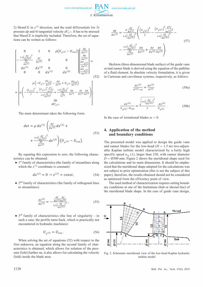
1138

Z. Krzemianowski

Bull. Pol. Ac.: Tech. 67(6) 2019

2) MomCE in x(1) direction, and the total differentials for 3) pressure dp and 4) tangential velocity dUx(2). It has to be stressed that MassCE is implicitly included. Therefore, the set of equa-tions can be written as follows:

6

Since ECE is quadratic equation with respect to tangential velocity 𝑈𝑈𝑥𝑥(2) , it is possible that in some cases of ill-posed problem there can be obtained no real solution for this equation due to the negative discriminant Δ:

𝑈𝑈𝑥𝑥(2) = 𝑈𝑈𝑟𝑟𝑟𝑟𝑟𝑟 ∓ √∆ (51)

It may occur when e.g. the blockage factor or/and blade loading at inlet are too high. In such a case the boundary conditions must be modified. If it is difficult to find the proper boundary conditions, this may indicate that meridional shape of blade is inappropriate for such boundary conditions. Here, it has to be added that positive sign in equation (51) is never encountered in hydraulic turbines. The circumferential velocity 𝑈𝑈𝑟𝑟𝑟𝑟𝑟𝑟 of runner is always larger than tangential velocity 𝑈𝑈𝑥𝑥(2) of flow in velocity triangles.

3. Blade shape generation

For the solution of conservation equations the method of characteristics was used because of hyperbolic type of the set of equations. It consists of: 1) differentiated ECE with respect to 𝑥𝑥(3), 2) MomCE in 𝑥𝑥(1) direction, and the total differentials for 3) pressure dp and 4) tangential velocity 𝑑𝑑𝑈𝑈𝑥𝑥(2). It has to be stressed that MassCE is implicitly included. Therefore, the set of equations can be written as follows:

[ 0 1 0 𝜌𝜌(𝑈𝑈𝑥𝑥(2) − 𝑈𝑈𝑟𝑟𝑟𝑟𝑟𝑟)

−1+( 𝜕𝜕𝜕𝜕

𝜕𝜕𝑥𝑥(3))2

𝜕𝜕𝜕𝜕𝜕𝜕𝑥𝑥(1)

𝜕𝜕𝜕𝜕𝜕𝜕𝑥𝑥(3) 0 0

𝑑𝑑𝑥𝑥(1) 𝑑𝑑𝑥𝑥(3) 0 00 0 𝑑𝑑𝑥𝑥(1) 𝑑𝑑𝑥𝑥(3) ]

[

𝜕𝜕𝜕𝜕𝜕𝜕𝑥𝑥(1)𝜕𝜕𝜕𝜕

𝜕𝜕𝑥𝑥(3)𝜕𝜕𝑈𝑈𝑥𝑥(2)𝜕𝜕𝑥𝑥(1)𝜕𝜕𝑈𝑈𝑥𝑥(2)𝜕𝜕𝑥𝑥(3) ]

=

[ 𝜌𝜌 (−𝑈𝑈𝑥𝑥(3)

𝜕𝜕𝑈𝑈𝑥𝑥(3)

𝜕𝜕𝑥𝑥(3) − 𝜕𝜕𝜕𝜕𝜕𝜕𝑥𝑥(3) + 𝑈𝑈𝑥𝑥(2)

𝜕𝜕𝑈𝑈𝑟𝑟𝑟𝑟𝑟𝑟𝜕𝜕𝑥𝑥(3))

𝜌𝜌 (− (𝑈𝑈𝑥𝑥(2))2

𝜕𝜕 +(𝑈𝑈𝑥𝑥(3))

2 𝜕𝜕2𝜕𝜕

𝜕𝜕𝑥𝑥(3)2

1+( 𝜕𝜕𝜕𝜕𝜕𝜕𝑥𝑥(3))

2 +1+( 𝜕𝜕𝜕𝜕

𝜕𝜕𝑥𝑥(3))2

𝜕𝜕𝜕𝜕𝜕𝜕𝑥𝑥(1)

𝜕𝜕𝜕𝜕𝜕𝜕𝑥𝑥(1) −

𝜕𝜕𝜕𝜕𝜕𝜕𝑥𝑥(3)

𝜕𝜕𝜕𝜕𝜕𝜕𝑥𝑥(3))

𝑑𝑑𝑑𝑑𝑑𝑑𝑈𝑈𝑥𝑥(2) ]

(52)

The main determinant takes the following form:

𝑑𝑑𝑑𝑑𝑑𝑑 = 𝜌𝜌 𝑑𝑑𝑥𝑥(1) ( 𝜕𝜕𝜕𝜕𝜕𝜕𝑥𝑥(3) 𝑑𝑑𝑥𝑥(1) +

1+( 𝜕𝜕𝜕𝜕𝜕𝜕𝑥𝑥(3))

2

𝜕𝜕𝜕𝜕𝜕𝜕𝑥𝑥(1)

𝑑𝑑𝑥𝑥(3)) (𝑈𝑈𝑥𝑥(2) −

𝑈𝑈𝑟𝑟𝑟𝑟𝑟𝑟) (53)

By equating this expression to zero the following characteristics can be obtained:

1st family of characteristics (the family of streamlines along which 𝑥𝑥(1) coordinate is constant):

𝑑𝑑𝑥𝑥(1) = 0 → 𝑥𝑥(1) = 𝑐𝑐𝑐𝑐𝑐𝑐𝑐𝑐𝑑𝑑 (54)

2nd family of characteristics (the family of orthogonal lines to streamlines):

𝑑𝑑𝑥𝑥(3)

𝑑𝑑𝑥𝑥(1) = −𝜕𝜕𝜕𝜕

𝜕𝜕𝑥𝑥(1)𝜕𝜕𝜕𝜕

𝜕𝜕𝑥𝑥(3)

1+( 𝜕𝜕𝜕𝜕𝜕𝜕𝑥𝑥(3))

2 (55)

3rd characteristics (the line of a singularity – in such a case the profile turns back what is practically not encountered in hydraulic machines):

𝑈𝑈𝑥𝑥(2) = 𝑈𝑈𝑟𝑟𝑟𝑟𝑟𝑟 (56)

Solving the set of equations (52) with respect to the first unknown, equation along the second family of characteristics is obtained, which allows for solution of the pressure field (further it allows calculating the velocity field) inside the blade area:

𝑑𝑑𝜕𝜕𝑑𝑑𝑥𝑥(1) =

𝜌𝜌 𝜕𝜕𝜕𝜕𝜕𝜕𝑥𝑥(1)

1+( 𝜕𝜕𝜕𝜕𝜕𝜕𝑥𝑥(3))

2 ((𝑈𝑈𝑥𝑥(2))

2

𝜕𝜕 −(𝑈𝑈𝑥𝑥(3))

2 𝜕𝜕2𝜕𝜕𝜕𝜕𝑥𝑥(3)2

1+( 𝜕𝜕𝜕𝜕𝜕𝜕𝑥𝑥(3))

2 −

1+( 𝜕𝜕𝜕𝜕𝜕𝜕𝑥𝑥(3))

2

𝜕𝜕𝜕𝜕𝜕𝜕𝑥𝑥(1)

𝜕𝜕𝜕𝜕𝜕𝜕𝑥𝑥(1) + 𝜕𝜕𝜕𝜕

𝜕𝜕𝑥𝑥(3)𝜕𝜕𝜕𝜕

𝜕𝜕𝑥𝑥(3)) (57)

Skeleton (three-dimensional blade surface) of the guide vane or/and runner blade is derived using Equation of the Pathline of a Fluid Element. In absolute velocity formulation it is given in Cartesian and curvilinear systems respectively as follows:

𝑑𝑑𝑥𝑥(2)

𝑈𝑈(2)−𝜔𝜔 = 𝑑𝑑𝑥𝑥(3)

𝑈𝑈(3) (58a)

𝑑𝑑𝑥𝑥(2)

𝑈𝑈𝑥𝑥(2)−𝑈𝑈𝑟𝑟𝑟𝑟𝑟𝑟=

√1+( 𝜕𝜕𝜕𝜕𝜕𝜕𝑥𝑥(3))

2

𝜕𝜕 𝑑𝑑𝑥𝑥(3)

𝑈𝑈𝑥𝑥(3) (58b)

In case of irrotational blades ω = 0.

4. Application of the method and boundary conditions

The presented model was applied to design the guide vane and runner blades for the low-head (H = 1.5 m) two-

6

Since ECE is quadratic equation with respect to tangential velocity 𝑈𝑈𝑥𝑥(2) , it is possible that in some cases of ill-posed problem there can be obtained no real solution for this equation due to the negative discriminant Δ:

𝑈𝑈𝑥𝑥(2) = 𝑈𝑈𝑟𝑟𝑟𝑟𝑟𝑟 ∓ √∆ (51)

It may occur when e.g. the blockage factor or/and blade loading at inlet are too high. In such a case the boundary conditions must be modified. If it is difficult to find the proper boundary conditions, this may indicate that meridional shape of blade is inappropriate for such boundary conditions. Here, it has to be added that positive sign in equation (51) is never encountered in hydraulic turbines. The circumferential velocity 𝑈𝑈𝑟𝑟𝑟𝑟𝑟𝑟 of runner is always larger than tangential velocity 𝑈𝑈𝑥𝑥(2) of flow in velocity triangles.

3. Blade shape generation

For the solution of conservation equations the method of characteristics was used because of hyperbolic type of the set of equations. It consists of: 1) differentiated ECE with respect to 𝑥𝑥(3), 2) MomCE in 𝑥𝑥(1) direction, and the total differentials for 3) pressure dp and 4) tangential velocity 𝑑𝑑𝑈𝑈𝑥𝑥(2). It has to be stressed that MassCE is implicitly included. Therefore, the set of equations can be written as follows:

[ 0 1 0 𝜌𝜌(𝑈𝑈𝑥𝑥(2) − 𝑈𝑈𝑟𝑟𝑟𝑟𝑟𝑟)

−1+( 𝜕𝜕𝜕𝜕

𝜕𝜕𝑥𝑥(3))2

𝜕𝜕𝜕𝜕𝜕𝜕𝑥𝑥(1)

𝜕𝜕𝜕𝜕𝜕𝜕𝑥𝑥(3) 0 0

𝑑𝑑𝑥𝑥(1) 𝑑𝑑𝑥𝑥(3) 0 00 0 𝑑𝑑𝑥𝑥(1) 𝑑𝑑𝑥𝑥(3) ]

[

𝜕𝜕𝜕𝜕𝜕𝜕𝑥𝑥(1)𝜕𝜕𝜕𝜕

𝜕𝜕𝑥𝑥(3)𝜕𝜕𝑈𝑈𝑥𝑥(2)𝜕𝜕𝑥𝑥(1)𝜕𝜕𝑈𝑈𝑥𝑥(2)𝜕𝜕𝑥𝑥(3) ]

=

[ 𝜌𝜌 (−𝑈𝑈𝑥𝑥(3)

𝜕𝜕𝑈𝑈𝑥𝑥(3)

𝜕𝜕𝑥𝑥(3) − 𝜕𝜕𝜕𝜕𝜕𝜕𝑥𝑥(3) + 𝑈𝑈𝑥𝑥(2)

𝜕𝜕𝑈𝑈𝑟𝑟𝑟𝑟𝑟𝑟𝜕𝜕𝑥𝑥(3))

𝜌𝜌 (− (𝑈𝑈𝑥𝑥(2))2

𝜕𝜕 +(𝑈𝑈𝑥𝑥(3))

2 𝜕𝜕2𝜕𝜕

𝜕𝜕𝑥𝑥(3)2

1+( 𝜕𝜕𝜕𝜕𝜕𝜕𝑥𝑥(3))

2 +1+( 𝜕𝜕𝜕𝜕

𝜕𝜕𝑥𝑥(3))2

𝜕𝜕𝜕𝜕𝜕𝜕𝑥𝑥(1)

𝜕𝜕𝜕𝜕𝜕𝜕𝑥𝑥(1) −

𝜕𝜕𝜕𝜕𝜕𝜕𝑥𝑥(3)

𝜕𝜕𝜕𝜕𝜕𝜕𝑥𝑥(3))

𝑑𝑑𝑑𝑑𝑑𝑑𝑈𝑈𝑥𝑥(2) ]

(52)

The main determinant takes the following form:

𝑑𝑑𝑑𝑑𝑑𝑑 = 𝜌𝜌 𝑑𝑑𝑥𝑥(1) ( 𝜕𝜕𝜕𝜕𝜕𝜕𝑥𝑥(3) 𝑑𝑑𝑥𝑥(1) +

1+( 𝜕𝜕𝜕𝜕𝜕𝜕𝑥𝑥(3))

2

𝜕𝜕𝜕𝜕𝜕𝜕𝑥𝑥(1)

𝑑𝑑𝑥𝑥(3)) (𝑈𝑈𝑥𝑥(2) −

𝑈𝑈𝑟𝑟𝑟𝑟𝑟𝑟) (53)

By equating this expression to zero the following characteristics can be obtained:

1st family of characteristics (the family of streamlines along which 𝑥𝑥(1) coordinate is constant):

𝑑𝑑𝑥𝑥(1) = 0 → 𝑥𝑥(1) = 𝑐𝑐𝑐𝑐𝑐𝑐𝑐𝑐𝑑𝑑 (54)

2nd family of characteristics (the family of orthogonal lines to streamlines):

𝑑𝑑𝑥𝑥(3)

𝑑𝑑𝑥𝑥(1) = −𝜕𝜕𝜕𝜕

𝜕𝜕𝑥𝑥(1)𝜕𝜕𝜕𝜕

𝜕𝜕𝑥𝑥(3)

1+( 𝜕𝜕𝜕𝜕𝜕𝜕𝑥𝑥(3))

2 (55)

3rd characteristics (the line of a singularity – in such a case the profile turns back what is practically not encountered in hydraulic machines):

𝑈𝑈𝑥𝑥(2) = 𝑈𝑈𝑟𝑟𝑟𝑟𝑟𝑟 (56)

Solving the set of equations (52) with respect to the first unknown, equation along the second family of characteristics is obtained, which allows for solution of the pressure field (further it allows calculating the velocity field) inside the blade area:

𝑑𝑑𝜕𝜕𝑑𝑑𝑥𝑥(1) =

𝜌𝜌 𝜕𝜕𝜕𝜕𝜕𝜕𝑥𝑥(1)

1+( 𝜕𝜕𝜕𝜕𝜕𝜕𝑥𝑥(3))

2 ((𝑈𝑈𝑥𝑥(2))

2

𝜕𝜕 −(𝑈𝑈𝑥𝑥(3))

2 𝜕𝜕2𝜕𝜕𝜕𝜕𝑥𝑥(3)2

1+( 𝜕𝜕𝜕𝜕𝜕𝜕𝑥𝑥(3))

2 −

1+( 𝜕𝜕𝜕𝜕𝜕𝜕𝑥𝑥(3))

2

𝜕𝜕𝜕𝜕𝜕𝜕𝑥𝑥(1)

𝜕𝜕𝜕𝜕𝜕𝜕𝑥𝑥(1) + 𝜕𝜕𝜕𝜕

𝜕𝜕𝑥𝑥(3)𝜕𝜕𝜕𝜕

𝜕𝜕𝑥𝑥(3)) (57)

Skeleton (three-dimensional blade surface) of the guide vane or/and runner blade is derived using Equation of the Pathline of a Fluid Element. In absolute velocity formulation it is given in Cartesian and curvilinear systems respectively as follows:

𝑑𝑑𝑥𝑥(2)

𝑈𝑈(2)−𝜔𝜔 = 𝑑𝑑𝑥𝑥(3)

𝑈𝑈(3) (58a)

𝑑𝑑𝑥𝑥(2)

𝑈𝑈𝑥𝑥(2)−𝑈𝑈𝑟𝑟𝑟𝑟𝑟𝑟=

√1+( 𝜕𝜕𝜕𝜕𝜕𝜕𝑥𝑥(3))

2

𝜕𝜕 𝑑𝑑𝑥𝑥(3)

𝑈𝑈𝑥𝑥(3) (58b)

In case of irrotational blades ω = 0.

4. Application of the method and boundary conditions

The presented model was applied to design the guide vane and runner blades for the low-head (H = 1.5 m) two-

6

Since ECE is quadratic equation with respect to tangential velocity 𝑈𝑈𝑥𝑥(2) , it is possible that in some cases of ill-posed problem there can be obtained no real solution for this equation due to the negative discriminant Δ:

𝑈𝑈𝑥𝑥(2) = 𝑈𝑈𝑟𝑟𝑟𝑟𝑟𝑟 ∓ √∆ (51)

It may occur when e.g. the blockage factor or/and blade loading at inlet are too high. In such a case the boundary conditions must be modified. If it is difficult to find the proper boundary conditions, this may indicate that meridional shape of blade is inappropriate for such boundary conditions. Here, it has to be added that positive sign in equation (51) is never encountered in hydraulic turbines. The circumferential velocity 𝑈𝑈𝑟𝑟𝑟𝑟𝑟𝑟 of runner is always larger than tangential velocity 𝑈𝑈𝑥𝑥(2) of flow in velocity triangles.

3. Blade shape generation

For the solution of conservation equations the method of characteristics was used because of hyperbolic type of the set of equations. It consists of: 1) differentiated ECE with respect to 𝑥𝑥(3), 2) MomCE in 𝑥𝑥(1) direction, and the total differentials for 3) pressure dp and 4) tangential velocity 𝑑𝑑𝑈𝑈𝑥𝑥(2). It has to be stressed that MassCE is implicitly included. Therefore, the set of equations can be written as follows:

[ 0 1 0 𝜌𝜌(𝑈𝑈𝑥𝑥(2) − 𝑈𝑈𝑟𝑟𝑟𝑟𝑟𝑟)

−1+( 𝜕𝜕𝜕𝜕

𝜕𝜕𝑥𝑥(3))2

𝜕𝜕𝜕𝜕𝜕𝜕𝑥𝑥(1)

𝜕𝜕𝜕𝜕𝜕𝜕𝑥𝑥(3) 0 0

𝑑𝑑𝑥𝑥(1) 𝑑𝑑𝑥𝑥(3) 0 00 0 𝑑𝑑𝑥𝑥(1) 𝑑𝑑𝑥𝑥(3) ]

[

𝜕𝜕𝜕𝜕𝜕𝜕𝑥𝑥(1)𝜕𝜕𝜕𝜕

𝜕𝜕𝑥𝑥(3)𝜕𝜕𝑈𝑈𝑥𝑥(2)𝜕𝜕𝑥𝑥(1)𝜕𝜕𝑈𝑈𝑥𝑥(2)𝜕𝜕𝑥𝑥(3) ]

=

[ 𝜌𝜌 (−𝑈𝑈𝑥𝑥(3)

𝜕𝜕𝑈𝑈𝑥𝑥(3)

𝜕𝜕𝑥𝑥(3) − 𝜕𝜕𝜕𝜕𝜕𝜕𝑥𝑥(3) + 𝑈𝑈𝑥𝑥(2)

𝜕𝜕𝑈𝑈𝑟𝑟𝑟𝑟𝑟𝑟𝜕𝜕𝑥𝑥(3))

𝜌𝜌 (− (𝑈𝑈𝑥𝑥(2))2

𝜕𝜕 +(𝑈𝑈𝑥𝑥(3))

2 𝜕𝜕2𝜕𝜕

𝜕𝜕𝑥𝑥(3)2

1+( 𝜕𝜕𝜕𝜕𝜕𝜕𝑥𝑥(3))

2 +1+( 𝜕𝜕𝜕𝜕

𝜕𝜕𝑥𝑥(3))2

𝜕𝜕𝜕𝜕𝜕𝜕𝑥𝑥(1)

𝜕𝜕𝜕𝜕𝜕𝜕𝑥𝑥(1) −

𝜕𝜕𝜕𝜕𝜕𝜕𝑥𝑥(3)

𝜕𝜕𝜕𝜕𝜕𝜕𝑥𝑥(3))

𝑑𝑑𝑑𝑑𝑑𝑑𝑈𝑈𝑥𝑥(2) ]

(52)

The main determinant takes the following form:

𝑑𝑑𝑑𝑑𝑑𝑑 = 𝜌𝜌 𝑑𝑑𝑥𝑥(1) ( 𝜕𝜕𝜕𝜕𝜕𝜕𝑥𝑥(3) 𝑑𝑑𝑥𝑥(1) +

1+( 𝜕𝜕𝜕𝜕𝜕𝜕𝑥𝑥(3))

2

𝜕𝜕𝜕𝜕𝜕𝜕𝑥𝑥(1)

𝑑𝑑𝑥𝑥(3)) (𝑈𝑈𝑥𝑥(2) −

𝑈𝑈𝑟𝑟𝑟𝑟𝑟𝑟) (53)

By equating this expression to zero the following characteristics can be obtained:

1st family of characteristics (the family of streamlines along which 𝑥𝑥(1) coordinate is constant):

𝑑𝑑𝑥𝑥(1) = 0 → 𝑥𝑥(1) = 𝑐𝑐𝑐𝑐𝑐𝑐𝑐𝑐𝑑𝑑 (54)

2nd family of characteristics (the family of orthogonal lines to streamlines):

𝑑𝑑𝑥𝑥(3)

𝑑𝑑𝑥𝑥(1) = −𝜕𝜕𝜕𝜕

𝜕𝜕𝑥𝑥(1)𝜕𝜕𝜕𝜕

𝜕𝜕𝑥𝑥(3)

1+( 𝜕𝜕𝜕𝜕𝜕𝜕𝑥𝑥(3))

2 (55)

3rd characteristics (the line of a singularity – in such a case the profile turns back what is practically not encountered in hydraulic machines):

𝑈𝑈𝑥𝑥(2) = 𝑈𝑈𝑟𝑟𝑟𝑟𝑟𝑟 (56)

Solving the set of equations (52) with respect to the first unknown, equation along the second family of characteristics is obtained, which allows for solution of the pressure field (further it allows calculating the velocity field) inside the blade area:

𝑑𝑑𝜕𝜕𝑑𝑑𝑥𝑥(1) =

𝜌𝜌 𝜕𝜕𝜕𝜕𝜕𝜕𝑥𝑥(1)

1+( 𝜕𝜕𝜕𝜕𝜕𝜕𝑥𝑥(3))

2 ((𝑈𝑈𝑥𝑥(2))

2

𝜕𝜕 −(𝑈𝑈𝑥𝑥(3))

2 𝜕𝜕2𝜕𝜕𝜕𝜕𝑥𝑥(3)2

1+( 𝜕𝜕𝜕𝜕𝜕𝜕𝑥𝑥(3))

2 −

1+( 𝜕𝜕𝜕𝜕𝜕𝜕𝑥𝑥(3))

2

𝜕𝜕𝜕𝜕𝜕𝜕𝑥𝑥(1)

𝜕𝜕𝜕𝜕𝜕𝜕𝑥𝑥(1) + 𝜕𝜕𝜕𝜕

𝜕𝜕𝑥𝑥(3)𝜕𝜕𝜕𝜕

𝜕𝜕𝑥𝑥(3)) (57)

Skeleton (three-dimensional blade surface) of the guide vane or/and runner blade is derived using Equation of the Pathline of a Fluid Element. In absolute velocity formulation it is given in Cartesian and curvilinear systems respectively as follows:

𝑑𝑑𝑥𝑥(2)

𝑈𝑈(2)−𝜔𝜔 = 𝑑𝑑𝑥𝑥(3)

𝑈𝑈(3) (58a)

𝑑𝑑𝑥𝑥(2)

𝑈𝑈𝑥𝑥(2)−𝑈𝑈𝑟𝑟𝑟𝑟𝑟𝑟=

√1+( 𝜕𝜕𝜕𝜕𝜕𝜕𝑥𝑥(3))

2

𝜕𝜕 𝑑𝑑𝑥𝑥(3)

𝑈𝑈𝑥𝑥(3) (58b)

In case of irrotational blades ω = 0.

4. Application of the method and boundary conditions

The presented model was applied to design the guide vane and runner blades for the low-head (H = 1.5 m) two-

6

Since ECE is quadratic equation with respect to tangential velocity 𝑈𝑈𝑥𝑥(2) , it is possible that in some cases of ill-posed problem there can be obtained no real solution for this equation due to the negative discriminant Δ:

𝑈𝑈𝑥𝑥(2) = 𝑈𝑈𝑟𝑟𝑟𝑟𝑟𝑟 ∓ √∆ (51)

It may occur when e.g. the blockage factor or/and blade loading at inlet are too high. In such a case the boundary conditions must be modified. If it is difficult to find the proper boundary conditions, this may indicate that meridional shape of blade is inappropriate for such boundary conditions. Here, it has to be added that positive sign in equation (51) is never encountered in hydraulic turbines. The circumferential velocity 𝑈𝑈𝑟𝑟𝑟𝑟𝑟𝑟 of runner is always larger than tangential velocity 𝑈𝑈𝑥𝑥(2) of flow in velocity triangles.

3. Blade shape generation

For the solution of conservation equations the method of characteristics was used because of hyperbolic type of the set of equations. It consists of: 1) differentiated ECE with respect to 𝑥𝑥(3), 2) MomCE in 𝑥𝑥(1) direction, and the total differentials for 3) pressure dp and 4) tangential velocity 𝑑𝑑𝑈𝑈𝑥𝑥(2). It has to be stressed that MassCE is implicitly included. Therefore, the set of equations can be written as follows:

[ 0 1 0 𝜌𝜌(𝑈𝑈𝑥𝑥(2) − 𝑈𝑈𝑟𝑟𝑟𝑟𝑟𝑟)

−1+( 𝜕𝜕𝜕𝜕

𝜕𝜕𝑥𝑥(3))2

𝜕𝜕𝜕𝜕𝜕𝜕𝑥𝑥(1)

𝜕𝜕𝜕𝜕𝜕𝜕𝑥𝑥(3) 0 0

𝑑𝑑𝑥𝑥(1) 𝑑𝑑𝑥𝑥(3) 0 00 0 𝑑𝑑𝑥𝑥(1) 𝑑𝑑𝑥𝑥(3) ]

[

𝜕𝜕𝜕𝜕𝜕𝜕𝑥𝑥(1)𝜕𝜕𝜕𝜕

𝜕𝜕𝑥𝑥(3)𝜕𝜕𝑈𝑈𝑥𝑥(2)𝜕𝜕𝑥𝑥(1)𝜕𝜕𝑈𝑈𝑥𝑥(2)𝜕𝜕𝑥𝑥(3) ]

=

[ 𝜌𝜌 (−𝑈𝑈𝑥𝑥(3)

𝜕𝜕𝑈𝑈𝑥𝑥(3)

𝜕𝜕𝑥𝑥(3) − 𝜕𝜕𝜕𝜕𝜕𝜕𝑥𝑥(3) + 𝑈𝑈𝑥𝑥(2)

𝜕𝜕𝑈𝑈𝑟𝑟𝑟𝑟𝑟𝑟𝜕𝜕𝑥𝑥(3))

𝜌𝜌 (− (𝑈𝑈𝑥𝑥(2))2

𝜕𝜕 +(𝑈𝑈𝑥𝑥(3))

2 𝜕𝜕2𝜕𝜕

𝜕𝜕𝑥𝑥(3)2

1+( 𝜕𝜕𝜕𝜕𝜕𝜕𝑥𝑥(3))

2 +1+( 𝜕𝜕𝜕𝜕

𝜕𝜕𝑥𝑥(3))2

𝜕𝜕𝜕𝜕𝜕𝜕𝑥𝑥(1)

𝜕𝜕𝜕𝜕𝜕𝜕𝑥𝑥(1) −

𝜕𝜕𝜕𝜕𝜕𝜕𝑥𝑥(3)

𝜕𝜕𝜕𝜕𝜕𝜕𝑥𝑥(3))

𝑑𝑑𝑑𝑑𝑑𝑑𝑈𝑈𝑥𝑥(2) ]

(52)

The main determinant takes the following form:

𝑑𝑑𝑑𝑑𝑑𝑑 = 𝜌𝜌 𝑑𝑑𝑥𝑥(1) ( 𝜕𝜕𝜕𝜕𝜕𝜕𝑥𝑥(3) 𝑑𝑑𝑥𝑥(1) +

1+( 𝜕𝜕𝜕𝜕𝜕𝜕𝑥𝑥(3))

2

𝜕𝜕𝜕𝜕𝜕𝜕𝑥𝑥(1)

𝑑𝑑𝑥𝑥(3)) (𝑈𝑈𝑥𝑥(2) −

𝑈𝑈𝑟𝑟𝑟𝑟𝑟𝑟) (53)

By equating this expression to zero the following characteristics can be obtained:

1st family of characteristics (the family of streamlines along which 𝑥𝑥(1) coordinate is constant):

𝑑𝑑𝑥𝑥(1) = 0 → 𝑥𝑥(1) = 𝑐𝑐𝑐𝑐𝑐𝑐𝑐𝑐𝑑𝑑 (54)

2nd family of characteristics (the family of orthogonal lines to streamlines):

𝑑𝑑𝑥𝑥(3)

𝑑𝑑𝑥𝑥(1) = −𝜕𝜕𝜕𝜕

𝜕𝜕𝑥𝑥(1)𝜕𝜕𝜕𝜕

𝜕𝜕𝑥𝑥(3)

1+( 𝜕𝜕𝜕𝜕𝜕𝜕𝑥𝑥(3))

2 (55)

3rd characteristics (the line of a singularity – in such a case the profile turns back what is practically not encountered in hydraulic machines):

𝑈𝑈𝑥𝑥(2) = 𝑈𝑈𝑟𝑟𝑟𝑟𝑟𝑟 (56)

Solving the set of equations (52) with respect to the first unknown, equation along the second family of characteristics is obtained, which allows for solution of the pressure field (further it allows calculating the velocity field) inside the blade area:

𝑑𝑑𝜕𝜕𝑑𝑑𝑥𝑥(1) =

𝜌𝜌 𝜕𝜕𝜕𝜕𝜕𝜕𝑥𝑥(1)

1+( 𝜕𝜕𝜕𝜕𝜕𝜕𝑥𝑥(3))

2 ((𝑈𝑈𝑥𝑥(2))

2

𝜕𝜕 −(𝑈𝑈𝑥𝑥(3))

2 𝜕𝜕2𝜕𝜕𝜕𝜕𝑥𝑥(3)2

1+( 𝜕𝜕𝜕𝜕𝜕𝜕𝑥𝑥(3))

2 −

1+( 𝜕𝜕𝜕𝜕𝜕𝜕𝑥𝑥(3))

2

𝜕𝜕𝜕𝜕𝜕𝜕𝑥𝑥(1)

𝜕𝜕𝜕𝜕𝜕𝜕𝑥𝑥(1) + 𝜕𝜕𝜕𝜕

𝜕𝜕𝑥𝑥(3)𝜕𝜕𝜕𝜕

𝜕𝜕𝑥𝑥(3)) (57)

Skeleton (three-dimensional blade surface) of the guide vane or/and runner blade is derived using Equation of the Pathline of a Fluid Element. In absolute velocity formulation it is given in Cartesian and curvilinear systems respectively as follows:

𝑑𝑑𝑥𝑥(2)

𝑈𝑈(2)−𝜔𝜔 = 𝑑𝑑𝑥𝑥(3)

𝑈𝑈(3) (58a)

𝑑𝑑𝑥𝑥(2)

𝑈𝑈𝑥𝑥(2)−𝑈𝑈𝑟𝑟𝑟𝑟𝑟𝑟=

√1+( 𝜕𝜕𝜕𝜕𝜕𝜕𝑥𝑥(3))

2

𝜕𝜕 𝑑𝑑𝑥𝑥(3)

𝑈𝑈𝑥𝑥(3) (58b)

In case of irrotational blades ω = 0.

4. Application of the method and boundary conditions

The presented model was applied to design the guide vane and runner blades for the low-head (H = 1.5 m) two-

.

6

Since ECE is quadratic equation with respect to tangential velocity 𝑈𝑈𝑥𝑥(2) , it is possible that in some cases of ill-posed problem there can be obtained no real solution for this equation due to the negative discriminant Δ:

𝑈𝑈𝑥𝑥(2) = 𝑈𝑈𝑟𝑟𝑟𝑟𝑟𝑟 ∓ √∆ (51)

It may occur when e.g. the blockage factor or/and blade loading at inlet are too high. In such a case the boundary conditions must be modified. If it is difficult to find the proper boundary conditions, this may indicate that meridional shape of blade is inappropriate for such boundary conditions. Here, it has to be added that positive sign in equation (51) is never encountered in hydraulic turbines. The circumferential velocity 𝑈𝑈𝑟𝑟𝑟𝑟𝑟𝑟 of runner is always larger than tangential velocity 𝑈𝑈𝑥𝑥(2) of flow in velocity triangles.

3. Blade shape generation

For the solution of conservation equations the method of characteristics was used because of hyperbolic type of the set of equations. It consists of: 1) differentiated ECE with respect to 𝑥𝑥(3), 2) MomCE in 𝑥𝑥(1) direction, and the total differentials for 3) pressure dp and 4) tangential velocity 𝑑𝑑𝑈𝑈𝑥𝑥(2). It has to be stressed that MassCE is implicitly included. Therefore, the set of equations can be written as follows:

[ 0 1 0 𝜌𝜌(𝑈𝑈𝑥𝑥(2) − 𝑈𝑈𝑟𝑟𝑟𝑟𝑟𝑟)

−1+( 𝜕𝜕𝜕𝜕

𝜕𝜕𝑥𝑥(3))2

𝜕𝜕𝜕𝜕𝜕𝜕𝑥𝑥(1)

𝜕𝜕𝜕𝜕𝜕𝜕𝑥𝑥(3) 0 0

𝑑𝑑𝑥𝑥(1) 𝑑𝑑𝑥𝑥(3) 0 00 0 𝑑𝑑𝑥𝑥(1) 𝑑𝑑𝑥𝑥(3) ]

[

𝜕𝜕𝜕𝜕𝜕𝜕𝑥𝑥(1)𝜕𝜕𝜕𝜕

𝜕𝜕𝑥𝑥(3)𝜕𝜕𝑈𝑈𝑥𝑥(2)𝜕𝜕𝑥𝑥(1)𝜕𝜕𝑈𝑈𝑥𝑥(2)𝜕𝜕𝑥𝑥(3) ]

=

[ 𝜌𝜌 (−𝑈𝑈𝑥𝑥(3)

𝜕𝜕𝑈𝑈𝑥𝑥(3)

𝜕𝜕𝑥𝑥(3) − 𝜕𝜕𝜕𝜕𝜕𝜕𝑥𝑥(3) + 𝑈𝑈𝑥𝑥(2)

𝜕𝜕𝑈𝑈𝑟𝑟𝑟𝑟𝑟𝑟𝜕𝜕𝑥𝑥(3))

𝜌𝜌 (− (𝑈𝑈𝑥𝑥(2))2

𝜕𝜕 +(𝑈𝑈𝑥𝑥(3))

2 𝜕𝜕2𝜕𝜕

𝜕𝜕𝑥𝑥(3)2

1+( 𝜕𝜕𝜕𝜕𝜕𝜕𝑥𝑥(3))

2 +1+( 𝜕𝜕𝜕𝜕

𝜕𝜕𝑥𝑥(3))2

𝜕𝜕𝜕𝜕𝜕𝜕𝑥𝑥(1)

𝜕𝜕𝜕𝜕𝜕𝜕𝑥𝑥(1) −

𝜕𝜕𝜕𝜕𝜕𝜕𝑥𝑥(3)

𝜕𝜕𝜕𝜕𝜕𝜕𝑥𝑥(3))

𝑑𝑑𝑑𝑑𝑑𝑑𝑈𝑈𝑥𝑥(2) ]

(52)

The main determinant takes the following form:

𝑑𝑑𝑑𝑑𝑑𝑑 = 𝜌𝜌 𝑑𝑑𝑥𝑥(1) ( 𝜕𝜕𝜕𝜕𝜕𝜕𝑥𝑥(3) 𝑑𝑑𝑥𝑥(1) +

1+( 𝜕𝜕𝜕𝜕𝜕𝜕𝑥𝑥(3))

2

𝜕𝜕𝜕𝜕𝜕𝜕𝑥𝑥(1)

𝑑𝑑𝑥𝑥(3)) (𝑈𝑈𝑥𝑥(2) −

𝑈𝑈𝑟𝑟𝑟𝑟𝑟𝑟) (53)

By equating this expression to zero the following characteristics can be obtained:

1st family of characteristics (the family of streamlines along which 𝑥𝑥(1) coordinate is constant):

𝑑𝑑𝑥𝑥(1) = 0 → 𝑥𝑥(1) = 𝑐𝑐𝑐𝑐𝑐𝑐𝑐𝑐𝑑𝑑 (54)

2nd family of characteristics (the family of orthogonal lines to streamlines):

𝑑𝑑𝑥𝑥(3)

𝑑𝑑𝑥𝑥(1) = −𝜕𝜕𝜕𝜕

𝜕𝜕𝑥𝑥(1)𝜕𝜕𝜕𝜕

𝜕𝜕𝑥𝑥(3)

1+( 𝜕𝜕𝜕𝜕𝜕𝜕𝑥𝑥(3))

2 (55)

3rd characteristics (the line of a singularity – in such a case the profile turns back what is practically not encountered in hydraulic machines):

𝑈𝑈𝑥𝑥(2) = 𝑈𝑈𝑟𝑟𝑟𝑟𝑟𝑟 (56)

Solving the set of equations (52) with respect to the first unknown, equation along the second family of characteristics is obtained, which allows for solution of the pressure field (further it allows calculating the velocity field) inside the blade area:

𝑑𝑑𝜕𝜕𝑑𝑑𝑥𝑥(1) =

𝜌𝜌 𝜕𝜕𝜕𝜕𝜕𝜕𝑥𝑥(1)

1+( 𝜕𝜕𝜕𝜕𝜕𝜕𝑥𝑥(3))

2 ((𝑈𝑈𝑥𝑥(2))

2

𝜕𝜕 −(𝑈𝑈𝑥𝑥(3))

2 𝜕𝜕2𝜕𝜕𝜕𝜕𝑥𝑥(3)2

1+( 𝜕𝜕𝜕𝜕𝜕𝜕𝑥𝑥(3))

2 −

1+( 𝜕𝜕𝜕𝜕𝜕𝜕𝑥𝑥(3))

2

𝜕𝜕𝜕𝜕𝜕𝜕𝑥𝑥(1)

𝜕𝜕𝜕𝜕𝜕𝜕𝑥𝑥(1) + 𝜕𝜕𝜕𝜕

𝜕𝜕𝑥𝑥(3)𝜕𝜕𝜕𝜕

𝜕𝜕𝑥𝑥(3)) (57)

Skeleton (three-dimensional blade surface) of the guide vane or/and runner blade is derived using Equation of the Pathline of a Fluid Element. In absolute velocity formulation it is given in Cartesian and curvilinear systems respectively as follows:

𝑑𝑑𝑥𝑥(2)

𝑈𝑈(2)−𝜔𝜔 = 𝑑𝑑𝑥𝑥(3)

𝑈𝑈(3) (58a)

𝑑𝑑𝑥𝑥(2)

𝑈𝑈𝑥𝑥(2)−𝑈𝑈𝑟𝑟𝑟𝑟𝑟𝑟=

√1+( 𝜕𝜕𝜕𝜕𝜕𝜕𝑥𝑥(3))

2

𝜕𝜕 𝑑𝑑𝑥𝑥(3)

𝑈𝑈𝑥𝑥(3) (58b)

In case of irrotational blades ω = 0.

4. Application of the method and boundary conditions

The presented model was applied to design the guide vane and runner blades for the low-head (H = 1.5 m) two-

6

Since ECE is quadratic equation with respect to tangential velocity 𝑈𝑈𝑥𝑥(2) , it is possible that in some cases of ill-posed problem there can be obtained no real solution for this equation due to the negative discriminant Δ:

𝑈𝑈𝑥𝑥(2) = 𝑈𝑈𝑟𝑟𝑟𝑟𝑟𝑟 ∓ √∆ (51)

It may occur when e.g. the blockage factor or/and blade loading at inlet are too high. In such a case the boundary conditions must be modified. If it is difficult to find the proper boundary conditions, this may indicate that meridional shape of blade is inappropriate for such boundary conditions. Here, it has to be added that positive sign in equation (51) is never encountered in hydraulic turbines. The circumferential velocity 𝑈𝑈𝑟𝑟𝑟𝑟𝑟𝑟 of runner is always larger than tangential velocity 𝑈𝑈𝑥𝑥(2) of flow in velocity triangles.

3. Blade shape generation

For the solution of conservation equations the method of characteristics was used because of hyperbolic type of the set of equations. It consists of: 1) differentiated ECE with respect to 𝑥𝑥(3), 2) MomCE in 𝑥𝑥(1) direction, and the total differentials for 3) pressure dp and 4) tangential velocity 𝑑𝑑𝑈𝑈𝑥𝑥(2). It has to be stressed that MassCE is implicitly included. Therefore, the set of equations can be written as follows:

[ 0 1 0 𝜌𝜌(𝑈𝑈𝑥𝑥(2) − 𝑈𝑈𝑟𝑟𝑟𝑟𝑟𝑟)

−1+( 𝜕𝜕𝜕𝜕

𝜕𝜕𝑥𝑥(3))2

𝜕𝜕𝜕𝜕𝜕𝜕𝑥𝑥(1)

𝜕𝜕𝜕𝜕𝜕𝜕𝑥𝑥(3) 0 0

𝑑𝑑𝑥𝑥(1) 𝑑𝑑𝑥𝑥(3) 0 00 0 𝑑𝑑𝑥𝑥(1) 𝑑𝑑𝑥𝑥(3) ]

[

𝜕𝜕𝜕𝜕𝜕𝜕𝑥𝑥(1)𝜕𝜕𝜕𝜕

𝜕𝜕𝑥𝑥(3)𝜕𝜕𝑈𝑈𝑥𝑥(2)𝜕𝜕𝑥𝑥(1)𝜕𝜕𝑈𝑈𝑥𝑥(2)𝜕𝜕𝑥𝑥(3) ]

=

[ 𝜌𝜌 (−𝑈𝑈𝑥𝑥(3)

𝜕𝜕𝑈𝑈𝑥𝑥(3)

𝜕𝜕𝑥𝑥(3) − 𝜕𝜕𝜕𝜕𝜕𝜕𝑥𝑥(3) + 𝑈𝑈𝑥𝑥(2)

𝜕𝜕𝑈𝑈𝑟𝑟𝑟𝑟𝑟𝑟𝜕𝜕𝑥𝑥(3))

𝜌𝜌 (− (𝑈𝑈𝑥𝑥(2))2

𝜕𝜕 +(𝑈𝑈𝑥𝑥(3))

2 𝜕𝜕2𝜕𝜕

𝜕𝜕𝑥𝑥(3)2

1+( 𝜕𝜕𝜕𝜕𝜕𝜕𝑥𝑥(3))

2 +1+( 𝜕𝜕𝜕𝜕

𝜕𝜕𝑥𝑥(3))2

𝜕𝜕𝜕𝜕𝜕𝜕𝑥𝑥(1)

𝜕𝜕𝜕𝜕𝜕𝜕𝑥𝑥(1) −

𝜕𝜕𝜕𝜕𝜕𝜕𝑥𝑥(3)

𝜕𝜕𝜕𝜕𝜕𝜕𝑥𝑥(3))

𝑑𝑑𝑑𝑑𝑑𝑑𝑈𝑈𝑥𝑥(2) ]

(52)

The main determinant takes the following form:

𝑑𝑑𝑑𝑑𝑑𝑑 = 𝜌𝜌 𝑑𝑑𝑥𝑥(1) ( 𝜕𝜕𝜕𝜕𝜕𝜕𝑥𝑥(3) 𝑑𝑑𝑥𝑥(1) +

1+( 𝜕𝜕𝜕𝜕𝜕𝜕𝑥𝑥(3))

2

𝜕𝜕𝜕𝜕𝜕𝜕𝑥𝑥(1)

𝑑𝑑𝑥𝑥(3)) (𝑈𝑈𝑥𝑥(2) −

𝑈𝑈𝑟𝑟𝑟𝑟𝑟𝑟) (53)

By equating this expression to zero the following characteristics can be obtained:

1st family of characteristics (the family of streamlines along which 𝑥𝑥(1) coordinate is constant):

𝑑𝑑𝑥𝑥(1) = 0 → 𝑥𝑥(1) = 𝑐𝑐𝑐𝑐𝑐𝑐𝑐𝑐𝑑𝑑 (54)

2nd family of characteristics (the family of orthogonal lines to streamlines):

𝑑𝑑𝑥𝑥(3)

𝑑𝑑𝑥𝑥(1) = −𝜕𝜕𝜕𝜕

𝜕𝜕𝑥𝑥(1)𝜕𝜕𝜕𝜕

𝜕𝜕𝑥𝑥(3)

1+( 𝜕𝜕𝜕𝜕𝜕𝜕𝑥𝑥(3))

2 (55)

3rd characteristics (the line of a singularity – in such a case the profile turns back what is practically not encountered in hydraulic machines):

𝑈𝑈𝑥𝑥(2) = 𝑈𝑈𝑟𝑟𝑟𝑟𝑟𝑟 (56)

Solving the set of equations (52) with respect to the first unknown, equation along the second family of characteristics is obtained, which allows for solution of the pressure field (further it allows calculating the velocity field) inside the blade area:

𝑑𝑑𝜕𝜕𝑑𝑑𝑥𝑥(1) =

𝜌𝜌 𝜕𝜕𝜕𝜕𝜕𝜕𝑥𝑥(1)

1+( 𝜕𝜕𝜕𝜕𝜕𝜕𝑥𝑥(3))

2 ((𝑈𝑈𝑥𝑥(2))

2

𝜕𝜕 −(𝑈𝑈𝑥𝑥(3))

2 𝜕𝜕2𝜕𝜕𝜕𝜕𝑥𝑥(3)2

1+( 𝜕𝜕𝜕𝜕𝜕𝜕𝑥𝑥(3))

2 −

1+( 𝜕𝜕𝜕𝜕𝜕𝜕𝑥𝑥(3))

2

𝜕𝜕𝜕𝜕𝜕𝜕𝑥𝑥(1)

𝜕𝜕𝜕𝜕𝜕𝜕𝑥𝑥(1) + 𝜕𝜕𝜕𝜕

𝜕𝜕𝑥𝑥(3)𝜕𝜕𝜕𝜕

𝜕𝜕𝑥𝑥(3)) (57)

Skeleton (three-dimensional blade surface) of the guide vane or/and runner blade is derived using Equation of the Pathline of a Fluid Element. In absolute velocity formulation it is given in Cartesian and curvilinear systems respectively as follows:

𝑑𝑑𝑥𝑥(2)

𝑈𝑈(2)−𝜔𝜔 = 𝑑𝑑𝑥𝑥(3)

𝑈𝑈(3) (58a)

𝑑𝑑𝑥𝑥(2)

𝑈𝑈𝑥𝑥(2)−𝑈𝑈𝑟𝑟𝑟𝑟𝑟𝑟=

√1+( 𝜕𝜕𝜕𝜕𝜕𝜕𝑥𝑥(3))

2

𝜕𝜕 𝑑𝑑𝑥𝑥(3)

𝑈𝑈𝑥𝑥(3) (58b)

In case of irrotational blades ω = 0.

4. Application of the method and boundary conditions

The presented model was applied to design the guide vane and runner blades for the low-head (H = 1.5 m) two-

(52)

The main determinant takes the following form:

6

Since ECE is quadratic equation with respect to tangential velocity 𝑈𝑈𝑥𝑥(2) , it is possible that in some cases of ill-posed problem there can be obtained no real solution for this equation due to the negative discriminant Δ:

𝑈𝑈𝑥𝑥(2) = 𝑈𝑈𝑟𝑟𝑟𝑟𝑟𝑟 ∓ √∆ (51)

It may occur when e.g. the blockage factor or/and blade loading at inlet are too high. In such a case the boundary conditions must be modified. If it is difficult to find the proper boundary conditions, this may indicate that meridional shape of blade is inappropriate for such boundary conditions. Here, it has to be added that positive sign in equation (51) is never encountered in hydraulic turbines. The circumferential velocity 𝑈𝑈𝑟𝑟𝑟𝑟𝑟𝑟 of runner is always larger than tangential velocity 𝑈𝑈𝑥𝑥(2) of flow in velocity triangles.

3. Blade shape generation

For the solution of conservation equations the method of characteristics was used because of hyperbolic type of the set of equations. It consists of: 1) differentiated ECE with respect to 𝑥𝑥(3), 2) MomCE in 𝑥𝑥(1) direction, and the total differentials for 3) pressure dp and 4) tangential velocity 𝑑𝑑𝑈𝑈𝑥𝑥(2). It has to be stressed that MassCE is implicitly included. Therefore, the set of equations can be written as follows:

[ 0 1 0 𝜌𝜌(𝑈𝑈𝑥𝑥(2) − 𝑈𝑈𝑟𝑟𝑟𝑟𝑟𝑟)

−1+( 𝜕𝜕𝜕𝜕

𝜕𝜕𝑥𝑥(3))2

𝜕𝜕𝜕𝜕𝜕𝜕𝑥𝑥(1)

𝜕𝜕𝜕𝜕𝜕𝜕𝑥𝑥(3) 0 0

𝑑𝑑𝑥𝑥(1) 𝑑𝑑𝑥𝑥(3) 0 00 0 𝑑𝑑𝑥𝑥(1) 𝑑𝑑𝑥𝑥(3) ]

[

𝜕𝜕𝜕𝜕𝜕𝜕𝑥𝑥(1)𝜕𝜕𝜕𝜕

𝜕𝜕𝑥𝑥(3)𝜕𝜕𝑈𝑈𝑥𝑥(2)𝜕𝜕𝑥𝑥(1)𝜕𝜕𝑈𝑈𝑥𝑥(2)𝜕𝜕𝑥𝑥(3) ]

=

[ 𝜌𝜌 (−𝑈𝑈𝑥𝑥(3)

𝜕𝜕𝑈𝑈𝑥𝑥(3)

𝜕𝜕𝑥𝑥(3) − 𝜕𝜕𝜕𝜕𝜕𝜕𝑥𝑥(3) + 𝑈𝑈𝑥𝑥(2)

𝜕𝜕𝑈𝑈𝑟𝑟𝑟𝑟𝑟𝑟𝜕𝜕𝑥𝑥(3))

𝜌𝜌 (− (𝑈𝑈𝑥𝑥(2))2

𝜕𝜕 +(𝑈𝑈𝑥𝑥(3))

2 𝜕𝜕2𝜕𝜕

𝜕𝜕𝑥𝑥(3)2

1+( 𝜕𝜕𝜕𝜕𝜕𝜕𝑥𝑥(3))

2 +1+( 𝜕𝜕𝜕𝜕

𝜕𝜕𝑥𝑥(3))2

𝜕𝜕𝜕𝜕𝜕𝜕𝑥𝑥(1)

𝜕𝜕𝜕𝜕𝜕𝜕𝑥𝑥(1) −

𝜕𝜕𝜕𝜕𝜕𝜕𝑥𝑥(3)

𝜕𝜕𝜕𝜕𝜕𝜕𝑥𝑥(3))

𝑑𝑑𝑑𝑑𝑑𝑑𝑈𝑈𝑥𝑥(2) ]

(52)

The main determinant takes the following form:

𝑑𝑑𝑑𝑑𝑑𝑑 = 𝜌𝜌 𝑑𝑑𝑥𝑥(1) ( 𝜕𝜕𝜕𝜕𝜕𝜕𝑥𝑥(3) 𝑑𝑑𝑥𝑥(1) +

1+( 𝜕𝜕𝜕𝜕𝜕𝜕𝑥𝑥(3))

2

𝜕𝜕𝜕𝜕𝜕𝜕𝑥𝑥(1)

𝑑𝑑𝑥𝑥(3)) (𝑈𝑈𝑥𝑥(2) −

𝑈𝑈𝑟𝑟𝑟𝑟𝑟𝑟) (53)

By equating this expression to zero the following characteristics can be obtained:

1st family of characteristics (the family of streamlines along which 𝑥𝑥(1) coordinate is constant):

𝑑𝑑𝑥𝑥(1) = 0 → 𝑥𝑥(1) = 𝑐𝑐𝑐𝑐𝑐𝑐𝑐𝑐𝑑𝑑 (54)

2nd family of characteristics (the family of orthogonal lines to streamlines):

𝑑𝑑𝑥𝑥(3)

𝑑𝑑𝑥𝑥(1) = −𝜕𝜕𝜕𝜕

𝜕𝜕𝑥𝑥(1)𝜕𝜕𝜕𝜕

𝜕𝜕𝑥𝑥(3)

1+( 𝜕𝜕𝜕𝜕𝜕𝜕𝑥𝑥(3))

2 (55)

3rd characteristics (the line of a singularity – in such a case the profile turns back what is practically not encountered in hydraulic machines):

𝑈𝑈𝑥𝑥(2) = 𝑈𝑈𝑟𝑟𝑟𝑟𝑟𝑟 (56)

Solving the set of equations (52) with respect to the first unknown, equation along the second family of characteristics is obtained, which allows for solution of the pressure field (further it allows calculating the velocity field) inside the blade area:

𝑑𝑑𝜕𝜕𝑑𝑑𝑥𝑥(1) =

𝜌𝜌 𝜕𝜕𝜕𝜕𝜕𝜕𝑥𝑥(1)

1+( 𝜕𝜕𝜕𝜕𝜕𝜕𝑥𝑥(3))

2 ((𝑈𝑈𝑥𝑥(2))

2

𝜕𝜕 −(𝑈𝑈𝑥𝑥(3))

2 𝜕𝜕2𝜕𝜕𝜕𝜕𝑥𝑥(3)2

1+( 𝜕𝜕𝜕𝜕𝜕𝜕𝑥𝑥(3))

2 −

1+( 𝜕𝜕𝜕𝜕𝜕𝜕𝑥𝑥(3))

2

𝜕𝜕𝜕𝜕𝜕𝜕𝑥𝑥(1)

𝜕𝜕𝜕𝜕𝜕𝜕𝑥𝑥(1) + 𝜕𝜕𝜕𝜕

𝜕𝜕𝑥𝑥(3)𝜕𝜕𝜕𝜕

𝜕𝜕𝑥𝑥(3)) (57)

Skeleton (three-dimensional blade surface) of the guide vane or/and runner blade is derived using Equation of the Pathline of a Fluid Element. In absolute velocity formulation it is given in Cartesian and curvilinear systems respectively as follows:

𝑑𝑑𝑥𝑥(2)

𝑈𝑈(2)−𝜔𝜔 = 𝑑𝑑𝑥𝑥(3)

𝑈𝑈(3) (58a)

𝑑𝑑𝑥𝑥(2)

𝑈𝑈𝑥𝑥(2)−𝑈𝑈𝑟𝑟𝑟𝑟𝑟𝑟=

√1+( 𝜕𝜕𝜕𝜕𝜕𝜕𝑥𝑥(3))

2

𝜕𝜕 𝑑𝑑𝑥𝑥(3)

𝑈𝑈𝑥𝑥(3) (58b)

In case of irrotational blades ω = 0.

4. Application of the method and boundary conditions

The presented model was applied to design the guide vane and runner blades for the low-head (H = 1.5 m) two-

6

Since ECE is quadratic equation with respect to tangential velocity 𝑈𝑈𝑥𝑥(2) , it is possible that in some cases of ill-posed problem there can be obtained no real solution for this equation due to the negative discriminant Δ:

𝑈𝑈𝑥𝑥(2) = 𝑈𝑈𝑟𝑟𝑟𝑟𝑟𝑟 ∓ √∆ (51)

It may occur when e.g. the blockage factor or/and blade loading at inlet are too high. In such a case the boundary conditions must be modified. If it is difficult to find the proper boundary conditions, this may indicate that meridional shape of blade is inappropriate for such boundary conditions. Here, it has to be added that positive sign in equation (51) is never encountered in hydraulic turbines. The circumferential velocity 𝑈𝑈𝑟𝑟𝑟𝑟𝑟𝑟 of runner is always larger than tangential velocity 𝑈𝑈𝑥𝑥(2) of flow in velocity triangles.

3. Blade shape generation

For the solution of conservation equations the method of characteristics was used because of hyperbolic type of the set of equations. It consists of: 1) differentiated ECE with respect to 𝑥𝑥(3), 2) MomCE in 𝑥𝑥(1) direction, and the total differentials for 3) pressure dp and 4) tangential velocity 𝑑𝑑𝑈𝑈𝑥𝑥(2). It has to be stressed that MassCE is implicitly included. Therefore, the set of equations can be written as follows:

[ 0 1 0 𝜌𝜌(𝑈𝑈𝑥𝑥(2) − 𝑈𝑈𝑟𝑟𝑟𝑟𝑟𝑟)

−1+( 𝜕𝜕𝜕𝜕

𝜕𝜕𝑥𝑥(3))2

𝜕𝜕𝜕𝜕𝜕𝜕𝑥𝑥(1)

𝜕𝜕𝜕𝜕𝜕𝜕𝑥𝑥(3) 0 0

𝑑𝑑𝑥𝑥(1) 𝑑𝑑𝑥𝑥(3) 0 00 0 𝑑𝑑𝑥𝑥(1) 𝑑𝑑𝑥𝑥(3) ]

[

𝜕𝜕𝜕𝜕𝜕𝜕𝑥𝑥(1)𝜕𝜕𝜕𝜕

𝜕𝜕𝑥𝑥(3)𝜕𝜕𝑈𝑈𝑥𝑥(2)𝜕𝜕𝑥𝑥(1)𝜕𝜕𝑈𝑈𝑥𝑥(2)𝜕𝜕𝑥𝑥(3) ]

=

[ 𝜌𝜌 (−𝑈𝑈𝑥𝑥(3)

𝜕𝜕𝑈𝑈𝑥𝑥(3)

𝜕𝜕𝑥𝑥(3) − 𝜕𝜕𝜕𝜕𝜕𝜕𝑥𝑥(3) + 𝑈𝑈𝑥𝑥(2)

𝜕𝜕𝑈𝑈𝑟𝑟𝑟𝑟𝑟𝑟𝜕𝜕𝑥𝑥(3))

𝜌𝜌 (− (𝑈𝑈𝑥𝑥(2))2

𝜕𝜕 +(𝑈𝑈𝑥𝑥(3))

2 𝜕𝜕2𝜕𝜕

𝜕𝜕𝑥𝑥(3)2

1+( 𝜕𝜕𝜕𝜕𝜕𝜕𝑥𝑥(3))

2 +1+( 𝜕𝜕𝜕𝜕

𝜕𝜕𝑥𝑥(3))2

𝜕𝜕𝜕𝜕𝜕𝜕𝑥𝑥(1)

𝜕𝜕𝜕𝜕𝜕𝜕𝑥𝑥(1) −

𝜕𝜕𝜕𝜕𝜕𝜕𝑥𝑥(3)

𝜕𝜕𝜕𝜕𝜕𝜕𝑥𝑥(3))

𝑑𝑑𝑑𝑑𝑑𝑑𝑈𝑈𝑥𝑥(2) ]

(52)

The main determinant takes the following form:

𝑑𝑑𝑑𝑑𝑑𝑑 = 𝜌𝜌 𝑑𝑑𝑥𝑥(1) ( 𝜕𝜕𝜕𝜕𝜕𝜕𝑥𝑥(3) 𝑑𝑑𝑥𝑥(1) +

1+( 𝜕𝜕𝜕𝜕𝜕𝜕𝑥𝑥(3))

2

𝜕𝜕𝜕𝜕𝜕𝜕𝑥𝑥(1)

𝑑𝑑𝑥𝑥(3)) (𝑈𝑈𝑥𝑥(2) −

𝑈𝑈𝑟𝑟𝑟𝑟𝑟𝑟) (53)

By equating this expression to zero the following characteristics can be obtained:

1st family of characteristics (the family of streamlines along which 𝑥𝑥(1) coordinate is constant):

𝑑𝑑𝑥𝑥(1) = 0 → 𝑥𝑥(1) = 𝑐𝑐𝑐𝑐𝑐𝑐𝑐𝑐𝑑𝑑 (54)

2nd family of characteristics (the family of orthogonal lines to streamlines):

𝑑𝑑𝑥𝑥(3)

𝑑𝑑𝑥𝑥(1) = −𝜕𝜕𝜕𝜕

𝜕𝜕𝑥𝑥(1)𝜕𝜕𝜕𝜕

𝜕𝜕𝑥𝑥(3)

1+( 𝜕𝜕𝜕𝜕𝜕𝜕𝑥𝑥(3))

2 (55)

3rd characteristics (the line of a singularity – in such a case the profile turns back what is practically not encountered in hydraulic machines):

𝑈𝑈𝑥𝑥(2) = 𝑈𝑈𝑟𝑟𝑟𝑟𝑟𝑟 (56)

Solving the set of equations (52) with respect to the first unknown, equation along the second family of characteristics is obtained, which allows for solution of the pressure field (further it allows calculating the velocity field) inside the blade area:

𝑑𝑑𝜕𝜕𝑑𝑑𝑥𝑥(1) =

𝜌𝜌 𝜕𝜕𝜕𝜕𝜕𝜕𝑥𝑥(1)

1+( 𝜕𝜕𝜕𝜕𝜕𝜕𝑥𝑥(3))

2 ((𝑈𝑈𝑥𝑥(2))

2

𝜕𝜕 −(𝑈𝑈𝑥𝑥(3))

2 𝜕𝜕2𝜕𝜕𝜕𝜕𝑥𝑥(3)2

1+( 𝜕𝜕𝜕𝜕𝜕𝜕𝑥𝑥(3))

2 −

1+( 𝜕𝜕𝜕𝜕𝜕𝜕𝑥𝑥(3))

2

𝜕𝜕𝜕𝜕𝜕𝜕𝑥𝑥(1)

𝜕𝜕𝜕𝜕𝜕𝜕𝑥𝑥(1) + 𝜕𝜕𝜕𝜕

𝜕𝜕𝑥𝑥(3)𝜕𝜕𝜕𝜕

𝜕𝜕𝑥𝑥(3)) (57)

Skeleton (three-dimensional blade surface) of the guide vane or/and runner blade is derived using Equation of the Pathline of a Fluid Element. In absolute velocity formulation it is given in Cartesian and curvilinear systems respectively as follows:

𝑑𝑑𝑥𝑥(2)

𝑈𝑈(2)−𝜔𝜔 = 𝑑𝑑𝑥𝑥(3)

𝑈𝑈(3) (58a)

𝑑𝑑𝑥𝑥(2)

𝑈𝑈𝑥𝑥(2)−𝑈𝑈𝑟𝑟𝑟𝑟𝑟𝑟=

√1+( 𝜕𝜕𝜕𝜕𝜕𝜕𝑥𝑥(3))

2

𝜕𝜕 𝑑𝑑𝑥𝑥(3)

𝑈𝑈𝑥𝑥(3) (58b)

In case of irrotational blades ω = 0.

4. Application of the method and boundary conditions

The presented model was applied to design the guide vane and runner blades for the low-head (H = 1.5 m) two-

6

Since ECE is quadratic equation with respect to tangential velocity 𝑈𝑈𝑥𝑥(2) , it is possible that in some cases of ill-posed problem there can be obtained no real solution for this equation due to the negative discriminant Δ:

𝑈𝑈𝑥𝑥(2) = 𝑈𝑈𝑟𝑟𝑟𝑟𝑟𝑟 ∓ √∆ (51)

It may occur when e.g. the blockage factor or/and blade loading at inlet are too high. In such a case the boundary conditions must be modified. If it is difficult to find the proper boundary conditions, this may indicate that meridional shape of blade is inappropriate for such boundary conditions. Here, it has to be added that positive sign in equation (51) is never encountered in hydraulic turbines. The circumferential velocity 𝑈𝑈𝑟𝑟𝑟𝑟𝑟𝑟 of runner is always larger than tangential velocity 𝑈𝑈𝑥𝑥(2) of flow in velocity triangles.

3. Blade shape generation

For the solution of conservation equations the method of characteristics was used because of hyperbolic type of the set of equations. It consists of: 1) differentiated ECE with respect to 𝑥𝑥(3), 2) MomCE in 𝑥𝑥(1) direction, and the total differentials for 3) pressure dp and 4) tangential velocity 𝑑𝑑𝑈𝑈𝑥𝑥(2). It has to be stressed that MassCE is implicitly included. Therefore, the set of equations can be written as follows:

[ 0 1 0 𝜌𝜌(𝑈𝑈𝑥𝑥(2) − 𝑈𝑈𝑟𝑟𝑟𝑟𝑟𝑟)

−1+( 𝜕𝜕𝜕𝜕

𝜕𝜕𝑥𝑥(3))2

𝜕𝜕𝜕𝜕𝜕𝜕𝑥𝑥(1)

𝜕𝜕𝜕𝜕𝜕𝜕𝑥𝑥(3) 0 0

𝑑𝑑𝑥𝑥(1) 𝑑𝑑𝑥𝑥(3) 0 00 0 𝑑𝑑𝑥𝑥(1) 𝑑𝑑𝑥𝑥(3) ]

[

𝜕𝜕𝜕𝜕𝜕𝜕𝑥𝑥(1)𝜕𝜕𝜕𝜕

𝜕𝜕𝑥𝑥(3)𝜕𝜕𝑈𝑈𝑥𝑥(2)𝜕𝜕𝑥𝑥(1)𝜕𝜕𝑈𝑈𝑥𝑥(2)𝜕𝜕𝑥𝑥(3) ]

=

[ 𝜌𝜌 (−𝑈𝑈𝑥𝑥(3)

𝜕𝜕𝑈𝑈𝑥𝑥(3)

𝜕𝜕𝑥𝑥(3) − 𝜕𝜕𝜕𝜕𝜕𝜕𝑥𝑥(3) + 𝑈𝑈𝑥𝑥(2)

𝜕𝜕𝑈𝑈𝑟𝑟𝑟𝑟𝑟𝑟𝜕𝜕𝑥𝑥(3))

𝜌𝜌 (− (𝑈𝑈𝑥𝑥(2))2

𝜕𝜕 +(𝑈𝑈𝑥𝑥(3))

2 𝜕𝜕2𝜕𝜕

𝜕𝜕𝑥𝑥(3)2

1+( 𝜕𝜕𝜕𝜕𝜕𝜕𝑥𝑥(3))

2 +1+( 𝜕𝜕𝜕𝜕

𝜕𝜕𝑥𝑥(3))2

𝜕𝜕𝜕𝜕𝜕𝜕𝑥𝑥(1)

𝜕𝜕𝜕𝜕𝜕𝜕𝑥𝑥(1) −

𝜕𝜕𝜕𝜕𝜕𝜕𝑥𝑥(3)

𝜕𝜕𝜕𝜕𝜕𝜕𝑥𝑥(3))

𝑑𝑑𝑑𝑑𝑑𝑑𝑈𝑈𝑥𝑥(2) ]

(52)

The main determinant takes the following form:

𝑑𝑑𝑑𝑑𝑑𝑑 = 𝜌𝜌 𝑑𝑑𝑥𝑥(1) ( 𝜕𝜕𝜕𝜕𝜕𝜕𝑥𝑥(3) 𝑑𝑑𝑥𝑥(1) +

1+( 𝜕𝜕𝜕𝜕𝜕𝜕𝑥𝑥(3))

2

𝜕𝜕𝜕𝜕𝜕𝜕𝑥𝑥(1)

𝑑𝑑𝑥𝑥(3)) (𝑈𝑈𝑥𝑥(2) −

𝑈𝑈𝑟𝑟𝑟𝑟𝑟𝑟) (53)

By equating this expression to zero the following characteristics can be obtained:

1st family of characteristics (the family of streamlines along which 𝑥𝑥(1) coordinate is constant):

𝑑𝑑𝑥𝑥(1) = 0 → 𝑥𝑥(1) = 𝑐𝑐𝑐𝑐𝑐𝑐𝑐𝑐𝑑𝑑 (54)

2nd family of characteristics (the family of orthogonal lines to streamlines):

𝑑𝑑𝑥𝑥(3)

𝑑𝑑𝑥𝑥(1) = −𝜕𝜕𝜕𝜕

𝜕𝜕𝑥𝑥(1)𝜕𝜕𝜕𝜕

𝜕𝜕𝑥𝑥(3)

1+( 𝜕𝜕𝜕𝜕𝜕𝜕𝑥𝑥(3))

2 (55)

3rd characteristics (the line of a singularity – in such a case the profile turns back what is practically not encountered in hydraulic machines):

𝑈𝑈𝑥𝑥(2) = 𝑈𝑈𝑟𝑟𝑟𝑟𝑟𝑟 (56)

Solving the set of equations (52) with respect to the first unknown, equation along the second family of characteristics is obtained, which allows for solution of the pressure field (further it allows calculating the velocity field) inside the blade area:

𝑑𝑑𝜕𝜕𝑑𝑑𝑥𝑥(1) =

𝜌𝜌 𝜕𝜕𝜕𝜕𝜕𝜕𝑥𝑥(1)

1+( 𝜕𝜕𝜕𝜕𝜕𝜕𝑥𝑥(3))

2 ((𝑈𝑈𝑥𝑥(2))

2

𝜕𝜕 −(𝑈𝑈𝑥𝑥(3))

2 𝜕𝜕2𝜕𝜕𝜕𝜕𝑥𝑥(3)2

1+( 𝜕𝜕𝜕𝜕𝜕𝜕𝑥𝑥(3))

2 −

1+( 𝜕𝜕𝜕𝜕𝜕𝜕𝑥𝑥(3))

2

𝜕𝜕𝜕𝜕𝜕𝜕𝑥𝑥(1)

𝜕𝜕𝜕𝜕𝜕𝜕𝑥𝑥(1) + 𝜕𝜕𝜕𝜕

𝜕𝜕𝑥𝑥(3)𝜕𝜕𝜕𝜕

𝜕𝜕𝑥𝑥(3)) (57)

Skeleton (three-dimensional blade surface) of the guide vane or/and runner blade is derived using Equation of the Pathline of a Fluid Element. In absolute velocity formulation it is given in Cartesian and curvilinear systems respectively as follows:

𝑑𝑑𝑥𝑥(2)

𝑈𝑈(2)−𝜔𝜔 = 𝑑𝑑𝑥𝑥(3)

𝑈𝑈(3) (58a)

𝑑𝑑𝑥𝑥(2)

𝑈𝑈𝑥𝑥(2)−𝑈𝑈𝑟𝑟𝑟𝑟𝑟𝑟=

√1+( 𝜕𝜕𝜕𝜕𝜕𝜕𝑥𝑥(3))

2

𝜕𝜕 𝑑𝑑𝑥𝑥(3)

𝑈𝑈𝑥𝑥(3) (58b)

In case of irrotational blades ω = 0.

4. Application of the method and boundary conditions

The presented model was applied to design the guide vane and runner blades for the low-head (H = 1.5 m) two-

.

(53)

By equating this expression to zero, the following charac-teristics can be obtained:● 1st family of characteristics (the family of streamlines along

which the x(1) coordinate is constant):

6

Since ECE is quadratic equation with respect to tangential velocity 𝑈𝑈𝑥𝑥(2) , it is possible that in some cases of ill-posed problem there can be obtained no real solution for this equation due to the negative discriminant Δ:

𝑈𝑈𝑥𝑥(2) = 𝑈𝑈𝑟𝑟𝑟𝑟𝑟𝑟 ∓ √∆ (51)

It may occur when e.g. the blockage factor or/and blade loading at inlet are too high. In such a case the boundary conditions must be modified. If it is difficult to find the proper boundary conditions, this may indicate that meridional shape of blade is inappropriate for such boundary conditions. Here, it has to be added that positive sign in equation (51) is never encountered in hydraulic turbines. The circumferential velocity 𝑈𝑈𝑟𝑟𝑟𝑟𝑟𝑟 of runner is always larger than tangential velocity 𝑈𝑈𝑥𝑥(2) of flow in velocity triangles.

3. Blade shape generation

For the solution of conservation equations the method of characteristics was used because of hyperbolic type of the set of equations. It consists of: 1) differentiated ECE with respect to 𝑥𝑥(3), 2) MomCE in 𝑥𝑥(1) direction, and the total differentials for 3) pressure dp and 4) tangential velocity 𝑑𝑑𝑈𝑈𝑥𝑥(2). It has to be stressed that MassCE is implicitly included. Therefore, the set of equations can be written as follows:

[ 0 1 0 𝜌𝜌(𝑈𝑈𝑥𝑥(2) − 𝑈𝑈𝑟𝑟𝑟𝑟𝑟𝑟)

−1+( 𝜕𝜕𝜕𝜕

𝜕𝜕𝑥𝑥(3))2

𝜕𝜕𝜕𝜕𝜕𝜕𝑥𝑥(1)

𝜕𝜕𝜕𝜕𝜕𝜕𝑥𝑥(3) 0 0

𝑑𝑑𝑥𝑥(1) 𝑑𝑑𝑥𝑥(3) 0 00 0 𝑑𝑑𝑥𝑥(1) 𝑑𝑑𝑥𝑥(3) ]

[

𝜕𝜕𝜕𝜕𝜕𝜕𝑥𝑥(1)𝜕𝜕𝜕𝜕

𝜕𝜕𝑥𝑥(3)𝜕𝜕𝑈𝑈𝑥𝑥(2)𝜕𝜕𝑥𝑥(1)𝜕𝜕𝑈𝑈𝑥𝑥(2)𝜕𝜕𝑥𝑥(3) ]

=

[ 𝜌𝜌 (−𝑈𝑈𝑥𝑥(3)

𝜕𝜕𝑈𝑈𝑥𝑥(3)

𝜕𝜕𝑥𝑥(3) − 𝜕𝜕𝜕𝜕𝜕𝜕𝑥𝑥(3) + 𝑈𝑈𝑥𝑥(2)

𝜕𝜕𝑈𝑈𝑟𝑟𝑟𝑟𝑟𝑟𝜕𝜕𝑥𝑥(3))

𝜌𝜌 (− (𝑈𝑈𝑥𝑥(2))2

𝜕𝜕 +(𝑈𝑈𝑥𝑥(3))

2 𝜕𝜕2𝜕𝜕

𝜕𝜕𝑥𝑥(3)2

1+( 𝜕𝜕𝜕𝜕𝜕𝜕𝑥𝑥(3))

2 +1+( 𝜕𝜕𝜕𝜕

𝜕𝜕𝑥𝑥(3))2

𝜕𝜕𝜕𝜕𝜕𝜕𝑥𝑥(1)

𝜕𝜕𝜕𝜕𝜕𝜕𝑥𝑥(1) −

𝜕𝜕𝜕𝜕𝜕𝜕𝑥𝑥(3)

𝜕𝜕𝜕𝜕𝜕𝜕𝑥𝑥(3))

𝑑𝑑𝑑𝑑𝑑𝑑𝑈𝑈𝑥𝑥(2) ]

(52)

The main determinant takes the following form:

𝑑𝑑𝑑𝑑𝑑𝑑 = 𝜌𝜌 𝑑𝑑𝑥𝑥(1) ( 𝜕𝜕𝜕𝜕𝜕𝜕𝑥𝑥(3) 𝑑𝑑𝑥𝑥(1) +

1+( 𝜕𝜕𝜕𝜕𝜕𝜕𝑥𝑥(3))

2

𝜕𝜕𝜕𝜕𝜕𝜕𝑥𝑥(1)

𝑑𝑑𝑥𝑥(3)) (𝑈𝑈𝑥𝑥(2) −

𝑈𝑈𝑟𝑟𝑟𝑟𝑟𝑟) (53)

By equating this expression to zero the following characteristics can be obtained:

1st family of characteristics (the family of streamlines along which 𝑥𝑥(1) coordinate is constant):

𝑑𝑑𝑥𝑥(1) = 0 → 𝑥𝑥(1) = 𝑐𝑐𝑐𝑐𝑐𝑐𝑐𝑐𝑑𝑑 (54)

2nd family of characteristics (the family of orthogonal lines to streamlines):

𝑑𝑑𝑥𝑥(3)

𝑑𝑑𝑥𝑥(1) = −𝜕𝜕𝜕𝜕

𝜕𝜕𝑥𝑥(1)𝜕𝜕𝜕𝜕

𝜕𝜕𝑥𝑥(3)

1+( 𝜕𝜕𝜕𝜕𝜕𝜕𝑥𝑥(3))

2 (55)

3rd characteristics (the line of a singularity – in such a case the profile turns back what is practically not encountered in hydraulic machines):

𝑈𝑈𝑥𝑥(2) = 𝑈𝑈𝑟𝑟𝑟𝑟𝑟𝑟 (56)

Solving the set of equations (52) with respect to the first unknown, equation along the second family of characteristics is obtained, which allows for solution of the pressure field (further it allows calculating the velocity field) inside the blade area:

𝑑𝑑𝜕𝜕𝑑𝑑𝑥𝑥(1) =

𝜌𝜌 𝜕𝜕𝜕𝜕𝜕𝜕𝑥𝑥(1)

1+( 𝜕𝜕𝜕𝜕𝜕𝜕𝑥𝑥(3))

2 ((𝑈𝑈𝑥𝑥(2))

2

𝜕𝜕 −(𝑈𝑈𝑥𝑥(3))

2 𝜕𝜕2𝜕𝜕𝜕𝜕𝑥𝑥(3)2

1+( 𝜕𝜕𝜕𝜕𝜕𝜕𝑥𝑥(3))

2 −

1+( 𝜕𝜕𝜕𝜕𝜕𝜕𝑥𝑥(3))

2

𝜕𝜕𝜕𝜕𝜕𝜕𝑥𝑥(1)

𝜕𝜕𝜕𝜕𝜕𝜕𝑥𝑥(1) + 𝜕𝜕𝜕𝜕

𝜕𝜕𝑥𝑥(3)𝜕𝜕𝜕𝜕

𝜕𝜕𝑥𝑥(3)) (57)

Skeleton (three-dimensional blade surface) of the guide vane or/and runner blade is derived using Equation of the Pathline of a Fluid Element. In absolute velocity formulation it is given in Cartesian and curvilinear systems respectively as follows:

𝑑𝑑𝑥𝑥(2)

𝑈𝑈(2)−𝜔𝜔 = 𝑑𝑑𝑥𝑥(3)

𝑈𝑈(3) (58a)

𝑑𝑑𝑥𝑥(2)

𝑈𝑈𝑥𝑥(2)−𝑈𝑈𝑟𝑟𝑟𝑟𝑟𝑟=

√1+( 𝜕𝜕𝜕𝜕𝜕𝜕𝑥𝑥(3))

2

𝜕𝜕 𝑑𝑑𝑥𝑥(3)

𝑈𝑈𝑥𝑥(3) (58b)

In case of irrotational blades ω = 0.

4. Application of the method and boundary conditions

The presented model was applied to design the guide vane and runner blades for the low-head (H = 1.5 m) two-

, (54)

● 2nd family of characteristics (the family of orthogonal lines to streamlines):

6

Since ECE is quadratic equation with respect to tangential velocity 𝑈𝑈𝑥𝑥(2) , it is possible that in some cases of ill-posed problem there can be obtained no real solution for this equation due to the negative discriminant Δ:

𝑈𝑈𝑥𝑥(2) = 𝑈𝑈𝑟𝑟𝑟𝑟𝑟𝑟 ∓ √∆ (51)

It may occur when e.g. the blockage factor or/and blade loading at inlet are too high. In such a case the boundary conditions must be modified. If it is difficult to find the proper boundary conditions, this may indicate that meridional shape of blade is inappropriate for such boundary conditions. Here, it has to be added that positive sign in equation (51) is never encountered in hydraulic turbines. The circumferential velocity 𝑈𝑈𝑟𝑟𝑟𝑟𝑟𝑟 of runner is always larger than tangential velocity 𝑈𝑈𝑥𝑥(2) of flow in velocity triangles.

3. Blade shape generation

For the solution of conservation equations the method of characteristics was used because of hyperbolic type of the set of equations. It consists of: 1) differentiated ECE with respect to 𝑥𝑥(3), 2) MomCE in 𝑥𝑥(1) direction, and the total differentials for 3) pressure dp and 4) tangential velocity 𝑑𝑑𝑈𝑈𝑥𝑥(2). It has to be stressed that MassCE is implicitly included. Therefore, the set of equations can be written as follows:

[ 0 1 0 𝜌𝜌(𝑈𝑈𝑥𝑥(2) − 𝑈𝑈𝑟𝑟𝑟𝑟𝑟𝑟)

−1+( 𝜕𝜕𝜕𝜕

𝜕𝜕𝑥𝑥(3))2

𝜕𝜕𝜕𝜕𝜕𝜕𝑥𝑥(1)

𝜕𝜕𝜕𝜕𝜕𝜕𝑥𝑥(3) 0 0

𝑑𝑑𝑥𝑥(1) 𝑑𝑑𝑥𝑥(3) 0 00 0 𝑑𝑑𝑥𝑥(1) 𝑑𝑑𝑥𝑥(3) ]

[

𝜕𝜕𝜕𝜕𝜕𝜕𝑥𝑥(1)𝜕𝜕𝜕𝜕

𝜕𝜕𝑥𝑥(3)𝜕𝜕𝑈𝑈𝑥𝑥(2)𝜕𝜕𝑥𝑥(1)𝜕𝜕𝑈𝑈𝑥𝑥(2)𝜕𝜕𝑥𝑥(3) ]

=

[ 𝜌𝜌 (−𝑈𝑈𝑥𝑥(3)

𝜕𝜕𝑈𝑈𝑥𝑥(3)

𝜕𝜕𝑥𝑥(3) − 𝜕𝜕𝜕𝜕𝜕𝜕𝑥𝑥(3) + 𝑈𝑈𝑥𝑥(2)

𝜕𝜕𝑈𝑈𝑟𝑟𝑟𝑟𝑟𝑟𝜕𝜕𝑥𝑥(3))

𝜌𝜌 (− (𝑈𝑈𝑥𝑥(2))2

𝜕𝜕 +(𝑈𝑈𝑥𝑥(3))

2 𝜕𝜕2𝜕𝜕

𝜕𝜕𝑥𝑥(3)2

1+( 𝜕𝜕𝜕𝜕𝜕𝜕𝑥𝑥(3))

2 +1+( 𝜕𝜕𝜕𝜕

𝜕𝜕𝑥𝑥(3))2

𝜕𝜕𝜕𝜕𝜕𝜕𝑥𝑥(1)

𝜕𝜕𝜕𝜕𝜕𝜕𝑥𝑥(1) −

𝜕𝜕𝜕𝜕𝜕𝜕𝑥𝑥(3)

𝜕𝜕𝜕𝜕𝜕𝜕𝑥𝑥(3))

𝑑𝑑𝑑𝑑𝑑𝑑𝑈𝑈𝑥𝑥(2) ]

(52)

The main determinant takes the following form:

𝑑𝑑𝑑𝑑𝑑𝑑 = 𝜌𝜌 𝑑𝑑𝑥𝑥(1) ( 𝜕𝜕𝜕𝜕𝜕𝜕𝑥𝑥(3) 𝑑𝑑𝑥𝑥(1) +

1+( 𝜕𝜕𝜕𝜕𝜕𝜕𝑥𝑥(3))

2

𝜕𝜕𝜕𝜕𝜕𝜕𝑥𝑥(1)

𝑑𝑑𝑥𝑥(3)) (𝑈𝑈𝑥𝑥(2) −

𝑈𝑈𝑟𝑟𝑟𝑟𝑟𝑟) (53)

By equating this expression to zero the following characteristics can be obtained:

1st family of characteristics (the family of streamlines along which 𝑥𝑥(1) coordinate is constant):

𝑑𝑑𝑥𝑥(1) = 0 → 𝑥𝑥(1) = 𝑐𝑐𝑐𝑐𝑐𝑐𝑐𝑐𝑑𝑑 (54)

2nd family of characteristics (the family of orthogonal lines to streamlines):

𝑑𝑑𝑥𝑥(3)

𝑑𝑑𝑥𝑥(1) = −𝜕𝜕𝜕𝜕

𝜕𝜕𝑥𝑥(1)𝜕𝜕𝜕𝜕

𝜕𝜕𝑥𝑥(3)

1+( 𝜕𝜕𝜕𝜕𝜕𝜕𝑥𝑥(3))

2 (55)

3rd characteristics (the line of a singularity – in such a case the profile turns back what is practically not encountered in hydraulic machines):

𝑈𝑈𝑥𝑥(2) = 𝑈𝑈𝑟𝑟𝑟𝑟𝑟𝑟 (56)

Solving the set of equations (52) with respect to the first unknown, equation along the second family of characteristics is obtained, which allows for solution of the pressure field (further it allows calculating the velocity field) inside the blade area:

𝑑𝑑𝜕𝜕𝑑𝑑𝑥𝑥(1) =

𝜌𝜌 𝜕𝜕𝜕𝜕𝜕𝜕𝑥𝑥(1)

1+( 𝜕𝜕𝜕𝜕𝜕𝜕𝑥𝑥(3))

2 ((𝑈𝑈𝑥𝑥(2))

2

𝜕𝜕 −(𝑈𝑈𝑥𝑥(3))

2 𝜕𝜕2𝜕𝜕𝜕𝜕𝑥𝑥(3)2

1+( 𝜕𝜕𝜕𝜕𝜕𝜕𝑥𝑥(3))

2 −

1+( 𝜕𝜕𝜕𝜕𝜕𝜕𝑥𝑥(3))

2

𝜕𝜕𝜕𝜕𝜕𝜕𝑥𝑥(1)

𝜕𝜕𝜕𝜕𝜕𝜕𝑥𝑥(1) + 𝜕𝜕𝜕𝜕

𝜕𝜕𝑥𝑥(3)𝜕𝜕𝜕𝜕

𝜕𝜕𝑥𝑥(3)) (57)

Skeleton (three-dimensional blade surface) of the guide vane or/and runner blade is derived using Equation of the Pathline of a Fluid Element. In absolute velocity formulation it is given in Cartesian and curvilinear systems respectively as follows:

𝑑𝑑𝑥𝑥(2)

𝑈𝑈(2)−𝜔𝜔 = 𝑑𝑑𝑥𝑥(3)

𝑈𝑈(3) (58a)

𝑑𝑑𝑥𝑥(2)

𝑈𝑈𝑥𝑥(2)−𝑈𝑈𝑟𝑟𝑟𝑟𝑟𝑟=

√1+( 𝜕𝜕𝜕𝜕𝜕𝜕𝑥𝑥(3))

2

𝜕𝜕 𝑑𝑑𝑥𝑥(3)

𝑈𝑈𝑥𝑥(3) (58b)

In case of irrotational blades ω = 0.

4. Application of the method and boundary conditions

The presented model was applied to design the guide vane and runner blades for the low-head (H = 1.5 m) two-

, (55)

● 3rd family of characteristics (the line of singularity – in such a case, the profile turns back, which is practically not encountered in hydraulic machines):

6

Since ECE is quadratic equation with respect to tangential velocity 𝑈𝑈𝑥𝑥(2) , it is possible that in some cases of ill-posed problem there can be obtained no real solution for this equation due to the negative discriminant Δ:

𝑈𝑈𝑥𝑥(2) = 𝑈𝑈𝑟𝑟𝑟𝑟𝑟𝑟 ∓ √∆ (51)

It may occur when e.g. the blockage factor or/and blade loading at inlet are too high. In such a case the boundary conditions must be modified. If it is difficult to find the proper boundary conditions, this may indicate that meridional shape of blade is inappropriate for such boundary conditions. Here, it has to be added that positive sign in equation (51) is never encountered in hydraulic turbines. The circumferential velocity 𝑈𝑈𝑟𝑟𝑟𝑟𝑟𝑟 of runner is always larger than tangential velocity 𝑈𝑈𝑥𝑥(2) of flow in velocity triangles.

3. Blade shape generation

For the solution of conservation equations the method of characteristics was used because of hyperbolic type of the set of equations. It consists of: 1) differentiated ECE with respect to 𝑥𝑥(3), 2) MomCE in 𝑥𝑥(1) direction, and the total differentials for 3) pressure dp and 4) tangential velocity 𝑑𝑑𝑈𝑈𝑥𝑥(2). It has to be stressed that MassCE is implicitly included. Therefore, the set of equations can be written as follows:

[ 0 1 0 𝜌𝜌(𝑈𝑈𝑥𝑥(2) − 𝑈𝑈𝑟𝑟𝑟𝑟𝑟𝑟)

−1+( 𝜕𝜕𝜕𝜕

𝜕𝜕𝑥𝑥(3))2

𝜕𝜕𝜕𝜕𝜕𝜕𝑥𝑥(1)

𝜕𝜕𝜕𝜕𝜕𝜕𝑥𝑥(3) 0 0

𝑑𝑑𝑥𝑥(1) 𝑑𝑑𝑥𝑥(3) 0 00 0 𝑑𝑑𝑥𝑥(1) 𝑑𝑑𝑥𝑥(3) ]

[

𝜕𝜕𝜕𝜕𝜕𝜕𝑥𝑥(1)𝜕𝜕𝜕𝜕

𝜕𝜕𝑥𝑥(3)𝜕𝜕𝑈𝑈𝑥𝑥(2)𝜕𝜕𝑥𝑥(1)𝜕𝜕𝑈𝑈𝑥𝑥(2)𝜕𝜕𝑥𝑥(3) ]

=

[ 𝜌𝜌 (−𝑈𝑈𝑥𝑥(3)

𝜕𝜕𝑈𝑈𝑥𝑥(3)

𝜕𝜕𝑥𝑥(3) − 𝜕𝜕𝜕𝜕𝜕𝜕𝑥𝑥(3) + 𝑈𝑈𝑥𝑥(2)

𝜕𝜕𝑈𝑈𝑟𝑟𝑟𝑟𝑟𝑟𝜕𝜕𝑥𝑥(3))

𝜌𝜌 (− (𝑈𝑈𝑥𝑥(2))2

𝜕𝜕 +(𝑈𝑈𝑥𝑥(3))

2 𝜕𝜕2𝜕𝜕

𝜕𝜕𝑥𝑥(3)2

1+( 𝜕𝜕𝜕𝜕𝜕𝜕𝑥𝑥(3))

2 +1+( 𝜕𝜕𝜕𝜕

𝜕𝜕𝑥𝑥(3))2

𝜕𝜕𝜕𝜕𝜕𝜕𝑥𝑥(1)

𝜕𝜕𝜕𝜕𝜕𝜕𝑥𝑥(1) −

𝜕𝜕𝜕𝜕𝜕𝜕𝑥𝑥(3)

𝜕𝜕𝜕𝜕𝜕𝜕𝑥𝑥(3))

𝑑𝑑𝑑𝑑𝑑𝑑𝑈𝑈𝑥𝑥(2) ]

(52)

The main determinant takes the following form:

𝑑𝑑𝑑𝑑𝑑𝑑 = 𝜌𝜌 𝑑𝑑𝑥𝑥(1) ( 𝜕𝜕𝜕𝜕𝜕𝜕𝑥𝑥(3) 𝑑𝑑𝑥𝑥(1) +

1+( 𝜕𝜕𝜕𝜕𝜕𝜕𝑥𝑥(3))

2

𝜕𝜕𝜕𝜕𝜕𝜕𝑥𝑥(1)

𝑑𝑑𝑥𝑥(3)) (𝑈𝑈𝑥𝑥(2) −

𝑈𝑈𝑟𝑟𝑟𝑟𝑟𝑟) (53)

By equating this expression to zero the following characteristics can be obtained:

1st family of characteristics (the family of streamlines along which 𝑥𝑥(1) coordinate is constant):

𝑑𝑑𝑥𝑥(1) = 0 → 𝑥𝑥(1) = 𝑐𝑐𝑐𝑐𝑐𝑐𝑐𝑐𝑑𝑑 (54)

2nd family of characteristics (the family of orthogonal lines to streamlines):

𝑑𝑑𝑥𝑥(3)

𝑑𝑑𝑥𝑥(1) = −𝜕𝜕𝜕𝜕

𝜕𝜕𝑥𝑥(1)𝜕𝜕𝜕𝜕

𝜕𝜕𝑥𝑥(3)

1+( 𝜕𝜕𝜕𝜕𝜕𝜕𝑥𝑥(3))

2 (55)

3rd characteristics (the line of a singularity – in such a case the profile turns back what is practically not encountered in hydraulic machines):

𝑈𝑈𝑥𝑥(2) = 𝑈𝑈𝑟𝑟𝑟𝑟𝑟𝑟 (56)

Solving the set of equations (52) with respect to the first unknown, equation along the second family of characteristics is obtained, which allows for solution of the pressure field (further it allows calculating the velocity field) inside the blade area:

𝑑𝑑𝜕𝜕𝑑𝑑𝑥𝑥(1) =

𝜌𝜌 𝜕𝜕𝜕𝜕𝜕𝜕𝑥𝑥(1)

1+( 𝜕𝜕𝜕𝜕𝜕𝜕𝑥𝑥(3))

2 ((𝑈𝑈𝑥𝑥(2))

2

𝜕𝜕 −(𝑈𝑈𝑥𝑥(3))

2 𝜕𝜕2𝜕𝜕𝜕𝜕𝑥𝑥(3)2

1+( 𝜕𝜕𝜕𝜕𝜕𝜕𝑥𝑥(3))

2 −

1+( 𝜕𝜕𝜕𝜕𝜕𝜕𝑥𝑥(3))

2

𝜕𝜕𝜕𝜕𝜕𝜕𝑥𝑥(1)

𝜕𝜕𝜕𝜕𝜕𝜕𝑥𝑥(1) + 𝜕𝜕𝜕𝜕

𝜕𝜕𝑥𝑥(3)𝜕𝜕𝜕𝜕

𝜕𝜕𝑥𝑥(3)) (57)

Skeleton (three-dimensional blade surface) of the guide vane or/and runner blade is derived using Equation of the Pathline of a Fluid Element. In absolute velocity formulation it is given in Cartesian and curvilinear systems respectively as follows:

𝑑𝑑𝑥𝑥(2)

𝑈𝑈(2)−𝜔𝜔 = 𝑑𝑑𝑥𝑥(3)

𝑈𝑈(3) (58a)

𝑑𝑑𝑥𝑥(2)

𝑈𝑈𝑥𝑥(2)−𝑈𝑈𝑟𝑟𝑟𝑟𝑟𝑟=

√1+( 𝜕𝜕𝜕𝜕𝜕𝜕𝑥𝑥(3))

2

𝜕𝜕 𝑑𝑑𝑥𝑥(3)

𝑈𝑈𝑥𝑥(3) (58b)

In case of irrotational blades ω = 0.

4. Application of the method and boundary conditions

The presented model was applied to design the guide vane and runner blades for the low-head (H = 1.5 m) two-

. (56)

When solving the set of equations (52) with respect to the first unknown, an equation along the second family of char-acteristics is obtained, which allows for solution of the pres-sure field (further on, it also allows for calculating the velocity field) inside the blade area:

6

Since ECE is quadratic equation with respect to tangential velocity 𝑈𝑈𝑥𝑥(2) , it is possible that in some cases of ill-posed problem there can be obtained no real solution for this equation due to the negative discriminant Δ:

𝑈𝑈𝑥𝑥(2) = 𝑈𝑈𝑟𝑟𝑟𝑟𝑟𝑟 ∓ √∆ (51)

It may occur when e.g. the blockage factor or/and blade loading at inlet are too high. In such a case the boundary conditions must be modified. If it is difficult to find the proper boundary conditions, this may indicate that meridional shape of blade is inappropriate for such boundary conditions. Here, it has to be added that positive sign in equation (51) is never encountered in hydraulic turbines. The circumferential velocity 𝑈𝑈𝑟𝑟𝑟𝑟𝑟𝑟 of runner is always larger than tangential velocity 𝑈𝑈𝑥𝑥(2) of flow in velocity triangles.

3. Blade shape generation

For the solution of conservation equations the method of characteristics was used because of hyperbolic type of the set of equations. It consists of: 1) differentiated ECE with respect to 𝑥𝑥(3), 2) MomCE in 𝑥𝑥(1) direction, and the total differentials for 3) pressure dp and 4) tangential velocity 𝑑𝑑𝑈𝑈𝑥𝑥(2). It has to be stressed that MassCE is implicitly included. Therefore, the set of equations can be written as follows:

[ 0 1 0 𝜌𝜌(𝑈𝑈𝑥𝑥(2) − 𝑈𝑈𝑟𝑟𝑟𝑟𝑟𝑟)

−1+( 𝜕𝜕𝜕𝜕

𝜕𝜕𝑥𝑥(3))2

𝜕𝜕𝜕𝜕𝜕𝜕𝑥𝑥(1)

𝜕𝜕𝜕𝜕𝜕𝜕𝑥𝑥(3) 0 0

𝑑𝑑𝑥𝑥(1) 𝑑𝑑𝑥𝑥(3) 0 00 0 𝑑𝑑𝑥𝑥(1) 𝑑𝑑𝑥𝑥(3) ]

[

𝜕𝜕𝜕𝜕𝜕𝜕𝑥𝑥(1)𝜕𝜕𝜕𝜕

𝜕𝜕𝑥𝑥(3)𝜕𝜕𝑈𝑈𝑥𝑥(2)𝜕𝜕𝑥𝑥(1)𝜕𝜕𝑈𝑈𝑥𝑥(2)𝜕𝜕𝑥𝑥(3) ]

=

[ 𝜌𝜌 (−𝑈𝑈𝑥𝑥(3)

𝜕𝜕𝑈𝑈𝑥𝑥(3)

𝜕𝜕𝑥𝑥(3) − 𝜕𝜕𝜕𝜕𝜕𝜕𝑥𝑥(3) + 𝑈𝑈𝑥𝑥(2)

𝜕𝜕𝑈𝑈𝑟𝑟𝑟𝑟𝑟𝑟𝜕𝜕𝑥𝑥(3))

𝜌𝜌 (− (𝑈𝑈𝑥𝑥(2))2

𝜕𝜕 +(𝑈𝑈𝑥𝑥(3))

2 𝜕𝜕2𝜕𝜕

𝜕𝜕𝑥𝑥(3)2

1+( 𝜕𝜕𝜕𝜕𝜕𝜕𝑥𝑥(3))

2 +1+( 𝜕𝜕𝜕𝜕

𝜕𝜕𝑥𝑥(3))2

𝜕𝜕𝜕𝜕𝜕𝜕𝑥𝑥(1)

𝜕𝜕𝜕𝜕𝜕𝜕𝑥𝑥(1) −

𝜕𝜕𝜕𝜕𝜕𝜕𝑥𝑥(3)

𝜕𝜕𝜕𝜕𝜕𝜕𝑥𝑥(3))

𝑑𝑑𝑑𝑑𝑑𝑑𝑈𝑈𝑥𝑥(2) ]

(52)

The main determinant takes the following form:

𝑑𝑑𝑑𝑑𝑑𝑑 = 𝜌𝜌 𝑑𝑑𝑥𝑥(1) ( 𝜕𝜕𝜕𝜕𝜕𝜕𝑥𝑥(3) 𝑑𝑑𝑥𝑥(1) +

1+( 𝜕𝜕𝜕𝜕𝜕𝜕𝑥𝑥(3))

2

𝜕𝜕𝜕𝜕𝜕𝜕𝑥𝑥(1)

𝑑𝑑𝑥𝑥(3)) (𝑈𝑈𝑥𝑥(2) −

𝑈𝑈𝑟𝑟𝑟𝑟𝑟𝑟) (53)

By equating this expression to zero the following characteristics can be obtained:

1st family of characteristics (the family of streamlines along which 𝑥𝑥(1) coordinate is constant):

𝑑𝑑𝑥𝑥(1) = 0 → 𝑥𝑥(1) = 𝑐𝑐𝑐𝑐𝑐𝑐𝑐𝑐𝑑𝑑 (54)

2nd family of characteristics (the family of orthogonal lines to streamlines):

𝑑𝑑𝑥𝑥(3)

𝑑𝑑𝑥𝑥(1) = −𝜕𝜕𝜕𝜕

𝜕𝜕𝑥𝑥(1)𝜕𝜕𝜕𝜕

𝜕𝜕𝑥𝑥(3)

1+( 𝜕𝜕𝜕𝜕𝜕𝜕𝑥𝑥(3))

2 (55)

3rd characteristics (the line of a singularity – in such a case the profile turns back what is practically not encountered in hydraulic machines):

𝑈𝑈𝑥𝑥(2) = 𝑈𝑈𝑟𝑟𝑟𝑟𝑟𝑟 (56)

Solving the set of equations (52) with respect to the first unknown, equation along the second family of characteristics is obtained, which allows for solution of the pressure field (further it allows calculating the velocity field) inside the blade area:

𝑑𝑑𝜕𝜕𝑑𝑑𝑥𝑥(1) =

𝜌𝜌 𝜕𝜕𝜕𝜕𝜕𝜕𝑥𝑥(1)

1+( 𝜕𝜕𝜕𝜕𝜕𝜕𝑥𝑥(3))

2 ((𝑈𝑈𝑥𝑥(2))

2

𝜕𝜕 −(𝑈𝑈𝑥𝑥(3))

2 𝜕𝜕2𝜕𝜕𝜕𝜕𝑥𝑥(3)2

1+( 𝜕𝜕𝜕𝜕𝜕𝜕𝑥𝑥(3))

2 −

1+( 𝜕𝜕𝜕𝜕𝜕𝜕𝑥𝑥(3))

2

𝜕𝜕𝜕𝜕𝜕𝜕𝑥𝑥(1)

𝜕𝜕𝜕𝜕𝜕𝜕𝑥𝑥(1) + 𝜕𝜕𝜕𝜕

𝜕𝜕𝑥𝑥(3)𝜕𝜕𝜕𝜕

𝜕𝜕𝑥𝑥(3)) (57)

Skeleton (three-dimensional blade surface) of the guide vane or/and runner blade is derived using Equation of the Pathline of a Fluid Element. In absolute velocity formulation it is given in Cartesian and curvilinear systems respectively as follows:

𝑑𝑑𝑥𝑥(2)

𝑈𝑈(2)−𝜔𝜔 = 𝑑𝑑𝑥𝑥(3)

𝑈𝑈(3) (58a)

𝑑𝑑𝑥𝑥(2)

𝑈𝑈𝑥𝑥(2)−𝑈𝑈𝑟𝑟𝑟𝑟𝑟𝑟=

√1+( 𝜕𝜕𝜕𝜕𝜕𝜕𝑥𝑥(3))

2

𝜕𝜕 𝑑𝑑𝑥𝑥(3)

𝑈𝑈𝑥𝑥(3) (58b)

In case of irrotational blades ω = 0.

4. Application of the method and boundary conditions

The presented model was applied to design the guide vane and runner blades for the low-head (H = 1.5 m) two-

6

Since ECE is quadratic equation with respect to tangential velocity 𝑈𝑈𝑥𝑥(2) , it is possible that in some cases of ill-posed problem there can be obtained no real solution for this equation due to the negative discriminant Δ:

𝑈𝑈𝑥𝑥(2) = 𝑈𝑈𝑟𝑟𝑟𝑟𝑟𝑟 ∓ √∆ (51)

It may occur when e.g. the blockage factor or/and blade loading at inlet are too high. In such a case the boundary conditions must be modified. If it is difficult to find the proper boundary conditions, this may indicate that meridional shape of blade is inappropriate for such boundary conditions. Here, it has to be added that positive sign in equation (51) is never encountered in hydraulic turbines. The circumferential velocity 𝑈𝑈𝑟𝑟𝑟𝑟𝑟𝑟 of runner is always larger than tangential velocity 𝑈𝑈𝑥𝑥(2) of flow in velocity triangles.

3. Blade shape generation

For the solution of conservation equations the method of characteristics was used because of hyperbolic type of the set of equations. It consists of: 1) differentiated ECE with respect to 𝑥𝑥(3), 2) MomCE in 𝑥𝑥(1) direction, and the total differentials for 3) pressure dp and 4) tangential velocity 𝑑𝑑𝑈𝑈𝑥𝑥(2). It has to be stressed that MassCE is implicitly included. Therefore, the set of equations can be written as follows:

[ 0 1 0 𝜌𝜌(𝑈𝑈𝑥𝑥(2) − 𝑈𝑈𝑟𝑟𝑟𝑟𝑟𝑟)

−1+( 𝜕𝜕𝜕𝜕

𝜕𝜕𝑥𝑥(3))2

𝜕𝜕𝜕𝜕𝜕𝜕𝑥𝑥(1)

𝜕𝜕𝜕𝜕𝜕𝜕𝑥𝑥(3) 0 0

𝑑𝑑𝑥𝑥(1) 𝑑𝑑𝑥𝑥(3) 0 00 0 𝑑𝑑𝑥𝑥(1) 𝑑𝑑𝑥𝑥(3) ]

[

𝜕𝜕𝜕𝜕𝜕𝜕𝑥𝑥(1)𝜕𝜕𝜕𝜕

𝜕𝜕𝑥𝑥(3)𝜕𝜕𝑈𝑈𝑥𝑥(2)𝜕𝜕𝑥𝑥(1)𝜕𝜕𝑈𝑈𝑥𝑥(2)𝜕𝜕𝑥𝑥(3) ]

=

[ 𝜌𝜌 (−𝑈𝑈𝑥𝑥(3)

𝜕𝜕𝑈𝑈𝑥𝑥(3)

𝜕𝜕𝑥𝑥(3) − 𝜕𝜕𝜕𝜕𝜕𝜕𝑥𝑥(3) + 𝑈𝑈𝑥𝑥(2)

𝜕𝜕𝑈𝑈𝑟𝑟𝑟𝑟𝑟𝑟𝜕𝜕𝑥𝑥(3))

𝜌𝜌 (− (𝑈𝑈𝑥𝑥(2))2

𝜕𝜕 +(𝑈𝑈𝑥𝑥(3))

2 𝜕𝜕2𝜕𝜕

𝜕𝜕𝑥𝑥(3)2

1+( 𝜕𝜕𝜕𝜕𝜕𝜕𝑥𝑥(3))

2 +1+( 𝜕𝜕𝜕𝜕

𝜕𝜕𝑥𝑥(3))2

𝜕𝜕𝜕𝜕𝜕𝜕𝑥𝑥(1)

𝜕𝜕𝜕𝜕𝜕𝜕𝑥𝑥(1) −

𝜕𝜕𝜕𝜕𝜕𝜕𝑥𝑥(3)

𝜕𝜕𝜕𝜕𝜕𝜕𝑥𝑥(3))

𝑑𝑑𝑑𝑑𝑑𝑑𝑈𝑈𝑥𝑥(2) ]

(52)

The main determinant takes the following form:

𝑑𝑑𝑑𝑑𝑑𝑑 = 𝜌𝜌 𝑑𝑑𝑥𝑥(1) ( 𝜕𝜕𝜕𝜕𝜕𝜕𝑥𝑥(3) 𝑑𝑑𝑥𝑥(1) +

1+( 𝜕𝜕𝜕𝜕𝜕𝜕𝑥𝑥(3))

2

𝜕𝜕𝜕𝜕𝜕𝜕𝑥𝑥(1)

𝑑𝑑𝑥𝑥(3)) (𝑈𝑈𝑥𝑥(2) −

𝑈𝑈𝑟𝑟𝑟𝑟𝑟𝑟) (53)

By equating this expression to zero the following characteristics can be obtained:

1st family of characteristics (the family of streamlines along which 𝑥𝑥(1) coordinate is constant):

𝑑𝑑𝑥𝑥(1) = 0 → 𝑥𝑥(1) = 𝑐𝑐𝑐𝑐𝑐𝑐𝑐𝑐𝑑𝑑 (54)

2nd family of characteristics (the family of orthogonal lines to streamlines):

𝑑𝑑𝑥𝑥(3)

𝑑𝑑𝑥𝑥(1) = −𝜕𝜕𝜕𝜕

𝜕𝜕𝑥𝑥(1)𝜕𝜕𝜕𝜕

𝜕𝜕𝑥𝑥(3)

1+( 𝜕𝜕𝜕𝜕𝜕𝜕𝑥𝑥(3))

2 (55)

3rd characteristics (the line of a singularity – in such a case the profile turns back what is practically not encountered in hydraulic machines):

𝑈𝑈𝑥𝑥(2) = 𝑈𝑈𝑟𝑟𝑟𝑟𝑟𝑟 (56)

Solving the set of equations (52) with respect to the first unknown, equation along the second family of characteristics is obtained, which allows for solution of the pressure field (further it allows calculating the velocity field) inside the blade area:

𝑑𝑑𝜕𝜕𝑑𝑑𝑥𝑥(1) =

𝜌𝜌 𝜕𝜕𝜕𝜕𝜕𝜕𝑥𝑥(1)

1+( 𝜕𝜕𝜕𝜕𝜕𝜕𝑥𝑥(3))

2 ((𝑈𝑈𝑥𝑥(2))

2

𝜕𝜕 −(𝑈𝑈𝑥𝑥(3))

2 𝜕𝜕2𝜕𝜕𝜕𝜕𝑥𝑥(3)2

1+( 𝜕𝜕𝜕𝜕𝜕𝜕𝑥𝑥(3))

2 −

1+( 𝜕𝜕𝜕𝜕𝜕𝜕𝑥𝑥(3))

2

𝜕𝜕𝜕𝜕𝜕𝜕𝑥𝑥(1)

𝜕𝜕𝜕𝜕𝜕𝜕𝑥𝑥(1) + 𝜕𝜕𝜕𝜕

𝜕𝜕𝑥𝑥(3)𝜕𝜕𝜕𝜕

𝜕𝜕𝑥𝑥(3)) (57)

Skeleton (three-dimensional blade surface) of the guide vane or/and runner blade is derived using Equation of the Pathline of a Fluid Element. In absolute velocity formulation it is given in Cartesian and curvilinear systems respectively as follows:

𝑑𝑑𝑥𝑥(2)

𝑈𝑈(2)−𝜔𝜔 = 𝑑𝑑𝑥𝑥(3)

𝑈𝑈(3) (58a)

𝑑𝑑𝑥𝑥(2)

𝑈𝑈𝑥𝑥(2)−𝑈𝑈𝑟𝑟𝑟𝑟𝑟𝑟=

√1+( 𝜕𝜕𝜕𝜕𝜕𝜕𝑥𝑥(3))

2

𝜕𝜕 𝑑𝑑𝑥𝑥(3)

𝑈𝑈𝑥𝑥(3) (58b)

In case of irrotational blades ω = 0.

4. Application of the method and boundary conditions

The presented model was applied to design the guide vane and runner blades for the low-head (H = 1.5 m) two-

6

Since ECE is quadratic equation with respect to tangential velocity 𝑈𝑈𝑥𝑥(2) , it is possible that in some cases of ill-posed problem there can be obtained no real solution for this equation due to the negative discriminant Δ:

𝑈𝑈𝑥𝑥(2) = 𝑈𝑈𝑟𝑟𝑟𝑟𝑟𝑟 ∓ √∆ (51)

It may occur when e.g. the blockage factor or/and blade loading at inlet are too high. In such a case the boundary conditions must be modified. If it is difficult to find the proper boundary conditions, this may indicate that meridional shape of blade is inappropriate for such boundary conditions. Here, it has to be added that positive sign in equation (51) is never encountered in hydraulic turbines. The circumferential velocity 𝑈𝑈𝑟𝑟𝑟𝑟𝑟𝑟 of runner is always larger than tangential velocity 𝑈𝑈𝑥𝑥(2) of flow in velocity triangles.

3. Blade shape generation

For the solution of conservation equations the method of characteristics was used because of hyperbolic type of the set of equations. It consists of: 1) differentiated ECE with respect to 𝑥𝑥(3), 2) MomCE in 𝑥𝑥(1) direction, and the total differentials for 3) pressure dp and 4) tangential velocity 𝑑𝑑𝑈𝑈𝑥𝑥(2). It has to be stressed that MassCE is implicitly included. Therefore, the set of equations can be written as follows:

[ 0 1 0 𝜌𝜌(𝑈𝑈𝑥𝑥(2) − 𝑈𝑈𝑟𝑟𝑟𝑟𝑟𝑟)

−1+( 𝜕𝜕𝜕𝜕

𝜕𝜕𝑥𝑥(3))2

𝜕𝜕𝜕𝜕𝜕𝜕𝑥𝑥(1)

𝜕𝜕𝜕𝜕𝜕𝜕𝑥𝑥(3) 0 0

𝑑𝑑𝑥𝑥(1) 𝑑𝑑𝑥𝑥(3) 0 00 0 𝑑𝑑𝑥𝑥(1) 𝑑𝑑𝑥𝑥(3) ]

[

𝜕𝜕𝜕𝜕𝜕𝜕𝑥𝑥(1)𝜕𝜕𝜕𝜕

𝜕𝜕𝑥𝑥(3)𝜕𝜕𝑈𝑈𝑥𝑥(2)𝜕𝜕𝑥𝑥(1)𝜕𝜕𝑈𝑈𝑥𝑥(2)𝜕𝜕𝑥𝑥(3) ]

=

[ 𝜌𝜌 (−𝑈𝑈𝑥𝑥(3)

𝜕𝜕𝑈𝑈𝑥𝑥(3)

𝜕𝜕𝑥𝑥(3) − 𝜕𝜕𝜕𝜕𝜕𝜕𝑥𝑥(3) + 𝑈𝑈𝑥𝑥(2)

𝜕𝜕𝑈𝑈𝑟𝑟𝑟𝑟𝑟𝑟𝜕𝜕𝑥𝑥(3))

𝜌𝜌 (− (𝑈𝑈𝑥𝑥(2))2

𝜕𝜕 +(𝑈𝑈𝑥𝑥(3))

2 𝜕𝜕2𝜕𝜕

𝜕𝜕𝑥𝑥(3)2

1+( 𝜕𝜕𝜕𝜕𝜕𝜕𝑥𝑥(3))

2 +1+( 𝜕𝜕𝜕𝜕

𝜕𝜕𝑥𝑥(3))2

𝜕𝜕𝜕𝜕𝜕𝜕𝑥𝑥(1)

𝜕𝜕𝜕𝜕𝜕𝜕𝑥𝑥(1) −

𝜕𝜕𝜕𝜕𝜕𝜕𝑥𝑥(3)

𝜕𝜕𝜕𝜕𝜕𝜕𝑥𝑥(3))

𝑑𝑑𝑑𝑑𝑑𝑑𝑈𝑈𝑥𝑥(2) ]

(52)

The main determinant takes the following form:

𝑑𝑑𝑑𝑑𝑑𝑑 = 𝜌𝜌 𝑑𝑑𝑥𝑥(1) ( 𝜕𝜕𝜕𝜕𝜕𝜕𝑥𝑥(3) 𝑑𝑑𝑥𝑥(1) +

1+( 𝜕𝜕𝜕𝜕𝜕𝜕𝑥𝑥(3))

2

𝜕𝜕𝜕𝜕𝜕𝜕𝑥𝑥(1)

𝑑𝑑𝑥𝑥(3)) (𝑈𝑈𝑥𝑥(2) −

𝑈𝑈𝑟𝑟𝑟𝑟𝑟𝑟) (53)

By equating this expression to zero the following characteristics can be obtained:

1st family of characteristics (the family of streamlines along which 𝑥𝑥(1) coordinate is constant):

𝑑𝑑𝑥𝑥(1) = 0 → 𝑥𝑥(1) = 𝑐𝑐𝑐𝑐𝑐𝑐𝑐𝑐𝑑𝑑 (54)

2nd family of characteristics (the family of orthogonal lines to streamlines):

𝑑𝑑𝑥𝑥(3)

𝑑𝑑𝑥𝑥(1) = −𝜕𝜕𝜕𝜕

𝜕𝜕𝑥𝑥(1)𝜕𝜕𝜕𝜕

𝜕𝜕𝑥𝑥(3)

1+( 𝜕𝜕𝜕𝜕𝜕𝜕𝑥𝑥(3))

2 (55)

3rd characteristics (the line of a singularity – in such a case the profile turns back what is practically not encountered in hydraulic machines):

𝑈𝑈𝑥𝑥(2) = 𝑈𝑈𝑟𝑟𝑟𝑟𝑟𝑟 (56)

Solving the set of equations (52) with respect to the first unknown, equation along the second family of characteristics is obtained, which allows for solution of the pressure field (further it allows calculating the velocity field) inside the blade area:

𝑑𝑑𝜕𝜕𝑑𝑑𝑥𝑥(1) =

𝜌𝜌 𝜕𝜕𝜕𝜕𝜕𝜕𝑥𝑥(1)

1+( 𝜕𝜕𝜕𝜕𝜕𝜕𝑥𝑥(3))

2 ((𝑈𝑈𝑥𝑥(2))

2

𝜕𝜕 −(𝑈𝑈𝑥𝑥(3))

2 𝜕𝜕2𝜕𝜕𝜕𝜕𝑥𝑥(3)2

1+( 𝜕𝜕𝜕𝜕𝜕𝜕𝑥𝑥(3))

2 −

1+( 𝜕𝜕𝜕𝜕𝜕𝜕𝑥𝑥(3))

2

𝜕𝜕𝜕𝜕𝜕𝜕𝑥𝑥(1)

𝜕𝜕𝜕𝜕𝜕𝜕𝑥𝑥(1) + 𝜕𝜕𝜕𝜕

𝜕𝜕𝑥𝑥(3)𝜕𝜕𝜕𝜕

𝜕𝜕𝑥𝑥(3)) (57)

Skeleton (three-dimensional blade surface) of the guide vane or/and runner blade is derived using Equation of the Pathline of a Fluid Element. In absolute velocity formulation it is given in Cartesian and curvilinear systems respectively as follows:

𝑑𝑑𝑥𝑥(2)

𝑈𝑈(2)−𝜔𝜔 = 𝑑𝑑𝑥𝑥(3)

𝑈𝑈(3) (58a)

𝑑𝑑𝑥𝑥(2)

𝑈𝑈𝑥𝑥(2)−𝑈𝑈𝑟𝑟𝑟𝑟𝑟𝑟=

√1+( 𝜕𝜕𝜕𝜕𝜕𝜕𝑥𝑥(3))

2

𝜕𝜕 𝑑𝑑𝑥𝑥(3)

𝑈𝑈𝑥𝑥(3) (58b)

In case of irrotational blades ω = 0.

4. Application of the method and boundary conditions

The presented model was applied to design the guide vane and runner blades for the low-head (H = 1.5 m) two-

.

(57)

Skeleton (three-dimensional blade surface) of the guide vane or/and runner blade is derived using the equation of the pathline of a fluid element. In absolute velocity formulation, it is given in Cartesian and curvilinear systems, respectively, as follows:

6

Since ECE is quadratic equation with respect to tangential velocity 𝑈𝑈𝑥𝑥(2) , it is possible that in some cases of ill-posed problem there can be obtained no real solution for this equation due to the negative discriminant Δ:

𝑈𝑈𝑥𝑥(2) = 𝑈𝑈𝑟𝑟𝑟𝑟𝑟𝑟 ∓ √∆ (51)

It may occur when e.g. the blockage factor or/and blade loading at inlet are too high. In such a case the boundary conditions must be modified. If it is difficult to find the proper boundary conditions, this may indicate that meridional shape of blade is inappropriate for such boundary conditions. Here, it has to be added that positive sign in equation (51) is never encountered in hydraulic turbines. The circumferential velocity 𝑈𝑈𝑟𝑟𝑟𝑟𝑟𝑟 of runner is always larger than tangential velocity 𝑈𝑈𝑥𝑥(2) of flow in velocity triangles.

3. Blade shape generation

For the solution of conservation equations the method of characteristics was used because of hyperbolic type of the set of equations. It consists of: 1) differentiated ECE with respect to 𝑥𝑥(3), 2) MomCE in 𝑥𝑥(1) direction, and the total differentials for 3) pressure dp and 4) tangential velocity 𝑑𝑑𝑈𝑈𝑥𝑥(2). It has to be stressed that MassCE is implicitly included. Therefore, the set of equations can be written as follows:

[ 0 1 0 𝜌𝜌(𝑈𝑈𝑥𝑥(2) − 𝑈𝑈𝑟𝑟𝑟𝑟𝑟𝑟)

−1+( 𝜕𝜕𝜕𝜕

𝜕𝜕𝑥𝑥(3))2

𝜕𝜕𝜕𝜕𝜕𝜕𝑥𝑥(1)

𝜕𝜕𝜕𝜕𝜕𝜕𝑥𝑥(3) 0 0

𝑑𝑑𝑥𝑥(1) 𝑑𝑑𝑥𝑥(3) 0 00 0 𝑑𝑑𝑥𝑥(1) 𝑑𝑑𝑥𝑥(3) ]

[

𝜕𝜕𝜕𝜕𝜕𝜕𝑥𝑥(1)𝜕𝜕𝜕𝜕

𝜕𝜕𝑥𝑥(3)𝜕𝜕𝑈𝑈𝑥𝑥(2)𝜕𝜕𝑥𝑥(1)𝜕𝜕𝑈𝑈𝑥𝑥(2)𝜕𝜕𝑥𝑥(3) ]

=

[ 𝜌𝜌 (−𝑈𝑈𝑥𝑥(3)

𝜕𝜕𝑈𝑈𝑥𝑥(3)

𝜕𝜕𝑥𝑥(3) − 𝜕𝜕𝜕𝜕𝜕𝜕𝑥𝑥(3) + 𝑈𝑈𝑥𝑥(2)

𝜕𝜕𝑈𝑈𝑟𝑟𝑟𝑟𝑟𝑟𝜕𝜕𝑥𝑥(3))

𝜌𝜌 (− (𝑈𝑈𝑥𝑥(2))2

𝜕𝜕 +(𝑈𝑈𝑥𝑥(3))

2 𝜕𝜕2𝜕𝜕

𝜕𝜕𝑥𝑥(3)2

1+( 𝜕𝜕𝜕𝜕𝜕𝜕𝑥𝑥(3))

2 +1+( 𝜕𝜕𝜕𝜕

𝜕𝜕𝑥𝑥(3))2

𝜕𝜕𝜕𝜕𝜕𝜕𝑥𝑥(1)

𝜕𝜕𝜕𝜕𝜕𝜕𝑥𝑥(1) −

𝜕𝜕𝜕𝜕𝜕𝜕𝑥𝑥(3)

𝜕𝜕𝜕𝜕𝜕𝜕𝑥𝑥(3))

𝑑𝑑𝑑𝑑𝑑𝑑𝑈𝑈𝑥𝑥(2) ]

(52)

The main determinant takes the following form:

𝑑𝑑𝑑𝑑𝑑𝑑 = 𝜌𝜌 𝑑𝑑𝑥𝑥(1) ( 𝜕𝜕𝜕𝜕𝜕𝜕𝑥𝑥(3) 𝑑𝑑𝑥𝑥(1) +

1+( 𝜕𝜕𝜕𝜕𝜕𝜕𝑥𝑥(3))

2

𝜕𝜕𝜕𝜕𝜕𝜕𝑥𝑥(1)

𝑑𝑑𝑥𝑥(3)) (𝑈𝑈𝑥𝑥(2) −

𝑈𝑈𝑟𝑟𝑟𝑟𝑟𝑟) (53)

By equating this expression to zero the following characteristics can be obtained:

1st family of characteristics (the family of streamlines along which 𝑥𝑥(1) coordinate is constant):

𝑑𝑑𝑥𝑥(1) = 0 → 𝑥𝑥(1) = 𝑐𝑐𝑐𝑐𝑐𝑐𝑐𝑐𝑑𝑑 (54)

2nd family of characteristics (the family of orthogonal lines to streamlines):

𝑑𝑑𝑥𝑥(3)

𝑑𝑑𝑥𝑥(1) = −𝜕𝜕𝜕𝜕

𝜕𝜕𝑥𝑥(1)𝜕𝜕𝜕𝜕

𝜕𝜕𝑥𝑥(3)

1+( 𝜕𝜕𝜕𝜕𝜕𝜕𝑥𝑥(3))

2 (55)

3rd characteristics (the line of a singularity – in such a case the profile turns back what is practically not encountered in hydraulic machines):

𝑈𝑈𝑥𝑥(2) = 𝑈𝑈𝑟𝑟𝑟𝑟𝑟𝑟 (56)

Solving the set of equations (52) with respect to the first unknown, equation along the second family of characteristics is obtained, which allows for solution of the pressure field (further it allows calculating the velocity field) inside the blade area:

𝑑𝑑𝜕𝜕𝑑𝑑𝑥𝑥(1) =

𝜌𝜌 𝜕𝜕𝜕𝜕𝜕𝜕𝑥𝑥(1)

1+( 𝜕𝜕𝜕𝜕𝜕𝜕𝑥𝑥(3))

2 ((𝑈𝑈𝑥𝑥(2))

2

𝜕𝜕 −(𝑈𝑈𝑥𝑥(3))

2 𝜕𝜕2𝜕𝜕𝜕𝜕𝑥𝑥(3)2

1+( 𝜕𝜕𝜕𝜕𝜕𝜕𝑥𝑥(3))

2 −

1+( 𝜕𝜕𝜕𝜕𝜕𝜕𝑥𝑥(3))

2

𝜕𝜕𝜕𝜕𝜕𝜕𝑥𝑥(1)

𝜕𝜕𝜕𝜕𝜕𝜕𝑥𝑥(1) + 𝜕𝜕𝜕𝜕

𝜕𝜕𝑥𝑥(3)𝜕𝜕𝜕𝜕

𝜕𝜕𝑥𝑥(3)) (57)

Skeleton (three-dimensional blade surface) of the guide vane or/and runner blade is derived using Equation of the Pathline of a Fluid Element. In absolute velocity formulation it is given in Cartesian and curvilinear systems respectively as follows:

𝑑𝑑𝑥𝑥(2)

𝑈𝑈(2)−𝜔𝜔 = 𝑑𝑑𝑥𝑥(3)

𝑈𝑈(3) (58a)

𝑑𝑑𝑥𝑥(2)

𝑈𝑈𝑥𝑥(2)−𝑈𝑈𝑟𝑟𝑟𝑟𝑟𝑟=

√1+( 𝜕𝜕𝜕𝜕𝜕𝜕𝑥𝑥(3))

2

𝜕𝜕 𝑑𝑑𝑥𝑥(3)

𝑈𝑈𝑥𝑥(3) (58b)

In case of irrotational blades ω = 0.

4. Application of the method and boundary conditions

The presented model was applied to design the guide vane and runner blades for the low-head (H = 1.5 m) two-

(58a)

6

Since ECE is quadratic equation with respect to tangential velocity 𝑈𝑈𝑥𝑥(2) , it is possible that in some cases of ill-posed problem there can be obtained no real solution for this equation due to the negative discriminant Δ:

𝑈𝑈𝑥𝑥(2) = 𝑈𝑈𝑟𝑟𝑟𝑟𝑟𝑟 ∓ √∆ (51)

It may occur when e.g. the blockage factor or/and blade loading at inlet are too high. In such a case the boundary conditions must be modified. If it is difficult to find the proper boundary conditions, this may indicate that meridional shape of blade is inappropriate for such boundary conditions. Here, it has to be added that positive sign in equation (51) is never encountered in hydraulic turbines. The circumferential velocity 𝑈𝑈𝑟𝑟𝑟𝑟𝑟𝑟 of runner is always larger than tangential velocity 𝑈𝑈𝑥𝑥(2) of flow in velocity triangles.

3. Blade shape generation

For the solution of conservation equations the method of characteristics was used because of hyperbolic type of the set of equations. It consists of: 1) differentiated ECE with respect to 𝑥𝑥(3), 2) MomCE in 𝑥𝑥(1) direction, and the total differentials for 3) pressure dp and 4) tangential velocity 𝑑𝑑𝑈𝑈𝑥𝑥(2). It has to be stressed that MassCE is implicitly included. Therefore, the set of equations can be written as follows:

[ 0 1 0 𝜌𝜌(𝑈𝑈𝑥𝑥(2) − 𝑈𝑈𝑟𝑟𝑟𝑟𝑟𝑟)

−1+( 𝜕𝜕𝜕𝜕

𝜕𝜕𝑥𝑥(3))2

𝜕𝜕𝜕𝜕𝜕𝜕𝑥𝑥(1)

𝜕𝜕𝜕𝜕𝜕𝜕𝑥𝑥(3) 0 0

𝑑𝑑𝑥𝑥(1) 𝑑𝑑𝑥𝑥(3) 0 00 0 𝑑𝑑𝑥𝑥(1) 𝑑𝑑𝑥𝑥(3) ]

[

𝜕𝜕𝜕𝜕𝜕𝜕𝑥𝑥(1)𝜕𝜕𝜕𝜕

𝜕𝜕𝑥𝑥(3)𝜕𝜕𝑈𝑈𝑥𝑥(2)𝜕𝜕𝑥𝑥(1)𝜕𝜕𝑈𝑈𝑥𝑥(2)𝜕𝜕𝑥𝑥(3) ]

=

[ 𝜌𝜌 (−𝑈𝑈𝑥𝑥(3)

𝜕𝜕𝑈𝑈𝑥𝑥(3)

𝜕𝜕𝑥𝑥(3) − 𝜕𝜕𝜕𝜕𝜕𝜕𝑥𝑥(3) + 𝑈𝑈𝑥𝑥(2)

𝜕𝜕𝑈𝑈𝑟𝑟𝑟𝑟𝑟𝑟𝜕𝜕𝑥𝑥(3))

𝜌𝜌 (− (𝑈𝑈𝑥𝑥(2))2

𝜕𝜕 +(𝑈𝑈𝑥𝑥(3))

2 𝜕𝜕2𝜕𝜕

𝜕𝜕𝑥𝑥(3)2

1+( 𝜕𝜕𝜕𝜕𝜕𝜕𝑥𝑥(3))

2 +1+( 𝜕𝜕𝜕𝜕

𝜕𝜕𝑥𝑥(3))2

𝜕𝜕𝜕𝜕𝜕𝜕𝑥𝑥(1)

𝜕𝜕𝜕𝜕𝜕𝜕𝑥𝑥(1) −

𝜕𝜕𝜕𝜕𝜕𝜕𝑥𝑥(3)

𝜕𝜕𝜕𝜕𝜕𝜕𝑥𝑥(3))

𝑑𝑑𝑑𝑑𝑑𝑑𝑈𝑈𝑥𝑥(2) ]

(52)

The main determinant takes the following form:

𝑑𝑑𝑑𝑑𝑑𝑑 = 𝜌𝜌 𝑑𝑑𝑥𝑥(1) ( 𝜕𝜕𝜕𝜕𝜕𝜕𝑥𝑥(3) 𝑑𝑑𝑥𝑥(1) +

1+( 𝜕𝜕𝜕𝜕𝜕𝜕𝑥𝑥(3))

2

𝜕𝜕𝜕𝜕𝜕𝜕𝑥𝑥(1)

𝑑𝑑𝑥𝑥(3)) (𝑈𝑈𝑥𝑥(2) −

𝑈𝑈𝑟𝑟𝑟𝑟𝑟𝑟) (53)

By equating this expression to zero the following characteristics can be obtained:

1st family of characteristics (the family of streamlines along which 𝑥𝑥(1) coordinate is constant):

𝑑𝑑𝑥𝑥(1) = 0 → 𝑥𝑥(1) = 𝑐𝑐𝑐𝑐𝑐𝑐𝑐𝑐𝑑𝑑 (54)

2nd family of characteristics (the family of orthogonal lines to streamlines):

𝑑𝑑𝑥𝑥(3)

𝑑𝑑𝑥𝑥(1) = −𝜕𝜕𝜕𝜕

𝜕𝜕𝑥𝑥(1)𝜕𝜕𝜕𝜕

𝜕𝜕𝑥𝑥(3)

1+( 𝜕𝜕𝜕𝜕𝜕𝜕𝑥𝑥(3))

2 (55)

3rd characteristics (the line of a singularity – in such a case the profile turns back what is practically not encountered in hydraulic machines):

𝑈𝑈𝑥𝑥(2) = 𝑈𝑈𝑟𝑟𝑟𝑟𝑟𝑟 (56)

Solving the set of equations (52) with respect to the first unknown, equation along the second family of characteristics is obtained, which allows for solution of the pressure field (further it allows calculating the velocity field) inside the blade area:

𝑑𝑑𝜕𝜕𝑑𝑑𝑥𝑥(1) =

𝜌𝜌 𝜕𝜕𝜕𝜕𝜕𝜕𝑥𝑥(1)

1+( 𝜕𝜕𝜕𝜕𝜕𝜕𝑥𝑥(3))

2 ((𝑈𝑈𝑥𝑥(2))

2

𝜕𝜕 −(𝑈𝑈𝑥𝑥(3))

2 𝜕𝜕2𝜕𝜕𝜕𝜕𝑥𝑥(3)2

1+( 𝜕𝜕𝜕𝜕𝜕𝜕𝑥𝑥(3))

2 −

1+( 𝜕𝜕𝜕𝜕𝜕𝜕𝑥𝑥(3))

2

𝜕𝜕𝜕𝜕𝜕𝜕𝑥𝑥(1)

𝜕𝜕𝜕𝜕𝜕𝜕𝑥𝑥(1) + 𝜕𝜕𝜕𝜕

𝜕𝜕𝑥𝑥(3)𝜕𝜕𝜕𝜕

𝜕𝜕𝑥𝑥(3)) (57)

Skeleton (three-dimensional blade surface) of the guide vane or/and runner blade is derived using Equation of the Pathline of a Fluid Element. In absolute velocity formulation it is given in Cartesian and curvilinear systems respectively as follows:

𝑑𝑑𝑥𝑥(2)

𝑈𝑈(2)−𝜔𝜔 = 𝑑𝑑𝑥𝑥(3)

𝑈𝑈(3) (58a)

𝑑𝑑𝑥𝑥(2)

𝑈𝑈𝑥𝑥(2)−𝑈𝑈𝑟𝑟𝑟𝑟𝑟𝑟=

√1+( 𝜕𝜕𝜕𝜕𝜕𝜕𝑥𝑥(3))

2

𝜕𝜕 𝑑𝑑𝑥𝑥(3)

𝑈𝑈𝑥𝑥(3) (58b)

In case of irrotational blades ω = 0.

4. Application of the method and boundary conditions

The presented model was applied to design the guide vane and runner blades for the low-head (H = 1.5 m) two-

. (58b)

In the case of irrotational blades ω = 0.

4. Application of the method and boundary conditions

The presented model was applied to design the guide vane and runner blades for the low-head (H = 1.5 m) two-adjust-able Kaplan turbine model characterized by a fairly high specific speed nsq (1), larger than 230, with runner diameter D = Ø300 mm. Figure 2 shows the meridional shape used for the calculations and its main dimensions. It should be empha-sized that the meridional shape adopted for the calculations was not subject to prior optimization (this is not the subject of this paper), therefore, the results obtained should not be considered as optimized from the efficiency point of view.

The used method of characterization requires setting bound-ary conditions at one of the limitations (hub or shroud line) of the meridional blade shape. In the case of guide vane design,

Fig. 2. Schematic meridional view of the low-head Kaplan hydraulic turbine model

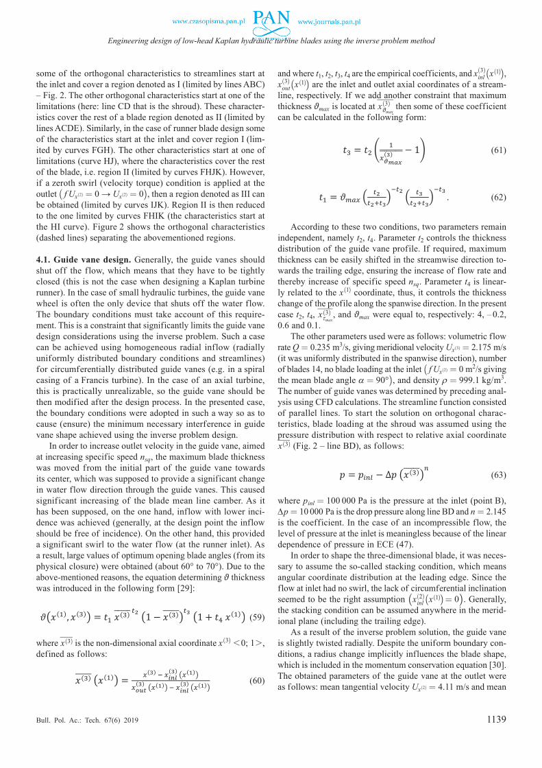
1139

Engineering design of low-head Kaplan hydraulic turbine blades using the inverse problem method

Bull. Pol. Ac.: Tech. 67(6) 2019

some of the orthogonal characteristics to streamlines start at the inlet and cover a region denoted as I (limited by lines ABC) – Fig. 2. The other orthogonal characteristics start at one of the limitations (here: line CD that is the shroud). These character-istics cover the rest of a blade region denoted as II (limited by lines ACDE). Similarly, in the case of runner blade design some of the characteristics start at the inlet and cover region I (lim-ited by curves FGH). The other characteristics start at one of limitations (curve HJ), where the characteristics cover the rest of the blade, i.e. region II (limited by curves FHJK). However, if a zeroth swirl (velocity torque) condition is applied at the outlet ( f Ux(2) = 0 → Ux(2) = 0), then a region denoted as III can be obtained (limited by curves IJK). Region II is then reduced to the one limited by curves FHIK (the characteristics start at the HI curve). Figure 2 shows the orthogonal characteristics (dashed lines) separating the abovementioned regions.

4.1. Guide vane design. Generally, the guide vanes should shut off the flow, which means that they have to be tightly closed (this is not the case when designing a Kaplan turbine runner). In the case of small hydraulic turbines, the guide vane wheel is often the only device that shuts off the water flow. The boundary conditions must take account of this require-ment. This is a constraint that significantly limits the guide vane design considerations using the inverse problem. Such a case can be achieved using homogeneous radial inflow (radially uniformly distributed boundary conditions and streamlines) for circumferentially distributed guide vanes (e.g. in a spiral casing of a Francis turbine). In the case of an axial turbine, this is practically unrealizable, so the guide vane should be then modified after the design process. In the presented case, the boundary conditions were adopted in such a way so as to cause (ensure) the minimum necessary interference in guide vane shape achieved using the inverse problem design.

In order to increase outlet velocity in the guide vane, aimed at increasing specific speed nsq, the maximum blade thickness was moved from the initial part of the guide vane towards its center, which was supposed to provide a significant change in water flow direction through the guide vanes. This caused significant increasing of the blade mean line camber. As it has been supposed, on the one hand, inflow with lower inci-dence was achieved (generally, at the design point the inflow should be free of incidence). On the other hand, this provided a significant swirl to the water flow (at the runner inlet). As a result, large values of optimum opening blade angles (from its physical closure) were obtained (about 60° to 70°). Due to the above-mentioned reasons, the equation determining ϑ thickness was introduced in the following form [29]:

7

adjustable Kaplan turbine model characterized by a fairly high specific speed nsq (1), larger than 230 with runner diameter D = Ø300 mm. Figure 2 shows the meridional shape used for calculations and its main dimensions. It should be emphasized that the meridional shape adopted for calculations was not subject to prior optimization (this is not the subject of this paper), therefore, the results obtained should not be considered as optimized from efficiency point of view.

Fig. 2. Schematic meridional view of the low-head Kaplan hydraulic turbine model

The used method of characteristics requires setting

boundary conditions at one of limitations (hub or shroud line) of the meridional blade shape. In the case of guide vane design some of the orthogonal characteristics to streamlines start at the inlet and cover a region denoted as I (limited by lines ABC) – Figure 2. The other orthogonal characteristics start at one of the limitations (here: line CD that is shroud). These characteristics cover the rest of a blade region denoted as II (limited by lines ACDE). Similarly, in the case of runner blade design some of the characteristics start at the inlet and cover a region I (limited by curves FGH). The other characteristics start at one of limitations (curve HJ), where the characteristics cover the rest of the blade, i.e. a region II (limited by curves FHJK). However, if a zeroth swirl (velocity torque) condition is applied at the outlet (𝑓𝑓𝑈𝑈𝑥𝑥(2) = 0 → 𝑈𝑈𝑥𝑥(2) = 0), then a region denoted as III can be obtained (limited by curves IJK). Region II is then reduced to the one limited by curves FHIK (the characteristics start at the curve HI). Figure 2 shows the orthogonal characteristics (dashed lines) separating the abovementioned regions.

4.1. Guide vane design. Generally, the guide vanes should shut off the flow, which means they have to be tightly closed (this is not the case when designing a Kaplan turbine runner). In the case of small hydraulic turbines, the guide vane wheel is often the only device that shuts off the water flow. The boundary conditions must take into account this requirement. This is a constraint that significantly limits the guide vane design considerations using the inverse problem. Such a case can be achieved using homogeneous radial inflow (radially uniformly distributed boundary conditions and streamlines) for circumferentially

distributed guide vanes (e.g. in a spiral casing of Francis turbine). In the case of axial turbine this is practically unrealizable, so the guide vane should be then modified after the design process. In the presented case, the boundary conditions were adopted in such a way so as to cause (ensure) the minimum necessary interference in guide vane shape achieved using the inverse problem design.

In order to increase the outlet velocity in guide vane, aimed at increasing the specific speed nsq, the maximum blade thickness was moved from the initial part of guide vane towards its centre, which was supposed to provide a significant change in water flow direction through the guide vanes. This caused significant increasing of the blade mean line camber. As it is supposed, on the one hand, the inflow with lower incidence was achieved (generally, in the design point the inflow should be free of incidence). On the other hand, this provided a significant swirl to the water flow (at the runner inlet). As a result, large values of optimal opening blade angles (from its physical closure) were obtained (about 60° to 70°). Due to the above-mentioned reasons, the equation determining ϑ thickness was introduced in the following form [29]:

𝜗𝜗(𝑥𝑥(1), 𝑥𝑥(3)) = 𝑡𝑡1 𝑥𝑥(3)̅̅ ̅̅ ̅ 𝑡𝑡2 (1 − 𝑥𝑥(3)̅̅ ̅̅ ̅)𝑡𝑡3 (1 + 𝑡𝑡4 𝑥𝑥(1)) (59)

where 𝑥𝑥(3)̅̅ ̅̅ ̅ is the non-dimensional axial coordinate 𝑥𝑥(3) <0;1>, defined as follows:

𝑥𝑥(3)̅̅ ̅̅ ̅ (𝑥𝑥(1)) = 𝑥𝑥(3) − 𝑥𝑥𝑖𝑖𝑖𝑖𝑖𝑖(3) (𝑥𝑥(1))

𝑥𝑥𝑜𝑜𝑜𝑜𝑜𝑜(3) (𝑥𝑥(1)) − 𝑥𝑥𝑖𝑖𝑖𝑖𝑖𝑖

(3) (𝑥𝑥(1)) (60)

and where t1, t2, t3, t4 are the empirical coefficients, and 𝑥𝑥𝑖𝑖𝑖𝑖𝑖𝑖

(3) (𝑥𝑥(1)), 𝑥𝑥𝑜𝑜𝑜𝑜𝑡𝑡(3) (𝑥𝑥(1)) are the inlet and outlet axial

coordinates of a streamline, respectively. If we add another constraint that maximum thickness 𝜗𝜗𝑚𝑚𝑚𝑚𝑥𝑥 is located at 𝑥𝑥𝜗𝜗𝑚𝑚𝑚𝑚𝑚𝑚

(3)̅̅ ̅̅ ̅̅ ̅ then some of these coefficient can be calculated in the following form:

𝑡𝑡3 = 𝑡𝑡2 ( 1𝑥𝑥𝜗𝜗𝑚𝑚𝑚𝑚𝑚𝑚

(3)̅̅ ̅̅ ̅̅ ̅̅ ̅̅ − 1) (61)

𝑡𝑡1 = 𝜗𝜗𝑚𝑚𝑚𝑚𝑥𝑥 ( 𝑡𝑡2𝑡𝑡2+𝑡𝑡3

)−𝑡𝑡2 ( 𝑡𝑡3

𝑡𝑡2+𝑡𝑡3)

−𝑡𝑡3 (62)

According to these two conditions two parameters remain independent, namely t2, t4. Parameter t2 controls the thickness distribution of guide vane profile. If required, maximum thickness can be easy shifted in the streamwise direction towards the trailing edge ensuring the increase of flow rate and thereby the increase of specific speed nsq. Parameter t4 is linearly related to 𝑥𝑥(1) coordinate, thus, it controls the thickness change of profile along the spanwise direction. In the present case t2, t4, 𝑥𝑥𝜏𝜏𝑚𝑚𝑚𝑚𝑚𝑚

(3)̅̅ ̅̅ ̅̅ ̅, and 𝜗𝜗𝑚𝑚𝑚𝑚𝑥𝑥 were equal, respectively: 4, -0.2, 0.6, and 0.1.

(59)

where –x(3) is the non-dimensional axial coordinate x(3) <0; 1>,

defined as follows:

7

adjustable Kaplan turbine model characterized by a fairly high specific speed nsq (1), larger than 230 with runner diameter D = Ø300 mm. Figure 2 shows the meridional shape used for calculations and its main dimensions. It should be emphasized that the meridional shape adopted for calculations was not subject to prior optimization (this is not the subject of this paper), therefore, the results obtained should not be considered as optimized from efficiency point of view.

Fig. 2. Schematic meridional view of the low-head Kaplan hydraulic turbine model

The used method of characteristics requires setting

boundary conditions at one of limitations (hub or shroud line) of the meridional blade shape. In the case of guide vane design some of the orthogonal characteristics to streamlines start at the inlet and cover a region denoted as I (limited by lines ABC) – Figure 2. The other orthogonal characteristics start at one of the limitations (here: line CD that is shroud). These characteristics cover the rest of a blade region denoted as II (limited by lines ACDE). Similarly, in the case of runner blade design some of the characteristics start at the inlet and cover a region I (limited by curves FGH). The other characteristics start at one of limitations (curve HJ), where the characteristics cover the rest of the blade, i.e. a region II (limited by curves FHJK). However, if a zeroth swirl (velocity torque) condition is applied at the outlet (𝑓𝑓𝑈𝑈𝑥𝑥(2) = 0 → 𝑈𝑈𝑥𝑥(2) = 0), then a region denoted as III can be obtained (limited by curves IJK). Region II is then reduced to the one limited by curves FHIK (the characteristics start at the curve HI). Figure 2 shows the orthogonal characteristics (dashed lines) separating the abovementioned regions.

4.1. Guide vane design. Generally, the guide vanes should shut off the flow, which means they have to be tightly closed (this is not the case when designing a Kaplan turbine runner). In the case of small hydraulic turbines, the guide vane wheel is often the only device that shuts off the water flow. The boundary conditions must take into account this requirement. This is a constraint that significantly limits the guide vane design considerations using the inverse problem. Such a case can be achieved using homogeneous radial inflow (radially uniformly distributed boundary conditions and streamlines) for circumferentially

distributed guide vanes (e.g. in a spiral casing of Francis turbine). In the case of axial turbine this is practically unrealizable, so the guide vane should be then modified after the design process. In the presented case, the boundary conditions were adopted in such a way so as to cause (ensure) the minimum necessary interference in guide vane shape achieved using the inverse problem design.

In order to increase the outlet velocity in guide vane, aimed at increasing the specific speed nsq, the maximum blade thickness was moved from the initial part of guide vane towards its centre, which was supposed to provide a significant change in water flow direction through the guide vanes. This caused significant increasing of the blade mean line camber. As it is supposed, on the one hand, the inflow with lower incidence was achieved (generally, in the design point the inflow should be free of incidence). On the other hand, this provided a significant swirl to the water flow (at the runner inlet). As a result, large values of optimal opening blade angles (from its physical closure) were obtained (about 60° to 70°). Due to the above-mentioned reasons, the equation determining ϑ thickness was introduced in the following form [29]:

𝜗𝜗(𝑥𝑥(1), 𝑥𝑥(3)) = 𝑡𝑡1 𝑥𝑥(3)̅̅ ̅̅ ̅ 𝑡𝑡2 (1 − 𝑥𝑥(3)̅̅ ̅̅ ̅)𝑡𝑡3 (1 + 𝑡𝑡4 𝑥𝑥(1)) (59)

where 𝑥𝑥(3)̅̅ ̅̅ ̅ is the non-dimensional axial coordinate 𝑥𝑥(3) <0;1>, defined as follows:

𝑥𝑥(3)̅̅ ̅̅ ̅ (𝑥𝑥(1)) = 𝑥𝑥(3) − 𝑥𝑥𝑖𝑖𝑖𝑖𝑖𝑖(3) (𝑥𝑥(1))

𝑥𝑥𝑜𝑜𝑜𝑜𝑜𝑜(3) (𝑥𝑥(1)) − 𝑥𝑥𝑖𝑖𝑖𝑖𝑖𝑖

(3) (𝑥𝑥(1)) (60)

and where t1, t2, t3, t4 are the empirical coefficients, and 𝑥𝑥𝑖𝑖𝑖𝑖𝑖𝑖

(3) (𝑥𝑥(1)), 𝑥𝑥𝑜𝑜𝑜𝑜𝑡𝑡(3) (𝑥𝑥(1)) are the inlet and outlet axial

coordinates of a streamline, respectively. If we add another constraint that maximum thickness 𝜗𝜗𝑚𝑚𝑚𝑚𝑥𝑥 is located at 𝑥𝑥𝜗𝜗𝑚𝑚𝑚𝑚𝑚𝑚

(3)̅̅ ̅̅ ̅̅ ̅ then some of these coefficient can be calculated in the following form:

𝑡𝑡3 = 𝑡𝑡2 ( 1𝑥𝑥𝜗𝜗𝑚𝑚𝑚𝑚𝑚𝑚

(3)̅̅ ̅̅ ̅̅ ̅̅ ̅̅ − 1) (61)

𝑡𝑡1 = 𝜗𝜗𝑚𝑚𝑚𝑚𝑥𝑥 ( 𝑡𝑡2𝑡𝑡2+𝑡𝑡3

)−𝑡𝑡2 ( 𝑡𝑡3

𝑡𝑡2+𝑡𝑡3)

−𝑡𝑡3 (62)

According to these two conditions two parameters remain independent, namely t2, t4. Parameter t2 controls the thickness distribution of guide vane profile. If required, maximum thickness can be easy shifted in the streamwise direction towards the trailing edge ensuring the increase of flow rate and thereby the increase of specific speed nsq. Parameter t4 is linearly related to 𝑥𝑥(1) coordinate, thus, it controls the thickness change of profile along the spanwise direction. In the present case t2, t4, 𝑥𝑥𝜏𝜏𝑚𝑚𝑚𝑚𝑚𝑚

(3)̅̅ ̅̅ ̅̅ ̅, and 𝜗𝜗𝑚𝑚𝑚𝑚𝑥𝑥 were equal, respectively: 4, -0.2, 0.6, and 0.1.

(60)

and where t1, t2, t3, t4 are the empirical coefficients, and x(3)inl (x(1)),

x(3)out(x(1)) are the inlet and outlet axial coordinates of a stream-

line, respectively. If we add another constraint that maximum thickness ϑmax is located at

–x(3)ϑmax

then some of these coefficient can be calculated in the following form:

7

adjustable Kaplan turbine model characterized by a fairly high specific speed nsq (1), larger than 230 with runner diameter D = Ø300 mm. Figure 2 shows the meridional shape used for calculations and its main dimensions. It should be emphasized that the meridional shape adopted for calculations was not subject to prior optimization (this is not the subject of this paper), therefore, the results obtained should not be considered as optimized from efficiency point of view.

Fig. 2. Schematic meridional view of the low-head Kaplan hydraulic turbine model

The used method of characteristics requires setting

boundary conditions at one of limitations (hub or shroud line) of the meridional blade shape. In the case of guide vane design some of the orthogonal characteristics to streamlines start at the inlet and cover a region denoted as I (limited by lines ABC) – Figure 2. The other orthogonal characteristics start at one of the limitations (here: line CD that is shroud). These characteristics cover the rest of a blade region denoted as II (limited by lines ACDE). Similarly, in the case of runner blade design some of the characteristics start at the inlet and cover a region I (limited by curves FGH). The other characteristics start at one of limitations (curve HJ), where the characteristics cover the rest of the blade, i.e. a region II (limited by curves FHJK). However, if a zeroth swirl (velocity torque) condition is applied at the outlet (𝑓𝑓𝑈𝑈𝑥𝑥(2) = 0 → 𝑈𝑈𝑥𝑥(2) = 0), then a region denoted as III can be obtained (limited by curves IJK). Region II is then reduced to the one limited by curves FHIK (the characteristics start at the curve HI). Figure 2 shows the orthogonal characteristics (dashed lines) separating the abovementioned regions.

4.1. Guide vane design. Generally, the guide vanes should shut off the flow, which means they have to be tightly closed (this is not the case when designing a Kaplan turbine runner). In the case of small hydraulic turbines, the guide vane wheel is often the only device that shuts off the water flow. The boundary conditions must take into account this requirement. This is a constraint that significantly limits the guide vane design considerations using the inverse problem. Such a case can be achieved using homogeneous radial inflow (radially uniformly distributed boundary conditions and streamlines) for circumferentially

distributed guide vanes (e.g. in a spiral casing of Francis turbine). In the case of axial turbine this is practically unrealizable, so the guide vane should be then modified after the design process. In the presented case, the boundary conditions were adopted in such a way so as to cause (ensure) the minimum necessary interference in guide vane shape achieved using the inverse problem design.

In order to increase the outlet velocity in guide vane, aimed at increasing the specific speed nsq, the maximum blade thickness was moved from the initial part of guide vane towards its centre, which was supposed to provide a significant change in water flow direction through the guide vanes. This caused significant increasing of the blade mean line camber. As it is supposed, on the one hand, the inflow with lower incidence was achieved (generally, in the design point the inflow should be free of incidence). On the other hand, this provided a significant swirl to the water flow (at the runner inlet). As a result, large values of optimal opening blade angles (from its physical closure) were obtained (about 60° to 70°). Due to the above-mentioned reasons, the equation determining ϑ thickness was introduced in the following form [29]:

𝜗𝜗(𝑥𝑥(1), 𝑥𝑥(3)) = 𝑡𝑡1 𝑥𝑥(3)̅̅ ̅̅ ̅ 𝑡𝑡2 (1 − 𝑥𝑥(3)̅̅ ̅̅ ̅)𝑡𝑡3 (1 + 𝑡𝑡4 𝑥𝑥(1)) (59)

where 𝑥𝑥(3)̅̅ ̅̅ ̅ is the non-dimensional axial coordinate 𝑥𝑥(3) <0;1>, defined as follows:

𝑥𝑥(3)̅̅ ̅̅ ̅ (𝑥𝑥(1)) = 𝑥𝑥(3) − 𝑥𝑥𝑖𝑖𝑖𝑖𝑖𝑖(3) (𝑥𝑥(1))

𝑥𝑥𝑜𝑜𝑜𝑜𝑜𝑜(3) (𝑥𝑥(1)) − 𝑥𝑥𝑖𝑖𝑖𝑖𝑖𝑖

(3) (𝑥𝑥(1)) (60)

and where t1, t2, t3, t4 are the empirical coefficients, and 𝑥𝑥𝑖𝑖𝑖𝑖𝑖𝑖

(3) (𝑥𝑥(1)), 𝑥𝑥𝑜𝑜𝑜𝑜𝑡𝑡(3) (𝑥𝑥(1)) are the inlet and outlet axial

coordinates of a streamline, respectively. If we add another constraint that maximum thickness 𝜗𝜗𝑚𝑚𝑚𝑚𝑥𝑥 is located at 𝑥𝑥𝜗𝜗𝑚𝑚𝑚𝑚𝑚𝑚

(3)̅̅ ̅̅ ̅̅ ̅ then some of these coefficient can be calculated in the following form:

𝑡𝑡3 = 𝑡𝑡2 ( 1𝑥𝑥𝜗𝜗𝑚𝑚𝑚𝑚𝑚𝑚

(3)̅̅ ̅̅ ̅̅ ̅̅ ̅̅ − 1) (61)

𝑡𝑡1 = 𝜗𝜗𝑚𝑚𝑚𝑚𝑥𝑥 ( 𝑡𝑡2𝑡𝑡2+𝑡𝑡3

)−𝑡𝑡2 ( 𝑡𝑡3

𝑡𝑡2+𝑡𝑡3)

−𝑡𝑡3 (62)

According to these two conditions two parameters remain independent, namely t2, t4. Parameter t2 controls the thickness distribution of guide vane profile. If required, maximum thickness can be easy shifted in the streamwise direction towards the trailing edge ensuring the increase of flow rate and thereby the increase of specific speed nsq. Parameter t4 is linearly related to 𝑥𝑥(1) coordinate, thus, it controls the thickness change of profile along the spanwise direction. In the present case t2, t4, 𝑥𝑥𝜏𝜏𝑚𝑚𝑚𝑚𝑚𝑚

(3)̅̅ ̅̅ ̅̅ ̅, and 𝜗𝜗𝑚𝑚𝑚𝑚𝑥𝑥 were equal, respectively: 4, -0.2, 0.6, and 0.1.

(61)

7

adjustable Kaplan turbine model characterized by a fairly high specific speed nsq (1), larger than 230 with runner diameter D = Ø300 mm. Figure 2 shows the meridional shape used for calculations and its main dimensions. It should be emphasized that the meridional shape adopted for calculations was not subject to prior optimization (this is not the subject of this paper), therefore, the results obtained should not be considered as optimized from efficiency point of view.

Fig. 2. Schematic meridional view of the low-head Kaplan hydraulic turbine model

The used method of characteristics requires setting

boundary conditions at one of limitations (hub or shroud line) of the meridional blade shape. In the case of guide vane design some of the orthogonal characteristics to streamlines start at the inlet and cover a region denoted as I (limited by lines ABC) – Figure 2. The other orthogonal characteristics start at one of the limitations (here: line CD that is shroud). These characteristics cover the rest of a blade region denoted as II (limited by lines ACDE). Similarly, in the case of runner blade design some of the characteristics start at the inlet and cover a region I (limited by curves FGH). The other characteristics start at one of limitations (curve HJ), where the characteristics cover the rest of the blade, i.e. a region II (limited by curves FHJK). However, if a zeroth swirl (velocity torque) condition is applied at the outlet (𝑓𝑓𝑈𝑈𝑥𝑥(2) = 0 → 𝑈𝑈𝑥𝑥(2) = 0), then a region denoted as III can be obtained (limited by curves IJK). Region II is then reduced to the one limited by curves FHIK (the characteristics start at the curve HI). Figure 2 shows the orthogonal characteristics (dashed lines) separating the abovementioned regions.

4.1. Guide vane design. Generally, the guide vanes should shut off the flow, which means they have to be tightly closed (this is not the case when designing a Kaplan turbine runner). In the case of small hydraulic turbines, the guide vane wheel is often the only device that shuts off the water flow. The boundary conditions must take into account this requirement. This is a constraint that significantly limits the guide vane design considerations using the inverse problem. Such a case can be achieved using homogeneous radial inflow (radially uniformly distributed boundary conditions and streamlines) for circumferentially

distributed guide vanes (e.g. in a spiral casing of Francis turbine). In the case of axial turbine this is practically unrealizable, so the guide vane should be then modified after the design process. In the presented case, the boundary conditions were adopted in such a way so as to cause (ensure) the minimum necessary interference in guide vane shape achieved using the inverse problem design.

In order to increase the outlet velocity in guide vane, aimed at increasing the specific speed nsq, the maximum blade thickness was moved from the initial part of guide vane towards its centre, which was supposed to provide a significant change in water flow direction through the guide vanes. This caused significant increasing of the blade mean line camber. As it is supposed, on the one hand, the inflow with lower incidence was achieved (generally, in the design point the inflow should be free of incidence). On the other hand, this provided a significant swirl to the water flow (at the runner inlet). As a result, large values of optimal opening blade angles (from its physical closure) were obtained (about 60° to 70°). Due to the above-mentioned reasons, the equation determining ϑ thickness was introduced in the following form [29]:

𝜗𝜗(𝑥𝑥(1), 𝑥𝑥(3)) = 𝑡𝑡1 𝑥𝑥(3)̅̅ ̅̅ ̅ 𝑡𝑡2 (1 − 𝑥𝑥(3)̅̅ ̅̅ ̅)𝑡𝑡3 (1 + 𝑡𝑡4 𝑥𝑥(1)) (59)

where 𝑥𝑥(3)̅̅ ̅̅ ̅ is the non-dimensional axial coordinate 𝑥𝑥(3) <0;1>, defined as follows:

𝑥𝑥(3)̅̅ ̅̅ ̅ (𝑥𝑥(1)) = 𝑥𝑥(3) − 𝑥𝑥𝑖𝑖𝑖𝑖𝑖𝑖(3) (𝑥𝑥(1))

𝑥𝑥𝑜𝑜𝑜𝑜𝑜𝑜(3) (𝑥𝑥(1)) − 𝑥𝑥𝑖𝑖𝑖𝑖𝑖𝑖

(3) (𝑥𝑥(1)) (60)

and where t1, t2, t3, t4 are the empirical coefficients, and 𝑥𝑥𝑖𝑖𝑖𝑖𝑖𝑖

(3) (𝑥𝑥(1)), 𝑥𝑥𝑜𝑜𝑜𝑜𝑡𝑡(3) (𝑥𝑥(1)) are the inlet and outlet axial

coordinates of a streamline, respectively. If we add another constraint that maximum thickness 𝜗𝜗𝑚𝑚𝑚𝑚𝑥𝑥 is located at 𝑥𝑥𝜗𝜗𝑚𝑚𝑚𝑚𝑚𝑚

(3)̅̅ ̅̅ ̅̅ ̅ then some of these coefficient can be calculated in the following form:

𝑡𝑡3 = 𝑡𝑡2 ( 1𝑥𝑥𝜗𝜗𝑚𝑚𝑚𝑚𝑚𝑚

(3)̅̅ ̅̅ ̅̅ ̅̅ ̅̅ − 1) (61)

𝑡𝑡1 = 𝜗𝜗𝑚𝑚𝑚𝑚𝑥𝑥 ( 𝑡𝑡2𝑡𝑡2+𝑡𝑡3

)−𝑡𝑡2 ( 𝑡𝑡3

𝑡𝑡2+𝑡𝑡3)

−𝑡𝑡3 (62)

According to these two conditions two parameters remain independent, namely t2, t4. Parameter t2 controls the thickness distribution of guide vane profile. If required, maximum thickness can be easy shifted in the streamwise direction towards the trailing edge ensuring the increase of flow rate and thereby the increase of specific speed nsq. Parameter t4 is linearly related to 𝑥𝑥(1) coordinate, thus, it controls the thickness change of profile along the spanwise direction. In the present case t2, t4, 𝑥𝑥𝜏𝜏𝑚𝑚𝑚𝑚𝑚𝑚

(3)̅̅ ̅̅ ̅̅ ̅, and 𝜗𝜗𝑚𝑚𝑚𝑚𝑥𝑥 were equal, respectively: 4, -0.2, 0.6, and 0.1.

. (62)

According to these two conditions, two parameters remain independent, namely t2, t4. Parameter t2 controls the thickness distribution of the guide vane profile. If required, maximum thickness can be easily shifted in the streamwise direction to-wards the trailing edge, ensuring the increase of flow rate and thereby increase of specific speed nsq. Parameter t4 is linear-ly related to the x(1) coordinate, thus, it controls the thickness change of the profile along the spanwise direction. In the present case t2, t4,

–x(3)τmax

, and ϑmax were equal to, respectively: 4, –0.2, 0.6 and 0.1.

The other parameters used were as follows: volumetric flow rate Q = 0.235 m3/s, giving meridional velocity Ux(3) = 2.175 m/s (it was uniformly distributed in the spanwise direction), number of blades 14, no blade loading at the inlet ( f Ux(2) = 0 m2/s giving the mean blade angle α = 90°), and density ρ = 999.1 kg/ m3. The number of guide vanes was determined by preceding anal-ysis using CFD calculations. The streamline function consisted of parallel lines. To start the solution on orthogonal charac-teristics, blade loading at the shroud was assumed using the pressure distribution with respect to relative axial coordinate –x(3) (Fig. 2 – line BD), as follows:

8

The other parameters used were as follows: volumetric flow rate Q = 0.235 m3/s giving meridional velocity 𝑈𝑈𝑥𝑥(3) = 2.175 m/s (it was uniformly distributed in the spanwise direction), number of blades 14, no blade loading at the inlet (𝑓𝑓𝑈𝑈𝑥𝑥(2) = 0 m2/s giving the mean blade angle α = 90°), and density ρ = 999.1 kg/m3. The number of guide vanes was determined by a preceding analysis using CFD calculations. The streamline function consisted of parallel lines. To start the solution on orthogonal characteristics the blade loading at shroud was assumed using the pressure distribution with respect to relative axial coordinate 𝑥𝑥(3)̅̅ ̅̅ ̅ (Figure 2 – line BD), as follows:

𝑝𝑝 = 𝑝𝑝𝑖𝑖𝑖𝑖𝑖𝑖 − Δ𝑝𝑝 (𝑥𝑥(3)̅̅ ̅̅ ̅)𝑖𝑖 (63)

where pinl = 100000 Pa is the pressure at the inlet (point B), Δp = 10000 Pa is the drop pressure along line BD, and n = 2.145 is the coefficient. In case of an incompressible flow, level of pressure at the inlet is meaningless, because of linear dependence of pressure in ECE (47).

In order to shape three-dimensional blade it was necessary to assume the so-called stacking condition, which means angular coordinate distribution at the leading edge. Since the flow at inlet had no swirl, the lack of circumferential inclination seemed to be right assumption (𝑥𝑥𝑖𝑖𝑖𝑖𝑖𝑖

(2)(𝑥𝑥(1)) = 0). Generally, the stacking condition can be assumed anywhere in the meridional plane (including the trailing edge).

As a result of the inverse problem solution the guide vane is slightly twisted radially. Despite the uniform

boundary conditions, a radius change implicitly influences the blade shape, what is contained in the momentum conservation equation [30]. The obtained parameters of the guide vane at the outlet were as follows: the mean tangential velocity 𝑈𝑈𝑥𝑥(2) = 4.11 m/s, and the mean meridional velocity 𝑈𝑈𝑥𝑥(3) = 2.17 m/s. Figure 3 shows the blade of single guide vane and guide vane wheel of the Kaplan turbine model and Figure 4 shows the results of pressure, meridional and tangential velocities obtained using the presented model (visually stretched from axi-radial (see Figure 2) to axial inflow direction). It should be highlighted that this is axisymmetric model, therefore the results represent the mean values in circumferential direction.

Fig. 3. Views of the single guide vane blade and guide vane wheel of the

low-head Kaplan hydraulic turbine model.

Fig. 4. Contours of the pressure, meridional and tangential velocities in guide vane channel obtained using the inverse problem method (stretched from axi-radial to axial inflow direction).

4.2. Runner blade design. Generally, in order to increase the flow rate (to increase the specific speed), a meridional length of blade should tend to decrease what causes the increase of torque. The applied meridional shape (Figure 2) was supposed to ensure a high specific speed larger than nsq = 230. The calculated blade and the entire runner wheel

are shown in Figure 5 and in Figure 6, respectively. At the outlet, no swirl condition was set, i.e. the tangential velocity was assumed to be 𝑈𝑈𝑥𝑥(2) = 0 m/s. This assumption theoretically ensures maximizing the efficiency, what results from the Euler’s hydraulic turbines equation.

(63)

where pinl = 100 000 Pa is the pressure at the inlet (point B), ∆p = 10 000 Pa is the drop pressure along line BD and n = 2.145 is the coefficient. In the case of an incompressible flow, the level of pressure at the inlet is meaningless because of the linear dependence of pressure in ECE (47).

In order to shape the three-dimensional blade, it was neces-sary to assume the so-called stacking condition, which means angular coordinate distribution at the leading edge. Since the flow at inlet had no swirl, the lack of circumferential inclination seemed to be the right assumption (x(2)

inl (x(1)) = 0). Generally, the stacking condition can be assumed anywhere in the merid-ional plane (including the trailing edge).

As a result of the inverse problem solution, the guide vane is slightly twisted radially. Despite the uniform boundary con-ditions, a radius change implicitly influences the blade shape, which is included in the momentum conservation equation [30]. The obtained parameters of the guide vane at the outlet were as follows: mean tangential velocity Ux(2) = 4.11 m/s and mean

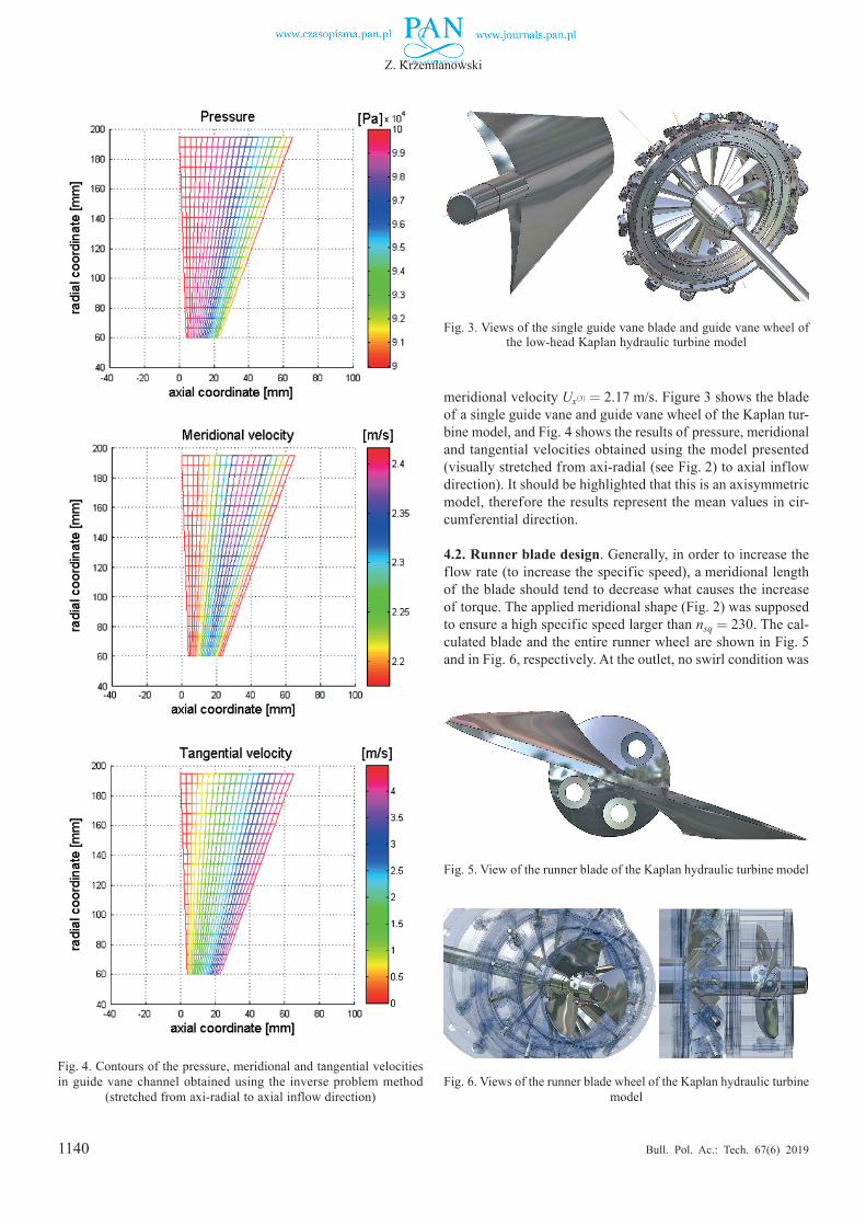
1140

Z. Krzemianowski

Bull. Pol. Ac.: Tech. 67(6) 2019

meridional velocity Ux(3) = 2.17 m/s. Figure 3 shows the blade of a single guide vane and guide vane wheel of the Kaplan tur-bine model, and Fig. 4 shows the results of pressure, meridional and tangential velocities obtained using the model presented (visually stretched from axi-radial (see Fig. 2) to axial inflow direction). It should be highlighted that this is an axisymmetric model, therefore the results represent the mean values in cir-cumferential direction.

4.2. Runner blade design. Generally, in order to increase the flow rate (to increase the specific speed), a meridional length of the blade should tend to decrease what causes the increase of torque. The applied meridional shape (Fig. 2) was supposed to ensure a high specific speed larger than nsq = 230. The cal-culated blade and the entire runner wheel are shown in Fig. 5 and in Fig. 6, respectively. At the outlet, no swirl condition was

Fig. 3. Views of the single guide vane blade and guide vane wheel of the low-head Kaplan hydraulic turbine model

Fig. 4. Contours of the pressure, meridional and tangential velocities in guide vane channel obtained using the inverse problem method

(stretched from axi-radial to axial inflow direction)

Fig. 5. View of the runner blade of the Kaplan hydraulic turbine model

Fig. 6. Views of the runner blade wheel of the Kaplan hydraulic turbine model

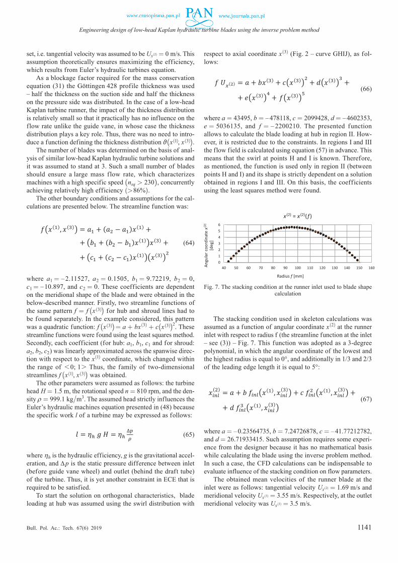
1141

Engineering design of low-head Kaplan hydraulic turbine blades using the inverse problem method

Bull. Pol. Ac.: Tech. 67(6) 2019

set, i.e. tangential velocity was assumed to be Ux(2) = 0 m/s. This assumption theoretically ensures maximizing the efficiency, which results from Euler’s hydraulic turbines equation.

As a blockage factor required for the mass conservation equation (31) the Göttingen 428 profile thickness was used – half the thickness on the suction side and half the thickness on the pressure side was distributed. In the case of a low-head Kaplan turbine runner, the impact of the thickness distribution is relatively small so that it practically has no influence on the flow rate unlike the guide vane, in whose case the thickness distribution plays a key role. Thus, there was no need to intro-duce a function defining the thickness distribution ϑ(x(1), x(3)).

The number of blades was determined on the basis of anal-ysis of similar low-head Kaplan hydraulic turbine solutions and it was assumed to stand at 3. Such a small number of blades should ensure a large mass flow rate, which characterizes machines with a high specific speed (nsq > 230), concurrently achieving relatively high efficiency (>86%).

The other boundary conditions and assumptions for the cal-culations are presented below. The streamline function was:

9

As a blockage factor required to the mass conservation equation (31) the Göttingen 428 profile thickness was used – half the thickness on the suction side and half the thickness on the pressure side was distributed. In the case of a low-head Kaplan turbine runner, the impact of the thickness distribution is relatively small so that it practically has no influence on the flow rate unlike the guide vane case, in which the thickness distribution plays a key role. Thus, there was no need to introduce a function defining the thickness distribution 𝜗𝜗(𝑥𝑥(1), 𝑥𝑥(3)).

The number of blades was determined on the basis of analysis of similar low-head Kaplan hydraulic turbine solutions and it was assumed to be of 3. Such a small number of blades should ensures a large mass flow rate, which characterizes machines with a high specific speed (nsq > 230), concurrently achieving relatively high efficiency (>86%).

Fig. 5. View of the runner blade of the Kaplan hydraulic turbine model.

Fig. 6. Views of the runner blade wheel of the Kaplan hydraulic turbine

model. The other boundary conditions and assumptions for the

calculations are presented below. The streamline function was:

𝑓𝑓(𝑥𝑥(1), 𝑥𝑥(3)) = 𝑎𝑎1 + (𝑎𝑎2 − 𝑎𝑎1)𝑥𝑥(1) + (𝑏𝑏1 + (𝑏𝑏2 −

𝑏𝑏1)𝑥𝑥(1))𝑥𝑥(3) + (𝑐𝑐1 + (𝑐𝑐2 − 𝑐𝑐1)𝑥𝑥(1))(𝑥𝑥(3))2 (64)

where 𝑎𝑎1 = -2.11527, 𝑎𝑎2 = 0.1505, 𝑏𝑏1 = 9.72219, 𝑏𝑏2 = 0, 𝑐𝑐1 = -10.897, and 𝑐𝑐2 = 0. These coefficients are dependent on the meridional shape of blade and were obtained in the following way. Firstly, two streamline functions of the same pattern 𝑓𝑓 = 𝑓𝑓(𝑥𝑥(3)) for hub and shroud lines had to be found separately. In considered example, this pattern was a quadratic function: 𝑓𝑓(𝑥𝑥(3)) = 𝑎𝑎 + 𝑏𝑏𝑥𝑥(3) + 𝑐𝑐(𝑥𝑥(3))2

. These streamline functions were found using the Least Square Method. Secondly, each coefficient (for hub: a1, b1,

c1 and for shroud: a2, b2, c2) was linearly approximated across the spanwise direction with respect to 𝑥𝑥(1) coordinate, which changed within the range of <0;1>. Thus, the family of two-dimensional streamlines 𝑓𝑓(𝑥𝑥(1), 𝑥𝑥(3)) was obtained.

The other parameters were assumed as follows: the turbine head H = 1.5 m, the rotational speed n = 810 rpm, and the density ρ = 999.1 kg/m3. The assumed head strictly influences the Euler’s hydraulic machines equation presented in (48) because the specific work l of a turbine may be expressed as follows:

𝑙𝑙 = 𝜂𝜂ℎ 𝑔𝑔 𝐻𝐻 = 𝜂𝜂ℎ∆𝑝𝑝𝜌𝜌 (65)

where ηh is the hydraulic efficiency, g is the gravitational acceleration, and Δp is the static pressure difference between inlet (before guide vane wheel), and outlet (behind the draft tube) of turbine. Thus, it is another constraint in ECE that is required to be satisfied.

To start the solution on orthogonal characteristics the blade loading at hub was assumed using the swirl distribution with respect to axial coordinate 𝑥𝑥(3) (Figure 2 – curve GHIJ), as follows:

𝑓𝑓 𝑈𝑈𝑥𝑥(2) = 𝑎𝑎 + 𝑏𝑏𝑥𝑥(3) + 𝑐𝑐(𝑥𝑥(3))2 + 𝑑𝑑(𝑥𝑥(3))3 + 𝑒𝑒(𝑥𝑥(3))4 +

𝑓𝑓(𝑥𝑥(3))5 (66)

where a = 43495, b = -478118, c = 2099428, d = -4602353, e = 5036135, and f = -2200210. Presented function allows calculating the blade loading at hub in region II. However, it is restricted due to the constraints. In regions I and III the flow field is calculated using equation (57) in advance. This means that the swirl in points H and I is known. Therefore, as mentioned the function is used only in region II (between points H and I) and its shape is strictly dependent on a solution obtained in regions I and III. On this basis, the coefficients using the Least Square Method were found.

The stacking condition used in skeleton calculations was assumed as a function of angular coordinate 𝑥𝑥(2) at the runner inlet with respect to radius f (the streamline function at the inlet – see (3)) – Figure 7. This function was adopted as a 3-degree polynomial, in which the angular coordinate of the lowest and the highest radius is equal 0°, and additionally in 1/3 and 2/3 of the leading edge length is equal 5°:

𝑥𝑥𝑖𝑖𝑖𝑖𝑖𝑖(2) = 𝑎𝑎 + 𝑏𝑏 𝑓𝑓𝑖𝑖𝑖𝑖𝑖𝑖(𝑥𝑥(1), 𝑥𝑥𝑖𝑖𝑖𝑖𝑖𝑖

(3)) + 𝑐𝑐 𝑓𝑓𝑖𝑖𝑖𝑖𝑖𝑖2 (𝑥𝑥(1), 𝑥𝑥𝑖𝑖𝑖𝑖𝑖𝑖

(3)) +

𝑑𝑑 𝑓𝑓𝑖𝑖𝑖𝑖𝑖𝑖3 (𝑥𝑥(1), 𝑥𝑥𝑖𝑖𝑖𝑖𝑖𝑖

(3)) (67)

where a = -0.23564735, b = 7.24726878, c = -41.77212782, and d = 26.71933415. Such assumption requires some experience from the designer because it has no

9

As a blockage factor required to the mass conservation equation (31) the Göttingen 428 profile thickness was used – half the thickness on the suction side and half the thickness on the pressure side was distributed. In the case of a low-head Kaplan turbine runner, the impact of the thickness distribution is relatively small so that it practically has no influence on the flow rate unlike the guide vane case, in which the thickness distribution plays a key role. Thus, there was no need to introduce a function defining the thickness distribution 𝜗𝜗(𝑥𝑥(1), 𝑥𝑥(3)).

The number of blades was determined on the basis of analysis of similar low-head Kaplan hydraulic turbine solutions and it was assumed to be of 3. Such a small number of blades should ensures a large mass flow rate, which characterizes machines with a high specific speed (nsq > 230), concurrently achieving relatively high efficiency (>86%).

Fig. 5. View of the runner blade of the Kaplan hydraulic turbine model.

Fig. 6. Views of the runner blade wheel of the Kaplan hydraulic turbine

model. The other boundary conditions and assumptions for the

calculations are presented below. The streamline function was:

𝑓𝑓(𝑥𝑥(1), 𝑥𝑥(3)) = 𝑎𝑎1 + (𝑎𝑎2 − 𝑎𝑎1)𝑥𝑥(1) + (𝑏𝑏1 + (𝑏𝑏2 −

𝑏𝑏1)𝑥𝑥(1))𝑥𝑥(3) + (𝑐𝑐1 + (𝑐𝑐2 − 𝑐𝑐1)𝑥𝑥(1))(𝑥𝑥(3))2 (64)

where 𝑎𝑎1 = -2.11527, 𝑎𝑎2 = 0.1505, 𝑏𝑏1 = 9.72219, 𝑏𝑏2 = 0, 𝑐𝑐1 = -10.897, and 𝑐𝑐2 = 0. These coefficients are dependent on the meridional shape of blade and were obtained in the following way. Firstly, two streamline functions of the same pattern 𝑓𝑓 = 𝑓𝑓(𝑥𝑥(3)) for hub and shroud lines had to be found separately. In considered example, this pattern was a quadratic function: 𝑓𝑓(𝑥𝑥(3)) = 𝑎𝑎 + 𝑏𝑏𝑥𝑥(3) + 𝑐𝑐(𝑥𝑥(3))2

. These streamline functions were found using the Least Square Method. Secondly, each coefficient (for hub: a1, b1,

c1 and for shroud: a2, b2, c2) was linearly approximated across the spanwise direction with respect to 𝑥𝑥(1) coordinate, which changed within the range of <0;1>. Thus, the family of two-dimensional streamlines 𝑓𝑓(𝑥𝑥(1), 𝑥𝑥(3)) was obtained.

The other parameters were assumed as follows: the turbine head H = 1.5 m, the rotational speed n = 810 rpm, and the density ρ = 999.1 kg/m3. The assumed head strictly influences the Euler’s hydraulic machines equation presented in (48) because the specific work l of a turbine may be expressed as follows:

𝑙𝑙 = 𝜂𝜂ℎ 𝑔𝑔 𝐻𝐻 = 𝜂𝜂ℎ∆𝑝𝑝𝜌𝜌 (65)

where ηh is the hydraulic efficiency, g is the gravitational acceleration, and Δp is the static pressure difference between inlet (before guide vane wheel), and outlet (behind the draft tube) of turbine. Thus, it is another constraint in ECE that is required to be satisfied.

To start the solution on orthogonal characteristics the blade loading at hub was assumed using the swirl distribution with respect to axial coordinate 𝑥𝑥(3) (Figure 2 – curve GHIJ), as follows:

𝑓𝑓 𝑈𝑈𝑥𝑥(2) = 𝑎𝑎 + 𝑏𝑏𝑥𝑥(3) + 𝑐𝑐(𝑥𝑥(3))2 + 𝑑𝑑(𝑥𝑥(3))3 + 𝑒𝑒(𝑥𝑥(3))4 +

𝑓𝑓(𝑥𝑥(3))5 (66)

where a = 43495, b = -478118, c = 2099428, d = -4602353, e = 5036135, and f = -2200210. Presented function allows calculating the blade loading at hub in region II. However, it is restricted due to the constraints. In regions I and III the flow field is calculated using equation (57) in advance. This means that the swirl in points H and I is known. Therefore, as mentioned the function is used only in region II (between points H and I) and its shape is strictly dependent on a solution obtained in regions I and III. On this basis, the coefficients using the Least Square Method were found.

The stacking condition used in skeleton calculations was assumed as a function of angular coordinate 𝑥𝑥(2) at the runner inlet with respect to radius f (the streamline function at the inlet – see (3)) – Figure 7. This function was adopted as a 3-degree polynomial, in which the angular coordinate of the lowest and the highest radius is equal 0°, and additionally in 1/3 and 2/3 of the leading edge length is equal 5°:

𝑥𝑥𝑖𝑖𝑖𝑖𝑖𝑖(2) = 𝑎𝑎 + 𝑏𝑏 𝑓𝑓𝑖𝑖𝑖𝑖𝑖𝑖(𝑥𝑥(1), 𝑥𝑥𝑖𝑖𝑖𝑖𝑖𝑖

(3)) + 𝑐𝑐 𝑓𝑓𝑖𝑖𝑖𝑖𝑖𝑖2 (𝑥𝑥(1), 𝑥𝑥𝑖𝑖𝑖𝑖𝑖𝑖

(3)) +

𝑑𝑑 𝑓𝑓𝑖𝑖𝑖𝑖𝑖𝑖3 (𝑥𝑥(1), 𝑥𝑥𝑖𝑖𝑖𝑖𝑖𝑖

(3)) (67)

where a = -0.23564735, b = 7.24726878, c = -41.77212782, and d = 26.71933415. Such assumption requires some experience from the designer because it has no

9

As a blockage factor required to the mass conservation equation (31) the Göttingen 428 profile thickness was used – half the thickness on the suction side and half the thickness on the pressure side was distributed. In the case of a low-head Kaplan turbine runner, the impact of the thickness distribution is relatively small so that it practically has no influence on the flow rate unlike the guide vane case, in which the thickness distribution plays a key role. Thus, there was no need to introduce a function defining the thickness distribution 𝜗𝜗(𝑥𝑥(1), 𝑥𝑥(3)).

The number of blades was determined on the basis of analysis of similar low-head Kaplan hydraulic turbine solutions and it was assumed to be of 3. Such a small number of blades should ensures a large mass flow rate, which characterizes machines with a high specific speed (nsq > 230), concurrently achieving relatively high efficiency (>86%).

Fig. 5. View of the runner blade of the Kaplan hydraulic turbine model.

Fig. 6. Views of the runner blade wheel of the Kaplan hydraulic turbine

model. The other boundary conditions and assumptions for the

calculations are presented below. The streamline function was:

𝑓𝑓(𝑥𝑥(1), 𝑥𝑥(3)) = 𝑎𝑎1 + (𝑎𝑎2 − 𝑎𝑎1)𝑥𝑥(1) + (𝑏𝑏1 + (𝑏𝑏2 −

𝑏𝑏1)𝑥𝑥(1))𝑥𝑥(3) + (𝑐𝑐1 + (𝑐𝑐2 − 𝑐𝑐1)𝑥𝑥(1))(𝑥𝑥(3))2 (64)

where 𝑎𝑎1 = -2.11527, 𝑎𝑎2 = 0.1505, 𝑏𝑏1 = 9.72219, 𝑏𝑏2 = 0, 𝑐𝑐1 = -10.897, and 𝑐𝑐2 = 0. These coefficients are dependent on the meridional shape of blade and were obtained in the following way. Firstly, two streamline functions of the same pattern 𝑓𝑓 = 𝑓𝑓(𝑥𝑥(3)) for hub and shroud lines had to be found separately. In considered example, this pattern was a quadratic function: 𝑓𝑓(𝑥𝑥(3)) = 𝑎𝑎 + 𝑏𝑏𝑥𝑥(3) + 𝑐𝑐(𝑥𝑥(3))2

. These streamline functions were found using the Least Square Method. Secondly, each coefficient (for hub: a1, b1,

c1 and for shroud: a2, b2, c2) was linearly approximated across the spanwise direction with respect to 𝑥𝑥(1) coordinate, which changed within the range of <0;1>. Thus, the family of two-dimensional streamlines 𝑓𝑓(𝑥𝑥(1), 𝑥𝑥(3)) was obtained.

The other parameters were assumed as follows: the turbine head H = 1.5 m, the rotational speed n = 810 rpm, and the density ρ = 999.1 kg/m3. The assumed head strictly influences the Euler’s hydraulic machines equation presented in (48) because the specific work l of a turbine may be expressed as follows:

𝑙𝑙 = 𝜂𝜂ℎ 𝑔𝑔 𝐻𝐻 = 𝜂𝜂ℎ∆𝑝𝑝𝜌𝜌 (65)

where ηh is the hydraulic efficiency, g is the gravitational acceleration, and Δp is the static pressure difference between inlet (before guide vane wheel), and outlet (behind the draft tube) of turbine. Thus, it is another constraint in ECE that is required to be satisfied.

To start the solution on orthogonal characteristics the blade loading at hub was assumed using the swirl distribution with respect to axial coordinate 𝑥𝑥(3) (Figure 2 – curve GHIJ), as follows:

𝑓𝑓 𝑈𝑈𝑥𝑥(2) = 𝑎𝑎 + 𝑏𝑏𝑥𝑥(3) + 𝑐𝑐(𝑥𝑥(3))2 + 𝑑𝑑(𝑥𝑥(3))3 + 𝑒𝑒(𝑥𝑥(3))4 +

𝑓𝑓(𝑥𝑥(3))5 (66)

where a = 43495, b = -478118, c = 2099428, d = -4602353, e = 5036135, and f = -2200210. Presented function allows calculating the blade loading at hub in region II. However, it is restricted due to the constraints. In regions I and III the flow field is calculated using equation (57) in advance. This means that the swirl in points H and I is known. Therefore, as mentioned the function is used only in region II (between points H and I) and its shape is strictly dependent on a solution obtained in regions I and III. On this basis, the coefficients using the Least Square Method were found.

The stacking condition used in skeleton calculations was assumed as a function of angular coordinate 𝑥𝑥(2) at the runner inlet with respect to radius f (the streamline function at the inlet – see (3)) – Figure 7. This function was adopted as a 3-degree polynomial, in which the angular coordinate of the lowest and the highest radius is equal 0°, and additionally in 1/3 and 2/3 of the leading edge length is equal 5°:

𝑥𝑥𝑖𝑖𝑖𝑖𝑖𝑖(2) = 𝑎𝑎 + 𝑏𝑏 𝑓𝑓𝑖𝑖𝑖𝑖𝑖𝑖(𝑥𝑥(1), 𝑥𝑥𝑖𝑖𝑖𝑖𝑖𝑖

(3)) + 𝑐𝑐 𝑓𝑓𝑖𝑖𝑖𝑖𝑖𝑖2 (𝑥𝑥(1), 𝑥𝑥𝑖𝑖𝑖𝑖𝑖𝑖

(3)) +

𝑑𝑑 𝑓𝑓𝑖𝑖𝑖𝑖𝑖𝑖3 (𝑥𝑥(1), 𝑥𝑥𝑖𝑖𝑖𝑖𝑖𝑖

(3)) (67)

where a = -0.23564735, b = 7.24726878, c = -41.77212782, and d = 26.71933415. Such assumption requires some experience from the designer because it has no

9

As a blockage factor required to the mass conservation equation (31) the Göttingen 428 profile thickness was used – half the thickness on the suction side and half the thickness on the pressure side was distributed. In the case of a low-head Kaplan turbine runner, the impact of the thickness distribution is relatively small so that it practically has no influence on the flow rate unlike the guide vane case, in which the thickness distribution plays a key role. Thus, there was no need to introduce a function defining the thickness distribution 𝜗𝜗(𝑥𝑥(1), 𝑥𝑥(3)).

The number of blades was determined on the basis of analysis of similar low-head Kaplan hydraulic turbine solutions and it was assumed to be of 3. Such a small number of blades should ensures a large mass flow rate, which characterizes machines with a high specific speed (nsq > 230), concurrently achieving relatively high efficiency (>86%).

Fig. 5. View of the runner blade of the Kaplan hydraulic turbine model.

Fig. 6. Views of the runner blade wheel of the Kaplan hydraulic turbine

model. The other boundary conditions and assumptions for the

calculations are presented below. The streamline function was:

𝑓𝑓(𝑥𝑥(1), 𝑥𝑥(3)) = 𝑎𝑎1 + (𝑎𝑎2 − 𝑎𝑎1)𝑥𝑥(1) + (𝑏𝑏1 + (𝑏𝑏2 −

𝑏𝑏1)𝑥𝑥(1))𝑥𝑥(3) + (𝑐𝑐1 + (𝑐𝑐2 − 𝑐𝑐1)𝑥𝑥(1))(𝑥𝑥(3))2 (64)

where 𝑎𝑎1 = -2.11527, 𝑎𝑎2 = 0.1505, 𝑏𝑏1 = 9.72219, 𝑏𝑏2 = 0, 𝑐𝑐1 = -10.897, and 𝑐𝑐2 = 0. These coefficients are dependent on the meridional shape of blade and were obtained in the following way. Firstly, two streamline functions of the same pattern 𝑓𝑓 = 𝑓𝑓(𝑥𝑥(3)) for hub and shroud lines had to be found separately. In considered example, this pattern was a quadratic function: 𝑓𝑓(𝑥𝑥(3)) = 𝑎𝑎 + 𝑏𝑏𝑥𝑥(3) + 𝑐𝑐(𝑥𝑥(3))2

. These streamline functions were found using the Least Square Method. Secondly, each coefficient (for hub: a1, b1,

c1 and for shroud: a2, b2, c2) was linearly approximated across the spanwise direction with respect to 𝑥𝑥(1) coordinate, which changed within the range of <0;1>. Thus, the family of two-dimensional streamlines 𝑓𝑓(𝑥𝑥(1), 𝑥𝑥(3)) was obtained.

The other parameters were assumed as follows: the turbine head H = 1.5 m, the rotational speed n = 810 rpm, and the density ρ = 999.1 kg/m3. The assumed head strictly influences the Euler’s hydraulic machines equation presented in (48) because the specific work l of a turbine may be expressed as follows:

𝑙𝑙 = 𝜂𝜂ℎ 𝑔𝑔 𝐻𝐻 = 𝜂𝜂ℎ∆𝑝𝑝𝜌𝜌 (65)

where ηh is the hydraulic efficiency, g is the gravitational acceleration, and Δp is the static pressure difference between inlet (before guide vane wheel), and outlet (behind the draft tube) of turbine. Thus, it is another constraint in ECE that is required to be satisfied.

To start the solution on orthogonal characteristics the blade loading at hub was assumed using the swirl distribution with respect to axial coordinate 𝑥𝑥(3) (Figure 2 – curve GHIJ), as follows:

𝑓𝑓 𝑈𝑈𝑥𝑥(2) = 𝑎𝑎 + 𝑏𝑏𝑥𝑥(3) + 𝑐𝑐(𝑥𝑥(3))2 + 𝑑𝑑(𝑥𝑥(3))3 + 𝑒𝑒(𝑥𝑥(3))4 +

𝑓𝑓(𝑥𝑥(3))5 (66)

where a = 43495, b = -478118, c = 2099428, d = -4602353, e = 5036135, and f = -2200210. Presented function allows calculating the blade loading at hub in region II. However, it is restricted due to the constraints. In regions I and III the flow field is calculated using equation (57) in advance. This means that the swirl in points H and I is known. Therefore, as mentioned the function is used only in region II (between points H and I) and its shape is strictly dependent on a solution obtained in regions I and III. On this basis, the coefficients using the Least Square Method were found.

The stacking condition used in skeleton calculations was assumed as a function of angular coordinate 𝑥𝑥(2) at the runner inlet with respect to radius f (the streamline function at the inlet – see (3)) – Figure 7. This function was adopted as a 3-degree polynomial, in which the angular coordinate of the lowest and the highest radius is equal 0°, and additionally in 1/3 and 2/3 of the leading edge length is equal 5°:

𝑥𝑥𝑖𝑖𝑖𝑖𝑖𝑖(2) = 𝑎𝑎 + 𝑏𝑏 𝑓𝑓𝑖𝑖𝑖𝑖𝑖𝑖(𝑥𝑥(1), 𝑥𝑥𝑖𝑖𝑖𝑖𝑖𝑖

(3)) + 𝑐𝑐 𝑓𝑓𝑖𝑖𝑖𝑖𝑖𝑖2 (𝑥𝑥(1), 𝑥𝑥𝑖𝑖𝑖𝑖𝑖𝑖

(3)) +

𝑑𝑑 𝑓𝑓𝑖𝑖𝑖𝑖𝑖𝑖3 (𝑥𝑥(1), 𝑥𝑥𝑖𝑖𝑖𝑖𝑖𝑖

(3)) (67)

where a = -0.23564735, b = 7.24726878, c = -41.77212782, and d = 26.71933415. Such assumption requires some experience from the designer because it has no

(64)

where a1 = –2.11527, a2 = 0.1505, b1 = 9.72219, b2 = 0, c1 = –10.897, and c2 = 0. These coefficients are dependent on the meridional shape of the blade and were obtained in the below-described manner. Firstly, two streamline functions of the same pattern f  =  f (x(3)) for hub and shroud lines had to be found separately. In the example considered, this pattern was a quadratic function: f (x(3)) = a + bx(3) + c(x(3))2. These streamline functions were found using the least squares method. Secondly, each coefficient (for hub: a1, b1, c1 and for shroud: a2, b2, c2) was linearly approximated across the spanwise direc-tion with respect to the x(1) coordinate, which changed within the range of <0; 1> Thus, the family of two-dimensional streamlines f (x(1), x(3)) was obtained.

The other parameters were assumed as follows: the turbine head H = 1.5 m, the rotational speed n = 810 rpm, and the den-sity ρ = 999.1 kg/m3. The assumed head strictly influences the Euler’s hydraulic machines equation presented in (48) because the specific work l of a turbine may be expressed as follows:

9

As a blockage factor required to the mass conservation equation (31) the Göttingen 428 profile thickness was used – half the thickness on the suction side and half the thickness on the pressure side was distributed. In the case of a low-head Kaplan turbine runner, the impact of the thickness distribution is relatively small so that it practically has no influence on the flow rate unlike the guide vane case, in which the thickness distribution plays a key role. Thus, there was no need to introduce a function defining the thickness distribution 𝜗𝜗(𝑥𝑥(1), 𝑥𝑥(3)).

The number of blades was determined on the basis of analysis of similar low-head Kaplan hydraulic turbine solutions and it was assumed to be of 3. Such a small number of blades should ensures a large mass flow rate, which characterizes machines with a high specific speed (nsq > 230), concurrently achieving relatively high efficiency (>86%).

Fig. 5. View of the runner blade of the Kaplan hydraulic turbine model.

Fig. 6. Views of the runner blade wheel of the Kaplan hydraulic turbine

model. The other boundary conditions and assumptions for the

calculations are presented below. The streamline function was:

𝑓𝑓(𝑥𝑥(1), 𝑥𝑥(3)) = 𝑎𝑎1 + (𝑎𝑎2 − 𝑎𝑎1)𝑥𝑥(1) + (𝑏𝑏1 + (𝑏𝑏2 −

𝑏𝑏1)𝑥𝑥(1))𝑥𝑥(3) + (𝑐𝑐1 + (𝑐𝑐2 − 𝑐𝑐1)𝑥𝑥(1))(𝑥𝑥(3))2 (64)

where 𝑎𝑎1 = -2.11527, 𝑎𝑎2 = 0.1505, 𝑏𝑏1 = 9.72219, 𝑏𝑏2 = 0, 𝑐𝑐1 = -10.897, and 𝑐𝑐2 = 0. These coefficients are dependent on the meridional shape of blade and were obtained in the following way. Firstly, two streamline functions of the same pattern 𝑓𝑓 = 𝑓𝑓(𝑥𝑥(3)) for hub and shroud lines had to be found separately. In considered example, this pattern was a quadratic function: 𝑓𝑓(𝑥𝑥(3)) = 𝑎𝑎 + 𝑏𝑏𝑥𝑥(3) + 𝑐𝑐(𝑥𝑥(3))2

. These streamline functions were found using the Least Square Method. Secondly, each coefficient (for hub: a1, b1,

c1 and for shroud: a2, b2, c2) was linearly approximated across the spanwise direction with respect to 𝑥𝑥(1) coordinate, which changed within the range of <0;1>. Thus, the family of two-dimensional streamlines 𝑓𝑓(𝑥𝑥(1), 𝑥𝑥(3)) was obtained.

The other parameters were assumed as follows: the turbine head H = 1.5 m, the rotational speed n = 810 rpm, and the density ρ = 999.1 kg/m3. The assumed head strictly influences the Euler’s hydraulic machines equation presented in (48) because the specific work l of a turbine may be expressed as follows:

𝑙𝑙 = 𝜂𝜂ℎ 𝑔𝑔 𝐻𝐻 = 𝜂𝜂ℎ∆𝑝𝑝𝜌𝜌 (65)

where ηh is the hydraulic efficiency, g is the gravitational acceleration, and Δp is the static pressure difference between inlet (before guide vane wheel), and outlet (behind the draft tube) of turbine. Thus, it is another constraint in ECE that is required to be satisfied.

To start the solution on orthogonal characteristics the blade loading at hub was assumed using the swirl distribution with respect to axial coordinate 𝑥𝑥(3) (Figure 2 – curve GHIJ), as follows:

𝑓𝑓 𝑈𝑈𝑥𝑥(2) = 𝑎𝑎 + 𝑏𝑏𝑥𝑥(3) + 𝑐𝑐(𝑥𝑥(3))2 + 𝑑𝑑(𝑥𝑥(3))3 + 𝑒𝑒(𝑥𝑥(3))4 +

𝑓𝑓(𝑥𝑥(3))5 (66)

where a = 43495, b = -478118, c = 2099428, d = -4602353, e = 5036135, and f = -2200210. Presented function allows calculating the blade loading at hub in region II. However, it is restricted due to the constraints. In regions I and III the flow field is calculated using equation (57) in advance. This means that the swirl in points H and I is known. Therefore, as mentioned the function is used only in region II (between points H and I) and its shape is strictly dependent on a solution obtained in regions I and III. On this basis, the coefficients using the Least Square Method were found.

The stacking condition used in skeleton calculations was assumed as a function of angular coordinate 𝑥𝑥(2) at the runner inlet with respect to radius f (the streamline function at the inlet – see (3)) – Figure 7. This function was adopted as a 3-degree polynomial, in which the angular coordinate of the lowest and the highest radius is equal 0°, and additionally in 1/3 and 2/3 of the leading edge length is equal 5°:

𝑥𝑥𝑖𝑖𝑖𝑖𝑖𝑖(2) = 𝑎𝑎 + 𝑏𝑏 𝑓𝑓𝑖𝑖𝑖𝑖𝑖𝑖(𝑥𝑥(1), 𝑥𝑥𝑖𝑖𝑖𝑖𝑖𝑖

(3)) + 𝑐𝑐 𝑓𝑓𝑖𝑖𝑖𝑖𝑖𝑖2 (𝑥𝑥(1), 𝑥𝑥𝑖𝑖𝑖𝑖𝑖𝑖

(3)) +

𝑑𝑑 𝑓𝑓𝑖𝑖𝑖𝑖𝑖𝑖3 (𝑥𝑥(1), 𝑥𝑥𝑖𝑖𝑖𝑖𝑖𝑖

(3)) (67)

where a = -0.23564735, b = 7.24726878, c = -41.77212782, and d = 26.71933415. Such assumption requires some experience from the designer because it has no

(65)

where ηh is the hydraulic efficiency, g is the gravitational accel-eration, and ∆p is the static pressure difference between inlet (before guide vane wheel) and outlet (behind the draft tube) of the turbine. Thus, it is yet another constraint in ECE that is required to be satisfied.

To start the solution on orthogonal characteristics, blade loading at hub was assumed using the swirl distribution with

respect to axial coordinate x(3) (Fig. 2 – curve GHIJ), as fol-lows:

9

As a blockage factor required to the mass conservation equation (31) the Göttingen 428 profile thickness was used – half the thickness on the suction side and half the thickness on the pressure side was distributed. In the case of a low-head Kaplan turbine runner, the impact of the thickness distribution is relatively small so that it practically has no influence on the flow rate unlike the guide vane case, in which the thickness distribution plays a key role. Thus, there was no need to introduce a function defining the thickness distribution 𝜗𝜗(𝑥𝑥(1), 𝑥𝑥(3)).

The number of blades was determined on the basis of analysis of similar low-head Kaplan hydraulic turbine solutions and it was assumed to be of 3. Such a small number of blades should ensures a large mass flow rate, which characterizes machines with a high specific speed (nsq > 230), concurrently achieving relatively high efficiency (>86%).

Fig. 5. View of the runner blade of the Kaplan hydraulic turbine model.

Fig. 6. Views of the runner blade wheel of the Kaplan hydraulic turbine

model. The other boundary conditions and assumptions for the

calculations are presented below. The streamline function was:

𝑓𝑓(𝑥𝑥(1), 𝑥𝑥(3)) = 𝑎𝑎1 + (𝑎𝑎2 − 𝑎𝑎1)𝑥𝑥(1) + (𝑏𝑏1 + (𝑏𝑏2 −

𝑏𝑏1)𝑥𝑥(1))𝑥𝑥(3) + (𝑐𝑐1 + (𝑐𝑐2 − 𝑐𝑐1)𝑥𝑥(1))(𝑥𝑥(3))2 (64)

where 𝑎𝑎1 = -2.11527, 𝑎𝑎2 = 0.1505, 𝑏𝑏1 = 9.72219, 𝑏𝑏2 = 0, 𝑐𝑐1 = -10.897, and 𝑐𝑐2 = 0. These coefficients are dependent on the meridional shape of blade and were obtained in the following way. Firstly, two streamline functions of the same pattern 𝑓𝑓 = 𝑓𝑓(𝑥𝑥(3)) for hub and shroud lines had to be found separately. In considered example, this pattern was a quadratic function: 𝑓𝑓(𝑥𝑥(3)) = 𝑎𝑎 + 𝑏𝑏𝑥𝑥(3) + 𝑐𝑐(𝑥𝑥(3))2

. These streamline functions were found using the Least Square Method. Secondly, each coefficient (for hub: a1, b1,

c1 and for shroud: a2, b2, c2) was linearly approximated across the spanwise direction with respect to 𝑥𝑥(1) coordinate, which changed within the range of <0;1>. Thus, the family of two-dimensional streamlines 𝑓𝑓(𝑥𝑥(1), 𝑥𝑥(3)) was obtained.

The other parameters were assumed as follows: the turbine head H = 1.5 m, the rotational speed n = 810 rpm, and the density ρ = 999.1 kg/m3. The assumed head strictly influences the Euler’s hydraulic machines equation presented in (48) because the specific work l of a turbine may be expressed as follows:

𝑙𝑙 = 𝜂𝜂ℎ 𝑔𝑔 𝐻𝐻 = 𝜂𝜂ℎ∆𝑝𝑝𝜌𝜌 (65)

where ηh is the hydraulic efficiency, g is the gravitational acceleration, and Δp is the static pressure difference between inlet (before guide vane wheel), and outlet (behind the draft tube) of turbine. Thus, it is another constraint in ECE that is required to be satisfied.

To start the solution on orthogonal characteristics the blade loading at hub was assumed using the swirl distribution with respect to axial coordinate 𝑥𝑥(3) (Figure 2 – curve GHIJ), as follows:

𝑓𝑓 𝑈𝑈𝑥𝑥(2) = 𝑎𝑎 + 𝑏𝑏𝑥𝑥(3) + 𝑐𝑐(𝑥𝑥(3))2 + 𝑑𝑑(𝑥𝑥(3))3 + 𝑒𝑒(𝑥𝑥(3))4 +

𝑓𝑓(𝑥𝑥(3))5 (66)

where a = 43495, b = -478118, c = 2099428, d = -4602353, e = 5036135, and f = -2200210. Presented function allows calculating the blade loading at hub in region II. However, it is restricted due to the constraints. In regions I and III the flow field is calculated using equation (57) in advance. This means that the swirl in points H and I is known. Therefore, as mentioned the function is used only in region II (between points H and I) and its shape is strictly dependent on a solution obtained in regions I and III. On this basis, the coefficients using the Least Square Method were found.

The stacking condition used in skeleton calculations was assumed as a function of angular coordinate 𝑥𝑥(2) at the runner inlet with respect to radius f (the streamline function at the inlet – see (3)) – Figure 7. This function was adopted as a 3-degree polynomial, in which the angular coordinate of the lowest and the highest radius is equal 0°, and additionally in 1/3 and 2/3 of the leading edge length is equal 5°:

𝑥𝑥𝑖𝑖𝑖𝑖𝑖𝑖(2) = 𝑎𝑎 + 𝑏𝑏 𝑓𝑓𝑖𝑖𝑖𝑖𝑖𝑖(𝑥𝑥(1), 𝑥𝑥𝑖𝑖𝑖𝑖𝑖𝑖

(3)) + 𝑐𝑐 𝑓𝑓𝑖𝑖𝑖𝑖𝑖𝑖2 (𝑥𝑥(1), 𝑥𝑥𝑖𝑖𝑖𝑖𝑖𝑖

(3)) +

𝑑𝑑 𝑓𝑓𝑖𝑖𝑖𝑖𝑖𝑖3 (𝑥𝑥(1), 𝑥𝑥𝑖𝑖𝑖𝑖𝑖𝑖

(3)) (67)

where a = -0.23564735, b = 7.24726878, c = -41.77212782, and d = 26.71933415. Such assumption requires some experience from the designer because it has no

9

As a blockage factor required to the mass conservation equation (31) the Göttingen 428 profile thickness was used – half the thickness on the suction side and half the thickness on the pressure side was distributed. In the case of a low-head Kaplan turbine runner, the impact of the thickness distribution is relatively small so that it practically has no influence on the flow rate unlike the guide vane case, in which the thickness distribution plays a key role. Thus, there was no need to introduce a function defining the thickness distribution 𝜗𝜗(𝑥𝑥(1), 𝑥𝑥(3)).

The number of blades was determined on the basis of analysis of similar low-head Kaplan hydraulic turbine solutions and it was assumed to be of 3. Such a small number of blades should ensures a large mass flow rate, which characterizes machines with a high specific speed (nsq > 230), concurrently achieving relatively high efficiency (>86%).

Fig. 5. View of the runner blade of the Kaplan hydraulic turbine model.

Fig. 6. Views of the runner blade wheel of the Kaplan hydraulic turbine

model. The other boundary conditions and assumptions for the

calculations are presented below. The streamline function was:

𝑓𝑓(𝑥𝑥(1), 𝑥𝑥(3)) = 𝑎𝑎1 + (𝑎𝑎2 − 𝑎𝑎1)𝑥𝑥(1) + (𝑏𝑏1 + (𝑏𝑏2 −

𝑏𝑏1)𝑥𝑥(1))𝑥𝑥(3) + (𝑐𝑐1 + (𝑐𝑐2 − 𝑐𝑐1)𝑥𝑥(1))(𝑥𝑥(3))2 (64)

where 𝑎𝑎1 = -2.11527, 𝑎𝑎2 = 0.1505, 𝑏𝑏1 = 9.72219, 𝑏𝑏2 = 0, 𝑐𝑐1 = -10.897, and 𝑐𝑐2 = 0. These coefficients are dependent on the meridional shape of blade and were obtained in the following way. Firstly, two streamline functions of the same pattern 𝑓𝑓 = 𝑓𝑓(𝑥𝑥(3)) for hub and shroud lines had to be found separately. In considered example, this pattern was a quadratic function: 𝑓𝑓(𝑥𝑥(3)) = 𝑎𝑎 + 𝑏𝑏𝑥𝑥(3) + 𝑐𝑐(𝑥𝑥(3))2

. These streamline functions were found using the Least Square Method. Secondly, each coefficient (for hub: a1, b1,

c1 and for shroud: a2, b2, c2) was linearly approximated across the spanwise direction with respect to 𝑥𝑥(1) coordinate, which changed within the range of <0;1>. Thus, the family of two-dimensional streamlines 𝑓𝑓(𝑥𝑥(1), 𝑥𝑥(3)) was obtained.

The other parameters were assumed as follows: the turbine head H = 1.5 m, the rotational speed n = 810 rpm, and the density ρ = 999.1 kg/m3. The assumed head strictly influences the Euler’s hydraulic machines equation presented in (48) because the specific work l of a turbine may be expressed as follows:

𝑙𝑙 = 𝜂𝜂ℎ 𝑔𝑔 𝐻𝐻 = 𝜂𝜂ℎ∆𝑝𝑝𝜌𝜌 (65)

where ηh is the hydraulic efficiency, g is the gravitational acceleration, and Δp is the static pressure difference between inlet (before guide vane wheel), and outlet (behind the draft tube) of turbine. Thus, it is another constraint in ECE that is required to be satisfied.

To start the solution on orthogonal characteristics the blade loading at hub was assumed using the swirl distribution with respect to axial coordinate 𝑥𝑥(3) (Figure 2 – curve GHIJ), as follows:

𝑓𝑓 𝑈𝑈𝑥𝑥(2) = 𝑎𝑎 + 𝑏𝑏𝑥𝑥(3) + 𝑐𝑐(𝑥𝑥(3))2 + 𝑑𝑑(𝑥𝑥(3))3 + 𝑒𝑒(𝑥𝑥(3))4 +

𝑓𝑓(𝑥𝑥(3))5 (66)

where a = 43495, b = -478118, c = 2099428, d = -4602353, e = 5036135, and f = -2200210. Presented function allows calculating the blade loading at hub in region II. However, it is restricted due to the constraints. In regions I and III the flow field is calculated using equation (57) in advance. This means that the swirl in points H and I is known. Therefore, as mentioned the function is used only in region II (between points H and I) and its shape is strictly dependent on a solution obtained in regions I and III. On this basis, the coefficients using the Least Square Method were found.

The stacking condition used in skeleton calculations was assumed as a function of angular coordinate 𝑥𝑥(2) at the runner inlet with respect to radius f (the streamline function at the inlet – see (3)) – Figure 7. This function was adopted as a 3-degree polynomial, in which the angular coordinate of the lowest and the highest radius is equal 0°, and additionally in 1/3 and 2/3 of the leading edge length is equal 5°:

𝑥𝑥𝑖𝑖𝑖𝑖𝑖𝑖(2) = 𝑎𝑎 + 𝑏𝑏 𝑓𝑓𝑖𝑖𝑖𝑖𝑖𝑖(𝑥𝑥(1), 𝑥𝑥𝑖𝑖𝑖𝑖𝑖𝑖

(3)) + 𝑐𝑐 𝑓𝑓𝑖𝑖𝑖𝑖𝑖𝑖2 (𝑥𝑥(1), 𝑥𝑥𝑖𝑖𝑖𝑖𝑖𝑖

(3)) +

𝑑𝑑 𝑓𝑓𝑖𝑖𝑖𝑖𝑖𝑖3 (𝑥𝑥(1), 𝑥𝑥𝑖𝑖𝑖𝑖𝑖𝑖

(3)) (67)

where a = -0.23564735, b = 7.24726878, c = -41.77212782, and d = 26.71933415. Such assumption requires some experience from the designer because it has no

9

As a blockage factor required to the mass conservation equation (31) the Göttingen 428 profile thickness was used – half the thickness on the suction side and half the thickness on the pressure side was distributed. In the case of a low-head Kaplan turbine runner, the impact of the thickness distribution is relatively small so that it practically has no influence on the flow rate unlike the guide vane case, in which the thickness distribution plays a key role. Thus, there was no need to introduce a function defining the thickness distribution 𝜗𝜗(𝑥𝑥(1), 𝑥𝑥(3)).

The number of blades was determined on the basis of analysis of similar low-head Kaplan hydraulic turbine solutions and it was assumed to be of 3. Such a small number of blades should ensures a large mass flow rate, which characterizes machines with a high specific speed (nsq > 230), concurrently achieving relatively high efficiency (>86%).

Fig. 5. View of the runner blade of the Kaplan hydraulic turbine model.

Fig. 6. Views of the runner blade wheel of the Kaplan hydraulic turbine

model. The other boundary conditions and assumptions for the

calculations are presented below. The streamline function was:

𝑓𝑓(𝑥𝑥(1), 𝑥𝑥(3)) = 𝑎𝑎1 + (𝑎𝑎2 − 𝑎𝑎1)𝑥𝑥(1) + (𝑏𝑏1 + (𝑏𝑏2 −

𝑏𝑏1)𝑥𝑥(1))𝑥𝑥(3) + (𝑐𝑐1 + (𝑐𝑐2 − 𝑐𝑐1)𝑥𝑥(1))(𝑥𝑥(3))2 (64)

where 𝑎𝑎1 = -2.11527, 𝑎𝑎2 = 0.1505, 𝑏𝑏1 = 9.72219, 𝑏𝑏2 = 0, 𝑐𝑐1 = -10.897, and 𝑐𝑐2 = 0. These coefficients are dependent on the meridional shape of blade and were obtained in the following way. Firstly, two streamline functions of the same pattern 𝑓𝑓 = 𝑓𝑓(𝑥𝑥(3)) for hub and shroud lines had to be found separately. In considered example, this pattern was a quadratic function: 𝑓𝑓(𝑥𝑥(3)) = 𝑎𝑎 + 𝑏𝑏𝑥𝑥(3) + 𝑐𝑐(𝑥𝑥(3))2

. These streamline functions were found using the Least Square Method. Secondly, each coefficient (for hub: a1, b1,

c1 and for shroud: a2, b2, c2) was linearly approximated across the spanwise direction with respect to 𝑥𝑥(1) coordinate, which changed within the range of <0;1>. Thus, the family of two-dimensional streamlines 𝑓𝑓(𝑥𝑥(1), 𝑥𝑥(3)) was obtained.

The other parameters were assumed as follows: the turbine head H = 1.5 m, the rotational speed n = 810 rpm, and the density ρ = 999.1 kg/m3. The assumed head strictly influences the Euler’s hydraulic machines equation presented in (48) because the specific work l of a turbine may be expressed as follows:

𝑙𝑙 = 𝜂𝜂ℎ 𝑔𝑔 𝐻𝐻 = 𝜂𝜂ℎ∆𝑝𝑝𝜌𝜌 (65)

where ηh is the hydraulic efficiency, g is the gravitational acceleration, and Δp is the static pressure difference between inlet (before guide vane wheel), and outlet (behind the draft tube) of turbine. Thus, it is another constraint in ECE that is required to be satisfied.

To start the solution on orthogonal characteristics the blade loading at hub was assumed using the swirl distribution with respect to axial coordinate 𝑥𝑥(3) (Figure 2 – curve GHIJ), as follows:

𝑓𝑓 𝑈𝑈𝑥𝑥(2) = 𝑎𝑎 + 𝑏𝑏𝑥𝑥(3) + 𝑐𝑐(𝑥𝑥(3))2 + 𝑑𝑑(𝑥𝑥(3))3 + 𝑒𝑒(𝑥𝑥(3))4 +

𝑓𝑓(𝑥𝑥(3))5 (66)

where a = 43495, b = -478118, c = 2099428, d = -4602353, e = 5036135, and f = -2200210. Presented function allows calculating the blade loading at hub in region II. However, it is restricted due to the constraints. In regions I and III the flow field is calculated using equation (57) in advance. This means that the swirl in points H and I is known. Therefore, as mentioned the function is used only in region II (between points H and I) and its shape is strictly dependent on a solution obtained in regions I and III. On this basis, the coefficients using the Least Square Method were found.

The stacking condition used in skeleton calculations was assumed as a function of angular coordinate 𝑥𝑥(2) at the runner inlet with respect to radius f (the streamline function at the inlet – see (3)) – Figure 7. This function was adopted as a 3-degree polynomial, in which the angular coordinate of the lowest and the highest radius is equal 0°, and additionally in 1/3 and 2/3 of the leading edge length is equal 5°:

𝑥𝑥𝑖𝑖𝑖𝑖𝑖𝑖(2) = 𝑎𝑎 + 𝑏𝑏 𝑓𝑓𝑖𝑖𝑖𝑖𝑖𝑖(𝑥𝑥(1), 𝑥𝑥𝑖𝑖𝑖𝑖𝑖𝑖

(3)) + 𝑐𝑐 𝑓𝑓𝑖𝑖𝑖𝑖𝑖𝑖2 (𝑥𝑥(1), 𝑥𝑥𝑖𝑖𝑖𝑖𝑖𝑖

(3)) +

𝑑𝑑 𝑓𝑓𝑖𝑖𝑖𝑖𝑖𝑖3 (𝑥𝑥(1), 𝑥𝑥𝑖𝑖𝑖𝑖𝑖𝑖

(3)) (67)

where a = -0.23564735, b = 7.24726878, c = -41.77212782, and d = 26.71933415. Such assumption requires some experience from the designer because it has no

(66)

where a = 43495, b = – 478118, c = 2099428, d = – 4602353, e = 5036135, and f  = – 2200210. The presented function allows to calculate the blade loading at hub in region II. How-ever, it is restricted due to the constraints. In regions I and III the flow field is calculated using equation (57) in advance. This means that the swirl at points H and I is known. Therefore, as mentioned, the function is used only in region II (between points H and I) and its shape is strictly dependent on a solution obtained in regions I and III. On this basis, the coefficients using the least squares method were found.

Fig. 7. The stacking condition at the runner inlet used to blade shape calculation

The stacking condition used in skeleton calculations was assumed as a function of angular coordinate x(2) at the runner inlet with respect to radius f (the streamline function at the inlet – see (3)) – Fig. 7. This function was adopted as a 3-degree polynomial, in which the angular coordinate of the lowest and the highest radius is equal to 0°, and additionally in 1/3 and 2/3 of the leading edge length it is equal to 5°:

9

As a blockage factor required to the mass conservation equation (31) the Göttingen 428 profile thickness was used – half the thickness on the suction side and half the thickness on the pressure side was distributed. In the case of a low-head Kaplan turbine runner, the impact of the thickness distribution is relatively small so that it practically has no influence on the flow rate unlike the guide vane case, in which the thickness distribution plays a key role. Thus, there was no need to introduce a function defining the thickness distribution 𝜗𝜗(𝑥𝑥(1), 𝑥𝑥(3)).

The number of blades was determined on the basis of analysis of similar low-head Kaplan hydraulic turbine solutions and it was assumed to be of 3. Such a small number of blades should ensures a large mass flow rate, which characterizes machines with a high specific speed (nsq > 230), concurrently achieving relatively high efficiency (>86%).

Fig. 5. View of the runner blade of the Kaplan hydraulic turbine model.

Fig. 6. Views of the runner blade wheel of the Kaplan hydraulic turbine

model. The other boundary conditions and assumptions for the

calculations are presented below. The streamline function was:

𝑓𝑓(𝑥𝑥(1), 𝑥𝑥(3)) = 𝑎𝑎1 + (𝑎𝑎2 − 𝑎𝑎1)𝑥𝑥(1) + (𝑏𝑏1 + (𝑏𝑏2 −

𝑏𝑏1)𝑥𝑥(1))𝑥𝑥(3) + (𝑐𝑐1 + (𝑐𝑐2 − 𝑐𝑐1)𝑥𝑥(1))(𝑥𝑥(3))2 (64)

where 𝑎𝑎1 = -2.11527, 𝑎𝑎2 = 0.1505, 𝑏𝑏1 = 9.72219, 𝑏𝑏2 = 0, 𝑐𝑐1 = -10.897, and 𝑐𝑐2 = 0. These coefficients are dependent on the meridional shape of blade and were obtained in the following way. Firstly, two streamline functions of the same pattern 𝑓𝑓 = 𝑓𝑓(𝑥𝑥(3)) for hub and shroud lines had to be found separately. In considered example, this pattern was a quadratic function: 𝑓𝑓(𝑥𝑥(3)) = 𝑎𝑎 + 𝑏𝑏𝑥𝑥(3) + 𝑐𝑐(𝑥𝑥(3))2

. These streamline functions were found using the Least Square Method. Secondly, each coefficient (for hub: a1, b1,

c1 and for shroud: a2, b2, c2) was linearly approximated across the spanwise direction with respect to 𝑥𝑥(1) coordinate, which changed within the range of <0;1>. Thus, the family of two-dimensional streamlines 𝑓𝑓(𝑥𝑥(1), 𝑥𝑥(3)) was obtained.

The other parameters were assumed as follows: the turbine head H = 1.5 m, the rotational speed n = 810 rpm, and the density ρ = 999.1 kg/m3. The assumed head strictly influences the Euler’s hydraulic machines equation presented in (48) because the specific work l of a turbine may be expressed as follows:

𝑙𝑙 = 𝜂𝜂ℎ 𝑔𝑔 𝐻𝐻 = 𝜂𝜂ℎ∆𝑝𝑝𝜌𝜌 (65)

where ηh is the hydraulic efficiency, g is the gravitational acceleration, and Δp is the static pressure difference between inlet (before guide vane wheel), and outlet (behind the draft tube) of turbine. Thus, it is another constraint in ECE that is required to be satisfied.

To start the solution on orthogonal characteristics the blade loading at hub was assumed using the swirl distribution with respect to axial coordinate 𝑥𝑥(3) (Figure 2 – curve GHIJ), as follows:

𝑓𝑓 𝑈𝑈𝑥𝑥(2) = 𝑎𝑎 + 𝑏𝑏𝑥𝑥(3) + 𝑐𝑐(𝑥𝑥(3))2 + 𝑑𝑑(𝑥𝑥(3))3 + 𝑒𝑒(𝑥𝑥(3))4 +

𝑓𝑓(𝑥𝑥(3))5 (66)

where a = 43495, b = -478118, c = 2099428, d = -4602353, e = 5036135, and f = -2200210. Presented function allows calculating the blade loading at hub in region II. However, it is restricted due to the constraints. In regions I and III the flow field is calculated using equation (57) in advance. This means that the swirl in points H and I is known. Therefore, as mentioned the function is used only in region II (between points H and I) and its shape is strictly dependent on a solution obtained in regions I and III. On this basis, the coefficients using the Least Square Method were found.

The stacking condition used in skeleton calculations was assumed as a function of angular coordinate 𝑥𝑥(2) at the runner inlet with respect to radius f (the streamline function at the inlet – see (3)) – Figure 7. This function was adopted as a 3-degree polynomial, in which the angular coordinate of the lowest and the highest radius is equal 0°, and additionally in 1/3 and 2/3 of the leading edge length is equal 5°:

𝑥𝑥𝑖𝑖𝑖𝑖𝑖𝑖(2) = 𝑎𝑎 + 𝑏𝑏 𝑓𝑓𝑖𝑖𝑖𝑖𝑖𝑖(𝑥𝑥(1), 𝑥𝑥𝑖𝑖𝑖𝑖𝑖𝑖

(3)) + 𝑐𝑐 𝑓𝑓𝑖𝑖𝑖𝑖𝑖𝑖2 (𝑥𝑥(1), 𝑥𝑥𝑖𝑖𝑖𝑖𝑖𝑖

(3)) +

𝑑𝑑 𝑓𝑓𝑖𝑖𝑖𝑖𝑖𝑖3 (𝑥𝑥(1), 𝑥𝑥𝑖𝑖𝑖𝑖𝑖𝑖

(3)) (67)

where a = -0.23564735, b = 7.24726878, c = -41.77212782, and d = 26.71933415. Such assumption requires some experience from the designer because it has no

9

As a blockage factor required to the mass conservation equation (31) the Göttingen 428 profile thickness was used – half the thickness on the suction side and half the thickness on the pressure side was distributed. In the case of a low-head Kaplan turbine runner, the impact of the thickness distribution is relatively small so that it practically has no influence on the flow rate unlike the guide vane case, in which the thickness distribution plays a key role. Thus, there was no need to introduce a function defining the thickness distribution 𝜗𝜗(𝑥𝑥(1), 𝑥𝑥(3)).

The number of blades was determined on the basis of analysis of similar low-head Kaplan hydraulic turbine solutions and it was assumed to be of 3. Such a small number of blades should ensures a large mass flow rate, which characterizes machines with a high specific speed (nsq > 230), concurrently achieving relatively high efficiency (>86%).

Fig. 5. View of the runner blade of the Kaplan hydraulic turbine model.

Fig. 6. Views of the runner blade wheel of the Kaplan hydraulic turbine

model. The other boundary conditions and assumptions for the

calculations are presented below. The streamline function was:

𝑓𝑓(𝑥𝑥(1), 𝑥𝑥(3)) = 𝑎𝑎1 + (𝑎𝑎2 − 𝑎𝑎1)𝑥𝑥(1) + (𝑏𝑏1 + (𝑏𝑏2 −

𝑏𝑏1)𝑥𝑥(1))𝑥𝑥(3) + (𝑐𝑐1 + (𝑐𝑐2 − 𝑐𝑐1)𝑥𝑥(1))(𝑥𝑥(3))2 (64)

where 𝑎𝑎1 = -2.11527, 𝑎𝑎2 = 0.1505, 𝑏𝑏1 = 9.72219, 𝑏𝑏2 = 0, 𝑐𝑐1 = -10.897, and 𝑐𝑐2 = 0. These coefficients are dependent on the meridional shape of blade and were obtained in the following way. Firstly, two streamline functions of the same pattern 𝑓𝑓 = 𝑓𝑓(𝑥𝑥(3)) for hub and shroud lines had to be found separately. In considered example, this pattern was a quadratic function: 𝑓𝑓(𝑥𝑥(3)) = 𝑎𝑎 + 𝑏𝑏𝑥𝑥(3) + 𝑐𝑐(𝑥𝑥(3))2

. These streamline functions were found using the Least Square Method. Secondly, each coefficient (for hub: a1, b1,

c1 and for shroud: a2, b2, c2) was linearly approximated across the spanwise direction with respect to 𝑥𝑥(1) coordinate, which changed within the range of <0;1>. Thus, the family of two-dimensional streamlines 𝑓𝑓(𝑥𝑥(1), 𝑥𝑥(3)) was obtained.

The other parameters were assumed as follows: the turbine head H = 1.5 m, the rotational speed n = 810 rpm, and the density ρ = 999.1 kg/m3. The assumed head strictly influences the Euler’s hydraulic machines equation presented in (48) because the specific work l of a turbine may be expressed as follows:

𝑙𝑙 = 𝜂𝜂ℎ 𝑔𝑔 𝐻𝐻 = 𝜂𝜂ℎ∆𝑝𝑝𝜌𝜌 (65)

where ηh is the hydraulic efficiency, g is the gravitational acceleration, and Δp is the static pressure difference between inlet (before guide vane wheel), and outlet (behind the draft tube) of turbine. Thus, it is another constraint in ECE that is required to be satisfied.

To start the solution on orthogonal characteristics the blade loading at hub was assumed using the swirl distribution with respect to axial coordinate 𝑥𝑥(3) (Figure 2 – curve GHIJ), as follows:

𝑓𝑓 𝑈𝑈𝑥𝑥(2) = 𝑎𝑎 + 𝑏𝑏𝑥𝑥(3) + 𝑐𝑐(𝑥𝑥(3))2 + 𝑑𝑑(𝑥𝑥(3))3 + 𝑒𝑒(𝑥𝑥(3))4 +

𝑓𝑓(𝑥𝑥(3))5 (66)

where a = 43495, b = -478118, c = 2099428, d = -4602353, e = 5036135, and f = -2200210. Presented function allows calculating the blade loading at hub in region II. However, it is restricted due to the constraints. In regions I and III the flow field is calculated using equation (57) in advance. This means that the swirl in points H and I is known. Therefore, as mentioned the function is used only in region II (between points H and I) and its shape is strictly dependent on a solution obtained in regions I and III. On this basis, the coefficients using the Least Square Method were found.

The stacking condition used in skeleton calculations was assumed as a function of angular coordinate 𝑥𝑥(2) at the runner inlet with respect to radius f (the streamline function at the inlet – see (3)) – Figure 7. This function was adopted as a 3-degree polynomial, in which the angular coordinate of the lowest and the highest radius is equal 0°, and additionally in 1/3 and 2/3 of the leading edge length is equal 5°:

𝑥𝑥𝑖𝑖𝑖𝑖𝑖𝑖(2) = 𝑎𝑎 + 𝑏𝑏 𝑓𝑓𝑖𝑖𝑖𝑖𝑖𝑖(𝑥𝑥(1), 𝑥𝑥𝑖𝑖𝑖𝑖𝑖𝑖

(3)) + 𝑐𝑐 𝑓𝑓𝑖𝑖𝑖𝑖𝑖𝑖2 (𝑥𝑥(1), 𝑥𝑥𝑖𝑖𝑖𝑖𝑖𝑖

(3)) +

𝑑𝑑 𝑓𝑓𝑖𝑖𝑖𝑖𝑖𝑖3 (𝑥𝑥(1), 𝑥𝑥𝑖𝑖𝑖𝑖𝑖𝑖

(3)) (67)

where a = -0.23564735, b = 7.24726878, c = -41.77212782, and d = 26.71933415. Such assumption requires some experience from the designer because it has no

9

As a blockage factor required to the mass conservation equation (31) the Göttingen 428 profile thickness was used – half the thickness on the suction side and half the thickness on the pressure side was distributed. In the case of a low-head Kaplan turbine runner, the impact of the thickness distribution is relatively small so that it practically has no influence on the flow rate unlike the guide vane case, in which the thickness distribution plays a key role. Thus, there was no need to introduce a function defining the thickness distribution 𝜗𝜗(𝑥𝑥(1), 𝑥𝑥(3)).

The number of blades was determined on the basis of analysis of similar low-head Kaplan hydraulic turbine solutions and it was assumed to be of 3. Such a small number of blades should ensures a large mass flow rate, which characterizes machines with a high specific speed (nsq > 230), concurrently achieving relatively high efficiency (>86%).

Fig. 5. View of the runner blade of the Kaplan hydraulic turbine model.

Fig. 6. Views of the runner blade wheel of the Kaplan hydraulic turbine

model. The other boundary conditions and assumptions for the

calculations are presented below. The streamline function was:

𝑓𝑓(𝑥𝑥(1), 𝑥𝑥(3)) = 𝑎𝑎1 + (𝑎𝑎2 − 𝑎𝑎1)𝑥𝑥(1) + (𝑏𝑏1 + (𝑏𝑏2 −

𝑏𝑏1)𝑥𝑥(1))𝑥𝑥(3) + (𝑐𝑐1 + (𝑐𝑐2 − 𝑐𝑐1)𝑥𝑥(1))(𝑥𝑥(3))2 (64)

where 𝑎𝑎1 = -2.11527, 𝑎𝑎2 = 0.1505, 𝑏𝑏1 = 9.72219, 𝑏𝑏2 = 0, 𝑐𝑐1 = -10.897, and 𝑐𝑐2 = 0. These coefficients are dependent on the meridional shape of blade and were obtained in the following way. Firstly, two streamline functions of the same pattern 𝑓𝑓 = 𝑓𝑓(𝑥𝑥(3)) for hub and shroud lines had to be found separately. In considered example, this pattern was a quadratic function: 𝑓𝑓(𝑥𝑥(3)) = 𝑎𝑎 + 𝑏𝑏𝑥𝑥(3) + 𝑐𝑐(𝑥𝑥(3))2

. These streamline functions were found using the Least Square Method. Secondly, each coefficient (for hub: a1, b1,

c1 and for shroud: a2, b2, c2) was linearly approximated across the spanwise direction with respect to 𝑥𝑥(1) coordinate, which changed within the range of <0;1>. Thus, the family of two-dimensional streamlines 𝑓𝑓(𝑥𝑥(1), 𝑥𝑥(3)) was obtained.

The other parameters were assumed as follows: the turbine head H = 1.5 m, the rotational speed n = 810 rpm, and the density ρ = 999.1 kg/m3. The assumed head strictly influences the Euler’s hydraulic machines equation presented in (48) because the specific work l of a turbine may be expressed as follows:

𝑙𝑙 = 𝜂𝜂ℎ 𝑔𝑔 𝐻𝐻 = 𝜂𝜂ℎ∆𝑝𝑝𝜌𝜌 (65)

where ηh is the hydraulic efficiency, g is the gravitational acceleration, and Δp is the static pressure difference between inlet (before guide vane wheel), and outlet (behind the draft tube) of turbine. Thus, it is another constraint in ECE that is required to be satisfied.

To start the solution on orthogonal characteristics the blade loading at hub was assumed using the swirl distribution with respect to axial coordinate 𝑥𝑥(3) (Figure 2 – curve GHIJ), as follows:

𝑓𝑓 𝑈𝑈𝑥𝑥(2) = 𝑎𝑎 + 𝑏𝑏𝑥𝑥(3) + 𝑐𝑐(𝑥𝑥(3))2 + 𝑑𝑑(𝑥𝑥(3))3 + 𝑒𝑒(𝑥𝑥(3))4 +

𝑓𝑓(𝑥𝑥(3))5 (66)

where a = 43495, b = -478118, c = 2099428, d = -4602353, e = 5036135, and f = -2200210. Presented function allows calculating the blade loading at hub in region II. However, it is restricted due to the constraints. In regions I and III the flow field is calculated using equation (57) in advance. This means that the swirl in points H and I is known. Therefore, as mentioned the function is used only in region II (between points H and I) and its shape is strictly dependent on a solution obtained in regions I and III. On this basis, the coefficients using the Least Square Method were found.

The stacking condition used in skeleton calculations was assumed as a function of angular coordinate 𝑥𝑥(2) at the runner inlet with respect to radius f (the streamline function at the inlet – see (3)) – Figure 7. This function was adopted as a 3-degree polynomial, in which the angular coordinate of the lowest and the highest radius is equal 0°, and additionally in 1/3 and 2/3 of the leading edge length is equal 5°:

𝑥𝑥𝑖𝑖𝑖𝑖𝑖𝑖(2) = 𝑎𝑎 + 𝑏𝑏 𝑓𝑓𝑖𝑖𝑖𝑖𝑖𝑖(𝑥𝑥(1), 𝑥𝑥𝑖𝑖𝑖𝑖𝑖𝑖

(3)) + 𝑐𝑐 𝑓𝑓𝑖𝑖𝑖𝑖𝑖𝑖2 (𝑥𝑥(1), 𝑥𝑥𝑖𝑖𝑖𝑖𝑖𝑖

(3)) +

𝑑𝑑 𝑓𝑓𝑖𝑖𝑖𝑖𝑖𝑖3 (𝑥𝑥(1), 𝑥𝑥𝑖𝑖𝑖𝑖𝑖𝑖

(3)) (67)

where a = -0.23564735, b = 7.24726878, c = -41.77212782, and d = 26.71933415. Such assumption requires some experience from the designer because it has no

(67)

where a = – 0.23564735, b = 7.24726878, c = – 41.77212782, and d = 26.71933415. Such assumption requires some experi-ence from the designer because it has no mathematical basis while calculating the blade using the inverse problem method. In such a case, the CFD calculations can be indispensable to evaluate influence of the stacking condition on flow parameters.

The obtained mean velocities of the runner blade at the inlet were as follows: tangential velocity Ux(2) = 1.69 m/s and meridional velocity Ux(3) = 3.55 m/s. Respectively, at the outlet meridional velocity was Ux(3) = 3.5 m/s.

x (2) = x (2)( f )65

321

4

040 50 60 70 80 90 100 110 120 130 140 150 160

Radius f [mm]

Angu

lar c

oord

inat

e x(2

) [d

eg]

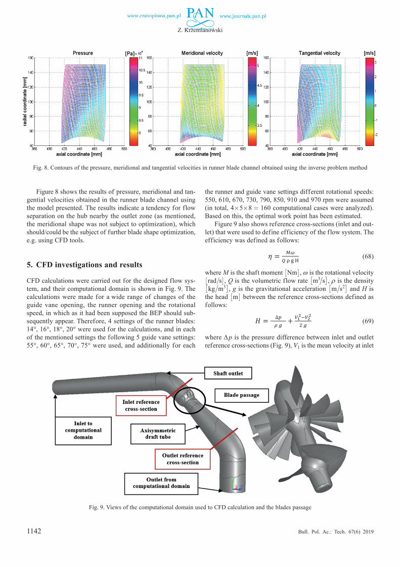
1142

Z. Krzemianowski

Bull. Pol. Ac.: Tech. 67(6) 2019

Figure 8 shows the results of pressure, meridional and tan-gential velocities obtained in the runner blade channel using the model presented. The results indicate a tendency for flow separation on the hub nearby the outlet zone (as mentioned, the meridional shape was not subject to optimization), which should/could be the subject of further blade shape optimization, e.g. using CFD tools.

5. CFD investigations and results

CFD calculations were carried out for the designed flow sys-tem, and their computational domain is shown in Fig. 9. The calculations were made for a wide range of changes of the guide vane opening, the runner opening and the rotational speed, in which as it had been supposed the BEP should sub-sequently appear. Therefore, 4 settings of the runner blades: 14°, 16°, 18°, 20° were used for the calculations, and in each of the mentioned settings the following 5 guide vane settings: 55°, 60°, 65°, 70°, 75° were used, and additionally for each

the runner and guide vane settings different rotational speeds: 550, 610, 670, 730, 790, 850, 910 and 970 rpm were assumed (in total, 4£5£8 = 160 computational cases were analyzed). Based on this, the optimal work point has been estimated.

Figure 9 also shows reference cross-sections (inlet and out-let) that were used to define efficiency of the f low system. The efficiency was defined as follows:

10

mathematical basis while calculation the blade using the inverse problem method. In such a case the CFD calculations can be indispensable to evaluate influence of the stacking condition on flow parameters.

Fig. 7. The stacking condition at the runner inlet used to blade shape

calculation.

The obtained mean velocities of the runner blade at the inlet were as follows: the tangential velocity 𝑈𝑈𝑥𝑥(2) = 1.69 m/s, and the meridional velocity 𝑈𝑈𝑥𝑥(3) = 3.55 m/s. Respectively, at the outlet the meridional velocity was 𝑈𝑈𝑥𝑥(3) = 3.5 m/s.

Figure 8 shows the results of pressure, meridional and tangential velocities obtained in runner blade channel using the presented model. The results indicate a tendency to flow separation on the hub nearby the outlet zone (as mentioned, the meridional shape was not subject to optimization), which should/could be the subject of further blade shape optimization e.g. using CFD tools.

Fig. 8. Contours of the pressure, meridional and tangential velocities in runner blade channel obtained using the inverse problem method.

5. CFD investigations and results

For the designed flow system CFD calculations were carried out, whose computational domain is shown in Figure 9. The calculations were made in a wide range of changes of the guide vane opening, the runner opening and the rotational speed, in which as it had been supposed the BEP should subsequently appear. Therefore, for calculations 4 settings of the runner blades: 14, 16, 18, 20 were used, and in each of the mentioned settings the following 5 guide vane settings: 55, 60, 65, 70, 75 were used, and additionally for each the runner and guide vane settings different rotational speeds: 550, 610, 670, 730, 790, 850, 910, 970 rpm were assumed (in total, 4 x 5 x 8 = 160 computational cases were analyzed). Based on this, the optimal work point has been estimated.

Figure 9 also shows reference cross-sections (inlet and outlet) that were used to define the efficiency of flow system. The efficiency was defined as follows:

𝜂𝜂 = 𝑀𝑀𝑀𝑀𝑄𝑄 ρ g H (68)

where M is the shaft moment [Nm], ω is the rotational velocity [rad/s], Q is the volumetric flow rate [m3/s], ρ is the density [kg/m3], g is the gravitational acceleration [m/s2], and H is the head [m] between the reference cross-sections defined as follows:

𝐻𝐻 = 𝑝𝑝1−𝑝𝑝2𝜌𝜌 𝑔𝑔 + 𝑉𝑉1

2−𝑉𝑉22

2 𝑔𝑔 (69)

where p1, p2 are the pressures at inlet and outlet reference cross-sections, respectively (Fig. 9), V1 is the mean velocity at inlet reference cross-section: V1 = Q/A1, V2 is the mean velocity at outlet reference cross-section: V2 = Q/A2, and A1, A2 are the areas of inlet and outlet reference cross-sections, respectively.

Computational mesh were made using two NUMECA programs: AutoGrid5™ and Hexpress™. The number of mesh nodes (entirely hexahedral) was ~20 million. The mesh was made according to requirements of the turbulent model k-ω SST used to calculations, for which the value of dimensionless distance from the wall Y+ has to be in range of 1÷3. It should be added that the runner tip gap had not been modelled, and as a result, the efficiency was expected not to contain volumetric losses. The calculations were

(68)

where M is the shaft moment £Nm¤, ω is the rotational velocity £

rad/s¤, Q is the volumetric flow rate

£m3/s¤, ρ is the density £

kg/m3¤, g is the gravitational acceleration £m/s2¤ and H is

the head £m¤ between the reference cross-sections defined as

follows:

10

mathematical basis while calculation the blade using the inverse problem method. In such a case the CFD calculations can be indispensable to evaluate influence of the stacking condition on flow parameters.

Fig. 7. The stacking condition at the runner inlet used to blade shape

calculation.

The obtained mean velocities of the runner blade at the inlet were as follows: the tangential velocity 𝑈𝑈𝑥𝑥(2) = 1.69 m/s, and the meridional velocity 𝑈𝑈𝑥𝑥(3) = 3.55 m/s. Respectively, at the outlet the meridional velocity was 𝑈𝑈𝑥𝑥(3) = 3.5 m/s.

Figure 8 shows the results of pressure, meridional and tangential velocities obtained in runner blade channel using the presented model. The results indicate a tendency to flow separation on the hub nearby the outlet zone (as mentioned, the meridional shape was not subject to optimization), which should/could be the subject of further blade shape optimization e.g. using CFD tools.

Fig. 8. Contours of the pressure, meridional and tangential velocities in runner blade channel obtained using the inverse problem method.

5. CFD investigations and results

For the designed flow system CFD calculations were carried out, whose computational domain is shown in Figure 9. The calculations were made in a wide range of changes of the guide vane opening, the runner opening and the rotational speed, in which as it had been supposed the BEP should subsequently appear. Therefore, for calculations 4 settings of the runner blades: 14, 16, 18, 20 were used, and in each of the mentioned settings the following 5 guide vane settings: 55, 60, 65, 70, 75 were used, and additionally for each the runner and guide vane settings different rotational speeds: 550, 610, 670, 730, 790, 850, 910, 970 rpm were assumed (in total, 4 x 5 x 8 = 160 computational cases were analyzed). Based on this, the optimal work point has been estimated.

Figure 9 also shows reference cross-sections (inlet and outlet) that were used to define the efficiency of flow system. The efficiency was defined as follows:

𝜂𝜂 = 𝑀𝑀𝑀𝑀𝑄𝑄 ρ g H (68)

where M is the shaft moment [Nm], ω is the rotational velocity [rad/s], Q is the volumetric flow rate [m3/s], ρ is the density [kg/m3], g is the gravitational acceleration [m/s2], and H is the head [m] between the reference cross-sections defined as follows:

𝐻𝐻 = 𝑝𝑝1−𝑝𝑝2𝜌𝜌 𝑔𝑔 + 𝑉𝑉1

2−𝑉𝑉22

2 𝑔𝑔 (69)

where p1, p2 are the pressures at inlet and outlet reference cross-sections, respectively (Fig. 9), V1 is the mean velocity at inlet reference cross-section: V1 = Q/A1, V2 is the mean velocity at outlet reference cross-section: V2 = Q/A2, and A1, A2 are the areas of inlet and outlet reference cross-sections, respectively.

Computational mesh were made using two NUMECA programs: AutoGrid5™ and Hexpress™. The number of mesh nodes (entirely hexahedral) was ~20 million. The mesh was made according to requirements of the turbulent model k-ω SST used to calculations, for which the value of dimensionless distance from the wall Y+ has to be in range of 1÷3. It should be added that the runner tip gap had not been modelled, and as a result, the efficiency was expected not to contain volumetric losses. The calculations were

(69)

where ∆p is the pressure difference between inlet and outlet reference cross-sections (Fig. 9), V1 is the mean velocity at inlet

Fig. 8. Contours of the pressure, meridional and tangential velocities in runner blade channel obtained using the inverse problem method

Fig. 9. Views of the computational domain used to CFD calculation and the blades passage

9

As a blockage factor required to the mass conservation equation (31) the Göttingen 428 profile thickness was used – half the thickness on the suction side and half the thickness on the pressure side was distributed. In the case of a low-head Kaplan turbine runner, the impact of the thickness distribution is relatively small so that it practically has no influence on the flow rate unlike the guide vane case, in which the thickness distribution plays a key role. Thus, there was no need to introduce a function defining the thickness distribution 𝜗𝜗(𝑥𝑥(1), 𝑥𝑥(3)).

The number of blades was determined on the basis of analysis of similar low-head Kaplan hydraulic turbine solutions and it was assumed to be of 3. Such a small number of blades should ensures a large mass flow rate, which characterizes machines with a high specific speed (nsq > 230), concurrently achieving relatively high efficiency (>86%).

Fig. 5. View of the runner blade of the Kaplan hydraulic turbine model.

Fig. 6. Views of the runner blade wheel of the Kaplan hydraulic turbine

model. The other boundary conditions and assumptions for the

calculations are presented below. The streamline function was:

𝑓𝑓(𝑥𝑥(1), 𝑥𝑥(3)) = 𝑎𝑎1 + (𝑎𝑎2 − 𝑎𝑎1)𝑥𝑥(1) + (𝑏𝑏1 + (𝑏𝑏2 −

𝑏𝑏1)𝑥𝑥(1))𝑥𝑥(3) + (𝑐𝑐1 + (𝑐𝑐2 − 𝑐𝑐1)𝑥𝑥(1))(𝑥𝑥(3))2 (64)

where 𝑎𝑎1 = -2.11527, 𝑎𝑎2 = 0.1505, 𝑏𝑏1 = 9.72219, 𝑏𝑏2 = 0, 𝑐𝑐1 = -10.897, and 𝑐𝑐2 = 0. These coefficients are dependent on the meridional shape of blade and were obtained in the following way. Firstly, two streamline functions of the same pattern 𝑓𝑓 = 𝑓𝑓(𝑥𝑥(3)) for hub and shroud lines had to be found separately. In considered example, this pattern was a quadratic function: 𝑓𝑓(𝑥𝑥(3)) = 𝑎𝑎 + 𝑏𝑏𝑥𝑥(3) + 𝑐𝑐(𝑥𝑥(3))2

. These streamline functions were found using the Least Square Method. Secondly, each coefficient (for hub: a1, b1,

c1 and for shroud: a2, b2, c2) was linearly approximated across the spanwise direction with respect to 𝑥𝑥(1) coordinate, which changed within the range of <0;1>. Thus, the family of two-dimensional streamlines 𝑓𝑓(𝑥𝑥(1), 𝑥𝑥(3)) was obtained.

The other parameters were assumed as follows: the turbine head H = 1.5 m, the rotational speed n = 810 rpm, and the density ρ = 999.1 kg/m3. The assumed head strictly influences the Euler’s hydraulic machines equation presented in (48) because the specific work l of a turbine may be expressed as follows:

𝑙𝑙 = 𝜂𝜂ℎ 𝑔𝑔 𝐻𝐻 = 𝜂𝜂ℎ∆𝑝𝑝𝜌𝜌 (65)

where ηh is the hydraulic efficiency, g is the gravitational acceleration, and Δp is the static pressure difference between inlet (before guide vane wheel), and outlet (behind the draft tube) of turbine. Thus, it is another constraint in ECE that is required to be satisfied.

To start the solution on orthogonal characteristics the blade loading at hub was assumed using the swirl distribution with respect to axial coordinate 𝑥𝑥(3) (Figure 2 – curve GHIJ), as follows:

𝑓𝑓 𝑈𝑈𝑥𝑥(2) = 𝑎𝑎 + 𝑏𝑏𝑥𝑥(3) + 𝑐𝑐(𝑥𝑥(3))2 + 𝑑𝑑(𝑥𝑥(3))3 + 𝑒𝑒(𝑥𝑥(3))4 +

𝑓𝑓(𝑥𝑥(3))5 (66)

where a = 43495, b = -478118, c = 2099428, d = -4602353, e = 5036135, and f = -2200210. Presented function allows calculating the blade loading at hub in region II. However, it is restricted due to the constraints. In regions I and III the flow field is calculated using equation (57) in advance. This means that the swirl in points H and I is known. Therefore, as mentioned the function is used only in region II (between points H and I) and its shape is strictly dependent on a solution obtained in regions I and III. On this basis, the coefficients using the Least Square Method were found.

The stacking condition used in skeleton calculations was assumed as a function of angular coordinate 𝑥𝑥(2) at the runner inlet with respect to radius f (the streamline function at the inlet – see (3)) – Figure 7. This function was adopted as a 3-degree polynomial, in which the angular coordinate of the lowest and the highest radius is equal 0°, and additionally in 1/3 and 2/3 of the leading edge length is equal 5°:

𝑥𝑥𝑖𝑖𝑖𝑖𝑖𝑖(2) = 𝑎𝑎 + 𝑏𝑏 𝑓𝑓𝑖𝑖𝑖𝑖𝑖𝑖(𝑥𝑥(1), 𝑥𝑥𝑖𝑖𝑖𝑖𝑖𝑖

(3)) + 𝑐𝑐 𝑓𝑓𝑖𝑖𝑖𝑖𝑖𝑖2 (𝑥𝑥(1), 𝑥𝑥𝑖𝑖𝑖𝑖𝑖𝑖

(3)) +

𝑑𝑑 𝑓𝑓𝑖𝑖𝑖𝑖𝑖𝑖3 (𝑥𝑥(1), 𝑥𝑥𝑖𝑖𝑖𝑖𝑖𝑖

(3)) (67)

where a = -0.23564735, b = 7.24726878, c = -41.77212782, and d = 26.71933415. Such assumption requires some experience from the designer because it has no

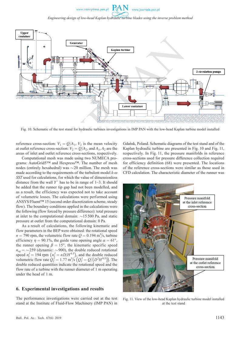
1143

Engineering design of low-head Kaplan hydraulic turbine blades using the inverse problem method

Bull. Pol. Ac.: Tech. 67(6) 2019

reference cross-section: V1 = Q/A1, V2 is the mean velocity at outlet reference cross-section: V2 = Q/A2, and A1, A2 are the areas of inlet and outlet reference cross-sections, respectively.

Computational mesh was made using two NUMECA pro-grams: AutoGrid5™ and Hexpress™. The number of mesh nodes (entirely hexahedral) was »20 million. The mesh was made according to the requirements of the turbulent model k-ω SST used for calculations, for which the value of dimensionless distance from the wall Y+ has to be in range of 1–3. It should be added that the runner tip gap had not been modelled, and as a result, the efficiency was expected not to take account of volumetric losses. The calculations were performed using ANSYS/Fluent™ 15 (second order discretization scheme, steady flow). The boundary conditions applied in the calculations were the following (flow forced by pressure difference): total pressure at inlet to the computational domain: »15 500 Pa, and static pressure at outlet from the computational domain: 0 Pa.

As a result of calculations, the following kinematic and flow parameters in the BEP were obtained: the rotational speed n = 790 rpm, the volumetric flow rate Q = 0.194 m3/s, turbine efficiency η = 90.1%, the guide vane opening angle α = 61°, the runner opening β  = 15°, the kinematic specific speed nsq = »259 (dynamic: »900), the double reduced rotational speed nI

I  = 194 rpm (nII = nD/H 0.5), and the double reduced

volumetric flow rate QII = 1.77 m3/s (QI

I = Q/ (D2H 0.5)). The double reduced quantities indicate the rotational speed and the flow rate of a turbine with the runner diameter of 1 m operating under the head of 1 m.

6. Experimental investigations and results

The performance investigations were carried out at the test stand at the Institute of Fluid-Flow Machinery (IMP PAN) in

Gdańsk, Poland. Schematic diagrams of the test stand and of the Kaplan hydraulic turbine are presented in Fig. 10 and Fig. 11, respectively. In Fig. 11, the pressure manifolds in reference cross-sections used for pressure difference collection required for efficiency definition (68) were presented. The locations of the reference cross-sections were similar as those used in CFD calculation. The characteristic diameter of the runner was

Fig. 10. Schematic of the test stand for hydraulic turbines investigations in IMP PAN with the low-head Kaplan turbine model installed

Fig. 11. View of the low-head Kaplan hydraulic turbine model installed at the test stand

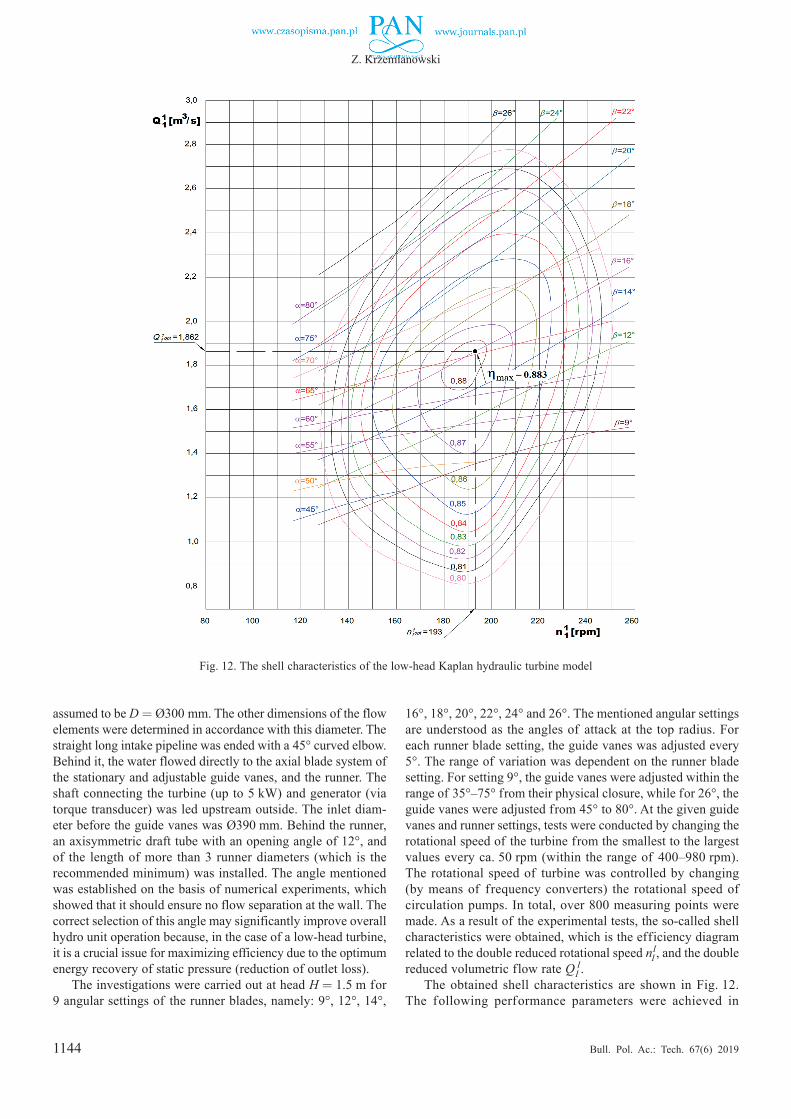
1144

Z. Krzemianowski

Bull. Pol. Ac.: Tech. 67(6) 2019

assumed to be D = Ø300 mm. The other dimensions of the flow elements were determined in accordance with this diameter. The straight long intake pipeline was ended with a 45° curved elbow. Behind it, the water flowed directly to the axial blade system of the stationary and adjustable guide vanes, and the runner. The shaft connecting the turbine (up to 5 kW) and generator (via torque transducer) was led upstream outside. The inlet diam-eter before the guide vanes was Ø390 mm. Behind the runner, an axisymmetric draft tube with an opening angle of 12°, and of the length of more than 3 runner diameters (which is the recommended minimum) was installed. The angle mentioned was established on the basis of numerical experiments, which showed that it should ensure no flow separation at the wall. The correct selection of this angle may significantly improve overall hydro unit operation because, in the case of a low-head turbine, it is a crucial issue for maximizing efficiency due to the optimum energy recovery of static pressure (reduction of outlet loss).

The investigations were carried out at head H = 1.5 m for 9 angular settings of the runner blades, namely: 9°, 12°, 14°,

16°, 18°, 20°, 22°, 24° and 26°. The mentioned angular settings are understood as the angles of attack at the top radius. For each runner blade setting, the guide vanes was adjusted every 5°. The range of variation was dependent on the runner blade setting. For setting 9°, the guide vanes were adjusted within the range of 35°–75° from their physical closure, while for 26°, the guide vanes were adjusted from 45° to 80°. At the given guide vanes and runner settings, tests were conducted by changing the rotational speed of the turbine from the smallest to the largest values every ca. 50 rpm (within the range of 400–980 rpm). The rotational speed of turbine was controlled by changing (by means of frequency converters) the rotational speed of circulation pumps. In total, over 800 measuring points were made. As a result of the experimental tests, the so-called shell characteristics were obtained, which is the efficiency diagram related to the double reduced rotational speed nI

I , and the double reduced volumetric flow rate QI

I.The obtained shell characteristics are shown in Fig. 12.

The following performance parameters were achieved in

Fig. 12. The shell characteristics of the low-head Kaplan hydraulic turbine model

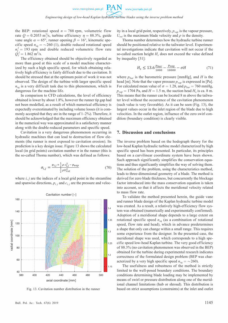
1145

Engineering design of low-head Kaplan hydraulic turbine blades using the inverse problem method

Bull. Pol. Ac.: Tech. 67(6) 2019

the BEP: rotational speed n = 788 rpm, volumetric f low rate Q = 0.2053 m3/s, turbine efficiency η = 88.3%, guide vane angle α = 65°, runner opening β = 16°, kinematic spe-cific speed nsq = »260 (1), double reduced rotational speed nI

I = 193 rpm and double reduced volumetric f low rate QI

I = 1.862 m3/s.The efficiency obtained should be objectively regarded as

more than good at this scale of a model machine character-ized by such a high specific speed, for which obtaining rela-tively high efficiency is fairly difficult due to the cavitation. It should be stressed that at the optimum point of work it was not observed. The design of the turbine with larger specific speed nsq is a very difficult task due to this phenomenon, which is dangerous for the machine life.

In comparison to CFD calculations, the level of efficiency obtained is lower by about 1.8%, however the runner tip gap had not been modelled, as a result of which numerical efficiency is expectedly overestimated by including volume losses (it is com-monly accepted that they are in the range of 1–2%). Therefore, it should be acknowledged that the maximum efficiency obtained in the numerical way was approximated in a satisfactory manner along with the double-reduced parameters and specific speed.

Cavitation is a very dangerous phenomenon occurring in hydraulic machines that can lead to destruction of flow ele-ments (the runner is most exposed to cavitation erosion). Its prediction is a key design issue. Figure 13 shows the calculated local (in grid points) cavitation number σ in the runner (this is the so-called Thoma number), which was defined as follows:

12

The investigations were carried out at a head H = 1.5 m for 9 angular settings of the runner blades, namely: 9°, 12°, 14°, 16°, 18°, 20°, 22°, 24°, and 26°. The mentioned angular settings are understood as the angles of attack at the top radius. For each runner blade setting, the guide vanes was adjusted every 5°. The range of variation was dependent on the runner blade setting. For setting 9°, the guide vanes was adjusted within the range of 35°÷75° from their physical closure, while for the 26°, the guide vanes was adjusted from 45° to 80°. At the given guide vanes and runner settings, tests were conducted by changing the rotational speed of the turbine from the smallest to the largest values every ca. 50 rpm (within the range of 400÷980 rpm). The rotational speed of turbine was controlled by changing (by means of frequency converters) the rotational speed of circulation pumps. In total, over 800 measuring points were made. As a result of the experimental tests, the so-called shell characteristics was obtained, which is the efficiency diagram related to the double reduced rotational speed nI

I, and the double reduced volumetric flow rate QI

I. The obtained shell characteristics is shown in

Figure 12. The following performance parameters were achieved in the BEP: the rotational speed n = 788 rpm, the volumetric flow rate Q = 0.2053 m3/s, the turbine efficiency η = 88.3%, the guide vane angle α = 65°, the runner opening β = 16°, the kinematic specific speed nsq = ~260 (1), the double reduced rotational speed nI

I = 193 rpm, and the double reduced volumetric flow rate QI

I = 1.862 m3/s.

Fig. 11. View of the low-head Kaplan hydraulic turbine model installed at the test stand.

Fig. 12. The shell characteristics of the low-head Kaplan hydraulic

turbine model. The efficiency obtained should be objectively regarded

as more than good at this scale of a model machine characterized by such a high specific speed, and for which obtaining relatively high efficiency is fairly difficult due to the cavitation. It should be stressed that at the optimum point of work it was not observed. The design of the turbine with a larger specific speed nsq is a very difficult task due to this phenomenon, which is dangerous for the machine life.

In comparison to CFD calculations, the level of efficiency obtained is lower by about 1.8%, however the runner tip gap had not been modelled, as a result of which the numerical efficiency is expectedly overestimated by volume losses (it is commonly accepted that they are in range of 1÷2%). Therefore, it should be acknowledged that the maximum efficiency obtained in the numerical way was approximated in a satisfactory manner, as well as the double-reduced parameters and the specific speed.

Cavitation is a very dangerous phenomenon occurring in hydraulic machines that can lead to destruction of flow elements (the runner is the most exposed to cavitation erosion). Its prediction is a key design issue. Figure 13 shows the calculated local (in grid points) cavitation number σ in the runner (this is the so-called Thoma number), which was defined as follows:

𝜎𝜎𝑖𝑖,𝑗𝑗 = 𝑝𝑝𝑖𝑖,𝑗𝑗 + 12 𝜌𝜌 𝑐𝑐𝑖𝑖,𝑗𝑗 2 − 𝑝𝑝𝑣𝑣𝑣𝑣𝑣𝑣

12 𝜌𝜌𝑈𝑈𝑟𝑟𝑟𝑟𝑟𝑟

2 (70) (70)

where i, j are the indices of a local grid point in the streamline and spanwise directions, pi, j and ci, j are the pressure and veloc-

ity in a local grid point, respectively, pvap is the vapour pressure, Urot is the maximum blade velocity and ρ is the density.

Thoma number determines how the hydraulic turbine runner should be positioned relative to the tailwater level. Experimen-tal investigations indicate that cavitation will not occur if the so-called suction height Hs does not exceed the value defined by inequality [31]:

13

where i, j are the indexes of a local grid point in streamline and spanwise directions, 𝑝𝑝𝑖𝑖,𝑗𝑗 and 𝑐𝑐𝑖𝑖,𝑗𝑗 are respectively the pressure and velocity in a local grid point, 𝑝𝑝𝑣𝑣𝑣𝑣𝑣𝑣 is the vapour pressure, 𝑈𝑈𝑟𝑟𝑟𝑟𝑟𝑟 is the maximum blade velocity, and ρ is the density.

Thoma number determines how the hydraulic turbine runner should be positioned relative to a tailwater level. Experimental investigations indicate that cavitation will not occur if the so-called suction height Hs does not exceed the value defined by inequality [31]:

𝐻𝐻𝑠𝑠 ≤ 13.6 𝑣𝑣𝑏𝑏𝑏𝑏𝑏𝑏1000 −

𝑣𝑣𝑣𝑣𝑏𝑏𝑣𝑣10000 − 𝜎𝜎𝐻𝐻 (71)

where 𝑝𝑝𝑏𝑏𝑣𝑣𝑟𝑟 is the barometric pressure [mmHg], and H is the head [m]. Note that the vapour pressure 𝑝𝑝𝑣𝑣𝑣𝑣𝑣𝑣 is expressed in [Pa]. For calculated mean value of σ = 1.28, and 𝑝𝑝𝑏𝑏𝑣𝑣𝑟𝑟 = 760 mmHg, 𝑝𝑝𝑣𝑣𝑣𝑣𝑣𝑣 = 1704 Pa, and H = 1.5 m, the suction head Hs is ca. 8 m. This means that runner can be located 8 m above the tailwater level without the occurrence of cavitation phenomenon (such value is very favourable). As it can be seen (Figure 13), the largest values occur in the inlet region of the blade due to high velocities. In the outlet region, the influence of zero swirl condition (boundary condition) is clearly visible.

Fig. 13. Cavitation number distribution in the runner.

7. Discussion and conclusions

The inverse problem based on the hodograph theory for the low-head Kaplan hydraulic turbine model characterized by a high specific speed has been presented. In particular, its principles based on a curvilinear coordinate system have been shown. Such approach significantly simplifies the conservation equations and thus significantly simplifies the way of solving them. The solution of the problem, using the characteristics method, leads to three-dimensional geometry of a blade. The method is derived for a zero blade thickness, but concurrently the blockage factor introduced

into the mass conservation equation is taken into account, so that it affects the meridional velocity related to mass flow rate.

To validate the presented method, the guide vane and runner blade design of the Kaplan hydraulic turbine model was created. As a result, relatively high efficiency flow system was obtained (numerically and experimentally confirmed). Adoption of a meridional shape highly depends on rotational specific speed nsq (as a combination of rotational speed, flow rate and head), which in advance predetermines a shape that only can change within small range. This requires some experience from the designer. In the presented case, the meridional shape was used, which corresponds to a high specific speed low-head Kaplan turbine. The obtained very good efficiency 88.3% (no cavitation phenomenon was observed in the BEP) of a turbine during experimental research indicates correctness of the formulated design problem (BEP was characterized by a very high specific speed nsq = ~260).

The usefulness and robustness of the method is strictly limited to the well-posed boundary conditions. The boundary conditions determining the blade loading may be implemented by means of swirl or pressure distribution along one of the meridional channel limitations (hub or shroud). This distribution is based on strict assumptions (constraints) at the inlet and outlet of a blade, resulting from hydraulic turbines theory. It should ensure a small margin of error in setting such a kind of boundary condition. Such condition can be optimized e.g. to maximize efficiency. Additionally, well-posed boundary conditions (which means that they exist, are unique and continuous) are a key to achieving the solution. If the problem is ill-posed, no real solution can be obtained due to the quadratic dependency of tangential velocity in energy conservation equation. The blockage factor, which accelerates the flow, has also a big influence on the solution obtained. Generally, the smaller number of blades the smaller influence of a blockage factor can be observed, so in the case of a runner blade (of a low-head Kaplan turbine) it is insignificant but in the case of a guide vane it is of an important meaning.

The presented method can be applied to other types of hydraulic machines (Francis turbines, axial and mixed flow pumps). Its usage allows conducting quick engineering blade design of a rotating machine. Because this is the inverse problem method, so the blade is designed for the optimal point of operation (BEP). Then, it seems necessary to check such a solution using commercial software CFD, in order to avoid a large mistake and additionally, to check the performance at off-design points of operation. Acknowledgements. This work was supported by the (Polish) National Centre of Sciences (NCN) under grant no. PB 6694/B/T02/2011/40 titled “Development of design methodology for low-head axial turbines”.

The CFD computations were carried out on a PL-Grid Infrastructure.

(71)

where pbar is the barometric pressure [mmHg], and H is the head [m]. Note that the vapor pressure pvap is expressed in [Pa]. For calculated mean value of σ  = 1.28, and pbar = 760 mmHg, pvap = 1704 Pa, and H = 1.5 m, the suction head Hs is ca. 8 m. This means that the runner can be located 8 m above the tailwa-ter level without the occurrence of the cavitation phenomenon (such value is very favorable). As it can be seen (Fig. 13), the largest values occur in the inlet region of the blade due to high velocities. In the outlet region, influence of the zero swirl con-dition (boundary condition) is clearly visible.

7. Discussion and conclusions

The inverse problem based on the hodograph theory for the low-head Kaplan hydraulic turbine model characterized by high specific speed has been presented. In particular, its principles based on a curvilinear coordinate system have been shown. Such approach significantly simplifies the conservation equa-tions and thus significantly simplifies the way of solving them. The solution of the problem, using the characteristics method, leads to three-dimensional geometry of a blade. The method is derived for zero blade thickness, but concurrently the blockage factor introduced into the mass conservation equation is taken into account, so that it affects the meridional velocity related to mass flow rate.

To validate the method presented herein, the guide vane and runner blade design of the Kaplan hydraulic turbine model was created. As a result, a relatively high-efficiency flow sys-tem was obtained (numerically and experimentally confirmed). Adoption of a meridional shape depends to a large extent on rotational specific speed nsq (as a combination of rotational speed, flow rate and head), which in advance predetermines a shape that only can change within a small range. This requires some experience from the designer. In the presented case, the meridional shape was used, which corresponds to a high spe-cific speed low-head Kaplan turbine. The very good efficiency of 88.3% (no cavitation phenomenon was observed in the BEP) obtained for the turbine during experimental research indicates correctness of the formulated design problem (BEP was char-acterized by a very high specific speed nsq = »260).

The usefulness and robustness of the method is strictly limited to the well-posed boundary conditions. The boundary conditions determining blade loading may be implemented by means of swirl or pressure distribution along one of the merid-ional channel limitations (hub or shroud). This distribution is based on strict assumptions (constraints) at the inlet and outlet Fig. 13. Cavitation number distribution in the runner

500480460440420400380

radi

al c

oord

inat

e [m

m]

axial coordinate [mm]

Cavitation number [–]160

1.4

1.35

1.3

1.25

1.2

1.15

140

120

100

80

60

40

1146

Z. Krzemianowski

Bull. Pol. Ac.: Tech. 67(6) 2019

of the blade, resulting from hydraulic turbines theory. It should ensure a small margin of error in setting such a type of bound-ary condition. Such condition can be optimized e.g. to maxi-mize efficiency. Additionally, well-posed boundary conditions (which means that they exist, are unique and continuous) are key for achieving the solution. If the problem is ill-posed, no real solution can be obtained due to the quadratic dependency of tangential velocity in the energy conservation equation. The blockage factor, which accelerates the flow, also has a large influence on the solution obtained. Generally, the smaller the number of blades, the smaller the influence of a blockage fac-tor that can be observed, so in the case of a runner blade (of a low-head Kaplan turbine) it is insignificant but in the case of a guide vane it is of crucial meaning.

The presented method can be applied to other types of hydraulic machines (Francis turbines, axial and mixed flow pumps). Its usage allows for conducting quick engineering blade design of a rotating machine. Because this is the inverse problem method, the blade is designed for the optimum point of operation (BEP). Then, it seems necessary to check such a solution using commercial CFD software, in order to avoid a large mistake and, additionally, to check the performance at off-design points of operation.

Acknowledgements. This work was supported by the (Polish) National Science Centre (NCN) under grant No. PB 6694/B/T02/2011/40 entitled “Development of design methodology for low-head axial turbines”. The CFD computations were carried out on PL-Grid infrastructure. In memoriam, the author spe-cially wishes to thank Professor Romuald Puzyrewski (1935–2016, R.I.P.) from Gdańsk University of Technology (Poland) with whom he collaborated through many years and who taught him the inverse problem method.

References [1] C.H. Wu, “A general theory of three-dimensional flow in subson-

ic and supersonic turbomachines of axial-, radial-, and mixed-flow types”, NACA Technical Note 2604, 1952.

[2] C.H. Wu, “A general theory of two- and three-dimensional ro-tational flow in subsonic and transonic turbomachines”, NASA Contractor Report 4496, 1993.

[3] W.R. Hawthorne, C. Wang, C.S. Tan, and J.E. McCune, “Theory of blade design for large deflections – Part 1: two-dimensional cascade”, ASME J. Eng. Gas Turbines Power 106(2), 346–353 (1984).

[4] C.S. Tan, W.R. Hawthorne, J.E. McCune, and C. Wang, “Theory of blade design for large deflections – Part 2: annular cascades”, ASME J. Eng. Gas Turbines Power 106(2), 354–365 (1984).

[5] M. Zangeneh, “A compressible three dimensional blade design method for radial and mixed flow turbomachinery blades”, Int. J. Numer. Methods Fluids 13(5), 599–624 (1991).

[6] M. Zangeneh, “Inverse design of centrifugal compressor vaned diffusers in inlet shear flows”, ASME J. Turbomach. 118(2), 385–393 (1996).

[7] A. Demeulenaere and R.A. van den Braembussche, “Three-di-mensional inverse method for turbomachinery blading design”, ASME J. Turbomach. 120(2), 247–255 (1996).

[8] L. de Vito, R.A. van den Braembussche, and H. Deconinck, “A novel two-dimensional viscous inverse design method for turbomachinery blading”, ASME J. Turbomach. 125(2), 310–316 (2003).

[9] A. Goto and M. Zangeneh, “Hydrodynamic design of pump dif-fuser using inverse design method and CFD”, ASME J. Fluids Engineering 124(2), 319–328 (2002).

[10] A. Goto, M. Nohmi, T. Sakurai, and Y. Sogawa, “Hydrodynam-ic design system of for pumps based on 3-D CAD, CFD, and inverse design method”, ASME J. Fluids Engineering 124(2), 329–335 (2002).

[11] S. Cao, G. Peng, and Z. Yu, “Hydrodynamic design of roto-dynamic pump impeller for multiphase pumping by combined approach of inverse design and CFD analysis”, ASME J. Fluids Engineering 127(2), 330–338 (2005).

[12] G. Peng, “A practical combined computation method of mean through-f low for 3D inverse design of hydraulic turbomachin-ery blades”, ASME J. Fluids Engineering 127(6), 1183–1190 (2005).

[13] R.H. Zhang, R. Guo, J.H. Yang, and J.Q. Luo. “Inverse method of centrifugal pump impeller based on proper orthogonal decom-position (POD) method”, Chin. J. Mech. Eng. 30(4), 1025–1031 (2017).

[14] L. Yeming, X.F. Wang, W. Wang, and F.M. Zhou, “Application of the modified inverse design method in the optimization of the runner blade of a mixed-flow pump”, Chin. J. Mech. Eng. 31(1), 105–121 (2018).

[15] G. Peng, S. Cao, M. Ishizuka, and S. Hayama, “Design optimiza-tion of axial flow hydraulic turbine runner: Part I – an improved Q3D inverse method”, Int. J. for Numerical Methods in Fluids 39(6), 517–531 (2002).

[16] G. Peng, S. Cao, M. Ishizuka, and S. Hayama, “Design optimiza-tion of axial flow hydraulic turbine runner: Part II – multi-object constrained optimization method”, Int. J. for Numerical Methods in Fluids 39(6), 533–548 (2002).

[17] M. Zangeneh, A. Goto, and T. Takemura, “Suppression of sec-ondary flows in a mixed flow pump impeller by application of 3D inverse design method: Part 1 – design and numerical vali-dation”, ASME J. Turbomach. 118(3), 536–543 (1996).

[18] K. Daneshkah and M. Zangeneh, “Parametric design of a Francis turbine runner by means of a three-dimensional inverse design method”, IOP Conf. Series: Earth and Environmental Science 12, 012058 (2010).

[19] H. Okamoto and A. Goto, “Suppression of cavitation in a Francis turbine runner by application of 3D inverse design method”. ASME Joint U.S.-European Fluids Engineering Division Con-ference, paper no. 31192, 851–858 (2002).

[20] D. Bonaiuti, M. Zangeneh, R. Aartojarvi, and J. Eriksson, “Para-metric design of a waterjet pump by means of inverse design. CFD calculations and experimental analyses”, ASME J. Fluids Engineering, 132(3), 031104 (2010).

[21] J.E. Borges, “A three-dimensional inverse method for turboma-chinery – Part 1: theory”, J. Turbomach. 112(3), 346–354 (1990).

[22] J. Jiang and T. Dang, “Design method for turbomachine blades with finite thickness by the circulation method”, J. Turbomach. 119(3), 539–543 (1997).

[23] J.C. Pascoa, A.C. Mendes, and L.M.C. Gato, “A fast iterative inverse method for turbomachinery blade design”, Mech. Res. Commun. 36(5), 630–637 (2009).

[24] N.P. Kruyt and R.W. Westra, “On the inverse problem of blade design for centrifugal pumps and fans”, Inverse Problems 30(6), 065003 (2014).

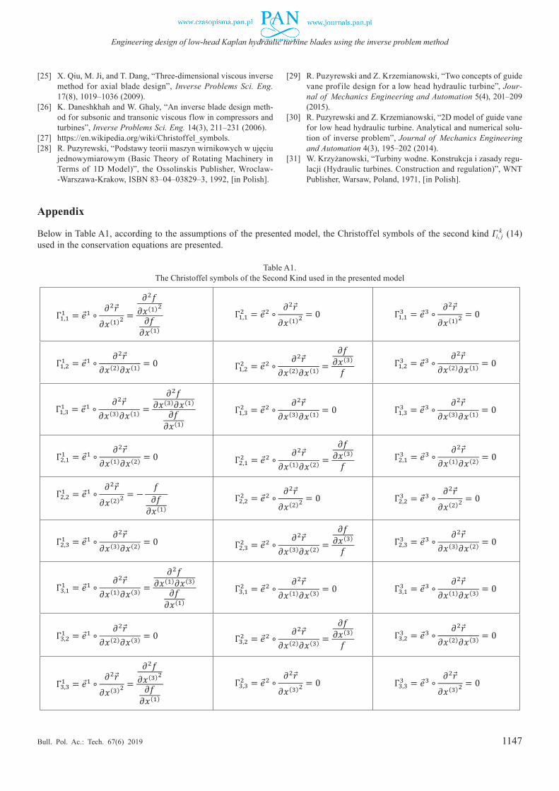
1147

Engineering design of low-head Kaplan hydraulic turbine blades using the inverse problem method

Bull. Pol. Ac.: Tech. 67(6) 2019

Table A1. The Christoffel symbols of the Second Kind used in the presented model

15

Table A1. The Christoffel symbols of the Second Kind used in the presented model.

Γ1,11 = 𝑒𝑒 1 ∘ 𝜕𝜕2𝑟𝑟

𝜕𝜕𝑥𝑥(1)2=

𝜕𝜕2𝑓𝑓𝜕𝜕𝑥𝑥(1)2

𝜕𝜕𝑓𝑓𝜕𝜕𝑥𝑥(1)

Γ1,12 = 𝑒𝑒 2 ∘ 𝜕𝜕2𝑟𝑟

𝜕𝜕𝑥𝑥(1)2= 0 Γ1,1

3 = 𝑒𝑒 3 ∘ 𝜕𝜕2𝑟𝑟 𝜕𝜕𝑥𝑥(1)2

= 0

Γ1,21 = 𝑒𝑒 1 ∘ 𝜕𝜕2𝑟𝑟

𝜕𝜕𝑥𝑥(2)𝜕𝜕𝑥𝑥(1) = 0 Γ1,22 = 𝑒𝑒 2 ∘ 𝜕𝜕2𝑟𝑟

𝜕𝜕𝑥𝑥(2)𝜕𝜕𝑥𝑥(1) =𝜕𝜕𝑓𝑓

𝜕𝜕𝑥𝑥(3)

𝑓𝑓 Γ1,23 = 𝑒𝑒 3 ∘ 𝜕𝜕2𝑟𝑟

𝜕𝜕𝑥𝑥(2)𝜕𝜕𝑥𝑥(1) = 0

Γ1,31 = 𝑒𝑒 1 ∘ 𝜕𝜕2𝑟𝑟

𝜕𝜕𝑥𝑥(3)𝜕𝜕𝑥𝑥(1) =𝜕𝜕2𝑓𝑓

𝜕𝜕𝑥𝑥(3)𝜕𝜕𝑥𝑥(1)

𝜕𝜕𝑓𝑓𝜕𝜕𝑥𝑥(1)

Γ1,32 = 𝑒𝑒 2 ∘ 𝜕𝜕2𝑟𝑟

𝜕𝜕𝑥𝑥(3)𝜕𝜕𝑥𝑥(1) = 0 Γ1,33 = 𝑒𝑒 3 ∘ 𝜕𝜕2𝑟𝑟

𝜕𝜕𝑥𝑥(3)𝜕𝜕𝑥𝑥(1) = 0

Γ2,11 = 𝑒𝑒 1 ∘ 𝜕𝜕2𝑟𝑟

𝜕𝜕𝑥𝑥(1)𝜕𝜕𝑥𝑥(2) = 0 Γ2,12 = 𝑒𝑒 2 ∘ 𝜕𝜕2𝑟𝑟

𝜕𝜕𝑥𝑥(1)𝜕𝜕𝑥𝑥(2) =𝜕𝜕𝑓𝑓

𝜕𝜕𝑥𝑥(3)

𝑓𝑓 Γ2,13 = 𝑒𝑒 3 ∘ 𝜕𝜕2𝑟𝑟

𝜕𝜕𝑥𝑥(1)𝜕𝜕𝑥𝑥(2) = 0

Γ2,21 = 𝑒𝑒 1 ∘ 𝜕𝜕2𝑟𝑟

𝜕𝜕𝑥𝑥(2)2= − 𝑓𝑓

𝜕𝜕𝑓𝑓𝜕𝜕𝑥𝑥(1)

Γ2,22 = 𝑒𝑒 2 ∘ 𝜕𝜕2𝑟𝑟

𝜕𝜕𝑥𝑥(2)2= 0 Γ2,2

3 = 𝑒𝑒 3 ∘ 𝜕𝜕2𝑟𝑟 𝜕𝜕𝑥𝑥(2)2

= 0

Γ2,31 = 𝑒𝑒 1 ∘ 𝜕𝜕2𝑟𝑟

𝜕𝜕𝑥𝑥(3)𝜕𝜕𝑥𝑥(2) = 0 Γ2,32 = 𝑒𝑒 2 ∘ 𝜕𝜕2𝑟𝑟

𝜕𝜕𝑥𝑥(3)𝜕𝜕𝑥𝑥(2) =𝜕𝜕𝑓𝑓

𝜕𝜕𝑥𝑥(3)

𝑓𝑓 Γ2,33 = 𝑒𝑒 3 ∘ 𝜕𝜕2𝑟𝑟

𝜕𝜕𝑥𝑥(3)𝜕𝜕𝑥𝑥(2) = 0

Γ3,11 = 𝑒𝑒 1 ∘ 𝜕𝜕2𝑟𝑟

𝜕𝜕𝑥𝑥(1)𝜕𝜕𝑥𝑥(3) =𝜕𝜕2𝑓𝑓

𝜕𝜕𝑥𝑥(1)𝜕𝜕𝑥𝑥(3)

𝜕𝜕𝑓𝑓𝜕𝜕𝑥𝑥(1)

Γ3,12 = 𝑒𝑒 2 ∘ 𝜕𝜕2𝑟𝑟

𝜕𝜕𝑥𝑥(1)𝜕𝜕𝑥𝑥(3) = 0 Γ3,13 = 𝑒𝑒 3 ∘ 𝜕𝜕2𝑟𝑟

𝜕𝜕𝑥𝑥(1)𝜕𝜕𝑥𝑥(3) = 0

Γ3,21 = 𝑒𝑒 1 ∘ 𝜕𝜕2𝑟𝑟

𝜕𝜕𝑥𝑥(2)𝜕𝜕𝑥𝑥(3) = 0 Γ3,22 = 𝑒𝑒 2 ∘ 𝜕𝜕2𝑟𝑟

𝜕𝜕𝑥𝑥(2)𝜕𝜕𝑥𝑥(3) =𝜕𝜕𝑓𝑓

𝜕𝜕𝑥𝑥(3)

𝑓𝑓 Γ3,23 = 𝑒𝑒 3 ∘ 𝜕𝜕2𝑟𝑟

𝜕𝜕𝑥𝑥(2)𝜕𝜕𝑥𝑥(3) = 0

Γ3,31 = 𝑒𝑒 1 ∘ 𝜕𝜕2𝑟𝑟

𝜕𝜕𝑥𝑥(3)2=

𝜕𝜕2𝑓𝑓𝜕𝜕𝑥𝑥(3)2

𝜕𝜕𝑓𝑓𝜕𝜕𝑥𝑥(1)

Γ3,32 = 𝑒𝑒 2 ∘ 𝜕𝜕2𝑟𝑟

𝜕𝜕𝑥𝑥(3)2= 0 Γ3,3

3 = 𝑒𝑒 3 ∘ 𝜕𝜕2𝑟𝑟 𝜕𝜕𝑥𝑥(3)2

= 0

15

Table A1. The Christoffel symbols of the Second Kind used in the presented model.

Γ1,11 = 𝑒𝑒 1 ∘ 𝜕𝜕2𝑟𝑟

𝜕𝜕𝑥𝑥(1)2=

𝜕𝜕2𝑓𝑓𝜕𝜕𝑥𝑥(1)2

𝜕𝜕𝑓𝑓𝜕𝜕𝑥𝑥(1)

Γ1,12 = 𝑒𝑒 2 ∘ 𝜕𝜕2𝑟𝑟

𝜕𝜕𝑥𝑥(1)2= 0 Γ1,1

3 = 𝑒𝑒 3 ∘ 𝜕𝜕2𝑟𝑟 𝜕𝜕𝑥𝑥(1)2

= 0

Γ1,21 = 𝑒𝑒 1 ∘ 𝜕𝜕2𝑟𝑟

𝜕𝜕𝑥𝑥(2)𝜕𝜕𝑥𝑥(1) = 0 Γ1,22 = 𝑒𝑒 2 ∘ 𝜕𝜕2𝑟𝑟

𝜕𝜕𝑥𝑥(2)𝜕𝜕𝑥𝑥(1) =𝜕𝜕𝑓𝑓

𝜕𝜕𝑥𝑥(3)

𝑓𝑓 Γ1,23 = 𝑒𝑒 3 ∘ 𝜕𝜕2𝑟𝑟

𝜕𝜕𝑥𝑥(2)𝜕𝜕𝑥𝑥(1) = 0

Γ1,31 = 𝑒𝑒 1 ∘ 𝜕𝜕2𝑟𝑟

𝜕𝜕𝑥𝑥(3)𝜕𝜕𝑥𝑥(1) =𝜕𝜕2𝑓𝑓

𝜕𝜕𝑥𝑥(3)𝜕𝜕𝑥𝑥(1)

𝜕𝜕𝑓𝑓𝜕𝜕𝑥𝑥(1)

Γ1,32 = 𝑒𝑒 2 ∘ 𝜕𝜕2𝑟𝑟

𝜕𝜕𝑥𝑥(3)𝜕𝜕𝑥𝑥(1) = 0 Γ1,33 = 𝑒𝑒 3 ∘ 𝜕𝜕2𝑟𝑟

𝜕𝜕𝑥𝑥(3)𝜕𝜕𝑥𝑥(1) = 0

Γ2,11 = 𝑒𝑒 1 ∘ 𝜕𝜕2𝑟𝑟

𝜕𝜕𝑥𝑥(1)𝜕𝜕𝑥𝑥(2) = 0 Γ2,12 = 𝑒𝑒 2 ∘ 𝜕𝜕2𝑟𝑟

𝜕𝜕𝑥𝑥(1)𝜕𝜕𝑥𝑥(2) =𝜕𝜕𝑓𝑓

𝜕𝜕𝑥𝑥(3)

𝑓𝑓 Γ2,13 = 𝑒𝑒 3 ∘ 𝜕𝜕2𝑟𝑟

𝜕𝜕𝑥𝑥(1)𝜕𝜕𝑥𝑥(2) = 0

Γ2,21 = 𝑒𝑒 1 ∘ 𝜕𝜕2𝑟𝑟

𝜕𝜕𝑥𝑥(2)2= − 𝑓𝑓

𝜕𝜕𝑓𝑓𝜕𝜕𝑥𝑥(1)

Γ2,22 = 𝑒𝑒 2 ∘ 𝜕𝜕2𝑟𝑟

𝜕𝜕𝑥𝑥(2)2= 0 Γ2,2

3 = 𝑒𝑒 3 ∘ 𝜕𝜕2𝑟𝑟 𝜕𝜕𝑥𝑥(2)2

= 0

Γ2,31 = 𝑒𝑒 1 ∘ 𝜕𝜕2𝑟𝑟

𝜕𝜕𝑥𝑥(3)𝜕𝜕𝑥𝑥(2) = 0 Γ2,32 = 𝑒𝑒 2 ∘ 𝜕𝜕2𝑟𝑟

𝜕𝜕𝑥𝑥(3)𝜕𝜕𝑥𝑥(2) =𝜕𝜕𝑓𝑓

𝜕𝜕𝑥𝑥(3)

𝑓𝑓 Γ2,33 = 𝑒𝑒 3 ∘ 𝜕𝜕2𝑟𝑟

𝜕𝜕𝑥𝑥(3)𝜕𝜕𝑥𝑥(2) = 0

Γ3,11 = 𝑒𝑒 1 ∘ 𝜕𝜕2𝑟𝑟

𝜕𝜕𝑥𝑥(1)𝜕𝜕𝑥𝑥(3) =𝜕𝜕2𝑓𝑓

𝜕𝜕𝑥𝑥(1)𝜕𝜕𝑥𝑥(3)

𝜕𝜕𝑓𝑓𝜕𝜕𝑥𝑥(1)

Γ3,12 = 𝑒𝑒 2 ∘ 𝜕𝜕2𝑟𝑟

𝜕𝜕𝑥𝑥(1)𝜕𝜕𝑥𝑥(3) = 0 Γ3,13 = 𝑒𝑒 3 ∘ 𝜕𝜕2𝑟𝑟

𝜕𝜕𝑥𝑥(1)𝜕𝜕𝑥𝑥(3) = 0

Γ3,21 = 𝑒𝑒 1 ∘ 𝜕𝜕2𝑟𝑟

𝜕𝜕𝑥𝑥(2)𝜕𝜕𝑥𝑥(3) = 0 Γ3,22 = 𝑒𝑒 2 ∘ 𝜕𝜕2𝑟𝑟

𝜕𝜕𝑥𝑥(2)𝜕𝜕𝑥𝑥(3) =𝜕𝜕𝑓𝑓

𝜕𝜕𝑥𝑥(3)

𝑓𝑓 Γ3,23 = 𝑒𝑒 3 ∘ 𝜕𝜕2𝑟𝑟

𝜕𝜕𝑥𝑥(2)𝜕𝜕𝑥𝑥(3) = 0

Γ3,31 = 𝑒𝑒 1 ∘ 𝜕𝜕2𝑟𝑟

𝜕𝜕𝑥𝑥(3)2=

𝜕𝜕2𝑓𝑓𝜕𝜕𝑥𝑥(3)2

𝜕𝜕𝑓𝑓𝜕𝜕𝑥𝑥(1)

Γ3,32 = 𝑒𝑒 2 ∘ 𝜕𝜕2𝑟𝑟

𝜕𝜕𝑥𝑥(3)2= 0 Γ3,3

3 = 𝑒𝑒 3 ∘ 𝜕𝜕2𝑟𝑟 𝜕𝜕𝑥𝑥(3)2

= 0

15

Table A1. The Christoffel symbols of the Second Kind used in the presented model.

Γ1,11 = 𝑒𝑒 1 ∘ 𝜕𝜕2𝑟𝑟

𝜕𝜕𝑥𝑥(1)2=

𝜕𝜕2𝑓𝑓𝜕𝜕𝑥𝑥(1)2

𝜕𝜕𝑓𝑓𝜕𝜕𝑥𝑥(1)

Γ1,12 = 𝑒𝑒 2 ∘ 𝜕𝜕2𝑟𝑟

𝜕𝜕𝑥𝑥(1)2= 0 Γ1,1

3 = 𝑒𝑒 3 ∘ 𝜕𝜕2𝑟𝑟 𝜕𝜕𝑥𝑥(1)2

= 0

Γ1,21 = 𝑒𝑒 1 ∘ 𝜕𝜕2𝑟𝑟

𝜕𝜕𝑥𝑥(2)𝜕𝜕𝑥𝑥(1) = 0 Γ1,22 = 𝑒𝑒 2 ∘ 𝜕𝜕2𝑟𝑟

𝜕𝜕𝑥𝑥(2)𝜕𝜕𝑥𝑥(1) =𝜕𝜕𝑓𝑓

𝜕𝜕𝑥𝑥(3)

𝑓𝑓 Γ1,23 = 𝑒𝑒 3 ∘ 𝜕𝜕2𝑟𝑟

𝜕𝜕𝑥𝑥(2)𝜕𝜕𝑥𝑥(1) = 0

Γ1,31 = 𝑒𝑒 1 ∘ 𝜕𝜕2𝑟𝑟

𝜕𝜕𝑥𝑥(3)𝜕𝜕𝑥𝑥(1) =𝜕𝜕2𝑓𝑓

𝜕𝜕𝑥𝑥(3)𝜕𝜕𝑥𝑥(1)

𝜕𝜕𝑓𝑓𝜕𝜕𝑥𝑥(1)

Γ1,32 = 𝑒𝑒 2 ∘ 𝜕𝜕2𝑟𝑟

𝜕𝜕𝑥𝑥(3)𝜕𝜕𝑥𝑥(1) = 0 Γ1,33 = 𝑒𝑒 3 ∘ 𝜕𝜕2𝑟𝑟

𝜕𝜕𝑥𝑥(3)𝜕𝜕𝑥𝑥(1) = 0

Γ2,11 = 𝑒𝑒 1 ∘ 𝜕𝜕2𝑟𝑟

𝜕𝜕𝑥𝑥(1)𝜕𝜕𝑥𝑥(2) = 0 Γ2,12 = 𝑒𝑒 2 ∘ 𝜕𝜕2𝑟𝑟

𝜕𝜕𝑥𝑥(1)𝜕𝜕𝑥𝑥(2) =𝜕𝜕𝑓𝑓

𝜕𝜕𝑥𝑥(3)

𝑓𝑓 Γ2,13 = 𝑒𝑒 3 ∘ 𝜕𝜕2𝑟𝑟

𝜕𝜕𝑥𝑥(1)𝜕𝜕𝑥𝑥(2) = 0

Γ2,21 = 𝑒𝑒 1 ∘ 𝜕𝜕2𝑟𝑟

𝜕𝜕𝑥𝑥(2)2= − 𝑓𝑓

𝜕𝜕𝑓𝑓𝜕𝜕𝑥𝑥(1)

Γ2,22 = 𝑒𝑒 2 ∘ 𝜕𝜕2𝑟𝑟

𝜕𝜕𝑥𝑥(2)2= 0 Γ2,2

3 = 𝑒𝑒 3 ∘ 𝜕𝜕2𝑟𝑟 𝜕𝜕𝑥𝑥(2)2

= 0

Γ2,31 = 𝑒𝑒 1 ∘ 𝜕𝜕2𝑟𝑟

𝜕𝜕𝑥𝑥(3)𝜕𝜕𝑥𝑥(2) = 0 Γ2,32 = 𝑒𝑒 2 ∘ 𝜕𝜕2𝑟𝑟

𝜕𝜕𝑥𝑥(3)𝜕𝜕𝑥𝑥(2) =𝜕𝜕𝑓𝑓

𝜕𝜕𝑥𝑥(3)

𝑓𝑓 Γ2,33 = 𝑒𝑒 3 ∘ 𝜕𝜕2𝑟𝑟

𝜕𝜕𝑥𝑥(3)𝜕𝜕𝑥𝑥(2) = 0

Γ3,11 = 𝑒𝑒 1 ∘ 𝜕𝜕2𝑟𝑟

𝜕𝜕𝑥𝑥(1)𝜕𝜕𝑥𝑥(3) =𝜕𝜕2𝑓𝑓

𝜕𝜕𝑥𝑥(1)𝜕𝜕𝑥𝑥(3)

𝜕𝜕𝑓𝑓𝜕𝜕𝑥𝑥(1)

Γ3,12 = 𝑒𝑒 2 ∘ 𝜕𝜕2𝑟𝑟

𝜕𝜕𝑥𝑥(1)𝜕𝜕𝑥𝑥(3) = 0 Γ3,13 = 𝑒𝑒 3 ∘ 𝜕𝜕2𝑟𝑟

𝜕𝜕𝑥𝑥(1)𝜕𝜕𝑥𝑥(3) = 0

Γ3,21 = 𝑒𝑒 1 ∘ 𝜕𝜕2𝑟𝑟

𝜕𝜕𝑥𝑥(2)𝜕𝜕𝑥𝑥(3) = 0 Γ3,22 = 𝑒𝑒 2 ∘ 𝜕𝜕2𝑟𝑟

𝜕𝜕𝑥𝑥(2)𝜕𝜕𝑥𝑥(3) =𝜕𝜕𝑓𝑓

𝜕𝜕𝑥𝑥(3)

𝑓𝑓 Γ3,23 = 𝑒𝑒 3 ∘ 𝜕𝜕2𝑟𝑟

𝜕𝜕𝑥𝑥(2)𝜕𝜕𝑥𝑥(3) = 0

Γ3,31 = 𝑒𝑒 1 ∘ 𝜕𝜕2𝑟𝑟

𝜕𝜕𝑥𝑥(3)2=

𝜕𝜕2𝑓𝑓𝜕𝜕𝑥𝑥(3)2

𝜕𝜕𝑓𝑓𝜕𝜕𝑥𝑥(1)

Γ3,32 = 𝑒𝑒 2 ∘ 𝜕𝜕2𝑟𝑟

𝜕𝜕𝑥𝑥(3)2= 0 Γ3,3

3 = 𝑒𝑒 3 ∘ 𝜕𝜕2𝑟𝑟 𝜕𝜕𝑥𝑥(3)2

= 0

15

Table A1. The Christoffel symbols of the Second Kind used in the presented model.

Γ1,11 = 𝑒𝑒 1 ∘ 𝜕𝜕2𝑟𝑟

𝜕𝜕𝑥𝑥(1)2=

𝜕𝜕2𝑓𝑓𝜕𝜕𝑥𝑥(1)2

𝜕𝜕𝑓𝑓𝜕𝜕𝑥𝑥(1)

Γ1,12 = 𝑒𝑒 2 ∘ 𝜕𝜕2𝑟𝑟

𝜕𝜕𝑥𝑥(1)2= 0 Γ1,1

3 = 𝑒𝑒 3 ∘ 𝜕𝜕2𝑟𝑟 𝜕𝜕𝑥𝑥(1)2

= 0

Γ1,21 = 𝑒𝑒 1 ∘ 𝜕𝜕2𝑟𝑟

𝜕𝜕𝑥𝑥(2)𝜕𝜕𝑥𝑥(1) = 0 Γ1,22 = 𝑒𝑒 2 ∘ 𝜕𝜕2𝑟𝑟

𝜕𝜕𝑥𝑥(2)𝜕𝜕𝑥𝑥(1) =𝜕𝜕𝑓𝑓

𝜕𝜕𝑥𝑥(3)

𝑓𝑓 Γ1,23 = 𝑒𝑒 3 ∘ 𝜕𝜕2𝑟𝑟

𝜕𝜕𝑥𝑥(2)𝜕𝜕𝑥𝑥(1) = 0

Γ1,31 = 𝑒𝑒 1 ∘ 𝜕𝜕2𝑟𝑟

𝜕𝜕𝑥𝑥(3)𝜕𝜕𝑥𝑥(1) =𝜕𝜕2𝑓𝑓

𝜕𝜕𝑥𝑥(3)𝜕𝜕𝑥𝑥(1)

𝜕𝜕𝑓𝑓𝜕𝜕𝑥𝑥(1)

Γ1,32 = 𝑒𝑒 2 ∘ 𝜕𝜕2𝑟𝑟

𝜕𝜕𝑥𝑥(3)𝜕𝜕𝑥𝑥(1) = 0 Γ1,33 = 𝑒𝑒 3 ∘ 𝜕𝜕2𝑟𝑟

𝜕𝜕𝑥𝑥(3)𝜕𝜕𝑥𝑥(1) = 0

Γ2,11 = 𝑒𝑒 1 ∘ 𝜕𝜕2𝑟𝑟

𝜕𝜕𝑥𝑥(1)𝜕𝜕𝑥𝑥(2) = 0 Γ2,12 = 𝑒𝑒 2 ∘ 𝜕𝜕2𝑟𝑟

𝜕𝜕𝑥𝑥(1)𝜕𝜕𝑥𝑥(2) =𝜕𝜕𝑓𝑓

𝜕𝜕𝑥𝑥(3)

𝑓𝑓 Γ2,13 = 𝑒𝑒 3 ∘ 𝜕𝜕2𝑟𝑟

𝜕𝜕𝑥𝑥(1)𝜕𝜕𝑥𝑥(2) = 0

Γ2,21 = 𝑒𝑒 1 ∘ 𝜕𝜕2𝑟𝑟

𝜕𝜕𝑥𝑥(2)2= − 𝑓𝑓

𝜕𝜕𝑓𝑓𝜕𝜕𝑥𝑥(1)

Γ2,22 = 𝑒𝑒 2 ∘ 𝜕𝜕2𝑟𝑟

𝜕𝜕𝑥𝑥(2)2= 0 Γ2,2

3 = 𝑒𝑒 3 ∘ 𝜕𝜕2𝑟𝑟 𝜕𝜕𝑥𝑥(2)2

= 0

Γ2,31 = 𝑒𝑒 1 ∘ 𝜕𝜕2𝑟𝑟

𝜕𝜕𝑥𝑥(3)𝜕𝜕𝑥𝑥(2) = 0 Γ2,32 = 𝑒𝑒 2 ∘ 𝜕𝜕2𝑟𝑟

𝜕𝜕𝑥𝑥(3)𝜕𝜕𝑥𝑥(2) =𝜕𝜕𝑓𝑓

𝜕𝜕𝑥𝑥(3)

𝑓𝑓 Γ2,33 = 𝑒𝑒 3 ∘ 𝜕𝜕2𝑟𝑟

𝜕𝜕𝑥𝑥(3)𝜕𝜕𝑥𝑥(2) = 0

Γ3,11 = 𝑒𝑒 1 ∘ 𝜕𝜕2𝑟𝑟

𝜕𝜕𝑥𝑥(1)𝜕𝜕𝑥𝑥(3) =𝜕𝜕2𝑓𝑓

𝜕𝜕𝑥𝑥(1)𝜕𝜕𝑥𝑥(3)

𝜕𝜕𝑓𝑓𝜕𝜕𝑥𝑥(1)

Γ3,12 = 𝑒𝑒 2 ∘ 𝜕𝜕2𝑟𝑟

𝜕𝜕𝑥𝑥(1)𝜕𝜕𝑥𝑥(3) = 0 Γ3,13 = 𝑒𝑒 3 ∘ 𝜕𝜕2𝑟𝑟

𝜕𝜕𝑥𝑥(1)𝜕𝜕𝑥𝑥(3) = 0

Γ3,21 = 𝑒𝑒 1 ∘ 𝜕𝜕2𝑟𝑟

𝜕𝜕𝑥𝑥(2)𝜕𝜕𝑥𝑥(3) = 0 Γ3,22 = 𝑒𝑒 2 ∘ 𝜕𝜕2𝑟𝑟

𝜕𝜕𝑥𝑥(2)𝜕𝜕𝑥𝑥(3) =𝜕𝜕𝑓𝑓

𝜕𝜕𝑥𝑥(3)

𝑓𝑓 Γ3,23 = 𝑒𝑒 3 ∘ 𝜕𝜕2𝑟𝑟

𝜕𝜕𝑥𝑥(2)𝜕𝜕𝑥𝑥(3) = 0

Γ3,31 = 𝑒𝑒 1 ∘ 𝜕𝜕2𝑟𝑟

𝜕𝜕𝑥𝑥(3)2=

𝜕𝜕2𝑓𝑓𝜕𝜕𝑥𝑥(3)2

𝜕𝜕𝑓𝑓𝜕𝜕𝑥𝑥(1)

Γ3,32 = 𝑒𝑒 2 ∘ 𝜕𝜕2𝑟𝑟

𝜕𝜕𝑥𝑥(3)2= 0 Γ3,3

3 = 𝑒𝑒 3 ∘ 𝜕𝜕2𝑟𝑟 𝜕𝜕𝑥𝑥(3)2

= 0

15

Table A1. The Christoffel symbols of the Second Kind used in the presented model.

Γ1,11 = 𝑒𝑒 1 ∘ 𝜕𝜕2𝑟𝑟

𝜕𝜕𝑥𝑥(1)2=

𝜕𝜕2𝑓𝑓𝜕𝜕𝑥𝑥(1)2

𝜕𝜕𝑓𝑓𝜕𝜕𝑥𝑥(1)

Γ1,12 = 𝑒𝑒 2 ∘ 𝜕𝜕2𝑟𝑟

𝜕𝜕𝑥𝑥(1)2= 0 Γ1,1

3 = 𝑒𝑒 3 ∘ 𝜕𝜕2𝑟𝑟 𝜕𝜕𝑥𝑥(1)2

= 0

Γ1,21 = 𝑒𝑒 1 ∘ 𝜕𝜕2𝑟𝑟

𝜕𝜕𝑥𝑥(2)𝜕𝜕𝑥𝑥(1) = 0 Γ1,22 = 𝑒𝑒 2 ∘ 𝜕𝜕2𝑟𝑟

𝜕𝜕𝑥𝑥(2)𝜕𝜕𝑥𝑥(1) =𝜕𝜕𝑓𝑓

𝜕𝜕𝑥𝑥(3)

𝑓𝑓 Γ1,23 = 𝑒𝑒 3 ∘ 𝜕𝜕2𝑟𝑟

𝜕𝜕𝑥𝑥(2)𝜕𝜕𝑥𝑥(1) = 0

Γ1,31 = 𝑒𝑒 1 ∘ 𝜕𝜕2𝑟𝑟

𝜕𝜕𝑥𝑥(3)𝜕𝜕𝑥𝑥(1) =𝜕𝜕2𝑓𝑓

𝜕𝜕𝑥𝑥(3)𝜕𝜕𝑥𝑥(1)

𝜕𝜕𝑓𝑓𝜕𝜕𝑥𝑥(1)

Γ1,32 = 𝑒𝑒 2 ∘ 𝜕𝜕2𝑟𝑟

𝜕𝜕𝑥𝑥(3)𝜕𝜕𝑥𝑥(1) = 0 Γ1,33 = 𝑒𝑒 3 ∘ 𝜕𝜕2𝑟𝑟

𝜕𝜕𝑥𝑥(3)𝜕𝜕𝑥𝑥(1) = 0

Γ2,11 = 𝑒𝑒 1 ∘ 𝜕𝜕2𝑟𝑟

𝜕𝜕𝑥𝑥(1)𝜕𝜕𝑥𝑥(2) = 0 Γ2,12 = 𝑒𝑒 2 ∘ 𝜕𝜕2𝑟𝑟

𝜕𝜕𝑥𝑥(1)𝜕𝜕𝑥𝑥(2) =𝜕𝜕𝑓𝑓

𝜕𝜕𝑥𝑥(3)

𝑓𝑓 Γ2,13 = 𝑒𝑒 3 ∘ 𝜕𝜕2𝑟𝑟

𝜕𝜕𝑥𝑥(1)𝜕𝜕𝑥𝑥(2) = 0

Γ2,21 = 𝑒𝑒 1 ∘ 𝜕𝜕2𝑟𝑟

𝜕𝜕𝑥𝑥(2)2= − 𝑓𝑓

𝜕𝜕𝑓𝑓𝜕𝜕𝑥𝑥(1)

Γ2,22 = 𝑒𝑒 2 ∘ 𝜕𝜕2𝑟𝑟

𝜕𝜕𝑥𝑥(2)2= 0 Γ2,2

3 = 𝑒𝑒 3 ∘ 𝜕𝜕2𝑟𝑟 𝜕𝜕𝑥𝑥(2)2

= 0

Γ2,31 = 𝑒𝑒 1 ∘ 𝜕𝜕2𝑟𝑟

𝜕𝜕𝑥𝑥(3)𝜕𝜕𝑥𝑥(2) = 0 Γ2,32 = 𝑒𝑒 2 ∘ 𝜕𝜕2𝑟𝑟

𝜕𝜕𝑥𝑥(3)𝜕𝜕𝑥𝑥(2) =𝜕𝜕𝑓𝑓

𝜕𝜕𝑥𝑥(3)

𝑓𝑓 Γ2,33 = 𝑒𝑒 3 ∘ 𝜕𝜕2𝑟𝑟

𝜕𝜕𝑥𝑥(3)𝜕𝜕𝑥𝑥(2) = 0

Γ3,11 = 𝑒𝑒 1 ∘ 𝜕𝜕2𝑟𝑟

𝜕𝜕𝑥𝑥(1)𝜕𝜕𝑥𝑥(3) =𝜕𝜕2𝑓𝑓

𝜕𝜕𝑥𝑥(1)𝜕𝜕𝑥𝑥(3)

𝜕𝜕𝑓𝑓𝜕𝜕𝑥𝑥(1)

Γ3,12 = 𝑒𝑒 2 ∘ 𝜕𝜕2𝑟𝑟

𝜕𝜕𝑥𝑥(1)𝜕𝜕𝑥𝑥(3) = 0 Γ3,13 = 𝑒𝑒 3 ∘ 𝜕𝜕2𝑟𝑟

𝜕𝜕𝑥𝑥(1)𝜕𝜕𝑥𝑥(3) = 0

Γ3,21 = 𝑒𝑒 1 ∘ 𝜕𝜕2𝑟𝑟

𝜕𝜕𝑥𝑥(2)𝜕𝜕𝑥𝑥(3) = 0 Γ3,22 = 𝑒𝑒 2 ∘ 𝜕𝜕2𝑟𝑟

𝜕𝜕𝑥𝑥(2)𝜕𝜕𝑥𝑥(3) =𝜕𝜕𝑓𝑓

𝜕𝜕𝑥𝑥(3)

𝑓𝑓 Γ3,23 = 𝑒𝑒 3 ∘ 𝜕𝜕2𝑟𝑟

𝜕𝜕𝑥𝑥(2)𝜕𝜕𝑥𝑥(3) = 0

Γ3,31 = 𝑒𝑒 1 ∘ 𝜕𝜕2𝑟𝑟

𝜕𝜕𝑥𝑥(3)2=

𝜕𝜕2𝑓𝑓𝜕𝜕𝑥𝑥(3)2

𝜕𝜕𝑓𝑓𝜕𝜕𝑥𝑥(1)

Γ3,32 = 𝑒𝑒 2 ∘ 𝜕𝜕2𝑟𝑟

𝜕𝜕𝑥𝑥(3)2= 0 Γ3,3

3 = 𝑒𝑒 3 ∘ 𝜕𝜕2𝑟𝑟 𝜕𝜕𝑥𝑥(3)2

= 0

15

Table A1. The Christoffel symbols of the Second Kind used in the presented model.

Γ1,11 = 𝑒𝑒 1 ∘ 𝜕𝜕2𝑟𝑟

𝜕𝜕𝑥𝑥(1)2=

𝜕𝜕2𝑓𝑓𝜕𝜕𝑥𝑥(1)2

𝜕𝜕𝑓𝑓𝜕𝜕𝑥𝑥(1)

Γ1,12 = 𝑒𝑒 2 ∘ 𝜕𝜕2𝑟𝑟

𝜕𝜕𝑥𝑥(1)2= 0 Γ1,1

3 = 𝑒𝑒 3 ∘ 𝜕𝜕2𝑟𝑟 𝜕𝜕𝑥𝑥(1)2

= 0

Γ1,21 = 𝑒𝑒 1 ∘ 𝜕𝜕2𝑟𝑟

𝜕𝜕𝑥𝑥(2)𝜕𝜕𝑥𝑥(1) = 0 Γ1,22 = 𝑒𝑒 2 ∘ 𝜕𝜕2𝑟𝑟

𝜕𝜕𝑥𝑥(2)𝜕𝜕𝑥𝑥(1) =𝜕𝜕𝑓𝑓

𝜕𝜕𝑥𝑥(3)

𝑓𝑓 Γ1,23 = 𝑒𝑒 3 ∘ 𝜕𝜕2𝑟𝑟

𝜕𝜕𝑥𝑥(2)𝜕𝜕𝑥𝑥(1) = 0

Γ1,31 = 𝑒𝑒 1 ∘ 𝜕𝜕2𝑟𝑟

𝜕𝜕𝑥𝑥(3)𝜕𝜕𝑥𝑥(1) =𝜕𝜕2𝑓𝑓

𝜕𝜕𝑥𝑥(3)𝜕𝜕𝑥𝑥(1)

𝜕𝜕𝑓𝑓𝜕𝜕𝑥𝑥(1)

Γ1,32 = 𝑒𝑒 2 ∘ 𝜕𝜕2𝑟𝑟

𝜕𝜕𝑥𝑥(3)𝜕𝜕𝑥𝑥(1) = 0 Γ1,33 = 𝑒𝑒 3 ∘ 𝜕𝜕2𝑟𝑟

𝜕𝜕𝑥𝑥(3)𝜕𝜕𝑥𝑥(1) = 0

Γ2,11 = 𝑒𝑒 1 ∘ 𝜕𝜕2𝑟𝑟

𝜕𝜕𝑥𝑥(1)𝜕𝜕𝑥𝑥(2) = 0 Γ2,12 = 𝑒𝑒 2 ∘ 𝜕𝜕2𝑟𝑟

𝜕𝜕𝑥𝑥(1)𝜕𝜕𝑥𝑥(2) =𝜕𝜕𝑓𝑓

𝜕𝜕𝑥𝑥(3)

𝑓𝑓 Γ2,13 = 𝑒𝑒 3 ∘ 𝜕𝜕2𝑟𝑟

𝜕𝜕𝑥𝑥(1)𝜕𝜕𝑥𝑥(2) = 0

Γ2,21 = 𝑒𝑒 1 ∘ 𝜕𝜕2𝑟𝑟

𝜕𝜕𝑥𝑥(2)2= − 𝑓𝑓

𝜕𝜕𝑓𝑓𝜕𝜕𝑥𝑥(1)

Γ2,22 = 𝑒𝑒 2 ∘ 𝜕𝜕2𝑟𝑟

𝜕𝜕𝑥𝑥(2)2= 0 Γ2,2

3 = 𝑒𝑒 3 ∘ 𝜕𝜕2𝑟𝑟 𝜕𝜕𝑥𝑥(2)2

= 0

Γ2,31 = 𝑒𝑒 1 ∘ 𝜕𝜕2𝑟𝑟

𝜕𝜕𝑥𝑥(3)𝜕𝜕𝑥𝑥(2) = 0 Γ2,32 = 𝑒𝑒 2 ∘ 𝜕𝜕2𝑟𝑟

𝜕𝜕𝑥𝑥(3)𝜕𝜕𝑥𝑥(2) =𝜕𝜕𝑓𝑓

𝜕𝜕𝑥𝑥(3)

𝑓𝑓 Γ2,33 = 𝑒𝑒 3 ∘ 𝜕𝜕2𝑟𝑟

𝜕𝜕𝑥𝑥(3)𝜕𝜕𝑥𝑥(2) = 0

Γ3,11 = 𝑒𝑒 1 ∘ 𝜕𝜕2𝑟𝑟

𝜕𝜕𝑥𝑥(1)𝜕𝜕𝑥𝑥(3) =𝜕𝜕2𝑓𝑓

𝜕𝜕𝑥𝑥(1)𝜕𝜕𝑥𝑥(3)

𝜕𝜕𝑓𝑓𝜕𝜕𝑥𝑥(1)

Γ3,12 = 𝑒𝑒 2 ∘ 𝜕𝜕2𝑟𝑟

𝜕𝜕𝑥𝑥(1)𝜕𝜕𝑥𝑥(3) = 0 Γ3,13 = 𝑒𝑒 3 ∘ 𝜕𝜕2𝑟𝑟

𝜕𝜕𝑥𝑥(1)𝜕𝜕𝑥𝑥(3) = 0

Γ3,21 = 𝑒𝑒 1 ∘ 𝜕𝜕2𝑟𝑟

𝜕𝜕𝑥𝑥(2)𝜕𝜕𝑥𝑥(3) = 0 Γ3,22 = 𝑒𝑒 2 ∘ 𝜕𝜕2𝑟𝑟

𝜕𝜕𝑥𝑥(2)𝜕𝜕𝑥𝑥(3) =𝜕𝜕𝑓𝑓

𝜕𝜕𝑥𝑥(3)

𝑓𝑓 Γ3,23 = 𝑒𝑒 3 ∘ 𝜕𝜕2𝑟𝑟

𝜕𝜕𝑥𝑥(2)𝜕𝜕𝑥𝑥(3) = 0

Γ3,31 = 𝑒𝑒 1 ∘ 𝜕𝜕2𝑟𝑟

𝜕𝜕𝑥𝑥(3)2=

𝜕𝜕2𝑓𝑓𝜕𝜕𝑥𝑥(3)2

𝜕𝜕𝑓𝑓𝜕𝜕𝑥𝑥(1)

Γ3,32 = 𝑒𝑒 2 ∘ 𝜕𝜕2𝑟𝑟

𝜕𝜕𝑥𝑥(3)2= 0 Γ3,3

3 = 𝑒𝑒 3 ∘ 𝜕𝜕2𝑟𝑟 𝜕𝜕𝑥𝑥(3)2

= 0

15

Table A1. The Christoffel symbols of the Second Kind used in the presented model.

Γ1,11 = 𝑒𝑒 1 ∘ 𝜕𝜕2𝑟𝑟

𝜕𝜕𝑥𝑥(1)2=

𝜕𝜕2𝑓𝑓𝜕𝜕𝑥𝑥(1)2

𝜕𝜕𝑓𝑓𝜕𝜕𝑥𝑥(1)

Γ1,12 = 𝑒𝑒 2 ∘ 𝜕𝜕2𝑟𝑟

𝜕𝜕𝑥𝑥(1)2= 0 Γ1,1

3 = 𝑒𝑒 3 ∘ 𝜕𝜕2𝑟𝑟 𝜕𝜕𝑥𝑥(1)2

= 0

Γ1,21 = 𝑒𝑒 1 ∘ 𝜕𝜕2𝑟𝑟

𝜕𝜕𝑥𝑥(2)𝜕𝜕𝑥𝑥(1) = 0 Γ1,22 = 𝑒𝑒 2 ∘ 𝜕𝜕2𝑟𝑟

𝜕𝜕𝑥𝑥(2)𝜕𝜕𝑥𝑥(1) =𝜕𝜕𝑓𝑓

𝜕𝜕𝑥𝑥(3)

𝑓𝑓 Γ1,23 = 𝑒𝑒 3 ∘ 𝜕𝜕2𝑟𝑟

𝜕𝜕𝑥𝑥(2)𝜕𝜕𝑥𝑥(1) = 0

Γ1,31 = 𝑒𝑒 1 ∘ 𝜕𝜕2𝑟𝑟

𝜕𝜕𝑥𝑥(3)𝜕𝜕𝑥𝑥(1) =𝜕𝜕2𝑓𝑓

𝜕𝜕𝑥𝑥(3)𝜕𝜕𝑥𝑥(1)

𝜕𝜕𝑓𝑓𝜕𝜕𝑥𝑥(1)

Γ1,32 = 𝑒𝑒 2 ∘ 𝜕𝜕2𝑟𝑟

𝜕𝜕𝑥𝑥(3)𝜕𝜕𝑥𝑥(1) = 0 Γ1,33 = 𝑒𝑒 3 ∘ 𝜕𝜕2𝑟𝑟

𝜕𝜕𝑥𝑥(3)𝜕𝜕𝑥𝑥(1) = 0

Γ2,11 = 𝑒𝑒 1 ∘ 𝜕𝜕2𝑟𝑟

𝜕𝜕𝑥𝑥(1)𝜕𝜕𝑥𝑥(2) = 0 Γ2,12 = 𝑒𝑒 2 ∘ 𝜕𝜕2𝑟𝑟

𝜕𝜕𝑥𝑥(1)𝜕𝜕𝑥𝑥(2) =𝜕𝜕𝑓𝑓

𝜕𝜕𝑥𝑥(3)

𝑓𝑓 Γ2,13 = 𝑒𝑒 3 ∘ 𝜕𝜕2𝑟𝑟

𝜕𝜕𝑥𝑥(1)𝜕𝜕𝑥𝑥(2) = 0

Γ2,21 = 𝑒𝑒 1 ∘ 𝜕𝜕2𝑟𝑟

𝜕𝜕𝑥𝑥(2)2= − 𝑓𝑓

𝜕𝜕𝑓𝑓𝜕𝜕𝑥𝑥(1)

Γ2,22 = 𝑒𝑒 2 ∘ 𝜕𝜕2𝑟𝑟

𝜕𝜕𝑥𝑥(2)2= 0 Γ2,2

3 = 𝑒𝑒 3 ∘ 𝜕𝜕2𝑟𝑟 𝜕𝜕𝑥𝑥(2)2

= 0

Γ2,31 = 𝑒𝑒 1 ∘ 𝜕𝜕2𝑟𝑟

𝜕𝜕𝑥𝑥(3)𝜕𝜕𝑥𝑥(2) = 0 Γ2,32 = 𝑒𝑒 2 ∘ 𝜕𝜕2𝑟𝑟

𝜕𝜕𝑥𝑥(3)𝜕𝜕𝑥𝑥(2) =𝜕𝜕𝑓𝑓

𝜕𝜕𝑥𝑥(3)

𝑓𝑓 Γ2,33 = 𝑒𝑒 3 ∘ 𝜕𝜕2𝑟𝑟

𝜕𝜕𝑥𝑥(3)𝜕𝜕𝑥𝑥(2) = 0

Γ3,11 = 𝑒𝑒 1 ∘ 𝜕𝜕2𝑟𝑟

𝜕𝜕𝑥𝑥(1)𝜕𝜕𝑥𝑥(3) =𝜕𝜕2𝑓𝑓

𝜕𝜕𝑥𝑥(1)𝜕𝜕𝑥𝑥(3)

𝜕𝜕𝑓𝑓𝜕𝜕𝑥𝑥(1)

Γ3,12 = 𝑒𝑒 2 ∘ 𝜕𝜕2𝑟𝑟

𝜕𝜕𝑥𝑥(1)𝜕𝜕𝑥𝑥(3) = 0 Γ3,13 = 𝑒𝑒 3 ∘ 𝜕𝜕2𝑟𝑟

𝜕𝜕𝑥𝑥(1)𝜕𝜕𝑥𝑥(3) = 0

Γ3,21 = 𝑒𝑒 1 ∘ 𝜕𝜕2𝑟𝑟

𝜕𝜕𝑥𝑥(2)𝜕𝜕𝑥𝑥(3) = 0 Γ3,22 = 𝑒𝑒 2 ∘ 𝜕𝜕2𝑟𝑟

𝜕𝜕𝑥𝑥(2)𝜕𝜕𝑥𝑥(3) =𝜕𝜕𝑓𝑓

𝜕𝜕𝑥𝑥(3)

𝑓𝑓 Γ3,23 = 𝑒𝑒 3 ∘ 𝜕𝜕2𝑟𝑟

𝜕𝜕𝑥𝑥(2)𝜕𝜕𝑥𝑥(3) = 0

Γ3,31 = 𝑒𝑒 1 ∘ 𝜕𝜕2𝑟𝑟

𝜕𝜕𝑥𝑥(3)2=

𝜕𝜕2𝑓𝑓𝜕𝜕𝑥𝑥(3)2

𝜕𝜕𝑓𝑓𝜕𝜕𝑥𝑥(1)

Γ3,32 = 𝑒𝑒 2 ∘ 𝜕𝜕2𝑟𝑟

𝜕𝜕𝑥𝑥(3)2= 0 Γ3,3

3 = 𝑒𝑒 3 ∘ 𝜕𝜕2𝑟𝑟 𝜕𝜕𝑥𝑥(3)2

= 0

15

Table A1. The Christoffel symbols of the Second Kind used in the presented model.

Γ1,11 = 𝑒𝑒 1 ∘ 𝜕𝜕2𝑟𝑟

𝜕𝜕𝑥𝑥(1)2=

𝜕𝜕2𝑓𝑓𝜕𝜕𝑥𝑥(1)2

𝜕𝜕𝑓𝑓𝜕𝜕𝑥𝑥(1)

Γ1,12 = 𝑒𝑒 2 ∘ 𝜕𝜕2𝑟𝑟

𝜕𝜕𝑥𝑥(1)2= 0 Γ1,1

3 = 𝑒𝑒 3 ∘ 𝜕𝜕2𝑟𝑟 𝜕𝜕𝑥𝑥(1)2

= 0

Γ1,21 = 𝑒𝑒 1 ∘ 𝜕𝜕2𝑟𝑟

𝜕𝜕𝑥𝑥(2)𝜕𝜕𝑥𝑥(1) = 0 Γ1,22 = 𝑒𝑒 2 ∘ 𝜕𝜕2𝑟𝑟

𝜕𝜕𝑥𝑥(2)𝜕𝜕𝑥𝑥(1) =𝜕𝜕𝑓𝑓

𝜕𝜕𝑥𝑥(3)

𝑓𝑓 Γ1,23 = 𝑒𝑒 3 ∘ 𝜕𝜕2𝑟𝑟

𝜕𝜕𝑥𝑥(2)𝜕𝜕𝑥𝑥(1) = 0

Γ1,31 = 𝑒𝑒 1 ∘ 𝜕𝜕2𝑟𝑟

𝜕𝜕𝑥𝑥(3)𝜕𝜕𝑥𝑥(1) =𝜕𝜕2𝑓𝑓

𝜕𝜕𝑥𝑥(3)𝜕𝜕𝑥𝑥(1)

𝜕𝜕𝑓𝑓𝜕𝜕𝑥𝑥(1)

Γ1,32 = 𝑒𝑒 2 ∘ 𝜕𝜕2𝑟𝑟

𝜕𝜕𝑥𝑥(3)𝜕𝜕𝑥𝑥(1) = 0 Γ1,33 = 𝑒𝑒 3 ∘ 𝜕𝜕2𝑟𝑟

𝜕𝜕𝑥𝑥(3)𝜕𝜕𝑥𝑥(1) = 0

Γ2,11 = 𝑒𝑒 1 ∘ 𝜕𝜕2𝑟𝑟

𝜕𝜕𝑥𝑥(1)𝜕𝜕𝑥𝑥(2) = 0 Γ2,12 = 𝑒𝑒 2 ∘ 𝜕𝜕2𝑟𝑟

𝜕𝜕𝑥𝑥(1)𝜕𝜕𝑥𝑥(2) =𝜕𝜕𝑓𝑓

𝜕𝜕𝑥𝑥(3)

𝑓𝑓 Γ2,13 = 𝑒𝑒 3 ∘ 𝜕𝜕2𝑟𝑟

𝜕𝜕𝑥𝑥(1)𝜕𝜕𝑥𝑥(2) = 0

Γ2,21 = 𝑒𝑒 1 ∘ 𝜕𝜕2𝑟𝑟

𝜕𝜕𝑥𝑥(2)2= − 𝑓𝑓

𝜕𝜕𝑓𝑓𝜕𝜕𝑥𝑥(1)

Γ2,22 = 𝑒𝑒 2 ∘ 𝜕𝜕2𝑟𝑟

𝜕𝜕𝑥𝑥(2)2= 0 Γ2,2

3 = 𝑒𝑒 3 ∘ 𝜕𝜕2𝑟𝑟 𝜕𝜕𝑥𝑥(2)2

= 0

Γ2,31 = 𝑒𝑒 1 ∘ 𝜕𝜕2𝑟𝑟

𝜕𝜕𝑥𝑥(3)𝜕𝜕𝑥𝑥(2) = 0 Γ2,32 = 𝑒𝑒 2 ∘ 𝜕𝜕2𝑟𝑟

𝜕𝜕𝑥𝑥(3)𝜕𝜕𝑥𝑥(2) =𝜕𝜕𝑓𝑓

𝜕𝜕𝑥𝑥(3)

𝑓𝑓 Γ2,33 = 𝑒𝑒 3 ∘ 𝜕𝜕2𝑟𝑟

𝜕𝜕𝑥𝑥(3)𝜕𝜕𝑥𝑥(2) = 0

Γ3,11 = 𝑒𝑒 1 ∘ 𝜕𝜕2𝑟𝑟

𝜕𝜕𝑥𝑥(1)𝜕𝜕𝑥𝑥(3) =𝜕𝜕2𝑓𝑓

𝜕𝜕𝑥𝑥(1)𝜕𝜕𝑥𝑥(3)

𝜕𝜕𝑓𝑓𝜕𝜕𝑥𝑥(1)

Γ3,12 = 𝑒𝑒 2 ∘ 𝜕𝜕2𝑟𝑟

𝜕𝜕𝑥𝑥(1)𝜕𝜕𝑥𝑥(3) = 0 Γ3,13 = 𝑒𝑒 3 ∘ 𝜕𝜕2𝑟𝑟

𝜕𝜕𝑥𝑥(1)𝜕𝜕𝑥𝑥(3) = 0

Γ3,21 = 𝑒𝑒 1 ∘ 𝜕𝜕2𝑟𝑟

𝜕𝜕𝑥𝑥(2)𝜕𝜕𝑥𝑥(3) = 0 Γ3,22 = 𝑒𝑒 2 ∘ 𝜕𝜕2𝑟𝑟

𝜕𝜕𝑥𝑥(2)𝜕𝜕𝑥𝑥(3) =𝜕𝜕𝑓𝑓

𝜕𝜕𝑥𝑥(3)

𝑓𝑓 Γ3,23 = 𝑒𝑒 3 ∘ 𝜕𝜕2𝑟𝑟

𝜕𝜕𝑥𝑥(2)𝜕𝜕𝑥𝑥(3) = 0

Γ3,31 = 𝑒𝑒 1 ∘ 𝜕𝜕2𝑟𝑟

𝜕𝜕𝑥𝑥(3)2=

𝜕𝜕2𝑓𝑓𝜕𝜕𝑥𝑥(3)2

𝜕𝜕𝑓𝑓𝜕𝜕𝑥𝑥(1)

Γ3,32 = 𝑒𝑒 2 ∘ 𝜕𝜕2𝑟𝑟

𝜕𝜕𝑥𝑥(3)2= 0 Γ3,3

3 = 𝑒𝑒 3 ∘ 𝜕𝜕2𝑟𝑟 𝜕𝜕𝑥𝑥(3)2

= 0

15

Table A1. The Christoffel symbols of the Second Kind used in the presented model.

Γ1,11 = 𝑒𝑒 1 ∘ 𝜕𝜕2𝑟𝑟

𝜕𝜕𝑥𝑥(1)2=

𝜕𝜕2𝑓𝑓𝜕𝜕𝑥𝑥(1)2

𝜕𝜕𝑓𝑓𝜕𝜕𝑥𝑥(1)

Γ1,12 = 𝑒𝑒 2 ∘ 𝜕𝜕2𝑟𝑟

𝜕𝜕𝑥𝑥(1)2= 0 Γ1,1

3 = 𝑒𝑒 3 ∘ 𝜕𝜕2𝑟𝑟 𝜕𝜕𝑥𝑥(1)2

= 0

Γ1,21 = 𝑒𝑒 1 ∘ 𝜕𝜕2𝑟𝑟

𝜕𝜕𝑥𝑥(2)𝜕𝜕𝑥𝑥(1) = 0 Γ1,22 = 𝑒𝑒 2 ∘ 𝜕𝜕2𝑟𝑟

𝜕𝜕𝑥𝑥(2)𝜕𝜕𝑥𝑥(1) =𝜕𝜕𝑓𝑓

𝜕𝜕𝑥𝑥(3)

𝑓𝑓 Γ1,23 = 𝑒𝑒 3 ∘ 𝜕𝜕2𝑟𝑟

𝜕𝜕𝑥𝑥(2)𝜕𝜕𝑥𝑥(1) = 0

Γ1,31 = 𝑒𝑒 1 ∘ 𝜕𝜕2𝑟𝑟

𝜕𝜕𝑥𝑥(3)𝜕𝜕𝑥𝑥(1) =𝜕𝜕2𝑓𝑓

𝜕𝜕𝑥𝑥(3)𝜕𝜕𝑥𝑥(1)

𝜕𝜕𝑓𝑓𝜕𝜕𝑥𝑥(1)

Γ1,32 = 𝑒𝑒 2 ∘ 𝜕𝜕2𝑟𝑟

𝜕𝜕𝑥𝑥(3)𝜕𝜕𝑥𝑥(1) = 0 Γ1,33 = 𝑒𝑒 3 ∘ 𝜕𝜕2𝑟𝑟

𝜕𝜕𝑥𝑥(3)𝜕𝜕𝑥𝑥(1) = 0

Γ2,11 = 𝑒𝑒 1 ∘ 𝜕𝜕2𝑟𝑟

𝜕𝜕𝑥𝑥(1)𝜕𝜕𝑥𝑥(2) = 0 Γ2,12 = 𝑒𝑒 2 ∘ 𝜕𝜕2𝑟𝑟

𝜕𝜕𝑥𝑥(1)𝜕𝜕𝑥𝑥(2) =𝜕𝜕𝑓𝑓

𝜕𝜕𝑥𝑥(3)

𝑓𝑓 Γ2,13 = 𝑒𝑒 3 ∘ 𝜕𝜕2𝑟𝑟

𝜕𝜕𝑥𝑥(1)𝜕𝜕𝑥𝑥(2) = 0

Γ2,21 = 𝑒𝑒 1 ∘ 𝜕𝜕2𝑟𝑟

𝜕𝜕𝑥𝑥(2)2= − 𝑓𝑓

𝜕𝜕𝑓𝑓𝜕𝜕𝑥𝑥(1)

Γ2,22 = 𝑒𝑒 2 ∘ 𝜕𝜕2𝑟𝑟

𝜕𝜕𝑥𝑥(2)2= 0 Γ2,2

3 = 𝑒𝑒 3 ∘ 𝜕𝜕2𝑟𝑟 𝜕𝜕𝑥𝑥(2)2

= 0

Γ2,31 = 𝑒𝑒 1 ∘ 𝜕𝜕2𝑟𝑟

𝜕𝜕𝑥𝑥(3)𝜕𝜕𝑥𝑥(2) = 0 Γ2,32 = 𝑒𝑒 2 ∘ 𝜕𝜕2𝑟𝑟

𝜕𝜕𝑥𝑥(3)𝜕𝜕𝑥𝑥(2) =𝜕𝜕𝑓𝑓

𝜕𝜕𝑥𝑥(3)

𝑓𝑓 Γ2,33 = 𝑒𝑒 3 ∘ 𝜕𝜕2𝑟𝑟

𝜕𝜕𝑥𝑥(3)𝜕𝜕𝑥𝑥(2) = 0

Γ3,11 = 𝑒𝑒 1 ∘ 𝜕𝜕2𝑟𝑟

𝜕𝜕𝑥𝑥(1)𝜕𝜕𝑥𝑥(3) =𝜕𝜕2𝑓𝑓

𝜕𝜕𝑥𝑥(1)𝜕𝜕𝑥𝑥(3)

𝜕𝜕𝑓𝑓𝜕𝜕𝑥𝑥(1)

Γ3,12 = 𝑒𝑒 2 ∘ 𝜕𝜕2𝑟𝑟

𝜕𝜕𝑥𝑥(1)𝜕𝜕𝑥𝑥(3) = 0 Γ3,13 = 𝑒𝑒 3 ∘ 𝜕𝜕2𝑟𝑟

𝜕𝜕𝑥𝑥(1)𝜕𝜕𝑥𝑥(3) = 0

Γ3,21 = 𝑒𝑒 1 ∘ 𝜕𝜕2𝑟𝑟

𝜕𝜕𝑥𝑥(2)𝜕𝜕𝑥𝑥(3) = 0 Γ3,22 = 𝑒𝑒 2 ∘ 𝜕𝜕2𝑟𝑟

𝜕𝜕𝑥𝑥(2)𝜕𝜕𝑥𝑥(3) =𝜕𝜕𝑓𝑓

𝜕𝜕𝑥𝑥(3)

𝑓𝑓 Γ3,23 = 𝑒𝑒 3 ∘ 𝜕𝜕2𝑟𝑟

𝜕𝜕𝑥𝑥(2)𝜕𝜕𝑥𝑥(3) = 0

Γ3,31 = 𝑒𝑒 1 ∘ 𝜕𝜕2𝑟𝑟

𝜕𝜕𝑥𝑥(3)2=

𝜕𝜕2𝑓𝑓𝜕𝜕𝑥𝑥(3)2

𝜕𝜕𝑓𝑓𝜕𝜕𝑥𝑥(1)

Γ3,32 = 𝑒𝑒 2 ∘ 𝜕𝜕2𝑟𝑟

𝜕𝜕𝑥𝑥(3)2= 0 Γ3,3

3 = 𝑒𝑒 3 ∘ 𝜕𝜕2𝑟𝑟 𝜕𝜕𝑥𝑥(3)2

= 0

15

Table A1. The Christoffel symbols of the Second Kind used in the presented model.

Γ1,11 = 𝑒𝑒 1 ∘ 𝜕𝜕2𝑟𝑟

𝜕𝜕𝑥𝑥(1)2=

𝜕𝜕2𝑓𝑓𝜕𝜕𝑥𝑥(1)2

𝜕𝜕𝑓𝑓𝜕𝜕𝑥𝑥(1)

Γ1,12 = 𝑒𝑒 2 ∘ 𝜕𝜕2𝑟𝑟

𝜕𝜕𝑥𝑥(1)2= 0 Γ1,1

3 = 𝑒𝑒 3 ∘ 𝜕𝜕2𝑟𝑟 𝜕𝜕𝑥𝑥(1)2

= 0

Γ1,21 = 𝑒𝑒 1 ∘ 𝜕𝜕2𝑟𝑟

𝜕𝜕𝑥𝑥(2)𝜕𝜕𝑥𝑥(1) = 0 Γ1,22 = 𝑒𝑒 2 ∘ 𝜕𝜕2𝑟𝑟

𝜕𝜕𝑥𝑥(2)𝜕𝜕𝑥𝑥(1) =𝜕𝜕𝑓𝑓

𝜕𝜕𝑥𝑥(3)

𝑓𝑓 Γ1,23 = 𝑒𝑒 3 ∘ 𝜕𝜕2𝑟𝑟

𝜕𝜕𝑥𝑥(2)𝜕𝜕𝑥𝑥(1) = 0

Γ1,31 = 𝑒𝑒 1 ∘ 𝜕𝜕2𝑟𝑟

𝜕𝜕𝑥𝑥(3)𝜕𝜕𝑥𝑥(1) =𝜕𝜕2𝑓𝑓

𝜕𝜕𝑥𝑥(3)𝜕𝜕𝑥𝑥(1)

𝜕𝜕𝑓𝑓𝜕𝜕𝑥𝑥(1)

Γ1,32 = 𝑒𝑒 2 ∘ 𝜕𝜕2𝑟𝑟

𝜕𝜕𝑥𝑥(3)𝜕𝜕𝑥𝑥(1) = 0 Γ1,33 = 𝑒𝑒 3 ∘ 𝜕𝜕2𝑟𝑟

𝜕𝜕𝑥𝑥(3)𝜕𝜕𝑥𝑥(1) = 0

Γ2,11 = 𝑒𝑒 1 ∘ 𝜕𝜕2𝑟𝑟

𝜕𝜕𝑥𝑥(1)𝜕𝜕𝑥𝑥(2) = 0 Γ2,12 = 𝑒𝑒 2 ∘ 𝜕𝜕2𝑟𝑟

𝜕𝜕𝑥𝑥(1)𝜕𝜕𝑥𝑥(2) =𝜕𝜕𝑓𝑓

𝜕𝜕𝑥𝑥(3)

𝑓𝑓 Γ2,13 = 𝑒𝑒 3 ∘ 𝜕𝜕2𝑟𝑟

𝜕𝜕𝑥𝑥(1)𝜕𝜕𝑥𝑥(2) = 0

Γ2,21 = 𝑒𝑒 1 ∘ 𝜕𝜕2𝑟𝑟

𝜕𝜕𝑥𝑥(2)2= − 𝑓𝑓

𝜕𝜕𝑓𝑓𝜕𝜕𝑥𝑥(1)

Γ2,22 = 𝑒𝑒 2 ∘ 𝜕𝜕2𝑟𝑟

𝜕𝜕𝑥𝑥(2)2= 0 Γ2,2

3 = 𝑒𝑒 3 ∘ 𝜕𝜕2𝑟𝑟 𝜕𝜕𝑥𝑥(2)2

= 0

Γ2,31 = 𝑒𝑒 1 ∘ 𝜕𝜕2𝑟𝑟

𝜕𝜕𝑥𝑥(3)𝜕𝜕𝑥𝑥(2) = 0 Γ2,32 = 𝑒𝑒 2 ∘ 𝜕𝜕2𝑟𝑟

𝜕𝜕𝑥𝑥(3)𝜕𝜕𝑥𝑥(2) =𝜕𝜕𝑓𝑓

𝜕𝜕𝑥𝑥(3)

𝑓𝑓 Γ2,33 = 𝑒𝑒 3 ∘ 𝜕𝜕2𝑟𝑟

𝜕𝜕𝑥𝑥(3)𝜕𝜕𝑥𝑥(2) = 0

Γ3,11 = 𝑒𝑒 1 ∘ 𝜕𝜕2𝑟𝑟

𝜕𝜕𝑥𝑥(1)𝜕𝜕𝑥𝑥(3) =𝜕𝜕2𝑓𝑓

𝜕𝜕𝑥𝑥(1)𝜕𝜕𝑥𝑥(3)

𝜕𝜕𝑓𝑓𝜕𝜕𝑥𝑥(1)

Γ3,12 = 𝑒𝑒 2 ∘ 𝜕𝜕2𝑟𝑟

𝜕𝜕𝑥𝑥(1)𝜕𝜕𝑥𝑥(3) = 0 Γ3,13 = 𝑒𝑒 3 ∘ 𝜕𝜕2𝑟𝑟

𝜕𝜕𝑥𝑥(1)𝜕𝜕𝑥𝑥(3) = 0

Γ3,21 = 𝑒𝑒 1 ∘ 𝜕𝜕2𝑟𝑟

𝜕𝜕𝑥𝑥(2)𝜕𝜕𝑥𝑥(3) = 0 Γ3,22 = 𝑒𝑒 2 ∘ 𝜕𝜕2𝑟𝑟

𝜕𝜕𝑥𝑥(2)𝜕𝜕𝑥𝑥(3) =𝜕𝜕𝑓𝑓

𝜕𝜕𝑥𝑥(3)

𝑓𝑓 Γ3,23 = 𝑒𝑒 3 ∘ 𝜕𝜕2𝑟𝑟

𝜕𝜕𝑥𝑥(2)𝜕𝜕𝑥𝑥(3) = 0

Γ3,31 = 𝑒𝑒 1 ∘ 𝜕𝜕2𝑟𝑟

𝜕𝜕𝑥𝑥(3)2=

𝜕𝜕2𝑓𝑓𝜕𝜕𝑥𝑥(3)2

𝜕𝜕𝑓𝑓𝜕𝜕𝑥𝑥(1)

Γ3,32 = 𝑒𝑒 2 ∘ 𝜕𝜕2𝑟𝑟

𝜕𝜕𝑥𝑥(3)2= 0 Γ3,3

3 = 𝑒𝑒 3 ∘ 𝜕𝜕2𝑟𝑟 𝜕𝜕𝑥𝑥(3)2

= 0

15

Table A1. The Christoffel symbols of the Second Kind used in the presented model.

Γ1,11 = 𝑒𝑒 1 ∘ 𝜕𝜕2𝑟𝑟

𝜕𝜕𝑥𝑥(1)2=

𝜕𝜕2𝑓𝑓𝜕𝜕𝑥𝑥(1)2

𝜕𝜕𝑓𝑓𝜕𝜕𝑥𝑥(1)

Γ1,12 = 𝑒𝑒 2 ∘ 𝜕𝜕2𝑟𝑟

𝜕𝜕𝑥𝑥(1)2= 0 Γ1,1

3 = 𝑒𝑒 3 ∘ 𝜕𝜕2𝑟𝑟 𝜕𝜕𝑥𝑥(1)2

= 0

Γ1,21 = 𝑒𝑒 1 ∘ 𝜕𝜕2𝑟𝑟

𝜕𝜕𝑥𝑥(2)𝜕𝜕𝑥𝑥(1) = 0 Γ1,22 = 𝑒𝑒 2 ∘ 𝜕𝜕2𝑟𝑟

𝜕𝜕𝑥𝑥(2)𝜕𝜕𝑥𝑥(1) =𝜕𝜕𝑓𝑓

𝜕𝜕𝑥𝑥(3)

𝑓𝑓 Γ1,23 = 𝑒𝑒 3 ∘ 𝜕𝜕2𝑟𝑟

𝜕𝜕𝑥𝑥(2)𝜕𝜕𝑥𝑥(1) = 0

Γ1,31 = 𝑒𝑒 1 ∘ 𝜕𝜕2𝑟𝑟

𝜕𝜕𝑥𝑥(3)𝜕𝜕𝑥𝑥(1) =𝜕𝜕2𝑓𝑓

𝜕𝜕𝑥𝑥(3)𝜕𝜕𝑥𝑥(1)

𝜕𝜕𝑓𝑓𝜕𝜕𝑥𝑥(1)

Γ1,32 = 𝑒𝑒 2 ∘ 𝜕𝜕2𝑟𝑟

𝜕𝜕𝑥𝑥(3)𝜕𝜕𝑥𝑥(1) = 0 Γ1,33 = 𝑒𝑒 3 ∘ 𝜕𝜕2𝑟𝑟

𝜕𝜕𝑥𝑥(3)𝜕𝜕𝑥𝑥(1) = 0

Γ2,11 = 𝑒𝑒 1 ∘ 𝜕𝜕2𝑟𝑟

𝜕𝜕𝑥𝑥(1)𝜕𝜕𝑥𝑥(2) = 0 Γ2,12 = 𝑒𝑒 2 ∘ 𝜕𝜕2𝑟𝑟

𝜕𝜕𝑥𝑥(1)𝜕𝜕𝑥𝑥(2) =𝜕𝜕𝑓𝑓

𝜕𝜕𝑥𝑥(3)

𝑓𝑓 Γ2,13 = 𝑒𝑒 3 ∘ 𝜕𝜕2𝑟𝑟

𝜕𝜕𝑥𝑥(1)𝜕𝜕𝑥𝑥(2) = 0

Γ2,21 = 𝑒𝑒 1 ∘ 𝜕𝜕2𝑟𝑟

𝜕𝜕𝑥𝑥(2)2= − 𝑓𝑓

𝜕𝜕𝑓𝑓𝜕𝜕𝑥𝑥(1)

Γ2,22 = 𝑒𝑒 2 ∘ 𝜕𝜕2𝑟𝑟

𝜕𝜕𝑥𝑥(2)2= 0 Γ2,2

3 = 𝑒𝑒 3 ∘ 𝜕𝜕2𝑟𝑟 𝜕𝜕𝑥𝑥(2)2

= 0

Γ2,31 = 𝑒𝑒 1 ∘ 𝜕𝜕2𝑟𝑟

𝜕𝜕𝑥𝑥(3)𝜕𝜕𝑥𝑥(2) = 0 Γ2,32 = 𝑒𝑒 2 ∘ 𝜕𝜕2𝑟𝑟

𝜕𝜕𝑥𝑥(3)𝜕𝜕𝑥𝑥(2) =𝜕𝜕𝑓𝑓

𝜕𝜕𝑥𝑥(3)

𝑓𝑓 Γ2,33 = 𝑒𝑒 3 ∘ 𝜕𝜕2𝑟𝑟

𝜕𝜕𝑥𝑥(3)𝜕𝜕𝑥𝑥(2) = 0

Γ3,11 = 𝑒𝑒 1 ∘ 𝜕𝜕2𝑟𝑟

𝜕𝜕𝑥𝑥(1)𝜕𝜕𝑥𝑥(3) =𝜕𝜕2𝑓𝑓

𝜕𝜕𝑥𝑥(1)𝜕𝜕𝑥𝑥(3)

𝜕𝜕𝑓𝑓𝜕𝜕𝑥𝑥(1)

Γ3,12 = 𝑒𝑒 2 ∘ 𝜕𝜕2𝑟𝑟

𝜕𝜕𝑥𝑥(1)𝜕𝜕𝑥𝑥(3) = 0 Γ3,13 = 𝑒𝑒 3 ∘ 𝜕𝜕2𝑟𝑟

𝜕𝜕𝑥𝑥(1)𝜕𝜕𝑥𝑥(3) = 0

Γ3,21 = 𝑒𝑒 1 ∘ 𝜕𝜕2𝑟𝑟

𝜕𝜕𝑥𝑥(2)𝜕𝜕𝑥𝑥(3) = 0 Γ3,22 = 𝑒𝑒 2 ∘ 𝜕𝜕2𝑟𝑟

𝜕𝜕𝑥𝑥(2)𝜕𝜕𝑥𝑥(3) =𝜕𝜕𝑓𝑓

𝜕𝜕𝑥𝑥(3)

𝑓𝑓 Γ3,23 = 𝑒𝑒 3 ∘ 𝜕𝜕2𝑟𝑟

𝜕𝜕𝑥𝑥(2)𝜕𝜕𝑥𝑥(3) = 0

Γ3,31 = 𝑒𝑒 1 ∘ 𝜕𝜕2𝑟𝑟

𝜕𝜕𝑥𝑥(3)2=

𝜕𝜕2𝑓𝑓𝜕𝜕𝑥𝑥(3)2

𝜕𝜕𝑓𝑓𝜕𝜕𝑥𝑥(1)

Γ3,32 = 𝑒𝑒 2 ∘ 𝜕𝜕2𝑟𝑟

𝜕𝜕𝑥𝑥(3)2= 0 Γ3,3

3 = 𝑒𝑒 3 ∘ 𝜕𝜕2𝑟𝑟 𝜕𝜕𝑥𝑥(3)2

= 0

15

Table A1. The Christoffel symbols of the Second Kind used in the presented model.

Γ1,11 = 𝑒𝑒 1 ∘ 𝜕𝜕2𝑟𝑟

𝜕𝜕𝑥𝑥(1)2=

𝜕𝜕2𝑓𝑓𝜕𝜕𝑥𝑥(1)2

𝜕𝜕𝑓𝑓𝜕𝜕𝑥𝑥(1)

Γ1,12 = 𝑒𝑒 2 ∘ 𝜕𝜕2𝑟𝑟

𝜕𝜕𝑥𝑥(1)2= 0 Γ1,1

3 = 𝑒𝑒 3 ∘ 𝜕𝜕2𝑟𝑟 𝜕𝜕𝑥𝑥(1)2

= 0

Γ1,21 = 𝑒𝑒 1 ∘ 𝜕𝜕2𝑟𝑟

𝜕𝜕𝑥𝑥(2)𝜕𝜕𝑥𝑥(1) = 0 Γ1,22 = 𝑒𝑒 2 ∘ 𝜕𝜕2𝑟𝑟

𝜕𝜕𝑥𝑥(2)𝜕𝜕𝑥𝑥(1) =𝜕𝜕𝑓𝑓

𝜕𝜕𝑥𝑥(3)

𝑓𝑓 Γ1,23 = 𝑒𝑒 3 ∘ 𝜕𝜕2𝑟𝑟

𝜕𝜕𝑥𝑥(2)𝜕𝜕𝑥𝑥(1) = 0

Γ1,31 = 𝑒𝑒 1 ∘ 𝜕𝜕2𝑟𝑟

𝜕𝜕𝑥𝑥(3)𝜕𝜕𝑥𝑥(1) =𝜕𝜕2𝑓𝑓

𝜕𝜕𝑥𝑥(3)𝜕𝜕𝑥𝑥(1)

𝜕𝜕𝑓𝑓𝜕𝜕𝑥𝑥(1)

Γ1,32 = 𝑒𝑒 2 ∘ 𝜕𝜕2𝑟𝑟

𝜕𝜕𝑥𝑥(3)𝜕𝜕𝑥𝑥(1) = 0 Γ1,33 = 𝑒𝑒 3 ∘ 𝜕𝜕2𝑟𝑟

𝜕𝜕𝑥𝑥(3)𝜕𝜕𝑥𝑥(1) = 0

Γ2,11 = 𝑒𝑒 1 ∘ 𝜕𝜕2𝑟𝑟

𝜕𝜕𝑥𝑥(1)𝜕𝜕𝑥𝑥(2) = 0 Γ2,12 = 𝑒𝑒 2 ∘ 𝜕𝜕2𝑟𝑟

𝜕𝜕𝑥𝑥(1)𝜕𝜕𝑥𝑥(2) =𝜕𝜕𝑓𝑓

𝜕𝜕𝑥𝑥(3)

𝑓𝑓 Γ2,13 = 𝑒𝑒 3 ∘ 𝜕𝜕2𝑟𝑟

𝜕𝜕𝑥𝑥(1)𝜕𝜕𝑥𝑥(2) = 0

Γ2,21 = 𝑒𝑒 1 ∘ 𝜕𝜕2𝑟𝑟

𝜕𝜕𝑥𝑥(2)2= − 𝑓𝑓

𝜕𝜕𝑓𝑓𝜕𝜕𝑥𝑥(1)

Γ2,22 = 𝑒𝑒 2 ∘ 𝜕𝜕2𝑟𝑟

𝜕𝜕𝑥𝑥(2)2= 0 Γ2,2

3 = 𝑒𝑒 3 ∘ 𝜕𝜕2𝑟𝑟 𝜕𝜕𝑥𝑥(2)2

= 0

Γ2,31 = 𝑒𝑒 1 ∘ 𝜕𝜕2𝑟𝑟

𝜕𝜕𝑥𝑥(3)𝜕𝜕𝑥𝑥(2) = 0 Γ2,32 = 𝑒𝑒 2 ∘ 𝜕𝜕2𝑟𝑟

𝜕𝜕𝑥𝑥(3)𝜕𝜕𝑥𝑥(2) =𝜕𝜕𝑓𝑓

𝜕𝜕𝑥𝑥(3)

𝑓𝑓 Γ2,33 = 𝑒𝑒 3 ∘ 𝜕𝜕2𝑟𝑟

𝜕𝜕𝑥𝑥(3)𝜕𝜕𝑥𝑥(2) = 0

Γ3,11 = 𝑒𝑒 1 ∘ 𝜕𝜕2𝑟𝑟

𝜕𝜕𝑥𝑥(1)𝜕𝜕𝑥𝑥(3) =𝜕𝜕2𝑓𝑓

𝜕𝜕𝑥𝑥(1)𝜕𝜕𝑥𝑥(3)

𝜕𝜕𝑓𝑓𝜕𝜕𝑥𝑥(1)

Γ3,12 = 𝑒𝑒 2 ∘ 𝜕𝜕2𝑟𝑟

𝜕𝜕𝑥𝑥(1)𝜕𝜕𝑥𝑥(3) = 0 Γ3,13 = 𝑒𝑒 3 ∘ 𝜕𝜕2𝑟𝑟

𝜕𝜕𝑥𝑥(1)𝜕𝜕𝑥𝑥(3) = 0

Γ3,21 = 𝑒𝑒 1 ∘ 𝜕𝜕2𝑟𝑟

𝜕𝜕𝑥𝑥(2)𝜕𝜕𝑥𝑥(3) = 0 Γ3,22 = 𝑒𝑒 2 ∘ 𝜕𝜕2𝑟𝑟

𝜕𝜕𝑥𝑥(2)𝜕𝜕𝑥𝑥(3) =𝜕𝜕𝑓𝑓

𝜕𝜕𝑥𝑥(3)

𝑓𝑓 Γ3,23 = 𝑒𝑒 3 ∘ 𝜕𝜕2𝑟𝑟

𝜕𝜕𝑥𝑥(2)𝜕𝜕𝑥𝑥(3) = 0

Γ3,31 = 𝑒𝑒 1 ∘ 𝜕𝜕2𝑟𝑟

𝜕𝜕𝑥𝑥(3)2=

𝜕𝜕2𝑓𝑓𝜕𝜕𝑥𝑥(3)2

𝜕𝜕𝑓𝑓𝜕𝜕𝑥𝑥(1)

Γ3,32 = 𝑒𝑒 2 ∘ 𝜕𝜕2𝑟𝑟

𝜕𝜕𝑥𝑥(3)2= 0 Γ3,3

3 = 𝑒𝑒 3 ∘ 𝜕𝜕2𝑟𝑟 𝜕𝜕𝑥𝑥(3)2

= 0

15

Table A1. The Christoffel symbols of the Second Kind used in the presented model.

Γ1,11 = 𝑒𝑒 1 ∘ 𝜕𝜕2𝑟𝑟

𝜕𝜕𝑥𝑥(1)2=

𝜕𝜕2𝑓𝑓𝜕𝜕𝑥𝑥(1)2

𝜕𝜕𝑓𝑓𝜕𝜕𝑥𝑥(1)

Γ1,12 = 𝑒𝑒 2 ∘ 𝜕𝜕2𝑟𝑟

𝜕𝜕𝑥𝑥(1)2= 0 Γ1,1

3 = 𝑒𝑒 3 ∘ 𝜕𝜕2𝑟𝑟 𝜕𝜕𝑥𝑥(1)2

= 0

Γ1,21 = 𝑒𝑒 1 ∘ 𝜕𝜕2𝑟𝑟

𝜕𝜕𝑥𝑥(2)𝜕𝜕𝑥𝑥(1) = 0 Γ1,22 = 𝑒𝑒 2 ∘ 𝜕𝜕2𝑟𝑟

𝜕𝜕𝑥𝑥(2)𝜕𝜕𝑥𝑥(1) =𝜕𝜕𝑓𝑓

𝜕𝜕𝑥𝑥(3)

𝑓𝑓 Γ1,23 = 𝑒𝑒 3 ∘ 𝜕𝜕2𝑟𝑟

𝜕𝜕𝑥𝑥(2)𝜕𝜕𝑥𝑥(1) = 0

Γ1,31 = 𝑒𝑒 1 ∘ 𝜕𝜕2𝑟𝑟

𝜕𝜕𝑥𝑥(3)𝜕𝜕𝑥𝑥(1) =𝜕𝜕2𝑓𝑓

𝜕𝜕𝑥𝑥(3)𝜕𝜕𝑥𝑥(1)

𝜕𝜕𝑓𝑓𝜕𝜕𝑥𝑥(1)

Γ1,32 = 𝑒𝑒 2 ∘ 𝜕𝜕2𝑟𝑟

𝜕𝜕𝑥𝑥(3)𝜕𝜕𝑥𝑥(1) = 0 Γ1,33 = 𝑒𝑒 3 ∘ 𝜕𝜕2𝑟𝑟

𝜕𝜕𝑥𝑥(3)𝜕𝜕𝑥𝑥(1) = 0

Γ2,11 = 𝑒𝑒 1 ∘ 𝜕𝜕2𝑟𝑟

𝜕𝜕𝑥𝑥(1)𝜕𝜕𝑥𝑥(2) = 0 Γ2,12 = 𝑒𝑒 2 ∘ 𝜕𝜕2𝑟𝑟

𝜕𝜕𝑥𝑥(1)𝜕𝜕𝑥𝑥(2) =𝜕𝜕𝑓𝑓

𝜕𝜕𝑥𝑥(3)

𝑓𝑓 Γ2,13 = 𝑒𝑒 3 ∘ 𝜕𝜕2𝑟𝑟

𝜕𝜕𝑥𝑥(1)𝜕𝜕𝑥𝑥(2) = 0

Γ2,21 = 𝑒𝑒 1 ∘ 𝜕𝜕2𝑟𝑟

𝜕𝜕𝑥𝑥(2)2= − 𝑓𝑓

𝜕𝜕𝑓𝑓𝜕𝜕𝑥𝑥(1)

Γ2,22 = 𝑒𝑒 2 ∘ 𝜕𝜕2𝑟𝑟

𝜕𝜕𝑥𝑥(2)2= 0 Γ2,2

3 = 𝑒𝑒 3 ∘ 𝜕𝜕2𝑟𝑟 𝜕𝜕𝑥𝑥(2)2

= 0

Γ2,31 = 𝑒𝑒 1 ∘ 𝜕𝜕2𝑟𝑟

𝜕𝜕𝑥𝑥(3)𝜕𝜕𝑥𝑥(2) = 0 Γ2,32 = 𝑒𝑒 2 ∘ 𝜕𝜕2𝑟𝑟

𝜕𝜕𝑥𝑥(3)𝜕𝜕𝑥𝑥(2) =𝜕𝜕𝑓𝑓

𝜕𝜕𝑥𝑥(3)

𝑓𝑓 Γ2,33 = 𝑒𝑒 3 ∘ 𝜕𝜕2𝑟𝑟

𝜕𝜕𝑥𝑥(3)𝜕𝜕𝑥𝑥(2) = 0

Γ3,11 = 𝑒𝑒 1 ∘ 𝜕𝜕2𝑟𝑟

𝜕𝜕𝑥𝑥(1)𝜕𝜕𝑥𝑥(3) =𝜕𝜕2𝑓𝑓

𝜕𝜕𝑥𝑥(1)𝜕𝜕𝑥𝑥(3)

𝜕𝜕𝑓𝑓𝜕𝜕𝑥𝑥(1)

Γ3,12 = 𝑒𝑒 2 ∘ 𝜕𝜕2𝑟𝑟

𝜕𝜕𝑥𝑥(1)𝜕𝜕𝑥𝑥(3) = 0 Γ3,13 = 𝑒𝑒 3 ∘ 𝜕𝜕2𝑟𝑟

𝜕𝜕𝑥𝑥(1)𝜕𝜕𝑥𝑥(3) = 0

Γ3,21 = 𝑒𝑒 1 ∘ 𝜕𝜕2𝑟𝑟

𝜕𝜕𝑥𝑥(2)𝜕𝜕𝑥𝑥(3) = 0 Γ3,22 = 𝑒𝑒 2 ∘ 𝜕𝜕2𝑟𝑟

𝜕𝜕𝑥𝑥(2)𝜕𝜕𝑥𝑥(3) =𝜕𝜕𝑓𝑓

𝜕𝜕𝑥𝑥(3)

𝑓𝑓 Γ3,23 = 𝑒𝑒 3 ∘ 𝜕𝜕2𝑟𝑟

𝜕𝜕𝑥𝑥(2)𝜕𝜕𝑥𝑥(3) = 0

Γ3,31 = 𝑒𝑒 1 ∘ 𝜕𝜕2𝑟𝑟

𝜕𝜕𝑥𝑥(3)2=

𝜕𝜕2𝑓𝑓𝜕𝜕𝑥𝑥(3)2

𝜕𝜕𝑓𝑓𝜕𝜕𝑥𝑥(1)

Γ3,32 = 𝑒𝑒 2 ∘ 𝜕𝜕2𝑟𝑟

𝜕𝜕𝑥𝑥(3)2= 0 Γ3,3

3 = 𝑒𝑒 3 ∘ 𝜕𝜕2𝑟𝑟 𝜕𝜕𝑥𝑥(3)2

= 0

15

Table A1. The Christoffel symbols of the Second Kind used in the presented model.

Γ1,11 = 𝑒𝑒 1 ∘ 𝜕𝜕2𝑟𝑟

𝜕𝜕𝑥𝑥(1)2=

𝜕𝜕2𝑓𝑓𝜕𝜕𝑥𝑥(1)2

𝜕𝜕𝑓𝑓𝜕𝜕𝑥𝑥(1)

Γ1,12 = 𝑒𝑒 2 ∘ 𝜕𝜕2𝑟𝑟

𝜕𝜕𝑥𝑥(1)2= 0 Γ1,1

3 = 𝑒𝑒 3 ∘ 𝜕𝜕2𝑟𝑟 𝜕𝜕𝑥𝑥(1)2

= 0

Γ1,21 = 𝑒𝑒 1 ∘ 𝜕𝜕2𝑟𝑟

𝜕𝜕𝑥𝑥(2)𝜕𝜕𝑥𝑥(1) = 0 Γ1,22 = 𝑒𝑒 2 ∘ 𝜕𝜕2𝑟𝑟

𝜕𝜕𝑥𝑥(2)𝜕𝜕𝑥𝑥(1) =𝜕𝜕𝑓𝑓

𝜕𝜕𝑥𝑥(3)

𝑓𝑓 Γ1,23 = 𝑒𝑒 3 ∘ 𝜕𝜕2𝑟𝑟

𝜕𝜕𝑥𝑥(2)𝜕𝜕𝑥𝑥(1) = 0

Γ1,31 = 𝑒𝑒 1 ∘ 𝜕𝜕2𝑟𝑟

𝜕𝜕𝑥𝑥(3)𝜕𝜕𝑥𝑥(1) =𝜕𝜕2𝑓𝑓

𝜕𝜕𝑥𝑥(3)𝜕𝜕𝑥𝑥(1)

𝜕𝜕𝑓𝑓𝜕𝜕𝑥𝑥(1)

Γ1,32 = 𝑒𝑒 2 ∘ 𝜕𝜕2𝑟𝑟

𝜕𝜕𝑥𝑥(3)𝜕𝜕𝑥𝑥(1) = 0 Γ1,33 = 𝑒𝑒 3 ∘ 𝜕𝜕2𝑟𝑟

𝜕𝜕𝑥𝑥(3)𝜕𝜕𝑥𝑥(1) = 0

Γ2,11 = 𝑒𝑒 1 ∘ 𝜕𝜕2𝑟𝑟

𝜕𝜕𝑥𝑥(1)𝜕𝜕𝑥𝑥(2) = 0 Γ2,12 = 𝑒𝑒 2 ∘ 𝜕𝜕2𝑟𝑟

𝜕𝜕𝑥𝑥(1)𝜕𝜕𝑥𝑥(2) =𝜕𝜕𝑓𝑓

𝜕𝜕𝑥𝑥(3)

𝑓𝑓 Γ2,13 = 𝑒𝑒 3 ∘ 𝜕𝜕2𝑟𝑟

𝜕𝜕𝑥𝑥(1)𝜕𝜕𝑥𝑥(2) = 0

Γ2,21 = 𝑒𝑒 1 ∘ 𝜕𝜕2𝑟𝑟

𝜕𝜕𝑥𝑥(2)2= − 𝑓𝑓

𝜕𝜕𝑓𝑓𝜕𝜕𝑥𝑥(1)

Γ2,22 = 𝑒𝑒 2 ∘ 𝜕𝜕2𝑟𝑟

𝜕𝜕𝑥𝑥(2)2= 0 Γ2,2

3 = 𝑒𝑒 3 ∘ 𝜕𝜕2𝑟𝑟 𝜕𝜕𝑥𝑥(2)2

= 0

Γ2,31 = 𝑒𝑒 1 ∘ 𝜕𝜕2𝑟𝑟

𝜕𝜕𝑥𝑥(3)𝜕𝜕𝑥𝑥(2) = 0 Γ2,32 = 𝑒𝑒 2 ∘ 𝜕𝜕2𝑟𝑟

𝜕𝜕𝑥𝑥(3)𝜕𝜕𝑥𝑥(2) =𝜕𝜕𝑓𝑓

𝜕𝜕𝑥𝑥(3)

𝑓𝑓 Γ2,33 = 𝑒𝑒 3 ∘ 𝜕𝜕2𝑟𝑟

𝜕𝜕𝑥𝑥(3)𝜕𝜕𝑥𝑥(2) = 0

Γ3,11 = 𝑒𝑒 1 ∘ 𝜕𝜕2𝑟𝑟

𝜕𝜕𝑥𝑥(1)𝜕𝜕𝑥𝑥(3) =𝜕𝜕2𝑓𝑓

𝜕𝜕𝑥𝑥(1)𝜕𝜕𝑥𝑥(3)

𝜕𝜕𝑓𝑓𝜕𝜕𝑥𝑥(1)

Γ3,12 = 𝑒𝑒 2 ∘ 𝜕𝜕2𝑟𝑟

𝜕𝜕𝑥𝑥(1)𝜕𝜕𝑥𝑥(3) = 0 Γ3,13 = 𝑒𝑒 3 ∘ 𝜕𝜕2𝑟𝑟

𝜕𝜕𝑥𝑥(1)𝜕𝜕𝑥𝑥(3) = 0

Γ3,21 = 𝑒𝑒 1 ∘ 𝜕𝜕2𝑟𝑟

𝜕𝜕𝑥𝑥(2)𝜕𝜕𝑥𝑥(3) = 0 Γ3,22 = 𝑒𝑒 2 ∘ 𝜕𝜕2𝑟𝑟

𝜕𝜕𝑥𝑥(2)𝜕𝜕𝑥𝑥(3) =𝜕𝜕𝑓𝑓

𝜕𝜕𝑥𝑥(3)

𝑓𝑓 Γ3,23 = 𝑒𝑒 3 ∘ 𝜕𝜕2𝑟𝑟

𝜕𝜕𝑥𝑥(2)𝜕𝜕𝑥𝑥(3) = 0

Γ3,31 = 𝑒𝑒 1 ∘ 𝜕𝜕2𝑟𝑟

𝜕𝜕𝑥𝑥(3)2=

𝜕𝜕2𝑓𝑓𝜕𝜕𝑥𝑥(3)2

𝜕𝜕𝑓𝑓𝜕𝜕𝑥𝑥(1)

Γ3,32 = 𝑒𝑒 2 ∘ 𝜕𝜕2𝑟𝑟

𝜕𝜕𝑥𝑥(3)2= 0 Γ3,3

3 = 𝑒𝑒 3 ∘ 𝜕𝜕2𝑟𝑟 𝜕𝜕𝑥𝑥(3)2

= 0

15

Table A1. The Christoffel symbols of the Second Kind used in the presented model.

Γ1,11 = 𝑒𝑒 1 ∘ 𝜕𝜕2𝑟𝑟

𝜕𝜕𝑥𝑥(1)2=

𝜕𝜕2𝑓𝑓𝜕𝜕𝑥𝑥(1)2

𝜕𝜕𝑓𝑓𝜕𝜕𝑥𝑥(1)

Γ1,12 = 𝑒𝑒 2 ∘ 𝜕𝜕2𝑟𝑟

𝜕𝜕𝑥𝑥(1)2= 0 Γ1,1

3 = 𝑒𝑒 3 ∘ 𝜕𝜕2𝑟𝑟 𝜕𝜕𝑥𝑥(1)2

= 0

Γ1,21 = 𝑒𝑒 1 ∘ 𝜕𝜕2𝑟𝑟

𝜕𝜕𝑥𝑥(2)𝜕𝜕𝑥𝑥(1) = 0 Γ1,22 = 𝑒𝑒 2 ∘ 𝜕𝜕2𝑟𝑟

𝜕𝜕𝑥𝑥(2)𝜕𝜕𝑥𝑥(1) =𝜕𝜕𝑓𝑓

𝜕𝜕𝑥𝑥(3)

𝑓𝑓 Γ1,23 = 𝑒𝑒 3 ∘ 𝜕𝜕2𝑟𝑟

𝜕𝜕𝑥𝑥(2)𝜕𝜕𝑥𝑥(1) = 0

Γ1,31 = 𝑒𝑒 1 ∘ 𝜕𝜕2𝑟𝑟

𝜕𝜕𝑥𝑥(3)𝜕𝜕𝑥𝑥(1) =𝜕𝜕2𝑓𝑓

𝜕𝜕𝑥𝑥(3)𝜕𝜕𝑥𝑥(1)

𝜕𝜕𝑓𝑓𝜕𝜕𝑥𝑥(1)

Γ1,32 = 𝑒𝑒 2 ∘ 𝜕𝜕2𝑟𝑟

𝜕𝜕𝑥𝑥(3)𝜕𝜕𝑥𝑥(1) = 0 Γ1,33 = 𝑒𝑒 3 ∘ 𝜕𝜕2𝑟𝑟

𝜕𝜕𝑥𝑥(3)𝜕𝜕𝑥𝑥(1) = 0

Γ2,11 = 𝑒𝑒 1 ∘ 𝜕𝜕2𝑟𝑟

𝜕𝜕𝑥𝑥(1)𝜕𝜕𝑥𝑥(2) = 0 Γ2,12 = 𝑒𝑒 2 ∘ 𝜕𝜕2𝑟𝑟

𝜕𝜕𝑥𝑥(1)𝜕𝜕𝑥𝑥(2) =𝜕𝜕𝑓𝑓

𝜕𝜕𝑥𝑥(3)

𝑓𝑓 Γ2,13 = 𝑒𝑒 3 ∘ 𝜕𝜕2𝑟𝑟

𝜕𝜕𝑥𝑥(1)𝜕𝜕𝑥𝑥(2) = 0

Γ2,21 = 𝑒𝑒 1 ∘ 𝜕𝜕2𝑟𝑟

𝜕𝜕𝑥𝑥(2)2= − 𝑓𝑓

𝜕𝜕𝑓𝑓𝜕𝜕𝑥𝑥(1)

Γ2,22 = 𝑒𝑒 2 ∘ 𝜕𝜕2𝑟𝑟

𝜕𝜕𝑥𝑥(2)2= 0 Γ2,2

3 = 𝑒𝑒 3 ∘ 𝜕𝜕2𝑟𝑟 𝜕𝜕𝑥𝑥(2)2

= 0

Γ2,31 = 𝑒𝑒 1 ∘ 𝜕𝜕2𝑟𝑟

𝜕𝜕𝑥𝑥(3)𝜕𝜕𝑥𝑥(2) = 0 Γ2,32 = 𝑒𝑒 2 ∘ 𝜕𝜕2𝑟𝑟

𝜕𝜕𝑥𝑥(3)𝜕𝜕𝑥𝑥(2) =𝜕𝜕𝑓𝑓

𝜕𝜕𝑥𝑥(3)

𝑓𝑓 Γ2,33 = 𝑒𝑒 3 ∘ 𝜕𝜕2𝑟𝑟

𝜕𝜕𝑥𝑥(3)𝜕𝜕𝑥𝑥(2) = 0

Γ3,11 = 𝑒𝑒 1 ∘ 𝜕𝜕2𝑟𝑟

𝜕𝜕𝑥𝑥(1)𝜕𝜕𝑥𝑥(3) =𝜕𝜕2𝑓𝑓

𝜕𝜕𝑥𝑥(1)𝜕𝜕𝑥𝑥(3)

𝜕𝜕𝑓𝑓𝜕𝜕𝑥𝑥(1)

Γ3,12 = 𝑒𝑒 2 ∘ 𝜕𝜕2𝑟𝑟

𝜕𝜕𝑥𝑥(1)𝜕𝜕𝑥𝑥(3) = 0 Γ3,13 = 𝑒𝑒 3 ∘ 𝜕𝜕2𝑟𝑟

𝜕𝜕𝑥𝑥(1)𝜕𝜕𝑥𝑥(3) = 0

Γ3,21 = 𝑒𝑒 1 ∘ 𝜕𝜕2𝑟𝑟

𝜕𝜕𝑥𝑥(2)𝜕𝜕𝑥𝑥(3) = 0 Γ3,22 = 𝑒𝑒 2 ∘ 𝜕𝜕2𝑟𝑟

𝜕𝜕𝑥𝑥(2)𝜕𝜕𝑥𝑥(3) =𝜕𝜕𝑓𝑓

𝜕𝜕𝑥𝑥(3)

𝑓𝑓 Γ3,23 = 𝑒𝑒 3 ∘ 𝜕𝜕2𝑟𝑟

𝜕𝜕𝑥𝑥(2)𝜕𝜕𝑥𝑥(3) = 0

Γ3,31 = 𝑒𝑒 1 ∘ 𝜕𝜕2𝑟𝑟

𝜕𝜕𝑥𝑥(3)2=

𝜕𝜕2𝑓𝑓𝜕𝜕𝑥𝑥(3)2

𝜕𝜕𝑓𝑓𝜕𝜕𝑥𝑥(1)

Γ3,32 = 𝑒𝑒 2 ∘ 𝜕𝜕2𝑟𝑟

𝜕𝜕𝑥𝑥(3)2= 0 Γ3,3

3 = 𝑒𝑒 3 ∘ 𝜕𝜕2𝑟𝑟 𝜕𝜕𝑥𝑥(3)2

= 0

15

Table A1. The Christoffel symbols of the Second Kind used in the presented model.

Γ1,11 = 𝑒𝑒 1 ∘ 𝜕𝜕2𝑟𝑟

𝜕𝜕𝑥𝑥(1)2=

𝜕𝜕2𝑓𝑓𝜕𝜕𝑥𝑥(1)2

𝜕𝜕𝑓𝑓𝜕𝜕𝑥𝑥(1)

Γ1,12 = 𝑒𝑒 2 ∘ 𝜕𝜕2𝑟𝑟

𝜕𝜕𝑥𝑥(1)2= 0 Γ1,1

3 = 𝑒𝑒 3 ∘ 𝜕𝜕2𝑟𝑟 𝜕𝜕𝑥𝑥(1)2

= 0

Γ1,21 = 𝑒𝑒 1 ∘ 𝜕𝜕2𝑟𝑟

𝜕𝜕𝑥𝑥(2)𝜕𝜕𝑥𝑥(1) = 0 Γ1,22 = 𝑒𝑒 2 ∘ 𝜕𝜕2𝑟𝑟

𝜕𝜕𝑥𝑥(2)𝜕𝜕𝑥𝑥(1) =𝜕𝜕𝑓𝑓

𝜕𝜕𝑥𝑥(3)

𝑓𝑓 Γ1,23 = 𝑒𝑒 3 ∘ 𝜕𝜕2𝑟𝑟

𝜕𝜕𝑥𝑥(2)𝜕𝜕𝑥𝑥(1) = 0

Γ1,31 = 𝑒𝑒 1 ∘ 𝜕𝜕2𝑟𝑟

𝜕𝜕𝑥𝑥(3)𝜕𝜕𝑥𝑥(1) =𝜕𝜕2𝑓𝑓

𝜕𝜕𝑥𝑥(3)𝜕𝜕𝑥𝑥(1)

𝜕𝜕𝑓𝑓𝜕𝜕𝑥𝑥(1)

Γ1,32 = 𝑒𝑒 2 ∘ 𝜕𝜕2𝑟𝑟

𝜕𝜕𝑥𝑥(3)𝜕𝜕𝑥𝑥(1) = 0 Γ1,33 = 𝑒𝑒 3 ∘ 𝜕𝜕2𝑟𝑟

𝜕𝜕𝑥𝑥(3)𝜕𝜕𝑥𝑥(1) = 0

Γ2,11 = 𝑒𝑒 1 ∘ 𝜕𝜕2𝑟𝑟

𝜕𝜕𝑥𝑥(1)𝜕𝜕𝑥𝑥(2) = 0 Γ2,12 = 𝑒𝑒 2 ∘ 𝜕𝜕2𝑟𝑟

𝜕𝜕𝑥𝑥(1)𝜕𝜕𝑥𝑥(2) =𝜕𝜕𝑓𝑓

𝜕𝜕𝑥𝑥(3)

𝑓𝑓 Γ2,13 = 𝑒𝑒 3 ∘ 𝜕𝜕2𝑟𝑟

𝜕𝜕𝑥𝑥(1)𝜕𝜕𝑥𝑥(2) = 0

Γ2,21 = 𝑒𝑒 1 ∘ 𝜕𝜕2𝑟𝑟

𝜕𝜕𝑥𝑥(2)2= − 𝑓𝑓

𝜕𝜕𝑓𝑓𝜕𝜕𝑥𝑥(1)

Γ2,22 = 𝑒𝑒 2 ∘ 𝜕𝜕2𝑟𝑟

𝜕𝜕𝑥𝑥(2)2= 0 Γ2,2

3 = 𝑒𝑒 3 ∘ 𝜕𝜕2𝑟𝑟 𝜕𝜕𝑥𝑥(2)2

= 0

Γ2,31 = 𝑒𝑒 1 ∘ 𝜕𝜕2𝑟𝑟

𝜕𝜕𝑥𝑥(3)𝜕𝜕𝑥𝑥(2) = 0 Γ2,32 = 𝑒𝑒 2 ∘ 𝜕𝜕2𝑟𝑟

𝜕𝜕𝑥𝑥(3)𝜕𝜕𝑥𝑥(2) =𝜕𝜕𝑓𝑓

𝜕𝜕𝑥𝑥(3)

𝑓𝑓 Γ2,33 = 𝑒𝑒 3 ∘ 𝜕𝜕2𝑟𝑟

𝜕𝜕𝑥𝑥(3)𝜕𝜕𝑥𝑥(2) = 0

Γ3,11 = 𝑒𝑒 1 ∘ 𝜕𝜕2𝑟𝑟

𝜕𝜕𝑥𝑥(1)𝜕𝜕𝑥𝑥(3) =𝜕𝜕2𝑓𝑓

𝜕𝜕𝑥𝑥(1)𝜕𝜕𝑥𝑥(3)

𝜕𝜕𝑓𝑓𝜕𝜕𝑥𝑥(1)

Γ3,12 = 𝑒𝑒 2 ∘ 𝜕𝜕2𝑟𝑟

𝜕𝜕𝑥𝑥(1)𝜕𝜕𝑥𝑥(3) = 0 Γ3,13 = 𝑒𝑒 3 ∘ 𝜕𝜕2𝑟𝑟

𝜕𝜕𝑥𝑥(1)𝜕𝜕𝑥𝑥(3) = 0

Γ3,21 = 𝑒𝑒 1 ∘ 𝜕𝜕2𝑟𝑟

𝜕𝜕𝑥𝑥(2)𝜕𝜕𝑥𝑥(3) = 0 Γ3,22 = 𝑒𝑒 2 ∘ 𝜕𝜕2𝑟𝑟

𝜕𝜕𝑥𝑥(2)𝜕𝜕𝑥𝑥(3) =𝜕𝜕𝑓𝑓

𝜕𝜕𝑥𝑥(3)

𝑓𝑓 Γ3,23 = 𝑒𝑒 3 ∘ 𝜕𝜕2𝑟𝑟

𝜕𝜕𝑥𝑥(2)𝜕𝜕𝑥𝑥(3) = 0

Γ3,31 = 𝑒𝑒 1 ∘ 𝜕𝜕2𝑟𝑟

𝜕𝜕𝑥𝑥(3)2=

𝜕𝜕2𝑓𝑓𝜕𝜕𝑥𝑥(3)2

𝜕𝜕𝑓𝑓𝜕𝜕𝑥𝑥(1)

Γ3,32 = 𝑒𝑒 2 ∘ 𝜕𝜕2𝑟𝑟

𝜕𝜕𝑥𝑥(3)2= 0 Γ3,3

3 = 𝑒𝑒 3 ∘ 𝜕𝜕2𝑟𝑟 𝜕𝜕𝑥𝑥(3)2

= 0

15

Table A1. The Christoffel symbols of the Second Kind used in the presented model.

Γ1,11 = 𝑒𝑒 1 ∘ 𝜕𝜕2𝑟𝑟

𝜕𝜕𝑥𝑥(1)2=

𝜕𝜕2𝑓𝑓𝜕𝜕𝑥𝑥(1)2

𝜕𝜕𝑓𝑓𝜕𝜕𝑥𝑥(1)

Γ1,12 = 𝑒𝑒 2 ∘ 𝜕𝜕2𝑟𝑟

𝜕𝜕𝑥𝑥(1)2= 0 Γ1,1

3 = 𝑒𝑒 3 ∘ 𝜕𝜕2𝑟𝑟 𝜕𝜕𝑥𝑥(1)2

= 0

Γ1,21 = 𝑒𝑒 1 ∘ 𝜕𝜕2𝑟𝑟

𝜕𝜕𝑥𝑥(2)𝜕𝜕𝑥𝑥(1) = 0 Γ1,22 = 𝑒𝑒 2 ∘ 𝜕𝜕2𝑟𝑟

𝜕𝜕𝑥𝑥(2)𝜕𝜕𝑥𝑥(1) =𝜕𝜕𝑓𝑓

𝜕𝜕𝑥𝑥(3)

𝑓𝑓 Γ1,23 = 𝑒𝑒 3 ∘ 𝜕𝜕2𝑟𝑟

𝜕𝜕𝑥𝑥(2)𝜕𝜕𝑥𝑥(1) = 0

Γ1,31 = 𝑒𝑒 1 ∘ 𝜕𝜕2𝑟𝑟

𝜕𝜕𝑥𝑥(3)𝜕𝜕𝑥𝑥(1) =𝜕𝜕2𝑓𝑓

𝜕𝜕𝑥𝑥(3)𝜕𝜕𝑥𝑥(1)

𝜕𝜕𝑓𝑓𝜕𝜕𝑥𝑥(1)

Γ1,32 = 𝑒𝑒 2 ∘ 𝜕𝜕2𝑟𝑟

𝜕𝜕𝑥𝑥(3)𝜕𝜕𝑥𝑥(1) = 0 Γ1,33 = 𝑒𝑒 3 ∘ 𝜕𝜕2𝑟𝑟

𝜕𝜕𝑥𝑥(3)𝜕𝜕𝑥𝑥(1) = 0

Γ2,11 = 𝑒𝑒 1 ∘ 𝜕𝜕2𝑟𝑟

𝜕𝜕𝑥𝑥(1)𝜕𝜕𝑥𝑥(2) = 0 Γ2,12 = 𝑒𝑒 2 ∘ 𝜕𝜕2𝑟𝑟

𝜕𝜕𝑥𝑥(1)𝜕𝜕𝑥𝑥(2) =𝜕𝜕𝑓𝑓

𝜕𝜕𝑥𝑥(3)

𝑓𝑓 Γ2,13 = 𝑒𝑒 3 ∘ 𝜕𝜕2𝑟𝑟

𝜕𝜕𝑥𝑥(1)𝜕𝜕𝑥𝑥(2) = 0

Γ2,21 = 𝑒𝑒 1 ∘ 𝜕𝜕2𝑟𝑟

𝜕𝜕𝑥𝑥(2)2= − 𝑓𝑓

𝜕𝜕𝑓𝑓𝜕𝜕𝑥𝑥(1)

Γ2,22 = 𝑒𝑒 2 ∘ 𝜕𝜕2𝑟𝑟

𝜕𝜕𝑥𝑥(2)2= 0 Γ2,2

3 = 𝑒𝑒 3 ∘ 𝜕𝜕2𝑟𝑟 𝜕𝜕𝑥𝑥(2)2

= 0

Γ2,31 = 𝑒𝑒 1 ∘ 𝜕𝜕2𝑟𝑟

𝜕𝜕𝑥𝑥(3)𝜕𝜕𝑥𝑥(2) = 0 Γ2,32 = 𝑒𝑒 2 ∘ 𝜕𝜕2𝑟𝑟

𝜕𝜕𝑥𝑥(3)𝜕𝜕𝑥𝑥(2) =𝜕𝜕𝑓𝑓

𝜕𝜕𝑥𝑥(3)

𝑓𝑓 Γ2,33 = 𝑒𝑒 3 ∘ 𝜕𝜕2𝑟𝑟

𝜕𝜕𝑥𝑥(3)𝜕𝜕𝑥𝑥(2) = 0

Γ3,11 = 𝑒𝑒 1 ∘ 𝜕𝜕2𝑟𝑟

𝜕𝜕𝑥𝑥(1)𝜕𝜕𝑥𝑥(3) =𝜕𝜕2𝑓𝑓

𝜕𝜕𝑥𝑥(1)𝜕𝜕𝑥𝑥(3)

𝜕𝜕𝑓𝑓𝜕𝜕𝑥𝑥(1)

Γ3,12 = 𝑒𝑒 2 ∘ 𝜕𝜕2𝑟𝑟

𝜕𝜕𝑥𝑥(1)𝜕𝜕𝑥𝑥(3) = 0 Γ3,13 = 𝑒𝑒 3 ∘ 𝜕𝜕2𝑟𝑟

𝜕𝜕𝑥𝑥(1)𝜕𝜕𝑥𝑥(3) = 0

Γ3,21 = 𝑒𝑒 1 ∘ 𝜕𝜕2𝑟𝑟

𝜕𝜕𝑥𝑥(2)𝜕𝜕𝑥𝑥(3) = 0 Γ3,22 = 𝑒𝑒 2 ∘ 𝜕𝜕2𝑟𝑟

𝜕𝜕𝑥𝑥(2)𝜕𝜕𝑥𝑥(3) =𝜕𝜕𝑓𝑓

𝜕𝜕𝑥𝑥(3)

𝑓𝑓 Γ3,23 = 𝑒𝑒 3 ∘ 𝜕𝜕2𝑟𝑟

𝜕𝜕𝑥𝑥(2)𝜕𝜕𝑥𝑥(3) = 0

Γ3,31 = 𝑒𝑒 1 ∘ 𝜕𝜕2𝑟𝑟

𝜕𝜕𝑥𝑥(3)2=

𝜕𝜕2𝑓𝑓𝜕𝜕𝑥𝑥(3)2

𝜕𝜕𝑓𝑓𝜕𝜕𝑥𝑥(1)

Γ3,32 = 𝑒𝑒 2 ∘ 𝜕𝜕2𝑟𝑟

𝜕𝜕𝑥𝑥(3)2= 0 Γ3,3

3 = 𝑒𝑒 3 ∘ 𝜕𝜕2𝑟𝑟 𝜕𝜕𝑥𝑥(3)2

= 0

15

Table A1. The Christoffel symbols of the Second Kind used in the presented model.

Γ1,11 = 𝑒𝑒 1 ∘ 𝜕𝜕2𝑟𝑟

𝜕𝜕𝑥𝑥(1)2=

𝜕𝜕2𝑓𝑓𝜕𝜕𝑥𝑥(1)2

𝜕𝜕𝑓𝑓𝜕𝜕𝑥𝑥(1)

Γ1,12 = 𝑒𝑒 2 ∘ 𝜕𝜕2𝑟𝑟

𝜕𝜕𝑥𝑥(1)2= 0 Γ1,1

3 = 𝑒𝑒 3 ∘ 𝜕𝜕2𝑟𝑟 𝜕𝜕𝑥𝑥(1)2

= 0

Γ1,21 = 𝑒𝑒 1 ∘ 𝜕𝜕2𝑟𝑟

𝜕𝜕𝑥𝑥(2)𝜕𝜕𝑥𝑥(1) = 0 Γ1,22 = 𝑒𝑒 2 ∘ 𝜕𝜕2𝑟𝑟

𝜕𝜕𝑥𝑥(2)𝜕𝜕𝑥𝑥(1) =𝜕𝜕𝑓𝑓

𝜕𝜕𝑥𝑥(3)

𝑓𝑓 Γ1,23 = 𝑒𝑒 3 ∘ 𝜕𝜕2𝑟𝑟

𝜕𝜕𝑥𝑥(2)𝜕𝜕𝑥𝑥(1) = 0

Γ1,31 = 𝑒𝑒 1 ∘ 𝜕𝜕2𝑟𝑟

𝜕𝜕𝑥𝑥(3)𝜕𝜕𝑥𝑥(1) =𝜕𝜕2𝑓𝑓

𝜕𝜕𝑥𝑥(3)𝜕𝜕𝑥𝑥(1)

𝜕𝜕𝑓𝑓𝜕𝜕𝑥𝑥(1)

Γ1,32 = 𝑒𝑒 2 ∘ 𝜕𝜕2𝑟𝑟

𝜕𝜕𝑥𝑥(3)𝜕𝜕𝑥𝑥(1) = 0 Γ1,33 = 𝑒𝑒 3 ∘ 𝜕𝜕2𝑟𝑟

𝜕𝜕𝑥𝑥(3)𝜕𝜕𝑥𝑥(1) = 0

Γ2,11 = 𝑒𝑒 1 ∘ 𝜕𝜕2𝑟𝑟

𝜕𝜕𝑥𝑥(1)𝜕𝜕𝑥𝑥(2) = 0 Γ2,12 = 𝑒𝑒 2 ∘ 𝜕𝜕2𝑟𝑟

𝜕𝜕𝑥𝑥(1)𝜕𝜕𝑥𝑥(2) =𝜕𝜕𝑓𝑓

𝜕𝜕𝑥𝑥(3)

𝑓𝑓 Γ2,13 = 𝑒𝑒 3 ∘ 𝜕𝜕2𝑟𝑟

𝜕𝜕𝑥𝑥(1)𝜕𝜕𝑥𝑥(2) = 0

Γ2,21 = 𝑒𝑒 1 ∘ 𝜕𝜕2𝑟𝑟

𝜕𝜕𝑥𝑥(2)2= − 𝑓𝑓

𝜕𝜕𝑓𝑓𝜕𝜕𝑥𝑥(1)

Γ2,22 = 𝑒𝑒 2 ∘ 𝜕𝜕2𝑟𝑟

𝜕𝜕𝑥𝑥(2)2= 0 Γ2,2

3 = 𝑒𝑒 3 ∘ 𝜕𝜕2𝑟𝑟 𝜕𝜕𝑥𝑥(2)2

= 0

Γ2,31 = 𝑒𝑒 1 ∘ 𝜕𝜕2𝑟𝑟

𝜕𝜕𝑥𝑥(3)𝜕𝜕𝑥𝑥(2) = 0 Γ2,32 = 𝑒𝑒 2 ∘ 𝜕𝜕2𝑟𝑟

𝜕𝜕𝑥𝑥(3)𝜕𝜕𝑥𝑥(2) =𝜕𝜕𝑓𝑓

𝜕𝜕𝑥𝑥(3)

𝑓𝑓 Γ2,33 = 𝑒𝑒 3 ∘ 𝜕𝜕2𝑟𝑟

𝜕𝜕𝑥𝑥(3)𝜕𝜕𝑥𝑥(2) = 0

Γ3,11 = 𝑒𝑒 1 ∘ 𝜕𝜕2𝑟𝑟

𝜕𝜕𝑥𝑥(1)𝜕𝜕𝑥𝑥(3) =𝜕𝜕2𝑓𝑓

𝜕𝜕𝑥𝑥(1)𝜕𝜕𝑥𝑥(3)

𝜕𝜕𝑓𝑓𝜕𝜕𝑥𝑥(1)

Γ3,12 = 𝑒𝑒 2 ∘ 𝜕𝜕2𝑟𝑟

𝜕𝜕𝑥𝑥(1)𝜕𝜕𝑥𝑥(3) = 0 Γ3,13 = 𝑒𝑒 3 ∘ 𝜕𝜕2𝑟𝑟

𝜕𝜕𝑥𝑥(1)𝜕𝜕𝑥𝑥(3) = 0

Γ3,21 = 𝑒𝑒 1 ∘ 𝜕𝜕2𝑟𝑟

𝜕𝜕𝑥𝑥(2)𝜕𝜕𝑥𝑥(3) = 0 Γ3,22 = 𝑒𝑒 2 ∘ 𝜕𝜕2𝑟𝑟

𝜕𝜕𝑥𝑥(2)𝜕𝜕𝑥𝑥(3) =𝜕𝜕𝑓𝑓

𝜕𝜕𝑥𝑥(3)

𝑓𝑓 Γ3,23 = 𝑒𝑒 3 ∘ 𝜕𝜕2𝑟𝑟

𝜕𝜕𝑥𝑥(2)𝜕𝜕𝑥𝑥(3) = 0

Γ3,31 = 𝑒𝑒 1 ∘ 𝜕𝜕2𝑟𝑟

𝜕𝜕𝑥𝑥(3)2=

𝜕𝜕2𝑓𝑓𝜕𝜕𝑥𝑥(3)2

𝜕𝜕𝑓𝑓𝜕𝜕𝑥𝑥(1)

Γ3,32 = 𝑒𝑒 2 ∘ 𝜕𝜕2𝑟𝑟

𝜕𝜕𝑥𝑥(3)2= 0 Γ3,3

3 = 𝑒𝑒 3 ∘ 𝜕𝜕2𝑟𝑟 𝜕𝜕𝑥𝑥(3)2

= 0

15

Table A1. The Christoffel symbols of the Second Kind used in the presented model.

Γ1,11 = 𝑒𝑒 1 ∘ 𝜕𝜕2𝑟𝑟

𝜕𝜕𝑥𝑥(1)2=

𝜕𝜕2𝑓𝑓𝜕𝜕𝑥𝑥(1)2

𝜕𝜕𝑓𝑓𝜕𝜕𝑥𝑥(1)

Γ1,12 = 𝑒𝑒 2 ∘ 𝜕𝜕2𝑟𝑟

𝜕𝜕𝑥𝑥(1)2= 0 Γ1,1

3 = 𝑒𝑒 3 ∘ 𝜕𝜕2𝑟𝑟 𝜕𝜕𝑥𝑥(1)2

= 0

Γ1,21 = 𝑒𝑒 1 ∘ 𝜕𝜕2𝑟𝑟

𝜕𝜕𝑥𝑥(2)𝜕𝜕𝑥𝑥(1) = 0 Γ1,22 = 𝑒𝑒 2 ∘ 𝜕𝜕2𝑟𝑟

𝜕𝜕𝑥𝑥(2)𝜕𝜕𝑥𝑥(1) =𝜕𝜕𝑓𝑓

𝜕𝜕𝑥𝑥(3)

𝑓𝑓 Γ1,23 = 𝑒𝑒 3 ∘ 𝜕𝜕2𝑟𝑟

𝜕𝜕𝑥𝑥(2)𝜕𝜕𝑥𝑥(1) = 0

Γ1,31 = 𝑒𝑒 1 ∘ 𝜕𝜕2𝑟𝑟

𝜕𝜕𝑥𝑥(3)𝜕𝜕𝑥𝑥(1) =𝜕𝜕2𝑓𝑓

𝜕𝜕𝑥𝑥(3)𝜕𝜕𝑥𝑥(1)

𝜕𝜕𝑓𝑓𝜕𝜕𝑥𝑥(1)

Γ1,32 = 𝑒𝑒 2 ∘ 𝜕𝜕2𝑟𝑟

𝜕𝜕𝑥𝑥(3)𝜕𝜕𝑥𝑥(1) = 0 Γ1,33 = 𝑒𝑒 3 ∘ 𝜕𝜕2𝑟𝑟

𝜕𝜕𝑥𝑥(3)𝜕𝜕𝑥𝑥(1) = 0

Γ2,11 = 𝑒𝑒 1 ∘ 𝜕𝜕2𝑟𝑟

𝜕𝜕𝑥𝑥(1)𝜕𝜕𝑥𝑥(2) = 0 Γ2,12 = 𝑒𝑒 2 ∘ 𝜕𝜕2𝑟𝑟

𝜕𝜕𝑥𝑥(1)𝜕𝜕𝑥𝑥(2) =𝜕𝜕𝑓𝑓

𝜕𝜕𝑥𝑥(3)

𝑓𝑓 Γ2,13 = 𝑒𝑒 3 ∘ 𝜕𝜕2𝑟𝑟

𝜕𝜕𝑥𝑥(1)𝜕𝜕𝑥𝑥(2) = 0

Γ2,21 = 𝑒𝑒 1 ∘ 𝜕𝜕2𝑟𝑟

𝜕𝜕𝑥𝑥(2)2= − 𝑓𝑓

𝜕𝜕𝑓𝑓𝜕𝜕𝑥𝑥(1)

Γ2,22 = 𝑒𝑒 2 ∘ 𝜕𝜕2𝑟𝑟

𝜕𝜕𝑥𝑥(2)2= 0 Γ2,2

3 = 𝑒𝑒 3 ∘ 𝜕𝜕2𝑟𝑟 𝜕𝜕𝑥𝑥(2)2

= 0

Γ2,31 = 𝑒𝑒 1 ∘ 𝜕𝜕2𝑟𝑟

𝜕𝜕𝑥𝑥(3)𝜕𝜕𝑥𝑥(2) = 0 Γ2,32 = 𝑒𝑒 2 ∘ 𝜕𝜕2𝑟𝑟

𝜕𝜕𝑥𝑥(3)𝜕𝜕𝑥𝑥(2) =𝜕𝜕𝑓𝑓

𝜕𝜕𝑥𝑥(3)

𝑓𝑓 Γ2,33 = 𝑒𝑒 3 ∘ 𝜕𝜕2𝑟𝑟

𝜕𝜕𝑥𝑥(3)𝜕𝜕𝑥𝑥(2) = 0

Γ3,11 = 𝑒𝑒 1 ∘ 𝜕𝜕2𝑟𝑟

𝜕𝜕𝑥𝑥(1)𝜕𝜕𝑥𝑥(3) =𝜕𝜕2𝑓𝑓

𝜕𝜕𝑥𝑥(1)𝜕𝜕𝑥𝑥(3)

𝜕𝜕𝑓𝑓𝜕𝜕𝑥𝑥(1)

Γ3,12 = 𝑒𝑒 2 ∘ 𝜕𝜕2𝑟𝑟

𝜕𝜕𝑥𝑥(1)𝜕𝜕𝑥𝑥(3) = 0 Γ3,13 = 𝑒𝑒 3 ∘ 𝜕𝜕2𝑟𝑟

𝜕𝜕𝑥𝑥(1)𝜕𝜕𝑥𝑥(3) = 0

Γ3,21 = 𝑒𝑒 1 ∘ 𝜕𝜕2𝑟𝑟

𝜕𝜕𝑥𝑥(2)𝜕𝜕𝑥𝑥(3) = 0 Γ3,22 = 𝑒𝑒 2 ∘ 𝜕𝜕2𝑟𝑟

𝜕𝜕𝑥𝑥(2)𝜕𝜕𝑥𝑥(3) =𝜕𝜕𝑓𝑓

𝜕𝜕𝑥𝑥(3)

𝑓𝑓 Γ3,23 = 𝑒𝑒 3 ∘ 𝜕𝜕2𝑟𝑟

𝜕𝜕𝑥𝑥(2)𝜕𝜕𝑥𝑥(3) = 0

Γ3,31 = 𝑒𝑒 1 ∘ 𝜕𝜕2𝑟𝑟

𝜕𝜕𝑥𝑥(3)2=

𝜕𝜕2𝑓𝑓𝜕𝜕𝑥𝑥(3)2

𝜕𝜕𝑓𝑓𝜕𝜕𝑥𝑥(1)

Γ3,32 = 𝑒𝑒 2 ∘ 𝜕𝜕2𝑟𝑟

𝜕𝜕𝑥𝑥(3)2= 0 Γ3,3

3 = 𝑒𝑒 3 ∘ 𝜕𝜕2𝑟𝑟 𝜕𝜕𝑥𝑥(3)2

= 0

15

Table A1. The Christoffel symbols of the Second Kind used in the presented model.

Γ1,11 = 𝑒𝑒 1 ∘ 𝜕𝜕2𝑟𝑟

𝜕𝜕𝑥𝑥(1)2=

𝜕𝜕2𝑓𝑓𝜕𝜕𝑥𝑥(1)2

𝜕𝜕𝑓𝑓𝜕𝜕𝑥𝑥(1)

Γ1,12 = 𝑒𝑒 2 ∘ 𝜕𝜕2𝑟𝑟

𝜕𝜕𝑥𝑥(1)2= 0 Γ1,1

3 = 𝑒𝑒 3 ∘ 𝜕𝜕2𝑟𝑟 𝜕𝜕𝑥𝑥(1)2

= 0

Γ1,21 = 𝑒𝑒 1 ∘ 𝜕𝜕2𝑟𝑟

𝜕𝜕𝑥𝑥(2)𝜕𝜕𝑥𝑥(1) = 0 Γ1,22 = 𝑒𝑒 2 ∘ 𝜕𝜕2𝑟𝑟

𝜕𝜕𝑥𝑥(2)𝜕𝜕𝑥𝑥(1) =𝜕𝜕𝑓𝑓

𝜕𝜕𝑥𝑥(3)

𝑓𝑓 Γ1,23 = 𝑒𝑒 3 ∘ 𝜕𝜕2𝑟𝑟

𝜕𝜕𝑥𝑥(2)𝜕𝜕𝑥𝑥(1) = 0

Γ1,31 = 𝑒𝑒 1 ∘ 𝜕𝜕2𝑟𝑟

𝜕𝜕𝑥𝑥(3)𝜕𝜕𝑥𝑥(1) =𝜕𝜕2𝑓𝑓

𝜕𝜕𝑥𝑥(3)𝜕𝜕𝑥𝑥(1)

𝜕𝜕𝑓𝑓𝜕𝜕𝑥𝑥(1)

Γ1,32 = 𝑒𝑒 2 ∘ 𝜕𝜕2𝑟𝑟

𝜕𝜕𝑥𝑥(3)𝜕𝜕𝑥𝑥(1) = 0 Γ1,33 = 𝑒𝑒 3 ∘ 𝜕𝜕2𝑟𝑟

𝜕𝜕𝑥𝑥(3)𝜕𝜕𝑥𝑥(1) = 0

Γ2,11 = 𝑒𝑒 1 ∘ 𝜕𝜕2𝑟𝑟

𝜕𝜕𝑥𝑥(1)𝜕𝜕𝑥𝑥(2) = 0 Γ2,12 = 𝑒𝑒 2 ∘ 𝜕𝜕2𝑟𝑟

𝜕𝜕𝑥𝑥(1)𝜕𝜕𝑥𝑥(2) =𝜕𝜕𝑓𝑓

𝜕𝜕𝑥𝑥(3)

𝑓𝑓 Γ2,13 = 𝑒𝑒 3 ∘ 𝜕𝜕2𝑟𝑟

𝜕𝜕𝑥𝑥(1)𝜕𝜕𝑥𝑥(2) = 0

Γ2,21 = 𝑒𝑒 1 ∘ 𝜕𝜕2𝑟𝑟

𝜕𝜕𝑥𝑥(2)2= − 𝑓𝑓

𝜕𝜕𝑓𝑓𝜕𝜕𝑥𝑥(1)

Γ2,22 = 𝑒𝑒 2 ∘ 𝜕𝜕2𝑟𝑟

𝜕𝜕𝑥𝑥(2)2= 0 Γ2,2

3 = 𝑒𝑒 3 ∘ 𝜕𝜕2𝑟𝑟 𝜕𝜕𝑥𝑥(2)2

= 0

Γ2,31 = 𝑒𝑒 1 ∘ 𝜕𝜕2𝑟𝑟

𝜕𝜕𝑥𝑥(3)𝜕𝜕𝑥𝑥(2) = 0 Γ2,32 = 𝑒𝑒 2 ∘ 𝜕𝜕2𝑟𝑟

𝜕𝜕𝑥𝑥(3)𝜕𝜕𝑥𝑥(2) =𝜕𝜕𝑓𝑓

𝜕𝜕𝑥𝑥(3)

𝑓𝑓 Γ2,33 = 𝑒𝑒 3 ∘ 𝜕𝜕2𝑟𝑟

𝜕𝜕𝑥𝑥(3)𝜕𝜕𝑥𝑥(2) = 0

Γ3,11 = 𝑒𝑒 1 ∘ 𝜕𝜕2𝑟𝑟

𝜕𝜕𝑥𝑥(1)𝜕𝜕𝑥𝑥(3) =𝜕𝜕2𝑓𝑓

𝜕𝜕𝑥𝑥(1)𝜕𝜕𝑥𝑥(3)

𝜕𝜕𝑓𝑓𝜕𝜕𝑥𝑥(1)

Γ3,12 = 𝑒𝑒 2 ∘ 𝜕𝜕2𝑟𝑟

𝜕𝜕𝑥𝑥(1)𝜕𝜕𝑥𝑥(3) = 0 Γ3,13 = 𝑒𝑒 3 ∘ 𝜕𝜕2𝑟𝑟

𝜕𝜕𝑥𝑥(1)𝜕𝜕𝑥𝑥(3) = 0

Γ3,21 = 𝑒𝑒 1 ∘ 𝜕𝜕2𝑟𝑟

𝜕𝜕𝑥𝑥(2)𝜕𝜕𝑥𝑥(3) = 0 Γ3,22 = 𝑒𝑒 2 ∘ 𝜕𝜕2𝑟𝑟

𝜕𝜕𝑥𝑥(2)𝜕𝜕𝑥𝑥(3) =𝜕𝜕𝑓𝑓

𝜕𝜕𝑥𝑥(3)

𝑓𝑓 Γ3,23 = 𝑒𝑒 3 ∘ 𝜕𝜕2𝑟𝑟

𝜕𝜕𝑥𝑥(2)𝜕𝜕𝑥𝑥(3) = 0

Γ3,31 = 𝑒𝑒 1 ∘ 𝜕𝜕2𝑟𝑟

𝜕𝜕𝑥𝑥(3)2=

𝜕𝜕2𝑓𝑓𝜕𝜕𝑥𝑥(3)2

𝜕𝜕𝑓𝑓𝜕𝜕𝑥𝑥(1)

Γ3,32 = 𝑒𝑒 2 ∘ 𝜕𝜕2𝑟𝑟

𝜕𝜕𝑥𝑥(3)2= 0 Γ3,3

3 = 𝑒𝑒 3 ∘ 𝜕𝜕2𝑟𝑟 𝜕𝜕𝑥𝑥(3)2

= 0

15

Table A1. The Christoffel symbols of the Second Kind used in the presented model.

Γ1,11 = 𝑒𝑒 1 ∘ 𝜕𝜕2𝑟𝑟

𝜕𝜕𝑥𝑥(1)2=

𝜕𝜕2𝑓𝑓𝜕𝜕𝑥𝑥(1)2

𝜕𝜕𝑓𝑓𝜕𝜕𝑥𝑥(1)

Γ1,12 = 𝑒𝑒 2 ∘ 𝜕𝜕2𝑟𝑟

𝜕𝜕𝑥𝑥(1)2= 0 Γ1,1

3 = 𝑒𝑒 3 ∘ 𝜕𝜕2𝑟𝑟 𝜕𝜕𝑥𝑥(1)2

= 0

Γ1,21 = 𝑒𝑒 1 ∘ 𝜕𝜕2𝑟𝑟

𝜕𝜕𝑥𝑥(2)𝜕𝜕𝑥𝑥(1) = 0 Γ1,22 = 𝑒𝑒 2 ∘ 𝜕𝜕2𝑟𝑟

𝜕𝜕𝑥𝑥(2)𝜕𝜕𝑥𝑥(1) =𝜕𝜕𝑓𝑓

𝜕𝜕𝑥𝑥(3)

𝑓𝑓 Γ1,23 = 𝑒𝑒 3 ∘ 𝜕𝜕2𝑟𝑟

𝜕𝜕𝑥𝑥(2)𝜕𝜕𝑥𝑥(1) = 0

Γ1,31 = 𝑒𝑒 1 ∘ 𝜕𝜕2𝑟𝑟

𝜕𝜕𝑥𝑥(3)𝜕𝜕𝑥𝑥(1) =𝜕𝜕2𝑓𝑓

𝜕𝜕𝑥𝑥(3)𝜕𝜕𝑥𝑥(1)

𝜕𝜕𝑓𝑓𝜕𝜕𝑥𝑥(1)

Γ1,32 = 𝑒𝑒 2 ∘ 𝜕𝜕2𝑟𝑟

𝜕𝜕𝑥𝑥(3)𝜕𝜕𝑥𝑥(1) = 0 Γ1,33 = 𝑒𝑒 3 ∘ 𝜕𝜕2𝑟𝑟

𝜕𝜕𝑥𝑥(3)𝜕𝜕𝑥𝑥(1) = 0

Γ2,11 = 𝑒𝑒 1 ∘ 𝜕𝜕2𝑟𝑟

𝜕𝜕𝑥𝑥(1)𝜕𝜕𝑥𝑥(2) = 0 Γ2,12 = 𝑒𝑒 2 ∘ 𝜕𝜕2𝑟𝑟

𝜕𝜕𝑥𝑥(1)𝜕𝜕𝑥𝑥(2) =𝜕𝜕𝑓𝑓

𝜕𝜕𝑥𝑥(3)

𝑓𝑓 Γ2,13 = 𝑒𝑒 3 ∘ 𝜕𝜕2𝑟𝑟

𝜕𝜕𝑥𝑥(1)𝜕𝜕𝑥𝑥(2) = 0

Γ2,21 = 𝑒𝑒 1 ∘ 𝜕𝜕2𝑟𝑟

𝜕𝜕𝑥𝑥(2)2= − 𝑓𝑓

𝜕𝜕𝑓𝑓𝜕𝜕𝑥𝑥(1)

Γ2,22 = 𝑒𝑒 2 ∘ 𝜕𝜕2𝑟𝑟

𝜕𝜕𝑥𝑥(2)2= 0 Γ2,2

3 = 𝑒𝑒 3 ∘ 𝜕𝜕2𝑟𝑟 𝜕𝜕𝑥𝑥(2)2

= 0

Γ2,31 = 𝑒𝑒 1 ∘ 𝜕𝜕2𝑟𝑟

𝜕𝜕𝑥𝑥(3)𝜕𝜕𝑥𝑥(2) = 0 Γ2,32 = 𝑒𝑒 2 ∘ 𝜕𝜕2𝑟𝑟

𝜕𝜕𝑥𝑥(3)𝜕𝜕𝑥𝑥(2) =𝜕𝜕𝑓𝑓

𝜕𝜕𝑥𝑥(3)

𝑓𝑓 Γ2,33 = 𝑒𝑒 3 ∘ 𝜕𝜕2𝑟𝑟

𝜕𝜕𝑥𝑥(3)𝜕𝜕𝑥𝑥(2) = 0

Γ3,11 = 𝑒𝑒 1 ∘ 𝜕𝜕2𝑟𝑟

𝜕𝜕𝑥𝑥(1)𝜕𝜕𝑥𝑥(3) =𝜕𝜕2𝑓𝑓

𝜕𝜕𝑥𝑥(1)𝜕𝜕𝑥𝑥(3)

𝜕𝜕𝑓𝑓𝜕𝜕𝑥𝑥(1)

Γ3,12 = 𝑒𝑒 2 ∘ 𝜕𝜕2𝑟𝑟

𝜕𝜕𝑥𝑥(1)𝜕𝜕𝑥𝑥(3) = 0 Γ3,13 = 𝑒𝑒 3 ∘ 𝜕𝜕2𝑟𝑟

𝜕𝜕𝑥𝑥(1)𝜕𝜕𝑥𝑥(3) = 0

Γ3,21 = 𝑒𝑒 1 ∘ 𝜕𝜕2𝑟𝑟

𝜕𝜕𝑥𝑥(2)𝜕𝜕𝑥𝑥(3) = 0 Γ3,22 = 𝑒𝑒 2 ∘ 𝜕𝜕2𝑟𝑟

𝜕𝜕𝑥𝑥(2)𝜕𝜕𝑥𝑥(3) =𝜕𝜕𝑓𝑓

𝜕𝜕𝑥𝑥(3)

𝑓𝑓 Γ3,23 = 𝑒𝑒 3 ∘ 𝜕𝜕2𝑟𝑟

𝜕𝜕𝑥𝑥(2)𝜕𝜕𝑥𝑥(3) = 0

Γ3,31 = 𝑒𝑒 1 ∘ 𝜕𝜕2𝑟𝑟

𝜕𝜕𝑥𝑥(3)2=

𝜕𝜕2𝑓𝑓𝜕𝜕𝑥𝑥(3)2

𝜕𝜕𝑓𝑓𝜕𝜕𝑥𝑥(1)

Γ3,32 = 𝑒𝑒 2 ∘ 𝜕𝜕2𝑟𝑟

𝜕𝜕𝑥𝑥(3)2= 0 Γ3,3

3 = 𝑒𝑒 3 ∘ 𝜕𝜕2𝑟𝑟 𝜕𝜕𝑥𝑥(3)2

= 0

15

Table A1. The Christoffel symbols of the Second Kind used in the presented model.

Γ1,11 = 𝑒𝑒 1 ∘ 𝜕𝜕2𝑟𝑟

𝜕𝜕𝑥𝑥(1)2=

𝜕𝜕2𝑓𝑓𝜕𝜕𝑥𝑥(1)2

𝜕𝜕𝑓𝑓𝜕𝜕𝑥𝑥(1)

Γ1,12 = 𝑒𝑒 2 ∘ 𝜕𝜕2𝑟𝑟

𝜕𝜕𝑥𝑥(1)2= 0 Γ1,1

3 = 𝑒𝑒 3 ∘ 𝜕𝜕2𝑟𝑟 𝜕𝜕𝑥𝑥(1)2

= 0

Γ1,21 = 𝑒𝑒 1 ∘ 𝜕𝜕2𝑟𝑟

𝜕𝜕𝑥𝑥(2)𝜕𝜕𝑥𝑥(1) = 0 Γ1,22 = 𝑒𝑒 2 ∘ 𝜕𝜕2𝑟𝑟

𝜕𝜕𝑥𝑥(2)𝜕𝜕𝑥𝑥(1) =𝜕𝜕𝑓𝑓

𝜕𝜕𝑥𝑥(3)

𝑓𝑓 Γ1,23 = 𝑒𝑒 3 ∘ 𝜕𝜕2𝑟𝑟

𝜕𝜕𝑥𝑥(2)𝜕𝜕𝑥𝑥(1) = 0

Γ1,31 = 𝑒𝑒 1 ∘ 𝜕𝜕2𝑟𝑟

𝜕𝜕𝑥𝑥(3)𝜕𝜕𝑥𝑥(1) =𝜕𝜕2𝑓𝑓

𝜕𝜕𝑥𝑥(3)𝜕𝜕𝑥𝑥(1)

𝜕𝜕𝑓𝑓𝜕𝜕𝑥𝑥(1)

Γ1,32 = 𝑒𝑒 2 ∘ 𝜕𝜕2𝑟𝑟

𝜕𝜕𝑥𝑥(3)𝜕𝜕𝑥𝑥(1) = 0 Γ1,33 = 𝑒𝑒 3 ∘ 𝜕𝜕2𝑟𝑟

𝜕𝜕𝑥𝑥(3)𝜕𝜕𝑥𝑥(1) = 0

Γ2,11 = 𝑒𝑒 1 ∘ 𝜕𝜕2𝑟𝑟

𝜕𝜕𝑥𝑥(1)𝜕𝜕𝑥𝑥(2) = 0 Γ2,12 = 𝑒𝑒 2 ∘ 𝜕𝜕2𝑟𝑟

𝜕𝜕𝑥𝑥(1)𝜕𝜕𝑥𝑥(2) =𝜕𝜕𝑓𝑓

𝜕𝜕𝑥𝑥(3)

𝑓𝑓 Γ2,13 = 𝑒𝑒 3 ∘ 𝜕𝜕2𝑟𝑟

𝜕𝜕𝑥𝑥(1)𝜕𝜕𝑥𝑥(2) = 0

Γ2,21 = 𝑒𝑒 1 ∘ 𝜕𝜕2𝑟𝑟

𝜕𝜕𝑥𝑥(2)2= − 𝑓𝑓

𝜕𝜕𝑓𝑓𝜕𝜕𝑥𝑥(1)

Γ2,22 = 𝑒𝑒 2 ∘ 𝜕𝜕2𝑟𝑟

𝜕𝜕𝑥𝑥(2)2= 0 Γ2,2

3 = 𝑒𝑒 3 ∘ 𝜕𝜕2𝑟𝑟 𝜕𝜕𝑥𝑥(2)2

= 0

Γ2,31 = 𝑒𝑒 1 ∘ 𝜕𝜕2𝑟𝑟

𝜕𝜕𝑥𝑥(3)𝜕𝜕𝑥𝑥(2) = 0 Γ2,32 = 𝑒𝑒 2 ∘ 𝜕𝜕2𝑟𝑟

𝜕𝜕𝑥𝑥(3)𝜕𝜕𝑥𝑥(2) =𝜕𝜕𝑓𝑓

𝜕𝜕𝑥𝑥(3)

𝑓𝑓 Γ2,33 = 𝑒𝑒 3 ∘ 𝜕𝜕2𝑟𝑟

𝜕𝜕𝑥𝑥(3)𝜕𝜕𝑥𝑥(2) = 0

Γ3,11 = 𝑒𝑒 1 ∘ 𝜕𝜕2𝑟𝑟

𝜕𝜕𝑥𝑥(1)𝜕𝜕𝑥𝑥(3) =𝜕𝜕2𝑓𝑓

𝜕𝜕𝑥𝑥(1)𝜕𝜕𝑥𝑥(3)

𝜕𝜕𝑓𝑓𝜕𝜕𝑥𝑥(1)

Γ3,12 = 𝑒𝑒 2 ∘ 𝜕𝜕2𝑟𝑟

𝜕𝜕𝑥𝑥(1)𝜕𝜕𝑥𝑥(3) = 0 Γ3,13 = 𝑒𝑒 3 ∘ 𝜕𝜕2𝑟𝑟

𝜕𝜕𝑥𝑥(1)𝜕𝜕𝑥𝑥(3) = 0

Γ3,21 = 𝑒𝑒 1 ∘ 𝜕𝜕2𝑟𝑟

𝜕𝜕𝑥𝑥(2)𝜕𝜕𝑥𝑥(3) = 0 Γ3,22 = 𝑒𝑒 2 ∘ 𝜕𝜕2𝑟𝑟

𝜕𝜕𝑥𝑥(2)𝜕𝜕𝑥𝑥(3) =𝜕𝜕𝑓𝑓

𝜕𝜕𝑥𝑥(3)

𝑓𝑓 Γ3,23 = 𝑒𝑒 3 ∘ 𝜕𝜕2𝑟𝑟

𝜕𝜕𝑥𝑥(2)𝜕𝜕𝑥𝑥(3) = 0

Γ3,31 = 𝑒𝑒 1 ∘ 𝜕𝜕2𝑟𝑟

𝜕𝜕𝑥𝑥(3)2=

𝜕𝜕2𝑓𝑓𝜕𝜕𝑥𝑥(3)2

𝜕𝜕𝑓𝑓𝜕𝜕𝑥𝑥(1)

Γ3,32 = 𝑒𝑒 2 ∘ 𝜕𝜕2𝑟𝑟

𝜕𝜕𝑥𝑥(3)2= 0 Γ3,3

3 = 𝑒𝑒 3 ∘ 𝜕𝜕2𝑟𝑟 𝜕𝜕𝑥𝑥(3)2

= 0

15

Table A1. The Christoffel symbols of the Second Kind used in the presented model.

Γ1,11 = 𝑒𝑒 1 ∘ 𝜕𝜕2𝑟𝑟

𝜕𝜕𝑥𝑥(1)2=

𝜕𝜕2𝑓𝑓𝜕𝜕𝑥𝑥(1)2

𝜕𝜕𝑓𝑓𝜕𝜕𝑥𝑥(1)

Γ1,12 = 𝑒𝑒 2 ∘ 𝜕𝜕2𝑟𝑟

𝜕𝜕𝑥𝑥(1)2= 0 Γ1,1

3 = 𝑒𝑒 3 ∘ 𝜕𝜕2𝑟𝑟 𝜕𝜕𝑥𝑥(1)2

= 0

Γ1,21 = 𝑒𝑒 1 ∘ 𝜕𝜕2𝑟𝑟

𝜕𝜕𝑥𝑥(2)𝜕𝜕𝑥𝑥(1) = 0 Γ1,22 = 𝑒𝑒 2 ∘ 𝜕𝜕2𝑟𝑟

𝜕𝜕𝑥𝑥(2)𝜕𝜕𝑥𝑥(1) =𝜕𝜕𝑓𝑓

𝜕𝜕𝑥𝑥(3)

𝑓𝑓 Γ1,23 = 𝑒𝑒 3 ∘ 𝜕𝜕2𝑟𝑟

𝜕𝜕𝑥𝑥(2)𝜕𝜕𝑥𝑥(1) = 0

Γ1,31 = 𝑒𝑒 1 ∘ 𝜕𝜕2𝑟𝑟

𝜕𝜕𝑥𝑥(3)𝜕𝜕𝑥𝑥(1) =𝜕𝜕2𝑓𝑓

𝜕𝜕𝑥𝑥(3)𝜕𝜕𝑥𝑥(1)

𝜕𝜕𝑓𝑓𝜕𝜕𝑥𝑥(1)

Γ1,32 = 𝑒𝑒 2 ∘ 𝜕𝜕2𝑟𝑟

𝜕𝜕𝑥𝑥(3)𝜕𝜕𝑥𝑥(1) = 0 Γ1,33 = 𝑒𝑒 3 ∘ 𝜕𝜕2𝑟𝑟

𝜕𝜕𝑥𝑥(3)𝜕𝜕𝑥𝑥(1) = 0

Γ2,11 = 𝑒𝑒 1 ∘ 𝜕𝜕2𝑟𝑟

𝜕𝜕𝑥𝑥(1)𝜕𝜕𝑥𝑥(2) = 0 Γ2,12 = 𝑒𝑒 2 ∘ 𝜕𝜕2𝑟𝑟

𝜕𝜕𝑥𝑥(1)𝜕𝜕𝑥𝑥(2) =𝜕𝜕𝑓𝑓

𝜕𝜕𝑥𝑥(3)

𝑓𝑓 Γ2,13 = 𝑒𝑒 3 ∘ 𝜕𝜕2𝑟𝑟

𝜕𝜕𝑥𝑥(1)𝜕𝜕𝑥𝑥(2) = 0

Γ2,21 = 𝑒𝑒 1 ∘ 𝜕𝜕2𝑟𝑟

𝜕𝜕𝑥𝑥(2)2= − 𝑓𝑓

𝜕𝜕𝑓𝑓𝜕𝜕𝑥𝑥(1)

Γ2,22 = 𝑒𝑒 2 ∘ 𝜕𝜕2𝑟𝑟

𝜕𝜕𝑥𝑥(2)2= 0 Γ2,2

3 = 𝑒𝑒 3 ∘ 𝜕𝜕2𝑟𝑟 𝜕𝜕𝑥𝑥(2)2

= 0

Γ2,31 = 𝑒𝑒 1 ∘ 𝜕𝜕2𝑟𝑟

𝜕𝜕𝑥𝑥(3)𝜕𝜕𝑥𝑥(2) = 0 Γ2,32 = 𝑒𝑒 2 ∘ 𝜕𝜕2𝑟𝑟

𝜕𝜕𝑥𝑥(3)𝜕𝜕𝑥𝑥(2) =𝜕𝜕𝑓𝑓

𝜕𝜕𝑥𝑥(3)

𝑓𝑓 Γ2,33 = 𝑒𝑒 3 ∘ 𝜕𝜕2𝑟𝑟

𝜕𝜕𝑥𝑥(3)𝜕𝜕𝑥𝑥(2) = 0

Γ3,11 = 𝑒𝑒 1 ∘ 𝜕𝜕2𝑟𝑟

𝜕𝜕𝑥𝑥(1)𝜕𝜕𝑥𝑥(3) =𝜕𝜕2𝑓𝑓

𝜕𝜕𝑥𝑥(1)𝜕𝜕𝑥𝑥(3)

𝜕𝜕𝑓𝑓𝜕𝜕𝑥𝑥(1)

Γ3,12 = 𝑒𝑒 2 ∘ 𝜕𝜕2𝑟𝑟

𝜕𝜕𝑥𝑥(1)𝜕𝜕𝑥𝑥(3) = 0 Γ3,13 = 𝑒𝑒 3 ∘ 𝜕𝜕2𝑟𝑟

𝜕𝜕𝑥𝑥(1)𝜕𝜕𝑥𝑥(3) = 0

Γ3,21 = 𝑒𝑒 1 ∘ 𝜕𝜕2𝑟𝑟

𝜕𝜕𝑥𝑥(2)𝜕𝜕𝑥𝑥(3) = 0 Γ3,22 = 𝑒𝑒 2 ∘ 𝜕𝜕2𝑟𝑟

𝜕𝜕𝑥𝑥(2)𝜕𝜕𝑥𝑥(3) =𝜕𝜕𝑓𝑓

𝜕𝜕𝑥𝑥(3)

𝑓𝑓 Γ3,23 = 𝑒𝑒 3 ∘ 𝜕𝜕2𝑟𝑟

𝜕𝜕𝑥𝑥(2)𝜕𝜕𝑥𝑥(3) = 0

Γ3,31 = 𝑒𝑒 1 ∘ 𝜕𝜕2𝑟𝑟

𝜕𝜕𝑥𝑥(3)2=

𝜕𝜕2𝑓𝑓𝜕𝜕𝑥𝑥(3)2

𝜕𝜕𝑓𝑓𝜕𝜕𝑥𝑥(1)

Γ3,32 = 𝑒𝑒 2 ∘ 𝜕𝜕2𝑟𝑟

𝜕𝜕𝑥𝑥(3)2= 0 Γ3,3

3 = 𝑒𝑒 3 ∘ 𝜕𝜕2𝑟𝑟 𝜕𝜕𝑥𝑥(3)2

= 0

15

Table A1. The Christoffel symbols of the Second Kind used in the presented model.

Γ1,11 = 𝑒𝑒 1 ∘ 𝜕𝜕2𝑟𝑟

𝜕𝜕𝑥𝑥(1)2=

𝜕𝜕2𝑓𝑓𝜕𝜕𝑥𝑥(1)2

𝜕𝜕𝑓𝑓𝜕𝜕𝑥𝑥(1)

Γ1,12 = 𝑒𝑒 2 ∘ 𝜕𝜕2𝑟𝑟

𝜕𝜕𝑥𝑥(1)2= 0 Γ1,1

3 = 𝑒𝑒 3 ∘ 𝜕𝜕2𝑟𝑟 𝜕𝜕𝑥𝑥(1)2

= 0

Γ1,21 = 𝑒𝑒 1 ∘ 𝜕𝜕2𝑟𝑟

𝜕𝜕𝑥𝑥(2)𝜕𝜕𝑥𝑥(1) = 0 Γ1,22 = 𝑒𝑒 2 ∘ 𝜕𝜕2𝑟𝑟

𝜕𝜕𝑥𝑥(2)𝜕𝜕𝑥𝑥(1) =𝜕𝜕𝑓𝑓

𝜕𝜕𝑥𝑥(3)

𝑓𝑓 Γ1,23 = 𝑒𝑒 3 ∘ 𝜕𝜕2𝑟𝑟

𝜕𝜕𝑥𝑥(2)𝜕𝜕𝑥𝑥(1) = 0

Γ1,31 = 𝑒𝑒 1 ∘ 𝜕𝜕2𝑟𝑟

𝜕𝜕𝑥𝑥(3)𝜕𝜕𝑥𝑥(1) =𝜕𝜕2𝑓𝑓

𝜕𝜕𝑥𝑥(3)𝜕𝜕𝑥𝑥(1)

𝜕𝜕𝑓𝑓𝜕𝜕𝑥𝑥(1)

Γ1,32 = 𝑒𝑒 2 ∘ 𝜕𝜕2𝑟𝑟

𝜕𝜕𝑥𝑥(3)𝜕𝜕𝑥𝑥(1) = 0 Γ1,33 = 𝑒𝑒 3 ∘ 𝜕𝜕2𝑟𝑟

𝜕𝜕𝑥𝑥(3)𝜕𝜕𝑥𝑥(1) = 0

Γ2,11 = 𝑒𝑒 1 ∘ 𝜕𝜕2𝑟𝑟

𝜕𝜕𝑥𝑥(1)𝜕𝜕𝑥𝑥(2) = 0 Γ2,12 = 𝑒𝑒 2 ∘ 𝜕𝜕2𝑟𝑟

𝜕𝜕𝑥𝑥(1)𝜕𝜕𝑥𝑥(2) =𝜕𝜕𝑓𝑓

𝜕𝜕𝑥𝑥(3)

𝑓𝑓 Γ2,13 = 𝑒𝑒 3 ∘ 𝜕𝜕2𝑟𝑟

𝜕𝜕𝑥𝑥(1)𝜕𝜕𝑥𝑥(2) = 0

Γ2,21 = 𝑒𝑒 1 ∘ 𝜕𝜕2𝑟𝑟

𝜕𝜕𝑥𝑥(2)2= − 𝑓𝑓

𝜕𝜕𝑓𝑓𝜕𝜕𝑥𝑥(1)

Γ2,22 = 𝑒𝑒 2 ∘ 𝜕𝜕2𝑟𝑟

𝜕𝜕𝑥𝑥(2)2= 0 Γ2,2

3 = 𝑒𝑒 3 ∘ 𝜕𝜕2𝑟𝑟 𝜕𝜕𝑥𝑥(2)2

= 0

Γ2,31 = 𝑒𝑒 1 ∘ 𝜕𝜕2𝑟𝑟

𝜕𝜕𝑥𝑥(3)𝜕𝜕𝑥𝑥(2) = 0 Γ2,32 = 𝑒𝑒 2 ∘ 𝜕𝜕2𝑟𝑟

𝜕𝜕𝑥𝑥(3)𝜕𝜕𝑥𝑥(2) =𝜕𝜕𝑓𝑓

𝜕𝜕𝑥𝑥(3)

𝑓𝑓 Γ2,33 = 𝑒𝑒 3 ∘ 𝜕𝜕2𝑟𝑟

𝜕𝜕𝑥𝑥(3)𝜕𝜕𝑥𝑥(2) = 0

Γ3,11 = 𝑒𝑒 1 ∘ 𝜕𝜕2𝑟𝑟

𝜕𝜕𝑥𝑥(1)𝜕𝜕𝑥𝑥(3) =𝜕𝜕2𝑓𝑓

𝜕𝜕𝑥𝑥(1)𝜕𝜕𝑥𝑥(3)

𝜕𝜕𝑓𝑓𝜕𝜕𝑥𝑥(1)

Γ3,12 = 𝑒𝑒 2 ∘ 𝜕𝜕2𝑟𝑟

𝜕𝜕𝑥𝑥(1)𝜕𝜕𝑥𝑥(3) = 0 Γ3,13 = 𝑒𝑒 3 ∘ 𝜕𝜕2𝑟𝑟

𝜕𝜕𝑥𝑥(1)𝜕𝜕𝑥𝑥(3) = 0

Γ3,21 = 𝑒𝑒 1 ∘ 𝜕𝜕2𝑟𝑟

𝜕𝜕𝑥𝑥(2)𝜕𝜕𝑥𝑥(3) = 0 Γ3,22 = 𝑒𝑒 2 ∘ 𝜕𝜕2𝑟𝑟

𝜕𝜕𝑥𝑥(2)𝜕𝜕𝑥𝑥(3) =𝜕𝜕𝑓𝑓

𝜕𝜕𝑥𝑥(3)

𝑓𝑓 Γ3,23 = 𝑒𝑒 3 ∘ 𝜕𝜕2𝑟𝑟

𝜕𝜕𝑥𝑥(2)𝜕𝜕𝑥𝑥(3) = 0

Γ3,31 = 𝑒𝑒 1 ∘ 𝜕𝜕2𝑟𝑟

𝜕𝜕𝑥𝑥(3)2=

𝜕𝜕2𝑓𝑓𝜕𝜕𝑥𝑥(3)2

𝜕𝜕𝑓𝑓𝜕𝜕𝑥𝑥(1)

Γ3,32 = 𝑒𝑒 2 ∘ 𝜕𝜕2𝑟𝑟

𝜕𝜕𝑥𝑥(3)2= 0 Γ3,3

3 = 𝑒𝑒 3 ∘ 𝜕𝜕2𝑟𝑟 𝜕𝜕𝑥𝑥(3)2

= 0

15

Table A1. The Christoffel symbols of the Second Kind used in the presented model.

Γ1,11 = 𝑒𝑒 1 ∘ 𝜕𝜕2𝑟𝑟

𝜕𝜕𝑥𝑥(1)2=

𝜕𝜕2𝑓𝑓𝜕𝜕𝑥𝑥(1)2

𝜕𝜕𝑓𝑓𝜕𝜕𝑥𝑥(1)

Γ1,12 = 𝑒𝑒 2 ∘ 𝜕𝜕2𝑟𝑟

𝜕𝜕𝑥𝑥(1)2= 0 Γ1,1

3 = 𝑒𝑒 3 ∘ 𝜕𝜕2𝑟𝑟 𝜕𝜕𝑥𝑥(1)2

= 0

Γ1,21 = 𝑒𝑒 1 ∘ 𝜕𝜕2𝑟𝑟

𝜕𝜕𝑥𝑥(2)𝜕𝜕𝑥𝑥(1) = 0 Γ1,22 = 𝑒𝑒 2 ∘ 𝜕𝜕2𝑟𝑟

𝜕𝜕𝑥𝑥(2)𝜕𝜕𝑥𝑥(1) =𝜕𝜕𝑓𝑓

𝜕𝜕𝑥𝑥(3)

𝑓𝑓 Γ1,23 = 𝑒𝑒 3 ∘ 𝜕𝜕2𝑟𝑟

𝜕𝜕𝑥𝑥(2)𝜕𝜕𝑥𝑥(1) = 0

Γ1,31 = 𝑒𝑒 1 ∘ 𝜕𝜕2𝑟𝑟

𝜕𝜕𝑥𝑥(3)𝜕𝜕𝑥𝑥(1) =𝜕𝜕2𝑓𝑓

𝜕𝜕𝑥𝑥(3)𝜕𝜕𝑥𝑥(1)

𝜕𝜕𝑓𝑓𝜕𝜕𝑥𝑥(1)

Γ1,32 = 𝑒𝑒 2 ∘ 𝜕𝜕2𝑟𝑟

𝜕𝜕𝑥𝑥(3)𝜕𝜕𝑥𝑥(1) = 0 Γ1,33 = 𝑒𝑒 3 ∘ 𝜕𝜕2𝑟𝑟

𝜕𝜕𝑥𝑥(3)𝜕𝜕𝑥𝑥(1) = 0

Γ2,11 = 𝑒𝑒 1 ∘ 𝜕𝜕2𝑟𝑟

𝜕𝜕𝑥𝑥(1)𝜕𝜕𝑥𝑥(2) = 0 Γ2,12 = 𝑒𝑒 2 ∘ 𝜕𝜕2𝑟𝑟

𝜕𝜕𝑥𝑥(1)𝜕𝜕𝑥𝑥(2) =𝜕𝜕𝑓𝑓

𝜕𝜕𝑥𝑥(3)

𝑓𝑓 Γ2,13 = 𝑒𝑒 3 ∘ 𝜕𝜕2𝑟𝑟

𝜕𝜕𝑥𝑥(1)𝜕𝜕𝑥𝑥(2) = 0

Γ2,21 = 𝑒𝑒 1 ∘ 𝜕𝜕2𝑟𝑟

𝜕𝜕𝑥𝑥(2)2= − 𝑓𝑓

𝜕𝜕𝑓𝑓𝜕𝜕𝑥𝑥(1)

Γ2,22 = 𝑒𝑒 2 ∘ 𝜕𝜕2𝑟𝑟

𝜕𝜕𝑥𝑥(2)2= 0 Γ2,2

3 = 𝑒𝑒 3 ∘ 𝜕𝜕2𝑟𝑟 𝜕𝜕𝑥𝑥(2)2

= 0

Γ2,31 = 𝑒𝑒 1 ∘ 𝜕𝜕2𝑟𝑟

𝜕𝜕𝑥𝑥(3)𝜕𝜕𝑥𝑥(2) = 0 Γ2,32 = 𝑒𝑒 2 ∘ 𝜕𝜕2𝑟𝑟

𝜕𝜕𝑥𝑥(3)𝜕𝜕𝑥𝑥(2) =𝜕𝜕𝑓𝑓

𝜕𝜕𝑥𝑥(3)

𝑓𝑓 Γ2,33 = 𝑒𝑒 3 ∘ 𝜕𝜕2𝑟𝑟

𝜕𝜕𝑥𝑥(3)𝜕𝜕𝑥𝑥(2) = 0

Γ3,11 = 𝑒𝑒 1 ∘ 𝜕𝜕2𝑟𝑟

𝜕𝜕𝑥𝑥(1)𝜕𝜕𝑥𝑥(3) =𝜕𝜕2𝑓𝑓

𝜕𝜕𝑥𝑥(1)𝜕𝜕𝑥𝑥(3)

𝜕𝜕𝑓𝑓𝜕𝜕𝑥𝑥(1)

Γ3,12 = 𝑒𝑒 2 ∘ 𝜕𝜕2𝑟𝑟

𝜕𝜕𝑥𝑥(1)𝜕𝜕𝑥𝑥(3) = 0 Γ3,13 = 𝑒𝑒 3 ∘ 𝜕𝜕2𝑟𝑟

𝜕𝜕𝑥𝑥(1)𝜕𝜕𝑥𝑥(3) = 0

Γ3,21 = 𝑒𝑒 1 ∘ 𝜕𝜕2𝑟𝑟

𝜕𝜕𝑥𝑥(2)𝜕𝜕𝑥𝑥(3) = 0 Γ3,22 = 𝑒𝑒 2 ∘ 𝜕𝜕2𝑟𝑟

𝜕𝜕𝑥𝑥(2)𝜕𝜕𝑥𝑥(3) =𝜕𝜕𝑓𝑓

𝜕𝜕𝑥𝑥(3)

𝑓𝑓 Γ3,23 = 𝑒𝑒 3 ∘ 𝜕𝜕2𝑟𝑟

𝜕𝜕𝑥𝑥(2)𝜕𝜕𝑥𝑥(3) = 0

Γ3,31 = 𝑒𝑒 1 ∘ 𝜕𝜕2𝑟𝑟

𝜕𝜕𝑥𝑥(3)2=

𝜕𝜕2𝑓𝑓𝜕𝜕𝑥𝑥(3)2

𝜕𝜕𝑓𝑓𝜕𝜕𝑥𝑥(1)

Γ3,32 = 𝑒𝑒 2 ∘ 𝜕𝜕2𝑟𝑟

𝜕𝜕𝑥𝑥(3)2= 0 Γ3,3

3 = 𝑒𝑒 3 ∘ 𝜕𝜕2𝑟𝑟 𝜕𝜕𝑥𝑥(3)2

= 0

15

Table A1. The Christoffel symbols of the Second Kind used in the presented model.

Γ1,11 = 𝑒𝑒 1 ∘ 𝜕𝜕2𝑟𝑟

𝜕𝜕𝑥𝑥(1)2=

𝜕𝜕2𝑓𝑓𝜕𝜕𝑥𝑥(1)2

𝜕𝜕𝑓𝑓𝜕𝜕𝑥𝑥(1)

Γ1,12 = 𝑒𝑒 2 ∘ 𝜕𝜕2𝑟𝑟

𝜕𝜕𝑥𝑥(1)2= 0 Γ1,1

3 = 𝑒𝑒 3 ∘ 𝜕𝜕2𝑟𝑟 𝜕𝜕𝑥𝑥(1)2

= 0

Γ1,21 = 𝑒𝑒 1 ∘ 𝜕𝜕2𝑟𝑟

𝜕𝜕𝑥𝑥(2)𝜕𝜕𝑥𝑥(1) = 0 Γ1,22 = 𝑒𝑒 2 ∘ 𝜕𝜕2𝑟𝑟

𝜕𝜕𝑥𝑥(2)𝜕𝜕𝑥𝑥(1) =𝜕𝜕𝑓𝑓

𝜕𝜕𝑥𝑥(3)

𝑓𝑓 Γ1,23 = 𝑒𝑒 3 ∘ 𝜕𝜕2𝑟𝑟

𝜕𝜕𝑥𝑥(2)𝜕𝜕𝑥𝑥(1) = 0

Γ1,31 = 𝑒𝑒 1 ∘ 𝜕𝜕2𝑟𝑟

𝜕𝜕𝑥𝑥(3)𝜕𝜕𝑥𝑥(1) =𝜕𝜕2𝑓𝑓

𝜕𝜕𝑥𝑥(3)𝜕𝜕𝑥𝑥(1)

𝜕𝜕𝑓𝑓𝜕𝜕𝑥𝑥(1)

Γ1,32 = 𝑒𝑒 2 ∘ 𝜕𝜕2𝑟𝑟

𝜕𝜕𝑥𝑥(3)𝜕𝜕𝑥𝑥(1) = 0 Γ1,33 = 𝑒𝑒 3 ∘ 𝜕𝜕2𝑟𝑟

𝜕𝜕𝑥𝑥(3)𝜕𝜕𝑥𝑥(1) = 0

Γ2,11 = 𝑒𝑒 1 ∘ 𝜕𝜕2𝑟𝑟

𝜕𝜕𝑥𝑥(1)𝜕𝜕𝑥𝑥(2) = 0 Γ2,12 = 𝑒𝑒 2 ∘ 𝜕𝜕2𝑟𝑟

𝜕𝜕𝑥𝑥(1)𝜕𝜕𝑥𝑥(2) =𝜕𝜕𝑓𝑓

𝜕𝜕𝑥𝑥(3)

𝑓𝑓 Γ2,13 = 𝑒𝑒 3 ∘ 𝜕𝜕2𝑟𝑟

𝜕𝜕𝑥𝑥(1)𝜕𝜕𝑥𝑥(2) = 0

Γ2,21 = 𝑒𝑒 1 ∘ 𝜕𝜕2𝑟𝑟

𝜕𝜕𝑥𝑥(2)2= − 𝑓𝑓

𝜕𝜕𝑓𝑓𝜕𝜕𝑥𝑥(1)

Γ2,22 = 𝑒𝑒 2 ∘ 𝜕𝜕2𝑟𝑟

𝜕𝜕𝑥𝑥(2)2= 0 Γ2,2

3 = 𝑒𝑒 3 ∘ 𝜕𝜕2𝑟𝑟 𝜕𝜕𝑥𝑥(2)2

= 0

Γ2,31 = 𝑒𝑒 1 ∘ 𝜕𝜕2𝑟𝑟

𝜕𝜕𝑥𝑥(3)𝜕𝜕𝑥𝑥(2) = 0 Γ2,32 = 𝑒𝑒 2 ∘ 𝜕𝜕2𝑟𝑟

𝜕𝜕𝑥𝑥(3)𝜕𝜕𝑥𝑥(2) =𝜕𝜕𝑓𝑓

𝜕𝜕𝑥𝑥(3)

𝑓𝑓 Γ2,33 = 𝑒𝑒 3 ∘ 𝜕𝜕2𝑟𝑟

𝜕𝜕𝑥𝑥(3)𝜕𝜕𝑥𝑥(2) = 0

Γ3,11 = 𝑒𝑒 1 ∘ 𝜕𝜕2𝑟𝑟

𝜕𝜕𝑥𝑥(1)𝜕𝜕𝑥𝑥(3) =𝜕𝜕2𝑓𝑓

𝜕𝜕𝑥𝑥(1)𝜕𝜕𝑥𝑥(3)

𝜕𝜕𝑓𝑓𝜕𝜕𝑥𝑥(1)

Γ3,12 = 𝑒𝑒 2 ∘ 𝜕𝜕2𝑟𝑟

𝜕𝜕𝑥𝑥(1)𝜕𝜕𝑥𝑥(3) = 0 Γ3,13 = 𝑒𝑒 3 ∘ 𝜕𝜕2𝑟𝑟

𝜕𝜕𝑥𝑥(1)𝜕𝜕𝑥𝑥(3) = 0

Γ3,21 = 𝑒𝑒 1 ∘ 𝜕𝜕2𝑟𝑟

𝜕𝜕𝑥𝑥(2)𝜕𝜕𝑥𝑥(3) = 0 Γ3,22 = 𝑒𝑒 2 ∘ 𝜕𝜕2𝑟𝑟

𝜕𝜕𝑥𝑥(2)𝜕𝜕𝑥𝑥(3) =𝜕𝜕𝑓𝑓

𝜕𝜕𝑥𝑥(3)

𝑓𝑓 Γ3,23 = 𝑒𝑒 3 ∘ 𝜕𝜕2𝑟𝑟

𝜕𝜕𝑥𝑥(2)𝜕𝜕𝑥𝑥(3) = 0

Γ3,31 = 𝑒𝑒 1 ∘ 𝜕𝜕2𝑟𝑟

𝜕𝜕𝑥𝑥(3)2=

𝜕𝜕2𝑓𝑓𝜕𝜕𝑥𝑥(3)2

𝜕𝜕𝑓𝑓𝜕𝜕𝑥𝑥(1)

Γ3,32 = 𝑒𝑒 2 ∘ 𝜕𝜕2𝑟𝑟

𝜕𝜕𝑥𝑥(3)2= 0 Γ3,3

3 = 𝑒𝑒 3 ∘ 𝜕𝜕2𝑟𝑟 𝜕𝜕𝑥𝑥(3)2

= 0

15

Table A1. The Christoffel symbols of the Second Kind used in the presented model.

Γ1,11 = 𝑒𝑒 1 ∘ 𝜕𝜕2𝑟𝑟

𝜕𝜕𝑥𝑥(1)2=

𝜕𝜕2𝑓𝑓𝜕𝜕𝑥𝑥(1)2

𝜕𝜕𝑓𝑓𝜕𝜕𝑥𝑥(1)

Γ1,12 = 𝑒𝑒 2 ∘ 𝜕𝜕2𝑟𝑟

𝜕𝜕𝑥𝑥(1)2= 0 Γ1,1

3 = 𝑒𝑒 3 ∘ 𝜕𝜕2𝑟𝑟 𝜕𝜕𝑥𝑥(1)2

= 0

Γ1,21 = 𝑒𝑒 1 ∘ 𝜕𝜕2𝑟𝑟

𝜕𝜕𝑥𝑥(2)𝜕𝜕𝑥𝑥(1) = 0 Γ1,22 = 𝑒𝑒 2 ∘ 𝜕𝜕2𝑟𝑟

𝜕𝜕𝑥𝑥(2)𝜕𝜕𝑥𝑥(1) =𝜕𝜕𝑓𝑓

𝜕𝜕𝑥𝑥(3)

𝑓𝑓 Γ1,23 = 𝑒𝑒 3 ∘ 𝜕𝜕2𝑟𝑟

𝜕𝜕𝑥𝑥(2)𝜕𝜕𝑥𝑥(1) = 0

Γ1,31 = 𝑒𝑒 1 ∘ 𝜕𝜕2𝑟𝑟

𝜕𝜕𝑥𝑥(3)𝜕𝜕𝑥𝑥(1) =𝜕𝜕2𝑓𝑓

𝜕𝜕𝑥𝑥(3)𝜕𝜕𝑥𝑥(1)

𝜕𝜕𝑓𝑓𝜕𝜕𝑥𝑥(1)

Γ1,32 = 𝑒𝑒 2 ∘ 𝜕𝜕2𝑟𝑟

𝜕𝜕𝑥𝑥(3)𝜕𝜕𝑥𝑥(1) = 0 Γ1,33 = 𝑒𝑒 3 ∘ 𝜕𝜕2𝑟𝑟

𝜕𝜕𝑥𝑥(3)𝜕𝜕𝑥𝑥(1) = 0

Γ2,11 = 𝑒𝑒 1 ∘ 𝜕𝜕2𝑟𝑟

𝜕𝜕𝑥𝑥(1)𝜕𝜕𝑥𝑥(2) = 0 Γ2,12 = 𝑒𝑒 2 ∘ 𝜕𝜕2𝑟𝑟

𝜕𝜕𝑥𝑥(1)𝜕𝜕𝑥𝑥(2) =𝜕𝜕𝑓𝑓

𝜕𝜕𝑥𝑥(3)

𝑓𝑓 Γ2,13 = 𝑒𝑒 3 ∘ 𝜕𝜕2𝑟𝑟

𝜕𝜕𝑥𝑥(1)𝜕𝜕𝑥𝑥(2) = 0

Γ2,21 = 𝑒𝑒 1 ∘ 𝜕𝜕2𝑟𝑟

𝜕𝜕𝑥𝑥(2)2= − 𝑓𝑓

𝜕𝜕𝑓𝑓𝜕𝜕𝑥𝑥(1)

Γ2,22 = 𝑒𝑒 2 ∘ 𝜕𝜕2𝑟𝑟

𝜕𝜕𝑥𝑥(2)2= 0 Γ2,2

3 = 𝑒𝑒 3 ∘ 𝜕𝜕2𝑟𝑟 𝜕𝜕𝑥𝑥(2)2

= 0

Γ2,31 = 𝑒𝑒 1 ∘ 𝜕𝜕2𝑟𝑟

𝜕𝜕𝑥𝑥(3)𝜕𝜕𝑥𝑥(2) = 0 Γ2,32 = 𝑒𝑒 2 ∘ 𝜕𝜕2𝑟𝑟

𝜕𝜕𝑥𝑥(3)𝜕𝜕𝑥𝑥(2) =𝜕𝜕𝑓𝑓

𝜕𝜕𝑥𝑥(3)

𝑓𝑓 Γ2,33 = 𝑒𝑒 3 ∘ 𝜕𝜕2𝑟𝑟

𝜕𝜕𝑥𝑥(3)𝜕𝜕𝑥𝑥(2) = 0

Γ3,11 = 𝑒𝑒 1 ∘ 𝜕𝜕2𝑟𝑟

𝜕𝜕𝑥𝑥(1)𝜕𝜕𝑥𝑥(3) =𝜕𝜕2𝑓𝑓

𝜕𝜕𝑥𝑥(1)𝜕𝜕𝑥𝑥(3)

𝜕𝜕𝑓𝑓𝜕𝜕𝑥𝑥(1)

Γ3,12 = 𝑒𝑒 2 ∘ 𝜕𝜕2𝑟𝑟

𝜕𝜕𝑥𝑥(1)𝜕𝜕𝑥𝑥(3) = 0 Γ3,13 = 𝑒𝑒 3 ∘ 𝜕𝜕2𝑟𝑟

𝜕𝜕𝑥𝑥(1)𝜕𝜕𝑥𝑥(3) = 0

Γ3,21 = 𝑒𝑒 1 ∘ 𝜕𝜕2𝑟𝑟

𝜕𝜕𝑥𝑥(2)𝜕𝜕𝑥𝑥(3) = 0 Γ3,22 = 𝑒𝑒 2 ∘ 𝜕𝜕2𝑟𝑟

𝜕𝜕𝑥𝑥(2)𝜕𝜕𝑥𝑥(3) =𝜕𝜕𝑓𝑓

𝜕𝜕𝑥𝑥(3)

𝑓𝑓 Γ3,23 = 𝑒𝑒 3 ∘ 𝜕𝜕2𝑟𝑟

𝜕𝜕𝑥𝑥(2)𝜕𝜕𝑥𝑥(3) = 0

Γ3,31 = 𝑒𝑒 1 ∘ 𝜕𝜕2𝑟𝑟

𝜕𝜕𝑥𝑥(3)2=

𝜕𝜕2𝑓𝑓𝜕𝜕𝑥𝑥(3)2

𝜕𝜕𝑓𝑓𝜕𝜕𝑥𝑥(1)

Γ3,32 = 𝑒𝑒 2 ∘ 𝜕𝜕2𝑟𝑟

𝜕𝜕𝑥𝑥(3)2= 0 Γ3,3

3 = 𝑒𝑒 3 ∘ 𝜕𝜕2𝑟𝑟 𝜕𝜕𝑥𝑥(3)2

= 0

Appendix

Below in Table A1, according to the assumptions of the presented model, the Christoffel symbols of the second kind Γi, jk (14)

used in the conservation equations are presented.

[25] X. Qiu, M. Ji, and T. Dang, “Three-dimensional viscous inverse method for axial blade design”, Inverse Problems Sci. Eng. 17(8), 1019–1036 (2009).

[26] K. Daneshkhah and W. Ghaly, “An inverse blade design meth-od for subsonic and transonic viscous flow in compressors and turbines”, Inverse Problems Sci. Eng. 14(3), 211–231 (2006).

[27] https://en.wikipedia.org/wiki/Christoffel_symbols. [28] R. Puzyrewski, “Podstawy teorii maszyn wirnikowych w ujęciu

jednowymiarowym (Basic Theory of Rotating Machinery in Terms of 1D Model)”, the Ossolinskis Publisher, Wroclaw- -Warszawa-Krakow, ISBN 83‒04‒03829‒3, 1992, [in Polish].

[29] R. Puzyrewski and Z. Krzemianowski, “Two concepts of guide vane prof ile design for a low head hydraulic turbine”, Jour-nal of Mechanics Engineering and Automation 5(4), 201–209 (2015).

[30] R. Puzyrewski and Z. Krzemianowski, “2D model of guide vane for low head hydraulic turbine. Analytical and numerical solu-tion of inverse problem”, Journal of Mechanics Engineering and Automation 4(3), 195–202 (2014).

[31] W. Krzyżanowski, “Turbiny wodne. Konstrukcja i zasady regu-lacji (Hydraulic turbines. Construction and regulation)”, WNT Publisher, Warsaw, Poland, 1971, [in Polish].