arX

iv:1

006.

3579

v1 [

astr

o-ph

.SR

] 17

Jun

201

0ACCEPTED TOAPJ, 2010 JUNE 15Preprint typeset using LATEX style emulateapj v. 11/10/09

ON THE DOPPLER SHIFT AND ASYMMETRY OF STOKES PROFILES OF PHOTOSPHERIC FeI ANDCHROMOSPHERIC MgI LINES

NA DENG AND DEBI PRASAD CHOUDHARYCalifornia State University Northridge, Physics and Astronomy Department, 18111 Nordhoff St., Northridge, CA 91330;na.deng@csun.edu,

debiprasad.choudhary@csun.edu

K. S. BALASUBRAMANIAMUSAF/Air Force Research Laboratory, Solar Disturbances Prediction , P.O. Box 62, Sunspot, NM 88349, U.S.A.; bala@nso.edu

Received 2010 February 27; accepted 2010 June 15; published–

ABSTRACTWe analyzed the full Stokes spectra using simultaneous measurements of the photospheric (FeI 630.15

and 630.25 nm) and chromospheric (MgI b2 517.27 nm) lines. The data were obtained with the HAO/NSOAdvanced Stokes Polarimeter, about a near disc center sunspot region, NOAA AR 9661. We compare thecharacteristics of Stokes profiles in terms of Doppler shifts and asymmetries among the three spectral lines,which helps us to better understand the chromospheric linesand the magnetic and flow fields in differentmagnetic regions. The main results are: (1) For penumbral area observed by the photospheric FeI lines,Doppler velocities derived from StokesI (νi) are very close to those derived from linear polarization profiles(νl p) but significantly different from those derived from StokesV profiles (νzc), which provides direct and strongevidence that the penumbral Evershed flows are magnetized and mainly carried by the horizontal magneticcomponent. (2) The rudimentary inverse Evershed effect observed by the MgI b2 line provides a qualitativeevidence on its formation height that is around or just abovethe temperature minimum region. (3)νzc andνl pin penumbrae andνzc in pores generally approach theirνi observed by the chromospheric MgI line, whichis not the case for the photospheric FeI lines. (4) Outer penumbrae and pores show similar behavior of theStokesV asymmetries that tend to change from positive values in the photosphere (FeI lines) to negativevalues in the low chromosphere (MgI line). (5) The StokesV profiles in plage regions are highly asymmetricin the photosphere and more symmetric in the low chromosphere. (6) Strong red shifts and large asymmetriesare found around the magnetic polarity inversion line within the common penumbra of theδ spot. We offerexplanations or speculations to the observed discrepancies between the photospheric and chromospheric linesin terms of the three-dimensional structure of the magneticand velocity fields. This study thus emphasizes theimportance of spectro-polarimetry using chromospheric lines.Subject headings:Sun: activity — Sun: atmospheric motions — Sun: chromosphere — Sun: magnetic fields

— Sun: photosphere — sunspots — line: profiles — techniques: polarimetric

1. INTRODUCTION

Solar photospheric magnetic fields and their associateddynamics have been extensively studied. However anunderstanding of their vertical variation from the pho-tosphere though the chromosphere to the corona needsbetter comprehension. Direct measurement and diagnosisof magnetic and flow fields in higher layers, especially inthe near force-free chromosphere can play an importantrole in fully understanding their three-dimensional (3D)structures. Nevertheless, such efforts were relatively rare dueto the paucity of chromospheric spectral lines with suitableZeeman-split sensitivity (Dalgarno & Layzer 1987) andthe complicated dynamics and topology of the magnetizedplasma in this particular layer. Taking advantage of modernobservational techniques and recognizing the critical need toexplore chromospheric magnetic fields, increasing attentionhas recently been paid to the spectro-polarimetry of the chro-mosphere (e.g., Socas-Navarro et al. 2000; Zhang & Zhang2000; Trujillo Bueno et al. 2002; López Ariste & Casini2002; Solanki et al. 2003; Leka & Metcalf 2003; Lagg et al.2004; Balasubramaniam et al. 2004), which reveal theheight-dependent variation of different types of magneticfeatures. Those analyses were made using magneticallysensitive spectral lines formed in the chromospheric levels,

such as CaII 849.8 and 854.2 nm, HeI 1083.0 nm and D3line, NaI D1 589.6 nm, Hα and Hβ lines. In particular, theMg I b2 517.27 nm line is favorable for spectro-polarimetryin the low chromosphere because its core forms in a narrowregion near or right above the temperature minimum region(TMR) with a relatively large Landé ge f f factor of 1.75(e.g., Briand & Solanki 1995). Theoretical calculation(Altrock & Canfield 1974; Lites et al. 1988; Mauas et al.1988) and observational analysis (Briand & Solanki 1998;Briand & Martínez Pillet 2001; Gosain & Choudhary 2003)have been carried out on MgI b2 Stokes polarization spectra,which corroborate that it is well suited for probing themagnetic and flow fields in the low chromosphere.

Doppler shifts of StokesI andQ,U,V signals can be usedto investigate mass flows in and around magnetic elements(Solanki 1986; Solanki & Pahlke 1988). In contrast to theStokesI that represents the total intensity of light, the StokesQ,U (the linearly polarized component) andV (the circularlypolarized component) have contribution only from the magne-tized plasma. Thus Doppler shifts of the StokesI andQ,U,Vprofiles reflect average line-of-sight (LOS) velocities of plas-mas in the whole resolution element and those within mag-netic regions, respectively (e.g., Solanki 1986).

Asymmetries of Stokes profiles are a powerful diagnos-

2 DENG ET AL.

tics of the height and spatial properties of magnetic andflow fields (e.g., Grigorev & Katz 1975). Under a restric-tive Milne-Eddington atmosphere where magnetohydrody-namic (MHD) conditions (e.g., plasma velocity, magneticfield vector, and temperature) are constant with depth andthe source function varies linearly with optical depth (Unno1956; Landi Deglinnocenti & Landi Deglinnocenti 1985), theZeeman-split StokesI ,Q,U profiles are symmetric, whileVis antisymmetric about the line center. Most of the observedStokes spectra, however, deviate from the ideal forms andexhibit notable difference between the blue and red wingsin amplitude and/or area. Therefore the Stokes asymme-try is able to reveal the inhomogeneous nature of the so-lar atmosphere (e.g., Illing et al. 1974a,b). Direct observa-tions (e.g., Balasubramaniam et al. 1997; Sigwarth 2001) andmodeling of synthetic Stokes profiles (e.g., Solanki & Pahlke1988; Sánchez Almeida & Lites 1992; Solanki & Montavon1993; Sánchez Almeida et al. 1996; Grossmann-Doerth et al.2000; Steiner 2000) have found possible physical conditionsfor producing asymmetric Stokes spectra, such as gradientsof flow velocity and/or magnetic field vector along the LOSdirection and nonuniform atmosphere that contains two ormore distinct magnetic and/or flow components in one reso-lution element. A more comprehensive study by López Ariste(2002) based on the analytical solution for the generalizedtransfer equation explicitly demonstrates that the velocity gra-dients are the necessary and sufficient condition for Stokesprofile asymmetries. The addition of other effects or gradi-ents of other MHD parameters (e.g., magnetic field and tem-perature) could enhance the asymmetries and give differentcharacteristics of asymmetries. For example, strong Stokes IandV asymmetries are usually found around magnetic fluxconcentrations in the photosphere, which is attributed to thepresence of the “magnetic canopy” (Grossmann-Doerth et al.1988, 1989; Solanki 1989; Leka & Steiner 2001). Strong gra-dients in both magnetic and flow fields are naturally generatedbecause the “magnetic canopy” spatially separates the field-free convective downdrafts from the more static flux tube thatfans out above the photosphere.

The aforementioned analyses of Stokes profiles predomi-nantly use photospheric spectral lines. In retrospect, only fewsuch attempts using chromospheric Stokes spectra have beenreported. As examples, Briand & Solanki (1998) inferred fastdown flows concentrated in narrow lanes surrounding the fluxtube below the “magnetic canopy” by using StokesV asym-metries of MgI b2 line in additional to photospheric lines.Gosain & Choudhary (2003) compared the StokesV asym-metries between photospheric FeI lines and chromosphericMg I lines and found differences in their spatial distributionwithin a simple sunspot. Additional investigation of chromo-spheric Stokes spectra in conjunction with photospheric mea-surements would improve our understanding of 3D magnetictopology and plasma flows.

In this paper, we study Doppler shifts and asymmetriesof Stokes profiles of three spectral lines simultaneously ob-served in an active region close to the disk center. The threespectral lines, FeI 630.25 nm (ge f f = 2.5), FeI 630.15 nm(ge f f = 1.67), and MgI b2, are formed at partially overlap-ping atmospheric layers spanning from the photosphere to thelow chromosphere. Even though both are regarded as photo-spheric lines, the FeI 630.15 nm line often forms above the630.25 nm line (e.g., Khomenko & Collados 2007). Combin-ing data from multiple atmospheric heights using these spec-tral lines thus enables us to shed new light on the propertiesof

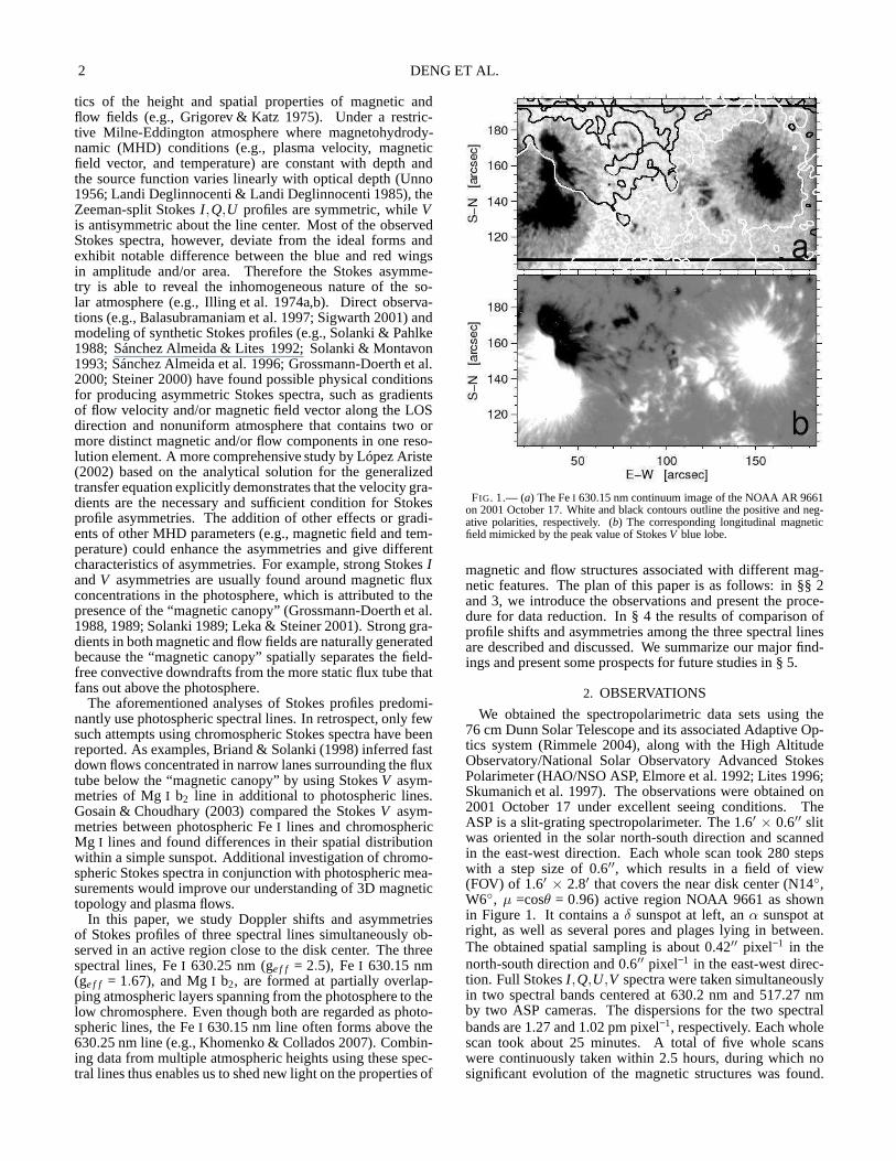
FIG. 1.— (a) The FeI 630.15 nm continuum image of the NOAA AR 9661on 2001 October 17. White and black contours outline the positive and neg-ative polarities, respectively. (b) The corresponding longitudinal magneticfield mimicked by the peak value of StokesV blue lobe.

magnetic and flow structures associated with different mag-netic features. The plan of this paper is as follows: in §§ 2and 3, we introduce the observations and present the proce-dure for data reduction. In § 4 the results of comparison ofprofile shifts and asymmetries among the three spectral linesare described and discussed. We summarize our major find-ings and present some prospects for future studies in § 5.

2. OBSERVATIONS

We obtained the spectropolarimetric data sets using the76 cm Dunn Solar Telescope and its associated Adaptive Op-tics system (Rimmele 2004), along with the High AltitudeObservatory/National Solar Observatory Advanced StokesPolarimeter (HAO/NSO ASP, Elmore et al. 1992; Lites 1996;Skumanich et al. 1997). The observations were obtained on2001 October 17 under excellent seeing conditions. TheASP is a slit-grating spectropolarimeter. The 1.6′ × 0.6′′ slitwas oriented in the solar north-south direction and scannedin the east-west direction. Each whole scan took 280 stepswith a step size of 0.6′′, which results in a field of view(FOV) of 1.6′ × 2.8′ that covers the near disk center (N14◦,W6◦, µ =cosθ = 0.96) active region NOAA 9661 as shownin Figure 1. It contains aδ sunspot at left, anα sunspot atright, as well as several pores and plages lying in between.The obtained spatial sampling is about 0.42′′ pixel−1 in thenorth-south direction and 0.6′′ pixel−1 in the east-west direc-tion. Full StokesI ,Q,U,V spectra were taken simultaneouslyin two spectral bands centered at 630.2 nm and 517.27 nmby two ASP cameras. The dispersions for the two spectralbands are 1.27 and 1.02 pm pixel−1, respectively. Each wholescan took about 25 minutes. A total of five whole scanswere continuously taken within 2.5 hours, during which nosignificant evolution of the magnetic structures was found.

DOPPLER SHIFT AND ASYMMETRY OF STOKES PROFILES OF FeI AND Mg I LINES 3

Other information about the observation run can be found inChoudhary & Balasubramaniam (2007).

3. DATA REDUCTION

We applied the standard ASP calibration procedures(Lites et al. 1991; Skumanich et al. 1997) to the data sets. Thecalibrated StokesI ,Q,U,V spectra were normalized to thequiet Sun continuum intensityIc that was obtained by fittingthe Kitt Peak FTS atlas to the observed StokesI profiles. Thedata sets from the five whole scans were then integrated to in-crease the signal to noise ratio (S/N). Furthermore, we calcu-lated the standard deviationσ in near continuum wavelengthrange for each integrated StokesI ,Q,U,V profile to representthe profile noise level. Only profiles with signal amplitudegreater than 7σ (an empirical S/N threshold that performs wellin our data analysis) were used for this study.

We extracted the parameters for analyzing the shift andasymmetry of Stokes profiles using the following procedures.

(1)Stokes I LOS velocitiesνi . We employed a Fourier phasemethod (see Schmidt et al. 1999) to determine the line corewavelength. We then converted the wavelength shifts to ve-locities (νi) by using the Doppler formula. As a frame of refer-ence, we use the average velocity of a small area in the nearlymotionless umbra.

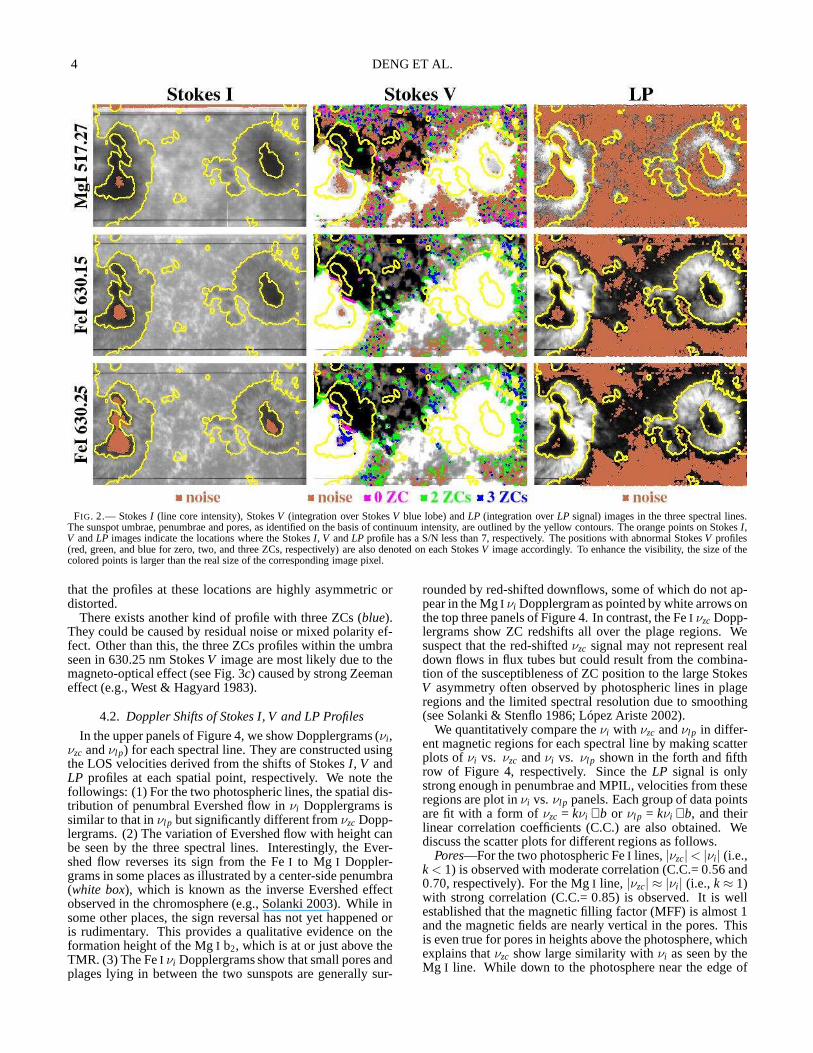
(2) Stokes V LOS velocitiesνzc. Normalized StokesV pro-files were smoothed to remove local noise. They were thendivided into two cases: normal profiles that have two oppositelobes and one zero-crossing (ZC) point in between, and abnor-mal profiles that have no or multiple ZCs within a wavelengthrange corresponding to±5 kms−1 from StokesI line center.Using this method, there is a small chance that we may im-properly classify normal profiles into an abnormal class. Forexample, strong magneto-optical effects (see Fig. 3c and textin § 4.1) produce StokesV profiles with 3 ZCs, although theprofile is essentially normal. Such improperly classified casesonly account for a small portion (< 0.3%) in the data and donot affect the analysis. For normal profiles, the ZC shifts areconverted to LOS velocities (νzc) in a same manner asνi . Theabnormal profiles will be discussed in § 4.1.

(3) Linear polarization (LP) LOS velocitiesνl p. The com-bination (Q2+U2)1/2 is a measure of the overallLP magnitude(e.g., Leka & Steiner 2001). TheLP profiles were smoothedto remove local noise. It is difficult to measure the positionofthe centralπ component as it is usually small and sometimeseven vanishes (see Figure 7). Instead we measure the peakpositions of the twoσ components and use their mid-pointas the position of theLP profile. We then converted theLPprofile shifts to LOS velocities (νl p) in a same manner asνi .

(4) Amplitude asymmetryδa and area asymmetryδA. Thepeak amplitudes of the blue (ab) and the red (ar) lobes of nor-mal StokesV profiles and those of the twoσ components ofLP profiles are determined. The areas of blue (Ab) and red(Ar) lobes are obtained by integrating over the same wave-length range (0.02 nm) on both sides of the ZC wavelength forStokesV profiles or the mid-point of the twoσ componentsfor LP profiles. The integrating range not only covers the ma-jority of the StokesV or LP signal corresponding to StokesI Doppler core, but also rules out the blends from the neigh-boring telluric lines. Following Solanki & Stenflo (1984), theamplitude asymmetryδa and area asymmetryδA are derivedusing the following formulae:

δa =|ab|− |ar |

|ab|+ |ar |, (1)

δA =|Ab|− |Ar |

|Ab|+ |Ar |. (2)

4. RESULTS AND DISCUSSIONS

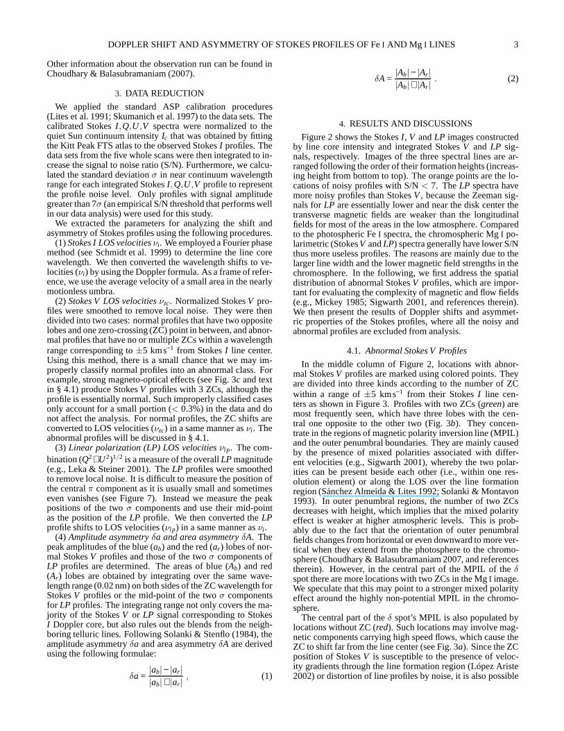
Figure 2 shows the StokesI , V andLP images constructedby line core intensity and integrated StokesV and LP sig-nals, respectively. Images of the three spectral lines are ar-ranged following the order of their formation heights (increas-ing height from bottom to top). The orange points are the lo-cations of noisy profiles with S/N< 7. TheLP spectra havemore noisy profiles than StokesV, because the Zeeman sig-nals forLP are essentially lower and near the disk center thetransverse magnetic fields are weaker than the longitudinalfields for most of the areas in the low atmosphere. Comparedto the photospheric FeI spectra, the chromospheric MgI po-larimetric (StokesV andLP) spectra generally have lower S/Nthus more useless profiles. The reasons are mainly due to thelarger line width and the lower magnetic field strengths in thechromosphere. In the following, we first address the spatialdistribution of abnormal StokesV profiles, which are impor-tant for evaluating the complexity of magnetic and flow fields(e.g., Mickey 1985; Sigwarth 2001, and references therein).We then present the results of Doppler shifts and asymmet-ric properties of the Stokes profiles, where all the noisy andabnormal profiles are excluded from analysis.

4.1. Abnormal Stokes V Profiles

In the middle column of Figure 2, locations with abnor-mal StokesV profiles are marked using colored points. Theyare divided into three kinds according to the number of ZCwithin a range of±5 kms−1 from their StokesI line cen-ters as shown in Figure 3. Profiles with two ZCs (green) aremost frequently seen, which have three lobes with the cen-tral one opposite to the other two (Fig. 3b). They concen-trate in the regions of magnetic polarity inversion line (MPIL)and the outer penumbral boundaries. They are mainly causedby the presence of mixed polarities associated with differ-ent velocities (e.g., Sigwarth 2001), whereby the two polar-ities can be present beside each other (i.e., within one res-olution element) or along the LOS over the line formationregion (Sánchez Almeida & Lites 1992; Solanki & Montavon1993). In outer penumbral regions, the number of two ZCsdecreases with height, which implies that the mixed polarityeffect is weaker at higher atmospheric levels. This is prob-ably due to the fact that the orientation of outer penumbralfields changes from horizontal or even downward to more ver-tical when they extend from the photosphere to the chromo-sphere (Choudhary & Balasubramaniam 2007, and referencestherein). However, in the central part of the MPIL of theδspot there are more locations with two ZCs in the MgI image.We speculate that this may point to a stronger mixed polarityeffect around the highly non-potential MPIL in the chromo-sphere.

The central part of theδ spot’s MPIL is also populated bylocations without ZC (red). Such locations may involve mag-netic components carrying high speed flows, which cause theZC to shift far from the line center (see Fig. 3a). Since the ZCposition of StokesV is susceptible to the presence of veloc-ity gradients through the line formation region (López Ariste2002) or distortion of line profiles by noise, it is also possible

4 DENG ET AL.

FIG. 2.— StokesI (line core intensity), StokesV (integration over StokesV blue lobe) andLP (integration overLP signal) images in the three spectral lines.The sunspot umbrae, penumbrae and pores, as identified on thebasis of continuum intensity, are outlined by the yellow contours. The orange points on StokesI ,V andLP images indicate the locations where the StokesI , V andLP profile has a S/N less than 7, respectively. The positions with abnormal StokesV profiles(red, green, and blue for zero, two, and three ZCs, respectively) are also denoted on each StokesV image accordingly. To enhance the visibility, the size of thecolored points is larger than the real size of the corresponding image pixel.

that the profiles at these locations are highly asymmetric ordistorted.

There exists another kind of profile with three ZCs (blue).They could be caused by residual noise or mixed polarity ef-fect. Other than this, the three ZCs profiles within the umbraseen in 630.25 nm StokesV image are most likely due to themagneto-optical effect (see Fig. 3c) caused by strong Zeemaneffect (e.g., West & Hagyard 1983).

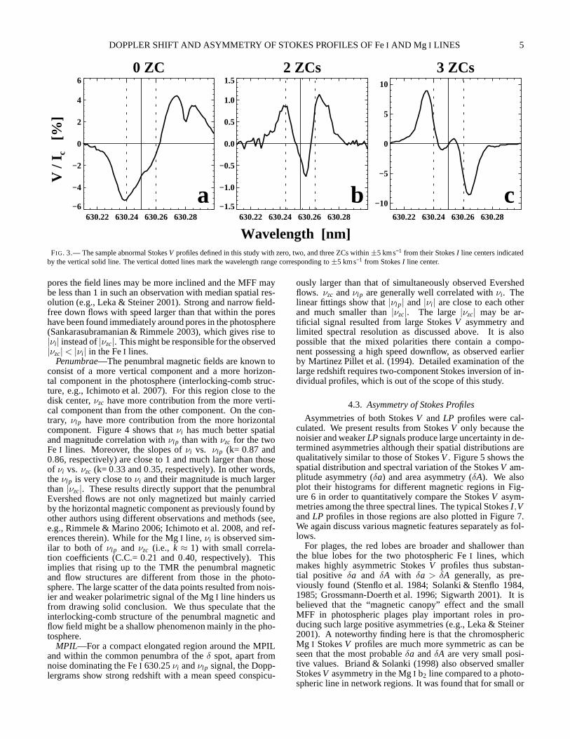
4.2. Doppler Shifts of Stokes I, V and LP Profiles

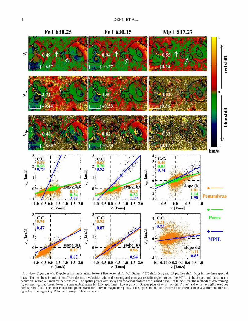
In the upper panels of Figure 4, we show Dopplergrams (νi ,νzc andνl p) for each spectral line. They are constructed usingthe LOS velocities derived from the shifts of StokesI , V andLP profiles at each spatial point, respectively. We note thefollowings: (1) For the two photospheric lines, the spatialdis-tribution of penumbral Evershed flow inνi Dopplergrams issimilar to that inνl p but significantly different fromνzc Dopp-lergrams. (2) The variation of Evershed flow with height canbe seen by the three spectral lines. Interestingly, the Ever-shed flow reverses its sign from the FeI to Mg I Doppler-grams in some places as illustrated by a center-side penumbra(white box), which is known as the inverse Evershed effectobserved in the chromosphere (e.g., Solanki 2003). While insome other places, the sign reversal has not yet happened oris rudimentary. This provides a qualitative evidence on theformation height of the MgI b2, which is at or just above theTMR. (3) The FeI νi Dopplergrams show that small pores andplages lying in between the two sunspots are generally sur-

rounded by red-shifted downflows, some of which do not ap-pear in the MgI νi Dopplergram as pointed by white arrows onthe top three panels of Figure 4. In contrast, the FeI νzc Dopp-lergrams show ZC redshifts all over the plage regions. Wesuspect that the red-shiftedνzc signal may not represent realdown flows in flux tubes but could result from the combina-tion of the susceptibleness of ZC position to the large StokesV asymmetry often observed by photospheric lines in plageregions and the limited spectral resolution due to smoothing(see Solanki & Stenflo 1986; López Ariste 2002).

We quantitatively compare theνi with νzc andνl p in differ-ent magnetic regions for each spectral line by making scatterplots ofνi vs. νzc andνi vs. νl p shown in the forth and fifthrow of Figure 4, respectively. Since theLP signal is onlystrong enough in penumbrae and MPIL, velocities from theseregions are plot inνi vs. νl p panels. Each group of data pointsare fit with a form ofνzc = kνi + b or νl p = kνi + b, and theirlinear correlation coefficients (C.C.) are also obtained. Wediscuss the scatter plots for different regions as follows.

Pores—For the two photospheric FeI lines,|νzc|< |νi | (i.e.,k< 1) is observed with moderate correlation (C.C.= 0.56 and0.70, respectively). For the MgI line, |νzc| ≈ |νi | (i.e.,k ≈ 1)with strong correlation (C.C.= 0.85) is observed. It is wellestablished that the magnetic filling factor (MFF) is almost1and the magnetic fields are nearly vertical in the pores. Thisis even true for pores in heights above the photosphere, whichexplains thatνzc show large similarity withνi as seen by theMg I line. While down to the photosphere near the edge of

DOPPLER SHIFT AND ASYMMETRY OF STOKES PROFILES OF FeI AND Mg I LINES 5

0 ZC

630.22 630.24 630.26 630.28−6

−4

−2

0

2

4

6

a

2 ZCs

630.22 630.24 630.26 630.28−1.5

−1.0

−0.5

0.0

0.5

1.0

1.5

b

3 ZCs

630.22 630.24 630.26 630.28

−10

−5

0

5

10

c

V /

I c

[%]

Wavelength [nm]FIG. 3.— The sample abnormal StokesV profiles defined in this study with zero, two, and three ZCs within ±5 kms−1 from their StokesI line centers indicated

by the vertical solid line. The vertical dotted lines mark the wavelength range corresponding to±5 kms−1 from StokesI line center.

pores the field lines may be more inclined and the MFF maybe less than 1 in such an observation with median spatial res-olution (e.g., Leka & Steiner 2001). Strong and narrow field-free down flows with speed larger than that within the poreshave been found immediately around pores in the photosphere(Sankarasubramanian & Rimmele 2003), which gives rise to|νi | instead of|νzc|. This might be responsible for the observed|νzc|< |νi | in the FeI lines.

Penumbrae—The penumbral magnetic fields are known toconsist of a more vertical component and a more horizon-tal component in the photosphere (interlocking-comb struc-ture, e.g., Ichimoto et al. 2007). For this region close to thedisk center,νzc have more contribution from the more verti-cal component than from the other component. On the con-trary, νl p have more contribution from the more horizontalcomponent. Figure 4 shows thatνi has much better spatialand magnitude correlation withνl p than withνzc for the twoFe I lines. Moreover, the slopes ofνi vs. νl p (k= 0.87 and0.86, respectively) are close to 1 and much larger than thoseof νi vs. νzc (k= 0.33 and 0.35, respectively). In other words,theνl p is very close toνi and their magnitude is much largerthan |νzc|. These results directly support that the penumbralEvershed flows are not only magnetized but mainly carriedby the horizontal magnetic component as previously found byother authors using different observations and methods (see,e.g., Rimmele & Marino 2006; Ichimoto et al. 2008, and ref-erences therein). While for the MgI line, νi is observed sim-ilar to both of νl p and νzc (i.e., k ≈ 1) with small correla-tion coefficients (C.C.= 0.21 and 0.40, respectively). Thisimplies that rising up to the TMR the penumbral magneticand flow structures are different from those in the photo-sphere. The large scatter of the data points resulted from nois-ier and weaker polarimetric signal of the MgI line hinders usfrom drawing solid conclusion. We thus speculate that theinterlocking-comb structure of the penumbral magnetic andflow field might be a shallow phenomenon mainly in the pho-tosphere.

MPIL—For a compact elongated region around the MPILand within the common penumbra of theδ spot, apart fromnoise dominating the FeI 630.25νi andνl p signal, the Dopp-lergrams show strong redshift with a mean speed conspicu-

ously larger than that of simultaneously observed Evershedflows. νzc andνl p are generally well correlated withνi . Thelinear fittings show that|νl p| and|νi | are close to each otherand much smaller than|νzc|. The large|νzc| may be ar-tificial signal resulted from large StokesV asymmetry andlimited spectral resolution as discussed above. It is alsopossible that the mixed polarities there contain a compo-nent possessing a high speed downflow, as observed earlierby Martinez Pillet et al. (1994). Detailed examination of thelarge redshift requires two-component Stokes inversion ofin-dividual profiles, which is out of the scope of this study.

4.3. Asymmetry of Stokes Profiles

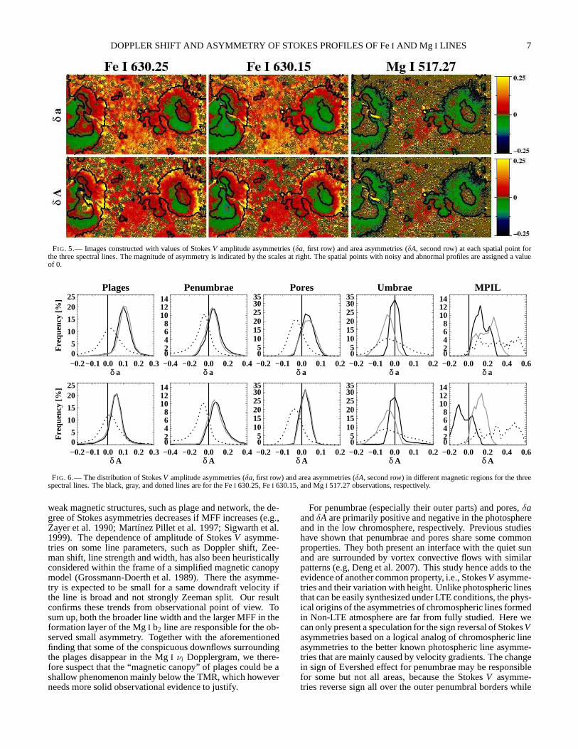
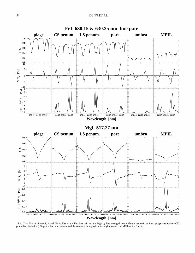
Asymmetries of both StokesV andLP profiles were cal-culated. We present results from StokesV only because thenoisier and weakerLP signals produce large uncertainty in de-termined asymmetries although their spatial distributions arequalitatively similar to those of StokesV. Figure 5 shows thespatial distribution and spectral variation of the StokesV am-plitude asymmetry (δa) and area asymmetry (δA). We alsoplot their histograms for different magnetic regions in Fig-ure 6 in order to quantitatively compare the StokesV asym-metries among the three spectral lines. The typical StokesI ,VandLP profiles in those regions are also plotted in Figure 7.We again discuss various magnetic features separately as fol-lows.

For plages, the red lobes are broader and shallower thanthe blue lobes for the two photospheric FeI lines, whichmakes highly asymmetric StokesV profiles thus substan-tial positive δa and δA with δa > δA generally, as pre-viously found (Stenflo et al. 1984; Solanki & Stenflo 1984,1985; Grossmann-Doerth et al. 1996; Sigwarth 2001). It isbelieved that the “magnetic canopy” effect and the smallMFF in photospheric plages play important roles in pro-ducing such large positive asymmetries (e.g., Leka & Steiner2001). A noteworthy finding here is that the chromosphericMg I StokesV profiles are much more symmetric as can beseen that the most probableδa andδA are very small posi-tive values. Briand & Solanki (1998) also observed smallerStokesV asymmetry in the MgI b2 line compared to a photo-spheric line in network regions. It was found that for small or

6 DENG ET AL.

FIG. 4.— Upper panels: Dopplergrams made using StokesI line center shifts (νi ), StokesV ZC shifts (νzc) andLP profiles shifts (νl p) for the three spectrallines. The numbers in unit of kms−1are the mean velocities within the strong and compact redshift region around the MPIL of theδ spot, and those in thepenumbral region outlined by the white box. The spatial points with noisy and abnormal profiles are assigned a value of 0. Note that the methods of determiningνi , νzc andνl p may break down in some umbral areas for fully split lines.Lower panels: Scatter plots ofνi vs. νzc (forth row) andνi vs. νl p (fifth row) foreach spectral line. The color-coded data points stand for different magnetic regions. The slopek and the linear correlation coefficient (C.C.) from the line fitsνzc = kνi + b or νl p = kνi + b for each group of data are labeled.

DOPPLER SHIFT AND ASYMMETRY OF STOKES PROFILES OF FeI AND Mg I LINES 7

FIG. 5.— Images constructed with values of StokesV amplitude asymmetries (δa, first row) and area asymmetries (δA, second row) at each spatial point forthe three spectral lines. The magnitude of asymmetry is indicated by the scales at right. The spatial points with noisy and abnormal profiles are assigned a valueof 0.

Plages

−0.2−0.1 0.0 0.1 0.2 0.3δ a

05

10

15

2025

Fre

quen

cy [%

]

−0.2−0.1 0.0 0.1 0.2 0.3δ A

05

10

15

2025

Fre

quen

cy [%

]

Penumbrae

−0.4 −0.2 0.0 0.2 0.4δ a

02468

101214

−0.4 −0.2 0.0 0.2 0.4δ A

02468

101214

Pores

−0.2 −0.1 0.0 0.1 0.2δ a

05

101520253035

−0.2 −0.1 0.0 0.1 0.2δ A

05

101520253035

Umbrae

−0.2 −0.1 0.0 0.1 0.2δ a

05

101520253035

−0.2 −0.1 0.0 0.1 0.2δ A

05

101520253035

MPIL

−0.2 0.0 0.2 0.4 0.6δ a

02468

101214

−0.2 0.0 0.2 0.4 0.6δ A

02468

101214

FIG. 6.— The distribution of StokesV amplitude asymmetries (δa, first row) and area asymmetries (δA, second row) in different magnetic regions for the threespectral lines. The black, gray, and dotted lines are for theFeI 630.25, FeI 630.15, and MgI 517.27 observations, respectively.

weak magnetic structures, such as plage and network, the de-gree of Stokes asymmetries decreases if MFF increases (e.g.,Zayer et al. 1990; Martínez Pillet et al. 1997; Sigwarth et al.1999). The dependence of amplitude of StokesV asymme-tries on some line parameters, such as Doppler shift, Zee-man shift, line strength and width, has also been heuristicallyconsidered within the frame of a simplified magnetic canopymodel (Grossmann-Doerth et al. 1989). There the asymme-try is expected to be small for a same downdraft velocity ifthe line is broad and not strongly Zeeman split. Our resultconfirms these trends from observational point of view. Tosum up, both the broader line width and the larger MFF in theformation layer of the MgI b2 line are responsible for the ob-served small asymmetry. Together with the aforementionedfinding that some of the conspicuous downflows surroundingthe plages disappear in the MgI νi Dopplergram, we there-fore suspect that the “magnetic canopy” of plages could be ashallow phenomenon mainly below the TMR, which howeverneeds more solid observational evidence to justify.

For penumbrae (especially their outer parts) and pores,δaandδA are primarily positive and negative in the photosphereand in the low chromosphere, respectively. Previous studieshave shown that penumbrae and pores share some commonproperties. They both present an interface with the quiet sunand are surrounded by vortex convective flows with similarpatterns (e.g, Deng et al. 2007). This study hence adds to theevidence of another common property, i.e., StokesV asymme-tries and their variation with height. Unlike photosphericlinesthat can be easily synthesized under LTE conditions, the phys-ical origins of the asymmetries of chromospheric lines formedin Non-LTE atmosphere are far from fully studied. Here wecan only present a speculation for the sign reversal of StokesVasymmetries based on a logical analog of chromospheric lineasymmetries to the better known photospheric line asymme-tries that are mainly caused by velocity gradients. The changein sign of Evershed effect for penumbrae may be responsiblefor some but not all areas, because the StokesV asymme-tries reverse sign all over the outer penumbral borders while

8 DENG ET AL.

plage

0.0

0.2

0.4

0.6

0.8

1.0

I / I

c

−10

−5

0

5

10

V /

I c

[%]

630.15 630.20 630.2501

2

3

4

56

(Q2 +

U2 )1/

2 / I c

[%

]

CS penum.

630.15 630.20 630.25

LS penum.

630.15 630.20 630.25

pore

630.15 630.20 630.25

umbra

630.15 630.20 630.25

MPIL

630.15 630.20 630.25

FeI 630.15 & 630.25 nm line pair

Wavelength [nm]

plage

0.0

0.2

0.4

0.6

0.8

I / I

c

−3−2

−1

0

1

23

V /

I c

[%]

517.20 517.25 517.30 517.350.0

0.2

0.4

0.6

0.8

(Q2 +

U2 )1/

2 / I c

[%

]

CS penum.

517.20 517.25 517.30 517.35

LS penum.

517.20 517.25 517.30 517.35

pore

517.20 517.25 517.30 517.35

umbra

517.20 517.25 517.30 517.35

MPIL

517.20 517.25 517.30 517.35

MgI 517.27 nm

Wavelength [nm]FIG. 7.— Typical StokesI , V andLP profiles of the FeI line pair and the MgI b2 line averaged over different magnetic regions: plage, center-side (CS)

penumbra, limb-side (LS) penumbra, pore, umbra, and the compact strong red-shifted region around the MPIL of theδ spot.

DOPPLER SHIFT AND ASYMMETRY OF STOKES PROFILES OF FeI AND Mg I LINES 9

the inverse of Evershed flow only occurs in some penumbralsectors. We speculate that the sign reversal of StokesV asym-metries in both outer penumbrae and pores could indicate thatthe velocity in and around them may change drastically fromthe photosphere to the low chromosphere. Figure 4 providesclues to some of the changes because some downflows in andaround pores do not hold in the MgI νi Dopplergram insteadmore upflows can be seen (e.g., in the scatter plot of the MgIline). Moreover, Sankarasubramanian & Rimmele (2003) ob-served pores in different wavelengths and found that veloci-ties in the narrow downflow region around pores tend to de-crease with height at first, and then change to upflow in thelow chromosphere. Such tendency is also visible in the MHDsimulation of pores (see Fig. 3 of Leka & Steiner 2001). TheStokesV asymmetries change from positive for the FeI linesto negative for the MgI line, if indeed all line asymmetrieshave a velocity gradient origin, thus provides important clueson the 3D structure of the flow field in and around pores andouter penumbrae.

For umbrae, since they lack of mass flows and have MFF of∼1 in the low photosphere, both of the most probableδa andδA of the FeI 630.25 nm line are close to 0. The large Zeemansplitting of the line in strong field may also contribute to theobserved small asymmetry (Grossmann-Doerth et al. 1989).However, the distributions ofδa andδA of the other two spec-tral lines show a clear shift toward negative. Besides the noiseinduced inaccuracy of the determined asymmetry due to lowlight level in the umbra, it is also possible that as height in-creases umbrae become less uniform and static compared withtheir structure in the low photosphere.

For the compact region with strong redshifts around theMPIL of theδ spot, bothδa andδA have prominent values thatincrease with height. It seems from Figure 7 that the red wingsof the StokesI , V, andLP profiles of the two photosphericlines obviously have further redward extension. Meanwhile,the blue damping wings of the MgI 517.27 nm line are sur-prisingly enhanced, which remains a puzzling issue. We con-jecture that the observed large asymmetries could be due tothe combination of the following two effects: the mixed po-larities or flows, and the large gradients in velocity, magneticfield vector, or temperature near the MPIL region. Consider-ing all the unusual properties observed in this region, we sug-gest that the magnetic and flow fields around the MPIL of theδ spot are very complex, which deserve a deeper investigationin the future.

5. SUMMARY

We have presented a comprehensive study of the Dopplershifts and asymmetric properties of the Stokes profiles, theuniqueness of which is especially in the combination of mag-netic sensitive spectral lines that form at different heightsspanning from the photosphere to the low chromosphere.Our quantitative analysis benefits from the simultaneous andhigh resolution spectro-polarimetric observation that includea chromospheric line. We summarize the major findings andinterpretations as follows.

1. νi is very close toνl p but significantly different fromνzcin penumbral areas near disc center for the photosphericFe I lines, which provides direct and strong evidencethat the penumbral Evershed flows are magnetized andmainly carried by the horizontal magnetic component.

2. The rudimentary inverse Evershed effect observed by

the Mg I b2 line provides a qualitative evidence on itsformation height that is around or just above the TMR.

3. νzc andνl p in penumbrae andνzc in pores generally ap-proach theirνi observed by the chromospheric MgIline, which is not the case for the photospheric FeIlines. We speculate that the interlocking-comb struc-ture of the penumbral magnetic and flow field might bea shallow phenomenon mainly in the photosphere.

4. The StokesV asymmetries exhibit similar behavior inthe regions of outer penumbrae and pores. Bothδa andδA evolve from primarily positive values observed byphotospheric FeI lines to primarily negative values ob-served by the chromospheric MgI line.

5. In plage regions where the “magnetic canopy” effectis present, StokesV profiles are highly asymmetric inthe photosphere but more symmetric in the low chro-mosphere. Moreover, some of the photospheric down-flows surrounding the plages disappear in the MgIDopplergram. These suggest that the plage “magneticcanopy” could be a shallow phenomenon mainly belowthe TMR.

6. All the νi , νzc andνl p Dopplergrams reveal strong red-shifts in a compact region around the MPIL and withinthe common penumbra of theδ spot. Large posi-tive StokesV asymmetries are also present and evenstrengthen with height. These unusual phenomena aremanifestations of the complex nature of the 3D topol-ogy of the highly non-potential region.

We conclude that analysis of Stokes profiles using boththe photospheric and chromospheric spectral lines can fur-nish crucial information on the 3D structure of the magneticand flow fields. Similar study using other chromospheric lineswill be essential to see if the behavior and trend of velocitiesand asymmetries observed by the MgI b2 line is general for allthe chromospheric lines. The speculations made in this study,such as the velocity gradient origin of the chromospheric lineasymmetries and the thinness of the interlocking-comb struc-ture of penumbral magnetic and flow fields, need further in-vestigation to justify. To advance firmly towards a sound andreliable measurement of magnetic fields in the chromosphere,not only more polarimetric observations using chromosphericlines are needed, but also a better understanding of their com-plicated profile formation conditions is critical.

We are truly grateful to Dr. S. Solanki for careful readingof the paper and many constructive suggestions throughoutthis study. Thanks are also given to Dr. C. Liu and A. Cook-son for polishing and improving the manuscript and Drs. L.Bellot Rubio, K. E., Rangarajan, and H. Wang for helpful dis-cussions. We thank the referee for valuable comments thathelp us to improve the paper. N.D. and D.P.C. were sup-ported by NASA grant NNX08AQ32G and NSF grant ATM05-48260. We acknowledge the use of the HAO/NSO Ad-vanced Stokes Polarimeter. The National Solar Observatoryis operated by the Association of Universities for ResearchinAstronomy under a cooperative agreement with the NationalScience Foundation, for the benefit of the astronomical com-munity. This research has made use of NASA’s AstrophysicsData System Bibliographic Services.

10 DENG ET AL.

REFERENCES

Altrock, R. C., & Canfield, R. C. 1974, ApJ, 194, 733Balasubramaniam, K. S., Christopoulou, E. B., & Uitenbroek, H. 2004, ApJ,

606, 1233Balasubramaniam, K. S., Keil, S. L., & Tomczyk, S. 1997, ApJ,482, 1065Briand, C., & Martínez Pillet, V. 2001, in Astronomical Society of the

Pacific Conference Series, Vol. 236, Advanced Solar Polarimetry –Theory, Observation, and Instrumentation, ed. M. Sigwarth, 565–+

Briand, C., & Solanki, S. K. 1995, A&A, 299, 596—. 1998, A&A, 330, 1160Choudhary, D. P., & Balasubramaniam, K. S. 2007, ApJ, 664, 1228Dalgarno, A., & Layzer, D., eds. 1987, Spectroscopy of astrophysical

plasmasDeng, N., Choudhary, D. P., Tritschler, A., Denker, C., Liu,C., & Wang, H.

2007, ApJ, 671, 1013Elmore, D. F., Lites, B. W., Tomczyk, S., Skumanich, A. P., Dunn, R. B.,

Schuenke, J. A., Streander, K. V., Leach, T. W., Chambellan,C. W., &Hull, H. K. 1992, in Presented at the Society of Photo-OpticalInstrumentation Engineers (SPIE) Conference, Vol. 1746, Polarizationanalysis and measurement; Proceedings of the Meeting, San Diego, CA,July 19-21, 1992 (A93-33401 12-35), p. 22-33., ed. D. H. Goldstein &R. A. Chipman, 22–33

Evershed, J. 1909, MNRAS, 69, 454Gosain, S., & Choudhary, D. 2003, Sol. Phys., 217, 119Grigorev, V. M., & Katz, J. M. 1975, Sol. Phys., 42, 21Grossmann-Doerth, U., Keller, C. U., & Schuessler, M. 1996,A&A, 315,

610Grossmann-Doerth, U., Schuessler, M., & Solanki, S. K. 1988, A&A, 206,

L37—. 1989, A&A, 221, 338Grossmann-Doerth, U., Schüssler, M., Sigwarth, M., & Steiner, O. 2000,

A&A, 357, 351Ichimoto, K., Shine, R. A., Lites, B., Kubo, M., Shimizu, T.,Suematsu, Y.,

Tsuneta, S., Katsukawa, Y., Tarbell, T. D., Title, A. M., Nagata, S.,Yokoyama, T., & Shimojo, M. 2007, PASJ, 59, 593

Ichimoto, K., Tsuneta, S., Suematsu, Y., Katsukawa, Y., Shimizu, T., Lites,B. W., Kubo, M., Tarbell, T. D., Shine, R. A., Title, A. M., & Nagata, S.2008, A&A, 481, L9

Illing, R. M. E., Landman, D. A., & Mickey, D. L. 1974a, A&A, 35, 327—. 1974b, A&A, 37, 97Khomenko, E., & Collados, M. 2007, ApJ, 659, 1726Lagg, A., Woch, J., Krupp, N., & Solanki, S. K. 2004, A&A, 414,1109Landi Deglinnocenti, E., & Landi Deglinnocenti, M. 1985, Sol. Phys., 97,

239Leka, K. D., & Metcalf, T. R. 2003, Sol. Phys., 212, 361Leka, K. D., & Steiner, O. 2001, ApJ, 552, 354Lites, B. W. 1996, Sol. Phys., 163, 223

Lites, B. W., Elmore, D., Murphy, G., Skumanich, A., Tomczyk, S., &Dunn, R. B. 1991, in 11. National Solar Observatory / Sacramento PeakSummer Workshop: Solar polarimetry, p. 3 - 15, 3–15

Lites, B. W., Skumanich, A., Rees, D. E., & Murphy, G. A. 1988,ApJ, 330,493

López Ariste, A. 2002, ApJ, 564, 379López Ariste, A., & Casini, R. 2002, ApJ, 575, 529Martínez Pillet, V., Lites, B. W., & Skumanich, A. 1997, ApJ,474, 810Martinez Pillet, V., Lites, B. W., Skumanich, A., & Degenhardt, D. 1994,

ApJ, 425, L113Mauas, P. J., Avrett, E. H., & Loeser, R. 1988, ApJ, 330, 1008Mickey, D. L. 1985, Sol. Phys., 97, 223Rimmele, T., & Marino, J. 2006, ApJ, 646, 593Rimmele, T. R. 2004, in Presented at the Society of Photo-Optical

Instrumentation Engineers (SPIE) Conference, Vol. 5490, Advancementsin Adaptive Optics. Edited by Domenico B. Calia, Brent L. Ellerbroek,and Roberto Ragazzoni. Proceedings of the SPIE, Volume 5490, pp. 34-46(2004)., ed. D. Bonaccini Calia, B. L. Ellerbroek, & R. Ragazzoni, 34–46

Sánchez Almeida, J., Landi degl’Innocenti, E., Martinez Pillet, V., & Lites,B. W. 1996, ApJ, 466, 537

Sánchez Almeida, J., & Lites, B. W. 1992, ApJ, 398, 359Sankarasubramanian, K., & Rimmele, T. 2003, ApJ, 598, 689Schmidt, W., Stix, M., & Wöhl, H. 1999, A&A, 346, 633Sigwarth, M. 2001, ApJ, 563, 1031Sigwarth, M., Balasubramaniam, K. S., Knölker, M., & Schmidt, W. 1999,

A&A, 349, 941Skumanich, A., Lites, B. W., Martinez Pillet, V., & Seagraves, P. 1997,

ApJS, 110, 357Socas-Navarro, H., Trujillo Bueno, J., & Ruiz Cobo, B. 2000,Science, 288,

1396Solanki, S. K. 1986, A&A, 168, 311—. 1989, A&A, 224, 225—. 2003, Astron. Astrophys. Rev. 11, 153Solanki, S. K., Lagg, A., Woch, J., Krupp, N., & Collados, M. 2003, Nature,

425, 692Solanki, S. K., & Montavon, C. A. P. 1993, A&A, 275, 283Solanki, S. K., & Pahlke, K. D. 1988, A&A, 201, 143Solanki, S. K., & Stenflo, J. O. 1984, A&A, 140, 185—. 1985, A&A, 148, 123—. 1986, A&A, 170, 120Steiner, O. 2000, Sol. Phys., 196, 245Stenflo, J. O., Solanki, S., Harvey, J. W., & Brault, J. W. 1984, A&A, 131,

333Trujillo Bueno, J., Landi Degl’Innocenti, E., Collados, M., Merenda, L., &

Manso Sainz, R. 2002, Nature, 415, 403Unno, W. 1956, PASJ, 8, 108West, E. A., & Hagyard, M. J. 1983, Sol. Phys., 88, 51Zayer, I., Stenflo, J. O., Keller, C. U., & Solanki, S. K. 1990,A&A, 239, 356Zhang, M., & Zhang, H. 2000, Sol. Phys., 194, 19