On the Consistency of Ranking Algorithms - Stanford University

On the Consistency of Ranking Algorithms

John C. Duchi [email protected]

Lester W. Mackey [email protected]

Computer Science Division, University of California, Berkeley, CA 94720, USA

Michael I. Jordan [email protected]

Computer Science Division and Department of Statistics, University of California, Berkeley, CA 94720, USA

Abstract

We present a theoretical analysis of super-vised ranking, providing necessary and suf-ficient conditions for the asymptotic consis-tency of algorithms based on minimizing asurrogate loss function. We show that manycommonly used surrogate losses are incon-sistent; surprisingly, we show inconsistencyeven in low-noise settings. We present anew value-regularized linear loss, establish itsconsistency under reasonable assumptions onnoise, and show that it outperforms conven-tional ranking losses in a collaborative filter-ing experiment.

The goal in ranking is to order a set of inputs in accor-dance with the preferences of an individual or a popu-lation. In this paper we consider a general formulationof the supervised ranking problem in which each train-ing example consists of a query q, a set of inputs x,sometimes called results, and a weighted graph G rep-resenting preferences over the results. The learningtask is to discover a function that provides a query-specific ordering of the inputs that best respects theobserved preferences. This query-indexed setting isnatural for tasks like web search in which a differentranking is needed for each query. Following existingliterature, we assume the existence of a scoring func-tion f(x, q) that gives a score to each result in x; thescores are sorted to produce a ranking (Herbrich et al.,2000; Freund et al., 2003). We assume simply thatthe observed preference graph G is a directed acyclicgraph (DAG). Finally, we cast our work in a decision-theoretic framework in which ranking procedures areevaluated via a loss function L(f(x, q), G).

Appearing in Proceedings of the 27 th International Confer-ence on Machine Learning, Haifa, Israel, 2010. Copyright2010 by the author(s)/owner(s).

It is important to distinguish between the loss functionused for evaluating learning procedures from the loss-like functions used to define specific methods (gener-ally via an optimization algorithm). In prior work theformer (evaluatory) loss has often been taken to be apairwise 0-1 loss that sums the number of misorderedpairs of results. Recent work has considered lossesthat penalize errors on more highly ranked instancesmore strongly. Jarvelin & Kekalainen (2002) suggestusing discounted cumulative gain, which assumes thateach result xi is given a score yi and that the loss is aweighted sum of the yi of the predicted order. Rudin(2009) uses a p-norm to emphasize the highest rankedinstances. Here we employ a general graph-based lossL(f(x, q), G) which is equal to zero if f(q,x) obeysthe order specified by G—that is, fi(x, q) > fj(x, q)for each edge (i → j) ∈ G, where fi(x, q) is the scoreassigned to the ith object in x—and is positive oth-erwise. We make the assumption that L is edgewise,meaning that L depends only on the relative order offi(x, q) rather than on its values. Such losses are nat-ural in settings with feedback in the form of orderedpreferences, for example when learning from click data.

Although we might wish to base a learning algorithmon the direct minimization of the loss L, this is gener-ally infeasible due to the non-convexity and discontinu-ity of L. In practice one instead employs a surrogateloss that lends itself to more efficient minimization.This issue is of course familiar from the classificationliterature, where a deep theoretical understanding ofthe statistical and computational consequences of thechoices of various surrogate losses has emerged (Zhang,2004; Bartlett et al., 2006). There is a relative paucityof such understanding for ranking. In the current pa-per we aim to fill this gap, taking a step toward bring-ing the ranking literature into line with that for clas-sification. We provide a general theoretical analysis ofthe consistency of ranking algorithms that are basedon a surrogate loss function.


The paper is organized as follows. In Section 1, wedefine the consistency problem formally and presenta theorem that provides conditions under which con-sistency is achieved for ranking algorithms. In Sec-tion 2 we show that finding consistent surrogate lossesis difficult in general, and we establish results showingthat many commonly used ranking loss functions areinconsistent, even in low-noise settings. We comple-ment this in Section 3 by presenting losses that areconsistent in these low-noise settings. We finish withexperiments and conclusions in Sections 4 and 5.

1. Consistency for Surrogate Losses

Our task is to minimize the risk of the scoring functionf . The risk is the expected loss of f across all queriesq, result sets x, and preference DAGs G:

R(f) = EX,Q,GL(f(X, Q), G). (1)

Given a query q and result set x, we define G to bethe set of possible preference DAGs and p to be (aversion of) the vector of conditional probabilities ofeach DAG. That is, p = [pG]G∈G = [P(G | x, q)]G∈G .In what follows, we suppress dependence of p, G, andG on the query q and results x, as they should be clearfrom context. We assume that the cardinality of anyresult set x is bounded above by M < ∞. We furtherdefine the conditional risk of f given x and q to be

ℓ(p,f(x, q)) =∑

G∈G

pGL(f(x, q), G)

=∑

G∈G

P(G | x, q)L(f(x, q), G). (2)

With this definition, we see the risk of f is equal to

EX,Q

[∑

G∈G

P(G | X, Q)L(f(X, Q), G)

]= EX,Qℓ(p,f).

We overload notation so that α takes the value off(x, q) in ℓ(p,α). The minimal risk, or Bayes’ risk, isthe minimal risk over all measurable functions,

R∗ = inff

R(f) = EX,Q infα

ℓ(p,α).

It is infeasible to directly minimize the true risk inEq. (1), as it is non-convex and discontinuous. Asis done in classification (Zhang, 2004; Bartlett et al.,2006), we thus consider a bounded-below surrogateϕ to minimize in place of L. For each G, we writeϕ(·, G) : R|G| → R. The ϕ-risk of the function f is

Rϕ(f) = EX,Q,G [ϕ(f(X, Q), G)]

= EX,Q

[∑

G∈G

P(G | X, Q)ϕ(f(X, Q), G)

],

while the optimal ϕ-risk is R∗ϕ = inff Rϕ(f).

To develop a theory of consistency for ranking meth-ods, we pursue a treatment that parallels that of Zhang(2004) for classification. Using the conditional risk inEq. (2), we define a function to measure the discrim-inating ability of the surrogate ϕ. Let G(m) denotethe set of possible DAGs G over m results, noting that

|G(m)| ≤ 3(m

2 ). Let ∆|G(m)| ⊂ R|G(m)| denote the prob-

ability simplex. For α,α′ ∈ Rm we define

Hm(ε) = infp∈∆,α

{ ∑

G∈G(m)

pGϕ(α, G)− infα′

∑

G∈G(m)

pGϕ(α′, G)

: ℓ(p,α)− infα′

ℓ(p,α′) ≥ ε}. (3)

Hm measures surrogate risk suboptimality as a func-tion of true risk suboptimality. A reasonable surrogateloss should declare any setting of {p,α} suboptimalthat the true loss declares suboptimal, which corre-sponds to Hm(ε) > 0 whenever ε > 0. We will seesoon that this condition is the key to consistency.

Define H(ε) = minm≤M Hm(ε). We immediately haveH ≥ 0, H(0) = 0, and H(ε) is non-decreasing on 0 ≤ε < ∞, since individualHm(ε) are non-decreasing in ε.We have the following lemma (a simple consequence ofJensen’s inequality), which we prove in Appendix A.

Lemma 1. Let ζ be a convex function such that ζ(ε) ≤H(ε). Then for all f , ζ(R(f)−R∗) ≤ Rϕ(f)−R∗

ϕ.

Corollary 26 from Zhang (2004) then shows as a conse-quence of Lemma 1 that if H(ε) > 0 for all ε > 0, thereis a nonnegative concave function ξ, right continuousat 0 with ξ(0) = 0, such that

R(f)−R∗ ≤ ξ(Rϕ(f)−R∗ϕ). (4)

Clearly, if limn Rϕ(fn) = R∗ϕ, we have consistency:

limn R(fn) = R∗. Though it is not our focus, it ispossible to use Eq. (4) to get strong rates of conver-gence if ξ grows slowly. The remainder of this paperconcentrates on finding conditions relating the surro-gate loss ϕ to the risk ℓ to make H(ε) > 0 for ε > 0.

We achieve this goal by using conditions based on theedge structure of the observed DAGs. Given a proba-bility vector p ∈ R

|G| over a set of DAGs G, we recallEq. (2) and define the set of optimal result scores A(p)to be all α attaining the infimum of ℓ(p,α),

A(p) = {α : ℓ(p,α) = infα′

ℓ(p,α′)}. (5)

The infimum is attained since ℓ is edgewise as de-scribed earlier, so A(p) is not empty. The followingdefinition captures the intuition that the surrogate loss


ϕ should maintain ordering information. For this def-inition and the remainder of the paper, we use thefollowing shorthand for the conditional ϕ-risk:

W (p,α) ,∑

G∈G

pGϕ(α, G). (6)

Definition 2. Let ϕ be a bounded-below surrogate losswith ϕ(·, G) continuous for all G. ϕ is edge-consistentwith respect to the loss L if for all p,

W ∗(p) , infα

W (p,α) < infα

{W (p,α) : α 6∈ A(p)} .

Definition 2 captures an essential property for the sur-rogate loss ϕ: if α induces an edge (i → j) via αi > αj

so that the conditional risk ℓ(p,α) is not minimal, thenthe conditional surrogate risk W (p,α) is not minimal.

We now provide three lemmas and a theorem thatshow that if the surrogate loss ϕ satisfies edge-consistency, then its minimizer asymptotically mini-mizes the Bayes risk. As the lemmas are direct analogsof results in Tewari & Bartlett (2007) and Zhang(2004), we put their proofs in Appendix A.

Lemma 3. W ∗(p) is continuous on ∆.

Lemma 4. Let ϕ be edge-consistent. ThenW (p,α(n)) → W ∗(p) implies that ℓ(p,α(n)) →infα ℓ(p,α) and α(n) ∈ A(p) eventually.

Lemma 5. Let ϕ be edge-consistent. For every ε > 0there exists a δ > 0 such that if p ∈ ∆, ℓ(p,α) −infα′ ℓ(p,α′) ≥ ε implies W (p,α)−W ∗(p) ≥ δ.

Theorem 6. Let ϕ be a continuous, bounded-belowloss function and assume that the size of the result setsis upper bounded by a constant M . Then ϕ is edge-consistent if and only the following holds: Wheneverfn is a sequence of scoring functions such that

Rϕ(fn)p→ R∗

ϕ, then R(fn)p→ R∗.

Proof We begin by proving that if ϕ is edge-consistent, the implication holds. By Lemma 5 andthe definition of Hm in Eq. (3), we have that if ε > 0,then there is some δ > 0 such that Hm(ε) ≥ δ > 0.Thus H(ε) = minm≤M Hm(ε) > 0, and Eq. (4) then

immediately implies that R(fn)p→ R∗.

Now suppose that ϕ is not edge-consistent, that is,there is some p so that W ∗(p) = infα{W (p,α) : α 6∈A(p)}. Let α(n) 6∈ A(p) be a sequence such thatW (p,α(n)) → W ∗(p). If we simply define the riskto be the expected loss on one particular example x

and set fn(x) = α(n), then Rϕ(fn) = W (p,α(n)).Further, by assumption there is some ε > 0 suchthat ℓ(p,α(n)) ≥ infα ℓ(p,α) + ε for all n. ThusR(fn) = ℓ(p,α(n)) 6→ R∗ = infα ℓ(p,α).

2. The Difficulty of Consistency

In this section, we explore the difficulty of finding edge-consistent ranking losses in practice. We first showthat unless P = NP many useful losses cannot beedge-consistent in general. We then show that even inlow-noise settings, common losses used for ranking arenot edge-consistent. We focus our attention on pair-wise losses, which impose a separate penalty for eachedge that is ordered incorrectly; this generalizes thedisagreement error described by Dekel et al. (2004).We assume we have a set of non-negative penalties aGijindexed by edge (i → j) and graph G so that

L(α, G) =∑

i<j

aGij1(αi≤αj) +∑

i>j

aGij1(αi<αj). (7)

We distinguish the cases i < j and i > j to avoid minortechnical issues created by doubly penalizing 1(αi=αj).

If we define aij ,∑

G∈G aGijpG, then

ℓ(p,α) =∑

i<j

aij1(αi≤αj) +∑

i>j

aij1(αi<αj). (8)

2.1. General inconsistency results

Finding an efficiently minimizable surrogate loss thatis also consistent for Eq. (8) for all p is unlikely, asindicated by the next lemma. The result is a conse-quence of the fact that the feedback arc-set problemis NP -complete (Karp, 1972); we defer its proof toAppendix A.

Lemma 7. Define ℓ(p,α) as in Eq. (8). Finding anα minimizing ℓ is NP -hard.

Since many convex functions are minimizable inpolynomial time or can be straightforwardly trans-formed into a formulation that is minimizable in poly-logarithmic time (Ben-Tal & Nemirovski, 2001), mostconvex surrogates are inconsistent unless P = NP .

2.2. Low-noise inconsistency

In this section we show that, surprisingly, many com-mon convex surrogates are inconsistent even in low-noise settings. Inspecting Eq. (7), a natural choicefor a surrogate loss is one of the form (Herbrich et al.,2000; Freund et al., 2003; Dekel et al., 2004)

ϕ(α, G) =∑

(i→j)∈G

h(aGij)φ(αi − αj) (9)

where φ ≥ 0 is a non-increasing function, and h is afunction of the penalties aGij . In this case, the condi-tional surrogate risk is W (p,α) =

∑i6=j hijφ(αi−αj),

where we define hij ,∑

G∈G h(aGij)pG.


If ϕ from Eq. (9) is edge-consistent, then φmust be dif-ferentiable at 0 with φ′(0) < 0. This is a consequenceof Bartlett et al.’s (2006) analysis of binary classifica-tion and the correspondence between binary classifi-cation and pairwise ranking; for the binary case, con-sistency requires φ′(0) < 0. Similarly, we must haveh ≥ 0 on R+ and strictly increasing. For the remainderof this section, we make the unrestrictive assumptionthat φ decreases more slowly in the positive directionthan it increases in the negative. Formally, we use therecession function (Rockafellar, 1970, Thm. 8.5) of φ,

φ′∞(d) , sup

t>0

φ(td)− φ(0)

t= lim

t→∞

φ(td)− φ(0)

t.

The assumption, satisfied for bounded below φ, is

Assumption A. φ′∞(1) ≥ 0 or φ′

∞(−1) = ∞.

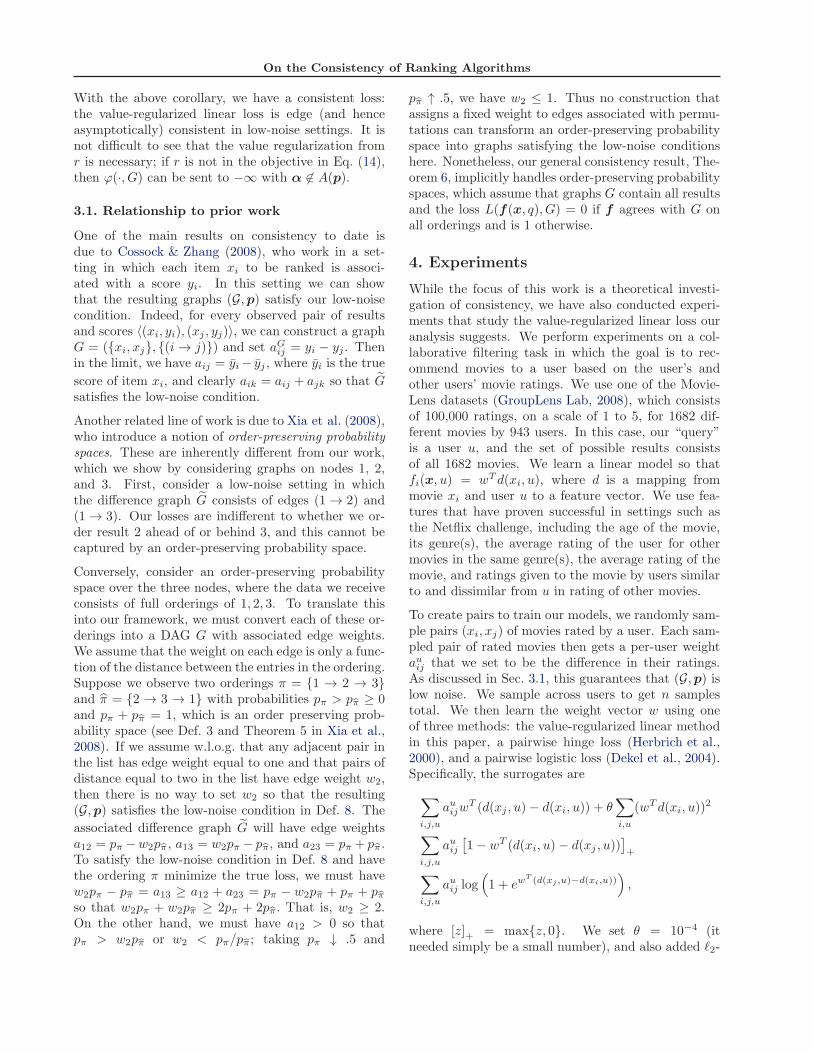
We now define precisely what we mean by a low-noisesetting. For any (G,p), let G be the difference graph,that is, the graph with edge weights max{aij − aji, 0}on edges (i → j), where aij =

∑G∈G aGijpG, and if

aij ≤ aji then the edge (i → j) 6∈ G (see Fig. 1).We define the following low-noise condition based onself-reinforcement of edges in the difference graph.

Definition 8. We say (G,p) is low-noise when the

corresponding difference graph G satisfies the followingreverse triangle inequality: whenever there is an edge(i → j) and an edge (j → k) in G, then the weightaik − aki on (i → k) is greater than or equal to thepath weight aij − aji + ajk − akj on (i → j → k).

It is not difficult to see that if (G,p) satisfies Def. 8,

its difference graph G is a DAG. Indeed, the definitionensures that all global preference information in G (thesum of weights along any path) conforms with andreinforces local preference information (the weight ona single edge). Reasonable ranking methods should beconsistent in this setting, but this is not trivial.

In the lemmas to follow, we consider simple 3-nodeDAGs that admit unique minimizers for their condi-tional risks. In particular, we consider DAGs on nodes1, 2, and 3 that induce only the four penalty valuesa12, a13, a23, and a31 (see Fig. 1). In this case, ifa13 > a31, any α minimizing ℓ(p,α) clearly will haveα1 > α2 > α3. We now show under some very generalconditions that if ϕ is edge-consistent, φ is non-convex.

Let φ′(x) denote an element of the subgradient set∂φ(x). The subgradient conditions for optimality of

W (p,α) = h12φ(α1 − α2) + h13φ(α1 − α3) (10)

+ h23φ(α2 − α3) + h31φ(α3 − α1)

1

32

2a12

2a13

2a23

1

32

2a31

1

32

a12

a13 - a31

a23

Figure 1. The two DAGsabove occur with proba-bility 1

2, giving the differ-

ence graph G on the left,assuming that a13 > a31.

are that

0 = h12φ′(α1 − α2) + h13φ

′(α1 − α3)− h31φ′(α3 − α1)

0 = −h12φ′(α1 − α2) + h23φ

′(α2 − α3). (11)

We begin by showing that under Assumption A on φ,there is a finite minimizer of W (p,α). The lemma istechnical and its proof is in Appendix A.

Lemma 9. There is a constant C < ∞ and a vectorα∗ minimizing W (p,α) with ‖α∗‖∞ ≤ C.

We use the following lemma to prove our main theoremabout inconsistency of pairwise convex losses.

Lemma 10 (Inconsistency of convex losses). Supposethat a13 > a31 > 0, a12 > 0, a23 > 0. Let ℓ(p,α) be

a121(α1≤α2) + a131(α1≤α3) + a231(α2≤α3) + a311(α3<α1)

and W (p,α) be defined as in Eq. (10). For convex φwith φ′(0) < 0, W ∗(p) = infα {W (p,α) : α /∈ A(p)}whenever either of the following conditions is satisfied:

Cond 1: h23 <h31h12

h13 + h12Cond 2: h12 <

h31h23

h13 + h23.

Proof Lemma 9 shows that the optimal W ∗(p) isattained by some finite α. Thus, we fix an α∗ satisfy-ing Eq. (11), and let δij = α∗

i − α∗j and gij = φ′(δij)

for i 6= j. We make strong use of the monotonicity ofsubgradients, that is, δij > δkl implies gij ≥ gkl (e.g.Rockafellar, 1970, Theorem 24.1). By Eq. (11),

g13 − g12 =h31

h13g31 −

(1 +

h12

h13

)g12 (12a)

g13 − g23 =h31

h13g31 −

(1 +

h23

h13

)g23. (12b)


Suppose for the sake of contradiction that α∗ ∈ A(p).As δ13 = δ12 + δ23, we have that δ13 > δ12 and δ13 >δ23. The convexity of φ implies that if δ13 > δ12, theng13 ≥ g12. If g12 ≥ 0, we thus have that g13 ≥ 0 and byEq. (11), g31 ≥ 0. This is a contradiction since δ31 < 0gives g31 ≤ φ′(0) < 0. Hence, g12 < 0. By identicalreasoning, we also have that g23 < 0.

Now, δ23 > 0 > δ31 implies that g23 ≥ g31, whichcombined with Eq. (12a) and the fact that g23 =(h12/h23)g12 (by Eq. (11)) gives

g13 − g12 ≤h31

h13g23 −

(1 +

h12

h13

)g12

=

(h31h12

h23− h13 − h12

)g12h13

.

Since g12/h13 < 0, we have that g13−g12 < 0 wheneverh31h12/h23 > h13 + h12. But when δ13 > δ12, we musthave g13 ≥ g12, which yields a contradiction underCondition 1.

Similarly, δ12 > 0 > δ31 implies that g12 ≥ g31, whichwith g12 = (h23/h12)g23 and Eq. (12b) gives

g13 − g23 ≤h31

h13g12 −

(1 +

h23

h13

)g23

=

(h31h23

h12− h13 − h23

)g23h13

.

Since g23/h13 < 0, we further have that g13 − g23 < 0whenever h31h23/h12 > h13 + h23. This contradictsδ13 > δ23 under Condition 2.

Lemma 10 allows us to construct scenarios underwhich arbitrary pairwise surrogate losses with convexφ are inconsistent. Assumption A only to specify anoptimal α with ‖α‖∞ < ∞, and can be weakened toW (p,α) → ∞ as (αi−αj) → ∞. The next theorem isour main negative result on the consistency of pairwisesurrogate losses.

Theorem 11. Let ϕ be a loss that can be written as

ϕ(α, G) =∑

(i→j)∈G

h(aGij)φ(αi − αj)

for h continuous and increasing with h(0) = 0. Evenin the low-noise setting, for φ convex and satisfyingAssumption A, ϕ is not edge-consistent.

Proof Assume for the sake of contradiction thatϕ is edge-consistent. Recall that for φ convex,φ′(0) < 0, and we can construct graphs G1 andG2 so that the resulting expected loss satisfiesCondition 1 of Lemma 10. Let G = {G1, G2}

where G1 = ({1, 2, 3}, {(1 → 2) , (1 → 3)}) andG2 = ({1, 2, 3}, {(2 → 3) , (3 → 1)}). Fix any weightsaG1

12 , aG1

13 , aG2

31 with aG1

13 > aG1

12 > 0 and aG1

13 > aG2

31 > 0,and let p = (.5, .5). As h is continuous withh(0) = 0, there exists some ε > 0 such that h(ε) <2h31h12/(h13 + h12), where hij =

∑G∈G h(aGij)pG.

Take aG2

23 = min{ε, (aG1

13 − aG1

12 )/2}. Then we haveh23 = h(aG2

23 )/2 ≤ h(ε)/2 < h31h12/(h13 + h12).Hence Condition 1 of Lemma 10 is satis-fied, so ϕ is not edge-consistent. Moreover,aG2

23 ≤ (aG1

13 − aG1

12 )/2 < aG1

13 − aG1

12 implies that

G is a DAG satisfying the low-noise condition.

2.3. Margin-based inconsistency

Given the difficulties encountered in the previous sec-tion, it is reasonable to consider a reformulation ofour surrogate loss. A natural alternative is a margin-based loss, which encodes a desire to separate rankingscores by a large margins dependent on the prefer-ences in a graph. Similar losses have been proposed,e.g., by Shashua & Levin (2002). In particular, wenow consider losses of the form

ϕ(α, G) =∑

(i→j)∈G

φ(αi − αj − h(aGij)

), (13)

where h is continuous and h(0) = 0. It is clear fromthe reduction to binary classification that h must beincreasing for the loss in Eq. (13) to be edge-consistent.When φ is a decreasing function, this intuitively saysthat the larger aij is, the larger αi should be whencompared to αj . Nonetheless, as we show below, sucha loss is inconsistent even in low-noise settings.

Theorem 12. Let ϕ be a loss that can be written as

ϕ(α, G) =∑

(i→j)∈G

φ(αi − αj − h(aGij))

for h continuous and increasing with h(0) = 0. Evenin the low-noise setting, for φ convex and satisfyingAssumption A, ϕ is not edge-consistent.

Proof Assume for the sake of contradiction that ϕ isedge-consistent. As noted before, φ′(0) < 0, and sinceφ is differentiable almost everywhere (Rockafellar,1970, Theorem 25.3), φ is differentiable at −cfor some c > 0 in the range of h. Consider-ing the four-graph setting with graphs containingone edge each, G1 = ({1, 2, 3}, {(1 → 2)}), G2 =({1, 2, 3}, {(2 → 3)}), G3 = ({1, 2, 3}, {(1 → 3)}), andG4 = ({1, 2, 3}, {(3 → 1)}), choose constant edgeweights aG1

12 = aG2

13 = aG3

23 = aG4

31 = h−1(c) > 0, and


set p = (.25, .01, .5, .24). In this setting,

W (p,α) = pG1φ(α1 − α2) + pG2

φ(α2 − α3)

+ pG3φ(α1 − α3) + pG4

φ(α3 − α1),

for φ(x) = φ(x − c). Notably, φ is convex, satisfiesAssumption A, and φ′(0) = φ′(−c) < 0. Moreover,a13 − a31 = h−1(c)(pG3

− pG4) ≥ h−1(c)(pG1

+ pG2) =

a12 + a23 > 0, so G is a DAG satisfying the low-noisecondition. However, pG2

<pG4

pG1

pG3+pG1

. Hence, by

Lemma 10, W ∗(p) = infα {W (p,α) : α /∈ A(p)}, acontradiction.

3. Conditions for Consistency

The prospects for consistent surrogate ranking appearbleak given the results of the previous section. Never-theless, we demonstrate in this section that there existsurrogate losses that yield consistency under some re-strictions on problem noise. We consider a new loss—specifically, a linear loss in which we penalize (αj−αi)proportional to the weight aij in the given graph G.To keep the loss well-behaved and disallow wild fluc-tuations, we also regularize the α values. That is, ourloss takes the form

ϕ(α, G) =∑

(i→j)∈G

aGij(αj − αi) + ν∑

i

r(αi). (14)

We assume that r is strictly convex and 1-coercive,that is, that r asymptotically grows faster than anylinear function. These conditions imply that the lossof Eq. (14) is bounded below. Moreover, we have thebasis for consistency:

Theorem 13. Let the loss take the form of a gener-alized disagreement error of Eq. (7) and the surrogateloss take the form of Eq. (14) where ν > 0 and r isstrictly convex and 1-coercive. If the pair (G,p) in-

duces a difference graph G that is a DAG, then

W ∗(p) < infα

{W (p,α) : α /∈ A(p)} ⇔∑

j

aij − aji >∑

j

akj − ajk for i, k s.t. aik > aki.

Proof We first note that G is a DAG if and only if

A(p) = {α : αi > αj for i < j with aij > aji,

αi ≥ αj for i > j with aij > aji}.

(For a proof see Lemma 16, though essentially all wedo is write out ℓ(p,α).) We have that

W (p,α) =∑

i

(αi

∑

j

(aji − aij) + νr(αi)).

Standard subgradient calculus gives that at optimum,

r′(αi) =

∑j aij − aji

ν.

Since r is strictly convex, r′ is a strictly increasing set-valued map with increasing inverse s(g) = {α : g ∈∂r(α)}. Optimality is therefore attained uniquely at

α∗i = s

(∑j aij − aji

ν

). (15)

Note that for any i, k, α∗i > α∗

k if and only if

s(∑

j aij−aji

ν

)> s

(∑j akj−ajk

ν

), which in turn occurs

if and only if∑

j aij−aji

ν>

∑j akj−ajk

ν. Hence, the op-

timal α∗ of Eq. (15) is in A(p) if and only if∑

j aij − aji

ν>

∑j akj − ajk

νwhen aik > aki. (16)

Thus, W ∗(p) = infα {W (p,α) : α /∈ A(p)} wheneverEq. (16) is violated. On the other hand, supposeEq. (16) is satisfied. Then for all α satisfying

‖α−α∗‖∞ < min{i,k:aik>aki}

1

2(α∗

i − α∗k),

we have α ∈ A(p), and infα {W (p,α) : α /∈ A(p)} >W ∗(p) since α∗ is the unique global minimum.We now prove a simple lemma showing that low-noisesettings satisfy the conditions of Theorem 13.

Lemma 14. If (G,p) is low noise, then for the asso-

ciated difference graph G, whenever aik > aki,∑

j

aij − aji >∑

j

akj − ajk.

Proof Fix (i, k) with aik > aki. There are two casesfor a third node j: either aij −aji > 0 or aij −aji ≤ 0.

In the first case, there is an edge (i → j) ∈ G. If

(k → j) ∈ G, the low-noise condition implies aij −aji ≥ akj − ajk + aik − aki > akj − ajk. Otherwise,akj−ajk ≤ 0 < aij−aji. In the other case, aij−aji ≤

0. If the inequality is strict, then (j → i) ∈ G, so thelow-noise condition implies that aji−aij < aji−aij +aik−aki ≤ ajk−akj , or akj−ajk < aij−aji. Otherwise,aij = aji, and the low-noise condition guarantees that

(j → k) /∈ G, so akj − ajk ≤ 0 = aij − aji.

The inequality in the statement of the lemma is strict,because aik − aki > 0 = akk − akk.The converse of the lemma is, in general, false. Com-bining the above lemma with Theorem 13, we have

Corollary 15. The linear loss of Eq. (14) is edge-consistent if (G,p) is low noise for all query-resultpairs.


With the above corollary, we have a consistent loss:the value-regularized linear loss is edge (and henceasymptotically) consistent in low-noise settings. It isnot difficult to see that the value regularization fromr is necessary; if r is not in the objective in Eq. (14),then ϕ(·, G) can be sent to −∞ with α 6∈ A(p).

3.1. Relationship to prior work

One of the main results on consistency to date isdue to Cossock & Zhang (2008), who work in a set-ting in which each item xi to be ranked is associ-ated with a score yi. In this setting we can showthat the resulting graphs (G,p) satisfy our low-noisecondition. Indeed, for every observed pair of resultsand scores 〈(xi, yi), (xj , yj)〉, we can construct a graphG = ({xi, xj}, {(i → j)}) and set aGij = yi − yj . Thenin the limit, we have aij = yi− yj , where yi is the true

score of item xi, and clearly aik = aij + ajk so that Gsatisfies the low-noise condition.

Another related line of work is due to Xia et al. (2008),who introduce a notion of order-preserving probabilityspaces. These are inherently different from our work,which we show by considering graphs on nodes 1, 2,and 3. First, consider a low-noise setting in whichthe difference graph G consists of edges (1 → 2) and(1 → 3). Our losses are indifferent to whether we or-der result 2 ahead of or behind 3, and this cannot becaptured by an order-preserving probability space.

Conversely, consider an order-preserving probabilityspace over the three nodes, where the data we receiveconsists of full orderings of 1, 2, 3. To translate thisinto our framework, we must convert each of these or-derings into a DAG G with associated edge weights.We assume that the weight on each edge is only a func-tion of the distance between the entries in the ordering.Suppose we observe two orderings π = {1 → 2 → 3}and π = {2 → 3 → 1} with probabilities pπ > pπ ≥ 0and pπ + pπ = 1, which is an order preserving prob-ability space (see Def. 3 and Theorem 5 in Xia et al.,2008). If we assume w.l.o.g. that any adjacent pair inthe list has edge weight equal to one and that pairs ofdistance equal to two in the list have edge weight w2,then there is no way to set w2 so that the resulting(G,p) satisfies the low-noise condition in Def. 8. The

associated difference graph G will have edge weightsa12 = pπ −w2pπ, a13 = w2pπ − pπ, and a23 = pπ + pπ.To satisfy the low-noise condition in Def. 8 and havethe ordering π minimize the true loss, we must havew2pπ − pπ = a13 ≥ a12 + a23 = pπ − w2pπ + pπ + pπso that w2pπ + w2pπ ≥ 2pπ + 2pπ. That is, w2 ≥ 2.On the other hand, we must have a12 > 0 so thatpπ > w2pπ or w2 < pπ/pπ; taking pπ ↓ .5 and

pπ ↑ .5, we have w2 ≤ 1. Thus no construction thatassigns a fixed weight to edges associated with permu-tations can transform an order-preserving probabilityspace into graphs satisfying the low-noise conditionshere. Nonetheless, our general consistency result, The-orem 6, implicitly handles order-preserving probabilityspaces, which assume that graphs G contain all resultsand the loss L(f(x, q), G) = 0 if f agrees with G onall orderings and is 1 otherwise.

4. Experiments

While the focus of this work is a theoretical investi-gation of consistency, we have also conducted experi-ments that study the value-regularized linear loss ouranalysis suggests. We perform experiments on a col-laborative filtering task in which the goal is to rec-ommend movies to a user based on the user’s andother users’ movie ratings. We use one of the Movie-Lens datasets (GroupLens Lab, 2008), which consistsof 100,000 ratings, on a scale of 1 to 5, for 1682 dif-ferent movies by 943 users. In this case, our “query”is a user u, and the set of possible results consistsof all 1682 movies. We learn a linear model so thatfi(x, u) = wT d(xi, u), where d is a mapping frommovie xi and user u to a feature vector. We use fea-tures that have proven successful in settings such asthe Netflix challenge, including the age of the movie,its genre(s), the average rating of the user for othermovies in the same genre(s), the average rating of themovie, and ratings given to the movie by users similarto and dissimilar from u in rating of other movies.

To create pairs to train our models, we randomly sam-ple pairs (xi, xj) of movies rated by a user. Each sam-pled pair of rated movies then gets a per-user weightauij that we set to be the difference in their ratings.As discussed in Sec. 3.1, this guarantees that (G,p) islow noise. We sample across users to get n samplestotal. We then learn the weight vector w using oneof three methods: the value-regularized linear methodin this paper, a pairwise hinge loss (Herbrich et al.,2000), and a pairwise logistic loss (Dekel et al., 2004).Specifically, the surrogates are

∑

i,j,u

auijwT (d(xj , u)− d(xi, u)) + θ

∑

i,u

(wT d(xi, u))2

∑

i,j,u

auij[1− wT (d(xi, u)− d(xj , u))

]+

∑

i,j,u

auij log(1 + ew

T (d(xj ,u)−d(xi,u))),

where [z]+ = max{z, 0}. We set θ = 10−4 (itneeded simply be a small number), and also added ℓ2-


Train pairs Hinge Logistic Linear20000 .478 (.008) .479 (.010) .465 (.006)40000 .477 (.008) .478 (.010) .464 (.006)80000 .480 (.007) .478 (.009) .462 (.005)120000 .477 (.008) .477 (.009) .463 (.006)160000 .474 (.007) .474 (.007) .461 (.004)

Table 1. Test losses for different surrogate losses.

regularization in the form of λ‖w‖2 to each problem.We cross-validated λ separately for each loss.

We partitioned the data into five subsets, and, in eachof 15 experiments, we used one subset for validation,one for testing, and three for training. In every exper-iment, we subsampled 40,000 rated movie pairs fromthe test set for final evaluation. Once we had learneda vector w for each of the three methods, we com-puted its average generalized pairwise loss (Eq. (7)).We show the results in Table 1. The leftmost col-umn contains the number of pairs that were subsam-pled for training, and the remaining columns show theaverage pairwise loss on the test set for each of themethods (with standard error in parentheses). Eachnumber is the mean of 15 independent training runs,and bold denotes the lowest loss. It is interesting tonote that the linear loss always achieves the lowest testloss averaged across all tests. In fact, it achieved thelowest test loss of all three methods in all but one ofour experimental runs. (We use these three losses tofocus exclusively on learning in a pairwise setting—Cossock & Zhang (2008) learn using relevance scores,while Xia et al. (2008) require full ordered lists of re-sults as training data rather than pairs.) Finally, wenote that there is a closed form for the minimizer of thelinear loss, which makes it computationally attractive.

5. Discussion

In this paper we have presented results on both the dif-ficulty and the feasibility of surrogate loss consistencyfor ranking. We have presented the negative resultthat many natural candidates for surrogate rankingare not consistent in general or even under low-noiserestrictions, and we have presented a class of surrogatelosses that achieve consistency under reasonable noiserestrictions. We have also demonstrated the potentialusefulness of the new loss functions in practice. Thiswork thus takes a step toward bringing the consistencyliterature for ranking in line with that for classifica-tion. A natural next step in this agenda is to establishrates for ranking algorithms; we believe that our anal-ysis can be extended to the analysis of rates. Finally,given the difficulty of achieving consistency using sur-rogate losses that decompose along edges, it may be

beneficial to explore non-decomposable losses.

Acknowledgments

JD and LM were supported by NDSEG fellowships.We thank the reviewers for their helpful feedback.

References

Bartlett, P., Jordan, M., and McAuliffe, J. Convexity, clas-sification, and risk bounds. Journal of the AmericanStatistical Association, 101:138–156, 2006.

Ben-Tal, A. and Nemirovski, A. Lectures on Modern Con-vex Optimization. SIAM, 2001.

Cossock, D. and Zhang, T. Statistical analysis of Bayes op-timal subset ranking. IEEE Transaction on InformationTheory, 16:1274–1286, 2008.

Dekel, O., Manning, C., and Singer, Y. Log-linear modelsfor label ranking. In Advances in Neural InformationProcessing Systems 16, 2004.

Freund, Y., Iyer, R., Schapire, R. E., and Singer, Y. Ef-ficient boosting algorithms for combining preferences.Journal of Machine Learning Research, 4:933–969, 2003.

GroupLens Lab. MovieLens dataset, 2008. URLhttp://www.grouplens.org/taxonomy/term/14.

Herbrich, R., Graepel, T., and Obermayer, K. Large mar-gin rank boundaries for ordinal regression. In Advancesin Large Margin Classifiers. MIT Press, 2000.

Jarvelin, K. and Kekalainen, J. Cumulated gain-basedevaluation of IR techniques. ACM Transactions on In-formation Systems, 20(4):422–446, 2002.

Karp, R. M. Reducibility among combinatorial problems.In Complexity of Computer Computations, pp. 85–103.Plenum Press, 1972.

Rockafellar, R.T. Convex Analysis. Princeton UniversityPress, 1970.

Rudin, C. The p-norm push: a simple convex ranking al-gorithm that concentrates at the top of the list. Journalof Machine Learning Research, 10:2233–2271, 2009.

Shashua, A. and Levin, A. Ranking with large marginprinciple: Two approaches. In Advances in Neural In-formation Processing Systems 15, 2002.

Tewari, A. and Bartlett, P. On the consistency of multi-class classification methods. Journal of Machine Learn-ing Research, 8:1007–10025, 2007.

Xia, F., Liu, T. Y., Wang, J., Zhang, W., and Li, H. List-wise approach to learning to rank – theory and algo-rithm. In Proceedings of the 25th International Confer-ence on Machine Learning, 2008.

Zhang, T. Statistical analysis of some multi-categorylarge margin classification methods. Journal of MachineLearning Research, 5:1225–1251, 2004.

http://www.grouplens.org/taxonomy/term/14


A. Auxiliary Proofs

Proof of Lemma 1 The proof of this lemma isanalogous to Zhang’s Theorem 24. Jensen’s inequalityimplies

ζ(E(ℓ(p,f)− inf

αℓ(p,α))

)

≤ Eζ(ℓ(p,f)− infα

ℓ(p,α))

≤ EX,QH(ℓ(p,f)− infα

ℓ(p,α))

≤ EX,Q

(∑

G

pGϕ(f(X, Q), G)− infα′

∑

G

pGϕ(α′, G)

)

= Rϕ(f)−R∗ϕ.

The second to last line is a consequence ofthe fact that H(ℓ(p,α) − infα′ ℓ(p,α′)) ≤∑

G pGϕ(α, G) − infα′

∑G pGϕ(α

′, G) for p ∈ ∆and any α.

Proof of Lemma 3 The proof of thislemma is entirely similar to the proofs of lemma16 from (Tewari & Bartlett, 2007) and lemma 27from (Zhang, 2004), but we include it for complete-ness.

Let p(n) be a sequence converging to p and Br

be a closed ball of radius r in R|G|. Since∑

G p(n)G ϕ(α, G) →

∑G ϕ(α, G) uniformly in α ∈ Br

(we have equicontinuity),

infα∈Br

∑

G∈G

p(n)G ϕ(α, G) → inf

α∈Br

∑

G∈G

pGϕ(α, G).

We then have W ∗(p(n)) ≤ infα∈Br

∑G p

(n)G ϕ(α, G) →

infα∈Br

∑G∈G pGϕ(α, G), and hence (as the infimum

is bounded below) we can let r → ∞ and have

lim supn

W ∗(p(n)) ≤ infα

∑

G∈G

pGϕ(α, G) = W ∗(p).

To bound the limit infimum, assume without loss ofgenerality that there is some subset G′ ⊂ G so thatpG = 0 for all G 6∈ G′. Define

W (p,α) =∑

G∈G′

pGϕ(α, G) and W ∗(p) = infα

W (p,α).

Note that W ∗(p(n)) is eventually bounded so that each

sequence of surrogate loss terms p(n)G ϕ(·, G) is also

eventually bounded. Thus we have the desired uni-form convergence, and

lim infn

W ∗(p(n)) ≥ lim infn

W ∗(p(n)) = W ∗(p).

This completes the proof thatW ∗(p(n)) → W ∗(p).

Proof of Lemma 4 Suppose that ℓ(p,α(n)) 6→infα ℓ(p,α). Then there is a subsequence α(nj) andε > 0 such that ℓ(p,α(nj)) ≥ ℓ(p,α)+ε. This in turn,since there is a finite set of orderings of the entries inα, implies that α(nj) 6∈ A(p). But by the definition ofedge-consistency,

W (p,α(nj)) > infα

{W (p,α) : α 6∈ A(p)} > W ∗(p).

The W (p,α(nj)) are thus bounded uniformly awayfrom W ∗(p), a contradiction.

Proof of Lemma 5 We prove this by contra-diction and using the continuity result in Lemma 3.Assume that the statement does not hold, so thatthere is a sequence (p(n),α(n)) with ℓ(p(n),α(n)) −infα′ ℓ(p(n),α′) ≥ ε but W (p(n),α(n)) −W ∗(p(n)) →0. Because ∆|G| is compact, we choose a conver-

gent subsequence nj so that p(nj) → p for somep ∈ ∆|G|. By Lemma 3 and our assumption that

W (p(nj),α(nj)) − W ∗(p(nj)) → 0, W (p(nj),α(nj)) →W ∗(p). Similar to the proof of the previous lemma,we assume that there is a set G′ ⊂ G with pG > 0 forG ∈ G′. We have

lim supnj

∑

G∈G

pGϕ(α(nj), G) = lim sup

nj

∑

G∈G′

p(nj)G ϕ(α(nj), G)

≤ limnj

∑

G∈G

p(nj)G ϕ(α(nj), G) = W ∗(p).

The above proves that W (p,α(nj)) → W ∗(p), andLemma 4 implies that ℓ(p,α(nj)) → infα ℓ(p,α) andα(nj) ∈ A(p) eventually. The continuity of ℓ in p

and the fact that p(nj) → p, however, contradictsℓ(p(n),α(n))− infα ℓ(p(n),α) ≥ ε.

Proof of Lemma 7 As stated earlier, this is astraightforward consequence of the fact that the feed-back arc set problem (Karp, 1972) is NP -complete. Inthe feedback arc set problem, we are given a directedgraph G = (V,E) and integer k and need to determinewhether there is a subset E′ ⊆ E with |E′| ≤ k suchthat E′ contains at least one edge from every directedcycle in G, or, equivalently, that G′ = (V,E \ E′) is aDAG.

Now consider the problem of deciding whether thereexists a α with ℓ(p,α) ≤ k, and let G be the graphover all the nodes in the graphs in G with average edgeweights aij =

∑G∈G aGijpG. Since α induces an order

of the nodes in this expected graphG, this is equivalent


to finding an ordering of the nodes i1, . . . , in (denotedi1 ≺ i2 ≺ · · · ≺ in) in G such that the sum of the backedges is less than k, i.e.,

∑

i�j

aij ≤ k.

Further, it is clear that removing all the back edges(edges (i → j) in the expected graph G such thati � j in the order) leaves a DAG. Now given a graphG = (V,E), we can construct the expected graph Gdirectly from G with weights aij = 1 if (i → j) ∈ Eand 0 otherwise (to be pedantic, set pij = 1/|E| andlet the ijth graph in the set of possible graphs G besimply the edge (i → j) with weight aij = |E|). Thenit is clear that there is a α such that ℓ(p,α) ≤ k if andonly if there is a feedback arc set E′ with |E′| ≤ k.

Proof of Lemma 9 Let (α(n))∞n=1 be a sequencewith α(n) ∈ A(p) = {α : α1 > α2 > α3} suchthat W (p,α(n)) → W ∗(p). Now suppose that

lim supn(α(n)i − α

(n)j ) = ∞ for some i < j. Since

α(n) ∈ A(p), this implies lim supn(α(n)1 − α

(n)3 ) = ∞.

But φ is convex with φ′(0) < 0 and so is unbounded

above, so certainly lim supn φ(α(n)3 − α

(n)1 ) = ∞.

The assumption that φ′∞(1) = 0 or φ′

∞(−1) = −∞then implies that lim supn W (p,α(n)) = ∞. Thiscontradiction gives that there must be some C

with |α(n)i − α

(n)j | ≤ C for all i, j, n. W (p,α)

is shift invariant with respect to α, so without

loss of generality we can let α(n)3 = 0, and thus

|α(n)i | ≤ C. Convex functions are continuous on

compact domains (Rockafellar, 1970, Chapter 10),and infα:‖α‖

∞≤C W (p,α) = W ∗(p), which proves the

lemma.

Lemma 16. Let G be the difference graph for the pair(G,p). G is a DAG if and only if

A(p) = {α : αi > αj for i < j with aij > aji,

αi ≥ αj for i > j with aij > aji}.

Proof We first prove that if G is a DAG, then A(p)is the set above. Assume without loss of generalitythat the nodes in G are topologically sorted in theorder 1, 2, . . . ,m, so that aij ≥ aji for i < j. Then we

can write

ℓ(p,α) =∑

i<j

aij1(αi≤αj) +∑

i>j

aij1(αi<αj)

=

m∑

i=1

m∑

j=i+1

aij1(αi≤αj) + aji1(αj<αi)

=

m∑

i=1

m∑

j=i+1

(aij − aji)1(αi≤αj) + aji.

Clearly, if aij > aji for some i < j, then any minimiz-ing α must satisfy αi > αj . If aij − aji = 0 for somej > i, then the relative order of αi and αj does notaffect ℓ(p,α).

Now suppose that G is not a DAG but that A(p) takesthe form described in the statement of the lemma. Inthis case, there are (at least) two nodes i and j with a

path going from i to j and from j to i in G. Let thenodes on the path from i to j be l1, . . . , lk and from jto i be l′1, . . . , l

′k′ . By assumption, we must have that

for any α ∈ A(p),

αi ≥ αl1 ≥ · · · ≥ αlk ≥ αj ≥ αl′1≥ · · · ≥ αl′

k′≥ αi.

One of the inequalities must be strict because we willhave some l or l′ > i, which is clearly a contradic-tion.

On the Consistency of Ranking Algorithms - Stanford University

Documents

Transcript of On the Consistency of Ranking Algorithms - Stanford University