On the complexity of regular-grammars with integer attributes
29
Journal of Computer and System Sciences 77 (2011) 393–421 Contents lists available at ScienceDirect Journal of Computer and System Sciences www.elsevier.com/locate/jcss On the complexity of regular-grammars with integer attributes M. Manna a , F. Scarcello b , N. Leone a,∗ a Department of Mathematics, University of Calabria, 87036 Rende (CS), Italy b Department of Electronics, Computer Science and Systems, University of Calabria, 87036 Rende (CS), Italy article info abstract Article history: Received 21 August 2009 Received in revised form 17 May 2010 Available online 27 May 2010 Keywords: Attribute grammars Computational complexity Models of computation Regular grammars with attributes overcome some limitations of classical regular grammars, sensibly enhancing their expressiveness. However, the addition of attributes increases the complexity of this formalism leading to intractability in the general case. In this paper, we consider regular grammars with attributes ranging over integers, providing an in-depth complexity analysis. We identify relevant fragments of tractable attribute grammars, where complexity and expressiveness are well balanced. In particular, we study the complexity of the classical problem of deciding whether a string belongs to the language generated by any attribute grammar from a given class C (call it parse [C] ). We consider deterministic and ambiguous regular grammars, attributes specified by arithmetic expressions over {| |, +, −, ÷, %, ∗}, and a possible restriction on the attributes composition (that we call strict composition). Deterministic regular grammars with attributes computed by arithmetic expressions over {| |, +, −, ÷, %} are P-complete. If the way to compose expressions is strict, they can be parsed in L, and they remain tractable even if multiplication is allowed. Problem parse [C] becomes NP-complete for general regular grammars over {| |, +, −, ÷, %, ∗} with strict composition and for grammars over {| |, +, −, ÷, %} with unrestricted attribute composition. Finally, we show that even in the most general case the problem is in polynomial space. © 2010 Elsevier Inc. All rights reserved. 1. Introduction 1.1. Motivation The problem of identifying, extracting and storing information from unstructured documents is widely recognized as a main issue in the field of information and knowledge management and has been extensively studied in the literature (see, for instance, [13,16,33,31,17]). Most existing approaches use regular expressions as a convenient mean for extracting information from text automatically. Regular grammars, indeed, offer a simple and declarative way to specify patterns to be extracted, and are suitable for efficient evaluation (recognizing whether a string belongs to a regular language is feasible in linear- time). However, regular grammars have a limited expressiveness, which is not sufficient for powerful information extraction tasks. There are simple extraction patterns, like, for instance, a n b n , that are relevant to information extraction but cannot be expressed by a regular grammar. To express such patterns, regular grammars can be enhanced by attributes, storing information at each application of a production rule (a single attribute acting as a counter is sufficient to express a n b n through a regular grammar). In fact, our interest in attribute grammars is strongly motivated by their high potential for information extraction. We have employed them in Hı LεX, an advanced system for ontology-based information extraction [49,48] used in real-world * Corresponding author. E-mail addresses: [email protected] (M. Manna), [email protected] (F. Scarcello), [email protected] (N. Leone). 0022-0000/$ – see front matter © 2010 Elsevier Inc. All rights reserved. doi:10.1016/j.jcss.2010.05.006
-
Upload
independent -
Category
Documents
-
view
0 -
download
0
Transcript of On the complexity of regular-grammars with integer attributes
Journal of Computer and System Sciences 77 (2011) 393–421
Contents lists available at ScienceDirect
Journal of Computer and System Sciences
www.elsevier.com/locate/jcss
On the complexity of regular-grammars with integer attributes
M. Manna a, F. Scarcello b, N. Leone a,∗a Department of Mathematics, University of Calabria, 87036 Rende (CS), Italyb Department of Electronics, Computer Science and Systems, University of Calabria, 87036 Rende (CS), Italy
a r t i c l e i n f o a b s t r a c t
Article history:Received 21 August 2009Received in revised form 17 May 2010Available online 27 May 2010
Keywords:Attribute grammarsComputational complexityModels of computation
Regular grammars with attributes overcome some limitations of classical regular grammars,sensibly enhancing their expressiveness. However, the addition of attributes increases thecomplexity of this formalism leading to intractability in the general case. In this paper,we consider regular grammars with attributes ranging over integers, providing an in-depthcomplexity analysis. We identify relevant fragments of tractable attribute grammars, wherecomplexity and expressiveness are well balanced. In particular, we study the complexity ofthe classical problem of deciding whether a string belongs to the language generated byany attribute grammar from a given class C (call it parse[C]). We consider deterministicand ambiguous regular grammars, attributes specified by arithmetic expressions over{| |,+,−,÷,%,∗}, and a possible restriction on the attributes composition (that we callstrict composition). Deterministic regular grammars with attributes computed by arithmeticexpressions over {| |,+,−,÷,%} are P-complete. If the way to compose expressionsis strict, they can be parsed in L, and they remain tractable even if multiplicationis allowed. Problem parse[C] becomes NP-complete for general regular grammars over{| |,+,−,÷,%,∗} with strict composition and for grammars over {| |,+,−,÷,%} withunrestricted attribute composition. Finally, we show that even in the most general casethe problem is in polynomial space.
© 2010 Elsevier Inc. All rights reserved.
1. Introduction
1.1. Motivation
The problem of identifying, extracting and storing information from unstructured documents is widely recognized as amain issue in the field of information and knowledge management and has been extensively studied in the literature (see, forinstance, [13,16,33,31,17]). Most existing approaches use regular expressions as a convenient mean for extracting informationfrom text automatically. Regular grammars, indeed, offer a simple and declarative way to specify patterns to be extracted,and are suitable for efficient evaluation (recognizing whether a string belongs to a regular language is feasible in linear-time). However, regular grammars have a limited expressiveness, which is not sufficient for powerful information extractiontasks. There are simple extraction patterns, like, for instance, anbn , that are relevant to information extraction but cannotbe expressed by a regular grammar. To express such patterns, regular grammars can be enhanced by attributes, storinginformation at each application of a production rule (a single attribute acting as a counter is sufficient to express anbn
through a regular grammar).In fact, our interest in attribute grammars is strongly motivated by their high potential for information extraction. We
have employed them in HıLεX, an advanced system for ontology-based information extraction [49,48] used in real-world
* Corresponding author.E-mail addresses: [email protected] (M. Manna), [email protected] (F. Scarcello), [email protected] (N. Leone).
0022-0000/$ – see front matter © 2010 Elsevier Inc. All rights reserved.doi:10.1016/j.jcss.2010.05.006
394 M. Manna et al. / Journal of Computer and System Sciences 77 (2011) 393–421
applications. Unfortunately, the complexity of grammars with attributes is sensibly harder than in the attribute-free case;for instance, the addition of string attributes to regular grammars leads to Exptime-hardness even in the simple case ofdeterministic grammars using only two attributes, if (string) concatenation of attributes is allowed [12]. Thus, a carefulcomplexity analysis, leading to the identification of tractable cases of attribute grammars where complexity and expressive-ness are well balanced, is called for, and will be carried out in this paper.
It is worthwhile noting that, even if our interest in attribute grammars came from their usage in Information Extraction,attribute grammars are employed in many other domains, ranging from databases to logic programming (see Section 1.5below). Thus, a precise characterization of their complexity can be profitably used in a wide range of applications.
1.2. The framework: Integer attribute grammars
The attribute grammar formalism is a declarative language introduced by Knuth as a mechanism for specifying thesemantics of context-free languages [27]. An attribute grammar AG is an extension of a context-free grammar G with anumber of attributes which are updated at any application of a production rule (by some suitable functions). Moreover,the applicability of a production rule is conditioned by the truth of some predicates over attribute values. The languagegenerated by an attribute grammar AG consists of all strings that have a legal parse tree in G where all attribute values arerelated in the prescribed way (that is, they satisfy the predicates). Thus, a parse tree of the original context-free grammarmay not be a legal parse tree of the attribute grammar, and the language accepted by an attribute grammar is in general asubset of the corresponding context-free language.
In this paper, we consider regular grammars with attributes ranging over integers, also called integer attribute grammarsor IRGs, for short. An IRG is a quadruple AG = 〈G,Attr, Func,Pred〉 where
• G is a regular grammar;• Attr is a set of integer attributes associated with the nonterminals of G ;• Func is a set of functions associated with the production rules of G , assigning values to attributes by means of arithmetic
expressions over {| |,+,−,÷,%,∗}1;• Pred is a set of predicates, associated with the production rules of G , checking values of attributes. A predicate is a
Boolean combination of comparison predicates of the form E1 � E2, where � is a standard comparison operator in{<,�,=,>,�, �=}, and E1 and E2 are arithmetic expressions over {| |,+,−,÷,%,∗}.
A valid parse tree for AG is a parse tree of G labeled by attributes (computed according to the functions of the correspondingproductions of G ) such that all predicates evaluate to true. The language generated by AG , denoted by L(AG), is the set ofall strings derived by some valid parse tree for AG .
There are many real world tasks easily described by means of regular grammars with (integer) attributes. Let us brieflyintroduce syntax and semantics of IRGs through two simple examples.
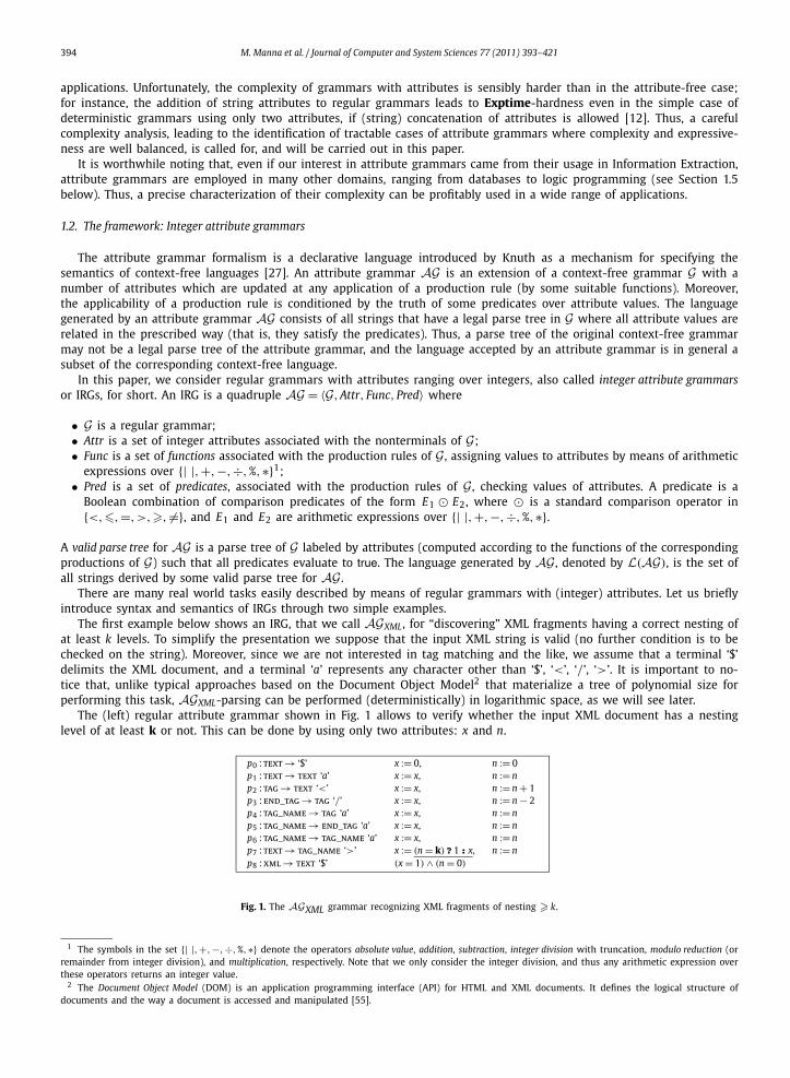
The first example below shows an IRG, that we call AG XML , for “discovering” XML fragments having a correct nesting ofat least k levels. To simplify the presentation we suppose that the input XML string is valid (no further condition is to bechecked on the string). Moreover, since we are not interested in tag matching and the like, we assume that a terminal ‘$’delimits the XML document, and a terminal ‘a’ represents any character other than ‘$’, ‘<’, ‘/’, ‘>’. It is important to no-tice that, unlike typical approaches based on the Document Object Model2 that materialize a tree of polynomial size forperforming this task, AG XML-parsing can be performed (deterministically) in logarithmic space, as we will see later.
The (left) regular attribute grammar shown in Fig. 1 allows to verify whether the input XML document has a nestinglevel of at least k or not. This can be done by using only two attributes: x and n.
p0 : text → ‘$’ x := 0, n := 0p1 : text → text ‘a’ x := x, n := np2 : tag → text ‘<’ x := x, n := n + 1p3 : end_tag → tag ‘/’ x := x, n := n − 2p4 : tag_name → tag ‘a’ x := x, n := np5 : tag_name → end_tag ‘a’ x := x, n := np6 : tag_name → tag_name ‘a’ x := x, n := np7 : text → tag_name ‘>’ x := (n = k)?1: x, n := np8 : xml → text ‘$’ (x = 1) ∧ (n = 0)
Fig. 1. The A GXML grammar recognizing XML fragments of nesting � k.
1 The symbols in the set {| |,+,−,÷,%,∗} denote the operators absolute value, addition, subtraction, integer division with truncation, modulo reduction (orremainder from integer division), and multiplication, respectively. Note that we only consider the integer division, and thus any arithmetic expression overthese operators returns an integer value.
2 The Document Object Model (DOM) is an application programming interface (API) for HTML and XML documents. It defines the logical structure ofdocuments and the way a document is accessed and manipulated [55].
M. Manna et al. / Journal of Computer and System Sciences 77 (2011) 393–421 395
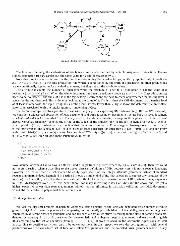
Fig. 2. A DFA for the regular grammar underlying A G XML .
The functions defining the evaluations of attributes x and n are specified by suitable assignment instructions. For in-stance, production rule p3 carries out the same value for x and decreases n by 2.
Note that predicate n = k is used in the function determining the x value for p7; while p8 applies only if predicatex = 1 ∧ n = 0 is true (p8 is the only production rule which is conditioned by the truth of a predicate; all other productionsare unconditionally applied as for standard grammars, but they set up the attribute values).
The attribute n counts the number of open-tags while the attribute x is set to 1 (production p7) if the value of nreaches k (x := (n = k)?1: x). When the whole document has been parsed, only predicate (x = 1)∧ (n = 0) (production p8)needs to be evaluated. If the value of n is 0, the tag-nesting is correct and we have to check only whether the nesting level isabove the desired threshold. This is done by looking at the value of x: if it is 1, then the XML document has a nesting levelof at least k, otherwise, the input string has a nesting level strictly lower than k. Fig. 2 shows the deterministic finite-stateautomaton associated with the regular grammar underlying AG XML .
The second example involves possible extensions of languages for expressing XML schemas (e.g., DTD or XML-Schema).We consider a widespread abstraction of XML documents and DTDs focusing on document structure [45]. An XML documentis a finite ordered, labeled, unranked tree t . For any node x of t , its label label(x) belongs to the alphabet Σ of the elementnames. Moreover, labcdrn(x) denotes the string of the labels of the children of x in the left-to-right order. A DTD over Σ
is a triple d = 〈Σ,π, s〉 where π is a function that maps each symbol in Σ to a regular language over Σ , and s ∈ Σ
is the start symbol. The language L(d) of d is a set of trees such that for each tree t ∈ L(d), root(t) = s, and for everynode x with label(x) = a, labcdrn(x) ∈ π(a). An example of DTD is d1 = 〈{s1,a,b},π1, s1〉 with π1(s1) = {anbm: n,m > 0} andπ1(a) = π1(b) = {ε}. An XML document satisfying d1 might be:
<s1><a> first a </a><a> second a </a><b> unique b </b>
</s1>
Now, assume we would like to have a different kind of legal trees, e.g., trees where π1(s1) = {anbn: n > 0}. Then, we couldnot express such a schema according to the above classical definition of DTD, because π1(s1) is not a regular language.However, it turns out that this schema can be easily expressed if we use integer attribute grammars, instead of standardregular grammars. Indeed, Example 4 in Section 3 shows a simple kind of IRG that allows us to express any language of theform {an
1 . . .anj : n > 0, j > 1}. It is thus quite natural to think of a more expressive notion of DTD, where π maps symbols
in Σ to IRG-languages over Σ . As this paper shows, for many interesting classes of IRGs (like the above one) we get ahigher expressive power than regular grammars without loosing efficiency. In particular, validating such XML documentswould still be feasible in polynomial time, or even less.
1.3. Main problems studied
We face the classical problem of deciding whether a string belongs to the language generated by an integer attributegrammar AG . To characterize precisely its complexity, and to identify possible islands of tractability, we consider languagesgenerated by different classes of grammars and, for any such a class C , we study its corresponding class of parsing problems,denoted by parse[C] . In particular, we consider deterministic and ambiguous regular grammars, and we also distinguishIRGs according to the set of operators (from {| |,+,−,÷,%,∗}) allowed to occur in the arithmetic expressions, as wellas according to possible restrictions on attributes compositions. In this respect, we consider both grammars with generalproductions over the considered set of functions, called free grammars, and the so-called strict grammars where, in any
396 M. Manna et al. / Journal of Computer and System Sciences 77 (2011) 393–421
production p, each p-attribute “contributes” at most once to the computation of new attribute values.3 For example, AG XML
is a strict grammar. Note that the latter syntactic condition reduces the possible growth of attribute values.
1.4. Overview of results
The analysis carried out in this paper provides many results on the complexity of parse[C] . Most of them are positiveresults, in that we are able to identify tractable classes of IRGs with rather natural restrictions, which keep a good expressivepower without loosing in efficiency. We also provide hardness results that are useful to identify the source of complexityfor more general IRGs. In summary, we show that
• parse[C] is tractable for the following classes of integer attribute grammars:(i) Deterministic regular strict grammars with (attributes specified by) arithmetic expressions over {| |,+,−,÷,%};
(ii) General (possibly ambiguous) regular strict grammars with arithmetic expressions over {| |,+,−,÷,%};(iii) Deterministic regular grammars with arithmetic expressions over {| |,+,−,÷,%}, without the strict-restriction;(iv) Deterministic regular strict grammars, without any restriction on the arithmetic operators (∗ may occur in arith-
metic expressions).In particular, parse[C] is– L-complete in case (i);– NL-complete in case (ii);– P-complete in cases (iii) and (iv).
• parse[C] is NP-complete for general regular grammars over operators {| |,+,−,÷,%} (without restrictions on attributecomposition);
• parse[C] is NP-complete for general regular grammars over the set {| |,+,−,÷,%,∗}, under strict composition;• parse[C] is still in PSPACE in the most general case of any regular grammar with any arithmetic expression over
{| |,+,−,÷,%,∗}. For this case, we miss a completeness result, and thus whether or not some IRG may yield a PSPACE-hard language remains an open question.
It is worthwhile noting that all P-completeness and L-completeness results we derived for deterministic regular grammarshold also for both left-regular and right-regular deterministic grammars.
1.5. Related work
As far as related work is concerned, attribute grammars, defined by Knuth for specifying and implementing the (static)semantic aspects of programming languages [27], have been a subject of intensive research, both from a conceptual andfrom a practical point of view. The first full implementation for parsing attribute grammars was produced by Fang [14],under the supervision of Knuth. Lewis et al. [35] defined two subclasses of attribute grammars, named S-attributed grammarsand L-attributed grammars, for one-pass compilation. Kennedy and Warren [26] presented a method of constructing, for agiven attribute grammar, a recursive procedure which performs the specified semantic evaluation. A wide class of attributegrammars (e.g., absolutely noncircular attribute grammars and ordered attribute grammars) can be handled, and the resultingevaluators are efficient. Kastens et al. [25], Farrow [15], and Koskimies et al. [30] developed systems (called GAG, LINGUIST-86, and HLP84, respectively) with high-level input languages, resulting in powerful language processing tools.
The versatility of attribute grammars is confirmed by the large number of application areas where these grammars areemployed, such as logic programming [10,11], databases [47], natural language interfaces [2], and pattern recognition [57]. Morerecently, it has been shown they are useful also for XML, and in particular for query languages and query processing (see, forinstance, [39,41,40,29]). Extensive reviews of attribute grammar theory, implementation, systems, and applications are givenin, e.g., [9,8,28,1,43].
Although complexity issues about regular grammars (without attributes) have been thoroughly studied [23], expressive-ness and complexity of regular grammars with attributes have not been analyzed in depth. A number of results on theexpressiveness of attribute grammars has been derived by Efremidis et al. [12], where the authors define two interestingclasses of string attribute grammars A p and A p
s , which are shown to be the same as the complexity class EXP and “roughlythe same” as the complexity class NP, respectively.
To the best of our knowledge, the present paper is the first work studying the complexity of regular grammars withinteger-domain attributes.
3 More precisely, we define an IRG to be strict if all of its productions are strict, where a production p is strict if the labeled dependency graph built fromthe functions in Func(p) is deterministic. That is, every attribute has at most one outgoing arc, or two mutually exclusive outgoing arcs (i.e., arcs whoselabels are the logical complements of each other). See Section 4.1 for the formal definition.

M. Manna et al. / Journal of Computer and System Sciences 77 (2011) 393–421 397
1.6. Structure of the paper
The sequel of the paper is organized as follows. Section 2 collects some preliminaries about formal grammars and lan-guages. Section 3 defines our notion of integer attribute grammar with bounded resources, and gives its semantics and anexample. Section 4 gives a detailed overview of the complexity results for parsing various classes of attribute grammars.Section 5 shows how to build a Turing machine for computing integer attribute grammars, which is useful for proving com-plexity upper-bounds. The comprehensive computational complexity analysis is carried out in Section 6. Finally, Section 7draws our conclusions. Some basic notions on languages and complexity classes which are used in the paper are recalled inAppendix A.
2. Preliminaries on Chomsky languages
Let W be an alphabet (finite and nonempty set of symbols). A string w (also, word) over W is a finite sequence ofsymbols from W . The number of symbols in w is its length and it is denoted by ‖w‖, while w[ j] denotes the jth symbolof w (0 � j < ‖w‖). Let ε be the empty string (‖ε‖ = 0) and W + denote all strings of finite length over W , then 〈W ∗,◦, ε〉is a free monoid where W ∗ = W + ∪ {ε} and ◦ is the binary relation of concatenation on W ∗ . A set L of strings from W ∗is a language over W , with Λ denoting the empty language. Let L1, L2 be two languages. Then, language L1L2 contains allstrings of the form w1 w2, with w1 ∈ L1 and w2 ∈ L2.
2.1. Context-free grammars and languages
A context-free grammar (CFG) G = 〈Σ, N, S,Π〉 consists of an alphabet of terminals Σ , an alphabet of nonterminals N ,a start symbol S ∈ N , and a finite set of productions Π ⊆ N × (Σ ∪ N)∗ . A production p ∈ Π is said to be an ε-production ifp ∈ (N × {ε}). Usually, a pair 〈A,α〉 ∈ Π is written as A → α. Let ⇒+
G be the binary relation of derivation [23] with respectto G .
The language of grammar G is the set
L(G) = {x ∈ Σ∗: S ⇒+
G x}.
A language L is a context-free language (CFL) if there exists a CFG G such that L = L(G).A context-free grammar G is cycle-free (or non-cyclic) if there is no derivation of the form A ⇒+
G A for some nontermi-nal A.
Given a context-free grammar G = 〈Σ, N, S,Π〉, a parse tree t of G is a tree such that: (i) the root node ρ(t) is labeled bythe start symbol S; (ii) each leaf node has label in Σ ∪ {ε}; (iii) each internal node is labeled by a nonterminal symbol; (iv) ifA ∈ N is a non-leaf node in t with children α1, . . . ,αh , listed from left to right, then A → α1 . . . αh is a production in Π . Byconcatenating the leaves of t from left to right we obtain the derived string x(t) of terminals, which is called the yield ofthe parse tree. The language generated by G can be also defined as:
L(G) = {x(t): t is a parse tree of G
}.
The size of a parse tree [38] is the number of its non-leaf nodes, while the height measures the longest path from the rootto some leaf. A tree consisting of a single node (the root) has height = 0. If G is cycle-free and t is a parse tree of G suchthat ‖x(t)‖ = n, then both size(t) � |N| ∗ (2n − 1) and height(t) � |N| ∗ n hold.
A context-free grammar G is unambiguous if it does not have two different parse trees for any string. A context-freelanguage is unambiguous if it can be generated by an unambiguous context-free grammar. Context-free grammars andlanguages are ambiguous if they are not unambiguous.
Example 1. Let L1 = {anbncn: n > 0} be a language on the alphabet Σ = {a,b, c}. It is well known that L1 is not a context-free language because there exists no context-free grammar for it.
Example 2. Let L2 = {anbn: n > 0} be a language over Σ = {a,b}. For L2 there exists a (unambiguous) context-free gram-mar G such that L(G) = L2. The productions of G are:
p0 : S → aA,
p1 : A → Sb,
p2 : A → b.
398 M. Manna et al. / Journal of Computer and System Sciences 77 (2011) 393–421
2.2. Regular grammars and languages
A regular grammar is a context-free grammar G = 〈Σ, N, S,Π〉 where either Π ⊆ N × (Σ ∪ (N ◦ Σ) ∪ {ε}) or Π ⊆ N ×(Σ ∪ (Σ ◦ N) ∪ {ε}) holds. Grammar G is said to be left-regular or right-regular, respectively. By construction, any regulargrammar G is non-cyclic, so the size of any parse tree t of G is either ‖x(t)‖+ 1 or ‖x(t)‖ (depending on whether ε appearsin t or not).
Regular grammars can also be ambiguous. Consider the grammar Ga having the following productions:
p0 : S → aS,
p1 : S → aA,
p2 : S → b,
p3 : A → aS,
p4 : A → aA,
p5 : A → b.
It is easy to see that L(Ga) = {anb: n � 0}, but every string w of length n can be derived by 2n different parse trees.However, it is well known that every regular language is unambiguous [54]. That is, for every regular language L, thereexists an unambiguous regular grammar G such that L = L(G).
Example 3. Let L3 be the above mentioned language {anb: n � 0} over Σ = {a,b}. The following unambiguous regulargrammar generates L3:
p0 : S → aS,
p1 : S → b.
2.3. Regular grammars and finite automata
2.3.1. NFA automataA non-deterministic finite automaton (NFA) is a quintuple [34] M = 〈K ,Σ,, s0, F 〉 where
– K is a finite set of states;– Σ is an alphabet of terminals disjoint from K ;– s0 ∈ K is the initial state;– F ⊆ K is the set of final states;– , the transition relation, is a subset of K × (Σ ∪ {ε}) × K . Each triple (q, u,q′) ∈ is called a transition of M .
If M is in state q ∈ K and the symbol under the input-cursor is a ∈ Σ , then M may move to state q′ ∈ K only if (q, u,q′) ∈
and u is either a or ε. Sometimes the notation q′ ∈ (q, u) is more convenient. Notice that if u = ε, so the input-cursordoes not change its position when M moves to q′ .
A configuration of M is an element of K × Σ∗ . Let (q, w) be a configuration, then w is the unread part of the input.Consider now the binary relation �→M between two configurations. Relation (q, w) �→M (q′, w ′) holds if and only if thereexists u ∈ Σ ∪ {ε} such that w = uw ′ and q′ ∈ (q, u).
Let �→∗M be the reflexive, transitive closure of �→M . The language generated by M is defined as:
L(M) = {w ∈ Σ∗ : (s0, w) �→∗
M (q, ε), q ∈ F}.
For any regular grammar G = 〈Σ, N, S,Π〉 there exists a non-deterministic finite automaton M(G) = 〈K ,Σ,, s0, F 〉,naturally isomorphic to G , such that L(G) = L(M). If G is left-regular, the automaton M(G) is defined as follows:
– K = N ∪ {s0};– B ∈ (A,a) if and only if B → Aa belongs to Π ;– B ∈ (s0,α) if and only if α ∈ Σ ∪ {ε} and B → α belongs to Π ;– F = {S}.
If G is right-regular, the automaton M(G) is defined as follows:
– K = N ∪ F , with F = {s f };– B ∈ (A,a) if and only if A → aB belongs to Π ;– s f ∈ (A,α) if and only if α ∈ Σ ∪ {ε} and A → α belongs to Π ;– s0 = S .
M. Manna et al. / Journal of Computer and System Sciences 77 (2011) 393–421 399
2.3.2. DFA automataA deterministic finite automaton (DFA) is a finite-machine M = 〈K ,Σ, δ, s0, F 〉 behaving like an NFA where the transition
function δ : K × Σ → K is a restriction of . A configuration of M and the language L(M) are defined exactly as in the NFAcase.
Given a regular grammar G = 〈Σ, N, S,Π〉, if M(G) is deterministic, also G is said to be deterministic. In this case, G isunambiguous as well. For instance, the grammar shown in Example 3 is deterministic.
Deterministic regular grammars are a proper subset of unambiguous regular grammars [42]. For completeness, we nextrecall two classical results about regular languages [34]:
Proposition 2.1. For each non-deterministic finite automaton, there is an equivalent deterministic finite automaton.
Proposition 2.2. A language is said to be regular if and only if it is accepted by a finite automaton.
3. Integer attribute regular grammars
An integer-attribute regular grammar (short: IRG) AG consists of an attribute system associated with the underlyingregular grammar G . Each nonterminal A of G has a set Attr(A) of symbols named (synthesized) attributes of A.4
Given a set Oper ⊆ {| |,+,−,÷,%,∗} of arithmetic operators, an integer-attribute regular grammar over Oper is, formally,a quadruple
AG = 〈G,Attr, Func,Pred〉where
• G = 〈Σ, N, S,Π〉 is a regular grammar, called the underlying grammar of the attribute regular grammar AG .• Attr maps every nonterminal symbol to its (synthesized) attributes, that is, for each nonterminal symbol A ∈ N , the set
Attr(A) contains the attributes of A. Each attribute is defined on the integer domain.• Func is a set of semantic rules for assigning values to attributes through arithmetic expressions on the operators specified
in the set Oper. For each production p ∈ Π , say α0 → α1α2 (where, either exactly one of α1,α2 is a nonterminalsymbol, or at least one of α1,α2 is ε), we denote by Func(p) ⊆ Func the set of rules of p computing attribute values.Any rule in Func(p) maps values of certain attributes (possibly none) of the nonterminal (if any) αi (i ∈ {1,2}) into thevalue of some attribute of α0, say a. Such a rule has the form a := E(a1, . . . ,ak), where E is an arithmetic expression onthe set of attributes a1, . . . ,ak , denoted by ExpAttr(E), and a j is an attribute of αi for any j ∈ {1, . . . ,k}. If p does notcontain any nonterminal symbol, then E is simply a constant value. We allow also rules with arithmetic-if expressionsof the form a := (Cond)? ET : E F , where (i) ET and E F are arithmetic expressions over Oper, and (ii) Cond is a Booleancombination of comparison predicates. A comparison predicate is of the form E1 � E2, with � ∈ {<,�,=,>,�, �=}, andwith E1 and E2 being arithmetic expressions over Oper. The value of an arithmetic-if statement is either E T , if Cond istrue, or E F , otherwise.
• Pred is a set of semantic rules for checking that, in any production, values of attributes satisfy certain desired conditions.For each production p ∈ Π , we denote by Pred(p) ∈ Pred its predicate, that is, a Boolean combination of comparisonpredicates (as specified above) involving attributes occurring in p.
A valid parse tree for AG is a parse tree of G labeled by the grammar attributes such that all labels of its (internal) nodessatisfy the following conditions: all attribute values are computed according to the rules of the corresponding productionsof G , and all the predicates evaluate to true. The language generated by AG , denoted by L(AG), is the set of all stringsderived by some valid parse tree for AG .
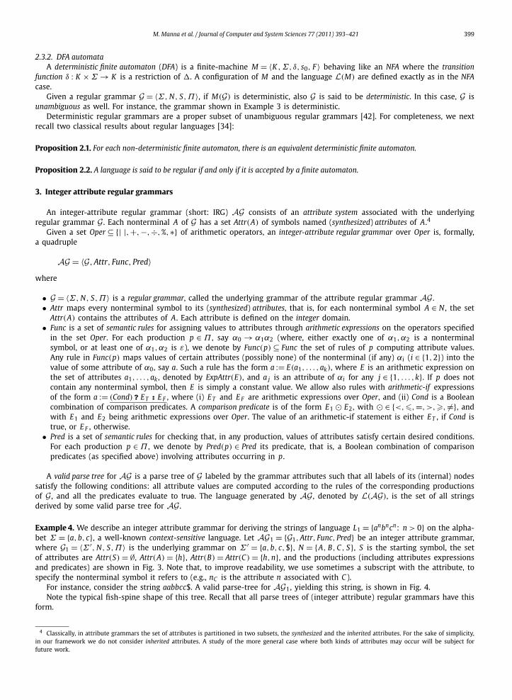
Example 4. We describe an integer attribute grammar for deriving the strings of language L1 = {anbncn: n > 0} on the alpha-bet Σ = {a,b, c}, a well-known context-sensitive language. Let AG 1 = {G1,Attr, Func,Pred} be an integer attribute grammar,where G1 = 〈Σ ′, N, S,Π〉 is the underlying grammar on Σ ′ = {a,b, c,$}, N = {A, B, C, S}, S is the starting symbol, the setof attributes are Attr(S) = ∅, Attr(A) = {h}, Attr(B) = Attr(C) = {h,n}, and the productions (including attributes expressionsand predicates) are shown in Fig. 3. Note that, to improve readability, we use sometimes a subscript with the attribute, tospecify the nonterminal symbol it refers to (e.g., nC is the attribute n associated with C ).
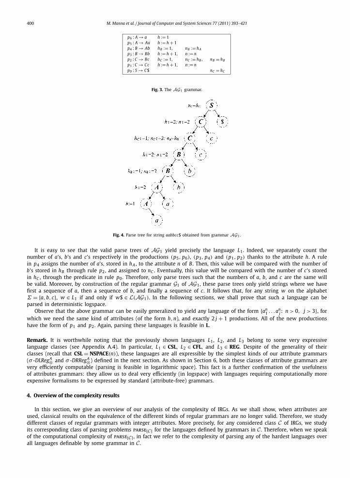
For instance, consider the string aabbcc$. A valid parse-tree for AG 1, yielding this string, is shown in Fig. 4.Note the typical fish-spine shape of this tree. Recall that all parse trees of (integer attribute) regular grammars have this
form.
4 Classically, in attribute grammars the set of attributes is partitioned in two subsets, the synthesized and the inherited attributes. For the sake of simplicity,in our framework we do not consider inherited attributes. A study of the more general case where both kinds of attributes may occur will be subject forfuture work.
400 M. Manna et al. / Journal of Computer and System Sciences 77 (2011) 393–421
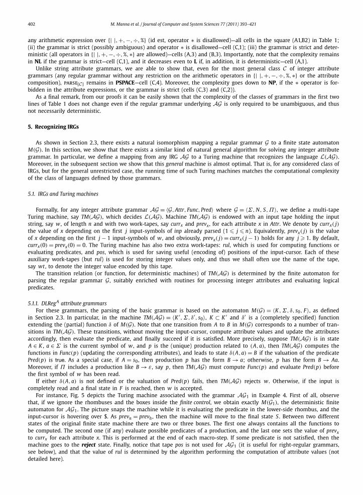
p6 : A → a h := 1p5 : A → Aa h := h + 1p4 : B → Ab hB := 1, nB := hA
p3 : B → Bb h := h + 1, n := np2 : C → Bc hC := 1, nC := hB , nB = hB
p1 : C → Cc h := h + 1, n := np0 : S → C$ nC = hC
Fig. 3. The A G 1 grammar.
Fig. 4. Parse tree for string aabbcc$ obtained from grammar A G 1.
It is easy to see that the valid parse trees of AG 1 yield precisely the language L1. Indeed, we separately count thenumber of a’s, b’s and c’s respectively in the productions (p5, p6), (p3, p4) and (p1, p2) thanks to the attribute h. A rulein p4 assigns the number of a’s, stored in hA , to the attribute n of B . Then, this value will be compared with the number ofb’s stored in hB through rule p2, and assigned to nC . Eventually, this value will be compared with the number of c’s storedin hC , through the predicate in rule p0. Therefore, only parse trees such that the numbers of a, b, and c are the same willbe valid. Moreover, by construction of the regular grammar G1 of AG 1, these parse trees only yield strings where we havefirst a sequence of a, then a sequence of b, and finally a sequence of c. It follows that, for any string w on the alphabetΣ = {a,b, c}, w ∈ L1 if and only if w$ ∈ L(AG 1). In the following sections, we shall prove that such a language can beparsed in deterministic logspace.
Observe that the above grammar can be easily generalized to yield any language of the form {an1 . . .an
j : n > 0, j > 3}, forwhich we need the same kind of attributes (of the form h,n), and exactly 2 j + 1 productions. All of the new productionshave the form of p1 and p2. Again, parsing these languages is feasible in L.
Remark. It is worthwhile noting that the previously shown languages L1, L2, and L3 belong to some very expressivelanguage classes (see Appendix A.4). In particular, L1 ∈ CSL, L2 ∈ CFL, and L3 ∈ REG. Despite of the generality of theirclasses (recall that CSL = NSPACE(n)), these languages are all expressible by the simplest kinds of our attribute grammars(σ -DLRegA⊗ and σ -DRRegA⊗) defined in the next section. As shown in Section 6, both these classes of attribute grammars arevery efficiently computable (parsing is feasible in logarithmic space). This fact is a further confirmation of the usefulnessof attributes grammars: they allow us to deal very efficiently (in logspace) with languages requiring computationally moreexpensive formalisms to be expressed by standard (attribute-free) grammars.
4. Overview of the complexity results
In this section, we give an overview of our analysis of the complexity of IRGs. As we shall show, when attributes areused, classical results on the equivalence of the different kinds of regular grammars are no longer valid. Therefore, we studydifferent classes of regular grammars with integer attributes. More precisely, for any considered class C of IRGs, we studyits corresponding class of parsing problems parse[C] for the languages defined by grammars in C . Therefore, when we speakof the computational complexity of parse[C] , in fact we refer to the complexity of parsing any of the hardest languages overall languages definable by some grammar in C .

M. Manna et al. / Journal of Computer and System Sciences 77 (2011) 393–421 401
4.1. Restricted classes of IRGs
We evaluate the complexity of parse[C] by varying the possible classes C according to three parameters concerning thestructure of the underlying regular grammars, the operators that are allowed in the arithmetic expressions computing theattribute values (i.e., the operators occurring in Pred or in Func), and the way how attributes can be composed. In particular,we consider the following restrictions for any integer attribute grammar AG belonging to the considered class C :
• Grammar. We distinguish among three kinds of grammars underlying AG , depending on whether they are determin-istic left-regular (DLReg), deterministic right-regular (DRReg) or simply regular (Reg). Accordingly, DLRegA , DRRegA , andRegA denote, respectively, the class of attribute grammars where the underlying grammar is deterministic left-regular,deterministic right-regular, or regular.
• Operators. We consider arithmetic expressions either over the full set of operators {| |,+,−,÷,%,∗} or over{| |,+,−,÷,%}. In the latter case, where the multiplication operator is not allowed, the restricted classes of attributegrammars are denoted by DLRegA⊗ , DRRegA⊗ , and RegA⊗ . Of course, when operator ∗ is allowed to occur in the expres-sions, the size of an attribute may grow up much more faster than in the ∗-free case. For instance, Example 5 showsan IRG with arithmetic expressions employing the ∗-operator, where the value of some attributes equals 2(2n−1) .
• Composition. We say that a production p of AG is strict if each attribute in the right-hand side of p gives a single con-tribution to the computation of values in all the arithmetic expressions occurring in Func(p). In particular, observe thatan attribute b appearing both in the then and in the else branches of an arithmetic-if statement, gives one contribution.The same holds if b occurs in such different branches belonging to different arithmetic-if statements, as long as theyhave the same if-condition. If an attribute occurs only in the condition of arithmetic-if statements, then its contributionis zero. All other occurrences in the right-hand side of arithmetic expressions count for one contribution. More formally,consider the labeled (directed) dependency graph G p = 〈Nodesp,Arcsp〉 built, from p, as follows:1. Nodesp = Attr;2. (a′,�,a) ∈ Arcsp if a := E is in Func(p) and a′ ∈ AttrExp(E);3. (a′,Cond,a) ∈ Arcsp if a := (Cond)? ET : E F is in Func(p) and a′ ∈ AttrExp(ET );4. (a′,¬Cond,a) ∈ Arcsp if a := (Cond)? ET : E F is in Func(p) and a′ ∈ AttrExp(E F ).We say that p is strict if G p is deterministic, that is, if each node has at most one outgoing arc, or exactly two mutuallyexclusive outcoming arcs (i.e., arcs whose labels are the logical complements of each other). The grammar AG is strictif all of its productions are strict. The fact that all grammars of a class have this restriction is denoted by the prefix σ -,e.g., σ -RegA denotes all IRGs (possibly non-deterministic) with the strict-composition restriction, but with no restrictionon the arithmetic operators.
For instance, observe that the grammar in Example 4 is a strict deterministic left-regular grammar with ∗-free arithmeticexpressions, and thus it belongs to σ -DLRegA⊗ .
Note that the three parameters above correspond with orthogonal sources of complexity for IRGs: the first one directlyemerges from the use of non-determinism, the second one follows from the different nature of multiplicative and additiveoperators, and the last one concerns the possible ways of combining attribute values in production rules.5
4.2. The complexity of IRGs
Table 1 summarizes the complexity results we derived for parse[C] under all combinations of the restrictions specifiedin Section 4.1, contrasted with the corresponding known results on regular grammars without attributes (column 0; seeAppendix A.4 for more details). Each row refers to a class of attribute grammars (DLRegA , DRRegA , and RegA ) where therelated regular grammars are deterministic left-regular, deterministic right-regular and (just) regular, respectively.
Each column refers to a pair of restrictions Operators/Composition. For instance, cell (B,3) refers to strict deterministicright-regular grammars with attributes specified by expressions over {| |,+,−,÷,%,∗}.
The results in Table 1 show many interesting tractable cases. In particular, tractability is guaranteed whenever the gram-mar AG satisfies (at least) one of the following conditions: (i) the grammar is deterministic and attributes are specified by
Table 1Complexity results.
[0] [1] [2] [3] [4]Reg σ -RegA⊗ RegA⊗ σ -RegA RegA
[A] DLReg NC1-complete L-complete P-complete P-complete PSPACE[B] DRReg NC1-complete L-complete P-complete P-complete PSPACE[C] Reg NC1-complete NL-complete NP-complete NP-complete PSPACE
5 Note that the notion of strict grammar is inspired by “strongly polynomial attribute grammar” in [12]. However, the former is a syntactic restriction,while the latter is a semantic one.
402 M. Manna et al. / Journal of Computer and System Sciences 77 (2011) 393–421
any arithmetic expression over {| |,+,−,÷,%} (id est, operator ∗ is disallowed)—all cells in the square (A1,B2) in Table 1;(ii) the grammar is strict (possibly ambiguous) and operator ∗ is disallowed—cell (C,1); (iii) the grammar is strict and deter-ministic (all operators in {| |,+,−,÷,%,∗} are allowed)—cells (A,3) and (B,3). Importantly, note that the complexity remainsin NL if the grammar is strict—cell (C,1), and it decreases even to L if, in addition, it is deterministic—cell (A,1).
Unlike string attribute grammars, we are able to show that, even for the most general class C of integer attributegrammars (any regular grammar without any restriction on the arithmetic operators in {| |,+,−,÷,%,∗} or the attributecomposition), parse[C] remains in PSPACE—cell (C,4). Moreover, the complexity goes down to NP, if the ∗ operator is for-bidden in the attribute expressions, or the grammar is strict (cells (C,3) and (C,2)).
As a final remark, from our proofs it can be easily shown that the complexity of the classes of grammars in the first twolines of Table 1 does not change even if the regular grammar underlying AG is only required to be unambiguous, and thusnot necessarily deterministic.
5. Recognizing IRGs
As shown in Section 2.3, there exists a natural isomorphism mapping a regular grammar G to a finite state automatonM(G). In this section, we show that there exists a similar kind of natural general algorithm for solving any integer attributegrammar. In particular, we define a mapping from any IRG AG to a Turing machine that recognizes the language L(AG).Moreover, in the subsequent section we show that this general machine is almost optimal. That is, for any considered class ofIRGs, but for the general unrestricted case, the running time of such Turing machines matches the computational complexityof the class of languages defined by those grammars.
5.1. IRGs and Turing machines
Formally, for any integer attribute grammar AG = 〈G,Attr, Func,Pred〉 where G = 〈Σ, N, S,Π〉, we define a multi-tapeTuring machine, say TM(AG), which decides L(AG). Machine TM(AG) is endowed with an input tape holding the inputstring, say w , of length n and with two work-tapes, say currx and prevx , for each attribute x in Attr. We denote by currx( j)the value of x depending on the first j input-symbols of inp already parsed (1 � j � n). Equivalently, prevx( j) is the valueof x depending on the first j − 1 input-symbols of w , and obviously, prevx( j) = currx( j − 1) holds for any j � 1. By default,currx(0) = prevx(0) = 0. The Turing machine has also two extra work-tapes: rul, which is used for computing functions orevaluating predicates, and pos, which is used for saving useful (encoding of) positions of the input-cursor. Each of theseauxiliary work-tapes (but rul) is used for storing integer values only, and thus we shall often use the name of the tape,say wt , to denote the integer value encoded by this tape.
The transition relation (or function, for deterministic machines) of TM(AG) is determined by the finite automaton forparsing the regular grammar G , suitably enriched with routines for processing integer attributes and evaluating logicalpredicates.
5.1.1. DLRegA attribute grammarsFor these grammars, the parsing of the basic grammar is based on the automaton M(G) = 〈K ,Σ, δ, s0, F 〉, as defined
in Section 2.3. In particular, in the machine TM(AG) = 〈K ′,Σ, δ′, s0〉, K ⊂ K ′ and δ′ is a (completely specified) functionextending the (partial) function δ of M(G). Note that one transition from A to B in M(G) corresponds to a number of tran-sitions in TM(AG). These transitions, without moving the input-cursor, compute attribute values and update the attributesaccordingly, then evaluate the predicate, and finally succeed if it is satisfied. More precisely, suppose TM(AG) is in stateA ∈ K , a ∈ Σ is the current symbol of w , and p is the (unique) production related to (A,a), then TM(AG) computes thefunctions in Func(p) (updating the corresponding attributes), and leads to state δ(A,a) = B if the valuation of the predicatePred(p) is true. As a special case, if A = s0, then production p has the form B → a; otherwise, p has the form B → Aa.Moreover, if Π includes a production like B → ε, say p, then TM(AG) must compute Func(p) and evaluate Pred(p) beforethe first symbol of w has been read.
If either δ(A,a) is not defined or the valuation of Pred(p) fails, then TM(AG) rejects w . Otherwise, if the input iscompletely read and a final state in F is reached, then w is accepted.
For instance, Fig. 5 depicts the Turing machine associated with the grammar AG 1 in Example 4. First of all, observethat, if we ignore the rhombuses and the boxes inside the finite control, we obtain exactly M(G1), the deterministic finiteautomaton for AG 1. The picture snaps the machine while it is evaluating the predicate in the lower-side rhombus, and theinput-cursor is hovering over $. As prevn = prevh , then the machine will move to the final state S . Between two differentstates of the original finite state machine there are two or three boxes. The first one always contains all the functions tobe computed. The second one (if any) evaluate possible predicates of a production, and the last one sets the value of prevxto currx for each attribute x. This is performed at the end of each macro-step. If some predicate is not satisfied, then themachine goes to the reject state. Finally, notice that tape pos is not used for AG 1 (it is useful for right-regular grammars,see below), and that the value of rul is determined by the algorithm performing the computation of attribute values (notdetailed here).

M. Manna et al. / Journal of Computer and System Sciences 77 (2011) 393–421 403
Fig. 5. The Turing machine TM(A G 1) for the grammar A G 1 in Example 4.
p6 : B → c h := 0p5 : B → bB h := h + 1p4 : A → bB hA := 0, nA := hB + 1p3 : A → aA h := h + 1, n := np2 : S → aA hA + 1 = nA
p1 : S → bB hB > 2
Fig. 6. The A G 2 grammar.
Fig. 7. The DFA for the regular grammar underlying A G 2.
5.1.2. DRRegA attribute grammarsThe case of right-regular grammars requires a quite different approach. Consider the following attribute grammar AG 2
(see Fig. 6) belonging to DRRegA and defining the language {anbnc: n > 0} ∪ {bnc: n > 3}.The grammar G underlying AG 2 is deterministic right-regular (see Fig. 7), and thus unambiguous. Fig. 8 shows the parse
trees for AG 2 on strings aabbc and bbbbc, respectively.Note that a machine based on M(G) such as TM(AG) (described above), which parses w from left to right, would require
an extra work-tape of polynomial space to decide whether w belongs to L(AG), because functions and predicates couldnot be directly computed. In fact, imagine we are parsing the example string aabbc as above, and the machine is at state A

404 M. Manna et al. / Journal of Computer and System Sciences 77 (2011) 393–421
Fig. 8. Parse trees for A G 2 on strings aabbc and bbbbc.
with the symbol b ∈ Σ under the input-cursor. Note that δ(A,b) = B , because of the production p of the form A → bB in G .Then, such a TM(AG) should compute Func(p) and evaluate Pred(p), but here the values of the attributes of B depend onthe whole substring of w not yet parsed. Therefore, the machine has to “stack” the sequence of functions and predicates(generally linear in ‖w‖) that may be computed when w has been parsed, until there are enough elements to evaluate thecurrent predicate.
The above drawback of the usual left-to-right string parsing is not acceptable for our purposes, because we are interestedin logspace membership results for classes of DRRegA grammars. We thus resort to a different approach, based on thereverse parsing direction.
Let AG = 〈G,Attr, Func,Pred〉 be any right-regular integer attribute grammar. We define the automaton Mr(G) =〈K ,Σ, δr, sr
0, {s0}〉 as the “reverse” of M(G), in that A ∈ δr(B,b) if and only if δ(A,b) = B . Observe that Mr(G) may benon-deterministic, even if M(G) is deterministic (as in the example above).
The Turing machine TM(AG) = 〈K ′,Σ, δ′, sr0〉 for AG is based on Mr(G) and parses the input string w from right to left.
Thus, at the beginning of its computation on w , TM(AG) moves to the end of w . Let B be the current state of TM(AG) andb be the symbol in position j under the input-cursor. If ‖δr(B,b)‖ > 1 (non-deterministic choice of the reverse automaton),then TM(AG) performs the following steps: (i) save the value of j in the work-tape pos; (ii) move to the first symbol of w;(iii) execute the deterministic automaton M(G) until the input-cursor is again in position j: say A ∈ δr(B,b) the currentstate; (iv) execute the functions and the predicate related to either the production p : A → b or p : A → bB depending onwhether B = sr
0 or not; (v) continue only if Pred(p) is true. As a special case, notice that if Π also includes a production pof the form A → ε, then TM(AG) must initially compute Func(p) and evaluate Pred(p) before the last symbol of w (recallthat TM(AG) works from right to left) has been read. Note that, compared with the machine for grammars in DLRegA , weuse here an additional work-tape for saving the value of j at step (i).
5.1.3. RegA attribute grammarsWe construct a multi-tape Turing machine as shown for the two cases above. However, recall that in this general case
the automaton M(G) may be non-deterministic, and thus TM(AG) may be non-deterministic, as well. Again, when G isright-regular, then TM(AG) works from right to left (extending Mr(G)).
5.2. On the properties of TM(AG)
We next prove that the above defined Turing machines correctly parse the various classes of IRGs we consider in thispaper, and we point out some interesting properties of these machines that will be exploited in the main results of thesubsequent section.
Proposition 5.1. Let AG be an IRG, then TM(AG) decides L(AG).
Proof. Let AG = 〈G,Attr, Func,Pred〉 be a DLRegA attribute grammar and w be a string to be checked for membership inL(AG). By construction, TM(AG) parses string w in the same way as M(G), but it additionally computes the values of theattribute functions and evaluates the predicate.
If w /∈ L(G), then TM(AG) rejects the input by construction. Otherwise, if w ∈ L(G), consider the (unique) parse tree tof G yielding w . By definition of parse tree for G , each non-leaf node v in t refers to a production of G , say p : B → β , suchthat v has label B . Since G is regular, v has at most one child labeled with a nonterminal symbol occurring in β . Moreover,as G is left-regular, this child (if there exists) is also left-regular. Now recall that TM(AG) (following M(G)) parses w fromleft to right. This means that t is “scanned” from the leftmost (and also deepest) non-leaf node to the rightmost one (theroot of t). So the value of any attribute of B in v depends on the only attributes of at most another non-leaf node alreadyparsed. Hence, TM(AG) correctly uses (as described above) just two memory-tapes for each attribute x, one for keeping the
M. Manna et al. / Journal of Computer and System Sciences 77 (2011) 393–421 405
current value of x and another one for storing the value computed at the previous step. Finally, if some predicate in Pred(p)
fails, TM(AG) immediately halts and rejects w , according to the definition of valid parse tree for AG . Otherwise, if the endof the string is reached, then all the predicates in t have been successfully evaluated. It follows that TM(AG) accepts w if,and only if, it belongs to L(AG ).
Let AG = 〈G,Attr, Func,Pred〉 be a DRRegA grammar and w be a string to be checked for membership in L(AG). If wdoes not belong to L(G), it is clearly rejected by TM(AG). Otherwise, let t be the (unique) parse tree of G yielding w . Here,when we are analyzing some character at position j, that is, we are considering some node v of t , unlike the previous case,the attribute values of the terminal symbol B at v depend on at least one non-leaf node of v dealing with characters to theright of v . For this reason, the machine is guided by Mr(G) and the string w is parsed from right to left. Indeed, this way,at each step j, there is information enough to compute all attributes and to evaluate the predicate. However, since Mr(G)
is non-deterministic in general, the “direct” automaton M(G) is exploited to decide, by starting on the left of the string,which choice should be taken at step j. More precisely, M(G) is executed until the character at position j is reached. Bystoring information on the state of M(G) before the step that eventually leads to position j, it is possible to remove thenon-determinism from Mr(G). Indeed, its choice from j to j − 1 may be guided by the knowledge of the state of Mr(G) atposition j − 1. It follows that, at each step, TM(AG) may require the execution of M(G) on w , and thus performs O(‖w‖2)
steps to parse w , plus the cost for computing the attribute values and evaluating the logical predicates.Finally, let AG = 〈G,Attr, Func,Pred〉 be a RegA grammar. In this case, the proof follows the same line of reasoning as in
the previous cases, but here the machine TM(AG) is inherently non-deterministic, because it is non-deterministic even thebasic parser M(G) it is based on. �
Thus, the general algorithm encoded by the Turing machine TM(AG) is able to parse all kinds of IRGs considered in thispaper. Moreover, from the above proof, it easily follows that for both left-regular and right-regular integer grammars such aTM(AG) is a deterministic Turing machine. Just observe that all operators and predicates dealing with the integer attributesmay be implemented as deterministic routines.
Proposition 5.2. For any attribute grammar AG belonging to either class DLRegA or DRRegA , TM(AG) is deterministic.
Moreover, we next point out that the number of calls to the sub-routines dealing with integer attributes is polynomiallybounded by the size of the input string.
Proposition 5.3. For any attribute grammar AG , TM(AG) performs a polynomial number of calls to the routines computing attributevalues and evaluating attribute predicates.
Proof. Let AG = 〈G,Attr, Func,Pred〉 be an attribute grammar and w be a string of length n to be checked for membershipin L(AG).
Note that the number of calls performed by TM(AG) for computing attribute values and evaluating attribute predicatesis polynomially related to the number of non-leaf nodes (recall that leaf nodes are labeled with terminal symbols which donot have attributes) in any parse tree t of G yielding w . However, for every regular grammar, and hence for G , every parsetree has precisely n non-leaf nodes. �Proposition 5.4. For any attribute grammar AG belonging to the class σ -RegA⊗ , TM(AG) operates within space O(logn).
Proof. Let x1, . . . , xk be the attributes of AG = 〈G,Attr, Func,Pred〉 and w be any input string of length n. In order todetermine an upper-bound for the space employed by the Turing machine TM(AG) for dealing with the integer attributes,we assume w.l.o.g. that AG contains only expressions over positive integers using the one operator + (because this is thecase leading to the maximum growth of the attribute-values in {| |,+,−,÷,%}). Recall that, at each step j (1 � j � n), thevalue of any integer attribute x computed until step j − 1 is stored in the work-tape prevx , and it is denoted by prevx( j).Moreover, the work-tape currx is (possibly) used to compute the new value currx( j) for x, according to the production rulesat hands.
Let h and c be the maximum number of terms and the maximum value occurring in any production rule of AG , respec-tively. Let j be the current step of the machine while parsing the input string, that is, assume we are focusing on the jthsymbol of w . Since AG is strict, at each step, every attribute may contribute to the computation of one attribute only. Thus,at step j let S = Sx1 , . . . , Sxk be a partition of the subset of Attr containing those attributes that contribute to attributecomputations at step j, with Sxi denoting those attributes that effectively contribute to the computation of xi (1 � i � k).Therefore, we have
currxi ( j) =∑
y∈Sxi
prevy( j) + c1 + · · · + cs
where c1, . . . , cs are the constant values occurring in such a production rule. It follows that
406 M. Manna et al. / Journal of Computer and System Sciences 77 (2011) 393–421
currxi ( j) �∑
y∈Sxi
curry( j − 1) + hc.
Since S is a partition of a subset of the attributes, by computing the summation over all the k attributes, we also get∑x∈Attr
currx( j) �∑
x∈Attr
( ∑y∈Sx
curry( j − 1) + hc
)�
∑x∈Attr
currx( j − 1) + khc.
Clearly, for each z ∈ Attr at step n,
currz(n) �∑
x∈Attr
currx( j − 1) + hc.
By exploiting the above relationship from step j − 1 down to 0, we get
currz(n) �∑
x∈Attr
currx( j − 2) + khc + hc �∑
x∈Attr
currx( j − 3) + 2khc + hc � · · · .
By recalling that currz(0) = 0 for each z ∈ Attr, it is easy to obtain
currz(n) � (n − 1)khc + hc.
Note that this upper-bound value can be represented in O(log n). Moreover, since we have only a constant number (k) ofattributes, in fact all of them may be encoded and evaluated in O(log n).
Also, observe that arithmetic expressions over {| |,+,−,÷,%} are (widely) linear space computable (see Appendix A.3),and that the logical expression to be evaluated for any production predicate has constant size, and hence involve a constantnumber of such arithmetic expressions. It follows that rul needs O(log n) space, too. Therefore, the application of anyfunction or predicate of AG (on attributes of size O(log n)) is still feasible in space O(log n).
Finally, observe that the work-tape pos is used to store a counter, and thus requires size O(log n), as well, and thatTM(AG) has no further memory requirements. �
It is easy to see that, whenever the strict requirement is not fulfilled or the multiplication operator ∗ is allowed tooccur in arithmetic expressions, the above O(logn) space upper-bound cannot be guaranteed. However, we next show thatTM(AG) can always be implemented in such a way that polynomial space is enough for parsing any IRG.
Proposition 5.5. For any attribute grammar AG belonging to the class σ -RegA , TM(AG) operates within space O(n).
Proof. We follow the same line of reasoning as in the proof of Proposition 5.4, but replacing the operator + with theoperator ∗. Therefore, at any step 1 � j � n we have that∏
x∈Attr
currx( j) � chk∏
x∈Attr
currx( j − 1),
and then, for each z ∈ Attr,
currz(n) � chk(n−1)ch.
It follows that these integer values may be represented and evaluated in space O(n). �Proposition 5.6. For any attribute grammar AG belonging to the class RegA⊗ , TM(AG) operates within space O(n).
Proof. Let x1, . . . , xk be the attributes of AG = 〈G,Attr, Func,Pred〉 and w be any input string of length n. Here, as forProposition 5.4, we next consider the only (worst-case) operator +.
Let h and c be the maximum number of terms and the maximum value occurring in any production rule of AG , respec-tively. Let j be the current step of the machine while parsing the input string, that is, assume we are focusing on the jthsymbol of w . Since AG is not strict, at each step, the value of an attribute computed at step j − 1 can contribute more thanonce to the computation of an attribute at step j. Thus, at the current step, S = Sx1 , . . . , Sxk is not a partition any more (itcould even happen that any Sxi ≡ Attr). Moreover, an attribute in Sxi may contribute more than once (and at most h times)to the computation of xi (1 � i � k). Therefore, we have
currxi ( j) �∑
y∈Sxi
h · curry( j − 1) + hc � h
( ∑x∈Attr
currx( j − 1) + c
).
Then, by computing the summation over all the k attributes, we also get

M. Manna et al. / Journal of Computer and System Sciences 77 (2011) 393–421 407
∑x∈Attr
currx( j) � kh
( ∑x∈Attr
currx( j − 1) + c
)and clearly, for each z ∈ Attr at step j = n,
currz(n) � h
( ∑x∈Attr
currx( j − 1) + c
).
By exploiting the above relationship from step j − 1 down to 0, we get
currz(n) � kh2( ∑
x∈Attr
currx( j − 2) + c
)+ hc � k2h3
( ∑x∈Attr
currx( j − 3) + c
)+ kh2c + hc · · · .
By recalling that currz(0) = 0 for each z ∈ Attr, it is easy to obtain
currz(n) � cn∑
i=1
k j−1h j = ch(hk)n − 1
hk − 1.
Note that this upper-bound value can be represented in O(n). Moreover, since we have only a constant number (k) ofattributes, in fact all of them may be encoded and evaluated in O(n). �
The case of general integer expression, where ∗ may occur in the production rules, and any attribute may contributemany times to the computation of one or more attributes seems much more difficult, as shown in the following example.
Example 5. Consider the following IRG:
p3 : A → a, h := 2, k := 2,
p2 : A → aA, h := h ∗ k, k := h ∗ k,
p1 : S → $A, hA = kA .
It is very easy to see that the value of both attributes h and k grows up to 2(2n−1) , which has an exponential spacerepresentation.
Nevertheless, we next show that, differently from similar problems like the parsing of string attribute grammars withthe concatenation operator [12], we may avoid here the curse of exponentiality. To this end, we have to implement thealgorithm encoded by TM(AG) on a suitable non-deterministic polynomial-time Random Access Machine (RAM) that can besimulated, in its turn, on a polynomial-space Turing machine [21]—see Appendix A.5.
Proposition 5.7. parse[RegA ] is in PSPACE.
Proof. Let AG = 〈G,Attr, Func,Pred〉 be any IRG in RegA , and assume for the sake of simplicity that G = 〈Σ, N, S,Π〉 isleft-regular. We first describe a non-deterministic RAM R(AG) that performs the same task as the Turing machine TM(AG)
in a polynomial number of steps, by simulating any TM(AG) computation.Without loss of generality, fix the alphabet Σ = {0,1}. Let w be any input string of length n for TM(AG). Then, the
input for R(AG) will be the integer w, whose string representation is 1 followed by the reverse w R of string w , that is, 2n
plus the integer value of w R . For instance, if w = 1100 then w is the number 19, or 10011, in binary representation. Bydefinition of RAM, its input w is stored in the register R0, when the computation starts. The other registers of R(AG) arethe following: a register Rstate containing (the integer-encoding of) the current state of the simulated M(G); two registers,say Rcurr(x) and Rprev(x) , for each attribute x in Attr, containing the same values as the corresponding work-tapes of M(G);and an additional register Rsymb that holds, at every step, the symbol currently read by the input-tape head of M(G), i.e.,more precisely, either the number 0 or 1, depending on such a current symbol.
The machine R(AG) performs n macro-iterations. Each iteration begins by executing the pair of instructions Rsymb ←R0 − (R0 ÷2)∗2 and R0 ← R0 ÷2 in such a way that, at iteration j, the register Rsymb holds (the integer whose string repre-sentation is) w[ j], while R0 encodes the remaining part of the string to be parsed. Moreover, suppose that, at the beginningof the current macro-iteration, Rstate = A and Rsym = a. Then, R(AG) jumps to one of the instructions labeled by aA, dealingwith some production of the form p : B → aA, by mimicking TM(AG). The instructions of R(AG) starting at this label act asfollows: (i) the functions contained in Func(p) are computed and the values of attributes are updated, accordingly; (ii) theregister Rstate is set to B; and (iii) a conditional jump is performed, leading R(AG) to the next macro-iteration if the pred-icate Pred(p) is evaluated true, and to the reject instruction otherwise. Clearly, the number of instructions executed at anyof these n macro-steps is bounded by a constant, and thus R(AG) requires O (n) steps to end its computation. Moreover, itaccepts w if, and only if, TM(AG) accepts w (instruction accept).

408 M. Manna et al. / Journal of Computer and System Sciences 77 (2011) 393–421
Since w can be (trivially) computed in deterministic polynomial time from w , the statement follows by recalling thatsuch a non-deterministic polynomial-time RAM R(AG) can be simulated on a polynomial-space Turing machine [21].6
For completeness, note that we may proceed with the same line of reasoning to simulate the Turing machine associatedwith a right-regular grammar, but in this case there is no need to reverse the string representation of w to build w. �6. The complexity of parsing IRGs
The above Proposition 5.7 shows that, in the general case, parsing any language generated by regular grammars withinteger attributes is feasible in PSPACE. In this section, we study the complexity of parsing IRGs under various kinds ofrestrictions, looking for possible tractable classes. All these results are completeness results, whose proofs of membershipare greatly simplified by the properties of the Turing machines described in the previous section, but whose proofs ofhardness are sometimes quite involved. Thus, for the sake of presentation and for giving more insights on the gadgets to beused with attribute grammars, we first describe some IRGs that encode classical complete problems for different complexityclasses, that will be later used in the complexity proofs.
6.1. Some useful grammars
The first problems that we consider are graph problems. Thus, to solve these problems by using IRGs, we next fix asuitable string encoding of graphs. Without loss of generality for our results we assume hereafter that graphs have noself-loops, that is, they have no arc of the form (i, i).
Any graph G = 〈V , E〉 (directed or undirected) can be represented in terms of its adjacency matrix, which can be lin-earized as a string in {0,1}∗ of length |V |2 by first arranging the first row of the matrix, then the second row, andso on. For our purposes, it is useful to consider matrices where rows and columns are separated by two special sym-bols, say # and �. Given any graph G , we denote by κ(G) this string. For example, if G = 〈{1,2,3}, {(1,2), (2,3)}〉 we haveκ(G) = 0 � 1 � 0 # 0 � 0 � 1 # 0 � 0 � 0.
Moreover, note that we are interested in regular grammars to be parsed in one string scanning, and in graph problemsthat, in general, require multiple accesses to the input graph to be solved. Therefore, we find useful to consider input stringswhere κ(G) is replicated m times, with m � |V | − 1. More precisely, for any graph G , we define the string
w(G) = v(G)(# κ(G)
)m$,
where # is a separator, $ is the string terminator, and v(G) is a string in {0,1}∗ that encodes the number of nodes of G , inthat its number of 1s is equal to |V |.
Of course, building the encoding w(G) from a graph G or, more precisely, from its natural encoding κ(G) is an easyproblem. However, we shall later discuss in some detail the precise complexity of this construction, because this issue isrelevant to prove membership in (low) complexity classes.
6.1.1. Grammar RAGThe first IRG showed in this section is called RAG. We will pay attention to it because of its interesting properties strictly
related to the problem reachability: given a directed graph G , decide whether there is a path in G from node 1 to node n.We show that G is a “yes” instance of reachability if and only if w(G) ∈ L(RAG). The regular grammar underling RAG,henceforth called RG, defines the language
L(RG) = {(0|1)h#(0|1)
((#|�)(0|1)
)k$: h > 0, k � 0
},
which of course includes the string encoding w(G) of every graph G .Fig. 9 shows an automaton recognizing this language and isomorphic to the regular grammar described below.We use this figure to give an intuition of how the IRG works, describing how the integer attributes are employed state-
by-state. At state A, we count the number of nodes of the graph, that is the number of 1s in the substring v(G) of w(G),
Fig. 9. The NFA associated with the grammar underlying RAG.
6 The RAMs considered in this paper are those called powerful RAMs, or PRAMs, in [21].
M. Manna et al. / Journal of Computer and System Sciences 77 (2011) 393–421 409
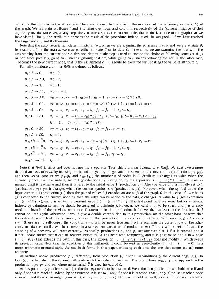
and store this number in the attribute ν . Then, we proceed to the scan of the m copies of the adjacency matrix κ(G) ofthe graph. We maintain attributes i and j ranging over rows and columns, respectively, of the (current instance of the)adjacency matrix. Moreover, at any step, the attribute c stores the current node, that is the last node of the graph that wehave visited. Finally, the attribute r encodes the result of the procedure. Indeed, it will be assigned 1 if we have reachedthe target node n, and 0 otherwise.
Note that the automaton is non-deterministic. In fact, when we are scanning the adjacency matrix and we are at state B ,by reading a 1 in the matrix, we may go either to state C or to state C . If i = c, i.e. we are scanning the row with thearcs starting from the current node c, this non-deterministic step is used to encode the choice of following some arc (i, j)or not. More precisely, going to C means ignoring that arc, while going to C means following the arc. In the latter case,j becomes the new current node, that is the assignment c := j should be executed for updating the value of attribute c.
Formally, attribute grammar RAG is defined as follows:
p0 : A → 0, ν := 0,
p1 : A → A0, ν := ν,
p2 : A → 1, ν := 1,
p3 : A → A1, ν := ν + 1,
p4 : B → A#, νB := νA, cB := 1, iB := 1, jB := 1, rB := (νA = 1)?1:0,
p5 : B → C#, νB := νC , cB := cC , iB := (iC = νC )?1: iC + 1, jB := 1, rB := rC ,
p6 : B → C�, νB := νC , cB := cC , iB := iC , jB := jC + 1, rB := rC ,
p7 : C → B1, νC := νB , cC := (iB = cB)? jB : cB , iC := iB , jC := (iB = cB)?0: jB ,
rC := (iB = cB ∧ jB = νB)?1: rB ,
p8 : C → B0, νC := νB , cC := cB , iC := iB , jC := jB , rC := rB ,
p9 : S → C$, rC = 1,
p10 : B → C#, νB := νC , cB := cC , iB := (iC = νC )?1: iC + 1, jB := 1, rB := rC ,
p11 : B → C�, νB := νC , cB := cC , iB := iC , jB := jC + 1, rB := rC ,
p12 : C → B1, νC := νB , cC := cB , iC := iB , jC := jB , rC := rB ,
p13 : S → C$, rC = 1.
Note that RAG is strict and does not use the ∗ operator. Thus, this grammar belongs to σ -RegA⊗ . We next give a moredetailed analysis of RAG, by focusing on the role played by integer attributes: Attribute ν first counts (productions p0–p3),and then keeps (productions p4–p8 and p10–p12) the number n of nodes in G . Attribute i changes its value when thecurrent symbol is #. It is initially set to 1 (productions p4). Going on, by the expression i := (i = ν)?1: i + 1, it is incre-mented until it reaches n and then it is reset to the initial value 1 (production p5). Also the value of j is initially set to 1(productions p4), yet it changes when the current symbol is � (productions p6). Moreover, when the symbol under theinput-cursor is 1 (production p7), then the pair of values i, j encodes an arc (i, j) of the graph G . In this case, if i = c holds( j is connected to the current node c), then the edge can be added to the path, c changes its value to j (see expressionc := (i = c)? j: c), and j is set to the constant value 0 ( j := (i = c)?0: j). This last point deserves some further attention.Indeed, by definition something should be assigned to attribute j. However, we want this IRG be strict, and j is alreadyused in a branch of the previous arithmetic-if statement in this production. It follows that, at least in the first branch, jcannot be used again, otherwise it would give a double contribution to this production. On the other hand, observe thatthis value 0 cannot lead to any trouble, because in this production i = c entails c is set to j. Then, since (i, j) ∈ E entailsi �= j (there are no self-loops), the condition i = c will be never true again while scanning the current row of the adja-cency matrix (i.e., until i will be changed in a subsequent execution of production p5). Then, j will be set to 1, and thescanning of a new row will start correctly. Eventually, productions p4 and p7 set attribute r to 1 if n is reached and 0if not. Please, notice that n can be reached before w(G) has been read completely, and it is possible to find a new edge(i = c = ν, j) that extends the path. In this case, the expression r := (i = c ∧ j = ν)?1: r does not modify r, which keepsits previous value. Note that the condition of this arithmetic-if could be written equivalently (|i − c| + | j − ν| = 0), in amore arithmetic-oriented style. We use both forms in this paper, choosing each time the one that seems (to us) morereadable.
As outlined above, production p12, differently from production p7, “skips” unconditionally the current edge (i, j). Infact, (i, j) is left also if the current path ends with the node i when c = i. The productions p10, p11 and p13 are like theproductions p5, p6 and p9, where nonterminal C is used instead of C .
At this point, only predicate r = 1 (production p9) needs to be evaluated. We claim that predicate r = 1 holds true if andonly if node n is reached. Indeed, by construction, r is set to 1 only if node n is reached, that is only if the last reached nodeis some i, and there is an outgoing arc (i, j), with j = n (i.e., j = ν). The reverse holds as well, because if node n is reachable
410 M. Manna et al. / Journal of Computer and System Sciences 77 (2011) 393–421
from node 1 there is a sequence of at most n − 1 arcs leading from 1 to n, and thus the non-deterministic automaton maycorrectly chose such arcs (going to state C rather than to C ), while scanning the n − 1 copies of the adjacency matrix of G .It follows that w(G) ∈ L(RAG) if and only if there is a path from node 1 to node n in G .
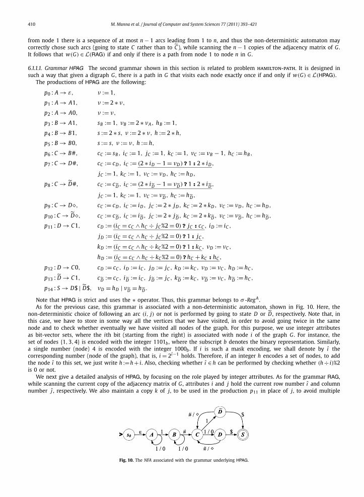
6.1.1.1. Grammar HPAG The second grammar shown in this section is related to problem hamilton-path. It is designed insuch a way that given a digraph G , there is a path in G that visits each node exactly once if and only if w(G) ∈ L(HPAG).
The productions of HPAG are the following:
p0 : A → ε, ν := 1,
p1 : A → A1, ν := 2 ∗ ν,
p2 : A → A0, ν := ν,
p3 : B → A1, sB := 1, νB := 2 ∗ νA, hB := 1,
p4 : B → B1, s := 2 ∗ s, ν := 2 ∗ ν, h := 2 ∗ h,
p5 : B → B0, s := s, ν := ν, h := h,
p6 : C → B#, cC := sB , iC := 1, jC := 1, kC := 1, νC := νB − 1, hC := hB ,
p7 : C → D#, cC := cD , iC := (2 ∗ iD − 1 = νD)?1:2 ∗ iD ,
jC := 1, kC := 1, νC := νD , hC := hD ,
p8 : C → D#, cC := cD , iC := (2 ∗ i D − 1 = νD)?1:2 ∗ i D ,
jC := 1, kC := 1, νC := νD , hC := hD ,
p9 : C → D�, cC := cD , iC := iD , jC := 2 ∗ jD , kC := 2 ∗ kD , νC := νD , hC := hD ,
p10 : C → D�, cC := cD , iC := i D , jC := 2 ∗ j D , kC := 2 ∗ kD , νC := νD , hC := hD ,
p11 : D → C1, cD := (iC = cC ∧ hC ÷ jC %2 = 0)? jC : cC , iD := iC ,
jD := (iC = cC ∧ hC ÷ jC %2 = 0)?1: jC ,
kD := (iC = cC ∧ hC ÷ kC %2 = 0)?1:kC , νD := νC ,
hD := (iC = cC ∧ hC ÷ kC %2 = 0)?hC + kC :hC ,
p12 : D → C0, cD := cC , iD := iC , jD := jC , kD := kC , νD := νC , hD := hC ,
p13 : D → C1, cD := cC , i D := iC , j D := jC , kD := kC , νD := νC , hD := hC ,
p14 : S → D$ | D$, νD = hD | νD = hD .
Note that HPAG is strict and uses the ∗ operator. Thus, this grammar belongs to σ -RegA .As for the previous case, this grammar is associated with a non-deterministic automaton, shown in Fig. 10. Here, the
non-deterministic choice of following an arc (i, j) or not is performed by going to state D or D , respectively. Note that, inthis case, we have to store in some way all the vertices that we have visited, in order to avoid going twice in the samenode and to check whether eventually we have visited all nodes of the graph. For this purpose, we use integer attributesas bit-vector sets, where the ith bit (starting from the right) is associated with node i of the graph G . For instance, theset of nodes {1,3,4} is encoded with the integer 1101b , where the subscript b denotes the binary representation. Similarly,a single number (node) 4 is encoded with the integer 1000b . If i is such a mask encoding, we shall denote by ı thecorresponding number (node of the graph), that is, i = 2ı−1 holds. Therefore, if an integer h encodes a set of nodes, to addthe node ı to this set, we just write h :=h + i. Also, checking whether ı ∈ h can be performed by checking whether (h ÷ i)%2is 0 or not.
We next give a detailed analysis of HPAG, by focusing on the role played by integer attributes. As for the grammar RAG,while scanning the current copy of the adjacency matrix of G , attributes i and j hold the current row number ı and columnnumber j , respectively. We also maintain a copy k of j, to be used in the production p11 in place of j, to avoid multiple
Fig. 10. The NFA associated with the grammar underlying HPAG.
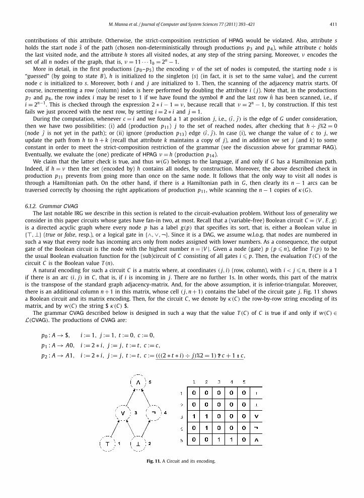
M. Manna et al. / Journal of Computer and System Sciences 77 (2011) 393–421 411
contributions of this attribute. Otherwise, the strict-composition restriction of HPAG would be violated. Also, attribute sholds the start node s of the path (chosen non-deterministically through productions p3 and p4), while attribute c holdsthe last visited node, and the attribute h stores all visited nodes, at any step of the string parsing. Moreover, ν encodes theset of all n nodes of the graph, that is, ν = 11 · · ·1b = 2n − 1.
More in detail, in the first productions (p0–p5) the encoding ν of the set of nodes is computed, the starting node s is“guessed” (by going to state B), h is initialized to the singleton {s} (in fact, it is set to the same value), and the currentnode c is initialized to s. Moreover, both i and j are initialized to 1. Then, the scanning of the adjacency matrix starts. Ofcourse, incrementing a row (column) index is here performed by doubling the attribute i ( j). Note that, in the productionsp7 and p8, the row index i may be reset to 1 if we have found the symbol # and the last row n has been scanned, i.e., ifi = 2n−1. This is checked through the expression 2 ∗ i − 1 = ν , because recall that ν = 2n − 1, by construction. If this testfails we just proceed with the next row, by setting i = 2 ∗ i and j = 1.
During the computation, whenever c = i and we found a 1 at position j, i.e., (ı, j ) is the edge of G under consideration,then we have two possibilities: (i) add (production p11) j to the set of reached nodes, after checking that h ÷ j%2 = 0(node j is not yet in the path); or (ii) ignore (production p13) edge (ı, j ). In case (i), we change the value of c to j, weupdate the path from h to h + k (recall that attribute k maintains a copy of j), and in addition we set j (and k) to someconstant in order to meet the strict-composition restriction of the grammar (see the discussion above for grammar RAG).Eventually, we evaluate the (one) predicate of HPAG ν = h (production p14).
We claim that the latter check is true, and thus w(G) belongs to the language, if and only if G has a Hamiltonian path.Indeed, if h = ν then the set (encoded by) h contains all nodes, by construction. Moreover, the above described check inproduction p11 prevents from going more than once on the same node. It follows that the only way to visit all nodes isthrough a Hamiltonian path. On the other hand, if there is a Hamiltonian path in G , then clearly its n − 1 arcs can betraversed correctly by choosing the right applications of production p11, while scanning the n − 1 copies of κ(G).
6.1.2. Grammar CVAGThe last notable IRG we describe in this section is related to the circuit-evaluation problem. Without loss of generality we
consider in this paper circuits whose gates have fan-in two, at most. Recall that a (variable-free) Boolean circuit C = 〈V , E, g〉is a directed acyclic graph where every node p has a label g(p) that specifies its sort, that is, either a Boolean value in{�,⊥} (true or false, resp.), or a logical gate in {∧,∨,¬}. Since it is a DAG, we assume w.l.o.g. that nodes are numbered insuch a way that every node has incoming arcs only from nodes assigned with lower numbers. As a consequence, the outputgate of the Boolean circuit is the node with the highest number n = |V |. Given a node (gate) p (p � n), define T (p) to bethe usual Boolean evaluation function for the (sub)circuit of C consisting of all gates i � p. Then, the evaluation T (C) of thecircuit C is the Boolean value T (n).
A natural encoding for such a circuit C is a matrix where, at coordinates ( j, i) (row, column), with i < j � n, there is a 1if there is an arc (i, j) in C , that is, if i is incoming in j. There are no further 1s. In other words, this part of the matrixis the transpose of the standard graph adjacency-matrix. And, for the above assumption, it is inferior-triangular. Moreover,there is an additional column n + 1 in this matrix, whose cell ( j,n + 1) contains the label of the circuit gate j. Fig. 11 showsa Boolean circuit and its matrix encoding. Then, for the circuit C , we denote by κ(C) the row-by-row string encoding of itsmatrix, and by w(C) the string $ κ(C) $.
The grammar CVAG described below is designed in such a way that the value T (C) of C is true if and only if w(C) ∈L(CVAG). The productions of CVAG are:
p0 : A → $, i := 1, j := 1, t := 0, c := 0,
p1 : A → A0, i := 2 ∗ i, j := j, t := t, c := c,
p2 : A → A1, i := 2 ∗ i, j := j, t := t, c := (((2 ∗ t ∗ i) ÷ j)%2 = 1)? c + 1: c,
Fig. 11. A Circuit and its encoding.
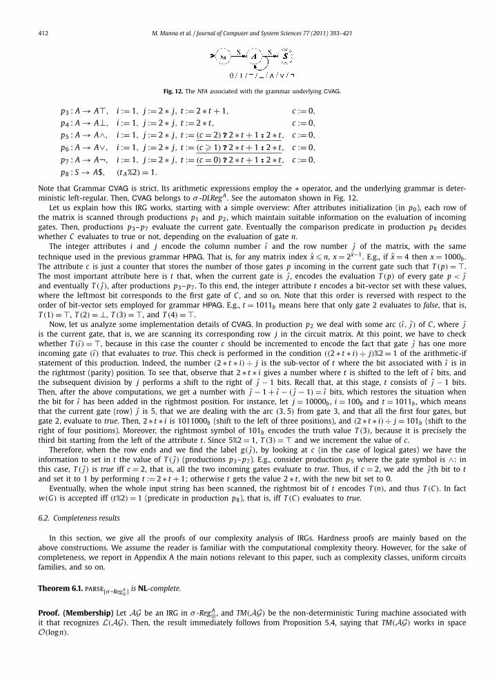
412 M. Manna et al. / Journal of Computer and System Sciences 77 (2011) 393–421
Fig. 12. The NFA associated with the grammar underlying CVAG.
p3 : A → A�, i := 1, j := 2 ∗ j, t := 2 ∗ t + 1, c := 0,
p4 : A → A⊥, i := 1, j := 2 ∗ j, t := 2 ∗ t, c := 0,
p5 : A → A∧, i := 1, j := 2 ∗ j, t := (c = 2)?2 ∗ t + 1:2 ∗ t, c := 0,
p6 : A → A∨, i := 1, j := 2 ∗ j, t := (c � 1)?2 ∗ t + 1:2 ∗ t, c := 0,
p7 : A → A¬, i := 1, j := 2 ∗ j, t := (c = 0)?2 ∗ t + 1:2 ∗ t, c := 0,
p8 : S → A$, (t A%2) = 1.
Note that Grammar CVAG is strict. Its arithmetic expressions employ the ∗ operator, and the underlying grammar is deter-ministic left-regular. Then, CVAG belongs to σ -DLRegA . See the automaton shown in Fig. 12.
Let us explain how this IRG works, starting with a simple overview: After attributes initialization (in p0), each row ofthe matrix is scanned through productions p1 and p2, which maintain suitable information on the evaluation of incominggates. Then, productions p3–p7 evaluate the current gate. Eventually the comparison predicate in production p8 decideswhether C evaluates to true or not, depending on the evaluation of gate n.
The integer attributes i and j encode the column number ı and the row number j of the matrix, with the sametechnique used in the previous grammar HPAG. That is, for any matrix index x � n, x = 2x−1. E.g., if x = 4 then x = 1000b .The attribute c is just a counter that stores the number of those gates p incoming in the current gate such that T (p) = �.The most important attribute here is t that, when the current gate is j , encodes the evaluation T (p) of every gate p < j
and eventually T (j ), after productions p3–p7. To this end, the integer attribute t encodes a bit-vector set with these values,where the leftmost bit corresponds to the first gate of C , and so on. Note that this order is reversed with respect to theorder of bit-vector sets employed for grammar HPAG. E.g., t = 1011b means here that only gate 2 evaluates to false, that is,T (1) = �, T (2) = ⊥, T (3) = �, and T (4) = �.
Now, let us analyze some implementation details of CVAG. In production p2 we deal with some arc (ı, j ) of C , where j
is the current gate, that is, we are scanning its corresponding row j in the circuit matrix. At this point, we have to checkwhether T (ı) = �, because in this case the counter c should be incremented to encode the fact that gate j has one moreincoming gate (ı) that evaluates to true. This check is performed in the condition ((2 ∗ t ∗ i) ÷ j)%2 = 1 of the arithmetic-ifstatement of this production. Indeed, the number (2 ∗ t ∗ i) ÷ j is the sub-vector of t where the bit associated with ı is inthe rightmost (parity) position. To see that, observe that 2 ∗ t ∗ i gives a number where t is shifted to the left of ı bits, andthe subsequent division by j performs a shift to the right of j − 1 bits. Recall that, at this stage, t consists of j − 1 bits.Then, after the above computations, we get a number with j − 1 + ı − (j − 1) = ı bits, which restores the situation whenthe bit for ı has been added in the rightmost position. For instance, let j = 10000b , i = 100b and t = 1011b , which meansthat the current gate (row) j is 5, that we are dealing with the arc (3,5) from gate 3, and that all the first four gates, butgate 2, evaluate to true. Then, 2 ∗ t ∗ i is 1011000b (shift to the left of three positions), and (2 ∗ t ∗ i) ÷ j = 101b (shift to theright of four positions). Moreover, the rightmost symbol of 101b encodes the truth value T (3), because it is precisely thethird bit starting from the left of the attribute t . Since 5%2 = 1, T (3) = � and we increment the value of c.
Therefore, when the row ends and we find the label g(j ), by looking at c (in the case of logical gates) we have theinformation to set in t the value of T (j ) (productions p3–p7). E.g., consider production p5 where the gate symbol is ∧: inthis case, T (j ) is true iff c = 2, that is, all the two incoming gates evaluate to true. Thus, if c = 2, we add the j th bit to tand set it to 1 by performing t := 2 ∗ t + 1; otherwise t gets the value 2 ∗ t , with the new bit set to 0.
Eventually, when the whole input string has been scanned, the rightmost bit of t encodes T (n), and thus T (C). In factw(G) is accepted iff (t%2) = 1 (predicate in production p8), that is, iff T (C) evaluates to true.
6.2. Completeness results
In this section, we give all the proofs of our complexity analysis of IRGs. Hardness proofs are mainly based on theabove constructions. We assume the reader is familiar with the computational complexity theory. However, for the sake ofcompleteness, we report in Appendix A the main notions relevant to this paper, such as complexity classes, uniform circuitsfamilies, and so on.
Theorem 6.1. parse[σ-RegA⊗] is NL-complete.
Proof. (Membership) Let AG be an IRG in σ -RegA⊗ , and TM(AG) be the non-deterministic Turing machine associated withit that recognizes L(AG). Then, the result immediately follows from Proposition 5.4, saying that TM(AG) works in spaceO(logn).
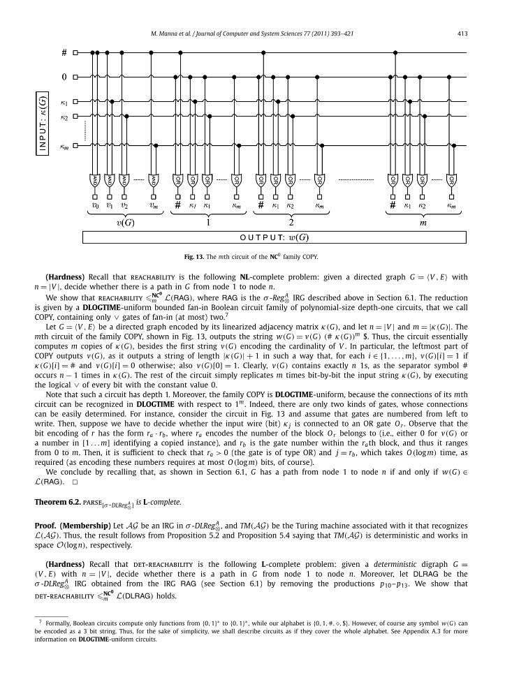
M. Manna et al. / Journal of Computer and System Sciences 77 (2011) 393–421 413
Fig. 13. The mth circuit of the NC0 family COPY.
(Hardness) Recall that reachability is the following NL-complete problem: given a directed graph G = 〈V , E〉 withn = |V |, decide whether there is a path in G from node 1 to node n.
We show that reachability �NC0
m L(RAG), where RAG is the σ -RegA⊗ IRG described above in Section 6.1. The reductionis given by a DLOGTIME-uniform bounded fan-in Boolean circuit family of polynomial-size depth-one circuits, that we callCOPY, containing only ∨ gates of fan-in (at most) two.7
Let G = 〈V , E〉 be a directed graph encoded by its linearized adjacency matrix κ(G), and let n = |V | and m = |κ(G)|. Themth circuit of the family COPY, shown in Fig. 13, outputs the string w(G) = v(G) (# κ(G))m $. Thus, the circuit essentiallycomputes m copies of κ(G), besides the first string v(G) encoding the cardinality of V . In particular, the leftmost part ofCOPY outputs v(G), as it outputs a string of length |κ(G)| + 1 in such a way that, for each i ∈ {1, . . . ,m}, v(G)[i] = 1 ifκ(G)[i] = # and v(G)[i] = 0 otherwise; also v(G)[0] = 1. Clearly, v(G) contains exactly n 1s, as the separator symbol #occurs n − 1 times in κ(G). The rest of the circuit simply replicates m times bit-by-bit the input string κ(G), by executingthe logical ∨ of every bit with the constant value 0.
Note that such a circuit has depth 1. Moreover, the family COPY is DLOGTIME-uniform, because the connections of its mthcircuit can be recognized in DLOGTIME with respect to 1m . Indeed, there are only two kinds of gates, whose connectionscan be easily determined. For instance, consider the circuit in Fig. 13 and assume that gates are numbered from left towrite. Then, suppose we have to decide whether the input wire (bit) κ j is connected to an OR gate O r . Observe that thebit encoding of r has the form ra · rb , where ra encodes the number of the block O r belongs to (i.e., either 0 for v(G) ora number in [1 . . .m] identifying a copied instance), and rb is the gate number within the rath block, and thus it rangesfrom 0 to m. Then, it is sufficient to check that ra > 0 (the gate is of type OR) and j = rb , which takes O (log m) time, asrequired (as encoding these numbers requires at most O (log m) bits, of course).
We conclude by recalling that, as shown in Section 6.1, G has a path from node 1 to node n if and only if w(G) ∈L(RAG). �Theorem 6.2. parse[σ-DLRegA⊗] is L-complete.
Proof. (Membership) Let AG be an IRG in σ -DLRegA⊗ , and TM(AG) be the Turing machine associated with it that recognizesL(AG). Thus, the result follows from Proposition 5.2 and Proposition 5.4 saying that TM(AG) is deterministic and works inspace O(log n), respectively.
(Hardness) Recall that det-reachability is the following L-complete problem: given a deterministic digraph G =(V , E) with n = |V |, decide whether there is a path in G from node 1 to node n. Moreover, let DLRAG be theσ -DLRegA⊗ IRG obtained from the IRG RAG (see Section 6.1) by removing the productions p10–p13. We show that
det-reachability �NC0
m L(DLRAG) holds.
7 Formally, Boolean circuits compute only functions from {0,1}∗ to {0,1}∗ , while our alphabet is {0,1,#,�,$}. However, of course any symbol w(G) canbe encoded as a 3 bit string. Thus, for the sake of simplicity, we shall describe circuits as if they cover the whole alphabet. See Appendix A.3 for moreinformation on DLOGTIME-uniform circuits.
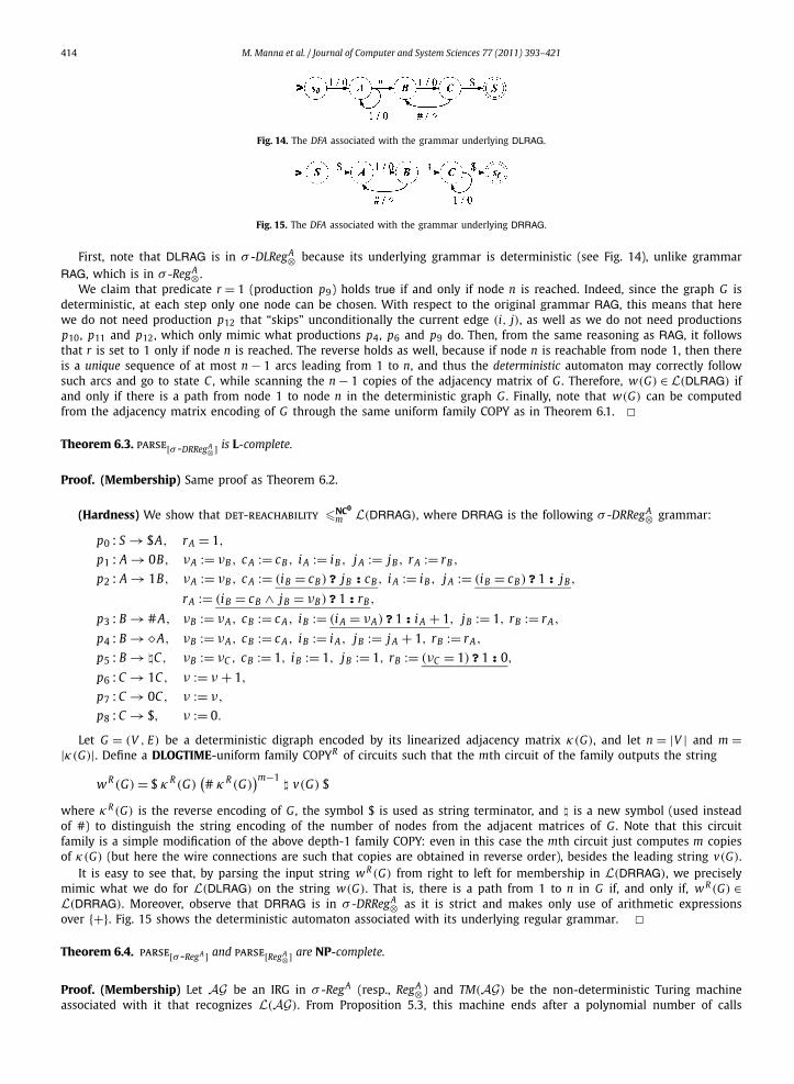
414 M. Manna et al. / Journal of Computer and System Sciences 77 (2011) 393–421
Fig. 14. The DFA associated with the grammar underlying DLRAG.
Fig. 15. The DFA associated with the grammar underlying DRRAG.
First, note that DLRAG is in σ -DLRegA⊗ because its underlying grammar is deterministic (see Fig. 14), unlike grammarRAG, which is in σ -RegA⊗ .
We claim that predicate r = 1 (production p9) holds true if and only if node n is reached. Indeed, since the graph G isdeterministic, at each step only one node can be chosen. With respect to the original grammar RAG, this means that herewe do not need production p12 that “skips” unconditionally the current edge (i, j), as well as we do not need productionsp10, p11 and p12, which only mimic what productions p4, p6 and p9 do. Then, from the same reasoning as RAG, it followsthat r is set to 1 only if node n is reached. The reverse holds as well, because if node n is reachable from node 1, then thereis a unique sequence of at most n − 1 arcs leading from 1 to n, and thus the deterministic automaton may correctly followsuch arcs and go to state C , while scanning the n − 1 copies of the adjacency matrix of G . Therefore, w(G) ∈ L(DLRAG) ifand only if there is a path from node 1 to node n in the deterministic graph G . Finally, note that w(G) can be computedfrom the adjacency matrix encoding of G through the same uniform family COPY as in Theorem 6.1. �Theorem 6.3. parse[σ-DRRegA⊗] is L-complete.
Proof. (Membership) Same proof as Theorem 6.2.
(Hardness) We show that det-reachability �NC0
m L(DRRAG), where DRRAG is the following σ -DRRegA⊗ grammar:
p0 : S → $A, rA = 1,
p1 : A → 0B, νA := νB , c A := cB , i A := iB , j A := jB , rA := rB ,
p2 : A → 1B, νA := νB , c A := (iB = cB)? jB : cB , i A := iB , j A := (iB = cB)?1: jB ,
rA := (iB = cB ∧ jB = νB)?1: rB ,
p3 : B → #A, νB := νA, cB := c A, iB := (i A = νA)?1: i A + 1, jB := 1, rB := rA,
p4 : B → �A, νB := νA, cB := c A, iB := i A, jB := j A + 1, rB := rA,
p5 : B → �C, νB := νC , cB := 1, iB := 1, jB := 1, rB := (νC = 1)?1:0,
p6 : C → 1C, ν := ν + 1,
p7 : C → 0C, ν := ν,
p8 : C → $, ν := 0.
Let G = (V , E) be a deterministic digraph encoded by its linearized adjacency matrix κ(G), and let n = |V | and m =|κ(G)|. Define a DLOGTIME-uniform family COPYR of circuits such that the mth circuit of the family outputs the string
w R(G) = $ κ R(G)(# κ R(G)
)m−1� v(G) $
where κ R(G) is the reverse encoding of G , the symbol $ is used as string terminator, and � is a new symbol (used insteadof #) to distinguish the string encoding of the number of nodes from the adjacent matrices of G . Note that this circuitfamily is a simple modification of the above depth-1 family COPY: even in this case the mth circuit just computes m copiesof κ(G) (but here the wire connections are such that copies are obtained in reverse order), besides the leading string v(G).
It is easy to see that, by parsing the input string w R(G) from right to left for membership in L(DRRAG), we preciselymimic what we do for L(DLRAG) on the string w(G). That is, there is a path from 1 to n in G if, and only if, w R(G) ∈L(DRRAG). Moreover, observe that DRRAG is in σ -DRRegA⊗ as it is strict and makes only use of arithmetic expressionsover {+}. Fig. 15 shows the deterministic automaton associated with its underlying regular grammar. �Theorem 6.4. parse[σ-RegA ] and parse[RegA⊗] are NP-complete.
Proof. (Membership) Let AG be an IRG in σ -RegA (resp., RegA⊗) and TM(AG) be the non-deterministic Turing machineassociated with it that recognizes L(AG). From Proposition 5.3, this machine ends after a polynomial number of calls

M. Manna et al. / Journal of Computer and System Sciences 77 (2011) 393–421 415
to arithmetic expressions evaluations, which take at most polynomial-time, in their turn. Indeed, there is no trouble innumbers-size explosion here, because from Proposition 5.5 (resp., Proposition 5.6) all such arithmetic operations requireonly space O(n) on the work-tape of TM(AG).
(Hardness) Recall that hamilton-path is the NP-complete problem defined as follows: Given a digraph G , decide whetherthere is a path that visits each node exactly once. In Section 6.1, we have described a σ -RegA IRG HPAG such that thereis a path in G that visits each node exactly once if, and only if, its associated string w(G) ∈ L(HPAG), where w(G) =v(G) (# κ(G))m $. Moreover, we have seen that such a string can be obtained by using the uniform family COPY of NC0
Boolean circuits. It follows that hamilton-path �NC0
m L(HPAG).Now, consider the IRG HPAG⊗ obtained from HPAG by replacing each expression of the form 2 ∗ x (where x is any
attribute) with x + x. The new grammar HPAG⊗ contains productions with attributes contributing more than once to thecomputation of attribute values, and thus it is not a strict grammar. However, the ∗ operator is not used in arithmeticexpressions, and thus it belongs to RegA⊗ , and it is clearly equivalent to HPAG. Therefore, hamilton-path �NC0
m L(HPAG⊗),too. �Theorem 6.5. parse[σ-DLRegA ] and parse[σ-DRRegA ] , as well as parse[DLRegA⊗] and parse[DRRegA⊗] are P-complete.
Proof. (Membership) Let AG be an IRG in σ -DLRegA or in σ -DRRegA (resp., in parse[DLRegA⊗] or in parse[DRRegA⊗]), and
TM(AG) be the Turing machine associated with it that recognizes L(AG). Since the regular grammar underlying AG isdeterministic, from Proposition 5.2 TM(AG) is a deterministic machine, and from Proposition 5.3 it ends after a polyno-mial number of calls to arithmetic expressions evaluations, which take at most polynomial-time, in their turn. Indeed, asobserved in the previous theorem, there is no trouble in numbers-size explosion here, because from Proposition 5.5 (resp.,Proposition 5.6) all such arithmetic operations require only space O(n) on the work-tape of TM(AG).
(Hardness) Recall that circuit-value is the P-complete problem defined as follows: given a digraph C = 〈V , E〉 repre-senting a variable-free Boolean circuit, decide whether the value (at the output gate) of circuit C is 1. In Section 6.1, wehave described a σ -DLRegA IRG CVAG such that its associated string w(C) = $ κ(C) $ belongs to L(CVAG) if, and onlyif, the value of circuit C is 1, where κ(C) is the linearized matrix string that encodes C . Then, clearly enough, we getcircuit-value �NC0
m L(CVAG). Indeed, the transformation from C ’s encoding to w(C) is trivial, because we have to add justa symbol $ at the beginning and at the end of the circuit encoding κ(C). Moreover, as far as parse[σ-DRRegA ] is concerned,
we can simply modify grammar CVAG to obtain an equivalent IRG in σ -DRRegA (see, for instance, Theorem 6.3).Now, consider the IRG CVAG⊗ obtained from CVAG by replacing each expression of the form 2 ∗ x (where x is any
attribute) with x + x. As observed for a similar case in the proof of the previous theorem, the new grammar CVAG⊗contains productions with attributes contributing more than once to the computation of attribute values, and thus it isnot a strict grammar. However, the ∗ operator is not used in arithmetic expressions, and thus it belongs to DLRegA⊗ , and
it is clearly equivalent to CVAG. Therefore, circuit-value �NC0
m L(CVAG⊗), too. Finally, this hardness result holds even forDRRegA⊗ grammars. Just apply the above modification to remove ∗ occurrences in arithmetic expressions to the P-hardσ -DRRegA IRG version of CVAG mentioned in the first part of this proof. �7. Conclusions
We have analyzed the complexity of the languages generated by integer attribute grammars. Since attribute grammarscan easily generate exponential-size attribute values, we have looked for tractable cases. We have proposed some non-severerestrictions on the grammars and their attributes that avoid the exponential explosion of attribute sizes, and that allow usto parse efficiently the languages generated by such grammars. Finally, we have shown that even in the most general casethe parsing process remains in polynomial space.
In fact, many tractability results are given for (possibly non-deterministic) space-based classes. Thus, for the sake ofcompleteness, we observe that the following good (time) complexities may easily be obtained in a realistic RAM model, byexploiting the properties described in this paper and state-of-the-art results about arithmetic operations8:
• σ -DLRegA⊗ and σ -DRRegA⊗ can be evaluated in time O(n log n log log n log log log n);• σ -DLRegA , σ -DRRegA , DLRegA⊗ , and DRRegA⊗ can be evaluated in time O(n2 logn log log n).
A thorough analysis of the most general cases without restrictions on operators and their compositions, or with non-deterministic grammars, will be a subject of future work.
8 Given two n-digit numbers, both addition and subtraction can be done in linear time; multiplication can be done in time O(n logn log logn) (see [52,18])which is very close to the lower bound Ω(n log n); integer division with truncation and modulo reduction have the same time complexity of multiplication,by the well-known Newton–Raphson method.
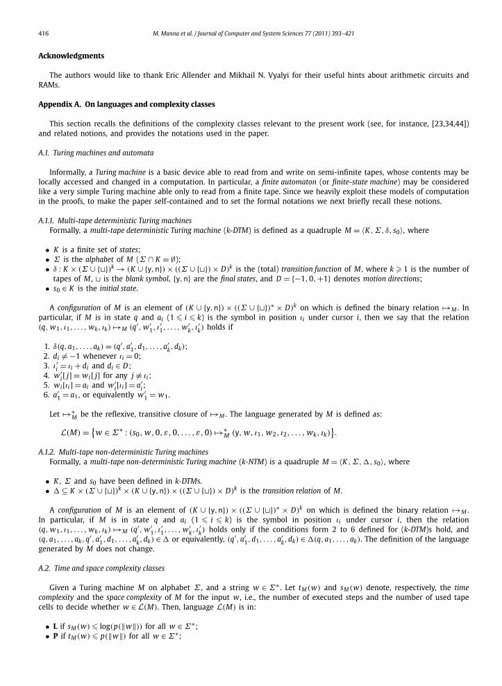
416 M. Manna et al. / Journal of Computer and System Sciences 77 (2011) 393–421
Acknowledgments
The authors would like to thank Eric Allender and Mikhail N. Vyalyi for their useful hints about arithmetic circuits andRAMs.
Appendix A. On languages and complexity classes
This section recalls the definitions of the complexity classes relevant to the present work (see, for instance, [23,34,44])and related notions, and provides the notations used in the paper.
A.1. Turing machines and automata
Informally, a Turing machine is a basic device able to read from and write on semi-infinite tapes, whose contents may belocally accessed and changed in a computation. In particular, a finite automaton (or finite-state machine) may be consideredlike a very simple Turing machine able only to read from a finite tape. Since we heavily exploit these models of computationin the proofs, to make the paper self-contained and to set the formal notations we next briefly recall these notions.
A.1.1. Multi-tape deterministic Turing machinesFormally, a multi-tape deterministic Turing machine (k-DTM) is defined as a quadruple M = 〈K ,Σ, δ, s0〉, where
• K is a finite set of states;• Σ is the alphabet of M (Σ ∩ K = ∅);• δ : K × (Σ ∪ {�})k → (K ∪ {y,n}) × ((Σ ∪ {�}) × D)k is the (total) transition function of M , where k � 1 is the number of
tapes of M , � is the blank symbol, {y,n} are the final states, and D = {−1,0,+1} denotes motion directions;• s0 ∈ K is the initial state.
A configuration of M is an element of (K ∪ {y,n}) × ((Σ ∪ {�})∗ × D)k on which is defined the binary relation �→M . Inparticular, if M is in state q and ai (1 � i � k) is the symbol in position ıi under cursor i, then we say that the relation(q, w1, ı1, . . . , wk, ık) �→M (q′, w ′
1, ı′1, . . . , w ′
k, ı′k) holds if
1. δ(q,a1, . . . ,ak) = (q′,a′1,d1, . . . ,a′
k,dk);2. di �= −1 whenever ıi = 0;3. ı′i = ıi + di and di ∈ D;4. w ′
i[ j] = wi[ j] for any j �= ıi ;5. wi[ıi] = ai and w ′
i[ıi] = a′i ;
6. a′1 = a1, or equivalently w ′
1 = w1.
Let �→∗M be the reflexive, transitive closure of �→M . The language generated by M is defined as:
L(M) = {w ∈ Σ∗ : (s0, w,0, ε,0, . . . , ε,0) �→∗
M (y, w, ı1, w2, ı2, . . . , wk, ık)}.
A.1.2. Multi-tape non-deterministic Turing machinesFormally, a multi-tape non-deterministic Turing machine (k-NTM) is a quadruple M = 〈K ,Σ,, s0〉, where
• K , Σ and s0 have been defined in k-DTMs.• ⊆ K × (Σ ∪ {�})k × (K ∪ {y,n}) × ((Σ ∪ {�}) × D)k is the transition relation of M .
A configuration of M is an element of (K ∪ {y,n}) × ((Σ ∪ {�})∗ × D)k on which is defined the binary relation �→M .In particular, if M is in state q and ai (1 � i � k) is the symbol in position ıi under cursor i, then the relation(q, w1, ı1, . . . , wk, ık) �→M (q′, w ′
1, ı′1, . . . , w ′
k, ı′k) holds only if the conditions form 2 to 6 defined for (k-DTM)s hold, and
(q,a1, . . . ,ak,q′,a′1,d1, . . . ,a′
k,dk) ∈ or equivalently, (q′,a′1,d1, . . . ,a′
k,dk) ∈ (q,a1, . . . ,ak). The definition of the languagegenerated by M does not change.
A.2. Time and space complexity classes
Given a Turing machine M on alphabet Σ , and a string w ∈ Σ∗ . Let tM(w) and sM(w) denote, respectively, the timecomplexity and the space complexity of M for the input w , i.e., the number of executed steps and the number of used tapecells to decide whether w ∈ L(M). Then, language L(M) is in:
• L if sM(w) � log(p(‖w‖)) for all w ∈ Σ∗;• P if tM(w) � p(‖w‖) for all w ∈ Σ∗;

M. Manna et al. / Journal of Computer and System Sciences 77 (2011) 393–421 417
• PSPACE if sM(w) � p(‖w‖) for all w ∈ Σ∗;• EXP if tM(w) � 2p(‖w‖) for all w ∈ Σ∗;
where p : N �→ N is a polynomial function.Classes L and P have the non-deterministic counterparts NL and NP if M is non-deterministic. The known relationships
among these classes are: L ⊆ NL ⊆ P ⊆ NP ⊆ EXP and P ⊂ EXP. We shall henceforth consider also generalizations of theabove classes, namely, complexity classes of the form DTIME( f (n)) (deterministic time), DSPACE( f (n)) (deterministic space),where f is any proper function. They contain exactly those languages that can be decided by a Turing machine M insuch a way that for any input string w with ‖w‖ = n, tM(w) (or sM(w), respectively) is O( f (n)). Their non-deterministiccounterparts are NTIME( f (n)) and NSPACE( f (n)). For instance, we have that:
• L = DSPACE(log n);• P = DTIME(nO(1)) = ⋃
k>0 DTIME(nk);
• PSPACE = DSPACE(nO(1)) = ⋃k>0 DSPACE(nk);
• EXP = DTIME(2nO(1)) = ⋃
k>0 DTIME(2nk).
Some fundamental relationships [44] are just recalled below. Let f (n) be a proper complexity function. Then,
• DTIME( f (n)) ⊂ DTIME( f (n) log2 f (n));• DSPACE( f (n)) ⊂ DSPACE( f (n) log f (n));• DSPACE( f (n)) ⊆ NSPACE( f (n));• DTIME( f (n)) ⊆ NTIME( f (n));• NTIME( f (n)) ⊆ DSPACE( f (n));• NSPACE( f (n)) ⊆ DTIME(klogn+ f (n));• NSPACE( f (n)) ⊆ DSPACE([ f (n)]2);
• DTIME( f (n)) ⊆ DSPACE(f (n)
log f (n)).
A.3. Circuit complexity
A transducer circuit is a finite directed acyclic graph9 C = 〈V , E〉 with n � 0 input nodes (each of in-degree 0) labeledx1, . . . , xn , and m � 1 output nodes (of out-degree 0). If m = 1, we say that C is a Boolean circuit, because it computes aBoolean function. The edges of the graph are called wires. Every non-input node v is called a gate, and has an associatedgate function gv : {0,1}r → {0,1}, that takes as many arguments as there are wires coming into v (r is the in-degree of v).The value of the gate is transmitted along each wire that goes out of v . The size of C is the number of its nodes, while thedepth is the length of the longest path in the circuit. Fan-in (fan-out) of C is the maximum in-degree (out-degree) of anygate in C . Since C is cycle-free, then every Boolean assignment x ∈ {0,1}n of values to the input nodes determines a uniquevalue for each gate and wire, and the value of the output gates is the output (or value) C(x) of the circuit. When C is aBoolean circuit, we say that C accepts x if, and only if, C(x) = 1.
A variable-free circuit is a circuit C where the n input nodes have a fixed Boolean assignment x ∈ {0,1}n .A circuit family {Cn} consists of a sequence of circuits {C1, C2, . . . , Cs}, where each Cn has n input nodes. The language
accepted by a family {Cn} of Boolean circuits is
L({Cn}
) = {x∣∣ x ∈ {0,1}+, C|x|(x) = 1
}.
The size complexity of family {Cn} is the function z(n) giving the number of nodes in Cn . The depth complexity is thefunction d(n) giving the depth of Cn . Family {Cn} is said to be uniform if circuit Cn can be constructed for any inputsize n. In particular, {Cn} is called P-uniform (respectively, L-uniform) if circuit Cn can be constructed from the string 1n inpolynomial time (resp., O(log n) space). For reductions among problems belonging to very low complexity classes (below L),DLOGTIME-uniform circuit families are typically employed. For such families, the circuit member Cn should be recognizedin DLOGTIME, that is, there exists a deterministic Turing machine T{Cn} that decides in O(log n) time the language
L({Cn}
) = {〈c, i, j,n〉 ∣∣ Cn[i] = c and j is an input for gate Cn[i], n � i > 0}.
Intuitively, the Turing machine has to answer in deterministic logarithmic time the question “Does node i in the circuit Cn
have gate-type c and node (or wire) j among its inputs?” Note that, as in the other above mentioned uniform classes ofcircuits, the cost is measured w.r.t. n, which is the size of string 1n . If the input of T{Cn} only contains the (standard) binaryencodings of numbers i, j, and n (the gate-type c is a constant), then the time-complexity of T{Cn} is in fact linear withrespect to its actual input size.
9 Since C is acyclic, then all edges can be assumed of the form (i, j), where i < j.
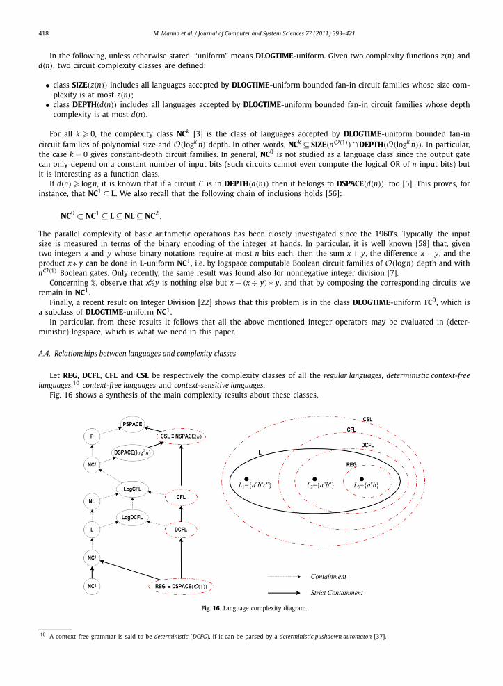
418 M. Manna et al. / Journal of Computer and System Sciences 77 (2011) 393–421
In the following, unless otherwise stated, “uniform” means DLOGTIME-uniform. Given two complexity functions z(n) andd(n), two circuit complexity classes are defined:
• class SIZE(z(n)) includes all languages accepted by DLOGTIME-uniform bounded fan-in circuit families whose size com-plexity is at most z(n);
• class DEPTH(d(n)) includes all languages accepted by DLOGTIME-uniform bounded fan-in circuit families whose depthcomplexity is at most d(n).
For all k � 0, the complexity class NCk [3] is the class of languages accepted by DLOGTIME-uniform bounded fan-incircuit families of polynomial size and O(logk n) depth. In other words, NCk ⊆ SIZE(nO(1))∩ DEPTH(O(logk n)). In particular,the case k = 0 gives constant-depth circuit families. In general, NC0 is not studied as a language class since the output gatecan only depend on a constant number of input bits (such circuits cannot even compute the logical OR of n input bits) butit is interesting as a function class.
If d(n) � log n, it is known that if a circuit C is in DEPTH(d(n)) then it belongs to DSPACE(d(n)), too [5]. This proves, forinstance, that NC1 ⊆ L. We also recall that the following chain of inclusions holds [56]:
NC0 ⊂ NC1 ⊆ L ⊆ NL ⊆ NC2.
The parallel complexity of basic arithmetic operations has been closely investigated since the 1960’s. Typically, the inputsize is measured in terms of the binary encoding of the integer at hands. In particular, it is well known [58] that, giventwo integers x and y whose binary notations require at most n bits each, then the sum x + y, the difference x − y, and theproduct x ∗ y can be done in L-uniform NC1, i.e. by logspace computable Boolean circuit families of O(log n) depth and withnO(1) Boolean gates. Only recently, the same result was found also for nonnegative integer division [7].
Concerning %, observe that x%y is nothing else but x − (x ÷ y) ∗ y, and that by composing the corresponding circuits weremain in NC1.
Finally, a recent result on Integer Division [22] shows that this problem is in the class DLOGTIME-uniform TC0, which isa subclass of DLOGTIME-uniform NC1.
In particular, from these results it follows that all the above mentioned integer operators may be evaluated in (deter-ministic) logspace, which is what we need in this paper.
A.4. Relationships between languages and complexity classes
Let REG, DCFL, CFL and CSL be respectively the complexity classes of all the regular languages, deterministic context-freelanguages,10 context-free languages and context-sensitive languages.
Fig. 16 shows a synthesis of the main complexity results about these classes.
Fig. 16. Language complexity diagram.
10 A context-free grammar is said to be deterministic (DCFG), if it can be parsed by a deterministic pushdown automaton [37].
M. Manna et al. / Journal of Computer and System Sciences 77 (2011) 393–421 419
In particular:
• REG ≡ DSPACE(O(1)) [46,53];• CSL ≡ NSPACE(n) [32];• CFL ⊆ DSPACE(log2 n) [36];• REG ⊂ DCFL ⊂ CFL ⊂ CSL by the well-known Chomsky Hierarchy [19,6];• L ⊆ LOGDCFL ⊆ LOGCFL and NL ⊆ LOGCFL and DCFL ⊆ LOGDCFL and CFL ⊆ LOGCFL. Moreover there is a DCFL
language being log-tape complete for the family LOGDCFL [56], and a CFL language, called Greibach’s hardest context-freelanguage [20], complete for LOGCFL;
• CFL ⊆ NC2 [50];• LOGCFL ⊆ NC2 [51];• Every regular language is computable by NC1 circuits of linear size, namely REG ⊆ NC1, and there are regular languages
being complete for the class NC1 as well [4];• Some other subclasses of CFL are in NC1 [24]. Then REG ⊂ NC1.
A.5. Random access machines
As defined in [21], a powerful RAM acceptor (we just say RAM, hereafter) is a (finite) set of registers R0, R1, . . . , Rs eachof which is capable of storing a nonnegative integer in binary representation, together with a finite program of (possiblylabeled) instructions chosen from the following set:
Ri ← R j (= k) (assignment)
Ri ← R R j (indirect addressing)
Ri ← R j + Rk (sum)
Ri ← R j−Rk (proper subtraction)
Ri ← R j ∗ Rk (product)
Ri ← R j ÷ Rk (integer division)
Ri ← R j bool Rk (Boolean operations)
if Ri comp R j label1 else label2 (conditional jump)
acceptreject
We recall that proper subtraction is the operation from N × N to N defined by a−b = max{0,a − b}. If no two labels arethe same, we say that the program is deterministic, otherwise it is non-deterministic. We call a RAM model deterministic ifwe consider only deterministic programs from the instruction set. Moreover:
• comp is a comparison operator from {<,�,=,>,�, �=};• bool may be any binary Boolean operation, e.g. ∧,∨, eor,nand, etc.
The computation of a RAM starts by putting the input in register R0, setting all registers to 0, and executing the firstinstruction of the RAM program. Instructions are executed in sequence until a conditional jump is encountered, then oneof the instructions with label label1 is executed if the condition is satisfied, and one of the instructions with label label2 isexecuted otherwise. Execution stops when either an accept or a reject instruction is met. A string x ∈ {0,1}∗ is acceptedby the RAM is there is a finite computation ending with the execution of an accept instruction. The complexity measuresdefined for RAMs are:
The class PTIME-RAM (resp., NPTIME-RAM) is the class of languages L for which there is a deterministic (resp., non-deterministic) machine that accepts L within a polynomial number of steps. The following remarkable result by Hartmanisand Simon [21] states that such polynomial-time powerful RAMs in fact characterize the class polynomial space.
Proposition A.1. PSPACE ≡ PTIME-RAM ≡ NPTIME-RAM.
References
[1] H. Alblas, B. Melichar (Eds.), SAGA’91: Proceedings of the International Summer School on Attribute Grammars, Applications and Systems, Prague,Czechoslovakia, June 4–13, 1991, Lecture Notes in Comput. Sci., vol. 545, Springer, Berlin, Heidelberg, 1991.
[2] Z. Alexin, T. Gyimóthy, T. Horváth, K. Fábricz, Attribute grammar specification for a natural language understanding interface, in: Proceedings of theInternational Conference WAGA on Attribute Grammars and Their Applications, Paris, France, September 19–21, 1990, in: Lecture Notes in Comput.Sci., vol. 461, Springer, Berlin, Heidelberg, 1990, pp. 313–326.
[3] E. Allender, M.C. Loui, K.W. Regan, Complexity Classes, CRC Press, 1998, pp. 27.1–27.23.[4] D.A. Barrington, Bounded-width polynomial-size branching programs recognize exactly those languages in NC1, in: STOC’86 – Proceedings of the
Eighteenth Annual ACM Symposium on Theory of Computing, Berkeley, CA, United States, May 28–30, 1986, ACM, New York, NY, USA, 1986, pp. 1–5.

420 M. Manna et al. / Journal of Computer and System Sciences 77 (2011) 393–421
[5] A. Borodin, On relating time and space to size and depth, SIAM J. Comput. 6 (4) (1977) 733–744.[6] F.-J. Brandenburg, On one-way auxiliary pushdown automata, in: Proceedings of the 3rd GI Conference Darmstadt on Theoretical Computer Science,
March 28–30, 1977, in: Lecture Notes in Comput. Sci., vol. 48, Springer, Berlin, Heidelberg, 1977, pp. 132–144.[7] A. Chiu, G. Davida, B. Litow, Division in logspace-uniform NC1, RAIRO Theor. Inform. Appl. 35 (3) (2001) 259–275.[8] P. Deransart, M. Jourdan (Eds.), WAGA’90: Proceedings of the International Conference on Attribute Grammars and Their Applications, Paris, France,
September 19–21, 1990, Lecture Notes in Comput. Sci., vol. 461, Springer, Berlin, Heidelberg, 1990.[9] P. Deransart, M. Jourdan, B. Lorho, Attribute Grammars – Definitions, Systems and Bibliography, Lecture Notes in Comput. Sci., vol. 323, Springer, Berlin,
Heidelberg, 1988.[10] P. Deransart, J. Maluszynski, Relating logic programs and attribute grammars, J. Log. Program. 2 (2) (1985) 119–155.[11] P. Deransart, J. Maluszynski, A Grammatical View of Logic Programming, MIT Press, Cambridge, MA, USA, 1993.[12] S. Efremidis, C.H. Papadimitriou, M. Sideri, Complexity characterizations of attribute grammar languages, Inform. and Comput. 78 (3) (1988) 178–186.[13] L. Eikvil, Information Extraction from World Wide Web – A Survey, Tech. Rep. 945, Norwegian Computing Center, 1999.[14] I. Fang, FOLDS – A declarative semantic formal language definition system, Tech. Rep. STAN-CS-72-239, Computer Science Department, Stanford Uni-
versity, Stanford, Calif., 1972.[15] R. Farrow, LINGUIST-86: Yet another translator writing system based on attribute grammars, in: SIGPLAN’82 – Proceedings of the 1982 SIGPLAN
Symposium on Compiler Construction, Boston, MA, United States, June 23–25, 1982, ACM, New York, NY, USA, 1982, pp. 160–171.[16] R. Feldman, Y. Aumann, M. Finkelstein-Landau, E. Hurvitz, Y. Regev, A. Yaroshevich, A comparative study of information extraction strategies, in:
Proceedings of the Third International Conference, CICLing 2002 on Computational Linguistics and Intelligent Text Processing, Mexico City, Mexico,February 17–23, 2002, in: Lecture Notes in Comput. Sci., vol. 2276, Springer, Berlin, Heidelberg, 2002, pp. 21–34.
[17] R. Feldman, B. Rosenfeld, M. Fresko, TEG—a hybrid approach to information extraction, Knowl. Inf. Syst. 9 (1) (2006) 1–18.[18] M. Furer, Faster integer multiplication, SIAM J. Comput. 39 (3) (2009) 979–1005.[19] S. Ginsburg, S.A. Greibach, Deterministic context free languages, in: SWCT’65 – Conference Record of the 6th Annual Symposium on Switching Circuit
Theory and Logical Design, 1965, IEEE Computer Society, Los Alamitos, CA, USA, 1965, pp. 203–220.[20] S.A. Greibach, The hardest context-free language, SIAM J. Comput. 2 (4) (1973) 304–310.[21] J. Hartmanis, J. Simon, On the power of multiplication in random access machines, in: SWAT’74 – Proceedings of the 15th IEEE Annual Symposium on
Switching and Automata Theory, University of New Orleans, USA, 14–16 October, 1974, IEEE Computer Society, Los Alamitos, CA, USA, 1974, pp. 13–23.[22] W. Hesse, E. Allender, D.A.M. Barrington, Uniform constant-depth threshold circuits for division and iterated multiplication, J. Comput. Syst. Sci. 65 (4)
(2002) 695–716.[23] J.E. Hopcroft, R. Motwani, J.D. Ullman, Introduction to Automata Theory, Languages, and Computation, 3/E, Addison–Wesley, 2007.[24] O.H. Ibarra, T. Jiang, B. Ravikumar, J.H. Chang, On some languages in NC1 (Extended abstract), in: VLSI Algorithms and Architectures (AWOC’88) –
Proceedings of the 3rd Aegean Workshop on Computing, Corfu, Greece, June 28–July 1, 1988, in: Lecture Notes in Comput. Sci., vol. 319, Springer,Berlin, Heidelberg, 1988, pp. 64–73.
[25] U. Kastens, B. Hutt, E. Zimmermann, GAG: A Practical Compiler Generator, Lecture Notes in Comput. Sci., vol. 141, Springer, Berlin, Heidelberg, 1982.[26] K. Kennedy, S.K. Warren, Automatic generation of efficient evaluators for attribute grammars, in: POPL’76 – Proceedings of the 3rd ACM SIGACT-
SIGPLAN Symposium on Principles on Programming Languages, Atlanta, Georgia, January 19–21, 1976, ACM, New York, NY, USA, 1976, pp. 32–49.[27] D.E. Knuth, Semantics of context-free languages, Theory Comput. Syst. 2 (2) (1968) 127–145.[28] D.E. Knuth, The genesis of attribute grammars, in: WAGA’90 – Proceedings of the International Conference on Attribute Grammars and Their Applica-
tions, Paris, France, September 19–21, 1990, in: Lecture Notes in Comput. Sci., vol. 461, Springer, Berlin, Heidelberg, 1990, pp. 1–12.[29] C. Koch, S. Scherzinger, Attribute grammars for scalable query processing on XML streams, VLDB J. 16 (3) (2007) 317–342.[30] K. Koskimies, O. Nurmi, J. Pakki, The design of a language processor generator, Software: Practice and Experience 18 (2) (1988) 107–135.[31] S. Kuhlins, R. Tredwell, Toolkits for generating wrappers – A survey of software toolkits for automated data extraction from web sites, in: Objects,
Components, Architectures, Services, and Applications for a Networked World – International Conference NetObjectDays, NODe 2002 Erfurt, RevisedPapers, Germany, October 7–10, 2002, in: Lecture Notes in Comput. Sci., vol. 2591, Springer, Berlin, Heidelberg, 2003, pp. 184–198.
[32] S.-Y. Kuroda, Classes of languages and linear-bounded automata, Inform. and Control 7 (2) (1964) 207–223.[33] A.H.F. Laender, B.A. Ribeiro-Neto, A.S. da Silva, J.S. Teixeira, A brief survey of web data extraction tools, SIGMOD Rec. 31 (2) (2002) 84–93.[34] H.R. Lewis, C.H. Papadimitriou, Elements of the Theory of Computation, Prentice Hall PTR, Upper Saddle River, NJ, USA, 1997.[35] P.M. Lewis, D.J. Rosenkrantz, R.E. Stearns, Attributed translations, J. Comput. System Sci. 9 (3) (1974) 279–307.[36] P.M. Lewis II, R.E. Stearns, J. Hartmanis, Memory bounds for recognition of context-free and context-sensitive languages, in: SWCT’65 – Conference
Record of the 6th Annual Symposium on Switching Circuit Theory and Logical Design, 1965, IEEE Computer Society, Los Alamitos, CA, USA, 1965,pp. 191–202.
[37] S.J. Løvborg, Declarative Programming and Natural Language, http://www2.imm.dtu.dk/pubdb/p.php?5388, 2007.[38] A.A. Muchnik, One application of real-valued interpretation of formal power series, Theoret. Comput. Sci. 290 (3) (2003) 1931–1946.[39] F. Neven, Extensions of attribute grammars for structured document queries, in: Research Issues in Structured and Semistructured Database Program-
ming (DBPL’99) – Revised Papers of the 7th International Workshop on Database Programming Languages, Kinloch Rannoch, UK, September 1–3, 1999,in: Lecture Notes in Comput. Sci., vol. 1949, Springer, Berlin, Heidelberg, 2000, pp. 99–117.
[40] F. Neven, Attribute grammars for unranked trees as a query language for structured documents, J. Comput. System Sci. 70 (2) (2005) 221–257.[41] F. Neven, J. Van Den Bussche, Expressiveness of structured document query languages based on attribute grammars, J. ACM 49 (1) (2002) 56–100.[42] T.J. Ostrand, M.C. Paull, E.J. Weyuker, Parsing regular grammars with finite lookahead, Acta Inform. 16 (2) (1981) 125–138.[43] J. Paakki, Attribute grammar paradigms—a high-level methodology in language implementation, ACM Comput. Surv. 27 (2) (1995) 196–255.[44] C.M. Papadimitriou, Computational Complexity, Addison–Wesley, Reading, MA, 1994.[45] Y. Papakonstantinou, V. Vianu, DTD inference for views of XML data, in: PODS’00 – Proceedings of the Nineteenth ACM SIGMOD-SIGACT-SIGART
Symposium on Principles of Database Systems, Dallas, TX, United States, May 14–19, 2000, ACM, New York, NY, USA, 2000, pp. 35–46.[46] M.O. Rabin, Two-way finite automata, in: Proceedings of the Summer Institute of Symbolic Logic, Cornell University, 1957, Communications Research
Division, Institute for Defense Analyses, Princeton, NJ, 1960, pp. 366–369.[47] D. Ridjanovic, M.L. Brodie, Defining database dynamics with attribute grammars, Inform. Process. Lett. 14 (3) (1982) 132–138.[48] M. Ruffolo, M. Manna, HıLεX: A system for semantic information extraction from web documents, in: Enterprise Information Systems, 8th Interna-
tional Conference, ICEIS 2006, Revised Selected Papers, Paphos, Cyprus, May 23–27, 2006, in: Lecture Notes in Business Information Processing, vol. 3,Springer, Berlin, Heidelberg, 2008, pp. 194–209.
[49] M. Ruffolo, M. Manna, L. Gallucci, N. Leone, D. Saccà, A logic-based tool for semantic information extraction, in: Proceedings of the 10th EuropeanConference, JELIA 2006 on Logics in Artificial Intelligence, Liverpool, UK, September 13–15, 2006, in: Lecture Notes in Comput. Sci., vol. 4160, Springer,Berlin, Heidelberg, 2006, pp. 506–510.
[50] W.L. Ruzzo, On uniform circuit complexity, in: FOCS’79 – Proceedings of the 20th IEEE Annual Symposium on Foundations of Computer Science,October 29–31, 1979, IEEE Computer Society, Los Alamitos, CA, USA, 1979, pp. 312–318.
[51] W.L. Ruzzo, Tree-size bounded alternation, J. Comput. Syst. Sci. 21 (2) (1980) 218–235.
M. Manna et al. / Journal of Computer and System Sciences 77 (2011) 393–421 421
[52] A. Schönhage, V. Strassen, Schnelle Multiplikation großer Zahlen, Computing 7 (1971) 281–292.[53] J.C. Shepherdson, The reduction of two-way automata to one-way automata, IBM J. Research and Development 3 (2) (1959) 198–200.[54] D.A. Simovici, R. Tenney, Theory of Formal Languages with Applications, World Scientific, Singapore, 1999.[55] J. Stenback, A. Heninger, Document Object Model (DOM) Level 3 Load and Save Specification, W3C Recommendation, http://www.w3.org/TR/
DOM-Level-3-LS/, April 2004.[56] I.H. Sudborough, On the tape complexity of deterministic context-free languages, J. ACM 25 (3) (1978) 405–414.[57] P. Trahanias, E. Skordalakis, Syntactic pattern recognition of the ECG, IEEE Trans. Pattern Analysis and Machine Intelligence 12 (7) (1990) 648–657.[58] I. Wegener, The Complexity of Boolean Functions, John Wiley & Sons, Inc., New York, NY, USA, 1987.