On the angular effect of residual clouds and aerosols in clear-sky infrared window radiance...

On the angular effect of residual clouds and aerosols in clear-skyinfrared window radiance observations: Sensitivity analyses

Nicholas R. Nalli,1 Christopher D. Barnet,2 Eric S. Maddy,3 and Antonia Gambacorta3

Received 22 February 2012; revised 19 April 2012; accepted 16 May 2012; published 29 June 2012.

[1] Accurate environmental satellite observations and calculations of top-of-atmosphereinfrared (IR) spectral radiances are required for the accurate retrieval of environmental datarecords (EDRs), including atmospheric vertical temperature and moisture profiles. For thisreason it is important that systematic differences between observations and calculationsunder well-characterized conditions be minimal, and because most sensors must scan theearth surface to facilitate global coverage, this should include unbiased agreement over therange of zenith angles encountered. This paper investigates the “clear-sky observations”commonly used in such analyses, which include “cloud-masked” data (as is typical fromimagers), as well as “cloud-cleared radiances” (as is typical from hyper/ultraspectralsounders). Here we derive simple physical conceptual models to examine quantitatively thelongwave IR brightness temperature sensitivity arising from the increasing probability ofcloudy fields-of-view with zenith angle, or alternatively from increased slant-path throughan aerosol layer. To model the angular effect of clouds, we apply previously derivedprobability of clear line-of-sight (PCLoS) models for single-layer broken opaque clouds.We then generalize this approach to account for the impact of high, semitransparent(non-opaque) cold clouds, by deriving analytical expressions for the mean slant-pathsthrough each of the idealized shapes under consideration. Our sensitivity analyses suggestthat contamination by residual clouds and/or aerosols within clear-sky observationscan have a measurable concave-up impact (i.e., an increasing positive bias symmetricover the scanning range) on the angular agreement of hypothetical “observations” with“calculations.” The magnitudes are typically on the order of couple tenths of a Kelvin ormore depending on the residual absolute cloud fraction and optical depth (i.e., the degreeof cloud contamination), the residual aerosol optical depth (i.e., the degree of aerosolcontamination), the temperature difference between the surface and the residualcloud/aerosol layers, and the shape and vertical aspect ratio of the clouds.

Citation: Nalli, N. R., C. D. Barnet, E. S. Maddy, and A. Gambacorta (2012), On the angular effect of residual cloudsand aerosols in clear-sky infrared window radiance observations: Sensitivity analyses, J. Geophys. Res., 117, D12208,doi:10.1029/2012JD017667.

1. Introduction

[2] Accurate satellite observations and calculations oftop-of-atmosphere infrared (IR) spectral radiances (hereafter“obs” and “calc,” respectively) are two necessary compo-nents required for the accurate retrieval of geophysical stateparameters. Ideally, it is desired that systematic differencesbetween obs and calc under well-characterized conditions be

minimal, and because most environmental sensors must scanthe earth surface to facilitate global coverage, this shouldinclude an unbiased agreement over the zenith angle scan-ning swath. A systematic angular dependence in calc minusobs (calc � obs) may lead to undesirable scan-dependentartifacts and/or errors in the calibration/validation (cal/val)of sensor data record (SDR) and environmental data record(EDR) products (also referred to as Level 1B radiancesand Level 2 retrievals, respectively), as physical retrievalmethodologies operate on the minimization of calc � obs (orequivalently, obs� calc). Generally speaking, SDR productsinclude radiance observations that are flagged as “clear-sky.”EDRs derived from SDRs include atmospheric vertical tem-perature and moisture profiles (AVTP and AVMP, respec-tively) from hyper/ultraspectral sounding systems [e.g., Smithet al., 2009], as well as land and sea surface temperatures(SSTs). AVTP and AVMP products are Key PerformanceParameters (KPPs) from the operational Joint Polar SatelliteSystem (JPSS) Cross-track Infrared Microwave Sounding

1I.M. Systems Group, Inc., STAR, NESDIS, NOAA, Camp Springs,Maryland, USA.

2Center for Satellite Applications and Research, NESDIS, NOAA,Camp Springs, Maryland, USA.

3Riverside Technology, Inc., STAR, NESDIS, NOAA, Camp Springs,Maryland, USA.

Corresponding author: N. R. Nalli, STAR, NESDIS, NOAA, AirmenMemorial Bldg., Ste. 204, 5211 Auth Rd., Camp Springs, MD 20746, USA.([email protected])

©2012. American Geophysical Union. All Rights Reserved.0148-0227/12/2012JD017667

JOURNAL OF GEOPHYSICAL RESEARCH, VOL. 117, D12208, doi:10.1029/2012JD017667, 2012

D12208 1 of 19

Suite (CrIMSS), and are also products routinely derived fromthe operational MetOp-A Infrared Atmospheric SoundingInterferometer (IASI) (for details on IASI, see Cayla [1993]and Hilton et al. [2012]) and Aqua Atmospheric InfraredSounder (AIRS) (for details on AIRS, see Chahine et al.[2006]). With the launch of the Suomi National Polar-orbiting Partnership (NPP) satellite in October 2011, cal/valof the CrIMSS sounding system is now a priority for ensuringthe KPP products comply with mission requirements andhave met global performance specifications [Nalli et al.,2012].[3] For example, toward this objective for SST products,

recent work on global-ocean comparisons of cloud-maskedAdvanced Very High Resolution Radiometer (AVHRR) IRwindow-channel obs against clear-sky calc (based uponMODTRAN using global SST and NCEP analyses fields,and assuming either blackbody or Fresnel specular surfaces)showed what may be referred to as a strong concave-up shapein the variation of calc� obs with zenith angle [cf. Dash andIgnatov, 2008, Figure 8]. (In this paper, we use the terms“concave-up” and “concave-down” to describe increasingpositive or negative bias in calc � obs symmetric over thescanning swath, respectively.) If we only consider the surfaceemissivity and reflection, a concave-up surface-leavingradiance (SLR) calc � obs signal is theoretically expectedfrom assuming a blackbody surface, but the opposite (con-cave-down) is expected from assuming a specular (Fresnel)surface. However, Dash and Ignatov [2008] showed only areduced concave-up result in their specular case [cf. Dashand Ignatov, 2008, Figure 8]. Thus, clearly there must havebeen other factors aside from the surface model term at playin the analysis. Subsequent consistency checks with theCommunity Radiative Transfer Model (CRTM) had con-firmed the expected concave-up shape for a black surface,whereas the CRTM surface emissivity resulted in nearly flatto slightly concave-down variation in the 3.7 mm band [cf.Liang et al., 2009, Figures 3a–3c]. Since these were pub-lished, over three years of nighttime data using the NationalOceanic and Atmospheric Administration (NOAA) Moni-toring of IR Clear-sky Radiances over Oceans for Sea Sur-face Temperature (MICROS) system [Liang and Ignatov,2011] indicate that the calc � obs angular dependenciesmay be concave-up or concave-down, depending upon bandand CRTM implementation, as well as the cloud-mask pro-cessing system used to identify clear-sky FOVs suitable forcalc � obs comparisons (A. Ignatov and X.-M. Liang, per-sonal communication, 2010).[4] These mixed results are indicative of the difficulties

inherent in achieving agreement between calc and obs. Thispaper thus sets out to investigate this problem further.However, rather than attribute discrepancies in calc � obs toa forward model (calc) undergoing development, we proceedfrom a different premise concerning the last considerationmentioned in the above paragraph, namely, how might theclear-sky observations (obs) themselves contribute to calc �obs behavior? To answer this, we must first revisit what ismeant by “clear-sky observations.” Generally speaking,when we refer to a set of IR observations as being “clear-sky,” what is really meant is that the data have been either“cloud-masked” (as is typical for imager systems such asAVHRR) or “cloud-cleared” (as is typical for sounding sys-tems such as IASI or AIRS). In the former, the clear-sky

observations are derived from a subsample of actual obser-vations that have been “screened” for clouds using a cloud-mask algorithm. In the latter, “cloud-cleared radiances” (or“clear-column spectra”) are derived from extrapolationof multiple coincident measurements. It is important hereto underscore that in both cases, an algorithm is employedto yield the desired “clear-sky” product.[5] Because of this, and because such algorithms are

not intentionally designed to mask aerosols, the clear-skyobservations will be subject to algorithmic errors beyond thatof the sensor itself, something referred to as “contamination”by residual clouds and/or aerosols. We thus consider inthis work the hypothetical potential angular effect of ideal-ized residual clouds and aerosols upon clear-sky radiancesamples. Approximations for quantitatively assessing theimpacts on window channel radiances are derived for variousscenarios, including single-layer broken opaque clouds(section 2), single-layer aerosols (section 3), single-layeraerosols overlying or underlying single-layer broken opaqueclouds (section 4), empirical global-mean aerosols andresidual clouds (section 5), and finally single-layer brokensemitransparent (non-opaque) clouds (section 6). N. R. Nalliet al. (On the angular effect of residual clouds and aerosols inclear-sky infrared window radiance observations: 2. Experi-mental analyses, submitted to Journal of GeophysicalResearch, 2012, hereinafter referred to as part 2) then presentresults obtained using high spectral resolution IR datamatched with correlative data from ocean-based validationfield campaigns. We find that the likelihood of contamina-tion by residual clouds and/or aerosols within hypothetical“clear-sky observations” can have a measurable concave-upimpact on the angular agreement with “calculations.”

2. Modeled Impact of Single-Layer BrokenOpaque Clouds

[6] In a seminal paper, Kauth and Penquite [1967] ana-lytically derived a general statistical model for predicting theprobability of observing a clear line of sight through a cloudyatmosphere, assuming individual clouds modeled as opaquespheres, ellipsoids and semiellipsoids, and randomly dis-tributed within a finite layer. Ellingson [1982] and Naber andWeinman [1984], based upon work by Avaste et al. [1974],independently devised models for calculating the impactof broken clouds upon hemispheric IR irradiance, assumingindividual clouds modeled as Poisson distributed, right-cylinder isothermal blackbodies. Minnis [1989] derivedsimilar expressions based upon the observed differencesfrom nearly coincident observations taken at different zenithangles obtained from the East and West NOAA Geosta-tionary Operational Environmental Satellites (GOES Eastand West, respectively).[7] Taylor and Ellingson [2008] recently compiled the

earlier related works into a single paper providing a con-venient reference for calculating probability of a clear lineof sight (PCLoS) for various geometric cloud shapes, namelyhemisphere, ellipsoid and semiellipsoid (circular base),isosceles trapezoid (square base) and right-cylinder. Theythen proceeded to find reasonable agreement of these PCLoSmodels against observations obtained from the tropicalwestern Pacific (TWP) Atmospheric Radiation Measurement(ARM) sites. A brief review and expository of the PCLoS

NALLI ET AL.: ANGULAR EFFECT OF RESIDUAL CLOUD/AEROSOL D12208D12208

2 of 19

model follows below; for complete details, the reader isreferred to Taylor and Ellingson [2008] and referencestherein.

2.1. Application of Probability of Clear Line of Sight(PCLoS) Model

[8] The PCLoS model here assumes individual opaqueclouds Poisson-distributed within a plane-parallel, hori-zontally unbounded layer. For any defined idealized cloudshape, the general expression for PCLoS is then given by[Kauth and Penquite, 1967;Ma, 2004; Taylor and Ellingson,2008]

P q;a;…ð Þ ¼ P 0ð Þfs q;a;…ð Þ; ð1Þ

where P(0) is the vertical PCLoS, and fs(q, a,…) is definedas the ratio of cloud fractional area projected onto q over thatprojected onto the horizonal plane (q = 0), called the “shapefactor” by Taylor and Ellingson [2008]. The shape factoris generally a function of q and vertical aspect ratio, a, whichis defined as the ratio of the cloud’s vertical to horizonalbase dimensions, that is

a ≡ dz=dx; ð2Þ

x being defined in the direction of the viewing azimuth; a > 1physically implies clouds taller than they are wide, and viceversa for a < 1. Note also that

P 0ð Þ ¼ 1� N ; ð3Þ

where N is the absolute cloud fraction parameter commonlyreferred to in the meteorological literature. In this work, weassume N to be roughly representative of the nadir-viewingprobability of a cloudy scene being mischaracterized as clear,which in practice is generally non-zero.[9] Taylor and Ellingson [2008] found semiellipsoid

(hemispheroid) cloud shapes provided the best agreementwith single-layer marine cumulus cloud observations. Thisis physically reasonable given that hemispheroids bestappear to resemble cumuliform clouds, possessing a roundedtop and a flat bottom. Physical intuition also suggeststhat ellipsoids (spheroids) or isosceles trapezoids may bestapproximate high level clouds (viz., cirrus), and Taylor andEllingson [2008] noted the latter has the capability to modelanvil clouds. Trapezoids also include the special cases ofrectangles and triangles. We thus consider these three basiccloud shapes (spheroids, hemispheroids and isosceles trape-zoids) in the present work, forgoing any further considera-tion of right cylinders. For spheroidal type clouds (i.e.,semiellipsoidal and ellipsoidal clouds with equal horizontalsemi-axes a = b), and major and minor axes, a and c, alignedwith the local horizontal and vertical axes, x and z, respec-tively, fs is given by [Kauth and Penquite, 1967; Taylor andEllingson, 2008]

fs q;að Þ ¼1

21þ

ffiffiffiffiffiffiffiffiffiffiffiffiffiffiffiffiffiffiffiffiffiffiffiffiffiffiffiffiffiffiffi1þ 4a2 tan2 qð Þ

q� �; hemispheroidal cloudsffiffiffiffiffiffiffiffiffiffiffiffiffiffiffiffiffiffiffiffiffiffiffiffiffiffiffi

1þ a2tan2 qð Þp

; spheroidal clouds:

8<:

ð4Þ

For isosceles trapezoid cloud shapes (with square basesand edges aligned with x and z), an additional parameter is

necessary, namely the inclination angle of the cloud sides[e.g., Ma, 2004], z, and the shape factor is derived as

fs q;a; zð Þ

¼1; qj j < z

1þ a tan qð Þ� tan zð Þ½ �; qj j ≥ z; isosceles trapezoidal clouds

�

which for the special case of z = 0 ≤ jqj reduces to rectanglesas given by

fs q;að Þ ¼ 1þ a tan qð Þ; rectangular clouds: ð6Þ

Equation (5) also reduces to isosceles triangles for the specialcase of the maximum possible inclination angle given bymax zð Þ ¼ arctan 1

2a

� �[Ma, 2004].

2.2. Window Channel Radiance Sensitivity

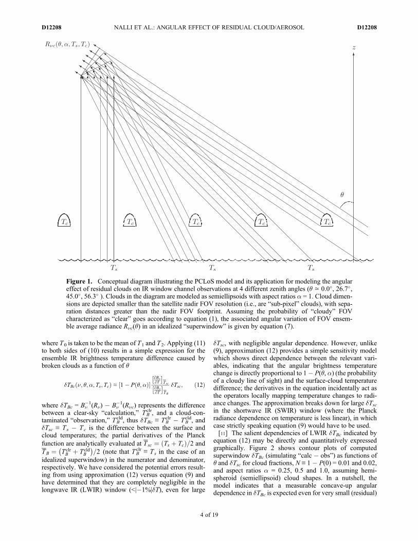
[10] Figure 1 provides a 2-D schematic showing theapplication of the PCLoS model for modeling the angulareffect of residual clouds (hemispheroidal shapes) on IRwindow channel observations. Naber and Weinman [1984]showed that a uniform broken cloud field (modeled as rightcylinders or cuboidal arrays) should result in a decrease inobserved brightness temperature with zenith angle. Assum-ing clouds to be isothermal blackbodies overlying a black-body surface, the variation of average upwelling radiance in a“superwindow” (i.e., an idealized super-transparent micro-window whereby we consider gas attenuation to be negligi-ble) for an ensemble of observations is then approximatedsimply as [e.g., Naber and Weinman, 1984]

Rnc q;a; Ts; Tcð Þ ≈ P q;að ÞBn Tsð Þ þ 1� P q;að Þ½ �Bn Tcð Þ; ð7Þ

where Tc is the cloud temperature. For this idealizedcase, given Ts, the clear-sky “calculation,” which assumesP(q, a) = 1, would simply be

Rn Tsð Þ ¼ Bn Tsð Þ: ð8Þ

Taking the inverse Planck functions of radiative transferequations (RTEs) (7) and (8), and differencing yields

B�1n Rnð Þ � B�1

n Rncð Þ ¼ Ts � B�1n P q;að ÞBn Tsð Þf

þ 1� P q;að Þ½ �Bn Tcð Þg; ð9Þ

which can be used to calculate the change in brightness tem-perature resulting from cloud contamination, dTBc. However,to convey the underlying physics, we choose instead to remainin radiance space, directly subtracting RTE (7) from (8)

Rn Tsð Þ � Rnc q;a; Ts; Tcð Þ ¼ 1� P q;að Þ½ � � Bn Tsð Þ � Bn Tcð Þ½ �:ð10Þ

and then expressing the dual radiance terms on both sides aslinear functions of temperature via first order Taylor seriesapproximations

Bn T1ð Þ ≈ Bn T0ð Þ þ T1 � T0ð Þ ∂Bn∂T jT0

Bn T2ð Þ ≈ Bn T0ð Þ þ T2 � T0ð Þ ∂Bn∂T jT0

)

⇒ Bn T2ð Þ � Bn T1ð Þ ≈ T2 � T1ð Þ∂Bn

∂T jT0; ð11Þ

(5)


3 of 19

where T0 is taken to be the mean of T1 and T2. Applying (11)to both sides of (10) results in a simple expression for theensemble IR brightness temperature difference caused bybroken clouds as a function of q

dTBc n; q;a; Ts; Tcð Þ ≈ 1� P q;að Þ½ �∂Bn∂T

� T sc

∂Bn∂T

� TB

dTsc; ð12Þ

where dTBc = Bn�1(Rn) � Bn

�1(Rnc) represents the differencebetween a clear-sky “calculation,” TB

clr, and a cloud-con-taminated “observation,” TB

cld, thus dTBc ≡ TBclr � TB

cld, anddTsc ≡ Ts � Tc is the difference between the surface andcloud temperatures; the partial derivatives of the Planckfunction are analytically evaluated at T sc ¼ Ts þ Tcð Þ=2 andTB ¼ T clr

B þ T cldB

� �=2 (note that TB

clr ≡ Ts in the case of anidealized superwindow) in the numerator and denominator,respectively. We have considered the potential errors result-ing from using approximation (12) versus equation (9) andhave determined that they are completely negligible in thelongwave IR (LWIR) window (<|�1%|dT), even for large

dTsc, with negligible angular dependence. However, unlike(9), approximation (12) provides a simple sensitivity modelwhich shows direct dependence between the relevant vari-ables, indicating that the angular brightness temperaturechange is directly proportional to 1� P(q, a) (the probabilityof a cloudy line of sight) and the surface-cloud temperaturedifference; the derivatives in the equation incidentally act asthe operators locally mapping temperature changes to radi-ance changes. The approximation breaks down for large dTscin the shortwave IR (SWIR) window (where the Planckradiance dependence on temperature is less linear), in whichcase strictly speaking equation (9) would have to be used.[11] The salient dependencies of LWIR dTBc indicated by

equation (12) may be directly and quantitatively expressedgraphically. Figure 2 shows contour plots of computedsuperwindow dTBc (simulating “calc � obs”) as functions ofq and dTsc for cloud fractions, N ≡ 1 � P(0) = 0.01 and 0.02,and aspect ratios a = 0.25, 0.5 and 1.0, assuming hemi-spheroid (semiellipsoid) cloud shapes. In a nutshell, themodel indicates that a measurable concave-up angulardependence in dTBc is expected even for very small (residual)

Figure 1. Conceptual diagram illustrating the PCLoS model and its application for modeling the angulareffect of residual clouds on IR window channel observations at 4 different zenith angles (q ≃ 0.0�, 26.7�,45.0�, 56.3� ). Clouds in the diagram are modeled as semiellipsoids with aspect ratios a = 1. Cloud dimen-sions are depicted smaller than the satellite nadir FOV resolution (i.e., are “sub-pixel” clouds), with sepa-ration distances greater than the nadir FOV footprint. Assuming the probability of “cloudy” FOVcharacterized as “clear” goes according to equation (1), the associated angular variation of FOV ensem-ble average radiance Rnc(q) in an idealized “superwindow” is given by equation (7).


4 of 19

N as well as small dTsc typical of low-level marine boundarylayer (MBL) clouds. The impact of the residual cloud amountN (i.e., the degree of cloud contamination) acts as a near-linear multiplier, as is implied by equations (12) and (1) forsmall dN. The surface-cloud temperature difference dTsc actsin a similar manner. The effect is exasperated by larger aspectratios (i.e., taller clouds), as would also be expected from thelarger vertical surface areas.[12] These results are fundamentally unchanged for cal-

culations in the SWIR, as can be seen in Figure 3, whichshows the results for 2616 cm�1 (i.e., the AIRS super-window) using equation (9). Comparison with Figure 2reveals similar patterns and magnitudes, with the SWIRchannel only exhibiting slightly less sensitivity. Furthermore,we compared these against SWIR calculations using theapproximation (12) and found only a slight underestimationof the dTBc at the larger dTsc and q (not shown here), therebynot altering the general conclusion. Thus, from here on in thispaper calculations are performed for the LWIRwindow using

sensitivity equations similar to (12) derived from the radiancelinearization approximation (11) without loss of generality.

3. Modeled Impact of an Aerosol Layer

[13] We may consider the angular variation of super-window radiance caused by a uniform, plane-parallel aerosollayer (e.g., Saharan dust) overlying a blackbody surface as

Rna q; tna; Ts; Tað Þ ≈ Bn Tsð ÞT na q; tnað Þ

þZ 1

T na

Bn Ta zð Þ½ �dT ′na q; tna z1; zð Þ½ �; ð13Þ

where Ta(z) is the aerosol layer temperature at level z,and T na q; tnað Þ, the aerosol layer IR channel transmittance(assuming negligible scattering), is defined by

T na q; tna z1; z2ð Þ½ � ≡ exp �tna z1; z2ð Þsec qð Þ½ �; ð14Þ

Figure 2. Modeled LWIR sensitivity dTBc (n= 909.1 cm�1; l = 11.0 mm) due to semiellipsoid cloudsbased on equation (12) as a function of surface-cloud layer temperature difference, dTsc, and zenith angle q,with residual cloud fractions (top) N = 0.01 and (bottom) N = 0.02, for aspect ratios (left) a = 0.25, (middle)a = 0.5, and (right) a = 1.


5 of 19

where tna(z1, z2) is the aerosol optical depth (AOD) in theIR channel n from z1 (bottom) to z2 (top). Defining a meanaerosol layer radiance pertaining to an effective mean tem-perature �Ta , that is Bn Ta

� �≡R 1T na

Bn Tað ÞdT ′na=R 1T na

dT ′na ,and applying to equation (13) yields

Rna q; tna; Ts; �Tað Þ ≈ T na q; tnað ÞBn Tsð Þ þ 1� T na q; tnað Þ½ �Bn �Tað Þ;ð15Þ

which is similar in form to equation (7), but is more gen-erally valid for each individual FOV as opposed to a largeensemble.[14] As above, a clear-sky superwindow “calculation” that

assumes T na q; tnað Þ ¼ 1, is again simply equation (8), andthus the LWIR dTBa due to aerosol contamination wouldapproximately be

dTBa n; q; tna; Ts; �Tað Þ ≈ 1� exp �tnasec qð Þ½ �∂Bn∂T

� T sa

∂Bn∂T

� TB

dTsa; ð16Þ

where dTBa represents Bn�1(Rn) � Bn

�1(Rna) ≡ TBclr � TB

aer,dTsa≡Ts � �Ta (the difference between the surface and aerosollayer temperatures), and �T sa is the mean of Ts and �Ta.[15] We again use contour plots to convey the implications

of equation (16) for dTBa in Figure 4, which, as above, showscomputed superwindow dTBa (simulating “calc � obs”) forAOD contamination with solar-spectrum magnitudes ta ={0.05, 0.1, 0.15, 0.2, 0.3, 0.4}. Note that because AOD iscommonly discussed in solar-spectrum magnitudes (due tothe vast preponderance of measurements, both satellite andsurface-based, in these wavelengths), we have chosen topresent results in these terms. We approximate AOD at IR nusing tna = 0.25 � ta, which Pierangelo et al. [2004] andDeSouza-Machado et al. [2010] both found as a good scalingfor comparing dust AOD derived from AIRS against otherA-Train visible-band sensors. Based upon the computed dTBain Figure 4, significant concave-up angular dependence indTBa is expected due to aerosol contamination (i.e., small ta)as well as small dTsa typical of lower-tropospheric aeolianaerosol advection. Magnitudes of dTBa for the smaller AODvalues in the figure are similar to those dTBc corresponding

Figure 3. Same as Figure 2 except SWIR sensitivity dTBc (n = 2616 cm�1) using equation (9).


6 of 19

Figure 4. Modeled LWIR sensitivity dTBc (K) (n = 909.1 cm�1; l = 11.0 mm) due to dust aerosols as afunction of surface-aerosol layer temperature difference, dTsa, and zenith angle q for a range of solar spec-trum AOD values, ta = {0.05, 0.10, 0.15, 0.20, 0.30, 0.40}, assuming tna = ta/4 dust AOD scaling betweenIR and solar channels.


7 of 19

to small cloud-fractions in Figure 2. Because of the IRscaling factor, the IR dtna depicted in the figure is rela-tively small (spanning only ≃0.09), thereby leading to thenear-linear sensitivity seen in the figure as implied byequation (16), similar to the residual cloud contaminationdiscussed in Section 2.2.

4. Modeled Impact of an Aerosol LayerOver/Under Broken Opaque Clouds

[16] We may extend the above models to cases involvingboth clouds and aerosols. In the first case the aerosol layeris assumed to lie at or below the cloud top heights, that is,za ≤ zc, and similarly, in the second case the aerosol layeris assumed to lie at or above the cloud bases, za ≥ zc(e.g., Saharan dust outflow over the Atlantic). Following theprevious lines of reasoning in sections 2.2 and 3, the equa-tions for the angular variation in radiance may be derived as

Rn q;a; tna; Ts; Tc; �Tað Þ ≈P q;að ÞRna q; tna;Ts; �Tað Þ þ 1� P q;að Þ½ �Bn Tcð Þ; za ≤ zc

T na q; tnað ÞRnc q;a;Ts; Tcð Þ þ 1� T na q; tnað Þ½ �Bn �Tað Þ; za ≥ zc;

�

ð17Þ

where Rna q; tna; Ts; �Tað Þ and Rnc(q, a, Ts, Tc) are theradiances emerging from the aerosol or cloud layers (found infirst terms on the right side), given by equations (15) or (7),respectively. Making these substitutions and subtractingfrom the clear-sky “calculation” (8) yields

dTBca n; q;a; tna; Ts; Tc; �Tað Þ ≈

dTsc∂Bn

∂T

��T sc

� P q;að ÞdTac∂Bn

∂T

��Tac

� P q;að ÞT na q; tnað ÞdTsa∂Bn

∂T

��T sa

!∂Bn

∂T

��1

�TB

; ð18Þ

and

dTBac n; q;a; tna; Ts; Tc; �Tað Þ ≈

dTsa∂Bn

∂T

��T sa

þ T na q; tnað ÞdTac∂Bn

∂T

��T ac

� P q;að ÞT na q; tnað ÞdTsc∂Bn

∂T

��T sc

!∂Bn

∂T

��1

�TB

; ð19Þ

where �T sc, dTsc and �T sa, dTsa are as defined for equations (12)and (16), respectively, with �Tac similarly defined as the meanof Tc and �Ta and dTac ≡ �Ta � Tc. For simplicity, it is useful toconsider the special case of �Ta ≈ Tc, which, after substitutinginto either (18) or (19), then making the substitution for T nagiven by (14), results in

dTB n; q;a; tna; Ts; Tc ¼ �Tað Þ ≈

½1� P q;að Þexp �tna sec qð Þ�∂Bn∂T

� �T sc

∂Bn∂T

� �TB

dTsc; ð20Þ

which is generally valid for an aerosol layer above or belowthe cloud layer.

[17] As in sections 2.2 and 3, Figure 5 shows plots ofcomputed LWIR superwindow dTBca based upon equation (20)for semiellipsoid clouds similar to those in section 2.2, exceptintroducing residual, solar-spectrum dust AOD contamina-tion ta = {0.05, 0.1}, with dTsc = {5.0, 10.0} K (dTsc basedroughly upon the empirical-hypothetical model comparisonin section 5, Figure 6). As with Figures 2 and 4, significantmeasurable angular impact on the order of tenths of a Kelvinis to be expected even from very small cloud fractions andmarine background levels of dust for what may be considereda surface-cloud/aerosol temperature difference typical ofMBL clouds and lower-tropospheric aeolian dust advection.Linearity is most clearly apparent as a function of dTsc(comparing the top plots against the bottom plots) as a directimplication of our sensitivity equation (20), where dTB isseen to be directly proportional to dTsc.

5. Empirical Impact of Aerosolsand Residual Clouds

[18] In addition to the simple models discussed above,we may also turn to previous studies empirically examiningthe impact of aerosols on IR observations. Specifically, Nalliand Stowe [2002] and Nalli and Reynolds [2006] conductedextensive global ocean analyses examining the depression ofAVHRR-derived multichannel SST (MCSST) [e.g., Waltonet al., 1998] against buoy measured SST versus AVHRR0.63 mm AOD. It was acknowledged in these papers thatthere would be an implicit correction for any residual cloudseluding the cloud mask and aliased as AOD. Because theseare empirical studies, there are limits of strict applicability,but the results nevertheless are useful in providing anempirical quantitative sense of global mean dTBa(q, ta)resulting from aerosol contamination as follows.[19] The cloud-masked aerosol correction (i.e., for anom-

alous levels elevated above background conditions, definedby ta ≥ 0.15) to a MCSST algorithm trained using a samplewith background aerosol and residual cloud conditions (i.e.,ta < 0.15) is given by a linear parametric equation of the formdTs ≡ Ts � Ts′ = b0 + b1x1, where x1 ≡ tasec(q), and Ts and Ts′are the buoy measured SST and aerosol/cloud-contaminatedMCSST, respectively. Assuming a hypothetical MCSSTalgorithm trained on a pristine atmosphere (i.e., aerosol andcloud free, P 0ð Þ ¼ T na ¼ 1 ), the constant parameter, b0,vanishes, leaving dTs = b1x1 for all ta, including backgroundlevels (assuming the linear relationship derived for ta ≥ 0.15extends below 0.15). Realizing that the hypothetical MCSSTalgorithm corrects for the remaining H2O absorption, theretrieved Ts′ is akin to the aerosol-contaminated observation,Ts′ ≃ Bn

�1(R′n), where R′n = Rna as defined by equation (13),and n within the range of ≃800–1000 cm�1. Thus, theempirical dTs may be considered to approximate the modeldTBa defined by equation (16) and we have

dTBa q; tað Þ ≈ b1tasec qð Þ; ð21Þ

where the parameter b1 was empirically determined to be|b1| = 1.98 by Nalli and Stowe [2002].[20] Note that equation (21) has the advantage of having

no explicit dependence on dTsa as in equation (16), but ratherimplicitly accounts for a global mean dTsa given it wasderived from a global multiyear sample. However, we must


8 of 19

keep in mind that this approach is valid insofar as theMCSSTused in the training of (21) accurately corrected for watervapor under all aerosol conditions. The premise of theMCSST algorithm is to correct a window channel measure-ment (11 mm) for water vapor given the known variation ofcontinuum absorption in the 800–1000 cm�1 LWIR window.The greater the column H2O, the more positive is the split-window difference (11–12 mm), which in turn provides thecorrection as desired. However, larger dust aerosol loadingleads to a smaller split-window difference, thereby reducingthe H2O correction, and thus leading to an additional coldbias artifact not directly related to the aerosol attenuation ina given channel.[21] Subtracting calculations derived from the hypothetical

model equation (16) from those predicted by equation (21),assuming tna = ta /4 for dust aerosols in a nominal LWIR

window channel n = 909.1 cm�1 (l = 11.0 mm), provides ahypothetical estimate of the magnitude of errors to beexpected from the use of (21) as given in Figure 6. Notethe existence of a zero line, which remains approximatelyconstant in the range of dsa ≃ 8.2 to 9.5 K, where the Nalliand Stowe [2002] aerosol correction is in exact agreementwith the model prediction given by equation (16). Given thattropospheric aerosols typically reside just above or withinthe boundary layer, this value is physically reasonable,and corroborates that equation (21) implicitly corrects fora global-mean, ocean surface-aerosol temperature differ-ence (8.2 ≲ dsa ≲ 9.5 K). Note also that the value of taused acts primarily as a multiplier; thus, any minor devia-tions from our assumption of tna = ta /4 will not significantlyalter the location of the zero line, nor substantially changethe overall dependencies. We thus conclude that there is

Figure 5. Modeled LWIR sensitivity dTBca (K) (n = 909.1 cm�1; l = 11.0 mm) due to a layer of semiel-lipsoid clouds (a = 0.5) and residual dust aerosols (for the special case of Tc ¼ �Ta) as a function of cloudfraction N and zenith angle q for surface-cloud/aerosol temperature differences (top) dTsc = dTsa = +5.0 Kand (bottom) dTsc = dTsa = +10.0 K. (left) Results without aerosols (ta = 0) equivalent to those shown inFigure 2 and (middle and right) introduction of an aerosol layer (solar spectrum AOD values, ta = 0.05and 0.1, respectively) assuming tna = ta /4 dust AOD scaling between the IR and solar channels.


9 of 19

reasonable agreement between the empirical and modeledaerosol effects.

6. Modeled Impact of a Layer of BrokenSemitransparent Clouds

[22] In this section, we generalize the model for Poisson-distributed opaque clouds presented in Section 2 to cloudsof a given arbitrary opacity and formulate the ensembleangular variation of superwindow radiance caused by a fieldof broken semitransparent clouds (assuming negligible IRscattering and that rays do not pass through more than onecloud), as is common with high level clouds composed ofice crystals (viz., cirrus):

Rnc q;a; tnc; Ts; �Tcð Þ ≈ P q;að ÞBn Tsð Þ þ 1� P q;að Þ½ �� Bn Tsð ÞT nc q; tncð Þ þ Bn �Tcð Þ 1� T nc q; tncð Þ½ �f g; ð22Þ

where, similar to aerosols, �Tc is the cloud mean temperature,and T nc q; tncð Þ is the mean cloud IR transmittance. Becausecloud shapes have finite horizontal extents, the cloud meanslant-path optical thickness is a function of the cloud shapeand aspect ratio, and thus cannot be determined simply bymultiplying by the secant of q, but instead is given moregenerally as

T nc q; tnc z1; z2ð Þ½ � ≡ exp �tnc z1; z2ð ÞS q;að Þ�

; ð23Þ

where tnc(z1, z2) is the cloud mean IR optical depth from z1to z2 (cloud bottom to top), and

S q;að Þ ≡ �s q;að Þ�s 0;að Þ ð24Þ

is the mean slant-path through the cloud shape, �s q;að Þ, nor-malized by its value evaluated at q = 0. We derive analytical

Figure 6. Difference between empirical and modeled LWIR dTBa (K) due to aerosols for n = 909.1 cm�1;l = 11.0 mm), determined by subtracting calculations using equation (16) from those using (21), assumingtna = ta / 4 dust AOD scaling between IR and solar channels. Note the existence of a zero line that remainsnearly constant in the range of dTsa ≃ 8.2 to 9.5 K.


10 of 19

expressions of S for cloud shapes used in the PCLoS modelbelow.

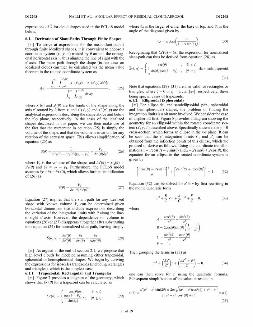
6.1. Derivation of Slant-Paths Through Finite Shapes

[23] To arrive at expressions for the mean slant-path �sthrough finite idealized shapes, it is convenient to choose acoordinate system (x′, y, z′) rotated by q around the orthog-onal horizontal axis y, thus aligning the line of sight with thez′ axis. The mean path through the shape (in our case, anidealized cloud) can then be calculated via the mean valuetheorem in the rotated coordinate system as

�s qð Þ ¼

Z y2

y1

Z x′2 qð Þ

x′1 qð Þsþ x′; yð Þ � s� x′; yð Þ½ �dx′dy

Z y2

y1

Z x′2 qð Þ

x′1 qð Þdx′dy

; ð25Þ

where x′1(q) and x′2(q) are the limits of the shape along theaxis x′ rotated by q from x, and s+(x′, y) and s�(x′, y) are theanalytical expressions describing the shape above and belowthe x′-y plane, respectively. In the cases of the idealizedshapes discussed in this paper, we can then make use ofthe fact that the numerator in equation (25) is simply thevolume of the shape, and that the volume is invariant for anyrotation of the cartesian space. This allows simplification ofequation (25) as

�s qð Þ ¼ Vs

x′2 qð Þ � x′1 qð Þ½ � y2 � y1ð Þ ¼Vs

dx′ qð Þdy ; ð26Þ

where Vs is the volume of the shape, and dx′(q) ≡ x′2(q) �x′1(q) and dy = y2 � y1. Furthermore, the PCLoS modelassumes dy = dx = dx′(0), which allows further simplificationof (26) as

�s qð Þ ¼ Vs

dx′ qð Þ dx′ 0ð Þ : ð27Þ

Equation (27) implies that the slant-path for any idealizedshape with known volume Vs can be determined givenhorizontal dimensions that include expressions describingthe variation of the integration limits with q along the line-of-sight x′-axis. However, the dependence on volume inequations (26) or (27) disappears altogether after substitutinginto equation (24) for normalized slant-path, leaving simply

S q;að Þ ¼ dx′ 0ð Þdx′ qð Þ ¼

dxdx′ qð Þ ¼

dzadx′ qð Þ : ð28Þ

[24] As argued at the end of section 2.1, we propose thathigh level clouds be modeled assuming either trapezoidal,spheroidal or hemispheroidal shapes. We begin by derivingthe expressions for isosceles trapezoids (including rectanglesand triangles), which is the simplest case.6.1.1. Trapezoidal, Rectangular and Triangular[25] Figure 7 provides a diagram of the geometry, which

shows that dx′(q) for a trapezoid can be calculated as

dx′ qð Þ ¼cos qð Þdx; qj j < z

cos q� qdð Þsin qdð Þ dz; qj j ≥ z ;

8<: ð29Þ

where dx is the larger of either the base or top, and qd is theangle of the diagonal given by

qd ¼ arctana

1� a tan zð Þ

� �: ð30Þ

Recognizing that dx′(0) = dx, the expression for normalizedslant-path can thus be derived from equation (28) as

S q;að Þ ¼sec qð Þ ; qj j < z

1

asin qdð Þsec q� qdð Þ ; qj j ≥ z

; slant-path; trapezoid:

(

ð31Þ

Note that equations (29)–(31) are also valid for rectangles ortriangles, where z = 0 or z ¼ arctan 1

2a

� �, respectively, these

being special cases of trapezoids.6.1.2. Ellipsoidal (Spheroidal)[26] For ellipsoidal and semiellipsoidal (viz., spheroidal

and hemispheroidal) shapes, the problem of finding theintegration limits is a bit more involved.We consider the caseof a spheroid first. Figure 8 provides a diagram showing thegeometry for an ellipsoid within the rotated coordinate sys-tem (x′, y, z′) described above. Specifically shown is the y = 0cross-section, which forms an ellipse in the x-z plane. It canbe seen that the x′ integration limits x′1 and x′2 can beobtained from the inflection points of this ellipse, which weproceed to derive as follows. Using the coordinate transfor-mations x = x′cos(q)� z′sin(q) and z = x′sin(q) + z′cos(q), theequation for an ellipse in the rotated coordinate system isgiven by

x′cos qð Þ � z′sin qð Þa

�2þ x′sin qð Þ þ z′cos qð Þ

c

�2¼ 1: ð32Þ

Equation (32) can be solved for z′ ≡ s by first rewriting inthe monic quadratic form

z′2 þ B

Cx′z′þ A

Cx′2 þ F

C¼ 0; ð33Þ

where

A ¼ cos2 qð Þa2

þ sin2 qð Þc2

B ¼ 2cos qð Þsin qð Þ 1

c2� 1

a2

� �

C ¼ sin2 qð Þa2

þ cos2 qð Þc2

F ¼ �1:

Then grouping the terms in (33) as

z′2 þ Bx′

C

� �zþ Ax′2 þ F

C

� �¼ 0; ð34Þ

one can then solve for z′ using the quadratic formula.Subsequent simplification of the solution results in

z′ qð Þ ¼x′ a2 � c2ð Þsin 2qð Þ � 2ac

ffiffiffiffiffiffiffiffiffiffiffiffiffiffiffiffiffiffiffiffiffiffiffiffiffiffiffiffiffiffiffiffiffiffiffiffiffiffiffiffiffiffiffiffiffiffiffiffiffiffiffiffiffia2 � c2ð Þcos2 qð Þ þ c2 � x′2

q2 a2 � c2ð Þcos2 qð Þ þ c2½ � ≡ s qð Þ;

ð35Þ


11 of 19

and taking the second derivative yields

∂2z′∂x′2

¼ � ac

a2 � c2ð Þcos2 qð Þ þ c2 � x′2� 3=2 : ð36Þ

Further inspection of Figure 8 reveals that the inflectionpoints occur where the first derivative ∂z′/∂x′ → ∞; thisimplies that we may expect that ∂2z′=∂x′2 →∞ at the inflec-tion points as well. This is certainly true for the cases of theellipse in canonical position (q = 0�) or for a rotation of 90�,

where we know that the inflection points are simply �aor �c, respectively — in both cases the denominator goesto zero in equation (36). Therefore we seek a solution to

1

∂2z′=∂x′2¼ 0; ð37Þ

which upon substitution of (36) yields the critical points

x ′c qð Þ ¼ �ffiffiffiffiffiffiffiffiffiffiffiffiffiffiffiffiffiffiffiffiffiffiffiffiffiffiffiffiffiffiffiffiffiffiffiffiffiffiffiffiffiffiffia2 � c2ð Þcos2 qð Þ þ c2

p: ð38Þ

Figure 7. Diagram showing geometry for deriving mean slant-path through an isosceles trapezoid (a < 1)with side inclination angles, z, and dx = dy, using a coordinate system (x′, y, z′) rotated by angle q from thelocal zenith (z) around the orthogonal horizontal (y) axis (directed into the page), aligning the observer line-of-sight with the z′ axis. Shown here is the case for q ≥ z rotation, whereby the x′-limits are determined bythe diagonal, defined at the diagonal angle qd measured relative to the cloud base/top (dx), as opposed tothose determined by dx for q < z. The diagram also applies to rectangles and isosceles triangles whenz = 0 or z = arctan[1/(2a)], respectively, these being special cases of a trapezoid.


12 of 19

To establish that x′c are indeed inflection points, we tested fora change in concavity by evaluating ∂2z′=∂x′2 at x′c � Dx′,where Dx′ = 1.0 � 10�6, and confirmed a change in sign tothis level of precision. Equation (38) may also be exactlyconfirmed as the x′ limits by substituting into the square rootterm in (35), which becomes zero, thus resulting in a singlevalue of z′(q) (instead of two) at �x′c(q), which is only pos-sible at the x′ tangent points. We thus conclude that the x′cgiven by (38) are the inflection points of the ellipse in therotated x′-z′ plane, these providing the x′ limits for integra-tion, and thus dx′(q) = 2|x′c(q)|. Given the known volume of aspheroid Vs ¼ 4

3pa2c , from equation (27) we arrive at

the expression for the mean slant-path through a spheroid interms of the semi-major and semi-minor axes

�s qð Þ ¼ pac3ffiffiffiffiffiffiffiffiffiffiffiffiffiffiffiffiffiffiffiffiffiffiffiffiffiffiffiffiffiffiffiffiffiffiffiffiffiffiffiffiffiffiffia2 � c2ð Þcos2 qð Þ þ c2

p : ð39Þ

From either (24) or (28) the normalized slant-path is then

S qð Þ ¼ affiffiffiffiffiffiffiffiffiffiffiffiffiffiffiffiffiffiffiffiffiffiffiffiffiffiffiffiffiffiffiffiffiffiffiffiffiffiffiffiffiffiffia2 � c2ð Þcos2 qð Þ þ c2

p ; ð40Þ

which, taking a = c/a and c = 1/2, may be written in finalform in terms of aspect ratio a as

S q;að Þ ¼ 1ffiffiffiffiffiffiffiffiffiffiffiffiffiffiffiffiffiffiffiffiffiffiffiffiffiffiffiffiffiffiffiffiffiffiffiffiffiffiffiffiffiffiffi1� a2ð Þcos2 qð Þ þ a2

p ; slant-path; spheroid: ð41Þ

6.1.3. Semiellipsoidal (Hemispheroidal)[27] For the case of a semiellipsoid (hemispheroid), the

situation is similar to that of the ellipsoid (spheroid), exceptthat the x′-limit at the observer side is no longer at the

inflection point, but rather at x′1 = a cos(q), as seen inFigure 9. Thus, given equation (38), dx′(q) becomes

dx′ qð Þ ¼ a cos qð Þ þffiffiffiffiffiffiffiffiffiffiffiffiffiffiffiffiffiffiffiffiffiffiffiffiffiffiffiffiffiffiffiffiffiffiffiffiffiffiffiffiffiffiffia2 � c2ð Þ cos2 qð Þ þ c2

p; ð42Þ

yielding the hemispheroid mean slant-path from (27) as

�sðqÞ ¼ pac

3ffiffiffiffiffiffiffiffiffiffiffiffiffiffiffiffiffiffiffiffiffiffiffiffiffiffiffiffiffiffiffiffiffiffiffiffiffiffiffiffiffiffiffiða2 � c2Þcos2ðqÞ þ c2

pþ a cosðqÞ

h i ; ð43Þ

and the normalized slant-path in terms of a as

S q;að Þ ¼2

cos qð Þ þffiffiffiffiffiffiffiffiffiffiffiffiffiffiffiffiffiffiffiffiffiffiffiffiffiffiffiffiffiffiffiffiffiffiffiffiffiffiffiffiffiffiffiffiffiffiffi1� 4a2ð Þcos2 qð Þ þ 4a2

p ; slant-path; hemispheroid:

ð44Þ

6.1.4. Discussion[28] The expressions for normalized mean slant-paths, S, as

given by equations (31), (41), and (44), are plotted inFigure 10 for shapes with aspect ratios of 0.5. The left plotshows the results on cartesian axes, whereas the right plotshows the same results on polar axes. Slant paths are seen toincrease from unity at q = 0� to twice that at q = 90�, asexpected. The rectangular shape actually experiences areduction in mean slant path from 0� to 53.1�, reaching aminimum at the diagonal angle, which from equation (30) isqd = 26.6�. This behavior stems from the large reduction inpath lengths at the corners. The trapezoid and semiellipsoid(hemispheroid) shapes exhibit similar behavior for this partic-ular trapezoid inclination angle, z = 0.75 � max(z) = 33.75�,but this similarity is lost as z is modified from this value, as seen

Figure 8. Same as Figure 7 except showing geometry for an spheroidal cloud (i.e., an ellipsoid with equalhorizontal semi-axes, a = b). The diagram shows the ellipse cross-section at the x-z plane, with the observerline-of-sight directed along the z′ axis, and is drawn with the vertical semiminor axis c = a/2 (a = 0.5). Thex′-limits for integration, x′1 and x′2, are derived from the inflection points of the ellipse, p1 and p2.


13 of 19

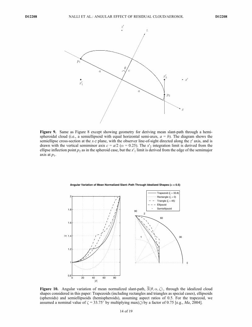
Figure 10. Angular variation of mean normalized slant-path, S q;a; zð Þ , through the idealized cloudshapes considered in this paper: Trapezoids (including rectangles and triangles as special cases), ellipsoids(spheroids) and semiellipsoids (hemispheroids), assuming aspect ratios of 0.5. For the trapezoid, weassumed a nominal value of z = 33.75� by multiplying max(z) by a factor of 0.75 [e.g., Ma, 2004].

Figure 9. Same as Figure 8 except showing geometry for deriving mean slant-path through a hemi-spheroidal cloud (i.e., a semiellipsoid with equal horizontal semi-axes, a = b). The diagram shows thesemiellipse cross-section at the x-z plane, with the observer line-of-sight directed along the z′ axis, and isdrawn with the vertical semiminor axis c = a/2 (a = 0.25). The x′2 integration limit is derived from theellipse inflection point p2 as in the spheroid case, but the x′1 limit is derived from the edge of the semimajoraxis at p1.


14 of 19

in the results for the rectangle (z = 0�) and triangle (z = 45�)cases. This is interesting given the potential similarity of the twoshapes (both with a flat end and tapered end) and the fact thatMa [2004] found the factor 0.74 brings the two into closestagreement in terms of the PCLoS. In the polar plot it is inter-esting to see how the angular variations of S q;að Þ take oncoherent characteristics related to the corresponding shapes.

6.2. Window Channel Radiance Sensitivity

[29] Given expressions for the angular variation of trans-mittance through finite shapes, equation (23), along with(31), (41), or (44), we return to equation (22). Introducingthe cloud effective emissivity, ɛnc(q, tnc), defined fromconservation of energy as [e.g., Platt and Stephens, 1980;Ackerman et al., 1990]

ɛnc q; tncð Þ ≡ 1� T nc q; tncð Þ; ð45Þ

(22) is then be expressed as

Rnc q;a; tnc; Ts; �Tcð Þ ≈ P q;að ÞBn Tsð Þ þ 1� P q;að Þ½ �� 1� ɛnc q; tncð Þ½ �Bn Tsð Þ þ ɛnc q; tncð ÞBn �Tcð Þf g; ð46Þ

which may be rewritten in a form analogous to (7), posses-sing individual surface and cloud emission terms

Rnc q;a; tnc; Ts; �Tcð Þ ≈ 1� ɛnc q; tncð Þ 1� P q;að Þ½ �f gBn Tsð Þþ ɛnc q; tncð Þ 1� P q;að Þ½ �Bn �Tcð Þ: ð47Þ

Subtracting (47) from the clear-sky “calculation” (8), rear-ranging and canceling terms, then yields a general LWIRcloud sensitivity equation

dTBc n; q;a; tnc; Ts; �Tcð Þ ≈ ɛnc q; tncð Þ 1� P q;að Þ½ �∂Bn∂T

� �T sc

∂Bn∂T

� �TB

dTsc;

ð48Þ

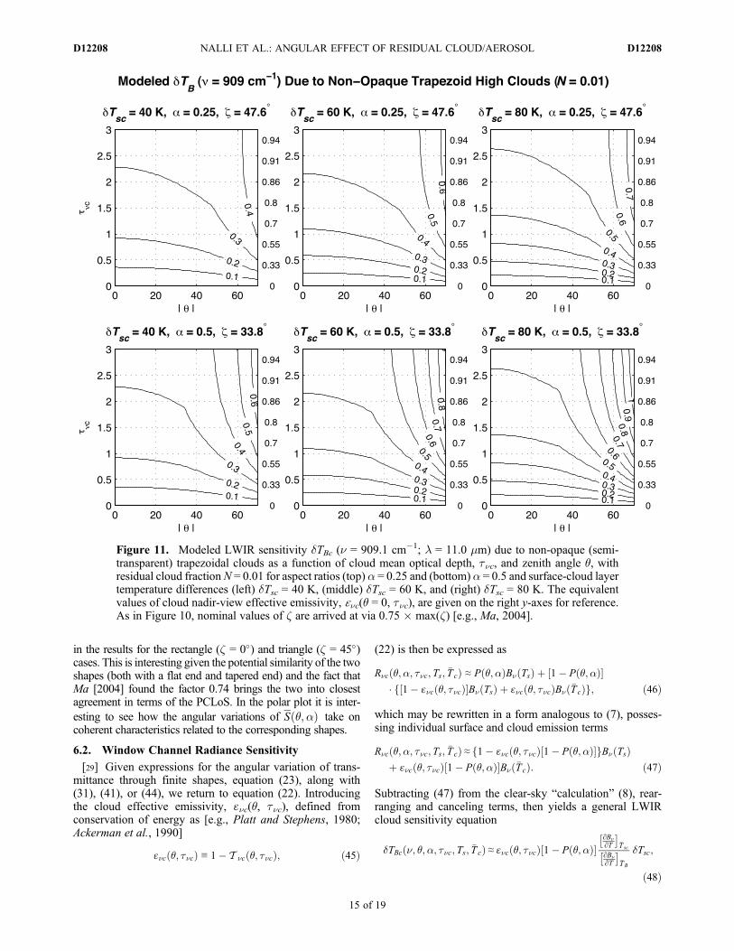
Figure 11. Modeled LWIR sensitivity dTBc (n = 909.1 cm�1; l = 11.0 mm) due to non-opaque (semi-transparent) trapezoidal clouds as a function of cloud mean optical depth, tnc, and zenith angle q, withresidual cloud fractionN = 0.01 for aspect ratios (top) a = 0.25 and (bottom) a = 0.5 and surface-cloud layertemperature differences (left) dTsc = 40 K, (middle) dTsc = 60 K, and (right) dTsc = 80 K. The equivalentvalues of cloud nadir-view effective emissivity, ɛnc(q = 0, tnc), are given on the right y-axes for reference.As in Figure 10, nominal values of z are arrived at via 0.75 � max(z) [e.g., Ma, 2004].


15 of 19

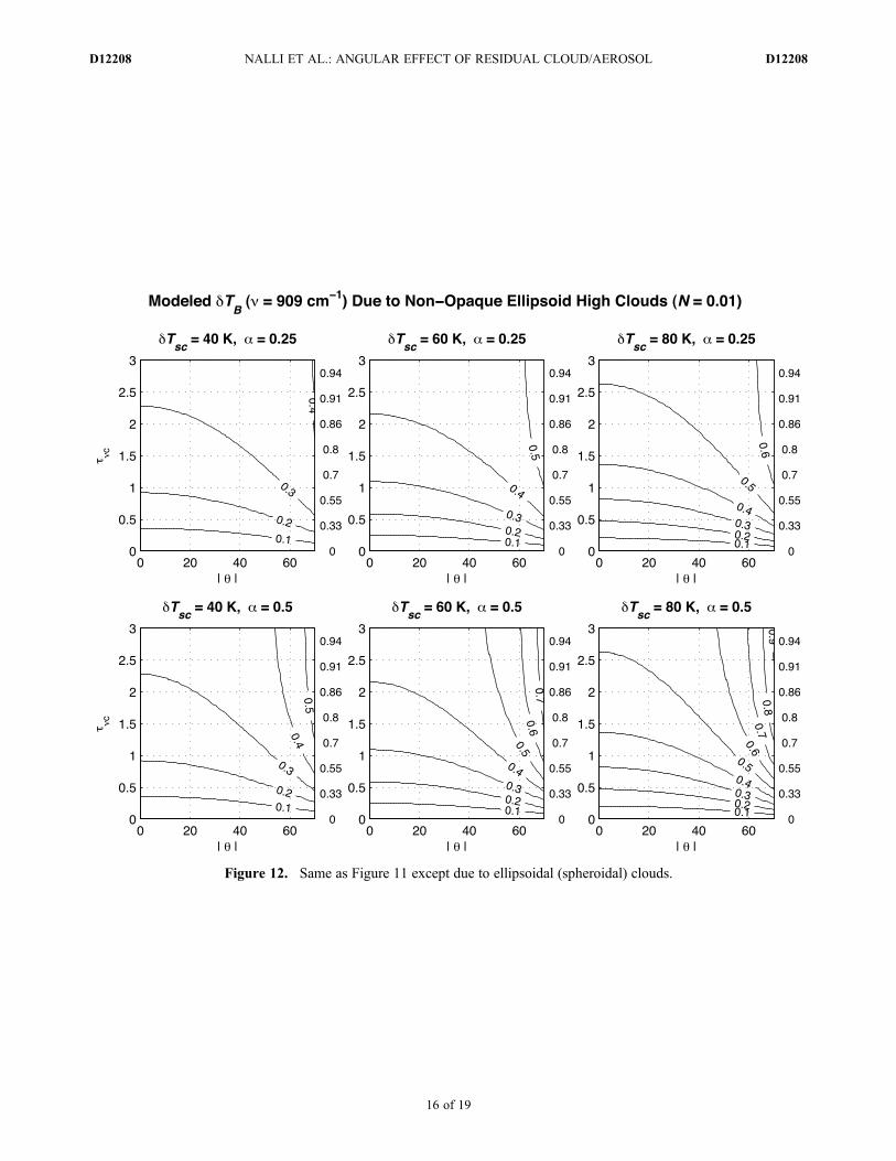
Figure 12. Same as Figure 11 except due to ellipsoidal (spheroidal) clouds.


16 of 19

which reduces to the special case of opaque clouds,equation (12), for tnc→∞, ɛnc(q, tnc) = 1. Note that the termɛnc(q)[1 � P(q, a)] represents the “effective cloud fraction,”a cloud parameter retrieved by IR sounders (viz., CrIMSS,IASI and AIRS) as will be discussed in part 2. Equation (48)implies that dTBc results from this parameter, which is amultiplicative combination of two effects, namely non-unityPCLoS, P(q,a) < 1, along with non-zero effective emissivity,ɛnc(q, tnc) > 0. Because increasing q brings about a decreasein P(q, a) and a simultaneous increase in ɛnc(q, tnc) (forclouds with a < 1), both effects act in the same direction withincreasing angle. Increasing a serves to increase the angularimpact of P, while simultaneously reducing the impact of ɛnc.[30] Figures 11–13 show contour plots of computed LWIR

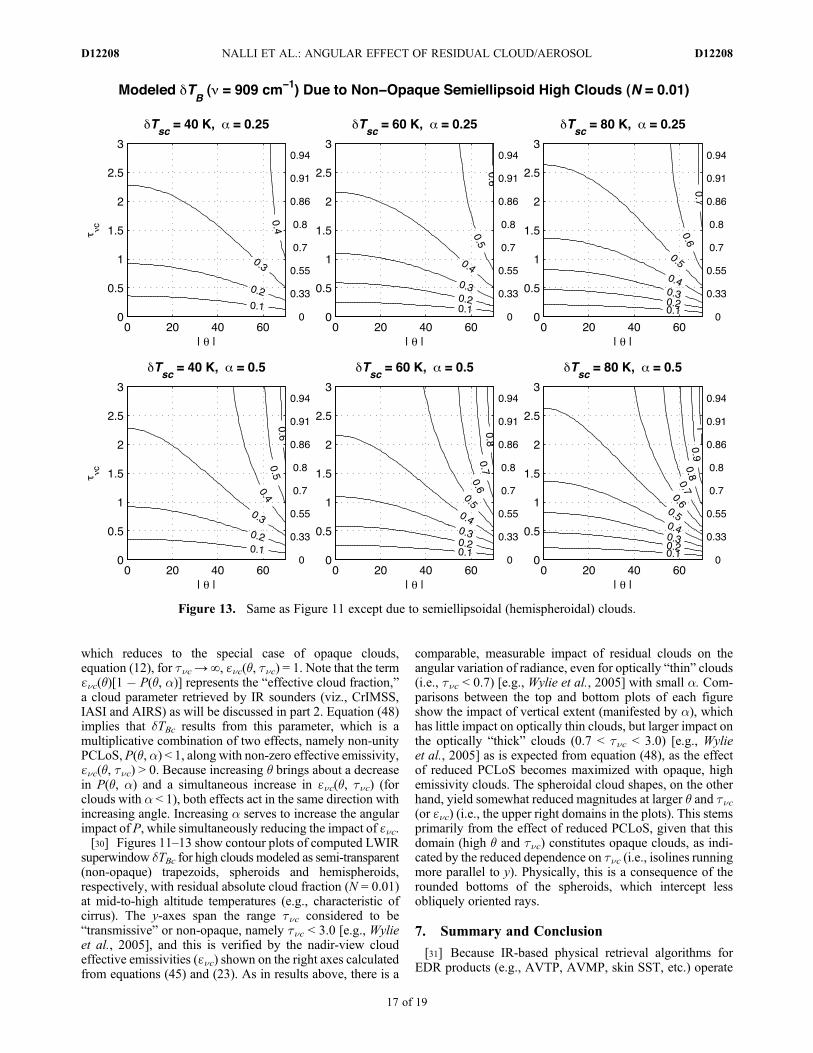
superwindow dTBc for high clouds modeled as semi-transparent(non-opaque) trapezoids, spheroids and hemispheroids,respectively, with residual absolute cloud fraction (N = 0.01)at mid-to-high altitude temperatures (e.g., characteristic ofcirrus). The y-axes span the range tnc considered to be“transmissive” or non-opaque, namely tnc < 3.0 [e.g., Wylieet al., 2005], and this is verified by the nadir-view cloudeffective emissivities (ɛnc) shown on the right axes calculatedfrom equations (45) and (23). As in results above, there is a

comparable, measurable impact of residual clouds on theangular variation of radiance, even for optically “thin” clouds(i.e., tnc < 0.7) [e.g., Wylie et al., 2005] with small a. Com-parisons between the top and bottom plots of each figureshow the impact of vertical extent (manifested by a), whichhas little impact on optically thin clouds, but larger impact onthe optically “thick” clouds (0.7 < tnc < 3.0) [e.g., Wylieet al., 2005] as is expected from equation (48), as the effectof reduced PCLoS becomes maximized with opaque, highemissivity clouds. The spheroidal cloud shapes, on the otherhand, yield somewhat reduced magnitudes at larger q and tnc(or ɛnc) (i.e., the upper right domains in the plots). This stemsprimarily from the effect of reduced PCLoS, given that thisdomain (high q and tnc) constitutes opaque clouds, as indi-cated by the reduced dependence on tnc (i.e., isolines runningmore parallel to y). Physically, this is a consequence of therounded bottoms of the spheroids, which intercept lessobliquely oriented rays.

7. Summary and Conclusion

[31] Because IR-based physical retrieval algorithms forEDR products (e.g., AVTP, AVMP, skin SST, etc.) operate

Figure 13. Same as Figure 11 except due to semiellipsoidal (hemispheroidal) clouds.


17 of 19

on the premise of minimizing clear-sky obs � calc, whereobs and calc are clear-sky observations and forward modelcalculations, respectively, it is important that differencesbetween obs and calc be minimal under well-characterizedconditions. In this vein, comparative analyses of calc and obsare often employed to improve the forward model physics, orotherwise “tune” the model for use with a particular sensor.In performing global analyses of this sort, however, there isan implicit assumption of accurate “clear-sky observations.”In this work, we revisited this assumption with considerationgiven to the fact that global clear-sky observations them-selves are usually obtained from either cloud-masking (in thecase of imagers) or cloud-clearing (in the case of sounders),and therefore in actuality constitute “products.” Furthermore,cloud-masking and cloud-clearing algorithms are not gener-ally designed to mask or correct for aerosols. Because of this,clear-sky observations will be subject to algorithmic errorsbeyond that of the sensor itself, this effect being referred to asresidual cloud and/or aerosol contamination. Generallyspeaking, residual clouds and aerosols remaining in clear-skywindow radiances will lead to an obs that is cold-biased [e.g.,Benner and Curry, 1998; Nalli and Stowe, 2002; Sokolik,2002; Maddy et al., 2011].[32] This work has explored this issue with attention given

to the potential for angular dependence resulting fromresidual cloud and/or aerosol contamination. In this paper,we presented idealized models that assume that residualcloud contamination may result in a signal similar to obser-vations obtained from a uniform cloud field with a very smallcloud fraction, where the probability of clear lines of sight(PCLoS) fundamentally diminishes with zenith observingangle. To model quantitatively the sensitivity of residualclouds on “superwindow” radiances, we uniquely appliedPCLoS models previously developed (for applications dif-ferent from ours) for single-layer broken opaque clouds (viz.,Kauth and Penquite [1967] and Taylor and Ellingson[2008]). Simple equations were derived for computing theimpact of opaque broken clouds on superwindow brightnesstemperatures, with similar equations derived for the impact ofcontamination by an aerosol layer, first in isolation, then overor underlying a cloud layer. The aerosol modeling resultswere then found to be reasonably consistent with previousglobal empirical parametric analyses using satellite imagerdata [e.g., Nalli and Stowe, 2002; Nalli and Reynolds, 2006].We then generalized the expression for opaque clouds toinclude semitransparent (non-opaque) clouds (viz., high-level cold clouds composed of ice-crystals). The latter effortrequired deriving analytical expressions for calculating themean slant-paths through finite idealized shapes.[33] Overall this work suggests that the possibility of

contamination by residual clouds and/or aerosols withinclear-sky observations can have a measurable concave-upimpact on the angular agreement with clear-sky calculationsthat do not, by definition, take into account these missingtransmittance terms (i.e., residual clouds and/or aerosols).Our hypothetical “superwindow” sensitivity models predictincreasing cold bias in contaminated “observations” withzenith angle on the order of tenths of Kelvins, the actualmagnitudes depending variously on the residual N and tnc(i.e., the degree of cloud contamination), the residual AOD(i.e., the degree of aerosol contamination), the dT between thesurface and the residual cloud/aerosol layers, and the cloud

shape and vertical aspect ratio. The angular dependencephysically stems from the increased probability of clouds atthese angles, as well as increased optical path in cases of non-opaque clouds with a < 1. The same goes for aerosol con-tamination due to increased optical path through the aerosollayer with angle. In the case of semitransparent clouds, thetwo effects tend to compensate each other: Larger (smaller)aspect ratios imply taller (shorter) clouds, which tend toenhance (reduce) the fundamental decrease in PCLoS(increase in cloudiness) with angle, but also reduce (enhance)the increase of slant-path (which can even be reversed in thecases of a > 1, assuming rays do not traverse more than onecloud). While the assumed cloud shapes have an impact theresults, these do not change the main thesis in any way. In allcases, the magnitudes are directly sensitive to the temperaturedifference between the cloud/aerosol layer and the surface.We test these hypothetical sensitivity results with experi-mental data in part 2.

[34] Acknowledgments. This research was supported by the NOAAJoint Polar Satellite System Office (NJO), NASA Research Announcement(NRA) NNH09ZDA001N, Research Opportunities in Space and EarthScience (ROSES-2009), Program Element A.41 (“The Science of Terraand Aqua”), the GOES-R Algorithm Working Group (AWG) (W. W. Wolfand T. Schmit, STARAWG leads), and the STAR Satellite Meteorology andClimatology Division (SMCD) (M. D. Goldberg, SMCD Division Chief ).We are grateful to the following individuals for their contributions in supportof this work: A. Ignatov and X. Liang (NESDIS/STAR), and CRTM inves-tigators P. van Delst (NWS/NCEP), Y. Han (STAR) and Y. Chen (JCSDA),for meetings and discussions pertaining to MICROS CRTM results (whichled to our finding and application of the PCLoS model to the problem ofcloud contamination), as well as their subsequent feedback on our initialresults presented at STAR in March 2011; and P. Keehn (NESDIS/STAR)for Java programming assistance needed for generating the ellipses inFigures 8 and 9. We also thank the three anonymous reviewers who pro-vided constructive feedback that we used to strengthen the paper. The near-realtime web-based MICROS system is accessible at: http://www.star.nesdis.noaa.gov/sod/sst/micros/. The views, opinions, and findings con-tained in this paper are those of the authors and should not be construed asan official NOAA or U.S. Government position, policy, or decision.

ReferencesAckerman, S. A., W. L. Smith, J. D. Spinhirne, and H. E. Revercomb(1990), The 27–28 October 1986 FIRE IFO cirrus case study: Specialproperties of cirrus clouds in the 8–12 mm window, Mon. Weather Rev.,118, 2377–2388.

Avaste, O. A., R. Mullamaa, K. Y. Niylisk, and M. A. Sulev (1974), On thecoverage of the sky by clouds, in Heat Transfer in the Atmosphere, editedby Y. M. Feygel’son and L. R. Tsvang, NASA Tech. Transl., TT F-790,173–181.

Benner, T. C., and J. A. Curry (1998), Characteristics of small tropicalcumulus clouds and their impact on the environment, J. Geophys. Res.,103(D22), 28,753–28,767.

Cayla, F. R. (1993), IASI infrared interferometer for operations andresearch, in High Spectral Resolution Infrared Remote Sensing forEarth’s Weather and Climate Studies, NATO ASI Ser., Ser. I, vol. 9,edited by S. Chedin, M. T. Chahine, and N. A. Scott, pp. 9–19, Springer,Berlin.

Chahine, M. T., et al. (2006), AIRS: Improving weather forecasting andproviding new data on greenhouse gases, Bull. Am. Meteorol. Soc.,87(7), 911–926.

Dash, P., and A. Ignatov (2008), Validation of clear-sky radiances overoceans simulated with MODTRAN4.2 and global NCEP GDAS fieldsagainst nighttime NOAA15-18 and MetOp-A AVHRR data, RemoteSens. Environ., 112, 3012–3029.

DeSouza-Machado, S. G., et al. (2010), Infrared retrievals of dust usingAIRS: Comparisons of optical depths and heights derived for a NorthAfrican dust storm to other collocated EOS A-Train and surface observa-tions, J. Geophys. Res., 115, D15201, doi:10.1029/2009JD012842.

Ellingson, R. G. (1982), On the effects of cumulus dimensions on longwaveirradiance and heating rate calculations, J. Atmos. Sci., 39, 886–896.


18 of 19

Hilton, F., et al. (2012), Hyperspectral Earth observation from IASI: Fiveyears of accomplishments, Bull. Am. Meteorol. Soc., 93(3), 347–370,doi:10.1175/BAMS-D-11-00027.1.

Kauth, R. J., and J. L. Penquite (1967), The probability of clear lines ofsight through a cloudy atmosphere, J. Appl. Meteorol., 6, 1005–1017.

Liang, X., and A. Ignatov (2011), Monitoring of IR clear-sky radiances overoceans for SST (MICROS), J. Atmos. Oceanic Technol., 28, 1228–1242,doi:10.1175/JTECH-D-10-05023.1.

Liang, X.-M., A. Ignatov, and Y. Kihai (2009), Implementation of the Com-munity Radiative Transfer Model in Advanced Clear-Sky Processor forOceans and validation against nighttime AVHRR radiances, J. Geophys.Res., 114, D06112, doi:10.1029/2008JD010960.

Ma, Y. (2004), Longwave radiative transfer through 3D cloud fields: Test-ing of the probability of clear line of sight models with the ARM cloudobservations, PhD thesis, 175 pp., Univ. of Md., College Park.

Maddy, E. S., et al. (2011), Using Metop-A AVHRR clear-sky measure-ments to cloud-clear Metop-A IASI column radiances, J. Atmos. OceanicTechnol., 28, 1104–1116, doi:10.1175/JTECH-D-10-05045.1.

Minnis, P. (1989), Viewing zenith angle dependence of cloudiness deter-mined from coincident GOES East and GOES West data, J. Geophys.Res., 94(D2), 2303–2320.

Naber, P. S., and J. A. Weinman (1984), The angular distribution of infraredradiances emerging from broken fields of cumulus clouds, J. Geophys.Res., 89(D1), 1249–1257.

Nalli, N. R., and R. W. Reynolds (2006), Sea surface temperature daytimeclimate analyses derived from aerosol bias-corrected satellite data, J. Clim.,19(3), 410–428.

Nalli, N. R., and L. L. Stowe (2002), Aerosol correction for remotely sensedsea surface temperatures from the National Oceanic and Atmospheric

Administration advanced very high resolution radiometer, J. Geophys.Res., 107(C10), 3172, doi:10.1029/2001JC001162.

Nalli, N. R., et al. (2012), Joint Polar Satellite System (JPSS) Cross-TrackInfrared Microwave Suite Sounding (CrIMSS) Environmental DataRecord validation status, in IGARSS 2012 Proceedings, Inst. of Electr.and Electron. Eng., New York, in press.

Pierangelo, C., A. Chédin, S. Heilliette, N. Jacquinet-Husson, and R. Armante(2004), Dust altitude and infrared optical depth from AIRS, Atmos. Chem.Phys. Discuss., 4, 3333–3358.

Platt, C. M. R., and G. L. Stephens (1980), The interpretation of remotelysensed high cloud emittances, J. Atmos. Sci., 37(10), 2314–2322.

Smith, W. L. S., H. Revercomb, G. Bingham, A. Larar, H. Huang, D. Zhou,J. Li, X. Liu, and S. Kireev (2009), Technical note: Evolution, currentcapabilities, and future advance in satellite nadir viewing ultra-spectralIR sounding of the lower atmosphere, Atmos. Chem. Phys, 9, 5563–5574.

Sokolik, I. N. (2002), The spectral radiative signature of wind-blownmineral dust: Implications for remote sensing in the thermal IR region,Geophys. Res. Lett., 29(24), 2154, doi:10.1029/2002GL015910.

Taylor, P. C., and R. G. Ellingson (2008), A study of the probability of clearline of sight through single-layer cumulus cloud fields in the tropicalwestern Pacific, J. Atmos. Sci., 65, 3497–3512.

Walton, C. C., W. G. Pichel, J. F. Sapper, and D. A. May (1998), The devel-opment and operational application of nonlinear algorithms for the mea-surement of sea surface temperatures with the NOAA polar-orbitingenvironmental satellites, J. Geophys. Res., 103(C12), 27,999–28,012.

Wylie, D. P., D. L. Jackson, W. P. Menzel, and J. J. Bates (2005), Trends inglobal cloud cover in two decades of HIRS observations, J. Clim., 18,3021–3031.


19 of 19

On the angular effect of residual clouds and aerosols in clear-sky infrared window radiance...

Documents

Transcript of On the angular effect of residual clouds and aerosols in clear-sky infrared window radiance...