Daylighting Simulations with Radiance using Matrix-based ...
145
Daylighting Simulations with Radiance using Matrix-based Methods Sarith Subramaniam October 2017
-
Upload
khangminh22 -
Category
Documents
-
view
0 -
download
0
Transcript of Daylighting Simulations with Radiance using Matrix-based ...

Daylighting Simulations with Radiance using Matrix-based Methods
Sarith Subramaniam
October 2017

Disclaimer
This document was prepared as an account of work sponsored by the United States Government. While
this document is believed to contain correct information, neither the United States Government nor any
agency thereof, nor The Regents of the University of California, nor any of their employees, makes any
warranty, express or implied, or assumes any legal responsibility for the accuracy, completeness, or
usefulness of any information, apparatus, product, or process disclosed, or represents that its use
would not infringe privately owned rights. Reference herein to any specific commercial product,
process, or service by its trade name, trademark, manufacturer, or otherwise, does not necessarily
constitute or imply its endorsement, recommendation, or favoring by the United States Government or
any agency thereof, or The Regents of the University of California. The views and opinions of authors
expressed herein do not necessarily state or reflect those of the United States Government or any
agency thereof or The Regents of the University of California.
Acknowledgments
This work was supported by the California Energy Commission through its Electric Program Investment
Charge (EPIC) Program on behalf of the citizens of California and by the Assistant Secretary for Energy
Efficiency and Renewable Energy, Building Technologies Program, of the U.S. Department of Energy,
under Contract No. DE-AC02-05CH11231.
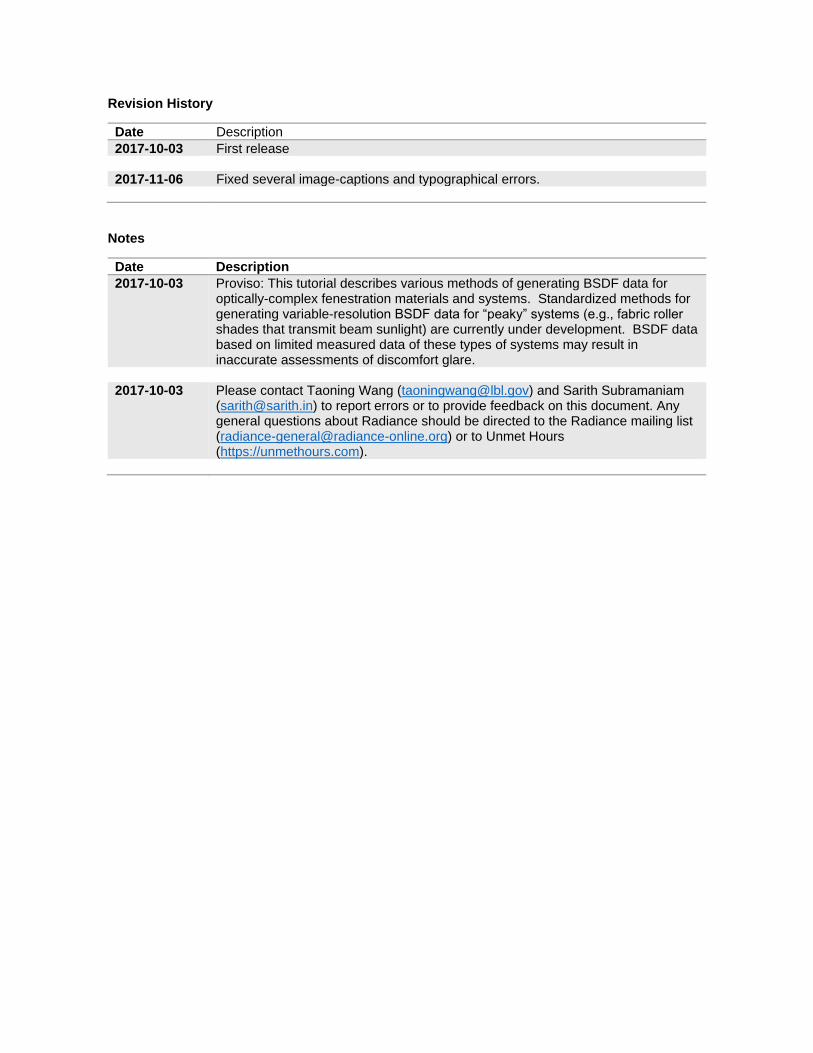
Revision History
Date Description
2017-10-03 First release 2017-11-06 Fixed several image-captions and typographical errors.
Notes
Date Description
2017-10-03 Proviso: This tutorial describes various methods of generating BSDF data for optically-complex fenestration materials and systems. Standardized methods for generating variable-resolution BSDF data for “peaky” systems (e.g., fabric roller shades that transmit beam sunlight) are currently under development. BSDF data based on limited measured data of these types of systems may result in inaccurate assessments of discomfort glare.
2017-10-03 Please contact Taoning Wang ([email protected]) and Sarith Subramaniam
([email protected]) to report errors or to provide feedback on this document. Any general questions about Radiance should be directed to the Radiance mailing list ([email protected]) or to Unmet Hours (https://unmethours.com).

Reviewers
This document was reviewed by the following individuals:
Greg Ward, Anyhere Software
David Geisler-Moroder, Bartenbach GmBH
Taoning Wang, Lawrence Berkeley National Laboratory (LBNL)
Eleanor Lee, LBNL

Table of Contents
Chapter 1. Introduction ........................................................................................................................... 8
1.1 Document Structure ................................................................................................................ 9
1.2 How to use this tutorial ............................................................................................................ 9
1.3 Text formatting ...................................................................................................................... 12
1.4 Navigation features in the PDF and a few notes on printing ................................................ 13
1.5 Some commonly used terms ................................................................................................ 14
Chapter 2. Theory ................................................................................................................................. 15
2.1 Background ........................................................................................................................... 15
2.2 Daylight Coefficients (The Two-Phase Method) and discretized skies ................................ 15
2.3 The Three-Phase Method ..................................................................................................... 18
2.4 The Four-Phase Method (with F-Matrix) ............................................................................... 20
2.5 Methods with accurate spatial resolution: Two-Phase DDS, Five Phase and Six-Phase .... 23
Chapter 3. Radiance programs for Daylighting simulations ................................................................. 29
3.1 Programs for creating sky definitions .................................................................................... 29
3.2 Programs for ray-tracing, ray-sampling and creating flux-transfer matrices ......................... 29
3.3 Programs for working with matrices ...................................................................................... 30
3.4 Programs for image-based simulations and analyses. ......................................................... 31
3.5 Miscellaneous programs ....................................................................................................... 31
Chapter 4. Exercise files and weather data .......................................................................................... 33
4.1 Radiance model used for simulations ................................................................................... 33
4.2 Weather data and simulation runtimes ................................................................................. 35
Chapter 5. Skies, Sky-Vectors and Sky-Matrices ................................................................................. 38
5.1 A point-in-time sky-vector using the CIE or Perez sky model ............................................... 38
5.2 Annual sky-matrix using TMY weather data. ........................................................................ 39
Chapter 6. Daylight Coefficients: The Two-Phase Method ................................................................... 41
6.1 Basic Daylight Coefficients simulation .................................................................................. 41
Chapter 7. Simulating variable Complex Fenestration Systems: The Three-Phase Method ............... 47
7.1 Flux transfer matrices ........................................................................................................... 47
7.2 Generating results ................................................................................................................. 49
7.3 Parametric simulations by reusing phases ........................................................................... 51
7.4 Simulating a vertically adjustable shading system ............................................................... 52
7.5 Simulating non-coplanar shading systems ........................................................................... 56
Chapter 8. Simulating non-coplanar shades with the F-Matrix: The Four-Phase Method ................... 58
8.1 Extending the Three-Phase Method to the Four-Phase Method .......................................... 58
8.2 F1 approach .......................................................................................................................... 58
8.3 FH approach ......................................................................................................................... 60
8.4 FN approach ......................................................................................................................... 61
8.5 Generating results ................................................................................................................. 64
8.6 Parametric simulation of non-coplanar shading systems ..................................................... 66
8.7 Simulating spaces with vertically adjustable shades ............................................................ 67
8.8 Simulating spaces with windows facing more than one direction ......................................... 68
8.9 Simulating fenestration systems that extend beyond the existing façade ............................ 72
Chapter 9. Simulating the direct solar contribution accurately: Five-Phase and Six-Phase Methods . 75
9.1 The Five-Phase Method ........................................................................................................ 75
9.2 The Six-Phase Method ......................................................................................................... 82
Appendix A. Adding non-coplanar systems to a Radiance scene .......................................................... 85
A.1 Creating an overhang with grates using genBSDF .............................................................. 85
A.2 Visualizing the generated BSDF file ..................................................................................... 86
A.3 Incorporating BSDF data into a Radiance scene by using the BSDF primitive .................... 88
A.4 Creating an overhang with a complex glass surface using Window 7.4 .............................. 91
Appendix B. Commands for the Two-Phase Method (Daylight Coefficients) .......................................... 92
B.1 Simple Daylight Coefficient Simulation (Two-Phase Method) .............................................. 92
B.2 More accurate solar component (Two-Phase Method – DDS version) ................................ 93
B.3 Simulation with a more discretized sky-vector ...................................................................... 96
B.4 Image-based simulations with different view specifications ................................................. 98
B.5 Generating renderings of sky-patches with the Two-Phase Method. ................................... 99
Appendix C. Commands for the Three-Phase Method ......................................................................... 102
C.1 Three-Phase Method Simulation ........................................................................................ 102
C.2 Parametric simulation through phase reuse (Variable: Transmission-Matrix) .................... 103
C.3 Parametric simulations through phase reuse (Variable: View-Matrix) ................................ 104
C.4 Simulating a vertically adjustable shading system ............................................................. 105
C.5 Simulating non-coplanar shading systems ......................................................................... 109
Appendix D. Commands for the Four-Phase Method (F-Matrix) ........................................................... 111
D.1 Four-Phase Simulation using F1 Approach ........................................................................ 111
D.2 Four-Phase Simulation using FH Approach ....................................................................... 112
D.3 Four-Phase Simulation using FN Approach ....................................................................... 114
D.4 Parametric Four-Phase Simulation ..................................................................................... 118
D.5 Four-Phase Simulation with variable shading heights ........................................................ 120
Appendix E. Commands for the Five-Phase and Six-Phase Methods .................................................. 127
E.1 Commands for the Five-Phase Method .............................................................................. 127
E.2 Commands for the Six-Phase Method ................................................................................ 132

Appendix F. Running simulations on Windows® .................................................................................. 139
F.1 Modifying commands to run on Windows®-based operating systems. .............................. 139
F.2 Known issues on Windows®-based systems. .................................................................... 139
Bibliography 141
Acknowledgements .................................................................................................................................. 145
Chapter 1 | Introduction 8
Chapter 1. Introduction
Radiance is a suite of freely available programs for lighting analysis and visualization. The applicability
of Radiance for physically accurate daylighting simulations has been validated by a large body of
empirical research. This document is a tutorial for climate-based parametric daylighting simulations
with Radiance. The parameter(s) in such simulations can be weather-based luminosity of the sun and
sky, geometry and surfaces properties of a space, and settings of the devices used for shading and
glare control.
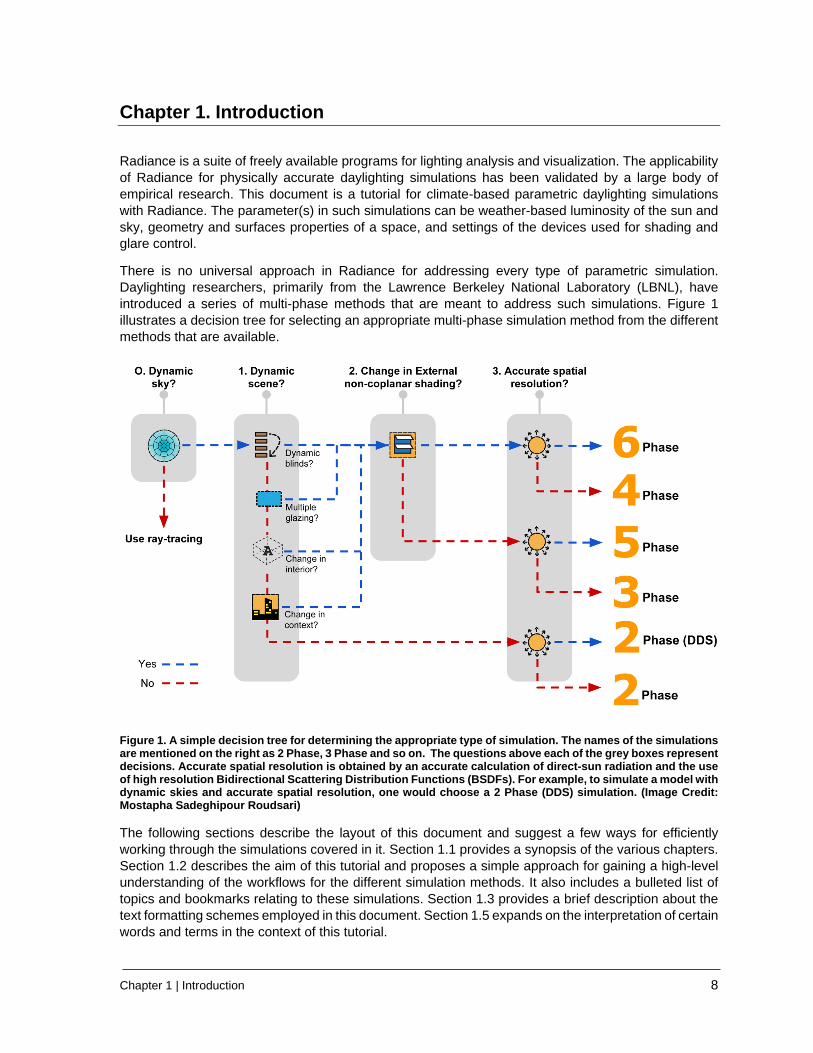
There is no universal approach in Radiance for addressing every type of parametric simulation.
Daylighting researchers, primarily from the Lawrence Berkeley National Laboratory (LBNL), have
introduced a series of multi-phase methods that are meant to address such simulations. Figure 1
illustrates a decision tree for selecting an appropriate multi-phase simulation method from the different
methods that are available.
Figure 1. A simple decision tree for determining the appropriate type of simulation. The names of the simulations are mentioned on the right as 2 Phase, 3 Phase and so on. The questions above each of the grey boxes represent decisions. Accurate spatial resolution is obtained by an accurate calculation of direct-sun radiation and the use of high resolution Bidirectional Scattering Distribution Functions (BSDFs). For example, to simulate a model with dynamic skies and accurate spatial resolution, one would choose a 2 Phase (DDS) simulation. (Image Credit: Mostapha Sadeghipour Roudsari)
The following sections describe the layout of this document and suggest a few ways for efficiently
working through the simulations covered in it. Section 1.1 provides a synopsis of the various chapters.
Section 1.2 describes the aim of this tutorial and proposes a simple approach for gaining a high-level
understanding of the workflows for the different simulation methods. It also includes a bulleted list of
topics and bookmarks relating to these simulations. Section 1.3 provides a brief description about the
text formatting schemes employed in this document. Section 1.5 expands on the interpretation of certain
words and terms in the context of this tutorial.

Chapter 1 | Introduction 9
1.1 Document Structure Based on the intent of the information conveyed, the chapters and appendices in this tutorial can be
loosely categorized into three parts. Chapters 2-4 provide the theoretical context and background
information for the simulation methods and exercise files. Chapters 6-9 explain the simulation methods
by walking the reader through a series of Radiance commands, and results obtained through those
commands. The appendices provide supplemental information in the form of modeling hints and stand-
alone command-line instructions for each of the simulations covered in Chapters 6-9. The following
paragraphs detail the scope of individual chapters.
Chapter 2 discusses the theoretical underpinnings behind the various simulation methods. Chapter 3
contains brief introductions to Radiance programs that are relevant to daylighting simulations. Chapter
4 describes the Radiance model and weather-data used for nearly all the simulations in this tutorial.
Chapter 5 discusses the steps involved in creating sky-vectors and sky-matrices. The commands
described in Chapter 5 are relevant to all the subsequent chapters. Chapter 6, Chapter 7 and Chapter
8 discuss the steps involved in Two-Phase, Three-Phase and Four-Phase simulations respectively.
The term “Two-Phase simulation” implies a Daylight Coefficients simulation. The term “Four-Phase
simulation” refers to a multi-phase simulation involving the recently introduced Façade matrix (F-
Matrix).
The workflows for Two-, Three- and Four-Phase methods approximate the sun as three or four
luminous patches, usually out of a total of 145 patches, in the sky. This results in an inaccurate
representation of the size, location and luminous intensity of the sun in these simulation methods.
Additionally, the use of Klems-basis Bi-directional Scattering Distribution Functions (BSDFs) in the
Three-Phase and Four-Phase Method compromise the accuracy of direct-sun calculations further. The
Five-Phase and Six-Phase methods, discussed in Chapter 9, are meant to improve the direct-sun
aspect of the results obtained through Three-Phase and Four-Phase methods respectively. Steps for
improving the direct-solar component of the results from the Two-Phase method, while not described
in the text, are explained through a full-fledged example in section B.2 of Appendix B.
1.2 How to use this tutorial This tutorial is intended to work on two levels. Firstly, it is expected to be an up-to-date compendium
and instruction manual for over twenty types of matrix-based annual daylighting simulation techniques
(which are discussed within the framework of the “phase”-based simulation methods). Secondly, this
tutorial also attempts to introduce matrix-based annual simulation methods to readers who are familiar
with the basic concepts of Daylighting but are inexperienced in Radiance. Readers who are well versed
with Radiance syntax, and have the experience of using programs such as rfluxmtx, are advised to skip
Chapter 3 and Chapter 5 and delve directly into chapters that focus on specific simulation(s) of interest.
1.2.2 provides the list of topics that are relevant for each simulation method. Readers who are unfamiliar
with Radiance-based annual simulation methods are advised to refer this tutorial in a linear manner till
Chapter 6. Subsequent chapters, that build on the concept of Daylight Coefficients, may be referred to
according to the specificity and depth of the simulation objectives that one wishes to tackle. The next
section provides a high-level overview of all the simulation methods covered in this tutorial.
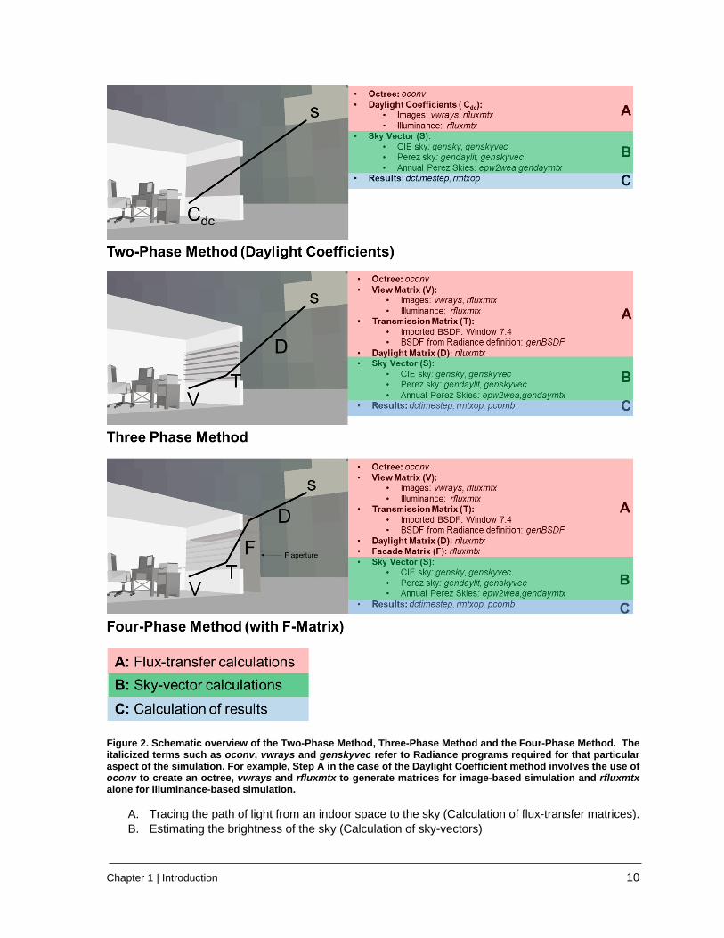
1.2.1 Commonality in matrix-based daylighting simulations The result of every simulation method described in this tutorial estimates the perception of daylight-
induced brightness inside a space. This perception can be physically quantified in terms of luminance
values captured in the pixels of a rendered image or through illuminance values measured at virtual
measurement points. Figure 2 provides an overview of the primary simulation methods covered in this
tutorial. The line-diagram in each of the images alludes to the steps involved in calculating illuminance
or luminance.
The processes involved in every daylighting simulation method depicted in Figure 2 can be summarized
in three broad steps:
Chapter 1 | Introduction 10
Figure 2. Schematic overview of the Two-Phase Method, Three-Phase Method and the Four-Phase Method. The italicized terms such as oconv, vwrays and genskyvec refer to Radiance programs required for that particular aspect of the simulation. For example, Step A in the case of the Daylight Coefficient method involves the use of oconv to create an octree, vwrays and rfluxmtx to generate matrices for image-based simulation and rfluxmtx alone for illuminance-based simulation.
A. Tracing the path of light from an indoor space to the sky (Calculation of flux-transfer matrices).
B. Estimating the brightness of the sky (Calculation of sky-vectors)

Chapter 1 | Introduction 11
C. Relating the brightness of the sky to the brightness inside a space (Multiplying, adding and
transforming matrices from Steps A and B to generate illuminance and luminance values).
The descriptions for the simulation methods described in Chapter 6, Chapter 7 and Chapter 8 begin
with such schematic diagrams. A closer examination of the labels A, B and C for each of the images
in Figure 2 indicates that there are several procedural overlaps between the different simulation
methods. For example, the commands and programs employed for creating sky-vectors and sky-
matrices are the same for all simulations. Similarly, the same command is used for creating the View
Matrix for the Three-Phase and Four-Phase methods. Such procedural overlaps also exist between the
more advanced methods depicted in Figure 3. Those methods facilitate a more accurate calculation of
the direct-solar component.
Figure 3. Schematic overview of the methods that feature a more accurate direct-solar contribution and therefore contribute to a better spatial resolution in results. The names of the simulations are mentioned on the left. Images in the first column refer to the Two-Phase Method (top), Three-Phase Method (middle) and the Four-Phase Method (bottom). As these images indicate, the Two-Phase DDS Method, Five-Phase Method and Six-Phase Method involve additional steps that improve the accuracy of the Two-Phase Method, Three-Phase Method and Four-Phase Method respectively. The + and – signs in the above image indicate arithmetic operations that are to be performed on results from each stage of the simulation.
In instances where the intent and syntax of the commands in the workflow between multiple simulation
methods are the same, the explanation for them is provided only once. While avoiding repetition in this
manner has made this document more concise, this somewhat disjointed way of describing simulations
might be confusing to some readers. This potential issue has been addressed by listing the pre-
requisites for each simulation method in the following section and also providing the full set of
commands for every simulation method in appropriately named appendices. The recommended way
to work through a simulation method is by referring the appendices alongside the relevant sections.
1.2.2 Sections relevant to different daylighting simulation methods The sections and appendices listed below relate to standard, base-case, simulations. Unusual cases
and scenarios for each simulation method are discussed within the individual chapters.

Chapter 1 | Introduction 12
1.2.2.1 The Two-Phase Method (Daylight Coefficients)
• Background, research and relevant literature: 2.2
• Workflow:
o Creating flux transfer matrices: 6.1
o Creating sky-vectors and sky-matrices: 5.1, 5.2
o Generating results: 6.1.2
• Complete set of commands: Appendix B
1.2.2.2 The Three-Phase Method
• Background, research and relevant literature: 2.3
• Conceptual Prerequisite(s): Daylight Coefficients, An understanding of BSDFs.
• Workflow:
o Creating flux transfer matrices: 7.1
o Creating sky-vectors and sky-matrices: 5.1, 5.2
o Generating results: 7.2
• Complete set of commands: Appendix C
1.2.2.3 The Four-Phase Method (with F-Matrix)
• Background, research and relevant literature: 2.4
• Conceptual Prerequisite(s): Three-Phase Method
• Workflow:
o Creating flux-transfer matrices: 7.1 (for creating View and Transmission Matrices), 8.2
(F1-type simulation), 8.3(FH-type simulation), 8.4(FN-type simulation).
o Creating sky-vectors and sky-matrices: 5.1, 5.2
o Generating results: 8.5
• Complete set of commands: Appendix D
1.2.2.4 The Five-Phase Method and the Six-Phase-Method
• Background, research, relevant literature: 2.5
• Conceptual Prerequisite(s): Three-Phase Method, Four-Phase Method
• Workflow:
o Five-Phase Method: 9.1
o Six-Phase Method: 9.2
• Complete set of commands: Appendix E
1.3 Text formatting Special formatting has been employed throughout the text to identify Radiance programs, example files
included with the tutorial, and commands for performing the simulations.
Radiance programs: Radiance programs can be identified in the text by italicized font. For example,
rfluxmtx refers to the Radiance program rfluxmtx, named rfluxmtx.exe in Windows, inside the bin sub-
directory of the Radiance installation directory. Except for genBSDF, all the Radiance programs
featured in this tutorial are named in lower-case format on Unix-like systems. The command-line
interface in Windows® is not case sensitive.
Example files: The example files are identified in the text by Comic Sans MS font. The path-names of
files are relative to a root directory called room inside the directory for exercise files. For example,
objects/Glazing.rad refers to the file Glazing.rad inside the directory room/objects.
Radiance and other command-line syntax: Command-line syntax, whether expressed separately as a
complete command or excerpted in-line in the text, is highlighted and formatted in monospaced

Chapter 1 | Introduction 13
font. Unless two lines are separated by whitespace, the line-breaks present in commands should be
ignored. For example, the following lines are two separate commands:
gensky 3 20 10:30EDT -m 75 -o 73.96 -a 40.78 > skies/NYC_CIE.sky
genskyvec -m 1 < skies/NYC_CIE.sky> skyVectors/NYC_CIE.vec
On the other hand, the lines below are for a single command and should be typed as such in the
terminal (or MS DOS) window.
rfluxmtx -ffc -v -n 8 -x 400 -y 222 -ld- -c 9 -ab 12 -ad 50000 -lw 1e-5 -o matrices/dc/hdr/%03d.hdr - skyDomes/skyglow.rad -i roomDC.oct < matrices/dc/viewRays.txt
While most of the syntax used in this document is specific to Radiance, there are some instances where
external OS based commands are used as well. Radiance-based commands and syntax are mostly
platform independent. All the OS based commands, unless mentioned otherwise, are discussed with
regards to Mac OS and Unix-like systems.
1.4 Navigation features in the PDF and a few notes on printing This tutorial was designed to be accessed as a PDF document on a color screen monitor with a
resolution of at least 1024x768px. Some of the navigation features in the PDF, which are highlighted in
Figure 4, will obviously be inaccessible on a printed copy. If this document is being printed regardless,
a colored print is highly recommended. The palette and scale employed for visualizing illuminance and
luminance values in Chapters6-9 can only be discerned through a colored print.
Figure 4. The above image shows a screen capture of the PDF file. Bookmarks and hyperlinks that would be available on a typical page are highlighted. The bookmarks were automatically assigned by Microsoft® Word® based on headings and document references. These features were tested on Adobe® Acrobat, Adobe® Reader, BlueBeam® PDF reader and the Foxit Reader.
Chapter 1 | Introduction 14
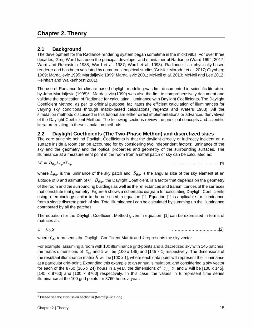
1.5 Some commonly used terms Radiance definition: implies the description of a physical object that is to be simulated, in terms of
Radiance materials and geometry. The definition is stored in simple ASCII format. A detailed description
of the Radiance scene format can be found in (Ward 1997) and (LBNL 2016a).
Scene: collectively refers to those Radiance definitions that are physically relevant to a daylighting
simulation.
Sampling Comment or Rfluxmtx Comment: refers to the controlling parameters relevant to rfluxmtx that
are to be included as a part of the Radiance definition of certain files. These parameters begin with the
term “#@rfluxmtx”.
Grid Points: refer to virtual locations, expressed in three-dimensional coordinates (x, y, z) and
directional vectors (x-direction-direction, z-direction), that are used to measure illuminance in a
simulation.
Primitive: refers to native Radiance surfaces and materials such as “polygon”, “sphere”, “source”,
“metal”, “plastic”, “BSDF” etc.
Additionally, the terms Two-Phase Method and the Daylight Coefficient method have been used
interchangeably and refer to the same simulation method. Similarly, the F-Matrix Method and the Four-
Phase method also refer to the same simulation method.
Chapter 2 | Theory 15
Chapter 2. Theory
2.1 Background The development for the Radiance rendering system began sometime in the mid-1980s. For over three
decades, Greg Ward has been the principal developer and maintainer of Radiance (Ward 1994; 2017;
Ward and Rubinstein 1988; Ward et al. 1987; Ward et al. 1998). Radiance is a physically-based
renderer and has been validated by numerous empirical studies(Geisler-Moroder et al. 2017; Grynberg
1989; Mardaljevic 1995; Mardaljevic 1999; Mardaljevic 2001; McNeil et al. 2013; McNeil and Lee 2012;
Reinhart and Walkenhorst 2001).
The use of Radiance for climate-based daylight modeling was first documented in scientific literature
by John Mardaljevic (1995)1. Mardaljevic (1999) was also the first to comprehensively document and
validate the application of Radiance for calculating illuminance with Daylight Coefficients. The Daylight
Coefficient Method, as per its original purpose, facilitates the efficient calculation of illuminances for
varying sky conditions through matrix-based calculations(Tregenza and Waters 1983). All the
simulation methods discussed in this tutorial are either direct implementations or advanced derivatives
of the Daylight Coefficient Method. The following sections review the principal concepts and scientific
literature relating to these simulation methods.
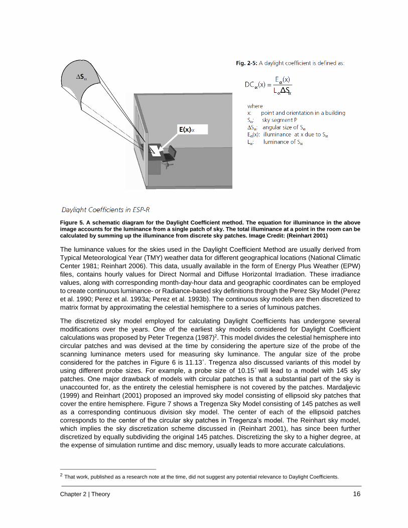
2.2 Daylight Coefficients (The Two-Phase Method) and discretized skies The core principle behind Daylight Coefficients is that the daylight directly or indirectly incident on a
surface inside a room can be accounted for by considering two independent factors: luminance of the
sky and the geometry and the optical properties and geometry of the surrounding surfaces. The
illuminance at a measurement point in the room from a small patch of sky can be calculated as:
∆𝑬 = 𝑫𝜽𝝋𝑳𝜽𝝋∆𝑺𝜽𝝋 …….…………………………….[1]
where 𝐿𝜃𝜑 is the luminance of the sky patch and 𝑆𝜃𝜑 is the angular size of the sky element at an
altitude of θ and azimuth of Φ. 𝐷𝜃𝜑, the Daylight Coefficient, is a factor that depends on the geometry
of the room and the surrounding buildings as well as the reflectances and transmittances of the surfaces
that constitute that geometry. Figure 5 shows a schematic diagram for calculating Daylight Coefficients
using a terminology similar to the one used in equation [1]. Equation [1] is applicable for illuminance
from a single discrete patch of sky. Total illuminance i can be calculated by summing up the illuminance
contributed by all the patches.
The equation for the Daylight Coefficient Method given in equation [1] can be expressed in terms of
matrices as:
E = CdcS …………………………….[2]
where 𝐶𝑑𝑐 represents the Daylight Coefficient Matrix and 𝑆 represents the sky vector.
For example, assuming a room with 100 illuminance grid-points and a discretized sky with 145 patches,
the matrix dimensions of 𝐶𝑑𝑐 and 𝑆 will be [100 x 145] and [145 x 1] respectively. The dimensions of
the resultant illuminance matrix 𝐸 will be [100 x 1], where each data point will represent the illuminance
at a particular grid-point. Expanding this example to an annual simulation, and considering a sky vector
for each of the 8760 (365 x 24) hours in a year, the dimensions of 𝐶𝑑𝑐, 𝑆 and 𝐸 will be [100 x 145],
[145 x 8760] and [100 x 8760] respectively. In this case, the values in E represent time series
illuminance at the 100 grid points for 8760 hours a year.
1 Please see the Discussion section in (Mardaljevic 1995).
Chapter 2 | Theory 16
Figure 5. A schematic diagram for the Daylight Coefficient method. The equation for illuminance in the above image accounts for the luminance from a single patch of sky. The total illuminance at a point in the room can be calculated by summing up the illuminance from discrete sky patches. Image Credit: (Reinhart 2001)
The luminance values for the skies used in the Daylight Coefficient Method are usually derived from
Typical Meteorological Year (TMY) weather data for different geographical locations (National Climatic
Center 1981; Reinhart 2006). This data, usually available in the form of Energy Plus Weather (EPW)
files, contains hourly values for Direct Normal and Diffuse Horizontal Irradiation. These irradiance
values, along with corresponding month-day-hour data and geographic coordinates can be employed
to create continuous luminance- or Radiance-based sky definitions through the Perez Sky Model (Perez
et al. 1990; Perez et al. 1993a; Perez et al. 1993b). The continuous sky models are then discretized to
matrix format by approximating the celestial hemisphere to a series of luminous patches.
The discretized sky model employed for calculating Daylight Coefficients has undergone several
modifications over the years. One of the earliest sky models considered for Daylight Coefficient
calculations was proposed by Peter Tregenza (1987)2. This model divides the celestial hemisphere into
circular patches and was devised at the time by considering the aperture size of the probe of the
scanning luminance meters used for measuring sky luminance. The angular size of the probe
considered for the patches in Figure 6 is 11.13˚. Tregenza also discussed variants of this model by
using different probe sizes. For example, a probe size of 10.15˚ will lead to a model with 145 sky
patches. One major drawback of models with circular patches is that a substantial part of the sky is
unaccounted for, as the entirety the celestial hemisphere is not covered by the patches. Mardaljevic
(1999) and Reinhart (2001) proposed an improved sky model consisting of ellipsoid sky patches that
cover the entire hemisphere. Figure 7 shows a Tregenza Sky Model consisting of 145 patches as well
as a corresponding continuous division sky model. The center of each of the ellipsoid patches
corresponds to the center of the circular sky patches in Tregenza’s model. The Reinhart sky model,
which implies the sky discretization scheme discussed in (Reinhart 2001), has since been further
discretized by equally subdividing the original 145 patches. Discretizing the sky to a higher degree, at
the expense of simulation runtime and disc memory, usually leads to more accurate calculations.
2 That work, published as a research note at the time, did not suggest any potential relevance to Daylight Coefficients.

Chapter 2 | Theory 17
Figure 6. Circular patches proposed by Tregenza for discretizing the hemispherical sky structure. Credit: (Tregenza 1987).
Figure 7. The image (a) shows the Tregenza sky subdivison scheme with 145 sky patches. Image (b) shows the continuous sky subdivision scheme proposed by Reinhart. Credit: (Bourgeois et al. 2008).
Figure 8. Fish-eye projections of a continuous sky model (a) and corresponding discretized versions. Images (b) , (c) and (d) contain 145, 580 and 2305 sky patches respectively. As is apparent in the images above, even with a high degree of discretization, the size of the sun is greatly overestimated in discrete sky models. Credit: (McNeil 2013b).

Chapter 2 | Theory 18
This improvement in accuracy can mostly be attributed to a better approximation of the size and
luminance of the sun brought about by use of smaller patches. As shown in Figure 8, in discretized sky
models, the actual position of the sun in the sky at a given time is approximated to 3-4 sky patches. As
is also evident from Figure 8, this approximation in position is accompanied by an overestimation of the
size of the sun with respect to the sky, especially in the case where a sky with 145 patches is
considered. Improvements pertaining to the direct solar component are discussed further in section
2.5.
Besides Mardaljevic’s dissertation (1999), a detailed account of the implementation of the Daylight
Coefficients through Radiance-based programs can also be found in (Reinhart 2001). At present, the
most popular and widely used Radiance-based implementation of Daylight Coefficients is in Daysim
(2015), an annual Daylighting simulation software. Several other software such as DIVA (Jakubiec and
Reinhart 2011), SPOT (Rogers 2006) and Ladybug-Honeybee (Roudsari and Pak 2014) employ
Daysim, or one of its derivatives, as the calculation engine for annual daylighting simulations. The
workflows for Daylight Coefficient simulations using native Radiance programs is discussed in Chapter
6.
The standard Daylight Coefficient method is suitable for models involving simple glazing and shading
systems that can be modeled as simple glass or translucent materials in Radiance (as “glass” or “trans”
primitives respectively). More complex type of glazing and shading systems can also be incorporated
into Daylight Coefficient based calculations by modeling these materials using a Bidirectional Scattering
Distribution Function (BSDF) primitive and then considering them to be a part of the overall scene3.
Often, the primary objective of daylighting simulations is to parametrically and iteratively evaluate only
a certain aspect of the scene. This is especially the case if multiple daylighting simulations are
performed to evaluate the performance of various types of glazing or shading systems while keeping
everything else in the scene constant. In such instances, the Daylight Coefficient method, which
involves tracing rays from inside the room to the sky in a single step, becomes prohibitively expensive.
The Three-Phase Method discussed in the next section is more suited for such simulations.
2.3 The Three-Phase Method The Three-Phase Method makes it possible to perform annual or point-in-time parametric daylighting
simulations with Complex Fenestration Systems (CFS). As depicted in Figure 9, this method builds on
the Daylight Coefficient Method by virtually splitting the flux-transfer path into multiple independent
phases, namely:
1. View (V): Flux transfer from illuminance grid-points or a view specification to glazing or CFS.
2. Transmission (T): Flux transfer through the glazing or CFS.
3. Daylight (D): Flux transfer from the exterior of glazing or CFS to the sky.4
The matrix equation [2] can be adapted to the Three-Phase Method as:
E = VTDS …………………………….[3]
The process for creating the sky vector remains the same as that in the case of Daylight Coefficient
method. The matrices for View (V) and Daylight (D) phases are generated through Radiance-based
workflows involving rfluxmtx or rcontrib. The Transmission (T) matrix, which is a BSDF definition stored
3 Considering the overall development timeline of Radiance, the functionality to incorporate BSDFs directly into scenes is a fairly recent development. More details can be found in Greg Ward’s presentation from the 10th International Radiance Workshop (Ward 2011). 4 Although light physically travels from a luminous source to the observer (or calculation point), the order of matrices is
intentionally listed in reverse order and also indicated as such by arrows in figures denoting these matrices. This is to highlight
the fact that Radiance performs reverse-tracing. Further details about the ray-tracing algorithms in Radiance can be found in
(Ward 1994) and (Ward et al. 1998).
Chapter 2 | Theory 19
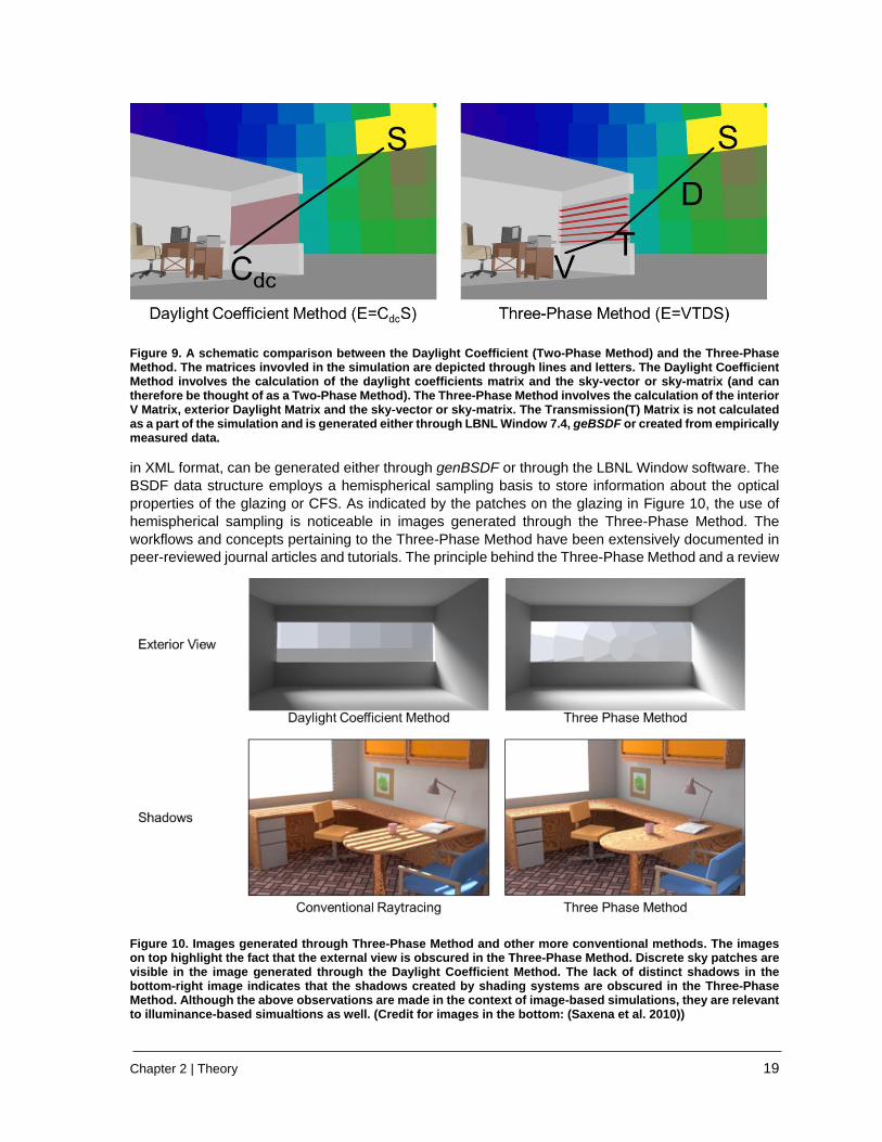
Figure 9. A schematic comparison between the Daylight Coefficient (Two-Phase Method) and the Three-Phase Method. The matrices invovled in the simulation are depicted through lines and letters. The Daylight Coefficient Method involves the calculation of the daylight coefficients matrix and the sky-vector or sky-matrix (and can therefore be thought of as a Two-Phase Method). The Three-Phase Method involves the calculation of the interior V Matrix, exterior Daylight Matrix and the sky-vector or sky-matrix. The Transmission(T) Matrix is not calculated as a part of the simulation and is generated either through LBNL Window 7.4, geBSDF or created from empirically measured data.
in XML format, can be generated either through genBSDF or through the LBNL Window software. The
BSDF data structure employs a hemispherical sampling basis to store information about the optical
properties of the glazing or CFS. As indicated by the patches on the glazing in Figure 10, the use of
hemispherical sampling is noticeable in images generated through the Three-Phase Method. The
workflows and concepts pertaining to the Three-Phase Method have been extensively documented in
peer-reviewed journal articles and tutorials. The principle behind the Three-Phase Method and a review
Figure 10. Images generated through Three-Phase Method and other more conventional methods. The images on top highlight the fact that the external view is obscured in the Three-Phase Method. Discrete sky patches are visible in the image generated through the Daylight Coefficient Method. The lack of distinct shadows in the bottom-right image indicates that the shadows created by shading systems are obscured in the Three-Phase Method. Although the above observations are made in the context of image-based simulations, they are relevant to illuminance-based simualtions as well. (Credit for images in the bottom: (Saxena et al. 2010))
Chapter 2 | Theory 20
of the theoretical concepts invoked in it are presented in (Ward et al. 2011). A discussion focusing on
the parametric capability and data-reuse aspect of the Three-Phase Method can be found in (Saxena
et al. 2010). (Jonsson et al. 2009) and (McNeil et al. 2013) contain discussions specifically relevant to
BSDFs and their application in the Three Phase Method. Finally, Andy McNeil’s tutorial on the Three-
Phase Method (McNeil 2013c) provides a step-by-step guide for applying this simulation technique to
different types of daylighting scenarios. Chapter 7 presents a slightly revised and simplified workflow
for the Three-Phase Method by utilizing the new rfluxmtx program.
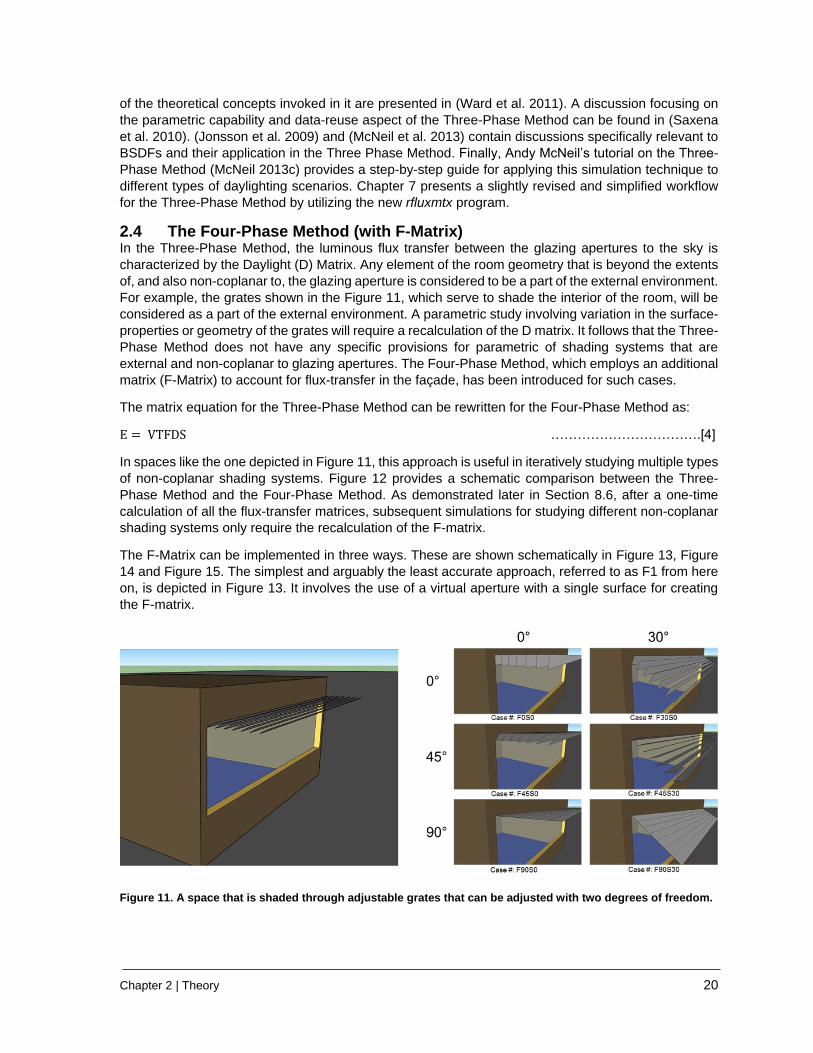
2.4 The Four-Phase Method (with F-Matrix) In the Three-Phase Method, the luminous flux transfer between the glazing apertures to the sky is
characterized by the Daylight (D) Matrix. Any element of the room geometry that is beyond the extents
of, and also non-coplanar to, the glazing aperture is considered to be a part of the external environment.
For example, the grates shown in the Figure 11, which serve to shade the interior of the room, will be
considered as a part of the external environment. A parametric study involving variation in the surface-
properties or geometry of the grates will require a recalculation of the D matrix. It follows that the Three-
Phase Method does not have any specific provisions for parametric of shading systems that are
external and non-coplanar to glazing apertures. The Four-Phase Method, which employs an additional
matrix (F-Matrix) to account for flux-transfer in the façade, has been introduced for such cases.
The matrix equation for the Three-Phase Method can be rewritten for the Four-Phase Method as:
E = VTFDS …………………………….[4]
In spaces like the one depicted in Figure 11, this approach is useful in iteratively studying multiple types
of non-coplanar shading systems. Figure 12 provides a schematic comparison between the Three-
Phase Method and the Four-Phase Method. As demonstrated later in Section 8.6, after a one-time
calculation of all the flux-transfer matrices, subsequent simulations for studying different non-coplanar
shading systems only require the recalculation of the F-matrix.
The F-Matrix can be implemented in three ways. These are shown schematically in Figure 13, Figure
14 and Figure 15. The simplest and arguably the least accurate approach, referred to as F1 from here
on, is depicted in Figure 13. It involves the use of a virtual aperture with a single surface for creating
the F-matrix.
Figure 11. A space that is shaded through adjustable grates that can be adjusted with two degrees of freedom.

Chapter 2 | Theory 21
Figure 12. Schematic comparison between the Three-Phase Method and the Four-Phase Method.
A single hemispherical basis, based on the direction normal of the F-aperture, is considered for creating
the F-matrix. The main drawback of this approach is that the use of a single surface F-aperture ignores
incoming luminous flux from all the other directions. A more accurate approach shown in Figure 14
involves surrounding the façade with an F-aperture containing multiple surfaces such that all directions
of flux transfer from the façade to the sky are accounted for. This approach, referred to as FH, employs
a single hemispherical sampling like the F1 approach. One of the shortcomings of using a single
sampling basis is that only the directions compatible with the “hemisphere up” direction for that basis
are accurately considered in the simulation. For example, in Figure 14, if the “hemisphere up” direction
is specified as +Z, the flux-transfer from the top direction will not be properly calculated. This is because
the front, left and right surfaces of the F-aperture have direction normals facing in +Y, +X and -X
directions respectively and are therefore compatible with the +Z “hemisphere-up specification.
Figure 13. Setup for an F1 type F-Matrix simulation. The translucent surface in front of the façade represents the F-aperture used in this simulation. As indicated by the location of the arrows, the D matrix is computed by considering the F-aperture and the sky dome.
However, the direction normal for the aperture surface on top faces the -Z direction and therefore is not
compatible with the +Z “hemisphere up direction. The final approach shown in Figure 15 and referred

Chapter 2 | Theory 22
to as FN, involves the use of multiple F matrices with individually assigned hemispherical sampling
basis. The surfaces for creating the F matrices are positioned as per the location of the external shading
device. The FN approach, while being more accurate and thorough than the previous approaches,
requires considerably greater effort in setting up and computing. The number of F matrices, and by
extension the number of Daylight Matrices, to be computed in these case is equal to the number of F-
aperture surfaces multiplied by the number of window groups.
Figure 14. Setup for an FH type F-Matrix simulation. The four translucent polygons on top, right, left and front constitute the F-aperture and envelope all sides of the façade. In case there is a considerable offset between the space and the ground plane, then a polygon should be provided at the bottom as well.
Figure 15. Setup for an FN type F-Matrix simulation. Like the FH approach, even in this case the F-aperture polygons completely envelope the Façade. The key distinction here is that the positioning of the polygons is also based on the location of the non-coplanar shading device and that a separate sampling basis is assigned for each F-aperture.
Chapter 2 | Theory 23
The Four-Phase method was introduced by Greg Ward at the 14th International Radiance
Workshop(Ward 2015). The empirical validation of the F-Matrix is discussed in (Wang et al. 2016;
2017). The workflows for the Four-Phase Method are described in Chapter 8.
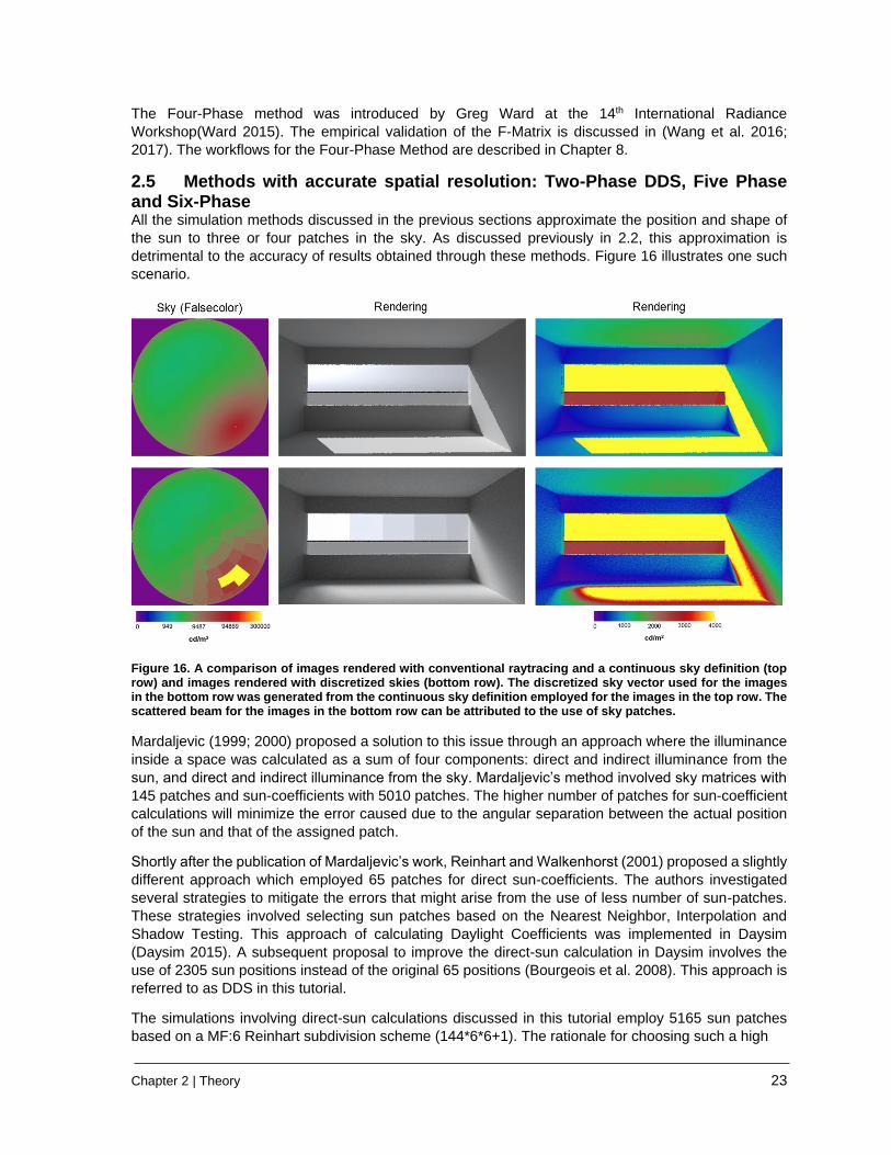
2.5 Methods with accurate spatial resolution: Two-Phase DDS, Five Phase and Six-Phase All the simulation methods discussed in the previous sections approximate the position and shape of
the sun to three or four patches in the sky. As discussed previously in 2.2, this approximation is
detrimental to the accuracy of results obtained through these methods. Figure 16 illustrates one such
scenario.
Figure 16. A comparison of images rendered with conventional raytracing and a continuous sky definition (top row) and images rendered with discretized skies (bottom row). The discretized sky vector used for the images in the bottom row was generated from the continuous sky definition employed for the images in the top row. The scattered beam for the images in the bottom row can be attributed to the use of sky patches.
Mardaljevic (1999; 2000) proposed a solution to this issue through an approach where the illuminance
inside a space was calculated as a sum of four components: direct and indirect illuminance from the
sun, and direct and indirect illuminance from the sky. Mardaljevic’s method involved sky matrices with
145 patches and sun-coefficients with 5010 patches. The higher number of patches for sun-coefficient
calculations will minimize the error caused due to the angular separation between the actual position
of the sun and that of the assigned patch.
Shortly after the publication of Mardaljevic’s work, Reinhart and Walkenhorst (2001) proposed a slightly
different approach which employed 65 patches for direct sun-coefficients. The authors investigated
several strategies to mitigate the errors that might arise from the use of less number of sun-patches.
These strategies involved selecting sun patches based on the Nearest Neighbor, Interpolation and
Shadow Testing. This approach of calculating Daylight Coefficients was implemented in Daysim
(Daysim 2015). A subsequent proposal to improve the direct-sun calculation in Daysim involves the
use of 2305 sun positions instead of the original 65 positions (Bourgeois et al. 2008). This approach is
referred to as DDS in this tutorial.
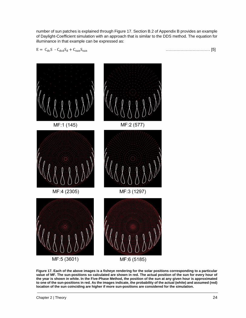
The simulations involving direct-sun calculations discussed in this tutorial employ 5165 sun patches
based on a MF:6 Reinhart subdivision scheme (144*6*6+1). The rationale for choosing such a high
Chapter 2 | Theory 24
number of sun patches is explained through Figure 17. Section B.2 of Appendix B provides an example
of Daylight-Coefficient simulation with an approach that is similar to the DDS method. The equation for
illuminance in that example can be expressed as:
E = CdcS - CdcdSd + CsunSsun …………………………… [5]
Figure 17. Each of the above images is a fisheye rendering for the solar positions corresponding to a particular value of MF. The sun-positions so calculated are shown in red. The actual position of the sun for every hour of the year is shown in white. In the Five-Phase Method, the position of the sun at any given hour is approximated to one of the sun-positions in red. As the images indicate, the probability of the actual (white) and assumed (red) location of the sun coinciding are higher if more sun-positions are considered for the simulation.

Chapter 2 | Theory 25
Cdcd and Sd denote direct-sky coefficients and direct-sky matrix respectively. Csun and Ssun denote
direct-sun coefficients and sun matrix respectively. The relative scale and luminance of the sky and sun
patches in a typical simulation are shown in Figure 18.
Figure 18. Sky and sun patches employed in Two-Phase DDS, Five-Phase Method and Six-Phase Method. The image on the left is standard continuous sky.
The steps relating to improving the calculation of direct-sun component, discussed till now in the context
of the Daylight Coefficients or the Two-Phase Method, are also applicable to the Three-Phase and
Four-Phase method. The Five-Phase Method, and the recently introduced Six-Phase method, improve
the direct-solar component of the results obtained through the Three-Phase and Four-Phase method
respectively. The steps incorporated into the Five- and Six-Phase Method are loosely analogous to the
improvements for the Daylight Coefficient Method proposed in the DDS model.
The Three-Phase Method, described in Equation [3], is extended to the Five-Phase Method as:
E = VTDS − VdTDdSd + CdsSsun …………………………… [6]
where the term 𝑉𝑑𝑇𝐷𝑑𝑆 denotes a separate three-phase simulation utilizing the same scene as the
original three-phase calculation denoted by 𝑉𝑇𝐷𝑆. 𝑉𝑑𝑇𝐷𝑑𝑆, which stands for the direct-sun aspect of a
Three-Phase Simulation, differs from the 𝑉𝑇𝐷𝑆 on account of its emphasis on isolating the direct-sun
component of the simulation. The direct-sun component is isolated by performing a flux-transfer
calculation with no ambient bounces and considering a sky-matrix with only the direct solar component.
The term 𝐶𝑑𝑠𝑆𝑠𝑢𝑛 denotes a more accurate simulation with direct solar contribution. 𝐶𝑑𝑠 denotes a
coefficient matrix for direct sun that was calculated by incorporating, wherever possible, a high-
resolution Tensor-Tree BSDF along with the physical geometry of the shading device that was used to
create the BSDF. Incorporating the physical geometry of the shading system in such a way overcomes
the issue of obscured shadows shown in Figure 10. The advantages of using a high-resolution BSDF
along with proxy geometry are shown in Figure 19.
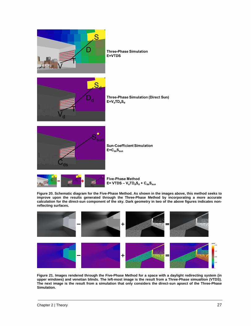
Figure 20 shows the schematic diagram for the Five-Phase Method. As the diagram indicates, just like
the Two-Phase DDS approach, the Five-Phase Method to involves three independent simulations.
Figure 21 provides an example of the phase-wise results generated through the Five-Phase Method.
The resultant image shows the sharp shadows cast by the shading device, which are otherwise
obscured in the case of the Three-Phase simulation.

Chapter 2 | Theory 26
A recently concluded validation study found that further improvements to accuracy for image-based
Five-Phase simulations can be made by splitting the direct-sun aspect of the simulation to two different
Figure 19. Images rendered through different types of BSDF representations for the same set of venetian blinds. The image on the right, which features Tensor Tree BSDFs with proxy geometry, represents the most accurate result as it incorporates both direct and diffuse part of luminous flux transfer. Credit (Ward et al. 2012).
matrices. These matrices address the interior of the space and overall scene separately (Geisler-
Moroder et al. 2017). The Five-Phase equation [5], can be modified for image-based simulations as:
E = VTDS − VdTDdSd + (CR−ds + CF−ds)Ssun …………………………… [7]
The term 𝐶𝑅−𝑑𝑠 refers to the direct sun coefficient matrix for the interior of the space and the term 𝐶𝐹−𝑑𝑠
refers to the direct sun coefficient matrix for the entire scene.
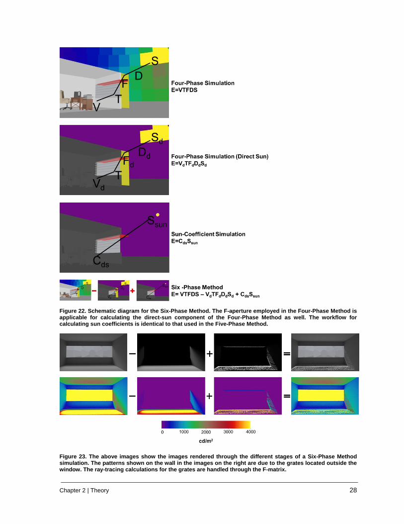
The Six-Phase Method, depicted schematically in Figure 22, is similar to the Five-Phase Method in its
intent and execution. The sole difference between the Five-Phase Method and the Six-Phase Method
relates to the inclusion of the F-Matrix. So, the Five-Phase equation can be extended for the Six-Phase
Method as:
E = VTFDS − VdTFdDdSd + CdsSsun …………………………… [8]
The modifications suggested for the Five-Phase image-based simulations are applicable for the Six-
Phase method as well. So, equation [6] can be rewritten for the Six-Phase Method as
E = VTFDS − VdTFdDdSd + (CR−ds + CF−ds)Ssun …………………………… [9]
Figure 23 shows the step-wise results obtained through a Six-Phase simulation. The workflows for the
Five-Phase and Six-Phase Method are described in Chapter 9. A detailed explanation of the Five-
Phase Method can also be found in the Five-Phase Method tutorial by Andy McNeil (McNeil 2013a).
Further information about Tensor Tree BSDFs and validation of the tool for generating them can be
found in (Ward et al. 2012) and (Molina et al. 2015) respectively.
The next chapter provides brief introductions to Radiance programs that will be employed to perform
the simulations described in this chapter.
Chapter 2 | Theory 27
Figure 20. Schematic diagram for the Five-Phase Method. As shown in the images above, this method seeks to improve upon the results generated through the Three-Phase Method by incorporating a more accurate calculation for the direct-sun component of the sky. Dark geometry in two of the above figures indicates non-reflecting surfaces.
Figure 21. Images rendered through the Five-Phase Method for a space with a daylight redirecting system (in upper windows) and venetian blinds. The left-most image is the result from a Three-Phase simualtion (VTDS). The next image is the result from a simulation that only considers the direct-sun apsect of the Three-Phase Simulation.
Chapter 2 | Theory 28
Figure 22. Schematic diagram for the Six-Phase Method. The F-aperture employed in the Four-Phase Method is applicable for calculating the direct-sun component of the Four-Phase Method as well. The workflow for calculating sun coefficients is identical to that used in the Five-Phase Method.
Figure 23. The above images show the images rendered through the different stages of a Six-Phase Method simulation. The patterns shown on the wall in the images on the right are due to the grates located outside the window. The ray-tracing calculations for the grates are handled through the F-matrix.
Chapter 3 | Radiance programs for Daylighting simulations 29
Chapter 3. Radiance programs for Daylighting simulations
Topical descriptions of use-cases for programs that feature in this tutorial are provided in the following
sections.5
3.1 Programs for creating sky definitions • epw2wea: extracts location details, Direct-Normal irradiances and Diffuse-Horizontal
irradiances from EnergyPlus Weather data (EPW) files and stores them in WEA (weather file)
format.
• gensky: generates a Radiance scene description of CIE standard sky for a specific time or
altitude/azimuth angles. The location details and irradiation values (for a single point-of-time)
from a WEA file can be included as input parameters for gensky.
• gendaylit: generates a Radiance scene description of Perez sky based on inputs that are similar
to gensky.
• genskyvec: generates a point-in-time sky-vector, usually based on input from gensky or
gendaylit.
• gendaymtx: generates a Perez Sky Model-based time-series of sky-vectors based on input
from a weather tape (which is usually a WEA file generated by epw2wea).
3.2 Programs for ray-tracing, ray-sampling and creating flux-transfer matrices
• rcontrib: computes “contribution coefficients” for geometric surfaces in a Radiance scene.
These surfaces are usually luminous in nature (such as the sky or electric light fixtures). For
the purposes of this tutorial it suffices to think of rcontrib as a program that can compute the
flux transfer matrix between two physical or virtual surfaces. It can also calculate the flux
transfer matrix between a set of input rays (specified as a grid-points file) or surface elements
and one or more surfaces.
• genklemsamp: generates ray samples for specified surfaces using Klems hemispherical
sampling basis. With the exception of the sky-vectors, Klems sampling basis are required for
every surface that is considered for creating flux-transfer matrices in this tutorial. A thorough
explanation of the relevance of Klems basis to matrix-based daylight simulation methods can
be found in (Ward et al. 2011). Although genklemsamp is not used for any of the workflows in
this tutorial, its use is still compatible with the simulation methods described herein. Readers
interested in knowing more about genklemsamp-based daylighting simulation workflows should
refer the Three-Phase Method tutorial (McNeil 2013c) and the Five-Phase Method tutorial
(McNeil 2013b).
• rfluxmtx: creates flux-transfer matrices between a sending surface and one or more receiving surfaces in a Radiance scene. It simplifies the process of setting up matrix-based simulations
5 If this document is being read in an electronic format, the manual pages for the programs listed above should be accessible by
clicking on their names. The manual pages for the above programs can also be downloaded by visiting radiance-
online.org/learning/documentation/manual-pages .Provided that the MANPATH variable has been correctly assigned, readers
on Mac OS and other Unix-based systems can access manual pages on the terminal through the man command as well.
Chapter 3 | Radiance programs for Daylighting simulations 30
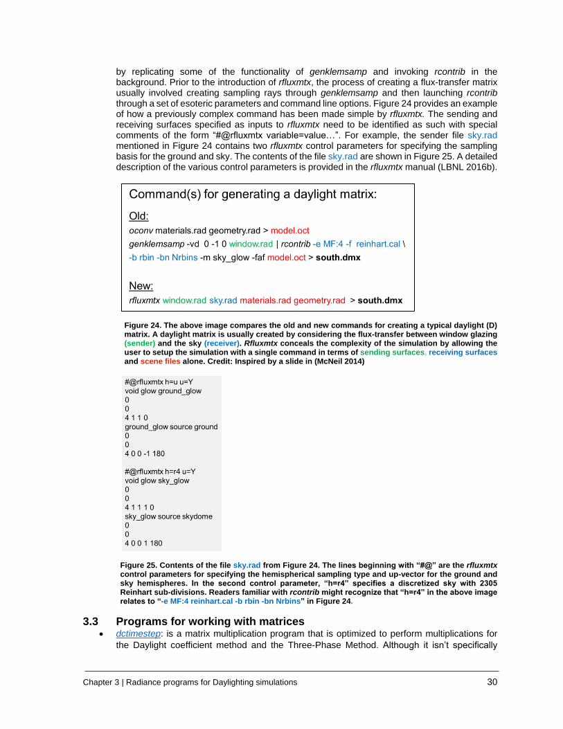
by replicating some of the functionality of genklemsamp and invoking rcontrib in the background. Prior to the introduction of rfluxmtx, the process of creating a flux-transfer matrix usually involved creating sampling rays through genklemsamp and then launching rcontrib through a set of esoteric parameters and command line options. Figure 24 provides an example of how a previously complex command has been made simple by rfluxmtx. The sending and receiving surfaces specified as inputs to rfluxmtx need to be identified as such with special comments of the form “#@rfluxmtx variable=value…”. For example, the sender file sky.rad mentioned in Figure 24 contains two rfluxmtx control parameters for specifying the sampling basis for the ground and sky. The contents of the file sky.rad are shown in Figure 25. A detailed description of the various control parameters is provided in the rfluxmtx manual (LBNL 2016b).
Figure 24. The above image compares the old and new commands for creating a typical daylight (D) matrix. A daylight matrix is usually created by considering the flux-transfer between window glazing (sender) and the sky (receiver). Rfluxmtx conceals the complexity of the simulation by allowing the user to setup the simulation with a single command in terms of sending surfaces, receiving surfaces and scene files alone. Credit: Inspired by a slide in (McNeil 2014)
Figure 25. Contents of the file sky.rad from Figure 24. The lines beginning with “#@” are the rfluxmtx control parameters for specifying the hemispherical sampling type and up-vector for the ground and sky hemispheres. In the second control parameter, “h=r4” specifies a discretized sky with 2305 Reinhart sub-divisions. Readers familiar with rcontrib might recognize that “h=r4” in the above image relates to “-e MF:4 reinhart.cal -b rbin -bn Nrbins” in Figure 24.
3.3 Programs for working with matrices • dctimestep: is a matrix multiplication program that is optimized to perform multiplications for
the Daylight coefficient method and the Three-Phase Method. Although it isn’t specifically
Chapter 3 | Radiance programs for Daylighting simulations 31
documented, dctimestep can also be used to combine F-matrices and D-matrices into a single
resultant matrix.
• rmtxop: can be used for matrix multiplication, addition, subtraction, transpose and scaling
operations. It is especially useful when combining results from different phases in the Five-
Phase Method as well as the F-matrix method.
• rcollate: is a tool for formatting, resizing or transposing matrix data from a single file. With
regards to the simulations described in this tutorial, it can be used for changing the dimensions
of the results calculated through rmtxop or dctimestep.
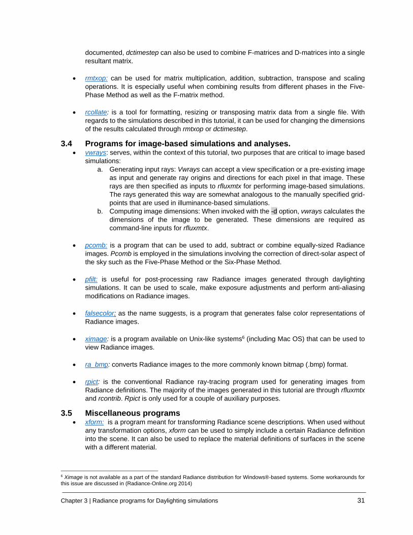
3.4 Programs for image-based simulations and analyses. • vwrays: serves, within the context of this tutorial, two purposes that are critical to image based
simulations:
a. Generating input rays: Vwrays can accept a view specification or a pre-existing image
as input and generate ray origins and directions for each pixel in that image. These
rays are then specified as inputs to rfluxmtx for performing image-based simulations.
The rays generated this way are somewhat analogous to the manually specified grid-
points that are used in illuminance-based simulations.
b. Computing image dimensions: When invoked with the -d option, vwrays calculates the
dimensions of the image to be generated. These dimensions are required as
command-line inputs for rfluxmtx.
• pcomb: is a program that can be used to add, subtract or combine equally-sized Radiance
images. Pcomb is employed in the simulations involving the correction of direct-solar aspect of
the sky such as the Five-Phase Method or the Six-Phase Method.
• pfilt: is useful for post-processing raw Radiance images generated through daylighting
simulations. It can be used to scale, make exposure adjustments and perform anti-aliasing
modifications on Radiance images.
• falsecolor: as the name suggests, is a program that generates false color representations of
Radiance images.
• ximage: is a program available on Unix-like systems6 (including Mac OS) that can be used to
view Radiance images.
• ra_bmp: converts Radiance images to the more commonly known bitmap (.bmp) format.
• rpict: is the conventional Radiance ray-tracing program used for generating images from
Radiance definitions. The majority of the images generated in this tutorial are through rfluxmtx
and rcontrib. Rpict is only used for a couple of auxiliary purposes.
3.5 Miscellaneous programs • xform: is a program meant for transforming Radiance scene descriptions. When used without
any transformation options, xform can be used to simply include a certain Radiance definition
into the scene. It can also be used to replace the material definitions of surfaces in the scene
with a different material.
6 Ximage is not available as a part of the standard Radiance distribution for Windows®-based systems. Some workarounds for this issue are discussed in (Radiance-Online.org 2014)
Chapter 3 | Radiance programs for Daylighting simulations 32
• oconv: compiles the given scene files into an octree for efficient ray-tracing. Creating an octree
is the preliminary step for most simulations in this tutorial. More details on the relevance of
octrees in Radiance can be found in (Ward 1994).
• cnt: is an index counter that is useful in iterating or counting through a specified number of
inputs.
• rcalc: is a record calculator (LBNL 2017a). It is extremely versatile and can be used for
calculations that range from simple arithmetic to complex ones such as mapping an image of
the sky to a cylindrical surface (Jacobs 2014). In this tutorial, rcalc is used in the Five-Phase
Method for calculating the position of solar-discs as per the chosen number of Reinhart sky-
subdivisions.
• getbbox: computes the extents of the physical geometry present in a Radiance scene.
• objview: can be used to interactively view a Radiance scene.
• genBSDF: is a program to create Bidirectional Scattering Distribution Function (BSDF)
descriptions of Radiance definitions. For example, it can convert a venetian blind defined in
terms of Radiance polygon primitives into an equivalent BSDF. More details about genBSDF
can be found in its tutorial (McNeil 2015).
• BSDF Viewer: is a program that can interactively visualize BSDF datasets. BSDF viewer is not
a part of the standard Radiance distribution and needs to be downloaded separately (LBNL
2013).
• bsdfview: is a recently introduced viewer for BSDF files. More details about this program can
be found in (Ward 2017). At the time of writing this document, bsdfview has not yet been ported
to Windows® (NREL 2017).
Chapter 4 | Exercise files and weather data 33
Chapter 4. Exercise files and weather data
The workflows for the different daylighting simulation methods covered in this tutorial are described in
the context of a simple room with a single south-facing glazing. A detailed description of this model is
provided in 4.1. The weather data used for the simulations is in the form of an abbreviated Energy Plus
Weather (EPW) file. An overview of this abbreviated weather data, as well as the rationale for the
abbreviation, is provided in 4.2.
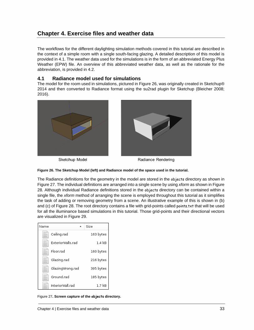
4.1 Radiance model used for simulations The model for the room used in simulations, pictured in Figure 26, was originally created in Sketchup®
2014 and then converted to Radiance format using the su2rad plugin for Sketchup (Bleicher 2008;
2016).
Figure 26. The Sketchup Model (left) and Radiance model of the space used in the tutorial.
The Radiance definitions for the geometry in the model are stored in the objects directory as shown in
Figure 27. The individual definitions are arranged into a single scene by using xform as shown in Figure
28. Although individual Radiance definitions stored in the objects directory can be contained within a
single file, the xform method of arranging the scene is employed throughout this tutorial as it simplifies
the task of adding or removing geometry from a scene. An illustrative example of this is shown in (b)
and (c) of Figure 28. The root directory contains a file with grid-points called points.txt that will be used
for all the illuminance based simulations in this tutorial. Those grid-points and their directional vectors
are visualized in Figure 29.
Figure 27. Screen capture of the objects directory.

Chapter 4 | Exercise files and weather data 34
Figure 28. Objview rendered screen-captures of room.rad. The xform commands on each line serve to add a
particular Radiance definition into the scene. The material definitions of all the objects are saved in
materials.rad. Assuming that current working directory is set to room, the command for launching objview will
be objview materials.rad room.rad. The images on the top row show screen captures of the files that were
rendered to create images in the bottom row. The grates shown in image (b) were added to the scene by adding “!xform ./overhang/aluminiumGrate.rad” to the definition in (a). Similarly, the ground polygon in (a) and (b) was removed in (c) by commenting out “!xform ./objects/Ground.rad” in (c) with a #.
Figure 29. A visualization of the grid-points that will be used for illuminance calculations is shown on the left.
The grid points are listed in points.txt. The geometry used to visualize the points can be found in
assets/ptsArray.rad. The upward direction of the arrows indicates that the illuminance measurement is being
done in the positive Z direction. The image on the right shows a typical two-dimensional data visualization of illuminance values measured at these grid-points. The letters A, B, C, D and E in both images refer to the same locations on the measurement grid.
Chapter 4 | Exercise files and weather data 35
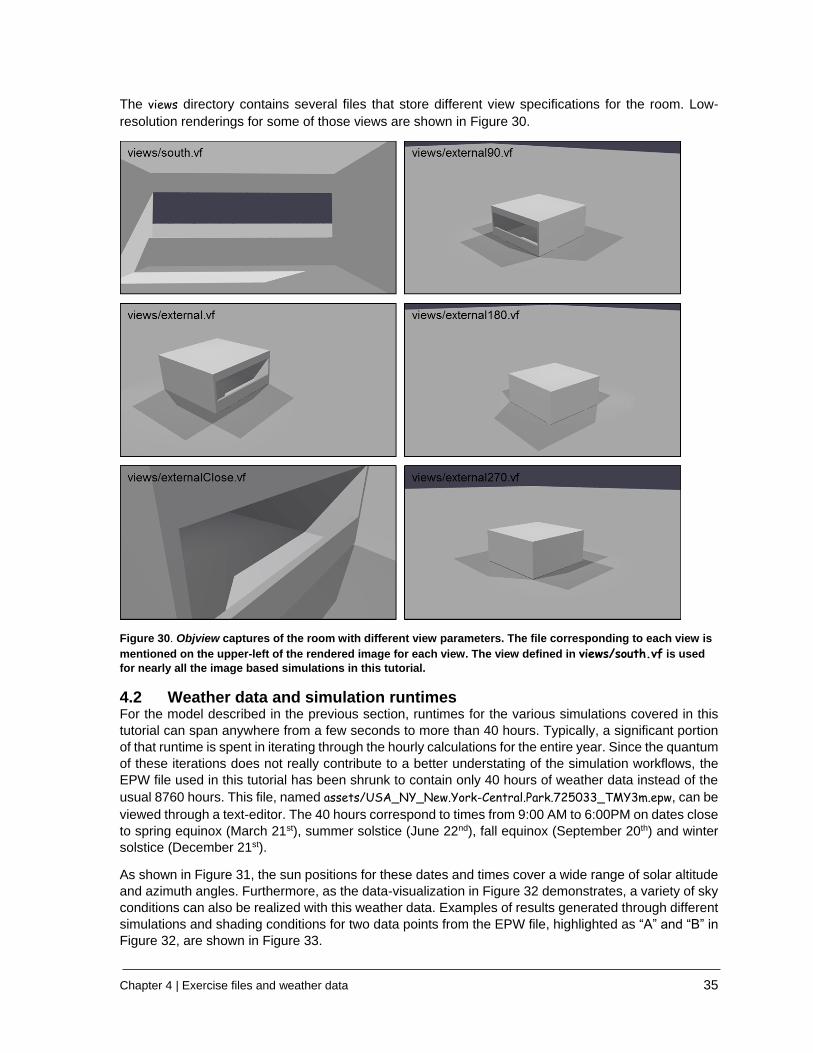
The views directory contains several files that store different view specifications for the room. Low-
resolution renderings for some of those views are shown in Figure 30.
Figure 30. Objview captures of the room with different view parameters. The file corresponding to each view is
mentioned on the upper-left of the rendered image for each view. The view defined in views/south.vf is used
for nearly all the image based simulations in this tutorial.
4.2 Weather data and simulation runtimes For the model described in the previous section, runtimes for the various simulations covered in this
tutorial can span anywhere from a few seconds to more than 40 hours. Typically, a significant portion
of that runtime is spent in iterating through the hourly calculations for the entire year. Since the quantum
of these iterations does not really contribute to a better understating of the simulation workflows, the
EPW file used in this tutorial has been shrunk to contain only 40 hours of weather data instead of the
usual 8760 hours. This file, named assets/USA_NY_New.York-Central.Park.725033_TMY3m.epw, can be
viewed through a text-editor. The 40 hours correspond to times from 9:00 AM to 6:00PM on dates close
to spring equinox (March 21st), summer solstice (June 22nd), fall equinox (September 20th) and winter
solstice (December 21st).
As shown in Figure 31, the sun positions for these dates and times cover a wide range of solar altitude
and azimuth angles. Furthermore, as the data-visualization in Figure 32 demonstrates, a variety of sky
conditions can also be realized with this weather data. Examples of results generated through different
simulations and shading conditions for two data points from the EPW file, highlighted as “A” and “B” in
Figure 32, are shown in Figure 33.
Chapter 4 | Exercise files and weather data 36
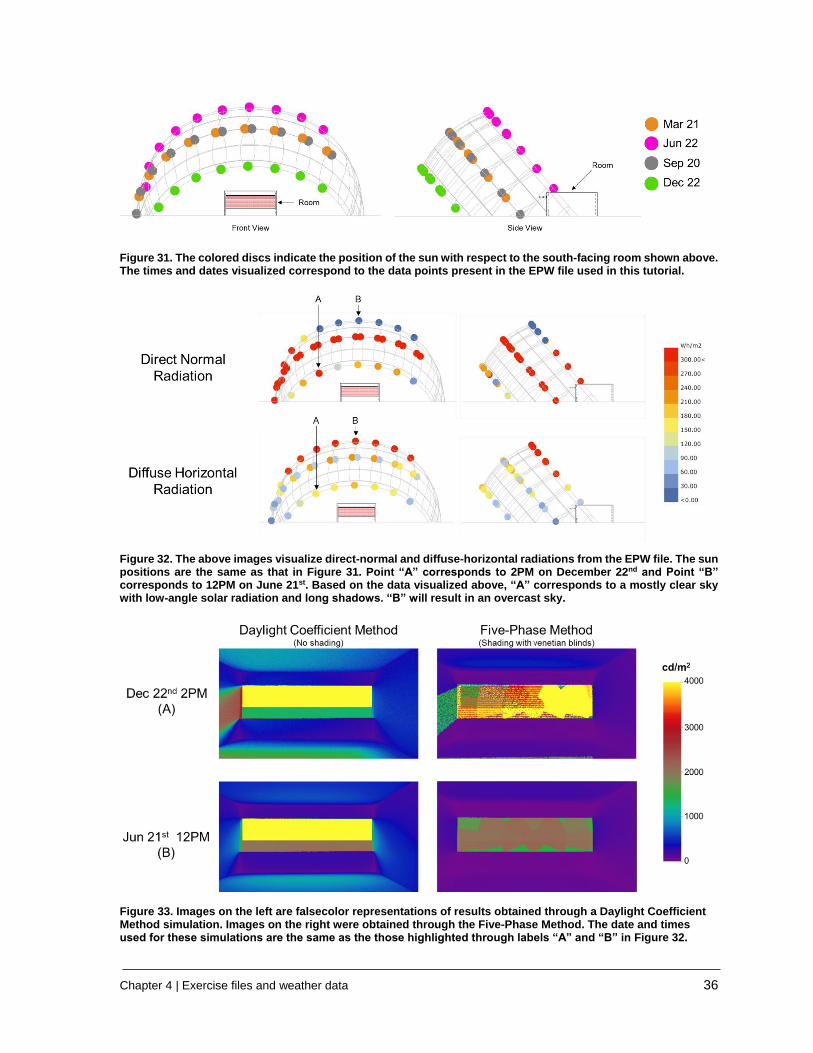
Figure 31. The colored discs indicate the position of the sun with respect to the south-facing room shown above. The times and dates visualized correspond to the data points present in the EPW file used in this tutorial.
Figure 32. The above images visualize direct-normal and diffuse-horizontal radiations from the EPW file. The sun positions are the same as that in Figure 31. Point “A” corresponds to 2PM on December 22nd and Point “B” corresponds to 12PM on June 21st. Based on the data visualized above, “A” corresponds to a mostly clear sky with low-angle solar radiation and long shadows. “B” will result in an overcast sky.
Figure 33. Images on the left are falsecolor representations of results obtained through a Daylight Coefficient Method simulation. Images on the right were obtained through the Five-Phase Method. The date and times used for these simulations are the same as the those highlighted through labels “A” and “B” in Figure 32.
Chapter 4 | Exercise files and weather data 37
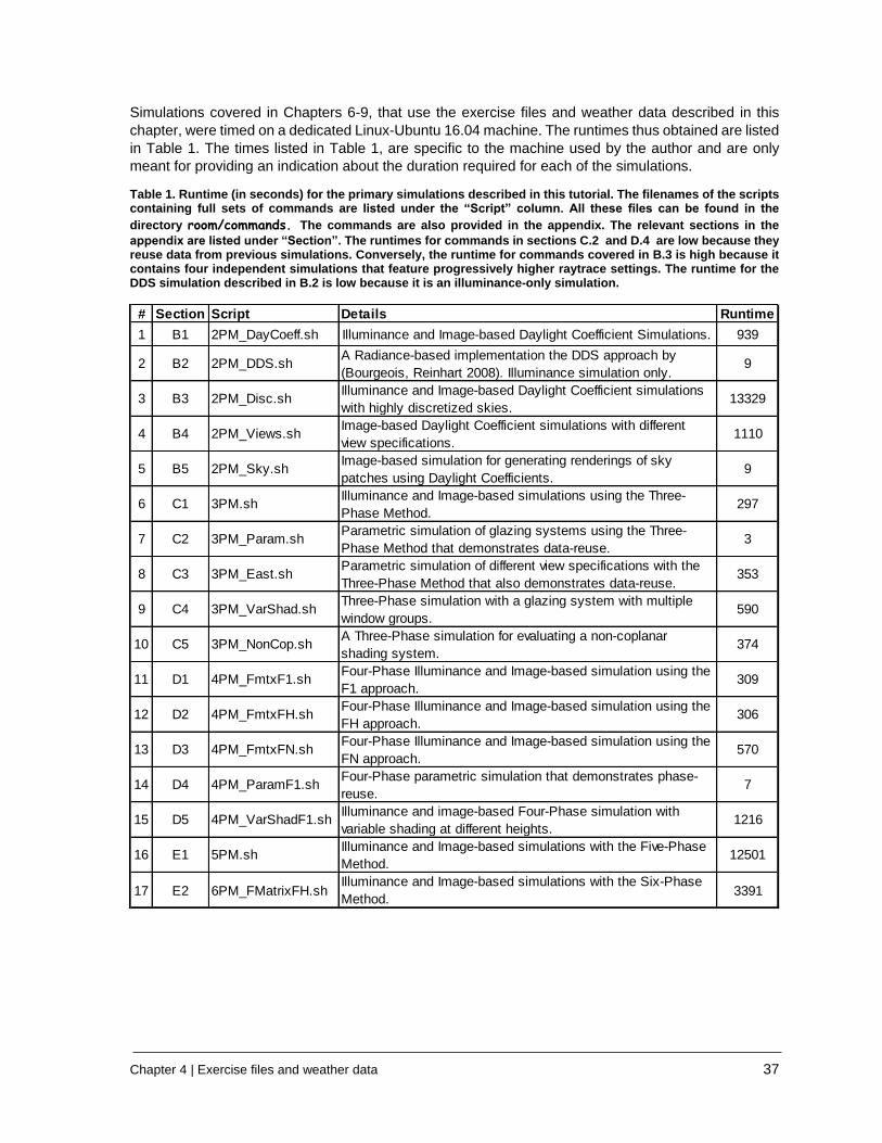
Simulations covered in Chapters 6-9, that use the exercise files and weather data described in this
chapter, were timed on a dedicated Linux-Ubuntu 16.04 machine. The runtimes thus obtained are listed
in Table 1. The times listed in Table 1, are specific to the machine used by the author and are only
meant for providing an indication about the duration required for each of the simulations.
Table 1. Runtime (in seconds) for the primary simulations described in this tutorial. The filenames of the scripts containing full sets of commands are listed under the “Script” column. All these files can be found in the
directory room/commands. The commands are also provided in the appendix. The relevant sections in the
appendix are listed under “Section”. The runtimes for commands in sections C.2 and D.4 are low because they reuse data from previous simulations. Conversely, the runtime for commands covered in B.3 is high because it contains four independent simulations that feature progressively higher raytrace settings. The runtime for the DDS simulation described in B.2 is low because it is an illuminance-only simulation.
# Section Script Details Runtime
1 B1 2PM_DayCoeff.sh Illuminance and Image-based Daylight Coefficient Simulations. 939
2 B2 2PM_DDS.shA Radiance-based implementation the DDS approach by
(Bourgeois, Reinhart 2008). Illuminance simulation only.9
3 B3 2PM_Disc.shIlluminance and Image-based Daylight Coefficient simulations
with highly discretized skies.13329
4 B4 2PM_Views.shImage-based Daylight Coefficient simulations with different
view specifications.1110
5 B5 2PM_Sky.shImage-based simulation for generating renderings of sky
patches using Daylight Coefficients.9
6 C1 3PM.shIlluminance and Image-based simulations using the Three-
Phase Method.297
7 C2 3PM_Param.shParametric simulation of glazing systems using the Three-
Phase Method that demonstrates data-reuse.3
8 C3 3PM_East.shParametric simulation of different view specifications with the
Three-Phase Method that also demonstrates data-reuse.353
9 C4 3PM_VarShad.shThree-Phase simulation with a glazing system with multiple
window groups.590
10 C5 3PM_NonCop.shA Three-Phase simulation for evaluating a non-coplanar
shading system.374
11 D1 4PM_FmtxF1.shFour-Phase Illuminance and Image-based simulation using the
F1 approach.309
12 D2 4PM_FmtxFH.shFour-Phase Illuminance and Image-based simulation using the
FH approach.306
13 D3 4PM_FmtxFN.shFour-Phase Illuminance and Image-based simulation using the
FN approach.570
14 D4 4PM_ParamF1.shFour-Phase parametric simulation that demonstrates phase-
reuse.7
15 D5 4PM_VarShadF1.shIlluminance and image-based Four-Phase simulation with
variable shading at different heights.1216
16 E1 5PM.shIlluminance and Image-based simulations with the Five-Phase
Method.12501
17 E2 6PM_FMatrixFH.shIlluminance and Image-based simulations with the Six-Phase
Method.3391
Chapter 5 | Skies, Sky-Vectors and Sky-Matrices 38
Chapter 5. Skies, Sky-Vectors and Sky-Matrices
The two commonly used sky types for daylighting simulations are based on the CIE sky model (CIE
2003) and the Perez sky model (Perez et al. 1990). These models are essentially mathematical
equations that calculate the continuous luminance distribution of the celestial hemisphere as a function
of variables such as geographical location, time and physically measured radiation data. The use of the
Perez Sky Model is more prevalent for climate based daylight modeling as it has been formulaized to
automatically generate the luminous distribution of the sky based on site longitude, latitude, meridian,
time, direct-normal radiation and diffuse horizontal radiation. These inputs alone are sufficient to
determine whether the sky would be overcast, clear or of an intermediate type. In the case of the CIE
sky model, the type of sky needs to be chosen manually from 15 luminance distributions such as CIE
Standard Overcast Sky, CIE Standard Clear Sky and Partly Cloudy Sky7.
5.1 describes the commands for generating point-in-time sky-vectors using genskyvec and 5.2
describes the commands for generating an annual sky-matrix using gendaymtx that is commonly used
in annual daylighting simulations. For all the simulation methods covered in this tutorial, the distinction
between a point-in-time simulation or an annual simulation is predicated on the selection of the point-
in-time sky-vector or annual sky-matrix respectively8.
5.1 A point-in-time sky-vector using the CIE or Perez sky model Creating a point-in-time sky-vector is a two-step process. Initially a Radiance definition of a continuous
sky model is created using gensky or gendaylit. Then a discretized sky-vector is created from that
continuous sky definition using genskyvec.
5.1.1 Radiance definition of a sky using the CIE Sky Model A point-in-time sky-vector based on the CIE sky model can be generated using gensky as:
gensky 3 20 10:30EDT -m 75 -o 73.96 -a 40.78 > skies/NYC_CIE.sky
The term 3 20 10:30EDT corresponds to 20th March, 10:30 AM Eastern Daylight Time. -o 73.96 -a
40.78 refers to a longitude of 73.83° W and an altitude of 40.71° N. Further options to tweak the above
command, such as adding or subtracting the radiation from sun, can be found in the manual for gensky.
As discussed earlier, the CIE sky model requires the sky type to be set manually. Various flags such
as +s, -s, -i, and -u can be assigned to gensky to select the desired CIE sky type. The default setting
in gensky is +s, which corresponds to a CIE clear sky.
5.1.2 Radiance definition of a sky using the Perez Sky Model A Perez Sky definition can be generated using gendaylit. A typical command with gendaylit would be:
gendaylit 3 20 10:30EDT -m 75 -o 73.96 -a 40.78 > skies/NYC_Per.sky
The parameters for generating a Perez Sky definition should also include direct-normal-irradiance and
diffuse-horizontal-irradiance. This can be done through the -W flag in gendaylit. For example, the
command described above can also be specified with direct-normal-irradiance and diffuse-horizontal-
irradiance values through -W 706 162 as shown below:
gendaylit 3 20 10:30EDT -m 75 -o 73.96 -a 40.78 -W 706 162 > skies/NYC_Per_DH.sky
7 A detailed description of the different types of CIE skies, as well as a mild critique of the Perez Sky Model, can be found in (CIE
2014). An approach that involves blending different types of CIE skies has been discussed in (Mardaljevic 2008). 8 As discussed in the previous chapter, the examples in this tutorial employ an abbreviated EPW for reducing the time taken for
simulations. That EPW file can be swapped with a normal EPW file for performing full-fledged annual simulations. Except for the corresponding changes to the “for” loops in the Five-Phase and Six-Phase Method simulations, where the count needs to be changed from 40 to 8760, no other changes are required to be made to the simulation workflows.
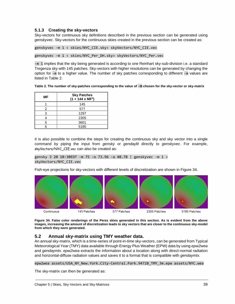
Chapter 5 | Skies, Sky-Vectors and Sky-Matrices 39
5.1.3 Creating the sky-vectors Sky-vectors for continuous sky definitions described in the previous section can be generated using
genskyvec. Sky-vectors for the continuous skies created in the previous section can be created as:
genskyvec -m 1 < skies/NYC_CIE.sky> skyVectors/NYC_CIE.vec
genskyvec -m 1 < skies/NYC_Per_DH.sky> skyVectors/NYC_Per.vec
-m 1 implies that the sky being generated is according to one Reinhart sky-sub-division i.e. a standard
Tregenza sky with 145 patches. Sky-vectors with higher resolutions can be generated by changing the
option for -m to a higher value. The number of sky patches corresponding to different -m values are
listed in Table 2.
Table 2. The number of sky-patches corresponding to the value of -m chosen for the sky-vector or sky-matrix
MF Sky Patches
(1 + 144 x MF2)
1 145
2 577
3 1297
4 2305
5 3601
6 5185
It is also possible to combine the steps for creating the continuous sky and sky vector into a single
command by piping the input from gensky or gendaylit directly to genskyvec. For example,
skyVectors/NYC_CIE.vec can also be created as:
gensky 3 20 10:30EDT -m 75 -o 73.96 -a 40.78 | genskyvec -m 1 >
skyVectors/NYC_CIE.vec
Fish-eye projections for sky-vectors with different levels of discretization are shown in Figure 34.
Figure 34. False color renderings of the Perez skies generated in this section. As is evident from the above images, increasing the amount of discretization leads to sky vectors that are closer to the continuous sky-model from which they were generated.
5.2 Annual sky-matrix using TMY weather data. An annual sky-matrix, which is a time-series of point-in-time sky-vectors, can be generated from Typical
Meteorological Year (TMY) data available through Energy Plus Weather (EPW) data by using epw2wea
and gendaymtx. epw2wea extracts the information about a location along with direct-normal radiation
and horizontal-diffuse radiation values and saves it to a format that is compatible with gendaymtx.
epw2wea assets/USA_NY_New.York.City-Central.Park.94728_TMY_3m.epw assets/NYC.wea
The sky-matrix can then be generated as:
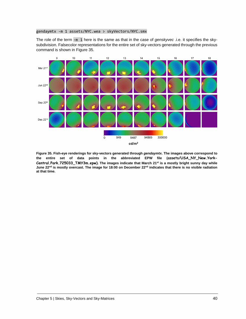
Chapter 5 | Skies, Sky-Vectors and Sky-Matrices 40
gendaymtx -m 1 assets/NYC.wea > skyVectors/NYC.smx
The role of the term -m 1 here is the same as that in the case of genskyvec .i.e. it specifies the sky-
subdivision. Falsecolor representations for the entire set of sky-vectors generated through the previous
command is shown in Figure 35.
Figure 35. Fish-eye renderings for sky-vectors generated through gendaymtx. The images above correspond to
the entire set of data points in the abbreviated EPW file (assets/USA_NY_New.York-
Central.Park.725033_TMY3m.epw). The images indicate that March 21st is a mostly bright sunny day while
June 22nd is mostly overcast. The image for 18:00 on December 22nd indicates that there is no visible radiation at that time.

Chapter 6 | Daylight Coefficients: The Two-Phase Method 41
Chapter 6. Daylight Coefficients: The Two-Phase Method
Overview: The core part of a Daylight Coefficient Method simulation, depicted in Figure 36, involves
creating a daylight coefficient file with rfluxmtx and a sky-vector or sky-matrix file with genskyvec or
gendaymtx respectively. The results are generated by multiplying the matrices contained in these files
with dctimestep. For illuminance-based simulations, dctimestep generates ASCII-format irradiance
values in sets of three numbers corresponding to the Red, Green and Blue channels (RGB). Rmtxop
is then used to convert the RGB values into illuminance.
Figure 36. Schematic diagram for the Daylight Coefficient Method along with a stage-wise list of Radiance programs involved in the workflow. Vwrays is only required in case the simulation is image-based.
6.1 Basic Daylight Coefficients simulation Daylight coefficients are created with rfluxmtx by specifying “senders” and “receivers” of light rays. The
“sender” is usually a set of rays that are either derived through grid-points in a file or from a view
specification through vwrays. Receiver is usually a couple of hemispherical domes that represent the
sky and ground. The definition for the receiver is saved in skyDomes/skyglow.rad. This file needs to be
specified with proper rfluxmtx control parameters before it can be used with rfluxmtx. Figure 37 shows
the modifications required to be made to skyDomes/skyglow.rad to prepare it as a receiver for rfluxmtx.
6.1.1.1 Daylight Coefficients for Illuminance The initial step for this simulation involves creating an octree for all the material and geometry definitions
relevant to the simulation. The octree can be created with oconv as:
oconv materials.rad room.rad objects/Glazing.rad > octrees/roomDC.oct Daylight coefficients for calculating illuminance can be calculated with rfluxmtx as:
rfluxmtx -I+ -y 100 -lw 0.0001 -ab 5 -ad 10000 -n 16 - skyDomes/skyglow.rad -i octrees/roomDC.oct < points.txt > matrices/dc/illum.mtx The term -I+ denotes that the simulation is being performed for calculating irradiance instead of
radiance. The 100 in -y 100 is equal to the number of lines in the file points.txt, where each line
specifies a grid-point location and vector direction. The number of processors assigned for the
simulation can be set by changing the 16 in -n 16 to a higher or lower value. The - before
skyDomes/skyglow.rad indicates that the sender for rfluxmtx will be specified through standard input
(< points.txt). Finally, > matrices/dc/illum.mtx implies that the output of this calculation will be
saved to the file matrices/dc/illum.mtx.
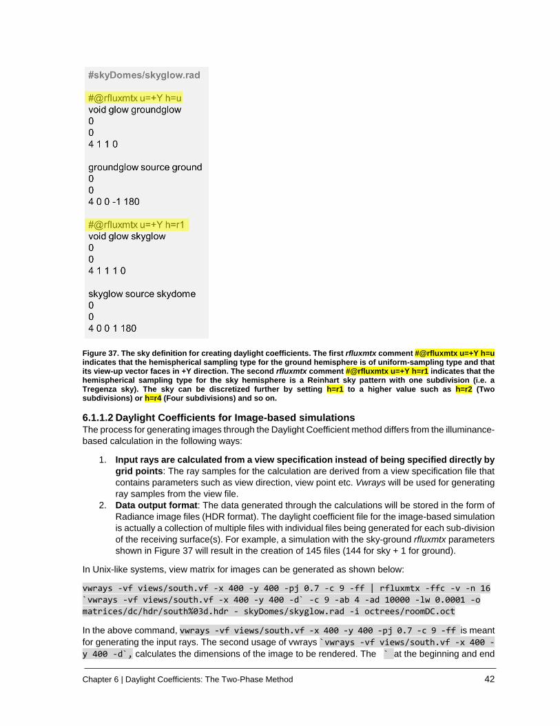
Chapter 6 | Daylight Coefficients: The Two-Phase Method 42
Figure 37. The sky definition for creating daylight coefficients. The first rfluxmtx comment #@rfluxmtx u=+Y h=u indicates that the hemispherical sampling type for the ground hemisphere is of uniform-sampling type and that its view-up vector faces in +Y direction. The second rfluxmtx comment #@rfluxmtx u=+Y h=r1 indicates that the hemispherical sampling type for the sky hemisphere is a Reinhart sky pattern with one subdivision (i.e. a Tregenza sky). The sky can be discretized further by setting h=r1 to a higher value such as h=r2 (Two subdivisions) or h=r4 (Four subdivisions) and so on.
6.1.1.2 Daylight Coefficients for Image-based simulations The process for generating images through the Daylight Coefficient method differs from the illuminance-
based calculation in the following ways:
1. Input rays are calculated from a view specification instead of being specified directly by
grid points: The ray samples for the calculation are derived from a view specification file that
contains parameters such as view direction, view point etc. Vwrays will be used for generating
ray samples from the view file.
2. Data output format: The data generated through the calculations will be stored in the form of
Radiance image files (HDR format). The daylight coefficient file for the image-based simulation
is actually a collection of multiple files with individual files being generated for each sub-division
of the receiving surface(s). For example, a simulation with the sky-ground rfluxmtx parameters
shown in Figure 37 will result in the creation of 145 files (144 for sky + 1 for ground).
In Unix-like systems, view matrix for images can be generated as shown below:
vwrays -vf views/south.vf -x 400 -y 400 -pj 0.7 -c 9 -ff | rfluxmtx -ffc -v -n 16
`vwrays -vf views/south.vf -x 400 -y 400 -d` -c 9 -ab 4 -ad 10000 -lw 0.0001 -o
matrices/dc/hdr/south%03d.hdr - skyDomes/skyglow.rad -i octrees/roomDC.oct
In the above command, vwrays -vf views/south.vf -x 400 -y 400 -pj 0.7 -c 9 -ff is meant
for generating the input rays. The second usage of vwrays `vwrays -vf views/south.vf -x 400 -
y 400 -d`, calculates the dimensions of the image to be rendered. The ` at the beginning and end
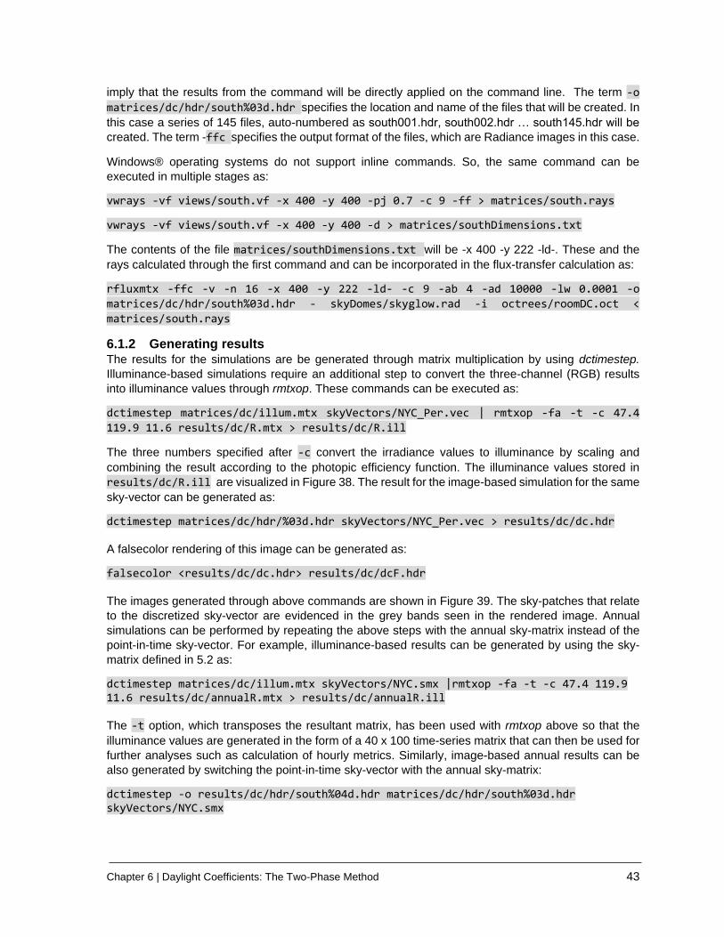
Chapter 6 | Daylight Coefficients: The Two-Phase Method 43
imply that the results from the command will be directly applied on the command line. The term -o
matrices/dc/hdr/south%03d.hdr specifies the location and name of the files that will be created. In
this case a series of 145 files, auto-numbered as south001.hdr, south002.hdr … south145.hdr will be
created. The term -ffc specifies the output format of the files, which are Radiance images in this case.
Windows® operating systems do not support inline commands. So, the same command can be
executed in multiple stages as:
vwrays -vf views/south.vf -x 400 -y 400 -pj 0.7 -c 9 -ff > matrices/south.rays
vwrays -vf views/south.vf -x 400 -y 400 -d > matrices/southDimensions.txt
The contents of the file matrices/southDimensions.txt will be -x 400 -y 222 -ld-. These and the
rays calculated through the first command and can be incorporated in the flux-transfer calculation as:
rfluxmtx -ffc -v -n 16 -x 400 -y 222 -ld- -c 9 -ab 4 -ad 10000 -lw 0.0001 -o
matrices/dc/hdr/south%03d.hdr - skyDomes/skyglow.rad -i octrees/roomDC.oct <
matrices/south.rays
6.1.2 Generating results The results for the simulations are be generated through matrix multiplication by using dctimestep.
Illuminance-based simulations require an additional step to convert the three-channel (RGB) results
into illuminance values through rmtxop. These commands can be executed as:
dctimestep matrices/dc/illum.mtx skyVectors/NYC_Per.vec | rmtxop -fa -t -c 47.4
119.9 11.6 results/dc/R.mtx > results/dc/R.ill
The three numbers specified after -c convert the irradiance values to illuminance by scaling and
combining the result according to the photopic efficiency function. The illuminance values stored in
results/dc/R.ill are visualized in Figure 38. The result for the image-based simulation for the same
sky-vector can be generated as:
dctimestep matrices/dc/hdr/%03d.hdr skyVectors/NYC_Per.vec > results/dc/dc.hdr A falsecolor rendering of this image can be generated as:
falsecolor <results/dc/dc.hdr> results/dc/dcF.hdr The images generated through above commands are shown in Figure 39. The sky-patches that relate
to the discretized sky-vector are evidenced in the grey bands seen in the rendered image. Annual
simulations can be performed by repeating the above steps with the annual sky-matrix instead of the
point-in-time sky-vector. For example, illuminance-based results can be generated by using the sky-
matrix defined in 5.2 as:
dctimestep matrices/dc/illum.mtx skyVectors/NYC.smx |rmtxop -fa -t -c 47.4 119.9 11.6 results/dc/annualR.mtx > results/dc/annualR.ill The -t option, which transposes the resultant matrix, has been used with rmtxop above so that the
illuminance values are generated in the form of a 40 x 100 time-series matrix that can then be used for
further analyses such as calculation of hourly metrics. Similarly, image-based annual results can be
also generated by switching the point-in-time sky-vector with the annual sky-matrix:
dctimestep -o results/dc/hdr/south%04d.hdr matrices/dc/hdr/south%03d.hdr skyVectors/NYC.smx
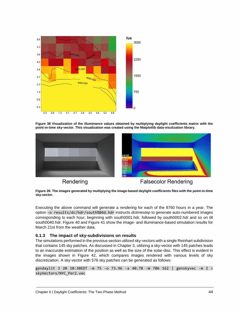
Chapter 6 | Daylight Coefficients: The Two-Phase Method 44
Figure 38 Visualization of the illuminance values obtained by multiplying daylight coefficients matrix with the point-in-time sky-vector. This visualization was created using the Matplotlib data-visulization library.
Figure 39. The images generated by multiplying the image-based daylight coefficients files with the point-in-time sky-vector.
Executing the above command will generate a rendering for each of the 8760 hours in a year. The
option -o results/dc/hdr/south%04d.hdr instructs dctimestep to generate auto-numbered images
corresponding to each hour, beginning with south0001.hdr, followed by south0002.hdr and so on till
south0040.hdr. Figure 40 and Figure 41 show the image- and illuminance-based simulation results for
March 21st from the weather data.
6.1.3 The impact of sky-subdivisions on results The simulations performed in the previous section utilized sky-vectors with a single Reinhart subdivision
that contains 145 sky patches. As discussed in Chapter 3, utilizing a sky-vector with 145 patches leads
to an inaccurate estimation of the position as well as the size of the solar-disc. This effect is evident in
the images shown in Figure 42, which compares images rendered with various levels of sky
discretization. A sky-vector with 576 sky patches can be generated as follows:
gendaylit 3 20 10:30EDT -m 75 -o 73.96 -a 40.78 -W 706 162 | genskyvec -m 2 >
skyVectors/NYC_Per2.vec
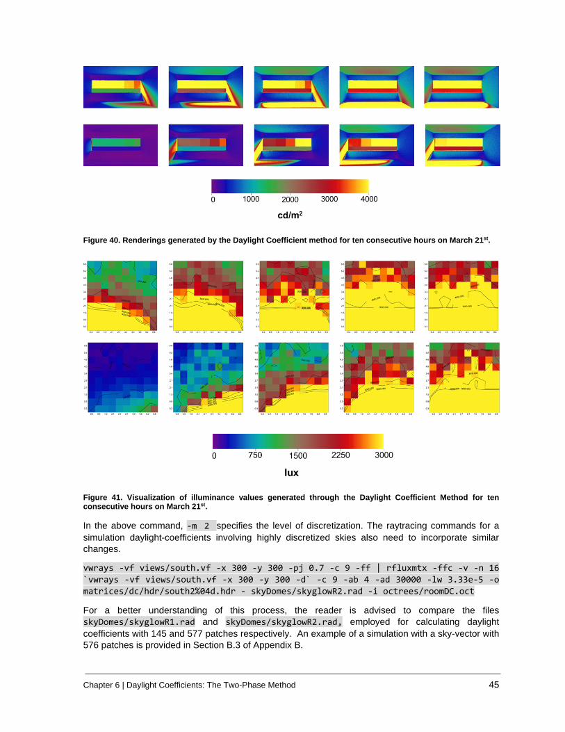
Chapter 6 | Daylight Coefficients: The Two-Phase Method 45
Figure 40. Renderings generated by the Daylight Coefficient method for ten consecutive hours on March 21st.
Figure 41. Visualization of illuminance values generated through the Daylight Coefficient Method for ten consecutive hours on March 21st.
In the above command, -m 2 specifies the level of discretization. The raytracing commands for a
simulation daylight-coefficients involving highly discretized skies also need to incorporate similar
changes.
vwrays -vf views/south.vf -x 300 -y 300 -pj 0.7 -c 9 -ff | rfluxmtx -ffc -v -n 16
`vwrays -vf views/south.vf -x 300 -y 300 -d` -c 9 -ab 4 -ad 30000 -lw 3.33e-5 -o
matrices/dc/hdr/south2%04d.hdr - skyDomes/skyglowR2.rad -i octrees/roomDC.oct
For a better understanding of this process, the reader is advised to compare the files
skyDomes/skyglowR1.rad and skyDomes/skyglowR2.rad, employed for calculating daylight
coefficients with 145 and 577 patches respectively. An example of a simulation with a sky-vector with
576 patches is provided in Section B.3 of Appendix B.

Chapter 6 | Daylight Coefficients: The Two-Phase Method 46
Figure 42. Image-based simulations for sky-vectors with varying levels of discretization. The daylighting conditions and view-specification for all the images are the same. The image featuring the highest number of sky-patches also has the most well defined shadows.
6.1.4 Simulations for multiple view specifications Image-based simulations for other view-definitions can be performed by changing the details pertaining
to view-specifications alone. The images shown in Figure 43 were generated by changing the view-file
in the steps described in Section 6.1.1.2. A similar example is provided in B.4 of Appendix B.
Figure 43. Images generated through Daylight Coefficient Method based simulations for different view specifications.
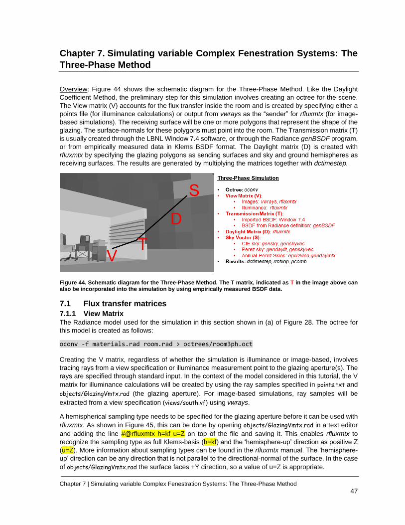
Chapter 7 | Simulating variable Complex Fenestration Systems: The Three-Phase Method
47
Chapter 7. Simulating variable Complex Fenestration Systems: The
Three-Phase Method
Overview: Figure 44 shows the schematic diagram for the Three-Phase Method. Like the Daylight
Coefficient Method, the preliminary step for this simulation involves creating an octree for the scene.
The View matrix (V) accounts for the flux transfer inside the room and is created by specifying either a
points file (for illuminance calculations) or output from vwrays as the “sender” for rfluxmtx (for image-
based simulations). The receiving surface will be one or more polygons that represent the shape of the
glazing. The surface-normals for these polygons must point into the room. The Transmission matrix (T)
is usually created through the LBNL Window 7.4 software, or through the Radiance genBSDF program,
or from empirically measured data in Klems BSDF format. The Daylight matrix (D) is created with
rfluxmtx by specifying the glazing polygons as sending surfaces and sky and ground hemispheres as
receiving surfaces. The results are generated by multiplying the matrices together with dctimestep.
Figure 44. Schematic diagram for the Three-Phase Method. The T matrix, indicated as T in the image above can also be incorporated into the simulation by using empirically measured BSDF data.
7.1 Flux transfer matrices
7.1.1 View Matrix The Radiance model used for the simulation in this section shown in (a) of Figure 28. The octree for
this model is created as follows:
oconv -f materials.rad room.rad > octrees/room3ph.oct Creating the V matrix, regardless of whether the simulation is illuminance or image-based, involves
tracing rays from a view specification or illuminance measurement point to the glazing aperture(s). The
rays are specified through standard input. In the context of the model considered in this tutorial, the V
matrix for illuminance calculations will be created by using the ray samples specified in points.txt and
objects/GlazingVmtx.rad (the glazing aperture). For image-based simulations, ray samples will be
extracted from a view specification (views/south.vf) using vwrays.
A hemispherical sampling type needs to be specified for the glazing aperture before it can be used with
rfluxmtx. As shown in Figure 45, this can be done by opening objects/GlazingVmtx.rad in a text editor
and adding the line #@rfluxmtx h=kf u=Z on top of the file and saving it. This enables rfluxmtx to
recognize the sampling type as full Klems-basis (h=kf) and the ‘hemisphere-up’ direction as positive Z
(u=Z). More information about sampling types can be found in the rfluxmtx manual. The ‘hemisphere-
up’ direction can be any direction that is not parallel to the directional-normal of the surface. In the case
of objects/GlazingVmtx.rad the surface faces +Y direction, so a value of u=Z is appropriate.
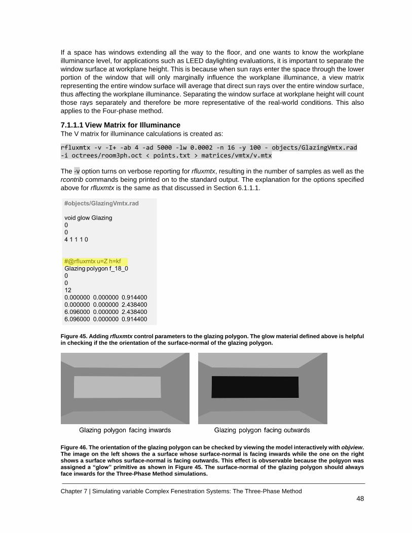
Chapter 7 | Simulating variable Complex Fenestration Systems: The Three-Phase Method
48
If a space has windows extending all the way to the floor, and one wants to know the workplane
illuminance level, for applications such as LEED daylighting evaluations, it is important to separate the
window surface at workplane height. This is because when sun rays enter the space through the lower
portion of the window that will only marginally influence the workplane illuminance, a view matrix
representing the entire window surface will average that direct sun rays over the entire window surface,
thus affecting the workplane illuminance. Separating the window surface at workplane height will count
those rays separately and therefore be more representative of the real-world conditions. This also
applies to the Four-phase method.
7.1.1.1 View Matrix for Illuminance The V matrix for illuminance calculations is created as:
rfluxmtx -v -I+ -ab 4 -ad 5000 -lw 0.0002 -n 16 -y 100 - objects/GlazingVmtx.rad -i octrees/room3ph.oct < points.txt > matrices/vmtx/v.mtx The -v option turns on verbose reporting for rfluxmtx, resulting in the number of samples as well as the
rcontrib commands being printed on to the standard output. The explanation for the options specified
above for rfluxmtx is the same as that discussed in Section 6.1.1.1.
Figure 45. Adding rfluxmtx control parameters to the glazing polygon. The glow material defined above is helpful in checking if the the orientation of the surface-normal of the glazing polygon.
Figure 46. The orientation of the glazing polygon can be checked by viewing the model interactively with objview. The image on the left shows the a surface whose surface-normal is facing inwards while the one on the right shows a surface whos surface-normal is facing outwards. This effect is obvservable because the polgyon was assigned a “glow” primitive as shown in Figure 45. The surface-normal of the glazing polygon should always face inwards for the Three-Phase Method simulations.
Chapter 7 | Simulating variable Complex Fenestration Systems: The Three-Phase Method
49
7.1.1.2 View Matrix for Image-based simulations The procedure for creating the V matrix for image based simulations is similar to the one described for
the Daylight Coefficient method in section 6.1.1.2. The main difference in the case of the Three-Phase
Method is that instead of tracing rays all the way up to the sky, the rays are traced only till the glazing
aperture.
The series of auto-numbered images that collectively represent the V-Matrix can be created as:
vwrays -vf views/south.vf -x 400 -y 400 -pj 0.7 -c 9 -ff | rfluxmtx -v -ffc `vwrays
-vf views/south.vf -x 400 -y 400 -d` -o matrices/vmtx/hdr/south%03d.hdr -ab 4 -ad
1000 -lw 1e-4 -c 9 -n 16 - objects/GlazingVmtx.rad -i octrees/room3ph.oct
In the above command, vwrays -vf views/south.vf -x 400 -y 400 -pj 0.7 -c 9 -ff creates
rays from the specified view file. `vwrays -vf views/south.vf -x 400 -y 400 -d` is an inline
command that calculates the dimensions of the image to be generated. The actual raytracing is done
through rfluxmtx which invokes rcontrib in the background. After execution, this command will create
146 auto-numbered images in the directory matrices/vmtx/hdr. The next section provides a brief
description of how different types of glazing and shading systems can be incorporated into the Three-
Phase Method.
7.1.2 Transmission Matrix The T matrix is included in the Three-Phase Method as a Bidirectional Scattering Distribution Function
(BSDF) File. The BSDF file serves as the means of relating incident flux directions to exiting flux
distributions for fenestration systems. BSDF files required for the T matrix can be generated either
through LBNL Window 7.4 or through genBSDF. An explanation of the process for generating such
files is secondary to the focus of this tutorial.
A detailed example for generating BSDFs with Window 7.4 is provided in Section 3.2.1 of the Three-
Phase Method tutorial (McNeil 2013c). An example for generating BSDFs with genBSDF is provided in
Chapter 4 of the genBSDF tutorial (McNeil 2015).
The directory matrices/tmtx contains three pre-calculated BSDF xml files that will be used for
simulations in this tutorial. The file matrices/tmtx/clear.xml represents a clear glazing. The files
matrices/tmtx/ven0.xml and matrices/tmtx/ven45.xml represent a venetian blind with slats oriented at
0° and 45° respectively.
7.1.3 Daylight matrix As indicated in Figure 44, the Daylight matrix accounts for flux transfer between the glazing aperture(s)
to the sky and ground. So, in this case the file containing the glazing aperture geometry
(objects/GlazingVmtx.rad) will be the sending surface for rfluxmtx and the sky and ground definition
(skydomes/skyglow.rad) will be the receiving surface. The hemispherical sampling basis for these files
have been previously assigned, as explained through Figure 37 and Figure 45 respectively.
The Daylight matrix can then be created as:
rfluxmtx -v -ff -ab 4 -ad 1000 -lw 0.001 -c 1000 -n 16 objects/GlazingVmtx.rad skyDomes/skyglow.rad -i octrees/room3ph.oct > matrices/dmtx/daylight.dmx
7.2 Generating results The results for the Three-Phase Method simulation are calculated in a manner that is similar to the one
used for the Daylight Coefficient Method (Section 6.1.2). The process involves multiplying the View
matrix, Transmission Matrix and Daylight Matrix with a point-in-time sky vector or an annual sky-matrix.
The sky-vectors used for this calculation were created in Chapter 5. The post-processing required for
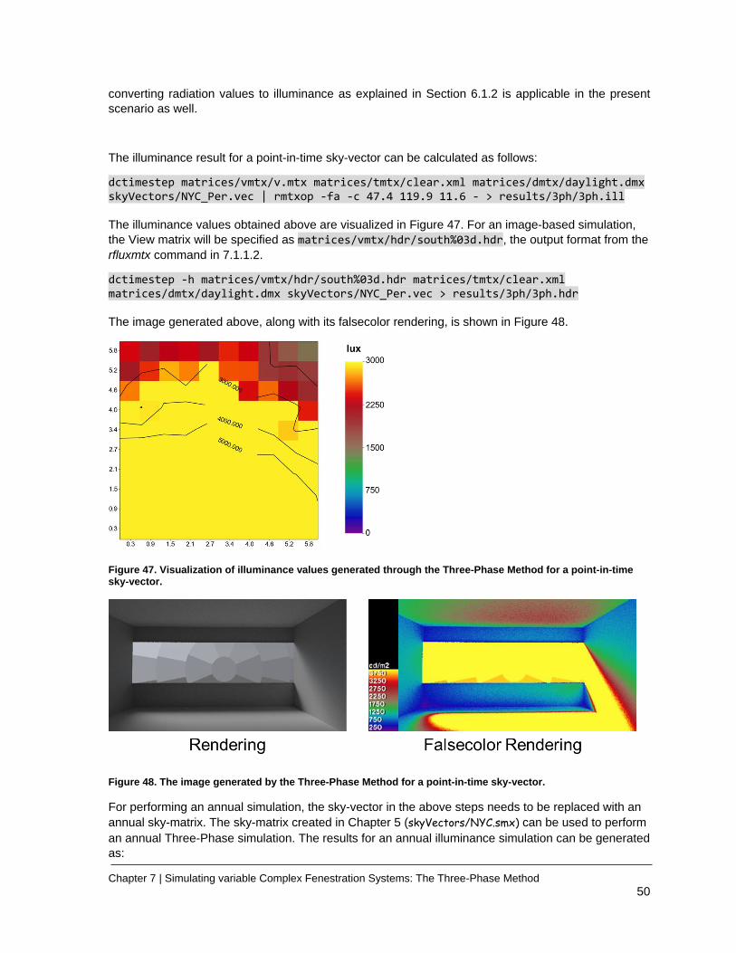
Chapter 7 | Simulating variable Complex Fenestration Systems: The Three-Phase Method
50
converting radiation values to illuminance as explained in Section 6.1.2 is applicable in the present
scenario as well.
The illuminance result for a point-in-time sky-vector can be calculated as follows:
dctimestep matrices/vmtx/v.mtx matrices/tmtx/clear.xml matrices/dmtx/daylight.dmx skyVectors/NYC_Per.vec | rmtxop -fa -c 47.4 119.9 11.6 - > results/3ph/3ph.ill The illuminance values obtained above are visualized in Figure 47. For an image-based simulation,
the View matrix will be specified as matrices/vmtx/hdr/south%03d.hdr, the output format from the
rfluxmtx command in 7.1.1.2.
dctimestep -h matrices/vmtx/hdr/south%03d.hdr matrices/tmtx/clear.xml matrices/dmtx/daylight.dmx skyVectors/NYC_Per.vec > results/3ph/3ph.hdr The image generated above, along with its falsecolor rendering, is shown in Figure 48.
Figure 47. Visualization of illuminance values generated through the Three-Phase Method for a point-in-time sky-vector.
Figure 48. The image generated by the Three-Phase Method for a point-in-time sky-vector.
For performing an annual simulation, the sky-vector in the above steps needs to be replaced with an
annual sky-matrix. The sky-matrix created in Chapter 5 (skyVectors/NYC.smx) can be used to perform
an annual Three-Phase simulation. The results for an annual illuminance simulation can be generated
as:
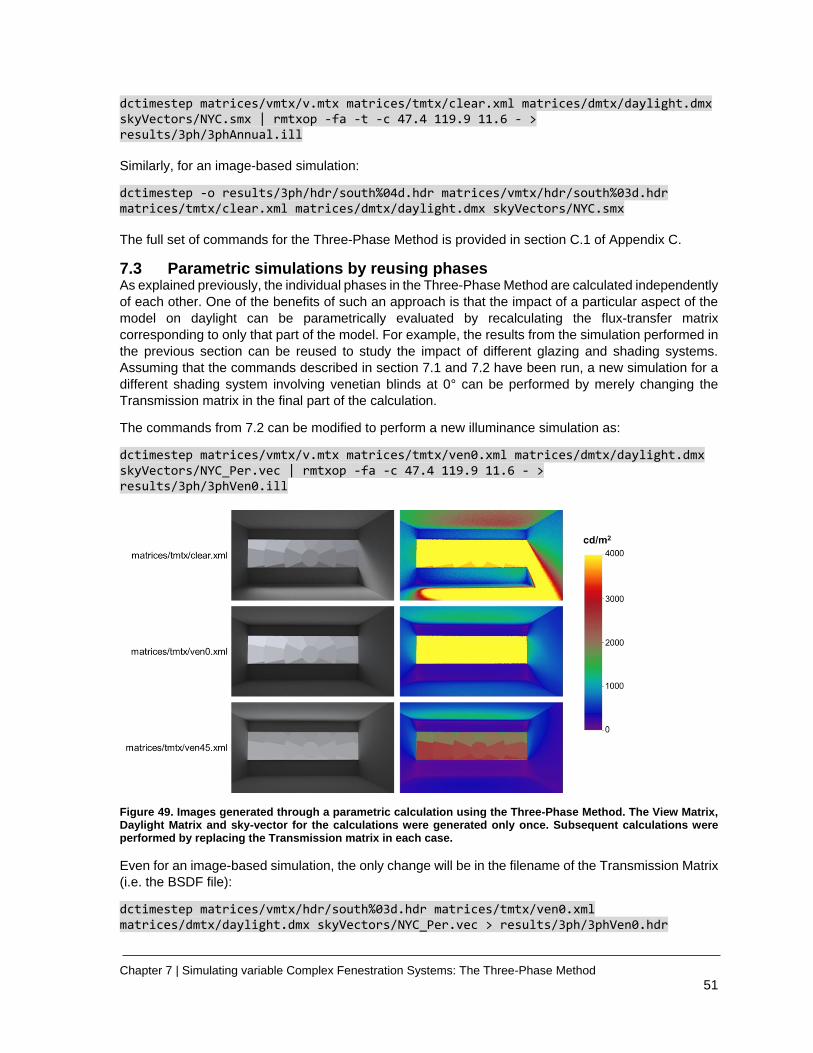
Chapter 7 | Simulating variable Complex Fenestration Systems: The Three-Phase Method
51
dctimestep matrices/vmtx/v.mtx matrices/tmtx/clear.xml matrices/dmtx/daylight.dmx skyVectors/NYC.smx | rmtxop -fa -t -c 47.4 119.9 11.6 - > results/3ph/3phAnnual.ill Similarly, for an image-based simulation:
dctimestep -o results/3ph/hdr/south%04d.hdr matrices/vmtx/hdr/south%03d.hdr matrices/tmtx/clear.xml matrices/dmtx/daylight.dmx skyVectors/NYC.smx The full set of commands for the Three-Phase Method is provided in section C.1 of Appendix C.
7.3 Parametric simulations by reusing phases As explained previously, the individual phases in the Three-Phase Method are calculated independently
of each other. One of the benefits of such an approach is that the impact of a particular aspect of the
model on daylight can be parametrically evaluated by recalculating the flux-transfer matrix
corresponding to only that part of the model. For example, the results from the simulation performed in
the previous section can be reused to study the impact of different glazing and shading systems.
Assuming that the commands described in section 7.1 and 7.2 have been run, a new simulation for a
different shading system involving venetian blinds at 0° can be performed by merely changing the
Transmission matrix in the final part of the calculation.
The commands from 7.2 can be modified to perform a new illuminance simulation as:
dctimestep matrices/vmtx/v.mtx matrices/tmtx/ven0.xml matrices/dmtx/daylight.dmx skyVectors/NYC_Per.vec | rmtxop -fa -c 47.4 119.9 11.6 - > results/3ph/3phVen0.ill
Figure 49. Images generated through a parametric calculation using the Three-Phase Method. The View Matrix, Daylight Matrix and sky-vector for the calculations were generated only once. Subsequent calculations were performed by replacing the Transmission matrix in each case.
Even for an image-based simulation, the only change will be in the filename of the Transmission Matrix
(i.e. the BSDF file):
dctimestep matrices/vmtx/hdr/south%03d.hdr matrices/tmtx/ven0.xml matrices/dmtx/daylight.dmx skyVectors/NYC_Per.vec > results/3ph/3phVen0.hdr
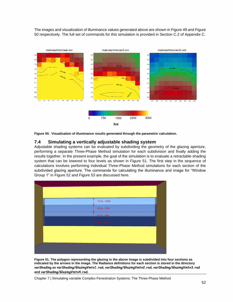
Chapter 7 | Simulating variable Complex Fenestration Systems: The Three-Phase Method
52
The images and visualization of illuminance values generated above are shown in Figure 49 and Figure
50 respectively. The full set of commands for this simulation is provided in Section C.2 of Appendix C.
Figure 50. Visualization of illuminance results generated through the parametric calculation.
7.4 Simulating a vertically adjustable shading system Adjustable shading systems can be evaluated by subdividing the geometry of the glazing aperture,
performing a separate Three-Phase Method simulation for each subdivision and finally adding the
results together. In the present example, the goal of the simulation is to evaluate a retractable shading
system that can be lowered to four levels as shown in Figure 51. The first step in the sequence of
calculations involves performing individual Three-Phase Method simulations for each section of the
subdivided glazing aperture. The commands for calculating the illuminance and image for “Window
Group 1” in Figure 52 and Figure 53 are discussed here.
Figure 51. The polygon representing the glazing in the above image is subdivided into four sections as indicated by the arrows in the image. The Radiance definitions for each section is stored in the directory
varShading as varShading/GlazingVmtx1.rad, varShading/GlazingVmtx2.rad, varShading/GlazingVmtx3.rad
and varShading/GlazingVmtx4.rad.
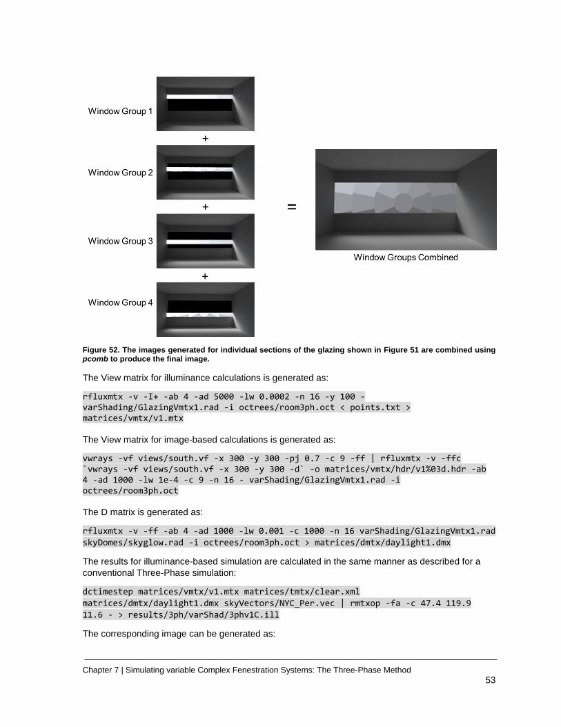
Chapter 7 | Simulating variable Complex Fenestration Systems: The Three-Phase Method
53
Figure 52. The images generated for individual sections of the glazing shown in Figure 51 are combined using pcomb to produce the final image.
The View matrix for illuminance calculations is generated as:
rfluxmtx -v -I+ -ab 4 -ad 5000 -lw 0.0002 -n 16 -y 100 - varShading/GlazingVmtx1.rad -i octrees/room3ph.oct < points.txt > matrices/vmtx/v1.mtx The View matrix for image-based calculations is generated as:
vwrays -vf views/south.vf -x 300 -y 300 -pj 0.7 -c 9 -ff | rfluxmtx -v -ffc `vwrays -vf views/south.vf -x 300 -y 300 -d` -o matrices/vmtx/hdr/v1%03d.hdr -ab 4 -ad 1000 -lw 1e-4 -c 9 -n 16 - varShading/GlazingVmtx1.rad -i octrees/room3ph.oct The D matrix is generated as:
rfluxmtx -v -ff -ab 4 -ad 1000 -lw 0.001 -c 1000 -n 16 varShading/GlazingVmtx1.rad
skyDomes/skyglow.rad -i octrees/room3ph.oct > matrices/dmtx/daylight1.dmx
The results for illuminance-based simulation are calculated in the same manner as described for a
conventional Three-Phase simulation:
dctimestep matrices/vmtx/v1.mtx matrices/tmtx/clear.xml
matrices/dmtx/daylight1.dmx skyVectors/NYC_Per.vec | rmtxop -fa -c 47.4 119.9
11.6 - > results/3ph/varShad/3phv1C.ill
The corresponding image can be generated as:
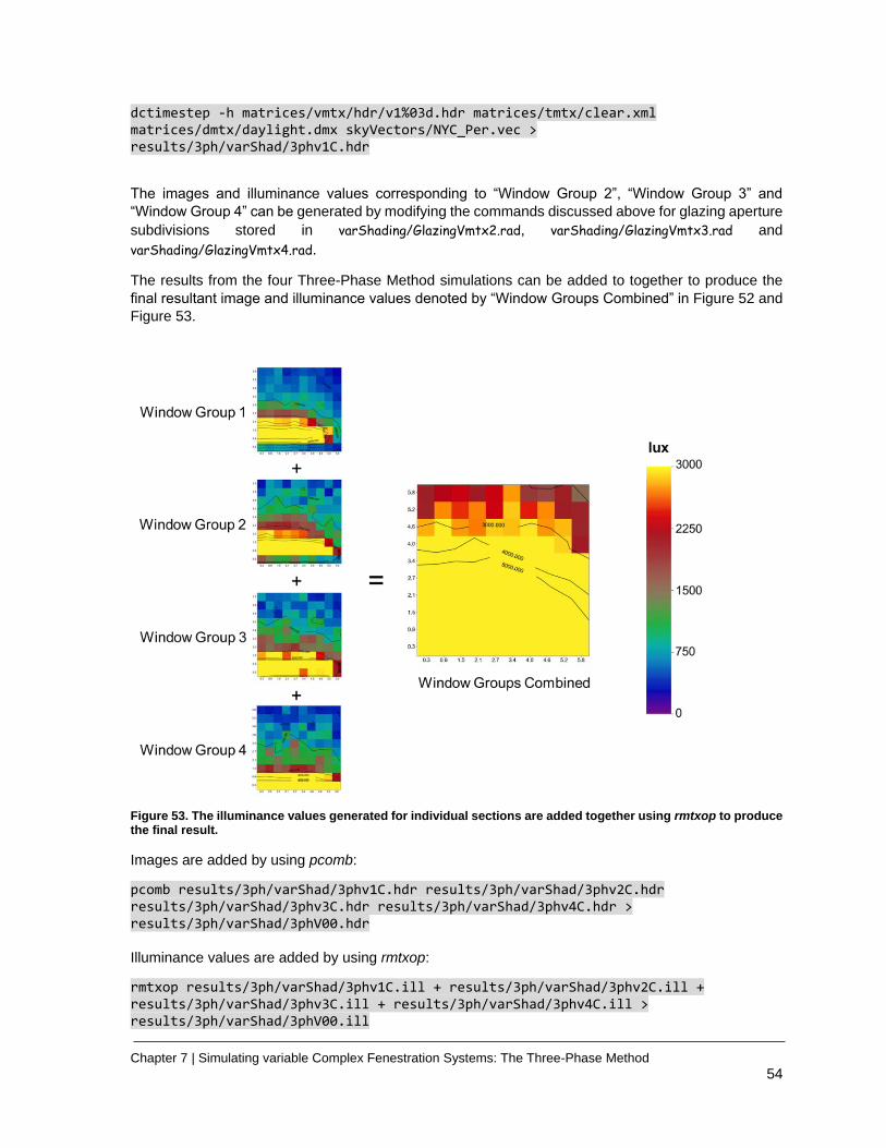
Chapter 7 | Simulating variable Complex Fenestration Systems: The Three-Phase Method
54
dctimestep -h matrices/vmtx/hdr/v1%03d.hdr matrices/tmtx/clear.xml matrices/dmtx/daylight.dmx skyVectors/NYC_Per.vec > results/3ph/varShad/3phv1C.hdr
The images and illuminance values corresponding to “Window Group 2”, “Window Group 3” and
“Window Group 4” can be generated by modifying the commands discussed above for glazing aperture
subdivisions stored in varShading/GlazingVmtx2.rad, varShading/GlazingVmtx3.rad and
varShading/GlazingVmtx4.rad.
The results from the four Three-Phase Method simulations can be added to together to produce the
final resultant image and illuminance values denoted by “Window Groups Combined” in Figure 52 and
Figure 53.
Figure 53. The illuminance values generated for individual sections are added together using rmtxop to produce the final result.
Images are added by using pcomb:
pcomb results/3ph/varShad/3phv1C.hdr results/3ph/varShad/3phv2C.hdr results/3ph/varShad/3phv3C.hdr results/3ph/varShad/3phv4C.hdr > results/3ph/varShad/3phV00.hdr Illuminance values are added by using rmtxop:
rmtxop results/3ph/varShad/3phv1C.ill + results/3ph/varShad/3phv2C.ill + results/3ph/varShad/3phv3C.ill + results/3ph/varShad/3phv4C.ill > results/3ph/varShad/3phV00.ill
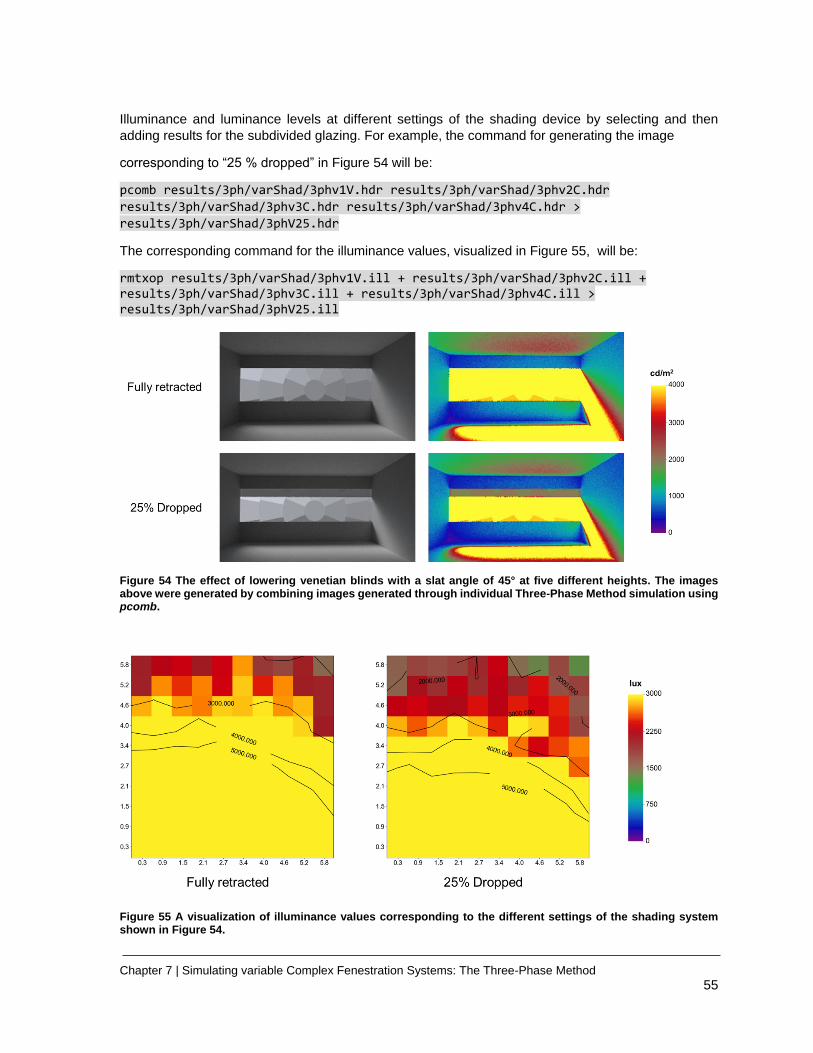
Chapter 7 | Simulating variable Complex Fenestration Systems: The Three-Phase Method
55
Illuminance and luminance levels at different settings of the shading device by selecting and then
adding results for the subdivided glazing. For example, the command for generating the image
corresponding to “25 % dropped” in Figure 54 will be:
pcomb results/3ph/varShad/3phv1V.hdr results/3ph/varShad/3phv2C.hdr
results/3ph/varShad/3phv3C.hdr results/3ph/varShad/3phv4C.hdr >
results/3ph/varShad/3phV25.hdr
The corresponding command for the illuminance values, visualized in Figure 55, will be:
rmtxop results/3ph/varShad/3phv1V.ill + results/3ph/varShad/3phv2C.ill + results/3ph/varShad/3phv3C.ill + results/3ph/varShad/3phv4C.ill > results/3ph/varShad/3phV25.ill
Figure 54 The effect of lowering venetian blinds with a slat angle of 45° at five different heights. The images above were generated by combining images generated through individual Three-Phase Method simulation using pcomb.
Figure 55 A visualization of illuminance values corresponding to the different settings of the shading system shown in Figure 54.
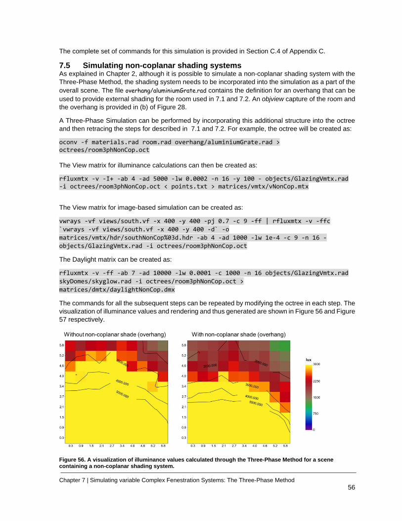
Chapter 7 | Simulating variable Complex Fenestration Systems: The Three-Phase Method
56
The complete set of commands for this simulation is provided in Section C.4 of Appendix C.
7.5 Simulating non-coplanar shading systems As explained in Chapter 2, although it is possible to simulate a non-coplanar shading system with the
Three-Phase Method, the shading system needs to be incorporated into the simulation as a part of the
overall scene. The file overhang/aluminiumGrate.rad contains the definition for an overhang that can be
used to provide external shading for the room used in 7.1 and 7.2. An objview capture of the room and
the overhang is provided in (b) of Figure 28.
A Three-Phase Simulation can be performed by incorporating this additional structure into the octree
and then retracing the steps for described in 7.1 and 7.2. For example, the octree will be created as:
oconv -f materials.rad room.rad overhang/aluminiumGrate.rad > octrees/room3phNonCop.oct The View matrix for illuminance calculations can then be created as:
rfluxmtx -v -I+ -ab 4 -ad 5000 -lw 0.0002 -n 16 -y 100 - objects/GlazingVmtx.rad -i octrees/room3phNonCop.oct < points.txt > matrices/vmtx/vNonCop.mtx
The View matrix for image-based simulation can be created as:
vwrays -vf views/south.vf -x 400 -y 400 -pj 0.7 -c 9 -ff | rfluxmtx -v -ffc
`vwrays -vf views/south.vf -x 400 -y 400 -d` -o
matrices/vmtx/hdr/southNonCop%03d.hdr -ab 4 -ad 1000 -lw 1e-4 -c 9 -n 16 -
objects/GlazingVmtx.rad -i octrees/room3phNonCop.oct
The Daylight matrix can be created as:
rfluxmtx -v -ff -ab 7 -ad 10000 -lw 0.0001 -c 1000 -n 16 objects/GlazingVmtx.rad
skyDomes/skyglow.rad -i octrees/room3phNonCop.oct >
matrices/dmtx/daylightNonCop.dmx
The commands for all the subsequent steps can be repeated by modifying the octree in each step. The
visualization of illuminance values and rendering and thus generated are shown in Figure 56 and Figure
57 respectively.
Figure 56. A visualization of illuminance values calculated through the Three-Phase Method for a scene containing a non-coplanar shading system.
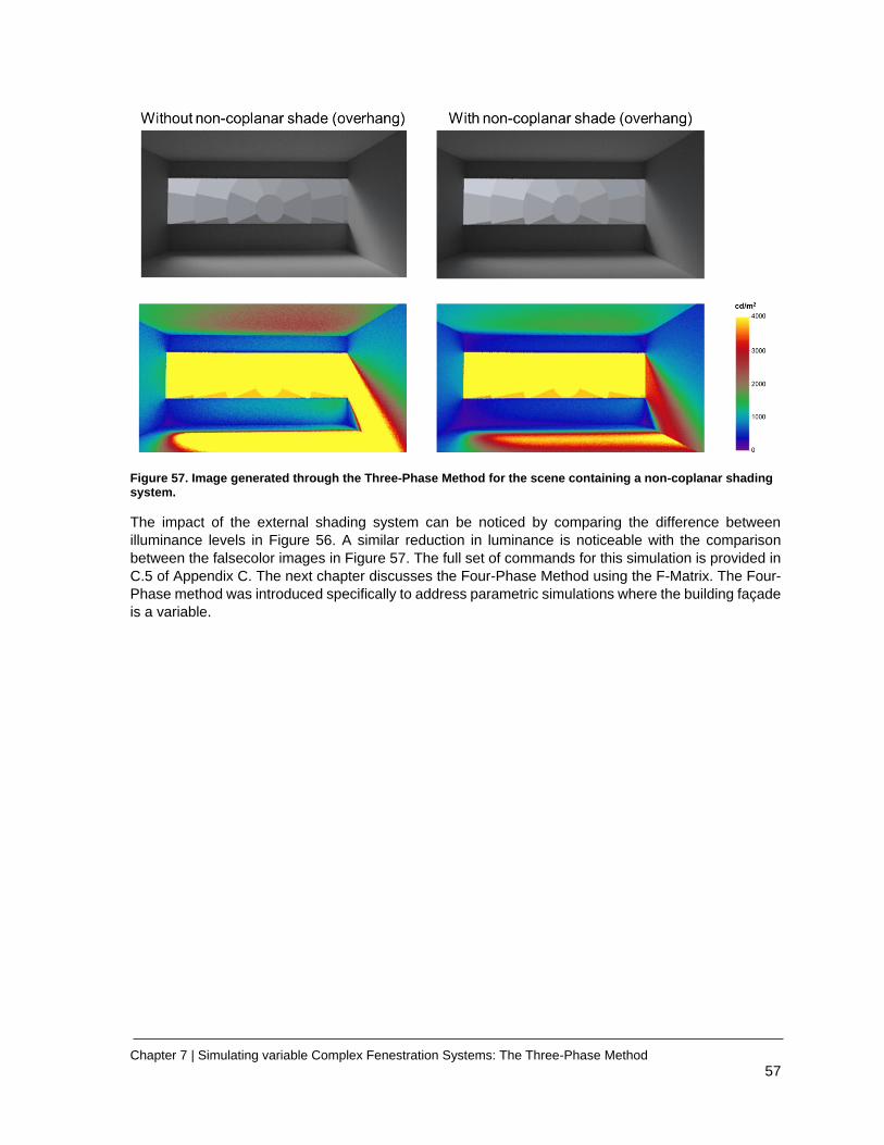
Chapter 7 | Simulating variable Complex Fenestration Systems: The Three-Phase Method
57
Figure 57. Image generated through the Three-Phase Method for the scene containing a non-coplanar shading system.
The impact of the external shading system can be noticed by comparing the difference between
illuminance levels in Figure 56. A similar reduction in luminance is noticeable with the comparison
between the falsecolor images in Figure 57. The full set of commands for this simulation is provided in
C.5 of Appendix C. The next chapter discusses the Four-Phase Method using the F-Matrix. The Four-
Phase method was introduced specifically to address parametric simulations where the building façade
is a variable.
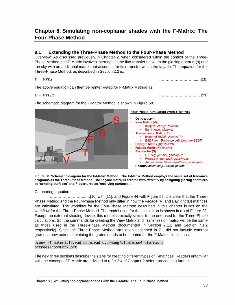
Chapter 8 | Simulating non-coplanar shades with the F-Matrix: The Four-Phase Method
58
Chapter 8. Simulating non-coplanar shades with the F-Matrix: The
Four-Phase Method
8.1 Extending the Three-Phase Method to the Four-Phase Method Overview: As discussed previously in Chapter 2, when considered within the context of the Three-
Phase Method, the F-Matrix involves intercepting the flux-transfer between the glazing aperture(s) and
the sky with an additional matrix that accounts for flux-transfer within the façade. The equation for the
Three-Phase Method, as described in Section 2.3 is:
𝐸 = 𝑉𝑇𝐷𝑆 ………………………...…[10]
The above equation can then be reinterpreted for F-Matrix Method as:
𝐸 = 𝑉𝑇𝐹𝐷𝑆 ………………………….. [11]
The schematic diagram for the F-Matrix Method is shown in Figure 58.
Figure 58. Schematic diagram for the F-Matrix Method. The F-Matrix Method employs the same set of Radiance programs as the Three-Phase Method. The Façade matrix is created with rfluxmtx by assigning glazing apertures as ‘sending surfaces’ and F-apertures as ‘receiving surfaces’.
Comparing equation
………………………...…[10] with [11], and Figure 44 with Figure 58, it is clear that the Three-
Phase Method and the Four-Phase Method only differ in how the Façade (F) and Daylight (D) matrices
are calculated. The workflow for the Four-Phase Method described in this chapter builds on the
workflow for the Three-Phase Method. The model used for the simulation is shown in (b) of Figure 28.
Except the external shading device, this model is exactly similar to the one used for the Three-Phase
calculations. So, the commands for creating the View Matrix and Transmission matrix will be the same
as those used in the Three-Phase Method (documented in Section 7.1.1 and Section 7.1.2
respectively). Since the Three-Phase Method simulation described in 7.1 did not include external
grates, a new octree containing the grates needs to be created for the F-Matrix simulations:
oconv -f materials.rad room.rad overhang/aluminiumGrate.rad > octrees/roomFmtx.oct The next three sections describe the steps for creating different types of F-matrices. Readers unfamiliar
with the concept of F-Matrix are advised to refer 2.4 of Chapter 2 before proceeding further.
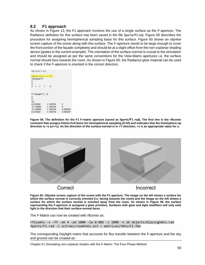
Chapter 8 | Simulating non-coplanar shades with the F-Matrix: The Four-Phase Method
59
8.2 F1 approach As shown in Figure 13, the F1 approach involves the use of a single surface as the F-aperture. The
Radiance definition for this surface has been saved in the file fports/F1.rad. Figure 59 describes the
procedure for assigning hemispherical sampling basis for this surface. Figure 60 shows an objview
screen capture of the scene along with this surface. The F-aperture needs to be large enough to cover
the front portion of the façade completely and should be at a slight offset from the non-coplanar shading
device (grates in the current example). The orientation of the surface-normal is crucial to the simulation
and should be assigned as per the same conventions for the View-Matrix apertures i.e. the surface
normal should face towards the room. As shown in Figure 60, the Radiance glow material can be used
to check if the F-aperture is oriented in the correct direction.
Figure 59. The definition for the F1 F-matrix aperture (saved as fports/F1.rad). The first line is the rfluxmtx
comment that assigns Klems-Full basis for hemispherical sampling (h=kf) and indicates that the hemisphere-up direction is +z (u=+z). As the direction of the surface-normal is in +Y direction, +z is an appropriate value for u.
Figure 60. Objview screen capture of the scene with the F1 aperture. The image on the left shows a surface for which the surface normal is correctly oriented (i.e. facing towards the room) and the image on the left shows a surface for which the surface normal is oriented away from the room. As shown in Figure 59, the surface representing the F-aperture is assigned a glow primitive. Surfaces with glow and light modifiers will only emit light in the direction that their surface-normal faces.
The F-Matrix can now be created with rfluxmtx as:
rfluxmtx -v -ff -ab 4 -ad 1000 -lw 0.001 -c 1000 -n 16 objects/GlazingVmtx.rad fports/F1.rad -i octrees/roomFmtx.oct > matrices/fmtx/F1.fmx The corresponding Daylight matrix that accounts for flux transfer between the F-aperture and the sky
and ground can be created as:
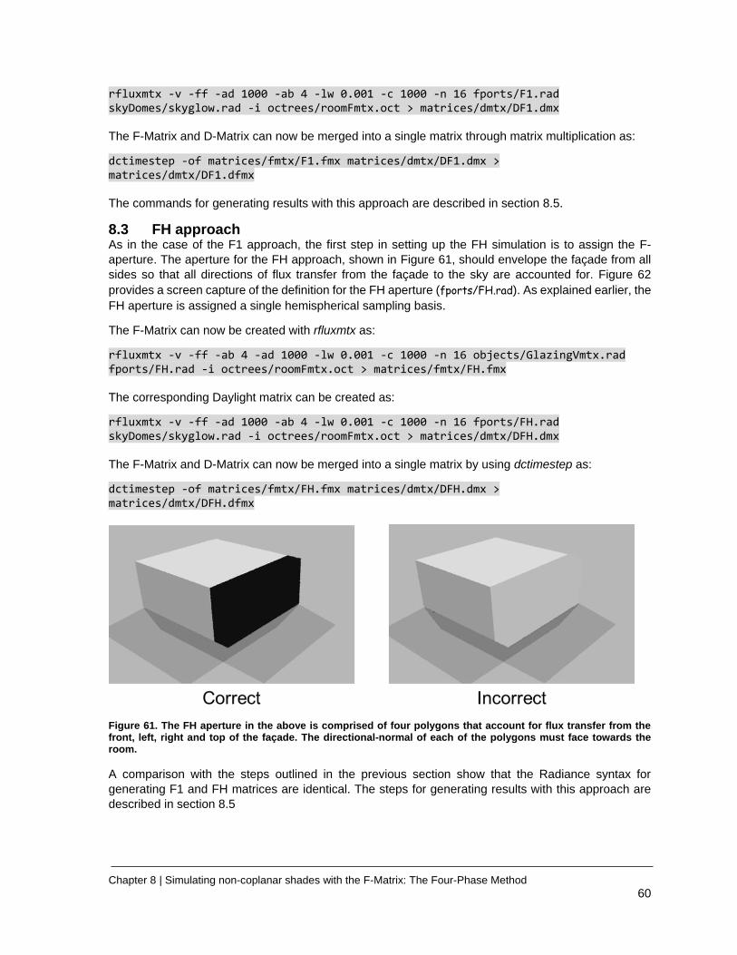
Chapter 8 | Simulating non-coplanar shades with the F-Matrix: The Four-Phase Method
60
rfluxmtx -v -ff -ad 1000 -ab 4 -lw 0.001 -c 1000 -n 16 fports/F1.rad skyDomes/skyglow.rad -i octrees/roomFmtx.oct > matrices/dmtx/DF1.dmx The F-Matrix and D-Matrix can now be merged into a single matrix through matrix multiplication as:
dctimestep -of matrices/fmtx/F1.fmx matrices/dmtx/DF1.dmx > matrices/dmtx/DF1.dfmx The commands for generating results with this approach are described in section 8.5.
8.3 FH approach As in the case of the F1 approach, the first step in setting up the FH simulation is to assign the F-
aperture. The aperture for the FH approach, shown in Figure 61, should envelope the façade from all
sides so that all directions of flux transfer from the façade to the sky are accounted for. Figure 62
provides a screen capture of the definition for the FH aperture (fports/FH.rad). As explained earlier, the
FH aperture is assigned a single hemispherical sampling basis.
The F-Matrix can now be created with rfluxmtx as:
rfluxmtx -v -ff -ab 4 -ad 1000 -lw 0.001 -c 1000 -n 16 objects/GlazingVmtx.rad fports/FH.rad -i octrees/roomFmtx.oct > matrices/fmtx/FH.fmx The corresponding Daylight matrix can be created as:
rfluxmtx -v -ff -ad 1000 -ab 4 -lw 0.001 -c 1000 -n 16 fports/FH.rad skyDomes/skyglow.rad -i octrees/roomFmtx.oct > matrices/dmtx/DFH.dmx The F-Matrix and D-Matrix can now be merged into a single matrix by using dctimestep as:
dctimestep -of matrices/fmtx/FH.fmx matrices/dmtx/DFH.dmx > matrices/dmtx/DFH.dfmx
Figure 61. The FH aperture in the above is comprised of four polygons that account for flux transfer from the front, left, right and top of the façade. The directional-normal of each of the polygons must face towards the room.
A comparison with the steps outlined in the previous section show that the Radiance syntax for
generating F1 and FH matrices are identical. The steps for generating results with this approach are
described in section 8.5
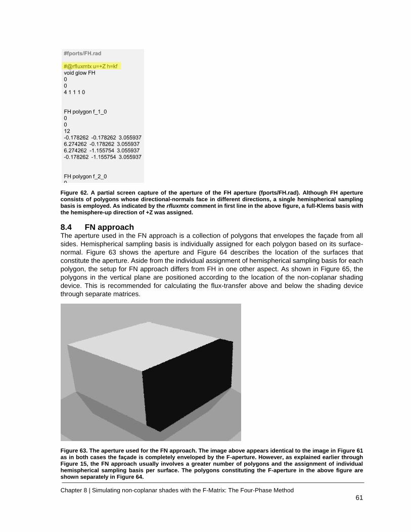
Chapter 8 | Simulating non-coplanar shades with the F-Matrix: The Four-Phase Method
61
Figure 62. A partial screen capture of the aperture of the FH aperture (fports/FH.rad). Although FH aperture consists of polygons whose directional-normals face in different directions, a single hemispherical sampling basis is employed. As indicated by the rfluxmtx comment in first line in the above figure, a full-Klems basis with the hemisphere-up direction of +Z was assigned.
8.4 FN approach The aperture used in the FN approach is a collection of polygons that envelopes the façade from all
sides. Hemispherical sampling basis is individually assigned for each polygon based on its surface-
normal. Figure 63 shows the aperture and Figure 64 describes the location of the surfaces that
constitute the aperture. Aside from the individual assignment of hemispherical sampling basis for each
polygon, the setup for FN approach differs from FH in one other aspect. As shown in Figure 65, the
polygons in the vertical plane are positioned according to the location of the non-coplanar shading
device. This is recommended for calculating the flux-transfer above and below the shading device
through separate matrices.
Figure 63. The aperture used for the FN approach. The image above appears identical to the image in Figure 61 as in both cases the façade is completely enveloped by the F-aperture. However, as explained earlier through Figure 15, the FN approach usually involves a greater number of polygons and the assignment of individual hemispherical sampling basis per surface. The polygons constituting the F-aperture in the above figure are shown separately in Figure 64.

Chapter 8 | Simulating non-coplanar shades with the F-Matrix: The Four-Phase Method
62
Figure 64. The seven polygons defined in files fports/FNa.rad, fports/FNb.rad …. fports/FNg.rad together
constitute the F-aperture for creating the F Matrix. The hemispherical sampling basis is individually assigned for
each polygon and is mentioned under the ‘Sampling Comment’ heading. The apertures fports/FNa.rad,
fports/FNd.rad and fports/FNf.rad are positioned above the grates. The directional normal for the polygon
defined in fports/FNg.rad is parallel to +Z so a hemisphere-up value other than +Z (i.e. +Y) was assigned for it.
The assignment of hemispherical sampling basis for rfluxmtx follows the same logic as explained in the
earlier sections. As shown in Figure 66 and Figure 67, full Klems-basis (h=kf) is assigned to each of
the polygons and the hemisphere-up direction is chosen to be any direction that is not parallel to the
directional normal of the polygon.

Chapter 8 | Simulating non-coplanar shades with the F-Matrix: The Four-Phase Method
63
Figure 65. Location of the surfaces defined in fports/FNa.rad (left image) and fports/FNb.rad (right image) with respect to the grates.
In this approach, the sampling basis need to be chosen carefully in order to achieve desired accuracy.
For example, if one wants to know accurately the depth of sun penetration, the sampling basis for the
side polygons, such as the ones shown in Figure 65, need to be set to a different sampling basis where
the basis resolution at grazing angle is higher than that of a Klems basis.
Figure 66. The assignment of “hemisphere-up” value and Klems-basis for the polygon saved in fports/FNa.rad
from Figure 65 . The rfluxmtx comment for fports/FNb.rad, fports/FNc.rad, fports/FNd.rad, fports/FNe.rad
and fports/FNf.rad can be the same as all of them will be assigned full Klems-basis (h=kf) and a hemisphere-
up direction of +Z.
Figure 67. The assignment of “hemisphere-up” value and Klems-basis for the polygon saved in fports/FNg.rad
from Figure 65. Out of all the polygons constituting the F-aperture, this is the only whose surface-normal is parallel to the +Z direction. So, the hemisphere-up direction for this surface is assigned as a direction not parallel to the Z direction (u=+Y).
The number of F matrices for the FN approach is equal to the number of F-apertures multiplied by the
number of T matrix apertures. The number of D matrices will be equal to the number of F matrices. So,
as per the arrangement shown in Figure 64, seven F and D matrices will be required in the current
example.
The F matrices can be created in a single step by concatenating the files fports/FNa.rad, fports/FNb.rad
… fports/FNg.rad to a single file (fports/FN.rad) and then using that file as the ‘sender’ in rfluxmtx.
rfluxmtx -v -ff -ab 4 -ad 1000 -lw 1e-4 -c 1000 -n 16 -o matrices/fmtx/%s.fmx objects/GlazingVmtx.rad fports/FN.rad -i octrees/roomFmtx.oct
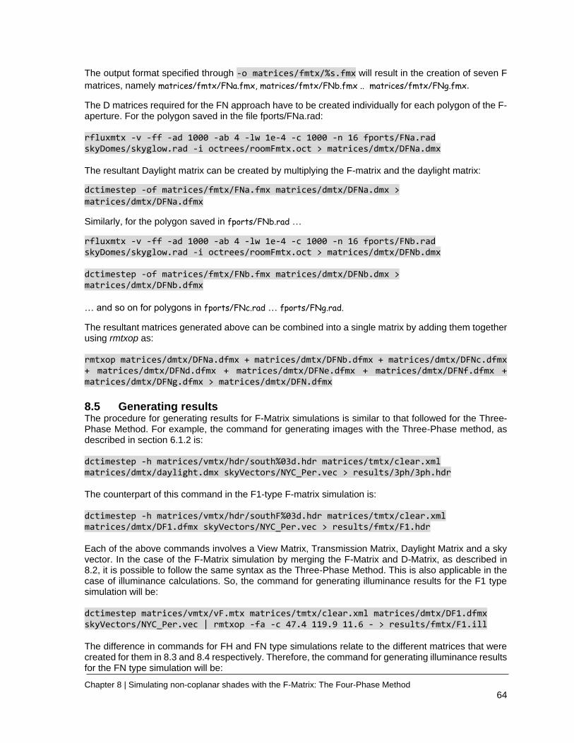
Chapter 8 | Simulating non-coplanar shades with the F-Matrix: The Four-Phase Method
64
The output format specified through -o matrices/fmtx/%s.fmx will result in the creation of seven F
matrices, namely matrices/fmtx/FNa.fmx, matrices/fmtx/FNb.fmx .. matrices/fmtx/FNg.fmx.
The D matrices required for the FN approach have to be created individually for each polygon of the F-aperture. For the polygon saved in the file fports/FNa.rad: rfluxmtx -v -ff -ad 1000 -ab 4 -lw 1e-4 -c 1000 -n 16 fports/FNa.rad skyDomes/skyglow.rad -i octrees/roomFmtx.oct > matrices/dmtx/DFNa.dmx The resultant Daylight matrix can be created by multiplying the F-matrix and the daylight matrix:
dctimestep -of matrices/fmtx/FNa.fmx matrices/dmtx/DFNa.dmx >
matrices/dmtx/DFNa.dfmx
Similarly, for the polygon saved in fports/FNb.rad …
rfluxmtx -v -ff -ad 1000 -ab 4 -lw 1e-4 -c 1000 -n 16 fports/FNb.rad skyDomes/skyglow.rad -i octrees/roomFmtx.oct > matrices/dmtx/DFNb.dmx dctimestep -of matrices/fmtx/FNb.fmx matrices/dmtx/DFNb.dmx > matrices/dmtx/DFNb.dfmx … and so on for polygons in fports/FNc.rad … fports/FNg.rad.
The resultant matrices generated above can be combined into a single matrix by adding them together using rmtxop as: rmtxop matrices/dmtx/DFNa.dfmx + matrices/dmtx/DFNb.dfmx + matrices/dmtx/DFNc.dfmx + matrices/dmtx/DFNd.dfmx + matrices/dmtx/DFNe.dfmx + matrices/dmtx/DFNf.dfmx + matrices/dmtx/DFNg.dfmx > matrices/dmtx/DFN.dfmx
8.5 Generating results The procedure for generating results for F-Matrix simulations is similar to that followed for the Three-Phase Method. For example, the command for generating images with the Three-Phase method, as described in section 6.1.2 is: dctimestep -h matrices/vmtx/hdr/south%03d.hdr matrices/tmtx/clear.xml matrices/dmtx/daylight.dmx skyVectors/NYC_Per.vec > results/3ph/3ph.hdr The counterpart of this command in the F1-type F-matrix simulation is: dctimestep -h matrices/vmtx/hdr/southF%03d.hdr matrices/tmtx/clear.xml matrices/dmtx/DF1.dfmx skyVectors/NYC_Per.vec > results/fmtx/F1.hdr Each of the above commands involves a View Matrix, Transmission Matrix, Daylight Matrix and a sky vector. In the case of the F-Matrix simulation by merging the F-Matrix and D-Matrix, as described in 8.2, it is possible to follow the same syntax as the Three-Phase Method. This is also applicable in the case of illuminance calculations. So, the command for generating illuminance results for the F1 type simulation will be: dctimestep matrices/vmtx/vF.mtx matrices/tmtx/clear.xml matrices/dmtx/DF1.dfmx skyVectors/NYC_Per.vec | rmtxop -fa -c 47.4 119.9 11.6 - > results/fmtx/F1.ill The difference in commands for FH and FN type simulations relate to the different matrices that were created for them in 8.3 and 8.4 respectively. Therefore, the command for generating illuminance results for the FN type simulation will be:
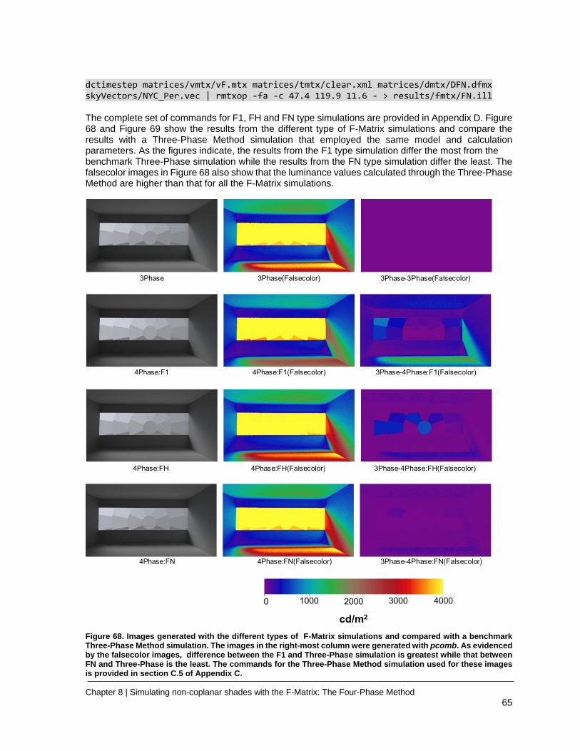
Chapter 8 | Simulating non-coplanar shades with the F-Matrix: The Four-Phase Method
65
dctimestep matrices/vmtx/vF.mtx matrices/tmtx/clear.xml matrices/dmtx/DFN.dfmx skyVectors/NYC_Per.vec | rmtxop -fa -c 47.4 119.9 11.6 - > results/fmtx/FN.ill The complete set of commands for F1, FH and FN type simulations are provided in Appendix D. Figure 68 and Figure 69 show the results from the different type of F-Matrix simulations and compare the results with a Three-Phase Method simulation that employed the same model and calculation parameters. As the figures indicate, the results from the F1 type simulation differ the most from the benchmark Three-Phase simulation while the results from the FN type simulation differ the least. The falsecolor images in Figure 68 also show that the luminance values calculated through the Three-Phase Method are higher than that for all the F-Matrix simulations.
Figure 68. Images generated with the different types of F-Matrix simulations and compared with a benchmark Three-Phase Method simulation. The images in the right-most column were generated with pcomb. As evidenced by the falsecolor images, difference between the F1 and Three-Phase simulation is greatest while that between FN and Three-Phase is the least. The commands for the Three-Phase Method simulation used for these images is provided in section C.5 of Appendix C.
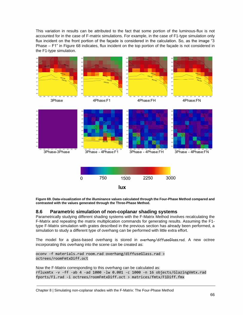
Chapter 8 | Simulating non-coplanar shades with the F-Matrix: The Four-Phase Method
66
This variation in results can be attributed to the fact that some portion of the luminous-flux is not
accounted for in the case of F-matrix simulations. For example, in the case of F1-type simulation only
flux incident on the front portion of the façade is considered in the calculation. So, as the image “3
Phase – F1” in Figure 68 indicates, flux incident on the top portion of the façade is not considered in
the F1-type simulation.
Figure 69. Data-visualization of the illuminance values calculated through the Four-Phase Method compared and contrasted with the values generated through the Three-Phase Method.
8.6 Parametric simulation of non-coplanar shading systems Parametrically studying different shading systems with the F-Matrix Method involves recalculating the F-Matrix and repeating the matrix multiplication commands for generating results. Assuming the F1-type F-Matrix simulation with grates described in the previous section has already been performed, a simulation to study a different type of overhang can be performed with little extra effort.
The model for a glass-based overhang is stored in overhang/diffuseGlass.rad. A new octree
incorporating this overhang into the scene can be created as: oconv -f materials.rad room.rad overhang/diffuseGlass.rad > octrees/roomFmtxDiff.oct Now the F-Matrix corresponding to this overhang can be calculated as: rfluxmtx -v -ff -ab 4 -ad 1000 -lw 0.001 -c 1000 -n 16 objects/GlazingVmtx.rad fports/F1.rad -i octrees/roomFmtxDiff.oct > matrices/fmtx/F1Diff.fmx
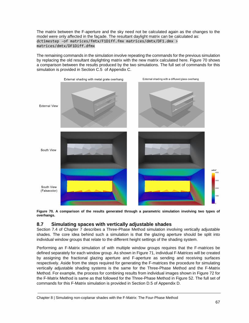
Chapter 8 | Simulating non-coplanar shades with the F-Matrix: The Four-Phase Method
67
The matrix between the F-aperture and the sky need not be calculated again as the changes to the model were only affected in the façade. The resultant daylight matrix can be calculated as: dctimestep -of matrices/fmtx/F1Diff.fmx matrices/dmtx/DF1.dmx > matrices/dmtx/DF1Diff.dfmx The remaining commands in the simulation involve repeating the commands for the previous simulation by replacing the old resultant daylighting matrix with the new matrix calculated here. Figure 70 shows a comparison between the results produced by the two simulations. The full set of commands for this simulation is provided in Section C.5 of Appendix C.
Figure 70. A comparison of the results generated through a parametric simulation involving two types of overhangs.
8.7 Simulating spaces with vertically adjustable shades Section 7.4 of Chapter 7 describes a Three-Phase Method simulation involving vertically adjustable
shades. The core idea behind such a simulation is that the glazing aperture should be split into
individual window groups that relate to the different height settings of the shading system.
Performing an F-Matrix simulation of with multiple window groups requires that the F-matrices be
defined separately for each window group. As shown in Figure 71, individual F-Matrices will be created
by assigning the fractional glazing aperture and F-aperture as sending and receiving surfaces
respectively. Aside from the steps required for generating the F-matrices the procedure for simulating
vertically adjustable shading systems is the same for the Three-Phase Method and the F-Matrix
Method. For example, the process for combining results from individual images shown in Figure 72 for
the F-Matrix Method is same as that followed for the Three-Phase Method in Figure 52. The full set of
commands for this F-Matrix simulation is provided in Section D.5 of Appendix D.
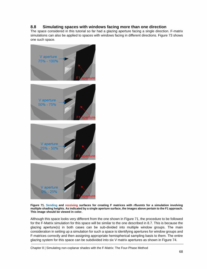
Chapter 8 | Simulating non-coplanar shades with the F-Matrix: The Four-Phase Method
68
8.8 Simulating spaces with windows facing more than one direction The space considered in this tutorial so far had a glazing aperture facing a single direction. F-matrix
simulations can also be applied to spaces with windows facing in different directions. Figure 73 shows
one such space.
Figure 71. Sending and receiving surfaces for creating F matrices with rfluxmtx for a simulation involving multiple shading heights. As indicated by a single aperture surface, the images above pertain to the F1 approach. This image should be viewed in color.
Although this space looks very different from the one shown in Figure 71, the procedure to be followed
for the F-Matrix simulation for this space will be similar to the one described in 8.7. This is because the
glazing aperture(s) in both cases can be sub-divided into multiple window groups. The main
consideration in setting up a simulation for such a space is identifying apertures for window groups and
F-matrices correctly and then assigning appropriate hemispherical sampling basis to them. The entire
glazing system for this space can be subdivided into six V matrix apertures as shown in Figure 74.

Chapter 8 | Simulating non-coplanar shades with the F-Matrix: The Four-Phase Method
69
Figure 72. The results from individual simulations for different window groups are combined to produce the final result. The images above, generated for the F1-type F-matrix simulation, are similar to the ones shown in Figure 52 for the Three-Phase simulation.
Figure 73. A space with multiple window groups and clerestories facing South and East. The image on the left was generated from a view-point outside the room with the viewing direction facing North-East. The image on the right was generated from a view-point inside the room with the viewing direction facing South-West.
The surfaces for the F-aperture are grouped together according to their directional-normals. Figure 75
shows the F-aperture for FH and FN approaches. As with all the previous examples involving FH and
FN, the F-apertures are required to enclose the façade from all directions. The assignment of
hemispherical sampling basis also follows the same reasoning as before. In FH, a single hemispherical
sampling basis will be applied to the entire group of surfaces for the F-aperture. The arrangement of
surfaces for the FN approach is explained through Figure 76. The total number of FH matrices for the
above space will be 6 (Number of V apertures). The number of FN matrices will be 78 (6 multiplied by
13 FN surfaces).
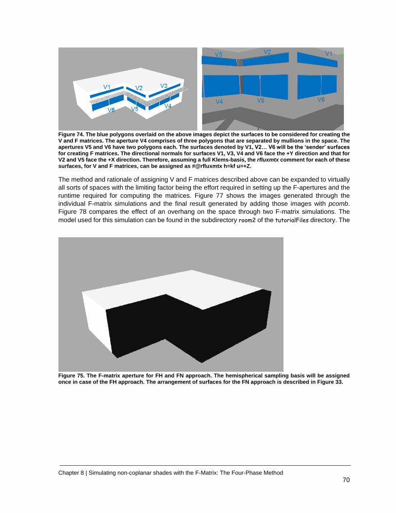
Chapter 8 | Simulating non-coplanar shades with the F-Matrix: The Four-Phase Method
70
Figure 74. The blue polygons overlaid on the above images depict the surfaces to be considered for creating the V and F matrices. The aperture V4 comprises of three polygons that are separated by mullions in the space. The apertures V5 and V6 have two polygons each. The surfaces denoted by V1, V2… V6 will be the ‘sender’ surfaces for creating F matrices. The directional normals for surfaces V1, V3, V4 and V6 face the +Y direction and that for V2 and V5 face the +X direction. Therefore, assuming a full Klems-basis, the rfluxmtx comment for each of these surfaces, for V and F matrices, can be assigned as #@rfluxmtx h=kf u=+Z.
The method and rationale of assigning V and F matrices described above can be expanded to virtually
all sorts of spaces with the limiting factor being the effort required in setting up the F-apertures and the
runtime required for computing the matrices. Figure 77 shows the images generated through the
individual F-matrix simulations and the final result generated by adding those images with pcomb.
Figure 78 compares the effect of an overhang on the space through two F-matrix simulations. The
model used for this simulation can be found in the subdirectory room2 of the tutorialFiles directory. The
Figure 75. The F-matrix aperture for FH and FN approach. The hemispherical sampling basis will be assigned once in case of the FH approach. The arrangement of surfaces for the FN approach is described in Figure 33.
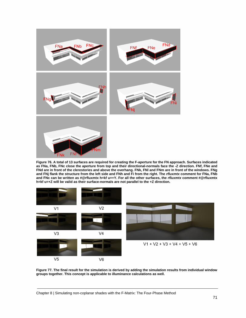
Chapter 8 | Simulating non-coplanar shades with the F-Matrix: The Four-Phase Method
71
Figure 76. A total of 13 surfaces are required for creating the F-aperture for the FN approach. Surfaces indicated as FNa, FNb, FNc close the aperture from top and their directional-normals face the -Z direction. FNf, FNe and FNd are in front of the clerestories and above the overhang. FNk, FNl and FNm are in front of the windows. FNg and FNj flank the structure from the left side and FNh and Fi from the right. The rfluxmtx comment for FNa, FNb and FNc can be written as #@rfluxmtx h=kf u=+Y. For all the other surfaces, the rfluxmtx comment #@rfluxmtx h=kf u=+Z will be valid as their surface-normals are not parallel to the +Z direction.
Figure 77. The final result for the simulation is derived by adding the simulation results from individual window groups together. This concept is applicable to illuminance calculations as well.
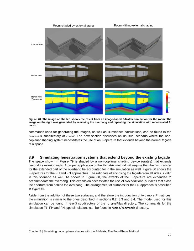
Chapter 8 | Simulating non-coplanar shades with the F-Matrix: The Four-Phase Method
72
Figure 78. The image on the left shows the result from an image-based F-Matrix simulation for the room. The image on the right was generated by removing the overhang and repeating the simulation with recalculated F-matrix.
commands used for generating the images, as well as illuminance calculations, can be found in the
commands subdirectory of room2. The next section discusses an unusual scenario where the non-
coplanar shading system necessitates the use of an F-aperture that extends beyond the normal façade
of a space.
8.9 Simulating fenestration systems that extend beyond the existing façade The space shown in Figure 79 is shaded by a non-coplanar shading device (grates) that extends
beyond its exterior walls. A proper application of the F-matrix method will require that the flux transfer
for the extended part of the overhang be accounted for in the simulation as well. Figure 80 shows the
F-apertures for the FH and FN approaches. The rationale of enclosing the façade from all sides is valid
in this scenario as well. As shown in Figure 80, the extents of the F-aperture are expanded to
accommodate the overhang. This expansion necessitates the use of two additional surfaces that close
the aperture from behind the overhang. The arrangement of surfaces for the FN approach is described
in Figure 81.
Aside from the addition of these two surfaces, and therefore the introduction of two more F matrices,
the simulation is similar to the ones described in sections 8.2, 8.3 and 8.4. The model used for this
simulation can be found in room3 subdirectory of the tutorialFiles directory. The commands for the
simulation F1, FH and FN type simulations can be found in room3/commands directory.
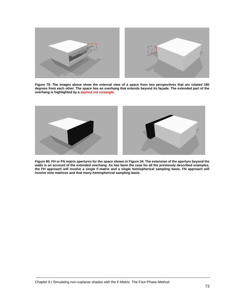
Chapter 8 | Simulating non-coplanar shades with the F-Matrix: The Four-Phase Method
73
Figure 79. The images above show the external view of a space from two perspectives that are rotated 180 degrees from each other. The space has an overhang that extends beyond its façade. The extended part of the overhang is highlighted by a dashed red rectangle.
Figure 80. FH or FN matrix apertures for the space shown in Figure 34. The extension of the aperture beyond the walls is on account of the extended overhang. As has been the case for all the previously described examples, the FH approach will involve a single F-matrix and a single hemispherical sampling basis. FN approach will involve nine matrices and that many hemispherical sampling basis.

Chapter 8 | Simulating non-coplanar shades with the F-Matrix: The Four-Phase Method
74
Figure 81. Arrangement of surfaces for the F-aperture in case of the FN approach. In some images, the
surfaces are either invisible because they are shielded by the room geometry or are obscured due to the
property of the glow material. The matrices corresponding to FNh and FNi account for flux transfer from
behind the façade.
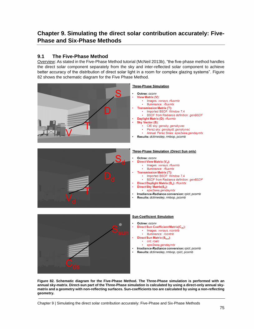
Chapter 9 | Simulating the direct solar contribution accurately: Five-Phase and Six-Phase Methods
75
Chapter 9. Simulating the direct solar contribution accurately: Five-
Phase and Six-Phase Methods
9.1 The Five-Phase Method Overview: As stated in the Five-Phase Method tutorial (McNeil 2013b), “the five-phase method handles
the direct solar component separately from the sky and inter-reflected solar component to achieve
better accuracy of the distribution of direct solar light in a room for complex glazing systems”. Figure
82 shows the schematic diagram for the Five Phase Method.
Figure 82. Schematic diagram for the Five-Phase Method. The Three-Phase simulation is performed with an annual sky-matrix. Direct-sun part of the Three-Phase simulation is calculated by using a direct-only annual sky-matrix and a geometry with non-reflecting surfaces. Sun-coefficients too are calculated by using a non-reflecting geometry.
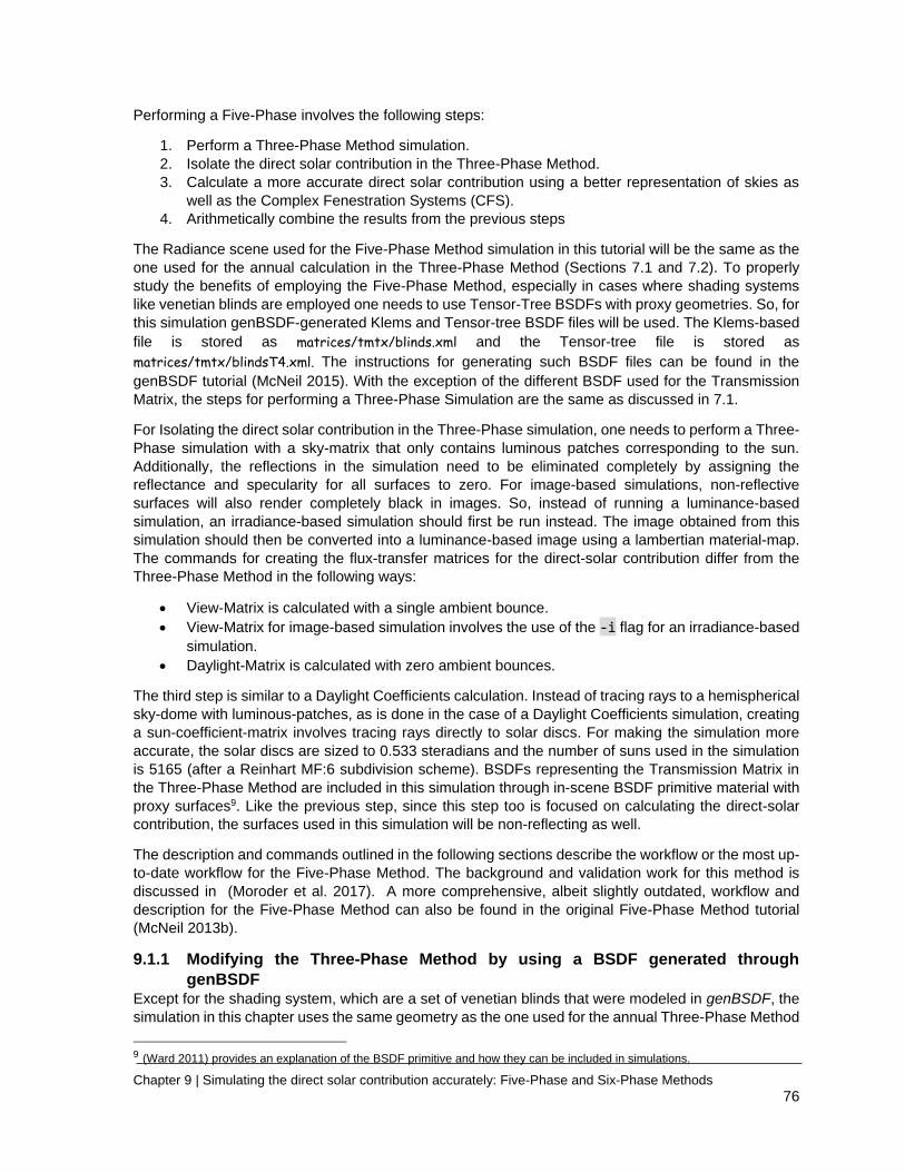
Chapter 9 | Simulating the direct solar contribution accurately: Five-Phase and Six-Phase Methods
76
Performing a Five-Phase involves the following steps:
1. Perform a Three-Phase Method simulation.
2. Isolate the direct solar contribution in the Three-Phase Method.
3. Calculate a more accurate direct solar contribution using a better representation of skies as
well as the Complex Fenestration Systems (CFS).
4. Arithmetically combine the results from the previous steps
The Radiance scene used for the Five-Phase Method simulation in this tutorial will be the same as the
one used for the annual calculation in the Three-Phase Method (Sections 7.1 and 7.2). To properly
study the benefits of employing the Five-Phase Method, especially in cases where shading systems
like venetian blinds are employed one needs to use Tensor-Tree BSDFs with proxy geometries. So, for
this simulation genBSDF-generated Klems and Tensor-tree BSDF files will be used. The Klems-based
file is stored as matrices/tmtx/blinds.xml and the Tensor-tree file is stored as
matrices/tmtx/blindsT4.xml. The instructions for generating such BSDF files can be found in the
genBSDF tutorial (McNeil 2015). With the exception of the different BSDF used for the Transmission
Matrix, the steps for performing a Three-Phase Simulation are the same as discussed in 7.1.
For Isolating the direct solar contribution in the Three-Phase simulation, one needs to perform a Three-
Phase simulation with a sky-matrix that only contains luminous patches corresponding to the sun.
Additionally, the reflections in the simulation need to be eliminated completely by assigning the
reflectance and specularity for all surfaces to zero. For image-based simulations, non-reflective
surfaces will also render completely black in images. So, instead of running a luminance-based
simulation, an irradiance-based simulation should first be run instead. The image obtained from this
simulation should then be converted into a luminance-based image using a lambertian material-map.
The commands for creating the flux-transfer matrices for the direct-solar contribution differ from the
Three-Phase Method in the following ways:
• View-Matrix is calculated with a single ambient bounce.
• View-Matrix for image-based simulation involves the use of the -i flag for an irradiance-based
simulation.
• Daylight-Matrix is calculated with zero ambient bounces.
The third step is similar to a Daylight Coefficients calculation. Instead of tracing rays to a hemispherical
sky-dome with luminous-patches, as is done in the case of a Daylight Coefficients simulation, creating
a sun-coefficient-matrix involves tracing rays directly to solar discs. For making the simulation more
accurate, the solar discs are sized to 0.533 steradians and the number of suns used in the simulation
is 5165 (after a Reinhart MF:6 subdivision scheme). BSDFs representing the Transmission Matrix in
the Three-Phase Method are included in this simulation through in-scene BSDF primitive material with
proxy surfaces9. Like the previous step, since this step too is focused on calculating the direct-solar
contribution, the surfaces used in this simulation will be non-reflecting as well.
The description and commands outlined in the following sections describe the workflow or the most up-
to-date workflow for the Five-Phase Method. The background and validation work for this method is
discussed in (Moroder et al. 2017). A more comprehensive, albeit slightly outdated, workflow and
description for the Five-Phase Method can also be found in the original Five-Phase Method tutorial
(McNeil 2013b).
9.1.1 Modifying the Three-Phase Method by using a BSDF generated through
genBSDF Except for the shading system, which are a set of venetian blinds that were modeled in genBSDF, the
simulation in this chapter uses the same geometry as the one used for the annual Three-Phase Method
9 (Ward 2011) provides an explanation of the BSDF primitive and how they can be included in simulations.

Chapter 9 | Simulating the direct solar contribution accurately: Five-Phase and Six-Phase Methods
77
simulation in 7.1 of Chapter 7. So, the Three-Phase Method simulation can be re-run by just substituting
the BSDF for the venetian blinds (saved as matrices/tmtx/blinds.xml). The command for re-running the
illuminance simulation will be:
dctimestep matrices/vmtx/v.mtx matrices/tmtx/blinds.xml
matrices/dmtx/daylight.dmx skyVectors/NYC.smx | rmtxop -fa -t -c 47.4 119.9 11.6
- > results/5ph/3ph/3phAnnual.ill
Similarly, for an image-based simulation:
dctimestep -o results/5ph/3ph/hdr/south%04d.hdr matrices/vmtx/hdr/south%03d.hdr
matrices/tmtx/blinds.xml matrices/dmtx/daylight.dmx skyVectors/NYC.smx
An example of the image generated by the above command is shown in Figure 87
9.1.2 The direct solar contribution in the Three-Phase Method. As discussed previously, the surfaces in the scene used for the Three-Phase method can be made
non-reflecting by assigning them a black material. Figure 83 shows the definition for that black material
and Figure 84 describes how xform can be used to create a scene with non-reflecting surfaces with
that material. Figure 85 shows objview captures of the model used for the Three-Phase Method and
the one used for isolating the direct-solar contribution.
Figure 83. The material with zero reflectance that will be used to modify all the surfaces in the scene.
Figure 84. The Radiance scene that will be used for isolating the direct solar component of the Three-Phase Method. The “-m black” that follows each “!xform” command replaces the existing material of every surface with a material named “black” .
The octree for this new non-reflecting scene can be created as:
oconv -f materialBlack.rad roomBlack.rad > octrees/room3phDirect.oct
View matrix for illuminance calculations is created with a single ambient bounce (by setting -ab 1) as:
rfluxmtx -v -I+ -ab 1 -ad 5000 -lw 0.0002 -n 16 -y 100 - objects/GlazingVmtx.rad -i octrees/room3phDirect.oct < points.txt > matrices/vmtxd/v.mtx View matrix for image-based simulations is created as:
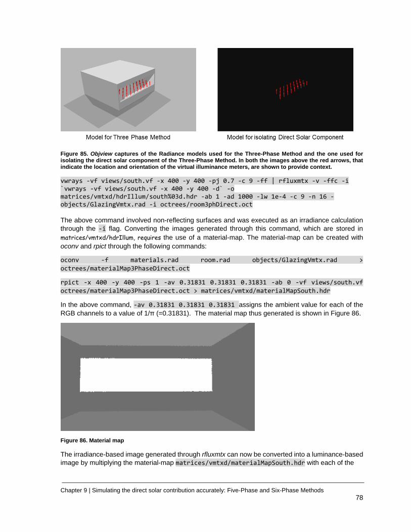
Chapter 9 | Simulating the direct solar contribution accurately: Five-Phase and Six-Phase Methods
78
Figure 85. Objview captures of the Radiance models used for the Three-Phase Method and the one used for isolating the direct solar component of the Three-Phase Method. In both the images above the red arrows, that indicate the location and orientation of the virtual illuminance meters, are shown to provide context.
vwrays -vf views/south.vf -x 400 -y 400 -pj 0.7 -c 9 -ff | rfluxmtx -v -ffc -i `vwrays -vf views/south.vf -x 400 -y 400 -d` -o matrices/vmtxd/hdrIllum/south%03d.hdr -ab 1 -ad 1000 -lw 1e-4 -c 9 -n 16 - objects/GlazingVmtx.rad -i octrees/room3phDirect.oct The above command involved non-reflecting surfaces and was executed as an irradiance calculation
through the -i flag. Converting the images generated through this command, which are stored in
matrices/vmtxd/hdrIllum, requires the use of a material-map. The material-map can be created with
oconv and rpict through the following commands:
oconv -f materials.rad room.rad objects/GlazingVmtx.rad >
octrees/materialMap3PhaseDirect.oct
rpict -x 400 -y 400 -ps 1 -av 0.31831 0.31831 0.31831 -ab 0 -vf views/south.vf
octrees/materialMap3PhaseDirect.oct > matrices/vmtxd/materialMapSouth.hdr
In the above command, -av 0.31831 0.31831 0.31831 assigns the ambient value for each of the
RGB channels to a value of 1/π (=0.31831). The material map thus generated is shown in Figure 86.
Figure 86. Material map
The irradiance-based image generated through rfluxmtx can now be converted into a luminance-based
image by multiplying the material-map matrices/vmtxd/materialMapSouth.hdr with each of the

Chapter 9 | Simulating the direct solar contribution accurately: Five-Phase and Six-Phase Methods
79
individual HDR files that constitutes the direct View-Matrix10:
for idx in {00..145}
do
pcomb -h -e 'ro=ri(1)*ri(2);go=gi(1)*gi(2);bo=bi(1)*bi(2)' -o
matrices/vmtxd/materialMapSouth.hdr -o matrices/vmtxd/hdrIllum/south${idx}.hdr >
matrices/vmtxd/hdrLum/south${idx}.hdr
done
The direct daylight matrix can be created as:
rfluxmtx -v -ff -ab 0 -ad 1000 -lw 0.001 -c 1000 -n 16 objects/GlazingVmtx.rad skyDomes/skyglow.rad -i octrees/room3phDirect.oct > matrices/dmtxd/daylight.dmx The annual sky-matrix used for this simulation requires that only the direct contribution of the sun be
considered for the simulation. Such a sky-matrix can be created by using the -d option in gendaymtx.
Figure 49 compares a typical sky used for the Three-Phase Method with the one used for isolating the
direct solar contribution.
gendaymtx -m 1 -d assets/NYC.wea > skyVectors/NYCd.smx The results for illuminance simulations can now be generated as:
dctimestep matrices/vmtxd/v.mtx matrices/tmtx/blinds.xml matrices/dmtxd/daylight.dmx skyVectors/NYCd.smx | rmtxop -fa -t -c 47.4 119.9 11.6 - > results/5ph/3phdir/3phAnnual.ill
The results for image-based simulation can be generated as:
dctimestep -o results/5ph/3phdir/hdr/south%04d.hdr matrices/vmtxd/hdrLum/south%03d.hdr matrices/tmtx/blinds.xml matrices/dmtxd/daylight.dmx skyVectors/NYCd.smx Figure 87 provides a comparison between the images generated for the Three Phase Method and the
direct-solar component of the Three Phase Method.
Figure 87. Results from a Three Phase simulation and the corresponding direct-only simulation
10 The for-loop described here is only applicable to shell-scripting in Unix-based systems. Readers on Windows® are should either replicate a for loop in a .bat batch file or use scripting language like Python or Perl to do so.

Chapter 9 | Simulating the direct solar contribution accurately: Five-Phase and Six-Phase Methods
80
9.1.3 Sun-Coefficient simulation
The following command creates a Radiance definition that places a solar disc at the center of every
patch in a sky-matrix with 5185 patches.
echo "void light solar 0 0 3 1e6 1e6 1e6" > skies/suns.rad cnt 5185 | rcalc -e MF:6 -f reinsrc.cal -e Rbin=recno -o 'solar source sun 0 0 4 ${Dx} ${Dy} ${Dz} 0.533' >> skies/suns.rad The Five-phase Method calculations can also be performed with a lower number of suns. However, as
explained in Chapter 2, using a greater number of suns increases the accuracy with which the direct
sun calculation is performed.
The octree for the simulation with accurate calculation of direct solar component can be generated as:
oconv -f materialBlack.rad roomBlack.rad skies/suns.rad blinds/blindsWithProxy.rad > octrees/sunCoefficients.oct The term blinds/blindsWithProxy.rad in the above command indicates that the geometry for the
glazing system is physically represented in the octree.
The sun-coefficients for illuminance can be calculated as:
rcontrib -I+ -ab 1 -y 100 -n 16 -ad 256 -lw 1.0e-3 -dc 1 -dt 0 -dj 0 -faf -e MF:6
-f reinhart.cal -b rbin -bn Nrbins -m solar octrees/sunCoefficients.oct < points.txt
> matrices/cds/cds.mtx
Irradiance-based sun-coefficients for the image-based simulation of the interior portion of the scene
can be generated as:
vwrays -vf views/south.vf -x 400 -y 400 -pj 0.7 -ff | rcontrib -w- -i -ab 1 -ad 256
-lw 1.0e-3 -dc 1 -dt 0 -dj 0 -ffc -n 16 `vwrays -vf views/south.vf -x 400 -y 400 -
d` -o matrices/cds/hdrIllSpace/southM6%04d.hdr -e MF:6 -f reinhart.cal -b rbin -bn
Nrbins -m solar octrees/sunCoefficients.oct
The material-map for converting these images to luminance-based images can be generated as:
oconv -f materials.rad room.rad objects/GlazingVmtxBlack.rad >
octrees/materialMap5Phase.oct
rpict -x 400 -y 400 -ps 1 -av 0.31831 0.31831 0.31831 -ab 0 -vf views/south.vf
octrees/materialMap3PhaseDirect.oct > matrices/cds/materialMapSouth.hdr
Luminance-based images for the entire scene, including the façade can be generated as:
vwrays -vf views/south.vf -x 400 -y 400 -pj 0.7 -ff | rcontrib -w- -ab 1 -ad 256 -
lw 1.0e-3 -dc 1 -dt 0 -dj 0 -ffc -n 16 `vwrays -vf views/south.vf -x 400 -y 400 -
d` -o matrices/cds/hdrLumFacade/southM6%04d.hdr -e MF:6 -f reinhart.cal -b rbin -
bn Nrbins -m solar octrees/sunCoefficients.oct
The images generated for the interior portion of the scene and the entire façade can generated as:
for idx in {0000..5185}
do
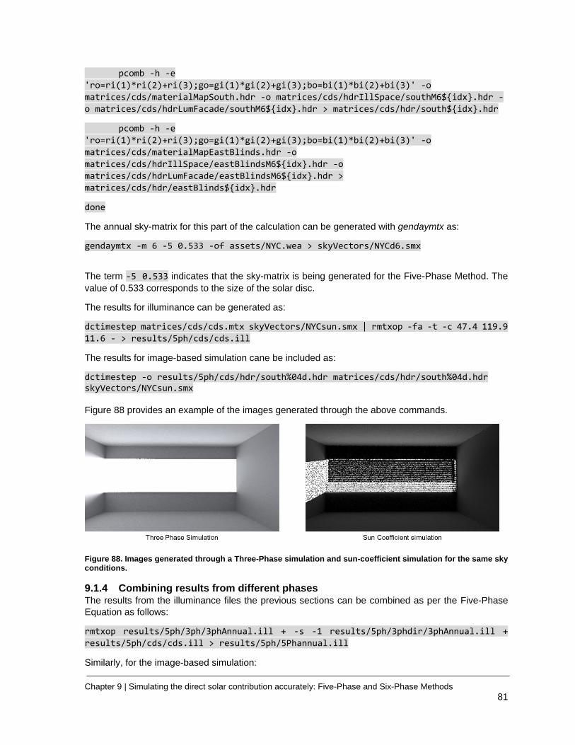
Chapter 9 | Simulating the direct solar contribution accurately: Five-Phase and Six-Phase Methods
81
pcomb -h -e
'ro=ri(1)*ri(2)+ri(3);go=gi(1)*gi(2)+gi(3);bo=bi(1)*bi(2)+bi(3)' -o
matrices/cds/materialMapSouth.hdr -o matrices/cds/hdrIllSpace/southM6${idx}.hdr -
o matrices/cds/hdrLumFacade/southM6${idx}.hdr > matrices/cds/hdr/south${idx}.hdr
pcomb -h -e
'ro=ri(1)*ri(2)+ri(3);go=gi(1)*gi(2)+gi(3);bo=bi(1)*bi(2)+bi(3)' -o
matrices/cds/materialMapEastBlinds.hdr -o
matrices/cds/hdrIllSpace/eastBlindsM6${idx}.hdr -o
matrices/cds/hdrLumFacade/eastBlindsM6${idx}.hdr >
matrices/cds/hdr/eastBlinds${idx}.hdr
done
The annual sky-matrix for this part of the calculation can be generated with gendaymtx as:
gendaymtx -m 6 -5 0.533 -of assets/NYC.wea > skyVectors/NYCd6.smx
The term -5 0.533 indicates that the sky-matrix is being generated for the Five-Phase Method. The
value of 0.533 corresponds to the size of the solar disc.
The results for illuminance can be generated as:
dctimestep matrices/cds/cds.mtx skyVectors/NYCsun.smx | rmtxop -fa -t -c 47.4 119.9
11.6 - > results/5ph/cds/cds.ill
The results for image-based simulation cane be included as:
dctimestep -o results/5ph/cds/hdr/south%04d.hdr matrices/cds/hdr/south%04d.hdr skyVectors/NYCsun.smx Figure 88 provides an example of the images generated through the above commands.
Figure 88. Images generated through a Three-Phase simulation and sun-coefficient simulation for the same sky conditions.
9.1.4 Combining results from different phases The results from the illuminance files the previous sections can be combined as per the Five-Phase
Equation as follows:
rmtxop results/5ph/3ph/3phAnnual.ill + -s -1 results/5ph/3phdir/3phAnnual.ill +
results/5ph/cds/cds.ill > results/5ph/5Phannual.ill
Similarly, for the image-based simulation:
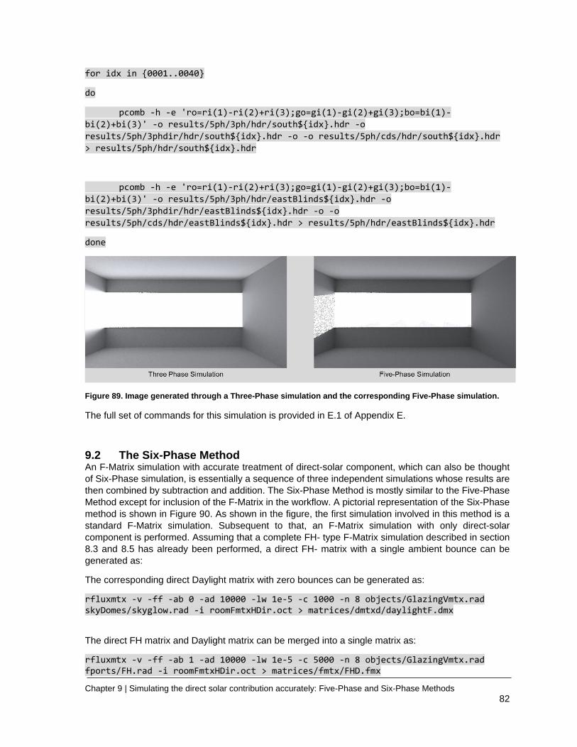
Chapter 9 | Simulating the direct solar contribution accurately: Five-Phase and Six-Phase Methods
82
for idx in {0001..0040}
do
pcomb -h -e 'ro=ri(1)-ri(2)+ri(3);go=gi(1)-gi(2)+gi(3);bo=bi(1)-
bi(2)+bi(3)' -o results/5ph/3ph/hdr/south${idx}.hdr -o
results/5ph/3phdir/hdr/south${idx}.hdr -o -o results/5ph/cds/hdr/south${idx}.hdr
> results/5ph/hdr/south${idx}.hdr
pcomb -h -e 'ro=ri(1)-ri(2)+ri(3);go=gi(1)-gi(2)+gi(3);bo=bi(1)-
bi(2)+bi(3)' -o results/5ph/3ph/hdr/eastBlinds${idx}.hdr -o
results/5ph/3phdir/hdr/eastBlinds${idx}.hdr -o -o
results/5ph/cds/hdr/eastBlinds${idx}.hdr > results/5ph/hdr/eastBlinds${idx}.hdr
done
Figure 89. Image generated through a Three-Phase simulation and the corresponding Five-Phase simulation.
The full set of commands for this simulation is provided in E.1 of Appendix E.
9.2 The Six-Phase Method An F-Matrix simulation with accurate treatment of direct-solar component, which can also be thought
of Six-Phase simulation, is essentially a sequence of three independent simulations whose results are
then combined by subtraction and addition. The Six-Phase Method is mostly similar to the Five-Phase
Method except for inclusion of the F-Matrix in the workflow. A pictorial representation of the Six-Phase
method is shown in Figure 90. As shown in the figure, the first simulation involved in this method is a
standard F-Matrix simulation. Subsequent to that, an F-Matrix simulation with only direct-solar
component is performed. Assuming that a complete FH- type F-Matrix simulation described in section
8.3 and 8.5 has already been performed, a direct FH- matrix with a single ambient bounce can be
generated as:
The corresponding direct Daylight matrix with zero bounces can be generated as:
rfluxmtx -v -ff -ab 0 -ad 10000 -lw 1e-5 -c 1000 -n 8 objects/GlazingVmtx.rad skyDomes/skyglow.rad -i roomFmtxHDir.oct > matrices/dmtxd/daylightF.dmx
The direct FH matrix and Daylight matrix can be merged into a single matrix as:
rfluxmtx -v -ff -ab 1 -ad 10000 -lw 1e-5 -c 5000 -n 8 objects/GlazingVmtx.rad fports/FH.rad -i roomFmtxHDir.oct > matrices/fmtx/FHD.fmx
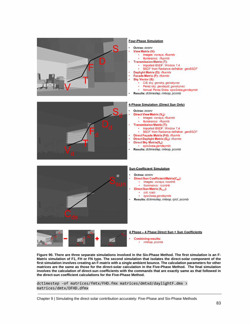
Chapter 9 | Simulating the direct solar contribution accurately: Five-Phase and Six-Phase Methods
83
Figure 90. There are three separate simulations involved in the Six-Phase Method. The first simulation is an F-Matrix simulation of F1, FH or FN type. The second simulation that isolates the direct-solar component of the first simulation involves creating an F-matrix with a single ambient bounce. The calculation parameters for other matrices are the same as those for the direct-solar calculation in the Five-Phase Method. The final simulation involves the calculation of direct-sun coefficients with the commands that are exactly same as that followed in the direct-sun coefficient calculations for the Five-Phase Method.
dctimestep -of matrices/fmtx/FHD.fmx matrices/dmtxd/daylightF.dmx > matrices/dmtx/DFHD.dfmx
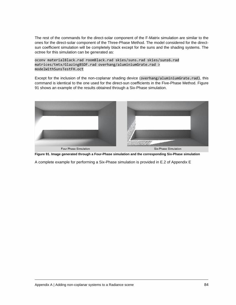
Appendix A | Adding non-coplanar systems to a Radiance scene 84
The rest of the commands for the direct-solar component of the F-Matrix simulation are similar to the
ones for the direct-solar component of the Three-Phase Method. The model considered for the direct-
sun coefficient simulation will be completely black except for the suns and the shading systems. The
octree for this simulation can be generated as:
oconv materialBlack.rad roomBlack.rad skies/suns.rad skies/suns6.rad matrices/tmtx/GlazingBSDF.rad overhang/aluminiumGrate.rad > modelWithSunsTestFH.oct Except for the inclusion of the non-coplanar shading device (overhang/aluminiumGrate.rad), this
command is identical to the one used for the direct-sun coefficients in the Five-Phase Method. Figure
91 shows an example of the results obtained through a Six-Phase simulation.
Figure 91. Image generated through a Four-Phase simulation and the corresponding Six-Phase simulation
A complete example for performing a Six-Phase simulation is provided in E.2 of Appendix E
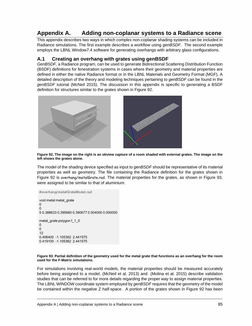
Appendix A | Adding non-coplanar systems to a Radiance scene 85
Appendix A. Adding non-coplanar systems to a Radiance scene This appendix describes two ways in which complex non-coplanar shading systems can be included in
Radiance simulations. The first example describes a workflow using genBSDF. The second example
employs the LBNL Window7.4 software for generating overhangs with arbitrary glass configurations.
A.1 Creating an overhang with grates using genBSDF GenBSDF, a Radiance program, can be used to generate Bidirectional Scattering Distribution Function
(BSDF) definitions for fenestration systems in cases where their geometry and material properties are
defined in either the native Radiance format or in the LBNL Materials and Geometry Format (MGF). A
detailed description of the theory and modeling techniques pertaining to genBSDF can be found in the
genBSDF tutorial (McNeil 2015). The discussion in this appendix is specific to generating a BSDF
definition for structures similar to the grates shown in Figure 92.
Figure 92. The image on the right is an obview capture of a room shaded with external grates. The image on the left shows the grates alone.
The model of the shading device specified as input to genBSDF should be representative of its material
properties as well as geometry. The file containing the Radiance definition for the grates shown in
Figure 92 is overhang/metalGrate.rad. The material properties for the grates, as shown in Figure 93,
were assigned to be similar to that of aluminium.
Figure 93. Partial definition of the geometry used for the metal grate that functions as an overhang for the room used for the F-Matrix simulations.
For simulations involving real-world models, the material properties should be measured accurately
before being assigned to a model. (McNeil et al. 2013) and (Molina et al. 2015) describe validation
studies that can be referred to for more details regarding the proper way to assign material properties.
The LBNL WINDOW coordinate system employed by genBSDF requires that the geometry of the model
be contained within the negative Z half-space. A portion of the grates shown in Figure 92 has been
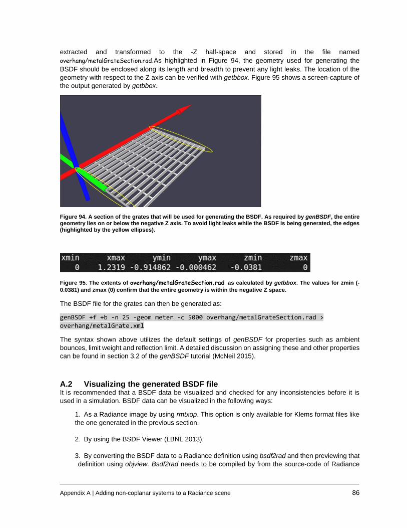
Appendix A | Adding non-coplanar systems to a Radiance scene 86
extracted and transformed to the -Z half-space and stored in the file named
overhang/metalGrateSection.rad.As highlighted in Figure 94, the geometry used for generating the
BSDF should be enclosed along its length and breadth to prevent any light leaks. The location of the
geometry with respect to the Z axis can be verified with getbbox. Figure 95 shows a screen-capture of
the output generated by getbbox.
Figure 94. A section of the grates that will be used for generating the BSDF. As required by genBSDF, the entire geometry lies on or below the negative Z axis. To avoid light leaks while the BSDF is being generated, the edges (highlighted by the yellow ellipses).
Figure 95. The extents of overhang/metalGrateSection.rad as calculated by getbbox. The values for zmin (-
0.0381) and zmax (0) confirm that the entire geometry is within the negative Z space.
The BSDF file for the grates can then be generated as:
genBSDF +f +b -n 25 -geom meter -c 5000 overhang/metalGrateSection.rad >
overhang/metalGrate.xml
The syntax shown above utilizes the default settings of genBSDF for properties such as ambient
bounces, limit weight and reflection limit. A detailed discussion on assigning these and other properties
can be found in section 3.2 of the genBSDF tutorial (McNeil 2015).
A.2 Visualizing the generated BSDF file It is recommended that a BSDF data be visualized and checked for any inconsistencies before it is
used in a simulation. BSDF data can be visualized in the following ways:
1. As a Radiance image by using rmtxop. This option is only available for Klems format files like
the one generated in the previous section.
2. By using the BSDF Viewer (LBNL 2013).
3. By converting the BSDF data to a Radiance definition using bsdf2rad and then previewing that
definition using objview. Bsdf2rad needs to be compiled by from the source-code of Radiance
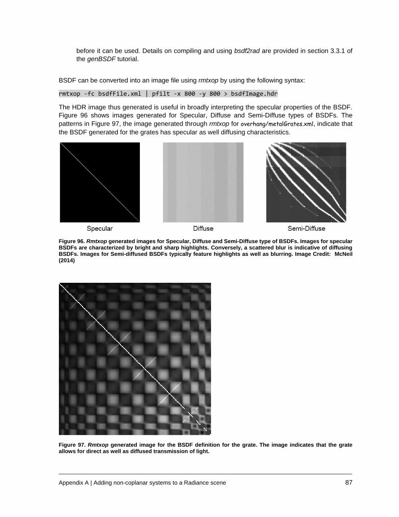
Appendix A | Adding non-coplanar systems to a Radiance scene 87
before it can be used. Details on compiling and using bsdf2rad are provided in section 3.3.1 of
the genBSDF tutorial.
BSDF can be converted into an image file using rmtxop by using the following syntax:
rmtxop -fc bsdfFile.xml | pfilt -x 800 -y 800 > bsdfImage.hdr
The HDR image thus generated is useful in broadly interpreting the specular properties of the BSDF.
Figure 96 shows images generated for Specular, Diffuse and Semi-Diffuse types of BSDFs. The
patterns in Figure 97, the image generated through rmtxop for overhang/metalGrates.xml, indicate that
the BSDF generated for the grates has specular as well diffusing characteristics.
Figure 96. Rmtxop generated images for Specular, Diffuse and Semi-Diffuse type of BSDFs. Images for specular BSDFs are characterized by bright and sharp highlights. Conversely, a scattered blur is indicative of diffusing BSDFs. Images for Semi-diffused BSDFs typically feature highlights as well as blurring. Image Credit: McNeil (2014)
Figure 97. Rmtxop generated image for the BSDF definition for the grate. The image indicates that the grate allows for direct as well as diffused transmission of light.

Appendix A | Adding non-coplanar systems to a Radiance scene 88
A more detailed and interactive visualization of BSDFs can be generated by using the BSDF viewer.
The screen captures of the BSDF viewer shown in Figure 98 indicate that the grates transmit flux
specularly when the flux is directly incident on them and transmit it in a diffused manner when the flux
is incident obliquely. This behavior appears to be in agreement with the structure of the grates shown
Figure 98. Screen-captures of the visualizations generated by BSDF viewer for overhang/metalGrate.xml. The image on top shows a representation of visible transmission from the grates for flux incident directly on it (through Patch 1). The image on the bottom shows visible transmission for flux that is incident obliquely (through Patch 116). In both the images, the smaller disc on the left represents the incident hemisphere and the yellow band within it represents the incident Klems patch being evaluated.
in Figure 94. After evaluating a BSDF’s flux transmission and reflection properties, it can be
incorporated into a scene by using the Radiance BSDF primitive.
A.3 Incorporating BSDF data into a Radiance scene by using the BSDF primitive The format for defining a BSDF primitive, as shown in Figure 99, is described in the Radiance reference
manual (LBNL 2016a).
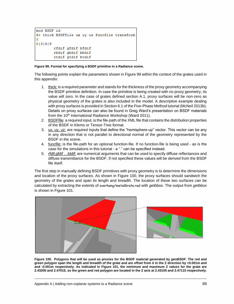
Appendix A | Adding non-coplanar systems to a Radiance scene 89
Figure 99. Format for specifying a BSDF primitive in a Radiance scene.
The following points explain the parameters shown in Figure 99 within the context of the grates used in
this appendix:
1. thick: is a required parameter and stands for the thickness of the proxy geometry accompanying
the BSDF primitive definition. In case the primitive is being created with no proxy geometry, its
value will zero. In the case of grates defined section A.1, proxy surfaces will be non-zero as
physical geometry of the grates is also included in the model. A descriptive example dealing
with proxy surfaces is provided in Section 6.1 of the Five-Phase Method tutorial (McNeil 2013b).
Details on proxy surfaces can also be found in Greg Ward’s presentation on BSDF materials
from the 10th International Radiance Workshop (Ward 2011).
2. BSDFfile: a required input, is the file-path of the XML file that contains the distribution properties
of the BSDF in Klems or Tensor-Tree format.
3. ux, uy, uz: are required inputs that define the “hemisphere-up” vector. This vector can be any
in any direction that is not parallel to directional normal of the geometry represented by the
BSDF in the scene.
4. funcfile: is the file-path for an optional function-file. If no function-file is being used - as is the
case for the simulations in this tutorial - a “.” can be specified instead.
5. rfdif,gfdif …btdif: are numerical arguments that can be used to specify diffuse reflectances and
diffuse transmittance for the BSDF. If not specified these values will be derived from the BSDF
file itself.
The first step in manually defining BSDF primitives with proxy geometry is to determine the dimensions
and location of the proxy surfaces. As shown in Figure 100, the proxy surfaces should sandwich the
geometry of the grates and span its length and breadth. The location of these two surfaces can be
calculated by extracting the extents of overhang/metalGrate.rad with getbbox. The output from getbbox
is shown in Figure 101.
Figure 100. Polygons that will be used as proxies for the BSDF material generated by genBSDF. The red and green polygon span the length and breadth of the grate and are offset from it in the Z direction by +0.001m and and -0.001m respectively. As indicated in Figure 101, the minimum and maximum Z values for the grate are 2.43205 and 2.47015, so the green and red polygon are located in the Z axis at 2.43105 and 2.47115 respectively.

Appendix A | Adding non-coplanar systems to a Radiance scene 90
The surface-normal of both polygons face in the +Z direction. The colors shown here are for illustration only and in the actual scene geometry the modifiers for the polygons are BSDF materials.
Figure 101. The getbbox output for the Radiance definition of grates. The thickness of the grate, derived by subtracting zmax from zmin is 0.0381m.
The final definition of the grates is shown in Figure 102. The value for ‘thick’, assigned as 0.03825 for
the top surface was calculated as the sum of (0.03810, 0.0001, 0.00005), where 0.03810 is the
thickness of the grate, 0.0001 is the offset of the proxy surface from the grate geometry and 0.00005
is a tolerance provided so that the proxy rays do not intersect with the system geometry or the opposite
proxy surface below the grate.
The value for the hemisphere-up vector, (ux uy uz) was assigned (0 1 0) as the direction normal of the
grates are facing in the Z direction.
It should be noted that the thickness specification for the bottom surface, -0.03825 is negative of the
value assigned for the top surface. The final definition of the grates with the BSDF proxy surfaces and
the physical geometry is saved in overhang/aluminiumGrate.rad.
Figure 102. A partial screen-capture of the final model of grates that will be used for the simulations. The dashed rectangles highlight different parts of the file. Part 1 and Part 2 are the material and surface definitions for the BSDF surface on top (colored in red in Figure 100). Part 3 and Part 4 are material and surface definitions for the bottom surface. Part 5 contains partial portion of the geometry of the grates. The contents in Part 5 are same as
the contents of the file overhang/metalGrate.rad.
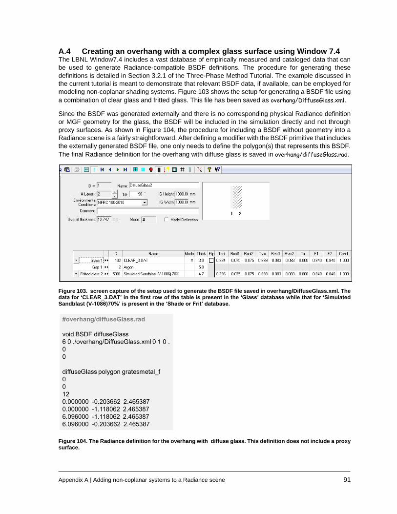
Appendix A | Adding non-coplanar systems to a Radiance scene 91
A.4 Creating an overhang with a complex glass surface using Window 7.4 The LBNL Window7.4 includes a vast database of empirically measured and cataloged data that can
be used to generate Radiance-compatible BSDF definitions. The procedure for generating these
definitions is detailed in Section 3.2.1 of the Three-Phase Method Tutorial. The example discussed in
the current tutorial is meant to demonstrate that relevant BSDF data, if available, can be employed for
modeling non-coplanar shading systems. Figure 103 shows the setup for generating a BSDF file using
a combination of clear glass and fritted glass. This file has been saved as overhang/DiffuseGlass.xml.
Since the BSDF was generated externally and there is no corresponding physical Radiance definition
or MGF geometry for the glass, the BSDF will be included in the simulation directly and not through
proxy surfaces. As shown in Figure 104, the procedure for including a BSDF without geometry into a
Radiance scene is a fairly straightforward. After defining a modifier with the BSDF primitive that includes
the externally generated BSDF file, one only needs to define the polygon(s) that represents this BSDF.
The final Radiance definition for the overhang with diffuse glass is saved in overhang/diffuseGlass.rad.
Figure 103. screen capture of the setup used to generate the BSDF file saved in overhang/DiffuseGlass.xml. The data for ‘CLEAR_3.DAT’ in the first row of the table is present in the ‘Glass’ database while that for ‘Simulated Sandblast (V-1086)70%’ is present in the ‘Shade or Frit’ database.
Figure 104. The Radiance definition for the overhang with diffuse glass. This definition does not include a proxy surface.
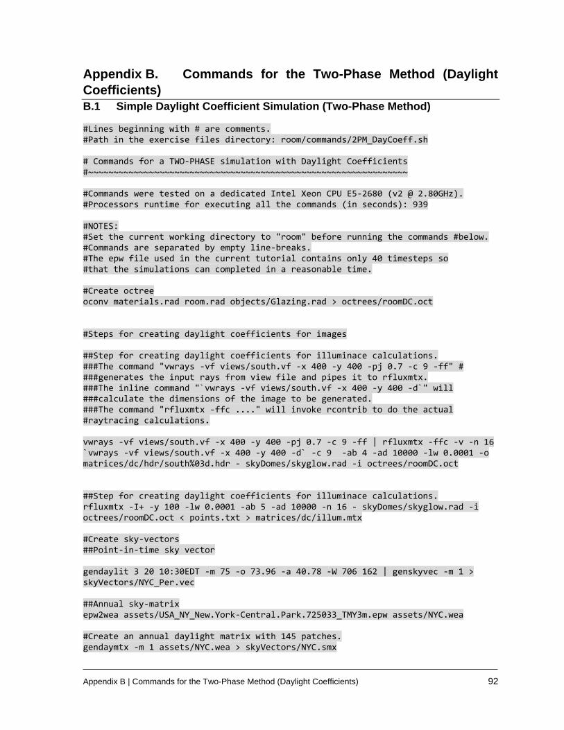
Appendix B | Commands for the Two-Phase Method (Daylight Coefficients) 92
Appendix B. Commands for the Two-Phase Method (Daylight
Coefficients)
B.1 Simple Daylight Coefficient Simulation (Two-Phase Method)
#Lines beginning with # are comments. #Path in the exercise files directory: room/commands/2PM_DayCoeff.sh # Commands for a TWO-PHASE simulation with Daylight Coefficients #~~~~~~~~~~~~~~~~~~~~~~~~~~~~~~~~~~~~~~~~~~~~~~~~~~~~~~~~~~~~~~~ #Commands were tested on a dedicated Intel Xeon CPU E5-2680 (v2 @ 2.80GHz). #Processors runtime for executing all the commands (in seconds): 939 #NOTES: #Set the current working directory to "room" before running the commands #below. #Commands are separated by empty line-breaks. #The epw file used in the current tutorial contains only 40 timesteps so #that the simulations can completed in a reasonable time. #Create octree oconv materials.rad room.rad objects/Glazing.rad > octrees/roomDC.oct #Steps for creating daylight coefficients for images ##Step for creating daylight coefficients for illuminace calculations. ###The command "vwrays -vf views/south.vf -x 400 -y 400 -pj 0.7 -c 9 -ff" # ###generates the input rays from view file and pipes it to rfluxmtx. ###The inline command "`vwrays -vf views/south.vf -x 400 -y 400 -d`" will ###calculate the dimensions of the image to be generated. ###The command "rfluxmtx -ffc ...." will invoke rcontrib to do the actual #raytracing calculations. vwrays -vf views/south.vf -x 400 -y 400 -pj 0.7 -c 9 -ff | rfluxmtx -ffc -v -n 16 `vwrays -vf views/south.vf -x 400 -y 400 -d` -c 9 -ab 4 -ad 10000 -lw 0.0001 -o matrices/dc/hdr/south%03d.hdr - skyDomes/skyglow.rad -i octrees/roomDC.oct ##Step for creating daylight coefficients for illuminace calculations. rfluxmtx -I+ -y 100 -lw 0.0001 -ab 5 -ad 10000 -n 16 - skyDomes/skyglow.rad -i octrees/roomDC.oct < points.txt > matrices/dc/illum.mtx #Create sky-vectors ##Point-in-time sky vector gendaylit 3 20 10:30EDT -m 75 -o 73.96 -a 40.78 -W 706 162 | genskyvec -m 1 > skyVectors/NYC_Per.vec ##Annual sky-matrix epw2wea assets/USA_NY_New.York-Central.Park.725033_TMY3m.epw assets/NYC.wea #Create an annual daylight matrix with 145 patches. gendaymtx -m 1 assets/NYC.wea > skyVectors/NYC.smx
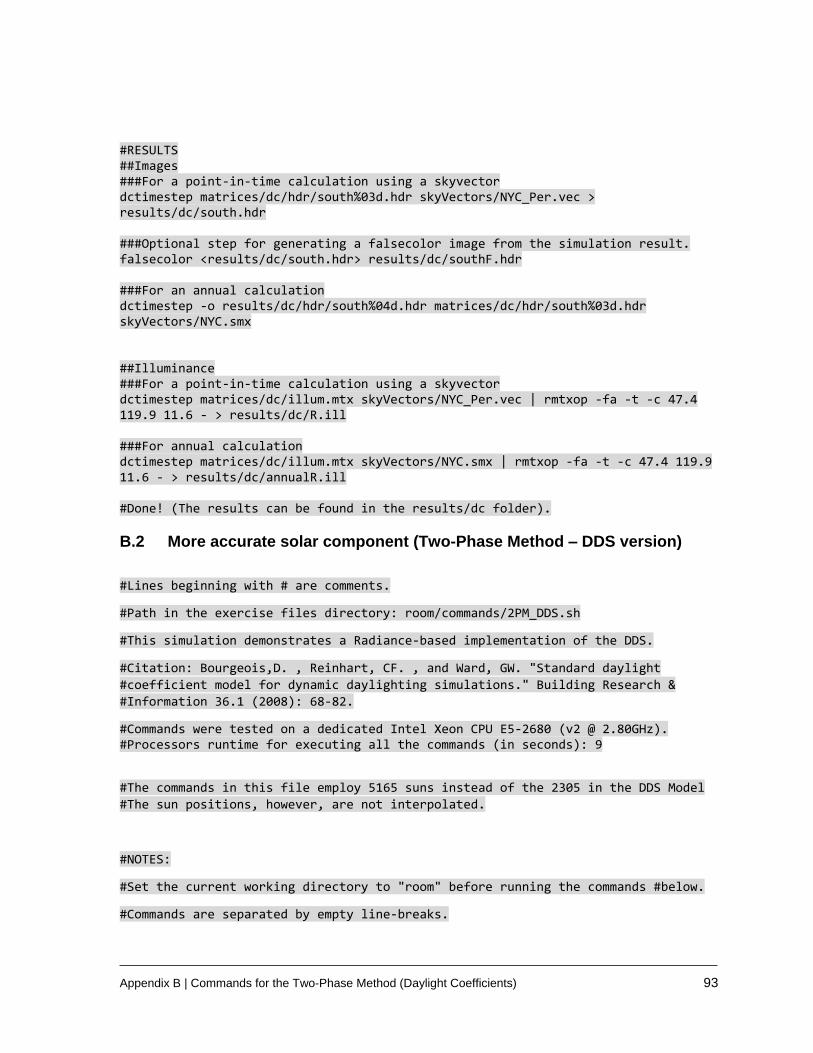
Appendix B | Commands for the Two-Phase Method (Daylight Coefficients) 93
#RESULTS ##Images ###For a point-in-time calculation using a skyvector dctimestep matrices/dc/hdr/south%03d.hdr skyVectors/NYC_Per.vec > results/dc/south.hdr ###Optional step for generating a falsecolor image from the simulation result. falsecolor <results/dc/south.hdr> results/dc/southF.hdr ###For an annual calculation dctimestep -o results/dc/hdr/south%04d.hdr matrices/dc/hdr/south%03d.hdr skyVectors/NYC.smx ##Illuminance ###For a point-in-time calculation using a skyvector dctimestep matrices/dc/illum.mtx skyVectors/NYC_Per.vec | rmtxop -fa -t -c 47.4 119.9 11.6 - > results/dc/R.ill ###For annual calculation dctimestep matrices/dc/illum.mtx skyVectors/NYC.smx | rmtxop -fa -t -c 47.4 119.9 11.6 - > results/dc/annualR.ill #Done! (The results can be found in the results/dc folder).
B.2 More accurate solar component (Two-Phase Method – DDS version)
#Lines beginning with # are comments.
#Path in the exercise files directory: room/commands/2PM_DDS.sh
#This simulation demonstrates a Radiance-based implementation of the DDS.
#Citation: Bourgeois,D. , Reinhart, CF. , and Ward, GW. "Standard daylight
#coefficient model for dynamic daylighting simulations." Building Research &
#Information 36.1 (2008): 68-82.
#Commands were tested on a dedicated Intel Xeon CPU E5-2680 (v2 @ 2.80GHz). #Processors runtime for executing all the commands (in seconds): 9
#The commands in this file employ 5165 suns instead of the 2305 in the DDS Model
#The sun positions, however, are not interpolated.
#NOTES:
#Set the current working directory to "room" before running the commands #below.
#Commands are separated by empty line-breaks.
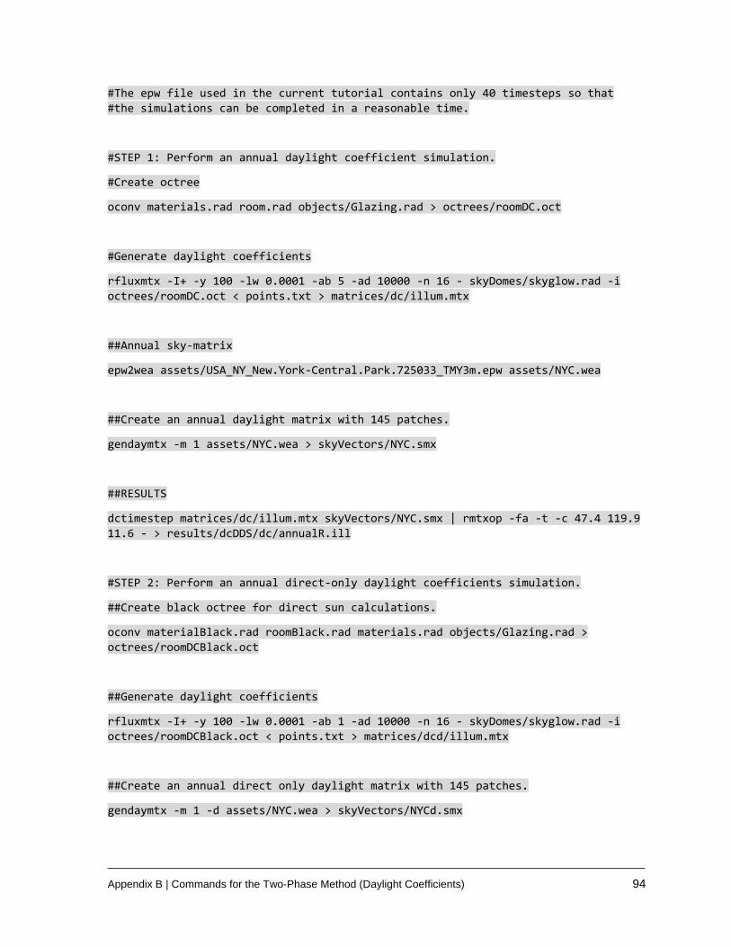
Appendix B | Commands for the Two-Phase Method (Daylight Coefficients) 94
#The epw file used in the current tutorial contains only 40 timesteps so that
#the simulations can be completed in a reasonable time.
#STEP 1: Perform an annual daylight coefficient simulation.
#Create octree
oconv materials.rad room.rad objects/Glazing.rad > octrees/roomDC.oct
#Generate daylight coefficients
rfluxmtx -I+ -y 100 -lw 0.0001 -ab 5 -ad 10000 -n 16 - skyDomes/skyglow.rad -i
octrees/roomDC.oct < points.txt > matrices/dc/illum.mtx
##Annual sky-matrix
epw2wea assets/USA_NY_New.York-Central.Park.725033_TMY3m.epw assets/NYC.wea
##Create an annual daylight matrix with 145 patches.
gendaymtx -m 1 assets/NYC.wea > skyVectors/NYC.smx
##RESULTS
dctimestep matrices/dc/illum.mtx skyVectors/NYC.smx | rmtxop -fa -t -c 47.4 119.9
11.6 - > results/dcDDS/dc/annualR.ill
#STEP 2: Perform an annual direct-only daylight coefficients simulation.
##Create black octree for direct sun calculations.
oconv materialBlack.rad roomBlack.rad materials.rad objects/Glazing.rad >
octrees/roomDCBlack.oct
##Generate daylight coefficients
rfluxmtx -I+ -y 100 -lw 0.0001 -ab 1 -ad 10000 -n 16 - skyDomes/skyglow.rad -i
octrees/roomDCBlack.oct < points.txt > matrices/dcd/illum.mtx
##Create an annual direct only daylight matrix with 145 patches.
gendaymtx -m 1 -d assets/NYC.wea > skyVectors/NYCd.smx
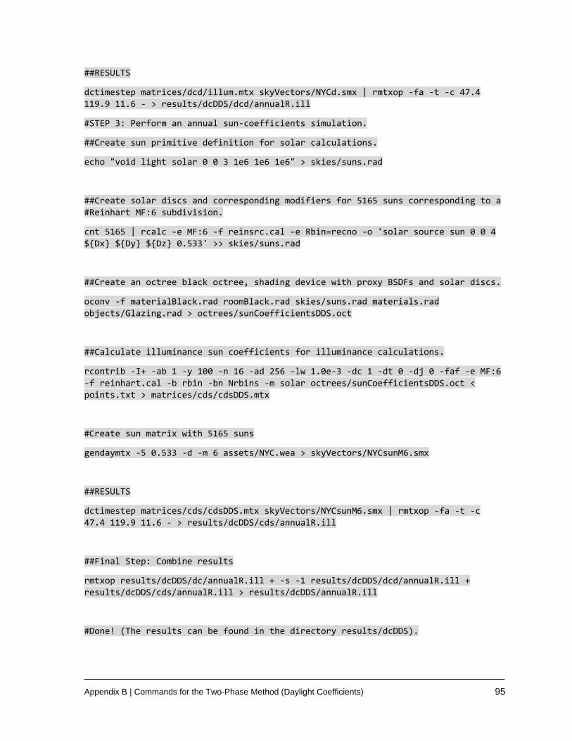
Appendix B | Commands for the Two-Phase Method (Daylight Coefficients) 95
##RESULTS
dctimestep matrices/dcd/illum.mtx skyVectors/NYCd.smx | rmtxop -fa -t -c 47.4
119.9 11.6 - > results/dcDDS/dcd/annualR.ill
#STEP 3: Perform an annual sun-coefficients simulation.
##Create sun primitive definition for solar calculations.
echo "void light solar 0 0 3 1e6 1e6 1e6" > skies/suns.rad
##Create solar discs and corresponding modifiers for 5165 suns corresponding to a
#Reinhart MF:6 subdivision.
cnt 5165 | rcalc -e MF:6 -f reinsrc.cal -e Rbin=recno -o 'solar source sun 0 0 4
${Dx} ${Dy} ${Dz} 0.533' >> skies/suns.rad
##Create an octree black octree, shading device with proxy BSDFs and solar discs.
oconv -f materialBlack.rad roomBlack.rad skies/suns.rad materials.rad
objects/Glazing.rad > octrees/sunCoefficientsDDS.oct
##Calculate illuminance sun coefficients for illuminance calculations.
rcontrib -I+ -ab 1 -y 100 -n 16 -ad 256 -lw 1.0e-3 -dc 1 -dt 0 -dj 0 -faf -e MF:6
-f reinhart.cal -b rbin -bn Nrbins -m solar octrees/sunCoefficientsDDS.oct <
points.txt > matrices/cds/cdsDDS.mtx
#Create sun matrix with 5165 suns
gendaymtx -5 0.533 -d -m 6 assets/NYC.wea > skyVectors/NYCsunM6.smx
##RESULTS
dctimestep matrices/cds/cdsDDS.mtx skyVectors/NYCsunM6.smx | rmtxop -fa -t -c
47.4 119.9 11.6 - > results/dcDDS/cds/annualR.ill
##Final Step: Combine results
rmtxop results/dcDDS/dc/annualR.ill + -s -1 results/dcDDS/dcd/annualR.ill +
results/dcDDS/cds/annualR.ill > results/dcDDS/annualR.ill
#Done! (The results can be found in the directory results/dcDDS).
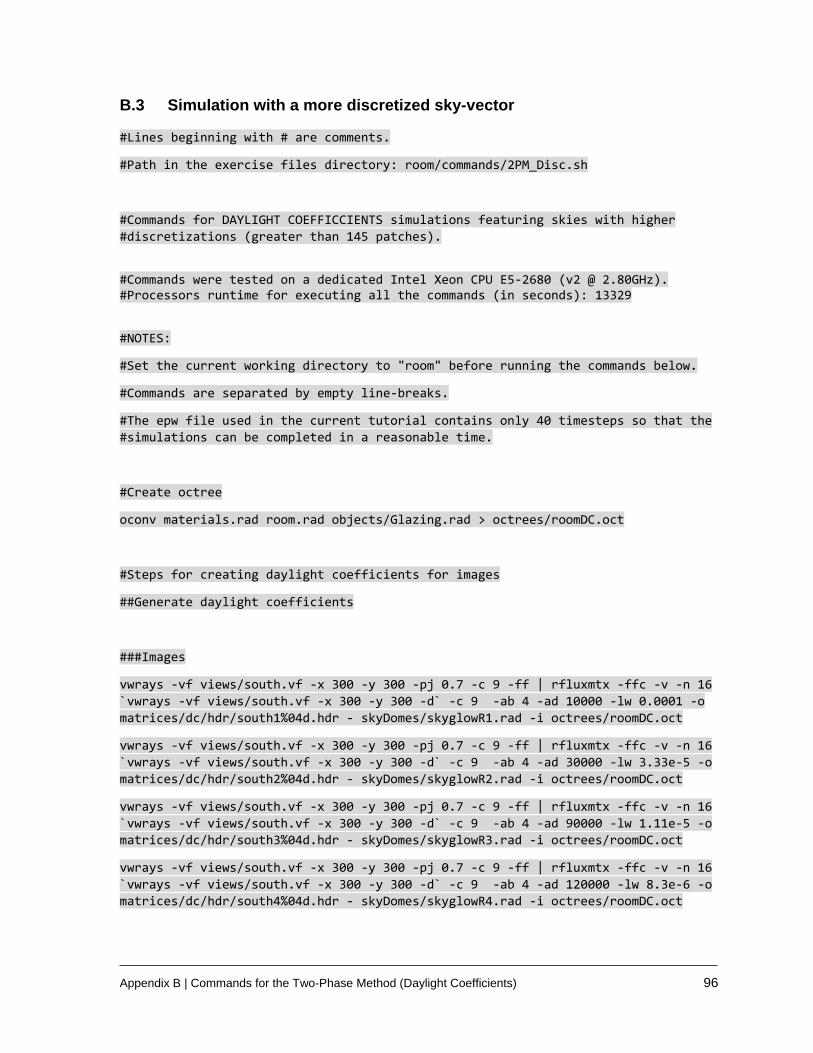
Appendix B | Commands for the Two-Phase Method (Daylight Coefficients) 96
B.3 Simulation with a more discretized sky-vector #Lines beginning with # are comments.
#Path in the exercise files directory: room/commands/2PM_Disc.sh
#Commands for DAYLIGHT COEFFICCIENTS simulations featuring skies with higher
#discretizations (greater than 145 patches).
#Commands were tested on a dedicated Intel Xeon CPU E5-2680 (v2 @ 2.80GHz). #Processors runtime for executing all the commands (in seconds): 13329
#NOTES:
#Set the current working directory to "room" before running the commands below.
#Commands are separated by empty line-breaks.
#The epw file used in the current tutorial contains only 40 timesteps so that the
#simulations can be completed in a reasonable time.
#Create octree
oconv materials.rad room.rad objects/Glazing.rad > octrees/roomDC.oct
#Steps for creating daylight coefficients for images
##Generate daylight coefficients
###Images
vwrays -vf views/south.vf -x 300 -y 300 -pj 0.7 -c 9 -ff | rfluxmtx -ffc -v -n 16
`vwrays -vf views/south.vf -x 300 -y 300 -d` -c 9 -ab 4 -ad 10000 -lw 0.0001 -o
matrices/dc/hdr/south1%04d.hdr - skyDomes/skyglowR1.rad -i octrees/roomDC.oct
vwrays -vf views/south.vf -x 300 -y 300 -pj 0.7 -c 9 -ff | rfluxmtx -ffc -v -n 16
`vwrays -vf views/south.vf -x 300 -y 300 -d` -c 9 -ab 4 -ad 30000 -lw 3.33e-5 -o
matrices/dc/hdr/south2%04d.hdr - skyDomes/skyglowR2.rad -i octrees/roomDC.oct
vwrays -vf views/south.vf -x 300 -y 300 -pj 0.7 -c 9 -ff | rfluxmtx -ffc -v -n 16
`vwrays -vf views/south.vf -x 300 -y 300 -d` -c 9 -ab 4 -ad 90000 -lw 1.11e-5 -o
matrices/dc/hdr/south3%04d.hdr - skyDomes/skyglowR3.rad -i octrees/roomDC.oct
vwrays -vf views/south.vf -x 300 -y 300 -pj 0.7 -c 9 -ff | rfluxmtx -ffc -v -n 16
`vwrays -vf views/south.vf -x 300 -y 300 -d` -c 9 -ab 4 -ad 120000 -lw 8.3e-6 -o
matrices/dc/hdr/south4%04d.hdr - skyDomes/skyglowR4.rad -i octrees/roomDC.oct

Appendix B | Commands for the Two-Phase Method (Daylight Coefficients) 97
###Illuminance
rfluxmtx -I+ -y 100 -ab 5 -ad 10000 -lw 0.0001 -n 16 - skyDomes/skyglowR1.rad -i
octrees/roomDC.oct < points.txt > matrices/dc/illumR1.mtx
rfluxmtx -I+ -y 100 -ad 30000 -lw 3.33e-5 -ab 5 -n 16 - skyDomes/skyglowR2.rad -i
octrees/roomDC.oct < points.txt > matrices/dc/illumR2.mtx
rfluxmtx -I+ -y 100 -ad 90000 -lw 1.11e-5 -ab 5 -n 16 - skyDomes/skyglowR3.rad -i
octrees/roomDC.oct < points.txt > matrices/dc/illumR3.mtx
rfluxmtx -I+ -y 100 -ad 120000 -lw 8.3e-6 -ab 5 -n 16 - skyDomes/skyglowR4.rad -i
octrees/roomDC.oct < points.txt > matrices/dc/illumR4.mtx
#Create sky-vectors
##Point-in-time sky vector.
gendaylit 3 20 10:30EDT -m 75 -o 73.96 -a 40.78 -W 706 162 | genskyvec -m 1 >
skyVectors/NYC_Per1.vec
gendaylit 3 20 10:30EDT -m 75 -o 73.96 -a 40.78 -W 706 162 | genskyvec -m 2 >
skyVectors/NYC_Per2.vec
gendaylit 3 20 10:30EDT -m 75 -o 73.96 -a 40.78 -W 706 162 | genskyvec -m 3 >
skyVectors/NYC_Per3.vec
gendaylit 3 20 10:30EDT -m 75 -o 73.96 -a 40.78 -W 706 162 | genskyvec -m 4 >
skyVectors/NYC_Per4.vec
#RESULTS
##Images
###For a point-in-time calculation using a skyvector
dctimestep matrices/dc/hdr/south1%04d.hdr skyVectors/NYC_Per1.vec >
results/dc/southR1.hdr
dctimestep matrices/dc/hdr/south2%04d.hdr skyVectors/NYC_Per2.vec >
results/dc/southR2.hdr
dctimestep matrices/dc/hdr/south3%04d.hdr skyVectors/NYC_Per3.vec >
results/dc/southR3.hdr
dctimestep matrices/dc/hdr/south4%04d.hdr skyVectors/NYC_Per4.vec >
results/dc/southR4.hdr
##Illuminance
###For a point-in-time calculation using a skyvector
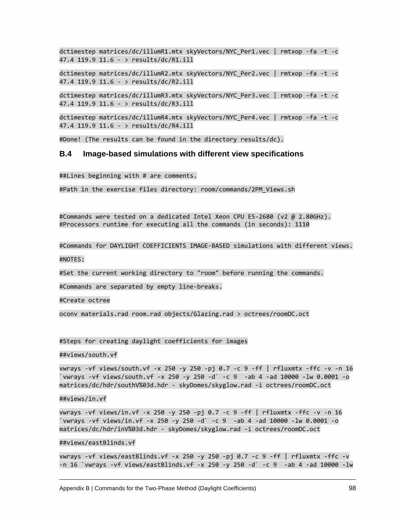
Appendix B | Commands for the Two-Phase Method (Daylight Coefficients) 98
dctimestep matrices/dc/illumR1.mtx skyVectors/NYC_Per1.vec | rmtxop -fa -t -c
47.4 119.9 11.6 - > results/dc/R1.ill
dctimestep matrices/dc/illumR2.mtx skyVectors/NYC_Per2.vec | rmtxop -fa -t -c
47.4 119.9 11.6 - > results/dc/R2.ill
dctimestep matrices/dc/illumR3.mtx skyVectors/NYC_Per3.vec | rmtxop -fa -t -c
47.4 119.9 11.6 - > results/dc/R3.ill
dctimestep matrices/dc/illumR4.mtx skyVectors/NYC_Per4.vec | rmtxop -fa -t -c
47.4 119.9 11.6 - > results/dc/R4.ill
#Done! (The results can be found in the directory results/dc).
B.4 Image-based simulations with different view specifications
##Lines beginning with # are comments.
#Path in the exercise files directory: room/commands/2PM_Views.sh
#Commands were tested on a dedicated Intel Xeon CPU E5-2680 (v2 @ 2.80GHz). #Processors runtime for executing all the commands (in seconds): 1110
#Commands for DAYLIGHT COEFFICIENTS IMAGE-BASED simulations with different views.
#NOTES:
#Set the current working directory to "room" before running the commands.
#Commands are separated by empty line-breaks.
#Create octree
oconv materials.rad room.rad objects/Glazing.rad > octrees/roomDC.oct
#Steps for creating daylight coefficients for images
##views/south.vf
vwrays -vf views/south.vf -x 250 -y 250 -pj 0.7 -c 9 -ff | rfluxmtx -ffc -v -n 16
`vwrays -vf views/south.vf -x 250 -y 250 -d` -c 9 -ab 4 -ad 10000 -lw 0.0001 -o
matrices/dc/hdr/southV%03d.hdr - skyDomes/skyglow.rad -i octrees/roomDC.oct
##views/in.vf
vwrays -vf views/in.vf -x 250 -y 250 -pj 0.7 -c 9 -ff | rfluxmtx -ffc -v -n 16
`vwrays -vf views/in.vf -x 250 -y 250 -d` -c 9 -ab 4 -ad 10000 -lw 0.0001 -o
matrices/dc/hdr/inV%03d.hdr - skyDomes/skyglow.rad -i octrees/roomDC.oct
##views/eastBlinds.vf
vwrays -vf views/eastBlinds.vf -x 250 -y 250 -pj 0.7 -c 9 -ff | rfluxmtx -ffc -v
-n 16 `vwrays -vf views/eastBlinds.vf -x 250 -y 250 -d` -c 9 -ab 4 -ad 10000 -lw
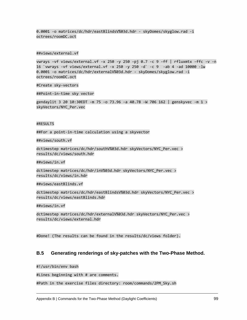
Appendix B | Commands for the Two-Phase Method (Daylight Coefficients) 99
0.0001 -o matrices/dc/hdr/eastBlindsV%03d.hdr - skyDomes/skyglow.rad -i
octrees/roomDC.oct
##views/external.vf
vwrays -vf views/external.vf -x 250 -y 250 -pj 0.7 -c 9 -ff | rfluxmtx -ffc -v -n
16 `vwrays -vf views/external.vf -x 250 -y 250 -d` -c 9 -ab 4 -ad 10000 -lw
0.0001 -o matrices/dc/hdr/externalV%03d.hdr - skyDomes/skyglow.rad -i
octrees/roomDC.oct
#Create sky-vectors
##Point-in-time sky vector
gendaylit 3 20 10:30EDT -m 75 -o 73.96 -a 40.78 -W 706 162 | genskyvec -m 1 >
skyVectors/NYC_Per.vec
#RESULTS
##For a point-in-time calculation using a skyvector
##views/south.vf
dctimestep matrices/dc/hdr/southV%03d.hdr skyVectors/NYC_Per.vec >
results/dc/views/south.hdr
##views/in.vf
dctimestep matrices/dc/hdr/inV%03d.hdr skyVectors/NYC_Per.vec >
results/dc/views/in.hdr
##views/eastBlinds.vf
dctimestep matrices/dc/hdr/eastBlindsV%03d.hdr skyVectors/NYC_Per.vec >
results/dc/views/eastBlinds.hdr
##views/in.vf
dctimestep matrices/dc/hdr/externalV%03d.hdr skyVectors/NYC_Per.vec >
results/dc/views/external.hdr
#Done! (The results can be found in the results/dc/views folder).
B.5 Generating renderings of sky-patches with the Two-Phase Method.
#!/usr/bin/env bash
#Lines beginning with # are comments.
#Path in the exercise files directory: room/commands/2PM_Sky.sh

Appendix B | Commands for the Two-Phase Method (Daylight Coefficients) 100
# Commands for generating images of sky patches using Daylight Coefficients.
#Commands were tested on a dedicated Intel Xeon CPU E5-2680 (v2 @ 2.80GHz). #Processors runtime for executing all the commands (in seconds): 9
#NOTES:
#Set the current working directory to "room" before running the commands below.
#Commands are separated by empty line-breaks.
#Create octree
oconv materials.rad objects/Ground.rad > octrees/sky.oct
#Steps for creating daylight coefficients for images
vwrays -vf views/skyUp.vf -x 300 -y 300 -pj 0.7 -c 9 -ff | rfluxmtx -ffc -v -n 16
`vwrays -vf views/skyUp.vf -x 300 -y 300 -d` -c 9 -ab 1 -ad 1000 -lw 0.001 -o
matrices/dc/hdr/skyTregenza%04d.hdr - skyDomes/skyglow.rad -i octrees/sky.oct
#Create a sky vector with 145 patches. The sky definition corresponds to 19th
September at 10:30AM EDT for New York City.
gendaylit 9 19 10:30EDT -m 75 -o 73.96 -a 40.78 -W 706 162 | genskyvec -m 1 >
skyVectors/NYC_Per.vec
#Create a similar sky vector with 145 patches for direct radiation only.
gendaylit 9 19 10:30EDT -m 75 -o 73.96 -a 40.78 -W 706 162 | genskyvec -m 1 -d >
skyVectors/NYC_Per_Direct.vec
#Generate the image for full sky.
dctimestep matrices/dc/hdr/skyTregenza%04d.hdr skyVectors/NYC_Per.vec >
results/dc/Sky.hdr
#Generate a falsecolor image of the above image
falsecolor -i results/dc/Sky.hdr -log 3 -s 3000000 -lh 150 >
results/dc/SkyFalsecolor.hdr

Appendix B | Commands for the Two-Phase Method (Daylight Coefficients) 101
#Generate the image
dctimestep matrices/dc/hdr/skyTregenza%04d.hdr skyVectors/NYC_Per_Direct.vec >
results/dc/SkyDirect.hdr
#Generate a falsecolor image of the above image
falsecolor -i results/dc/SkyDirect.hdr -log 3 -s 3000000 -lh 150 >
results/dc/SkyDirectFalsecolor.hdr
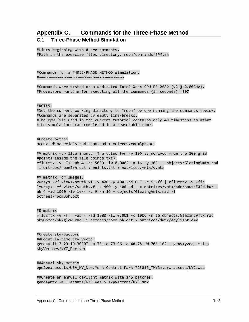
Appendix C | Commands for the Three-Phase Method 102
Appendix C. Commands for the Three-Phase Method
C.1 Three-Phase Method Simulation
#Lines beginning with # are comments. #Path in the exercise files directory: room/commands/3PM.sh
#Commands for a THREE-PHASE METHOD simulation. #~~~~~~~~~~~~~~~~~~~~~~~~~~~~~~~~~~~~~~ #Commands were tested on a dedicated Intel Xeon CPU E5-2680 (v2 @ 2.80GHz). #Processors runtime for executing all the commands (in seconds): 297 #NOTES: #Set the current working directory to "room" before running the commands #below. #Commands are separated by empty line-breaks. #The epw file used in the current tutorial contains only 40 timesteps so #that #the simulations can completed in a reasonable time. #Create octree oconv -f materials.rad room.rad > octrees/room3ph.oct #V matrix for Illuminance (The value for -y 100 is derived from the 100 grid #points inside the file points.txt). rfluxmtx -v -I+ -ab 4 -ad 5000 -lw 0.0002 -n 16 -y 100 - objects/GlazingVmtx.rad -i octrees/room3ph.oct < points.txt > matrices/vmtx/v.mtx #V matrix for Images. vwrays -vf views/south.vf -x 400 -y 400 -pj 0.7 -c 9 -ff | rfluxmtx -v -ffc `vwrays -vf views/south.vf -x 400 -y 400 -d` -o matrices/vmtx/hdr/south%03d.hdr -ab 4 -ad 1000 -lw 1e-4 -c 9 -n 16 - objects/GlazingVmtx.rad -i octrees/room3ph.oct #D matrix rfluxmtx -v -ff -ab 4 -ad 1000 -lw 0.001 -c 1000 -n 16 objects/GlazingVmtx.rad skyDomes/skyglow.rad -i octrees/room3ph.oct > matrices/dmtx/daylight.dmx #Create sky-vectors ##Point-in-time sky vector gendaylit 3 20 10:30EDT -m 75 -o 73.96 -a 40.78 -W 706 162 | genskyvec -m 1 > skyVectors/NYC_Per.vec ##Annual sky-matrix epw2wea assets/USA_NY_New.York-Central.Park.725033_TMY3m.epw assets/NYC.wea ##Create an annual daylight matrix with 145 patches. gendaymtx -m 1 assets/NYC.wea > skyVectors/NYC.smx
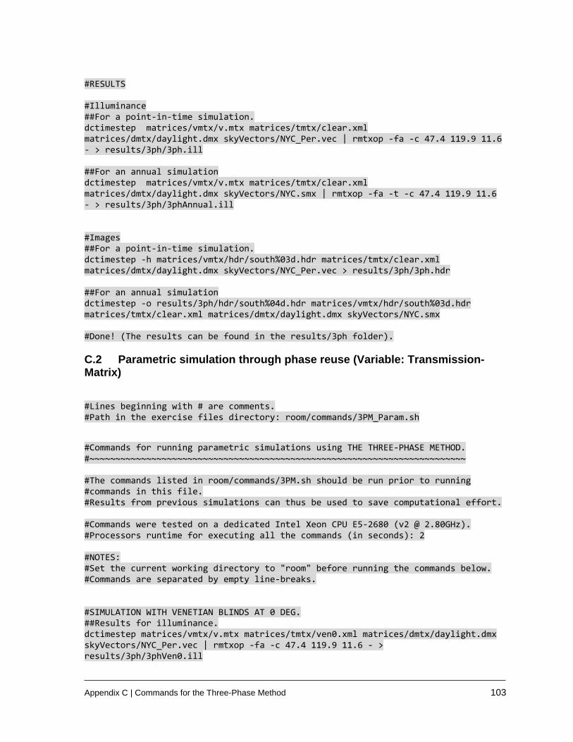
Appendix C | Commands for the Three-Phase Method 103
#RESULTS #Illuminance ##For a point-in-time simulation. dctimestep matrices/vmtx/v.mtx matrices/tmtx/clear.xml matrices/dmtx/daylight.dmx skyVectors/NYC_Per.vec | rmtxop -fa -c 47.4 119.9 11.6 - > results/3ph/3ph.ill ##For an annual simulation dctimestep matrices/vmtx/v.mtx matrices/tmtx/clear.xml matrices/dmtx/daylight.dmx skyVectors/NYC.smx | rmtxop -fa -t -c 47.4 119.9 11.6 - > results/3ph/3phAnnual.ill #Images ##For a point-in-time simulation. dctimestep -h matrices/vmtx/hdr/south%03d.hdr matrices/tmtx/clear.xml matrices/dmtx/daylight.dmx skyVectors/NYC_Per.vec > results/3ph/3ph.hdr ##For an annual simulation dctimestep -o results/3ph/hdr/south%04d.hdr matrices/vmtx/hdr/south%03d.hdr matrices/tmtx/clear.xml matrices/dmtx/daylight.dmx skyVectors/NYC.smx #Done! (The results can be found in the results/3ph folder).
C.2 Parametric simulation through phase reuse (Variable: Transmission-Matrix)
#Lines beginning with # are comments. #Path in the exercise files directory: room/commands/3PM_Param.sh
#Commands for running parametric simulations using THE THREE-PHASE METHOD. #~~~~~~~~~~~~~~~~~~~~~~~~~~~~~~~~~~~~~~~~~~~~~~~~~~~~~~~~~~~~~~~~~~~~~~~~~ #The commands listed in room/commands/3PM.sh should be run prior to running #commands in this file. #Results from previous simulations can thus be used to save computational effort. #Commands were tested on a dedicated Intel Xeon CPU E5-2680 (v2 @ 2.80GHz). #Processors runtime for executing all the commands (in seconds): 2 #NOTES: #Set the current working directory to "room" before running the commands below. #Commands are separated by empty line-breaks. #SIMULATION WITH VENETIAN BLINDS AT 0 DEG. ##Results for illuminance. dctimestep matrices/vmtx/v.mtx matrices/tmtx/ven0.xml matrices/dmtx/daylight.dmx skyVectors/NYC_Per.vec | rmtxop -fa -c 47.4 119.9 11.6 - > results/3ph/3phVen0.ill

Appendix C | Commands for the Three-Phase Method 104
##Results for images. dctimestep matrices/vmtx/hdr/south%03d.hdr matrices/tmtx/ven0.xml matrices/dmtx/daylight.dmx skyVectors/NYC_Per.vec > results/3ph/3phVen0.hdr #SIMULATION WITH VENETIAN BLINDS AT 45 DEG. ##Results for illuminance. dctimestep matrices/vmtx/v.mtx matrices/tmtx/ven45.xml matrices/dmtx/daylight.dmx skyVectors/NYC_Per.vec | rmtxop -fa -c 47.4 119.9 11.6 - > results/3ph/3phVen45.ill ##Results for images. dctimestep -h matrices/vmtx/hdr/south%03d.hdr matrices/tmtx/ven45.xml matrices/dmtx/daylight.dmx skyVectors/NYC_Per.vec > results/3ph/3phVen45.hdr #Done! (The results can be found in the results/3ph folder).
C.3 Parametric simulations through phase reuse (Variable: View-Matrix) #Lines beginning with # are comments. #Path in the exercise files directory: room/commands/3PM_East.sh
# THREE-PHASE image-based simulation using a different view. #~~~~~~~~~~~~~~~~~~~~~~~~~~~~~~~~~~~~~~~~~~~~~~~~~~~~~~~~~~~ #The objective of this simulation to demonstrate the applicability of phase-#reuse. #The commands for generating the Daylight Matrix and Sky Matrix, and the files #thus generated, are the same as before. #Commands were tested on a dedicated Intel Xeon CPU E5-2680 (v2 @ 2.80GHz). #Processors runtime for executing all the commands (in seconds): 353 #NOTES: #Set the current working directory to "room" before running the commands below. #Commands are separated by empty line-breaks. #The epw file used in the current tutorial contains only 40 timesteps so that the #simulations can completed in a reasonable time. #Create octree oconv -f materials.rad room.rad > octrees/room3ph.oct #V matrix for Images. vwrays -vf views/eastBlinds.vf -x 400 -y 400 -pj 0.7 -c 9 -ff | rfluxmtx -v -ffc `vwrays -vf views/eastBlinds.vf -x 400 -y 400 -d` -o matrices/vmtx/hdr/eastBlinds%03d.hdr -ab 4 -ad 1000 -lw 1e-4 -c 9 -n 16 - objects/GlazingVmtx.rad -i octrees/room3ph.oct #D matrix
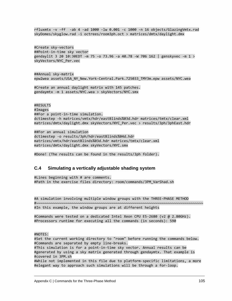
Appendix C | Commands for the Three-Phase Method 105
rfluxmtx -v -ff -ab 4 -ad 1000 -lw 0.001 -c 1000 -n 16 objects/GlazingVmtx.rad skyDomes/skyglow.rad -i octrees/room3ph.oct > matrices/dmtx/daylight.dmx #Create sky-vectors ##Point-in-time sky vector gendaylit 3 20 10:30EDT -m 75 -o 73.96 -a 40.78 -W 706 162 | genskyvec -m 1 > skyVectors/NYC_Per.vec ##Annual sky-matrix epw2wea assets/USA_NY_New.York-Central.Park.725033_TMY3m.epw assets/NYC.wea #Create an annual daylight matrix with 145 patches. gendaymtx -m 1 assets/NYC.wea > skyVectors/NYC.smx #RESULTS #Images ##For a point-in-time simulation. dctimestep -h matrices/vmtx/hdr/eastBlinds%03d.hdr matrices/tmtx/clear.xml matrices/dmtx/daylight.dmx skyVectors/NYC_Per.vec > results/3ph/3phEast.hdr ##For an annual simulation dctimestep -o results/3ph/hdr/eastBlinds%04d.hdr matrices/vmtx/hdr/eastBlinds%03d.hdr matrices/tmtx/clear.xml matrices/dmtx/daylight.dmx skyVectors/NYC.smx #Done! (The results can be found in the results/3ph folder).
C.4 Simulating a vertically adjustable shading system
#Lines beginning with # are comments. #Path in the exercise files directory: room/commands/3PM_VarShad.sh
#A simulation involving multiple window groups with the THREE-PHASE METHOD #~~~~~~~~~~~~~~~~~~~~~~~~~~~~~~~~~~~~~~~~~~~~~~~~~~~~~~~~~~~~~~~~~~~~~~~~~~~~~~~~ #In this example, the window groups are at different heights #Commands were tested on a dedicated Intel Xeon CPU E5-2680 (v2 @ 2.80GHz). #Processors runtime for executing all the commands (in seconds): 590 #NOTES: #Set the current working directory to "room" before running the commands below. #Commands are separated by empty line-breaks. #This simulation is for a point-in-time sky vector. Annual results can be #generated by using a sky matrix generated through gendaymtx. That example is #covered in 3PM.sh #While not implemented in this file due to platform-specific limitations, a more #elegant way to approach such simulations will be through a for-loop.

Appendix C | Commands for the Three-Phase Method 106
#Create an octree oconv -f materials.rad room.rad > octrees/room3ph.oct #V matrices for Illuminance. Four matrices corresponding to four shading groups # #will be created. rfluxmtx -v -I+ -ab 4 -ad 5000 -lw 0.0002 -n 16 -y 100 - varShading/GlazingVmtx1.rad -i octrees/room3ph.oct < points.txt > matrices/vmtx/v1.mtx rfluxmtx -v -I+ -ab 4 -ad 5000 -lw 0.0002 -n 16 -y 100 - varShading/GlazingVmtx2.rad -i octrees/room3ph.oct < points.txt > matrices/vmtx/v2.mtx rfluxmtx -v -I+ -ab 4 -ad 5000 -lw 0.0002 -n 16 -y 100 - varShading/GlazingVmtx3.rad -i octrees/room3ph.oct < points.txt > matrices/vmtx/v3.mtx rfluxmtx -v -I+ -ab 4 -ad 5000 -lw 0.0002 -n 16 -y 100 - varShading/GlazingVmtx4.rad -i octrees/room3ph.oct < points.txt > matrices/vmtx/v4.mtx #V matrices for Images. Four sets of matrices corresponding to four shading #groups will be created. vwrays -vf views/south.vf -x 300 -y 300 -pj 0.7 -c 9 -ff | rfluxmtx -v -ffc `vwrays -vf views/south.vf -x 300 -y 300 -d` -o matrices/vmtx/hdr/v1%03d.hdr -ab 4 -ad 1000 -lw 1e-4 -c 9 -n 16 - varShading/GlazingVmtx1.rad -i octrees/room3ph.oct vwrays -vf views/south.vf -x 300 -y 300 -pj 0.7 -c 9 -ff | rfluxmtx -v -ffc `vwrays -vf views/south.vf -x 300 -y 300 -d` -o matrices/vmtx/hdr/v2%03d.hdr -ab 4 -ad 1000 -lw 1e-4 -c 9 -n 16 - varShading/GlazingVmtx2.rad -i octrees/room3ph.oct vwrays -vf views/south.vf -x 300 -y 300 -pj 0.7 -c 9 -ff | rfluxmtx -v -ffc `vwrays -vf views/south.vf -x 300 -y 300 -d` -o matrices/vmtx/hdr/v3%03d.hdr -ab 4 -ad 1000 -lw 1e-4 -c 9 -n 16 - varShading/GlazingVmtx3.rad -i octrees/room3ph.oct vwrays -vf views/south.vf -x 300 -y 300 -pj 0.7 -c 9 -ff | rfluxmtx -v -ffc `vwrays -vf views/south.vf -x 300 -y 300 -d` -o matrices/vmtx/hdr/v4%03d.hdr -ab 4 -ad 1000 -lw 1e-4 -c 9 -n 16 - varShading/GlazingVmtx4.rad -i octrees/room3ph.oct #D Matrices corresponding to four shading groups. rfluxmtx -v -ff -ab 4 -ad 1000 -lw 0.001 -c 1000 -n 16 varShading/GlazingVmtx1.rad skyDomes/skyglow.rad -i octrees/room3ph.oct > matrices/dmtx/daylight1.dmx
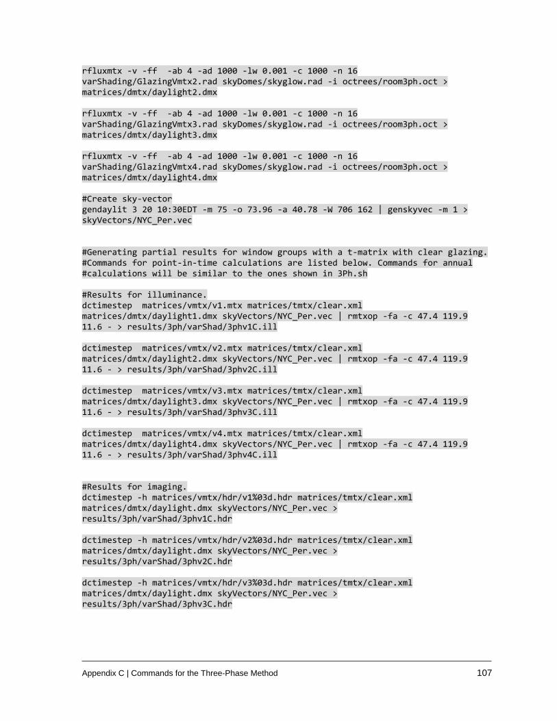
Appendix C | Commands for the Three-Phase Method 107
rfluxmtx -v -ff -ab 4 -ad 1000 -lw 0.001 -c 1000 -n 16 varShading/GlazingVmtx2.rad skyDomes/skyglow.rad -i octrees/room3ph.oct > matrices/dmtx/daylight2.dmx rfluxmtx -v -ff -ab 4 -ad 1000 -lw 0.001 -c 1000 -n 16 varShading/GlazingVmtx3.rad skyDomes/skyglow.rad -i octrees/room3ph.oct > matrices/dmtx/daylight3.dmx rfluxmtx -v -ff -ab 4 -ad 1000 -lw 0.001 -c 1000 -n 16 varShading/GlazingVmtx4.rad skyDomes/skyglow.rad -i octrees/room3ph.oct > matrices/dmtx/daylight4.dmx #Create sky-vector gendaylit 3 20 10:30EDT -m 75 -o 73.96 -a 40.78 -W 706 162 | genskyvec -m 1 > skyVectors/NYC_Per.vec #Generating partial results for window groups with a t-matrix with clear glazing. #Commands for point-in-time calculations are listed below. Commands for annual #calculations will be similar to the ones shown in 3Ph.sh #Results for illuminance. dctimestep matrices/vmtx/v1.mtx matrices/tmtx/clear.xml matrices/dmtx/daylight1.dmx skyVectors/NYC_Per.vec | rmtxop -fa -c 47.4 119.9 11.6 - > results/3ph/varShad/3phv1C.ill dctimestep matrices/vmtx/v2.mtx matrices/tmtx/clear.xml matrices/dmtx/daylight2.dmx skyVectors/NYC_Per.vec | rmtxop -fa -c 47.4 119.9 11.6 - > results/3ph/varShad/3phv2C.ill dctimestep matrices/vmtx/v3.mtx matrices/tmtx/clear.xml matrices/dmtx/daylight3.dmx skyVectors/NYC_Per.vec | rmtxop -fa -c 47.4 119.9 11.6 - > results/3ph/varShad/3phv3C.ill dctimestep matrices/vmtx/v4.mtx matrices/tmtx/clear.xml matrices/dmtx/daylight4.dmx skyVectors/NYC_Per.vec | rmtxop -fa -c 47.4 119.9 11.6 - > results/3ph/varShad/3phv4C.ill #Results for imaging. dctimestep -h matrices/vmtx/hdr/v1%03d.hdr matrices/tmtx/clear.xml matrices/dmtx/daylight.dmx skyVectors/NYC_Per.vec > results/3ph/varShad/3phv1C.hdr dctimestep -h matrices/vmtx/hdr/v2%03d.hdr matrices/tmtx/clear.xml matrices/dmtx/daylight.dmx skyVectors/NYC_Per.vec > results/3ph/varShad/3phv2C.hdr dctimestep -h matrices/vmtx/hdr/v3%03d.hdr matrices/tmtx/clear.xml matrices/dmtx/daylight.dmx skyVectors/NYC_Per.vec > results/3ph/varShad/3phv3C.hdr
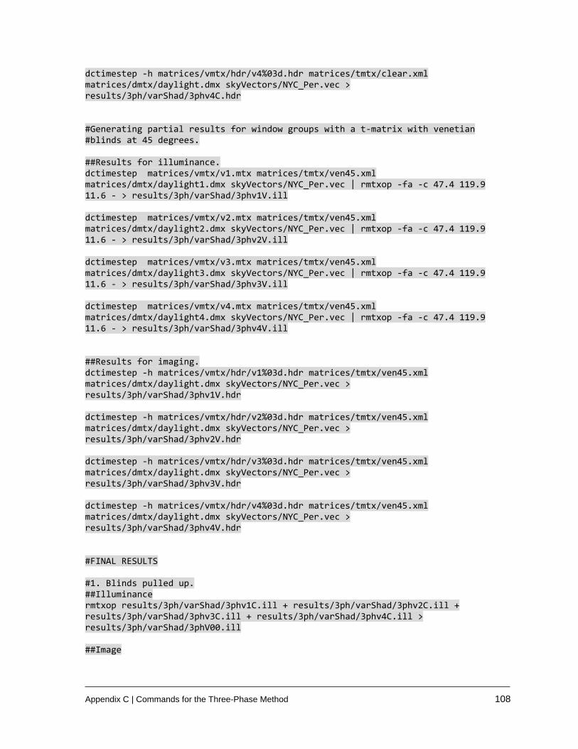
Appendix C | Commands for the Three-Phase Method 108
dctimestep -h matrices/vmtx/hdr/v4%03d.hdr matrices/tmtx/clear.xml matrices/dmtx/daylight.dmx skyVectors/NYC_Per.vec > results/3ph/varShad/3phv4C.hdr #Generating partial results for window groups with a t-matrix with venetian #blinds at 45 degrees. ##Results for illuminance. dctimestep matrices/vmtx/v1.mtx matrices/tmtx/ven45.xml matrices/dmtx/daylight1.dmx skyVectors/NYC_Per.vec | rmtxop -fa -c 47.4 119.9 11.6 - > results/3ph/varShad/3phv1V.ill dctimestep matrices/vmtx/v2.mtx matrices/tmtx/ven45.xml matrices/dmtx/daylight2.dmx skyVectors/NYC_Per.vec | rmtxop -fa -c 47.4 119.9 11.6 - > results/3ph/varShad/3phv2V.ill dctimestep matrices/vmtx/v3.mtx matrices/tmtx/ven45.xml matrices/dmtx/daylight3.dmx skyVectors/NYC_Per.vec | rmtxop -fa -c 47.4 119.9 11.6 - > results/3ph/varShad/3phv3V.ill dctimestep matrices/vmtx/v4.mtx matrices/tmtx/ven45.xml matrices/dmtx/daylight4.dmx skyVectors/NYC_Per.vec | rmtxop -fa -c 47.4 119.9 11.6 - > results/3ph/varShad/3phv4V.ill ##Results for imaging. dctimestep -h matrices/vmtx/hdr/v1%03d.hdr matrices/tmtx/ven45.xml matrices/dmtx/daylight.dmx skyVectors/NYC_Per.vec > results/3ph/varShad/3phv1V.hdr dctimestep -h matrices/vmtx/hdr/v2%03d.hdr matrices/tmtx/ven45.xml matrices/dmtx/daylight.dmx skyVectors/NYC_Per.vec > results/3ph/varShad/3phv2V.hdr dctimestep -h matrices/vmtx/hdr/v3%03d.hdr matrices/tmtx/ven45.xml matrices/dmtx/daylight.dmx skyVectors/NYC_Per.vec > results/3ph/varShad/3phv3V.hdr dctimestep -h matrices/vmtx/hdr/v4%03d.hdr matrices/tmtx/ven45.xml matrices/dmtx/daylight.dmx skyVectors/NYC_Per.vec > results/3ph/varShad/3phv4V.hdr #FINAL RESULTS #1. Blinds pulled up. ##Illuminance rmtxop results/3ph/varShad/3phv1C.ill + results/3ph/varShad/3phv2C.ill + results/3ph/varShad/3phv3C.ill + results/3ph/varShad/3phv4C.ill > results/3ph/varShad/3phV00.ill ##Image

Appendix C | Commands for the Three-Phase Method 109
pcomb results/3ph/varShad/3phv1C.hdr results/3ph/varShad/3phv2C.hdr results/3ph/varShad/3phv3C.hdr results/3ph/varShad/3phv4C.hdr > results/3ph/varShad/3phV00.hdr #2. Blinds at 25% ##Illuminance rmtxop results/3ph/varShad/3phv1V.ill + results/3ph/varShad/3phv2C.ill + results/3ph/varShad/3phv3C.ill + results/3ph/varShad/3phv4C.ill > results/3ph/varShad/3phV25.ill ##Image pcomb results/3ph/varShad/3phv1V.hdr results/3ph/varShad/3phv2C.hdr results/3ph/varShad/3phv3C.hdr results/3ph/varShad/3phv4C.hdr > results/3ph/varShad/3phV25.hdr #3. Blinds at 100% ##Illuminance rmtxop results/3ph/varShad/3phv1V.ill + results/3ph/varShad/3phv2V.ill + results/3ph/varShad/3phv3V.ill + results/3ph/varShad/3phv4V.ill > results/3ph/varShad/3phV100.ill ##Image pcomb results/3ph/varShad/3phv1V.hdr results/3ph/varShad/3phv2V.hdr results/3ph/varShad/3phv3V.hdr results/3ph/varShad/3phv4V.hdr > results/3ph/varShad/3phV100.hdr #Done! (The results can be found in the results/3ph/varShad folder).
C.5 Simulating non-coplanar shading systems #Lines beginning with # are comments. #Path in the exercise files directory: room/commands/3PM_NonCop.sh
#Commands for simulating non-coplanar shades using the THREE-PHASE METHOD. #~~~~~~~~~~~~~~~~~~~~~~~~~~~~~~~~~~~~~~~~~~~~~~~~~~~~~~~~~~~~~~~~~~~~~~~~ #Commands were tested on a dedicated Intel Xeon CPU E5-2680 (v2 @ 2.80GHz). #Processors runtime for executing all the commands (in seconds): 374 #The shading system is considered as a part of the overall scene. #A more efficient way to evaluate such a system would be using the F-Matrix #Method (4PM). #NOTES: #Set the current working directory to "room" before running the commands below. #Commands are separated by empty line-breaks. #Create octree oconv -f materials.rad room.rad overhang/aluminiumGrate.rad > octrees/room3phNonCop.oct
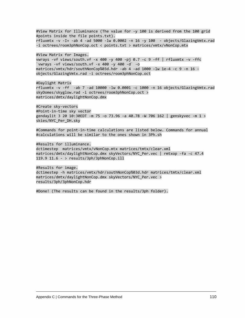
Appendix C | Commands for the Three-Phase Method 110
#View Matrix for Illuminance (The value for -y 100 is derived from the 100 grid #points inside the file points.txt). rfluxmtx -v -I+ -ab 4 -ad 5000 -lw 0.0002 -n 16 -y 100 - objects/GlazingVmtx.rad -i octrees/room3phNonCop.oct < points.txt > matrices/vmtx/vNonCop.mtx #View Matrix for Images. vwrays -vf views/south.vf -x 400 -y 400 -pj 0.7 -c 9 -ff | rfluxmtx -v -ffc `vwrays -vf views/south.vf -x 400 -y 400 -d` -o matrices/vmtx/hdr/southNonCop%03d.hdr -ab 4 -ad 1000 -lw 1e-4 -c 9 -n 16 - objects/GlazingVmtx.rad -i octrees/room3phNonCop.oct #Daylight Matrix rfluxmtx -v -ff -ab 7 -ad 10000 -lw 0.0001 -c 1000 -n 16 objects/GlazingVmtx.rad skyDomes/skyglow.rad -i octrees/room3phNonCop.oct > matrices/dmtx/daylightNonCop.dmx #Create sky-vectors #Point-in-time sky vector gendaylit 3 20 10:30EDT -m 75 -o 73.96 -a 40.78 -W 706 162 | genskyvec -m 1 > skies/NYC_Per_DH.sky #Commands for point-in-time calculations are listed below. Commands for annual #calculations will be similar to the ones shown in 3Ph.sh #Results for illuminance. dctimestep matrices/vmtx/vNonCop.mtx matrices/tmtx/clear.xml matrices/dmtx/daylightNonCop.dmx skyVectors/NYC_Per.vec | rmtxop -fa -c 47.4 119.9 11.6 - > results/3ph/3phNonCop.ill #Results for image. dctimestep -h matrices/vmtx/hdr/southNonCop%03d.hdr matrices/tmtx/clear.xml matrices/dmtx/daylightNonCop.dmx skyVectors/NYC_Per.vec > results/3ph/3phNonCop.hdr #Done! (The results can be found in the results/3ph folder).
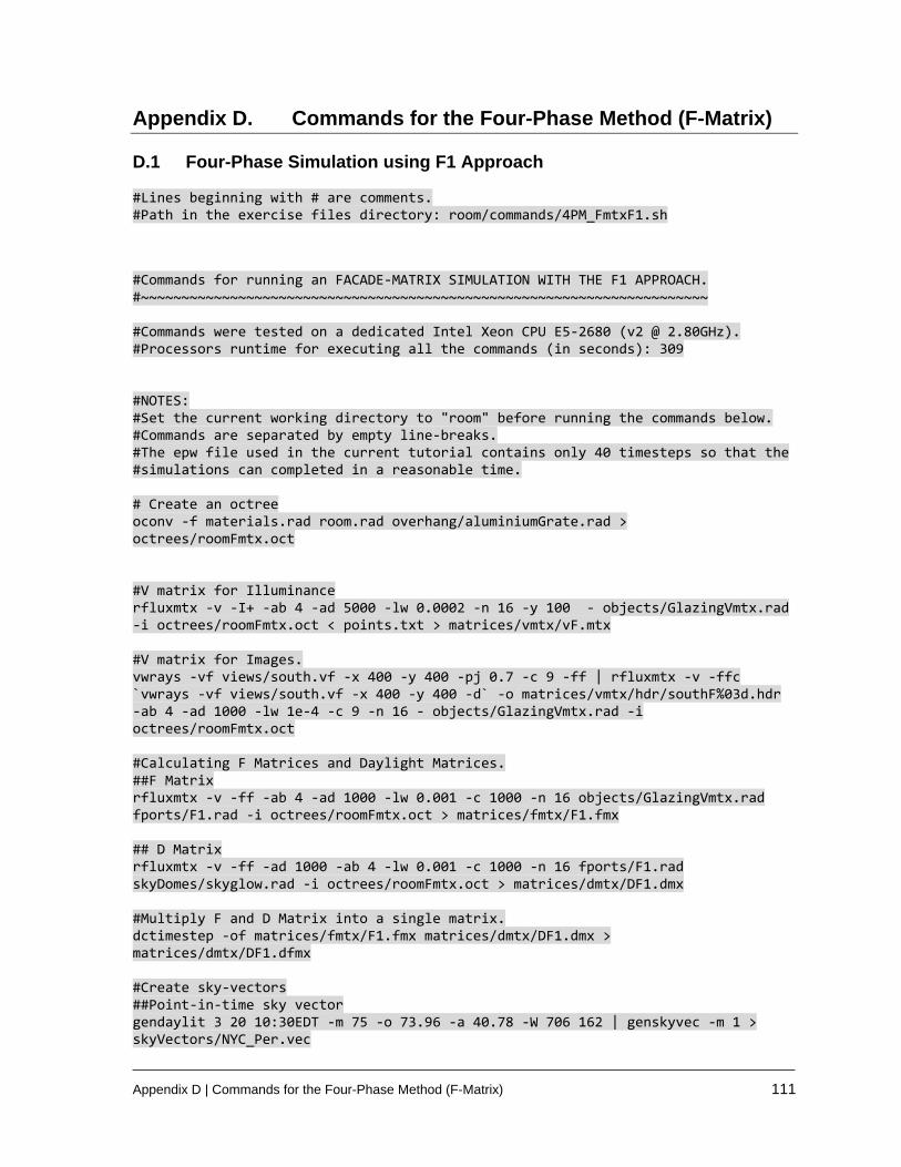
Appendix D | Commands for the Four-Phase Method (F-Matrix) 111
Appendix D. Commands for the Four-Phase Method (F-Matrix)
D.1 Four-Phase Simulation using F1 Approach #Lines beginning with # are comments. #Path in the exercise files directory: room/commands/4PM_FmtxF1.sh
#Commands for running an FACADE-MATRIX SIMULATION WITH THE F1 APPROACH. #~~~~~~~~~~~~~~~~~~~~~~~~~~~~~~~~~~~~~~~~~~~~~~~~~~~~~~~~~~~~~~~~~~~~~~ #Commands were tested on a dedicated Intel Xeon CPU E5-2680 (v2 @ 2.80GHz). #Processors runtime for executing all the commands (in seconds): 309 #NOTES: #Set the current working directory to "room" before running the commands below. #Commands are separated by empty line-breaks. #The epw file used in the current tutorial contains only 40 timesteps so that the #simulations can completed in a reasonable time. # Create an octree oconv -f materials.rad room.rad overhang/aluminiumGrate.rad > octrees/roomFmtx.oct #V matrix for Illuminance rfluxmtx -v -I+ -ab 4 -ad 5000 -lw 0.0002 -n 16 -y 100 - objects/GlazingVmtx.rad -i octrees/roomFmtx.oct < points.txt > matrices/vmtx/vF.mtx #V matrix for Images. vwrays -vf views/south.vf -x 400 -y 400 -pj 0.7 -c 9 -ff | rfluxmtx -v -ffc `vwrays -vf views/south.vf -x 400 -y 400 -d` -o matrices/vmtx/hdr/southF%03d.hdr -ab 4 -ad 1000 -lw 1e-4 -c 9 -n 16 - objects/GlazingVmtx.rad -i octrees/roomFmtx.oct #Calculating F Matrices and Daylight Matrices. ##F Matrix rfluxmtx -v -ff -ab 4 -ad 1000 -lw 0.001 -c 1000 -n 16 objects/GlazingVmtx.rad fports/F1.rad -i octrees/roomFmtx.oct > matrices/fmtx/F1.fmx ## D Matrix rfluxmtx -v -ff -ad 1000 -ab 4 -lw 0.001 -c 1000 -n 16 fports/F1.rad skyDomes/skyglow.rad -i octrees/roomFmtx.oct > matrices/dmtx/DF1.dmx #Multiply F and D Matrix into a single matrix. dctimestep -of matrices/fmtx/F1.fmx matrices/dmtx/DF1.dmx > matrices/dmtx/DF1.dfmx #Create sky-vectors ##Point-in-time sky vector gendaylit 3 20 10:30EDT -m 75 -o 73.96 -a 40.78 -W 706 162 | genskyvec -m 1 > skyVectors/NYC_Per.vec
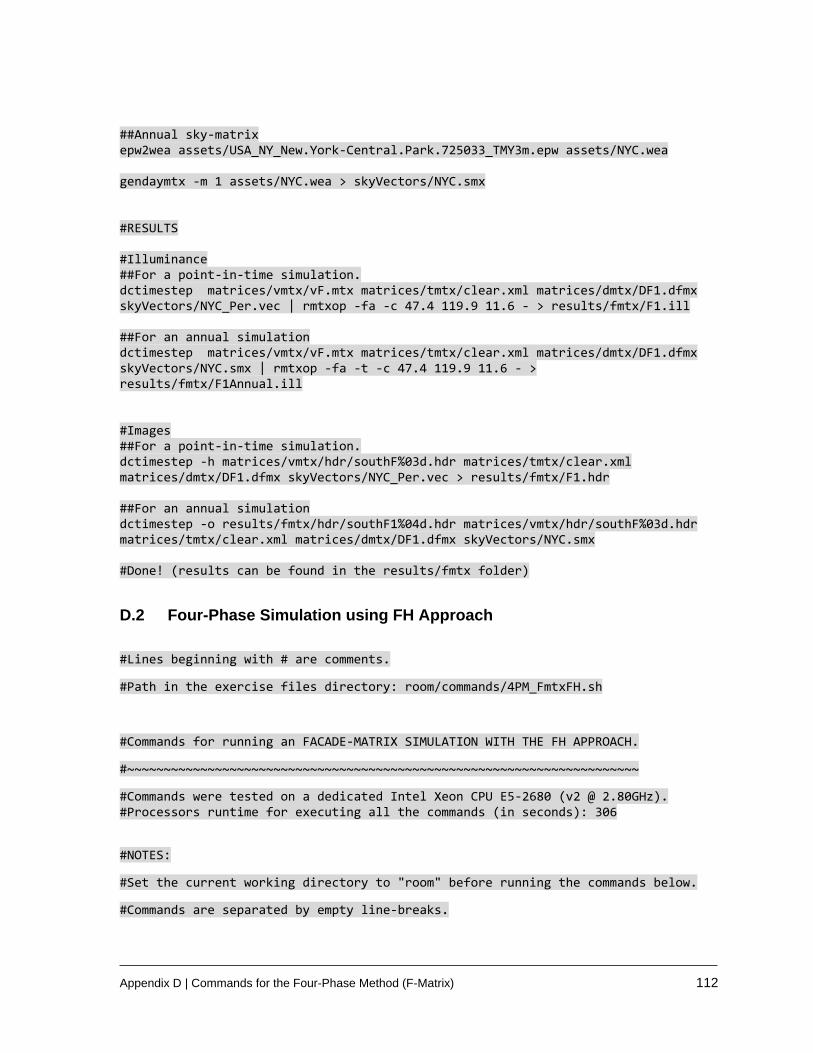
Appendix D | Commands for the Four-Phase Method (F-Matrix) 112
##Annual sky-matrix epw2wea assets/USA_NY_New.York-Central.Park.725033_TMY3m.epw assets/NYC.wea gendaymtx -m 1 assets/NYC.wea > skyVectors/NYC.smx #RESULTS #Illuminance ##For a point-in-time simulation. dctimestep matrices/vmtx/vF.mtx matrices/tmtx/clear.xml matrices/dmtx/DF1.dfmx skyVectors/NYC_Per.vec | rmtxop -fa -c 47.4 119.9 11.6 - > results/fmtx/F1.ill ##For an annual simulation dctimestep matrices/vmtx/vF.mtx matrices/tmtx/clear.xml matrices/dmtx/DF1.dfmx skyVectors/NYC.smx | rmtxop -fa -t -c 47.4 119.9 11.6 - > results/fmtx/F1Annual.ill #Images ##For a point-in-time simulation. dctimestep -h matrices/vmtx/hdr/southF%03d.hdr matrices/tmtx/clear.xml matrices/dmtx/DF1.dfmx skyVectors/NYC_Per.vec > results/fmtx/F1.hdr ##For an annual simulation dctimestep -o results/fmtx/hdr/southF1%04d.hdr matrices/vmtx/hdr/southF%03d.hdr matrices/tmtx/clear.xml matrices/dmtx/DF1.dfmx skyVectors/NYC.smx #Done! (results can be found in the results/fmtx folder)
D.2 Four-Phase Simulation using FH Approach
#Lines beginning with # are comments.
#Path in the exercise files directory: room/commands/4PM_FmtxFH.sh
#Commands for running an FACADE-MATRIX SIMULATION WITH THE FH APPROACH.
#~~~~~~~~~~~~~~~~~~~~~~~~~~~~~~~~~~~~~~~~~~~~~~~~~~~~~~~~~~~~~~~~~~~~~~
#Commands were tested on a dedicated Intel Xeon CPU E5-2680 (v2 @ 2.80GHz). #Processors runtime for executing all the commands (in seconds): 306
#NOTES:
#Set the current working directory to "room" before running the commands below.
#Commands are separated by empty line-breaks.

Appendix D | Commands for the Four-Phase Method (F-Matrix) 113
#The epw file used in the current tutorial contains only 40 timesteps so that the
simulations can completed in a reasonable time.
# Create an octree
oconv -f materials.rad room.rad overhang/aluminiumGrate.rad >
octrees/roomFmtx.oct
#V matrix for Illuminance
rfluxmtx -v -I+ -ab 4 -ad 5000 -lw 0.0002 -n 16 -y 100 - objects/GlazingVmtx.rad
-i octrees/roomFmtx.oct < points.txt > matrices/vmtx/vF.mtx
#V matrix for Images.
vwrays -vf views/south.vf -x 400 -y 400 -pj 0.7 -c 9 -ff | rfluxmtx -v -ffc
`vwrays -vf views/south.vf -x 400 -y 400 -d` -o matrices/vmtx/hdr/southF%03d.hdr
-ab 4 -ad 1000 -lw 1e-4 -c 9 -n 16 - objects/GlazingVmtx.rad -i
octrees/roomFmtx.oct
#Calculating F Matrices and Daylight Matrices.
##F Matrix
rfluxmtx -v -ff -ab 4 -ad 1000 -lw 0.001 -c 1000 -n 16 objects/GlazingVmtx.rad
fports/FH.rad -i octrees/roomFmtx.oct > matrices/fmtx/FH.fmx
## D Matrix
rfluxmtx -v -ff -ad 1000 -ab 4 -lw 0.001 -c 1000 -n 16 fports/FH.rad
skyDomes/skyglow.rad -i octrees/roomFmtx.oct > matrices/dmtx/DFH.dmx
#Multiply F and D Matrix into a single matrix.
dctimestep -of matrices/fmtx/FH.fmx matrices/dmtx/DFH.dmx >
matrices/dmtx/DFH.dfmx
#Create sky-vectors
##Point-in-time sky vector
gendaylit 3 20 10:30EDT -m 75 -o 73.96 -a 40.78 -W 706 162 | genskyvec -m 1 >
skyVectors/NYC_Per.vec
##Annual sky-matrix
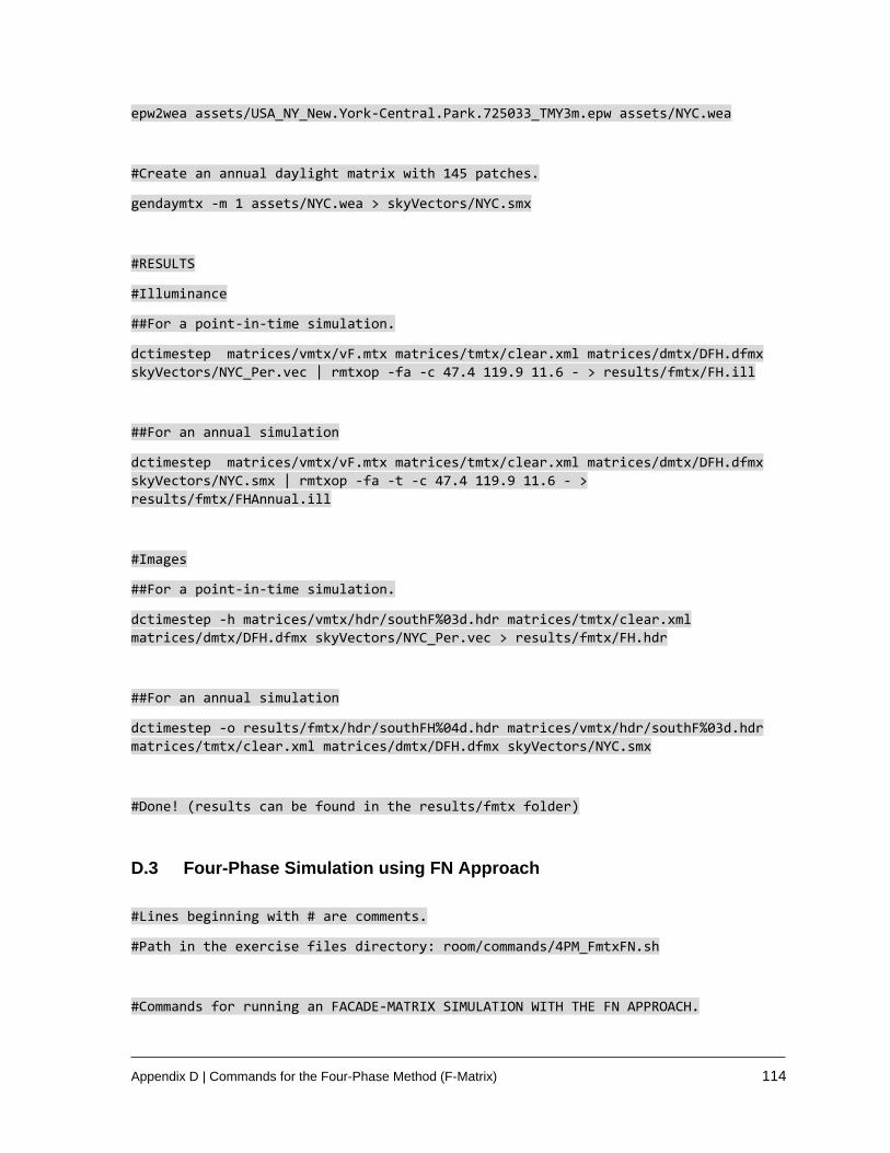
Appendix D | Commands for the Four-Phase Method (F-Matrix) 114
epw2wea assets/USA_NY_New.York-Central.Park.725033_TMY3m.epw assets/NYC.wea
#Create an annual daylight matrix with 145 patches.
gendaymtx -m 1 assets/NYC.wea > skyVectors/NYC.smx
#RESULTS
#Illuminance
##For a point-in-time simulation.
dctimestep matrices/vmtx/vF.mtx matrices/tmtx/clear.xml matrices/dmtx/DFH.dfmx
skyVectors/NYC_Per.vec | rmtxop -fa -c 47.4 119.9 11.6 - > results/fmtx/FH.ill
##For an annual simulation
dctimestep matrices/vmtx/vF.mtx matrices/tmtx/clear.xml matrices/dmtx/DFH.dfmx
skyVectors/NYC.smx | rmtxop -fa -t -c 47.4 119.9 11.6 - >
results/fmtx/FHAnnual.ill
#Images
##For a point-in-time simulation.
dctimestep -h matrices/vmtx/hdr/southF%03d.hdr matrices/tmtx/clear.xml
matrices/dmtx/DFH.dfmx skyVectors/NYC_Per.vec > results/fmtx/FH.hdr
##For an annual simulation
dctimestep -o results/fmtx/hdr/southFH%04d.hdr matrices/vmtx/hdr/southF%03d.hdr
matrices/tmtx/clear.xml matrices/dmtx/DFH.dfmx skyVectors/NYC.smx
#Done! (results can be found in the results/fmtx folder)
D.3 Four-Phase Simulation using FN Approach
#Lines beginning with # are comments.
#Path in the exercise files directory: room/commands/4PM_FmtxFN.sh
#Commands for running an FACADE-MATRIX SIMULATION WITH THE FN APPROACH.
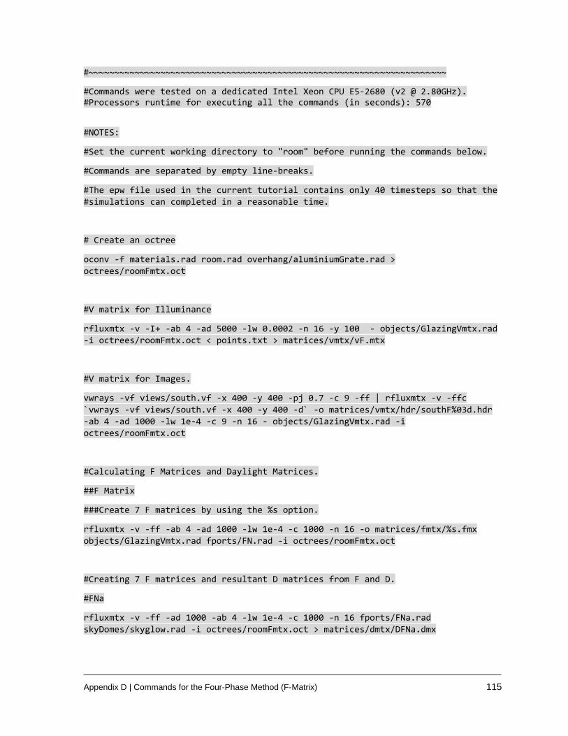
Appendix D | Commands for the Four-Phase Method (F-Matrix) 115
#~~~~~~~~~~~~~~~~~~~~~~~~~~~~~~~~~~~~~~~~~~~~~~~~~~~~~~~~~~~~~~~~~~~~~~
#Commands were tested on a dedicated Intel Xeon CPU E5-2680 (v2 @ 2.80GHz). #Processors runtime for executing all the commands (in seconds): 570
#NOTES:
#Set the current working directory to "room" before running the commands below.
#Commands are separated by empty line-breaks.
#The epw file used in the current tutorial contains only 40 timesteps so that the
#simulations can completed in a reasonable time.
# Create an octree
oconv -f materials.rad room.rad overhang/aluminiumGrate.rad >
octrees/roomFmtx.oct
#V matrix for Illuminance
rfluxmtx -v -I+ -ab 4 -ad 5000 -lw 0.0002 -n 16 -y 100 - objects/GlazingVmtx.rad
-i octrees/roomFmtx.oct < points.txt > matrices/vmtx/vF.mtx
#V matrix for Images.
vwrays -vf views/south.vf -x 400 -y 400 -pj 0.7 -c 9 -ff | rfluxmtx -v -ffc
`vwrays -vf views/south.vf -x 400 -y 400 -d` -o matrices/vmtx/hdr/southF%03d.hdr
-ab 4 -ad 1000 -lw 1e-4 -c 9 -n 16 - objects/GlazingVmtx.rad -i
octrees/roomFmtx.oct
#Calculating F Matrices and Daylight Matrices.
##F Matrix
###Create 7 F matrices by using the %s option.
rfluxmtx -v -ff -ab 4 -ad 1000 -lw 1e-4 -c 1000 -n 16 -o matrices/fmtx/%s.fmx
objects/GlazingVmtx.rad fports/FN.rad -i octrees/roomFmtx.oct
#Creating 7 F matrices and resultant D matrices from F and D.
#FNa
rfluxmtx -v -ff -ad 1000 -ab 4 -lw 1e-4 -c 1000 -n 16 fports/FNa.rad
skyDomes/skyglow.rad -i octrees/roomFmtx.oct > matrices/dmtx/DFNa.dmx
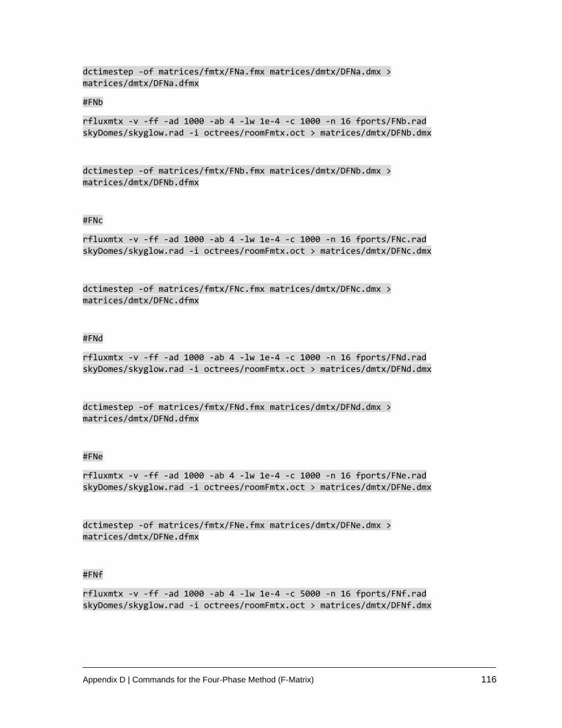
Appendix D | Commands for the Four-Phase Method (F-Matrix) 116
dctimestep -of matrices/fmtx/FNa.fmx matrices/dmtx/DFNa.dmx >
matrices/dmtx/DFNa.dfmx
#FNb
rfluxmtx -v -ff -ad 1000 -ab 4 -lw 1e-4 -c 1000 -n 16 fports/FNb.rad
skyDomes/skyglow.rad -i octrees/roomFmtx.oct > matrices/dmtx/DFNb.dmx
dctimestep -of matrices/fmtx/FNb.fmx matrices/dmtx/DFNb.dmx >
matrices/dmtx/DFNb.dfmx
#FNc
rfluxmtx -v -ff -ad 1000 -ab 4 -lw 1e-4 -c 1000 -n 16 fports/FNc.rad
skyDomes/skyglow.rad -i octrees/roomFmtx.oct > matrices/dmtx/DFNc.dmx
dctimestep -of matrices/fmtx/FNc.fmx matrices/dmtx/DFNc.dmx >
matrices/dmtx/DFNc.dfmx
#FNd
rfluxmtx -v -ff -ad 1000 -ab 4 -lw 1e-4 -c 1000 -n 16 fports/FNd.rad
skyDomes/skyglow.rad -i octrees/roomFmtx.oct > matrices/dmtx/DFNd.dmx
dctimestep -of matrices/fmtx/FNd.fmx matrices/dmtx/DFNd.dmx >
matrices/dmtx/DFNd.dfmx
#FNe
rfluxmtx -v -ff -ad 1000 -ab 4 -lw 1e-4 -c 1000 -n 16 fports/FNe.rad
skyDomes/skyglow.rad -i octrees/roomFmtx.oct > matrices/dmtx/DFNe.dmx
dctimestep -of matrices/fmtx/FNe.fmx matrices/dmtx/DFNe.dmx >
matrices/dmtx/DFNe.dfmx
#FNf
rfluxmtx -v -ff -ad 1000 -ab 4 -lw 1e-4 -c 5000 -n 16 fports/FNf.rad
skyDomes/skyglow.rad -i octrees/roomFmtx.oct > matrices/dmtx/DFNf.dmx
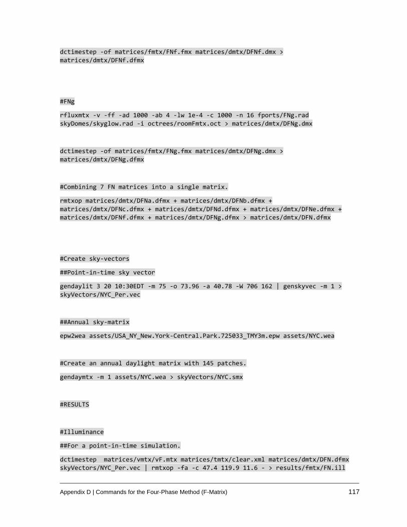
Appendix D | Commands for the Four-Phase Method (F-Matrix) 117
dctimestep -of matrices/fmtx/FNf.fmx matrices/dmtx/DFNf.dmx >
matrices/dmtx/DFNf.dfmx
#FNg
rfluxmtx -v -ff -ad 1000 -ab 4 -lw 1e-4 -c 1000 -n 16 fports/FNg.rad
skyDomes/skyglow.rad -i octrees/roomFmtx.oct > matrices/dmtx/DFNg.dmx
dctimestep -of matrices/fmtx/FNg.fmx matrices/dmtx/DFNg.dmx >
matrices/dmtx/DFNg.dfmx
#Combining 7 FN matrices into a single matrix.
rmtxop matrices/dmtx/DFNa.dfmx + matrices/dmtx/DFNb.dfmx +
matrices/dmtx/DFNc.dfmx + matrices/dmtx/DFNd.dfmx + matrices/dmtx/DFNe.dfmx +
matrices/dmtx/DFNf.dfmx + matrices/dmtx/DFNg.dfmx > matrices/dmtx/DFN.dfmx
#Create sky-vectors
##Point-in-time sky vector
gendaylit 3 20 10:30EDT -m 75 -o 73.96 -a 40.78 -W 706 162 | genskyvec -m 1 >
skyVectors/NYC_Per.vec
##Annual sky-matrix
epw2wea assets/USA_NY_New.York-Central.Park.725033_TMY3m.epw assets/NYC.wea
#Create an annual daylight matrix with 145 patches.
gendaymtx -m 1 assets/NYC.wea > skyVectors/NYC.smx
#RESULTS
#Illuminance
##For a point-in-time simulation.
dctimestep matrices/vmtx/vF.mtx matrices/tmtx/clear.xml matrices/dmtx/DFN.dfmx
skyVectors/NYC_Per.vec | rmtxop -fa -c 47.4 119.9 11.6 - > results/fmtx/FN.ill

Appendix D | Commands for the Four-Phase Method (F-Matrix) 118
##For an annual simulation
dctimestep matrices/vmtx/vF.mtx matrices/tmtx/clear.xml matrices/dmtx/DFN.dfmx
skyVectors/NYC.smx | rmtxop -fa -t -c 47.4 119.9 11.6 - >
results/fmtx/FNAnnual.ill
#Images
##For a point-in-time simulation.
dctimestep -h matrices/vmtx/hdr/southF%03d.hdr matrices/tmtx/clear.xml
matrices/dmtx/DFN.dfmx skyVectors/NYC_Per.vec > results/fmtx/FN.hdr
##For an annual simulation
dctimestep -o results/fmtx/hdr/southFN%04d.hdr matrices/vmtx/hdr/southF%03d.hdr
matrices/tmtx/clear.xml matrices/dmtx/DFN.dfmx skyVectors/NYC.smx
#Done! (results can be found in the results/fmtx folder)
D.4 Parametric Four-Phase Simulation
#Lines beginning with # are comments.
#Path in the exercise files directory: room/commands/4PM_ParamF1.sh
#Commands for running PARAMETRIC SIMULATIONS USING THE FACADE-MATRIX METHOD.
#~~~~~~~~~~~~~~~~~~~~~~~~~~~~~~~~~~~~~~~~~~~~~~~~~~~~~~~~~~~~~~~~~~~~~~~~~~~
#Commands were tested on a dedicated Intel Xeon CPU E5-2680 (v2 @ 2.80GHz). #Processors runtime for executing all the commands (in seconds): 7
#The commands below demonstrate this in the context of the F1 approach. This can
# be expanded to FH and FN approaches as well.
#The commands listed in 4PM_FmtxF1.sh should be run prior to running the commands
#in this file.

Appendix D | Commands for the Four-Phase Method (F-Matrix) 119
#NOTES:
#Set the current working directory to "room" before running the commands below.
#Commands are separated by empty line-breaks.
#The epw file used in the current tutorial contains only 40 timesteps so that the
# simulations can completed in a reasonable time.
# Recreate octree with the glass overhang.
oconv -f materials.rad room.rad overhang/diffuseGlass.rad >
octrees/roomFmtxDiff.oct
#Recalculate F1 F-Matrix with the new octree.
rfluxmtx -v -ff -ab 4 -ad 1000 -lw 0.001 -c 1000 -n 16 objects/GlazingVmtx.rad
fports/F1.rad -i octrees/roomFmtxDiff.oct > matrices/fmtx/F1Diff.fmx
#Recalculate the resultant matrix. The D Marix from F1.sh can be reused as no
#changes were affected to the Daylight Matrix.
dctimestep -of matrices/fmtx/F1Diff.fmx matrices/dmtx/DF1.dmx >
matrices/dmtx/DF1Diff.dfmx
#RESULTS
#Commands for point-in-time calculations are listed below. Commands for annual
#calculations will be similar to the ones shown in F1.sh
#Images
dctimestep -h matrices/vmtx/hdr/southF%03d.hdr matrices/tmtx/clear.xml
matrices/dmtx/DF1Diff.dfmx skyVectors/NYC_Per.vec > results/fmtx/F1Diff.hdr
#Illuminance
dctimestep matrices/vmtx/vF.mtx matrices/tmtx/clear.xml
matrices/dmtx/DF1Diff.dfmx skyVectors/NYC_Per.vec | rmtxop -fa -c 47.4 119.9 11.6
- > results/fmtx/F1Diff.ill
#Done! (results can be found in results/fmtx folder)
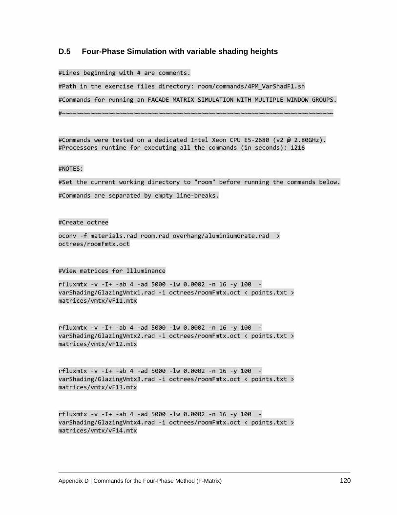
Appendix D | Commands for the Four-Phase Method (F-Matrix) 120
D.5 Four-Phase Simulation with variable shading heights
#Lines beginning with # are comments.
#Path in the exercise files directory: room/commands/4PM_VarShadF1.sh
#Commands for running an FACADE MATRIX SIMULATION WITH MULTIPLE WINDOW GROUPS.
#~~~~~~~~~~~~~~~~~~~~~~~~~~~~~~~~~~~~~~~~~~~~~~~~~~~~~~~~~~~~~~~~~~~~~~~~~~~~
#Commands were tested on a dedicated Intel Xeon CPU E5-2680 (v2 @ 2.80GHz). #Processors runtime for executing all the commands (in seconds): 1216
#NOTES:
#Set the current working directory to "room" before running the commands below.
#Commands are separated by empty line-breaks.
#Create octree
oconv -f materials.rad room.rad overhang/aluminiumGrate.rad >
octrees/roomFmtx.oct
#View matrices for Illuminance
rfluxmtx -v -I+ -ab 4 -ad 5000 -lw 0.0002 -n 16 -y 100 -
varShading/GlazingVmtx1.rad -i octrees/roomFmtx.oct < points.txt >
matrices/vmtx/vF11.mtx
rfluxmtx -v -I+ -ab 4 -ad 5000 -lw 0.0002 -n 16 -y 100 -
varShading/GlazingVmtx2.rad -i octrees/roomFmtx.oct < points.txt >
matrices/vmtx/vF12.mtx
rfluxmtx -v -I+ -ab 4 -ad 5000 -lw 0.0002 -n 16 -y 100 -
varShading/GlazingVmtx3.rad -i octrees/roomFmtx.oct < points.txt >
matrices/vmtx/vF13.mtx
rfluxmtx -v -I+ -ab 4 -ad 5000 -lw 0.0002 -n 16 -y 100 -
varShading/GlazingVmtx4.rad -i octrees/roomFmtx.oct < points.txt >
matrices/vmtx/vF14.mtx
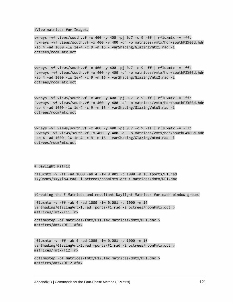
Appendix D | Commands for the Four-Phase Method (F-Matrix) 121
#View matrices for Images.
vwrays -vf views/south.vf -x 400 -y 400 -pj 0.7 -c 9 -ff | rfluxmtx -v -ffc
`vwrays -vf views/south.vf -x 400 -y 400 -d` -o matrices/vmtx/hdr/southF1%03d.hdr
-ab 4 -ad 1000 -lw 1e-4 -c 9 -n 16 - varShading/GlazingVmtx1.rad -i
octrees/roomFmtx.oct
vwrays -vf views/south.vf -x 400 -y 400 -pj 0.7 -c 9 -ff | rfluxmtx -v -ffc
`vwrays -vf views/south.vf -x 400 -y 400 -d` -o matrices/vmtx/hdr/southF2%03d.hdr
-ab 4 -ad 1000 -lw 1e-4 -c 9 -n 16 - varShading/GlazingVmtx2.rad -i
octrees/roomFmtx.oct
vwrays -vf views/south.vf -x 400 -y 400 -pj 0.7 -c 9 -ff | rfluxmtx -v -ffc
`vwrays -vf views/south.vf -x 400 -y 400 -d` -o matrices/vmtx/hdr/southF3%03d.hdr
-ab 4 -ad 1000 -lw 1e-4 -c 9 -n 16 - varShading/GlazingVmtx3.rad -i
octrees/roomFmtx.oct
vwrays -vf views/south.vf -x 400 -y 400 -pj 0.7 -c 9 -ff | rfluxmtx -v -ffc
`vwrays -vf views/south.vf -x 400 -y 400 -d` -o matrices/vmtx/hdr/southF4%03d.hdr
-ab 4 -ad 1000 -lw 1e-4 -c 9 -n 16 - varShading/GlazingVmtx4.rad -i
octrees/roomFmtx.oct
# Daylight Matrix
rfluxmtx -v -ff -ad 1000 -ab 4 -lw 0.001 -c 1000 -n 16 fports/F1.rad
skyDomes/skyglow.rad -i octrees/roomFmtx.oct > matrices/dmtx/DF1.dmx
#Creating the F Matrices and resultant Daylight Matrices for each window group.
rfluxmtx -v -ff -ab 4 -ad 1000 -lw 0.001 -c 1000 -n 16
varShading/GlazingVmtx1.rad fports/F1.rad -i octrees/roomFmtx.oct >
matrices/fmtx/F11.fmx
dctimestep -of matrices/fmtx/F11.fmx matrices/dmtx/DF1.dmx >
matrices/dmtx/DF11.dfmx
rfluxmtx -v -ff -ab 4 -ad 1000 -lw 0.001 -c 1000 -n 16
varShading/GlazingVmtx2.rad fports/F1.rad -i octrees/roomFmtx.oct >
matrices/fmtx/F12.fmx
dctimestep -of matrices/fmtx/F12.fmx matrices/dmtx/DF1.dmx >
matrices/dmtx/DF12.dfmx
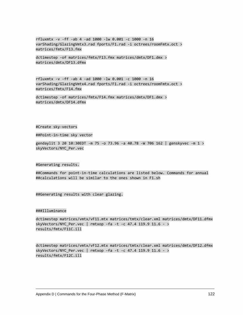
Appendix D | Commands for the Four-Phase Method (F-Matrix) 122
rfluxmtx -v -ff -ab 4 -ad 1000 -lw 0.001 -c 1000 -n 16
varShading/GlazingVmtx3.rad fports/F1.rad -i octrees/roomFmtx.oct >
matrices/fmtx/F13.fmx
dctimestep -of matrices/fmtx/F13.fmx matrices/dmtx/DF1.dmx >
matrices/dmtx/DF13.dfmx
rfluxmtx -v -ff -ab 4 -ad 1000 -lw 0.001 -c 1000 -n 16
varShading/GlazingVmtx4.rad fports/F1.rad -i octrees/roomFmtx.oct >
matrices/fmtx/F14.fmx
dctimestep -of matrices/fmtx/F14.fmx matrices/dmtx/DF1.dmx >
matrices/dmtx/DF14.dfmx
#Create sky-vectors
##Point-in-time sky vector
gendaylit 3 20 10:30EDT -m 75 -o 73.96 -a 40.78 -W 706 162 | genskyvec -m 1 >
skyVectors/NYC_Per.vec
#Generating results.
##Commands for point-in-time calculations are listed below. Commands for annual
##calculations will be similar to the ones shown in F1.sh
##Generating results with clear glazing.
###Illuminance
dctimestep matrices/vmtx/vF11.mtx matrices/tmtx/clear.xml matrices/dmtx/DF11.dfmx
skyVectors/NYC_Per.vec | rmtxop -fa -t -c 47.4 119.9 11.6 - >
results/fmtx/F11C.ill
dctimestep matrices/vmtx/vF12.mtx matrices/tmtx/clear.xml matrices/dmtx/DF12.dfmx
skyVectors/NYC_Per.vec | rmtxop -fa -t -c 47.4 119.9 11.6 - >
results/fmtx/F12C.ill
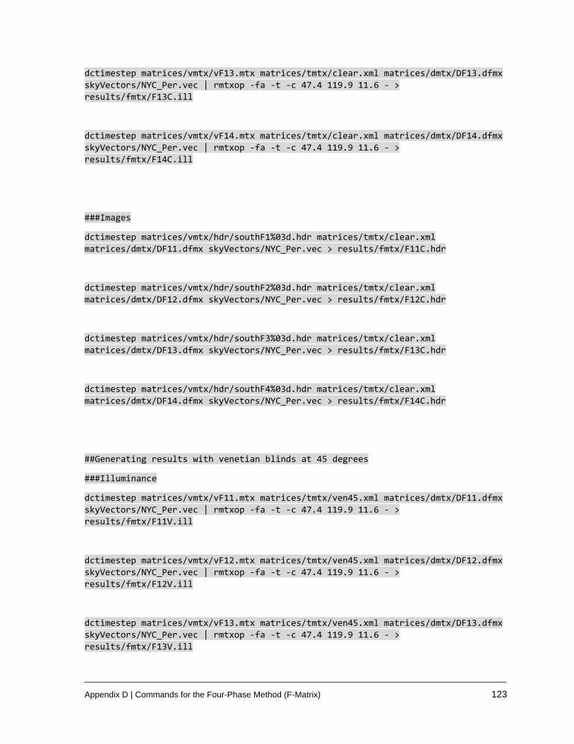
Appendix D | Commands for the Four-Phase Method (F-Matrix) 123
dctimestep matrices/vmtx/vF13.mtx matrices/tmtx/clear.xml matrices/dmtx/DF13.dfmx
skyVectors/NYC_Per.vec | rmtxop -fa -t -c 47.4 119.9 11.6 - >
results/fmtx/F13C.ill
dctimestep matrices/vmtx/vF14.mtx matrices/tmtx/clear.xml matrices/dmtx/DF14.dfmx
skyVectors/NYC_Per.vec | rmtxop -fa -t -c 47.4 119.9 11.6 - >
results/fmtx/F14C.ill
###Images
dctimestep matrices/vmtx/hdr/southF1%03d.hdr matrices/tmtx/clear.xml
matrices/dmtx/DF11.dfmx skyVectors/NYC_Per.vec > results/fmtx/F11C.hdr
dctimestep matrices/vmtx/hdr/southF2%03d.hdr matrices/tmtx/clear.xml
matrices/dmtx/DF12.dfmx skyVectors/NYC_Per.vec > results/fmtx/F12C.hdr
dctimestep matrices/vmtx/hdr/southF3%03d.hdr matrices/tmtx/clear.xml
matrices/dmtx/DF13.dfmx skyVectors/NYC_Per.vec > results/fmtx/F13C.hdr
dctimestep matrices/vmtx/hdr/southF4%03d.hdr matrices/tmtx/clear.xml
matrices/dmtx/DF14.dfmx skyVectors/NYC_Per.vec > results/fmtx/F14C.hdr
##Generating results with venetian blinds at 45 degrees
###Illuminance
dctimestep matrices/vmtx/vF11.mtx matrices/tmtx/ven45.xml matrices/dmtx/DF11.dfmx
skyVectors/NYC_Per.vec | rmtxop -fa -t -c 47.4 119.9 11.6 - >
results/fmtx/F11V.ill
dctimestep matrices/vmtx/vF12.mtx matrices/tmtx/ven45.xml matrices/dmtx/DF12.dfmx
skyVectors/NYC_Per.vec | rmtxop -fa -t -c 47.4 119.9 11.6 - >
results/fmtx/F12V.ill
dctimestep matrices/vmtx/vF13.mtx matrices/tmtx/ven45.xml matrices/dmtx/DF13.dfmx
skyVectors/NYC_Per.vec | rmtxop -fa -t -c 47.4 119.9 11.6 - >
results/fmtx/F13V.ill
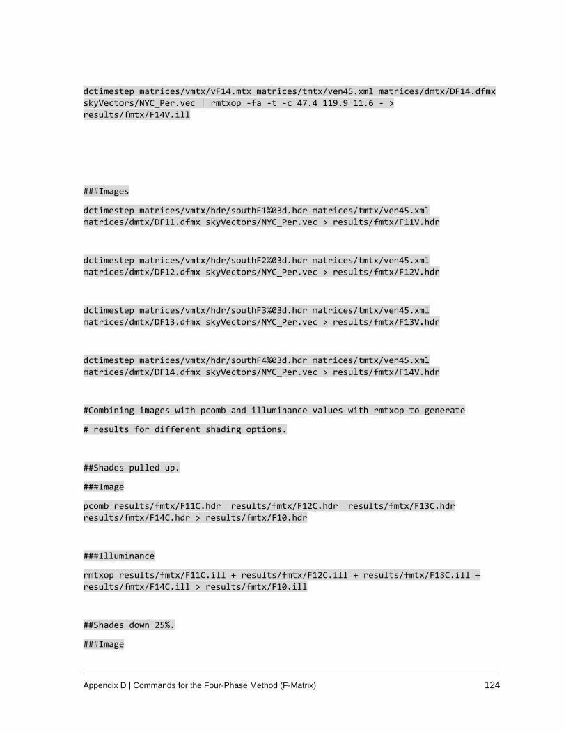
Appendix D | Commands for the Four-Phase Method (F-Matrix) 124
dctimestep matrices/vmtx/vF14.mtx matrices/tmtx/ven45.xml matrices/dmtx/DF14.dfmx
skyVectors/NYC_Per.vec | rmtxop -fa -t -c 47.4 119.9 11.6 - >
results/fmtx/F14V.ill
###Images
dctimestep matrices/vmtx/hdr/southF1%03d.hdr matrices/tmtx/ven45.xml
matrices/dmtx/DF11.dfmx skyVectors/NYC_Per.vec > results/fmtx/F11V.hdr
dctimestep matrices/vmtx/hdr/southF2%03d.hdr matrices/tmtx/ven45.xml
matrices/dmtx/DF12.dfmx skyVectors/NYC_Per.vec > results/fmtx/F12V.hdr
dctimestep matrices/vmtx/hdr/southF3%03d.hdr matrices/tmtx/ven45.xml
matrices/dmtx/DF13.dfmx skyVectors/NYC_Per.vec > results/fmtx/F13V.hdr
dctimestep matrices/vmtx/hdr/southF4%03d.hdr matrices/tmtx/ven45.xml
matrices/dmtx/DF14.dfmx skyVectors/NYC_Per.vec > results/fmtx/F14V.hdr
#Combining images with pcomb and illuminance values with rmtxop to generate
# results for different shading options.
##Shades pulled up.
###Image
pcomb results/fmtx/F11C.hdr results/fmtx/F12C.hdr results/fmtx/F13C.hdr
results/fmtx/F14C.hdr > results/fmtx/F10.hdr
###Illuminance
rmtxop results/fmtx/F11C.ill + results/fmtx/F12C.ill + results/fmtx/F13C.ill +
results/fmtx/F14C.ill > results/fmtx/F10.ill
##Shades down 25%.
###Image
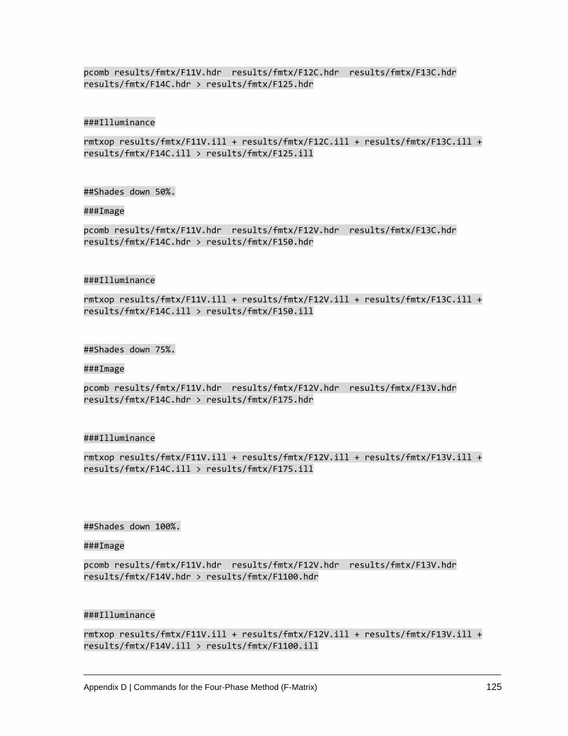
Appendix D | Commands for the Four-Phase Method (F-Matrix) 125
pcomb results/fmtx/F11V.hdr results/fmtx/F12C.hdr results/fmtx/F13C.hdr
results/fmtx/F14C.hdr > results/fmtx/F125.hdr
###Illuminance
rmtxop results/fmtx/F11V.ill + results/fmtx/F12C.ill + results/fmtx/F13C.ill +
results/fmtx/F14C.ill > results/fmtx/F125.ill
##Shades down 50%.
###Image
pcomb results/fmtx/F11V.hdr results/fmtx/F12V.hdr results/fmtx/F13C.hdr
results/fmtx/F14C.hdr > results/fmtx/F150.hdr
###Illuminance
rmtxop results/fmtx/F11V.ill + results/fmtx/F12V.ill + results/fmtx/F13C.ill +
results/fmtx/F14C.ill > results/fmtx/F150.ill
##Shades down 75%.
###Image
pcomb results/fmtx/F11V.hdr results/fmtx/F12V.hdr results/fmtx/F13V.hdr
results/fmtx/F14C.hdr > results/fmtx/F175.hdr
###Illuminance
rmtxop results/fmtx/F11V.ill + results/fmtx/F12V.ill + results/fmtx/F13V.ill +
results/fmtx/F14C.ill > results/fmtx/F175.ill
##Shades down 100%.
###Image
pcomb results/fmtx/F11V.hdr results/fmtx/F12V.hdr results/fmtx/F13V.hdr
results/fmtx/F14V.hdr > results/fmtx/F1100.hdr
###Illuminance
rmtxop results/fmtx/F11V.ill + results/fmtx/F12V.ill + results/fmtx/F13V.ill +
results/fmtx/F14V.ill > results/fmtx/F1100.ill

Appendix D | Commands for the Four-Phase Method (F-Matrix) 126
#Done! (results can be found in results/fmtx folder)

Appendix E | Commands for the Five-Phase and Six-Phase Methods 127
Appendix E. Commands for the Five-Phase and Six-Phase
Methods
E.1 Commands for the Five-Phase Method
#Lines beginning with # are comments. #Path in the exercise files directory: room/commands/5PM.sh
#Commands for running a FIVE-PHASE SIMULATION. #~~~~~~~~~~~~~~~~~~~~~~~~~~~~~~~~~~~~~~~~~~~~~ #Commands were tested on a dedicated Intel Xeon CPU E5-2680 (v2 @ 2.80GHz). #Processors runtime for executing all the commands (in seconds): 12501 #Ulimit needs to be set to a high enough value so that multiple files can be #opened simulataneously. #For the present simulation, maximum number of open files will be 5165. #This command is applicable to Unix-like systems only. On Windows the number of #simultaneous files is limited to 512. ulimit -n 9999 #Set the current working directory to "room" before running the commands below. #Commands are separated by empty line-breaks. #PART1: THREE-PHASE METHOD SIMULATION. ##Create octree oconv -f materials.rad room.rad > octrees/room3ph.oct ##View matrix for Illuminance (The value for -y 100 is derived from the 100 grid ###points inside the file points.txt). rfluxmtx -v -I+ -ab 4 -ad 5000 -lw 0.0002 -n 16 -y 100 - objects/GlazingVmtx.rad -i octrees/room3ph.oct < points.txt > matrices/vmtx/v.mtx ##View matrix for Images. vwrays -vf views/south.vf -x 400 -y 400 -pj 0.7 -c 9 -ff | rfluxmtx -v -ffc `vwrays -vf views/south.vf -x 400 -y 400 -d` -o matrices/vmtx/hdr/south%03d.hdr -ab 4 -ad 1000 -lw 1e-4 -c 9 -n 16 - objects/GlazingVmtx.rad -i octrees/room3ph.oct vwrays -vf views/eastBlinds.vf -x 400 -y 400 -pj 0.7 -c 9 -ff | rfluxmtx -v -ffc `vwrays -vf views/eastBlinds.vf -x 400 -y 400 -d` -o matrices/vmtx/hdr/eastBlinds%03d.hdr -ab 4 -ad 1000 -lw 1e-4 -c 9 -n 16 - objects/GlazingVmtx.rad -i octrees/room3ph.oct ##D matrix rfluxmtx -v -ff -ab 4 -ad 1000 -lw 0.001 -c 1000 -n 16 objects/GlazingVmtx.rad skyDomes/skyglow.rad -i octrees/room3ph.oct > matrices/dmtx/daylight.dmx
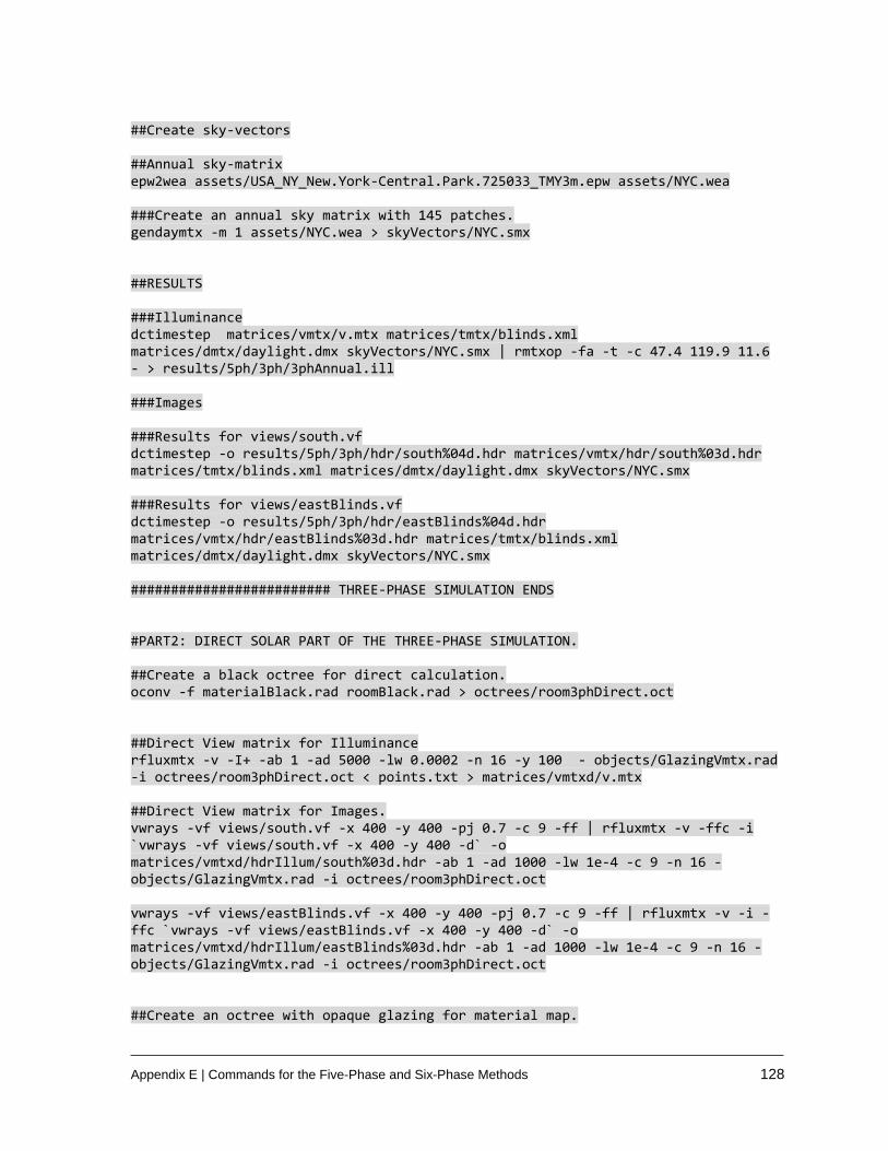
Appendix E | Commands for the Five-Phase and Six-Phase Methods 128
##Create sky-vectors ##Annual sky-matrix epw2wea assets/USA_NY_New.York-Central.Park.725033_TMY3m.epw assets/NYC.wea ###Create an annual sky matrix with 145 patches. gendaymtx -m 1 assets/NYC.wea > skyVectors/NYC.smx ##RESULTS ###Illuminance dctimestep matrices/vmtx/v.mtx matrices/tmtx/blinds.xml matrices/dmtx/daylight.dmx skyVectors/NYC.smx | rmtxop -fa -t -c 47.4 119.9 11.6 - > results/5ph/3ph/3phAnnual.ill ###Images ###Results for views/south.vf dctimestep -o results/5ph/3ph/hdr/south%04d.hdr matrices/vmtx/hdr/south%03d.hdr matrices/tmtx/blinds.xml matrices/dmtx/daylight.dmx skyVectors/NYC.smx ###Results for views/eastBlinds.vf dctimestep -o results/5ph/3ph/hdr/eastBlinds%04d.hdr matrices/vmtx/hdr/eastBlinds%03d.hdr matrices/tmtx/blinds.xml matrices/dmtx/daylight.dmx skyVectors/NYC.smx ######################### THREE-PHASE SIMULATION ENDS #PART2: DIRECT SOLAR PART OF THE THREE-PHASE SIMULATION. ##Create a black octree for direct calculation. oconv -f materialBlack.rad roomBlack.rad > octrees/room3phDirect.oct ##Direct View matrix for Illuminance rfluxmtx -v -I+ -ab 1 -ad 5000 -lw 0.0002 -n 16 -y 100 - objects/GlazingVmtx.rad -i octrees/room3phDirect.oct < points.txt > matrices/vmtxd/v.mtx ##Direct View matrix for Images. vwrays -vf views/south.vf -x 400 -y 400 -pj 0.7 -c 9 -ff | rfluxmtx -v -ffc -i `vwrays -vf views/south.vf -x 400 -y 400 -d` -o matrices/vmtxd/hdrIllum/south%03d.hdr -ab 1 -ad 1000 -lw 1e-4 -c 9 -n 16 - objects/GlazingVmtx.rad -i octrees/room3phDirect.oct vwrays -vf views/eastBlinds.vf -x 400 -y 400 -pj 0.7 -c 9 -ff | rfluxmtx -v -i -ffc `vwrays -vf views/eastBlinds.vf -x 400 -y 400 -d` -o matrices/vmtxd/hdrIllum/eastBlinds%03d.hdr -ab 1 -ad 1000 -lw 1e-4 -c 9 -n 16 - objects/GlazingVmtx.rad -i octrees/room3phDirect.oct ##Create an octree with opaque glazing for material map.

Appendix E | Commands for the Five-Phase and Six-Phase Methods 129
oconv -f materials.rad room.rad objects/GlazingVmtx.rad > octrees/materialMap3PhaseDirect.oct rpict -x 400 -y 400 -ps 1 -av 0.31831 0.31831 0.31831 -ab 0 -vf views/south.vf octrees/materialMap3PhaseDirect.oct > matrices/vmtxd/materialMapSouth.hdr rpict -x 400 -y 400 -ps 1 -av 0.31831 0.31831 0.31831 -ab 0 -vf views/eastBlinds.vf octrees/materialMap3PhaseDirect.oct > matrices/vmtxd/materialMapEastBlinds.hdr #Calculate luminance-based images from illuminance based images using material #maps. for idx in {00..145} do pcomb -h -e 'ro=ri(1)*ri(2);go=gi(1)*gi(2);bo=bi(1)*bi(2)' -o matrices/vmtxd/materialMapSouth.hdr -o matrices/vmtxd/hdrIllum/south${idx}.hdr > matrices/vmtxd/hdrLum/south${idx}.hdr pcomb -h -e 'ro=ri(1)*ri(2);go=gi(1)*gi(2);bo=bi(1)*bi(2)' -o matrices/vmtxd/materialMapEastBlinds.hdr -o matrices/vmtxd/hdrIllum/eastBlinds${idx}.hdr > matrices/vmtxd/hdrLum/eastBlinds${idx}.hdr done ##D matrix rfluxmtx -v -ff -ab 0 -ad 1000 -lw 0.001 -c 1000 -n 16 objects/GlazingVmtx.rad skyDomes/skyglow.rad -i octrees/room3phDirect.oct > matrices/dmtxd/daylight.dmx ##A direct-only sky-matrix gendaymtx -m 1 -d assets/NYC.wea > skyVectors/NYCd.smx ##RESULTS ###Illuminance dctimestep matrices/vmtxd/v.mtx matrices/tmtx/blinds.xml matrices/dmtxd/daylight.dmx skyVectors/NYCd.smx | rmtxop -fa -t -c 47.4 119.9 11.6 - > results/5ph/3phdir/3phAnnual.ill ###Images dctimestep -o results/5ph/3phdir/hdr/eastBlinds%04d.hdr matrices/vmtxd/hdrLum/eastBlinds%03d.hdr matrices/tmtx/blinds.xml matrices/dmtxd/daylight.dmx skyVectors/NYCd.smx ###Images dctimestep -o results/5ph/3phdir/hdr/south%04d.hdr matrices/vmtxd/hdrLum/south%03d.hdr matrices/tmtx/blinds.xml matrices/dmtxd/daylight.dmx skyVectors/NYCd.smx ######################### DIRECT SOLAR PART OF THE THREE-PHASE SIMULATION ENDS.
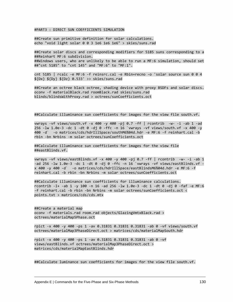
Appendix E | Commands for the Five-Phase and Six-Phase Methods 130
#PART3 : DIRECT SUN COEFFICIENTS SIMULATION ##Create sun primitive definition for solar calculations. echo "void light solar 0 0 3 1e6 1e6 1e6" > skies/suns.rad ##Create solar discs and corresponding modifiers for 5185 suns corresponding to a ##Reinhart MF:6 subdivision. ##Windows users, who are unlikely to be able to run a MF:6 simulation, should set ##"cnt 5185" to "cnt 145" and "MF:6" to "MF:1". cnt 5185 | rcalc -e MF:6 -f reinsrc.cal -e Rbin=recno -o 'solar source sun 0 0 4 ${Dx} ${Dy} ${Dz} 0.533' >> skies/suns.rad ##Create an octree black octree, shading device with proxy BSDFs and solar discs. oconv -f materialBlack.rad roomBlack.rad skies/suns.rad blinds/blindsWithProxy.rad > octrees/sunCoefficients.oct ##Calculate illuminance sun coefficients for images for the view file south.vf. vwrays -vf views/south.vf -x 400 -y 400 -pj 0.7 -ff | rcontrib -w- -i -ab 1 -ad 256 -lw 1.0e-3 -dc 1 -dt 0 -dj 0 -ffc -n 16 `vwrays -vf views/south.vf -x 400 -y 400 -d` -o matrices/cds/hdrIllSpace/southM6%04d.hdr -e MF:6 -f reinhart.cal -b rbin -bn Nrbins -m solar octrees/sunCoefficients.oct ##Calculate illuminance sun coefficients for images for the view file ##eastBlinds.vf. vwrays -vf views/eastBlinds.vf -x 400 -y 400 -pj 0.7 -ff | rcontrib -w- -i -ab 1 -ad 256 -lw 1.0e-3 -dc 1 -dt 0 -dj 0 -ffc -n 16 `vwrays -vf views/eastBlinds.vf -x 400 -y 400 -d` -o matrices/cds/hdrIllSpace/eastBlindsM6%04d.hdr -e MF:6 -f reinhart.cal -b rbin -bn Nrbins -m solar octrees/sunCoefficients.oct ##Calculate illuminance sun coefficients for illuminance calculations. rcontrib -I+ -ab 1 -y 100 -n 16 -ad 256 -lw 1.0e-3 -dc 1 -dt 0 -dj 0 -faf -e MF:6 -f reinhart.cal -b rbin -bn Nrbins -m solar octrees/sunCoefficients.oct < points.txt > matrices/cds/cds.mtx ##Create a material map oconv -f materials.rad room.rad objects/GlazingVmtxBlack.rad > octrees/materialMap5Phase.oct rpict -x 400 -y 400 -ps 1 -av 0.31831 0.31831 0.31831 -ab 0 -vf views/south.vf octrees/materialMap3PhaseDirect.oct > matrices/cds/materialMapSouth.hdr rpict -x 400 -y 400 -ps 1 -av 0.31831 0.31831 0.31831 -ab 0 -vf views/eastBlinds.vf octrees/materialMap3PhaseDirect.oct > matrices/cds/materialMapEastBlinds.hdr ##Calculate luminance sun coefficients for images for the view file south.vf.

Appendix E | Commands for the Five-Phase and Six-Phase Methods 131
vwrays -vf views/south.vf -x 400 -y 400 -pj 0.7 -ff | rcontrib -w- -ab 1 -ad 256 -lw 1.0e-3 -dc 1 -dt 0 -dj 0 -ffc -n 16 `vwrays -vf views/south.vf -x 400 -y 400 -d` -o matrices/cds/hdrLumFacade/southM6%04d.hdr -e MF:6 -f reinhart.cal -b rbin -bn Nrbins -m solar octrees/sunCoefficients.oct ##Calculate luminance sun coefficients for images for the view file #eastBlinds.vf. vwrays -vf views/eastBlinds.vf -x 400 -y 400 -pj 0.7 -ff | rcontrib -w- -ab 1 -ad 256 -lw 1.0e-3 -dc 1 -dt 0 -dj 0 -ffc -n 16 `vwrays -vf views/eastBlinds.vf -x 400 -y 400 -d` -o matrices/cds/hdrLumFacade/eastBlindsM6%04d.hdr -e MF:6 -f reinhart.cal -b rbin -bn Nrbins -m solar octrees/sunCoefficients.oct ##Calculate luminance sun coefficients for images for the view files #views/eastBlinds.vf and views/south.vf. for idx in {0000..5185} do pcomb -h -e 'ro=ri(1)*ri(2)+ri(3);go=gi(1)*gi(2)+gi(3);bo=bi(1)*bi(2)+bi(3)' -o matrices/cds/materialMapSouth.hdr -o matrices/cds/hdrIllSpace/southM6${idx}.hdr -o matrices/cds/hdrLumFacade/southM6${idx}.hdr > matrices/cds/hdr/south${idx}.hdr pcomb -h -e 'ro=ri(1)*ri(2)+ri(3);go=gi(1)*gi(2)+gi(3);bo=bi(1)*bi(2)+bi(3)' -o matrices/cds/materialMapEastBlinds.hdr -o matrices/cds/hdrIllSpace/eastBlindsM6${idx}.hdr -o matrices/cds/hdrLumFacade/eastBlindsM6${idx}.hdr > matrices/cds/hdr/eastBlinds${idx}.hdr done ##Generate a sun-matrix for the sun coefficients calculation. gendaymtx -5 0.533 -d -m 6 assets/NYC.wea > skyVectors/NYCsun.smx ###Images dctimestep -o results/5ph/cds/hdr/eastBlinds%04d.hdr matrices/cds/hdr/eastBlinds%04d.hdr skyVectors/NYCsun.smx dctimestep -o results/5ph/cds/hdr/south%04d.hdr matrices/cds/hdr/south%04d.hdr skyVectors/NYCsun.smx ###Illuminance dctimestep matrices/cds/cds.mtx skyVectors/NYCsun.smx | rmtxop -fa -t -c 47.4 119.9 11.6 - > results/5ph/cds/cds.ill ######################### DIRECT SUN COEFFICIENTS SIMULATION ENDS ##Combine Image results using the 5 Phase Equation. for idx in {0001..0040} do pcomb -h -e 'ro=ri(1)-ri(2)+ri(3);go=gi(1)-gi(2)+gi(3);bo=bi(1)-bi(2)+bi(3)' -o results/5ph/3ph/hdr/south${idx}.hdr -o results/5ph/3phdir/hdr/south${idx}.hdr -o -o results/5ph/cds/hdr/south${idx}.hdr > results/5ph/hdr/south${idx}.hdr

Appendix E | Commands for the Five-Phase and Six-Phase Methods 132
pcomb -h -e 'ro=ri(1)-ri(2)+ri(3);go=gi(1)-gi(2)+gi(3);bo=bi(1)-bi(2)+bi(3)' -o results/5ph/3ph/hdr/eastBlinds${idx}.hdr -o results/5ph/3phdir/hdr/eastBlinds${idx}.hdr -o -o results/5ph/cds/hdr/eastBlinds${idx}.hdr > results/5ph/hdr/eastBlinds${idx}.hdr done #Combine illuminance results using the 5 Phase equation. rmtxop results/5ph/3ph/3phAnnual.ill + -s -1 results/5ph/3phdir/3phAnnual.ill + results/5ph/cds/cds.ill > results/5ph/5Phannual.ill #Done! (results can be found in the results/5ph folder)
E.2 Commands for the Six-Phase Method
##Lines beginning with # are comments.
#Path in the exercise files directory: room/commands/6PM.sh
#Commands for running a SIX-PHASE SIMULATION
#~~~~~~~~~~~~~~~~~~~~~~~~~~~~~~~~~~~~~~~~~~~
# (This implies a FACADE-MATRIX SIMULATION WITH DIRECT-SUN CORRECTION.)
#Commands were tested on a dedicated Intel Xeon CPU E5-2680 (v2 @ 2.80GHz). #Processors runtime for executing all the commands (in seconds): 3391
#NOTES:
#Set the current working directory to "room" before running the commands below.
#Commands are separated by empty line-breaks.
#The epw file used in the current tutorial contains only 40 timesteps so that the
#simulations can completed in a reasonable time.
#Ulimit needs to be set to a high enough value so that multiple files can be
#opened simulataneously.
#For the present simulation, maximum number of open files will be 5165.
ulimit -n 9999
#PART1: Facade-Matrix (FH) Simulation.
## Create an octree
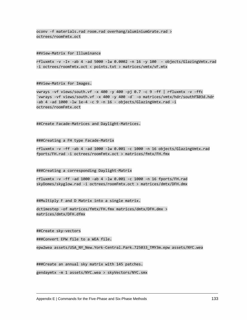
Appendix E | Commands for the Five-Phase and Six-Phase Methods 133
oconv -f materials.rad room.rad overhang/aluminiumGrate.rad >
octrees/roomFmtx.oct
##View-Matrix for Illuminance
rfluxmtx -v -I+ -ab 4 -ad 5000 -lw 0.0002 -n 16 -y 100 - objects/GlazingVmtx.rad
-i octrees/roomFmtx.oct < points.txt > matrices/vmtx/vF.mtx
##View-Matrix for Images.
vwrays -vf views/south.vf -x 400 -y 400 -pj 0.7 -c 9 -ff | rfluxmtx -v -ffc
`vwrays -vf views/south.vf -x 400 -y 400 -d` -o matrices/vmtx/hdr/southF%03d.hdr
-ab 4 -ad 1000 -lw 1e-4 -c 9 -n 16 - objects/GlazingVmtx.rad -i
octrees/roomFmtx.oct
##Create Facade-Matrices and Daylight-Matrices.
###Creating a FH type Facade-Matrix
rfluxmtx -v -ff -ab 4 -ad 1000 -lw 0.001 -c 1000 -n 16 objects/GlazingVmtx.rad
fports/FH.rad -i octrees/roomFmtx.oct > matrices/fmtx/FH.fmx
###Creating a corresponding Daylight-Matrix
rfluxmtx -v -ff -ad 1000 -ab 4 -lw 0.001 -c 1000 -n 16 fports/FH.rad
skyDomes/skyglow.rad -i octrees/roomFmtx.oct > matrices/dmtx/DFH.dmx
##Multiply F and D Matrix into a single matrix.
dctimestep -of matrices/fmtx/FH.fmx matrices/dmtx/DFH.dmx >
matrices/dmtx/DFH.dfmx
##Create sky-vectors
###Convert EPW file to a WEA file.
epw2wea assets/USA_NY_New.York-Central.Park.725033_TMY3m.epw assets/NYC.wea
###Create an annual sky matrix with 145 patches.
gendaymtx -m 1 assets/NYC.wea > skyVectors/NYC.smx

Appendix E | Commands for the Five-Phase and Six-Phase Methods 134
##RESULTS
###Illuminance
dctimestep matrices/vmtx/vF.mtx matrices/tmtx/clear.xml matrices/dmtx/DFH.dfmx
skyVectors/NYC.smx | rmtxop -fa -t -c 47.4 119.9 11.6 - >
results/6ph/fmtx/FHAnnual.ill
###Images
dctimestep -o results/6ph/fmtx/hdr/southFH%04d.hdr
matrices/vmtx/hdr/southF%03d.hdr matrices/tmtx/clear.xml matrices/dmtx/DFH.dfmx
skyVectors/NYC.smx
######################### F-MATRIX SIMULATION ENDS ########################
#PART2: DIRECT SOLAR PART OF THE F-MATRIX SIMULATION.
##Create a black octree for direct calculation.
oconv -f materialBlack.rad roomBlack.rad overhang/aluminiumGrate.rad >
octrees/roomFmtxDirect.oct
##Direct View matrix for Illuminance
rfluxmtx -v -I+ -ab 1 -ad 5000 -lw 0.0002 -n 16 -y 100 - objects/GlazingVmtx.rad
-i octrees/roomFmtxDirect.oct < points.txt > matrices/vmtxd/vFH.mtx
##Direct View matrix for Images.
vwrays -vf views/south.vf -x 400 -y 400 -pj 0.7 -c 9 -ff | rfluxmtx -v -ffc -i
`vwrays -vf views/south.vf -x 400 -y 400 -d` -o
matrices/vmtxd/hdrIllum/southFH%03d.hdr -ab 1 -ad 1000 -lw 1e-4 -c 9 -n 16 -
objects/GlazingVmtx.rad -i octrees/roomFmtxDirect.oct
##Create an octree with opaque glazing for material map.
oconv -f materials.rad room.rad objects/GlazingVmtx.rad
overhang/aluminiumGrate.rad > octrees/materialMapFHMatrixDirect.oct
##Create the material map.
rpict -x 400 -y 400 -ps 1 -av 0.31831 0.31831 0.31831 -ab 0 -vf views/south.vf
octrees/materialMapFHMatrixDirect.oct > matrices/vmtxd/materialMapSouthFH.hdr
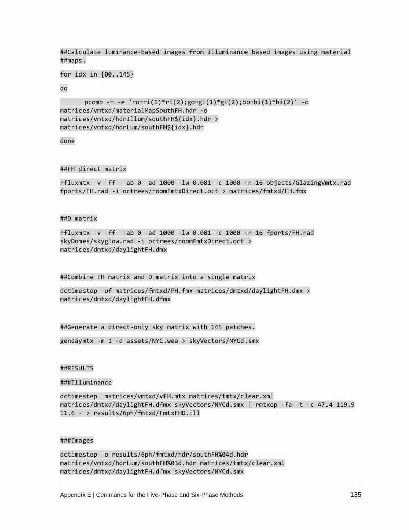
Appendix E | Commands for the Five-Phase and Six-Phase Methods 135
##Calculate luminance-based images from illuminance based images using material
##maps.
for idx in {00..145}
do
pcomb -h -e 'ro=ri(1)*ri(2);go=gi(1)*gi(2);bo=bi(1)*bi(2)' -o
matrices/vmtxd/materialMapSouthFH.hdr -o
matrices/vmtxd/hdrIllum/southFH${idx}.hdr >
matrices/vmtxd/hdrLum/southFH${idx}.hdr
done
##FH direct matrix
rfluxmtx -v -ff -ab 0 -ad 1000 -lw 0.001 -c 1000 -n 16 objects/GlazingVmtx.rad
fports/FH.rad -i octrees/roomFmtxDirect.oct > matrices/fmtxd/FH.fmx
##D matrix
rfluxmtx -v -ff -ab 0 -ad 1000 -lw 0.001 -c 1000 -n 16 fports/FH.rad
skyDomes/skyglow.rad -i octrees/roomFmtxDirect.oct >
matrices/dmtxd/daylightFH.dmx
##Combine FH matrix and D matrix into a single matrix
dctimestep -of matrices/fmtxd/FH.fmx matrices/dmtxd/daylightFH.dmx >
matrices/dmtxd/daylightFH.dfmx
##Generate a direct-only sky matrix with 145 patches.
gendaymtx -m 1 -d assets/NYC.wea > skyVectors/NYCd.smx
##RESULTS
###Illuminance
dctimestep matrices/vmtxd/vFH.mtx matrices/tmtx/clear.xml
matrices/dmtxd/daylightFH.dfmx skyVectors/NYCd.smx | rmtxop -fa -t -c 47.4 119.9
11.6 - > results/6ph/fmtxd/FmtxFHD.ill
###Images
dctimestep -o results/6ph/fmtxd/hdr/southFH%04d.hdr
matrices/vmtxd/hdrLum/southFH%03d.hdr matrices/tmtx/clear.xml
matrices/dmtxd/daylightFH.dfmx skyVectors/NYCd.smx

Appendix E | Commands for the Five-Phase and Six-Phase Methods 136
########## DIRECT SOLAR PART OF THE F-MATRIX SIMULATION ENDS###############
#PART3: DIRECT SUN COEFFICIENTS SIMULATION
##Create sun primitive definition for solar calculations.
echo "void light solar 0 0 3 1e6 1e6 1e6" > skies/suns.rad
##Create solar discs and corresponding modifiers for 5185 suns corresponding to a
##Reinhart MF:6 subdivision.
##Windows users, who are unlikely to be able to run a MF:6 simulation, should set
##"cnt 5185" to "cnt 145" and "MF:6" to "MF:1".
cnt 5185 | rcalc -e MF:6 -f reinsrc.cal -e Rbin=recno -o 'solar source sun 0 0 4
${Dx} ${Dy} ${Dz} 0.533' >> skies/suns.rad
##Create an octree black octree, shading device with proxy BSDFs and solar discs.
oconv -f materialBlack.rad roomBlack.rad skies/suns.rad materials.rad
objects/Glazing.rad overhang/aluminiumGrate.rad > octrees/sunCoefficientsFH.oct
##Calculate illuminance sun coefficients for images for the view file south.vf.
vwrays -vf views/south.vf -x 400 -y 400 -pj 0.7 -ff | rcontrib -w- -i -ab 1 -ad
256 -lw 1.0e-3 -dc 1 -dt 0 -dj 0 -ffc -n 16 `vwrays -vf views/south.vf -x 400 -y
400 -d` -o matrices/cds/hdrIllSpace/southM6FH%04d.hdr -e MF:6 -f reinhart.cal -b
rbin -bn Nrbins -m solar octrees/sunCoefficientsFH.oct
##Calculate illuminance sun coefficients for illuminance calculations.
rcontrib -I+ -ab 1 -y 100 -n 16 -ad 256 -lw 1.0e-3 -dc 1 -dt 0 -dj 0 -faf -e MF:6
-f reinhart.cal -b rbin -bn Nrbins -m solar octrees/sunCoefficientsFH.oct <
points.txt > matrices/cds/cdsFH.mtx
##Create an octree for the material map
oconv -f materials.rad room.rad objects/GlazingVmtxBlack.rad >
octrees/materialMapFHcds.oct
##Create the material map
rpict -x 400 -y 400 -ps 1 -av 0.31831 0.31831 0.31831 -ab 0 -vf views/south.vf
octrees/materialMapFHcds.oct > matrices/cds/materialMapSouthFH.hdr
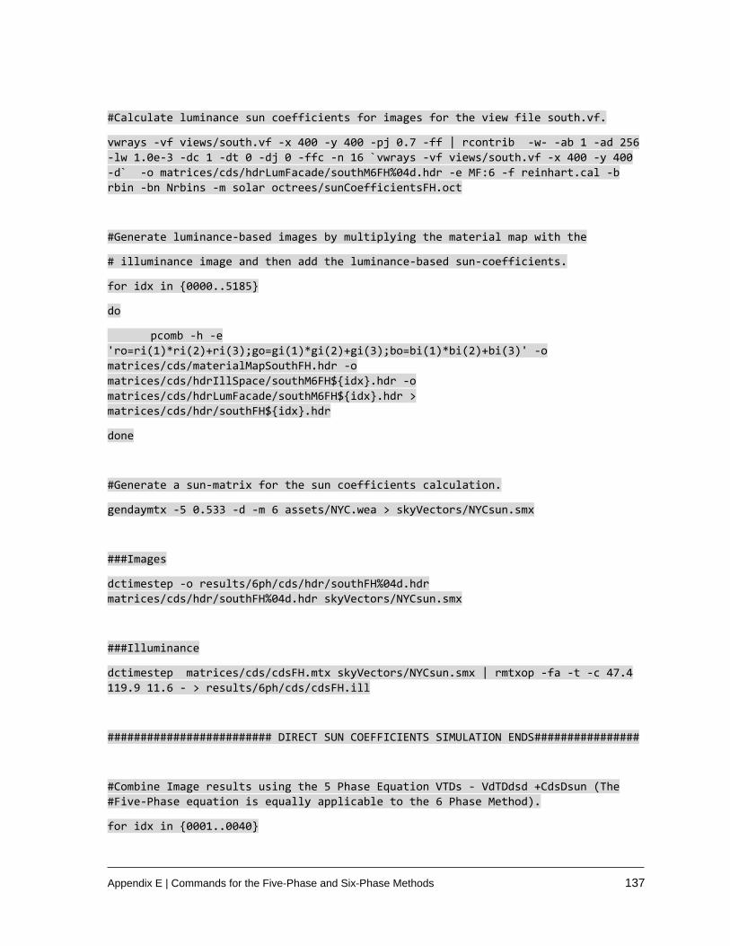
Appendix E | Commands for the Five-Phase and Six-Phase Methods 137
#Calculate luminance sun coefficients for images for the view file south.vf.
vwrays -vf views/south.vf -x 400 -y 400 -pj 0.7 -ff | rcontrib -w- -ab 1 -ad 256
-lw 1.0e-3 -dc 1 -dt 0 -dj 0 -ffc -n 16 `vwrays -vf views/south.vf -x 400 -y 400
-d` -o matrices/cds/hdrLumFacade/southM6FH%04d.hdr -e MF:6 -f reinhart.cal -b
rbin -bn Nrbins -m solar octrees/sunCoefficientsFH.oct
#Generate luminance-based images by multiplying the material map with the
# illuminance image and then add the luminance-based sun-coefficients.
for idx in {0000..5185}
do
pcomb -h -e
'ro=ri(1)*ri(2)+ri(3);go=gi(1)*gi(2)+gi(3);bo=bi(1)*bi(2)+bi(3)' -o
matrices/cds/materialMapSouthFH.hdr -o
matrices/cds/hdrIllSpace/southM6FH${idx}.hdr -o
matrices/cds/hdrLumFacade/southM6FH${idx}.hdr >
matrices/cds/hdr/southFH${idx}.hdr
done
#Generate a sun-matrix for the sun coefficients calculation.
gendaymtx -5 0.533 -d -m 6 assets/NYC.wea > skyVectors/NYCsun.smx
###Images
dctimestep -o results/6ph/cds/hdr/southFH%04d.hdr
matrices/cds/hdr/southFH%04d.hdr skyVectors/NYCsun.smx
###Illuminance
dctimestep matrices/cds/cdsFH.mtx skyVectors/NYCsun.smx | rmtxop -fa -t -c 47.4
119.9 11.6 - > results/6ph/cds/cdsFH.ill
######################### DIRECT SUN COEFFICIENTS SIMULATION ENDS################
#Combine Image results using the 5 Phase Equation VTDs - VdTDdsd +CdsDsun (The
#Five-Phase equation is equally applicable to the 6 Phase Method).
for idx in {0001..0040}

Appendix E | Commands for the Five-Phase and Six-Phase Methods 138
do
pcomb -h -e 'ro=ri(1)-ri(2)+ri(3);go=gi(1)-gi(2)+gi(3);bo=bi(1)-
bi(2)+bi(3)' -o results/6ph/fmtx/hdr/southFH${idx}.hdr -o
results/6ph/fmtxd/hdr/southFH${idx}.hdr -o -o
results/6ph/cds/hdr/southFH${idx}.hdr > results/6ph/hdr/south${idx}.hdr
done
#Combine illuminance results using the 5 Phase equation.
rmtxop results/6ph/fmtx/FHAnnual.ill + -s -1 results/6ph/fmtxd/FmtxFHD.ill +
results/6ph/cds/cdsFH.ill > results/6ph/6Phannual.ill
#Done (results can be found in the results/6ph folder)!
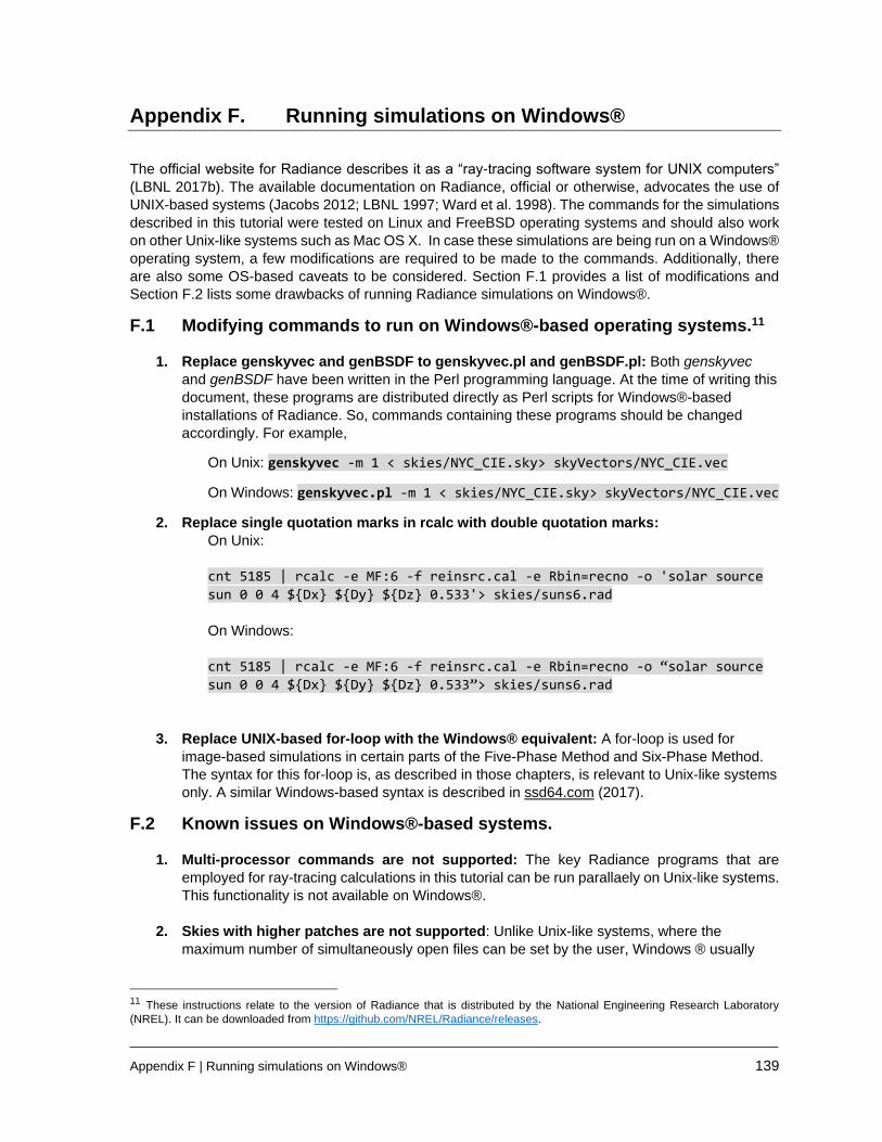
Appendix F | Running simulations on Windows® 139
Appendix F. Running simulations on Windows®
The official website for Radiance describes it as a “ray-tracing software system for UNIX computers”
(LBNL 2017b). The available documentation on Radiance, official or otherwise, advocates the use of
UNIX-based systems (Jacobs 2012; LBNL 1997; Ward et al. 1998). The commands for the simulations
described in this tutorial were tested on Linux and FreeBSD operating systems and should also work
on other Unix-like systems such as Mac OS X. In case these simulations are being run on a Windows®
operating system, a few modifications are required to be made to the commands. Additionally, there
are also some OS-based caveats to be considered. Section F.1 provides a list of modifications and
Section F.2 lists some drawbacks of running Radiance simulations on Windows®.
F.1 Modifying commands to run on Windows®-based operating systems.11
1. Replace genskyvec and genBSDF to genskyvec.pl and genBSDF.pl: Both genskyvec
and genBSDF have been written in the Perl programming language. At the time of writing this
document, these programs are distributed directly as Perl scripts for Windows®-based
installations of Radiance. So, commands containing these programs should be changed
accordingly. For example,
On Unix: genskyvec -m 1 < skies/NYC_CIE.sky> skyVectors/NYC_CIE.vec
On Windows: genskyvec.pl -m 1 < skies/NYC_CIE.sky> skyVectors/NYC_CIE.vec
2. Replace single quotation marks in rcalc with double quotation marks:
On Unix:
cnt 5185 | rcalc -e MF:6 -f reinsrc.cal -e Rbin=recno -o 'solar source
sun 0 0 4 ${Dx} ${Dy} ${Dz} 0.533'> skies/suns6.rad
On Windows:
cnt 5185 | rcalc -e MF:6 -f reinsrc.cal -e Rbin=recno -o “solar source
sun 0 0 4 ${Dx} ${Dy} ${Dz} 0.533”> skies/suns6.rad
3. Replace UNIX-based for-loop with the Windows® equivalent: A for-loop is used for
image-based simulations in certain parts of the Five-Phase Method and Six-Phase Method.
The syntax for this for-loop is, as described in those chapters, is relevant to Unix-like systems
only. A similar Windows-based syntax is described in ssd64.com (2017).
F.2 Known issues on Windows®-based systems.
1. Multi-processor commands are not supported: The key Radiance programs that are
employed for ray-tracing calculations in this tutorial can be run parallaely on Unix-like systems.
This functionality is not available on Windows®.
2. Skies with higher patches are not supported: Unlike Unix-like systems, where the
maximum number of simultaneously open files can be set by the user, Windows ® usually
11 These instructions relate to the version of Radiance that is distributed by the National Engineering Research Laboratory
(NREL). It can be downloaded from https://github.com/NREL/Radiance/releases.

Appendix F | Running simulations on Windows® 140
limits the number of simultaneously open files. It is unlikely that skies with more than 512
patches can be created on Windows® machines.

Bibliography 141
Bibliography Bleicher T. 2008 su2rad - Radiance exporter for SketchUp. 7th International Radiance Workshop; 2008
of Conference; Fribourg, Germany. Available from: https://www.radiance-online.org/community/workshops/2008-fribourg/Content/Bleicher/su2rad.pdf
Bleicher T. Github code repository for Su2rad [Internet]. Acessed: 10/15/2016. Available from: https://tbleicher.github.io/su2rad/
Bourgeois D, Reinhart CF, Ward G. 2008. Standard daylight coefficient model for dynamic daylighting simulations. Building Research & Information 36(1):68-82. Available from: http://dx.doi.org/10.1080/09613210701446325
CIE. 2003. Spatial distribution of daylight-CIE standard general sky. CIE. CIE. 2014. CIE Standard General Sky Guide (CIE 215:2014). ISBN 978-3-902842-54-1 Daysim. Daysim: Advanced daylight simulation software [Internet]. Acessed: 10/15/2016. Available
from: http://daysim.ning.com/ Geisler-Moroder D, Lee ES, Ward G. Year Validation of the Five-Phase Method for Simulating Complex
Fenestration Systems with Radiance against Field Measurements. 15th International Conference of the International Building Performance Simulation Association; 2017; San Francisco, CA, USA.
Grynberg A. 1989. Validation of Radiance. Lawrence Berkeley National Laboratory. Available from: https://eetd.lbl.gov/sites/all/files/publications/lbid-1575.pdf
Jacobs A. Radiance Tutorial. Available from: http://www.jaloxa.eu/resources/radiance/documentation/docs/radiance_tutorial.pdf
Jacobs A. Radiance Cookbook [Internet]. 2014. Available from: http://www.jaloxa.eu/resources/radiance/documentation/docs/radiance_cookbook.pdf
Jakubiec JA, Reinhart CF. 2011. DIVA 2.0: Integrating daylight and thermal simulations using Rhinoceros 3D, Daysim and EnergyPlus. Proceedings of Building Simulation 2011. Available from: http://ibpsa.org/proceedings/BS2011/P_1701.pdf
Jonsson JC, Rubin MD, Nilsson AM, Jonsson A, Roos A. 2009. Optical characterization of fritted glass for architectural applications. Optical Materials 31(6):949-958. Available from: www.sciencedirect.com/science/article/pii/S0925346708002693
LBNL. The RADIANCE Lighting Simulation and Rendering System [Internet]. Acessed: 02/11/2017. Available from: http://radsite.lbl.gov/radiance/framew.html
LBNL. BSDF Viewer [Internet]. Acessed: 10/15/2016. Available from: http://www.radiance-online.org/download-install/bsdf-viewer
LBNL. Radiance Reference Manual [Internet]. Acessed: 10/15/2016. Available from: http://radsite.lbl.gov/radiance/refer/ray.html
LBNL. Rfluxmtx [Internet]. Acessed: 10/15/2016. Available from: https://www.radiance-online.org/learning/documentation/manual-pages/pdfs/rfluxmtx.pdf
LBNL. Rcalc [Internet]. Acessed: 10/15/2016. Available from: https://www.radiance-online.org/learning/documentation/manual-pages/pdfs/rcalc.pdf
LBNL. What is RADIANCE? [Internet]. Acessed: 02/11/2017. Available from: http://radsite.lbl.gov/radiance/framew.html
Mardaljevic J. 1995. Validation of a lighting simulation program under real sky conditions. Lighting Research and Technology 27(4):181-188. Available from: http://lrt.sagepub.com/content/27/4/181.full.pdf
Mardaljevic J. 1999. Daylight simulation: validation, sky models and daylight coefficients. De Montfort University. Available from: https://dspace.lboro.ac.uk/dspace-jspui/bitstream/2134/23356/1/Mardaljevic-PhD-2000.pdf
Mardaljevic J. 2000. Simulation of annual daylighting profiles for internal illuminance. Lighting Research and Technology 32(3):111-118. Available from: http://lrt.sagepub.com/content/32/3/111.full.pdf
Mardaljevic J. 2001. The BRE-IDMP dataset: a new benchmark for the validation of illuminance prediction techniques. Lighting Research and Technology 33(2):117-134. Available from: http://lrt.sagepub.com/content/33/2/117.full.pdf
Bibliography 142
Mardaljevic J. 2008. Sky model blends for predicting internal illuminance: a comparison founded on the BRE-IDMP dataset. Journal of Building Performance Simulation 1(3):163-173. Available from: http://www.tandfonline.com/doi/pdf/10.1080/19401490802419836
McNeil A. 2013a The 5-phase method. 12th International Radiance Workshop; 2013a of Conference; Golden, CO. Available from: https://www.radiance-online.org/community/workshops/2013-golden-co/McNeil-5phase.pdf
McNeil A. The Five-Phase Method for Simulating Complex Fenestration with Radiance. Available from: http://www.radiance-online.org/learning/tutorials/fivephasetutorialfiles/Tutorial-FivePhaseMethod_v2.pdf
McNeil A. The Three-Phase Method for Simulating Complex Fenestration with Radiance. Available from: http://www.radiance-online.org/learning/tutorials/Tutorial-ThreePhaseMethod.pdf
McNeil A. 2014 BSDFs, Matrices and Phases. 13th International Radiance Workshop; 2014 of Conference; London, UK. Available from: https://www.radiance-online.org/community/workshops/2014-london/presentations/day1/McNeil_BSDFsandPhases.pdf
McNeil A. genBSDF Tutorial [Internet]. 2015. Available from: https://www.radiance-online.org/learning/tutorials/Tutorial-genBSDF_v1.0.1.pdf
McNeil A, Jonsson CJ, Appelfeld D, Ward G, Lee ES. 2013. A validation of a ray-tracing tool used to generate bi-directional scattering distribution functions for complex fenestration systems. Solar Energy 98(C). Available from: https://www.sciencedirect.com/science/article/pii/S0038092X13003940
McNeil A, Lee ES. 2012. A validation of the Radiance three-phase simulation method for modeling annual daylight performance of optically-complex fenestration systems. Journal of Building Performance Simulation April 2012. Available from: https://eetd.lbl.gov/sites/all/files/publications/5606e.pdf
Molina G, Bustamante W, Rao J, Fazio P, Vera S. 2015. Evaluation of radiance's genBSDF capability to assess solar bidirectional properties of complex fenestration systems. Journal of Building Performance Simulation 8(4):216-225. Available from: www.tandfonline.com/doi/abs/10.1080/19401493.2014.912355
Moroder DG, Lee ES, Ward G. 2017. Validation of the Five-Phase Method for Simulating Complex Fenestration Systems with Radiance against Field Measurements. Proceedings of the 15th International IBPSA Conference, San Francisco, USA.
National Climatic Center. 1981. TD-9734:Typical Meteorological Year User's Manual. Asheville, North Carolina, USA. Available from: ftp://ftp.ncdc.noaa.gov/pub/data/metadata/documents/C00045_TD-9734-TMY-manual-1981.pdf
NREL. Radiance Release 5.1.0 [Internet]. Acessed: 09/25/2017. Available from: https://github.com/NREL/Radiance/releases/tag/5.1.0
Perez R, Ineichen P, Seals R, Michalsky J, Stewart R. 1990. Modeling daylight availability and irradiance components from direct and global irradiance. Solar energy 44(5):271-289. Available from: www.sciencedirect.com/science/article/pii/0038092X9090055H
Perez R, Seals R, Michalsky J. 1993a. All-weather model for sky luminance distribution—preliminary configuration and validation. Solar energy 50(3):235-245. Available from: www.sciencedirect.com/science/article/pii/0038092X9390017I
Perez R, Seals R, Michalsky J. 1993b. Modeling Skylight Angular Luminance Distribution from Routine Irradiance Measurements. Journal of the Illuminating Engineering Society 22(1):10-17. Available from: http://dx.doi.org/10.1080/00994480.1993.10748012
Radiance-Online.org. Radiance ximage viewer [Internet]. Available from: http://www.radiance-online.org/pipermail/hdri/2014-August/000549.html
Reinhart CF. 2001. Daylight availability and manual lighting control in office buildings: Simulation studies and analysis of measurement. Fraunhofer-IRB-Verlag. Available from: www.enob.info/fileadmin/media/Publikationen/EnOB/Dissertation_C.Reinhart.pdf
Reinhart CF. Tutorial on the use of daysim simulations for sustainable design [Internet]. 2006. Available from: http://web.stanford.edu/group/narratives/projects/charette/Tutorials/DaysimTutorial.pdf

Bibliography 143
Reinhart CF, Walkenhorst O. 2001. Validation of dynamic RADIANCE-based daylight simulations for a test office with external blinds. Energy & Buildings 33(7):683-697. Available from: www.sciencedirect.com/science/article/pii/S0378778801000585
Rogers Z. 2006. Daylighting metric development using daylight autonomy calculations in the sensor placement optimization tool. Boulder, CO: Architectural Energy Corporation. Available from: https://www.daylightinginnovations.com/system/public_assets/original/SPOT_Daylight%20Autonomy%20Report.pdf
Roudsari M, Pak M. 2014 Ladybug: A Parametric Environmental Plugin for Grasshopper to Help Designers Create an Environmentally-Conscious Design. Proceedings of BS2013: 13th Conference of International Building Performance Simulation Association; 2014 of Conference; Chambery, France. Available from: http://www.ibpsa.org/proceedings/BS2013/p_2499.pdf
Saxena M, Ward G, Perry T, Heschong L, Higa R. 2010. Dynamic Radiance–Predicting annual daylighting with variable fenestration optics using BSDFs. Proceedings of SimBuild:11-13. Available from: http://ibpsa-usa.org/index.php/ibpusa/article/view/314
ssd64.com. For - Loop through command output [Internet]. Acessed: 12/18/2016. Available from: https://ss64.com/nt/for_cmd.html
Tregenza PR. 1987. Subdivision of the sky hemisphere for luminance measurements. Lighting Research and Technology 19(1):13-14. Available from: http://lrt.sagepub.com/cgi/content/abstract/19/1/13
Tregenza PR, Waters IM. 1983. Daylight coefficients. Lighting Research and Technology 15(2):65-71. Available from: http://journals.sagepub.com/doi/pdf/10.1177/096032718301500201
Wang T, Ward G, Lee ES. 2016 Validation of F-matrix and six-phase method 15th International Radiance Workshop; 09/25/2017 2016 of Conference; Padova, Italy. Available from: https://www.radiance-online.org/community/workshops/2017-portland-or/presentations/02_GW_WhatsNew2017.pdf
Wang T, Ward G, Lee ES. Year Validating Radiance methods for parametric analysis of non-coplanar shading system — an update. 16th International Radiance Workshop; 2017; Portland, Oregon. Available from: https://www.radiance-online.org/community/workshops/2017-portland-or/presentations/05_TW_ValidatingNonCoplanar.pdf
Ward G. 1994 The RADIANCE lighting simulation and rendering system. Proceedings of the 21st annual conference on Computer graphics and interactive techniques; 1994 of Conference: ACM. p. 459-472. Available from: http://radsite.lbl.gov/radiance/papers/sg94.1/Siggraph1994a.pdf
Ward G. Radiance File Formats [Internet]. 1997. Available from: https://radsite.lbl.gov/radiance/refer/filefmts.pdf
Ward G. 2011 The Bidirectional Scattering Distribution Function as a First-class Citizen in Radiance. 10th International Radiance Workshop; 2011 of Conference; Berkeley, CA, USA. Available from: https://www.radiance-online.org/community/workshops/2011-berkeley-ca/presentations/day2/GW5_BSDFFirstClass.pdf
Ward G. 2015 Annual Simulation for Out-of-Plane Shading Systems. 14th International Radiance Workshop; 11/23/2015 2015 of Conference; Philadelphia, PA, USA. Available from: https://www.radiance-online.org/community/workshops/2015-philadelphia/presentations/day1/OutOfPlaneShading.pdf
Ward G. 2017 What’s New in Radiance for 2017. 16th International Radiance Workshop; 09/25/2017 2017 of Conference; Portland, Oregon, USA. Available from: https://www.radiance-online.org/community/workshops/2017-portland-or/presentations/02_GW_WhatsNew2017.pdf
Ward G, Kurt M, Bonneel N. A Practical Framework for Sharing and Rendering Real-World Bidirectional Scattering Distribution Functions.
Ward G, R Mistrick P, Lee ES, McNeil A, J Jonsson P. 2011. Simulating the Daylight Performance of Complex Fenestration Systems Using Bidirectional Scattering Distribution Functions within Radiance. LEUKOS 7(4):241. Available from: https://gaia.lbl.gov/btech/papers/4414.pdf
Ward G, Rubinstein FM. 1988. A new technique for computer simulation of illuminated spaces. Journal of the Illuminating Engineering Society 17(1):80-91. Available from: https://gaia.lbl.gov/btech/papers/23042.pdf

Bibliography 144
Ward G, Rubinstein FM, Grynberg A. 1987. Luminance in computer-aided lighting design. Lawrence Berkeley Lab., CA (United States). Available from: https://www.osti.gov/scitech/servlets/purl/6527531
Ward G, Shakespeare R, Ehrlich C, Mardaljevic J, Phillips E, Apian-Bennewitz P. 1998. Rendering with radiance: the art and science of lighting visualization. Morgan Kaufmann San Francisco, CA. ISBN 978-0974538105

Acknowledgements 145
Acknowledgements
The author would like to thank the following individuals for their contributions to this tutorial:
Greg Ward, Anyhere Software
David Geisler-Moroder, Bartenbach GmBH
Taoning Wang, Lawrence Berkeley National Laboratory (LBNL)
Eleanor Lee, LBNL
Richard Mistrick, Penn State University
Mostapha Sadeghipour, Ladybug Tools