ON SOME PROPAGATION CHARACTERISTICS OF TROPICAL ATMOSPHERIC AND COSMIC RADIO NOISE

ON SOME PROPAGATION CHARACTERISTICS OF TROPICAL

ATMOSPHERIC AND COSMIC RADIO NOISE

A.B.BHATTACHARYA

Department of Physics, University of Kalyani Kalyani 741235, India [email protected]

D.K.TRIPATHI

Department of Physics, Narula Institute of Technology Calcutta 700109, India

[email protected]

A.NAG

Department of Physics, Modern Institute of Engineering and Technology Rajhat, Bandel, Hooghly 712123, India

[email protected]

D.HALDER

Department of Physics, University of Kalyani Kalyani 741235, India

[email protected]

J.PANDIT

Department of Physics, J I School Polytechnic Kalyani 741235, India

[email protected]

Abstract: Sources responsible for generating noise in the magnetospheric and ionospheric cavities with reference to the relative power levels in different frequency bands are examined. Some propagation characteristics of both atmospheric and cosmic radio noise as recorded at Kalyani have been examined. The characteristics obtained are compared with other reported results.

Key words: Radio communication, Propagation characteristics, Electromagnetic noise, Thunderstorms, Cosmic noise.

A.B.Bhattacharya et al. / International Journal of Engineering Science and Technology (IJEST)

ISSN : 0975-5462 Vol. 3 No. 7 July 2011 5475

1. Introduction

The terrestrial environment is exposed to electromagnetic radiation continuously producing background electromagnetic noise. For frequency below 300 GHz i.e. within the Non Ionizing Radiation (NIR) band this background noise can have a natural origin which is generally atmospheric or cosmic. Natural noise originates from a variety of sources based on different physical phenomena and showing various propagation characteristics [1, 2]. Measurements of natural electromagnetic noise in presence of the background man-made radiations are important for interpreting the relative power levels in the different bands and their influences on upper atmospheres by various means [3-6]. In this paper some interesting propagation characteristics of both atmospheric and cosmic radio noise as recorded in our laboratory at Kalyani have been examined and compared with other reported results.

2. Natural Noise Sources

Different sources are responsible for generating natural noise inside the cavity of the magnetosphere. A primary source of noise is produced by the interaction of particles and waves originating in outer space with the magnetosphere plasma at different altitudes. A second source is formed inside the ionospheric cavity where atmospheric lightning discharges contribute significantly. It is interesting that as one proceeds towards the higher frequency, contribution of atmospheric radio noise becomes insignificant but the cosmic noise becomes the main contributor. In VLF to HF band atmospheric radio noise is larger than man-made noise; sometimes even in order of tenth of dB.

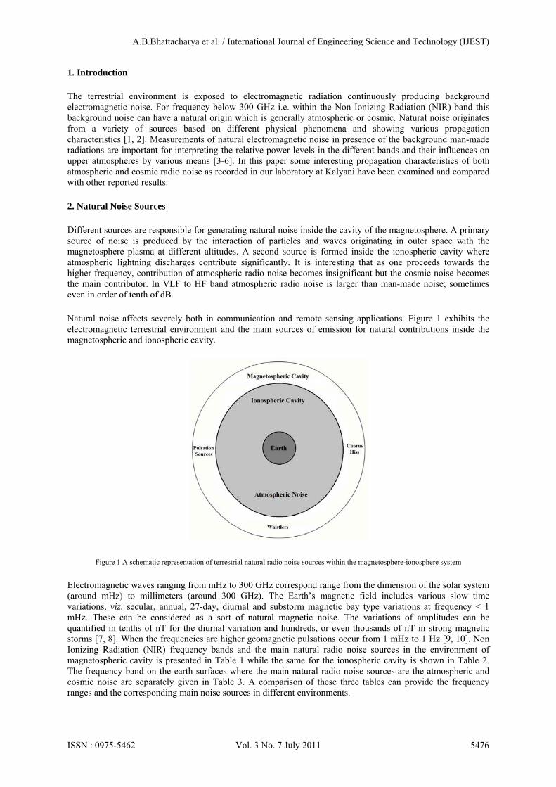
Natural noise affects severely both in communication and remote sensing applications. Figure 1 exhibits the electromagnetic terrestrial environment and the main sources of emission for natural contributions inside the magnetospheric and ionospheric cavity.

Figure 1 A schematic representation of terrestrial natural radio noise sources within the magnetosphere-ionosphere system

Electromagnetic waves ranging from mHz to 300 GHz correspond range from the dimension of the solar system (around mHz) to millimeters (around 300 GHz). The Earth’s magnetic field includes various slow time variations, viz. secular, annual, 27-day, diurnal and substorm magnetic bay type variations at frequency < 1 mHz. These can be considered as a sort of natural magnetic noise. The variations of amplitudes can be quantified in tenths of nT for the diurnal variation and hundreds, or even thousands of nT in strong magnetic storms [7, 8]. When the frequencies are higher geomagnetic pulsations occur from 1 mHz to 1 Hz [9, 10]. Non Ionizing Radiation (NIR) frequency bands and the main natural radio noise sources in the environment of magnetospheric cavity is presented in Table 1 while the same for the ionospheric cavity is shown in Table 2. The frequency band on the earth surfaces where the main natural radio noise sources are the atmospheric and cosmic noise are separately given in Table 3. A comparison of these three tables can provide the frequency ranges and the corresponding main noise sources in different environments.


ISSN : 0975-5462 Vol. 3 No. 7 July 2011 5476

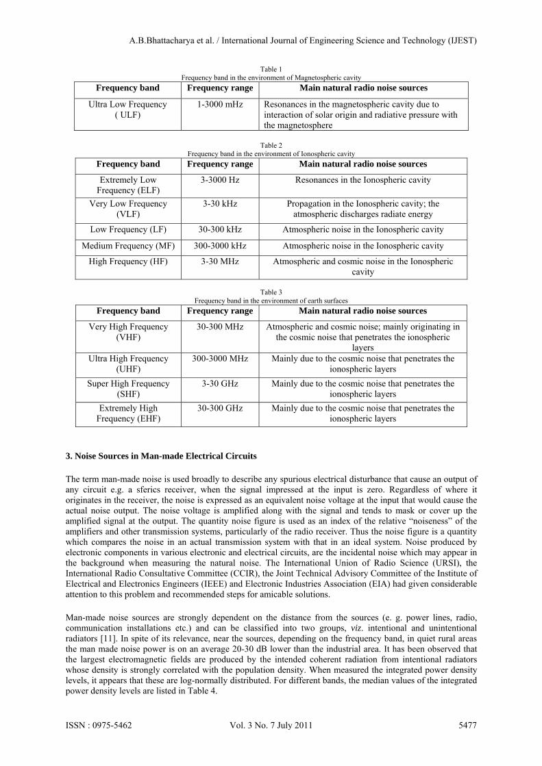
Table 1 Frequency band in the environment of Magnetospheric cavity

Frequency band Frequency range Main natural radio noise sources

Ultra Low Frequency ( ULF)

1-3000 mHz Resonances in the magnetospheric cavity due to interaction of solar origin and radiative pressure with the magnetosphere

Table 2

Frequency band in the environment of Ionospheric cavity


Extremely Low Frequency (ELF)

3-3000 Hz Resonances in the Ionospheric cavity

Very Low Frequency (VLF)

3-30 kHz Propagation in the Ionospheric cavity; the atmospheric discharges radiate energy

Low Frequency (LF) 30-300 kHz Atmospheric noise in the Ionospheric cavity

Medium Frequency (MF) 300-3000 kHz Atmospheric noise in the Ionospheric cavity

High Frequency (HF) 3-30 MHz Atmospheric and cosmic noise in the Ionospheric cavity

Table 3

Frequency band in the environment of earth surfaces


Very High Frequency (VHF)

30-300 MHz Atmospheric and cosmic noise; mainly originating in the cosmic noise that penetrates the ionospheric

layers Ultra High Frequency

(UHF) 300-3000 MHz Mainly due to the cosmic noise that penetrates the

ionospheric layers

Super High Frequency (SHF)

3-30 GHz Mainly due to the cosmic noise that penetrates the ionospheric layers

Extremely High Frequency (EHF)

30-300 GHz Mainly due to the cosmic noise that penetrates the ionospheric layers

3. Noise Sources in Man-made Electrical Circuits

The term man-made noise is used broadly to describe any spurious electrical disturbance that cause an output of any circuit e.g. a sferics receiver, when the signal impressed at the input is zero. Regardless of where it originates in the receiver, the noise is expressed as an equivalent noise voltage at the input that would cause the actual noise output. The noise voltage is amplified along with the signal and tends to mask or cover up the amplified signal at the output. The quantity noise figure is used as an index of the relative “noiseness” of the amplifiers and other transmission systems, particularly of the radio receiver. Thus the noise figure is a quantity which compares the noise in an actual transmission system with that in an ideal system. Noise produced by electronic components in various electronic and electrical circuits, are the incidental noise which may appear in the background when measuring the natural noise. The International Union of Radio Science (URSI), the International Radio Consultative Committee (CCIR), the Joint Technical Advisory Committee of the Institute of Electrical and Electronics Engineers (IEEE) and Electronic Industries Association (EIA) had given considerable attention to this problem and recommended steps for amicable solutions.

Man-made noise sources are strongly dependent on the distance from the sources (e. g. power lines, radio, communication installations etc.) and can be classified into two groups, viz. intentional and unintentional radiators [11]. In spite of its relevance, near the sources, depending on the frequency band, in quiet rural areas the man made noise power is on an average 20-30 dB lower than the industrial area. It has been observed that the largest electromagnetic fields are produced by the intended coherent radiation from intentional radiators whose density is strongly correlated with the population density. When measured the integrated power density levels, it appears that these are log-normally distributed. For different bands, the median values of the integrated power density levels are listed in Table 4.


ISSN : 0975-5462 Vol. 3 No. 7 July 2011 5477

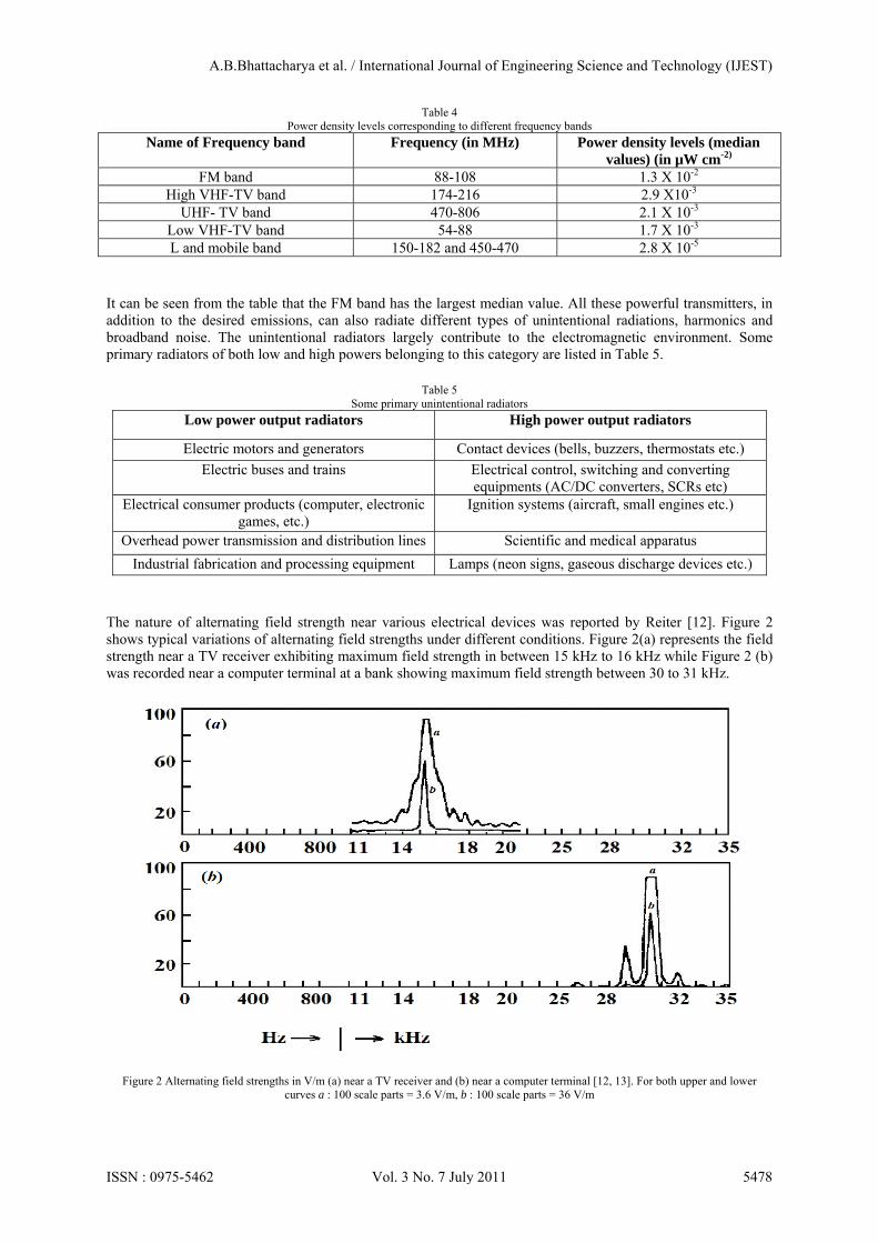
Table 4 Power density levels corresponding to different frequency bands

Name of Frequency band Frequency (in MHz) Power density levels (median values) (in µW cm-2)

FM band 88-108 1.3 X 10-2 High VHF-TV band 174-216 2.9 X10-3

UHF- TV band 470-806 2.1 X 10-3 Low VHF-TV band 54-88 1.7 X 10-3 L and mobile band 150-182 and 450-470 2.8 X 10-5

It can be seen from the table that the FM band has the largest median value. All these powerful transmitters, in addition to the desired emissions, can also radiate different types of unintentional radiations, harmonics and broadband noise. The unintentional radiators largely contribute to the electromagnetic environment. Some primary radiators of both low and high powers belonging to this category are listed in Table 5.

Table 5 Some primary unintentional radiators

Low power output radiators High power output radiators

Electric motors and generators Contact devices (bells, buzzers, thermostats etc.)

Electric buses and trains Electrical control, switching and converting equipments (AC/DC converters, SCRs etc)

Electrical consumer products (computer, electronic games, etc.)

Ignition systems (aircraft, small engines etc.)

Overhead power transmission and distribution lines Scientific and medical apparatus

Industrial fabrication and processing equipment Lamps (neon signs, gaseous discharge devices etc.)

The nature of alternating field strength near various electrical devices was reported by Reiter [12]. Figure 2 shows typical variations of alternating field strengths under different conditions. Figure 2(a) represents the field strength near a TV receiver exhibiting maximum field strength in between 15 kHz to 16 kHz while Figure 2 (b) was recorded near a computer terminal at a bank showing maximum field strength between 30 to 31 kHz.

Figure 2 Alternating field strengths in V/m (a) near a TV receiver and (b) near a computer terminal [12, 13]. For both upper and lower curves a : 100 scale parts = 3.6 V/m, b : 100 scale parts = 36 V/m


ISSN : 0975-5462 Vol. 3 No. 7 July 2011 5478

4. Measurement of Atmospheric Noise

Atmospheric noise generally appears in the form of a continuous background over which distinct noise bursts are superposed. Extensive investigations classify the atmospheric radio noise into three different categories. These are: low amplitude continuous noise, burst form of noise from near source with an occurrence of 20/min and burst form of noise invariably due to local sources of shorter duration and higher amplitudes with occurrences of ordinarily 40/min. The electromagnetic radiations from lightning discharges is propagated through long distances even up to several thousand kms and are received by sensitive receivers as sferics. The integrated field intensity of sferics is the resultant of a large number of individual impulses originating in different lightning flashes. The impulses numbering several thousand per second and arrive at the receiver directly and also through reflections from the ionospheric layers. Various instruments and techniques have been developed for the measurement of atmospheric noise [14, 15], some of which have pointed out below.

4.1 Peak Meter

The peak amplitude represents the highest pulse amplitude occurring in a noise burst. This is necessary for the design of data communication systems. The peak amplitude can be derived by feeding the output of the last intermediate frequency stage of the receiver to an output unit. The unit is to be calibrated suitably by using continuous wave signals and considering their peak amplitudes. With a view to measure the VHF sferics a receiver may be installed with a dipole antenna, a balun to match the antenna to the coaxial feeder and the receiver set. The output of the receiver can exhibit the peak field strength of VHF sferics.

4.2 Quasi Peak Meter

This can be utilized to measure the interfering effect of atmospheric noise. It consists of an aerial system, a communication receiver and an output fed from the detector to the receiver. The output has a semi-logarithmic amplifier and a detector unit with typical charging and discharging time constants 10 ms and 500 ms respectively. The time constants are selected in such a manner that the output unit has characteristics almost similar to those of average human ear. The frequency response of the output unit is flat in the range 100-5000 Hz. In order to calibrate the noise meter the signal is modulated by a 400 Hz note to a level of 100%. The receiver sensitivity can be changed in steps of 6 dB with about 20 dB amplitude range in each position. This can cover the amplitudes originating in a single frontal storm. This method provides the quasi peak value of the individual audible noise bursts and the average value of the envelope voltage in the form of a steady reading of the meter for the continuous background noise. An average of the quasi-peak values of ten highest noise bursts received per minute over a short period of 6 min represents the annoyance felt by the ear and is called the ‘noise bursts level’.

4.3 Average and R.M.S. Meters

Both the average and r.m.s values of the amplitude of a noise bursts are essential to deduce the continuous noise equivalent used in data communication system. These values are obtained by feeding the output of the last intermediate-frequency stage of the receiver to the output units. For the average value the charging and the discharging time constants are 170 and 500 ms respectively while for the r.m.s value these time constants are 80 and 500 ms respectively. Calibrations can be done properly by using the peak carrier values of continuous signal modulated 100% by a sinusoidal tone of 400 Hz.

4.4 Atmospheric Noise Burst Generator

The instrument employs zener diodes and gas tubes as sources of noise and multivibrators for the simulation of pulses in the noise bursts. This artificial noise burst is generated using an instrument that exhibits all the observed characteristics of natural noise bursts over the frequency range 0.1- 10 MHz.

4.5 Lightning Flash Counters

Lightning flash counters with different threshold values can be used at different frequencies up to MHz order. These can be successfully utilized for studying noise burst rates and characteristics of the associated thunderstorms.


ISSN : 0975-5462 Vol. 3 No. 7 July 2011 5479

4.6 Pulse Rate Counter

This counter can be constructed for counting the number of pulses in a noise burst crossing a certain amplitude threshold to record the burst duration corresponding to the pulses. The instrument can be developed for receiving noise pulses even up to a frequency of 3 MHz.

5. Sferics Record in VLF Band at Kalyani

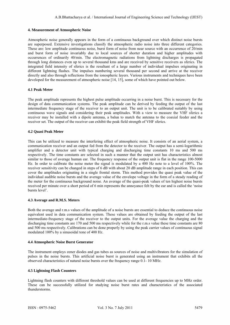
The integrated field intensity of sferics can be specified in terms of average, rms, peak value or the amplitude probability distribution of the noise envelope. Of these, the average value of the noise envelope voltage provides most extensive information. Tuned VLF receiver at a frequency of 27 kHz has been used to amplify the input atmospheric noise. We designed the receiver in a manner to have large dynamic range of field intensities particularly during severe nor’westers and also to obtain solar flare effects. The mean monthly median, upper decile and lower decile values of sferics for a period of 3-year, 2008 to 2010, as recorded over Kalyani are plotted in Figure 3. The plot provides an overall idea of the noise level at the frequency concerned. These data we have chosen for the days or part of a day when local sky was free from clouds.

In pre monsoon months (March to May) severe storms are experienced in eastern part of India, particularly in West Bengal and its surroundings. The electrical activity associated with the nor’wester has been the subject of much investigation [16] as it severely affects the radio communication over a wide area. Many eyewitness accounts of the unusual electrical activity in and around the nor’wester have been reported time to time [17]. A close examination of some of these severe storms as seen by X-band Radar in Kolkata (220 31/ N, 880 25/ E), West Bengal in conjunction with the field strength of atmospheric radio noise record at 27 kHz, over Kalyani (220 58/ N, 880 28/ E), West Bengal reveals interesting results.

Radar echoes due to thunderstorm accompanied by lightning discharges are believed to be caused by the reflection of radio energy [18]. The beam from the meteorological radar at Kolkata was directed towards thunder squalls during the period under consideration and a large number of echoes have been recorded.

Figure 3 Mean monthly median, upper decile and lower decile values of atmospherics at 27 kHz (in dB above 1μV/m; bandwidth 1 kHz)

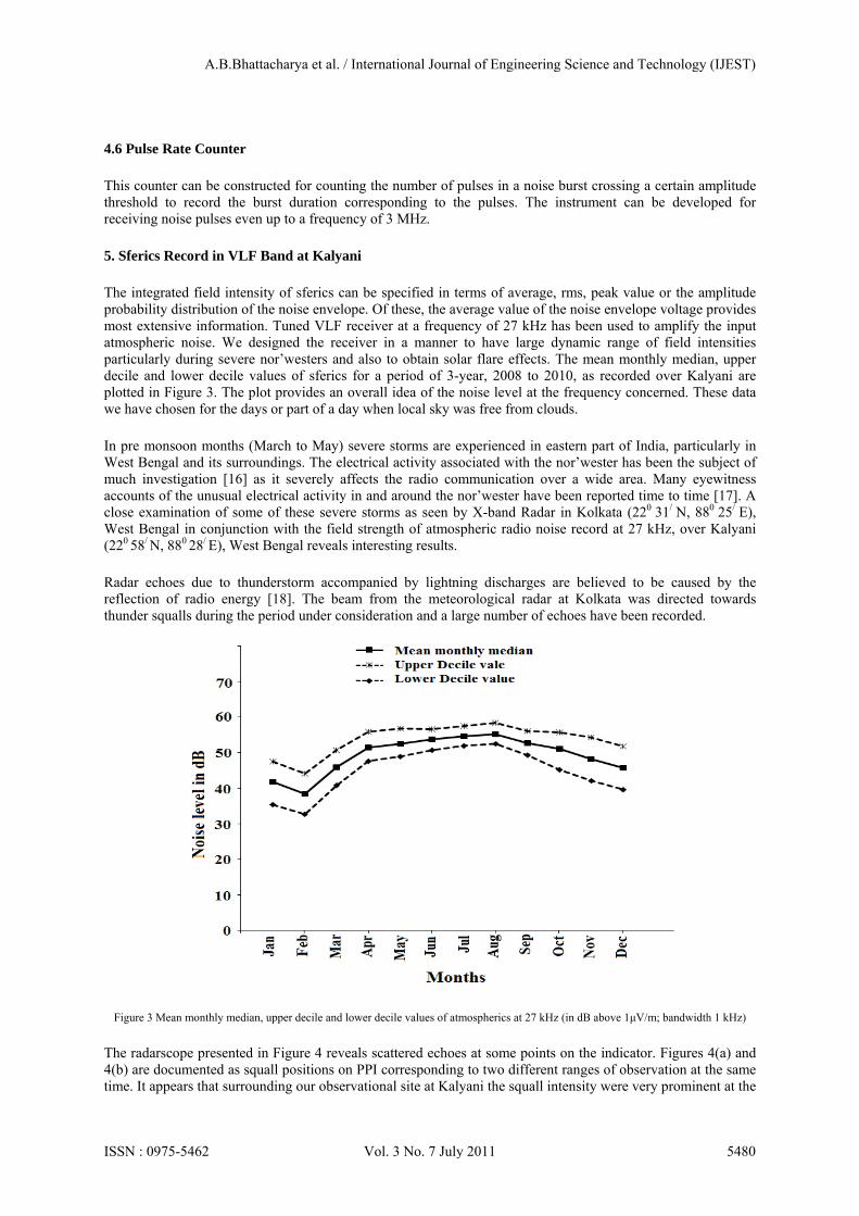
The radarscope presented in Figure 4 reveals scattered echoes at some points on the indicator. Figures 4(a) and 4(b) are documented as squall positions on PPI corresponding to two different ranges of observation at the same time. It appears that surrounding our observational site at Kalyani the squall intensity were very prominent at the


ISSN : 0975-5462 Vol. 3 No. 7 July 2011 5480

time exhibited in the figure. The intensity of the squall echoes in subsequent records gradually diminishes on the indicator.

Figure 4 Radarscopes (a) and (b) exhibit echo signals associated with the pre-monsoon thundercloud

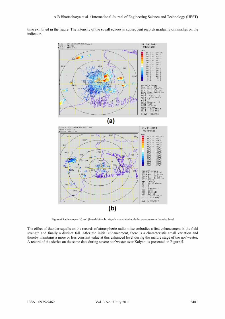
The effect of thunder squalls on the records of atmospheric radio noise embodies a first enhancement in the field strength and finally a distinct fall. After the initial enhancement, there is a characteristic small variation and thereby maintains a more or less constant value at this enhanced level during the mature stage of the nor’wester. A record of the sferics on the same date during severe nor’wester over Kalyani is presented in Figure 5.


ISSN : 0975-5462 Vol. 3 No. 7 July 2011 5481

Figure 5 Typical record of sferics during severe nor’wester at Kalyani

By a close scrutiny of the radarscopes in many occasions it has been noted that the thunder cells in most of the events, are isolated or scattered initially which shortly increase in number and size and subsequently form a full-fledged storm [16]. The local thunder cells are the continuation of those occurring earlier either in (i) Jharkhand (Hazaribagh area) or in (ii) the western part of West Bengal (Asansol and neighboring areas). From a detailed study of different nor’westers of three years as received on PPI display as an hourly routine observation and also from the analysis of noise level of sferics the following dominant characteristic are found:

Observation 1

The thunder cells initially developed in Asansol, Hazaribagh or neighboring areas when come in contact with the moist air from the Bay of Bengal under favorable synoptic conditions produce a towering cumulus. This cumulus clouds are generally of a soft fluffy nature and are responsible to produce the nor’wester finally with the right conditions of heat and moist air. By an analysis of the relevant meteorological parameters at the incidences of nor’westers, it has been noticed that the rainfall occurs when the cloud is converted to cumulonimbus. The absence of precipitation we noted in few cases seems to be due to an insufficient increase of convection currents resulting in the failure of cumulus head to produce dense cumulonimbus clouds

Observation 2

The vigorous activity of the nor’wester as well as the variation in the sferics level depend widely on the distance of origin, the degree of development and the direction of movement of the particular nor’wester towards the observing station. The location of the main storm areas associated with the nor’westers is widely distributed but still they follow a particular direction in general and thus justifying the name nor’wester. The enhancement and fall time of the atmospheric radio noise field strength for most of the cases lie in the range of 10-30 min and 20-40 min respectively with a good correlation between the duration of enhancement and fall.

6. Observation of cosmic noise

Radio waves are reflected by the upper Ionospheric layers up to a particular frequency, called critical frequency which is largely dependent on local ionosphere. The angle of incidence between the wave and the Ionospheric layers has a vital role [19]. Depending on the geometry of the path of the originated noise some propagating


ISSN : 0975-5462 Vol. 3 No. 7 July 2011 5482

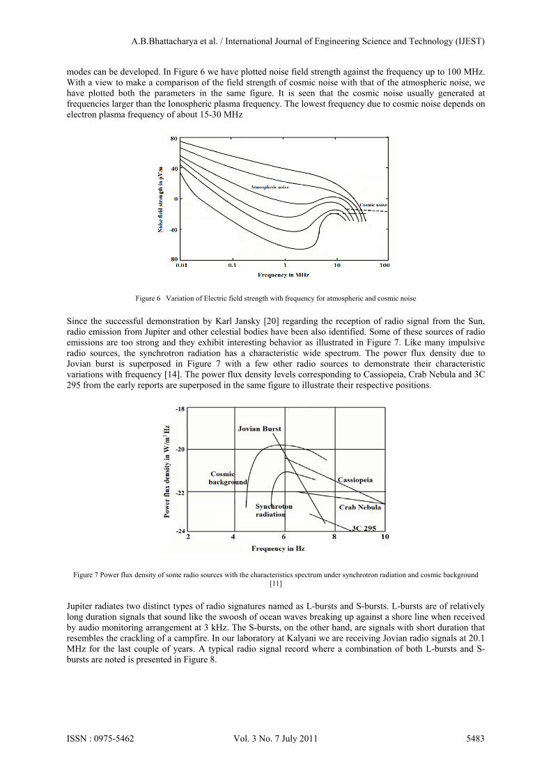
modes can be developed. In Figure 6 we have plotted noise field strength against the frequency up to 100 MHz. With a view to make a comparison of the field strength of cosmic noise with that of the atmospheric noise, we have plotted both the parameters in the same figure. It is seen that the cosmic noise usually generated at frequencies larger than the Ionospheric plasma frequency. The lowest frequency due to cosmic noise depends on electron plasma frequency of about 15-30 MHz

Figure 6 Variation of Electric field strength with frequency for atmospheric and cosmic noise

Since the successful demonstration by Karl Jansky [20] regarding the reception of radio signal from the Sun, radio emission from Jupiter and other celestial bodies have been also identified. Some of these sources of radio emissions are too strong and they exhibit interesting behavior as illustrated in Figure 7. Like many impulsive radio sources, the synchrotron radiation has a characteristic wide spectrum. The power flux density due to Jovian burst is superposed in Figure 7 with a few other radio sources to demonstrate their characteristic variations with frequency [14]. The power flux density levels corresponding to Cassiopeia, Crab Nebula and 3C 295 from the early reports are superposed in the same figure to illustrate their respective positions.

Figure 7 Power flux density of some radio sources with the characteristics spectrum under synchrotron radiation and cosmic background [11]

Jupiter radiates two distinct types of radio signatures named as L-bursts and S-bursts. L-bursts are of relatively long duration signals that sound like the swoosh of ocean waves breaking up against a shore line when received by audio monitoring arrangement at 3 kHz. The S-bursts, on the other hand, are signals with short duration that resembles the crackling of a campfire. In our laboratory at Kalyani we are receiving Jovian radio signals at 20.1 MHz for the last couple of years. A typical radio signal record where a combination of both L-bursts and S-bursts are noted is presented in Figure 8.


ISSN : 0975-5462 Vol. 3 No. 7 July 2011 5483

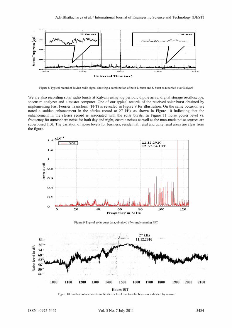
Figure 8 Typical record of Jovian radio signal showing a combination of both L-burst and S-burst as recorded over Kalyani

We are also recording solar radio bursts at Kalyani using log periodic dipole array, digital storage oscilloscope, spectrum analyzer and a master computer. One of our typical records of the received solar burst obtained by implementing Fast Fourier Transform (FFT) is revealed in Figure 9 for illustration. On the same occasion we noted a sudden enhancement in the sferics record at 27 kHz as shown in Figure 10 indicating that the enhancement in the sferics record is associated with the solar bursts. In Figure 11 noise power level vs. frequency for atmosphere noise for both day and night, cosmic noises as well as the man-made noise sources are superposed [13]. The variation of noise levels for business, residential, rural and quite rural areas are clear from the figure.

Figure 9 Typical solar burst data, obtained after implementing FFT

Figure 10 Sudden enhancements in the sferics level due to solar bursts as indicated by arrows


ISSN : 0975-5462 Vol. 3 No. 7 July 2011 5484

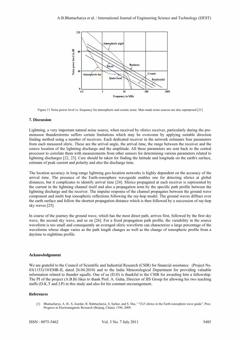
Figure 11 Noise power level vs. frequency for atmospheric and cosmic noise. Man-made noise sources are also superposed [21]

7. Discussion

Lightning, a very important natural noise source, when received by sferics receiver, particularly during the pre-monsoon thunderstorms suffers certain limitations which may be overcome by applying suitable direction finding method using a number of receivers. Each dedicated receiver in the network estimates four parameters from each measured sferic. These are the arrival angle, the arrival time, the range between the receiver and the source location of the lightning discharge and the amplitude. All these parameters are sent back to the central processor to correlate them with measurements from other sensors for determining various parameters related to lightning discharges [22, 23]. Care should be taken for finding the latitude and longitude on the earth's surface, estimate of peak current and polarity and also the discharge time.

The location accuracy in long-range lightning geo-location networks is highly dependent on the accuracy of the arrival time. The presence of the Earth-ionosphere waveguide enables one for detecting sferics at global distances, but it complicates to identify arrival time [24]. Sferics propagated at each receiver is represented by the current in the lightning channel itself and also a propagation term by the specific path profile between the lightning discharge and the receiver. The impulse response of the channel propagates between the ground wave component and multi hop ionospheric reflections following the ray-hop model. The ground waves diffract over the earth surface and follow the shortest propagation distance which is then followed by a succession of ray-hop sky waves [25].

In course of the journey the ground wave, which has the most direct path, arrives first, followed by the first sky wave, the second sky wave, and so on [26]. For a fixed propagation path profile, the variability in the source waveform is too small and consequently an averaged sferic waveform can characterize a large percentage of the waveforms whose shape varies as the path length changes as well as the change of ionospheric profile from a daytime to nighttime profile.

Acknowledgement

We are grateful to the Council of Scientific and Industrial Research (CSIR) for financial assistance (Project No. 03(1153)/10/EMR-II, dated 26.04.2010) and to the India Meteorological Department for providing valuable information related to thunder squalls. One of us (D.H) is thankful to the CSIR for awarding him a fellowship. The PI of the project (A.B.B) likes to thank Prof. A. Guha, Director of JIS Group for allowing his two teaching staffs (D.K.T and J.P) in this study and also for his constant encouragement.

References

[1] Bhattacharya, A. B., S, Joardar, R. Bahttacharya, S. Sarkar, and S. Das, “ VLF sferics in the Earth-ionosphere wave guide”, Proc. Progress in Electromagnetic Research (Beijing, China), 1396, 2009.


ISSN : 0975-5462 Vol. 3 No. 7 July 2011 5485

[2] Bhattacharya, R., R. Das, R. Guha, S. De and A. B. Bhattacharya, “ Some aspects of acoustic and electromagnetic radiations during pre monsoon lightning”, The International Journal of Meteorology, 34, 255, 2009.

[3] Bhattacharya, A. B., S. Das, A. Nag, and A. Bhoumick, “Earth’s transient luminous events and their electromagnetic environment”, International Journal of Physics, 3, 87, 2010.

[4] Bhattacharya, A. B., S, Joardar, R. Bahttacharya, A. Bhoumick, A. Nag, M. Debnath and D. Halder, “Reception of Jovian radio signals in a tropical station”, International Journal of Engineering Science and Technology, 2, 5704, 2010.

[5] Inan, U. S., “Subionospheric VLF signatures and their association with sprites observed during Eurosprite”, J. Atoms. Solar Terr. Physics, 67, 1580, 2005.

[6] Masuda, T., Y. Miyazaki, and Y. Kashiwagi, “Analysis of Electromagnetic Wave Propagation in Out-door Active RFID System Using FD-TD Method”, PIERS online, 3, 2007.

[7] Kivelson, M. and C. T. Russel, “Introduction to space physics”, Cambridge University Press, 568, 1995. [8] Merril, R. T., M. W. Mcelhinny and P. L. Mcfaddel, “The Magnetic field of the Earth”, Academic Press, 549, 1998. [9] Hughes, W. J., “Magnetospheric ULF waves: a tutorial with a historical perspective, in Solar Wind Sources of Magnetospheric

Ultralow-Frequency Waves, Geophysical Monogr., 81, 1, 1994. [10] Richmond, A. D., and G. Lu, “Upper-atmospheric effects of magnetic storms: a brief tutorial, J. Atmos. Solar-Terr. Phys., 62,

1115, 2000. [11] Bianchi, C., and A. Meloni, “Natural and man-made terrestrial electromagnetic noise: an outlook”, Annals of Geophysics, 50,

2007. [12] Reiter, R., “Influences of natural atmospheric electricity on biological systems, facts and fallacies in biometeorology 8, part 2”

(Lectures and Reports), edited by D. Overdieck and others (Swets and Zeitlinger, Germany), 1983. [13] CCIR/ITU, “Man-made radio noise”, Int. Radio Consultive Comm., Int. Telecommunication. Union, Rep. 258-5, 1990. [14] Bhattacharya, A. B., “Measurements of radio atmospherics and techniques for locating the sources”, Proc. IETE, Natrional

Conference on Materials, Devices and Circuits in Communication Technology, IETE Burwan Sub-center, 22, 2010. [15] Barr, R., “The generation of ELF and VLF radio waves in the ionosphere using powerful HF transmitters”, Adv. Space Res., 21,

677, 1988. [16] Bhattacharya, A.B., “Multitechnique studies of nor’wester using electrical and meteorological parameters”, Ann Geophys, 12,

232, 1994. [17] Bhattacharya, A. B., M.K.Chatterjee, S.K.Kar, and R. Bhattacharya, “Influence of thunderstorm on atmospheric radio noise”,

Indian J.Radio and Sp. Phys., 26, 22, 1997. [18] Williams, E. R., S. G. Geotis and A. B. Bhattacharya, “A radar study of the plasma and geometry of lightning, J. Atmos. Sci., 46,

1173, 1989. [19] Hargreaves, J., “The solar-terrestrial environment, Cambridge University Presss, 1992. [20] Jansky, K. G., “Radio waves from outside the solar system”, Nature, 66, 132, 1933. [21] CCIR/ITU, “Man-made electromagnetic noise”, Int. Radio Consultive Comm., Int. Telecommunication. Union, Rep. 258-5,

1990. [22] Fieve, S., P. Portala, and L. Bertel, “A new VLF/LF atmospheric noise model”, Radio Sci., 42, RS3009, doi:

10.1029/2006RS003513, 2007. [23] Greifinger, P. S., V. C. Mushtak and E. R. Williams, “On modeling the lower characteristic ELF altitude from aeronomical data,

Radio Sci., 42, RS2S12, doi: 10.1029/2006RS003500, 2007. [24] Brooks, H. E., “A global view of severe thunderstorms: estimating the current distribution and possible future changes”,

Preprints, AMS Severe Local Storms Special Symposium Atlanta, Georgia, 2006. [25] Rietveld, M. T., F. Honary, W. Singer and M. J. Kosch, “Measurements and modeling of cosmic noise absorption changes due to

radio heating on the D region ionosphere, Journal of Geophysical Research, 116,10, 2011. [26] McLennan, N., R. C. McTaggart, J. Milbrandt, and L. Tong, “Environment Canada’s experimental numerical weather prediction

systems for the Vancouver 2010 winter Olympic and Paraolympic games, Bull. Amer. Metero. Soc., 91, 1073, 2010.


ISSN : 0975-5462 Vol. 3 No. 7 July 2011 5486

ON SOME PROPAGATION CHARACTERISTICS OF TROPICAL ATMOSPHERIC AND COSMIC RADIO NOISE

Documents

Transcript of ON SOME PROPAGATION CHARACTERISTICS OF TROPICAL ATMOSPHERIC AND COSMIC RADIO NOISE