Global distribution of atmospheric waves in the equatorial upper

troposphere and lower stratosphere: AGCM simulation of sources

and propagation

Yoshio Kawatani,1 Masaaki Takahashi,1,2 Kaoru Sato,3 Simon P. Alexander,4,5

and Toshitaka Tsuda4

Received 6 May 2008; revised 8 October 2008; accepted 29 October 2008; published 9 January 2009.

[1] The global distribution, sources, and propagation of atmospheric waves in theequatorial upper troposphere and lower stratosphere were investigated using anatmospheric general circulation model with T106L60 resolution (120-km horizontaland 550-m vertical resolution). The quasibiennial oscillation (QBO) with a period of�1.5–2 years was simulated well without gravity wave drag parameterization. Thezonal wave number versus the frequency spectra of simulated precipitation representrealistic signals of convectively coupled equatorial trapped waves (EQWs). Thetemperature spectra in the stratosphere also indicate dominant signals of EQWs. EQWswith equivalent depths in the range of 8–90 m from the n = �1 mode to n = 2 modewere extracted separately. Each EQW in the stratosphere generally corresponded wellwith the source of each convectively coupled EQW activity in the troposphere. Thepropagations of Kelvin waves and n = 0 eastward/westward propagating EQWs arestrongly influenced by the Walker circulation and the phase of the QBO. Potentialenergy associated with EQWs is generally larger in the westerly than in the easterlyshear phase of the QBO. EQWs with vertical wavelengths � 7 km contribute up to�30% of total potential energy � 7 km over the equator at an altitude of 20–30 km.Gravity waves generated by cumulus convection with periods � 24 h are clearly visibleover areas of Africa, the Amazon, and around Indonesia, and result in localized PEdistributions in areas short distances from the source region. Comparisons of the modelresults and recent satellite observations are discussed.

Citation: Kawatani, Y., M. Takahashi, K. Sato, S. P. Alexander, and T. Tsuda (2009), Global distribution of atmospheric waves in

the equatorial upper troposphere and lower stratosphere: AGCM simulation of sources and propagation, J. Geophys. Res., 114, D01102,

doi:10.1029/2008JD010374.

1. Introduction

[2] Numerous observational, theoretical, and modelingstudies have shown that energy and momentum transportsby gravity waves have important effects on the large-scalecirculation and thermal structure of the middle atmosphere[Fritts and Alexander, 2003]. In addition to stationarygravity waves induced by mountains, nonstationary gravitywaves are generated by convection, fronts, and jets [Frittsand Nastrom, 1992]. In the equatorial region, convectively

generated waves make the most important contribution togravity-wave drag [Horinouchi et al., 2002, 2003]. Thequasibiennial oscillation (QBO) in the equatorial lowerstratosphere is thought to be driven by atmospheric waves,such as equatorial trapped waves (EQWs) and three-dimen-sionally propagating gravity waves (3D-gravity waves)through wave-mean flow interaction [Sato and Dunkerton,1997; Horinouchi and Yoden, 1998; Baldwin et al., 2001].Atmospheric waves over the equatorial region also contrib-ute to driving the stratopause and mesopause semi-annualoscillation (SAO) and the mesospheric QBO [Baldwin etal., 2001].[3] Ground-based observational instruments such as

radiosondes [e.g., Allen and Vincent, 1995; Yoshiki andSato, 2000], rockets [e.g., Hirota, 1984; Hamilton, 1991;Eckermann et al., 1995], and radar [e.g., Tsuda et al., 1990;Sato, 1994; Dhaka et al., 2003] are used to study atmo-spheric waves. For example, Kelvin waves and mixedRossby-gravity (MRG) waves were discovered by radio-sonde observations [Wallace and Kousky, 1968; Yanai andMaruyama, 1966]. Wada et al. [1999] used radiosondemeasurements of horizontal winds and temperature taken

JOURNAL OF GEOPHYSICAL RESEARCH, VOL. 114, D01102, doi:10.1029/2008JD010374, 2009ClickHere

for

FullArticle

1Frontier Research Center for Global Change, Japan Agency forMarine-Earth Science and Technology, Yokohama, Japan.

2Center for Climate System Research, University of Tokyo, Kashiwa,Japan.

3Department of Earth and Planetary Science, Graduate School ofScience, University of Tokyo, Tokyo, Japan.

4Research Institute for Sustainable Humanosphere, Kyoto University,Kyoto, Japan.

5Australian Antarctic Division, Kingston, Tasmania, Australia.

Copyright 2009 by the American Geophysical Union.0148-0227/09/2008JD010374$09.00

D01102 1 of 23

at 10 stations during the Tropical Ocean Global Atmo-sphere Coupled Ocean Atmosphere Response Experiment(TOGA-COARE) intensive observational period to revealn = 0 and n = 1 eastward-propagating inertia-gravity waves(n is the order of the solution for the dispersion relation ofEQWs; see equation (4) in section 3). Ground-based instru-ments can also provide information on momentum fluxbecause they can observe wind components. However, mostobservational points are located on land areas.[4] Satellite observations have the advantage of observing

gravity waves globally [e.g., Wu and Waters, 1996; Tsuda etal., 2000; Preusse et al., 2002; Ratnam et al., 2004; Randeland Wu, 2005; Hei et al., 2008]. Tsuda et al. [2000] usedGlobal Positioning System radio occultation (GPS RO) datato study the global distribution of wave potential energy(PE) with vertical wavelengths � 10 km. They observedseasonal variation in PE with considerable longitudinalvariation. Large PE was generally found in tropical regionsbetween 20�N and 20�S, and a clear relationship betweenwave activity and cumulus convection was demonstrated inthe equatorial region [Ratnam et al., 2004].[5] The relatively small temporal and spatial scales of

gravity waves preclude comprehensive investigations ofgravity waves over a wide geographic range using onlyobservational data. Atmospheric general circulation models(AGCMs) are effective tools with which to study thecharacteristics of gravity waves, including global propagationand momentum fluxes [O’Sullivan and Dunkerton, 1995;Hayashi et al., 1997; Sato et al., 1999; Kawatani et al.,2003, 2004, 2005; Watanabe et al., 2006, 2008]. Sato et al.[1999] examined the characteristics of gravity waves usingan aqua planet AGCM with a resolution of T106L53.Their simulated gravity waves showed good agreementwith mesosphere-stratosphere-troposphere (MST) radarobservations. They also found a new phenomenon bywhich gravity waves generated around the polar night jetpropagating downward. These results indicated that thepolar night jet may be one source of gravity waves [Hei etal., 2008]. The existence of these downward-propagatinggravity waves was confirmed by radiosonde observationsafter their simulation [Yoshiki and Sato, 2000; Sato andYoshiki, 2008].[6] Kawatani et al. [2003] conducted a simulation using a

T106L60-resolution AGCM with realistic boundary condi-tions and compared the simulated results with GPS RO data.Tsuda et al. [2000] noted interesting regions of large PEaround the tropical Atlantic (�0–30�W, 0–10�S). This is aregion with little convection or topographic sources ofgravity waves. AGCM simulation has also revealed largePE over the Atlantic Ocean. In their AGCM study, Kawataniet al. [2003] clarified the mechanism of PE and showed thatthe diurnal cycle of convection around the Bay of Guineagenerated 3D-gravity waves with a period of approximately24 h; these gravity waves then propagated southwestwardacross the equator, and large energy was formed over theAtlantic Ocean.[7] Mean wind distributions and tropospheric cumulus

activities are not zonally uniform in equatorial regions.Thus, gravity waves propagating upward into the strato-sphere are not zonally uniform [Bergman and Salby, 1994].Kawatani et al. [2005] successfully simulated QBO-likeoscillation in a T106L60-resolution AGCM without gravity-

wave drag parameterization. The vertical resolution was setat 550 m, because several previous studies indicated thathigh vertical resolution is required to simulate the QBO-likeoscillation in an AGCM [Takahashi, 1996, 1999; Hamiltonet al., 1999, 2001; Giorgetta et al., 2002; Horinouchi et al.,2003]. Kawatani et al. [2005] investigated the zonal distri-bution of gravity waves with periods of �3 days during thewesterly shear phase (i.e., the westerly is situated over aneasterly) of the QBO. They demonstrated a nonuniformdistribution between the eastern hemisphere and westernhemisphere in vertical flux of the zonal momentum (u0w0) ofgravity waves in the upper troposphere because of differ-ences in the vertical shear of the Walker circulation. Large-magnitude upward fluxes with eastward momentum (u0w0 >0) dominated in the eastern hemisphere, whereas relativelysmall-magnitude upward fluxes with westward momentum(u0w0 < 0) dominated in the western hemisphere. The wavemomentum flux divergence also varied with longitude. As aresult, the eastward forcing due to gravity waves in theeastern hemisphere was much greater than that in thewestern hemisphere at the altitude where the QBO changedfrom easterly to westerly.[8] Recently, Alexander et al. [2008b] reported the global

distribution of PE associated with atmospheric waves in theequatorial upper troposphere and lower stratosphere(UTLS), using temperature profiles derived from GPS ROdata from the Constellation Observing System for Meteo-rology, Ionosphere, and Climate (COSMIC) satellite net-work. COSMIC GPS RO data have markedly improvedtemporal and spatial resolutions in comparison to previousGPS RO data. Interestingly, Alexander et al. [2008b]reported off-equatorially trapped PE structures that mayhave been caused by MRG waves. Satellites with lowtemporal resolutions have observed long-period Kelvinwaves, but may not have detected clear EQW signals withrelatively short periods. The dominant periods and zonalwavelengths of MRG waves are shorter and smaller thanthose of Kelvin waves [Yanai and Maruyama, 1966;Wallace and Kousky, 1968]. In fact, previous analyses usingsatellite data often focused on Kelvin waves with zonalwave numbers of 1–2. Alexander et al. [2008b] extractedthe wave components of Kelvin waves and MRG waveswith zonal wave numbers � 9 and discussed the interactionsbetween these waves and the mean flow. Recently, Ern et al.[2008] conducted equatorial wave analysis from Soundingof the Atmosphere using Broadband Emission Radiometry(SABER) temperatures, which had a high resolution ofapproximately 2 km vertically and covered zonal wavenumbers up to 6–7. They illustrated the activities of Kelvinwaves, n = 1 equatorial Rossby waves, MRG waves, andn = 0 eastward-propagating waves in time-height andlongitude-time cross-sections. Their results indicated thatEQWs with relatively small vertical wavelengths aremainly modulated by the QBO.[9] High-resolution GPS RO data allow calculation of

temperature, but not of wind components. Therefore globalpropagation direction and momentum fluxes of gravitywaves cannot be calculated directly using observationaldata. In this case, the comparison of satellite observationsand AGCM results is useful to understand the globalcharacteristics of atmospheric waves [Kawatani et al.,2003; Alexander et al., 2008a]. Alexander et al. [2008a]

D01102 KAWATANI ET AL.: EQUATORIAL ATMOSPHERIC WAVES IN AN AGCM

2 of 23

D01102

used COSMIC GPS RO data and analyzed PE with verticalwavelength � 7 km during northern winter in 2006–2007.Large PE at 17–23 km associated with the subtropical jetwas observed and showed significant longitudinal variabil-ity. COSMIC results were compared with those of theT106L60 AGCM, and they concluded that gravity wavesgenerated around the subtropical jet with eastward ground-based zonal phase velocity (Cx) of �10 m s�1 propagatedupward, creating large PE around the 0–10 m s�1 back-ground westerly (eastward wind) in the stratosphere.[10] In the present study, we illustrated the global distri-

bution, sources, and propagation of EQWs and 3D-gravitywaves simulated by an AGCM and compare the results withrecent satellite observations. As the model has sufficientspatial and temporal resolution, EQWs from the n = �1mode (Kelvin waves) to the n = 2 mode were investigated.Eastward-propagating and westward-propagating inertia-gravity waves with a mode of n = 1/n = 2 are referred toas n = 1/n = 2 EIGWs and WIGWs, respectively. For the n =0 mode, eastward and westward-propagating EQWs arereferred to as n = 0 EIGWs and MRG waves, respectively,as in previous studies [e.g., Wheeler and Kiladis, 1999]. Wedescribe the model in section 2. In section 3, we discussgeneral aspects of the study. In section 4, we describe theglobal distribution, sources, and propagation of atmosphericwaves, which is followed up with summary and concludingremarks in section 5.

2. Model Description

[11] We used the Center for Climate System Research/National Institute for Environmental Studies/FrontierResearch Center for Global Change (CCSR/NIES/FRCGC)AGCM [K-1 Model Developers, 2004]. The model hasT106 truncation, which corresponds to a grid interval ofapproximately 120 km in the tropics. There are 60 verticallayers (L60), and the top boundary is at 1 hPa (�50 km).The thickness of the model layers is �35 m in the lowestpart of the troposphere, which increases gradually to 900 min the middle troposphere, and then decreases to 550 m inthe upper troposphere and middle stratosphere. The maxi-mum altitude analyzed in the present study was 32 km(10 hPa) for which a high vertical resolution was set. The

cumulus parameterization was based on that reported byArakawa and Schubert [1974]. A relative humidity limitmethod was incorporated into the cumulus convectionscheme [Emori et al., 2001]. If the ratio between the verticalintegration of the specific humidity and that of the satura-tion specific humidity from the bottom to the top of a cloudis less than a critical value (here, 0.7), the cloud mass flux isset to zero (see Emori et al. [2001] for further details). Theprognostic cloud water was computed using the scheme ofLe Treut and Li [1991].[12] The Mellor and Yamada [1982] level-2 closure

scheme was used for vertical diffusion. A dry convectiveadjustment was applied to represent wave breaking in thestratosphere. More detailed explanations of vertical diffusionand dry convective adjustments in the AGCM have beenprovided by Watanabe et al. [2008]. This experimentincluded no gravity-wave drag parameterization. Fourth-order horizontal diffusion with a damping time of 4 days atthe maximum wave number reduced numerical noise. Dailysea surface temperature (SST), which was temporally inter-polated from the climatology of monthly SSTs, and realistictopography were used as bottom boundary conditions. Otherparameterizations and numerical methods matched the stan-dard CCSR/NIES/FRCGC AGCM [K-1 Model Developers,2004]. Gravity waves were investigated using 3-hourly datasampled for four periods in January–February (Jan–Feb)and July–August (Jul–Aug) when the westerly and easterlyshear phases of the QBO were obvious, respectively.

3. General Aspects

[13] The model successfully simulated the observed fea-tures of the atmospheric general circulation. The positionand strength of the subtropical jet were realistic in bothhemispheres. The results also indicated realistic separationbetween the subtropical jet and the polar night jet [Kawataniet al., 2004]. Cumulus convective activity, such as west-ward-propagating cloud clusters and eastward-propagatingsuper cloud cluster-like structures, were simulated reason-ably well as shown by comparison with observations[Nakazawa, 1988].[14] Simulated equatorial winds in the lower stratosphere

were also reasonable. Figure 1 shows a time-height cross-

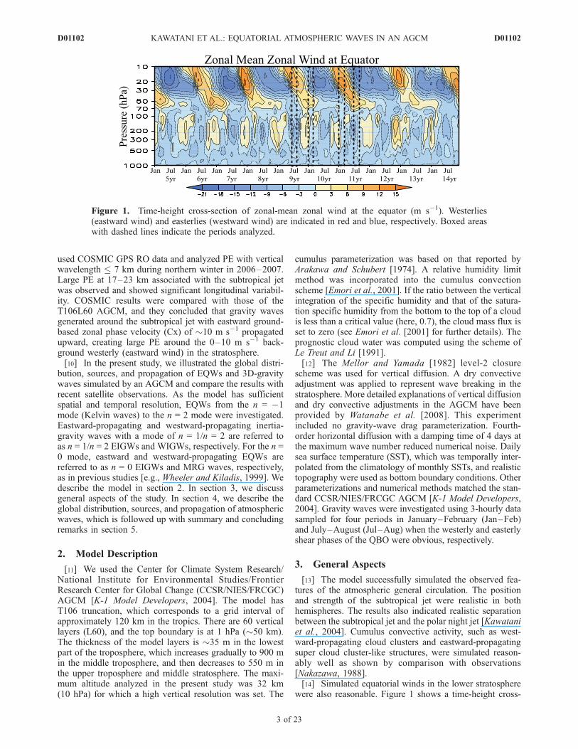
Figure 1. Time-height cross-section of zonal-mean zonal wind at the equator (m s�1). Westerlies(eastward wind) and easterlies (westward wind) are indicated in red and blue, respectively. Boxed areaswith dashed lines indicate the periods analyzed.

D01102 KAWATANI ET AL.: EQUATORIAL ATMOSPHERIC WAVES IN AN AGCM

3 of 23

D01102

section of zonal-mean zonal wind along the equator. Anobvious QBO-like oscillation has a period of approximately1.5–2 years. The maximum speed of the easterly (westwardwind) was approximately 20 m s�1, and that of the westerly(eastward wind) was 15 m s�1. In contrast, Naujokat [1986]reported amplitudes of 35 and 20 m s�1 for easterly andwesterly winds, respectively. The simulated amplitude ofthe easterly was larger than that of the westerly, as in thereal atmosphere, despite the smaller amplitude of theoscillation. The easterly extends down to approximately40–50 hPa in the model, which is slightly higher than theobserved. The downward propagation of the westerly shearzones of zonal wind (@u/@z > 0, where z denotes altitude) wasfaster than the downward propagation of easterly shear zones(@u/@z < 0), which agreed with observations. We analyzedfour periods when the QBO was in its westerly and easterlyshear phases in Jan–Feb and Jul–Aug, respectively, asindicated by the boxed areas in Figure 1. The 0 m s�1 zonalwinds were at approximately 30 hPa during these periods.[15] Figure 2 shows the global distribution of precipita-

tion in Jan–Feb and Jul–Aug obtained by observation andin the model. The observation data are Center for ClimatePrediction (CPC) Merged Analysis of Precipitation (CMAP;Xie and Arkin, 1996) 26-year averaged values (1979–2004). The simulated precipitation is 17-year averaged.The model reasonably simulated the global distribution ofprecipitation. In Jan–Feb, most large precipitation areaswere distributed around or to the south of the equator overthe Indian Ocean, whereas in Jul–Aug strong precipitation

occurred over the Indian monsoon region in the NorthernHemisphere. Strong precipitation also occurred over Africaand South America in both Jan–Feb and Jul–Aug. TheInter-Tropical Convergence Zone (ITCZ) in the equatorialregion was also well simulated. The separation between theITCZ and the South Pacific Convergence Zone (SPCZ) isclearly illustrated.[16] To evaluate how well the model simulates convec-

tively coupled EQWs, we performed space-time spectralanalysis of precipitation according to the method of Lin etal. [2006] using daily data from the Global PrecipitationClimatology Project (GPCP) and the model output. The datalength for spectral calculation was 2 years. GPCP data from2004 to 2005 were used when the influence of El Nino orLa Nina was small, based on the criteria for those eventsdefined by the Japan Metrological Agency.[17] Here we present a brief outline of the procedure;

further details were provided byWheeler and Kiladis [1999]and Lin et al. [2006]. Grid data D(8) as a function oflatitude 8 can be expressed as the sum of symmetric DS(8)and antisymmetric DA(8) components as follows:

D 8ð Þ ¼ DS 8ð Þ þ DA 8ð Þ ð1Þ

DS 8ð Þ ¼ D 8ð Þ þ D �8ð Þ½ =2 ð2Þ

DA 8ð Þ ¼ D 8ð Þ � D �8ð Þ½ =2 ð3Þ

Precipitation data were decomposed into symmetric andantisymmetric components and averaged from 15�N to

Figure 2. Global distribution of precipitation (mm day�1) in (a, c) Jan–Feb and (b, d) Jul–Aug obtainedwith (a, b) CMAP and (c, d) the model. The observational values are 26-year averages, whereas the modelvalues are 17-year averages. The shaded interval is 2 mm day�1; values � 2 mm day�1 are shown.

D01102 KAWATANI ET AL.: EQUATORIAL ATMOSPHERIC WAVES IN AN AGCM

4 of 23

D01102

15�S. Space-time spectra were then calculated for succes-sive overlapping segments of data and averaged. Here128 days, with 78 days of overlap between each segment,were calculated. The ‘‘background spectra’’ were calculatedby averaging the powers of DA and DS and smoothing witha 1–2–1 filter in frequency and wave number. Thissmoothing was applied to remove any periodic signals thatmay be present in the spectra at a particular zonal wavenumber and frequency.[18] Matsuno [1966] derived the dispersion relation of

EQW modes in shallow-water equations on an equatorialbeta plane as follows:

m2w2

N2� k2 � bk

w¼ 2nþ 1ð Þbjmj

N; n ¼ 0; 1; 2; ::: ð4Þ

where m, w, N, k, b, and n are the vertical wave number, theintrinsic frequency, the buoyancy frequency, zonal wavenumber, meridional gradient of the Coriolis parameter, andorder of the solution, respectively. The solutions of wavemodes have structures trapped at the equator. For an EQWwith zero meridional wind components, i.e., Kelvin waves(n = �1), the dispersion relation is the same as that for

internal gravity waves with zero meridional wavenumber asfollows:

w2

k2¼ ghe ð5Þ

where he is equivalent depth, which is connected with thevertical wave number m as follows

m2 ¼ N2

ghe� 1

4H2

� �ð6Þ

where H is the scale height, and the vertical wavelength lzis calculated from the vertical wave number as lz = 2p/m(see Andrews et al. [1987] for detailed derivation of aboveequations).[19] Figure 3 shows the zonal wave number versus the

frequency spectra of symmetric and antisymmetric compo-nents of precipitation divided by the background spectraappearing in the GPCP data and the model (15�S–15�Naverage). Following Lin et al. [2006], powers of 1.1 timesthe background or greater are drawn. The dispersion curvesof the odd (n = �1, 1) and even modes (n = 0, 2) of

Figure 3. Zonal wave number versus frequency spectra of precipitation averaged from 15�N to 15�S.(a, c) Symmetric and (b, d) antisymmetric components of precipitation divided by the backgroundspectrum appearing in the (a, b) GPCP data and (c, d) the model. Positive (negative) zonal wave numbercorresponds to positive (negative) Cx. The shading interval is 0.2; values � 1.1 are shown. Dispersioncurves indicate the odd and even modes of equatorial waves with the five equivalent depths of 8, 12, 25,50, and 90 m. The frequency spectral width is 1/128 cpd.

D01102 KAWATANI ET AL.: EQUATORIAL ATMOSPHERIC WAVES IN AN AGCM

5 of 23

D01102

equatorial waves for the five equivalent depths of 8, 12, 25,50, and 90 m are superposed under the assumption of zerobackground wind. The frequency spectral width is 1/128circles per day (cpd). As the time resolution of precipitationis 1 day, the minimum resolvable period is 0.5 cpd (2 days).In the areas corresponding to the dispersion curves, there areclear signals of Kelvin waves, n = 1 WIGWs, and n = 1equatorial Rossby waves in symmetric components, where-as MRG waves and n = 0 EIGWs are obvious in antisym-metric components, in both the observation and modelresults.[20] Lin et al. [2006] evaluated the tropical variability of

precipitation data in 14 atmosphere-ocean coupled GCMsparticipating in the Intergovernmental Panel on ClimateChange (IPCC) Fourth, Assessment Report (AR4). Theyreported that the Model for Interdisciplinary Research onClimate (MIROC; the CCSR/NIES/FRCGC AGCM usedhere is an atmospheric part of MIROC) most realisticallysimulated power at periods of�6 days among the 14 models.As shown in their Figures 5–7, MIROC showed goodresults in simulating convectively coupled equatorialwaves. It was also confirmed that spectral values of bothsymmetric and antisymmetric components are relativelyquantitatively well simulated (not shown). Like otherAGCMs [cf. Lin et al., 2006], the AGCM used heregenerally underestimates signals of the Madden-Julianoscillation (MJO [Madden and Julian, 1971]). However,analysis of momentum flux indicated that disturbancesassociated with the MJO did not contribute to drivingthe simulated QBO (not shown).[21] Horinouchi et al. [2003] conducted a comprehensive

comparison of low-latitude middle atmospheric waves usingnine AGCMs and showed that the variability of the precip-itation spectrum differed greatly among the models. Thewave spectrum in the middle atmosphere is linked to thevariability of convective precipitation, which is determinedby cumulus parameterization. The well-simulated spectrumof precipitation in this study would result in better simula-tion of equatorial wave activity in the stratosphere.

4. Global Distribution, Sources, and Propagationof Atmospheric Waves

4.1. Waves With Vertical Wavelengths ����������������������� 7 km

[22] PE due to short vertical wavelengths is often used asan indicator of the global distribution of gravity waves (i.e.,EQWs and/or 3D-gravity waves) in studies based on GPSRO because PE can be calculated from observed tempera-ture alone. Alexander et al. [2008b] reported the globaldistribution of PE with vertical wavelengths � 7 km (PE �7 km). For comparison with their recently obtained results,we also calculated PE � 7 km, with PE given by

PE ¼ 1

2

g

N

� �2 T 0

T

� �2

ð7Þ

Here we briefly explain the procedure for extracting shortvertical wavelengths of temperature. First, the backgroundtemperature profile of T was defined by the 2-monthaverage at each grid point. The background temperature Twas then subtracted from the temperature T of an individual

profile, and the linear trend was removed. Next, a cosine-type window was applied to both ends of the data to reducespectral leakage, and a high-pass filter using fast Fouriertransform (FFT) with a cut-off vertical wavelength ofapproximately 7 km was applied to obtain T0 with verticalwavelengths � 7 km. The analyzed height ranges in thisstudy do not contain the altitude where the window wasapplied.[23] Alexander et al. [2008b] binned COSMIC data into

horizontal grid cells of 20� 5� to secure a sufficientnumber of data points before calculating PE, which allowsfor the study of waves with zonal wave number � 9. In theAGCM, PE is calculated every 3 h using 2-month averagedbackground temperature T at each grid point; these valuesare then averaged for 2 months in each of the four termsillustrated in Figure 1. Therefore the simulated PE consistsof waves with periods from approximately 6 h to 2 months,vertical wavelengths � 7 km, and horizontal wavelengths of�380 to 40,000 km at the equator. Therefore the simulatedwaves have much wider spectral ranges than those shownby COSMIC data, and the value of simulated PE � 7 kmshould be larger than that observed by COSMIC GPS RO.[24] Figure 4 shows longitude-height cross-sections of

PE � 7 km averaged from 10�N to 10�S for the fourterms examined (2-month averages), during which theQBO was in westerly and easterly shear phases in Jan–Feb and Jul–Aug. Contour lines show the zonal wind.The zonal distribution of zonal wind was well simulateddespite the slightly larger amplitude of the Walker circu-lation as compared with that in the real atmosphere. Thelongitudinal variation in outgoing long-wave radiation(OLR) averaged from 10�N to 10�S is shown below eachfigure. Low values of OLR (note that the vertical axis ofthe OLR is inverted) correspond to active cumulus convec-tion. The convective activity is large over the Indian Ocean tomid-Pacific and at approximately 60–80�W. In the UTLSregion, much larger PE elongates from east to west over theeastern hemisphere than in the western hemisphere, which isconsistent with the COSMIC results. Larger PE is alsodistributed in the eastern hemisphere around the altitudewhere the zonal wind changes from easterly to westerly atapproximately 30 hPa (Figures 4a and 4c), which was alsoobserved in the COSMIC GPS RO data. Simulated PEranging from 8 to 10 J kg�1 was observed at approximately60–80�W in the UTLS region for all four terms, where asecondary maximum of convective activity occurs. Thevalues of PE � 7 km in this simulation were larger thanthose calculated using the COSMIC data, resulting from themuch wider spectral ranges covered in the AGCM. Aquantitative comparison is presented in section 4.3.[25] To clarify which phase velocities of waves are

dominant, PE as a function of zonal phase velocity relativeto the ground (Cx) was calculated. Figure 5 shows theheight distribution of PE � 7 km as a function of Cxaveraged from 10�N to 10�S for the four terms, which areshown separately as averages in the eastern hemisphere (0–180�E) and western hemisphere (0–180�W). The sign ofzonal wind associated with the Walker circulation changesat approximately �180�E (Figure 4). The 2-month meanvertical profiles of zonal wind with vertical wavelengths> 7 km (i.e., background zonal wind for waves with verticalwavelengths � 7 km) averaged in the eastern hemisphere/

D01102 KAWATANI ET AL.: EQUATORIAL ATMOSPHERIC WAVES IN AN AGCM

6 of 23

D01102

western hemisphere and 10�S–10�N are shown by thicksolid lines. The background zonal wind changes in longi-tude, latitude, and time direction must influence the localpropagation of waves. The two dashed lines show theaveraged zonal winds plus/minus their standard deviations(i.e., root mean square of longitude, latitude, and timevariance of the zonal wind). Note that some stratosphericPE in the western hemisphere (eastern hemisphere) origi-nates from waves generated in the troposphere in the easternhemisphere (western hemisphere) and then enters the west-ern hemisphere (eastern hemisphere). However, thesewave propagations do not critically alter the features men-tioned below (zonal propagations of EQWs are shown inFigures 10 and 11).

[26] In the eastern hemisphere (left panels), the easterly(westward wind) associated with the Walker circulationallows most of the eastward waves to propagate from theupper troposphere to the stratosphere, whereas most of thewestward-propagating waves with Cx of approximately�10 m s�1 are prevented from entering the stratosphere(some westward waves with Cx of ��10 m s�1 couldpropagate upward because of local changes in the zonalwind; see the width of the standard deviation). The situationis reversed in the western hemisphere. Most westward-propagating waves are not influenced by the westerly(eastward wind) in the upper troposphere.[27] In addition to differences in the zonal wind profiles

in the troposphere, the wave sources (cumulus convection)

Figure 4. Longitude-height cross-section of PE (shaded) due to waves with vertical wavelengths� 7 kmand zonal wind (contour lines). (a, c) Westerly and (b, d) easterly shear phases of the QBO in (a, b) Jan–Feband (c, d) Jul–Aug. The shading and contour intervals are 2 J kg�1 and 4m s�1, respectively. The line graphindicates the zonal variation in 2-monthly mean OLR (W m�2). Note that the vertical axis of the OLR isinverted. These values are averaged from 10�N to 10�S.

D01102 KAWATANI ET AL.: EQUATORIAL ATMOSPHERIC WAVES IN AN AGCM

7 of 23

D01102

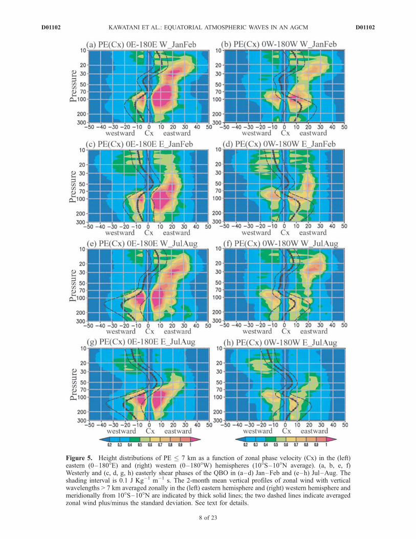
Figure 5. Height distributions of PE � 7 km as a function of zonal phase velocity (Cx) in the (left)eastern (0–180�E) and (right) western (0–180�W) hemispheres (10�S–10�N average). (a, b, e, f)Westerly and (c, d, g, h) easterly shear phases of the QBO in (a–d) Jan–Feb and (e–h) Jul–Aug. Theshading interval is 0.1 J Kg�1 m�1 s. The 2-month mean vertical profiles of zonal wind with verticalwavelengths > 7 km averaged zonally in the (left) eastern hemisphere and (right) western hemisphere andmeridionally from 10�S–10�N are indicated by thick solid lines; the two dashed lines indicate averagedzonal wind plus/minus the standard deviation. See text for details.

D01102 KAWATANI ET AL.: EQUATORIAL ATMOSPHERIC WAVES IN AN AGCM

8 of 23

D01102

are generally larger in the eastern hemisphere than in the westernhemisphere, which could result in larger PE in the easternhemisphere than in the western hemisphere in the UTLSregion (Figure 4). PE generally shows large values aroundthe tropopause, which might partially result from a sharpcold point tropopause in the tropical regions [Alexander etal., 2008b]. In addition, the wave energy accumulationmight occur around the tropopause because the verticalgroup velocity is inversely proportional to buoyancy fre-quency if the zonal wind does not change vertically[Andrews et al., 1987].[28] In the stratosphere, waves are markedly influenced

by the phase of the QBO. In the westerly shear phase of theQBO in the eastern hemisphere (Figures 5a and 5e), thedominant Cx of waves is �10 m s�1 from 200 to 50 hPa,but changes to �20 m s�1 at approximately 30 hPa.Eastward-propagating waves generated in the eastern hemi-sphere do not encounter the zonal wind until �30 hPa.Therefore most of the eastward waves can exist until 30hPa. On the other hand, in the westerly shear phase of theQBO in the western hemisphere (Figures 5b and 5f),isolated large PE occurs at approximately 20–30 hPa withCx of �20 m s�1. These Cx values are larger than those ofthe mean westerly associated with the Walker circulation inthe upper troposphere (note also that some PE at thisaltitude originates from waves generated in the easternhemisphere, as mentioned above). In the easterly shearphase of the QBO (Figures 5c, 5d, 5g, and 5h), PE withCx of approximately �10 m s�1 is generally larger than thatwith Cx of approximately 10 m s�1 over 20–30 hPa. ThePE distribution in the stratosphere generally agrees with thefact that temperature variances associated with zonally andvertically propagating gravity waves in background shear

flow have a functional dependence of ju � Cxj�1, where uis background zonal wind. Nonlinear effects and dissipationwould limit the growth close to the critical level, so thattemperature variances maximize below [Randel and Wu,2005 and references therein]. The results obtained fromFigures 4 and 5 indicate that the distribution of the PEresults from three factors: the source strengths, the Walkercirculation, and the phase of the QBO.[29] Alexander et al. [2008b] showed the global distribu-

tion of PE � 7 km at 15, 22, 26, and 32 km in January 2007and 2008, when the QBO was in its easterly and westerlyshear phases, respectively. For both 2007 and 2008, theyfound similar PE distributions at 15 km, as well as similarOLR distributions. Large PE is visible from the IndianOcean through the Western Pacific and over South America.However, the stratospheric PE is different between thedifferent phases of the QBO. Around the altitude wherethe zonal wind is �0 m s�1, relatively large PE elongatesmore zonally in the westerly than in the easterly shear phaseof the QBO. Another interesting point is that large PE isfound over South America in both the easterly and westerlyshear phases of the QBO.[30] Figure 6 shows the global distribution of PE in Jan–

Feb at 100 hPa (Figures 6a and 6b) and the altitude at whichzonal wind is approximately 0 m s�1 at the equator in thewesterly (approximately 32–35 hPa; Figure 6c) and easterly(approximately 30–32 hPa; Figure 6d) shear phases of theQBO. The PE distributions at 100 hPa do not differ muchbetween the two phases; large PE is observed mainly fromthe Indian Ocean to the western Pacific, and PE of approx-imately 8–16 J kg�1 is located over South America, theeastern Pacific, and the Congo Basin. These results arequalitatively similar to those observed by COSMIC. The PE

Figure 6. Global distribution of PE � 7 km in Jan–Feb at (a, b) 100 hPa, and (c) 32–35 hPa and(d) 30–32 hPa where zonal wind (contour lines) is approximately 0 m s�1 at the equator. (a, c) Westerlyand (b, d) easterly shear phases of the QBO. The shading interval is 2 J kg�1 for (a, b) and 1 J kg�1 for (c, d).The solid and dashed lines illustrate westerly and easterly, and thick solid lines show 0 m s�1. The contourinterval is 10 m s�1.

D01102 KAWATANI ET AL.: EQUATORIAL ATMOSPHERIC WAVES IN AN AGCM

9 of 23

D01102

distribution is quite different between the westerly andeasterly shear phases of the QBO for which zonal wind is�0 m s�1 (Figures 6c and 6d). Zonally elongating PE withlarge values occurs from 10–330�E (30�W) above theequator in the westerly shear phase. During the easterlyshear phase, relatively small values of PE elongate aroundthe equator and are more scattered than those in the westerlyshear phase. Large PE is observed over South America inboth the westerly and easterly shear phases. The illustratedPE consists of both EQWs and 3D-gravity waves. The PEwith a meridional symmetric mode may be due to EQWs,whereas that scattered in the latitudinal direction is probablydue to 3D-gravity waves, as discussed in section 4.3.

4.2. Equatorial Trapped Waves

[31] To investigate what kind of EQWs appear in themodel, Figure 7 shows the zonal wave number versus thefrequency spectra of the symmetric and antisymmetriccomponents of temperature for the westerly shear phase inJan–Feb. Spectra of symmetric and antisymmetric compo-nents were computed separately for each latitude beforeaveraging from the equator to 10� (i.e., equivalent to the

average of 10�S–10�N). Note that temperature data werenonfiltered in both space and time before calculation of thespectra (i.e., the vertical wavelength filter used in section4.1 was not applied). In the stratospheric temperatures, thespectrum is not the red noise-like background spectrumdominating in OLR data or precipitation data [e.g., Wheelerand Kiladis, 1999]. Therefore symmetric and antisymmetricspectra were not divided by the background spectra.[32] The altitude ranges were selected from 83–35 hPa

and 35–15 hPa. The boundary of 35 hPa correspondsroughly to the altitude at which the zonal wind changesfrom easterly to westerly. Dispersion curves for symmetriccomponents include Kelvin waves, n = 1 EIGWs andWIGWs, and n = 1 equatorial Rossby waves, whereasantisymmetric components include MRG waves, n = 0EIGWs, n = 2 EIGWs and WIGWs, and n = 2 equatorialRossby waves. Equivalent depths were selected as 8, 12, 25,50, and 90 m, as in Figure 3 (note that the frequency rangewas extended to �1.1 cpd because 3-hourly data were usedto calculate the spectra). The effect of background wind wasneglected when drawing the dispersion curves of the equa-torial waves.

Figure 7. Zonal wave number versus the frequency spectra of the (a, c) symmetric and (b, d)antisymmetric components of temperature for the westerly shear phase in Jan–Feb at (a, b) 83–35 hPaand (c, d) 35–15 hPa. Spectral units are log10(K

2 wave number�1 cpd�1). Dispersion curves forsymmetric components include Kelvin waves, n = 1 EIGWs and WIGWs, and n = 1 equatorial Rossbywaves, whereas antisymmetric components include MRG waves, n = 0 EIGWs, n = 2 EIGWs andWIGWs, and n = 2 equatorial Rossby waves. Equivalent depths are selected as 8, 12, 25, 50, and 90 m,which are the same as in Figure 3. The effect of background wind is neglected to draw the dispersioncurves of the equatorial waves. Note that the ranges of shading are different between the symmetric andantisymmetric components. Smoothing was conducted with a 1-2-1 moving mean in frequency.

D01102 KAWATANI ET AL.: EQUATORIAL ATMOSPHERIC WAVES IN AN AGCM

10 of 23

D01102

[33] For zonally propagating waves, the intrinsic fre-quency w is written as follows:

w ¼ w � ku ð8Þ

where w, k, and u are the ground-based frequency, zonalwave number, and background zonal wind, respectively.The intrinsic frequencies w and vertical wavelengths changebecause u changes with altitude. On the other hand, theground-based frequency w of a wave is defined at the wavesource level. Note that the ground-based frequency w andzonal wave number k do not change with altitude, assuminga slowly varying background wind field, even through thebackground wind changes with altitude; the distribution ofthe zonal wave number versus the frequency spectra isindependent of altitude. The distribution of the spectrawould be changed only if a wave were to undergo criticallevel filtering and/or wave dissipation. Therefore in Figure 7we selected the same dispersion curves of EQWs as those ofthe sources (Figure 3) to compare spectral features in thestratosphere with those of the sources. A more detaileddiscussion was presented by Ern et al. [2008, and referencestherein]. We did not use a vertical wavelength filter topreserve this wave property.[34] Clear signals of Kelvin waves, MRG waves, n = 0

EIGWs, and n = 1 equatorial Rossby waves can be seen inFigure 7. The peaks corresponding to n = 1 EIGWs becamemuch clearer when the same spectral figures were drawnusing meridional wind data in which Kelvin waves do notappear (not shown). Note that the spectral distributions ofthe temperature at 83–35 hPa (Figures 7a and 7b) wererelatively similar to those of precipitation (Figure 3) in therange of 8 � he � 90 m. These results imply a connectionbetween stratospheric EQWs and tropospheric wave sourcesof convectively coupled EQWs. On the other hand, thewave spectrum also shows distributions outside the he of 8–90 m, especially at 35–15 hPa (Figures 7c and 7d), whichare likely independent of convectively coupled EQWs.Waves with large equivalent depth could be an indication

of processes involving longer vertical scales in the tropo-sphere, which become visible at higher altitudes due to adecrease of atmospheric density and an increase in statisticstability [Ern et al., 2008]. The powers of Kelvin waves andn = 0 EIGWs with small equivalent depths (he � 8 m)decreased with height, implying that these waves interactwith the mean zonal wind. There are other spectral peakswith periods of approximately 1 day and a wide zonal wavenumber range in both symmetric and antisymmetric com-ponents. These wave numbers may correspond to the tideand 3D-gravity waves generated by the diurnal cycle ofconvection [Kawatani et al., 2003].[35] To investigate the global distribution, sources, and

propagation of EQWs, an equatorial wave filter was con-structed. Kelvin waves, MRG waves, n = 0 EIGWs, n = 1and n = 2 EIGWs and WIGWs, and n = 1 and n = 2equatorial Rossby waves were extracted separately forfurther examination according to the methods of Wheelerand Kiladis [1999]. To avoid degradation of the actualamplitude of EQWs during the analyzed periods, we in-cluded data from both before and after each analyzedperiod. For example, when the EQWs in January–Februarywere extracted, the last few days of December and the firstfew days of March were included. Then, a cosine-typewindow was applied only to the data from December andMarch. After applying FFT to the combined data, only thedata from 1 January to the end of February were extracted.[36] Figure 8 shows the spectral ranges between the lines

indicating equivalent depths of 8 and 90 m under theassumption of zero background wind in the zonal wavenumber-frequency domain for odd and even modes. Theequivalent depths of 8 to 90 m correspond to verticalwavelengths of 2.3 and 7.6 km with N2 = 6 10�4 s�2,which is the representative value in the lower stratosphere(�80 hPa). The vertical wavelength range is similar to thatused in the PE calculation in Figures 4–6. The zonal wavenumbers of the EQWs were selected from 1 to 9 accordingto the method of Alexander et al. [2008b]; this rangecorresponds to zonal wavelengths from 4444 to 40,000 km

Figure 8. Equatorial wave filter for (a) odd and (b) even modes. Superposed are the dispersion curvesof each EQW for two equivalent depths of 8 and 90 m. Hatched areas between the two lines are thefiltering range of (a) Kelvin, n = 1 EIGWs and WIGWs, n = 1 equatorial Rossby waves, (b) MRG waves,n = 0 EIGWs, n = 2 EIGWs and WIGWs, and n = 2 equatorial Rossby waves. The minimum period is setat 1.1 day (�0.9 cpd) to avoid including waves with a period of 1 day. Some overlapping areas occurbetween the Kelvin waves and n = 1 EIGWs and between n = 0 and n = 2 EIGWs.

D01102 KAWATANI ET AL.: EQUATORIAL ATMOSPHERIC WAVES IN AN AGCM

11 of 23

D01102

over the equator. The minimum period was set at 1.1 day(�0.9 cpd) to avoid including waves with a period of 1 day.[37] Ern et al. [2008] reported that EQW activity in a

slow phase speed wave band between equivalent depths of8 and 90 m was mainly modulated by the QBO and thathigher equivalent depths (90–2000 m) showed less pro-nounced variation due to the QBO but more variation due tothe stratopause SAO. As we could analyze data up toapproximately 32 km in this model, we focused on waveactivity related to the QBO. Therefore the selected waveband was set between 8 and 90 m.[38] In this section, we describe application of the equa-

torial wave filter to unfiltered data (i.e., original data withno temporal or spatial filtering). The propagation propertiesof EQWs in relation to background winds from the tropo-sphere to the stratosphere can be investigated using thisfilter since the ground-based frequency w and zonal wavenumber k of a wave do not change unless a wave hasdissipated, as mentioned above. The spectral range of n = 1EIGWs may include some fast Kelvin waves (he > 90 m)with periods of less than �3 days (see Figures 7a, 7c, and8a). However, most fast Kelvin waves do not exist in thefiltering range of n = 1 EIGWs. In fact, fast Kelvin waveshave periods of approximately 6–10 days [Hirota, 1978;Hitchman and Leovy, 1988]. Ultra-fast Kelvin waves withperiods of 3–4 days [Salby et al., 1984] are dominant atmuch higher altitudes than those examined here. There aresome areas of overlap between the Kelvin waves and n = 1EIGWs, and between n = 0 and n = 2 EIGWs.[39] The amplitudes of the extracted wave component in

temperature associated with Kelvin waves and MRG wavesare �2–3 K and �1 K, respectively. These results wereconsistent with those from COSMIC GPS RO data[Alexander et al., 2008b] and SABER data [Ern et al.,2008]. We confirmed that the period, zonal phase speedrelative to the ground, and vertical wavelength were alsosimulated realistically in the model. Not only temperature,but also the zonal and meridional wind and geopotentialheight of EQW components, were extracted using theequatorial wave filter. In addition, we confirmed that thespatial structures of extracted EQWs in the stratosphereagreed with those derived theoretically by Matsuno [1966].[40] To investigate source distributions of these EQWs,

the equatorial wave filter was also applied for OLR data.The spectral characteristics of the zonal wave numberversus the frequency spectra of OLR (not shown) are similarto those of precipitation shown in Figure 3. Signals ofconvectively coupled EQWs that appeared in OLR datawere extracted using the same equatorial wave filter shownin Figure 8. Therefore we can investigate the wave sourcedistributions, propagations, and global distributions ofEQWs.[41] Figure 9 illustrates the global distribution of OLR

variance due to each convectively coupled EQW componentand the PE associated with each EQWat 32–35 hPa in Jan–Feb during the westerly shear phase of the QBO. Thevariances of equatorial Rossby waves with equivalentdepths of 8–90 m are much larger in the upper tropospherethan in the stratosphere. The connection of the equatorialRossby waves between the upper troposphere and strato-sphere is not very clear (not shown). The vertically prop-agating responses of convectively coupled n = 1 equatorial

Rossby waves are confined to within a few kilometers of thewave forcing (see discussions by Wheeler et al., 2000 andreferences therein). Therefore EQWs without equatorialRossby waves are discussed in this section. Wheeler et al.[2000] reported the global distributions of OLR variancedue to each EQW for northern/southern summer using datafor a period of �17 years (see their Figure 3). They alsopresented the temporal variation of OLR variance for eachEQW. Our results shown in Figure 9 are from 2-monthaveraged fields, and the range of the equatorial wave filter isslightly different from that used by Wheeler et al. [2000].Therefore it is not necessary for the model results to beidentical to the observational climatological results. Never-theless, the distributions of simulated OLR variances aresimilar to those observed, and the simulated variance ofEQWs is in the range of the time variation of observed OLRvariance.[42] Wheeler et al. [2000] reported that waves of rela-

tively short vertical wavelength (�10 km) are indeedimportant for the coupling of large-scale dynamics andconvection. Therefore the global distributions of PE dueto EQWs shown in Figure 9 may be related to the activity ofconvectively coupled OLR. Convectively coupled EQWswould be a sufficient condition for the generation of EQWspropagating into the stratosphere. Concerning MRG waves,Magana and Yanai [1995] discussed that extratropical wavepropagating into the tropical region is another possiblesource of MRG waves. In general, large PE associated withEQWs is observed from the equator to 10�N–10�S. ForKelvin waves, large PE in the stratosphere (Figure 9b) isgenerally located to the east of source distributions(Figure 9a), suggesting that Kelvin waves generated in theupper troposphere propagate eastward. In contrast, larger PEof n = 0 EIGW (Figure 9f) occurs over the Indian Oceandespite larger variance in OLR (Figure 9e) in the Pacific thanin the Indian Ocean. It was also interesting that the distribu-tions of large PE with MRG waves and other EQWs do notcorrespond directly with those of the large variance in OLR.[43] EQWs propagate eastward or westward from the

source region and should be influenced by the back-ground zonal wind. To investigate the propagation ofEQWs, 2-month averages of zonal and vertical energyfluxes (f0u0; f0w0) (overbars denote the 2-month average)were used. The ratio of energy flux to energy density isequivalent to the ratio of wave action flux to wave actiondensity when Wentzel-Kramers-Brillouin (WKB) theoryholds in space and time. A number of previous studies haveprovided detailed discussions of wave action flux and waveaction density [Dunkerton, 1983; Andrews et al., 1987, andreference therein]. The direction of wave group propagationis expressed by energy flux F to energy density E as follows[cf. Gill, 1982]:

F ¼ f0u0;f0w0� �

¼ E Cgx; Cgz� �

ð9Þ

E ¼ 1=2 u02 þ v02 þ w02� �

þ 1=2 g=Nð Þ2 T 0=T� �2 ð10Þ

where E is wave energy (kinetic energy plus potentialenergy) per unit mass, and Cgx and Cgz represent zonal and

D01102 KAWATANI ET AL.: EQUATORIAL ATMOSPHERIC WAVES IN AN AGCM

12 of 23

D01102

Figure 9. Global distribution of (left) OLR variance due to each convectively coupled EQW componentand (right) PE due to each EQW at 32–35 hPa in Jan–Feb during the westerly shear phase of the QBO.(a, b) Kelvin waves, (c, d) MRG waves, (e, f) n = 0 EIGWs, (g, h) n = 1 EIGWs, (i, j) n = 1 WIGWs, (k, l)n = 2 EIGWs, and (m, n) n = 2 WIGWs. The shading intervals are 15 W2 m�4 for (a), 5 W2 m�4 for (c),3 W2 m�4 for (e, g, i, k, m), 0.5 J kg�1 for (b), and 0.05 J kg�1 for (d, f, h, j, l, n).

D01102 KAWATANI ET AL.: EQUATORIAL ATMOSPHERIC WAVES IN AN AGCM

13 of 23

D01102

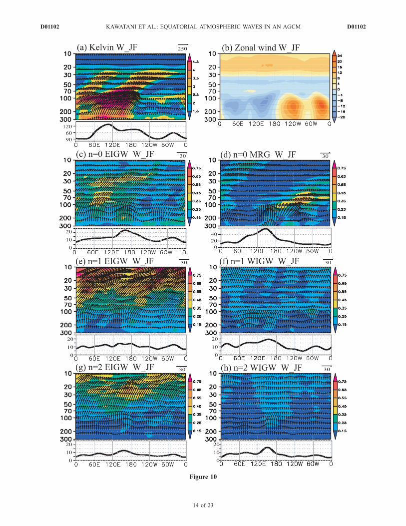
Figure 10

D01102 KAWATANI ET AL.: EQUATORIAL ATMOSPHERIC WAVES IN AN AGCM

14 of 23

D01102

vertical intrinsic group velocity, respectively. Because theenergy fluxes are parallel to the intrinsic group velocity ofgravity waves in the context of WKB theory, the sign ofenergy flux shows the direction of gravity wave propagationrelative to the mean wind.[44] Longitude-height cross-sections of PE and zonal/

vertical energy flux (f0u0; f0w0) in Jan–Feb during thewesterly and easterly shear phases of the QBO are shownin Figures 10 and 11, respectively (10�S–10�N average).Note that energy fluxes are 2-monthly averaged pictures thatshould look different at any given time. The line graphindicates the zonal variation in OLR variance due to eachwave component averaged from 10�N to 10�S (note thedifferent ranges of the ordinate axes for Kelvin waves,MRG waves, and other EQWs). The top right panel showsthe 2-monthly mean and 10�S–10�N average zonal wind.[45] PE associated with Kelvin waves is most dominant

among EQWs (note that the shading intervals in Figures 10and 11 are different between PE associated with Kelvinwaves and those associated with other EQWs). In thetroposphere, there are large sources of Kelvin waves inthe eastern hemisphere, and most Kelvin waves generated inthe eastern hemisphere propagate into the stratosphere(Figures 10a and 11a). Kelvin waves are also excited inthe western hemisphere, but energy fluxes suddenly becomeweak below 100 hPa. These results indicate that the verticalshear of the Walker circulation in the western hemisphereprevents most Kelvin waves from entering the stratosphereby the same mechanism (critical-level filtering) presented inFigure 5. Interestingly, some Kelvin waves generated atapproximately 180�E propagate eastward and encounter thewesterly in the troposphere at approximately 170–150�W.The value of the energy flux decreases rapidly in the zonaldirection. These results indicate that Kelvin waves dissipatenot only via vertical propagation, but also via zonalpropagation [Fujiwara and Takahashi, 2001; Suzuki andShiotani, 2008].[46] In the westerly shear phase of the QBO, most Kelvin

waves in the eastern hemisphere propagate from the tropo-sphere into the middle stratosphere, and their propagationbecomes much weaker around 20–30 hPa (Figure 10a),when the QBO is in the westerly phase. On the other hand,in the easterly shear phase, most of the Kelvin waves stoppropagating vertically within the range of the westerlyphase of the QBO around 50 hPa (Figure 11a). Thesedifferent propagation characteristics result in the differentglobal distributions of PE around the altitude at which thezonal wind approaches zero (see Figures 6c and 6d).[47] Even in the westerly shear phase of the QBO

(Figure 10a), some Kelvin waves in the eastern hemisphereseem to dissipate around 70 hPa, where zonal wind is nearly0 m s�1 (2-month mean zonal wind averaged from 10�S–

10�N is shown in Figure 10b, but there are some areaswhere zonal wind is positive over the equator; see thevertical profiles of zonal wind with standard deviationsshown in Figure 5a). Spectral analysis indicates that veryslow Kelvin waves with Cx < �5 m s�1 dissipate around70–100 hPa (not shown).[48] From equations (9) and (10), the intrinsic group

velocities Cgx and Cgz of each EQW can be estimatedafter calculating both potential energy and kinetic energydue to each EQW. Note that the 2-monthly mean intrinsicgroup velocity averaged for the spectral domain in zonalwave number-frequency extracted by the equatorial wavefilter can be estimated. Here we mention the case of Kelvinwaves in the westerly shear phase of the QBO (Figure 10a).The estimated Cgx and Cgz in the eastern hemisphere at70–30 hPa within 10�S–10�N are approximately 25 m s�1

and 1.2 10�2 m s�1, respectively (not shown). During 5.7days, the wave packet propagates an estimated �12,000 km(108�) in the zonal and �5.9 km (the distance from 70 to 30hPa) in the vertical direction relative to the mean wind. Thedirection of energy flux shown in Figure 10a is consistentwith this estimation.[49] In contrast to Kelvin waves, PE due to MRG waves

is large in the western hemisphere in the UTLS region. It isinteresting that most MRG waves generated from the IndianOcean to the western Pacific do not enter the stratosphere,despite the large sources (Figures 10d and 11d). Theeasterly associated with the Walker circulation filters mostof the MRG waves in the upper troposphere. MRG wavesgenerated at approximately 150�E–150�W propagate east-ward and upward, and contribute to the PE in the strato-sphere; note that the intrinsic zonal phase velocity Cx ofMRG waves is negative (i.e., westward), while the intrinsiczonal group velocity Cx of MRG waves is positive (i.e.,eastward). In contrast to Kelvin waves, more MRG wavespropagate into the middle stratosphere (up to �20 hPa)during the easterly shear phase of the QBO (Figure 11d). Inthis phase, some MRG waves reach approximately 0–30�Ein the stratosphere. Careful examination of Figure 6dindicates an off-equatorial PE distribution at approximately30�W–30�E. MRG waves contribute to the PE around thisregion.[50] In the westerly shear phase, most of the n = 0 EIGWs

propagate until 20–30 hPa (Figure 10c), where the zonalwind is 0–8 m s�1, and generate large PE at this altitude. Inthe easterly shear phase, some n = 0 EIGWs are influencedby the westerly at 70–30 hPa, but more n = 0 EIGWs seemto propagate toward the upper stratosphere (Figure 11c), incontrast to Kelvin waves. This is because n = 0 EIGWsgenerally have faster Cx values than Kelvin waves, whichcan pass through weak westerly zones. These results may be

Figure 10. Longitude-height cross-sections of PE and zonal and vertical energy fluxes (f0u0; f0w0) due to each EQW inthe westerly shear phase in Jan–Feb (10�N–10�S average). PE due to (a) Kelvin waves, (c) n = 0 EIGWs, (d) MRG waves,(e) n = 1 EIGWs, (f) n = 1 WIGWs, (g) n = 2 EIGWs, and (h) n = 2 WIGWs averaged between 10�N and 10�S. (b) Zonalwind averaged from 10�N to 10�N. The line graph indicates zonal variation in OLR variance (W2 m�4) due to each EWQcomponent. Note the different ranges of the ordinate axes for Kelvin waves, MRG waves, and other EQWs. The arrow unitis 250 J kg�1 m s�1 for (a) and 30 J kg�1 m s�1 for (c–h). The vertical component of energy flux is multiplied by a factorof 1000 to coincide with their direction parallel to the propagation of wave path. The shading interval is 0.5 J kg�1 for (a)and 0.1 J kg�1 for (c–h). The shading interval is 4 m s�1 for zonal wind for (b).

D01102 KAWATANI ET AL.: EQUATORIAL ATMOSPHERIC WAVES IN AN AGCM

15 of 23

D01102

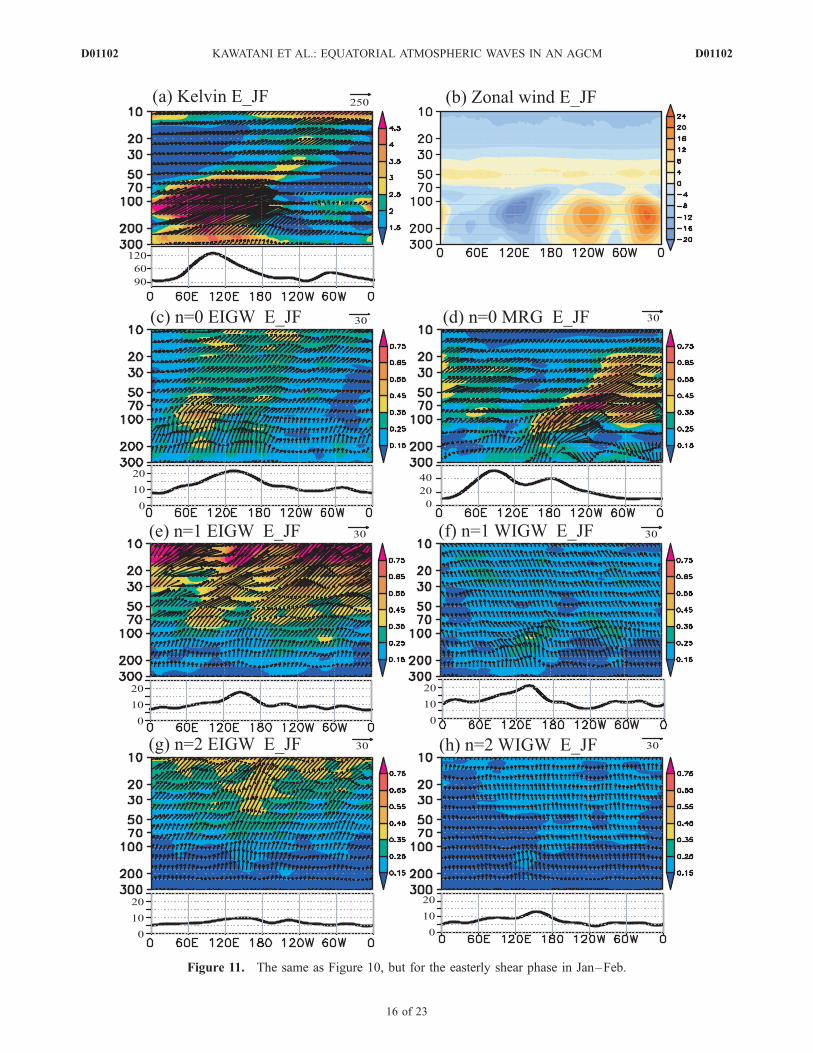
Figure 11. The same as Figure 10, but for the easterly shear phase in Jan–Feb.

D01102 KAWATANI ET AL.: EQUATORIAL ATMOSPHERIC WAVES IN AN AGCM

16 of 23

D01102

dependent on the strength of the background zonal winds,which have seasonal and interannual variation.[51] Around 70–30 hPa, more n = 1 WIGWs propagate

into the middle stratosphere in the easterly shear phase(Figure 11f) than in the westerly shear phase of the QBO(Figure 10f), as for MRG waves. However, in general, n = 1and n = 2 EIGWs/WIGWs are not influenced much by thebackground zonal wind (Figures 10e–10h and 11e–11h) tothe same extent as Kelvin waves and n = 0 EQWs becausen = 1 and n = 2 EIGWs/WIGWs generally have larger Cxwith zonal wave numbers ranging from 1 to 9 (see Figure8; the gradient between the zonal wave number versus thefrequency is proportional to Cx). There is also a clearcorrespondence of wave generation in the troposphere andwave sources for n = 1 and n = 2 EQWs. For example, themaximum upward propagation of n = 1 and n = 2 WIGWsin the troposphere occurs at approximately 120–180�E,where the sources of these waves are large.[52] Waves with larger Cx may interact with the SAO,

whereas some n = 1 and n = 2 waves with relatively smallCx should interact with the QBO. As clearly illustrated inthis section, the distributions of stratospheric PE caused byEQWs are greatly affected by the source distribution, theWalker circulation, and the QBO phase. Therefore thestratospheric variation (e.g., interannual and seasonal vari-ation) of PE should be associated with tropospheric varia-tion [Tsuda et al., 2008] in addition to the QBO phase. Thesimulation results should serve as useful information to gaina better understanding of the observed PE distribution.

4.3. Ratio Between EQWs and 3D-Gravity Waves

[53] The PE associated with EQWs has equatoriallytrapped structures (Figure 9), and most PE associated with3D-gravity waves must show no mode to the equator. ThePE � 7 km shown in Figure 6 is the sum of EQWs � 7 kmand 3D-gravity waves � 7 km. In this section, we discussinvestigation of the extent to which EQWs and/or 3D-gravity waves contribute to the PE � 7 km. To assess thisquestion in accurate detail, the equatorial-wave filter dis-cussed in section 4.2 was used for temperature data withvertical wavelengths � 7 km (T0 � 7 km). In calculating thetemperature associated with EQWs, overlaps betweenKelvin waves and n = 1 EIGWs and between n = 0 EIGWsand n = 2 EIGWs were avoided. That is, a Kelvin and n = 1EIGW, n = 1 WIGW, and n = 1 equatorial Rossby wavefilter was applied for the symmetric component of T0 � 7 kmand an MRG wave, n = 0 and n = 2 EIGW, n = 2 WIGW,and n = 2 equatorial Rossby wave filter was applied forantisymmetric T0 � 7 km. The PE � 7 km associated withEQWs was then calculated. Here PE values associated with3D-gravity waves were regarded as the residual of total PE� 7 km minus the PE � 7 km associated with EQWs.[54] Figure 12 shows the global distribution of PE� 7 km,

PE associated with EQWs� 7 km, 3D-gravity waves� 7 km,and PE associated with EQWs divided by total PE � 7 km at20–30 km (�57–15 hPa) in Jan–Feb during the westerlyand easterly shear phases of the QBO. PE � 7 km isgenerally larger in the westerly than in the easterly shearof the QBO (Figures 12a and 12b). The PE with EQWs �7 km is also larger in the westerly shear phase withdominant symmetric structures. On the other hand, in theeasterly shear phase, off-equatorial structures of PE with

EQWs � 7 km were clearly seen around 0–60�E and 0–160�W due to the small activity of Kelvin waves in theeasterly shear phase, as discussed in section 4.2. The north-south extent of EQWs is described by the equatorial radiusof deformation y0 as follows:

y0 ¼ffiffiffiffiffiffiffiffiffiffiffiffiffiffiffiN= mj jb

p¼

ffiffiffiffiffiffiffiffiffiffiffiffiffiffiffiffiffiffiffiNlz=2pb

pð11Þ

The amplitude of EQWs becomes 1/ffiffiffie

pwhere y = y0 (y is

the meridional axis, and y = 0 at the equator; see Andrews etal. [1987]). The value of y0 for EQWs with verticalwavelength of 7 km is approximately 1100 km. ThereforePE (as a function of T02) associated with EQWs � 7 kmshould be reduced to less than 1/e � 37% within 1100 km.For example, PE with a value of �3 (J kg�1) in the westerlyshear phase over the middle Pacific decreases to a value ofapproximately �1.2 (J kg�1) around 10�N (Figure 12c),which is consistent with the estimated meridional range.[55] PE with 3D-gravity waves � 7 km shows a scattered

structure with a wide meridional range (Figures 12e and12f). Large values are observed over areas that include theCongo basin, South America, the Indian Ocean to the mid-Pacific, and northern Australia. GPS RO data also showlocalized PE, such as over South America [Tsuda et al.,2000, 2008; Alexander et al., 2008b], most likely due to 3D-gravity waves. In Jul–Aug, large PE due to 3D-gravitywaves � 7 km is distributed around the Indian monsoonregion (not shown) in association with large amounts ofprecipitation (Figure 2d), which is also consistent with GPSRO measurements made by the Challenging Mini-Payload(CHAMP) satellite as described by Tsuda et al. [2008].[56] Of the total PE at 20–30 km, approximately 30%

from the Indian Ocean to the eastern Pacific is contributedby EQWs � 7 km (Figures 12g and 12h) over the equator,indicating that 3D-gravity waves � 7 km contribute �70%to PE � 7 km at this altitude. The contribution of EQWsbecomes smaller away from the equator. The contribution ofEQWs to PE is smaller over the Atlantic Ocean. In thestratosphere, the ratio in the westerly shear phase is gener-ally larger than in the easterly shear phase of the QBO dueto greater propagation of Kelvin waves, which have thelargest amplitude of T0 among EQWs. The latitude-heightcross-section of the ratio averaged between 10�S and 10�Nin both Jan–Feb and Jul–Aug reaches up to 40% at thealtitude where Kelvin wave activity is large (not shown).[57] The model covers a much wider spectral range than

those in COSMIC GPS RO data as mentioned in section4.1. This is one possible reason why simulated total PE �7 km was generally larger than that in COSMIC. In fact, thestrength of PE � 7 km associated with EQWs (Figures 12cand 12d) was comparable to PE with an equatorially trappedstructure observed in COSMIC GPS RO data [Alexander etal., 2008b].[58] The periods of the simulated QBO were shorter than

those in the real atmosphere, which implies overestimationof simulated gravity wave activity. Kawatani et al. [2005]calculated the simulated net u0w0 and absolute value ofju0w0j (i.e., ju0w0j with eastward waves plus ju0w0j withwestward waves) with periods less than 3 days using thesame AGCM as in this study. They compared simulatedvalues with radiosonde observations from Singapore

D01102 KAWATANI ET AL.: EQUATORIAL ATMOSPHERIC WAVES IN AN AGCM

17 of 23

D01102

reported by Sato and Dunkerton [1997] and confirmed thatthe simulated u0w0 and ju0w0j were quantitatively in goodagreement with the observational results. Kawatani et al.[2005] also revealed that simulated u0w0 has strong longi-tudinal variation. More observations of gravity waves atdifferent stations are needed to verify the model results.

4.4. Gravity Waves With Periods ����������������������� 24 Hours

[59] As noted in section 1, Tsuda et al. [2000] reportedlarge PE over the tropical Atlantic Ocean, and Kawatani etal. [2003] concluded that the source of this PE was 3D-gravity waves generated by a diurnal cycle of convectionaround the Bay of Guinea. Relatively large PE was alsosimulated over the Amazon and Indonesia. Kawatani et al.[2003] presented results obtained in only 1 week of June. Inthis section, gravity waves with periods� 24 h for 2-monthlymeans in Jan–Feb and Jul–Aug are investigated during the

easterly shear phase of the QBO. Note that the 24-h cyclehas a repeatable well-defined phase at each point, whereasintraday variance arises from short-lived disturbance at anytime of the day. Gravity waves with periods � 24 h aregenerated by both the diurnal cycle of convection andanother intraday variability. We extracted wave componentsby applying a high-pass filter with a cut-off period of 24 h.The terms of the applied cosine-type window and theextracted terms are the same as those explained in section4.2. The high-pass filter was applied to temperature, geo-potential height and wind components to obtain PE � 24 hand energy flux � 24 h. Note that the vertical wavelengthfilter was not applied.[60] Figure 13 shows the 2-monthly mean amplitudes of

cumulus precipitation with periods � 24 h for Jan–Feb andJul–Aug during the easterly shear phase of the QBO(different from the previous figures, the starting point of

Figure 12. (a, b) Global distribution of total PE with vertical wavelength � 7 km at 20–30 km inJan–Feb. The PE due to (c, d) EQW� 7 km components and (e, f) 3D-gravity wave components� 7 km.(g, h) The ratio between total PE � 7 km and PE due to EQWs � 7 km. The left and right panels show thewesterly and easterly shear phases of the QBO, respectively. The shading intervals are 0.5 J kg�1 for (a, b, e,f), 0.3 J kg�1 for (c, d), and 3% for (g, h).

D01102 KAWATANI ET AL.: EQUATORIAL ATMOSPHERIC WAVES IN AN AGCM

18 of 23

D01102

longitude is 180�W). The values indicate the ratio ofprecipitation amplitude with periods � 24 h to that withperiods > 24 h. The ratio was calculated when the 2-monthlymean convective precipitation exceeded 1 mm day�1.Cumulus precipitation � 24 h includes not only 24 h, butalso 6- to 23-h components. Spectral analysis of cumulusconvection � 24 h over the land indicated a dominantperiod at 24 h, with a secondary maximum at 12 h. We alsocalculated the amplitude of cumulus precipitation withperiods including only 12-h and 24-h components. In thiscase, the amplitude became much smaller over the ocean.Regions with strong amplitudes of cumulus convection �24 h are located over South America, the Congo Basin, andaround Indonesia in Jan–Feb, and over South America, theBay of Guinea, and the India, Indochina, and Indonesiaregion in Jul–Aug. Therefore gravity waves � 24 h shouldbe excited over these regions. Ricciardulli and Sardeshmukh[2002] used satellite-observed blackbody temperature (TBB)data to show the amplitude of the diurnal cycle of convec-tion relative to the long-term mean. The simulated distribu-tions in the present study were similar to their results.[61] Figure 14 shows PE � 24 h at 100–60 and 35–

15 hPa in Jan–Feb and Jul–Aug during the easterly shearphase of the QBO, as well as the three dimensional (3-D)energy fluxes (f0u0; f0v0; f0w0) � 24 h at 100–60 and 60–35 hPa. Horizontal energy fluxes were vectored (the pointsof origin for the energy fluxes show the strength, position,

and propagating direction of gravity waves, and the arrow-heads do not show the reaching point of a gravity wave) andvertical energy fluxes with values of more than 0.2 (J Kg�1

m s�1) are shaded. For example, if an area shows south-westward vectors with shading, gravity waves propagatesouthwestward and upward on average. Therefore globalthree-dimensional propagation of gravity waves � 24 h canbe seen in Figure 14.[62] In Jan–Feb, there were three localized strong PE

areas over South America, the Congo Basin, and aroundIndonesia at 100–60 hPa, while in Jul–Aug, localized PEwas observed over South America. the Bay of Guinea andthe Indian monsoon region. These results correspond well tothe distribution of the amplitude of cumulus precipitation �24 h (Figure 13). The 3D-gravity waves generated in theseareas propagate three-dimensionally and contribute large PEto the stratosphere in areas a short distance from the sourceregion. (Although figures are not shown here we checkedthe properties of three-dimensional propagation both inzonal-vertical and in meridional-vertical cross-sections ofenergy fluxes). For example, energy fluxes indicate thatlarge PE at 35–15 hPa around South America is due to 3D-gravity waves generated convectively over the Amazon.Gravity waves with periods of 24 h can propagate until30�N or 30�S when background zonal winds are zero. Thedominant period of the gravity waves generated over land is24 h, as mentioned above. Therefore most gravity waves

Figure 13. Amplitude of cumulus convection with periods � 24 h for (a) Jan–Feb and (b) Jul–Augduring the easterly shear phase of the QBO. Values indicate the ratio between precipitation with periods� 24 h and that with periods > 24 h where the 2-monthly mean values of convective precipitation are�1 mm day�1.

D01102 KAWATANI ET AL.: EQUATORIAL ATMOSPHERIC WAVES IN AN AGCM

19 of 23

D01102

could propagate until 30�N or 30�S and then be reflected tothe lower latitudes. Further details were reported previouslyby Kawatani et al. [2003], who described meridional-vertical cross-sections of energy fluxes. We also calculatedPE with periods including only 12-h and 24-h components.The PE is relatively large over the lands and areas a shortdistance from the lands, while the PE becomes muchsmaller far away from the land such as over the middlePacific. These results indicated that most PE � 24 h overthe middle Pacific is due to gravity waves generated byintraday variability, not diurnal cycle of convection.[63] Interestingly, there were some differences between

Jan–Feb and Jul–Aug. In Jul–Aug, as demonstrated byKawatani et al. [2003], convectively generated gravitywaves around the Bay of Guinea propagate southwestwardacross the equator with large upward propagation (Figures 14d

and 14f), which results in large PE over the tropical AtlanticOcean in the stratosphere (Figure 14h). In contrast, in Jan–Feb, a great deal of precipitation occurs over the CongoBasin, rather than the Bay of Guinea (see Figures 2c and13a). As clearly shown, convectively generated gravitywaves around the Congo Basin propagate westward andupward with altitude (Figures 14c and 14e) and thengenerate large PE over the tropical Atlantic Ocean in theSouthern Hemisphere. Therefore the main source of PE overthe tropical Atlantic Ocean in Jan–Feb is precipitation overthe Congo Basin, which is different in Jul–Aug. Precipita-tion over the Bay of Guinea makes a secondary contributionto PE over the tropical Atlantic in Jan–Feb.[64] In Jul–Aug, precipitation � 24 h over the Indian

monsoon region acts as a strong source of 3D-gravity waves� 24 h, and large PE � 24 h is distributed in this region

Figure 14. PE with periods � 24 h at (a, b) 100–60 hPa and (g, h) 35–15 hPa, and three-dimensionalenergy fluxes (f0u0; f0v0; f0w0) � 24 h at (c, d) 100–60 hPa and (e, f) 60–35 hPa in (left) Jan–Feb and(right) Jul–Aug during the easterly shear phase of the QBO. Horizontal energy fluxes are indicated byvectors, and vertical energy fluxes � 0.2 J kg�1 m s�1 are shaded. The arrow unit is 300 J kg�1 m s�1,and horizontal energy fluxes � 30 J kg�1 m s�1 are shown. The shading intervals are 0.5 J kg�1 for

PE � 24 and 0.1 J kg�1 m s�1 for f0w0 � 24 h.

D01102 KAWATANI ET AL.: EQUATORIAL ATMOSPHERIC WAVES IN AN AGCM

20 of 23

D01102

(Figures 14b and 14h). Large PE � 7 km is also locatedover the Indian monsoon region in Jul–Aug (not shown),indicating that Indian monsoon precipitation is a strongsource of gravity waves with a wide range of periods. Itis also of interest that the propagating directions ofgravity waves over the Indian monsoon region are west-ward in the midlatitudes in Jan–Feb (Figure 14e) andeastward the midlatitudes in Jul–Aug (Figure 14f), whichmay be responsible for the different background zonalwind directions (i.e., westerly in Jan–Feb and easterly inJul–Aug).[65] Tsuda et al. [2000] reported localized large PE over

the Atlantic, but Alexander et al. [2008b] found no distinctlarge PE in this region, as in our simulated PE � 7 km(Figure 12). One possible explanation is that Tsuda et al.[2000] selected gravity waves with vertical wavelengths �10 km, whereas Alexander et al. [2008b] extracted wavecomponents of �7 km. Kawatani et al. [2003] reported thatthe vertical wavelengths of gravity waves generated overthe Bay of Guinea are 5–10 km, and dominant verticalwavelengths are �8–10 km. Therefore the different resultsmay reflect the selection of different vertical wavelengthranges. In addition, PE � 7 km includes both 3D-gravitywaves and EQWs, whereas PE � 24 h does not consist ofEQWs. This may also explain why isolated PE � 24 h isclearly observed over the tropical Atlantic Ocean.[66] Using an aqua planet AGCM, Sato et al. [1999]

showed that zonally averaged gravity waves � 24 h gener-ated over the equatorial region propagated poleward. TheAGCM used here, which included a realistic boundarycondition, also showed that gravity waves � 24 h generatedin the low latitudes generally propagate to higher latitudewith height. Global distribution of sources and three-dimen-sional propagation of gravity waves � 24 h obtained in thepresent study provide additional information regardingwhere gravity waves are generated and the 3-D directionin which gravity waves propagate (Figures 13 and 14).

5. Summary and Concluding Remarks

[67] We investigated the global distribution, sources, andpropagation of EQWs and 3D-gravity waves using theCCSR/NIES/FRCGC AGCM with T106L60 resolution.The QBO-like oscillations with periods of approximately1.5–2 years were simulated well without gravity-wave dragparameterization. The zonal wave number versus the fre-quency spectra of simulated precipitation represents realisticsignals of convectively coupled EQWs such as Kelvinwaves, MRG waves, n = 0 EIGWs, n = 1 equatorialRossby waves and n = 1 WIGWs. The temperature spectraalso revealed the signals of EQWs in the stratosphere.[68] It appears to have been difficult to detect coherence

between the troposphere and stratosphere with equatorialwave observations because the troposphere and stratosphereare very different with regard to statistic stability, presenceor absence of latent heating, and mean flow speed. In thepresent study, each EQW component was extracted using anequatorial wave filter, with fixed spectral ranges in the zonalwave number-frequency domain. Because the ground-basedfrequency w and zonal wave number k of a wave do notchange unless a wave is dissipated, we were able to

investigate the wave propagation properties from the tropo-sphere through the stratosphere.[69] Each EQW generation generally corresponded well

with the source of each convectively coupled EQW activityin the troposphere. The difference in the vertical shear of theWalker circulation between the eastern and western hemi-spheres plays an important role in wave filtering, whichresults in different PE distributions between the easternhemisphere and western hemisphere in the UTLS region.The propagation of Kelvin waves, MRG waves, and n = 0EIGWs is strongly influenced by the Walker circulation andthe phase of the QBO. The distributions of stratospheric PEassociated with EQWs are greatly affected by (1) the sourcedistribution, (2) Walker circulation, and (3) QBO phase.[70] EQWs with vertical wavelength � 7 km contribute

up to �30% of total PE � 7 km in the stratosphere. Thus3D-gravity waves � 7 km, which do not have a mode to theequator, account for �70% of the PE � 7 km. Theminimum simulated horizontal wavelength, vertical wave-length, and period of the simulated 3D-gravity waves are�380 km, 1.1 km, and 6 h, respectively. The AGCM coversa wide spectrum range of atmospheric waves, which resultsin larger PE in the AGCM than that observed in COSMICGPS RO data.[71] Areas with large amplitudes of cumulus precipitation

�24 h are located over South America, the Congo Basin,and Indonesia in Jan–Feb and over South America, the Bayof Guinea, and the India, Indonesia, and Indochina region inJul–Aug, which is in good agreement with observations.The 3D-gravity waves generated over these areas contributeto localized PE � 24 h at short distances from the sourceregion. There are some differences in the sources, three-dimensional propagation, and global distribution of PE �24 h between Jan–Feb and Jul–Aug.[72] The model results were essentially consistent with

recent results obtained from GPS RO data [Alexander et al.,2008b; Tsuda et al., 2008]. The COSMIC GPS RO data andthe AGCM results shared the following characteristics. (1)Much larger PE elongates from east to west over the easternhemisphere than over the western hemisphere in the UTLSregion. (2) Around the altitude where the phase of the QBOchanges, zonally nonuniform PE distributions are moreapparent in the easterly shear phase than in the westerlyshear phase of the QBO. (3) Temperature disturbancesassociated with Kelvin waves in the stratosphere are gener-ally larger in the eastern hemisphere than in the westernhemisphere. (4) MRG waves are more dominant in thewesterly shear phase than in the easterly shear phase of theQBO. (5) Large PE � 7 km is observed over SouthAmerica, which should be due to 3D-gravity waves. Themechanisms of these shared characteristics were wellexplained in the present analysis.[73] The global distribution of PE depends on the height,

background wind (the QBO and the Walker circulation),and wave sources, as was clearly demonstrated in this study.The present study has discussed only four cases in Jan–Feband Jul–Aug with easterly and westerly shear phases of theQBO (see Figure 1), using an AGCM with a climatologicalboundary condition. In the real atmosphere, PE in thestratosphere should show distinct interannual and seasonalvariation, associated with tropospheric variability, such asEl Nino Southern Oscillation (ENSO) events [cf. Tsuda et

D01102 KAWATANI ET AL.: EQUATORIAL ATMOSPHERIC WAVES IN AN AGCM

21 of 23

D01102

al., 2008]. Alexander et al. [2008b] noted that MRG wavesare sometimes active in the eastern hemisphere, as in thewestern hemisphere, while larger model-simulated MRGwaves are distributed mainly in the western hemisphereduring analyzed terms. To investigate interannual andseasonal variation of EQWs in the model, analysis overlonger periods is required. The modeled zonal wind asso-ciated with the Walker circulation is stronger and thesimulated QBO has smaller amplitude compared with thosein the real atmosphere. A more accurate simulation of thezonal wind in the equatorial region is necessary for a morequantitative evaluation of gravity wave activity.[74] In this study, we focused on investigating what kinds

of waves contribute to the global PE distribution, which canbe captured by recent satellite observations. Another inter-esting question is which EQWs and/or 3D-gravity wavesdrive the QBO. In addition, many waves also dissipate tothe upper part of the Walker circulation (Figures 5, 10, and11), which implies the interaction between gravity wavesand the mean flow. Kawatani et al. [2005] showed zonalasymmetry of gravity wave forcing � 3 days associatedwith the vertical derivation of net vertical flux of zonalmomentum (@(u0w0)/@z) in UTLS regions. They indicatedthat large eastward forcing occurs in the eastern hemisphere,while westward forcing is dominant in the western hemi-sphere in these regions. Recently, Watanabe et al. [2008]conducted a 3-year integration using a much higher resolu-tion CCSR/NIES/FRCGC AGCM (T213L256; from thesurface to �85 km). They reported that the amplitude ofthe QBO-like oscillation was improved despite showing ashorter period. Further studies using the AGCM in conjunc-tion with observations are required to understand globalwave activities.

[75] Acknowledgments. We thank T.J. Dunkerton for helpful com-ments and variable advice on this study. We express our gratitude toJ. Austin for editing the manuscript and two anonymous reviewers forconstructive comments on the original manuscripts. This study is supportedby a grant-in-aid for Young Scientists (B) (20740280) from the JapanSociety for the Promotion of Science. The GFD-DENNOU library was usedfor spectral calculations and drawing figures. GrADS was also used fordrawing figures.

ReferencesAlexander, S. P., T. Tsuda, and Y. Kawatani (2008a), COSMIC GPSobservations of Northern Hemisphere winter stratospheric gravity wavesand comparisons with an atmospheric general circulation model, Geo-phys. Res. Lett., 35, L10808, doi:10.1029/2008GL033174.

Alexander, S. P., T. Tsuda, Y. Kawatani, and M. Takahashi (2008b), Globaldistribution of atmospheric waves in the equatorial upper troposphere andlower stratosphere region: 1. COSMIC observations of wave mean flowinteractions, J. Geophys. Res., doi:10.1029/2008JD010039, in press.

Allen, S. J., and R. A. Vincent (1995), Gravity wave activity in the loweratmosphere: Seasonal and latitudinal variations, J. Geophys. Res., 100,1327–1350.

Andrews, D. G., J. R. Holton, and C. B. Leovy (1987), Middle AtmosphereDynamics, 489 pp., Academic Press, New York.

Arakawa, A., and W. H. Schubert (1974), Interactions of cumulus cloudensemble with the large-scale environment. part I, J. Atmos. Sci., 46,661–685.

Baldwin, M. P., et al. (2001), The quasi-biennial oscillation, Rev. Geophys.,39, 179–229.

Bergman, J. W., and M. L. Salby (1994), Equatorial wave activity derivedfrom fluctuations in observed convection, J. Atmos. Sci., 51, 3791–3806.

Dhaka, S. K., M. Takahashi, Y. Kawatani, S. Malik, Y. Shibagaki, andS. Fukao (2003), On the convective updrafts in generation of thegravity waves during tropical convection events, J. Meteorol. Soc.Jpn., 81, 1185–1199.

Dunkerton, T. J. (1983), The evolution of latitudinal shear in Rossby grav-ity wave, mean flow interaction, J. Geophys. Res., 88, 3836–3842.

Eckermann, S. D., I. Hirota, and W. K. Hocking (1995), Gravity wave andequatorial wave morphology of the stratosphere derived from long-termrocket soundings, Q. J. R. Meteorol. Soc., 121, 149–186.

Emori, S., T. Nozawa, A. Numaguti, and I. Uno (2001), Importance ofcumulus parameterization for precipitation simulation over East Asia inJune, J. Meteorol. Soc. Jpn., 79, 939–947.

Ern, M., P. Preusse, M. Krebsbach, M. G. Mlynczak, and J. M. Russell III(2008), Equatorial wave analysis from SABER and ECMWF tempera-tures, Atmos. Chem. Phys., 8, 845–869.

Fritts, D. C., and M. J. Alexander (2003), Gravity wave dynamics andeffects in the middle atmosphere, Rev. Geophys., 41(1), 1003,doi:10.1029/2001RG000106.

Fritts, D. C., and G. D. Nastrom (1992), Sources of mesoscale variability ofgravity waves: part I. Frontal, convective, and jet stream excitation,J. Atmos. Sci, 49, 111–127.

Fujiwara, M., and M. Takahashi (2001), Role of the equatorial Kelvin wavein stratosphere-troposphere exchange in a general circulation model,J. Geophys. Res., 106, 22,763–22,780.

Gill, A. E. (1982), Atmospheric-Ocean dynamics, Academic Press, NewYork.

Giorgetta, M. A., E. Manzini, and E. Roechner (2002), Forcing of the quasi-biennial oscillation from a broad spectrum of atmospheric waves, Geo-phys. Res. Lett., 29(8), 1245, doi:10.1029/2002GL014756.

Hamilton, K. (1991), Climatological statistics of stratospheric inertia-grav-ity waves deduced from historical rocketsonde wind and temperaturedata, J. Geophys. Res., 96, 20,831–20,839.

Hamilton, K., R. J. Wilson, and R. Hemler (1999), Atmosphere simulatedwith high vertical and horizontal resolution versions of a GCM: Improve-ment in the cold pole bias and generation of a QBO-like oscillation in thetropics, J. Atmos. Sci., 56, 3829–3846.

Hamilton, K., R. J. Wilson, and R. Hemler (2001), Spontaneous strato-spheric QBO-like oscillations simulated by the GFDLSKYHI generalcirculation model, J. Atmos. Sci., 58, 3271–3292.

Hayashi, Y., D. G. Golder, and P. W. Jones (1997), Tropical gravity wavesand superclusters simulated by high-horizontal-resolution SKYHI generalcirculation models, J. Meteorol. Soc. Jpn., 75, 1125–1139.

Hei, H., T. Tsuda, and T. Hirooka (2008), Characteristics of atmosphericgravity wave activity in the polar regions revealed by GPS radio occulta-tion data with CHAMP, J. Geophys. Res., 113, D04107, doi:10.1029/2007JD008938.

Hirota, I. (1978), Equatorial waves in the upper stratosphere and mesospherein relation to the semiannual oscillation of the zonal wind, J. Atmos. Sci.,35, 714–722.

Hirota, I. (1984), Climatology of gravity waves in the middle atmosphere,J. Atmos. Terr. Phys., 46, 767–773.

Hitchman, M. H., and C. B. Leovy (1988), Estimation of the Kelvin wavecontribution to the semiannual oscillation, J. Atmos. Sci, 45, 1462–1475.

Horinouchi, T., and S. Yoden (1998), Wave-mean flow interactionassociated with a QBO-like oscillation simulated in a simplifiedGCM, J. Atmos. Sci., 55, 502–526.

Horinouchi, T., T. Nakamura, and J. Kosaka (2002), Convectively gener-ated mesoscale gravity waves simulated throughout the middle atmo-sphere, Geophys. Res. Lett., 29(21), 2007, doi:10.1029/2002GL016069.

Horinouchi, T., et al. (2003), Tropical cumulus convection and upward-propagating waves in middle-atmospheric GCMs, J. Atmos. Sci., 60,2765–2782.

K-1 Model Developers (2004), K-1 Coupled GCM (MIROC) Description,K-1 Tech. Rep., 1, pp. 1–34, University of Tokyo, Tokyo, Japan.

Kawatani, Y., S. K. Dhaka, M. Takahashi, and T. Tsuda (2003), Largepotential energy of gravity waves over a smooth surface with little con-vection: Simulation and observation, Geophys. Res. Lett., 30(8), 1438,doi:10.1029/2003GL016960.

Kawatani, Y., M. Takahashi, and T. Tokioka (2004), Gravity waves aroundthe subtropical jet of the southern winter in an atmospheric general circula-tionmodel,Geophys. Res. Lett., 31, L22109, doi:10.1029/2004GL020794.

Kawatani, Y., K. Tsuji, and M. Takahashi (2005), Zonally non-uniform dis-tribution of equatorial gravity waves in an atmospheric general circulationmodel, Geophys. Res. Lett., 32, L23815, doi:10.1029/2005GL024068.

Le Treut, H., and Z.-X. Li (1991), Sensitivity of an atmospheric generalcirculation model to prescribed SST changes: Feedback effects associatedwith the simulation of cloud optical properties, Clim. Dyn., 5, 175–187.

Lin, J.-L., et al. (2006), Tropical intraseasonal variability in 14 IPCC AR4climate models: part I. Convective signals, J. Clim., 19, 2665–2690,doi:10.1175/JCLI3735.1.

Madden, R. A., and P. R. Julian (1971), Detection of a 40–50 day oscilla-tion in the zonal wind in the tropical Pacific, J. Atmos. Sci., 28, 702–708.

Magana, V., and M. Yanai (1995), Mixed Rossby-gravity waves triggeredby lateral forcing, J. Atmos. Sci., 52, 1473–1486.

D01102 KAWATANI ET AL.: EQUATORIAL ATMOSPHERIC WAVES IN AN AGCM

22 of 23

D01102

Matsuno, T. (1966), Quasi-geostrophic motions in the equatorial area,J. Meteorol. Soc. Jpn., 44, 25–43.

Mellor, G. L., and T. Yamada (1982), Development of a turbulence closuremodel for geostrophic fluid problems, Rev. Geophys., 20, 851–875.

Nakazawa, T. (1988), Tropical super clusters within intraseasonal variationsover the western Pacific, J. Meteorol. Soc. Jpn., 66, 823–839.

Naujokat, B. (1986), An update of the observed quasi-biennial oscillation ofthe stratospheric wind over the tropics, J. Atmos. Sci., 43, 1873–1877.

O’Sullivan, D., and T. J. Dunkerton (1995), Generation of inertia-gravitywaves in a simulated life cycle of baroclinic instability, J. Atmos. Sci., 52,3695–3716.

Preusse, P., A. Dornbrack, S. D. Eckermann, M. Riese, B. Schaeler, J. T.Bacmeister, D. Broutman, and K. U. Grossmann (2002), Space-basedmeasurements of stratospheric mountain waves by CRISTA: 1. Sensitiv-ity, analysis method, and a case study, J. Geophys. Res., 107(D23), 8178,doi:10.1029/2001JD000699.

Randel, W. J., and F. Wu (2005), Kelvin wave variability near the equatorialtropopause observed in GPS radio occultation measurements, J. Geophys.Res., 110, D03102, doi:10.1029/2004JD005006.

Ratnam, M. V., G. Tetzlaff, and C. Jacobi (2004), Global and seasonalvariations of stratospheric gravity wave deduced from the CHAMP/GPS satellite, J. Atmos. Sci., 61, 1610–1620.

Ricciardulli, L., and P. D. Sardeshmukh (2002), Local time- and spacescales of organized tropical deep convection, J. Clim., 15, 2775–2790.

Salby, M. L., D. L. Hartmann, P. L. Bailey, and J. C. Gille (1984),Evidence for equatorial Kelvin modes in Nimbus-7 LIMS, J. Atmos.Sci., 41, 220–235.

Sato, K. (1994), A statistical study of the structure, saturation and sourcesof inertia-gravity waves in the lower stratosphere observed with the MUradar, J. Atmos. Terr. Phys., 56, 755–774.

Sato, K., and T. J. Dunkerton (1997), Estimates of momentum flux asso-ciated with equatorial Kelvin and gravity waves, J. Geophys. Res., 102,26,247–26,261.

Sato, K., and M. Yoshiki (2008), Gravity wave generation around the polarvortex in the stratosphere revealed by 3-hourly radiosonde observations atSyowaStation, J. Atmos. Sci., 65, 3719–3735, doi:10.1175/2008JAS2539.1.

Sato, K., T. Kumakura, and M. Takahashi (1999), Gravity waves appearingin a high resolution GCM simulation, J. Atmos. Sci., 56, 1005–1018.

Suzuki, J., and M. Shiotani (2008), Space-time variability of equatorialKelvin waves and intraseasonal oscillations around the tropical tropo-pause, J. Geophys. Res., 113, D16110, doi:10.1029/2007JD009456.

Takahashi, M. (1996), Simulation of the stratospheric quasi-biennial oscilla-tion using a general circulation model, Geophys. Res. Lett., 23, 661–664.

Takahashi, M. (1999), Simulation of the quasi-biennial oscillation in ageneral circulation model, Geophys. Res. Lett., 26, 1307–1310.

Tsuda, T., Y. Murayama, M. Yamamoto, S. Kato, and S. Fukao (1990),Seasonal variation of momentum flux in the mesosphere observed withthe MU radar, Geophys. Res. Lett., 17, 725–728.

Tsuda, T., M. Nishida, C. Rocken, and R. H. Ware (2000), A global mor-phology of gravity wave activity in the stratosphere revealed by the GPSoccultation data (GPS/MET), J. Geophys. Res., 105, 7257–7273.

Tsuda, T., M. V. Ratnam, S. P. Alexander, T. Kozu, and Y. Takayabu (2008),Temporal and spatial distributions of atmospheric wave energy in theequatorial stratosphere revealed by GPS radio occultation temperaturedata obtained with the CHAMP Satellite during 2001–2006, Earth Pla-nets Space, in press.

Wada, K., T. Nitta, and K. Sato (1999), Equatorial inertia-gravity waves inthe lower stratosphere revealed by TOGA-COARE IOP data, J. Meteorol.Soc. Jpn., 77, 721–736.

Wallace, J. M., and V. E. Kousky (1968), Observation evidence of Kelvinwaves in the tropical stratosphere, J. Atmos. Sci., 25, 900–907.

Watanabe, S., K. Sato, and M. Takahashi (2006), A general circulationmodel study of orographic gravity waves over Antarctica excited bykatabatic winds, J. Geophys. Res., 111, D18104, doi:10.1029/2005JD006851.

Watanabe, S., Y. Kawatani, Y. Tomikawa, K. Miyazaki, M. Takahashi, andK. Sato (2008), General aspects of a T213L256 middle atmosphere gen-eral circulation model, J. Geophys. Res., 113, D12110, doi:10.1029/2008JD010026.

Wheeler, M., and G. N. Kiladis (1999), Convectively coupled equatorialwaves: Analysis of clouds and temperature in the wave number-frequency domain, J. Atmos. Sci., 56, 374–399.

Wheeler, M., G. N. Kiladis, and P. J. Webster (2000), Large-scale dynamicalfields associated with convectively coupled equatorial waves, J. Atmos.Sci., 57, 613–640.

Wu, D. L., and J. W. Waters (1996), Satellite observations of atmosphericvariances: A possible indication of gravity waves, Geophys. Res. Lett.,23, 3631–3634.

Xie, P., and P. A. Arkin (1996), Analyses of global monthly precipitationusing gauge observations, satellite summaries, and numerical model pre-dictions, J. Clim., 9, 840–858.

Yanai, M., and T. Maruyama (1966), Stratospheric wave disturbances pro-pagating over the equatorial Pacific, J. Meteorol. Soc. Jpn., 44, 291–294.

Yoshiki, M., and K. Sato (2000), A statistical study of gravity waves in thepolar regions based on operational radiosonde data, J. Geophys. Res.,105, 17,995–18,011.

�����������������������S. P. Alexander and T. Tsuda, Research Institute for Sustainable

Humanosphere, Kyoto University, Gokasho, Uji, Kyoto 611-0011, Japan.Y. Kawatani and M. Takahashi, Frontier Research Center for Global

Change, Japan Agency for Marine-Earth Science and Technology, 3173-25Showamachi, Kanazawa-ku, Yokohama City, Kanagawa 236-0001, Japan.(yoskawatani@jamstec.go.jp)K. Sato, Department of Earth and Planetary Science, Graduate School of

Science, University of Tokyo, 7-3-1, Hongo, Bunkyo-ku, Tokyo 113-0033,Japan.

D01102 KAWATANI ET AL.: EQUATORIAL ATMOSPHERIC WAVES IN AN AGCM

23 of 23

D01102