lable at ScienceDirect

Atmospheric Environment 99 (2014) 227e238

Contents lists avai

Atmospheric Environment

journal homepage: www.elsevier .com/locate/atmosenv

LiDAR observations of the vertical distribution of aerosols in freetroposphere: Comparison with CALIPSO level-2 data over the centralHimalayas

Raman Solanki a, b, Narendra Singh a, *

a Aryabhatta Research Institute of Observational Sciences, Nainital 263 002, Uttarakhand, Indiab Department of Physics and Astrophysics, University of Delhi, India

h i g h l i g h t s

� Yearlong LiDAR observation and aerosol layers over the central Himalayas.� Comparison and validation of CALIPSO aerosol backscatter with LiDAR data.� Strong variability in vertical profiles of aerosol extinction coefficient.

a r t i c l e i n f o

Article history:Received 13 June 2014Received in revised form2 September 2014Accepted 30 September 2014Available online 2 October 2014

Keywords:LiDARAerosol backscatterLiDAR ratioLong range transportCALIPSOBias

* Corresponding author. ARIES, Atmospheric ScieUttarakhand 263002, India.

E-mail address: narendra@aries.res.in (N. Singh).

http://dx.doi.org/10.1016/j.atmosenv.2014.09.0831352-2310/© 2014 Elsevier Ltd. All rights reserved.

a b s t r a c t

This study elucidates the seasonality in aerosol vertical profiles acquired using LiDAR measurements andcompares it with the CALIPSO level-2 data products over central Himalayas. A detailed analysis on thevertical distribution of aerosols over the central Himalayan region is carried out during different seasons.We present intermittent observations that were made over Manora Peak (29.36� N, 79.45� E, 1951 m,AMSL) Nainital, during March 2012 to May 2013 amounting to a total of 360 h of LiDAR operation, out ofwhich 57 suitable cases were subjected to further analysis. Aerosol loading in the vertical column wasfound to be highest with 3.40 (Mm sr)�1 at 3.3 km during the spring and summer seasons (MAMJ-2012),and the lowest with 0.48 (Mm sr)�1 at 2.5 km, during winter season (DJF 2012e13). The aerosol layerreaches to the maximum altitude of 5.6 km in the period of MAMJ-2012 and a minimum at 2.8 km in thewinter (DJF). The highest value (124 Mm�1) of extinction coefficient is found at 3.3 km, during MAMJ-2012 and minimum (7 Mm�1) at 2.5 km during the winter season. A comparison of ground basedLiDAR observations with the CALIPSO satellite derived aerosol backscatter profiles has been carried outfor 37 suitable cases. To determine the LiDAR ratio, AOD measurements from MODIS were used asconstrain. The mean percent bias for different seasons is found to be þ18 ± 42%, þ22 ± 28%, þ32 ± 36%and þ18 ± 51% for MAMJ-2012, SON-2012, DJF-2012e13 and MAM-2013 respectively.

© 2014 Elsevier Ltd. All rights reserved.

1. Introduction

Aerosols play a vital role in the earth's radiation budget, cloudformation and climate change. The measurements of vertical dis-tribution of aerosol are critical to assess the radiative impact ofaerosol on the surface and atmosphere (Liu et al., 2012; Kaufmanet al., 1997; Pelon et al., 2008). In addition, aerosols influence thelifetime and microphysical properties of clouds, precipitation rates,and tropospheric photochemistry (Towmey, 1977; IPCC, 2001). Due

nce, Manora Peak, Nainital,

to the presence of distinct aerosol layers, the columnar propertiescan be entirely different from the surface properties of aerosol(Ramanathan et al., 2001). Considering such an importance,numerous efforts were made from ground based and space borneobservations to study aerosol distribution and properties, alongwith model simulations around the globe, but such studies are verylimited over the Indian region particularly those having the infor-mation on the vertical distribution of aerosol. Over the Indian re-gions, satellite based observations have demonstrated very highpollution loadings in terms of aerosol optical depth (AOD), partic-ularly over the Indo-Gangetic Plain (IGP) region. Although inte-grated columnar properties of aerosols over the central Himalayashave been studied extensively (Sagar et al., 2004; Guleria et al.,2012) but a very limited study on vertical profile exists over

R. Solanki, N. Singh / Atmospheric Environment 99 (2014) 227e238228

Himalayan region (Ramana et al., 2004; Hegde et al., 2009,Srivastava et al., 2011a). The study of aerosol vertical distributionis essential in many aspects such as radiative transfer calculations,vertical mixing in the lower troposphere in order to understandaerosol variability and aerosolecloud interaction. Two recentstudies on vertical distribution of aerosol have been reported in theadjoining IGP region by Komppula et al. (2012) and Misra et al.(2012), but results of these studies cannot be implemented overcomplex terrains such as the Himalayas. Therefore, in this study weattempt to reveal the loading in vertical column, and analyzed atotal of 57 night observations in order to understand day-to-dayand seasonal variability in the vertical distribution of aerosolsover Manora Peak, which is a high altitude regional representativesite in central Himalayas (Kumar et al., 2010).

Further, a comparison of the satellite (CALIPSO) retrieved ver-tical profiles over the central Himalayas with ground based mea-surement is being studied, as satellite observations provide timeconstrained observations of aerosol vertical distributions butground based LiDAR can give information on the evolution of thedistribution over a location. Thus, with the aid of a composite studyon satellite, ground based observations and transport models; onecan extricate the temporal, spatial distribution and the evolution ofaerosol on a regional to global scale (Ansmann, 2006). Studies oncomparison of CALIPSO data with ground based observations havebeen reported in several research articles (Mamouri et al., 2009;Pappalardo et al., 2010; Tesche et al., 2013) indicating the utilityand importance of the satellite observations and comparison withground truth at different locations over the globe. Vertical aerosoldistribution with CALIPSO measurements over Delhi has been

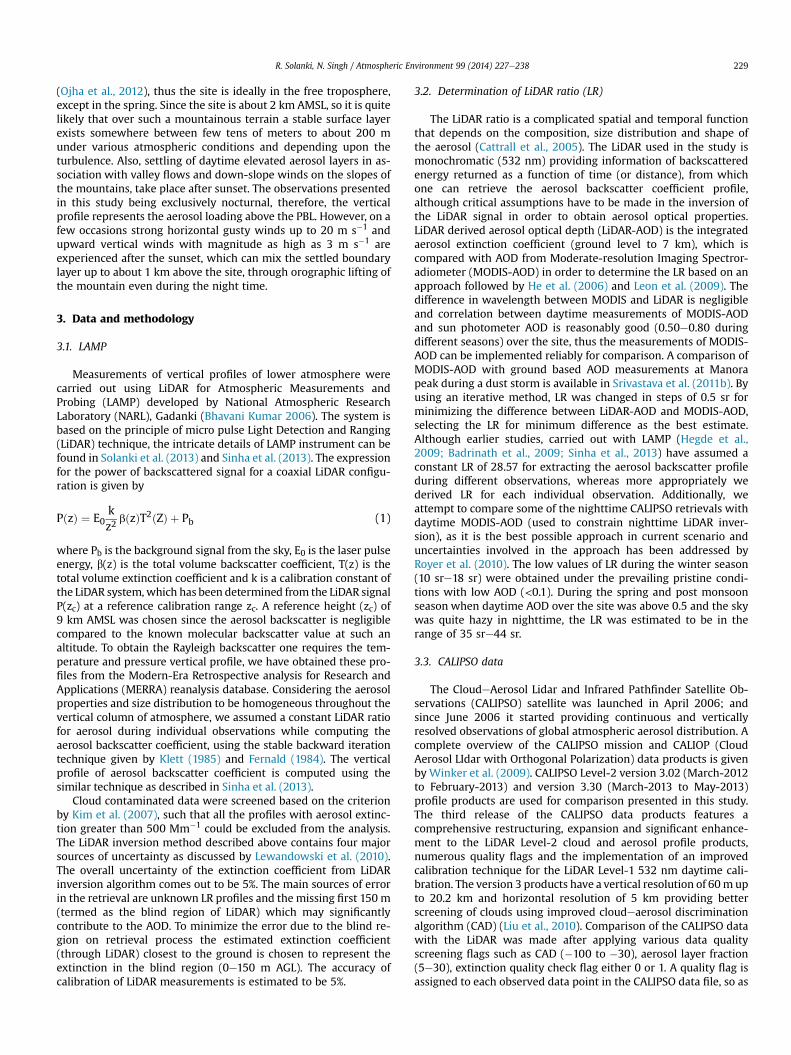
Fig. 1. (a) Geographical location (marked by yellow star) of observation site at Nainital andaround observation site Manora Peak, and the city of Nainital, in the Google earth imagery. (Fthe web version of this article.)

studied by Srivastava et al. (2012) during winter and summerseason. However, due to sparsity of the ground-based observations,such comparisonwith the satellite data is still severely lacking overHimalayan region. This comparison study over such a complexterrain would enable the CALIPSO satellite retrievals to be usedwith greater confidence over the Himalayas and the adjoining IGPregion. This study will also assist in quantifying the impact ofpollution on the climate and hydrological cycle of the Himalayas.

2. Site description

The observation site Manora Peak (29.36� N, 79.45� E), 1951 mabove mean sea level (AMSL), is situated at an aerial distance ofabout 2 km from the City of Nainital, in the North India as shown inFig. 1. Observations are being made at the peak of the mountainwith steep slopes on the east and west sides. To the south of thepeak, mountains gradually decrease in altitude and merge into asmall city called Haldwani, whereas in the North and North-Easthigher altitude mountains create complex topography. Overallimage of site reveals the complex terrain of the central Himalayas.The site is free from any major local source of aerosol or anthro-pogenic activities, hence, considered to be pristine (Sagar et al.,2004), but due to complex topography it has got a local boundarylayer (LBL) different from the planetary boundary layer (PBL). Theextensive measurements of the LBL height during different seasonsover this site are not available. However, the model simulatedaverage planetary boundary layer height at a nearby low altitudesite Pantnagar, does not evolve above 1.5 km, except in the springseasonwhen the average PBL or mixed layer height goes up to 4 km

nearest megacity Delhi (marked by red star), on the map of India (b) The topographyor interpretation of the references to color in this figure legend, the reader is referred to

R. Solanki, N. Singh / Atmospheric Environment 99 (2014) 227e238 229

(Ojha et al., 2012), thus the site is ideally in the free troposphere,except in the spring. Since the site is about 2 km AMSL, so it is quitelikely that over such a mountainous terrain a stable surface layerexists somewhere between few tens of meters to about 200 munder various atmospheric conditions and depending upon theturbulence. Also, settling of daytime elevated aerosol layers in as-sociation with valley flows and down-slope winds on the slopes ofthe mountains, take place after sunset. The observations presentedin this study being exclusively nocturnal, therefore, the verticalprofile represents the aerosol loading above the PBL. However, on afew occasions strong horizontal gusty winds up to 20 m s�1 andupward vertical winds with magnitude as high as 3 m s�1 areexperienced after the sunset, which can mix the settled boundarylayer up to about 1 km above the site, through orographic lifting ofthe mountain even during the night time.

3. Data and methodology

3.1. LAMP

Measurements of vertical profiles of lower atmosphere werecarried out using LiDAR for Atmospheric Measurements andProbing (LAMP) developed by National Atmospheric ResearchLaboratory (NARL), Gadanki (Bhavani Kumar 2006). The system isbased on the principle of micro pulse Light Detection and Ranging(LiDAR) technique, the intricate details of LAMP instrument can befound in Solanki et al. (2013) and Sinha et al. (2013). The expressionfor the power of backscattered signal for a coaxial LiDAR configu-ration is given by

PðzÞ ¼ E0kz2

bðzÞT2ðZÞ þ Pb (1)

where Pb is the background signal from the sky, E0 is the laser pulseenergy, b(z) is the total volume backscatter coefficient, T(z) is thetotal volume extinction coefficient and k is a calibration constant ofthe LiDAR system,which has been determined from the LiDAR signalP(zc) at a reference calibration range zc. A reference height (zc) of9 km AMSL was chosen since the aerosol backscatter is negligiblecompared to the known molecular backscatter value at such analtitude. To obtain the Rayleigh backscatter one requires the tem-perature and pressure vertical profile, we have obtained these pro-files from the Modern-Era Retrospective analysis for Research andApplications (MERRA) reanalysis database. Considering the aerosolproperties and size distribution to be homogeneous throughout thevertical column of atmosphere, we assumed a constant LiDAR ratiofor aerosol during individual observations while computing theaerosol backscatter coefficient, using the stable backward iterationtechnique given by Klett (1985) and Fernald (1984). The verticalprofile of aerosol backscatter coefficient is computed using thesimilar technique as described in Sinha et al. (2013).

Cloud contaminated data were screened based on the criterionby Kim et al. (2007), such that all the profiles with aerosol extinc-tion greater than 500 Mm�1 could be excluded from the analysis.The LiDAR inversion method described above contains four majorsources of uncertainty as discussed by Lewandowski et al. (2010).The overall uncertainty of the extinction coefficient from LiDARinversion algorithm comes out to be 5%. The main sources of errorin the retrieval are unknown LR profiles and the missing first 150 m(termed as the blind region of LiDAR) which may significantlycontribute to the AOD. To minimize the error due to the blind re-gion on retrieval process the estimated extinction coefficient(through LiDAR) closest to the ground is chosen to represent theextinction in the blind region (0e150 m AGL). The accuracy ofcalibration of LiDAR measurements is estimated to be 5%.

3.2. Determination of LiDAR ratio (LR)

The LiDAR ratio is a complicated spatial and temporal functionthat depends on the composition, size distribution and shape ofthe aerosol (Cattrall et al., 2005). The LiDAR used in the study ismonochromatic (532 nm) providing information of backscatteredenergy returned as a function of time (or distance), from whichone can retrieve the aerosol backscatter coefficient profile,although critical assumptions have to be made in the inversion ofthe LiDAR signal in order to obtain aerosol optical properties.LiDAR derived aerosol optical depth (LiDAR-AOD) is the integratedaerosol extinction coefficient (ground level to 7 km), which iscompared with AOD from Moderate-resolution Imaging Spectror-adiometer (MODIS-AOD) in order to determine the LR based on anapproach followed by He et al. (2006) and Leon et al. (2009). Thedifference in wavelength between MODIS and LiDAR is negligibleand correlation between daytime measurements of MODIS-AODand sun photometer AOD is reasonably good (0.50e0.80 duringdifferent seasons) over the site, thus the measurements of MODIS-AOD can be implemented reliably for comparison. A comparison ofMODIS-AOD with ground based AOD measurements at Manorapeak during a dust storm is available in Srivastava et al. (2011b). Byusing an iterative method, LR was changed in steps of 0.5 sr forminimizing the difference between LiDAR-AOD and MODIS-AOD,selecting the LR for minimum difference as the best estimate.Although earlier studies, carried out with LAMP (Hegde et al.,2009; Badrinath et al., 2009; Sinha et al., 2013) have assumed aconstant LR of 28.57 for extracting the aerosol backscatter profileduring different observations, whereas more appropriately wederived LR for each individual observation. Additionally, weattempt to compare some of the nighttime CALIPSO retrievals withdaytime MODIS-AOD (used to constrain nighttime LiDAR inver-sion), as it is the best possible approach in current scenario anduncertainties involved in the approach has been addressed byRoyer et al. (2010). The low values of LR during the winter season(10 sre18 sr) were obtained under the prevailing pristine condi-tions with low AOD (<0.1). During the spring and post monsoonseason when daytime AOD over the site was above 0.5 and the skywas quite hazy in nighttime, the LR was estimated to be in therange of 35 sre44 sr.

3.3. CALIPSO data

The CloudeAerosol Lidar and Infrared Pathfinder Satellite Ob-servations (CALIPSO) satellite was launched in April 2006; andsince June 2006 it started providing continuous and verticallyresolved observations of global atmospheric aerosol distribution. Acomplete overview of the CALIPSO mission and CALIOP (CloudAerosol LIdar with Orthogonal Polarization) data products is givenby Winker et al. (2009). CALIPSO Level-2 version 3.02 (March-2012to February-2013) and version 3.30 (March-2013 to May-2013)profile products are used for comparison presented in this study.The third release of the CALIPSO data products features acomprehensive restructuring, expansion and significant enhance-ment to the LiDAR Level-2 cloud and aerosol profile products,numerous quality flags and the implementation of an improvedcalibration technique for the LiDAR Level-1 532 nm daytime cali-bration. The version 3 products have a vertical resolution of 60m upto 20.2 km and horizontal resolution of 5 km providing betterscreening of clouds using improved cloudeaerosol discriminationalgorithm (CAD) (Liu et al., 2010). Comparison of the CALIPSO datawith the LiDAR was made after applying various data qualityscreening flags such as CAD (�100 to �30), aerosol layer fraction(5e30), extinction quality check flag either 0 or 1. A quality flag isassigned to each observed data point in the CALIPSO data file, so as

R. Solanki, N. Singh / Atmospheric Environment 99 (2014) 227e238230

not to modify the original observed data point, and still be able toassess its quality.

Over the period of study, a total number of 52 overpassesoccurred within a spatial distance of less than 220 km and a tem-poral difference of less than 18 h between our LiDAR and satelliteoverpass. However, previous studies (Tesche et al., 2013) haveconsidered spatial distances of 500 km for comparison purpose.According to Anderson et al. (2003), in PBL a 12 h of time differenceand 120 km of spatial difference is too far away to expect the PBLaerosol distribution to be similar, but since this comparison is beingmade 2 km AMSL, which is well above the PBL height, hence,assuming that we are comparing the free tropospheric column ofthe atmosphere, a high correlation can still be expected. Out of 52overpasses of satellite, 37 qualified for comparison, remaining 15cases were excluded due to unavailability of data and presence ofclouds over our LiDAR site. In order to compare an individualobservation, all profiles within the horizontal separation of 220 kmfrom LiDAR site, were averaged and interpolated to the verticalresolution of 15 m, equal to that of our LiDAR. Details of 37 casessubjected to the comparison are listed in Table 1.

4. Results and discussion

4.1. Inter-day variability

Intermittent LiDAR observations were conducted over the siteduring 89 nights in different seasons and details are given in

Table 1Days of LiDAR observations and CALIPSO overpasses (within 220 km distance) usedfor comparison.

S. No. LiDAR observationsdate

CALIPSO overpass details

Delay (h:min) Separation (km)

1 22-Mar-12 13:40 1972 24-Mar-12 2:00 1093 30-Mar-12 7:24 364 6-Apr-12 5:42 1335 23-Apr-12 14:48 1966 27-Apr-12 2:41 2187 30-Apr-12 15:31 328 24-May-12 6:05 1309 13-Jun-12 18:00 10610 25-Jun-12 6:18 13111 21-Sep-12 14:18 3312 26-Sep-12 16:45 5213 1-Oct-12 5:42 19614 11-Oct-12 4:29 4515 31-Oct-12 6:06 13716 1-Nov-12 7:37 19617 2-Nov-12 6:02 19618 17-Nov-12 17:54 19619 2-Dec-12 4:30 13420 5-Dec-12 3:55 11021 23-Dec-12 4:29 21922 25-Jan-13 17:06 21723 31-Jan-13 0:00 5024 7-Feb-13 1:02 12225 20-Feb-13 1:52 14726 25-Feb-13 4:09 20827 1-Mar-13 5:16 1828 4-Mar-13 2:26 4329 8-Mar-13 5:08 14530 11-Mar-13 3:43 11931 13-Mar-13 2:42 21432 5-Apr-13 2:53 4833 18-Apr-13 5:50 2834 21-Apr-13 3:17 5035 7-May-13 3:29 5936 13-May-13 6:01 20137 29-May-13 6:45 199

Table 2. A total of 32 nights were cloud contaminated and theseobservations were excluded from the analysis of aerosol verticaldistribution. Hence, for this study a total of 57 nights of LiDARobservations are analyzed and presented, with a seasonal aggregateof 17, 12, 11, and 17 nights in MAMJ-2012, SON-2012, DJF-2012e13and MAM-2013 respectively. Due to the presence of low altitudethick layer of monsoon clouds over the site the system is not usuallyoperated during JJA; however, at occasions under clear sky condi-tions in the month of June and July, 3 and 1 observationwere takenrespectively. Hence, these 4 days were combined with spring sea-son forming one group ofMAMJmonths. Fig. 2 depicts the inter-dayvariability over different seasons during the period of study. InMAMJ-2012 prominent inter-day variability is seen up to 3.5 kmwith aerosol backscatter of 3.0 (Mm sr)�1 in March and Aprilthough for the month of May backscatter is quite high and above10.0 (Mm sr)�1. In June and July the backscatter varies from 7.0(Mm sr)�1 before the arrival of monsoon at site to 2.3 (Mm sr)�1

after the onset of monsoon respectively. During the autumn seasonthe inter day variations are quite suppressed with all the verticalprofiles showing backscatter up to 1.5 (Mm sr)�1 from ground to3 km, except for the case of November 7, 2012 under prevailinghazy atmosphere over the site, leading to higher backscatter up to5.6 (Mm sr)�1. The winter season displays least variability fromday-to-day, with most of the profiles having backscatter coefficientbelow 1.0 (Mm sr)�1 except for 25 February which is nearly thebeginning of the spring season when the aerosol layer at 4 km isobserved with backscatter of 2.2 (Mm sr)�1. The spring season ofthe year 2013 shows reasonably lower aerosol loading in the at-mosphere and subdued inter day variability in comparison to thespring season of the year 2012. The lower aerosol loading could beexplained by the fact that, during MAM 2013 the region witnessedmany rainfall events about a period of every 10-days that occurreddue to western disturbances and prevented the buildup of aerosolloading in the vertical column of free troposphere. The maximumbackscatter of 4.7 (Mm sr)�1 is observed on 21 April 2013 at 4 km inthe spring season. Significant loading is seen in the column up to5.5 km during spring of 2012 and 2013 as well, which could beascribed to the eastward transport of west Asian aerosols, andincreased convective mixing in the nearby lower plains adjacent tothe site.

4.2. Air mass back trajectory analysis

In order to attribute the possible sources of aerosol at differentaltitudes of vertical profile we analyzed 7-day iso-sigma back airtrajectory simulated using the Hybrid Single Particle Lagrangian

Table 2Number of observations in a month and total hours of LiDAR operation at ManoraPeak, Nainital.

Months Observations Duration (h)

March-2012 9 30.83April-2012 8 35.93May-2012 7 21.17June-2012 4 8.87July2012 1 2.67August-2012 0 0September-2012 3 9.17October-2012 5 17.03November-2012 7 29.83December-2012 10 51.98January-2013 7 38.15Feburuary-2013 6 28.83March-2013 7 29.4April-2013 8 30.13May-2013 7 26.38

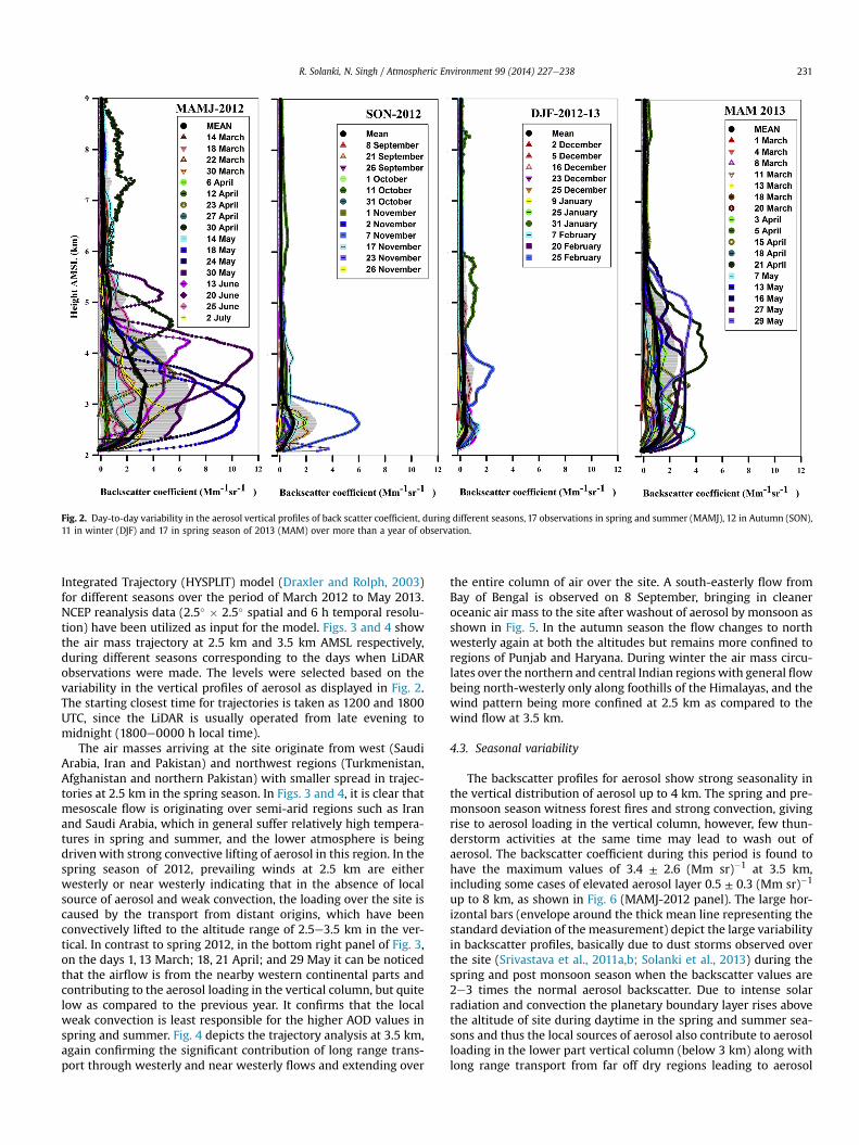
Fig. 2. Day-to-day variability in the aerosol vertical profiles of back scatter coefficient, during different seasons, 17 observations in spring and summer (MAMJ), 12 in Autumn (SON),11 in winter (DJF) and 17 in spring season of 2013 (MAM) over more than a year of observation.

R. Solanki, N. Singh / Atmospheric Environment 99 (2014) 227e238 231

Integrated Trajectory (HYSPLIT) model (Draxler and Rolph, 2003)for different seasons over the period of March 2012 to May 2013.NCEP reanalysis data (2.5� � 2.5� spatial and 6 h temporal resolu-tion) have been utilized as input for the model. Figs. 3 and 4 showthe air mass trajectory at 2.5 km and 3.5 km AMSL respectively,during different seasons corresponding to the days when LiDARobservations were made. The levels were selected based on thevariability in the vertical profiles of aerosol as displayed in Fig. 2.The starting closest time for trajectories is taken as 1200 and 1800UTC, since the LiDAR is usually operated from late evening tomidnight (1800e0000 h local time).

The air masses arriving at the site originate from west (SaudiArabia, Iran and Pakistan) and northwest regions (Turkmenistan,Afghanistan and northern Pakistan) with smaller spread in trajec-tories at 2.5 km in the spring season. In Figs. 3 and 4, it is clear thatmesoscale flow is originating over semi-arid regions such as Iranand Saudi Arabia, which in general suffer relatively high tempera-tures in spring and summer, and the lower atmosphere is beingdrivenwith strong convective lifting of aerosol in this region. In thespring season of 2012, prevailing winds at 2.5 km are eitherwesterly or near westerly indicating that in the absence of localsource of aerosol and weak convection, the loading over the site iscaused by the transport from distant origins, which have beenconvectively lifted to the altitude range of 2.5e3.5 km in the ver-tical. In contrast to spring 2012, in the bottom right panel of Fig. 3,on the days 1, 13 March; 18, 21 April; and 29 May it can be noticedthat the airflow is from the nearby western continental parts andcontributing to the aerosol loading in the vertical column, but quitelow as compared to the previous year. It confirms that the localweak convection is least responsible for the higher AOD values inspring and summer. Fig. 4 depicts the trajectory analysis at 3.5 km,again confirming the significant contribution of long range trans-port through westerly and near westerly flows and extending over

the entire column of air over the site. A south-easterly flow fromBay of Bengal is observed on 8 September, bringing in cleaneroceanic air mass to the site after washout of aerosol by monsoon asshown in Fig. 5. In the autumn season the flow changes to northwesterly again at both the altitudes but remains more confined toregions of Punjab and Haryana. During winter the air mass circu-lates over the northern and central Indian regions with general flowbeing north-westerly only along foothills of the Himalayas, and thewind pattern being more confined at 2.5 km as compared to thewind flow at 3.5 km.

4.3. Seasonal variability

The backscatter profiles for aerosol show strong seasonality inthe vertical distribution of aerosol up to 4 km. The spring and pre-monsoon season witness forest fires and strong convection, givingrise to aerosol loading in the vertical column, however, few thun-derstorm activities at the same time may lead to wash out ofaerosol. The backscatter coefficient during this period is found tohave the maximum values of 3.4 ± 2.6 (Mm sr)�1 at 3.5 km,including some cases of elevated aerosol layer 0.5 ± 0.3 (Mm sr)�1

up to 8 km, as shown in Fig. 6 (MAMJ-2012 panel). The large hor-izontal bars (envelope around the thick mean line representing thestandard deviation of the measurement) depict the large variabilityin backscatter profiles, basically due to dust storms observed overthe site (Srivastava et al., 2011a,b; Solanki et al., 2013) during thespring and post monsoon season when the backscatter values are2e3 times the normal aerosol backscatter. Due to intense solarradiation and convection the planetary boundary layer rises abovethe altitude of site during daytime in the spring and summer sea-sons and thus the local sources of aerosol also contribute to aerosolloading in the lower part vertical column (below 3 km) along withlong range transport from far off dry regions leading to aerosol

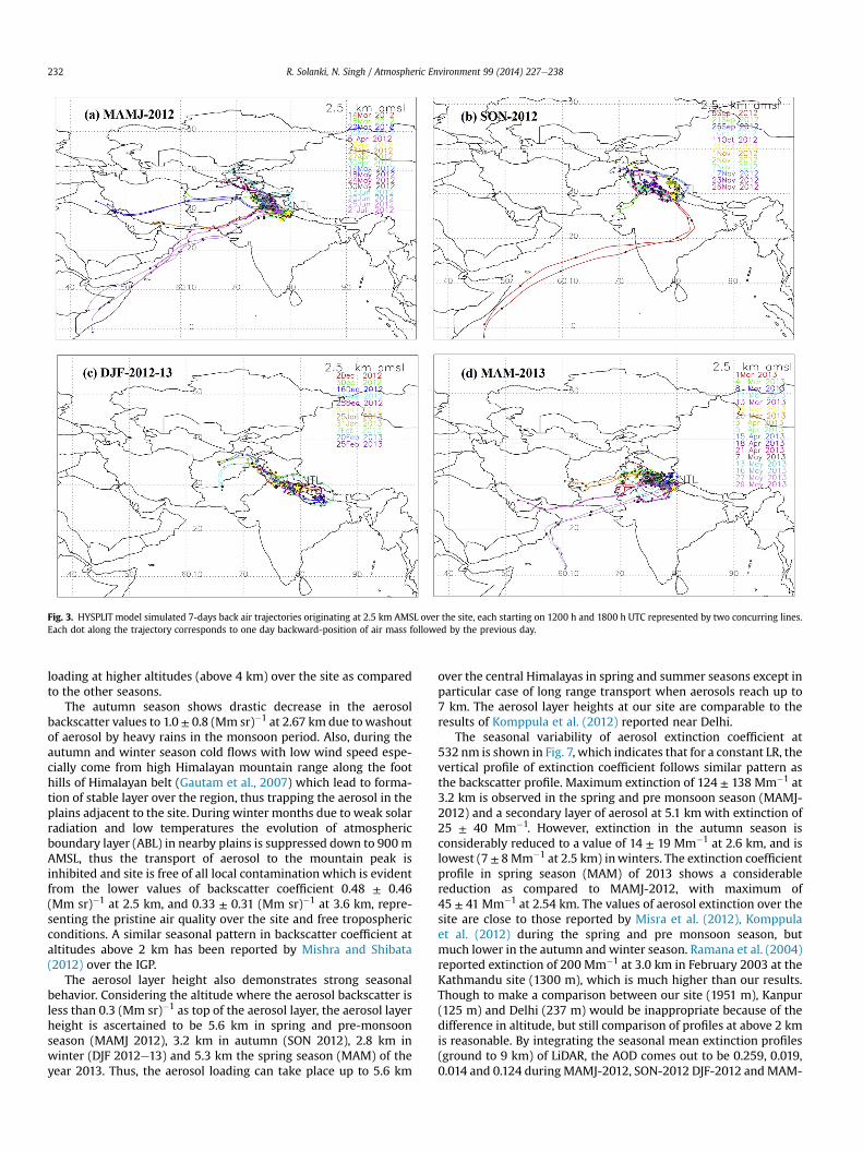
Fig. 3. HYSPLIT model simulated 7-days back air trajectories originating at 2.5 km AMSL over the site, each starting on 1200 h and 1800 h UTC represented by two concurring lines.Each dot along the trajectory corresponds to one day backward-position of air mass followed by the previous day.

R. Solanki, N. Singh / Atmospheric Environment 99 (2014) 227e238232

loading at higher altitudes (above 4 km) over the site as comparedto the other seasons.

The autumn season shows drastic decrease in the aerosolbackscatter values to 1.0 ± 0.8 (Mm sr)�1 at 2.67 km due towashoutof aerosol by heavy rains in the monsoon period. Also, during theautumn and winter season cold flows with low wind speed espe-cially come from high Himalayan mountain range along the foothills of Himalayan belt (Gautam et al., 2007) which lead to forma-tion of stable layer over the region, thus trapping the aerosol in theplains adjacent to the site. During winter months due to weak solarradiation and low temperatures the evolution of atmosphericboundary layer (ABL) in nearby plains is suppressed down to 900mAMSL, thus the transport of aerosol to the mountain peak isinhibited and site is free of all local contamination which is evidentfrom the lower values of backscatter coefficient 0.48 ± 0.46(Mm sr)�1 at 2.5 km, and 0.33 ± 0.31 (Mm sr)�1 at 3.6 km, repre-senting the pristine air quality over the site and free troposphericconditions. A similar seasonal pattern in backscatter coefficient ataltitudes above 2 km has been reported by Mishra and Shibata(2012) over the IGP.

The aerosol layer height also demonstrates strong seasonalbehavior. Considering the altitude where the aerosol backscatter isless than 0.3 (Mm sr)�1 as top of the aerosol layer, the aerosol layerheight is ascertained to be 5.6 km in spring and pre-monsoonseason (MAMJ 2012), 3.2 km in autumn (SON 2012), 2.8 km inwinter (DJF 2012e13) and 5.3 km the spring season (MAM) of theyear 2013. Thus, the aerosol loading can take place up to 5.6 km

over the central Himalayas in spring and summer seasons except inparticular case of long range transport when aerosols reach up to7 km. The aerosol layer heights at our site are comparable to theresults of Komppula et al. (2012) reported near Delhi.

The seasonal variability of aerosol extinction coefficient at532 nm is shown in Fig. 7, which indicates that for a constant LR, thevertical profile of extinction coefficient follows similar pattern asthe backscatter profile. Maximum extinction of 124 ± 138 Mm�1 at3.2 km is observed in the spring and pre monsoon season (MAMJ-2012) and a secondary layer of aerosol at 5.1 km with extinction of25 ± 40 Mm�1. However, extinction in the autumn season isconsiderably reduced to a value of 14 ± 19 Mm�1 at 2.6 km, and islowest (7 ± 8Mm�1 at 2.5 km) inwinters. The extinction coefficientprofile in spring season (MAM) of 2013 shows a considerablereduction as compared to MAMJ-2012, with maximum of45 ± 41 Mm�1 at 2.54 km. The values of aerosol extinction over thesite are close to those reported by Misra et al. (2012), Komppulaet al. (2012) during the spring and pre monsoon season, butmuch lower in the autumn and winter season. Ramana et al. (2004)reported extinction of 200 Mm�1 at 3.0 km in February 2003 at theKathmandu site (1300 m), which is much higher than our results.Though to make a comparison between our site (1951 m), Kanpur(125 m) and Delhi (237 m) would be inappropriate because of thedifference in altitude, but still comparison of profiles at above 2 kmis reasonable. By integrating the seasonal mean extinction profiles(ground to 9 km) of LiDAR, the AOD comes out to be 0.259, 0.019,0.014 and 0.124 during MAMJ-2012, SON-2012 DJF-2012 andMAM-

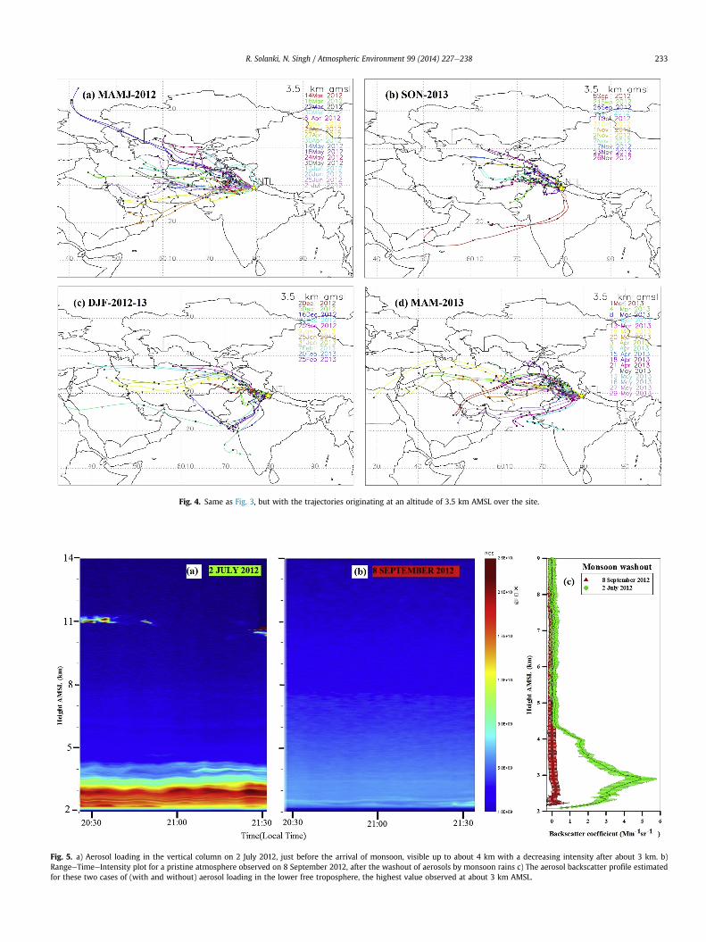
Fig. 4. Same as Fig. 3, but with the trajectories originating at an altitude of 3.5 km AMSL over the site.

Fig. 5. a) Aerosol loading in the vertical column on 2 July 2012, just before the arrival of monsoon, visible up to about 4 km with a decreasing intensity after about 3 km. b)RangeeTimeeIntensity plot for a pristine atmosphere observed on 8 September 2012, after the washout of aerosols by monsoon rains c) The aerosol backscatter profile estimatedfor these two cases of (with and without) aerosol loading in the lower free troposphere, the highest value observed at about 3 km AMSL.

R. Solanki, N. Singh / Atmospheric Environment 99 (2014) 227e238 233

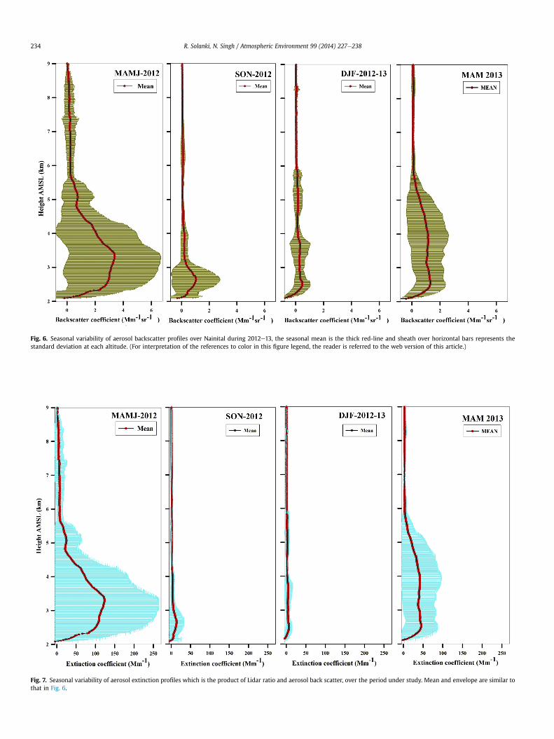
Fig. 6. Seasonal variability of aerosol backscatter profiles over Nainital during 2012e13, the seasonal mean is the thick red-line and sheath over horizontal bars represents thestandard deviation at each altitude. (For interpretation of the references to color in this figure legend, the reader is referred to the web version of this article.)

Fig. 7. Seasonal variability of aerosol extinction profiles which is the product of Lidar ratio and aerosol back scatter, over the period under study. Mean and envelope are similar tothat in Fig. 6.

R. Solanki, N. Singh / Atmospheric Environment 99 (2014) 227e238234

R. Solanki, N. Singh / Atmospheric Environment 99 (2014) 227e238 235

2013 respectively. The extinction profiles were constrained usingthe MODIS-AOD; hence these values are a direct function of theMODIS measurements.

4.4. Comparison with satellite observations

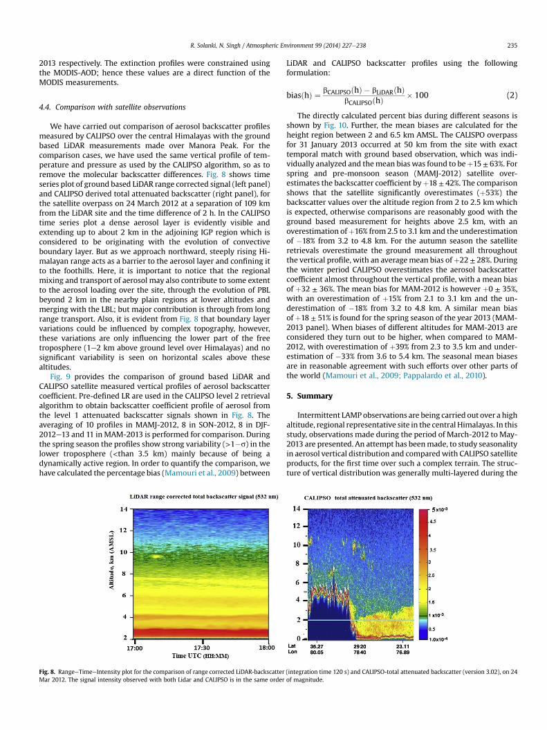
We have carried out comparison of aerosol backscatter profilesmeasured by CALIPSO over the central Himalayas with the groundbased LiDAR measurements made over Manora Peak. For thecomparison cases, we have used the same vertical profile of tem-perature and pressure as used by the CALIPSO algorithm, so as toremove the molecular backscatter differences. Fig. 8 shows timeseries plot of ground based LiDAR range corrected signal (left panel)and CALIPSO derived total attenuated backscatter (right panel), forthe satellite overpass on 24 March 2012 at a separation of 109 kmfrom the LiDAR site and the time difference of 2 h. In the CALIPSOtime series plot a dense aerosol layer is evidently visible andextending up to about 2 km in the adjoining IGP region which isconsidered to be originating with the evolution of convectiveboundary layer. But as we approach northward, steeply rising Hi-malayan range acts as a barrier to the aerosol layer and confining itto the foothills. Here, it is important to notice that the regionalmixing and transport of aerosol may also contribute to some extentto the aerosol loading over the site, through the evolution of PBLbeyond 2 km in the nearby plain regions at lower altitudes andmerging with the LBL; but major contribution is through from longrange transport. Also, it is evident from Fig. 8 that boundary layervariations could be influenced by complex topography, however,these variations are only influencing the lower part of the freetroposphere (1e2 km above ground level over Himalayas) and nosignificant variability is seen on horizontal scales above thesealtitudes.

Fig. 9 provides the comparison of ground based LiDAR andCALIPSO satellite measured vertical profiles of aerosol backscattercoefficient. Pre-defined LR are used in the CALIPSO level 2 retrievalalgorithm to obtain backscatter coefficient profile of aerosol fromthe level 1 attenuated backscatter signals shown in Fig. 8. Theaveraging of 10 profiles in MAMJ-2012, 8 in SON-2012, 8 in DJF-2012e13 and 11 in MAM-2013 is performed for comparison. Duringthe spring season the profiles show strong variability (>1�s) in thelower troposphere (<than 3.5 km) mainly because of being adynamically active region. In order to quantify the comparison, wehave calculated the percentage bias (Mamouri et al., 2009) between

Fig. 8. RangeeTimeeIntensity plot for the comparison of range corrected LiDAR-backscatterMar 2012. The signal intensity observed with both Lidar and CALIPSO is in the same order

LiDAR and CALIPSO backscatter profiles using the followingformulation:

biasðhÞ ¼ bCALIPSOðhÞ � bLiDARðhÞbCALIPSOðhÞ

� 100 (2)

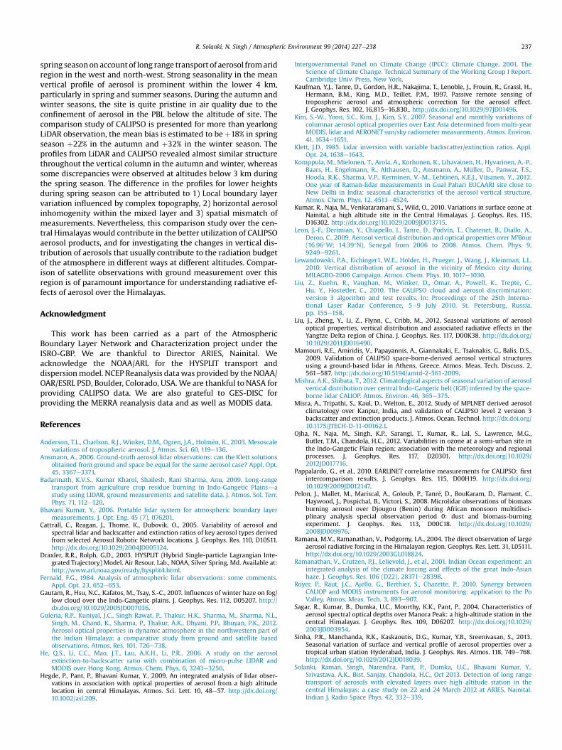
The directly calculated percent bias during different seasons isshown by Fig. 10. Further, the mean biases are calculated for theheight region between 2 and 6.5 km AMSL. The CALISPO overpassfor 31 January 2013 occurred at 50 km from the site with exacttemporal match with ground based observation, which was indi-vidually analyzed and themean bias was found to beþ15 ± 63%. Forspring and pre-monsoon season (MAMJ-2012) satellite over-estimates the backscatter coefficient byþ18 ± 42%. The comparisonshows that the satellite significantly overestimates (þ53%) thebackscatter values over the altitude region from 2 to 2.5 km whichis expected, otherwise comparisons are reasonably good with theground based measurement for heights above 2.5 km, with anoverestimation ofþ16% from 2.5 to 3.1 km and the underestimationof �18% from 3.2 to 4.8 km. For the autumn season the satelliteretrievals overestimate the ground measurement all throughoutthe vertical profile, with an averagemean bias ofþ22 ± 28%. Duringthe winter period CALIPSO overestimates the aerosol backscattercoefficient almost throughout the vertical profile, with a mean biasof þ32 ± 36%. The mean bias for MAM-2012 is however þ0 ± 35%,with an overestimation of þ15% from 2.1 to 3.1 km and the un-derestimation of �18% from 3.2 to 4.8 km. A similar mean biasofþ18 ± 51% is found for the spring season of the year 2013 (MAM-2013 panel). When biases of different altitudes for MAM-2013 areconsidered they turn out to be higher, when compared to MAM-2012, with overestimation of þ39% from 2.3 to 3.5 km and under-estimation of �33% from 3.6 to 5.4 km. The seasonal mean biasesare in reasonable agreement with such efforts over other parts ofthe world (Mamouri et al., 2009; Pappalardo et al., 2010).

5. Summary

Intermittent LAMP observations are being carried out over a highaltitude, regional representative site in the central Himalayas. In thisstudy, observations made during the period of March-2012 to May-2013 are presented. An attempt has beenmade, to study seasonalityin aerosol vertical distribution and comparedwith CALIPSO satelliteproducts, for the first time over such a complex terrain. The struc-ture of vertical distribution was generally multi-layered during the

(integration time 120 s) and CALIPSO-total attenuated backscatter (version 3.02), on 24of magnitude.

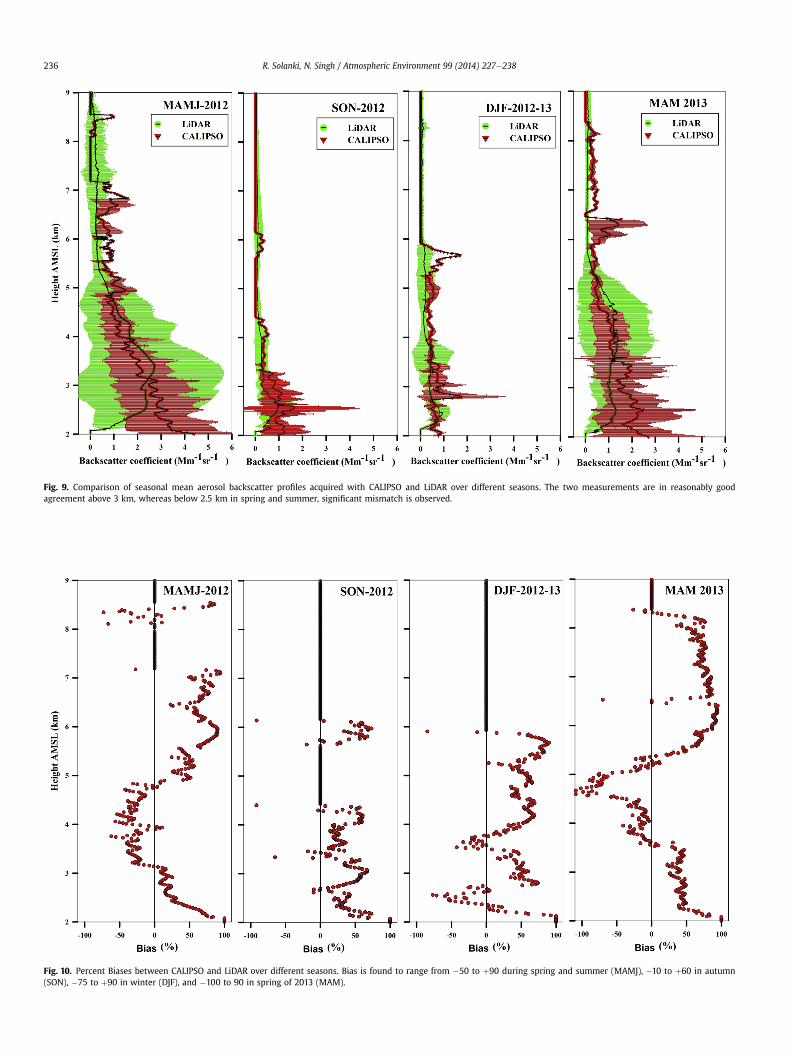
Fig. 10. Percent Biases between CALIPSO and LiDAR over different seasons. Bias is found to range from �50 to þ90 during spring and summer (MAMJ), �10 to þ60 in autumn(SON), �75 to þ90 in winter (DJF), and �100 to 90 in spring of 2013 (MAM).

Fig. 9. Comparison of seasonal mean aerosol backscatter profiles acquired with CALIPSO and LiDAR over different seasons. The two measurements are in reasonably goodagreement above 3 km, whereas below 2.5 km in spring and summer, significant mismatch is observed.

R. Solanki, N. Singh / Atmospheric Environment 99 (2014) 227e238236

R. Solanki, N. Singh / Atmospheric Environment 99 (2014) 227e238 237

spring seasonon accountof long range transport of aerosol fromaridregion in the west and north-west. Strong seasonality in the meanvertical profile of aerosol is prominent within the lower 4 km,particularly in spring and summer seasons. During the autumn andwinter seasons, the site is quite pristine in air quality due to theconfinement of aerosol in the PBL below the altitude of site. Thecomparison study of CALIPSO is presented for more than yearlongLiDAR observation, the mean bias is estimated to be þ18% in springseason þ22% in the autumn and þ32% in the winter season. Theprofiles from LiDAR and CALIPSO revealed almost similar structurethroughout the vertical column in the autumn and winter, whereassome discrepancies were observed at altitudes below 3 km duringthe spring season. The difference in the profiles for lower heightsduring spring season can be attributed to 1) Local boundary layervariation influenced by complex topography, 2) horizontal aerosolinhomogenity within the mixed layer and 3) spatial mismatch ofmeasurements. Nevertheless, this comparison study over the cen-tral Himalayas would contribute in the better utilization of CALIPSOaerosol products, and for investigating the changes in vertical dis-tribution of aerosols that usually contribute to the radiation budgetof the atmosphere in different ways at different altitudes. Compar-ison of satellite observations with ground measurement over thisregion is of paramount importance for understanding radiative ef-fects of aerosol over the Himalayas.

Acknowledgment

This work has been carried as a part of the AtmosphericBoundary Layer Network and Characterization project under theISRO-GBP. We are thankful to Director ARIES, Nainital. Weacknowledge the NOAA/ARL for the HYSPLIT transport anddispersionmodel. NCEP Reanalysis datawas provided by the NOAA/OAR/ESRL PSD, Boulder, Colorado, USA.We are thankful to NASA forproviding CALIPSO data. We are also grateful to GES-DISC forproviding the MERRA reanalysis data and as well as MODIS data.

References

Anderson, T.L., Charlson, R.J., Winker, D.M., Ogren, J.A., Holm�en, K., 2003. Mesoscalevariations of tropospheric aerosol. J. Atmos. Sci. 60, 119e136.

Ansmann, A., 2006. Ground-truth aerosol lidar observations: can the Klett solutionsobtained from ground and space be equal for the same aerosol case? Appl. Opt.45, 3367e3371.

Badarinath, K.V.S., Kumar Kharol, Shailesh, Rani Sharma, Anu, 2009. Long-rangetransport from agriculture crop residue burning in Indo-Gangetic Plainsdastudy using LIDAR, ground measurements and satellite data. J. Atmos. Sol. Terr.Phys. 71, 112e120.

Bhavani Kumar, Y., 2006. Portable lidar system for atmospheric boundary layermeasurements. J. Opt. Eng. 45 (7), 076201.

Cattrall, C., Reagan, J., Thome, K., Dubovik, O., 2005. Variability of aerosol andspectral lidar and backscatter and extinction ratios of key aerosol types derivedfrom selected Aerosol Robotic Network locations. J. Geophys. Res. 110, D10S11.http://dx.doi.org/10.1029/2004JD005124.

Draxler, R.R., Rolph, G.D., 2003. HYSPLIT (Hybrid Single-particle Lagrangian Inte-grated Trajectory) Model. Air Resour. Lab., NOAA, Silver Spring, Md. Available at:http://www.arl.noaa.gov/ready/hysplit4.html.

Fernald, F.G., 1984. Analysis of atmospheric lidar observations: some comments.Appl. Opt. 23, 652e653.

Gautam, R., Hsu, N.C., Kafatos, M., Tsay, S.-C., 2007. Influences of winter haze on fog/low cloud over the Indo-Gangetic plains. J. Geophys. Res. 112, D05207. http://dx.doi.org/10.1029/2005JD007036.

Guleria, R.P., Kuniyal, J.C., Singh Rawat, P., Thakur, H.K., Sharma, M., Sharma, N.L.,Singh, M., Chand, K., Sharma, P., Thakur, A.K., Dhyani, P.P., Bhuyan, P.K., 2012.Aerosol optical properties in dynamic atmosphere in the northwestern part ofthe Indian Himalaya: a comparative study from ground and satellite basedobservations. Atmos. Res. 101, 726e738.

He, Q.S., Li, C.C., Mao, J.T., Lau, A.K.H., Li, P.R., 2006. A study on the aerosolextinction-to-backscatter ratio with combination of micro-pulse LIDAR andMODIS over Hong Kong. Atmos. Chem. Phys. 6, 3243e3256.

Hegde, P., Pant, P., Bhavani Kumar, Y., 2009. An integrated analysis of lidar obser-vations in association with optical properties of aerosol from a high altitudelocation in central Himalayas. Atmos. Sci. Lett. 10, 48e57. http://dx.doi.org/10.1002/asl.209.

Intergovernmental Panel on Climate Change (IPCC): Climate Change, 2001. TheScience of Climate Change. Technical Summary of the Working Group I Report.Cambridge Univ. Press, New York.

Kaufman, Y.J., Tanre, D., Gordon, H.R., Nakajima, T., Lenoble, J., Frouin, R., Grassl, H.,Hermann, B.M., King, M.D., Teillet, P.M., 1997. Passive remote sensing oftropospheric aerosol and atmospheric correction for the aerosol effect.J. Geophys. Res. 102, 16,815e16,830,. http://dx.doi.org/10.1029/97JD01496.

Kim, S.-W., Yoon, S.C., Kim, J., Kim, S.Y., 2007. Seasonal and monthly variations ofcolumnar aerosol optical properties over East Asia determined from multi-yearMODIS, lidar and AERONET sun/sky radiometer measurements. Atmos. Environ.41, 1634e1651.

Klett, J.D., 1985. Lidar inversion with variable backscatter/extinction ratios. Appl.Opt. 24, 1638e1643.

Komppula, M., Mielonen, T., Arola, A., Korhonen, K., Lihavainen, H., Hyvarinen, A.-P.,Baars, H., Engelmann, R., Althausen, D., Ansmann, A., Müller, D., Panwar, T.S.,Hooda, R.K., Sharma, V.P., Kerminen, V.-M., Lehtinen, K.E.J., Viisanen, Y., 2012.One year of Raman-lidar measurements in Gual Pahari EUCAARI site close toNew Delhi in India: seasonal characteristics of the aerosol vertical structure.Atmos. Chem. Phys. 12, 4513e4524.

Kumar, R., Naja, M., Venkataramani, S., Wild, O., 2010. Variations in surface ozone atNainital, a high altitude site in the Central Himalayas. J. Geophys. Res. 115,D16302. http://dx.doi.org/10.1029/2009JD013715.

Leon, J.-F., Derimian, Y., Chiapello, I., Tanre, D., Podvin, T., Chatenet, B., Diallo, A.,Deroo, C., 2009. Aerosol vertical distribution and optical properties over M'Bour(16.96�W; 14.39�N), Senegal from 2006 to 2008. Atmos. Chem. Phys. 9,9249e9261.

Lewandowski, P.A., Eichinger1, W.E., Holder, H., Prueger, J., Wang, J., Kleinman, L.I.,2010. Vertical distribution of aerosol in the vicinity of Mexico city duringMILAGRO-2006 Campaign. Atmos. Chem. Phys. 10, 1017e1030.

Liu, Z., Kuehn, R., Vaughan, M., Winker, D., Omar, A., Powell, K., Trepte, C.,Hu, Y., Hostetler, C., 2010. The CALIPSO cloud and aerosol discrimination:version 3 algorithm and test results. In: Proceedings of the 25th Interna-tional Laser Radar Conference, 5e9 July 2010, St. Petersburg, Russia,pp. 155e158.

Liu, J., Zheng, Y., Li, Z., Flynn, C., Cribb, M., 2012. Seasonal variations of aerosoloptical properties, vertical distribution and associated radiative effects in theYangtze Delta region of China. J. Geophys. Res. 117, D00K38. http://dx.doi.org/10.1029/2011JD016490.

Mamouri, R.E., Amiridis, V., Papayannis, A., Giannakaki, E., Tsaknakis, G., Balis, D.S.,2009. Validation of CALIPSO space-borne-derived aerosol vertical structuresusing a ground-based lidar in Athens, Greece. Atmos. Meas. Tech. Discuss. 2,561e587. http://dx.doi.org/10.5194/amtd-2-561-2009.

Mishra, A.K., Shibata, T., 2012. Climatological aspects of seasonal variation of aerosolvertical distribution over central Indo-Gangetic belt (IGB) inferred by the space-borne lidar CALIOP. Atmos. Environ. 46, 365e375.

Misra, A., Tripathi, S., Kaul, D., Welton, E., 2012. Study of MPLNET derived aerosolclimatology over Kanpur, India, and validation of CALIPSO level 2 version 3backscatter and extinction products. J. Atmos. Ocean. Technol. http://dx.doi.org/10.1175/JTECH-D-11-00162.1.

Ojha, N., Naja, M., Singh, K.P., Sarangi, T., Kumar, R., Lal, S., Lawrence, M.G.,Butler, T.M., Chandola, H.C., 2012. Variabilities in ozone at a semi-urban site inthe Indo-Gangetic Plain region: association with the meteorology and regionalprocesses. J. Geophys. Res. 117, D20301. http://dx.doi.org/10.1029/2012JD017716.

Pappalardo, G., et al., 2010. EARLINET correlative measurements for CALIPSO: firstintercomparison results. J. Geophys. Res. 115, D00H19. http://dx.doi.org/10.1029/2009JD012147.

Pelon, J., Mallet, M., Mariscal, A., Goloub, P., Tanr�e, D., BouKaram, D., Flamant, C.,Haywood, J., Pospichal, B., Victori, S., 2008. Microlidar observations of biomassburning aerosol over Djougou (Benin) during African monsoon multidisci-plinary analysis special observation period 0: dust and biomass-burningexperiment. J. Geophys. Res. 113, D00C18. http://dx.doi.org/10.1029/2008JD009976.

Ramana, M.V., Ramanathan, V., Podgorny, I.A., 2004. The direct observation of largeaerosol radiative forcing in the Himalayan region. Geophys. Res. Lett. 31, L05111.http://dx.doi.org/10.1029/2003GL018824.

Ramanathan, V., Crutzen, P.J., Lelieveld, J., et al., 2001. Indian Ocean experiment: anintegrated analysis of the climate forcing and effects of the great Indo-Asianhaze. J. Geophys. Res. 106 (D22), 28371e28398.

Royer, P., Raut, J.C., Ajello, G., Berthier, S., Chazette, P., 2010. Synergy betweenCALIOP and MODIS instruments for aerosol monitoring: application to the PoValley. Atmos. Meas. Tech. 3, 893e907.

Sagar, R., Kumar, B., Dumka, U.C., Moorthy, K.K., Pant, P., 2004. Characteristics ofaerosol spectral optical depths over Manora Peak: a high-altitude station in thecentral Himalayas. J. Geophys. Res. 109, D06207. http://dx.doi.org/10.1029/2003JD003954.

Sinha, P.R., Manchanda, R.K., Kaskaoutis, D.G., Kumar, Y.B., Sreenivasan, S., 2013.Seasonal variation of surface and vertical profile of aerosol properties over atropical urban station Hyderabad, India. J. Geophys. Res. Atmos. 118, 749e768.http://dx.doi.org/10.1029/2012JD018039.

Solanki, Raman, Singh, Narendra, Pant, P., Dumka, U.C., Bhavani Kumar, Y.,Srivastava, A.K., Bist, Sanjay, Chandola, H.C., Oct 2013. Detection of long rangetransport of aerosols with elevated layers over high altitude station in thecentral Himalayas: a case study on 22 and 24 March 2012 at ARIES, Nainital.Indian J. Radio Space Phys. 42, 332e339.

R. Solanki, N. Singh / Atmospheric Environment 99 (2014) 227e238238

Srivastava, A.K., Singh, S., Tiwari, S., Kanawade, V.P., Bisht, D.S., 2012. Variationbetween near-surface and columnar aerosol characteristics during winters andsummers at a station in the Indo-Gangetic Basin. J. Atmos. Sol. Terr. Phys. 77,57e66. http://dx.doi.org/10.1016/j.jastp.2011.11.009.

Srivastava, A.K., Pant, P., Hegde, P., Singh, S., Dumka, U.C., Naja, M., Singh, N., Bhavanikumar, Y., 2011a. Influence of southAsiandust stormonaerosol radiative forcing at ahigh-altitude station in central Himalayas. Int. J. Remote Sens. 32 (22), 7827e7845.

Srivastava, S.K., Srivastava, M.K., Saha, A., Tiwari, S., Singh, S., Dumka, U.C.,Singh, B.P., Singh, N.P., 2011b. Aerosol optical properties over Delhi and Manorapeak during a rare dust event in early April 2005. Int. J. Remote Sens. 32 (23),7939e7954.

Twomey, S., 1977. The influence of pollution on the short-wave albedo of clouds.J. Atmos. Sci. 34, 1149e1152.

Tesche, M., Wandinger, U., Ansmann, A., Althausen, D., Müller, D., Omar, A.H., 2013.Ground-based validation of CALIPSO observations of dust and smoke in theCape Verde region. J. Geophys. Res. Atmos. 118, 2889e2902. http://dx.doi.org/10.1002/jgrd.50248.

Winker, David M., Vaughan, Mark A., Ali, Omar, Hu, Yongxiang, Powell, Kathleen A.,Liu, Zhaoyan, Hunt, William H., Young, Stuart A., 2009. Overview of the CALIPSOMission and CALIOP data processing algorithms. J. Atmos. Ocean. Technol. 26,2310e2323.