On ramified covers of the projective plane I: Segre's theory and classification in small degrees,...
48
arXiv:0903.3359v7 [math.AG] 31 Jul 2010 ON RAMIFIED COVERS OF THE PROJECTIVE PLANE I: SEGRE’S THEORY AND CLASSIFICATION IN SMALL DEGREES (WITH AN APPENDIX BY EUGENII SHUSTIN) MICHAEL FRIEDMAN AND MAXIM LEYENSON 1 Abstract. We study ramified covers of the projective plane P 2 . Given a smooth surface S in P n and a generic enough projection P n → P 2 , we get a cover π : S → P 2 , which is ramified over a plane curve B. The curve B is usually singular, but is classically known to have only cusps and nodes as singularities for a generic projection. Several questions arise: First, What is the geography of branch curves among all cuspidal-nodal curves? And second, what is the geometry of branch curves; i.e., how can one distinguish a branch curve from a non-branch curve with the same numerical invariants? For example, a plane sextic with six cusps is known to be a branch curve of a generic projection iff its six cusps lie on a conic curve, i.e., form a special 0-cycle on the plane. We start with reviewing what is known about the answers to these questions, both simple and some non-trivial results. Secondly, the classical work of Beniamino Segre gives a complete answer to the second question in the case when S is a smooth surface in P 3 . We give an interpretation of the work of Segre in terms of relation between Picard and Chow groups of 0-cycles on a singular plane curve B. We also review examples of small degree. In addition, the Appendix written by E. Shustin shows the existence of new Zariski pairs. Contents 1. Introduction 2 2. Ramified covers 3 2.1. ´ Etale covers 3 2.2. Ramified covers of complex analytic spaces 3 2.3. Ramified covers of P 2 4 3. Moduli of branch curves and their geography 4 3.1. Severi-Enriques varieties of nodal-cuspidal curves 5 3.2. Geography of branch curves 7 3.3. Construction of the variety of branch curves B(d,c,n) 11 4. Surfaces in P 3 13 4.1. Smooth surfaces in P 3 13 4.2. Adjoint curves to the branch curve 16 4.3. Adjoint curves and Linear systems 19 4.4. Segre’s theorem 24 4.5. Special 0-cycles 28 4.6. Dimension of B(d,c,n) 29 4.7. Projecting surfaces with ordinary singularities. 30 5. Classification of singular branch curves in small degrees 34 6. Appendix A : New Zariski pairs (By Eugenii Shustin) 38 6.1. Introduction 38 1 This work is partially supported by the Emmy Noether Research Institute for Mathematics (center of the Minerva Foundation of Germany), the Excellency Center “Group Theoretic Methods in the Study of Algebraic Varieties” of the Israel Science Foundation. 1
Transcript of On ramified covers of the projective plane I: Segre's theory and classification in small degrees,...

arX
iv:0
903.
3359
v7 [
mat
h.A
G]
31
Jul 2
010
ON RAMIFIED COVERS OF THE PROJECTIVE PLANE I:
SEGRE’S THEORY AND CLASSIFICATION IN SMALL DEGREES
(WITH AN APPENDIX BY EUGENII SHUSTIN)
MICHAEL FRIEDMAN AND MAXIM LEYENSON1
Abstract. We study ramified covers of the projective plane P2. Given a smooth surface S in Pn
and a generic enough projection Pn→ P2, we get a cover π : S → P2, which is ramified over a plane
curve B. The curve B is usually singular, but is classically known to have only cusps and nodes assingularities for a generic projection.
Several questions arise: First, What is the geography of branch curves among all cuspidal-nodalcurves? And second, what is the geometry of branch curves; i.e., how can one distinguish a branchcurve from a non-branch curve with the same numerical invariants? For example, a plane sexticwith six cusps is known to be a branch curve of a generic projection iff its six cusps lie on a coniccurve, i.e., form a special 0-cycle on the plane.
We start with reviewing what is known about the answers to these questions, both simple andsome non-trivial results. Secondly, the classical work of Beniamino Segre gives a complete answerto the second question in the case when S is a smooth surface in P3. We give an interpretation ofthe work of Segre in terms of relation between Picard and Chow groups of 0-cycles on a singularplane curve B. We also review examples of small degree.
In addition, the Appendix written by E. Shustin shows the existence of new Zariski pairs.
Contents
1. Introduction 22. Ramified covers 32.1. Etale covers 32.2. Ramified covers of complex analytic spaces 32.3. Ramified covers of P2 43. Moduli of branch curves and their geography 43.1. Severi-Enriques varieties of nodal-cuspidal curves 53.2. Geography of branch curves 73.3. Construction of the variety of branch curves B(d, c, n) 114. Surfaces in P3 134.1. Smooth surfaces in P3 134.2. Adjoint curves to the branch curve 164.3. Adjoint curves and Linear systems 194.4. Segre’s theorem 244.5. Special 0-cycles 284.6. Dimension of B(d, c, n) 294.7. Projecting surfaces with ordinary singularities. 305. Classification of singular branch curves in small degrees 346. Appendix A : New Zariski pairs (By Eugenii Shustin) 386.1. Introduction 38
1This work is partially supported by the Emmy Noether Research Institute for Mathematics (center of the MinervaFoundation of Germany), the Excellency Center “Group Theoretic Methods in the Study of Algebraic Varieties” ofthe Israel Science Foundation.
1

2 M. FRIEDMAN, M. LEYENSON
6.2. Construction 387. Appendix B : Picard and Chow groups for nodal-cuspidal curves 438. Appendix C : Bisecants to a complete intersection curve in P3 45References 46
1. Introduction
Let S be a non-singular algebraic surface of degree ν in the complex projective space Pr. One canobtain information on S by projecting it from a generically chosen linear subspace of codimension3 to the projective plane P2. The ramified covers of the projective plane one gets in this way werestudied extensively by the Italian school (in particular, by Enriques, who called a surface witha given morphism to P2 a “multiple plane”, and later by Segre, Zariski and others.) The mainquestions of their study were which curves can be obtained as branch curves of the projection, andto which extent the branch curve determines the pair (S, π : S → P2). In the course of this study,Zariski studied the fundamental groups of complements of plane curves and in particular introducedwhat later became known as Enriques-Zariski-Van Kampen theorem (see Zariski’s foundationalpaper [6]). It was also discovered by the Italian school that a branch curve of generic projections ofsurfaces in characteristics 0 has only nodes and cusps as singularities, though we were not able totrace a reference to a proof from that era (but see [63] for a modern proof). Segre-Zariski criterion(see [6] and also Zariski’s book [22]) for a degree 6 plane curve with 6 cusps to be a branch curveis well known and largely used, but Segre’s generalization ([8]), where he gave a necessary andsufficient condition for a plane curve to be a branch curve of a ramified cover of a smooth surfacein P3 in terms of adjoint linear systems to the branch curve, was largely forgotten (see Theorem4.32).
Two recent surveys, by D’Almeida ([41]) and Val. S. Kulikov ([60]), were written on Segre’sgeneralization. However, our approach is different, for we give an interpretation of Segre’s work interms of studying various equivalence relations of 0-cycles on nodal-cuspidal curves. We also em-phasize the logic of passing from adjoint curves for a plane singular curve to rational objects whichbecome regular on the normalization of this curve, (what would be called ”weakly holomorphicfunctions” in analytic geometry [18, Chapter VI] ), and control geometry of its space models.
The geometry of ramified covers in dimension two is very different from the geometry in dimensionone. In dimension one, for any set of points B in the projective line P1 we always have manypossible (non isomorphic) ramified covers of P1 for which B is the branch locus. In terms ofmonodromy data, the fundamental group G = π1(P
1−B) is free, and thus admits many epimorphicrepresentations G → Symν for multiple values of ν; and, moreover, every such a representation isactually coming from a ramified cover due to the Riemann-Grauert-Remmert theorem (see Theorem2.2). However, in dimension two Chisini made a surprising conjecture (circa 1944, cf. [14]) thatthe pair (S, π : S → P2), where π is generic, can be uniquely determined by the branch curve B, ifdeg π ≥ 5 (and in the case of generic linear projections, if this curve is of sufficiently high degree).This conjecture was proved only recently by Kulikov ([52],[65]). In terms of monodromy data, byGrauert-Remmert theorem, even though it is true that every representation ρ : π1(P
2−B) → Symν
comes from a ramified cover S → P2 of degree ν with a normal surface S, one has to ensure certain“local” conditions on the representation ρ which ensure that S is non-singular, which sharplyreduce the number of admissible representations into the symmetric group. In fact, the Chisini’sconjecture implies that once the degree of the ramified cover sufficiently high, there is only onesuch representation.
The structure of the paper is as follows. Sections 2 and 3 contain preliminary material. Insection 2 we recall some facts about ramified coverings and Grauert-Remmert theorems, and in thefollowing section 3 we look at V (d, c, n) (resp. B(d, c, n)) the variety of degree d plane curves (resp.

ON RAMIFIED COVERS OF THE PROJECTIVE PLANE 3
branch curves) with c cusps and n nodes (in addition, we prove the following interesting fact: incoordinates (d, c, χ), with geometric Euler characteristic χ, the duality map (d, c, χ) → (d∗, c∗, χ∗)becomes a linear reflection). We also recall a number of necessary numerical conditions for a curveto be a branch curve. In the main section, Section 4 we re-establish the results of Segre for smoothsurfaces in P3 and discuss the geography of surfaces with ordinary singularities and their branchcurves. Looking at the variety of nodal cuspidal plane curves, we also compute the dimension ofthe component which consists of branch curves of smooth surfaces in P3 (see Subsection 4.6). InSection 5 we classify admissible (i.e. nodal-cuspidal irreducible) branch curves of small degree.Appendix A is written by Eugenii Shustin, where new Zariski pairs are found. Each Zariski pairconsists of a branch curve of a smooth surface in P3 and a nodal–cuspidal curve which is not abranch curve. In the other Appendices we recall some facts on the Picard and Chow groups ofnodal cuspidal curves we use, and on the bisecants to complete intersection curves in P3.
In the subsequent papers (see [67]) we will deal with an analogue of the Segre theory for sur-faces with ordinary singularities in P3, and also give a combinatorial reformulation of the Chisiniconjecture.
Acknowledgments: Both authors are deeply thankful to Prof. Mina Teicher and the EmmyNoether Research Institute at the Bar Ilan University (ENRI) for support during their work, andalso thankful to Prof. Teicher for attention to the work, various important suggestions and stimu-lating discussions.
The authors wish also to thank deeply E. Shustin for writing the Appendix. This is a major andimportant contribution to this work.
The authors are also very grateful to Valentine S. Kulikov and to Viktor S. Kulikov, for payingour attention to the paper of Valentine S. Kulikov on branch curves in Russian [60]. We are gratefulto Fabrizio Catanese for scanning and sending us a rare paper by Segre ([8]). We also thank TatianaBandman, Ciro Ciliberto, Dmitry Kerner, Ragni Piene, Francesco Polizzi and Rebecca Lehman forfruitful discussions and advices.
The second author also wants to thank the department of Mathematics at the Bar Ilan Universityfor an excellent and warm scientific and working atmosphere.
2. Ramified covers
In this section we start with a general discussion on branched coverings, continuing afterwardsto investigation of surfaces and generic projections.
2.1. Etale covers. Let S be a scheme (of finite type) over C, and San be the corresponding
analytic space. Let EtfS be the category of finite etale schemes over S, and EtfSanbe the category
of finite etale complex-anaytic spaces over San. One can verify (cf. [16] and [17, XI.4.3]) that the“analytization” functor
aS : EtfS → EtfSan
is faithfully flat. The following Grauert-Remmert theorem generalizes the so-called Riemann exis-tence theorem in case dimS = 1:
Theorem 2.1 (Grauert-Remmert). If S is normal, then aS is equivalence of categories.
2.2. Ramified covers of complex analytic spaces. Let X be a complex analytic space, Y ⊂ Xbe a closed analytic subspace in X, and U = X − Y be the complement. Assume that U is densein X.
Theorem 2.2 (Grauert-Remmert). If X is normal, then the restriction functor
resU : (normal analytic covers of X etale over U) −→ (etale analytic covers of U)
is an equivalence of categories.

4 M. FRIEDMAN, M. LEYENSON
For other formulations of Theorem 2.2 and the proof, see [21, Proposition 12.5.3, Theorem12.5.4.].
We say that f : X ′ → X is a ramified cover branched over Y if f |U is etale and the ramificationlocus of f (i.e. supp(Ω1
X′/X)) is contained in Y . Note that even if X is smooth, we still have to allow
ramified covers X ′ → X with normal singularities in order to get an essentially surjective restrictionfunctor, as seen in the following example. Let X = A2, Y = (xy = 0), U = X −Y , and f : U ′ → Ube a degree 2 unramified cover given by the monodromy representation πan1 (U) ≃ Z ⊕ Z → Z/2which sends both generators to the generator of Z/2. It is easily seen in this example that f cannot be extended to a ramified cover X ′ → X with smooth X ′, but if we allow normal singularitiesone gets canonical extension given in coordinated by z2 = xy, a cone with A1 singularity.
2.3. Ramified covers of P2. From now on, we restrict ourselves to char = 0. Let S be a smoothsurface in Pr = P(V ). Let W ⊂ V be a codimension 3 linear subspace such that P(W )∩S = ∅ andlet p the resulting projection map p : P(V ) → P(V/W ) and π : S → P2 its restriction to S. It isclear that π is a finite morphism of degree equals to degS.
for a generic choice of W , π is called a generic projection map and the following is classical (see,for example, [15], [26] and [63]):
(i) π is ramified along an irreducible curve B ⊂ P2 which has only nodes and cusps as singu-larities;
(ii) The ramification divisor B∗ ⊂ S is irreducible and smooth, and the restriction π : B∗ → Bis a resolution of singularities;
(iii) π−1(B) = 2B∗ +Res for some residual curve Res which is reduced.
Remark 2.3. Note that not every ramified cover S of P2 with a branch curve B ⊂ P2 can be givenas a restriction of generic linear projection Pr → P2 (to a smooth surface S). See, for example,Remark 5.7.
Remark 2.4. Note that generically cusps to not occur in a generic projection of a smooth spacecurve, but do occur for the projection of a ramification curve of surfaces, already in the basicexample of smooth surfaces in P3 and its projection to P2. Consider, for example, the case of asmooth surface S in P3 and its generic projection to P2. Since the branch curve B is the projectionof the ramification curve B∗ which is a space curve, it generically has double points corresponding tobisecants of B∗ containing the projection center O. The cuspidal points are somewhat more unusualfor projections of smooth space curves, since they do not occur in the projections of generic smoothspace curves. However, the projections of generic ramification curves have cusps. To give a typicalexample, consider a family of plane (affine) cubic curves z3 − 3az + x = 0 in the (x, z) - plane,where a is a parameter. The real picture is the following: for a > 0 the corresponding cubicparabola has 2 extremum point, for a = 0 one inflection point and for a < 0 no real extremums;the universal family in the (x, z, a) space is the so-called real Whitney singularity , and projectionto the “horizontal” (x, a) plane gives a semi-cubic parabola a2 − x3 with a cusp. In other words,substituting y = −3a, we see that the affine cubic surface S can be considered as the “universalcubic polynomial” in z, p(z) = z3 + y · z + x = 0, and its discriminant ∆ = 27y2 + 4x3 has an A2
singularity, which is a cusp. (Recall that in general a discriminant of a polynomial of degree n withan−1 = 0 has singularity of type An−1).
3. Moduli of branch curves and their geography
The geography of surfaces was introduced and studied by Bogomolov-Miyaoka-Yau, Persson,Bombieri, Catanese and more. Parallel to the terminology of geography of surfaces, we will usethe term geography of branch curves for the distribution of branch curves in the variety of nodal-cuspidal curves. Subsection 3.1 recalls few facts on nodal-cuspidal degree d curves with c cusps

ON RAMIFIED COVERS OF THE PROJECTIVE PLANE 5
and n nodes and introduces a more natural coordinate to work with: χ – the Euler characteristic.The main subsection is Subsection 3.2, which compares the geography of branch curves in the(d, c, χ) coordinates to the geography of surfaces in (c21, c2) coordinates. Subsection 3.3 constructsthe variety of branch curves.
3.1. Severi-Enriques varieties of nodal-cuspidal curves.
Notation 3.1. For a triple (d, c, n) ∈ N3 let V (d, c, n) be the variety of plane curves of degree dwith c cusps and n nodes as their only singularities.
It is easy to prove that V (d, c, n) is a disjoint union of locally closed subschemes of PN , whereN = 1
2d(d + 3).A curve C ∈ V (d, c, n), has arithmetic genus pa and geometric genus g = pg when
(1) pa =1
2(d− 1)(d− 2),
(2) g = pa − c− n =1
2(d− 1)(d − 2)− c− n,
and we let χ to be the topological Euler characteristics of the normalization of C
(3) χ.= 2− 2g.
We shall use the coordinates (d, c, χ) instead of (d, c, n) since many formulas, such as Pluckerformulas, become linear in these coordinates. Note that one can present n in terms of (d, c, χ) asfollows:
n =1
2(d− 1)(d− 2)− c+
1
2χ− 1 =
1
2d(d− 3)− c+
1
2χ.
Let C ∈ V (d, c, n) be a Plucker curve, i.e., a curve that its dual C∨ is also a curve in someV (d∗, c∗, n∗) (Note that this is an open condition in V (d, c, n) and that (C∨)∨ = C.) Then thefollowing Plucker formulas hold:
(4) d∗ = d(d− 1)− 3c− 2n,
(5) g = g∗
where g∗ is the geometric genus of C∨.The formula from c∗ can be induced from Equations (2), (4) for C∨, i.e.
c∗ = 3d2 − 6d− 8c− 6n.
3.1.1. Linearity of the Plucker formulas. The Plucker formulas become linear in the (d, c, χ) coor-dinates (and also the formulas for the Chern classes of a surface whose branch curve B ∈ V (d, c, χ).See Lemma 3.9 and 3.10.), which is the primarily reason we want to consider them. Namely,
d∗ = 2d− c− χ,(6)
c∗ = 3d− 2c− 3χ,(7)
χ∗ = χ,(8)
in other words, in these coordinates projective duality is given by a linear transformation
D =
2 −1 −13 −2 −30 0 1

6 M. FRIEDMAN, M. LEYENSON
which is diagonalizable with eigenvalues (−1, 1, 1) where the eigenvector d− c− χ = d∗ − d corre-sponds to the eigenvalue (-1), i.e., gives a reflection in the lattice Z⊕ Z⊕ 2Z. We hope to explainthis phenomenon elsewhere.
The fact that the invariants d, c, n and g of the curve are not negative implies, in the (d, c, χ)coordinates, the following inequalities:
(n ≥ 0) ⇒ 2c− χ ≤ d(d− 3),(9)
(g ≥ 0) ⇒ χ ≤ 2,(10)
(d∗ ≥ 0) ⇒ c+ χ ≤ 2d,(11)
(c∗ ≥ 0) ⇒ 2c+ 3χ ≤ 3d.(12)
Zariski also proved ([9, Section 3]) the following inequality
(13) c <1
2(d− β)(d − β − 3) + 2,
where β = [(d− 1)/6]. His proof uses the computation of the virtual dimension of complete linearsystem of curves of order d− β− 3 passing through the c cusps of C. (see also [22, Chapter VIII]).But his inequality is stronger then the ones given by Plucker formulas only for small d‘s; we use itonce for d = 8 when classifying branch curves of small degree (see Section 5).
Remark 3.2. For a nodal–cuspidal curve C ∈ V (d, c, n) we have the following inequality
2c+ n ≤ (d− 1)2
or, in (d, c, χ) coordinates:
2c+ χ ≤ d2 − d+ 2,
which is induced from intersecting two generic polars of C and Bezout theorem.
c
n
1/2.(d-1)(d-2) = pa1/3.d(d-1)1/4.d(d+3)
1/2.(d-1)(d-2) = pa
1/2.d(d-1)
d(d+3)
g = 0
d* = 0
Figure 1 : Geography of admissible plane curves in the (c, n)–plane for large d.The dashed line is where the expected dimension of family of degree d curves with n nodes and c cusps =
1
2d(d+ 3)− n− 2c = 0.

ON RAMIFIED COVERS OF THE PROJECTIVE PLANE 7
c
c
2
d
2d
6d
2d 3d3/2d
1/2.d(d-3)
-d(d-3)
d* = 0
c* = 0
n = 0
Figure 2 : Geography of admissible plane curves in the (c, χ)–plane for large d.The dashed line is where the expected dimension of family of degree d curves with n nodes and c cusps =
3d− 1
2χ− c = 0.
For more obstructions on the existence of singular plane curves and a recent survey on equisin-gular families and, in particular, nodal-cuspidal curves see [59].
3.2. Geography of branch curves.
Notation. Let B(d, c, n) be the subvariety in V (d, c, n) consisting of branch curves of generic linearprojections to P2. We discuss it in Subsection 3.3.
Let B ∈ B(d, c, n) be the branch curve of a generic linear projection π : S → P2 for a smoothirreducible projective surface S ⊂ Pr. Let ν = deg π, and g = pg(B) be the geometric genus of B.An important invariant of B is the fundamental group of its complement π1(P
2 −B).
Remark 3.3. Let C ∈ V (d, c, n). If c = 0, i.e., C is a nodal curve, then, by Zariski-Deligne-Fulton’stheorem, the fundamental group π1(P
2−C) of the complement of C is abelian ([22],[64],[31]). Thistheorem was proved by Zariski under the assumption that the Severi variety of nodal curves isirreducible (this was assumed to be established by Severi, but later was found to be mistaken). Thecorrect proof of the irreducibility of the Severi variety V (d, 0, n) was given by Harris [37], whichcompleted Zariski’s proof. Independent proofs were given later by Deligne and Fulton ([64],[31])and others.
We begin with a consequence from Nori’s result on fundamental groups of complements planecurves. Though the proof is known, we bring it as it is enlightening and brings together variousaspects of the subject.
Lemma 3.4 (Nori [34]). Let B ∈ B(d, c, n). Then 6c+ 2n ≥ d2.
Proof. Let ψ : π1(P2 −B) → Symν be the monodromy representation, sending each generator to a
permutation, which describes the exchange of the sheets. Since π : S → P2 is a generic projection,the image H = Im(ψ) is generated by transpositions. As S is irreducible, H is acts transitively ona set of n points. This implies that H = Symν and thus ψ is an epimorphism. Thus for ν > 2, thefundamental group π1(P
2 −B) is not abelian and therefore c > 0 (by Remark 3.3).
8 M. FRIEDMAN, M. LEYENSON
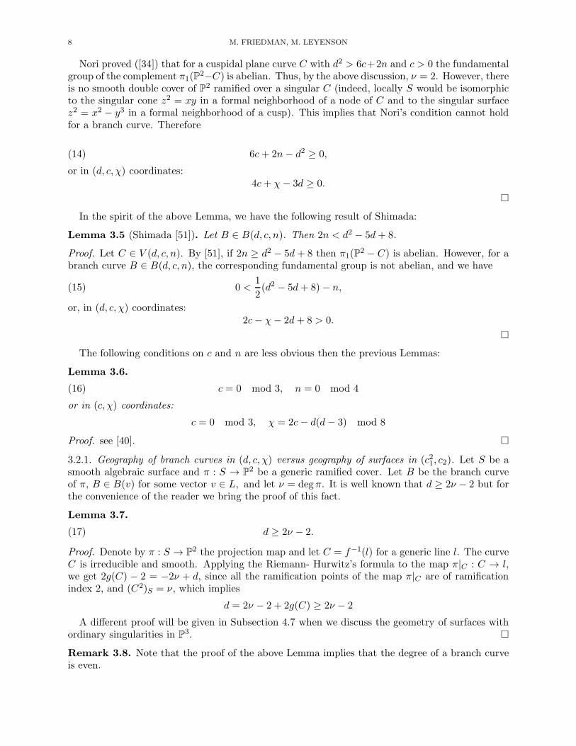
Nori proved ([34]) that for a cuspidal plane curve C with d2 > 6c+2n and c > 0 the fundamentalgroup of the complement π1(P
2−C) is abelian. Thus, by the above discussion, ν = 2. However, thereis no smooth double cover of P2 ramified over a singular C (indeed, locally S would be isomorphicto the singular cone z2 = xy in a formal neighborhood of a node of C and to the singular surfacez2 = x2 − y3 in a formal neighborhood of a cusp). This implies that Nori’s condition cannot holdfor a branch curve. Therefore
(14) 6c+ 2n− d2 ≥ 0,
or in (d, c, χ) coordinates:4c+ χ− 3d ≥ 0.
In the spirit of the above Lemma, we have the following result of Shimada:
Lemma 3.5 (Shimada [51]). Let B ∈ B(d, c, n). Then 2n < d2 − 5d+ 8.
Proof. Let C ∈ V (d, c, n). By [51], if 2n ≥ d2 − 5d + 8 then π1(P2 − C) is abelian. However, for a
branch curve B ∈ B(d, c, n), the corresponding fundamental group is not abelian, and we have
(15) 0 <1
2(d2 − 5d+ 8)− n,
or, in (d, c, χ) coordinates:2c− χ− 2d+ 8 > 0.
The following conditions on c and n are less obvious then the previous Lemmas:
Lemma 3.6.
(16) c = 0 mod 3, n = 0 mod 4
or in (c, χ) coordinates:
c = 0 mod 3, χ = 2c− d(d− 3) mod 8
Proof. see [40].
3.2.1. Geography of branch curves in (d, c, χ) versus geography of surfaces in (c21, c2). Let S be asmooth algebraic surface and π : S → P2 be a generic ramified cover. Let B be the branch curveof π, B ∈ B(v) for some vector v ∈ L, and let ν = degπ. It is well known that d ≥ 2ν − 2 but forthe convenience of the reader we bring the proof of this fact.
Lemma 3.7.
(17) d ≥ 2ν − 2.
Proof. Denote by π : S → P2 the projection map and let C = f−1(l) for a generic line l. The curveC is irreducible and smooth. Applying the Riemann- Hurwitz’s formula to the map π|C : C → l,we get 2g(C) − 2 = −2ν + d, since all the ramification points of the map π|C are of ramificationindex 2, and (C2)S = ν, which implies
d = 2ν − 2 + 2g(C) ≥ 2ν − 2
A different proof will be given in Subsection 4.7 when we discuss the geometry of surfaces withordinary singularities in P3.
Remark 3.8. Note that the proof of the above Lemma implies that the degree of a branch curveis even.

ON RAMIFIED COVERS OF THE PROJECTIVE PLANE 9
We want to express the Chern invariants c21(S) and c2(S) in terms of (d, c, χ) and, equivalently,in terms of (d, c, n), so we give 2 formulas for each invariant.
Lemma 3.9. (see [52])
c21(S) = 9ν −9
2d−
1
2χ(18)
c21(S) = 9ν −9
2d+
(
(d− 1)(d − 2)
2− n− c
)
− 1(19)
Proof. Let π : S → P2 be the ramified cover, R = B∗, the ramification curve and C = f−1(l) for la generic line.
First, we want to compute [R]2 and [C]2.By Riemann-Hurwitz, KS = −3f∗([l]) + [R] = −3[C] + [R]. As π : R→ B is a normalization of
the branch curve B, we apply adjunction formula to R we get
2g − 2 = (KS + [R]) ·R = (−3[C] + 2[R]) · R = −3[C] ·R+ 2[R] ·R = −3f∗[l] ·R+ 2[R]2 =
= −3[l] · f∗[R] + 2[R]2 = −3 degB + 2[R]2 = −3d+ 2[R]2
and thus
[R]2 =3
2d+ g − 1.
We also have
(20) [C]2 = f∗[l] · [C] = [l] · f∗[C] = [l] · (deg f [l]) = ν[l]2 = ν.
We can now compute c21(S):
c21(S) = K2S = (−3[C] + [R])2 = 9[C]2 − 6[C] · [R] + [R]2 = 9ν − 6d+
3
2d+ g − 1 =
= 9ν −9
2d+ g − 1 = 1 = 9ν −
9
2d−
1
2χ
The expression in (d, c, n)-coordinates follows easily.
Lemma 3.10. (see [52])
c2(S) = 3ν − χ− c, or(21)
c2(S) = 3ν + d2 − 3d− 3c− 2n.(22)
Proof. To compute c2(S) we use the usual trick of considering a pencil of lines in P2 passing througha generic point p ∈ P2 and its corresponding preimage with respect to π : S → P2 – the Lefshetzpencil Ct of curves on S.
We then apply the following formula on Ct
c2(S) = χ(S) = 2χ(generic fiber) + #(singular fibers)− (self-intersection of Ct)
(see, for example, [28, section 4.2]).The generic fiber of Ct is a ramified cover of a line l with d simple ramification points (i.e.
ramification index 2 at every point), and thus χ(generic fiber) = 2ν − d by the Riemann–Hurwitzformula.
The number of singular fibers in the pencil Ct is clearly equal to the degree d∗ of the curve B∨ (thedual to the branch curve B), which by the Plucker formulas for B satisfies d∗ = d(d− 1)− 3c− 2n.The self-intersection [Ct]
2 of the fiber equals to ν (by (20)). Thus

10 M. FRIEDMAN, M. LEYENSON
c2(S) = χ(S) = 2(2ν − d) + d∗ − ν = 2(2ν − d) + (d(d− 1)− 3c− 2n)− ν =
= 3ν + d2 − 3d− 3c− 2n = 3ν − χ− c.
Remark 3.11. Equation (21) can be written as an analog to Riemann-Hurwitz formula for themap S → P2
c2(S)− νc2(P2) = −χ− c,
as Iversen described in [20].
Remark 3.12. Inverting the formulas above, we get n and c in terms of c21, c2, ν and d:
n = −3c21(S) + c2(S) + 24ν +d2
2− 15d,
c = 2c21(S)− c2(S)− 15ν + 9d
We use these formulas below in Subsection 4.7.1.
The next two results are rather surprising, as one gets an inequality for the branch curve whichis independent of the degree of the projection:
Lemma 3.13. (see, .e.g., the introduction of [35]) Let B ∈ B(d, c, n) a branch curve of a linearprojection to P2 of a surface of general type, where d, c, n, χ and ν as above. Then
(23) 5χ+ 6c− 9d ≤ 0
or, equivalently, in (d, c, n) coordinates:
10n+ 16c − 5d2 + 6d ≤ 0
Proof. Substituting the expressions for c21(S) and c2(S) (from Lemmas 3.9,3.10) in terms of ν and(d, c, χ) and (d, c, n) into the Bogomolov inequality c21(S) ≤ 3c2(S), we get the desired inequality.
There is, however, an inequality which is true for every branch curve, restricting the sum of thenodes and the cusps (though it is weaker than inequality (23)).
Lemma 3.14. Let B ∈ B(d, c, n). Then
15d− 5χ− 6c > 0
or
10n + 16c < 5d2.
Proof. Note that Nemirovski’s inequality (see [54]) for branch curves is
3d− χ
3d− χ− c< 6
or, equivalently
15d − 5χ− 6c > 0.
Remark 3.15. The variety B(d, c, n) is not necessarily connected. See, for example, [66], where itis proven that B(48, 168, 840) has at least two disjoint irreducible components.

ON RAMIFIED COVERS OF THE PROJECTIVE PLANE 11
3.2.2. Chisini’s conjecture. The following theorem was known as Chisini’s Conjecture, by nowproved by Victor Kulikov (see [52], [65]):
Theorem 3.16. Let B be the branch curve of generic projection π : S → P2 of degree at least 5.Then (S, f) is uniquely determined by the pair (P2, B).
Kulikov proved this conjecture for generic covers of degree greater than 11 and for generic linearprojections of degree greater than 4. Kulikov considered two surfaces S1, S2 ramified over the samebranch curve, and studied the fibred product S1 ×P2 S2, proving that the normalization of thisfibred product contradicts Hodge’s Index Theorem if (S1, f1) is not isomorphic to (S2, f2).
Remark 3.17. We want to mention that a version of a Generalized Chisini’s conjecture alsoexists, for surfaces with normal isolated singular points:
Conjecture 3.18. Let fi : Si → P2, i = 1, 2 be two generic coverings with the same branch curveB where Si can have singular points, denoted as SingSi. Assume f1(SingS1) = f2(SingS2). Theneither there exists a morphism φ : S1 → S2 s.t. f1 = f2 φ or (f1, f2) is an exceptional pair.
See [57] for the definition of an exceptional pair. This theorem was partially proven by V. S.Kulikov and Vik. S. Kulikov for f1, f2 generic m–canonical coverings, for m ≥ 5 (see [55]) or whenmax(deg f1,deg f2) ≥ 12 or max(deg f1,deg f2) ≤ 4 (see [57]).
Remark 3.19. One of the theorems induced from the proof of the Chisini’s conjecture was the factthat a class of certain factorization associated to the branch curve B (i.e. the Braid MonodromyFactorization) determines the diffeomorphism type of S as a smooth 4-manifold. We refer thereader to [33], [39] for an introduction of this factorization, and to Kulikov and Teicher’s proof [53]of the above theorem.
3.2.3. Representation-theoretic reformulation. Let Gi (resp. Γi) be the local fundamental groupof P2 − B at the neighborhood of a cusp (resp. a node) of B. Note that each Gi is isomorphicto the group with presentation a, b : aba = bab and every Γi is isomorphic to the group withpresentation a, b : ab = ba = Z2.
Let l be a line in P2 in generic position with B, pi (i = 1, . . . , d) be the intersection points of Band l, p∗ be a generically chosen point in l and γi be a small loop around pi starting and ending atp∗. The map Freed → π1(P
2−B) sending generators of Freed to [γi] is epimorphic by Zariski–VanKampen theorem, and the classes [γi] are called geometric generators of π1(P
2 −B).It is well known (see [44] or [52, Proposition 1]) that given a ramified cover S → P2, the
monodromy map ϕ : π1(P2 −B) → Symν satisfies the following three conditions:
(i) for each geometric generator γ, the image ϕ(γ) is a transposition in Symν ;(ii) for each cusp qi, the image of the two geometric generators of Gi is two non-commuting
transpositions in Symν ;(iii) for each node pi, the images of two geometric generators of Γi are two different commuting
transpositions in Symν .
The inverse assertion is a group theoretic reformulation on the Chisini’s theorem ([44]):
Proposition 3.20. The map associating the monodromy representation with each ramified coverS → P2 gives an isomorphism of the set of the isomorphism classes of generic ramified coversof P2 of degree ν with the branch curve B and the set of isomorphism classes of epimorphismsϕ : π1(P
2 −B) → Symν satisfying the conditions (i),(ii) and (iii) above, with respect to the actionof Symν on the set of such representations by inner automorphisms.
3.3. Construction of the variety of branch curves B(d, c, n). Let V = V (d, c, n) be the Severi-Enriques subvariety in |dh| of degree d plane curves with n nodes and c cusps. Let B = B(d, c, n) ⊆V the subset consists of branch curves. In this subsection we show that B(d, c, n) is a subvariety

12 M. FRIEDMAN, M. LEYENSON
of V (d, c, n). Although it is standard, we have not found it in the literature, though references toits existence can be found in [24] or in [61]. The following lemma proves that the variety of branchcurves of ramified covers is a union of connected components of V . Using the same techniques in thefollowing proof, and the fact that the Chisini’s conjecture is proven (for generic linear projections),one can prove that also B is a union of connected components of V .
Lemma 3.21. Over the field k = C, every connected component Vi of V either does not containbranch curves of generic covers at all, or every curve C ∈ Vi is a branch curve of a generic cover.Explicitly, every component of B is a connected component of V .
Proof. Let us fix a connected component V1 of V = V (d, c, n), let p ∈ V1, and let C be thecorresponding plane curve. Take q ∈ V1, q 6= p and choose a path I = [0, 1] → V1 connecting p andq. Let us denote GC = π1(P
2 −C), GCt = π1(P2 −Ct) with Ct ∈ V1, t ∈ I where C1 corresponds to
q. As these curves are equisingular, we get an identification of fundamental groups
GCt
∼→ GC .
For every t ∈ I. Consider the group Hom(GC ,SymN ) and its subgroup Homgeom(GC ,SymN ) ofgeometric homomorphisms – i.e., homomorphisms which satisfy the conditions (i),(ii),(iii) above– which can be empty. From the above identification, we get a canonical set bijection fromHom(GCt ,SymN ) → Hom(GC ,SymN ) preserving the set of geometric homomorphisms. In par-ticular, Homgeom(GC ,SymN ) is empty if and only if Homgeom(GC1
,SymN ) is empty, and thus C isa branch curve if and only if C1 is. Therefore B(d, c, n) is a union of connected components of Vand thus it is a subvariety.
Remark 3.22. We want to describe here on the action of the fundamental group π1(V ) on G =π1(P
2 − C). Let p ∈ V , C be the corresponding degree d plane curve and U = P2 − C. A loopγ : I → V (starting and ending at p), induces an automorphism of the group G = π1(U), andthus an automorphism of the set of representations Hom(π1(U), SymN ) which preserves the set ofgeometric representations Homgeom(π1(U), SymN ). To describe it more explicitly, note that we canchoose a line l ⊂ P2 in generic position to every Ct, t ∈ I (since the set of lines in special position toa fixed curve in P2 forms a dual curve in the dual plane, and thus the space of lines which are specialto some Ct is of real codimension 1 in the dual plane). Note that l− l∩C = l∩U ≃ P1−d points.Let us now choose a base point a∗ on l not belonging to any of the curves Ct, and a “geometricbasis” Γ of π1(U, a∗) = π1(P
2 − C, a∗), which gives an epimorphism
e(Γ) : π1(l ∩ U, a∗) → π1(U, a∗).
Recall that the group of classes of diffeomorphism of (P1−d points) modulo diffeomorphisms homo-topic to identity can be identified with the commutator of the braid groupB′
d = Braidd/Center(Braidd)(see e.g. [33]). A loop γ ∈ π1(V ) gives a diffeomorphism of l ∩ U , which in turn induces an auto-morphism of π1(l ∩ U), i.e. an element in Aut(π1(l ∩ U)) or equivalently, an element bγ ∈ B′
d. Itfollows that there is a natural diagram
π1(V )α //
β
((P
P
P
P
P
P
P
P
P
P
P
P
Autπ1(U) // Aut(Homgeom(π1(U), SymN ))
Autπ1(l ∩ U) ≃ B′d
and a commutative triangle:
π1(V )α //
β
((P
P
P
P
P
P
P
P
P
P
P
P
Im(α) ⊆ Autπ1(U)
Im(β) ⊆ B′d
OO

ON RAMIFIED COVERS OF THE PROJECTIVE PLANE 13
An element bγ ∈ B′d which is the image of γ admits a decomposition of bγ into a product of canonical
generators of B′d, i.e. bγ = x±1
1 · ... · x±1k . Since π1(l ∩ U) = Freed = 〈y1, ..., yd〉, we can describe
explicitly the action of each xi on Aut(Freed):
xi(yj) = yj if j 6= i, i+ 1
xi(yi) = yi+1
xi(yi+1) = y−1i+1 · yi · yi+1.
Thus, the action of an element γ ∈ π1(V ) on the group G = π1(U, a∗) can be expressed as a map onthe generators yi of G : (yi 7→ bγ(yi) = (x±1
1 ·...·x±1k )·yi) where xj ·yi is given by the above action.
Note that this action is non-trivial in general, and thus π1(V, p) acts generically non-trivially onthe set of good covers S → P2 ramified over a given curve C. However, in a situation when such acover is unique up to a deck transformation, like in the case of a high degree ramified cover, (due toChisini’s conjecture), this action reduces to the action of the deck transformation group Aut(S/P2)which is the trivial group, for geometric reasoning.
4. Surfaces in P3
Let X be a smooth surface in Pr and p : Pr → P2 be generic projection; we decompose p as
a composition of projections Pr p1→ P3 p2
→ P2 such that S = p1(X) is smooth or has ordinarysingularities in P3. We begin in section 4.1 with the examination of branch curves of smoothsurfaces in P3 and proceed to singular surface in section 4.7.
4.1. Smooth surfaces in P3. Our goal here is to reformulate and give a more modern proof toa result of Segre [8] published in 1930. Segre proved that the set of singular points of the branchcurve of a smooth surface in P3 is a special 0-cycle with respect to some linear systems on P2, i.e.,it lies on some curves of unexpectedly low degree. (We remind that a curve passing through thesingularities of a given one is called adjoint curve. See Definition 4.7). For example, if degS = 3,we get the following result Zariski published in 1929 (cf. [6]): the variety of plane 6-cuspidal sexticshas two disjoint irreducible components. Every curve in the first component is a branch curveof a smooth cubic surface and all its six cusps are lying on a conic, while the second componentdoes not contain any branch curves. (Miraculously, this condition does not define a subvariety ofpositive codimension in the variety of all plane curves of degree 6 with 6 cusps, but rather selectsone of its two irreducible components, which was probably the most surprising discovery of Zariskiconcerning this variety.)
In the following paragraphs we recall Segre’s method for constructing some adjoint curves tobranch curves of ramified covers. The main result is the following: a nodal–cuspidal curve B is abranch curve iff there are two adjoint curves of (some particular) low degree passing through allthe singularities of B (see Theorem 4.32). Though this result was presented in [60] (by Val. S.Kulikov) and in [41] (by J. D’Almeida), our point of view is different, as we emphasize the relationsbetween the Picard and Chow groups of 0–cycles of the singularities of the branch curve. We alsoinvestigate the connections between adjoint curves and the sheaf of weakly holomorphic rationalfunctions on a nodal–cuspidal curve C. We hope that the study of the Picard group of branchcurves and the study of adjunction with values in sheaf of weakly holomorphic rational functions(see [18]) gives a new understanding of the work of Segre.
Let S be a smooth surface of degree ν in P3, and let π : P3 → P2 be a projection from a pointO which is not on S. Let B ⊂ P2 be a branch curve of π. It is easy to see that the degree of Bis d = ν(ν − 1): indeed, B is naturally a discriminant of a homogeneous polynomial of degree νin one variable. The curve B is in general singular, however, for a generic projection it has onlynodes and cusps as singularities (see e.g. [63]).

14 M. FRIEDMAN, M. LEYENSON
Assume now that S is given by a homogeneous form f(x0, . . . , x3) of degree ν, andO = (O0, .., O3)is a point in P3 which is not on S. The polar surface PolO(S) is given by the degree ν − 1 form∑
Oifi, where fi =∂f∂xi
. The following lemma is well known:
Lemma 4.1. Let π : S → P2 be the projection with center O. The ramification curve B∗ of π isthe intersection of S and the first polar surface PolO(S).
Indeed, the intersection of S and PolO(S) consists of such points p on S that the tangent planeto S at p, TpS, contains the point O. This implies that the line joining O and p intersects S withmultiplicity at least 2 at p.
Note that this gives yet another proof that degB∗ = degS · deg(PolO(S)) = ν(ν − 1).
Notation:
(1) H ∈ A2P3 is a class of hyperplane in P3;
(2) h ∈ A1P2 is a class of a line in P2;
(4) ℓ∗ = H|B∗ , ℓ∗ ∈ A0B∗;
(3) ℓ = h|B , ℓ ∈ A0B;
We also denote
(5) S′O = PolO(S) ⊂ P3, and
(6) S′′O = Pol2O(S) is the second polar surface to S w.r.t. the point O; it is given by a homoge-
neous form f ′′ = (∑
Oi∂∂xi
)2f =∑
OiOjfij of degree ν − 2.
(7) We call a 0-subscheme with length 1 at every point a 0-cycle.(8) Let P ⊂ B be the 0-cycle of nodes on B, and P ∗ be its preimage on B∗. Note that
degP ∗ = 2deg P , as can be seen from Lemma 4.2.(9) Let Q ⊂ B be the 0-cycle of cusps on B, and Q∗ be its preimage on B∗. Note that
degQ∗ = degQ (see Lemma 4.2).(10) ξ be the 0-cycle of singularities of B.
From now on we assume that O is chosen generically for a given surface S. It follows that B∗ issmooth, and B has only nodes and cusps as singularities. Already in the 19th century the numberof nodes and cusps of a branch curve was computed for a smooth surface of a given degree.
Lemma 4.2 (Salmon [1]). (a) There is one-to-one correspondence between bisecant lines for B∗
passing through O and nodes of B. Moreover, the number of bisecant lines through O does notdepend on S, and is equal to
(24) n = n(ν) =1
2ν(ν − 1)(ν − 2)(ν − 3)
(b) If Q∗ is the set of points q on B∗ such that the tangent line TqB∗ contains the point O, then
the set Q = π(Q∗) iis the set of cusps of B.(c) Moreover, Q∗ is the scheme-theoretic intersection of B∗ and the second polar surface S′′
O. Inother words, they intersect transversally at each point of Q∗, and B∗ ∩ S′′ = Q∗. In particular, theclass [Q∗] in A0B
∗ is equal to (ν − 2)l∗.(d) It follows that degQ does not depend on a choice of the surface S, and is equal to
(25) c = c(ν) = ν(ν − 1)(ν − 2)
Proof. (a) The first statement is geometrically clear; for the second see [1, art. 275, 279]. Yetanother proof is given below, in Proposition 4.8. See also [15, Chapter IX, sections 1.1,1.2] for away to induce the formula for the number of bisecant of a complete intersection curve in P3 (i.e.the number n+ c). For (b), see [1, art. 276]. (c) is a straightforward computation, and (d) followsfrom (c).

ON RAMIFIED COVERS OF THE PROJECTIVE PLANE 15
Lemma 4.3. Let ℓ ∈ A0(B) be the class of a plane section on B. Then
[Q] = (ν − 2)ℓ in A0(B),
(2) The equality above can be lifted to PicB: there is a Cartier divisor Q0 such that can(Q0) = Qwith respect to the canonical map
can : Cartier(B) → Weil(B)
associating Weil divisor with a Cartier divisor, and
[Q0] = (ν − 2)ℓ
in Pic(B).
Proof. We have Q = π∗(Q∗), and Q∗ = B∗ ∩ S′′
O. Since [S′′O] = (ν − 2)H in A2P
3, we have[Q∗] = (ν − 2)ℓ∗ in A0B
∗, and thus
[Q] = [π∗(Q∗)] = π∗([Q
∗]) = (ν − 2)π∗ℓ∗ = (ν − 2)ℓ
in A0B.To see that π∗ℓ
∗ = ℓ it is enough to consider a hyperplane in P3 containing the point O.(2) Consider the rational function r = f ′′O/H
(ν−2), where f ′′O is by definition the equation of the
second polar Pol2(O,S), and H is an equation of a generic hyperplane containing the projectioncenter O. Since the curves B∗ and B are birational, r can be considered as a rational function onB, where it gives the desired linear equivalence.
Remark 4.4. Note that both cusps and nodes on a curve are associated with Cartier divisors onthe curve, even though these Cartier divisors are not positive. For example, on the affine cuspidalcurve C given by the equation y2−x3 = 0 the divisor (y/x) = 3[0]−2[0] = [0] is a principle Cartier,but since y/x is not in the local ring of the point [0], it is not locally given a section of the sheaf
OC . For the nodal curve C given by the equation xy = 0, the divisor(
y−x2
y−2x
)
= 3[0] − 2[0] = [0] is
also a principle Cartier, though not positive.
4.1.1. Example: smooth cubic surface in P3. Let S be a smooth cubic surface in P3. Then Lemma4.2 imply that B is a plane curve with 6 cusps and no other singularities, and Lemma 4.3 impliesthat
[Q] = ℓ
in A0B. Q is, of course, not a line section of the curve B; the linear equivalence above implies thatthe map
PH0(P2,O(1)) ≃ PH
0(B,O(1)) → |ℓ|
is not epimorphic, where |ℓ| is the set of all Weil divisors linearly equivalent to a generic line sectionof B. Even though Q is associated with a Cartier divisor b/a, this Cartier divisor is not positive.
It is well known that 6 points in general position on P2 do not lie on a conic. As for the 6 cuspsQ on the branch curve we have the following result of Zariski and Segre (see [6],[8]).
Corollary 4.5. All 6 cusps of a degree 6 plane curve B which is a branch curve of a smooth cubicsurface lie on a conic.
Remark 4.6. Explicit construction of a branch curve of a cubic. By change of coordinates a cubicsurface S is given by the equation
f(z) = z3 − 3az + b,

16 M. FRIEDMAN, M. LEYENSON
where a and b are homogeneous forms in (x, y, w) of degrees 2 and 3, and the projection π isgiven by (x, y, w, z) 7→ (x, y, w). In these coordinates the ramification curve is given by the ideal(f, f ′) = (f, z2 − a) = (z3 − 1
2b, z2 − a) and the branch curve B is given by the discriminant
∆(f) = b2 − 4a3
In particular, one can easily see that it has 6 cusps at the intersection of the plane conic definedby a and the plane cubic defined by b, as illustrated on the Figure 3. It is also clear that the conicdefined by a coincides with one constructed in Corollary 4.5.
Figure 3 : The branch curve of a smooth cubic surface
The ideal of Q∗ is equal to (f, f ′, f ′′) = (f, f ′, z) = (a, b, z). Note that z equal to b2a as a rational
section of OB∗(1). We want to explicate the linear equivalence of Q∗ and the intersection of B∗
with the “vertical” plane (one containing the point O). For this, let l(x, y, w) be a linear form inx, y, w, and consider the rational function on B∗
φ =z
l=
b
2alThen φ gives the linear equivalence
0 = (φ) = (b)− (a)− (l) = 3Q− 2Q− (l) = Q− (l),
which gives an explicit proof that [Q] = ℓ in A0B. (We used the fact that cubic b is tangent to Bat the cusps, while conic a is not.) This example has a “natural” continuation in example 4.30.
4.2. Adjoint curves to the branch curve. We begin with the definition of an adjoint curve.This type of curves will play an essential role when studying branch curve.
Definition 4.7. Given a plane curve C, a second curve A is said to be adjoint to C if it containseach singular point of C of multiplicity r with multiplicity at least r− 1. In particular, A is adjointto a nodal-cuspidal curve C if it contains all nodes and all cusps of C.
For more on adjoint curves see [2, § 7], [15, Chapter II, § 2], or [29] for a more recent survey.Below, following Segre, we construct more adjoint curves to B (i.e. W , L, L1) and relate them
to the geometry of B∗ in P3.
We continue this subsection with Proposition 4.8 from [8] and we bring its proof for the conve-nience of the reader.
Proposition 4.8. (a) One has in A0(B)
2[P ] + 3[Q] = ν(ν − 2)ℓ.
(b) The equality above can be lifted to PicB: there are Cartier divisors P1 and Q1 such that inPicB:
can(P1) = 2P,
can(Q1) = 3Q, and
[P1] + [Q1] = ν(ν − 2)ℓ

ON RAMIFIED COVERS OF THE PROJECTIVE PLANE 17
In fact, Q1 is the canonically defined “tangent” Cartier class Qτ .
Proof. (following Segre [8]).Let us choose a plane Π in P3 not containing the point O, and consider the projection with center
O as a map to Π. Let us also choose a generic point O′ = (O′0, O
′1, O
′2) ∈ Π, and let B′ = PolO′(B)
be the polar curve of B, defined as follows: if B is given by the homogeneous form g(x0, x1, x2) of
degree d = ν(ν − 1), then PolO′(B) = ∑2
i=0O′i∂g∂xi
= 0. Note that the first polar B′ = PolOB isadjoint to B.
It is clear that
(26) [B ∩B′] = 2P + 3Q+R,
where R (for “residual”) is the set of non-singular points p on B such that the tangent line to Bat p contains O′, and thus
(27) [2P + 3Q+R] = (d− 1)ℓ
in A0B (Here we used the fact that O′ is generic, in particular, it does not belong to B and to theunion of tangent cones to B at nodes and cusps.)
Let R∗ be the preimage of R on B∗. We claim that R∗ = B∗ ∩ S′O′ , where S′
O′ = PolO′(S).Indeed, if p ∈ R, then TpB contains the point O′, and if p∗ is the preimage of p on B∗, then thetangent space to S at p∗ can be decomposed into a direct sum of the line l joining p and p∗ (andcontaining O) and the tangent line Tp∗B
∗ which projects to the tangent line TpB, (as illustratedon Figure 4 below).
o`
B P
o
p
B*p*
Figure 4 : R∗ = B∗ ∩ S′
O′
It follows that
[R] = π∗([R∗]) = π∗([B
∗ ∩ S′O′ ]) = π∗((ν − 1)ℓ∗) = (ν − 1)ℓ
in A0B, and thus
[2P + 3Q] = [2P + 3Q+R]− [R] = (d− 1)ℓ− (ν − 1)ℓ = (d− ν)ℓ = ν(ν − 2)ℓ
The proof of the second part is parallel, as the Weil divisors 2P and 3Q can be lifted to PicB.
Note that this gives yet another proof for the formula for the number of nodes n = n(ν).
Proposition 4.9. There exist a (unique) curve W in the plane Π of degree ν(ν − 2) such that inA0(B)
[W ∩B] = 2[P ] + 3[Q].

18 M. FRIEDMAN, M. LEYENSON
Proof. By the previous proposition, the cycle 2[P ] + 3[Q] is in the linear system |ν(ν − 2)ℓ| on B.Note that 2P + 3Q is actually a Cartier divisor (see Remark 4.4). Now, since degB = ν(ν − 1) isgreater than ν(ν − 2), there is a restriction isomorphism
0 → H0(Π,O(ν(ν − 2))) → H0(B,O(ν(ν − 2))) → 0
which completes the proof.
Note that W is an adjoint curve to B which is tangent to B at each cusp of B.
Proposition 4.10. Let a = (ν − 1)(ν − 2).(1) We have
[2P + 2Q] = aℓ
In A0(B).(b) The equality above can be lifted to Pic(B): there are Cartier divisors P2 and Q2 such that in
Pic(B):
can(P2) = 2P,
can(Q2) = 2Q, and
[P2] + [Q2] = aℓ
(2) There is a (unique) curve L of degree a such that
[L ∩B] = 2P + 2Q.
Proof. (1) We have
[2P + 2Q] = [2P + 3Q]− [Q] = ν(ν − 2)ℓ− (ν − 2)ℓ = (ν − 1)(ν − 2)ℓ = aℓ.
The computation in Pic(B) is parallel: we let P2 = P1 and Q2 = Q1 −Q0.(2) Note that (ν − 1)(ν − 2) < degB, which completes the proof.
Note that L is an adjoint curve to B which is not tangent to B at the cusps of B.
Notation 4.11. Let ζL be the Cartier divisor on B given by restricting the equation of L to B.Recall that ζL is supported on the 0–cycle of singularities ξ.
Definition 4.12. Let V (d, c, n) be the variety of plane curves of degree d with c cusps and n nodes,abd let B(d, c, n) be the subvariety in V (d, c, n) consisting of branch curves of all ramified covers of
P2.
Example 4.13. By substituting ν = 3 and ν = 4 we get the classical example of a sextic with sixcusps on a conic we discussed above, and the example of a degree 12 curve with 24 cusps and 12nodes, all of them are on a sextic:(1) The branch curve C of a smooth cubic surface in P3 is a sextic with six cusps, C ∈ B(6, 6, 0).We have degL = 2; two different constructions of this conic was given above in Corollary 4.5 andRemark 4.6. See also Figure 3 above.(2) The branch curve C of a smooth quartic surface in P3 is of degree 12, and has 24 cusps and 12nodes, i.e., C ∈ B(12, 24, 12). We have degL = 6. Moreover, the 24 cusps lie on the intersection ofa quartic and a sextic curves (see e.g. [8]).
ON RAMIFIED COVERS OF THE PROJECTIVE PLANE 19
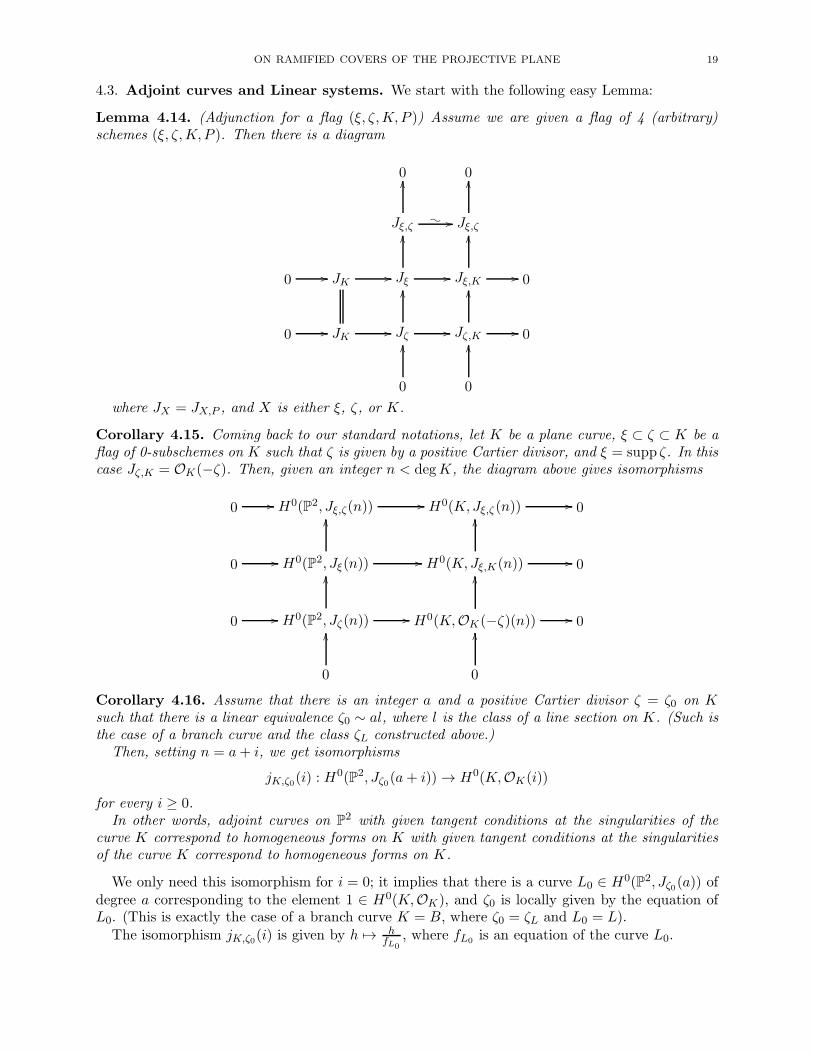
4.3. Adjoint curves and Linear systems. We start with the following easy Lemma:
Lemma 4.14. (Adjunction for a flag (ξ, ζ,K, P )) Assume we are given a flag of 4 (arbitrary)schemes (ξ, ζ,K, P ). Then there is a diagram
0 0
Jξ,ζ
OO
/o // Jξ,ζ
OO
0 // JK // Jξ //
OO
Jξ,K //
OO
0
0 // JK // Jζ //
OO
Jζ,K //
OO
0
0
OO
0
OO
where JX = JX,P , and X is either ξ, ζ, or K.
Corollary 4.15. Coming back to our standard notations, let K be a plane curve, ξ ⊂ ζ ⊂ K be aflag of 0-subschemes on K such that ζ is given by a positive Cartier divisor, and ξ = supp ζ. In thiscase Jζ,K = OK(−ζ). Then, given an integer n < degK, the diagram above gives isomorphisms
0 // H0(P2, Jξ,ζ(n)) // H0(K,Jξ,ζ(n)) // 0
0 // H0(P2, Jξ(n))
OO
// H0(K,Jξ,K(n))
OO
// 0
0 // H0(P2, Jζ(n))
OO
// H0(K,OK(−ζ)(n))
OO
// 0
0
OO
0
OO
Corollary 4.16. Assume that there is an integer a and a positive Cartier divisor ζ = ζ0 on Ksuch that there is a linear equivalence ζ0 ∼ al, where l is the class of a line section on K. (Such isthe case of a branch curve and the class ζL constructed above.)
Then, setting n = a+ i, we get isomorphisms
jK,ζ0(i) : H0(P2, Jζ0(a+ i)) → H0(K,OK(i))
for every i ≥ 0.In other words, adjoint curves on P2 with given tangent conditions at the singularities of the
curve K correspond to homogeneous forms on K with given tangent conditions at the singularitiesof the curve K correspond to homogeneous forms on K.
We only need this isomorphism for i = 0; it implies that there is a curve L0 ∈ H0(P2, Jζ0(a)) ofdegree a corresponding to the element 1 ∈ H0(K,OK), and ζ0 is locally given by the equation ofL0. (This is exactly the case of a branch curve K = B, where ζ0 = ζL and L0 = L).
The isomorphism jK,ζ0(i) is given by h 7→ hfL0
, where fL0is an equation of the curve L0.

20 M. FRIEDMAN, M. LEYENSON
Our next goal is to study curves of various degrees n > a containing the 0-cycle ξ but restrictingto different Cartier divisors with support on ξ, not necessarily coinciding with ζ0. Assume that weare given a positive Cartier divisor ζ1 on K; We will study adjoint curves restricting to K as ζ1 .
Note that Jζ1,K = OK(−ζ1), and consider the restriction map
resK : H0(P2, Jζ1(a+ i)) → H0(K,OK(−ζ1)(a+ i))
To introduce notations we need to recall some basic facts about linear equivalence of Cartierdivisors. Assume that we are given two positive Cartier divisors D1 and D2 on a scheme Xand a linear equivalence D1 − D2 = (r) for a meromorphic function r. We realize both OX(D1)and OX(D2) as subsheaves of the sheaf MX of meromorphic functions on X, and describe theisomorphism OX(D1) → OX(D2) given by the function r explicitly. Locally, on a small enoughaffine open set U ⊂ X, U ≃ SpecA, D1 and D2 are given by equations f1 and f2, fi ∈ A, f1/f2 = rin the full ring of fractions MA of A, and O(Di) is given by the A-submodule 1
fiA in MA, i = 1, 2.
The isomorphism jr : 1f1A → 1
f2A, a/f1 7→ r · (a/f1) = a/f2 gives rise to an automorphism of the
sheafMX given by the multiplication by r. Thus, globally, the sheaf automorphism jr :MX →MX
given by the multiplication by r takes O(D1) to O(D2).Now, using the linear equivalence ζ0 ∼ al on K, we get an isomorphism
jr : OK(−ζ1)(a+ i) → OK(−ζ1)(ζ0)(i) ≃ OK(ζ0 − ζ1)(i)
given by multiplication with the rational function
r = fal /fL0
where fl is an equation of a line l, and fL0is the equation of L0 ∈ H0(P2, Jζ0(a)). Thus the image
for an adjunction belongs to the sheaf OK(ζ0 − ζ1)⊗OK(i), which is the sheaf of meromorphicfunctions on K with zeroes at ζ1 and poles at ζ0, shifted by i.
Since we want to study adjoint curves to K, we are interested in positive Cartier divisors of
the form ζ1 = ζξ1 + ζres1 , where ζξ1 is supported on ξ, i.e., supp(ζξ1) = supp(ζ0) = ξ, and ζres1 (resfor ”residual”) is supported on the set of smooth points of K. Note that the sections of the sheafOK(ζ0 − ζ1) can locally be given by r = h1/h0 · g, where hi is the local equation for the Cartierdivisor ζi, and g is regular, i.e., g ∈ OK,p.
Thus we introduce the following module and sheaf:
Definition 4.17. For a commutative ring A, we define an A-submodule RA in the full ring offractions MA,
A ⊂ RA ⊂MA,
as the set of all fractions r = g1/g0 such that ordp(g1) ≥ ordp(g0) for each height one ideal p of A.Given a scheme X, one can define the sheaf RX ; this sheaf is the subsheaf of the sheaf of
meromorphic functions MX given locally by fractions r = g1/g0 such that ordZ(r) = ordZ(g1) −ordZ(g0) ≥ 0 for each codimension one subvariety Z of X.
The sheaf RX coincides with the structure sheaf OX at the set of smooth points of X, and thereis a filtration
OX ⊂ RX ⊂MX .
Moreover, we have the following easy Lemma:
Lemma 4.18. The normalization NA of A in the full ring of fractions MA is a submodule of RA.I.e., there is a filtration
A ⊂ NA ⊂ RA ⊂MA
Note that sheaf NX coincides with the sheaf π∗(OX∗), the pushforward of the structure sheafalong the normalization X∗ → X.

ON RAMIFIED COVERS OF THE PROJECTIVE PLANE 21
Combining this all together, we get an adjunction sequence
aK,i,ζ1 : Jζ1,P(a+ i)resK→ OK(−ζ1)(a+ i)
fal
fL∼→ OK(ζ0 − ζ1)(i) =
= OK(ζ0 − ζξ1)(i)(−ζres1 ) ⊂ OK(ζ0 − ζξ1)(i) ⊂ RK(i)
and, taking union over all positive Cartier divisors ζ1, we finally get our main adjunction
(28) aK,i : Jξ,P(a+ i)r→ RK(i),
wherer = fal /fL.
Now we study the image of the map aK,i.
Definition 4.19. Let C be a plane curve. We say that a line l containing a cuspidal or nodal pointp of C is strictly tangent to C at p if l intersects C with multiplicity 3 at p.
We also say that a curve C1 containing p is strictly tangent to C at the nodal or cuspidal pointp of C if C1 intersects C with multiplicity at least 3 at p.
Assume from now on that the adjoint curve L0 to K is not (strictly) tangent to K at its singularpoints, and does not intersect K elsewhere.
We want to introduce a sheaf of rational functions with denominator vanishing exactly along L0.This sheaf is clearly the image of the adjunction map aK defined above.
Definition 4.20. Let RL0
K be a subsheaf of RK consisting of sections r which can be given byr = f/fL0
, where f is a homogeneous polynomial on P2, and fL0is an equation of the curve L0.
Proposition 4.21. If K is a nodal-cuspidal curve and L0 is an adjoint curve not tangent to K atthe singularities of K and not intersecting it elsewhere, then the natural inclusion
RL0
K ⊂ RK
is an equality. Moreover, they both coincide with the sheaf π∗OK∗.
Proof. The proof follows easily from the fact that nodal and cuspidal singularities of curves areresolved by a single blow-up, and, moreover, we can take t = f1/f0 or t = f1/fL0
as a localcoordinate on the resolution, where f1 and f0 vanish at the singular points of K and have separatedtangents to K at the singularities of K. In this way, both of the sheaves are equal to π∗OK∗ , andthus they coinside.
Remark 4.22. This proposition is an example for the analytic theory of weakly holomorphicfunctions and universal denominator theorem (see, for example, [18]) in case our base field is thefield of complex numbers. In this case the equation of the adjoint curve L0 works as the universaldenominator for the sheaf of weakly holomorphic functions at each point of K.
Combining the proposition above and the construction of the adjunction map aK,i (which isessentially a division by the equation of L0), we get the following theorem:
Theorem 4.23. For a nodal-cuspidal curve K and an adjoint curve L0 as above, the map aK,i isepimorphic onto RK(i), and there is an exact sequence
0 // JK,P(a+ i) // Jξ,P(a+ i)aK,i // RL0
K (i) //
O
0
RK(i)

22 M. FRIEDMAN, M. LEYENSON
In other words, adjoint curves of degree a+ i to the curve K on the plane induce rational functionson the curve K for which ordp(r) ≥ 0 for each point p ∈ K.
The map aK,i is an isomorphism modulo ideal spanned by the equation of K.
Passing to the global sections for a+ i < degK, we get the following theorem:
Theorem 4.24. For a+ i < degK, there are isomorphisms⊕
H0(P2, Jξ(a+ i))∼→
⊕
H0(K,RK(i))∼→
⊕
H0(K∗,OK∗(i))
For higher degrees i ≥ degK − a one can modify these isomorphisms readily to get a correctversion including adjoint curves containing K as a component.
Proof. This theorem follows immediately from Theorem 4.23 and Proposition 4.21 if we take intoaccount the projection formula for π : K∗ → K,
π∗(OK∗(i)) ≃ π∗(OK∗ ⊗π∗OK(i)) ≃ π∗(OK∗)⊗OK(i) ≃ RK ⊗OK(i).
The meaning of the theorem is that plane curves through ξ exactly correspond to homogeneousfunctions on K∗.
Remark 4.25. (Graded algebras interpretation) Assume we are given a smooth space curveK∗ not contained in a plane in P3 and a projection p : K∗ → K to a plane curve K. Since K∗ isbirational to K, in order to reconstruct K∗ from K, we have to say what is the “vertical coordinatez” on K∗ in terms of K. Since K∗ and K are birational, the regular (holomorphic) objects onK∗ are rational (meromorphic) objects on K, and thus we should have an equality of the formz = fn+1/fn for some integer n and plane curves fn and fn+1 of degrees n and n+ 1.
More precisely, let S = ⊕Si, Si = H0(K,O(i)) be the graded algebra of homogeneous functionson K, and T be the graded algebra of homogeneous functions on K∗. The inclusion S → T givesan isomorphism of fraction fields Q(S) → Q(T ), since K and K∗ are birational. Now T1 = S1 ⊕ kzfor some element (“vertical coordinate”) z ∈ T1; since T1 ⊂ Q(T ) ≃ Q(S), we would have
z =fn+1
fn
for some integer n and plane curves fn and fn+1 of degrees n and n+ 1, both passing through thesingularities of K.
Corollary 4.26. As in the previous remark, assume that we are given a smooth space curve K∗,a projection p : P3 → P2 with center O not on K∗ such that K = p(K∗) is a nodal-cuspidal curve,and an adjoint curve L0 of degree a to K which is smooth at the singularities of K and is not(strictly) tangent to K there.
Then the “vertical coordinate” z on K∗, z ∈ H0(K∗,OK∗(1)), is the image of a uniquely definedplane curve L1 of degree a+ 1 under the adjunction map aK,1 defined by the formula (28).
In other words, we can choose n = a in the remark above, and
z =fL1
fL0
,
where fC is an equation of a plane curve C, C = L0 or L1, degL1 = a + 1, and the curve L1 isnot a union of L0 and a line, i.e., is a “new” adjoint curve.
The curves L0 and L1 are smooth at the points of ξ and have different tangents at every pointp ∈ ξ.
Proof. There are two ways to prove it. First, this statement is a corollary of the theorem 4.24. Thefact L1 is “new”, i.e., not a union of L0 and a line, follows from the fact that z is “new”, i.e., doesnot come from a linear form on P2 (explicitly, z ∈ H0(P3,O(1)) ≃ H0(K∗,OK∗(1))). The fact that

ON RAMIFIED COVERS OF THE PROJECTIVE PLANE 23
L1 is smooth at the singularities of K follows from the fact that the fraction z = fL1/fL0
resolvesthe singularities of K.
A more straightforward proof is the following: let S be the graded homogeneous algebra of Kand T be the graded homogeneous algebra of K∗; and consider the element t = z ·fL0
of Ta+1. It isenough to prove that t actually belongs to Sa+1, since then we can let fa+1 = t and z = fa+1/fL0
.Now this is an easy local computation for each singular point of K, since the exact sequence
0 → Sa+1 → Ta+1 → Ta+1/Sa+1 → 0
is obtained from the sheaf exact sequence
0 → OK(a+ 1) → p∗OK∗(a+ 1) → F (a+ 1) → 0,
where F is by definition the factor sheaf p∗OK∗/OK , by passing to global sections:
0 → H0(K,OK(a+ 1))p∗→ H0(K∗,OK∗(a+ 1)) → coker p∗ → 0
Since the factorsheaf F is a product of sheaves supported at singular points of K, this makescomputing the image of t in H0(K,F (a + 1))) an easy local computation at nodes and cusps.
The intuitive meaning of this computation is that fL0vanishes at the singularities of K, which
implies that t = zfL0is a regular (holomorphic) object on K, and thus belongs to Sa+1.
In particular, this is the case when K = B is a branch curve of a smooth surface S in P3, whereξ is the 0–cycle of singularities of K. In this case we can take L = L0, a = (ν − 1)(ν − 2), whereν = degS. Segre refers to the existence of the second adjoint curve L1 as something known fromthe Cayley’s ”monoıde construction” (see [3, pg. 278]).
Remark 4.27. Summarizing what is written above, the branch curve B has an adjoint curve L ofdegree equal to a. In this case, we have
z =fL1
fLThe curves L and L1 are smooth at the points of ξ = P +Q and have separated tangents at everypoint p ∈ ξ.
Remark 4.28. Note that if the plane nodal-cuspidal curve K has two adjoint curves of degreesn and n+ 1 with separated tangents at SingK for any integer n, then K is the image of a smoothspace curve K∗ under the projection from P3, but it is only n = a = (ν − 1)(ν − 2) that K mayactually be a branch curve of a surface projection.
Remark 4.29. We the following isomorphisms:
H0(P2, Jξ(a+ 1)) ≃ H0(K∗,OK∗(1)) ≃ H0(P3,O(1)).
I.e., linear forms on K∗ correspond to adjoint curves of degree equal to a+ 1 on K.
Example 4.30. For a cubic surface f = z3−3az+ b the branch curve B = b2−4a3. The six cuspsof B are given by the intersection of a conic and a cubic (a = b = 0), and in this case L = a is aconic in general position to B at the cusps, the cubic W = b is strictly tangent to B at the cusps(see definition 4.19), and both of them do not intersect B elsewhere. We claim that L1 = W inthis case. Indeed, we have on B∗
f = z3 − 3az + b = 0,
f ′ = 3(z2 − a) = 0
and thus
z =1
2
b
aon B∗. It follows that L1 is given by b.

24 M. FRIEDMAN, M. LEYENSON
Remark 4.31. In the previous example we can choose the curve L1 as any of the curves W + l0L,where l0 is a linear form on P (perhaps 0). An easy computation shows that L1 is strictly tangentto K at q ∈ Q iff l0 contains the point q (or if l0 = 0), but even in this case l0 the curves L and L1
have different tangents at q.
4.4. Segre’s theorem. Consider again a smooth surface S in P3 and a projection π : S → P
2 witha center O ∈ P3 − S. Let B be the branch curve of p, and ξ be the 0-cycle of singularities of B.
Consider now the graded vector space ⊕H0(P2, Jξ(n)). It follows from the Segre’s computationthat a = (ν − 1)(ν − 2) is the smallest integer such that there are adjoint curves of degree a to B.The vector space H0(P2, Jξ(a)) is one-dimensional and generated by the the curve L. Let ζL = L|Bbe the corresponding divisor class in Pic(B). Note that for n = a the class ζL gives a canonicallifting of 2ξ = 2P + 2Q to PicB, and thus H0(P2, Jξ(a)) ≃ H0(P2, Jζ(a)). We have
ζL ∈ |al|,(29)
[ζL] = 2ξ in A0(B),(30)
k = kL∼→ H0(P2, JζL(a))
∼→ H0(P2, Jξ(a)),(31)
H0(P2, JζL(a)) ≃ H0(B,OB(−ζL)(a)) ≃ H0(B,OB)(32)
Now L is smooth at the points of ξ and is not strictly tangent to B at these points by Remark4.27, and thus ζL is given by a tangent vector to p at each point p ∈ ξ, which follows from thedescriptio of Cartier divisors supported at nodes and cusps. The picture for the branch curve of asmooth cubic surface is drawn below.
Figure 5 : Cartier divisor ζL
Segre proves that this data is sufficient to reconstruct the surface S:
Theorem 4.32 (Segre). A plane curve B of degree d = ν(ν − 1) is a branch curve of a smoothsurface of degree ν in P3 if and only if
(1) B has n = 12ν(ν − 1)(ν − 2)(ν − 3) nodes;
(2) B has c = ν(ν − 1)(ν − 2) cusps;(3) There are two curves, L of degree a = (ν − 1)(ν − 2) and L1 of degree a + 1, which both
contain the 0-cycle ξ of singularities of B and have separated tangents at the points of ξ.
Proof. The necessity of these conditions was proved in the preceding sections. We now prove thatthey are sufficient.
Let B be such a curve in the plane P2. First, since L is adjoint to B, the 0-cycle associated withthe scheme-theoretic intersection L ∩B contains 2ξ = 2P + 2Q, but by conditions of the theorem
degB · degL = 2deg ξ = ν(ν − 1)2(ν − 2)

ON RAMIFIED COVERS OF THE PROJECTIVE PLANE 25
It follows that the 0-cycle associated with L ∩B is
[L ∩B] = 2P + 2Q.
Let us denote ξ = P +Q. It follows immediately that 2ξ is in the linear system |aℓ| on B, where|ℓ| is the linear system associated with the given plane embedding of B. In particular, we concludethat
ξ ∈
∣
∣
∣
∣
1
2a · ℓ
∣
∣
∣
∣
Note also that [L1 ∩B] = 2P + 2Q+R, where degR = d = ν(ν − 1).Now the space H0(P2, Jξ(a + 1))) contains a 4–dimensional subspace of the form kf1 + kxf +
kyf + kwf , where f1 is the equation of L1 and f is the equation of L. (Recall that k is our basefield.)
Now consider the linear system on B given by restriction of (f1, xf, yf, wf) = kL1⊕H0(P2,O(1))⊗ kL.
It has ξ as a set of base points. It follows that it defines a rational map
φ : B − ξ → P3.
Let π : B∗ → B be the normalization of B. We claim that the rational map φ can be lifted to givea regular map φ∗ : B∗ → P3. Indeed, we have the following lemma:
Lemma (A). Let B be a plane nodal-cuspidal curve with the set of singularities ξ, and let f ∈H0(B, Jξ(j)) and f1 ∈ H0(B, Jξ(j+1)) be non-zero elements determining adjoint curves C = Z(f)and C1 = Z(f1) on the plane, such that TpC 6= TpC1 at any point p ∈ ξ.
Let
Ω = kf1 ⊕H0(P2,O(1))⊗ kf = (f1, xf, yf, wf).
Then the rational map φΩ : B 99K P3 can be resolved as
B∗ //
π
P3
pr
B // P2
where π : B∗ → B is the normalization of B.
Note that TpC 6= TpC1 implies that f1 /∈ H0(P2, O(1))⊗ kf , and also that Ω → TpC is epimorphicat every point p ∈ ξ.
Proof. It is clear that we only have to verify the statement at nodes and cusps of B as well assmooth points p on B such that f1(p) = f(p) = 0.
For a node p we can choose coordinates in the local ring of P2 at p such that B is given by theequation xy = 0.
Assume that f1 is given by the equation a1,0x + a0,1y + (order 2 terms), and f is given by theequation b1,0x+ b0,1y+(order 2 terms). Note that φΩ = (f1, fx, fy, fw) = (f1/f, x, y, w). One caneasily see that φΩ maps the point p on the branch (y = 0) of B to a1,0/b1,0, and the same point onthe branch (x = 0) to a0,1/b0,1. Thus, if a1,0b0,1 − a0,1b1,0 6= 0, then φW can be lifted to a regularmap B∗ → P3 with a smooth image in the neighborhood of p.
In the same way, in a neighborhood of a cups B can be given by the local equation y2 − x3 = 0,and thus
f1/f =a1,0x+ a0,1y + (order 2)
b1,0x+ b0,1y + (order 2)=a1,0 + a0,1t+ (order 2)
b1,0 + b0,1t+ (order 2),
where t = y/x is the coordinate on the exceptional divisor in the resolution of the cusp. Now itis clear that if a1,0/b1,0 6= a0,1/b0,1, then φW lifts to an embedding of the exceptional divisor andthus the normalization of the curve as well.

26 M. FRIEDMAN, M. LEYENSON
If now p is a smooth point of B such that f1(p) = f(p) = 0, then it is a standard fact that themap (B − p) → P3 can be uniquely extended to the map B → P3 in a neighborhood of the pointp, since P3 is proper. (Note also that we do not have any such points in the application of thisLemma below, due to the intersection multiplicity computation for C1 and C.)
This gives a non-singular model C ⊂ P3, and a projection π : C → B with some center O. Notethat if we start from a given ramification curve B∗, the curve we reconstruct from B coinsides withB∗.
Lemma (B). If B is a branch curve of the generic projection π : S → P2, where S is a smoothsurface in P(V ) ≃ P3, and B∗ is the ramification curve of π, then there is an isomorphism P(V ) →
P(kL1 ⊕ H0(P2,O(1))⊗ kL) which takes B∗ ⊂ P(V ) to C. In other words, the linear system(f1, xf, yf, wf) reconstructs the curve B∗.
The idea of the proof is, as in the previous lemma, to set z = f1/f on B∗.Recall that preimages of the nodes of B belong to the bisecant lines to B∗ containing ithe point
O, and preimages of cusps belong to the tangent lines to B∗ containing the point O. Consideringtangent lines to B∗ as a limiting case of bisecants to B∗, we see that B∗ has
n+ c =1
2ν(ν − 1)2(ν − 2)
of bisecants (and tangents) containing the point O, which belong to a cone of order (ν − 1)(ν − 2)above L with vertex O.
Lemma (C). B∗ does not belong to a surface of degree m < ν − 1.
Proof. Assume that S1 is such a surface of degree m; we can assume that it is irreducible. ConsiderS′1 = PolO(S1). First, if S1 is smooth, note that S′
1 contains the preimage of the 0-cycle of cuspsQ∗, since at each point q ∈ Q∗, the tangent line l to B∗ is contained in TqS1, and also l containsO, since q projects to a cusp of B. It follows that q ∈ S1 ∩ S
′1. Secondly, if S1 is not smooth, then
S′1 still contains q.However, then it follows that the number of cusps c ≤ ν(ν − 1) · (m − 1), which contradicts to
assumption that c = ν(ν − 1)(ν − 2).
We now have to prove that the model B∗ we constructed is a complete intersection of a surfaceS of degree ν and its polar PolO(S) of degree ν− 1 with respect to the (fixed) point O which is thecenter of the projection π : B∗ → B. For these, following Segre, we apply the following theorembelonging to Halphen (See [3, pg. 359]):
Theorem (Halphen). Let C be a space curve of order a·b in P3 s.t. a < b which has 12a(a−1)b(b−1)
bisecants all lying on a cone of degree (a − 1) · (b − 1). Assume also that C is not on a surface ofdegree smaller than a. Then C is a complete intersection of two surfaces of degree a and b.
The inverse statement to the Halphen’s theorem is easy; see [1, art. 343] or [15, Chapter IX,sections 1.1, 1.2].
Alternatively, instead of invoking Halphen’s theorem, one can invoke a theory of Gruson andPeskine, as it is done by D’Almeida in [41]; we cite his reasoning for the convenience of the reader:
Lemma (D). [41, pg. 231] The curve B∗ constructed above is a complete intersection of twosurfaces of degrees ν and ν − 1.
Proof. To prove the lemma, we introduce first the following definition:
Definition 4.33. Given a space curve C, we define its index of speciality as
s(C) = maxn : h1(C,OC(n)) 6= 0.
ON RAMIFIED COVERS OF THE PROJECTIVE PLANE 27
Now we state the following Speciality Theorem of Gruson and Peskine [27]:
Let C be an integral curve in P3 of degree d, not contained in a surface of degree less than t.Let s = s(C). Then s ≤ t+ d
t − 4, with equality holding if and only if C is a complete intersection
of type (t, dt ) (and thus OC(s) is special, i.e., h1(OC(s)) 6= 0).
Let now p : B∗ → B be the projection from the pointO. The conductor of the structure sheafOB∗
in OB is Ann(p∗OB∗/OB), which by duality is isomorphic to Ann(ωB/p∗(ωB∗)) (see e.g. [19, Chap-ter 8]). By the definition of the conductor, we get that Ann(ωB/p∗(ωB∗)) = Hom(ωB, p∗(ωB∗)) =
p∗(ωB∗)⊗ω∨
B. It is well known that for a nodal-cuspidal curve, H is a global section of the con-ductor sheaf iff H passes through the nodes and the cusps of the curve (see e.g. [32, Proposition3.1]).
By Serre duality, for all i, H1(OB∗(i)) = H0(ωB∗(−i)). Thus, the minimal degree of the curvecontaining the singular points of B is
ν(ν − 1)− 3− s(B∗).
Indeed, for a curve to pass through the singular points of B, the conductor has to have sections,i.e. p∗(ωB∗)⊗(ωB)
∨
has sections. Since we know that the minimal degree of the curve containingthe singular points of B is (ν − 1)(ν − 2), we get s(B∗) = 2ν − 5.
As B∗ does not lie on any surface of degree ν − 2 (by Lemma (C)), then the Speciality The-orem shows that B∗ is a complete intersection of two surfaces of degrees ν and ν − 1 (takingt = ν − 2, d = ν(ν − 1)).
Either way, by results of Halphen or Gruson-Peskine, the curve B∗ is a complete intersection oftwo surfaces, say, Sν and F ν−1 of degrees ν and ν − 1.
We still have to prove that B∗ can be written as an intersection of a surface of degree ν and itspolar with respect to the given point O.
Let W = H0(P3, JB∗(ν)) be the linear system of surfaces of degree ν containing B∗,
W = kS ⊕(
H0(P3,O(1)) ⊗ kF)
,
as for any complete intersection of type (ν, ν− 1). For a point t ∈ PW , let St be the correspondingsurface of degree ν containing B∗. (here we also denoted by S and F some particular equations forthe surfaces S and F , even though they are defined only up to Gm action).
Consider now the linear map
∂O : W = H0(P3, JB∗(ν)) → H0(P3,O(ν − 1)),
which maps f to PolOf =∑
Oi∂if , its polar with respect to the fixed point O. We claim that ∂0is injective. Indeed, if ∂0(f) = 0, then f vanishes on a cone of degree ν, containing the curve B∗.Note that F ν−1 vanishes on B∗ but also gives a degree ν − 1 form on every line generator of thecone (f = 0), which implies that the projection map B∗ → B has degree ν − 1, which is not thecase.
Now, for every t ∈ P(W ) and the corresponding surface St of degree ν, consider the tripleintersection
ηt = St ∩ Fν−1 ∩ PolO St
First, we have St ∩ F = B∗. Let Rt = St ∩ PolO St. Rt is a ramification curve for the surface Stwith respect to the projection with the given center O. We have ηt = B∗ ∩Rt.
Note that Q∗ ⊂ Rt for every t, since B∗ belongs to St and has all tangent lines at the points of
Q∗ contain the projection center O.

28 M. FRIEDMAN, M. LEYENSON
Thus for every t either the polar surface PolO St contains the curve B∗, or we have a decompo-sition of 0-cycles on B∗ of the form
ηt = Q∗ + rt
Also note that Q∗ ⊆ B∗∩PolO F by the same geometric argument, i.e., since at the points of Q∗
the tangent lines to B∗ contain the projection center O, these points are on the intersection of B∗
with O-polar of every surface containing B∗. But since these two 0-cycles have the same degree,they coinside. It follows that Q∗ ∈ |(ν − 2)h| on the curve B∗, where h is a class of hyperplanesection.
Now, since ηt ∈ |∂0St| = |(ν − 1)h| on B∗, we have rt ∈ |h| on B∗ whenever PolO St intersectsnon-trivially with the curve B∗, i.e., does not contain it.
Since B∗ is complete intersection, it is linearly normal (which follows easily from the cosiderationof Koszul complex). It follows that rt gives a map
W → H0(B∗,O(1))
from the 5-dimensional space W to the 4-dimensional vector space H0(B∗,O(1)) ≃ H0(P3,O(1)).Such a map must have a kernel, and let S0 be the corresponding surface in the linear system
|W |. It follows that Pol(O,S0) contains the curve B∗, and thus B∗ = S0 ∩ Pol(O,S0), i.e., B∗ is a
ramification curve for the projection of the surface S0 to P2 with the given center O. This finishesthe proof.
Remark 4.34. We generalize Segre’s theory for smooth surfaces in PN , N > 3, in the subsequentpaper [67].
Let us notice that the 0–cycle of singularities of the branch curve B is special. We would like toemphasize this in the next subsection.
4.5. Special 0-cycles. Let ξ be a 0-cycle in P2. Define the superabundance of ξ (relative to degreen curves) as:
δ(ξ, n) = h1Jξ(n)
We have the following
Lemma 4.35. If deg ξ ≤ dim |nh|, then
dim |nh− ξ| = (dim |nh| − deg ξ) + δ(ξ, n),
in other words, δ(ξ, n) is the speciality index of the 0-cycle ξ with respect to the linear system |nh|.
Also note that
δ(ξ, n + 1) ≤ δ(ξ, n).
Let now ξ = P +Q - the zero cycle of singularities of B, and, as before, a = (ν − 1)(ν − 2).
Proposition 4.36. (Speciality index of ξ) There are following identities for the speciality index ofξ:
δ(ξ, a) =1
2(ν − 1)(ν − 2)(2ν − 5)
δ(ξ, a + 1) =1
2(ν − 3)(2ν2 − 7ν + 4)
In particular, the 0-cycle ξ is special with respect to |ah| for all surfaces of degree at least 3, andspecial with respect to |(a+ 1)h| for all surfaces of degree at least 4.

ON RAMIFIED COVERS OF THE PROJECTIVE PLANE 29
Proof. For the expected dimension vdim |Jξ(a)| we have
vdim |Jξ(a)| = dim |ah| − deg ξ =1
2a(a+ 3)−
1
2ν(ν − 1)2(ν − 2)
Since a = (ν − 1)(ν − 2), we get
vdim |Jξ(a)| =1
2(ν − 1)(ν − 2)(5 − 2ν)
Since, by definition of speciality index,
dim |Jξ(d)| = vdim |Jξ(d)|+ δ(ξ, d)
and since |Jξ(a)| = L, we get the first equality.The proof of the second formula is parallel; we use isomorphism |Jξ(a+1)| ≃ PH0(P3,O(1)) (see
Remark 4.29).
Example 4.37 (6-cuspidal sextic). Let ξ6 be a 0-cycle of degree 6 on a plane which is an intersec-tion of conic and cubic curves in P2, given by a degree 2 (resp. 3) polynomial f2 (resp. f3). Notethat generic 0-cycle of degree 6 is not like this, because generic 6 points do not belong to a conic.Note that for ξ6 given by (f2, f3) there is a Koszul resolution
0 → OP2(n− 5)
[
f3f2
]
→ OP2(n− 2)⊕OP2(n− 3)[−f2 f3]→ Jξ6(n) → 0
An easy computation shows that δ(ξ6, 2) = 1, δ(ξ6, 3) = 0, δ(ξ6, 4) = 0 (see Subsection 4.5 for thedefinition of δ(·, ·)), and that H0Jξ6(2) = kf2, H0Jξ6(3) = kf3 + kxf2 + kyf2 + kwf2. Note thatwe start the computation from n = 2, since δ(ξ, 1) = 3 is not a defect w.r.t. the linear system.Also note that For a generic 0-cycle ξ of degree 6, δ(ξ, 2) = 0, otherwise it would lie on conic.
4.6. Dimension of B(d, c, n). In this subsection, let d(ν) = ν(ν − 1), c(ν) = ν(ν − 1)(ν − 2),n(ν) = 1
2ν(ν − 1)(ν − 2)(ν − 3). Motivated by Segre’s theory and the Chisini conjecture, We wantto compute the dimension of the component B3(ν) of B(d(ν), c(ν), n(ν)) which consists of branchcurves of smooth surfaces in P3 of degree ν with respect to generic projection.
Let S(ν) be the variety parameterizes smooth surfaces in P3 of degree ν. It is well known thatdimS(ν) = 1
6(ν + 1)(ν + 2)(ν + 3) − 1. Let B ∈ B3(ν), a branch curve in the plane Π of a
smooth surface S in P3 of degree ν, when projected from the point O = (0 : 0 : 0 : 1) (we workwith the coordinates (x : y : w : z)). Now, B is also the branch curve of a smooth surface S′
iff there is a linear transformation in PGL4(C) that fixes that point O, fixes the plane Π (withcoordinates (x : y : w)) and takes S to S′. It is easy to see that the dimension of this subgroup oftransformations G is 5 (in GL4(C)), but as we are in a projective space, dimP (G) = 4.
By the Chisini’s conjecture (proven completely for a generic projection, see [65]), the branchcurve B determines the surface uniquely up to an action of P (G). Thus,
(33) dimS(ν)− 4 = dimB3(ν).
Denote by V (ν) = 12d(ν)(d(ν) + 3)− n(ν)− 2c(ν) the virtual dimension of a family of degree d(ν)
curves with n(ν) nodes and c(ν) cusps.
Example 4.38. (1) For ν = 3, 4 , dimB3(ν) = S(ν) − 4 = V (ν), as expected (as for thesebranch curves, c(ν) < 3d(ν). See [22, p. 219]).
(2) For ν ≥ 5, dimB3(ν) = S(ν) − 4 > V (ν). This gives examples of nodal cuspidal curves,whose characteristic linear series is incomplete (for other examples see e.g. Wahl [24]).

30 M. FRIEDMAN, M. LEYENSON
4.7. Projecting surfaces with ordinary singularities. We bring here a short subsection onsurfaces in P3 with ordinary singularities, as we use it in the next section, where we classify branchcurves of small degree. The generalization of Segre’s theory for these surfaces will be presented in[67].
It is classical that (see e.g. [28]) any projective surface in characteristics 0 can be embedded inP3 in such a way that its image has at most so-called ordinary singularities, i.e., a double curvewith some triple and pinch points on it. Any projection S ⊂ Pn → P2 can be factorized then asa composition of projections S ⊂ Pn → P3 → P2 such that the image S1 of S in P3 has ordinarysingularities in P3. However, if we project S to P3 first, and then from P3 to P2, we get an extracomponent of the branch curve, which would be the image of the double curve.
Assume now that we are given a degree ν surface S ⊂ P3 = P(V ) with ordinary singularitiesand a point O not on S. Let E∗ be the double curve of S. Consider the projection map π : S →P(V/lO) ≃ P2. We define the ramification curve B∗ of the projection as an intersection of S andthe polar surface S′
O. (To justify this definition, one can check that S ∩ S′O is the support of the
sheaf Ω1S/P2 .)
One can now see that B∗ can be decomposed as
B∗ = B∗res + F ∗,
where [F ∗] = 2[E∗], when [F ∗] is the Weil divisor associated with the 1-dimensional Cartier divisor2[E∗]. Note that B∗
res in its intersection with the smooth locus of S is set-theoretically the set ofsmooth points p on S such that the tangent plane Tp(S) contains O. (To be more careful, B∗
res isthe scheme-theoretical support of the kernel sheaf of the canonical map Ω1
S/P2 → i∗i∗Ω1
S/P2 → 0,
where i is the embedding of F ∗ to S. For a different scheme-theoretic description of E∗ and B∗res,
see [26, Section 2]).It follows that the branch curve B can also be decomposed as
B = Bres + 2E,
where E is the image of E∗.Let e = degE∗ and d = degB∗
res = ν(ν− 1)− 2e. Now a generic hyperplane section of S, S ∩H,is a plane curve of degree ν with nodes at the finite set E∗ ∩H, and thus there is a restriction
0 ≤ e ≤(ν − 1)(ν − 2)
2,
since the number of nodes of a plane curve can not exceed its arithmetic genus.It follows that the pair (ν, d) satisfies
2(ν − 1) ≤ d ≤ ν(ν − 1),
as illustrated on Figure 6 below.

ON RAMIFIED COVERS OF THE PROJECTIVE PLANE 31
Figure 6 : Geography of surfaces in P3 with a double curve.We examine in Subsection 4.7.1 the cases where ν = 3, 4.
What is important here is that for a given d there is only a finite number of possible ν’s suchthat a plane curve C of degree d can be a pure branch curve of degree ν surface in P3 with ordinarysingularities.
As before, we define Q∗ to be an intersection of B∗ and the second polar surface S′′O, i.e., as an
intersection of S, S′O and S′′
O. However, for a singular surface S not all points of Q∗ form cusps onthe branch curve. This is shown, for example, at [15, Chapter IX, section 3.1].
Notation 4.39. Denote by v∗ ∈ E∗ a point, such that the tangent plane to S at v∗ contains thecenter of projection O. These points are called vertical points (or points of immersion) and wedenote the set of such points as V ∗.Denote by T ∗ the set of triple points of E∗, and by t the number of these points. Let also Pi∗ bethe set of pinch points of E∗ and let p be the number of these points.
Remark 4.40. Note that the number of pinch points p is always positive (see [30]). We will usethis fact to prove the inexistence of branch curves in V (8, 12, 0) in Section 5.
The following Lemma is proved at [15, Chapter IX, sections 3.1, 3.2]. This Lemma is the base forgeneralizing Segre’s theory for singular surfaces, a generalization which will be presented in [67].
Lemma 4.41. (1) Q∗ = S′′O ∩B∗ can be decomposed as
Q∗ = (S′′O ∩ 2E∗) +Q∗
res
Note that the images of (S′′O ∩ E∗) under the projection are smooth points on Bres.
(2) points in B∗res ∩ E∗ do not form cusps of the branch curve, i.e., their images are smooth
points on Bres. Explicitly,
B∗res ∩ E
∗ = Pi∗ + V ∗.
(3) S′′O ∩E∗ can be decomposed as
S′′O ∩E∗ = V ∗ + 3T ∗
and S′′O ∩B∗
res can be decomposed as
S′′O ∩B∗
res = V ∗ +Q∗res

32 M. FRIEDMAN, M. LEYENSON
Remark 4.42. Denote by e∗ the degree of E∨ the dual curve of E in P2. Given a surface S in P3,we can express the number of nodes and cusps of its branch curve Bres by terms of ν, e, e∗ and t.The following result is proved at [15, Chapter IX, section 3]:
c = ν(ν − 1)(ν − 2)− 3e(ν − 2) + 3t,
n =1
2ν(ν − 1)(ν − 2)(ν − 3)− 2e(ν − 2)(ν − 3)− 2e∗ − 12t+ 2e(e − 1).
Remark 4.43. Let u be the number of components of E∗, and g =∑u
i=1 gi the geometric genusof E∗. By [28, pp. 624, 628] we can express c21, c2 and the number of pinch points p by terms ofν, e, t and (g − u):
c21 = ν(ν − 4)2 − 5νe+ 24e+ 4(g − u) + 9t,
c2 = ν2(ν − 4) + 6ν + 24e − 7νe+ 8(g − u) + 15t,
p = 2e(ν − 4)− 4(g − u)− 6t.
4.7.1. Examples. We survey the well known examples of surfaces of degree 3 and 4 in P3 with ordi-nary singularities and use the results from Remarks 3.12 and 4.42 in order to calculate the numberof nodes and cusps of the branch curve Bres of the surface S. These numbers can be expressed interms of c21(S), c2(S),deg(S) and deg(Bres) or in terms of ν, e, e∗ and t.
Degree 3 surfaces
We know from the inequality above that 0 ≤ degE∗ = e ≤ 1, in other words, the only cubicsurfaces with ordinary singularities are those with double line.
(1) e = 0. This is a smooth cubic surface, with the branch curve B being a 6-cuspidal sextic.(2) e = 1.
Such a surface has a double line, and thus d = degBres = 4. Since we consider onlygeneric projections, we can choose coordinates (x, y, w, z) in P3 in such a way that theprojection center O = (0, 0, 0, 1) and the double line E∗ = l∗ is given by equations (z = w =0). In these coordinates the projection is given by the (rational) map (x, y, w, z) 7→ (x, y, w),and E = l is the “line at infinity” (w = 0) in the “horizontal” plane (z = 0).
It is easy to see that such a cubic surface can be given by a degree 3 form
f = z3 + a1z2 + b1wz + c1w
2,
where (a1, b1, c1) are homogeneous forms in (x, y) of degree 1.One can see from the definition of the normal cone ([48]) that the normal cone to l∗ in
S is given by the degree 2 part of f in (z, w), i.e., by the form
[f ]2 = a1z2 + b1wz + c1w
2
We can consider [f ]2 as a section of O(1, 2) on the ruled surface
PNl∗/P3 ≃ l∗ × P1.
Note that [f ]2, being a quadratic form of the variables (z, w) with coefficients in k[x, y],degenerates in the zeroes of its discriminant ∆([f ]2) = b21 − 4a1c1. It follows that there are2 points p1 and p2 on l∗ where this quadratic form degenerates into a double line, whichproves that a cubic surface with a double line has 2 pinch points.
Note also that B∗res ∩ l
∗ consists of such points p on l∗ such that one of the normal linesto l∗ in S at p is the “vertical” line (one that contains the point O): it is the only pointof immersion. In the normal plane to the line l∗ with coordinates (z, w) this vertical lineis given by the equation (w = 0). It follows that such points p are exactly those where a1

ON RAMIFIED COVERS OF THE PROJECTIVE PLANE 33
vanishes. This gives just one point p0, different from the two pinch points p1 and p2 definedabove, and a decomposition
S′′O ∩B∗
res = p0 +Q∗res
We have deg(S′′O ∩ B∗
res) = degB∗res = 6 − 2 = 4, and thus degQ∗
res = 3. It follows thatthe pure branch curve Bres has 3 cusps. Note also that Bres has no nodes, since a planequartic with 3 cusps is rational and can not have any other singularities; i.e., we obtain apoint [Bres] in B(4, 3, 0).
Degree 4 surfaces
We should have 0 ≤ e = degE∗ ≤ 3.
(1) e = 0. This is the case of a smooth quartic surface with degree 12 branch curve, whichbelongs to B(12, 24, 12).
(2) e = 1. Let S be a quartic surface with a double line l∗. We have
B∗ = 2l∗ +B∗res,
where d = degB∗res = 4 · 3− 2 = 10.
Arguing as above we can see that the normal cone to l∗ in S can be given by the equation
a2z2 + b2wz + c2w
2 = 0
for some homogeneous forms (a2, b2, c2) of degree 2 of variables (x, y). It follows that Shas 4 pinch points on the line l∗, and the intersection of l∗, B∗
res and S′′O consists of two
(different) points p1, p2 which are the points of immersion. It follows that
S′′O ∩B∗
res = p1 + p2 +Q∗res,
where degQ∗res = deg(S′′
O ∩B∗res)− 2 = 18.
It is known that a quartic surface with a double line is the image of P2 blown up at 9points (see [28, pg. 632]). Computing its Chern invariants c21 and c2 and using the formulasfrom Remark 3.12, one can check that the number of cusps is indeed 18, and the numberof nodes is 8. Thus [Bres] ∈ B(10, 18, 8). Alternatively, since e∗ = t = 0, by remark 4.42 wefind out that indeed [Bres] ∈ B(10, 18, 8).
Remark 4.44. It is easy to see from the above the classical fact that for a singular surfaceof degree ν in P3 with a double line, the number of pinch points is p = 2(ν − 2) and thenumber of the vertical points is ν − 2.
(3) e = 2. In this case we have degE∗ = 2. A curve of degree 2 in P3 is either a smooth coniccontained in a plane, or a union of two skew lines, or a union of two intersecting lines, or adouble line. By definition, the last two curves can not be double curves of a surface withordinary singularities. Both of the two remaining cases are actually realized, as explained,for example, in [28].
If the double curve is a smooth conic, then it is classical that the surface S is a projectionto P3 of the intersection of two quadrics in P4, (cf. [28]), and one can check (using remark3.12 or 4.42) that the branch curve is in B(8, 12, 4).
If the double curve is a union of 2 skew lines, then it is known that S is a ruled surfaceover elliptic curve (cf, say, [28], who deduces it from the classification of surfaces with q = 1).
From this classification one can conclude now that c2(S) = c21(S) = 0, and, using thesame formulas as before, that the branch curve Bres gives a point in B(8, 12, 8).
(4) e = 3. A double curve E∗ of a surface S with ordinary singularities is either smooth, or hassome triple points. Thus E∗ can be either (a) a rational space cubic, or (b) a non-singularplane cubic, or (c) a union of a conic and a non-intersecting line, or (d) a union of 3 skew

34 M. FRIEDMAN, M. LEYENSON
lines, or (e) union of 3 lines intersecting in a point. It is explained, for example, in [28],that only cases (a) and (e) are realized.
In the case (a) the surface S is the projection of P1×P1 embedded with the linear system|ℓ1 + 2ℓ2| to P5, and the branch curve is in B(6, 6, 4). We discuss this case in details inSubsection 5.
In the case (e) the surface S is the projection of the 2-Veronese-embedded P2 in P5, andthe branch curve is in B(6, 9, 0); see the discussion in Subsection 5.
5. Classification of singular branch curves in small degrees
For B a smooth curve of even degree d defined by the equation fB = 0, let π : S → P2 a degreeν cover ramified over B which is generic in sense of Subsection 2.3. We have that d is even (seeRemark 3.8). By Zariski-Van Kampen theorem [11], π1(P
2 − B) ≃ Z/dZ which is abelian. Sincethe monodromy representation of a generic cover into the symmetric group should be epimorphic(see the proof of Lemma 3.4), we conclude that π is of degree 2, i.e., isomorphic to the double covergiven by z2 = fB in the total space of the line bundle OP2(d/2).
Remark 5.1. As was stated in subsection 2.3, we study generic linear projections p : PN = P(V ) →
P(V/W ) (where W ⊂ V be a codimension 3 linear subspace) where P(W ) ∩ S = ∅. Explicitly, if Sis a surface in P3, then the projection is from a point O 6∈ S. However, see remark 5.7.
All possible non-smooth branch curves of degrees 4 and 6 are known and we list them in the nextparagraphs. For each case we give examples (and sometimes complete classification) of coveringswith a given branch curve. We then give all the numerical possible singular degree 8 branch curves(see Theorem 5.5).
We denote 〈a, b〉 = (aba)(bab)−1, ab = bab−1, and for the rest of this section we will use thecoordinates (d, c, n) in the variety of the nodal–cuspidal curves.
Degree 4 singular branch curvesThere is only one branch curve of degree 4, as the following has to be satisfied: 4|n, 3|c, and
the geometric genus g(B) = (d − 1)(d − 2)/2 − n − c ≥ 0. It follows that the only possibility is(c = 3, n = 0). This unique curve is the famous complexification of the classical deltoid curve,which is a cycloid with 3 cusps, i.e., the trace of a point on a circle of radius 1/3 rotating within acircle of radius 1. It is not hard to show that all other curves in V (4, 3, 0) are obtained from thedeltoid by linear transformation, since the dual curve belongs to V (3, 0, 1), which is an irreduciblespace.
Zariski computed the braid monodromy for a deltoid using elliptic curves [6] and proved thatπ1(P
2 −B) is isomorphic to the group with presentation
a, b : 〈a, b〉 = 1, a2b2 = 1
,
where the notation 〈a, b〉 was introduced above. This is the dicyclic group of order 12. Themonodromy representation is the obvious one: a 7→ (1, 2), b 7→ (2, 3).
Zariski [6] noted that the discriminant of a cubic surface S in P3 with a double line is a planecurve of degree 6 which is a union of double line (the image of the double line of S) and a quarticcurve (which is straightforward), and moreover proved that the residual quartic has 3 cusps. Thusthe variety B(4, 3, 0) is not empty and thus B(4, 3, 0) = V (4, 3, 0)

ON RAMIFIED COVERS OF THE PROJECTIVE PLANE 35
Degree 6 singular branch curves
(i) The cases (c = 0, n > 0) and c = 3 are not realized.For c = 0, π1(P
2−B) is abelian (by Remark 3.3), and there are no generic covers ramifiedover C, as we argued in Lemma 3.4. In the second case, c = 3 , Nori’s result we cited (seeEquation (14)) implies that the group π1(P
2 −B) is also abelian.It follows that there are no branch curves with these (d, c, n) triples, even though the
corresponding varieties V (6, 0, n) and V (6, 3, n) are not empty.(ii) (c = 6, n = 0): This case was studied by Zariski, as we discussed in the introduction
to Section 4.1. If S is a smooth cubic surface in P3, then the branch curve B of a genericprojection of S to P2 is in V (6, 6, 0), and Segre’s result we discussed (or a direct computation)shows that these 6 cusps lie on a conic. See subsection 4.1.1 and Corollary 4.5.
Zariski proved the inverse statement: C ∈ V (6, 6, 0) is a branch curve if and only if 6cusps of C lie on a conic. It follows from Zariski’s work that branch curves form one of theconnected components of V (6, 6, 0); and, moreover, Zariski proved the existence of otherconnected components. Degtyarev proved in [64] that V (6, 6, 0) has exactly two irreduciblecomponents.
Zariski also proved [6] that for B ∈ B(6, 6, 0) the group π1(P2 − B) is isomorphic to
Z/2 ∗ Z/3, whereas for C ∈ V (6, 6, 0) \ B(6, 6, 0) the group π1(P2 − C) is isomorphic to
Z/2⊕ Z/3.
Remark 5.2. As a generalization of the above result, Moishezon [33] proved that the funda-mental group of the complement of B in P2 is isomorphic to the quotient Braidν/Center(Braidν)of the braid group Braidν by its center.
(iii) (c = 6, n = 4). Consider the surface S = P1×P1 embedded to P5 by linear system |ℓ1+2ℓ2|.Then S is of degree 4 in P5, and the image of its generic projection to P3 is a quartic witha rational normal curve (the twisted cubic) as its double curve (see [28, pg. 631]). Thebranch curve B of S is in B(6, 6, 4) as can be seen from Remark 3.12 or from Remark 4.42and it is known [7] that the fundamental group π1(P
2−B) is braid group of the sphere with3 generators (see [58] for an explicit calculation). Note that V (6, 6, 4) is irreducible since itis dual to V (4, 0, 3).
(iv) (c = 9, n = 0). First, we describe the variety V = V (6, 9, 0). For a curve B ∈ V , its dualis a smooth plane cubic; this gives an isomorphism of V and an open subset in the linearsystem of plane cubics |3h| consisting of smooth curves. It follows immediately that V isirreducible.
In this case B(6, 9, 0) = V (6, 9, 0): there is a direct classical construction of a cover witha given branch curve C ∈ V (6, 9, 0) from the dual smooth cubic, discussed in Remark 5.4.Moreover, every curve in V (6, 9, 0) is a branch curve of exactly four different ramified cover-ings, the construction of which was given by Chisini ([14]). This is the only counterexampleto the Chisini’s conjecture (see subsection 3.2.2).
More precisely, we have the following proposition:
Proposition 5.3. (a) Given a sextic B with 9 cusps and no nodes, there are four covershaving B as a branch curve. Three of them are degree 4 maps P2 → P2, obtained as threevarious projections of Veronese-embedded P2 in P5, and the fourth one is of degree 3. Theconstruction of the fourth is given in Remark 5.4.
(b) The fundamental group π(P2 − B) has exactly 4 non-equivalent representations intosymmetric groups Symν for all ν which rise to smooth generic covers ramified over B.
Proof. (a) See [36].(b): Note that G = π1(P
2 −B) was already calculated by Zariski in [12], showing that:
G ≃ ker(B3(T ) → H1(T )),

36 M. FRIEDMAN, M. LEYENSON
where B3(T ) is the braid group of the torus. We compute it here in a different method,using the degeneration techniques explained in [42]. Let S be the image of the Veroneseembedding of P2 into P5; the branch curve B of a generic projection S → P2 belongs toV (6, 9, 0) (see e.g. [38]). Since V (6, 9, 0) is irreducible, it is enough to look at B. Now S canbe degenerated into a union of four planes is P5, with combinatorics shown on the Figure 7below, as explained in [42].
Figure 7 : degeneration of V2
Using the techniques of [43],[45], one can prove that G has a presentation with generatorsγ1, γ1′ , γ2, γ2′ , γ3, γ3′ and relations
〈γ2, γ1〉, 〈γ2, γ1′〉, 〈γ1′ , γγ22′ 〉, 〈γ3, γ1〉, 〈γ3, γ1′〉, 〈γ3, γ
γ−1
1′
1 〉,
〈γ2′ , γ3〉, 〈γ2′ , γ3′〉, 〈γ2′ , γγ33′ 〉, γ−1
2 · γγ2γ1′γ12′ , γ−1
3 · γγ3γ1′γ13′ , γ−1
2 · γγ−1
3γ−1
3′
2′ ,
γ1γ1′γ2γ2′γ3γ3′
Using GAP [62] one can prove that G is actually generated by the set γ1′ , γ2, γ3, γ3′. andhaving the following relations
γ−13 γ2γ3γ2γ
−13 γ−1
2 , γ−11′ γ3′γ1′γ3′γ
−11′ γ
−13′ , γ
−12 γ−1
3′ γ−12 γ3′γ2γ3′ , γ2γ1′γ2γ
−11′ γ
−12 γ−1
1′ ,
γ3γ1′γ3γ−11′ γ
−13 γ−1
1′ , γ3′γ−11′ γ
−13′ γ
−13 γ−1
1′ γ−12 γ−1
3′ γ2γ−13 γ−1
2 , γ−13′ γ1′γ3γ
−11′ γ3′γ1′γ2γ3γ3′γ2,
γ3γ3′γ2γ−13′ γ
−13 γ3′γ
−12 γ−1
1′ γ−13′ γ
−13 γ−1
1′ γ13′γ3γ
−12 γ−1
3′ γ2γ−13 γ−1
3′
.
It follows that it suffices to look for the homomorphisms G→ Symν , when ν = 3, 4, 5, since4 transpositions can generate at most symmetric group on 5 letters. Note also that thehomomorphisms, in order to correspond to generic covers, have to satisfy Proposition 3.20.Using GAP again, one shows that the only epimorphisms are the following:
π1(P2 −B) → Sym3 :
(1) γ1′ , γ2, γ3, γ3′ → (1, 3), (2, 3), (1, 2), (1, 2)π1(P
2 −B) → Sym4 :(2) γ1′ , γ2, γ3, γ3′ → (2, 4), (2, 3), (3, 4), (1, 2)(3) γ1′ , γ2, γ3, γ3′ → (1, 3), (2, 3), (3, 4), (1, 2)(4) γ1′ , γ2, γ3, γ3′ → (2, 4), (2, 3), (1, 2), (1, 2)and there are no epimorphisms to Sym5.
Remark 5.4. We recall a construction of Chisini (see [14] or [36, Section 3]). Let B ⊂ P2
a curve with nodes and cusps only, such that its dual A = B∨ ⊂ (P2)∨ is a smooth curve ofdegree d. Let
Σ = (λ, y) ∈ (P2)∨ × P2 : λ(y) = 0, λ ∈ A
and ψ : Σ → P2 be the projection to the second factor. For a given point y ∈ P2 − B,the line lλ in P2 is not tangent to A (i.e. intersects A in d distinct points) iff ψ−1(y) hasd points. Hence Σ is a degree d covering of P2 with B as the branch curve. For d = 3 weget the fourth example in Proposition 5.3, a degree 3 ramified cover of P2 branched along a9-cuspidal sextic. Note that this does not contradict to the fact that the only plane curveswhich are branch curves of projections of smooth cubic surfaces in P3 are sextics with six

ON RAMIFIED COVERS OF THE PROJECTIVE PLANE 37
cusps, since the surface constructed above is naturally embedded into Fl.= (l, x) : l is a
line in P2, x ∈ P2, x ∈ l ⊂ (P2)∨ × P2, and not in P3.
Degree 8 singular branch curves
Theorem 5.5. The only degree 8 singular branch curves of generic linear projections have either9 cusps and 12 nodes or 12 cusps and 4 nodes.
Proof. By simple calculations (see subsection 3.1,3.2 for the obstructions), one can conclude thatthere are only finite number of possibilities for c and n for a degree 8 singular branch curve.
It was proven by Zariski-Deligne-Fulton theorem 3.3 on nodal curves that the case (c = 0, n > 0)cannot be realized as a branch curve. The cases (c = 3, n > 0), (c = 6, n > 0), (c = 9, n = 0)and (c = 9, n = 4) are ruled out as branch curves by Nori’s theorem 3.4 (though the correspondingnodal–cuspidal varieties are not empty). Moreover, the case (c = 18, n = 0) cannot be realizedeven as nodal–cuspidal curve: By the Zariski’s inequality (13), the number of cusps of a degree 8curve should be less then 16, and thus V (8, 18, 0) is empty. By considering the dual curve, it’s easyto see that also V (8, 15, 4) is empty.
We are left to show that there are no degree 8 branch curves with (c, n) = (9, 8), (12, 0), (15, 0), (12, 8)(although the corresponding nodal–cuspidal varieties are not empty since the genus of these curvesis less than 5).
(i) (c = 9, n = 8).Assume that there exists a surface S ⊂ P3 such that its branch curve is B ∈ B(8, 9, 8),
such that S is its smooth model in P5 (i.e. S → S by generic projection). Since d ≥ 2ν− 2,ν = 3, 4 or 5. By the examples in subsection 4.7.1 we see that ν = 5 and thus e = 6. In thiscase, by Lemma 3.9 and 3.10, we can see that c21(S) = c2(S) = 12. The degree 6 doublecurve (of the quintic) cannot lie on a hyperplane for degree reasons. Therefore the canonicalsystem |KS | is empty (since it is the pull-back of the linear system cut out by hyperplanes
passing through the double curve. See [28, pp. 627]). Therefore pg(S) = 0. But sincec21 = c2 = 12, we get that χ(OS) = 2. Thus 2 = 1− q+ pg or q = −1 – contradiction. ThusB(8, 9, 8) is empty.
(ii) (c = 12, n = 0) Assume that there exist B ∈ B(8, 12, 0). s.t. it is the branch curve of asurface S in P3. By the same argument as in case (i) we see that ν = 5 and thus e = 6. Inthis case, by Lemma 3.9 and 3.10, we can see that c21(S) = 17, c2(S) = 19. So by Remark4.43, we can find that the number of pinch points p = 0 – but this cannot happen, byRemark 4.40. Therefore B(8, 12, 0) is empty.
Remark 5.6. Note that Zariski proved ([5]) that the twelve cusps of C ∈ V (8, 12, 0) cannotbe the intersection of a cubic and a quartic curves. We conjecture that this restriction isdirectly linked to the fact that B(8, 12, 0) is empty.
Remark 5.7. Considering a quartic surface S with a double line in P3, we can projectit from a generic smooth point O ∈ S. The resulting branch curve will be a curve inV (8, 12, 0) (see [10]). However, we do not consider this projection as generic. Note thatthis phenomena happens also in other cases. For example, a branch curve in V (10, 18, 0) ofa generic projection does not exist, but if we project a smooth quartic surface in P3 from apoint on the quartic, the branch curve of this projection would be in V (10, 18, 0).
(iii) (c = 15, n = 0) As in cases (i) and (ii), we can see that a surface S with such a branchcurve could only be a quintic in P3 with a degree 6 double curve E∗ with 3 triple points (byRemark 4.42). Considering Π – the plane passing through these three points – and lookingat E∗ ·Π, we see that E∗ ⊂ Π. However, degΠ ∩ S = 5, so such a surface does not exist.

38 M. FRIEDMAN, M. LEYENSON
Note that in this case Zariski demonstrated in ([5]) that the 15 cusps cannot lie on aquartic curve.
Remark 5.8. The nonexistence in cases (ii) and (iii) can also be proven by the methodindicated in (i).
(iv) (c = 12, n = 8). The variety V (8, 12, 8) is irreducible, since it is dual to the V (4, 0, 2).If S is a quartic surface in P3 which double curve is a union of two skew lines, then weprove in Subsection 4.7 that a branch curve of S is in B(8, 12, 8). By [12], π1(P
2 − B) ≃ker(B4(T ) → H1(T )). However the double curve of an image a smooth surface in PN in P3
is an irreducible curve (unless the surface is the Veronese surface, where in this case thedouble curve is a union of three lines. See e.g. [25, Theorem 3]). Thus B is not a branchcurve of generic linear projection.
We now shall construct degree 8 branch curves with (c, n) = (9, 12), (12, 4). With this we coveredall the possible numerics for the possible number of nodes and cusps of a degree 8 branch curve.
(I) (c = 9, n = 12). First, note that V (8, 9, 12) is irreducible, since it is dual to the varietyV (5, 0, 6).
Now note that if we consider the Hirzebruch surface F1 embedded into P6 by |2f + s|(where f is the class of a fiber and s is the class of a movable section, so that f2 = 1,f · s = 1, s2 = 1.) A projection of this model of F1 to P2 factorizes as a composition of aprojection to P3, where the image of F1 is a quintic surface with a double curve of degree6, and a projection from P3 → P2. One can check that the branch curve B of the resultingmap has 9 cusps and 12 nodes (see [46] or Remark 3.12) and that π1(P
2 −B) is isomorphicto the braid group of the sphere with 4 generators (see [7]).
(II) (c = 12, n = 4). We do not know whether V (8, 12, 4) is irreducible. If S is a smoothintersection of two quadrics in P4, then the branch curve of a projection of S to P2 is inB(8, 12, 4), see Subsection 4.7 for the details. By [49], π1(C
2 −B) ≃ Braid4/〈[x2, xx1x3
2 ]〉.
6. Appendix A : New Zariski pairs (By Eugenii Shustin)
6.1. Introduction. Along Lemma 3.21, The family B(d, c, n) of the plane branch curves of degreed with c cusps and n nodes as their only singularities consists of entire components of V (d, c, n), thespace parameterizing all irreducible plane curves of degree d with c cusps and n nodes as their onlysingularities. In the particular case of the branch curves of generic projections of smooth surfacesof degree ν ≥ 3 in P
3 onto the plane, one has (cf. [1] and Lemma 4.2)
(34) d(ν) = ν(ν − 1), c(ν) = ν(ν − 1)(ν − 2), n(ν) =1
2ν(ν − 1)(ν − 2)(ν − 3) .
The celebrated Zariski result [6] says that, in the case ν = 3, d = 6, c = 6, n = 0, the varietyV (6, 6, 0) contains a component which is disjoint with B(6, 6, 0). This suggests
Conjecture 6.1. For each ν ≥ 3, the variety V (d(ν), c(ν), n(ν)) contains a component disjointwith B(d(ν), c(ν), n(ν)).
Here we confirm this conjecture for few small values of ν.
Theorem 6.2. Conjecture 6.1 holds true for 3 ≤ ν ≤ 10.
We prove Theorem 6.2 explicitly constructing curves C ∈ V (d(ν), c(ν), n(ν))\B(d(ν), c(ν), n(ν)).Our construction is based on the patchworking method as developed in [50]. It seems that thismethod does not allow one to cover sufficiently large values of ν.
6.2. Construction.

ON RAMIFIED COVERS OF THE PROJECTIVE PLANE 39
6.2.1. The main idea. The variety V (d, c, n) is said to be T -smooth at C ∈ V (d, c, n) if the germof V (d, c, n) at C is the transverse intersection in |OP2(d)| of the germs at C of the smooth1
equisingular strata corresponding to individual singular points of C (cf. [47]). In particular, thisimplies that, for any subset S ⊂ Sing(C), there exists a deformation CS
t , t ∈ (C, 0), such that CS0 =
C, CSt ∈ V (d, c′, n′), where c′, n′ are the numbers of cusps and nodes in Sing(C)\S, respectively,
and, furthermore, the deformation CSt smoothes out all the singular points of C in S. Clearly, the
T -smooth part V T (d, c, n) of V (d, c, n) is an open subvariety (if not empty) of V (d, c, n).We derive Theorem 6.2 from
Proposition 6.3. (1) Let ν ≥ 3. If V T (d(ν), c(ν), n(ν) + 1) 6= ∅, then
V (d(ν), c(ν), n(ν))\B(d(ν), c(ν), n(ν)) 6= ∅.
(2) If 3 ≤ ν ≤ 10, then V T (d(ν), c(ν), n(ν) + 1) 6= ∅.
6.2.2. Proof of Proposition 6.3(1). If ν ≥ 5 then as noticed in Subsection 4.6, B3(d(ν), c(ν), n(ν))is not T -smooth, since a T -smooth family must have the expected dimension. On the otherhand, smoothing out one node of a curve C ∈ V T (d(ν), c(ν), n(ν) + 1), we obtain an elementof V T (d(ν), c(ν), n(ν)), a component whose dimension differs from that of B3(d(ν), c(ν), n(ν)).
This reasoning does not cover the case of ν = 3 and 4. We then provide another argument which,in fact, works for all ν ≥ 3.
Let ν ≥ 3, C ∈ V T (d(ν), c(ν), n(ν) + 1). We intend to show that there is a nodal point p ∈ Csuch that Sing(C)\p is not contained in a plane curve of degree d′(ν) = (ν − 1)(ν − 2). Thisis enough, since by [8] (see also Proposition 4.2), all the singular points of a branch curve D ∈B(d(ν), c(ν), n(ν)) lie on a plane curve of degree d′(ν), and, on the other hand, a deformationCpt ∈ V (d(ν), c(ν), n(nu)), t ∈ (C, 0), of C which smoothes out the node p, contains curves whose
singular points are not contained in a curve of degree d′(ν).We prove the existence of the required node p ∈ C arguing for contradiction. Let p1, p2 be
some distinct nodes of C and let C1 ⊃ Sing(C)\p1, C2 ⊃ Sing(C)\p2 be some curve of degreed′(ν). Since d(ν) · d′(ν) = 2(c(ν) + n(ν)), the curves C1 and C2 are non-singular along theirintersection with C, in particular, they are reduced. Furthermore, p1 6∈ C1 and p2 6∈ C2. LetD be the (possibly empty) union of the common components of C1 and C2 with degD = k,0 ≤ k < d(ν). So, C1 = DD1, C2 = DD2, where the curves D1,D2 of degree d(ν) − k have nocomponent in common. By Bezout’s theorem D ∩ C consists of kd(ν)/2 points of Sing(C), andDi ∩C = Sing(C)\(D ∩C ∪ pi), i = 1, 2. Take two distinct generic straight lines L1, L2 throughp1. By Noether’s AF +BG theorem (see, for instance, [23])2,
• if k ≤ d′(ν) + 1 − d(ν)/2, then there are polynomials A1, A2 of degree d′(ν) + 2 − k andpolynomials B1, B2 of degree 2d′(ν)+2−d(ν)−2k such that D2
2L2i = AiD1+BiC, i = 1, 2,
• if k ≥ d′(ν) + 2 − d(ν)/2, then there are polynomials A1, A2 of degree d′(ν) + 2 − k suchthat D2
2L2i = AiD1, i = 1, 2.
The latter case is impossible since D22L
2i and D1 have no component in common. In the former
case, we obtain that D1 divides D22(L
21B2 − L2
2B1), and hence divides L21B2 − L2
2B1. In view of
degD1 = (ν − 1)(ν − 2)− k > 2 + (ν − 1)(ν − 4)− 2k = deg(L21B2 − L2
2B1) ,
we conclude that L21B2 = L2
2B1, in particular, L21 divides B1, but then L
21 divides A1 too, and hence
D22 = A′
1D1 +B′1C contrary to the fact that p2 6∈ D2 and p2 ∈ D1 ∩ C.
1In the case of nodes and cusps, the smoothness of these equisingular strata always holds.2For the sake of notation we denote a plane curve and its defining homogeneous polynomial (given up to a constant
factor) by the same symbol, no confusion will arise.

40 M. FRIEDMAN, M. LEYENSON
6.2.3. Proof of Proposition 6.3(2). We suppose that ν ≥ 4. Using the patchworking construc-tion of [50, Theorem 3.1], we obtain curves in V T (12, 24, 16), V T (20, 63, 67), V T (30, 126, 191),V T (42, 216, 435), V T (56, 336, 902), V T (72, 504, 1550), and V T (90, 720, 2526), what suffices for ourpurposes in view of Proposition 6.3(1), since
d(4) = 12, c(4) = 24, n(4) = 12 < 16 ,
d(5) = 20, c(5) = 60 < 63, n(5) = 60 < 67 ,
d(6) = 30, c(6) = 120 < 126, n(6) = 180 < 191 ,
d(7) = 42, c(7) = 210 < 216, n(7) = 420 < 435 ,
d(8) = 56, c(8) = 336, n(8) = 840 < 902 ,
d(9) = 72, c(9) = 504, d(9) = 1512 < 1550 ,
d(10) = 90, c(10) = 720, n(10) = 2520 < 2526 .
Referring to [50] for details, we only recall that the patchworking construction uses a convex3
lattice subdivision of the triangle Td = conv(0, 0), (0, d), (d, 0). Pieces ∆1, ...,∆N of the sub-division will serve as Newton polygons of polynomials in two variables (called block polynomials)which define curves with nodes and cusps leaving in the respective toric surfaces: Ck ⊂ Tor(∆k),k = 1, ..., N . Along [50, Theorem 4.1], the patchworking construction can be performed under thefollowing sufficient conditions:
(C1) Any two block polynomials have the same coefficients along the common part of theirNewton polygons, and the truncations of block polynomials to any edge is a nondegenerate(quasihomogeneous) polynomial.
(C2) The adjacency graph of the pieces of the subdivision can be oriented without oriented cyclesso that if, for each polygon ∆k, ≤ k ≤ N , we mark its sides which correspond to the arcsof the adjacency graph coming inside the polygon and denote by Dk ⊂ Tor(∆k) the unionof the unmarked toric divisors, then the number of cusps of any component C of Ck is lessthan CDk.
By [50, Theorems 3.1 and 4.1], the resulting curve with the Newton triangle Td belongs toV T (d, c, n), and the numbers c and n are obtained by summing up the numbers of cusps and nodesover all the block curves.
Condition (C2) formulated above is, in fact, sufficient for the following transversality propertydefined in [50, Definition 2.2] and used in the patchworking construction of [50, Theorem 3.1]: thevariety VC consisting of the curves in the linear system |C| on Tor(∆k) which are equisingular toC and intersect D′
k at the same points as C, where D′k is the union of the marked toric divisors of
Tor(∆k), is smooth at C of codimension 2c(C) + n(C) + CD′k, where c(C), n(C) are the numbers
of cusps and nodes of C. We shall call this property the T -smoothness relative to D′k. Let L be a
coordinate line in P2 corresponding to a side σ of Td. Then the patchworking construction producesa curve, where the variety V (d, c, n) is T -smooth relative to L, if one replaces condition (C2) bythe following one:
(C2’) The adjacency graph of the pieces of the subdivision can be oriented without oriented cyclesso that if, for each polygon ∆k, ≤ k ≤ N , we mark its sides which correspond to the arcsof the adjacency graph coming inside the polygon or are contained in σ, and denote byDk ⊂ Tor(∆k) the union of the unmarked toric divisors, then the number of cusps of anycomponent C of Ck is less than CDk.
3Convexity means that the subdivision lifts up to a graph of a convex function linear on each subdivision polygonand having a break along each common edge.

ON RAMIFIED COVERS OF THE PROJECTIVE PLANE 41
We consider the subdivisions of T12, T20, T30, T42, T56, T72, and T90 shown in Figures 1, 2(b), 3,where all the slopes are 0, −1, or ∞. We leave to the reader an easy exercise to check that thesesubdivisions are convex. Next we describe the block polynomials.
(1) If d = 12, we take the block polynomial F1(x, y) with Newton triangle T6 defining a curveC1 ∈ V (6, 6, 4) (such a curve is dual to an irreducible quartic with three nodes). The other blockpolynomials are obtained via affine automorphisms of Z2 which interchange two adjacent trianglesof the subdivision keeping their common side fixed. Thus, the patchworking construction gives acurve C12 ∈ V
T (12, 24, 16).
(2) If d = 20, we take the block polynomial F2(x, y) with Newton triangle T6 defining a curveC2 ∈ V (6, 9, 0) (such a curve is dual to a non-singular cubic). The other block polynomials withthe Newton triangles with side length 6 are obtained from F2 by suitable reflections. For anyother polygon in the given subdivision, we take a block polynomial splitting into the product oflinear polynomials, defining (reducible) nodal curves, and satisfying (C1). It is easy to check thatcondition (C2) holds, and thus, one obtains a curve C20 ∈ V T (20, 63, 67).
(3) If d = 30 or 42, for each triangle in the subdivision having side length 6 and intersecting witha coordinate axis, we take the block polynomial obtained from F2 as described above, and, for anyother polygon of the subdivision, we take a suitable polynomial splitting into the product of linearpolynomials. This gives us the curves C30 ∈ V T (30, 126, 191) and C42 ∈ V T (42, 216, 435).
(4) If d = 56 we use the block polynomial F3 defining a curve C9 ∈ V (9, 16, 10) which is obtainedvia a slight modification of the construction of a curve C ′
9 ∈ V (9, 20, 0) in [50, Section 4.3]. Weconsider the subdivision of T9 shown in Figure 2(a) (cf. [50, Figure 2]) and take the followingblock curves: those with two symmetric Newton quadrangles have 8 cusps each (as in [50, Proofof Theorem 4.3]), the block curve with Newton triangle has one node, and the block curve withNewton square splitting onto 6 lines, has 9 nodes.
Now we subdivide the triangle T56 as shown in Figure 2(b) and take the following block curves:
• The block curves with the triangles intersecting with the coordinate axes and the trianglemarked with asterisk are defined by the polynomial F3 and its appropriate transforms,
• each other block curve is defined by a polynomial splitting into linear factors.
Observe that the conditions (C1) and (C2) can be satisfied in this situation, which, finally, givesus a curve in V T (56, 336, 902).
(5) Observe that the construction of step (3) gives a curve C30 at which the variety V (30, 126, 191)is T -smooth relative to the y-axis. Clearly, this T -smoothness property at C30 hold relatively toalmost all lines in P2, and hence by an appropriate coordinate change we can make V (30, 126, 191)to be T -smooth at C30 relative to each of the coordinate lines. Let F4(x, y) be a defining polynomialof C30.
Consider the subdivision of T72 presented in Figure 3(a). For the triangle incident to the origin,we take the above polynomial F4(x, y), and, for the other triangles with side length 30, we takethe transforms of F4 as described in step (1). For the other polygons of the subdivision we takeappropriate polynomials splitting into linear factors. The relative T -smoothness of V (30, 126, 191)at C30 ensures condition (C2); hence the patchworking procedure is performable, and it gives acurve C72 ∈ V
T (72, 504, 902).
(6) In the case d = 90 we need a curve C ′30 ∈ V (30, 120, 199) at which the variety V (30, 120, 199)
is T -smooth relatively to each of the coordinate lines. Assuming that such a curve exists, we takeits defining polynomial F5(x, y) and spread it through all the triangles in the subdivision shown inFigure 3(b) except for the right-most one (marked by asterisk). For the latter triangle and for theparallelogram we take suitable polynomials splitting into linear factors. Again, due to the relative

42 M. FRIEDMAN, M. LEYENSON
6
-
6
-
6
-
6
-
@@
@
@@
@@
@@
@@
@
@@
@
@@
@@
@@
@@
@@
@@
@@
@@
@@
@@@
(c)
6 12 18 24 30@
@@
@@
@@
@@
@@
@
@@
@
@@
@
@@
@
@@
@@
@@
@@
@@
@@
@@
@@
@@
@@
@@
@@
@@
@@
@@
@@
(d)
6 12 18 24 30 36 42
@@
@@
@@
@@
@@
@@
@@
@@
@@
(a)
6 12@
@@
@@
@@
@@
@@
@
@@
@@
@@
@@
@@
(b)
6 12 18 20
Figure 1. Patchworking construction: The case ν = 4, 5, 6, 7
T -smoothness of V (30, 120, 199) at C ′30, the condition (C2) holds true, and hence the patchworking
procedure gives a curve in V (90, 720, 2526).The required curve C ′
30 can be constructed using the modified construction of step (3) and ageneric coordinate change afterwards. The modification is as follows: for the upper and the right-most triangles with side length 6 in the subdivision shown in Figure 1(c), we take polynomialsdefining curves in V (6, 6, 4) (instead of V (6, 9, 0) as in the original construction of step (3)). Curvesof degree 6 with 6 cusps and 4 nodes do exist: they are dual to rational quartics with 3 nodes. Toensure condition (C1), we need the sextics as above which cross one of the coordinate lines along aprescribed configuration of 6 points. Notice that, given a straight line L ⊂ P2, the varieties V (6, 6, 4)and V (6, 9, 0 are T -smooth elative to L at each curve crossing L transversally (it immediately followsfrom condition (C2’)). In particular, this yields that the rational maps V (6, 6, 4) → Sym6(L) and

ON RAMIFIED COVERS OF THE PROJECTIVE PLANE 43
6
-
6
-
@@@
@@@@@@
@@@@@@@@@
@@@
@@@
@@@@@@@@@@@@@@@@@@
@@@@@@@@@@@@@@@@@@@
@@@
@@@
@@@@@@@@@@@@@
(b)
(a)
3
3
4 5 9
9 18 27 36 45 54 56
∗
Figure 2. Patchworking construction: The case ν = 8
V (6, 9, 0) → Sym6(L) defined by C 7→ C ∩ L are dominant. Hence we can choose polynomialsdefining curves a curve in V (6, 6, 4) and a curve in V (6, 9, 0) so that the considered patchworkingdata will meet condition (C1).
7. Appendix B : Picard and Chow groups for nodal-cuspidal curves
In this Appendix we remind the reader the connections between Cartier and Weil divisors andthe connection of the Picard and Chow groups on a nodal–cuspidal curve with c cusps and n nodes.This connection is implicit in Segre [8], and here we recall the explicit formulation.

44 M. FRIEDMAN, M. LEYENSON
6
-
6
-
@@@@@@
@@@@@@@@@@@@
@@@@@@@@@@@@@@@
@@@@@@
@@@@@@@@@@@@
@@@@@@@@@@@@@@@@@@
(a) (b)
30 60 72 30 60 90
∗
Figure 3. Patchworking construction: The case ν = 9 and 10
Let B a nodal–cuspidal plane curve, with B∗ its normalization in P3. First, by definitions of Picand A0, we have for B
0
0
0 //
Cart. Princ.B
// Weil. Princ.B //
0
0 // GS
// Cartier B
// Weil B
// 0
0 // GS
// PicB
// A0B
// 0
0 0 0
where the canonical map PicB → A0B is the map induced by associating the class of a Weildivisor with each Cartier divisor on B, S is the set of singular points of B, and GS is the subgroupof the group of Cartier divisors on B such that their associated Weil divisors are trivial. Note thatthe map Cartier B →Weil B is surjective since B is a nodal-cuspidal curve.
Secondly, there is an exact sequence
0 → H0QS → PicBπ∗
→ PicB∗ → 0
where QS = π∗(O∗B∗)/O∗
B =∏
p∈SingB(∏
p∗π→p
O∗p∗)/O
∗p.
We also have the following excision diagram:
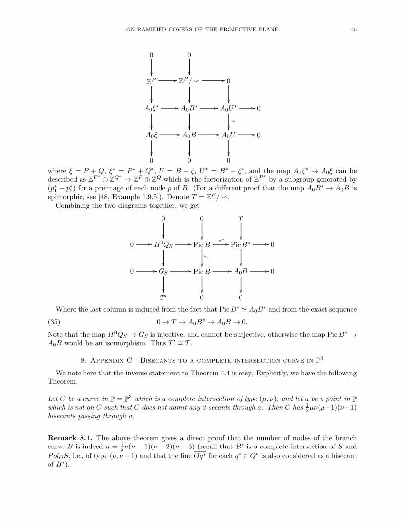
ON RAMIFIED COVERS OF THE PROJECTIVE PLANE 45
0
0
ZP
// ZP / ∽
// 0
A0ξ
∗ //
A0B∗ //
A0U∗ //
≃
0
A0ξ //
A0B //
A0U //
0
0 0 0
where ξ = P + Q, ξ∗ = P ∗ + Q∗, U = B − ξ, U∗ = B∗ − ξ∗, and the map A0ξ∗ → A0ξ can be
described as ZP ∗
⊕ ZQ∗
→ ZP ⊕ ZQ which is the factorization of ZP ∗
by a subgroup generated by(p∗1 − p∗2) for a preimage of each node p of B. (For a different proof that the map A0B
∗ → A0B isepimorphic, see [48, Example 1.9.5]). Denote T = ZP / ∽.
Combining the two diagrams together, we get
0
0
T
0 // H0QS
//
PicBπ∗
//
∼=
PicB∗ //
0
0 // GS//
PicB //
A0B //
0
T ′ 0 0
Where the last column is induced from the fact that PicB∗ ≃ A0B∗ and from the exact sequence
(35) 0 → T → A0B∗ → A0B → 0.
Note that the map H0QS → GS is injective, and cannot be surjective, otherwise the map PicB∗ →A0B would be an isomorphism. Thus T ′ ∼= T .
8. Appendix C : Bisecants to a complete intersection curve in P3
We note here that the inverse statement to Theorem 4.4 is easy. Explicitly, we have the followingTheorem:
Let C be a curve in P = P3 which is a complete intersection of type (µ, ν), and let a be a point in P
which is not on C such that C does not admit any 3-secants through a. Then C has 12µν(µ−1)(ν−1)
bisecants passing through a.
Remark 8.1. The above theorem gives a direct proof that the number of nodes of the branchcurve B is indeed n = 1
2ν(ν − 1)(ν − 2)(ν − 3) (recall that B∗ is a complete intersection of S and
PolOS, i.e., of type (ν, ν−1) and that the line Oq∗ for each q∗ ∈ Q∗ is also considered as a bisecantof B∗).

46 M. FRIEDMAN, M. LEYENSON
Proof. Our proof is essentially a reformulation of a proof by Salmon, [1, art. 343]. See also [15,Chapter IX, sections 1.1,1.2] for another way to induce this formula. Consider the moduli spaceM of data line l in P which is bisecant for C, a point p′ ∈ l ∩ C, a point p ∈ l, p /∈ C. (see thefollowing Figure)
c
p
l
p
the parameters (l, p′, p)
It is clear that the line l can be reconstructed uniquely from p′ and p as lp,p′ , and thus M can beembedded into P×P, (l, p′, p) 7→ (p′, p). For a point (l, p′, p) in M , let q be a point in l∩C differentfrom p′. Then there is a number t ∈ k such that q = p′+ tp. If C is given by 2 equations u, v, thenwe have u(q) = 0, v(q) = 0. Let us write u(q) = u(p′ + tp) = u0(p
′) + tu1(p′, p) + · · ·+ tµuµ(p
′, p),where ui is of degree µ − i in p′ and i in p. In the same way we can write v(q) = v(p′ + tp) =v(p′) + tv1(p
′, p) + · · · + tνvν(p′, p). Consider now two polynomials,
a(t) = u1(p′, p) + · · ·+ tµ − uµ(p
′, p),
b(t) = v1(p′, p) + · · ·+ tν − uν(p
′, p).
Let R(p′, p) be the resultant of a(p′, p, t) and b(p′, p, t) in t. It has (see the the Sylvester definition ofresultant) bidegree ((µ− 1)(ν − 1), µν − 1) in (p′, p). Lemma: Let U ⊂ P×P = (p′, p) : p′ 6= p.Then
U ∩ (R = 0) ∩ (C × P) =M
Indeed, let (p′, p) be such that R(p′, p) = 0, p′ 6= p. Then there is a number t ∈ k such thata(p′, p, t) = 0, b(p′, p, t) = 0. Let q = p′ + tp. We have
u(q) = u(p′) + ta(p′, p) = u(p′)
v(q) = v(p′) + tb(p′, p) = v(p′).
Thus q ∈ C iff p′ ∈ C. It follows that (p′, p) is in M iff p′ ∈ C. This proves the lemma. It followsnow that
R ∩ (C × a) =M ∩ (P×a) = ( bisecants through a to C with a marked point p′ in l ∩ C )
The order of this set is equal to degp′ C · degC = (µ − 1)(ν − 1)µν. Since C does not have any3-secants through a, it follows that the number of bisecants through a is one half of the numberabove.
References
[1] G. Salmon, A treatise on analytic geometry of three dimensions edition by Hodges, Smith, & Co., Dublin (1862),fourth edition.
[2] A. Brill, M. Nother, Uber die algebraischen Functionen und ihre Anwendung in der Geometrie, Math. Ann. 7(1874) 269-310.
[3] G. H. Halphen, Memoire sur la classification des courbes gauches algebriques J. Ec. Polyt. 52 (1882), 1200.

ON RAMIFIED COVERS OF THE PROJECTIVE PLANE 47
[4] S. Lefschetz, On the existence of loci with given singularities, Transactions of the American Mathematical Society,Vol. 14, No. 1 (1913), 23-41.
[5] O. Zariski, On the linear connection index of the algebraic surfaces zn = f(x, y), Proceedings of the NationalAcademy of Sciences, vol. 15 (1929), 494-501.
[6] O. Zariski, On the Problem of Existence of Algebraic Functions of Two Variables Possessing a Given Branch
Curve, American Journal of Mathematics, Vol. 51, No. 2 (1929), 305-328.[7] O. Zariski, On the Poincare group of rational plane curves, American Journal of Mathematics, Vol. 58, (1930),
607-619.[8] B. Segre, Sulla Caratterizzazione delle curve di diramazione dei piani multipli generali Mem. R. Acc. d’Italia, I
4 (1930), 531.[9] O. Zariski, On the irregularity of cyclic multiple planes, Annals of Mathematics (2), vol. 32 (1931), 485 - 511.
[10] P. Du Val, On Triple Planes Having Branch Curves of Order Not Greater Than Twelve, J. London Math. Soc.,s1-8 (1933), 199-206.
[11] E.R. Van Kampen, On the fundamental group of an algebraic curve, Am. J. Math. 55 (1933), 255-260.[12] O. Zariski, On the topological discriminant group of a Riemann surface of genus p, Amer. J. Math., 59, (1937),
335-358.[13] T.R. Hollcroft, Anomalous plane curve systems associated with singular surfaces, Bull. Amer. Math. Soc. Volume
46, Number 4 (1940), 252-257.[14] O. Chisini, Sulla identita birazionale delle funzioni algebriche di due variabili dotate di una medesima curva di
diramazione, Rend. Ist. Lombardo 77 (1944), 339-356.[15] J. Semple, L. Roth, Introduction to Algebraic Geometry, Oxford University Press (1949).[16] E.R. Grauert, R. Remmert, Komplexe Raume, Math. Ann. 136 (1958), 245 - 318.[17] A. Grothendieck, Fondements de la Geometrie algebrique, Seminaire Bourbaki, Exp. No. 190, (1959/60).[18] R. Narasimhan, Introduction to the Theory of Analytic Spaces, Lecture Notes in Mathematics, Volume 25,
Springer-Verlag (1966).[19] A. Altman, S. Kleiman, Introduction to Grothendieck duality theory, Springer (1970).[20] B. Iversen, Numerical invariants and multiple planes, Amer. J. Math. 92 (1970), 968-996.[21] A. Grothendieck, SGA1, Revetements etales et groupe fondamental, 1960-1961, Lecture Notes in Mathematics
224 (1971).[22] O. Zariski, Algebraic surfaces Springer, Heidelberg (1971), 2nd. ed.[23] Van der Waerden, B. L.: Einfuhrung in die algebraische Geometrie, 2nd edition. Springer (1973).[24] J. M. Wahl, Deformations of plane curves with nodes and cusps, Amer. J. Math. 96 (1974), 529-577.[25] B. Moishezon, Complex surfaces and connected sums of complex projective planes, Lecture Notes in Mathematics,
603. Springer-Verlag, New York, 1977.[26] R. Piene, Some formulas for a surface in P3, Algebraic geometry (Proc. Sympos., Univ. Tromsø, Tromsø, (1977)),
pp. 196–235, Lecture Notes in Math., 687, Springer, Berlin, (1978).[27] L. Gruson, C. Peskine, Genre des courbes de l’espace projectif, Algebraic Geometry (Tromsø 1977), Springer-
Verlag, Lect. Notes in Math. 687(1978), 31-59.[28] P. Grithis, J. Harris, Principles of Algebraic Geometry Wiley, New York (1978).[29] S. Greco, P. Valabrega, On the Theory of Adjoints, in ”Algebraic Geometry” (K. Lønsted, ed.), Springer-Verlag
LNM, vol. 732, (1979), pp. 98-123.[30] W. Fulton, J. Hansen,A Connectedness Theorem for Projective Varieties, with Applications to Intersections and
Singularities of Mappings, Annals of Mathematics, Second Series, Vol. 110, No. 1 (1979), 159-166.[31] W. Fulton, On the fundamental group of the complement of a node curve, Ann. of Math. 111 (1980), 407-409.[32] L. Chiantini, On some algebraic and geometric extension of the theory of adjoints, Rendiconti del Seminario
Matematico della Universita di Padova, tome 64 (1981).[33] B. Moishezon, Stable branch curves and braid monodromy, Lectur Notes in Math., 862, Springer-Verlag, (1981)
pp. 107-192.
[34] M. Nori, Zariskis conjecture and related problems, Ann. Sci. Ecole Norm. Sup. (4) 16 (1983), 305-344.[35] A. Libgober, Fundamental groups of the complements to plane singular curves, Algebraic geometry, Bowdoin,
1985 (Brunswick, Maine, 1985), Proc. Sympos. Pure Math., vol. 46, Amer. Math. Soc., Providence, RI, 1987,pp. 2945.
[36] F. Catanese, On a problem of Chisini, Duke Math. J. 53 (1986), 3342.[37] J. Harris, On a problem of Severi, Invent. Math. 84 (1986), 445-461.[38] B. Moishezon, M. Teicher, Galois covers in theory of algebraic surfaces , Amer. Math. Soc. Pub. PSPM 46 (1987),
47-65.[39] B. Moishezon, M. Teicher, Braid group technique in complex geometry, I, Line arrangements in P2, Contemp.
Math. 78, (1988), 425-555.
48 M. FRIEDMAN, M. LEYENSON
[40] B. Moishezon, M. Teicher, Braid group technique in complex geometry, II, From arrangements of lines and conics
to cuspidal curves, Algebraic Geometry, Lecture Notes in Math., vol. 1479 (1990), 131-180.[41] J. D’Almeida, Courbe de ramification de la projection sur P2 dune surface de P3, Duke Math. J. Volume 65,
Number 2 (1992), 229-233.[42] B. Moishezon, M. Teicher, Braid group techniques in complex geometry III: Projective degeneration of V3, Con-
temp. Math. 162, (1993), 313-332.[43] B. Moishezon, M. Teicher, Braid group techniques in complex geometry IV: Braid monodromy of the branch curve
S3 of V3 → P2 and application to π1 : (P2− S3), Contemp. Math. 162 (1993), 332-358.
[44] B. Moishezon, The arithmetic of braids and a statement of Chisini, Contemporary Math 164 (1994), 151-175.[45] B. Moishezon, M. Teicher, Braid group techniques in complex geometry, V: The fundamental group of comple-
ments of a branch curve of Veronese generic projection, Communications in Analysis and Geometry 4, (1996),no. 1, 1-120.
[46] B. Moishezon, A. Robb and M. Teicher, On Galois covers of Hirzebruch surfaces, Math. Ann. 305, (1996),493-539.
[47] Shustin, E. Geometry of equisingular families of plane algebraic curves, J. Alg. Geom. 5 (1996), no. 2, 209–234.[48] W. Fulton, Intersection theory, Springer-Verlag (1997).[49] A. Robb, On branch curves of algebric surfaces, AMS/IP Studies in Advanced Mathematics, vol. 5 (1997).[50] Shustin, E. Gluing of singular and critical points. Topology 37 (1998), no. 1, 195–217.[51] I. Shimada, On the commutativity of fundamental groups of complements to plane curves, Math. Proc. Cambridge
Philos. Soc. 123 (1998), no. 1, 49–52.[52] Vik. Kulikov, On Chisini’s Conjecture Izv. RAN. Ser. Mat. (1999), 63:6, 83116[53] Vik. Kulikov, M. Teicher,Braid monodromy factorizations and diffeomorphism types, Izv. Ross. Akad. Nauk Ser.
Mat. 64(2), 89-120 (2000) [Russian]; English transl., Izvestiya Math. 64(2), 311-341 (2000).[54] S. Nemirovski, A remark on the Chisini conjecture, e-print AG/0001113.[55] V. S. Kulikov, Vik. S. Kulikov Generic coverings of the plane with A-D-E-singularities, Izv. RAN. Ser. Mat.,
(2000), 64:6.[56] C. Ciliberto, R. Miranda, M. Teicher, Pillow Degenerations of K3 Surfaces, Applications of Algebraic Geometry
to Coding Theory, Physics, and Computation, NATO Science Series II, Vol. 36 (2001), 53-64.[57] Vik. S. Kulikov, Generalized Chisini’s Conjecture, Tr. MIAN (2003).[58] M. Amram, O. Shoetsu, Degenerations and fundamental groups related to some special Toric varieties, Michigan
Math. J. Volume 54, Issue 3 (2006), 587-610.[59] G.-M. Greuel, C. Lossen, E. Shustin, Global aspects of complex geometry, F. Catanese et al., eds., Springer
(2006), pp. 171-209.[60] Val. S. Kulikov , On characterization of branch curves of generic coverings, Interuniversity proceedings “Mathe-
matics: fundamental problems, applications, teaching”, vol.2, 66-102, Moscow State University Publisher (2002)(In Russian).
[61] R. Vakil, Murphys law in algebraic geometry: Badly-behaved deformation spaces, Invent. Math. 164 (2006), no.3, 569-590.
[62] The GAP Group, GAP – Groups, Algorithms, and Programming, Version 4.4.10; 2007.(http://www.gap-system.org)
[63] C. Ciliberto, F. Flamini On the branch curve of a general projection of a surface to a plane, arXiv:0811.0467v1(2008).
[64] A. Degtyarev, On deformations of singular plane sextics, J. Algeb. Geom. 17 (2008), 101-135.[65] Vik. Kulikov, On Chisini’s Conjecture II Izv. Math. 72 (2008).[66] M. Friedman, M. Teicher, On non fundamental group equivalent surfaces, Algebraic & Geometric Topology 8
(2008) 397-433.[67] M. Friedman, M. Leyenson, R. Lehman, On ramified covers of the projective plane II: Segre’s theory for singular
surfaces in P3 , in preperation.
Michael Friedman, Department of Mathematics, Bar-Ilan University, 52900 Ramat Gan, IsraelE-mail address: [email protected]
Maxim LeyensonE-mail address: [email protected]
Eugenii Shustin, School of Mathematical Sciences, Raymond and Beverly Sackler Faculty of ExactSciences, Tel Aviv University, Ramat Aviv, 69978 Tel Aviv, Israel
E-mail address: [email protected]