On Welfare-Enhancing Free Trade Areas*

Arvind Panagariya Pravin Krishna Department of Economics Department of Economics

University of Maryland Brown University College park, MD 20742 Providence, RI 02912

Revised: May 2001

The well-known Kemp-Vanek-Ohyama-Wan proposition establishes that if two or more countries form a customs union (CU) by freezing their net external trade vector through a common external tariff and eliminating internal trade barriers, the union as a whole and the rest of the world cannot be worse off than before. Owing to the fact that a Free Trade Area (whose member countries impose country specific external tariff vectors) does not equalize marginal rates of substitution across its member countries (in contrast to a CU), the literature has been unable to provide a parallel demonstration regarding welfare improving Free Trade Areas (FTAs). The present paper eliminates this gap. In extending the result to the case with intermediate inputs, the paper also sheds new light on the rules of origin required to support such necessarily welfare enhancing FTAs. We show here that provided no trade deflection is permitted, all that is required by way of rules of origin is that the goods produced within the union —whether final or intermediate — be allowed to be traded freely. The proportion of domestic value added in final goods does not enter as a criterion in the rules of origin.

*We are indebted to Jagdish Bhagwati and especially Rob Feenstra for many detailed and helpful comments. Pravin Krishna gratefully acknowledges the hospitality and the intellectual and financial support of the Center for Research on Economic Development and Policy Reform at Stanford University where part of this research was completed.

1. Introduction

The literature on preferential trade areas (PTAs), being concerned essentially with

“second-best” contexts,1 rarely offers clear-cut answers with respect to question of the

welfare impact of the formation of trading blocs between nations. A singular exception is

the well known result relating to customs unions (CUs)2, stated independently by Kemp

(1964) and Vanek (1965) and proved subsequently by Ohyama (1972) and Kemp and Wan

(1976), that if two or more countries freeze their net external trade vector with the rest of the

world through a set of common external tariffs (CET) and eliminate the barriers to internal

trade, the welfare of the union as a whole necessarily improves and that of the rest of the

world does not fall.3

The logic behind the Kemp-Vanek-Ohyama-Wan theorem is as follows: By fixing

the combined, net extra-union trade vector of member countries at its pre-union level, we

can guarantee non-members their original level of welfare. Moreover, taking the extra-

union trade vector as an endowment, the joint welfare of the union is maximized by

equating the marginal rate of substitution and marginal rate of transformation for each pair

of commodities to each other and across all agents in the union. This implies the

elimination of all internal distortions. The PTA thus constructed has a common internal

price vector implying further a common external tariff; it is therefore a Customs Union.

More than three decades have passed since the publication of the original statement

of the Kemp-Vanek-Ohyama-Wan theorem. However progress in the literature on this

subject has been minimal. In particular, we still lack a parallel result on Free Trade Areas

(FTAs) where members could use member-specific external tariff vectors rather than the

common external tariff vector required by CUs. The purpose of the present paper is to fill

1 On some general results concerning policy intervention in the presence of second best distortions and a unification of such results in the international trade literature, see Krishna and Panagariya (2000) 2 To get the basic definitions out of the way: A Customs Union (CU) is a preferential trade agreement in which member countries maintain a common external tariff vector against non-members. In contrast, in a Free Trade Area (FTA), member countries may maintain member-specific external tariff vectors. For a recent, comprehensive survey of the literature on preferential trading, see Panagariya (2000). 3 Panagariya (1997) offers a detailed history of this result.

this gap in the literature – a major gap, in our judgment, given the relative popularity of

FTAs over CUs in practice.

It should be straightforward to see that a demonstration regarding welfare-improving

FTAs is substantially more complex than that for CUs: In the case of an FTA, member-

specific tariff vectors imply that the domestic-price vectors differ across member countries.

This, in turn, implies that an FTA (as opposed to a CU) generally fails to equalize marginal

rates of substitution across union members.4 It is this difficulty, which accounts for why the

Kemp-Vanek-Ohyama-Wan result has not been extended to FTAs to-date. In this paper, we demonstrate that as long as goods produced within the union move

free of duty across member-country borders, a welfare-enhancing FTA can be constructed

even if the goods prices differ across member countries. The welfare-improving FTA we

propose has the property that member countries within the FTA individually import the

same vector of quantities from the rest of the world in the post-FTA equilibrium as in the

pre-FTA equilibrium. Our analysis begins in Section 2 where we explaining intuitively,

within a partial-equilibrium framework, why an FTA constructed in this manner must

enhance joint welfare. In Section 3, we extend this to a full general-equilibrium setting and

provide a formal proof. In Section 4, we show that the result is robust to the inclusion of

intermediate inputs in production. Section 5 discusses in substantial detail the rules of origin

necessary to support the FTA equilibrium. Section 6 concludes.

2. Partial Equilibrium Analysis

We consider first the simplest model capable of capturing the difference between the

Kemp-Vanek-Ohyama-Wan customs union and our FTA construction. Call the potential

union members Home and Foreign and the rest of the world ROW. Unless otherwise noted,

lower-case letters are used to denote variables associated with Home and upper case letters

those associated with Foreign. Assume that preferences are quasi-linear with the marginal

utility of consumption of the numeraire good being constant. Also assume that the

numeraire good uses only labor while non-numeraire goods use labor and a sector-specific

4 It should be readily evident that this non-equalization of the marginal rates of substitution and transformation across agents within the FTA implies that the Kemp-Wan proof methodology cannot be directly applied here.

factor. These assumptions validate the partial-equilibrium analysis on which we rely in the

present section. Since we will be holding the prices in ROW constant by freezing the

quantities traded by it, we define units of goods in such a manner that the prices in ROW are

all unity.

In Figures 1a and 1b, we depict the demands by Home and Foreign by dd and DD,

respectively, for a non-numeraire good that is not produced at home. Home levies a tariff at

rate t0 and Foreign at rate T0 > t0. Since the price in ROW is 1, the domestic price in Home

settles at 1+t0 and in Foreign at 1+T0. Home and Foreign consume and import quantities oc0

and OC0, respectively.

Suppose now that Home and Foreign form a customs union, holding their joint

imports at oc+OC. This would require setting the common external tariff at rate tcu (=TCU),

where T0 > tcu > t0 and the joint demand by the member countries at price 1+tcu is oc1+OC1.

The increase in the price in Home lowers its welfare while the decrease in price in Foreign

does the opposite. But since the marginal benefit of consumption is higher in Foreign in the

initial equilibrium, the shift in consumption from Home to Foreign until the marginal

benefits are equalized across members leads to a net gain for the union as a whole. Thus,

the customs union improves the welfare of the union and does not hurt the outside world.

The loss to Home is measured by trapezium ghkv and the gain to Foreign by GHKV. But

since kv = KV and hk = HK, the gain is necessarily bigger than the loss. Moreover, holding

the union-wide imports fixed, the union cannot improve upon this equilibrium.

Suppose, next, that Home and Foreign form an FTA rather than the customs union,

each fixing the external tariff such that its imports are unchanged. Because the member

countries do not produce the good, the only way to achieve this outcome is to fix the

external tariffs at the same rate as initially and adopt the rule of origin whereby goods are

not allowed to be transshipped; that is to say, goods consumed in Foreign are not permitted

to be imported via Home at the lower tariff. Since there is no production of the good within

the union to take advantage of duty-free movement of goods produced inside the union,

under this arrangement, the outcome is the same as under the nondiscriminatory tariff. The

FTA neither improves nor lowers welfare.5

It is worth noting here that in this FTA equilibrium, prices (of the imported good)

are different in the two partner countries – therefore creating the incentive to import the

good through the low tariff country and simply transship it to the partner country by

exploiting the free access to the latter’s market. To prevent this type of transshipment (which

effectively undermines the effort to maintain different tariff rates across the two partner

countries), additional rules prohibiting such transshipment need to be introduced. These are

the so-called rules-of-origin (ROOs). We proceed for the moment by simply assuming that

ROOs that effectively prevent transshipment of this type are in place and defer a full

discussion of what form these ROOs must take until Section 5.

Let us now modify this simple case to allow for internal production. This is done in

Figures 2a and 2b where ss and SS represent the supply curves in Home and Foreign,

respectively. As before, initially, each country levies a nondiscriminatory tariff so that

internal prices are given by 1+t0 in Home and 1+T0 in Foreign. At 1+t0, the quantities

consumed, produced and imported equal ox0, oc0 and x0c0 in Home. The corresponding

quantities in Foreign are OX0, OC0 and X0C0.

Suppose now that Home and Foreign form a customs union, holding their joint

imports fixed at x0c0 + X0C0. This is accomplished by a common external tariff that lies

between t0 and T0. Without demonstrating in Figures 2a and 2b, we note that, as before,

taking the total union-wide imports as fixed, the common external tariff maximizes the joint

welfare of the union by equating the marginal benefit and marginal cost of production with

each other and across Home and Foreign.

Next, consider the formation of an FTA between Home and Foreign. This requires

fixing the imports of each country at their pre-FTA level. To show how this works, subtract

Home’s initial imports, x0c0, from its demand curve and obtain d′d′ as the residual demand

that must be satisfied by within-union sources of supply. Analogously, obtain D′D′ by

5 In differentiated goods models, this is not an altogether implausible outcome.

subtracting X0C0 from DD as the demand in Foreign that must be satisfied by within-union

sources of supply.

The key point to emphasize is that if imports are subject to different tariff rates and

the rules of origin forbid the low-tariff member from importing goods from outside for duty-

free sales in the high-tariff country, the prices consumers pay in the two countries will differ

from each other. In particular, they will be higher in the member with the higher tariff.

Suppose, as will turn out to be true in our example, the post-FTA tariff that supports the pre-

FTA imports is higher in Foreign than Home. It is then immediate that all within-union

output will be sold in Foreign. Conversely, if the post-FTA tariff happens to be higher in

Home, all within-union output will be sold in that country. Only if the post-union tariff

happens to be the same in the two countries, implying a coincidence of the FTA and

customs union solutions in the good under consideration, will the internal supply be sold in

both countries.

In Figure 2, given the post-FTA tariff and hence the consumer price is higher in

Foreign, no within-union output is sold in Home. This means the tariff in Home must be set

at tf such that 1+tf represents the “reservation price.” At this price, all demand in Home is

satisfied by imports while its entire supply is sold in Foreign.

In Foreign, the available internal supply is the horizontal sum of ss and SS and is

shown by the dotted line denoted s+S. To clear the market, the internal price must be 1+Tf,

the height of the point of intersection of D′D′ and s+S. Thus, we have Tf as the tariff in

Foreign under the FTA. The reader can verify that the joint welfare of the union members,

as measured by the sum of their consumers’ and producers’ surpluses and tariff revenues, is

higher at the FTA equilibrium than at the initial equilibrium.

The outcome shown in Figure 2 has the feature that the tariff rates that support

country-specific pre-FTA imports in Home and Foreign are strictly different. This feature

results from the fact that even after the entire within-union supply is diverted to Foreign, at

1+tf, it falls short of the demand for within-union output. If within-union supply is

sufficiently large to rule this out, ex post, the outcome will coincide with the customs union

outcome.

For example, suppose we rotate ss clockwise and SS anti-clockwise, holding the

initial tariff rates and total union-wide supply at each price constant. This will shift d′d′ to

the right and D′D′ to the left. Eventually, the horizontal line from 1+tf will come to pass

through the intersection of d′d′ and D′D′. At this configuration of demands, supplies and

initial tariffs, the FTA solution will just coincide with the customs union solution in the

good under consideration. As we continue to rotate ss clockwise and SS anti-clockwise, the

customs union solution will continue to obtain with the internal supply sold in both union

members.

In Figure 2, holding the initial tariff rates and demands constant, if we rotate ss anti-

clockwise and SS clockwise, d′d′ shifts to the left and D′D′ to the right. In this case, tf and

Tf move in opposite directions. Thus, ceteris paribus, the lower the tariff in the country with

smaller supply, the more likely that the outcome will be a strict FTA. And, conversely, the

higher the tariff in the country with lower supply, the more likely that the outcome will

coincide with the customs union.

We conclude this section by noting a key point that will be important for proving our

general result in the next section. For some products, the FTA solution may coincide with

the customs union solution. When it does not, a single producer price nevertheless rules

within the union and it equals the consumer price in the member country with the higher

tariff.

3. Proof in the General Case

To begin with we consider economies with only final goods. Intermediate inputs are

added to the model in the next section. The proof in this case turns out to be surprisingly

simple. The maintained assumption throughout is that in the event of differences in final

prices between FTA partners on external imports, Rules of Origin (ROOs), which

effectively prevent transshipment of these goods from low tariff countries to high tariff

countries, are in place. As noted before, we defer our discussion of what form these ROOs

may take until Section 5.

We continue to denote Home variables by lower case letters and Foreign variables

by upper case letters. Occasionally, we need to use the price vector in the rest of the world.

We denote it by an upper case letters with subscript W. A superscript 0 is used to identify

the values of the variables in the initial, pre-FTA equilibrium and superscript f in the post-

FTA equilibrium. If the pre- and post-FTA values of a variable happen to coincide, we use

superscript 0.

Denote by e(.) and E(.) the standard expenditure functions and r(.) and R(.) the

standard revenue functions in Home and Foreign, respectively. The consumer price vectors

are denoted p and P and welfare levels u and U. We assume that the utility of Foreign in the

post-FTA equilibrium is held fixed at its pre-FTA level through a lump sum transfer from

Home. The transfer may turn out to be positive or negative. Under this assumption, weak

superiority of the FTA is established provided

(1) f f f 0e(p , u ) e(p , u )≥

Our proof involves demonstrating the validity of this inequality.

The income-expenditure inequality for the union as a whole in the post-FTA

equilibrium implies

(2) , f f f 0 f f 0 0 f f 0W We(p ,u ) E(P , U ) r(q ) (p P )m R(q ) (P P )M+ = + − + + − 0

where m0 and M0 are vectors of quantities imported by Home and Foreign, respectively,

from the rest of the world (i.e., not including the imports from each other) in the post-FTA

equilibrium, which are the same as in the pre-FTA equilibrium (recall that, in the post-FTA

equilibrium, we are fixing each country’s import vector from the rest of the world at its pre-

FTA level). We note that m0 is defined to include any goods that may have entered Home

through Foreign in the pre-FTA equilibrium. That is to say, in fixing the external import

vector of a member, we include in it any goods that may have imported or exported

indirectly through the partner. A similar statement applies to M0. Vector PW0 is the world

price vector in the post-FTA equilibrium, which coincides with the pre-FTA equilibrium

since we freeze the external trade vectors of both Home and Foreign at their pre-FTA levels.

Vector qf is the producer-price vector in the post-FTA equilibrium, which is the same in

Home and Foreign.

By the definition of the expenditure function, we have

(3a) , f 0 f 0 f 0 0 0e(p ,u ) p d p [x m n ]≤ = + +

where d and x are used to represent the consumption (or demand) and output vectors,

respectively. Vector n0 represents net imports by Home from Foreign. This vector is

defined to include the quantities originating in Foreign only. As stated earlier, any goods

imported by Foreign from the rest of the world and re-exported to Home are included in m0.

Analogous to (3a), we have for Foreign,

(3b) f 0 f 0 f 0 0 0E(P , U ) P D P [X M N ]≤ = + +

By definition, we have n0 = -N0. Subtracting the sum of (3a) and (3b) from (2), we obtain

(4) f f f 0

f f f 0 f 0 0 0 0 f 0 fW

e(p ,u ) e(p ,u ) [r(q ) R(q )] [p x P X ] P (m M ) [p n P N ]

−

≥ + − + − + − + 0

0

0

0

By the trade balance condition of the rest of the world, we can set PW0(m0+M0) = 0. In

addition, we have N0 = -n0. Therefore, we can rewrite (4) as

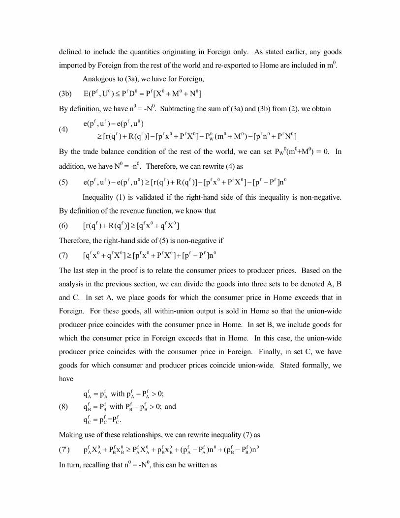
(5) f f f 0 f f f 0 f 0 f fe(p , u ) e(p ,u ) [r(q ) R(q )] [p x P X ] [p P ]n− ≥ + − + − −

Inequality (1) is validated if the right-hand side of this inequality is non-negative.

By definition of the revenue function, we know that

(6) f f f 0 f[r(q ) R(q )] [q x q X ]+ ≥ +

Therefore, the right-hand side of (5) is non-negative if

(7) f 0 f 0 f 0 f 0 f f 0[q x q X ] [p x P X ] [p P ]n+ ≥ + + −

The last step in the proof is to relate the consumer prices to producer prices. Based on the

analysis in the previous section, we can divide the goods into three sets to be denoted A, B

and C. In set A, we place goods for which the consumer price in Home exceeds that in

Foreign. For these goods, all within-union output is sold in Home so that the union-wide

producer price coincides with the consumer price in Home. In set B, we include goods for

which the consumer price in Foreign exceeds that in Home. In this case, the union-wide

producer price coincides with the consumer price in Foreign. Finally, in set C, we have

goods for which consumer and producer prices coincide union-wide. Stated formally, we

have

(8)

f f f fA A A Af f f fB B B Bf f fC C C

q p with p P 0;q P with P p 0; andq p =P .

= − >

= − >

=

Making use of these relationships, we can rewrite inequality (7) as

(7′) f 0 f 0 f 0 f 0 f f 0 f fA A B B A A B B A A B Bp X P x P X p x (p P )n (p P )n+ ≥ + + − + −

In turn, recalling that n0 = -N0, this can be written as

(7″) f f 0 0 f f 0 0A A A A B B B B(p P )(X N ) (P p )(x n ) 0.− + + − + ≥

Given (8) and the fact that domestic output must necessarily be at least as large as the

exports to the union partner (recall that since m0 and M0 are defined to include all imports

from and exports to the outside world including those channeled through the partner, n0 and

N0 cannot include the goods imported from or exported to the outside world), this inequality

is necessarily satisfied. Thus, we have established inequality (1) and hence the main result

of the paper.

4. Extension to Intermediate Inputs

The proof above is extended readily to incorporate intermediate inputs. We note here

the first few steps – these should be sufficient to see how the extension works. Since

intermediate inputs do not enter the utility function and, hence, the expenditure function,

holding the utility of Foreign fixed through a lump sum transfer at the pre-FTA level,

Condition (1) continues to be necessary and sufficient for the FTA to weakly improve the

joint welfare of the union.

The main new issue that the presence of intermediate inputs raises is that of the rules

of origin. We impose here the same rules of origin as in the previous section: both the final

and intermediate inputs can move free of duty within the union provided they are produced

internally. In the case of final goods, it does not matter whether the inputs used in it are

imported or produced internally. As we detail in section 5, irrespective of the proportion of

internal value added, they must receive the duty-free treatment if the final stage of

production takes place within the union.

The buyers as well as sellers of intermediate inputs are firms. For reasons similar to

those in the previous section, the buyer prices can differ between the union members while

the seller or producer price is the same. We now use a subscript I to distinguish inputs from

outputs. Thus, we denote by pI the vector of buyer prices and qI the vector of seller prices of

inputs in Home. We can then write the revenue function, representing the maximized value

of output of final and intermediate inputs, net of inputs used up, as r(q, pI, qI). The partial

derivatives of r(.) with respect to buyer prices of inputs, pI, give the negative of the demand

for inputs and those with respect to seller prices, qI, give the supplies of the inputs in Home.

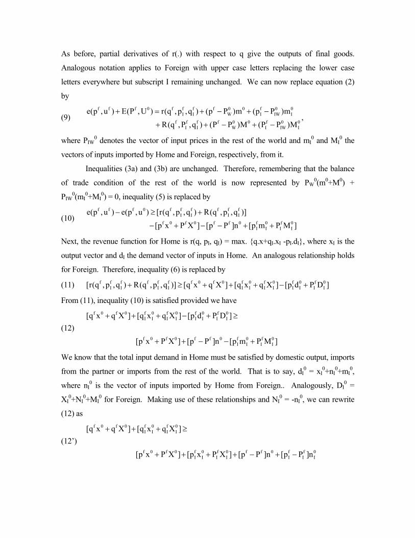
As before, partial derivatives of r(.) with respect to q give the outputs of final goods.

Analogous notation applies to Foreign with upper case letters replacing the lower case

letters everywhere but subscript I remaining unchanged. We can now replace equation (2)

by

(9) , f f f 0 f f f f 0 0 f 0 0

I I W I IW If f f f 0 0 f 0

I I W I IW

e(p ,u ) E(P , U ) r(q ,p ,q ) (p P )m (p P )m

R(q ,P ,q ) (P P )M (P P )M

+ = + − + −

+ + − + − 0I

where PIW0 denotes the vector of input prices in the rest of the world and mI

0 and MI0 the

vectors of inputs imported by Home and Foreign, respectively, from it.

Inequalities (3a) and (3b) are unchanged. Therefore, remembering that the balance

of trade condition of the rest of the world is now represented by PW0(m0+M0) +

PIW0(mI

0+MI0) = 0, inequality (5) is replaced by

(10) f f f 0 f f f f f f

I I I If 0 f 0 f f 0 f 0 f 0

I I I I

e(p , u ) e(p ,u ) [r(q ,p ,q ) R(q ,p ,q )] [p x P X ] [p P ]n [p m P M ]

− ≥ +

− + − − + +

Next, the revenue function for Home is r(q, pI, qI) = max. {q.x+qI.xI -pI.dI}, where xI is the

output vector and dI the demand vector of inputs in Home. An analogous relationship holds

for Foreign. Therefore, inequality (6) is replaced by

(11) f f f f f f f 0 f 0 f 0 f 0 f 0 f 0I I I I I I I I I I I I[r(q , p ,q ) R(q ,p ,q )] [q x q X ] [q x q X ] [p d P D ]+ ≥ + + + − +

From (11), inequality (10) is satisfied provided we have

(12)

f 0 f 0 f 0 f 0 f 0 f 0I I I I I I I I

f 0 f 0 f f 0 f 0 f 0I I I I

[q x q X ] [q x q X ] [p d P D ]

[p x P X ] [p P ]n [p m P M ]

+ + + − + ≥

+ + − − +

We know that the total input demand in Home must be satisfied by domestic output, imports

from the partner or imports from the rest of the world. That is to say, dI0 = xI

0+nI0+mI

0,

where nI0 is the vector of inputs imported by Home from Foreign.. Analogously, DI

0 =

XI0+NI

0+MI0 for Foreign. Making use of these relationships and NI

0 = -nI0, we can rewrite

(12) as

(12’)

f 0 f 0 f 0 f 0I I I I

f 0 f 0 f 0 f 0 f f 0 f f 0I I I I I I I

[q x q X ] [q x q X ]

[p x P X ] [p x P X ] [p P ]n [p P ]n

+ + + ≥

+ + + + − + −

This inequality tracks inequality (7’) identically, taking into account the fact that we now

have intermediate inputs. The remainder of the proof is straightforward in view of the proof

in the previous section.

5. Rules of Origin Necessary to Prevent Transshipment

In proving the existence of welfare improving FTAs, we have assumed so far that

we use rules of origin to prevent transshipment of imports. This implies that goods imported

by the low-tariff member are not permitted to cross over to the high-tariff member country

duty free unless they have undergone some transformation. Thus, duty free access

necessarily applies to goods produced wholly within the union. Additionally, the goods

containing foreign intermediate components are given duty-free status provided the

intermediates have undergone some transformation. Imported goods, whether intermediate

or final, may not be transshipped in their original form.

In of itself, this requirement may be seen as being somewhat incomplete for the

following reason. In the FTA equilibrium that obtains, consumer prices differ across

member countries (else, the FTA is in fact just a CU). Given the differing consumer prices

across countries, agents have the incentive to import a given product through the low-tariff

country, repackage and, thus, transform it into a trivially different good, and avail

themselves of the duty free status in the higher-tariff partner country. This unrestrained

transshipment would render the FTA arbitrarily close to a CU.

To avoid this possibility, we need to elaborate on the rule of origin necessary to

support the FTA keeping in mind that the proposed rule does not interfere with the

equilibrium outcomes [and indeed conditions (6) and (7) and (11) and (12)] for welfare

improvement described in Sections 3 and 4. We first describe the precise rule of origin

required within our theoretical model and then discuss its practical counterpart.

Rule of Origin: A good wholly produced within the union is given duty free access to all

countries within the union. Alternatively, if the good contains imported intermediates, it is

allowed duty free access provided it differs from any of the intermediates it contains and is a

good that existed prior to the formation of the FTA. Thus, we require additionally that any

new good (i.e., goods not existing in the pre-FTA equilibrium) be given duty free access to

union countries only if it is wholly produced within the union.

To explain how this rule works (without interfering with the welfare improving

equilibrium outcome described in our proof) suppose there are 100 final and intermediate

products in the pre-FTA equilibrium, which are denoted 1, 2…100. Now consider a product

crossing the intra-union border. The importer must first declare whether the product

corresponds to one of these 100 products. If yes, he identifies the precise classification

number of the product, say, 80. He must then identify the classification numbers of

components imported from outside the union. If these are all different from 80, the product

enters duty free. If one or more of them coincide with 80, duty-free status is not given.

Observe that the importer no longer has an incentive to bring product 80, repackage

it and claim it as a different product. If he were to do that, he will have to declare it as a new

product that is different from product 80. This will automatically result in the denial of the

duty-free status. Of course, if he were to declare the product as 80, the imported

components would coincide with the product and the importer would fail to satisfy the

transformation rule.

Thus our rule ensures that there is no transshipment of imports from the low-tariff

member to the high-tariff member without imposing any new constraints on the problem. It

is important to note that the rule prohibiting the transshipment of products (product 80 in the

above example) does not imply a more restrictive environment than in the pre-FTA

equilibrium. Any transshipment that existed in the pre-FTA equilibrium continue to reach

the country of its final destination; only that they now come directly to that country since the

external trade vector of each member includes not only the imports it received directly from

the rest of the world but also those it receives through the partner in the form of

transshipments [see the discussion following equation (2) above]. Therefore, our rule of

origin fully preserves our proof.

We have, thus, shown that theoretically there exists a rule of origin capable of

supporting the FTA equilibrium we have identified. We can now ask how this rule can be

applied in practice. For most products, our transformation rule can be applied using the

harmonized system of classification. Duty-free status is necessarily given to a product that

is produced wholly within the union or belongs to a classification category different from all

components imported from extra-union trading partners. The harmonized system of

classification, which is used by virtually all countries, disaggregates products up to the ten-

digit level. In most cases, this level of disaggregation suffices to distinguish products that

satisfy our theoretical rule from those that have been simply repackaged and do not satisfy

it.6 For example, an automobile imported from an outside country and simply repackaged

will fail this test since it will fail to move from one classification category to another.

We note that that the transformation requirement we have stated above and its

implementation is entirely consistent with the rules of origin implemented in actual practice

– in NAFTA, for instance. In the appendix, we reproduce a description of the NAFTA rules

of origin from LaNasa (1993). It should be readily evident that the first three rules described

there match very closely our transformation rule. It may be interesting to note further that to

rule out trivial transformations of the type we have considered earlier in this section, the

NAFTA rules of origin explicitly state that ‘mere dilution with water or another substance

that do not materially alter the characteristics of the product do not count as a

transformation.’

6. Concluding Remarks

As emphasized in Bhagwati and Panagariya (1996a, 1996b) and Bhagwati, Greenaway

and Panagariya (1997), we conclude this paper by noting that these results are existence

6 While the transformation rule we have described satisfies our theoretical requirements completely, in practice, there remain a small fraction of products that may have undergone transformation according to our theoretical criterion but are classified in the same category as its components. For example, the harmonized system places a finished bicycle and its completely knocked down (CKD) kit under the same tariff heading. If a union member produces a bicycle by assembling a CKD kit imported from an extra-union partner, our theoretical criterion is satisfied but the implementation rule fails to identify it as an item qualified for duty-free access. To rule out this possibility, we need an addition valued-added rule to be calculated as follows. Compute the FTA equilibrium we have outlined in Section 3 or 4 as the case may be. The computed equilibrium values of various variables allow us to calculate the ex post value added necessary to convert the CKD kit into a finished bicycle. We set the valued-added requirement for duty-free entry for finished bicycle equal to this value added. Since this valued added has been computed at the equilibrium that satisfies conditions (6) and (7) or their equivalent, (11) and (12) in Section 4, adding the valued added rule of origin has no impact on the outcome while it ensures that the CKD kit is not transshipped. The fourth NAFTA rule of origin in the appendix provides the real world parallel to this criterion, though we hasten to add that since the actual value added requirement there is ad hoc, the resulting FTA is different from the one we have computed here.

results and should not be taken to imply that any particular FTA is welfare improving.

Indeed, as we have already noted, both Kemp-Vanek-Ohyama-Wan and the present

results require a particular structure of external tariffs to guarantee an improvement in

welfare relative to the initial equilibrium. Finally, though our result implies that there

exists an FTA path to complete multilateral free trade along which global welfare rises

monotonically, it does not and cannot imply that such a path will actually be adopted.

The latter question requires a political-economy theoretic, incentive-structure analysis

and raises a different set of problems as analyzed in the recent contributions of Krishna

(1998) and Levy (1997).

An interesting implication of our analysis relates to rules of origin, which did not form a part

of the Kemp-Vanek-Ohyama-Wan analysis for the reason that there they only dealt with the

customs union problem. We have shown here that provided no trade deflection is

permitted7, all that is required by way of rules of origin is that the goods produced within the

union —whether final or intermediate — be allowed to be traded freely. The proportion of

domestic value added in final goods does not enter as a criterion in the rules of origin.

7 By no trade deflection, we mean that in the post-FTA equilibrium, extra-union imports pay the tariff rate of the country of final destination. They should not be permitted to enter the union through the border of a member with a lower tariff and then shipped freely to another member with higher tariff.

Appendix: NAFTA Rules of Origin

In this appendix, we draw on LaNasa (1993) to offer a brief description of the NAFTA rules

of origin. A product qualifies for preferential treatment under NAFTA, if it passes one of

the following five tests:

i. The product is wholly obtained or produced in the territory of one or more of the

member countries.

ii. The product is produced entirely in the territory of one or more of the Parties

exclusively from originating materials.

iii. If a product contains any materials not originating in North America, it is

classified as a North American good if each non-originating material

undergoes a change in tariff classification caused by production that occurs

entirely within Canada, Mexico, or the United States. NAFTA defines the

required change by reference to changes in the HTS. The HTS is an international

standard that harmonizes tariff nomenclature worldwide. It classifies products

according to a hierarchical framework that reflects increasing degrees of

technical sophistication and economic effort). The type and degree of change

required depends upon the type of product.

iv. If a non-originating part does not qualify under the change in tariff classification

test because the tariff heading for it and the product crossing the border is the

same, the product can still be treated as originating in North America if it meets

the required regional value content test

v. If a good fails all of the above tests, the product will be classified as North

American if the non-originating material is de minimis, that is, less than seven

percent of the transaction value (price) or total cost of the good.

There are three cases in which a good that qualifies for North American origin can

be disqualified from preferential treatment. First, the good is disqualified if after qualifying,

it undergoes further processing outside North America. Second, mere dilution with water

or another substance that does not materially alter the characteristics of the product

does not count as a qualifying operation. Finally, any good undergoing any process, work

or pricing practice aimed at circumventing NAFTA's rules of origin is disqualified from

preferential treatemnt.”

References

Bhagwati, Jagdish, Greenaway, David and Panagariya, Arvind, 1997, "Trading Preferentially: Theory and Policy," mimeo., July 1997, Economic Journal.

Bhagwati, Jagdish and Panagariya, Arvind, 1996a, "Preferential Trading Areas and Multilateralism: Strangers, Friends or Foes?" in Jagdish Bhagwati and Arvind Panagariya, eds., The Economics of Preferential Trade Agreements, 1996, AEI Press, Washington, D.C.

Bhagwati, Jagdish and Panagariya, Arvind, 1996b, "The Theory of Preferential trade Agreements: Historical Evolution and Current Trends," American Economic Review. Papers and Proceedings, May.

Grossman, Gene and Helpman, Elhanan, 1995, "The Politics of Free Trade Agreements," American Economic Review, September, 667-690.

Kemp, Murray, C., 1964, The Pure Theory of International Trade, Prentice-Hall, Englewood Cliffs, N.J., 176-177.

Kemp, Murray C. and Wan, Henry, 1976, "An Elementary Proposition Concerning the Formation of Customs Unions," Journal of International Economics 6 (February), 95-8.

Krishna, Pravin, 1998, "Regionalism and Multilateralism: A Political Economy Approach," Quarterly Journal of Economics.

Krishna, Pravin and Arvind Panagariya, 1997, "A Unification of the Theory of Second Best," Journal of International Economics 52(2), 235-257, December 2000..

Krugman, P., 1980, "Scale Economies, Product Differentiation, and the Pattern of Trade," American Economic Review 70, no. 5 (December 1980): 950-959.

in LaNasa III, Joseph A., 1993, “Rules of Origin under North American Free Trade Agreement: A Substantial Transformation into Objectively Transparent Protectionism,” Harvard International Law Journal 34, No. 2, Spring, 381-406

Levy, Philip, 1997, "A Political Economic Analysis of Free Trade Agreements," American Economic Review.

Lipsey, Richard, 1958, The Theory of Customs Unions: A General Equilibrium Analysis, University of London, Ph.D. thesis.

Lloyd, Peter J., 1982, "3x3 Theory of Customs Unions," Journal of International Economics 12, 41-63.

McMillan, John and McCann, Ewen, 1981, "Welfare Effects in Customs Union," Economic Journal 91, 697-703, September.

Ohyama, M., 1972, "Trade and Welfare in General Equilibrium," Keio Economic Studies 9, 37-73.

Panagariya, Arvind, 2000, “Preferential Trade Liberalization: The Traditional Theory and New Developments,” Journal of Economic Literature, June 2000, 287-331.

Panagariya, Arvind and Findlay, Ronald, 1996, "A Political Economy Analysis of Free Trade Areas and Customs Unions," Robert Feenstra, Douglas Irwin and Gene Grossman, eds., The Political Economy of Trade Reform, Essays in Honor of Jagdish Bhagwati, MIT Press.

Panagariya, Arvind, 1997, "The Meade Model of Preferential Trading: History, Analytics and Policy Implications," in Cohen, B.J., ed., International Trade and Finance:

New Frontiers for Research. Essays in Honor of Peter B. Kenen, Cambridge University Press, New York.

Vanek, Jaroslav, 1965, General Equilibrium of International Discrimination: The Case of Customs Unions. Cambridge, MA: Harvard University Press.

p

c

d

d

c0

1+tcu

1

o

D

D

1+T0

P

C0 C1

g h

k v

H

G

K V

Figure 1a Figure 1b

O C

1+t0

c1

1+TCU

p

c, x

d

d 1+t0

1

o c0 x0

D

D

1+T0

P

C0

d′

s

s d′

S+s

S

D′

S

Figure 2a Figure 2b

O X0

D′

1+tf

1+Tf

1

C, X

L K