
On Multiple Criteria Decision Support for Suppliers on the Competitive Electric Power Market
26
Annals of Operations Research 121, 79–104, 2003 2003 Kluwer Academic Publishers. Manufactured in The Netherlands. On Multiple Criteria Decision Support for Suppliers on the Competitive Electric Power Market MARIUSZ KALETA, WLODZIMIERZ OGRYCZAK, EUGENIUSZ TOCZYLOWSKI ∗ and IZABELA ˙ ZÓLTOWSKA [email protected] Warsaw University of Technology, Institute of Control & ComputationEngineering, 00-665 Warsaw, Poland Abstract. As an active participant of a competitive energy market, the generator (the energy supplier) chal- lenges new management decisions being exposed to the financial risk environment. There is a strong need for the decision support models and tools for energy market participants. This paper shows that the stochas- tic short-term planning model can be effectively used as a key analytical tool within the decision support process for relatively small energy suppliers (price-takers). A self-scheduling method for the thermal units on the energy market is addressed. A schedule acquired for given preferences can be used as a desired pattern for bidding process. The uncertainty of the market prices is modeled by a set of possible scenarios with assigned probabilities. Several risk criteria are introduced leading to a multiple criteria optimization problem. The risk criteria are well appealing and easily computable (by means of linear programming) but they meet the formal risk aversion standards. The aspiration/reservation based interactive analysis applied to the multiple criteria problem allows us to find an efficient solution (generation scheme) well adjusted to the generator preferences (risk attitude). Keywords: energy market, decision support, risk, multiple criteria optimization, short-term planning, unit commitment Introduction Very complex systems are often beyond efficient direct control and management. There- fore, in many countries various large scale technical systems, such as electric power industry, or telecommunication sector, are undergoing unprecedented changes related to deregulations. The trends are toward deregulating whole industries, that have tradition- ally been a regulated monopoly, in order to allow for economic competition. On the technical site, a whole industry sector, such as the electric power industry, is a large, hierarchically coordinated system which has to provide various services to customers and meet strict global performance objectives (power demand, frequency, voltage levels, safety of delivery) and which has to manage various system-wide resources required to assure proper operation of the system. These resources may belong to independent sub- systems, which may be defined according to administrative divisions among particular companies. ∗ Corresponding author.
Transcript of On Multiple Criteria Decision Support for Suppliers on the Competitive Electric Power Market
Annals of Operations Research 121, 79–104, 2003 2003 Kluwer Academic Publishers. Manufactured in The Netherlands.
On Multiple Criteria Decision Support for Supplierson the Competitive Electric Power Market
MARIUSZ KALETA, WŁODZIMIERZ OGRYCZAK, EUGENIUSZ TOCZYŁOWSKI ∗and IZABELA ZÓŁTOWSKA [email protected] University of Technology, Institute of Control & Computation Engineering, 00-665 Warsaw,Poland
Abstract. As an active participant of a competitive energy market, the generator (the energy supplier) chal-lenges new management decisions being exposed to the financial risk environment. There is a strong needfor the decision support models and tools for energy market participants. This paper shows that the stochas-tic short-term planning model can be effectively used as a key analytical tool within the decision supportprocess for relatively small energy suppliers (price-takers). A self-scheduling method for the thermal unitson the energy market is addressed. A schedule acquired for given preferences can be used as a desiredpattern for bidding process. The uncertainty of the market prices is modeled by a set of possible scenarioswith assigned probabilities. Several risk criteria are introduced leading to a multiple criteria optimizationproblem. The risk criteria are well appealing and easily computable (by means of linear programming) butthey meet the formal risk aversion standards. The aspiration/reservation based interactive analysis appliedto the multiple criteria problem allows us to find an efficient solution (generation scheme) well adjusted tothe generator preferences (risk attitude).
Keywords: energy market, decision support, risk, multiple criteria optimization, short-term planning, unitcommitment
Introduction
Very complex systems are often beyond efficient direct control and management. There-fore, in many countries various large scale technical systems, such as electric powerindustry, or telecommunication sector, are undergoing unprecedented changes related toderegulations. The trends are toward deregulating whole industries, that have tradition-ally been a regulated monopoly, in order to allow for economic competition. On thetechnical site, a whole industry sector, such as the electric power industry, is a large,hierarchically coordinated system which has to provide various services to customersand meet strict global performance objectives (power demand, frequency, voltage levels,safety of delivery) and which has to manage various system-wide resources required toassure proper operation of the system. These resources may belong to independent sub-systems, which may be defined according to administrative divisions among particularcompanies.
∗ Corresponding author.
80 KALETA ET AL.
Under deregulation, the elements of the system are undergoing drastic restructur-ing and transformation from cost-conscious, regulated utilities to competitive marketparticipants. In the deregulated framework for control and management, instead of oper-ating according to central rules and plans established by a hierarchical control structurein a centralized system, the system operates through cooperative behavior of many in-teractive subsystems which are organized as the competitive market participants. Thesubsystems may have their own independent interests, values, different tasks, operationsand services.
The market mechanisms can be implemented through pool or bilateral arrange-ments. A pool facilities the market by providing a forum for matching supply and de-mand, where all transactions are cleared at the same price. These prices may be obtainedthrough some sort of iterative bidding process. In a bilateral market, supply and demandare matched through individual contracts between buyer and seller, and each transactionis cleared at a different price based on details agreed in the contract. A typical electricpower system may consist of one or many power pools that are operated at the samelevel of hierarchy. Within each power pool the lower level of hierarchy may be formedby independent utilities. Each utility owns some resources, such as generators (generat-ing units) or transmission lines, it may enjoy some operating autonomy and may becomea competitive market participant. In this paper we focus on a generator (manager of apower generation utility) as an active participant of the energy markets.
Bidding and clearing process is still a new phenomenon for the energy market par-ticipants. Apart from the return maximization or the risk reduction, their operationaldecisions must take into account various other objectives. A generator is then enforcedto serve as a decision maker (DM) dealing with new goals and decision processes aswell as new types of necessary information [16,38]. Under deregulation, the key obliga-tion and responsibility of obtaining an optimal schedule of units, satisfying all the plantstechnical requirements (unit commitment) is transferred from the Independent SystemOperator to individual generators (decentralized unit commitment). The change in plan-ning process enforces the generators to take into account various risk factors [39]. Thereis a strong need for a decision support system (DSS) dedicated to electricity market par-ticipants. An appropriate system should offer all the necessary functionality to supportdecision processes in several energy market segments: long-term production planningand contracts administration, as well as short-term planning and spot market bids prepa-ration. Furthermore, the system should provide solutions consistent with the generator’spreferences and risk attitude.
Various formal methods were introduced for strategic decisions related to the en-tire power system including priority lists, dynamic programming, integer programming(branch and bound methods), Benders decomposition, Lagrangian relaxation [6,8,12,24,30,31,37,40]. Methods of stochastic optimization and multiple criteria programmingwere applied to power generation planning with both supply-side [3] and demand-sidemanagement [28]. Especially, decisions related to the environmental impact of the powerproduction were analyzed with the use of multiple criteria optimization and related de-cision support techniques [15,50]. On the other hand, the single generator decisions
MULTIPLE CRITERIA DECISION SUPPORT 81
considered for a long horizon are hard to formal modeling and effective optimization forthe sake of their mostly qualitative attributes as well as a strong uncertainty factor.
In the recent years various methods of scheduling and bidding in a competitivemarket have been addressed. The main goal of the research is to provide methods max-imizing suppliers profit from selling energy in the spot market and through bilateralcontracts. Paper [4] proposes mixed-integer linear programming approach that allows arigorous modeling of thermal unit technical constraints. Methods for price risk manage-ment in hydropower systems are detailed in [12,29]. Decision analysis tools for gencodispatchers are analyzed in [39]. Paper [17] presents method for solving the unit com-mitment problem by simulation of a competitive market. Procedures for bidding andmarket clearing are described under the assumption of perfect competition. Discussionon long-term project valuation and power portfolio management in a competitive marketis presented in [42].
Self-scheduling and bidding strategies were analyzed under various specific model-ing assumptions like, availability of the complete information about competitors [26], thelimited number of suppliers/buyers [23,47], the linear form of the supply function [5,43]and many others [13,29,35,41,53]. One of the crucial assumption is related to the pricemaking capability of a single supplier. Typical game theory approaches [10,11] coverprice-making suppliers. However, while dealing with a perfectly competitive market ofrelatively small suppliers one may accept the price-taker assumption. This assumptionallows one to simplify significantly the model. In particular, from the perspective of aproducer who does not influence significantly the market prices, the prices themselvescan be modeled as uncertain quantities with the scenarios approach. Under the price-taker assumption self-scheduling problem can be decomposed by thermal units. But insome circumstances, units cannot be considered independently, because of generationand transmission constraints relating commitment decisions for several units.
High volatility of energy market forces participants to be able to make tacticaland operational decisions repeatedly in a short time under risk. Mathematical modelsand formal methods are necessary to achieve satisfactory results on time. Therefore,while designing models and algorithms for a DSS to be used by a single generator, weespecially focus on the short-term planning problems for the energy market. Other mar-kets, e.g., ancillary service market are not addressed. We also assume the supplier is aprice-taker, small producer with few generators, which are technically related. The pa-per shows that the stochastic short-term planning model can be effectively used as a keyanalytical tool within the decision support process concerning self scheduling task. As aresult of presented model optimization, one obtains the best generation schedule in themeaning of provided preferences. The schedule can be used as a basis for the construc-tion of a bidding strategy. It is a complex and hardly formalized process, although thereare some initial results in its formalization [46]. Therefore, we leave this issue out of thescope of our paper assuming that the schedule is used by the decision maker (analyst) todevelop the bidding strategy. The latter assumption is consistent with the basic decisionsupport paradigm of avoiding any attempts to replace a decision maker with any (stiff)automatic optimization tool [50].
82 KALETA ET AL.
There are two basic short-term planning decision problems: unit commitment andgeneration dispatch. Unit commitment is the process of deciding when and which gen-erating units to start-up and to shut-down [1]. Generation dispatch is the process ofdeciding what the individual power outputs should be of the scheduled generating unitsat each time point. The short-term self-scheduling planning model, we consider, coversboth types of decision processes simultaneously. One needs to find out the start-up andshut-down schedule as well as the hourly production of each unit. Nevertheless, sucha deterministic planning model can be applied only to search for an optimal scheduleof the units operations when the final results of the bidding process are known and thegenerator needs to maximize profit while providing a reliable supply of the agreed loadand fulfilling all the technical constraints. To make the planning model capable to sup-port operational decisions including the bids preparation process, uncertainty of marketprices is introduced to the model thus transforming it into a stochastic one. The uncer-tainty is modeled by a set of possible scenarios with assigned probabilities which allowus to build several risk criteria leading to a multiple criteria optimization problem. Theaspiration/reservation based interactive analysis is applied to the multiple criteria prob-lem thus allowing to find an efficient solution (generation schedule) well adjusted to thegenerator preferences (risk attitude). This “optimal” generation schedule may be usedwhile dealing with operational decisions.
The paper is organized as follows. In the next section the short-term planningmodel is formulated. The technical constraints result in a mixed-integer linear programwhile the market price uncertainty leads to the stochastic objective function. Section 3introduces the risk measures to be used as multiple criteria for modeling the generator’srisk attitude. Apart from typical dispersion measures some extreme events risk mea-sures are available. In section 4 the aspiration/reservation based interactive technique tohandle multiple criteria is described. It is followed by an illustrative example analyzedin section 5. Finally, in section 6 we outline the structure of the entire DSS, we aredeveloping, for active participants of the energy market.
1. Short-term planning model
The short-term planning and scheduling problems are considered for a horizon corre-sponding to a few cycles of the market auction (typically a few days). The generatorseeks an optimal schedule of the units operation while the decisions on the units opera-tion may strongly affect the financial result (the return). The main scheduling decisionsare related to the units commitment in a sense that it must be decided when and whichgenerating units to start-up and to shut-down. Opposite to the traditional unit commit-ment problem where the generator has no option beside of providing a reliable supplyof the required load, the decentralized unit commitment decisions assume the generatorto be responsible for meeting all the technical constraints. The failure of completing ofany technical requirement may result in infeasible schedules and severe financial losses.Hence, in the planning model they are implemented as stiff constraints for the optimiza-tion process [16].
MULTIPLE CRITERIA DECISION SUPPORT 83
The unit commitment problem can be modeled as a mixed-integer linear pro-gram [9]. It covers some number of generation units j ∈ J scheduled for several timeunits (hours) h ∈ H within the horizon. To model the main scheduling (commitment)decisions we introduce two set of binary (integer 0/1) variables vjh and rjh defined foreach generation unit and for each hour (time unit) within the horizon:
vjh ={
1, if unit j is committed at hour h,0, otherwise,
rjh ={
1, if unit j is concluded start-up at hour h,0, otherwise.
To preserve the logic of running and start-up changes the binary variables have to satisfythe following constraints:
vjh − vj,h−1 � rjh � vjh ∀j, h, (1)
vj,h−1 +Tj∑t=0
rj,h+t � 1 ∀j, h, (2)
T 0j∑
h=0
rjh = 0 ∀j, h, (3)
where Tj – start-up time of unit j , T 0j – the earliest time when unit j can be committed.
Inequalities (1) guarantee that vjh − vj,h−1 = 1 (unit j committed at hour h whilenot being committed at hour h− 1) implies rjh = 1 (start-up of unit j concluded at hourh), and rjh = 1 implies vjh = 1 (unit j is committed at hour h). Constraints (2) enforcethe minimum start-up time while inequalities (3) define the initial conditions by intro-ducing the earliest time after the beginning of the planning horizon, when unit j can becommitted. Inequalities (1)–(3) represent only basic unit commitment constraints [16]but the discrete variables enable easy modeling of various additional requirements. Forinstance, the requirement that unit 1 and unit 2 are allowed to work only when at leastone of units 3 or 4 is working can be modeled with the following inequality [51]:v1,h + v2,h � 2v3,h + 2v4,h.
To model the generation dispatch decisions, we introduce (continuous) variablesPjh representing power output of unit j at hour h. The power output (if not equal to 0)need to be always between the minimum and the maximum power output of the corre-sponding unit. This is enforced by the constraints:
P lj vjh � Pjh � P u
j vjh ∀j, h, (4)
where P uj – maximum power output of unit j , P l
j – minimum power output of unit j .Again, inequalities (4) represent only the simplest constraints related to the gener-
ating units characteristics. Nevertheless, they can be extended to take into account morespecific generation characteristics.
84 KALETA ET AL.
Finally, we need to model the generation costs corresponding to various generationschedules. The generation costs are defined by the following quantities:
• K0 – overall fixed cost of the generator;
• bj – start-up cost of unit j ;
• Kjh – (variable) generation cost of unit j at hour h.
While quantities K0 and bj represent some constant data, the generation cost Kjh isa variable representing the cost depending on the scheduled generation level at unit j .That means, Kjh = Kj(Pjh) where Kj is a function representing variable generationcosts of unit j . We assume piecewise linear convex functions:
Kj(Pjh) ={
0, if Pjh = 0,Ak
jPjh + Bkj , if Pjh ∈ I k,
where Akj – slope of the kth linear segment of variable cost, Bk
j – intercept of the kthlinear segment of variable cost, I k – power output interval for the kth linear segment.
Due to its convexity, the variable cost function can be expressed as
Kj(Pjh) = maxk
{Ak
jPjh + Bkj vjh
}.
Hence, under the natural assumption on the cost minimization, the variable generationcost Kjh can be defined in the model by the following inequalities:
Kjh � AkjPjh + Bk
j vjh ∀j, k, h. (5)
While we have introduced constant start-up cost, one may easily consider start-upcost as function of the boiler temperature. Our model can be also extended to considervarious costs for cold, warm and hot start-ups, respectively.
For better modeling of thermal units, nonconvex (piecewise linear) cost functionsmay be introduced by the use of some auxiliary binary variables [4,51], thus preservingthe mixed integer structure of the entire model.
When the auction cycle is completed and the market-clearing prices are known it ispossible to calculate the total return of the generator implementing a specific generationschedule:
z =∑h
∑j
(chPjh − Kjh − bj rjh) − K0, (6)
where z – variable representing the total return, ch – market-clearing price at hour h.Formula (6) represents the return from selling the generated power over the entire
planning horizon at market-clearing prices. It includes revenues from selling reduced bythe costs of production and start-ups.
Formula (6) can be applied to search for an optimal schedule of the units opera-tions when the final results of the bidding process are known and the generator needs tomaximize profit while providing a reliable supply of the agreed power supply (load) andfulfilling all the technical constraints. The corresponding optimization problem depends
MULTIPLE CRITERIA DECISION SUPPORT 85
on maximization of z subject to generation constraints (1)–(5) and the load requirementswhich in the simplest form can be written as
∑j
Pjh = Dh, (7)
where Dh denotes the required power load at hour h. Such a short term planning model isa Linear Programming (LP) problem including some integer decision variables (Mixed-Integer LP). When considered for the entire power system it leads to a large-scale prob-lems requiring special techniques [6] to be solved. However, the problems related toa single generator managing several generation units can be effectively solved with astandard general purpose Mixed-Integer LP solvers.
The short-term planning model, formulated above, is based on maximization ofthe overall return z as a function of the generation decisions. All the model parameters(data) have been assumed to be known in advance. In particular, the energy prices havebeen assumed known leading to the deterministic return. In the decision process, weconsider, all the data are related to the future which causes their uncertainty. Uncertaintyof the energy prices is crucial while supporting decisions of a market participant since itdirectly introduces the risk factor into the return measurement. Therefore, we suggest,the stochastic planning model with uncertain energy prices as an optimization kernel ofthe decision support system.
We use the scenario analysis approach [3,36] for incorporating uncertainty into themodel. One can consider a set S of possible energy price scenarios. Each scenario s ∈ S
has assigned the weight ps that reflects the probability of its occurrence. Hence, theoverall return is a discrete random variable Z defined by its realizations zs under severalscenarios s ∈ S. That means zs represents the overall return under a given scenarioof energy prices. It is a function of the generation decisions given by the deterministicreturn formula (6) with the price coefficients defined according to the specific scenario s,i.e.,
zs =∑h
∑j
(cshPjh − Kjh − bj rjh
) − K0 ∀s ∈ S, (8)
where csh denotes the energy price in hour h under scenario s while all the other parame-ters are given as in the deterministic model.
Although the number of all price scenarios can be potentially extremely huge, inpractice, a limited number of scenarios can be used as a representative set [29]. In mostof historical demand scenarios there are time zones, where demand trends are similar,e.g., peak demand, increasing demand curve zone. We can even group all hours in a dayinto few demand time zones, so that the number of reasonably and remarkably differentdemand scenarios can be reduced. Moreover, when experts deal with scenarios, theyconsider rather limited number of demand scenarios.
86 KALETA ET AL.
2. Risk and criteria
A common approach to optimize uncertain return is to focus on its expected value (themean). In the case of our scenario analysis the expected return
z = E{Z} =∑s∈S
zsps (9)
can easily be used as a combined optimization criterion. Such a simple deterministicequivalent of the stochastic decision problem melds scenarios corresponding to all de-grees of return (or loss) and probability of occurrence. Due to the nature of mathematicalaveraging the mean value criterion equally treats a guaranteed return as well as a lotteryof possible high losses or high returns resulting in the same expectation. In other words,the mean value criterion (9) itself is not capable to model typical risk attitudes.
Following the seminal work by Markowitz [27], the problem of optimization underrisk is modeled as a mean–risk bicriteria optimization problem where the mean z is max-imized and some risk measure ρ(Z) is minimized. In the original Markowitz model [27]the risk is measured by the standard deviation or variance: σ 2(Z) = E{(z−Z)2}. Severalother risk measures have been later considered thus creating the entire family of mean–risk (Markowitz-type) models. While the original Markowitz model forms a quadraticprogramming problem, many attempts have been made to linearize the optimization pro-cedure (cf. [44] and references therein). The LP solvability is very important for ourapplication where the feasible set of generation decisions is defined by the mixed integerLP constraints (1)–(5).
The mean–variance model is frequently criticized as not consistent with axiomaticmodels of preferences for choice under risk. Namely, except for the case of returns meet-ing the multivariate normal distribution, the mean–variance model may lead to inferiorconclusions with respect to the stochastic dominance order. The concept of stochasticdominance order [48] is based on an axiomatic model of risk-averse preferences. Instochastic dominance, uncertain returns (random variables) are compared by pointwisecomparison of functions constructed from their distribution functions. The first functionF
(1)Z is given as the right-continuous cumulative distribution function of the rate of return
F(1)Z (η) = FZ(η) = P{Z � η}. The second function is derived from the first as
F(2)Z (η) =
∫ η
−∞FZ(ξ) dξ for real numbers η,
and defines the (weak) relation of second degree stochastic dominance (SSD)
Z′ SSD Z′′ ⇐⇒ F(2)Z′ (η) � F
(2)Z′′ (η) for all η.
If Z′ SSD Z′′, then Z′ is preferred to Z′′ within all risk-averse preference models wherelarger outcomes are preferred. It is therefore a matter of primary importance that a modelfor the uncertain return optimization be consistent with the SSD relation, in the sense thatZ′ SSD Z′′ implies that the performance measure of Z′ takes a value not worse thanthat of Z′′.
MULTIPLE CRITERIA DECISION SUPPORT 87
Function F(2)Z used to define the SSD relation, can also be presented as follows [33]:
F(2)Z (η) = P{Z � η}E{η − Z|Z � η} = E
{max{η − Z, 0}} (10)
thus expressing the mean below-target deviations (the expected shortages) for each tar-get return η. Hence, the SSD relation can be seen as a multidimensional (continuum-dimensional) risk measurement scheme. It is consistent with a very intuitive understand-ing of the notion of risk as a possible failure of achieving some targets.
The simplest scalar risk measure induced by the stochastic dominance is the meanbelow-target deviation for the specific target value τ :
δτ (Z) = E{
max{τ − Z, 0}} = F(2)Z (τ ). (11)
In the case of returns represented by their realizations under several scenarios, as we dealwith, the mean below-target deviation is a convex piecewise linear function of realiza-tions zs: δτ (Z) = ∑
s∈S max{τ−zs, 0}ps . Hence, for any target τ , the mean below-targetdeviation is LP computable with respect to values zs .
The mean below-target deviations are very useful for decisions with clearly de-fined minimum acceptable returns. In the energy planning problem, we consider, such acritical target is defined by the zero return level. We use the mean below-zero deviation
δ0(Z) = E{
max{−Z, 0}} (12)
as a risk criterion expressing the mean loss.Certainly one may consider some other specified return levels as possible targets to
define risk criteria with the corresponding mean below-target deviations. Alternatively,when the expected return is already used as a performance measure, then one may con-sider extending the concept of shortage by using the mean itself as a target. This resultsin the risk measure known as the downside mean semideviation from the mean
δ(Z) = E{
max{z − Z, 0}} = F(2)Z (z). (13)
The downside mean semideviation from the mean is always equal to the upside one [33](E{max{z−Z, 0}} = E{max{Z− z, 0}}) and we will call it simply the mean semidevia-tion. Actually, the mean semideviation is a half of the mean absolute deviation from themean (the MAD measure), δ(Z) = (1/2)E{|z − Z|}. Hence, the corresponding mean–risk approach is equivalent to the so-called MAD model [21] which is an LP computableMarkowitz-type model. For returns given with a discrete random variable representedby its realizations zs , the mean semideviation (13) is LP computable.
The expected value of risk does not accentuate the extreme events and their conse-quences, thus misrepresenting what would have been a perceived unacceptable risk [14].The expected value of shortage to a specific target or to the mean return when used as arisk measure assumes the decision maker to have a constant trade-off for a unit deviationfrom the target. This assumption does not allow for the distinction of risk associatedwith larger losses. Therefore, we need to introduce additional risk criteria to emphasizeconsequences of more pessimistic scenarios [14].
88 KALETA ET AL.
For a discrete random variable Z represented by its realizations zs , the worst real-ization
M(Z) = mins∈S
zs (14)
is a well-appealing extreme scenario performance measure. Maximization of the worstrealization corresponds to a common approach to multiple deterministic outcomes. Theso-called maximin (or minimax) approaches are crucial solution concepts in multiplecriteria optimization [45]. Recently, the measure M(z) was applied to portfolio opti-mization [52]. The worst realization although expressing the notion of risk is not atypical (dispersion type) risk measure as its larger values are preferred. The maximum(downside) semideviation "(Z) = z − M(Z) = maxs∈S(z − zs) may be consideredthe corresponding (dispersion) risk measure. The worst realization can easily be intro-duced to our decision model as additional risk criterion z = M(Z) defined by the LPcomputable formula:
z = max y s.t. y � zs, for s ∈ S, (15)
where y is an auxiliary (unbounded) variable.A natural generalization of the measure M(Z) is the worst conditional expectation
defined as the mean of the specified size (quantile) of worst realizations. For the simplestcase of equally probable scenarios (ps = 1/|S|), one may define the worst conditionalexpectation Mk/|S|(Z) as the mean return under the k worst scenarios. In general, forany tolerance level 0 < β � 1 (replacing the quotient k/|S|) the worst conditionalexpectation is defined as
Mβ(Z) = 1
β
∫ β
0F
(−1)Z (α) dα for 0 < β � 1, (16)
where F(−1)Z (p) = inf{η: FZ(η) � p} is the left-continuous inverse of the cumulative
distribution function FZ . Note that M1(Z) = E{Z} and Mβ(Z) tends to M(Z) for β
approaching 0.By the theory of convex conjugent (dual) functions, the worst conditional expecta-
tion may be defined by optimization [32]:
Mβ(Z) = maxη∈R
(η − 1
βF
(2)Z (η)
)= max
η∈R
(η − 1
βE
{max{η − Z, 0}}
), (17)
where η is a real variable taking the value of β-quantile Qβ(Z) = F(−1)Z (β) at the opti-
mum. For any 0 < β � 1 the conditional worst realization Mβ(Z) is an SSD consistentmeasure. Actually, the conditional worst expectations provide an alternative character-ization of the SSD relation [32]. Similar to the worst realization, the worst conditionalexpectation although expressing the notion of risk is not a typical (dispersion type) riskmeasure as its larger values are preferred. The conditional (downside) semideviation"β(Z) = z − Mβ(Z) may be considered the corresponding (dispersion type) risk mea-sure.
MULTIPLE CRITERIA DECISION SUPPORT 89
While the value of β-quantile Qβ(Z) = F(−1)Z (β) is commonly called Value-at-
Risk (VaR) measure, the worst conditional expectation is closely related to the so-calledConditional Value-at-Risk (CVaR) or Expected Shortfall which may be expressed asCVaRβ(Z) = E{Z|Z � Qβ(Z)}. Exactly, Mβ(Z) = CVaRβ(Z) in the case of continu-ous distributions of returns, while they can take different values for discrete distributions.For instance, with returns Z given as
P{Z = ξ } =
0.03, ξ = −10,0.05, ξ = −4,0.90, ξ = 10,0.02, ξ = 25,0, otherwise,
for tolerance level β = 0.05 we get M0.05(Z) = (−10 · 0.03 − 4 · 0.02)/0.05 = −7.6while Q0.05(Z) = −4 and CVaR0.05(Z) = (−10 · 0.03 − 4 · 0.05)/0.08 = −6.26. Nev-ertheless, recently considered models for portfolio optimization [2] use formula (17) forthe worst conditional expectation as a computational approximation to CVaR for contin-uous distributions. Therefore, the maximization of the worst conditional expectation wewill refer to as the CVaR criterion optimization.
For a discrete random variable represented by its realizations zs , problem (17) be-comes an LP. This allows us to extend the decision model with the CVaR risk criterionzβ = Mβ(Z) defined by the LP computable formula:
zβ = max
(yβ − 1
β
∑s∈S
zβs ps
)s.t. yβ − zβs � zs, zβs � 0 for s ∈ S, (18)
where yβ is an auxiliary (unbounded) variable.Although well defined for any 0 < β � 1, the CVaR criterion with a relatively
small value of the tolerance level β is interesting as a potential measure of extreme risk.In our system we use the tolerance level 0.05 to define the CVaR criterion. Certainlyone may consider a different value or to introduce a few CVaR criteria related to severaltolerance levels.
Finally, for our stochastic power generation decision problem we are able to for-mulate a deterministic equivalent which is based on multiple criteria optimization of thefollowing performance measures:
• the mean return to be maximized;
• the mean loss to be minimized;
• the mean semideviation below the mean return to be minimized;
• the worst return realization to be maximized;
• the CVaR criterion to be maximized.
While the first criterion is focused on the expected return maximization, all other fourcriteria are risk related. The risk criteria represent quite different risk measures and,therefore, they allow us to model various risk attitudes of a DM.
90 KALETA ET AL.
In order to keep the multiple criteria model consistent we unify all the criteria tobe maximized. Instead of the mean loss δ0(Z) minimization we will rather maximize itscomplement criterion
z− = 0 − δ0(Z) = E{min{Z, 0}} (19)
expressing the mean loss-effected underachievement. In the scenario analysis approachthe latter is LP computable as
z− = max
(−
∑s∈S
z−s ps
)subject to z−
s � −zs, z−s � 0 for s ∈ S. (20)
Similarly, we replace the mean semideviation δ(Z) minimization with maximization ofits complement criterion
zu = z − δ(Z) = E{min{Z, z}} (21)
expressing the mean below-mean underachievement. The latter is LP computable withrespect to the realizations zs as:
zu = max∑s∈S
zusps subject to zu
s � zs, zus � z for s ∈ S. (22)
With these modified criteria we get the multiple criteria maximization model
max{q = (q1, q2, . . . , qm) | q ∈ Q
}, (23)
where q1 = z, q2, . . . , qm represent the risk criteria, and Q represents the set of attainablevalues when taking into account the generation constraints and the price scenarios. Weessentially focus on the case of m = 5 and q2 = z−, q3 = zu, q4 = z, q5 = zβ .However, some risk criteria may be not used in the model or one may consider morecriteria, like a few CVaR criteria for various tolerance levels. Due to the use multiplerisk criteria, model (23) provides tools for modeling various risk attitudes in connectionwith the overall return maximization. It is important to notice that the model preservesrisk-averse preferences since it is consistent with the SSD relation. Exactly, from theproperties of the risk criteria used in the model [32,33], the multiple criteria model (23)is SSD consistent in the sense that Z′ SSD Z′′ implies q ′
i � q ′′i for all i = 1, . . . , m.
Note that all the criteria used in model (23) are LP computable with respect thereturn realizations zs . Hence, the multiple criteria model maintains the original structureof the deterministic planning model. Exactly, due to LP computable formulas (9), (20),(22), (15) and (18), the set Q of attainable outcomes in model (23) can be expressed inthe following form:
q1 =∑s∈S
zsps,
q2 � −∑s∈S
z−s ps,
MULTIPLE CRITERIA DECISION SUPPORT 91
z−s � −zs, z−
s � 0, for s ∈ S,
q3 �∑s∈S
zusps,
zus � zs, zu
s � q1, for s ∈ S,
q4 � zs, for s ∈ S,
q5 � yβ − 1
β
∑s∈S
zβs ps,
yβ − zβs � zs, zβs � 0, for s ∈ S,
zs =∑h
∑j
(cshPjh − Kjh − bj rjh
) − K0, for s ∈ S,
and generation constraints (1)–(5).
3. Interactive multiple criteria analysis
In the previous section we formulated our decision problem under uncertainty asmultiple criteria optimization model (23). In the model, an outcome vector q =(q1, q2, . . . , qm) evaluates a corresponding generation scheme with respect to the speci-fied criteria of mean return and four risk measures. It is clear that an outcome vector isbetter than another if all of its individual outcomes are better or at least one individualoutcome is better whereas no other one is worse. Such a relation is called dominationof outcome vectors. Unfortunately, there usually does not exist an outcome vector thatdominates all others with respect to all the criteria. Thus in terms of strict mathemati-cal relations we cannot distinguish the best outcome vector. The nondominated vectorsare incomparable on the basis of the specified set of criteria. The decisions that gener-ate nondominated outcome vectors are called efficient or Pareto-optimal solutions to themultiple criteria problem.
In theory, one may consider a multiple criteria optimization as a problem dependingon identification of the entire set of efficient solutions. We are interested, however, in anoperational use of multiple criteria analysis as a DSS module to help the decision makerto select one efficient solution for implementation. Certainly, the original criteria do notallow one to select any efficient solution as better than any other one. Therefore, thedecision support process must depend on additional preference information gained fromthe DM. This can be achieved with the so-called quasi-satisficing approach to multiplecriteria decision problems. The best formalization of the quasi-satisficing approach tomultiple criteria optimization was proposed and developed mainly by Wierzbicki [49]as the reference point method. The reference point method was later extended and,eventually, led to efficient implementations of the so-called aspiration/reservation baseddecision support (ARBDS) approach with many successful applications [25,50].
The ARBDS approach is an interactive technique. The basic concept of the inter-active scheme is as follows. The DM specifies requirements in terms of aspiration andreservation levels, i.e., by introducing acceptable and required values for several crite-
92 KALETA ET AL.
ria. Depending on the specified aspiration and reservation levels, a special scalarizingachievement function is built which may be directly interpreted as expressing utility to bemaximized. Maximization of the scalarizing achievement function generates an efficientsolution to the multiple criteria problem. The computed efficient solution is presented tothe DM as the current solution in a form that allows comparison with the previous onesand modification of the aspiration and reservation levels if necessary.
While building the scalarizing achievement function the following properties ofthe preference model are assumed. First of all, for any individual outcome qi more ispreferred to less (maximization). To meet this requirement the function must be strictlyincreasing with respect to each outcome. Second, a solution with all individual outcomesqi satisfying the corresponding reservation levels is preferred to any solution with atleast one individual outcome worse (smaller) than its reservation level. Next, providedthat all the reservation levels are satisfied, a solution with all individual outcomes qiequal to the corresponding aspiration levels is preferred to any solution with at least oneindividual outcome worse (smaller) than its aspiration level. That means, the scalarizingachievement function maximization must enforce reaching the reservation levels priorto further improving of criteria. In other words, the reservation levels represent somesoft lower bounds on the maximized criteria. When all these lower bounds are satisfied,then the optimization process attempts to reach the aspiration levels. Thus, similar tothe goal programming approaches [7], the aspiration levels are then treated as the targetsbut following the quasi-satisficing approach they are interpreted consistently with basicconcepts of efficiency in the sense that the optimization is continued even when the targetpoint has been reached already.
The generic scalarizing achievement function takes the following form [49]:
a(q) = min1�i�m
{ai
(qi, q
ai , q
ri
)} + ε
m∑i=1
ai(qi, q
ai , q
ri
), (24)
where ε is an arbitrary small positive number and ai : R3 → R, for i = 1, 2, . . . , m,
are the partial achievement functions measuring actual achievement of the individualoutcome qi , with respect to the corresponding aspiration and reservation levels (qa
i andqri , respectively). Thus the scalarizing achievement function is, essentially, defined by
the worst partial (individual) achievement but additionally regularized with the sum ofall partial achievements. The regularization term is introduced only to guarantee thesolution efficiency in the case when the maximization of the main term (the worst partialachievement) results in a non-unique optimal solution.
The partial achievement function ai , can be interpreted as a measure of the DM’ssatisfaction with the current value of outcome of the ith criterion. It is a strictly increas-ing function of outcome qi with value ai = 1 if qi = qa
i , and ai = 0 for qi = qri . Thus
the partial achievement functions map the outcomes values onto a normalized scale ofthe DM’s satisfaction. Various functions can be built meeting those requirements [50].
MULTIPLE CRITERIA DECISION SUPPORT 93
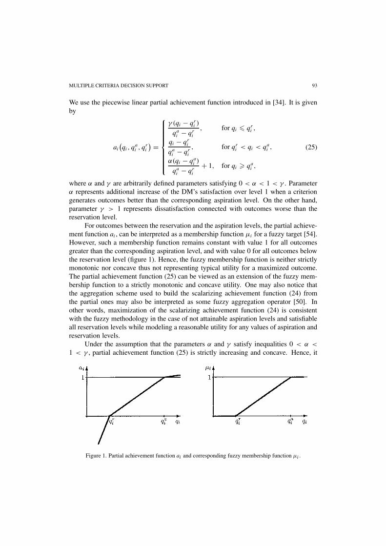
We use the piecewise linear partial achievement function introduced in [34]. It is givenby
ai(qi, q
ai , q
ri
) =
γ (qi − qri )
qai − qr
i
, for qi � qri ,
qi − qri
qai − qr
i
, for qri < qi < qa
i ,
α(qi − qai )
qai − qr
i
+ 1, for qi � qai ,
(25)
where α and γ are arbitrarily defined parameters satisfying 0 < α < 1 < γ . Parameterα represents additional increase of the DM’s satisfaction over level 1 when a criteriongenerates outcomes better than the corresponding aspiration level. On the other hand,parameter γ > 1 represents dissatisfaction connected with outcomes worse than thereservation level.
For outcomes between the reservation and the aspiration levels, the partial achieve-ment function ai , can be interpreted as a membership function µi for a fuzzy target [54].However, such a membership function remains constant with value 1 for all outcomesgreater than the corresponding aspiration level, and with value 0 for all outcomes belowthe reservation level (figure 1). Hence, the fuzzy membership function is neither strictlymonotonic nor concave thus not representing typical utility for a maximized outcome.The partial achievement function (25) can be viewed as an extension of the fuzzy mem-bership function to a strictly monotonic and concave utility. One may also notice thatthe aggregation scheme used to build the scalarizing achievement function (24) fromthe partial ones may also be interpreted as some fuzzy aggregation operator [50]. Inother words, maximization of the scalarizing achievement function (24) is consistentwith the fuzzy methodology in the case of not attainable aspiration levels and satisfiableall reservation levels while modeling a reasonable utility for any values of aspiration andreservation levels.
Under the assumption that the parameters α and γ satisfy inequalities 0 < α <
1 < γ , partial achievement function (25) is strictly increasing and concave. Hence, it
Figure 1. Partial achievement function ai and corresponding fuzzy membership function µi .

94 KALETA ET AL.
can be expressed in the form:
ai(qi, q
q
i , qri
) = min
{γqi − qr
i
qai − qr
i
,qai − qr
i
qai − qr
i
, αqi − qa
i
qai − qr
i
+ 1
}
which guarantees LP computability with respect to outcomes qi . Finally, maximizationof the entire scalarizing achievement function (24) can be implemented by the followingauxiliary LP constraints:
max a + ε
m∑i=1
ai
s.t. ai � a, for i = 1, . . . , m,
ai � γqi − qr
i
qai − qr
i
, for i = 1, . . . , m,
ai � qi − qri
qai − qr
i
, for i = 1, . . . , m,
ai � αqi − qa
i
qai − qr
i
+ 1, for i = 1, . . . , m,
where ai for i = 1, . . . , m and a are unbounded variables introduced to represent valuesof several partial achievement functions and their minimum, respectively.
4. Illustrative example
In order to show an outline of the interactive multiple criteria analysis performed withthe ARBDS methodology, we consider a small sample problem. The data for short-termplanning model considered in this example are based on real-life characteristics of agenerator owning four coal-fired 180 MW units. The variable cost function of each unitis considered to be convex and it is approximated by 3 linear pieces. The mean variablecost is about 10.75 USD/MWh and start-up cost is 875 USD (for simplicity no shut-downcost and constant start-up cost is considered). The units have quite elastic characteristics(minimum power output is 60 MW), and their minimum up time is 5 hours. At thebeginning of the planning horizon all units have been off, but they could be committedimmediately at hour 0.
The planning horizon lasts for 48 hours which corresponds to two cycles of themarket auction. It is assumed that energy spot prices forecast over planning horizonconsists of 100 equally probable different scenarios. The scenarios have been generatedunder the assumption that prices fluctuate over a day within specified probability distri-bution. The price forecast distribution profiles are selected that the minimum price isat least 8 USD (at night hours), the maximum price is at most 40 USD (at peak hours),and the daily average price over all the scenarios is 19 USD. Hourly values of prices aredrawn at random from those distributions thus they may be considered to be correlatedas they are in historical data. Besides, a few distinctive scenarios are modeled. Hence,
MULTIPLE CRITERIA DECISION SUPPORT 95
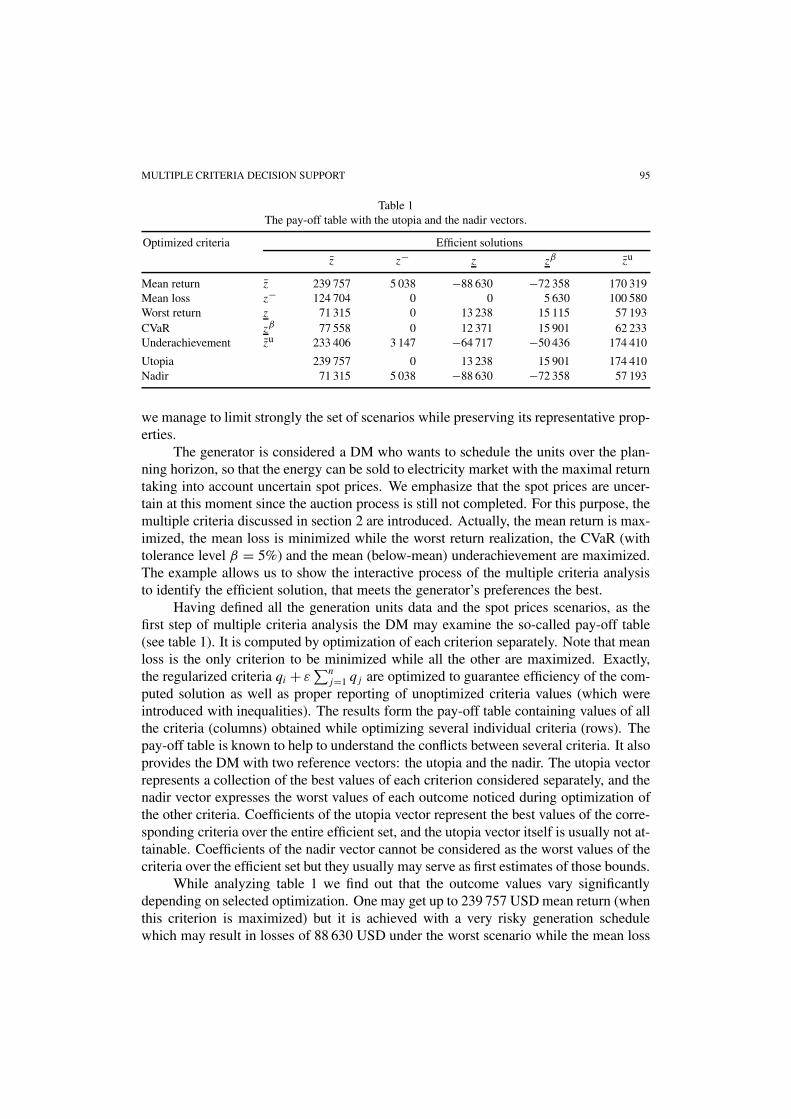
Table 1The pay-off table with the utopia and the nadir vectors.
Optimized criteria Efficient solutions
z z− z zβ zu
Mean return z 239 757 5 038 −88 630 −72 358 170 319Mean loss z− 124 704 0 0 5 630 100 580Worst return z 71 315 0 13 238 15 115 57 193CVaR zβ 77 558 0 12 371 15 901 62 233Underachievement zu 233 406 3 147 −64 717 −50 436 174 410
Utopia 239 757 0 13 238 15 901 174 410Nadir 71 315 5 038 −88 630 −72 358 57 193
we manage to limit strongly the set of scenarios while preserving its representative prop-erties.
The generator is considered a DM who wants to schedule the units over the plan-ning horizon, so that the energy can be sold to electricity market with the maximal returntaking into account uncertain spot prices. We emphasize that the spot prices are uncer-tain at this moment since the auction process is still not completed. For this purpose, themultiple criteria discussed in section 2 are introduced. Actually, the mean return is max-imized, the mean loss is minimized while the worst return realization, the CVaR (withtolerance level β = 5%) and the mean (below-mean) underachievement are maximized.The example allows us to show the interactive process of the multiple criteria analysisto identify the efficient solution, that meets the generator’s preferences the best.
Having defined all the generation units data and the spot prices scenarios, as thefirst step of multiple criteria analysis the DM may examine the so-called pay-off table(see table 1). It is computed by optimization of each criterion separately. Note that meanloss is the only criterion to be minimized while all the other are maximized. Exactly,the regularized criteria qi + ε
∑nj=1 qj are optimized to guarantee efficiency of the com-
puted solution as well as proper reporting of unoptimized criteria values (which wereintroduced with inequalities). The results form the pay-off table containing values of allthe criteria (columns) obtained while optimizing several individual criteria (rows). Thepay-off table is known to help to understand the conflicts between several criteria. It alsoprovides the DM with two reference vectors: the utopia and the nadir. The utopia vectorrepresents a collection of the best values of each criterion considered separately, and thenadir vector expresses the worst values of each outcome noticed during optimization ofthe other criteria. Coefficients of the utopia vector represent the best values of the corre-sponding criteria over the entire efficient set, and the utopia vector itself is usually not at-tainable. Coefficients of the nadir vector cannot be considered as the worst values of thecriteria over the efficient set but they usually may serve as first estimates of those bounds.
While analyzing table 1 we find out that the outcome values vary significantlydepending on selected optimization. One may get up to 239 757 USD mean return (whenthis criterion is maximized) but it is achieved with a very risky generation schedulewhich may result in losses of 88 630 USD under the worst scenario while the mean loss
96 KALETA ET AL.
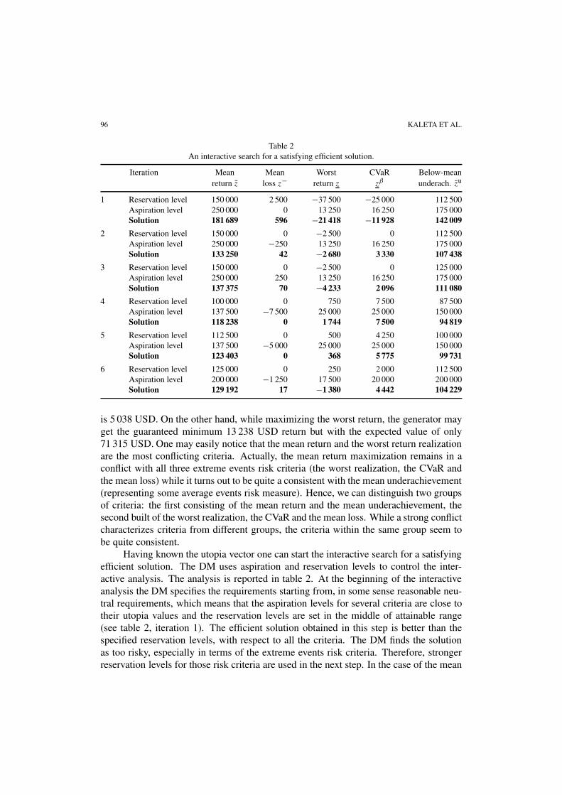
Table 2An interactive search for a satisfying efficient solution.
Iteration Mean Mean Worst CVaR Below-meanreturn z loss z− return z zβ underach. zu
1 Reservation level 150 000 2 500 −37 500 −25 000 112 500Aspiration level 250 000 0 13 250 16 250 175 000Solution 181 689 596 −21 418 −11 928 142 009
2 Reservation level 150 000 0 −2 500 0 112 500Aspiration level 250 000 −250 13 250 16 250 175 000Solution 133 250 42 −2 680 3 330 107 438
3 Reservation level 150 000 0 −2 500 0 125 000Aspiration level 250 000 250 13 250 16 250 175 000Solution 137 375 70 −4 233 2 096 111 080
4 Reservation level 100 000 0 750 7 500 87 500Aspiration level 137 500 −7 500 25 000 25 000 150 000Solution 118 238 0 1 744 7 500 94 819
5 Reservation level 112 500 0 500 4 250 100 000Aspiration level 137 500 −5 000 25 000 25 000 150 000Solution 123 403 0 368 5 775 99 731
6 Reservation level 125 000 0 250 2 000 112 500Aspiration level 200 000 −1 250 17 500 20 000 200 000Solution 129 192 17 −1 380 4 442 104 229
is 5 038 USD. On the other hand, while maximizing the worst return, the generator mayget the guaranteed minimum 13 238 USD return but with the expected value of only71 315 USD. One may easily notice that the mean return and the worst return realizationare the most conflicting criteria. Actually, the mean return maximization remains in aconflict with all three extreme events risk criteria (the worst realization, the CVaR andthe mean loss) while it turns out to be quite a consistent with the mean underachievement(representing some average events risk measure). Hence, we can distinguish two groupsof criteria: the first consisting of the mean return and the mean underachievement, thesecond built of the worst realization, the CVaR and the mean loss. While a strong conflictcharacterizes criteria from different groups, the criteria within the same group seem tobe quite consistent.
Having known the utopia vector one can start the interactive search for a satisfyingefficient solution. The DM uses aspiration and reservation levels to control the inter-active analysis. The analysis is reported in table 2. At the beginning of the interactiveanalysis the DM specifies the requirements starting from, in some sense reasonable neu-tral requirements, which means that the aspiration levels for several criteria are close totheir utopia values and the reservation levels are set in the middle of attainable range(see table 2, iteration 1). The efficient solution obtained in this step is better than thespecified reservation levels, with respect to all the criteria. The DM finds the solutionas too risky, especially in terms of the extreme events risk criteria. Therefore, strongerreservation levels for those risk criteria are used in the next step. In the case of the mean
MULTIPLE CRITERIA DECISION SUPPORT 97
loss criterion the reservation level is set at the corresponding utopia level (0) while theaspiration level is advanced to an unattainable value (−250). This results in an efficientsolution (iteration 2) which is much more satisfying in terms of risk criteria but it ismore than 20% worse with respect to the mean return. Actually, both the mean returnand the mean underachievement are then below their reservation levels. Next, the DMmakes an attempt to improve a solution by focusing more on the average events risk cri-terion. For this purpose, the reservation level for the mean underachievement is slightlyincreased. Solution obtained in the third iteration brings a few percent improvement onthe mean return and the mean underachievement but significant worsening of the othercriteria.
Further, the DM wants to examine consequences of assuring a safe schedule whichcan guarantee no losses to be suffered under any scenario. For this purpose, the aspira-tion and reservation levels of the extreme events risk criteria are much more strengthenwhile the ones corresponding to the mean return and the mean underachievement arerelaxed. Note that in order to stress the importance of some criteria the DM may setlevels which are not attainable. Iterations 4 and 5 results in solutions with the worstreturn equal to 1 744 USD and 368 USD, respectively. However, the mean return in bothsolutions is below 125 000 USD which makes the schedules not acceptable for our gen-erator. Nevertheless, a strongly risk avert generator would probably select the solutionfrom iteration 4 as a very safe schedule for implementation.
The DM makes a further attempt to find a solution assuring higher mean return,while not causing significant losses if more pessimistic scenario would occur. For thispurpose, the parameters from iteration 5 are modified by strengthening the requirementson the mean return and the mean underachievement and by simultaneous slight relaxingof the requirements on the extreme events risk criteria (iteration 6). Now, again there aresome losses that may occur, but the mean loss is only 17 USD. All the extreme eventsrisk criteria take much better values than those in iterations 2 and 3 while the mean returnand the mean underachievement are only about 5% worse. As the mean return exceeds areasonably high level of 125 000 USD with relatively good risk measures, the generatorfinally accepts this result and concludes the interactive analysis.
The final selection of an efficient solution depends on the DM’s preferences. Nev-ertheless, the example illustrates how the interactive analysis allows the DM to learnthe decision problem and to search effectively for a satisfying solution. For the pre-sented example covering 4 generation units scheduled over 48 hours under uncertaintydescribed with 100 scenarios, the average computing time of each iteration is about 100seconds on a Pentium III processor using the CPLEX optimization package [18]. Whileanalyzing larger problems related to scheduling 12 generation units over a horizon ofone week (168 hours), we have noticed the computing times approaching 10 minutes.It should be emphasized that the size of the problem depends mostly on the number ofgeneration units and hours within considered horizon. The number of price scenarios hasa relatively less impact on the resulting MILP problem size. Thus, the multiple criteriamodel, we consider, can be effectively used as an on-line interactive analysis tool withina DSS for the energy market participant.
98 KALETA ET AL.
5. The DSS concept
In a competitive electricity market there are the physical, financial and risk-managementoperations. On the physical site, the electricity is produced by generators and deliveredfrom generators to customers through transmission and distribution facilities. Moreover,ancillary services are needed to assure reliable operation of the system. Such servicesinclude installed capability, operable capability, spinning and nonspinning reserves, au-tomatic generation control (AGC), transmission services, etc.
On the financial site, the contracts and payments specify planned and actual gener-ation and consumption, terms for payment for electrical energy, and financial issues ofcontracted services. The risk-management arrangements (such as futures markets andlong-term contracts) are used to manage risk, and they may or may not have any relationto the physical delivery of electricity.
The deregulated power system may be operated and managed as an interactivenetwork of the following different types of energy markets:
• forward energy market (Power Exchange), which may be in the form of a day-aheadenergy auction (DAA);
• planned production market (PPM), a day-ahead (or hour-ahead) market for powergeneration plan which should meet the demand forecasts, systems resource con-straints and system-wide performance objectives;
• real-time production market (RTM), the market for real-time power generation whichmeets the real demand for energy and assures safety delivery and others system-wideperformance objectives;
• ancillary services markets (ASM), which provide appropriate level of systems ser-vices (installed and operable capabilities, AGC, spinning reserve, fast nonspinningreserve, slow reserve, transmission capacities).
The stochastic short-term planning model and its multiple criteria interactive analy-sis tool is used as a key analytic module of the I-enviser decision support system [19].The system is developed for companies that operate within power production, physicalpower transactions and distribution in several energy market segments. The decisionprocess supported by I-enviser may be divided into three main stages (figure 2):
1. Data preparation. In this initial stage all the necessary information and data arespecified. Input data are gained from outer sources, prepared by the user, as well asacquired from other applications. The user needs to specify all technical parametersof the power production and network units but this customization is usually madeonce and rarely modified. The main responsibility of the user at this stage is to definewhat elements and in which way need to be included. In particular, it is importantto select the outside forecasting software (and appropriate parameters) to generaterepresentative scenarios and assign them appropriate probabilities.
2. Strategic decision support. In this stage decisions in the long-term or medium-termtime horizon are supported. The following main activities are handled:
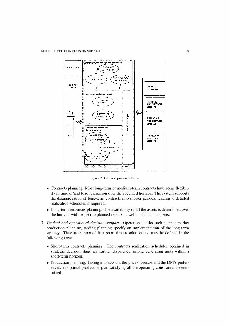
MULTIPLE CRITERIA DECISION SUPPORT 99
Figure 2. Decision process scheme.
• Contracts planning. Most long-term or medium-term contracts have some flexibil-ity in time or/and load realization over the specified horizon. The system supportsthe disaggregation of long-term contracts into shorter periods, leading to detailedrealization schedules if required.
• Long-term resources planning. The availability of all the assets is determined overthe horizon with respect to planned repairs as well as financial aspects.
3. Tactical and operational decision support. Operational tasks such as spot marketproduction planning, trading planning specify an implementation of the long-termstrategy. They are supported in a short time resolution and may be defined in thefollowing areas:
• Short-term contracts planning. The contracts realization schedules obtained instrategic decision stage are further dispatched among generating units within ashort-term horizon.
• Production planning. Taking into account the prices forecast and the DM’s prefer-ences, an optimal production plan satisfying all the operating constraints is deter-mined.
100 KALETA ET AL.
• Bidding. Depending on the optimal production plan, production costs and theDM risk attitudes, optimal bids are built to be submitted on several energy marketsegments.
• Final dispatching. Typical deterministic unit commitment problem is solved to findthe optimal production schedule after all the market clearing processes have beenfinished.
Short-term planning module is a key element of the I-enviser system. The entiretactical and operational decision support is achieved by repeatedly use of the module.The module itself implements the stochastic short-term planning model and the multiplecriteria interactive methodology described in this paper. Directly, the stochastic modelwith multiple risk criteria is used for optimization of contract positions and genera-tion plans for several generation units, thus allowing to support the short-term contractsplanning and the production planning decisions, respectively. The risk criteria are wellappealing and the ARBDS interactive analysis tool enables to find an efficient solution(production plan) well adjusted to the generator preferences (risk attitude).
The criteria express the expected return and several risk measures including theextreme events measures. Hence, the multiple criteria model well depicts the uncertaintyof market prices, thus allowing the optimal generation plan to be used as a backgroundfor various operational decisions. In particular, it can be used in the bids preparationprocess enabling an active participation in the market segments based on the clearingprocess mechanisms. A bid to be submitted for a particular market segment must meetspecific technical requirements. Therefore, I-enviser is equipped with a special bidspreparation module with predefined technical requirements. The bids themselves arebuilt for each hour (auction time unit) of the horizon, according to the production costcaused by the implementation of the optimal production plan.
When the final results of the auction process are already known, the generationdispatch module is used to define the final production schedule for all the units. Theshort-term planning model based on maximization of the overall return as a functionof the generation decisions. As all the model parameters, including the energy prices,are known one needs to maximize the deterministic return (6) under the typical unitcommitment constraints (1)–(5) and (7).
The strategic decisions are typically related to the long-term resource planning andlong-term contracts management. The decisions considered for a long horizon are hardto formal modeling and effective optimization for the sake of their mostly qualitativeattributes as well as a strong uncertainty (risk) factor. The stochastic programming modelcan be built for the long-term resource planning [3]. Hence, there is a possibility toextend our short-term planning methodology based on the multiple risk criteria analysisto be applied to the resource planning. This is our goal, but currently I-enviser dependson possible use of external software to support resource planning decisions.
The long-term contracts management is currently supported only by verificationand evaluation of solution submitted by the DM. The solutions are evaluated with sim-ple criteria, such as schedule feasibility or the expected return. Moreover, I-enviser
MULTIPLE CRITERIA DECISION SUPPORT 101
provides various decision-aid tools from suitable data presentation and visualization tosimple heuristics. Nevertheless, an analytical decision support for dis-aggregation of thelong-term contracts obligations into shorter periods remains an important goal for ourfuture developments. We intend to exploit the concepts of equitable optimization [22] toformalize dis-aggregation decisions.
6. Concluding remarks
As deregulation in the power sector is advancing, the electricity markets are movingtoward greater reliance on competition. In most markets the competition is limited toinclude only the wholesale energy market. Even such a limited deregulation causesthat the traditional methods of operating in the energy market continue to change andreformulate which makes the energy suppliers facing a necessity of new managementdecisions. In a regulated market only technical aspects of generation are considered bythe generator (electric power producer), as the minimization of the production costs as-sures the maximum profit. A new competitive environment relates the profit to a successin bidding and clearing process, and the generator becomes an active market partici-pant. This enforces the generator to serve as a decision maker (DM) dealing with newgoals and decision processes as well as new types of necessary information. There isa strong need for a decision support system (DSS) dedicated to such electricity marketparticipants.
In this paper it has been shown that the stochastic short-term planning model can beeffectively used as a key analytical tool within the DSS for active participants of the elec-tricity markets. The technical constraints result in a mixed-integer linear program whilethe market price uncertainty leads to the stochastic objective function. The uncertaintyis modeled by a set of possible scenarios with assigned probabilities. Several risk mea-sures have been introduced to be used as multiple criteria for modeling the generator’srisk attitude. Apart from typical dispersion measures some extreme events risk measuresare available. The aspiration/reservation based interactive analysis is applied to the mul-tiple criteria problem thus allowing to find an efficient solution (generation schedule)well adjusted to the generator’s preferences (risk attitude). All the criteria are LP com-putable while the feasible set of generation decisions defined by the mixed-integer LPconstraints. Our computational experience shows that the resulting mixed-integer LPproblems can be effectively solved for the scheduling several generation units over ahorizon covering up to one week (168 hours) with 100 price scenarios.
Acknowledgments
Research conducted by W. Ogryczak was supported by the grant PBZ-KBN-016/P03/99from The State Committee for Scientific Research.
102 KALETA ET AL.
References
[1] E.H. Allen, M.D. Ilic, Price-Based Commitment Decision in the Electricity Markets (Springer, Lon-don, 1999).
[2] F. Andersson, H. Mausser, D. Rosen and S. Uryasev, Credit risk optimization with conditional value-at-risk criterion, Math. Program. 89 (2001) 273–291.
[3] C.J. Andrews, Evaluating risk management strategies in resource planning, IEEE Trans. Power Syst.10 (1995) 420–426.
[4] J.M. Arroyo and A.J. Conejo, Optimal response of a thermal unit to an electricity spot market, IEEETrans. Power Syst. 15 (2000) 1098–1104.
[5] G.A. Berry, B.F. Hobbs, W.A. Meroney, R.P. O’Neil and W.R. Stewart, Analyzing strategic biddingbehaviour in transmission networks, in: IEEE Tutorial on Game Theory Applications in ElectricPower Markets, ed. H. Singh (IEEE Press, 1999) pp. 7–32.
[6] D.P. Bertsekas, G.S. Lauer, N.R. Sandell and T.A. Posbergh, Optimal short-term scheduling of largescale power systems, IEEE Trans. Automat. Control 28 (1983) 1–11.
[7] A. Charnes and W.W. Cooper, Management Models and Industrial Applications of Linear Program-ming (Wiley, New York, 1961).
[8] D. Dentcheva, R. Gollmer, A. Möller, W. Römisch and R. Schultz, Solving the unit commitmentproblem in power generation by primal and dual methods, in: Progress in Industrial Mathematics atECMI 96, Stuttgart (1997) pp. 332–339.
[9] T.S. Dillon, W. Edwin, H.D. Kochs and R.J. Taud, Integer programming commitment with probabilis-tic reserve determination, IEEE Trans. Power App. Syst. 97(6) (1978) 2154–2166.
[10] R.W. Ferrero, S.M. Shahidehpour and V.C. Ramesh, Transactions analysis in deregulated power sys-tem using game theory, IEEE Trans. Power Syst. 12 (1997) 1340–1347.
[11] R.W. Ferrero, J.F. Rivera and S.M. Shahidehpour, Application of games with incomplete informationfor pricing electricity in deregulated power pools, IEEE Trans. Power Syst. 13 (1998) 184–189.
[12] O.B. Fosso, A. Gjelsvik, A. Haugstad and M.B. Wangensteen, Generation scheduling in a deregulatedsystem: the Norwegian case, IEEE Trans. Power Syst. 14 (1999) 75–80.
[13] X. Guan, Y.-C. Ho and F. Lai, An ordinal optimization based bidding strategy for electric powersuppliers in the daily energy market, IEEE Trans. Power Syst. 16 (2001) 788–797.
[14] Y.Y. Haimes, Risk of extreme events and the fallacy of the expected value, Control Cybernet. 22(1993) 7–31.
[15] B.F. Hobbs and P. Meier, Energy Decisions and the Environment: A Guide to the Use of MulticriteriaMethods (Kluwer, Dordrecht, 2000).
[16] B.F. Hobbs, M.H. Rothkopf, R.P. O’Neill and H.P. Chao (eds.), The Next Generation of Electric PowerUnit Commitment Models (Kluwer, Dordrecht, 2001).
[17] E.S. Huse, I. Wangensteen and H.H. Faanes, Thermal power generation scheduling by simulatedcompetition, IEEE Trans. Power Syst. 14 (1999) 472–476.
[18] ILOG Inc., Using the CPLEX Callable Library (ILOG Inc., Incline Village, 1997).[19] IMPAQ Inc., I-Enviser (IMPAQ Information Management Inc., Warsaw, 2001).[20] T.A. Johnsen, Demand, generation and price in the Norwegian market for electric power, Energy
Economics 23 (2001) 227–251.[21] H. Konno and H. Yamazaki, Mean-absolute deviation portfolio optimization model and its application
to Tokyo stock market, Management Sci. 37 (1991) 519–531.[22] M.M. Kostreva and W. Ogryczak, Linear optimization with multiple equitable criteria, RAIRO Rech.
Opér. 33 (1999) 275–297.[23] J.W. Lamont and S. Rajan, Strategic bidding in an energy brokerage, IEEE Trans. Power Syst. 12
(1997) 1729–1733.[24] C. Lemarechal, Short-term optimization of power plants by decomposition, in: Proc. of the 14th
Sympos. on Operation Research, Ulm (1989).
MULTIPLE CRITERIA DECISION SUPPORT 103
[25] A. Lewandowski and A.P. Wierzbicki (eds.), Aspiration Based Decision Support Systems – Theory,Software and Applications (Springer, Berlin, 1989).
[26] C.A. Li, A.J. Svoboda, X.H. Guan and H. Singh, Revenue adequate bidding strategies in competitiveelectricity markets, IEEE Trans. Power Syst. 14 (1999) 492–497.
[27] H. Markowitz, Portfolio selection, J. Finance 7 (1952) 77–91.[28] A.G. Martins, D. Coelho, C.H. Artunes and J. Climaco, A multiple objective linear programming
approach to power generation planning, Internat. Trans. Oper. Res. 3 (1996) 305–317.[29] B. Mo, A. Gjelsvik and A. Grundt, Integrated risk management of hydro-power scheduling and con-
tract management, IEEE Trans. Power Syst. 16 (2001) 216–221.[30] A. Möller and W. Römisch, A dual method for the unit commitment problem, in: Proc. 9th ECMI
Conf., Lyngby/Copenhagen (1996).[31] J.A. Muckstadt and S.A. Koenig, An application of Lagrangian relaxation in power generation, Work-
ing paper, WP-96-109, IIASA, Laxenburg (1996).[32] W. Ogryczak, Stochastic dominance relation and linear risk measures, financial modelling, in: Proc.
23rd Meeting of the EURO Working Group on Financial Modelling, ed. A.M.J. Skulimowski (Progress& Business Publ., Cracow, 1999) pp. 191–212.
[33] W. Ogryczak and A. Ruszczynski, From stochastic dominance to mean–risk models: semideviationsas risk measures, European J. Oper. Res. 116 (1999) 33–50.
[34] W. Ogryczak, K. Studzinski and K. Zorychta, DINAS: a computer-assisted analysis system for multi-objective transshipment problems with facility location, Comput. Oper. Res. 19 (1992) 637–647.
[35] Ch.W. Richter, Jr. and G.B. Sheble, Genetic algorithm evolution of utility bidding strategies for thecompetitive marketplace, IEEE Trans. Power Syst. 13 (1998) 256–261.
[36] R.T. Rockafellar and R.J.-B. Wets, Scenarios and policy aggregation in optimization under uncer-tainty, Math. Oper. Res. 16 (1991) 119–147.
[37] S.M. Shahidehpour, Unit commitment with transmission security and voltage constraints, IEEE Trans.Power Syst. 14 (1999) 757–764.
[38] M. Shahidehpour and M. Marwali, Maintenance Scheduling in a Restructured Power System (Kluwer,Dordrecht, 2000).
[39] G.B. Sheble, Decision analysis tools for GENCO dispatchers, IEEE Trans. Power Syst. 14 (1999)745–750.
[40] G.B. Sheble and G.N. Fahd, Unit commitment literature synopsis, IEEE Trans. Power Syst. 9 (1994)128–135.
[41] G.B. Shrestha, S. Kai and L. Goel, Strategic bidding for minimum power outpout in the competitivepower market, IEEE Trans. Power Syst. 16 (2001) 813–818.
[42] S.N. Siddiqi, Project valuation and power portfolio management in a competitive market, IEEE Trans.Power Syst. 15 (2000) 116–121.
[43] H.L. Song, C.C. Liu and J. Lawarree, Decision making of an electricity suppliers bid in a spot market,in: Proc. IEEE Power Engineering Society 1999 Summer Meeting, Vol. 1 (1999) pp. 692–696.
[44] M.G. Speranza, Linear programming models for portfolio optimization, Finance 14 (1993) 107–123.[45] R.E. Steuer, Multiple Criteria Optimization – Theory, Computation & Applications (Wiley, New York,
1986).[46] E. Toczyłowski and I. Zółtowska, Analysis of optimization models for utilities acting in the pres-
ence of market risk, in: Optimization in Electric Power Systems, IV National Conference, Jachranka,Poland (2001) pp. 122–128 (in Polish).
[47] P. Visudhiphan and M.D. Ilic, Dynamic games-based modeling of electricity markets, in: Proc. ofIEEE Power Engineering Society 1999 Winter Meeting, Vol. 1 (1999) pp. 274–281.
[48] G.A Whitmore and M.C. Findlay (eds.), Stochastic Dominance: An Approach to Decision-MakingUnder Risk (DC Heath, Lexington, MA, 1978).
[49] A.P. Wierzbicki, A mathematical basis for satisficing decision making, Math. Model. 3 (1982) 391–405.

104 KALETA ET AL.
[50] A.P. Wierzbicki, M. Makowski and J. Wessels (eds.), Model Based Decision Support Methodologywith Environmental Applications (Kluwer, Dordrecht, 2000).
[51] H.P. Williams, Model Building in Mathematical Programming (Wiley, New York, 1993).[52] M.R. Young, A minimax portfolio selection rule with linear programming solution, Management Sci.
44 (1998) 673–683.[53] D. Zhang, Y. Wang and P.B. Luh, Optimization based bidding strategies in the deregulated market,
IEEE Trans. Power Syst. 15 (2001) 981–986.[54] H.-J. Zimmermann, Fuzzy Sets Theory and Its Applications, 3rd ed. (Kluwer, Dordrecht, 1996).