On Graph Problems in a Semi-Streaming Model?

Joan Feigenbaum ??1, Sampath Kannan2 ? ? ?, Andrew McGregor2 †, SiddharthSuri2 ‡, and Jian Zhang §1

1 Yale University, New Haven, CT 06520, USAfeigenbaum-joan, zhang-jian@cs.yale.edu

2 University of Pennsylvania, Philadelphia, PA 19104, USAkannan, andrewm, ssuri@cis.upenn.edu

Abstract. We formalize a potentially rich new streaming model, thesemi-streaming model, that we believe is necessary for the fruitful studyof efficient algorithms for solving problems on massive graphs whoseedge sets cannot be stored in memory. In this model, the input graph,G = (V, E), is presented as a stream of edges (in adversarial order),and the storage space of an algorithm is bounded by O(n · polylog n),where n = |V |. We are particularly interested in algorithms that useonly one pass over the input, but, for problems where this is provablyinsufficient, we also look at algorithms using constant or, in some cases,logarithmically many passes. In the course of this general study, we givesemi-streaming constant approximation algorithms for the unweightedand weighted matching problems, along with a further algorithm im-provement for the bipartite case. We also exhibit log n/ log log n semi-streaming approximations to the diameter and the problem of computingthe distance between specified vertices in a weighted graph. These arecomplemented by Ω(log(1−ε) n) lower bounds.

1 Introduction

Streaming [14, 3, 10] is an important model for computation on massive datasets. Recently, there has been a large body of work on designing algorithms inthis model [11, 3, 10, 15, 13, 12]. Yet, the problems considered fall into a smallnumber of categories, such as computing statistics, norms, and histograms. Veryfew graph problems [5] have been considered in the streaming model.

The difficulty of graph problems in the streaming model arises from thememory limitation of the model combined with input-access constraints. We canview the amount of memory used by algorithms with sequential (one-way) input

? This work was supported by the DoD University Research Initiative (URI) admin-istered by the Office of Naval Research under Grant N00014-01-1-0795.

?? Supported in part by ONR and NSF.? ? ? Supported in part by ARO grant DAAD 19-01-1-0473 and NSF grant CCR-0105337.

† Supported in part by NIH.‡ Supported in part by NIH grant T32 HG000046-05.§ Supported by ONR and NSF.

access as a spectrum. At one end of the spectrum, we have dynamic algorithms [9]that may use memory enough for the whole input. At the other end, we havestreaming algorithms that use only polylog space. At one extreme, there is a lotof work on dynamic graph problems; on the other, general graph problems areconsidered hard in the (poly)log-space streaming model. Recently, it has beensuggested by Muthukrishnan [19] that the middle ground, where the algorithmscan use O(n ·polylog n) bits of space is an interesting and open area. This is thearea that we explore.

Besides taking a middle position in the memory-size spectrum, the semi-streaming model allows multiple passes over the input stream. In certain appli-cations with massive data sets, a small number of sequential passes over the datawould be much more efficient than many random accesses to the data. Only afew works [8, 4] have considered the multiple-pass model and a lot remains to bedone.

Massive graphs arise naturally in many real world scenarios. Two examplesare the call graph, where nodes correspond to telephone numbers and edges tocalls between numbers that call each other during some time interval, and theweb graph, where nodes are web pages, and the edges are links between pages.The streaming model is necessary for the study of the efficient processing ofsuch massive graphs. In [1], the authors introduce the semi-external model forcomputations on massive graphs, i.e., one in which the vertex set can be storedin memory, but the edge set cannot. However, this work addresses the problemsin an external memory model in which random access to the edges, althoughexpensive, is allowed. This is a major difference between their model and ours.Indeed, the authors of [18] argue that one of the major drawbacks of standardgraph algorithms, when applied to massive graphs such as the web, is their needto have random access to the edge set. Furthermore, there are situations in whichthe graph is revealed in a streaming fashion, such as a web crawler exploring theweb graph.

We consider a set of classical graph problems in this semi-streaming model.We show that, although the computing power of this model is still limited,there are semi-streaming algorithms for a variety of graph problems. Our mainresult is a semi-streaming algorithm that computes a (2/3− ε)-approximation inO( log 1/ε

ε ) passes for unweighted bipartite graph matching. We also provide a one-pass semi-streaming algorithm for 1/6-approximating the maximum weightedgraph matching. We also provide log n/ log log n approximations for diameterand shortest paths in weighted graphs which we complement with Ω(log(1−ε) n)lower bounds for these problems in unweighted graphs.

2 Preliminaries

Unless stated otherwise, we denote by G(V,E) a graph G with vertex set V =v1, v2, . . . , vn and edge set E = e1, e2, . . . , em. Note that n is the number ofvertices and m the number of edges.

Definition 1. A graph stream is a sequence of edges ei1 , ei2 , . . . , eim, where

eij ∈ E and i1, i2, . . . , im is an arbitrary permutation of [m] = 1, 2, . . . ,m.

While an algorithm goes through the stream, the graph is revealed one edgeat a time. This definition generalizes the streams of graphs in which the adja-cency matrix or the adjacency list is presented as a stream. In a stream in theadjacency-matrix or adjacency-list models, the edges incident to each vertex aregrouped together. We need the more general model to account for graphs suchas call graphs where the edges might generated in any order.

The efficiency of a graph algorithm in the semi-streaming model is measuredby the space it uses, the time it requires to process each edge, and the numberof passes it makes over the graph stream.

Definition 2. A semi-streaming graph algorithm computes over a graphstream using S(n, m) bits of space. The algorithm may access the input stream ina sequential order(one-way) for P (n, m) passes and use T (n, m) time to processeach edge. It is required that S(n, m) be O(n · polylog (n)) bits.

To see the limitation of the (poly)log-space streaming model for graph prob-lems, consider the following simple problem. Given a graph, determining whetherthere is a length-2 path between two vertices, x and y, is equivalent to decidingwhether two vertex sets, the neighborhood of x and the neighborhood of y, have anonempty intersection. Because set disjointness has linear-space communicationcomplexity [17], the length-2 path problem is impossible in the (poly)log-spacestreaming model. See [4] for a more comprehensive treatment of finding commonneighborhoods in the streaming model.

3 Graph Matching

3.1 Unweighted Bipartite Matching

In this subsection, we present an algorithm for approximating unweighted bipar-tite matching. First, a bipartition can be found by the following algorithm. Notethat the labeling of the vertices keeps track of the connected components in thegraph seen so far, and the signs keep a partition for each connected component.

Algorithm 1 (Bipartition). As edges stream in, we use a disjoint set datastructure to maintain the connected components of the graph so far. We associatea sign with each vertex such that no edge joins two vertices of the same sign. Ifthis condition ever fails and cannot be corrected by flipping the sign of a vertexand the vertices in its connected component, then we output that the graph isnon-bipartite.

The disjoint set data structure with union by rank and path compressioncan be augmented to maintain the signs without increasing the amortized time,α(m,n) needed per edge.

Given a matching M , we call a vertex free if it doesn’t appear as the endpoint of any edge in M . It is easy to see that a maximal matching (thus a 1/2-approximation) for a graph can be constructed by a semi-streaming algorithm inone pass over the graph stream: when going through the stream, the algorithmadds an edge to the current matching M if both ends of the edge are free w.r.t.M . (This constructs a maximal matching for an arbitrary graph, not just forbipartite graphs.)

Consider a matching M for a bipartite graph G = (L ∪ R,E). A length-3augmenting path for an edge e = (u, v) ∈ M , u ∈ L and v ∈ R, is a quadruple(wl, u, v, wr) such that (u, wl), (wr, v) ∈ E, and wl and wr are free vertices. Wecall wl and wr the wing-tips of the augmenting path, (u, wl) the left wing and(wr, v) the right wing. A set of simultaneously augmentable length-3 augmentingpaths is a set of length-3 augmenting paths that are vertex disjoint.

We now provide an algorithm that will be used as a subroutine in our mainunweighted bipartite matching algorithm. Given a bipartite graph and a match-ing of the graph, this algorithm finds a set of simultaneously augmentable length-3 augmenting paths.

Algorithm 2 (Find Augmenting Paths). The input to the algorithm is agraph G = (L ∪R,E), a matching M for G and a parameter 0 < δ < 1.

1. In one pass, find a maximal set of disjoint left wings. If the number of leftwings found is ≤ δM , terminate.

2. In a second pass, for the edges in M with left wings, find a maximal set ofdisjoint right wings.

3. In a third pass we identify the set of vertices that(a) Are endpoints of a matched edge that got a left wing.(b) Are the wing tips of a matched edge that got both wings.(c) Are endpoints of a matched edge that is no longer 3 augmentable.We remember these vertices and in subsequent passes, we ignore any edgeincident on one of these vertices.

4. Repeat.

Our main unweighted bipartite matching algorithm increases the size of amatching by repeatedly finding a set of simultaneously augmentable length-3augmenting paths and augmenting the matching using these paths.

Algorithm 3 (Unweighted Bipartite Matching). The input to the algo-rithm is a bipartite graph G = (L ∪R,E) and a parameter 0 < ε < 1/3.

1. In one pass, find a maximal matching M and the bipartition of G.2. For k = 1, 2, . . . , d log 6ε

log8/9e Do:(a) Run the algorithm 2 with G, M and δ = ε

2−3ε .(b) For each e = (u, v) ∈ M for which an augmenting path (wl, u, v, wr) is

found by algorithm 2, remove (u, v) from M and add (u, wl) and (wr, v)to M .

We now establish a relationship between the size of a maximal set of simul-taneously augmentable length-3 augmenting paths and the size of a maximumsuch set.

Lemma 1. The size of a maximal set of simultaneously augmentable length-3augmenting paths is at least 1/3 of the size of a maximum set of simultaneouslyaugmentable length-3 augmenting paths.

Proof. Let APmax be some maximal set of simultaneously length-3 augmentablepaths. Note that each path that we find destroys at most 3 paths that APmax

might have used, one involving each of the wing tips that we use and a thirdpath involving the matched edge we used. Thus we have a 1/3-approximation.

Lemma 2. Let X be a maximum-sized set of simultaneously augmentable length-3 augmenting paths for a maximal matching M . Let α = |X|

|M | and Opt a maxi-mum matching. |M |(1 + α) ≥ 2/3 |Opt|.

Proof. See for example, [16], page 156.

Lemma 3. Algorithm 2 finds α|M |−2δ|M |3 simultaneously augmentable length-3

augmenting paths in 3/δ passes.

Proof. Let L(M) be the set of the end vertices of the edges in M that are in Land VL(M) = v ∈ R | v is free w.r.t. M and ∃u ∈ L(M) s.t. (u, v) ∈ E. Wecall one repetition of step 1–4 in the algorithm a phase. The number of phasesis at most 1/δ because at least δ|M | edges in M are removed at each phase.

When the algorithm terminates, the number of left wings found is at mostδ|M |. Note that the set of left wings found form a maximal matching betweenthe remaining vertices in L(M) and VL(M). Hence there are fewer than 2δ|M |disjoint left wings that could have been found at this phase. Consequently, thereare fewer than 2δ|M | simultaneously augmentable length-3 augmenting paths inthe remaining graph, which we denote G′.

Let G′′ = G \ G′. Note that a maximum set of simultaneously augmentablelength-3 augmenting paths in G′′ would have a size at least α|M | − 2δ|M |. Alsonote that the set of length-3 augmenting paths found by the algorithm form amaximal set w.r.t. G′′. By Lemma 1, the size of such a set is at least α|M |−2δ|M |

3 .

Theorem 1. For any 0 < ε < 1/3 and a bipartite graph, algorithm 3 finds a2/3−ε approximation of maximum matching in O

(log 1/ε

ε

)passes. The algorithm

processes each edge in O(1) time in each pass except the first pass, in whichthe bipartition is found. The amortized per-edge processing time is α(m,n) forfinding the bipartition. The storage space required by the algorithm is O(n log n).

Proof. It is easy to see the bounds for the per-edge processing time and storagespace. We now show the correctness of the algorithm. Let Opt be the size ofthe maximum matching. At the ith phase, let Mi be the matching found by thealgorithm and Xi a maximum-sized set of simultaneously augmentable length-3augmenting paths for the matching Mi. Let αi = |Xi|

|Mi| and si = |Mi|Opt .

Note that we only need to consider the case where αi > 3ε2−3ε . Otherwise, by

Lemma 2, the matching Mi is already a 23

11+αi

≥ 23−ε approximation. Assuming

αi > 3ε2−3ε for all stage i, let δ = ε

2−3ε . Then δ ≤ αi

3 for all αi. By Lemma 3,the number of simultaneously augmentable length-3 augmenting paths found byAlgorithm 2 is then αi|Mi|−2δ|Mi|

3 ≥ αi|Mi|9 .

Because M0 is a maximal matching, s0 ≥ 1/2. At any stage, by Lemma 2,|Mi|+ αi|Mi| ≥ 2/3 ·Opt. This gives:

si + αisi ≥ 2/3 (1)

By Lemma 3, |Mi+1| = |Mi| · (1 + αi−2δ3 ) ≥ |Mi| · (1 + αi/9). This gives:

si+1 ≥ si + αisi/9 (2)

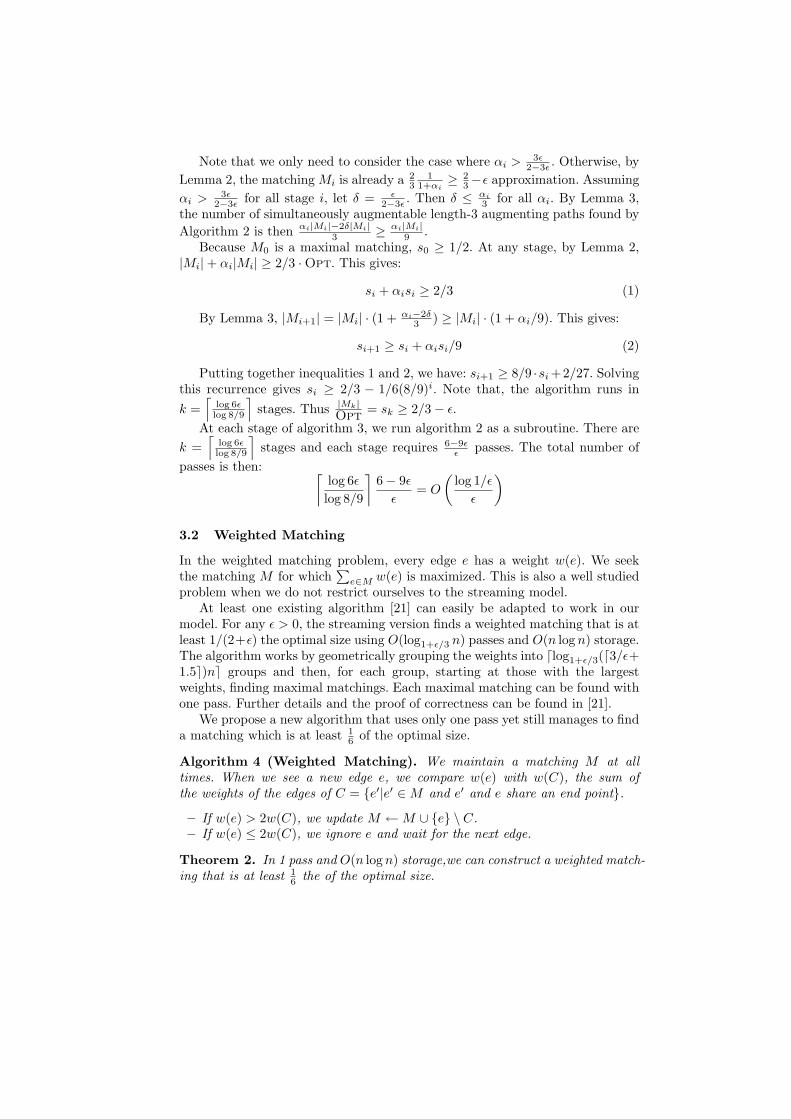
Putting together inequalities 1 and 2, we have: si+1 ≥ 8/9 ·si +2/27. Solvingthis recurrence gives si ≥ 2/3 − 1/6(8/9)i. Note that, the algorithm runs ink =

⌈log 6εlog 8/9

⌉stages. Thus |Mk|

Opt = sk ≥ 2/3− ε.At each stage of algorithm 3, we run algorithm 2 as a subroutine. There are

k =⌈

log 6εlog 8/9

⌉stages and each stage requires 6−9ε

ε passes. The total number ofpasses is then: ⌈

log 6ε

log 8/9

⌉6− 9ε

ε= O

(log 1/ε

ε

)

3.2 Weighted Matching

In the weighted matching problem, every edge e has a weight w(e). We seekthe matching M for which

∑e∈M w(e) is maximized. This is also a well studied

problem when we do not restrict ourselves to the streaming model.At least one existing algorithm [21] can easily be adapted to work in our

model. For any ε > 0, the streaming version finds a weighted matching that is atleast 1/(2+ε) the optimal size using O(log1+ε/3 n) passes and O(n log n) storage.The algorithm works by geometrically grouping the weights into dlog1+ε/3(d3/ε+1.5e)ne groups and then, for each group, starting at those with the largestweights, finding maximal matchings. Each maximal matching can be found withone pass. Further details and the proof of correctness can be found in [21].

We propose a new algorithm that uses only one pass yet still manages to finda matching which is at least 1

6 of the optimal size.

Algorithm 4 (Weighted Matching). We maintain a matching M at alltimes. When we see a new edge e, we compare w(e) with w(C), the sum ofthe weights of the edges of C = e′|e′ ∈M and e′ and e share an end point.

– If w(e) > 2w(C), we update M ←M ∪ e \ C.– If w(e) ≤ 2w(C), we ignore e and wait for the next edge.

Theorem 2. In 1 pass and O(n log n) storage,we can construct a weighted match-ing that is at least 1

6 the of the optimal size.

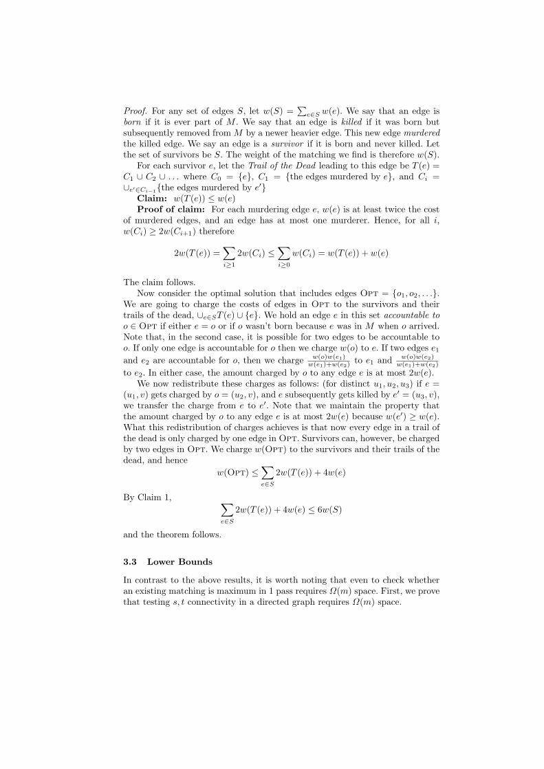
Proof. For any set of edges S, let w(S) =∑

e∈S w(e). We say that an edge isborn if it is ever part of M . We say that an edge is killed if it was born butsubsequently removed from M by a newer heavier edge. This new edge murderedthe killed edge. We say an edge is a survivor if it is born and never killed. Letthe set of survivors be S. The weight of the matching we find is therefore w(S).

For each survivor e, let the Trail of the Dead leading to this edge be T (e) =C1 ∪ C2 ∪ . . . where C0 = e, C1 = the edges murdered by e, and Ci =∪e′∈Ci−1the edges murdered by e′

Claim: w(T (e)) ≤ w(e)Proof of claim: For each murdering edge e, w(e) is at least twice the cost

of murdered edges, and an edge has at most one murderer. Hence, for all i,w(Ci) ≥ 2w(Ci+1) therefore

2w(T (e)) =∑i≥1

2w(Ci) ≤∑i≥0

w(Ci) = w(T (e)) + w(e)

The claim follows.Now consider the optimal solution that includes edges Opt = o1, o2, . . ..

We are going to charge the costs of edges in Opt to the survivors and theirtrails of the dead, ∪e∈ST (e) ∪ e. We hold an edge e in this set accountable too ∈ Opt if either e = o or if o wasn’t born because e was in M when o arrived.Note that, in the second case, it is possible for two edges to be accountable too. If only one edge is accountable for o then we charge w(o) to e. If two edges e1

and e2 are accountable for o, then we charge w(o)w(e1)w(e1)+w(e2)

to e1 and w(o)w(e2)w(e1)+w(e2)

to e2. In either case, the amount charged by o to any edge e is at most 2w(e).We now redistribute these charges as follows: (for distinct u1, u2, u3) if e =

(u1, v) gets charged by o = (u2, v), and e subsequently gets killed by e′ = (u3, v),we transfer the charge from e to e′. Note that we maintain the property thatthe amount charged by o to any edge e is at most 2w(e) because w(e′) ≥ w(e).What this redistribution of charges achieves is that now every edge in a trail ofthe dead is only charged by one edge in Opt. Survivors can, however, be chargedby two edges in Opt. We charge w(Opt) to the survivors and their trails of thedead, and hence

w(Opt) ≤∑e∈S

2w(T (e)) + 4w(e)

By Claim 1, ∑e∈S

2w(T (e)) + 4w(e) ≤ 6w(S)

and the theorem follows.

3.3 Lower Bounds

In contrast to the above results, it is worth noting that even to check whetheran existing matching is maximum in 1 pass requires Ω(m) space. First, we provethat testing s, t connectivity in a directed graph requires Ω(m) space.

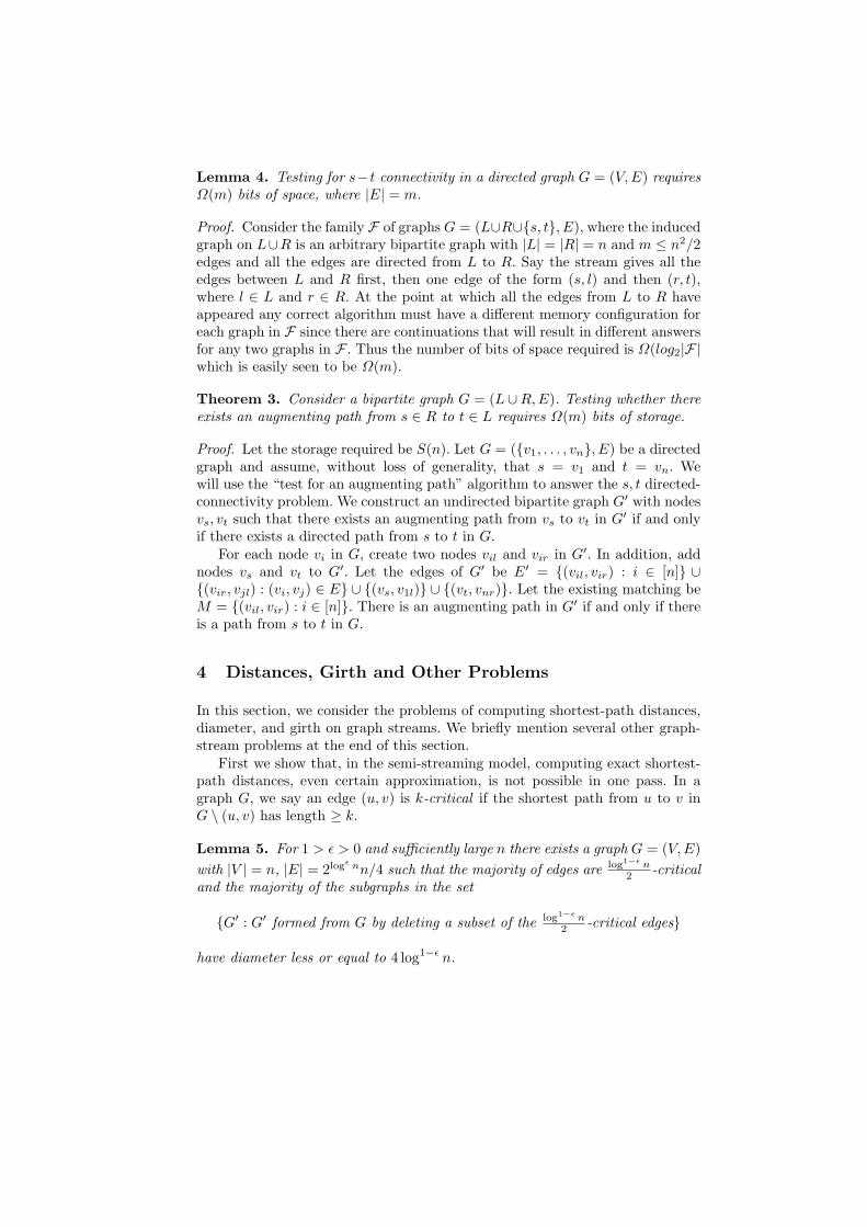
Lemma 4. Testing for s−t connectivity in a directed graph G = (V,E) requiresΩ(m) bits of space, where |E| = m.

Proof. Consider the family F of graphs G = (L∪R∪s, t, E), where the inducedgraph on L∪R is an arbitrary bipartite graph with |L| = |R| = n and m ≤ n2/2edges and all the edges are directed from L to R. Say the stream gives all theedges between L and R first, then one edge of the form (s, l) and then (r, t),where l ∈ L and r ∈ R. At the point at which all the edges from L to R haveappeared any correct algorithm must have a different memory configuration foreach graph in F since there are continuations that will result in different answersfor any two graphs in F . Thus the number of bits of space required is Ω(log2|F|which is easily seen to be Ω(m).

Theorem 3. Consider a bipartite graph G = (L ∪R,E). Testing whether thereexists an augmenting path from s ∈ R to t ∈ L requires Ω(m) bits of storage.

Proof. Let the storage required be S(n). Let G = (v1, . . . , vn, E) be a directedgraph and assume, without loss of generality, that s = v1 and t = vn. Wewill use the “test for an augmenting path” algorithm to answer the s, t directed-connectivity problem. We construct an undirected bipartite graph G′ with nodesvs, vt such that there exists an augmenting path from vs to vt in G′ if and onlyif there exists a directed path from s to t in G.

For each node vi in G, create two nodes vil and vir in G′. In addition, addnodes vs and vt to G′. Let the edges of G′ be E′ = (vil, vir) : i ∈ [n] ∪(vir, vjl) : (vi, vj) ∈ E ∪ (vs, v1l) ∪ (vt, vnr). Let the existing matching beM = (vil, vir) : i ∈ [n]. There is an augmenting path in G′ if and only if thereis a path from s to t in G.

4 Distances, Girth and Other Problems

In this section, we consider the problems of computing shortest-path distances,diameter, and girth on graph streams. We briefly mention several other graph-stream problems at the end of this section.

First we show that, in the semi-streaming model, computing exact shortest-path distances, even certain approximation, is not possible in one pass. In agraph G, we say an edge (u, v) is k-critical if the shortest path from u to v inG \ (u, v) has length ≥ k.

Lemma 5. For 1 > ε > 0 and sufficiently large n there exists a graph G = (V,E)with |V | = n, |E| = 2logε nn/4 such that the majority of edges are log1−ε n

2 -criticaland the majority of the subgraphs in the set

G′ : G′ formed from G by deleting a subset of the log1−ε n2 -critical edges

have diameter less or equal to 4 log1−ε n.

Proof (Sketch). We show existence by considering a random graph G ∈ Gn,p

where n is very large and p = 2logε n/n. Clearly the number of edges in G is atleast (2logε nn)/4 with high probability.

Claim 1: w.h.p. the majority of edges are k-critical where k = log1−ε n2 .

Proof of Claim 1: By the Chernoff bound, with high probability, no vertexhas degree greater than 2 · 2logε n. We henceforth assume this to be the case.Consider an edge (u, v). Let Γi(v) be the vertices up to a distance i from v inG \ (u, v) and then

|Γk(v)| ≤∑

0≤i≤k

(2 · 2logε n)i ≤ (2 · 2logε n)k+1 ≤ 22(log n)/3

Hence the probability that (u, v) was k-critical is 1− 22(log n)/3−log n → 1. Thus,by the Chernoff bound, the majority of edges are k-critical with high probability.

Claim 2: Consider G ∈ Gn,p/2 w.h.p. the diameter of G is < D = 4 log1−ε n.Proof of Claim 2: Pick a node v ∈ G. Let Si = Γi(v) \ Γi−1(v). By the

Chernoff bound, with high probability, for all i such that |Γi(v)| < n/2 we have|Si+1| > |Si|2logε n/4. Consider the first value of i for which |Γi| ≥ n/2. By theabove bound Si ≥ n/4 and with high probability |Γi+1| = n. Hence the distancebetween v and every other vertex is ≤ log n

logε n−2 < 2 log1−ε n and so the diameteris < 4 log1−ε n.

Let G ∈ Gn,p and G′ be a random subgraph of G. Picking a random subgraphof a graph picked from Gn,p is the same as picking a graph from Gn,p/2. Considerthe events

A = G ∈ Gn,p : majority of E(G) are k-criticalB = G ∈ Gn,p/2 : diameter of G is < D

for each graph H, BH = subgraphs H ′ of H : diameter of H ′ is < D

From claim 2 we know P (B) is large and from claim 1 we know P (¬A) issmall. Thus P (A ∩B) ≥ P (B)−P (¬A) > 1/2. P (A ∩B) =

∑G I[A]P (G) P (BG)

and so there exists a graph G ∈ A such that P (BG) ≥ 1/2, i.e. the majority ofsubgraphs of G have diameter < D. Now, undeleting edges that weren’t k-criticalcan only decrease the diameter and hence there exists a least one graph G suchthat majority of G′ : G′ formed from G by deleting a subset of k-critical edgeshave diameter < D.

Theorem 4. For 1 > ε > 0, it is impossible in one pass to approximate thediameter of an unweighted graph within a factor of o(log1−ε n) in the semi-streaming model.

Proof. Let k = log1−ε n2 and D = 8k. Consider a graph G on η = n−2D

D verticeswith the properties in Lemma 5. Let the subgraphs of this G with diameter < Dbe F(G). Observe that

|F(G)| ≥ 22logε nn/8 = 2ω(n·polylog n)

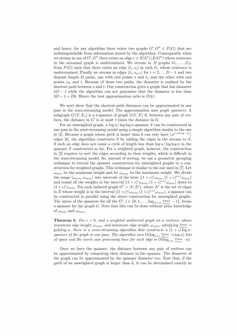
and hence, for any algorithm there exists two graphs G′, G′′ ∈ F(G) that areindistinguishable from information stored by the algorithm. Consequently whenwe stream in one of G′, G′′ there exists an edge e ∈ E(G′)\E(G′′) whose existencein the streamed graph is undetermined. We stream in D graphs G1, . . . , GD

from F(G) such that there exists an edge (ti, si) in each Gi whose existence isundetermined. Finally we stream in edges (ti, si+1) for i = 2, . . . D − 1 and twodisjoint length D paths, one with end points s and t1 and the other with endpoints sD and t. Because of these two paths, the diameter is realized by theshortest path between s and t. Our construction gives a graph that has diameter4D − 1 while the algorithm can not guarantee that the diameter is less than3D − 1 + Dk. Hence the best approximation ratio is Ω(k).

We next show that the shortest-path distances can be approximated in onepass in the semi-streaming model. The approximation uses graph spanners. Asubgraph G′(V,Es) is a t-spanner of graph G(V,E) if, between any pair of ver-tices, the distance in G′ is at most t times the distance in G.

For an unweighted graph, a log n/ log log n-spanner S can be constructed inone pass in the semi-streaming model using a simple algorithm similar to the onein [2]. Because a graph whose girth is larger than k can only have dn1+2/(k−1)eedges [6], the algorithm constructs S by adding the edges in the stream to S,if such an edge does not cause a cycle of length less than log n/ log log n in thespanner S constructed so far. For a weighted graph, however, the constructionin [2] requires to sort the edges according to their weights, which is difficult inthe semi-streaming model. So, instead of sorting, we use a geometric groupingtechnique to extend the spanner construction for unweighted graphs to a con-struction for weighted graphs. This technique is similar to the one used in [7]. Letωmin be the minimum weight and let ωmax be the maximum weight. We dividethe range [ωmin, ωmax] into intervals of the form [(1 + ε)iωmin, (1 + ε)i+1ωmin)and round all the weights in the interval [(1 + ε)iωmin, (1 + ε)i+1ωmin) down to(1 + ε)iωmin. For each induced graph Gi = (V,Ei), where Ei is the set of edgesin E whose weight is in the interval [(1+ ε)iωmin, (1+ ε)i+1ωmin), a spanner canbe constructed in parallel using the above construction for unweighted graphs.The union of the spanners for all the Gi, i ∈ 0, 1, . . . , log(1+ε)

ωmax

ωmin− 1, forms

a spanner for the graph G. Note that this can be done without prior knowledgeof ωmin and ωmax.

Theorem 5. For ε > 0, and a weighted undirected graph on n vertices, whosemaximum edge weight, ωmax, and minimum edge weight, ωmin, satisfy log ωmax

ωmin=

polylog n, there is a semi-streaming algorithm that constructs a (1 + ε) log n-spanner of the graph in one pass. The algorithm uses O(log1+ε

ωmax

ωmin·n log n) bits

of space and the worst case processing time for each edge is O(log1+εωmax

ωmin· n).

Once we have the spanner, the distance between any pair of vertices canbe approximated by computing their distance in the spanner. The diameter ofthe graph can be approximated by the spanner diameter too. Note that, if thegirth of an unweighted graph is larger than k, it can be determined exactly in

a k-spanner of the graph. The construction of the log n/ log log n-spanner thusprovides a log n/ log log n-approximation for the girth.

We end this section by briefly mentioning some graph problems that aresimple in the semi-streaming model but may be impossible in a (poly)log-spacestreaming setting.

A minimum spanning tree can be constructed in one pass and O(log n) timeper edge using a simple adaptation of an existing on-line algorithm [20]. Planaritytesting is impossible in the (poly)log-space streaming model, because decidingthe existence of a K5 minor of a graph would require O(n) bits of space. Because aplanar graph would have at most 3n−6 edges, using O(n) storage, many existingalgorithms can be adapted to the semi-streaming model.

The following is an algorithm for finding articulation points in the semi-streaming model. It uses one disjoint set data structure, SF, for keeping trackof the connected components of the spanning forest, T . It also uses one disjointset data structure per vertex v, in order to store v’s neighbors.

Algorithm 5 (Articulation Points).

T = (V, ∅)For each v ∈ V : SF.makeset(v)For each input edge (u, v):

if SF.find-set(u) = SF.find-set(v) then:find the path, u = a0, a1, . . . , ak = v from u to v in TFor each ai, 0 < i < k, ai.union(ai−1, ai+1).

else:SF.union(u,v)T = T ∪ (u, v)u.makeset(v)v.makeset(u)

For each v ∈ V :if the neighbors of v w.r.t. T lie in at least two different sets

then output v as an articulation point.

If u is an articulation point there exists two neighbors v and w of u in Tsuch that any path from v to w passes through u. In this case, in the disjointset structure for u the components containing v and w will never be unioned.

5 Conclusion

We considered a set of classical graph problems in the semi-streaming model.We showed that although exact answers to most of these problems are stillimpossible, certain approximations are possible. More research is needed for acomplete understanding of the model. Particularly, the efficiency of an algorithmin the semi-streaming model is measured by S(m,n), P (m,n) and T (m,n) asin definition 2. Together with the approximation factor, an algorithm thus has4 parameters. It would be interesting to develop a better understanding of thetradeoffs among these parameters.

References

1. J. Abello, A.L. Buchsbaum, J.R. Westbrook. A Functional Approach to ExternalGraph Algorithms. Algorithmica, 32(3): 437–458, 2002.

2. I. Althofer, G. Das, D. Dobkin, and D. Joseph. Generating sparse spanners forweighted graphs. In Proc. 2nd Scandinavian Workshop on Algorithm Theory(SWAT’90), LNCS 447, 26–37, 1990.

3. N. Alon, Y. Matias, and M. Szegedy. The space complexity of approximating thefrequency moments. Journal of Computer and System Sciences, 58(1):137–147,Feb. 1999.

4. A.L. Buchsbaum, R. Giancarlo and J.R. Westbrook. On finding common neigh-borhoods in massive graphs. Theoretical Computer Science, 299 (1-3):707–718,2003.

5. Z. Bar-Yossef, R. Kumar, and D. Sivakumar. Reductions in streaming algorithms,with an application to counting triangles in graphs. In Proc. 13th ACM-SIAMSymposium on Discrete Algorithms, pages 623–632, 2002.

6. B. Bollobas. Extremal Graph Theory. Academic Press, New York, 1978.7. E. Cohen. Fast algorithms for constructing t-spanners and paths with stretch t.

SIAM J. on Computing, 28:210-236, 1998.8. P. Drineas and R. Kannan. Pass Efficient Algorithm for approximating large

matrices. In Proc. 14th ACM-SIAM Symposium on Discrete Algorithms, pages223-232, 2003.

9. D. Eppstein, Z. Galil, and G.F. Italiano. Dynamic graph algorithms. CRC Hand-book of Algorithms and Theory of Computation, Chapter 8, 1999.

10. J. Feigenbaum, S. Kannan, M. Strauss, and M. Viswanathan. An approximateL1 difference algorithm for massive data streams. SIAM Journal on Computing,32(1):131–151, 2002.

11. P. Flajolet and G.N. Martin. Probabilistic counting. In Proc. 24th IEEE Sympo-sium on Foundation of Computer Science, pages 76–82, 1983.

12. A.C. Gilbert, S. Guha, P. Indyk, Y. Kotidis, S. Muthukrishnan, and M. Strauss.Fast, small-space algorithms for approximate histogram maintenance. In Proc.34th ACM Symposium on Theory of Computing, pages 389–398, 2002.

13. S. Guha, N. Koudas, and K. Shim. Data-streams and histograms. In Proc. 33thACM Symposium on Theory of Computing, pages 471–475, 2001.

14. M. Rauch Henzinger, P. Raghavan, and S. Rajagopalan. Computing on datastreams. Technical Report 1998-001, DEC Systems Research Center, 1998.

15. P. Indyk. Stable distributions, pseudorandom generators, embeddings and datastream computation. In Proc. 41th IEEE Symposium on Foundations of ComputerScience, pages 189–197, 2000.

16. M. Karpinski and W. Rytter Fast Parallel Algorithms for Graph Matching Prob-lems, Oxford Lecture Series in Math. and its Appl. Oxford University Press, 1998.

17. B. Kalyanasundaram and G. Schnitger. The Probabilistic Communication Com-plexity of Set Intersection. SIAM Journal on Discrete Math., 5:545–557, 1990.

18. R. Kumar, P. Raghavan, S. Rajagopalan, and A. Tomkins. Extracting large-scaleknowledge bases from the web. In Proceedings of the 25th VLDB Conference,pages 639–650, 1999.

19. S. Muthukrishnan. Data streams: Algorithms and applications. 2003. Availableat “http://athos.rutgers.edu/∼muthu/stream-1-1.ps”

20. R. Tarjan. Data Structures and Network Algorithms. SIAM, Philadelphia, 1983.21. R. Uehara and Z. Chen. Parallel approximation algorithms for maximum weighted

matching in general graphs. Information Processing Letters, 76(1–2):13–17, 2000.