On flow magnitude and field-flow alignment at Earth's core surface

Geophys. J. Int. (2011) doi: 10.1111/j.1365-246X.2011.05032.x

GJI

Geo

mag

netism

,ro

ckm

agne

tism

and

pala

eom

agne

tism

On flow magnitude and field-flow alignment at Earth’s core surface

Christopher C. Finlay1 and Hagay Amit21Institut fur Geophysik, Sonneggstrasse 5, ETH Zurich, Zurich, CH-8092, Switzerland. E-mail: [email protected] UMR 6112, Universite de Nantes, Laboratoire de Planetologie et de Geodynamique, 2 Rue de la Houssiniere, Nantes, F-44000, France

Accepted 2011 March 31. Received 2011 March 30; in original form 2010 November 23

S U M M A R YWe present a method to estimate the typical magnitude of flow close to Earth’s core surfacebased on observational knowledge of the geomagnetic main field (MF) and its secular variation(SV), together with prior information concerning field-flow alignment gleaned from numericaldynamo models. An expression linking the core surface flow magnitude to spherical harmonicspectra of the MF and SV is derived from the magnetic induction equation. This involvesthe angle γ between the flow and the horizontal gradient of the radial field. We study γ

in a suite of numerical dynamo models and discuss the physical mechanisms that controlit. Horizontal flow is observed to approximately follow contours of the radial field close tohigh-latitude flux bundles, while more efficient induction occurs at lower latitudes wherepredominantly zonal flows are often perpendicular to contours of the radial field. We showthat the amount of field-flow alignment depends primarily on a magnetic modified Rayleighnumber Raη = αg0�TD/η�, which measures the vigour of convective driving relative to thestrength of magnetic dissipation. Synthetic tests of the flow magnitude estimation scheme areencouraging, with results differing from true values by less than 8 per cent. Application toa high-quality geomagnetic field model based on satellite observations (the xCHAOS modelin epoch 2004.0) leads to a flow magnitude estimate of 11–14 km yr−1, in accordance withprevious estimates. When applied to the historical geomagnetic field model gufm1 for theinterval 1840.0–1990.0, the method predicts temporal variations in flow magnitude similar tothose found in earlier studies. The calculations rely primarily on knowledge of the MF and SVspectra; by extrapolating these beyond observed scales the influence of small scales on flowmagnitude estimates is assessed. Exploring three possible spectral extrapolations we find thatthe magnitude of the core surface flow, including small scales, is likely less than 50 km yr−1.

Key words: Dynamo: theories and simulations; Satellite magnetics; Planetary interiors.

1 I N T RO D U C T I O N

Flow of electrically conducting fluid in the Earth’s liquid outercore generates the geomagnetic field via motional induction. De-tailed understanding of this process requires reliable, observation-based, estimates of the typical magnitude of the core flow U . Forexample, knowledge of U is needed to calculate fundamental non-dimensional parameters such as the magnetic Reynolds numberRm = UL/η and the Rossby number Ro = U/�L, where L is acharacteristic length scale, η is the magnetic diffusivity and � isthe angular rotation rate of the system. Rm and Ro, respectively,diagnose the kinematic and dynamic regime of dynamos driven byrotating convection. Without robust knowledge of U it is difficultto assess how close numerical dynamo models are to an earth-likeregime. Since present simulations yield results spanning a widerange of Rm (Roberts & Glatzmaier 2000; Christensen & Tilgner2004) and Ro (Christensen & Aubert 2006; Olson & Christensen2006; Sreenivasan & Jones 2006) that encompass distinct be-

haviours ranging from non-reversing and dipole-dominated, to re-versing multipolar fields (Kutzner & Christensen 2002), it would beextremely helpful if geomagnetic observations could place tighterlimits on acceptable values of Ro and Rm. In this study, we attemptto make some progress towards this goal by developing a new tech-nique to estimate the typical magnitude of horizontal flow at theEarth’s core surface 〈uH〉 which hereafter is used as a proxy for U .

Previous efforts to estimate 〈uH〉 have focused on inferencesfrom observed changes [i.e. secular variation (SV)] in the Earth’score-generated main field (MF), following an idea originating withElsasser (1939). From scale analysis of the magnetic induction equa-tion (and neglecting magnetic diffusion), one can estimate the orderof magnitude of flow required to explain the observed SV, giventhe observed magnitude of the MF and an assumed length scalefor core motions (Elsasser 1946; Elsasser 1950a). A later idea wasto determine the angular speed of foci of non-dipole field at theEarth’s surface, and then to calculate the magnitude of flow at thecore surface necessary to produce this motion (Bullard et al. 1950).

C© 2011 The Authors 1Geophysical Journal International C© 2011 RAS

Geophysical Journal International

2 C. C. Finlay and H. Amit

Roberts & Scott (1965) pointed out that detailed maps of thehorizontal flow uH , just below the thin Ekman–Hartmann bound-ary layer at the top of the core, could be obtained from spher-ical harmonic models of the radial MF, Br and its SV, ∂ Br/∂t ,again provided magnetic diffusion can be neglected; Vestine andco-workers proceeded to calculate such maps (see Kahle et al.1967a; Kahle et al. 1967b). Later Backus (1968) pointed outthat such core flow determinations are inherently non-unique,due to a lack of information from the radial frozen-flux in-duction equation concerning the solenoidal part of the productBr uH . A simple example of this difficulty is that flow along nullflux contours (where Br = 0) produces no SV, so it is unconstrainedby observations of the MF evolution. Backus (1968) also provedthat unique estimates of certain flow components were possible atspecific topological locations. These point estimates provide usefuldirect estimates (see, e.g. Booker 1969; Whaler & Holme 2007),but unfortunately sample only a very small portion of the core sur-face, capture only one component of the flow, and are subject todifficulties in estimating the amplitude of errors on point estimatesof the MF at the core surface.

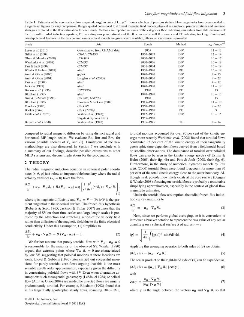
Over the past three decades, modern core flow inversion stud-ies have exploited a variety of dynamical constraints and trunca-tion and regularization assumptions (for comprehensive reviews seeBloxham & Jackson 1991; Holme 2007; Finlay et al. 2010) in anattempt to mitigate the effects of non-uniqueness. In such studies,estimates of 〈uH〉 are derived from the root mean square (rms) mag-nitude of uH at the core surface. In Table 1 we present a selection ofpublished flow magnitude estimates. These encompass both earlyfoci tracking and point estimate methods, and results from morerecent flow inversions involving a diverse range of dynamical as-sumptions, inversion strategies and sets of magnetic observations.These previous observation-based estimates of 〈uH〉 at the Earth’score surface range from 4–22 km yr−1.

The spread in the values reported in Table 1 is a consequenceboth of the different geomagnetic observations used, and of the dif-ferent methods of flow estimation employed. All previous estimatesof 〈uH〉 suffer from a number of fundamental limitations. First, asmentioned above, flow along contours of Br at the core surfaceproduces no SV (Backus 1968; Backus & LeMouel 1986) so thisflow component is unconstrained by magnetic observations. Sec-ondly, small scales of the MF and SV cannot be resolved in presentgeomagnetic field models, limiting flow inversions to large scales(Hulot et al. 1992). Moreover, large-scale SV can be generated bythe interactions of small-scale field and large-scale flow, or large-scale field and small-scale flow (Bullard & Gellman 1950), so coreflow models based only on the observed MF and SV may be biased(Eymin & Hulot 2005; Gillet et al. 2009). Finally, the influence ofmagnetic diffusion is almost always ignored in inversion schemeswhich may lead to local biases in the flow determination (Amit &Christensen 2008). These difficulties have been well illustrated instudies of core flow inversions of the output from numerical dy-namo models. Rau et al. (2000) found that the mean core surfaceflow magnitude obtained by inversion underestimated the true sur-face flow magnitude by as much as a factor of 2 (see their table 2)even if information concerning all length scales of the core surfaceMF is provided. The magnitude estimates of Amit et al. (2007) us-ing their helical flow inversion method are better, typically withinabout ±15 per cent of the true rms flow magnitude, but when theSV was low-pass filtered, removing the small-scale details, theirestimates also deteriorated significantly.

Uncertainties related to existing core flow magnitude estimatesmotivate us to explore a new alternative scheme. The approach set

out below allows one to estimate the rms core surface flow mag-nitude 〈uH〉 from knowledge of spatial spectra of MF and SV at aparticular epoch together with prior knowledge on field-flow align-ment obtained from numerical dynamo models. We argue belowthat global aspects of this essential facet of magnetic induction areadequately captured in the present generation of numerical dynamomodels.

Knowledge concerning the relative alignment of magnetic fieldand flow in rapidly rotating, convection-driven, dynamos is centralto our approach. Field-flow alignment, how it arises dynamically(Mason et al. 2006), its relation to dynamo saturation (Cameron &Galloway 2006; Cattaneo & Tobias 2009; Schrinner et al. 2010) andits influence on the partitioning between kinetic and magnetic ener-gies (Archontis et al. 2007) are subjects of ongoing debate amongdynamo theoreticians. It is also intimately related to an integralproperty called cross-helicity (Moffatt 1978), which is of great in-terest in studies of magnetohydrodynamic (MHD) turbulence (Perez& Boldyrev 2007) where problems are formulated in terms of theElsasser variables (u ±B) (Elsasser 1950b). To our knowledge theonly previous study of field-flow alignment in numerical models ofthe geodynamo was that by Takahashi & Matsushima (2005). Theyobserved that as the convective forcing (measured by the Rayleighnumber Ra) was increased, less flow perpendicular to field linesoccurred, the dynamos became less efficient, and there was a reduc-tion in magnetic energy. In this investigation we focus on field-flowalignment close to the outer boundary and on extracting the informa-tion required by our flow magnitude estimation scheme. We studythe relation between different characteristic field structures and thedegree of field-flow alignment. We also investigate the dependenceof the globally averaged amount of field-flow alignment close tothe outer boundary on the non-dimensional parameters controllingthe numerical dynamo models.

In Section 2 we present the mathematical details of our new flowmagnitude estimation scheme; the information required is shown totake the form of MF and SV spectra together with an rms measureof the field-flow alignment at the core surface. In Section 3 wetest the method using a small suite of numerical dynamo models,and propose a scaling law for applying it to the Earth’s core. Wealso present spatial variations of field-flow alignment in the modelsand discuss the underlying mechanisms at work. In Section 5 weapply our scheme to the Earth, using both recent and historicalgeomagnetic field models, and derive new estimates for 〈uH〉 inthe Earth’s core and how this has varied with time. The impact ofunobserved small scales on estimates of 〈uH〉 is discussed and anew range of plausible values is proposed.

In Section 6 we report new estimates of Rm and Ro based onour results. Flow magnitude estimates based on the observed MFand SV, and also estimates taking into account possible extrapola-tions to smaller scales are considered. In the calculation of Ro weassign flow length scales Lu based on the SV spectrum. In addi-tion to the traditional Rm = ULh

B/η, we consider an alternativemagnetic Reynolds number Rmr = U(Lr

B)2/ηLhB that takes into

account radial magnetic diffusion. Here LhB is the length scale of

the MF in the horizontal direction while LrB is the length scale of

the MF in the radial direction, associated with a magnetic diffusionboundary layer close to the core surface. A magnetic Reynolds num-ber containing two distinct length scales was previously proposedby Takahashi & Matsushima (2005) and Takahashi et al. (2008).Their analysis focused on comparing the importance of stretch-ing of MF by the flow to the effects of magnetic diffusion, thatis, they instead accounted for distinct flow and field length scales.In contrast, we consider the importance of horizontal advection

C© 2011 The Authors, GJI

Geophysical Journal International C© 2011 RAS

Core flow magnitude and field-flow alignment 3

Table 1. Estimates of the core surface flow magnitude 〈uH 〉 in units of km yr−1 from a selection of previous studies. Flow magnitudes have been rounded to2 significant figures for easy comparison. Ranges quoted correspond to different magnetic field models, physical assumptions, parametrizations and inversionstrategies explored in the flow estimation for each study. Methods are reported in terms of the categories INV indicating rms values from full inversions ofthe frozen-flux radial induction equation, PE indicating rms point estimates of the flow normal to null flux curves and TF indicating tracking of individualnon-dipole field features. In the data column names of field models are given where available, otherwise a reference is provided.

Study Data Epoch Method 〈uH 〉/km yr−1

Lesur et al. (2010) Co-estimated from CHAMP data 2005 INV 11 − 13Gillet et al. (2009) CM4 / xCHAOS 1960–2007 INV 12 − 14Olsen & Mandea (2008) xCHAOS 2000–2007 INV 10 − 17Wardinski et al. (2008) CHAOS 2000–2006 INV 16 − 18Pais & Jault (2008) CHAOS 2001–2004 INV 16 − 19Whaler & Holme (2007) ufm1 1970–1980 PE 16 − 19Amit & Olson (2006) gufm1 1840–1990 INV 8 − 15Amit & Olson (2004) Langlais et al. (2003) 1980–2000 INV 7 − 22Pais et al. (2004) ufm1 1840–1990 INV 4 − 12Jackson (1997) ufm1 1840–1990 INV 11 − 19Backus et al. (1996) IGRF1980 1980 PE 13Bloxham (1992) ufm1 1840–1990 INV 10 − 13Gire & LeMouel (1990) USGS80, GSFC80 1980 INV 15Bloxham (1989) Bloxham & Jackson (1989) 1915–1980 INV 11 − 19Voorhies (1986) GSFC80 1960–1980 INV 9 − 22Booker (1969) GSFC(12/66) 1945–1960 PE 9Kahle et al. (1967b) Vestine et al. (1947); 1912–1955 INV 10 − 15

Nagata & Syono (1961) 1955–1960Bullard et al. (1950) Vestine et al. (1947) 1905–1945 TF 8 − 14

compared to radial magnetic diffusion by using distinct radial andhorizontal MF length scales. We evaluate Ro, Rm and Rmr forvarious possible choices of Lu and Lh

B . Limitations of the newmethodology are also discussed. In Section 7 we conclude witha summary of our findings, describe possible extensions to otherMHD systems and discuss implications for the geodynamo.

2 T H E O RY

The radial magnetic induction equation in spherical polar coordi-nates (r , θ , φ) just below an impenetrable boundary where the radialvelocity vanishes (ur = 0) takes the form

∂ Br

∂t+ uH · ∇H Br + Br (∇H · uH ) = η

[1

r 2

∂2

∂r 2(r 2 Br ) +∇H

2 Br

],

(1)

where η is magnetic diffusivity and ∇H = ∇ − (∂/∂r )r is the gra-dient tangential to the spherical surface. The frozen-flux hypothesis(Roberts & Scott 1965; Jackson & Finlay 2007) assumes that themajority of SV on short time-scales and large length scales is pro-duced by the advection and stretching action of the velocity fieldrather than diffusion of the magnetic field due to the finite electricalconductivity. Under this assumption, (1) simplifies to

∂ Br

∂t+ uH · ∇H Br + Br (∇H · uH ) = 0. (2)

We further assume that purely toroidal flow with ∇H · uH = 0is responsible for the majority of the observed SV. Whaler (1980)argued that extreme points where ∇H Br = 0 are characterizedby low SV, suggesting that poloidal motions at these locations areweak. Lloyd & Gubbins (1990) later carried out successful inver-sions for purely toroidal core flows arguing that this is the mostsensible zeroth order approximation, especially given the difficultyin constraining poloidal flows with SV. Even when alternative as-sumptions such as tangential geostrophy (LeMouel 1984) or helicalflow (Amit & Olson 2004) are made, the inverted flows are usuallypredominantly toroidal. For example, Bloxham (1992) found thatin his tangentially geostrophic steady flows, spanning 1840–1990,

toroidal motions accounted for over 90 per cent of the kinetic en-ergy; more recently Wardinski et al. (2008) found that toroidal flowsconstituted 93 per cent of the kinetic energy of their tangentiallygeostrophic time-dependent flows derived from a field model basedon satellite observations. The dominance of toroidal over poloidalflows can also be seen in the kinetic energy spectra of Eymin &Hulot (2005, their fig. 4b) and Pais & Jault (2008, their fig. 6).Furthermore, in the study of numerical dynamos models by Rauet al. (2000) toroidal flows were found to account for more than 90per cent of the total kinetic energy close to the outer boundary. Al-though weak poloidal flow likely exists at the core surface (Beggan& Whaler 2008), focusing on toroidal flows is probably a reasonablesimplifying approximation, especially in the context of global flowmagnitude estimates.

Under the toroidal flow assumption, the radial frozen-flux induc-tion eq. (2) simplifies to

∂ Br

∂t= −uH · ∇H Br . (3)

Next, since we perform global averaging, so it is convenient tointroduce a bracket notation to represent the rms value of any scalarquantity g on a spherical surface S of radius r = c

〈g〉 =√√√√ 1

4π

∫S

[g(c)]2 sin θdθ dφ. (4)

Applying this averaging operator to both sides of (3) we obtain,

〈∂ Br/∂t〉 = 〈uH · ∇H Br 〉. (5)

The scalar product on the right-hand side of (5) can be expanded as,

〈∂ Br/∂t〉 = 〈|uH | |∇H Br | | cos γ |〉, (6)

with

cos γ = uH · ∇H Br

|uH | |∇H Br | , (7)

where γ is the angle between the vectors uH and ∇H Br so that




(π/2 − γ ) is the angle between a Br–contour and the core surfaceflow uH . Note that cos γ (θ , φ) is a local scalar quantity, for whichthe rms on a spherical surface may be calculated in the usual manner.

To make further progress, an additional step is required. Weproceed assuming that |uH (θ , φ)|, |∇H Br(θ , φ)| and | cos γ (θ , φ)|are spatially uncorrelated, which makes it possible to separate therms of their product into the product of their respective rms values.

〈|uH | |∇H Br | | cos γ |〉 = 〈uH〉〈∇H Br 〉〈cos γ 〉, (8)

where we have been able to dispense with the absolute signs onthe right-hand side because |g|2 = g2. We are unable to justifythe assumption of spatially uncorrelated quantities in (8) a priori,but by analysing the output from numerical dynamos models wehave found that empirically this is often the case (see Section 3).A related assumption was previously made by Hulot et al. (1992)in their study of the effects of field truncation on the flow. Theyconsidered that the spectral coefficients representing the field andflow were independent, zero mean, random variables which enableduseful expressions for rms interaction terms to be obtained (seetheir section 4.2 and especially eq. 31b). It is worth recalling thatour treatment does, of course, account for the directional correlationbetween the vector quantities uH and ∇H Br through the factor cos γ

in the expansion of the scalar product; it is only the magnitudes ofthese two vector quantities and the magnitude of the cosine of theangle between them that we assume to be spatially uncorrelated.

Substituting (8) into (6) and rearranging gives

〈uH 〉 = 〈∂ Br/∂t〉〈∇H Br 〉〈cos γ 〉 . (9)

This relation may easily be interpreted physically; it states that therms flow magnitude is proportional to the rms magnitude of the SVand inversely proportional to the rms magnitude of the horizontalgradient of the radial field (with a large gradient even a weak flowcan produce large SV). It also clearly reveals that if the flow is onaverage nearly parallel to contours of the radial field (i.e. 〈 cos γ 〉 ∼0) then a very strong flow will be necessary to explain the observedSV.

Considering the velocity and magnetic fields output from numer-ical dynamo models on a latitude–longitude grid, one can directlyestimate the quantities in (9), ∇H Br, ∂ Br/∂t as well as cos γ , inphysical space. In Section 3, quantities that involve spatial deriva-tives (such as ∇H Br) are calculated using centred finite-differencingon the same grid that was used for the dynamo calculations. Therms quantities are then be calculated by a numerical approximationto (4).

Alternatively, 〈 ∂ Br/∂t 〉 and 〈∇H Br〉 can be calculated directlyin spectral space by summing appropriate combinations of sphericalharmonics. This turns out to be particularly useful when workingwith observation-based field models where the MF and SV aretypically provided in the form of spherical harmonic coefficients(see Section 5). As shown in the Appendix, (9) can be written interms of Schmidt quasi-normalized spherical harmonic spectra as

〈uH 〉 =

√∞∑

l=1

(l+1)(2l+1) Ql (c)

√∞∑

l=1

l(l+1)2

c2(2l+1)Rl (c) 〈cos γ 〉

, (10)

where l is the spherical harmonic degree, and Rl(c) and Ql(c) areMauersberger–Lowes spectra (Mauersberger 1956; Lowes 1966;Lowes 1974) of the MF and the SV, respectively, at the core surface,as defined in the Appendix. Since (10) is written in terms of the

spherical harmonic spectra, it is evident that our estimate of 〈uH〉uses only information concerning the globally averaged propertiesof the field and is not based on any particular local features, sinceall phase information is absent. In the next section we use numericaldynamo models to test this flow estimation scheme.

3 T E S T S W I T H N U M E R I C A L DY NA M OM O D E L S

3.1 Setup and non-dimensional parameters for numericalexperiments

In this section we report a series of synthetic tests of the methodproposed in the previous section. These tests involve 3-D numeri-cal dynamo models computed using the simulation code MAGIC(Wicht 2002). We use an earth-like geometry of ri/ro = 0.35, whereri is the inner boundary radius and r 0 is the radius of the outerboundary. We examined models sampling a range of control param-eters in an attempt to characterize the parameter dependence of ourresults. All the models studied have electrically insulating, no-slipand isothermal (fixed temperature) boundary conditions. In all casesa spherical harmonic truncation degree of 64 was employed exceptin case M8 where it was increased to 168. The same truncationlevel was used for both the field and the flow. In physical space thegrid is regular in the horizontal direction, that is, fixed angular gridstep in both longitude and latitude, with 192 longitude grid pointsand 96 latitude grid points for all cases except M8 which used 480and 240 points, respectively. The number of radial grid points in-creases with decreasing Ekman number so that each model has atleast five grid points resolving the Ekman boundary layers. Becausewe are mostly interested in magnetic field evolution on time-scalesshort compared to the magnetic diffusion time, and because we willlater apply our method to observations of the geomagnetic field, wefocused on dipole-dominated non-reversing dynamos.

The control parameters, the Ekman number Ek = ν/�D2,the Rayleigh number Ra = αg0�T D3/κν, the Prandtl numberPr = ν/κ and the magnetic Prandtl number Pm = ν/η, for theruns investigated are given in Table 2. Here α is the thermal expan-sivity, g0 is the value of gravity on the outer boundary, �T is thetemperature difference between the inner and outer boundaries, Dis the shell thickness, ν is the kinematic viscosity, κ is the thermaldiffusivity, � is the rotation rate and η is as before the magneticdiffusivity. The suite of models studied here is the same as that pre-viously studied by Amit & Christensen (2008) with the addition ofone extra model with lower magnetic Prandtl number (model M9 inTable 2). Also given in Table 2 are the diagnostic output values ofthe global magnetic Reynolds number Rm = UD/η and the globalRossby number Ro = U/�D calculated using U based on the totalkinetic energy in the spherical shell and a single length scale D.The models differ in the complexity of the small-scale features, thatis, by the amount of kinetic energy which is accommodated by thesmall scales. Due to numerical limitations, all the models exploredhere are unfortunately many orders of magnitude away from theEarth-like values of Ra, Ek and Pm. They do however have the cor-rect order of magnitude for the global magnetic Reynolds number,which suggests they may correctly mimic kinematic and inductionprocesses relevant to the Earth’s core.

We also report the value of an additional parameter, which weterm the ‘magnetic modified Rayleigh number’,

Raη = αg0�T D

η�= Ra · Ek · Pm

Pr= Ra′ · Pm, (11)




Table 2. Input control parameters for the numerical dynamos and estimated values for Earth’s core: Rayleigh number Ra, Ekman number Ek, magnetic Prandtlnumber Pm and Prandtl number Pr (see text for definitions). Also given are the model outputs Rm and Ro and a new non-dimensional parameter Raη that weterm the magnetic modified Rayleigh number. All estimates for the Earth’s core are from Christensen & Aubert (2006) except Rm from Bloxham & Jackson(1991).

Case Ra Ek Pm Pr Rm Ro Raη

M1 3 × 105 10−3 4 1 110 2.75 × 10−2 1200M2 1.5 × 106 3 × 10−4 2 1 96 1.44 × 10−2 900M3 3 × 106 3 × 10−4 3 1 296 2.96 × 10−2 2700M4 8 × 106 2 × 10−4 3 1 487 3.25 × 10−2 4800M5 1.5 × 107 1 × 10−4 2 1 329 1.65 × 10−2 3000M6 8 × 106 1 × 10−4 2 1 177 8.85 × 10−3 1600M7 1.5 × 107 1 × 10−4 4 1 617 1.54 × 10−2 6000M8 1.2 × 108 3 × 10−5 2.5 1 876 1.05 × 10−2 9000M9 7.5 × 106 2 × 10−4 0.5 1 51 2.04 × 10−2 375Earth 1023 5 × 10−15 2 × 10−6 0.25 500 6 × 10−6 4000

Table 3. 〈 cos γ 〉 and the ratio 〈uH 〉cal/〈uH 〉tr at the top of the free stream of the numerical dynamos. 〈uH 〉cal is the value computed using scheme (9) and〈uH 〉tr is the true core surface flow from the dynamo model. The range, mean (μ) and standard deviation (σ ) from 10 arbitrarily sampled snapshots are givenfor both quantities.

Case 〈 cos γ 〉〈uH 〉cal/〈uH 〉tr

Range μ σ Range μ σ

M1 0.607 − 0.652 0.633 0.013 0.784 − 0.981 0.849 0.065M2 0.615 − 0.645 0.628 0.008 0.822 − 1.273 0.962 0.127M3 0.653 − 0.666 0.661 0.004 0.801 − 0.971 0.902 0.051M4 0.670 − 0.685 0.677 0.005 0.930 − 1.085 0.985 0.042M5 0.662 − 0.671 0.667 0.003 0.879 − 1.061 0.989 0.050M6 0.636 − 0.653 0.644 0.005 0.916 − 1.277 1.026 0.097M7 0.673 − 0.688 0.681 0.005 0.893 − 1.055 1.002 0.045M8 0.661 − 0.671 0.667 0.003 0.877 − 1.039 0.951 0.047M9 0.627 − 0.655 0.641 0.009 1.145 − 1.439 1.319 0.090

where Ra′ = Ra · Ek/Pr is the modified Rayleigh number oftenemployed in studies of rotating convection (see, e.g. Olson et al.1999; Christensen et al. 2001). Physically, the traditional Rayleighnumber, Ra, measures the competition between buoyancy forces re-sulting from a temperature (and hence density) difference, and thedissipative effects of viscosity and thermal conduction. However,in the MHD environment of the geodynamo, viscosity is expectedto be weak in the bulk of the fluid where strong magnetic fieldsare also present. In this scenario a moving fluid parcel will dissi-pate energy not through the familiar viscous effects but throughthe electrical currents and concommittant Ohmic dissipation pro-duced as it distorts magnetic field lines; conduction of heat on theother hand continues to play a similar role as before. It thus seemsintuitively reasonable that a magnetic modified Rayleigh numberRaη, which is the modified Rayleigh number Ra′ with ν replacedby η (in analogy to the magnetic Reynolds number where ν is re-placed by η compared to the hydrodynamic Reynolds number), willbe of relevance in rapidly rotating, convection-driven dynamos.∗

We will show later that Raη turns out to be very useful when in-vestigating the average amount of field-flow alignment and that itmay be related to the efficiency of induction in numerical dynamomodels.

∗ Note that Raη also arises naturally when one assumes a balance be-tween Coriolis and buoyancy forces in the Navier–Stokes equation andan advection–diffusion balance in the induction equation, thus it appears tobe rather fundamental to the saturated state in rapidly rotating, convection-driven dynamos.

3.2 Synthetic tests of flow magnitude estimation scheme

One important step in the scheme outlined in Section 2 was theassumption that the magnitudes |uH|, |∇H Br| and | cos γ | are spati-ally uncorrelated. Before proceeding further, we first examined thisassumption with our suite of numerical dynamos. The correlationcoefficient (see, e.g. Rau et al. 2000) was computed between thethree pairs of scalar functions for each dynamo case, for each of10 arbitrarily sampled snapshots. We found that the correlationcoefficients between the fields were usually low, indicating thatour assumption that these fields are uncorrelated is an acceptableapproximation.

Next we applied our flow magnitude estimation scheme (9)to the dynamo models described in Table 2. 〈 cos γ 〉 can be di-rectly obtained in numerical dynamos by calculating the rmsvalue of cos γ (φ, θ ) on a spherical surface just below the outerEkman–Hartmann boundary layer. These calculations were carriedout on the numerical grid used for the dynamo modelling. 10 arbi-trary snapshots were used in each case to obtain the range, time-average and standard deviation measures for each dynamo model.The results are summarized in Table 3. A typical value of 〈 cos γ 〉 ∼0.65 corresponds to an angle γ ∼ 50◦ between uH and ∇H Br or toan angle of ∼40◦ between the velocity vector and a Br-contour.

Once 〈 cos γ 〉 had been estimated, the validity of the flow mag-nitude estimation scheme was assessed using the synthetic SV pro-duced by the numerical dynamos. This series of experiments testswhether, despite the assumptions and approximations being made,the method is capable of producing useful flow magnitude esti-mates. In each dynamo model snapshot we evaluated the rms values




Figure 1. Spatial distribution of | cos γ | from a snapshot of case M2 at the top of the free stream, values close to 0 are white while values close to 1 are black,(top left panel); radial magnetic field at the outer boundary (top right panel); and radial vorticity at the top of the free stream (bottom panel). All maps arecentred at φ = 0◦.

〈 ∂ Br/∂t 〉 and 〈 ∇H Br 〉 at the top of the free stream. Then, using thevalue of 〈 cos γ 〉 for that snapshot, we applied (9) to find the ‘cal-culated’ magnitude of the horizontal velocity 〈uH〉cal and comparedthis with the rms value of the ‘true’ horizontal velocity 〈uH〉tr. Thedeviation of the ratio 〈uH〉cal/〈uH〉tr from unity quantifies the errordue to the approximations made in the flow estimation method.

The results of these tests are reported in Table 3. The errors inthe flow magnitudes detailed there quantify the combined influenceof failure of the frozen-flux assumption, the presence of poloidalflows and departures from the assumption that the magnitudes of|uH|, |∇H Br| and | cos γ | are uncorrelated. The average differencebetween 〈uH〉tr and 〈uH〉cal, over all the cases studied, is 7.9 percent; in individual cases this difference varies from 0.2–32 per cent.The generally good agreement between the true and calculated flowmagnitudes is very encouraging. Note that the results presented inTable 3 are generally better than those achieved for the retrieval ofrms flow magnitude by conventional inversion schemes that werepreviously tested on dynamo simulations (Rau et al. 2000; Amitet al. 2007). On the basis of Table 3 we would expect (9) to yielda flow magnitude estimate within 8 per cent of the true value,assuming 〈 cos γ 〉 along with the MF and its SV are perfectly known;of course in reality these conditions will not be satisfied and largererrors should be expected.

4 F I E L D - F L OW A L I G N M E N T I NN U M E R I C A L DY NA M O M O D E L S

4.1 Spatial distribution and physical significance of | cos γ |Local alignment between the magnetic fields and the flow in numer-ical models of the geodynamo was previously studied by Takahashi& Matsushima (2005). Given its central role in our scheme, and itspotential relevance to the dynamo saturation mechanisms (Cameron& Galloway 2006), we investigate here spatial variations of | cos γ |and discuss the insights provided concerning induction processes atthe core surface.

In Fig. 1 we present a map of | cos γ (θ , φ)| just below the outerEkman–Hartmann boundary layer in a snapshot from a relativelylarge-scale numerical dynamo (case M2). This case is representa-tive of the main features found in other models which possess morecomplex small-scale field and flow structures. We also present theradial magnetic field at the outer boundary and the radial vortic-ity just below the boundary layer. High-latitude intense flux patchesmaintained by cyclonic flow structures are in general associated withlow values of | cos γ |, that is, low efficiency of induction, whereaslow-latitude field structures are often associated with higher val-ues of | cos γ | and thus higher efficiency of induction. Zooming




Figure 2. Zoom into a regions of low | cos γ | (top panel) and high | cos γ |(bottom panel) from Fig. 1. Radial magnetic field (colours) and horizontalflow (arrows) are shown.

into each of these structures reveals further details. In Fig. 2(a)we find low values of | cos γ | at a high-latitude region where acolumnar flow structure, resulting from convection under the in-fluence of rapid rotation, intersects the outer boundary. Cyclonic,columnar flows involve downwelling close to the outer boundary(Olson et al. 1999; Olson et al. 2002) with converging flow that con-centrates radial field into characteristic intense flux bundles at theouter boundary (Gubbins et al. 2000; Olson & Christensen 2002).In these intense field structures, contours of Br are nearly parallelto uH thus leading to low values of | cos γ |. In Fig. 2(a), we ob-serve that the toroidal flow is mostly around the flux bundle, almost

parallel to Br-contours. In contrast, considering Fig. 2(b), at low-and mid-latitudes magnetic field structures drift with the large-scalepredominantly zonal flow. For these structures the toroidal flow isoften perpendicular to Br-contours, yielding large local | cos γ | val-ues. The nearly perpendicular relation between uH and Br-contoursin Fig. 2(b) is particularly evident at the two intense patches centredat ∼25◦E.

In Fig. 3 we present a histogram showing the distribution of| cos γ (θ , φ)| calculated at the dynamo model collocation gridpoints; the sign of cos γ (θ , φ) is of course irrelevant to the rmsvalue 〈 cos γ 〉. This distribution is certainly not uniform, as mightnaively have been expected if | cos γ (θ , φ)| was assumed to be arandom variable. Instead it shows two peaks, one at | cos γ | ∼ 0(horizontal flow parallel to contours of Br), the other at | cos γ | ∼ 1(horizontal flow perpendicular to contours of Br). The distributionis characterized by lower occurrences for intermediate | cos γ |.In this dynamo, for a large fraction of the core surface the fieldand flow are in good alignment and hence induction is weak, see forexample, Fig. 2(a). In addition, there is a significant region wherethe field and flow are nearly perpendicular and significant inductiontakes place (as in Fig. 2b). It is the combined effect of regions withslow-evolving magnetic structures maintained by columnar convec-tion (with nearly field-aligned flow contributing to low | cos γ |), to-gether with lower latitude regions where predominantly zonal flowsact perpendicular to field patches (giving high | cos γ |) that givesrise to the intermediate global values of 〈 cos γ 〉 ∼ 0.65 reported inTable 3.

We suggest that the quantity | cos γ | is a useful local diagnosticof the induction process. Low | cos γ | corresponds to horizontalflow nearly parallel to contours of Br and hence weak advectiveSV and inefficient induction, whereas high | cos γ | corresponds toflow nearly perpendicular to contours of Br and efficient motionalinduction for a given magnitude of flow and field gradient. Wetherefore term | cos γ | the ‘local induction efficiency’, and 〈 cos γ 〉the ‘global induction efficiency’.

The dynamo models presented here are in a regime where anα2 dynamo mechanism operates (Olson et al. 1999). We find thatconsideration of the local efficiency of induction | cos γ | providesadditional insight to the working of such dynamos. The low-latitudefeatures are the surface manifestation of the strong stretching ofpoloidal field by radial outflow between a cyclone and an anti-cyclone. This is known to be a key ingredient in the α2 dynamo

Figure 3. Histogram of | cos γ | from the same snapshot of M2 presented in Fig. 1. The histogram was constructed using all spatial grid points used in thedynamo calculation.




Figure 4. Power-law fit to 〈 cos γ 〉 from the numerical dynamo models based on (13).

mechanism, see fig. 5 of Olson et al. (1999) and fig. 3(a) of Wicht& Tilgner (2010). The value of | cos γ | close to 1 associated withthese features indicates efficient induction and marks their impor-tance in the operation of the dynamo. In contrast the high-latitudecyclonic features possess low | cos γ | and perhaps indicate surfaceregions of importance for the saturation of the dynamo.

4.2 Parameter dependence and scaling of 〈 cos γ 〉To implement the proposed scheme for estimating the flow mag-nitude at Earth’s core surface, we need to extrapolate 〈 cos γ 〉 tothe conditions pertaining to the core. In this section, we perform apower-law scaling analysis of 〈 cos γ 〉 from our suite of numericaldynamo models to obtain the required estimate. Scaling approacheshave previously been successfully applied for other global diagnos-tic properties of numerical dynamos (Christensen & Tilgner 2004;Christensen & Aubert 2006; Olson & Christensen 2006; Chris-tensen 2010). Since Pr is thought to have a similar value in thenumerical dynamo models and in the Earth’s core, we consider thevariation of 〈 cos γ 〉 as a function of Ek, Ra and Pm, beginning witha general power law of the canonical form,

〈cos γ 〉 = C1Rax1 Ekx2 Pmx3 , (12)

where C1 is a constant pre-factor and xi are powers. The best fittingresult gives small positive values (less than 0.1) for all three powers,indicating that 〈 cos γ 〉 depends only very weakly on the controlparameters. Furthermore, the similarity in the values of x1, x2 and x3

suggests that the scaling may be governed by a simpler power lawof the form,

〈cos γ 〉 = A(Raη)x (13)

where Raη is the magnetic modified Rayleigh number (11) and Ais a constant. The best least-squares fit using law (13) occurs withA = 0.55 and x = 0.023 (Fig. 4) and was found to be almost assuccessful a fit with the more general power law (12).

The physical implication of (13) is that the global efficiency ofinduction 〈 cos γ 〉 is largely controlled by the magnetic modifiedRayleigh number Raη. Recall that Raη is identical to the modifiedRayleigh number Ra′ except that magnetic diffusivity substitutes for

the viscosity. It therefore measures how strongly the system is beingforced by convection (against the influence of rotation) compared tohow rapidly energy can be lost by Ohmic dissipation. For the Earth’score Raη ∼ 4000 is well within the range we have explored withnumerical dynamos (Table 2); this indicates that present numericaldynamo models may already capture in a reasonable manner theglobal efficiency of induction (degree of field-flow alignment) attheir outer surface. The dependence on Raη furthermore suggeststhat a trade-off must exist between the effects of more vigorousconvection and stronger magnetic diffusion as an earth-like regimeis approached. The effect of stronger driving (which will increaseRaη and hence increase 〈 cos γ 〉) together with stronger magneticdissipation (which will tend to decrease 〈 cos γ 〉) are predicted tocombine to produce moderately efficient global induction charac-terized by an intermediate value of 〈 cos γ 〉 � 0.65, at least fordipole-dominated non-reversing dynamos of the type studied here.For the flow magnitude estimation scheme the most important as-pect of (13) is that 〈 cos γ 〉 depends only extremely weakly on Raη;this gives us hope that inferences from the numerical dynamos in-vestigated here may provide useful prior information for estimatesof the flow magnitude in the Earth’s core.

Substituting the values of the control parameters expected forthe Earth’s outer core (see Table 2) into power law (13) leads toa predicted value of 〈 cos γ 〉 � 0.666; this is shown in Fig. 4 asthe pink star. Note that in the construction of our power law wedid not impose that the value of 〈 cos γ 〉 for the Earth’s core mustlie in the range 0–1. This was achieved naturally from the veryweak dependence of 〈 cos γ 〉 on the control parameters and thetrade-off between increasing 〈 cos γ 〉 with increasing Ra, and de-creasing 〈 cos γ 〉 with decreasing Pm towards earth-like conditions.Given the uncertainties in the control parameters for the Earth’score, and possible errors in the scaling law due to the small numberof dynamo models studied, we henceforth adopt a (rather large)range 〈 cos γ 〉 = 0.65 ± 0.05 as being appropriate for the Earth’score. Note that the standard deviations in Table 3 suggest variationsof ∼ ±0.05 are in any case associated with the time-dependenceof the dynamo process, so consideration of a range of values〈 cos γ 〉 = 0.6–0.7 seems prudent.




5 F L OW M A G N I T U D E E S T I M AT E S ATE A RT H ’ S C O R E S U R FA C E

In this section we present results of the application of the schemeset out above to geomagnetic observations, and provide new esti-mates for the flow magnitude at Earth’s core surface. We begin byapplying the method to the large-scale MF and SV derived fromhigh-quality observations performed by the Ørsted, CHAMP andSAC-C satellites as encapsulated by the xCHAOS model of Olsen& Mandea (2008). We also quantify how uncertainty in 〈 cos γ 〉affects our flow magnitude estimates. The method is next appliedto the MF and SV between 1840 and 1990 from the field modelgufm1 of Jackson et al. (2000). This enables variations in the flowmagnitude over the historical era to be determined. We conclude byexploring possible spectral extrapolations of the observed MF andSV which permit investigation of the influence of unobserved smallscales on flow magnitude estimates.

5.1 Core flow magnitude estimates from the observedlarge-scale MF and SV

An estimate of the core flow magnitude is obtained using (10),the spectra of the MF, Rl and the spectra of the SV, Ql, at the coresurface from the xCHAOS model (Olsen & Mandea 2008) evaluatedin epoch 2004.0. We truncate the field model at degree L = 10because above this level there are discrepancies among core surface

SV models produced by different authors (Gillet et al. 2010), andbecause unwanted crustal field may already significantly contributeto the MF signal by degree L = 12. We also tested our schemeusing the GRIMM field model (Lesur et al. 2008) also truncated atdegree 10; the results obtained were essentially identical to thosereported here. Fig. 5 shows Br and ∂ Br/∂t from xCHAOS at the coresurface in 2004.0 as used for the calculations reported here. Basedon the estimate of 〈 cos γ 〉 = 0.65 from scaling law (13) appliedto the Earth’s core, we obtain the result 〈uH 〉 =12.5 km yr−1, wellwithin the range of conventional core flow magnitude estimates (seeTable 1).

5.2 Impact of uncertainty in field-flow alignment factor〈cos γ 〉Fig. 6 shows how estimates of 〈uH〉 derived from the xCHAOS MFand SV models in 2004.0 change as 〈 cos γ 〉 varies. For the extreme(and physically implausible) but formally limiting case of a coresurface flow that is everywhere perpendicular to Br-contours, thatis 〈 cos γ 〉 = 1, we obtain a lower bound for the large-scale flowmagnitude of 〈uH〉 = 8.15 km yr−1. This is a formal lower limitgiven the assumptions inherent in our method; however it is veryunlikely that such extreme flow-field alignment exists in the Earth’score and none of the numerical dynamo models studied possesssuch a high 〈 cos γ 〉 value.

Figure 5. Radial magnetic field Br in μT at the core–mantle boundary (top panel) and its secular variation ∂ Br/∂t in μT yr−1 (bottom panel) from thexCHAOS model of Olsen & Mandea (2008) in 2004.0 truncated at degree L = 10.




Figure 6. Variation of core surface flow magnitude 〈uH 〉 determined from xCHAOS truncated at degree L = 10, as a function of 〈 cos γ 〉.

In the opposite limit of horizontal flow along Br-contours (field-aligned flow) for which 〈 cos γ 〉 = 0, there is a singularity in (10).Infinite 〈uH〉 is thus predicted if the flow were entirely along con-tours of Br at the core surface. In that case no SV could be producedand all flow estimation methods based on frozen-flux inversion ofSV will fail. However, a perfectly field-aligned flow also seems im-probable and none of the numerical dynamo models we investigatedsuggest such a relation. Consideration of the range of 〈 cos γ 〉 =0.65 ± 0.05 leads to a range of core surface flow magnitudes 〈uH〉of 11.6–13.6 km yr−1 (see Fig. 6). The very weak dependence ofthe result on the value of 〈 cos γ 〉 gives confidence in the inferredflow magnitude.

5.3 Temporal variations in flow magnitude

To investigate temporal fluctuations in the rms flow magnitude,we applied our method to the gufm1 historical core field model(Jackson et al. 2000) at yearly intervals between 1840.0 and 1990.0with 〈 cos γ 〉 = 0.65. Fig. 7 shows the results with gufm1 truncated atL = 8 and 10. For comparison we also present the rms flow variationsdetermined by Amit & Olson (2006) using a full flow inversionof gufm1 truncated at degree L =14 (see the orange dashed line).Both techniques show similar variations in flow magnitude with themaximum amplitude occurring close to 1915. The same generalpattern was also found by Jackson (1997) using his fully time-dependent, tangentially geostrophic flow inversion (see his fig. 4a).

It is noteworthy that the maximum in core flow magnitude in 1915coincides with a maximum in the observed change in the length ofday at the same time (see fig. 11 of Jackson 1997). Furthermore,the subsequent decrease in flow magnitude until around 1940, theincrease from 1950 until 1970 and the weak decrease towards 1990also follow the general trends in the observed change in the lengthof day over the past century (Jackson et al. 1993). The variationswe find in flow magnitude are therefore qualitatively consistentwith independent geodetic observations of the decadal changes offlow magnitude in the Earth’s core. We therefore conclude thatour approach is a feasible method for monitoring rms temporal

1840 1860 1880 1900 1920 1940 1960 1980Year

8

10

12

14

16

<u H

> /

km/y

r

L=8L=10From Amit and Olson (2006)

Figure 7. Core flow magnitude estimates based on the historical core fieldmodel gufm1 (Jackson et al. 2000) between 1840.0 and 1990.0, assuming〈 cos γ 〉 = 0.65 and using two possible truncation levels (black line is L = 8,red line is L = 10). Also presented is the time-dependent rms flow of Amit& Olson (2006) from a full flow inversion of the same historical field model(dashed orange line).

variations of core flow magnitude on decadal timescales that avoidssome of the complications associated with full core flow inversions.Excluding the low flow magnitudes prior to 1870, which shouldprobably be interpreted with caution since the field models fromthis period are based on less comprehensive data, we find here thatflow magnitudes varied by 3 km yr−1 or ∼25 per cent over severaldecades.

The main difference between our results and those of Amit &Olson (2006) is that our flow magnitudes are 0–4 km yr−1 slower. Apossible reason for this discrepancy is that our estimate of the field-flow alignment parameter 〈 cos γ 〉 is too large (see Fig. 6). However,the precise rms magnitudes obtained in flow inversions are knownto rely heavily on prior assumptions (e.g. choice of damping param-eters) not necessarily related to the underlying physics. An example




of this is given in fig. 4(a) of Jackson (1997) where a change of theregularization parameter alters the rms magnitude of the inferredcore flow by 5–10 km yr−1, with results particularly sensitive before1960 when the data constraints are weaker. Similarly, the magnitudeof the helical flow inferred by Amit & Olson (2006) and plotted inFig. 7 depends on an assumed ratio for the horizontal divergence tothe radial vorticity of the flow.

Note that the temporal variation of the flow derived from gufm1(Fig. 7) is slightly lower (9–12 km yr−1) than our earlier estimateof the core flow magnitude of ∼12.5 km yr−1 based on xCHAOS(Fig. 6). The reason for this is that the historical field model gufm1has lower spatial resolution (especially for SV) than the xCHAOSmodel, with regularization often dominating even below degree 10.The degree to which we can obtain reliable knowledge concern-ing the core MF and its SV obviously plays an important role inestimates of core flow magnitude. We explore this issue further inthe next section.

5.4 Accounting for unresolved small scales

A major uncertainty in applying our method, or any other core flowinversion technique, is that observational knowledge consists onlyof a spatially low-pass filtered version of the core surface field andits temporal evolution. The origin of this low-pass filter lies in thepresence of noise from non-core magnetic sources, in particularcrustal magnetization, as well as ionospheric or magnetosphericcurrents. This problem has been discussed in detail by Hulot et al.(1992), and more recently by Eymin & Hulot (2005), Pais & Jault(2008) and Gillet et al. (2009), who describe how to account forthe interactions of unobserved small-scale field with large-scaleflow, and small-scale flow with large-scale field, when invertinglarge-scale SV to obtain maps of the large-scale flow. Because (10)requires only the MF and SV spectra as inputs, it is possible tosystematically study the impact of unobserved small scales on flowmagnitude estimates by exploring possible spectral extrapolations;this avenue is not possible for conventional core flow inversions.

Here we explore three possible spectral extrapolations of the MFat the core surface r = c. The first was proposed by Roberts et al.(2003) as being compatible with the magnetic spectra obtained innumerical dynamo models, while also satisfying the observed large-scale geomagnetic spectrum. It takes the exponential form

RRl (c) = C2e−Bl , (14)

with B = 0.055. This produces a spectrum similar to that obtainedin the high-resolution numerical dynamo model studied by Roberts& Glatzmaier (2000). The constant C2 is determined, followingLowes (1974) and Roberts et al. (2003), by fitting the observedmagnetic spectrum for l ≥ 3 with the dipole and quadrupole termsexcluded to obtain a better fit to higher degrees. Hereafter we referto spectrum (14) as RJC03.

The second spectral extrapolation considered is based on a sta-tistical model of compact eddies motivated by scaling arguments ofa magnetostrophic vorticity balance at the core surface (Voohrieset al. 2002; Voohries 2004). As explained by Voohries (2004), it isthe generalization of a spectral form earlier proposed by Stevenson(1983) on the basis of the theory of turbulence expected for a heli-cal dynamo, and it was also suggested by McLeod (1996) from thepoint of view of a stochastic model of scattered dipole sources atthe core surface. It takes the form

RVl (c) = K

(l + 1/2)

l(l + 1)

( cs

c

)2l+4, (15)

where K is a constant determined by fitting the observed magneticspectrum. We simplify this model by setting the source radius pa-rameter cs to the seismologically determined value of the core radiusc. Hereafter we refer to spectrum (15) as V04.

The third spectral extrapolation considered is another version ofthe classic power-law form originally proposed by Lowes (1974).It was recast by Buffett & Christensen (2007) with the purpose ofsatisfying not only magnetic observations, but also geodetic con-strains related to nutations, as well as Ohmic heating requirements.They argued that the following spectral form represents a plausi-ble extrapolation of numerical dynamo model results towards anearth-like regime.

RBl (c) = Rχ l , (16)

where R is a constant determined by fitting the non-dipole part ofthe observed spectrum and χ = 0.99 is fixed to ensure there is suf-ficient power at short wavelengths to explain nutation observations(for further details see Buffett & Christensen 2007). Although theprevious spectral form (14) can be rewritten in the same format as(16), the latter is more restricted as it contains only one free param-eter, and forces a very flat spectrum. Note that this extrapolation isless extreme than the completely flat spectral extrapolation recentlydiscussed by Jackson & Livermore (2008). We refer to spectrum(16) as BC07.

To compute 〈uH〉 from (10), one requires not only Rl(c) butalso the spectra of the SV at the core surface, Ql(c). We obtainQl(c) from Rl(c) by assuming that the ratio between the MF andSV spectra, which physically represents a reorganization time forlength scales associated with spherical harmonic degree l (Stacey1992; Hulot & LeMouel 1994),

τl =√

Rl (c)

Ql (c)(17)

can be adequately modelled by the power law

τl = C3l−D, (18)

where the constants C3 and D are determined by an empirical fit tothe observed large-scale MF and SV. Holme & Olsen (2006) andOlsen et al. (2006) have discussed this empirical law in some detailand have argued that it may reflect the trade-off between advectionand diffusion of the magnetic field occurring at all length scales.Substituting (18) into (17) we obtain

Ql (c) = Rl (c)

(C3l−D)2. (19)

We determined the free parameters in the various spectral ex-trapolations C2, K , R, C3 and D by least-squares fits to the satel-lite observation-based xCHAOS MF and SV spectra up to degree10. For the RJC03 spectrum (14), the best fit for l ≥ 3 was ob-tained with C2 = 1.22 × 1010 nT2, for V04 (15) with K = 6.97 ×1010 nT2, for the BC07 spectra (16) the best fit to the non-dipolefield was obtained with R = 9.20 × 109 nT2, while in (18) C3 =778.87 yr and D = 1.33 give the best fit to the ratio of xCHAOS MFand SV spectra up to degree L = 10. The resulting extrapolationsof the MF and SV spectra up to degree L = 1000 are presented inFig. 8.

Using these spectral extrapolations, our preferred value of〈 cos γ 〉 = 0.65, and (10), we explored 〈uH〉 as a function of thetruncation level L. The results of these computations are presentedin Fig. 9. We find that for all three spectral extrapolations 〈uH〉increases with L, with equal predicted magnitudes of ∼22 km yr−1




Figure 8. Top panel: Lowes–Mauersberger spatial power spectra of the MF at the core surface from the xCHAOS model (Olsen & Mandea 2008) in 2004.0(black diamonds) and the fit of three possible extrapolations (RJC03: blue line, V04: green line, BC07: red line) extending out to spherical harmonic degree1000. Bottom panel: Extrapolated spectra for the SV based on (19) and the respective MF spectra.

reached by L = 40. The predictions of the different extrapola-tions begin to differ markedly above L = 60. For L > 150 theprediction of RJC03 reaches an asymptotic value of 29 km yr−1.The extrapolations V04 and BC07 are practically identical un-til L = 200, where 〈uH〉 ∼ 41 km yr−1. For larger L the pre-dictions of BC07 and V04 diverge, with V04 growing exponen-tially, while BC07 reaches an asymptotic value of ∼56 km yr−1 forL > 1000.

Fig. 10 summarizes a large number of calculations focusing on theBC07 extrapolation and exploring a very wide range of values forboth 〈 cos γ 〉 and the truncation degree L. It should however be re-membered that Buffett & Christensen (2007) argued their spectrumis capable of satisfying geodetic constraints derived from nutationobservations, while remaining compatible with Ohmic heating con-straints, only for a truncation degree in the range 160 < L < 250.More generally, Fig. 10 shows that to obtain flow speeds in excessof 60 km yr−1, with the BC07 spectral extrapolation, it is necessaryfor 〈 cos γ 〉 to be less than 0.6. Flow speeds are always less than

50 km yr−1 if 〈 cos γ 〉 lies between 0.4 and 0.8 and the truncationdegree is less than 100.

What truncation degree L, above which magnetic dissipationdominates and the magnetic spectrum decays, is appropriate forthe Earth’s core? Unfortunately the Ohmic dissipation scale inthe Earth’s core is not known. Christensen & Tilgner (2004), ina study of scaling laws in numerical and experimental dynamos,concluded that a magnetic dissipation time of 42 yr was appro-priate for the Earth’s core. This corresponds to a length scale ofLdiss ∼ 50 km (see also Buffett & Christensen 2007) or a spheri-cal harmonic degree L = π D/Ldiss ∼ 150. Beyond this dissipationscale, magnetic diffusion is expected to dominate SV, the frozen-fluxapproximation fails and our method would become inapplicable. Ascan be seen from Fig. 9, taking L = 150 leads to predictions of〈uH〉 ∼ 29 km yr−1 from the RJC03 extrapolation, 38 km yr−1

from the BC07 extrapolation and 37 km yr−1 from the V04 ex-trapolation, all with 〈 cos γ 〉 = 0.65. For upper estimates obtainedusing 〈 cos γ 〉 = 0.60 and L = 250 (equivalent to a dissipation




10 100 1000Spherical Harmonic Degree (L)

20

40

60

80

<u H

>/k

m/y

r

Using Buffett and Christensen (2007) ExtrapolationUsing Voohries (2004) ExtrapolationUsing Roberts et al. (2003) Extrapolation

Figure 9. Estimates of the core flow magnitude 〈uH 〉 as a function of spherical harmonic degree of truncation L of the MF and SV for the spectral extrapolationsof BC07 (red), V04 (green) and RJC03 (blue).

Figure 10. Colour scale plot of the predicted flow magnitude 〈uH〉 in km yr−1 at the core surface, accounting for the effect of unobserved small scales, derivedfrom (10) for a wide range of 〈 cos γ 〉 between 0.4 and 0.8 and using the observed spectra from xCHAOS in 2004.0 (to degree L = 10) extrapolated up to L =1000 using BC07 form (16) and the assumption that (19) holds for the SV spectrum.

scale ∼30 km), RJC03 predicts a flow magnitude of 31 km yr−1,BCO7 predicts 48 km yr−1 while V04 predicts a similar ampli-tude of 49 km yr−1. Rounding to 50 km yr−1 gives what we taketo be an upper estimate for the plausible magnitude of flow at theEarth’s core surface, accounting for the influence of unobservedsmall scales. Note that for almost flat MF spectra such as BC07 andV04 having L much larger than 250 will produce more Ohmic heat-ing than is thought to be reasonable. Readers should bear in mindthat our upper estimate of 50 km yr−1 depends both on the spectralextrapolations employed and on the assumed magnetic dissipationscale for the Earth’s core, so it is not a formal upper bound.

6 D I S C U S S I O N

The intermediate value of 〈 cos γ 〉 = 0.6–0.7 suggested by scalinglaw (13) for the Earth’s core, indicates a combined influence ofregions of field-aligned flow near high-latitude intense flux patches[as also seen in numerical dynamos with tomographic outer bound-ary heat flux (Amit et al. 2010)] and mid- to low-latitude regionswhere flow is more often perpendicular to Br-contours. This degreeof field-flow alignment is compatible with earlier helical core flowinversions which reported a ratio of 1.2–1.4 between the flow par-allel and the flow perpendicular to Br-contours, corresponding to〈 cos γ 〉 ∼ 0.58–0.64 (Amit & Olson 2004; Amit & Olson 2006).




Table 4. Estimates of non-dimensional parameters for the Earth’s core. The flow magnitude is calculated with and without spectral extrapolation, for twochoices of field-flow alignment factor (for 〈 cos γ 〉 = 0.6 and 0.7), and for various choices of field and flow length scales. In the extrapolated cases, the flowlength scale is taken to be that of the maximum in the SV spectrum so that Lu = π D/LSVmax, unless this is below the dissipation length scale defined by thetruncation degree Ldiss = π D/L , in which case Lu = Ldiss. Here D is the shell thickness which is 2260 km for the Earth’s core. Three choices for LB areconsidered. These are Lh

B (1000 km as associated with the large-scale observed magnetic field), Lh′B (the same as Lu ) and Lr

B (based on a radial length scaleof 40 km for the magnetic diffusive boundary layer). All results are reported to two significant figures. A magnetic diffusivity for the Earth’s core of 1 m2 s−1

and a rotation rate of � = 7.3 × 10−5 s−1 have been used. Conventional estimates for Ro and Rm using LhB are highlighted in bold.

Sph. harm. Ldiss 〈uH 〉 Lu LhB Lh′

B LrB Ro Rm Rm′ Rmr Rm′

r

Extrap. Trunc. Deg L (km) 〈 cos γ 〉 (km yr−1) (km) (km) (km) (km) 〈uH 〉�Lu

〈uH 〉LhB

η

〈uH 〉Lh′B

η

〈uH 〉(LrB )2

ηLhB

= 〈uH 〉(LrB )2

ηLh′B

None 10 1000 0.7 11 1000 1000 40 4.9 × 10−6 350 0.55None 10 1000 0.6 14 1000 1000 40 6.1 × 10−6 440 0.71RJC03 150 48 0.7 27 160 1000 160 40 7.3 × 10−5 860 140 1.4 8.6RJC03 150 48 0.6 31 160 1000 160 40 8.4 × 10−5 980 160 1.6 9.8RJC03 250 28 0.7 27 160 1000 160 40 7.3 × 10−5 860 140 1.4 8.6RJC03 250 28 0.6 31 160 1000 160 40 8.4 × 10−5 980 160 1.6 9.8BC07 150 48 0.7 35 48 1000 48 40 3.2 × 10−4 1100 53 1.8 37BC07 150 48 0.6 41 48 1000 48 40 3.7 × 10−4 1300 62 2.1 43BC07 250 28 0.7 41 30 1000 30 40 5.9 × 10−4 1300 39 2.1 69BC07 250 28 0.6 48 30 1000 30 40 4.9 × 10−4 1500 46 2.4 81V04 150 48 0.7 35 48 1000 55 40 3.2 × 10−4 1100 53 1.8 37V04 150 48 0.6 40 48 1000 55 40 3.6 × 10−4 1300 61 2.0 42V04 250 28 0.7 42 28 1000 30 40 6.5 × 10−4 1300 37 2.1 71V04 250 28 0.6 49 28 1000 30 40 7.6 × 10−4 1600 44 2.5 89

The estimate of 〈uH〉 = 11–14 km yr−1, derived from (10) usingthe xCHAOS MF and SV without any spectral extrapolation, usingthe range 〈 cos γ 〉 = 0.6–0.7 inferred from numerical dynamo mod-els, also lies well within the range of flow magnitudes reported inprevious studies (see Table 1). Temporal variations in flow magni-tude inferred from investigations with the MF and SV from gufm1were further found to be in qualitative agreement with fluctua-tions previously inferred in full flow inversions of SV (Jackson1997; Amit & Olson 2006), and with geodetic inferences ofchanges in the length of day. These agreements give confidencethat the approach presented here is sensible, encouraging us toexplore its implications when extrapolated to unobserved lengthscales.

We have demonstrated that 〈uH〉 could conceivably be as largeas 50 km yr−1, depending on details of the unobserved MF andSV spectra, and on the length scale at which dissipation forcesthe magnetic spectrum to decay. This upper estimate is notablyhigher than previous estimates of the core flow magnitude (seeTable 1). The source of the discrepancy is that we have explicitlyquantified the influence of unobserved small scales which wereinaccessible in previous studies. On the other hand, for 〈uH〉 tobe larger than 50 km yr−1, either 〈 cos γ 〉 must be less than 0.6(unlikely according to the dynamos we have studied), the magneticspectra must be flatter and contain more power at small scales thaneither the BC07 or V04 spectra (though these spectra are alreadyvery flat compared to most existing numerical dynamos), or themagnetic dissipation scale in the Earth’s core must be considerablyless than the minimum length scale of 30 km that we have considered(probably unlikely from Ohmic heating considerations, see Buffett& Christensen 2007; Christensen 2010). We therefore propose that50 km yr−1 is a defensible, if rather extreme, upper estimate of howstrong flow in the Earth’s core could possibly be.

It should however be emphasized that 50 km yr−1 is in our opiniona rather extreme upper estimate of the magnitude of the core surfaceflow. The actual value of 〈uH〉 could be considerably less than50 km yr−1, and may in fact lie closer to our initial estimate of

〈uH〉 ∼ 11–14 km yr−1 derived from the observed MF and SVwithout any extrapolation. The latter scenario would require that themagnetic energy spectrum in the Earth’s core decays much morerapidly than in BC07 model and that there is an alternative couplingmechanism to enable the geodetic constraints to be satisfied (see,e.g. Deleplace & Cardin 2006). It is noteworthy that in many lowPm MHD systems the magnetic energy spectrum has its dissipationscale at larger length scales (at smaller L) than the kinetic energyspectrum (Ponty et al. 2004; Schaeffer & Cardin 2006; Takahashiet al. 2008; Brandenberg 2009).

We now use our estimates of 〈uH〉 to compute the non-dimensional parameters Rm, Rmr and Ro that give valuable insightinto the dynamic and kinematic regimes in the Earth’s core. InTable 4 we explore a range of estimates of these parameters basedon conceivable values for 〈 cos γ 〉 and possible length scales of thefield and flow at the core surface. Precise definitions of the parame-ters and details concerning the choices of length scales are providedin the table caption.

With 〈uH〉 = 11–14 km yr−1 and taking Lu = LhB = 1000 km

we obtain conventional estimates of Rm ∼ 350–440 and Ro ∼5–6 × 10−6 in agreement with previous studies. By considering therange of alternative estimates for these non-dimensional numberspresented in Table 4 one can, however, see that the assumptionsmade concerning the unobserved small scales of the field and floware critical; nonetheless some general conclusions may be drawn.

A first conclusion is that given the range of 〈 cos γ 〉 ∼ 0.6–0.7,and exploring the three possible extrapolations of the MF and SVwith two choices of truncation degree, the magnitude of the coresurface flow 〈uH〉 is found to lie in the range 27–50 km yr−1. Notethat for a wider range of 〈 cos γ 〉, the range of flow magnitudes issimply linearly stretched. For example, with 〈 cos γ 〉 = 0.55–0.75a revised flow magnitude range of 〈uH〉 = 25–55 km yr−1 isobtained.

Using our favoured range of 27–50 km yr−1, if a length scale of1000 km is adopted for the horizontal magnetic field, then Rm liesin the range 350–1600. Instead assuming that the horizontal length




scale of the magnetic field is the same as that of the velocity field(thus taking into account smaller scales), we find Rm′ is consider-ably smaller, in the range 37–160. Assuming a radial length scaleof 40 km associated with the magnetic diffusion boundary layer[the estimate of Chulliat & Olsen (2010) with η = 1 m2 s−1], andadopting a large horizontal length scale of 1000 km, then Rmr isfound to lie in the range 0.5–2.5. This indicates that radial mag-netic diffusion could become comparable to magnetic advectionin some locations. Accounting for both radial magnetic diffusionand assuming a small horizontal length scale for the magnetic fieldgives Rm′

r of 8–90 suggesting that magnetic advection generallydominates, though diffusive effects may be more important than iscommonly assumed. This scenario agrees with inferences from astudy of numerical dynamos (Amit & Christensen 2008) and withthe conclusions of some studies of observed geomagnetic field evo-lution (Bloxham & Gubbins 1986; Chulliat & Olsen 2010).

Regarding the Rossby number, we find 5 × 10−6 < Ro < 8 ×10−4, that is, inertia is always very small compared to the Coriolisforce, even when the influence of small-scale flows is considered.For comparison, the historical time-variations in the flow magni-tude inferred in Section 5.3 permit an order of magnitude estimateof the flow accelerations |∂u/∂t | compared to the Coriolis acceler-ation |� × u|. Changes in the core flow magnitude of 25 per centover an interval of 40 yr as found in Fig. 7 lead to an estimate ofRo ∼ |∂u/∂t |/|� × u | ∼ 1 × 10−5. This agrees well with the esti-mate of 2 × 10−5 previously obtained by Olsen & Mandea (2008)who derived core flow maps from satellite geomagnetic observa-tions. It is noteworthy that even if one adopts our largest estimate ofthe Rossby number, the effects of inertia are still more than factor100 smaller than the critical (local) Rossby number that is proposedas the transition point between non-reversing to reversing dynamos(Olson & Christensen 2006; Christensen 2010).

When evaluating the above results one should remember that ourflow magnitude estimation scheme involves a number of assump-tions, and has some fundamental limitations. First, it was assumedfrom the outset that frozen-flux is a good approximation on aver-age, and that toroidal flows dominate at the core surface. Secondly,the inferred values for 〈 cos γ 〉 were derived from a limited suiteof numerical dynamo models whose control parameters were re-stricted by the available computing power. Thirdly, the form andtruncation level of the spectral extrapolations of the MF and SVremain uncertain; we have simply explored some possible scenar-ios. Fourthly, the methodology is restricted to the study of flow atthe surface of the core and cannot probe the flow within the vol-ume of the outer core, unless further assumptions are made. Ideallyestimates of the flow within the volume would enter into Ro andRm. For the suite of numerical dynamo models we have studied, theratio between the magnitude of the flow at the core surface and thataveraged over the volume of the outer core takes values between1.16 and 1.27 with no obvious dependence on control parameters(see also Christensen & Aubert 2006), so it is unclear how to accu-rately infer volumetric flow magnitude from surface flow. Finally,there remains some uncertainty in the exact value of the magneticdiffusivity with published values ranging between 1 and 3 m2s−1

(Secco & Schloessin 1989; Poirier 2000; Stacey & Loper 2007).Despite these limitations, the scheme we have presented performedwell in synthetic tests, is consistent with the large-scale estimates ofprevious studies, and enables one to quantify the effects of small-scale field and flow on core flow magnitude estimates. The inferredvalues of Ro and Rm for the Earth’s core therefore provide use-ful guidance concerning the dynamic and kinematic regimes of thegeodynamo.

7 C O N C LU D I N G R E M A R K S

A new approach for estimating the rms flow magnitude 〈uH〉 atEarth’s core surface has been presented and validated using numer-ical dynamo models. The method is capable of accounting for bothfield-aligned flow and unobserved small scales. We estimate that〈uH〉 lies within the range 11–50 km yr−1. The lower estimate of11 km yr−1 comes from considering only the part of the flow thatcan be constrained by geomagnetic observations (i.e. it involves nospectral extrapolation) and it is in agreement with previous esti-mates. The upper estimate of 50 km yr−1 is not a hard bound, butis an extreme scenario consistent with the observed geomagneticspectrum and with presently available numerical dynamo models.Study of field-flow alignment in numerical dynamos has revealedthat in the vicinity of high-latitude convective rolls the field and theflow are well aligned resulting in low induction efficiency there. Atlower latitudes zonal flow can often be perpendicular to contours ofBr, leading to efficient induction and enhanced SV in these regions.

Applications of the method presented here need not be restrictedto Earth’s core. Similar schemes could be applied to any MHDsystem with sufficiently high Rm, so that the majority of the fieldevolution occurs by a frozen-flux induction mechanism, and wheretoroidal flow dominates close to the outer boundary. To obtain therequired prior knowledge concerning 〈 cos γ 〉, sufficient numericaldynamo model runs with appropriate geometry, kinematics and (asfar as possible) force balance, do however need to be carried out.Finally sufficient high-quality observations of the magnetic fieldand its temporal variability must be available to determine the MFand SV spectra.

One possible future application could be to monitor the magni-tude of flow in the cores of other planetary bodies. For example,terrestrial planets or solid-ice satellites generating planetary scalemagnetic fields (such as Mercury or Ganymede) could be feasiblesubjects. The method could also perhaps be applied to rotating MHDexperiments carried out in a spherical geometry to study dynamoaction or magnetostrophic dynamics (Cardin & Brito 2007), if theseare monitored using magnetic observations. It is very difficult to di-rectly observe fluid motions in liquid metals by visual means, due totheir opacity, and doppler ultrasonic measurements are challengingand give only local estimates (Brito et al. 2001). A possible ob-stacle may be the requirement that field evolution occurs primarilyby frozen-flux advection; existing experiments typically have Rmnot much greater than 1, so it is unclear whether the frozen-fluxhypothesis is a reasonable approximation even on short timescales.It would however be of great interest to test the method directlyusing a controlled natural system, rather than relying on synthetictests with numerical dynamo models.

According to our new upper estimate for the flow magnitude inthe Earth’s core of 50 km yr−1, it is no longer reasonable to arguethat unquantified field-aligned and small-scale flows permit flowmagnitudes many orders of magnitudes larger than the traditionalestimates of 10–20 km yr−1. To obtain more refined estimates, abetter understanding of the factors controlling the unobserved partof the MF and SV spectra is required. Further study of field-flowalignment in numerical dynamo models spanning a wider range ofcontrol parameters, including investigation of regions within thevolume where dynamo action takes place, may also provide freshinsight to the nature of the geodynamo process.

A C K N OW L E D G M E N T S

This work is the outcome of discussions between CF and HA atthe Dynamos Summer School held in Les Houches during summer




2007; we wish to thank Philippe Cardin for organizing this school.We also thank Chris Jones for bringing to our attention the impor-tance of observation-based estimates of core flow magnitude. IngoWardinski and an anonymous reviewer are thanked for providingconstructive comments that helped to improve the manuscript. CFwas supported partially by the European Commission under contractNo. 028670 (EC research project MAGFLOTOM).

R E F E R E N C E S

Amit, H. & Christensen, U.R., 2008. Accounting for magnetic diffusion incore flow inversions from geomagnetic secular variation, Geophys. J. Int.,175, 913–924.

Amit, H. & Olson, P., 2004. Helical core flow from geomagnetic secularvariation, Phys. Earth planet. Inter., 147, 1–25.

Amit, H. & Olson, P., 2006. Time-average and time-dependent parts of coreflow, Phys. Earth planet. Inter., 155, 120–139.

Amit, H., Olson, P. & Christensen, U.R., 2007. Tests of core flow imagingmethods with numerical dynamos, Geophys. J. Int., 168, 27–39.

Amit, H., Aubert, J. & Hulot, G., 2010. Stationary, oscillatingor drifting mantle-driven flux patches, J. geophys. Res., 115,doi:10.1029/2009JB006542.

Archontis, V., Dorch, S.B.F. & Nordlund, A., 2007. Nonlinear MHD dynamooperating at equipartition, Astron. Astrophys., 472, 715–726.

Backus, G., 1968. Kinematics of geomagnetic secular variation in a perfectlyconducting core, Phil. Trans. R. Soc. Lond. A., 263, 239–266.

Backus, G. & LeMouel, J.L., 1986. The region on the core mantle boundarywhere a geostrophic velocity field can be determined from frozen fluxmagnetic data, Geophys. J. R. astr. Soc., 85, 617–628.

Backus, G., Parker, R.L. & Constable, C.G., 1996. Foundations of Geomag-netism, pp. 247–260, Cambridge Univ. Press, Cambridge.

Beggan, C. & Whaler, K., 2008. Core flow modelling assumptions, Phys.Earth planet. Inter., 167, 217–222.

Bloxham, J., 1989. Simple models of fluid flow at the core surface derivedfrom geomagentic field models, Geophys. J. Int., 99, 173–182.

Bloxham, J., 1992. The steady part of the secular variation of the Earth’smagnetic field, J. geophys. Res., 97, 19 565–19 579.

Bloxham, J. & Gubbins, D., 1986. Geomagnetic field analysis, IV. Testingthe frozen-flux hypothesis, Geophys. J. Int., 84, 139–152.

Bloxham, J. & Jackson, A., 1989. Simultaneous stochastic inversion forgeomagnetic main field and secular variation, II: 1820-1980, J. geophys.Res., 94, 15 753–15 769.

Bloxham, J. & Jackson, A., 1991. Fluid flow near the surface of the Earth’souter core, Rev. Geophys., 29, 97–120.

Booker, J.R., 1969. Geomagnetic data and core motions, Proc. R. Soc. Lond.A., 309, 27–40.

Brandenberg, A., 2009. Large scale dynamos at low magnetic Prandtl num-bers, Astrophys. J., 697, 1206–1213.

Brito, D., Nataf, H., Cardin, P., Aubert, J. & Masson, J.P., 2001. Ultrasonicdoppler velocimetry in liquid gallium, Exp. Fluids, 31, 653–663.

Buffett, B.A. & Christensen, U.R., 2007. Magnetic and viscous coupling atthe core-mantle boundary: inferences from observations of the Earth’snutations, Geophys. J. Int., 171, 145–157.

Bullard, E.C. & Gellman, H., 1950. Homogeneous dynamos and terrestrialmagnetism, Phil. Trans. R. Soc. Lond. A., 247, 213–278.

Bullard, E.C., Freedman, C., Gellman, H. & Nixon, J., 1950. The westwarddrift of the Earth’s magnetic field, Phil. Trans. R. Soc. Lond. A., 243,67–92.

Cameron, R. & Galloway, D., 2006. Saturation properties of the Archontisdynamo, Mon. Not. R. astr. Soc., 365, 735–746.

Cardin, P. & Brito, D., 2007. Survey of experimental results, in MathematicalAspects of Natural Dynamos, pp. 361–407, eds Dormy, E. & Soward,A.M., CRC Press, Boca Raton, FL.

Cattaneo, F. & Tobias, S.M., 2009. Dynamo properties of the turbulentvelocity field of a saturated dynamo, J. Fluid. Mech., 621, 205–214.

Christensen, U.R., 2010. Dynamo scaling laws and applications to the plan-ets, Space Sci. Rev., 152, 565–590.

Christensen, U.R. & Aubert, J., 2006. Scaling properties of convection-driven dynamos in rotating spherical shells and applications to planetarymagnetic fields, Geophys. J. Int., 166, 97–114.

Christensen, U.R. & Tilgner, A., 2004. Power requirement of the geodynamofrom ohmic losses in numerical and laboratory dynamos, Nature, 439,169–171.

Christensen, U.R. et al., 2001. A numerical dynamo benchmark, Phys. Earth.planet. Int., 128, 25–34.

Chulliat, A. & Olsen, N., 2010. Observation of magnetic diffusion in theEarth’s outer core from Magsat, Ørsted, and CHAMP data, J. geophys.Res., 115, B05105, doi:10.1029/2009JB006994.

Deleplace, B. & Cardin, P., 2006. Viscomagnetic torque at the core mantleboundary, Geophys. J. Int., 167, 557–566.

Elsasser, W.M., 1939. On the origin of the Earth’s magnetic field, Phys. Rev,55, 489–498.

Elsasser, W.M., 1946. Induction effects in terrestrial magnetism. Part II. Thesecular variation, Phys. Rev, 70, 202–212.

Elsasser, W.M., 1950a. The Earth’s interior and geomagnetism, Rev. Mod.Phys., 22, 1–40.

Elsasser, W.M., 1950b. The hydromagnetic equations, Phys. Rev, 79,183–183.

Eymin, C. & Hulot, G., 2005. On surface core flows inferred from satellitemagnetic data, Phys. Earth planet. Inter., 152, 200–220.

Finlay, C.C., Dumberry, M., Chulliat, A. & Pais, M., 2010. Short timescalecore dynamics: theory and observationns, Space Sci. Rev., 155, 177–218.

Gillet, N., Pais, M.A. & Jault, D., 2009. Ensemble inversion of time-dependent core flow models., Geochem. Geophys. Geosyst., 10, Q06004,doi:10.1029/2008GC002290.

Gillet, N., Lesur, V. & Olsen, N., 2010. Ensemble inversion of time-dependent core flow models., Space Sci. Rev., 155, 129–145.

Gire, C. & LeMouel, J.L., 1990. Tangentially geostrophic flow at the core-mantle boundary compatible with the observed geomagnetic secular vari-ation: the large-scale component of the flow, Phys. Earth planet. Inter.,59, 259–287.

Gubbins, D., Barber, C.N., Gibbons, S. & Love, J.J., 2000. Kinematic dy-namo action in a sphere: I effects of differential rotation and meridionalcirculation on solutions with axial dipole symmetry, Proc. R. Soc. Lond.,A456, 1333–1353.

Holme, R., 2007. Large-scale flow in the core, in Treatise on Geophysics,Vol. 8, pp. 107–130, ed. Olson, P., Elsevier Science, Amsterdam.

Holme, R. & Olsen, N., 2006. Core surface flow modelling from high-resolution secular variation, Geophys. J. Int., 166, 518–528.

Hulot, G. & LeMouel, J.L., 1994. A statistical approach to the Earth’s mainmagnetic field, Phys. Earth planet. Inter., 82, 167–183.

Hulot, G., LeMouel, J.L. & Wahr, J., 1992. Taking into account truncationproblems and geomagnetic model accuracy in assessing computed flowsat the core-mantle boundary, Geophys. J. Int., 108, 224–246.

Jackson, A., 1997. Time-dependency of tangentially geostrophic core sur-face motions, Phys. Earth planet. Inter., 103, 293–311.

Jackson, A. & Finlay, C.C., 2007. Geomagnetic secular variation and itsapplications to the core, in Treatise on Geophysics, Vol. 5, pp. 147–193,ed. Olson, P., Elsevier Science, Amsterdam.

Jackson, A. & Livermore, P.W., 2008. On Ohmic heating in the Earth’s coreI: nutation constraints, Geophys. J. Int., 177, 367–382.

Jackson, A., Bloxham, J. & Gubbins, D., 1993. Time-dependent flow at thecore surface and conservation of angular momentum in the coupled core-mantle system, in Dynamics of Earth’s Deep Interior and Earth Rotation,eds LeMouel, J.-L., Smylie, D. & Herring, T., AGU/IUGG.

Jackson, A., Jonkers, A.R.T. & Walker, M.R., 2000. Four centuries of ge-omagnetic secular variation from historical records, Phil. Trans. R. Soc.Lond., A358, 957–990.

Kahle, A., Ball, R.H. & Vestine, E.H., 1967a. Comparison of estimatedsurface fluid motions of the core for various epochs, J. geophys. Res., 72,1095–1108.

Kahle, A., Vestine, E.H. & Ball, R., 1967b. Estimated surface motions ofthe Earth’s core, J. geophys. Res., 72, 4917–4925.

Kutzner, C. & Christensen, U.R., 2002. From stable dipolar towards reversingnumerical dynamos, Phys. Earth. planet. Inter., 131, 29–45.




Langlais, B., Mandea, M. & Ultre-Guerard, P., 2003. High resolution mag-netic field modelling: application to MAGSAT and Ørsted data, Phys.Earth. planet. Inter., 135, 77–91.

LeMouel, J.L., 1984. Outer core geostrophic flow and secular variation ofEarth’s magnetic field, Nature, 311, 734–735.

Lesur, V., Wardinski, I., Rother, M. & Mandea, M., 2008. GRIMM: theGFZ reference internal magnetic model based on vector satellite andobservatory data, Geophys. J. Int., 173, 382–394.

Lesur, V., Wardinski, I., Asari, S., Minchev, B. & Mandea, M., 2010. Mod-elling the Earth’s core magnetic field under flow constraints, Earth, Plan-ets Space, 10, 503–516.

Lloyd, D. & Gubbins, D., 1990. Toroidal fluid motion at the top of Earth’score, Geophys. J. Int., 100, 455–467.

Lowes, F.J., 1966. Mean-square values on the sphere of spherical harmonicvector fields, J. geophys. Res., 71, 2179.

Lowes, F.J., 1974. Spatial power spectrum of the main geomagnetic field,Geophys. J. R. astr. Soc., 36, 717–730.

Mason, J., Cattaneo, F. & Boldyrev, S., 2006. Dynamic alignmentin driven magnetohydrodynamic turbulence, Phys. Rev. Lett., 97,255002, doi:10.1103/PhysRevLett.97.25502.

Mauersberger, P., 1956. Das mittel der energiedichte des geomagnetischenhauptfeldes and der erderflaeche unde seine saekulare anderung, An-derung, Gerlands Beitr. Geophys., 65, 207–215.

McLeod, M.G., 1996. Spatial and temporal power spectra of the geomagneticfield, J. geophys. Res, 101, B2, 2745–2763.

Moffatt, H.K., 1978. Magnetic Field Generation in Electrically ConductingFluids, Cambridge Univeristy Press, Cambridge.

Nagata, T. & Syono, Y., 1961. Geomagnetic secular variation during theperiod from 1955 to 1960, J. Geomagnet. Geoelec., 12, 84–98.

Olsen, N. & Mandea, M., 2008. Rapidly changing flows in the Earth’s core,Nat. Geosci., 1, 390–394.

Olsen, N., Luhr, H., Sabaka, T.J., Mandea, M., Rother, M., Tøffner-Clausen,L. & Choi, S., 2006. CHAOS: a model of the Earth’s magnetic field derivedfrom CHAMP, Ørsted and SAC-C magnetic satellite data, Geophys. J. Int.,166, 67–75.

Olson, P. & Christensen, U.R., 2002. The time averaged magnetic field innumerical dynamos with nonuniform boundary heat flow, Geophys. J.Int., 151, 809–823.

Olson, P. & Christensen, U.R., 2006. Dipole moment scaling for convection-driven planetary dynamos, Earth planet. Sci. Lett., 250, 561–571.

Olson, P., Christensen, U.R. & Glatzmaier, G.A., 1999. Numerical modelingof the geodynamo: mechanisms of field generation and equilibration, J.geophys. Res., 104, 10 383–10 404.

Olson, P., Sumita, I. & Aurnou, J., 2002. Diffusive magnetic images of coreupwellings, J. geophys. Res., 107, doi:10.1029/JB000384.

Pais, M.A. & Jault, D., 2008. Quasi-geostrophic flows responsible for thesecular variation of the Earth’s magnetic field, Geophys. J. Int., 173,421–443.

Pais, M.A., Oliveira, O. & Nogueira, F., 2004. Nonuniqueness of invertedcore-mantle boundary flows and deviations from tangential geostrophy,J. geophys. Res., 109, B08105, doi:10.1029/2004JB003012.

Perez, J.C. & Boldyrev, S., 2007. Role of cross-helicity inmagnetohydrodynamic turbulence, Phys. Rev. Lett., 102, 025003,doi:10.1103/PhysRevLett.102.025003.

Poirier, J.P., 2000. Introduction to the Physics of the Earth’s Interior,Cambridge University Press, Cambridge.

Ponty, Y., Politano, H. & Pinton, J.F., 2004. Simulation of induc-tion at low magnetic Prandtl number, Phys. Rev. Lett., 92, 1144503,doi:10.1103/PhysRevLett.92.144503.

Rau, S., Christensen, U.R., Jackson, A. & Wicht, J., 2000. Core flow inversiontested with numerical dynamo models, Geophys. J. Int., 141, 485–497.

Roberts, P.H. & Glatzmaier, G.A., 2000. A test of the frozen flux approxi-mation using a new geodynamo model, Phil. Trans. R. Soc. Lond. A., 358,1109–1121.

Roberts, P.H. & Scott, S., 1965. On analysis of the secular variation, 1, ahydromagnetic constraint: theory, J. Geomagn. Geoelectr., 17, 137–151.

Roberts, P.H., Jones, C.A. & Calderwood, A.R., 2003. Energy fluxes andohmic dissipation in the Earth’s core, in Earth’s Core and Lower Mantle,

eds Jones, C., Soward, A. & Zhang, K., Taylor and Francis, London.Schaeffer, N. & Cardin, P., 2006. Quasi-geostrophic kinematic dynamos

at low magnetic Prandtl number, Earth planet. Sci. Lett., 245, 595–604.

Schrinner, M., Schmitt, D., Cameron, R. & Hoyng, P., 2010. Saturationand time dependence of geodynamo models, Geophys. J. Int., 182, 675–681.

Secco, R.A. & Schloessin, H.H., 1989. The electrical resistivity ofsolid and Fe at pressures up to 7 GPa, J. geophys. Res., 94, 5887–5894.

Sreenivasan, B. & Jones, C.A., 2006. The role of inertia in the evolution ofspherical dynamos, Geophys. J. Int., 164, 467–476.

Stacey, F.D., 1992. Physics of the Earth, Brookfield Press, Brisbane.Stacey, F.D. & Loper, D.E., 2007. A revised estimate of the conductivity of

iron alloy at high pressure and implications for the core energy balance,Phys. Earth planet. Int., 161, 13–18.

Stevenson, D.J., 1983. Planetary magnetic fields, Rep. Prog. Phys., 46,555–620.

Takahashi, F. & Matsushima, M., 2005. Dynamo action in a rotatingspherical shell at high Rayleigh numbers, Phys. Fluids, 17, 076601,doi:10.1063/1.1972016.

Takahashi, F., Matsushima, M. & Honkura, Y., 2008. Scale variability inconvection-driven MHD dynamos at low Ekman number, Phys. Earthplanet. Inter., 167, 168–178.

Vestine, E.H., Laporte, L., Cooper, C., Lange, I. & Hendrix, W.C., 1947.Description of the Earth’s Main Magnetic Field and its Secular Change,Carnegie Institution Publ., Washington, DC.

Voorhies, C.V., 1986. Steady flows at the top of Earth’s core de-rived from geomagnetic field models, J. geophys. Res., 91, 12 444–12 466.

Voohries, C.V., 2004. Narrow-scale flow and a weak field by the top of Earth’score: evidence from Ørsted, magsat and secular variation, J. geophys. Res.,109, B03106, doi:10.1029/2003JB002833.

Voohries, C.V., Sabaka, T.J. & Purucker, M., 2002. On magnetic spectra ofEarth and Mars, J. geophys. Res., 107, 5034, doi:10.1029/2001JE001534.

Wardinski, I., Holme, R., Asari, S. & Mandea, M., 2008. The 2003 geomag-netic jerk and its relation to core surface flows, Earth planet. Sci. Lett.,267, 468–481.

Whaler, K.A., 1980. Does the whole of Earth’s core convect? Nature, 287,528–530.

Whaler, K. & Holme, R., 2007. Consistency between flow at the top ofthe core and the frozen-flux approximation, Earth, Planets, Space, 1,1219–1259.

Wicht, J., 2002. Inner-core conductivity in numerical dynamo simulations,Phys. Earth planet. Inter., 132, 281–302.

Wicht, J. & Tilgner, A., 2010. Theory and modeling of planetary dynamos,Space Sci. Rev., 152, doi:10.1007/s11214–010–9638–y.

A P P E N D I X : T H E F L OW M A G N I T U D EE Q UAT I O N I N S P E C T R A L F O R M

Assuming a source free region, the geomagnetic field due to internalsources can be represented in terms of the gradient of a magneticpotential B = −∇ � such that

� =∞∑

l=1

l∑m=0

�ml =

∞∑l=1

l∑m=0

a(a

r

)l+1 [gm

l (t) cos mφ

+ hml (t) sin mφ

]Pm

l (cos θ ), (A1)

where �ml are the spherical harmonic constituents of the scalar

potential, r is the radius in kilometres, a is the spherical ref-erence radius of the Earth’s surface (6371.2 km), θ is co-latitude, φ is longitude, Pm

l (cos θ ) are associated Legendrepolynomials of degree l and order m and gm

l (t) and hml (t)

are the Gauss coefficients that define the field morphology attime t.




Following Mauersberger (1956) and Lowes (1966), the rms valueof the vector field B on a spherical surface of radius c can be writtenas

〈B〉 =√√√√ ∞∑

l=1

Rl (c), (A2)

where

Rl (c) = (l + 1)(a

c

)2l+4 l∑m=0

[(gm

l

)2 + (hm

l

)2](A3)

is commonly referred to as the Mauersberger–Lowes spectrum. Itindicates how the magnetic energy varies as a function of l at radiusc. In the present context it is of interest to note that the rms value ofBr averaged over a sphere of radius c may also be written in termsof Rl(c) as

〈Br 〉 =√√√√ ∞∑

l=1

(l + 1)

(2l + 1)Rl (c). (A4)

A similar expression can also be written for the rms radial SV atr = c,

〈∂ Br/∂t〉 =√√√√ ∞∑

l=1

(l + 1)

(2l + 1)Ql (c), (A5)

where

Ql (c) = (l + 1)(a

c

)2l+4 l∑m=0

[(gm

l )2 + (hml )2

], (A6)

with gml (t) and hm

l being the spherical harmonic coefficients of theSV.

It is also possible to directly obtain an expression for the rmsvalues of ∇H Br on a spherical surface (where ∇H = ∇ − ∂

∂r r) asfollows. First note than one can write ∇H Br in terms of the spherical

harmonic constituents of the scalar potential �ml as,

∇H Br =∞∑

l=1

l∑m=0

(l + 1)

r∇H �m

l . (A7)

Then, as demonstrated by Lowes (1966) (see his eqs 4 and 5), themean square value of the non-radial part of the gradient of the scalarpotential on a spherical surface of radius r is

1

4π

∫ 2π

0

∫ π

0(∇H �m

l ) · (∇H �ml ) sin θ dθ dφ =

(a

r

)2l+4 l(l + 1)

(2l + 1)

× [(gm

l

)2 + (hm

l

)2].

(A8)

The rms value of ∇H Br on the spherical surface r = c is then

〈∇H Br 〉 =√√√√ ∞∑

l=1

l(l + 1)3

c2(2l + 1)

(a

c

)2l+4 [(gm

l

)2 + (hm

l

)2]

=√√√√ ∞∑

l=1

l(l + 1)2

c2(2l + 1)Rl (c).

(A9)

Taking c to be the radius of the Earth’s core, and substituting(A5) and (A9) into (9) gives an expression for the rms value of uH

in terms of the MF spectrum Rl(c) and the SV spectrum Ql(c) atthe core surface,

〈uH 〉 =

√∞∑

l=1

(l+1)(2l+1) Ql (c)

√∞∑

l=1

l(l+1)2

c2(2l+1)Rl (c) 〈cos γ 〉

. (A10)

Note that this estimate depends only on the spectral properties ofthe observed magnetic field. Any phase information associated withthe efficiency of induction is contained within the factor 〈 cos γ 〉.



On flow magnitude and field-flow alignment at Earth's core surface

Documents

Transcript of On flow magnitude and field-flow alignment at Earth's core surface