On eliminating packet droppers in MANET: A modular solution

Ad Hoc Networks xxx (2013) xxx–xxx

Contents lists available at SciVerse ScienceDirect

Ad Hoc Networks

journal homepage: www.elsevier .com/locate /adhoc

Fast distributed multi-hop relative time synchronizationprotocol and estimators for wireless sensor networks

1570-8705/$ - see front matter � 2013 Elsevier B.V. All rights reserved.http://dx.doi.org/10.1016/j.adhoc.2013.06.001

⇑ Corresponding author. Tel.: +213 (0)554 689372; fax: +213 (0)21912126.

E-mail addresses: [email protected] (D. Djenouri), [email protected] (N. Merabtine), [email protected] (F.Z. Mekahlia),[email protected] (M. Doudou).

Please cite this article in press as: D. Djenouri et al., Fast distributed multi-hop relative time synchronization protocol and estimawireless sensor networks, Ad Hoc Netw. (2013), http://dx.doi.org/10.1016/j.adhoc.2013.06.001

Djamel Djenouri a,⇑, Nassima Merabtine b, Fatma Zohra Mekahlia b, Messaoud Doudou a

a CERIST Center of Research, Ben-aknoun, BP 143, Algiers 16030, Algeriab Saad Dahlab University, Blida, Algeria

a r t i c l e i n f o a b s t r a c t

Article history:Received 27 March 2013Received in revised form 5 June 2013Accepted 7 June 2013Available online xxxx

Keywords:Wireless sensor networksTime synchronizationDistributed algorithms

The challenging problem of time synchronization in wireless sensor networks is consideredin this paper, where a new distributed protocol is proposed for both local and multi-hopsynchronization. The receiver-to-receiver paradigm is used, which has the advantage ofreducing the time-critical-path and thus improving the accuracy compared to commonsender-to-receiver protocols. The protocol is fully distributed and does not rely on anyfixed reference. The role of the reference is divided amongst all nodes, while timestampexchange is integrated with synchronization signals (beacons). This enables fast acquisi-tion of timestamps that are used as samples to estimate relative synchronization parame-ters. An appropriate model is used to derive maximum likelihood estimators (MLE) and theCramer-Rao lower bounds (CRLB) for both the offset-only, and the joint offset/skew estima-tion. The model permits to directly estimating relative parameters without using or refer-ring to a reference’ clock. The proposed protocol is extended to multi-hop environment,where local synchronization is performed proactively and the resulted estimates are trans-ferred to the intermediate/end-point nodes on-demand, i.e. as soon as a multi-hop commu-nication that needs synchronization is initiated. On-demand synchronization is targetedfor multi-hop synchronization instead of the always-on global synchronization model,which avoids periodic and continuous propagation of synchronization signals beyond a sin-gle-hop. Extension of local MLE estimators is proposed to derive relative multi-hop estima-tors. The protocol is compared by simulation to some state-of-the-art protocols, and resultsshow much faster convergence of the proposed protocol. The difference has been on theorder of more than twice compared to CS-MNS, more than ten times compared to RBS,and more than twenty times compared to TPSN. Results also show scalability of the pro-posed protocol concerning the multi-hop synchronization. The error does not exceed fewmicroseconds for as much as 10 hops in R4Syn, while in CS-MNS, and TPSN, it reachesfew tens of microseconds. Implementation and tests of the protocol on real sensor motesconfirm microsecond level precision even in multi-hop scenarios, and high stability (longlifetime) of the skew/offset model.

� 2013 Elsevier B.V. All rights reserved.

1. Introduction

Time synchronization has always been one of the fun-damental problems in distributed systems. The lack of acommon clock and a shared memory makes message-ex-change-based algorithms the only way to ensure synchro-nization. However, delays of exchanged messages are not

tors for

http://dx.doi.org/10.1016/j.adhoc.2013.06.001

mailto:[email protected]






http://www.sciencedirect.com/science/journal/15708705

http://www.elsevier.com/locate/adhoc


2 D. Djenouri et al. / Ad Hoc Networks xxx (2013) xxx–xxx

constant, which raises the need of appropriate and accu-rate estimators. The problem is more complex in wirelessnetworks, where communication may be prone to high de-lay variability. In wireless sensor networks (WSN), nodelimitations (computation, memory, energy) add more con-straints to the problem, while fine-grained synchronizationremains essential for many applications and protocols insuch networks; e.g., data fusion/aggregation, TDMA sched-uling, duty- cycle coordination, realtime monitoring/actua-tion, etc. Several synchronization protocols for WSN havebeen proposed in the literature; they can be classified indifferent ways [1], e.g., single-hop vs. multi-hop, clock cor-rection vs. relative synchronization, sender-to-receiver vs.receiver-to-receiver, etc. We consider in this paper relativeon-demand synchronization, instead of the global always-on synchronization where nodes are continuously kepttuned to a reference clock (wall-clock model). The latter re-quires high overhead and periodic propagation of synchro-nization messages through the network [2]. This is inaddition to the problem of the single-point of failure(reference).

The receiver-to-receiver approach applied to WSN bythe Reference Broadcast Synchronization (RBS) protocol[3] exploits the broadcast property of the wireless commu-nication medium; The broadcast medium allows receiverslocated within listening distance from the same sender toreceive a broadcast message at approximately the sametime, with little variability due to the reception timestam-ping at the receivers. RBS uses a sequence of synchroniza-tion messages (beacons) from a fixed sender (reference),which allows its neighboring nodes receiving the beaconsto estimate relative synchronization parameters that areused for time conversion. Detailed description of RBS willbe given in the next section. It is important here to men-tion that RBS exploits the concept of time-critical path,which is defined as the path of a message that contributesto non-deterministic errors in a protocol [2].

With any sender-to-receiver protocol, the time involvedin sending a message from a sender to a receiver is the re-sult of the following four factors that can vary non-deter-ministically: (i) Send time, which is the time spent by thesender for message construction along with the time spentto transmit the message from the sender’s host to the net-work interface. (ii) Access time; the time spent for mediumaccess at the MAC layer. (iii) Propagation time, as the timefor the message to reach the receiver once it has left thesender’s radio. (iv) Receive time, which is the time spentby the receiver to process the message. RBS removes thesend time and the access time from the critical path [1,p. 294], which represent the two largest sources of non-determinism. This provides a high degree of synchroniza-tion accuracy. Still, timestamping may witness some vari-ability due to the reception delays at the receivers.Appropriate estimators are then essential. RBS can alsobe extended to multi-hop networks by simply applying aseries of conversion through the active route. The majordrawback of RBS is the need of/dependency on a fixed ref-erence. This centralization of the reference might be inap-propriate for some self-organized WSN applications. RBSalso requires important steps (time) to acquire samples,as each timestamping must be separately exchanged be-

Please cite this article in press as: D. Djenouri et al., Fast distributed muwireless sensor networks, Ad Hoc Netw. (2013), http://dx.doi.org/10.10

tween synchronizing nodes. To tackle these issues, a newsynchronization protocol for WSN is proposed in this pa-per. The protocol takes advantage of the receiver-to-recei-ver approach, while being totally decentralized. Itdistributes the role of the reference amongst all nodesand integrates beaconing and timestamp exchange in asingle step. Local synchronization between direct neigh-bors is performed proactively, but the multi-hop extensionoperates on-demand according to the application need.This is motivated by the gradient property considering thatthe local synchronization (between neighboring nodes) tobe more important than global one for most applications[4].

Models that are appropriate to relative receiver-to-re-ceiver synchronization are defined. These models permitto derive maximum likelihood estimators (MLE) and thecorresponding Cramer-Rao lower bounds (CRLB). The esti-mators are numerically analyzed and compared with theappropriate CRLB, and the protocol is compared with exist-ing solutions by simulation. It is also implemented on realsensor motes and empirically evaluated in single-hop, aswell as multi-hop scenarios.

The rest of the paper is organized as follows. Thenext section introduces background concepts and thenetwork model. The solution description is provided inSection 3, and the simulation study in Section 4. Imple-mentation of the protocol on sensor motes and empiricalresults are described in Section 5. Section 6 summarizesthe related work, and finally, Section 7 drawsconclusions.

2. Background and network model

Like any computing device, a sensor mote is equippedwith a hardware oscillator that is used to implement theinternal clock. Let C(t) denotes the value of the internalclock at time t. The oscillator frequency determines therate at which the clock runs. The rate of an ideal clock,@C/@t, would equal 1. However, such a clock is not availablein practice, and all clocks are subject to clock drift; i.e.oscillator frequency will vary unpredictably due to variousphysical effects. Despite clock drifting over time, its valuecan be approximated using appropriate estimators. Twotypes of models can be used for the estimation; the off-set-only vs. joint offset/skew model. The former has theadvantage of deriving simple and easy-to-implement esti-mators but does not ensure long-term estimation, and thusbeacons need to be exchanged at a high frequencies to as-sure good precision. The second model provides long-termestimators and allow for low frequency beaconing once theestimators converge, which is power-efficient. Nonethe-less, calculation complexity of the estimators is relativelyhigh compared to the first model. Both models are consid-ered in this paper.

2.1. Offset-only model

For some node in the network, say ni, the local clock canbe approximated by [3]:CiðtÞ ¼ t þ hi; ð1Þ

lti-hop relative time synchronization protocol and estimators for16/j.adhoc.2013.06.001


D. Djenouri et al. / Ad Hoc Networks xxx (2013) xxx–xxx 3

where hi is the absolute offset of node i’s clock.1

Relative equation relating two nodes’ clocks, Ci and Cj,can be given by:

CjðtÞ ¼ CiðtÞ þ hni!nj; ð2Þ

where hni!njrepresents the relative offset relating time at

node, ni, to the corresponding one at node, nj.The purpose of any relative synchronization protocol is

to efficiently and accurately estimate these parametersthat varies over time. Relative synchronization enablesnodes to run their local clocks independently and use theestimated values to convert time whenever needed. Thisis conceptually different from clock update protocols,which define distributed mechanisms for nodes to updatetheir clocks and converge to common values. This updategenerally involve jump/freeze of the clock value, whichmay affect correctness of local events’ timestamping. Rela-tive synchronization does not suffer from such a problem.Further, conversion to a reference (global) time is still pos-sible with relative synchronization, provided that one ofthe nodes executing the protocol uses/provides such atime. RBS uses relative synchronization and implementsthe receiver-to-receiver synchronization. A sequence ofsynchronization messages (beacons) are periodically trans-mitted from a given and fixed sender – termed reference –and intercepted by all synchronizing nodes. The nodestimestamp the arrival-time of each beacon using their localclocks, then every pair of nodes exchange the recordedtimestamps to construct samples. That is, if the ith beaconis timestamped, ui, by node, n1, and vi, by node, n2, then thepair (ui, vi) forms a sample. These samples are used to esti-mate the relative offset and skew between nodes n1 and n2.

As mentioned in Section 1, RBS reduces the time-criticalpath compared to the send-to-receiver protocols by onlyconsidering the instants at which a message reaches differ-ent receivers. This eliminates the send-time and access-time, and it provides a high degree of synchronizationaccuracy [3,1]. For this reason, the proposed protocol usesthe RBS receiver-to-receiver concept. The protocol also al-lows for multi-hop relative synchronization extension,where no synchronization signals are exchanged beyonda single-hop, contrary to tree-based single reference proto-cols (e.g., FTSP [5]). Intermediate routers can perform con-version in a hop-by-hop process using local estimate, as itwill be illustrated later. However, RBS supposes the exis-tence of a fixed reference, which may be inappropriatefor self-organized WSN. High latency is needed for nodesto acquire samples due to the exchange of timestamps inseparate steps. Moreover, the reference is left unsynchro-nized. All these issues are tackled in this paper that pro-poses a fully-distributed solution, where all nodes havethe same role and get synchronized faster.

Let, dui, dvi, denote the reception delays for the ith sam-ples, respectively ui and vi, i 2 {1, . . ., K}, where K is thenumber of samples. Each of dui (respectively dvi) is com-posed of a fixed portion, say fdui (respectively fdvi), and avariable portion, say Xui (respectively Xvi). The fixed por-tions are assumed to be equal and the variable portions

1 Absolute offset denotes the offset to realtime.


to be Gaussian distributed random variables (rv) with thesame parameters, i.e., Xvi;Xui � N l;r2

0

� �. Note that Gauss-

ian distribution for the delays – when packet transmissioninvolve no queueing delay – has been empirically justifiedin [3]. It follows that dui � dvi = Xui � Xvi. Let us denote Xui -� Xvi by Xi; Application of Eq. (2) yields, ui = vi + h + Xi.Therefore,

Xi ¼ ui � v i � h; ð3Þ

where h denotes the relative offset. Xi is the difference be-tween two Gaussian rv with the same parameters. It is thusa zero mean Gaussian rv; i.e. Xi � Nð0;r2Þ, wherer2 ¼ 2r2

0.

2.2. Joint offset/skew model

The local clock of node, ni, can be approximated by [2],

CiðtÞ ¼ ait þ bi; ð4Þ

where ai(t) is the absolute skew, and bi(t) is the absoluteoffset of node i’s clock. Relative equation relating twonodes’ clocks, Ci and Cj, is given by,

CjðtÞ ¼ ani!njCiðtÞ þ bni!nj

; ð5Þ

where ani!njand bni!nj

represents the relative offset andskew, respectively, relating time at node, ni, to the corre-sponding one at node, nj.

Application of Eq. (5), and by removing indices of a andb for simplification, we get, ui = avi + b + Xi. Therefore,

Xi ¼ ui � av i � b; ð6Þ

3. Proposed solution

3.1. Assumptions

The following assumptions are supposed:

� The network topology may be arbitrary, with the onlyrequirement that the network density is high enoughto make sure there is at least one common neighborfor every couple of neighboring nodes.� Nodes are neighbor-aware, i.e., every node is supposed

to have a list of current neighbors that it can communi-cate with. This can be achieved using some neighbordiscovery/management protocol, such as [6].� Relative synchronization is used, where every node has

its own clock that runs independently from the others.The synchronization is achieved by estimating parame-ters reflecting relative deviation with respect to oneother, and no local-clock update is needed.� For multi-hop synchronization, on-demand synchroni-

zation is considered instead of the global always-onmodel. That is, the aim is not to keep all the nodes tunedto a common global time (wall-clock model), but to pro-vide reactive mechanisms allowing nodes to mutuallysynchronize whenever needed (on-demand).� A synchronous MAC protocol is used where nodes have

common active periods. This is to facilitate broadcast-ing, which is problematic in duty-cycled MAC protocols.



n2

n1

n3

n4

B j,1

B j,2

B j,3

B j,4

t j,3 t j,4

t j,2 t j,4t j,3

t j,1 t j,2t j,4

t j,1 t j,2 t j,3

jth Cycle

1 11

22 2t j,3

3 3 3

444

Fig. 1. Example of beacon broadcast during one cycle.

2 These beacons are actually used to form samples between othercouples, i.e. (n1, n3)(n1, n4), (n3, n4), and (n2, n3), (n2, n4), (n3, n4)respectively.


However, it is not important which paradigms the MACprotocol uses (contention, FDMA, TDMA, etc.), and theproposed protocol works with any of them.� Timestamping may be performed at any layer. The pro-

posed protocol and estimators are not limited to a par-ticular timestamping layer. But low-layer timestampingimplementation trivially provides higher accuracy com-pared to high-layer tiemstamping.

3.2. Single-hop synchronization

3.2.1. DescriptionContrary to RBS, no anchor (reference) or super node is

needed; all nodes are sensor motes that cooperatively getsynchronized. The solution is proposed at a high level ofabstraction, independently of the underlying protocols.This enables its implementation with any protocol stack,but there is ample room for optimization in real imple-mentation through the use of particular protocols andcross-layer design, such as by using/integrating MAC pro-tocol’s messages/cycles. Despite continuous beaconbroadcasting (as it will be shown in the following), dutycycling is enabled. The nodes just need to send beaconsduring active periods. The RBS reference role is equally di-vided amongst all participating nodes, while beacons andtimestamp exchange are merged in the same packets/steps.

The proposed protocol runs in cycles, where nodessequentially broadcast enhanced beacons, i.e. beacons car-rying timestamps. IDs can be used to determine the orderof the sequence. By knowing the IDs of its neighborsthrough the underlying neighbor discovery protocol, everynode sends its beacon upon getting the one from its prede-cessor. If a node does not report its beacon during a prede-fined timeout, then the next one can implicitly use its slot.This ensures fault-tolerance, where the protocol continuesperforming correctly despite node failure. A beacon carriestimestamps that report local reception times of previousbeacons. For a neighborhood of N nodes, every beaconwould carry N � 1 timestamps. Without loss of generality,the beacon/timestamp exchange process for N = 4, and one


cycle, is illustrated with the example of Fig. 1. Bi,j denotesthe jth beacon (beacon transmitted at the jth cycle) ofnode, ni, and tk

i;j refers to the reception timestamp at node,nk, of node ni’s jth beacon. Every beacon piggybacks theprevious 3 timestamps. For instance, B1,j includest1

2;j�1; t13;j�1; t1

4;j�1, while B4,j includes t41;j; t4

2;j; t43;j. These

timestamps are then used by every node as samples toestimate relative synchronization parameters. Note thattimestamp piggybacking into the beacons is not repre-sented in the figure, but for each beacon, the receptiontimestamps at neighboring nodes are illustrated.

In what follows, synchronization between two arbitrarynodes, say, n1 and n2, is described, i.e., n2’s estimation ofsynchronization parameters with regard to n1. The sameprocess is to be applied for each pair of communicatingnodes. Let ui and vi, i 2 {1, . . ., K}, denote the ith beaconreception timestamp of nodes, n1 and n2, respectively,and, dui, dvi the corresponding reception delays. Only bea-cons received by both nodes are used to construct samples,(ui, vi). The protocol tolerates beacon loss that is commondue to the lossy wireless channels. A beacon loss at somenode engenders a miss of one sample, which will besubstituted by the next bacon received by the two sides.Refer to the previous example (Fig. 1) and assume – tosimplify the description – all packets are received. Thesamples are, t1

3;1 ¼ u1; t14;1 ¼ u2, . . ., t1

3;j ¼ u2j�1; t14;j ¼ u2j,

and t23;1 ¼ v1; t2

4;1 ¼ v2, . . ., t23;j ¼ v2j�1; t2

4;j ¼ v2j. Note thatonly timestamps of beacons received by the two synchro-nizing nodes from common neighbors are used to formtuples (ui, vi), where timestamps of beacons not receivedfrom both nodes are not used e.g., B2,j and B1,j.2

3.2.2. EstimatorsIn the offset-only model, the maximum likelihood esti-

mator (MLE) is trivially the same as that of [3], which is gi-ven by:




hmle ¼

XK

i¼1

ðui � v iÞ

K: ð7Þ

Few has been done for the joint offset/skew estimation inthe receiver-to-receiver synchronization. The model of [7]is the only one that considers MLE, but it completely devi-ates from the receiver-to-receiver concepts as it will be de-tailed in Section 6. In the following, the MLE in the jointoffset/skew model is derived.

Using Eq. (6), the likelihood function gathering K sam-ples, Lða; bjX1; . . . XKÞ, is given by,

Lða;bjX1; . . . XKÞ ¼YK

i¼1

1ffiffiffiffiffiffiffiffiffiffiffiffi2pr2p e

�12r2ðXiÞ2

¼ 1ffiffiffiffiffiffiffiffiffiffiffiffi2pr2p� �K

e

�12r2

XK

i¼1

ðui�av i�bÞ2

: ð8Þ

Since

amle; bmle ¼ arg maxðlnLða; bjX1; . . . XKÞÞ; ð9Þ

amle; bmle may be obtained by vanishing the partial deriva-tives of the likelihood function’s logarithm. That is, byresolving the system of equations,

@ lnLða; bjX1; . . . XKÞ@a

¼ 0; and@ lnLða;bjX1; . . . XKÞ

@b¼ 0:

The resulted estimators are:

amle ¼PK

i¼1uiPK

i¼1v i � KPK

i¼1v iuiPKi¼1v i

� �2� K

PKi¼1v2

i

; ð10Þ

bmle ¼1K

XK

i¼1

ui � amle

XK

i¼1

v i

!

¼ 1K

XK

i¼1

ui �PK

i¼1uiPK

i¼1v i � KPK

i¼1v iuiPKi¼1v i

� �2� K

PKi¼1v2

i

XK

i¼1

v i

0B@

1CA:

ð11Þ

Therefore, node n2 uses samples (ui, vi), and applies Eq. (10)(resp. Eq. (11)) to calculate MLE for the relative skew, a,(respectively offset, b), or it applies Eq. (7) to calculate therelative offset (if the offset-only model is used). This is with-out the need to estimate the unknown delays. That is, all thedelay parameters used in the model are unknown; l, r, Xui,Xvi, dui, dvi, fui, fvi, and there is no need to estimate them. Onlysamples (ui, vi) are empirically observed and used for theestimation (by node n2), while the other parameters are van-ished through the standard MLE method.

3.2.3. Lower-bounds and analysisThe CRLB (Cramer-Rao lower-bound) represents the

theoretical lower-bound for any unbiased estimator. Inother words, it is the lower-bound for the variance of anyunbiased estimator. In this section, the CRLB is derivedfor both the offset-only and the joint offset/skew models.

Offset-only model: The CRLB is given by [8, p. 327].

VarðhÞP 1IðHÞ ; ð12Þ


where I(h) is the Fisher information defined as:

IðHÞ ¼ E@ lnLðx; hÞ

@h

� �2" #

¼ �E@2 lnLðx; hÞ

@h2

!" #ð13Þ

and Lðx; hÞ denotes the likelihood function with K observa-tions of x, i.e., LðhjX1; . . . XKÞ. It is given by,

LðhjX1; . . . XKÞ ¼YK

i¼1

1ffiffiffiffiffiffiffiffiffiffiffiffi2pr2p e

�12r2ðXiÞ2

¼ 1ffiffiffiffiffiffiffiffiffiffiffiffi2pr2p� �K

e

�12r2

XK

i¼1

ðui�v i�hÞ2

: ð14Þ

After calculating second derivative of the logarithm of theprevious expression, the following has be obtained.

VarðhÞP r2

K; ð15Þ

Joint offset/skew model: The CRLB can be derived fromthe inverse of the 2 � 2 Fisher information vector, say I�1,using the property, VarðaÞP ðI�1Þ1;1, VarðbÞP ðI�1Þ2;2. I isdefined as [8, p. 343].

I ¼� @2 lnLða;bjXiÞ

@a2 � @2 lnLða;bjXiÞ@a@b

� @2 lnLða;bjXiÞ@b@a � @2 lnLða;bjXiÞ

@b2

24

35:

I�1 can thus be given by,

I�1 ¼ 1@2 lnLða;bjXiÞ

@a2@2 lnLða;bjXiÞ

@b2 � @2 lnLða;bjXiÞ@a@b

� �2

�� @2 lnLða;bjXiÞ

@b2@2 lnLða;bjXiÞ

@a@b

@2 lnLða;bjXiÞ@b@a � @2 lnLða;bjXiÞ

@a2

24

35: ð17Þ

After calculating partial derivatives, the following boundsare obtained,

VarðaÞP ðI�1Þ1;1 ¼Kr2

KPK

i¼1v2i �

PKi¼1v i

� �2 ; ð18Þ

VarðbÞP ðI�1Þ2;2 ¼r2PK

i¼1v2i

KPK

i¼1v2i �

PKi¼1v i

� �2 : ð19Þ

A numerical analysis has been carried out to analyze the esti-mators and compare their mean square errors (MSE) withtheir respective theoretical lower-bound (CRLB). l and sig-ma has been fixed to 10–3 s, while the relative skew and off-set have been randomly sleeted in each run. The aim here islimited to analyzing the estimators in generic settings. Pro-tocol simulation and comparison with some state-of-the-artprotocols in a network simulation is given later.

Fig. 2 shows simulation results for the offset-only mod-el, while plots of Fig. 3 show the results in the joint offset/skew model. Each point of these plots is the average of 104

measurements. Even with 99% confidence interval, the er-ror bars are completely invisible. The figures illustrate howthe proposed estimators’ MSE decrease and quickly con-verge of the parameters to their respective CRLB as thenumber of beacons (K) increases.



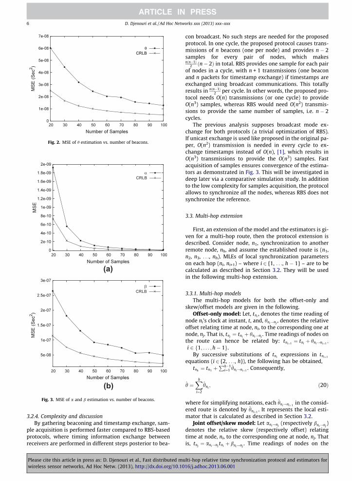
Fig. 2. MSE of h estimation vs. number of beacons.

(b)

(a)

Fig. 3. MSE of a and b estimation vs. number of beacons.


3.2.4. Complexity and discussionBy gathering beaconing and timestamp exchange, sam-

ple acquisition is performed faster compared to RBS-basedprotocols, where timing information exchange betweenreceivers are performed in different steps posterior to bea-


con broadcast. No such steps are needed for the proposedprotocol. In one cycle, the proposed protocol causes trans-missions of n beacons (one per node) and provides n � 2samples for every pair of nodes, which makesnðn�1Þ

2 ðn� 2Þ in total. RBS provides one sample for each pairof nodes in a cycle, with n + 1 transmissions (one beaconand n packets for timestamp exchange) if timestamps areexchanged using broadcast communications. This totallyresults in nðn�1Þ

2 per cycle. In other words, the proposed pro-tocol needs O(n) transmissions (or one cycle) to provideO(n3) samples, whereas RBS would need O(n2) transmis-sions to provide the same number of samples, i.e. n � 2cycles.

The previous analysis supposes broadcast mode ex-change for both protocols (a trivial optimization of RBS).If unicast exchange is used like proposed in the original pa-per, O(n2) transmission is needed in every cycle to ex-change timestamps instead of O(n), [1], which results inO(n3) transmissions to provide the O(n3) samples. Fastacquisition of samples ensures convergence of the estima-tors as demonstrated in Fig. 3. This will be investigated indeep later via a comparative simulation study. In additionto the low complexity for samples acquisition, the protocolallows to synchronize all the nodes, whereas RBS does notsynchronize the reference.

3.3. Multi-hop extension

First, an extension of the model and the estimators is gi-ven for a multi-hop route, then the protocol extension isdescribed. Consider node, n1, synchronization to anotherremote node, nh, and assume the established route is (n1,n2, n3, . . ., nh). MLEs of local synchronization parameterson each hop (ni, ni+1) – where i 2 {1, . . ., h � 1} – are to becalculated as described in Section 3.2. They will be usedin the following multi-hop extension.

3.3.1. Multi-hop modelsThe multi-hop models for both the offset-only and

skew/offset models are given in the following.Offset-only model: Let, tni

, denotes the time reading ofnode ni’s clock at instant, t, and, hni!nj

, denotes the relativeoffset relating time at node, ni, to the corresponding one atnode, nj. That is, tnj

¼ tniþ hni!nj

. Time readings of nodes onthe route can hence be related by: tniþ1 ¼ tni

þ hni!niþ1 ;

i 2 f1; . . . ;h� 1g.By successive substitutions of tni

expressions in tniþ1

equations (i 2 {2, . . ., h}), the following has be obtained,tnh¼ tn1 þ

Ph�1i¼1 hni!niþ1 . Consequently,

h ¼Xh

i¼2

hni; ð20Þ

where for simplifying notations, each hni!niþ1in the consid-

ered route is denoted by hniþ1. It represents the local esti-

mator that is calculated as described in Section 3.2.Joint offset/skew model: Let ani!nj

(respectively bni!nj)

denotes the relative skew (respectively offset) relatingtime at node, ni, to the corresponding one at node, nj. Thatis, tnj

¼ ani!njtniþ bni!nj

. Time readings of nodes on the



9

8

72 1

3

5

4

6

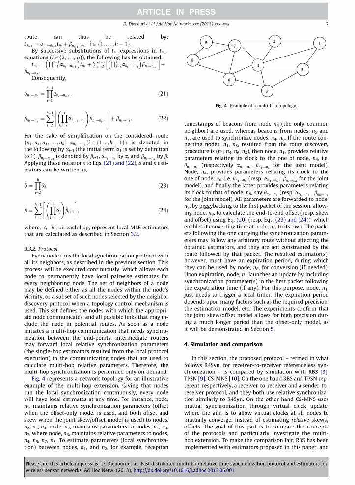
Fig. 4. Example of a multi-hop topology.


route can thus be related by:tniþ1 ¼ ani!niþ1 tni

þ bniþ1!ni; i 2 f1; . . . ;h� 1g.

By successive substitutions of tniexpressions in tniþ1

equations (i 2 {2, . . ., h}), the following has be obtained,tnh¼

Qh�1i¼1 ani!niþ1

� �tnhþPh�1

i¼2

Qij¼2anj�1!nj

� �bni!niþ1

h iþ

bn1!n2.

Consequently,

an1!nh¼Yh�1

i¼1

ani!niþ1; ð21Þ

bn1!nh¼Xh�1

i¼2

Yi

j¼2

anj�1!nj

!bni!niþ1

" #þ bn1!n2

: ð22Þ

For the sake of simplification on the considered routefn1;n2;n3; . . . ;nhg;ani!niþ1

ði 2 f1; ::;h� 1gÞ is denoted inthe following by ai+1 (the initial term a1 is set by definitionto 1), bni!niþ1

is denoted by bi+1, an1!nhby a, and bn1!nh

by b.Applying these notations to Eqs. (21) and (22), a and b esti-mators can be written as,

a ¼Yh

i¼2

ai; ð23Þ

b ¼Xh�1

i¼1

Yi

j¼1

aj

!biþ1

" #; ð24Þ

where, ai; bi, on each hop, represent local MLE estimatorsthat are calculated as described in Section 3.2.

3.3.2. ProtocolEvery node runs the local synchronization protocol with

all its neighbors, as described in the previous section. Thisprocess will be executed continuously, which allows eachnode to permanently have local pairwise estimates forevery neighboring node. The set of neighbors of a nodemay be defined either as all the nodes within the node’svicinity, or a subset of such nodes selected by the neighbordiscovery protocol when a topology control mechanism isused. This set defines the nodes with which the appropri-ate node communicates, and all possible links that may in-clude the node in potential routes. As soon as a nodeinitiates a multi-hop communication that needs synchro-nization between the end-points, intermediate routersmay forward local relative synchronization parameters(the single-hop estimators resulted from the local protocolexecution) to the communicating nodes that are used tocalculate multi-hop relative parameters. Therefore, themulti-hop synchronization is performed only on-demand.

Fig. 4 represents a network topology for an illustrativeexample of the multi-hop extension. Giving that nodesrun the local synchronization continuously, every nodewill have local estimates at any time. For instance, node,n1, maintains relative synchronization parameters (offsetwhen the offset-only model is used, and both offset andskew when the joint skew/offset model is used) to nodes,n2, n3, n4, node, n2, maintains parameters to nodes, n1, n4,n7, where node, n6, maintains relative parameters to nodes,n4, n5, n7, n8. To estimate parameters (local synchroniza-tion) between nodes, n1, and n2, for example, reception


timestamps of beacons from node n4 (the only commonneighbor) are used, whereas beacons from nodes, n5 andn7, are used to synchronize nodes, n4, n6. If the route con-necting nodes, n1, n8, resulted from the route discoveryprocedure is (n1, n4, n6, n8), then node, n1, provides relativeparameters relating its clock to the one of node, n4, i.e.hn1!n4 (respectively an1!n4 ; bn1!n4

for the joint model).Node, n4, provides parameters relating its clock to theone of node, n6, i.e. hn4!n6 (resp. an4!n6 ; bn4!n6

for the jointmodel), and finally the latter provides parameters relatingits clock to that of node, n8, say hn6!n8 (resp. an6!n8 ; bn6!n8

for the joint model). All parameters are forwarded to node,n8, by piggybacking to the first packet of the session, allow-ing node, n8, to calculate the end-to-end offset (resp. skewand offset) using Eq. (20) (resp. Eqs. (23) and (24)), whichenables it converting time at node, n1, to its own. The pack-ets following the one carrying the synchronization param-eters may follow any arbitrary route without affecting theobtained estimators, and they are not constrained by theroute followed by that packet. The resulted estimator(s),however, must have an expiration period, during whichthey can be used by node, n8, for conversion (if needed).Upon expiration, node, n1 launches an update by includingsynchronization parameter(s) in the first packet followingthe expatriation time (if any). For this purpose, node, n1,just needs to trigger a local timer. The expiration perioddepends upon many factors such as the required precision,the estimation model, etc. The experiments confirm thatthe joint skew/offset model allows for high precision dur-ing a much longer period than the offset-only model, asit will be demonstrated in Section 5.

4. Simulation and comparison

In this section, the proposed protocol – termed in whatfollows R4Syn, for receiver-to-receiver referenceless syn-chronization – is compared by simulation with RBS [3],TPSN [9], CS-MNS [10]. On the one hand RBS and TPSN rep-resent, respectively, a receiver-to-receiver and a sender-to-receiver protocol, and they both use relative synchroniza-tion similarly to R4Syn. On the other hand CS-MNS usesmutual synchronization through virtual clock update,where the aim is to allow virtual clocks at all nodes tomutually converge, instead of estimating relative skews/offsets. The goal of this part is to compare the conceptsof the protocols and particularly investigate the multi-hop extension. To make the comparison fair, RBS has beenimplemented with estimators proposed in this paper, and



5e-006

1e-005

1.5e-005

2e-005

2.5e-005

3e-005

3.5e-005

4e-005

4.5e-005

5e-005

100 200 300 400 500 1000 2000 3000 4000

Sync

hron

izat

ion

Erro

r (se

c)

Time (sec)

(1)(2)

(3)

(4)

R4Syn:(1)RBS:(2)

TPSN:(3)CS-MNS:(4)

Fig. 6. Precision vs. time.

0

50

100

150

200

250

300

3 4 5 6 7 8 9

Num

ber o

f Sam

ples

Number of Nodes

R4SynRBS

TPSNCS-MNS

Fig. 5. Number of samples vs. number of nodes.


TPSN with the estimators proposed in [11] that use thejoint skew/offset model and are appropriate to sender-to-receiver protocols. CS-MNS as described in the original pa-per considers skew update in its model, through the calledcorrection factor that is mutually updated.

First, the protocols are compared in single-hop environ-ment, where all the nodes are within the vicinity of eachother. Neighborhood has been statically fixed at everynode without any topology control. The number of nodeshas been varied to measure the performance metrics. Forsimplification, the propagation model has been simulatedwith no packet loss. Each point of the following plots isthe average of 200 measurements, where in each run thedelays (jitters) have been randomly set to values in theinterval ]0 ms, 10 ms], which represents a typical rangeof values for delays in WSN when timestamping at a higherlayer. The clock skews have been picked up from the inter-val [1:001; 1:002] for each node. The high layer timestam-ping has been simulated to investigate the impact of fastsample acquisition. Note that no significant difference withrespect to the precision would be noted between the pro-tocols when timestamping at the MAC layer, notably forthe offset-only model, where the sample size will haveno significant impact. The results presented in the follow-ing have been obtained with 99% confidence interval.3

Fig. 5 shows the obtained number of samples, in one cycle,vs. the number of nodes. The cycle has been fixed to 10 sfor all protocols. It is clear that the proposed protocol ac-quires more samples as the number of nodes rises, and thatits growth is much more important than the other protocols.This confirms the analysis of Section 3.2.4 reporting thatR4syn enables in one cycle to acquire (n � 2) samples forevery pair of nodes, which makes O(n3) in total. Like RBS,TPSN allows to get a single sample for every pair of nodes,which makes O(n2) in total. CS-MNS allows to get samplesin a faster rate compared to RBS and TPSN, as every beacontransmitted by a node will carry one timestamp that can beused by all its neighborhood for updating the correction fac-tor [10]. This results in n ⁄ (n � 1) samples in a cycle, whichis twice compared to RBS and TPSN, but the difference withR4syn is more important where the number of samples isproportional to the number of pairs of nodes for everybeacon.

The impact of the fast sample acquisition on the syn-chronization precision is investigated in the following.Fig. 6 represents the absolute synchronization error vs.time. The real skew and offsets are randomly selected forall nodes, and synchronization error between two ran-domly selected nodes has been measured after nodes esti-mate relative skew/offset by running the appropriateprotocol, or after updating virtual time in case of CS-MNS. Note that the same values are selected for all the pro-tocols. Two different scales have been used for the x axis;The smaller scale on the left side (from 0 to 500 s) clarifiesthe difference between RBS and R4syn, whereas the re-laxed scale on the remaining period permits to investigatethe convergence of the protocols’ precision on a long peri-

3 Note that the error bars could not be made visible in all plots, as theyare at a tiny scale compared to the y-axis scale.


od. All the protocols converge towards almost the sameprecision, about 5 ls, with a slightly larger value for CS-MNS (about 7 ls). However, there is a clear difference forthe convergence time. R4syn converges in less than 200 s,where CS-MNS needs about 500 ls (more than twice high-er than R4syn), and RBS needs about 2000 s (10 times high-er than R4syn). TPSN needs the largest period, more than4000 s (more than 20 times higher than R4syn). It has beennoted that after 4500 s, all the protocols stabilize around5 ls (or around 7 ls for CS-MNC), and no significant vari-ance would be shown. The fast convergence of the pro-posed protocol is basically due to the fast acquisition ofsamples, as explained previously. The minor additional er-ror for CS-MNS can be argued by the fact that it does notconsider the delay jitter and its distribution in the model,contrary to the other protocols.

To measure the precision in multi-hop environmentand investigate the proposed multi-hop extension, the net-work presented in Fig. 7 has been simulated. It consists of33 nodes ranged in a greed-like-topology, with a 10-hopdiameter. The simulation started by a warm-up step thatconsists in running local synchronization in every neigh-borhood for a long period. This is to assure local parameterestimators convergence for all the protocols. The



5e-00

6 5.2e

-006 5.

4e-00

6 5.6e

-006 5.

8e-00

6 6e-00

6 6.2e

-006 6.

4e-00

6 6.6e

-006 6.

8e-00

6 7e-00

6

1 2 3 4 5 6 7 8 9 10

Sync

hron

izat

ion

Erro

r (se

c)

Hop number

1e-00

5 1.

5e-00

5 2e-00

5 2.

5e-00

5 3e-00

5 3.

5e-00

5 4e-00

5R4Syn

RBSTPSN

CS-MNS

Fig. 8. Precision in multi-hop environment.

Fig. 9. Preliminary experiment setup.

0 1 2 3 4 5 6 7 8 9 10

Fig. 7. Multi-hop simulation topology.


synchronization error has been then measured betweennode n0, and nodes n1, n2, . . ., n10, respectively, which rep-resents a series from one to ten hops. The results shown inFig. 8 clearly demonstrate that the proposed protocol out-performs the other ones. R4Syn synchronization error did


not exceed 5.6 ls, even for 10 hops synchronization. RBSalso provides good precision, and its error is below 7 lsfor 10 hops. However, the gap between the previous proto-cols and the sender-to-receiver ones (TPSN and CS-MNS) isimportant. The error of the TPSN exceeds 10 ls upon 3




hops, and it reaches 20 ls for 10 hops, while that of CS-MNS is even higher and it exceeds 30 ls for 10 hops. Notethe use of two different scales for the y axis; the use of thehigher scale would not show any difference/variance be-tween/for RBS and R4Syn, where the other scale wouldnot allow to plot TPSN and CS-MNS that have relativelymuch higher values. This difference is basically due tothe use of completely different paradigms. The receiver-to-receive extends better to multi-hop environment,where the error precision considerably amplifies in mul-ti-hop environment with the sender-to-receiver synchro-nization. Further, the mutual clock update of CS-MNSdemonstrates the worst performance in the multi-hop sce-nario. The results also show clear improvement of R4synover RBS in multi-hop environment, as the gap rises withthe increase of hop number. Finally, note that the protocolsdo not use multi-hop signaling, so it is insignificant to mea-sure the other metrics in multi-hop environment.

5. Implementation on sensor motes and tests

To investigate its accuracy and effectiveness and con-firm the simulation results, the proposed solution has beenimplemented on real senor motes. MICAz mote4 has beenused, along with TinyOS as the underlying operating system[12]. The used mote has an IEEE 802.15.4 radio (CC2420),which is a ZigBee compliant RF transceiver that operates inthe Industrial Scientific and Medical (ISM) band, at 2.4 to2.4834 GHz. MICAz has low power consumption and usestwo AA batteries. Its micro-controller is an 8-bit, 8 MHz AT-mega128L, with a 4 KB RAM and 128 KB of external flashmemory. The mote integrates two clocks: (i) an internalclock with a high granularity, but also with a drift at the or-der of few tens PPM (up to 100PPM) [13], and (ii) a more sta-ble external crystal clock but with 32kHz frequency, i.e.enabling a tick (granularity) of about 32 ls. Although beingmore stable, the later does not allow for a microsecond levelprecision. Given that the aim is to confirm the high precisionof the proposed solution, the former clock has been used inthe experiment. It is straight forward to use the currentimplementation with the other clock, if a lower precisionsatisfies the application requirements (e.g., a precision atthe order of milliseconds or tens of microseconds). An Ardu-ino has been used for measuring the synchronization error.This microcontroller is an 8-bit, 16 MHz ATmega328P, with2 KB RAM, and 32 KB flash memory.5

The major problem we faced was the implementation ofthe estimators proposed in Eqs. (10) and (11). Theses for-mulas include multiplications of very large numbers (clockvalues), which causes memory overflow after few secondsdue to sensors’ limitation on memory and arithmetic unit,together with TinyOS that does not support float numbersbeyond 64 bits. This prevents getting large samples, andthus achieving microsecond level precision would not bepossible. To tackle this, the formulas have been rewritten.It can be noticed that both the numerator and denominatorof Eq. (10) are the difference of two large terms, but the

4 http://www.memsic.com/userfiles/files/DataSheets/WSN/micaz_data-sheet-t.pdf.

5 http://arduino.cc/en/Main/ArduinoBoardUno.


final differences are small numbers that do not cause anycomputation problem for division. The problem is causedby the calculation of the large intermediate terms. Forthe numerator, the first term can be seen as the sum ofproducts (uivj), consisting of k2 elementary terms overall,and the second is the sum of products ujvj that repeats Ktimes, resulting in k2 elementary terms as well. Therefore,instead of calculating the two large terms separately thensubtracting them, it is more practical to subtracting fromeach elementary term of the first term, uivj, an elementaryterm of the second one, ujvj. The same principle is appliedto the denominator, which yields the following expression,

amle ¼PK

i¼1

PKj¼1ðuiv j � ujv jÞPK

i¼1

PKj¼1 v iv j � v2

j

� � : ð25Þ

The difference of large products are then transformed intothe sum of differences of small products, which does notcause any problem for the implementation. b estimator isthen calculated by replacing the resulted estimator of ain Eq. (11).

5.1. Preliminary experiment

In the first preliminary tests, three nodes running theprotocol have been used, two of them have been pluggedto an Arduino through available pins for precision mea-surement (Fig. 9). The size of the binary code of this threenodes implementation was (for every node) 17,600 bytesin ROM and 984 bytes in RAM for the offset-only model,28,470 bytes in ROM and 1434 bytes in RAM for theskew/offset model. This includes code for protocol signal-ing, estimator calculations, the operating system kerneland libraries, and control operations for measurement, alluploaded as a single file.

The Arduino has been programmed to transmit a signalto both motes at regular intervals. This is after few secondsof warm-up phase, allowing estimators to converge at bothnodes. The interrupt handler for the appropriate pin oneach node has been programmed as follows. The first motepicks its clock up, and the second one picks its clock up andconverts the obtained value to the other’s clock (estimatethe other node’s clock at the same moments the latterpicks it up). This conversion is performed using the estima-tors resulted from the execution of the protocol. Everynode then writes the obtained value into a laptop throughthe serial connection to construct a log file.

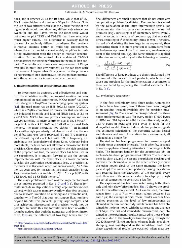
The experiment has been conducted using both offset-only and joint skew/offset models. Fig. 10 shows the preci-sion for the offset-only model. As it can be seen, the errorranges from 1 ls to 7 ls, with most values between 3 lsand 5 ls; the average is 3.50. These results confirm fine-grained precision at the level of few microseconds asclaimed in the simulation study. Similar result has been ob-tained for the joint model, with the same range and averageof 3.24 ls. The fast and immediate microsecond level ob-tained in the experiment results, compared to those of sim-ulation, is due to the low-layer timestamping through theCC2420ReceiveP TinyOS module, whereas high layer time-stamping was investigated in the simulation. Note thatthese experimental results are obtained when measure-


http://www.memsic.com/userfiles/files/DataSheets/WSN/micaz_datasheet-t.pdf

http://www.memsic.com/userfiles/files/DataSheets/WSN/micaz_datasheet-t.pdf

http://arduino.cc/en/Main/ArduinoBoardUno


Mote 1

Mote 7

communication topology :

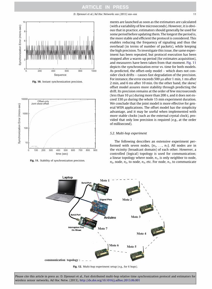
Fig. 12. Multi-hop experiment

10

100

1000

10000

0 100 200 300 400 500 600 700 800 900

Sync

hron

izat

ion

Erro

r (m

icro

-sec

)

time (sec)

Offset-onlyJoint skew-offset

Fig. 11. Stability of synchronization precision.

0

2

4

6

8

10

0 200 400 600 800 1000

Sync

hron

izat

ion

Erro

r (m

icro

-sec

)

Sequence

Fig. 10. Instant synchronization precision.



ments are launched as soon as the estimators are calculated(with a variability of few microseconds). However, it is obvi-ous that in practice, estimators should generally be used forsome period before updating them. The longest the period is,the more stable and efficient the protocol is considered. Thisenables reducing the frequency of signaling and thus theoverhead (in terms of number of packets), while keepingthe high precision. To investigate this issue, the same exper-iment has been repeated, but protocol execution has beenstopped after a warm-up period (for estimates acquisition),and measurers have been taken from that moment. Fig. 11depicts the synchronization error vs. time for both models.As predicted, the offset-only model – which does not con-sider clock drifts – causes fast degradation of the precision.For instance, the error exceeds 500 ls after 1 min, 1 ms after2 min, and 6 ms after 10 min. On the other hand, the skew/offset model assures more stability through predicting thedrift. Its precision remains at the order of few microseconds(less than 10 ls) during more than 200 s, and it does not ex-ceed 330 ls during the whole 15 min experiment duration.We conclude that the joint model is more effective for gen-eral WSN applications. The offset model has the simplicityadvantage, and it may be useful when implemented withmore stable clocks (such as the external crystal clock), pro-vided that only low precision is required (e.g., at the orderof millisecond).

5.2. Multi-hop experiment

The following describes an extensive experiment per-formed with seven nodes, {n1, . . ., n7}. All nodes are inthe vicinity (broadcast domain) of each other. However, acontrolled (logical) topology is used for communication;a linear topology where node, n1, is only neighbor to node,n2, node, n2, to node, n3, etc. For node, n1, to communicate

Mote 6 Mote 5

Mote 4

Mote 3

Mote 2

setup (e.g., for 6 hops).



0

2

4

6

8

10

0 100 200 300 400 500 600 700 800 900 1000

Sync

hron

izat

ion

Erro

r (m

icro

-sec

)

Sequence

Fig. 13. Synchronization error in seven nodes scenario, one hop.

0

5

10

15

20

0 100 200 300 400 500 600 700 800 900 1000

Sync

hron

izat

ion

Erro

r (m

icro

-sec

)

Sequence

Fig. 15. Synchronization error in seven nodes scenario, three hops.

0

5

10

15

20

0 100 200 300 400 500 600 700 800 900 1000

Sync

hron

izat

ion

Erro

r (m

icro

-sec

)

Sequence

Fig. 16. Synchronization error in seven nodes scenario, four hops.

0

2

4

6

8

10

12

14

0 200 400 600 800 1000

Sync

hron

izat

ion

Erro

r (m

icro

-sec

)

Sequence

Fig. 14. Synchronization error in seven nodes scenario, two hops.


with node, n4, for instance, it must use the unique route(n1, n2, n3, n4), instead of direct communication. Therefore,full-power is used to exchange beacons between all nodes,but the predefined topology is used for data communica-tion. This is to enforce multi-hop communications. Syn-chronization follows the same route followed by the firstpacket, as described previously. In other words, local syn-chronization is executed between the seven nodes, butnodes are programmed to use multi-hop synchronizationfor time conversion. For example, node, n1, uses parame-ters of nodes, n2, n3, to estimate relative skew/offset tonode, n4, instead of using local (direct) estimation. Thisis, obviously, for the purpose of evaluating the multi-hopprotocol/estimators.

Synchronization between node, n1, and nodes, n2, n3, . . .,n7, respectively for, 1-hop, 2-hop, . . ., 6-hop are investi-gated. Similar setting as presented in Fig. 9 is used, wherethe two synchronizing nodes are plugged to Arduino (noden1, and node, ni, i 2 {2, . . ., 7}, respectively). Fig. 12 illus-trates the setting for 6-hop synchronization measurement,i.e. between nodes, n1, and, n7. The memory footprint ofthis seven-node implementation was 17,600 bytes inROM and 1046 bytes in RAM for the offset-only model,28,470 bytes in ROM and 1945 bytes in RAM for theskew/offset model. Fig. 13, through Fig. 18 represent re-sults from 1-hop to 6-hop, respectively, and Table 1 sum-marizes the results.

Fig. 13 confirms the results obtained with the three-node experiment, as the same precision order has been ob-tained, although the number of nodes has doubled. Thesynchronization error was between 1 ls and 6 ls with2.45 ls on average. Similar results are obtained for theskew/offset model – which are not presented to avoid a

Table 1Error precision in ls.

1-hop

2-hop

3-hop

4-hop

5-hop

6-hop

Average 2.45 3.65 3.74 12.58 14.84 19.93Worst case 6 12 16 19 29 39Best case 1 0 0 8 3 2Below average

(%)60.3 50.8 54.3 57.9 63.2 51.3


redundant and overwhelming presentation – and the syn-chronization error was between 0 ls and 5 ls, with 2.59 lson average. Fig. 14–18 illustrate the behavior of the pro-posed multi-hop synchronization. They demonstrate thatthe increase in both synchronization error with the num-ber of hops is smooth, and such is the flip of this error.The average value ranges from 3.65 ls for two hops to19.93 ls for six hops. The highest value has been below40 ls. Further, most of the values are below the average



0

5

10

15

20

25

30

0 100 200 300 400 500 600 700 800 900 1000

Sync

hron

izat

ion

Erro

r (m

icro

-sec

)

Sequence

Fig. 17. Synchronization error in seven nodes scenario, five hops.

0

5

10

15

20

25

30

35

40

0 100 200 300 400 500 600 700 800 900 1000

Sync

hron

izat

ion

Erro

r (m

icro

-sec

)

Sequence

Fig. 18. Synchronization error in seven nodes scenario, six hops.


value, i.e., more than 50% of values are below the averagevalue for all numbers hops. We should point out here thedifference in values obtained in comparison with the sim-ulation results. Although both simulation and testbedexperiment demonstrated precision at the microsecond le-vel, real experiment results are higher. This is because idealmodels have been used in the simulation (propagationwith no packet loss, similar delays in all links, etc.), wherethe experimentation with real motes reflects results inmore realistic conditions.

6. Related work

Sivrikaya and Yener [2] published a good introductivesurvey on time synchronization in wireless sensor net-works (WSN), while Sundararaman et al. [1] provide moretaxonomy and descriptions. Many solutions have been pro-posed after the publication of these two papers. Simeoneet al. [14] and Lenzen et al. review some recent solutions,while Wu et al. [15] present an interesting analysis of theestimation methods used for time synchronization. Still,an up to date comprehensive review on time synchroniza-tion protocols in wireless sensor networks is missing, giventhe massive work in recent years.

Most of the protocols proposed thus far use sender-to-receiver synchronization, where the synchronizing nodes


exchange messages and use sending and receiving eventsto record timestamps. Some solutions allow nodes to runtheir clocks independently and define mechanisms to cal-culate (estimate) relative skews and/or offsets, i.e. relativesynchronization. Noh et al. [11] consider local (one-hop)relative synchronization and provide general offset/skewMLE estimators for sender/receiver protocols, where onlythe first and last observations of timing message ex-changes are used. The approach was generalized in [16].A similar mathematical approach is used in this paper,but the model, and consequently all the derived estimatorsand bounds, are completely different. The model of [11]does not apply to the proposed solution, as the latter is re-ceiver-to-receiver-based. RAT [17] is another local sender/receiver synchronization protocol. It has been integratedwith B-MAC to incrementally improve its performance.Since the authors’ aim was to reduce the preamble periodat the MAC layer, the protocol provides a weak synchroni-zation, where linear regression was used to calculate rela-tive skews/offsets. The Elapsed Time on Arrival (ETA) isanother relative synchronization based algorithm [18].This has been used in two implementations; The RoutingIntegrated Time Synchronization (RITS), which is a reactivetime synchronization protocol that can serve in correlatingmultiple event detections at one or more locations, and theRapid Time Synchronization (RATS) as a proactive protocolthat utilizes RITS to achieve network-wide synchroniza-tion. Useful API is also provided for application use.

Another category of solutions consists in defining dis-tributed mechanisms that allow nodes to update theirclocks and converge to common values, i.e. continuouslyperforming clock updates. This is conceptually differentfrom relative synchronization (relative offset/skew estima-tion). In [19,4,20] the authors propose solutions that dealboth with single and multi-hop synchronization. Thesesolutions have the gradient property and focus on localsynchronization, where high precision is provided forneighboring nodes (their clock values converge closely),but the precision decreases with the distance. The solutionproposed in this paper uses this property in the sense thatmore importance is given to local synchronization that isperformed continually, but the performance evaluation re-sults for multi-hop synchronization reflect high precision.Solutions based on distributed consensus techniques arevery similar to gradient ones. AverageTimeSynch [21] andDCTS [22] protocols are examples of such solutions. The la-ter has been analyzed in [23] for a Gaussian-delay environ-ment. Sadler [24] considers the uses of an externalaccurate clock whose values may be occasionally observedthrough broadcast signal reception (such as GPS receivers).He provides estimators to synchronize the sensor mote’sclock to such an accurate clock. A common feature of allthese solutions is that nodes continuously update theirclocks with respect to each other. This update generally in-volves jump/freeze of the clock value, which may affectcorrectness of local events’ timestamping.

Contrary to gradient solutions, other ones focus on glo-bal synchronization and attempt to improve the multi-hopprecision. [25] proposes a global synchronization protocolbased on spanning tree. [26] provides probabilistic lowerbounds for multi-hop synchronization. Secondis [13]




defines strategies to disseminate synchronization mes-sages from the root to the whole network. CS-MNS by Ren-tel et al. [10] define a mutual synchronization multi-hopsolution that applies to both MANET (mobile ad hoc net-works) and WSN. Time update of virtual clocks is used,where a correction factor of the skew is mutually updatedupon beacon exchange using the sender-to-receiver para-digm. The protocol has been implemented on TelosB/MI-CAz motes [27], where the external low resolution clockhave been used permitting only a weak resolution (32 ls/tick). The protocol proposed in [28] deals with multi-hopsynchronization by clustering the networks. The protocolstarts by synchronizing cluster-heads to the base station,then cluster-heads synchronize regular nodes. In [29], acentralized approach to estimate clock relative offset isproposed, where topology constraints are considered. Thebasic idea is that in a cycle, the sum of all relative offsetsmust be null. The authors formulated the problem withgraph theory and the mean square method, as a con-strained optimization problem. FTSP [5], TPSN [9], solu-tions of [30–32] are other examples of other multi-hop-centric synchronization protocols.

As described previously, RBS [3] uses a completely dif-ferent approach, namely the receiver-to-receiver synchro-nization, which has the advantage of reducing the time-critical path [1, p. 294]. However, the major drawback ofRBS is the need of a fixed reference, which might be inap-propriate for some self-organized wireless sensor network(WSN) applications. The work in [7] is the only one thatconsiders joint skew/offset maximum likelihood estima-tion (MLE) for RBS. The model used herein is different fromthe one of Sari et al. In the latter, synchronization is pro-portional to a single reference, while there is no such acommon reference with the proposed solution’s model.Further, [7] considers exponentially distributed delays,while the proposed one considers Gaussian distributed de-lays. Exponential model is more appropriate when delaysinclude queueing time, which is typical when the sendingdelay is affecting the time critical path. However, it hasbeen realized that the reception delays tend to followGaussian distributions [3]. Therefore, Gaussian distributionis more suitable for receiver-to-receiver protocols. Moreimportantly, the model of [7] does not synchronize receiv-ers directly but through synchronization to the referenceclock, which completely deviates from the RBS concept.Note that the concept of a reference in RBS is to use a com-mon source for signal broadcast, but not a common sourceof time. Although relative parameters can be determinedby synchronizing the receivers to the reference, this wayof synchronization causes cumulative errors on the estima-tors. Moreover, eliminating the sender uncertainty fromthe critical path is at the core of RBS, while this uncertaintyis not eliminated by relating the transmitter’s (reference’s)time to the receiver’s time in the model.6 The model in thispaper is different, it allows to directly estimating relativeparameters without using or referring to the reference clock.This faithfully reflects the RBS concept.

6 Refer to Eqs. (1) and (2) in [7, p. 1], vx;kx ; vy;ky would be the noise(variable delay) due to both transmission and reception. This addstransmission delays to the time critical path.


The authors in [33] apply artificial intelligence (AI)techniques to an RBS-like solution. The applicability ofsuch AI method to resource constrained sensors is ques-tionable. PBS [34] is a hybrid solution between sender-to-receiver and receiver-to-receiver approaches, whichuses overhearing of the sender/receiver message exchange.The basic sender-to-receiver approach is used to synchro-nize two super nodes, while all the other nodes withinthe range of both nodes overhear messages and synchro-nize to the super nodes. The solution reduces the over-heard of RBS, but it is also centralized. In [35], theauthors tried to make the solution more distributed byproposing round-robin timing exchange protocol (RRTE),where one reference is fixed and the other changes in around robin way. Still, one fixed reference is needed. Somesolutions are applications-driven and attempt to couplesynchronization with application services. For instance,Glossy [36] exploits IEEE 802.15.4 interferences, to couplesynchronization with network flooding. In [37], a solutionthat couples localization to synchronization is proposed.Liu et al. [38] consider synchronization for mobile under-water networks, where the precision is at the order of hun-dreds of ms and even the s level due to the high latency ofthe acoustic communications. Some other hardware solu-tions propose synchronization techniques to be imple-mented at the physical layer such as [39]. This mayprovide high precision but would require additional hard-ware modules at the sensor motes. The solution proposedin this paper does not need any such modules, and it issimply implementable at the software level.

7. Conclusion

Time synchronization has always been a challengingproblem in distributed systems. This problem is more com-plex in wireless networks, where communication may beprone to high delay variability. In wireless sensor networks(WSN), node limitations (computation, memory, energy)add more constraints to the problem. The problem hasbeen dealt with in this work, and a new distributed refer-enceless protocol has been proposed for single-hop syn-chronization, and then extended to multi-hopsynchronization. The proposed protocol is receiver-to-re-ceiver based, but it is fully distributed and does not relyon any fixed reference. The role of the reference is distrib-uted amongst all nodes, while timestamps are piggybackedto synchronization signals (beacons). This enables to per-form beaconing and timestamp exchange in a single step,and it provides fast acquisition of timestamps that are usedas samples to estimate relative synchronization parame-ters. The proposed relative synchronization protocol hasbeen extended to multi-hop environment, where local syn-chronization is performed proactively, and the resultedparameters are transferred to the intermediate/end-pointnodes as soon as a multi-hop communication that needssynchronization is initiated. The multi-hop extension ison-demand, as no signals are periodically transferred onmulti-hop links.

The maximum likelihood estimators (MLE) and the Cra-mer-Rao lower bounds (CRLB) has been proposed for both




the offset-only and the joint offset/skew estimation. Con-trary to existing MLE models for receiver-to-receiver syn-chronization, the model used in this paper directlyrelates the synchronization parameters of the receiverswithout using the sender’s clock, which accurately reflectsthe receiver-to-receiver principle. The proposed estimatorshave been numerically analyzed and compared to theCRLB, as the theoretical optimum. Results show conver-gence of the proposed estimators’ precision to their respec-tive CRLB with the increase of the number of signals. Theprotocol has been compared by simulation to some state-of-the-art sender-to-receiver (TPSN, CS-MNS), and recei-ver-to-receiver (RBS) protocols. Results show much fasterconvergence of the proposed protocol, in the order of morethan twice compared to CS-MNS, more than ten timescompared to RBS, and more than twenty times comparedto TPSN. Obtained results also show that the proposed pro-tocol outperforms all the protocols in with respect to thesynchronization precision, both in single-hop and multi-hop synchronization. In addition to the simulation evalua-tion, the proposed protocol has been implemented andtested on real sensor motes both in one-hop and multi-hop scenarios. The results were very satisfactory and con-firm microsecond precision of both offset-only and skew/offset models, and the synchronization error has not ex-ceeded 6 ls for 1-hop scenario and 39 ls for 6-hop sce-nario, in the worst cases. On average, it was between2.45 ls for 1-hop and 19.93 ls for 6-hop, and most valueswere always below the average value. The skew/offsetmodel – which captures clock drifts – demonstrated morestability, where the estimators have much longer lifetimeand remain effective in keeping the microsecond-level pre-cision for several minutes.

Acknowledgment

This work has been carried out at CERIST research cen-ter and supported by the Algerian Ministry of Higher Edu-cation and Scientific Research. The authors thank theanonymous referees for devoting their time to reviewingthe paper and their invaluable comments and suggestions,which significantly helped to improve the quality of themanuscript.

References

[1] B. Sundararaman, U. Buy, A.D. Kshemkalyani, Clock synchronizationfor wireless sensor networks: a survey, Ad Hoc Networks 3 (3)(2005) 281–323.

[2] F. Sivrikaya, B. Yener, Time synchronization in sensor networks: asurvey, IEEE Network Magazine 18 (4) (2004) 45–50.

[3] J. Elson, L. Girod, D. Estrin, Fine-grained network timesynchronization using reference broadcasts, in: 5th USENIXSymposium on Operating System Design and Implementation(OSDI’02), 2002.

[4] P. Sommer, R. Wattenhofer, Gradient clock synchronization inwireless sensor networks, in: Proceedings of the 8th ACMInternational Conference on Information Processing in SensorNetworks (IPSN’08), 2009, pp. 37–48.

[5] M. Maróti, B. Kusy, G. Simon, Á. Lédeczi, The flooding timesynchronization protocol, in: SenSys, 2004, pp. 39–49.

[6] M. Kohvakka, J. Suhonen, M. Kuorilehto, V. Kaseva, M. Hännikäinen,T.D. Hämäläinen, Energy-efficient neighbor discovery protocol formobile wireless sensor networks, Ad Hoc Networks 7 (1) (2009)24–41.


[7] I. Sari, E. Serpedin, K.-L. Noh, Q.M. Chaudhari, B.W. Suter, On the jointsynchronization of clock offset and skew in rbs-protocol, IEEETransactions on Communications 56 (5) (2008) 700–703.

[8] A. Papoulis, S.U. Pillai, Probability, Random Variables and StochasticProcesses, 4th ed., McGraw Hill Higher Education, 2002.

[9] S. Ganeriwal, R. Kumar, M.B. Srivastava, Timing-sync protocol forsensor networks, in: Proceedings of the 1st international conferenceon Embedded networked sensor systems, SenSys ’03, 2003, pp. 138–149.

[10] C.H. Rentel, T. Kunz, A mutual network synchronization method forwireless ad hoc and sensor networks, IEEE Transactions on MobileComputing 7 (5) (2008) 633–646.

[11] K.-L. Noh, Q.M. Chaudhari, E. Serpedin, B.W. Suter, Novel clock phaseoffset and skew estimation using two-way timing messageexchanges for wireless sensor networks, IEEE Transactions onCommunications 55 (4) (2007) 766–777.

[12] P. Levis, D. Gay, TinyOs Programming, Cambridge University Press,2009.

[13] F. Ferrari, A. Meier, L. Thiele, Secondis: an adaptive disseminationprotocol for synchronizing wireless sensor networks, in: Proceedingsof the 7th IEEE Conference on Sensor Mesh and Ad HocCommunications and Networks (SECON’10), 2010, pp. 1–9.

[14] O. Simeone, U. Spagnolini, Y. Bar-Ness, S.H. Strogatz, Distributedsynchronization in wireless networks, IEEE Signal ProcessingMagazine 25 (5) (2008) 81–97.

[15] Y.-C. Wu, Q.M. Chaudhari, E. Serpedin, Clock synchronization ofwireless sensor networks, IEEE Signal Processing Magazine 28 (1)(2011) 124–138.

[16] M. Leng, Y.-C. Wu, On clock synchronization algorithms for wirelesssensor networks under unknown delay, IEEE Transactions onVehicular Technology 59 (1) (2010) 182–190.

[17] S. Ganeriwal, I. Tsigkogiannis, H. Shim, V. Tsiatsis, M.B. Srivastava, D.Ganesan, Estimating clock uncertainty for efficient duty-cycling insensor networks, IEEE/ACM Transactions on Networking 17 (2009)843–856.

[18] B. Kusy, P. Dutta, P. Levis, M. Maroti, A. Ledeczi, D. Culler, Elapsedtime on arrival: a simple and versatile primitive for canonical timesynchronisation services, International Journal of Ad Hoc andUbiquitous Computing 1 (4) (2009).

[19] R.M. Pussente, V.C. Barbosa, An algorithm for clock synchronizationwith the gradient property in sensor networks, Journal of ParallelDistributed Computing 69 (2009) 261–265.

[20] C. Lenzen, T. Locher, R. Wattenhofer, Tight bounds for clocksynchronization, Journal of the ACM 57 (2) (2010).

[21] L. Schenato, F. Fiorentin, Average timesynch: a consensus-basedprotocol for clock synchronization in wireless sensor networks,Automatica 47 (9) (2011) 1878–1886.

[22] A. Scaglione, R. Pagliari, Non-cooperative versus cooperativeapproaches for distributed network synchronization, in: IEEEPerCom Workshops Proceedings, 2007, pp. 537–541.

[23] G. Xiong, S. Kishore, Analysis of distributed consensus timesynchronization with gaussian delay over wireless sensornetworks, EURASIP Journal on Wireless Communications andNetworking (May) (2009).

[24] B.M. Sadler, Local and broadcast clock synchronization in a sensornode, IEEE Signal Processing Letters 13 (1) (2006) 9–12.

[25] L.-M. He, Time synchronization based on spanning tree for wirelesssensor networks, in: Proceedings of the 4th IEEE Conference onWireless Communications, Networking and MobileComputing(WiCOM’08), 2008, pp. 1–4.

[26] C. Lenzen, P. Sommer, R. Wattenhofer, Optimal clocksynchronization in networks, in: Proceedings of the 7th ACMInternational Conference on Embedded Networked Sensor Systems(SenSys’09), 2009, pp. 225–238.

[27] T. Kunz, E. McKnight-MacNeil, Implementing clock synchronizationin wsn: Cs-mns vs. ftsp, in: WiMob, 2011, pp. 157–164.

[28] L. Kong, Q. Wang, Y. Zhao, Time synchronization algorithm based oncluster for wsn, in: The 2nd IEEE International Conference onInformation Management and Engineering (ICIME), 2010, pp. 126–130.

[29] I. Shames, A.N. Bishop, Relative clock synchronization in wirelessnetworks, IEEE Communications Letters 14 (2010) 348–350.

[30] J. Koo, R.K. Panta, S. Bagchi, L.A. Montestruque, A tale of twosynchronizing clocks, in: Proceedings of the 7th ACM InternationalConference on Embedded Networked Sensor Systems (SenSys’09),2009, pp. 239–252.

[31] B. Wehbi, A. Laouiti, A.R. Cavalli, Efficient time synchronizationmechanism for wireless multi-hop networks, in: PIMRC, 2008,pp. 1–6.


http://refhub.elsevier.com/S1570-8705(13)00122-4/h0005




























































[32] A.-s. Hu, S.D. Servetto, Algorithmic aspects of the timesynchronization problem in large-scale sensor networks, MobileNetworks and Applications 10 (4) (2005) 491–503.

[33] L. Paladina, A. Biundo, M. Scarpa, A. Puliafito, Artificial intelligenceand synchronization in wireless sensor networks, Journal ofNetworks 4 (6) (2009) 382–391.

[34] K.-L. Noh, E. Serpedin, K.A. Qaraqe, A new approach for timesynchronization in wireless sensor networks: pairwise broadcastsynchronization, IEEE Transactions on Wireless Communications 7(9) (2008) 3318–3322.

[35] Y.-H. Huang, S.-H. Wu, Time synchronization protocol for small-scalewireless sensor networks, in: IEEE Wireless Communications andNetworking Conference (WCNC’10), 2010, pp. 1–5.

[36] F. Ferrari, M. Zimmerling, L. Thiele, O. Saukh, Efficient networkflooding and time synchronization with glossy, in: IPSN, 2011, pp.73–84.

[37] J. Zheng, Y.-C. Wu, Joint time synchronization and localization of anunknown node in wireless sensor networks, Transactions on SignalProcessing 58 (3) (2010) 1309–1320.

[38] J. Liu, Z. Zhou, Z. Peng, J.-H. Cui, M. Zuba, L. Fiondella, Mobi-sync:efficient time synchronization for mobile underwater sensornetworks, IEEE Transactions on Parallel and Distributed Systems24 (2) (2013) 406–416.

[39] T. Beluch, D. Dragomirescu, F. Perget, R. Plana, Cross-layeredsynchronization protocol for wireless sensor networks, in:Proceedings of the 2010 Ninth International Conference onNetworks (ICN’10), 2010, pp. 167–172.

Djamel Djenouri obtained the engineerdegree, the master degree, and the PhD incomputer science from the University of Sci-ence and Technology USTHB Algiers, Algeria,respectively in 2001, 2003 and 2007. Duringhis PhD he has been granted an internship atJohn Moors university in Liverpool, UK, wherehe carried out collaborative work withresearchers of the Distributed MultimediaSystems and security group. From 2008 to2009 he was granted a post-doctoral fellow-ship from the European Research Consortium

on Informatics and Mathematics (ERCIM), and he worked at the Norwe-gian university of Science and Technology (NTNU), in Trondheim, Nor-way, where he participated in the MELODY project supported by the
Norwegian Research Council. Currently, he is a permanent full-timesenior researcher at the CERIST research center in Algiers. He is workingon topics related to wireless and sensor networking, with focus on qualityof service, power management, routing protocols, MAC protocols, timesynchronization, fault tolerance, sensor and actuator networks, vehicularapplications, and the internet of things. He participated in many inter-national conferences. He published more than 50 papers in internationalpeer-reviewed journals and conference proceedings, and two books. He isa professional member of the ACM, and chaired workshops held in con-junction with DCOSS 2010/2011 and GlobCom 2010–2013. He also served

as TPC member of many international conferences, guest editor of aspecial issue with Int. J. Communication Networks and Distributed Sys-tems, and reviewer for many international Journals. In 2008, he wasgranted the best publication award from ANDRU, supported by theAlgerian government, and the CERIST best researcher awards in 2010.

Nassima Merabtine obtained the Master’sdegree from Blida university in 2012, awardedwith congratulations by the jury after suc-cessful implementation and tests of sensornetwork protocols on real motes using Tiny-OS. She served as a temporary assistant lec-turer at the computer science department ofBlida University during 2012. Currently, she isworking towards her PhD in Computer Sci-ence at ESI, Algiers, where she is working onPBST based routing.

Fatma Zohra Mekahlia obtained the Master’sdegree from Blida university in 2012, awardedwith congratulations by the jury, after suc-cessful implementation and tests of sensornetwork protocols on real motes using Tiny-OS. She served as a temporary assistant lec-turer at the computer science department ofBlida University during 2012. Currently, she isworking towards her PhD in Computer Sci-ence at Oran University. Her PhD project isrelated to Formalization, Analysis, and Controlof Temporal and Spatial Coherence of SMILDocuments’.

Messaoud Doudou obtained his EngineerDegree in computing science from NationalInstitute of Computer science (INI-Algiers) in2005. He obtained his Masters degree fromthe University of Science and TechnologyUSTHB Algiers in 2008, where he worked onwireless mesh networks and MAC protocols.Currently, he is a PhD student at the USTHBUniversity. He is also a permanent Full-timeResearcher at the Center of Research on Sci-entific and Technical Information (CERIST) inAlgiers, where he is a research member of

SensLab research group. His research interest includes medium accesscontrol, wireless sensor networks, and QoS in wireless networks.




















On eliminating packet droppers in MANET: A modular solution

Documents

Transcript of On eliminating packet droppers in MANET: A modular solution