Coastal Engineering 60 (2012) 299–318

Contents lists available at SciVerse ScienceDirect

Coastal Engineering

j ourna l homepage: www.e lsev ie r .com/ locate /coasta leng

On berm breakwaters: Recession, crown wall wave forces, reliability

Alf Tørum ⁎, Mohammad Navid Moghim 1, Kenneth Westeng 2, Nurin Hidayati 3, Øivind ArntsenNorwegian University of Science and Technology, Department of Civil and Transport Engineering, Høgskoleringen 7a, 7491 Trondheim, Norway

⁎ Corresponding author. Tel.: +47 73594561, +47 93E-mail address: alf.torum@ntnu.no (A. Tørum).

1 Currently with: Department of Civil Engineering, Sh115, Shahrekord, Iran.

2 Currently with: AF Offshore & Civil Construction, AF6272, 0603 Oslo, Norway.

3 Currently with: Department of Marine Science, Facuence, Brawijaya University, Veteran Street, Malang, 651

0378-3839/$ – see front matter © 2011 Elsevier B.V. Alldoi:10.1016/j.coastaleng.2011.11.003

a b s t r a c t

a r t i c l e i n f o

Article history:Received 8 July 2011Received in revised form 1 November 2011Accepted 3 November 2011Available online 1 December 2011

Keywords:Berm breakwatersCrown wallWave forcesProbability of failure

The paper reviews different formulae, Lykke Andersen (2006), Lykke Andersen and Burcharth (2010), Tørum(2007) andMoghim et al. (2011), for recession of berm breakwaters and compares calculated recession with pre-vious and new recession test data. There are differences of the results by different formulae, but by and large all theformulae give reasonable results on the recession for shallowwater bermbreakwaters. It seems that the Lykke An-dersen (2006) formula works best for the deep water cases although the Tørum (2007) formula seems to work asgood for the homogenous berm breakwater case. TheMoghim et al. (2011) formula was not included in the com-parison for the deep water cases because the deep water cases are outside the validity of the formula. Results oftests on different alternative berm breakwater designs, which may be considered as practical/economic designs,have also been included, but without any comparison with any formulae simply because the formulae do notcover the specific designs. Wave forces from model tests on crown walls on berm breakwaters are presentedand compared with an existing formula for wave forces on a crownwall on conventional rubble mound breakwa-ters, Pedersen (1995). It appears that the wave forces on a crownwall on a berm breakwater are smaller than thewave forces on a crownwall on a conventional rubblemound breakwater. Finally a probability of failure analysis ofa site specific berm breakwater, the Sirevåg berm breakwater, Norway, is presented, using Monte Carlo simula-tions. The probability of failure analysis shows that the Sirevåg berm breakwater is extremely strong.

© 2011 Elsevier B.V. All rights reserved.

1. Introduction

The first berm breakwaters were built with homogenous berms,e.g. the berm consisted of only one stone class. In the 1980s and 1990sthe Icelandic Maritime Administration developed the multilayer bermbreakwater, e.g. the berm consisted of several layers of different stoneclasses. Experience from many berm breakwater projects has shownthatworkingwith several stone classes andplacement of stones increasethe construction costs only insignificantly while leading to a better utili-zation of the quarry material, thus lowering the total costs.

One of the primary benefits of berm breakwaters when comparedwith conventional rubblemound breakwaters is their greater acceptancetoleranceswith respect to placement accuracy and the lowermass of theindividual armor stones. The success of the berm breakwater depends toa large extent on the porosity of the structure, it is imperative to try toeliminate material smaller than the minimum required to meet grada-tion. The contractor should avoid pushing small material onto the bermin order to build pads for the equipment to work on the berm.

419226; fax: +47 73597021.

ahrekord University, P.O. Box

Gruppen, Innspurten 15, POB

lty of Fisheries and Marine Sci-45, Indonesia.

rights reserved.

Today the construction methods for berm breakwaters master thesepoints quite well, similar to what is achieved for conventional rubblemound breakwaters. A berm breakwater can be constructed using read-ily available and less specialized construction equipment and labor com-pared to the construction of a conventional rubble mound breakwater.

The usual equipment for construction of berm breakwaters consistsof a drilling rig, two or more backhoe excavators, one or two front endloaders, and several trucks depending on hauling distance and the sizeof project. In addition stones may be dumped from barges, in mostcases split barges.

Backhoe excavators with open buckets or prongs are used to placearmor stones. In projects with maximum stone size up to 12–15 tonsit is common to use backhoe excavators of 40 to 50 tons. At the Sirevågberm breakwater, Norway (Fig. 6), constructed during the years 2000–2001, a 110 ton backhoewas used to place stones up to 20 tons down to−7.0 m water depth and up to 30 tons down to−1.0 m. At Sirevåg thecontractor used thick steel plates as a working pad for the excavator.

Recently the Laukvik breakwater in Norway was repaired as aberm breakwater. The design significant wave height is approximate-ly 9.0 m. Several construction strategies were considered by the con-tractor, but the final choice of machines was the following: a 120 tonbackhoe, a 60 ton backhoe and a 105 ton wheel loader.

The construction of the Laukvik berm breakwater was organizedas follows, mainly from Westeng (2009): all quarry blasting wasdone before the construction itself started. The armor blocks, 27–36 tons, were transported from the quarry, approximately 0.5 kmfrom the breakwater site, by trucks. The armor stones were stored

Fig. 1. Cross section of a berm breakwater.

300 A. Tørum et al. / Coastal Engineering 60 (2012) 299–318

temporarily at the land end of the breakwater and later transported outto the construction site on the breakwater by awheel loader or by bargefor locations below sea level.

Large cranes have been used in some berm breakwater projects(Gilman, 2001). But cranes are usually considered more expensive thanbackhoe excavators. The placing rate with cranes is much lower thanwith backhoes and the machine cost per hour is higher (Sigurdarson etal., 1999). Cranes need a much finer and more stable work pad than abackhoe, which can crawl on a much more uneven layer.

Several investigations have been carried out on different issues ofberm breakwaters: e.g. recession, stone breaking strength, and scour.The present paper reviews some of the earlier works and new workon recession. Comparison is made between these test results and ofthe results of the formulas of Lykke Andersen (2006), Tørum (2007)and Moghim et al. (2011) for the calculations of the berm recession,primarily on multilayer berm breakwaters.

As far as is known, crownwalls on berm breakwaters have not beenused, but were considered in a feasibility study to allow for an accessroad along the berm breakwater. No information on the wave forceson crown walls on berm breakwaters was available. Some preliminaryresults on wave forces on a crown wall as Hidayati (2010) obtainedare therefore included.

Probability of failure analysis of berm breakwaters using MonteCarlo simulations is also included in this paper.

2. Previous work on recession

Fig. 1 shows a sketch of a berm breakwater cross-section withrecession.

The most used parameters in relation to the stability and reshapingof berm breakwaters are the following:

H0≡Ns¼Hs

ΔDn50; stability number;

H0T0¼Hs

ΔDn50

ffiffiffiffiffiffiffiffiffiffig

Dn50

rTz; period stability number;

T0¼ffiffiffiffiffiffiffiffiffiffig

Dn50

rTz

Δ ¼ ρsρw

−1

fg ¼ Dn85=Dn15; gradation factor;

where Hs = significant wave height, W50 =median stone mass, i.e. 50%of the stones are larger (or smaller) thanW50, Dn50= (W50/ρs)0.333, Tz=meanwave period, g=acceleration of gravity, ρs=density of stone, andρw = density of water.

Moghim (2009), and Moghim et al. (2011) introduced a modifica-tion of the H0T0 parameter into a new a parameter,

H0

ffiffiffiffiffiT0

p¼ Hs

ΔDn50

ffiffiffiffiffiffiffiffiffiffig

Dn50

4

r ffiffiffiffiffiTz

p:

Berm breakwaters may be divided in three categories:

• Non-reshaped static stable berm breakwater, e.g. only some fewstones are allowed to move similar to what is allowed on a conven-tional rubble mound breakwater.

• Reshaped static stable berm breakwater, e.g. the profile is reshapedinto a stable profile where the individual stones are also stable.

• Reshaped dynamic stable berm breakwater, e.g. the profile isreshaped into a stable profile, but the individual stones may moveup and down the slope.

The suggested threshold design criteria for the trunk section, al-most head on waves, for different categories of berm breakwatersare shown in Table 1.

It is recommended to design for “Non-reshaping” or “Reshaping, staticstable” conditions in order to avoid excessive abrasion and crushing ofthe stones by rolling up and down the berm breakwater slope.

Most of the early research works on the stability and reshaping ofberm breakwaters have been for homogenous berms. Van der Meer(1988) and van Gent (1995) were among the pioneers in this field.The latest major investigation on the reshaping of homogenousberms is the one by Lykke Andersen (2006), Lykke Andersen andBurcharth (2010) and by Moghim et al. (2011). Lykke Andersen(2006) investigated the influence of many parameters on the reshap-ing. But there has also been other work carried out on the stabilityand reshaping of multilayer berm breakwaters, although these inves-tigations have not covered the same wide variation of parameters asLykke Andersen (2006) covered.

Before proceeding to present the different formulas for reshapingsome few words are stated about the measurements of recession.

3. Recession measurements

In Fig. 1it is indicated that the recession, Rec, is measured at thetop level of the berm. However, for small waves and small recessionsthe recession at this level is not necessarily the largest, but may be ata lower level as indicated in Fig. 1.

In the tests by Tørum and Krogh (2000), Menze (2000), andTørum et al. (2003) the recession was based on laser profiling mea-surements for profiles located 10 cm (7 m) from each other. Themethod is described in Tørum et al. (2003). Briefly it can be saidthat an outer envelope to the measured profile is formed as shownin Fig. 2. The recession at different elevations is then taken as the differ-ences between the “as built” outer envelope and the reshaped outer en-velope. This method takes care of recessions at levels below the top ofthe berm. Especially for low wave heights the recession may be largestat levels below the berm top elevation.

Westeng (2011) used both the method of measuring the recessionat the top of the berm and at a level as indicated in Fig. 3. He concludedthat the twomethods to a large extent gave equal results. However, themethod indicated in Fig. 3 is considered to be more objective and willprobably give recessions for smaller waves than themethod of measur-ing the recession on top of the berm.

Normally profiles are taken at several locations along a breakwa-ter model. The profiles are taken frequently with some laser profiler,but other profiling equipment has also been used. The distance be-tween the profiles varies from one test set-up to another, but are fre-quently about 10 cm for berm breakwater models with Dn50=2–3 cm. The recessions for the different profiles vary considerably asshown in Fig. 4. Each point in the diagram represents a measured pro-file recession and the scatter is inherent similar to what it is for con-ventional rubble mound breakwater stability testing. The inherentscatter is due to several reasons. One reason is that each stone hasits own mass and own size and shape, and the stones are placed indifferent orientation and location, leading to different stabilities ofthe individual stones. In rubble mound breakwater stability testing

Fig. 3. Example of recession taken as the horizontal difference between the “as built”outer envelope and the outer envelope of the reshaped cross section. The recession istaken at the location when the “gap” is equal to Dn50. In this case the recession istaken as 110 mm. At the top of the berm, height approximately 100 mm, the indicatedrecession is somewhat unreliable.

Table 1Stability criterion for different categories of berm breakwaters for modest angle of at-tack, βo=±20° (the criterion depends to some extent on stone gradation). Partlybased on PIANC (2003).

Category H0 H0T0

Non reshaping b1.75–2.0 b30–55Reshaping, static stable 1.75–2.7 55–70Reshaping, dynamic stable >2.7 >70

301A. Tørum et al. / Coastal Engineering 60 (2012) 299–318

W50 or Dn50 is determined from samples with 100–200 stones. “Sam-ple variability” has not been much addressed in breakwater designand testing. It is believed that even in a well graded laboratorystone mixture there will be inherent scatter of the stone size, W50,on a “micro” level. Lefebre et al. (1992) and Belfadhel et al. (1996)refer to measurements of stone gradation on dam slopes. Theyfound that of sample sizes of approximately 70 stones, the ratioW50,max/W50,min for each dam (four to eight samples) varied consid-erably and was in the range of 1.4–2.7. Similar investigations for rub-ble mound breakwaters are not known.

Newberry et al. (2002) found that the stability of conventionalrubble mound structures increased with the increase of the volumereduction factor. The volume reduction factor is defined ask=W/(ρs ∙ l ∙w ∙ t), where W = mass of the stone, l = length of thestone, w = width of the stone and t = thickness of the stone. Onthe other hand Frigaard et al. (1996) showed that there is no signifi-cant effect on the profile development of reshaping berm breakwa-ters for varying stone shapes, except for oblique wave attack. Sincewe are not dealing with oblique wave attack cases in the followingcomparisons we do not see stone shape as a possible reason for thedifferences we observe in recession test results.

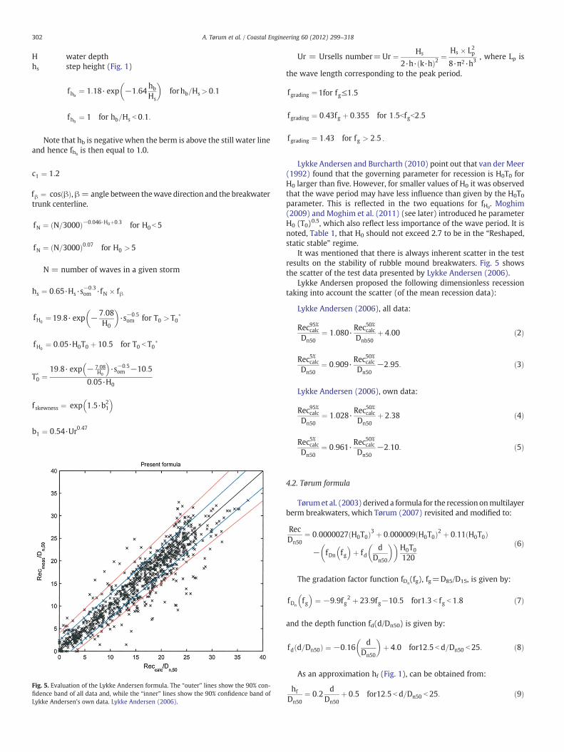
The circles in Fig. 4 represents the average recession for a specificsignificant wave height, Hs. When deriving a formula for the recessiona polynomial fit to all data may be used (Tørum et al., 2003), or theaverage data points (Lykke Andersen, 2006). Fig. 5 shows the com-parison between the calculated dimensionless recession, Reccal/Dn50,using the Lykke Andersen formula (see later) and his measured di-mensionless recession, Recmeas/Dn50. In this figure each data pointrepresents the average for all profiles for a given wave condition. Inaddition there will be a scatter between profiles as indicated in Fig. 4.Lykke Andersen has in Fig. 5 plotted his own data together with datafrom Hall and Kao (1991), van der Meer (1992), Tørum and Krogh(2000) and Tørum (1998).

It should be noted that for multilayer berm breakwaters that aredesigned as “Reshaping static stable” the non-dimensional recessionRec/Dn50 seldom exceeds 10.

Fig. 2. Measured profiles and outer envelopes. Westeng (2011).

4. Different formulae for the recession of berm breakwaters

4.1. Lykke Andersen formula

Lykke Andersen (2006) arrived at the following dimensionlessequation for the recession:

RecDn50

¼ fhb·½ 1þ c1ð Þh−c1hs

h−hb·fN � fβ � fH0

� fskewness � fgrading

þ cotðαdÞ−1:052·Dn50

· hb−hð Þ � ð1Þ

where

hb height of berm. Note that hb is negative when the berm isabove the still water line.

Fig. 4. Recession vs. significant wave height for tests with model scale 1:70 on the Sirevågberm breakwater. Each point represents the recession in a specific profile. Westeng(2011).

302 A. Tørum et al. / Coastal Engineering 60 (2012) 299–318

H water depthhs step height (Fig. 1)

fhb¼ 1:18· exp −1:64

hb

Hs

� �forhb=Hs> 0:1

fhb¼ 1 for hb=Hs b 0:1:

Note that hb is negative when the berm is above the still water lineand hence fhb

is then equal to 1.0.

c1 ¼ 1:2

fβ ¼ cos βð Þ, β= angle between thewave direction and the breakwatertrunk centerline.

fN ¼ N=3000ð Þ−0:046·H0þ0:3 for H0 b 5

fN ¼ N=3000ð Þ0:07 for H0 > 5

N = number of waves in a given storm

hs ¼ 0:65·Hs·s−0:3om ·fN � fβ

fH0¼19:8· exp −7:08

H0

� �·s−0:5

om for T0 > T0�

fH0¼ 0:05·H0T0 þ 10:5 for T0 b T0

�

T�0 ¼19:8· exp − 7:08

H0

� �·s−0:5

om −10:5

0:05·H0

fskewness ¼ exp 1:5·b21

� �

b1 ¼ 0:54·Ur0:47

Fig. 5. Evaluation of the Lykke Andersen formula. The “outer” lines show the 90% con-fidence band of all data and, while the “inner” lines show the 90% confidence band ofLykke Andersen's own data. Lykke Andersen (2006).

Ur = Ursells number=Ur ¼ Hs

2·h· k·hð Þ2¼ Hs � L2p

8·π2·h3 , where Lp is

the wave length corresponding to the peak period.

fgrading ¼1for fg≤1:5

fgrading ¼ 0:43fg þ 0:355 for 1:5bfgb2:5

fgrading ¼ 1:43 for fg > 2:5 :

Lykke Andersen and Burcharth (2010) point out that van der Meer(1992) found that the governing parameter for recession is H0T0 forH0 larger than five. However, for smaller values of H0 it was observedthat the wave period may have less influence than given by the H0T0parameter. This is reflected in the two equations for fH0

. Moghim(2009) and Moghim et al. (2011) (see later) introduced he parameterH0 (T0)0.5, which also reflect less importance of the wave period. It isnoted, Table 1, that H0 should not exceed 2.7 to be in the “Reshaped,static stable” regime.

It was mentioned that there is always inherent scatter in the testresults on the stability of rubble mound breakwaters. Fig. 5 showsthe scatter of the test data presented by Lykke Andersen (2006).

Lykke Andersen proposed the following dimensionless recessiontaking into account the scatter (of the mean recession data):

Lykke Andersen (2006), all data:

Rec95%calc

Dn50¼ 1:080·

Rec50%calc

Dnb50þ 4:00 ð2Þ

Rec5%calcDn50

¼ 0:909·Rec50%calc

Dn50−2:95: ð3Þ

Lykke Andersen (2006), own data:

Rec95%calc

Dn50¼ 1:028·

Rec50%calc

Dn50þ 2:38 ð4Þ

Rec5%calcDn50

¼ 0:961·Rec50%calc

Dn50−2:10: ð5Þ

4.2. Tørum formula

Tørumet al. (2003) derived a formula for the recessiononmultilayerberm breakwaters, which Tørum (2007) revisited and modified to:

RecDn50

¼ 0:0000027 H0T0ð Þ3 þ 0:000009 H0T0ð Þ2 þ 0:11 H0T0ð Þ

− fDn fg� �

þ fdd

Dn50

� �� �H0T0120

ð6Þ

The gradation factor function fDn(fg), fg=D85/D15, is given by:

fDnfg� �

¼ −9:9fg2 þ 23:9fg−10:5 for1:3 b fg b 1:8 ð7Þ

and the depth function fd(d/Dn50) is given by:

fd d=Dn50ð Þ ¼ −0:16d

Dn50

� �þ 4:0 for12:5 b d=Dn50 b 25: ð8Þ

As an approximation hf (Fig. 1), can be obtained from:

hf

Dn50¼ 0:2

dDn50

þ 0:5 for12:5 b d=Dn50 b 25: ð9Þ

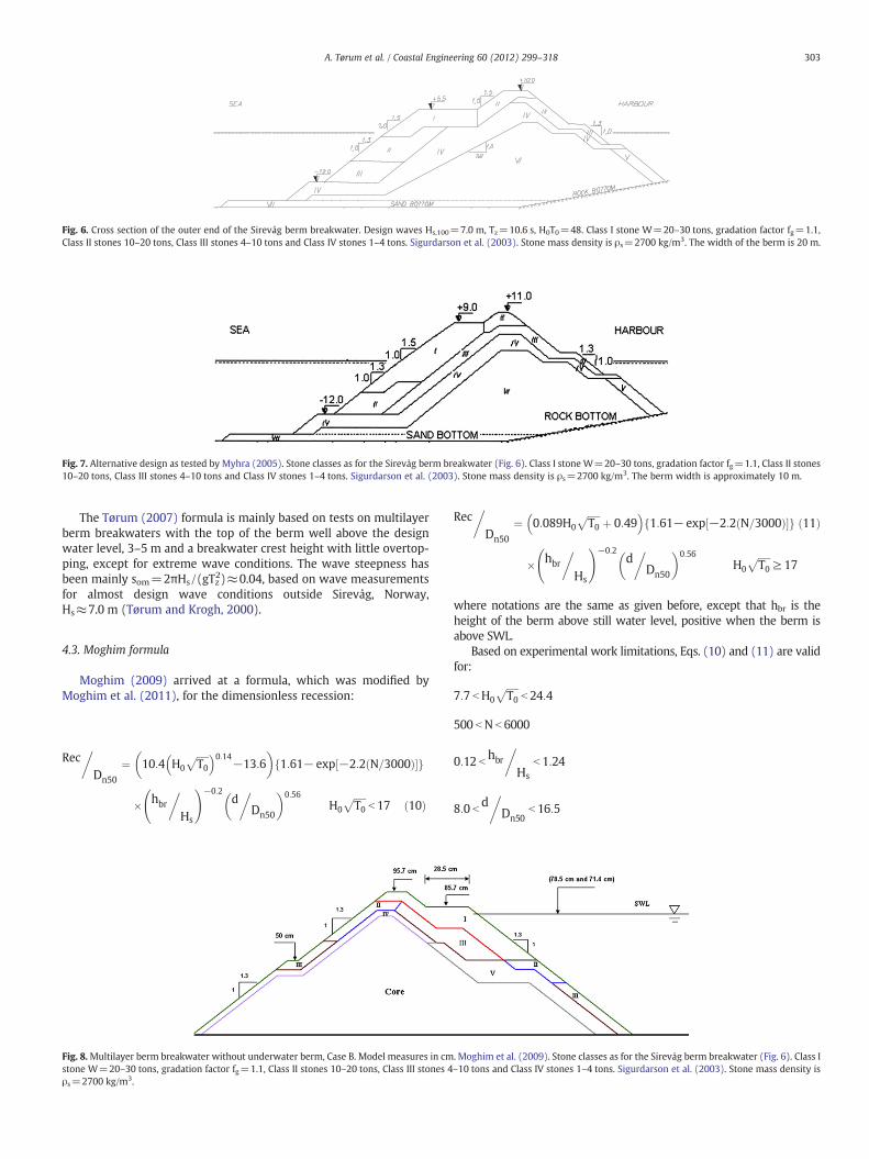
Fig. 7. Alternative design as tested by Myhra (2005). Stone classes as for the Sirevåg berm breakwater (Fig. 6). Class I stone W=20–30 tons, gradation factor fg=1.1, Class II stones10–20 tons, Class III stones 4–10 tons and Class IV stones 1–4 tons. Sigurdarson et al. (2003). Stone mass density is ρs=2700 kg/m3. The berm width is approximately 10 m.

Fig. 6. Cross section of the outer end of the Sirevåg berm breakwater. Design waves Hs,100=7.0 m, Tz=10.6 s, H0T0=48. Class I stone W=20–30 tons, gradation factor fg=1.1,Class II stones 10–20 tons, Class III stones 4–10 tons and Class IV stones 1–4 tons. Sigurdarson et al. (2003). Stone mass density is ρs=2700 kg/m3. The width of the berm is 20 m.

303A. Tørum et al. / Coastal Engineering 60 (2012) 299–318

The Tørum (2007) formula is mainly based on tests on multilayerberm breakwaters with the top of the berm well above the designwater level, 3–5 m and a breakwater crest height with little overtop-ping, except for extreme wave conditions. The wave steepness hasbeen mainly som=2πHs/(gTz2)≈0.04, based on wave measurementsfor almost design wave conditions outside Sirevåg, Norway,Hs≈7.0 m (Tørum and Krogh, 2000).

4.3. Moghim formula

Moghim (2009) arrived at a formula, which was modified byMoghim et al. (2011), for the dimensionless recession:

Rec�Dn50

¼ 10:4 H0

ffiffiffiffiffiT0

p� �0:14−13:6� �

1:61− exp −2:2 N=3000ð Þ½ �f g

� hbr

�Hs

!−0:2d

Dn50

� �0:56H0

ffiffiffiffiffiT0

pb 17 ð10Þ

�

Fig. 8.Multilayer berm breakwater without underwater berm, Case B. Model measures in cmstone W=20–30 tons, gradation factor fg=1.1, Class II stones 10–20 tons, Class III stones 4ρs=2700 kg/m3.

Rec�Dn50

¼ 0:089H0

ffiffiffiffiffiT0

pþ 0:49

� �1:61− exp −2:2 N=3000ð Þ½ �f g

� hbr

�Hs

!−0:2d

Dn50

� �0:56H0

ffiffiffiffiffiT0

p≥ 17

�ð11Þ

where notations are the same as given before, except that hbr is theheight of the berm above still water level, positive when the berm isabove SWL.

Based on experimental work limitations, Eqs. (10) and (11) are validfor:

7:7 bH0

ffiffiffiffiffiT0

pb 24:4

500 bN b 6000

0:12 bhbr

�Hs

b 1:24

8:0 bd

Dn50b 16:5

�

. Moghim et al. (2009). Stone classes as for the Sirevåg berm breakwater (Fig. 6). Class I–10 tons and Class IV stones 1–4 tons. Sigurdarson et al. (2003). Stone mass density is

Fig. 9. Bermbreakwaterwith a crownwall tested byHidayati (2010) for amodelwater depth 78.5 cmor prototypewater depth 55 m formodel scale 1:70. Stone classes as for the Sirevågberm breakwater (Fig. 6). Class I stone W=20–30 tons, gradation factor fg=1.1, Class II stones 10–20 tons, Class III stones 4–10 tons and Class IV stones 1–4 tons. Sigurdarson et al.(2003). Stone mass density is ρs=2700 kg/m3.

Fig. 10. Cross section and dimensions of a multilayer berm breakwater tested by Lykke Andersen et al. (2008).

Fig. 11. Cross section tested by Tørum and Krogh (2000). Measures in m.

304 A. Tørum et al. / Coastal Engineering 60 (2012) 299–318

0:09 bd

L b 0:25.

1:2 b fg b 1:5

5. Results of some berm breakwater tests compared to test resultsof recession formulae

5.1. Previous and recent tests at NTNU/SINTEF and Aalborg University

Fig. 6 shows a cross section of the Sirevåg berm breakwater. Testson this breakwater have been carried out for different purposes(Menze, 2000; Myhra, 2005; Westeng, 2011). The tests of Menze(2000) and Myhra (2005) have also been included in Tørum et al.(2003) and Tørum et al. (2005) respectively.

The tests of Menze (2000) andWesteng (2011) were in scale 1:70.The tests set-up was in a 5 m wide wave flume. The breakwater headand part of the breakwater trunk were included, covering approxi-mately half of the width of the wave flume. Menze (2000) carriedout tests with Class I stones with mass density ρs=2700 kg/m3 andρs=3100 kg/m3. Myhra (2005) carried out 2D tests in scale 1:70 ina 0.60 m wide flume. The Menze (2000), Myhra (2005) andWesteng (2011) tests were carried out with the same model armorstone material.

Myhra (2005) carried also out tests on an alternative cross sectionas shown in Fig. 7, with a higher and narrower berm than for the Sirevågberm breakwater, but with the same stone classes as for the Sirevågberm breakwater. Note also that the Class I stones are placed to alower level on this alternative design than on the Sirevåg design. Thereason for the higher level of the Sirevåg design was that the Class Istones were specified to be placed orderly by a backhoe. It is not possi-ble to place stones orderly to a lower level than 1 m below low waterbecause the back-hoe driver cannot control the stone placement at alower depth, mainly due to low visibility. For the alternative designthe stones were placed pell-mell and can then just be thrown downthe slope, which is at its almost natural slope.

Moghim et al. (2009) carried out tests on a deep water multilayerberm breakwater as shown in Fig. 8. The same model stone classes asin the Sirevåg berm breakwater tests were used. Fig. 8 shows themeasures in cm. If a scale of 1:70 is applied the water depth at thisbreakwater is 50 and 55 m and the stone classes correspond tothose shown for the Sirevåg berm breakwater (Fig. 6).

Hidayati (2010) carried out tests on the same cross section asMoghim et al. (2009) (Fig. 8), but with a crown wall on top of thebreakwater as shown in Fig. 9.

We have also included for our comparison data from tests on amultilayer berm breakwater carried out by Lykke Andersen et al.(2008) with dimensions, water depth, stone classes and mass densi-ties as shown in Fig. 10. This cross section is almost the same as theSirevåg berm breakwater, except that the berm width is narrower(12 m vs. 20 m) and the mass density is higher (ρs=2908 kg/m3 vs.ρs=2700 kg/m3).

Tørum and Krogh (2000) carried out 2D tests in a 1.00 m wideflume on a semi-homogenous berm breakwater as shown in Fig. 11.The main objective of these tests was to study the velocity of thestones as they rolled on the berm, but recession was also measuredby profiling at 10 cm distance between the profiles with a laserprofiler.

If a length scale of 1:100 is applied to the cross section shown inFig. 11 the water depth corresponds to 55 m, the berm heightto 5 m and the crest height to 30 m, e.g. no overtopping. Dn50

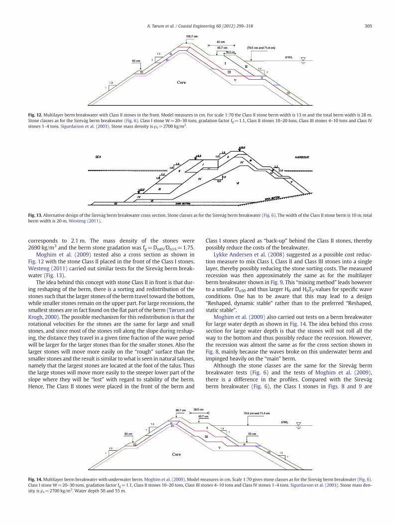
Fig. 12. Multilayer berm breakwater with Class II stones in the front. Model measures in cm. For scale 1:70 the Class II stone berm width is 13 m and the total berm width is 28 m.Stone classes as for the Sirevåg berm breakwater (Fig. 6). Class I stone W=20–30 tons, gradation factor fg=1.1, Class II stones 10–20 tons, Class III stones 4–10 tons and Class IVstones 1–4 tons. Sigurdarson et al. (2003). Stone mass density is ρs=2700 kg/m3.

Fig. 13. Alternative design of the Sirevåg berm breakwater cross section. Stone classes as for the Sirevåg berm breakwater (Fig. 6). The width of the Class II stone berm is 10 m, totalberm width is 20 m. Westeng (2011).

305A. Tørum et al. / Coastal Engineering 60 (2012) 299–318

corresponds to 2.1 m. The mass density of the stones were2690 kg/m3 and the berm stone gradation was fg=Dn85/Dn15=1.75.

Moghim et al. (2009) tested also a cross section as shown inFig. 12 with the stone Class II placed in the front of the Class I stones.Westeng (2011) carried out similar tests for the Sirevåg berm break-water (Fig. 13).

The idea behind this concept with stone Class II in front is that dur-ing reshaping of the berm, there is a sorting and redistribution of thestones such that the larger stones of the berm travel toward the bottom,while smaller stones remain on the upper part. For large recessions, thesmallest stones are in fact found on the flat part of the berm (Tørum andKrogh, 2000). The possible mechanism for this redistribution is that therotational velocities for the stones are the same for large and smallstones, and since most of the stones roll along the slope during reshap-ing, the distance they travel in a given time fraction of the wave periodwill be larger for the larger stones than for the smaller stones. Also thelarger stones will move more easily on the “rough” surface than thesmaller stones and the result is similar towhat is seen in natural taluses,namely that the largest stones are located at the foot of the talus. Thusthe large stones will move more easily to the steeper lower part of theslope where they will be “lost” with regard to stability of the berm.Hence, The Class II stones were placed in the front of the berm and

Fig. 14.Multilayer berm breakwater with underwater berm. Moghim et al. (2009). Model mClass I stone W=20–30 tons, gradation factor fg=1.1, Class II stones 10–20 tons, Class III stsity is ρs=2700 kg/m3. Water depth 50 and 55 m.

Class I stones placed as “back-up” behind the Class II stones, therebypossibly reduce the costs of the breakwater.

Lykke Andersen et al. (2008) suggested as a possible cost reduc-tion measure to mix Class I, Class II and Class III stones into a singlelayer, thereby possibly reducing the stone sorting costs. The measuredrecession was then approximately the same as for the multilayerberm breakwater shown in Fig. 9. This “mixing method” leads howeverto a smaller Dn50 and thus larger H0 and H0T0-values for specific waveconditions. One has to be aware that this may lead to a design“Reshaped, dynamic stable” rather than to the preferred “Reshaped,static stable”.

Moghim et al. (2009) also carried out tests on a berm breakwaterfor large water depth as shown in Fig. 14. The idea behind this crosssection for large water depth is that the stones will not roll all theway to the bottom and thus possibly reduce the recession. However,the recession was almost the same as for the cross section shown inFig. 8, mainly because the waves broke on this underwater berm andimpinged heavily on the “main” berm.

Although the stone classes are the same for the Sirevåg bermbreakwater tests (Fig. 6) and the tests of Moghim et al. (2009),there is a difference in the profiles. Compared with the Sirevågberm breakwater (Fig. 6), the Class I stones in Figs. 8 and 9 are

easures in cm. Scale 1:70 gives stone classes as for the Sirevåg berm breakwater (Fig. 6).ones 4–10 tons and Class IV stones 1–4 tons. Sigurdarson et al. (2003). Stone mass den-

Fig. 15. Storm progression. Sirevåg 98-12-27 and Sirevåg 99-02-04 are storm durationsduring storms when the significant wave heights were approximately 6–7 mmeasuredin 20 m water depth outside 400 m the outer end of the breakwater. NPD is the stormprogression as stated by NPD (1998) to evaluate the soil resistance to cyclic loading onconcrete platforms. Hs,max for the tests is corresponding to approximately 9.3 m.

0 2 4 6 8 10 120

5

10

15

20

25

Hs, m

Rec

ess

ion

, Rec

, m

Moghim (2011)Menze (2000)Tørum (2007)LA (2006)LA 95%LA 5%

d=17.5m, ros=3100kg/m3, Dn50=1.45m, fg=1.1, hb=-5.0m, hbr=5.0m, som=0.04, N=2000

Fig. 17. Recession data of Menze (2000) (multilayer) compared with different formu-lae. Sirevåg berm breakwater case (Fig. 6) with armor stones with mass densityρs=3100 kg/m3. d = water depth, ros = ρs, mass density of the stone, Dn50 =(W50/ρs)0.33, hb = Lykke Andersen definition of berm height (hb is negative whenthe berm is above still water line), hbr = Moghim definition of berm height (hbr is pos-itive when the berm is above still water level), som=2πHs/(gTz2), N = number ofwaves. Model scale 1:70.

306 A. Tørum et al. / Coastal Engineering 60 (2012) 299–318

terminated at a lower level than on the Sirevåg berm breakwater forthe cross section shown in Fig. 6. Tørum et al. (2005) pointed out thatthere might be a weakness in the Sirevåg berm breakwater designthat the Class II stones below level−1 mwill first start tomove, thus re-moving the support for the Class I stones. To improve the stability theClass I stones are terminated at a lower level on the profiles tested byMoghim et al. (2009) and by Hidayati (2010). Sveinbjørnson (2008)recommended that the lower level of the Class I stones on the frontslope should be at:

hI–II ≥ 1:45·Δ·Dn50;ClassI or hI–II ≥ 1:85·Δ·Dn50;ClassII;

the largest one is recommended:

The tests by Menze (2000), Tørum and Krogh (2000), Tørum et al.(2003), Moghim et al. (2009), Hidayati (2010) and by Westeng(2011) were carried out with a wave steepness sm ¼ 2πHs= gT2z

� �≈

0 2 4 6 8 10 120

5

10

15

20

25

Hs, m

Re

cess

ion

, Re

c, m

d=17.5m, ros=2700kg/m3, Dn50=2.10m, fg=1.1, hb=-5.0m, hbr=5.0m, som=0.04, N=2000

Moghim (2011)Menze (2000)Myhra (2005)Westeng (2010)Tørum (2007)LA (2006)LA 95%LA 5%

Fig. 16. Recession data of Menze (2000), Myhra (2005) and Westeng (2011) (all mul-tilayer) compared with different formulae. Sirevåg berm breakwater case (Fig. 6) witharmor stone with mass density ρs=2700 kg/m3. d = water depth, ros = ρs, mass den-sity of the stone, Dn50=(W50/ρs)0.33, hb = Lykke Andersen definition of berm height(hb is negative when the berm is above still water line), hbr = Moghim definitionof berm height (hbr is positive when the berm is above still water level), som=2πHs/(gTz2), N = number of waves. Model scale 1:70.

0.04 and a target JONSWAPwave spectrumwith γ=3.3. These valueswere based on wave measurements approximately 450 m outside theSirevåg berm breakwater (Tørum and Krogh, 2000). The storm pro-gression for all these tests is shown in Fig. 15, compared with somemeasured storm progression outside Sirevåg. This model storm pro-gression has frequently been used in EC research projects (Tørum etal., 2003).

5.2. Comparison of recession from model tests results and results fromdifferent formulae

5.2.1. GeneralWe have in the following calculations shown recession results by

using the formulae by Lykke Andersen (2006), Tørum (2007), and

0 2 4 6 8 10 120

5

10

15

20

25

30

35

40

Hs, m

Rec

ess

ion

, Rec

, m

d=20m, ros=2906kg/m3, Dn50=2.0m, fg=1.1, hb=-5.0m, hbr=5.0m, sop=0.04, N=1200

Moghim (2011)LA (2008)Tørum (2007)LA (2006)LA 95%LA 5%

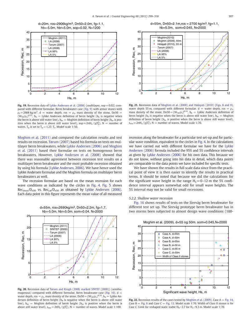
Fig. 18. Recession data of Lykke Andersen et al. (2008) (multilayer, sop=0.04) com-pared with different formulae. Berm breakwater case (Fig. 9) with armor stones withρs=2908 kg/m3. d = water depth, ros = ρs, mass density of the stone, Dn50=(W50/ρs)0.33, hb = Lykke Andersen definition of berm height (hb is negative whenthe berm is above still water line), hbr = Moghim definition of berm height (hbr is pos-itive when the berm is above still water level), sop=2πHs/(gTp2), N = number ofwaves. Tp is set to Tp=1.25 ∙Tz. Model scale 1:50.

0 2 4 6 8 10 120

5

10

15

20

25

30

35

40

Hs, m

Rec

essi

on, R

ec, m

d=20m, ros=2906kg/m3, Dn50=2.0m, fg=1.1, hb=-5.0m, hbr=5.0m, sop=0.02, N=1200

Moghim (2011)LA (2008)Tørum (2007)LA (2006)LA 95%LA 5%

Fig. 19. Recession data of Lykke Andersen et al. (2008) (multilayer, sop=0.02) com-pared with different formulae. Berm breakwater case (Fig. 9) with armor stones withρs=2908 kg/m3. d = water depth, ros = ρs, mass density of the stone, Dn50 =(W50/ρs)0.33, hb = Lykke Andersen definition of berm height (hb is negative whenthe berm is above still water line), hbr = Moghim definition of berm height (hbr is pos-itive when the berm is above still water level), sop=2πHs/(gTp2), N = number ofwaves. Tp is set to Tp=1.25 ∙Tz. Model scale 1:50.

0 2 4 6 8 10 120

5

10

15

20

25

30

35

40

Hs, m

Rec

ess

ion

, Rec

, m

d=55m, Dn50=2.1m,ros = 2700 kg/m3, fg=1.1, hb=5.0m, som=0.045, N=2000

Moghim(2010)Moghim (2009), 55mHidayati (2010), 55 mTørum (2007)LA (2006)LA 95%LA 5%

Fig. 21. Recession data of Moghim et al. (2009) and Hidayati (2010) (Figs. 8 and 9),water depth 55 m, compared with different formulae. d = water depth, ros = ρs,mass density of the stone, Dn50=(W50/ρs)0.33, hb = Lykke Andersen definition ofberm height (hb is negative when the berm is above still water line), hbr = Moghimdefinition of berm height (hbr is positive when the berm is above still water level),som=2πHs/(gTz2), N = number of waves. Model scale 1:70.

307A. Tørum et al. / Coastal Engineering 60 (2012) 299–318

Moghim et al. (2011) and compared the calculation results and testresults on recession. Tørum (2007) based his formula on tests on mul-tilayer berm breakwaters, while Lykke Andersen (2006) and Moghimet al. (2011) based their formulae on tests on homogenous bermbreakwaters. However, Lykke Andersen et al. (2008) showed thatthere was reasonable agreement between recession test results on amultilayer berm breakwater and the most probable recession obtainedby using his formula (Lykke Andersen, 2006). We have hence used theLykke Andersen formulae and the Moghim formula onmultilayer bermbreakwaters as well.

The recession formulae are based on the mean recession for eachwave conditions as indicated by the circles in Fig. 4. Fig. 5 showsRecmeas/Dn50 vs. Reccal/Dn50 as obtained by Lykke Andersen (2006).Each data point in this figure represents the mean value of all measured

0 2 4 6 8 10 120

5

10

15

20

25

Hs, m

Rec

ess

ion

, Rec

, m

d=55m, ros=2690kg/m3, Dn50=2.2m, fg=1.7, hb=-5.0m, hbr=5.0m, som=0.04, N=2000

Moghim (2011)SINTEF (2000)Tørum (2007)LA (2006)LA 95%LA 5%

Fig. 20. Recession data of Tørum and Krogh (2000, marked SINTEF (2000)) (semiho-mogenous) compared with different formulae. Berm breakwater case (Fig. 10). d =water depth, ros = ρs, mass density of the stone, Dn50=(W50/ρs)0.33, hb = Lykke An-dersen definition of berm height (hb is negative when the berm is above still waterline), hbr = Moghim definition of berm height (hbr is positive when the berm isabove still water level), som=2πHs/(gTz2), N = number of waves. Model scale 1:100.

recession along the breakwater for a particular test set-up and for partic-ular wave condition, equivalent to the circles in Fig. 4. In the calculationswe have carried out with different formulae we have for the LykkeAndersen (2006) formula included the 95% and 5% confidence intervalsas given by Lykke Andersen (2006) for his own data. This because wedo not know, without going into his data in detail, which data pointsare comparable to the data points we have included for specific tests.

We have shown the results in full scale data since from the practi-cal point of view it is then easier to identify the results in practicalterms. It should be noted that because we did the calculations forthe significant wave height in the range Hs=0–12 m the 5% confi-dence interval appears somewhat odd for small wave heights. The5% interval may not be valid for small recessions.

5.2.2. Shallow water recessionFig. 16 shows results of tests on the Sirevåg berm breakwater for

different test set up. The Sirevåg prototype berm breakwater has intwo storms been subjected to almost design wave conditions (100-

0 2 4 6 8 10 120

5

10

15

20

25

30

35

40

Significant wave height, Hs, m

Rec

essi

on, R

ec, m

Moghim et al. (2009). d=55 og 50m. som=0.045,N=2000

Case A, d=55m

Case A, d=50m

Case B, d=55m

Case B, d=50 m

Case C, d=55 m

Case C, d=50m

Width of Class II stones

Fig. 22. Recession results of the cases tested by Moghim et al. (2009). Case A = Fig. 14,Case B = Fig. 8 and Case C = Fig. 12. Model scale 1:70. Width of Class II stones is forCase C. Limit for reshaped static stable H0b2.7 for Hsb9.3 m. Model scale 1:70.

0 2 4 6 8 10 120

5

10

15

20

25

30

35

40

Significant wave height, Hs, m

Rec

essi

on, R

ec, m

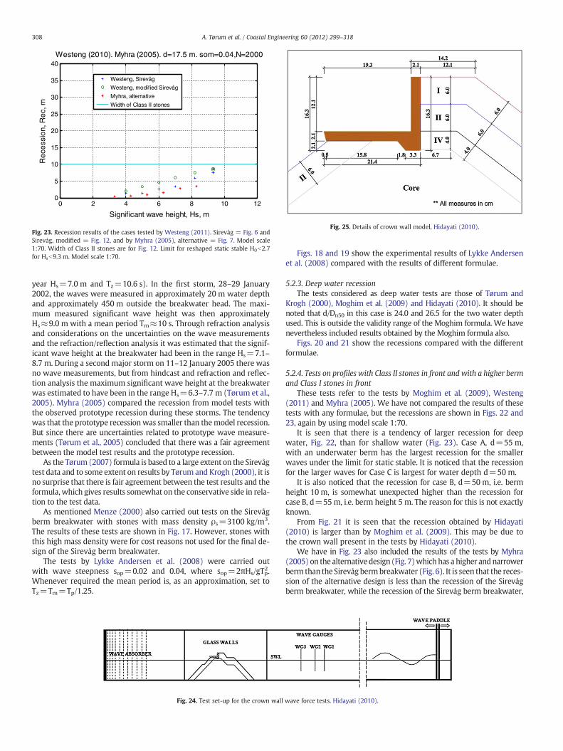
Westeng (2010). Myhra (2005). d=17.5 m. som=0.04,N=2000

Westeng, Sirevåg

Westeng, modified Sirevåg

Myhra, alternative

Width of Class II stones

Fig. 23. Recession results of the cases tested by Westeng (2011). Sirevåg = Fig. 6 andSirevåg, modified = Fig. 12, and by Myhra (2005), alternative = Fig. 7. Model scale1:70. Width of Class II stones are for Fig. 12. Limit for reshaped static stable H0b2.7for Hsb9.3 m. Model scale 1:70.

Fig. 25. Details of crown wall model, Hidayati (2010).

308 A. Tørum et al. / Coastal Engineering 60 (2012) 299–318

year Hs=7.0 m and Tz=10.6 s). In the first storm, 28–29 January2002, the waves were measured in approximately 20 m water depthand approximately 450 m outside the breakwater head. The maxi-mum measured significant wave height was then approximatelyHs≈9.0 m with a mean period Tm≈10 s. Through refraction analysisand considerations on the uncertainties on the wave measurementsand the refraction/reflection analysis it was estimated that the signif-icant wave height at the breakwater had been in the range Hs=7.1–8.7 m. During a secondmajor storm on 11–12 January 2005 there wasno wave measurements, but from hindcast and refraction and reflec-tion analysis the maximum significant wave height at the breakwaterwas estimated to have been in the range Hs=6.3–7.7 m (Tørum et al.,2005). Myhra (2005) compared the recession from model tests withthe observed prototype recession during these storms. The tendencywas that the prototype recession was smaller than themodel recession.But since there are uncertainties related to prototype wave measure-ments (Tørum et al., 2005) concluded that there was a fair agreementbetween the model test results and the prototype recession.

As the Tørum (2007) formula is based to a large extent on the Sirevågtest data and to some extent on results by Tørum and Krogh (2000), it isno surprise that there is fair agreement between the test results and theformula, which gives results somewhat on the conservative side in rela-tion to the test data.

As mentioned Menze (2000) also carried out tests on the Sirevågberm breakwater with stones with mass density ρs=3100 kg/m3.The results of these tests are shown in Fig. 17. However, stones withthis high mass density were for cost reasons not used for the final de-sign of the Sirevåg berm breakwater.

The tests by Lykke Andersen et al. (2008) were carried outwith wave steepness sop=0.02 and 0.04, where sop=2πHs/gTp2.Whenever required the mean period is, as an approximation, set toTz=Tm=Tp/1.25.

Fig. 24. Test set-up for the crown wall

Figs. 18 and 19 show the experimental results of Lykke Andersenet al. (2008) compared with the results of different formulae.

5.2.3. Deep water recessionThe tests considered as deep water tests are those of Tørum and

Krogh (2000), Moghim et al. (2009) and Hidayati (2010). It should benoted that d/Dn50 in this case is 24.0 and 26.5 for the two water depthused. This is outside the validity range of the Moghim formula. We havenevertheless included results obtained by the Moghim formula also.

Figs. 20 and 21 show the recessions compared with the differentformulae.

5.2.4. Tests on profiles with Class II stones in front and with a higher bermand Class I stones in front

These tests refer to the tests by Moghim et al. (2009), Westeng(2011) and Myhra (2005). We have not compared the results of thesetests with any formulae, but the recessions are shown in Figs. 22 and23, again by using model scale 1:70.

It is seen that there is a tendency of larger recession for deepwater, Fig. 22, than for shallow water (Fig. 23). Case A, d=55 m,with an underwater berm has the largest recession for the smallerwaves under the limit for static stable. It is noticed that the recessionfor the larger waves for Case C is largest for water depth d=50 m.

It is also noticed that the recession for case B, d=50 m, i.e. bermheight 10 m, is somewhat unexpected higher than the recession forcase B, d=55m, i.e. berm height 5 m. The reason for this is not exactlyknown.

From Fig. 21 it is seen that the recession obtained by Hidayati(2010) is larger than by Moghim et al. (2009). This may be due tothe crown wall present in the tests by Hidayati (2010).

We have in Fig. 23 also included the results of the tests by Myhra(2005) on the alternative design (Fig. 7)which has a higher andnarrowerberm than the Sirevåg bermbreakwater (Fig. 6). It is seen that the reces-sion of the alternative design is less than the recession of the Sirevågberm breakwater, while the recession of the Sirevåg berm breakwater,

wave force tests. Hidayati (2010).

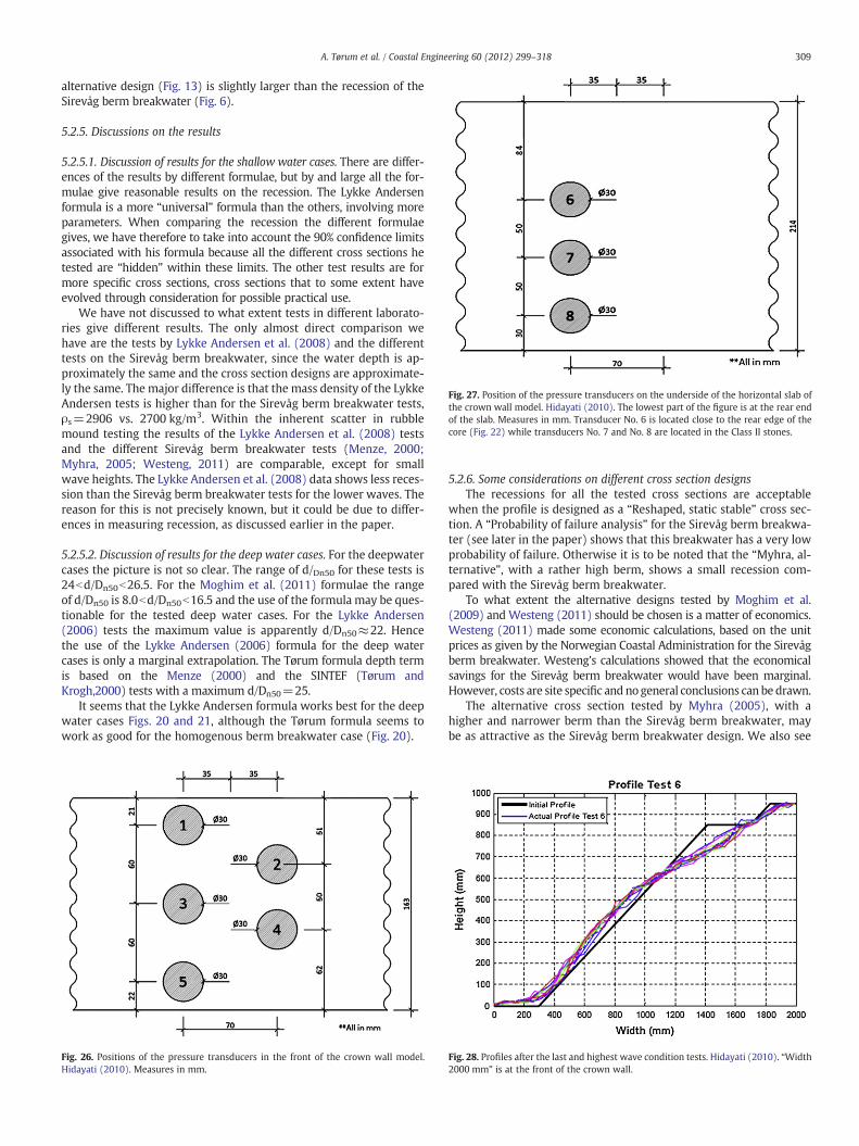
Fig. 27. Position of the pressure transducers on the underside of the horizontal slab ofthe crown wall model. Hidayati (2010). The lowest part of the figure is at the rear endof the slab. Measures in mm. Transducer No. 6 is located close to the rear edge of thecore (Fig. 22) while transducers No. 7 and No. 8 are located in the Class II stones.

309A. Tørum et al. / Coastal Engineering 60 (2012) 299–318

alternative design (Fig. 13) is slightly larger than the recession of theSirevåg berm breakwater (Fig. 6).

5.2.5. Discussions on the results

5.2.5.1. Discussion of results for the shallow water cases. There are differ-ences of the results by different formulae, but by and large all the for-mulae give reasonable results on the recession. The Lykke Andersenformula is a more “universal” formula than the others, involving moreparameters. When comparing the recession the different formulaegives, we have therefore to take into account the 90% confidence limitsassociated with his formula because all the different cross sections hetested are “hidden” within these limits. The other test results are formore specific cross sections, cross sections that to some extent haveevolved through consideration for possible practical use.

We have not discussed to what extent tests in different laborato-ries give different results. The only almost direct comparison wehave are the tests by Lykke Andersen et al. (2008) and the differenttests on the Sirevåg berm breakwater, since the water depth is ap-proximately the same and the cross section designs are approximate-ly the same. The major difference is that the mass density of the LykkeAndersen tests is higher than for the Sirevåg berm breakwater tests,ρs=2906 vs. 2700 kg/m3. Within the inherent scatter in rubblemound testing the results of the Lykke Andersen et al. (2008) testsand the different Sirevåg berm breakwater tests (Menze, 2000;Myhra, 2005; Westeng, 2011) are comparable, except for smallwave heights. The Lykke Andersen et al. (2008) data shows less reces-sion than the Sirevåg berm breakwater tests for the lower waves. Thereason for this is not precisely known, but it could be due to differ-ences in measuring recession, as discussed earlier in the paper.

5.2.5.2. Discussion of results for the deep water cases. For the deepwatercases the picture is not so clear. The range of d/Dn50 for these tests is24bd/Dn50b26.5. For the Moghim et al. (2011) formulae the rangeof d/Dn50 is 8.0bd/Dn50b16.5 and the use of the formula may be ques-tionable for the tested deep water cases. For the Lykke Andersen(2006) tests the maximum value is apparently d/Dn50≈22. Hencethe use of the Lykke Andersen (2006) formula for the deep watercases is only a marginal extrapolation. The Tørum formula depth termis based on the Menze (2000) and the SINTEF (Tørum andKrogh,2000) tests with a maximum d/Dn50=25.

It seems that the Lykke Andersen formula works best for the deepwater cases Figs. 20 and 21, although the Tørum formula seems towork as good for the homogenous berm breakwater case (Fig. 20).

Fig. 26. Positions of the pressure transducers in the front of the crown wall model.Hidayati (2010). Measures in mm.

5.2.6. Some considerations on different cross section designsThe recessions for all the tested cross sections are acceptable

when the profile is designed as a “Reshaped, static stable” cross sec-tion. A “Probability of failure analysis” for the Sirevåg berm breakwa-ter (see later in the paper) shows that this breakwater has a very lowprobability of failure. Otherwise it is to be noted that the “Myhra, al-ternative”, with a rather high berm, shows a small recession com-pared with the Sirevåg berm breakwater.

To what extent the alternative designs tested by Moghim et al.(2009) and Westeng (2011) should be chosen is a matter of economics.Westeng (2011) made some economic calculations, based on the unitprices as given by the Norwegian Coastal Administration for the Sirevågberm breakwater. Westeng's calculations showed that the economicalsavings for the Sirevåg berm breakwater would have been marginal.However, costs are site specific and no general conclusions can be drawn.

The alternative cross section tested by Myhra (2005), with ahigher and narrower berm than the Sirevåg berm breakwater, maybe as attractive as the Sirevåg berm breakwater design. We also see

Fig. 28. Profiles after the last and highest wave condition tests. Hidayati (2010). “Width2000 mm” is at the front of the crown wall.

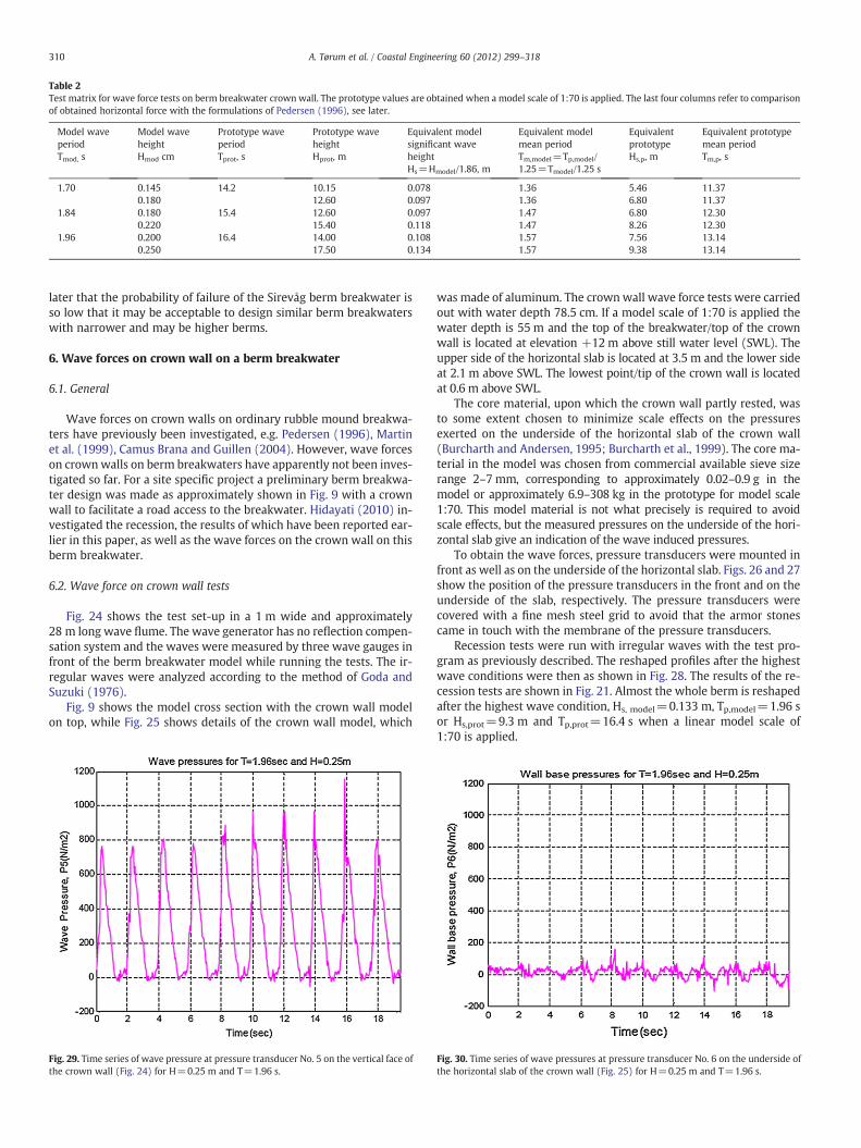
Table 2Test matrix for wave force tests on berm breakwater crown wall. The prototype values are obtained when a model scale of 1:70 is applied. The last four columns refer to comparisonof obtained horizontal force with the formulations of Pedersen (1996), see later.

Model waveperiodTmod, s

Model waveheightHmod cm

Prototype waveperiodTprot, s

Prototype waveheightHprot, m

Equivalent modelsignificant waveheightHs=Hmodel/1.86, m

Equivalent modelmean periodTm,model=Tp,model/1.25=Tmodel/1.25 s

EquivalentprototypeHs,p, m

Equivalent prototypemean periodTm,p, s

1.70 0.145 14.2 10.15 0.078 1.36 5.46 11.370.180 12.60 0.097 1.36 6.80 11.37

1.84 0.180 15.4 12.60 0.097 1.47 6.80 12.300.220 15.40 0.118 1.47 8.26 12.30

1.96 0.200 16.4 14.00 0.108 1.57 7.56 13.140.250 17.50 0.134 1.57 9.38 13.14

310 A. Tørum et al. / Coastal Engineering 60 (2012) 299–318

later that the probability of failure of the Sirevåg berm breakwater isso low that it may be acceptable to design similar berm breakwaterswith narrower and may be higher berms.

6. Wave forces on crown wall on a berm breakwater

6.1. General

Wave forces on crown walls on ordinary rubble mound breakwa-ters have previously been investigated, e.g. Pedersen (1996), Martinet al. (1999), Camus Brana and Guillen (2004). However, wave forceson crownwalls on berm breakwaters have apparently not been inves-tigated so far. For a site specific project a preliminary berm breakwa-ter design was made as approximately shown in Fig. 9 with a crownwall to facilitate a road access to the breakwater. Hidayati (2010) in-vestigated the recession, the results of which have been reported ear-lier in this paper, as well as the wave forces on the crown wall on thisberm breakwater.

6.2. Wave force on crown wall tests

Fig. 24 shows the test set-up in a 1 m wide and approximately28 m long wave flume. The wave generator has no reflection compen-sation system and the waves were measured by three wave gauges infront of the berm breakwater model while running the tests. The ir-regular waves were analyzed according to the method of Goda andSuzuki (1976).

Fig. 9 shows the model cross section with the crown wall modelon top, while Fig. 25 shows details of the crown wall model, which

Fig. 29. Time series of wave pressure at pressure transducer No. 5 on the vertical face ofthe crown wall (Fig. 24) for H=0.25 m and T=1.96 s.

was made of aluminum. The crownwall wave force tests were carriedout with water depth 78.5 cm. If a model scale of 1:70 is applied thewater depth is 55 m and the top of the breakwater/top of the crownwall is located at elevation +12m above still water level (SWL). Theupper side of the horizontal slab is located at 3.5 m and the lower sideat 2.1 m above SWL. The lowest point/tip of the crown wall is locatedat 0.6 m above SWL.

The core material, upon which the crown wall partly rested, wasto some extent chosen to minimize scale effects on the pressuresexerted on the underside of the horizontal slab of the crown wall(Burcharth and Andersen, 1995; Burcharth et al., 1999). The core ma-terial in the model was chosen from commercial available sieve sizerange 2–7 mm, corresponding to approximately 0.02–0.9 g in themodel or approximately 6.9–308 kg in the prototype for model scale1:70. This model material is not what precisely is required to avoidscale effects, but the measured pressures on the underside of the hori-zontal slab give an indication of the wave induced pressures.

To obtain the wave forces, pressure transducers were mounted infront as well as on the underside of the horizontal slab. Figs. 26 and 27show the position of the pressure transducers in the front and on theunderside of the slab, respectively. The pressure transducers werecovered with a fine mesh steel grid to avoid that the armor stonescame in touch with the membrane of the pressure transducers.

Recession tests were run with irregular waves with the test pro-gram as previously described. The reshaped profiles after the highestwave conditions were then as shown in Fig. 28. The results of the re-cession tests are shown in Fig. 21. Almost the whole berm is reshapedafter the highest wave condition, Hs, model=0.133 m, Tp,model=1.96 sor Hs,prot=9.3 m and Tp,prot=16.4 s when a linear model scale of1:70 is applied.

Fig. 30. Time series of wave pressures at pressure transducer No. 6 on the underside ofthe horizontal slab of the crown wall (Fig. 25) for H=0.25 m and T=1.96 s.

Fig. 31. Time series of wave pressures for all pressure transducers on the vertical frontwall for H=0.25 m, T=1.96 s.

Fig. 33. Pressures on the underside of the horizontal slab. Note that 0 for the horizontalface axis is at the rear (harbor) side of the slab. It has been assumed that the pressure atthe forward edge is equal to the pressures at the lowest pressure transducer on the ver-tical face.

311A. Tørum et al. / Coastal Engineering 60 (2012) 299–318

During the recession test with irregular waves we saw that onlysome few waves caused any significant pressures/forces on thecrown wall. Because of this and because it was expected that therewould be a variation (scatter) of the pressures from wave to wave, alsofor regular waves, it was decided to run wave force test on the crownwall with regular waves on the final reshaped form of the berm break-water (Fig. 28).

Martin et al. (1999) carried out tests on wave forces on crownwalls with regular and irregular waves. The tested structure was amodel of the breakwater at Gijón, Spain, with a crown wall extendingsome 6 m above the top of the120 tons parallel piped blocks. The re-sults of the regular wave tests were used to calculate the forces in ir-regular waves through the hypothesis of equivalence, for breakingwaves, e.g. waves that break on the breakwater slope. The calculated

Fig. 32. The max-mean-min horizontal pressures plotted vs. the vertical face of thewall. H=0.25 m, T=1.96 s. It has been assumed that the pressures are zero at thetop of the wall and that the pressure at the base is equal to the pressure at the lowestpressure transducer.

wave force statistical distribution was then compared with the statis-tical distribution obtained from the tests with irregular waves. Therewas a reasonable agreement between the two methods. The statisti-cal nature of the hypothesis of equivalence is pointed out by Martinet al. (1999). It does not necessarily imply that each individualwave produce the same force as the equivalent regular wave becausethe waves change as they travel from the point of measurement tothe breakwater. To use regular waves may be better for the under-standing of the relation between waves and wave forces, similar towhat is used to some extent for obtaining wave forces on verticalcaisson breakwaters, e.g. the Goda method (Goda, 2010).

On a berm breakwater the waves normally break on the berm.Hence it is believed that the comparison we have made (see later)with the results of Pedersen (1996) formula, based on irregularwave tests, give reasonable background to the conclusions on waveforces on crown walls on berm breakwaters relative to the waveforces on crown wall forces conventional rubble mound breakwaters.

In order to avoid any further reshaping when the recession testswas completed, the berm was covered with a wire net to keep the

Fig. 34. Expanded time series around 12 s of wave pressures for all pressure trans-ducers on the vertical front wall for H=0.25 m, T=1.96 s.

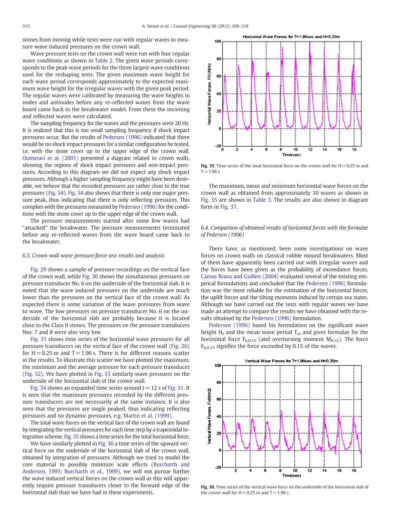
Fig. 35. Time series of the total horizontal force on the crown wall for H=0.25 m andT=1.96 s.

Fig. 36. Time series of the vertical wave force on the underside of the horizontal slab ofthe crown wall for H=0.25 m and T=1.96 s.

312 A. Tørum et al. / Coastal Engineering 60 (2012) 299–318

stones from moving while tests were run with regular waves to mea-sure wave induced pressures on the crown wall.

Wave pressure tests on the crown wall were run with four regularwave conditions as shown in Table 2. The given wave periods corre-sponds to the peak wave periods for the three largest wave conditionsused for the reshaping tests. The given maximum wave height foreach wave period corresponds approximately to the expected maxi-mumwave height for the irregular waves with the given peak period.The regular waves were calibrated by measuring the wave heights innodes and antinodes before any re-reflected waves from the waveboard came back to the breakwater model. From these the incomingand reflected waves were calculated.

The sampling frequency for the waves and the pressures were 20 Hz.It is realized that this is too small sampling frequency if shock impactpressures occur. But the results of Pedersen (1996) indicated that therewould be no shock impact pressures for a similar configuration he tested,i.e. with the stone cover up to the upper edge of the crown wall.Oumeraci et al. (2001) presented a diagram related to crown walls,showing the regions of shock impact pressures and non-impact pres-sures. According to this diagram we did not expect any shock impactpressures. Although a higher sampling frequencymight have been desir-able, we believe that the recorded pressures are rather close to the truepressures (Fig. 34). Fig. 34 also shows that there is only one major pres-sure peak, thus indicating that there is only reflecting pressures. Thiscomplieswith the pressuresmeasured by Pedersen (1996) for the condi-tions with the stone cover up to the upper edge of the crown wall.

The pressure measurements started after some few waves had“attacked” the breakwater. The pressure measurements terminatedbefore any re-reflected waves from the wave board came back tothe breakwater.

6.3. Crown wall wave pressure/force test results and analysis

Fig. 29 shows a sample of pressure recordings on the vertical faceof the crown wall, while Fig. 30 shows the simultaneous pressures onpressure transducer No. 6 on the underside of the horizontal slab. It isnoted that the wave induced pressures on the underside are muchlower than the pressures on the vertical face of the crown wall. Asexpected there is some variation of the wave pressures from waveto wave. The low pressures on pressure transducer No. 6 on the un-derside of the horizontal slab are probably because it is locatedclose to the Class II stones. The pressures on the pressure transducersNos. 7 and 8 were also very low.

Fig. 31 shows time series of the horizontal wave pressures for allpressure transducers on the vertical face of the crown wall (Fig. 26)for H=0.25 m and T=1.96 s. There is for different reasons scatterin the results. To illustrate this scatter we have plotted the maximum,the minimum and the average pressure for each pressure transducer(Fig. 32). We have plotted in Fig. 33 similarly wave pressures on theunderside of the horizontal slab of the crown wall.

Fig. 34 shows an expanded time series around t=12 s of Fig. 31. Itis seen that the maximum pressures recorded by the different pres-sure transducers are not necessarily at the same instance. It is alsoseen that the pressures are single peaked, thus indicating reflectingpressures and no dynamic pressures, e.g. Martin et al. (1999).

The total wave forces on the vertical face of the crown wall are foundby integrating the vertical pressures for each time step by a trapezoidal in-tegration scheme. Fig. 35 shows a time series for the total horizontal force.

We have similarly plotted in Fig. 36 a time series of the upward ver-tical force on the underside of the horizontal slab of the crown wall,obtained by integration of pressures. Although we tried to model thecore material to possibly minimize scale effects (Burcharth andAndersen, 1995; Burcharth et al., 1999), we will not pursue furtherthe wave induced vertical forces on the crown wall as this will appar-ently require pressure transducers closer to the forward edge of thehorizontal slab than we have had in these experiments.

The maximum, mean and minimum horizontal wave forces on thecrown wall as obtained from approximately 10 waves as shown inFig. 35 are shown in Table 3. The results are also shown in diagramform in Fig. 37.

6.4. Comparison of obtained results of horizontal forces with the formulaeof Pedersen (1996)

There have, as mentioned, been some investigations on waveforces on crown walls on classical rubble mound breakwaters. Mostof them have apparently been carried out with irregular waves andthe forces have been given as the probability of exceedance forces.Camus Brana and Guillen (2004) evaluated several of the existing em-pirical formulations and concluded that the Pedersen (1996) formula-tion was the most reliable for the estimation of the horizontal forces,the uplift forces and the tilting moments induced by certain sea states.Although we have carried out the tests with regular waves we havemade an attempt to compare the results we have obtained with the re-sults obtained by the Pedersen (1996) formulation.

Pedersen (1996) based his formulation on the significant waveheight Hs and the mean wave period Tm and gives formulae for thehorizontal force Fh,0.1% (and overturning moment M0.1%). The forceFh,0.1% signifies the force exceeded by 0.1% of the waves.

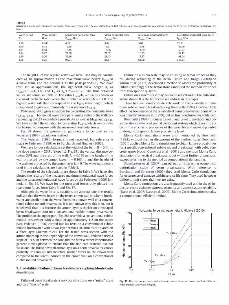
Table 3Maximum, mean and minimum horizontal forces on crown wall. The calculated forces, last column, refer to approximate calculations using the Pedersen (1996) formulations (seelater).

Wave periodT, s

Wave heightH, m

Maximum horizontal forceFh,max, N/m

Mean horizontal forceFh,mean, N/m

Minimum horizontal forceFh,min, N/m

Calculated horizontal wave forceFh,cal N/m

1.70 0.145 4.27 3.64 3.07 17.551.70 0.18 6.15 5.57 4.78 45.901.84 0.18 8.45 5.86 4.69 58.771.84 0.22 27.08 21.62 16.23 92.171.96 0.20 39.16 29.43 17.77 91.041.96 0.25 98.04 81.17 61.00 135.33

0.1 0.15 0.2 0.25 0.30

20

40

60

80

100

H, m

Hor

izon

tal f

orce

,Fh,

N/m

Horizontal force vs. wave height. Hidayati (2010)

T=1.70 s

T=1.84 s

T=1.96 s

FmaxFmeanFmin

Fig. 37. The maximum, mean and minimum wave forces on crown wall for differentwave periods and wave heights.

313A. Tørum et al. / Coastal Engineering 60 (2012) 299–318

The height H of the regular waves we have used may be consid-ered as an approximation as the maximum wave height Hmax ina wave train, and the periods T as the peak periods Tp. We havethus set, as approximations, the significant wave height Hs asHmax/1.86=H/1.86 and Tm as Tp/1.25=T/1.25. The thus obtainedvalues are found in Table 2. The ratio Hmax/Hs=1.86 is chosen asthe most probable ratio when the number of waves N=1000. Thehighest wave will then correspond to the H0.1% wave height, whichis supposed to give approximately the wave force Fh,0.1%.

Pedersen(1996) gives equations for calculating the horizontal forceFh,0.1%, Fh,0.1%=horizontal wave force per runningmeter of thewall cor-responding to 0.1% exceedance probability as well as M0.1% and pb,0.1%.We have applied the equation for calculating Fh,0.1%, which we considercan be used to compare with the measured horizontal forces.

Fig. 38 shows the geometrical parameters to be used in thePedersen (1996) calculation method.

The Pedersen (1996) formula is not repeated, but reference ismade to Pedersen (1996) or to Burcharth and Hughes (2002).

We have for our calculations set the width of the berm B=0.11 m,the slope angleα=26.5°, (slope 1:2, Fig. 28), the vertical distance be-tween SWL and the crest of the wall, Ac=0.176 m, the height of thewall protected by the armor layer h′=0.163 m, and the height ofthe wall not protected by the armor layer fc=0. The wave parametersused in the calculations are listed in Table 2.

The results of the calculations are shown in Table 3. We have alsoplotted the results of the measured maximum horizontal wave forcesand the calculated horizontal wave forces by the Pedersen (1996) for-mula in Fig. 39. We have for the measured forces only plotted themaximum forces from Table 3 and Fig. 37.

Although the wave force calculations are approximate, the resultsindicate that thewave forces on the tested crownwall on a berm break-water are smaller than the wave forces on a crown wall on a conven-tional rubble mound breakwater. It is not known why this is so, but itis believed that it is because the armor layer is thicker on a reshapedberm breakwater than on a conventional rubble mound breakwater.The profiles in the upper part (Fig. 28) resemble a conventional rubblemound breakwater with a slope of approximately 1:2 on the upperpart. Pedersen (1996) carried out his tests on a conventional rubblemound breakwater with a two-layer armor (100 mm thick) placed ona filter layer (40 mm thick). For the tested cross section with thearmor stones up to the upper edge of the crown wall, Pedersen used aslope of 1:1.5. In between the core and the filter a rather impermeablegeotextile was placed to ensure that the fine core material did notwash out. The thicker overall armor layer on a berm breakwater causesprobably less run-up and therefore smaller forces on the crown wallcompared to the forces induced on the crown wall on a conventionalrubble mound breakwater.

7. Probability of failure of berm breakwaters applyingMonte Carlosimulations

Failure of berm breakwaters may possibly occur on a “micro” scaleand on a “macro” scale.

Failure on a micro scale may be crushing of armor stones as theyroll during reshaping of the berm. Tørum and Krogh (2000)andTørum et al. (2002) developed a method to assess the probability offailure (crushing) of the armor stones and used the method for stonesfrom two specific quarries.

Failure on a macro scale may be due to relocations of the individualarmor stones. It is the latter case we address in this paper.

There has been done considerable work on the reliability of tradi-tional rubblemoundbreakwaters, e.g. Burcharth (1994). However, littleeffort has beenmade on the reliability of berm breakwaters. Someworkwas done by Tørum et al. (1999), but no final conclusion was obtained.

Burcharth (1994) discusses Level II and Level III methods and de-scribe also an advanced partial coefficient systemwhich takes into ac-count the stochastic properties of the variables and make it possibleto design to a specific failure probability level.

Monte Carlo simulations were also mentioned by Burcharth(1994), without further discussions of the method. Later, Burcharth(2001) applied Monte Carlo simulations to obtain failure probabilitiesfor a specific conventional rubble mound breakwater with cubic con-crete armor blocks. Oumeraci et al. (2001) also mention Monte Carlosimulations for vertical breakwaters, but without further discussions,except referring to the method as computational demanding.

Sigurdarson et al. (2007) carried out an interesting economicaloptimization study of berm breakwaters. With reference toBurcharth and Sørensen (2005) they used Monte Carlo simulationsfor occurrence of damage within service life time. They used howeverdifferent limit states than we are using.

Monte Carlo simulations are also frequently used within the oil in-dustry, e.g. to estimate extreme response and assess system reliability(Næss et al., 2007; Næss et al., 2009). Monte Carlo simulation is todaya computational efficient method.

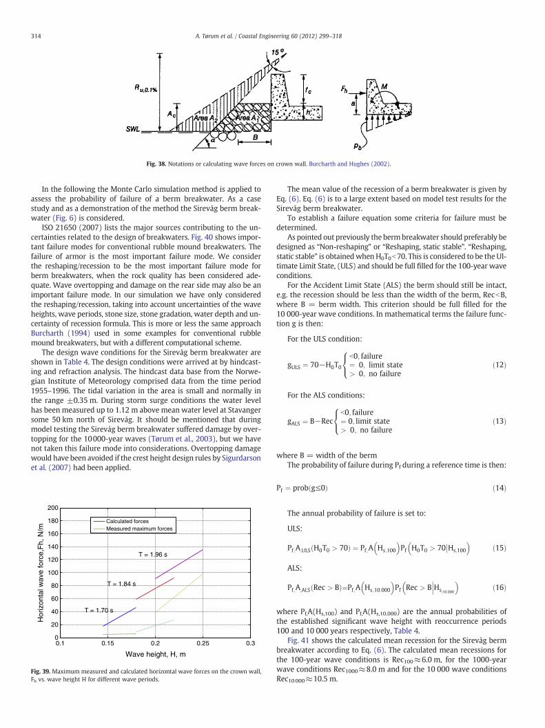
Fig. 38. Notations or calculating wave forces on crown wall. Burcharth and Hughes (2002).

314 A. Tørum et al. / Coastal Engineering 60 (2012) 299–318

In the following the Monte Carlo simulation method is applied toassess the probability of failure of a berm breakwater. As a casestudy and as a demonstration of the method the Sirevåg berm break-water (Fig. 6) is considered.

ISO 21650 (2007) lists the major sources contributing to the un-certainties related to the design of breakwaters. Fig. 40 shows impor-tant failure modes for conventional rubble mound breakwaters. Thefailure of armor is the most important failure mode. We considerthe reshaping/recession to be the most important failure mode forberm breakwaters, when the rock quality has been considered ade-quate. Wave overtopping and damage on the rear side may also be animportant failure mode. In our simulation we have only consideredthe reshaping/recession, taking into account uncertainties of the waveheights, wave periods, stone size, stone gradation, water depth and un-certainty of recession formula. This is more or less the same approachBurcharth (1994) used in some examples for conventional rubblemound breakwaters, but with a different computational scheme.

The design wave conditions for the Sirevåg berm breakwater areshown in Table 4. The design conditions were arrived at by hindcast-ing and refraction analysis. The hindcast data base from the Norwe-gian Institute of Meteorology comprised data from the time period1955–1996. The tidal variation in the area is small and normally inthe range ±0.35 m. During storm surge conditions the water levelhas been measured up to 1.12 m above mean water level at Stavangersome 50 km north of Sirevåg. It should be mentioned that duringmodel testing the Sirevåg berm breakwater suffered damage by over-topping for the 10000-year waves (Tørum et al., 2003), but we havenot taken this failure mode into considerations. Overtopping damagewould have been avoided if the crest height design rules by Sigurdarsonet al. (2007) had been applied.

0.1 0.15 0.2 0.25 0.30

20

40

60

80

100

120

140

160

180

200

Wave height, H, m

Hor

izon

tal w

ave

forc

e,F

h, N

/m

T = 1.70 s

T = 1.84 s

T = 1.96 s

Calculated forcesMeasured maximum forces

Fig. 39. Maximum measured and calculated horizontal wave forces on the crown wall,Fh vs. wave height H for different wave periods.

The mean value of the recession of a berm breakwater is given byEq. (6). Eq. (6) is to a large extent based on model test results for theSirevåg berm breakwater.

To establish a failure equation some criteria for failure must bedetermined.

As pointed out previously the bermbreakwater should preferably bedesigned as “Non-reshaping” or “Reshaping, static stable”. “Reshaping,static stable” is obtainedwhenH0T0b70. This is considered to be the Ul-timate Limit State, (ULS) and should be full filled for the 100-year waveconditions.

For the Accident Limit State (ALS) the berm should still be intact,e.g. the recession should be less than the width of the berm, RecbB,where B = berm width. This criterion should be full filled for the10 000-year wave conditions. In mathematical terms the failure func-tion g is then:

For the ULS condition:

gULS ¼ 70−H0T0b0; failure¼ 0; limit state> 0; no failure

8<: ð12Þ

For the ALS conditions:

gALS ¼ B−Recb0; failure¼ 0; limit state> 0; no failure

8<: ð13Þ

where B = width of the bermThe probability of failure during Pf during a reference time is then:

Pf ¼ prob g≤0ð Þ ð14Þ

The annual probability of failure is set to:

ULS:

Pf ;A;ULS H0T0 > 70ð Þ ¼ Pf ;A Hs ;100

� �Pf H0T0 > 70 Hs;100

�� ��ð15Þ

ALS:

Pf ;A;ALS Rec > Bð Þ¼Pf ;A Hs ;10:000

� �Pf Rec > B Hs;10:000

��� ��ð16Þ

where Pf,A(Hs,100) and Pf,A(Hs,10.000) are the annual probabilities ofthe established significant wave height with reoccurrence periods100 and 10 000 years respectively, Table 4.

Fig. 41 shows the calculated mean recession for the Sirevåg bermbreakwater according to Eq. (6). The calculated mean recessions forthe 100-year wave conditions is Rec100≈6.0 m, for the 1000-yearwave conditions Rec1000≈8.0 m and for the 10 000 wave conditionsRec10000≈10.5 m.

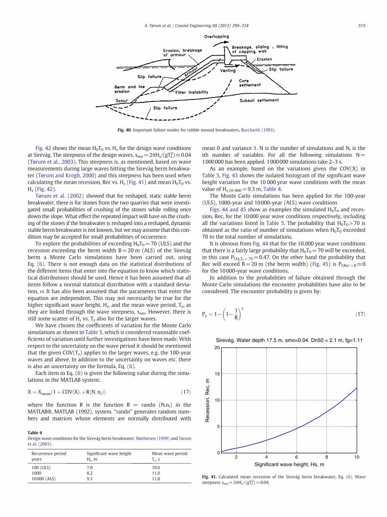
Fig. 40. Important failure modes for rubble mound breakwaters, Burcharth (1993).

10

15

20

Rec

essi

on, R

ec, m

Sirevåg. Water depth 17.5 m. smo=0.04. Dn50 = 2.1 m, fg=1.11

315A. Tørum et al. / Coastal Engineering 60 (2012) 299–318

Fig. 42 shows the mean H0T0 vs. Hs for the design wave conditionsat Sirevåg. The steepness of the design waves, smo=2πHs/(gTz2)≈0.04(Tørum et al., 2003). This steepness is, as mentioned, based on wavemeasurements during large waves hitting the Sirevåg berm breakwa-ter (Tørum and Krogh, 2000) and this steepness has been used whencalculating the mean recession, Rec vs. Hs (Fig. 41) and mean H0T0 vs.Hs (Fig. 42).

Tørum et al. (2002) showed that for reshaped, static stable bermbreakwater, there is for stones from the two quarries that were investi-gated small probabilities of crushing of the stones while rolling oncedown the slope.What effect the repeated impactwill have on the crush-ing of the stones if the breakwater is reshaped into a reshaped, dynamicstable bermbreakwater is not known, butwemay assume that this con-dition may be accepted for small probabilities of occurrence.

To explore the probabilities of exceeding H0T0=70 (ULS) and therecession exceeding the berm width B=20 m (ALS) of the Sirevågberm a Monte Carlo simulations have been carried out, usingEq. (6). There is not enough data on the statistical distributions ofthe different items that enter into the equation to know which statis-tical distributions should be used. Hence it has been assumed that allitems follow a normal statistical distribution with a standard devia-tion, σ. It has also been assumed that the parameters that enter theequation are independent. This may not necessarily be true for thehigher significant wave height, Hs, and the mean wave period, Tz, asthey are linked through the wave steepness, som. However, there isstill some scatter of Hs vs. Tz also for the larger waves.

We have chosen the coefficients of variation for the Monte Carlosimulations as shown in Table 5, which is considered reasonable coef-ficients of variation until further investigations have been made. Withrespect to the uncertainty on the wave period it should be mentionedthat the given COV(Tz) applies to the larger waves, e.g. the 100-yearwaves and above. In addition to the uncertainty on waves etc. thereis also an uncertainty on the formula, Eq. (6).

Each item in Eq. (6) is given the following value during the simu-lations in the MATLAB system:

X ¼ Xmean 1þ COV Xð Þ: � R N;nið Þð Þ ð17Þ

where the function R is the function R = randn (N,ni) in theMATLAB®, MATLAB (1992), system. “randn” generates random num-bers and matrices whose elements are normally distributed with

Table 4Design wave conditions for the Sirevåg berm breakwater. Mathiesen (1999) and Tørumet al. (2003).

Recurrence periodyears

Significant wave heightHs, m

Mean wave periodTz, s

100 (ULS) 7.0 10.61000 8.2 11.010000 (ALS) 9.3 11.8

mean 0 and variance 1. N is the number of simulations and Ni is theith number of variables. For all the following simulations N=1000000 has been applied. 1000000 simulations take 2–3 s.

As an example, based on the variations given the COV(X) inTable 5, Fig. 43 shows the isolated histogram of the significant waveheight variation for the 10 000 year wave conditions with the meanvalue of Hs,10 000=9.3 m, Table 4.

The Monte Carlo simulations has been applied for the 100-year(ULS), 1000-year and 10000-year (ALS) wave conditions

Figs. 44 and 45 show as examples the simulated H0T0 and reces-sion, Rec, for the 10000 year wave conditions respectively, includingall the variations listed in Table 5. The probability that H0T0>70 isobtained as the ratio of number of simulations when H0T0 exceeded70 to the total number of simulations.

It is obvious from Fig. 44 that for the 10.000 year wave conditionsthat there is a fairly large probability that H0T0=70 will be exceeded,in this case Pf,H0T0>70=0.47. On the other hand the probability thatRec will exceed B=20 m (the berm width) (Fig. 45) is Pf,Rec>B≈0for the 10000-year wave conditions.

In addition to the probabilities of failure obtained through theMonte Carlo simulations the encounter probabilities have also to beconsidered. The encounter probability is given by:

Pe ¼ 1− 1− 1R

� �Tð17Þ

2 4 6 8 100

5

Significant wave height, Hs, m

Fig. 41. Calculated mean recession of the Sirevåg berm breakwater, Eq. (6). Wavesteepness smo=2πHs/(gTz2)=0.04.

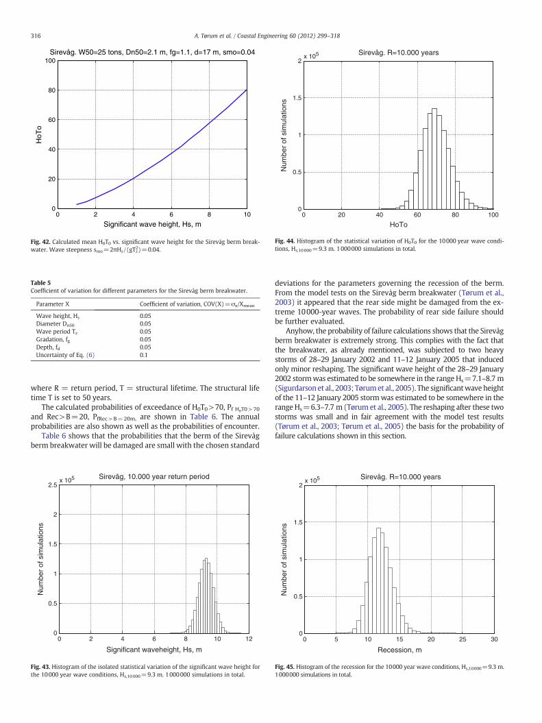
0 2 4 6 8 100

20

40

60

80

100

Significant wave height, Hs, m

HoT

o

Sirevåg. W50=25 tons, Dn50=2.1 m, fg=1.1, d=17 m, smo=0.04

Fig. 42. Calculated mean H0T0 vs. significant wave height for the Sirevåg berm break-water. Wave steepness smo=2πHs/(gTz2)=0.04.

Table 5Coefficient of variation for different parameters for the Sirevåg berm breakwater.

Parameter X Coefficient of variation, COV(X)=σx/Xmean

Wave height, Hs 0.05Diameter Dn50 0.05Wave period Tz 0.05Gradation, fg 0.05Depth, fd 0.05Uncertainty of Eq. (6) 0.1

0 20 40 60 80 1000

0.5

1

1.5

2x 105

HoTo

Num

ber

of s

imul

atio

ns

Sirevåg. R=10.000 years

Fig. 44. Histogram of the statistical variation of H0T0 for the 10000 year wave condi-tions, Hs,10000=9.3 m. 1000000 simulations in total.

316 A. Tørum et al. / Coastal Engineering 60 (2012) 299–318

where R = return period, T = structural lifetime. The structural lifetime T is set to 50 years.

The calculated probabilities of exceedance of H0T0>70, Pf H0T0>70

and Rec>B=20, PfRec>B=20m, are shown in Table 6. The annualprobabilities are also shown as well as the probabilities of encounter.

Table 6 shows that the probabilities that the berm of the Sirevågberm breakwater will be damaged are small with the chosen standard

0 2 4 6 8 10 120

0.5

1

1.5

2

2.5x 105

Significant waveheight, Hs, m

Num

ber

of s

imul

atio

ns

Sirevåg, 10.000 year return period

Fig. 43. Histogram of the isolated statistical variation of the significant wave height forthe 10000 year wave conditions, Hs,10 000=9.3 m. 1000000 simulations in total.

deviations for the parameters governing the recession of the berm.From the model tests on the Sirevåg berm breakwater (Tørum et al.,2003) it appeared that the rear side might be damaged from the ex-treme 10000-year waves. The probability of rear side failure shouldbe further evaluated.

Anyhow, the probability of failure calculations shows that the Sirevågberm breakwater is extremely strong. This complies with the fact thatthe breakwater, as already mentioned, was subjected to two heavystorms of 28–29 January 2002 and 11–12 January 2005 that inducedonly minor reshaping. The significant wave height of the 28–29 January2002 stormwas estimated to be somewhere in the range Hs=7.1–8.7 m(Sigurdarson et al., 2003; Tørumet al., 2005). The significantwave heightof the 11–12 January 2005 stormwas estimated to be somewhere in therange Hs=6.3–7.7 m (Tørum et al., 2005). The reshaping after these twostorms was small and in fair agreement with the model test results(Tørum et al., 2003; Tørum et al., 2005) the basis for the probability offailure calculations shown in this section.

0 5 10 15 20 25 300

0.5

1

1.5

2x 105

Recession, m

Num

ber

of s

imul

atio

ns

Sirevåg. R=10.000 years

Fig. 45. Histogram of the recession for the 10000 year wave conditions, Hs,10000=9.3 m.1000000 simulations in total.

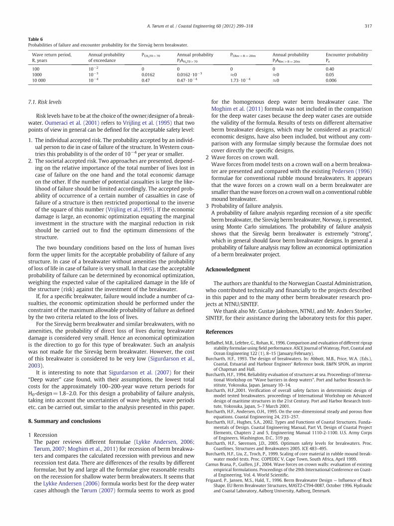
Table 6Probabilities of failure and encounter probability for the Sirevåg berm breakwater.

Wave return period,R, years

Annual probabilityof exceedance

Pf,H0T0>70 Annual probabilityPfAH0T0>70

Pf,Rec>B=20m Annual probabilityPfARec>B=20m

Encounter probabilityPe

100 10−2 0 0 0 0 0.401000 10−3 0.0162 0.0162 ∙10−3 ≈0 ≈0 0.0510 000 10−4 0.47 0.47 ∙10−4 1.73 ∙10−4 ≈0 0.006

317A. Tørum et al. / Coastal Engineering 60 (2012) 299–318

7.1. Risk levels

Risk levels have to be at the choice of the owner/designer of a break-water. Oumeraci et al. (2001) refers to Vrijling et al. (1995) that twopoints of view in general can be defined for the acceptable safety level:

1. The individual accepted risk. The probability accepted by an individ-ual person to die in case of failure of the structure. In Western coun-tries this probability is of the order of 10−4 per year or smaller.

2. The societal accepted risk. Two approaches are presented, depend-ing on the relative importance of the total number of lives lost incase of failure on the one hand and the total economic damageon the other. If the number of potential casualties is large the like-lihood of failure should be limited accordingly. The accepted prob-ability of occurrence of a certain number of casualties in case offailure of a structure is then restricted proportional to the inverseof the square of this number (Vrijling et al.,1995). If the economicdamage is large, an economic optimization equating the marginalinvestment in the structure with the marginal reduction in riskshould be carried out to find the optimum dimensions of thestructure.

The two boundary conditions based on the loss of human livesform the upper limits for the acceptable probability of failure of anystructure. In case of a breakwater without amenities the probabilityof loss of life in case of failure is very small. In that case the acceptableprobability of failure can be determined by economical optimization,weighing the expected value of the capitalized damage in the life ofthe structure (risk) against the investment of the breakwater.

If, for a specific breakwater, failure would include a number of ca-sualties, the economic optimization should be performed under theconstraint of the maximum allowable probability of failure as definedby the two criteria related to the loss of lives.

For the Sirevåg berm breakwater and similar breakwaters, with noamenities, the probability of direct loss of lives during breakwaterdamage is considered very small. Hence an economical optimizationis the direction to go for this type of breakwater. Such an analysiswas not made for the Sirevåg berm breakwater. However, the costof this breakwater is considered to be very low (Sigurdarson et al.,2003).

It is interesting to note that Sigurdarson et al. (2007) for their“Deep water” case found, with their assumptions, the lowest totalcosts for the approximately 100–200-year wave return periods forH0-design=1.8–2.0. For this design a probability of failure analysis,taking into account the uncertainties of wave heights, wave periodsetc. can be carried out, similar to the analysis presented in this paper.

8. Summary and conclusions

1 RecessionThe paper reviews different formulae (Lykke Andersen, 2006;Tørum, 2007; Moghim et al., 2011) for recession of berm breakwa-ters and compares the calculated recession with previous and newrecession test data. There are differences of the results by differentformulae, but by and large all the formulae give reasonable resultson the recession for shallow water berm breakwaters. It seems thatthe Lykke Andersen (2006) formula works best for the deep watercases although the Tørum (2007) formula seems to work as good

for the homogenous deep water berm breakwater case. TheMoghim et al. (2011) formula was not included in the comparisonfor the deep water cases because the deep water cases are outsidethe validity of the formula. Results of tests on different alternativeberm breakwater designs, which may be considered as practical/economic designs, have also been included, but without any com-parison with any formulae simply because the formulae does notcover directly the specific designs.

2 Wave forces on crown wall.Wave forces frommodel tests on a crown wall on a berm breakwa-ter are presented and compared with the existing Pedersen (1996)formulae for conventional rubble mound breakwaters. It appearsthat the wave forces on a crown wall on a berm breakwater aresmaller than thewave forces on a crownwall on a conventional rubblemound breakwater.

3 Probability of failure analysis.A probability of failure analysis regarding recession of a site specificbermbreakwater, the Sirevåg berm breakwater, Norway, is presented,using Monte Carlo simulations. The probability of failure analysisshows that the Sirevåg berm breakwater is extremely “strong”,which in general should favor berm breakwater designs. In general aprobability of failure analysis may follow an economical optimizationof a berm breakwater project.

Acknowledgment

The authors are thankful to the Norwegian Coastal Administration,who contributed technically and financially to the projects describedin this paper and to the many other berm breakwater research pro-jects at NTNU/SINTEF.

We thank also Mr. Gustav Jakobsen, NTNU, and Mr. Anders Storler,SINTEF, for their assistance during the laboratory tests for this paper.

References

Belfadhel, M.B., Lefebre, G., Rohan, K., 1996. Comparison and evaluation of different riprapstability formulae using field performance. ASCE Journal ofWateray, Port, Coastal andOcean Engineering 122 (1), 8–15 (January/February).

Burcharth, H.F., 1993. The design of breakwaters. In: Abbott, M.B., Price, W.A. (Eds.),Coastal, Estuarial and Harbour Engineer' Reference book. E&FN SPON, an imprintof Chapman and Hall.

Burcharth, H.F., 1994. Reliability evaluation of structures at sea. Proceedings of Interna-tional Workshop on “Wave barriers in deep waters”. Port and harbor Research In-stitute, Yokosuka, Japan. January 10–14.

Burcharth, H.F.,2001. Verification of overall safety factors in deterministic design ofmodel tested breakwaters. proceedings of International Workshop on Advanceddesign of maritime structures in the 21st Century. Port and Harbor Research Insti-tute, Yokosuka, Japan, 5–7 March 2001.

Burcharth, H.F., Andersen, O.H., 1995. On the one-dimensional steady and porous flowequations. Coastal Engineering 24, 233–257.

Burcharth, H.F., Hughes, S.A., 2002. Types and Functions of Coastal Structures. Funda-mentals of Design. Coastal Engineering Manual, Part VI, Design of Coastal ProjectElements, Chapters 2 and 5, Engineering Manual 1110-2-1100. U.S. Army Corpsof Engineers, Washington, D.C.. 319 pp.

Burcharth, H.F., Sørensen, J.D., 2005. Optimum safety levels for breakwaters. Proc.Coastlines, Structures and Breakwaters 2005. ICE 483–495.

Burcharth, H.F., Liu, Z., Troch, P., 1999. Scaling of core material in rubble mound break-water model tests. Proc. COPEDEC V, Cape Town, South Africa, April 1999.

Camus Brana, P., Guillen, J.F., 2004. Wave forces on crown walls: evaluation of existingempirical formulations. Proceedings of the 29th International Conference on Coast-al Engineering, Vol. 4. World Scientific.

Frigaard, P., Jansen, M.S., Hald, T., 1996. Berm Breakwater Design — Influence of RockShape. EU Berm Breakwater Structures, MAST2-CT94-0087, October 1996. Hydraulicand Coastal Laboratory, Aalborg University, Aalborg, Denmark.

318 A. Tørum et al. / Coastal Engineering 60 (2012) 299–318

Gilman, J., 2001. St. George harbor — berm breakwater construction issues. Paper Pre-sented at the 5th Regional Symposium on Pacific Congress on Marine Science andTechnology (PACON), San Francisco, California, USA, 8–11 July 2001.

Goda, Y., 2010. Random Seas and Design of Maritime Structures. World Scientific.Goda, Y., Suzuki, Y., 1976. Estimation of incident waves in random wave experiment.

Proceedings 15th International Conference on Coastal Engineering, Honolulu, Hawaii,Vol. 1, pp. 828–854.

Hall, K., Kao, S., 1991. A study of the stability of dynamically stable breakwaters. CanadianJournal of Civil Engineering 18, 916–925.

Hidayati, N., 2010. Deepwater bermbreakwaterwith crownwall.Master thesis, NorwegianUniversity of Science and Technology, Department of Civil and Transport Engineering,Trondheim, Norway.

Lefebre, G., Rohan, K., Belfadhel, M.B., Dascal, O., 1992. Field performance and analysisof steep riprap. ASCE Journal og Geotechnical 118 (9), 1431–1448 (September).

Lykke Andersen, Th., 2006. Hydraulic response of rubble mound breakwaters. Scaleeffects — berm breakwaters. PhD thesis Hydraulics & Coastal Engineering, De-partment of Civil Engineering, Aalborg University, Denmark.

Lykke Andersen, Th., Burcharth, H.F., 2010. A new formula for front slope recession ofberm breakwaters. Coastal Engineering, vol. 57. Elsevier, pp. 359–374.

Lykke Andersen, Th., Skals, K.T., Burcharth, H.F., 2008. Comparison of homogenous andmulti-layered bermbreakwaterswith respect to overtopping and front slope stability.Proceedings of the International Conference on Coastal Engineering, Hamburg,Germany.

Martin, F.M., Losada, M., Medina, R., 1999. Wave loads on rubble mound breakwatercrown walls. Coastal Engineering 37, 149–174.

Mathiesen, M., 1999. Sirevåg harbour. Wave analysis. SINTEF Report STF60 F95029,February 1999. (in Norwegian).

Menze, A., 2000. Stability of multilayer berm breakwaters. Master thesis, NorwegianUniversity of Science and Technology, Trondheim, Norway and Leichtweiss Institutfür Wasserbau, Technical University of Braunschweig, Germany.

Moghim, M.N., 2009. Experimental study of hydraulic stability of reshaping bermbreakwaters. PhD thesis, Department of Civil Engineering, School of Engineering,Tarbiat Modares University, Tehran, Iran. In Persian.

Moghim, M.N., Tørum, A., Arntsen, Ø., Brørs, B., 2009. Stability of berm breakwaters fordeep water. Proceedings 4th International Short Conference on Applied Coastal Re-search (SCACR), Barcelona, Spain, 15–17 June.

Moghim, M.N., Shafieefar, M., Tørum, A., Chegini, V., 2011. A new formula for the seastate and structural parameters influencing the stability of homogeneous reshap-ing berm breakwaters. Coastal Engineering, 58. Elsevier, pp. 706–721.

Myhra, H.A., 2005. Berm Breakwaters. Influence of construction method and storm du-ration on stability. Ice ride up. Master thesis, Norwegian University of Science andTechnology, Department of Civil and Transportation Engineering, Marine Group,2005.

Næss, A., Gaidai, O., Haver, S., 2007. Efficient estimation of extreme response of drag-dominated offshore structures by Monte Carlo simulations. Ocean Engineering34, 2188–2197.

Næss, A., Leira, B., Batsevych, O., 2009. System reliability analysis by Monte Carlo simula-tions. Structural Safety 31 (2009), 349–355.

Newberry, S.N., Latham, J.-P., Stewart, T., Simm, J., 2002. The effect of rock shape andconstruction method on rock armour layers. Proc. International Conference onCoastal Engineering. ASCE, UK.

Oumeraci, H., Kortenhaus, A., Allsop, W., de Groot, M., Couch, R., Vrijling, H., Voortman,2001. Probabilistic Design Tools for Vertical Breakwaters. A.A. Balkema Publishers.

Pedersen, J., 1996. Wave forces and overtopping on crown walls for rubble moundbreakwaters — an experimental study. PhD thesis, Hydraulics & Coastal Engineer-ing Laboratory, Department of Civil Engineering, Aalborg University, Denmark.

Sigurdarson, S., Bjørnson, B.J., Skulason, J., Viggoson, G., Helgason, K., 1999. A bermbreakwater on weak soil. Extension of the port of Hafnafjórdur. Proceedings ofCOPEDEC V, South Africa, April 1999.

Sigurdarson, S., Jakobsen, A., Smarason, O., Bjørdal, S., Urrang, C., Tørum, A., 2003. Sirevågberm breakwater. Design, construction and experience after design storm. Proceed-ings of the International Conference on “Coastal Structures'03”, Portland, Oregon,USA, 26–30 August. ASCE.

Sigurdarson, S., van der Meer, J.W., Burcharth, H.F., Dalgård Sørensen, J., 2007. Optimumsafety levels and design rules for the Icelandic-type berm breakwaters. Proceedingsof the 5th International Conference “Coastal Structures 2007”, Venice, Italy, 2–4 July.World Scientific.

Sveinbjørnson, P.I., 2008. Stability of Icelandic Type Berm Breakwaters. Delft Universityof Technology, Faculty of Engineering and geosciences, Deåpartment of HydraulicEngineering. May 2008.

Tørum, A., 1998. On the stability of berm breakwaters in shallow and deep water. Proc.26th International Conference on Coastal Engineering, Copenhagen, Denmark, June1998. ASCE.

Tørum, A., 2007. Berm Breakwaters Revisited. Preliminary Internal Note, Departmentof Civil and Transportation Engineering. Norwegian University of Science andTechnology, Trondheim, Norway.

Tørum, A., Krogh, S.R., 2000. Berm breakwaters. Stone quality. SINTEF Report SFT22A00207 to the Norwegian Coastal Administration. SINTEF, Trondheim, Norway.July 2000.

Tørum, A., Krogh, S.R., Bjørdal, S., Fjeld, S., Archetti, R. and Jakopbsen, A.,1999. Designcriteria and design procedures for berm breakwaters. Proceedings of the interna-tional conference on "Coastal Structures' 99". I.J. Losada (ed), A.A. Balkema/Rotterdam.

Tørum, A., Krogh, S.R., Fjeld, S., 2002. Berm breakwaters: stone breaking strength. Journalof Waterway, Port, Coastal, and Ocean Engineering 128 (4) (July/August 2002. ASCE).

Tørum, A., Kuhnen, F., Menze, A., 2003. On berm breakwaters. Stability, scour, overtop-ping. Coastal Engineering 49, 209–238.

Tørum, A., Løset, S., Myhra, H., 2005. Sirevåg berm breakwater — comparison betweenmodel and prototype reshaping. International Coastal Symposium, Höfn, Iceland,5–8 June 2005.

Van derMeer, J.W., 1988. Rock slopes and gravel beaches. Doctoral thesis, Delft Universityof Technology, November 1988.

Van der Meer, J.W., 1992. Stability of the seaward slope of berm breakwaters. CoastalEngineering 16, 205–235.

Van Gent, M.R.A., 1995. Wave interaction with permeable coastal structures. PhD the-sis, Delft University of Technology, December 1995.

Vrijling, J.K., VanHengel,W., Houben, R.J., 1995. A framework for risk evaluation. Journal ofHazardousmaterials, Amsterdam, TheNetherlands: Elsevier Science B.V. 43, 245–261.

Westeng, K.O., 2009. Rubble mound and berm breakwaters. Emphasis on the Sirevåg andthe Laukvik berm breakwaters. Project work. Norwegian University of Science andTechnology, Department of Civil and Transport Engineering, Trondheim, Norway.fall semester.

Westeng, K.O., 2011. Berm breakwaters — a modified version. Master Thesis, NorwegianUniversity of Science and Technology, Department of Civil and Transport Engineering,Trondheim, Norway, January 2011.