Internal sources of finance and the Great Recession

No. 10-15

Internal Sources of Finance and the Great Recession

Michelle L. Barnes and N. Aaron Pancost

Abstract: The rising stockpile of cash as a share of total assets at U.S. firms has intrigued economists since at least the paper of Bates, Kahle, and Stulz (2006), yet there has been relatively little work on where this cash has come from and how it is related to investment performance. We exploit Statement of Cash Flows data from Compustat to decompose firms’ cash stocks and show that the rise in cash holdings has coincided with an increased willingness to save internally generated cash. We show that although investment is normally sensitive to externally generated cash, the increased sensitivity of investment to cash during the Great Recession is driven by cash from internal sources. Smaller firms were also more affected by the recent downturn than larger firms. Our results agree with the findings of Almeida, Campello, and Weisbach (2004) on cash hoarding and financial constraints, as well as the estimates in Duchin, Ozbas, and Sensoy (2010) on the important role of saved cash during the financial crisis. Keywords: corporate investment, corporate liquidity, cash, financial constraints, Great Recession JEL Classifications: G01, G31, G32 Michelle L. Barnes is a senior economist and policy advisor and N. Aaron Pancost is a research associate, both in the research department of the Federal Reserve Bank of Boston. Their e-mail addresses are [email protected] and [email protected], respectively. This paper, which may be revised, is available on the web site of the Federal Reserve Bank of Boston at http://www.bos.frb.org/economic/wp/index.htm. The authors owe Giovanni Olivei a debt of gratitude for this frequent and insightful comments and encouragement with this project. They would also like to thank Jeff Fuhrer, Fabià Gumbau-Brisa, Richard Kopcke, Alexey Levkov, Catherine Mann, Judit Montoriol-Garriga, Ali Ozdagli, Robert Triest, Vladimir Yankov, Egon Zakrajšseminar, and seminar participants at the Federal Reserve Bank of Boston for helpful comments. All remaining errors are the responsibility of the authors. The views expressed in here are those of the authors and do not necessarily reflect the views of the Federal Reserve Bank of Boston or the Federal Reserve System.

This version: December 17, 2010; first version August 23, 2010

1 Introduction

The financial crisis and ensuing credit supply shock that began in August 2007 was distinguished in part

by the largest and most persistent drop in real private nonresidential equipment and software investment

growth since the Bureau of Economic Analysis (BEA) began data collection in 1947. At the same time,

aggregate cash holdings as a share of total assets for nonfinancial corporations were at a 30-year high as the

crisis began, which should have provided firms with a very large cushion to absorb any shock to the supply

of credit. These data (from the Bureau of Economic Analysis and the Federal Reserve’s Flow of Funds) are

plotted in Figure 1. A similar picture for the rising trend in cash holdings can be seen using Compustat

data (Figure 2), which covers only publicly traded firms.

In this paper we seek to shed light on two basic questions: 1) What role did cash and its attributes play

in the investment performance of firms during what has been called the Great Recession, and how does this

compare with its role in previous recession and “credit crunch” episodes (Bernanke and Lown 1991)? and

2) In terms of investment, what are the characteristics of firms that were hardest hit during the most recent

recession? In particular, we seek to contribute to the current policy debate regarding the need to restore the

flow of credit to small firms (Bernanke 2010, Duygen-Bump, Levkov, and Montoriol-Garriga 2010), although

our results argue that a broad-based policy to ease credit conditions more generally is also helpful.

Figure 1: Average Cash Stock as a Share of Total Assets

The striking upward trend in corporate cash holdings has been noted earlier (Bates, Kahle, and Stulz

2

2006, later published as Bates, Kahle, and Stulz 2009), as has its potential role in alleviating credit constraints

in the recent recession (Duchin, Ozbas, and Sensoy 2010, henceforth DOS). However, we do not know of any

paper on investment financing that looks as deeply as we do into firms’ sources of cash holdings. By using

variables not hitherto examined in the literature, we are able to decompose firms’ cash stocks by source and

show how use of these sources has varied over time. In particular, we shed light on the role of cash and its

sources over business cycles, with an emphasis on understanding their role during the Great Recession. In

this context, we also directly examine the role of firm size in investment financing over the business cycle,

because size has been identified in the literature as indicative of financial-constraint status.


Bates, Kahle, and Stulz (2009) (henceforth BKS) argued that the rise in cash holdings was due in part

to an increase in cash-flow volatility. The distribution of cash holdings for different values of operating cash

inflows for our sample is given in Figure 3. Consistent with the BKS story, firms at the extreme ends of the

cash-flow distribution do indeed have higher stocks of cash. However, given that these cash stocks do not

come from current operating inflows, at least not for the firms at the bottom (negative) end of the cash-flow

distribution, a natural question arises: how do these firms finance their cash holdings—by raising funds

externally, or by saving systematically out of cash flows over time? Which behavior would be indicative of a

firm facing financial constraints? In an earlier paper, Almeida, Campello, and Weisbach (2004) (henceforth

ACW) showed theoretically that firms expecting future funding shortfalls (for example, because they need

3

to finance losses) will systematically save more cash out of income. ACW identify these “hoarding” firms

empirically, and show that they are firms that are typically estimated to be more “financially constrained”—

smaller, without bond ratings, and not paying dividends. This suggests that in order to understand how

firms might be financially constrained, we need to identify the sources of firms’ accumulation of cash.

Figure 3: Distribution of Cash Stock over Values of Current Cash Flows from Operations

The financial-constraint literature stems from a seminal paper by Fazzari, Hubbard, and Petersen (1988)

(hereinafter FHP) documenting the sensitivity of investment to operating cash flows at the firm level. FHP

argued that the apparent sensitivity of investment to cash flows, even after controlling for future investment

opportunities using Tobin’s Q, indicate that capital market frictions prevent firms from investing in all

profitable opportunities, and that internal cash flows provide an additional source of financing. Most of the

literature since FHP has similarly focused on cash flows, despite the theoretical results of Gomes (2001)

and Alti (2003) that empirical investment/cash-flow sensitivities can be observed even in the absence of

financial constraints, the argument of Erickson and Whited (2000) that cash-flow sensitivities disappear

when measurement error in Q is treated, and work by Cleary, Povel, and Raith (2007) and Kaplan and

Zingales (1997) that shows that the positive cash-flow sensitivities are largely a result of sample selection.

Regardless, cash flows were originally intended only as a proxy for firm liquidity; although current cash flows

may indeed be important, it also seems reasonable to suspect that previous cash flows, saved to the present,

should also be considered as affecting firms’ investment choices, particularly against a backdrop of a large

4

secular increase in cash holdings.1

Other than ACW and Opler et al. (1999), there has been comparatively little attention paid to the stock

of cash as it relates to financial constraints, despite its secular rise as documented by BKS. One exception

is DOS, who showed that large cash stocks before the crisis are correlated with higher investment during

the crisis and argue that this is consistent with the identification of the period from 2007:Q3 to 2008:Q2—

which partly coincides with the NBER recession dating of the Great Recession—as one characterized by a

supply shock to external credit markets, a shock that firms with higher internal liquidity were better able to

weather. Although we largely agree with DOS’s premises and conclusion, Figure 3 should give one pause. If

external financial markets were functional prior to the crisis, then firms’ cash stocks are choice variables and

thus probably endogenous to most dependent variables of interest, as argued above. For example, firms may

issue a large amount of debt prior to embarking on a large investment project for transaction reasons; this

could induce a cash-stock/investment correlation even though in this scenario financial markets are perfectly

functional.

A standard way around these difficulties is to use a difference-in-differences regression specification,

which controls for lower investment demand during recessions, as well as the “usual” correlation of cash and

investment during normal times. In this set-up we would use the estimated interaction between recessions

and the stock of cash to measure the presence of financial constraints; this is essentially the approach taken

by DOS. In addition, firm fixed-effects arguably control for any time-invariant investment demand effects

at the firm level, and inclusion of Tobin’s Q could be expected to control for some time-varying future

investment opportunities.

However, even a difference-in-differences methodology does not get around the fact that the stock of cash

is a matter of firm choice and thus—even lagged one year, or sampled prior to the crisis, as in DOS—it

is not truly exogenous to investment if firms are forward-looking. We propose to mitigate this issue by

decomposing firms’ cash stocks by component source. Since firms that accumulate cash by issuing debt

or equity in order to finance future investment would not, under normal credit conditions, be considered

financially constrained, whereas firms that meticulously save out of operating cash flows in order to finance

future investment opportunities would be, it is important to distinguish between the two sources of cash. It

is only financially constrained firms that we would expect to invest more out of their internally generated

cash stocks. We exhaustively define our categories of internal and external sources of funds in Table 2

and in Section 2, but essentially internal sources include things like income before extraordinary items,

depreciation and amortization, deferred taxes, sale of plant property and equipment, inventory decreases,

and net disinvestment, while external sources include things like sale of equity stock, debt issuance, decreases

1We demonstrate that our main findings are robust to the inclusion of cash-flow variables.

5

in accounts receivable, increases in accounts payable, and changes in current debt. We also experiment with

excluding working capital components as these are arguably used for day-to-day investment purposes for

normal operations as opposed to more irregular investment in equipment, software, and structures. Although

we argue that we are better able to identify firms that are financially constrained using this breakdown of

cash stock into its sources, we do not claim to identify a supply shock.

As argued in DOS, under conditions of weak demand, firms’ desired investment is likely to be lower,

and potential credit constraints may no longer bind. In other words, we might expect the sensitivity of

investment to internally generated cash to be lower during a recession than at other points in the business

cycle, holding all else, including credit conditions, equal. But, in the event of a decline in credit supply,

this sensitivity should increase as the extra liquidity from saved cash alleviates possibly binding financial

constraints. We show that while investment is sensitive to cash accumulated from external sources of funds

during non-recession periods, it has been sensitive to internally generated cash stocks only during the recent

Great Recession episode, which was predated by and coincided with a financial crisis of historic proportions

and a very difficult credit environment. To the extent that weak aggregate demand would bias this result

downward, we can be relatively confident that this increased sensitivity—which appears only during the

Great Recession and not during the previous two recessions or non-recessionary periods—is indeed evidence

of firms’ being financially constrained.

Using our decomposition of firms’ cash stocks, we find the following:

• The rise in cash stocks first documented by BKS has been financed largely from internal sources.

• The rise in internal funds has been driven primarily by small and medium-sized firms, as well as firms

that do not pay dividends.

• Lagged cash stocks are always correlated with investment, but much more so in the last recession.

• The components of cash to which investment is sensitive have changed: in “normal” times investment

is most sensitive to externally generated cash, and this did not change during the last recession. The

increase in cash-sensitivity was due to an increase in the sensitivity of investment to internally generated

cash. Furthermore, it is not just small firms that appear constrained during the Great Recession by

this metric.

Our findings are broadly consistent with the previous literature on financial constraints. ACW derive

a model that predicts that constrained firms will save cash out of income for precautionary reasons; our

identification of saving behavior is different from theirs, but our findings on which firms are doing the saving

(smaller, not paying dividends, etc.) are similar. BKS suggest a precautionary motive behind the general

6

cash build-up; our story is consistent with this in the sense that the build-up was driven by internal funds,

and these funds seem to have alleviated financing constraints in the latest downturn. DOS argue that the

last recession coincided with an exogenous shock to credit supply that was partly overcome by firms that

had larger stocks of cash prior to the financial crisis. We report similar findings, but extend the DOS result

by estimating a “normal-times” effect of saved cash, and showing that the higher sensitivity of investment

to lagged cash in the last recession is driven by internally generated funds.

The rest of the paper is organized as follows. In Section 2 we describe our sample and derive our

decomposition of the stock of cash using Statement of Cash Flows data from Compustat. In Section 3 we

show that the sensitivity of investment to internal funds increased during the Great Recession, although the

sensitivity of investment to external funds has remained constant, and examine how this effect varies for

firms of different sizes. We examine the robustness of these results in Section 4. Section 5 concludes. Our

data and variables are described in detail in the appendix.

2 Composition of the Cash Stock

Our dataset consists of an unbalanced quarterly panel of almost 9,000 publicly traded firms from 1989 to

2009 from the Compustat database. Summary statistics for our sample are given in Table 1. Among larger

firms, cash holdings are lower, and leverage is higher. On average, smaller firms invest more as a percentage

of their assets, but in terms of medians this is reversed, suggesting the highly skewed nature of this variable.

Other variables, such as our estimated share of cash from internal sources, are defined in Table 2.

Our approach to determining the saving behavior of firms is in the same spirit as ACW, although our

methodology is different. They regress the change in cash stock on cash inflows, Tobin’s Q, size, and a few

other sources and uses of funds, arguing that although this is a partial accounting identity, the coefficient

on cash inflows can still be given a behavioral interpretation as a propensity to save. Instead, we use the

complete accounting identity to decompose firms’ cash stocks using the perpetual inventory method. This

gives us an estimate of the share of each firm’s cash stock by component source.

∆CashHoldings = Net Cash Flow(operations)

+ Net Cash Flow(investment)

+ Net Cash Flow(financing) (1)

+ Exchange-Rate Adjustment + ε

7

Table 1: Sample Summary Statistics

Panel A: Means

Variable Whole Sample Bottom 10% of Size Middle 80% of Size Top 10% of SizeTotal Assets (Mil.1982$) 1188.66 9.837 280.931 9629.525Capital Expenditures as a share of TA (%p.a.) 7.393 9.167 7.247 6.792Tobin’s Q 1.606 1.659 1.603 1.581Employees (thous) (raw) 9.271 .216 4.27 57.03Percent Growth in Employment (y-o-y, log%) 5.174 1.8 5.915 2.611Productivity (Mil.1982$ per Employee) .04 .025 .04 .055Growth in Real Productivity (y-o-y, log%) 2.487 4.295 2.299 2.282Return on Assets (Operating Income over Total Assets) (%) 2.33 -1.106 2.593 3.642Firm Age in Quarters (Field-Ritter Founding Data) 98.316 66.193 98.843 146.686Firms with a Long-Term or CP Bond Rating .248 0 .194 .927Net Debt Issuance as a Share of Total Assets .003 .002 .003 .003Net Equity Issuance as a Share of Total Assets .005 .017 .005 -.004Annualized Stock Return (log%) -4.9 -15.513 -4.574 1.867Firms Paying Dividends .318 .099 .294 .727Std Dev of Income (IB + DP) (by firm) 46.637 3.101 23.871 272.311Cash Flow from Ops (IBDP) as a Share of TA .012 -.019 .014 .024Sales Growth (y-o-y, log%) 10.422 8.457 10.99 7.796Std Dev of Sales (by firm) 176.78 5.825 83.977 1090.185Accounts Payable / Sales (%) 56.837 120.492 50.716 43.516Leverage (share) .307 .278 .295 .438Cash as a Share of Total Assets .157 .167 .167 .074Share of TA from Internal Cash .088 .085 .094 .049Share of TA from External Cash .058 .071 .062 .019

Panel B: Medians

Variable Whole Sample Bottom 10% of Size Middle 80% of Size Top 10% of SizeTotal Assets (Mil.1982$) 123.746 10.041 123.746 4201.799Capital Expenditures as a share of TA (%p.a.) 4.332 4.244 4.251 4.982Tobin’s Q 1.342 1.305 1.34 1.367Employees (thous) (raw) 1.29 .129 1.275 30.9Percent Growth in Employment (y-o-y, log%) 3.031 .707 3.679 .866Productivity (Mil.1982$ per Employee) .025 .018 .024 .033Growth in Real Productivity (y-o-y, log%) 1.64 2.251 1.571 1.798Return on Assets (Operating Income over Total Assets) (%) 3.025 1.387 3.071 3.423Firm Age in Quarters (Field-Ritter Founding Data) 71 54 71 103Firms with a Long-Term or CP Bond Rating 0 0 0 1Net Debt Issuance as a Share of Total Assets 0 0 0 0Net Equity Issuance as a Share of Total Assets 0 0 0 0Annualized Stock Return (log%) 1.581 -12.699 1.986 8.861Firms Paying Dividends 0 0 0 1Std Dev of Income (IB + DP) (by firm) 7.67 .978 7.553 160.081Cash Flow from Ops (IBDP) as a Share of TA .021 .011 .022 .024Sales Growth (y-o-y, log%) 8.195 6.682 8.657 6.41Std Dev of Sales (by firm) 26.163 2.254 25.826 663.476Accounts Payable / Sales (%) 26.918 31.492 25.955 31.216Leverage (share) .283 .226 .263 .433Cash as a Share of Total Assets .07 .093 .076 .036Share of TA from Internal Cash .038 .042 .041 .021Share of TA from External Cash .018 .028 .019 .008

quantile tabs.doRun at 15:27:28 on 14Dec2010Data file used: bd quarterly256776 observations for 9290 firms in 1989:Q1-2009:Q4

8

The complete accounting identity is given in equation 1. As noted by ACW, the change in the cash stock

is equal to the sum of all sources and uses of funds. In the Statement of Cash Flows data, these are organized

into three broad categories: net cash flow from operations, investment (generally a use rather than a source

of funds), and external financing, as well as an exchange-rate adjustment. In addition, although equation 1

represents an accounting identity, in practice it does not generally hold exactly in the data, because of

misreported items, missing values, etc.; we therefore must add a residual term. We show below that this

residual term is not large empirically relative to the components of interest, nor does it have interesting

time-series variation that could bias our results.

Each broad component in equation 1 is made up of detail components—cash flow from operations is

composed mainly of income before extraordinary items and depreciation, but also changes in inventory,

accounts receivable, and deferred taxes. External financing activities include both sources (debt and equity

issuance) and uses (dividend payments; share buy-backs) of funds. The Compustat mnemonics and the exact

form of each identity are given in Appendix A.

Using equation 1 we are able to categorize all the cash flowing into and out of firms in the Compustat

database, to the extent that the residual is small. In particular, we can examine the shares of cash flows

coming in from external sources versus cash generated internally by the firm. However, with a few additional

assumptions we can do more than this. If we assume that all gross cash outflows are financed out of the

cash stock and that they are financed with identical proportions of the components of the cash stock, so

that gross cash outflows do not change the relative composition of the stock, then we can use a form of the

perpetual inventory method to characterize the composition of each firm’s cash stock.

In order to define our cash-stock decomposition explicitly, let Xitj be the gross cash flow of component j

at time t for firm i, where a positive value represents an increase in the cash stock (in what follows we drop

the firm subscript i for convenience). Component j might represent one of the right-hand-side variables of

equation 1, or one of the detail components of the identities described in Appendix A. No matter how we

combine the detail gross cash-flow components, as long as we include everything we will have J components

(including residuals) such thatJ∑

j=1

Xj = ∆C. Define

X+tj = max(0, Xtj)

X−tj = −min(0, Xtj),

9

so that

∆Ct =J∑

j=1

Xtj

=J∑

j=1

X+tj −

J∑j=1

X−tj

= ∆C+t −∆C−

t .

Let XStj be the stock of component j at time t. Ideally, we could use the perpetual inventory method

directly as

XStj = XS

t−1,j +Xtj .

However, for many components it is possible that Xtj is negative, that is, a use rather than a source of funds

(in the data, even for components such as debt issuance, which should never be a use of funds, there are

always observations where they are negative).2 We prefer to keep these “problem” observations because it

is possible that dropping them could induce sample selection bias, because these issues are likely correlated

with firm age, size, and other covariates of interest. To show that keeping these observations is not an issue,

Figure 4 plots the decomposition of Figure 2 into the three column categories in Table 2. It is clear from

Figure 4 that the magnitude of these practical data problems is not large relative to the categories of interest

after about 1990; nor is there significant time-variation in these components.

Because we cannot tell which inflowing funds were used to finance which outgoing funds, we assume that

gross cash outflows do not change the relative composition of the cash stock. In other words, we need only

look at gross inflows and the previous shares of the current stock in order to estimate the current shares.3

This would be

XStj = XS

t−1,j +X+tj ,

except that now the stock of component j is too large—in fact in many cases it would be larger than the

2We drop observations with negative capital expenditures, total assets, cash holdings, and stockholder’s equity, consistentwith much of the literature on investment and financial constraints. Although we retain other “unusual” negative-valuedobservations, it is clear from Figure 4 that the sum of these inflows (black section) is not large relative to our quantities ofinterest. Moreover, we show in Section 4 that our results are robust to including or not including these components.

3We make two exceptions to this rule: because long-term debt issuance and reduction are so highly correlated (see Table 9),we include the net debt issuance as a single component. The same applies to increases and sales of investments (Table 8). Thehigh correlations among these components suggests that firms use the inflow from one to pay for the outflow of the other, thatis, that much debt reduction or increase of investments is in effect a rebalancing, not a true change in the external position ofthe firm. Notice “investments” here refers to investments in securities, not capital stock as in our regressions in Section 3—seethe precise data definitions in Appendix A.

10

Figure 4: Average Cash Stock as a Share of Total Assets, Decomposed

entire current stock of cash. In order to use the gross flow and previous stock information to estimate the

next period’s stock we normalize it by the size of the previous cash stock plus gross inflows relative to the

end-of-period stock:

XStj = (XS

t−1,j +X+tj)

Ct

∆C+t + Ct−1

.

Another way to interpret this equation is as

XStj = XP

tjCt,

where

XPtj =

XSt−1,j +X+

tj

Ct−1 + ∆C+t

(2)

is the share of component j in the current cash stock, which is a weighted average of the previous stock’s

11

share and the share in the current gross inflow. At t = 0 we have4

XP0,j =

X+0,j

C−1 + ∆C+0

. (3)

An obvious and immediate problem to this method is that the J components X+0,j will not sum to the

total C−1 +∆C+0 unless C−1 = 0. In other words, because we do not know the sources of the cash that firms

start with, there is always some chunk of their cash stock whose composition is unknown to us.

All of the sources and uses of funds in the Compustat database (including residual terms) are given in

Table 2. The row categories correspond to the right-hand elements of equation 1; Compustat mnemonics for

these variables, as well as the exact identities, are given in Appendix A. We have organized each variable

into one of three categories: internal, external, and “nether,” which comprises all of the problem sources and

uses: residuals for cases when the identities do not hold exactly, uses of funds that should not be sources

(such as cash dividends, which can sometimes be negative), and the initial stock of cash described above.

In our baseline regressions we include these terms in the category of “internal” funds, so that internal and

external sum to total cash holdings; nevertheless, in Section 4 we drop these items to verify that our results

are not driven by their behavior.

From the figure it is clear that at the onset of both recessions, firms began shifting the composition

of their cash stock from external towards internal sources. This is consistent with the standard financial-

constraints story: during a recession, when information asymmetries and other market frictions increase the

wedge between the cost of external vs. internal funds, firms shift away from the more expensive source. Also

clear from Figure 4 is that although there has been time variation in the share of cash stocks from external

sources, the large build-up since about 2000 has been primarily from internal sources of funding. In Figure 6

we verify that this effect is more pronounced for subsamples that the literature has identified as a-priori

more financially constrained.

Subsample Variation

Although the Compustat database consists of only publicly traded firms—generally the largest and most

transparent firms in the economy—the patterns in Figures 2 and 4 still hide a good deal of heterogeneity

across firms in our sample. In Figure 5 we plot the average cash holdings as a share of total assets across

time by payout status and size.

The solid line in Figure 5(a) represents the share of cash in total assets averaged across firms paying

4Notice that because Compustat has variables for both the stock of cash (cheq) and the change in the stock of cash (chechq),we can use both to determine C−1, the cash stock at t = −1.

12

Tab

le2:

Inte

rnal

,E

xte

rnal

,an

dN

eth

erS

ourc

esof

Fu

nd

s

Inte

rnal

Exte

rnal

Net

her

Op

erat

ing

Act

ivit

ies

Inco

me

Bef

ore

Extr

aord

inar

yIt

ems

Dep

reci

atio

nan

dA

mort

izat

ion

Extr

aor

din

ary

Item

san

dD

isc

Op

sE

qu

ity

inN

etL

oss

(Ear

nin

gs)

Sal

eof

PP

&E

-G

ain

(Los

s)A

ccou

nts

Rec

eiva

ble

-D

ecre

ase

(In

crea

se)

Res

idu

alN

etC

ash

Flo

wfr

om

Op

erati

on

sF

un

ds

from

Op

erat

ion

s-

Oth

erA

ccts

Pay

able

and

Acc

rued

Lia

bs

(εops

inA

pp

end

ixA

,E

qu

ati

on

6)

Inven

tory

-D

ecre

ase

(In

crea

se)

Ass

ets

&L

iab

ilit

ies

-O

ther

(Net

Ch

ange

)D

efer

red

Taxes

(Cash

Flo

w)

Inco

me

Tax

esA

ccru

ed-

Incr

ease

(Dec

reas

e)

Inves

tin

gA

ctiv

itie

s

Net

Dis

inve

stm

ent

Cap

ital

Exp

end

itu

res

Sh

ort-

Ter

mIn

vest

men

ts-

Ch

ange

Acq

uis

itio

ns

Sal

eof

Pro

per

tyP

lant

&E

qu

ipm

ent

Res

idu

alN

etC

ash

Flo

wfr

om

Inve

stin

gIn

ves

tin

gA

ctiv

itie

s-

Oth

er(ε

inv

inin

Ap

pen

dix

A,

equ

ati

on

7)

Fin

anci

ng

Act

ivit

ies

Sal

eof

Com

mon

and

Pre

ferr

edSto

ckP

urc

has

eof

Com

mon

an

dP

refe

rred

Sto

ckN

etD

ebt

Issu

ance

Cas

hD

ivid

end

sC

urr

ent

Deb

t-

Ch

ange

sR

esid

ual

Net

CF

from

Fin

an

cin

gF

inan

cin

gA

ctiv

itie

s-

Oth

er(ε

fin

inA

pp

end

ixA

,eq

uati

on

8)

Oth

erR

esid

ual

Net

Cas

hF

low

(εin

equ

ati

on

1)

Exch

ange

Rat

eE

ffec

tIn

itia

lU

nkn

own

Sou

rce

(see

equ

ati

on

3)

13

(a) By Payout Status (b) By Size Decile


dividends or repurchasing stock; the dashed line is the average share for all other firms in the sample. Firms

that do not pay dividends, which much of the literature (FHP, Alti 2003, Cleary, Povel, and Raith 2007)

identify as financially constrained, hold much more cash than other firms. Similar to the findings of BKS,

it is clear that non-dividend-paying firms have been increasing their share of cash over the entire sample;

dividend-paying firms only began to do so just before the 2001 recession. Perhaps the most interesting

difference between the two types of firms in Figure 5(a) is the behavior of cash stocks during the Great

Recession: it is only non-dividend-paying firms that have run down their stocks of cash during the current

episode, creating the large drop evident in Figure 2. Dividend-paying firms have been increasing their cash

stocks since well before the current recession and do not appear to have run them down quite as fast. All

of these observations are consistent with the hypothesis that non-dividend-paying firms are more financially

constrained than other firms, despite holding more cash as a share of total assets.

In Figure 5(b) we plot the same averages, but conditioning on firm size (as measured by real book value

of assets). The solid and dotted lines represent the top and bottom 10 percent of the sample in terms of real

book-value of assets, while the dashed line represents the middle 80 percent of the distribution. Interestingly,

the main difference is between the largest firms and the other 90 percent of the sample: the largest 10 percent

of firms hold much lower stocks of cash than anyone else. This is consistent with the findings of Duchin

(2010) that multi-division firms, which tend to be much larger than others, hold less cash on average because

their investment opportunities are more diversified. It is also clear from Figure 5(b) that it is the smallest

firms that have run down their cash stocks the most during the last recession. It should be noted, though,

that the middle size group has a similar but less striking pattern; these size characteristics of the time-series

behavior of internal sources of cash during the Great Recession presage our regression results pertaining to

firm size, the sources of cash stocks, and financial constraint. Again, these results are broadly consistent

with the hypothesis that larger firms are generally less financially constrained than smaller firms.

14

(a) By Payout Status (b) By Size Decile

(c) By Payout Status (d) By Size Decile

Figure 6: Share of Cash Stock from Internal and External Sources by Size and Payout Status

In Figure 6 we plot our estimates of the share of the cash stock that comes from internal sources of

funds for the two subsamples. Perhaps not surprising given the different time-series behaviors of the amount

of cash for each subsample, it is evident from the figure that the composition of cash is quite different as

well. Firms that do not pay dividends or repurchase stock have a lower internal share (more reliant on

external financing) and are responsible for most of the variation and secular increase that can be seen in

the “internal cash” region of Figure 4. Similarly to Figure 5(b), the distinction again appears to be large

firms against the rest of the sample: the largest 10 percent of firms finance their cash stocks more through

internal sources, and this has been more stable over time. Smaller firms have increased their internal share

over time, particularly in the current recession, but also prior to the 2001 recession.

Regarding the cash accumulation behavior over the Great Recession period, firms that do not pay divi-

dends had the largest run-up in the stock of cash from internal sources and the largest drop-off in the share

of cash from external sources; small and, to a lesser extent, medium-sized firms similarly had the largest

accumulation of cash from internal sources and decumulation of cash from external sources over this period.

Again, this is consistent with a financial constraints story. It foreshadows our regression results, which sup-

port the conjecture that the sensitivity of investment to internally generated cash stocks is a better indicator

of financial constraint than is the sensitivity of investment to total cash stock and that this sensitivity is

15

stronger for small firms, but still quite strong for even medium-sized firms during the Great Recession.

3 Regression Analysis

In their paper DOS find that cash holdings prior to the current recession are a significant predictor of

investment during the recession: although all firms invested less during the downturn than previously, those

that had more of their assets in cash prior to the crisis do not seem to be as affected. DOS argue that

this reflects financing constraints faced by firms during the financial crisis (which they identify as a “credit

crunch”), constraints that a previously built-up cash hoard helped to alleviate. DOS also show that this

effect holds only for the early part of the current episode, and not for the later stages of the recession when,

they argue, demand factors reduced the demand for investment and made the constraints no longer bind.

They also show, using “crisis placebos,” that investment only shows such a cash-stock sensitivity during the

current recession, and not anywhere else in 2003–2006.

To elucidate the role of saved cash in alleviating financing constraints, we include it as a right-hand-side

variable in our regressions in Table 3. Because investment is generally “lumpy,” and any large expenditure

will necessarily be negatively correlated with the current stock of cash, we lag the cash stock by four quarters

in these regressions. Notice that this is also similar to the approach of DOS, who sample each firm’s cash

position once, before the regression sample begins, and use that measure in all regression periods. This

method is not practical for our sample, which covers many more years (including two other recessions), so

instead we lag the cash stock measure by four quarters and include firm fixed-effects. We show later in

Section 4 that our results are robust to using different lag lengths.

In column 1 of Table 3 we regress investment intensity, defined as capital expenditures I divided by total

assets K, as an annualized percentage(4 ∗ 100% ∗ I

K

)on three recession dummies and beginning-of-period

(that is, once-lagged) Tobin’s Q. The recession dummies are defined as

r1990t =

1 tε{1990:Q3-1991:Q1}

0 otherwise

r2001t =

1 tε{2001:Q2-2001:Q4}

0 otherwise

and

r2008t =

1 tε{2008:Q1-2009:Q2}

0 otherwise.

16

The dummy on the most recent recession is large, negative, and highly significant, consistent with the

intuition that the recent recession episode has been especially severe for all firms. The 2001 recession dummy

is also negative and significant, though not as large as the dummy for the last recession. The dummy for

the 1990s recession is actually positive and significant, although we will show in later regressions that this is

due to a size effect peculiar to that recession.

In column 2 we add lagged cash holdings; it appears that previous cash holdings are generally a good

predictor of investment. This result is robust to all our specifications and is not in opposition to DOS:

their specification only allows them to measure times when cash is more correlated with investment than

on average, because they sample cash only once per firm. This means that in their specification a cash

coefficient, uninteracted with recession dummies, is perfectly collinear with the firm fixed-effects and thus

cannot be estimated.

In column 3 we allow the cash-stock coefficient to vary during the three recessions in our sample. The

specification is

IitKi,t−1

∗ 400% = γ0Qi,t−1 + δ0Ci,t−4

Ki,t−4

+ r1990t ∗(β1 + δ1

Ci,t−4

Ki,t−4

)+ r2001t ∗

(β2 + δ2

Ci,t−4

Ki,t−4

)(4)

+ r2008t ∗(β3 + δ3

Ci,t−4

Ki,t−4

)+ αi + εit.

The results in column 3 show that the cash-stock effect is not driven by recession, or by any one recession

in particular. On the contrary, the general cash-stock effect is only slightly diminished, while the effect in

the last recession is higher. As specified, the t-statistic on the recession interactions is an implicit test of the

difference between the two effects; we can reject the null hypothesis that the cash-stock effect is the same in

the current episode as in “normal” times. This finding is right in line with the main result of DOS, that in

the current recession saved cash seems to have allowed firms to invest more.

Notice from Table 1 that large firms on average invest less, and also hold less cash than smaller firms. It

is possible, therefore, that our result that cash seems to predict investment could be driven by size, which

is omitted in columns 1–3. To show that this is not the case, and because we are interested in the role of

17

Table 3: Cash Reserves, Size, and Investment in Three Recessions

(1) (2) (3) (4) (5)Qi,t−1 2.479*** 2.377*** 2.384*** 1.985*** 1.975***

(37.60) (36.21) (36.28) (30.55) (30.44)Size -1.901*** -1.779***

(-25.12) (-20.64)Cash 4.371*** 4.226*** 3.763*** 6.537***

(13.28) (12.68) (11.60) (6.929)Size x Cash -0.675***

(-3.271)Early 90s Recession Dummy 1.310*** 1.279*** 1.030*** -0.287 -0.252

(11.16) (10.90) (7.437) (-0.706) (-0.621)1990s Rec. x Cash 2.193** 1.481 1.242

(2.413) (1.642) (1.389)1990s Rec. x Size 0.169** 0.167**

(2.435) (2.414)2001 Recession Dummy -0.566*** -0.534*** -0.558*** -0.431 -0.440

(-6.173) (-5.828) (-4.908) (-1.176) (-1.202)2001 Rec. x Cash 0.126 0.448 0.634*

(0.358) (1.190) (1.673)2001 Rec. x Size 0.0350 0.0294

(0.621) (0.522)Current Recession Dummy -1.041*** -1.037*** -1.314*** -1.413*** -1.487***

(-11.68) (-11.59) (-11.37) (-4.255) (-4.478)2008 Rec. x Cash 1.549*** 1.564*** 1.866***

(3.988) (3.875) (4.620)2008 Rec. x Size 0.173*** 0.176***

(3.520) (3.584)Constant 3.933*** 3.357*** 3.368*** 13.41*** 12.86***

(36.69) (28.26) (28.34) (33.35) (28.88)

Observations 256776 256776 256776 256776 256776R-squared 0.046 0.050 0.050 0.071 0.071Number of firms 9290 9290 9290 9290 9290t-statistics in parentheses*** p<0.01, ** p<0.05, * p<0.1flex regs2.doRun at 14.11.59 on 14Dec2010Regression from 1989:Q1-2009:Q4Standard errors clustered by firmFirm- and 1st-, 2nd-, and 3rd-quarter effects included

18

firms’ size in its own right, in column 4 of Table 3 we add firm size to the regression defined as

sizeit = log(Kit

CPIt).

We lag the size measure by four quarters to better line up with the cash measure, although our results are

robust to using contemporaneous firm size (see Section 4). The new specification is

IitKi,t−1

∗ 400% = γ0Qi,t−1 + δ0Ci,t−4

Ki,t−4+ φ0sizei,t−4

+ µ1Ci,t−4

Ki,t−4∗ sizei,t−4

+ r1990t ∗(β1 +δ1

Ci,t−4


)(5)

+ r2001t ∗(β2 +δ2

Ci,t−4


)+ r2008t ∗

(β3 +δ3

Ci,t−4


)+ αi + εit.

Notice that in column 4 and all subsequent regressions that include these interaction terms, the 1990s

recession dummy now has the correct sign and its interaction with size is positive and significant. Thus

although the coefficient on size is -1.901 in non-recessions (column 4), we estimate that during the 1990s

recession it was actually -1.901 + 0.169 = -1.732, in other words the gap between the investment behavior of

large and small firms narrowed. The fact that the coefficient on the recession dummy had been positive and is

now negative suggests that the 1990s recession saw more investment from large firms, relative to investment

by large firms in other periods (they still invest less than smaller firms). This effect is also operative in the

most recent recession, although it is smaller and less statistically significant.

In column 5 of Table 3 we also interact firm size with cash to show that the estimated cash effect varies

for firms of different size. In particular, the sensitivity of investment to cash is stronger for smaller firms

than for larger firms. We will show later that this effect is driven entirely by internal cash (see Table 4, or

Figure 7).

Although it is clear from Table 3 that lagged cash holdings are correlated with investment, and especially

so in the last recession, this correlation may exist even in the absence of financing constraints. For example,

firms may wish to have cash on hand before beginning a large investment project whose completion date

extends beyond the time unit of estimation (in this case, one quarter). Looking only at the cash stock may

be inappropriate because unconstrained firms might raise transaction cash before investing, say, by issuing

19

debt or equity; this suggests examining the source of cash as a clue to the firm’s motives.

Therefore, in Table 4 we split firms’ lagged cash stock by source. In particular, we assign each separate

component (see Table 2 and Appendix A for details) to either “internal” or “external” categories, so that the

sum of the two equals the total cash stock. Although the fit of the regressions in Table 4 is only marginally

better than the fit in Table 3, the effect of internally and externally generated cash is significantly different,

both economically and statistically. For example, it is clearly external cash that is driving the “normal-

times” significance of cash for investment (columns 2–4), while it is internal cash whose effect on investment

has increased during the last recession. This is entirely consistent with the notion that firms issue debt

and equity to finance large investment projects; this creates a correlation between cash stocks (particularly

external cash stocks) and investment. However, when there are large shocks to external funding sources, it

is mainly firms that are financed internally that can invest, inducing a sensitivity of investment to internal

cash stocks.

Although the internal cash effect is not driven purely by firm size, it does vary across firms of different

sizes: the Size x Internal coefficient is statistically significant, while Size x External coefficient is not. A

graphical representation of the sensitivity of investment to internal and external cash is given in Figure 7.

The intercepts in these graphs are the estimated coefficients on internal and external cash from column 5;

the slopes of each line are the estimated size interactions. This distinction is important: although it appears

that the level effect of internal cash becomes significant in column 5 of Table 4, this is only the intercept of

the line plotted in Figure 7(a): in other words, it is the estimated effect of internal cash as a share of assets

for a firm with zero assets. The effects of internal and external cash in column 5 are conditional on the value

of the size variable, which does not get much below about 2 in these data (Figure 7, or by taking the natural

logarithm of the bottom-10-percent value in the first row of Table 1).

The left-hand-side graphs in Figure 7 plot the “normal-times” coefficients, while the right-hand-side

graphs add the estimated recession dummy for the Great Recession. What is clear from the figure that

is not immediately obvious from the estimates given in Table 4, is that it is smaller firms that have the

highest sensitivity of investment to internal cash (Figure 7(a)). We estimate that this curve shifted upward

during the last recession, so that firms as large as the 50th percentile of the size distribution displayed an

internal-cash investment sensitivity. The sensitivity of investment to external cash, on the other hand, did

not change materially in the last recession (the Current Rec. x External Cash coefficient in Table 4 is

insignificantly different from zero; see also Figures 7(c) and 7(d)). It is also more or less the same for firms

of different size.5

5Notice that we cannot reject the hypothesis that the two recession interactions are equal at conventional levels; thus it ispossible that the sensitivity to internal and external funds increased by the same amount in the last recession. However, evenif the sensitivity to external funds did increase by the same amount as the sensitivity to internal funds, the size of this increase

20

Table 4: Cash Reserves, Internal Financing, and Investment in Three Recessions

(1) (2) (3) (4) (5)Qi,t−1 2.479*** 2.354*** 2.361*** 1.958*** 1.954***

(37.60) (36.10) (36.17) (30.30) (30.22)Size -1.909*** -1.805***

(-25.33) (-20.86)Internal Cash 1.806*** 1.413*** 0.801* 5.141***

(4.254) (3.279) (1.948) (4.209)External Cash 6.695*** 6.797*** 6.462*** 5.799***

(16.54) (16.07) (15.58) (3.940)Size x Internal Cash -1.024***

(-4.082)Size x External Cash 0.204

(0.583)Early 90s Recession Dummy 1.310*** 1.282*** 0.969*** -0.392 -0.368

(11.16) (10.93) (6.980) (-0.963) (-0.905)1990s Rec. x Internal Cash 1.618 1.014 0.641

(1.444) (0.924) (0.590)1990s Rec. x External Cash 5.753** 4.903** 4.933**

(2.445) (2.095) (2.108)1990s Rec. x Size 0.177** 0.177**

(2.550) (2.559)2001 Recession Dummy -0.566*** -0.610*** -0.603*** -0.351 -0.316

(-6.173) (-6.573) (-5.183) (-0.959) (-0.858)2001 Rec. x Internal Cash 1.636** 1.159 1.382*

(2.294) (1.608) (1.916)2001 Rec. x External Cash -1.763*** -1.069* -1.186**

(-3.157) (-1.867) (-2.051)2001 Rec. x Size 0.0179 0.00520

(0.318) (0.0920)Current Recession Dummy -1.041*** -0.989*** -1.370*** -1.410*** -1.510***

(-11.68) (-11.09) (-11.61) (-4.251) (-4.574)2008 Rec. x Internal Cash 3.315*** 2.808*** 3.275***

(5.053) (4.241) (5.016)2008 Rec. x External Cash -0.118 0.648 0.654

(-0.130) (0.719) (0.725)2008 Rec. x Size 0.167*** 0.176***

(3.400) (3.606)Constant 3.933*** 3.498*** 3.519*** 13.62*** 13.14***

(36.69) (29.61) (29.80) (33.87) (29.21)

Observations 256776 256776 256776 256776 256776R-squared 0.046 0.051 0.051 0.073 0.073Number of firms 9290 9290 9290 9290 9290t-statistics in parentheses*** p<0.01, ** p<0.05, * p<0.1flex regs2.doRun at 14.08.24 on 14Dec2010Regression from 1989:Q1-2009:Q4Standard errors clustered by firmFirm- and 1st-, 2nd-, and 3rd-quarter effects included

21

(a) Internal Cash (b) Internal Cash, Last Recession

(c) External Cash (d) External Cash, Last Recession

Figure 7: Estimated Cash-Stock Effects by Firm Size (from Table 4 column 5)

4 Robustness Checks

In this section we investigate the robustness of our claim that the sensitivity of investment to internally

generated cash increased during the last recession, and that this sensitivity is highest for smaller firms. To

do so, in Table 5 we estimate the same regression as in Table 4 column 5, under alternative specifications.

Specifically, in column 1 of Table 5 we cluster our standard errors by firm and quarter using the method

of Petersen (2009), instead of just clustering by firm as is standard in the literature. This gives us slightly

larger standard errors than just clustering by firm, but our main results are still statistically significant at

conventional levels.

In column 2 of Table 6 we purge the internal-cash measure of what we have called “nether cash,” that is,

cash from unknown sources (the initial stock of cash, identity residuals, etc.). Notice that in this regression

the sum of internal and external cash does not equal total cash holdings anymore; nevertheless, the coefficient

estimates are very similar to the last column of Table 4. If anything, under this definition of internal cash,

the coefficient on internal cash in the last recession is actually higher, with a higher t-statistic, consistent

(say, 1.665) at all points of the size distribution is quite small relative to the size of the “normal-times” external-cash effect (seeFigure 7). For internal cash, on the other hand, an increase of 1.665 means that the effect for small firms almost doubles, andmedium-sized firms that were previously not sensitive to internal cash now are.

22

with the hypothesis that including “nether cash” adds a small bit of measurement error to this variable. In

this column the Size x Internal coefficient is also still negative, and roughly the same magnitude. The same

can be said for excluding the working capital components of inventories, accounts payable, and accounts

receivable from the definitions of internal and external cash, as we do in column 3 of Table 5, where the

coefficient on internal cash in the Great Recession is even higher than when nether cash is eliminated.

In column 4 of Table 5 we take eight-quarter lags of the three right-hand-side variables (internal/external

cash and size) instead of a four-quarter lag. Under this specification, the internal-cash coefficient in the

current recession is still higher than in normal times, although this coefficient is neither as large nor as

precise as before. The size interactions also do not behave in the same way as in our other regressions. This

is consistent with some degree of measurement error in using longer lags.

In the last two columns of Table 5 we return to the four-quarter lag structure for the cash variables and

instead use two different definitions of firm size. In column 5 we do not lag size at all: although eight or four

quarters lagged may be more or less the same, clearly using contemporaneous size is not, because the Size

coefficient is much smaller and less precisely estimated. However, in this regression our main coefficients of

interest—the size of the internal-cash effect in the Great Recession, and the interaction of firm size with the

internal-cash effect—are still large, with the expected sign, and different from zero.

In the final column of Table 5 we define firm size as total number of employees (in thousands), rather

than as the natural logarithm of real total assets. Not surprisingly, these two variables are correlated (see

Table 1), and we have no compelling reason to use one rather than the other. Again, our results are largely

robust to this change of specification: internal cash is more highly correlated with investment in the last

recession, and is (at the 10 percent level) more highly correlated with investment in general for smaller firms

than for larger firms.

Another potential criticism of our results in Tables 4 and 5 is that we are not controlling adequately

for firm investment demand. We control for investment demand in equations 4 and 5 in two ways, by (1)

using a difference-in-differences specification, and (2) controlling for future investment opportunities using

Tobin’s Q. However, it is well known that Tobin’s Q, for all its ubiquity in the literature, is an imperfect

measure of future investment opportunities. In addition, DOS argue that their estimated correlation of

cash and investment holds only for the earliest part of the crisis, when investment demand had not yet

been affected by the downturn. We find it difficult to come up with a story more plausible than financial

constraints during the recent downturn to explain why it is internal cash in particular whose effect has

increased recently; nevertheless, our baseline regressions are somewhat different from those in most of the

literature, and it is possible that our results are driven by exclusion of more “canonical” regressors, such as

cash flow from operations or sales growth.

23

Table 5: Robustness Check 1: Table 4 Column 5 under Alternative Specifications

(1) (2) (3) (4) (5) (6)Clustered by No No Working 8-quarter Contemporaneous Size ≡

firm and quarter Nethers Capital lag Size employees (thous)Qi,t−1 1.954*** 1.965*** 1.958*** 1.952*** 2.324*** 2.328***

(18.81) (30.43) (30.28) (27.66) (35.88) (34.78)Size -1.805*** -1.848*** -1.863*** -1.881*** -0.700*** -0.00631

(-15.97) (-21.76) (-22.12) (-21.84) (-7.615) (-1.463)Internal Cash 5.141*** 3.080** 4.374*** 0.393 10.11*** 1.672***

(3.895) (2.184) (2.964) (0.325) (7.942) (3.724)External Cash 5.799*** 5.696*** 5.373*** -0.267 5.950*** 6.780***

(3.505) (3.833) (3.466) (-0.214) (4.167) (15.55)Size x Internal Cash -1.024*** -0.833*** -0.898*** -0.0781 -2.025*** -0.0449*

(-3.702) (-2.877) (-2.986) (-0.314) (-7.872) (-1.930)Size x External Cash 0.204 0.187 0.366 0.775*** 0.199 -0.0387

(0.534) (0.529) (0.980) (2.728) (0.601) (-0.898)Early 90s Recession Dummy -0.368 -0.338 -0.271 -0.901** -0.366 0.827***

(-0.719) (-0.833) (-0.679) (-1.987) (-0.965) (5.578)1990s Rec. x Internal Cash 0.641 1.257 1.784 3.085** 0.831 1.835

(0.509) (0.770) (1.091) (2.463) (0.767) (1.607)1990s Rec. x External Cash 4.933** 4.969** 5.205** -0.114 6.143*** 6.056**

(1.976) (2.057) (1.992) (-0.0356) (2.585) (2.552)1990s Rec. x Size 0.177* 0.167** 0.159** 0.279*** 0.235*** 0.00679**

(1.944) (2.413) (2.300) (3.686) (3.651) (2.382)2001 Recession Dummy -0.316 -0.322 -0.327 0.227 -0.292 -0.621***

(-0.787) (-0.868) (-0.898) (0.619) (-0.827) (-4.987)2001 Rec. x Internal Cash 1.382* 1.523* 1.382* 0.643 1.623** 1.609**

(1.763) (1.942) (1.722) (0.929) (2.256) (2.215)2001 Rec. x External Cash -1.186 -1.250** -1.464** -1.918*** -1.596*** -1.464***

(-1.588) (-2.207) (-2.517) (-3.002) (-2.754) (-2.582)2001 Rec. x Size 0.00520 0.00608 0.00654 -0.0829 -0.0466 -0.000825

(0.112) (0.107) (0.116) (-1.490) (-0.858) (-0.831)Current Recession Dummy -1.510*** -1.522*** -1.434*** -0.800** -1.899*** -1.345***

(-2.631) (-4.674) (-4.494) (-2.344) (-6.030) (-10.61)2008 Rec. x Internal Cash 3.275*** 3.847*** 3.924*** 1.773*** 3.857*** 3.172***

(3.058) (5.393) (5.672) (3.147) (5.930) (4.546)2008 Rec. x External Cash 0.654 0.505 0.117 1.165 0.173 0.00357

(0.538) (0.560) (0.124) (1.493) (0.188) (0.00366)2008 Rec. x Size 0.176*** 0.178*** 0.169*** 0.0950* 0.142*** 2.98e-05

(2.938) (3.674) (3.536) (1.901) (3.051) (0.0334)Constant 13.14*** 13.45*** 13.55*** 13.61*** 7.152*** 3.661***

(23.07) (30.51) (30.96) (29.98) (14.97) (28.45)

Observations 256776 256776 256776 213835 256776 244480R-squared 0.073 0.073 0.073 0.069 0.057 0.051Number of firms 9290 9290 9290 8159 9290 8910t-statistics in parentheses*** p<0.01, ** p<0.05, * p<0.1flex regs r.doRun at 14.30.54 on 14Dec2010Regression from 1989:Q1-2009:Q4Standard errors clustered by firm, except in Column 1 where they are clustered by firm and quarterFirm- and 1st-, 2nd-, and 3rd-quarter effects included

24

Therefore, in Table 6 we estimate equation 5 as in Table 4 column 5, including extra regressors that are

typically found in the literature. Column 1 includes cash flow from income before extraordinary items and

depreciation divided by total assets; this is the variable most often used to demonstrate financial constraints

on different subsamples. Our results are essentially the same. Column 2 splits this cash-flow measure into

positive and negative components, after the pioneering work of Cleary, Povel, and Raith (2007) showing that

negative cash flows (net losses) have a very different effect on investment than positive ones do. We obtain

a similar result to theirs, that net losses are estimated to actually increase investment, but our coefficients

of interest in this paper are still more or less unchanged.

Columns 3 and 4 add two other regressors, year-ago sales growth and leverage, to the equation. Not

surprisingly, firms with previous high sales growth are estimated to invest more on average than others;

this is consistent with the usual story that Tobin’s Q is mismeasured, and that therefore other variables

correlated with a firm’s future prospects (including current income) are estimated with positive coefficients.

The negative coefficient on leverage could have something to do with financial flexibility; Arslan, Florackis,

and Ozkan (2010) argue that firms with less leverage and more cash are financially flexible, and that flexible

firms tend to invest more on average.

Finally, in column 5 of Table 6 we estimate the augmented equation 5 using annual instead of quarterly

Compustat data. With the exception of DOS, the vast majority of corporate-finance papers in the literature

that use Compustat data use the annual files. We prefer to use quarterly data in order to better identify the

three recessions in our data, two of which lasted for only three quarters; quarterly data are also preferable for

dealing with the initialization problem explained in Section 2. Nevertheless, our main results still hold using

annual Compustat data: the effect of external funds is more or less unchanged in the last recession, while

the effect of internal funds has increased; moreover, smaller firms in general are more sensitive to internal

funds. In fact, the estimated increase in sensitivity of investment to internal cash in the last recession is

higher in the last column of Table 6 than any of our previous estimates.

5 Conclusion

We show, using accounting identities and a few simplifying assumptions, that the large build-up in cash

noted by Bates, Kahle, and Stulz (2009) and other authors is the result of increased saving of internally

generated cash flows. Consistent with a precautionary motive for saving cash, we show that firms that had

stock-piled more internal cash had better investment outcomes in the Great Recession than other firms.

We use standard difference-in-differences regressions to show that (1) lagged cash holdings are always

correlated with investment, but (2) they became more so in the Great Recession. We then decompose the

25

Table 6: Robustness Check 2: Table 4 Column 5 With Added Regressors

(1) (2) (3) (4) (5)Qi,t−1 1.977*** 1.776*** 1.749*** 1.746*** 1.497***

(29.45) (26.71) (24.87) (24.47) (22.69)Cash Flow from Ops (IB+DP) as a Share of TA 3.819***

(6.011)Cash Flow (IB+DP) as a Share of Total Assets (> 0) 27.97*** 25.23*** 24.65*** 18.84***

(15.25) (13.79) (13.27) (24.82)Cash Flow (IB+DP) as a Share of Total Assets (< 0) -3.348*** -3.216*** -3.422*** -2.024***

(-4.927) (-4.904) (-5.077) (-3.721)Lagged Sales Growth (log%) 0.00992*** 0.0101*** 0.00380***

(12.44) (12.47) (4.228)Leverage (share) -1.131*** 1.003***

(-4.598) (3.927)Size -1.808*** -1.715*** -1.599*** -1.600*** -1.384***

(-19.98) (-18.93) (-16.89) (-16.65) (-14.36)Internal Cash 5.121*** 5.242*** 5.713*** 5.893*** 5.971***

(4.007) (4.123) (3.969) (4.008) (3.968)External Cash 5.564*** 5.886*** 3.980** 3.648* 5.023**

(3.633) (3.867) (2.184) (1.955) (2.231)Size x Internal Cash -1.019*** -1.055*** -1.181*** -1.257*** -1.808***

(-3.890) (-4.056) (-4.133) (-4.299) (-6.219)Size x External Cash 0.263 0.265 0.537 0.595 0.430

(0.720) (0.732) (1.289) (1.393) (0.864)Early 90s Recession Dummy -0.669 -0.646 -0.735 -0.738 -1.210***

(-1.552) (-1.505) (-1.502) (-1.477) (-3.350)1990s Rec. x Internal Cash 0.427 0.197 -0.134 0.219 -1.466

(0.391) (0.182) (-0.110) (0.171) (-1.100)1990s Rec. x External Cash 5.770** 5.524** 5.836* 6.131* 7.657***

(2.257) (2.179) (1.857) (1.869) (2.610)1990s Rec. x Size 0.224*** 0.224*** 0.262*** 0.264*** 0.299***

(3.068) (3.088) (3.176) (3.128) (5.062)2001 Recession Dummy -0.477 -0.554 -0.248 -0.130 0.102

(-1.293) (-1.513) (-0.689) (-0.358) (0.293)2001 Rec. x Internal Cash 1.873** 2.081*** 1.778** 1.628** 2.289***

(2.465) (2.745) (2.281) (2.043) (2.637)2001 Rec. x External Cash -1.437** -1.633*** -2.257*** -2.365*** -1.535*

(-2.341) (-2.679) (-3.116) (-3.260) (-1.867)2001 Rec. x Size 0.0364 0.0557 0.00394 -0.00743 -0.0819

(0.639) (0.988) (0.0722) (-0.134) (-1.515)Current Recession Dummy -1.489*** -1.504*** -1.461*** -1.440*** -1.763***

(-4.432) (-4.511) (-4.450) (-4.355) (-4.860)2008 Rec. x Internal Cash 3.371*** 3.443*** 3.427*** 3.180*** 4.222***

(5.116) (5.200) (4.756) (4.292) (5.578)2008 Rec. x External Cash 0.534 0.285 0.596 0.793 1.829

(0.583) (0.309) (0.575) (0.752) (1.414)2008 Rec. x Size 0.182*** 0.182*** 0.173*** 0.181*** 0.113**

(3.675) (3.706) (3.590) (3.718) (2.180)Constant 13.18*** 12.30*** 11.77*** 12.13*** 9.542***

(28.11) (25.82) (23.12) (23.11) (18.10)

Observations 235293 235293 212964 205269 55192R-squared 0.073 0.077 0.075 0.076 0.157Number of firms 9027 9027 8395 8347 7637t-statistics in parentheses*** p<0.01, ** p<0.05, * p<0.1flex regs r.doRun at 14.30.54 on 14Dec2010Regression from 1989:Q1-2009:Q4, except Column 5 from 1989-2009Standard errors clustered by firmFirm- and 1st-, 2nd-, and 3rd-quarter effects included

26

stock of cash into component sources and find that the normal-times correlation of cash with investment is

due to externally financed cash, while the recent increase is tied to internally financed cash. The internal-

cash effect does not occur in the 2001 or early-1990s recession; we estimate that although it is positive and

significantly different from zero for the smallest firms at all times, the shift in the recent recession has given

an internal-cash sensitivity to firms as high as the 50th percentile of real total assets. We also estimate that

small firms are more affected than larger firms during this recession, despite their higher stocks of cash as a

share of assets.

Our results have important implications for the policy response to the recent financial crisis. Our evidence

suggests that the recent financial turmoil has affected the real side of the economy by constraining firms

financially; thus policies that aim to ease credit conditions should be helpful in increasing investment and

speeding up the recovery. We also show that these financial constraints are greatest on smaller firms,

suggesting that measures specifically designed to make credit available to smaller firms might also be helpful.

However, we should note that a “small firm” in the Compustat data is still large relative to the rest of the

economy (see Table 1—the 5th percentile of total assets in 1982 dollars, which is the median for firms

below the 10th percentile, is about $10 million); this biases our results against finding a size effect, and we

conjecture that financial constraints on even smaller, non-publicly traded firms may be even greater. Too,

our results suggest that firms as high as the 50th percentile of the Compustat size distribution were affected

by financial constraints in this recession (Figure 7). These firms are not small; thus credit-easing policies

aimed at the economy as a whole are also important in combating this recession.

There are numerous directions for future research along these lines. In particular, a closer look at the

behavior of some of the detail components we estimate—for example, income before extraordinary items,

depreciation, net debt issuance, or sale of investments—might help reveal why some firms saved more internal

cash than others. Indeed, armed with these detail data, it may even be possible to understand why there is

a break in many of the cash-stock series around the time of the 2001 recession. Also, further analysis of the

detailed cash-stock data may help in understanding the depth and duration of the Great Recession to the

extent that it is related to a constrained credit environment. It also seems worthwhile to better understand

the role of working capital and inventory investment along the lines of the analysis in this paper. Given

that we have detailed information about the composition of the stock of cash, it might also be interesting to

evaluate the age of different components and their role in hoarding behavior. It should also be possible to

derive a new measure of financial flexibility using a Herfindahl concentration index on the sources of funds

that constitute the stock of cash and see how this compares with other measures put forth in the literature,

such as those of Arslan, Florackis, and Ozkan (2010). Finally, it might be profitable to use quantile regression

analysis to determine precisely which firms fared best and worst over the Great Recession and to study their

27

relative financial characteristics.

A Data Appendix

A perennial problem in the financial-constraints literature is the availability of good data. Most studies rely

on Standard & Poor’s Compustat database, which compiles balance-sheet and statement-of-cash-flows data

for thousands of publicly traded firms. This dataset is plagued with problems: outliers, missing variables,

the existence of unobserved ownership ties among reporting entities, and others. A portfolio manager tasked

with comparing only a few dozen companies at a time can get around these problems by looking up specific

“strange numbers” in other databases, for example the SEC’s EDGAR service; financial economists hoping

to use this data en toto do not have this luxury. The result is that many studies throw out the vast majority

of the data—firms with any missing values for data are out; firms with very large swings in the key variables

are out; firms with values for some variables that defy economic interpretation are out. These strange values

indicate either that (1) data have been entered incorrectly, or quite possibly (2) that the economic concept of

the variable does not match the accounting concept of the variable, which is what is captured by Compustat.

If the true reason for the strange values is (2), then it is not just the negative or very large values that are

suspect, but all of them.

If it is true that smaller, less well-known firms are more financially constrained (because they present

greater information-gathering problems to investors, or because they cannot afford the high fixed costs of

floating public equity, for example), and that these firms also are more likely to be dropped from studied

Compustat samples because of missing or strange values, then the literature actually understates the degree

to which financial constraints affect investment. Indeed, Cleary, Povel, and Raith (2007) demonstrate the

severe bias introduced in many studies by such wanton dismissal of data. Therefore, in this paper we do

everything we can to include as much of the Compustat universe as possible.

The data used for this analysis are quarterly observations of firms from Standard & Poor’s Compustat

database. Duchin, Ozbas, and Sensoy (2010) use the same dataset to answer similar questions, and our data

treatment is along the same lines as theirs. We convert all year-to-date variables to a quarterly frequency

by subtraction, then convert these from a fiscal to a calendar-year basis—in cases where firms change their

fiscal year, we use the most recent fiscal convention. This is important for aligning firm-specific observations

to calendar-dated macroeconomic events: for example, a firm with a fiscal year ending in July that is

negatively impacted by the recession in 2008:Q4 will report the relevant numbers as fiscal 2009:Q2. An

otherwise identical firm with a May fiscal year will report the same numbers as fiscal 2008:Q2. We want

both of these data-points to be where they belong in the chronology, which is 2008:Q4.

28

Another problem with using quarterly Compustat data is that of missing observations. For most variables

we leave missing values alone; this means that our sample varies from regression to regression, depending on

which variables we include. We make an exception to this rule for the Statement of Cash Flows variables.

Many of these variables are esoteric and are reported by firms only in quarters for which the value is non-

zero. Moreover, we require each of these variables to be non-missing at all times in order to construct our

cash-stock decomposition; restricting attention to only those firms that never “skip” reporting these items

would not only severely restrict the size of our sample but would skew it towards the largest and oldest firms.

A similar situation arises with firms that drop out of the dataset completely for a few quarters, only to

re-enter it later. When constructing our cash-stock-component measures we assume that the re-entering firm

has the same proportions as it had when it left the data, rather than setting the “unknown” proportion to

1 and restarting the decomposition.

A difficult issue arises when trying to identify individual firms in the data. The Compustat gvkey iden-

tifier concept does not line up exactly with the usual economic idea of the firm; in particular, the Compustat

database contains subsidiaries whose values for sales, capital expenditures, and the like are included in the

consolidated statements of other companies. According to Standard & Poor’s, some subsidiaries can be

identified as those gvkey-quarters with exactly one common shareholder (variable cshr).

However, after dropping all such observations, a brief look at the data reveals that some subsidiaries

remain. Indeed, these “double-counted” firms include some of the largest firms in the data. For example,

gvkeys 113546 and 2337 are both in the top 250 firms by average net property plant & equipment (variable

ppentq) in our sample. They both also happen to have the exact same number of employees in every quarter

for which data are available for both of them; their quarterly sales, cash flow, employees, and property plant

& equipment are plotted below in Figure 8.6 For many other series in the data these two gvkeys have near-

identical data; in Panels (c) and (b) of Figure 8 the two series are nearly indistinguishable. Nor is it clear

how many such cases exist in the data: in a sample of almost 10,000 firms, making all pairwise comparisons

would be a monumental task. Solving this issue is beyond the scope of the present paper; in what follows

we include only firms from Compustat that have been successfully merged with CRSP primary-stock data.

Because in general no primary-stock issue in the CRSP data is merged to more than one gvkey in the

Compustat data, this ensures that we have no double-counting. However it also cuts out all firms in the

data with no publicly traded equity. If the double-count issue does not affect many firms, this represents

6Notice that both “firms” also have essentially the same name; in general the name cannot be used to determine ownershipstatus because Compustat back-dates company names. This means that if a firm changes its name (for example, because it isacquired) then all observations for that firm receive the new name, all the way back to its first appearance in the data. Thus, forexample, gvkey 8537 refers to Citigroup Global Market Holdings Inc.; although today this firm is a wholly-owned subsidiaryof Citigroup (gvkey 3243), what is actually referred to in the Compustat data is the firm before it was acquired. Using thecontemporary name of the firm in each period would eliminate the confusion, since before it was acquired by Citigroup gvkey8537 was known as Salomon Brothers.

29

(a) Sales (b) Income Before Extraordinary Items

(c) (Annual) Number of Employees (d) Property Plant & Equipment

Figure 8: Some Revealing Series for AbitibiBowater Inc.

about 25 percent of our sample.

Notice also from Figure 8 that Bowater’s acquisition of the Canadian timber firm Abitibi is quite clearly

marked by a surge in sales, employees, and cash flow at the end of the sample. Eliminating such surges, which

are not economically valid in that they result only from acquisitions, is another challenge of using Compustat

data. Many studies (Gilchrist and Himmelberg 1995, Hubbard, Kashyap, and Whited 1995, Erickson and

Whited 2000) eliminate entire firms if they ever appear to have had a merger. Rather than do this, we

winsorize all ratio variables at the 1 percent level, as in Bhagat, Moyen, and Suh (2005), Duchin, Ozbas,

and Sensoy (2010), and Baker, Stein, and Wurgler (2003). This leaves us with a larger sample comprising

more small and young firms.

For our regression analysis we drop all finance and utilities firms, because these firms may hold cash for

regulatory or statutory reasons unrelated to financial constraint criteria (Opler et al. 1999, Bates, Kahle,

and Stulz 2006). We also drop all foreign-incorporated firms, and firms with less than $2 million of total

assets—for these firms total assets may not be an accurate gauge of the size of their effective capital stock.

This leaves us with a final dataset of 256,776 quarterly observations on 9,290 publicly traded firms from

1989:Q1 to 2009:Q4. Our variable definitions are described below. Codes in bold refer to Compustat or

CRSP variable mnemonics. All dollar-valued variables are in millions, except as noted. Data are quarterly

30

unless otherwise noted.

• I = Investment = capxq

• K = Capital Stock = atq

• Ct = End-of-Period Cash Stock = cheq

• ∆Ct = Ct − Ct−1 = chechq

• We define Q similarly to Duchin, Ozbas, and Sensoy (2010) and Baker, Stein, and Wurgler (2003), so

that it is bounded above at 10:

Q =Market Value of Assets

.9 ∗ (Capital Stock) + .1 ∗ (Market Value of Assets),

where

Market Value of Assets = market cap+ Total Assets− Common Equity−Deferred Taxes

= market cap+ atq + ceqq− txdbq

and

market cap = (Last Available Non-Missing Trade-Only Price, adjusted) ∗ (Shares Outstanding, adjusted)

= (adjtprcprev) ∗ (adjshr)/1000.

(We divide market cap by 1000 because CRSP data are in thousands, while Compustat data are in

millions.)

• Cash Flow (IB+DP) = CFit

Ki,t−1, where CFit = Income Before Extraordinary Items + Depreciation =

ibq + dpq

• Cash Flow (IB+DP) (> 0) = max(Cash Flow (IB+DP), 0)

• Cash Flow (IB+DP) (< 0) = min(Cash Flow (IB+DP), 0)

• Leverage (share) = DebtDebt+Equity = dlttq+dlcq

dlttq+dlcq+seqq

• ∆log (sales) = Year-over-Year Sales Growth in % = 100 ∗ log(

Sit

Si,t−4

), where S = Quarterly Sales =

saleq.

31

The main accounting identity we exploit in equation 1 (we drop all firm subscripts for convenience) is

∆CashHoldings = Net Cash Flow from Operations

+ Net Cash Flow from Investment Activity

+ Net Cash Flow from Financing Activity

+ Exchange Rate Adjustment

+ Residual,

which in Compustat mnemonics is

chechq = oancfq + ivncfq + fincfq + exreq + ε∆C .

Each of the three net cash flow components has its own identity. Net cash flow from operations is

Net Cash Flow(operations) = Income Before Extraordinary Items

+ Depreciation and Amortization

+ Extraordinary Items and Discontinued Operations

+ Deferred Taxes (Cash Flow)

+ Equity in Net Loss (Earnings)

+ Sale of Property Plant & Equipment - Gain (Loss)

+ Funds from Operations - Other

+ Accounts Receivable - Decrease (Increase)

+ Inventory - Decrease (Increase)

+ Accounts Payable and Accrued Liabilities - Increase (Decrease)

+ Income Taxes Accrued - Increase (Decrease)

+ Assets & Liabilities - Other (Net Change))

+ Residual.

oancfq = ibcq + dpcq + xidocq + txdcq + esubcq + sppivq

+ fopoq + recchq + invchq + apalchq

+ txachq + aolochq + εops. (6)

32

Table 7: Correlations of Operating Cash Flow Components

ibcq dpcq xidocq txdcq esubcq sppivq fopoq recchq invchq apalchq txachq aolochq

ibcq 1dpcq 0.296 1xidocq -0.062 0.013 1txdcq 0.170 -0.031 -0.026 1esubcq -0.102 0.049 0.047 -0.090 1sppivq -0.124 -.0057 -0.119 -0.066 -0.034 1fopoq -0.305 0.310 -0.014 -0.326 0.059 -0.015 1recchq -0.340 -0.300 0.116 0.016 -0.028 -0.045 -0.342 1invchq 0.185 0.011 -0.080 -0.037 0.044 0.011 0.192 -0.348 1apalchq 0.339 0.322 -0.057 0.015 0.047 0.020 0.299 -0.663 0.207 1txachq 0.366 0.378 -0.019 -0.022 0.053 -0.013 0.420 -0.657 0.456 0.763 1aolochq -0.198 0.286 -0.050 -0.0130 -0.051 0.0280 -0.400 0.390 -0.335 -0.553 -0.730 1

Table 8: Correlations of Investing Cash Flow Components

ivchq sivq ivstchq capxq sppeq aqcq ivacoq

ivchq 1sivq 0.966 1ivstchq 0.003 0.013 1capxq 0.412 0.398 0.052 1sppeq 0.329 0.308 0.022 0.53 1aqcq 0.056 0.045 0.0510 0.154 0.102 1ivacoq 0.136 0.040 -0.105 0.0890 0.051 0.0320 1

Net Cash Flow from Investing Activities is

Net Cash Flow(investment) = Sale of Investments

− Increase in Investments

+ Short-Term Investments - Change

− Capital Expenditures

+ Sale of Property Plant & Equipment

−Acquisitions

+ Investing Activities - Other

+ Residual

ivncfq = sivq− ivchq + ivstchq− capxq + sppeq− aqcq + ivacoq + εinv (7)

33

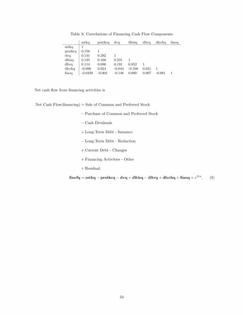
Table 9: Correlations of Financing Cash Flow Components

sstkq prstkcq dvq dltisq dltrq dlcchq fiaoq

sstkq 1prstkcq 0.156 1dvq 0.131 0.292 1dltisq 0.135 0.160 0.231 1dltrq 0.114 0.096 0.191 0.852 1dlcchq -0.096 0.024 -0.044 -0.108 0.021 1fiaoq -0.0430 -0.002 -0.146 0.000 0.007 -0.081 1

Net cash flow from financing activities is

Net Cash Flow(financing) = Sale of Common and Preferred Stock

− Purchase of Common and Preferred Stock

− Cash Dividends

+ Long-Term Debt - Issuance

− Long-Term Debt - Reduction

+ Current Debt - Changes

+ Financing Activities - Other

+ Residual.

fincfq = sstkq− prstkcq− dvq + dltisq− dltrq + dlcchq + fiaoq + εfin. (8)

34

References

Almeida, Heitor, Murillo Campello, and Michael S. Weisbach. 2004. “The Cash Flow Sensitivity of Cash.”

Journal of Finance 59(4): 1777–1804. ISSN 00221082.

Alti, Aydogan. 2003. “How Sensitive Is Investment to Cash Flow When Financing Is Frictionless?” Journal

of Finance 58(2): 707–722. ISSN 00221082.

Arslan, Ozgur, Chrisostomos Florackis, and Aydin Ozkan. 2010. “Financial Flexibility, Corporate Investment

and Performance.” SSRN eLibrary.

Baker, Malcolm, Jeremy C. Stein, and Jeffrey Wurgler. 2003. “When Does the Market Matter? Stock Prices

and the Investment of Equity-Dependent Firms.” Quarterly Journal of Economics 118(3): 969–1005. ISSN

00335533.

Bates, Thomas W., Kathleen M. Kahle, and Rene M. Stulz. 2006. “Why Do U.S. Firms Hold So Much More

Cash Than They Used To?” Working Paper 12534. National Bureau of Economic Research.

Bates, Thomas W., Kathleen M. Kahle, and Rene M. Stulz. 2009. “Why Do U.S. Firms Hold So Much More

Cash Than They Used To?” Journal of Finance 64(5): 1985–2021. ISSN 00221082.

Bernanke, Ben S. 2010. “Restoring the Flow of Credit to Small Businesses.” Remarks given at the Federal

Reserve Meeting Series: Addressing the Financing Needs of Small Businesses. Washington, DC, July 12

2010.

Bernanke, Ben S., and Cara S. Lown. 1991. “The Credit Crunch.” Brookings Papers on Economic Activity

1991(2): 205–247. ISSN 00072303.

Bhagat, Sanjai, Nathalie Moyen, and Inchul Suh. 2005. “Investment and Internal Funds of Distressed Firms.”

Journal of Corporate Finance 11(3): 449–472. ISSN 0929-1199. doi:DOI: 10.1016/j.jcorpfin.2004.09.002.

Cleary, Sean, Paul Povel, and Michael Raith. 2007. “The U-Shaped Investment Curve: Theory and Evi-

dence.” Journal of Financial and Quantitative Analysis 42(1): 1–39. ISSN 00221090.

Duchin, Ran. 2010. “Cash Holdings and Corporate Diversification.” Journal of Finance 65(3): 955–992.

ISSN 00221082.

Duchin, Ran, Oguzhan Ozbas, and Berk A. Sensoy. 2010. “Costly External Finance, Corporate Investment,

and the Subprime Mortgage Credit Crisis.” Journal of Financial Economics 97(3): 418–435. ISSN 0304-

405X. doi:DOI: 10.1016/j.jfineco.2009.12.008.

35

Duygen-Bump, Burcu, Alexey Levkov, and Judit Montoriol-Garriga. 2010. “Financing Constraints and

Unemployment: Evidence from the Great Recession.” Federal Reserve Bank of Boston Working Paper

No. QAU10-6.

Erickson, Timothy, and Toni M. Whited. 2000. “Measurement Error and the Relationship between Invest-

ment and ‘q’.” Journal of Political Economy 108(5): 1027–1057. ISSN 00223808.

Fazzari, Steven M., R. Glenn Hubbard, and Bruce C. Petersen. 1988. “Financing Constraints and Corporate

Investment.” Brookings Papers on Economic Activity 1988(1): 141–206. ISSN 00072303.

Gilchrist, Simon, and Charles P. Himmelberg. 1995. “Evidence on the Role of Cash Flow for Investment.”

Journal of Monetary Economics 36(3): 541–572. ISSN 03043923.

Gomes, Joao F. 2001. “Financing Investment.” American Economic Review 91(5): 1263–1285. ISSN

00028282.

Hubbard, R. Glenn, Anil K. Kashyap, and Toni M. Whited. 1995. “Internal Finance and Firm Investment.”

Journal of Money, Credit and Banking 27(3): 683–701. ISSN 00222879.

Kaplan, Steven N., and Luigi Zingales. 1997. “Do Investment-Cash Flow Sensitivities Provide Useful Mea-

sures of Financing Constraints?” The Quarterly Journal of Economics 112(1): 169–215. ISSN 00335533.

Opler, Tim, Lee Pinkowitz, Rene Stulz, and Rohan Williamson. 1999. “The Determinants and Implications

of Corporate Cash Holdings.” Journal of Financial Economics 52(1): 3–46. ISSN 0304-405X. doi:DOI:

10.1016/S0304-405X(99)00003-3.

Petersen, Mitchell A. 2009. “Estimating Standard Errors in Finance Panel Data Sets: Comparing Ap-

proaches.” 22(1): 435–480. doi:10.1093/rfs/hhn053.

36

Internal sources of finance and the Great Recession

Documents

Transcript of Internal sources of finance and the Great Recession