Oldeman, AM, Baatsen, MLJ, Von Der Heydt, AS, Dijkstra, H.

Oldeman, A. M., Baatsen, M. L. J., Von Der Heydt, A. S., Dijkstra, H.A., Tindall, J. C., Abe-ouchi, A., Booth, A. R., Brady, E. C., Chan, W.,Chandan, D., Chandler, M. A., Contoux, C., Feng, R., Guo, C.,Haywood, A. M., Hunter, S. J., Kamae, Y., Li, Q., Li, X., ... Williams, C.J. R. (2021). Reduced El Niño variability in the mid-Pliocene accordingto the PlioMIP2 ensemble. Climate of the Past, 17(6), 2427-2450.https://doi.org/10.5194/cp-17-2427-2021

Publisher's PDF, also known as Version of recordLicense (if available):CC BYLink to published version (if available):10.5194/cp-17-2427-2021

Link to publication record in Explore Bristol ResearchPDF-document

This is the final published version of the article (version of record). It first appeared online via Copernicus athttps://doi.org/10.5194/cp-17-2427-2021 .Please refer to any applicable terms of use of the publisher.

University of Bristol - Explore Bristol ResearchGeneral rights

This document is made available in accordance with publisher policies. Please cite only thepublished version using the reference above. Full terms of use are available:http://www.bristol.ac.uk/red/research-policy/pure/user-guides/ebr-terms/

https://doi.org/10.5194/cp-17-2427-2021

https://doi.org/10.5194/cp-17-2427-2021

https://research-information.bris.ac.uk/en/publications/94b124c7-dcb4-4037-8f95-28b520c931ab

https://research-information.bris.ac.uk/en/publications/94b124c7-dcb4-4037-8f95-28b520c931ab

Clim. Past, 17, 2427–2450, 2021https://doi.org/10.5194/cp-17-2427-2021© Author(s) 2021. This work is distributed underthe Creative Commons Attribution 4.0 License.

Reduced El Niño variability in the mid-Pliocene according to thePlioMIP2 ensembleArthur M. Oldeman1, Michiel L. J. Baatsen1, Anna S. von der Heydt1,2, Henk A. Dijkstra1,2, Julia C. Tindall3,Ayako Abe-Ouchi4, Alice R. Booth5, Esther C. Brady6, Wing-Le Chan4, Deepak Chandan7, Mark A. Chandler8,Camille Contoux9, Ran Feng10, Chuncheng Guo11, Alan M. Haywood3, Stephen J. Hunter3, Youichi Kamae12,Qiang Li13, Xiangyu Li14, Gerrit Lohmann15, Daniel J. Lunt16, Kerim H. Nisancioglu17,18, Bette L. Otto-Bliesner6,W. Richard Peltier7, Gabriel M. Pontes19, Gilles Ramstein9, Linda E. Sohl8, Christian Stepanek15, Ning Tan9,20,Qiong Zhang13, Zhongshi Zhang14, Ilana Wainer19, and Charles J. R. Williams16,21

1Institute for Marine and Atmospheric research Utrecht (IMAU), Department of Physics,Utrecht University, 3584 CC Utrecht, the Netherlands2Centre for Complex Systems Science, Utrecht University, 3584 CE Utrecht, the Netherlands3School of Earth and Environment, University of Leeds, Woodhouse Lane, Leeds, West Yorkshire, LS2 9JT, UK4Atmosphere and Ocean Research Institute, The University of Tokyo, Kashiwa, 277-8564, Japan5School of Ocean and Earth Science, University of Southampton, National Oceanography Centre, Southampton, UK6National Center for Atmospheric Research, (NCAR), Boulder, CO 80305, USA7Department of Physics, University of Toronto, Toronto, M5S 1A7, Canada8CCSR/GISS, Columbia University, New York, NY 10025, USA9Laboratoire des Sciences du Climat et de l’Environnement, LSCE/IPSL, CEA-CNRS-UVSQ Université Paris-Saclay,91191 Gif-sur-Yvette, France10Department of Geosciences, College of Liberal Arts and Sciences, University of Connecticut, Storrs, CT 06033, USA11NORCE Norwegian Research Centre, Bjerknes Centre for Climate Research, 5007 Bergen, Norway12Faculty of Life and Environmental Sciences, University of Tsukuba, Tsukuba, 305-8572, Japan13Department of Physical Geography and Bolin Centre for Climate Research, Stockholm University,Stockholm, 10691, Sweden14Department of Atmospheric Science, School of Environmental studies, China University of Geoscience,Wuhan 430074, China15Alfred-Wegener-Institut – Helmholtz-Zentrum für Polar and Meeresforschung (AWI), 27570 Bremerhaven, Germany16School of Geographical Sciences, University of Bristol, Bristol, BS8 1SS, UK17Bjerknes Centre for Climate Research, Department of Earth Science, University of Bergen, 5007 Bergen, Norway18Centre for Earth Evolution and Dynamics, University of Oslo, 0315 Oslo, Norway19Oceanographic Institute, University of São Paulo, 05508-120 São Paolo Brazil20Key Laboratory of Cenozoic Geology and Environment, Institute of Geology and Geophysics,Chinese Academy of Sciences, Beijing 100029, China21NCAS-Climate, Department of Meteorology, University of Reading, RG6 6ET Reading, UK

Correspondence: Arthur M. Oldeman ([email protected])

Received: 21 May 2021 – Discussion started: 3 June 2021Revised: 26 September 2021 – Accepted: 22 October 2021 – Published: 1 December 2021

Published by Copernicus Publications on behalf of the European Geosciences Union.

2428 A. M. Oldeman et al.: Pliocene ENSO

Abstract. The mid-Pliocene warm period (3.264–3.025 Ma)is the most recent geological period during which atmo-spheric CO2 levels were similar to recent historical val-ues (∼ 400 ppm). Several proxy reconstructions for the mid-Pliocene show highly reduced zonal sea surface tempera-ture (SST) gradients in the tropical Pacific Ocean, indicatingan El Niño-like mean state. However, past modelling stud-ies do not show these highly reduced gradients. Efforts tounderstand mid-Pliocene climate dynamics have led to thePliocene Model Intercomparison Project (PlioMIP). Resultsfrom the first phase (PlioMIP1) showed clear El Niño vari-ability (albeit significantly reduced) and did not show thegreatly reduced time-mean zonal SST gradient suggested bysome of the proxies.

In this work, we study El Niño–Southern Oscillation(ENSO) variability in the PlioMIP2 ensemble, which con-sists of additional global coupled climate models and updatedboundary conditions compared to PlioMIP1. We quantifyENSO amplitude, period, spatial structure and “flavour”, aswell as the tropical Pacific annual mean state in mid-Plioceneand pre-industrial simulations. Results show a reducedENSO amplitude in the model-ensemble mean (−24 %) withrespect to the pre-industrial, with 15 out of 17 individualmodels showing such a reduction. Furthermore, the spectralpower of this variability considerably decreases in the 3–4-year band. The spatial structure of the dominant empiricalorthogonal function shows no particular change in the pat-terns of tropical Pacific variability in the model-ensemblemean, compared to the pre-industrial. Although the time-mean zonal SST gradient in the equatorial Pacific decreasesfor 14 out of 17 models (0.2 ◦C reduction in the ensemblemean), there does not seem to be a correlation with the de-crease in ENSO amplitude. The models showing the most“El Niño-like” mean state changes show a similar ENSO am-plitude to that in the pre-industrial reference, while modelsshowing more “La Niña-like” mean state changes generallyshow a large reduction in ENSO variability. The PlioMIP2results show a reasonable agreement with both time-meanproxies indicating a reduced zonal SST gradient and recon-structions indicating a reduced, or similar, ENSO variability.

1 Introduction

The mid-Piacenzian or mid-Pliocene warm period (mPWP,3.264–3.025 Ma) was a recent geological interval of sus-tained warmth with global mean temperatures 2–5 ◦C higherthan the pre-industrial (Haywood et al., 2010; Dowsett et al.,2010, 2016; Haywood et al., 2020). Atmospheric CO2 lev-els were ∼ 400 ppm (Badger et al., 2013; Fedorov et al.,2013; Haywood et al., 2016a; de la Vega et al., 2020), sim-ilar to values of the early 21st century. This makes this pe-riod an interesting case study for our near-future climate,also because the mid-Pliocene had a similar geography tothe present (outside of ice-sheet regions). Efforts to under-

stand the mPWP climate have been ongoing for more than25 years and led to the coordination of the Pliocene Mod-elling Intercomparison Project (PlioMIP) phase 1 in 2010(Haywood et al., 2010). The PlioMIP1 ensemble shows arange of global mean surface temperature anomalies, eventhough the models have nearly identical boundary condi-tions. Furthermore, comparison with proxies highlights thatmost models underestimate polar amplification (Haywoodet al., 2013). The PlioMIP phase 2 was initiated to further un-derstand the mPWP climate and more specifically designedto reduce uncertainties in model boundary conditions and inproxy data reconstruction (Haywood et al., 2016a, 2020). Itemploys boundary conditions from the Pliocene Research,Interpretation and Synoptic Mapping (PRISM) version 4, in-cluding updated reconstructions of ocean bathymetry andland-ice surface topography, as well as Pliocene soils andlakes (Dowsett et al., 2016; Haywood et al., 2016a). ThePlioMIP2 simulations are specifically tuned to the KM5c in-terglacial (3.205 Ma), a time slice within the mPWP with or-bital parameters close to the present-day configuration. Im-portant changes in boundary conditions compared to the ex-perimental design of PlioMIP1 include the closure of theCanadian Archipelago and the Bering Strait, and the shoalingof the Sahul and Sunda shelves. The PlioMIP2 global aver-age, annual mean surface air temperature (SAT) increase is1.7–5.2 ◦C (3.3 ◦C in the ensemble mean) compared to thepre-industrial, when implementing PRISM4 boundary con-ditions in PlioMIP2 (Haywood et al., 2020; Williams et al.,2021).

One of the more perplexing and still unanswered topics inthe Pliocene research community is the behaviour of tropicalPacific variability in the mid-Pliocene, in particular of the ElNiño–Southern Oscillation (ENSO). In the present-day cli-mate, ENSO is the most prominent mode of variability oninterannual timescales. It has its origin in the tropical Pacific,while having teleconnections to many regions in the world(Philander, 1990). The ENSO phenomenon can be explainedas an internally generated mode of variability of the coupledequatorial ocean–atmosphere system – either self-sustainedor excited by random noise (Fedorov et al., 2003). The back-ground climate such as meridional and zonal sea surface tem-perature (SST) gradients, vertical temperature gradients, andthe trade wind strength is thought to play an important rolein the properties of this internal mode of variability. A re-cent review by Cai et al. (2021) shows that ENSO-relatedSST variability has increased in the past decades and is pro-jected to increase further under future greenhouse warming.However, many of these findings are strongly influenced byinternal variability and interactions with the mean state, andthere is by no means a consensus on many aspects of past aswell as future ENSO behaviour (IPCC, 2021). It is thereforean interesting issue to study ENSO variability in the warmconditions of the mid-Pliocene.

Early proxy reconstructions indicated that the mid-Pliocene tropical Pacific may have highly reduced zonal SST

Clim. Past, 17, 2427–2450, 2021 https://doi.org/10.5194/cp-17-2427-2021

A. M. Oldeman et al.: Pliocene ENSO 2429

gradients (Molnar and Cane, 2002; Wara et al., 2005; Raveloet al., 2006). This pointed in the direction of an “El Niño-like” mean state in the mid-Pliocene, and it was even sug-gested that there might be a “permanent El Niño” withoutany interannual variability around that state (Fedorov et al.,2006). The coarse temporal resolution and choice of calibra-tion of ocean sediment proxy reconstructions make it chal-lenging to say anything about such variability. Because ofthis, even a “La Niña-like” mean state has been proposedfor the mPWP (Rickaby and Halloran, 2005). Scroxton et al.(2011) present evidence for clear ENSO variability in thePliocene based on ocean sediment isotopes, possibly despitereduced zonal SST gradients. Watanabe et al. (2011) presentcoral skeleton data showing ENSO variability that is sim-ilar to that of the present day. Mg/Ca measurements indi-cating subsurface temperatures in the western equatorial Pa-cific again point towards a reduced zonal temperature gra-dient (Ford et al., 2015), while more recent alkenone proxyreconstructions show a moderate reduction in the tropical Pa-cific zonal SST gradient (Tierney et al., 2019). The latestproxy reconstructions by White and Ravelo (2020) show thatthe mid-Pliocene ENSO amplitude varied between reducedand similar to the present day, and they associate that with aweaker thermocline feedback.

The earliest modelling studies on the early Pliocene andmid-Pliocene ENSO are in favour of the “permanent ElNiño”, when using idealized experiments with ocean-onlyor forced atmosphere GCMs (Fedorov et al., 2006; Bar-reiro et al., 2006). However, later studies using a coupledatmosphere–ocean GCM (Haywood et al., 2007; Bonhamet al., 2009) and using a Zebiak–Cane model (von der Heydtet al., 2011) clearly resolved ENSO-like interannual variabil-ity. While most modelling studies show (slightly) reducedzonal SST gradients, a study using the Zebiak–Cane modelof the tropical Pacific suggests a westward shift in the posi-tion of the “cold tongue” (CT) under increased backgroundtemperatures, whereas a weaker zonal SST gradient wouldbe mostly associated with weaker background trade winds(von der Heydt et al., 2011). Later, in the coordinated mod-elling efforts of PlioMIP1, all models show ENSO-like vari-ability, and eight out of nine studies agree on a reducedENSO variability compared to the pre-industrial (Brierley,2015), although the magnitude of reduction varies consider-ably among different models. This robustly weaker ENSO isaccompanied by a shift to lower frequencies (i.e. longer peri-ods) in most models, while again the magnitude of the domi-nant frequency varies among the model ensemble. Moreover,the PlioMIP1 models do not show a consistent reduction inthe mean zonal SST gradient, and a clear reason for weakerENSO variability is not found. Research with the HadCM3model has pointed out the importance of centennial-scalevariability in ENSO behaviour, suggesting there could haveexisted periods with both weaker and stronger ENSO vari-ability in the mid-Pliocene (Tindall et al., 2016).

Modelling efforts on past as well as future climates showdifferent responses of ENSO variability to radiative and ge-ographical forcings. Collins et al. (2010) show that from theCMIP3 ensemble, it is not possible to determine whether theamplitude and frequency of ENSO variability will change inthe future under climate change. Also the more recent CMIP5ensemble provides no clear consensus on whether ENSO am-plitude would decrease or increase in the future, and whatfeedbacks might change (Kim et al., 2014). However, Caiet al. (2014) do suggest a shift to higher ENSO frequen-cies under global warming based on the CMIP5 ensemble.The latest studies with the CMIP6 ensemble still show am-biguous results regarding ENSO amplitude, with Fredriksenet al. (2020) suggesting a slight increase under future scenar-ios while Beobide-Arsuaga et al. (2021) suggest no change,employing slightly different methods. Moreover, Fredriksenet al. (2020) show that, interestingly, the increase in El NiñoSST variability is linked to a decrease in the zonal SST gradi-ent in the tropical Pacific. Idealized warming experiments byCallahan et al. (2021) show a robust decrease in ENSO am-plitude in the long term. Yeh et al. (2009) and Ashok and Ya-magata (2009) show that the “flavour” of El Niño will changein the future, shifting from mainly cold tongue El Niño eventsto more “warm pool” (WP) El Niño events, implying thatthe largest temperature variations will shift more towardsthe central Pacific. However, recent work using CMIP5 andCMIP6 data does not necessarily agree with this, showingthat changes in El Niño flavour are model-dependent (Fre-und et al., 2020). When reproducing the climate in recentdecades, climate models suggest a reduced zonal SST gradi-ent in the tropical Pacific due to rising greenhouse gas con-centrations, while observations show a strengthened gradi-ent (Coats and Karnauskas, 2017). This discrepancy betweencoupled models and observations is attributed to the coldbias in the equatorial cold tongue by Seager et al. (2019).However, Heede et al. (2020) show that the initial transientresponse to CO2 forcing is characterized by a strengthenedzonal SST gradient, while the equilibrium response shows awarmer cold tongue. Jiang et al. (2021) show that this coldbias reduces in the CMIP6 ensemble, when comparing withCMIP5, but still exists. Brown et al. (2020) investigate ENSOboth in the mid-Holocene, last glacial maximum (lgm) andlast interglacial (lig) simulations of PMIP3/4 and idealizedwarming experiments of CMIP5/6. They find a clear de-crease in ENSO variability in the lig and mid-Holocene sim-ulations, despite a stronger zonal SST gradient. Closer in-spection demonstrates no clear correlation between the meanzonal SST gradient in the tropical Pacific and ENSO ampli-tude, when considering the PMIP3/4 and CMIP5/6 ensem-bles.

While the PlioMIP1 ensemble was able to adequately re-produce many of the spatial patterns in surface temperatureas reconstructed from proxies, a number of uncertainties andmodel–data mismatches remained, in particular regarding thewarming in high latitudes (Haywood et al., 2013). High-

https://doi.org/10.5194/cp-17-2427-2021 Clim. Past, 17, 2427–2450, 2021


latitude temperatures clearly also affect the tropical climate,for example through effects on the Hadley Cell and trade-wind strength caused by an altered Equator-to-pole temper-ature gradient. In order to reduce uncertainties and model–data mismatches, a completely new reconstruction of palaeo-geography was used in PlioMIP2 as boundary condition forthe models. Analysis of large-scale features of the ensem-ble by Haywood et al. (2020) shows a larger SAT anomalycompared to PlioMIP1, because of the inclusion of moremodels with a higher equilibrium climate sensitivity (ECS).It is also shown that the ensemble mean SSTs agree wellwith newly reconstructed SST proxies by Foley and Dowsett(2019). The PlioMIP2 ensemble also agrees well with recon-structions from a recent SST synthesis study focusing on thesame mid-Pliocene time slice (McClymont et al., 2020).

In this work, we study changes in ENSO variability in thePlioMIP2 ensemble compared to the pre-industrial and re-late this to differences in the mean background climate of thetropical Pacific. In Sect. 2, we briefly introduce the modelsthat participate in the PlioMIP2 ensemble and describe themethods used to analyse ENSO. Following this, we inves-tigate ENSO variability in PlioMIP2 in terms of amplitude,frequency, spatial structure and “flavour” and compare this topre-industrial reference simulations in Sect. 3.1. Next, we in-vestigate the relation between ENSO amplitude and the meanzonal SST gradient and study whether the tropical Pacificmean state is El Niño-like in the mid-Pliocene, in Sect. 3.2.In Sect. 4, the results are discussed by comparing them withobservational data as well as highlighting intermodel differ-ences within the ensemble. We conclude with a summary andoutlook.

2 Methods

2.1 The PlioMIP2 ensemble

A total of 17 climate models form the PlioMIP2 ensemble,which is almost double the size of the PlioMIP1 ensemble. Alist of the models, performing institute and reference to thework describing the individual models in more detail is pre-sented in Table 1. All models have performed simulationsfollowing the PlioMIP2 experimental protocol (Haywoodet al., 2016b), providing both the pre-industrial control exper-iment (E280) and the mid-Pliocene experiment (Eoi400) data.Pre-industrial simulations are forced with∼ 280 ppmv atmo-spheric CO2 concentrations. The mid-Pliocene simulationsare forced with 400 ppmv CO2 and all models apart fromHadGEM3 use significantly different geographic boundaryconditions, including closed Arctic Ocean gateways (BeringStrait, Canadian archipelago) and reduced land ice coverage(Greenland ice sheet, West Antarctic ice sheet). Results ofseveral large-scale features, such as global mean surface airtemperature (SAT), polar amplification factor and equilib-rium climate sensitivity (ECS) of the PlioMIP2 ensemble,are presented in Haywood et al. (2020). Note that the results

of the HadGEM3 model were not included in that paper, asthe simulations finished after the time of writing. Details forHadGEM3 can be found in Williams et al. (2021). More de-tails on the Eoi400 simulations of the individual models canbe found in the references listed in Table 1.

Each modelling group has provided (at least) 100 years ofboth the E280 and Eoi400 simulation for analysis. In this work,we consider the last 100 years of monthly SST data in orderto quantify and investigate ENSO variability. In the Supple-ment, we discuss the robustness of our analysis methods us-ing the results of two ensemble members, using 500 yearsof data. Data were regridded onto a regular 1◦× 1◦ grid us-ing a bilinear interpolation, in order to analyse the modelresults in the same way. Interpolating data on a commongrid could smooth out spatial variations and remove local ex-tremes, while it can also act to suppress certain unreliablegrid-box-scale features (Räisänen and Ylhäisi, 2011). Themajority of the models use a nominal horizontal ocean reso-lution that is close to 1◦. Some of the models employ a tele-scoping grid that results in a finer resolution near the Equator,such as IPSLCM6A-LR as well as CCSM4-Utr (∼ 0.33◦ and∼ 0.67◦, respectively). Since we are not interested in grid-box-scale features, and often considering spatial means aswell as ensemble means, we do not expect the regridding tosignificantly impact the results.

2.2 Analysis methods

2.2.1 Niño indices

The Niño 3.4 index, defined as the monthly SST anomaly inthe Niño 3.4 region in the equatorial Pacific, is most com-monly used in present-day ENSO analysis. It can be used todetermine the amplitude and period of ENSO variability. TheNiño 3.4 region is used since it shows the largest correlationwith SST variability in the whole tropical Pacific. However,the question remains as to whether this is also true for themid-Pliocene ENSO.

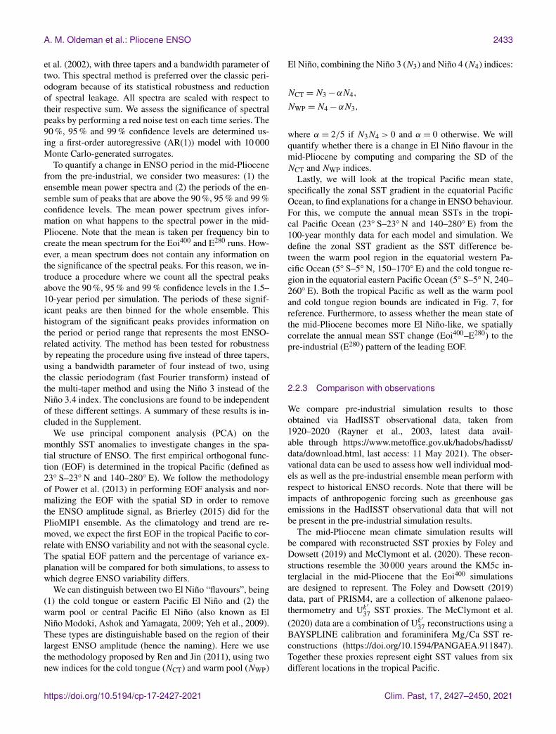
Figure 1 shows the standard deviation (SD) of the SSTanomalies in the tropical Pacific for (a) the pre-industrialE280 ensemble mean and (b) the mid-Pliocene Eoi400 ensem-ble mean. Indicated in the plot are the four commonly usedregions to study ENSO variability: the Niño 4, Niño 3.4,Niño 3 and Niño 1+2 regions. The magnitude of SST vari-ability decreases in the mid-Pliocene equatorial Pacific, butit seems that the region with the largest ENSO-related vari-ability keeps its position.

To determine the SST anomaly pattern with the largestvariance, we perform principal component analysis (PCA) onthe detrended monthly SST anomalies. As the climatology issubtracted, we expect the leading principal component (PC1)in the tropical Pacific to capture ENSO variability. We cor-relate the PC1 with the four different Niño indices to checkwhich region is representative for ENSO variability, both in



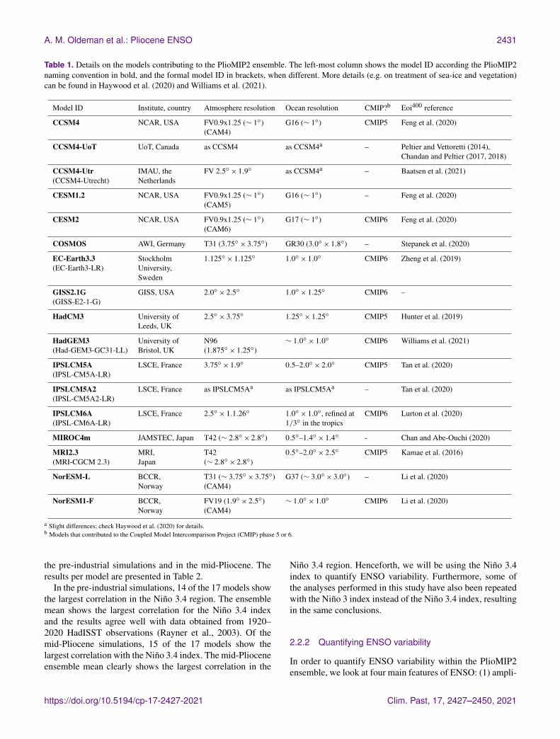
Table 1. Details on the models contributing to the PlioMIP2 ensemble. The left-most column shows the model ID according the PlioMIP2naming convention in bold, and the formal model ID in brackets, when different. More details (e.g. on treatment of sea-ice and vegetation)can be found in Haywood et al. (2020) and Williams et al. (2021).

Model ID Institute, country Atmosphere resolution Ocean resolution CMIP?b Eoi400 reference

CCSM4 NCAR, USA FV0.9x1.25 (∼ 1◦) G16 (∼ 1◦) CMIP5 Feng et al. (2020)(CAM4)

CCSM4-UoT UoT, Canada as CCSM4 as CCSM4a – Peltier and Vettoretti (2014),Chandan and Peltier (2017, 2018)

CCSM4-Utr IMAU, the FV 2.5◦× 1.9◦ as CCSM4a – Baatsen et al. (2021)(CCSM4-Utrecht) Netherlands

CESM1.2 NCAR, USA FV0.9x1.25 (∼ 1◦) G16 (∼ 1◦) – Feng et al. (2020)(CAM5)

CESM2 NCAR, USA FV0.9x1.25 (∼ 1◦) G17 (∼ 1◦) CMIP6 Feng et al. (2020)(CAM6)

COSMOS AWI, Germany T31 (3.75◦× 3.75◦) GR30 (3.0◦× 1.8◦) – Stepanek et al. (2020)

EC-Earth3.3 Stockholm 1.125◦× 1.125◦ 1.0◦× 1.0◦ CMIP6 Zheng et al. (2019)(EC-Earth3-LR) University,

Sweden

GISS2.1G GISS, USA 2.0◦× 2.5◦ 1.0◦× 1.25◦ CMIP6 –(GISS-E2-1-G)

HadCM3 University of 2.5◦× 3.75◦ 1.25◦× 1.25◦ CMIP5 Hunter et al. (2019)Leeds, UK

HadGEM3 University of N96 ∼ 1.0◦× 1.0◦ CMIP6 Williams et al. (2021)(Had-GEM3-GC31-LL) Bristol, UK (1.875◦× 1.25◦)

IPSLCM5A LSCE, France 3.75◦× 1.9◦ 0.5–2.0◦× 2.0◦ CMIP5 Tan et al. (2020)(IPSL-CM5A-LR)

IPSLCM5A2 LSCE, France as IPSLCM5Aa as IPSLCM5Aa – Tan et al. (2020)(IPSL-CM5A2-LR)

IPSLCM6A LSCE, France 2.5◦× 1.1.26◦ 1.0◦× 1.0◦, refined at CMIP6 Lurton et al. (2020)(IPSL-CM6A-LR) 1/3◦ in the tropics

MIROC4m JAMSTEC, Japan T42 (∼ 2.8◦× 2.8◦) 0.5◦–1.4◦× 1.4◦ - Chan and Abe-Ouchi (2020)

MRI2.3 MRI, T42 0.5◦–2.0◦× 2.5◦ CMIP5 Kamae et al. (2016)(MRI-CGCM 2.3) Japan (∼ 2.8◦× 2.8◦)

NorESM-L BCCR, T31 (∼ 3.75◦× 3.75◦) G37 (∼ 3.0◦× 3.0◦) – Li et al. (2020)Norway (CAM4)

NorESM1-F BCCR, FV19 (1.9◦× 2.5◦) ∼ 1.0◦× 1.0◦ CMIP6 Li et al. (2020)Norway (CAM4)

a Slight differences; check Haywood et al. (2020) for details.b Models that contributed to the Coupled Model Intercomparison Project (CMIP) phase 5 or 6.

the pre-industrial simulations and in the mid-Pliocene. Theresults per model are presented in Table 2.

In the pre-industrial simulations, 14 of the 17 models showthe largest correlation in the Niño 3.4 region. The ensemblemean shows the largest correlation for the Niño 3.4 indexand the results agree well with data obtained from 1920–2020 HadISST observations (Rayner et al., 2003). Of themid-Pliocene simulations, 15 of the 17 models show thelargest correlation with the Niño 3.4 index. The mid-Plioceneensemble mean clearly shows the largest correlation in the

Niño 3.4 region. Henceforth, we will be using the Niño 3.4index to quantify ENSO variability. Furthermore, some ofthe analyses performed in this study have also been repeatedwith the Niño 3 index instead of the Niño 3.4 index, resultingin the same conclusions.

2.2.2 Quantifying ENSO variability

In order to quantify ENSO variability within the PlioMIP2ensemble, we look at four main features of ENSO: (1) ampli-



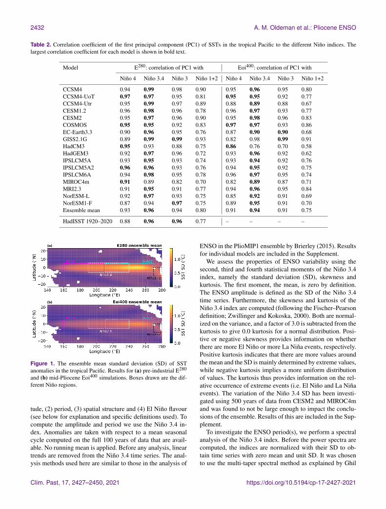
Table 2. Correlation coefficient of the first principal component (PC1) of SSTs in the tropical Pacific to the different Niño indices. Thelargest correlation coefficient for each model is shown in bold text.

Model E280: correlation of PC1 with Eoi400: correlation of PC1 with

Niño 4 Niño 3.4 Niño 3 Niño 1+2 Niño 4 Niño 3.4 Niño 3 Niño 1+2

CCSM4 0.94 0.99 0.98 0.90 0.95 0.96 0.95 0.80CCSM4-UoT 0.97 0.97 0.95 0.81 0.95 0.95 0.92 0.77CCSM4-Utr 0.95 0.99 0.97 0.89 0.88 0.89 0.88 0.67CESM1.2 0.96 0.98 0.96 0.78 0.96 0.97 0.93 0.77CESM2 0.95 0.97 0.96 0.90 0.95 0.98 0.96 0.83COSMOS 0.95 0.95 0.92 0.83 0.97 0.97 0.93 0.86EC-Earth3.3 0.90 0.96 0.95 0.76 0.87 0.90 0.90 0.68GISS2.1G 0.89 0.99 0.99 0.93 0.82 0.98 0.99 0.91HadCM3 0.95 0.93 0.88 0.75 0.86 0.76 0.70 0.58HadGEM3 0.92 0.97 0.96 0.72 0.93 0.96 0.92 0.62IPSLCM5A 0.93 0.95 0.93 0.74 0.93 0.94 0.92 0.76IPSLCM5A2 0.96 0.96 0.93 0.76 0.94 0.95 0.92 0.75IPSLCM6A 0.94 0.98 0.95 0.78 0.96 0.97 0.95 0.74MIROC4m 0.91 0.89 0.82 0.70 0.82 0.89 0.87 0.71MRI2.3 0.91 0.95 0.91 0.77 0.94 0.96 0.95 0.84NorESM-L 0.92 0.97 0.93 0.75 0.85 0.92 0.91 0.69NorESM1-F 0.87 0.94 0.97 0.75 0.89 0.95 0.91 0.70Ensemble mean 0.93 0.96 0.94 0.80 0.91 0.94 0.91 0.75

HadISST 1920–2020 0.88 0.96 0.96 0.77 – – – –

Figure 1. The ensemble mean standard deviation (SD) of SSTanomalies in the tropical Pacific. Results for (a) pre-industrial E280

and (b) mid-Pliocene Eoi400 simulations. Boxes drawn are the dif-ferent Niño regions.

tude, (2) period, (3) spatial structure and (4) El Niño flavour(see below for explanation and specific definitions used). Tocompute the amplitude and period we use the Niño 3.4 in-dex. Anomalies are taken with respect to a mean seasonalcycle computed on the full 100 years of data that are avail-able. No running mean is applied. Before any analysis, lineartrends are removed from the Niño 3.4 time series. The anal-ysis methods used here are similar to those in the analysis of

ENSO in the PlioMIP1 ensemble by Brierley (2015). Resultsfor individual models are included in the Supplement.

We assess the properties of ENSO variability using thesecond, third and fourth statistical moments of the Niño 3.4index, namely the standard deviation (SD), skewness andkurtosis. The first moment, the mean, is zero by definition.The ENSO amplitude is defined as the SD of the Niño 3.4time series. Furthermore, the skewness and kurtosis of theNiño 3.4 index are computed (following the Fischer–Pearsondefinition; Zwillinger and Kokoska, 2000). Both are normal-ized on the variance, and a factor of 3.0 is subtracted from thekurtosis to give 0.0 kurtosis for a normal distribution. Posi-tive or negative skewness provides information on whetherthere are more El Niño or more La Niña events, respectively.Positive kurtosis indicates that there are more values aroundthe mean and the SD is mainly determined by extreme values,while negative kurtosis implies a more uniform distributionof values. The kurtosis thus provides information on the rel-ative occurrence of extreme events (i.e. El Niño and La Niñaevents). The variation of the Niño 3.4 SD has been investi-gated using 500 years of data from CESM2 and MIROC4mand was found to not be large enough to impact the conclu-sions of the ensemble. Results of this are included in the Sup-plement.

To investigate the ENSO period(s), we perform a spectralanalysis of the Niño 3.4 index. Before the power spectra arecomputed, the indices are normalized with their SD to ob-tain time series with zero mean and unit SD. It was chosento use the multi-taper spectral method as explained by Ghil



et al. (2002), with three tapers and a bandwidth parameter oftwo. This spectral method is preferred over the classic peri-odogram because of its statistical robustness and reductionof spectral leakage. All spectra are scaled with respect totheir respective sum. We assess the significance of spectralpeaks by performing a red noise test on each time series. The90 %, 95 % and 99 % confidence levels are determined us-ing a first-order autoregressive (AR(1)) model with 10 000Monte Carlo-generated surrogates.

To quantify a change in ENSO period in the mid-Pliocenefrom the pre-industrial, we consider two measures: (1) theensemble mean power spectra and (2) the periods of the en-semble sum of peaks that are above the 90 %, 95 % and 99 %confidence levels. The mean power spectrum gives infor-mation on what happens to the spectral power in the mid-Pliocene. Note that the mean is taken per frequency bin tocreate the mean spectrum for the Eoi400 and E280 runs. How-ever, a mean spectrum does not contain any information onthe significance of the spectral peaks. For this reason, we in-troduce a procedure where we count all the spectral peaksabove the 90 %, 95 % and 99 % confidence levels in the 1.5–10-year period per simulation. The periods of these signif-icant peaks are then binned for the whole ensemble. Thishistogram of the significant peaks provides information onthe period or period range that represents the most ENSO-related activity. The method has been tested for robustnessby repeating the procedure using five instead of three tapers,using a bandwidth parameter of four instead of two, usingthe classic periodogram (fast Fourier transform) instead ofthe multi-taper method and using the Niño 3 instead of theNiño 3.4 index. The conclusions are found to be independentof these different settings. A summary of these results is in-cluded in the Supplement.

We use principal component analysis (PCA) on themonthly SST anomalies to investigate changes in the spa-tial structure of ENSO. The first empirical orthogonal func-tion (EOF) is determined in the tropical Pacific (defined as23◦ S–23◦ N and 140–280◦ E). We follow the methodologyof Power et al. (2013) in performing EOF analysis and nor-malizing the EOF with the spatial SD in order to removethe ENSO amplitude signal, as Brierley (2015) did for thePlioMIP1 ensemble. As the climatology and trend are re-moved, we expect the first EOF in the tropical Pacific to cor-relate with ENSO variability and not with the seasonal cycle.The spatial EOF pattern and the percentage of variance ex-planation will be compared for both simulations, to assess towhich degree ENSO variability differs.

We can distinguish between two El Niño “flavours”, being(1) the cold tongue or eastern Pacific El Niño and (2) thewarm pool or central Pacific El Niño (also known as ElNiño Modoki, Ashok and Yamagata, 2009; Yeh et al., 2009).These types are distinguishable based on the region of theirlargest ENSO amplitude (hence the naming). Here we usethe methodology proposed by Ren and Jin (2011), using twonew indices for the cold tongue (NCT) and warm pool (NWP)

El Niño, combining the Niño 3 (N3) and Niño 4 (N4) indices:

NCT =N3−αN4,

NWP =N4−αN3,

where α = 2/5 if N3N4 > 0 and α = 0 otherwise. We willquantify whether there is a change in El Niño flavour in themid-Pliocene by computing and comparing the SD of theNCT and NWP indices.

Lastly, we will look at the tropical Pacific mean state,specifically the zonal SST gradient in the equatorial PacificOcean, to find explanations for a change in ENSO behaviour.For this, we compute the annual mean SSTs in the tropi-cal Pacific Ocean (23◦ S–23◦ N and 140–280◦ E) from the100-year monthly data for each model and simulation. Wedefine the zonal SST gradient as the SST difference be-tween the warm pool region in the equatorial western Pa-cific Ocean (5◦ S–5◦ N, 150–170◦ E) and the cold tongue re-gion in the equatorial eastern Pacific Ocean (5◦ S–5◦ N, 240–260◦ E). Both the tropical Pacific as well as the warm pooland cold tongue region bounds are indicated in Fig. 7, forreference. Furthermore, to assess whether the mean state ofthe mid-Pliocene becomes more El Niño-like, we spatiallycorrelate the annual mean SST change (Eoi400–E280) to thepre-industrial (E280) pattern of the leading EOF.

2.2.3 Comparison with observations

We compare pre-industrial simulation results to thoseobtained via HadISST observational data, taken from1920–2020 (Rayner et al., 2003, latest data avail-able through https://www.metoffice.gov.uk/hadobs/hadisst/data/download.html, last access: 11 May 2021). The obser-vational data can be used to assess how well individual mod-els as well as the pre-industrial ensemble mean perform withrespect to historical ENSO records. Note that there will beimpacts of anthropogenic forcing such as greenhouse gasemissions in the HadISST observational data that will notbe present in the pre-industrial simulation results.

The mid-Pliocene mean climate simulation results willbe compared with reconstructed SST proxies by Foley andDowsett (2019) and McClymont et al. (2020). These recon-structions resemble the 30 000 years around the KM5c in-terglacial in the mid-Pliocene that the Eoi400 simulationsare designed to represent. The Foley and Dowsett (2019)data, part of PRISM4, are a collection of alkenone palaeo-thermometry and Uk

′

37 SST proxies. The McClymont et al.(2020) data are a combination of Uk

′

37 reconstructions using aBAYSPLINE calibration and foraminifera Mg/Ca SST re-constructions (https://doi.org/10.1594/PANGAEA.911847).Together these proxies represent eight SST values from sixdifferent locations in the tropical Pacific.


https://www.metoffice.gov.uk/hadobs/hadisst/data/download.html

https://www.metoffice.gov.uk/hadobs/hadisst/data/download.html

https://doi.org/10.1594/PANGAEA.911847


3 Results

3.1 ENSO variability

3.1.1 Statistical moments

Figure 2 shows the SD, skewness and kurtosis for all mod-els with respect to their pre-industrial values. The ensemblemean is also shown in the plots, and the HadISST obser-vational data are included as reference. Individual Niño 3.4index time series for all ensemble members are included inFig. S1 in the Supplement.

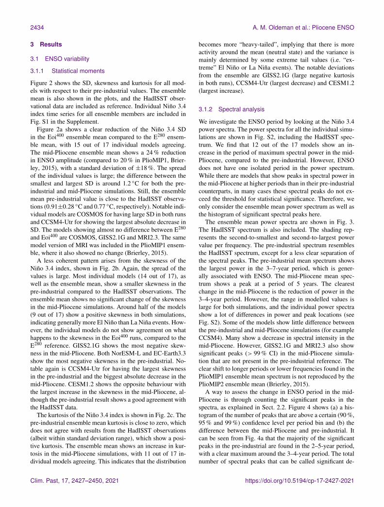
Figure 2a shows a clear reduction of the Niño 3.4 SDin the Eoi400 ensemble mean compared to the E280 ensem-ble mean, with 15 out of 17 individual models agreeing.The mid-Pliocene ensemble mean shows a 24 % reductionin ENSO amplitude (compared to 20 % in PlioMIP1, Brier-ley, 2015), with a standard deviation of ±18 %. The spreadof the individual values is large; the difference between thesmallest and largest SD is around 1.2 ◦C for both the pre-industrial and mid-Pliocene simulations. Still, the ensemblemean pre-industrial value is close to the HadISST observa-tions (0.91±0.28 ◦C and 0.77 ◦C, respectively). Notable indi-vidual models are COSMOS for having large SD in both runsand CCSM4-Utr for showing the largest absolute decrease inSD. The models showing almost no difference between E280

and Eoi400 are COSMOS, GISS2.1G and MRI2.3. The samemodel version of MRI was included in the PlioMIP1 ensem-ble, where it also showed no change (Brierley, 2015).

A less coherent pattern arises from the skewness of theNiño 3.4 index, shown in Fig. 2b. Again, the spread of thevalues is large. Most individual models (14 out of 17), aswell as the ensemble mean, show a smaller skewness in thepre-industrial compared to the HadISST observations. Theensemble mean shows no significant change of the skewnessin the mid-Pliocene simulations. Around half of the models(9 out of 17) show a positive skewness in both simulations,indicating generally more El Niño than La Niña events. How-ever, the individual models do not show agreement on whathappens to the skewness in the Eoi400 runs, compared to theE280 reference. GISS2.1G shows the most negative skew-ness in the mid-Pliocene. Both NorESM-L and EC-Earth3.3show the most negative skewness in the pre-industrial. No-table again is CCSM4-Utr for having the largest skewnessin the pre-industrial and the biggest absolute decrease in themid-Pliocene. CESM1.2 shows the opposite behaviour withthe largest increase in the skewness in the mid-Pliocene, al-though the pre-industrial result shows a good agreement withthe HadISST data.

The kurtosis of the Niño 3.4 index is shown in Fig. 2c. Thepre-industrial ensemble mean kurtosis is close to zero, whichdoes not agree with results from the HadISST observations(albeit within standard deviation range), which show a posi-tive kurtosis. The ensemble mean shows an increase in kur-tosis in the mid-Pliocene simulations, with 11 out of 17 in-dividual models agreeing. This indicates that the distribution

becomes more “heavy-tailed”, implying that there is moreactivity around the mean (neutral state) and the variance ismainly determined by some extreme tail values (i.e. “ex-treme” El Niño or La Niña events). The notable deviationsfrom the ensemble are GISS2.1G (large negative kurtosisin both runs), CCSM4-Utr (largest decrease) and CESM1.2(largest increase).

3.1.2 Spectral analysis

We investigate the ENSO period by looking at the Niño 3.4power spectra. The power spectra for all the individual simu-lations are shown in Fig. S2, including the HadISST spec-trum. We find that 12 out of the 17 models show an in-crease in the period of maximum spectral power in the mid-Pliocene, compared to the pre-industrial. However, ENSOdoes not have one isolated period in the power spectrum.While there are models that show peaks in spectral power inthe mid-Pliocene at higher periods than in their pre-industrialcounterparts, in many cases these spectral peaks do not ex-ceed the threshold for statistical significance. Therefore, weonly consider the ensemble mean power spectrum as well asthe histogram of significant spectral peaks here.

The ensemble mean power spectra are shown in Fig. 3.The HadISST spectrum is also included. The shading rep-resents the second-to-smallest and second-to-largest powervalue per frequency. The pre-industrial spectrum resemblesthe HadISST spectrum, except for a less clear separation ofthe spectral peaks. The pre-industrial mean spectrum showsthe largest power in the 3–7-year period, which is gener-ally associated with ENSO. The mid-Pliocene mean spec-trum shows a peak at a period of 5 years. The clearestchange in the mid-Pliocene is the reduction of power in the3–4-year period. However, the range in modelled values islarge for both simulations, and the individual power spectrashow a lot of differences in power and peak locations (seeFig. S2). Some of the models show little difference betweenthe pre-industrial and mid-Pliocene simulations (for exampleCCSM4). Many show a decrease in spectral intensity in themid-Pliocene. However, GISS2.1G and MRI2.3 also showsignificant peaks (> 99 % CI) in the mid-Pliocene simula-tion that are not present in the pre-industrial reference. Theclear shift to longer periods or lower frequencies found in thePlioMIP1 ensemble mean spectrum is not reproduced by thePlioMIP2 ensemble mean (Brierley, 2015).

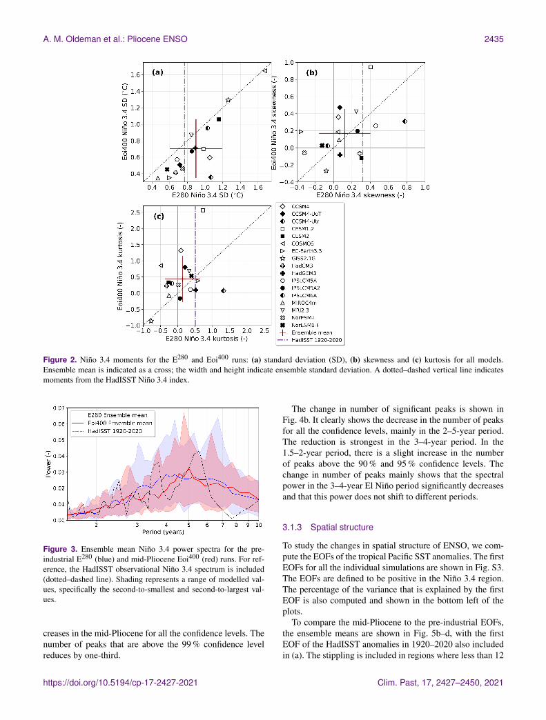
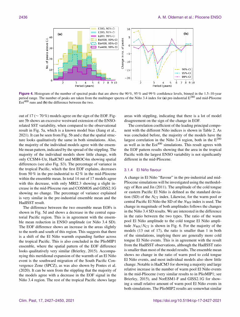
A way to assess the change in ENSO period in the mid-Pliocene is through counting the significant peaks in thespectra, as explained in Sect. 2.2. Figure 4 shows (a) a his-togram of the number of peaks that are above a certain (90 %,95 % and 99 %) confidence level per period bin and (b) thedifference between the mid-Pliocene and pre-industrial. Itcan be seen from Fig. 4a that the majority of the significantpeaks in the pre-industrial are found in the 2–5-year period,with a clear maximum around the 3–4-year period. The totalnumber of spectral peaks that can be called significant de-



Figure 2. Niño 3.4 moments for the E280 and Eoi400 runs: (a) standard deviation (SD), (b) skewness and (c) kurtosis for all models.Ensemble mean is indicated as a cross; the width and height indicate ensemble standard deviation. A dotted–dashed vertical line indicatesmoments from the HadISST Niño 3.4 index.

Figure 3. Ensemble mean Niño 3.4 power spectra for the pre-industrial E280 (blue) and mid-Pliocene Eoi400 (red) runs. For ref-erence, the HadISST observational Niño 3.4 spectrum is included(dotted–dashed line). Shading represents a range of modelled val-ues, specifically the second-to-smallest and second-to-largest val-ues.

creases in the mid-Pliocene for all the confidence levels. Thenumber of peaks that are above the 99 % confidence levelreduces by one-third.

The change in number of significant peaks is shown inFig. 4b. It clearly shows the decrease in the number of peaksfor all the confidence levels, mainly in the 2–5-year period.The reduction is strongest in the 3–4-year period. In the1.5–2-year period, there is a slight increase in the numberof peaks above the 90 % and 95 % confidence levels. Thechange in number of peaks mainly shows that the spectralpower in the 3–4-year El Niño period significantly decreasesand that this power does not shift to different periods.

3.1.3 Spatial structure

To study the changes in spatial structure of ENSO, we com-pute the EOFs of the tropical Pacific SST anomalies. The firstEOFs for all the individual simulations are shown in Fig. S3.The EOFs are defined to be positive in the Niño 3.4 region.The percentage of the variance that is explained by the firstEOF is also computed and shown in the bottom left of theplots.

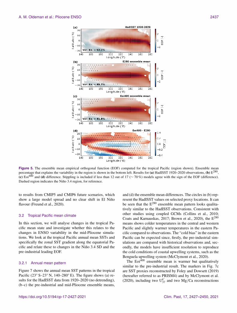
To compare the mid-Pliocene to the pre-industrial EOFs,the ensemble means are shown in Fig. 5b–d, with the firstEOF of the HadISST anomalies in 1920–2020 also includedin (a). The stippling is included in regions where less than 12



Figure 4. Histogram of the number of spectral peaks that are above the 90 %, 95 % and 99 % confidence levels, binned in the 1.5–10-yearperiod range. The number of peaks are taken from the multitaper spectra of the Niño 3.4 index for (a) pre-industrial E280 and mid-PlioceneEoi400 runs and (b) the difference between the two.

out of 17 (∼ 70 %) models agree on the sign of the EOF. Fig-ure 5b shows an excessive westward extension of the ENSO-related SST variability, when compared to the observationalresult in Fig. 5a, which is a known model bias (Jiang et al.,2021). It can be seen from Fig. 5b and c that the spatial struc-ture looks qualitatively the same in both simulations. Also,the majority of the individual models agree with the ensem-ble mean pattern, indicated by the spread of the stippling. Themajority of the individual models show little change, withonly CCSM4-Utr, HadCM3 and MIROC4m showing spatialdifferences (see also Fig. S3). The percentage of variance inthe tropical Pacific, which the first EOF explains, decreasesfrom 50 % in the pre-industrial to 42 % in the mid-Pliocenewithin the ensemble mean. In total 14 out of 17 models agreewith this decrease, with only MRI2.3 showing a slight in-crease in the mid-Pliocene run and COSMOS and GISS2.1Gshowing no change. The percentage of variance explainedis very similar in the pre-industrial ensemble mean and theHadISST result.

The difference between the two ensemble mean EOFs isshown in Fig. 5d and shows a decrease in the central equa-torial Pacific region. This is in agreement with the ensem-ble mean reduction in ENSO amplitude (or Niño 3.4 SD).The EOF difference shows an increase in the areas slightlyto the north and south of this region. This suggests that thereis a shift of the El Niño warmth expanding further acrossthe tropical Pacific. This is also concluded in the PlioMIP1ensemble, where the spatial pattern of the EOF differencelooks qualitatively very similar (Brierley, 2015). Accompa-nying this meridional expansion of the warmth of an El Niñoevent is the southward migration of the South Pacific Con-vergence Zone (SPCZ), as was also shown by Pontes et al.(2020). It can be seen from the stippling that the majority ofthe models agree with a decrease in the EOF signal in theNiño 3.4 region. The rest of the tropical Pacific shows large

areas with stippling, indicating that there is a lot of modeldisagreement on the sign of the change in EOF.

The correlation coefficient of the leading principal compo-nent with the different Niño indices is shown in Table 2. Aswas concluded before, the majority of the models have thelargest correlation in the Niño 3.4 region, both in the E280

as well as in the Eoi400 simulations. This result agrees withthe EOF pattern results showing that the area in the tropicalPacific with the largest ENSO variability is not significantlydifferent in the mid-Pliocene.

3.1.4 El Niño flavour

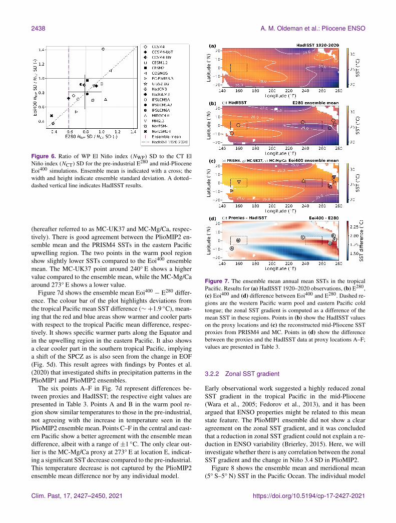
A change in El Niño “flavour” in the pre-industrial and mid-Pliocene simulations will be investigated using the methodol-ogy of Ren and Jin (2011). The amplitude of the cold tongueor eastern Pacific El Niño is defined as the standard devia-tion (SD) of the NCT index. Likewise, for the warm pool orcentral Pacific El Niño the SD of the NWP index is used. Thechange in magnitude of both amplitudes follows the changesin the Niño 3.4 SD results. We are interested in the differencein the ratio between the two types. The ratio of the warmpool El Niño amplitude to the cold tongue El Niño ampli-tude NWP/NCT is shown in Fig. 6. For the majority of themodels (13 out of 17), the ratio is smaller than 1 in bothof the simulations, implying there are generally more coldtongue El Niño events. This is in agreement with the resultfrom the HadISST observations, although the HadISST ratiois smaller than most of the model results. The ensemble meanshows no change in the ratio of warm pool to cold tongueEl Niño events, and most individual models also show littlechange. Notable is HadCM3 for showing a majority and largerelative increase in the number of warm pool El Niño eventsin the mid-Pliocene (very similar results to in PlioMIP1; seeBrierley, 2015), and NorESM1-F and GISS2.1G for show-ing a small relative amount of warm pool El Niño events inboth simulations. The PlioMIP2 results are somewhat similar



Figure 5. The ensemble mean empirical orthogonal function (EOF) computed for the tropical Pacific (region shown). Ensemble meanpercentage that explains the variability in the region is shown in the bottom left. Results for (a) HadISST 1920–2020 observations, (b) E280,(c) Eoi400 and (d) difference. Stippling is included if less than 12 out of 17 (∼ 70 %) models agree with the sign of the EOF (difference).Dashed region indicates the Niño 3.4 region, for reference.

to results from CMIP5 and CMIP6 future scenarios, whichshow a large model spread and no clear shift in El Niñoflavour (Freund et al., 2020).

3.2 Tropical Pacific mean climate

In this section, we will analyse changes in the tropical Pa-cific mean state and investigate whether this relates to thechanges in ENSO variability in the mid-Pliocene simula-tions. We look at the tropical Pacific annual mean SSTs andspecifically the zonal SST gradient along the equatorial Pa-cific and relate these to changes in the Niño 3.4 SD and thepre-industrial leading EOF.

3.2.1 Annual mean pattern

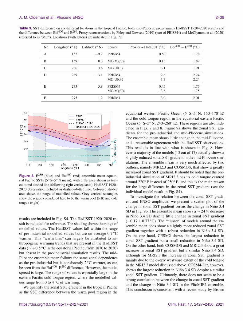
Figure 7 shows the annual mean SST patterns in the tropicalPacific (23◦ S–23◦ N, 140–280◦ E). The figure shows (a) re-sults for the HadISST data from 1920–2020 (no detrending),(b–c) the pre-industrial and mid-Pliocene ensemble means,

and (d) the ensemble mean differences. The circles in (b) rep-resent the HadISST values on selected proxy locations. It canbe seen that the E280 ensemble mean pattern looks qualita-tively similar to the HadISST observations. Consistent withother studies using coupled GCMs (Collins et al., 2010;Coats and Karnauskas, 2017; Brown et al., 2020), the E280

means shows colder temperatures in the central and westernPacific and slightly warmer temperatures in the eastern Pa-cific compared to observations. The “cold bias” in the easternPacific can be expected since, firstly, the pre-industrial sim-ulations are compared with historical observations and, sec-ondly, the models have insufficient resolution to reproducethe cold conditions of coastal upwelling systems, such as theBenguela upwelling system (McClymont et al., 2020).

The Eoi400 ensemble mean is warmer but qualitativelysimilar to the pre-industrial result. The markers in Fig. 7care SST proxies reconstructed by Foley and Dowsett (2019)(hereafter referred to as PRISM4) and by McClymont et al.(2020), including two Uk

′

37 and two Mg/Ca reconstructions



Figure 6. Ratio of WP El Niño index (NWP) SD to the CT ElNiño index (NCT) SD for the pre-industrial E280 and mid-PlioceneEoi400 simulations. Ensemble mean is indicated with a cross; thewidth and height indicate ensemble standard deviation. A dotted–dashed vertical line indicates HadISST results.

(hereafter referred to as MC-UK37 and MC-Mg/Ca, respec-tively). There is good agreement between the PlioMIP2 en-semble mean and the PRISM4 SSTs in the eastern Pacificupwelling region. The two points in the warm pool regionshow slightly lower SSTs compared to the Eoi400 ensemblemean. The MC-UK37 point around 240◦ E shows a highervalue compared to the ensemble mean, while the MC-Mg/Caaround 273◦ E shows a lower value.

Figure 7d shows the ensemble mean Eoi400− E280 differ-

ence. The colour bar of the plot highlights deviations fromthe tropical Pacific mean SST difference (∼+1.9 ◦C), mean-ing that the red and blue areas show warmer and cooler partswith respect to the tropical Pacific mean difference, respec-tively. It shows specific warmer parts along the Equator andin the upwelling region in the eastern Pacific. It also showsa clear cooler part in the southern tropical Pacific, implyinga shift of the SPCZ as is also seen from the change in EOF(Fig. 5d). This result agrees with findings by Pontes et al.(2020) that investigated shifts in precipitation patterns in thePlioMIP1 and PlioMIP2 ensembles.

The six points A–F in Fig. 7d represent differences be-tween proxies and HadISST; the respective eight values arepresented in Table 3. Points A and B in the warm pool re-gion show similar temperatures to those in the pre-industrial,not agreeing with the increase in temperature seen in thePlioMIP2 ensemble mean. Points C–F in the central and east-ern Pacific show a better agreement with the ensemble meandifference, albeit with a range of ±1 ◦C. The only clear out-lier is the MC-Mg/Ca proxy at 273◦ E at location E, indicat-ing a significant SST decrease compared to the pre-industrial.This temperature decrease is not captured by the PlioMIP2ensemble mean difference nor by any individual model.

Figure 7. The ensemble mean annual mean SSTs in the tropicalPacific. Results for (a) HadISST 1920–2020 observations, (b) E280,(c) Eoi400 and (d) difference between Eoi400 and E280. Dashed re-gions are the western Pacific warm pool and eastern Pacific coldtongue; the zonal SST gradient is computed as a difference of themean SST in these regions. Points in (b) show the HadISST valueson the proxy locations and (c) the reconstructed mid-Pliocene SSTproxies from PRISM4 and MC. Points in (d) show the differencebetween the proxies and the HadISST data at proxy locations A–F;values are presented in Table 3.

3.2.2 Zonal SST gradient

Early observational work suggested a highly reduced zonalSST gradient in the tropical Pacific in the mid-Pliocene(Wara et al., 2005; Fedorov et al., 2013), and it has beenargued that ENSO properties might be related to this meanstate feature. The PlioMIP1 ensemble did not show a clearagreement on the zonal SST gradient, and it was concludedthat a reduction in zonal SST gradient could not explain a re-duction in ENSO variability (Brierley, 2015). Here, we willinvestigate whether there is any correlation between the zonalSST gradient and the change in Niño 3.4 SD in PlioMIP2.

Figure 8 shows the ensemble mean and meridional mean(5◦ S–5◦ N) SST in the Pacific Ocean. The individual model



Table 3. SST difference on six different locations in the tropical Pacific, both mid-Pliocene proxy minus HadISST 1920–2020 results andthe difference between Eoi400 and E280. Proxy reconstructions by Foley and Dowsett (2019) (part of PRISM4) and McClymont et al. (2020)(referred to as “MC”). Locations (with letters) are indicated in Fig. 7d.

No. Longitude (◦ E) Latitude (◦ N) Source Proxies – HadISST (◦C) Eoi400− E280 (◦C)

A 152 −9.2 PRISM4 0.50 1.78

B 159 0.3 MC-Mg/Ca 0.13 1.89

C 236 3.8 MC-UK37 3.1 1.91

D 269 −3.1 PRISM4 2.6 2.24MC-UK37 1.7 2.24

E 273 5.8 PRISM4 0.45 1.75MC-Mg/Ca −3.6 1.75

F 275 1.2 PRISM4 3.0 2.01

Figure 8. E280 (blue) and Eoi400 (red) ensemble mean equato-rial Pacific SSTs (5◦ S–5◦ N mean), with difference shown as teal-coloured dashed line (following right vertical axis). HadISST 1920–2020 observation included as dashed–dotted line. Coloured shadedarea shows the range of modelled values. Grey vertical rectanglesshow the region considered here to be the warm pool (left) and coldtongue (right).

results are included in Fig. S4. The HadISST 1920–2020 re-sult is included for reference. The shading shows the range ofmodelled values. The HadISST values fall within the rangeof pre-industrial modelled values but are on average 0.7 ◦Cwarmer. This “warm bias” can largely be attributed to an-thropogenic warming trends that are present in the HadISSTdata (∼+0.5 ◦C in the equatorial Pacific, from 1870 to 2020)but absent in the pre-industrial simulation results. The mid-Pliocene ensemble mean follows the same zonal dependenceas the pre-industrial but is consistently 2 ◦C warmer, as canbe seen from the Eoi400–E280 difference. However, the modelspread is large. The range of values is especially large in theeastern Pacific cold tongue region, where the modelled val-ues range from 0 to 4 ◦C of warming.

We quantify the zonal SST gradient in the tropical Pacificas the SST difference between the warm pool region in the

equatorial western Pacific Ocean (5◦ S–5◦ N, 150–170◦ E)and the cold tongue region in the equatorial eastern PacificOcean (5◦ S–5◦ N, 240–260◦ E). These regions are also indi-cated in Figs. 7 and 8. Figure 9a shows the zonal SST gra-dients for the pre-industrial and mid-Pliocene simulations.The ensemble mean shows little change in the mid-Pliocene,and a reasonable agreement with the HadISST observations.This result is in line with what is shown in Fig. 8. How-ever, a majority of the models (13 out of 17) actually shows aslightly reduced zonal SST gradient in the mid-Pliocene sim-ulations. The ensemble mean is very much affected by twooutliers, namely MRI2.3 and COSMOS, that show a greatlyincreased zonal SST gradient. It should be noted that the pre-industrial simulation of MRI2.3 has its cold tongue centredaround 220◦ E instead of 250◦ E, and this is the main reasonfor the large difference in the zonal SST gradient (see theindividual model result in Fig. S4).

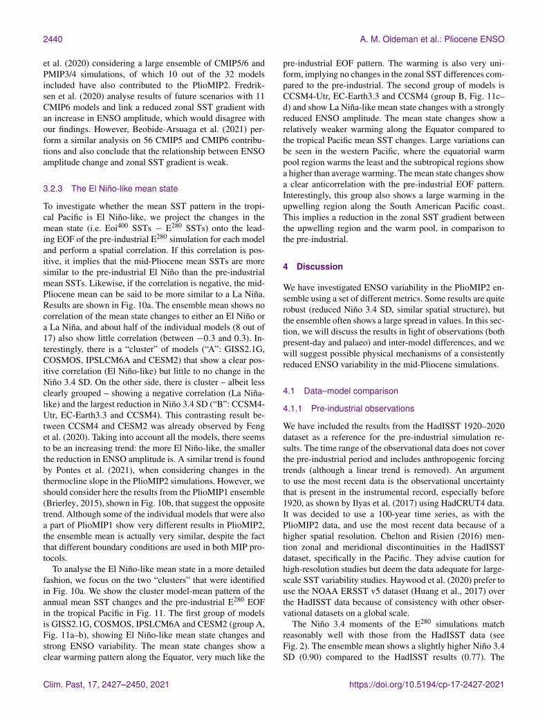
To investigate the relation between the zonal SST gradi-ent and ENSO amplitude, we present a scatter plot of thechange in zonal SST gradient versus the change in Niño 3.4SD in Fig. 9b. The ensemble mean shows a ∼ 24 % decreasein Niño 3.4 SD despite little change in zonal SST gradient(−0.17± 0.77 ◦C). The “cluster” of models around the en-semble mean does show a slightly more reduced zonal SSTgradient together with a robust reduction in Niño 3.4 SD.On the one hand, CESM2 shows the largest reduction inzonal SST gradient but a small reduction in Niño 3.4 SD.On the other hand, both COSMOS and MRI2.3 show a greatincrease in zonal SST gradient but a similar Niño 3.4 SD,although for MRI2.3 the increase in zonal SST gradient ismainly due to the overly westward extent of the cold tonguein the MRI2.3 model discussed above. CCSM4-Utr, however,shows the largest reduction in Niño 3.4 SD despite a similarzonal SST gradient. Ultimately, there does not seem to be astrong correlation between the change in zonal SST gradientand the change in Niño 3.4 SD in the PlioMIP2 ensemble.This conclusion is consistent with a recent study by Brown



et al. (2020) considering a large ensemble of CMIP5/6 andPMIP3/4 simulations, of which 10 out of the 32 modelsincluded have also contributed to the PlioMIP2. Fredrik-sen et al. (2020) analyse results of future scenarios with 11CMIP6 models and link a reduced zonal SST gradient withan increase in ENSO amplitude, which would disagree withour findings. However, Beobide-Arsuaga et al. (2021) per-form a similar analysis on 56 CMIP5 and CMIP6 contribu-tions and also conclude that the relationship between ENSOamplitude change and zonal SST gradient is weak.

3.2.3 The El Niño-like mean state

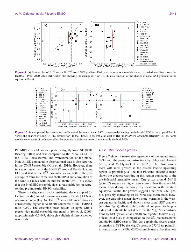
To investigate whether the mean SST pattern in the tropi-cal Pacific is El Niño-like, we project the changes in themean state (i.e. Eoi400 SSTs − E280 SSTs) onto the lead-ing EOF of the pre-industrial E280 simulation for each modeland perform a spatial correlation. If this correlation is pos-itive, it implies that the mid-Pliocene mean SSTs are moresimilar to the pre-industrial El Niño than the pre-industrialmean SSTs. Likewise, if the correlation is negative, the mid-Pliocene mean can be said to be more similar to a La Niña.Results are shown in Fig. 10a. The ensemble mean shows nocorrelation of the mean state changes to either an El Niño ora La Niña, and about half of the individual models (8 out of17) also show little correlation (between −0.3 and 0.3). In-terestingly, there is a “cluster” of models (“A”: GISS2.1G,COSMOS, IPSLCM6A and CESM2) that show a clear pos-itive correlation (El Niño-like) but little to no change in theNiño 3.4 SD. On the other side, there is cluster – albeit lessclearly grouped – showing a negative correlation (La Niña-like) and the largest reduction in Niño 3.4 SD (“B”: CCSM4-Utr, EC-Earth3.3 and CCSM4). This contrasting result be-tween CCSM4 and CESM2 was already observed by Fenget al. (2020). Taking into account all the models, there seemsto be an increasing trend: the more El Niño-like, the smallerthe reduction in ENSO amplitude is. A similar trend is foundby Pontes et al. (2021), when considering changes in thethermocline slope in the PlioMIP2 simulations. However, weshould consider here the results from the PlioMIP1 ensemble(Brierley, 2015), shown in Fig. 10b, that suggest the oppositetrend. Although some of the individual models that were alsoa part of PlioMIP1 show very different results in PlioMIP2,the ensemble mean is actually very similar, despite the factthat different boundary conditions are used in both MIP pro-tocols.

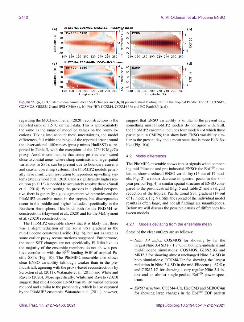
To analyse the El Niño-like mean state in a more detailedfashion, we focus on the two “clusters” that were identifiedin Fig. 10a. We show the cluster model-mean pattern of theannual mean SST changes and the pre-industrial E280 EOFin the tropical Pacific in Fig. 11. The first group of modelsis GISS2.1G, COSMOS, IPSLCM6A and CESM2 (group A,Fig. 11a–b), showing El Niño-like mean state changes andstrong ENSO variability. The mean state changes show aclear warming pattern along the Equator, very much like the

pre-industrial EOF pattern. The warming is also very uni-form, implying no changes in the zonal SST differences com-pared to the pre-industrial. The second group of models isCCSM4-Utr, EC-Earth3.3 and CCSM4 (group B, Fig. 11c–d) and show La Niña-like mean state changes with a stronglyreduced ENSO amplitude. The mean state changes show arelatively weaker warming along the Equator compared tothe tropical Pacific mean SST changes. Large variations canbe seen in the western Pacific, where the equatorial warmpool region warms the least and the subtropical regions showa higher than average warming. The mean state changes showa clear anticorrelation with the pre-industrial EOF pattern.Interestingly, this group also shows a large warming in theupwelling region along the South American Pacific coast.This implies a reduction in the zonal SST gradient betweenthe upwelling region and the warm pool, in comparison tothe pre-industrial.

4 Discussion

We have investigated ENSO variability in the PlioMIP2 en-semble using a set of different metrics. Some results are quiterobust (reduced Niño 3.4 SD, similar spatial structure), butthe ensemble often shows a large spread in values. In this sec-tion, we will discuss the results in light of observations (bothpresent-day and palaeo) and inter-model differences, and wewill suggest possible physical mechanisms of a consistentlyreduced ENSO variability in the mid-Pliocene simulations.

4.1 Data–model comparison

4.1.1 Pre-industrial observations

We have included the results from the HadISST 1920–2020dataset as a reference for the pre-industrial simulation re-sults. The time range of the observational data does not coverthe pre-industrial period and includes anthropogenic forcingtrends (although a linear trend is removed). An argumentto use the most recent data is the observational uncertaintythat is present in the instrumental record, especially before1920, as shown by Ilyas et al. (2017) using HadCRUT4 data.It was decided to use a 100-year time series, as with thePlioMIP2 data, and use the most recent data because of ahigher spatial resolution. Chelton and Risien (2016) men-tion zonal and meridional discontinuities in the HadISSTdataset, specifically in the Pacific. They advise caution forhigh-resolution studies but deem the data adequate for large-scale SST variability studies. Haywood et al. (2020) prefer touse the NOAA ERSST v5 dataset (Huang et al., 2017) overthe HadISST data because of consistency with other obser-vational datasets on a global scale.

The Niño 3.4 moments of the E280 simulations matchreasonably well with those from the HadISST data (seeFig. 2). The ensemble mean shows a slightly higher Niño 3.4SD (0.90) compared to the HadISST results (0.77). The



Figure 9. (a) Scatter plot of E280 versus Eoi400 zonal SST gradient. Red cross represents ensemble mean; dashed–dotted line shows theHadISST 1920–2020 value. (b) Scatter plot showing the change in Niño 3.4 SD as a function of the change in zonal SST gradient in theequatorial Pacific.

Figure 10. Scatter plot of the correlation coefficient of the annual mean SST changes to the leading pre-industrial EOF in the tropical Pacificversus the change in Niño 3.4 SD. Results for (a) the PlioMIP2 ensemble as well as (b) the PlioMIP1 ensemble (Brierley, 2015). Somemodels were a part of both ensembles, but note that a different protocol was used in the both MIPs.

PlioMIP1 ensemble mean reported a slightly lower SD (0.78,Brierley, 2015) and was compared to the Niño 3.4 SD ofthe ERSST data (0.69). The overestimation of the modelNiño 3.4 SD compared to observational data is also reportedin the CMIP5 ensemble (Kim et al., 2014). However, thereis a good match with the HadISST tropical Pacific leadingEOF and that of the E280 ensemble mean; both in the per-centage of variance explained (both 50 %) and correlation ofthe Niño 3.4 index with the first PC (both 0.96). This showsthat the PlioMIP2 ensemble does a reasonable job in repre-senting pre-industrial ENSO variability.

There is a slight mismatch considering the warm pool (orCentral Pacific) to cold tongue (or eastern Pacific) El Niñooccurrence ratio (Fig. 6). The E280 ensemble mean shows aconsiderably higher ratio (0.80) compared to the HadISSTratio (0.60). The ensemble mean results do agree with apresent-day model ensemble presented in Yeh et al. (2009)(approximately 0.6–0.9, although a slightly different methodwas used).

4.1.2 Mid-Pliocene proxies

Figure 7 shows a reasonable agreement of the annual meanSSTs with the proxy reconstructions by Foley and Dowsett(2019) and McClymont et al. (2020). The close agree-ment with most proxies in the eastern Pacific upwellingregion is promising, as the mid-Pliocene ensemble meanshows the greatest warming in this region compared to thepre-industrial ensemble mean. One proxy around 240◦ E(point C) suggests a higher temperature than the ensemblemean. Considering the two proxy locations in the westernequatorial Pacific, the proxies suggest a flat zonal SST pro-file, possibly indicating an El Niño-like mean state. How-ever, the ensemble mean shows more warming in the west-ern equatorial Pacific and shows a clear zonal SST gradient(see also Fig. 8), albeit slightly reduced compared to the pre-industrial. It should be noted here that the Mg/Ca reconstruc-tions by McClymont et al. (2020) are reported to have a sig-nificant cold bias, in comparison to the Uk

′

37 reconstructionsand the PlioMIP2 results. This can explain the severe under-estimation in SST by the Mg/Ca proxy at 273◦ E (at point E),in comparison to the PlioMIP2 ensemble mean. Another note



Figure 11. (a, c) “Cluster”-mean annual mean SST changes and (b, d) pre-industrial leading EOF in the tropical Pacific. For “A”: CESM2,COSMOS, GISS2.1G and IPSLCM6A (a, b). For “B”: CCSM4, CCSM4-Utr and EC-Earth3.3 (c, d).

regarding the McClymont et al. (2020) reconstructions is thereported error of 1.5 ◦C on their data. This is approximatelythe same as the range of modelled values on the proxy lo-cations. Taking into account these uncertainties, the modeldifferences fall within the range of the reported error aroundthe observational differences (proxy minus HadISST) as re-ported in Table 3, with the exception of the 273◦ E Mg/Caproxy. Another comment is that some proxies are locatedclose to coastal areas, where sharp contrasts and large spatialvariations in SSTs can be present due to boundary currentsand coastal upwelling systems. The PlioMIP2 models gener-ally have insufficient resolution to reproduce upwelling sys-tems (McClymont et al., 2020), and a significantly higher res-olution (∼ 0.1◦) is needed to accurately resolve these (Smallet al., 2014). When putting the proxies in a global perspec-tive, there is generally a good agreement with proxies and thePlioMIP2 ensemble mean in the tropics, but discrepanciesoccur in the middle and higher latitudes, specifically in theNorthern Hemisphere. This holds both for the PRISM4 re-constructions (Haywood et al., 2020) and for the McClymontet al. (2020) reconstructions.

The PlioMIP2 ensemble shows that it is likely that therewas a slight reduction of the zonal SST gradient in themid-Pliocene equatorial Pacific (Fig. 8), but not as large assome earlier proxy reconstructions suggested. Furthermore,the mean SST changes are not specifically El Niño-like, asthe majority of the ensemble members do not show a pos-itive correlation with the E280 leading EOF of tropical Pa-cific SSTs (Fig. 10). The PlioMIP2 ensemble also showsclear ENSO variability (although weaker than in the pre-industrial), agreeing with the proxy-based reconstructions byScroxton et al. (2011), Watanabe et al. (2011) and White andRavelo (2020). More specifically, White and Ravelo (2020)suggest that mid-Pliocene ENSO variability varied betweenreduced and similar to the present day, which is also capturedby the PlioMIP2 ensemble. Watanabe et al. (2011), however,

suggest that ENSO variability is similar to the present day,something most PlioMIP2 models do not agree with. Still,the PlioMIP2 ensemble includes four models (of which threeparticipate in CMIP6) that show both ENSO variability sim-ilar to the present day and a mean state that is more El Niño-like (Fig. 10a).

4.2 Model differences

The PlioMIP2 ensemble shows robust signals when compar-ing mid-Pliocene and pre-industrial ENSO: the Eoi400 simu-lations show a reduced ENSO variability (15 out of 17 mod-els, Fig. 2), a robust decrease in spectral peaks in the 3–4-year period (Fig. 4), a similar spatial structure of ENSO com-pared to the pre-industrial (Fig. 5 and Table 2) and a (slight)reduction of the tropical Pacific zonal SST gradient (14 outof 17 models, Fig. 9). Still, the spread of the individual modelresults is often large, and not all findings are unambiguous.Below we will discuss the possible causes of differences be-tween models.

4.2.1 Models deviating from the ensemble mean

Some of the clear outliers are as follows:

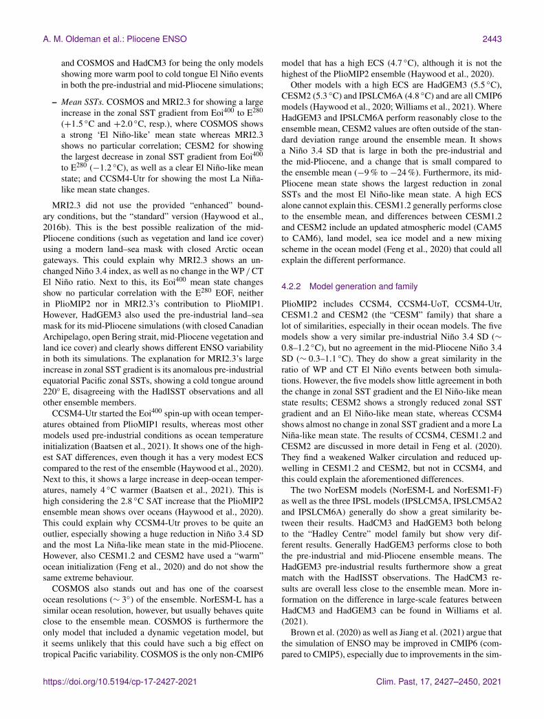
– Niño 3.4 index. COSMOS for showing by far thelargest Niño 3.4 SD (∼ 1.7◦C) in both pre-industrial andmid-Pliocene simulations; COSMOS, GISS2.1G andMRI2.3 for showing almost unchanged Niño 3.4 SD inboth simulations; CCSM4-Utr for showing the largestreduction in Niño 3.4 SD in the mid-Pliocene (−67 %);and GISS2.1G for showing a very regular Niño 3.4 in-dex and an almost single-peaked Eoi400 power spec-trum;

– ENSO structure. CCSM4-Utr, HadCM3 and MIROC4mfor showing large changes in the Eoi400 EOF pattern



and COSMOS and HadCM3 for being the only modelsshowing more warm pool to cold tongue El Niño eventsin both the pre-industrial and mid-Pliocene simulations;

– Mean SSTs. COSMOS and MRI2.3 for showing a largeincrease in the zonal SST gradient from Eoi400 to E280

(+1.5 ◦C and +2.0 ◦C, resp.), where COSMOS showsa strong ‘El Niño-like’ mean state whereas MRI2.3shows no particular correlation; CESM2 for showingthe largest decrease in zonal SST gradient from Eoi400

to E280 (−1.2 ◦C), as well as a clear El Niño-like meanstate; and CCSM4-Utr for showing the most La Niña-like mean state changes.

MRI2.3 did not use the provided “enhanced” bound-ary conditions, but the “standard” version (Haywood et al.,2016b). This is the best possible realization of the mid-Pliocene conditions (such as vegetation and land ice cover)using a modern land–sea mask with closed Arctic oceangateways. This could explain why MRI2.3 shows an un-changed Niño 3.4 index, as well as no change in the WP /CTEl Niño ratio. Next to this, its Eoi400 mean state changesshow no particular correlation with the E280 EOF, neitherin PlioMIP2 nor in MRI2.3’s contribution to PlioMIP1.However, HadGEM3 also used the pre-industrial land–seamask for its mid-Pliocene simulations (with closed CanadianArchipelago, open Bering strait, mid-Pliocene vegetation andland ice cover) and clearly shows different ENSO variabilityin both its simulations. The explanation for MRI2.3’s largeincrease in zonal SST gradient is its anomalous pre-industrialequatorial Pacific zonal SSTs, showing a cold tongue around220◦ E, disagreeing with the HadISST observations and allother ensemble members.

CCSM4-Utr started the Eoi400 spin-up with ocean temper-atures obtained from PlioMIP1 results, whereas most othermodels used pre-industrial conditions as ocean temperatureinitialization (Baatsen et al., 2021). It shows one of the high-est SAT differences, even though it has a very modest ECScompared to the rest of the ensemble (Haywood et al., 2020).Next to this, it shows a large increase in deep-ocean temper-atures, namely 4 ◦C warmer (Baatsen et al., 2021). This ishigh considering the 2.8 ◦C SAT increase that the PlioMIP2ensemble mean shows over oceans (Haywood et al., 2020).This could explain why CCSM4-Utr proves to be quite anoutlier, especially showing a huge reduction in Niño 3.4 SDand the most La Niña-like mean state in the mid-Pliocene.However, also CESM1.2 and CESM2 have used a “warm”ocean initialization (Feng et al., 2020) and do not show thesame extreme behaviour.

COSMOS also stands out and has one of the coarsestocean resolutions (∼ 3◦) of the ensemble. NorESM-L has asimilar ocean resolution, however, but usually behaves quiteclose to the ensemble mean. COSMOS is furthermore theonly model that included a dynamic vegetation model, butit seems unlikely that this could have such a big effect ontropical Pacific variability. COSMOS is the only non-CMIP6

model that has a high ECS (4.7 ◦C), although it is not thehighest of the PlioMIP2 ensemble (Haywood et al., 2020).

Other models with a high ECS are HadGEM3 (5.5 ◦C),CESM2 (5.3 ◦C) and IPSLCM6A (4.8 ◦C) and are all CMIP6models (Haywood et al., 2020; Williams et al., 2021). WhereHadGEM3 and IPSLCM6A perform reasonably close to theensemble mean, CESM2 values are often outside of the stan-dard deviation range around the ensemble mean. It showsa Niño 3.4 SD that is large in both the pre-industrial andthe mid-Pliocene, and a change that is small compared tothe ensemble mean (−9 % to −24 %). Furthermore, its mid-Pliocene mean state shows the largest reduction in zonalSSTs and the most El Niño-like mean state. A high ECSalone cannot explain this. CESM1.2 generally performs closeto the ensemble mean, and differences between CESM1.2and CESM2 include an updated atmospheric model (CAM5to CAM6), land model, sea ice model and a new mixingscheme in the ocean model (Feng et al., 2020) that could allexplain the different performance.

4.2.2 Model generation and family

PlioMIP2 includes CCSM4, CCSM4-UoT, CCSM4-Utr,CESM1.2 and CESM2 (the “CESM” family) that share alot of similarities, especially in their ocean models. The fivemodels show a very similar pre-industrial Niño 3.4 SD (∼0.8–1.2 ◦C), but no agreement in the mid-Pliocene Niño 3.4SD (∼ 0.3–1.1 ◦C). They do show a great similarity in theratio of WP and CT El Niño events between both simula-tions. However, the five models show little agreement in boththe change in zonal SST gradient and the El Niño-like meanstate results; CESM2 shows a strongly reduced zonal SSTgradient and an El Niño-like mean state, whereas CCSM4shows almost no change in zonal SST gradient and a more LaNiña-like mean state. The results of CCSM4, CESM1.2 andCESM2 are discussed in more detail in Feng et al. (2020).They find a weakened Walker circulation and reduced up-welling in CESM1.2 and CESM2, but not in CCSM4, andthis could explain the aforementioned differences.

The two NorESM models (NorESM-L and NorESM1-F)as well as the three IPSL models (IPSLCM5A, IPSLCM5A2and IPSLCM6A) generally do show a great similarity be-tween their results. HadCM3 and HadGEM3 both belongto the “Hadley Centre” model family but show very dif-ferent results. Generally HadGEM3 performs close to boththe pre-industrial and mid-Pliocene ensemble means. TheHadGEM3 pre-industrial results furthermore show a greatmatch with the HadISST observations. The HadCM3 re-sults are overall less close to the ensemble mean. More in-formation on the difference in large-scale features betweenHadCM3 and HadGEM3 can be found in Williams et al.(2021).

Brown et al. (2020) as well as Jiang et al. (2021) argue thatthe simulation of ENSO may be improved in CMIP6 (com-pared to CMIP5), especially due to improvements in the sim-



ulation of the mean state in the tropical Pacific, such as a re-duced double intertropical convergence zone (ITCZ) bias andcold tongue bias. When only the results of CMIP6 models(CESM2, EC-Earth3.3, GISS2.1G, HadGEM3, IPSLCM6A,NorESM1-F) are considered, the ensemble mean results andthe conclusions on mid-Pliocene ENSO variability are sim-ilar. However, the CMIP6 models do show the strongest re-duction in zonal SST gradient in the mid-Pliocene (Fig. 9).Also, it is mainly the CMIP6 models that show El Niño-likemean state changes (Fig. 10), although EC-Earth3.3 exhibitsa La Niña-like mean state.

4.2.3 PlioMIP2 versus PlioMIP1

In total, 7 of the 17 models that participate in PlioMIP2also participated in PlioMIP1, namely CCSM4, COSMOS,HadCM3, IPSLCM5A, MIROC4m, MRI2.3 and NorESM-L. Some of the PlioMIP1 conclusions presented in Brierley(2015) are similar: the Niño 3.4 SD decreases (24 % (±18 %)in PlioMIP2 versus 20 % in PlioMIP1), the spatial struc-ture of El Niño is similar and the El Niño flavour showsno robust change. However, there are also some clear differ-ences. PlioMIP2 shows a significant reduction of the spec-tral power in the 3–4-year period, where PlioMIP1 mainlyshows a shift of power to longer periods; the PlioMIP1 resultsshowed a clear “low-frequency” peak in the pre-industrialaround 5–6 years that seemed to shift to 7–8 years in themid-Pliocene ensemble mean. The significance of the spec-tral peaks was not assessed, however. Another differenceis that the PlioMIP2 models show a clear but small re-duction in zonal SST gradient where PlioMIP1 shows “nopreferential warming in the eastern equatorial Pacific”. Anexplanation for the difference between the ensemble re-sults is that PlioMIP2 encompasses more and newer mod-els (most CMIP6) that have a higher resolution and includethe newest ocean–atmosphere models and parametrizations.Next to this, the boundary conditions of PlioMIP2 are morespecifically tuned to a specific time slice in the mid-Pliocene(Dowsett et al., 2016). It should also be noted that Brierley(2015) used more than 100 years of data (up to 200 years) foranalysis of some of the models, sometimes including moreyears of pre-industrial data than mid-Pliocene data for onemodel. This can impact the statistical confidence of spectralpower density, particularly for the longer periods. We choseto use 100 years of data for all the simulations for the sakeof consistency, as some models only had 100 years of dataavailable. The different simulation protocol and ensemblecomposition means that differences between PlioMIP1 andPlioMIP2 can be expected. However, the similarities betweenboth ensembles make the reduction of the ENSO amplitudein the mid-Pliocene more robust.

4.3 Robustness of ENSO amplitude andsignificant-peak analysis

Previous studies from Wittenberg (2009) and Tindall et al.(2016) show that ENSO variability can exhibit significantchanges on the interdecadal and centennial scale. While atime-series length of 100 years as used here is clearly suf-ficient to study properties such as amplitude and spectra ofENSO on its typical interannual timescales, the presence ofcentennial-scale modulations on ENSO properties could im-ply that the choice of the 100-year segment affects our con-clusions on interannual variability differences between pre-industrial and mid-Pliocene. In order to address this issue,we repeated the calculation of the ENSO amplitude with 500years of data. For this we used data of two PlioMIP2 models,MIROC4m and CESM2. The results are included in the Sup-plement. There are clear variations in the ENSO amplitudeon centennial timescales. The change in Niño 3.4 SD variesaround ±9 % and ±4 % of the value when using 500 yearsof data for CESM2 and MIROC4m, respectively. However,these variations are not large enough to change the conclu-sion regarding the clear reduction of the ENSO amplitude inthe PlioMIP2 ensemble. These results are in accordance withthe findings by Tindall et al. (2016), who use 2500 modelyears of HadCM3 simulations. When interpreting the ±9 %variation as an error margin on the change in Niño 3.4 SD,only three out of the seven models that contributed to bothPlioMIP1 and PlioMIP2 show a similar result in the bothMIPs, namely IPSLCM5A, MIROC4m and MRI2.3. Theother models (CCSM4, COSMOS, HadCM3 and NorESM-L) show no overlap in their PlioMIP1 and PlioMIP2 values.These discrepancies cannot be explained by centennial-scalevariations of ENSO amplitude and are thus likely caused bythe differences in the MIP protocols.

Next to this, the spectral “peak-counting” method is testedfor robustness by repeating the procedure using differentspectral settings and the Niño 3 instead of Niño 3.4 index.The conclusions are found to be independent of these differ-ent settings. A summary of these results is included in theSupplement. In conclusion, both the reduction of ENSO am-plitude as well as the changes in significant spectral peaks inthe PlioMIP2 ensemble are robust.

4.4 Physical mechanisms

What the PlioMIP2 simulations have in common is the useof identical forcing and (nearly) identical boundary condi-tions. The changes in ENSO response and mean state in themid-Pliocene should therefore be a response to the CO2 forc-ing and the PRISM4 boundary conditions. Brierley (2015)discusses the impact of the PRISM3 boundary conditionson ENSO and cannot find a clear explanation when consid-ering geography. Differences in boundary conditions fromPlioMIP1 to PlioMIP2 mainly include changes to lakes, soilsand vegetation, land ice cover, and Arctic gateways such as



the Bering strait and Canadian archipelago (Dowsett et al.,2016; Haywood et al., 2016b). We do not expect these dif-ferences to directly impact ENSO properties. Brierley andFedorov (2016) find that the closing of the Bering strait af-fects ENSO properties but mention it is hard to estimatethe statistical significance of these changes. Other changesto the land–sea mask include the shoaling of the Sahul andSunda shelves. This can affect the Indonesian throughflow,which can affect ENSO properties as shown by Jochum et al.(2009) as well as Brierley and Fedorov (2016). We did notinvestigate the changes in the Indonesian throughflow in thePlioMIP2 ensemble in this study.

Proxy records suggest the mid-Pliocene mean state sus-tained El Niño-like conditions (Fedorov et al., 2006; Waraet al., 2005) or at least a weak zonal SST gradient (Fedorovet al., 2013). Manucharyan and Fedorov (2014) state that theweak zonal SST gradient was less favourable for ENSO oc-currence. The PlioMIP2 results do show a reduced zonal SSTgradient, but only slightly, together with a reduced ENSOamplitude. However, a consistent relationship between thetwo is absent, as can be seen in Fig. 9. Brown et al. (2020)investigate the relationship between zonal SST gradient andNiño 3.4 SD for PMIP3/4 simulations of the mid-Holocene,last glacial maximum and last interglacial, as well as 1 %CO2 and abrupt 4× CO2 experiments, and also find no clearrelationship. Hu et al. (2013) suggest the relationship be-tween zonal SST gradient and ENSO amplitude might benonlinear.

Feedback analysis shows that reduction of ENSO variabil-ity in the mid-Holocene is likely due to the increase in thenegative feedback (mean current thermal advection, An andBong, 2018), the reduction of major positive feedback pro-cesses (thermocline, zonal advection and Ekman feedbacks,Chen et al., 2019) or an enhanced seasonal cycle (Iwakiriand Watanabe, 2019). However, PlioMIP1 (Brierley, 2015)as well as PMIP3 and PMIP4 models (Brown et al., 2020)do not show any consistent relationship between changesin the seasonal amplitude and changes in ENSO variability.More recently it has been suggested that the mid-Pliocenesaw a generally deeper thermocline and thus a weaker ther-mocline feedback (White and Ravelo, 2020). Brown et al.(2020) acknowledge that the changes in feedback processesin PMIP3/4 simulations are model-dependent. They alsopoint out that ENSO feedbacks are still inaccurately sim-ulated in most current GCMs (Bayr et al., 2019; Bellengeret al., 2014; Kim et al., 2014; Kim and Jin, 2011).

Recent work by Pontes et al. (2021), analysing bothPlioMIP1 and PlioMIP2 results, find that models with asteeper thermocline (deemed La Niña-like in that paper) arerelated to major ENSO reduction, while a flatter thermocline(El Niño-like) is associated with a similar ENSO amplitudecompared to the pre-industrial. This finding is in agreementwith the results we find on ENSO amplitude and the El Niño-like mean state (Fig. 10), although a different methodologyis used. Pontes et al. (2021) furthermore find that a combina-

tion of off-equatorial mean state changes in the mid-Plioceneis not favourable for ENSO. They find a northward displace-ment of the ITCZ, increased south-eastern trade winds inthe western Pacific and an intensified South Pacific Subtropi-cal High in the mid-Pliocene simulations, all associated withsuppression of ENSO variability.

5 Conclusions

The Pliocene Model Intercomparison Project phase 2(PlioMIP2) coordinated 17 global coupled climate models tosimulate the mid-Pliocene and pre-industrial climate. In thiswork, we have studied the changes in ENSO variability inthe mid-Pliocene using the PlioMIP2 ensemble and relatedthose to SST changes in the tropical Pacific mean climate.Even with (nearly) identical forcing and geographical bound-aries, the PlioMIP2 ensemble includes a range of model res-olutions, parametrizations and initializations, all which con-tribute to a considerable model spread in the PlioMIP2 en-semble.

The PlioMIP2 ensemble shows a robust decrease in ENSOamplitude. The Niño 3.4 SD decreases for 15 of the 17models with an ensemble mean decrease of 24 %, com-pared to 20 % in PlioMIP1 (Brierley, 2015). Changes inNiño 3.4 skewness and kurtosis are less coherent. Spectralanalysis shows a clear reduction of spectral power in the3–4-year period in the mid-Pliocene. Furthermore, the to-tal number of spectral peaks that are above the 99 % confi-dence level decreases by one-third in the PlioMIP2 ensem-ble. The shift towards longer periods that is suggested bythe PlioMIP1 models does not occur in PlioMIP2. The mid-Pliocene ENSO is similar in spatial structure in comparisonto the pre-industrial. EOF analysis shows that the percentageof variance explained by the first EOF decreases from 50 %to 42 % and suggests that El Niño warmth expands meridion-ally across the tropical Pacific. Correlation with the principalcomponent time series shows that the Niño 3.4 index bestcaptures the ENSO-related variability in the Pacific in boththe pre-industrial and mid-Pliocene, also suggesting a simi-lar spatial structure. Analysis of El Niño flavour suggests noparticular change in the mid-Pliocene, although the modelspread is large.

The tropical Pacific mean SSTs show a clear warmingin the eastern Pacific upwelling region, in agreement withproxy data. The PlioMIP2 models do not show a unanimousweakening of the mean zonal SST gradient, with an ensem-ble mean change of −0.17± 0.77 ◦C. However, 14 out ofthe 17 models show a (slight) reduction of the zonal SSTgradient. A clear connection with the reduced ENSO am-plitude is not found, agreeing with recent work by Brownet al. (2020). Mean SST changes are correlated with the pre-industrial EOF to study whether the mid-Pliocene is El Niño-like, as suggested by certain proxy studies (Wara et al., 2005;Fedorov et al., 2006). The PlioMIP2 ensemble does not show



a unanimous response, and a correlation with the ENSO am-plitude and a more or less El Niño-like mean state is notfound. Interestingly, there is a “cluster” of four models (ofwhich three are CMIP6 models) that suggest an El Niño-like mean state but a similar ENSO amplitude in the mid-Pliocene. Proxy data suggest that the mid-Pliocene ENSOwas reduced (Scroxton et al., 2011), similar to the presentday (Watanabe et al., 2011) or possibly varying between both(White and Ravelo, 2020). The PlioMIP2 ensemble showsa range of ENSO amplitudes, varying between strongly re-duced and similar to pre-industrial, possibly even despite aslightly reduced zonal SST gradient. As such, it seems togenerally agree with most proxy studies on ENSO variabilityas well as tropical Pacific SSTs so far.

Although it becomes more and more clear that the mid-Pliocene saw generally reduced ENSO variability, the rea-sons for this are still not clear. White and Ravelo (2020) sug-gest a weaker thermocline feedback due to a generally deeperthermocline. Pontes et al. (2021) suggest a combination ofoff-equatorial mean state changes that are unfavourable forENSO activity. Future research should aim to find an answerto the question of why exactly ENSO variability was reducedin the mid-Pliocene. These answers can help us to understandthe physical behaviour of ENSO in warm climates and willhelp us to understand the behaviour of ENSO in the future.

Code and data availability. A selection of the data presentedin the figures in this paper is available in the Supplement. The100-year regridded SST data are available upon request fromAlan M. Haywood ([email protected]), as well as morecomplete data for PlioMIP2 (with exception of IPSLCM6A andGISS2.1G). PlioMIP2 data from CESM2, EC-Earth3.3, NorESM1-F, IPSLCM6A and GISS2.1G can be obtained through the EarthSystem Grid Federation (ESGF) (https://esgf-node.llnl.gov/search/cmip6/, last access: 25 February 2021, ESGF, 2020). A selection ofthe data from the scatter plots presented in the paper is available inthe Supplement.

The Python scripts (Jupyter Notebooks) used fordata analysis are freely accessible through Zenodo(https://doi.org/10.5281/zenodo.5718483, Oldeman, 2021).

Supplement. The supplement related to this article is availableonline at: https://doi.org/10.5194/cp-17-2427-2021-supplement.

Author contributions. AMO, MLJB, ASvdH and HAD con-ceived the presented ideas in this study. AMO performed the analy-sis and wrote the draft of the paper. JCT contributed data and advicein data analysis. The remaining authors provided the PlioMIP2 ex-periments and contributed to the writing of the paper.

Competing interests. At least one of the (co-)authors is a mem-ber of the editorial board of Climate of the Past.

Disclaimer. Publisher’s note: Copernicus Publications remainsneutral with regard to jurisdictional claims in published maps andinstitutional affiliations.

Special issue statement. This article is part of the special issue“PlioMIP Phase 2: experimental design, implementation and scien-tific results”. It is not associated with a conference.

Acknowledgements. The work by Arthur M. Oldeman, Anna S.von der Heydt, Michiel L. J. Baatsen and Henk A. Dijkstra wascarried out under the program of the Netherlands Earth System Sci-ence Centre (NESSC), financially supported by the Ministry of Ed-ucation, Culture and Science (OCW grant no. 024.002.001). Simu-lations with CCSM4-Utr were performed at the SURFsara Dutchnational computing facilities and were sponsored by NWO-EW(Netherlands Organisation for Scientific Research, Exact Sciences)(project no. 17189).

Alan M. Haywood, Julia C. Tindall and Stephen J. Hunter ac-knowledge the FP7 Ideas programme from the European ResearchCouncil (grant no. PLIO-ESS, 278636), the Past Earth Network(EPSRC grant no. EP/M008.363/1) and the University of Leeds Ad-vanced Research Computing service. Julia C. Tindall was also sup-ported through the Centre for Environmental Modelling and Com-putation (CEMAC), University of Leeds.

Bette L. Otto-Bliesner, Esther C. Brady and Ran Feng ac-knowledge that material for their participation is based uponwork supported by the National Center for Atmospheric Re-search, which is a major facility sponsored by the NationalScience Foundation (NSF) (cooperative agreement no. 1852977and NSF OPP grant no. 1418411). Ran Feng is also supportedby NSF grant no. 1903650. The CESM project is supportedprimarily by the National Science Foundation. Computing anddata storage resources, including the Cheyenne supercomputer(https://doi.org/10.5065/D6RX99HX), were provided by the Com-putational and Information Systems Laboratory (CISL) at NCAR.NCAR is sponsored by the National Science Foundation.

Ning Tan, Camille Contoux and Gilles Ramstein were grantedaccess to the HPC resources of TGCC under the allocations2016-A0030107732, 2017-R0040110492 and 2018-R0040110492(gencmip6) and 2019-A0050102212 (gen2212) provided byGENCI. The IPSL-CM6 team of the IPSL Climate Modelling Cen-tre (https://cmc.ipsl.fr/, last access: 28 April 2021) is acknowledgedfor having developed, tested, evaluated and tuned the IPSL climatemodel, as well as having performed and published the CMIP6 ex-periments.

Christian Stepanek acknowledges funding from the HelmholtzClimate Initiative REKLIM. Christian Stepanek and GerritLohmann acknowledge funding via the Alfred Wegener Institute’sresearch programme Marine, Coastal and Polar Systems.

Qiong Zhang acknowledges support from the Swedish ResearchCouncil (2013-06476 and 2017-04232). Simulations with EC-Earthwere performed on resources provided by the Swedish National In-frastructure for Computing (SNIC) at the National SupercomputerCentre (NSC).

Wing-Le Chan and Ayako Abe-Ouchi acknowledge fundingfrom JSPS (KAKENHI grant no. 17H06104 and MEXT KAKENHI


https://esgf-node.llnl.gov/search/cmip6/


https://doi.org/10.5281/zenodo.5718483

https://doi.org/10.5194/cp-17-2427-2021-supplement

https://doi.org/10.5065/D6RX99HX

https://cmc.ipsl.fr/


grant no. 17H06323). Their simulations with MIROC4m were per-formed on the Earth Simulator at JAMSTEC, Yokohama, Japan.

W. Richard Peltier and Deepak Chandan wish to acknowledgethat data they have contributed from the CCSM4-UoT model wasproduced with the support of Canadian NSERC Discovery GrantA9627 t WRP, and they wish to acknowledge the support of theSciNet HPC Consortium for providing computing facilities. SciNetis funded by the Canada Foundation for Innovation under the aus-pices of Compute Canada, the Government of Ontario, the On-tario Research Fund – Research Excellence and the University ofToronto.

Zhongshi Zhang and Xiangyu Li acknowledge financial sup-port from the National Natural Science Foundation of China (grantno. 42005042), the China Scholarship Council (201804910023)and the China Postdoctoral Science Foundation (project no.2015M581154). The NorESM simulations benefitted from re-sources provided by UNINETT Sigma2 – the National Infrastruc-ture for High Performance Computing and Data Storage in Norway.

Charles J. R. Williams and Dan Lunt are thankful for NERCgrant NE/P01903X/1 and the NEXCS High Performance Comput-ing facility funded by the Natural Environment Research Counciland delivered by the Met Office.

Gabriel M. Pontes and Ilana Wainer acknowledge the São PauloResearch Foundation (FAPESP 2016/23670-0).

The authors would like to thank Chris Brierley and an anony-mous reviewer for helpful feedback and comments on an earlierversion of the manuscript.

Financial support. This research has been supported bythe Netherlands Earth System Science Centre (OCW (grantno. 024.002.001)).

Review statement. This paper was edited by Steven Phipps andreviewed by Chris Brierley and one anonymous referee.

References

An, S. I. and Bong, H.: Feedback process responsible for thesuppression of ENSO activity during the mid-Holocene, Theor.Appl. Climatol., 132, 779–790, https://doi.org/10.1007/s00704-017-2117-6, 2018.

Ashok, K. and Yamagata, T.: The El Niño with a difference, Nature,461, 481–484, https://doi.org/10.1038/461481a, 2009.

Baatsen, M. L. J., von der Heydt, A. S., Kliphuis, M. A., Olde-man, A. M., and Weiffenbach, J. E.: Warm mid-Pliocene con-ditions without high climate sensitivity: the CCSM4-Utrecht(CESM 1.0.5) contribution to the PlioMIP2, Clim. Past Discuss.[preprint], https://doi.org/10.5194/cp-2021-140, in review, 2021.

Badger, M. P., Schmidt, D. N., Mackensen, A., and Pancost, R. D.:High-resolution alkenone palaeobarometry indicates relativelystable pCO2 during the Pliocene (3.3–2.8 Ma), Philos. T. Roy.Soc. A, 371, https://doi.org/10.1098/rsta.2013.0094, 2013.

Barreiro, M., Philander, G., Pacanowski, R., and Fedorov, A.:Simulations of warm tropical conditions with application tomiddle Pliocene atmospheres, Clim. Dynam., 26, 349–365,https://doi.org/10.1007/s00382-005-0086-4, 2006.

Bayr, T., Wengel, C., Latif, M., Dommenget, D., Lübbecke, J., andPark, W.: Error compensation of ENSO atmospheric feedbacksin climate models and its influence on simulated ENSO dynam-ics, Clim. Dynam., 53, 155–172, https://doi.org/10.1007/s00382-018-4575-7, 2019.

Bellenger, H., Guilyardi, E., Leloup, J., Lengaigne, M.,and Vialard, J.: ENSO representation in climate models:From CMIP3 to CMIP5, Clim. Dynam., 42, 1999–2018,https://doi.org/10.1007/s00382-013-1783-z, 2014.

Beobide-Arsuaga, G., Bayr, T., Reintges, A., and Latif, M.:Uncertainty of ENSO-amplitude projections in CMIP5and CMIP6 models, Clim. Dynam., 56, 3875–3888,https://doi.org/10.1007/s00382-021-05673-4, 2021.

Bonham, S. G., Haywood, A. M., Lunt, D. J., Collins, M.,and Salzmann, U.: El Niño-Southern Oscillation, Pliocene cli-mate and equifinality, Philos. T. Roy. Soc. A, 367, 127–156,https://doi.org/10.1098/rsta.2008.0212, 2009.

Brierley, C. M.: Interannual climate variability seen in thePliocene Model Intercomparison Project, Clim. Past, 11, 605–618, https://doi.org/10.5194/cp-11-605-2015, 2015.

Brierley, C. M. and Fedorov, A. V.: Comparing the im-pacts of Miocene–Pliocene changes in inter-ocean gate-ways on climate: Central American Seaway, Bering Strait,and Indonesia, Earth Planet. Sci. Lett., 444, 116–130,https://doi.org/10.1016/j.epsl.2016.03.010, 2016.

Brown, J. R., Brierley, C. M., An, S.-I., Guarino, M.-V., Steven-son, S., Williams, C. J. R., Zhang, Q., Zhao, A., Abe-Ouchi,A., Braconnot, P., Brady, E. C., Chandan, D., D’Agostino,R., Guo, C., LeGrande, A. N., Lohmann, G., Morozova, P.A., Ohgaito, R., O’ishi, R., Otto-Bliesner, B. L., Peltier, W.R., Shi, X., Sime, L., Volodin, E. M., Zhang, Z., and Zheng,W.: Comparison of past and future simulations of ENSO inCMIP5/PMIP3 and CMIP6/PMIP4 models, Clim. Past, 16,1777–1805, https://doi.org/10.5194/cp-16-1777-2020, 2020.

Cai, W., Borlace, S., Lengaigne, M., Van Rensch, P., Collins,M., Vecchi, G., Timmermann, A., Santoso, A., Mcphaden,M. J., Wu, L., England, M. H., Wang, G., Guilyardi, E., andJin, F. F.: Increasing frequency of extreme El Niño eventsdue to greenhouse warming, Nat. Clim. Change, 4, 111–116,https://doi.org/10.1038/nclimate2100, 2014.

Cai, W., Santoso, A., Collins, M., Dewitte, B., Karamperidou,C., Kug, J.-S., Lengaigne, M., McPhaden, M. J., Stuecker,M. F., Taschetto, A. S., Timmermann, A., Wu, L., Yeh, S.-W., Wang, G., Ng, B., Jia, F., Yang, Y., Ying, J., Zheng, X.-T., Bayr, T., Brown, J. R., Capotondi, A., Cobb, K. M., Gan,B., Geng, T., Ham, Y.-G., Jin, F.-F., Jo, H.-S., Li, X., Lin, X.,McGregor, S., Park, J.-H., Stein, K., Yang, K., Zhang, L., andZhong, W.: Changing El Niño–Southern Oscillation in a warm-ing climate, Nature Reviews Earth & Environment, 2, 628–644,https://doi.org/10.1038/s43017-021-00199-z, 2021.

Callahan, C. W., Chen, C., Rugenstein, M., Bloch-Johnson, J.,Yang, S., and Moyer, E. J.: Robust decrease in El Niño/SouthernOscillation amplitude under long-term warming, Nat. Clim.Change, 11, 752–757, https://doi.org/10.1038/s41558-021-01099-2, 2021.

Chan, W.-L. and Abe-Ouchi, A.: Pliocene Model IntercomparisonProject (PlioMIP2) simulations using the Model for Interdisci-plinary Research on Climate (MIROC4m), Clim. Past, 16, 1523–1545, https://doi.org/10.5194/cp-16-1523-2020, 2020.


https://doi.org/10.1007/s00704-017-2117-6

https://doi.org/10.1007/s00704-017-2117-6

https://doi.org/10.1038/461481a

https://doi.org/10.5194/cp-2021-140

https://doi.org/10.1098/rsta.2013.0094

https://doi.org/10.1007/s00382-005-0086-4

https://doi.org/10.1007/s00382-018-4575-7

https://doi.org/10.1007/s00382-018-4575-7

https://doi.org/10.1007/s00382-013-1783-z

https://doi.org/10.1007/s00382-021-05673-4

https://doi.org/10.1098/rsta.2008.0212

https://doi.org/10.5194/cp-11-605-2015

https://doi.org/10.1016/j.epsl.2016.03.010

https://doi.org/10.5194/cp-16-1777-2020

https://doi.org/10.1038/nclimate2100

https://doi.org/10.1038/s43017-021-00199-z

https://doi.org/10.1038/s41558-021-01099-2

https://doi.org/10.1038/s41558-021-01099-2

https://doi.org/10.5194/cp-16-1523-2020


Chandan, D. and Peltier, W. R.: Regional and global climate for themid-Pliocene using the University of Toronto version of CCSM4and PlioMIP2 boundary conditions, Clim. Past, 13, 919–942,https://doi.org/10.5194/cp-13-919-2017, 2017.

Chandan, D. and Peltier, W. R.: On the mechanisms of warm-ing the mid-Pliocene and the inference of a hierarchy of cli-mate sensitivities with relevance to the understanding of climatefutures, Clim. Past, 14, 825–856, https://doi.org/10.5194/cp-14-825-2018, 2018.

Chelton, D. and Risien, C.: Zonal and Meridional Discontinu-ities and Other Issues with the HadISST1.1 Dataset, Collegeof Earth, Ocean and Atmospheric Sciences, Oregon State Uni-versity, ScholarsArchive@OSU, Tech. rep., available at: http://ir.library.oregonstate.edu/xmlui/handle/1957/58385 (last access:22 November 2021), 2016.

Chen, L., Wang, L., Li, T., and Liu, J.: Drivers of reduced ENSOvariability in mid-Holocene in a coupled model, Clim. Dy-nam., 52, 5999–6014, https://doi.org/10.1007/s00382-018-4496-5, 2019.

Coats, S. and Karnauskas, K. B.: Are Simulated and Ob-served Twentieth Century Tropical Pacific Sea Sur-face Temperature Trends Significant Relative to Inter-nal Variability?, Geophys. Res. Lett., 44, 9928–9937,https://doi.org/10.1002/2017GL074622, 2017.

Collins, M., An, S. I., Cai, W., Ganachaud, A., Guilyardi, E., Jin,F. F., Jochum, M., Lengaigne, M., Power, S., Timmermann, A.,Vecchi, G., and Wittenberg, A.: The impact of global warming onthe tropical Pacific Ocean and El Niño, Nat. Geosci., 3, 391–397,https://doi.org/10.1038/ngeo868, 2010.

de la Vega, E., Chalk, T. B., Wilson, P. A., Bysani, R. P., and Fos-ter, G. L.: Atmospheric CO2 during the Mid-Piacenzian WarmPeriod and the M2 glaciation, Scientific Reports, 10, 14–21,https://doi.org/10.1038/s41598-020-67154-8, 2020.

Dowsett, H., Robinson, M., Haywood, A. M., Salzmann, U., Hill,D., Sohl, L. E., Chandler, M., Williams, M., Foley, K., andStoll, D. K.: The PRISM3D paleoenvironmental reconstruction,Stratigraphy, 7, 123–139, available at: https://pubs.er.usgs.gov/publication/70044350 (last access: 22 November 2021), 2010.

Dowsett, H., Dolan, A., Rowley, D., Moucha, R., Forte, A. M.,Mitrovica, J. X., Pound, M., Salzmann, U., Robinson, M., Chan-dler, M., Foley, K., and Haywood, A.: The PRISM4 (mid-Piacenzian) paleoenvironmental reconstruction, Clim. Past, 12,1519–1538, https://doi.org/10.5194/cp-12-1519-2016, 2016.

ESGF: WCRP Coupled Model Intercomparison Project (Phase6), available at: https://esgf-node.llnl.gov/search/cmip6/ (last ac-cess: 25 February 2021), 2020.

Fedorov, A. V., Harper, S. L., Philander, S. G., Winter, B., and Wit-tenberg, A.: How predictable is El Niño?, B. Am. Meteorol. Soc.,84, 911–920, https://doi.org/10.1175/BAMS-84-7-911, 2003.

Fedorov, A. V., Dekens, P. S., McCarthy, M., Ravelo, A. C.,DeMenocal, P. B., Barreiro, M., Pacanowski, R. C., andPhilander, S. G.: The Pliocene Paradox (mechanismsfor a permanent El Niño), Science, 312, 1485–1489,https://doi.org/10.1126/science.1122666, 2006.

Fedorov, A. V., Brierley, C. M., Lawrence, K. T., Liu, Z.,Dekens, P. S., and Ravelo, A. C.: Patterns and mech-anisms of early Pliocene warmth, Nature, 496, 43–49,https://doi.org/10.1038/nature12003, 2013.

Feng, R., Otto-Bliesner, B. L., Brady, E. C., and Rosen-bloom, N.: Increased Climate Response and Earth SystemSensitivity From CCSM4 to CESM2 in Mid-Pliocene Sim-ulations, J. Adv. Model. Earth Sy., 12, e2019MS002033,https://doi.org/10.1029/2019MS002033, 2020.

Foley, K. and Dowsett, H.: Community sourced mid-Piacenzian seasurface temperature (SST) data, U.S. Geological Survey [dataset], https://doi.org/10.5066/P9YP3DTV, 2019.

Ford, H. L., Ravelo, A. C., Dekens, P. S., Lariviere, J. P., and Wara,M. W.: The evolution of the equatorial thermocline and the earlyPliocene El Padre mean state, Geophys. Res. Lett., 42, 4878–4887, https://doi.org/10.1002/2015GL064215, 2015.

Fredriksen, H.-B., Berner, J., Subramanian, A. C., and Capotondi,A.: How Does El Niño–Southern Oscillation Change UnderGlobal Warming–A First Look at CMIP6, Geophys. Res. Lett.,47, e2020GL090640, https://doi.org/10.1029/2020GL090640,2020.

Freund, M. B., Brown, J. R., Henley, B. J., Karoly, D. J., andBrown, J. N.: Warming Patterns Affect El Niño Diversityin CMIP5 and CMIP6 Models, J. Climate, 33, 8237–8260,https://doi.org/10.1175/JCLI-D-19-0890.1, 2020.

Ghil, M., Allen, M. R., Dettinger, M. D., Ide, K., Kon-drashov, D., Mann, M. E., Robertson, A. W., Saunders, A.,Tian, Y., Varadi, F., and Yiou, P.: Advanced spectral meth-ods for climatic time series, Rev. Geophys., 40, 3-1–3-41,https://doi.org/10.1029/2000RG000092, 2002.

Haywood, A. M., Valdes, P. J., and Peck, V. L.: A permanentEl Niño-like state during the Pliocene?, Paleoceanography, 22,PA1213, https://doi.org/10.1029/2006PA001323, 2007.

Haywood, A. M., Dowsett, H. J., Otto-Bliesner, B., Chandler, M. A.,Dolan, A. M., Hill, D. J., Lunt, D. J., Robinson, M. M., Rosen-bloom, N., Salzmann, U., and Sohl, L. E.: Pliocene Model Inter-comparison Project (PlioMIP): experimental design and bound-ary conditions (Experiment 1), Geosci. Model Dev., 3, 227–242,https://doi.org/10.5194/gmd-3-227-2010, 2010.

Haywood, A. M., Hill, D. J., Dolan, A. M., Otto-Bliesner, B. L.,Bragg, F., Chan, W.-L., Chandler, M. A., Contoux, C., Dowsett,H. J., Jost, A., Kamae, Y., Lohmann, G., Lunt, D. J., Abe-Ouchi,A., Pickering, S. J., Ramstein, G., Rosenbloom, N. A., Salz-mann, U., Sohl, L., Stepanek, C., Ueda, H., Yan, Q., and Zhang,Z.: Large-scale features of Pliocene climate: results from thePliocene Model Intercomparison Project, Clim. Past, 9, 191–209,https://doi.org/10.5194/cp-9-191-2013, 2013.

Haywood, A. M., Dowsett, H. J., and Dolan, A. M.: Inte-grating geological archives and climate models for themid-Pliocene warm period, Nat. Commun., 7, 10646,https://doi.org/10.1038/ncomms10646, 2016a.

Haywood, A. M., Dowsett, H. J., Dolan, A. M., Rowley, D.,Abe-Ouchi, A., Otto-Bliesner, B., Chandler, M. A., Hunter, S.J., Lunt, D. J., Pound, M., and Salzmann, U.: The PlioceneModel Intercomparison Project (PlioMIP) Phase 2: scientificobjectives and experimental design, Clim. Past, 12, 663–675,https://doi.org/10.5194/cp-12-663-2016, 2016b.

Haywood, A. M., Tindall, J. C., Dowsett, H. J., Dolan, A. M., Fo-ley, K. M., Hunter, S. J., Hill, D. J., Chan, W.-L., Abe-Ouchi,A., Stepanek, C., Lohmann, G., Chandan, D., Peltier, W. R., Tan,N., Contoux, C., Ramstein, G., Li, X., Zhang, Z., Guo, C., Ni-sancioglu, K. H., Zhang, Q., Li, Q., Kamae, Y., Chandler, M.A., Sohl, L. E., Otto-Bliesner, B. L., Feng, R., Brady, E. C.,


https://doi.org/10.5194/cp-13-919-2017

https://doi.org/10.5194/cp-14-825-2018

https://doi.org/10.5194/cp-14-825-2018

http://ir.library.oregonstate.edu/xmlui/handle/1957/58385

http://ir.library.oregonstate.edu/xmlui/handle/1957/58385

https://doi.org/10.1007/s00382-018-4496-5

https://doi.org/10.1007/s00382-018-4496-5

https://doi.org/10.1002/2017GL074622

https://doi.org/10.1038/ngeo868

https://doi.org/10.1038/s41598-020-67154-8

https://pubs.er.usgs.gov/publication/70044350

https://pubs.er.usgs.gov/publication/70044350

https://doi.org/10.5194/cp-12-1519-2016


https://doi.org/10.1175/BAMS-84-7-911

https://doi.org/10.1126/science.1122666

https://doi.org/10.1038/nature12003

https://doi.org/10.1029/2019MS002033

https://doi.org/10.5066/P9YP3DTV

https://doi.org/10.1002/2015GL064215

https://doi.org/10.1029/2020GL090640

https://doi.org/10.1175/JCLI-D-19-0890.1

https://doi.org/10.1029/2000RG000092

https://doi.org/10.1029/2006PA001323

https://doi.org/10.5194/gmd-3-227-2010

https://doi.org/10.5194/cp-9-191-2013

https://doi.org/10.1038/ncomms10646

https://doi.org/10.5194/cp-12-663-2016


von der Heydt, A. S., Baatsen, M. L. J., and Lunt, D. J.: ThePliocene Model Intercomparison Project Phase 2: large-scale cli-mate features and climate sensitivity, Clim. Past, 16, 2095–2123,https://doi.org/10.5194/cp-16-2095-2020, 2020.

Heede, U., Fedorov, A., and Burls, N.: Time Scales and Mecha-nisms for the Tropical Pacific Response to Global Warming: ATug of War between the Ocean Thermostat and Weaker Walker,J. Climate, 33, 6101–6118, https://doi.org/10.1175/JCLI-D-19-0690.1, 2020.

Hu, Z.-Z., Kumar, A., Ren, H.-L., Wang, H., L’Heureux, M.,and Jin, F.-F.: Weakened Interannual Variability in the Trop-ical Pacific Ocean since 2000, J. Climate, 26, 2601–2613,https://doi.org/10.1175/JCLI-D-12-00265.1, 2013.

Huang, B., Thorne, P. W., Banzon, V. F., Boyer, T., Chep-urin, G., Lawrimore, J. H., Menne, M. J., Smith, T. M.,Vose, R. S., and Zhang, H.-M.: Extended Reconstructed SeaSurface Temperature, Version 5 (ERSSTv5): Upgrades, Val-idations, and Intercomparisons, J. Climate, 30, 8179–8205,https://doi.org/10.1175/JCLI-D-16-0836.1, 2017.

Hunter, S. J., Haywood, A. M., Dolan, A. M., and Tindall, J. C.:The HadCM3 contribution to PlioMIP phase 2, Clim. Past, 15,1691–1713, https://doi.org/10.5194/cp-15-1691-2019, 2019.

Ilyas, M., Brierley, C. M., and Guillas, S.: Uncertainty in regionaltemperatures inferred from sparse global observations: Applica-tion to a probabilistic classification of El Niño, Geophys. Res.Lett., 44, 9068–9074, https://doi.org/10.1002/2017GL074596,2017.

IPCC: Climate Change 2021: The Physical Science Basis. Con-tribution of Working Group I to the Sixth Assessment Reportof the Intergovernmental Panel on Climate Change, edited by:Masson-Delmotte, V., Zhai, P., Pirani, A., Connors, S. L., Péan,C., Berger, S., Caud, N., Chen, Y., Goldfarb, L., Gomis, M. I.,Huang, M., Leitzell, K., Lonnoy, E., Matthews, J. B. R., May-cock, T. K., Waterfield, T., Yelekçi, O., Yu, R., and Zhou, B.,Cambridge University Press, in press, 2021.

Iwakiri, T. and Watanabe, M.: Mechanisms Reducing ENSOAmplitude and Asymmetry via an Enhanced SeasonalCycle in the Mid-Holocene, J. Climate, 32, 8069–8085,https://doi.org/10.1175/JCLI-D-19-0110.1, 2019.

Jiang, W., Huang, P., Huang, G., and Ying, J.: Origins ofthe Excessive Westward Extension of ENSO SST Simulatedin CMIP5 and CMIP6 Models, J. Climate, 34, 2839–2851,https://doi.org/10.1175/JCLI-D-20-0551.1, 2021.

Jochum, M., Fox-Kemper, B., Molnar, P. H., and Shields, C.: Differ-ences in the Indonesian seaway in a coupled climate model andtheir relevance to pliocene climate and El niño, Paleoceanogra-phy, 24, PA1212, https://doi.org/10.1029/2008PA001678, 2009.

Kamae, Y., Yoshida, K., and Ueda, H.: Sensitivity of Pliocene cli-mate simulations in MRI-CGCM2.3 to respective boundary con-ditions, Clim. Past, 12, 1619–1634, https://doi.org/10.5194/cp-12-1619-2016, 2016.

Kim, S. T. and Jin, F. F.: An ENSO stability analysis. Part I: Resultsfrom a hybrid coupled model, Clim. Dynam., 36, 1593–1607,https://doi.org/10.1007/s00382-010-0796-0, 2011.

Kim, S. T., Cai, W., Jin, F. F., Santoso, A., Wu, L., Guilyardi, E.,and An, S. I.: Response of El Niño sea surface temperature vari-ability to greenhouse warming, Nat. Clim. Change, 4, 786–790,https://doi.org/10.1038/nclimate2326, 2014.

Li, X., Guo, C., Zhang, Z., Otterå, O. H., and Zhang, R.: PlioMIP2simulations with NorESM-L and NorESM1-F, Clim. Past, 16,183–197, https://doi.org/10.5194/cp-16-183-2020, 2020.

Lurton, T., Balkanski, Y., Bastrikov, V., Bekki, S., Bopp, L., Bra-connot, P., Brockmann, P., Cadule, P., Contoux, C., Cozic, A.,Cugnet, D., Dufresne, J.-L., Éthé, C., Foujols, M.-A., Ghattas, J.,Hauglustaine, D., Hu, R.-M., Kageyama, M., Khodri, M., Lebas,N., Levavasseur, G., Marchand, M., Ottlé, C., Peylin, P., Sima,A., Szopa, S., Thiéblemont, R., Vuichard, N., and Boucher, O.:Implementation of the CMIP6 Forcing Data in the IPSL-CM6A-LR Model, J. Adv. Model. Earth Sy., 12, e2019MS001940,https://doi.org/10.1029/2019MS001940, 2020.

Manucharyan, G. E. and Fedorov, A. V.: Robust ENSO acrossa wide range of climates, J. Climate, 27, 5836–5850,https://doi.org/10.1175/JCLI-D-13-00759.1, 2014.

McClymont, E. L., Ford, H. L., Ho, S. L., Tindall, J. C., Haywood,A. M., Alonso-Garcia, M., Bailey, I., Berke, M. A., Littler, K.,Patterson, M. O., Petrick, B., Peterse, F., Ravelo, A. C., Rise-brobakken, B., De Schepper, S., Swann, G. E. A., Thirumalai, K.,Tierney, J. E., van der Weijst, C., White, S., Abe-Ouchi, A., Baat-sen, M. L. J., Brady, E. C., Chan, W.-L., Chandan, D., Feng, R.,Guo, C., von der Heydt, A. S., Hunter, S., Li, X., Lohmann, G.,Nisancioglu, K. H., Otto-Bliesner, B. L., Peltier, W. R., Stepanek,C., and Zhang, Z.: Lessons from a high-CO2 world: an oceanview from ∼ 3 million years ago, Clim. Past, 16, 1599–1615,https://doi.org/10.5194/cp-16-1599-2020, 2020.

Molnar, P. and Cane, M. A.: El Niño’s tropical climate and telecon-nections as a blueprint for pre-Ice Age climates, Paleoceanog-raphy, 17, 11-1–11-11, https://doi.org/10.1029/2001pa000663,2002.

Oldeman, A. M.: arthuroldeman/pliomip2-enso: v1.0, pliomip2_enso, Zenodo [code],https://doi.org/10.5281/zenodo.5718483, 2021.

Peltier, W. R. and Vettoretti, G.: Dansgaard-Oeschger oscilla-tions predicted in a comprehensive model of glacial climate: A“kicked” salt oscillator in the Atlantic, Geophys. Res. Lett., 41,7306–7313, https://doi.org/10.1002/2014GL061413, 2014.

Philander, S. G. H.: El Niño and the Southern Oscillation, AcademicPress, New York, 1990.

Pontes, G. M., Wainer, I., Taschetto, A. S., Sen Gupta, A., Abe-Ouchi, A., Brady, E. C., Chan, W. L., Chandan, D., Contoux, C.,Feng, R., Hunter, S. J., Kame, Y., Lohmann, G., Otto-Bliesner,B. L., Peltier, W. R., Stepanek, C., Tindall, J., Tan, N., Zhang,Q., and Zhang, Z.: Drier tropical and subtropical Southern Hemi-sphere in the mid-Pliocene Warm Period, Scientific Reports, 10,13458, https://doi.org/10.1038/s41598-020-68884-5, 2020.

Pontes, G. M., Taschetto, A. S., Gupta, A. S., Santoso, A., Wainer,I., Haywood, A., Chan, W.-L., Abe-Ouchi, A., Stepanek, C.,Lohmann, G., Hunter, S., Tindall, J., Chandler, M., Sohl, L.,Peltier, R., Chandan, D., Kamae, Y., Nisancioglu, K., Zhang,Z., Contoux, C., Tan, N., Zhang, Q., Otto-Bliesner, B., Brady,E., Feng, R., von der Heydt, A., Baatsen, M., and Oldeman,A.: Northward ITCZ shift drives reduced ENSO activity in theMid-Pliocene Warm Period, Nature Portfolio Journal [preprint],https://doi.org/10.21203/rs.3.rs-402220/v1, in review, 2021.

Power, S., Delage, F., Chung, C., Kociuba, G., and Keay,K.: Robust twenty-first-century projections of El Niñoand related precipitation variability, Nature, 502, 541–545,https://doi.org/10.1038/nature12580, 2013.


https://doi.org/10.5194/cp-16-2095-2020





https://doi.org/10.5194/cp-15-1691-2019

https://doi.org/10.1002/2017GL074596



https://doi.org/10.1029/2008PA001678

https://doi.org/10.5194/cp-12-1619-2016

https://doi.org/10.5194/cp-12-1619-2016

https://doi.org/10.1007/s00382-010-0796-0

https://doi.org/10.1038/nclimate2326

https://doi.org/10.5194/cp-16-183-2020

https://doi.org/10.1029/2019MS001940


https://doi.org/10.5194/cp-16-1599-2020

https://doi.org/10.1029/2001pa000663

https://doi.org/10.5281/zenodo.5718483

https://doi.org/10.1002/2014GL061413

https://doi.org/10.1038/s41598-020-68884-5

https://doi.org/10.21203/rs.3.rs-402220/v1



Räisänen, J. and Ylhäisi, J. S.: How much should climatemodel output be smoothed in space?, J. Climate, 24, 867–880,https://doi.org/10.1175/2010JCLI3872.1, 2011.

Ravelo, A. C., Dekens, P. S., and McCarthy, M.: Evi-dence for El Niño-like conditions during the Pliocene,GSA Today, 16, 4–11, https://doi.org/10.1130/1052-5173(2006)016<4:EFENLC>2.0.CO;2, 2006.

Rayner, N. A., Parker, D. E., Horton, E. B., Folland, C. K., Alexan-der, L. V., Rowell, D. P., Kent, E. C., and Kaplan, A.: Globalanalyses of sea surface temperature, sea ice, and night marine airtemperature since the late nineteenth century, J. Geophys. Res.,108, 4407, https://doi.org/10.1029/2002jd002670, 2003.

Ren, H. L. and Jin, F. F.: Niño indices for twotypes of ENSO, Geophys. Res. Lett., 38, L04704,https://doi.org/10.1029/2010GL046031, 2011.

Rickaby, R. E. and Halloran, P.: Cool La Niña duringthe warmth of the Pliocene?, Science, 307, 1948–1952,https://doi.org/10.1126/science.1104666, 2005.

Scroxton, N., Bonham, S. G., Rickaby, R. E., Lawrence, S. H., Her-moso, M., and Haywood, A. M.: Persistent El Niño-Southern Os-cillation variation during the Pliocene Epoch, Paleoceanography,26, PA2215, https://doi.org/10.1029/2010PA002097, 2011.

Seager, R., Cane, M., Henderson, N., Lee, D.-E., Abernathey, R.,and Zhang, H.: Strengthening tropical Pacific zonal sea surfacetemperature gradient consistent with rising greenhouse gases,Nat. Clim. Change, 9, 517–522, https://doi.org/10.1038/s41558-019-0505-x, 2019.

Small, R. J., Bacmeister, J., Bailey, D., Baker, A., Bishop, S.,Bryan, F., Caron, J., Dennis, J., Gent, P., Hsu, H.-m., Jochum,M., Lawrence, D., Muñoz, E., diNezio, P., Scheitlin, T., Tomas,R., Tribbia, J., Tseng, Y.-h., and Vertenstein, M.: A new synopticscale resolving global climate simulation using the CommunityEarth System Model, J. Adv. Model. Earth Sy., 6, 1065–1094,https://doi.org/10.1002/2014MS000363, 2014.

Stepanek, C., Samakinwa, E., Knorr, G., and Lohmann, G.: Con-tribution of the coupled atmosphere–ocean–sea ice–vegetationmodel COSMOS to the PlioMIP2, Clim. Past, 16, 2275–2323,https://doi.org/10.5194/cp-16-2275-2020, 2020.

Tan, N., Contoux, C., Ramstein, G., Sun, Y., Dumas, C., Sepulchre,P., and Guo, Z.: Modeling a modern-like pCO2 warm period(Marine Isotope Stage KM5c) with two versions of an InstitutPierre Simon Laplace atmosphere–ocean coupled general circu-lation model, Clim. Past, 16, 1–16, https://doi.org/10.5194/cp-16-1-2020, 2020.

Tierney, J. E., Haywood, A. M., Feng, R., Bhattacharya, T.,and Otto-Bliesner, B. L.: Pliocene Warmth Consistent WithGreenhouse Gas Forcing, Geophys. Res. Lett., 46, 9136–9144,https://doi.org/10.1029/2019GL083802, 2019.

Tindall, J. C., Haywood, A. M., and Howell, F. W.: Account-ing for centennial-scale variability when detecting changes inENSO: A study of the Pliocene, Paleoceanography, 31, 1330–1349, https://doi.org/10.1002/2016PA002951, 2016.

Tan, N., Contoux, C., Ramstein, G., Sun, Y., Dumas, C., Sepulchre,P., and Guo, Z.: Modeling a modern-like pCO2 warm period(Marine Isotope Stage KM5c) with two versions of an InstitutPierre Simon Laplace atmosphere–ocean coupled general circu-lation model, Clim. Past, 16, 1–16, https://doi.org/10.5194/cp-16-1-2020, 2011.

Wara, M. W., Ravelo, A. C., and Delaney, M. L.: Cli-mate change: Permanent El Niño-like conditions dur-ing the Pliocene warm period, Science, 309, 758–761,https://doi.org/10.1126/science.1112596, 2005.

Watanabe, T., Suzuki, A., Minobe, S., Kawashima, T., Kameo,K., Minoshima, K., Aguilar, Y. M., Wani, R., Kawahata, H.,Sowa, K., Nagai, T., and Kase, T.: Permanent El Niño during thePliocene warm period not supported by coral evidence, Nature,471, 209–211, https://doi.org/10.1038/nature09777, 2011.

White, S. M. and Ravelo, A. C.: Dampened El Niño inthe Early Pliocene Warm Period, Geophys. Res. Lett., 47,e2019GL085504, https://doi.org/10.1029/2019GL085504, 2020.

Williams, C. J. R., Sellar, A. A., Ren, X., Haywood, A. M.,Hopcroft, P., Hunter, S. J., Roberts, W. H. G., Smith, R. S.,Stone, E. J., Tindall, J. C., and Lunt, D. J.: Simulation of themid-Pliocene Warm Period using HadGEM3: experimental de-sign and results from model–model and model–data comparison,Clim. Past, 17, 2139–2163, https://doi.org/10.5194/cp-17-2139-2021, 2021.

Wittenberg, A. T.: Are historical records sufficient to con-strain ENSO simulations?, Geophys. Res. Lett., 36, L12702,https://doi.org/10.1029/2009GL038710, 2009.

Yeh, S. W., Kug, J. S., Dewitte, B., Kwon, M. H., Kirtman, B. P., andJin, F. F.: El Niño in a changing climate, Nature, 461, 511–514,https://doi.org/10.1038/nature08316, 2009.

Zheng, J., Zhang, Q., Li, Q., Zhang, Q., and Cai, M.: Contributionof sea ice albedo and insulation effects to Arctic amplificationin the EC-Earth Pliocene simulation, Clim. Past, 15, 291–305,https://doi.org/10.5194/cp-15-291-2019, 2019.

Zwillinger, D. and Kokoska, S.: CRC Standard Probability andStatistics Tables and Formulae, Chapman & Hall, New York,2000.


https://doi.org/10.1175/2010JCLI3872.1

https://doi.org/10.1130/1052-5173(2006)016<4:EFENLC>2.0.CO;2

https://doi.org/10.1130/1052-5173(2006)016<4:EFENLC>2.0.CO;2

https://doi.org/10.1029/2002jd002670

https://doi.org/10.1029/2010GL046031


https://doi.org/10.1029/2010PA002097

https://doi.org/10.1038/s41558-019-0505-x

https://doi.org/10.1038/s41558-019-0505-x

https://doi.org/10.1002/2014MS000363

https://doi.org/10.5194/cp-16-2275-2020

https://doi.org/10.5194/cp-16-1-2020

https://doi.org/10.5194/cp-16-1-2020

https://doi.org/10.1029/2019GL083802

https://doi.org/10.1002/2016PA002951

https://doi.org/10.5194/cp-16-1-2020

https://doi.org/10.5194/cp-16-1-2020



https://doi.org/10.1029/2019GL085504

https://doi.org/10.5194/cp-17-2139-2021

https://doi.org/10.5194/cp-17-2139-2021

https://doi.org/10.1029/2009GL038710


https://doi.org/10.5194/cp-15-291-2019

Oldeman, AM, Baatsen, MLJ, Von Der Heydt, AS, Dijkstra, H.

Documents

Transcript of Oldeman, AM, Baatsen, MLJ, Von Der Heydt, AS, Dijkstra, H.