Psychological Bulletin Colwright 1987 by the American Psychological Assooation, Inc. 1987, Vol. 101, No. 1,126-135 0033-2909/87/$00.75

Offending Estimates in Covariance Structure Analysis: Comments on the Causes of and Solutions to Heywood Cases

William R. Dillon Department of Marketing

Bernard M. Baruch College

Ajith Kumar Department of Marketing

State University of New York at Albany

Narendra Mulani Department of Marketing

Rutgers University Graduate School

In this article we discuss, illustrate, and compare the relative efficacy of three recommended ap- proaches for handling negative error variance estimates (i.e., Heywood cases): (a) setting the offend- ing estimate to zero, (b) adopting a model parameterization that ensures positive error variance estimates, and (c) using models with equality constraints that ensure nonnegative (but possibly zero) error variance estimates. The three approaches are evaluated in two distinct situations: Heywood cases caused by lack of fit and misspecification error, and Heywood cases induced from sampling fluctuations. The results indicate that in the case of sampling fluctuations the simple approach of setting the offending estimate to zero works reasonably well. In the case of lack of fit and misspecifi- cation error, the theoretical difficulties that give rise to negative error variance estimates have no ready-made methodological solutions.

Overview

Psychologists and other behavioral scientists are using struc- tural covariance analysis with increasing regularity (Bagozzi, 1981; Bentler & Bonett, 1979; Bentler & Speckart, 1981; Fred- ricks & Dossett, 1983; Judd & Krosnick, 1982). Structural analysis of covariance matrices, which subsumes confirmatory factor analytic and structural equations models as special cases, is a general method for analyzing multiple measurements. Its purpose is to detect and assess latent sources of variation and covariation in the observed measurements. This technique ex- plicitly recognizes the role of latent variables in accounting for the interrelations among the observed variables. Ideally, the la- tent variables contain all of the essential information on the linear interrelations among a set of variables and are derived from substantive theory. The theoretical covariance structure, which reflects the presumed relations among the observed vari- ables if the theory it is based on is reasonable, is compared with the sample data to determine the fit of the hypothesized model and ultimately the appropriateness of the theory.

The most frequently used approach for parameter estimation in structural covariance analysis is through the widely distrib- uted computer program LISREL (JOreskog & S6rbom, 1982). The LISREL series, now in its sixth commercial version, is also available in sPss-x (SPSS, 1983). The newest version, LISREL VI, offers several different options for parameter estimation (maxi-

We thank David Rindskopf for his valuable comments on an earlier version of this article.

Correspondence concerning this article should be addressed to Wil- liam R. Dillon, Department of Marketing, Box 508, Bernard M. Baruch College, 17 Lexington Avenue, New York, New York 10010.

mum likelihood estimation and generalized least squares), gen- erates automatic starting values for parameter estimates, and provides improved diagnostics and goodness-of-fit indices.

Structural Covariance Models

In presenting structural covariance models with observable and unobservable variables it is usually convenient to use a path diagram. Several conventions are followed in drawing path dia- grams. Observable exogenous variables are denoted by Xs and observable endogenous variables by Ys. All observable vari- ables are represented by squares and unobservable variables by circles. Unobservable exogenous variables are denoted by ~s and unobservable endogenous variables by ns. The effects of endogenous variables on endogenous variables are denoted by B coefficients and the effects of exogenous variables on endoge- nous variables by 3, coefficients. The correlations between un- observable exogenous variables are denoted by r The error term for each equation relating a set of exogenous and endoge- nous explanatory variables to an endogenous criterion variable is denoted by L The regression coefficient relating each observ- able variable to its unobservable counterpart is denoted by ~,. Errors in the measurement of exogenous variables are denoted by ~ and errors in the measurement of endogenous variables by ,. The correlation between exogenous variables is depicted by curved lines with arrowheads at both ends. This signifies that one variable is not considered a cause of the other. Paths, in the form of unidirectional arrows, are drawn from the variables taken as causes (exogenous, independent) to the variables taken as effects (endogenous, dependent). The meaning of the various terms will become clearer in the discussions and examples that follow.

126

OFFENDING ESTIMATES IN COVARIANCE STRUCTURE ANALYSIS 127

Perspective and Objectives

Although confirmatory factor analysis and structural equa- tion models with unobservable variables have enhanced our ability to investigate the interrelations among a set of variables, and specifically to confront theory with data, there are several problems and areas of confusion in the application of these techniques. Consider, for example, the standard confirmatory factor analysis model (JOreskog & S6rbom, 1982), which can be written as

x = A~ + 6, (1)

where x is a vector of q observed variables, ~ is a vector of m unobservable latent factors such that m < q, A is a q • m matrix of weights or factor ioadings relating the observed variables to their latent counterparts, and ~ is a vector of q unique factors representing random measurement error and indicator speci- ficity. Under suitable conditions the variance-covariance ma- trix for x. denoted by Z, can be represented as

= A,I,A' + O~, (2)

where �9 is the m • m covariance matrix o f f and On is the diago- nal q • q matrix of unique variances or uniquenesses, that is, E(~6'). A ditficulty common to all methods of finding maximum likelihood estimates is that the likelihood function may not have any true maximum within the region for which all the unique variances are positive. Unfortunately, nonpositive unique vari- ance estimates are frequently encountered (cf. JOreskog, 1967); in fact, according to Lee (1980), "It is well known that in prac- tice about one-third of the data yield one or more nonpositive estimates of the unique variances" (p. 313).

When nonpositive unique variance estimates are obtained the solution is said to be improper. In exploratory maximum likelihood factor analysis (i.e., ,I, = I is assumed), solutions were said to be improper when one or more unique variance esti- mates in On were less than an arbitrarily small positive value, say .005 (cf. J0reskog, 1967, p. 451). Unique variance estimates can also be negative, as the maximum likelihood estimation procedure used in LISREL VI does not impose any constraints on the permissible values that parameter estimates can as- sume; l thus, variances can be negative and correlations greater than one. When negative unique variance estimates are ob- tained, the solution is commonly referred to as a Heywood case (Harman, 1971, p. 117). Thus, a Heywood case necessarily yields an improper solution, but not every improper solution is a Heywood case.

Because the commonsense expectation is for error variances to be positive and present to some degree in one's observed measures, improper solutions, particularly Heywood cases, have been a source of concern and consternation. Several strate- gies for handling Heywood cases have been suggested. In this review we discuss, illustrate, and compare the relative efficacy of three recommended approaches for handling negative vari- ance estimates: (a) setting the offending estimate equal to zero, (b) adapting a model parameterization that ensures positive er- ror variance estimates (Bentler, 1976), and (c) using models with equality constraints that ensure nonnegative (but possibly zero) error variance estimates (Rindskopf, 1983). The three ap- proaches are evaluated in two distinct situations: Heywood

cases caused by lack of fit and misspecification error, and Hey- wood cases induced from sampling fluctuations. The results in- dicate that in the case of sampling fluctuations the simple ap- proach of setting the negative variance estimate to zero works reasonably well. No adequate solution has, however, been pro- posed to handle the theoretical difficulties that give rise to nega- tive variance estimates in the case of lack of fit and misspecifi- cation error.

We begin by providing some background on the possible rea- sons why Heywood cases are encountered. We then discuss the three recommended strategies for handling negative variance estimates. In the Method section we describe the two settings in which the three remedial approaches are evaluated. Then in the penultimate section, we report the results of each analysis setting. Finally, we conclude by discussing the implications of the findings and provide some general recommendations.

H e y w o o d Cases

Until recently there have been few attempts to explain why Heywood cases occur. In this section we review the conceptual and empirical reasons for this kind of irregularity. As we dem- onstrate, the problem is particularly insidious because in many instances there is little evidence to suggest which restrictions actually cause the offending results.

Conceptual Explanations

One common explanation of why Heywood cases occur is that the common factor model does not fit the empirical data. Though lack of fit can cause Heywood cases, it is not the only cause. For example, in the context of exploratory factor analy- sis, Driel (1978) identified and empirically explicated three ma- jor causes of Heywood cases: (a) sampling fluctuations, in com- bination with a population value close to the boundary of an interpretable region (e.g., a negative error variance estimate when the true value approaches zero because of fluctuations in sampling); (b) the inappropriate fitting of the common factor model to empirical data (e.g., the patterns of signs and the mag- nitudes of the elements of the correlation matrix are not consis- tent with a single factor model); and (c) the indefiniteness (un- deridentification) of the model (e.g., a factor containing a num- ber of small loadings indicates there are alternative nonunique solutions, some of which may be ditficult to interpret).

Under the classical factor analytical model these three causes are hopelessly indistinguishable. Thus, in order to analyze Hey- wood cases, Driel adopted a nonclassical approach, in which the usual constraints on On and AIA' were relaxed, z With the nonclassical approach the three potential causes of Heywood cases could be distinguished by examining the confidence inter- val around the negative uniqueness estimate obtained by using the corresponding estimated standard error. For example, the

The only constraint imposed in LISREL V1 is that Z is positive defi- nite (J6reskog & S6rbom, 1982).

2 In classical confirmatory analysis O~ is assumed to be positive defi- nite (i.e., all eigenvalues are strictly positive) and AIA' is assumed to be positive semidefinite (i.e., all eigenvalues are strictly nonnegative with at least one eigenvalue being zero).

128 W. DILLON, A. KUMAR, AND N. MULANI

Heywood case would be attributed to sampling variation when the confidence interval for the offending estimate covers zero, and the magnitude of the corresponding estimated standard er- ror is roughly the same as the other estimated standard errors; the Heywood case would be attributed to lack of fit when the confidence interval for the offending estimate does not cover zero; finally, the Heywood case would be attributed to indefi- niteness when the confidence interval for the offending estimate covers zero but the relative magnitude of the corresponding esti- mated standard error is so large it results in an elongated confi- dence interval.

E m p i r i c a l Ident i f icat ion as a Poten t ia l E x p l a n a t i o n

The concept of empirical underidentification (Kenny, 1979) can be used to understand why Heywood cases and such related problems as improper solutions, factor loadings and factor cor- relations outside the permissible range, and large variances of parameter estimates may occur. Empirical identification is inti- mately related to the concept of identification. As Koopmans (1949) noted, in establishing the identifiability of a model one often imposes certain seemingly innocuous assumptions that may not be true. When these assumptions are wrong, in a strict sense one cannot say that the model is identified, but only that it may be identified under certain conditions. 3 As Rindskopf (1984) recently discussed, the conditions generally require that certain parameters not be zero, or that parameters not equal one. Thus, whenever factor loadings are close to zero, or factor correlations are close to one, or factor correlations are close to zero, there may potentially be a problem. What constitutes "small," "large: ' "close to zero," or "close to one" is not impor- tant, because the exact values of parameters that can either cause or prevent improper solutions and related problems is unfortunately a matter of judgment and can change from situa- tion to s i tuat ion:

Examples of empirical underidentification can be found in Kenny (1979), McDonald and Krane ( 1977, 1979a) and Rinds- kopf (1984). A simple yet insightful example of how empirical underidentification can cause a number of problems can be seen in the following three-variable (Xt,)(2, and X3), one-factor model:

X3 and

2; = AA' + O~, (3)

where all of the above terms are as previously defined. In gen- eral, a three-variable, one-factor model is thought to be exactly identified. However, as Kenny (1979) and McDonald and Krane (1979) have shown, if one of the factor loadings is zero, the model is not identified. If one of the factor Ioadings is close to zero, some parameter estimates will have large standard errors. The problem is rather insidious because the variable whose standard error is adversely affected is not the one with the small factor loading. Instead the factor loading standard errors and the error variances for the other variables are the parameter esti- mates affected. This can be seen by examining the following relations.

and

hi = cov(Xl , X2)cov(Xl, X3) , (4)

~2 ),3

x22 = cov(X~, X2)cov(X2, X3) (5) Xl ~3

X3z = coy(X3, X0cov(X2, )(3) (6)

Xl X2

Note that if one of the factor loadings is close to zero then in the covariance matrix of the observed variables two covariances will be near zero; hence, in practice the covariance matrix can strongly indicate which factor loading is close to zero. However, the standard error for the factor loading close to zero will not be large, as the above relations show. For example, if we arbi- trarily take ~k 3 a s close to zero, the estimates of ~,j and >,2 will be very unstable with correspondingly large standard errors be- cause these terms involve the >,3 parameter estimate (see Equations 4 and 5). As a by-product, the error variances for these variables will also have large standard errors and estimates of error variances for some of them could be negative. It is also obvious that a s ~k 3 approaches zero, any values for ),~ and ~,2 that reproduce the observed correlations are possible, regardless of whether the estimates fall within the permissible range. In other words, only the product of ~,t ~2 is well determined and hence either ),l or ~2 can be greater than one, accompanied by a nega- tive error variance. This appears to be the most common type of Heywood case.

The problem can become more acute as the complexity of the model increases. Consider, for example, the structural equation model shown in Figure 1. The model corresponds to a second- order factor model. To implement this model with the LISREL VI computer program we need to specify the following:

M O N Y = 7 N E = 3 N X = 0 N K = 1 L Y = f u , f r TE = di, f r BE = ze PS = di, f r GA = fu, f r PH = sy, f r

PA LY

1 t 0 0

1 0 0 0 I t 0 0 1 0 0 1 0 0 0 I t 0 0 1 PA TE

1 1 1 1 1 1 1

3 This line of reasoning is also implicit in the work of Koopmans and Reiersol (1950), Reiersol (1950), and Anderson and Rubin (1956).

4 In discussing these problems, Rindskopf (1984) offers the following guidelines: Factor loadings less than. 1 in absolute value should be con- sidered small, whereas one smaller than .2 in absolute value should be considered suspect; a correlation greater than .95 should be considered close to one, whereas one greater than .90 should be considered suspect; similar remarks apply to correlations that are within .05-. 10 of zero.

OFFENDING ESTIMATES IN COVARIANCE STRUCTURE ANALYSIS 129

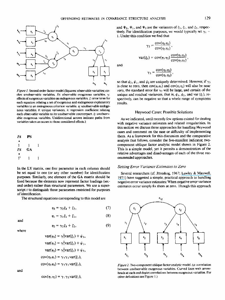
Figure 1. Second order factor model (Squares: observable variables; cir- cles: unobservable variables. Xs: observable exogenous variables. 3': effects of exogenous variables on endogenous variables. ~. error term for each equation relating a set of exogenous and endogenous explanatory variables to an endogenous criterion variable, n: unobservable endoge- nous variables. 0: unique variances. ),: regression coet~cient relating each observable variable to its unobservable counterpart. 6: unobserv- able exogenous variables. Unidirectional arrows indicate paths from variables taken as causes to those considered effects.)

PA PS

1 1 1 PA GA

1 t 1 1

a n d xl/3, XI/l, and XII 2 a r e the variances of ~'3, ~'~, and f2, respec- tively. For identification purposes, we would typically set 3'1 = 1. Under this condition we find that

COV(TI3 rl2)

"}/2 -- COV(.O3,r]I) ,

COV('I7 3 '171 ) var(~l) = COV('r/l '02)

C0V073 712) '

and

cov(n3n2) 'Y3 = COV(TI 1 r]2),

so that if3, r and if2 are uniquely determined. However, if 3"3 is close to zero, then cov(n3n0 and cov(n3n2) will also be near zero, the standard error for 3'2 will be large, and certain of the unique and residual variances, that is, ~ , %, and var (~), re- spectively, can be negative so that a whole range of symptoms results.

H e y w o o d Cases: Possible So lu t i ons

As we indicated, unti l recently few options existed for dealing with negative variance estimates and related irregularities. In this section we discuss three approaches for handling Heywood cases and comment on the ease or difficulty of implement ing them. As a framework for this discussion and the comparative analysis that follows, consider the five-manifest indicator, two- component oblique factor analytic model shown in Figure 2. This is a simple model, yet it permits a demonstrat ion of the relative advantages and disadvantages of each of the three rec- ommended approaches.

In the LY matrix, one free parameter in each co lumn should be set equal to one (or any other number) for identification purposes. Similarly, one element of the GA matrix should be fixed because the elements now represent factor loadings (sec- ond order) rather than structural parameters. We use a super- script t to distinguish those parameters restricted for purposes of identification.

The structural equations corresponding to this model are

Set t ing Error Variance E s t i m a t e s to Zero

Several researchers (cf. JOreskog, 1967; Lawley & Maxwell, 1971) have suggested a simple, practical approach to handling negative error variance estimates: When negative error variance estimates occur simply fix them at zero. Though this approach

and

where

and

var(n3)

var(n3

vat(n2)

cov(n3n~)

COV(n3 n2)

n3 = "r3~l + ~'3,

rll = "Yl~l + ~'1,

n2 = 'Y2~l + ~'2,

= "r~var(~h) + if3,

= -r~var(6~) + 1~,

= -r2var(h) + %,

= "y3"Y2 var(~l),

= ~3'Y1 var(~i),

COV(nl/ /2) = "Yl 'Y2var(61),

(7)

(8)

(9)

Figure 2. Two-component oblique factor analytic model. (r correlation between unobservable exogenous variables. Curved lines with arrow- heads at each end depict correlations between exogenous variables. For other definitions see Figure 1.)

130 W. DILLON, A. KUMAR, AND N. MULANI

that requires fixing error variance estimates at zero can be han- dled by the LISREL VI program, it suffers from a number of well- known drawbacks. First, and perhaps most serious, maximum likelihood theory has not been proven to be valid at boundary minima. Second, as Bentler (1976) discussed, setting negative error variances to zero results in a mixed factor-component model. Bentler uses the term mixed factor-component model to describe the case where one or more of the manifest indicators of a latent construct are assumed to be measured without error. Setting a negative variance estimate to zero implies, at least con- ceptually, that the observable variable is measured without er- ror, which is consistent with a principal-components analysis specification. The problem with mixed factor-component models is that the parameter estimates obtained with maximum likelihood methods are, in a strict sense, nonunique when viewed as nonrestricted estimates. 5

Reparameterization o f the Model

Recently, several researchers have developed different con- ceptualizations of linear structural models than that of JOre- skog's LISREL model (cf. Bentler, 1976; Bentler & Weeks, 1980; Lee, 1980; Lee & Tsui, 1982; McDonald, 1980). These alterna- tive conceptualizations allow the user to impose rather general types of constraints on model parameters. In theory, at least, the nature of the constraints permitted is such that all error variance estimates must be strictly positive. Unfortunately these methods are not currently available to the typical user of structural equation models nor, in general, can they be imple- mented with the LISREL VI computer program. An exception is Bentler's (1976) structural factor analysis model. As we shall demonstrate, the LISREL model, in certain instances, can be viewed as a restricted version of this model and thus can be implemented with the LISREL VI computer program.

The covariance matrix ofx under Bentler's (1976) structural factor analysis model has the form

2; = Z ( A M A ' + I)Z. (10)

This structure has several interesting features. First, the struc- tural form of the covariance matrix shown in Equation 10 can- not reduce to a principal-components analysis model of the form 2; = AA'. Second, it can reduce to the structural covari- ance matrix shown in Equation 2 by specifying A = ZA, r = M, and O, = Z 2. Interestingly, Z cannot be taken as null, because of the positive variances in X; in addition, even if some elements in Z are negative, all error variances must be strictly positive because Os = Z 2 > 0. Because it may not be clear how to opera- tionalize Bentler's model with the LISREL VI computer program, we shall give details on its implementation.

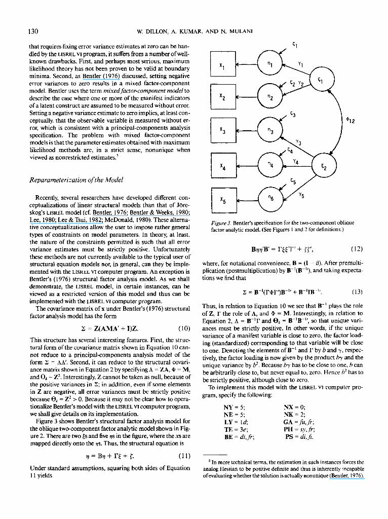
Figure 3 shows Bentler's structural factor analysis model for the oblique two-component factor analytic model shown in Fig- ure 2. There are two ~s and five ns in the figure, where the xs are mapped directly onto the ns. Thus, the structural equation is

n = Br /+ F~ + L (11)

Under standard assumptions, squaring both sides of Equation 11 yields

Figure 3. Bentler's specification for the two-component oblique factor analytic model. (See Figures 1 and 2 for definitions.)

Br/n'B ' = F ~ ' F ' + ~'~", (12)

where, for notational convenience, B = (I - 3). After premulti- plication (postmultiplication) by B-I(B-~'), and taking expecta- tions we find that

2; = B-I(I'~I'F')B -l ' + B-qB -1'. (13)

Thus, in relation to Equation 10 we see that B -t plays the role of Z, F the role of A, and r = M. Interestingly, in relation to Equation 2, A = B-~F and O, = B-aB -~', so that unique vari- ances must be strictly positive. In other words, if the unique variance of a manifest variable is close to zero, the factor load- ing (standardized) corresponding to that variable will be close to one. Denoting the elements ofB -~ and F by b and 3', respec- tively, the factor loading is now given by the product b~, and the unique variance by b:. Because b3' has to be close to one, b can be arbitrarily close to, but never equal to, zero. Hence b 2 has to be strictly positive, although close to zero.

To implement this model with the LISREL VI computer pro- gram, specify the following:

NY = 5; NX = 0; NE = 5; NK = 2; LY = ld; GA =fu, fr; TE = 3e; PH = sy, fr; BE = di, fr; PS = di, fi.

5 In more technical terms, the estimation in such instances forces the analog Hessian to be positive definite and thus is inherently incapable of evaluating whether the solution is actually nonunique (Bentler, 1976).

OFFENDING ESTIMATES IN COVARIANCE STRUCTURE ANALYSIS 131

Placing Constraints on the Unique Variance

Rindskopf (1983) has demonstrated a method for preventing Heywood cases. His method involves the'parameterization pre- sented by Bentler and Weeks (1980) and combines a suggestion made by Bentler (1976) with a class of models proposed by Werts, Linn, and J0reskog ( 1971 ) in which the unique variances were viewed as factors with the same nominal status as other latent variables to allow error correlation.

In the usual parameterization of structural models with LIS- REL the coefficients for residuals and unique variances are usu- ally fixed at one, whereas their variances are considered free and thus need to be estimated. As we have discussed, in the conventional model the error variances need not be positive. Using Bentler and Weeks's parameterization, however, Rind- skopf demonstrates a simple solution to this problem: Fix the variance of the residual or unique variance at one and estimate the coefficient. According to Rindskopf, "Regardless of whether the coefficient is positive or negative, the square of the coeffi- cient will be positive, so the variance will be positive" (1983, p. 75). We demonstrate how this can be implemented with the LISREL VI computer program next.

To implement Rindskopf's method we simply need to intro- duce as many ~s as there are independent variables and com- mon factors, whether observed or latent, and whether they rep- resent unique or residual variables or not. In the case of our illustrative model, two of the ~s are reserved for the latent fac- tors, whereas each of the remaining five ~s corresponds to one of the unique factors. Thus, the factor loading matrix has as many rows as there are observed independent variables and as many columns as there are latent factor variables in the model. We see, therefore, that the matrix contains more than one type of effect: It contains the loadings that map the observed vari- ables onto their latent counterparts as well as the effects of the unique variables, where the squares of these unique variable effects give the error variance estimates. To fix the variance of the unique variables at one we need to simply set the relevant elements in �9 equal to 1.0. Note that ,I, also contains more than one type of effect: It contains the variances and covariances of the common factors as well as the unique variances.

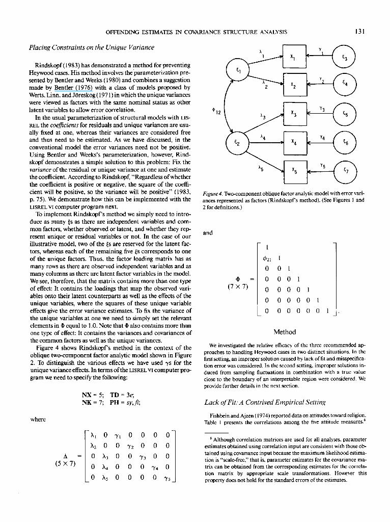
Figure 4 shows Rindskopf's method in the context of the oblique two-component factor analytic model shown in Figure 2. To distinguish the various effects we have used "rs for the unique variance effects. In terms of the LISREL VI computer pro- gram we need to specify the following:

N X = 5 ; T D = 3 e ; N K = 7 ; P H = s y , fi;

where

A (5 • 7)

~k 1

X2

= 0

0

0

0 "YI 0 0 0 0-7

0 0 "r2 0 0 0

~k 3 0 0 "~'3 0 0

~,4 0 0 0 3'4 0

~,5 0 0 0 0 ~'5

Figure 4. Two-component oblique factor analytic model with error vari- ances represented as factors (Rindskopf's method). (See Figures 1 and 2 for definitions.)

and

(7 • 7)

1

~b21

0

= 0

0

0

0

1

0 1

0 0

0 0

0 0

0 0

1

0 1

0 0 1

0 0 0

Method

We investigated the relative efficacy of the three recommended ap- proaches to handling Heywood cases in two distinct situations. In the first setting, an improper solution caused by lack of fit and misspecifica- tion error was considered. In the second setting, improper solutions in- duced from sampling fluctuations in combination with a true value close to the boundary of an interpretable region were considered. We provide further details in the next section.

Lack of Fit: A Contrived Empirical Setting

Fishbein and Ajzen (1974) reported data on attitudes toward religion. Table 1 presents the correlations among the five attitude measures?

6 Although correlation matrices are used for all analyses, parameter estimates obtained using correlation input are consistent with those ob- tained using covariance input because the maximum likelihood estima- tion is "scale-free," that is, parameter estimates for the covariance ma- trix can be obtained from the corresponding estimates for the correla- tion matrix by appropriate scale transformations. However this property does not hold for the standard errors of the estimates.

132 W. DILLON, A. KUMAR, AND N. MULANI

These data have been used to test various conceptualizations of the structure and dimensionality of attitudes (cf. Bagozzi & Burnkrant, 1979; Dillon & Kumar, 1985). In one conceptualization, attitudes are hypothesized to be multidimensional, represented by an oblique two- component factor analytic model similar to that shown in Figure 2, in which the self-rating (Xt) and semantic differential (X2) indicators load on the affective component and the Guttman (X3), Liken (X4), and Thurstone (X~) indicators load on the cognitive component. To create an improper solution the epistemic correlation (r between the affec- tive and cognitive components is set equal to .50. For these data, this is a sufficiently small value to cause lack of fit and irregularities in the 8x2 parameter estimate (specifically ~x2 = -.248).

Sampling Fluctuations: A Monte Carlo Simulation

A small Monte Carlo study was designed in the context of the oblique two-component factor analytic model of Figure 2. The loading for the X~ indicator was set at .9, which is the upper bound of indicator reliabil- ity obtained in practice. A loading of .7 was set for all other indicators. The correlation between factors was set at .50, a moderate value as some correlation between factors is usually posited in confirmatory factor analysis applications. A population correlation matrix was constructed using the rules of path analysis. Using the IMSL subroutines GGNSM and GGUBS (IMSL, 1980), 7 a multivariate normal population based on the specified population correlation matrix was constructed along with 500 samples of size 62. Given the small number of indicators per factor and the small sample size, we expected to obtain a significant number of improper solutions.

A n a l y s e s

Lack-of-Fit Results

Setting the offending estimate to zero. This approach recom- mends setting the offending estimate, in this case 0x2, equal to zero and reestimating the model. Not surprisingly the revised model still does not fit the data, • = 17.58, p < .01, GFI = .912, AGFI = .781. However, no other offending estimates ap-

pear. Reparameterization--Bentler's model. When fitting Bent-

ler's model, the LISREL VI computer program indicated that the free parameter corresponding to "r2 may not be identified. In our experience, when the LISREL VI computer program warns of a possible unidentified parameter that appears to be algebra- ically identified, its assessment is probably correct, with empir i - cal underidentification the likely culprit. In the present case the

Table 1 Correlations for the Self-Reported Behaviors Sample

Indicator SR SD G L T

SR 1.000 SD .800 1.000 G .519 .644 1.000 L .652 .762 .790 1.000 T .584 .685 .744 ,785 1.000

Note. No. of observations = 62. SR = Guilford self-rating (X~). SD = semantic differential (X2). G = Guttman (X3). L = Likert (X4). T = Thurstone (Xs). Adapted from "Attitudes Towards Objects as Predic- tors of Single and Multiple Behavioral Criteria" by M. Fishbein and I. Ajzen, 1974, Psychological Review, 81, p. 63. Copyright 1974 by the American Psychological Association. Adapted by permission.

Table 2 Parameter Estimates for the Two-Component Attitude Model Using Rindskopf's Method

LISREL

Parameter estimate SE

hi 0.726 )~2 0.902 ~,a 0.777 ),4 0.842 ~,s 0.777 71 0.600 3'2 0.000 ~ ~'3 0.517 74 0.373 7s 0.517 ~21 0.500b

X2(5) 17.58 p <.01

GFI .912 AGFI .737

0.113 0.120 0.099 0.093 0.099 0.095

32,822.095 0.064 0.076 0.064

Note. The variances of all seven factors were fixed at unity. "Parameter evaluated to zero. b Fixed parameter.

problem can be explained as follows. The max imum likelihood solution yields a negative variance estimate for 8x2; however, with Bentler's model negative variance estimates are strictly not permitted. A reasonable approach in such instances, and this is actually what the program at tempts to do, is to find the solution closest to the max imum such that Ox2 is near zero but positive. If 0x2 is near zero and positive, then its corresponding loading is by necessity near one. Yet how can this loading be close to one? Obviously, because A = 13-~ F, we can arbitrarily make the 1~2 and "~2 elements large so that I~-q3-r will be small. Thus, a basic indeterminancy exists in that only the product I3 -~ F is uniquely determined, whereas the individual parameters are in- determinate and thus their individual estimates explode. As the Monte Carlo simulations that follow indicate, this property of Bentler's model is not restricted to improper solutions caused by lack o f fit or misspecification error.

Constraining unique variances--Rindskopf's method. Table 2 presents the results of applying Rindskopf 's method. It is in- teresting to note that the error variance estimate for the seman- tic differential scale i tems ('Y2) does not differ from zero. In es- sence this is the same solution as produced by the method in which the offending estimate is set to zero. There is, however, a difference. Though the goodness-of-fit statistics are identical, the degrees of freedom for the two models are different. Under Rindskopf 's approach the degrees of freedom are the same as in the unconstrained model. This is because the constraints im- posed under Rindskopf 's method are inequality constraints and as such they do not add to the degrees of freedom (Rindskopf, 1983). Note also the extremely large standard error associated with the ")'2 parameter effect. With a standard error of this mag-

7 An initial random number is supplied as a seed that is then replaced by an internally generated random number on each of the subsequent calls to GGNSM. The random number seed for each sample generated was different.

OFFENDING ESTIMATES IN COVARIANCE STRUCTURE ANALYSIS 133

nitude, this effect is, for all intents and purposes, uninterpret- able. We say more about these and other aspects of Rindskopf's method in the Discussion section following the Monte Carlo sampling results.

Sampling Fluctuations

Of the 500 Monte Carlo sampling runs performed, 133 (26.6%) yielded improper solutions. To compare each of the al- ternative approaches across the 133 improper solutions, five qualitative measures of performance were defined.

1. Convergence. Did the trial run produce a solution that reached the convergence criteria (see J0reskog, 1967, p. 406) after 250 iterations?

2. Identification. Did the trial run produce a warning indi- cating that one (or more) of the parameters may be unidenti- fied?

3. Zero estimate. Did the trial run produce a solution in which the offending estimate was not different from zero (within three significant digits)?

4. Large standard errors. Did the trial run produce parame- ter estimates that have large, uninterpretable standard errors?

5. Other offending estimates. Did the trial run produce a so- lution in which one (or more) other offending estimates sur- faced?

All of the qualitative performance measures just described are of practical importance to the applied researcher. Models that do not converge, or are unidentified, or have large standard errors for parameter estimates are not interpretable. Whether the offending estimate is not significantly different from zero (after correction) and the extent to which other offending esti- mates surface (after correction) are important indicators of the relative superiority of Bentler's model and Rindskopf's con- strained approach vis-a-vis the simpler approach of setting the offending estimate to zero. If Bentler's model and Rindskopf's constrained approach yield solutions in which the offending es- timate is zero and/or other unique variance estimates are nega- tive, then the simpler approach of setting the offending estimate to zero may be preferred.

Table 3 presents the Monte Carlo sampling results in terms of the number and proportion of times each performance measure occurred for each of the alternative approaches.

Setting the offending estimate to zero. This approach, which recommends setting the offending estimate Ox2 to zero and re- estimating the model, compared favorably with the other ap- proaches. In 100% of the trial runs this approach yielded a solu- tion that met convergence criteria after 250 iterations, with no apparent identification problems; in addition, standard errors were reasonable in all cases and no other offending estimates surfaced.

Reparameterization--Bentler's model. With Bentler's model 26% of the trial runs produced a solution that did not meet the convergence criteria after 250 iterations. Of the 99 trial runs that produced solutions that converged, 99% had identification problems, s and in cases where parameter standard errors could be computed, unreasonable (especially large) estimates re- suited. Note also that no cases had a nonzero parameter esti- mate for the offending estimate.

Constraining unique variances--Rindskopf's method. This

Table 3

Monte Carlo Sampling Results

Approaches

Performance measure Fixed Bentler Rindskopf

Convergence Yes 1.00 (133)" .74(99) .98(130) No .00 (0) .26 (34) .02 (3)

Identification Yes .00 (0) .99 (98) b .45 (59) b No 1.00(133) .01 (1) .55 (71)

Zero estimate Yes c 1.00 (99) b 1.00 (120) b No - - .00 (0) .00 (0)

Large SE Yes .00 (0) .00 (1) d .00 (71) a No 1.00 (133) .00 (0) .00 (0)

Other offending estimates Yes .00 (0) .00 (0) .00 (0) No 1.00(133) 1.00(99) b 1.00(130) b

�9 Values in parentheses are numbers of times measures occurred. b Percentages based on total number of trial runs producing solutions that met convergence criteria after 250 iterations, c Not applicable-- this approach always produces a zero estimate, d Percentages based on total number of trial runs for which no identification problems were obtained. If any parameter is detected to be unidentified, the LISREL VI computer program will not compute standard errors.

approach also yielded unsatisfactory results. In particular, of the 130 trial runs that produced solutions meeting the conver- gence criteria after 250 iterations, 45% had identification prob- lems, and in all cases a zero parameter estimate for the offend- ing estimate was obtained. Note, finally, that all of the 71 trial runs for which an identified model was obtained yielded unrea- sonable (especially large) standard errors for the parameter esti- mate in question.

Discussion

The models discussed previously correspond to three differ- ent versions of the factor analysis model. In the conventional form of the model Heywood cases are possible. Two other forms of the model have been suggested. In one form (Bentler, 1976), unique variances must be strictly positive. In the other form (Rindskopf, 1983), negative error variances are not possible, though zero error variances are possible. The usual form of the model can be viewed as a restricted version of these latter two forms, although the inequality constraints are never made di- rectly (Rindskopf, 1983).

On the surface at least, the second and third forms of the model appear to offer great promise as potential methods for

s We suspect that for the single trial run in which no identification problems were detected the likelihood function had multiple minima, one or more of which occurred within the permissible region. Thus, using Bentler's model the program is not "permitted" to enter that part of the parameter space for which "the error" variance estimate is nega- tive, and is "redirected" to one of the other local minima. In cases where the likelihood function is smooth and well-behaved this does not occur, and the resulting estimate for the offending parameter is quite close to zero.

134 W. DILLON, A. KUMAR, AND N. MULANI

preventing negative error variance estimates. However, though these two approaches represent theoretically elegant ways of handling this problem, they have limited practical usefulness compared with the simpler approach in whieh the offending parameter estimate is fixed at zero. Consider first Bentler's for- mulation. As we have seen in cases where the maximum likeli- hood solution produces a negative error variance estimate, re- gardless of its cause, attempts to restrict all of the error variance estimates to be strictly positive will generally result in identifi- cation problems. In other words, there is a basic indetermi- nancy in the solution. Because the loadings and error variances are parameterized in terms of the product of other parameters, the effect estimates for the offending variable or variables can be made arbitrarily large. The individual effect estimates are underidentified; only the product is uniquely determined.

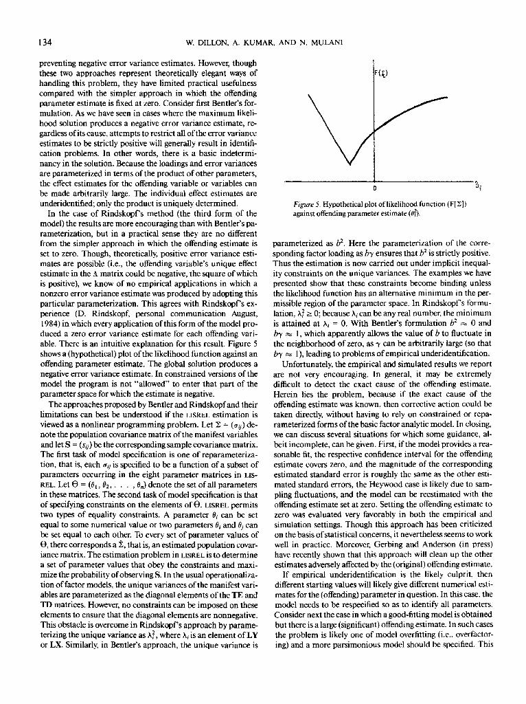
In the case of Rindskopf's method (the third form of the model) the results are more encouraging than with Bentler's pa- rameterization, but in a practical sense they are no different from the simpler approach in which the offending estimate is set to zero. Though, theoretically, positive error variance esti- mates are possible (i.e., the offending variable's unique effect estimate in the 5_ matrix could be negative, the square of which is positive), we know of no empirical applications in which a nonzero error variance estimate was produced by adopting this particular parameterization. This agrees with Rindskopf's ex- perience (D. Rindskopf, personal communication August, 1984) in which every application of this form of the model pro- duced a zero error variance estimate for each offending vari- able. There is an intuitive explanation for this result. Figure 5 shows a (hypothetical) plot of the likelihood function against an offending parameter estimate. The global solution produces a negative error variance estimate. In constrained versions of the model the program is not "allowed" to enter that part of the parameter space for which the estimate is negative.

The approaches proposed by Bentler and Rindskopfand their limitations can best be understood if the LISREL estimation is viewed as a nonlinear programming problem. Let ~ = (~r0) de- note the population covariance matrix of the manifest variables and let S = (sij) be the corresponding sample covariance matrix. The first task of model specification is one of reparameteriza- tion, that is, each ~rij is specified to be a function of a subset of parameters occurring in the eight parameter matrices in LIS- REL. Let O = (0~, 02 . . . . . 0n) denote the set of all parameters in these matrices. The second task of model specification is that of specifying constraints on the elements of O. LISREL permits two types of equality constraints. A parameter O~ can be set equal to some numerical value or two parameters Oi and Oj can be set equal to each other. To every set of parameter values of O, there corresponds a ~, that is, an estimated population covar- iance matrix. The estimation problem in LISREL is to determine a set of parameter values that obey the constraints and maxi- mize the probability of observing S. In the usual operationaliza- tion of factor models, the unique variances of the manifest vari- ables are parameterized as the diagonal elements of the TE and TD matrices. However, no constraints can be imposed on these elements to ensure that the diagonal elements are nonnegative. This obstacle is overcome in Rindskopf's approach by parame- terizing the unique variance as )`2, where )`i is an element of LY or LX. Similarly, in Bentler's approach, the unique variance is

Figure 5. Hypothetical plot of likelihood function (F[Z]) against offending parameter estimate (012).

parameterized as b 2. Here the parameterization of the corre- sponding factor loading as b~' ensures that b 2 is strictly positive. Thus the estimation is now carried out under implicit inequal- ity constraints on the unique variances. The examples we have presented show that these constraints become binding unless the likelihood function has an alternative minimum in the per- missible region of the parameter space. In Rindskopf's formu- lation, )2 > 0; because )`i can be any real number, the minimum is attained at )`i = 0. With Bentler's formulation b 2 ~ 0 and b3, ~ 1, which apparently allows the value of b to fluctuate in the neighborhood of zero, as 3' can be arbitrarily large (so that b3, ~ 1), leading to problems of empirical underidentification.

Unfortunately, the empirical and simulated results we report are not very encouraging. In general, it may be extremely difficult to detect the exact cause of the offending estimate. Herein lies the problem, because if the exact cause of the offending estimate was known, then corrective action could be taken directly, without having to rely on constrained or repa- rameterized forms of the basic factor analytic model. In closing, we can discuss several situations for which some guidance, al- beit incomplete, can be given. First, if the model provides a rea- sonable fit, the respective confidence interval for the offending estimate covers zero, and the magnitude of the corresponding estimated standard error is roughly the same as the other esti- mated standard errors, the Heywood case is likely due to sam- pling fluctuations, and the model can be reestimated with the offending estimate set at zero. Setting the offending estimate to zero was evaluated very favorably in both the empirical and simulation settings. Though this approach has been criticized on the basis of statistical concerns, it nevertheless seems to work well in practice. Moreover, Gerbing and Anderson (in press) have recently shown that this approach will clean up the other estimates adversely affected by the (original) offending estimate.

If empirical underidentification is the likely culprit, then different starting values will likely give different numerical esti- mates for the (offending) parameter in question. In this case, the model needs to be respecified so as to identify all parameters. Consider next the case in which a good-fitting model is obtained but there is a large (significant) offending estimate. In such cases the problem is likely one of model overfitting (i.e., overfactor- ing) and a more parsimonious model should be specified. This

OFFENDING ESTIMATES IN COVARIANCE STRUCTURE ANALYSIS 135

typically occurs in mult i t rai t-mult imethod analysis using covar- iance structure models (cf. Farh, Hoffman, & Hegarty, 1984).

Finally, in cases suffering from lack of fit and misspecification error in which large (significant) negative error variance esti- mates are obtained, there is no satisfactory solution for han- dling the offending estimate, except to critically examine the theory and data on which the model is based. In such cases there are no ready-made methodological solutions because the prob- lem is neither methodological nor statistical. Negative variance estimates surface in such cases because the covariance model is ad hoc and atheoretical; in general, post hoc remedial measures can rarely if ever correct for theoretical deficiencies in a model.

R e f e r e n c e s

Anderson, T. W., & Rubin, H. (1956). Statistical inference in factor analysis. Proceedings of the Third Berkeley Symposium on Mathe- matical Statistics and Probability, 5, 111-150.

Bagozzi, R. P. (1981). Attitudes, intentions, and behavior: A test of some key hypotheses. Journal of Personality and Social Psychology,, 41, 607-627.

Bagozzi, R. P., & Burnkrant, R. E. (1979). Attitude organization and the attitude-behavior relationship. Journal of Personality and Social Psychology, 37, 913-929.

Bentler, P. M. (1976). Multistructure statistical model applied to factor analysis. Multivariate Behavioral Research, 11, 3-25.

Bentler, P. M., & Bonett, D. G. (1979). Models of attitude-behavior relations. Psychological Review, 86, 452-464.

Bentler, P. M., & Speckart, G. (1981). Attitudes "cause" behaviors: A structural equation analysis. Journal of Personality and Social Psy- chology, 40, 226-238.

Bentler, P. M., & Weeks, D. G. (1980). Linear structural equations with latent variables. Psychometrika, 45, 289-308.

Dillon, W. R., & Kumar, A. (1985). Attitude organization and the atti- tude-behavior relation: A critique of Bagozzi and Burnkrant's re- analysis of Fishbein and Ajzen. Journal of Personality and Social Psy- chology, 49, 33-46.

Driel, O. P. van (1978). On various causes of improper solutions in max- imum likelihood factor analysis. Psychometrika, 43, 225-243.

Farh, J., Hoffman, R. C., & Hegarty, W. H. (1984). Assessing environ- mental scanning at the subunit level: A multitrait-multimethod anal- ysis. Decision Sciences, 15, 197-220.

Fishbein, M., & Ajzen, I. (1974). Attitudes towards objects as predictors of single and multiple behavioral criteria. Psychological Review, 81, 59-74.

Fredricks, A. J., & Dossett, D. L. (1983). Attitude-behavior relations: A comparison of the Fishbein-Ajzen and the Bentler-Speckart models. Journal of Personality and Social Pscholog)~, 45, 501-512.

Gerbing, D. W., & Anderson, J. C. (in press). Improper solutions in the

analysis of covariance structures: Their interpretability and a com- parison of alternative specifications. Psychometrika.

Harman, H. H. ( 1971 ). Modern factor analysis. Chicago: University of Chicago Press.

IMSL. (1980). International Mathematical and Statistical Libraries. Houston, TX: Author.

JOreskog, K. G. (1967). Some contributions to maximum likelihood factor analysis. Psychometrika, 32, 443-482.

J6reskog, K. G., & Si~rbom, D. (1982). LlSREL VI: Analysis of linear structural relationships by maximum likelihood. Morresville, IN: Scientific Software.

Judd, C. M., & Krosnick, J. A. (1982). Attitude centrality, organization, and measurement. Journal of Personality and Social Psychology, 42, 436--447.

Kenny, D. A. (1979). Correlation and causality New York: Wiley. Koopmans, T. C. (1949). Identification problems in econometric model

construction. Econometrica, 17, 125-143. Koopmans, T. C., & Reiersol, O. (1950). The identification of structural

characteristics. Annals of Mathematical Statistics, 21.165-181. Lawley, D. N., & Maxwell, A. E. ( 1971 ). Factor analysis as a statistical

method. London: Butterworths. Lee, S. Y. (1980). Estimation of covariance structure models with pa-

rameters subject to functional restraints. Psychometrika, 45, 309- 324.

Lee, S. Y., & Tsui, K. L. (1982). Covariance structure analysis in several populations. Psychometrika, 47, 297-308.

McDonald, R. P. (1980). A simple comprehensive model for the analysis ofcovariance structures: Some remarks on applications. British Jour- nal of Mathematical and Statistical Psychology, 33, 161 - 183.

McDonald, R. P., & Krane, W. R. (1977). A note on local identifiability and degrees of freedom in the asymptotic likelihood ratio test. British Journal of Mathematical and Statistical Psychology,, 30, 198-203.

McDonald, R. P., & Krane, W. R. (1979). A Monte Carlo study of local identifiability and degrees of freedom in the asymptotic likelihood ratio test. British Journal of Mathematical and Statistical Psychology, 30, 198-203.

Reiersol, O. (1950). On the identifiability of parameters in Tburstone's multiple factor analysis. Psychometrika, 15, 121-149.

Rindskopf, D. (1983). Parameterizing inequality constraints on unique variances in linear structural models. Psychometrika, 48, 73-83.

Rindskopf, D. (1984). Structural equation models: Empirical identifi- cation, Heywood cases, and related problems. Sociological Methods &Research, 13, 109-119.

SPSS, Inc. (1983). sPss-x User's Guide. New York: McGraw-Hill. Werls, C. E., Linn, R. L., & JOreskog, K. G. (1971). Estimating the

parameters of path models involving unmeasured variables. In H. M. Blalock, Jr. (Ed.), Causal models in the social sciences. Chi- cago: Aldine-Atherton.

Received September 16, 1985 �9