TID UNIVERSITY OF I'ÍANITOBA

Comput erized Budgetingof Alternative Crop

Model for the EvaluationProduction Prograus

by

Gary G. Craven

A TT{ESIS

SUBMITTED TO TITE FACULTY OF GRADUATE STUDIES

IN PARTIAL FULFILI,ÍENT OF THE REQUIREMENTS FOR THE DEGREE

OF I4ASTER OF SCIENCE

DEPARTMENT OF AGRICULTURAI. ECONOMICSA}ID FARM MANAGEMENT

I^IINNIPEG, MANITOBA

May,1981

A COMPUTERIZTD BUDGITING MODEL FOR THE EVALUATION

0F ALTERNATIVT CROP PR0DUCTI0N PROGRAI'1S

BY

GARY G. CRAVTN

A rhcsis st¡bnlittccl ro thc lìacLrlty of Graduatc Stuclies of'

tltc [-;rtivcrsity ol' tr4allitoba rn partial firlfillnrcnt of the recllrirenients

ol- tllc dcgree ol

¡1ASTTR OF SCITNCE

O " l98l

Pcr.nrissio¡r has bccn grantccl to the LIBRARY OF THE UNIVER-

SIT\' ()[.] MANITOIIA to lcnd or sell copics of this thcsis, to

the NA^'l'IONAL LIBIìAIIY OF CANADA to microfilnr this

the sis uncl to lcncl or' -ssll copics of the film, and UNIVERSITY

f'/l( Ìì.()lrlLNIS to ¡rublish an abstract of this thesis.

I'hc :rirtlior rescrvcs otlicr prrblicatiort rights, and ueither the

thc:;i:; tror cxtcnsivc cxtracls lrolll it niay be printecl or other-

rvisc t'cproclLrccd r,vithout Llte author's written perniission.

ABSTRACT

One useful tool which has always been available Lo managers r¿ith the

ski11s necessary to enploy it has been Ëhe farn budget. The preparation

of deËailed farm enterprise budgets has required extensive resources of

both information and time. The development of a programmed budget nodel

makes this fonn of analysis available to farmers, and others, who have

previously lacked the skill, training or the tirqe to successfully ernploy

it.

This study reviews the revelant theg,ry used to provide a concept,ual

framework for the decision making process. After considering t,he lini-

tations of various decision naking aids Ehe Èechnique of budget símula-

tion rá7as select,ed to evaluate Ehe effects of alternative croppi.ng prac-

Ëices and various corobinations of inputs.

The enpirical uodel is based on an earlier raodel developed in Ehe De-

partnent, of Agricultural Economics and Farm Management at the University

of Manj.toba for research, to generate budgets depicting the cosËs and

returns of crop producËi.on. These budgets are based on user supplied

physical infomation representing equipraent, land and cultural practic-

€s, and rely on secondary cost data.

The uodel was validated Lhrough the use of a case farm study. The

comparative analysis of the case fara indicated that the nodel is capa-

b1e of generaEing acceptable estiroaËes of enËerprise costs and reËurns

when only physical infornation is available.

-11--

The potenËiaL exists for a wide variety of applications of the rood.el.

The nost extensive applicati.on to daËe has been for research. The sys-

Èem can be used as a deci.sion uaking tool by the farm manager when look-ing at erop production alternatives. Potential applications also exj.st

r¿henever insight ínËo t.he costs and benefits of cropping syste*s is de-

sired. such infornation rnay be of use to educaËional, financiar, and

consultative institutions. The potential also exists for model useage

by government to generate daËa for the administraÈion of existing pro-grams and to assess the fÍnancial irnpact on the farrn firm of legislativeproposals.

- ltr_ -

ACKNOWLEDGEMENTS

I would like t.o Lake this opportunity to express ny appreciation of

several individuals who made this work possible. Thanks are extended to

Dr. Charles Framingham, my advisor, whose encouragenenL, leadership and

advice led to its eompletion. My rhanks are also extended to Dr. Ed

Tyrchniewicz and Prof. Paul Stelnaschuck for their comments and con-

structive criticisns which aided in iËs final preparation.

I would like to thank Mr. Neil Longmuir for his help in untangling

the conputer program, and my co-workers on the study for their assis-

tance in compiling the data necessary for iLs operaËion.

I am grateful to Lhe North Lab Lovelies and Ehe Annex Animals for

their technical assistance and moral support enabling rne Èo nai.ntain roy

sanity.

Finally, I would like to express ny deep appreciaËion t,o ny fanily,

who encouraged uy studies, for t,heir sacrifices in rnany ways which a1-

lowed ne to conLinue uy education.

-1V-

CONTENTS

ABSTRACT

ACKNOI4TLEDcEIfrNTS

Chapter

I. INTRODUCTION

.ii

..iv

page

Historical OverviewSysÈen DynamicsThe Setting

The Problen0bjecÈives

I7

L2L4T4

II. THE PROBLEM IN PERSPECTIVE

tlistorical Developnent .Related Studies

III. TIIEORETICAI CONSIDERATIONS

ConceptualModel.. 30TheoreticalBody.. ..34

Theory of Resource Allocation . 35Static Theory of rhe Firn 35Adaptive Theory of rhe Firn 3g

DecisionTheory.. .4IDecision-naking under certainty . 4IDecisj.on-naking under risk . . 4LDecision-naking under uncertainËy . 42

AdaptiveDecision-Making ".47IV. OPERATIONAL SYSTEMS

Prearnble . .Analytic Approaches .

Differential CalculusLÍnear Programrn-ing .Dynamic Prograrnmi.ng

Synthetic Approaches .Regression Analysis .Systems Sinulation .

Simulat,ion Methodology .Steps . .Fornulatiort of the Model

-v-

L7

T720

5t

5155555659606061626366

v.

Programming . 67Validation and Verification . . 67Experimentation . . 67

Randou Search 68Experimental Design 69LearningMechanisu.. .70Hill Clinbing . 70

THE EMPIRICAL MODEL . 72

The Mathematical StatementApplication

Problem Fornulation .Analysis

SLruct.ure of the model . .Calculations for Machinery . .Other InpuE Cost Calculationsttvalue of Outputtt CalculationsReturn IndicaLors .

7276767878B486898989Detailed cosË/return calculat

Prelininary Calculations10n s

per field operaËionalculationsS.osf .1 and lubrication costs. .air costs.tom charges

Acres per hour . .SwaEhers and inplements .

' Conbines .Trucks, bale wagonsCusËom work.

90909l939497

IO10T2

I41516

Time requiredMachinery Cost C

Vari.able CostLabor c

FueRepCus

Fixed Costs

9B98989B

100r03104105

Input Cost CalculationsVariable costsFixed costsValue of output calculations .

ReËurn indicaEors .Input Dat,a

System ResidenË InfomaËionAnnual Infornation . II7Producer Infornation . 1I9

Farm Machinery Cost Analysis . I2IIndividual Crop Enterprise . . I23Total Farm Summary . . L25

VI. EVALUATION

VII. R-ECOMI,ßNDATIONS AND CONCLUSIONS

Procedural Recommendations 135Conbined Field OperaËions . I35Alternate Faru Income Sources . 136

L7

r27

135

-vL-

Fixed CostExpans ion

Rent.alUnitsMacro-0peraEionsAlphanumeri.cs

Expansion of Output Inforrnation . . I42Operation Tirne 142Return Indicators . 143Cash Flow

S t n-rctural RecommendaËi onsInpuË-OuËput. ControlFile MainEenance and Retrieval

Ileuristic ExpansionResident Fam DescriptionsUser StatisticsReport Generation

Enterprise IntegrationConclusions

Allocation . 137of rnputrr,rorr"iiår,'"::..: 138and Custom Charges 138

139140r40

L45145r45I48148L49r49150150150

t52

page

r57

r67

189

r90

190i91

BIBLIOGRAPIIY

Appendix

A. SYSTEM INFORMATION

B. DEFAULT COST DATA FOR 1979

C. USER,S GUIDE

Fertilizer Description CardChenical Description CardTillage Practíce CardInteractive InputClient InfornationField Infonuation

General Description .Input Description .Tillage Practices . .

Exauple of Interactive Operation . .Assumptions Used t.o Code Crop Enterprises

General Client Infornati.onMachinery InvenËory DescriptionGeneral Production Inf ormaLion

-vii-

Input Data Forrnat GuideClient Header Card . 190Machinery Inventory Description CardLivesÈock }fachinery InfornationTillage Practice Header Card . L92Irrigation Operating CosL Card . . L92Crop infornation CardSeed Inforroation Card

193193194194t94i951961971971971981992r52r52r5217

Crop InformaËionSeed informâtionFert,ilizer Inf ornaËionChero:lcal Inf or¡na tionTillage Practices

218218219220220

237

2402482s5

279

280

PRODUCER QUESTIONNAIRE

Master Machinery ListMaster Land List . .Cropping Practices

E. CASE FARM RESULTS

Default Case Farrn ResultsAdjusted Case Fam Result,s 313

- vl-11- -

TabIe

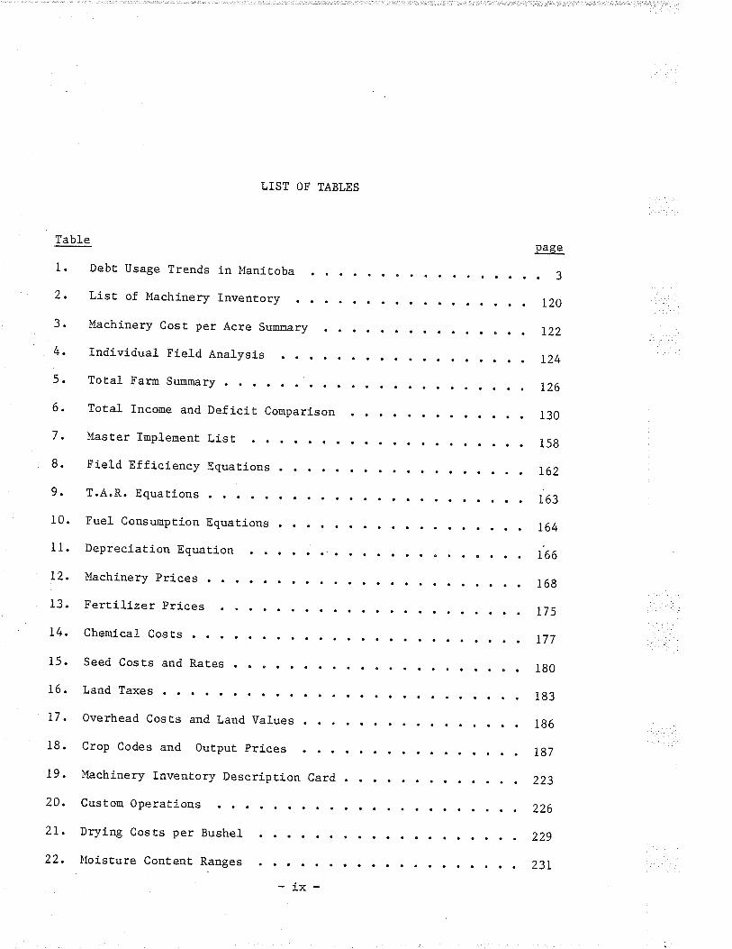
LIST OF TABLES

Debt Usage Trends in Manlt,oba

List of Machinery InvenÈory

Machinery Cost per Acre Summary

Individual Field Analysis

Total Farn Sumnary .

Total Income and Deficit Comparison

Master luplenent, List

Field Efficiency Equations

T.A.R. Equations . .

EueI Consumption Equations

DepreciaEion EquaËion

Machinery Prices

f 3. Fertilizer pri.ces

Page

1.

a

3.

4.

5.

6.

7.

8.

9.

10.

11.

12.

3

120

122

r24

r26

r.30

i58

L62

163

r64

r66

168

175

14.

15.

r.6 .

77.

18.

19.

20.

Che¡nica1 Cos ts

Seed Costs and Rates

Land Taxes .

177

180

Overhead Costs and Land Values

Crop Codes and Output prices

Machinery Inventory Description Card

183

186

187

223

226

229

23L

Custom Operations

2I. Drying Costs per

22. lloisture Content

BusheI

Ranges

-l-x-

23. Seeding Data 232

LIST OF FIGURES

Figure

1. Bank of Canada prine

2. Ad justed llheaË prices

page

Rate 4

3. The Decision-lfaking process 10

4. Machinery Price EsÈi¡oar,ion . . . Zg

5. Schematic Representation of a Decision problem . 45

6. Murphy's Adaptive Decision proeess . . . 50

7. The Methodology of Siraularion .658. rllustrative Description of steps in Budget Generation . . . gz

9. Elements of the Cost ReporE . . g3

10. Summary of Crop Enterprise Input Costs . . gg

11. Elements of the Return Analysis . 90

12. Typical Farn Machinery Cosrs . I05

13' Rernaining Values for Farn Machinery as a Percentage of New Cost.109

14. I'fonthly Costs

15. Proposed Farn Firm Sinulator

141

L47

-x1 -

Chapter I

INTRODUCTION

1 .1 THN SETT.ING

AgriculËural producÈion in Canada has depend.ed upon Lhe inherenË

ability of producers to utilize available capital and labor to m¡xi.mize

returns. Modern commercial agriculture in Canada is characterized by

rapid and dramatic change. There have been rapid Ëechnological advances

in production teehniques accompanied by an increased substitution ofcapital for labor and subsËantial increases in average farm size. This

has increased the frequency and importance of d.eci.sions which farrners

must make to adjust Ëo these changing condj.tions. Decisions respecting

such adjustments require careful appraisal and may result in changes

which will have a long lasting effecL on the far¡n and the farn fanily.IL is necessary to carefully evaluate the consequences of a1Ëernative

decisions before resotlrces are conmi.tted.

The conplexity of the decision-naking process suggests thatfarmers could benefit naterially from computer-oriented ,nan-agenent tools which have Lhe capacity' and flexibility to ac-commodate their part,icular situations.t

One of the uost productive resources available to farm managers isLhe use of debt financing. Dramatic inc,reases j.n debt use have occurred

in agriculture in Canada and Manitoba over the 1970's as detailed in Ta-

1 u.r. Sonntag, "UsingEconomics, Volume 7,p.3

Comput.ers in the Farm Business", CanadÍ.an FarraNo. 3 August, L972. AgriculÈure C"""¿"1 OttaÍ¡a.

-1-

2

ble 1. Debt outstanding has increased froro $41S rnillion in IgTI to

çL,324 uillion by 1979 in Manitoba. This has uore than doubled since

I975 after re'n¡Íning constant since I97I. Interest paid on this debt

has increased from $29 rnillion annually to $142 nillion annually over

the same period. More importantly, interest. expense has increased frou

20 percent of gross margin in 1971 to 40 percent by 1919. These figures

show the increased use of financial leverage and the increased exposûre

to financial risk. Interest expense is consuming a uuch great.er propor-

tion of net. incone, and also increasing as a proportÍon of farm expen-

ses. This indicates Lhat interest costs are rising at a faster rate

than other farm inputs. out.standing debt has a l-atent and rasting ef-

fect on farm costs. Both recent high leve1s of int.erest. rates and. in-

creased annual volatility of int.erest rat.es, as illustraEed in Figure 1,

further increases the risk of using debt capital.

The increased risks associated with the use of debt capital intensi-

fies the need for the judicious management of working capital. I^Iorking

capital is the najor ueasure of liquidity through which the farm busi-

ness operates. Defined as currenE assets mínus currenË, liabilities,

working capítal management refers to t,he adminisËration or management of

current asseLs and current liabilitíes. tr^/orking eapital managenent in-

cludes the estímation of seasonal inflows of income, the intelligent

Ëining of operaLing expenses, wise investment of surplus cash flow anci

roanagement of Ehe oPerating line of credit. Misnanagement of working

capital wÍll lead to lost investment opporËunities, operating credit

over-runs and possible insolvency. In times of rising operaËing costs,

higher Proportions of operaEing inpuËs fi.nanced by external capital and

Deb

tY

ear

Out

stan

ding

71 l1 l) 74 qE t) 76 77 7B 79

4rB

46t

526

597

595

Bzz

944

1,1O

41

,)24

Far

mE

x¡re

nses

Tab

le 1

Deb

t U

sage

Tre

nds

I¡r

Man

itoba

mill

ion

Sou

rce:

Man

itoba

Yea

rboo

k, 1

978,

Sta

tistic

s C

anad

a, A

gric

ui-t

r.re

Can

ada.

27J

307

164

47o

>>

t64

271

984

496

)

Inte

rest

on

Deb

t

29 J5 4z 51 51 7B 94 115

142

Gro

ssM

argi

-n

Inte

rest

Exp

. as

Per

cent

of

Net

Inco

me

152

166

)71

t1B

)98

290

30)

139

7C.7

19 21 11 16 1J ¿[

11 14 4o

Inte

rest

as

Per

cent

of

Far

m E

xp.

11 11 12 11 10 12 11 14 15

Fiære 1

BarÀ of Canada Prime Rate

BÊ\] K 3=PRIMT BÊTE

CÊI\ÊDÊ

FJ3ct ñJ

c--t--V)t!̂-O

"OLLJ

Fcoz.

1973t 19741 t975t t97

Souree: Barrk of Canada, Ba¡k of Canada Revi-ew, Ottawa, Carrada.

5

high interest rates, the proper manageuent of working capital is criti-

cal to survival.

The recent increased cost of capital has rnade producers acutely av¡are

of i.ts importance in modern crop production. UnfortunaËely, these ris-

ing costs have not been matched by corresponding increases in agrieul-

tural product prices. For example, see Figure 2, the price of wheat.,

while aE Limes quite variable, has made few real gains. Farmers have

met these problems with the application of ever rnore sophisticat,ed and

efficient producti-on systems. Farms have expanded in order to intensify

(or diversify) and to utilize more cosE effectj.ve uachi.nery complónents.

Each of these adjustments has entailed a plethora of ur,ajor decisions by

the farm manager.

Even as farruers have moved to'raore efficienË production practices in

nany cases t,his adjustment process has lagged. The failure to respond

quickly t,o change has resulted in subopEinal crop product,ion efficiency

in lfanitoba. For exauple, one innovation which has slowly been adopted

by sorae farm uanagers in the province has been the practice of conti.nu-

ous cropping.

During the past several years, the unqualified use of frequentfallowing in a crop rotaËion has come under increasing ques-tioning from nany areas within \^resEern Canadian agriculturalindustry. Improvements in herbicides, better cultural prac-tices, and increased useage of fertilizers have left the tra-ditional position of. sumrnerfallow open to questitn i.n t,hoseareas where severe r^rater shortages are not conmon.-

2 O.r. Kraft and P.Graham. DepartuentaÌ paper in progress. The Univer-sity of Mani.toba, Dept. of Agricultural Economi.cs and Fano ltfanagement.February, 1979. p. I

3 J. Darrid Dyck, "The lupacl of Technologieal Change on Farmland Pricesin l,lanitoba.'r Unpublished M.Sc. thesis, The University of Manitoba,Department of Agricultural Economics and Fatm Management, L979.

Figure 2

Âcijusted l¡lheat Prices

IAFI EÊT PBICIS DTFLÊTTDBY FRRM INPUT PRICE INDIX

cfclO3

cfclO

O¡¡o/o¿-t)Ð*F

V)troar-oJO.JcoÐO

cfO

U.a

O{f

O.+-1 qqq

Source: Manitobalnlirrni_peg,

Department of Agricultr.rre,Manitoba.

Manitoba Yearbook,

In a recent study3 a

technologi.cal change

nined Lhat,

7

model was construct,ed Eo deËermj-ne the impact, of

upon farmland prices in Manitoba. The study deter-

If, in 1976 under current prices 10 percent of the total crop-land had been fallowed and recommended fertilizer applicaEionrat.es had been adapted, expected provincial production wguldhave been valued at $916.4 nillion, a 16 percent increase.a

Therefore, the potential exist,s, through the irnprovement of farm uanage-

ment practices for substantial increases in the efficiency of crop pro-

duction in Mani.toba.

L.2 SYSTEM DYNÆ,ÍICS

The decísions faced by the far¡o manager are coraplicaLed by the sto-

chastic and dynamic nature of the environmenE in which he operates.5

the farn firm is to be viewed as an organízational systemwhich changes over time. Frou this it follows Èhat a plan fora farn firm should not be roade with a yiew towards the besËoptimal plan for a given (average) year.o

The detailed long run analysis of a farxn business under 'average' condi-

tions is futile if the variabÍlity present in the system is such that

the chances of t.he survival of the firn as an economic enËity are re-

mot e.

tr{iÈhin the spectrum of decisions which a farm manager is required to

make, some of the most discretly discernable centre around rnajor capital

expend:'.'tures. Ìrrhile the raarketing iuplicaÈ.ions of these decisions mLlst

Ibid., p. 101

J.B. Dent and J.R. Anderson, Systems Analysis in Agricultural I'fanage-ent, Sidney: John l^Iiley, L97I. p. 384

Eisgruber and Lee. "A Systems Approach to Studying the Growth of theFarm Firro", _ÐS!"t" Analysis in Agricultural Management, ed. J.B. Dentand J.R. Anderson. Sidney: John l^iiley, 197i p. 330

4

5

be considered, thelr nost immediate manifestation rnay be dealt with in

Ëerns of their impact on the areas of product.ion and taxation manage-

nenl . The liason beEvreen Ë,hese ET¡/o areas is very special , as the suc-

cess i.n the latter determines the extent to which returns remain avai.la-

ble for the conËi.nuance and growËh of the former. This has been defined

AS

Ehe process through which firms acquire conErol of the servi-ces of addit,ional resources by paying a price less "than theywill earn and thus add to the net \,rorLh of the farm.'

The dynanics of the f arm f irm, as \.rith all enterprises, flows f ron

the interplay of the elements of capital, 1abor, and rnanagenenË. The

potential and extent of labor-capital substlcution has been exÈensivelya

researched." An area that has received consi.derably less attentÍon is

that of the substitution of capital for xoanagement.

UntÍ1 recent times the substitution of capital for management was ef-

fected t,hrough the use of specialized forms of m:nual assistance, i.e.

consultants, whet,her public or private. The existence of rnanageuent re-

lated computer software has created the potential for what can be

thought of as 'rcanned experËiserr. This has made Ehe marketing of man-

ageroent, aids as tangÍ.ble as that of any ot,her conmodity. In .the future

the purchase of managemenË as with any other input. uay play an increas-

Sonntag, op. cit. p. 3

Examples may be found in:

1. Earl 0. Heady, Agricultural Policy Under Econouic Development,Iowa SEate University Press,.Ames 1962. pp- 94-109 and

2. Y. l{ayani and V. RuËtan, "Factor Prices and Technical Change inAgricult,ural Developuent: The United States and Japan,f880-1960", The Journal of Political Economy, Vol.7B, No.5,Sept. /oct. I970.

7

8

9

ing role in farm production.

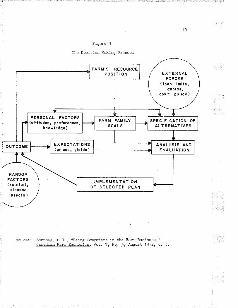
In the course of designing any decision-naking aid it is necessary to

examine the process of decision-naking itself. Any decision nade by the

farn manager is predj.cated. on certain factors:9

1. Facts concerning his financial situati.on, personal limitations,

and inforuation of existing instit.utional factors.

2. Personal factors which result in preferences and. affect fanilygoal formation.

3. ExpecEaÈions about stochasË,ic factors in the production process

such as weather and about institutional factors such as quoÈas.

These components are not linear or static but interact in a dynamic

process illustrated in Figure 3. The outcome of a previous decision can

affect both the preferences and expectations of the farmer. This in

turn must be conditioned by changes ín eiternal constrainËs such as

credit availabÍlity and government policy. All of these factors define

a set of alternaEives which are evaluated by either fornal or intuitive

means in rhe light of the decision maker's goals and expectat.ions.

This decision-naking process is used to direct the growth of the farm

firm. To assist this function it is necessary to investigate the dynam-

ics of the farm firm growth process. At any juncture the productive ca-

pacity of the farm is a function of its existi.ng capital stock from pre-

vious periods and returns which are available for re-investmenË in

productive activity. IÈ Ís important to note the interdependence of

production and investment decisions. The system is dynamic in that eve-

ry decision is influenced by the results of previous periods. rt is iu-

9 Sonntag 1oc. cit.

10

Figure l

the Decision-Making Process

OUTCOME

RANDOMFAC T ORS(roinfoll,

diseosei nsecls )

Source: Sonntag, 8.H.,Canadian Farm

'rUsJ,ng ComputersEconomics, YoL. J,

in the Farm Bus j-rress, rl

No-. J, August 1972, p.

EXTERNALFORCES

( loon limits,quolos,

gov't. policy )

FARM'S RESOURCEPOStTION

PERSONAL FACTORS(ottitudes, preferences,

know ledge )

FARM FAMILYGOA LS

SPECIFICATION OFALTERNATIVES

E X PECTATIONS( prices, yields )

ANALYS IS ANDEVALUATION

IMPLEMENTATIONOF SELECTED PLAN

II

portant also to consider how current. decisions will affect the options

which remaj.n avaj.lable in subsequent time periods.

The type of sysËeu described is precisely the focus of the science of

cyberneEics " Cybernetics is an interdiciplinary science of communica-

tion and control in anirnate and uechanical syste*".10 In particular,

"cybernetics in concerned with the study of exceedingly complex and dy-ì1

namic systemstt. *'

A basic cybernetic princÍ.ple, the faw of requísite variety,12 then

assures us that the variety (i.e. complexity) of the mechanisra for anal-

ysis xrusË approach the variety of Ëhe system Lo be analysed, if analysis

is to be successful. This means Ëhat the decision system must consider

al-1 relevant factors. Variety in the real world is handled by,an equiv-

alent varieËy in the decision system and cannot be competently handled

by 1ess. This Eeans Ëhat, couplex, high-variety decision problems cannoc

be solved effectively by sinple, low variety ¡oethods.

A study of most conventional techniques shows that they useonly a smal1 segment, of the infonaat,ion spectruu. In oËherwords, Ëhey are essenEially ínformat.ion destroying and varietycompressing prqcpdures and, therefore, their usefulness israther limi t,ed. '"

10*- Jerry Felsen, Decision Making Under Uncertainty: An Artificial In-telligence Approach, CDS Publishing Company, New York. 1976. p. 2L.

l1 _. ..I br_cl .

12 inr.Ro"" Ashby, An Introduct,ionNew York, 1956. p. 206.

13 Fels"ttr op. cit. p.85.

to Cybernetics, John !üi1ey & Sons Inc.,

T2

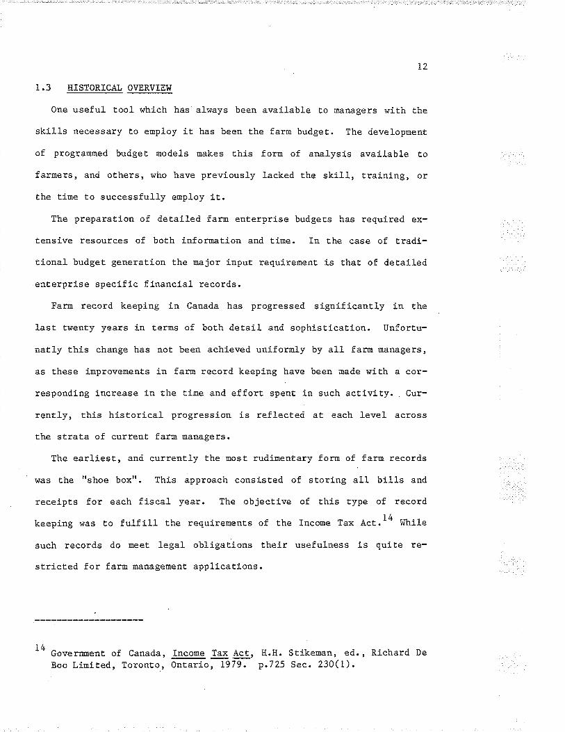
1,3 HISTORICAL OVERVIEI.T

One useful tool which has always been available to managers with the

skills necessary Ëo enploy it, has been the farm budgeL. The developnent

of prograrnrned budget nodels makes this for¡o of analysis avai.lable to

farmers, and others, who have previously lacked the skill, training, or

the time to successfully enploy it.

The preparation of detailed farm enterprise budgets has required ex-

Ëensive resources of both infonûation and time. In the case of tradi-

tional budget generation the major input requirement, is thaL of detailed

ent.erprise specific financial records.

Fann record keeping in Canada has progressed significant.ly in the

last twenty years in terms of both detail and sophistication. Unfortu-

naË1y this change has not been achieved unifonoly by all farm managers,

as these improveuent,s in farm record keeping have been made with a cor-

responding increase in the time and. effort spenË in such acË,iviÈy. Cur-

rently, this historical progression is reflected at each leveI across

the strata of current farro Eanagers.

The earliest, and currently the ruost rudimentary form of farm records

rías the "shoe boxt'. This approach consisted of stori.ng aIl bills and

receipts for each fiscal year. The objectÍ.ve of this type of record

keeping was to fulfill the requirements of Ehe Income Tax e"t.14 lfhile

such records do meet legal obligarions their usefulness is qui.te re-

stricted for farm nanagement applications.

Government of Canada,Boo Liuit.ed, ToronÈo,

Income Tax Act, H.It. Stikenan, ed., RichardOnËario, 1979. p.725 Sec.230(1).

I4 De

i3

The second leve1 of farm record keeping found on Canadian farms re-

quires a definite allocatj-on of tirne and effort. Records of this type

are kept in one of several types of farm account books. One of the uost

common is the Prairie Provinces Fann Account Book prepared for Lhe farm-

ers of the Canadian Prairies by the l,Iestern Farn ManagemenË Extension

Commit,tee.15 Srr"h records do allow the analysis of the existing business

t,o deteruine the level of technical and econonic efficiency within the

different enterpri.ses on Ëhe farm. These records can be used to provide

information to generate budgets for managenent decisions abouE e*isting

farn enterprises.

The nost sophisticated farm managemenË record keeping in Canada now

i.nvolves the use of computerized sysLeES for both record keeping and

analysis. I{hile these systems do provide the most detailed reports and

analysis functions they also maintain the nost, onerous inpuË require-

Bents

AccuraËe reliable farm enterprise budgets require equally detailed

information frou farm records upon which to base the analysis. This

situaËion is assured by the previously nentioned 1aw of requisite varie-

Ey. Fortunately this detailed inforuation can cone from more than one

source. IË uay be extracted from farm records such as t.hose previously

described. This is possible only if such records do exist and have been

maintained with sufficient diligence and detail. In this situation the

enËerprise itself nust also exisL in soue forn. The other opEion is to

supply detail in general Ë,erus from an outside source. The only re-

15 I,Iestern Farn Management Extensíon Comuittee, Prairie Provinces FarmAccount Book, The Departments of Agriculture of Alberta and Manitoba,and The University of Manitoba. September 1973.

t4

quirement placed upon the individual manager Ëhen is to supply physical

descriptions of existing and proposed enterprises. The requisite varie-

ty is still maintained within the model, but a portion of t,he informa-

Ëion required is shífËed from the individual faru manager to an endoge-

nous data base which can be centrally mej.ntaj.ned and is applicable to

large numbers of farms and farm ent,erprises.

I.4 THE PROBLEM

To the extent t.hat the productive efficiency of farm m¡¡1¿geuent can

be improved, benefits will accrue not only to fanoers, but ultiuately to

the agri-business community and everyone who eat,s. To rhis end our spe-

cific concern is that

At present, no techniqrre is available Iin Manitoba] to quicklyforecast |he results of alt,ernative farro plans or alËernative. Ibde cLs l-ons

1.5 OBJECTIVES

The objectj.ves of this study are addressed to the problens of farnn

production inefficiency and the decisions faced by farrn decision-makers.

A najor agricultural enterprise in western Canada is that of field crop

production. The scope of this study is linited to the considerat,ion of

alternaËives withi.n this enterprise set. In viev¡ of these problerns and

in consideration of Ehe dynamics of the decisj.on process of the farm

Ðanager the objectives of this study are:

l6 Syl.rio Sabourin, "A CompuËerized Sinulation Model forÈernative Cow-Ca1f Plans." Unpublished MSc. thesis,Manitoba,DeparËment'ofAgricu1tura1Economicsand1977. p. 9

Evaluati.ng A1-University of

Farm Management

15

I. To develop a conputerized nodel for the evaluation of alternative

farm developmenE plans and production techniques which can:

a) ¡e used to test a whole series of alterations to the existing

seË of resources and t,hereby provide a basis on which to rnake

feasible and beneficial changes in the organization of Lhe

b)

c)

farn.

províde a tool Ëo alert farroers,

business personnel to the value

for farm business planning.

be used as a Ëoo1 by researchers

returns of producing field crops

to gauge the inpacL of exogenous

structure

extensi.on workers, and agri-

and existence of techniques

to i.nvesti.gate the costs and

in Manitoba and can be used

forces upon that cost-return

consistency of Ë,he resulËs subject

principles, engineering relation-

consistency and correspondence t,o

d) Ue flexible enough to accept, and utilize aJ-L pertinent infor-

maËion about, Lhe farm but is able to supply uissing data and

provide useful and valid results with minimuro input require-

menEs.

e) be used with linited knowledge of computer systems or progran-

uing.

2. EvaluaËe the model by:

a) Verifying the accuracy and

to esËablished accounting

ships, and economic theory.

b) Validating the results for

an actual farn situaËion.

L6

c) DemonsLrat.ing the model's usefulness in an actual farm plan-

ning situation.

The succeeding secÈions will review the relevanl theory used to pro-

vide a conceptual fra¡qework for the rnodel. A critical evaluaËion of a1-

ternative farrn planning and decision rnaking aids and techniques will

provide an operational framework for the developmenË of the enpirical

node1. The model is then described and evaluaËed in light of the stated

objecËives. A series of recommendatiobns are uade to augment, the flexi-

bility and useability of the model and to provide direction for Èhe

course of its future development.

Chapter II

THE PROBLEM IN PERSPECTIVE

2"r IIISTORICAT DEVELOPMENT

The concept of computer assistance for farm m:nagement is not a re-

cent developnent. Since the late 1950's farm ûtanagement specialists in

the United States have been int.erested in the application of computers

for the benefit of f.mers.17

During Ehe '60's, the need to bet.ter nanage Ehe business sideof çþe farm became obvious to farm managemenl leaders in Cana-. r9cla.

This recognition was coupled with the need for comprehensive data

collect,ion for research. The decisi.on was made Lo develop a national

system Ë.hat would provide a consisEent, cenÊralized service all across

Canada. The system was initiated in 1968 to provide record keeping ser-

vices and Tras later extended Lo financi.al planning progr.r".l9 The

CASIIPLAN service provided a met,hod for Lhe projection of infornaLion

frou the previous yeat' s incoue tax forns or from farru records i.nto a

financial plan for the succeeding year. The CASIIFLOI,I FOR-ECASTER provid-

ed an examination of cashflow problens and alternatives. Several other

17

18

A descripËion of several of these applicaËions may beProceedings of the annual IBM Agricultural Synposia.Business Machines Inc. EndicoÈt, Nev¡ York.

John Lawrence, "CAI{FARM - I{orking Together for a BetterAgrologist, Autumn 1978. p. 9

found in theInternational

AgriculËure",

19 CAI{FARM promotional advertising.,,Agrologist Autunn 1978, p. 8

18

prograns \,rere offered to provide aids to decision analysis concerning

buy vs. custon hi.re, uachinery replacemenË, and feed formulation. It is

the use of these planning and projection rnanagement components of the

CANFARIÍ sysLeno, which concerns us here.

A large library of coupuË erízed tools have been developed as a result

of the efforts of the agricultural professionals located at a number of

Land Grant. InstiËutions in the United SËates. This development, effort

was summarízed by Hughes2o "",In each case we have concentrated on the development of useroriented, micro-type, single decision models. This is a re-sult of a consci.ous, initial decision wÍ.th respect to direc-tion, concurred in by our key production specialist colleaguesin the College.

There are currently three major cornputer libraries operat,i.ng in the

United StaËes. They are:

1. TELPLAN which started in Michigan in L969,

2. CMN which started in Virginia in the early 1970's,

3. AGNET which started in Nebraska in L975.

All three of these computer líbraries have a large library of Couputer-

ized Management Aids to which farmers can subscribe.

The TELPLAN21 Systen operated at Michigan State University has been

in operation for 8 years and represents an approach somewhat different

fron that of CANFARM. The TELPLAN System is directly available to users

t,hrough a variety of terrninals inc.luding touch-tone telephones. The in-

2O tt. llughes, Paper presented at 'rCouputer Technology in Agriculture", a

short course, The School of Agriculture, University of Manitoba, trIin-nipeg, Manitoba, 1981.

21 St.ph.n B. Marsh, "A Progress Report on TELPLAN ActiviËiesr', Unpub-lished report. Department of Agricultural Economics, Michigan Stateünivers ity.

19

crease in TELPLAN progran useage for the last few years has been:

1975-13 percenË,, L976-4I percent, and L977-L5 percent.

This compares to an annual net increase in CANFARM use in Manitoba of

approximately l0 percent.22 Much of the recent increase in TELPLAN use

has been frou users in the forn of agri-business firns expanding Eheir

cusËomer service faciliËies. This may herald the developnent, and promo-

tion of viable syst.ens entirely within the private sector.

The Agricult,ural Computer Network (AGNET) r¡/as seË up in 1975 as a pi-

1ot project by the Insti.tuLe of Agriculture and Natural Resources at the

University of Nebraska. Its objective v/as to provide a variety of

users, from university specialist.s Lo farraers, with the ability t,o use

the computer in roaking farm production and management decisiorr".23 In

l4ay 1977, the Governors of Montana, North Dakota, l,Iyoning, South Dakota

and Nebraska approved a granË to forrnally ext,end AGNET into t.hose five

st,ates. The grant r¡ras to provide seed noney Ëo explore and develop

original application of AGNET for farmers, ranchers and consumers. In

1980 the states of tr{ashington and l,Iisconsin joined AGNET as full part-

ners. Today there are over 200 agricultural and consumer related pro-

graus available in Èhe AGNET library. All of these are available

through a computer teruinal or micro computer equipped with an acousti-

cal coupler.

A. Chambers, "CAI'IFARM Should Have BeenSeptenber, 1978. p. 16.

Ilughes, loc. cit., Dr. Ilarlan llughes isate Professor, Division of Agriculturalming.

Dropped Long Agot', Grainews,

AGNET Coordinator and Associ-Economics, University of Wyo-

22

23

20

In additíon to the budgeting models avaj.lable as part of the array of

farm managemenË software offered by the sysLeros described these models

have been developed by a number of insti-tuEions. An early exauple of

this type of nodel is the Oklahorna SËate Universi.ty (OSU) Crop Budget

t1!Generator.-' The OSU model, like those described previously, is capable

of generating budgets based upon a couplete specification of both the

physical and financial description of the enterprise by the user. I,rrhen

the financial and price couponents are absent or incomplete it is not

possible Ëo generate even esËimated budgets using these nodels.

2.2 RELATED STI]DIES

I^Iork more specifically direct,ed toward the development of computer-

ized budgets has been published by t,he Agricultural Economics Research

UniL of Lincoln Co11ege.25 th. examples used are drawn from t,he Nort,h

Island of New Zealand and consist of sheep and dairy farrn development

programs. The C0PE26 system uses a "rolling plan approach" to uncover

bot,tlenecks in the farrn developnent programrnes. The analysis predict,s

overdraft levels and is able to calculate present debt situatÍons from

the ínitial conditions and terms of Ehe nortgage contracts. This COPE

prograo assumes thaË Ehe farmer and adviser have already deternined

their priorities.

R.L. I.Ialker, and D.D. Kletke, gser's Manual Oklahona State UniversityCrop Budget Generator, Oklahorna State University Agrieultural Experi-mental Station, Progress Report P-656, November, L971.

K"T. Sanderson and A. McArLhur. Computer Methods for DevelopmentBudgets. Agricultural Economics Research Unit, Lincoln Co11ege. Uni-versity of Cantebury. Cant.ebury, New Zealand. PublicaLion No.451967 .

Comput,er Overdraft Projection and Evaluation

24

25

26

2I

A recent study using Monte Carlo si.mul-ation vzas developed by Mikea'7

Ilardintt as patt of a regional research project., "An Economic EvaluaËion

of Methods of I'fanaging Risks in Agricultural Productionrt. The model was

designed to relax the limiting assurnption of certain knowledge of prod-

uct prices and yields. In addition to neE present value, the tradition-

a1 measure of investment success, annual net worth, net cash flow, and

probabiliEy of firm financj.al faílure are calculated, providing inforna:

Ëj.on on these additional dinensions of the manager's utility space. In-

fluences of investmenË Ëax crediÈ, depreciation, and capital gaÍ.ns taxes

are evaluated for t,he proposed investment and addiËional capital asseËs

required to operaÈe the proposed investment.

The sinulatj.on ¡oodel provides a marginal analysis of the proposed in-

vestnent, a total farm analysis which includes that, of t.he investment,

or a conparaÈive analysis of the current situation and Ehe new proposed

size of firro. The nodel can also be used t,o determine the relative de-

sirability of alternative capital investment. Different parcels of

1and, lease or purchase decisions, and additional investroenËs such as

irrigation can be analysed to determine t.he profitability and chance of

financial failure.

CompuËer models have been developed and used "in the construction of

individual budgets to estimate present value and maximum indebted-ôo

nessttrtt with regard to Ëhe ttinteracting occurrences of borrowing taxa-

27 l'rit "

i.. Ilardin, "A Siuulat,ion Model for Analysing Farrn Capital In-vestmenÈsrr, Unpublished PhD. thesis, Oklahoma SË,ate UniversiËy, Julyr97 8.

28 ".

Candler and Cartwright. "Estimation of Perfornance Functions forBudgeting and SiraulaËion Studies"' n.n.r n.P., n.d., P. 160

22

t.ion and. debt repaynent. over a period"29 of years.

A number of computerized budget models have been developed in Canada

for use in both farm managenent decisi.on-making and research. Tn 1972

economi sts aË, the Lethbridge Research Station of Agriculture Canada and

the Department of Agrícultura1 Economics, University of SaskaËcher¿an j.n-

itiated a project, ained at Ëhe development of systems mod.els of the ma-

jor farn types in inlesËern canada. rn the spring of 1974 work began on

the d.evelopnent of a dryland cereal and oilseed. crops node1.30 tt. "p-

proach taken in the construction of the siuulat.ion model was to develop

a rrskeleton raodel" Ëhat represents the logical stïucture and relation-

ships and includes only the basic parameters of the real system.

The above noted crops simulator is viewed as consisting of Ëhree com-

ponent.s: a model (Fortran program), a base data block and a control

data b1ock. The Fortran program contains Lhe skeletal relaLi.onships and

interrelationships of the biological, physical and ecomornic processes

comprising the produetion space of the farm. The base data block con-

tains a listing of the product.ion alternatives and productíon coeffi-

cients for the specific relationships involved. The control data block

acts as a supplemenLary unit to the base data block containing inforna-

Èion and data specific to the individual farrn being considered. As

well, the control data block instructs the nodel as to the production

a1Ëernatives t,o be considered and controls the manner in which the in-

form¡tion provided is to be processed.

rbid.

R.P. ZenLner, B.H. Sonntag and G.E. Lee, rtsimulation Model for Dry-land crop Product.ion in the canadi.an Prairies", Agricultural systems,Vol. 3, 1978, Applied Science Publishers LËd., England, L978.

29

30

¿J

The simulator proceeds through three stages in the process of

sinulating a farm siEuation over Ëime. In the first stage t,he Fortran

program is initialized and the base and control data blocks are read.

0n the basis of the information and data contained in the control data

block, the production alLernaËives that are not relevant t.o the farm be-

ing considered are elirainated, as wel1, the production coefficients con-

tained in the base data block are Eodified to make them specific to the

farm. The use of this roodel is liuiEed to Ëhe specification of prede-

fined alternaLives for production processes. The user does not, have t.he

flexibility to alter existing processes or to define new ones. The rnod-

el proceeds through a routine for selecting among the producËion alter-

natives that are open at each decision point. In t,his respect che rnodel

has a normative dinension that does not consider the fu11 spectrun of

possible objectives that may be speeified by the farm manager. The set.

of alLernatives selected by the rnodel constiLutes Ehe decision space

that has been defined.

In the second sÈage the production plan is disaggregated into a num-

ber of speci.fic tasks or jobs Lhat must be perforrued in given time peri-

ods. At Ëhe same time the physical resources required to perform each

job are identified. This stage allows the nodel Ëo investigate the Eem-

poral limitations existing withfn the farm system. These resErictions

can be very important and are often not considered in sinpler budget

preparation algorithms.

In the thírd stage the model proceeds through a budgeting process for

the selected producËion plan" To accommodaEe resource and product flows

Ëhe year is divided into 26 bi-weekly periods. The resources requi.red

24

for each of the jobs are compared with E,he available resources as indi-

caËed by the control data block. rf resources are not adequate to per-

forn the job within t.he specified tirne period additj.onal resources are

purchased. This represents a normative action based upon a predefined

ttraEionaltr action of a farn manager. Expenses, receipt,s, producËion

leve1s, resource use, eËc. are calculated and recorded in che mode1.

This allows the user to generaEe a budget fron basic financial and phys-

ical- data but linits the flexibility in naking specific changes to the

producËion process and the direct allocat,ion of resources.

The nodel repeats st,ages two and Ehree for each year in the planning

horizon (1 to 10 years). The evaluati.on of the selected production plan

is now compleËed. This process is able to capËure the longer term fi-

nancial iroplications of a parËicular plan that nay be nissed by analysis

on a simple annual basis. The user may elect Lo repeat E,his whole pro-

cedure a number of Eimes using the Monte Carlo Method in order t.hat Ëhe

"best" production plan be found (the plan with the highest 1eve1 of ter-

rninal net. worth). Having found t.he 'rbest" p1an, the user can test the

sensitivity of this plan over a number of weather distribution pat,terns

t,o det.ermine its stability. The model a11ows the user to determi.ne the

sensitivity of the producEion system to the stochastic influences con-

sidered. The determj-nination of the "bestil plan is based strictly upon

the economic criteria previously defined. hrhile this ¡oodel allows esti-

mating of the long run impacts of a particular allocation of resources

iË is not. able to accomodate changing objectives based upon this new in-

formation.

25

Financi.al budgeting models have been developed for specialized re-

search projects by a number of instit.utions. A recent application of

such a model was the OnËario Dairy Farn Accounting Project.3l Th. pnr-

pose of the project \^ras to respond to the questionttt¡hat was the average

cosL of producing nilk in Ontario in 1977?" The nodel used for Lhis

study is tuore properly an accounting rather than a simulation model.

Actual financial inforroation was gathered from a sample of dairy produc-

ers in Ontarj.o and processed t.hrough a computer program to estim¡te the

average cost of rnilk production. The Average Total Cost of productÍ.on

I¡7AS expreSSed aS:n

ATC=TCIY=(E C. )lY..La=l

where: C_. is the total cost, of usiqg input iI

and Y is the amounË of product.

This Lechnique is distinct from a budget simulation model where ATC is

expressed as:n

(1)

(2)ATC=TCIY=(E P-& )/Y!ra=-l

where: P, is the price per unÍ.t of input il_

and X, is the auount of input i used in Ehe productÍon Process.1

Because C. must be accurately est,imated, the accounting model is not, ap-1-

propriate for the invesËigation of production systems which are not cur-

rent.ly in existence or for which good financial records are not availa-

b1e.

H. Driverr Ontario Dairy Farn Accounting Project Progress Report1977, A joint project of Agriculture Canada, Ontario Milk MarketingBoard, Ontario Ministry of Agriculture and Food and The University ofGuelph, released July, I978.

31

26

In 1970 a model was developed at the University of Manit.oba by I,I .J.2,'

c.raddock-- wit,h Ehe assistance of D.F. Kraft in order Ëo provide daËa

needed for an Economic Councj.l study published in 1971. The mod.e1 has

subsequently been substantially nodified and updated by researchers

within the Departroent of Agricultural Economics and Farn Manageuent at.

the University. D.F. Kraft with t,he assístance of D.O. Ford developed

and used a uodified form Eo estÍmnte the costs and returns in crop en-

terprises based on zero tillage pracËices. The model has also been re-

fined and used by C.F. Framingh.r33 and. others for t,he evaluation of the

Farn Diversification Prograu conducted for the Interlake region of Mani-

t.oba.

In response Lo interest deuonsErated by potential users of the com-

puEer progran a user'" grride34 \,ras prepared by Framingham et aI and. made

available as a Research Bu11eEin. This publication contained a descrip-

tion of the structure of the mod.e1 euployed. rn it a detailed specifÍ-

cation of the calculations used to calculate both costs and returns is

presented. This is followed by a listing of the i.nput dat,a required by

t,he program. An outstanding feature of this uodel is the organizaxion

and type of data required for its operation. The data is divided into

Ëwo blocks. The first data block consist,s of nachine operation and gen-

I,I.J. Craddock, InË.erregional Cornpet,i.tion in Canadian Cereal Produc-tion, Special Study No.12, The Queen's Printer, Ottawa, Canada, L97L

D.0. Ford, "Economic Evaluation of Inpacts of the Fara Diversifica-tion Program in the Inter1ake", Unpublished Research Report, Depart-ment of Agricultural Economics and Farm Management, Universily ofllanit,oba, I976.

C.F" Franingham, C.N. Longmuir, M. Senkiw, and A.D. Pokrant, CropProduction Simulator, Research Bulletin No. 78-2, DeparËment of Agri-c"it"ra1Ecffin¿FarmManagemenÈ',TheUniversityofManitoba,I,Iinnipeg, L97I .

32

JJ

34

.27eral cost inform¡tion. The second data block conÈ.ai-ns the producer in-

fornation specific to the individual farrn being studied. The pricing

information in the general cost, inforrnation daÈa block is conbined with

the physical description of t,he production process to yield a financial

pj.cËure of the ent,erprise. The significance of this nethodology is that

no financial infonoation is required of the farmer about his specJ.fic

farm. IË is therefore possible to analyse enterprises for which no fi-

nancial records are available or which uay not. even exist.

The model as it exi.sted in 197B was the product of the various nodi-

ficat,ions which had been roade to it, to facilitate its use in the re-

search projects where iL had been applied. As such it had several seri-

ous short,comings which hindered its application in a fanu planning

context. The coding procedure was particularly onerous and time consum-

ning. The procedure involved referencing the physical dat,a into tables

which provided t.he appropriate code numbers for t,he categories used in

the program. The procedure was also very rigid and did not a1low cer-

taín user price information Lo be used even when it, was available. The

machinery pricing rnethodology introduced an unnecessary nargi.n of error

into the calculations which \,ras not aeceptable for individual farm plan-

ning. To pri.ce the machinery a linear regressi.on equation \,ras esËinated

for a particular rnachine type for all sizes having available price in-

formation. The array of sizes available r^las then divided into 'a number

of nachinery size classes. A price $ras calculated for the mean size in

each machinery class and assigned Ëo any machine falling within Lhat,

c1ass. This process resulted in the loss of information concerning both

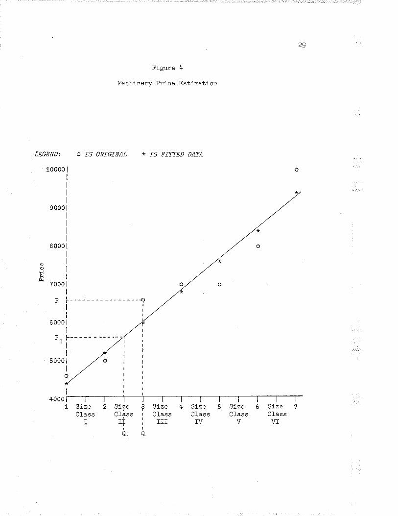
the price and the exact size of the rnachine. This can be shown by the

28

hypothetical case illustraÈed in Figure 4. In this example the actuaL

price of the machine P would have been estimated by Pl which has had er-

ror introduced by the artj.t,rary class designation process of p-p1.

Si.nce this size classíficatj.on was used in Ëhe engineering calculations

the error of Q-Ql was inËroduced into all of the calculations used to

estimate the cost of operaË,ing the machine. These inaccuracies eoupled

r,rith the difficulry in using rhe roodel did nor make ir appropriate in

its existing form for use in farm planning.

Several of the raodels rlentioned. have been used to gain insight intodecisions faci.ng the farn mânager. Some nodels have onerous data re-

quirement,s. A number of rnodels require detailed financial infor¡oation

regarding the system to be studied. They are Lherefore not appropriaËe

when no such information is available. Soue models have extensive as-

suupEions built into theu regarding the objecËives of the entrepreneur.

These- results are not. useful when the uanager's objectives are changing

or are unable Ë.o fit withín the restrictive framework provided. The

succeeding seet,ion will proceed to develop a conceptual framework t,o

specify the characteristics of the decision space of Ëhe farm manager so

that a roodel useful in dealing with that situation nay be deternined.

)o

Figure 4

Machì-nery Price Estimation

LEGEND:

loooo I

I

9 000

8 000

7000 I

6ooo I

I

D'1

O TS OHTGTNAL I' TS FTTTED DATA

o

c)

'rlS{Êr

-4I

I

I

t--I

I

sooo I

I

o

4000 [ I

Si zeCl-ass

I

I

Qi oa

ClassI+

I

a.I

I

SizeClassrII

I

SizeClass

TV

I

SizeCfass

V

I

SizeCl-ass

VT

tI

7I

6I

5I

3I

I

I

I

I

a

I

2I

4

Chapter III

TIIEORETICAL CONSIDERATIONS

3.I CONCEPTUAI MODEL

The basic unit of production is Ëhe firn. According to L""r35 a firn

is considered to be an organization of productive resources geared to

the production of one or nore products and operated by a definable enti-

ty (enLrepreneur) which makes Ëhe decj-sions and accepts Lhe financial

responsibility for the firm's actions. The fina owes it,s existence to

Ëhe fact that the entrepreneur has an opportunity to se1l some produc-

tive process more profitably than if he were to se1l the resources di-_36rect,l-y.

The farro-firrn at this sÈ,age can be thought of as a black bo*37 or de-

vice that converts inputs of a specified type into outputs by means of a

process or, more correctly, a complex of processes that are neither cou-

pletely identified nor understood. The productive process Lakes place

when two or nore factors of production are combined. The environment in

which the transformation of input.s Ëo outputs occurs nay be Lerrned Ë.he

ttproduction spacett of the firm.

35 c.s. Lee, t'Exploitation ofUncert,ainËy", Unpublished25.

Information for Capital Accumulation UnderPh.D. thesis, Purdue University, I97I, p.

36 e.a. Hart, Anticipati.on, Uncertainty, and Business Planning, New

York, A.M. Kelly, 1951, p.3

37 f.f. Orr, Structured Syst.eüs Development, Yourdon Press, New York,N.Y., 1977 . p. 13

-30-

31

Input s-------->FIRM- -----)Outpur

(x1,x2,...xn) (Y1 ,Y2, .. .Ym)

the manner in which the factors of production (inputs) are allocated,

subject to the technical relationships of the firm, deteruines the t,ype

of out.puE that will be forthcouing. The object.ive of the entrepreneur

is Ëo "knotnr" the productÍon space of the firn (aËtempt to understand the

relationships involved) so as to be better able to control or direct the

processes involved. The enËrepreneur attelnpts to allocate Ehe facË,ors

of production under his control (land, 1abor, and capital)

in a way such Ehat the goals of the firm are achieved.

The understanding of the production space is fundamental to Ëhe study

of resource allocation. The int,eraction between the inputs and outputs

uust be understood (at leasË, to some degree) in order that the resources

are allocated efficiently. The attempt t.o "kno.rr" the production space

is referred to as the modelling pro"u"".38

At any one point in Ë,ime, the firm can be envisioned as a uníque or-

ganization possessing a unique production space.20

Lee" descrj.bes the product,ion space of the firrn as the transformn-

Ëion or napping of a set of a priori conditions (inputs) into a set of a

posteriori conditions (outputs). Any eleuent or factor that has a po-

tential impact on t,he final outcorne can be classified as an inpuË. In-

puËs (XO:k=I,...n) can be'divided inË,o three groups: the alternatives

available {a}, the uncontrollable factors or states of nat,ure {s}, and

38 rrr" modelling process refersnathenatical representaLion ofwith observable phenomena.

39 Lu"r op. cit. pp. 25-42.

Ëo the development of arl abstract. orthe firrn. The rnodel links reality

the decision-ruaking characËeristics of Ëhe entrepreneur {d}.

32

In

addition, each class of input can contain several items {i:i=lr...I},

several levels of each iten {1:1=1,...Li, and can be appropriate during

specific tirne periods {t:t=l,...T}. Thus the output. of the systeE can

be descrived as:

OuEput=f ("rrr, "ilt, d:_f-) (3)

where, f represents t,he functional relationship between inputs and out-

puts. A producEion decision relating Ëo a specific alternat,ive, at a

specific level and in a speeific time interval is one a ilt This deci-

si.on is made by the entrepreneur characterised by one d..-, wiËh the re-

sult or outcone subject Co one or a set of srrr.

A sinilar conplexity applies on the output side of equatíon 3. Out-

put(Y.:j=Ir...¡n) can be disaggregated into several kinds of saleable¿

product, bi, aË several levels bit, and in several periods bi_l-t. As

wel1, Ëhe decisions taken in one production peri.od often have effects

which nodify t,he structure and opporËuniti.es of the firTr for the follow-

i.ng production period, cilt. In addition, the possible alterations that,

m¡y have occurred Lo Lhe uncontrollable facËors of production musË be

íncluded. s.-..' r-_Lt

To nake this concept,ualization couplete, a met.hod of evaluating the

differenË ouEcones is needed. Thus, a measure of goodness or desirabil-

ity, g, is required Ëo facilitaËe the select,ion or choice of those al-

Ëerriati.ves that are consist,ent with the objectives of the firn.

The objectives of the firn are reflected in t,he difference in out-

comes between selling t,he inputs directly and selling Ëhe output,s from

the transformation process. It is inportant Ëhat these objectives be

33

rational in the sense that they can be roeasured by some verbal or ¡nathe-

mat.ical rneans. Given that. this is possible, the compleLe specification

of the production space of the firm can be stated mathematically as:

m(a-., * s..- * d.-.-)=(b-.--- * s.,-- * c.---)' rrt 1l-r r_rr- r_rrg r_rrg r_rrg' (4)

where

1. a:a A refers Lo the actions that can be taken by the firm,

2. s:s S refers to Lhe states of Ehe variables beyond the control of

t,he firm,

3. d:d D refers lo the decision-rnaking character of t.he entrepre-

neur,

4. b:b B refers to Lhe outcoues (products) of Lhe actions taken by

the firm,

5. c:c C refers to.the unique int,ernal structure of the firm result-

ing fron previous decisions and stat,es of nature,

6. i:i I refers to the items in a set,

7. 1:1 L refers to the 1evel of the iËem,

8. g:g G refers to the desirability of the right hand product sets,

9. È:t T ref ers to the ti.rne period involved and,

10. n refers to the Eatrix that describes Ëhe roapping of the left

side of Ehe equation onto the right side variables.

Equation 4 says that for every action that can be taken by a finn at

a given 1eve1 and point in time, in a given setting, a particular level

of result is forthcorning. It is not inplied that Èhese relationshi.ps

are known, but it does inply Lhat they exist and Ehat efforts are rnade

Ë,o know more about, them in order to control or direct the processes in-

volved.

34

At the practical leveI, such complete specification of the production

space is not possible. Even if iË, r,rere, a search of all the alterna-

t.ives would be ext,remely coscly. The alternative is a reducËion in Ëhe

size of Ehe sets and simplification of the napping Eo make the specifi-

cation of such a systexo

1. conceptually possible and

2. operationally or analytically feasiUte.40

The reductions and sinplifications are accomplished by utilizing appro-

priate Ëheoret,ical deductive t.ools.

3.2 TIIEORETICAI. BODY

The world is observed as a sequence of events. Any explanation of

how these events are linked togeËher is a theoretical consËruc¡.41 Theo-

ries give form t,o an otherr¿rise shapless üass of meaningless observations

by aLLer0pting to explain, or account for, certain observed phenomena.

If correct, a theory a11ows one to predict in advance the consequences

of various choices.

A Ëheory consists of:

1. an hypothesis about the way in which certain phenomena behave,

2. a set of assumptions under which the theory or hypothesis ap-

plies, and

3. a set, of principles or logieal statenents Ëhat describe the rela-

tionships auong the observed events.

40

4t

Lee,

R.G.1969,

op.cit. p. 29.

Lipsey and P.0. Steiner,p.16.

Econouics, Ilarper & Row, New York, N.Y.

35

A Ëheory represents a mental or abstract rabor-saving device (a

sinplified nodel) Ín the sense that an individual need not start from

scratch r¿ith each investigation but can draw upon accept.ed theories or

lav¡s in the fornulaLion and soluËion of a problem.

3.2.L Theory of Resource Allocation

3 .2 . I .1 S tatic Theory of the Firn

The traditíonal theory of the firrn is Ë,he basic building block upon

which a model for farm resource allocation can be conceptualized. The

theory is concerned with

1. the efficient allocation of resources among productive units de-

voËed to the production of a single output in a mnnner thaE max-

imizes the net value of the physical ouËput, and

2. the allocation of resources among alternative outputs in a manner

that naximízes the net value of production.

The lhree basic principles of prod.uction economics (factor-

product, factor-fact,or, and product-producÈ relationships) a11ow

one to deduce the general shape of the production space. By as-

sumi.ng a rational decision-maker, only Ëhe outer edge of the pro-

duction surface need be considered. Any point not on this outer

edge is Ëechnically inferior. By liroiEing the analysis ro only

the technically feasible points, the number of alt,ernatives that

need be considered are greatly reduced.

The assumpLion of perfect knowledge means the ent,repreneur has

complete knowledge about the alÈernatives avaj.lable, the states

of nature and the outcomes associated with each alternaEive and

36

state of nature" This assumption serves to remove all risk and

uncertainLy involved with management choice. Further assumpEions

regarding timeless production, cardinal measurability of output

(usually measured in terrns of dollars), perfect competiti.on in

the input and product, market.s, and t,he goal of profit uaximiza-

Ëion a11ows the produclion space to be reduced to a rnapping of

the technically feasible a1Ëernatives into levels of outcomes

that are known with certainty. The role of Lhe entrepreneur is

to select that alternat.ive that leads to the highest level of

profits. In Ëerms of the producËion space synboli.zed by equation

4, the static Lheory of the firrn is siuply:

ro( a ,r) =b ,,(s)

The traditional theory of the firro provides a very simplified

nodel of the producEion space and managemenL choice. Hovever,

because of its restrictive assumptions it has been criticized by

nany for its lack of realism. The assumption criLicized most

consj.stently is that the entrepreneur maximizes the profits in a

nanner that is "objectÍ.vely rational".42 Th.t i", Lhe entrepre-

neur selecEs from the seÈ of all possible alternatives that al-

ËernaÈive t,hat, leads to naximurn profits. Challenges to the prof-

iÈ-rnaxirnization assumption t,ake two forns.

1. It is argued that profit is siuply one of many possible

goals of the entrepreneur. Other goals include such

things as producÈion goa1s, inventory goals, and personal

and Decision Models of

-rnc.l-19@lp.t33. -T.II . Naylor and J.trrl. Vernon,the Fim, New York,. Ilarcourt,

Micro-economics42

Brace and [,Iorld,

37

goals (eg. , salary, securit.y, stat.us, power).

2. Other critics do noË deny the import,ance of profit but

question the assumption of maximizat.ion. They conLend

that the entrepreneur aËtenpts to achieve a satisfactory

level of profit but not necessarily the maxi.mum level.

The second area of criticism relaËes Ëo the assumption of per-

fect knowledge on the parË of Ëhe entrepreneur wiËh respect Lo

the technical relationships and factor and product prices. Crit-

icisus centre around the fact thaË risk and uncertainty are a

very large part of reality and cannot be overlooked. Producers,

because of Èheir lack of knowledge, are continually faced with

risk and uncert,ainty in Ëheir decision-rnaking processes. Exoge-

nous factors such as markeE condi.tions, v¡eather, government poli-

cies, etc. are responsible for less than perfecË knowledge.

The third area of criticisn of the traditional theory of the

firm relates to the production process. The traditional theory

deals wiËh a firn in a static, timeless environment. The theory

does not explain Lhe dynarnic nature of the production process.

It fails t,o account for the time 1ag between inputs and ouËputs

and Ehe linkages between consecutive production periods. The

theory assumes all inputs purchased in a certain perÍ.od are used

up in that period. IE also assumes all inputs and outputs are

perfectly divisible. In reah.ty, decisions dealing wiËh invest-

nenE in durable asset,s and Lhe problem with "lumpiness" of re-

sources are everyday occurrences and should be viewed according-

Ly.

38

A final criticism of the traditional theory of the firm staËes

that the theory is basically raarkeË.-orj-ented and, as such, is ap-

propriate for a different set of questions Èhan one that a mi cro

or nlanagenent. orientat.ion requires. It is felt that a theory of

the firn should centre more on the decision-making process of the

entrepreneur and Ehe changi-ng environmenË of the firm. These

cri.ticsms have led to the developmenË of a ner¡r set of theories

ref erred to as ttadaptivett theories.

3"2.L.2 Adaptive Theory of the Firm

Adapt,ive theory concerrrs iEself with describing hor¡¡ the firra responds

over Ëime to changes in its environment. The firn is visualized.,as:

i. operating in an environment characterized by inperfect. knowledge,

2. not so1ely concerned wíth profits but recognizing a rnulti-dimen-

sional objective, and

3. operat.ing as a dynamic organization that changes over t,ime.

UncertainÈy as to Ehe states of nature is an integral part, of adap-

tive theory. The entrepreneur has no way of knowing exactly which state

of nature will prevail. All he has is a subjective estim¡Èe of the

probability of each state being the Ërue state. By processing this par-

tial information iÈ is possible to construct an a priori probability

distribution over the sËat,es of nature. By doi.ng so, rational choices

can be mede based on expected ouËcones. As Li.me passes and oore infor-

uation is accumulated about the staEes of nature, the probabilÍty dis-

Ëribution can be continuously refined until it approaches that of the

real wor1d.

.39A requisite for the decision process is an adequate system for sup-

plying information on production relationships, price relationships

(both factor and product), and frequency of occurrence (probabilities)

of specific st,aËes of nature. Since the states of nature are given and

beyond the control of the deci.sion-maker, Ehey can be treated as sto-

chastic variables Ehat act to influence the resulting outcomes, thus

reducing the complexity of the production space Ëo a ltrore uanageable

leve1.

A firru is not solely concerned with naximizing profits. Rather, a

firm has several goals t,hat it wishes to attaj.n simultaneously. Oft.en

these goals are in competition for the firm's resources. A decision to

move in one directíon roay maximize one goal buË at the same time prevent

other goals fron being realÍ.2'ed, or lhe action taken Eay contribute rnod-

estly Ëo the attainmenË of several goa1s.

Utility theory can be utilized to accommodate nultiple goal objec-

tives. Ordinal utility analysis enables Lhe entrepreneur to develop a

set of indifference curves Lhat have as many dinensions as the entrepre-

neur's objectives. A sËrategy can then be chosen that uaximizes (or

satisfies) the expected utility of the entrepreneur.

Producti.on is viewed as conti.nuing over a number of tirae periods.

The product,ion space, although finite at any point in tine, mâY either

expand or contract over time. Changes are brought about by changes in

the technical and market, relationships ardfor through changes resulting

from entrepreneurial decisions in the history of the firm. This ueans

that r,rithin each production period decisions are made as to the course

of acEion to be followed and implies that one set of decisions necessar-

40

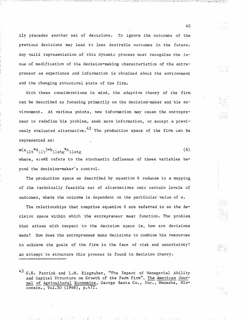
i1y precedes another set of decisions. To ignore t,he outcomes of the

previous decisions nay lead to less desj.rable outcones in the future.

Any valid representation of this dynamic process Eust recognize the is-

sue of nodificat,ion of the decisi.on-making characteristics of the entre-

preneur as experience and informat,ion is obtaÍned about the environment

and the changing structural sËate of the firm.

i^Iith these considerat,ions in raind, t.he adapLive theory of Ëhe firm

can be described as focusing prirnarily on the decision-maker and his en-

vironment. At various points, ner¡r inforuation nay cause the entrepre-

neur to redefine his problem, seek more information, or accept a previ-

ously evaLuated alternati.r".43 The production space of the firn can.be

represented as i

n(arta*drrt)=bit"tgo"ir"tg (6)

where, e:etE refers to t,he stochastic influence of those variables be-

yond the deci.sion-maker's control.

The product.ion space as described by equation 6 reduces to a rnapping

of the Èechnically feasible set of alternatives onto certain levels of

outcomes, where the outcome is dependent on the partícular value of e.

The relationships that comprise equation 6 are referred to as the de-

cision space within which Ëhe entrepreneur É-ust function. The problero

that, arises wiËh respect to the decision space is, how are decisions

rnade? How does the entrepreneur ruake decisions to coubine his resources

to achieve Ehe goals of the firro in the face of risk and uncertainty?

An at,tenpt to sËructure this process is found in decision Ëheory.

43 c.tt. PaLrick and L.M. Eisgruber, "The Impact ofand Capital Structure on Growth of the Faru Firn",na1 of Agricultural Economics, George Banta Co.,consin., Vol.50 (i968) , p.472

Managerial AbilityThe American -Jo"r-

Inc. , Menasha, trIis-

4T

3.2.2 Decision Theory

The nost vital function that management perforns is decision-naking.

To nake decisions means to choose a course of action from among various

alt.ernatives. Decision-naking requires expliciË use of information.

The amount of infornatÍon needed for a particular decision is directly

related to the amount of uncertainty present.

3.2.2.L Decision-naking under certainty

Under these conditions the decision-roaker has perfect knowledge about

the acËions open to him and the states of nature. Therefore, the deci-

sion-maker knows exactly what the payoffs will be under various combina-

tions of actions and states of nature. The optinal decision is that

course of action that yields the highest payoff under the state of na-

ture which will occur. This represents the condiËions under whích the

tradiËiona1 theory of the firn applies.

3.2.2.2 Decision-maki.ng under risk

Under these conditions t,he decision-maker is aerare of the relevant

courses of action and "knows" the probabi1iti."44 of each of the possi-

ble states of nature being the true stat,e. As a result, the probabili-

Ëies of the consequences of the various courses of acËion are also

known. A deci.sion-maker may then choose Lhat course of action that will

maximize the expected value or sone other üeasure of payoff.

44 tfr" decision-maker objectively Eeasures thesÈates of nature based on [0any observationsFrom Lhis process, the decision-maker becomesthe probabilities of various staEes of nature.

probabilities of thefrom Past experience.

relatively confident of

42

3.2"2"3 Decision-rnaking under uncertainty

Change plus unpredictability give rise t,o the ent.repreneur's uncer-

tainty. Several factors are involved.

1. technical factors-these refer Ëo the lack of complet,e knowledge

regarding the production processes for a particular outpuE (e.g.,

weat.her, pests , di.sease) ;

2. market or price factors- these refer to the lack of complete

knowledge concerning future markets and prices for products yet

to be produced;

3. Ëechnological factors- these refer to the lack of complete knowl-

edge concerning future discoveries or developments Èhat nay occur

in the production methods and pracLises for farn producËs and hor¡

these fact,ors affect Ehe,cost and returns of the farm;

4. institution factors- these refer to the lack of eomplete knowl-

edge concerning future changes in laws, regulations, group act,ion

or broadly exËending customs that will affect the farning opera-

tion; and,

5. human traits- these refer to t.he lack of conplete knowledge about

how individuals in or related to the farrn will change or behave

in Ëhe future.

Under conplete uncert.aint,y, t.he decision maker has no a priori infor-

mation as to what the true staËe of nature will be, not, eVen in a proba-

bilistic sense. To facilitate a raÈional decision, uncertainËy must be

reduced. Several criteria have been developed to aid in the process of

45 r. Eisgruber and.Benttt, Canadian

1963, p.60.

J. Nielson,Journal of

"Decis ion-Making Mode lsAgricultural Economics,

in Farm Manage-

,l/i ¡f.É.tri : '';+e'T,

ìir

...

decision-naking under complete uncertainty. These "r.,45

43

maximumr

minimâx, pessimism-optimism index, principle of insuffici.ent reason, po-

tenEial surprise, and satisficing. In Eost cases, however, decision-

uakers do not directly employ one of these criteria; they seem to rely

more heavily on their subjective feelings. The decision-maker through

the process of defining the problem and det,ernining the possible states

of nature, acquires sone knowledge of the relative probabilities of the

sËaËes of nature. By processing this partial informat,ion, an a priori

subjeetive probabi tfty46 distributi.on over the states of nature is de-

veloped and then used for making decisions.

In the real world, entrepreneurs always aËËenûpt, to move from an ttun-

cerLainrt environnent t.o a ttcertaintt environment, however, decisions made

under uncertainty or aE least a high degree of risk are Eost common.

The ability of the entrepreneur to exploit avaj-1able infornation in rnak-

ing the selections becomes Èhe very essence of decision-naking. Any

siluation in which a decision-maker is confronted with a choice auong

actions constituËes a decision problem. A decision problera is composed

of decision inputs, decision outputs, and decision rules. The decision

inputs refer to Ehe various alternaËives that are open for selection as

well as the states of t,hose variables beyond the control of the deci-

sion-maker. The decision outputs refer to the payoffs or outcomes asso-

ciated with each combina;ion of available alt,ernatives and states of na-

ture. The decj.sion rules are the standards or principles uÈilized by

46 Sob3."tive probabitities are based on past experíence and infornatj.onaccumulated by the decision-maker. They are not, "objective" in thesense that they were scientifically obtained. However, if formalized,they have the same mathematical properties as an objectively deter-n:Lned probability distribuËion.

44

Ëhe decision-maker in evaluating the alternatives and naking a choice.

the decision problem can be represenËed with a decision tree formaE

where, ã.ií=Lr2r...n, refers to the alternatives or specific courses ofI

action that are available, "jrj=I,2¡...ur¡

refers Ëo the specific state

of the variables beyond uhe decision-maker's control; and bi¡ refers Ëo

Ëhe outcome or payoff Ehat coues forth when selecting action i and hav-

ing the state of stochastic varÍ.able j occur (Figure 5). At each deci-

sion poinL, synbolized by a square, a decision rule must be applied to

select among the alternatives that are present,. The stochastic effect

of the variables beyond the the decision-maker's conË.rol are represented

by decision (circles). the payoffs become t,he output of the deci.sion,

gÍven the state of the stochastic variable j _occurring. Any continuous

paLh Ehrough the network is associaËed with a final outcome for the sys-

tem.

The

stages.

1.

decision-naking process involves several discrete and sequential

There must be a complet.e specificati.on of the problem siLuation.

llhen framing Ëhe problem special consideraÈ,ion should be gj-ven to

t,he objectives of the firn.

2. A listing of the set of alt.ernati.ves available for selection must,

be made. In uost cases the decision-maker will only define a

subset, of the alternatives actually available. This will likely

include only Ëhose which his knowledge and conventí.ona1 wisdom

indicate as feasible altern*ii,r.".47

A.N. Ilalter and G.l,l. Dean,Publishing Co., Cincinnati

47 Decisions Under Uncertainty, South-Western, Ohio. L971, p.173.

45

Figure

Schematic Representaiion

5

of a Deci sion Problem

brr

brz

br¡I

II

btn

DecisionPoint bsr

bzz

bs¡tt?

bgn

O - Decision Node bnr

bne

bnsI

II

bnm

46

The decision-rnaker must choose the set of alternatives that ap-

pear xnost appropriate in Eerms of reachÍng his objectives. To

accomplish this, t.he decision-maker disaggregates each alterna-

tive into discrete production steps. Probabilities are then as-

signed to each possible outcone. Statistical decision theory can

then be applied Eo calculate the expected payoffs.

The decision-maker must init.iate act.ions t,o carry ouL Ehe a1Ëer-

natives chosen. This involves the collection, allocation and di-

rection of the resources under his control into Ëhe Ëransfonna-

tion process in the manner indicaEed by the decisi.on or course of

action chosen. The outcooe that result,s will hopefully approach

that visuaLízed by the decision-uaker.

The decision-maker must examine the actual results of his choi.ce

in view of subsequent developnenLs. the i-nformation received

from this action may alt,er the parameters of the decision problem

and/or facilitate a tnore objective assignment of probabilities to

the states of nature and """o"i"a.d outcomes for future prod.uc-

tion periods.

ThroughouË. the entire decision-making process there is a basic need

for an infornation system that supplies information on the various rela-

tionships to facilitate the definiLion and interpretaËion of t.he deci-

sion space at any point in time. Infornation is required to assist in

Ë,he selection of Lhe finite set of alternatives and in assigning proba-

bilities t,o the stat,es of nature. Because the production space is al-

ways changing over time, new information is continually required to fa-

cilitate rational decisions. The ability of the decision-maker to

J.

4.

5.

integrate his personal knowledge with other informaLion and

production plan in light of this new information deËermines

as the unit of control within the firm.

47

Eo adapt his

his success

3.2.3 Adaptive DecÍsion-MakinglLRMurphy'' presenËs a nodel of the adaptive decision process. The ¡ood-

el can be used to portray the role of the decision-¡oaker in the produc-

Ëion space of the firm. The uodel of the producÈion space is composed

of an a priori structural state vect,or that describes Èhe state of the

sysLen, the sËructural environmenL vector that contains the staEes of

nature or exogenous factors, and the decision vecEor which is a function

of not only the previous structural state vector and t,he decision-mak-

er's environmental vector buË also an a priori historical infornation

vecËor. This a priori historical infornation vector cont.ains a complete

list of the outcomes from previous periods and is t,he only clue to the

random effects of the environment,al vectors on t,he structural state of

the system. The a priori historical infornat,ion vector may also contain

information accumulated from other sources ouEside the syst,em.

This verbal discussion is represented by ltrrphy49 in the following

equation:

Sr*., =f ( S- , U¿, Dtr)

where:

1. St*1 r.f.rs to the a posteríori structural state vector,

(7)

, Adaptive Process1965. pp.1-31 .

48 R"E. Murphy Jr.Press, New York,

rbid.49

in Economic Systems, Academic

48

2. St

3. u.c

4. D-t

CE)o L

It rtpt y50

refers to t,he a priori structural state vector,

refers Ëo the structural environnerrt vecEor,

refers to Ehe decision vector, and,

refers to the struct,ural transítion function.

further represenËs the decision vecEor as:

D =D(S¿-¡,H¿_¡rV¡)

È=0,112... (8)

where:

1. V, refers to the decision-meker's evnironuenËa1 vecLor which con-

tains the physiological nake-up and t.raits of the decision naker,

2. Htr refers Ëo the historical information vect.or,

3. t refers to the time period, and,

4. r refers to the tine 1ag.

The adaptation is observed during the passage of time. The transfor-

mat,ion of Ëhe a priori st,ruct,ural state vector into the a posteriori

structural sÈaËe vector is described by Murphysl as follows:(Figure 6)

1. reception of the a priori historical informatj.on vecror. At the

beginning of each sËage a "package" of inforroation is recelved

frou the previous sÈage which contains Ehe a priori structtlral

stat,e vector and the historical information veetor;

2. determïnation of Ëhe decision-¡oaker's acËion. The a priori his-

torical information vector suggests a number of possible alterna-

ti.ve actions from which a unique action is deternined by the de-

cision function;

rbid.

Ibid.

50

51

J.

49

Ëhe Ëransformatíon of the structural state vector and historical

infor¡nation vector. The action deternined by the decision func-

tion and lhe effects of the external paraneters on the process

Ëransfor¡os the a priori structural st,ate vector. This nevr vector

nay differ from the expectations of the decj.sion-maker when the

decision was nade. This difference generates a transfornation of

the historical infornation vector producing the new inforoation

package for Ehe following stage.

This adaptive process illustrat,es the explicit use of informa-

tion. It consËitutes a continuous eycle of receiving infor¡na-

tion, naking decisions on the basis of this infornati.on, and j.m-

plementing the decision whereby more infornation is gained for

the following period. Over t,ime, thi.s "learning" process ruay re-

sult in the decision-maker's a prlorl subjective probability dis-

tribution approaching that of the real world

The prevÍous discussion demonstrated that, theory can provÍde a

generalized deduct,ive systeu Lhat can greaÈly facilitate the con-

struction of a nodel in a decision-making situation. But, since

these Lheories are of an abstract or conceptual naÈure, they do

not determine a specific st,rucËure for the nodel. The production

space as developed by Lhese theories can only becorae explicit

Lhrough Ë,be adoption of an operaËional system. This is the pur-

pose of the following chapter.

50

F-i sure 6

Murphy's Adaptive Decision Process

Stnrctural Environnental

Decision Vector (Da)

otherïnfo:¡ration

Decision-Makerr s EnvironnentalVecror (V.)

a pT1oÎ]-

Stn¡ctural State Vector

Historical Info:rnationVector

Decision-Maker

Chapt,er IV

OPERATIONAL SYSTEMS

4.T PREAMBLE

The study of the deeision space of the entrepreneur is facilitated by

the nani.pulation of a suitable ¡nodel Ehat mirrors the production pro-

cesses involved. Models are Ëhe means by which t,he theory becomes wor-

kable. Models are constructed and utilized for experÍ.menEation as a

substituLe for experimenËation on Ëhe real system because rnan is limited

in his ability to perceive and evaluate inforrnation and because experi-

mentatj.on v¡ith the real system is too costly and time consuuing. An-

ssrers obtained from a properly constructed nodel renove a certain amount

of uncertainty when used as inf ornation in the user's or¡In decision

space. Thus the value of a model is measured by the amount and accuracy

of the information it provides.

A nodel is a fornal assembly of t,he "essential" elements of real

world situations. It ís composed of siuplified representations of the

relationships involved. A nodel rnay be based on Ë.heory, eupirical ob-

servations or a combination of Lhe two. Consequently, a model must be

realis¡ic in terns of the input-output coefficients and flexible enough

Eo accommodaËe diverse external effects (states of nat,ure). A nodel

concerned with some sub-seÈ of the production space of the firm runs the

risk of overlooking or distorting inportant relatj.onshi-ps. Many of the

relationships comprising Ehe production space of the firm are intrinsi-

- 5t -

52

cal1y linked and must be EreaEed accordi.ngly. For this reason, sys-

tems analysis seeros nost appropriate.

A system can be described as a set of factors or elements that are

interrelated and integrated in such a \{ay that a change irr one component

can affecË soue or all of the other components. It iraplies that a con-

cepËual boundary nay be erected around the complex as a lirnit t.o it,s

identily and organizational autonomy. Any element falling outside of

this boundary becoues part of t,he environment of the systen. The de-

scription also irnplies that to undersËand Ehe syst,en one must understand

the relationships of Ëhe elements called subsyst,ems, and how Ëhey are

integrated into the whol-e.

The farm system is composed of biological, physical and economìc sub-

systens, operating Ín an uncerËain environment,, t,hat, are controlled or

directed t.hrough tine by Ëhe entrepreneur in an efforË to achi.eve so6e

predominantly economic objective(s) referred Ëo as the goal(s) of the

firm.

General systems theory

some cases matheroatical)

ships of Ëhe real wor1d.

sary Lo construct a model/\['(o itt ' Y irJ = Fir¡.ts .

where:

is concerned with developing a syst.ernatic (in

framework for describing the general relaËion-

Since a model parallels reality iË is neces-

of the following form:

oirÀte (e)

a is some

T is some

p i.s sorne

S is some

À is some

subset of {a}

subset of {d}

subset of {b}

subseË of {c}

subset of {e}

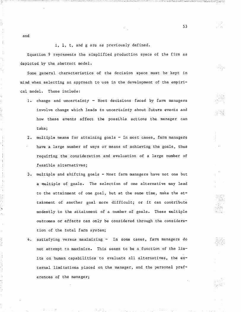
53

and

i, 1, t, and g are as previously defined.

Equation 9 represents the siraplified product,ion space of the firm as

depicted by the abst.racL nodel.

Sone general characterisËics

nind when selecting an approach

cal rnodel. These include:

of the decision space nust be kepË in

to use in the development of the erapiri-

change and uncertainty - Most decisions faced by farn managers

involve ehange which leads to uncertainty about future events and

how these events affect the possible actions the manager can

Lake;

nultiple means for attaining goals - In most cases, farrn managers

have a large number of ways or means of achieving the goa1s, thus

requiring the consideration and evaluation of a large number of

f easible a1Ëernatives ;

nultiple and shifting goals - Most farm managers have not one but

a nultiple of goa1s. The selection of one alt,ernatj.ve nay lead

to the attainnent of one goal, buË at the same tiue, make Ëhe at-

tainment of another goal nore difficult; or iÈ can contribute

nodestly to Èhe attainnent of a number of goals. These nultiple

ouLcoues or effects can only be considered through Èhe considera-

tion of the Ëotal farm system;

satisfying versus maximizing - In sone cases, farm Tnanagers do

not att,empL Eo maximize. This seems to be a funcËion of the 1im-

its on hum¡n capabilities to evaluate all alt,ernatives, the ex-

ternal liruitaLions placed on the úanager, and the personal pref-

erences of the nanager;

1.

2.

3.

4.

54

5. cornplexity of the production processes - In many cases the pro-

ducÈion relationships involve non-lineariËies, discontinul-t,ies,

tj.me delays, and irreversibilities. Adequate representaLion of

all types of relationships requires an extreuely flexible ap-

proach;

6. factors of production - In most cases the resources avaj.lable for

producËion are limited. As wel1, soue resources can only be pur-

chased in discreËe size units. These characteristics may prevent

the farIn Eanager from attaining the opt,imal production level in

terms of his objective; and,

7. many production periods - A large number of the decisions nay re-

, late in some r^ray t.o tine. In order that all rauifications of a

decision can be seen, production uust be carried'forward for a

number of productive periods.

Another consideratíon in selecting an approach relates to t,he future

operation of the model. As indicated previously, the model rnay have a

number of future usages inplying that the model will be run a large num-

ber of tixoes. As a result, efficiency in terms of operaLing costs be-

comes a very imporËant consideraEion.

It is recognized Ehat no one approach can efficiently handle all of

these requirements. For this reason, soue trade-offs uust. be uade in

the final selection. The approach to be selecËed is that which handles

the majority of these requireuents in Lhe most adequate manner.

The approaches Ëhat can be used to portray the conceptual model can

be classified into tT¡¡o caËegories:

1. analytical approaches, and

55

synt,heti.c approaches.

4.1.1 Analytic Approaches

An analytical approach is defined t.o be the art or science of resolv-

ing a problen into its basic couponents in order that a specific solu-

tion procedure can be utilized for t,he attaj.nment of an opt.inal solution

or answer. A solut.ion procedure refers to a specific algorithm such as

calculus, or simplex procedure for linear programming models. IË refers

to a specific set of deduct.ive rules which facilitate attainment of an

anS\¡/ef .

4. I .1 .1 Differential Calculus

DifferenËial calculus is the set of deductive rules that facilitates

the determination of a uaximum or uinum value for a conËinuous funcEion.

This technique is nornally used on static Eheory, alt,hough it $/orks

equally well in dynanic theory, \^rhere it provides a theoretically error

free, precise soluËion Lo a problem. The advantages of differential

calculus are that it can be applied to any Ëype of interacE.ion, is rela-

tively easy t,o use, and fits adrnirably into the marginality concept.s of<o

econo.ics." The roajor disadvantage of this t,echinque is the limited

number o'f variables ÈhaÈ can be handled from an operatj.onal point of

view.

,)

52 L"u, op. ciË. p. 43.

56

4.L.L "2 Linear Prograrnrning

Linear programming as described by Agrawal and Hu"dy53 is a computa-

tional- method to decermine the best plan or course of action, among nany

which are possible, when a numerical objective exists and the ueans or

resources available for attaining it are 1imit,ed.

This technique is based on four najor assumptions or

These include:

.54predecls]-ons.

1. linearity - this assuupËion implies consËanË returns to sca1e,

indicating Lhat the relationship among the various inputs, out-

puts and income remains proportional at, all levels of activity,

e.9., it assuues single value expecLations and linear relation-

ships,

finiteness - Èhis assumption iroplies that there are a lirniËed

number of act,ivit,ies and resource restrictions cornprising the

problem,

divisibility this assumption implies that inputs and outputs

can be used and produced in fracti.onal units, and

53 Agt"*rl, R.C. and E.0. Ileady, Operations Research Methods for 1$gi-cultural Decisloqs, The lowa SEate University Press, Ames, L972, p.ß.

54 Th".u .t" tT¡ro types of decisions that nay be made when d.ealing withabstract, models. The first is referred to as predecisions. Theserefer to assuuptions or decisions mnde in constructing the ¡qodel.These take tvro forns: (i) theoretical - those Ëhat can be justifiedbecause of an invarianee; and (ii) facilitatÍng - those made so as Eo

adopÈ or change Ëhe st.ructure of the problem or frarnework of the mod-e1 so that a specific solution procedure j.s applicable. The secondtype of decj-sion is referred to as soluËion decisions. These referto decisions Lhat are uade during the process of arriving at a solu-tion or ansÌ^/er Ëo Èhe problen.

2.

3.

57

4. additivity - this assurnpËion inplies thaË the activities are in-

dependent in the sense that Lhe productivity of one act,ivity is

not influenced by the level of anoLher activity.

Linear programming problens utilize the static theory of the firm

with data input that is determinj.stic, thus resulting in a solut.ion Ëhat

55is normative-- and stati-c in nature. The main advanËage of this techni-

que is the rigorous examinaLion of nany activities and resource use al-

t,ernatives. In principle, the ¡oaj.n aj-m is to assess the value of Ëhe

marginal products of all resources when used in each feasible enËerprise

combination so that the available resources might be a11ocaËed to the

greatest overall advantage.

Linear programming per se has a number of disadvantages thaË linit

its applicability. Most of these rise ouÈ of t,he restrictive assump-

Ë,ions under which the approach applies. To overcome sore of these lin-

itations, a number of modifications have been developed. These include

the following:

1. Integer Progranming - This technique is identical to linear pro-

gramrning except thaE the assumption of divisibility is dropped.

Some inputs or resources are used in whole or integer units.

This overcomes the problem of lumpiness of resources.

2. Multi-period Programrning - This technique is concerned with nu1-

ti-stage decision problems where a decision at one stage affect,s

subsequenE decisions. This type of nodel or technique involves a

block diagonal mat,rix where the activities and restrictions are

arranged by tine periods with normally one overlapping resource

55 Notr.tirr. nodels generate rules indicat,j.ng what the decision-uakerought t,o do, given infornation and a goal.

J.

58

(e.g., net farro incoroe) which affects the solution of the next

diagonal block. The main advanËage of thj.s technique is its dy-

namÍc charact.er (ttre recogniEion of time as an explicit, vari-

able).

Stochastic Programming - This t,echnique a11ows coeffj-cients to be

random variates drar,¡n from a specified frequency distribution.

The main advantage is the recognition of risk as an inportant el-

ement of the decision space.

Recursive Programmi.ng - Recursive programiling attempts Lo predict

the actual behavior of the firm. Satri56 describes recursive pro-

gramuing nodels as being based on the Cobweb principle ín which

current production depends on past prices, but current prices de-

pend upon currenË production. If price for the period t-l is

known, output for year t can be predicted. this predicted output

for year t can be used to determine the price for year t.. This

permits output to be forecast for t,he t*I year and so on.

Recursive prograrnrning becoues a predictive device by the use

of upper and lower flexibility constraints thaË represent the

range over which product,ion can change in any one period. The

main advantage of this technique is that iË is dynamic and pre-

dictive in nature.

5. Quadratic Programrning - Quadratic progranning is described to be

the maxi.mization of a concave or mininization of a convex objec-

tive function, subjecl to linear consËraints. This technique has

4.

56 n.f. Sahi, "A Recursive Programming Model of Canadian Agriculture",National and Regional Econornic Models of Agriculture, AgriculËure¿Aaa;-conox0i-AiBranch; Pu6l N ofi|T, l-aT

59

a rat,her linited use in its application because of the

difficulties i.n developing working algorithns and the high cosrs

involved in using this technique. The najor advantage of this

technique is the recognition of a rnulti-dimensioned objective.

The uajor disadvanEage of linear programming per se and its rnany

forms of modificat,íons relates Ëo the size of model required to repre-

sent complex problens and the difficulty in undersËandÍ.ng and/or ex-

plaining the results produced. The size of ¡aodel increases dranatically

as more realism is built into it through the use of these ¡oodifications.

The result is a roodel that is costly to operaËe for a large number of

runs.

4.1 .I .3 Dynamic Progran¡ming

Dynamic progranmíng is a method of converting an optimization problern

of high dimensi.onality into a series of equivalent, problens each of

whieh contains no uore t,han one or tr^/o variables. The lransf ormation is

invari.ant in thaL the number of feasible solutions and the value of the

objective function associated wiEh each feasible solution j.s preserved.

The transformation is based on the principle that an optinal set of de-

cisions has the propert,y that whaÈever Lhe first decision is, che re-

maining decisions rnust. be optiloal \Àrith respect to the outcome which re-

su]-ts from the first decision.

The formulation does not requÍre any specific relationship between

input,s and outputs but does iupose rigorous structural requirenents be-

Ëween certain sets of input-output coubinations. The roajor advantages

of this technique lie in the fact that it ís directly applicable to dis-

60

crete systelts and the fact that. the computational effort required i.n-

creases roughly linearly with the nu¡ober of stages, while Ëhe computa-

tional effort, required by uost convent.ional met,hods increases roughly

exponentially with the number of stages.

The major disadvantages arise from the fact that only one parameter

is used Ë.o define the state at each stage, the inoperability of this

technique in problen settings having nore than one or Ë\,ro consËraints

which hold over the range of t,he problem, and the linited number of ele-

ments in the input veclor Ëhat can be handled from an operational view-

point.

4.L.2 Synthetic Approaches

A synthet,ic approach can be defined as

ing the separat.e parts of a probl-em inLo a

be a precise algoriÈhn for the attainmenË

sr,rer. As a result, Ëhe ansv/ers tend Eo

sense.

the art or science of combin-

whole for which there Eay not

of an opËimura solution or an-

hold only in a sÈatistical

4.L.2.L Regression Analysis

This technique attempts to fit an appropriate equation to the rele-

vant. portion of the producÈion surface. This Ëeehnique becomes unwieldy

when there are many variables and interrelatj.onships involved. Specifi-

cally, problems arising frorq the specification of the function, the way

the chosen funcÈion is to be estiroated, the choice of variables, meas-

urenent of the variables and the problerns arising from a violation of

the basic assumptions combine to make the use of this t,echnique unsuita-

ble in the given problern situaLion.

61

4 "L "2.2 Systems Sirnulation

Ifaisel and Gnugnoti5T define siuulation t,o be a numerical t.echnique

for conducting experiraents on a digital computer; this technique in-

volves certain types of maËhematical and logical models that, describe

the behavior of business, economic, social, biological, physical or

chemical systems (or some component thereof) over periods of t.ime. The

rnajor characterist,ic of this technique is that it is not in it,self a so-

lution procedure or algorithm; it is a \^7ay of approaching a probleu

through t.he use of systems analysis. There is no defined criteria or

framework for developing a simulation model; thus eaeh problem is uni-

que.

Sinulation is usually considered to be a two-phase technique in which

a model of t,he real system is constructed, and experimenEs are performed

on the ¡oode1. Unlike the analytical techniques, simulation does not in-

volve solving a model to find a unique optimum. As a result, simufation

is not used to define a precise optinal operat,ional strategy; however,

near optimal sLrategies can be approached by using procedures Eo system-

atically search the entire decisi.on space for a minumum or uaximum value

of the objective function.

The advantages of the simulation approach include:

I. sËructural flexibility t,hat perni.ts representation of all types

of relationships;

2. provision of a framework for obtaining operational insight into

the system;

I{. Maisel and G.Science Research

Gnugnoli, Simulation of Discrete Stochastic Systeros,Associates, Iric., L972, p. 4.

57

62

3. it requires fewer predecisions;

4. it, can accept intui.tíve judgement. by the farm manager in the so-

luËion procedure; and

5. iË has lower run-time cost.s for a large number of runs.

Disadvantages are:

1. the high costs involved in constructing the nodel, and

2. the high degree of couplexity that can be easily built into these

models naking it nore difficult to interpreË.

0f Ëhe approaches noted, the sinulation approach appears best availa-

ble to represent the uajor characteristics of the production space of a

farm firm. The appeal is in the flexibility to accomodate all types of

interrelaË.ionships and temporal aspecËs of stochastic systems. As well,

the ability to urore easily and efficiently handle multiple production

periods combined with somewhat higher efficiency in run time has result-

ed in the selection of Ehe simulaEÍon approach as thaÈ Ëo be used in the

erapirical model. The application of this technique is described in the

following sectj.on.

4.2 SIMiILATION }ÍEfl{ODOLOGY

Si¡nulatj.on refers to Ëhe operat,ion of a numerical nodel of a real

systen, designed to trace out the dynaro:ic interactions in order to an-

s$rer specific questions relating to the system. The r¡ai.n building

blocks of a simulation roodel are Ëhe deseription of Èhe components and

the deseription of the linkages. The comPonents may be described in

t.erus of input-output relaËionships wiËhin enEerprises or within major

production a1Ëernatives. Linkages tie Ëhe various units togeLher (e.9.,

63

they descrÍbe how the Ínputs are transforned int.o outpuËs for the par-

ticular production alternative).

4 .2.I Steps

Wrigfrt5S describes the procedure the inodel builder goes through in

utilílizing the simulati.on technique Lo solve a problem (Figure 7). The

ínitial step is to clearly define Lhe problem and list the specific ob-

jectives or aims towards which efforts will be directed. This involves

setting hypoEheses that require testing and learning about the systen.

One must identify syst,em conponent.s, systern boundaries, types of inter-

actions that exisË among conponents, appropriate measures of system per-

formance and alternat,ive means available for achieving the objectives of

the systeu. The second step involves constructing an inilial systems

rnodel and incorporaLing into it Lhe knowledge of the relationships t.hat

was previously gained. Once this initial version is operational daÈa is

collected to represent the relationships conLained in the model. The

model is then refined. This involves expanding the scope and content of

Lhe nodel to Eore accurately represent. t.he real systern. These changes

normally come from the added knowledge accumulat,ed about the system over

the previous steps. The third step involves programming the nodel for

computer operation. This is a continuing operation or task as the nodel

is revised, expanded or refined. The fourth step involves Eesting the

model as to its accuracy in represent,ing the real systen. Questions

raised at t,his point, are: Does the nodel adequately represent the pro-

58 O. Wright, "Fami.ng Systens, Models and Sinulationtt, in sysÈems 4".1-ysis in Agricultural }lanagement, by J.B. Dent and J.R. Anderson, JohnI^Ii1ey & Sons, Inc., L97I, P. 24.

64

cesses it is intended Lo represenË,? Does it simulate reality? and, are

the results generated plausible and realistic? Tf. the oodel passes

these tests, it can then be used for experimentaËion. Here the problem

as described is put into the model and run. The final step involves

analysis of the results froro the experinent and testing the validity of

the hypothesis stated.

The forewarcd arror¿s in Figure 7 indicate the general movement, of this

process frou problern definition towards model application. The reverse

arrovrs indicat.e that the process is iterative or ttlearningtt in nature.

A prior stage night have Eo be repeated on the basis of new inforrnaËion

acquired during a subsequent stage. This iterative or "learning'r nature

of the simulatlon technique results in an ernpirical nodel that more

closely approximates the real system.

Given the specificaÈion of the rnodel jusË described the actual imple-

mentaËion of this procedure is now outlined. The process begins with

the explicit statement of the problem and statement of objectives. The

purpose of Ëhis study is to provide a tool t.o aid the farm rnanager in

the analysi.s and evaluaË,ion phase of the decision-nakj.ng process as i1-

lustrated in Figure 3.

ot

Fieure 7

The Methodology of Sim;l-ation

Problem

Formul-ation

Model

Construction

Val-idation

Experimen-

tation

66

4.2"2 Formulation of the Model

The variables to be considered by the rnodel are those parameters

which uake the individual enterprises or cropping systems unique. A

parËial 1ist. includes crop types, cultural pracEices, and machinery in-

ventory. These inputs are exogenous Èo the rnodel.

In order Ëo make the model useful to a wide range of potent,ial users

it is necessary to have a large body of coefficient, infornation r¡rhich

can be used to supplant any shorËfalls in the available data. With this

¡uethod it will be possible t,o obtain reasonable results with a ¡oÍnimurn

of descriptive data. Bul, more importanËly, the model should be able to

make maxiüuu use of all specific data which is available.

In addiËion to Ëhis default infornati.on t,here exist,s a body of coef-

ficients which are endogenous to the model. They have been built into

the model because of their axionatic nature and are are not expected to

change across users or circumstances. Thís informat,ion includes engi-

neering data on naehinery efficiency and the account,ing ident,ities nec-

essary to complete the analysis.

The fornulation of the functional relationship between input,s and

outputs result,s from the coefficient structure and accounEing fornula-

tion of the nodel. The model is conpletely deterministic and the inves-

tigation of sLochastic variables is available only through nanipulat.ion

by the user of infonoation supplied Eo the program.

67

4 .2 "3 Prograuming

Once the algoriLhn for the budgeting procedure has been outlÍned in

detail the translation into a couputer progran is a one to one roapping

of Èhe algorithnic specification inEo program language.

4.2.4 Validation and Verification

This sËage actually consisÈ,s of two part.s. VerificaËion is t,he pro-

cess of determining that the model is performing correctly and Ehat the

results are accurate. Validation is more difficult to quantify but it

simply amounts to deterroining whether or not the rnodel does indeed accu-

rately represent the essential elements of the sysLem being sinulaËed.

The Fam Budget, Generator will be verified Lo determine that the

coefficients estimated and tbe calculation procedures used are correct.

The validation procedure will be done by sirnulating historical produc-

tion sequences and comparing the result.s to the actual outcomes. The

sensitivity and direction of change of the input-ou.tput relationship

will be evaluated to det,ermine whether or noË Lhe results are consistent,

with observable facÈs and wiËh the basi.c rnicroeconomic theory of the

f irn.

4.2.5 Experimentation

The ultinate purpose of Èhe nodel is realized when it is put, into Ehe

hands of an actual decision maker and used to simulate the operation of

an existing (or hypothetical) farn. It is possible for Lhe farm manager

or researcher to vary differenE comPonents of the system, i.e. add uore

plant and equipnent, and deEernine the long and short range impacts of

his actions..

68

One unique characteristíc of the sinulation technique as pointed out

earlier is that it. does noE possess a precise algorithm for E.he attain-

ment of an optimum solution or anslrer. Ilowever, procedures have been

developed to systeuatically search Lhe entire decision space so t,hat t.he

optimum can be approached. These procedures can be grouped into four- 59classes:-- random nethods, experiment,al designs, learnÍ.ng devices and

hill clinbing procedures.

4.2.5.I Random Search

The sinplest procedure of this type is the Monte Carlo Method. This

method uses a random sarnpling process to choose specific values for the

decision variables consistent with Lhe const.rainEs Èhat. have been i¡o-

posed on the decision space. This is usually accomplished by assigning

equal probabilities (uniforrn probability distribution) to the seË of

feasible values for each decision variable and then using a random num-

ber generat.or E,o select specific values froro t,his distribution. These

values of the decision variables are budgeted to obt,ain a response t.hat

can be conpared t.o other responses obtai.ned in a sinilar uanner. The

set of alternatives which generates the highest (or lowest) response is

then chosen as the best.

A brief discussion of each procedure is presented by M. Boehlje, "0p-Ëinization and Decision Models: The Use of Statistical Search Proce-dures", Canadian Journal of Agricultural Economics, Ju1y, I973, PP.43-53.

59

69

4.2.5"2 Experimental Design

A number of experimental designs60 have been developed for response

surface analysis. Most Lend Ë,o use soae forur of sequential sanpling de-

sign to determine the optimum. The direction of the search is guided by

some form of response function that leads to successively higher points

until t,he maxj.mum is reached. These procedures are designed Eo reduce

the computational burden involved in locating t,he optinal point on the

response surface.

The cenLral couposite desigrr6l is one procedure used for response

surface investigaLion. It is a particular type of fractional factorial

design that, requires (ZK+Zf+t) treatment combinations, where K is Ëhe

number of independent variables. The only stipulation is t.hat the hy-

pothesized roodel should be a polynonial. 0nqe the regression equation

has been developed it can be used to map the response surface for any

levels of the variables. the optinal point can then be determined using

diff erentÍa1 calculus.

1. R.A. Fisher, The Design of Experiments, SÍxth EdiËion, Oliverand Boyd, 1951.

2. 0. Kempthorne, The Design and Analysj.s of Experinents, JohnI{iley & Sons, Inc., New York, L952.

1. J.S. Hunter, and T.H. Naylor, "Experimental Designs for Com-puter Simulat,ion ExperimenËs", Management Science, Vo1. 16,No. 7, 1970.

2. I^I.C. Cochrane and G.M. Cox, Experimental DesÍgns, Second Edí-tÍ.on, John l^iiley & Sons, Inc., L957.

60

61

70

4.2.5 "3 Learning Mechanism

The learning r..h.rrisr62 initially assigns a discrete rect.angular

probability distribution to all decision variables. A randou number

generator is then used to generate an out.cone or response which is then

coupared Ëo a norm. If the response of the current decision set is

higher Ë,han the norm of the previous responses, Ëhe learning paramet,er

values, ê.8., the probability, for that. particular set of decision va1-

ues are systeuatically adjust,ed upwards. This skews Ëhe probability

distribution so thaË there is a higher probability of choosing this par-

Ëicular value of the decision variable during subsequent. simulation ex-

perinents, and vice versa. After a number of iterations, the probabili-

ty distribution for each set of alternatives is skewed towards those

Lhat generate the highest response.

4.2.5.4 t1i11 Climbing

This technique uses a simple random procedure to select a set of a1-

ternaËives as well as an initial starting point (combinati.on of prod-

ucLs). A producL mj.x ratio t.hat specifies the relative proportions in

which production will increase if excess resources are available is also

selected. An iterative procedure, whereby Èhe production of products is

increased in a fi.xed ratio, is continued unt.il a consÈraint is reached.

To obtain a near opËiuum, a new rauio of products is randouly generated

and the procedure is repeated.

62-- A discussion of several types of learning mechanisms is given byScott B. Guthrie in "GLEAP: A Generalized Program for Game LearningSimulation", Behavioral ScÍence, Vo1. 13, 1968, pp. 336-342.

7L

The solution procedures described above provide near optinal solu-

tions for the model under given levels of independent variables, thus

facilitating the use of the proposed nodel framework in analysing Ehe

sËated problen" It is Lherefore the approach employed in application of

t,he model developed hereín. The following chapter is concerned with de-

scribing the model framework and its componenLs.

Chapter V

TITE EMPIRICA], MODEL

5.1 THE MATHEMATÏCAL STATE}ÍENT

The conceptual nature of t,he model is represented in equat.ion l0:

¡, (oirt " y'J = F'ttrtg' sit^tg (10)

IL is important to note Ehat Ehe following description of the concep-

tual model as presented in equation (10) outlines the structure of Ehe

decision space of the fino of which the empirical roodel forns only that

part which lends itself to quantifi.catlon. The ernpirical nodel in equa-

tion (I1) places only a very broad const,raint upon Ëhe alÈernatj.ves (ø)

available Ëo the entrepreneur. In the current configuration the enter-

prise nust fa11 vrithin the general descripti.on of a field crop produc-

t.ion enterprise which is either dryland or irrigated. However, the type

of resources (i), and their 1evel of usage (1) are chosen by the manager

as inpuËs specified for the conputer nodel. The tining (t) for an in-

tra-annual production period is not possible Ëo investigate within t,he

empirical modeL per se and uust be inferred by the user.

An iuportant departure which this nodel makes frou much of the work

which has been done in this field is in maintaining the characteristics

of the decj.sion-maker (Y) conpletely exogenous from the empirical node1.

Therefore, the rnodel does not ¡aake normative judgements concerning the

production process. These characteristics are left t,o the user of Ëhe

model at any particular t,ine (t) as no atËeupt Ís made Ëo measure the

-72-

73

relaÈive strength's of a particular enLrepreneur's various goals in any

Itranner.

The right side of equation (10) consists of measures of t,he outcome

of the production process. In using Ëhe model the analyst. specifies the

expected products (F, ) and their levei-s (1) based upon his expectaÈions

about Ëhe effects of exogenous random factors (¡.) in any time period

(t). For each of Ehese products the empírical nodel provides a finan-

cial valuation which the manager can then use to map into his personal

utility function to assess the goodness (g) of the result. sinilarly

Ehe a posteriori condition of the firm (S) is determined subjectively by

Ehe user from his evaluaË,ion of the resultant product.ion ( p). The pur-

pose of the eupirical model is not to represent the,se conceptual rela-

t,ionships but to aid Lhe decision maker in dealing with their complexÍ-

ty.

To make thís conceptual model quantitatively rneaningful requi.res a

transformat.íon into measurable variables. For a producing firm, the

alternatives open to the enLrepreneur (oi_ft) are assumed to be present

in the form of "production syst,ems". A production systen represents the

seE of inputs that are utilized in the producËion of a particular set of

ouÈputs lthe set of inputs nust be logical (consistenË) fron a technical

point of view]. A particular systeu is referred to as sysLem t,

(r:ren), in time period t, (t:tet). The 1eve1 of a particular produc-

tion systeu in any one tine period (S"a) is li¡oited by the available in-

puts (Irr) within the const,raínts placed on the systen.

The next set of variables (Yrfa ) relate to the nature of the deci-

sion-maker and how he perceives Lhe alternatives in relation to the al-

74

ternaEives in relation to some EulËi-dinensional objective. The Ëradi-

tional assumption of roaxirnizing dollar values was used in Ëhe nodel for-

nulation. This objective measured in terus of dollars is reflecËed in

the difference betr,reen selling some productive process and selling the

resources directly. This implies that the firrn want.s to maximize the

net value of production over tirae.

The first set of variables on the right hand side of equation 10 rep-

resents the probabilistic outcomes ( Fil l¡*) associated with Ehe produc-

tion systeüs. Given the objective of maximizing returns, variables that

can be used to Eeasure output are the do11ar value of saleable produce

(Y.* PY .- ) .Jv J r/

The second set of variables on the right side of equation 10 ( Qlffte)

represents the unique characteristics of the fi.rm that are carried for-

ward to Ëhe next production period. The result,s of any one production

period are dependent, upon t.he Lransformation that occurs within that

period as well as Lhe t,ransfonnaËions of previous periods. These char-

acteristics nay affect Ëhe alËernatives and objectives of t,he firm in

subsequent production periods.

The production space of the firm can be described as:

r( (srt ) (q"req"t ) )= 3 t¡r"rtj."

where:

1. Srt is the production system r in t,ime period E, This systen is

defined by the user of the model for the particular budget (peri-

od t) which is Ëo be produced. This definiÈion is effected

through the specification of a subset of tillage practices for

each field to be considered"

(11)

,)

75

I. , is available inpuE i (integer) needed for syst,eo r in periodartt, The input levels of capital equipment (land and machinery) as

well as seed and chemicals (fertilizer and pesËicide) are sup-

plied directly by the user of the progran for each field in each

tine period t.

J.

4.

PI. is prieer_rt

seË of prices :

in Appendix B.

Y. is outputJtJ

each product j

period t.

rnapping functÍon.

7. r:reR - where R is the number of

8. i:iel - where I is the number of

9. t:tgl - where T is the number of

10. j:jeJ - where J is the number of

of input i needed for system r in period t, This

is supplied internally within the roodel as outlined

j in period L, The level of output is supplied for

from each field for which a budgec is prepared in

5.

6.

PY.- is the.price of outpuE j in period L, This price infonnationJt/

ís supplied internally by the program as indicated in Appendix B.

f is the funct,ional relationship between the two sides of Lhe

equation, This function is the result of the individual relation-

ships which make up the model. The levels of input of labor tine

and required petroleum products are generaEed internally as a

funct,ion of the production sysËem S and the 1evel of output Y

specifÍed. The accounting identities in the nodel are used in

conjunction with the price information to compleËe the financial

possible production systems,

possible inpuËs,

ti.me periods,

possible outputs,

lI. e:eEE - where e is Ehe sËochast,ic influence fro¡r

the firm's cont.rol, and, where the objective is

ret,urns f rom a specif ied period of Ëj.rae.

76

variables beyond

to maximize net

5.2 APPLICATION

5.2.L Problem Formulation

To begin, Ehe farmer, either directly or Lhrough a questionnaire de-

scribes his farm. This description includes whatever detail is availa-

ble coacernÍ.ng the capiËal assets (i.e. rnachinery, land, and buildings),

as well as labor availability, and the stat,e of other financial resourc-

es. The program is able to ease t,his task considerably by providing de-

fault infornation which can be used to supplant any informaËion which

the manager is unable or unwilling to supply. This feature will also

enhance Lhe ease of use by individuals, such as researchers, who are

only interesËed in representative results for a class of far¡ns. This

default data will be estimated and adjusted to accurately reflect the

actual year being siroulated. Subsequent to the run the farmer will re-

ceive a report. of exactly what default inforuation $tas used for his par-

Ëicular run and will have Lhe opportunity to adjust it.

Once the productive assets of the farm have been described the farner

t,hen outlines a cropping programrne and tillage and culËural practices

associated with the production of each crop. The farmer will also

specify yietd levels for each field cropped. i^IiLh this rnerhod it is

possible for the farm manager to synthesize a great deal of subjective

information (concerning field conditions and weaLher expectations) into

one datum. This also places the responsibility for the consi.deration of

the stochastic elements of the production process upon Lhe

model.

77

user of the

Once t,his information is available to the progran it is then possible

Ëo determine the ret.urns to the enterprise. Total production is deter-

¡rined from field areas and user-supplied yield leve1s. The user is also

required to supply expecLed values for prices. IIe is Eherefore also re-

sponsible for the sLochasti.c elements of the narkeËing process. This

information coupled with general engineering relationships is used to

det,ermine returns above the variable costs of producing each crop. Af-

ter quota and tax consideraËions as well as fixed credit responsibili-

ties are meL then a figure is generated to reflect the estimated 1evel

of disposable income. At this point cont,rol is passed back to the farm-

er. Ile determines Ëhe effect of this result upon consunption 1eve1s and

decides. producÈion and invesËuent levels for the subsequenË year or ad-

ditional analysis for a given year. Thus the decision-maker and the

model interact through each time period in an int,eracÈive, dynamic,

learning process.

The learning process defines a system of which the farm manager and

Ëhe computer model are buË tr¡o conponenLs. A coupling of the inËuj-tion

and creativity of the hunan rrind with Ëhe fast and large information

processing capacity of the corputer Ehen night result in man-machine

synergism.63 u, "synergisro" ,nle mean the complex man-conputer inLerrela-

tionships which mây cause the man-machine systen to perforn better Ëhan

either man or conputer working alone. The learning uechanism together

with man-computer synergism may result in superior uanagement perform-

63.--"" Felsen, op. cit. p.8.

78

ance. Thus rnan and compuËer working together roay make bet,Ëer

rnânagement decisions than each could rnake alone.

5.2.2 Analysis

The ultiroate críteria for the evaluation of the performance of vari-

ous managenent strategies lies in Ehe utility function of the nanager.

This is extrenely imporËant when it is necessary to consider his subjec-

tive evaluation of risk.

Techniques have been devised to inLernalize the nanager's preference

space into Ëhe objective evaluation of the system. These nethods are

very difficult to apply efficiently and with generality. Therefore, Í.t

v¡as decided rather to provide the farm manager with results which are

merely componenËs of his t,ota1 utility. The farmer roust t,hen proceed to

evaluate this information in terms of his g1oba1 objectives and prefer-

ences and J-mplement subsequent. plans conditi.oned by each nerv set of re-

su1ts.

5.3 STRUCTURE OF THE MODEL

An existing computer model was found to contain most of the essenÈial

elements of t,he concepEual framework. The progran \{as fírst developed

by !ü.J Craddock in order to provide data needed for an Economic Councj.l

"t,rdy64 published in 1971. Since that time, modified and updated ver-

64 ".r.

Craddock, Interregional Competition in Canadian Cerea1 Produc-tion, Special SLudy No. 12, The Queen's Printer, 0ttawa, Canada,T97T.

65 c.n.t-ongmuir, 14.Senkiw, and A.D.Pokrant, C.F. Framingham, Crop Pro-

79

sions have been employed by D.o. Ford, c..F. Frauingh^r65 D.F. Kraft and

L.R. Rigaux. The author has assisted Ín constructing the current form

of the couputerized budgeË generator, prepared the documentatj-on and has

part.icipated in its application to study the cost of field crop produc-

t.ion in Manitoba.

The form reported in Crop Producti.o¡ Simulato€ had several defi-ciencies' solBe of which have been rnentÍoned in Chapter II. These short-

c.emmings arose nainly in the accuracy and in the useability of the pro-

gram. The accuracy problems were due Ëo the strategy of category

specificaLi-on used. This had been a product of its original research

orientation. the averaging error introduced by the categorizing process

T¿ras not serious when Ëhe results. presented \,rere aggregaËions of the

budgets frou a large number of fanos. unfortunately, this error is

unacceptable when preparing a budget for an individual farro farn.

Ifodifications were made to the prograra which both eased the task of

record coding and produced rnore accurat.e resulÈs. the actual sfze of

Ëhe ruachÍne is now coded insÈead on a size class number. Thus the pro-

gram noi,¡ uses the exacE size of the nachine for both capital cost ap-

praisal and operating cosË calculations. The default pricing is calcu-

lated by substi.tuting the size of the nachine into the regressÍon

equation, noTr esEimated on unit,s of machine size, Ë,o yield a unique

price for each uachine.

duct.i.on sinrulator_, Research Bulletin No. 78-2, Department of Agricur-IuraT ncono*icsãnd Fano Management, Faculty of AgricuJ-ture, univer-sity of Manitoba. trIinnipeg, Manit,oba. November 1978. pp.3-34.

Ibid.66

80

The L978 version of the model did not readily accepL additional

user-supplied inforroatj.on concerning uachi.nery purchase and rent,al pric-

es. This resulted in a model which failed to efficiently use avaj.lable

infornation and resulted in a high 1eve1 of user frustrati.on. The nodel

has been uodified to a1low the user t,o override the default priees sup-

plied for ov¡ned and renÈed rnachínery as well as custon r.¡ork raËes.

The second problem liniting the model's usefulness as a mânagement

decision aide was the difficulty one encounËered when trying to actually

use Lhe prograro. Part of this problem has been allevlated through Lhe

changes t.o t,he size coding previously described. To further facilitate

the entire coding procedure a pre-processor was writ.ten which can be in-

teractively execuËed under the University's PLI processor of Ëhe Tine

Sharing Opt,ion of the MVS operating system. The progran provides the

user with a series of questions regarding the physical description of

his far¡o and his production practices. The responses t.o these quesËions

are edited and then stored into the coding format requi.red by Ë,he crop

budget generat,or. i,IÍËh the' use of the pre-processor progran a person

having no pri.or experience with the coding convenËions is able to pre-

pare his farm description for processing.

The nodificaLions to Lhe crop production simulator have resulLed in a

nodel which is able t.o address Ehe objectives stated at Èhe outset in

Chapter I. The detailed structure of the uodel- which makes thÍs possíble

is delineated in Ëhe following section.

The model as summarized in Figure B is designed to calculate the t.o-

tal cost,s and gross returns of crop enËerprises. These results are then

used to comput,e net returns as well as certain performance indj.cators

81

for each enterprise. Each crop enterprise j.s analysed on a per field

basis. Both the fixed and variable costs of each field operation are

calcuLated and allocated t,o ËhaË fie1d. Machinery costs for each field

are a function of the age and size of the uachineryrpert,inent rental and

custon rates, as well as field size. Other input cosEs are determined

by the quantity and price of fertilizer, chemicals, and seed. Other

cosLs included are overhead costs as well as the cost.s associated with

owning or renti.ng t,he land. The net returns from a part,icular field are

calculated as gross returns or value of product,ion roi.nus the total cost

of that production. The results of each field growing a particular crop

are aggregated to present a picË,ure of the financial results of the en-

Ëire enterprise as illustrated in figure 9.

The most detailed cosË calculations involve those costs which are as-

sociated with the operaLion. and ownership of fano machinery. The pro-

ducer supplies information about the age and size of the nachine. This

in-fornaEion is used in conjunction with secondary infornat,ion about

pri-ce, field efficiency, repair cosEs, fuel consumpEion, depreciat,Íon,

eL ceËera, to calculate both fixed and variable costs. The costs are

then present,ed for each operation on every fie1d.

The urachinery costs calculated for each field are totalled by cost

category and included in the cost and return suumary presented for each

field. The machinery and other input costs are aggregated as variable

costs, cash costs, fixed costs and then as total production cost. The

variable costs are the total of all charges for fuel- and lubrication,

repairs, chenicals(including fertilízer, herbicide, and pesLicide) as

well as seed, twine, and labor. Cash costs are the sum of variable

ö¿

Iìi ørro R

Illustrative Description of Steps inBudget Generation

Average Retail Price Data producer Supplied physical Data

Average Regional Costs

Run Infornation

-Machinery Prices-Fertilizer Prices-Chenlcal Prices-Seed Prices-Seed Treatment Costs-F\.:.el Prices-Crop Prices

-Tì-Ilage Practices by Field.-Crops Grown by Field.-Crop Yields-Machinery Inventory by Type,

Year and Size-Optional- Price Information

-Investrnent i-n Land and.Buildì-ngs

-Overhead-Taxes

Estimate variable, fixed. and.and total- machinery costfield

-Fuel Consi.mption Esti.mates-Repai-r Estjmates-Lubrication Estimates-lnterest Rates-Depreciation Scheduf_es-Recornrnended Seeding Rates-Reco¡¡mended Herbi-cide Rates

Estimate cost of productiongross enterprise retr:rnsreturns to investment,labor, a:rd management

Sr:¡nmarize cost and returnsby field for the totalfarm

ö)

Figure 9

Elements of the Cost Report

Iï. Cost of Production

1 . F\.:.el and Lubrication2. Repairs3. Fertilizer+. Chemicals5. Seed Treatment Costs6. Seed. and Cleaning Costs7, Tw-ine Costs8. Labor9. Custom Charges

10. ïnterest Operating Capital11. Crop Insurarrce Prern-ium12. Drying Costs13. Equipment Rental Charges14. Rent15. Taxes16. Machinery Insurance17. Overhead, Miscellaneous18. Total Cash Costs19. ïnvestment, Land and Bulldings20. fnvestment, Machinery21 . Machinery Depreci-ation22. Total- Fixed Costs

23. Total- Costs

84

costs plus the cost of insurance, taxes, rent,, custom work charges, and

overhead costs. Fixed costs are the sum of taxes or rent, insurance,

overhead, depreciation, and investment. For each field this cost infor-

m¡Èion is presenËed along with a summary of the returns from the year's

product,ion. Both costs and returns are shown on a per acre basis for

each field. A summary table is also supplied which provides a weighted

average (by field area) of all fields wit,hin a particular cropping en-

terprise.

5.3.1 Calculations for Machinery

As staËed in the preceding section the ovmership and operation of

farn machinery incurs both fixed, and variable costs. Fixed costs con-

sisÈ of depreciation, insurance, and investment costs. Variable costs

consísË of fue1, lubrication and repairs as well as any labor and twine

cosLs associated with the operation.

A cash cost, of owning machi.nery is that of insurance. Since raachin-

ery must be proteeted from fire, accidents and other hazards the opera-

tor uust either bear this cost, or alternatively bear the long run costs

of such daroage directly.

If any nachinery is rented or hj.red as cusLom 'r¡ork this constitutes a

cash cost. These charges are usually specified on either a per acre or

per hour basis for the type of field operation.

Depreciation is not a cash cost to the farm operator. It is the loss

in value of nachinery over time due to obsolescence and deterioratj-on

due to use. 0f Ëhese tsro coroponents the firsu is a fixed cost and the

second is a variable cost of ownership. The depreciat,ion is deternined

85

from Ëhe currenL value and the age of t.he machine. Since the variable

and fixed components are extremely difficult to identify the total

depreciation is considered to be a fixed cost.

The investment cost incurred in the ownership of farru machinery is

considered whether or not it. occurs as an explicit or an inplicit cost.

InvestmenË. cost is explicit if it is comprised of the int.erest charged

on borrowed funds which are invested in the machine. If producer equity

was used to purehase the machine no actual interest. costs are realized.

The owner is rather foregoÍng income which could have been earned fro¡o

investuent in some other income generating asset. This 'opportunity

cost' is then allocated as an Ínvestment. cost of ovmership.

The'opport,unity' principle is also applied to assessing the cost of

labor required for crop productÍon. This labor cost is a function of

Ëhe ti¡ne spent operating farm nachinery and the current wage rate. The

wage rate assessed may be adjusted by the user to reflecE the effective

market value of alternative labor applicat,ions. Thi.s cost is either ex-

plicitly paid to hired labor or impliciEly paid to the operator and his

fanily members.

The operation of faru machinery also incurs cash costs for fue1, 1u-

brication, and repalrs. These costs are a functlon of the âgê, si.ze,

and usage of the machinery as well as prevailing prices for these in-

puts.

86

5.3.2 Other Input Cost Calculations

Crop production also involves both fixed and variable costs which are

not directly assoeiated r,7ith the operation of farm machinery. The fixed

costs include Ëhose which represent Ëaxes, overhead, and investment.

Variable costs are comprised of chemicals (fertilÍzer,

and pesticides), seed, rent.al charges, and twine costs.

Taxes and overhead are considered cash costs. Taxes are a function

of land assessnent and the rnill rate w1Ëhin the ruunícipality. Overhead

costs are those att,ribuÈable only Ëo the farm busj-ness and include t,he

f,arm' s share of hydro and telephone as well as insurance and other mis-

cellaneous expenses such as accounting charges and office supplies.

The investment cost for land is handled exactly the sane as that for

machi.nery. If it has been purchased r¡/ith borrowed funds, the interest

charged on the outst.anding balance is a cash cosE. As an opport,unity

cost of the owner's equity fixed in the asset it is a "non-cash" cost.

T,and rental payment,s as cas_h rent, are a fixed cash cost. This type

of arrangeoent has become t,he most conmon form of rental agreement. The

terms and cost of the lease are Èhe result of a landlord-tenant, negoti-

ated agreenenÈ. The second type of rental agreement commonly used is a

crop share agreement. This type of agreement is a variable cash cost Eo

the producer since it is a function of the field's production.

Renaining cash costs include chenical, and seed costs. These are a

function of field. area, and t,he rnanagemenL practices of the producer as

well as prevailing prices. Seed cosEs include seed cleaning and t.reat-

ment where applicable and also depend upon seed grade and application

rates " Because both field si.ze and management practices are field de-

pendenr these costs are also field specific.

87

The information required Ëo generate both total fixed and variable

costs for an enterprise analysis must include machinery, production, and

price information. Both fixed and variable costs uay agai.n be divided

into cash and ttnon-cash" cos Ls . This categorization 1s surnmarized j-n

Figure 10.

Fix

ed C

osts

Land

Tax

esC

ash

Ren

tal C

harg

es f

or L

and

Cas

h C

osts

O

verh

ead

Cos

tsM

achl

nery

fns

r-lra

nce

Inte

rest

Pa¡

rmen

ts o

n O

i^rn

edM

achi

nery

and

Lan

d M

ortg

ages

and

Loan

s

Fig

ure

10

Sun

rnar

y of

Cro

p an

d F

orag

e E

nter

pris

e fn

put

Cos

ts

Dep

reci

atio

n C

ost

ofN

on-C

ash

Cos

ts

Mac

hine

ryIn

vest

men

t C

ost

of M

achi

nery

and

Land

Oi^

rned

Var

iabl

-e C

osts

Sha

re R

enta

l- C

harg

esfo

r La

ndH

ired

Labo

r C

ost

Fer

tiliz

er

Cos

tC

hem

ical

Cos

tS

eed

Cos

tS

eed

Cfe

anin

g an

dT

reat

men

t C

ost

F\r

el-

and

Lubr

icat

ion

Cos

tsR

epai

r C

ost

Tw

ine

Cos

tF

arm

Ope

rato

r or

Fam

ily L

abor

Cus

tom

Cha

rges

CO co

89

5.3.3 "I.1gg of Output'r Calculatj.ons

The valuation of the enËerprise production is the product of the

yield, the total area of production and the price of the product. These

values are aggregated for all fields within Ehe enterprise to deternine

Ëhe gross value of product produced in a particular year and presented

as shov¡n in Figure 11.

5.3 "4 Return Indicat,ors

Once both Ëhe costs and returns of an enterprise have been deter-

nined, net returns are calculated as the difference between gross re-

turns and t.oÈa1 costs.

The rnodel provides a segregation of cosls for each field operation

and for each individual field. The aggregation of t,hese detailed cost

calculations provides an annual assessnent of the financial posÍ.tíon of

the entire enterprise in terms of total cost,s, gross returns and result-

ing net return values as shovm in figure 11

5.4 DEÎAILED COST/RETIIRN CAICTJLATIONS

The costs of operation and ownership of farn nachinery comprise a tna-

jor portion of the model. These costs are described separately from the

other costs ínvolved in crop production.

Prior to the estimaËion of the actual costs of operation and ovmer-

ship of the farm's uachinery, calculations \.¡ere necessary to determine

the usage 1evel of the machinery. This r¡Ias necessary since all of the

costs, both fixed and variable, are a function of usage.

90

Figure 1'1

Elements of the Return Analysis

III . Gross Retrrrns

24. Average Yield per Acre25. Average Pr"ice26. Crop Insurance Revenue27. Straw ($ per acre)28. Grazing ($ per acre)

Tota] Gross Returns

IV. Net Returns to Management

V. Returns to Labor and Management

VI. Returns to ïnvestmentLabor and Management

\fII . Retr:rns to InvestmentDepreciation, Labor and Management

5 .4 . t Prelirninary Calculat,ions

The costing for all field operations tras calculated as a function o.f

the time spent on each operation. The first computation required lhen

is to calculate the capacity of each uachine in terus of acres covered

per hour. Once this value has been, determined, the time required to

cover any field can be calculat.ed for each field operation.

5 .4 .1 . I Acres per hour

The algorithu used t.o calculate the field capacity in acres per hour is

not the sane for all types of field operations. For the purposes of

this calculation all field operations have been divided into Ëhree

91

classes. Each class, namely tractor dravrn implements and self-propelled

swaEhers, combines, Ërucks and wagons, are discussed in turn.

(1) Tractor-drawn implements and self-propelled swathers. This

class excludes PTO combines" The field capacity for all mnchines in

Èhis class is a funct,ion of :

a) rnachine size,

b) operatÍ.ng speed,

c) overlap,

d) field size, and

e) fiel¿ efficiency. Field efficiency6T i" a measure of Ehe re1-

ative productivity of a uachine under field conditions.

The najority of ti¡ne lost in Ëhe field is accounted for by:

1. turning., time spent $/ith the nachine in moEion while noË actually

perforning the tillage or other field operation. This loss is

increased as average field size decreases.

2. loading and unloadi.ng tine for such naterials as seed, chemicals,

grain and forage

3. unclogging plugged equipment

4. adjusting machinery

5. fueling and lubrication in excess of regular service time,

6. \"raiting f or other connponent,s of the operat,ion to be completed

7 . repai.ring rnaihinery

ASAE Farrq Management CommiLtee, I976 Agricultural EngineersYearbookr "AgriculË,ural Machinery Management Data"' A.merican Societyof Agricultural Engineers, St. Joseph, Michigan, I976.

.67

92

B. handling any other interruptions.

These considerations mean that the full capaeity of a nachine aË its

optirnal operarj.ng speed cannot be used. This efficiency is only consid-

ered in relation Eo actual field time and does not include nornal daily

service and uaj.ntenance. The theoretical field capacity is calculated

4Þ.

Theoretical Field

Capacity

( acres /hour )

[Machine l^IidËh (f eet) - Overlap (feet)]

x 0ptinal Operating Speed (mi1es per

hour / 8.25) (r2)

The net widÈh of the machine is the difference between the total machine

width and the overlap. This width when multiplied by norraal operating

speed provides the area covered in one hour. This is the theoretical

fíeld capacity expressed in Equatio+ (12). This square footage figure

divided by 43r560 (the square feet per acre) yields Lhe theoretical

field capacity. A sinplification of the calculation has already been

made in equaLion (12) Ëhrough division of the numerator and denouinator

by 5,280.

The next calculaÈj.on j.s t,hat of practical field capaciE,y. This is

the theoretical field capacity adjusted for efficiency. Field efficien-

cy is a function of both the machine type and field size.

To estimate field efficiency the faru urachinery is broken down into

six classes. These categories can be determined from Table 7 Appendix

A. The field efficiency equations associated with each of Ehese classes

is presenËed in Table 8 Appendix A. To determing Ëhe efficiency of a

particular field operat.ion the class determined frou Table 7 Appendix

93

A is used to .select t,he corresponding regression equaEi.on from Table 8

Appendix A. Once the correct equaËion Ís determined the field size is

substit,uËed in to determine the efficiency level. If this leve1 fa11s

beyond the range of efficiencies associat.ed with the esEination of the

particular equation ttren the leve1 is set at the upper Linit of the

range. The practical or effective field capacity is then the producË of

the theoretical field capacity and the calculated efficiency of the par-

ticular field operation. The t,ime requi.red for field operations is ca1-

culated to include only those factors previously mentioned. The physi-

cal disEribution of farm land operated has a significant impact upon the

average travel time between fields. The scheduling and sequeneing of

field operations can substantially a1t,er t.he total time involved in

highway travel. At present iË is beyond the scope of the presenË model

Ëo accurately assess this efficiency 1oss. Therefore Ehe onus is plaeed

upon the user of Ehe nodel to consider Ehis Ëine loss when interpreting

the results.

(2) Conbines. A previous study conducted by Craddo"k6S ""gtessed

theoreËi.ca1 capacities for combines. Since material handling is an im-

portant facet of combine efficiency, yíeld, as well as field size was

necessary Eo estimate the practical field capacity. The size classes

and the corresponding equations used Lo estimate the effect of yield on

fietd capacity are as follows:

1. separaEing area < 10,000 square inches,

Acres/hour = 7.87 - 0.76 x yield

I,I.J. Craddock, Interregional ComPeËiÈ,iontj.on, Special Study No.12, oÈtawa: Queen'

in Canadi.an Cereal-s Printer, i971.

68 Produc-

94

10,000 square inches ( separati.ng area <15r000 square inches,

Acres/hour = 7.47I '0.48 x yield

3. separating area > 15,000 square inches.

Acres/hour = 8.74 - 0.58 x yield

The practical field capacity of a combine is estimated from the sepa-

rating area and the yield of Ë.he crop. The separating area classes t,he

combine by size to identify the appropriat,e regression equation. The

theoretical acres per hour are then calculaËed frorn the yield of t,he

crop.

Delays result in field efficiency loss in harvesting as with other

field operaÈions. Regression equation (5) in Table 8 Appendix A had

been esti¡oated t,o calculate the efficiency leve1. The uPper range of

efficiencies from which this equaËion was estiuated was 1.00. Therefore

if the efficiency factor calculated by this equation has a value greaËer

than 1.00 then it is set equal to 1.00. The product of this efficiency

factor and t.he t,heoretical capacity results in the acÈua1 harvesting

field capacity of the combine.

(3) Trucks and wagons. The effecÈive field capacity of trucks

when hauling produce fron field to storage to narket, is a funcEion of

box capacity, distance travelled, and average operating speed. If the

product is valued aË the market then the time required for transloading

on Ehe faru and t,ravel time as well as unload time must also be consid-

ered. For cereal and oilseed production the Èime sPent loading the

truck in the field does noL contribute substanLially to the EoLal tine

involved in the Erucking operation. Therefore t,he effective field ca-

,)

pacity can be expressed as:

95

Field

Capacity = (yie1d/capacity) { [ (distancex2) / 30J+I .251 ( r3)

tr{here Lhe field capacity expressed in acres per hour is the reciprocal

of the number of loads times the amount, of Eime required for each load.

The number of loads is the yield of the crop divided by the capacity of

the truck box. The Ëiroe required per load is the one r¡ray distance from

field to st.orage doubled and divided by an average road speed of 30

uiles per hour plus 1.25 hours for loading and t.ravel to narket as well

as back t,o the fano. Because infornation for indivÍdual farm to market

distances was not avaiLable an average distance of 1069 rnj.les r¡Ias as-

sumed wiËh a travel speed of 30 miles per hour to derive the 1.25 hours

spent loading, unloadi.ng, and driving the round trip.

The tine spent loading the truck in the field contributes substan-

tia1ly Ëo the total tine involved in the trucking operation when har-

vesting such products as potatoes, sugar beets, or silage. When the

produce is harvested directly into the truck or wagon the effective

field capacity of the truck is less than or equal to the effective har-

vesting capacity. I^Ihen harvesting such crops the following fornula is

used to consider the tine spent loading the t,ruck from Ehe harvesËer:

Field Capacity = [yield/box size] [(box si.ze/harvest capacity

x yield) * 2 x distance / SO + I.251

(1s)

E.i^I. Tyrchniewicz, A.I1 . Butler, and 0.P. Tangri, The Cost of Trans-porting Graín by Farn Truck, Research Report No. 8 (Winnipeg: Cen¡erfor transportation SLudies, University of Manitoba, July, 1971).

69

96

The first part of the calculaËj-on determines t.he number of loads which

must be transported from the field. The box size is the mean box capac-

iËy of all trucks used in the harvesting operation. The second compo-

nent of the equation calculaLes the time required to fill the average

size truck box. The rime required t.o haul from Ehe field to st.orage is

calculated as that distance divided by average speed of 30 roiles per

hour. The additionaL L.25 hours per load is that tine required t,o

transload Ëhe product at, farm sËorage as well as travel and unload aL

the terminus of another 10 nile haul.

The calculation of the field capacity for non-mechanical bale wagons

is sinilar to the corresponding ealculation for t,rucks.

Acres per

Ilour

t4.0/ (one way distance x 2) + (wagon

= (tons))/3 x 4l x [I,Iagon Capacity (tons)/

Yield (tons per acre)l x L/2 ( 16)

The first secEion of lhe equation calculates the nuuber.of loads which

nay be t,ransported fron field to storage per hour. The second couponent

represents the equíva1ent, dist,ance which could be travelled during t,he

time it takes two people to unload a 1oad. The final couponent is a

calculat,ion of the field area necessary to provide enough bales to fill

a r,ragon. The area which can be covered by one man, t,hen, is half of the

product of the loads which can be transported per hour and the area re-

quired to fill a load. This, again is because the estinated times assume

that two ruen are hauling the bales to provide for loading and unloading

Ëhe wagon.

97

The effective field capacity for mechanj-cal bale vragons is similar to

the manual operation but with a different set. of assumptions. The com-

putat.i.on is perforroed by the folowing equation:

Acres per

Hour

= [8.O/(one-v¡ay distance x 2) + (wagon capacity/6.0

x 8l x [I^]agon Capacity (tons)/yief¿

(Tons per acre)i ( 18)

IE is assumed that eight miles per hour would represent the average

travelling speed and that loading and unloading a three ton wagori would

require one man an hour and a half. The first line of the equation rep-

resents the distance which could have been Lravelled during Ëhe period

required Eo load and unload the wagon. The field to storage distance s

added Ëo the denominator of this expressión to determine the total

equivalent dj.stance per load. The quoti.ent, of this calculation repre-

sents Ëhe number of loads per hour which can be hauled. The second part

of the equation determínes the field area required to fill a \¡ragon which

is a functi.on of the crop yield. The final producË. is the number of

acres per hour a r¡an can harvest $7ith a mechanical bale r¡Iagon.

(4) Custom work. The cost of any custom work which is indicat-

ed by the user is estiuated by first calculating the effective field ca-

pacity of the uachine in the same tnanner as f or or.med machines. Once

Ëhis is done, supplied or default cusËom rates are applied to Lhe resulL

to calculat.e a charge Per acre for the r^¡ork hired.

98

5.4.L.2 Time required per field operation

It is import,ant to note that the effective field capacity of each me-

chine is calculated for each individual field. This value is used to

deterrnine the tine required to complete the field operations. When t,he

field size is divided by ehe effective field capacity and multiplied by

the number of times the operation $ras perforned the total number of

hours requi-red to cooplete the operat.ion is calculat,ed for that particu-

1ar machine.

5.4.2 Machinery Cost CalculatÍons

Costs have been divided into:

1. Operating or variable costs

2. Ownership or fixed costs

5.4.2.L Variable Costs

The variable costs of ¡oachine operation have been further divided

inËo the following four major componenLs:

1. 1abor,

2. fuel and lubrication,

3. repairs,

4. custon charges.

(1) Labor. It is difficult t,o associate a specific labor tirue

wiËh individual tasks due t,o individual work rate variaLions. Alnost.

all of the labor required for the production of field crops is associat-

ed wit.h Ëhe preparaLj.on, operation, or maintenance of farm rnachinery.

The following equation (18) was derived Èo express this relationship:

Labortime=C+luf+R, ( 1B)

99

Where:

l{=

Ehe auount of labor required for nachinery preparation for

field work. This val-ue includes Ei.me spent removing and re-

turni-ng the rnachine to storage as well as travel time to and

from the field. The values of C are nearly constant for any

type of machine regardless of farm size. A typical value of

C would be 20 hours per year.

labor tj.me associaLed with the operation of the machine in

Lhe field, including turning, loading and unloading and mak-

ing adjustments. This aspect of labor time is affected by

field size and is adjusted to reflect field efficiency.

ft = the time required for ¡naintenance, servicing and repairs.

Consultation with the staff in the Department of Agricultur-

al Economics and Farn Business Management at the University

of Manitoba determined that a reasonable estirnate of R would

be 0.85 per cenË of operating tine for tract,ors and 1.7 per

cenË of operating t,ime for all other implements.

An adjusted labor time coefficient was developed

tnent t,o derive the actual labor time associated wich the

each operating hour. The equalion is then:

C + M + R = Labor Adjustrnent FacEor

for each inple-

value of M for

20

100

The total labor required by each índividual field operati.on is the

producE of the hours of operation on a given field times the associated

labor coefficient for that machine. The total labor for each field is

accumulat.ed for each operaËion perforroed on that field. The labor cost

associated with the field ís this Lotal labor Èime nultiplied by Ëhe

given \^rage rat.e

(2) Fuel and lubrication costs. The fuel consumption of any rnachine

is a function of both Ëhe povrer rat,ing of the engine and the load which

is placed on Ëhe engine. Considering these factors the fuel consumpt.ion

of each different power source was determined. The five classes of pow-

er sources considered are: tractors, trucks, self-propelled combines,

self-propelled swathers as well as sprayers and self-propelled bale wag-

ons

(i) TracÈors. Nebraska Tractor Test daLa r,ras regressed in order to

det,erroine the function for the fuel consuuption levels of gasoline and

diesel powered Ëractors. DaËa was used covering test results frou the

year L970 until July, 1980.

The power sizes for diesel tractors r,ras eategorized into 10 H.P. in-

tervals over Lhe range fron 50 to 250 H.P. with provision for pol¡rer

units beyond this range. A single relationship was estiroated to cover

gas tract.ors f rom zero to 40 drawbar H.P. From 40 to 90 I1 .P. the por¿rer

sized were classed in 10 H.P. incremenEs. A single equaEion was used for

sizes larger Ehan 90 II.P.

A regression analysis was perforrued on the Eractors sorted into the

previously nentioned classes. Fuel consumpËion l^¡as noted at 100, 75,

and 50 percent load. The equation was estinated in each class with fuel

101

consunpË,ion as a funct,ion of percent load. The result,s of the study ap-

pear in Table (10) Appendix A.

inlhen esËimat.ing the fuel se¡sumpt,ion of a tractor drawing an imple-

ment is is necessary t,o have infornation regardi.ng the draft of t.he im-

plenent in order to estimate Ehe load on the engine. The draft per foot

for different impleuents is listed in Table (7) Appendix A on both heavy

and light t,ext,ured soils. Therefore, the Drawbar H.P. required to pul1

an implement is computed as the width of the implenent times the draft

per foot on light or heavy soi.l times the fraction of light or heavy

soi1. This flgure is then divided by Ëhe drawbar H.P. available Ëo ar-

rive at the percent load on uhe tractor. The appropriate regression

equation frou Table 10 Appendix A is selected and used to estirnate the

fuel consumption in terms of gallons per hour. The fuel consumption is

divided by the effective field capacity of the machine to determine Ehe

fuel consumed on a rrper acre" basis. This figure is sinply nultiplied

by lhe number of times t.he operatíon Ís perforned to arrive at a fuel

consumption figure for the completed field operation.

(ii) Trucks. The truck sizes considered are one-half ton, one ton,

trùo ton, three ton, as r.¡e11 as larger tandems. The fuel consumption of

Ëhese trucks per hour is given in Table 10 Appendix A. The costing for

the field is reduced to a per acre basis by dividing the estj.rnated fuel

consunþtion figure by the effecÈive field capacity.

(j.ii) Self-propelled combines. The est,ination of combine fuel con-

sumpt,ion was done on a basis similar to that for trucks except Ëhat the

size classÍfications \^rere based on rnachine separating area. The classes

used represent combines with separaËing areas from 7,000 to 16'000

. ro2

square inches in 1000 square inch incremenËs with equations also esti-

rnated for combj.ne sizes outside of this range. The fuel consumption on

a rrper hour" basis is listed in Table 10 Appendix A. This infonnaËion

when considered with the effective harvesting capacity of the combine

can be used t,o calculate the fuel consumption on a "per acrett basis.

(iv) Self-propelled swat.hers and sprayers. The variation among the

,fuel consumptlon of self-propelled swaËhers is very sna1l and a value of

1.75 gallons of fuel per hour is used in the node1.70

Self-propelled sprayers come in basically t'wo sizes. The smaller

size category is assumed to also consuue I.75 gallons per hour. The

larger size class of self-propelled diesel sprayers is considered to be

used mainly for custon operations and i.s not included in the nodel for

owner operaEed equipment. The fuel consumption figure for both swathers

and sprayers ís divided by t,he effective fíe1d capacity to calculate

fuel consumption per acre

(v) Self-propelled bale Ì.ragons. The fuel consr.rmption equation for

self-propelled bale wagons is assumed to be the same as that for a Èrac-

Èor with the same por¡rer. The load placed on the bale wagon engine was

estiuated to be 75 percent. As with all other nachines the fuel con-

sumption cost per acre is the resulti.ng consumption per hour calculated

from the fuel consumption equation divided by the effective field capac-

ity in acres per hour

Once the fuel consumption for each machine is couputed the total fuel

consumption per acre is sÍup1y calculated as the sum of each machine for

each time over the field. The total cost per acre is that sum times Ëhe

70 "..1.

Craddock, op.cit., p.114.

103

gost of fuel. Further uultiplicat.ion by field size gi.ves us Ëhe total

fuel cosË for the entire field.

Lubrication costs, including filters, have been estimated as 15 per-

cent of the total cosÈ of fuel- consumed by a parËicular r"chirr".7l

Therefore Ehe lubricat,ion costs associated with a particular field oper-

ation is calculated as 15 pereent of the fuel cost associated r^rith that

oPeration.

(3) Repairs. The accurate estimation of repair costs is extremely

difficult. The method used in this nodel is based on exponential annual

repair equations published in the Agricultural Engineers Y.arbook.72

The rnachinery is classed into seven categorÍ.es and an equation was

derived Èo est,imate the wear-out, life used to date. The resulË express-

es accumulated repai.r cost. as a percentage of list price. For example,

the percent, of wêar-out life is computed as 100 times the rnachine's age

times the actual calculated annual hours of use divided by the wear out

life fron Table 7 Appendix A Then frou Table 9 Appendix A the appropri-

ate repair equatÍon is selected. This is used to select Ëhe correct re-

pair equation from Table 9 Appendix A. This equat.ion is used to calcu-

late total accumulated repair cost percentage for both year n and year

n-l , where n represent,s t,he age of the machine ln years. The difference

beËr,¡een these two figures gives Ëhe annual repair cost for year n as a

percentage of list price. This figure divided by 100 and nultiplied by

Ëhe new price gives an estimate of the net repair costs incurred in the

currenË year.

A.S.A.E. Farn Machinery Managemenl

rbid.

7L

72

Conmittee, op.cit., p.355.

104

Repair costs are allocated on a per acre basis Ë.o each field in

proportion to the fraction of total usage ti.me spent on that field.

(4) Custom charges are included as a variable cash roachinery cost

because they offer an alternative to the costs associated with the ovm-

ership and operation of farn machinery. Most of the rental charges ex-

cept as noted in Table 11 are from the 1979 edition of Rental and Custom

Charges for Faru l,lachinery.T3 t noËable exclusion from this table is the

rate for custon trucking. For this operation the charge of 4.5 cents

per bushel for Ëhe fj.rst 3 niles plus 0.5 cents per bushel for each ad-

ditional mile was tr""d.74

The difference between rental rates and custom charges used for farm

nachinery in the nodel are a function of the specified wage rate. The

rental charge rnay be specif ied on a per hour or a per acre basis. I,Ihen

a Per acre charge is specified the fíeld capacity of the machine is used

Lo calculate Lhe corresponding charge per hour. trIhen a custom operaEion

is specified for a drawn implement a rental charge is included for a

tractor at Ëhe specified rate per H.P. hour. Both renË,al and custom

co¡obines are described in Lerms of their separaËing capacity expressed

in Ëhousands of square inches.

The costing for each cusÈon operation is handled separat,ely and is

included as a variable cost.

l.{anit,oba Department of Agriculture, Rent.al and CusËom Charges f orFarro Machinery, Technical Servj.ces Branch, ManiËoba Department of Ag-riculture, I979.

SaskaEchewan Department. of Agri.culture, Farm Machinery Custom andRental RaËes: I979 Det.aÍled Supplement, Marketing and EconomicsBranch. negÉ"", Saskatchewan. Ig7g.

73

74

105

5 .4 .2.2 Fixed Costs

The calculatj.on of fixed cost.s is difficult and uncertain for maûy

farmers and hence, is often overlooked when determining ownership costs.

Figure LZ illustrates the importance of the fixed costs conponent to

owning and operating raachinery. The fixed costs associated with the

otmership of farm roachinery have been subdivided into the following com-

ponents:

f. insurance

2. depreciation

3. investment or opportunity cost

Figure Typical Farn Machinery Costs

FueJ andLubrication

26%

Soutce: "Machinerg 1lanagetrr.nt,,Machíne Opetation, John Deere,

, FundamentaLs of7975, p. 57.

106

l. Insurance cost. The current value of the machine is first calcu-

lated as the new price minus the EoËal accumulated depreciat.ion. The

current value is then nultiplied by 0,003975 to calculate the premiuu

required. The insurance premìum is divided by the Ëota1 number of acres

on the farm and allocated equally across every acre of the farm. This

is necessary because although the nachine nay not be used for any par-

ti-cular farm ent,erprise, the cost of ownership uust be borne by the en-

tire farm uni.t.

2. Depreciat,i.on. As previously mentioned, depreciaÈion is the loss

in value over time due to wear and obsolescence. the loss due to obso-

lescence is a fixed cost and alt,hough the loss due Eo v¡ear is a variable

cost its contribution to Ëhe total loss in value is difficult t,o deËer-

mine. Therefore depreciation has been completely allocated as a fixed

cost. This loss in value can be represent"d "",76

Depreciation / ¡ = (V1-V2) / (tl-t2) (21 )

The sirnplesE roethod of calculaËing depreci.aÈion is that of a st,raight

line approach. The underlying assumption is that Ehe nachine loses val-

ue aE a constant rate over its useful life. While this neËhod has seri.-

ous limitatíons for use in farn manageuent it is a straight forward and

accepted accounting procedure. For lhis reason iË was chosen for the

validation phase of Ëhe study. The schedules used for this method are

This figure was obtained from competitive raÈes offered by severaltlinnípeg insurance companies for general farm machinery insurance.L979.

Lloyd Andruchow and J. Shortreed, Farm l'fachinery Costs, Marketing In-telligence Division, Product,ion Economics Branch, Alberta DeparËEentof Agriculture. 1976, p.5.

75

76

ro711

those specified by Revenue Canada." This method. of calculating d.epreci-

ation can be more properly termed the calculation of Ëhe capital cost

al-lowance for the machi.nery. The capital cost allowance for any year is

sirnply the product of the new list price times the specified deprecia-

tion rate tiroes The nuuber of years of or'mership.

The capital cost is allocated equally across the total acres of the

fann. The distribution of capit.al cost in this fashion is consist.ent

wiËh Ëhe allocation of machinery insurance costs because the entire farro

unit must bear the costs of ownership.

The straight line nethod of calculating depreciation is sinple and

consistenL wiLh conventional accounËing procedures. Ilowever, enpirical.78 -research'- has deuonstraEed that iE does not gi.ve an accurat,e indication

of the true loss in value of farm machinery over ti-me. To achi.eve a

more realistic approxi.mation Eo actual depreciation the nodel has op-

Ë.ionally available ernpirically estimated depreeiation functíorr".79 for

t.ractors and three cl-asses of far¡o machinery

The top equation in figure 13 was est,i.ruat,ed Eo represent the depreci-

ation cosË of Ëractor ownership. Other farm raachi.nery can be matched

with the appropriate function through the use of Table 11 Appendix A.

The renaining value is Ëhen calculated with the function for both the

current year n and year n-I. The difference betv¡een these two values is

Èhe actual net, depreciation experienced in the current, year. This value

is then allocated to the cropping enterprises on a "per acre" basis as

Revenue Canada, Farner'sPrinter, Ottawa, L976).

Andruchow and Shortreed,

Ibid. , p.6

and Fishernan's Income77

78

79

loc.cit.

Tax Guide, (Queen's

r08

rÀ7iLh the capital cost allor¡rance.

3. rnvestment or opportunity cost. rnterest costs occur in two

forns. if the asset has been acquired with borrowed capital then a di-rect cash investnent cost is assessed for the itero. If the asseE isovmed as part of the operaËor's equity in the business then there iscapiËal involved which could have been carnrni ¡¡sd to earning a guaranteed.

incoue through an alternate investment,.

Because the ¡oodeI does not request information regarding the equity

position of the farmer it is not possible to differentiat.e acgual inter:est charges frou opportunity cost. Therefore a common interest rate isapplied Eo Ëhe t.otal current value of the asset and allocated as a fixed

cost Ëo the enterprises associated with it on a proporËionaEe basis over

field area.

Ïo estimate machinery investment the current value is deternined. as

the replacemenË cosË of the nachine less the total accumulated. deprecia-

tion. This roet,hod, is but one way of calculating this value and \¡ras

deemed to represenE a more accurate assessment of the value of the na-

chine Ehan methods which depreciate the original purchase price to de-

rive a "booktt value for Ëhe equipnent.

The investmenË cost is allocated across all fields. This assures

that the total cost of the invesEnenË is carried by soue segment. of the

farn business.

109

(Û

mod

Sro'-l.qlJc) crl(do=c)g3Fr q)dz

çFrOocrr C)

h0codoÐ-l O(dc)>hob0 Ê{

'i'¡l(d

od

Figure 1J

Remaining Values for Farm Machinery as aPereentage of New Cost

îractors - Group 4

= 87 (o .92)n

¿-

R.F.V.

Group 1

R.F.V. = 84.7 (o.8Bl)n

= Tj.4 (0.885)"

Group J -ElT ( .B8r)'

^1)7¿r 1) B 91011121j14 1'6 iT 1 10 )^Age in Years (n)

Refer to Table 1, Appendix A, for description of machlnery groupi-ngswhich are used for depreciation.

1I0

5.4.3 Input Cost CalculaËions

The costs associated with the ownership and operation of farrn nachin-

ery cornprise only a portion of the Ëotal cosLs of crop production. The

rernaining varj.able costs are calculated on a "per field" basis and de-

scribed in the following sections.

5.4.3.1 Variable costs

1. Fertilizer cosËs. Fertilizer costs are a function of the price

and quantiEy of fertilizer applied on a partj-cular field. Each ferti-

lizer formulation has a specific code associated with it as indicated in

Table t3 Appendix B. The user specifies the type .åä" rrr¿ the quantity

applied to Ëhe fie1d. The type is then natched to a previously speci-

fied price and the product of the quanËity, price, and field size gives

Èhe total cost of fertilizing the field. In the event thaË Ëhe exact

formulation is not listed in Table 13 Appendix B then any other fornula-

t,ion may be specified as ils analysis in terms of nitrogen (N), phos-

phoric aci-d (P), potash (K), and sulphur (S). trlhen this nethod is used

an average cost per pound is determined on the basis of the proportional

cost of the specified conponents

1. Cheuical costs. Another major variable cost of crop production

is that of the herbícides, fungicides, and insecticides necessary to

produce and co protect Lhe crop. Conceptually fertilizer costs could

fall under this category but because they comprise such a najor cost

component,, they are lisLed separaÈely from other cheraical expenses. The

che¡ricaI codes available for different, Eypes of pesticides are list.ed in

111

Table 14 Appendix B. The code nuober relates a price to the cheuical

type. The rate in active ounces per acre at which the chexËLca1 is ap-

plied may be supplied by the user. Alternatively a table of reconnended

rates is j.ncluded in the progran r,¡hich nay be defaulËed at t.he user's

option. Ifhen rate and price have been determined their product gÍves a

cost per acre. when this cost is roultiplied by field size Ëhe total

cosË for the field is the result,.

3. Seed cosLs. The total cost of seed like the oËher variable in-

puls is a function of rate, price and tot,al area seeded. If the faruer

uses his own seed the costs of seed cleaning and treatment may be in-

cluded separately from Ehe seed cost. it.self. In the case of cornmercÍ.al,

certified, registered, or foundation seed t,he costs of cleaning, treat-

ment, and innoculation are generally assumed to be included in the price

of the seed.

4. Tv¡ine costs. The cost of twine used in baling a crop is also a

funcËion of the price of the twine and the total area of the fieId. The

rat.e at, which twine is used per acre is itself a function of the yield

of the crop. The cost of twíne per acre for square bales is calculated

Cost of twine = Yield x 2000 / gale weight / 588 x Twine Cost Q2)

The cost of twÍne per acre for round bales is calculated usiag the same

equation. It is assumed t,haË. a bale of twine could tie 33 round bales

insËead of 588 square bales which use L7 feet of twine per ba1e. The

resulË of Equation (22) is used to calculat.e Lhe twine cosË for the en-

tire field by nultiplying the Ë,wine cost per acre by the number of acres

in Èhe field.

r72

5.4 "3 "2 Fixed costs

The following sections deals with the calculation of the non-machin-

ery fixed cost components of the crop production process. These conpo-

nents include taxes, overhead, investmenË costs and cash rerital charges.

1. Land t,axes. If the farmer owns the land which he operat.ed the

land t,axes represent a fixed cost to his enEerprise. Land taxes for im-

proved and unimproved land are determined from operaEing taxes within

thaÈ municipality for that year. Table 16 Appendix B summarizes t.he

Ëaxes per improved acre for the 106 ruunicipalities in Manitoba for 1979.

The per acre tax rate is calculated by the product of the tax nill rate

and the average land assessnent for iroproved land is nultiplied by the

number of improved,acres Ë,o determine the total land tax cost..

2. Investment cost of land and buildings. The cost of the owner's

invesËroent in land and buildings nay occur as either a direct or an im-

plicit cost, Eo the ov¡ner. Since no equity infornation is requested of

the user the program does not distinguish between the i.nËerest cost of

land and buildings purchased with borrowed capital or the opportunÍ"ty

cost of equiËy capital.

The average value of farm land and buildings on a per acre basis is

published annually in the Manitoba Agriculture Yearbook by the l"lanitoba

Department of AgriculËure. These figures have been adjusted to reflect

only the value of buildings and improved land. Since Ëhese figures are

presented on a "per acre" basis t.he appropriate crop disÈrict value de-

terrni nes an average cost estimate for Èhe particular farm.

It is possible to enËer actual valuation estim¡tes for the land and

buildings as well as for all other parameters of Ëhe model. However,

113

the emphasis of the present model is the ability to operate where no

such information is available. Therefore Lhe present configurat,ion of

the program does not specifically request this data from the user.

3. Overhead cosËs. Overhead costs account for the balance of the

cost items whi.ch musË be assessed against the various farm enterprises.

Overhead includes such iterns as hydro, Lelephone, accounting and legal

expenses etc. Overhead costs are classified as fixed costs since in

most cases they are not direct,ly ËÍed to production levels.

The overhead costs were determined for each farm size in each crop

district as a percentage of tocal capital investment8o ir, land, build-

ings and machinery. For f arm size I the overhead r,ras calculated as

2.26%8I of farn capital stock. This faru overhead tot,al was then divid-

ed by the nedian number of inproved acres Eo deteruine the overhead

costs in dollars per improved acre. The respective percenEage values

for faru size II and III were I.647" and 1.30% respectively. The three

farn sizes consÍdered were 0'239 acres, 240-759 acres, and over 759

acres. The total overhead cost, is determined by selecting the appropri-

ate farm size and crop dist,rict and rnultiplying this value by the total

number of acres on the farm.

1979 values $rere determined by D. McNair, DepË. of Agricultural Eco-nomics and Farm ManagemenË, University of I'lanitoba from Lhe applica-tion of the Elasticity Price Index Eo Eaterial from Popul-ation A.re-age and Assessments for the Year 1977, SËatistics Canada PublicationNo.92-831, L977. p.6.

C.F. Frarningham, J.II . MacMillan and D.J. Sandell, The Interlake Fact,I{ignell Printing Lirnited, tr{innipeg, Manitoba, November, 1970. pP. 66

and 70.

80

B1

rt4

4. Cash rent.al charges f or land. Rental agreements betr,¡een landlord

and tenant involving both cash and crop share paynenËs are comrnon in

Manitoba. Unfortunately the variety of such agreemenËs mekes it very

difficult to provide the flexibility wiEhin a conputer model to meet any

possible contingency. Therefore the onus is placed upon the user of the

model t,o specify an equivalent value cash renË when an acË,ual cash

agreenent, is not the case. Since yield levels are deterruined a priori

to program executj.on this procedure is a straight forward calculation of

the landlord's crop share valued in cash terns.

once a calculated or actual cash rent is deternined then Ë,he value is

applied to the acreage of those fÍe1ds which are actually renled to de-

terro-ine t,otal land rental cost.

The preceeding sect,Íons have delineaËed the actual neËhodology and

some of. the assumptions associated with the determination of both fixed

and variable cost of crop production on a certain fie1d. To deteruine

the cost of produeing a particular crop Ehe fixed and variable costs

from each field engaged in producing that crop are totaled. The total

farm costs are correspondingly aggregaLed across all farn enterprises.

5.4.3.3 Value of output calculatlons

The net returns from the various crop enterprises on the farn are de-

fined as Ehe difference between Lhe costs and returns for that enter-

prise. The cost estimation procedure for producíng individual field

crops has been dealt with in the preceeding sect,ions. Therefore, it re-

mains to esËimate the value of t.he outPut produced by field' enter-

prise, and farm. The value of the crops produced from a Particular

115

cropping enterprÍse is a function of the yield and the price of the crop

as well as the number of acres upon which it is produced. Due Ëo the

eomplexity of estimating a production for field crops no attenpt has

been made to generaËe crop yields endogenous to the ruodel. A greater

degree of flexibility and accuracy is achieved through user speeified

yield levels. tr{hen a farner specifies expected yields he is able t.o

consider a host of factors which would not be praetical Lo specify in a

yield generating sub-roodel i.e. intra-fie1d productivity variat.ions due

to saline sr.reeps et, cetera.

The deter¡oinatÍon of an average price for the products produced is a

more straighË forward procedure and therefore price is included directly

in the nodel. The prices as presented j.n Table 18 Appendi.x B were Eak-

êD, except as otherwise noted, from the Manitoba Agriculture Yearbook.

Once both yield and price have been determined their product gives

t,he value of production per acre. When this is nultiplied by the acres

in each field the value for each field is obtai.ned. Then all fields of

each crop are summed Ëo calculate total enterprise returns.

5,4.4 Return lndicators

The f inancial perfornance

of three ret.urn indicators.

field, each crop enterPrise'

f arm.

of each enterprise is present.ed in the form

These indicators are calculated for each

and for the entire crop production of the

ttReturns t,o invesÈmenÈ, labor and managementrr

turns minus the total cost of production excepEing

Thls indicator is what the farm operat,or without

his cash returns from the enÈerprise.

is equal to

investment

hired labor

gross re-

and labor.

considers

1r6

ttReturns to all labor and managenenËtt are calculated by subtracting

the t.otal cost. of production except labor from the gross returns. If

all of the labor is supplied by the farm operator, then Lhis value indi-

cates Lhe reEurrrs accrued to Ehat labor.

ttNet ret,urns to managemenLtt are deteruined by subËracting all costs

of production, both explicit and inplícit, fron gross returns for the

ent.erprise. Ifhen the opportunity cost of the operator's labor is ac-

counted for, the residual is considered Ehe returns to the producer's

supervisory and managerial functions.

Using the rnethods descri.bed the program estirnates the input costs and

the returns to each enterprise. The input. costs est,irnated consist of

both fixed and variable as well as cash and non-cash costs. However,

even given the correctriess of the algorithns presented the rnodel re-

qui.res accurate price information and an adequate producer deseripÈ.ion

of the physical assets of the farm, ínput requirements, field pracEices

and expected production levels.

5.4.5 Input Data

The input. data required for the computerized urodel can be broken dovrn

by its relative 1eve1 of pernanence within the systen. The daË,a base

nust consist, of engineeríng, price, and producer infor¡oation. Three

levels of information exist within the roodel on a pernÉnenË, annual, and

user related tine basis.

L17

5.4.5.1 System Resident Information

In the roost general sense the structure of the nodel itself nay be

included within this category. The accounting identiËies and costing

algorithms built into the rnodel assume t.he same relative leve1 of perrnr-

nence as Ëhe basic infornati.on included in Ehe mode1. The inforroation

contained within the model at this leveI is assumed const,ant. To be

certain, technological change may render some of the relationships obso-

1ete, and this will require updating on a regular basis by future users

if Ëhe rnodel is to be kept current.

Most. of the naËeria1 thus required, in addition to the basic struc-

ture of Ëhe model, is associaËed with roachine operation. The program

requires infonnat,ion regarding each machine type and the corresponding

tillage code in Table 7 Appendix A. These codes are used to link Lo the

appropriate field efficiency equations used Ëo deÈernine Ëhe practical

field capacity of ¡oachi.nery in Table B Appendix A. They are also used

to determine the corresponding t,otal accumulated repair (T.A.R) equa-

tÍons in Table 9 Appendix A and the fuel consumpËion relaËionships. Ad-

ditional infonoation required at this level includes the estimated life

time use, labor coefficienË, overlap, draft (light and heavy soil) and

Ëhe depreciation funcEions applicable to each machine.

5.4.5 .2 Annual Inf or¡oation

The model places no demands on Èhe individual producer for a detailed

financial description of his farn. A reliable way to accomplish this

is to maintain an extensive data bank of current accuraEe and detailed

price infornation for all aspects of crop produclion. this informaÈion

118

roust exist on an annual basis" The program must be able to associate

the size of the iuplenent and the nanufacturer's suggesËed list price

for each rnachine. IL is assumed that the farmer's replacement cost

equals the nanufacturer's list price.

The data base must specify the labor, fue1, and tr.rine cost for the

year being budgeted. The labor cost is equal to the provincial rninimurn

i^lage. Actual fuel cosÈ is calculated as the average price of fuel to

Manitoba farmers adjusted for federal rebates. The Lr¡ine cost is an av-

erage produeer cost for twine.

CurrenÈ estimates of custom and renËal rates are required. The rent-

al charge is equal to Ëhe cost of ownership plus a nargin for profit.

The custou charge is equal Ëo Ëhe renËa1 charge plus labor, fuel, lubri-

eation, and profit.

The annual daËa base also includes the

chemicals. Fertilizer formulation prices

prices of fertilizer to Manitoba producers.

mon pesticides are also included.

prices of all agri.cult,ural

are average reÈai1 selling

The costs of the more con-

The costs of seed grain and forage seed are based on average retail

selling prÍ.ces of seed to producers on a cleaned basis.

Annual daËa is also included for the taxes per acre paid on agricul-

tural land within rural nuni.cipalj.ties in }lanitoba. Overhead costs are

summarized for Ëhe 12 crop districts in Manitoba based on Ehe farm size.

the three farm si.ze categories are 0-239 acres, 240-759 acres, and

greaÈer than or equal to 760 acres. Infornation is also maintained in-

dicating the average value of inproved land including buildings for each

crop district i,/ithin Manitoba.

r19

Of addiÈional inportance is the maintenance of accurate average pric-

espaidtoproducersduringt'heyearforfieldcropandforagecropPro-

ducËion since Ehese prices are used to determine the value of production

for an enterPrise in a given Year'

5.4.5"3 Producer Inform¡tion

The Ehird level of information is relatively transient in the current

version of the model. In a future configuration this data may be sepa-

rated Ínto farm information and field inforrnation. The general farm de-

scripË,ion can be uaj-ntained on file available for annual changes' The

mânagenent pracEices for each field would be coupled with Èhis farru in-

fonnation to form a complete physical description of each producer's en-

t.erprises. AL present both of these components are uaintained together

and supplied to the program for each annual budget calculation'

The first thing the producer l0rrst supply is a description of his ma-

chinerybytypersízerandageforallthenachineryheownsorrents'

SamplesofEhetyPeofnachineryinvent'oryoutputgeneratedforthecase

farm are Presented in the following sections'

cEoP

Pro

duct

lon

Eud

geL

siau

la

| --

----

--:-

-II

BE

C0A

D0

8l|

____

____

__J

LIS

T O

F I

IÀC

lIIN

EN

T

INV

EI{

TO

RY

fEY

ê n

to r

yU

u¡be

r1 2 J

Tlll

age

¡¡ R

ente

d5

Ren

têd

6 I 0 910 11 17 l3 14 l5 16 t? 16 l9 20 21 22 2l 2q 25 26 2t 2ù 29

code

T

lllag

e N

are

101

TR

ÀC

rOR

{D

TB

SE

LIr0

1 rR

Àcl

oR (

DT

ES

ELI

10 I

TR

Àcr

oR

(DT

ES

ELI

101

rRÀ

cloR

(D

TE

SE

L)10

1 rR

rclo

R (

DT

ES

EL¡

16 T

R U

CI(

36 lR

UC

K6

C0L

TM

TO

R $

.D.

6 C

ÍTLT

MT

OB

ll.

D.

ft cu

LTrv

ÀT

o8 L

. D

.1 l

TÀ

HD

Bü

DIS

C-C

2¡¡

ilAR

Ror

(s.

100r

Hl

ó4 H

ÀN

RO

H P

ÀC

KE

N20

PR

ES

S D

AT

LL2O

PR

ES

S D

RII.

L26

SP

BÀ

YP

R2d

s9Ä

TH

BB

{s.P

.l12

con

BrN

E P

1033

coF

BrN

E (

5.

P.

I10

ÀU

GE

R-|

OT

OR

I I

Â0G

ER

-P10

3II

OR

IER

ÀIID

EQ

UIP

264

C.

BR

oÀD

CÀ

ST

ER

201

CI.I

ST

OII

SP

RÀ

TIN

G20

2 C

0ST

O|

PT

OS

HÀ

TH

208

CU

ST

OL

S0.

BÀ

LE22

0 cu

sroË

sP

fÀ

Gol

t26

SP

NÀ

YE

R10

Àfr

GE

R-ü

O1(

}R

Tab

le 2

List

of

Mac

hine

ry I

nven

tory

or V

erst

on 8

0-1

Janu

arY

198

0

512

e25

0.15

6.

66.

1 s5

. t.35

0.35

0.35

.¡¡

1.39

.29

.60

.ó0

.q2

.?8

.60

.20

.1¡

¡.12

.6. 7. 0. 60.

ó0.

18.

18. 5. 74.

6.

ear

975

9?s

975 0 0

976

963

973

979

977

976

978

e79

979

973

97A

976

975

977

9?0

9't7

979 0 0 0 0 0

977

967

R e

p la

ce F

e nt

ItouE

s U

sêd

valu

e2t

2.92

'1

8125

.62

6. r

¡0

¡¡8'

r50.

I rf

l. ¡

r8

2062

5.2q

r.B

5 0.

0.0

0.t¡

.1.lr

¡ 15

900.

rt3.

3¡¡

1590

0.q2

.69

9925

.20

9.9'

' 2'

1120

.21

5.05

91

07.

22.9

5 12

122.

t70.

91

3660

.26

.80

7000

.11

.77

10?5

0.lfn

.48

1750

0.10

3.76

12

8U0.

159.

3'

1311

3.27

7.28

35

r¡20

.llt

z.09

50

¡100

.13

.00

1150

.2¡

¡.01

16

12.

0. 0

¿

0000

.78

.09

0.¡r

l. 67

0.

7. 8

8 0.

13.9

2 0.

31. -r

3 0

.0.

0

1552

.33

. 00

____

!f!qr

rt36

t6t.

De pE

ecLa

tlon

In Y

e gt

¡¡ao

t1 t7

18.7

4 25

39.0

67

312,

.t9

1584

. J?

30e1

.75

670.

J10.

0 0.

ù0.

0 0.

J23

85.0

0 82

6.S

00.

0 0.

099

2. 5

0 3

87.0

727

12.O

0 31

73.0

tr91

0.70

82

ð.lq

1212

.20

1260

.ô9

36ó.

00

180.

6q70

0.00

81

9.1i

)30

?5.0

0 35

e7.7

51?

50.0

0 68

2.50

1288

.00

t139

.5¿

1966

.98

601.

0935

r¡2.

00

2J0;

¿.3

075

59.9

9 36

03.6

0l:t

rt. 96

0.

c16

1. 2

4 r

q6.

r 2

2000

.00

2J¡t

0.00

0.0

0.0

0.0

0.0

0.0

0.0

0.0

0.0

0.0

0.0

J55.

20

123.

2J0.

0 0.

0

Cur

EêD

t va

¡.ue

7953

1.2'

ì72

18't

"52

5r56

.25

0.0

0.0

6360

.00

0.0

2e77

.50

2{q0

8.00

63?4

.90

9ó9r

.60

¿92

8.00

6100

.00

2767

5.00

5250

.00

1030

q.00

524

5. ?

Bl?

7r0.

00:¿

7720

.01

0.0

1128

.ó5

1800

0.00

0.0

0.0

0.0

0.0

0.0

2rr8

6.rt

0--

---Q

.9.-

211.

¡q0.

00

flepr

ec

L at

, i.

nR

tse

0.1

500.

t50

0. t

50

0.1

500.

1 50

0.1

500.

1 50

0.10

00.

100

0.10

00.

100

0.10

00.

r00

0.10

00.

100

0.10

00.

150

0.1

000.

r50

0. t

000.

100

0.t0

00.

100

0.10

00.

100

0. r

000.

150

0.1

000"

100

N)

O

L2T

5.5 FARI"I MACI1INERY COST ANA],YSIS

The farm machinery cost, analysis gives the invent,ory of farm machin-

eËy, t,he number of hours Ëhe machine was used, Ëhe replacement cost, of

the inplements, the annual depreciation, the annual investuent, the cur-

rent value of the inplements and the depreciation rate used.

If the producer has had any custom work done during the year he must

indicate the type, quant,iLy and opEionally È.he cost. Then for each

field the producer must describe the rnanageroent pract,ices consisting of

field operaË.ions, fertilizer types and applicat,ion rates, seed and seed-

ing rates, and renËal payments.

the system resident accounting and engineering information must be

combined with accurate and reliable price data and complemented with an

adequate producer enterprise deseripLi.on. The cost/reÈ,urn budget simu-

lator can be used for any year for which price and producer infornation

is available.

Following the list of machinery inventory cont,ained in Table 2 is a na-

chine cost per acre sunmary for each field of the type illustrated in

Table 3. Tillage practi.ces for each field are given along with Ëhe ef-

fective field capacity and price of each nachine as well as the vari-

able, fixed, and total cosË for each operation. The simulated budget

resulÈs for Ehe nachinery analysis conducted on the case farm are shown

in Appendix E for 1979.

Cro

P

ÀcE

egav

erag

e F

leId

S

fze

Cod

ot

Tlll

age

NaE

e

ó C

ULÎ

IYåT

OR

H.D

.2r

¡ H

AR

80fl(

5.T

OO

1[f

20 P

SE

SS

DR

ILL

26 S

PR

ÀI

E8

Tab

le J

Mac

hine

ry C

ost

Per

Acr

e S

umm

ary

F Ia

xse

ed

2'7. 60

.

28 s

rÀT

HE

R(S

.P.l

J2 C

OtB

r[E

P10

2ô 5

PR

ÀY

BR

36 îR

frC

K36

ÎR

UC

K10

Àuc

BB

-tto

1()8

1 I

ÀU

GE

B.P

TO

t0 À

uGE

n-ño

ToB

l0l

TR

ÀcT

oR lD

rEsE

Ll26

¡r C

.BR

OÀ

DC

ÀS

ÎBR

10t

ÎRÀ

CT

On

(DT

ES

ELI

l0r

18À

cTon

(D

fEsB

L)0n

allo

catè

d In

suE

anca

lOT

ÀL

CO

St/À

CB

E,/P

IELD

Yar

labl

e C

osts

P

t¡ed

Cos

rsI

Tot

a I

Tft

ÀL

Tlo

es À

crÊ

s tu

el

Lub.

Rep

arrs

Var

Labl

e fn

sur.

Io

vasE

. O

ePre

c. F

rrel

l)t

rlsl

ze

oyer

,/H

our

Pr]

.ce

S/^

C

S/À

C

'/iC

C

ost

t/ÀC

t/^

C

s/LC

C

ost

Cos

t. co

st-I

i:--Í

õõ-i

e:7i

-117

10a-

õ;A

tî6-õ

;o7l

t--õ

:¡îm

----

õ;ût

ãi-õ

;0ãt

ã'--

-î]ã

ü6;-

-î;0

3r

t--t

. te

6--i;

î¡¡

60.

!.o0

21.',

6 J6

60.0

.162

1 0.

02ttl

0.

0552

0.

2q1'

' 0.

00J3

0.

1t|'¡

t 0.

1192

0.2

6'

0.5¿

92V

. 1.

00 1

0.86

175

00.0

.r9ó

8 0.

0295

1.8

726

2.09

90 0

.006

0 0.

25r5

0.

665¡

1 0.

e31

1.0J

060

. 1.

00 2

2.69

t28

80.0

.165

2 0.

02¡t

g o.

2922

0.

r¡82

1 0.

0118

0.

509J

0.q

897

1.01

1 1.

493

20.

l.0o

9.0t

ll1

13.0

.1tlr

t 0.

0200

0.{

rr?2

0.

6006

0.0

060

0.25

91 0

.?tr

79 1

.013

l.6

l¡¡tf¡

. 0.

50

5.55

J5r

¡20.

1.0

592

0.l5

Be

3.70

68

r¡.9

2q9

0.02

02

0.8r

5¡¡

1.l¡¡

68 2

,242

7.

167

60.

0.50

22.

69 1

2880

.0.1

652

0.02

¡¡8

0.29

22

0.¡t

821

0.0l

lB

0.50

91 0

.489

7 r.

011

l.rr9

335

0.

fr.5

0 6¡

¡.28

r59

00.0

.0J5

7 0.

005.

' 0.

0282

0.

0692

0.0

073

0.Jl

rt¡¡

o.

9068

1.2

¿A

1.2

9ð35

0.

0.50

6r¡

.28

1590

0.0.

0357

0.0

053

0.05

211

0.09

34 0

.0

0.0

0.0

0.0

c.09

¡ó.

0.

lJ

r¡0.

99 1

J50.

0.01

15 0

.001

/ 0.

00.ìq

0.

0r97

0.0

0.

0 0.

0511

0.0

51 0

.07t

7.

0.3f

5f,.

20 1

612.

0.00

8¡l

0.00

1J 0

j002

9 0.

012ó

0.0

0rJ

0.05

58 0

.061

3 0.

118

0.1J

16.

0.

33 r

¡0.9

9 11

50.0

.011

5 0.

001?

0.0

0'12

0.

0205

0.0

0.

0 0.

0 0.

0 0.

o¿0

250.

78

125,

0.

r¡J7

8 0.

q379

0.0

223

0.96

5rt

q.r¡

558

5.{q

J 5.

881

60.

1 .0

0 22

. 69

Ù

. 5

l015

6.

4875

0.

0.7'

199

0.7

'99

0.01

39

0.b0

2tt

2.?8

0{

3.39

¡ r.

177

66.

2062

5,

0.0?

¡13

0.07

41 0

.005

9 0.

25¡¡

9 1.

1763

1.r

.rl7

1.5

110.

103

, 0.

10q

0.

10f¡

5:îî¡

ã õ;

[6î2

-î¡

5]z

-=iil

õiî5

olã

Íîi-

-519

5õr-

tõ.5

¡¡îõ

-zõl

s[õ

]í;6s

6-'

f+t

t+r

tfû

FÍO

Id E

clie

ar

¡

l0

À)

N)

123

5.6 INDIVIDUAL CROP ENTERPRISE

As seen i.n Table 4 each fÍeld has a detailed analysis computed to

give the components of total variable costs, cash cost,s, total fixed

costs, gross and net returns. T¡liËh this report a producer can determine

the profitablilty of each parti.cular field and crop produced. Case farm

results are shown in Appendix E.

Table 4 illustraËes a sauple of the cost and reLurn report generated

for a single field. The Eable begins with Ehe variable costs of produc-

tion expressed on a per acre basis. These costs are flagged with the

designator V and tot,alled in Lhe extreme righË hand column. Belov¡ this

infornation the cash fixed costs are listed first and subtotalled with

the variable costs to yield total cash costs for the field. Cont,inuing

down the page the non-cash fixed costs are presented and summed with Ëhe

cash costs to determine toEal costs. The value of production is calcu-

laEed and displayed on an acre and field basi.s. The output calculation

is followed by the return indicat,ors listing returns to investnent, la-

bor, and oanagement.

ïêaE

I9'r9

Inpu

t

Bu6

L t

Lubr

¡.ca

tlon

Rep

ôlcs

FeE

t1l

lze

r48

.0 L

bslA

cre

8200

00tJ

0

che'

lcal

s -

6.9

Àsu

ror

!8.

0 B

uctr

ll Ë

See

d T

reat

rent

cos

tsS

ê€d

Cos

ts I

ncì.u

dlng

See

d cl

ean:

-ng

3q.0

0 P

ound

s,/À

cEe

Làbo

r 21

0.92

ñou

rs ô

Cus

toE

ChÄ

rges

.

fnte

rost

on

oper

atln

g C

aplta

l

CE

op f

osur

anc6

Pr€

rlqns

Tot

al v

arla

Þl€

cos

t

Ben

t

Hac

hlue

fns

uran

ce

Oro

rboa

d, ä

lsco

ì.1ôn

€ous

Tot

ô1,

cÀsh

Cos

ts

tlach

lner

y ID

vêst

re¡¡

È

Tot

al ia

chln

eEy

Dep

recl

ôt1o

n

Tab

le 4

Inci

ivic

iual

Fie

l-ri .

&na

lysl

sC

roP

Ent

erpr

lse

SU

D¡a

ry f

or

Rec

ord

¡ I

Phy

slca

I A

ecor

d

zt't

.0 t

'¿77

.O t

217.

0 t

¿77

.0 X

277.

0 t

4.46

27

7.0

I27

'l .O

t

277.

O I

z'r't

,o x

277.

A X

277.

0 t.

27't

.0 t

277.

0 X

277.

O t

277,

O t

2-t7

.0 r

27'l

.O t.

Àcr

es

Cos

t/Àcr

e lo

tal

lotô

l flx

ed C

osts

'¿77

.O t

3. 5

8 e9

2.2!

U

lotò

l cÕ

st

outp

ut (

Acr

es I

lle

ld

=

2-17

,O t

rz.tO

l

Ret

urtr

s to

Lan

d fn

yest

ront

Lèb

or O

ltan

age¡

€nt

ngtu

rns

to À

lI ía

Oor

anO

ãan

age¡

ent

H€t

Ret

urns

to

llana

geB

ent

Dol

lar

neco

rd

?.05

le

5J.?

4 V

5.57

15

rt:¿

.3r¡

y

3.89

10

r8.

85

Y

¡i t.

?¡¡

1035

. 98

C.

0.0

7

9.69

26

6rt.t

t v

3. ¡

t I

9q.¡

.92

V

0.5¡

14

1.J8

Y

3.58

e9

2. 5

0 V

1.18

J2

6.86

V

42.2

1

12.0

0 33

24.0

0 F

0.2r

t ó6

.81

rq.

25

Il7r.

9ô

t58

.71

t 0.

r¡5

2H

95.0

rt

ÍI¡xs

èrJ

!sgÈ

I

15¡¡

¿.

¡r¡

2ll{.

81

Prs

ld

ú

!s!1

!-

r0

335t

. 70

Í

7.26

51r¡

.50

+

2895

.0r¡

+

2411

3. l¡

t -

2q'|6

J.'1

5 +

2¡¡J

J3.

J4

- 2¡

t'r63

. 15

277,

O t

20.2

q

lt7.l9

89.4

0

5607

. 05

I 1 6e

2.90

1626

1.6

7

241J

3. J

.r

0.o

3q09

.54

94tt.

92

5lr¡

.50

-430

.r¡l

I 30

?0.8

ó

2r¡7

63"

75

N) .F

r25

5.7 ÎOTAL FARM SUMMARY

At the end of the individual crop analysis, a summary by field is

provided. The table allows the producer to coupare the profitability of

one crop with another. IË is also possible to judge each crop's per-

formance in comparison with the total enterprise. The L979 case farm

suumry is presented in Table 5.

The case farn analysis is presented in Appendix E to illustrate the

use of the crop budget sinulator. In the year Lg7g, the case fano pro-

ducer had 2630 acres of land upon which he grew 120 acres of wheaË, 276

acres of barley, 716 acres of flax, 325 acres of rapeseed, 930 acres of

sunflowers and 60 acres of al.taLta hay. He also surnmerfallowed 203

acres. the results of the analysis conducted for 1979 are shovm in Ap-

pendix E.

The generat.ion of a simulaLed budget for any farn consists of Ehree

phases:

1. The deterroination of the costs of owning and operating all na-

chinery on a per field basis.

2. The analysis of all other costs and returns by field.

3. The presentation of the toEal farm summary by field, enterprise,

and totál farm averages.

Further examples of the fornat of the crop enEerprise summary can be

seen in the presentation of the results from Lhe case farm analysis in

Appendix E. In the succeeding chapter the verity and validity of these

resulËs is exanined.

Tab

le !

Tot

al-

Far

m S

unrn

ary

rn'l

Fet

u:n

PÈ

r ^c

r-

P;r

c:

oP F

or F

.-cc

rd N

ufltl

Fr

i.lC

ast

f. À

3Eea

q¿ 8

Y C

r)P

(ilcr

:3)

fI.

Cos

t ot

pr

odrr

ct:)

nl.

Pìr

el ¿

Lut

rric

¡t-t

o¡¡

2.

Rêp

airs

.l .

Fer

trliz

€rr¡

. C

hêm

lcaI

s5.

5ê

ed l

ree

tD.ìn

t co

sts

tt.

Seê

d ¿

Cle

anrn

g co

st7.

T

Yin

e co

sts

tl .

La b

oE9.

C

usto

o C

haE

qès

10.

Inte

rest

O

Pc:

. C

an.

11.

crop

In

suE

ancê

Pr€

m.

1 2

. D

rYi ng

Cos

tsl.l

. E

qulp

ûenr

Ren

tal

cha

14.

Tot

al

Yar

laþl

e C

ost

15.

Ren

t'1

6. T

axes

1 l.

Itach

iner

y fn

sura

nce

18.

ocer

head

, llr

sc.

19.

tota

l C

ash

cost

s20

. In

sest

Een

t La

nd¡;

Bld

g21

. In

vest

¡ent

in

Ia

ch.

22.

llach

lner

v D

epc.

2J.

lota

l fir

ed

Cos

ts

Hha

a+

120. 5.

5:¿

'l.ttJ

25.

t¡fì

1J.fr

50.

06.

610.

05.

2r¡

1.O

25.

:tl¡

tt.0

0.0

0.o

',0.9

J12

.00

0.0

0.2.

rtt.

25$'

I .tt

z0.

010

.q5

20.2

q4?

. l9

2r¡.

îot

al

cost

s 11

t.12

9J.5

¡l

III.

cros

s R

etur

ns

25.

Àve

rage

Yie

ld/À

cre

2(r.

00

26.0

0B

real

(eve

n Y

lflld

/ÀcE

4 19

.51

25.5

52b

. À

vera

ge P

rice

t¡.{

tt 2.

tltB

reak

êven

P

rice

4.37

2.

t12

2r.

crop

In

sur.

B

even

ue

0.0

0.0

28.

Str

ar

(t,/¡

crel

o.

o 0.

c29

. G

razl

ng

($,/À

crel

0.

0 0.

0

t3ta

l cr

oss

Ret

urns

t1

9.60

ô3

.96

IV.

Ret

uEns

to

Ir,v

est0

€nt

LaÞ

oE E

llan

ageo

ent

'12.

b2

-1¡r

.89

v.

Rst

uEns

to

Lebo

r D

ilgt

ri-.

-¿J.

¿?

-25.

3q

Vf.

Ret

urns

to

Land

6 t

19m

t. -1

8.u7

-1

9.93

vrr.

lle

t R

etuc

ns t

. llq

Dt.

'211

.52

-29.

5tt

.l)tð

l cà

sh c

osts

gq

uaIs

th?

su

n or

T

ares

, F

uel

¿ L

ut)!

1cat

ran,

Sêe

rl C

lean

ing

and

Tre

at¡0

ent.

Cro

P a

nd il

achi

ne

I¡su

rônc

¿,

üisc

.À

ssr¡

nes

lJ.0

Ol)

il R

erug

n on

Cap

].tal

.

Bar

Ld y

21 6

. 4. ¡

t76.

5t,

9.7.

l14

.UH

0.0

't. 7

10.

0q.

2uc.

9l3.

8q0.

00.

00.

0r¿

6. J

6'r2

.00

0.0

0.2r

¡q,

2562

.85

0.0

10.¡

¡52C

.24

{7.1

9

l.'Ia

xfì.;

d

71t. :ì.

t¡H

(t.

222.

15e.

50

0. c

9. 6

90.

0l.

550.

48J.

¡¡.

t

l. lll

0.0

c.0

39.

{)B

12.

D0

0.0

c. 2

4t¿

.25

56.

lBc.

c'I 0.

l¡5

2C.

2447

.19

Pào

^sei

4 i;u

¡¡llo

v¿rs

T

.1o:

ll ly

t'¿5. J.

l86.

56

1 1.

60l l

. lfì

0.0

.t.zt

t0.

1r

J.55

rJ.5

1l.

I /

1.?4

0.0

0.0

45.1

20.

rJ2,

350.

2rt

¿r.

2551

.9'

30.6

910

. rt

h2Q

.2tl

68.2

J

Pe

'¡ -'

9JÛ

. {.05

d. d

{¡¿

i. 47

ò. 1

20.

0l,J

.c0

J.0

J.50

0.5r

5. 3

-'c.

04.

d8

ù.ti

,1.5

71¿

.rì0

ù.0

0. ¿

r¡t¡

.25

d8.0

60.

0lù

. t¡

5¿

ù.2q

r¡l-

19

rJ6.

8¡

113.

35

11d.

75

'10.

2r!

6.20

9r

o.-r

4',.

tq

8.00

9/

d.¡lr

¡7.

2r\

6.50

0.

ùe5.

51

8.18

Ù

.09

o.0

0.0

0.0

c.c

o.0

J.0

0.0

0.0

0.0

'rq .

05

rr 0

. i0

d,

, d7

1. 1

8 -'¿

f1.3

6 -1

6.91

-9.2

7 -l¡

9.5O

-¿

7.Jt

l

-1.

17

-q2.

16

-21.

2t

-12.

$2

-71.

05

-JÙ

.d8

lle0a

::s,

Fer

r !I!

zrr,

ch

oDlc

ala,

S.iü

,O

verh

f:ad,

RF

nt,

¡.al

)1r,

â11

Tsr

-nè.

b0. 1.59

1. iq

b.á7

0.l

0.J

r¡.,¡

60.

01

. Jr

¡'¿

¿.)

>l.

5sl.l 0.

00.

J¡¡

2.1r

¡1¿

.l00.

00.

¿'l

l¡. ¿

558

.ôrt

c.J

10.

¡¡5

20.¿

r¡r¡

7.19

BY

.,JJ

1.40

1 .5

b,7

. 50

/.t l.

'ìB0.

J0.

)c.

ù

52.5

r¡

-25.

ùq

-35.

49

-¿7.

tB

-Jb.

Jl

N)

O\

727

Chapter VI

EVAII]ATION

Sirnulation ¡qodels are used \^rith t,he goal of learning something about

some process. The two stages involved requi.re first Ehat. \./e understand

the behavior of Ëhe simulator itself in terms of the relations thaË ex-

ist between inputs and outpuÈs. This is verification.

The second task involves translating ttlearningtt from Ehe simulaËion

into r'learning" about the actual prqcess. This is the focus of valida-

tion. Fortunat,ely validation is not an absolute process. It rnerely in-

volves the process of building an accepËable leve1 of confidence thaE an

inference about a simulated. process is a val-id or correct inference for

the actual process. This will not result in a rrproof" that the simula-

Èor i.s arrcorrectttmodel of the real process. !,Ie are not prirnâri1y in-

terested in provÍng Ëhe truth of the rnodel itself but in evaluaËing the

correctness of a particular insight which it nay produce.

The verification process is necessary to det,ermìne wheËher Ehe esti-

mátes of the paranaters used are theoreËically meanÍngful and statísti-

ca1ly saËi.sfacEory. Since Ehis program uakes few demands upon the user

it is necessary to uaintain an extensir¡e data base of engineering, and

price infornation. The veracity of this infornation is critical to the

usefulness of the nodel and it is being updated constanËly. The infor-

tation required for the operation of the nodel has been secured from

several secondary sources which are referenced in the preceeding chapter

-r27-

. r28

and the appendices. The engineering relationships were conpiled by W.J.

Craddock eË a1 for the InËerregional ConpeLj.tion in Grain Productiono.)

Study." The updated inforrnation for the pricing used has been prepared

by S. Sabourin, M. Kapitany, D. McNair, A. Pokrant, B. Randals and the

auËhor as part of current projects of C.F. Franingham and D.F. Kraft of

the Department of Agricultural Economics and Far¡n ManagemenË at the Uni.-

versity of Manitoba.

The primary roethod of validation used is the compari.son t.o Ehe input-

ouËput transformaËions frou t,he rnodel with a case farn history. The

historical results of the case farm study indicate Ëhe validiËy of the

simulated financial results. It is important to note that, no statisti-

ca1 validity is Eo be inplied fron the results presented. A rigorous

staEistical evaluation of the perfor-ance of the model would consist of

obtaining confidence inËervals not larger than a stated length and with

detectíng differences of a stated si.ze. this would involve a number of

replications Ëhat are beyond the means and scope of t.he current study.

The calculation of the number of replicates required, would depend on

1. An esËimate of Ëhe variance

2. The size of the difference to be detect,ed

3. The assurance with which iË is desired t.o detect the difference

(Type II error)

4. The level of bignif icance to be used in Ë,he actual estiroate (Type

I error).

82 ct"ddock, loc. cit,.

r29

The requirements of this type of analysis indicate the amount of work

remaining to fully validate the nodel. At presenË no estimate of the

variance of financial outcomes usi.ng a particular resource set, has been

esEixûated for Manitoba farms. The size of the difference to be detected

must, be a funct,ion of the context within whÍch the model is being used.

This also applies when one deternines t,he assurance with which it is de-

sired to detect the difference bethreen the actual and the esEimated re-

sults. This value rnay well vary depending upon whether the user is a

farmer or a researcher and wit,h the type of problero being studied. The

1evel of significance to be used in t,he esEinati.on procedure itself can

be nodified by varying the detail and specificity with which individual

farm enterprises are described. The accuracy required is a function of

the needs and objec|ives of the user. The nature of the following anal-

ysis is then Eo determine the plausibility of Ehe results presented

rather than their sLaËi.sLica1 validity.

The infornati.on in Table 6 presents a Eotal cost and return sunmary

comparison for the sirnulaEed and actual results of a case farm analysis

for the.year 1979. The comparison was made on a total farm leve1 be-

cause detailed records on a field by field basis qrere not available"

Table 6 present,s the components of t,he t.ota1 f arn cos t picture as

sinulated by the budget generator and as recorded in t,he financial re-

cords of the case firrn. The third coltrmn presents Lhe error of estima-

ti.on in t.erms of a percentage difference between the actual and estimnt-

ed cosl figures. For the purpose of this illustrative comparison

default prices and application rates were used for. all- items. It would

be possible to achieve subsËantially nore accurate cost estinates by

providing actual raËe-price information t,o the program.

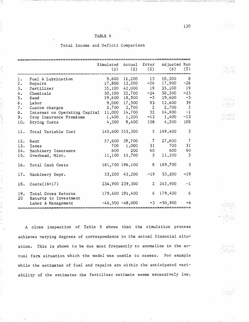
TABLE 6

and Deficit Comparison

r30

ToÈal Inco¡ue

Sinulated Actual($) ($)

Error Adjusted Run("/.) ($) ("/")

1" Fuel & Lubrication2. Repairs3. Fertih-eer4. Cheuícals5. Seed6. Labor7. Custom charges8. Interest on Operating Capital9. Crop Insurance Premiums10" Drying Cost,s

11. Total Variable Cost

12. Rent13. Taxes14. Machinery Insurance15. Overhead, lulisc.

L6. Total Cash Costs

L7 . MachÍ.nery Depr.

18. Costs(16+17)

19. Total Gross Returns20 Returns to Investment

Labor & Managenent

9 ,6001 7 ,80035,10030, 10019,600

9 ,0002,700

I I ,0001,4004,500

I45,600

27 ,600700600

I I ,100

I1,200l3 ,20042 ,00022 ,7 0O18,500t7 ,5002,700

L4 ,7 001 ,2009 ,400

153,300

29 ,7 001,000

20011,700

181,700 196,100

53,200 43,200

234,900 239,300

179,400 19I,400

-46,500 -48,000

15 10,300 I-26 17,900 -2619 35,100 19

-24 30,300 -25-5 19,600 -593 12,600 392 2,700 2

32 14,900 -1-13 1,400 -13108 4,500 108

5 149,400 3

7

3160

5

8

-19

)

27,600 7

700 31600 60

1I,I00 5

189,700

53,200 -I9

242,900 -I

6 r79,400 b

-3 -50,900 -6

A close inspection of Table 6 shows Lhat the simulation process

achieves varying degrees of correspondence to the actual- financial situ-

ation. lhis is shown t.o be due mosË frequently to anomalies in the ac-

tual farn situation which the nodel was unable to assess. For example

while the estimates of fuel and repairs are \,/ithin the anLieipated vari-

ability of the estimates the fertilizer estimale seeus excessively low.

i3r

Factors contributing to the excessive fertilÍzer costing on the case

farm were that a large proportion of the phosphate was applied in liquid

forn. Since this is the most expensive forn of the product Ehe Ëota1

fertilizer bill is inflated from t.he mean cost. Another factor affect-

ing fertilízer prices is Ehe location of the case farn. The farm is 1o-

cated in the extreme south \,restern corner of Manitoba and experiences

freight rates for both ÍnpuËs and production which are higher Ehan pro-

vincial averages "

The chenical cosË estimâtes for the farm are 25 percent

This is at least partially due t,o t.he fact that subsEantial

counts are available t,o farms of this si.ze and these are not,

in the average quoted retail chemical prices"

The seed est,imates are less Lhan Ehat actually recorded. for

This nay be due to higher than recommended seeding rates on

farrn but it is due in part t.o a large stock of rape seed which

chased in 1979 but not actually used.

too high.

bulk dis-

reflecEed

Lhe farn.

the case

r¡/aS pUf-

One of t.he most serious deviations between the actual and simulated

costs is the cost of labor. This is because the model only accounts for

actual producLive tine requÍred Ë,o complete all of the required opera-

tions. As the figures indicate Ëhis and probably rnany other farms pay

for labor t,iine that is efther non-productive or is used in farrn activl-

tj.es outside the scope of the cur:':ent model

Custom charges, interesL on operating capital and crop insurance pre-

miums are wíthin an accepËab1e error of estimate. This varies due to

Ëhe nature of the cosÈ iten. One should expect relatively accurate as-

sessuenË of crop insurance premiums since the only variation is the pre-

132

mium 1eve1 change over soil productivity type. The actual operatj.ng

capital interest is as much a function of the recent financial history

of the firm as the cost.s involved in the current product.ion effort.

Therefore, discrepancy between the estinate and the actual value indi-

cates a divergence of Lhe assumpËi.ons upon which it is based from the

actual situation.

The esti.mate of drying costs is showrt to be extrenely low. This is

due to the fact that the farm has recently erecLed a very capital inten-

sive drying system and is facing the first years of high fixed ownership

cos Ès "

The taxes shown in line 13 are possibly noË under estimated Lo the

degree indicated because the current farmer took possession of the land

within the year 1979 and no taxes r^rere actually paid. Because L979 fíg-

ures \^rere not available Ë,he 1980 assessnent was used and is assumed to

be slightly higher than that of the preceeding year.

.The machinery insurance estimate is higher than the actual expendi-

ture for Li{o reasons. First only Ëhe powered nachinery complement is

actually insured on the case farn. Second Ehe cost of insurance for

highway vehicles owned by the farm is included in the vehicle registra-

t,ion cost by the Manitoba Public Insurance Corporati.on. This portion of

the insurance cost, then is included with overhead adjusting thls figure

closer t.o the esLinaEed value.

The values used for machinery depreciaËion on t.he farm and in Ehe

simulator are not directly comparable. This is because even though both

calculations are made using Revenue Canada depreciation rates the simu-

lator is working from the replacemenË cost of Ëhe item while the case

farm accounts are based on the book value of the item.

r33

The estimate of tot,al gross returns is higher than the actual- reËurns

achieved by the case farm. Since a large portion of the case farm's

production was sunflower seed which moves at compensatory freight, rates

this factor alone may account for t.he case farm's deviation froo the

provincial average.

In conclusion the esËinates of both costs and returns are within such

margins of error as to maintain Cheir usefullness for the stated objec-

tives. Most. of the errors occur due to the inability to completely de-

scribe soue facet, of the farm enterprise. Errors in the cost calcula-

tions seem to reflect anomalies in the operation of the case farm rather

than serious errors of estimation.

The preceding analysi.s was designed to demonstrate the budgeting ca-

pabilities of the model ¡¿ith very lirnited informaËion. The provincial

and regional default values were used for all variables. As is often

the case soue additional infornation was available for t,he case farru.

The acËual average effective int.erest. paid on operating capital for the

period was 17 percenL in lieu of the default 13 percent. The prices of

gasoline and diesel oi1 were 83 cents and 74 cents rather than 79 cents

and 69 cenLs respectively. The effective wage rate on t.he case farn was

ç6.25 instead of the default value of $4.48.

i{hen these values are considered, and a further analysis presented

given adjustments for the case farm's specific condit.ions discussed

above, substanEi.al improvements may be detected in Table 6 in the tr^/o

right hand columns. Two excepEions are the estimaËes of custom charges

and the final estimate of returns Ëo investnent, labor, and managenent.

The discrepancy in the estinate for custom charges mây nor¡z indicate a

134

difference between the wage rate on Ehe case farm and thaÈ used to cal-

culate the actual custom charges. The increase in Ehe apparenË error in

the estimate of returns Eo investnent, labor, and management is a func-

tion of the more accurate invesEroent of costs failing Eo counter the er-

rors in the gross return calculations. Therefore, the comparison of the

esËj-nation accuracy of t,he net f igures presented is not rneaningf u1.

Differences for fuel and lubrication drops from L6 to 8 percent. The

error in labor cosË estination is reduced froro 96 xo 97 percenE" Also

the error of t.he est,imaÈe of the interesl on operat,ing capital is re-

duced from 33 percent, to -I percent.. The accuracy of estiroation of cash

costs is increased with Ëhe error falling frou 8 percent to 3 percent.

The preceeding analysis has demonstrated that in a particular case

reasonable estimaEes have been obtained of crop production costs and re-

turns with very linited infonnaLion. Ifhen some additj-onal firm specific

data is included these estimates can be substantial-1y improved. These

results indicate the the model produces valid estimates of, production

costs for the case farrq for the year 1979. This does not indicate a

definitive or even a statisEically significant validation of the rnodel.

llo¡¡ever, given the resources available, it does demonst.rate Ehat the

nodel has proven reasonable in this situation and increases Ehe 1eve1 of

confidence in ius adequacy for oEher circumstances.

Chapter VII

RECOMMENDATIONS AND CONCLUSIONS

The model as presented in Ëhe previous chapter is technically com-

plete. However, there are areas in which additional effort, would en-

hance the program's useablitiy and increase its utility. Several areas

of iuprovenent, have been identified and have been divided into procedur-

a1 and sËructural components. Procedural recommendatj-ons concern rnodi-

ficaË,ions and enhanceuents possible within Lhe existing basic forrnaË of

t,he program. The following suggestions should roake it possible for the

exist,ing model t.o present nore efficient accurate and consistent re-

sults. Recommended structural changes would require najor revisions to

Ëhe exisËing ¡aode1. The recommendations wou.l-d increase the program's

ease of use and accessability while expanding its analysis capability

and flexibilfty.

7 "T PROCEDURA]. RECOMMENDATIONS

7 .I.L Combined Field Operat,ions

At present the roodel does have a linited capability to handle com-

bined field operaËi.ons. Thet is, the ruodel is capable of handl-ing sev-

eral machines pulled by one t.ractor" The capability is necessary be-

cause the cost of a tractor pulling a culËivator followed by a harrow is

substantially dj-fferent fron having a tractor make . two passes in the

fie1d, where one pass is made with Lhe cult,ivator and one with the har-

-135-

i36

row. The laEter case great.ly over estimâtes, for example, lhe cost. of

fuel and labor.

The current facility for such operations is only available for prede-

fined com.binations. rn the master implernenc list (table 19) of Appero-

dix c certain codes have been reserved for this purpose. For these

codes the draft per foot, for the combined machine operatj.ons has been

calculated as the suro of the draft per foot of each masþj.ns. Given the

number of such possible, or even c,qrnmenly used, combinations iE has only

been possible to define a s¡0a11 subset of such operations.

If Ëhe input data forroat was changed so that each tillage operation

identified both the Ëractor and the user, rather than a co¡obination,

definitions of combined field operations would be possible. This ruet.hod

would provide more flexibility and accuracy in Ëhe a1locaËion of Eractor

t,ime among inplenents. I,Iith the speci-ficaÈion of a second or third iro-

plement in a particular Ëillage operation the cornbined field operat.ion

could be recognized and costs properly calculated.

7 "I.2 AlLernate Farn Income Sources

Llhile the inclusion of income from off farrn labor may be desirable

this is a relatively straight forward resource to allocate anong farm

and non-f ar.ttr enterprises. l,fore dif f icult t,o consider is the allocation

of fixed costs and ret,urns when incomes such as revenues derived from

custom work, land and/or equipment rental and the rental of machinery

shelter space or grain storage are considered.

rf sone consideration could be given Ëo the proportion of tiue or

space allocat,ed Lo non-farm activities the cost could be pro-raËed.

This would allocate an accurate incidence of

es. This is certainly as importanE as it is

on-farm enterprises. Unfortunatly such cost

ble if the informat,ion regarding alternate

present.

137

cosE to the farm enterpris-

to allocate expenses among

apportionment is not possi-

farm income sources is not

7.1.3 Fixed Cost Allocation

The fixed costs of farn uachinery ovmership are comprised of the cost

of insurance, depreciation, and investment.. The current configuration

of che Progralo does not allocate the fixed cosËs of machinery ownership

auong Lhe fields on the basls of useage. The justification for this

uethod i.s the assertion thaË the entire productive farm unit must bear

these costs wheÈher Ehe machine is actually used or not. The rnachine j.s

also potentially available for use on every acre of t.he farm.

One important applicaLion of the ruodel is for the comparaËive analy-

sis of the profitability of different crop production enterprises. A

furËher refinement of this analysis would result. from the allocation of

the fixed cosE.s auong crop enterprises prorated by the leve1 of use in

each fie1d.

If a machine \.ras used in the producLion sequence i.n any field Ehen

Ëhe fixed costs would be allocated to the toEal acres of those on which

iË was used. In t,he case where a machine was not used i-n any field

then the fixed costs would be divided by the total number of acres on

the farm and allocated equally across every acre of the farm. The fixed

costs wouLd be allocaEed to those fields and enterprises which actually

use the machine and across the enLire farm if it was not used. Ei-ther an

138

enLerprise or else the entire farm unit must, bear the costs of machinery

ownership.

7 .I.4 Expansion of Input Infonnation

7 .L.4.L Rental and Custom Charges

At present the sane limitation exists with the rental and custon

charges as that of combined field operations. The only operations

avail-able are Ëhose which have been predefined and included in the ruas-

Ëer implement list,. The reason for this is thaE if the charges for such

operations are not specified defaults musE be provided. To date those

defaults have been specified from tables of recommended rat,es as previ-

?l"fy described. This process is inflexible, time consuming to main-

tain, and can introduce inconsistencies into the analysis" An allernat.e

nethod would be to calculate both renE,al and custon rates on an individ-

ual basis within the program. All of the required information is cur-

rently available and 1n Ehe model's daËa base, To calculate a renEal

rate the fixed ovmership costs are calculated exactly the same as for an

or¡ned machine. This figure is divided by the expected hours of use per

year and a specifÍed pereentage profit is added to the figure to give a

rent,al raË,e on a per hour basis.

The calculation of a custom rate proceeds in exactly the same mânnex

except that t.he variable costs (labor, repairs, fuel and lubrication)

are also included. This figure is then divided by the expected hours of

use per year and the requisite margin added.

When a user wishes to speci.fy a custom or renEal operaE.ion it is de-

scribed exactly the same \,ray as owned equipment. Instead of the toËal

I39

cost of ownership being alLocated across farm enterprises iË is used to

calculate an hourly rental charge which is allocated to those fields

specifying Lhe operat.ion as a function of the nachine's effective field

capacity.

The specificatj.on of rental and custom charges in this fashion would

greatly enhance Lhe usefulness of t,he simulator. In lieu of the current

necessiLy to constanÈly updaEe and include custom raËe recommendat,ions

which have been calculaËed under varying assumptions (ie. Iabor and fuel

costs) the refined machinery costing capabilities of Ehe sirnulat.or could

be used to generate accurate and consistenË schedules of such rates for

nachines which hitherto have had no such detailed basis.

7 "I.4 "2 Unit,s

Many of the problems and errors caused in using the current version of

the budget generat.or arise from confusion concerning the required uniEs

when describing raachinery, inputs, and production. Some sinplification

of this process would occur if the internat,ional systen of meËric units

were used for all input description. If the nodel r+as completely and

consistently operated in this fashion a great deal of confusion could be

elininaËed. Ilowever, it. is recognized that the demand for the ability

to use standard units for input description will exist for the forsee-

able life of the progran. Therefore, the use of sËandard netric unit.s

should be assumed buÈ sÈandard inperial unj.ts should be recognized and

used on input when specified.

As previously mentioned wich respected

amount of confusion exisEs concerning the

the reporËs produced by the program.

Eo input inforraation a certain

units of items represented in

140

Again, although the complete use of standard uetric units would

enable sinple and more consistent 1abe1ling of these documents it is

recognized Ëhat t.he demand for iroperial unit. references will persist

into rhe future"

7 .I "4.3 Macro-Operations

Experience in using t.he model to analyse large numbers of farms has

demonstrated that a great deal of repetition ofEen exists in the speci-

fication of field tillage practices" The input of tillage practice

specificaËions into Ëhe progran would be expedited if Ehe user could de-

fine a ttmacro" operation which would in fact be a commonly used set of

tillage practÍ.ces for Ehe individual farmer. Once this set of opera-

Ëions has been specifed it could be referred to by name only without the

need to recode each individual operation.

7.I.4.4 Alphanumerics

The current version of t,he program recognizes the specificatÍ-on of

all user descripËion only in terms of coded numbers" Once a user be-

comes familiar with such specification it is reasonably easy to use.

However, if the model is Ëo be directly used by large numbers of people

uhís system is tine consuming, tedious, prone to producing errors and

provides difficulty in detecting the same.

a2Figure 14"' shows the rnonthly cosLs of an average ninicouputer system

versus clerical labor. Although Figure 14 refers specifically to mini-

compuËers, Lhe same general cost trends have occured throughout the in-

83 Dorr"ld Kennedy, Minicomputers: Low-CosË CompuEer Power for Manage-ment, Amacon, New York.1978. p. 49

141

oo

o2

Figure 14

Monthly Costs--Average MinicomputerSystem Versus Clerical- I-abor

Averagesystem cost

1 97501 965

Soi.¡rce: Donald P. Kenney, Minicornputers - Low-Cost Computer Power forManagement, revised edi-r,ion, A Di¡rision of American Management.tssociãtion, New York, 1978, p. 4g.

Year

t42

dustry. WiËh this fact in view we can see the rnagnitude of the benefit.s

of long term gains of the substitution of computer time for clerical

time.

The use of descriptive words instead of code numbers would provide

substantial saving in Ehe tiue required to code a parËicular farm record

for analysis. It would also decrease the possibility of errors while

looking up the codes and provide 1abel1ing of the input to facilitate

error ehecking. This improvement could only be gained aE Ëhe expense of

additional machine Ei.me. But as indicated this cosË is reducing rela-

tive to the cost of skilled labor. Therefore substantial savi.ngs can be

realized by having the machine assume that, portion of the coding pro-

cess.

The determination of adequate machine capaci.ty for a certaj.n enter-

prise is one of the mosE critical decisíons faced by the farm manager"

Adequat.e nachine capacity is necessary so thaË the required operations

roay be compleEed before excessive losses occur.

The model provides detailed calculations of the tine required for in-

dividual field operations. This information is valuable Eo a farm nan-

ager at.ten'pting to determine adequate roachine capacity. However, the

program does not consider the scheduling of operations. Therefore it is

difficult to deternine Ehe probable delay tiroes encountered. If the or-

7.L.5 Expansion of OuËput

7.1.5.f Operation Time

Inf onoation

Principles of }lanagement Science:DecisÍons, Prentice Hall, Englevood

84 __Harvey Wagner,to Executivesy.1970. p.250

lliEh applicationsCliffs, New Jer-

r43

dering of operaEions is indicared a c.p.M.84 (crirical path Merhod) type

of analysis could be conducted to determine total expected compleEion

times for the critical seeding and harvesting operati-on. This i.nforma-

tion, if provided in a conci.se optional report, could be used by Ëhe

farm manager in facing inport,ant machinery investuent decisions as wel-l-

as Ëo alert the farro manager or management advisor Ëo cri.tical bottle-

necks in the productÍon process of a partlcular period.

7 "l "5 "2 ReËurn Indicators

The presenlat,ion of Ehe budget results shou.l-d be structured to re-flect the needs of the eventual user. Individual farn managers, univer-

sity educators and governnûent extensi.on personel have expressed. concern.

over Ehe reLurn indicators chosen for presentation. The traditional ec-

onomic indicaÈors have not been enthusiastically accepÈed as appropriate

t,o assist actual farra management, decision naking. The suggestiorr85 h""

been made thaË, t,he use of Lhe Ëeru gross ,nargin86 *, alleviate some of

the confuslon surrounding Ehe existing indicaËors.

Although not co'n-only used in North America, Lhe concepÈ of gross

margin analysis has been applied extensively to partial budgeting tech-

niques elswr¿here.87 fn. syst.em is based upon a consid.eration of Lhe con-

tribution uade by a partieular enterprise in excess of the additional

G. Therrien, chief Economist,, Manitoba Department of Agriculture,cost of Production study Advisory committee M.eeting, March 31, lggI .

c.s. Barnard and J.s. Nix, Farm Planning and control, carnbridge uni-versity Press, Cambridge, 198I. pp 45-47.

G.F. Tat,e, "Gross Margin Analysis: A critical Evaluationrr, Farm B"gg-et Manual, Part 2 Financiar L972, Lincoln college Department of FamrManagemenË and Rural Valuation, New ZeaLand, L972. pp.L79-187.

85

86

87

144

variable cosËs necessary to operate it. From this contribution the

fixed comüitments, overhead expenses and all other costs of the firm

must be met. The assumptions underlying the analysis are currently

found within Ehe existing forrnulation of the budgeting rnodel. The Lech-

nique assumes linearity of returns from rnarkeEing field crop production

as does the budget generator. It also assumes thaL a certaín amount of

financial isolat.j.on is possible when dealing with the variable costs.

This is also consistent with the sËructure of the analysis provided by

the progran.

When dealing with restricted cash flows iE has become very inportant

Lo be able to assess the cash ret.urns from a particular enterprise as

well as it profitability. For this reason a value indicat.ing Ehe net

cash returns for each enËerprise would be useful in evaluating t.he con-

tribution of an enterprise to the firm's net cash position.

The long run viability of any enterprise is dererro-ined by its ability

to provide an acceptable 1evel of ret,urn to all factors of production.

Therefore t.he current. calculation of net returns to rnanageuent should be

mainLained to indicate the residual to all inputs into the production

process or a pure economic profit. The proposed ret,urn indicaË,ors would

Èhen consist of:

i. Gross Margin defined as the difference between gross enË,erprise

returns and varj-able costs for the enterprise.

2. Net Cash Returns as the difference between toËal cash ret.urns and

t,otal cash costs.

3. Pure Profit or net, returns to al-l factors including nanagement as

it is now calculated but including non-cash reLurns such as the

appreciation of real property.

145

7.I"5.3 Cash Flow

The analysis conducEed by the current version of the rnodel is pre-

sented as an annual suunary. In this fornat. it suffers some of the in-

formaLion compressing features that have been criticize¿88 in other mod-

e1s. An important facet of the farm financial picture that is not dealt

with is that of the cash f1ow. The final net position of the producer

aË the end of the year is of no relevance if such casliL flow diffi.culties

occur during the season render the business nonviable.

Program enhancements would make iE possible to present both receipts

and expenses on a monthly, or at least quarËer1y, basí.s. This informa-

tion will help the manager Eo make accurate determinaLions of operating

capital requirmenËs and help him to deaL wiuh lending insËituËions for

their provision.

7.2 STRUCTURAI- RECOMMENDATIONS

7 "2.I Input-Output Control

The program is currently executed in what is terued a rrbatchrr mode.

That, is, the data is completely prepared and then it, and the program,

are presented to the computer for execution. The report,s are then

printed. This roet,hod has proven very effecËive for handling large

amounts of data but suffers frorn a degree of inflexibility. IÈ is also

difficult for users who are not experienced in job submission and mn-

chine usage or who roay be working at, reuote locat.ions. The direct, use-

age of the prograrn by unskilled individuals will only be practical when

lhe program has been restructured in an ttinteractive" mode. ttlnterac-

88 F"1""rrr 1oc. cit.

r46

t.ive" is really a word t,hat iuplies machÍne initiative. An interactive

program controls all phases of the execution process directly from dat.a

entry to report generaÈ,ion. ttThe more inLeractive a prograxo is, the

more initiative t.he nachine takes and Ë.he less t.rai.ning is required of

the user."89 Figlrre 15 indicat.es a proposed struct.ure to effect this and

the other recommendations of this section.

Interactive input of the user daËa al1ows much more flexibility and

reliability to be designed into t,he system. It. allows the prograE to

edit each piece of data as it is entered and to pronpt Ehe user for in-

correct or incomplete information. The data is correcE,ed and verified

before the analysis is even attempËed. Int,eractive input can make t.he

inpul procedure more concise. The progran can make decisions such as if

an enterprise is not present to surpress all irrelevant questions and

references to the particular enEerprise.

An inÈeractive program also provides more flexibility in terns of the

type and quanLiËy of reporËs generaE,ed. A major criticism of previous

90.systems-- has been t,he abundance of unwanted and unread reports generat-

ed by the systern. Copious reports instead of providíng useful informa-

tion can only serve t,o roask what valuable results are presented. \^iith

an interactive system the user can xequesE a summary report and then re-

quest only Ehose more detailed results as rnay be of signifÍcant inter-

esE. This uode allows the user to focus on what is important to hin

while sLill having access to all of the detailed resulËs the system can

produce.

89 Frud Dahl and c.J. Sippl, CouputerPrentÍce-Hall, Inc., Englewood Cliffs,

90- - See previous dj.scussion of Canfarm.

Power for the Snall Business,NJ, tglg. p"it.

147

Fri ørrr,e 1

Proposed Farm Firm Sinml-ator

. I'fai¡rt ena¡c e

Update

'rGenerelizedrl

148

7 "2"2

7.2.2.

As

File Maintenance and Retrieval

I l{euristic Expansion

stressed in the previous chapter t.he support,ing information for

the program is as important to Lhe generation of accuraËe and reliable

results as the algorithro it.self. This infornation is also necessary to

make the rnodel as easy to use as possible. Currently lisËs of such

items as pricing information are prepared, checked, and included as soon

as possible to provide default information for the user" UnfortunaËely

default information is only available on this basis " As Ehe number of

users expands it is probable t,hat. sone users will possess information

useful for the operation of the model. IË would benefit ot,her users and

faciliËate Ëhe file mainÈenance procedure if this informat,ion could be

easi-ly added Eo Ehe exist.ing data base.

For example, a user requests default pricing and application rates

for a cheruical which hiEherto had no information available. The user

would be informed of this fact and prornpted to enter a namer rate, and

price for the chemical. If Ehis was not possible the chemical would be

deleted but if iË was entered the information would be included in the

daËa base and would be made available to other users. It ís iltrporÈant

Ëo note thaË such infornation would be flagged as not havíng been veri-

fied for the infornation of ot,her users. This would also provide a list

of infornation which had been qemmonly requested by users to those re-

sponsible for maintaining the data base.

r49

7 "2.2"2 Resideut Farm Descriptions

the current version of the prograu requires the conplete entry of the

farm descrÍpti-on each tine the progran is executed. When the nodel is

used in a planning cont.ext, implicit in t.he learning procedure is that

the user will nake a number of runs of the same farm plan with probably

minor nodificatj.ons. To facilitate this process Ehe structure as shown

i.n Figure 15 would allow a farmer t.o store the general description of

the farn and irs assets. The farm manager could then call up this farm

description and generate complete budgets by rnaking only specific chang-

es to exist,ing planning operations, and capital equipment. This proce-

dure would facilitate certain forns of research where si.mulation experi-

xoents could be conducted upon standard farm firm uodels available within

the system.

7.2.2.3 User Statistics

One of Lhe major uses of the Canfarm project was to collect sEatistics

about the users of the system. While Canfarro was able to collect actual

financial information the nodel described is able to assess the finan-

cial profile of the enterprises described only in physical terms" This

inforrnation if properly collecLed and documented could be of use in a

varieEy of research efforts" The presence of the physical information

coupled with the program's financial budget generation capacity can pro-

vide infornoation for a hosL of other economic models. This has in fact.

been the major use of the model to this juncture.

150

7 "2.2.4 Report Generation

several types of reports are going to be requesLed of the system in

succeedj.ng years. The types of user reports are alluded to in the pro-

cedural recomrnendation. 0ther types of reporËs must deal with summaries

of user st.atistics mentioned in the preceeding section. It will also

become increasingly inportanË, to generaËe tables of information from Ehe

data base so that price and oEher information may be updated and veri-

fied" The ease with which these reports can be produced will determine

nuch of the acceptance, utiliEy and cosË of maj.ntaining the systeE.

7.2.3 Enterprise Integration

As j-ndicated by Figure 15 the crop budget generator is jusË one com-

ponent of a farm firn budget generation system. Expansion of the sËruc-

ture as described will facilitate the inclusi-on of new enEerprises, the

flexibility and concision of reporËs produced, and the maintenance of

the daEa required t,o make the entire systeu effective and easy to use"

7.3 CONCLUSIONS

The mod.el as Presented. generaLes budgets depicting the costs and re-

turns of crop producËion. The variable and Lhe fixed costs of produc-

tion are examined. The costs are derived from the producer's physical

description of his m¡chj.nery, land, EanagemenË and culLural pracLices

eroployed. This infornation is int,egrated with Lhe price data associated

r,rith the particular year of production.

The nodel produces output at t.hree levels of detail. At t,he firsË

level a set of tables is generaËed depicting Ëhe detailed costing of

151

each machine and each machine operation on every field. At t,he second

1evel a field sumuary is produced for every field. This table sunrra-

rizes machi.nery cos ts and lj. sts all other cos ts and ret,urns . AE the

third leve1 a whole farm summary is produced for all crop enterprises

vriËh fields aggregated by type and also expressed on a "per acre" basis

for ease of comparison.

The raodel was validated through the use oÍ a case farrn study. The

comparative analysis of the case farm indicated that the roodel is capa-

b1e of generating acceptable financial est,imates of ent,erprise cosls and

reËurns when only physical information i.s available"

lfinor effort could implement some of the recommendations suggested.

Changes to the model should be nade with t.he nature of the application

in rnind. The priority associated r,¡ith those changes should be deter-

nined by the users of the nodel.

The potential exists for a wide vari.ety of applicaËions of the ¡oodel.

The nost exËensive application to date has been for research. The sys-

ten conceivably could be used as a decision making tool by the farm man-

ager when looking at crop production alternaE,ives. Potential applica-

tions also exist whenever insight into the costs and benefits of

cropping systeos is desired. Such inforroation uay be of use to educa-

tional, financial, and consultative institutions. The potential also

exists for rnodel useage by governmenÈ Eo generate data for the adninÍs-

trat,ion of existing programs and to assess the financial impact, on the

farrn firrc of legislative proposals.

BIBLIOGRAPI{Y

Agrawal, R.C. and E.0. Heady, OperaËions Research Methods forAgricultural Decisions, The Iowa State Universiry Press, Ames, I972.

American Society of Agricultural Engineers Farm ManagemenË Commlttee,"Agricultural Machinery l'lanagement Dat,a", 1976 Agricultural EnglneersYearbook, American Society of Agricultural Engineers, St. Joseph,Michigan, 1976.

Andruchow, Lloyd and Jirn Shortreed, Farm Machinery Cost,s, AlbertaDepartuent of Agriculture, Production Economícs Branch, Edraonton,Alberta, 1976.

Archer, Stephen II., ttThe Structure of ManagemenE Decision Theory", inInforroation for Decision Making, ed. Alfred Rappaport, New Jersey,

Babb, E.M. and C.E. French, "Use of SimulationFarm Economics, Vo1. 45, No. 4, Nov. 1963.

Boehlje, M., "0ptirnization and Decision

Procedurestt Journal of

Ifodels: The Use of Statisticalof Agricultural Economics, Vol.Search Procedurestt, Canadían

21, No. 2, July, 1973..Journal

Bowers, tr^Iendell, Fundamentals of Machine Operation: MachineryManagement, , .lo 1i[- tttinois , I97 5 .

Campbell, D.R., Comtois, Gilson, MacFarlane, and Thain, CanadianAgriculture in the Seventies, Report of the Federal Task Force onAgriculture, Information Canada: 0ttawa, December 1969"

Candler, tr^I. and i,i. Cartwright, I'Estimat,ion of Perforroance Functions forBudgeting and Simulation Studies".

CANFARI'Í promotional advertising. Agrologist Autu¡nn 1978.

Chambers, A. "CANFAIM Should lfave Been Dropped Long Ago," Grainews,Septenber 1978.

Charlton, P.J.Journal of

and S.C. Thompson, "Simulation of Agricultural Systems'rAgricultural Economics, Vo1. 2!, No. 3, September 1970.

Cochrane, W.C. and G.M. Cox, Experimental Designs, Second Edition, JohnWiley & Sons, Inc., L957.

Craddock, W.J., Interregional Competition in Canadian Cereal Production,Special Study No. 12, The Queen's PrinËer, OÈtawa, Canada, L97I.

-r52-

153

DenË, J.B. and J.R. Anderson, Systems Analysis in Agriculturalllanagement., Sidney: John l^Ii1ey, l9 71 .

Department of Agricultural Economi.cs and Farm Management, "FarmDiversif ication Project Analytical Framework", IJnpublished Paper,UniversiËy of Manitoba. i,linnipeg, Manitoba, 1975.

DeparËuent of Farm Management and Rural Valuation, Farm Budget, Manual,Part 2 Financial L972, Lincol College, New Zealand, L972.

Donaldson, G.F. and J.P.G. I,Iebster, "A Simulation Approach to theSelections and Cornbination of Farm Enterprises." Farn Economi$,Vo1. 11, Nor6, I968.

Driver, H., OnLario Dairy Farro Account,ing Project Progress Report I977 ,Agriculture Canada, OnËario Milk MarkeEing Board, Ontario Ministry ofAgriculture and Food and the University of Guelph Guelph Ontario,L978.

Dyck, J.David, "The Impact of Technological Change on Farmland Prices inIfanitoba." unpublished M.Sc. thesis, The University of Manitoba,Department of Agricultural Economics and Fann ManagemenL, L979.

Eisgruber, L., and J.Nielson, "Decfsion-Making Models in FarnIlanagement'r, Canadian Journal of Agriculcural Economi.cs, Vo1. 9 No.1, I963.

Felsen, Jerry, Decision l'lakíng Under Uncertainty: An Artif icialIntelligenee Approach, CDS Publishing Company, New York, 1976"

Fisher, R.4., The Design of ExPeriments, Oliver and Boyd, 1951"

Fraroingham, C.F.,,J.4. MacMillan and D.J. Sandell , The Interlake Fact,Hignell Printing Limited, Winnipeg, Manitoba. November' I970.

F.R.E.D Adrn:inistration, Interlake Flyer, Box 2000, Arborg, April 1975.

Friesen, O.H., lle¿ and Forage Harvesting Methods, Manitoba Department ofAgriculture, I^Iinnipeg, Manitoba.

Giles, J.D. ARDA in Manitoba, Province of Manit,oba, January 1968.

Guthrie, Scott 8., "GLEAP: A GeneraU.zed Program for Game LearningSirnulation", Behavioral !9iSt"., Vo1. 13, 1968.

Ilardaker, J.B. "The Use of Sirnulation Technique in Farm Management" FarmEconomist, Vol. 1I, L967.

Hardin, Mike L. "A Simulation Model for Analysing Fam CapitalInvestmenÈs", Unpublished Ph.D. thesis, Oklahoma StaLe University,July 1978.

ilart, 4.G., Anticipation, Uncertainty and Business Planning, A.M. Ke1ly,New York, f951.

154

Hayani, Y. and V. Ruttan, "Factor Prices and Technical Change inAgricultural Developnent: The United States and Japan, 1880-1960",The Journal of Polítical Economy, Vol 78, No.5, Sept./Oct" I97O

Ileady, Earl 0. Agricultural Policy Under Economic Development, IowaState University Press. Ames L962.

IIeady and Agrawal. Operations Research Methods for AgriculturalDecisions. The lowa St,ate UniversÍ.ty Press, Ames: L973.

Ilouse of Comrnons of Canada, The VJestern Grain Stabilization Act, BillC-41 (Ottawa: Infornation Canada, January, L976)

Hunter, J.S. and T.II. Naylor, "Experimental Designs for CornputerSinulation Experiments", Manageroent Eig*gg, Vo1. 16, No. 7, 1970.

JohnsonrG.L. r "Philisophical FoundaEions of Agricultural EconomicThought", unpublished draft paper Agricultural- Economics Literature,Volume 3, A.A.E.A., May 1978.

Kempthorne, 0., The Design and Analysis of Experiments, John l^Iiley &

Sons, Inc., New York, L952

Kraft, D.F. and P. Graham. DepartmenEal paper in progress. TheUniversity of Manitoba, Dept. of Agricultural Economics and FarmManagemenË. February, 1979.

Lawrence, John. "CANFARM - irlorking TogeEher for a Bett,er Agriculture",Agrologist, Autumn f978.

Lee, G.E., "Exploitat,ion of Information for Capít.al Accumulation UnderUncertaintyrr, Unpublished Ph.D. t,hesis, Purdue University, I97L.

Longmuir, C.N., M. Senkiw, A. PokranË, and C.F. Fraraingham, CropProduction Simulator, Research Bulletin No. 7B-2, Department of@cs and Farm Management., The University ofìfanitoba, Winnipeg Man. November 1978.

Maisel, I1 . and G. Gnugnoli, Si.rnulaton of Discrete Stochastic Systems,Science Research Association, Inc., 1972.

Manitoba Department of Agriculture, Farn DaEa Handbook, EconomicsBranch, I^Iinnipeg Manitoba, I972.

"Machinery Price Data", Unpublished Data, Farm òfachinery Board,irlinnipeg Manitoba, L974-L979 .

Manitoba AgriculËure Yearbook, Winnipeg, Manitoba, I970-1979.

Rental and CusÈom Charges for Fart Mac,hinery, TechnicalServices Branch, I,IinnÍpeg, Manitoba, L973'1979.

155

Marsh, Stephen B. "A progress Report on TELPLAN Activities", Unpublishedreport" Departroent of Agricultural Economics¡ Michigan StateUnivers ity.

Mc].aughlin, F.S., and R.c. pickhardr, QuantitaËive Techniques forManagement Decisions, HoughËon Mifflin Company, Boston, L979"

Mize, J.l1 . and J.G. cox, Elements of sinulation, prent,ice-Hall , rnc.,Englewood Cliffs, New Jersey, 1968.

Morgenthaler, G.i,l . "The Theory and Application of simulation inOperaÈ,ions Research" in Achoff (Ed.) progress in OperationsResearch, John l^ii1ey, New York, f 961.

Murphy, R.E., Jr., Adapt,j.ve Processes in Economic systems, Acad.emicPress, New York, 1965.

Naylor, T.H. 9ornpuçer Sirnulation Experiments tr^Iith Models of EconouicSys t,ems , John tr/iley, New York , L97 I "

Naylor, T.H. and J.trI. Vernon, Micro-economics and Decision Models of theFirn, llarcourt, Brace and triorld, Inc., New york, L969.

Nebraska Board of Tractor Test Engineers, "Nebraska TracLor Test Data,Agricultural Engineers Yearbook, American society of Agri.culturalEngineers, St. Joseph, Michigan, I970-1979.

orcutt, G.II. "simulation of Economic systems" Amerj.can Economic Review,Vol. 50, 1966

Patrick, G.F. and L.M. Eisgruber, "The rmpact of Managerial Ability andCapital Structure on Growth of the Farm Finn", The American Journalof Agricultural Econo¡oics, Vo1. 50, 1968.

Revenue canada, Farner's and Fisherman's rncome Tax Guide, The Queen'sPrint,er, Ottawa, Canada, L979.

sanderson, K.T. and A. McArthur. computer Methods for DevelopmentBudgets. Agricultural Economics Researeh uniË,, Lincoln corlege.universiLy of cantebury. canËebury, New Zealand. publication No. 451967 .

Sabourin, Sylvio. "A Comput,erized Siroulation Model for EvaluatingAlternative Cow-Calf Farn Plans". Unpublished M.Sc. thesis,Unj.versity of Manitoba, Department of Agricultural Economics and FarmManagement, L977 .

SahÍ., R.K", "A Recursive Prograroming Model of Canadian Agriculture",National and Regj-onal Economic Models of Agriculture, Agriculturec"n"¿., uG-oniClnraìctr puu. 7W, tg12

SonntagrB.H., ttusing Comput,ers in the Fann Businesstt, Canadian FarnEconomics, Volume 7, No.3, AugusË, 1972. Agriculture Canada, Ottawa.

SEatistics Canada, Farm InputCanada, I970-L979.

156

Index, The Queen's PrinËer, Ottawa,Price

Suttor, R.E. and R.J. Crom. "Computer Models and Sinulations", Journalof Farn Economics, Vol. 46, 1964.

irralker, R.L. and D.D. Kletke, User's Manual Oklahoroa SLate UniversityCrop Budget Generator, Oklahoua SÈate UniversiËy AgriculturalExperi.mental Station, Progress Report P-656, Oklahoma StateUniversity, Oklahoma, L97I.

Winters, G.R., ttSimulation in Agricult,ural Economics Research", Paperpresented to the IBM 5th Agricultural Sytoposiuro, Toront.o, Ontario.October 1967 "

Zentner, R.P., B.H. Sonntag and G.E. Lee, "Simulation lfodel for DrylandCrop Production in Lhe Canadian Prairies", .{gr:þtlt.tuI _Sysl!g-, Vo1.3, I978, Applied Science Publishers Ltd', England, i978.

Appendix A

SYSTEM INFORMATION

-r57-

158

J_4UrC (

Master Inplement List

Index of Îlllage NaEe PLeld ExpectedTll1áge Efficfeney Annusl LffePractice Equstloo Use Use

Låbor Overlap Draft SpeedCoefflcfent Llght Eeavy

SoiI So11

T.A.R. DeprecfatlonEquatlon Rate EquaÈ1onNube r

1 PLO!'-TRÄ[L ÎYPE2 PLOW-HOUNIE)3 CULTIVAÎOR L "D.4 CULTTVAÎOR L.D.5 CI¡LTIVATOR R.D.6 CIILTIVAÎOR 8.D.7 sîAtK culrER8 STÁTK CUÎTER9 AUGER.ELECTRIC

IO AUGER-I'IOTORII, A¡¡GER-PÎOI2 TANDEM DISC-TI3 ÎANDEI DISC.ÍJ14 ONE I{AY DISCI5 DISCER-SEED.FERl16 ROD-IJEEDER17 NOBLE 6' BLADE18 NOBLE 7' BLADE19 ROE DRILL20 PRESS DRILL2I SEED DRILL22 CORN PLANTER23 HARROI{ (DRAG)

24 EA¡.RorJ(S.T00rR)25 PACKER26 SPRAYER

2 7 sr.lATr{ER ( PTo )28 sr¡AlgER(S.P . )29 s!¡ATnER(C0ND)30 SWAÎIIER(REEL)3I COMBINE(ROTARY)32 COMBINE PTO

33 coHErNE (S.P.)34 DRTER AND EQUTP¡5 GR.ANI'LAR APP.36 TRUCK37 BAJ.E I'AGON38 SPRAYER S.P.39 FORAGE HARVESÎER40 BAI,ER (ROUND)4I BATER (SQUARE)

42 ROTOTILLER43 r'or.JER

167. 2500.t67. 2500.208. 2500-208. 2500.208. 2500.208. 2500.

0. 2000.0. 2000.0. 2500.0. 2500.0. 2500.

150. 2500.I50. 2500.

0. 2500.167. 2500"

0. 2500.0. 2500.0. 2500.

60. 1200.60. 1200.60. 1200.0. 2500.

r25. 2500.100. 2000.r00. 2500.

0. I 200.r00. 2500.100. 2500.t00. 2500.r00. 2500.100. 2000.I 00. 2000.ls0. 2000.

0. 0.0. 1200.

150. 4000.lso. 3000.r00. 2500.80. 2000.0. 2000.

100. 2000.167. 2500.125. 2000.

I.180 0.01.180 0.01.220 1"0L.Z?0 1.01.220 t,01.220 1.0t.140 0.0I " t40 0.00.250 0"00.250 0.00.250 0.01.r90 t.0I .190 1 "0r.220 0.0L190 0.0r.t60 r.51"220 r"51"220 t.51.230 0.0I "230 0 "0t.230 0.01 "250 0.0r"160 1.5I . 160 I.5t.I60 1"81.220 1.5L1.40 0.0I "I40 0.0I "140 0.0I . I40 0.01.2t0 0.01.2I0 0.01.2t0 0.00 "000 0.0t.140 1.5I "050 0.02 "080 0,01.095 0.01.2t0 0.0I.210 0"02 .2 r0 0.01.180 0,0I .140 0.0

7 "6 9.07.6 9.02.3 3.02.3 3.02.9 4"22"9 4.21.6 1.6I.6 1.ó0.0 0.00.0 0"00.0 0.03.6 4"23 .6 4.22.6 3.I2"2 2.5l.l I.I2"5 3.42.5 3 "41.2 1"21.2 L "21.7 t"71.7 1.70.5 0.5o.7 0"70.5 0"50.4 0.4t.4 t.41.4 1.41.4 1.41.4 1.40 .0 0.00 "0 0.00.0 0 "00.0 0.00.3 0.30.0 0"00.0 0.01.4 I .40.0 0.00.7 0.70.7 0.75 ,0 !0,0I.6 1.6

0.10000.10000. 10000. 10000.r0000 . r0000. 10000. r 0000 " 10000.10000. 10000 " I0000 " 10000 " r0000. I0000.10000.10000 " 10000.10000. t0000 .10000 .10000 " I0000.t0000. I0000 .10000.10000.15000.15000.15000, I0000.10000

" r500

0.10000.10000. 15000. r5000.10000.10000. I0000. I0000. 10000. 1000

4.64.64"54"54.54"54.54.58.38"38.34.54"53.54.05.04"54"54.04"04.04.54"54.56.04"04.54.54"54"50.00.00"00.04.0

20.o8.04"52.52.52.53.04.5

7

44444

ç

7

7

7

5

5

5

55

5

5

5

306

2

2

222

2

2J

3I

2,2

2

2

159

Table 7 (Continued)

Iudex of Îfl1age Naue Fletd ExpectedTlllåge Efficlency Annual LifePract{ce Equatíon Use tse

Labor overlap Draft Speed T.A.R. DeprecfatfonCoefflclent Lfght neavy Equatlon RaÈe Equatlon

sotl Sotl Nunber

44 ¡f)WER-CONDIlION45 RAKE-Í.¡EEEL46 RAKE-P-BAR47 SIACK!ÐVER48 BALE IdAGON SP

49 FORAGE BLOIiIR5O IIATSÎACKER5I BROADCASÎER52 HAY BTND PTO

53 BALE ELEVATOR54 BALE CARRÍER55 F.E.LOADER56 FOR H.ARV & IIAGON

57 STOOKER

58 ROIJ CROP CULI.59 RolARr CLLT(UoE)60 POÎÀlo FT¡¡DROÍJER

ó1 E.ARVESIER62 PLA¡IÎER63 BIN PILER64 gÂRROH PACKER65 BEEÍ HÀRVESTER66 BEEtr 1OPPER67 BEEÎ PL.A¡¡TER

68 ROf{ CROP SPRåYER69 ONIO¡ PLANTER70 ONION WII{DROIIER7I ONTON B.ARVESTER

72 SIJEEÍ CORN PICK73 HEffi. BALE WAGON

2OO CUS!oH BALE I.IAGN

2OI fl'SToM SPRÀYING202 CûSToH Prosr{atH203 CST SP SIJATHNOC

204 CST SP Sr¿ATEr.rC

205 qltsmu IRUCK206 flrsmu SPCoHBINE207 C. P10 CoÌ'fBINE208 c1ts10H SQ.BALE209 c. sQ. BALETHROS2IO C.BAI,ER ROUI{D 5'2II C.BÁIER ROUND 6'212 cusloH HoI,JING213 C. MOÍ¡ER-CoND214 C" RAN.E I.THEEL

215 i. RAKE P.BAR2Ió CUSTOI{ DRILL218 C. DISCER SEEDER

125. 2000.125. 2000.LZs. 2000.125. 2000.250. 3000.80. 2000.

r25. 2000.0. I 200.0. 2500.0. 2500.0. 2500.0. 2500.

80. 2250.t00. 2500.

0. 2500.0. 2500.0. 1000.

80. 2000.0. 2500.0. 2000.

t00. 2000.80. 2500.80. 2500.0. 2500.0. 1200.0. 2500.0. 1000.0. 2000.

i50. 2000.¡.50. 3000.150. 3000.

0. I 200.100. 2500.¡00. 2500.100. 2500.150. 2000.150. 2000.100. 2000.100. 2000.r00. 2000,

0. 2000.0. 2000.

125. 2000.L?5. 2000.IZs. 2000.125. 2000.60. 1200.

167. 2500.

1.r40 0.0 1.61.r40 0.0 1.6t.140 0"0 I .6l.140 0.0 0.0t. t40 0.0 0.0t.250 0.0 r0.0I.t40 0.0 0"01.140 1.5 0.3I "r40 0.0 1.4I "200 0.0 0.0I .140 0.0 10.0t.t40 0.0 t0.0I.210 0.0 2.51.2I0 0.0 0"0I.220 0.0 0.7I.220 0.0 0"71.220 0"0 4"61.220 0.0 6"12.230 0.0 3.4r .0s0 0.0 0 "0r. 160 1.5 L "21.220 0.0 6"11.220 0.0 6"12"230 0"0 3.4r.220 1"5 0.42.230 0.0 3"4r.220 0.0 4 "61.220 0"0 6.1I.2I0 0.0 0.01.140 0.0 0.01.080 0.0 0.01.220 1.5 0.4I.140 0.0 1.5I.140 0"0 1.41.100 0"0 1.4r.050 0.0 0 "0l. t60 0.0 0.01.210 0.0 0.0t.210 0.0 0.71.210 0.0 0"71.2t0 0.0 0.71.210 0.0 0.71.140 0.0 I.61.140 0.0 I "ó1.t40 0.0 1"6l"Ì40 0.0 1.61.230 0.0 1.21.190 0.0 2.2

l.ó 4.5I .6 4.51.6 4.50.0 8.30.0 I "0r0.0 8 "30.0 2.50.3 4,01.4 4"50"0 8"310,0 8.310.0 8.32"5 8,30"0 8"30.9 3 "50.9 3.56.1 3.07.8 2"08.4 3.00.0 8.31.2 4.57 "8 2.07.8 2"08.4 3.00.4 4"08.4 3.06.1 3.07.8 2.00.0 0"00"0 8.00 "0 8.00.4 4"0I "5 4.5L "4 4.5I "4 4"50.0 20 "00.0 4"50"0 0.00 "7 2"50.7 2"50"7 2.50.7 2.51.6 4"5I.6 4"5l.ó 4.5I .6 4.5L.Z 4.O2.s 4.0

7 0. 10005 ,0"10005 0.10005 0. 10005 0.15004 o.tobo5 0.10006 o"iooo5 0"10004 0"10003 0.10003 0.10004 0.rI705 0"10007 0. 10007 0.10006 0.10006 0.10007 0.10004 0.10007 0. 10006 0.10006 0. 10007 0. 10005 0.10007 0.10006 0.10006 0. 10003 0. 15005 0.15005 0.15005 0. 10005 0.10005 0. 15005 0.15004 0"15003 0.15005 0. 10004 0. 10004 0.10004 0.10004 0.10007 0. 10007 0.10005 0.10005 0.1 0005 0. 10007 0.1000

3a

22

22t2

22

2

z2

22

2

33

3

32

2

222

0

160

Tabl-e / (Continued)

Index of llllege l¡aEe Fleld Erp€ctedTlllage Efffclency Aonu6l LlfePractlce EquatLoq Uge Uge

Labor Overlap Draft SpeedCoefffcfent Llght Heavy

Soll sotl

T.A"R. DepreciaclonEquatl,on Rate EquaÈlon

Nunbe r

219 cusmH HÁRROÍ¡220 ct sTflH sP HAGoN221 C. P"rO HAGoNl60222 C. Y10 !JAGONI04227 CUSÎOH PACKER228 cusmM PLOft sEltl229 CuSloM PLos TR¡\I.230 C. CULT.LD SOLTD

23I C. CULT.LD IJING232 C. CTLT.HD SOLID233 C" CULI.HD r{Ir¡G234 c" Ror{ cRoP crrl.t235 C. FORAGE BLOÍ,IER

236 F.8.&r{ F.E..PtCK237 F.H.úr{ F.E.2ROH238 LARGE P.H..PTCK239 LARGE F.IT.2RO[J240 ¡{ED F.E.&I{ PTCK24I HED F.H.ÉIJ 2ROf{242 r.ßE F.U.&¡{ PICK243 LGE P.H.6W zROs244 r.rEDnnf F.n. PICK245 }fEDIIJI'I F.8. 2ROH

24ó TARCE F.H. PICK247 ¡,ARGE F.H.zROIJ248 4ROf{ PLANîER249 óROW PI¡}¡ÎER250 SROII PI,ANTER251 c.PoTAlo HARVSÎR252 C.POIATO fûNDr{ER253 CUSTOI,I RODITEEDER254 STACKT'|oVER 3T0N255 SÎ/\CK¡'ÍOVER 6T0N256 STACK¡TOVER 810N257 STACK}ÍVR CAB 8T258 C.4 ROg BEEÎ HAR259 C.6 ROT,¡ BEEÎ HAR

260! ClrSTo¡r BEEI T 4R261 ctSloH BEEr I 6R262 CI'STOII TANDET263 CUSTOII AIR SPRAY264 C.BRO¿IDCASTERIOI ÎRACTOR(DIESEL)lo2 TRÂCTOR(c^S)IIO STDE ROLLIII BlG GUNS

I12 CENTRE PIVOTI13 IIOVEASLE PIVOT

t25. 2500.150. 3000.I50. 3000.150. 3000.

0. 0.167. 2500.167. 2500.208. 2500.208. 2500.208, 2500.208. 2500.

0. 2500.80. 2000.80. 2250.80. 2250.80. 2250.80. 2250.80. 2250.80. 2250.80. 2250.80. 2250.80. 2250.80. 2250.80. 2250.80. 2250.0. 2500.ô. 2soo.0. 2500.0. 2000.0. 1000.0. 2500.

125, 2000.125. 2000.125. 2000"125. 2000,

0. 2000.0. 2000.0. 2000.0. 2000.

r50. 2500.0. 0.0. I 200.

800. t2000.800. t2000.

0. 0.0. 0.0. 0"0. 0.

l.160 1.51.095 0.0l. I50 0.0I.140 0.0L200 1.8I " 180 0.0I .180 0.01.220 1.0r.220 1.0t.220 1.01.220 1.0r.220 0"01.250 0.01.210 0.01.210 0.01.210 0.0I.2t0 0.0I.210 0.0t .2I0 0 .0t.¿t0 0.0t.2r0 0.01.2I0 0.0I,:lt0 0.0I "2t0 0.0r.2t0 0.01.250 0.01.250 0.0I "250 0.01.220 0.01"220 0.OI .160 t .5t "140 0.01.I40 0.0t. I40 0.0l. r40 0"01.220 0.0t.220 0.01.220 0"01.220 0.0I"r90 1.00.000 0.01.t40 t.51.050 0"01.050 0.01.000 0"01.000 0"01.000 0.0I .000 0.0

0.5 0 .5 6.00.0 0.0 8.00.0 0.0 8"00.0 0.0 8.00.0 0"0 6.07.6 9.0 4"67.6 9.0 4.62.3 3.0 4.52"3 3.0 4.52"3 3.0 4.52.3 3.0 4"50 "7 0.9 3.5

10.0 10.0 8.325.0 25.0 I "325.O 25.O 8.325.0 25.0 8.3z5.o 25.0 8"325.0 25 "0 I "325.O 25.0 I .325"0 25.0 8.3z5"o 25.O 8"325.0 25.0 8"325.0 25 "O 8"325"O 25.0 8.325"0 25,0 8.3I .7 1.7 4.5t.7 1"7 4"5I "7 t.7 4"56"1 7.8 2.O4"6 6.1 3.0l.l Lr 5.00.0 0.0 8"30.0 0.0 8.30.0 0.0 8.30,0 0.0 8.36,1 7"6 2.06.1 7 "8 2.06. I 7.8 Z.O6"1 7.8 2.03.6 4.2 4.50.0 0.0 0.00.3 0.3 4.00.0 0.0 4.50.0 0.0 4"50.0 0.0 0.00"0 0.0 0.00.0 0"0 0.00 .0 0.0 0.0

444444444447

77

667

555

5666

67

06I

20000

2

2

22,07

z222

22

I24

0.10000.15000.Ì5000.15000" 10000. t0000. ¡0000.10000 " I0000. I0000. 10000" 10000. r 0000.1t700. t 1700. u700.11700. I 1700"tt700.11700. I 1700.1t700.tI700. I t700.tI700. 10000. 10000. t0000.10000" I0000.10000. I0000.10000 " 10000.10000 " Ì0000. 10000.10000.I0000. I0000.00000.10000"15000.15000,07500.07500.07500.0750

161

Table 7 (Continued)

Index of lfllage Naoe Fleld ExpecÈedTlllage Efficlency Annual LlfePrâctlce EquatÍon Use Use

Labor overlap Drafc SpeedCoefflcient Llght tleavy

sofl Soll

1.4.R. DeprecfatlonEquatfon Race EquâcfonNuber

ll4 PUHeromRt 15 PtfiP ePToI I6 Í{ELLSII7 PIPEI18 DRÂINACEI19 IfISC. CA¡ITAL

10000. 1.000 0.012000. I,000 0.0

0. 1.000 0.00. 1.000 0"00. 1.000 0.00. 1.000 0.0

0"0 0.00.0 0.00.0 0.00 .0 0.00.0 0.00.0 0.0

0.0 3 0.07500"0 2 0.15000"0 0 0"00500.0 0 0.05000 "0 0 0.00500.0 0 0.0500

l.l.t.l.l.I.

700.700.

0"0.0.

;9'

162

Tab1e B

Field Efficiency Equations

1. Efficiency = 0.75 + 0.0026 x field slze

2. Efficiency = 0.75 + 0.0020 x

.75 < Efficiency <

.75< Efficiency (

.75 < Efficiency 5!

.75<Efficiency( .81

.65< Efficiency! 1"00

.55<EfficiencySl.00

oÃ

Efficiency = 0.75 + 0.0020 x

field size

1'r-eId sr-ze

on

.Boz

L

E

6.

Efficiency = O.7)

Efficiency = O.6J

0.001J x field size

O.0026 x field size

Efficiency = 0.55 + 0.0000 x field size

Production, Speci.al StudyInterreeional Competition in Canadian CerealNo. 12, Ottawa: Queents Printer, L97I.

fu..1. Craddock,

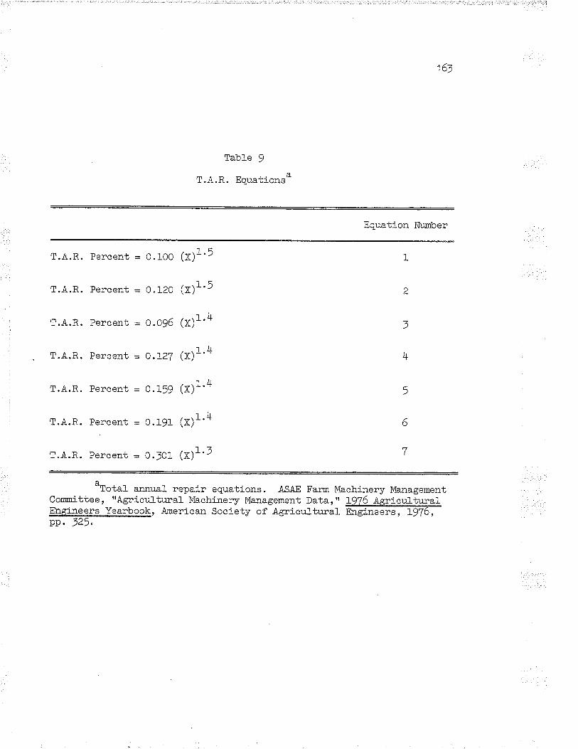
16J

Table !

T.A.R. Equations

Equation Nwnber

T.Ä.R.

fn^D

T.A.R.

T.A.R.

T.A.R.

T.A.R"

m^D

Percent = O.1OO (x)1'5

Percent - O.l-20 (x)1'5

Percent = 0.096 (x)l'a

Percent = 0.L27 (x)1'4

Percent = 0.159 (x)l'4

Percent = 0.191 (X)1'4

Percent = O.JOl (x)1'l

1

2

z)

4

5

6

7

tTot"l- annual repair equations. ASÁE Farm Machinery ManagementCommittee, I'Agricultural Machinery Management Data, " f.!@!gg$.turalEngineers Yearbook, American Society of Agricultural @pp. J25.

Â,

Die

seL

lfrac

tors

Hor

se P

oHer

Cod

e

Tab

le

1 0

Fue

l co

nsw

Þtio

ru f

o" D

iese

l ar

ìd G

asol

ine

lract

ors,

T

ruck

s,C

onbl

nes

md

gelf-

Pro

pelle

d S

wat

hers

B.

Cas

olin

e fr

acto

rs

1 2 J 4 5 6 7 I 9 10 11 12 1) 1¡t

15 16 17 18

I 2 3 4 5 6 1 2 tt 1 2 ) 4 6 7 B 9 10 11 12

trac

tor

Cla

gs(D

.B.H

. P

. )

C.

ltruc

kec

D,

Se1

f-P

rope

lled

Com

blne

sc

<40

H.P

.40

- 49

.99

50 -

59.9

960

- 69

.99

70 -

79.9

9B

o -

89.9

990

- 99

.99

100 -

109.

9911

O -

119.

9912

o -

129.

9911

o -

1)9.

991\

o -

1\9.

991f

r -

159.

9916

0 -

169.

9917

o -

179.

99'tg

o -

199.

992o

o -

2\9.

9925

O+

<lro

H.P

.\o

-

49.9

950

- 59

.99

60 -

69.9

9,to

- 79

.99

80 -

89.9

9

Fue

l C

on8ù

nptio

n -

Tru

ck S

ize

Reg

reaa

lon

Equ

atlo

n"

(ton

e)

y=0,

822+

o.01

5xv=

1,30

1+o.

022x

y=1.

\12+

o.0J

0Xy=

1.82

4+o.

oJ4x

y=2.

745+

o.ol

9xy=

2.57

1 +

o.o4

2Xr=

2.91

4+o.

olt4

xv=

1.61

\+o.

o45x

y=).

By]

-+0.

o50x

v =

).67

2 +

o.o

58x

v=\.7

19+

0.o6

6xy=

4.70

o+0.

061

v=4.

78)+

o.o7

7xy=

q.46

o+o,

o8lx

y=5,

\28+

o.o8

lxy=

r.\1

6+o.

o87x

v=7,

687+

o.o8

6xy

=1O

.))B

+ 0

.102

xy=

1.55

8+o.

o18x

y=2.

851

+0.

o27x

y=2.

918+

o.0J

0Xv=

7.46

8+o,

ol1x

v=).

9o9+

o.o{

fxv=

1,81

6+o.

o46x

E.

Seü

-Pro

pell.

ed S

uatlr

ersd

Sel

f-P

rope

lled

Spr

ayer

s

F\je

l CoD

Bw

ptlo

n(r

mpe

rlal

GaI

lons

per

hour

)

It is

ass

ured

tha

t'sel

f-pr

opel

ìed

suat

hers

use

gepa

ratin

g A

Ìea

(Inc

hee

)c

1/2

1 2

>J

1.75

l¡n

perla

l ga

llons

of

gaso

line

per

hou.2.O

22.

172.

)1j.)

)4.

o

2.1

2.5

J.o

4.o

4.5

5.o

5.\

5.8

6.0

6.1

6.8

(6,o

oo6,

0c,0

-

6,99

9?,

ooo

- 7,

999

8,oo

o -

8,99

99,

ooo

- 9,

999

10,O

00 -

10,9

9911

,000

- 11

,999

12,O

OO

- 12

,999

1j,o

oo -

17,

999

1r{

, oo

o -

1q ,9

9915

,ooo

- 15

,999

>16

,ooo

taU

fel

O (

noot

note

s C

ontin

ued)

alhe

regr

essi

on a

nâIy

siÂ

ls

base

d on

Neb

rask

a T

ract

or T

est

Dat

a (l9

ZO

-i9B

O).

bTlu

*ug"

u""io

n eq

uaLl

on i

s of

the

fom

y =

s +

b x

uhe

re y

rep

rege

nts

the

hour

ly f

uel

cons

wpt

lon,

and

x r

epre

aent

a th

e pe

rcen

t lo

ad..

Uni

ted

Sta

tes

gello

ns.

"M*l

tob"

D

epùt

mÊ

n! o

f A

grfc

ultw

e, E

cono

mic

e B

rmch

, F

am D

ata

Hm

dboo

k,

1972

, W

lmip

eg,

Ms¡

ltoba

, p.

1-2

8.

tI.J.

C

radd

ock,

Int

eneg

lonâ

] C

omÞ

etitl

on ln

cm

adiâ

n C

erea

l P

rodu

ctio

n,

Spe

clal

Stu

dy N

o. 1

2, O

LtaH

a: Q

ùeen

ts P

rlnte

r,

l9?1

.

Not

e y

ls i

n

O\

\n

166

TASLE i 1

Depreciation EquaËion

Equation Numberl Depreciation at End of Year n

I

2

3

4

(I00 - 157.4(0.885)"1)/100x New cosE

(100 - [73.4(0.8s5)n])/roox New cosr

(100 - 162.1(0.s85)"1)/100x New cost

(100 - t87.0(0.92)nl)/100 x New cosr,

1 R"f". to Table 7 Lor description of machinerygroupings used for depreciaÈ,ion.L. Andruchow and J.ShorLreed, Loc. cit"

Appendix B

DEFATILT COST DATA FOR 1979

-L67-

Table 12

Machinery Prices

168

îillage Code ï.:riplement Name Price

1.

2.7

)r

R

6.n

ô

o

10.

11.

12.17

rJr

L5.

ro.L7.

rC).

19.

20.

2r.

)7

24.tq

¿o.

)a¡Qav.

Plow-Trai1 T¡pe

Pl-ow-Mounted T¡rpe

Cultivator-light duty fieldCr:-ltivator-Iight duty f ield-w-ing

Cul-tivator-heavy duty fieldCulti-vator-heavy duty field-wingStalk Cutter-integralStalÌ Cutter-trailGrain Auger-electricÉr.ain Auger-motor

Grain Auger-FTO

Tandem Disc-trailingîandem Disc-w-ing

One-tiay Disct ..-Discer (i"r-ith seed & fertil-izer

attachment)

Rod-lüeeder

Noble bl-ad.e 6' blad.es

Noble bl-ade /r blades

Hoe DrillPress Drilt & Double Disc

No till- d-ril-l (seed d-rill)Corn Planter (J'/row)

\Haffow (drag)

Harrow (spring tooth)Packer

Sprayer

Swather (Pt'o)

Swather (S.P" )

or

#85o/rt.#61=/tt"#t6j/rt.#2t3/ft-.#2o5/f1-"

#zs=/tt.fi242/ft.#3Ø/ft.

0.0

0"0

0.0

#72J/ft.$4r8,zrt.

#tg]/tt.

#4zo/rt,.

$150lrt.#zl>/rt.#zog/ft,.#4r=/n.#625/ft,.

$8l-7.4/rt"#496/rt.

#t49o/row

#44/tt.#6t/rt.#65/ft.#rgo/ft "

$190. 35/ft.#555.66/tt.

169

Tabte 12 (Continued)

Tì-llage Code I-:rplement Name Pri ce

Jo.

3L.

7Z

4t

ZÃ

)o.7.7

38.

J9.40.

4r.42.)tz

Jrlr

4j"46.)tt

48.Lo

tr^

51.q)

r)¡

55.

)o.57.

Swather w-ith conditionerSi¡ather i,,rith pick-up reelCombíne (Pfo)

Combíne (self propelled)Conlrine (rotary)Dryer and Equipment

Grarnrl-ar ApplicatorTruckslalagons

Sprayer (self propelled)Forage Harvester

/ -\BaJ-er (rourj.d)

Ba1er (square)

Roto-ti11erMower

Mower-conditionerRake (w-heel)

Rake (para1leJ- bar)Stack mover

Bale trriagon (self propelled)Forage Bl-ower

Haystacker

Fertilizer Broadcaster

Haybind or trrlindrower

Bale el-evator

Bale carrierFbont-end loaderForage harvester wagons

S¿ookers

#832/rt.fi7o1/ft "

#2,jjo/i,ooo in#4,zoo/i, ooo in.See price fistSee price listSee príce listSee price listSee price listSee price listSee price listSee price l-ist

, See price l-istSee prì ce list#24>/rt.#725Æt.

#t9o/rt.#22o/1t.See price listSee price listSee price listSee price listSee price listSee price list#zg.g>/tt.See price listSee price listSee price listSee price list

2

2

170

Table 12 (Continued)

Tillage Code Irçlement Name Pri-ce

58.

Ão

ou.

6t.

o¿.

64.

101 .

102.

Row Crop Cul-tivator

Rotary Cul-tivator (ttoe)

Potato Windrower

Potato Harvester

Potato Planter

Bin Pil-er

Harrow Packer

Tractor (ai-esel)

îractor (sa")

#492/row

#5Jo/row

See price list

See price list

See price list

See price list

See price li-st

#ji2.5o/hp

#3tz.5o/hp

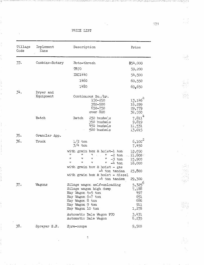
171

PRICE LÏST

TillageCode

I-uplementName

Description Price

15.

to.

=2 Combine-Rotary

34. Dryer andEquipment

Batch

Roto-threshTR70

rHc1440

1460

148o

Continuous P,:u.. /b:".L5O-25Ot5o-5oo6jo-7io

over BOO

Batch 210 bushelsJlO bushels4!O bushels100 bushels

Silage wagon sel-f-rrnl-oadingSilage i¡ragon high dl:mpHay hJagon +-) tonHay Wagon O-'l tontlay Wagon ö tonHay tlagon ! tonHay'Wagon lO tonAutomatic Bale Talagon PTOAutomatic Bale ltlagon

Spra-coupe

Granular App.

lnrck

$54, ooo

Ão 2n^)), ¿vv

54,5OO

60,55o

691650

. -l+13,r+6L8,29929,779J2,550

LT,3Lr'9,8L9

-r 1 tr'zfLL, ))L

t3,oI5

6tr 2aÉ.-)e)a)7,l-BB

4gl6rt6869IL

L,278z hzr-/t t-/L

o, ¿)?

9,500

t/2 .con 6,toozJ/4 ton T,4|¡O

w-itir grain box & hr-oist-l- .ton IE,O5O

:l :: :: ,, -2 ton 11,Boo, ,? ,, :: rí ;:i i3;3BB

t^ri-th grain box & hoist - gas

with grain box --H:ï -iÏ:i"' ii:,i',27n lùagons

)ó. Sprayer S.P.

I l¿

Price List (Continued)

Tillage InplementCode Name

Descrintion Price

ZO ForageHarvester

-ual-er (Hoiirld.J

Baler (Square)

Roto-ti11erStachover

Bale 'lrlagon(S.P)

Forage Blower

Haystacker

FertilizerBroadcaster

Hay BirÍd.or i,'¡-indrower

BaleCarri-er

F?ontendLoader

40.

4r.42.

41.

Medium - pick-upMediun - 2 rcwheaderLarge - pick-upLarge -2row header

1"5 n dia.1.8 m di.a.

755 x 4Jr t*t (standard)E4L) LVe

(cable) B t(chain) j t

). ) v

8t1069 S.P.

PTO driveTractor-hydraulic (l.Z' sweep)

reg.high liftw-ith push-off

Costed with fertil-izer

PTO feetfeet

1 ror:nd bale (2 prongson J poi-nt hLtch)4 baleO bal-eQ u^r ^U U4IE

12 bal-e

2000 }bs.2000-J000 tbs.J000-4000 ]bs.4ooo-5ooo r¡s.over 5000 lbs.Bobcat Skid Ioader

$7,90019,000

t0,20011,200

7,50019,2OO

5,6OO1

3,5206

5,OOO1j,6005,6007,500

38,4oo1

2r2OO1

)rc ¡z)t'19v¿/ t

2,570,h zhJL

0

A2,106"2,65r4,65o

2< ,(ô*6,55o

72501

4,zoo'5,0006, ooo7,2OO

)rr rQzTLtLV)1 ,8582,710r oo,[¿9//'L ozn,t/lv

r3,844

48.Lo

50.

5L.

52.

54.

2 ton5 ton6 ton

(2 ton(

9

ñÃ

173

Price List (Continued.)

Tillage ïmplementCode Name

Description Price

,Õ.

trn

6o.

or.

o¿.

Forage Harvester l.^Iagon S.U.ïrlagons hiagon H.D.

Stookers 6 ¡alelO bale15 bale

Potatolrlindrower

PotatoHarvester

Potato Plarrter w-ith Fert. attachment

Bif: Pil-er Potato piler

65, zoo 1

7,000t,4zo6L,7o4L,893

g,5001

z6,5oo1

6,6oo4L2,692L7,768

B,z\z4L7,432

7,000

LO,938114,06317,lBB20,3r323,43826,56329,68832,8L335,978)9 ruo)4e, rBB45,3tJ48,478,L,56357,8r7LoJBBSt = =â.2t) s )w)l6,32'19,300>c >62

25,238

2 rot¡4 row6 row

64.

101.

24'40'

Harrow Packer

Tractor Diesel(e wa and 4 wd)

o-39 DBIIP4o-496c)-Ão¿v ))

6o-6970-798o-Bg90-99

100-109110=11!1 )ñ-t )oL¿v L't

L1O-L39140-149L5O-r59160-t69L7o-L99

7O-J9 DBrÐIn-,Lo50-596o-6970-79Bo-89

LO2. Tractor Gas

174

Price List (Continued.)

1m,¡. 1979 price.zsni-

:-9T9 price.

1F"o consul-ting producers.)+-ADA f97b price indexed.

q-f97T prices from tabl-e I indexed using power machinery j_nd.ex.

6-1977 príces from table I indexed. usi-ng non-power machinery fnd.ex"

175

Code

TABLE 13

Fertilizer Prices

Forroul-aËion Costl(1979 $/Ton¡

0t2J

4567

89

10111)13T4t5T6

No Fertilizer usedI l-55-0-0I 1-54-0-0r 1-48-0-0

r6-20-0-L423-23-O-O2 6- r 3-0-30-0-62-027-27-0-034-0-0-034-0-0-1 I2r-o-0-244 6-0-0-08-24-24-2

r0-30-10-413-16-10-1124-0-O-0

L4-r4-7-15I 6-20-0-02 1-0-0-0

13-r6-10-0I 1-5I-0-027 -26-0-034- 16-0-01 9-37-0-0I 7-34-0-0

I 6-r 6- r6-30-0-0-9028-0-0-010-34-0-082-0-0-033-0-0-0I 3-52-0-025-25-0-0

1 0-30- r 0-0I 3-32-0-028-28-0-0

Hog ManureCattle Manure

27 -14-0-0I 2- 5 3-0-0Actual N

Actual P

Actual K

0 .00267 "00263 "002 38 .00I 48 .00r86"00i64"00I 04 .00218.001 55 .00r 60 .00r 35 .00I 86 .00l7 4 .00187"00158.00

97 .OO

r 56 .00r45 .0085.00

1 35 .00250.002L4,00202.00226.00206 .00r 57 .00I89.00I 44 .00178.00232 "00r 33 .00263 "00202.00178.00182 .00226.00287 "00r86.001 66 .00263.00404 " 00404 "00I 68 .00

T71819202I))2324252627282930313233343536373839404I4243

176

44 Act,ual S 210 "00

= ===::========= ========l::::=:l:::::l========3!33=!3===

1_- Prices are company reconmended retail prÍ-ces for Manitoba dealers,spring I979 "

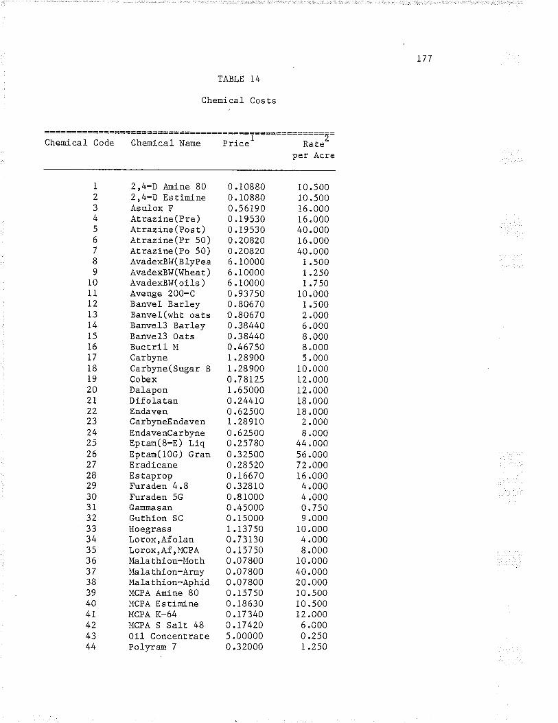
177

TABLE 14

Che¡rical Cos Es

=================================:====T=============z=Chern'ical Code Chemical Narne Price' Rate-

per Aere

1

)J

4567

89

IO1II2I3T415L6I718i9202I22232425¿o27282930313233343536373B39404I424344

2r4-D Amine 802,4-D EstimineAsulox FAt razine ( Pre )Atrazine (Pos t )Arrazine(Pr 50)Atrazine(Po 50)AvadexBI,I(BlyPeaAvadexBI,I(Wheat )AvadexBW( oils )Avenge 200-CBanvel BarleyBanvel(wht oatsBanvel3 BarleyBanvel3 OaÈsBuctril M

CarbyneCarbyne(Sugar B

CobexDalaponDifolatanEndavenCarbyneEndavenEndavenCarbyneEprarn(8-E) LiqEptan(10G) GranEradicaneEstapropFuraden 4.8Furaden 5GGammasanGuthion SC

IloegrassLoroxrAfolanLoroxrAf, MCPA

Mal-athion-Mothl,falathion-ArmyMalathion-AphidMCPA Aroine 80MCPA EstinineMCPA K-64MCPA S Salt 480i1 ConcenÈratePolyrarn 7

0.108800 .108800.561900.r95300 .195300 .208200.208206. i00006 .1 00006 " i00000.937500 .806700.806700.384400 .384400.467 501.289001.289000 .7 81251.650000.244L00 " 62500r.289r00.625000 "257 800.325000.285200.r66700.328100.8 10000.450000.i5000I .137500.731300. r57500.078000.078000.078000.157500. i86300.173400.17 4205.000000 .3 2000

I 0.500r0.5001 6 .00016 "00040

" 000r 6 .00040 .000

r "500i .2501.750

i 0 .000r.5002.0006 .0008 .0008 "0005 .000

r0.000I 2 .0001 2 .00018.000i8 "000

2 .0008 "000

44.00056 .0007 2 "00016.000

4 .0004.0000"7509 "000

I 0 .0004.0008 .000

10.00040.00020.00010"50010.500I 2 .0006.0000.2501.250

178

=-===== = == = = === = == ==== == = = === = == === === === == == = = = =::= = =Chenical Code Chemical Naroe pricel Rat"2

per Acre

45464748495051525354555657585960616263646566676869707L727374757677787980B182OJ

B48586878889909T

9293

RoundupSevin 80SS tampedeSuÈanf8ETCATreflan(0i1seedTreflan(Cereals )Diazi.nonTorchEmbutox E

EkkoEkko & 0i1RegloneLorsbanDyvelBeEanolBeËanexBasagranSencor 5Herbicide 273EsasolLanaËe .

BravoSupercideThfadann-45TeuikDimethoateI't-H-30Tok Rl"t

PremergeTotrilTok-E-25M-H-30RandoxCIPCGrauoxonePol-xrarn80Dalapn-F1axDalpn-Grass ConE thionDiathaneMatavenWipeouEVitavaxTarge tRandthalAsyleneSweep

1.210900.548000.348800.24i801.229700.507800.507800 . s00000 "776700 " 343803 .1 00003.100000.737500.232200 "37 920L.879402.35270

1 4.834000.247 50

10.4r0000.000000.000000.460000.6s0000 .70000r .780002.450000 .6 60000.160007.000003.310002.080007.080002.53000B .7 50004.93000

65 .000000 .200002.500002.500000.000000.00000r.48100i.201000 .297 100.000000 .000000 " 000000 .86000

32 .000r 9 .200I 4 .00056 .000

1.0001 6 .0001 0.0002.0004.500

i8.0003.000I .500

r 2 .000r 7 .5007.500

16"000r6.000

0 "800I 2.000I .1000.0000 "000

I 9 .0004.0008.0001.5002 "0004 .000

I 30.0001.2001.2006"8001.5006.5001.0001.000i "000

I 2 .0001 .0001.5000 .000

32.0007 .5005.0002.4008.0000 .0000.000

1 6 .000

179

======================================================1)ChernicaL Code Chemical Name Price^ Rate'

per Acre

- --=====:1======3:::::::::========9:3::::=======l=3!3=

1_- Prices are company recommended retail prices for Manitoba dealers,Spring 1979 "

t- Rate is expressed in standard units so that a consistenË raEe-pricerelationship is maintained.

180

TABLE 15

Seed Costs and Rat.es

CropCode

Price ofCommercial Seed and

0r Mosl SeedConvent.i onal Cleaning

Per Unít

InputRate of UnitsSeeding /Lcre

Cost ofSeed

TreatmeritPer Uni.l

I)345

6

7

89

t011L213T415L6T718

1920

2I

22

23

24

^trL)

26

Itrlheaf -

Oats- ?

øarLqy-Flax-"-Jljurutn nRye (Fal])'Raoeseed't't rstard5

oSunt-LôürersBuckwheat)-Field P.""/Haylage q

Corn Silage'GrazingS trawMixed GrainÕ-Tinothy SeedSAlfalfa Seed'

Sweet Clover5Bromegrass' Seed.

Meadow F"scrre5Seed -

Trefoil)Seed

Single-Cut Red)Clover Seedf

Cres t,ed I"IheatJ-grass seed -

Alsike CloverJSeed

Slender Wheat)-grass Ç6ed

Tame Hay^'

11Soybeans^' , ^ 0.L67urilitv l^IheaEr" 4.17porrtoå"1' o.o6Kencucky) L.24

Bluegrass Seed

4 "45r "372 "020.164.r32 "480.580 "303 .00.1955 "170.0

0.9680.00.0

i.70I .142.55

0.27i.15

i.00

2.65

0.67

0.76

0.47

0 .63

2.55

.46

.46

.46

.60

.46

.46

.540.00.00.0

0 .590.00.00.00.0

0.460.00.0

0.00.0

0.0

0.0

0.0

0.0

0.0

0.0

0.0

0 .005.46

0 .0040.0

1.52.25L"75342"01.0

6

8.53"0

42"02"750.0L4

00

1.52.0

2"0/6=0.336.0

3"0/4=0 .753.s/4=0.883"0/4=0 "753.0/4=0.753"0/4=0.752"014=0 .50s.0/4=1.257 /4=t"75r04

r"75I 000

bu.bu.bu.1b.bu.bu.lb"lb.1b.lb.bu.lb.lb.1b.bu"bu.lb.lb.

lb"1b

lb.

1b"

1b.

lb"

lb.

1b"

rb.

lb.bulb.1b.

27

333435Jb

18r

============================================================Price of

Commercíal Seed and Cost of0r Most Seed Seed

Convent.ional Cleaning TreatllentPer Unit per Unit

CropCode

InpuERate of Uni.tsSeeding /Acre

37 SugarbeeËs1438 Field Bean"l54I Lentilsro43 Canary t"*gt45 Fababåans147 Grain C?6r548 Pasture"

50 Srrmmerf a11or¿5 1 Onions52 Sweet Corn53 Sudan Grass Seed

8"75NOc 0.25

.450 "250.230 .85r.r5

0.0

0.00.0

0.0050.00.00.00.0

0"0

2.045.0

608.0

I20"012.012 "6=2 "0

0

1b.1b.lb.1b.1b.1b.1b.

bu.1b"lb"1b.

:============

I rgza-tg79 canadian tr/hear Board price of No. r canadianiniesË.ern wheat plus cleani.ng. seed treatment is vitavax.

2 ßlA Manitoba yearbook price plus cleaning. SeedtreatEent is Vitavax.

3 rgza-tg79 canadian wheat Board. price of No. I canadi.antrIestern l{heat plus cleaning. seed treaËnent, is vit,avax.

L' March 7979, Manitoba pool Elevator price of Regent orTower Certified No. I-2. Seed Lreatment is Furadan.

q- The price is derived frour the Seeding Data table.c.

' The price is our estimate for treated oil-typehybrids.

7

treatxoent

Ibarley.barley.

o- The price is derived from the Seeding Data table. A6 year produetive stand is assumed.

I0 th" default is for alfal-fa hay only and assumes a 4year productive stand. The seed price used is Algonquin,Beaver, Certified No. L-2 ALf.aIfa seed from Manitoba poolElevaË,ors, March L979.

1978 Manitoba Yearbook price plus cleaning. Seedinclude inoculation plus Captan.

Mixed Grain consi.sts of 50 percent oats and 50 percentThe price of seed coues from those of oat.s andThe seed treatment used is Vitavax.

tI - r82

-- Seed price Íncludes seed t,reatment. and cleaning. Seedtreatnent cost is for i-noculation.

t2-- 1978-1979 Canadj.an l,lheat Board price of No. I CanadaUËi1ity Wheat plus cleaning. Seed treatment is Vitavax.

13_-- Seed treatment. is polyran 7. Cost, of cutting is notincluded in the seed or t,he seed treatmenL prices.

1l!^' The seed price includes all seed treatments requiredand was obtained froro the Manitoba Sugar Coupany.

15-Seed price includes inoculation.16 S""d price is 1980 Manitoba Pool Price for seed.

Seed ÈreaË,nent. i.s for inoculaEion.17

Seed pri.ce is l9B0 Manitoba Pool Price for seed.

18 S".d treatment is for inoculation.19 P""t.rre seed consists of. 75 percenË Brome and

25 percent Alfalfa, Canada No. I lfixt,ure froo Manitoba Pool,March 1979 price 1ist. A 6 year production stand is assuned.

183

TABLE i6

Land Taxes

============================================================Municipality Naroe Assesed

ValueMi1l Rate

Per (000$)Land Taxes

per acre

10I Albert119 Alonsal3I Archie132 Argyle139 Armstrong141 Arthur171 Bifrost181 Birtle191 Blanchard201 Boulton211 Brenda212 Brokenhead221 Carneron231 Cartier251 Clanwilliaro252 Coldwell26I Cornwallis27I DaIy272 Daupt:.ín281 Desalaberry282 Dufferin302 Edward3ll Ellice312 E1Èon33I Eriksdale332 Ethelbert339 Fisher361 Franklin371 GilberË Plains381 cinli401 G1enella402 Glenwood409 Graharndaie421 Grandview451 Grey452 Haniota461 Hanover462 HarrisonlrT l Hillsburg481 La Broquerie482 Lae du Bonnet491 Lakeview492 Langf,ord493 Lansdowne

L7 .04r.50

2r.722L.203.30

2L.3223.8623.9532.5316 .0926.9927 .29r8.8556.27L2.454.84

i3.8623.6518.7634.2746 .83L7 .T212.9437 .6r

3 .993.76

10.3023.6023 "392r.2216.2630. 102.40

17.7727 .9r34.7 3

25.952r.06

7 .375.43I "51

r0 .9219.6216.27

96.200009 6 .5 000085.60001

108.50000I 12.30000

9 7 .0000097 "8999987.7000093 .2000093.3999992 .0000098.2000084 .2000098. 00000

r 06 .50000I 6 r .8000066.8000072 .5000099 "50000

100.200006 r .89999

103.2000066. 1000rB 5 .50000

l 55 .00000168.89999

3 6 " 20000L22.3999990.1000r

r03.7000099.0000089 .30000

r 19 .7000092 .30000

100.6000r77.89999

104.1000197.s0000

111.1000it42.39999I 13.2000079.80000

1 04 . s00001 00 .7 0000

I .6390.145r.8592.3000 "3712 "0682.3362 .1003 "0321.5032.4832.680r.5875.5i4L.3260.7830.926r.715L.8673.4342.899r.7670.8553.2160 .6180 .6350.3732.8892.r072.20rI .6102.6880.2871.6402.BOB2.7052.7 0L2 "0530.8r90.7730.9630.87r2.0501.638

184

ìlunicipality Narae AssesedValue

Mill RatePer (000$ )

Land Taxesper acre

501 Lawrence502 Lorne503 Louise5 l0 MacDonald531 McCreary541 Miniota542 Minitonas551 Minto552 l"lontcaln561 Morris57I MorËon572 Mossey River601 North Cypress611 North Norfolk621 Oakland622 Oehre River623 Odanah641 Penbina66I Pipestone671 Portage689 Reynolds691 Rhineland692 Ritchot701 Riverside7 I I Roblin721 Rockwood722 Roland723 Rosedale724 Rossburn732 Russell730 Rosser741 St. Andrews7 42 St. Anne76L St. Clement77L SE. Laurent791 Ste. Rose801 Saskatchewan812 Shell Ri.ver811 Shellmouth813 Shoal Lake821 Sifton822 Siglunes823 Silver Creek841 South Cypress842 South Norfolk850 Springfield851 Stanley862 St,ratcona861 Strathclair

6.9833.4730.9048.88

8 "4224.59L6.2I27 "2145.7 944.432r.87

3 .5524.8024.s729.2715.1130.2730.4623.0638 .91

2 "3058 .0267.1723.3922.6931.9955.8020"00i5.652r.6642.7 5

37.7319.7529.17L0.7712.6030 .3017.75r5.6822.37L6.745.34

23.301r.9920.5948.4745.0817.5825.80

1 i8 .30000r 19 .7000082.7000089.60001

196.2000093.89999

1 I 2 .8000095.10001

108.3000086 " 80000

103.10001243.80000i05.00000

9 6.0000095.8000080.8000095.0000095.10001

102.1000184. r 000186.3999991.5000099.1000190.1000193.300007 3.2000067 .39999

118 .6000r.r07 .60001r04.70000

7 0 .7 000090.0000092.3999995.8000073.20000

r 18 .5000085.6000 1

9 I .2000094.0000098.3999997. 1000r

15 r.700009 6 .00000

10r.300001 14.89999

7 5.8999991.50000

1 16 .50000108.30000

0.8264.0062.5554.380r.6522.309r.8282.5884 "9593.8572 "2550 "8652.6042.3592.804I "2212.87 6

2,8972.3543.2720.r995.3096.6572 "r072.1T72.3423.7 6L2.37 2

r "6842.2683.0223 .396r.8252.7940.7881.4932.594r.619r.4742 "20t1.6250.8r02.237r.21.52.3663 "6794 "r252.0482.794

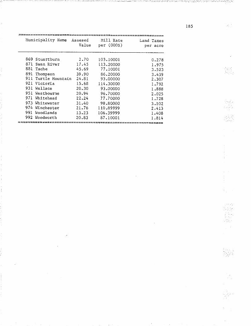
r85

Municipality Nane AssesedVa.l-ue

lfill Rateper (000$)

Land TaxesPer acre

869 Stuartburn 2.7087I Swan River L7 "45881 Tache 45.69891 Thornpson 39.9091 1 Turtle l'lountain 24 "8I92I Victoria 15.68931 l,lallace 20.30951 Westbourne 20"94971 Whitehead 22.249 73 White!¡ater 31 " 40974 l^Iinchester 2I .7 6991 i{oodlands L3 "23992 Woodworth 20.83

103. I00011 13 .2000077.1000186.2000093 .00000

1 r4.3000093 "0000096"7000077 .7 000098.80000

I 10.89999r 06 " 3999987"10001

0.2781.9753.5233.4392 "307r.792r.8882.025r "7283 .1022.4r31.4081.814

186

TABLE 17

Overhead Costs and Land Values

===================================================ICrop Overhead Costs' Land

District fann SiãErno SiããÏãrro Size VatueIII II

r 4.452 6"38

3 .653.49

3 .7 6 2L4 .433 .48 L86 .223 "43 162 "263"29 17s.rr3 .7 5 22L .413.48 348. i44.48 202.665 .03 214 "555.39 354 "8i5.46 L69 "065.53 41s.404.77 172.64

3 4.r4 3.604 3.97 3.605 4.746 4"847 6.46 5.248 6.62

4.093.52

9

10I1T2

6 "573.927.r73.20

5.385.774.006.533 .68

===================================================

1-1979 values, D. McNair, Dept. of AgriculËural Economics and-FarrnManagement, Universit,y of Manitoba.See Chapter 5 for indexing procedure.

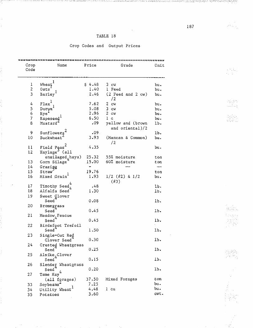
r87

TABLE 18

Crop Codes and Output Prices

============================================================CropCode

Name Price Grade Unit

I2

J

456

7

8

9

10

IIT2

13T415T6

T7

l8I9

20

2I

22

23

)lL

25

26

27

1

I^Iheaç-Oats-

rBarley'

I¡'lax-IDurçmRy"t- .1Kapeseegl"lus tard-

)Sunflowerg-Buckwheat-

)Field Pças-IIaylage' (a11

ensilagedohays )Corn Silage'Grazipg_)s treü7Mixed .Grai.nr

Llimothy Seed,Alfalfa Seed'Sweet Clover4

Seed'Broueg¡ass

Seed'MeadowrFescue

Seed'Birdsfoot Trefoil

SeedaSingle-Cut Ref

Clover Seed'CresteÍ Wheatgrass

Seed'Als ike . C love r

hSeed'

Slende¡ InlheatgrassSeed'

Tame Haya(a11 fgrages)

Soybeans- 1

Utility WheatrPolatoes

3 cw bu.1 Feed bu"(2 Feed and 2 cw) bu"

/z2 cw bu.3 cw bu.2 cw bu.Ic bu.yellow and (brown 1b.

and oriental-)/2lb.

(Mancan & Common) bu.Itt L

bu.

55% noisture60% rnoisture

L/2 (lfz) & r/2(#3 )

$ 4.48I "402.46

7 .625 .082 "966 .50

.09

.093 .93

4.35

25.32r 5.00

19.76r .93

.481.30

0 "08

0.45

0"45

r .50

0.30

0.25

0. i5

0.20

37.507 .254.483 .60

ton

':1tonbu.

1b.lb.

lb"

lb"

lb.

1b.

lb.

lb.

lb.

lb.

tonbu.bu.c$/t.

3334J)

Mixed Forages

1cu

188

Name PrÍce Grade UnitCropCode

36 Kentucþy Bluegrassseed" , 0.60

37 Sugarbeets', 30.4538 Fietd Bçans' .194I Lentils' .2043 Canary Seçdb .iI545 Fabaþeanst .0747 Corn' 3.0048 Improved Pasture50 Summerfallow5t Onions52 Sweet Corn53 Sudan Grass Seed

lb.tonlb.lb.lb.lb.o::

CI,It .doz.lb.

:= === == = = == ==== = ====== === = ==

lM"oitob" Yearbook - estinat ed. I979 prices.)-MDA John Rogalsky"l!'Haylage is assigned the value of alfalfa - brome haylage.This value is based on corn silage and alfalfa - bronehaylage's relative TDN and cotal proteln.lL-Manitoba Yearbook - 1978 prices.5Bas.d on Alfalfa and strar¿'s relative TDN and total protein.6fggO contract prices - Northern Sales"

Appendix C

USER,S GUIDE

-189-

c"l INPUT DATA FORMAT GUIDE

All client input data i,/i11 be free

each piece of dara infornation. The

rea1, or alphanumeric. A decimaL must

with the int,egers. Alphanuneric data

format.

data is

be used

nay only

That is a

specif ied

wi th real-

beaTor

blank

either

number

Ë

190

separaEes

inL ege r,

and none

C.2 CLIENT HEADER CARD

1. Client record number. (Integer)

2. Total number of acres" (Real)

3" the municipality number. (Integer)

4. NLABCH 0 Read number of changed labor coefficients. The changed

labor coefficients have the format Tillage Code, New Labor Coef-

ficient and folIow the Clienc Ileader Card. (Integer)

C.3 MACIIINERY INVENTORY DESCRIPTION CARD

1. Tillage code. (Integer)

2. Year of machine. (Integer)

a) Rental equipment -- the price code is $/hour if year=O, if the

year is l, the pri.ce code is $/acre.

b) Custon operations -- Lhe default price can be overridden when

year = 0 and the optional price is given Ehe charge is $/hour;

when year -1 and the optional price is given Ëhe charge j-s

$/acre. If the year is greater than I and charge per hour is

seL equal to 0.0, the default charges per acre are used.

3. the inventory number of the tractor that is used to pul1 the im-

plement. (ff applicable, oÈherwise 0) (Integer)

191

4" The size of the implemenË - width, capaciËy, horsepower etc.

(Rea1 )

5. 0ptional price data. (i.e. user supplied price) (Real) irlhen

equipmenË is rested and for custon operaEions , this fieLd con-

tains either the $/hour or $/acre charge depending whether the

year is 0 or I.

this daÈa nust. be placed one per card with at least one blank sepa-

rati.ng each dat,a item.

The end of the nachinery inventory is coded 999 0 0 0. 0.

C.4 LIVESTOCK MACHINERY INFORMATION

1. Number of set,s of dat,a inforlrat.ion to be read between 1 and ten.

(Integer)

2. Machine Inventory Number. (Integer)

3. Ilours used on the livestock enterprise. (Real)

This data can be placed one per card or it can be punched across the

card as long as a blank separates each data item" This data is the

Ë,ractor hours used on livestock.

192

C"5 TILLAGE PRACTICE ITEADER CARD

1. Dist.ance field Eo on-farrn storage or market. (Rea1)

2. i^teight per bale. (Real) If this weight is zero, then a default of

50 lbs is used.

3. Percent of land Ëhat j-s heavy soil. (Real) The percent of land

rhat is heavy soil will be defaulÈed ro 507" íf. chis data field is

coded as a negative number.

4" T - Client own the land. (Alphanurneric) F - Client rents the

1and. (Alphanu¡oeric)

5. Rent per acre ($) of land if it is rented, otherwise it is 0.0.

If land is rented and rent per acre is zeto, rent is t,hen de-

faulted to investment in land & buildings + taxes. (Real)

6. T - Unirnproved land. F - Iuproved land. (Alphanu¡neric)

7. Crop Insurance Payments received by the farmer (Total $ per

acre). (Real)

8. Is the field irrigated? T - yes F - No

C.6 IRRIGATION OPERATING COST CARD

9. l{iscellaneous Capi.tal Costs per Acre. (Real)

10. Total Acres of this field that is irrigared. (Real)

11" The hours of use the system is used on this field. (Real)

12. The hours of labor that are used on rhis field" (Real)

13" The gallons punped per minute in U.S. Gallons. (Real)

14" The lift in feet. (Real)

I5. The purnping pressure. (Real)

r93

C,7 CROP INFORMATION CARD

i. Crop code. (Integer)

2" Acres of the crop gro\./n. (Rea1 )

3. Average field size. (Real)

4. Yield per acre of principal crop. (Real)

5. Crop code of secondary crop (e.g. sËral¡¡, grazing).(Integer)

6. Yield per acre of secondary crop. (Real)

7. Crop insurance preuiuro (yield + hail) paid by the farmer. (Real)

8. Drying cost per bushel. (Real)

C.8 SEED INFOR},ÍATION CARD

1. Number of differenE seed types per field Ëo be read in up to a

maximum of 5" (Integer)

2. Price of the first seed type including seed cleaning. (Oefaulted

if -1.) (Real)

3. Cost of seed treatüent for the first seed type. (Defaulted if

-1.) (Rea1)

4" Seed rate of application. (Defaulted if 0.) (Real)

5. Input units" (Integer)

a) -bushels/acre-I

b) -pound/acre-2

c) -kilograms/acre-3

d) -tota] cosË/acre-4

194

C"9 FERTILIZER DESCRIPTION CARD

1 " Number of different types of fertilizer to be used on t.his field

up to a maximum of 5. (Integer)

2" Fertil-izer code. (Integer)

3. Fert,ilizer applicaËion rate. (Real)

C.10 CHEMICAI DESCRIPTION CARD

t. Number of dif f erent chemicals t.o be used on this f ield up t,o a

maximum of 15. (Integer)

2. Chemical code. (Integer)

3. Chemical rate of application. (Defaulted if 0.) (Real)

4. Acres sprayed. (Oefaulted = all if 0") (Real)

C.11 TILLAGE PRACTICE CARD

t. Machine Inventory Number. (Integer)

2. Number of tines over ( Real )

Columns 1-3 = 999 indicated the end of a field record.

Columns l-3 = 888 indicates Ehe end of a client record.

The end of field record is coded as 999 0.

The end of client record is coded as 888 0.

** NOTE ** Whenever an end of field record is coded i.e. a 999 0.

card, the next field starts with a Tillage Practice l{eader Card.

195

C.Lz INTERACTIVE INPUT

Al1 client input data will be free format. That is a blank separates

each piece of data informat.ion.

Default values are available for all items when a zero is entered in

lieu of requested infornation. This feature should be used wit,h cau-

Ëion" A full list of default information will be provided.

196

C"13 CLTENT INFORI4ATION

1. Do you wish to receive the short or long forn of Ehe questions?

This question applies to the inLeractive operation of the prograûr

but roust be answered to maj.ntain operaËiona1 consistency.

2. Enter client record identification number.

3. Enter farm identification title or name.

4. Enter the total culËivat,ed area of the farm.

5. Enter Ehe municipality number.

6. Do you have any livestock?

7. Enter t,he nachinery inventory one machine at a tine. The values

on each h.ne are:

a) l,fachine. type code number.

b) Size of machine.

c) Year of manufacture.

d) Current replaceuent cost,.

e) If there i.s stock also enter the hours/year that this nachine

is used in the livestock enterprise.

8. Do you wish to enter field and crop information?

197

C.L4 FIELD INFORMATION

C.L4.1 General Description

l. Enter the field identification name, title or number.

2. What is Ehe cultivated area of the field?

3. I^Ihat is the average distance from field to storage Eo market?

4. hrhat percent,age of the f ield i.s heavy soil?

5. Is this field on ovmed land?

6. If hay or straw was harvested from this field, what was Ehe aver-

age bale weight?

C.14"2 Input Descrlption

1. Enter the value of crop insurance prerníums paid by the farmer.

2" Enter the drying cost and the quantity dried"

3. Variable inputs and crop production are all entered in the same

ûlanlr.er.

a) Iteu code number.

b) Rate or yield.

c) Price per unit of t,he above.

d) Area of use or production. This option may be used to pernit

partial use on crop or when less than the entire field in

treated or harvested"

4. Repeat 3 to enter the inforroation for:

a) Seed

b) Fertilízer. The codes used for fertilizer are Ëhe actual

f or¡oulations "

c) Che¡uicals

198

d) Crop production

5. Enter 0 0 0 0 to terninate each list.

6. Enter crop insurance payments receíved by the farmer.

C.i4"3 Tillage Practices

1 " Tillage pracEices are enËered using the sequential nuuber as-

signed in t,he Machinery InvenEory Section. They are entered as:

a) Inplenent inventory number.

b) Inventory number of associated Ëractor if applicable; other-

wise 0.

c) Nunber of times over.

2. This list is terminaËed by 0 0 0.

3. Are Lhere more fields? Tf, this question is answered yes, then

. responses to quesËions in the Field Information Section must. be

repeated.

199

C.I5 EXAMPLE OF INTERACTIVE OPERATION

\famCongratulatfonsl You âre qow executlng

The Unlver8{ly of ¡{anl¿obs

Iot.t""tlr" Fam ManateEenÈ Software PackêBe

AE pre8ent che packåge conafst8 of only five uÈllity prograEa.More slll be added a! a laÈer dace"(l) A fertflfzer protraE shlch fncorporates probabllltles of qeather

condltlona, containing sithfn the progræ a Eype of rfsk aMlysls.(2) ¿ gratn atorage and fam atorage pro8r@ shoHlng coats for Lnterest,

lnaurance, storâge, shrluk and handlfng.(3) A uchtnery cosr progran vhlch developa coat per ecre and per hour

for dlfferent. coaË-size cmblÉtione of equipoenÈ.(4) A progræ qhlch pemfts the u6er Êo lncorporaÈe hls begt guesses

abouc an uncertaln future lnÈo a discouncfng analysfs whlchdeceralnes hos ouch can be pald for land"

(5) A progræ Èo calfbraÈe different sprayer tank Bizes.(6) A detalled crop encerprlae budget generatlon progran.The progru qæes are :

[å] äiåi(3) ¡rAclr(4) L.AND(5) ÎANK(6) cRoP

the pro8ra@er aaaues no responsibfllÈy for the operatlon of the routlnes.GOOD LUCKI

RC 0012Enter nane of progran.:erop

RC 0012PLII CHECKOIJ'T VI R3.O PTF27 9 SEPT 80

TIME I5.34.16OPTIONS SPECIFIEDF(s)

NO SYNÎAX MESSAGES

NO GLOBAT, IÍESSAGESMESSAGES SUPPRESSED 6 ITRANSLATE TIIfE O.OI MINS

Do you sanÈ the long fom of ¿he questlons? 2 y

INTRO BLURSEnÈer cllent record ldentiflcaÈlonCLIENT# : 8

!

Enter farn ldentlflcaÈ1on t1ÈIe.NA-IiE : leateâE Fama Inc.

WhaÈ EunfcfpalfÈy Is thfs ln?IIUNICIPALIIY# : 88I

200

Do you have any lLvestock?STOCK : no

Encer the mchfnery lnventory one @chlneaÈ a cfEe ag the descrlptlon order fndicaÈes.At the end of the llsc rype 0 0 0 0

IWENTORY : }'ACHINE : MACHINE: YEART LISTNIJHBER :CODE :SIZE :NEIJ :pRICE

I :I0I 70 1975 0

2 : l0l r50 1977 0

3:2O20197704:52619970

5:2360196906 :28 l8 1972 O

7 |32 12 1975 o

I : 36 100 t975 o

9 : 36 275 1975 0

l0

ltT2 :00 00

Do you wleh Èo enter fleld and croplnfomtlon?

yes

Nos enter the descrlpefon of each fleld to be budgetedFlrsC enter the ffeld ldentÍffcaclon naEe

FIELD NAME : IJhea!

What ls the cultfvated area of the ffeld?AREA : 150

l.Ihar ls the aveiage dfstance froo fleld cosÈorage to narket?DISTANCE

Whac percenÈage of the fleld ls heavy soll?SOIL :50

Is thls ffeld on omed land?oITNERSHIP : yes

ls chis loproved land?IIÍPROVED : yes

: 26 50 1970 0

: 10. 6 1970 0

t4

201

I,¡hac ls Èhe average field slze?thls reflecÈs @chinery efflcfency loes"

SIZE : 150

If hay or straw was harvesced froE thlsfleld, whac waa Èhe average bale uelght?

BATE HEIGHÎ

Is the fleld lrr{gated? Yes or No.IRRIGATED :NO

Eneer Èhe crop lnsurance preElu pald, oCherwlse 0PRnlIIru

:0

;0Encer drylng cost æd percentage of the crop thaÈ Is drled.DRYING: RAÎE PERCENTCoSTS : 0 0

Varlable ftrputa êre â11 e¡tered fn the sauesay. Rate snd Prfce are optlonaland Area Eay be uaed to pemft parÈfal u8e on the ffeld.When Èhe llst 1s conplete enter 0 0 0 0

EMIER: SEED RATE PRICEI : 1.5 1.5 4 "35

2 :0 0 0

E}¡ÎER: FERTILIZER RAÎE PRICEl:362"502 : 9 274 0

3:000ENTER: CIIEMICA¡ RATE PRICE

l:8002tO0O

AREA0

0

AREA0

0

0

AREA0

0

Enter fteld productlon ln Èhe saEe Mnner. The lfsÈ ends sLfh 0 0 0 0EMTER: CROP YIELD PRICE AREA

l:14001502:0000

202

Now Ehe tillage pracÈlces are enÈeredu8lng the nuber code assigned in the¡lachlnery InvenÈory 6ectlon.End the llst Hich 0 0 0

I

7

J

4

5

6

7

I

9

IO

ll

Are Èhere Eore fields?

yes

FIELD NAME : Rapeseed

What lE Èhe cultlvated ârea of the ffeld?AREA : 380

What fs che average diatance froE ffeld toatoEage ¿o Earkec?DISTANCE 2 4

f{haÈ percenÈage of the fleld fs heavy soll?sotL : l0

Is thfs ffeld on oqned land?oÍ.¡NERSHIP : yea

Is thls luproved land?IMPROVED : yes

f{har ls che average fleLd slze?This reflectg Mchlnery efflcfency loes.

IMPLBIENT I

NTJHBER I

:3:4:5:6

:10:9: ll:l.J

:0

TRACTOR I TIHESMfiBER I OVER

II24L40t2TII0l

30 I

0tOI00

: 380

¿\))

If hay or strav eas harveeted fEoE lhlsfleld, uhac uas lhe average bale selght?

BA.LE mIGET : 0

Is lhe ffeld lrrl8ated? Yea or No.TRRIGAlED :No

EnÈer the crop fnsurance preofu paldt othemlse 0PR.&lltlt i0

Enter dryfng cost ed percentage of the crop Èhst 18 drted.DRYING: SATE PERGNÎCoSTS : 0 0

Varlable lnputa are all encered ln the saueway. Rate and Prl.ce are opÈfomland Area my be used to pemit partlal use on the fleld.l{hen Ëhe l1st is coaplete enter 0 0 0 0

ENIER: SEED R-dtE PRICE Â.REA

t : 7 .12 7.35

2.000ENTER: FERTILIZER R.ATE PRICE

l:412802275803332304.916905:000

ENTER: CHE¡IICAL RÂTE PRICEl:ZSl0022000

Enter f leld producÈ1on ln lhe sate Emer o

EMTER: CROP YIEID PRICEl:7400Z:000

AREA0

0

0

b

0

A.REA

0

The l1sÈ ends vlth 0 0 0 0A.R,EA

0

0

204

Now Èhe tlllâge prsctlce8 are enÈereduslng the nuEber code assigned fn theMachfnery InvenÈory sectlón.End rhe llst sith 0 0 0

I

2

3

4

5

6

7

I9

l0

ItAre Ehere uore flelds?

ye9

FIELD NA¡IE : Sll@erf allow

Hhat 1s the cultfvaced area of the fleld?A.REA I 27O

l{hat ls the average dlsÈance froE fleld tosÈorage Ëo EarkeË?DISTANCE

IMPI^EMENI I

N1JUBER I

!4

t6

:10.o

: l1

30

TRÁCTOR I ÎIMESNIJHBER I OVER

II

¿4

t40l2LIIOI

30 I

0l0l00

:l

f{haÈ percentage of rhe fleld le heavy sotl?sorL : l0

Is thls fleld on. omed land?oI.INERSHIP ' : yes

IIs Èhls lnproved land?IHPROVED : yes

l{hac ls the average fleld slze?Thls reflects Mchlnery efflclency 1oes.

stzE : 27Q

205

If hay or stras waa harveated fron thlsfield, shat Has the average bale uelght?

8ÁTE WEIGHÍ

Is che field lrrlgaced? Yes or No.IRRIGAÎED :NO

Enter the crop lnsurance preEl.u pa1d, otheruise 0PREMIT'}1

:0

30

Enter drylng coaÈ aEd percentage of the crop that ls drled.DRYING: RAIE PERCENÎCoSTS : 0 0

Varfable fûpuËs are ali. entered lD Èhe saoeway. Rate end Prlce are opÈlonaland Area æy be ueed co pemlt partlal use on rhe ffeld.

When the llst 18 conplete enÈer 0 0 0 0EI¡TER: SEED RÂTE PRICE AREA

l:0000

ENIER:t:

FERTI,LIZER RAÎE PRICE AREA000

RATE PRICE AR.EA

000ENTER: CHEMICAL

l:0

Encer fleld productfon ln the sane Danner.ENTER: CROP YIELD PRTCE

1:5000

Noo the tlllage practlces are enteredusing the nuber code asslgned ln thel,fachlnery InvenÈory sectlon.End Èhe LisÈ s1Èh 0 0 0

the llsc ends ulÈh 0 0 0 0AREA

0

0

I

2

3

4l

5

A¡e there oore ffelde?

IHPLEHEI{I I TRACTOR I TIMESNIJ}IBERINTJMBERIOVER

t424:5I4:101z20l:000

:no

Do you wish to enÈer fleld and croplnfo rEaElon?

no

Is Èhere anocher cllent?: no

T--

----

--

r

I R

EC

0RD

Í 8l

I lt Inve

ntor

y T

lllag

eN

urul

¡er

Cod

e T

lllag

e N

ane

Slz

er

rot rR

Ácr

oR(D

rssE

L)

70.

2 lo

t T

RA

CT

oR(D

IES

EL)

15

0.1

20 P

RE

SS

DR

ILL

20.

4 5

CU

LÎIV

AT

OR

H.D

. 26

.5

23 H

AR

RO

U (

DR

âC)

60.

6 28

S!T

AT

HE

R(S

.P.)

t8

.7

32 C

OM

BIN

E P

TO

12

.I

36 T

RU

CK

t0

0.9

36 T

RU

CK

27

5.IO

26

SP

RA

YE

R

50.

I I

t0 À

UG

ER

-HoT

OR

6.

Non

-Irr

lgat

lon

Equ

lpoe

nt

lrrlg

atlo

n E

qulp

Een

t

To

tal

Val

ue o

f La

nd a

nd B

ulld

lnga

Cro

p P

rodu

cÈlo

n B

udge

t S

loul

ator

Ver

slon

80-

l Ja

nuar

y t9

80

Ll6t

of

¡tac

hlne

ry I

nven

tory

Rep

lace

Een

t R

eÞla

ceae

nÈ C

urre

ntY

ear

Hou

ra U

sed

Val

ue

Fun

d V

alue

1975

202

.06

2t87

5.

2322

.85

t254

3.t4

1977

34

2.50

468

75.

5082

.98

317s

5.86

t977

68

.32

r250

0.

2064

.35

6359

,68

1977

247

.O2

5330

. 88

0.24

Z7r

t.77

1969

t0

5.56

26

40.

360.

71

505.

45t9

72

63.5

1 10

002.

t3

27.8

3 31

87.9

419

75

95.4

8 27

960.

37

78. r0

12

85ó.

9rl9

7s

0.0

0.

0.0

0.0

t975

¡9

0.16

0.

0.

0 0.

019

70

28.1

7 24

00.

330.

72

sl9.

2r19

70

42.7

4 tt5

7 .

2rr.

73

1307

39.

¡631

3.94

706

5t.6

2

0.

0.0

0.0

1307

39.

163t

3.94

706

5t.6

2"

,orr

rr.r

,

N) o o\

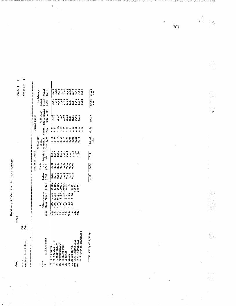
Cro

p

Ac

res

Àve

rage

F

leld

Slz

e

Cod

e t 5 C

ULT

IVA

TO

R H

.D.

23 lr

ÂR

Rot

.¡ (

DR

AG

)28

sr.

rAltr

ER

(s.P

.)32

CO

¡IB

INE

P

TO

26 S

PR

AY

BR

3ó T

RU

CK

IO A

UG

ER

-HO

TO

Rl0

t T

RA

CT

OR

(DIE

SE

L)IO

I ÎR

ÂC

TO

R(D

IES

EL)

Una

lloca

ted

Inau

ranc

e

TO

TA

L C

OS

l/AC

RE

/FIE

LD

Hac

hlne

Èy

& L

abor

Cos

t P

er A

cre

Suu

nary

Hhe

at

Tlll

age

NaE

e

150.

l 50.

I TlE

es A

crea

Slz

e O

ver /ll

our

Prf

ce

26.

ó0,

I8.

t2.

50.

27 5

. ó. 70.

¡ 50

.

4.00

t2.9

5 53

30.

4.00

30.

31 2

640.

r.00

8.3

5 10

002.

1.00

5.5

5 27

960.

1.00

18.

81 2

400.

L.O

O 2

.79

0.t,0

0 ¡2

.40

1157

.2t

875.

4687

5.

Var

labl

e C

oats

ìlach

l ne

ryF

uelÀ

T

otal

Labo

r Lu

b. R

epal

rs V

arla

ble

$/¡c

$/

¡c

$/A

c co

st g

/Ac

2.r0

0.

59

0.17

0.85

0.0

9 0.

040.

76 0

.r7

0.35

t.2t

r.22

l.9

r0.

36 0

. l2

0.

082.

10 0

.95

0.0

0.rl

0.04

0.

020.

280

.76

I.:E

- 5.

50

5. x

Flx

ed C

ostg

Mac

hlne

ryH

åchl

nery

Tot

alfn

aur.

Rep

lace

oent

Flx

ed T

otal

$/eC

F

und

$/A

C

Coa

t C

oar

o.7

5

0. l3

0.51

3.13

0.20

0.9

50.

060.

28o.

76

FIe

Id

fl

Clte

nt

4

0.0t

t.l

00.

00

0.45

0.0t

t.6

60.

0s

4 .7

20.

00

0.4t

0.0

0.0

o.00

0.

2 t

0.05

2.

900.

12

6 .3

50

.00

10.6

2 0.

26

20.3

9

l.ll

1.87

0.45

0.5

8I .6

7 2.

l84.

77 7

.90

o.42

0.6

20.

0 0.

950.

2r

o.21

2.95

3.2

36.

47 7

.24

0.00

0.0

0

20.6

6 3t

.28

***

***

N) O __l

Cro

p

Acr

eaA

vera

ge

Fle

ld

Sfz

e

Cod

et

Hac

l¡lne

ry &

Lab

or C

o6t

per

Acr

e S

umm

ary

Rap

eeee

d

380.

380.

5 C

ULT

IVA

TO

R H

.D.

23 lr

AR

RO

l{ (D

R.A

G)

28 S

r.rA

lHE

R(S

.P.)

32 c

ollB

tNE

P10

2ó S

PR

AY

ER

36 T

RU

CK

IO A

UG

ER

-}IO

TO

Rt0

t ÎR

.ôC

TO

R(D

IES

EL)

l0l

TR

AC

T0R

(DT

ES

EL)

Una

lloca

ted

Inau

ranc

e

TO

TA

I. C

OS

T/A

CR

E/F

IELD

Ttll

age

NaB

e

I TlE

ea A

crea

Slz

e O

ver

/Hou

r P

rlce

26.

60.

18.

t2.

50.

275. 6. 70.

t 50

.

4.00

12"

95 5

330,

4.00

30.

3¡ 2

640.

t.00

8.35

t000

2"1.

00 5

.55

2796

0.r.

00 1

8.8r

240

0.r .0

0 2.

79

0 "

1.00

r2.

40 I1

57.

2t87

5.

4687

5.

Var

iabl

e C

ostg

Ì4ac

hlne

ryF

uel&

T

otal

Labo

r Lu

b. R

epal

re V

arla

ble

$/¡c

$/

Ac

$/A

c co

sr g

/Ac

2. r0

0.

54

0. r

70.

85 0

.09

0.04

o.76

0.1

7 0.

3st"

2r

t.22

l.9l

0.36

0.1

2 0.

082,

l0

0.95

0.

00.

rr

0,04

0.

020.

280.

?6

l;58

--i.3

0 --

3:T

I

FlK

ed C

ostg

Hac

hlne

ry¡la

chln

ery

Tot

alIn

our.

Rep

lace

rent

. F

lxed

ToÈ

al$/

ec

Fun

d g/

Ac

Coa

r co

ar

0.70

0. l3

0 .5

13.

130.

200

.9s

0,06

0. 2

80

.76

Fte

ld I

Clle

nt f

0.0t

I.

t00.

00

0.4

50.

0t

1.66

0.05

4.

120.

00

0.41

0.0

0.0

0.00

0.

210.

05

2.90

0. 1

2 6

.35

0.00

t0.4

2 0.

26

20.3

9

¡.tt

l,8t

0.45

0.5

8t.6

7 2.

t8

4.77

7.

90o.

42 0

.62

0.0

0.95

0.21

o,2

72.

95 1

.23

6.47

7.2

40.

00 0

.00

-7õt

66 -

li.¡7

*t*

Á**

N'

O co

Mac

hfne

ry ú

Lab

or C

o6t pe

t A

cre

Sum

mar

y

Cro

p S

uuer

fallo

w

Acr

ee

210"

Àve

rage

F

leld

Slz

e 27

O.

Cod

elt 23

IA

RR

o$ (

DR

AG

)IO

I T

RA

CT

OR

(DIE

SE

L)¡0

1 T

RA

CIO

R(D

TE

SE

L)t na

lloca

ted

I¡¡s

uran

ce

llllå

ge

Nee

TO

TA

L C

OS

l/AC

RE

/FIE

LD

ÀC

CU

MU

I'ÀT

ED

C

OS

T/A

CR

E/F

OR

EN

TE

RP

RIS

E

I Tln

es A

cree

Slz

e O

ver

./llo

ur P

rlce

4.00

30"

3r

Var

labl

e C

osÈ

g¡f

achl

nery

Fue

l&

Tor

alLa

bor

Lub.

Rep

alre

Var

labl

e$/

ec

9/¡c

$/

ec

cosr

g/A

c

2t87

5 .

4687

s.

0.85

0.0

9 0.

040.

120.

48

-a:tî

--î

:4,

-t:ä

4.39

3.

88

Flx

ed C

oBrg

ltach

lne

ry

l,lsc

hlne

ry T

oÈaI

Ineu

r. R

epla

cene

nt F

lxed

Tot

al$/

ec

Fun

d $/

AC

C

ost

CoB

r

0. 1

3 0.

00

0.45

0. r2

0.

05

2 "9

00.

48 0

.t2

6.35

0.09

- l.g

a -

o¿o

r0.8

I

8.27

0.2

6 17

.16

Fle

ld

f

Clte

nt

f

0.4

5 0.

582.

95 3

.O7

6.47

6.9

60,

09 0

.09

rT.o

7 ¡m

I**

* **

*

t7.4

2 25

.69

N) O \o

Yea

r 19

79

Inpu

t

Fue

l &

Lub

rfca

tlon

Rep

a 1r

g

Fer

t I llz

e r

62.5

LbB

/Acr

e It4

8000

027

4.0

Lbe/

Acr

e 34

0000

00

Che

ELc

alg

1.5

Ava

dexB

H(B

lype

a1.

3 B

anve

l B

arle

y

See

d T

reat

nent

Coa

ts1.

50 B

ushe

ls,/A

cre

See

d C

oara

Inc

ludl

ng S

eed

Cle

anln

g1.

50 B

ushe

ls/A

cre

Labo

r 22

5.70

Hou

rs

Inte

reat

oo

Ope

ratln

g C

aplta

l

Tot

al V

arla

ble

Cos

t

Tax

ea

MÂ

chln

e ln

aura

nce

Ele

ctrlc

ty,

Hle

cella

neou

g O

verh

ead

Cro

p E

nter

prls

e S

unM

ry f

or R

ecor

d #

Phy

6lca

l R

ecor

d

For

15

0. A

cres

of

Tot

al C

aBh

Cos

tg

Cas

h R

etur

n8 (

Yle

ld X

prlc

e -

NeÈ

Cas

h R

etur

n

Dol

lar

Rec

ord

5.50

5.ll

7 .4

42t

.23

9. r

5r.

03

0.69

6.53

I .3

8

4.90

69.9

7

3.9r

0.26

6. r

0

73 "

57

825.

59 v

767.

10 v

tll5.

62 V

3185

.25

V

1372

"50

vr5

4.89

V

t03.

50 v

978.

75 v

t257

.58

V

734.

62 U

586.

95 F

39.7

1 F

914,

41 F

l.lhe

at

'40.

0 x

4300

.87

t527

"39

Fle

1d I

4.48

)r7

9.20

r 05

.ó3

I 04

95

.38

tt035

"54

2 68

80.0

0

rs84

4 "4

6

N) O

Iear

197

9

Inpu

t

Fue

l &

Lub

rlcat

lon

Rep

alra

Fe

rt I

llze

r12

8.0

Lbs/

Acr

e ló

2000

t458

.0 L

bs/A

cre

6200

23.0

LbB

/Acr

e 11

4800

0016

9.0

Lbs,

/Acr

e 34

0000

00

Che

ol c

a I

s

10.0

Ept

ao(8

-E)

Lfq

See

d T

reat

Den

t C

oata

0"12

Bu8

hels

/Acr

eS

eed

Co6

ta ln

clud

lnB

See

d C

.lean

fng

0. l2

Bue

hele

/Acr

e

Labo

r 57

I.76

Hou

re

Inte

rest

on

Ope

ratln

g C

aplta

i.

Tot

ál V

arla

ble

CoB

È

'Iaxe

a

Mac

hlne

Ineu

ranc

e

Ele

ctrlc

ty.

MLs

cella

neou

s O

verh

ead

Cro

p E

nter

prls

e S

umna

ry fo

r R

ecor

d I

Phy

alca

l R

ecor

d

For

38

0. A

cres

of

Tot

al

Ca6

h C

ostg

Dol

lar

Rec

ord

5. 3

0

5.Il

9.47

3.O

22.

74r3

. t0

2.58

0.0ó

0.88

8. 3

8

3 .5

3

s4 "

t7

r .3

0

o.26

2.03

57.7

8

Cas

h R

erur

ns (

ytel

d X

prr

.ce

-

Net

Ca6

h R

etur

n

2015

.12

v

1943

.32

V

3599

.36

vIt4

6.08

v10

40.0

6 v

4977

.O4

v

979.

64 u

24.6

2 v

335.

t6 v

3t85

.86

v

1339

.95

v

495.

65 F

100.

59 F

772.

t7 F

Rap

eeee

d

40.0

x

to?

62.5

4

979.

64

Fte

ld I

6.s0

)26

0.00

202-

22

20s8

6 .2

0

2r9s

4 "6

0

9880

0.00

7 68

45 "3

7

N)

Yea

r 19

79

Inpu

t

Fue

l 6

Lubr

lcat

lon

Rep

alrB

Fer

È 1

112e

r

Cro

p E

nter

prls

e S

@m

ary

for

Rec

ord

#

Che

nlca

Ìe

No

Che

ulca

le U

sed

See

d T

reat

eent

Co8

Èa

See

d C

oatB

Inc

ludl

ng S

eed

Cle

anln

g0.

0 B

ushe

I6/A

cre

Labo

r t4

3.04

Hou

re

Inte

reat

on

Ope

ratln

g C

splta

l

Tot

el V

arla

ble

Cos

r

Tax

ea

Hac

hlne

lna

uran

ce

Ele

ct.r

lcty

, M

lece

llane

ous

Oye

rhea

d

lota

l C

aBh

Cos

tg

Phy

alca

l R

ecor

d

No

Fer

tfllz

er

U6e

d

Caa

h R

etur

ns (

Yte

ld X

Prlc

e -

Net

Cas

h R

etur

n

For

27

0. A

crea

of

Dol

lar

Rec

ord

673.

49 v

390.

10 v

Sum

me

rfaI

IoH

0.0

2.95

0.68

7 .5

7

1.30

0.26

2.03

u. t7

0.0

x

0.0

v

0.0

v

797.

OO

V

184.

r4 v

352.

17 F

7t.4

7 F

548.

ó5 F

3017

.03

0.0

)

Fle

ld

I

0.0

-t l.

r7

2044

.7

4

0.0

-301

7.03

N)

N)

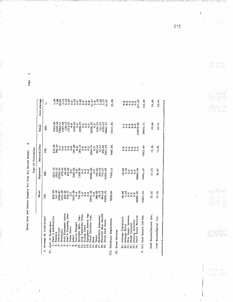
L A

crea

ge

By

Cro

p(ac

ree)

IL

CoB

t of

Pro

ducE

lon

l. F

uel ú

Lubr

lcar

lon

2. R

epal

ra3.

Fer

¡lllz

er4.

Che

nlca

le5.

See

d T

reaÈ

Een

t C

oets

6. S

eed

É C

Ìean

ln8

Co6

È7.

Tel

ne C

o6tg

8. L

abor

9. C

usto

n C

harg

eg10

. I¡

¡ter

est

Ope

r. C

åp.

ll.

Cro

p In

aurs

nce

preE

.12

. D

ryln

g C

osts

¡3.

Equ

lpE

ent

Ren

taI

Cha

l4.

lota

l V

arla

ble

CoB

t15

. R

ent

16.

Tax

ee17

. l,f

achl

nery

lna

urån

ce18

. E

lecÈ

ric }

llsc

Ove

rhd

19.

Tot

al C

âsh

cost

8

III.

Hac

hlne

ry R

epla

ceoe

nt

IV.

Gro

as R

etur

ns

21"

Ave

râge

Y

leld

/Acr

e22

. A

vera

ge pr

lce

23"

Cro

p In

eur.

Rev

enue

24,

Str

aw (

g/A

cre)

25.

Gra

zlng

($/

Acr

e)26

. T

otal

Gro

aa R

etur

ns

V.

Net

Cae

tì R

etur

n (2

ó-19

)

CaB

h R

etur

n/C

urre

nE I

nvô

Ca6

h R

erur

n/R

plcE

r ln

v.

Tot

al C

ost

a¡rd

Ret

urn

Sun

Mry

per

Cro

p F

or R

ecor

d N

mbe

r g

Typ

e of

Ent

erpr

lae

t50.

825.

5976

7.rO

4300

.87

t527

.39

103.

5097

8.7

50.

012

57.5

80.

073

4.62

0.0

0.0

0.0

r 04

95.

380.

058

6.95

39.7

191

4 .4

1t

r03s

. s

4

3058

.86

40.0

04.

480.

00.

00"

026

880.

00

1584

4 .4

6

22.3

2

19.2

6

Rap

esee

d S

umre

rfal

low

380.

2015

.12

t943

.32

t07

62.5

497

9 .6

424

.62

335.

l6

0,o

3 r8

5 .8

60.

0I

339

.95

0.0

0.0

0.0

2058

6 .2

00.

04

95 .

65r0

0.59

772.

172t

954.

60

7749

.t2

40 .0

06.

500.

00.

00.

098

800.

00

7 68

45 "

37

t 2.

73

36.8

7

270.

673.

4939

0. l0

0.0

0.0

0.0

0.0

0.0

797.

000.

018

4.t4

0.o

0.0

0.0

2044

.7

40.

035

2.17

7t.4

754

8.65

30r7

.03

s505

.95

0.0

0.0

0.0

0.0

0.0

0.0

-301

7.03

-2,3

6

-2.O

4

Tot

al

800.

3514

.20

3 r 00

.53

r 50

63 .

4 I

2507

.03

t28

"12

l3t

3.91

0.0

5240

.44

0.0

2258

.7 I

0.0

0.0

0.0

33t2

6.32

0.0

t434

.71

2lr

.7 7

2235

.23

3600

7 .

t 7

r631

3.94

0.0

0.0

0.0

0.0

0.0

t256

79.9

4

896'

t2.7

5

23.6

8

20.4

4

Fam

Ave

rage l. 4.39

3.88

r8.8

33.

130.

l6I

.64

0.0

6.55

0.0

2.82

0.0

0.0

0.0

41.4

10.

0r.

790.

262.

7945

.0t

20 .

39

0.0

0.0

0,0

0.0

0.0

157

. l0

1t2,

09

23.6

8

20.4

4

Psg

e

N)

UJ

I. A

crea

ge B

y C

rop(

acre

e)

II.

Cos

t of

Pro

duct

lon

l. F

uel

 L

ubrlc

atlo

n2.

Rep

alrB

3. F

erttl

lzer

4. C

heE

lcal

g5.

See

d lre

atE

ent.

Coa

ta6"

See

d &

Cle

anln

g C

o6t

7. T

vlne

cos

t88.

Lab

or9.

Cus

too

Cha

rgea

10.

Inte

rest

0pe

r. C

ap.

ll.

Cro

p In

aura

nce

Pr@

.12

. D

ryln

g C

oscg

13.

Equ

lpue

nt R

enta

l C

ha14

. T

otal

Var

labl

e C

ost

15.

Ren

t16

. la

xea

17.

I'f.a

chin

ery

lnau

ranc

e18

. E

lect

rlc [

tlsc

Ove

rhd

19.

Tot

al C

êBh

CoB

ts

III.

lfacl

rtne

ry R

epla

ceoe

nt

lV.

Gro

ss R

etur

ns

21.

Ave

rage

Y

letd

/.Acr

e22

" A

vera

ge P

rlce

23.

Cro

p In

sur.

Rev

enue

24.

Str

ás (

9/A

cre)

25.

Gra

zfng

($/

Acr

e)26

. T

otsl

Cro

6s R

etur

na

V"

Net

CaB

h R

etur

n (2

6-19

)

CaB

h R

etur

n/C

urre

nt I

nv.

Cas

h R

eÈur

n/R

plco

t lo

v.

Coa

t an

d R

etur

n P

er A

cre

per

Cro

p F

or R

ecor

d N

umbe

r

r 50

.

5 .5

05.

u28

.67

r0.

l80.

696.

520.

08.

38

0.0

4 .9

00.

00.

00"

069

.97

0.0

3 .9

ro.

266.

l073

.57

20.3

9

40.0

04.

480.

00.

00.

017

9.20

r05.

63

22.1

2

19.2

6

Rap

esee

d

380. s.

305.

u28

.32

2 .5

80.

060.

880.

08.

380.

03

.53

0.0

0.0

0.0

54.r

70.

0I

.30

o.26

2.03

57 "

78

20.3

9

4 0.

006

.50

0.0

0.0

0.0

2 60

.00

202.

22

42-7

3

36.8

7

Sum

erfa

lloc

270. 2.

491.

440.

00.

00.

00.

00.

02

.95

0.0

0.68

0.0

0.0

0.0

7 .5

70.

01"

300.

262.

03l¡.

t7

20.3

9

0.0

0.0

0.0

0.0

0.0

0.0

-tl.r

7

-2 "

36

-2.O

4

N)

2L5

c"16

c"16.i

c.16.2

1"

ASSI]MPTIONS USED TO CODE CROP ENTERPRISES

General Client InfornaÈion

The following is a list

Eion when coding.

of the exceptions thaE require speci.al at.ten-

l. Value of improved land is defaulted by municipality.

2. Taxes on improved land are defaulted by rnunicipality.

Machinery Inventory Description

I^Ihen a producer owns a I/2 share of a particular implement or a

set of implemenËs, the machines have been entered in Ehe progran

as machines of one-half t.he value of machi-nes of tha! size for

the clienL. Therefore, depreciation and investment costs will be

one-half that, of a producer who owns the enËire rnachine.

All pieces of equipment used by a producer in any of his forage

operat,ions are completely costed to Ehe crop and forage enter-

prises. These pÍeces of equipnenl are not included in the iirt"-

stock cost calculations. Tractors are an exception to this rule.

All inplements used mainly for livest.ock are allocated to live-

stock enterprises. Exanples: livest.ock equipment such as rnanure

spreaders, feed grinders and post hole augers; implernents used

only in winter such as snow blowers.

Forage Harvester - code Actual H.P. in the i.Iidth field of Inven-

Eory

Auger - Code tube dianeter inco The Width Field of Inventory

Auger Code H.P. Code=LengËh int.o Hp Tractor used in Inventory.

S.P. Swather & Custom Swalher - Code H.P. = 0 in Inventory

n

J.

4"

5.

6"

7.

216

8. S.P. Spray Coup - Code H.P. = 0 in Inventory.

g. Bin Piler CapaciEy=750 llundredweights per hour, t.herefore the

width field =750.

10" Bale ElevaËors Capacity is 30 tons per hour, therefore 30.0 is

coded into the width field of the inventory.

1I" Note -- the prograro will divide t.he necessary width fields by

crop yield, so no manual work needs t.o be done"

L2. Coding a machine for which there is insufficient supporEing data

is done by placing acres per hour in Ëhe width field. i.e. BALE

CARRIER.

13" Code Ëhe horsepor¡Ier of the TRACTOR in the width field.

14. Conbines are coded per thousand sguare inches of separating area

in the width field.

15. Custom operations are added to Ëhe inventory fist and are refer-

red to. just like any ot.her implement.

16. The wÍdth of Ërucks are coded by bushel capacit.y"

a) - to 100.0 = half ton

b) -100.0 to i75.0 = I ton

c) -175.0 to 275.0 = 2 ton

d) -275.0 to 375.0 = 3 Ë,on

e)- >375.0=3-5ton

17. The capacity of wagons is in tons"

c" 16.3

1.

2.

6.

7.

8.

3.

4.

5.

217

General ProducËion Infonnat,ion

Do not code the wasteland, bush, or any unimproved land.

rf the producer does not indicace Ehe weight. of straw or tame hay

bales, assune the following weight for each type of bale: square

straw: 40 pounds square tame hay: 50 pounds round tame hay:

consistenË with Ëhe size of round baler used in the operat.ion.

rf no informarion is available it is assumed t.haË a round bale of

tame hay weighs 1200 pounds. A round bale of strav¡ is assumed t,o

weigh 4/5 that of a bale of Eame hay (i.e" 4/5 of. L20O 1bs.= 960

pounds)" These values are defaulted internally.

Fields which are being cleared are not, included. similarly, any

land clearing operations are excluded.

rf the field is 0 niles (or unspecified in the questionnaire)

disLance of 0.1 niles from field to storage is assumed. If

range is given, use t,he average of the two distances.

conbine the infornation in the questj-onnaire and in the "crop

Insurance PamphleË,srr to calculaEe the crop j.nsurance premiums,

Ëhe crop insurance paynents and the reseeding payments received.

Code the rent.ed f ields last.

Assume that 50% of the land is heavy soil.

Ëhe currenË year crop insurance price options and premium rates

were used.

Any crop insurance prernium paid in the current year by a producer

to insure new forage seeding is a cost lo the companion crop in

Èhe current year. A1so, âfly crop insurance payment obt.ained from

that forage crop in Ehe current year is a revenue to Ehe compan-

ion crop in the current year.

a

a

o

218

C"L6.4 Crop Informat,ion

i. If the producer baled his straw but has not indicated the amouriL

of strar¡r taken off a particular field, assume that one ton of

straw was Eaken off the field.

2" Use the weight of bales at harvest to calculate the yields of

forage crops, not the r¡reight of bales at f eeding tí.rne.

3. Improved pasture always has 0 yield.

4. If the number of years of product,ive stand is not specified use 6

years.

5. The number of years of productive sËand is equal to Ë,he number of

consecutive years the field is in forage and the nunber of years

it is left as pasture (if applicable), before the field is bro-

ken.

6. I,rÏhen bot,h tame hay and grazing occur in the same f ield the yield

of uhe hay production uust be coded first to yield correct twine

cos t.

C.16.5 Seed information

1. Seed cost,s of taroe hay or pasture are distributed over the number

of years of the productive stand. The seeding rate in the year

the field was seeded is divided by the number of years of the

s Ëand.

2" It is assumed thaË Ehe pasËure was seeded with the type of forage

seed which is nost predoñinent on t,he farm"

3 " In the event Ëhe producer did not j.ndicaËe the seeding rate for

forages of grain crops, the recommended seeding rate was used.

4"

219

tr{hen a forage was seeded with a companion crop in the currenE

year, t,he cost of the forage seed was not included. That cost is

taken into account in other forage or pasture fields of that same

farm or of other producers'farms. ThaË, is, the seed cosL is i.n-

curred during the years of produetive stand only"

Fertiliz er Inf orrnationc" 16 .6

1. FerÈilizer spread in the current year

current year on a crop underseeded t.o

companion crop and noE to the forage.

or

a

chemical applied

forage is a cost

in

to

the

the

2. Use producer's information to det,ermine the amounË of manure ap-

plied to a particular fie1d. If the quesÈionnaire does not indi-

cate Èhe au.ount applied to each field, allocaËe the amount. of ma-

nure spread equally across t,he total area of fields receiving

Eanure. Only the nanure spread is taken into consideration as a

cos t.

3. All fertilizer prices are based on bagged fertilizer" These

prices qrere obtained by adding $12.00/Ton to the average bulk

Ifanitoba fertj.lizer prices.

4. The value of a fertilizer used by a producer bu¡ not included in

ttre fertilizer list is derived frou a weighted average of nut-

rient, prices available in common formulations, i.e. value of I

acË,Íve pound of N equal to $0.202 and the value of I active pound

of P2O5 equal Eo $0.202. $12.00/Ton is Lhen added to converË

frou bulk Èo bagged fertilizer prices.

c.16.7

1"

c. r6 .8

1.

,)

220

Chemical Infornation

If t,he producer j.ndj.cated that a particular f ield \.ras sprayed

without indicating the cheraical applied nor the application rate,

it is assumed Ëhat the recomrnended chemical was applied to the

field. i.e. I'ÍCPA Anine 80 was assumed to be applied on oats and

barley; 2r4-D Anine 80 was assumed for wheat.

If the chemical is specified , but not Ehe rate of application,

use the recom-ended rates as provided in t,he default option of

t,he program"

If the chero-ical is MCPA is specified, assume MCPA Anine 80 was

used.

If ttre chemical is 2,4-D is specified, assuûe 2" 4-D Amine 80 was

used.

Tillage Practices

Assume that 2 minutes are requi.red Eo load 10 square bales onto a

h/agon with a front.-end loader. Assume thaË.5 rainutes are re-

quired to load and unload one round bale onto a r¡ragon with a

front-end loadêr.

The tillage operat.ions associated with the seeding atd/ot break-

ing of the forage or pasture field are distributed over the num-

ber of years of productive stand. The number of times for a par-

ticular tillage operation uay be less than one. inlhen a forage is

seeded in the same operaÈion as the companion crop (i.e. oats or

barley) the cosE of the seeding operations ís allocaËed to the

companion crop.

4"

2.

J"

22r

If Lhe producer did not specify a particular set. of tillage oper-

atÍons during Lhe year in which his pasture or tane hay was bro-

ken up, then a certaÍn set. of tillage operations is assumed which

complJ.ments the implements on his farm. Assume thac one of the

following set of tillage operaEions occurred in descending order

of preference:

a) 1 plowing; 2 double disc; 2 harrowings

b) I plowing; 2 cultivations; 2 harrowings

c) I plowing; 2 light cultivations; 2 harrowings

d) 1 cust,om plowing; 2 custom cultivaËions; 2 custom harrowings

Al1 Eillage operat.ions occurring during the period commencing

with the coropletion of harvest of the previous croP to Ehe har-

vesting operaEion for the crop Ehat is grown are considered as

costs to Ehe crop in that year.

5" Assume thaÈ Ehe producer hires a custom operator for a certain

operaEion if he does noË have t.he equipment for that particular

operation.

6 " Assume Ë.haË t,he client uses a bale elevaLor to unl-oad square

bales from the \^ragon. If no bale elevator is listed in the pro-

ducer's machinery inventory, t.hen assume the producer owns a 1960

price code I bale elevator. The same assumptions apply to a grain

auger.

The acres/hr. for the bale carrier are coded in the width field.

The acres/hr. for the bale carrier are calculaLed in fhe follow-

ing manner. Assume that 15 uinutes are required to load and un-

load the bale carrier and assume that it travels 4 ¡ailes Per

4.

7.

8"

o

222

hour. Therefore, the hours /bal-e=,25 +(distance from yard to

field in miles)/4. Number of hours/acre = hrs./bai-e x bales/

acre. Number of acres/hour=1.0/number of hours/acre. AdjustmenË

for efficiency coefficient = acres/hr/O.8

Any drainage or rock-picking operaËions are not included.

If a forage field gave tT¡ro or Ehree cuts and a \^zagon was used to

bring the forage horne in each cut, code the wagon operation as

ttonce overrt because \.ragon calculations are based on the Eotal

yield and not Ehe yield obtained in each cut.

10. The implement used for a particular tillage operation must be

roaLched with a tractor of the appropriate horsepower required for

that tillage operaËion.

ll. Assune that a combine of

the capaciÈy or model of

tionnaire.

10000in2. r.las used by the producer if

coubine is not specified in the ques-

L2. In order that Ëhe twine cost associated with a baling operaEion

be determined correctly in the program, it is necessary thaË the

baling operation is coded only once in the set of tillage opera-

Ëions associated with a parËicular fie1d. The number of times

over for the baler on a particular field may be speeified as be-

ing more than I with fractional values allowed in the codÍ-ng for-

rnat for the nunber of Eines over.

13. Tractors that are used must be eoded one time over.

TABLE 19

Machinery Inventory Description Card

Size(Iten /i4)

223

0ptional Price( Ite¡o #5 )

Tillage Implenent NameCode

Implement No.of Tractor

I)3

4

5

6

7

8

9

II1

I1

1

01

2

34

5

Plow-TraÍl Type tractor used width (feet) options pricePlor¿-MounËed Type tractor used width (feet) options priceCult iva tor-Iigh r

duty field tractor used width (feet) options priceCult iva tor-1ight

duËy field-wing tractor used width (feet) opt,ions priceCult iva tor-heavy

duty field tractor used width (feet) options prÍeeCult iva tor-heavy

duty field-wing tractor used width (feet) opËions priceStalk Cutter-

integral tractor used qiidth (feet) options priceStalk Cutter-trail tractor used width (feet) options priceGrain Auger-

electric length (feet) diam. (inches) options priceGrain Auger-Eotor length (feet) diam. (inches) options priceGrain Auger-PTO length (feeE) diam. (ínches) options priceTandem Disc-

trailing t,ractor used width (feet) opÈions priceTandem Disc-wing tractor used width (feet) options priceOne-l,Iay Disc tractor used r.ridth (f eet) options price

T6L7

18

1920

2T

22

¿J24

2526272829

Discer (with seed& fertilizeratt,achrnenE )

Rod-i'leederNoble blade 6'

bladesNoble blade 7'

bladesHoe DrillPress Dri11 e

Double DiscNo ti1l dri11 (seed

drill)Corn Planter

(3'/row)Ilarrow (drag)Harrow (spring

roorh)PackerSprayerSwarher (PTO)Swat,her (S.P.)Swather with

tractor usedt,racËor used

Ëractor used

tractor usedtractor used

tractor used

tractor used

t.racLor usedtractor used

Eractor usedLractor usedtractor usedE,ractor used

0

width (feet)width (feet)

r¡idth (feet)

width (feet)width (feet)

width (feet)

width (feet)

width (feet)width (feet)

width (feet)width (feet)width (feet)width (feet)width (feet)

options priceoptions price

options price

options priceopt,ions price

opLions price

opËions price

opt.ions priceoptions price

opEions priceoptions priceoptions priceoptions priceoptions price

224

Tillage Implement Name

Code

ImplemenE No.of Tractor

Size(Iten #4)

0ptional Price(Itero //5)

30

31

32

JJ

conditioner (S.P.)SwaLher vrith pick-

up real (S.P.)Combine (PTO)

Coubine (selfpropelled)

Combine (rotary)(s.P. )

Dryer andEquipment

Gran. Appl.TrucksInlagonsSprayer (self

propelled )Forage HarvesterBaler (round)

Baler (square)

Roto-tillerMovrerMower-condi tionerRake (wheel)Rake (bar)Stack EoverBale triagon

(se1f propelled)Forage BlowerHaystackerFertilizer

BroadcasterHaybind or

[.IindrowerBale elevaËorBale carrierFronË-end loaderForage harvester

wagonsSt,ookersRow CultivatorRotary Cultivator

(Hoe)Potato WindrowerPotato HarvesterPotaEo PlanÈerBin PilerHarrow Packer

U

0Eractor used

0

0tractor used

0t,ractor used

0tractor hptractor used

tract,or used

tractor usedtractor usedtractor usedtractor usedtractor usedtractor used

0tract,or usedtractor used

tractor used

t,racÈor used0

tractor usedtractor used

tracLor used0

tract,or used

tractor usedtracËor usedtracÈor usedtract,or used

0

tractor used

width (feet)

width (feet)(Square inches)divided by 1000(Square inches)divided by 1000(Square inches)divided by 1000

0width (feet)capacity (U,-,. ¡capacity (tons)

width (feet)width (feeL)width (feetbetween swaths)width (feetbetween sI^raths )width (feeu)width (feet)width (feeL)width (feet)width (feet)acres /hour

capacity (tons)acres/hour

width (feet)

rvidth (feet)30.0

acres/houracres /hour

capacity (tons)0

widEh (feet)

width (feet)widÈh (feet)width (feet)width (feer)

750.0width (feet)

opt.ions price

op t.ions priceoptions price

options price

actual pri-ce

actual priceactual priceactual priceactual price

acËual priceactual priceacEual price

actual price

actual priceoptions priceoptions priceopLions priceoptions priceactual price

actual priceactual priceactual price

actual price

actual priceacËua1 priceact.ual priceactual price

actual priceact,ual priceoptions price

opt.ions priceactual priceactual priceactual priceactual priceactual price

34

35363738

3940

4L

42434445464748

495051

52

53545556

575859

6061626364

Tillage Inplement NameCode

Inplernent No.of Tractor

Size( Iten //4 )

0ptional Price( Item /15)

r0tt02

Tractor (diesel)Tractor (gas)

00

drawbar hpdrawbar hp

options priceopt,ions price

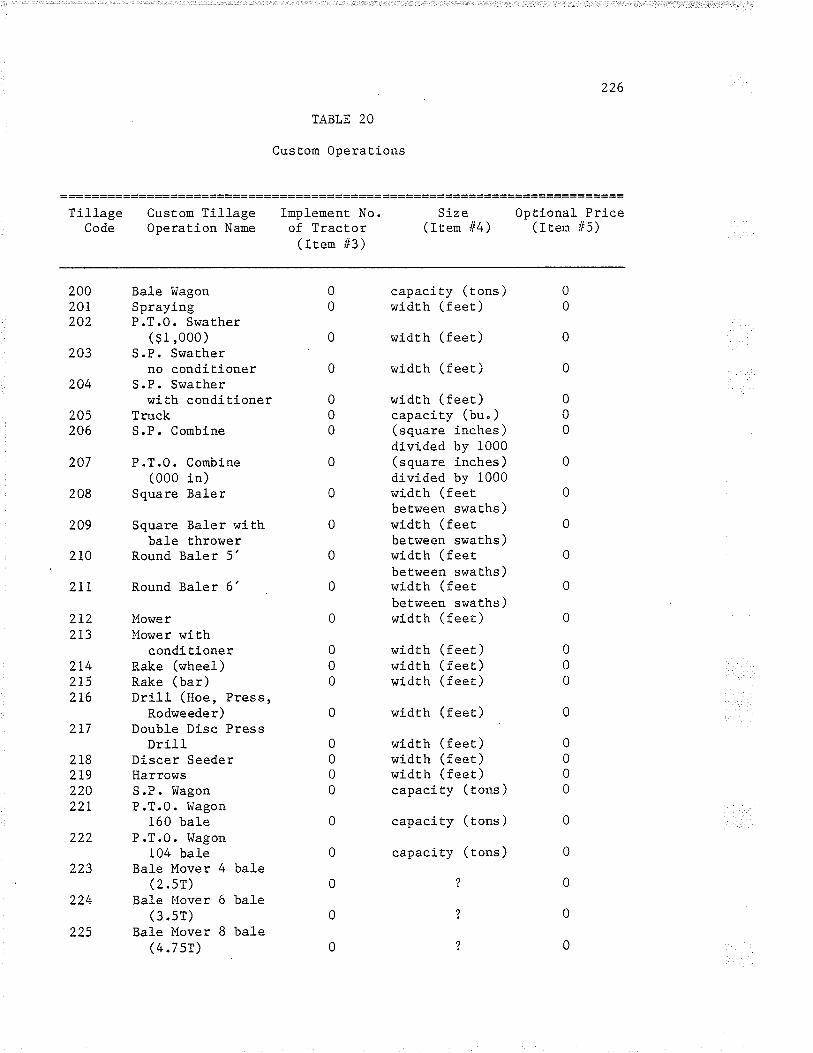
226

TABLE 20

Custom Operat.ions

= ======================================== ======== =======================Tillage Custo¡r Tillage Implement No. Size Optional Price

Code Operation Name of Tractor (Iten /É4) (Itern #5)(Iten /i3)

200 Bale trrlagon 0 capacity (tons) 020I Spraying 0 width (feet) 0202 P.T.O. Swather

($1,000) O width (feet) 02O3 S.P. SwaEher

no conditioner 0 width (feet) 0204 S.P. Swather

wj-th conditj-oner 0 width (feet) 0205 Truck 0 capacity (bu" ) 0206 S.P. Coubine 0 (square inches) 0

divided by 1000207 P.T.O. Corobine 0 (square inches) 0

(000 in) divided by 1000208 Square Baler 0 width (feet 0

between swaths)209 Square Baler with 0 width (feet 0

bale thrower between swaths)210 Round Baler 5' 0 width (feet 0

beLween swaths)2I1 Round Baler 6' 0 width (feet 0

between swaths)2I2 Mower 0 width (feet) 0

2I3 }lower wÍthconditioner 0 width (feet) 0

2I4 Rake (wheel) 0 width (feet) 0

2I5 Rake (bar) O width (feet) 0

216 Dri1l (Hoe, Press,Rodweeder) 0 width (feet) 0

2L7 Double Disc PressDrill 0 width (feet) 0

2L8 Discer Seeder 0 width (feet) 0

2I9 Harrows 0 width (feet) 0

220 S.P. Wagon 0 capacity (tons) 0

22I P.T.O. i^Iagon160 bale 0 capacity (tons) O

222 P .T.0. i^Iagon104 bale 0 capacity (tons) 0

223 Bale Mover 4 bale(2.5T) 0 2. 0

224 Bale Mover 6 bale(3.sr) o ? o

225 Bal-e Mover 8 bale(4.7sr) 0 ? 0

227

= ==== ==== == = = ==== == ==== == = == ==== === == == ==== == = = == = == === = = == = ===== === == ==Tillage custou Tillage rrnplement No. size optional priceCode Operation Name of Tracror (Iren //4) (Iten //5)

( rten //3 )

226 Bale Mover 12 bale(7 .21) 0 ?

227 Packer 0 wídrh (feer)228 Plor¿ Semi-mounE,ed 0 widrh (f eet)229 Plow Trail 0 widrh (feet)230 Cultivaror (L.p. )

Solid 0 widrh (feer)23L Culrivaror (L.o. )

ï{ing 0 widrh (feer)232 Cultivaror (H.D. )

Solid 0 widrh (feer)233 Culri.varor (U.n. )

Wing 0 widrh (feer)234 Row Crop Culti.varor

($i,000) 0 width (feet)235 Forage Blower 0 ?

236 Forage Box andtrIagon Self Unloadand Medium ForageHarvester Pickup 0 tractor hp

237 Forage Box andWagon Self Unloadand Medíun F.H. 2

row header 0 tractor hp238 Forage Box and

Wagon Unload andF.H. Pickup 0 tracror hp

239 Forage Box andI.Iagon Self Unloadand F.H. 2 RowHeader Large 0 Ëractor hp

240 Forage Box andiiagon lligh Dunpand Mediun F.H.Pickup 0 tractor hp

24L Forage Box andI^lagon l{igh Dump

and F.II. 2 rowIleader Medium 0 traccor hp

242 Forage Box andl,Iagon High Dunpand Large F"H.Pickup 0 tractor hp

243 Forage Box andtrIagon High DunpandF.II .2rowIleader Large 0 tract.or hp

244 Forage Harvester

000U

Size Optional price(Irem #4) (rrem //5)

Tillage Cusrom Tillage ImplenenÈ No.Code Operation Name of Tractor( rLen //3 )

245Pickup Medium

Forage Harvester2 Row HeaderMediun

246 Forage HarvesterPickup Large

247 Forage llarves ter2 Row lleaderLarge

248 Row Crop planrer -4 row

249 Row Crop planter -6 row

250 Row Crop planter -8 row

257 Potato Harvester252 Potato trrlíndrower253 Rod trIeeder254 Stackmover chain

type 3T255 Stackmover chain

type 6T256 Stacknover chain

type 8T257 Stackuover cable

rype 8T

0 tract,or hp 0

0 tractor hp 0

0 tractor hp 0

0 tractor hp 0

0 widrh (feer) O

0 width (feer) O

0 widrh (feeL) O0 widrh (feer) 00 widrh (feer) O

0 widrh (feer) 0

020

0't0

010

0r00 widrh (feer) 0

0 widrh (feer) 00 widrh (feet) 00 width (feer) 00-00 width (feer) 0

258

259

25026L262

Beet l{arvester4 row

Beet llarvesËer6 row

Beet Topper 4 rowBeet Topper 6 rowBlank

263 Gran. Spreader============================================== ==========================

229

TABLE 2I

Drying Costs per Bushel

i.

(A) I.fith an AirWheat

or^med2Recirculating BatchContinuous FlowBin Batch

Custom3RecirculaEÍng BatchContinuous Flov¡Average

owned2Recircul-at.ing Bat.chContinuous FlowAverage

Custom3Recirculating BatchContinuous FlowAverage

Temperature of *15: C

and gapeseedM.C. I

Low l4edium

.07

.04"03

.13

.08

.11

.13

.07

.05

.24

.13lo

.10

.05"04

.20

.I0

.I5

.23

.12

.09

"42.23

1,)

High

"20.11.06

.37"2rto

2.

1.

t

1"

t

Barley, Oats, Sunflowers, Rye(Adjust to 1b. Basis)

.05

.03.025

.11

.06

.09

Flax andLf.c.

LCorn'

.15

.08

.05

.29

.16

.¿J

.2OI^mecl

Recirculating BatchContinuous FlowBin Batch

_3CustomRecirculating BatchContinuous FlowAverage

.12

.07

.05

ôtc LJ

.14

.18

.35

"19.11

"65.37.51

(B) i,Iirh an Air Temperature of -I0: C

230

1.

,

2Ov¡ned-

Recirculat,ing BatchContinuous FlowBin Batch

^-JuustomRecirculating BatchContinuous Fl-owAverage

Barley,.1

Uf^tneCl

Recirculatíng BatchContinuous FlowBin Batch

Custon3Recirculating BatchContinuous FlowAverage

1. owned2Recirculating BatchContinuous FlowBin Batch

2 . Custo¡03Recirculating BatchConLinuous Flov¡Average

irrheaË and Rapeseed

M.C.

L67"

.08

.05

.04

.14

.08

.ll

Oats, Sunflowers,

.i1

.06

.09

Flax and Corrr4

M.C.

.r4

.09

.07

.25

.L4

.19

L7 "5"/.

.15

.08

.06

.26

.r4"20

Rye

.11

.06

.05

.20

.ll

.16

20"/"

.) .)

.r3

.08

.39oa

"31

"17.10.06

.29

"17"23

.39

.23

.I4

"68.40.54

.06

.04

.03

o

.26

"14"11

"46.25.35

lSee table I-2-.

2--In the case of an owned dryer, the following variable costs areincluded: dryer repairs, bin repalrs, tract,or power, propane,electricit,y, and labor.

3Ir, th" case of a custon dryer, the above variable costs areincluded plus Ehe following fixed costs: depreciatj.on, investnent,insurance and housing, and propane tank rental.

lt-Flax and corn calculated as 1.75 x cost of drying wheat.

23r

TABLE 22

MoisÈure ConË,ent Ranges

Crop LowI"loisture Contentl

Medium High

Wheat0atsBarleyFlaxCornFababeansPeasRyeSunflowersRapeseedIlustardLentilsBuckwheaLField Beans

1'For purposes ofconlents are used Lo

14 .7 -r7 "Or4.1-r6.514 .7 -r7 .O

10.6-r3.015.6-18 .0i6.1-18.5r6.r-18.514"1-r6.5

9 "6-12.010.6-13.0r0.6-13"014.1-16 "5l6 . 1-18 .516;1-18.5

17.I-19.5r6.6-I9.0r.7 . I- 19 .513.1-15.5r8 .1-20 "518.6-21.0I8.6-21.016.6-19.0L2.r-L4 .5I3.1-i5"5I3.1-15.516.6-19.018.6-21.0r8.6-21.0

over 19.5over 19.0over I9 "5over 15.5over 20.5over 21.0over 2I.0over 19 "0over 14.5over 15 "5over 15.5over 19.0gver 21.0over 2I.0

this study, the following ranges in moistureestimat,e the drying costs.

272-/-Table 2J

Seeding Data

Crop Code Name and DescriptionSeeding

Price Rate Unit

9o

tö

B47)

Cereals arrd Oilseed.sl

I¡lheat (Sinton, Neepawa, Napayo, Selkir.k)

- Foundation ff1-2- Registered ft|-2- Certified #1-2- BuJ-k Certi-fjed #1-2

Oats - Foundation fft-Z- Registered ff1-2- Certifiea #t-Z- Bulk Certífíed ft1-2

Barley (Bonanza and. Conquest)

- For:ndati.on fil-Z- Registered fi1-2- Certifiea ffl-Z- Bul-k Ceri-j.fíed. #1-2

.1100

.0988

.0950

.0773

"1 225.1088"1038. o8t8

.1125

.o975

.0925

.o775

.0950

. OBOO

.tooo J4"2850. ¿o)u.25OO

1b

1b

t_b

Barley (l'ergus, Herta, I{lond.ike, peguis)

- Foundatton #t-2 .1050- Registered, ffl-Z .O9OO- Certified. #1-z .OB5o- Bulk Certífled. #1-2 .O7OO

Barley (Srmni-t)

- Certified #1-2- Bu]-k Certified

Ffax (DLlfferin, Linott, Raja)

- Fcurrdation rt1-2- Registered #1-2- Certifiea #l-Z- Canada ff1-2

1b

272

Crop Code Name arrd Description--..- Soodi¡o

Price Rate Unit

Durum (I.Iakooma, Macoun, Coulter)- For-rndatton ftt-Z- Registere1, $t-Z- Certified, #1-2- Bul-k Cerr,ified ff1-Z

Fall- Rye - Cougar, Pt:ma Certified, #j-z- Canada ffl

Rapeseed (Arg,entine )

- Regent and Tower Certified #1-2Canada ff1-2

Rapeseed. (eof:.sir)

- Torch Certified #t-Z2ltustard- Yel-1ow Cert ff1

Brown Canada ff1Cert ft1

Oriental Canada $lCert fft

Sirnflowers ( i{rasnodarets )

- Certified 1

- Canada 1

Sru:flowers (Saturn)

- Certified 1

- Canada 1

Hybrids204)^tr,

254304

Buckwheat Cert. Mancar:.Cornnon Can" l

1b

6

112q Oaì)v

.111j

.1100

.1 000

.1050 6s

.0900

.5400 6

"3750

5

.4400

.)) e" )

.25 5-7tr

)qÃ.1) )

7E")))" )

.4ooo"3500

Etr)" ).5000" 4ooo

3.o2.10)t^2"502.20

.2200 4z

.1700

1b

1b

1b

IbB

1b

1b

Lb10

Crop Code Name and Description- - \êô.{.jñô-

Price Rate Unit

11 Field Peas Can. 1 .1900 1.65 tb

13 Corn Silage (Cargill- Prices) l4 tbPAG SX111 (zjoo ht. unit, Bo aay) j.ojCargitl Bto (2500 ht. unit, 8o aay) .%jPAG SX121 (t-z6oo hr. unit) .92o

27 Tame Hay - See Forage sheets

33 Soybeans .t6T 104 tb

J4 Utitity T¡Iheat (ctentea)

- Foundatíon rtl-Z .1 1OO 90 lb- Registered fft-Z .O9BB- Certified fft-Z .O9jO- Bul-k Certified #1-2 .OTTI

4t Lentits2 .4j 60 tb

4l canary seed2 cerl. ff1 .zo B.o tbCanada ftl . 18

4S Fababeans Carr. 1 "ZJOO jZO Ib

4l corn

/ì¡ræì.,., fele 5or (z1oo ht. units ) . Booo iz rbarsiI1 tB5 (e4oo ht" units) .l>>o

Co-op 5259 60 lb. units) .gg6o

I Cereals and Oj-lseeds - average of Manitoba Pool Elevators pricesand Cargl-ll prices.

2*M;stard, Canary Seed. and tentils - 19BO prices Northern Sal-es Co"

,zqIabl-e 23

,1!'orage Seed. Data f'or

(Continued)

Production of Hay or Seed

Name Descriotion Price Seedi::g Rate Unit

A. Legumes

Alfalfa

Al-sike

Sweet Clover

White Clover

Red Clover(Double Cut)

Red Cloveú(Singre Cut)

Birdsfoot Trefoil

Sai¡foin

B. Grasses

Brome

Timothy

Creeping RedFescue

Ç1Ç BRAND Can. 1 NOC2Tfror Cert. 1 NOC

Verrral- Cert. 1 NOC

Coronon Can" 1 NOC

Canada 1 NOC

Yel-low Blossom Can. 1

NOC

Plowdov¡n Can. 2

Ladino Cert. ICorrnon Can. 1

Florex Cert. 1 NOC

Corrnon Can. 1 NOC

Cor¡rnon Can. 1 NOC

Leo Cert. 1

Co¡rnon Can" 1

Melrose Cert. 1

Conmon Can. 1

Common Can. 2

Carl-ton Cert. 1

Contmgt 6u''. 1

Timfor Cert. 1-2Ch¡nax Cert. 1-2ÇOrnmgn Q¿11. 1

Cournon Can. 2

Boreal Cerb. 1

D;rlaurn Cert. 1.

Cómmon Can. 1

7

t Q)'

4 (z)

7(6)

7

B

3)

5(J)

B (¡)

2 (2)

2.552.582"522"03

)tz

tn. t)

2"J31.82

1"971.41

.61

10Ã

oaì

"7o2q

1.35oJr

t.¿)1.251.051 .00

cìÃ

oÃQry

1b

1b

rb.

1b

tb

lb

lb

Ib

1b

4 (2) 1b

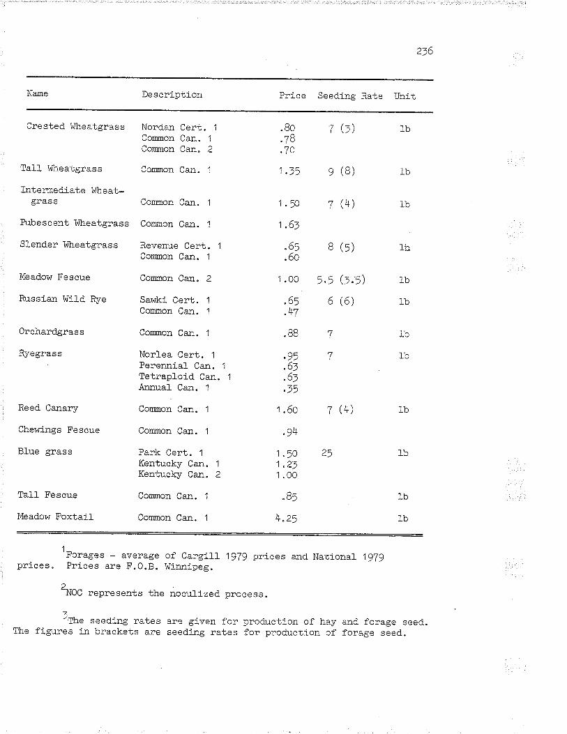
2.'^

Name Description Price Seeding Rate Unit

Crested Wheatgrass

Tal-l- Wheatgrass

Intermediate I{heat-dþâêeõ¡ ueu

R:be sc ent'lalheatgras s

Slender lalheatgrass

Meadow Fescue

Russian Wild Rye

Orchardgrass

Ryegrass

Reed Canary

Chernrings Fescue

Blue grass

Tall Fescue

Meadow Foxtail-

Nordan Cert. 1

Common Can. 1

Cor¡mon Can. 2

Comnon Can. 1

Con'¡non Can. 1

Cormon Can. 1

Revenue Cert. 1

Corrnon Can. 1

Co¡nnon Ca¡." 2

Sawki Cert. 1

Cor¡non Can. 1

Common Can. 1

Norlea Cert. 1

Pereru:ia1 Can. 1

Tetraploid Can. 1

Annual- Can. 1

Cor¡¡non Ca¡." 1

Common Can. 1

Park Cert. 1

Kentucky Can. 1

Kentucþ Can. 2

Cormon Can. 1

Common Can. 1

73) 1b

e (8)

7u)

.Bo

.(o

.7o

1.9

t.ot

"6j.ou

1 .00

AL

)tt

.88

oÃ

.o)

.ot?E

1"60

oL

1.501.2t1 .00

.Bj

4.zj

lb

o \)/

r n /z r\-).) \-).))o to)

7 (4)

1b

1b

1b

1b

1b

1b

1b

7

7

1b)q

1b

1b

4

'Forages - average of Cargill jg|g prices and. NatiorraL 1gT9pri-ces. Prices are F.O.B. Wimipeg.

2*NOC represents the nocul-ized process.

JThe "eedlng rates are given for production of hay and forage seed..

The figures in brackets are seeding rates for production of forage seed-.

Appendix D

PRODUCER QUESTIONNAIRE

-237-

238

PRODUCER QUESTIONNAME

Producer Number:

Name:

Address:

'j'e-LeDflone :

Date Interviewed:

Municipality of majority of lands:

Note : All information contai-ned in this sì¿rvey is confidentiaL "

239

The inforrnation in Ehe paragraph at the beginning of each section

gives the procedure essenEial to your conpletion of the questionnaire

quickley and efficiently. ( Reading the preliminary infornation in each

step will sinplify the corapletion of the questionnaire for you. )

The questionnai.re is designed in a logical sequence to obtain infor-mation as Èo the inventories and far¡o practices you use on your farm.

There are !T¡/o inventorÍes required. These are machinery, and land" The

farn practices refer to your cropping procedures.

Examples of the j.nvent,ories and farm practices are given. The trüo

Iists called EasLer machinery and land list are Eo be used Ëo fill inyour inventories on t,he supplied sheets called Inventory Machinery, and

rnvenEory Land. Any unique equipment, etc., on your farm not on the

master lists should be included at the end of each invent,ory list. The

naster list gives the units required. As an example, when filling in

Tractors, all tractors should be included first. The next column is an

inventory number. The year. column is year manufactured.. Size column

for tractor is the horsepo$/er rat,ing at the drawbar. The Eype column is

either diesel or gasoline. The owned, rented or custom column requires

just a leËter 0, R, or c. The last co.l-umn |tTracLor used" refers to the

tractor that pulls an inplenent and the Eractor invenÈory number should

be included in this column. As an example, if you have five tract.ors

and tractor #5 is used for pulling the cultivator, then a 5 is put j-n

Ëhis col-umn. Please refer closely to t,he Easter list for the proper

uniËs.

240

D"1 MASTER MACITINERY LIST

The cropping and haying nachinery should all be Íncluded on the forms

that folLow. The master list is a guide to fil-ling the blanks supplied.

The tractors shoul-d be included first. The invenEory nuuber associated

with the tracËor used v¡i11 be required when you fill in the implements.

As an example, if you have four tractors and tractor number three pul1s

Èhe baler then Lhe three will be required in the t,ractor inventory num-

ber comumn of the balers. The units required in the various columns are

specified in the master list. Please follow this closely to include all

t,he required informaËion"

The baling, forage and pasture maj-nLenance operations are considered

as cropping operacions and the relevant machinery should be included in

Ehe crop section for uachinery.

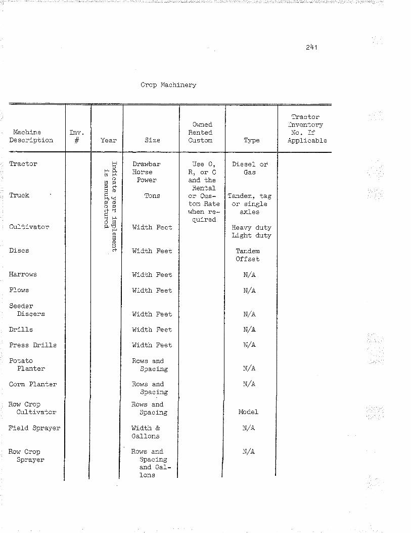
241

Crop Machinery

MachineDescrlption

Inv.JI Year Size

OumedRentedCustom Tlrpe

TractorInvenioryNo. ff

Applicable

Tractor

Truck

Cu]-tivator

Discs

Harrows

Pl-ows

SeederDiscers

Dril-1s

Press Dril-ls

Pota-uoPlanter

Corn Planter

Row CropCultivator

Field Sprayer

Row CropSprayer

HP. Q.oH.

Õãg)Êj cf5o'-,qgpoc)Ê,cFrytsJ H.ô5p,U

Foão+

Drawbarllorse

Power

Tons

Width Feet

I¡Iidth Feet

't¡Iidth Feet

T¡Iidth Feet

I¡iidth Feet

I¡Iidth Feet

Width Feet

Rows andSpacing

Rows andSpacing

Rows andSpacing

ï\ii-dth &Gall-ons

Rows andSpacingand Ga1-Ions

Use 0,R, orCand theRental-

or Cus-tom Ratewhen re-qulred

Díesel orGas

Tandem, tagor single

axles

Heavy dutyLight duty

TandemOffset

N/A

N/A

N/A

N/A

N/A

N/A

N,/A

ModeI

N/A

N/A

Row

Fie

Row

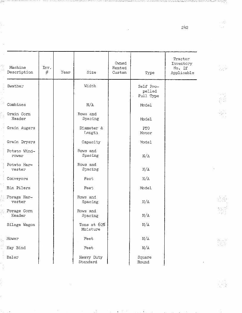
242

lVachineDescription

Inv.tr Year Size

Ol^n'led

RentedCustom TVpe

TractorInventoryNo. If

Applicable

Swather

Combi¡res

Grai-n CornHeader

Grain Augers

Grain Dryers

Potato t^Iind-rower

Potato Har-vester

Conveyors

Bi¡r Pilers

Forage Har-vester

Forage CornHeader

Silage I'Iagon

Mower

Hay Bind

Baler

width

N/A

Rows andSpacing

Diameter &Length

Capacity

Rows andSpacing

Rows andSpacing

Feet

Ela al

Rows andSpacing

Rows andSpacing

Tlons at 60%Moisture

Feet

Feet

Heavy DutyStandard

Self Pro-pe11ed

Pul1 Type

Model-

ModeI

PTO

Motor

Model

N/A

N/A

N/A

Model

m/¡

N/A

N/A

m,/¿

N/L

SquareRound

Hay

241

MachineDescription

Inv.JIlf Year Size

OvmedRentedCustom Tlpe

TractorInventoryÀlo. ff

Appiicabi-e

Stooker

Hay Wagon

Bal-e Stacker

Trailers

Bale Eleva-tor

Bale Carrier

AutomaticBale lrlagon

Stack Mover

. Bales

Tons orBales

BaIes

Tons

Feet

P¡'l ao

Bal-es

Bales

N/A

N/A

N/A

N/A

N/A

N/A

Self Pro-peIled

PulI TVpe

N/A

244

Machl-nerx¡ (Crops ) I-nventory

Co - br'n €

Continued

)ìlq

Itfachinery (Crops) Inventory

continued

Macbinery (Crops) T-nventory (Contj:rued)246

Machine T3çeInventory

No.

OwnedRentedCustom TYpe

TractorInventory No.If Applicable

26

¿l

28

¿y

J1

3i

J4

35

,o

40

4r

+¿

4J

44

45

46

47

48

49

(Continued)

247

Machilery (Crops) Inventory (Continued)

Mach-ine TypeInventory

No. Year Slze

OwnedRentedCustom Type

TbactorInventory No.If .{pplicable

50

51

52

53

54

55

MASTER I,AND LIST

This tist contaj-ns four colu.nrrs . The crops, the i-nventory

number, the size and the ovrnership of the land. Please refer to the

land lnventory example for an il-]ustration of the la:rd requirements.

Owned/Rented

248

An 0 for or^rnedand an R forrenteci is

sufficient here.ff rented, j-ndicaterental cost peracre.

Crops Grown

Wheat

0ats

\Barley (lvla-L-Ur-ngJ

.\Barley (t"eed,)

Durum Wheat

Fa1l Rye

Rapeseed

Mustard

Sunffowers (Oif-tvpe)

Sunflowers(Confectionary-type )

Buckwheat

Field Peas

Mixed Grai-n

Utility Wheat

This columnis alreadym.¡mbered.

Size (acres)

(Continued )

2)ro

(Llontr-nuedJ

Or^medrlRented

Soybeans

ProcessingPotatoes

Table Potatoes

Sugar Beets

Field Beans

Lentils

Canary Seed

Fababeans

Grain Corn

Sr.r¡nnerfallow

Fl-ax

Forage_ a¡d HayGrowr

Tame Hay

Haylage

Corn Silage

Pastures

Improved

Unimproved

Grass Seeds

Size (acres)InventoryNr.mber

(Continued)

Timothy Seed

250

(ContÍnued )

Slze (acres) Or^med.r/Rented

Al-fa1fa Seed

Sweet CloverSeed

Bromegrass Seed

Meadow FescueSeed

BirdsfootTrefoil Seed

Single Cut Redñ1 nrran

CrestedWheatgrass

'Alsike CloverSeed

Slender l.{heat-grass Seed

Sudan GrassSeed

c=oo c",/o-'tfnventory ] Size

Nr..mber | (acres) L\med/Hented-

I, .r IVxl he-o- þ 1 tbo c

WF-ea-Li

2 ' tt ^; l\o\-/ ine øfo /ac,re

ÞLo- f -//---\

3) ãn ()tt'

Sarler/ -.-'\ 4/ i'r -lú. i ni 13 i L)

5 15 i Ro /3sho-re

,4tFal fa *oV/TrnPeO ve-¿t PasL,uç.." 7 /50S*.., rnQ-( So-lta w Ri

-!I

6 lo9 t,,

10,i

.\- I

11

i

1) i

Ii

l,t l

14

t6 \

17

Contlnued

251

Land Inventory

-forn t 6/ C

Land Inventory

Uli'Bred/Hented

Continued

253

Land Inventory (Continued.)

Inventory I SizeNumber I (acres)

Conti.nued

254

, /^ ,\Lano Invenfory (uonl1nueo,

Inventory I SizeNi-:mber I (acres)

lñ^m^T ^^DDOfvfru åvfu9

255

D"3 CROPPING PRACTICES

The questions on your cropping practices are divided inËo six sec-

tj.ons: A - Grain, Oilseed and Summerfallow; B - Forages; C - Silages and

Haylages; D - Forage Seeds; E - Inproved PasËures; and F - Unimproved

PasËures. Each crop given in your land inventory applies to one of the

above sect,ions. Each colnn can acconmodate one field. Additional cop-

ies of each section are available at the end of the questionnaire. Use

then as required. Please follow the Land Inventory Numbers given in

your mâster inventory list to nake sure no fields are orniÈted and in-

clude these numbers in the space provided in the relevant secËions.

256

Crops A-1

CROP PFACTTCES

/(̂Grain, Oilseed and Summerfallow)

CROP:

1. ïtem Field Inventory #

Total acres seeded

Average distance to storage (onfarm) (mi-fes)

Yield in 1!80 (r:nits)

Yiel-d of harvested. straw

Acres of harvested straw

2. Insurance

Hail (coverage/acre)

Crop (coverage option - 5O%,60%, or 70% and, dol-Iar option- low or high)

Value of claj-ms i_n 1!BO

Number of acres claimed on

Indicate any other crop insur-ance coverage and clajms onthis field in 1980, ifapplicable

3. Seed

Seed Cl-ass: Commercial ,Certífied or Other

Seed treatment (chenieal used.)

ïf reseedi_ng was done in 1980,indicate previ ous seed.ingand seed types

257

Crops A-2

4. Fertil-izer (Include previous fal-l-s application)

Analysis of I st applicaiion

Application Rate

Method of application

Analysis of 2nd application

Application Rate

Method of Application

Analysis of 3rd applieation

Application Rate

Method of Application

5. Weed. Controll (Inc1ud.e previous falls application).-f\--Chemical(s) Used in First

Application2

Nr.mber of Acres- Treated

Rate of Application if otherthan Recoroiended Rate

Chemical(s) Used in Second.Application

Number of Acres Treated

Rate of Appli-cation if otherthan Recounmended Rate

Chemical(s) Used. in flrirdApplication

1'Specify whether liqr-r:td or granular form of a chemical r^r-as used(1."., liqr.:-id. or granular Treflan).

2_^ --If less than the whole field was treated.

258

Crops A-l

6.

Nr:nber of Acres Treated

Rate of Application if otherthan Recommended Rate

Insect Control-

First Chern-ì-cal Used

Number of Acres Treated

Rate of Chemj-cal- Application

Second Chenical Used

Number of Acres Treated

Rate of Chemical Application

Miscel-laneous

B. Fall Tillage and pre-seedj.ng practices

- please list all operations

over the fields from previous

harvest to seeding; specify

jmplement used (i.e., pJ-ow,

cultivator H.D., cultivator

L.D., d.isc, harrows, sprayer)

by indicating inventory num-

ber or implement name and

number oftimes over. If the

field r^ras sumrnerfatlowed- the

prerrious year then no fall

cultivations are included.

17

2tr'o

Crops A-4

If the fiel-d 1s currently

sunrnerf allowed, indicate

all- the 1p8O practices.

9" Seed.ing (i."., press d.rill,

packers )

'10. Post-seeding (i.e. weed

Sprayer, ror^r Crop cultivator,

haruows)

11. Harvesting (cereal-s and

oilseeds )

Indicate Swather(s) used

Indicate Combine(s) used

l-ndr-cate't'ruck( s,) used

ïndicate Other

12" Drying (if applicabte)

Number of bushels dried

Moistlre level before drying

Moisiure l-evel after drying

¿ol)

Crops A-5

-1 1 Harvesting (potatoes,t,/.-'-

sugarbeets, etc. )

Indicate lli-ndrower( s ) used

Ind.icate Harvester( s ) used.

Indicate Truck(s) used

Indicate Binpiler(s) used

fndicate Other

14. Harvesting (strar¡)

Indicate Baler(s) used.

(Please list the equipmentused to bring the strawto storage).

261

Crops B-1

FORAGE PRACTICES

CROP:

1. Description Field. InventorY #

Totat acres seeded

Average distance to storage(on farm) (rniles )

2" Yield

1 st cut

(i) Yield in t98o (rmits)(ii) Round. or square bales?

(iii) Bate weight (i-n lbs.)

2nd cut (if applicable)

(l) Yierd in t98o (r:n:its)

(ii) Rorrnd or square bales?/...\ f , \( r-r-r- , IJaIe \^reagnl \ ln IDs . /

Jrd cut (if appJ-icable)

(r:.) Yiel-d in 1980 (units)(ii) Round. or square bales?

(iii) Bale wei-ght (in tbs.)

3. Fal-l grazing (if applicabre)

(i) No. of beef calves XNc. of daYs

(ii) No. of dairy calves XNo. of days

(iii) No. of steers or heifersX No. of days

(i") No. of beef cows andbul-l-s X No. of daYs

(v) No. of dairy cows ¿¡.d-

bu].l-s X No. of days

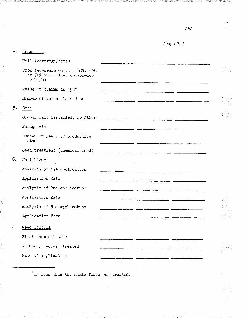
262

Crops B-2

4. Insurance

Hai:t- ( coverage/acre )

Crop (coverage option--!O%, 60%or 70% and. d.oll-ar option-lowor hieh)

Val-ue of cl-aims in 1980

Number of acres clai-med on

5. Seed

Cororercial , Certified, or Other

Forage rnix

Nr:¡nber of years of productivestand

Seed treatment (chem'ical used)

ao. t"er-tl.Ll_zer

Analysis of 1 st application

Application Rate

Analysis of 2nd application

Application Rate

Ánalysis of Jrd application

Application Rate

7 . I¡ieed Contrcil

Fi-rst chen-ical used

Nunber of acresl treated

Rate of application

1trf 1""" than the whole field. was treated.

^/-cv)

Crops B-J

Second chernica] used

Nr;mber of acres treated

Rate of application

Third chemi cal- used

Nr.mber of acres treated

Rate of application

B. fnsect Control

First chernical used

Number of acres treated

Rate of application

Second chenlcal used

Number of acres treated

Rate of application

9. Miscel-laneous

10. Before harvest practices

(i.". weed sprayer, fertilj-zerbroadcaster)

264

Crops B-4

11. Harvesting

- please list all operatJ-ons

over the field from time of

'1 st cut to the l-ast harvest-

ing operatÍon; specify

implement used. (i.e.,

swather [etO o= pull type],

mower, rake; ba1er, hay wagon,

bale wagon, hay stacker,

stack mover, front-end loader,

etc. ) Indicate inventory

number or implement name.

12. Breaking Praetices

- please list normal operat-

i-ons over the field to break

tho forage in the last year

of production (i.e., plow,

tandem disc, cultivator, etc.)

265

Crops C-1

SÏLAGE AND HAYf,AGE PRACTTCES

CROP:

1 . Pesefi.ption Fie1d Irrveniory #

lotal- acres seeded

Average distance to storage (onfa:sn) (mifes)

2. Yield

1st cut

(i) yietd in lg8o (units)

(r:l) Moisture content atharvest

2nd cut (if appticabte)

(i) yield in 1980 (units)

(ii) Moisture content atharvest

Jrd cut (if applicable)

(i) yield in 19BO (units)/..\(1i-) Moisture content at

harvest

1. Fall grazing (if applicable)

(i) No. of beef calves X No.of days

(ii) No. of dairy calves XNo. of days

(iii) No. of steers or heifersX No. of days

(i") No. of beef cows and buLlsX No. of days

(") No. of dairy cows and bul-lsX No. of days

266

Crops C-2

4. Insurance

Hail (coverage/aere)

Crop (average option-5O%, 60%or 70% and doll-ar option-lowor high)

Value of claims in 1980

Nuinber of acres c]aimed on

,, Seed

Conrnercial, Certified or other

Forage rnix (haylages)

Nrmber of years of productívestand (haylages)

Seed treatment (chemical used)

f -

\3, Fertilizer (Include previous falls anplication)

.Ana1ysis of 1st application

Application Rate

Method of application

Analysis of 2nd application

Application Rate

Method of application

4nalysis of 3rd application

Application Rate

Method of application

267

Crops C-l- I /-

7 . trrleed Control' (Includ.e previous fatls application). -/ \Chemical(s) used in first

application

Number of acres2 treated.

Rate of chernlcal(s) applied., ifother than recon¡nended rate

Chenical(s) used. in second.application

Nr.¡mber of acres treated

Rate of chem'i cal ( s ) applied.

Chemj.cal(s) used in thirdapplication

Number of acres treated

Rate of chemical(s) applied.t

-5. Insect Control

First chemical used

Nr.mber of acres treated

Rate of application

Second cherúcal used

Nr¡mber of acres treated

Rate of application

9, Miscell-aneous

1^'Specify whether tiquid or granular form of a chereical- was used.(i."., lì-quid. or granular Treflan).

2_^ --If less than the whofe field was treated.

268

Crops C-4

'10. Fall Tillage and. pre-seed.ing

practices (silages)

- please l-ist all- operations

over the fields from previous

harvest to seeding; specì.fy

implement used. (i.e., plow,

cultivator H.D., cultivator

L.D., disc, harrows, sprayer,

fertilizer broadcaster by

indícating inventory ni-:nbe:: or

irnplement name ) . If the field

was summerfallowed the previous

year then no fal_i cultivations

are included.

11" Seedins (sil-ages)

(i.u., press drill, packers)

12" Post-seeding (silages)

(1."., rieed sprayer, fertilizerbroadcaster, roür cropcultivator).

269

Crops C-f

|J. Non-harvest practices/1¡o"'1 oaa\\¿røJ ¿øõv /

(1."., i^reed sprayer, fertiJ-izerbroadcaster)

14. Harvesting

- please list all operati-ons

over the field from time of

1st cut to the ]ast harvest-

ing operation; specify imple-

ment used (i.e., forage har-

vester, Tr'ragon, tnrck, front-

end. load.er, etc. ) Ind.icate

implement inventory number

or i.:nplement name.

270

Crops C-6

Breaking Practices (ha¡¡lages)

- please li.st normal operations

over the field to break the

forage in the last year of

produetion (i.e., plow,

tandem disc, culti-vator,

al-n \vvv.l

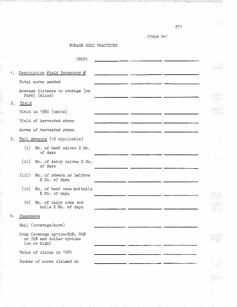
271

Crops D-1

FOFAGE SEED PBACTICES

CROP:

1. Description tr'ietd Inventory #

Total acres seeded

Average distance to storage (onfarm) (ntires)

2. Yield

Yield in 1980 (u:r:its)

Yield of harvested straw

Acres of harvested straw

t, Fa].l- grazing (if applicable)

(i) No. of beef calves X No.of days

(ii) No. of dairy calves X No.of days

/...\(iii) No. of steers or heifersX No. of days

(i") No. of beef cows andbul-tsX No. of days

(") No. of d.airy cows arrdbulls X No. of days

4. Insurance

' .o /onno\lLar-I ( coverat,/

Crop (average option-5O%, 60%

or 70% and dollar option-low or hieh)

Va]ue of claims in 1980

Nr¡nber of acres cl-aimed on

¿(¿

Crops D-2

5. Seed

Con¡nercial, Registered or Other

Forage nlx

Nr.mber of years of productivestand

Seed treatment (chenrlcal- used)

6. Fertilizer

Analysis of 1st application

Application Rate

Analysis of 2nd application

AppJ-ication Rate

Analysis of Jrd application

Application Rate

(. Weed Uontrol

tt""t """*-1 used.

Nuaber of acresl treated.

Rate of Application, if otherthan recormrend.ed rate

Second chemi-cal used

Nr.mber of acres treated

Rate of applicati-on, if otherthan recorsnended rate

1If 1""" than the whole field was treated..

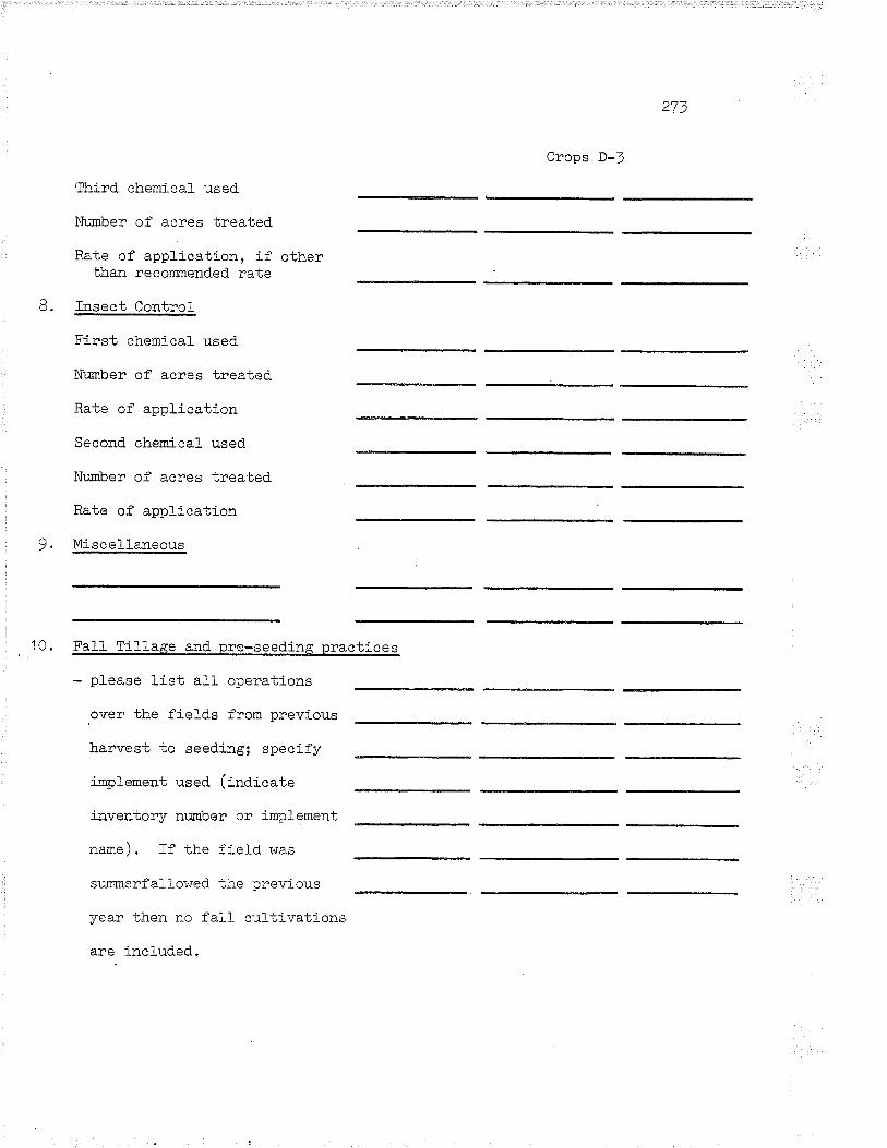
273

Crops D-J

fhird chenical used

Number of acres treated

Rate of application, if otherthan recorrnended rate

õ. Insect Control

First chemi cal used

Nr:mber of acres treated

Rate of application

Second cheralcal used

Nrmber of acres treated

Rate of application

9, IVliscellaneous

. 10. Fall Tillage and nre-seedin&practj_ces

- please l-ist all operations

over the fields from previous

harvest to seeding; specify

implement used (indicate

inventory m:mber or implement

name). r-f the f ield. was

sunrnerf al-f owed the prerrious

year then no fall cultivations

are lncl-uded.

)'7 )J-

Crops D-4

11 Seed.ing (i.e. , press drill,packers )

12" PqÞt-seed.ing (i.e., weed.sprayer)

13. a) Harvesting (forage seed)

Indicate Swather(s) used

Indicate Combine(s) used.

Indicate Truck(s) used

b) Drying (if appticable)

Number of bushels dried

Moistr:re level before drying

Moisture level after drying

c) Harvesting (straw)

Indicate Baler used.

(Please tist the equipment

used to bring the straw

to storage)

¿l)

Crops D-5

t )t Breaking Practices (forages)

- please list all operations

over the field to break the

forage in the last year of

production (i.e., plow,

tandem disc, cultivator, etc.)

276

Crops E-1

IMPROVED PASTURE PFACTICES

1, Description Fie1d Inventory #

Total acres seeded

2 " Gra-zing

(i) mo. of beef cal-vesX no. of days

(ii) Xo. of d.airy calvesX no. of days

(iii) No. of steers or heifersX no. of days

(:.v) Wo. of beef cows and bultsX no. of days'

(v) }[o. of dalry cows a¡rd. bullsX no. of days

Z Qaa¡l/.

co]o*"""i"r, certified., or other

Forage mix

Number of years of productivestand

Seed. treatment (chemical used.)

t, -+. ti'er-b1-Ll-zer

Ánalysis of 1 st application

Application rate

Analysis of 2nd application

Application rate

Improved pastures are defined as arry l-and which have been broken, seeded,and are presently being used as pasture.

)nn

Crops E-2

Analysis of Jrd application

Application rate

5. hleed Control

First chemicaL used

Nr.mber of acresl treated.

Rate of application, if othertha¡r recormended rate

Second chemical- used

Number of acres treated

Rate of application, if othertha¡. recor¡mended rate

Third chemical used

Number of acres treated

Rate of application, if. otherthan recommended rate

6. Insect Control

First chemical used

Nr:mber of acres treated

Rate of application

Second chemical used

Nr.mber of acres treated

Rate of applicai;ion

7 . lvllsceLlaneous

lIf 1u"" than the whole fiel-d. was treated..

278

Crops E-J

8. Su¡mrer Practices

(i."., weed sprayer,f ertil j-zer broad.caster )

, ). Breaking Practices

- please l-ist usual operationsover the field to break thepasture in the last year ofproduction (i.e., plow,tandem disc, cultivator,

Appendix E

CASE FARM RESI]LTS

- 279 -

280

8.1 DEFAULT CASE FARM RXSTILTS

ll I R

EC

OR

DT

gl

L_-_

____

____

____

_1

LIS

I O

F T

IÀC

IIII¡

EF

Y T

NV

EN

!ôB

I

Invg

ntor

y T

lIIàq

ellu

mÞ

cr

Cod

e T

illag

e N

al¡e

I 10

1 ÎR

ÀC

TO

R (

DrE

59L)

2 10

1 T

RA

CT

0R (

DIP

SE

Lt,I

101

TB

AC

TO

R (

DIE

SE

L'rt

Ren

ted

101

TR

ÀC

ToR

(DIE

s9l.)

5 pe

nred

101

TR

ÀC

TO

F

(DIE

SB

LI6

16 ÎR

UC

K,

]6

TR

UC

KrJ

6

CU

LTT

VÀ

TO

F [

.D.

9 6

CÍIL

TIY

ÀÎO

R H

. D

.l0

¡¡

cuL

Ttv

ÀT

on L

.D.

ll 13

TÀ

[nE

ú D

ISC

-r¡

12

2q I

ÀR

qOH

(S

.TO

olH

l13

ó¡

¡ H

ÀR

RO

II P

ÀC

ÑE

RI¡

I 20

PR

ES

S D

FIL

L15

20

FR

ES

S D

gTLL

16

26 S

PR

ÀT

EF

17

28 S

HÀ

TH

ER

(S

. P

" I

18

]2

CO

IBIN

B P

TO

19

33 C

Oirì

INg

lS.P

.)20

10

AU

GE

R-I

IOT

OR

2l

1 t

À0G

ER

-P10

22

34 D

ntE

R À

NO

EQ

UIP

2!

264

C.D

RO

AD

CÀ

ST

SR

ztt

201

c0sT

oll

sPR

ÀY

Mc

25

202

Clrs

Tod

PT

osrÀ

Tn

26

208

C0S

Ton

SQ

.BA

LE27

22

0 C

0ST

On

SP

lÀcO

N2T

' 26

SP

RÀ

YE

R29

10

AU

Gen

-ñO

TO

R

Cro

P F

rodr

lcfio

n B

u.l9

-¡ S

rmìr

latc

r V

Êrs

i ?n

lì0

-1 .

lrrù¡

ry

1990

papl

lceñ

e n¡

Siz

è lÊ

ar ¡

lour

s lts

ed V

alr¡

e¿

5U.

1975

2.

t2"'r

2 /8

125.

15b.

197

5 62

6. ¡

¡O

4575

0ì.

66.

1975

18

1" t¡

8 ¿

t''62

5.15

5.

0 2q

1.rr

5 0.

l. 0

0.0

0.15

0. 1

976

q3..t

rr

1590

0.15

0. 1

963

4l.',

tr¡

1590

0.35

.197

J q2

.69

9925

.41

" 19

79

209.

et

¿71

20.

39.

197'

t 21

5. 0

5 91

07.

29.

1978

27

.95

1'¿

12?.

60.

1978

1'

r0. 91

16

60.

60"

t9?9

26

. rr

0 70

00.

112.

19'

19

t1 .

''l

_r0

75C

.2u

. 19

71

1rì1

. q8

1

1500

.60

. 19

78

103.

76

r288

0.¿

0. 1

976

159,

3'ì

1111

.1 .

1q"

1975

27

'l ,2

8 Jb

r¡20

.1¿

.197

7 1q

2.O

g 50

r¡c0

.6.

197

0 11

"00

1J50

.7,

197

7 24

.Ot

1612

.0.

197

9 0.

(l

2000

0.60

. 0

78. 0e

0.

6C.

0 r¡

1.67

0.

lB.

0 7.

8rt

0.1l

ì. 0

13" 92

0.

5.

0 11

.7t

0.74

. 19

77

0.0

1552

.6.

196

7 33

.00_

___1

1Þq:

4Jö1

61.

Dcn

rect

t:ion

fnv

esto

Jr¡E

Cu¡

ja:n

l Val

,¡)

t1?1

8.rr

¡ 25

19.0

6 19

5tl,2

'7:

r1 ¿

.\(t

l584

.Jt

1¿1A

ì.52

3091

.75

r,7J

.J1

5156

.25

4.0

0.û

0.0

0. r

)

2 JH

5 .

TJQ

0. l

l99

2. 5

027

1¿.o

A91

0. ,0

1 ¿

12 "2

036

6. 0

0?0

0. r

)0

1075

.01

1 75

0. 0

012

rìrJ

.00

19rì

6. 1

18

35rt

2.01

'r559

. ()

t¡

1 .|l

¡ "

9616

1.2r

¡20

00.

000.

c0.

fl

0.0

0. f.

ì

0" J

't55.

20

0. ù

0.

082

b.80

6J

60.0

0ú.

J 0"

03t

rt.ù

7 ¿

.q17

,51

J1 ll

.0r¡

2¡

rq0t

ì.00

826.

1q

6174

.90

1260

.69

96e7

.6C

lB0.

6q

¿92

8.00

819.

J1

o100

.00

J597

.75

¿76

75.O

O6t

t2.5

0 52

50.0

013

J9.5

¿

10lo

rt.0

0fì

rtl .

89

52q5

.28

2lr)

¿.J

C

l?71

0.00

160t

.60

¿77

2ît.0

1u.

) 0.

01t

t6 .l

¿

I 12

8. 6

521

q0"0

0 18

000.

000.

J 0.

o0,

0 0.

0c.

J 0"

00.

1 0.

0c.

0 0.

0Jz

J.¿

l 2q

86.{

0o.

ù

----

-Qr9

-¿

l lrt

t¡0.

00

D:p

rèc¡

.a'-1

onR

ìte0.

150

0.1r

00.

150

0"15

00.

t 5

0c.

t50

0.15

0c.

t00

0.1t

00.

100

0.1J

00.

100

0.1

000.

1 00

0.10

00.

t00

0.15

00.

100

0.r5

00.

¡c0

0. r

000.

1J0

0.1c

00.

100

0.1J

00.

100

0.1i

00.

100

0.1c

0

f\) co

crop

Àc

E-o

sA

verig

ì

Flà

Id

Siz

-1

L-od

eI

Tlll

aqè

llaE

€

-6-c

ur rif

Àão

R-il

õ:2q

íÀ

n!ìo

9(s.

Too

Till

6 C

ULT

IYÀ

TO

R H

.N.

4 C

ULT

IV[T

OR

L.

D.

6O II

AÂ

IIOfI

PÀ

CK

EÊ

2O P

R9S

S D

RIL

L26

I¡ C

. B

RO

AD

CÀ

ST

ER

Atp

fsÊ

?l

J25.

t25.

26 S

PR

AfE

R2B

SrA

Tt¡

BR

(S.P

.)J2

:OI.I

BII¡

E P

TO

33 C

OñS

rNe

lS.P

.ll0

À

0G88

-lloT

oFI 1

ÀU

GE

R-P

TO

10 À

ucE

R-h

oToR

J6 T

R0C

t(]6

T

RU

CK

l0 1

18À

CT

JR (

DIE

SE

LI10

1 în

ÀC

loA

(D

tES

ELI

101

TR

Aer

oR (

DIB

SP

LI0n

l, l.l

ocat

ed

Insu

Ean

ce

TO

TÀ

L C

TS

T/À

CR

E

//PIE

LD

ü1ch

inêr

y C

osr

n€:

Àcr

': S

unna

ry

Vrr

iaht

e C

csts

P

ix ]

l C

osit

I T

DIIL

T

otal

Tln

es

À:r

3s

Fue

L Lu

r¡.

RÊ

pai:s

var

ilþIè

In

lr!:.

If¡vs

sL.

DeD

rec.

P

irll

flttl

Siz

e O

ver

/llou

r pr

ice

S,/.

\C

$/A

C

$/A

C

Cos

- S

,/nC

S/^

C

i/^C

C

rst

Cos

È

:ost

'¡i;-

-î .

0õ-t

õ;il-

ã?1ã

õ:-õ

;,¡ 6

I s-

0:õt

õ r-

- n:

t e rr

l-- -

- 0;

Blt¡

-õ;õ

ãtrr

---

i;tJ6

5--1

: D

liz--

i:r6g

- - i;1

0160

. 2.

00 3

0.J1

366

0. 0

.1¡t

tt5 0

.022

.1 c

.050

6 (r

.2¿

1.t

0.00

.JJ

0.'1

qq,

0.11

92 0

.2rlt

,)

.509

35.

1.U

0 1r

.62

9925

. 0.

4'rt

l5 0

.062

rt C

.r81

5 0.

662r

0.t0

1rt

0.14

t¿

0.1?

.r¡¡

0.5

2rì

t.191

J9.

1.00

19.

69 9

107.

0.-t

r¡16

0.0

512

0.lrt

15

0.5'

rr¡3

0.r

)0r-

l 0.

1151

D.J

r¡61

0.6

b9 1

.¿\)

60.

1.00

J0.

J1 7

0C0.

0.18

99 0

.02f

'5 0

"017

9 0.

256.

r 0.

00'r2

0.

J11{

0.

¿66

2 0.

58)

).8r

tlzt

l. 1.

{J0

10.8

6 l?

500.

0.r9

68 0

.029

5 l.8

r2fi

2.09

9C 0

.006

0 ù.

259>

O.6

65t¡

0.9

J1

1.0J

060

. 1

.OO

22.

69

c.51

060

. 1.

00 2

2.69

12u

80.0

.165

2 0.

02r¡

r.r

O"2

922

0.r¡

B2l

0.o

118

0.50

rJ

o.r¡

rJ9,

t.0

1¡

l.¡r9

32û

. 1.

00

e.2l

131

13.0

.r¿

99 0

.019

5 0.

¡¡35

7 0"

5R51

0.0

06ù

û.25

e'

o.tr

t79

1.01

J t.5

981r

¡. 0

.50

?.17

35¡

120.

0.tÌ

200

0.1¿

30 2

.f|69

7 1.

R12

.r 0

.02n

¿

0.ur

5'¡

1..tq

68 2

.¿tlz

6.0

5512

. 0.

50

-r. l?

50t

¡00.

0.5

102

O.0

777

1.4t

|99

2.O

tl5tl

0.0J

16

l,3tt)

¿

'¿.tt

7tt5

rl .2

¡b

6. J

626.

rJ

..tJ

tto.0

0 t3

50.

0.00

59 0

"000

9 0"

003?

0,

0105

0"0

0.

ù 0.

q 0.

0 J.

01C

1.

0..|J

109.

69 ¡

612.

0"O

0rr3

0.0

007

c.or

J15

ô.0n

65 0

.001

3 ù.

055d

0.0

611

0.11

8 ü.

1¿5

6.

0"33

t10

.00

1J50

.0.c

059

0.00

0e 0

.OrJ

-J3

0.{}

ro1

0.0

0.ù

0.05

rJ

0.05

1 J.

061

350.

0"

50 3

8.9J

159

C0.

0.05

89 0

"008

rì O

.046

5 n"

1lr¡

2 0.

0071

0.

3lrl.

t 0.

9c6r

t 1.

22r1

'l.lr

¡l.1

50.

0.50

J8.

93 1

5900

. 0.

0589

0.0

0rJr

J 0.

0,J6

5 0,

1542

0.0

c.

J ()

.0

0.0

c. 1

5425

0.

7812

5.

0.13

92

0. lJ

92 Q

.O22

J 0.

9ò5.

t r¡

.055

1t 5

.4¡¡

_l 5

.581

156.

48

't50.

C

.6eq

2 0.

6982

0"0

1t9

0.6J

¿¡t

Z.?

Bor

t t.

J9,

,t.09

566

. 20

625.

0.

0143

0.

0rr¡

.t 0.

0059

c.

¿5r

¡9 t

.t76l

1"

417

¡.51

t0.

0660

0.

066

0.06

6

Z;9

¡ì0-

õ;¡

¡rî2

-ã1

56îs

---

q:E

,'iit

a:14

72-

-715

tì5-

r7lîi

B5-

z5l5

¡q t

b-;õ

o¡-

**t

*t+

+

*r

Fi:l

d r

clrln

: d

N)

co N)

Cro

p

Àc

res

Àve

rà9Þ

Fi.:

ì-'d

Slz

Q

Cor

lsr

Ti-t

lage

lla

ne

4 C

Uf,T

Mm

R

L.D

.20

pR

US

S D

ntLL

202

CU

Sm

6 P

loS

rÀT

H20

u cu

srot

r sQ

. B

ALE

¿20

:usT

ol't

5P r

aÀco

filrr

1 T

8ÂcT

0R (

DT

ES

ELI

r01

TR

ÀC

TO

R (

DIE

SE

LI

1lF

è r

la y

6Cì.

20,

Itnal

loca

ted

fnsu

ranc

e

TO

ÎÀL

CO

ST

/ÀC

8 E

,/FIE

LD

iach

iner

y C

cst

Per

Àcr

e S

r¡m

m¡r

y

S lz

e

Var

iabl

e C

osts

F

ir3d

Cos

lsr

Tot

at

Tct

?,l.

Tln

es

ÀcE

es

F0e

I Lu

b. F

epai

rs

va:i1

Þ1.

fn

sur.

In

vèir,

. D

Èr¡

rec.

F

ixgi

fo

t¡L

Ove

r /H

ouc

Prlc

e 5/

^C

5/^C

S

/^C

C

ôst

5,/À

C Ã

/AC

i/t

a C

ost

Cos

: C

ost

39.

ttz .

10.

1r," 5. ô6.

1 56

.

t:õõ-

ìã:6

ã--

õì¡?

:-'r:

i õo

¡-õ;

õ5¡6

--õ:

ãi.jõ

----

õ;6

ã[5-

0 .

õ0 7

r --

-0

:jTS

i --

õ;]

'¡ 6j

- -õ

;6 6O

- -i;

lj5

2.00

16.

09 J

0750

.0.1

016

o.04

52 0

.J71

9 o.

t¿ûi

0.0

J16

1.Ju

óù 1

.169

¿ 2

.569

t.¿

rr9

1"O

O 7

.62

t.rr¡

ot "0

0 4.

Jl1.

OO

l.B

9 t'u

3l1J

. J6

rt20

625.

0.

0 0"

o 0"

0059

0.

25¡t

9 t.

l76J

1.

41?

1.r¡

J?Ir

8750

. 0.

367C

0"

:t67n

0.0

119

0.6\

,2,1

2.

790q

i.J

9t

,..t6

t)0.

lH?6

0.

18J

0.1r

tl

T;ig

Sd

õ:tõ

7{, -î

l5rn

o --

-1.îl

tq o

:2\a

7- -

Z;S

4ú¡-

.i;,

¡7tZ

- ã;

ti[ t

¡¡;ii

i-rr

+

+*t

g$

*

Pi)1

1 ¡

clrè

n--

I

N)

oo \n

Éac

hine

ry C

osr

Per

Àcr

" S

unna

ry

crop

S

unne

rf¡ll

rv

¡,ia

ld

t

Àcr

es

1bnJ

. C

li¿nr

I

.lver

rge

Pie

ld

Slz

e 10

0.

U.1

rlahl

e co

sts

Fir¿

l C

os:s

t -â

iàl

Tor

-al

Cod

e T

iees

À

Cre

s P

Uel

Lù

b. I

ìeF

ai.r

s V

erlà

þI¿

In

sr¡!

. .ln

vejr.

D

eprp

c.

Fir:

1 fJ

ttl,

Tlll

aqe

tlam

e S

lze

Ove

r /H

our

Pric

e ï/^

C

$,/À

C

S/^

C

Cos

t S

./ÀC

t/^

C

S,/Å

-:

Cos

t C

ost

:osr

-:-:

:-:::

-:--

----

----

:-ll

îÀllD

Etl

Dls

C-ll

29

. 1.

00

1t|.5

1 12

'122

.0.5

162

0.09

24

0..1

'¡34

0.t1

52(,

0.01

11

0.q7

9J

0.tt6

09

0.9-

l -l;

Ù01

26 S

PR

ÀÍE

F

60"

1.00

22.

69 1

2St0

. 0.

1115

2 0.

02qq

a.

Z'tZ

¿

0.r.

¡821

0"r

)118

0.

509J

0.

489?

1.

011

1"r¡

9J10

1 T

BÀ

cToF

(DIE

SE

LI

250.

7t

r125

. 0.

lg,J

B

0" l"

fìB

O,O

T?J

ù"

965,

t ¿

t.q55

8 5.

4{l

5.6q

210

1 T

nAC

T0R

(DT

ES

ELI

15

6.

r¡87

50.

0.13

O1

0.1t

01

0"01

39

0.b0

24

2.7A

04

3.J9

7 t.5

¿'t

l0l

TR

AC

TO

R(D

IES

ELI

66

. 20

625.

0.

C

0.0

0.00

59

0.2)

¡¡,

t.t?6

1 l.¡

¡Jt

t"r¡

JzU

nrllo

cate

d In

sura

nce

0.1?

63

0. l?

6 0.

1 t6

f O

TÀ

L C

bSI/À

CR

P,/F

I E

LDõ;

7ñî[

6:71

1, -

d]76

õq -

--î:-

6-61

õ 0:

2ûî2

- -7

;õîî¡

- 91

561)

-rãl

îT6

î,¡"õ

7E-

t+a

*t+

t(

È

N) æ

¡lach

iner

l C

ost

ner

À.r

c:ìr

lnm

ery

CE

op

Sum

mer

fa lló

s F

iêla

l $

Àcr

es

35.

cli?

o--

,À

vera

ge F

leLd

sj.z

ê :i5

.

Var

ial,l

e C

osrs

R

ix:l

Cos

Es

, îô

tål

Tot

âtco

de

Ît!ìe

s À

cres

F

ueL

Luh.

PÊ

plirs

va

rieþI

Þ

Insu

r.

ItrvÊ

sc.

D:p

rec,

F

lxej

to

tal

r fll

ì.age

N

ane

S1z

€ O

cer

/Hou

r P

rlce

S/Þ

-C

s/A

C

S/A

C

Cos

r- S

,/ÀC

f/À

C

t/L:

Cos

+_

Cos

c C

ost

--6-

-õuL

iÏ v

t16ñ

-H:r

,. --

----

----

----

- --

¡ì:-

-¡;õ

0-ì

r,:1

5-ltî

zõ;

-õ;5

it6-õ

;0îã

e--õ

;lîtõ

----

6. t

t6,¡

-õ:

õãtd

---î

;tõô;

--i:

ô\12

--r:

26a-

-t;i

eã¡r

cul

Trv

^ToR

¡..0

. 39

. ¡¡

.00

1?.4

J 91

07.

0.1?

2ft

0.05

59

0.20

50

0.61

1,

r).0

0?J

0.Jx

5l

0"3r

t61

0.ó6

9 1,

J,r2

2r¡

HA

RR

OL(

S.T

oOT

lll

60.

3.00

26"

17

3660

.0.1

t20

0.02

5rJ

o.05

86

O.2

564

0.O

OJJ

J.

lr¡4'

0.

119¿

0.

2û7

),5r

¡410

1 T

AÀ

CtO

R (D

rES

ELI

25

0.

7A12

5.

0.62

fìr,

0.62

fl8 O

,O22

J 0.

965f

¡ ¡t

.rt5

54

5.tr

r¡J

6.ot

¿10

1 T

BA

CT

o!ì(

DIE

SF

LI

l5t.

¡¡87

50.

c.13

85

0.JJ

¡,5

0.01

39

0.6J

¿¡t

2.

'nt}

4 .t.

.t9,

J"7J

510

1 T

RItc

ToF

(DIE

sEl,l

66

. ¿

0625

. o.

0 0.

r)

0.00

59

0.2)

'.19

t.t76

l t.r

¡.t,

l,tr|

tun

illo

cat-

etl

Insu

ranc

e 0.

169

7 t)

. 16

I C

. 1 6l

lOT

AL

CO

ST

/ÀC

88/P

IELf

)¡;

õEî¡

õ:6

õû-6

-lllî

og -

--7:

EtÃ

0 o:

iú11

- -j;

'¡ãtõ

- .r

leId

2-rl.

6BE

,i;6

i6-

*ri

*¡r

ù¡È

N)

CO \n

nach

l.ner

y C

ost

Per

Àcr

e:ìu

nBar

v

L-ro

p S

l¡n tl

oger

Ì

ÀcÊ

qs

110.

Àve

râ9e

Ft3

Id

5izÊ

tlo

.

Cod

et

lilla

ge

Nan

e

6:U

LTfV

À10

R H

.D.

2r¡

HÀ

RR

OÍlS

.Too

T[)

I¡ C

ULT

IVA

lOR

L.

D.

2O P

TIE

SS

DR

ILL

2r¡

ft,\R

qoI

(s.

Too

Till

26 5

PN

ÀY

ER

26q

C.B

RO

'IDC

ÀS

TE

RJ2

CO

nBI[e

PtO

]6

TN

UC

K36

ÎR

UC

K1O

ÀU

GE

R-I

tOT

OB

1 1

Àf¡

G E

R-P

TO

I O

AU

G E

R.T

IOT

OR

10 1

TP

ÂC

rOR

(D

IES

ELI

101

lR.r

cloR

(or

ES

ELl

101

rnÀ

cloH

(D

IES

eL)

0nal

loca

tgd

Insu

ranc

e

ICT

AL

CO

ST

,/ÀC

RÉ

/PIE

LD

V 1

:i at

¡ le

C

ost s

P lx

eil

Cos

:ss

Tot

al

Tot

atT

iDes

À:r

es

Fr!

eI

Luh.

Fip

airs

va

:iabI

e tn

sqç.

In

vèsr

. D

?p:e

c.

pix:

1 tlt

ll51

ze

oyer

/llo

ut

Pric

e 5/

{c

s/ic

$,

/Àc

co-c

t t/A

c î/À

c ö/

ìtc

ccst

co

st

Sos

t

¡i;

i.oo

1o:¡

i-r7l

2c:-

õ;[5

]s-õ

.0ãr

rì--

o;ãt

r,l--

--õ;

¡roì

-0:õ

tlu--

-î;t0

65--

î;oli¡

--ã;

t6s-

-t.0

s6-

ó0.

2.00

10.

11 3

66u.

0.tt

ttl5

0.02

2J 0

.05t

t6

t),2

21!

0"00

1J

0.1r

t¡t,

0.13

92 r

J,zt

il ).

5u9

39.

2"oU

19.

69 9

'107

. 0.

1100

0.0

t195

O.1

tl 15

0.

5t'1

0 0.

007J

ù.

.115

1 (-

1.lq

61 0

.669

1.2

J02'

-J .

1.O

0 10

.86

1750

0.0.

r968

O.0

2e5

1.87

?.6

2.0e

90 0

.006

0 0.

259¡

0.

665r

¡ o.

9Jl

i.0J0

60.

1.00

30.

31 1

660.

0.1

i¡tl5

0.0

22J

0.05

06

(l .2

21 t

0.0

0J.J

0.

trt¡

¡¡

0"13

92 0

.28¡

- 1.

509

ó0.

'1 .î

O 2

2.69

128

80.0

.165

2 0.

02t¡

8 O

.292

2 0.

r¡82

1 C

.Cl1

8 ù.

5ù91

0.¡

t89t

1.

01t

'1 .'

¡9J

60.

1.O

O 2

2,69

1.

510

14.

1.00

¡¡

.?6

3542

0. 1

.2J5

1 0.

1H51

tt.3

¿2'

¿

5.7t

125

t).0

2Q2

0.$7

5,1

l.Jtt6

8 2,

21t¿

7.9

tt535

0.

0.50

t9.

44 1

59c0

.0.1

119

0"0r

?7 0

.0eJ

1 0.

2?87

0.0

0?J

J.llr

¡¡t

o.e0

6q 1

.228

t.r

¡5?

J50.

0"

50 1

9.r¡

4 15

900.

0.11

?9 0

.017

7 0.

1''J

2 0.

10R

8 0.

0 0.

0 0.

0 0.

0 J.

309

6.

0..1

3 12

.q0

1150

. 0.

0.t8

0 0.

0057

0.0

211

0.fjf

,5o

0.0

0.J

0.05

¡J

?.05

1 c.

.¡16

',.

0.3J

1?.

00 1

612.

0.02

?7 0

.00r

¡2 0

.009

6 0.

0q15

0.0

011

0,05

5d o

.061

J 0.

119

).1f

,06"

0.

13 r

2.40

1t

50.0

.0Jr

,0 0

.005

7 0.

02J8

0.

()ô7

5 0.

0 0.

ù q.

,)

0.0

J.05

725

0.

7812

5.

0.2?

83

r',,.2

]q't

o.oz

'¿J

0.9ò

5¡l

r¡.t¡

558

5.4¡

tl >

.722

156.

t¡

8750

. 1.

0420

1"

0rt2

Q 0

.01

19

0.60

2i¡

2.?8

04 J

.l9t

4.rr

j966

. 20

.,25.

0.

0¡r¡

tt 0"

0,4J

0.0

059

0.25

r¡9

.t.17

6J 1

"4J¡

1.

511

0. 1

10'J

0.

111

0.

r 11

l;76-

r¡ õ

;5ã[

¡ -Ç

ïq-a

z --

i]ld?

îd 0

;24î

:- -

5]66

ãî-r

ll5E

9?-r

Tli?

l 3t

;16õ

-{l+

+

+t

*+*

Frr

lil

ü

CI1

3nr

i

^)CO O\

íach

j-ner

y C

ost

Per

ÀÇ

t-.

sr¡m

¡ary

Cro

p su

n tlo

Íecs

t'i

:td

t

Àcr

es

18C

. C

li:¡r

: ú

Àve

raqe

Fl-e

ld s

lze

60.

Vâr

lâbl

e C

osts

P

lred

CoS

LjI

lDta

l T

cttl

côd3

T

lÐes

Àcr

es

Ftle

l Lr

rh.

8:pâ

1rs

varÍ

ahte

fn

sur.

Io

v¿iE

, D

Jp:e

c. F

fx:l

IttàI

t T

lll¡g

e tla

ne

Stz

e O

ver

/Hou

r P

rrce

S

/iC

i/AC

$,

/ÀC

Cos

t S

,/ÀC

g./À

C

S/À

: C

osC

C

ost

:ost

6 C

ULT

MT

ûR l

l.D.

q1.

3.C

ì0 1

9.71

271

2C.

0.rl?

stl

0.07

1r¡

0.31

2t1

0.H

600

0"02

7d

l.2lrr

5 t.0

J12

¿,¿

65 i

. i¿

5.r

CU

LTM

T'E

L.t)

. 39

. 1.

00 1

tt.76

910

7" 0

.146

0 0.

0519

0.1

q0-i

0.5H

q2 0

.ô0r

J 0"

1151

O. Jq

6t 0

"669

1.¿

572{

r llÀ

Rno

Í(s.

100r

Hl

60.

1.oo

27.

16 3

660.

0.'t

621

0.o2

ttJ 0

"055

2 0"

2tt1

't 0.

0olJ

0.

t{¡¡

l o.

119¿

o.2

B¡

J.51

920

PR

ES

S 0

RIL

L 28

" 1.

00 1

0.86

175

00.

0. r

96tJ

0.0

295

1"r{

72ô

2.U

e90

0.00

60

0.¿

595

0.66

5r¡

0.9J

1 J.

0J0

24 fl

ÀR

Rog

(s.T

ooT

Hl

60.

?.0O

27.

16 1

660.

0.1

621

0.02

43 0

.055

2 0.

2!t1

t 0.

0033

r)

.1q0

? 0.

139¿

0.2

8t

).5¿

926

q C

.BP

OÀ

DC

AS

TE

R

60"

1.00

22.

69

).51

02b

SP

FÀ

YE

R

60.

1"00

22.

69 1

2800

.0.1

652

0.02

r¡8

e.2\

t22

0.4i

121

0.0l

rB

ù.50

rJ

O.¡

¡897

1.0

11 l

"¡¡9

312

col

lEIN

E P

To

1l¡.

1.

00

r¡.8

6 J5

¡l 20

" 1.

2t01

0.1

815

u,2t

qg

5.62

65 0

.020

¿

0.87

i¡¡

r.lr¡

6r,

Z.¿

rt\

?"U

6936

T80

Cl(

J50.

0.

50 2

5.93

159

00.0

.088

¡¡ 0

"011

J 0.

069r

J 0.

1tl5

0.0

0¡J

C.J

l'¡r¡

f)

.906

8 1.

?26

1.¡¡

0036

lRrr

CK

35

0.

0.50

25.

91 1

5900

.0.0

Ér8

r¡ 0

.013

t 0.

1299

0.

2J16

o.O

,1

.ü

0.0

0.0

).2r

210

ÀU

GE

R-ll

oToR

6.

0"

13 1

6.5J

115

0.0"

0285

0.0

0tlJ

0"0

160

0.ot

{s0

0.0

rJ.ù

O

.O5l

r 0.

051

J.rC

O1l

ÂU

GE

R-P

To

'ì.

O"t

r 22

.61

1612

. 0.

f208

0.0

C31

c.0

rì?Z

0.

0J11

0.0

01J

0"C

5)d

O.0

6tJ

0.1l

d ù.

149

10 a

UG

RR

-nol

oR

6"

0.J3

tó.

53

135t

. 0.

0285

0.0

041

o.01

rB

q.05

06 0

.0

0.ü

0.0

0.0

t.051

101

TR

ÀC

toF

(DIP

SE

LI

250.

,8

125.

c.

tr37

s 0.

¡r1?

rì O

,o2Z

t 0.

9b5r

r r¡

.q55

0 5.

qr¡J

5.s

gl10

1 ÎF

AC

TC

R(D

IES

BL)

ls

b.

4875

0.

1.05

6q

1.05

64 0

.01.

t9

ù.6t

2¡t

2.?8

0q 1

.19t

q.

451

10-l

Î8À

CT

OR

(DT

ES

ELI

66

. 20

625.

Lr

.otr

t3

0.0t

r¡3

0.00

59

0.25

ft9 1

"17ó

J l.r

¡lt

t.5r1

frna

lloca

ted

Insu

ranc

e 0.

1108

0.

111

0.11

1

TO

tÀ1.

coS

T/À

cF

E,/F

IELD

l;Eõ6

i õ;

se-Ì

e- -

61f7

5., --

l:¡;q

litì

o;Z

ûî7-

-5l

o-68

î-¡î

15F

97-r

Çl[I

l ]î.

to-j-

*rr

*$*

t++

N) æ __l

iach

lner

y C

ost

Per

Àcr

? S

unm

ary

crop

S

ltntlo

vêr:

ì F

f:Id

I

Àcr

es

165.

C

lL3n

: n

Àve

rage

Fre

lrl

Slz

e 80

"

I v¡

riabl

e co

sts

Pire

l C

oiLS

Tot

al

Tct

âlco

tle

Tlo

es À

cres

!'r

rel

Lub.

Rep

airs

var

i¡Þle

fn

sur.

In

v?st

. D

Âpr

ec.

pire

l tc

tôt

t îil

lage

N

aEe

slze

ov

er /

llouE

Pri-

c€ $

/Àc

5/Ã

c $/

Àc

cost

s./À

c t/^

c $.

/ÀJ

cost

co

st

:ost

-:-:

=::=

::-6

cnLT

lVA

mn

H.D

. 41

. 1.

00 2

0.73

271

20,0

.q53

8 0.

06Ê

1 0.

2983

0.

8201

0.0

2-rd

1.

2065

1.0

112

2,r6

t t;0

U6

¡¡ c

uLlrv

ÀT

oR L

.D.

J9.

1"00

19.

ô'

9107

.0"3

ì0U

0.0

r¡95

0.1

815

0.56

10 0

.n0?

J 0"

J151

9.:J

q63

0.66

9 1.

2J0

lJ T

À!l

oElt

Drs

c-9

29.

1.00

1r¡

"57

1212

2.0.

61Á

2 0"

092¡

1 0.

1434

0.

852r

) O

.011

1 0.

¡¡r9

¡ 0.

4609

0.9

51 l

.S0J

2t¡

llÀF

Rof

(s.

Too

llu

60.

2.00

30.

Jl

3660

.0.r

r¡85

0.Q

22J

0.05

06

0.22

1 .t

0.00

1J

0.1¡

¡r¡t

0.1

'19¿

0.2

8,

J.50

926

4 C

. B

iIOÀ

DC

AS

TE

R

60 .

| .0

0 22

. 69

J.

5 I

026

SP

RÀ

YE

R

60.

1.00

22.

69 1

2080

.0.1

652

0.02

qtl

O.2

9'¿

2 O

.r¡8

2r 0

.C1l

B

0.5J

9J 0

.r¡8

9? t

"Ctl

1.r¡

9120

PR

E5S

DR

rLL

28,

1.00

t0.

86 1

7500

.0.1

968

0.02

95 1

.8?2

6 2.

O9q

r) 0

.006

0 0.

259)

0.

665q

0.9

Jl

t.0:1

0-t

2 co

t0lN

E P

TO

lq

. 1.

00

¿t.9

0 J5

420.

1.2

005

0"18

01 .

r.20

11

5.58

17 0

,t)zt

)¿

0.úr

5¡¡

t.trt

68

2.24

2 t.8

¿r¡

16 lR

ltcK

15

0.

0"50

21.

21 1

5900

.0.1

081

0.01

62 0

.085

1 O

.2n9

6 0.

00'rl

0"

31¡t

rr 0

.906

8 1.

2¿ù

'1.¡

¡38

J6 Î

RU

CK

J5

0.

0.50

l¿1.

21 1

5900

.0.1

081

0.01

62 0

.15{

8 0.

2rìll

o.o

0"

0 0.

0 0.

0 ).

2sJ

10 À

UG

ER

-IO

T(}

R

6.

0.-lJ

13.

5J 1

351.

0"O

l¡¡8

0.00

52 0

"c19

5 0.

0596

0.0

0.

0 0.

0513

0.0

51 .

?. ll

tll

À0G

ER

-PT

O

ì. 0.

13 1

t1.5

5 16

12.

0"02

5r¡

0.00

3r,

0.00

88

0.0t

80 0

.o01

3 0.

0)5d

0.

0611

0.1

18 ù

. 15

610

A0G

ER

-üO

ÎoR

ó.

O

.lJ 1

3.51

135

0. 0

.034

8 0.

0052

0.0

218

0.06

18 0

.0

0"0

0.0

0.0

û.06

¿l0

l ÎR

ÀC

TO

R(D

TE

SE

LI

250.

78

125.

0.

1180

0.

3.18

0 o.

o22r

0.

9651

1 0.

r¡55

8 5.

441

5.rs

l10

1 T

RÀ

CÎO

R(D

IES

ELI

15

6.

r¡U

750.

o.

92'tt

0.

92?1

0.0

119

0.bJ

¿¡r

2.?

804

.t.39

' {"

l2r¡

101

TR

ÀC

IOR

(DT

ES

ELI

66

. 20

625.

0.

0?43

o"

orft,

(,.0

059

0.¿

549

1.17

6J 1

.qlt

1.51

1U

nallo

cate

d ln

sura

nce

0. I

0.j t

0.

lO3

0. 1

0J

îOT

ÀL

CO

ST

,/À C

R E

/ P

TE

LDl;ì

eeî

0;50

Eq

-ãl5

cE,¡

--iZ

:,¡ttu

0;Z

îì:-

-51y

67¿

-rl.Ç

î1õ-

zõll]

l 3T

;1ii-

r+*

t++

û*

t

N) æ CO

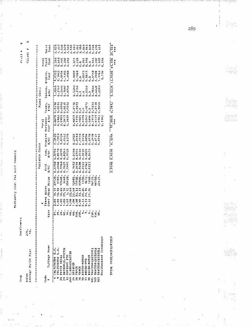
(:ro

P

Acr

es

Àve

rrgo

F1?

ld S

i.za

Cod

eg

T¡,

llaqe

¡la

Be

6 C

ULI

rVÂ

mR

H.D

.l¡

cuLT

IyÀ

Ît)R

t.D

.20

PR

ES

S D

RIL

L24

HA

nBO

¡J (

S.T

OO

TH

)12

coñ

oIN

E P

TO

264

C.B

RO

ÀD

CÀ

ST

BR

Sun

tIôuc

rs

2 t5

"60

.

26 S

PR

Àf

ER

3ó l

Rfr

CÍ

.16

TR

0C

Í10

ÀU

GE

R-r

.roT

oR1 1

ÀuG

En-

pTo

10 À

0c9R

-to1

0R10

1 T

RÀ

CT

OR

ID

IES

ELI

101

TnÀ

CT

OR

(D

IES

EL)

101

T8À

cToR

(D

IES

ELI

Una

lloca

ted

Insu

rânc

e

lOT

AL

CO

ST

,/ÀC

F E

/FIE

LN

I'tac

hine

ry C

osi

Per

Acr

+ S

unm

try

varia

hl.e

C

osts

F

itêl

Cos

LSü

îo+

èl

Tot

atllD

cs

Àcr

es

Fu?

l l,u

b.

tlepa

irs

varlâ

Þ19

T

nsur

. In

vesr

. D

?prp

c.

Frx

gl

Iot.¡

lS

Lze

Ove

r /tl

cur

Pric

e 5/

\C

$/¡r

C

ç¿/Ã

C

Cos

t S

,/ÀC

î/^

C

$/À

J C

ost

Cos

t C

osr,

'¡ì:-

-r:o

õ-ìe

-.1i

-177

2õ .-

o:"

tSg-

õ;õî

î¡--

õ:lît

ã---

-õ.

ur ñ

¡ -0

;6¡7

d--

-î;tõ

ã5 -

-i;õt

i2-

-t;t

6B- -j;

ît 5

39.

1.00

1t|.

76 9

107.

0.J

r¡60

0.0

519

0.19

03

0.58

82 0

.00r

J 0.

Jl5l

t)

. Jr

t61

0.66

9 l.¿

57zt

t. 1.

00 1

0.8ö

l?5

00.

{J.1

968

0.02

95 1

,fJ12

6 2.

0e90

0.0

060

0.25

e5 0

.665

q 0.

9.J1

1.0

J060

. 1.

00 2

7.76

366

0. 0

.162

1 0.

0241

0.0

552

0"zt

r17

0.00

J3

0" lr

t4,

0.13

92 0

.29'

, 0.

529

1r¡.

1.

Lro

5. 1

2 l5

l¡20.

1.1

t19'

l 0.

1?zt

l ¡¡

.021

5 5.

ltt30

O.C

2O¿

0.8

15¡¡

1..t

46t

Z.Z

q¿ f

.5S

5f.U

. 1.

00 2

2.69

J.

510

60.

1.O

O 2

2,69

l2t

l80.

0.1

652

0.02

rtlJ

0.2

922

0.q8

21 0

.011

8 0.

5J9J

0.r

¡897

1"0

11 1

.q9J

ì50.

0.

50 3

J.JJ

159

00.

0.C

f'flB

0.0

103

0.05

q3

0.11

1t¡

0.00

?3

0.llr

¡¡¡

0.90

68 1

.2¿

S l.

J62

J50.

0.

50 3

J"33

159

00.

0.06

89 0

.010

J 0.

1010

0.

1fto

1 0.

0 0.

0 c.

0 0.

0 J.

180

6.

0.3J

21.

2ó 1

350.

0.A

222

0.00

31 0

.0r2

q 0.

01?9

0.0

0.

0 0.

0511

0.0

51 J

.08,

7.

0"ll

29"1

q 16

12"

0.01

62 0

.002

r¡ 0

.005

6 0.

02t¡

2 0.

o01J

rJ

.r)5

5d 0

.061

1 O

.1tg

ü.lq

l6.

0.

33 2

1.26

lJ5

0. 0

,022

2 0.

0031

0.0

1 :t9

0.

0t9¡

r 0,

0 0.

0 0.

0 0.

0 .t.

0J9

250.

78

125.

0.

2919

0.

2919

0.1

\22J

0.9

65{

rt.4

55f'

5.¡r

qJ 5

.7J5

156.

r¡

8750

. 0.

81J1

o.

rrl.t

l 0"

0119

0.

6u2{

2.

?8or

¡ J.

39t

rt.2

l066

. ¿

ç625

. 0.

0?r¡

3 0.

07rt

j 0.

0059

0.

2549

1.1

?6J

l.rrl7

.1

.511

0.11

q2

0.11

r¡ o

.lt¡l

i;0'5

-ç'r

0;[5

e0 -

ã]17

õs -

-iî;n

q56

0;i[ì

7- -

5]si

¡,¡-

-rl.

a5õs

-r g

lîõi îî:

í[q-

fr+

14

* +

is

Fr:

ld

ü

CIr

ènt

F

^)co \o

tro

P

Àcr

esÀ

veD

age

F1â

ld S

lz.?

codã I

Till

age

llôm

e

--6-

õ -u

r. iiY

- À

iõ R

-- f

r :

õ : -

¿6q

c.

FR

OÀ

DC

ÀS

TE

n2¡

¡ H

ÀB

RO

IIS.T

OO

TH

I

'T C

ULT

IVA

TO

R

L.D

.6

CU

LTM

IOn

[.D.

20 P

RE

SS

DE

ÍLL

lt he

a r_

120. J0

.

26 S

P r

¡ A

f E

126

r¡ c

. B

noaD

cÀsl

ER

28 S

rÀT

n8R

(S.P

.lJ2

CO

II B

I !I E

PT

Oll

conB

IIE

(s.

P.l

36 I

RU

CÍ

J6 T

RU

CK

10 À

uGsR

-to1

0R1 1

AU

GE

R-P

1010

À0G

ER

-úO

TO

R10

1 T

R^C

ToR

ID

TE

SE

Ltl0

l T

Rrc

ToB

(D

IES

ELI

101

TR

AC

îoR

(D

tES

ELI

tlnal

loca

ted

fnsu

:anc

e

¡oT

ÀL

CO

ST

/ÀC

F

E/F

TE

LD

l!ach

lner

y C

ost

Per

Act

5 s¡

lmm

lty

VlE

iabl

e C

osts

F

j.xel

Cos

lsI

Tot

al

Tot

alT

imes

¡lc

rÊs

Pu?

l Lu

b. t

f€pa

irs

varir

blg

Insu

r.

Inv¿

ss.

Dep

:ec.

F

ircC

tc

tal

Slz

e O

ver

/llor

¡Ê P

rice

S/J

\C

f/ÂC

f/^

C

Cos

t S

,/IIC

F/À

C

S/À

.: C

ost

Cos

,-

Cos

E

¡ì:-

-l;0õ

-i¡ .u

1- r

17ao

.-õ

:5 lî

e-õ

:õü

ct--

õ:ãû

iã--

--õ

;e6-

0 I -0

;õt?

;--

-i:20

b3 --

i: D

)ii-

-r:r

6i'-

t: ?¿

E60

. 1

"OO

22.

69

0. 5

1060

. q.

00 2

5.85

J66

0.0"

1'r.

t1 0

.026

1 C

.059

3 0.

2596

0.0

03J

0.1r

tr¡¡

0.1

ì92

0.28

1. J

.5{7

J9.

J.00

1r"

t6

9107

" 0.

J919

0.0

5118

0.z

t)A

? 0.

658e

(r.

o0?J

0.

3151

x.lr

¡61

0.66

9 1.

J28

35.

l.o0

15.J

6 99

25.

0.r¡

801

0.07

20 0

.208

2 0.

?60r

t o.

o0lr¡

0.

lqrl

o.l?

7r¡

f).5

28 1

.288

q2.

1.00

16.

29 J

0750

.0.2

9'r9

0.0

44?

0.3b

q2

0.r1

1? 0

.0.J

r6

1.16

UJ

1.16

92 2

.569

1.2

8060

. 2.

OO

22.

69 1

2880

. 0.

1652

0.0

240

0.29

22

0.48

21 0

.O1l

B

0.50

9J 0

.48e

' 1.

011

1.49

J60

. 1 .0

0 22

.69

J. 5

1 0

20.

¡.00

9.

61 1

3113

.0.tq

00 0

.021

0 0.

469J

0.

6.t0

.t t)

,006

0 u.

259J

0.?

¡|?9

1.0

.1J

1.64

11t

l .

0.50

l¡.

7t¡

35¡¡

20.

1"2r

¡10

0. 1

tl6t

t¡.3

t¡30

5.

?701

o.O

zf,¿

d.8

75¡t

r.

irt6g

Z.Z

qZ 8

.012

12.

0.50

4.

7r¡

50r¡

00.

0.78

t¡3

0' 1

176

2.25

U5

J.15

6? 0

.0.ì1

6 1"

JlO

¿ ?

.tt7t

J5 t

!.2t6

¡.

r¡Jl

350.

0.

50 2

0.59

159

00"

0.1t

ll 0.

0167

0.0

8?9

0.21

60 0

.0(r

7l

0.Jl

rt¡¡

0.

9068

1.2

28 l

.r¡q

q15

0.

0.so

20.

59 1

5900

" 0"

111

3 0"

01fi7

0.1

61fì

0.29

16 0

.0

0.0

0.0

0.0

0.29

26.

0.

33 2

q.rJ

o 13

50"

0.11

90 0

.002

9 0.

0106

0"

0125

q.0

0.

J 0.

0511

0.0

51 )

.us4

7.

0.33

3r¡

"00

1612

. 0.

0119

0.0

021

0.00

48

0.02

ôs 0

.001

1 u.

ù55ü

o.0

61l

0.1

ld

0..1

19ó.

0"

13 2

r¡.8

0 11

50.0

.q19

0 0.

0029

0.0

11e

0.01

16 0

.0

0.0

0.0

0.0

0.0J

r¡25

0.

7812

5.

0.15

9-,

0.15

9t O

.OZ

2ì O

.9o5

.t q.

r¡55

rJ 5

.qr¡

J 5.

60J

156.

¡¡

0?50

. 1.

4018

1.

u018

rì"

01 1

9 0.

602{

2.

7804

3.1

9'

r¡.7

996l

'. 20

b25.

0.

0 0.

0 0.

0059

0.

25q9

t.tz

6j

1"4J

7 X

.qJ7

0.0r

¡76

0.0r

.r9

0.04

8

q:7

e\1

o.12

,to -

7lE

lõ¡¡

--î

l;35õ

ì o;

ã[îi-

-ã

. ]ã

85-t

îlq

5'¡î

-z6l

Esq

qõ;

e55-

**l

+**

ûú

t

Piè

l aì

¡

clL=

nt !

N)

\o

Itacl

tln€f

y C

cst

Per

Àcr

'5 S

'tmm

a:y

,:rop

Ê

l ax

see(

l F

tltd

d l0

Acf

,es

2I'1

. C

li:nE

t

tÀ

vera

ge F

leld

S

izì

rì0.

Ver

iatr

lP

Ccs

ts

Fix

;:l

Coj

isI

To!

?l

Tct

ttC

ode

Tj-n

es À

cres

F

uel

Lub.

PÈ

palrs

Var

llþIâ

In

su:.

Inve

iL.

D?p

rec.

fix

e¡

lcta

lr

l1lla

qe

Nån

e Íìi

ze

Oye

r /t{

ruÊ

P

rice

6/^C

S

/AC

S

,/^C

C

ost

S/A

e S

/AC

i/i

la

Cos

t C

osc

Cos

t--

ã-õõ

;îiv

A ff

iF -r

ñ:--

----

----

----

--¡ì

:--

j:õõ-

l e:i1

-117

10:-

a:

'¡ E

î6-õ

;oî

lt--õ

:11ã

ri---

-0;r

rt¡î

-õ:0

ttr

---

i. Z

r- 6

; --

ì;õlì

t - -ã

:iõF

- -¡

. iõ,

¡2r

¡ rlÀ

RR

og(s

.Too

ltll

6u.

3.u0

27.

t6

J660

.0.1

621

O.O

2qr

0.05

52

0.2¿

r1¡

0.00

1J

u.lr¡

r¡,

r.11

92

0.28

t \)

"529

20 P

RfìS

S D

RIL

L ¿

8.

r.0o

10.

86 1

7500

.0"1

e68

0.02

e5 1

"s't2

6 2.

oeq0

0.0

060

0.¿

59>

0.6

65q

0.93

1 t.0

Jo26

SP

FqY

ER

60

. 1.

OO

22.

69 1

2880

.0.r

652

0.02

rilì

o.2e

2'¿

0.

¡¡r.

t2't

t).(

,118

0.

5J91

q.q

R97

1.0

11 l

.¡t9

.t28

5fÀ

lllsR

(S.P

.)

¿O

. 1.

00

(r.0

J 13

113.

0.1r

3t1

0.02

00 O

.Uq'

t2

O.6

00l¡

0.q0

60

iì.25

9J 0

.?t¡

79 1

.0lJ

1.

614

.r2

coftB

rile

PT

o l¡t

. 0.

50

5.55

35r

¡20.

1"0

592

0.r5

rt9

.l .7

()6t

r u.

92ug

o"0

202

{J.8

r54

1..r

06ft

2.¿

42 t

. 16

?26

SP

Rây

ER

60

. 0.

50 2

2.69

128

00.0

"165

2 O

.Ozq

S O

,2s2

2 0.

q$21

0.0

118

0"50

9J 0

.489

7 1.

011

1.49

J36

TR

UC

K

350.

0.

50 6

r¡.2

8 15

900.

0.0.

r5?

0.00

5t

0.02

¡t2

0.rJ

6q2

o.o0

7J

o.ll4

,r

Ð.9

06rì

1.2

¿S

l.¿

98J6

TR

IICK

J5

0.

0.50

64.

28 1

5900

.0.0

.15?

0.

005J

0.0

52q

0.0e

14 0

.0

0.c

0.0

o.ct

c.

091

10 A

UG

ER

-IIO

îoR

6.

0.

JJ r

¡0.9

9 13

50.0

.0tt5

0.1

011

0.00

6r¡

0.01

9? 0

.0

0.u

0.05

1J 0

.051

0.0

711l

À0G

ER

-PT

o 'r.

0.

J3 5

ô.20

161

2. 0

.018

4 0.

001J

0.0

029

0.01

26 0

.001

1 0.

055ú

0.0

611

0.11

t J.

1lr

10 À

rJcB

R-n

oroR

6.

0,

t3 4

0.99

1J5

0.0.

0t15

0.0

01t

0.oo

?2

0.02

05 0

.o

c.J

0.0

0.0

0.02

010

1 T

BÀ

CT

OR

(DIE

SE

L)

250.

78

125.

0.

rrl7

8 0.

43?8

O"O

22r

ù.9ô

5¡¡

rt.r

t558

5.¡

¡'¡,

5.09

1?6

q c.

nBoÀ

DcA

ST

ER

60

. t.0

0 22

.69

J.5r

0l0

l T

RA

croR

(orE

sELl

15

6.

¡¡87

50.

0.71

99

O,7

't99

0.01

19

0.b0

24 2

.?8o

tt !.t

st

q..tT

t10

1 îR

ÀC

ÎOR

(DIE

SE

L|

66.

¿O

b25.

(r

.o?r

r3

o.o?

0j 0

.005

9 0.

25r¡

9 1.

176'

l"q

jt 1.

511

una

lloca

ted

Insu

ranc

e O

. I 0l

? 0.

lO¡t

0.

1 O

r¡

tolÀ

L co

51/À

cR

E,/F

tELD

llli4

E d

;¡õ'

72 -

71õ5

1¿ -

--îd

;ãl5

l o:2

tîZ-

-519

5õt-

rEtl4

TÇ

-zõt

5dõ'

tî;

d'86

--+

ti **

t +

ûr

N)

\o

t:àch

j.ner

y C

osi

EÌ9

r À

cr5

:ìum

mlry

Cro

p P

Ltxs

eerl

pr,ll

d 6

l lÀ

cres

28

t1,

Cli:

oE

ü B

Àve

rlge

Fle

lrl

Slz

a 60

.

Var

laþL

e C

osts

l,i

x=l

Cos

lsI

Tr.

aI

totâ

lC

ôde

Tin

es

À:E

3s

Fu"

l Lu

b. R

epai

rs v

arla

bl.

Tns

ur.

Iny¿

st.

lrlpr

-c.

pixq

ì IJ

tàI

0 lll

lage

N

eme

Slz

e O

yer

/Hou

r P

rj.ce

5/

\C

5/A

C

S,/À

C

Ccs

+-

s/tc

Í/A

C.

t/^C

C

ose

Cos

t C

ost

-6-ð

û;õi

v iîô

ñ-r':

õ;--

---

¡¡î;-

î:0õ-

ie:1

7-21

1ro:

- o:

r' tî6

-õ:

0îlt-

- 0;

lîts-

---

õ; r,

;n ì-

õ:õ

iid--

-î;1

0-ã;

--T

:õjT

i--t;t

6 l--

;: T

,¡ 6

2tt

tlÂR

8ol(s

.Too

Tlll

ó0

. 1.

00 2

7.?6

J66

0. r

J.16

21 0

.02¡

¡:r

0.05

52

0.2q

1? O

.00l

J c.

144t

0.

11e2

o.z

\t c.

529

201

C0S

TO

| S

PR

ÀlIt

lG

t'0.

1.00

22.

69

J. {

66.r

ctL

ÎIvÀ

ToR

L.D

. 39

. J"

0(ì

18.7

8 91

07"

0.J5

82 0

.05J

7 0.

19î3

0.

6tt2

2 0"

00?3

0.

Jl5t

0.

t461

0.

669

l,¿11

6rr

RÂ

8RO

l P

ÀC

KE

R

60.

r.00

2?.

?6 7

000.

0.2

07¡t

0.o

ltt

0.or

t1q

o.2t

sg 0

"00?

2 0.

3114

o.2

662

0.58

5 3.

865

20 P

R85

5 D

nrLL

28

. 1"

00 1

0"86

l?50

0.0.

1e68

0.0

295

1.u?

26

2.O

9c0

0.00

60

0.25

95 0

.665

r¡ 0

.9J1

J.0

J028

SIA

TH

ER

IS.P

"I

20.

1.00

9.

03 lJ

113.

0"1r

]q

0.02

r)o

0.r¡

r¡?2

0.

ó006

0.0

060

0.25

91 0

.?¿

t?9

1.01

1 1.

614

3l c

ostr

NE

(s.

F.l

12.

1.00

5.

6? 5

0r¡(

;0.

o.65

52 0

.09r

ìJ 1

.8flJ

1.r

2.6t

7J 0

.031

6 r.

3702

2.8

7r¡5

t4.

zil,

6.91

rr36

TS

UC

K

150.

0.

5c 3

7.u¡

l 159

00.0

.061

9 0.

0091

o.o

4fr9

0.

120

1 O

.o()

'Æ 0

.ll¡¡

r¡

0.90

68 1

.225

1.J

r¡9

16 T

RIJ

CK

35

0.

0.50

3?.

04 1

5900

. 0.

cì61

e 0.

0093

0.0

909.

0.

1621

0.0

0"

0 0.

0 0.

0 0.

16¿

l0 À

UG

ER

-IoT

OR

6.

0.

13 5

5.11

lJ5

0.0.

Coe

6 0.

0011

0.0

0r¡8

0.

010?

0,0

0.

0 0.

0513

0.0

51 î

.066

11 À

U3E

R-P

10

7.

0.33

75"

5b 1

612.

0.00

61 0

.000

9 0.

0022

0.

oo9q

0.c

o1J

0.05

5d 0

.ct6

1l 0

.110

ù.1

2s'1

0 À

UG

ER

-rlo

roR

6.

0.

31 5

5.11

135

0.0.

0086

0.

00rJ

0.

0051

o.

or52

0.0

0.

0 0.

0 0.

0 ù.

tjls

101

ÎnÀ

ctoR

lDIE

sELl

25

0.

?u12

5.

0.1r

¡59

O. 14

59 O

.O22

r 0"

965'

¡ r¡

.r¡5

58 5

.qr¡

¡ 5.

5d9

101

TF

ICÎo

R(D

IES

BLI

-1

5b.

¡t8?

50.

0.10

63

0.10

63 0

.0.1

39 0

"60¿

11 2

.780

4 3.

19t

J.50

J10

1 T

RÀ

CIO

R(D

TE

SE

LI

66.

2062

5.

0.0?

¡t3

0.0?

4J 0

.005

9 0.

25¡1

9 1.

1761

1.¡

¡l¡

l.5ll

frna

lloca

teal

fns

uran

ce

0.10

11¡

0. 1

01 0

.101

lOT

ÀL

CO

ST

/ÀC

R

E,/F

IELD

Z:q

906

0-;[4

ã6 -

515ã

"r -

--õ;

õ2]q

ol2

Ei2

- -6

1õ59

t-rF

lEd7

6-zî

lEõt

Ill

tÐt-

l+i

ltt

ûû+

N)

\o N)

CE

op

Âcr

es

^ver

f,ge

Fíe

ld S

lz.

¡ V

aria

ble

Cos

ts

Fj.x

cd C

osrs

Tfta

L

Tct

rlC

ode

dine

s À

cres

F

u+L

f.ub,

Rcp

airs

va

lirþl

e In

sur.

In

vef"

.. D

ep:e

c.

Ftx

ciI

Tlll

age

tlalle

si

ze

over

/llc

ur

Pric

e 5/

ic

$/À

c 5/

^c

cos+

- s,

/Àc

Ã/^

c 5/

Ã:

cîs.

- co

si

6 cn

Lrrt

Àm

R H

;n:

qr.

z.oõ

-ìtt:

63-ã

-lîro

;-õ.

;tis-

o;õt

u2--

o.llî

o---

-0;ti

16-ô

:0tts

---î

;206

5--i:

õlît-

-ã;tb

5--i;

ie7

2q f

l¡TR

RO

H(S

.TO

OlH

t 60

. 1.

00 2

6.r¡

8 16

60.

0.r6

99 0

.025

5 O

.057

9 O

.25t

l 0.

00Jt

0.

1.tr

r, 0

.1.t9

2 0.

¿81

).5

r¡.1

6fl f

ÀR

RO

II P

AC

KE

R

60.

1.00

26.

r¡u

70C

,0.0

.21?

r¡ 0

.012

6 0.

0r¡.

14

0.29

ltt 0

.r!1

-r¿

?.

lll4

1.'¿

66¿

0.5

t,5 \

.¡.U

/820

1 cr

tsT

on S

PR

ÀY

Í.JG

60

. 1.

00 2

2. ô

9 J.

4(ì

64

CU

LTT

VÀ

T(}

R L.

D.

39.

1.00

17.

70 9

107.

0.J

800

0.05

'/0 0

.201

9 o.

6lrJ

e 0.

007J

ù.

Jt51

0.

Jrt6

l 0.

669

1.J0

820

pR

ess

ÍTR

ILL

2a.

1.00

10.

86 1

7500

.0.1

96ft

0.02

e5 1

.872

6 2.

r)9¡

ro C

.00ô

0 0.

¿5e

5 0.

6654

0.9

11 t

.0J0

28 S

rÀÎH

ER

(S.P

.l 20

. 1.

00

8.75

1Jl

13.

0.11

77 0

.020

7 0.

q617

0.

6201

0.0

060

0.25

9J 0

. r¡

¡79

1"O

lJ

l.bJ3

3l s

oltE

rNB

(S

.P.l

12.

1.00

5.

J1 5

0¡00

. 0.

?OC

r¡ 0

.105

1 2.

011?

2.

A19

2 0"

0316

l.J

7ü¿

2.

ft7rt

5 tt.

2't6

7.0

9636

IP

UC

I(

350.

0.

50 J

?.0q

159

00.0

.061

9 0.

009.

1 0.

0489

0.

1201

0.0

0r1

0.t1

'¡4

0.90

68 1

.22S

l.J

rt9

16 T

Rrr

cK

150.

0.

50 J

r.ot

¡ 15

900.

0.0

619

0.00

9.t

0.0e

(ì9

0.16

21 0

.o

0.0

0.0

0.0

J.16

2l0

AU

GE

R-I

iOT

OR

6.

0.

33 5

5.11

115

0. 0

.rt0

86 0

.001

3 0.

0n48

O

.eì1

¡t?

O.r

) O

.ù

O.O

5ll

0.05

1 c.

06b

11 À

UG

ER

-PT

O

?.

0.3J

?5.

56 1

612.

0.00

61 0.

00r'9

tt,o

o22

0.flo

94 0

.001

J ,r

.J55

d o.

061l

0.

118

ù.1¿

8l0

Àflc

BR

-nor

oR

6.

0.lJ

55

.11

1350

.0.C

0t6

0.00

11 0

.005

3 0.

01s2

0.o

0.

J 0.

0 o.

o J.

015

101

1RÂ

C1O

8(D

rEsE

L'

250.

7U

125.

0.

30eó

0.

3196

0.0

22)

0.9b

54 f

¡"45

58 5

.4rt

j 5.

t5l

101

ÎnÀ

croR

(DtE

snll

156.

¡1

8750

. 0.

1115

0.

1115

q,0

1'J9

0.

6J¿

¡t 2

.780

q l.l

9?

t.508

101

TF

ÀC

TO

R(D

TE

SE

LI

66.

2ù62

5.

0.ol

rt3

0.0/

43 0

.005

9 o.

¿5q

9 1.

1761

1.r

tJt

1.51

1Itn

allo

cate

d ln

sura

ncê

r).1

01s

0.10

1 O

. to

l

Ftlx

seeC

155. 40

.

i,!ac

hrne

:y C

os--

ler

À

ct?

Sun

nary

TO

TA

L C

OS

T/À

CF

E/F

TE

LD?:

ET

Eõ

õ;'¡-

l?t

-51-

B'ìr

¡¡ -

--ql

2l6l

s ol

2'¡-

17-

-o-lo

-596

-r51

5õ26

'-zîlE

õî f

T:tõ

6-!t*

ft+

t+

*

Frr

ld

ð

CIr

:nr

s

1¿

lcta

l

N)

\o \ñ

Cro

p

ÀcF

eiÀ

verô

qe

Fie

ld

Siz

-

V a

rlabl

;)

Cos

ts

FlrÊ

J C

osrJ

I F

ôt¡r

l T

o+-a

Lco

dà

Tla

es

Àtr

:s

Fu

3I

Lub.

FÐ

palrs

var

rabl

c rn

sur"

Ín

v.is

t. D

znre

c.

gt x

fl fJ

rtÌ

I lrl

lage

lla

m"

51ze

O

ver

/¡lo

ur

Pric

e 5/

^C

S,/À

C

f ,/.

qC

Cos

t $,

/tìC

$/

ÀC

i/^

C

Cos

t C

osr

3ost

-6-.

uL rï

îÍîõn

ï;n .

----

- ¡i:

--î;o

õ-ìÇ

77-1

111õ

.-

o-.,r

e 1

ã-õ

. õt

Jt-

-õ:tì

¡ã-

---õ

; st

r,ì -õ

;õttü

-- -

T. ;J

6s-

--T

. õl

Tt-

-ã:¡

6 i-

-i; T

î,,20

1 C

US

TO

II S

PR

ÀlIr

"c

60.

Z.A

0 22

.69

J.9l

¿2t

r H

ÀF

Ro¡

l(s.T

oorH

l 60

. 1.

0c 2

t.7Þ

Jb

60.0

"162

1 0.

ozq3

0.0

552

0.?u

tt 0.

0013

0.

l4rlt

c.

tj9¿

o.

zlt

0.52

9ó

SllL

TM

loR

ll.n

. J5

. 1.

00 1

6.U

0 99

25.0

.t¡3t

ìtt 0

.0()

5tl 0

.1{l0

J 0"

69r¡

9 {-

}.0t

ìlq

0.1{

¡l 0"

1?rq

0.5

28 l

.¿¿

lq

cuLT

rvÀ

10R

L.D

. 39

. 3.

00 1

fl.?8

91C

r7.

0.15

82 0

.05J

7 0.

190J

o.

6u2¿

0.0

0?J

0.J1

51 0

.1r¡

6, c

.669

t.¿

t120

PR

ES

S 0

FrL

L 42

. 1.

00 1

6.29

30r

50.

Q.2

97e

0.O

r¡r¡

7 0.

3692

C

.'r11

? 0.

0316

1.

Jbd0

1.1

692

2.56

9 J.

280

26 S

PR

qYE

R

ô0.

1.$o

2'¿

"69

1208

0.0.

1652

O.O

2rtr

r O

.2s2

2 0.

r¡dz

1 0.

0118

0.

509J

0.r

,trJg

¡ 1.

011

t.r¡9

J2t

l sH

ÀT

HE

R (

s.P

.l 20

. 1.

|J0

9.01

131

11.

0.13

34 0

.020

0 o.

qtt-

t2

0.rì

00r¡

0.0

060

0.25

yJ o

.-tq

79 1

.01J

t.6

trt

12 c

ollB

IllE

PT

O

lq.

0.50

5.

02 J

5q20

. l.l

7:¿

8 0.

1?59

4.1

0¡12

5.

t¡52

e O

.O2O

¿ 0

"U15

¡¡ 1

.lq6g

?.

.2q¿

,.6

95ll

3otlB

rllE

(s.

P.t

12.

0.50

5.

02 5

0r¡0

0" 0

.?rl1

l 0.

1112

2.1

J0r.

r 2.

9831

0.0

J16

1.Jt

¿2

2.tt7

4> t

t.2t6

1.

¿5g

10 À

UG

ER

-íor

oR

r,.

0.:t3

19.

0b 1

J50"

0.0

2¡t7

0.0

0.J7

0.0

1J8

0.r)

q2j

0.1

0.J

0"05

1.1

0.05

1 0.

09q

l1 À

trcE

R-P

ro

'1 .

0.lJ

26

.15

1612

. 0.

0lf|1

0.)

02',

0.00

62

0.4?

70 n

.ool

J ü.

J558

O.0

6lJ

0.1l

lj ).

lrt5

l0 a

UG

ER

-Eoî

oR

6.

0"13

',19.

08 l

l50.

0.o2

rt7

0.00

1',

0.01

5r¡

0.0¡

¡19

0.0

ù.J

0.o

0.0

c.04

¡¡16

TR

tlcK

35

0.

0.50

15.

8r¡

1590

0.0.

1qq?

0.0

217

0.11

41

0.?8

0¡t

0.00

?J

0"3t

4rr

0.90

61t

1..¿

ztJ

1.50

936

TnU

CK

35

0.

0"50

15.

rJ¡¡

159

00.

0.1r

t47

0.02

1? 0

.212

7 0.

l?q1

().

¡J

0.0

0.0

0.0

t.3r9

l0l

TR

AC

ToR

IDIE

SE

LI

250.

78

125.

9.

1459

0.

1115

9 n.

o22|

0.

9b54

r¡.

455f

t 5.

'¡r¡l

5"58

910

1 T

nÀC

ToR

(DIE

SE

L,

156.

q8

750.

.J

.tlfj?

r,

0.tls

?6 0

.011

9 0"

6J¿

q 2"

7804

l.j9

t r¡

.2s4

101

ÎRÀ

CT

OR

(DIE

SE

LI

66.

2062

5.

o.0

0.0

(r.0

u59

0.25

¡¡9

1.1?

6t

1"r¡

l?

t.qj7

Una

lloca

têd

Insu

ranc

e ô.

0r¡?

6 q.

oqq

0. O

qtì

8a r

le y

216.

60.

'tach

lner

y C

osi

Per

Àc:

:e S

umm

a¡y

rOT

ÀL

CO

ST

,/ÀC

R

E/P

IELD

AC

:UIIÚ

LÀT

gD C

OS

T,/À

CR

E

,/FO

R E

FT

ER

PR

IS

E

l;8s7

6 õ:

5Elî

-õ'1

56'r-

r

I " 19

55 0

.479

3 6.

805

r¡

Pr-

5Id

r

CIi:

rr'-

¡

1l

--îî;

01,¡

s 0:

tdìt-

-u.

Iiu6-

rî.

õEqî

-zõl

5o[

3B;5

50-

+t*

*t

a r+

t

10"4

fro2

0.¿

s1¿

6"

1¿rl

1r¡.

6571

21.

025

31"5

06

N)

\o È

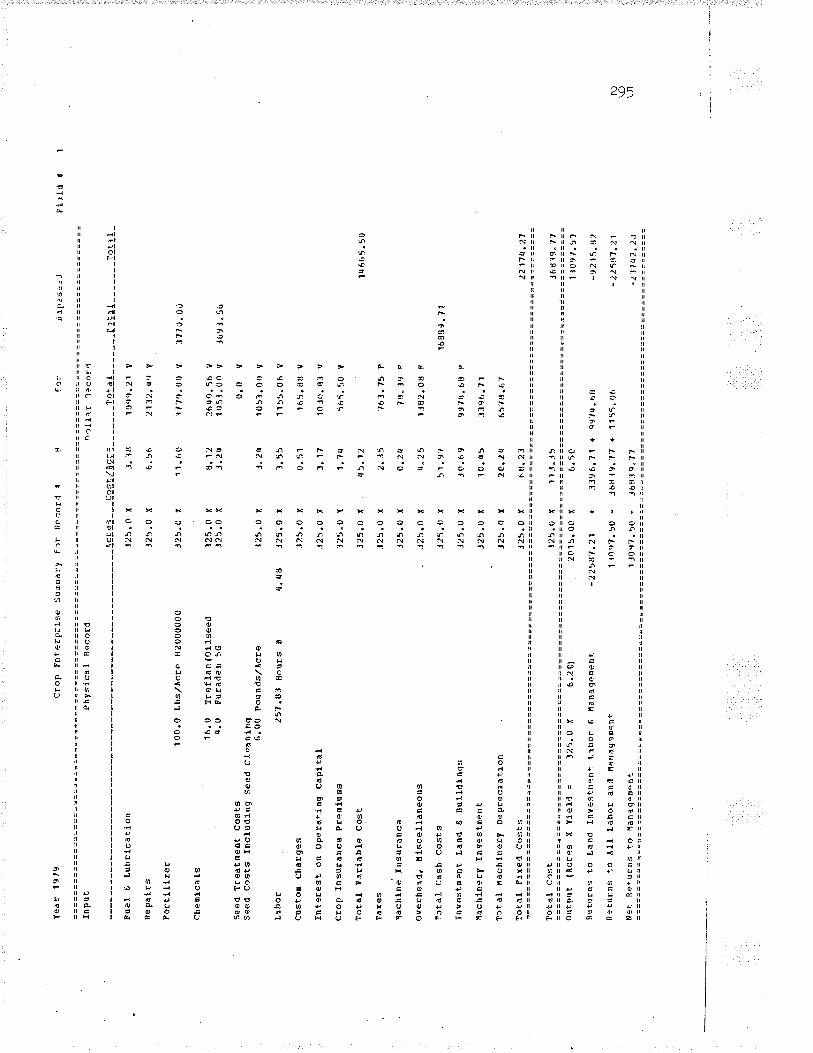
Yea

E 1

9r9

fnpr

rÈ

Fue

l C

Luh

rLcô

tlon

Rep

alE

s

FeE

L ll

lze

r10

0.0

Lbsl

Àcr

e 82

0000

00

che

olca

Is

16.0

lrc

flan

(olls

eeil

It. 0

F

urad

e i¡

56

See

d T

reat

neot

C

osts

seed

cos

ts

fncl

udln

g se

ed c

leaf

¡1ng

6.00

Pou

nds/

Àcr

e

Laþo

r ¿

51"ð

J H

ôurs

ô

cust

o¡

char

ges

Inte

r€st

on

Ope

ratln

g C

aplte

l

CE

op fn

sura

trce

prg

Elu

Es

Tot

al

v¡rla

bIe

Cos

t

Tax

es

lach

lne.

Ins

t¡E

ance

Ove

rhel

d,

lllsc

sllã

neol

¡s

TJt

aÌ

Cas

h C

osts

Inve

stsQ

nt

Lanr

l E B

ulld

lnqs

i\¡la

chln

e rl

I nY

estn

ent

Tf,t

al

ñach

lner

y D

epre

cÍat

¡.on

Cro

p F

nteE

p;is

c S

uDna

::y f

)r

Rec

or,l

Í

Phy

sica

I

Rec

ord

nolla

f'1+

cor4

!sË

e.:_

__ q

s!!/À

ç::_

____

__T

9:sl

_ __

___

_q I

!1!_

_ _

___

_i2.

!1I_

J25.

0 x

J.ltt

10

q9.2

1 v

325.

0 X

J25.

0 x

125.

0 x

J25.

0 X

t25.

0 x

r¡. f¡

8 J2

5.0

r

.r25

.0 x

J2s.

tl f

t25"

0 f

J25.

0 X

.r25

.0 r

J25.

0 x

. J2

5.0

f

J25.

0 X

J25.

0 x

J25.

0 f

J2b.

0 f

J25.

0 f

Tot

aI

Plx

eil

cost

s

lota

l cô

st

outp

uÈ (

Àcr

es x

Y1e

1.l

=

125.

0 I

ô.20

)

Ret

r¡rn

s to

La

nd I

nves

tmcn

! Lt

bor

¿ ü

anag

enen

t

netu

rns

to

Àll

Labo

r an

il na

nage

Den

t

N9t

Re+

uEns

to

Éan

ågôm

9n+

-

icr

6.56

11.1

r0

lt.12

3.2t

¡

3.2t

t

3. 5

5

0.51

l" 17

1"'rq

rr5.

12

2.35

0.24

tt" 2

5

51.9

7

30.6

9

1C.t¡

5

20.2

q

6H.2

J

21 1

2. t

ttt u

t?7r

).{r

0 v

26¡¡

0" 5

6 V

1rJ5

l.0fì

Y

0. (

, v

r051

.00

v

1r55

.06

v

165.

88 V

t0_r

o. fJ

l v

565.

50

V

?61.

?5

P

78.

_19

P

1 '8

2.0I

J F

99 r

rr.6

0 P

Jlq6

.?1

lì57r

J.67

i,lP

Js¿

.1

37¡0

.0ù

Jô9

l. 56

Fi.)

Id

t

?015

.0c

x 6.

5c

-225

117,

21 +

33

96.7

1 +

cgr

q.hu

Llo,

l7.5

0 -

368t

9"t/

+ 1

15s.

r)6

1J09

7" 5

r.r -

Jôtìt

q.7

7

i25.

0 x

ll3..t

5

1q66

5.50

1658

r.?t

¿2

11rt

" 27

J681

9" 7

7

1 ì0

97.

5C

-9 2

15.

ft2

-¿¿

531.

¿1

-¿tlt

¿2.

¿ù

N)

\o L¡

Yea

r l9

r9

fnpu

t

Fue

l E

Lub

rlcat

ron

R-.

pa

l rs

FeE

ttllz

er50

.0 L

bslÀ

cre

I155

0000

Che

olct

ls

Èo

Che

Glc

als

Use

d

See

d T

reàt

E9n

t C

osts

See

d C

osts

Inc

lual

ing

See

d C

lean

lng

1.75

Pou

nds,

/Àcr

e

Labo

iltr.

gU

Hou

rs ð

rt

.4g

Cus

trn

Cha

rges

Inte

rest

on

Ope

Eat

InE

Cap

leat

lota

l. V

aria

bl€

cost

R9n

t

liach

tne

Insu

ranc

€

oYer

held

, ífs

cella

neou

s

Tot

al

câsh

Cos

ts

ñach

ioer

y In

yest

Den

t

Tct

aI

Éac

hlne

ry

Dep

reci

ar-lo

n

Cro

p F

nrer

pris

: S

urrn

ary

for

!ìêc5

rd t

Phy

sica

l- R

ecol

d

Tot

al

Ptr

eil

Cos

ts

60.0

f

r¡?.

19

lcfe

s C

aSt,/

Àcr

ê T

otâ

I

Tot

aI

Cos

t

60.0

x

1.59

e5

.57

v

60.0

x

1. 5

r¡

92.

6lJ

V

60.0

x

6.6'

ì r¡

00.5

0 v

outp

r¡t

(Acr

es I

yl

eld

=

60.0

x

1.r¡

01

pâtu

rns

to

L.an

d In

vest

eent

La

bor

ô Ë

anag

eDen

+

Pet

urns

to

{ll

Laho

r an

d ¡ll

nage

nent

:let

Fet

'lrns

to

ia

nag"

nenr

.

Dol

ll¡

1?cô

rd

fôr

0.0

v

ó0.0

x

t¡.q

6 26

1.15

V

60.0

x

1. l4

80

.56

v

60.0

x

22.9

5 13

16.

7r¡

v

60.0

Í 3.

58

21q.

72 U

60.0

x

42.1

rt

2528

.52

60.0

f

1 2.

00

?20.

00 P

60"0

x

0.2¡

t lr¡

.t¡.¡

F

60.0

x

l¡.25

25

5.15

P

60.0

x

5 8.

6r¡

15

18"

14

60.0

X

10.q

5 (t

2 l.q

8

60.0

x

'¿o.

zu

1214

.51

lùn;

ll¡

y

IJta

I

lotì

I

4J0.

50

Fi:I

d '

8q.0

0 x

37.5

0

-21¿

9.19

|

62 l.

OA

+

0.0

J150

.00

- 53

59.7

5 0

80.5

6

.t150

.00

- 51

59.7

5

60"0

x89

.11

2fJl

1"2ì

5J59

.t5

r150

.0c

- 1 50

2.1

C

-212

9"79

_2 ¿

0e.7

5

N)

\o

Yea

r 19

/9

Inpu

t

Pue

l 0

Lubr

icât

ion

Rep

a lc

s

FeE

tlllz

er

ilo F

cEtil

lzeE

U

sed

Che

oi.c

t ls

J2.0

F

ound

up

168.

0 X

3t

J. 1

5

See

d T

reat

oen

t C

osts

See

d C

osts

Inc

Ludj

-ng

Sre

d C

lean

ing

0.0

Bus

hels

/¡lc

re

16t,.

0 X

0.

C

Labo

r 22

.81

tfour

s a

q. q

8 16

8.(J

t

0.f,

1

Tnt

eres

t on

Ope

ratln

g C

aplta

l l6

ft.O

X

3.?q

Tot

al

Vac

labl

e C

ost

168.

0 [

rtrt

.'¡6

Rsn

t r6

u.o

x r2

.oo

iach

ine

Inso

ranc

e 16

8.0ì

x

c.?,

q

Ose

rhsì

d,

¡lisc

4lla

neou

s 16

8.0

X

r¡.2

5

Tot

aì.

Câs

h C

osts

16

8.0

X

61.?

5

Itach

iner

y In

vest

oent

16

8.0

x 10

.¡¡5

Tot

al

tach

''ner

y D

epre

clat

lon

169.

0 X

¿

O"Z

U

Tot

al

f tr

erl

Cos

ts

r6U

.0 X

¡t

?.1

9

Cro

p E

nfôr

p[:.s

r S

umea

rT f

or

P,:,

c)r4

I

PhÍ

sica

I F

ecor

dD

ol l

;ì :

e.co

:4

À!Ë

.-s

___q

2s_!

lÀçs

:.___

____

Iq!q

¡__

____

_! n

! è!

- _

_ __

_ _:

e l1

! _

16rl.

(¡ X

0.

90

15{)

.96

V

161i

.0 [

0.

16

124"

tt2 V

Tot

rl co

st

outp

ut

(ÀcD

es x

fie

ld

- 16

r.1.

0 I

0.o

l

netu

Eni

to

I.and

Iny

esto

enf.

Labo

r ¿

lla

nage

nênt

eetu

cns

to

All-

Lat

tor

tn¿

l rla

nage

nent

{}t

ne'u

rns

to

llanà

g€m

-ônt

-

tot

Sum

¡crt

ìIl

Jy

6509

.8o

V

b50j

.80

¡).t)

v

0.0

v

10?.

20 v

628.

05 V

201

6.00

F

40.5

2 P

't14"

t¡ì

F

't02J

0 "

l7

l r55

.8t¡

.lr¡0

0" 6

?

Fr3

ld

o

0.0

- 't

53 ¿

tu .

(ì? c.0

0. f

)

168.

0 X

91.9

5

0.0

t r5

5. t

l4 +

n.

4

15ltq

6.rt

7 ì

102.

20

15¡r

4 6

. rr

7

1 11

9. q

2

7927

.t]5

1 5q

q6"

8 '

0.0

-l J5

8¡l.r

ìJ

-151

44.6

7

- 1 5q

q6.8

'

N)

\o -_l

Y¿

ar l

9 r9

rn p

ut

Fuè

I E

l,u

brrc

at i

on

qepa

fr

s

Fer

tiltz

er

Che

nic

ä ls

See

d T

reat

men

t C

osts

5--e

C C

osts

Inc

ludr

ng

Sse

d C

lean

inq

0.0

Labo

r

Inte

rest

on

ope

ratin

g C

aplta

l

Tot

âl

Uar

labl

c C

ost

nent

üàch

ine

Insu

ranc

e

Ove

Ehe

rd,

ílsc€

llane

ous

Tot

al

Cas

h C

osts

Itlch

j,ne

ry l

nves

t¡en

t

Tot

al

tlchl

nery

D

epre

clat

lon

Crc

'P P

nteE

pris

È S

umm

ûry

for

Pec

orrl

F

R

fo:

PhY

slca

l P

ecor

d D

olllr

a-

ien!

-1

No

Fer

tiliz

er

Itsed

No

Ch€

nlca

ls U

setl

B u

s he

ls /

Acr

e

2:1"

?6 lt

ours

A

4.48

Tot

al

Plx

ed C

osts

Tot

aL c

ost

Out

put

(ÀcE

es f

rt

-.ld

.

t5.0

.X

(r.0

)

Ret

urns

to

Lana

l T

nggs

tnen

+.

Labo

r ¿

lla

nage

ngnt

nètu

Ens

to

AII

Labo

r an

d üâ

n19e

ngn:

ll4+

- R

t'ìrt

Et¡

s ùo

Ita

nagc

a3nr

15.0

f

s"6t

lr.

t.ll

v

15.0

x

3.l1

11

5.11

8 v

35.0

x

15"0

x

35.0

x

35.C

r I

35.0

Í35

.0 f

15.0

x

15.0

[

15"0

[

35.0

r

:t5.0

x

Sun

illèr

flllc

¡ F

i-rll

i

If,rd

l ro

tal

0.0

3.04

1" t

9

'12.

rì1

12"0

0

0.24

q. ¿

5

29.3

0

1 0.

45

20.2

4

u7"

19

0.0

v

1" O

V

106.

q5

v

fr2.

59 V

r¡2'

).00

F

9.4r

r P

1q8.

8q P

.165

.80

7rjft

.4,

0.0

f 0.

0

-199

l. 1

3 f

t65.

8n +

35.0

x

0.0

0.0

59"

()(¡

- 2(

ì99.

-r8

+

- 2C

q9-7

A

q4l).

2 J

tù25

.51

0.0

1(rf

) "

45

1651

"55

2 09

9 .',

ì 1

().t)

- 16

27 .

5 t

-'l9e

3.

J '

-2l(t

9.,tl

N)

\o co

Yea

: l9

r9

Cro

p F

x+er

prts

¿ S

upna

ry f

or

Fec

oii

I

Inpr

¡¡

Phy

slca

l R

€cor

d

Flls

I ¿

Lub

rrca

tlon

Rep

ai.r

s

Fer

t il

rze

r64

.0 ¡

.bs/

ÀcE

€ tì2

0000

002J

5.0

Lbs,

/Acr

e 10

3t¡0

000

Che

nlc

e Is

16.0

T

retla

n (O

ilsee

l

Sce

d lre

atoe

nt

Cos

tsS

eed

Cos

ts I

ncIu

dlng

S

e€d

Cle

anln

g1.

60 P

ound

s/À

cre

Labo

r 26

J.tt5

8or

¡rs

ô

Cus

ttrm

Cha

Ege

s

fnt€

rest

on

Ope

ratln

g C

aplta

l

Dry

ln9

Cos

ts

Tot

al

Var

labl

e C

ost

R9n

t

fach

lne

Iosu

ranc

e

Ov€

EhÈ

âtlr

ttlsc

ellå

neou

s

Tot

aI

Cas

h C

osts

l'tac

htne

ry f

nye

sto¿

nt

lota

I ña

chln

erf

Dep

rec!

atio

n

Tot

ð1.

Fl¡

3rl

cost

-3

OcI

l3.:

nêco

¡rl

ÀçE

es_

--(:

2¡!/¡

c !Ê

____

_ _

_12!

1 !

___

____

1,:.!

s!__

___

__ls

!4!

_

JlC

ì.C X

r¡

.ll

t341

.Jl

V

.110

.c x

.r10

.0:(

.110

. 0

x

rt0.

c x

J10.

0 f

r¡"4

d '1

0.0

x

J10.

0 t(

J10.

0 f

310.

0 x

310.

0 x

J10.

0 x

110.

0 x

310.

O X

J10.

0 x

J 10

.0 x

J10.

C r

Jto.

0 r

Ttta

I C

ost

outp

ut

(AcE

es Í

yi

eld

=

310.

0 x

1200

,001

Ret

urns

to

f,and

Iny

estE

ent

Libo

E ñ

ían

agcn

ent

Pet

'¡ç¡.

to

À

lì. L

ôþor

and

lanl

gem

ent

l{+t

Bêt

urn,

ì to

ña

nage

0"nt

ic:

9. l

rt

7 .4

220

.91

8.12

10.

Èr)

J. tt

1

0" 5

1

5.69

6.00

7 6.

't q

12.(

r0

0.2t

|,i ¡¡.2

5

93"2

4

l0"l¡

5

20.

2t\

Ir7.

t9=

==

==

f==

==

12 3

.97

Sun

tIgriE

S

?¡lJ

rr.7

1 v

2J01

.Atr

v64

8t.6

t¡

V

251r

J,69

V

0.0

v

110

8, 0

r) v

r180

.2t¡

v

15rì

.2J

Y

1764

" 05

V

1Rö0

.00

l?20

" 00

F

7q"'t

7 ?

1J1r

r"29

P

32J9

.9t¡

62 1

5. 0

r¡

u7d5

.0d

251

{J.6

9

Fi:i

-d

¡

J 12

q00.

00

x

-3?5

8.09

+

3 Jr

¡ 7C

. q9

-

J10"

0 r

3 J¿

t 79

. 99

-

0" 0

q

.12.

t9.9

4 +

0.

0

I8r¡

l8.1

2 +

1 lr

to.2

r¡

ìtsq1

8..r

2

2 t7

t)o

"29

28 9

C l.

l5

1tt

628

"O2

J8t¡

r 8

. 12

Jtq7

9.99

- 51

8. 1

5

- 1

r51.

t. D

q

-49t

fì. J

.'N

)\o \o

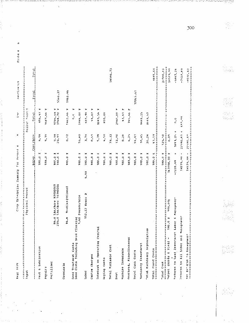
Yea

r 19

79

C:o

p !ìn

terp

cis;

S

unD

ary:

or

Ileco

rd I

Inpu

t

Fue

l ô

Lubr

lcat

i.on

iepa

lr s

1 $0

.0

x

Fêr

+- ¡.

1 1z

e r

t16.

0 Lb

s/A

cre

8200

001J

0 18

0.0

X

2J5.

ú Í.b

slÀ

cre'

10J4

000U

18

0.0

X

Che

mic

a ls

16.U

T

retlä

n(O

llsee

al

1110

.0 X

See

d T

reat

men

t C

osts

See

d C

osts

fnc

lIdin

9 S

eed

clea

nlnq 'ì.60

P

ound

s/¡lc

re

1tJ0

.C f

Labo

r 15

2.22

Hou

rs A

q.

4g

180.

0 X

¡ hy

s lc

a I

Rec

or¡l

cust

o0 c

harg

es

Tnt

eEes

t on

Ope

ratln

q C

arllt

al

Dry

ing

Cos

ts

Tot

al

YaE

labl

e C

osÈ

18

rJ.0

X

Ren

ì, 18

0.0

X

¡lach

lng

Insu

Ean

ce

1gct

.0 X

over

herô

, ill

scel

l.ãne

ous

180.

0 X

Iota

l C

ash

Cos

t s

1 f1

0,0

f

tach

inâr

y rn

sest

nlnt

18

0.0

r

fìoIl.

ìf

D-c

c:rl

[s!Ê

s _ __

çe¡!

/Àc:

s._

____

_ _

I2!1

! _

___

___

t ]i3

!___

____

Is:

t !

_

1t10

.0 X

¡r

.51¡

B

tl).r

t, V

-ot

al-

[âch

lner

y I]e

prec

lat-

1on

lota

l F

rred

Cos

ts

-5!a

l co

st

lutp

'¡t

(Acr

ès X

Ylq

Ii =

{le

turn

s to

f,a

nl

Inve

s-.n

ãnq

Labo

r ñ

Éan

agem

enè

¡?tu

rns

to

Àll-

Lah

or a

níl

rtan

agÃ

oêrì

t

t ar

9.3l

t

9.98

20"r

J1

8.12

10.8

0

:1.7

9

0.51

5.79

r¡.5

0

74,3

2

12.O

rJ

o.2u

t1.2

5

9¡¡.

fì1

10.q

5

20.2

q

Net

RÊ

| ¡r

ns

+ o

ll a

n ag

cucn

r

Jdût

IJr-

'rs

1trt

l7.6

6 V

1?95

.6fr

Vl7

6r¡.

70

v

I r¡

h2. 4h

v

1. t

) v

I q4

4. O

() V

6u1,

94 V

91.8

' V

10 r

¡ 1.

5rì

v

tì10.

00

216(

ì.00

P

ql.r

l 1

F

't65.

t¡6

F

r'ì81

.25

J541

.5?

180

.0 x

18t1

.0 x

1t 0

.0 x

lncì

.o x

.r

00.0

0ì

55b0

.17

I 46

2. 4

b

Fie

ld

{

180.

0 x

lflo.

0 f

q7.1

9

1620

00.0

0 x

0.0q

-7J2

tì. (

9 +

18

9 1.

25 +

l¡t57

9. c

9 -

2259

0.q1

+

1'¡5

79.9

9 -

2259

0,01

1s0.

0 x

125.

50

tq0e

6.7l

17C

ì65"

61

It¡5'

C.9

q

0. (.

) -5

u¡¡7

.24

681.

qq

-712

1ì.r

¡9

¡tr¡

91.6

9

225t

l0.tt

t

-,t0

lc.q

lU

J O

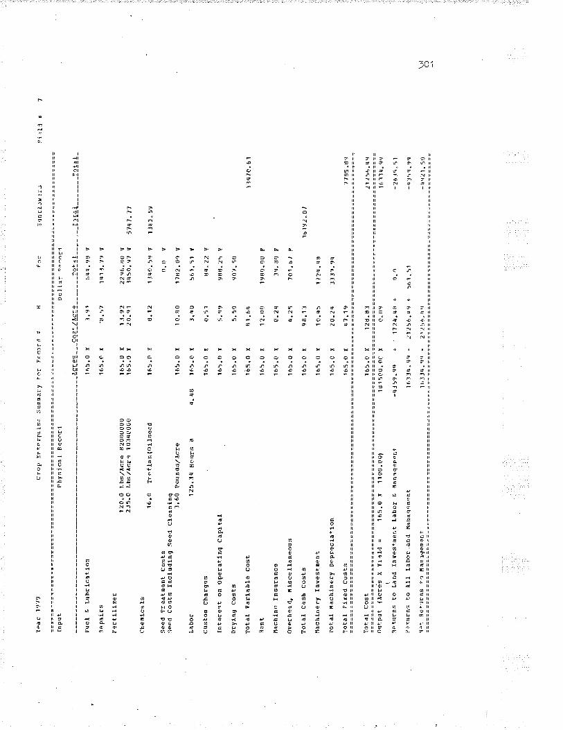
YÞ

a r

1'.r

,9

In p

ut

È'u

e.l.

¿ L

ubrlc

etlo

n

Rep

ãirs

Per

tlltz

er12

0.0

Lhs/

Àcr

ê t|2

0O00

01)

2J5.

0 f,b

s/A

cre

-l 01

t|000

0

che

ñlca

ls

16.0

T

refla

n(oj

.lsee

d

See

d T

reat

osnt

C

osts

Sec

d C

osts

Inc

ludt

ng

See

d C

leln

lng

1.60

Pou

nds/

Àcr

e

LabÕ

r 12

5.3q

flo

t¡rs

ô

Cr¡

sto[

Cha

rges

Inte

rest

on

Ope

ratln

q C

aplta

l

OE

ylng

Cos

ts

Tot

al-

varla

ble

cost

Ren

t

tlach

lne

fnsu

rànc

ê

Ovc

thee

rl, l

lsce

llane

ous

Tot

al

cash

Cos

ts

flach

iner

y In

yest

oent

Tot

aL

lach

iner

y D

epre

crat

-1on

TÕ

ta l

Fi.x

ecl

Cos

ts

crop

Ent

Þrp

ri.s:

sum

nary

tor

F

Êca

rd I

Phy

sica

l R

ecôr

,l

ÀsL

eÞ.-

_-çq

:.:lÀ

s!3

rrr5

.0 X

.ì.

91

165.

0 X

'8

. 5?

165.

0 x

1t.9

216

5.0

f 20

.e1

165.

0 X

g.

12

Tct

al

Cos

t

Out

-püt

(À

cEel

s X

ytå

lrl

=

I65.

0 X

11

00.(

r0l

tR

etur

ns t

o La

nd I

nves

tme.

.,t

Latlo

E 0

fta

ntq+

nenr

P9r

urns

ï.o

ÀIL

LaÞ

or.a

nd il

ônaq

enen

t

DoI

ll:-

D-c

ôr.l

l it

165.

0 x

10.8

0

4. q

8 16

5.0

X

3.r¡

(J

165.

0 [

0"5X

165.

0 f

5"q9

165.

0 r

5. 5

0

1b5.

0 x

rJ1.

6rr

165.

0 Í

12.o

Q

1ô5.

0 x

0.2¡

.¡

165.

0 X

tt.

25

165.

0 X

9u

.1t

lh5"

() r

10

.tt5

'r 65

.0 x

¿

o.24

1ô5.

() X

r¿

-¡.1

9

'¡õr:

Rei

trns

tD

lla

nage

nant

19ll!

____

-__

!ìEÀ

!___

___

_I?!

1À_

6r¡u

.9r,

v

1rr1

l. ,e

v

2296

.rt0

vt0

50.e

, u

57q1

.77

t.ìq0

.59

v 1t

4J"5

9

c.0

v

1782

.0,)

v

561.

51 V

trt!

" 22

u

98rr

" 25

V

90'r.

5()

1960

" 00

F

39.8

r) F

70r"

b, F

16ty

2.0,

1r2q

"q8

3 t J'

t.9¡.

¡

:i'rn

tlJr:

riF

i)Il

r

1U15

00.0

C

X

-r¡J

59.

qq

+

lÍ.lJ

l¡.99

-

lhlJ

r¡.

q'¡

-

165.

0 X

l2{r

.81

0" 0

9

1724

.t)tt

o .)

.^

It25l

ì.!9

+

561.

51

21,,|

':6.r

¡q

tìq70

.61

r?rJ

5.8'

l

¿12

56.r

r9

1 fì

'l 'l

l¡. 9

,,

-26J

5.51

-u35

9.9(

l

-r¡e

21"

50\j] o

Yèa

r 19

r9

f n

Prl:

F[e

l E

Lub

ricat

ion

iì?pa

irs

Per

tlÌiz

erî¡

¡ r.

0 Lb

s,/lt

crÊ

10J

q000

C

Che

nicì

Is

16.0

T

retla

n (o

iIsee

C

Sêe

{1 I

reat

men

t C

osts

See

d C

)sts

In

clud

ing

See

d C

Ieah

lng

3.60

Pou

nds/

Acr

e

Labo

r l¡J

s.tjr

¡ H

oDrs

ô

::op

lln+

grpr

rs:

Sum

ma:

y fîr

tì.

cfr4

+

Cus

tom

Cha

rges

fntê

resÈ

on

Ope

ratln

q C

apÍta

I

Dry

lng

Cos

ts

lota

l V

arla

ble

Cos

r.

Iìèn

t

[ach

lns

fnsu

Ean

ce

Ove

r h+

td,

fllsc

ella

neou

s

Tot

al

Cls

h C

osts

Hâc

hln¡

ry

Inve

stne

nt

Tôt

aI

Tac

hine

ry

Dep

Eec

iatlo

n

Tot

al

Flx

erl

cùst

s

Tot

al

Cos

t

Phy

srca

l F

€cor

d

275.

rJ x

2',r

5.0

x

275.

0r X

2't 5.

tì x

¡r. qe

27

5.0

x

275.

0 x

275.

0 Í

275.

0 x

2?5.

0 X

275.

0 x

275.

O t

2-r5

.0 x

275.

0 r

2r5.

0 x

275.

r)

(

2?5.

0 x

¿75

.O X

1.

52

96t.6

r,

V

r)ut

put

(Acr

es X

Yle

ld

=

2 15

.0 L

00.

r)0)

ì

D¿

tuE

ns t

o Þ

and

fave

stre

nt

LabD

r ¿

; lla

naq-

Õm

ent

Îe tu

rns

to

Àll

Laþo

r an

rl

lana

qêm

lnt

DoI

Ilr

D.1

1:rt

1"o:

iu

nfllH

):i

8.32

22

8,r.

rì

U

1 l.0

t|l5-

ttì.tt

¿

v

t|.12

22

tu.

¡Z V

0.0

v

10. fr

o 29

?D. tìc

v

1.13

ril

z.55

V

0.51

14

0.1h

v

tr.:ì

8 12

01¡.

q7 v

3. 5

rì

e{ì?

. 50

55.2

t

12.o

0 lt0

().0

0 F

0.20

11

6. l!

F

t1"7

.5

1l6q

.q5

P

't1,

t6

1C.l¡

5 28

7r¡"

1r¡

20.2

4 55

6b.5

¡

¡t7.

19

llet

R¿

ji ¡r

ns

tÒlla

nago

¡.¡¡

I)ra

i

J5)1

.ú2

¿¿

14"

J¿

Fr

r ld

¡

I?:1

!-

1925

10.

O0

x

-100

17.9

1 +

1 r1

24.

(|9

-

1712

4" 9

q -

275.

U X

l0 2

. l¡6

0.09

2tìr

r¡.lq

è

1.0

2R1i

5.48

+

a J2

"55

I 5

199.

00

19r.

i4.?

9

lfrl¡5

.urt

IA1

r5,

l¡tì

l¡ì20

.99

-7tr

4J.-

19

-1r1

01?.

91

-1r)

850.

r¡,)

129r

6.4.

r

\,J U N)

Yea

E 1

9 r9

lnpu

t

Pu6

l ¿ L

unrlc

a+,ío

n

Rep

airs

Pèr

t ili

-zer

r¡3"

0 L

bslÀ

cr€

ti200

0000

2J0.

(l Lþ

s,/à

cs€

lU3l

¡000

0

chen

ica.

l-s1.

J A

vade

¡8fl

(¡rh

ô1tl

10.0

T

refla

n (c

eral

s)10

.5

Z'4

-D A

min

e 8C

Sas

d T

reac

nent

Cos

tsS

eerl

Cos

ts I

nclu

dlng

!ìê

ed C

lean

ing

'1 .5

U D

ushe

ls,/A

cre

Labo

r 1l

¡(r.

48 H

ouE

s ä

Cro

p Ê

nt+

rnris

: S

r¡nn

ary

f1r

Þ!c

)r(l

d

!rhy

s ic

a I

Pec

ord

Cus

t)n

Cha

rges

Inte

rest

on

Ope

ratln

g C

apita

l

Tot

al v

erlrÞ

le

Cos

t

nsnt

Ëac

htne

Ins

uran

ce

over

held

, ll ls

cel

lane

orts

Tot

aI C

ash

Cos

r-s

Slc

hlne

ry In

Yes

tnen

t

Tot

aI í

¡chl

nery

D

epre

ct a

tron

Tot

aI F

lxed

Cos

ts

Tot

al.

Cos

t

19!.:

=.

_ --

ç2::

¿¡ç

r_:.

120.

C [

5.

5.¿

120.

0 f

7.8J

120.

0 x

l2').

0 x

120.

Ct

x

120

.0 x

4,q8

12

0.0

x

120

.0 x

120.

0 Í

120.

0 x

12U

.0 \

120.

0 '(

-t20

.0 r

120.

0 f

12Lì

" 0

l(

120.

0 Í

120

.0 {

.)ut

prrt

(À

cret

x Í

leld

=

12

0.0

x 2o

.01)

tR

etur

ns t

o l.a

nal

Tnv

es!:F

4nt

Labo

E t

lrana

gem

en+

Rôt

r¡E

rìs

to À

lI La

hor

and

!lana

gem

ent

120 .0

x12

0.0

x

l)c Il

r:

D. co

r 4

for

{et

R€t

r¡rn

s to

tfa

nage

r¡en

t

tl.9r

,2 0.

4'l

't.5

t5.

081.

1t¡

6.r.

l

5.24

1.n2

5.lrt

70.9

3

12.0

0

0.2r

¡

l¡.25

81 "

tt2

10.4

5

'¿0.

2u

¡r7"

1<

ì

lo!

1l

tJta

l T

otì

I

6ô:¿

. t6

V

9J9.

65

V

59rJ

.56

V

?f¡5

6. ¡

¡0 V

915.

00

V

609.

l6

V

1.17

.0,r

v

0.0

v

fJl)1

. Q

n v

62e.

l6

V

122.

50 V

6arl.

2H V

1440

.0r)

F

2tl.

(t0

F

51n.

11

F

't254

.17

ztl ¿

9 . 05

'd¡ì

iJL

Ft:

tù s

3054

. 96

l6b

1 .

t¡5

't 20

. c

f

'lltt

"'l ¿

2l¡f

)0.0

0 x

4.qt

l

-21'

t¿"6

l +

1 07

52.

O0

-

1075

2.00

-

f25¿

t.17

+

0.1ì

1l¡1

,l¡.

011

+

h2q.

lfì

1f¡lr

q.n?

tl51

1" 5

fr

1Crr

9ù .

80

566¿

.tt6

lrl l

rq.r

)2

10?5

2.01

-151

8.5r

)

'¿19

2.rt

l

' 1t2

2" t

)z\ñ o \n

lear

19

t9

Cro

p lìn

terp

rtsè

S

umm

dl-y

tor

D

è1c)

r.l

t

Inpu

t P

hysi

cal

Fec

ord

Fue

l t

Lubr

icat

lon

ReP

alrs

Per

tlIrz

eEq8

.0 L

bs/A

cre

8200

0000

chen

lcal

s6.

9 lts

ulox

F8.

0 B

uctr

l I

ü

See

d lre

atE

ent

Cos

tsS

eed

Cos

ts f

nclu

dlng

See

d C

lean

ing

3l¡.

00 P

ound

s,/A

cre

Labo

r 21

0.92

Hou

rs ô

cust

oa c

haE

qes

fnte

Ees

t on

Ope

f,atln

g C

aplta

l

crop

Ins

uran

ce P

Eeo

luE

S

lota

l va

Eta

ble

cost

nent

-

Itech

lne

Insu

ranc

e

Ove

rhea

rl,

ñ ls

cella

neou

s

Tot

al C

âsh

cost

s

ñach

lnèr

y fn

v¡)s

tmen

t

Tol

- eL

É.ìc

hlne

Ey

Dep

rccf

atlo

n

Tot

al F

lred

Cos

ts

\

2'17

.O X

27't.

O r.

'277

.O r,

277.

4 r.

277.

O Y

,

¡{.

rr B

27

7 .0

r.2'

17 .O

X

277.

O t

'¿'1

, .0

t27

1.0

r,

'¿'r7

.o L

'¿7'

t.I Y

,

277.

0 r

'¿77

.O r,

277,

O X

lcE

e.g

-- -

!a,s

!¿Â

sE

2-_

____

_12l

r I

'2'r'

l.a Y

l.5

rì

99¿

.2J

V

Tot

aÌ C

cst

2't7

.O f

B

9.rt

0

outp

rrt

¡ncr

eJ x

yie

lil

=

277.

o r

12.1

0)

,tbt.7

0 x

?.?r

¡t

9eqi

lrns

go L

and

Inyg

stoe

nr:

Labo

r 0

Ìlana

qom

€nt

514.

50

+

2tt9

5.01

r o

1.1

Dol

la !

: P

ecor

l

tor

Fet

urns

to

ÀIt

Labo

r an

d fa

nag-

men

t

7.05

5.5?

3"ue

3.7¡

¡

9. r

.9

3.4

1

0.51

3.5

n

1.18

q2"¿

1

t2.o

c

o. 2

l¡

tt. 2

5

58.7

1

10.r

t5

Net

!c:

'¡rns

to

tia

naqc

nent

¿

r¡l1

3" J

l¡ -

2t¡

161.

15

195t

.'ru

v

15q¿

.l4 V

107f

r. f

J5 v

't(lJ

5.9r

ì v

0.0

v

268r

t.1..t

V

gqq.

92 U

141.

3r' V

992.

50 V

J2t¡

. tl6

V

1J24

.00

F

6b.8

1 F

11 7

7. 9

(' F

2895

" O

¡l

560

r.05

Flì{

s:id

15r¡

2. J

¡¡

2114

"81

Pi:I

J I

r0

277.

0 t

2t.2

4

21','

,O r

, ¿

¡ 7"

1 9

2ftlì

l.lq

- 2u

76).

¡5

r 9r

¡rr.

92

I 1 69

2. 9

0

1ô¿

6 1.

b7

I 30

?0"

46

¿4

t6.l

. t\

¿ul

ll..1

4

_{40

9.5r

t

5l 4

.51

-q.i0

. f¡

1\,J È

Yea

r 19

r9

InP

ut

Phy

srca

l F

+co

fd

nolll

r oô

corr

t

Lcrq

rì

rôsr

./Àcr

ê __

__!2

:å!_

-___

__t¿

tÈ!

t'uel

6 l

.ubr

lcaù

r.on

28

r¡.0

X

J.rt

tr

976.

r8

V

Rep

airs

2g

r¡.0

x

5.5u

15

{6"t

ìrl

V

Fer

t tl

lzer

chè

nicã

ls

See

rl T

reat

nent

Cos

tsS

eêd

Ccs

ì-s

Incl

udln

g S

eed

Cle

anln

gl¡¡

.otj

poun

ds/À

cre

Labo

r 2J

q"41

tto

r¡ts

A

Cus

tom

Cha

rqes

Inte

rest

- on

Ope

ratln

g C

aÞl,t

al

Cro

p In

surln

ce P

reF

lr!B

s

Tot

.al V

aEla

ble

Cos

t

qen

t

Hac

hinâ

ID

sura

nce

0ver

he¡d

, ll ls

c¿Ila

neou

s

Tot

al c

âsh

cost

s

l'lac

hln

3ry

I nY

estq

en t

-ota

l,tac

hine

ry

Dêp

reci

atio

n

Tot

aL F

i.xed

cos

ts

ciop

Ent

erD

il,sa

Sum

màr

y tlr

p+

cf,r

rl ¡

l¡o P

ertll

izèr

us

ed

l. fl

Ava

dex

BH

(o1

].s)

Tot

al

Cos

t

r)ut

put

(Àcr

eF x

fic

ld

=

28r¡

.ct

( 9.

oot

t

rletu

En.

s to

Lìn

d Iq

vest

nent

Laþ

or E

¡la

nage

ncn+

9etu

rns

to À

Il La

t¡or

a0i

l ia

ntge

mên

r

Net

Re+

,¡rn

s to

ñaF

agen

ent

2H¡l'

0 X

2fJ4

.0 x

t¡" r¡

8 28

r¡.0

x

28r¡

.0 I

zfìr

¡.0

x

. 28

rt .0

{

28fi

.0 x

28q.

0 x

2tto

'0 X

2ttq

.0 x

28r¡

.0 [

28rt

.0 x

2fìr

t.0 x

¿8q

.0 r

f rr

1O.r

r',

9.69

'I .7

0

0.1¡

-,

J..ì.

ì

1.1t

!

-1t

. 0f

)

12.

o0

0.2t

¡

l¡.25

5ll"5

f)

10.r

¡5

2î.?

q

rt7"

19

3iår

s':l(

l

Jlll"

rn

v

D.O

V

z-r5

1.96

V

r95r

1.17

v

't32.

28 U

9t¡5

.61

v

lJ5.

12

v

l40r

r. o

'J F

6ft.5

0 3

l20r

. tI

P

2rt 6û

" 20

5ll¡9

" r5

Fi:I

d I

:2!È

!_

10J1

"?c

11

2556

,00

x 7.

'¿^

1rì5

56.5

6

-l¡6r

jq.0

5 +

29

É8"

21ì

ê q"

rì

-16ì

5.95

It155

6.56

-

2r¡2

10"'r

o +

1fr

5o.1

7 -t

600.

05

1115

56.5

6 -

2q21

0.r'r

-5

rr5s

,2|

?8ft

. tt

frJ

5.25

l0rt

?9.6

2

15r¡

9J.u

lt

lì,t4

1.16

¿r¡

210.

r9

u] o \'l

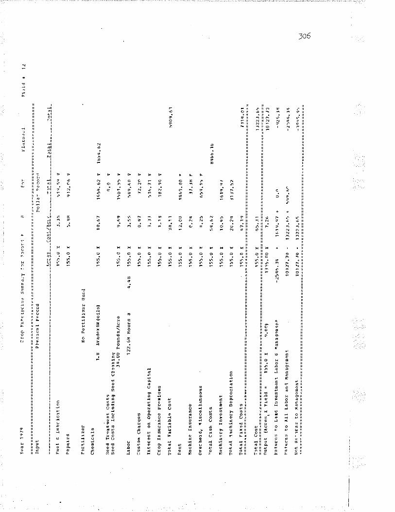
Yea

r 1t

lr9

InP

ut

Fue

l 6

Lubr

ica

t io

n

PeP

atE

s

F?E

tillz

er

ùo F

ertll

l-z3D

usÉ

d

chem

icrls

l" I

Ava

dex

Bg (o

ltsl

See

d T

Eea

t;€nt

cos

tsS

fed

Cos

+-s

Inc

Llrr

ring

See

il C

leln

lng

3u.0

0 P

ound

s/À

cre

Labó

r 12

2.61

1 H

ours

A

Cus

ton

Cha

rqes

Tnt

eres

t on

Ope

rat-

1rg

Cap

ltal

cEop

Insu

r¡;c

e P

reE

lìrns

Tct

al v

aria

ble

cost

Rèn

t

llach

ing

Insr

rran

ce

over

hold

, il

lscê

llane

ous

¡ota

l C

ash

Cos

ts

I'trc

hln

ery

f nv

est¡

¡ent

Tot

al l

achl

nery

D"p

r€ct

atlo

n

Tot

aI F

¡.fe

d co

sts

Cro

p !'n

tF r

Frr

st

5lìm

md-

'y f

tr

P?c

)r1

þ

Phv

srca

I

Pec

ord

Þol

.la-

?')r

o:d

lc:

is, --

-ç9.

:.',

¿t!ç

LÇ _

__

_ __

I l:

1 !

___

_ __

_E ¿

iÈ !

_ _

_ _

__ _

I9 !

I !

_

155.

0 x

J.35

51

.J.5

q V

155.

0 x

5.rr

fr

912.

06

v

T"t

al

Cos

t

155.

0 x

155.

0 t(

r¡.r

¡8

155.

0 x

155.

0 x

'I 55

.0 x

r55.

0 t(

155.

0 x

155.

0 x

155.

tl

x

155.

0 x

155.

0 r

155.

0 x

155.

0 X

155.

0 x

outp

ut (

Àcr

est

x Y

reId

=

155"

cì [

9.r.

r0l

Ret

ucns

to

Låld

I¡v

esto

ènt

Labo

r 6,

r!a

naql

Een

t

Pât

urns

to

Àll

Labo

r an

.l tta

nag€

E"n

t

Nct

RE

' ¡rn

s to

Iän

agem

ent

for

10.6

I

9.69

3.55

0.4?

l" ll

t.1H

I8.1

3

1 2.

00

c.2q

u.25

5r¡"

62

10.r

¡5

2(\,2

q

07.1

9

¡ I,i

Ks,

):,1

1fì5

4. ó

2 V

I b5

4. 6

2

tr.9

v'1

501.

95 V

549.

60

V

',2.2

î v

516.

71

V

1rJ2

" 90

V

5909

.61

186?

.00

P

.17.

_lll

F

{ì59

" 15

P

8r¡6

b "

l6

t619

.et

11J7

" 52

FirI

d r

1¿

1l?5

.0Q

){

-25t

1â.3

¿l

+

1Q12

7.7(

) -

l0l¿

7"

r0 -

155.

0 x

¡15.

:11

7.26

1f.l9

.q',

+

U.n

'l 32

23.f.

5 I

5r¡q

.6ô

lJ22

J.lì5

7llo

.0l

1 tz

z J .6

'10

1 ¿

7. t

X

-9¿

6.ìt)

-¿\tt

6.

l4

-.Ì.1

q5.9

5\ñ al

Yea

r 1

9 r9

Inpu

t

Fue

l ¿ L

r¡br

icat

lon

Rep

alrs

Pcr

tlllz

eE?4

.0 L

bs/A

cr€

115¿

¡000

0

chem

lcl

ls1.

5 À

Yad

erB

P (

FÌe

Pea

tl.9

Àve

nge

200-

c10

.5

2'tl-

D À

olne

80

See

d lre

atm

ent

Cos

tsS

eed

Crs

ts I

ncIu

dlng

See

d C

lean

ing

I .7

5 P

ound

s,/À

cre

L.rb

or

261

.otl

ltour

s A

Cus

+c¡

¡ C

harg

es

lnte

rest

on

oP

eEat

lng

caP

ltal

IÕta

l va

rLab

le c

ost

Itach

lne

fnsu

rànc

e

Ove

rh¿

rd,

tl !s

cella

neou

s

Tot

al c

ash

Cos

ts

Hac

hlne

ry T

ny-.

stnê

nt

Tot

al ¡

tichi

nery

D"p

reci

atlu

n

Crc

p F

ntÈ

rDrr

ss

Sui

lrüra

i.y 1'

cI'

necf

,c(

i

Phy

slca

l F

ecor

d

{cr9

s C

ost/À

crÊ

2'16

.C t

U

.q'l

276.

0 X

6.

56

276.

0 t(

9.

7J

?76.

0 x

9"15

2'16

.q *

4.

5927

6.0

t 1"

1r1

îota

I F

lxe4

C

osts

lota

l C

ost

Or¡

tPut

(À

cEet

s X

Tt.c

lrl =

¿

'16.

O f

2ô

.0(ì

)

R€t

urns

to

I.nnd

fnv

estm

ent

Llbo

!. E

¡1a

någe

Den

t

Ret

urns

to

Àll

Labo

r an

d na

naqe

n4nt

Nct

R€

-.,lr

ns

to

IaÌa

qen"

nl

Dcì

ì e

r D

?cor

l

fô:

216.

0 X

l.'

1q.

r¡8

216.

0 (

¡t.z

r¡

276.

0 x

0"91

2?6.

0 x

3.8r

¡

216.

A r

. [6

.16

276.

0 x

1 2.

10

276.

0 r

0.2r

t

276.

0 f

1t.2

5

276,

0 r.

62

"n5

2rf,.

0 Í

10.4

5

276.

0 [

¿Q

, ¿

q

276.

O f

rt

l.19

Tit

1l

r¿_r

J.ql

v

lHl t

.6rt

v

2685

. 7f

ì v

¿52

5.qO

V12

65"

fr2

V

Jl5.

t0

v

0.0

v

r¡74

.92

V

116r

r.60

v

25 r

" 11

v

1(t5

8.70

v

3J12

.'!Q

F

6f'.5

/ P

111t

.t1 ?

2'ìU

r¡.5

9

55 8

6" lJ

I

BlrL

jy

!29.

È!_

__ _

___!

c!è!

_

2t¡ù

5. t

ó

r¡11

6" l2

Fre

ld

{1.

1

,1 '6

. O

0 x

-69,

15.1

2 è

1 16

52.9

6 -

1 rb

52.9

6 -

276.

0 X

ql

.5r.

t

2. r'

¡ 6

20llr

¡.59

+

r)

.^

25H

17./1

+

1'l

6(l.f

rll

25ld

.17.

7'l

1279

4.05

17l'¡

6"J2

1112

1.66

l5u1

7" t

t

l ¡65

2. (

lr'

-r¡1

't0.5

J

-bq9

5. l2

-cì lb

u. 1

6U

J__

l

I. 'lc

reaq

e tly

crc

P(a

cEes

l

II.

Cos

t ot

Pro

tluct

-ion

1. F

uel

Ê L

ilb!ic

atio

n2.

Rep

aÍrs

J. P

Ert

lllze

rq "

Che

mi-c

als

5. S

.ed

Tre

atnÞ

nt c

csts

6. S

eed

E C

lean

lng

Cos

t'1

. T

sine

cos

ts8.

Lab

tE9.

Cus

tom

Cha

Eqe

s10

. In

teE

est

Ope

r. C

aD.

11.

crop

Ins

uran

ce P

reo.

12.

Dry

ing

cost

s1.

J. E

qr¡!

.pne

nr R

enta

I C

ha1t

¡. T

otaI

Var

labl

e C

ost

15.

R?n

t16

. T

lres

1r.

Éac

hlne

Ey

fnsu

Ean

ce1r

l. ov

erhe

ad,

llfsc

.19

. T

otal

Cas

h C

osts

20.

Inve

stÀ

ert

Land

o8ltl

g21

" I

nvos

t0en

t in

tlå

ch.

22"

nach

lner

y D

epc.

2.1 .

Tor

-aL

Ffx

ed C

osts

':otà

l cc

sr.:r

q{ P

Êî'¡

rn s

umm

lry P

:}r

crc[

) F

or D

.ccr

d ìlu

nbÉ

-r

TY

I'e c

t irn

'Ê:P

ti:'

Pap

es+

red

Tam

Ê ll

av

Sum

m:r

faJ-

los

'r25.

1099

.21

'¿1:

l¿.4

9tr

70.c

nJ6

9J.5

h0.

01 05

1.00

0.0

1155

.Cì6

165"

8ft

r0J0

.8J

5t5.

500.

00.

01

qófr

5.5O

0.0

'ró3.

75?$

.tq11

82.0

8r6

889"

?l99

?4 .

6 I

t396

" t1

6578

.6'

2¿1t

u.2

I

24.

Tct

al C

osts

J6

6.19

"?7

5359

.75

fII.

Gro

ss R

etur

ns

25"

Àve

rage

Yle

ld/lc

re

6.20

1"

¿t0

2b.

Ave

raqe

f'ri

ce

6"50

37

.5r)

2 ¡.

C

rop

lnsu

r.

Rev

enue

0.

O

0.0

28.

Str

au l

$/rì

cEel

0.

0 0.

029

. G

razf

nq (

S,/À

cre¡

0.

0 0.

C

Tf,t

al G

ross

Pct

urns

13

09'r.

50

J150

.t10

I

IV.

F+

:urn

s to

Iìv

estn

ant

Llbo

r Û

i,la

nart

emcn

t -9

¿15

.112

-1

501.

1'ì

V.

P1t

-'rrn

-s r

o La

boç

0 ng

n+.

-2¿

58'l

.21

- 21

29.1

9

Vf.

fietu

rns.

-o

Land

Ê t

lgm

t. -1

1'16

t.59

-16.

10.7

5

VT

I. N

Èl

R?l

r¡E

ns t

o tlq

mt.

-¿.1

'lU2.

2ll

-220

9.'1

5

Tot

ll ca

sh c

or;Ìs

eq

ual.s

th-

) su

m o

t T

a¡Ê

fì,

Fue

l t

Lu¡,

rrca

t:on,

Se€

d C

laan

rnq

an4

Tre

âtm

cn.,

Cro

p an

d lra

chin

ô In

surd

nce,

¡:

i¡c.

Àss

r¡ne

s I

l.U0(

) t

Fe+

_'¡r

n on

Cap

lta l

"

60.

e5.5

'92

.brj

1¡00

.51ì

0.0

0.0

26t.7

50.

080

.5b

1J7

6, l

tt

21q.

7 2

0"0

0"0

0.0

2528

.5',¿

-t20

.cD

0.0

14"r

1?25

5.1

535

18.1

40.

062

7.0t

)12

1 tt

. 52

¿8J

1,2)

'I 68

.

1 50

. 96

12t1

, q2

0. o

6509

. 80

0.0

0. n

{).

{ì10

¿,2

00.

062

U.0

50.

00.

cc.

0?5

19.

t¡2

2016

. ?0

().

04n

. 52

'¡1t¡

.4J

r 02

90.

't7

0.0

1755

. $r

¡Jq

rJc,

6779

27 .

u5

Srr

r¡m

art¡

-Ilo

r

ì5.

16.1

" r1

115.

rJ4

0.0

o.0

0.0

0.0

1o(r

,tl5

0.0

62.

19Q

. f)

0. r

l

0.f)

ttut)

.2 t

420.

000.

0lr.

r¡4

1q8.

tt4

In25

.51

0"0

165.

rJt

,0H

" q.

,16

51"

55

s un

froY

fIs

JIJ.

llrtl"

l1¿

dJ.t.

71J

' IJ5.

ùR

¿5l

d.6q

0.0

JJ4d

.0n

0.0

I l8

J. 2

4l5

d.2J

1 T

brt

. 05

.J.0

lJb0

. c0

J.0

2J79

J.29

J, ¿

,/. 0

0J.

ù14

"77

lJ l{

r. 2

e28

r0 J

. l5

û.0

J¿J9

,9r¡

6l /

5. ù

t¡1'

.t6 ¿

t¡.

0?

PA

.J:

Sr¡

nt l)

riirs

15rt

46.8

7 2t

!99.

-18

JUr¡

lrJ.1

2

0. c

n.

0 11

0ù.0

00.

0 0"

0 o.

J,r

0"0

0.0

J.0

0"0

0.0

0"0

n.0

0.u

ù.t)

0.0

0.0

J3,¡

rr.9

q

-1.'l

5{ltl

.tll

-lt'?

7.5j

-5

IÌJ.tl

- 15

lr¡l¡.

67

- lq

q l"

J J

-J r

58.

09

-11t

125.

66

-1rf

.2.0

1 -l9

4o.d

i

-15q

4rr.

ft'/

-21(

¡rl.r

8 -.

¡rlu

.Jì

FoD

tirs.

Fìr

''iliz

€r,

Chc

nlca

ls,

;;:.;d

,O

vDrh

+ìd

, P

Ê':i

, La

Þo!

', in

d T

vrî.:

.

1U0.

ú16.

97l6

rJ ' .ó

655

60.

'7I

l¡62

. '¡b

0.ù

19r¡

t¡ .

00c"

J68

1 .9

t91

. i7

1041

.56

0.1

81 0

. J0

J.)

1q09

6, 1

3

-_21

60.t0

0.0

4J.ir

l76

5.{6

-t70

65.6

1c.

,18

J1 .

25J6

41.

57¡ì

rt9J

" 69

2251

0.{l

e00,

c0

c. 1

9c.

)C

.!)0.

0

1r¡5

79.9

9

-54f

¡ '.

.¿r¡

--t

t¿J

"q)

-fl2

lJ.

¡.ì

-rtîl

C,

¡lU

J oc

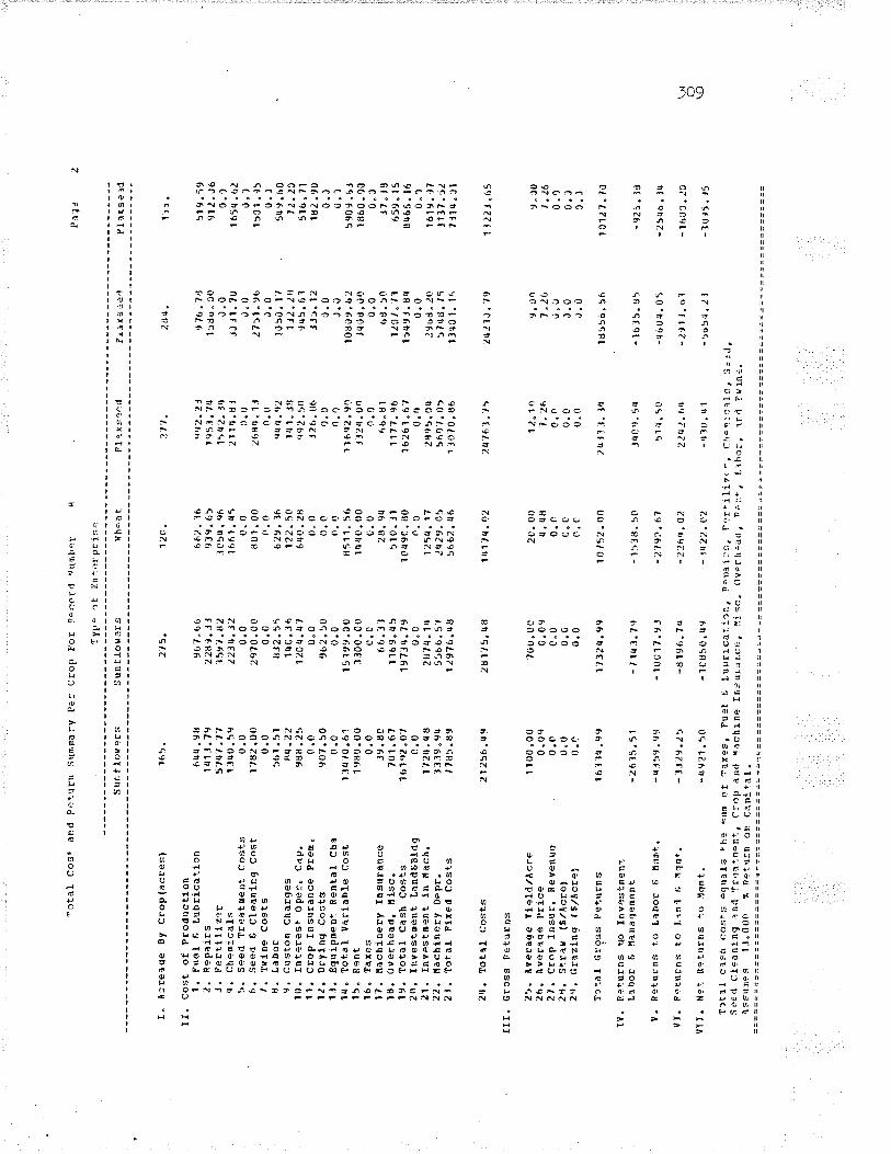
I"

Â:r

eâqe

By

Cro

p(ac

res)

If.

Cos

t ot

Pro

duct

lon

1 "

Fue

l F

, Lu

bric

atio

n2.

Rep

ai"r

sJ.

Fer

tlllz

.lrr¡

. C

heû1

cals

5. S

eed

Tr4

at[e

nt C

osts

6. S

eerl

t C

lean

lng

Cos

t,.

Tul

ne C

osts

tJ.

Labo

r9 .

Cus

to,n

Ch

arge

s10

. In

tere

st

Ope

:. ca

p.1 1.

cE

op f

n sr

¡ran

ce P

Eeo

.'¡ ¿

. D

ryln

g C

osts

1-l .

Equ

ÍP

¡¡en

t R

enta

l cha

'lU.

lota

l V

aria

ble

Cos

t15

. R

ânt

16.

lare

s17

. Ita

chin

eEy

Insu

ranc

e10

. O

verh

ead,

ll ls

c.19

. T

otal

. C

âsh

Cos

ts2o

. fn

vest

Een

t La

nd0B

Iilg

21.

Invc

stoe

nt 1

n la

ch.

22.

Éac

hine

ry D

cpr.

2r"

Tot

al-

Plre

d co

sf-s

"tal

- C

os+

and

PÊ

+-U

rrr

Sum

nary

P¿

: C

rop

['or

3êco

rd r

¡um

l'cr

. T

fp"

at ¡

:n..r

rDri.

se

Sun

tlocg

rs

suni

loH

ers

qh..a

t

1(ì5

"

6l¡r

t.98

141.

r.?9

5'rq

t .7

71J

r¡0.

590.

0l'r

n2.o

00"

05ô

1 .5

1A

q"¿

¿9U

8.25

0.0

e07.

500.

01.

lf¡r0

.ó'l

1980

.00

0"0

39.8

070

1.67

161q

2 .0

t0.

017

2q"4

813

39.9

r¡,'1

u5.

ue

zfl.

Tot

tl C

osts

21

256.

q1)

281r

5.q8

IIf.

Grc

ss R

€tur

ns

25.

Àve

Eag

e Y

ield

/Àc!

€

1 10

0.00

70

0. L

ì026

. A

vcra

qe P

rlca

0.09

0.

092

l. C

rop

Insu

r.

Rev

enue

O

.0

C"0

24.

srra

Y

($/A

cret

0.

0 0.

02r

,. cr

azin

g (î

/Ãc.

.e,l

0.C

0.

0

ÎJ:a

l cr

oss

Pet

urns

ilì

l.lr¡

.99

1r32

rt.9

9

lV.

R?t

urns

t-

{o I

nves

tnen

r.La

boD

f,

tìtan

aqeD

ent

-261

5.5t

-r

1q1.

7,)

V.

R3t

-r¡r

ns t

o La

bor

6 tir

ìm+

_.

-q.J

59.9

9 -1

0017

.9.!

Vf .

R.tr

¡rns

tc

Ll

nl

I f qm

r.

- f J¿

9,25

-U

196.

Zr¡

vII.

t¡er

_ R

_otu

rns

+.o

Hqn

t. -0

921.

50

-101

,50.

¡19

Tltl

l ct

sh

Cos

ts

êqlta

ls

Ih9

Gun

ot

îaxe

s,

Fuâ

l ¿

Luu

r]-c

àLi1

n,S

aÉrl

C1Ê

anj.n

g an

d T

Eet

i-mcn

I, C

rop

an(f

íâc

hrne

In

:^ur

rr.c

Ê,

!lisc

.ds

sum

çs

lJ"0

0n

t nÞ

irr:n

on

Cin

itâ1.

2t5.

96 7

.6 6

22rì

9. J

J15

9'l "A

2¿

23q,

320.

029

70.0

00.

08J

2.55

1t¡0

.JÉ

'12

0 4.

U',l

0"0

962.

500.

015

1e9.

0 0

1300

.c0

0. c

66.1

111

69.¿

¡519

734

.7 9

0"c

28'l

4 .

1tt

5566

.57

1¿97

6,q8

12()

.

662.

t6

¡r39

. 65

ìc5u

.96

1661

. (5

0.0

1101

. 0c

o.0

629,

76

122.

s|

6fi0

. 28

()"

00.

0o,

085

1 1.

56

1q4(

ì. O

0t.0

2 8.

9ll

51C

.ll10

49C

. iro

ô.0

125r

¡" 1

7Jq

29.0

556

62.

46

Fl l

xs"

c.l

:! ,'l

.

\trz.

2 t

195J

. '¡¡

l5 r

¡2.

'q21

14.t)

t0.

0z6

R4

" 1.

1

0. (!

qq ll

. (1

2

l4 1

. J8

'{|92

.5fì

J26.

860.

uo.

q11

6rì2

. 9r

)Jl

?q.0

î0.

066

"U1

I 17

?. q

6'1

6261

.67

0.0

2'19

5.0r

t56

0 r.

05

1 t0

70.8

6

FI.ì

xs ¿

¿,ì

2u{.

,t 16

.7tt

15du

.0('

ù.0

JJJI

. T

Où.

027

51 "

96J.

0lü

5ù"

171t

¿.¿

tl9¡

.t5.6

:lrJ

)" 1

2ù.

0J.

0tr

080,

" b2

J4ùd

. ù0

0"0

bd.5

01¿

Cl "

t-l

15i¡9

J.d¿

r0.

029

Dd

" l0

574d

.75

l3{C

l.1r'

l'àlr

FIa

rse

lrl

1rt1

74.

Q2

¿tr

t6t"

,\ ¿

q¿1J

,79

2t'.0

0 12

"1O

9.

dOl¡.

1¡l.l

l"¿

(.

7.¿

60.

c 0.

c ù"

ùC

.0

0.0

ù"0

0.c

0.0

J.ù

1015

2. O

0 2t

¡r1J

. t4

1r

r55o

.56

-153

tr.5

0 Jq

0e.5

r¡

-163

5.U

5

-¿19

',1 .

67

51tl"

5Lì

-tló

U¡t

,05

'¿?.

6q.O

Z

2¿u2

.t,q

-¿Jl

J,bl

-lu2?

.0'¿

-4

'J0.

¡tl

-,¡o

5.1

.2Ì

.rro

n1 i:

s,

l.gr.

rliz!

-,

C

hôni

r;iL

s, S

::J,

OV

Êfh

id{l

, tr

o:ì.,

l,1

hO:,

ln4.

l'VI0

-:.

1)).

5l 9

. 59

91¿

. J6

0.1

165r

¡ .6

2ù"

)15

C 1

. .¡

5

0.)

5tl9

.b0

t ¿

.20

516"

71l8

¿.9

00.

Jü.

159

09"6

31

860.

100.

cJ7

.J8

659"

t5

8r¡6

5.16

0.1

1619

..)?

J1t7

.52

7Jl't

.i,tl

'l t¿

2J.{

i5

9" )

0t.¿

60.

00.

i)3.

)

1012

7"t0

-925

. ìc

-2s¡

tb.

llr

- 1f

ì03.

.10

-101

5. J

5

\¡l \o

I "

À.r

eaqe

8y

Cro

p(ac

res)

II.

Cos

t ot

Pro

duct

lon

1. F

uel f

; Lu

bric

atio

n2.

R3p

alrs

J. F

artll

fzâr

q. c

he¡!

rcal

s5.

Sse

d T

reat

esnt

Cos

ts.Á

. S

ced

t C

lean

ing

Cos

t,.

Tcl

ne c

osts

8. L

ìbcr

9. C

usto

_E C

harg

es10

. In

tere

st

Ope

r. C

ap.

1 1.

cro

p In

sura

nce

Pre

u.12

. D

ryln

g C

osts

1J.

Equ

lpE

ent

Ren

tal C

ha1t

¡. l

otaI

Y

arla

þle

Cos

t15

. R

ent

16.1

¡res

lr.

ñrch

lnef

,I In

sura

nce

ltl .

Ova

rhea

d, lt

isc.

19.

Tot

al C

ash

Cos

ts20

. In

vest

oent

Lan

aleB

ldg

21.

Inve

stne

nr-

ln l

lach

.22

. na

chin

ery

Dep

r.2J

. lo

tal

Flx

ed C

osts

ñcta

l C

os'a

nd

Bei

urn

Sr¡

mm

ary

F3r

cro

i, po

r oâ

cord

{r

¡nb;

i:

TY

t"

ct

Dn*

erf'r

Ís+

Ra

r le

y

'¿ la

r.

12r3

"e 3

1811

"6tì

2h85

"?6

qrc6

.32

0"0

t!7c,

920"

01

169.

6425

7 "'t

1

1058

.',r

00.

0n.

o0.

012

79t¡

.05

J3r2

.rt0

0.0

66 .5

?11

13

" r

1

l?J¡

¡6.3

20"

c2t

ì8r¡

.59

5586

.81

1:10

2J.6

6

2r¡.

Tot

âl

cost

s 25

b1'l

.7 1

IIf.

Gro

ss R

et-r

lrns

25.

Àv€

rage

Yie

ld,/À

cEe

26.C

ttr26

. A

eera

ge P

Eic

c 2"

u62

r.

Cro

p In

sufo

P

even

u?

0.O

2tr"

S

tras

ÍS

lÄcr

el

0.tJ

,¿9.

Gra

zlng

(S

,/Àcr

el

0.(,

Tot

al

GF

oss

netu

lns

l?65

2"96

IV"

R2t

'¡rns

lr.

o ln

Yes

tDen

+-

Labo

r Ê

¡là

nage

eôn¿

-q

110.

53

v.

R?t

uIns

:o

Laho

r 6

ilqm

r_"

-h99

5.12

VI.

Re+

uEns

ro

Lånd

D ll

qDt.

-550

1. J

6

IIII.

Net

R+

turn

s to

ll/

¡mt.

-H16

r¡.'1

6

Tf

te I

cl

sh

cost

s ?q

rlìI:ì

t-

h+ s

uû o

f la

XÊ

s,

F|l,

tlS

r¿rl

Cl¿

anln

g aD

d îr

¿i.m

tn..,

C

:,)P

a:ld

üac

hinå

Àss

ttn+

s 1.

r"00

0 f

FF

I'¡¡n

cn

Cân

1tal

.

Tot

al-

t'a r

m I

vÊ

rì g

a

163

0.

966r

t.75

1¡89

8.0(

_¡J5

1r¡l¡

.60

J0J2

rJ.3

r0.

0'l

957r

r.7

00.

09C

¡¡4.

192.

7 q2

.'l I

llc88

"3.r

1¡.r

10.3

r,45

ft0.0

00.

0lq

l¡¡35

.t 1

2766

0.00

763.

7563

q.

J2ltl

8t¡.

1118

167r

r.'l

299

7¡¡.

6U27

ttg

? .1

951

236.

ô11 J0

940.

56

2'12

37 6

.5q

0.0

0.0

0.9

0,0

0"0

179J

rJ9.

75

-4bq

80"6

t

-ul9

rl?.

J,

-607

68.8

fì

-92r

]86

,1,

¿

0 Lu

llri

càt

i-c n

,ltr

sur

l!.c.

ì, "i

sc.

1. 3. 6

','6.

81

1J.

1611

. 5l

0.0

7..tq

0.0

l"l¡4

1. 0

l¡tt.

220.

srt

1. r

J0.

(l

51.

7810

.52

0. 2

90.

2r¡

t¡.

256q

" 08

l. 7(

,1(

; .4

520

.ztt

4i.7

9

10 3

. 57

rl1.J

è

(ì.0

0.0

0.0

0" 0

c.0

6U.2

1

-1t"

6t_

J1 "9

2

-?J"

11

- J\

" 16

l:.:n

ai3s

, !'r

'rf i1

1z.r

, C

\in:c

1,tG

. :;_

)rl,

(lVÉ

::lrì

rrl

, F

-nf

, la

hôr,

ìr

,,1

.Ht¡

;.:,

U]

(-J

Cos

t an

d R

etur

n P

lr À

cri

Per

cf:o

p po

r R

É:o

rd N

uEb?

r

I. À

crea

q-o

By

Cro

p (a

cres

,

II.

Cos

t ot

Pro

duct

icn

l. F

uel Ê

L'rb

ricat

ion

2. S

epai

,rs

3. F

ertll

izer

l¡. C

hesì

lcal

s5.

See

d lre

atde

nt C

osts

6. S

eêd

0 C

ì€an

inq

Cos

t.t.

T¡r

in"

Cos

tstl .

Labo

r9.

Cus

rod

Cha

rqes

lLr"

Int

eres

t op

eró

Cap

.1 l.

crop

Ins

uEan

ce p

rerû

.12

. D

ryfn

q C

osts

1r.

Equ

r,po

ent R

cnta

l C

ha1r

¡. T

otôI

var

labl

e co

st'l 5.

Ren

t16

. T

axes

11.

ütch

rneE

y ln

suE

ance

1fl .

Ove

rhea

d, I

tfsc.

19.

Tot

al C

ash

Cos

ts20

. fn

vest

Den

t La

ndqB

ldg

21"

Inye

stE

ênt

1n !l

ach"

22.

I'lôc

hlne

ry D

epE

.21

. T

otal

Fix

ed C

osts

Lhea

r

120

.

5.52

, .8

J25

. q6

1.t.8

50"

0ó.

f'70.

05.

',¿u

1.02

5.34

0.0

0.0

0.0

70"9

312

.00

0.0

0 "2

r¡rt

.25

a7 .4

20.

010

" t¡

520

.2tt

¡t?.

19

2q.

Tot

al c

osts

'!r

S.1

2 93

.5q

ïfI"

G:o

ss n

et-r

rrns

25.

Àue

rage

Yle

ld/À

cre

20.0

0 26

.00

Bre

akey

en Y

leld

/Acr

e il¡

.Sr

25.5

52b

. A

vera

ge P

rlcc

rt "r

¡8

2.¡¡

6B

reaK

even

PE

lcÊ

4.

3'l

2.ttz

2 r.

C

rop

Insu

r.

Fev

enuc

0.

0 0.

024

. S

trac

l$/

Àcr

el

0.0

0"0

29 .

Gra

zlng

( S

/Àcr

el

0.0

0.0

Trt

al

c\os

s P

etur

ns

89.6

0 63

.96

fV.

R?t

rrrn

s to

fn

vest

0ent

Labo

r t

llana

geE

ent

-1'¿

.82

-lq.B

gV

" R

-.'-u

rns

to L

abor

6 Ë

qn+

.

-2.t.

27

-25.

l¡¡

VI.

R?t

ucns

to

Lanr

l E f

gnt.

-18.

Bt

-19.

9JvI

I. Ie

t R

erur

ns r

o ñq

mt.

-¿tt.

52

-29,

53T

fl-rl

ctsh

cos

fs ê

rlual

s r-

he s

t¡m

ot

Tax

es,

Fuc

L i

Lul¡r

icat

tî-,

S"?

'l C

lq¡n

lng

and

Triä

+m

an+

-. C

:rp

anrl

ltach

tnc

Insu

iâ¡.

ce,

l,lis

c.

narlÉ

y

2t6, ¡¡

.4'

6.5f

¡9.

1JI

¡¡.8

rt0.

01.

710.

0tt.

2tt

0.9

33.

8q0.

00.

00.

046

.3ó

12.0

00.

cr

0. 2

l¡q"

2562

.85

0.0

10.q

520

.24

r¡7.

19

Flrx

sÞÊ

¿l

71Á

.

3,l¡B

6. ?

22,

15

9. 5

00.

09"

69

0.0

.1 .5

5o.

l¡8

l. 43

1. 1

tjc.

cc.

039

.68

1¿.

OO

0" 0

0. 2

r¡rt

. 25

56"

l8c.

0-1

0" ¡

¡5zl

t. zt

l47

.19

P,r

n-

SÀ

? 1

.t25. J.

J{

6.5ô

1 1.

br)

11.J

60.

cJ.

24l-r

. 0

3. 5

5()

.51

1. 1

'1"

?0

(ì.

o()

" o

1t5.

12D

.02.

J5

n. 2

qrt

"25

51 "

9''

30.

691n

.q5

20.?

tt6t

t .2

.1

Âss

r¡ne

s I J.

l.l0f

J f

Rêt

rtrn

on

Cap

l+al

.À

ct,t

r.l

-L!,r

ZÞ

9 I

pe+

.urn

s Õ

n C

toit

aL

5 un

rIcu

:rsPt.¡

.

9J0. 4.

05d.

tJI¡

¿5.

f¡7

'.1.

X ?

J.0

1J.

df)

0. r)

3.51

0.51

5.J'

u.0

{ "

s¡l

0.0

¡1"

5?12

. 0ß

0.0

0.2q

q. 2

588

. 06

0. d

10.

¡¡5

¿c

" ¿

tt.¡

7. tr

e

la m

: Il

rf

86.8

? 11

J.15

X

ld.7

5

10" 20

6.

2t1

9/b.

l47.

74

8.00

9r

tJ"4

qt.2

6 6.

50

0.09

5. b

l {r

. l8

,)

. ta

0.0

ô.0

J.ù

0.0

l-1.0

\r

" û

c'.c

0.

0 J.

o

7q.0

5 rr

Q"r

0 u,

.81

l.lrj

-2ft.

.tfi

-16.

rl

-1r.

27

-{r.

r.5(

) -¿

t.J¡J

--1.

1?

-tt¿

. tlt

-¿

1 , ¿

t

-1¿

,U?

-7.1

.05

-J0.

ljft

n¡D

ì¡.is

, Ê

+r"

1liz

c:,

Che

mtc

l!s,

S:)

d,O

vâr¡

Êad

, !ì"

.n*,

Lal

ìir,

lrrt

-yin

:.

60. i .59

1"54

5"57

c.l

d"0

t¡ .0

6c.

,)1

. ltt

¿¿

"95

l"18

c.)

0.0

)")

42"

lq1¿

.00

0.l

0 "

2rl

¡t"2

550

. 6r

¡

0.?

l0 .

r¡5

¿0"

¿r¡

tr7.

t9

S9.

JJ

tr.

't01.

5b.1

7 "

50{

1. $

80.

Jc.

l0"

)

5¿ "

50

-¿5.

Jr¡

-15.

x9

-¿1.

1a

- t6

.83

ur

CO

s+-

and

Ret

rtrn

Per

llcr

e P

er C

rap

Fof

, A

Éco

rd N

umbr

r

I. A

cEea

g€ B

y C

rop(

acE

esl

If.

Cos

t of

Pro

duct

ion

1. F

uel ñ

L'lb

rlcat

lon

2. R

epal

rsJ.

FeE

tiliz

erl¡.

che

mlc

als

5. 5

-âe

d T

reat

Een

t C

osts

6. S

eed

0 C

lêan

lng

Cos

t,.

Tui

nc C

osts

U.

.Lrb

oEir.

Cus

ton

Cha

rqes

10.

Ir¡t

e=es

t O

per.

Cap

.11

. C

rop

Insu

ranc

e P

ren.

12 .

Dry

l:rg

Cas

ts1J

. E

qurp

oent

Ren

taI

cha

lq.

lota

l V

aria

ble

Cos

t15

. R

ant

16.

Tar

as'l I.

ltach

lner

y In

sura

nce

1tJ.

Oye

rhea

d, ¡

l1sc

.19

. T

otal

Cas

h C

osts

20"

Inve

stE

enr_

Lan

dtB

ldg

21.

InY

gsto

cnt

1n l,

lach

.22

" ila

cbln

ery

Dcp

E.

2.1 "

Tot

a-t

Plx

etl

Cos

t-s

S u

n m

3r t

aÌ lo

r

'¿q3

.

1"55

1.20

0.0

:t2 "

070.

o0.

00.

or.

030.

03.

t¡0

0"0

0"c

0.0

39"2

512

.00

0"0

o.2t

¡t¡

.25

55.r

q0.

010

"45

20 "2

qr¡

7. 1

9

2r¡.

lota

l C

osts

86

"qrt

ffI.

Gro

ss R

etr¡

rns

25.

Àve

rage

Yle

ld/A

cre

0.0

Bre

akev

ên Y

leld

,/AcE

e O

.00

2ó.

Àve

Eag

e P

rlce

0.e

Br€

akev

en P

Eic

e 0.

0:¿

r" C

rop

Insr

¡r.

Fev

enrr

e 0.

r)?8

. S

trac

(5,

/Àcr

e)

0.0

29.

Gra

zinq

(S

/Àcr

e)

0.0

T)t

a I

cços

s P

etur

ns

0.0

t

IY.

P?r

-'¡rn

s lto

f

n ve

stm

ent

Laþo

r 6

{ana

qeo4

nt

-74

"96

V"

Fet

urns

to

La

bor

E t

lqm

t. -r

ì5.r

¡1

VI"

R

+tu

rns.

to

Land

C, ilq

nt.

-'trr

.7r)

VII.

tli

t R

etrt

rns

to

tfqnt

. -f

t6.q

r¡

Tct

tl cl

sh

cost

s aq

uals

th

g su

¡ì o

f aa

xÊs,

F

u:l

Ses

d C

lean

lnq

and

Tre

atm

e¡t,

Cro

p an

d Ía

chtn

eÀ

ssrln

Êî

11.0

0t)

f R

Êr,

lrn o

¡ C

api+

a L.

l,ci:r

¡rI

-1,1

¿2.

Þ!

$ F

c.ur

.ns

on C

ðpir_

ùl

P1a

.:

C L

uþric

atio

'ì,ln

sura

lrcc,

üis

c.S

enâ:

¡;,

I.ârÌ

iIizc

r,

('h¡m

icìls

, S

rO

ve:h

.:rrl,

fr

ê¡ìt,

l,:

ìlrot

, iìr

.t lH

:o:.

il,

\,J N)

313

8"2 ADJUSTED CASE FARI'{ RESÌ]LTS

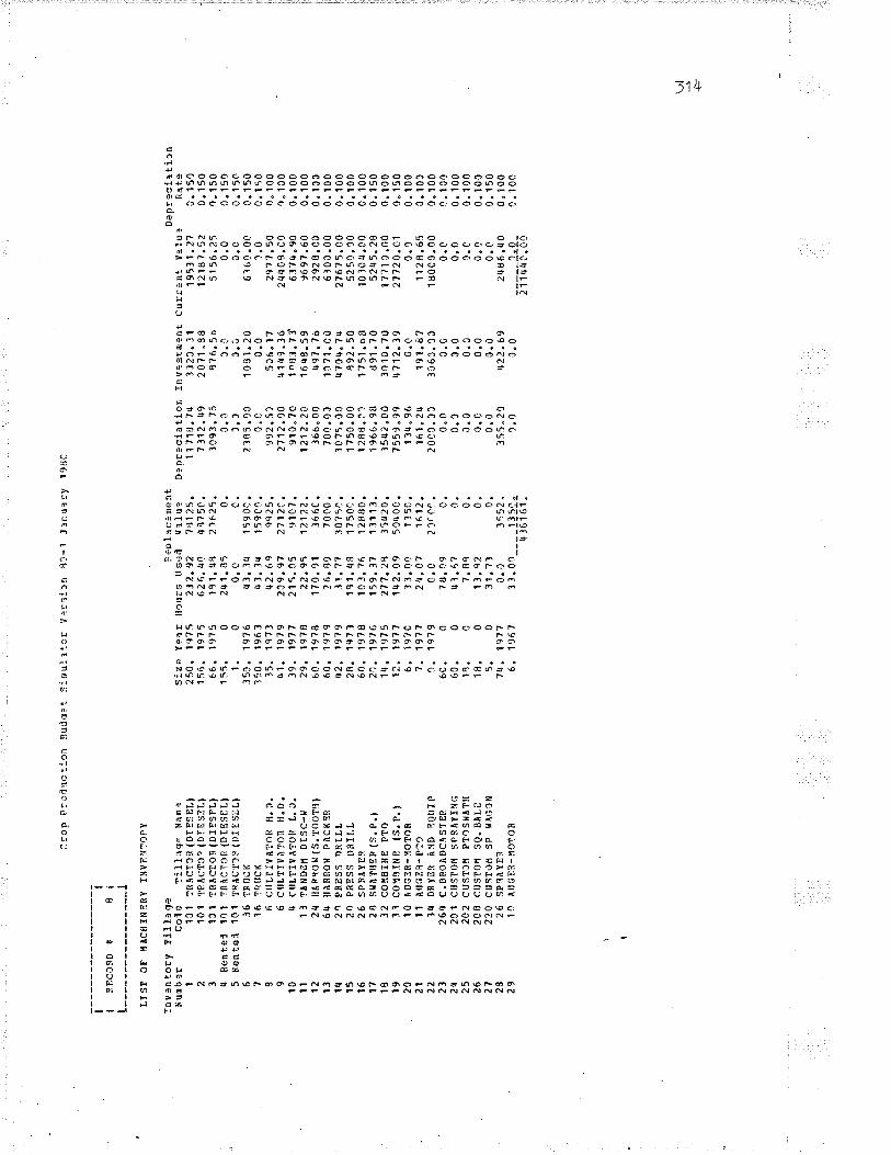
:rop

P:ù

d'¡c

:ion

Buù

.¡:t

i----

----

---

---

---r

I R

EC

oRD

{ 8i

r___

_ -_

__-_

____

___l

LIS

T O

F I

IÀC

fIIN

ER

Y

TN

VN

U:O

PY

:nv-

.nÈ

ory

Till

age

Nuo

b 3r

co

l e

Till

¡qÊ

tla

n:1

1Cl

?RA

CT

3ì (

DT

ES

EL)

2 10

1 T

PA

clC

" (D

TE

SD

LI3

1? 1

TnA

CT

OR

(D

TE

SF

L)4

Ren

tel

1Q1

rn.q

cTcR

(D

IES

ELI

5 R

enta

l 101

TR

AC

T?P

(D

TE

SD

LI6

36 T

tìrrc

K7

î 6

Tnu

cK8

6 cl

rLtlv

ÀT

oR [.t

.9

6 C

I'LT

IVÀ

TO

R H

.D.

10

r¡ c

ulT

rvÀ

îo0

L. D

.11

1l

TÀ

ND

or,l

DIS

C-!

{12

2q

[AF

RO

H (

5.T

oOT

{}13

64

IIA

RR

OI.I

PÀ

CK

9R1{

2'

P

RE

SS

DR

ILL

T5

20 P

ÌìES

S D

RIL

L16

26

SP

RÀ

YE

R77

28

SH

ôTIE

P (

s. P

.)18

32

cO

irBrB

E P

TO

19

3 ì

coflR

INE

(s.

P.

l20

10

Àuc

f R

-¡to

roR

21

11 À

rrcE

R-P

TC

22

}0 D

RY

EIì

AN

D E

QU

IP23

26

¡t c

.BR

oÀt¡

cAsT

EP

2II

2C 1

CÍIS

TO

M S

PR

ÀY

ING

25

202

cusT

cH P

Tos

rJÀ

Tt]

26

208

CU

ST

OT

i S

Q.

BÀ

LD2'

t 2?

0 ct

¡sT

ùÌa

sP H

À(;

cr¡

2g

26 S

PÎA

YE

R29

l0

¡r

UG

E3-

iloT

oR

S:Ír

ulrlc

r vr

rs:)

n 8?

-1 J

¡ntr

ìsy

l9lJ

C

Sep

lac3

next

Siz

¿ Y

ear

llDur

s U

scd

Vilu

?25

0. 1

,¡75

23

2,92

't'

t125

"15

6. 1

975

626.

trt.r

tt9

750.

ó6.

t975

13

1. r

¡8

2162

5.15

5.

0 2q

1.85

0.

1.

0 0.

0 0.

l5c.

19

76

rt3.

3r¡

1590

C.

350.

196

3 ¡¡

1. l4

15

9C1.

35.

1971

{¡

2.69

9q

25.

uI,

1979

2X

9.97

27

12C

.39

.'t97

7 21

5.C

5 q1

07.

29.

1918

22

.97

1212

2.60

,197

8 17

0.9r

16

6C.

60.

1979

26

.80

7000

.tt2

, 19

79

.ì1.7

? 10

75C

.28

. 1q

7l

191.

q9

1750

C.

60.

1978

10

3.76

12

880.

24.

1976

15

9.17

1.

ì113

"1r

¡. 1

975

277.

2q

35u2

0.1?

. 19

'17

1ttz

.09

50r¡

0C

.6.

197C

33

.04

1350

.7.

19'

17

2q.A

7 1^

12.

0.

1979

C

.C

21.0

^.6C

. 0

7 {r

. C

9 0.

60.

0 r¡

1.5?

0.

lq.

0 7.

8q

0.18

. 0

13"e

2 0.

5.

0 31

.?t

0.7t

t, 19

77

0.0

1552

"6"

1e6

7 33

.01_

___1

l5gg

4J61

61.

D?p

r=ci

atio

¡i fn

vesr

[¡en

t cu

rr¿

nt-

valu

:11

718.

7!r

3120

.11

1953

r.27

7312

.ttg

2071

"88

12

1ò7.

5210

93.7

5 87

6.5b

51

56.2

5c.

0 l.c

0.

0l.l

J.

a 0.

c2.

]85.

0C

1081

" 20

61

60.0

C0.

c 0.

c 1.

099

2.s1

5C

6.17

29

'17.

5027

17.C

0 {1

r¡9.

36

2rtq

G8.

C0

910"

70

1183

.7î

6374

.90

1212

.20

16r¡

8.59

96

97.6

036

6"00

¿

t97.

7ó

2928

.C0

700.

01

1171

.Cù

6r00

.00

t075

.0c

470¡

¡"74

27

6't5

.00

1750

.00

q92"

50

5250

.10

128t

J.î1

17

51.b

8 10

104.

0019

66.9

n 89

1.70

52

t!5.2

835

42"0

0 1t

10.7

0 t7

71C

.00

7 55

9.99

q7

12"

39

2772

0.C

113

r¡.9

6 0.

0 0.

116

1.2q

19

1.d7

11

28.6

52o

ec.J

l 10

63.0

0 18

0c0.

000.

0 c.

0 0.

0c.

t c.

0 0,

0J.

0 0.

0 0.

cD

.C

0.0

0"D

0.0

c.ù

0.c

155.

20

q22.

69

2486

.r¡0

r .0

0.

0

____

_1,Q

._21

1q4C

.00

Dap

reci

ltitn

Rat

ec.

150

0. 1

50.)

. 15

00.

150

0.15

00.

150

0. 1

s00.

100

0. 1

000.

100

0. 1

000.

10c

0. 1

000.

100

0"10

00.

100

0.15

00"

100

0. 1

500.

100

0.10

î0.

100

1. 1

000.

100

0.10

00.

r00

0. 1

500"

100

0. 1

00

UJ È

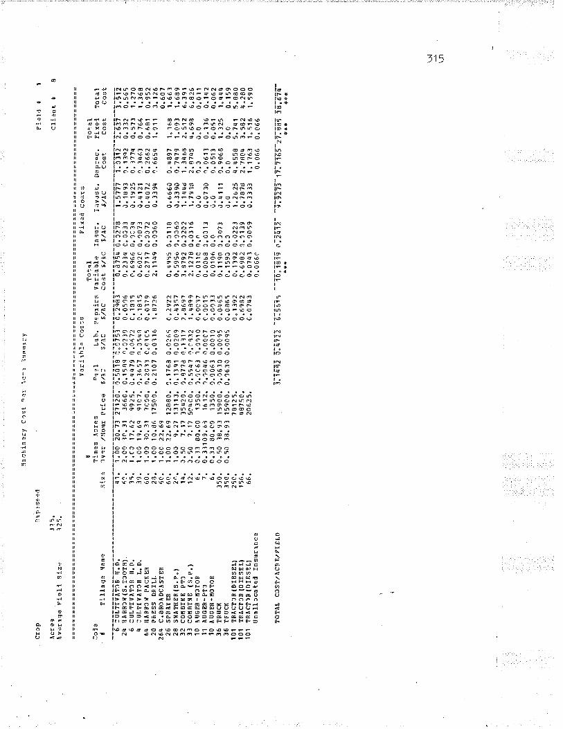
11cÌ

¡j.n:

fy C

rst

n.-t

- lc

:t -ì

unm

l:y

CE

cp

làpl

sÊ+

(ì

F:è

ìal t

¡lcre

3 12

5"

Clie

nt

ôllv

¿c¡

ge F

Lelì

Slz

4.

125.

I V

arith

l- cc

s--s

F

ix¿

d co

srs

Tol

al

Tot

al:ó

lê

Tim

ès À

;res

F

,¡31

Lu

b. P

çpei

rs v

eria

lrle

lr¡su

r.

I;¡và

st.

D-.

p:ec

. F

ixeì

T

otal

I lil

lag:

{a

me

Siz

: lv

er,/!

lour

P

ri.ce

S/\a

5/

Àc

s,/^

c co

st $

/Ac

ß/A

c s/

ac

côst

co

st

cost

--?-

:::=

=::

6:U

LTÍV

ÀT

lF H

.0.

r¡1.

1.

00 2

0.'t3

271

20.0

.501

8 0.

0?5ì

0.

2e83

0.

i)754

0.tJ

27B

1"

5777

1.C

312

2.63

7 l.s

it24

HA

RR

cS(S

.Tco

rHl.

61.

2.00

ìC

.31

3660

.0.1

58q

0.02

t8

0.05

96

0.23

1r¡

C.C

013

J.18

93 1

.13q

2 0.

332

0.56

56

cuLr

IvÀ

llR H

.0.

15.

'1.(

.c 1

7.62

992

5.0.

r¡r¡

79 0

.067

2 C

.131

5 0.

6966

0.C

C3r

¡ 0.

1925

0,)

77q

0.5?

3 1.

270

l¡ ru

r.T

rvA

TcR

L.D

. .3

9. 1

.00

19.6

a 91

C7.

0.1

657

1.C

5r¡9

C.1

815

0.60

2l:,0

.C07

3 O

.¡¡1

21 1

.31¡

63 0

.766

1.

368

64 tl

ÀR

Rgl

{ P

ÀcK

ER

60

. 1.

0C 1

0.31

7C

C0.

0.2

Cll

c"01

C5

0.01

79

C"2

'l 17

0.1

372

0.i¡0

72 0

.266

2 0"

681

0.95

220

t¡R

sss

DR

rLL

28.

1.00

10.

86 r

7500

. 0.

2107

0.0

316

1.87

?6

2.11

49 C

.0C

60

0.13

9rr

1.66

5¡¡

1.C

11 3

,126

264

c.B

RoÀ

DcÀ

sTE

R

6C.

1.00

22.

69

0.60

726

sP

nÀrE

R

60.

1,00

22.

69 1

2880

. C

.r76

8 C

.026

5 Ì,2

922

C.4

es5

0.J1

18

0.66

60 0

.r¡8

97 1

"168

1.6

6328

SH

AT

HE

R(s

.P"l

2^.

1.00

9.

2-l

1111

3. 0

.139

1 0.

0209

C.r

¡157

0.

595ó

t.C

060

ù.33

90 O

.1t!7

9 1.

093

1.68

932

col

lBrll

E P

Î)

lt¡.

J.50

7"

17 3

5u?0

.7.q

778

0.1t

1?

2,86

91

3.87

92 o

,X2o

2 1.

lr¡r¡

d 1.

31¡6

8 2.

512

6"39

133

col

lFr:

lE (

s.P

.)

12.

J.50

?.

17 5

1r¡0

0. 0

"554

7 0.

Cq3

2 1.

r¡89

9 2.

1278

0.0

316

1.79

18 2

.B7t

t5 r

¡.69

8 6.

826

10 r

ucE

R-ü

cloR

6.

0.

13 8

0.00

13

50.

t.1c6

l 1.

0110

0.0

037

0.01

10 0

.ô

0.0

0.c

0.0

0.01

111

ÀU

GE

R-P

Î)

1.

0.33

109.

6ì

1612

.1.)

0q6

r'ì"0

0C7

C.C

015

0.00

68 c

.0)1

3 0.

0?30

ô.0

613

0.13

6 0.

1r¡2

10 A

UG

ER

-¡to

roR

6.

0.

13 8

0.c0

13

50.

c.00

63 0

.001

î 0.

0031

0.

0106

0.0

ù.

0 1"

0513

0.0

51

0.06

236

lnuc

K

350.

0.

50 3

8.93

159

00.')

.06.

10 0

.009

5 0.

0t¡ó

5 C

.119

0 C

.lo?3

ù.

rttt1

0.

9068

1.3

25

l.r¡¡

trr

36 T

FU

CK

35

0.

0.50

3fJ

.93

159C

0.0.

1630

0.0

09s

0.08

65

0.15

9J O

.C

ù.0

0.0

0.0

0"15

910

1 IR

AC

TIR

(DIE

SE

LI

25C

. 78

125,

0.

1192

0.

1392

0.0

22J

1,26

25 ¡

¡"r¡

558

5.7¡

t1 5

.880

101

TB

ÀC

rf,R

(DrD

sEL)

15

6.

48?5

0.

0"69

82

0.69

S2

0.11

39

0.?8

78 2

"780

4 3.

582

4"28

010

1 T

nÀc1

18(D

rEsE

Ll

66.

2062

5,

C.0

743

0.07

q.1

0.c0

59

0.33

33 1

.1?ó

l 1.

s16

1.59

0t na

llcca

te¿

l In

surln

ce

0.06

60

0.06

6 0.

C66

TO

TÀ

L C

CS

T,/A

CN

E/P

I E

LDj.

i{'-¡

i i:n

1ü -

8"5s

ì: --

iõ;îã

îe 0

:t[î2

- -I

li775

-r1]

?îe5

-27"

õel

îs;

ã7,r

-.*

* t+

* **

*

uJ \n

Crr

p

.{cr

eìA

veE

lqe

Fie

l.l 5

lz"

va:ia

bl:

Ccs

ts

Fix

ed C

oscs

¡ T

oÌal

T

rt a

lC

ols

limìs

À

3rÈ

s F

u?l

L.¡h

. S

enai

rs V

rrla

bl¿

In

su!.

InvË

s:.

Drp

rec.

F

ixal

t lil

lâge

lla

ne

slze

ov

:r

/Hcu

r P

:icÈ

$,

/A:

ï/\c

$,/À

c co

st $

,/.qc

ß/ic

i/a

,c

cÕst

co

st-

¡¡--

utrt

vAiõ

R-I

-D.-

---

-ïõ;

--t;õ

o-î6

;6ã-

-õîd

î;-õ;

,rîã

¡-õ;

õ6iõ

--õ;

ZìE

õ---

-n;6

õñi-d

;õdT

l---õ

;4î;T

--õ;

Trr

6t--

õ:7ã

ã--T

;¡eã

20 P

FE

SS

DR

rLL

trz.

2.

00 1

6.C

9 30

750.

1.3

2?-9

C.0

r¡sq

0.3

719

0.7q

52 J

.?31

6 1.

7869

1.1

692

2.99

0 1.

735

202

cusT

f,'l P

lost

lÀT

tl 19

. 1.

00

't.62

Z

.O3t

208

cusT

flt S

0.B

ÀLE

18

. 1.

00

t1.3

1 1.

693

220

cusT

3ir

sp 'd

Àco

N

5.

1.00

1,

89

14.1

8910

1 rR

Àcr

f,RlD

rEsE

L)

66.

2062

5.

0"0

0.0

0.c0

59

ù.33

33 1

.176

3 1.

s16

t.516

101

lRA

cllR

(DrE

sEL)

15

6.

¡¡8?

50.

0.3ó

?0

0.36

7c c

.ct3

9 0.

787s

2.7

804

l.sB

2 j.9

q9c.

1826

0.

183

0.18

3U

nlllc

cãte

d fn

surln

ce

Tam

ì llr

y

6Ð.

20.

¡'lrc

hinc

ry

C^s

: P

çr

lct?

S

umnl

:.,1

ICT

ÀL

CO

ST

/AC

FE

,/FIE

LDî;4

8-i5

- 6.

1r2î

-T

l5[[o

---

3;t']

e-õ

0;2[

12-

-];5

22õ-

Ê.î1

22-

Pie

ld

{

clle

n t T

ota

Ico

st

9"01

530

.1¡0

f¡

\n o\

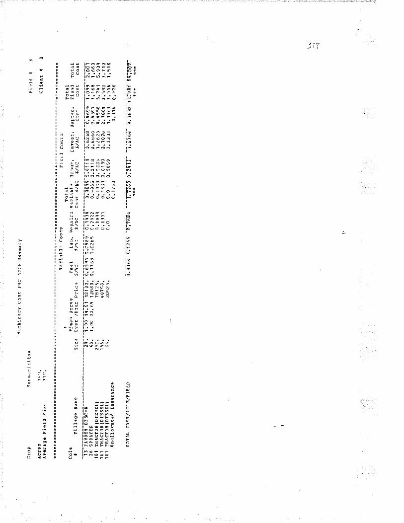
3 E

op

Àcr

9sA

YeE

age

Fie

ld s

izF

col

eI

Tll]

age

l,lam

e

13 t

Àt¡

DE

H D

ISC

-¡t

26 5

PR

ÀfE

N10

1 T

RÀ

CT

ln (

DIE

SE

L)lC

'1 T

RÀ

cIcR

(DIE

SE

LI10

1 T

RÀ

CT

3R (D

IES

EI.t

lrnaÌ

loca

teil

Insu

ranc

e

rCT

ÂT

Cf,

ST

,/ÀC

II E

,/FIE

LDSuI

m¿

rf r

lIoH

16C

.11

1.

vrch

ir.ar

y C

)st

PÊ

: \1

::5'ln

ma:

y

Var

lahl

? C

Õsl

s F

ixË

l C

csrs

{ T

otal

T

otal

11m

3s A

cE?s

F

tl¿1

L0b.

Rep

¡irs

Vrr

labl

i In

sur.

In

vês"

-. D

,.p:3

c. F

lxrC

T

otaL

slzè

ov

eE,/l

l3ur

P:ic

.r

5/\=

$/

\a

fi/^C

co

st $

/Àc

,t,/\C

5/

lr:

Cos

t co

st

Cos

t--

---ã

õ.--

î;,rõ

-î,¡

:sì-

iãîti

l-õ;e

Eõ6

-õ;0

qIe-

-c.i¡

'j,¡-

----

õ;õõ

1õ-ã

;tîiî-

--c-

:6ã6

s--õ

;,,4î

õ--T

;0ee

--ã;

00T

r,a,

1.

00 2

2.69

12r

)80.

q"1

7rr8

î.G

265

C,2

922

0.q9

55 0

.1!1

3 0.

6bô0

0.¡

¡897

1.1

68

1.66

32\

C.

?812

5.

1.19

qS

0.19

ru J

.i22J

1.

¿62

5 4.

¿15

58 5

.7u1

5.

939

156.

4r

J750

. C

.îlrl

0. 1

301

1.01

39

J"78

7ú 2

.780

4 3.

582

3.71

266

. 20

625.

C

.0

0"c

c.J0

59

J.3J

33

1.1?

63 1

.516

1.

516

c.'t7

63

0.1?

6 0.

176

õ:ql

G¡

¡;î2

85 -

ñl76

dq -

--î;7

Zdt

0;2

¡îZ

- -l;

6?6¡

- Ð

"36-

12-r

ll2ãT

T5:

õõ7-

***

*r*

**É

Pi rli

ë

clie

nt

S

UJ

-_l

::c p

Àcr

?s.\v

ecag

e F

ield

siz

"

col 3 I

Till

âge

tlam

e

6:IIL

TIV

ÀT

OR

H.D

.I¡

C U

LTI

VàT

C R

L.

O.

2r¡

[aR

RO

H (

S.T

]O1H

)10

1 T

RIìC

TIR

(D

IES

ELI

101

TP

ÀC

TIR

(D

IES

DL)

101

TR

ÀC

TIB

(D

rEsE

Ll

Sun

ilerf

ri.l

os

r5.

15.

lrnaL

l cca

tea

l In

srrE

lnc.

-j

TO

TÀ

L C

OS

T/A

CP

E/P

IET

D

l'!a

chio

È r

v

Siz

=

vlril

hl:

CÕ

s:s

Fix

êJ c

osrs

t T

otll

To+

_al

Tio

ls

Àc:

?s

Fu"

1 Lu

h. P

epai

is V

aria

ble

Insì

lE.

Inve

sr.

DaD

rec.

nlre

d T

otaI

)ver

/ll

our

Pric

e õ,

/\:

S,/.

\C S

/AC

C

JSI

$,/À

C f

i/IrC

$/

ÀC

C

ost

Cos

t C

ost

{¡.c

0'18

.35

2't1

20.

¡.5r

rB?

0.C

32ì

C.l3

?0

0.96

8c C

.C27

8 1.

5777

1.0

112

2.63

7 3.

605

r¡.C

0 17

.r¡3

910

7.0.

199C

0.0

599

C.2

C5C

C

.6f¡

19 C

.0C

73

ù.¡¡

1Zl

0.lr¡

63

0.76

6 1"

q29

3.10

26.

17

366q

. J.

r8q

1 1.

0276

C.0

536

0.27

^l 0

.311

3 0.

18e3

7.1

392

0.13

2 0.

602

7812

5.

0.62

98

0.62

59 0

"022

1 1.

2625

0.{

¡558

5.7

q1

6.16

9r¡

875C

. 0.

3185

0.

1385

1.c

Î39

0.78

78 2

.783

'¡ 3.

582

1.92

12C

6?5.

0.

0 C

.0

0.00

59

ù.33

31 1

.176

1 1.

516

1.51

60.

1607

c.

161

0.16

1

tr:3

651

õ;6q

i5 -

il5îîs

---

B;iõ

56 o

;i¡îZ

- -¡

:sE

ã6--

Eiã

7õ2-

rõ.7

ît tl;

õ10-

*r+

**

* **

*

r¡1.

39.

60.

25f:r

.1 56

.66

.

Piì1

4 I

Cli:

nt

UJ

CO

cr)p

Acr

es

Àve

râge

Fle

ll sl

z+

co d

6$

IIlIa

ge

Nam

e

- - 6-

-:õ;

îi i i

ñtñ-

ä;õ;

2q H

ÀR

nCr(

s.T

lolfr

lI¡

C U

LTI

VÀ

TO

R L

. D

.20

PN

ES

S D

RIL

L2r

¡ flÀ

RR

OH

lS

.TC

oTH

l26

SP

RA

YE

F26

4 C

.BF

f,ÀD

CÀ

ST

ER

32 C

OIIB

IHE

PT

O36

TR

UC

K36

TN

UC

K1O

AU

GE

R.II

CT

OR

11 À

UG

ER

.PT

f10

[oG

ER

-ttC

ÎoR

1 01

TR

Àcl

lR (

DIE

SE

LI1C

1 lR

AcT

lP (

DIE

SE

LI1 01

lnA

CT

oR {

DrE

s E

L)U

nallc

ca+

-ed

lnsu

Eln

a?

IoT

AL

CC

ST

/ÀC

R E

,/PIE

LD

Sun

flre)

rs'1

1 íì" rJl.

'r3:ia

bl?

cost

s F

iK€d

cos

Es

Í T

etal

T

o:al

Tlm

¿s

ilcr?

s F

r¡ll

L,rl¡

. ¡e

pai-:

s V

rrie

bl:

Insr

¡r.

Iûve

st.

De[

rrec

. F

lxei

l lo

tal

Siz

e O

v-r.

/llou

E

P.ic

: S

/rC

i/^

C

1/À

C

Crs

l $,

/¡lC

5/

AC

.6

/ÃC

C

ost

C"s

t C

cst

¡rì;-

-t;a

õ- z

o:1

1-17

11õ-

.- a

;¡s

s7-õ

;attE

- -0

:Zeõ

5---

-õ.

siãt

-ô;5

ttB--

-î;6

7t7-

-i;¡lì

ã--t

;6lî-

-¡;[õ

õ6C

. 2.

00 1

0.31

36

60.

0.15

89 '

,!.¡2

39 0

.05.

6 0.

213r

¡ C

. ^C

3J

0.1t

s9.1

0.1

3q2

0.ti2

0.

565

39.

2.C

0 19

.69

9107

.0.1

512

0.05

30 C

.1B

l5

0.58

77 0

.0C

73

ù.41

21 0

.3q6

3 0.

766

1.35

328

, 1.

qC 1

0.86

175

00.

C.2

107

0.C

l't6

1.87

26

2,11

49 t

.006

0 C

.339

{ 0.

665r

¡ 1.

C11

1.1

2660

. 1.

00 1

0.31

16

60.

c.15

89 1

.C21

8 0"

05C

6 0.

211'

t 0.

col

3 0"

1893

ô.1

192

0.33

2 0.

565

(,(r

, 1.

CC

22.

69 1

28fì0

. 1.

1768

).0

?.65

A.2

922

0.u9

55 0

.C11

8 0.

b660

0.t¡

89?

1.16

9 1"

663

6C.

1.10

22.

69

0.60

?1t

r.

1.t0

rt

.76

35q2

0. 1

,122

1 0.

1981

tt.3

222

5.8r

¡2ú

0"02

C2

1.1q

4rJ

1.14

68 2

.512

8.

35r¡

150.

0.

50 1

9.44

159

C0.

ù.1

2t>

2 0.

01tJ

9 0.

0911

0.

2182

0.C

073

0.rt

111

0.90

68 1

.325

1.

Sri3

150.

0.50

19

.4r¡

159C

1.0.

1262

t1 .1

189

C.1

732

0.31

840.

C

0.0

0.0

0.0

0.1t

86.

0.

ll

12.4

0 11

50.

0.c¡

¡07

0.c1

61 1

.021

1 c.

068l

1.t

ù.c

0.05

11 0

.051

0.

119

7,

0.:ll

17

.00

1612

. ).

1297

0.0

Cr¡

5 0.

0096

0.

0437

1.0

013

0.07

30 C

.061

3 0.

116

0.17

96.

1.

33 1

2.r¡

o 13

50.

t.1r¡

07 C

.006

t 0.

02t8

C

.c70

6 c.

ù 0.

0 0.

0 0.

0 0.

0?1

25C

. 79

125,

0.

2't8

1 0.

273J

0.0

221

1. ¿

625

r¡. r¡

558

5. ?

rr1

6.01

915

6.

4875

0.

1.01

120

1.0r

¡20

0.c1

19

0.78

78 2

"'t8o

r! 3

.582

t¿

"624

66.

2062

5,

C.0

7r¡3

0.

C?r

t3 0

.C05

9 C

.333

3 1.

1763

1"5

16 1

.590

0"11

08

0.11

1 0.

111

f;tt7

5 d:

6d[î

-9]iq

[z -

-î];t

ist

o;irr

ii- :

Tllu

6d-I

jlB-a

q7-z

il?îî

î5;6

õõ-

**È

*ù

* rS

+û

Fie

ld

*

clie

nt

ð

UJ \o

Cro

p :ìu

t f l l

e ìr

s

AcE

?s

1qî.

àvec

age

Pie

ld

Siz

" 6.

a.

Col

eS

T

lllr9

: N

ame

6 cU

LÎM

TO

R [

.n.

lr :u

LTIv

ÀT

OF

L.¡

¡.24

ÍÀR

RJr

{ (5

. T

lOT

ill.2

0 P

RE

SS

DN

ILL

2q B

ÀnR

lÍ(s.

Tlo

Till

26¡I

C"

BR

CÀ

DC

A S

î E

î26

SP

RÀ

f R

R

32 C

OI'

BT

N E

PT

]36

TR

UC

K36

TR

UC

K1O

AU

GE

R-í

lTO

N1 1

åUG

ER

-PT

CIO

ÀU

GE

R-I

tOT

OF

101

IRA

CT

lR (

DIE

SE

L¡10

1 lR

AcT

0R(D

rEsE

Lll0

l T

nÀcr

f,R (

DIE

SE

Lft nô

llcca

tecl

f n

suE

ânc3

rOT

ÀL

C]S

T,/À

CP

E

,/FIE

tD

qìch

it ):

y C

)st

Var

iabl

: C

os:s

F

ix¿

¿l c

osrs

$ T

cr_a

l T

ot a

lT

lme:

; A

aíes

F

u-5I

L'

-th.

PpD

airs

vi:i

able

fn

su:.

fnvÈ

s-,.

DÊ

prec

. P

ixed

T

otal

S!.2

: D

v:r

,/tlô

u: P

ric+

6/

\=

:$./r

C

:i/A

C

Cos

f- $

,/lC

$./À

C

5/t C

C

¡st

Cos

t C

ost

41.

l.î0

19.7

7 27

120.

1.5

091

0.07

r¡

0.11

28

C"8

985

C.0

278

1"57

77 1

.031

2 2.

637

3.51

539

" 1.

00 1

8.78

910

7. 0

.17r

\¡¡

C"0

556

C.1

911

C.6

162

C.3

l?3

ù.tt1

21 0

. l¡t

63

0.76

6 1.

382

60.

1.)0

27.

76

lÁ60

. C

.173

6 0.

0260

0.0

552

C.2

50ft

J.C

C3_

¡ 0.

1893

ô.1

1s2

0.33

2 0.

58?

2q,

1.0C

10.

8t¡

1750

0. )

.21A

7 0.

0316

1,8

126

2.11

49 0

.00ó

C

C.3

39tt

J.66

5q 1

.011

3.

126

6C.

2,00

27.

76

3660

. 0.

1736

0.0

260

1.05

52

C.2

5'¡3

4.C

0lt

0.18

9J .

ì. 13

92 0

.332

0.

58?

60.

1.00

22.

69

0.60

?6'

),

1.00

22.

69 1

2,18

0. C

.176

11 0

"026

5 q.

2922

0.

'195

5 0.

C1l

B

0.66

60 0

.r¡8

9? 1

.168

1.

663

14.

1.10

rt

.86

35t¡

20.

1"29

5t¡

û.19

41 ¡

¡.2l

tr9

5.72

q5 )

.a20

2 l.

14qB

1. jrt

68

2,s1

2 8.

236

350.

0.

50 2

5.93

15c

C0.

1,q

gqr,

0.C

1t¡2

f.C

698

0"17

87 C

.00?

3 0.

tt111

0.9

068

1.12

5 1.

504

350"

0.

50 2

5.93

159

00.0

.09¿

¡6 r

ì.0rr

r2

0.12

99

0.2t

88 C

.0

ù.û

1.0

0.0

0.23

96.

0"

31 1

6.53

1.

350.

J.C

315

3.01

¡¡6

0.C

16J

C.ù

5r1

4..1

ù.

ù 0.

1513

0.0

51

0"10

27.

0.

37 2

¿"6

7 16

12"

C.3

221

C.0

0ll

D,O

O72

0.

0328

0.C

013

J"07

30 0

.061

3 0.

136

0.16

86.

C

.33

16.5

3 13

50.

0.01

05 C

.C1¡

!6 3

.C17

8 C

.052

9 0.

0 ù.

0 0.

1 0.

0 0.

053

25A

. 79

125,

C

.rtl7

8 0.

'tt78

).A

223

1,26

25 r

r"45

58 5

"741

6.1

?016

6.

¡¡87

5C.

1.05

611

1.05

6q C

"013

9 û.

7878

2"'t

80q

3"58

2 ¡¡

"638

66.

2C62

5.

e.C

743

0.07

r¡3

0.i0

59

C.:1

333

1. 1

?61

1.51

6 1.

590

0. 1

108.

0.

111

0.11

1

¡;ãi

[i õ;

6-tjB

-õl

î7ís

--i¡

¡;t]l

a r;

2[îZ

- -7

. :

s3õ-

rî.

5Ã-g

i- 27

i717

3-6

;õ5ã

-**

t r*

+

**+

îielil

ü

cli:n

t t

\,i N) o

crop

S

r¡n

fl )c

ì:s

lcrs

s 1 ó5

.^{

eeca

qe F

ield

Slz

t' 41

.

col

ãI

TiII

agê

t{âm

e

- -6

--;E

i ri

v i1

õf -

rl; D

:-II

: U

LlT

V À

TO

R L

. D

..1

3 IÀ

IIDE

5 D

ISC

-H2¡

r H

ÀR

ncH

(s.T

oDT

H!

26q

C.8

RJÀ

DC

ÀS

TE

F26

5P

RÀ

YE

F2O

PR

ES

S D

BT

LL32

CO

¡1 B

Ir¡ E

PT

l.1

6 T

RU

CK

36 T

R I

'CK

1O À

UG

ER

-IIC

TO

R11

À0c

ER

-PÎC

1O À

UG

ER

.IIf,T

OF

101

TR

ÀC

lln (

DIE

SE

L)10

1 T

RÀ

CT

o8 (

DIE

sEr.

)10

1 T

RÀ

CllR

(D

rEsE

LlU

nallf

,cat

Êä

Insu

rloce

TO

TÀ

L C

CS

T,/A

CR

E

,/FIE

LD

Ylc

hin?

Ev

cDs:

t P

¡r'À

trÊ

5,

¡nm

ì!y

Vrr

:âbl

€ co

sts

Pix

sd c

osrs

* T

2+-a

1 T

ot a

lT

im?s

¡l:r

':s

e,tlI

L!

¡h.

FÂ

pairs

vrr

iahl

e In

sr¡r

. In

vcst

. D

:pr?

c.

pixe

¿l

Tot

alS

lze

Ove

E,/l

lour

Pric

: $/

ìl $,

/ÀC

S

/^C

C

ost

$,/.{

C $

/qC

S

/^C

C

ost

Côs

t C

ost

4r.

1"C

C 2

0.11

271

20.

C.q

q57

C.0

729

C.2

983

C.8

569

0.ù2

?B

1,57

77 1

.Cì1

2 2.

637

3.49

439

. 1.

C0

19.É

.9 9

107.

0.1

512

0.C

510

0.18

15

C.5

877

0.J1

73

J.¡t

121

n. tq

63

0.?6

6 1.

353

29.

1.00

î4.

51 1

2122

. C

"659

6 q.

0989

0.1

r¡3r

l 0.

9019

3.0

111

o.b2

6d C

. rt

609

1.09

9 2.

C01

60.

2.C

0 30

.31

1660

.0.1

589

1.02

3ß C

.050

6 0.

231r

¡ 0.

0013

0.

1891

0.1

192

O.jl

2 0.

565

60.

1.00

22.

69

0.60

?6C

. 1.

OC

22.

69 1

2Blì0

. 0.

1768

0.0

265

C.2

922

C.¡

¡955

0.0

11S

0.

6660

O.r

¡897

1.1

68

1.66

323

. 1.

10 1

0.86

175

00.

q.21

07 0

.031

6 1.

8726

2.

11rt

9 C

.C06

0 0.

339f

¡ 1.

665r

¡ 1.

011

3.12

614

. 1.

c0

¡¡.9

0 3s

tt20.

1.2

850

c.19

28 t

¡.20

11

5.6?

89 0

.320

2 l.1

r¡qB

t"

346

9 2.

512

8. i9

135

C.

0.50

21.

21 1

5900

.0.1

157

0.01

74 C

.085

3 0.

218r

¡ 0.

007J

O

.r¡1

11 1

.c06

8 ,|.

325

1.s4

r¡r5

0.

0.50

21.

21 1

5900

.3.1

157

r.01

74

0.15

88

0.29

18 0

.0

0.0

0.0

0.t

0"29

26.

0.

13 1

3"51

13s

0. c

.037

3 1.

1056

0.0

195

0.06

2r¡

C.0

0.

0 0.

0513

0.0

51

0.11

.t7"

0.

l3 1

8.55

16

12.

0.C

272

0.00

r¡1

0.00

88

0.c4

01 0

.001

1 0.

0730

0.0

613

0.13

6 0.

176

6.

1.33

11.

53

1350

. 0.

0173

0.1

056

0.02

1¡t

0.06

¡.t?

0.c

0.

0 0.

0 0.

0 0.

065

25C

. 7ì

125,

0.

3180

0.

3180

tl.o

223

1"¿

625

4.rr

558

5.?0

1 6.

079

156.

q8

?50.

0.

9273

0.

92't3

0.0

119

ù"7d

78 2

"'t8o

t1 3

.582

.t.

509

6r,.

2ct6

25.

0.07

'13

0"07

41 0

.005

9 0.

3311

1.

1?63

1.5

16

1.59

00.

1031

0.

103

0" 1

03

3;B

iE6

¡;5õ

58 -

ã.56

54'-7

2:1i

26 o

:i112

- -7

;ã21

6- r

3" îl

iq--

zî"f

îõ 3

-s"5

58-

*+*

**t

*+*

Fi e

lal

$

cll¿

nt

UJ N)

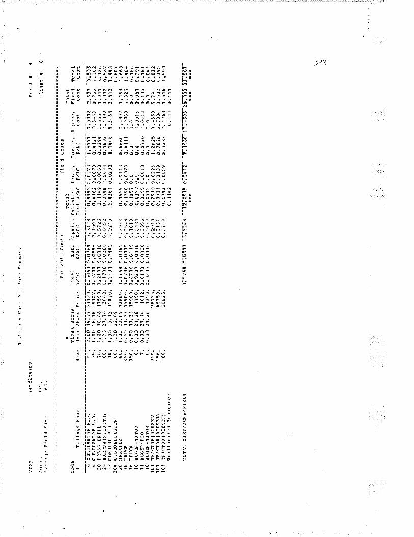
Cro

p

Acr

e s

Àve

rrge

Fie

ld S

iz"

Val

iahl

e C

os,,s

F

!x=

d C

osrs

¡ T

o-.1

1 T

ctal

3ctle

T

imús

¡.3

rts

nr¡?

l Lu

b. I

ìêpã

irs v

l:iah

le

Insr

rc.

InvÊ

si.

D?p

Eec

. P

lred

Tot

alI

Till

age

N¡m

e si

z?

Ov+

E,/f

¡crr

r P

rice

ß/\C

t,/

AC

$/

ÀC

co

st J

ilÀc

S,/!

tC

5/^C

co

st

Cos

t C

ost

----

----

-.--

6 sU

LTrv

ÀT

3P H

.D.

r¡1.

2.

00 1

9"'t7

271

20.0

.509

3 1)

.076

4 0.

3r28

0.

8985

C.C

27{J

1,5

777

1"03

12 2

.637

1.

535

r¡ c

ulT

rvÀ

rlF L

.D.

19.

1.00

18.

78

9107

. 0.

1?0i

¡ 1.

0556

0.1

903

0.61

62 1

.0C

73

0.¡t

121

1.lr¡

63

0.?6

6 1.

182

20 P

RE

SS

DR

ILL

ztt,

1.00

10.

86 1

7500

. 0,

210'

t t.0

116

1.87

26

2.11

49 0

.0C

60

0.33

9¡t

0.66

5tt

1.01

1 3.

126

2f¡

ilÀR

R3r

{(S

.Tro

rul

60.

1.C

0 27

.76

3660

.0"1

716

1.02

60 0

.055

2 0.

25q8

î.C

01.'t

0.

1893

0.1

392

0.33

2 0.

58?

32 c

oilB

r!,¡

E P

T)

1¿¡.

1.0

0 5.

12 3

5t12

0. 1

.23C

1 0.

1845

r¡.

0215

5.

rtl6

1 0.

0202

1.

14¡¡

8 1.

3468

2.5

12

7.9¡

¡826

4 C

.BR

OÀ

DC

AS

TE

P

f;0.

1.00

22.

69

0.60

726

sP

RA

fEs

61.

1.00

22.

69 1

288C

. 0.

1765

1.0

265

Ç.2

922

0.{9

55 1

.011

8 0.

6660

t.r

¡89?

1.

168

1.66

336

ÎR

UC

K

350.

C

.50

31.3

3 15

9C0.

1.0

71€i

0.0

110

0.05

r¡3

0.13

9C 1

.007

3 0.

¡r11

1 0.

9068

1.1

25

1.46

!¡36

TR

UC

K

350.

0.

50 3

1.33

159

C0.

0.37

36

).C

111

C.1

010

0.18

57 0

.C

0.0

0.0

0.0

0.18

610

âU

GE

R-Í

3ToR

6.

0.

31 2

1.26

1i

5¡.

0.02

37 0

.003

6 0.

0124

0.

03c7

0.0

0.

0 1.

0511

0.1

51

0.09

111

AU

GE

E-P

ro

7.

0.13

29"

1r¡

161

2. 0

.417

J 1.

0126

C.0

156

0.02

55 ù

.001

3 ù.

0730

1.0

613

0.13

6 0.

16t

10 À

ucE

R-H

lToF

6.

q.

71 2

1.26

13

50.

C.C

23?.

0.00

16 0.

0119

0.

0412

1.C

0.

0 0.

0 0.

0 0"

0r¡1

101

TR

ÀC

TO

IÌ(D

IES

ELì

25

t:.

7812

5.

C.2

919

11.2

919

0.02

21

1.26

25 r

l.q55

8 5.

?41

6.03

210

1 rR

AC

l)B(D

rEsE

L)

156.

08

750.

0.

8111

0.

8131

1.J

139

0"78

7d 2

,780

q 3.

582

q.39

510

1 IR

AC

T)R

(DrE

sEr.

l 66

. 20

625.

0.

0743

0"

07r¡

l 0.0

059

0.33

33

1.17

63 1

"516

1.5

90un

allo

cete

rl In

sura

ncê

C.1

1t¡2

0.

114

0.11

q

îu!ìr

1,)r

)¡s

27 5

.6t

.

I'lac

hin,

otV

C

ost

ÞÊ

r À

c:?

Í,-'¡r

tìmaa

v

TO

lÀL

CC

ST

/ÀC

F E

/FIE

LDi;ã

75¡

5.¡ã

i1 -

ã13ã

qa -

-ì2;

õõ15

0;ã

,rî7

- -7

;it6E

-rî.'

¡Eõ5

-zõl

õB-B

1l;5

ã7-

trt

+**

*û

*

Fie

Iù 0

clie

nt

I

u! N)

N)

Cr3

p

lcE

es

{ver

age

Fie

lC

5!z+

varia

blû

Ccs

.-s

Fix

ed C

osts

t T

ot a

l lo

tal

:o¿

le

Tim

es À

crès

F

'r?l

L'¡l¡

. F

enai

rs V

eria

l¡l -

. In

sur.

In

vesÊ

. D

eprè

c. P

lxed

T

otal

I T

lllåg

e l{a

me

Slz

¿

Ove

r,/ll

our

Pric

e 5/

\a

fi/IC

:È

/AC

Cos

t $,

/ÀC

$/À

C

S/A

C

ccst

co

st

Cos

t- -6

-õ'¡;

îi iIl

tF-ä

;õ;-

-- -

-I

ìl - -¡

;;5-1

-B-.

õ1-1

i110

;-

õ:E

tE {

J-õ;

õ ã

Aõ-

-6;

l6tã

- --

-1;õ

¡[q

- õ;

0-ti0

---

i;57î

i--1'

.õ17

2--1

;6it-

- 5

. 6[

i26

r¡ C

.8nC

ÀD

CLS

TE

R

6c.

1.qO

2?.

69

0.60

72t

¡ H

AR

Ro'

r(s.

lcoT

H)

60.

¡.1.

00 2

5.85

36

60.0

.186

4 0.

0280

0.0

593

C.2

737

0.00

13

0.18

93 0

.139

2 0.

332

0.6C

5q

cfrL

Trv

ÀÎf,

n L.

D.

19.

3.00

17"

16 9

10?.

0.41

c5

0.06

29 C

.208

2 0.

6917

0.C

J?l

ù.41

21 û

.311

63 0

.766

t.r

¡56

6 cu

LTrv

AT

R H

.D.

15.

1.0C

15.

36 9

925.

0.51

19 1

.C77

1 î.2

082

0.79

9J t

.303

q û.

1925

i),

1't7

U 0

.5?3

1.

372

20 P

RE

SS

DF

rLL

't2.

1.00

16.

29 1

0750

. C

.31q

9 1.

0q7q

0.3

692

0"73

59 0

"031

6 1.

78ily

1.

r692

2.

990

3.72

626

spR

ÀyE

R

60.

2.00

22.

69 1

2880

. 0.

1768

i.C

265

î.292

2 0.

¡t95

5 0.

0118

û.

6660

1.4

89?

1.16

8 1.

663

264

C. B

RoA

DC

ÀS

TE

R

60.

1.00

22.

69

0.60

728

sllÂ

TtlE

S(s

.P.)

2C

. 1.

C0

8.61

131

13"

C.1

r¡98

0.C

225

C.r

¡691

0.

6r¡1

6 0.

0060

0.

339'

l 0.

7q79

1.0

93

1.?3

532

coü

BIN

E p

lt lu

. C

.50

r¡.?

r¡ 3

5420

. 1.

128¡

¡ 1.

1991

r¡.

3430

5.

8707

0,0

202

1.1r

¡48

1.3q

68 2

"512

8.3

8233

coü

BrN

E (

s.p.

) 12

, 0.

50

r¡.7

4 50

r¡C

0. 0

.939

5 0.

1259

2.2

548

3,22

i2 o

.Cl1

6 1.

7918

2.8

7tt5

¡¡.

698

7.91

836

TR

UC

K

350.

0.

50 2

0.59

159

00.

C.1

192

0.C

179

e.03

79

C,2

250

C.C

073

û.q1

11 0

.906

8 1"

325

1.55

036

lFrJ

cK

3irl.

c.

50 2

0.59

159

00.

C.1

192

1"1r

?9

C.1

616

0"30

07 C

,0

0.ù

1.0

0.0

0.30

110

Àuc

ER

-ilo?

OR

(,

. 0.

-?3

2rt.8

0 13

50.

1.)2

04 o

.CJ3

1 0.

01C

6 0.

03r¡

l 0.

0 0.

0 0.

0513

0.0

51

0.08

511

Àuc

ER

-pr3

7.

0.

13

3rt.0

0 16

12.

0.01

r¡9

0.0C

22 0

.034

8 0.

0219

0.0

013

0.07

30 0

.061

1 0.

136

0.15

710

AU

cER

-lrro

R

6.

0.33

24.

80

1350

.0.1

20r¡

o.c

C31

C.0

119

0.03

53 C

.0

0.0

0.0

0.0

0.03

510

1 T

RÀ

CT

OR

(DÌC

SE

LI

2aO

, 78

125.

0.

1597

0"

1597

0"0

223

1.26

25 r

¡.r¡

558

5.7r

¡t

5.90

010

1 T

RA

CT

IE(D

TE

SE

L)

156.

rl8

750.

1.

r¡ 1

8 1"

rt01

8 0.

C13

9 0.

7878

2.7

80r¡

3.5

82

rt.9

8q10

1 rB

ÀcT

1R(D

rEsE

Ll

66.

2062

5.

0.0

0.0

0.03

59

ù.3J

31

1" 1

763

1.51

6 1.

516

Una

lloca

teal

fns

uran

ce

0.04

76

C.o

qB 0

.C¡¡

8

:t h.

.e t

12C

.3l

.

i'f :c

hin:

rv

Cos

Ì P

+:

4îr?

.;u

nmr:

y

TO

TÀ

L C

OS

T/À

CR

E,/F

IELD

E;îl

tõ -o

-.i1

ô7 -

71ãl

õq -

-i3;7

jõ¡

o;i¡i

r- T

õlg6

s6-r

7lf5

[i-z

s. 1

65 "

q rì

õ-**

* *+

* **

f

Èie

lil

*

ci.ie

nt

{

\n N)

\n

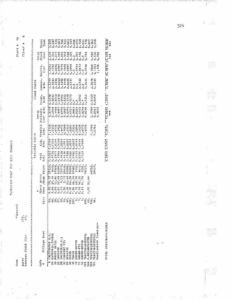
51ch

!n 9

rv C

osl

pçr

Àcl

-- S

rlniln

lty

Cro

p F

1àxì

:+.1

F

ieli

ð lO

Acr

es

27'1

. C

lient

0

gÀ

vera

gê P

ield

siz

. r>

f;.

Vl:'

irbl.)

C

os:s

F

ixed

Cos

rsI

Tol

-1I

Tor

_al

col3

T

imes

Acr

es

Ê'r:

l L,

¡b.

Ilepa

irs v

aria

ble

Insu

f. In

vÈst

. D

e[,:È

c. p

lxed

T

otal

r lil

l.ge

Nlm

e S

iz:

Ove

r,/ll

our

PE

icc

i/^J

$/¡\

C

[./Ã

C

Ccs

t ô,

/ÀC

$,/À

C

$,/À

C

Cls

r C

cst

Cos

t--

6--;

ffiie

ÀÌõ

f-H

;õ;-

--

--¡i:

--r-

;õõ-

16:1

î-11

11õ;

-õ;5

t;:

-i:õi

Bl-

-¡:iT

iã--

--õl

õTì

e- õ

;õt?

ã---

T:E

T n

--1:

õ171

--t:e

r7--

ã;sB

E24

tlA

RR

otr(

s"Î3

oÎt¡

l 60

. 3"

00 2

7.76

36

60.

0.11

36 0

.C2t

,0 (

].055

2 0.

25r¡

g 0.

0033

u.

lB9J

0.

1192

0.3

12

0.5s

720

PR

ES

S D

RrL

L 28

. 1.

C0

1C.8

6 17

5C0.

C,2

1t7

1.01

16 1

.ft?2

6 2"

1149

0.0

C60

ù.

339r

¡ 1.

665r

¡ 1.

011

3.12

626

sP

nÀY

EP

61

. 1.

A)

2?.6

9 12

8R0.

-0.1

768

0.02

65 r

.292

2 1.

rt95

5 0.

0118

0.

6660

0.¡

¡89?

1.1

68

1.66

328

sflA

îHE

R(S

.P")

20

. 1.

10

9.C

3 13

113.

1.1r

¡28

î.021

rr

e,qu

72

0"61

1q c

.0c6

0 c.

3390

0.?

¿t?

9 1.

091

1.70

r¡32

CO

IIBIN

E P

Tf

14.

1.50

5.

55 3

5'¡2

0. 1

.1llB

0.1

7C1

3.70

68

5.01

07 0

.020

2 t.1

q48

t.1r¡

68

2.51

2 7.

522

26 s

PnÀ

YE

F

60.

0"5C

22,

69 1

2880

. 0.

1768

0.0

265

1..2

922

0.r¡

955

0.01

1S

ù.66

60 0

"{18

97 1

.168

1.

663

36 T

nucf

i 15

0.

0.50

6rr

.28

1590

0¡ 0

.t382

0.0

057

1.02

82

0.07

21 0

.10?

3 J.

¡r11

1 0.

9068

1.3

25

1.39

?36

Tnt

rcK

l5

c.

c.50

6r¡

.28

1590

c. t

j.qiq

z 0.

0c57

c.c

524

0.09

63 0

.0

0.0

0.0

0.0

0.09

610

ÀU

GE

R-ll

oÎoR

6.

0.

13

40.9

9 13

s0.

1.C

l21

0.00

1e 0

.c06

4 0.

0206

0.0

0.

0 c.

0513

0.

051

0.07

211

IoG

ER

-PT

] 7.

0.

31 5

6.20

16

12.

O"0

le0

1.0c

14 0

.c02

9 0.

0133

0.c

011

ù.o?

Jo t

.061

3 0.

136

0"1r

r910

AU

GtiR

-lloT

on

6"

0.3:

l t¡

c.99

13

5c.

J.11

23 1

.o01

9 î,.

0D72

0.

O21

rt 0

.4

ù"0

c.0

0.0

0.02

110

1 T

RA

CT

CR

(DT

ES

EL)

25

0.

7û12

5.

C.4

378

C.r

¡178

J.0

22a

1.26

25 r

¡.r¡

558

5.7q

1 6.

178

264

C.B

nCA

DC

AS

TE

R

60.

1.O

j 22

,69

0.60

?10

1 T

FA

CT

IR(D

IES

EI.)

15

6.

r¡87

50.

1.77

99

0.77

99 0

.013

9 J.

?878

2,7

80q

3.58

2 rr

.362

101

lRA

crlR

(D

rEsE

Ll

66.

2062

5.

C.C

743

0. O

?r¡3

0.0

059

,1.3

133

1.17

6)

1" 5

16

1.59

0lrn

àllc

c¡te

d In

surt

nce

0.10

1?

C.1

0r¡

0.10

t¡

TO

TÀ

L C

OS

T,/A

CP

E,/F

IELD

U]

N) +

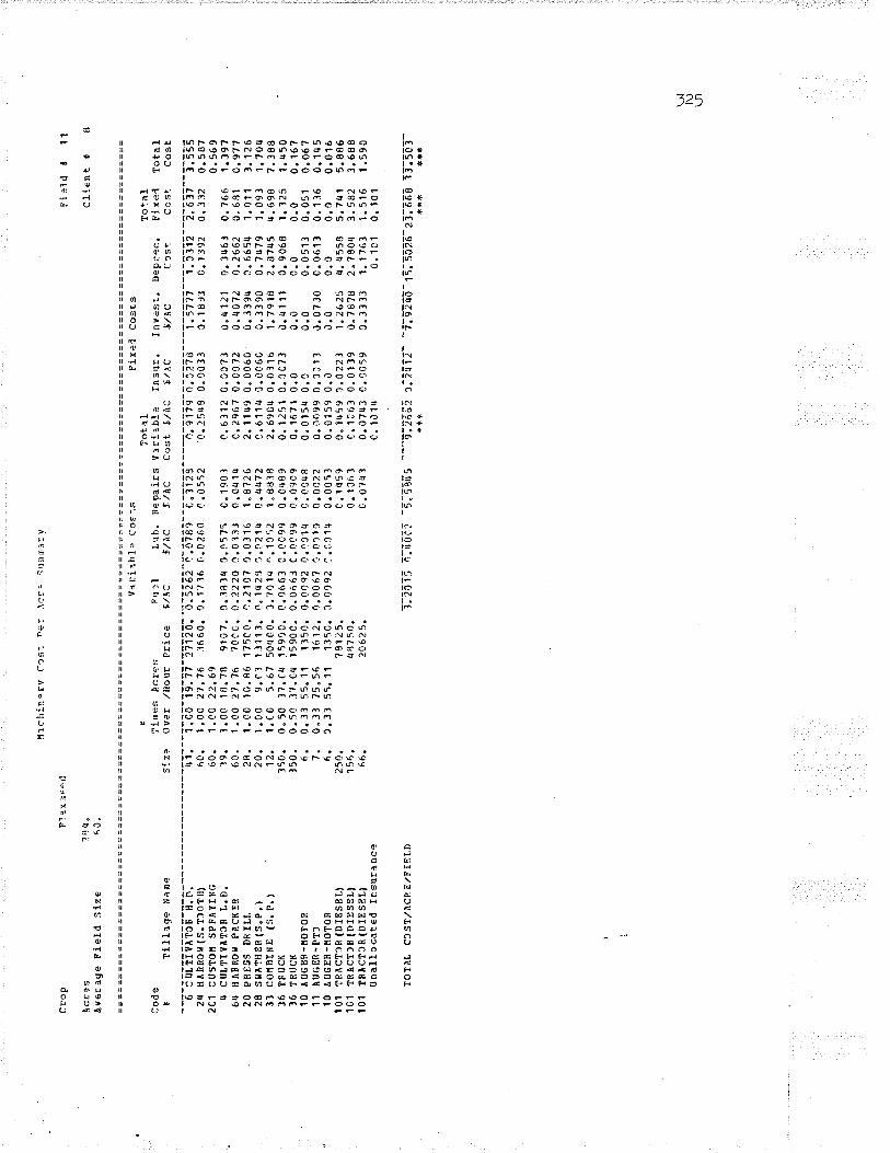
Cro

p

Àcr

:sÀ

YeE

age

Fie

ld s

lze

co¿

leü

Tlll

age

Nam

c

6 aU

LIM

TC

F H

.tì.

2q H

ÂhR

Cí(

S.T

)OT

H)

2C1

CU

5IO

II S

PF

IIYIN

Gq

CU

LTIV

ÀT

CN

L.

D.

6q H

ÀN

NO

fl P

AC

K E

R

20 P

RE

SS

DR

ILT

.28

s¡r

¡ìT

ilEn

(s.P

.l3l

coÉ

Blr¡

E (

s.P

. l

ltìch

i.n.r

v C

trì'.

nÊ

: l\c

r.

s'rr

ml:v

F11

xiq.

d

?41r

"60

"

36 IR

UC

K36

TR

UC

K1O

AU

GE

R-H

OT

OR

11 À

OG

ER

'PT

]1O

ÀU

GE

R-I

IOT

OR

I 01

TR

r\C

ToR

(D

IES

ELI

101

TR

AC

TIR

(D

IES

9LI

I O

1 T

RÀ

CT

CR

(D

IES

EL¡

tt na

lLcc

àt€d

Insu

Eân

ce

TO

lÂL

C3S

T,/À

CR

E

/FIE

LT)

Var

ilhl"

Cos

-.s

Fix

Èi

Cos

tsÈ

T

otal

T

o+-a

I?i

m€s

Àcr

es

Fìll

l Lt

¡b.

Rep

airs

Vrr

Lrbl

a In

sr¡r

. In

v¿st

, D

ep?e

c. R

ixei

l T

otal

51z:

ou

er ,

/llou

r P

rice

$/À

a õ/

Ac

f' /A

C

Cos

t ¡,

/¡\C

'5/

\C

5/\C

C

ost

cosl

- C

ost

¡¡1.

1.

00 1

9.17

271

20.

0.5

262

1.07

89 C

.312

S

0.91

79 0

,C27

ò 1.

5777

1" C

.112

2.6

37

3.55

560

. 1,

DA

'27,

16 1

6ó0.

0.1

716

0.02

60 1

.05s

2 0.

2543

0.0

033

C.1

8Jl

C.1

392

0.33

2 0.

58?

60.

1.C

0 22

.69

0.56

9ì9

. 1.

00 1

8.?8

910

7. C

.18l

4 1.

0575

C.1

90.1

C

.631

2 0.

0C71

ù.

¡t12

1 0.

3r¡6

1 0.

766

r.39

?fi0

. 1,

00 2

7.76

?0

CC

.0.2

220

0.03

11 0

.0¡¡

l4

0.2c

67 C

).C

072

0,r¡

07¿

0.2

662

0.68

1 0.

977

2s.

1.00

10.

86 1

7500

. 1.

2107

0.0

316

1"57

26

2. 1

1¡¡9

0.0

0ó0

0.33

9r{

-1.6

6511

1.0

11

3. 1

2620

. 1.

00

9.cl

1.

1113

. 0.

1q29

C.C

21rr

0.4

r¡72

C

.ó11

4 C

.C06

0 C

.339

0 0"

7r¡7

9 1.

093

1.7o

rt12

. 1.

C0

5.67

50t

tC0.

1.7

01r¡

¡.1

C52

1"

8838

2.

69C

t¡ 0

.031

tt 1.

7918

2.8

?r¡5

tt.6

98

?.38

835

0.

0"50

37.

Ctr

159

00.0

.066

3 0.

0C99

0.o

trB

9 0.

1251

C.t0

73

ù.¡r

'111

0.9

068

1.12

5 1.

450

150.

0.

50 l

7.cr

¡ 15

90c.

0.0

663

c.00

99 c

.090

9 0.

1671

0.0

0.

û 0.

0 0.

0 0.

16?

6.

0. 1

3 55

.11

1350

. 0.

00e2

0.1

31r¡

C.0

Cq8

0.

015¡

¡ 0.

c 0.

0 0.

0513

0.0

51

0.06

77.

0"

33 7

5.56

16

12,

q.00

67 !

.011

C A

.002

2 0.

0099

0.3

J13

ù.07

30 C

.061

3 0.

136

0.1r

¡56.

3.

33 5

5.11

13

5C.

C.D

C92

l.C

;11r

¡ C

.0C

53

0.01

s9 0

.û

0.0

0.c

0.0

0.01

625

0,

7812

5,

C.1

r¡59

0.

1'¡5

9 J.

0223

1"

2625

rt.

¿t5

58 5

.?r¡

1 5.

886

156.

r¡

8750

. 0"

1c6

3 C

.1C

63 0

"011

9 0.

7878

2.?

B0r

t 3.

582

3.68

866

. 20

625.

C

.o?t

¡l 0.

0743

0.0

059

1.33

33 1

.176

3 1.

516

1.59

0c.

101r

¡ 0.

1c1

0. 1

01

l;2õî

i ¡;d

o¡i -

5.S

Eds

---

E;2

66ã

j.2n7

Z-

-7:0

rrt0

--rE

lSõ7

6-zl

.G6ã

33

:5õl

-**

* *f

* û*

t

Fi 3

ltl

f

cI1€

nt

ü

11

U]

N) \¡

lrJp

Àcr

9sÀ

vera

ge F

i€1d

Siz

Ê

v¡ria

l)lc

Cos

ls

Pix

èd

Cos

tsf

Tot

al

Tlta

lS

ode

Tim

es A

crÉ

s F

u:l

L'rb

. P

epai

:s

Ver

lat¡

I+

Irsu

r.

Inv¿

sL.

D.p

rcc.

F

lx:d

I tll

lag.

N

eme

siz3

O

v?r

/Hou

E P

rice

fi/irc

$,

/ÀC

$/

ÀC

C

ost

t/ilc

$/

Ac

$/À

c cc

st

côst

--6

-¡ õ

;îi iÍ

1of-

iî; D

;---

--

.'i;-

-t;õ

õ-ii;

¡:-?

îîtõ:

-õ;E

6 ãi

-5:õ

qi i-

- c;

l;îã-

---õ

; ei

iB -

c;5

tts--

-i;s?

7? --

î:õlîã

--ã

;6 5t

- -5

;6ii

2r¡

trÀ

RR

c¡t(

5.T

1ôril

t 6C

. 1.

00 2

6.u8

36

60.

0.1q

19 0

.02?

3 0.

0579

0.

267

1 0.

0031

C

.189

3 Q

.13c

2 0.

312

0.59

96q

flÀ

8RO

B P

AC

Kq9

60

. 1.

00 2

6.r¡

8 7C

¡00.

0.23

27 Q

,C3u

9 C

.043

¿¡

0.31

10 0

.007

2 ù.

q07¿

0.2

662

0.68

1 0.

992

201

crrs

ll:t

spR

AyI

Nc

6C.

1.C

0 22

.69

0.56

9¡¡

crJ

llrvÀ

TcR

L.D

. 19

. 1.

00 1

7.70

91

C7.

0.4

.16î

0.0

61C

C.2

919

0.66

97 0

.03?

3 J.

¡t12

1 0.

3463

0.7

66

1.rr

3520

pF

ES

S D

RrL

L 24

. 1.

C0

10.8

6 1?

500.

q.2

10'1

0.0

316

1,87

26

2. l1

'¡9 0

.006

ù 0.

139r

¡ 0.

6651

1 1.

011

3.12

628

sH

Afll

EP

(s.q

.l 2C

. 1.

00

8.75

131

13.

C.lu

'lq 0

.C22

1 C

.¡¡6

17

0.63

12 0

.CC

60

ù.J1

90

q,1q

79 1

.091

1"

'12¿

t33

Col

t8rf

lE (

S.p

.ì 12

. 1.

00

5.t1

504

00.0

.7rt

98 C

.112

5 2.

0117

2.

8759

0.0

316

1.79

18 2

.97U

5 4.

698

7.57

436

TR

UC

K

35C

. 0.

50 3

7.C

r¡ 1

59C

0. 0

.166

3 0.

¡:ì1

99 C

.048

9 0.

1251

0.0

073

0.41

11 0

.906

8 1.

125

t.r¡5

036

TR

UC

K

35C

. 1.

s0 3

7.C

rr 1

5900

. 0.

C66

3 0.

0099

0.0

909

C.1

671

0.0

0.0

0.0

0.0

0.16

710

ÂU

GE

R-¡

!oîo

R

6.

C.3

3 55

.11

1350

. 0.

0C92

0.0

Clr¡

0.0

0r¡8

0.

0',1

54 0

.0

ù.0

a.05

13 0

.051

0.

067

lt A

UG

ER

-pro

?o

0.

31 7

5"56

16

12.0

.006

7 0.

C01

1 C

.002

2 C

.00e

9 C

.101

1 0.

0730

0.0

613

0.11

6 0.

1q5

l0 À

ûGE

n-lrc

ro8

6.

0.33

55.

11

1150

. C

.009

2 1.

0C1¡

¡ 0.

0053

0.

0159

0.0

C

.0

C.0

0.

0 0.

016

101

TR

ÀC

T38

(DIE

SE

L)

250.

?8

125.

0.

3C96

0.

309f

i 0.

0223

1.

2625

r¡.

q558

5.7

t11

6.05

010

1 T

RÀ

cTl8

(DrE

sELl

15

6.

4875

0.

0.11

15

0.11

',t5

0.01

39

0.78

7d 2

.780

r¡ 3

.582

3.

69.r

l0l

ÎRÀ

CT

IR(D

rEsE

L)

66.

2062

5.

0.07

43

0.0?

43 C

.005

9 0.

3313

't.1

763

1.51

6 1.

590

unal

¡.oc

ate¿

l fn

suf,l

ncâ

C. 10

14

0.10

1 0.

101

Flrx

sç.'d

155. 41

.

q:ch

inor

y co

st P

lr À

cre

Sun

mì:y

TO

TA

L C

OS

T,/À

C9

E./F

IEI.D

î:î2õ

l 0:

úBsî

-51ã

Eq

¡ - --

g-,

q111

c:î4

1 2-

-îlg

2îõ-

rEl5

õã6-

zllB

6e

îf;7õ

q-r*

* **

f ú*

û

Fi:l

l $

clic

nt

#

12

lota

IC

ost

UJ N O\

Cro

P

fì'rr

l:Y

Àcr

es

27 6

.À

vera

ge F

lelrl

Siz

e 6n

.

col

è¿

fll

lagc

N

trm

e

6 :U

LTIV

ÀT

ON

H

.D.

2OI

CU

ST

OIÍ

SP

FA

YIN

G2l

¡ H

ÀR

R3[

(5.

T]O

T¡t

]6

C U

LTIV

ÀT

OP

II.

D.

q C

OLT

I Y

ÀT

ON

L.

D.

20 P

RE

SS

DR

ILL

26 S

PN

ÀY

EP

28 s

r¡¡T

TH

ER

(S

.P.

)32

CO

IIBIN

E P

TO

33 c

o¡tB

I N

E (

S.

P.

I¡O

ÀU

GE

R-í

JTO

R1 1

ÀU

CE

R-

PÎ0

10 À

UG

ER

-ñlT

On

36 T

RU

CK

36 T

NU

CK

101

TR

ÀcT

lR (

DrE

sELl

101

TR

ÀC

TO

R (

DrE

sEL)

101

lRA

Cl)R

(D

IES

ELI

tlnal

loca

teil

J rì

sr¡r

a nc

?

t0T

ÀL

clS

T/À

cR E

/FT

DLD

:llch

ir er

y C

âsc

P:r

Àcr

è S

usm

lry

Ffe

li ó

1 l

clie

nt

0 I

Va:

iahl

Ê C

os'-s

F

i.xèa

l C

osts

t T

o+-à

l T

or-a

l11

m¡s

Àcr

ês

Fu?

l Lu

h. F

epai

rs V

rrla

hle

Insr

¡r.

I Iv

es-.

. D

eps-

.c.

Fix

ecl

lota

lS

J z¿

O

v?r

,/llo

uE P

rj.ce

\/A

: f,,

/AC

$/

ÀC

C

ost

$/lC

$/

lC

ó/A

,C

Ccs

t C

ost

Cos

t--

''i.

--i:õ

õ-1s

-.ii-

1711

il-¡:

qtãi

-c;¡

t B

ç- -

ð;li7

E- --

-î:îi

iõ-

c; õ

tîã-

--î;s

i7t-

-1:

cãîã

--ã;

6t7-

-1:5

586C

. 2.

C0

7.2.

69

1.13

''61

. 1.

C0

2?"7

6 36

60.

C.1

736

0.02

6e 0

.055

2 C

.254

8 0.

0031

ù.

1rJ9

3 0.

1392

0.3

32

0.58

715

. 1.

C0

16.8

0 99

25.

0.r¡

697

0.07

05 0

.19C

1 0.

?3J5

C.0

C3r

t J.

1925

0.i7

1q

0.57

3 1.

30r¡

39.

3.C

0 18

.78

910?

.0.3

81¡l

0.05

75 0

.193

3 0.

6312

0.1

373

J.t¡

121

0.1r

¡63

0"76

6 1.

397

ttz,

1.00

16.

2e 3

0?50

. C

.l18e

9.0

r¡78

C.3

692

C.7

359

0.01

16

1.78

rJ9

1.16

92 2

.990

3.

726

6C.

1,00

22.

69 1

2880

. 0.

1768

0.0

265

?.29

22

0.rt

955

0.01

18

t.bbb

0 0.

r189

7 1.

169

1.66

33C

. 1.

00

9.{ì

3 13

113.

0.

1r¡2

8 0.

021r

1 C

.t¿tt7

2 C

.611

4 0.

0060

0.

3390

1.7

q79

1.09

3 1.

70.r

14.

0"50

5.

C2

35'¡2

0. 1

.255

'¡ C

. 18

83 q

.104

2 5.

5r¡7

9 q.

0202

1.

1¡¡4

8 1.

3'¡6

8 2.

512

8"06

012

, 0.

50

5.02

50t

¡C0.

0.79

.irt

4.11

90 2

.131

8 3.

0'¡1

2 0.

0316

1"

?9lU

2.3

7r¡5

¡1.

698

1.7U

16.

0.

31 1

9"08

135

0. 1

.026

5 0.

00t¡

0 0.

C13

8 C

.04q

3 C

.0

0.u

0.05

13 0

.C51

0.0

967.

0.

33 2

6"15

161

2. C

.:119

3 C

.C12

9 0.

00ó2

0.

0285

0.0

013

ù.ü7

3u 0

.061

3 0.

136

0"16

rt6.

0.

13 1

9.08

13

50.0

.¡26

s 0"

C1q

0 0.

015r

r 0.

0459

C.0

0.

0 0.

0 0.

0 0.

0r¡6

150.

0.

5c 1

5.84

159

00.0

.15q

9 0.

0232

0"1

141

0.29

25 0

.007

3 0"

r¡1u

0.

9068

1"3

25

1.61

83s

0.

0.50

15.

84 1

5900

. 0.

1s{9

0.0

232

0.21

27

0" 3

e09

0.0

0.0

0.0

0.0

0"39

121

0,

78't.

25.

0"1r

¡59

0.1r

¡59

0.02

23

1.26

25 ¿

r. l¡

558

5.74

1 5.

886

156.

48

750.

0.

8876

0.

8876

0"0

119

0.78

78 2

.780

4 1.

582

¡¡"r

¡70

(,6.

20

625.

c.

0 0.

0.

3.00

59

0.3J

33

1.17

61 1

.516

1.

516

0.0r

¡76

C.0

l¡8 0

.0¡1

8

q;i;T

E ú

â-2û

, -s

TE

6[t --

Til]

dtg

a:iû

71-

1õlÇ

6Eõ-

rï16

5[ì-

zõ]lo

B

¡i;6E

Z-

ùåi

tüt

t*r

AC

CO

IIULÀ

1FD

C

OS

T./À

CR

E,/F

OR

EN

TE

R P

lTS

El.r

¡206

0.5

131

6"8ô

5u

10.7

391

0,24

128.

012r

¡ 1r

¡.65

71 2

2.91

1 33

.650

UJ N)

-l

Ysl

F

1979

lnpu

t

Fue

l 6

Lubr

lca+

ion

Rep

llEs

Fe rt

i 1l

zê

r'lC

).0

Lbs,

/âcr

e B

?001

0J,

Che

mic

als

16.t

Trr

flâr

(oiL

s€e4

4.4

Ft¡

91.1

Ên

5G

s€ed

lre

ntns

nt

cost

sse

el c

osts

Inc

lu.li

ng 3

e+d

c1+

anin

q6.

C0

Pou

ntls

/Àc1

3

Labc

E

257.

1)1

Hôr

¡rs

a

cust

cn c

haE

ges

fnte

rest

on

ope

ra+

-ing

capi

taL

crcp

fns

uran

ce P

reni

un"s

ToÈ

al V

aEia

bl€

Cos

+-

Tå

¡( e

s

üach

lne

lnsu

Ean

ce

Cv€

rheâ

d, ll

lsce

llan

.olt¡

s

Tot

al c

ash

cos!

s

I¡ve

st0e

ot L

and

t B

oila

l:n(ls

Hac

hlne

ry I

nves

tIenL

Ìcta

I Ita

chin

ery

Dep

r:c1

â:lc

n

Tot

el F

ixed

Cos

ts

c:ag

lrn

:;lp:

is:

sum

nacy

:rr

l,'

cf,lr

i ú

PÌìv

r;ic

aI

F?c

ord

-!g;

.Ès_

_ _ ç2

: :¿

!9t_

2

3?5.

1 \

3.62

125.

I x

125.

0 x

Tot

al C

ost

--_-

_-__

_._:

Dcl

la:

:)cc

rd

outP

ut

(Àcr

es

x Y

lell

=

325.

¿ x

6"

2o!.

Net

RÈ

turn

s t-

c l',

lan1

g:nç

ìt

Ret

rlrrs

to

À

11 L

tbfr

ì¡

l I

'11n

1(t'n

lnÞ

-

lel,u

Ens

+-o

l,ân

ð T

rve;

rm'rt

Lt

l)a:8

ll1

n1q+

,n9n

r

R€t

urns

tf

Inve

stm

înt,

!)'o

:ìcia

--:o

n La

l),):

an1

!få

naqF

nÈn!

325.

1 x

325.

C Í

fcr

325.

0 l(

6.25

32

5.0

x

325.

î x

125.

0 x

325"

0 x

325.

C x

325.

1 X

125.

0:(

125,

0 I

325.

0 x

325.

I x

125.

C x

325.

4 x

I25.

rì

x

6.56

11.6

0

iìapê

s¿cd

F

ield

ü

:s:s

]1

176.

65

v

2132

. r¡

9 v

1770

.00

v

26r¡

0.56

V10

53.0

0 v

c" 0

v

1053

.00

v

1611

.42

V

197.

12 Y

1 39

6. C

5 v

5ó5"

50

v

761"

75

F

?8.3

9 f'

1182

.C8

F

212'

t1.2

5 Y

qq41

.85

6 57

8. 6

7

s.12

3.24

| ,24

4. 9

6

9.61

4. l0

1.7t

r

4?"

99

2" 3

5

0.24

r¡.2

5

5rr.

83

65"4

5

13"6

7

20.2

r¡

10 6

. 2C

iE!q

l----

---

1s:1

I _

377ù

.00

3ó9

3.56

2r'1

5. D

l x

1iq9

7.5)

_13

19""

5û

--li

r¡oì

"01

+

t25.

4 x

154.

19

5011

1.92

6. 5

i I

3f 9

7. 5

0

'[559

5.95

1782

0" 1

6

5^11

1"92

5111

1.92

+ '1

611.

1t2

fr¡¡

41.!ì

5 +

?127

1.2i

1451

5.97

-l?c1

l¡.i¡l

-J5r

r:1.

c1

-9fii

19.9

1

-311

1"2'

¡

\n N)

CO

Yer

r

1 97

9

Irìp

ut

Phy

ìic¡l

Pec

or¡l

Fue

I t

Lubr

i:atiÐ

n 61

.1 X

1"

'11

Rsp

llEs

6C.0

X

1.5t

r

Fer

t-l}l

zsr

5l.C

Lhs

/Àc:

e'11

551C

00

60.1

I

6.67

cheE

ical

s N

c ch

emic

els

Use

tl

See

d T

reat

uent

Cos

ts5€

ê¿l C

osts

Inc

luli-

ng S

eed

Cl3

anin

ct1"

75

Pou

nals

,/Àcr

e

Llbc

r 1 ".

99 H

ours

ò

6. 2

5

Cus

tor!

Cha

rges

Inte

Ees

t Jn

ope

ratin

g ca

pitå

1

Tot

aI V

arla

ble

Cos

t

R e

nt

'lach

ine

Insu

ranc

e

?vsr

h€ad

, !ll

scel

lane

ous

Tot

al C

ash

Cos

ts

Itâch

lner

y In

vest

Egn

t

fota

l tta

chi.n

er)'

Dep

r€ci

1+-io

n

Tot

ll F

lxad

Cos

t.s

cr)p

In

r-ìr

Dris

l

Sur

mat

y :.r

9ì

aor,

,l É

Tot

al C

ost

outp

ut

(Acr

es

x Y

ielll

=

6)

" 0

x 1.

qc)

llet

Rât

-uE

ns t

o ltn

agen

en{:

A¿

turn

s tc

lil

La

hcr

ìni

!an1

g.l0

¡?n!

-

Ret

Urn

s tf,

La

nil

fÍves

:mçn

: La

Þor

Ê f

ãneq

enen

t

R€t

urns

tJ

fn

vesì

m?n

t D

+rr

:?ci

atio

r¡

Ltl)r

r at

:d l

1¡ìa

q-¡m

eni

Dcl

la!

3Èco

rd

Tî:

leea

I --

- --

--Ie

!sl--

____

- 3e

!1I_

6J. )

x

6û.0

x

60.0

x

60.I

x

60.c

x

60.4

x

6C.'

x

60.0

x

6C.1

X

60.1

X

60.0

x

60.n

x

102.

3C y

92.6

8 v

'¡J0.

51 v

qct.5

0

c. c

v26

7 ,7

5 v

112.

39 v

1îfJ

?.11

V

259.

r¡5

v

720.

00 F

'l¡1.

47 r

255.

15 F

J311

"82

B2C

.Cl

121r

r .

52

T1n

È H

ay

q. l

¡6

1. 8

7

18.1

2

q,32

38.7

0

12.

00

0. 2

'r

tt .2

5

s5.2

0

1 7 .6

'l

20.2

q

50"

rl0

Fie

l¡ c

Br¡

.00

x

3150

.01

_

115C

.11

--2

191.

99 +

60.c

xq9

.11

-3 ?

. 5C

5 I

¡16.

37

5346

"ì7

+

112.

19

820.

)3 +

0"

0

2322

.19

lc2¡

¡"18

53q6

"37

3150

.00

-?19

6.3?

-?^q

1 0q

-126

3" 9

5

-lr9"

l¡ìU

J N)

\o

lear

1 9

79

Inpu

t

Fue

l t

Lr.lb

Eic

aÌio

n

Rep

alrs

Fer

ti llz

erC

heol

cels

J2.

r'

5ee¿

l T

Eel

l-nen

t co

sts

Sea

l cos

ts I

nclu

clln

q S

eed

clea

:ìing

0.0

La b

rr

Inte

rest

on

ope

ratln

g ca

pltr

l

Tot

al v

aEIa

blÉ

cos

t

Ren

t

ñach

Lne

Insu

rar¡

ce

over

head

, lli

scel

lane

ous

Tot

al C

èsh

cost

s

tlach

lneE

y fn

vest

Een

t

Tot

al ¡

tach

lneE

y D

epr?

cilt:

on

Tot

eL F

ixet

l C

osts

cron

lnte

rp:!s

. su

nmar

y:rr

Ra-

côF

d I '..

Phy

s ic

a I

Ir-"

corr

l

[o F

sr:il

izer

ry

ssd

Pct

t¡llu

P

Brr

sheL

s/A

cre

22.8

1 H

ours

ò

!sr:

Þ--

- ç

?E

: ¿

LE

E?

- - -

----

r? !

atr

lota

l co

st

outp

ut (

Àcr

?s x

Yla

ld =

t6

4.0

x 0.

0 I

0.0

x 0.

0 0.

0

llet

Ret

uEns

to

l1na

q:ne

nt

0.0

_ 16

235,

72

-162

15"7

2

Ret

urns

tc

à11

Labo

r àn

d i|

anag

.n¿

nt

0.0

_ 16

215.

72 +

'1

q2"5

7 -1

6C91

.14

Fet

urn-

s t1

dân

d fn

vest

mln

t La

blr

E la

nag?

n€nt

-1

óa91

.14

+

2296

,09

+

0.0

-1??

97.0

5

Ret

uEns

tâ I

nves

tm?r

r- D

:n:-

:cia

tiân

Làh)

r at

d ila

nlge

men

: -1

0396

.38

168.

1 r

0.96

16

1.59

v

164.

0 x

0.76

12

8.42

U

163.

C X

1 68

.0 x

6.25

16

9.C

x

168.

0 x

168.

0 X

168.

0 r

168"

0 X

16ù.

0 x

1 69

.0 x

168.

0 x

1 68

" C

X

168.

C X

DcI

lar

RÊ

ccrd

fo:

Sum

n:;fa

Ii-ov

3 8.

75

0.c

0.85

4"91

q6.2

4

12 "

00

c" 2

l¡

tt .2

5

62.7

3

13"6

7

2q"2

4

51.4

0

!9,r

sI--

----

-.Ie

!Â!-

6509

.8C

V

0.0

v

0.0

v

1q2,

57 v

825.

63 V

2016

.00

F

4 "5

2 F

714"

1¡3

F

2296

" C

9

Irr0

c.67

FiÈ

Id

f

6509

.80

168.

1 x

96.6

4

77 6

8 "0

2

r 05

3 8.

96

8t!6

7 "7

0

1 62

35 ,

7 2

u.l

\n o

lear

1 9

79

Inpu

t

Pue

l t

Lr¡b

rica:

ior

Rep

llrs

FeE

tlIl-z

ac

cheE

lcal

s ilo

che

mic

als

Uss

d

s€ea

l Tre

atne

nt c

osts

See

l cos

ts I

nclu

lling

5€e

,l cl

eani

nq0.

1 B

r¡sh

+Is

,/¡.c

re

LabJ

r 21

.76

llou:

s ò

6,25

Int6

Ees

t on

lper

atin

q C

apl+

al

ToÈ

al V

arlrb

l€ c

ost

Ren

t

llach

lne

Iosu

ranc

e

over

heat

l, ll

lsce

Ila

n:or

¡s

lota

L C

ash

cosL

s

ttach

l ner

y In

vest

oer.

t

ToL

al la

chin

ery

D€p

E)c

Ial-i

on

Tot

ll F

lxâa

l C

osts

crcp

Enl

e!pr

ís,:

Su¡

mar

y fr

! 3.

rorl

4

Phv

si.c

r I

F:c

ord

No

Fer

tiliz

er

Ised

!sr3

s--

-g?s

:/Às;

9,35

.0 X

rt

"99

15.0

r

3"11

Tot

al

Cos

t

outp

ut (

Àcr

es ¡

( Y

l-sll

=

15.c

x

0.1

)

Net

Pet

urns

to

{'lan

act'l

rçnt

Ret

uEns

tot

ÀlI

Labc

r in

l ts

anÀ

9:m

ì!lt

Ret

urns

tc

iLan

d f nv

es;m

.nt

Ll5)

r ¿

llan

àget

ûen.

-

Ret

ucns

to

lnve

stm

3:r!

D-'p

rêc:

a:i,)

n Lt

hcr

1nd

ìlana

g¿m

en+

_

Dol

-lar

Rec

ord

!or

!s!è

l-- -

----

!e!å

!

15.0

x

l5.o

x35

.0 x

'ì5.

C x

l5.c

x35

.0 x

35.1

x

35.0

K

15.c

x

ì5.C

x

35.0

x

Sum

m )

rfaI

IoH

17tt.

82 u

1 15

.88

V

0.0

q.2l

t

2.47

1 5.

02

12.C

0

0.24

tt.25

31.5

1

13.6

7

2C.z

tt

50.

'¡0

0.0

v

0. )

v

1r¡8

.51

V

86.

r¡0

v

420"

00 F

8" r

¡4 F

1 q8

.8u

F

11C

2.89

478"

l5

7 08

. r¡

7

Rie

ld

S

Tof

- a I

1.0

x

0.0

0.0

-214

1.20

+

35"

C x

-95t

t.38

(t5

.42

1.0

2289

"71

2289

.71

+

1r¡8

.51

r¡78

.-ì5

+

1" I

525

" 61

1764

.10

2289

.7 1

0.0

-22

89 .

7 1

-21t

!1.2

0

-166

2.85

u.r

\-xl

Yel

r 19

79

Inpu

t

Fue

l 0

Luhr

lcal

lon

Rep

llrs

Fer

tlllz

srr¡

q.0

Lbs/

Ac=

e 82

0000

0023

5.0

Lbs/

Àcr

e 10

31¡1

C00

che

Ef

ca Is

16"0

lre

flan

(01l

se€i

l

S€e

d T

reltn

ent

Cos

'-sS

e¿l

Cos

ts I

nclu

ding

sG

r4

clÊ

anin

g1.

60 P

ounl

s/À

cre

Labr

r 26

3.1¡

5 H

oucs

ô

cust

or c

h¡E

ges

fnte

rest

on

ope

ratin

g ca

pit-

31

Dry

lng

cost

s

Tot

al V

aria

ble

cost

Ren

t

ñach

lne

fnsu

ranc

è

over

head

, nl

scel

lane

o'¡s

lota

l C

ash

Cos

ts

:lech

lner

y In

vest

Een

t

Tot

aI t

tach

iner

y D

epsr

:ia".

lon

Tot

ll F

lxB

d C

os+

,s

ctop

Þnt

::p-is

? su

mm

ary

:lE

F"c

f: I

Ë

Pþy

sicå

I ¡3

cord

À s

qes-

- -

çs:,

:./À

st :-

-- -

---

!9 !r

ll1

J. ^

X

4. f)

] 1t

¡35.

81 V

110.

4 f

9.14

28

34.7

1 V

ToÈ

al c

ost

311.

0 X

310.

â X

6,25

31

0.0

x

310.

0 x

Itr).

1 I

110.

0 x

310.

0 x

31C

.C x

310.

0 x

310.

1 X

310"

0 x

110.

) x

l1c.

D x

310.

1 X

310.

^ x

31J.

0 x

cutp

ut

(Àcr

es x

Y

1-rI

l =

31

C.C

x

12C

1.00

t

{et

Re+

-urn

s to

t{

1na,

¡)n?

5i

Rgt

uEns

to

Þ.ll

Ll

bcr

ìnd

í1n1

q+m

ànt

Ret

urns

tf,

La

nl

Inv+

.;lm

-.n:

Li

bJr

4 11

1n1q

+m

snt

0etu

cns

tf,

I:lve

stm

-nt

Frp

rcci

atic

n La

t)rr

àr

ì .la

nlr¡

erne

n+

noIll

r i¿

cc:a

l

fc:

7 "4

220

.91

8.12

1C.8

1

5.l1

0. 6

1

7"60

6.îC

80"5

6

12.0

0

0.24

4 ,2

5

9?.

06

13.6

7

20 ,

2q

50.4

0

Sui

tfl.o

v.:¡

s

2lc1

.4r¡

V6l

¡83.

61¡

V

25tB

.69

V

0" 0

v

33r¡

8.00

v

161¡

6.55

V

188.

21 V

2r57

.06

v

r 86

0. 0

0

3720

" 00

F

7u"7

7 F

1118

.29

F

42 3

6" 8

¡¡

6275

.Crt

ierâ

]---

----

1?:a

l-

878

5.08

251

8.69

Fl e

lrl È

172C

0C.0

0 x

1.0.

)-l3

f¡79

.99

_ 40

599.

.'ìf

1147

9" 9

9 -

qC59

s.00

+ 1

6r¡6

.55

-5q7

2.47

+l¡Z

ff:.r

ll¡+

C"0

l1').

^ x

130"

96

24 9

?¡¡.

07

3008

7.13

1562

4" 9

3

4059

9.03

311¡

79.9

q

-711

9"02

-5¡{

72.q

7

-121

5.61

5Clg

"r¡1

UJ

UJ N)

IeaE

1 9

79

Inpu

t

Fue

l E L

ubE

lcat

ion

Reg

lIrs

Pec

tlllz

er86

"0 L

bs,/À

cre

8200

41C

021

5.0

Lbs,

/À.r

e 10

340C

11

Che

n I

c¡Is

1 6.

0

Trà

fI¡

n (o

i I s

eeì

seed

1rê

ltnen

t co

sts

See

d C

.sts

fnc

ludi

ng 5

eeil

clea

ning

3. 6

0 P

oun¿

ls/A

cre

L¡bo

E

152.

22 t

louE

s ri

Cus

t.cm

Cha

rges

Inte

rest

cn

ope

ratin

q ca

pita

l

Drf

ing

Cos

ts

Tot

âl V

aEla

ble

cost

Ren

t

Hac

hln3

Ins

uran

ce

Dve

rhea

tl, ñ

lsca

llane

ous

Tot

al c

àsh

cost

s

lach

iner

y In

ves+

-qen

t

Tot

al n

rchi

nery

Dèp

Eêc

latio

n

Tct

al

Fire

d C

os+

-s

Cro

p tn

r-er

pris

Ì S

lrDm

r;y

fcr

P.:.

-rril

I

Phy

s j.c

a I

Pec

o:il

Às!

33--

-ç2

S !/

åcr:

----

---I

slqI

I rJ

0.1

X

4. B

6 87

4. .

¡l V

1 8C

.1 X

1ß1"

I x

180.

1 r(

Tol

-1I

Co3

t 1 81

.C X

outp

ut (

Àcr

es.x

yie

lll

=

1rrc

"0 x

90

0.tîl

16

21^0

.10

tì

l¡et

Re:

urns

to

l'lln

1ger

¡?nq

14

579.

9q -

RÊ

turn

s to

nll

Llbo

e in

d'la

naqr

mìn

t 1l

¡579

.99

_

IìÊtu

rns

tf, l

.anC

Inv

estm

ao.:

Lab)

! Ê

ltan

agèû

€nl

-â33

2.C

5 +

Dol

ler

Rèc

oril

180.

n x

180.

C X

6.25

18

0.0

x

1 80

.0 x

18C

.1 x

180.

0 x

18C

.0 x

1 80

.0 x

180.

C x

180.

1 x

1r10

.0 x

180,

0 x

1 80

.0 x

180"

0 x

9.38

9.98

20.9

1

8."1

2

10.8

0

5. 2

9

0. 6

1

7"73

r¡.5

0

82"1

7

12.0

0

a "2

q

4" 2

5

98.6

7

11"6

7

20 "2

rì,

50.r

¡c

Ret

ucns

tc

Inve

stn,

f,n¿

D?p

!¿ci

â::o

n Lâ

bcr

ind

ilana

.c¡e

sìÊ

nt

suìr

flose

rs

1687

.66

V

1795

.68

V

3?64

.70

V

1462

,46

U

0. c

v

19r¡

q.c0

v

951.

37 v

109.

28 V

1391

. 32

v

810.

00

2160

.00

F

43"

q 1

F

765.

r¡6

F

2r¡6

0" 1

0

36 4

3. 5

7

la!ê

À--

----

Is!

El-

FiÈ

Id s

5s60

.37

1¡¡6

2"r¡

6

1f2,

57

1.0e

2l86

l"rrl

2386

1.41

+

q51.

17

2l¡6

ô. lC

+

0")

1r¡?

90.8

7

1 ?7

59 "

75

9072

" 5q

2',ì8

63.r

¡1

1¡¡5

79"

99

-929

i. tt

2

-931

2.05

-sfì7

1.95

-222

q. 3

s

\ñ \n \r.l

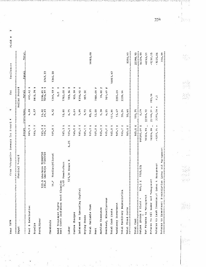
Yea

E 1

9?q

Inpu

t

Fue

l E

Lub

rlcat

ion

Rep

aLrs

SeE

ti 11

2ã r

120"

0 Lb

s,/A

cre

8200

0100

215.

0 Lb

s/À

cre

1034

1C00

Cbe

nl

ca ls

16.0

T

refla

n (o

j.1sÊ

eal

See

d T

reltm

ent

cost

sse

el c

osts

Inc

ludl

ng s

eed

clea

ning 3.60

Pou

n.ls

lÀc1

3

LabJ

r 12

5.3t

t llo

urs

A

cust

oE C

harg

es

Inte

rest

on

0pa

ratln

g C

aplta

l

oryl

ng c

osts

fota

l Y

aEla

ble

eost

Ren

t

tlach

tne

I ns

uran

ce

over

head

, I'l

Lsce

llane

o'¡s

ToL

al C

ash

Cos

ts

üach

l,ner

y f

nves

toen

g-

Tot

al l

tach

iner

y D

epre

cllti

cn

Tot

el P

ireil

Cos

f-s

c:cp

Srt

erp¡

is-?

Sum

mar

y:rr

Fnc

c¡rl

d

Phy

slca

l Þ

Ðco

rrl

Dol

lar

Rec

ord

-aE

t9:-

--ç2

= g

lÀçr

.Ê--

----

-re!

al--

----

-Let

àl16

5.0

x ¡¡

.18

165.

1 f

8.5?

165.

0 x

1).9

216

5.C

x

20.9

1

165.

0 X

8.

12

165"

0 x

10.8

0

6"25

16

5.0

x U

"75

1 65

.0 x

0.

61

1 65

.0 x

7.

9q

165.

1 x

5.s1

1 65

.0 x

85

.35

16s.

0 x

12.0

0

1 65

.0 x

q.

zq

165.

C x

4.

25

165"

0 x

1Cl"8

r¡

165,

)T,

11.6

?

. 16

5.0

x 20

"2'4

165.

ù f

50"4

0

Tot

al c

ost

outp

ut l

Àcr

es x

Yie

ld =

16

5.0

x 11

0.).

ccl

Net

Fe

turn

s +

-o la

tagl

in?n

t

Ret

urns

to

À11

Lab

or t

nd r

,!tna

g)n)

n:

Ret

ucns

t3

Lnnd

Inv

ssi.m

r:n:

Lab

cr D

tl1n

ag:o

en+

Ret

uEns

to

fnve

stnÈ

ta D

ìnre

cià¡

-ion

Labl

r ãn

d ,la

r.eg

emèn

n-

for

690.

42 V

1rt1

3.79

v

2296

.8q

u3l

¡50.

97 V

t3r¡

0.59

V

0.0

v

1782

.00

v

781.

36 V

r00.

18 v

11r6

.40

v

907.

5C

1980

.C0

F

39.8

0 F

701"

67 F

2255

.09

3339

" 9r

¡

Sun

:lou3

r-s

57 4

7 .7

7

13rt

0. 5

9

Fi È

lil

Þ

!sl1

I -

1815

n0.

C1

x 0.

Crt

1613

4" 9

9 _

2239

8.5¡

l

1633

r¡.9

9 -

221q

8.5ô

+

783.

76

-529

1.15

+

2255

"99

+

0.C

165.

0 x

135"

75

t{r0

82"

00

1680

3.

.¡7

8316

.49

223C

8.50

1613

r1.9

9

-6C

63"

51

-52

80.1

5

- l0

25.

06

31q.

89

\ri

UI

Yeà

r 1

979

Inpu

t

Fuê

l 0

Lubr

ica¡

:lon

Rep

atrs

Per

tlllz

er14

7.0

Lbs,

/Àcr

e lC

ll¡00

01

chen

Lcr ls

16.0

T

r¿fIa

n (c

11s€

eal

seed

lE

eath

ent

cost

sse

el c

D.s

ts r

nclu

dinq

see

il cl

eeni

nå po

und=

,rq.

r=

Labc

E

1 I

5. g

t¡ H

o ur

s A

cust

oq c

hlrg

es

Intq

rest

on

Ope

ratln

'l C

apita

L

Dry

inq

ccst

s

Tot

al v

aEia

ble

cost

Ren

t

llach

lne

fnsu

Dan

ce

oYer

head

, ül

scel

lane

ous

lota

l ca

sh c

osts

üach

lner

ï In

vesl

-Een

t

Tot

al

tlach

lner

y D

epr-

.cla

tlcn

lota

l F

ixed

Cos

ts

Cao

n C

nter

p:i.-

io

Sum

nù:v

fc:

F

:csl

d !

P!:y

sica

l 3"

co:d

IEr:

s--

-çss

:/Àsr

:,---

---

-3s!

al27

5.0

x 3.

77

10 3

5.8r

¡ v

275.

¡ r

B.lZ

22

89.3

1 u

2't5

.0 X

275.

0 x,

275"

0 x

6.25

27

5.3

X

275.

0 X

275"

0 X

275.

1 't

275.

0 f

275.

1 Y

.

275.

0 x

275.

C x

275.

0 r

275.

0 x

?75.

1 x

215"

1 X

::::l=

::::=

=ou

tp'rt

{À

cfes

X Y

!e1.

1 =

27

5"0

X

7ôC

.001

Net

Ret

urnd

to

ìlana

gsn?

nt

Ret

urns

to

ÀIl

Labo

r ân

i I't

anag

:men

t

Ret

uDns

tc

Land

Inv

esi.m

?n+

Lab

or 0

¡l1

nag¿

men

t

netu

rns

t)

Tnv

eslm

ânt.

¡epr

ecia

ii.n

Labr

r l'n

rl Ìlâ

ntge

men

t

DoI

lar

Rec

oEd

for

13.0

8

8. 1

2

10"

8C

tt, Z

z

0.61

5. 8

6

1.50

58.2

9

12.

CC

0.2q

4"25

?q "

78

13.6

7

2C.2

q

50.4

0

sun

floH

crs

3597

.82

V

223\

.32

V

0" I

v

2970

"0C

v

1 16

1.49

V

166.

96 v

1611

.C9

v

962.

50

3300

"c'0

F

66.

-13

F

1169

.q5

F

3753

.49

s566

.5?

IegÀ

l

1597

.82

'223

q.32

Pie

lal

$

Ie!e

!-

1925

t0.0

i.) x

1712

q.

99 -

1712

t¡"g

c _

-114

C3.

69 +

275"

0 ï

10 8

. 69

0.09

2989

0" 1

6

29rJ

9C"1

6 +

116

1.q9

3758

"49

+

0"1

160

29.

3 3

2C56

5.11

2989

0.16

't732

¡r.9

9

-125

65.1

7

-114

13"6

8

-76¿

t5.1

9

-2C

78.6

2

1186

0.83

u{ \¡l

LN

Y€a

r 1

979

Inpu

t

Fue

l t

Lubr

ica+

-lon

qepa

lrs

fêrt

l llz

er

che

ml

ca ls

See

d T

reat

Den

t co

sts

seei

l co

sts

Incl

urlin

g S

eed

clea

ninc

l

Crô

p E

nter

p:is

? su

nnar

y :c

r P

cc^r

'l É

I

for

Phy

s ic

a I

Rec

orrì

LåbO

T

Cus

tots

Cha

rges

Inte

rest

oD

0ps

ratin

g ca

plta

l

Tot

aL V

aria

ble

cosc

R e

nt

tlach

lne

Insu

ranc

e

over

head

, üi

scel

lan¿

ous

Tot

al c

ash

cost

s

íach

inÈ

ry I

nees

tnen

t

Tf ta

I la

chln

eEy

Dep

recl

a+-lo

n

Tct

rl F

ixet

l C

osts

t¡3.

0 Lb

s/À

cEe

8200

0C00

230.

0 Lb

s,/À

cre

1034

c00C

1"3

Àva

d:xR

tl(H

hear

l10

.0

Tr¡

flan

(cer

als)

10. 5

2, {

¡- D

Àm

in ?

8c

'l " 50

Bus

hels

,/AcE

e

1¡¡0

.43

ltour

s rù

!EE

-?E

-- -

çe9

!/Àsi

ì- -

----

-r?!

âl12

C"0

X

5.91

70

9.C

1 V

120.

C X

. ?.

Bl

Ct9

.ó5

It

1 2C

.0 X

r¡

" 99

59

8. 5

6 V

120.

0 x

20.r

¡7

2456

.r¡0

V

305q

.96

Tot

al C

ost

tutp

ut

(lcre

s X

flel

t =

120"

J X

1 20

.0 r

120.

0 x

1 20

.0 l(

6.25

12

0.0

x

1 20

.0 x

1 20

.0 r

120.

0 x

120.

0 X

120.

0 x

1 20

.1 x

120.

C x

1 20

.0 x

1 20

.0 x

120.

c x

Þol

lar

lìêco

rû

Net

Ret

urns

to

llann

qâß

Ên:

1C

752.

00 -

Rèt

urns

to

ÀIl

Labo

r rn

'i l'l

lnãg

-.n3

nt

1075

2.0C

-:ìe

turn

s tâ

Lan

d In

vest

nsnt

Lab

or t

tla

nr(le

mÊ

n+-

-347

2.51

+

Pet

urns

:c

Inv-

ostn

an:

D.?

prec

iaLi

on L

ab)r

ãni

l I'll

neq+

nsnt

7 ,6

35.

C8

1.14

6 .6

7

't .3

2

1.21

7 .2

0

75.q

5

'I 2.

0C

q.2q

q.25

91"9

5

13"6

7

20 "2

4

50"

40

lihcâ

t

ls.E

sI

12C

.0 x

20

.00t

24

00.3

e x

915.

00 v

609.

36 v

137.

09 V

0.0

v

801.

C0

v

878.

01 V

1q5.

?1 v

864.

3?

V

1 4¡

r0. 00

F

28.

9¡¡

F

510"

31

F

16¡¡

0.C

7

2429

.05

Fie

ld

i

fe:å

!-

1661

.¡t5

1 20

.0 x

125.

85

q"48

151C

2" 5

l

151f

2.51

+

878.

01

1 64

1.07

r

0.0

905q

.17

110.

13"¡

¡2

6040

" 36

1510

2.53

1C?5

2.00

-435

0.50

-1r¡

72.5

3

-1ß

.12.

r¡6

596.

59

\,J ut o"\

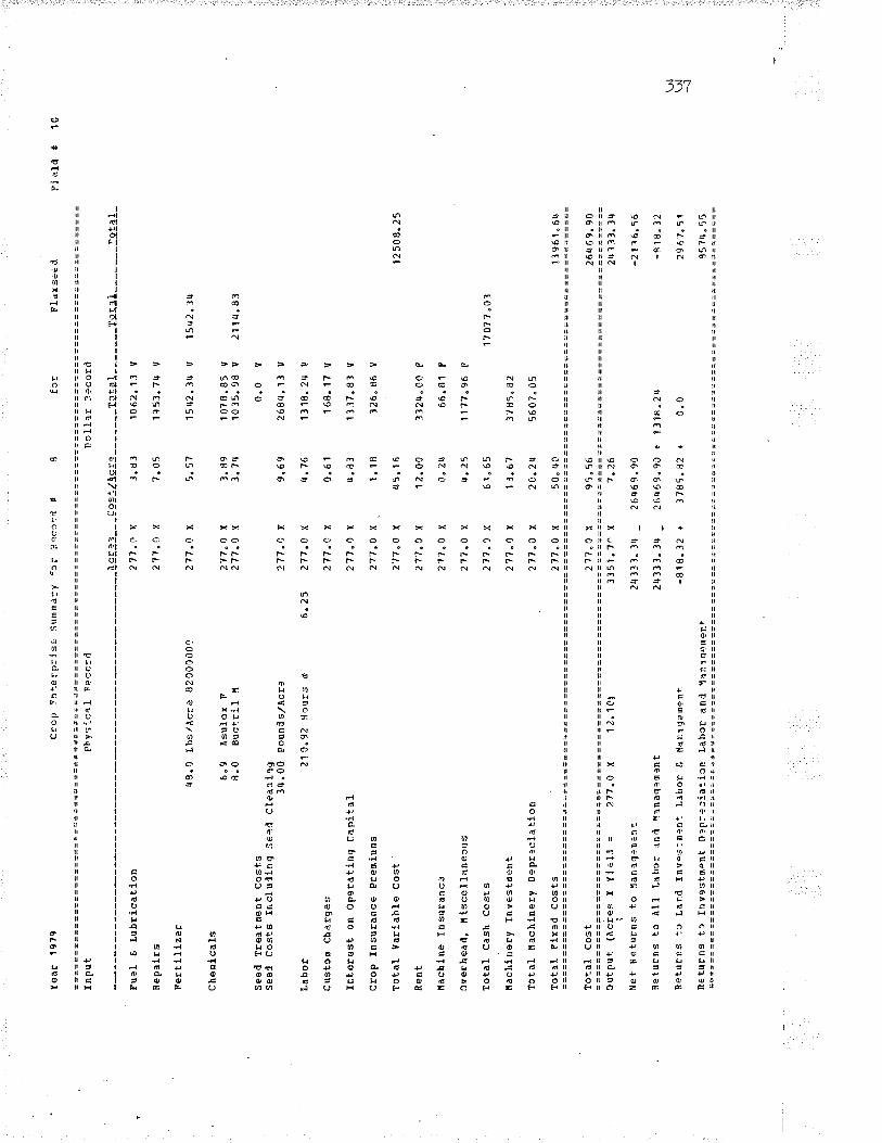
Y€a

r 1

979

Inpu

t

Fue

I 6

Lubr

icat

lon

Rep

alrs

FeE

Llliz

erl¡8

.0 L

bs/À

crê

8200

0001

C h

e ni

ca ls

6"9

Asu

lox

F¡1

.0

Buc

trll

I

Ses

d T

Eee

teen

t co

sts

seel

cos

ts I

r,cl

ullin

g se

?il C

leax

i'rg

3q.0

0 P

oun,

ls,/À

c13

l,abo

r 21

C.9

2 H

ours

ô

Cus

tcn

cher

ges

Inte

rest

on

ope

ratin

g ca

pita

l

Cro

p In

suE

aoce

PE

eniu

ns

Tot

.al

Yar

labl

e co

st

R e

nt

ttach

lne

Insu

ranc

è

cser

head

, lli

scel

lane

cr¡s

Tot

al C

ash

Co.

st s

llach

lner

y In

vest

úent

TcÈ

aL lt

achi

nery

Dep

r¿ci

atio

n

Tot

¡I

Flx

atl

Cos

ts

Cro

p F

r+,e

rp:is

: S

rrnm

à:y:

3r !

ìccc

arl

ü

Phy

s:ca

l F

eco:

d

ÀsE

.?!-

- -ç

es:/À

ci:

277.

o r.

1.

83

271.

0 t

2?7.

0 x

Tot

al C

ost

277

"0 'x

.

277.

C x

217.

q x.

6,25

27

7.C

r

271.

C x

277.

0 '[.

2't7

.0 x

27?.

0 x

271.

0 r,

217

"q x,

2't7

.0 x.

277.

) x.

277

"q x.

. 27

7.0

t

277.

0 x

cutp

ut (

Àcr

es x

yiâ

I,l

=

7--1

7.0

ï. 12

,1c'

llet

Ret

urns

to

llana

q+na

n'-

Ret

uEns

to

À11

Lab

cr ¡

nd r

,!1na

qeüà

nt

Ret

urns

'-c L

and

Invo

s--o

?nt

Låbo

E 0

Car

.t,re

nÊnr

_

Ret

urns

to

Invg

stm

pnt

D3p

:rci

a:io

n La

bcE

ani

l iln

nlqc

men

+

Ilollâ

r:ì'?

cor(

1

fcr

7.05

5.57

3" 8

93.

74

9.69

q.'t6

0.61

4.83

1.18

r¡5.

16

1 2.

00

11"

2lt

q. 2

5

61.

65

1J,6

1

2A ,2

4

50.

q0

1?!ê

I10

62.1

3 v

1C53

.7rr

v

15¡¡

2.34

V

1078

.85

v10

35.

98

V

0.0

v

2684

.1 3

V

13 1

8. 2

¡¡ V

168.

17 v

13i7

.81

v

326.

86 V

3r24

. C

0 F

66. 81

F

t177

"96

F

3785

.82

5607

.05

Fl

d ¡

ScÈ

,1

terå

l----

--le

!â1-

15'¡2

.l4

2114

.83

Fiè

ld s

10

211

"0 x.

3151

.7^

x

2rtl3

3" l

q _

2433

1.3r

¡ _

-818

.32

|

95"5

tr

7 '2

t'26

469"

90

26r¡

69.9

J +

131

8.2r

t

3785

.82

+

C.0

1250

8.2s

1707

7.03

'!396

1" 6

r¡

26u

69.

90

2413

3" l

¡¡

-21i

6.56

-818

. l2

2967

.51

8574

.55

u.l

\n -_l

Yea

E 1

979

crcP

Ent

erpr

j.se

Sum

mar

y flr

R

"cor

l Í

I

Inpu

t fth

vsic

al

R?"

ord

----

--!s

!:s--

-ç2

s!/À

sr:

FuÊ

l 6 L

ubric

àf.lo

n 2$

4.0

X

1.68

nepa

lrs

281t

.0 x

5.

58

Fer

tlllz

er

No

Fer

tillz

er

Use

d

Che

nlc

a Is

1.8

Ava

dèxB

H (

oils

)

seed

lrer

tnen

t C

osts

See

l Cos

ts I

nclu

dlng

See

cl C

lean

ing

3¿r.

00

Lab3

r 23

4.1¡

1 H

ours

ô

6.25

cust

cD c

hlrg

es

fnte

rest

on

cpe

ratln

g ca

plta

l

crop

Ins

uran

ce P

reD

luûs

Tot

al V

arla

ble

cost

Ren

t

ttach

lne

Iosu

ranc

e

oYer

head

, ñl

scel

lane

ous

Tot

al C

ash

Cos

ts

ttach

lner

y In

Yes

tosn

t

lota

l f ac

hine

ry D

epre

cl-a

l.1on

Tot

àl F

lfed

Cos

ts

Pou

atl s,

/AcE

:

1oì,

al C

os t

outp

ut (

ÀcE

es x

Yiê

ll =

28

r¡.0

x

9.00

1

{et

Ret

uEns

i to

¡la

naga

nÊnt

Bet

urns

to

À1I

Lab

or a

n,ì

!,lan

acta

nent

Ret

uRns

tc

Land

Inv

es+

-m"n

t La

bor

E Ii

anag

emer

ìt

Ret

urns

tr

fnve

stoe

n+,

D9p

:ecl

atio

n La

bcr

ar.d

Íln

tger

ènt

Dol

lar

RF

ccrd

28r¡

.0 x

10

"6?

2 8¡

¡.0

x 9.

69

28¡t

.0 x

5.

16

284.

0 X

0.

57

28r¡

.0 x

4.

51

2 84

.0 X

1"

18

2 8q

. ¡

x r¡

1.0

5

28q"

ô x

12.0

c

28q.

0 x

c"2r

¡

2 8r

¡.0

X

4" 2

5

28u.

C r

{ 57

.54

28¡¡

.0 x

13

"67

28r¡

.0 X

20

.2t¡

f)r

Fl-ù

rs¿

€d

Fie

ld

12!a

I --

----

-Xgs

ql10

45.6

C v

15rì

6. 0

0 v

3031

.70

V

3031

.70

0.0

v

27 5

1.96

V

1rt6

5. 0

8 v

r61.

52 Y

't280

" 20

v

335.

12 V

1165

7.16

3¡¡0

3"00

F

68"5

0 F

1207

.7i

F

16lr¡

1.38

388t

r" 4

9

57r¡

8.75

3otÂ

l-

11

28tr

.O x

50

" rt

o l¡r

31¡¡

.¿t5

284.

0 K

2556

.0C

x

1855

6.56

_

1855

6.56

_

-594

9. 97

c

9',|

" r¡

5

7.26

2591

1.6

1

2597

1.61

+ 1

q65.

08

3881

.49

+

0.0

2597

1.61

1855

6" s

6

-741

5.05

-59r

¡ 9.

97

-206

8.48

1690

.27

uJ UJ @

Yea

r 19

79

Tnp

ut

Fue

l D L

ubric

at-io

n

Sep

alrs

Fer

tlliz

ec

Nc

Fer

tiliz

er

Use

C

Che

mic

als

1. I

.lv ìl

Ëx

Bu

(o il

s)

seed

Tre

ltEen

t eo

sts

Ses

l cos

ts l

ncLu

dinq

Se€

d cl

eani

ngJ4

. 00

Pcu

n¿ls

/.lcr

?

Lab3

r 12

2,68

HoU

ES

a

cust

oo c

hlrg

es

Inte

rest

on

ope

ratin

g ca

pita

l

Cro

p In

sura

nce

Pre

nluo

s

Tot

a} V

acla

ble

cost

Ren

t

nach

lne

fosu

ranc

o

oYer

heat

l, tl

isc-

olla

neou

s

lota

l C

âsh

Cos

Ès

tlach

iner

y In

vest

nent

lota

I na

chin

ery

D€p

r?ci

ltion

Tot

âl F

irad

Cos

'-s

crop

1nt

,ìrp:

ls:

Srr

mm

ary

j'o:-

Pec

o:rl

å

Fh.

ysic

À1

Rec

ord

!st.?

!--

-ç2s

i/¡ç

!315

5.0

X

3"5(

'

155.

0 X

5.

88

Tot

al C

ost

1 55

.1 X

155.

C X

6.25

1 55

.0 x

1 55

.0 x

155.

0 X

155.

0 t{

155.

t x

155.

{:'

Y

155.

C X

1 55

.1 x

155.

0 x

1 55

.1 X

155.

0 x

155.

0 x

outp

ut (

Acr

es x

Yi3

li =

15

5.0

x c.

001

1 ì9

5.0f

ì x

Net

Ret

urns

ito l

lana

qem

?rt

1112

7"7õ

_

Ret

rrE

ns l

-c À

ll La

bcr

lni

{âna

q--m

lnt

1C12

7" 7

1 _

Ret

urns

tf,

L1n4

lr.

vest

mln

t Lä

bc!'Ê

lla

nag+

n¿nt

-3

279.

29 +

Dol

lar

Bec

oril

fcr

netn

Ens

tc

f n

v?st

mtn

+-

D,.D

rcjc

ia:

!oiì

Llbf

r

atd

I'ltn

lgF

màn

.:=

==

==

==

==

==

ls g

ql--

- --

--1e

!sI-

----

--3e

!âl-

556.

20 V

912.

C6

V

17,6

7

9.6q

t¡.9

5

0. 5

?

4"51

1.18

01"0

q

1 2.

00

0 .2

q

q.25

57.5

3

1 .3

. 67

20.2

4

50.

¡¡C

FIa

xse€

d

165r

¡.62

v

1654

"62

0.c

v

1501

.95

V

766.

75 V

88.1

5 V

698.

63 v

182.

90 v

1860

" 00

F

37.3

8 F

659.

15 F

891

7.79

2118

" r¡

2

11 3

7 .5

2

Fie

ld

d12

155.

0 :(

91 "

t¡4

't .2

6

1U11

3.72

1t!1

'l'1"

72 +

?6

6" 7

5

2118

.r¡2

+

C.0

636i

.26

7812

"¡¡6

t'¡17

1.72

7012

1 "7

'.)

-¡10

46.0

2

-377

9.28

-116

C.8

6

1 _o

76.

66

\n \n \o

tear

1 9

?9

fnpu

t P

hysi

cal

Fec

ord

DoI

Iar

P?c

or.l

Bue

l 6 L

ubrlc

ai-io

n 27

6.4

x 4.

79

1320

. 86

v

Rêp

alcs

rert

i llz

er7¡

¡.0

Lbs,

/Àcr

e 11

5qnC

00

che

n!ca

ls1"

5

Au1

¡lèxB

H (

Bly

Pea

¿t.9

[y

?¡r¡

: 20

0-C

10.5

2,

q-D

AE

ine

8C

seed

Tre

atna

nt C

osts

seel

cos

ts I

ncl-u

clin

g S

eed

clea

ning

1. 7

5 P

ounl

s/À

cr?

Labc

E

261"

08 H

ours

ò

6,25

Cus

toD

Cha

rges

Inte

rest

on

Ope

ratln

g C

aFlta

I

Tot

al V

aEla

ble

Cos

t

Ren

t

tlach

lne

Insu

ranc

€

oYeE

head

, üI

scel

Ìane

ous

Cro

p E

n+-9

rp:is

¿ S

umm

arv

fcr

Pec

o:rì

!

Tot

al C

ash

Cos

ts

276.

C X

66

.41

tlach

lner

y T

nves

+-o

ent

276.

0 [,

1 3.

67

Tot

al t

tach

iner

y D

:pre

ci.a

tlon

276.

0 x

2î"2

4

Tot

al F

lletl

Cos

ts

276"

0 X

50

. ¿

10

2't6

.Q

276.

0

2't6

,C27

6,r

)27

6.O

276"

0

Tot

al c

osL

276,

C r

, 1C

0. 1

2

Out

put

(Àcr

es X

Yi.3

lt =

27

6.0

X

2ó.1

01

Het

Ret

urns

ì to

!la

nage

msì

t

Ret

urns

to

Àll

Lsbo

r ln

il lfâ

nag¿

m?n

t

Ret

urns

ta

Land

Inv

e;ln

.-nt

Lib

o= F

, M

anaq

emén

r-

Ret

uEns

to

In v

?str

q:n'

. tt.

:p:-

:ci.a

:i)n

LÀb)

r an

d Ì'l

àni(l

;-m

ent-

f:c:

6. 5

6

9.71

9. 1

54.

591.

1q

1 ,7

1

1811

.68

V

2685

.76

V

2525

. rr

0 U

1265

.62

u31

5.30

v

0.0

v

r¡ 7

0. 9

2 V

1611

.75

v

313.

9r¡

V

1r¡3

5. 9

5 v

3112

.00

F

66" 5?

F

1173

.71

F

3772

.16

5586

" 81

276.

0 't

5. 9

1

2'16

.1 x

. t.1

r¡

276.

0 X

5"

2q

2 76

. C

X

r¡ 9

.92

276.

0 x

12,t)

O

276.

0 x

0.2¡

r

2?6.

0 X

q"

25

naE

I èy

!e!q

I

26ù5

.76

4 1C

6. l2

-!e!

3!-

Pie

ld

tl3

71?6

.00

x

1165

2.96

-17

652.

96 _

-.q¿

J0 3

" 70

+

2" l¡

6

2768

3"40

2768

8.¡¡

0 +

163

1.75

77'1

2.16

r

0.0

137

77.1

7

1832

9.1¡

¡t

îl9xx

"2l

2768

8.¡r

0

x7ó5

2"96

- 10

0 35

.1¡

r¡

-84

03.

?C

-463

1.5r

¡

955.

27\.}

I È (J

f. À

crge

ge B

y cr

op(a

cEes

l

lI.

Cos

t of

PE

oduc

tion

1. F

uel ô

Lub

rlcat

ion

2. R

epal

rs3.

FeE

til l

zeE

l¡. C

heF

lcal

s5"

See

il T

Eea

tden

t co

sts

6. S

ee¿

l 6 C

lean

ing

C0s

t7.

Tiri

n€ c

osts

8. L

abor

9..

Cus

toD

cha

rgàs

10.

Inte

rest

0p

er.

Cap

.11

. C

rop

Insu

ranc

e P

Een

.12

. D

ryln

I co

sts

13.

Equ

lpm

ent

Ren

taI

Cha

ll¡.

lota

l V

arla

ble

Cos

t1¡

¡. R

enÈ

15.Îa

xes

16.

tlach

lner

y In

sura

nce

1 7.

f, ve

r he

ail ,

¡l l

sc .

18.

Tot

aI C

ash

Cos

'-s19

. In

eest

üent

Lln

tl0B

lAg

20.

Inve

stoe

nt l

n ¡!

ach.

21.

ltach

lner

y D

epr.

22.

'Iota

l S

lxeâ

Cos

+-s

Tot

aI C

ost

anl

Ret

urn

Sum

mrr

y P

Èr

Crr

p F

or h

-.-.

o:d

Num

b:r

I Ilt

19

79

Tyn

+ f

f E

: tÊ

r D

Ei s

e

PrÞ

ese-

.d

Tam

e !l1

y S

umm

:cfâ

llot

su

mm

erfa

Llor

325.

r 1?

6.65

2112

. tr

g3

770.

0036

93.5

60.

010

53.0

00.

c16

11.r

¡219

7 .3

21

396.

05s6

5.50

0.0

0"0

1559

5.95

0.0

1 63

.75

?8.l9

1 38

2. 0

817

820.

1621

27 1

" 2s

r¡4r

t1 "

8565

78.6

73r

¡515

.97

23.

Tot

rl C

osts

50

111.

92

fII.

cros

s R

etuE

ns

2q.

Avs

rage

Yle

lì/¡lc

Ee

6.20

25.

Àce

rage

Pric

e 6,

5026

. C

Eop

Ins

uro

Rev

enue

0"

027

. st

râr

($,/À

creì

0"

028

" cr

azln

g ($

,/Acr

e)

0"0

lota

l qr

css

Fet

urns

1

3097

. 50

IV.

Net

Ret

i¡rns

to

ügm

t. -3

701¡

¡"43

V.

Rat

urns

tc

Labo

r r;

' ¡l1

m:.

-35¡

¡Cl.

C1

Vf.

Set

urns

to

lnve

s.-n

ent

Lab)

r 6

ltgnt

. -9

689"

91

VII.

R

etuc

ns t

o In

vest

men

tD

epr.

Lah

cr t

ilg

ml

3111

.25

Trt

aI

cash

co-

t< 3

,f rr

a ls

th

e s,

¡¡ o

f T

txcs

, F

uel

sãea

l cle

anin

g an

d T

relç

.men

t, cr

op l

nl

Iach

ine

Àss

unes

17.

00C

ß R

er.u

rn o

n ca

pita

l"

60.

1 02

. 30

92.6

840

0.5,

0.0

0.c

267

.75

0.0

112.

l910

87.

1 l

259.

450.

10.

00.

023

22.1

91

20 .0

00"

01q

.0?

255.

1533

11.8

20.

082

0.03

12't4

.52

3024

"18

168"

161

. 59

'128

. 42

0.0

650C

. 80

0.0

0.0

0.0

1 u2

. 57

0.0

825.

63e"

I0.

0c.

071

68.0

220

1 6"

00

0.0

4 0.

5?71

4. q

310

538.

e6

0" 0

2296

" 09

34C

0,67

846

?. 7

0

35.

17q"

821

15.

880.

00.

00.

00.

0c.

01¡

¡8.5

10.

086

.4C

0.0

0.0

525"

61

rr20

.00

0.0

B"

¡¡q

1¿t8

" 84

1 1 02

.89

0. c

r¡78

.35

708"

47

176¿

¡" 1

0

S'¡n

flose

rs

53r¡

6" 3

7 16

235.

72

2289

.'t't

4059

9.00

1"40

0.

0 0.

0 12

00.0

037

.50

0.1

0.0

0.09

0"0

0.0

0.0

ù.0

0.0

0"0

0.0

0"c

0.0

1"0

c"0

0.0

31 5

0.00

0"

0

0.0

33¿

¡79.

99

-219

6.37

-1

6235

.'t2

-228

9.71

-7

X 1

9.02

-2^8

3.99

-1

6093

" lrt

-2

'tfil.

20

-547

2.47

-126

-1.9

5 -1

3797

.05

- 16

62. 85

-1

215.

61

-!q"

{l -1

c196

.38

-954

" l8

50

l9.q

lE

Lr¡

br!c

atlo

o, F

cpâi

rs,

Pcr

tiliz

,?r,

ch

emi.c

als,

sc.

:rl,

fnsu

:'rnc

e, ¡

lisc.

ove

rhca

d, R

qnt "

Ltbo

r. ¿

niì

Tci

n¿"

31ù.

1r¡3

5.81

28 3

rt.

?187

85.0

825

18.6

90"

033

48.0

00.

016

'¡6.5

518

8.21

2J57

" 06

0.0

1860

" 00

0.0

2q97

q. O

737

20

.00

0.0

74 ,7

713

18.

29

3008

7.13

0.0

r¡23

6.8q

6275

" 0q

1562

4.93

Paq

e

sun

floce

rs

180.

874.

4316

87.6

655

60.3

71r

¡62.

1¡6

0.0

1 9q

¡¡.

000"

095

1.

3710

9.

2813

9 1"

32

0.0

81 0

.00

0"0

1 q

790.

87

2160

.00

0.0

43"4

176

5. r

¡61'

t't59

"'r5

0"0

2r¡6

0. 1

03

643.

5?

907

2. 5

q

2186

3.4'

t

900.

00

0.09

0.0

0"0

0.0

X¡¡

579.

99

-928

1.42

-831

2.05

-587

1.95

-222

8,38

UJ È

T"

II.

Tct

aI C

ost

anal

letu

En

Sun

mar

y P

cE C

ror)

For

3ec

or4

Num

hàr

I In

197

9

Typ

è of

Fnt

prr¡

:ise

Àcr

srge

By

Cro

p(ac

:es)

Cos

t of

Pro

iluct

lon

1" F

uel

t Lu

bric

atio

n2.

Eep

aics

3. F

ertil

ízer

{"

Che

r¡ic

als

5. S

eed

Tre

atrì

3nt

cost

s6.

5eel

D

Cl2

anin

g C

os!

7. l

rlne

cost

s8.

Lab

or9.

cus

toD

cha

¡ges

lC.

fnte

rest

op

?r.

cap.

11.

Cro

p fn

suE

ance

Pre

no12

. D

r¡1n

9 co

s'-s

13.

Equ

lpue

nt R

Pnt

al c

ha10

. T

otal

Var

labl

e C

ost

1¡1"

Ren

t15

. T

ares

16.

tlach

lner

y fn

suca

nce

17.

cver

heat

lo ll

sc.

18.

lota

l ca

sh c

osts

19o

InY

estn

ent

Lànt

lCR

l¿lg

20"

Inve

stne

nt !

n ra

ch.

21"

üach

iner

y D

rpró

22.

Tot

aI P

Ixed

cos

ts

sun

f lo

tre:

s

165.

690.

r¡2

1r¡1

.1.7

957

r!7

.77

1 34

0. 5

90.

c1 78

2. C

00.

078

3 .

3610

0.18

1316

. rl0

t.090

7.50

0.0

14C

82"0

01

980.

C0

0.0

39.8

07

01 .6

71

6 8e

3. 4

70"

022

55.

09

3339

e9r¡

8316

. r¡

9

St¡

nflo

cers

H

heat

F

Iaxs

ÊeC

21.

Tot

al c

osts

22

398.

50

2989

0.16

fII"

Gro

ss R

etur

ns

24.

Àv3

rage

Yle

li./{

cre

1100

"00

?00.

C0

25"

Àve

rage

Pric

: 0.

09

0.09

26.

Cro

p In

sl¡E

. R

ev€n

ue

0.0

0.1

27.

stra

u (S

,/Àc!

Èl

t.0

0.0

28.

Gra

zlng

($,

/Acr

el

0.0

0.0

Tot

al I

ìros

s P

e+-u

rnE

16

114.

99

1732

4.99

IV.

Net

net

urns

+-o

l:In

t"

-606

1"51

-1

2565

.17

V.

Aat

urns

tc

Låbc

E t

ttg

nt.

-528

0.15

-l1

r¡03

.6q

VI.

R?t

uFns

to

fnve

s+-n

?n+

Lìhf

,r t

ll1

ß+

-.

-302

5.06

-7

f¡4i

" 19

Ufl.

R

etuE

ns t

o fn

vÊì*

-n:n

tD

èpE

. La

boE

t

r'|.-

¡nÌ.

314.

Ê9

-207

8.62

Tof

aI c

ash

cost

s ?,

lulls

:h¿

sr

rn o

f T

ax)s

, F

u¿l 6

Lrr

uric

aÌio

t,se

ùô c

leln

:ng

anC

Tr-

'1:m

:n:,

crop

an¡

l ya

chin

e In

rìuE

encÞ

, fis

c.À

ssrln

es 1

7.C

Dr

l{ P

"'-,!i

n on

Cap

itaI.

275.

10 3

5.84

2289

,31

3597

.82

223t

t.32

'0.0

29't0

.Dq

0.1

1161

.rr9

1 66

. 96

1611

. C

90.

196

2.50

0.1

1602

9" 3

333

00.0

00.

066

" 33

1169

.45

2056

5. 1

10.

037

58.

q955

66.5

713

86C

.83

120.

7Ce.

0393

9"65

3054

" 96

166

1. 4

50.

08C

1.0

00.

08?

8.01

1l¡5

.71

86q.

370"

00.

00"

090

5¡¡"

1?

1440

.00

0.0

28"

9r¡

51C

.31

1103

3.42

0" î

16r¡

C.0

72u

29.

0560

48.3

6

217

.

1C62

.13

1953

. 7¡

¡15

¡¡2.

3rt

211r

t.83

0.0

268r

¡. 1

30.

013

18.2

'¡16

8.1?

1337

.83

326.

860.

00.

012

5C8.

25l3

2r¡.

0c0"

066

.81

1 17

7.96

1707

7"01

0"0

3785

.82

56C

7"05

1396

1.64

FIa

rs¿

é,i

2 8¡

¡.

1 0

r¡5.

60

1586

.00

0.0

30 3

1.70

0.0

2? s

l. 96

0.0

1¡{6

5. 0

g1

61 .5

212

80.2

03J

5.12

0.0

0.0

11ó5

7" 1

634

08.0

00.

068

, 50

1207

.73

163r

¡l "

380.

038

81"

r¡9

57q8

" 75

1r¡3

1¡¡

. ¡t

5

Pag

e

Fla

xsee

d

151C

2.53

26

1169

.90

2597

1.61

2C.0

0 12

.10

9"00

¡¡.4

8 't.

26

7.26

0.0

0.0

0.0

0.0

0"0

0.0

C"0

0"

0 r)

.0

107<

2.00

2f

¡313

"3rr

18

556.

56

-rr1

50.5

4 -2

136.

5b

-741

5.05

-3¡¡

72"

53

-818

" 32

-5

9119

.97

-193

2.tt6

29

67.5

1 -2

06d"

q8

5'16

.59

857t

¡.55

36

8r,.2

7

Fen

airs

, F

rrtj-

liz

rr,

Ch:

mic

als,

5:e

d,ov

€rh¡

1 il ,

tìãnt

, La

bor,

and

1t¿

ine.

155.

556.

2091

2.06

0.0

1 65

r¡.

620.

015

01.9

s0.

076

6.75

88.1

569

8.63

1 82

. 90

0.0

0.0

6361

.26

1860

.00

0.0

3?.3

865

9.15

99t7

.79

0.0

2118

.42

3117

"52

7812

.q6

1417

3.7

2

9.00

7.26

0.0

0.0

0.0

1012

7.70

-004

6.02

-f27

9.2A

-116

0.86

1976

.66

\n È N)

I. À

crea

ge B

y C

roP

(acr

esl

ff"

Cos

t of

PE

oduc

tion

1. F

uel

E L

ubric

lt-10

n2.

Rep

airs

l. F

ertll

lzer

l¡. c

henl

cals

5. s

e-.d

TE

eatr

¡:n+

, co

s:s

6. s

eed

E c

lean

ing

cost

7. l

vine

co

sts

8. L

aboE

9" C

usto

n ch

arge

s10

" In

tere

sr-

OpÐ

8. C

ep.

11.

crop

fns

uran

ce P

ren.

12.

Drll

ng c

osts

13.

Equ

lpne

nt R

anta

l Cha

1¡¡.

lota

l va

rlabl

e co

st14

. R

ent

15.

Tar

es16

. tla

chin

ery

Insu

ranc

e17

. ov

erhe

ad"

Hls

c.18

. T

otal

cas

h co

sts

19.

fnY

estE

ånt

Lrna

lEB

Ilg20

. In

vest

men

t ln

üa

ch.

2 1 "

tach

ln

ery

D3

pr.

22.

Tot

al F

ireil

côst

s

îo+

-al

Cos

t an

d R

atur

n S

umna

ry p

er C

rop

For

D¿

cc!¡

l NIn

b:r

tì In

1]7

9

lYf?

cf

Ent

ÈrP

rise

Bar

ley

lota

l F

arm

Àv€

rage

276.

1123

.86

1811

.68

2 68

5.7

6rr

106

.32

0.!

q7 0

,92

c.0

1631

"75

113

. 9r

¡1r

¡35.

95

0.0

0.3

c.0

1377

7 "1

733

12.0

00.

066

" 5'

l11

73.7

118

329.

q¡¡

0.0

37't

2 .

1655

86.8

113

911.

23

2f.

Tot

al c

osts

27

689"

40

300

1t¡0

"69

IïI.

cEos

s R

etur

ns

24.

Ave

rage

Yle

ll/A

c:Ê

26

"00

0.0

25"

Ave

rage

Pric

+

2.q6

0.

C26

. C

rop

Insu

r.

Rev

enuâ

0.

0 0"

027

" st

rae

(t/\c

tel

0. C

0"

028

" G

razi

nq l

$./A

cre)

0"

1 0.

1

Tot

al c

[oss

lì3

turn

s 17

652.

96

1791

89.7

5

Iv.

Net

Ret

rlrns

to

¡lgm

'-"

-110

35"¡

¡l¡

-120

750^

69

v. R

6t-u

rns

tc L

abo:

f;

Hgm

+-.

-8

'¡03.

70

- 10

9 13

3.

25

Vf.

Re+

,urn

s tÕ

fnv

gs'-0

?n¡

Labt

E D

l'!q

m+

-.

-461

1"54

-5

0917

.39

VII.

R

etur

ns t

o ln

v-âs

:mcn

rD

èpE

. La

h.'D

E t

fr

]ot.

c55.

27

211q

.23

26 3

0.

't03q

5"66

1789

8"09

351r

¡4.6

130

328.

310.

c19

57r¡

.70

0.0

1261

7 "

452'

l 26.

5tl

1q86

0.36

141C

.38

45rr

0.00

0.ô

1¿t9

r¡ q

5. B

727

660.

007

63.7

56

3l¡.

32

1118

4.21

1896

88"

1221

271"

2535

94¿

¡.?9

5323

6.61

1506

94.6

2

'I . 3.93

6.91

13.

3 6

11.

530.

0't.

qq0.

t¡¡

"80

1.04

5.65

0. 5

41.

73c.

056

.82

10.

520.

290,

24q.

25'1

2. 1

28.

09

11.6

720

" 2t

)57

.l0

't 14

. 12

0.0

0"0

0.0

0.0

0.0

68.2

1

-l¡ 5

. 9l

-41.

12

Ista

seed

As

su

I ca

sh c

o:ts

¿

.{ua

Ls :

h3 s

um o

f r.

txas

, ou

Al t

L'

¡hric

a.-ir

tì,C

lean

in(f

ani

Trç

aìm

+nt

, C

rop

an I

faac

hin€

Ins

uran

ce,

"lisc

.ne

s 1?

"001

I,

Pô'

.¡r3

on

capl

tal.

P a

gÊ

-19.

l6

c" B

8

F.iD

eirs

o F

+r'-

iliz;

r,

chìm

ical

s, S

eido

1v:r

h?ìd

, P

'nt,

Labo

s, a

nd lu

in;.

\n F UJ

cf,s

t an

rl R

)t,¡

:n P

c! A

cEe

9or

C:o

p F

or F

ecoE

¿l

Num

btrr

f. A

creì

ge B

y cr

op(¡

cres

)

II.C

ost

of P

roãu

cl.

Fue

l D

Lub

2. F

epai

rsl.

Fer

tillz

er4.

Che

nlca

ls5.

See

d T

reat

6. S

ee¿

l 6

cle

7. t

vlne

C

ost

B.

Labo

r9.

cus

tor

cha

10.

lnte

rBst

o

11.

crop

Ins

ur,l2

. D

ryln

g C

os13

. E

qulp

nant

14.

Tot

al v

arl

14.

Ren

t15

. T

axes

16.

tach

iner

y17

. ov

erhe

atl

¿

18.

Tot

al c

ash

19"

Inre

stre

nt20

. In

gesr

-men

t2l

. tt

ach

in e

ry22

. lo

tal

Pix

€

t lo

nr

ica

t io

n

cost

s9

Cos

ttr

rnt

anln

s Ege

sP

e r.

anc

ets R

èn t

ab le

fnst

¡tl is

cco

sLa

nln

Ds

Pr

dco

Hhe

a+-

Bar

lf,y

121, 5.

917.

8125

. r¡

6

13.8

50.

16,

670.

0't.

i21

.21

7 .2

00.

00.

00.

075

.45

12 .

000"

00.

2¡¡

4.25

91"

950.

013

" 6?

20.2

U50

. rr

0

caP

.P

re 0

.

23.

Tot

al c

osts

12

5.85

10

0" 1

2

IfI"

cros

s R

etur

ns

24.

Aee

rage

Yie

lå/À

cre

2C.0

0 26

"00

Bre

akev

en T

ielil

,/Acr

e 20

.52

27 .

0025

. A

veE

age

Pric

¿

4. q

B

2. ¡1

6

Bre

akev

-1n

Pric

e 4.

60

2.57

26.

crcp

Ins

ur.

Rêv

enue

0.

0 0.

02?

" st

râu

(S/¡

ìcre

' 0"

0 0.

028

. cr

az l

n g

($/Â

c¡ o

¡ 1.

0 0.

1

Tot

ll G

Eos

s P

4tur

ns

89.6

0 6

3.96

Iv"

Nst

Ret

urns

to

ügm

t"

-36.

25

- 16

. 16

V"

Ret

urns

to

LabD

r â

$gm

+-"

-z

ò.qq

-3

0.45

VI"

Ret

uEns

to

fnue

sEn?

ntLa

bor

å ñg

mt.

-X5"

27

-16.

78

VII.

R

etur

ns t

o In

ve;r

nÊ:ìt

DeP

r. L

aboE

t

M,.|

mr-

. t)

.97

3. r

l(i

Tf,t

al c

ash

côst

s:,lu

tls

cha

sr¡m

cf

T1x

es,

f-u?

I e

Luhr

ica.

-!oî

,S

?ed

Cl€

anln

q an

d lr?

atm

?nt,

Cro

p ¡n

rl üa

chin

e fn

sura

nc-,

tli;

r.

al c

haC

os t

Ea

nce

ts df,B

li!q

la c

h.

sts

27 6

, ¡¡.7

96.

56

9.7

3

1t¡.

88

0.0

1.71

0.0

5. 9

11.

1q

5,20

c.0

0.0

0.1

¡¡ 9

. C

212

.0q

0.0

0.24

tt. 2

566

" ¡¡

1

0.1

13.6

720

.21t

50 .

r1ù

8 In

197

9

Fla

xs€?

tl

71 6

. 3.72

6. 2

22.

159"

s0

0.c

9.69

0.0

q"96

0. 5

8Ir

.63

1"18

0.0

0.0

u2,6

tt12

.00

0. I

0 .z

tt4.

2559

.13

0.0

13.

6720

"2q

50"

¡¡0

I a

D¿

s€ed

325. 3.

626.

561

1. 6

C11

. 36

0.0

3.21

¡0.

04"

96

0.61

4.30

1.7¡

¡c.

00.

0¡¡

7.99

0.0

2, 3

50.

2tr

(t.2

55r

t.83

65.

t¡5

13.6

720

,2q

1 06

.20

sunf

Iouè

rs

Àss

um:s

17.

1100

( F

Ê+

u:n

on C

npi.a

l"À

ctua

l -1

9r-?

l? Í

lì-

¡rtr

ns :

ln c

api+

11

Pâo

e

930. ¡¡

.3q

8. 8

425

. q'

l8.

12

0" 0

10.

800.

04.

88

0.61

7 ,1

80"

0q"

880.

075

. l4

12.0

00.

00.

2q

tr.2

591

" 63

0.0

13.6

720

.24

50.

r¡0

Tan

? H

ay

9t.0

q 15

¿1.

19

l25.

5rt

10.2

0 6"

20

976.

3r¡

8. 1

4 8.

r¡{

t 10

18.

11

7"26

6.

50

0.09

5.80

8"

8¡¡

0.

090.

0 0.

0 0.

00.

0 0"

0 '1

.00.

0 0.

0 0.

0

?r¡.

05

4c.3

0 87

" 87

-18.

99

-111

"89

-37.

67

-14"

03

-108

.93

-12"

78

-0.'1

7 -2

9"92

-1

9.12

19.8

8 -')

.57

1.13

fl::p

r!:s

, F

eFtiI

izer

, ch

c=¡n

ic1l

s. S

.:c i,

ov"r

h.:a

d" R

Èrt

, Lè

boro

an(

i T

Bin

È"

60. 1. 7

11.

51¡

6. 6

70.

00"

04"

46

0.0

1" 8

718

" t2

tt. 3

20.

00.

00.

018

. ?0

12.0

00.

00"

2rr

q.25

s5.2

00"

01 3.

6720

"24

50.q

0

89"1

1

1. .

¡0'1

"q1

3?.5

C39

" ¡¡

3

0.0

0.0

0.0

52.5

0

-36"

61

-34"

?3

-21.

07

-0.8

2

UJ È F

cost

an4

R9L

!!:ì

P9r

Àcr

e P

;r c

:op

For

Fec

ord

Num

b?r

I. À

cEê1

9e B

y cr

op(a

cres

l

lI.

cost

of

Pro

duct

i¡n1.

Fue

l ¿

Lub

El,:

1t i

on2.

Rep

airs

3. r

ert

lI Iz

er4.

Cha

oica

ls5.

See

il T

:èat

ßan

t co

sts

6. S

eed

c cl

3ani

nq c

ost

7" T

ulne

cos

ts8.

Lab

or9o

Cus

tom

Cha

Eg:

s10

. In

tere

st

op3E

. ca

p.11

" cr

op I

nsur

ance

Pre

no12

. D

rfln

g co

s'-s

13.

Equ

lpur

ent-

Ren

tal c

ha1l

¡. T

otal

var

labl

e co

st14

" R

ent

15.

Tax

es16

" üa

chln

eEy

fnsu

ranc

è17

" ov

erhe

ad.

Hls

c.18

. lo

tal

cash

cos

Ès

19"

fnve

stne

nt L

aniE

Bld

g20

. In

vest

¡ent

In

tlach

.21

. la

chln

ery

Dåp

r.22

. T

otal

. tlr

eil

Ccs

ts

sum

m€r

fallo

H

203. 1"

66

1" 2

00.

032

.07

0.0

0"a

1.43

0.0

q. r

t90.

00.

00"

040

.86

12"0

00"

0D

.2tt

4"25

5?.3

50.

013

. 6?

20"

2450

. rl0

23.

Tot

al c

osts

91

"26

XIÍ.

G

Eos

s ne

turn

s

2q"

Àve

rage

Yl.e

ll/À

cre

1.0

Bre

akev

en Y

ielil

/Acr

e 0.

125

" A

vera

q? Þ

Elc

e C

"0B

reak

even

P:lc

ê 0"

126

" cr

cp I

nsur

" R

even

r¡e

0.1

2?"

Str

au (

$/À

crel

q

"q28

. G

razi

ng (

$,/A

cEe)

0.

0

Tot

ll G

ross

Pê:

urns

1,

1

IV"

Net

Red

urns

ro

[qm

t"

-91.

26

Vo

Ret

urns

to

Labâ

r Ë

tl,t

n+-.

-q

9 "8

2V

I. R

etur

ns t

o Jn

vêsr

.men

+-

Labr

r t

Fgm

t. -7

6"16

YfI.

R

el-u

rns

to T

nves

tm+

n.:

DeD

r. L

ebar

Ê t

lgÌt.

-1

t5.9

2

Tf,t

aL c

ash

cost

s ì,l

ua ls

tl¡

e sl

¡m o

f la

rîs,

P

u;1.

5ea¿

l cl€

ânln

q an

rl .tr

:ìtm

cn:,

crop

an,

l lla

chin

eA

ssuE

es 1

7.0J

C ß

8e:

rrr:

n on

cap

iÌ11.

Act

ual

-!.0

r!ll

I F

¿irr

rns.

n ca

pitll

.

q In

19

7cP

rg ¿

ô Lr

¡hric

at i

ox ,

Insu

ranc

,r,

'lisc

.F

.'-pa

irs,

F3r

:iIiz

.rr,

C

h:m

ical

sc S

:êd,

Ov:

rlìèå

¿1,

F

ent,

L1ho

E,

anil

Tvi

nÊ.

ui F L.fi