Ocean climate variability in the eastern North Atlantic

during interglacial marine isotope stage 11:

A partial analogue to the Holocene?

Lucia de Abreu,1,2 Fatima F. Abrantes,2 Nicholas J. Shackleton,1

Polychronis C. Tzedakis,1,3 Jerry F. McManus,4 Delia W. Oppo,4 and Michael A. Hall1

Received 3 September 2004; revised 8 March 2005; accepted 8 April 2005; published 30 August 2005.

[1] Similar orbital geometry and greenhouse gas concentrations during marine isotope stage 11 (MIS 11) andthe Holocene make stage 11 perhaps the best geological analogue period for the natural development of thepresent interglacial climate. Results of a detailed study of core MD01-2443 from the Iberian margin suggest thatsea surface conditions during stage 11 were not significantly different from those observed during the elapsedportion of the Holocene. Peak interglacial conditions during stage 11 lasted nearly 18 kyr, indicating a Holoceneunperturbed by human activity might last an additional 6–7 kyr. A comparison of sea surface temperatures(SST) derived from planktonic foraminifera for all interglacial intervals of the last million years reveals thatwarm temperatures during peak interglacials MIS 1, 5e, and 11 were higher on the Iberian margin than duringsubstage 7e and most of 9e. The SST results are supported by heavier d18O values, particularly during 7e,indicating colder SSTs and a larger residual ice volume. Benthic d13C results provide evidence of a stronginfluence of North Atlantic Deep Water at greater depths than present during MIS 11. The progressive oceanclimate deterioration into the following glaciation is associated with an increase in local upwelling intensity,interspersed by periodic cold episodes due to ice-rafting events occurring in the North Atlantic.

Citation: de Abreu, L., F. F. Abrantes, N. J. Shackleton, P. C. Tzedakis, J. F. McManus, D. W. Oppo, and M. A. Hall (2005), Ocean

climate variability in the eastern North Atlantic during interglacial marine isotope stage 11: A partial analogue to the Holocene?,

Paleoceanography, 20, PA3009, doi:10.1029/2004PA001091.

1. Introduction

[2] Stage 11 (428–360 kyr B.P.) is the interglacial periodoften considered to be the closest analogue to the Holocene,both in orbital forcing conditions and degree of climatevariability/stability. The importance of this interglacial forunderstanding climate changes lies in its insolation geom-etry. The orbital parameters during the early part of thisisotope stage were very similar to those prevailing at thepresent day, with low eccentricity, high obliquity and lowprecessional amplitude [Berger and Loutre, 1991; Loutreand Berger, 2003]. The levels of greenhouse gases werealso similar to the preindustrial Holocene, at least during itslater part [Petit et al., 1999; EPICA Community Members,2004]. Deep-sea records suggest the persistence of warminterglacial conditions for longer than any other interglacialof the late Quaternary [McManus et al., 1999; Hodell et al.,2000; Federici and McManus, 2003]. This is considered to

be controlled by the eccentricity modulation of precession:low eccentricity (more circular orbit) leads to a dampeningof the precessional variations, resulting in the absence ofextensive cold substages [Berger and Loutre, 1991; Bergeret al., 1996].[3] In spite of recent studies of stage 11, several ambigu-

ities remain. These are related to the magnitude of thewarming associated with this interglacial and its possibleinfluence on ice sheet reduction and sea level changes, andthe role of thermohaline circulation on the preservation ofwarm conditions during such an unusually long period.[4] Data from the Labrador Sea [Aksu et al., 1992]

suggest a more significant warming in stage 11 than duringthe Holocene, but in this particular work the Holocene isanomalously cold when compared even with previousinterglacials such as stages 7 and 9. In the western part ofthe Nordic Sea, evidence for lower surface temperaturesduring stage 11 has been published by Bauch et al. [2000]and Bauch and Erlenkeuser [2003] and Helmke et al.[2003]. On the other hand northeastern Atlantic data suggesta warm early middle stage 11 not very dissimilar to thepresent interglacial in terms of the range of planktonic d18Ovalues and sea surface temperature variation (1�–2�C)[Oppo et al., 1998; McManus et al., 1999, 2003].[5] Modeling work [Loutre and Berger, 2003] indicates a

reduction in global ice volume during the first 20 kyr ofstage 11 but the geological evidence for higher sea level issomewhat controversial [Rohling et al., 1998; Bowen,

PALEOCEANOGRAPHY, VOL. 20, PA3009, doi:10.1029/2004PA001091, 2005

1Godwin Laboratory, University of Cambridge, Cambridge, UK.2Departamento de Geologia Marinha, Instituto Nacional de Engenharia

Tecnologia e Inovacao, Alfragide, Portugal.3Earth and Biosphere Institute, Department of Geography, University of

Leeds, Leeds, UK.4Woods Hole Oceanographic Institution, Woods Hole, Massachusetts,

USA.

Copyright 2005 by the American Geophysical Union.0883-8305/05/2004PA001091$12.00

PA3009 1 of 15

2003]. Several data sets indicate that sea level was at leastthirteen [Brigham-Grette, 1999; Bowen, 1999] and possiblyas much as 20 m [Hearty et al., 1999; Kindler and Hearty,2000] above the modern levels. The mechanism proposedfor explaining such a sea level rise is a bipolar ice sheetdisintegration, partially affecting the Greenland ice sheet[Stanton-Frazee et al., 1999] and the West Antarctic icesheet [Scherer et al., 1998; Scherer, 2003]. Although a 20-msea level rise cannot be accounted for by these two icesheets alone, about 5 m could be derived from a partialmelt of the East Antarctic ice sheet [EPICA CommunityMembers, 2004]. The isotopic composition of carbonateshells and the air content record of the Vostok ice core[Raynaud et al., 2003] do not support a significant meltingof polar ice and suggest an ice volume (sea level) similar tothe present day, an hypothesis corroborated also by diatomrecords from the East Antarctic circumpolar region[Becquey and Gersonde, 2002; Gersonde and Zielinski,2000]. A vigorous thermohaline circulation during stage11 may be one possible explanation for the apparentlycontradictory results. As postulated by Oppo et al. [1998]and Poli et al. [2000], this would increase the benthicisotopic gradients between the Atlantic and the Pacific

basins, along with changes in the path of surface currents.The combined influence of factors such as temperature,salinity and d18Oseawater may have generated a climaterecord close in some aspects to the Holocene, but theexact mechanisms behind this partial similarity are not yetdisclosed.[6] As a contribution toward the improvement of palae-

oclimatic reconstructions for the North Atlantic duringstage 11, this paper aims to describe the palaeoclimaticevolution of stage 11 on the Iberian margin to point outregional differences and similarities relative to the Holocenerecord, and also to compare it with other interglacialintervals in the same region. Finally, we compare our newrecords from the Iberian margin to published records fromODP Site 980 (55�290N, 14�420W; 2189 mbsl) collectedfrom the Feni Drift [e.g. Oppo et al., 1998; McManus et al.,1999, 2003].

2. Study Area

[7] Detailed micropalaeontological, sedimentological andgeochemical data were obtained for the lower sections ofcore MD01-2443 (37�52.890N, 10�10.570W; 29.49 m long)(Figure 1), a Calypso giant piston core collected from thewestern Iberian margin at 2941 m water depth, during theMD123Geosciences Scientific Cruise on board the R/VMarion Dufresne. This core was collected as part of the‘‘POP’’ Project (Pole-Ocean-Pole: A Global Stratigraphyfor Millennial-Scale Variability). Previous work from thisregion has provided high-resolution records of ocean-climate variability, comparable to both Northern and South-ern Hemisphere ice cores [e.g., Shackleton et al., 2000; deAbreu et al., 2003], and showing that climate variabilityoccurred in a systematic way through interhemisphericteleconnections.[8] Off Iberia, distinct eastern boundary seasonal surface

circulation regimes are governed by meridional displace-ments of the Azores anticyclonic cell and its associatedlarge-scale wind pattern [e.g., Fiuza, 1984; Fiuza et al.,1998]. During summer months, coastal upwelling of deepcold, nutrient-rich waters occurs, in association with thenorthward displacement and strengthening of the Azoreshigh-pressure cell and the weakening of the Iceland Low[Fiuza, 1984]. The strong northerlies along the Portuguesecoast are one of the factors responsible for the onset of theupwelling, which may extend from 30–50 km to 100–200 km offshore (e.g., E. D. Barton, Eastern boundary ofthe North Atlantic–northwest Africa and Iberia, coursenotes from Advanced Study Course on Upwelling Systems,15 pp., University de Las Palmas de Gran Canaria, LasPalmas de Gran Canaria, Spain, 1995). Eastern NorthAtlantic Central Water (ENACW) is the source of theupwelled water. It consists of two branches with diverseorigin and distinct thermohaline characteristics: the Sub-tropical Eastern North Atlantic Central Water, formed alongthe Azores Front mainly during the winter, and the SubpolarEastern North Atlantic Central Water, which flows under thesubtropical ENACW and is derived from the descendingbranch of the North Atlantic Drift [Fiuza, 1984; Fiuza et al.,1998]. This summer circulation pattern features a group of

Figure 1. Location map of core MD01-2443 on theIberian margin and Ocean Drilling Program Site 980 (FeniDrift) [McManus et al., 2003]. Cores MD95-2042 [Cayre etal., 1999; Shackleton et al., 2000], MD01-2444 (N. J.Shackleton et al., unpublished results, 2003), SO75-3KL[Schonfeld and Zahn, 2000], and MD95-2041 (J. Schonfeldand R. Zahn, unpublished results, 2001) are plotted forcomparison between stage 11 and earlier interglacials.

PA3009 DE ABREU ET AL.: OCEAN CLIMATE DURING INTERGLACIAL MIS 11

2 of 15

PA3009

mesoscale structures such as jets, meanders, eddies andupwelling filaments. The latter features are not simplysuperficial structures and have clear biological and chemicalsignatures. During the rest of the year, in particular duringwinter months, coastal convergence conditions prevail, andthe most relevant transport mechanism is the northwardflowing warm undercurrent, which takes the designation ofPortugal Coastal Counter Current [e.g., Fiuza et al., 1998].The Poleward Current advects subtropical (and partly Med-iterranean Water) northward, adding warm and saline inputsinto the study region [Haynes and Barton, 1990].[9] Intermediate circulation is dominated by North Atlan-

tic Central Water (NACW) and the Mediterranean OutflowWater (MOW). The present influence of MOW has longbeen documented in the vicinity of the Portuguese margin,not only following a poleward route, but also propagatingtoward the west in the form of ‘‘meddies.’’ MOW isrepresented off Iberia into two main branches: An uppercore is centered around 700–800 m, and a lower core is atabout 1200 m [Ambar and Howe, 1979]. Below Mediterra-nean water, at about �2000 m, deep water masses arecontrolled by the interplay between North Atlantic DeepWater (NADW) and Antarctic Bottom Water (AABW),which currently circulates in the eastern Atlantic basin atdepths greater than 4000 m [Emery and Meinke, 1986; vanAken, 2000]. At the present day, the cored site is under theinfluence of NADW.

3. Methods

3.1. Stable Isotope Measurements

[10] In order to assess variations in the surface and near-surface water mass properties, stable isotope measurementshave been performed at the Godwin Laboratory on fivespecies of planktonic foraminifera for the interval between360–420 ka, which includes most of stage 11. Thesetaxa represent a set of surface (Globigerinoides ruber),to subsurface (Globigerina bulloides and dextralNeogloboquadrina pachyderma) and deep dwellers(Globorotal ia inf lata and dextral Globorotal iatruncatulinoides). To avoid size-related offsets, samplescontaining an average of 30 planktonic foraminifera werepicked from the sediment fraction larger than 250 mm andprepared following the standard procedure described by deAbreu et al. [2003]. Depending on the sample size, theywere analyzed using different mass spectrometers andpreparation systems. The larger samples were reacted with100% orthophosphoric acid at 90�C using a VG IsotechIsocarb common acid bath system, and the carbon dioxideproduced during this reaction was then analyzed by a VGIsotech SIRA-Series II mass spectrometer. For the smallersamples (less than 100 mg) analyses were performed using aPRISM mass spectrometer with a Micromass Multicarbsample preparation system. Results were calibratedto VPDB (Vienna PeeDee belemnite) using the repeatedanalysis of an internal carbonate standard (Carrara Marble).The analytical long-term precision was better than 0.08%for oxygen and 0.06% for carbon. The standard deviation ofthe analyses of replicate samples is 0.14% for d18O and0.08% for d13C.

[11] Stable isotope analysis of benthic foraminifera wascarried out so as to detect ventilation changes in the deep-sea environment, associated with variations in the produc-tion of NADW. For the benthic d18O record several differentspecies were analyzed because of the relative scarcity ofbenthic specimens in the sediments of core MD01-2443.Where possible, two or three separate measurements ofdifferent species were made per sample; a correction factorwas applied according to the species and the average of allthe corrected values at each level is shown in Figure 2d(and Figure 6a). A composite record constitutes thefinal result. The following species were analyzed andcalibrated to Uvigerina peregrina as indicated: Cibicidoidesrobertsonianus, +0.50; Uvigerina peregrine, 0.0;Globobulimina affinis, �0.30; Cibicidoides wuellerstorfi,+0.64; Cibicidoides kullenbergi, +0.51; Hoeglundinaelegans, �0.60; Oridorsalis umbonatus, 0.0; andCassidulina carinata, 0.0. For the benthic d13C record, weused the values for Cibicidoides spp. However, the valuesfor endobenthic genera were not used because these do notmaintain a constant d13C offset with respect to the over-lying deep water. To directly compare the benthic d18Orecords of the cores discussed in this paper, a calibration toUvigerina peregrina of 0.64% was also applied to thepublished measurements of site 980 [McManus et al.,2003].

3.2. Planktonic Foraminifera Fauna and Sea SurfaceTemperature Reconstruction

[12] The identification of the planktonic foraminiferalspecies in the sediment fraction larger than 150 mm is basedon the work of Kennett and Srinivasan [1983]. Twenty-fivedifferent species of planktonic foraminifera have beenidentified all belonging to the living fauna in the area[Duprat, 1983; Levy et al., 1995; Martins and Gomes,2004]. Species relative abundance data were used to iden-tify six distinctive assemblages based on species distribu-tions in surface water masses and surface sediments [e.g.,Kipp, 1976; Chaisson et al., 2002]. The six assemblages arepolar, subpolar, temperate/transitional, subtropical, tropicaland gyre margin. Sea surface temperature (SST) was esti-mated from the planktonic foraminifera using a modernanalogue technique, SIMMAX 28, as described byPflaumann et al. [1996], but using the updated 2004version, with a larger data set with 947 samples.

4. Chronological Framework

[13] The chronology employed in this paper for coreMD01-2443 (Table 1) was developed by aligning thebenthic d18O record to the Antarctic Vostok deuteriumrecord [Petit et al., 1999] as described by Tzedakis et al.[2004]. This was based on the implications of the work ofShackleton et al. [2000] who showed the similarity betweenbenthic d18O records off Portugal and temperature overAntarctica. The improved Vostok timescale used as thebasis for our comparison has been developed by F. Parrenin(personal communication, 2004) through alignment with theEuropean Programme for Ice Coring in Antarctica (EPICA)Dome C record [EPICA Community Members, 2004]. The

PA3009 DE ABREU ET AL.: OCEAN CLIMATE DURING INTERGLACIAL MIS 11

3 of 15

PA3009

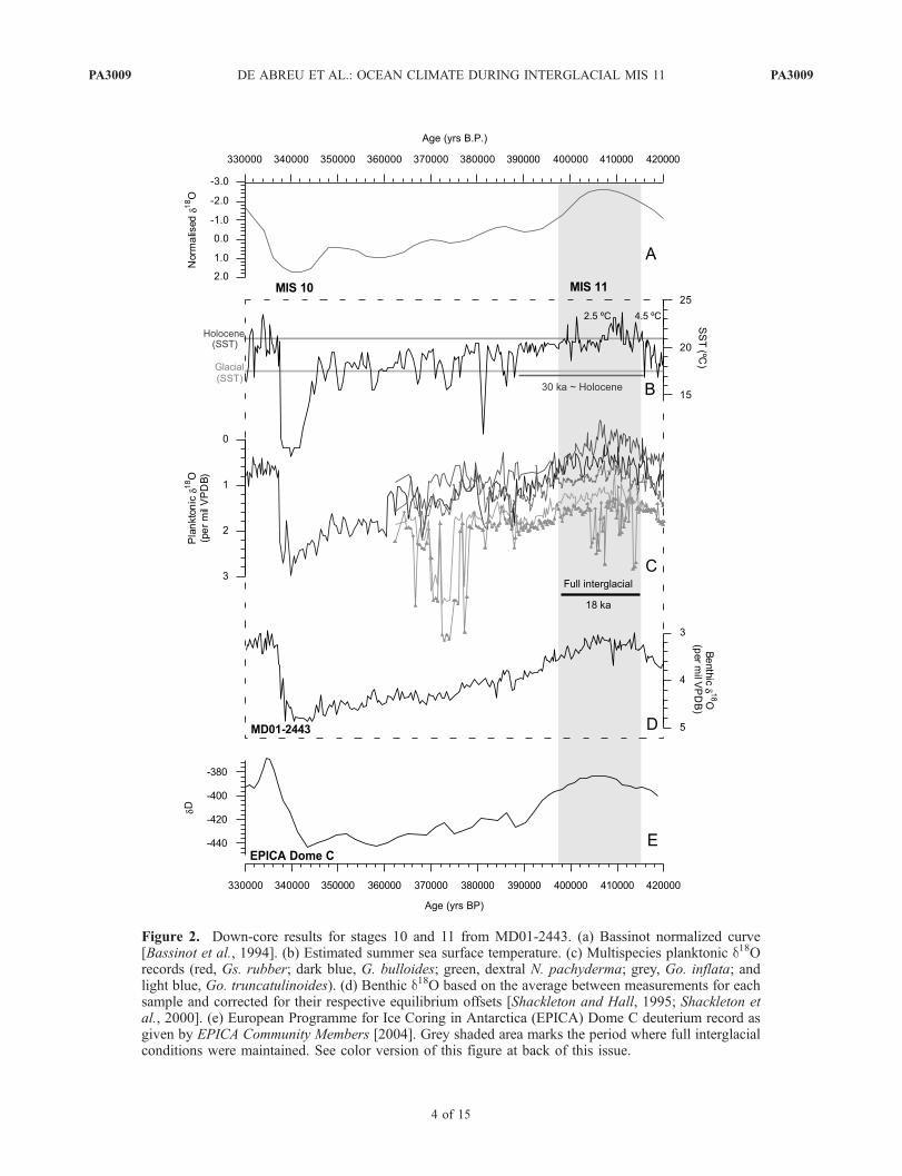
Figure 2. Down-core results for stages 10 and 11 from MD01-2443. (a) Bassinot normalized curve[Bassinot et al., 1994]. (b) Estimated summer sea surface temperature. (c) Multispecies planktonic d18Orecords (red, Gs. rubber; dark blue, G. bulloides; green, dextral N. pachyderma; grey, Go. inflata; andlight blue, Go. truncatulinoides). (d) Benthic d18O based on the average between measurements for eachsample and corrected for their respective equilibrium offsets [Shackleton and Hall, 1995; Shackleton etal., 2000]. (e) European Programme for Ice Coring in Antarctica (EPICA) Dome C deuterium record asgiven by EPICA Community Members [2004]. Grey shaded area marks the period where full interglacialconditions were maintained. See color version of this figure at back of this issue.

PA3009 DE ABREU ET AL.: OCEAN CLIMATE DURING INTERGLACIAL MIS 11

4 of 15

PA3009

base of MD01-2443 was defined by comparison with theEPICA Dome C deuterium record [EPICA CommunityMembers, 2004] as this extends in time the previouslyavailable Vostok records. Mean linear sedimentation ratesfor this core were estimated, assuming a constant accumu-lation rate between dated levels. The sampling at 2-cmintervals gives an average resolution of 330 years for stage11 (Figure 2).[14] For comparison, the independently created chronol-

ogy of ODP Site 980 [McManus et al., 1999] was revisedby tuning Termination V to the astronomically calibratedlow-latitude stack [Bassinot et al., 1994], consistent with thetime interval defined through 40Ar/39Ar dating for Termi-nation V [Karner and Morra, 2003] and not very far fromthe limit attributed to the new Antarctic ice core record[EPICA Community Members, 2004].

5. Results

5.1. Benthic Isotopic Measurements

[15] Benthic d18O measurements indicate that the corerdid not penetrate into MIS 12 at site MD01-2443. Near thebeginning of our record, the benthic d18O decreases from3.7% to 3.1%, indicating a reduction in ice volume(Figure 2). According to the present age model, the periodof lowest ice volume, and thus establishment of peakinterglacial conditions lasted nearly 7 –8 kyr, until�402 ka, with short-term variations of �0.2%. The nextdominant feature is the long-term increase in d18O (up to amaximum of 3.5%), with a superimposed higher-frequencyvariability from 396 ka onward toward glacial stage 10,coincident with the growth of ice sheets. This is indicatedby an increase of nearly 1.4% in the benthic d18O values upto the start of the glacial. In stage 10, a further increase isrecorded off the Iberian margin, reaching the highest ben-thic isotope ratio of 4.8% between 341 and 345 ka.

5.2. Multispecies Planktonic Isotopic Record

[16] The interpretation of the stable isotopic compositionof foraminiferal shells in upwelling areas, such as theIberian margin, is difficult and often hampered by thedynamic character of such settings [e.g., Peeters et al.,2002]. In such a complex hydrological regime, the differ-ences in the signal between species must not only beinterpreted taking into consideration both their sequenceof development, but the contemporaneous differences be-tween distinct habitats. Since there are currently few sedi-ment trap or water column data for the Iberian marginavailable, we support our observations with ecological datafrom adjacent North Atlantic regions, as well as with thebehavior described for some species in other upwelling

areas [e.g., Levy et al., 1995; Thunell and Sautter, 1992;Peeters et al., 2002]. Future sediment trap data from ESFEuromargins project SEDPORT might shed light on themicrofauna seasonal variability.[17] Most of the planktonic species chosen for this com-

parison characterize distinct seasons [e.g., Levy et al., 1995;Schiebel and Hemleben, 2000]: Gs. ruber is a warm season,surface dweller, while G. bulloides occurs in the upper 50 mof the water column, associated with the spring/summerupwelling system when the degree of mixing of the upperwater column is high. Recent observations indicate thatGs. ruber can also be found during the upwelling season(F. Peeters, personal communication, 2003) but unlikeG. bulloides it survives in the distal areas of the upwelledwater. Toward the end of the upwelling season, thedextral N. pachyderma appear in great numbers, whenthe influence of warmer Azores Current waters increasesoff Portugal [Rogerson et al., 2004]. This species hasbeen observed at depths of up to 250 m. Deep dwellersGo. inflata (100–250 m) and dextral Go. truncatulinoides(250–300 m up to 1000 m) were selected with thepurpose of detecting possible changes in the structureof the deep thermocline [e.g., Hemleben et al., 1989;Abrantes et al., 2001; Matzumoto and Lynch-Stieglitz,2003].[18] Bearing in mind the complexity and the limitations of

this approach, the combination of the monospecific profilesof d18Oruber, d18Obulloides, d18Opachyderma, d18Oinflataand d18Otruncatulinoides (Figure 2) show several distinct,previously unreported features. Through an interval of circa20 kyr (from �416 to 396 ka), the oxygen isotope valuesfrom intermediate-depth dwellers generally did not varymore than 0.25–0.28%, which is equivalent to approxi-mately 1�C. However, some excursions of up to 0.5%occurred, suggesting occasional greater sea surface temper-ature changes or even possible salinity anomalies at theIberian margin. In contrast, surface dweller Gs. ruber dis-plays a significant shift toward heavier values from 402 ka,which became more accentuated after 396 ka. The lack of acomparable initial increase in intermediate to deeper dwell-ers suggests some type of seasonal or depth habitat com-pensating effect.[19] The beginning of our sequence (at 420 ka) up to the

peak interglacial conditions as defined by the lightest d18OGs. ruber values (416 to 402 ka) suggest a well-definedupper water column stratification, as surface, intermediateand deep dwellers show progressively higher isotopic ratios.Surface dweller Gs. ruber is typically lighter throughoutstage 11 (�0.3 to 0.2%), and the same trend is followed bythe intermediate dwellers in particular up to the end of thepeak interglacial. The deeper dwellers exhibit a clearly

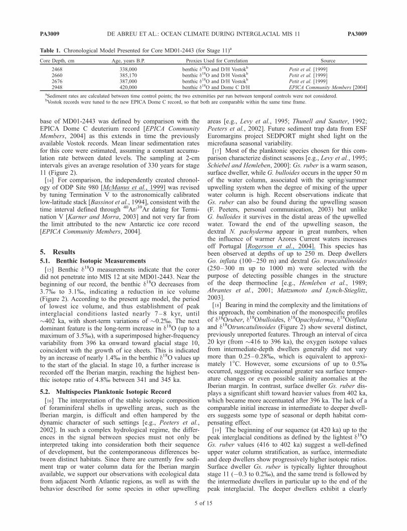
Table 1. Chronological Model Presented for Core MD01-2443 (for Stage 11)a

Core Depth, cm Age, years B.P. Proxies Used for Correlation Source

2468 338,000 benthic d18O and D/H Vostokb Petit et al. [1999]2660 385,170 benthic d18O and D/H Vostokb Petit et al. [1999]2676 387,000 benthic d18O and D/H Vostokb Petit et al. [1999]2948 420,000 benthic d18O and Dome C D/H EPICA Community Members [2004]

aSediment rates are calculated between time control points; the two extremities per run between temporal controls were not considered.bVostok records were tuned to the new EPICA Dome C record, so that both are comparable within the same time frame.

PA3009 DE ABREU ET AL.: OCEAN CLIMATE DURING INTERGLACIAL MIS 11

5 of 15

PA3009

heavier oxygen isotope ratio (by as much as 0.8 to 1%).The deep-living foraminifera Go. truncatulinoides dextralshows a trend similar to the other deep species, but withseveral rapid excursions in d18O of over 1%, centered at413 ka and 405 ka, respectively. These isotopic excursionsduring the progression to peak interglacial conditions,although not seen in any other record, coincide with achange in the Go. truncatulinoides population toward thedominance of left coiling forms, which preferentially live incold waters and typically display heavier isotopic ratios. It isthen possible that we have different genotypes throughoutour stage 11 samples, that because of morphological con-vergence are not fully distinguishable under the binocularmicroscope [de Vargas et al., 2001], and this in turn mayaccount for the observed isotopic shifts. With the declineof interglacial conditions, an increase in the levels of upperwater column mixing is suggested by the smaller range inthe Dd18O between surface/intermediate and deeper dwell-ers. The larger amplitude variability which characterizesthe progression toward a new glacial (stage 10) is one ofthe main features of the record. G. bulloides andN. pachyderma display very similar d18O values (between0.9 and 1.2%), occasionally also close to Go. inflata, withthe exception of three prominent excursions towardheavier values of G. bulloides, respectively at 388, 381and 369 ka.[20] The hydrological complexity of this region appears

to be more evident during the cool intervals of stage 11. Thed18O of dextral N. pachyderma show the same trend as datafrom G. bulloides and, in most warm periods, to Go. inflata,possibly as a function of the ice volume effect on seawatercomposition. However, during cool intervals they showlighter d18O values, with differences of up to 0.4%. Onepossible explanation for this feature lies in the narrowlyoverlapping season that these two species exist off Iberiaand the possibility of a dual surface water mass influence atthe site of MD01-2443. Assuming that G. bulloides usuallythrives in cooler waters (being a subpolar species and anupwelling form), an isotopically heavier signal might beevidence of upwelling. If dextral N. pachyderma, whichdominates toward the end of the upwelling season, thrivesmore under the influence of a warmer water mass ofsubtropical origin – derived from the Azores Current[e.g., Fiuza, 1984] then it records the cool events in amore attenuated form. On the other hand, living towardthe Autumn/Winter months, the decrease in dextralN. pachyderma d18O may be related to periodic salinityanomalies.[21] At the end of stage 11 both deep dwellers, Go. inflata

and dextral Go. truncatulinoides, show much more signif-icant variations, reaching over 2%. As such variations arenot recorded in the remaining species, and given that the leftcoiling variety of Go. truncatulinoides is once again dom-inant, we believe there is sufficient evidence to implicate achange in the ecological conditions and the additionalinfluence of an oligotrophic intermediate water mass duringthis period [e.g., Peeters et al., 2002; Matzumoto andLynch-Stieglitz, 2003]. Further studies of these particularsediment samples will shed some light into the possibilitythat these heavier values are due to the presence of second-

ary calcite, formed at deeper water levels, and thuscorresponding to colder conditions.

5.3. Faunal Changes

[22] Grouped into faunal assemblages (Figure 3) [e.g., Be,1977; Ottens, 1991], the 25 different species of planktonicforaminifera show evidence of three main surface environ-mental ‘‘modes’’ within stage 11. The development ofprogressively warmer sea surface conditions is shown bythe presence of an increasing number of tropical (36–40%)species toward the peak interglacial (Figure 3), coincidingwith the lightest planktonic d18O values. The succession ofwarm water species include N. dutertrei (up to 1.5%) whichis considered a postupwelling species, and can be used as aproxy for the stabilization of the upper water column(following trap data of Thunell and Honjo [1983] andThunell and Sautter [1992] as a potential analogue).[23] From �402 ka onward, the warm water planktonic

fauna was progressively replaced by cold subtropical,transitional and even subpolar species (such as G. bulloidesand dextral N. pachyderma) that dominate throughout theremaining interglacial interval (50%), and become progres-sively more important toward stage 10. The decrease intropical species, after 396 ka, agrees with the enrichment inboth Gs. ruber d18O and benthic d18O, marking the end offull interglacial conditions and the gradual decline ofclimate.[24] A third mode of faunal succession is detected in

the periodic increase of the polar species left coilingN. pachyderma, which at times reaches 23% of theplanktonic population. Increases in transitional/temperatespecies (by over 10%) indicate the recovery of seasurface conditions up to an interglacial mode and strongoscillation in the position of the subpolar front. A closerlook into the variation of individual species reveals anextra degree of complexity, which points toward distincttrophic situations as the interglacial progressed. Speciesusually associated with the seasonal upwelling system,such as T. quinqueloba and G. bulloides show a pro-gressive increase toward the end of stage 1l, suggestingan enhanced upwelling and increased nutrient levels.Additionally, the increasingly high abundance of dextralN. pachyderma (from 10% at the peak interglacial toover 40% at the end of stage 11), usually associated withthe end of the upwelling events, may be indicative of amore continuous degree of mixing of the upper watercolumn. This hypothesis is supported by the presence ofOrbulina bilobata, considered an indicator of high nutri-ent levels [e.g., Robbins, 1988; Hemleben et al., 1989],the convergence of some of the multispecies planktonicd18O records, and an increase in the organic carbon by�0.5%.

5.4. Sea Surface Temperature Changes

[25] As indicated by the planktonic isotope record, the seasurface temperature reconstructions suggest that this longinterglacial (stage 11) evolved in three distinctive phases onthe Iberian margin. The summer sea surface temperature(SST) rise from deglacial conditions to the interglacialmaximum was about 4.5�C. This rise occurred over a period

PA3009 DE ABREU ET AL.: OCEAN CLIMATE DURING INTERGLACIAL MIS 11

6 of 15

PA3009

of nearly 5–6 kyr but appears to have been disruptedseveral times, in particular during the interval of highestinsolation (between 408 and 412 ka). Peak interglacialtemperatures (SSTs around 20.5�–23.3�C) occurred be-

tween 412 and 406 ka. However, if the average Holocenetemperature (21�C) for this region is considered as athreshold, the duration of this interglacial phase lasted fornearly 27 kyr (from 416 up to 389 ka) in good agreement

Figure 3. Relative abundance of the different planktonic foraminifera assemblages throughout stage 11in core MD01-2443.

PA3009 DE ABREU ET AL.: OCEAN CLIMATE DURING INTERGLACIAL MIS 11

7 of 15

PA3009

with previous estimates of McManus et al. [2003] andBauch and Erlenkeuser [2003].[26] Only after 389 ka do the surface records start to show

a greater magnitude of variability, with sporadic abrupt SSTdecreases of up to 7�C. These are values close to theaverage value found for the last glacial period (17�C) inthis region (Figure 2). However, the average value may notbe the best way to compare the two records; in fact, both thetemperature estimates and the periodic pattern of largecooling events resemble the palaeoceanographic changesdescribed for stages 2 and 3 in nearby cores [e.g., Cayre etal., 1999; Bard et al., 2000; de Abreu et al., 2003]. Thepronounced SST decrease during peak stage 10 was com-parable to the surface water cooling recorded during Hein-rich events 2, 3 and 5, whereas SSTs reached even moreextreme values (with differences of up to 2�C) duringHeinrich events 1 and 4 [Cayre et al., 1999].

6. Discussion

6.1. Iberian Margin: Regional Expression ofInterglacial Stage 11

[27] High-frequency excursions are more evident in therecords of surface d18O and foraminifera-derived SSTs thanin the benthic d18O record, since they are directly dependenton surface hydrology, in particular on temperature andsalinity. Regarding the magnitude of these variations insurface water indicators, stage 11 can be roughly interpretedin terms of three distinct phases: (1) the deglacial intervalwhich extended up to the establishment of full interglacialconditions at �416 ka; (2) the peak interglacial intervalwhere the range of oscillations in the planktonic record wassmall, reaching up to 0.1–0.25%, and changes in SST wereof the order of 1�–2�C; and (3) the progressive climatedeterioration, starting at �396 ka when excursions in d18Obegan to gradually increase in amplitude, surpassing thevariability recorded in the early part of stage 11, and thetransition into MIS 10. Both the planktonic foraminiferalfauna (in particular the significant decrease in tropicalspecies), the surface dwelling Gs. ruber isotope record,and the benthic d18O record show the end of the fullinterglacial conditions and new ice volume increase. Thisoccurred, according to the present age model, nearly 7 kyrbefore a significant planktonic enrichment was recorded byintermediate-depth dwelling species (Figure 2).[28] The discrepancy between planktonic isotopic values

from surface and deeper dwellers suggests some kind ofcompensating effect, either related to the different seasonaldistribution of the selected species, or perhaps a function oftheir distinct depth habitat. Species that are usually associ-ated with stronger mixing conditions and thus greaterhomogenization of the water column, such as G. bulloidesand N. pachyderma, display a restricted amplitude of theisotopic anomalies in response to hydrological events, andmay indicate the presence of a dampened NACW signal.These faunal successions could also be influenced by themigration of the subpolar front southward and/or thestrengthening of the gyre/Eastern Boundary Current, withthe Portugal Current transporting more water to the southduring the spring/summer season. On the other hand, Gs.

ruber is the first planktonic species recording climaticchange possibly of subtropical origin, as it calcifies in theAzores current.

6.2. Comparison With Succeeding Interglacials:Role of Ventilation Changes and Influence ofSouthern Ocean Waters

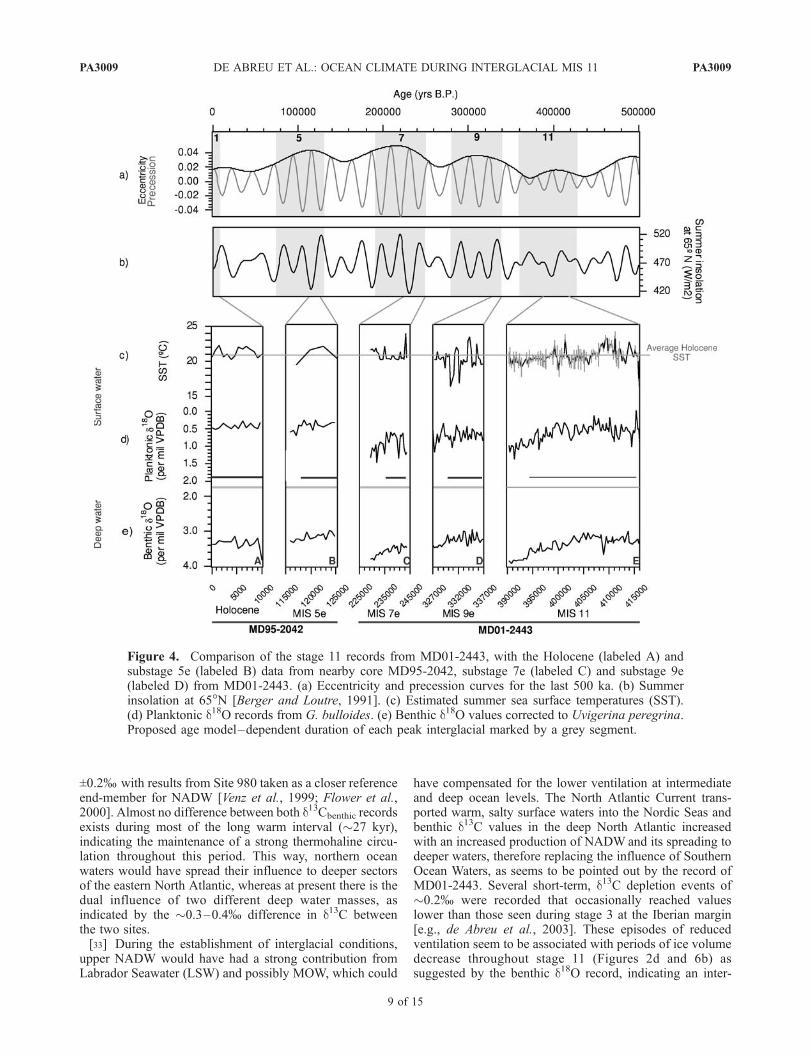
[29] A comparison of peak interglacial planktonic d18Oand SST records of stage 11 with those of younger warmintervals (substages 9e and 7e from core MD01-2443,and substage 5e and the Holocene along nearby coreMD95-2042) reveals pronounced warm conditions, withstages 1, 5e and 11 generally 1�C warmer than the maximalSSTs obtained for substage 7e and most of 9e (Figure 4).Faunal analysis shows a distinct pattern in the assemblagecomposition during peak interglacials, in particular duringsubstages 7e and 9e, where along with a temperate tosubtropical fauna, subpolar species are abundant. Theresults for substages 7e and 9e gain further support fromboth the planktonic and benthic d18O records (Figure 4)which show heavier values, in particular during substage 7e,indicating colder surface temperatures and a larger global icevolume, when compared to other interglacials [McManus etal., 1999]. This agrees with Kandiano and Bauch [2003] inthe sense that the closest interglacials in terms of absolutetemperature are the Holocene, substage 5e and stage 11,with SSTs being slightly higher in the latter.[30] In addition, benthic d18O values in stage 11 are

lighter by up to 0.3% than the average Holocene isotopicratio [Shackleton et al., 2000], which might correspond to asmaller ice volume and/or a potentially warmer deep ocean[e.g., McManus et al., 2003]. Overall estimates for bothinterglacials agree well within the error of our calculation(Figure 4). These proxy data alone suggest that the icevolume/sea level was not significantly different than atpresent, assuming that the ice volume was the single factoraffecting the isotopic record.[31] The comparison between benthic d13C records from

the Holocene and stage 11 presented in Table 2 can givesome clues toward a better understanding of the influence ofwater masses with distinct characteristics in this region. Inagreement with other published North Atlantic records [e.g.,Venz et al., 1999; Flower et al., 2000], the compiled resultsare interpreted to indicate an enhanced contribution of high-d13C NADW during peak interglacial 11 at intermediate anddeep sites in the northeast Atlantic basin, versus a strongerinfluence of less ventilated deep waters at 37�N during theHolocene. Similarities in the behavior of some of thepalaeoceanographic proxies used in this paper may thusresult from a changing influence of distinct sourced inter-mediate and deep water masses.[32] Expanding our geographic coverage, a comparison

between the high-resolution benthic isotope records fromsites MD01-2443 and ODP 980 indicates the presence ofwater masses with uniform characteristics at intermediateand deepwater eastern North Atlantic sites during stage 11(Figures 5 and 6). Maximum d13Cbenthic values of �1.3%,higher than Holocene records from neighboring cores[Shackleton et al., 2000; Schonfeld and Zahn, 2000;Schonfeld and Zahn, unpublished results], agree within

PA3009 DE ABREU ET AL.: OCEAN CLIMATE DURING INTERGLACIAL MIS 11

8 of 15

PA3009

±0.2% with results from Site 980 taken as a closer referenceend-member for NADW [Venz et al., 1999; Flower et al.,2000]. Almost no difference between both d13Cbenthic recordsexists during most of the long warm interval (�27 kyr),indicating the maintenance of a strong thermohaline circu-lation throughout this period. This way, northern oceanwaters would have spread their influence to deeper sectorsof the eastern North Atlantic, whereas at present there is thedual influence of two different deep water masses, asindicated by the �0.3–0.4% difference in d13C betweenthe two sites.[33] During the establishment of interglacial conditions,

upper NADW would have had a strong contribution fromLabrador Seawater (LSW) and possibly MOW, which could

have compensated for the lower ventilation at intermediateand deep ocean levels. The North Atlantic Current trans-ported warm, salty surface waters into the Nordic Seas andbenthic d13C values in the deep North Atlantic increasedwith an increased production of NADW and its spreading todeeper waters, therefore replacing the influence of SouthernOcean Waters, as seems to be pointed out by the record ofMD01-2443. Several short-term, d13C depletion events of�0.2% were recorded that occasionally reached valueslower than those seen during stage 3 at the Iberian margin[e.g., de Abreu et al., 2003]. These episodes of reducedventilation seem to be associated with periods of ice volumedecrease throughout stage 11 (Figures 2d and 6b) assuggested by the benthic d18O record, indicating an inter-

Figure 4. Comparison of the stage 11 records from MD01-2443, with the Holocene (labeled A) andsubstage 5e (labeled B) data from nearby core MD95-2042, substage 7e (labeled C) and substage 9e(labeled D) from MD01-2443. (a) Eccentricity and precession curves for the last 500 ka. (b) Summerinsolation at 65�N [Berger and Loutre, 1991]. (c) Estimated summer sea surface temperatures (SST).(d) Planktonic d18O records from G. bulloides. (e) Benthic d18O values corrected to Uvigerina peregrina.Proposed age model–dependent duration of each peak interglacial marked by a grey segment.

PA3009 DE ABREU ET AL.: OCEAN CLIMATE DURING INTERGLACIAL MIS 11

9 of 15

PA3009

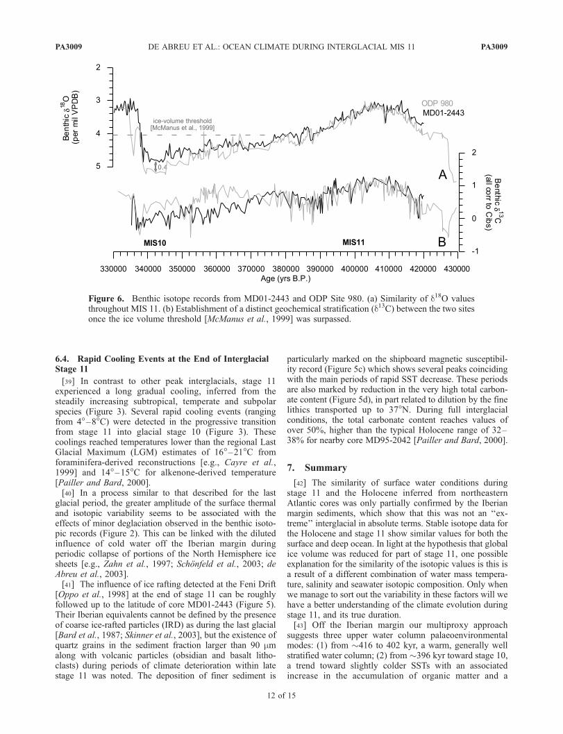
ference with deepwater production/circulation. Cold eventsdetected during the transition between stages 11 and 10 arealso associated with benthic d13C depletions of 0.4–0.5%in MD01-2443, indicative of a more diluted influence ofNADW at this site. These shifts are more attenuated on theIberian margin than at Site 980, which is closer to thedeepwater source region. The shift to higher amplitudesoccurs when the ice volume threshold suggested byMcManus et al. [1999] is passed (d18Obenthic of �4.1%).Beyond this value climate variability seems to be amplifiedby feedback mechanisms. The progressive enrichment ofthe benthic d18O records may derive from a compositeinfluence of ice volume increase and a renewed cooling ofthe deep oceanic environment [McManus et al., 1999]. Theincrease in the isotopic gradient between our two differentdepth sites and the changes in d13Cbenthic during late stage11 and glacial stage 10 are consistent with the redistributionof deep and intermediate water masses, associated with adistinct chemical stratification.[34] During stage 10, the benthic record of ODP Site 980

shows an enrichment in d18O, suggestive of the presence ofcolder deep water during the glacial interval, in a similarfashion to the variability described during the last glacialperiod [Skinner et al., 2003], and the decrease in polewardheat flux. The slower glacial circulation may have contrib-uted to the enhancement of the thermal/isotopic gradientbetween these sites. However, once again we cannot ignorethat these sites would be affected by the combined, variableinfluence of two distinct main deep water masses.

6.3. Duration and Variability of Interglacial Intervals

[35] In core MD01-2443, a deglacial phase leadingtoward peak interglacial values occurred during the first4–5 kyr of the record. Bearing in mind that by comparisonwith Site 980 we may be missing a sediment recordequivalent to nearly 7 kyr, our estimates for the length ofthis deglacial warming are not far from independent mod-eling results from Loutre and Berger [2003], who proposedthat interglacial conditions were achieved after a period of�20 kyr. According to our timescale, a convincing rela-tionship between the two sites is observed, with full

interglacial conditions prevailing at the Iberian margin for�18 kyr (Figure 5), surpassing the length of the elapsedportion of the Holocene. The foraminifera-derived SSTspoint to the maintenance of the mild sea surface conditionsfor a longer period (of nearly 27 kyr) in agreement topreviously published work [e.g., McManus et al., 1999] butthe high temperatures estimated may derive from thedominance of subtropical and transitional species immedi-ately after surface and deep records point to the end ofinterglacial conditions. See Figure 6.[36] The observed differences between the last five inter-

glacial periods are probably a reflection of the distinctorbital configurations and different insolation values thatcharacterize each one of these warm intervals (Figures 4aand 4b). For example, while there is a very similar insola-tion geometry between stage 11 and the Holocene, theinsolation parameters for substage 5e show large differencesin terms of total insolation and amplitude. These resultssuggest that, on the basis of comparison to stage 11, theHolocene may last another 6–7 kyr.[37] In addition to insolation, another important mecha-

nism for maintaining the warm conditions in the NorthAtlantic would be to have a strong thermohaline circulation[e.g., Oppo et al., 1998; McManus et al., 1999] whichcontinuously supplies warm waters to the northern regionsduring a period when insolation levels were low [McManuset al., 2002]. A third factor that needs to be studied further isthe variable influence of differently sourced deep watermasses to the deep ocean environment, and whether or nottheir properties were similar to modern days.[38] In stage 11 evidence points to gradual ice volume

decay up to �402 ka, and characterized by a transient high-frequency variability. In the case of Termination II, thebenthic d18O shows a very rapid shift (less than 5 kyr)toward lighter values, very similar to those of stage 11.Future work should focus on the possibility either that deepwater was slightly warmer than during the Holocene andsubstage 5e, or that sea level was a few meters above present,implying less ice on Antarctica and/or Greenland. In addi-tion, work is needed to establish the distribution of ice thatgenerated the IRD that started to appear at about 390 ka.

Table 2. Comparison of Benthic d13C Values Between the Holocene and Stage 11 From Different Depth Iberian Margin Cores

Core Latitude Longitude Depth, mRange of

Benthic d13C, % Time Period Source

MD95-2042 37.811 �10.150 3146 0.4–0.92 Holocene Shackleton et al. [2000]MD01-2444 37.574 �11.468 2656 0.85–1.09 Holocene N. J. Shackleton,

unpublished results (2003)SO75-3K 37.920 �9.900 2430 0.4–1.0 Holocene Schonfeld and Zahn [2000]MD95-2041 37.833 �9.518 1123a 0.96–1.09 Holocene J. Schonfeld and R. Zahn,

unpublished results (2001)MD01-2443 37.891 �10.183 2941 0.9–1.3 stage 11 this paper

aRecords mainly Mediterranean Outflow Water.

Figure 5. Expression of northern Atlantic ice-rafting events off Iberia in comparison with the Feni Drift. (a) Relativeabundance of left coiling N. pachyderma and ice-rafted debris (IRD) in Site 980 [e.g., Oppo et al., 1998; McManus et al.,1999]. (b) The d18O records of dextral N. pachyderma from Site 980. (c) Onboard magnetic susceptibility (plotted onreverse scale). (d) Total carbonate content. (e) Organic carbon. (f) Estimated summer sea surface temperatures. (g) Relativeabundance of left coiling N. pachyderma. (h) The d18O record of G. bulloides.

PA3009 DE ABREU ET AL.: OCEAN CLIMATE DURING INTERGLACIAL MIS 11

10 of 15

PA3009

Figure 5

PA3009 DE ABREU ET AL.: OCEAN CLIMATE DURING INTERGLACIAL MIS 11

11 of 15

PA3009

6.4. Rapid Cooling Events at the End of InterglacialStage 11

[39] In contrast to other peak interglacials, stage 11experienced a long gradual cooling, inferred from thesteadily increasing subtropical, temperate and subpolarspecies (Figure 3). Several rapid cooling events (rangingfrom 4�–8�C) were detected in the progressive transitionfrom stage 11 into glacial stage 10 (Figure 3). Thesecoolings reached temperatures lower than the regional LastGlacial Maximum (LGM) estimates of 16�–21�C fromforaminifera-derived reconstructions [e.g., Cayre et al.,1999] and 14�–15�C for alkenone-derived temperature[Pailler and Bard, 2000].[40] In a process similar to that described for the last

glacial period, the greater amplitude of the surface thermaland isotopic variability seems to be associated with theeffects of minor deglaciation observed in the benthic isoto-pic records (Figure 2). This can be linked with the dilutedinfluence of cold water off the Iberian margin duringperiodic collapse of portions of the North Hemisphere icesheets [e.g., Zahn et al., 1997; Schonfeld et al., 2003; deAbreu et al., 2003].[41] The influence of ice rafting detected at the Feni Drift

[Oppo et al., 1998] at the end of stage 11 can be roughlyfollowed up to the latitude of core MD01-2443 (Figure 5).Their Iberian equivalents cannot be defined by the presenceof coarse ice-rafted particles (IRD) as during the last glacial[Bard et al., 1987; Skinner et al., 2003], but the existence ofquartz grains in the sediment fraction larger than 90 mmalong with volcanic particles (obsidian and basalt litho-clasts) during periods of climate deterioration within latestage 11 was noted. The deposition of finer sediment is

particularly marked on the shipboard magnetic susceptibil-ity record (Figure 5c) which shows several peaks coincidingwith the main periods of rapid SST decrease. These periodsare also marked by reduction in the very high total carbon-ate content (Figure 5d), in part related to dilution by the finelithics transported up to 37�N. During full interglacialconditions, the total carbonate content reaches values ofover 50%, higher than the typical Holocene range of 32–38% for nearby core MD95-2042 [Pailler and Bard, 2000].

7. Summary

[42] The similarity of surface water conditions duringstage 11 and the Holocene inferred from northeasternAtlantic cores was only partially confirmed by the Iberianmargin sediments, which show that this was not an ‘‘ex-treme’’ interglacial in absolute terms. Stable isotope data forthe Holocene and stage 11 show similar values for both thesurface and deep ocean. In light at the hypothesis that globalice volume was reduced for part of stage 11, one possibleexplanation for the similarity of the isotopic values is this isa result of a different combination of water mass tempera-ture, salinity and seawater isotopic composition. Only whenwe manage to sort out the variability in these factors will wehave a better understanding of the climate evolution duringstage 11, and its true duration.[43] Off the Iberian margin our multiproxy approach

suggests three upper water column palaeoenvironmentalmodes: (1) from �416 to 402 kyr, a warm, generally wellstratified water column; (2) from �396 kyr toward stage 10,a trend toward slightly colder SSTs with an associatedincrease in the accumulation of organic matter and a

Figure 6. Benthic isotope records from MD01-2443 and ODP Site 980. (a) Similarity of d18O valuesthroughout MIS 11. (b) Establishment of a distinct geochemical stratification (d13C) between the two sitesonce the ice volume threshold [McManus et al., 1999] was surpassed.

PA3009 DE ABREU ET AL.: OCEAN CLIMATE DURING INTERGLACIAL MIS 11

12 of 15

PA3009

convergence of the oxygen isotope ratios of G. bulloides,dextral N. pachyderma and occasionally Go. inflata,indicating a possible increase in local upwelling intensityand stronger trade winds; and (3) periodic cold events,bringing SSTs nearly to local glacial levels (Heinrichevents), with the lowest temperatures associated withthe presence of polar and subpolar species. This thirdmode, characteristic of the later part of stage 11 coincideswith the ice-rafting episodes detected for the same inter-val at 55�N (ODP Site 980), and shows that even duringan interglacial interval North Atlantic ice-rafting eventscan have a detectable expression on the sensitive Iberianmargin palaeoenvironment.[44] Interglacial duration was recorded differently by

surface and intermediate dwellers, because of possiblecompensation mechanisms related to seasonal or depthdistribution. Thus the selection of proxies used to charac-terize full interglacial conditions is important in order toestablish a more accurate comparison with the Holocene.Indications from both the surface and benthic stable isotopedata are that the interglacial conditions were preserved for aperiod of 18 kyr. However, intermediate water dwellersdisplay a separate behavior, with light isotope ratiosrecorded for a period of nearly 20–27 kyr. A third proxy,foraminifera-derived SST, extends the estimated duration ofwarm surface conditions to nearly 27 kyr, suggesting thatthe modern analogue technique may be too sensitive to thepresence of a high percentage of subtropical and temperatespecies after 396 kyr, when the tropical assemblage suffers areduction of nearly 20%.[45] In a broader geographic context, no deep water mass

isotopic gradient during stage 11 was detected betweenMD01-2443 and ODP Site 980, and the d18Obenthic andd13Cbenthic records show very similar values and trends,indicating the influence of a deep water mass of uniformcharacteristics. These results suggest that NADW wouldhave been present at intermediate and deep levels, but thedynamic equilibrium between different sourced deep water

masses must have been kept for most of stage 11. Thegreater variability displayed by the d13C record of ODP Site980 may point to changes in the source and/or properties ofNADW, in a similar way to the one observed for theHolocene [e.g., Skinner et al., 2003]. An increase inbathymetric d13C gradient by <0.4% between Site 980and MD01-2443 during late stage 11 and glacial stage 10indicates a distinct combination of UNADW, decrease inLNADW and stronger influence of nutrient-rich SOW.Oscillations in deepwater production were synchronouswith the main changes in sea surface temperature in theeastern North Atlantic.[46] One important conclusion that stands out from our

work is the necessity to compare and interrelate similarreconstructions from different areas of the world, not just inpalaeoceanographic terms, but as an expression of a coupledinfluence of the atmospheric circulation and ocean watermasses. Only via a larger study, both geographically andwith the use of complementary proxies focused on theevolution of the two main Atlantic deep water massesduring this long interglacial, will we be able to evaluatethe still controversial apparent analogy to the elapsedportion of the Holocene.

[47] Acknowledgments. Authors are grateful to Rainer Zahn andJoachim Schonfeld for providing access to the unpublished benthic isotoperecords of core MD95-2041, to Antje Voelker for helpful advice anddiscussion of preliminary results, and to David Cox for the thoroughediting of the final text. We are also grateful to Larry Peterson, ElsaCortijo, and Frank Lamy for the thoughtful and thorough reviews thatsignificantly improved the manuscript. A special acknowledgment is due toJames Rolfe for his assistance in the preparation of many samples for stableisotopic analysis at the Godwin Laboratory and to Cremilde Monteiro forthe total carbonate content analysis at the Department of Marine Geology(INETI, Lisbon). This work was partially undertaken in association with the‘‘POP Project,’’ EC grant EVK2-2000-00089. Funding for L.A. wasprovided by the Portuguese Foundation for Science and Technology underthe fellowship contract SFRH/BPD/1588/2000 and by the Calouste Gul-benkian Foundation, through a visiting fellowship to Woods Hole Ocean-ographic Institution. We are also grateful to the French MENRT, TAAF,CNRS/INSU, and especially to IFRTP for the coring operations aboard theMarion Dufresne II.

PA3009 DE ABREU ET AL.: OCEAN CLIMATE DURING INTERGLACIAL MIS 11

13 of 15

PA3009

ReferencesAbrantes, F., N. Loncaric, J. Moreno, M. Mil-Homens, and U. Pflaumann (2001), Paleocea-nographic conditions along the PortugueseMargin during the last 30 ka: A multiple proxystudy, Comun. Inst. Geol. Min. Portugal, 88,161–184.

Aksu, A. E., P. J. Mudie, A. de Vernal, andH. Gillespie (1992), Ocean-atmosphere re-sponses to climate change in the LabradorSea: Pleistocene plankton and pollen records,Palaeogeogr. Palaeoclimatol. Palaeoecol., 92,121–138.

Ambar, I., and M. Howe (1979), Observations ofthe Mediterranean Outflow-I. Mixing in theMediterranean flow, Deep Sea Res., Part A,26, 535–554.

Bard, E., M. Arnold, P. Maurice, J. Duprat,J. Moyes, and J.-C. Duplessy (1987), Re-treat velocity of the North Atlantic polarfront during the last deglaciation determinedby 14C accelerator mass spectrometry, Nature,328, 791–794.

Bard, E., F. Rostek, J. L. Turon, and S. Gendreau(2000), Hydrological impact of Heinrichevents in the subtropical northeast Atlantic,Science, 289, 1321–1324.

Bassinot, F. C., L. D. Labeyrie, E. Vincent,X. Quidelleur, N. J. Shackleton, andY. Lancelot(1994), The astronomical theory of climate andthe age of the Brunhes-Matuyama magnetic re-versal, Earth Planet. Sci. Lett., 126, 91–108.

Bauch, H., and H. Erlenkeuser (2003), Interpret-ing glacial-interglacial changes in ice-volumeand climate from subarctic deep-water forami-niferal d18O, in Earth’s Climate and Orbital Ec-centricity: The Marine Isotope Stage 11Question,Geophys. Monogr. Ser., vol. 137, edi-ted by A. W. Droxler, R. Z. Poore, and L. H.Burckle, pp. 87–102, AGU,Washington, D. C.

Bauch, H., H. Erlenkeuser, J. P. Helmke, andU. Struck (2000), A paleoclimatic evaluationof marine oxygen isotope stage 11 in thehigh-northern Atlantic (Nordic Seas), GlobalPlanet. Change, 24, 27–39.

Be, A. (1977), Recent planktonic foraminifera, inOceanic Micropaleontology, vol. 1, edited byA. T. S. Ramsay, pp. 1–100, Elsevier, NewYork.

Becquey, S., and R. Gersonde (2002), Pasthydrography and climate changes in theSubantarctic Zone of the South Atlantic –The Pleistocene record from ODP Site 1090,Palaeogeogr. Palaeoclimatol. Palaeoecol.,182, 221–239.

Berger, A., and M. F. Loutre (1991), Insolationvalues for the climate of the last 10 millionyears, Quat. Sci. Rev., 10, 297–317.

Berger, W. H., T. Bickert, M. K. Yasuda, andG.Wefer (1996), Reconstruction of atmosphericCO2 from ice-core data and the deep-sea recordof Ontong Java plateau: The MilankovitchChron, Geol. Rundsch., 85, 466–495.

Bowen, D. Q. (1999), Stage 11 sea level uncer-tainty: Revised British Isles estimate of �13 ±3, Eos Trans AGU, 80(46), Fall Meet. Suppl.,F555.

PA3009 DE ABREU ET AL.: OCEAN CLIMATE DURING INTERGLACIAL MIS 11

14 of 15

PA3009

Bowen, D. Q. (2003), In search of stage 11 sea-level: Traces on the global shore, paper pre-sented at XVI INQUA Congress, Int. Quat.Assoc., Reno, Nevada.

Brigham-Grette, J. (1999), Marine isotopic stage11 high sea level record from northwest Alas-ka, Eos Trans. AGU, 80(46), Fall Meet. Supp.,F555–F556.

Cayre, O., Y. Lancelot, E. Vincent, and M. Hall(1999), Palaeoceanographic reconstructionsfrom planktonic foraminifers off the Iberianmargin: Temperature, salinity and Heinrichevents, Paleoceanography, 14, 384–396.

Chaisson, W. P., M. S. Poli, and R. C. Thunell(2002), Gulf Stream and Western BoundaryUndercurrent variations during MIS10-12 atSite 1056, Blake-Bahama Outer Ridge, Mar.Geol., 189, 79–105.

de Abreu, L., N. J. Shackleton, J. Schonfeld,M. Hall, and M. Chapman (2003), Millennial-scale oceanic climate variability off the wes-tern Iberian margin during the last two glacialperiods, Mar. Geol., 196, 1–20.

de Vargas, C., S. Renaud, H. Hilbrecht, andJ. Pawlowski (2001), Pleistocene adaptativeradiation in Globorotalia truncatulinoides:Genetic, morphologic and environmental evi-dence, Paleobiology, 27(2), 104–125.

Duprat, J. (1983), Les Foraminiferes planctoni-ques du Quaternaire terminal d’un domainepericontinental (Golfe de Gascogne, CotesOuest-Iberiques, Mer d’Alboran): Ecologie-Biostratigraphie, Bull. Inst. Geol. Bassind’Aquitaine, 33, 71–150.

Emery, W. J., and J. Meinke (1986), Globalwater masses summary and review, Oceanol.Acta, 9, 383–391.

EPICA Community Members (2004), Eight gla-cial cycles from an Antarctic ice core, Nature,429, 623–628.

Federici, L., and J. F. McManus (2003), Oceancirculation and climate during the stage 11 in-terglacial, Geophys. Res. Abstr., 5, 04712.

Fiuza, A. F. G. (1984), Dinamica e Hidrologiadas Aguas Costeiras Portuguesas, Ph.D. thesis,294 pp., Univ. of Lisbon, Lisbon.

Fiuza, A. F. G., H. Meike, I. Ambar, G. Diaz delRio, N. Gonzalez, and J. M. Cabanas (1998),Water masses and their circulation off westernIberia during May 1993, Deep Sea Res., Part I,45, 1127–1160.

Flower, B. P., D. W. Oppo, J. F. McManus,K. A. Venz, D. A. Hodell, and J. L. Cullen(2000), North Atlantic intermediate to deep-water circulation and chemical stratificationduring the past 1 Myr, Paleoceanography,15, 388–403.

Gersonde, R., and U. Zielinski (2000), Thereconstruction of late Quaternary Antarcticsea-ice distribution–The use of diatoms asa proxy for sea-ice, Palaeogeogr. Palaeocli-matol. Palaeoecol., 162, 263–286.

Haynes, R. D., and E. D. Barton (1990), A pole-ward flow along the Atlantic coast of the Iber-ian Peninsula, J. Geophys. Res., 95(C7),11,425–11,442.

Hearty, P. J., P. Kindler, H. Cheng, and R. L.Edwards (1999), A + 20 m middle Pleistocenesea-level highstand (Bermuda and the Baha-mas) due to partial collapse of Antarctic ice,Geology, 27(4), 375–378.

Helmke, J. P., H. Bauch, and H. Erlenkeuser(2003), Development of glacial and intergla-cial conditions in Nordic Seas between 1.5and 0.35 Ma, Quat. Sci. Rev., 22, 1717–1728.

Hemleben, C., M. Spindler, and O. R. Anderson(1989), Modern Planktonic Foraminifera,363 pp., Springer, New York.

Hodell,D.A., C.D.Charles, andU. S.Ninnemann(2000), Comparison of interglacial stages in theSouth Atlantic sector of the southern ocean forthe past 450 kyr: Implications for marine iso-tope stage (MIS) 11, Global Planet. Change,24, 7–26.

Kandiano, E., and H. Bauch (2003), Surfaceocean temperatures in the north-east Atlanticduring the last 500,000 years: Evidence fromforaminiferal census data, Terra Nova, 15,265–271.

Karner, D. B., and F. Morra (2003), 40Ar/39Ardating of glacial Termination V and the dura-tion of marine isotopic stage 11, in Earth’sClimate and Orbital Eccentricity: The MarineIsotope Stage 11 Question, Geophys. Monogr.Ser., vol. 137, edited by A. W. Droxler, R. Z.Poore, and L. H. Burckle, pp. 61–66, AGU,Washington, D. C.

Kennett, J. P., and M. S. Srinivasan (1983), Neo-gene Planktonic Foraminifera: A PhylogeneticAtlas, 265 pp., John Wiley, Hoboken, N. J.

Kindler, P., and P. J. Hearty (2000), Elevatedmarine terraces from Eleuthera (Bahamas)and Bermuda: Sedimentological, petrographicand geochronological evidence for importantdeglaciation events during the middle Pleisto-cene, Global Planet. Change, 24, 41–58.

Kipp, N. (1976), New transfer function for esti-mating past sea-surface conditions from sea-bed distribution of planktonic foraminiferalassemblages in the North Atlantic, in Investi-gation of Late Quaternary Paleoceanographyand Paleoclimatology, edited by R. M. Clineand J. D. Hays, Mem. Geol. Soc. Am., 145, 3–41.

Levy, A., R. Mathieu, A. Poignant, M. Rousset-Moulinier, M. L. Ubaldo, and S. Lebreiro(1995), Present-day foraminifera of the Portu-guese continental margin inventory and distri-bution, Mem. Inst. Geol. Min. Portugal, 32,166 pp.

Loutre, M. F., and A. Berger (2003), Marineisotope stage 11 as an analogue for the presentinterglacial, Global Planet. Change, 36, 209–217.

Martins, M. V. A., and V. C. R. D. Gomes(2004), Foraminıferos da Margem ContinentalNW Iberica: Sistematica, Ecologia e Distribui-cao, edited by C. de Sousa Figueiredo Gomes,377 pp., XXXX, XXXXXX.

Matzumoto, K., and J. Lynch-Stieglitz (2003),Persistence of the Gulf Stream separation dur-ing the Last Glacial Period: Implications forcurrent separation theories, J. Geophys. Res.,108(C6), 3174, doi:10.1029/2001JC000861.

McManus, J., D. W. Oppo, and J. L. Cullen(1999), A 0.5 million-year record of millen-nial-scale climate variability in the N. Atlantic,Science, 283, 971–975.

McManus, J. F., D. W. Oppo, L. D. Keigwin,J. L. Cullen, and G. C. Bond (2002), Ther-mohaline circulation and prolonged intergla-cial warmth in the North Atlantic, Quat. Res.,58, 17–21.

McManus, J., D. Oppo, J. Cullen, and S. Healey(2003), Marine isotope stage 11 (MIS 11):Analog for Holocene and future climate?, inEarth’s Climate and Orbital Eccentricity: TheMarine Isotope Stage 11 Question, Geophys.Monogr. Ser., vol. 137, edited by A.W. Droxler,R. Z. Poore, and L. H. Burckle, pp. 69–85,AGU, Washington, D. C.

Oppo, D. W., J. McManus, and J. L. Cullen(1998), Abrupt climate events 500,000 to340,000 years ago: Evidence from subpolarNorth Atlantic sediments, Science, 279,1335–1338.

Ottens, J. J. (1991), Planktic foraminifera asNorth Atlantic watermass indicators, Oceanol.Acta, 14, 123–140.

Pailler, D., and E. Bard (2000), High frequencypalaeoceanographic changes during the past140,000 years recorded by the organic matterin sediments off the Iberian margin, Palaeo-geogr. Palaeoclimatol. Palaeoecol., 181,431–452.

Peeters, F., G. A. Brummer, and G. Ganssen(2002), The effect of upwelling on the distri-bution and stable isotope composition of Glo-bigerina bulloides and Globigerinoides ruber(planktonic foraminifera) in modern surfacewaters of the NWArabian Sea, Global Planet.Sci., 34, 269–291.

Petit, J. R., et al. (1999), Climate and atmo-spheric history of the past 420,000 years fromthe Vostok ice-core, Antarctica, Nature, 399,429–436.

Pflaumann, U., J. Duprat, C. Pujol, and L. D.Labeyrie (1996), SIMMAX: A modern analo-gue technique to deduce Atlantic sea surfacetemperatures from planktonic foraminifera indeep-sea sediments, Paleoceanography, 11,15–35.

Poli, M. S., R. C. Thunell, and D. Rio (2000),Millennial-scale changes in the North AtlanticDeep Water circulation during marine isotopestages 11 and 12: Linkage to Antarctic climate,Geology, 28(9), 807–810.

Raynaud, D., M. F. Loutre, C. Ritz, J. Chappellaz,J. M. Barnola, J. Jouzel, V. Y. Lipenkov, J. R.Petit, and F. Vimieux (2003), Marine isotopestage (MIS) 11 in the Vostok ice core: CO2

forcing and stability of East Antarctica, inEarth’s Climate and Orbital Eccentricity: TheMarine Isotope Stage 11 Question, Geophys.Monogr. Ser., vol. 137, edited by A. W.Droxler, R. Z. Poore, and L. H. Burckle,pp. 27–40, AGU, Washington, D. C.

Robbins, L. L. (1988), Environmental signifi-cance of morphologic variability in open-ocean versus ocean-margin assemblages ofOrbulina universa, J. Foraminiferal Res.,18(4), 326–333.

Rogerson, M., E. J. Rohling, P. P. E. Weaver, andJ. Murray (2004), The Azores Front since theLast Glacial Maximum, Earth Planet. Sci.Lett., 222, 779–789.

Rohling, E. J., M. Fenton, F. J. Jorissen,P. Bertrand, G. Ganssen, and J. P. Caulet(1998), Magnitudes of sea-level lowstands ofthe past 500,000 years, Nature, 394, 162–165.

Scherer, R. P. (2003), Quaternary interglacialsand the West Antarctic ice-sheet, in Earth’sClimate and Orbital Eccentricity: The MarineIsotope Stage 11 Question, Geophys. Monogr.Ser., vol. 137, edited by A. W. Droxler, R. Z.Poore, and L. H. Burckle, pp. 103–112, AGU,Washington, D. C.

Scherer, R. P., A. Aldahan, S. Tulaczy,G. Possnert, K. Engelhardt, and B. Kamb(1998), Pleistocene collapse of theWest Antarc-tic ice sheet, Science, 281, 82–85.

Schiebel, R., and C. Hemleben (2000), Interann-ual variability of planktic foraminiferal popu-lations and test flux in the eastern NorthAtlantic Ocean (JGOFS), Deep Sea Res., PartII, 47, 1809–1852.

Schonfeld, J., and R. Zahn (2000), Late Glacialto Holocene history of the Mediterranean Out-flow: Evidence from the benthic foraminiferalassemblages and stable isotopes at the Portu-guese Margin, Palaeogeogr. Palaeoclimatol.Palaeoecol., 159, 85–111.

Schonfeld, J., R. Zahn, and L. de Abreu (2003),Surface to deep water coupling of ocean’s re-

PA3009 DE ABREU ET AL.: OCEAN CLIMATE DURING INTERGLACIAL MIS 11

15 of 15

PA3009

sponse to rapid climate changes at the westernIberian margin, Global Planet. Sci., 36(4),237–264.

Shackleton, N. J., and M. A. Hall (1995), Stableisotope records in bulk sediments (Leg 138),Proc. Ocean Drill. Program Sci. Results, 138,797–805.

Shackleton, N. J., M. A. Hall, and E. Vincent(2000), Phase relationships between millen-nial-scale events 64,000–24,000 years ago,Paleoceanography, 15, 565–569.

Skinner, L., N. J. Shackleton, and H. Elderfield(2003), Millennial-scale variability of deep-water temperature and d18Odw indicatingdeep-water source variations in the northeastAtlantic, 0–34 cal. ka BP, Geochem. Geo-phys. Geosyst., 4(12), 1098, doi:10.1029/2003GC000585.

Stanton-Frazee, C., D. A. Warnke, K. Venz, andD. A. Hodell (1999), The stage 11 problem asseen at ODP site 982, in Workshop Report,edited by R. Z. Poore et al., U.S. Geol. Surv.Open File Rep., 99–312, 75.

Thunell, R. C., and S. Honjo (1983), Plank-tonic foraminifera flux to the deep ocean:

Sediment trap results from the tropicalAtlantic and central Pacific, Mar. Geol.,40, 237–253.

Thunell, R. C., and L. R. Sautter (1992), Plank-tonic foraminiferal fauna and stable isotopicindices of upwelling: A sediment trap studyin the San Pedro Basin, southern California,in Upwelling Systems: Evolution Since theEarly Miocene, edited by C. P. Summerhayes,W. L. Prell, and K. C. Emeis, Geol. Soc. Spec.Publ., 64, 77–91.

Tzedakis, P. C., K. H. Roucoux, L. de Abreu, andN. J. Shackleton (2004), The duration of foreststages in southern Europe and interglacial cli-mate variability, Science, 306, 2231–2235,doi:10.1126/science.1102490.

van Aken, H. (2000), The hydrography of themid-latitude northeast Atlantic Ocean I: Thedeep water masses, Deep Sea Res., Part I,47, 757–787.

Venz, K. A., D. Hodell, C. Stanton, and D. A.Warnke (1999), A 1.0 Myr record of GlacialNorth Atlantic Intermediate Water variabilityfrom ODP site 982 in the northeast Atlantic,Paleoceanography, 14, 42–52.

Zahn, R., J. Schonfeld, H.-R. Kudrass, M.-H.Park, H. Erlenkeuser, and P. Grootes (1997),Thermohaline instability in the North Atlanticduring meltwater events: Stable isotope andice-rafted records from core SO75– 26KL,Portuguese Margin, Paleoceanography, 12,696–710.

�������������������������F. F. Abrantes, Departamento de Geologia

Marinha, Instituto Nacional de Engenharia,2610-008 Alfragide, Portugal.L. de Abreu, M. A. Hall, and N. J. Shackleton,

Godwin Laboratory, University of Cambridge,Cambridge CB2 3SA, UK. (ld206@cus.cam.ac.uk)J. F. McManus and D. W. Oppo, Woods Hole

Oceanographic Institution, Woods Hole, MA02543, USA.P. C. Tzedakis, Earth and Biosphere Institute,

School of Geography, University of Leeds,Leeds LS2 9JT, UK.

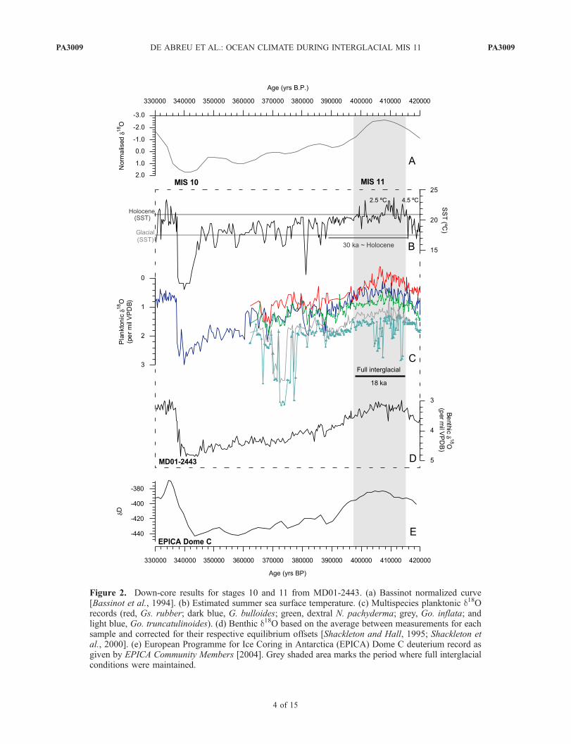
Figure 2. Down-core results for stages 10 and 11 from MD01-2443. (a) Bassinot normalized curve[Bassinot et al., 1994]. (b) Estimated summer sea surface temperature. (c) Multispecies planktonic d18Orecords (red, Gs. rubber; dark blue, G. bulloides; green, dextral N. pachyderma; grey, Go. inflata; andlight blue, Go. truncatulinoides). (d) Benthic d18O based on the average between measurements for eachsample and corrected for their respective equilibrium offsets [Shackleton and Hall, 1995; Shackleton etal., 2000]. (e) European Programme for Ice Coring in Antarctica (EPICA) Dome C deuterium record asgiven by EPICA Community Members [2004]. Grey shaded area marks the period where full interglacialconditions were maintained.

PA3009 DE ABREU ET AL.: OCEAN CLIMATE DURING INTERGLACIAL MIS 11 PA3009

4 of 15