OCCASIONAL PAPERS - Reserve Bank of India
194
RESERVE BANK OF INDIA OCCASIONAL PAPERS Vol. 34, No. 1 & 2: 2013 ISSN 0972 - 7493 Cyclicality of Social Sector Expenditures: Evidence from Indian States Balbir Kaur, Sangita Misra and Anoop K. Suresh International Financial Integration, Capital Flows and Growth of Asian Economies Amarendra Acharya and Anupam Prakash Total Factor Productivity of Indian Banking Sector - Impact of Information Technology Sujeesh Kumar S Determinants of Corporate Investments in India: An Empirical Analysis on Firm Heterogeneity M. Sreeramulu, A. Ramanathan and Krishnan Narayanan What Explains Credit Inequality Across Indian States? An Empirical Analysis Snehal Herwadkar and Saurabh Ghosh Special Notes Book Reviews RESERVE BANK OF INDIA
-
Upload
khangminh22 -
Category
Documents
-
view
0 -
download
0
Transcript of OCCASIONAL PAPERS - Reserve Bank of India

RESERVE BANK OF INDIA
OCCASIONAL PAPERS
Vol. 34, No. 1 & 2: 2013 ISSN 0972 - 7493
Cyclicality of Social Sector Expenditures: Evidence from Indian States
Balbir Kaur, Sangita Misra and Anoop K. Suresh
International Financial Integration, Capital Flows and Growth of Asian Economies
Amarendra Acharya and Anupam Prakash
Total Factor Productivity of Indian Banking Sector - Impact of Information Technology
Sujeesh Kumar S
Determinants of Corporate Investments in India: An Empirical Analysis on Firm Heterogeneity
M. Sreeramulu, A. Ramanathan and Krishnan Narayanan
What Explains Credit Inequality Across Indian States? An Empirical Analysis Snehal Herwadkar and
Saurabh Ghosh
Special Notes
Book Reviews
RESERVE BANK OF INDIA

EDITORIAL COMMITTEE
Chairman : Deepak MohantyMembers : M. D. Patra Deepak Singhal G. Mahalingam A. B. Chakraborty B. M. Misra A. S. Ramasastri Rajeev Jain Sanjib Bordoloi Binod B. Bhoi
The objective of the Reserve Bank of India Occasional Papers is to publish high quality research produced by the staff of the Reserve Bank of India on a broad array of issues of interest to a large audience including academics and policy makers. The papers selected for publications are subject to intense review by internal and external referees. The views expressed in the articles, notes and reviews published in this journal are those of the authors and do not reflect the views of the Editorial Committee or of the Reserve Bank of India. Moreover, the responsibility for the accuracy of statements contained in the contributions rests with the author(s).
The Reserve Bank of India Occasional Papers are only published through the website and no hard copies are printed.
© Reserve Bank of India 2013
All rights reserved. Reproduction is permitted provided an acknowledgement of the source is made.
All correspondence may be addressed to the Editorial Committee, Reserve Bank of India Occasional Papers, Department of Economic and Policy Research, Reserve Bank of India, Post Box No. 1036, Mumbai-400 001; E-mail: [email protected] or [email protected].

R E S E R V E B A N K O F I N D I A
OCCASIONAL PAPERS
RESERVE BANK OF INDIA


RESERVE BANK OF INDIA
OCCASIONALPAPERSVOL. 34, NO. 1 & 2: 2013
Articles Author
Cyclicality of Social Sector Expenditures: Evidence from Indian States
: Balbir Kaur, Sangita Misra and Anoop K. Suresh ....................1
International Financial Integration, Capital Flows and Growth of Asian Economies
: Amarendra Acharya and Anupam Prakash ..................37
Total Factor Productivity of Indian Banking Sector - Impact of Information Technology
: Sujeesh Kumar S..................66
Determinants of Corporate Investments in India: An Empirical Analysis on Firm Heterogeneity
: M. Sreeramulu, A. Ramanathan and Krishnan Narayanan .............87
What Explains Credit Inequality Across Indian States? An Empirical Analysis
: Snehal Herwadkar and Saurabh Ghosh .................. 112
Special Notes
SME Financing through IPOs – An Overview
: R. K. Jain, Avdhesh Kumar Shukla and Kaushiki Singh ....................138
Beautiful Minds: The Nobel Memorial Prize in Economics
: Saibal Ghosh ......................152
Book Reviews
Global Financial Contagion: Building a Resilient World Economy after the Subprime Crisis
: Devasmita Jena ..................177
In Bed with Wall Street, The conspiracy crippling our global economy
: Sakshi Parihar ....................185

Published by Deepak Mohanty for the Reserve Bank of India and printed byhim at Alco Corporation, Gala No. A-25, A Wing, Gr. Floor, Veerwani Industrial Estate, Goregaon (E), Mumbai-400063.

CYCLICALITY OF SOCIAL SECTOR EXPENDITURES: 1 EVIDENCE FROM INDIAN STATES
Reserve Bank of India Occasional Papers
Vol. 34, No. 1 & 2: 2013
Cyclicality of Social Sector Expenditures: Evidence from Indian States
Balbir Kaur, Sangita Misra and Anoop K. Suresh*
This paper attempts to study the cyclical behaviour of social sector spending including that on education and health for the 17 non-special category states covering the period 2000-01 to 2012-13. It finds that while overall social spending is acyclical in India at the state level, education spending is pro-cyclical, with the pro-cyclicality being more pronounced during upturns than it is during downturns. Further, the pro-cyclicality is more significant for bigger states (in terms of income) than it is for low income states. This possibly hints at the combined impact of political economy factors, pro-cyclical state revenues and the role of discretionary transfers. Fiscal deficit is observed to impact social sector expenditures negatively, providing support to the fiscal voracity effect hypothesis. In order to ensure that the low growth does not hamper human capital formation, states are expected to increase their social sector spending during difficult times. This would, however, require the building of adequate fiscal space during good times to enable them to spend more when required on human capital investments, which is the key to achieving long-term inclusive and sustainable development.
JEL Classification: E32, H5, H62
Key words : Social Sector Expenditures, Business Cycles, Fiscal Deficit, Transfers
Introduction
Human capital is critically intertwined with economic growth, with education and health constituting its major components. Investment in education and health makes the labour force more productive, healthy, competitive and efficient, all of which taken together contribute to higher economic growth. In the backdrop of the global financial crisis, there is renewed focus on attaining social sustainability to achieve the objective of sustainable growth. In line with this objective, there
* The authors are working in the Department of Economic and Policy Research (DEPR) of the Reserve Bank of India. Smt. Balbir Kaur is Adviser in DEPR. Smt. Sangita Misra and Shri Anoop K. Suresh are working as Assistant Adviser and Research Officer in the Structural Issues Division (SID) of DEPR respectively. The paper was presented at the 3rd RBI Chair Professor’s and DEPR Research Conference in December 2014. The authors are thankful to Professor Hari K. Nagarjan of IRMA for his valuable observations on the paper in the conference and to Shri Omkar Rane for assistance in data compilation. The views expressed by the authors are personal and not of the institution that they belong to. Usual disclaimer applies.

2 RESERVE BANK OF INDIA OCCASIONAL PAPERS
is a greater emphasis on investment in human capital with a view to improving life expectancy, ensuring availability of human capital with appropriate skill sets to support business activity while in that process also helping to develop innovative capacity and entrepreneurship in an economy. Particularly, commenting on India, the World Development Report (WDR) 2013 observed that providing key services like health and education can help create the right jobs while also contributing to improved standards of living and inclusive growth. The use of policies with a focus on strengthening the human resource base is considered extremely relevant for India which is expected to contribute a significant proportion of the global labour force in the coming years.
In the Indian context, development initiatives undertaken by planners have been driven by these concerns and are reflected in increasing importance being assigned to the provisioning of social services by the central and state governments since the inception of the Plan era. Public sector outlays on social services (both projected and actual realization) have been on the rise, with the increase being significant since the Sixth Five Year (FY) Plan. The public sector outlay on social services as a proportion of total expenditure more than doubled from 14.4 per cent in the Sixth FY Plan to 30.2 per cent in the Eleventh Plan and is projected at 34.7 per cent in the 12th FY Plan (Table 1).
While there has been a steady increase in the share of social sector expenditure in total plan expenditure, which is noteworthy, total public sector expenditure1 on important social sector heads remains low when compared with international standards. The combined expenditure of the central and state governments in India on education is just about 3.3 per cent of GDP;2 while that on the health sector is even lower at 1.3 per cent of GDP. In contrast, countries of the European Union spend 5.5
1 Comprising expenditure on social and economic services. Social services comprise of (a) education, sports, art and culture, (b) medical and public health, (c) family welfare, (d) water supply and sanitation, (e) housing, (f) urban development, (g) welfare of SCs, STs and OBCs, (h) labour and labour welfare, (i) social security and welfare, (j) nutrition, (k) expenditure on natural calamities and (i) others. Economic services comprise of (a) rural development and (b) food storage and warehousing.2 The National Policy on Education, 1986 had recommended that public investment in education should be more than 6 per cent of GDP.

CYCLICALITY OF SOCIAL SECTOR EXPENDITURES: 3 EVIDENCE FROM INDIAN STATES
per cent of GDP (from their general government account) on education and 7.5 per cent of GDP on health. Canada’s public spending on health alone is over 11 per cent of its GDP and that on education is nearly 5 per cent. Apart from the low public sector expenditure levels (relative to international standards), significant disparities p e r s i s t across states when it comes to expenditure of state governments on social services in India. Available data indicates that the states lagging behind with regard to expenditure on social sector have not attempted to catch up with the better-performing states through higher allocations of expenditure for social sector which is a key contributor to human development outcomes. The per capita social sector expenditure in the laggard states remained significantly lower than that of the leading states, resulting in the persistence of disparities in human development indicators (HDI) across states during the 2000s (RBI 2013).
Given the importance of social sector expenditure in the Indian context, it is not only pertinent to analyse the trends in social sector expenditures (including education and health) over a period of time but also to examine their response to situations of economic volatility in general and growth slowdown in particular. There are two reasons for this. First, the conventional Keynesian argument that holds for any kind of public
Table 1: Pattern of Plan Outlay on Social Services(` billion)
Period Outlay Actuals
Sixth Plan 1981-85 140.35(14.4)
159.17(14.5)
Seventh Plan 1985-1990 315.45(17.5)
349.60(16.0)
Eighth Plan 1992-97 790.12(18.2)
888.07(18.3)
Ninth Plan 1997-2002 1,832.73(21.3)
1,945.29(20.6)
Tenth Plan 2002-2007 3,473.91(22.8)
4,365.29(27.0)
Eleventh Plan 2007-12 11,023.27(30.2)
11,975.76(32.6)
Twelfth Plan 2012-17 26,648.43(34.7)
Note: Figures in brackets indicate percentage to total plan outlay.

4 RESERVE BANK OF INDIA OCCASIONAL PAPERS
sector expenditure as a counter-cyclical tool holds for social sector expenditure as well. An increase in social spending could form part of a counter-cyclical fiscal policy response of the government to support aggregate demand and foster economic recovery during the period of economic slowdown. Second, increase in social spending during this phase may also be an appropriate policy strategy to provide adequate social protection thereby mitigating the adverse human development implications of output shocks. This strategy, though desirable, may however, be constrained by available fiscal space at the level of the central and state governments.
It is against this backdrop that this paper attempts to analyse the behaviour of social sector expenditures at the state level in India – whether they are pro-cyclical, counter-cyclical or acyclical. Do these expenditures get squeezed or remain protected during downturns? Are there any inter-state differentials in these expenditures based on the size of the states? And lastly, whether a progressive move towards fiscal consolidation at the state level has impacted their social sector expenditures? Section II covers a review of literature on these issues. Trends in social sector expenditures are analysed in Section III. Section IV attempts to examine these questions in a panel data framework. Section V gives the conclusions and policy implications. The major contribution of this paper to empirical literature is that it is the first attempt of its kind to study cyclicality of social sector expenditure at the state level in India.
Section II Review of Literature
Cyclicality of fiscal policy is a well-studied and researched area. Conventional macroeconomic wisdom says that fiscal policy should act as a stabilizing policy tool by counteracting business cycle fluctuations via increasing expenditures and reducing taxes during recessions. There is extensive literature on the issue of cyclicality of fiscal policy in general, including its implications for macroeconomic stability and growth (Annexure I). The cyclicality of fiscal policy has also been examined in a cross-country framework. Fiscal policy has m o s t l y been observed to be counter-cyclical/acyclical in advanced economies. On the contrary, empirical evidence indicates a pro-cyclical behaviour

CYCLICALITY OF SOCIAL SECTOR EXPENDITURES: 5 EVIDENCE FROM INDIAN STATES
of fiscal policy in developing countries, demonstrating thereby that fiscal policy tends to expand in periods of economic growth (‘good times’) while it contracts during recessions or slowdowns (‘bad times’) (Gavin and Perotti 1997; Talvi and Vegh 2000; Lane 2003; Caballero and Krishnamurthy 2004).
Pro-cyclicality of fiscal policy in developing countries has been attributed to various factors in empirical studies. The ‘financial channel’ hypothesis attributes pro-cyclicality of fiscal policy to inadequate capital markets or limited access to these markets during downturns which restricts government spending when most needed (Gavin et al. 1996).
Tornell and Lane (1999) draw attention to the ‘voracity effect’ for the strong increase in fiscal demands during expansions. According to their reasoning, if a particular group does not increase its appropriation during a boom, other groups will. Thus, there is a strong incentive to grab part of the newly available resources before other groups do, and that the incentive to do so increases with the size of the pie; thus, this common pool problem becomes stronger in an expansion delivering a pro-cyclical result. Alesina et al. (2008) developed a model to show that public/voters’ pressure forces a government into pro- cyclical public spending, and even borrowings. Woo (2009) has argued that greater heterogeneity of preferences of different social groups, as measured by the Gini coefficient, causes fiscal policy to be pro-cyclical.
While available empirical literature mostly relates to the cyclicality of fiscal policy at the central government level, either individually or in a cross-country framework, one aspect that has been relatively less studied is the connection between the so-called ‘vertical imbalances’ in fiscal policy across different tiers of government and its effect on the overall pro-cyclicality of fiscal policy. Very little is known about the cyclicality of sub-national fiscal policies. This is surprising considering the fact that the general trend the world over has been towards greater fiscal decentralisation. A large proportion of spending, and to a lesser extent taxation, takes place at the sub-national level.
There are a few empirical studies which analyse the behaviour of social sector expenditure at the sub-national level across business cycles. In

6 RESERVE BANK OF INDIA OCCASIONAL PAPERS
a study of 21 OECD countries between 1982-2003, Darby and Melitz (2008) found that some fiscal expenditure items like health, retirement benefits, incapacity and sick pay and unemployment compensation responded in a stabilising manner to business cycle fluctuations. Granado et al. (2013) studied the cyclical behaviour of public spending on health and education in 150 countries (both developed and developing), covering the time period 1987-2007. Empirical results of the study show that total social spending was pro-cyclical in developing countries in both good and bad times, but more so during good times.3 When it comes to education and health expenditures, an asymmetric pattern was observed implying thereby that they are pro-cyclical during periods of positive output gaps but acyclical during periods of negative output gaps. Furthermore, the degree of cyclicality was observed to be higher the lower the level of economic development. Our current study essentially draws upon this paper.
Wibbels and Rodden (2006) studied the sensitivity of provincial government finances to regional business cycles in eight federal republics including India. In a panel framework, using data for 14 major states for 1980-98, both revenues and expenditures for Indian states were found to be pro-cyclical. Within revenues, own-source taxes of the states were found to be highly pro-cyclical whereas revenue-sharing and discretionary transfers were either acyclical or pro-cyclical. Based on these results, they came to a conclusion that a move towards decentralisation in developing countries would heighten overall pro-cyclicality, especially of health, education and social expenditures.
In India, the cyclical properties of fiscal policy have primarily been tested for central/general government revenues and expenditures. Examining the cyclicality of various components of central and general government (centre and states combined) expenditures in India, revenue expenditures have been found to be pro-cyclical in the long run, while capital expenditures have exhibited pro-cyclical behaviour both in the short and long run (Shah and Patnaik 2010; RBI Annual Report 2012-13).
3 Good [bad] times are defined as periods in which the output gap is positive [negative].

CYCLICALITY OF SOCIAL SECTOR EXPENDITURES: 7 EVIDENCE FROM INDIAN STATES
In empirical literature on social sector expenditures at the state level in India, the analysis has been confined mainly to issues such as trends in social sector expenditure during the post-reform period and its impact on the social sector in India (Dev et al. 2002; Joshi 2006). Social sector expenditures have been found to have a positive impact on social outcomes and hence, enhancing such expenditures from their low levels in India is viewed as crucial to achieving overall human development goals (Kaur and Misra 2003). However, there is a gap in empirical literature with regard to an analysis of the cyclical properties of state spending on social sectors like education and health in India.
Recognizing this gap, this paper attempts to analyse the cyclical properties of state spending on social sectors like education and health at the state level (in a panel framework) in India.
Section III Social Sector Expenditure: Trend Analysis
In India, the provision of social services is primarily the responsibility of state governments even as they receive large financial support from the central government under centrally sponsored schemes. Available data indicates that about 80 per cent of combined (centre and states) government expenditure on social services is incurred by state governments.4 Within social services, it is education and health services (including medical, public health and family welfare) which taken together account for around 60 per cent of the total social sector expenditure of state governments (Table 2).5
At the state level, social sector expenditure as a percentage of GDP exhibited both way movements in the range of 6-8 per cent during 1990-91 to 2012-13. On a per capita basis, social sector expenditure (in real terms) recorded a 3-fold increase during the period covered in the study. The increase was about 2.7 times for education expenditure and
4 As computed using data from State Finances: A Study of Budgets, various issues.5 Another sector which has not been considered in this paper but has seen a large increase in its share since 2008 is social security and welfare which essentially comprises of rehabilitation, social welfare as well as other social security and welfare programmes (such as construction of anganwadi buildings, marketing of Stree Shakti products, construction of training institute for SHGs and clusters, state plan schemes as well as the Women Development Corporation).

8 RESERVE BANK OF INDIA OCCASIONAL PAPERS
about 2.3 times for health expenditure on a real per capita basis. A large part of the increase in real per capita social sector expenditure has been achieved in the post-2000 period. However, despite this increase, social sector expenditure in India remains low by the international standards (WDR 2013).
A state-wise comparison of expenditure on social sector, health and education during 1990-91 to 2000-01, 2001-02 to 2009-10 and 2010-11 to 2012-13 for the 17 non-special category (NSC) states6 reveals considerable variations across states with the differences continuing to persist during the period under review. Social sector expenditure as a per cent of Gross State Domestic Product (GSDP) was in the range of 4.8 per cent to 11.5 per cent during 2010-13 in the case of NSC states. While the variation in health expenditure as a per cent of GSDP was in the range of 0.5 to 1.2 per cent, the education expenditure-GSDP ratio showed larger inter-state variations of 2.1 to 4.6 per cent (Table 3). During 2010-13, a
6 From here on, the analysis is based on non-special category states only.
Table 2: Composition of Expenditure on Social Services(Revenue and Capital Accounts)
(Per cent to total expenditure on social services)
Item 1990-98 1998-2004
2004-08 2008-10 2010-14
Average1 2 3 4 5 6Expenditure on Social Services (a to k) 100.0 100.0 100.0 100.0 100.0(a) Education, Sports, Art and Culture 51.9 52.6 47.3 44.3 46.9(b) Medical, public Health and Family
Welfare15.7 14.2 12.9 12.0 12.3
(c) Water Supply and Sanitation 7.3 7.6 8.2 6.7 4.6(d) Housing 2.9 2.9 2.9 3.1 2.9(e) Urban Development 2.4 3.2 5.4 8.7 7.3(f) Welfare of SCs, ST and OBCS 6.6 6.3 7.0 6.9 7.5(g) Labour and Labour Welfare 1.4 1.1 1.1 1.0 1.1(h) Social Security and Welfare 4.4 4.7 6.5 9.4 10.3(i) Nutrition 2.2 2.2 2.5 3.1 3.3(j) Expenditure on Natural Calamities 2.8 3.3 4.0 2.7 2.1(k) Others 2.4 2.0 2.2 2.2 2.0
Source: State governments’ budget documents.

CYCLICALITY OF SOCIAL SECTOR EXPENDITURES: 9 EVIDENCE FROM INDIAN STATES
Table 3: Expenditure on Social Sector, Education and Health: A State-wise Picture
(As per cent of GSDP at current market prices)
Social Sector Education Health
1990s 2000s 2010-13 1990s 2000s 2010-13 1990s 2000s 2010-13Andhra Pradesh
6.5 6.5 7.4 2.3 2.1 2.5 0.8 0.7 0.8
Bihar 12.0 10.5 10.9 5.9 5.1 4.6 1.6 1.1 1.0Chhattisgarh NA 8.1 11.5 NA 2.3 4.2 NA 0.6 0.9Goa 8.2 6.4 7.9 4.0 2.8 3.4 1.6 1.0 1.2Gujarat 5.4 5.4 5.3 2.6 2.1 2.1 0.7 0.5 0.6Haryana 4.7 4.7 5.5 2.1 2.0 2.4 0.6 0.4 0.5Jharkhand NA 9.8 10.0 NA 3.5 3.6 NA 1.1 0.9Karnataka 6.5 6.3 7.2 2.8 2.7 2.8 0.9 0.7 0.7Kerala 5.2 5.5 6.0 2.7 2.7 3.0 0.7 0.8 0.9Madhya Pradesh
9.5 7.8 9.3 3.6 2.7 3.4 1.1 0.8 0.9
Maharashtra 5.0 5.0 5.3 2.3 2.6 2.5 0.6 0.5 0.5Odisha 7.7 7.1 8.2 3.3 3.0 3.3 0.9 0.7 0.7Punjab 4.1 4.0 4.8 2.4 2.1 2.3 0.7 0.6 0.7Rajasthan 6.9 7.8 7.0 3.1 3.3 3.0 1.0 0.9 0.8Tamil Nadu 6.4 5.9 6.5 2.8 2.3 2.4 0.9 0.7 0.7Uttar Pradesh 6.2 7.0 9.3 3.0 3.1 4.0 0.9 1.0 1.1West Bengal 5.8 5.5 6.9 2.9 2.7 3.1 0.9 0.8 0.8Total 6.1 6.2 7.0 2.8 2.6 2.9 0.8 0.7 0.7
Source: Computed from State Finances: A Study of Budgets, various issues
majority of the states exhibited an increase in social sector expenditure (including health and education expenditure) when compared with 2001-02 to 2009-10. It may be noted that a decline in health expenditure between 2001-12 may have been compensated through higher private sector expenditure on health during these years. It is also argued that fiscal consolidation at the state level has been achieved primarily at the cost of lower health and education spending, which is examined separately in this paper.
In this context, it is interesting to examine the relationship between real social sector expenditure of states and their real incomes. A simple plotting of real growth in social sector expenditures, including education and health and real GSDP for all NSC states taken together during 1990-91 and 2012-13 reveals some kind of co-movement. However, its precise quantification necessitates further examination (Charts 1, 2 and 3).

10 RESERVE BANK OF INDIA OCCASIONAL PAPERS

CYCLICALITY OF SOCIAL SECTOR EXPENDITURES: 11 EVIDENCE FROM INDIAN STATES
On an individual state-wise basis also, some correlation is observed between expenditures and real incomes of select states. Chart 4 shows the correlation between growth in real social sector expenditures and the real GSDP for 17 NSC states over the last two decades (1990-91 to 2011-12).7 As can be seen from the chart, a majority of the states exhibit positive correlation hinting at pro-cyclicality of social sector expenditures. Preliminary evidence of pro-cyclicality is also observed for education and health expenditures across states (Charts 5 and 6) necessitating the need to explore the relationship further in an econometric framework.
7 For states like Chhattisgarh and Jharkhand, correlation is for the period from 2001-02 as data is available since then.

12 RESERVE BANK OF INDIA OCCASIONAL PAPERS
Apart from state real GSDP, gross transfers from the central government as grants or share in central tax receipts tend to influence the capacity of state governments to undertake expenditures in general, and social sector expenditure in particular.Even though the real GSDP remains an important determinant of the level of expenditure on the social sector, it is important to evaluate the impact of fiscal positions of states consequent to the enactment and implementation of the Fiscal Responsibility and Budget Management Acts/Fiscal Responsibility legislations by state governments on their social sector expenditures. It is interesting to note that social sector expenditure8 has exhibited a generally rising trend since 2004-05 (Chart 7).
8 Social sector expenditure to GDP ratio in Chart 7 is not comparable with that in Chart 1 as the former is based on all-India GDP while all states’ GSDP has been used in the latter to make it comparable to social sector expenditure-GSDP ratios of SC and NSC states.

CYCLICALITY OF SOCIAL SECTOR EXPENDITURES: 13 EVIDENCE FROM INDIAN STATES
Section IV Panel Data Analysis
Having examined the trends in social sector expenditures across states, this section tries to empirically examine whether state level-social sector expenditure is pro-cyclical, that is, whether the education and health spending of states increases during periods of high GDP growth and vice versa. This analysis is done in a panel framework for 17 NSC states. Since data for Chhattisgarh and Jharkhand are available only from the early 2000s when these states came into being, the empirical analysis is restricted to the period 2000-01 to 2012-13.9
The empirical analysis is based on data relating to expenditure on social sector (revenue expenditure) of these selected states, as given in the State Finances: A Study of Budgets and Handbook of Statistics of the Indian Economy brought out by the Reserve Bank of India. Although capital expenditure constitutes nearly 17-18 per cent of the total expenditure of the states, its share in total expenditure on education is between 0.2 per cent and 1.4 per cent for most states except Goa, for which it is around 3.6 per cent. The share of capital expenditure in total health expenditure of states is even lower. State-wise revenue expenditure on the social sector was deflated by the respective GSDP deflator to arrive at real social sector expenditure. Similarly, real education and health sector10 expenditures of the NSC states were computed.
A number of control variables have been used in cross-country and sub-national studies which include foreign aid, transfers from abroad, foreign portfolio investment, terms of trade, tax revenue as a share of GDP and provincial debt. In addition, other control variables that have been used in several cross-country studies include the lagged fiscal balance-GDP ratio, an indicator of the potential effect of borrowing constraints on public spending (Jaimovich and Panizza 2007; Granado et al. 2013), fiscal transfers to states as a determinant of their capacity to incur social spending (Arena and Revilla 2009) and political economy variable
9 Even though one could extend the data range since 1990-91 by excluding Jharkhand and Chhattisgarh, this was avoided in view of the adjustments required to address the break in the data observed for Bihar and Madhya Pradesh since 2000-01.10 Includes expenditure on health and family welfare.

14 RESERVE BANK OF INDIA OCCASIONAL PAPERS
(Cukierman et al. 1992; Brunetti 1997). Political economy variable is taken using the logic that if there is a similarity between the governing parties at the centre and state levels, the states tend to become more important in the federal set up and enjoy greater bargaining power.
We have chosen the control variables that are relevant for our analysis at the sub-national level in India, and for which data are readily available. Further, the selection of control variables has been made to ensure that the possible multi-collinearity between the explanatory variables does not distort empirical results.11 We selected the gross fiscal deficit-GSDP ratio as a control variable in our empirical analysis. It may be noted here that for Indian states, even though states’ revenue expenditures as a proportion to GDP has not declined, there was a slight compositional shift towards developmental expenditure during the 2000s. This was on account of a decline in the share of interest payments in total revenue expenditure as also in the interest payments-GDP ratio in the recent period vis-à-vis 2004-08 (RBI 2013). The political economy variable has been captured through dummy in this paper. The dummy takes a value of one if the party at the state is the same as the one at the centre and a value of zero if they are different.12
Summary statistics for the variables used in the empirical work are given in Table 4. State-wise descriptive statistics are given in Annex II.
The Model
In line with literature, the following regression equation is estimated using panel data:
d(log SS EXP i, t ) = β0i + γt + β1 d(log Yit) + β2 FDi,t-1 + β1 d(log TRi,t) + u i,t ……… (1)
where β0 represents state fixed effect which controls for heterogeneity across states, γ is time effect capturing common shocks across states at a given time period, SS EXP denotes real social sector expenditure, Y
11 In case of multi-collinearity, regression coefficients get drastically altered when an additional variable is added or dropped. In this empirical exercise, mostly growth rates have been used that are less likely to be correlated. As long as one variable cannot be expressed as a function of the other, that is, as long as there is some information in say the fiscal deficit variable which is not captured by the GSDP variable, inclusion of that variable in the equation is desirable (Belsley et al.1980; Brien 2009).12 It may be noted here that this is a general assumption, though there are at times exceptions.

CYCLICALITY OF SOCIAL SECTOR EXPENDITURES: 15 EVIDENCE FROM INDIAN STATES
Table 4: Descriptive Statistics: 2000-01 to 2012-13
Real Growth in per cent Fiscal deficit
to GSDP ratio (per cent)
Growth in Transfer
receipts in real terms (per cent)
Social Sector Expenditure
Education Expenditure
Health Expenditure
GSDP
Mean 8.7 7.6 7.5 7.3 3.4 9.8Median 8.9 6.5 5.3 7.5 3.2 8.1Maximum 51.8 44.1 102.6 28.7 8.1 191.4Minimum -26.4 -29.2 -31.0 -9.9 -1.0 -44.1Std. Dev. 12.1 11.9 14.5 4.9 1.8 19.3Observations 217 217 217 217 217 217
denotes GSDP in real terms, FD denotes gross fiscal deficit as a per cent of GSDP, TR denotes gross transfers in real terms and u is an error term. The subscripts i and t denote state and time period respectively. The coefficient β1 measures the cyclicality of social sector expenditure at the state level. A positive and significant value of β1 implies pro-cyclical behaviour, while a negative and significant value implies counter-cyclical behaviour. A non-significant β1 implies acyclical behaviour.
Before the estimation was done, all the data series were tested for stationarity. Based on panel unit root tests involving the common unit root process (LLC) as well as individual unit root process (IPS), the dependent and explanatory variable series were found to be stationary, that is, I (0) (Table 5). It is observed that growth in health expenditure is either non-stationary or stationary with low significance. Recognising this, health expenditure was dropped as one of the dependent variables from the regression estimations. Most variables used in the model were normalised and transformed into logarithms to minimise heteroscadasticity.
In literature, in a cross-country framework, instrument variables (IV) - fixed effect models have generally been used to address potential endogeneity of the RHS variable (output), that is, while economic downturns limit government’s capacity to undertake counter-cyclical policies, counter-cyclical fiscal policies (including social spending) may offset the impact of downturns through a positive push to boost

16 RESERVE BANK OF INDIA OCCASIONAL PAPERS
the economy (Nadia et al. 2010). Some of the instrument variables used in empirical literature include interest rate, world growth rate, terms of trade and lagged GDP growth. The 2-stage least squares (2SLS) technique is also frequently used to address endogeneity issues. Arena and Revilla (2009) found that fiscal spending responded to business cycles in a contemporaneous manner in different Brazilian states. Given that our analysis relates to response of public spending at the state level, the results are reported for GSDP at levels on the lines of the Brazilian study. However, to rule out any potential endogeneity, the results of IV estimation (with lagged output growth as the IV) as well as the 2SLS estimation are also reported so as to ensure the robustness of the results.
Empirical Results
Results of the panel estimates for social sector and education expenditures are reported in Table 6.
State social expenditures are generally observed to be acyclical during the 2000s. This may be due to the fact that these expenditures, being on the revenue account, exhibit downward rigidity. Expenditure on education was, however, observed to be pro-cyclical in the least squares estimate although its pro-cyclical behaviour is not seen in the case of IV and 2SLS estimates. Fiscal deficit (with a one period lag) turns out to be an important factor influencing public spending on social sector including that on education. Transfers from the centre to states explain to a large extent the observed acyclical behavior with regard to social
Table 5: Results of Panel Unit Root Tests
Variables (Levels) LLC t Statistics IPS W Statistics
Growth in real Social sector expenditure -6.83** -4.69**Growth in real Education expenditure -5.33** -2.60**Growth in real Health expenditure -2.16** -1.42GSDP growth -7.73** -6.15**Fiscal deficit to GSDP ratio -4.50** -1.60*Real Gross Transfers Growth -6.01** -5.70**
1. LLC = Levin, Lin, Chu (2002); IPS = Im, Paseran, Shin (2003).2. ** and * indicate the rejection of the null hypothesis of non-stationarity at 1 per cent and 5
per cent levels of significance.3. Automatic selection of lags through Schwarz Information Criteria (SIC).4. All panel unit root tests are defined by Bartlett kernel and Newly West bandwidth

CYCLICALITY OF SOCIAL SECTOR EXPENDITURES: 17 EVIDENCE FROM INDIAN STATES
sector expenditures. However, the role of transfers diminishes in explaining the cyclical response of education expenditures.
Upturn and Downturn
This analysis tries to assess cyclicality using the relationship between social sector spending and GDP growth rates. However, the state of the economy may also have an influence on cyclicality results. In other words, GDP growth may be above its potential and vice versa. Thus, it needs to be examined whether the acyclicality in social sector expenditure that we have observed holds true at all times – irrespective of the output gap position. Descriptive statistics also suggest that the average growth in real social sector expenditure, including on education and health, is significantly higher during positive output gap periods (upturns) than during negative output gap periods (downturns). The standard test of equality of mean and median was conducted to see whether mean and median of these expenditure variables remained the same during both the periods (Table 7). The test rejects the null hypothesis, as the mean and median growth rates of expenditures turn out to be significantly different during the periods of upturns and downturns (except median growth in social sector expenditure). Given this inference, the analysis
Table 6: Cyclicality of Social Sector Expenditure: Panel Regression Coefficients
Social Sector Expenditure Education Expenditure
LS IV 2SLS LS IV 2SLS
Constant 0.14** 0.15** 0.27** 0.13** 0.13** 0.20**GSDP 0.19 0.16 -1.30 0.33** 0.14 -0.08Fiscal deficit (Lagged) -0.03** -0.03** -0.03** -0.03** -0.02** -0.02**Gross Transfers 0.18** 0.13** 0.19** 0.07* 0.03 0.06Political Party Dummy 0.01 0.01 0.01 0.03* 0.03* 0.04AR(1) -0.16* -0.06*Number of States 17 17 17 17 17 17Number of Observations 204 187 187 204 187 187
Note: 1. ** and * indicate significance of coefficient at 1 per cent and 5 per cent levels, respectively.
2. LS: Least Squares; IV: Instrumental Variable; 2SLS: Two Stage Least Squares. 3. Hausman test has been used to decide on the fixed effect model.

18 RESERVE BANK OF INDIA OCCASIONAL PAPERS
was extended to see whether the cyclicality results across states differed during the periods of positive and negative output gaps.
Two methodologies were used for this analysis. First, we examined the response of social sector spending to output gap, as indicated by the ratio of actual to potential output13 (computed using the HP filter) for different states. This was attempted using equation (1) as given earlier, but replacing the output variable by the output gap variable along with other control variables. Second, the time period covered in the study was distinctly split into good and bad times (upturns versus downturns) using appropriate dummies. The period of upturn was taken as the one when the actual output was higher than the trend output as computed using the HP filter and vice versa for downturns. Further, we used two interaction variables, one between real GSDP growth and the upturn dummy variable and the other between real GSDP growth and the downturn dummy variable. To test for the asymmetric reaction of state-level government spending to positive and negative output gaps, the following equation is used:
d(log EXP it) = β0i + γt + βu d(log Yut)*dumu + βd d(log Ydt)*dumd+ β2 FDi,t-1 + β3 d(log TR it) + u it …(2)
where βu ≠ βd and the suffixes u and d indicate whether the coefficient applies to a positive or negative output gap period. For example, when
Table 7: Test of Equality of Mean/Median for Growth in Real Expenditures During Upturns and Downturns
Mean Median
T-statistics@ p-value Chi-square$ p-value
Social Sector Expenditure -2.66 0.00 2.02 0.15Education Expenditure -3.33 0.00 5.02 0.02
Note: @: Test of equality of means based on H0: µ1=µ2 where µ1 and µ2 are mean values of growth in real expenditure during upturn and downturn, respectively.$: Test of equality of median based on H0: m1=m2 where m1 and m2 are median values of growth in real expenditure during upturn and downturn, respectively.
13 The ratio approach (actual/potential) to represent output gap has been generally preferred over the subtraction approach (actual minus potential) in many recent studies (particularly IMF studies) in view of the difficulty in computing log of a negative number.

CYCLICALITY OF SOCIAL SECTOR EXPENDITURES: 19 EVIDENCE FROM INDIAN STATES
the observation for the output gap is positive, log Yut equals the observed value of real GSDP growth; when the output gap is negative, log Yut is zero.
Tables 8 and 9 report the responses of social sector and education expenditures to upturns and downturns as measured in terms of positive and negative output gaps. Regression coefficients clearly indicate that
Table 8: Pro-cyclicality of Social Sector Expenditure to Output Gap: Panel Regression Coefficients
Social Sector Expenditure Education Expenditure
LS IV 2SLS LS IV 2SLS
Constant -0.01 0.20 -0.09* -0.5** -0.19 -0.17*Output Gap 0.17 -0.04 0.08 0.60** 0.33* 0.98**Fiscal deficit (Lagged) -0.03** -0.03** -0.02** -0.02** -0.03** -0.01*Gross Transfers 0.18** 0.18** 0.16** 0.07* 0.08* 0.03Political Party Dummy 0.01 0.01 -0.03 0.03* -0.04 -0.04AR(1) -0.16** -0.01
Number of States 17 17 17 17 17 17Number of Observations 204 187 187 204 187 187
Note: 1. ** and * indicate significance of coefficient at 1 per cent and 5 per cent levels, respectively.
2. LS: Least Squares; IV: Instrumental Variable; 2SLS: Two Stage Least Squares.
Table 9: Pro-cyclicality of Social Sector Expenditure during Upturns andDownturns: Panel Regression Coefficients
Social Sector Expenditure Education Expenditure
LS IV 2SLS LS IV 2SLS
Constant 0.14** 0.14** 0.29** 0.12** 0.13** 0.11*GSDP - Upturn 0.22 0.18 -1.48 0.44** 0.30** 0.81GSDP - Downturn 0.01 0.15 -1.33 -0.05 -0.08 -0.35Fiscal deficit -0.03** -0.03** -0.03** -0.02** -0.02** -0.01*Gross Transfers 0.17** 0.13** 0.19** 0.05 0.02 0.01Political Party Dummy 0.01 0.01 -0.02 0.03* 0.03* -0.04AR(1) -0.15* -0.01
Number of States 17 17 17 17 17 17Number of Observations 204 187 187 204 187 187
Note: 1. ** and * indicate significance of coefficient at 1 per cent and 5 per cent levels, respectively. 2. LS: Least Squares; IV: Instrumental Variable; 2SLS: Two Stage Least Squares.

20 RESERVE BANK OF INDIA OCCASIONAL PAPERS
when we use the output gap as the variable, education expenditures turn out to be pro-cyclical even as social sector expenditures continue to be acyclical. Further, social sector expenditures remain acyclical during both the upturn and downturn phases, while education expenditures show asymmetric behaviour - being pro-cyclical during upturns and acyclical during downturns. This result is similar to the findings of Clements et al. (2007) and Granado et al. (2013) that education and health expenditures are pro-cyclical in good times but acyclical in bad times. While the pro-cyclical behaviour during upturns may be indicative of the fiscal ‘voracity effect’, acyclical behaviour during downturns is attributed by Granado et al. (2013) to asymmetric behavior prompting countries to protect social spending during times when the GDP falls below the potential level. This logic may also hold for Indian states as they do not allow spending on education and health to fall below a particular level, despite a downturn due to socio-political reasons.14 This also reflects the increasing priority that has been accorded by the states to the education sector in line with the implementation of the Sarva Shiksha Abhiyan (SSA) and subsequently the Right to Education Act,15 for which they receive financial support from the central government.
Fiscal balance is observed to be a consistent and significant determinant of social sector expenditure in all time periods, albeit its coefficient is smaller vis-à-vis other explanatory variables. Among other control variables, gross transfers from the central government and the political dummy variable seem to be influencing social sector expenditure and education expenditures respectively.
Big States versus Small States
Given that education expenditures are observed to be pro-cyclical, the empirical analysis is extended to examine whether this holds for all the NSC states or there are variations across these states based on their income levels. Following Arena and Revilla’s (2009) approach in their study on the cyclicality of fiscal policy at the sub-national level in Brazil, 17 NSC states in India were classified into two categories- big and small
14 Although the empirical testing of this could not be done for health expenditures for Indian states due to statistical reasons, it appears that the same logic may also hold for health expenditures. 15 A detailed list of flagship programmes on education is given in Annex III.

CYCLICALITY OF SOCIAL SECTOR EXPENDITURES: 21 EVIDENCE FROM INDIAN STATES
(in terms of income) - based on their per capita GSDP as per the 2011 Census. Accordingly, the top nine states were taken as big states that had per capita GSDP (at current prices) higher than `75,000 in 2011. These include Andhra Pradesh, Goa, Gujarat, Haryana, Karnataka, Kerala, Maharashtra, Punjab and Tamil Nadu. The smaller states include Bihar, Chhattisgarh, Jharkhand, Madhya Pradesh, Odisha, Rajasthan, Uttar Pradesh and West Bengal. Table 10 provides the cyclicality coefficients of education expenditure with respect to output gap separately for big and small states.
Education expenditure is observed to be strongly pro-cyclical with respect to the output gap in the case of big states. More than state incomes, it is gross transfers from the central government that influence education expenditures of small states. This is probably because transfers, on an average, account for close to 60 per cent of the revenue receipts of the states falling in this group. Fiscal balance is also observed to be a significant determinant of education expenditure in both big and small states, albeit its coefficient is smaller vis-à-vis other explanatory variables namely, real GSDP and fiscal transfers from the centre to these states.
Table 10: Pro-cyclicality of Education Expenditure in Big and Small States: Panel Regression Coefficients
Big States Small States
LS IV 2SLS LS IV 2SLS
Constant 0.11** 0.12** -0.12* 0.13** 0.14** 0.16*Output gap 0.89** 0.48* 0.85* 0.12 -0.02 0.27Fiscal deficit -0.02** -0.02** -0.02* -0.02** -0.02** -0.01*Gross Transfers 0.01 0.03 0.03 0.40** 0.39* 0.09Political Party Dummy 0.03* 0.04* -0.01 -0.01 -0.01 -0.11AR(1) -0.04* -0.02*
Note: 1. ** and * indicate significance of coefficient at 1 per cent and 5 per cent levels, respectively.
2. LS: Least Squares; IV: Instrumental Variable; 2SLS: Two Stage Least Squares.

22 RESERVE BANK OF INDIA OCCASIONAL PAPERS
Section V Conclusion and Policy Implications
The paper studied the cyclical behaviour of social sector expenditure across Indian states during the 2000s. Empirical evidence suggests that the overall social sector spending is acyclical in India at the state level, while education spending turns out to be pro-cyclical with the pro-cyclicality being more pronounced in situations of positive output gaps (upturns) and for bigger states. As states tend to protect social sector expenditures during negative output gap periods, it explains their acyclical behaviour. This is also evident from a consistent increase in the share of social sector expenditure in total revenue expenditure of NSC states.
Fiscal deficit, albeit with a small coefficient value, was the most significant and consistent variable impacting social sector expenditures in the 2000s. This provides support to the fiscal voracity effect hypothesis (Tornell and Lane 1999; Talvi and Vegh 2000). Improvement in the fiscal position provokes intense lobbying for higher social sector spending which holds for all states and during all time periods. The paper reinforces the need for further fiscal consolidation as this would provide more headroom to state governments for carrying out social sector expenditures during phases of growth slowdown.
To conclude, state governments need to ensure that their social sector spending is protected to achieve inclusive and sustainable development in the medium to long-term. High income states which are fiscally better placed should be the front runners in pursuing this objective. Needless to say, this is extremely relevant for India that has a huge demographic dividend which it can tap in the future. Going forward, further research in the area could explore the impact of other factors influencing social sector expenditures in India like the level of fiscal autonomy (Binswanger et al. 2014), service delivery framework. The study can also be extended to special category states depending upon the availability of data.

CYCLICALITY OF SOCIAL SECTOR EXPENDITURES: 23 EVIDENCE FROM INDIAN STATES
Ann
ex-I
Pro-
cycl
ical
ity o
f Soc
ial S
ecto
r E
xpen
ditu
re: A
Rev
iew
of L
itera
ture
Stud
ySc
ope
Met
hod/
Dat
a/Pe
riod
Focu
sFi
ndin
g/co
nclu
sion
I. C
ross
- co
untr
y st
udie
s on
cycl
ical
ity o
f fisc
al p
olic
y at
agg
rega
te le
vel
Aki
toby
, Cle
men
ts,
Gup
ta &
Inch
aust
e (2
004)
51
Cou
ntrie
s-
Exam
inat
ion
of
shor
t ter
m a
nd
long
term
m
ovem
ent o
f go
vern
men
t sp
endi
ng re
lativ
e to
out
put.
Focu
ses o
n th
e cy
clic
al a
nd
long
-term
be
havi
our
of
gove
rnm
ent
expe
nditu
res
in d
evel
opin
g co
untri
es.
- Th
e m
ain
com
pone
nts
of
gove
rnm
ent
spen
ding
are
pro
-cyc
lical
in
abou
t ha
lf of
th
e co
untri
es,
the
degr
ee o
f w
hich
var
ies
acro
ss sp
endi
ng c
ateg
orie
s.
- O
utpu
t vol
atili
ty an
d fina
ncia
l risk
s con
tribu
te
to p
ro-c
yclic
ality
of g
over
nmen
t spe
ndin
g.
Mic
hael
Gav
in &
R
ober
t Per
rotti
(1
997)
Latin
A
mer
ica
and
indu
stria
l co
untri
es
- 19
68 to
199
5
- R
egre
ssio
n an
alys
is u
sing
fis
cal i
ndic
ator
s of
the
gene
ral
gove
rnm
ent.
A
com
paris
on
of
pro-
cycl
ical
ity o
f fis
cal
polic
y in
La
tin
Am
eric
a an
d in
dust
rialis
ed c
ount
ries.
- Fi
scal
po
licy
in
Latin
Am
eric
a is
pr
o-cy
clic
al
whe
reas
it
is
acyc
lical
in
in
dust
rialis
ed c
ount
ries.
- Th
e maj
or re
ason
s for
pro
-cyc
lical
ity ar
e the
‘v
orac
ity e
ffect
’” a
s w
ell a
s lim
ited
acce
ss
to
inte
rnat
iona
l cr
edit
mar
kets
du
ring
dow
ntur
ns.
Ale
sina
, Tab
ellin
a &
Cam
pant
e (2
007)
OEC
D a
nd
non-
O
ECD
co
untri
es
- 196
0-20
03
- Pan
el re
gres
sion
us
ing
fisca
l po
licy
indi
cato
rs
- O
bser
ves
cycl
ical
re
spon
se o
f th
e bu
dget
su
rplu
s an
d to
tal
gove
rnm
ent
spen
ding
in
diffe
rent
cou
ntrie
s.
- Ex
amin
es t
he s
ourc
es o
f pr
o-cy
clic
ality
.
- D
urin
g bo
oms,
peop
le d
eman
d m
ore
publ
ic
good
s or l
ower
taxe
s the
reby
lead
ing
to p
ro-
cycl
ical
ity o
f fisc
al p
olic
y.
- Th
e m
ajor
rea
sons
for
pro
-cyc
lical
ity i
n a
dem
ocra
tic co
untry
are
corr
uptio
n as
wel
l as
cred
it co
nstra
ints
.

24 RESERVE BANK OF INDIA OCCASIONAL PAPERS
Stud
ySc
ope
Met
hod/
Dat
a/Pe
riod
Focu
sFi
ndin
g/co
nclu
sion
Kam
insk
y, R
einh
art
and
Vegh
(200
4)O
ECD
&
Non
- O
ECD
co
untri
es
- 19
60-2
003
- A
naly
tical
fr
amew
ork
for
inte
rpre
ting
the
beha
viou
r of
fisca
l ind
icat
ors.
Empi
rical
ly
docu
men
ting
the
cycl
ical
pro
perti
es o
f m
acro
econ
omic
pol
icie
s in
de
velo
ping
cou
ntrie
s.
In d
evel
opin
g co
untri
es, fi
scal
pol
icy
is p
ro-
cycl
ical
whe
reas
in O
ECD
coun
tries
it is
eith
er
acyc
lical
or c
ount
er-c
yclic
al.
Jaim
ovic
h an
d Pa
nizz
a (2
007)
Indu
stria
l an
d de
velo
ping
co
untri
es.
- 19
70-2
003
- In
stru
men
t va
riabl
e es
timat
ion
- C
halle
ngin
g th
e co
nven
tion
that
fis
cal
polic
y is
pro
-cyc
lical
in
deve
lopi
ng c
ount
ries.
No
statis
tical
ly s
igni
fican
t diff
eren
ce b
etw
een
the
cycl
ical
ity o
f fis
cal
polic
y in
dev
elop
ing
and
indu
stria
l cou
ntrie
s.
II. C
ross
-cou
ntry
stud
ies o
n th
e cy
clic
ality
of s
ocia
l exp
endi
ture
at a
ggre
gate
leve
l
Javi
er A
rze,
Sa
njee
v G
upta
, and
A
leja
ndro
H
ajde
nber
g (2
012)
29
deve
lope
d an
d 12
1 de
velo
ping
co
untri
es
- IM
F’s d
atab
ase
- R
egre
ssio
n te
chni
ques
.
Exam
inat
ion
of
cycl
ical
be
havi
our
of
publ
ic
spen
ding
on
he
alth
an
d ed
ucat
ion.
- Th
e sp
endi
ng o
n ed
ucat
ion
and
heal
th i
s pr
o-cy
clic
al
in
deve
lopi
ng
coun
tries
w
here
as
it is
ac
yclic
al
in
deve
lope
d co
untri
es.
- Th
e de
gree
of
cy
clic
ality
is
in
vers
e to
ec
onom
ic d
evel
opm
ent.
Nad
ia D
oytc
h,
Bin
gjie
Hu,
Ron
ald
U M
endo
za (2
010)
Latin
A
mer
ica,
C
arib
bean
- W
orld
B
ank
data
set f
rom
198
0 to
200
9.
- Is
soc
ial
spen
ding
pro
- cy
clic
al?
- H
igh-
inco
me
econ
omie
s and
low
est i
ncom
e ec
onom
ies
are
able
to
im
plem
ent
the
polic
ies
of c
ount
er-c
yclic
al s
ocia
l spe
ndin
g
Ann
ex-I
(Con
td...
)

CYCLICALITY OF SOCIAL SECTOR EXPENDITURES: 25 EVIDENCE FROM INDIAN STATES
Stud
ySc
ope
Met
hod/
Dat
a/Pe
riod
Focu
sFi
ndin
g/co
nclu
sion
and
low
in
com
e co
untri
es
of th
e w
orld
.
- O
LS, F
ixed
Ef
fect
s (FE
) use
d fo
r em
piric
al
anal
ysis
.
Are
mor
e st
able
and
les
s co
rrup
t go
vern
men
ts m
ore
likel
y to
und
erta
ke co
unte
r-cy
clic
al so
cial
spen
ding
?
whe
reas
the
low
er m
iddl
e in
com
e co
untri
es
are
unab
le to
do
so.
- B
urea
ucra
cy q
ualit
y, c
ontro
l of
cor
rupt
ion
and
gove
rnm
ent s
tabi
lity
prom
ote
coun
ter-
cycl
ical
spen
ding
.
Julia
Dar
by &
Ja
cque
s Mel
itz
(200
8)
21 O
ECD
co
untri
es-
OEC
D
soci
al
expe
nditu
re
and
OEC
D
econ
omic
ou
tlook
da
taba
se
from
198
2 to
200
3.
Ana
lyse
s cy
clic
al
resp
onsi
vene
ss
of
fisca
l ex
pend
iture
item
s.
Expe
nditu
res o
n he
alth
, ret
irem
ent,
inca
paci
ty,
sick
pa
y as
w
ell
as
unem
ploy
men
t co
mpe
nsat
ion
are
high
ly p
ro-c
yclic
al.
III.
Cro
ss-c
ount
ry st
udie
s on
the
cycl
ical
ity o
f soc
ial e
xpen
ditu
re a
t the
sub-
natio
nal l
evel
Wib
bels
and
R
odde
n (2
006)
8 fe
dera
tions
(U
S,
Can
ada,
G
erm
any,
A
ustra
lia,
Spai
n,
Indi
a,
Bra
zil a
nd
Arg
entin
a)
- U
tilis
ing
annu
al
data
per
tain
ing
to
reve
nue,
ex
pend
iture
, de
ficit
and
GSD
P.-
Pane
l est
imat
ion.
Inve
stig
atio
n of
th
e se
nsiti
vity
of
pr
ovin
cial
go
vern
men
t fin
ance
s to
re
gion
al b
usin
ess c
ycle
s.
- Su
b-na
tiona
l fin
ance
s in
the
wor
ld’s
mos
t de
cent
raliz
ed fe
dera
tions
are
pro
-cyc
lical
.-
Mor
e de
cent
ralis
atio
n w
ill h
eigh
ten
pro-
cycl
ical
ity e
spec
ially
of
heal
th,
educ
atio
n an
d so
cial
spen
ding
.
Ann
ex-I
(Con
td...
)

26 RESERVE BANK OF INDIA OCCASIONAL PAPERS
Stud
ySc
ope
Met
hod/
Dat
a/Pe
riod
Focu
sFi
ndin
g/co
nclu
sion
Stur
zene
ggar
&
Wer
neck
(200
6)A
rgen
tina
& B
razi
l-
Arg
entin
a 19
92-
2002
- B
razi
l 199
7-20
02
- Ti
me
serie
s an
d cr
oss-
sect
iona
l m
odel
s.
- A
re
the
sub-
natio
nal
fisca
l po
licie
s pr
o-cy
clic
al a
s w
ell
as t
he
caus
es fo
r pro
-cyc
lical
ity.
- Th
e sp
endi
ng o
f su
b-na
tiona
l gov
ernm
ents
ha
s be
en p
ro-c
yclic
al in
bot
h A
rgen
tina
and
Bra
zil.
- R
easo
ns f
or p
ro-c
yclic
ality
: Vor
acity
effe
ct
and
lack
of a
cces
s to
cre
dit m
arke
ts d
urin
g tim
es o
f cris
is.
Mar
co A
rena
&
Julio
Rev
illa
(200
7)B
razi
lian
stat
es-
1991
-200
6
- Ti
me
serie
s and
cr
oss-
sect
iona
l da
ta
- O
LS, F
ixed
Ef
fect
s and
Fe
asib
le
Gen
eral
ized
Fi
xed
Squa
res
(FG
FS) u
sed.
Exam
inat
ion
of
pro-
cycl
ical
ity
of
Bra
zilia
n st
ates
’ exp
endi
ture
s.
- Th
ere
is p
ro-c
yclic
ality
in B
razi
lian
stat
es’
expe
nditu
res
whi
ch is
mor
e du
ring
perio
ds
of d
ownt
urn.
- Th
e m
ain
sour
ces
of t
he o
bser
ved
pro-
cy
clic
ality
lie i
n th
e sta
tes’
own
tax
reve
nues
.
- Sm
alle
r st
ates
are
mor
e pr
o-cy
clic
al t
han
larg
er st
ates
for a
ll re
venu
e an
d ex
pend
iture
ca
tego
ries.
IV. I
ndia
n st
udie
s on
soci
al se
ctor
exp
endi
ture
ana
lysi
sB
albi
r Kau
r &
Sang
ita M
isra
(2
003)
15 G
ener
al
cate
gory
st
ates
in
Indi
a
- 19
85-8
6 to
20
00-0
1A
naly
ses
the
leve
l an
d ef
fect
iven
ess
of
soci
al
sect
or
expe
nditu
re
in
educ
atio
n an
d he
alth
.
- Pu
blic
spen
ding
on
educ
atio
n ha
s bee
n m
ore
prod
uctiv
e in
the
case
of p
rimar
y ed
ucat
ion
than
in th
e ca
se o
f sec
onda
ry e
duca
tion.
Ann
ex-I
(Con
td...
)

CYCLICALITY OF SOCIAL SECTOR EXPENDITURES: 27 EVIDENCE FROM INDIAN STATES
Stud
ySc
ope
Met
hod/
Dat
a/Pe
riod
Focu
sFi
ndin
g/co
nclu
sion
- Reg
ress
ion
anal
ysis
usi
ng
pane
l dat
a.
- R
elat
ions
hip
betw
een
publ
ic e
xpen
ditu
re
and
heal
th h
as b
een
quite
wea
k in
dica
ting
inad
equa
cy o
f hea
lth e
xpen
ditu
re.
Mah
endr
a D
ev
(200
2)In
dia
- Tr
end
Ana
lysi
sA
naly
sis
of
gove
rnm
ent
spen
ding
on
ag
ricul
ture
an
d so
cial
sect
ors.
- C
entra
l gov
ernm
ent a
s wel
l as s
tate
spen
ding
on
soci
al se
ctor
is st
ill q
uite
low.
Seem
a Jo
shi (
2006
)In
dia
Pre-
Ref
orm
(198
1-82
to 1
990-
91) a
nd
post
-ref
orm
per
iod
(199
1-92
to 2
000-
01).
Exam
ines
th
e im
pact
of
ec
onom
ic re
form
s on
soci
al
sect
or e
xpen
ditu
re.
- A
dec
ade
of re
form
s has
not
bro
ught
muc
h im
prov
emen
t in
soci
al s
ecto
r sp
endi
ng a
s th
e sh
are
of so
cial
sect
or to
GD
P re
mai
ned
at a
ver
y lo
w le
vel o
f 2.7
per
cen
t in
2000
-01
(whi
ch w
as 2
.62
per c
ent i
n 19
86-8
7).
Ann
ex-I
(Con
td...
)

28 RESERVE BANK OF INDIA OCCASIONAL PAPERS
Social Sector Expenditures
Education Expenditures
Health Expenditures
GSDP Fiscal Deficit
to GSDP ratio (per cent)
Growth in
transfer receipts in real terms
(per cent)
Real Growth in per cent
Andhra Pradesh
Mean 9.6 8.8 7.4 7.6 3.2 8.2Median 11.2 7.6 5.9 8.2 2.9 7.7Maximum 21.3 36.0 24.3 12.0 4.8 28.6Minimum -9.9 -2.7 -2.9 2.7 1.9 -18.4Std.Deviation 9.4 11.3 7.5 2.8 0.9 13.6Observations 13 13 13 13 13 13
Bihar
Mean 6.8 5.6 5.3 8.5 4.1 8.9Median 3.0 4.2 1.3 11.8 3.2 9.5Maximum 42.3 33.0 56.2 16.0 8.1 27.7Minimum -26.2 -27.5 -31.0 -5.1 1.5 -12.5Std.Deviation 18.6 16.7 24.7 7.5 2.3 12.4Observations 13 13 13 13 13 13
Chhattisgarh
Mean 13.6 16.1 12.0 8.6 1.8 12.5Median 10.2 16.9 4.0 8.4 1.8 13.5Maximum 36.0 33.0 56.3 18.6 5.6 31.2Minimum -6.4 1.7 -3.0 2.5 -0.3 -0.3Std.Deviation 12.8 11.3 17.7 4.7 1.7 9.4Observations 11 11 11 11 11 11
Goa
Mean 10.7 8.7 7.8 7.6 4.1 18.5Median 8.3 7.9 2.4 9.4 4.2 0.9Maximum 44.2 44.1 39.0 10.2 5.5 191.4Minimum -0.8 -13.9 -6.9 -3.7 1.7 -44.1Std.Deviation 12.2 15.8 13.2 3.9 1.1 57.3Observations 13 13 13 13 13 13
Gujarat
Mean 7.9 6.0 8.2 8.9 3.4 7.2Median 9.0 4.9 7.4 8.9 2.8 5.3Maximum 21.0 30.0 35.4 14.9 6.7 28.0Minimum -14.5 -15.7 -22.7 -4.9 1.4 -14.2Std.Deviation 10.7 11.1 15.1 4.8 1.5 12.9Observations 13 13 13 13 13 13
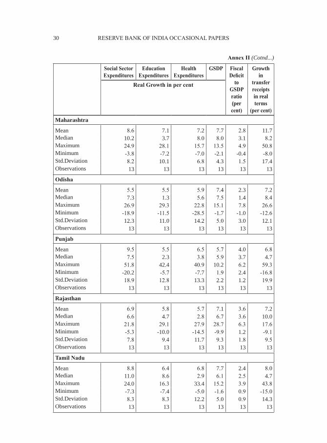
Annex II
Descriptive Statistics

CYCLICALITY OF SOCIAL SECTOR EXPENDITURES: 29 EVIDENCE FROM INDIAN STATES
Social Sector Expenditures
Education Expenditures
Health Expenditures
GSDP Fiscal Deficit
to GSDP ratio (per cent)
Growth in
transfer receipts in real terms
(per cent)
Real Growth in per cent
Haryana
Mean 10.8 9.2 7.8 8.7 2.3 10.5Median 19.2 10.0 4.8 8.4 2.5 5.1Maximum 30.3 24.9 30.0 11.7 4.5 54.9Minimum -26.4 -5.4 -8.7 6.5 -0.9 -18.6Std.Deviation 16.3 8.6 11.8 1.5 1.6 20.3Observations 13 13 13 13 13 13
Jharkhand
Mean 9.1 11.0 10.1 7.0 4.7 12.7Median 11.9 11.5 -0.2 7.2 4.3 22.6Maximum 28.4 41.4 102.6 20.5 8.1 32.5Minimum -15.9 -29.2 -10.1 -3.2 1.8 -20.8Std.Deviation 11.2 19.1 32.5 7.1 2.3 19.7Observations 11 11 11 11 11 11
Karnataka
Mean 8.5 7.4 6.7 7.3 2.9 9.9Median 9.1 9.1 5.7 7.1 2.8 10.1Maximum 17.0 17.1 28.3 12.6 5.0 28.2Minimum -4.7 -5.8 -11.0 1.3 1.9 -11.9Std.Deviation 6.4 7.5 10.4 3.2 0.9 10.8Observations 13 13 13 13 13 13
Kerala
Mean 7.9 7.3 8.6 6.1 3.6 9.8Median 5.7 7.0 7.1 8.1 3.4 6.1Maximum 29.1 28.0 29.6 11.4 5.2 33.3Minimum -12.1 -7.6 -8.5 -6.9 2.5 -11.2Std.Deviation 14.9 9.9 10.0 5.5 0.8 16.2Observations 13 13 13 13 13 13
Madhya Pradesh
Mean 7.4 6.6 6.4 7.7 3.6 9.4Median 8.3 4.4 5.3 9.2 2.8 8.0Maximum 24.8 23.6 26.2 16.5 7.3 27.5Minimum -16.8 -23.8 -20.9 -5.2 1.7 -13.8Std.Deviation 11.9 14.3 12.0 5.8 1.7 12.1Observations 13 13 13 13 13 13
Annex II (Cotnd...)
30 RESERVE BANK OF INDIA OCCASIONAL PAPERS
Social Sector Expenditures
Education Expenditures
Health Expenditures
GSDP Fiscal Deficit
to GSDP ratio (per cent)
Growth in
transfer receipts in real terms
(per cent)
Real Growth in per cent
Maharashtra
Mean 8.6 7.1 7.2 7.7 2.8 11.7Median 10.2 3.7 8.0 8.0 3.1 8.2Maximum 24.9 28.1 15.7 13.5 4.9 50.8Minimum -3.8 -7.2 -7.0 -2.1 -0.4 -8.0Std.Deviation 8.2 10.1 6.8 4.3 1.5 17.4Observations 13 13 13 13 13 13
Odisha
Mean 5.5 5.5 5.9 7.4 2.3 7.2Median 7.3 1.3 5.6 7.5 1.4 8.4Maximum 26.9 29.3 22.8 15.1 7.8 26.6Minimum -18.9 -11.5 -28.5 -1.7 -1.0 -12.6Std.Deviation 12.3 11.0 14.2 5.0 3.0 12.1Observations 13 13 13 13 13 13
Punjab
Mean 9.5 5.5 6.5 5.7 4.0 6.8Median 7.5 2.3 3.8 5.9 3.7 4.7Maximum 51.8 42.4 40.9 10.2 6.2 59.3Minimum -20.2 -5.7 -7.7 1.9 2.4 -16.8Std.Deviation 18.9 12.8 13.3 2.2 1.2 19.9Observations 13 13 13 13 13 13
Rajasthan
Mean 6.9 5.8 5.7 7.1 3.6 7.2Median 6.6 4.7 2.8 6.7 3.6 10.0Maximum 21.8 29.1 27.9 28.7 6.3 17.6Minimum -5.3 -10.0 -14.5 -9.9 1.2 -9.1Std.Deviation 7.8 9.4 11.7 9.3 1.8 9.5Observations 13 13 13 13 13 13
Tamil Nadu
Mean 8.8 6.4 6.8 7.7 2.4 8.0Median 11.0 8.6 2.9 6.1 2.5 4.7Maximum 24.0 16.3 33.4 15.2 3.9 43.8Minimum -7.3 -7.4 -5.0 -1.6 0.9 -15.0Std.Deviation 8.3 8.3 12.2 5.0 0.9 14.3Observations 13 13 13 13 13 13
Annex II (Cotnd...)

CYCLICALITY OF SOCIAL SECTOR EXPENDITURES: 31 EVIDENCE FROM INDIAN STATES
Annex II (Cotnd...)
Social Sector Expenditures
Education Expenditures
Health Expenditures
GSDP Fiscal Deficit
to GSDP ratio (per cent)
Growth in
transfer receipts in real terms
(per cent)
Real Growth in per cent
Uttar Pradesh
Mean 9.7 8.7 10.8 5.7 4.0 9.1Median 8.3 9.0 9.5 6.5 3.6 10.4Maximum 25.2 23.8 32.1 8.1 7.0 19.6Minimum -4.8 -3.9 -8.5 2.2 2.4 -4.5Std.Deviation 9.9 9.0 12.3 1.9 1.3 6.7Observations 13 13 13 13 13 13
West Bengal
Mean 6.7 5.0 5.0 6.4 5.1 11.1Median 4.4 6.5 3.9 6.3 4.4 13.1Maximum 31.8 39.7 37.9 8.0 7.6 45.7Minimum -14.2 -18.5 -7.9 3.8 2.6 -13.6Std.Deviation 11.5 13.2 12.2 1.4 1.6 16.3Observations 13 13 13 13 13 13
Note: For Chhattisgarh and Jharkand, data is available from 2001-02 onwards.

32 RESERVE BANK OF INDIA OCCASIONAL PAPERS
Annex III Central Government Flagship Programmes on Education
Sarva Shiksha Abhiyan (SSA)/ Education for All Movement: Sarva Shiksha Abhiyan is the Government of India’s flagship programme for achieving Universalisation of Elementary Education (UEE) in a time bound manner. SSA is being implemented in partnership with state governments to cover the entire country. It has been operational since 2000-01. The expenditure on the programme is shared by the central government (85 per cent) and state governments.
The Right of Children to Free and Compulsory Education Act or Right to Education Act (RTE) is a legislation enacted by the Parliament of India on August 4, 2009, which describes the modalities of the importance of free and compulsory education for children between 6 and 14 years in India under Article 21A of the Indian Constitution. The Act came into force on April 1, 2010. The RTE Act lays down specific responsibilities for the centre, states and local bodies for its implementation. In April 2010 the central government agreed to share the funding for implementing the law in the ratio of 65 to 35 between the centre and the states, and a ratio of 90 to 10 for the north-eastern states. However, in mid-2010, the centre agreed to raise its share to 68 per cent.
Mid-day Meal Scheme (MDMS): The Mid-day Meal Scheme is a multi-faceted programme of the Government of India. The cost of the MDMS is shared between the central and state governments. At present 75 per cent of the scheme is funded by the central government whereas 25 per cent of the funds are provided by state governments. The central government provides free foodgrains to the states. The cost of cooking, infrastructure development, transportation of foodgrains and payment of honorarium to cooks and helpers is shared by the centre with the state governments. The contribution of state governments to the scheme differs from state to state.

CYCLICALITY OF SOCIAL SECTOR EXPENDITURES: 33 EVIDENCE FROM INDIAN STATES
Rashtriya Madyamik Shiksha Abhiyan (RMSA): This scheme was launched in March 2009 with the objective of enhancing access to secondary education and for improving its quality. The implementation of the scheme started in 2009-10. The scheme is being implemented by state government societies established for its implementation. The central share is released to the implementing agency directly. The applicable state share is also released to the implementing agency by the respective state government. As regards the financing pattern, the union government met 75 per cent of the project expenditure during the 11th Five Year Plan, with 25 per cent of the cost being borne by state governments. The sharing pattern is 50:50 for the 12th Five Year Plan. For both the 11th and 12th Plans, funding pattern has been 90:10 for the north-eastern states.
Saakshar Bharat: The main objective of this scheme is to further promote and strengthen adult education, especially for women. The share of funding between the central and state governments is in the ratio of 75:25 and in the case of north-eastern states including Sikkim in the ratio of 90:10.

34 RESERVE BANK OF INDIA OCCASIONAL PAPERS
References
Akitoby, B., B. Clements, S. Gupta and G. Inchauste (2004), ‘The Cyclical and Long-Term Behaviour of Government Expenditures in Developing Countries’, IMF Working Paper No. WP/04/202.
Alesina, Alberto, R. Filipe Campante and Guido Tabellini (2008), ‘Why is Fiscal Policy Often Procyclical?’, Journal of European Economic Association 6(5): 1006-1036.
Alesina, Alberto and Guido Tabellini (2005), ‘Why is Fiscal Policy Often Procyclical?’, NBER Working Paper No. 11600. Cambridge, Massachusetts: MIT Press.
Arena, Marc and Julio E. Revilla (2009), ‘‘Pro-cyclical fiscal policy in
Brazil: evidence from the states’, Policy research working paper series
5144, The World Bank.
Belsley, d.a., E. Kuh and R.E. Welsch (1980), Regression Diagnostics: Identifying Influential Data and Sources of Collinearity. New York: Wiley Publications.
Binswanger-Mkhize, H.P., H.K. Nagarajan, N. Prasad and A. Tagat (2014), ‘The Determinants and Impacts, of Local Revenue raising and Higher Level Grants in Rural India’, RBI Endowment Unit Working Paper No.5.Institute of Rural Management (IRMA).
Brunetti, Aymo (1997), ‘Political variables in cross country growth analysis’, Journal of Economic Surveys 2.
Caballero, Richard J. and Arvind Krishnamurthy (2004), ‘Fiscal Policy and Financial Depth’, NBER Working Paper 10532. National Bureau of Economic Research, Inc.
Clements, B., C. Fair cloth and M. Varhoeven (2007), ‘Public Expenditure in Latin America: Trends and Key Policy issues’, CEPAL Review 93: 37-60.
Cukierman, Alex, Sebastin Edwards and Guido Tablellini (1992), ‘Seignorage and Political Instability’, American Economic Review 82 (3): 537-55.

CYCLICALITY OF SOCIAL SECTOR EXPENDITURES: 35 EVIDENCE FROM INDIAN STATES
Darby, Julia and Jacques Melitz (2008), ‘Social spending and automatic stabilizers in the OECD’, Economic Policy 23 (56): 715–56.
Dev, S. Mahendra (2003), ‘Agriculture, employment & social sector neglected’, Economic and Political Weekly 38 (14): 1353-56.
Dev, S. Mahendra and Jos Mooij (2002), ‘Social sector expenditure in the 1990s: Analysis of central and state budgets’, Economic and Political Weekly 37 (9): 853-66.
Granado, Del, Arze G. Javier and A. Hajdenberg (2013), ‘Is social spending procyclical? Evidence for developing countries’, World Development 42 (C): 16-27.
Gavin, Michael and Roberto Perotti (1997), ‘Fiscal policy in Latin America’, National Bureau of Economic Research Macroeconomic Annual 12: 11–61.
Gavin, M., R. Hausman, R. Perotti and E. Talvi (1996), ‘Managing Fiscal Policy in Latin America and the Caribbean: Volatility, Procyclicality and limited creditworthiness’, IDB Working Paper No.326. Inter-American Development Bank.
Im, Kyung So, M .Hashem Pesaran and Yongcheol Shin (2003), ‘Testing for Unit roots in Heterogeneous Panels’, Journal of Econometrics 115 (1): 53-74.
Jaimovich, Dany and Ugo Panizza (2007), ‘Procyclicality or Reverse Causality?’, IDB Working Paper No. 599. Inter American Development Bank.
Javier, Arze G., S. Gupta and A. Hajdenberg (2010), ‘Is social Spending Procyclical?’, IMF Working Paper No. WP/10/234.
Joshi, Seema (2006), ‘Impact of economic reforms on social sector expenditure in India’, Economic and Political Weekly 41 (4): 358-65.
Kaminsky, G., C. Reinhart and C. Vegh (2004), ‘When it Rains it Pours: Procyclical Capital Flows and Macroeconomic Policies’, NBER Macroeconomic Annual. Cambridge, MA.: MIT Press.
Kaur, Balbir and Sangita Misra (2003), ‘Social sector expenditure and attainments: An Analysis of Indian states’, RBI Occasional Papers, 24 (1 &2): 105-43.

36 RESERVE BANK OF INDIA OCCASIONAL PAPERS
Lane, Philip R. (2003), ‘The Cyclical Behavior of Fiscal Policy: Evidence from the OECD’, Journal of Public Economics 87 (12): 2661-75.Levin, A., C. Lin and C. J. Chu (2002), ‘Unit root tests in Panel data: Asymptotic and finite sample properties’, Journal of Econometrics 108 (1): 1-24.Nadia, Doytch, Hu Bingjie and Ronald Mendoza (2010), ‘Social spending, fiscal space & governance: An analysis of pattern over the business cycles’, UNICEF Policy and Practice, March.Pinto, Brian (2009), ‘How can (and should) developing countries engage in countercyclical fiscal policies?’, The Shadow GN, the World Bank.Reserve Bank of India (2013) Report on State Finances: Study of Budgets of 2012–13. Mumbai: RBI.——— (2012) Annual Report 2011–12.——— (2012) Handbook of Statistics of Indian Economy.Rodden, J and R. Wibbels (2006), ‘Fiscal decentralisation of the business cycle: An empirical study of eight federations’, available at: http://citeseerx.ist.psu.edu/viewdoc/download?doi=10.1.1.118.9649&rep=rep1&type=pdfShah, Ajay and Illa Patnaik (2010), ‘Stabilising the Indian business cycle’, NIPFP Working Paper 67. National Institute of Public Finance and Policy.Sturzeneggar, F. and R. Werneck (2006), ‘Fiscal federalism & pro cyclical spending: The cases of Argentina & Brazil’, Economica, La plata LII (1&2): 151-93.Talvi, Ernesto and Carlos A. Végh (2000), ‘Tax Base Variability and Procyclical Fiscal Policy’, NBER Working Paper No. 7499. National Bureau of Economic Research.The World Bank (2012), World Development Report 2013. Washington, D.C: The World Bank.Tornell, Aaron and Phillip R. Lane (1999), ‘The Voracity Effect’, American Economic Review 89 (1): 22–46.Woo, J. (2009), ‘Why do more polarized countries run more procyclical policies?’, Review of Economics and Statistics 91(4): 850-70.

INTERNATIONAL FINANCIAL INTEGRATION, CAPITAL FLOWS 37 AND GROWTH OF ASIAN ECONOMIES
Reserve Bank of India Occasional Papers
Vol. 34, No. 1 & 2: 2013
International Financial Integration, Capital Flows and Growth of Asian Economies
Amarendra Acharya and Anupam Prakash*
The 2008 global financial crisis has brought the issue of global financial integration to the forefront. In the recent period, Asian economies have emerged as the new engines of growth. Many Asian economies have increasingly adopted outward oriented policies which have led to their progressive integration with the global economy. Furthermore, the outward oriented policies of many Asian economies are believed to have led them to a high growth path. This study examines the relationship between international financial integration (opening the economy both outwards and inwards) and economic growth in 11 Asian economies during 1991-2010. The approaches adopted in this paper are both analytical as well as empirical. The results of the empirical analysis indicate that evidence on the impact of international financial integration on growth is mixed. However, at a more disaggregated level, the analysis supports positive effects of the total capital inflows on growth; this holds true for both direct investment and portfolio flows.
JEL Classification: D53, O11
Keywords: International Financial Integration, Financial Vulnerability
Introduction
Asia has witnessed rapid growth over the past few decades. Asian growth remained resilient even during the global financial crisis. The outward oriented policies of many Asian countries brought high growth and in the process helped in pulling many people out of poverty in these economies. In this context, the role of international financial integration (IFI) in the growth process has become a subject of passionate debate,
* Amarendra Acharya and Anupam Prakash are Assistant Adviser and Director in the Department of Economic and Policy Research, Reserve Bank of India, Mumbai. This paper was presented at the 3rd RBI Chair Professors’ and DEPR Researchers’ Conference, December 2014. The authors would like to thank Dr Rajeev Jain (Assistant Adviser) for clarifying many doubts on the subject. The authors would also like to thank Prabhat Kumar (Research Officer) and Dipak Chaudhari (Research Officer) for their valuable comments and proofreading of the paper. The authors are grateful to an anonymous referee for insightful comments. The responsibility for the views expressed in the paper lies with the authors only and not to the organization to which they belong.

38 RESERVE BANK OF INDIA OCCASIONAL PAPERS
particularly at a time when the global financial crisis is creating doubt about its benefits. This topic is assuming enormous importance, particularly for those Asian countries which are still in the early stages of development and the timing and pace for further opening up of their economies is expected to decide the fate of billions of people residing in this part of the world.
When exchange controls are removed and entry barriers are brought down financial resources flow from one country to another. This brings about international integration of financial markets. Financial markets all over the world are also getting integrated due to advances in information technology, deregulation and globalization. Application of international best practices in macro-prudential regulations with competitive pricing of products has also added to the integration process (RBI 2007).
The IFI of an economy generates some positive effects. However, the benefits of global integration are dependent on size, composition and quality of capital flows (RBI 2007). Further, it generates benefits like international risk sharing, meeting the domestic saving-investment gap and maintaining macroeconomic discipline (Agenor 2001). In addition, IFI helps in increasing factor productivity, increasing the efficiency of the financial intermediation process and lowering the cost of investments (Levine 1996, 2001, Capiro and Honhan 1999). The removal of entry barriers brings in new players and promotes competition at the global level. It reduces the cost of funds and financial services. Liberalized markets allow a capital scarce country to search for capital outside its border to finance its investment activities. Availability of different financial sources reduces not only funding costs but also the fund availability risk for a borrower. For international investors availability of various risk instruments improves the risk return profile. It brings in new financial techniques and products. It also forces financial intermediaries to go for innovation and be competitive.
Greater market integration has increased competition and streamlined restrictions and increased the liquidity of markets. Access to world capital markets increases opportunities for portfolio diversification for

INTERNATIONAL FINANCIAL INTEGRATION, CAPITAL FLOWS 39 AND GROWTH OF ASIAN ECONOMIES
investors and increases the potential for higher risks-adjusted rates of return. It also allows countries to borrow to smooth consumption in the face of adverse shocks, while the potential growth and welfare gains resulting from risk sharing can be large (Obstfeld 1994).
Despite various economic crises, developing countries have moved towards financial openness as it has many economic benefits. Reforms which are needed to make economies safe in the face of international financial flows also help in curtailing vested interests and allow the economy’s productive potential to be fully achieved. There is empirical record that benefits are likely when reforms are implemented in a phased manner and complemented by policies to enhance stability and growth (Obstfeld 2009).
The IFI of economies, however, also poses numerous challenges. While excessive capital inflows lead to an appreciation of the local currency, outflow of capital triggers panic in financial markets and makes the operation of the economic policies hostage to it.
The growth of Asian economies, particularly those in South East Asia, was hampered by the south-east Asian currency crisis of 1997. A year before the crisis, five Asian economies (Korea, Indonesia, Malaysia, Thailand and the Philippines) witnessed US$93 billion of net private capital inflows; but one year after that they witnessed an outflow of around US$12 billion. The turnaround of outflow amounting to more than US$105 billion put these economies in severe economic crisis (Rodrik 1998).
The financial crisis in advanced economies (AEs) was transmitted to other parts of the world inter alia due to financial linkages. In 2013, the financial markets of the major emerging market economies (EMEs) witnessed much volatility after a statement made by former Fed Chairman Ben Bernanke (on 22 May 2013) about the likely tapering of monetary expansion. This was associated with the spill-over of volatility across economies. Later, volatility returned to the financial markets in the second half of January 2014 when equities fell, spreads rose and currencies depreciated. There was broad-based pressure even though countries with weaker domestic macroeconomic fundamentals in the

40 RESERVE BANK OF INDIA OCCASIONAL PAPERS
form of higher CAD and inflation faced more pronounced volatility. The markets recovered subsequently with various steps taken by various economies. Nevertheless, these ‘taper tantrums’ highlighted the challenges posed by international financial integration of economies and the vulnerabilities generated by it.
Capital market liberalization makes a country vulnerable to the external economic environment; a change in perception can lead to capital outflows, often undermining the viability of the entire financial system (Stiglitz 2000). Further, it is also argued that capital flows are characterized by panics and manias. Short-term borrowings under free capital mobility add to economic difficulties and attracting foreign direct investment may be preferred to free capital mobility. At one extreme, there are also cases of countries that have grown without capital account convertibility. There is a difference between free portfolio capital mobility and attracting foreign direct investment. Crises attendant on capital mobility are not something that can be ignored. Financial crises are an inevitable by-product of international integration (Bhagwati 1998). But there is little formal empirical support for the argument that financial globalization is responsible for the spate of financial crises that the world has seen over the last decade (Kose et al. 2009). However, in the long-run, international integration is likely to solve its own problems and can make financial crises less likely (Krugman 2000).
Literature reveals many conflicting effects of IFI on growth. The relationship between financial openness and growth changes with the change in context or the economies taken for study. While there have been many studies on the effect of IFI on growth, these studies are broadly based either on AEs or on developing countries or on high-income or middle-income group countries. However, there have been very few studies on the effects of IFI in Asia. A reason that can be cited for this lack of empirical work in the Asian region is the absence of reliable historical data for a number of countries.
This study applies similar models as in previous papers; however, its aim is different. The goal of this paper is to see whether IFI has

INTERNATIONAL FINANCIAL INTEGRATION, CAPITAL FLOWS 41 AND GROWTH OF ASIAN ECONOMIES
contributed to the growth process of Asian economies and in what way it has helped. The choice of Asia is due to the lack of much study in this area. This research paper is organized as follows: Section II gives a literature review on the subject of IFI and its effect on growth. Section III describes Asian growth and the trends in capital inflows to it. Section IV explores the extent of external integration of major Asian economies. Section V highlights the data sources, methodology and gives an empirical analysis. Section VI concludes the study.
Section II Literature Review
Issues relating IFI with economic growth have attained prominence in economic literature only recently. International financial flows influence economic growth through various channels. Liberalizing restrictions on international financial inflows increases stock market liquidity and helps in economic growth by improving productivity. Similarly, allowing entry of foreign banks in domestic markets enhances the efficiency of domestic banking systems. Overall, IFI promotes growth by improving domestic financial systems (Levine 2001). However, two large developing countries - India and China - have survived many crises and grown remarkably while both have strong controls on capital flows (Stiglitz 2000).
There have been a number of studies in this context across the globe. In general, two types of arguments exist in existing literature. One school of thought argues that there is a positive relationship between capital account openness and growth while another school of thought finds no relationship between the two. The results show a mixed response which is inconclusive in nature.
Among earlier empirical studies, Quinn (1997), Klein and Olevei (1999), Baillue (2000) and Kose et al. (2009) found a positive relationship between capital account openness and growth. These studies used panel data techniques, mostly dynamic panel. Quinn (1997) took data from the Annual Report on Exchange Arrangements and Exchange Restrictions (AREAER) in 66 countries over the period 1960-89 for building an index on capital account openness. However,

42 RESERVE BANK OF INDIA OCCASIONAL PAPERS
the positive relationship may have arisen as the sample of years did not cover the low growth period of the 1980s. Baillue (2000) investigated that capital flows foster economic growth only when the banking sector has achieved a certain level of development. The relationship turned negative when the banking sector was poorly developed broadly arguing that the domestic financial sector helps in the generation of economic growth from international capital flows.
There have been some other studies that have looked for indirect effects of financial sector development, institutions, governance and macroeconomic stability (Kose et al. 2009), and argued that international integration is likely to have positive effects under a higher level of development and macroeconomic discipline. Klein and Olevei (1999) examined whether there is a link between capital account liberalization and financial depth with economic growth and showed that countries with open capital accounts have more financial depth than others which have restrictions on their capital accounts. Further, the study mentions that with the deepening of financial markets, capital account convertibility has a positive effect on growth. However, this finding is largely driven by the presence of industrial countries in the sample. Capital account liberalization promotes financial depth when associated with institutional quality. The study further suggests that policy change associated with adequate institutions and macroeconomic policies can bring in benefits of capital account liberalization.
On the other side, there are studies that have also found an opposite relationship between capital account liberalization and growth. Rodrik (1998) investigated the impact of capital account liberalization on macroeconomic performance and showed that there is no significant effect of capital account convertibility on macroeconomic performance indicators like growth, investment or inflation after controlling some other growth determinants. With the extension of the estimation to countries having strong institutions, the study could not establish any significant beneficial effects.
Further, Prasad et al. (2006) attempted to find a relationship between growth and foreign capital through a cross-country analysis, but could

INTERNATIONAL FINANCIAL INTEGRATION, CAPITAL FLOWS 43 AND GROWTH OF ASIAN ECONOMIES
not establish a positive and significant relationship between the two. Their study showed that non-industrial countries which relied more on foreign finance did not grow faster in the long-run though there was the existence of a positive relationship in the case of industrial countries, with the possible reason for this being the limited ability of non-industrial countries to absorb foreign capital. Edison et al. (2002) examined the effect of IFI on economic growth and did not reject the null hypothesis that IFI does not accelerate economic growth. This remained true even after controlling for various economic, financial and institutional factors. Grilli et al. (1995) found that high inflation and lower interest rates were more likely to be present with capital controls. Inflation was more prevalent under left-wing and coalition governments. Further, a lower interest rate was seen in countries which had capital account and current account restrictions. Their study did not find any robust relationship between capital account restrictions and growth. A large black market premium was associated with low growth. Capital controls were more prevalent when central banks lacked independence and also in countries with underdeveloped tax systems and closed economies. The problems with financial globalization can be remedied through deep institutional reforms.
Rodrik and Subramanian (2009) argued that developing countries are more likely to be investment-constrained than savings-constrained, and foreign capital sometimes aggravated this investment constraint by appreciating the real exchange rate and reducing profitability and investment opportunities in the traded goods sector. This was not helpful for long-run growth.
The low correlation between capital account openness and economic growth has also been examined by Henry (2007), and it has been observed that most studies do not address the theory. Studies that address theory have enough reasons for finding significant effects of liberalization on price of capital, investment and growth. This study argues that theory always advocates a short-run impact of liberalization on growth, while generally studies test for a permanent effect. Further, a separate treatment for developed and developing countries has also been advocated. It has also been shown that the highly used share

44 RESERVE BANK OF INDIA OCCASIONAL PAPERS
variable that shows the number of years without capital restrictions has sources of measurement errors.
Evidence shows that capital account liberalization brings in a temporary increase in investments and higher growth. The prevalence of cross-sectional regressions of national growth rates on policy variables has been cited as the main reason for the little correlation of capital account liberalization with growth.
The idea of capital account liberalization generating growth being dependent on the level of development has found some evidence in Edwards (2001).An open capital account positively affects growth only after an economy reaches a minimum level of economic development, supporting the view that capital account liberalization should be sequenced properly. This interpretation has been explored by interacting capital account openness term with standard measures of financial development, and has found that while the capital account term has negative coefficients the interactive term has positive coefficients. For financially developed economies capital account openness is a boon, but at a low level of development it may have a negative effect on performance. Overall, it has also been shown that the effects on EMEs are very different from those on AEs.
From a review of empirical literature on capital account convertibility and growth it is clear that capital account convertibility does not necessarily lead to growth. The results reported are clearly sensitive to the variables employed, countries used and even on the econometric methodology employed. In the present study, the most used econometric methodology was chosen, while restricting the sample of countries. Many empirical investigations have used either de jure measures like restrictions on capital flows or de facto measures like actual capital flows. However, de jure measures are criticized for not revealing the actual severity of restrictions placed in accessing domestic markets. Given these difficulties, de facto IFI indicators are used in this study, that is, total capital flows as a share of GDP, total capital inflows as a share of GDP, etc. Further, to highlight the average level of external openness over a period of time, stock measures are applied to the empirical work.

INTERNATIONAL FINANCIAL INTEGRATION, CAPITAL FLOWS 45 AND GROWTH OF ASIAN ECONOMIES
Section III Growth and Capital Inflow
The Asian continent, particularly the emerging and developing Asia1 is getting more and more significant in the world economy. With rapid growth, it is capturing a bigger share in world GDP (Chart 1). In terms of purchasing power parity (PPP), it accounts for one-fifth of the total world GDP. It may be added that this share will increase (upto one-third of the world GDP) if the GDP of AEs like Japan and South Korea is added to it. The growth potential of this region has also attracted heavy capital inflows.
The past five years have been a period of high monetary easing in AEs. During this period central banks of AEs like US, UK, Japan and the Euro area went in for massive injection of liquidity into the financial systems to fight the adverse impacts of the global financial crisis of 2008. Following this, global liquidity increased in the past five years and led to an increase in private capital flows into the emerging and
1 Emerging and developing Asia comprises of 29 countries (following the IMF classification): Bangladesh, Bhutan, Brunei Darussalam, Cambodia, China, Fiji, India, Indonesia, Kiribati, Lao P.D.R., Malaysia, Maldives, Marshall Islands, Micronesia, Mongolia, Myanmar, Nepal, Palau, Papua New Guinea, Philippines, Samoa, Solomon Islands, SriLanka, Thailand, Timor-Leste, Tonga, Tuvalu, Vanuatu and Vietnam.
Source: WEO database

46 RESERVE BANK OF INDIA OCCASIONAL PAPERS
developing economies of Asia 2 (Chart 2). Further, in the last one year, private capital flows were mostly dominated by private portfolio flows.
GDP growth in Asian economies during 1991-2010 was impressive despite the two crises of 1997 and 2008. GDP growth was less than 5 percent in the early 1990s. It saw robust growth in the mid-1990s, only to be followed by sharp decline to below 4 per cent in 1998. After 1998, it started soaring and reached a level of more than 11 percent around 2007. The impact of the global crisis was evident in the decline in growth in subsequent years. In sum, GDP growth was at an impressive rate of around 8 percent during 1991-2012.
The Asian region witnessed capital inflows as a corollary to its high growth. Private financial flows remained robust; average private financial flows remained at around 2.5 percent of its GDP during this period. There was an increase from about 3 percent of the region’s GDP
2 First, weighted average series of annual money supply for the G7 countries was calculated, in which the growth rate of money for each G-7 country (in domestic currency terms) was weighted by the respective country’s GDP share when taken in US dollars. In the second step, the weighted average GDP growth was obtained for the G7 countries at an annual frequency where the growth rate of nominal GDP (in local currency) for each G7 country was weighted by the country’s GDP (calculated in US dollars) share in the G7. As a final step, the excess money growth was calculated by subtracting the average GDP growth series from the average money supply growth series (Rishabh and Sharma 2014).

INTERNATIONAL FINANCIAL INTEGRATION, CAPITAL FLOWS 47 AND GROWTH OF ASIAN ECONOMIES
in 1991 to around 5 percent in 1996. In 1996-99, the region witnessed a massive outflow due to the crisis. However, capital inflows picked up again before falling around the time of the global financial crisis of 2008, and resumed later till 2011. The high growth phase has always been associated with high capital flows that indicate a possible relationship between the two (Chart 3).
The current account of emerging and developing Asia remained continuously positive after the 1997 crisis. This indicates that savings were more than investments (Chart 4). It also highlights that in Asia
US$
bill
ion
(RHS)

48 RESERVE BANK OF INDIA OCCASIONAL PAPERS
the dependence of growth on external finance declined over a period of time. Further, in private financial flows, direct flows always remained positive, while portfolio flows turned negative during the crisis period of 1997 and 2008 (Chart 5).
Capital flows to Asia are driven by both pull and push factors. The pull factors are: the region has remained politically stable despite insurgency in some countries. Almost all countries are going through a democratization process. Property rights are secure in this region and it gives investors enough protection against any change in law. Economic conditions have remained robust and have improved with rapid economic growth over the years. Despite the global crisis, the growth prospect remained bright for the region. The growth is bringing rapid transformation in infrastructure and is generating more positive spill-overs to investments. The region has largely remained resilient to the crises emanating from other places in the world. Unlike most other regions, this region has a very stable economic atmosphere. The high population offers a big place for marketing and also favourable low wages. It also provides high returns to investments in the region.
The push factors are also equally important. Internationally, yield has remained low. AEs have been in a monetary accommodation phase for a long period. International investors are in search of yield. In an attempt to diversifying and to reduce risks to their overall investment portfolios, investors have been putting excess cash into instruments of this region.

INTERNATIONAL FINANCIAL INTEGRATION, CAPITAL FLOWS 49 AND GROWTH OF ASIAN ECONOMIES
Section IV External Integration of Asian Economies
The modernization of the Asian economies has propelled them towards more integration with the outside world. Taking the ratio of external assets and liabilities to GDP as a broad indicator of international financial integration, the figures for external integration of Asian economies are given in Table 1, along with the figures of two AEs - UK and the US for comparison. In Asia the figures of selected major economies show that generally their external integration is following a rising trend. In most of the economies, the external integration did not decline even after the crises of 1997 or 2008. It may be observed that Asian economies are not as open as AEs like UK and the US. In Asia, while Japan and Malaysia have the most integrated external sectors, external sectors of India, Pakistan and Bangladesh are the least integrated with the outside world.
In most of the economies external liabilities are more than external assets. In the case of China and Japan, assets are more than liabilities (Table 2). Gross asset positions have expanded over the years and their rapid expansion beyond the minimum required for settling current account transactions shows that it is for enhanced risk sharing
Table 1: International Financial Integration of Major Asian Economies (per cent of GDP)
Country 1981 1991 1997 2008 2011
Bangladesh 31 55 45 47 44China 15 43 62 100 109India 16 34 38 66 62Indonesia 37 88 95 69 80Japan 34 103 104 184 195Korea 64 32 58 111 142Malaysia 96 118 144 176 230Pakistan 40 51 55 61 53Philippines 71 97 93 94 104Thailand 44 80 112 135 171Vietnam 0 0 102 112 119UK 229 330 484 1204 1405USA 49 80 118 302 318
Source: Philip-Lane database and WDI.

50 RESERVE BANK OF INDIA OCCASIONAL PAPERS
and, at the same time, it also raises the risks of counterparty failure (Obstfeld 2005).
For an emerging and developing Asia, financial vulnerability indicators are improving over the years with external integration. The current account of developing Asia is in surplus while earlier it was in deficit. Further, the reserve level has also improved. The external debt to GDP ratio has improved significantly after the recent global crisis and in recent times the share of direct investment in total private capital flows has also improved. All these indicate that Asia’s financial vulnerability indicators have been getting better over the years (Table 3). The share of short-term debt in total external debt has
Table 2: Assets and Liabilities of Major Asian Economies (per cent of GDP)
Country Assets Liabilities1991 1997 2008 2011 1991 1997 2008 2011
Bangladesh 7 6 11 12 48 38 36 32China 24 29 66 65 19 33 34 44India 3 9 25 22 32 29 41 40Indonesia 17 14 20 22 71 81 49 58Japan 57 63 118 126 46 41 67 69Korea 12 24 53 67 20 34 59 75Malaysia 50 50 94 117 68 94 81 113Pakistan 5 7 10 11 46 48 51 41Philippines 23 24 37 48 73 69 57 57Thailand 22 26 65 80 58 86 70 91Vietnam 0 12 34 23 0 90 78 96UK 165 238 599 694 166 245 605 711USA 37 54 139 146 43 64 163 173
Source: Philip-Lane database and WDI.
Table 3: Indicators of Financial Vulnerability of Asian Economies
1991-97 1998-2008 2009-2013
Change in Current account balance (US$ billion) -16 150 146Current account balance (to GDP) -1 3 2Change in reserves (US$ billion) 30 218 408External debt, total (to GDP) 31 24 15Share of direct investment in private financial flows 65 -31 99
Source: WDI and WEO database.

INTERNATIONAL FINANCIAL INTEGRATION, CAPITAL FLOWS 51 AND GROWTH OF ASIAN ECONOMIES
also remained broadly stable in various economies, except in the case of China and Malaysia (Chart 6).
Section V Empirical Work on a Relationship between IFI and Growth
In this section, the effect of capital account liberalization on growth is examined. It is generally argued that IFI has an effect on growth. To obtain an intuitive impression about the effect of IFI on growth, Table 4 presents the growth of major economies of Asia and the indicator
Table 4: Growth of Asian Economies and their International Integration
Economies Mean Integration Average GDP Growth ( %)
Bangladesh 49 3.82China 76 9.51India 48 5.00Indonesia 84 3.27Japan 149 0.69Korea 87 4.04Malaysia 174 3.47Pakistan 52 1.95Philippines 100 2.11Thailand 125 3.42Vietnam 59 5.90
Source: Philip-lane database and WDI.

52 RESERVE BANK OF INDIA OCCASIONAL PAPERS
of their integration with the outside world in terms of average external assets and liabilities to GDP ratio during 1991-2010. It makes clear that there are fast growing countries which are less integrated with the outside world, and there are also some slow growth economies which are more integrated with the outside world. From Table 4 it can be inferred that external integration does not have much correlation with the growth rates of major Asian economies.
However, a detailed empirical analysis is required on IFI and growth for finding a robust relationship between the two.
Data sources
While there are arguments and counter-arguments over whether IFI enhances growth, the difficulty in undertaking any empirical exercise on this aspect is compounded by the choice of indicators to measure IFI. Countries apply a wide range of price and quantity controls on various financial transactions to modulate the flow of capital. Measuring differences in the nature, intensity and effectiveness of barriers to international financial transactions creates technical problems for researchers (Eichengreen 2001). The International Monetary Fund’s (IMF’s) restriction measure is mostly used as an indicator of government restrictions on international transactions. It divides countries as per the presence and absence of restrictions and it does not give any indication of the actual magnitude of these restrictions. Hence, most empirical studies use de facto measures like actual capital flow to GDP ratio as an indicator of international financial integration.
These types of measures are not subjective and are widely available (Edison et al. 2002). The problems associated with both de jure and de facto measures of IFI are well known. Overall, de jure measures are subjective. There are instances of countries which apply different regulations for different nationalities and different regulations for inflows and outflows but all these affect de jure measures similarly. Though all these arguments compel us to use de facto measures, the problems associated with them are also unlimited. Even if they provide more information about openness, they have limitations when it comes to showing the actual severity of regulations (Obstfeld 2012).

INTERNATIONAL FINANCIAL INTEGRATION, CAPITAL FLOWS 53 AND GROWTH OF ASIAN ECONOMIES
In this study, de facto indicators such as total capital flows and total capital inflows to GDP ratio are used as indicators of IFI as they highlight the ability to receive foreign capital and the ability of residents to go for international investments. Further, capital inflow as a share of GDP is used as it has often been emphasized that this has an effect on growth. Secondly, Lane and Milesi-Ferretti’s ratio of total stock of foreign assets and liabilities to GDP and ratio of total stock of foreign liabilities to GDP are taken as indicators as these help in giving the idea of an average level of openness.
Most of the studies on the effect of IFI on growth generally augment a basic growth model comprising schooling, investment, population growth and initial year GDP by an indicator of capital account liberalization. In line with this, in this paper, the model and econometric techniques availed from recent literature have been applied (Edison et al. 2002). In growth regressions, initial economic conditions are controlled to take out the effect of these drivers of growth (Barro and Sala-I-Martin, 1992). In line with the earlier model, real per capita income growth was regressed on initial income, average years of schooling, average consumer price inflation, budget deficits and on the measure of IFI. The likely effects of economic variables are given in Table 5.
A panel data technique was used to exploit the time series as well as the cross-sectional nature of the data. For assessing the growth effects of
Table 5: Variables and Expected Effect on Growth
Variables Measurement /Description Likely Effect
Initial Income
Real per capita GDP in the initial year of the period (Generally countries with lower initial income are expected to see higher growth)
Negative
Initial schooling
Total year of secondary schooling in the initial year (Generally higher human capital is likely to generate higher growth)
Positive
Inflation Change in Consumer Price Index (shows macroeconomic policy management )
Negative
Government Balance
Fiscal deficit to GDP ratio (Another measure of macroeconomic policy which is expected to have a positive contribution when it is in surplus)
Negative

54 RESERVE BANK OF INDIA OCCASIONAL PAPERS
IFI, the effects of other growth determinants were controlled. Growth refers to real per capita GDP growth. This study used panel data from 11 major economies of Asia during 1991-2010. The countries are Bangladesh, China, India, Thailand, Malaysia, Indonesia, Pakistan, Vietnam, Philippines, Japan and Korea. The variables used in this study were taken from various sources: (i) Real per capita GDP (source:World Development Indicator, the World Bank), (ii) investment–GDP ratio (source: WDI), (iii) inflation (source: WDI), (iv) government balance (source: ADB and others), and (v) enrolment rate (source: the Barro-Lee data base). Total capital flows and total capital inflows data were taken from IFS (International Financial Statistics, International Monetary Fund). Data for 20 years were taken and the averages calculated (except in case of initial income) for a non-overlapping four years interval so that five data points were created for every economy. Averaging was done to take out the cyclical behaviour of the data and smooth out its short-run fluctuations.
Methodology
A system generalized method of moment (GMM) and random effect model were used. Since the random effect model is very common, only the methodology of GMM is described here.
System GMM
GMM was used as it takes care of the endogeneity of the capital inflow, that is, a high growing economy is likely to attract more foreign capital.
The elementary level of panel estimation follows the regression equation:
(1)
where is the real per capita income, is the explanatory variables, is the country specific effect and shows the disturbance term and i and t represent country and time period.
Rearranging equation1 leads to a dynamic model of first order:
(2)

INTERNATIONAL FINANCIAL INTEGRATION, CAPITAL FLOWS 55 AND GROWTH OF ASIAN ECONOMIES
To eliminate the country specific effect, equation2 can be written in first differences:
(3)
Instruments were used to control the endogeneity of the explanatory variables and correlation of the error term with lagged dependent variables. In this context, the system GMM estimator was used.
The system GMM adds a standard set of equations in first differences with lagged levels as instruments with an additional set of equations in levels with lagged first differences as instruments (Arellano and Bover 1995).
Estimation Results
Most of the studies augment a basic growth model by an indicator of capital account liberalization. In line with this, real per capita income growth was regressed on initial income, average years of schooling, average consumer price inflation and budget deficits and on the measure of IFI.
In this case, a cross-sectional analysis using OLS can be biased if capital flows are influenced by growth rate. The system GMM methodology takes care of this potential fallacy. The system GMM methodology was applied to the panel data and the results are given in Table 6.
The results show that initial income enters the equation negatively, indicating conditional convergence. Further, initial schooling is found to be positive and mostly significant. The government fiscal deficit appears with the expected negative sign but it is insignificant. Inflation remains mostly insignificant but its sign changes. Overall, control variables are well behaved.
The results do not reject the premise that IFI does not help in faster growth. However, the results change with the use of an alternative proxy of IFI. IFI affects growth significantly when gross capital inflow to GDP ratio or total stock of liabilities to GDP ratio is used as a proxy of IFI. Only for the gross capital inflow to GDP ratio, does IFI generate a positive

56 RESERVE BANK OF INDIA OCCASIONAL PAPERS
relationship with growth. These types of results can be interpreted as not rejecting the null hypothesis of no statistical relationship between IFI and economic growth. Even the sign of the impact changes when other indicators of IFI are used. Further, the results are mixed and are not consistent across indicators. Since the relationship between IFI and growth varies with a change in proxy of IFI, the study is unable to establish any robust relationship between the two.
The estimation passes through the specification tests successfully. The sargan test results do not contradict the econometric specification and the validity of the instruments. Further, the serial correlation test in the error terms at the second order level does not reject the model for the presence of serial correlation.
The evidence found so far is based on calculations done by lumping together various types of capital flows. All types of capital flows are not
Table 6: Benchmark Growth Regression
Dependent variable: Real per capita GDP growth (System GMM estimation)
Proxy of IFI Gross capital flow
Gross capital inflow
Total stock of external asset and liabilities
Total stock of liabilities
Initial income -0.00 (0.11)
-0.00 (0.00)
-0.00 (0.42)
-0.00 (0.26)
Initial schooling 0.004 (0.15)
0.009 (0.00)
0.006 (0.02)
0.006 (0.03)
Government balance -0.002 (0.31)
-0.002 (0.30)
-0.001 (0.22)
-0.001 (0.17)
Inflation -0.001 (0.25)
-0.002 (0.07)
0.000 (0.93)
0.000 (0.62)
IFI 0.001 (0.34)
0.003 (0.01)
-0.000 ( 0.39)
-0.000 (0.00)
Constant 0.031 (0.22)
0.015 (0.43)
0.015 (0.40)
0.042 (0.03)
AR (2) (p-value) 0.57 0.81 0.41 0.41Sargan test (p-value) 0.74 0.80 0.64 0.66
Note: The results are of robust one-step Arellano-Bond System GMM dynamic panel estimation. P-values are given in the brackets. For the system GMM, international financial integration is treated as an endogenous variable, while initial income, initial schooling, government balance and inflation are treated as exogenous variables.

INTERNATIONAL FINANCIAL INTEGRATION, CAPITAL FLOWS 57 AND GROWTH OF ASIAN ECONOMIES
equal. FDI is believed to yield more benefits than other types of capital flows. The effects of financial openness are likely to be more revealing with the use of disaggregated data. A disaggregated data analysis can also reveal the channel through which capital flows affect growth.
It has been argued that it is not just capital flows but there are other benefits from international integration like development of the financial sector, building of good institutions and macroeconomic discipline. These collateral benefits can bring in higher growth. A corollary of this argument is that collateral benefits may boost growth by increase in total factor productivity (Kose et al. 2009).
Further, while more integrated economies do not grow faster, it is possible that the growth effect is conditional on the types of capital flows or third factors such as the institutional framework (Edwards 2001, Alfrao et al. 2005), and exploring these issues in greater detail is a very important area of further research. The mixed result of the previous estimation highlights the need to look into the growth effects of different types of capital flows. Even though the overall opening of the economy (both inward and outward) can have a mixed impact on growth, whether the capital flows have any significance for the growth process needs to be empirically tested. In this paper, the growth effects of various types of capital flows were examined in detail keeping the other issue of institutional framework for another research paper.
The real per capita GDP growth was regressed on different types of capital flows; the results are given in Table 7. It may be added that the effect of capital flows on growth changes with the use of different types of capital flows. When total inward capital inflow is used, there is a positive and significant relationship. Similarly, inward direct investment and inward portfolio flows have a positive and significant relationship with growth. In the case of other type of flows, the result is positive but insignificant.
These results indicate that capital flows do accentuate growth in Asia. In order to gain clarity over the issue, there is a need to look into the theoretical aspect. Theory says capital flow (or international financial integration) affects growth through enhancing investment and also by
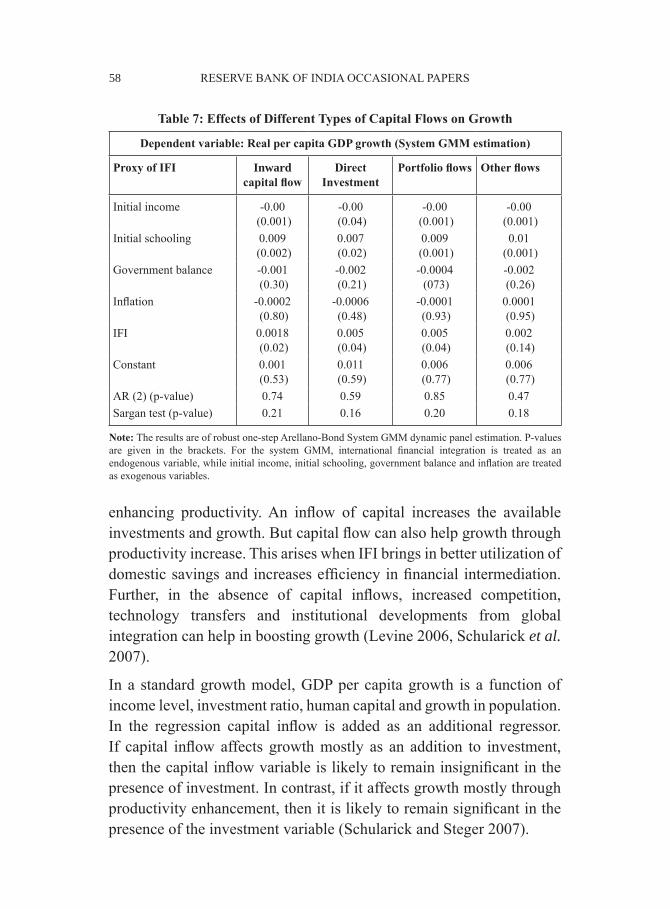
58 RESERVE BANK OF INDIA OCCASIONAL PAPERS
enhancing productivity. An inflow of capital increases the available investments and growth. But capital flow can also help growth through productivity increase. This arises when IFI brings in better utilization of domestic savings and increases efficiency in financial intermediation. Further, in the absence of capital inflows, increased competition, technology transfers and institutional developments from global integration can help in boosting growth (Levine 2006, Schularick et al. 2007).
In a standard growth model, GDP per capita growth is a function of income level, investment ratio, human capital and growth in population. In the regression capital inflow is added as an additional regressor. If capital inflow affects growth mostly as an addition to investment, then the capital inflow variable is likely to remain insignificant in the presence of investment. In contrast, if it affects growth mostly through productivity enhancement, then it is likely to remain significant in the presence of the investment variable (Schularick and Steger 2007).
Table 7: Effects of Different Types of Capital Flows on Growth
Dependent variable: Real per capita GDP growth (System GMM estimation)
Proxy of IFI Inward capital flow
Direct Investment
Portfolio flows Other flows
Initial income -0.00 (0.001)
-0.00 (0.04)
-0.00 (0.001)
-0.00 (0.001)
Initial schooling 0.009 (0.002)
0.007 (0.02)
0.009 (0.001)
0.01 (0.001)
Government balance -0.001 (0.30)
-0.002 (0.21)
-0.0004 (073)
-0.002 (0.26)
Inflation -0.0002 (0.80)
-0.0006 (0.48)
-0.0001 (0.93)
0.0001 (0.95)
IFI 0.0018 (0.02)
0.005 (0.04)
0.005 (0.04)
0.002 (0.14)
Constant 0.001 (0.53)
0.011 (0.59)
0.006 (0.77)
0.006 (0.77)
AR (2) (p-value) 0.74 0.59 0.85 0.47Sargan test (p-value) 0.21 0.16 0.20 0.18
Note: The results are of robust one-step Arellano-Bond System GMM dynamic panel estimation. P-values are given in the brackets. For the system GMM, international financial integration is treated as an endogenous variable, while initial income, initial schooling, government balance and inflation are treated as exogenous variables.

INTERNATIONAL FINANCIAL INTEGRATION, CAPITAL FLOWS 59 AND GROWTH OF ASIAN ECONOMIES
The regression shows that inward capital flows and inward portfolio flows affect growth primarily through the productivity channel (Table 8).
Even after the impact of investment is controlled, both these inflows have a significant effect. In the presence of capital flow variable, the significance of the investment declines to below the conventional significance level, which highlights some degree of collinearity between capital flow and the investment ratio.
There are some interesting findings from the estimation results. The basic neo-classical growth model appears to have worked well in this regression also. Conditional convergence is achieved as initial income has a negative sign. Both physical investment and human capital work in the desired direction, though the human capital variable is marginally above the 10 percent level of significance. The population growth variable appears with the expected negative sign.
Table 8: The Standard Neo-classical Growth Model
Dependent variable: Real per capita GDP growth (System GMM estimation)
Regression Without capital flow
Inward capital flow
Inward Direct
capital flow
Inward portfolio
flow
Inward other flow
Initial income -0.00 (0.038)
-0.00 (0.02)
-0.00 (0.17)
-0.00 (0.03)
-0.00 (0.02)
Initial schooling 0.007 (0.11)
0.007 (0.09)
0.005 (0.21)
0.004 (0.25)
0.008 (0.08)
Population growth -0.48 (0.47)
-0.43 (0.49)
-0.52 (0.42)
-0.91 (0.13)
-0.37 (0.57)
Investment 0.001 (0.07)
0.001 (0.27)
0.001 (0.21)
0.001 (0.36)
0.001 (0.16)
Capital flow - 0.002 (0.06)
0.004 (0.19)
0.006 (0.02)
0.001 (0.33)
Arellano-Bond test (P-value)
0.99 0.48 0.17 0.91 0.32
Sargan test (P-value)
0.09 0.68 0.23 0.73 0.45
Note: The results are of robust one-step Arellano-Bond System GMM estimation. For the system GMM, international financial integration is treated as an endogenous variable, while initial income, initial schooling, population growth and investment are treated as exogenous variables. P-values are given in the brackets.

60 RESERVE BANK OF INDIA OCCASIONAL PAPERS
Looking at the channels through which capital inflows affect growth, it is evident that there are signs of the productivity channel working here. It appears that total capital inflows have a productivity effect on the growth process. However, though capital flow variables are significant in growth regressions, some of them turn insignificant in the presence of the investment ratio. The significance of investment also declines in the presence of the capital flow variable, which indicates that there is some collinearity between the capital inflow and investment ratio. To delve deeper, aggregate investment is regressed on capital inflow variables. If capital inflow brings in higher investments, then there is most likely to be a significant relationship between capital inflows and investments.
To find the relationship between capital inflows and investment, investment was regressed on initial income, inflation, government balances, human capital, and then the capital flow variable was added to it. The random effect panel regression was applied, as suggested by the Hausman test. The results of the random effect panel regressions which are given in the Table 9 highlight the relationship between capital
Table 9: Determinants of Aggregate Investment
Dependent variable : Investment GDP ratio (Random Effect panel estimation)
Inward capital flow 0.86 (0.00)
Inward direct capital flow 1.93 (0.00)
Inward portfolio flow 1.84 (0.01)
Inward other flows 0.79 (0.003)
Initial income -0.0002 (0.38)
-0.0001 (0.95)
-0.0002 (0.40)
-0.0003 (0.20)
Govt balance -1.07 (0.00)
-1.39 (0.00)
-1.44 (0.00)
-1.23 (0.001)
Inflation 0.08 (0.63)
0.04 (0.80)
0.14 (0.47)
0.179 (0.345)
Initial schooling 0.20 (0.78)
-0.20 (0.78)
0.34 (0.67)
0.87 (0.26)
Constant 26.74 (0.00)
28.83 (0.00)
28.63 (0.00)
25.08 (0.00)
Note: Random-effect panel estimation. P-values are given in the brackets.

INTERNATIONAL FINANCIAL INTEGRATION, CAPITAL FLOWS 61 AND GROWTH OF ASIAN ECONOMIES
inflows and investments in Asia. All the regressions suggest capital inflow measures to be statistically significant. This seems to suggest that with greater openness, Asian economies witnessed an increase in investments.
Section VI Conclusion
This analysis of the process of international financial integration of some major economies of Asia is unique in certain respects. The investigation of a relationship between IFI and economic growth in 11 Asian countries over 1991-2000 is the first comprehensive study of its kind even though such investigations have been done in other parts of the globe. Another distinguishing feature of this study is that it uses a wide array of IFI indicators to study the effect of IFI on growth in Asia. Further, it chose different capital inflows as proxy for IFI and studied their effect on growth. It also examined channels of growth from capital inflows.
To study the relationship between IFI and economic growth, this study employed GMM estimation. The models were run while controlling for initial income, human capital and macroeconomic variables. The possible reason for the lack of a robust positive relationship may be that these countries have not crossed threshold conditions for international integration. These conditions may be linked with the absence of well-developed financial markets and better institutional and regulatory frameworks.
Even though the overall impact of IFI on growth was found to be mixed, this study threw up some useful results. It reconfirmed the general observation about the low degree of Asia’s financial integration both with the world and within the region (IMF 2011).The paper observed that Asian economies, barring Japan and Malaysia, were not as much externally open as advanced countries such as the US and the UK. However, the external financial integration of Asian economies was following a rising trend. Further, financial vulnerability indicators of the Asian economies too have improved over the years.

62 RESERVE BANK OF INDIA OCCASIONAL PAPERS
At the disaggregated level, it may be added that capital inflows had a significant positive association with the growth process. Growth in Asian economies came from both investment and productivity channels. Both direct investment and portfolio flows had positive effects on growth, though portfolio flows primarily had an effect on productivity increase also. Keeping in view the lack of research on this aspect in Asia, this study was an attempt to open up new research in this area.
To conclude, we would like to mention some recent developments which might encourage trends towards greater IFI in the region in the future. Following the great financial crisis, the exit of European banks and the entry of Australian and Japanese banks in other Asian countries is a trend which may be indicative of higher financial integration within the region. The setting of the BRICS Bank and the Asian Infrastructure Investment Bank (AIIB) also heralds an era with finance getting centred towards emerging economies in general, and Asian economies in particular. The slow growth in AEs except the US, is also forcing the Asian economies to focus within the region for exports markets. Higher trade integration might prove to be a harbinger of higher financial integration within the region. Talking specifically about India, policymakers are considering pacing up its move towards capital account convertibility as India thrives to become one of the fastest growing economies in the world.
References
Agenor, Pierre R.(2001),‘Benefits and Costs of International Financial Integration’, Paper for the Conference on Financial Globalisation: Issues and Challenges for Small States. Saint Kitts, 27-28 March.
Alfaro, Laura, Sebnem Kalemli-Ozcan and V. Volosovych (2005),‘Why does not capital flow from rich to poor countries? An empirical investigation’, Harvard Business School Working Paper No.4-40.
Arellano, Manuel and Bover Olympia (1995). ‘Another Look at the Instrumental Variable Estimation of Error-Components Models’, Journal of Econometrics 68 (1).

INTERNATIONAL FINANCIAL INTEGRATION, CAPITAL FLOWS 63 AND GROWTH OF ASIAN ECONOMIES
Bailliu, Jeannine (2000),‘Private Capital Flows, Financial Development, and Economic Growth in Developing Countries’, Bank of Canada Working Paper No.15.
Barro, Robert J. and Sala-i-Martin (1992),‘Convergence’, Journal of Political Economy 100 (21).
Bhagwati, Jagdish (1998), ‘The capital Myth-The difference between trade in Widget and Dollars’, Foreign Affairs, May/June,77.
Caprio, Gerard and Patrick Honohan (1999), ‘Restoring Banking Stability: Beyond Supervised Capital Markets’, Brookings Paper on Economic Activity 1: 143-80.
Edison, Hali J., R. Levine, L. Ricci and T. Slok (2002), ‘International Financial Integration and Economic Growth’, IMF Working Paper, No.145.
Edison, Hali J., M. Klein, L. Ricci and T. Slok (2004),‘Capital Account liberalisation and economic performance: Survey and Synthesis’, IMF Working Paper No.120.
Edwards, Sebastian (2001), ‘Capital Mobility and Economic Performance: Are emerging economies different?’, NBER Working Paper No. 8076.
Eichengreen, Barry (2001), ‘Capital Account liberalisation: What do cross country studies tell us?’, World Bank Economic Review 15(3): 341-65.
Grilli, Vittorio and Gian M. M. Ferretti (1995), ‘Economic Effects and structural determinants of Capital controls’, IMF Staff Papers 42 (3).
Henry, Peter B.(2007),‘Capital Account liberalisation: Theory, Evidence and Speculation’, Journal of Economic literature 45(4):887-935.
Khan, Harun R.(2014),‘Regulating Capital Account: Some thoughts’, 9thAnnual Conference of FEDAI, CapeTown,12 April.
Klein,M. and G. Olivei(1999),‘Capital Account Liberalisation, Financial Depth and Economic Growth’, NBER Working Paper No. 7384.
Kose,M.A., E. Prasad, K. Rogoff and S.J. Wei (2009), ‘Financial Globalisation: A Reappraisal’, IMF Staff Papers 56(1).

64 RESERVE BANK OF INDIA OCCASIONAL PAPERS
Krugman, Paul (2000), ‘Crises: The price of Globalisation?’ Paper presented at 2000 Symposium on Global Integration. Kansas City: Federal Reserve Bank of Kansas.
Levine, Ross (1996), ‘Foreign Banks, Financial Development and Economic Growth’, in Claude E. Barfield (ed.), International Financial Markets: Harmonisation versus Competition. Washington DC: American Enterprise Institute.
Levine, Ross (2001), ‘International Financial liberalisation and Economic growth’, Review of International Economics 9(4): 688-902.
Levine, Ross (2006), ‘Finance and Growth: Theory and Evidence’, NBER Working Paper No. 10766.
Obstfeld, Maurice (1994), ‘Risk-Taking, Global Diversification, and Growth’, American Economic Review 84(5): 1310-29.
Obstfeld, Maurice (2005), ‘Reflections upon Rereading “The Capital Myth”, Jagdish Bhagwati 70th birthday celebrations, Columbia University.
Obstfeld, Maurice (2009), ‘International Finance and Growth in Developing countries: What have we learned?’ NBER Working paper No. 14691.
Obstfeld, Maurice (2012), ‘Financial flows, financial crises and global imbalances’, Journal of International Money and Finance 31(3): 469-80.
Prasad, Eswar, R. Rajan and A. Subramanian (2006),‘Patterns of International Capital Flows and Their implications for economic development’, Paper presented at the symposium, ‘The Economic Geography: Effects and Policy implications’, The Federal Reserve Bank of Kansas City, Jackson Hole.
Quinn, Dennis (1997), ‘The correlates of Change in International Financial Regulation’, American Political Science Review 91(3): 531-51.

INTERNATIONAL FINANCIAL INTEGRATION, CAPITAL FLOWS 65 AND GROWTH OF ASIAN ECONOMIES
Rishabh, Kumar and S. Sharma (2014), ‘Global Liquidity, Financialisation and Commodity Price Inflation’, RBI Working Paper WPS(DEPR): 01 / 2014.
Rodrik, Dani (1998), ‘Who needs capital account convertibility’, Essays in International Finance, No.207.Princeton,NJ: Princeton University.
Rodrik, Dani and A. Subramanian (2009), ‘Why did Financial globalisation disappoint?’, IMF Staff Papers 56(1): 112–38.
Schularick, Moritz and T. M. Steger (2007), ‘Financial integration, Investment and Economic growth: Evidence from Two eras of Financial Globalisation’, CESifo Working Paper No. 1691.
Stiglitz, Joseph E. (2000), ‘Capital Market Liberalisation, Economic Growth and Instability’, World Development 28(6): 1075–86.
The Reserve Bank of India (2007), Report on Currency and Finance. Mumbai: RBI.
*****

66 RESERVE BANK OF INDIA OCCASIONAL PAPERS
Reserve Bank of India Occasional Papers
Vol. 34, No. 1 & 2: 2013
Total Factor Productivity of Indian Banking Sector - Impact of Information Technology
Sujeesh Kumar S*
Technological changes play a vital role in increasing Total Factor Productivity (TFP) of an economy. This study focuses on the TFP of Indian banking sector and the impact of information technology on productivity. TFP is worked out for the Indian banking sector covering public, private and foreign banks operating in India using a non–parametric Data Envelopment Analysis (DEA). An attempt is also made to find out the impact of information technology on the productivity of the Indian banking sector using a multiple regression model. The results of the study show that the Indian banking industry experienced a growth in productivity as judged by Malmquist Productivity Index during 2008-10. The succeeding years showed a diminished growth of productivity. Further, the multiple regression model suggests that increased electronic transactions in the banking channel have resulted in increase in productivity. Additionally, the intermediation cost which is a proxy for technology investment is also significant for the productivity of the banking sector.
JEL Classification : G21,C14,C25,C67.
Key words : Data Envelopment Analysis, Malmquist Productivity Index, Total Factor Productivity, Multiple Regression
Introduction
Since the banking sector reforms, the Indian banking sector has been evolving with increased emphasis on competition and enthused technology-based services towards universal banking. Banks have implemented core banking solutions, enterprise risk management and business process re-engineering and reached social banking which has enrooted the performance, productivity and efficiency of the Indian banking sector. Banking sector reforms in India were initiated in 1992 with one of the major objectives being the strengthening of Indian
* Sujeesh Kumar. S is Manager in the Department of Information Technology, the Reserve Bank of India, Mumbai. The views expressed are the author’s own and not of the Reserve Bank of India. The author is thankful to Shri A.S. Meena and Dr. Anil Kumar Sharma, General Managers, Department of Information Technology, Reserve Bank of India, Mumbai for their valuable support and suggestions that were extended to the author for the completion of this work. The author is also grateful to an anonymous referee for insightful comments.

TOTAL FACTOR PRODUCTIVITY OF INDIAN BANKING 67 SECTOR - IMPACT OF INFORMATION TECHNOLOGY
banks by improving their productivity, efficiency and profitability. The advancement of information technology (IT) in the Indian banking sector and other financial intermediaries resulted in growth and development of banks’ productivity and efficiency. There has been noticeable improvement in the performance of financial institutions and the service sector by incorporating IT into their functionality. These show an increasing share and enhanced competitiveness at the global level because of adopting the IT culture (Leeladhar 2006). Higher productivity led to a decrease in credit risk and a positive influence on bank capitalization, whereas poor performers were more prone to risk taking than better performing organizations (Das and Ghosh 2004). IT improvements are useful for reducing costs and improving the efficiency of banks. Technological efficiency can result in lower transaction costs and increased revenues for banks (Rishi and Saxena 2004). Finance growth literature suggests that if banks become better functioning entities, this will expectedly be reflected in safety and soundness of the financial system and will ultimately lead to an increase in the rate of economic growth. The efficiency and productivity analysis of the banking sector is also useful to enable policymakers to identify the success or failure of policy initiatives or, alternatively, highlight different strategies undertaken by banking firms which contribute to their successes (Mohan 2005).1 It is evident from the fact that the intermediation cost of the Indian banking sector has been drastically reduced from year 1990 to 2012 which is an indication of reduction of operating expenses. The operational cost for technology and technology based services is one of the component of operating expenses. Banks’ h igh value transactions are routed through Real Time Gross Settlement Systems (RTGS) which is a proven efficient payment and settlement mechanism provided by the Reserve Bank of India and has led to a paradigm shift due to IT initiatives in the banking sector. The gross value of electronic payments cleared and settled in the country is presently almost 7.5 times larger than India’s annual GDP.2
1 Author’s calculations using data from statistical tables relating to banks in India of the Reserve Bank of India’s publication (various years).2 Author’s calculations using the Reserve Bank of India’s monthly bulletin.

68 RESERVE BANK OF INDIA OCCASIONAL PAPERS
The banks need to implement robust information systems and IT architecture and should harness the power of IT systems for business development. Besides, a strong IT system will also aid in the adoption of better risk management practices (Chakraborty 2013).
The objective of this paper is 2-fold. First, the study estimates TFP for the Indian banking sector covering public, private and foreign banks operating in India using non-parametric the Malmquist Productivity Index approach employing t h e Data Envelopment Analysis (DEA). Second, it estimates the impact of information technology on the productivity of the Indian banking sector by using a multiple regression model. The rest of the paper is organized as follows. Section II deals with the review of related literature. Section III depicts the methodology employed. Section IV is about data, variables and analysis. Section V provides a conclusion to the study.
Section II Review of literature
There are few studies related to the impact of IT on the banking industry. However, research contributions available in this area are reviewed in this section. A literature review is arranged chronologically in both the foreign as well as Indian context.
Berg et al. (1992) studied the change in productivity in the Norwegian banking industry for 1980-89. Their study concluded that productivity declined on average before deregulation and it showed an increasing trend after deregulation in 1984-85. Grifell et al. (1997) analysed the various causes of productivity change in the Spanish banking industry for 1986-93 by using the Malmquist Productivity Index. They found that commercial banks had a lower rate of productivity growth as compared to saving banks but these banks had a higher rate of potential productivity growth. Das and Ghosh (2006) examined the inter-relationship among risk, capital and productivity changes in public sector banks in India from 1995-96 through 2000-2001. He concluded that higher productivity led to a decrease in credit risk and a positive influence on bank capitalization. Poor performers were more prone to

TOTAL FACTOR PRODUCTIVITY OF INDIAN BANKING 69 SECTOR - IMPACT OF INFORMATION TECHNOLOGY
risk taking than better performing organizations. The study supported the fact that productivity, capital and risk taking tend to be determined jointly and that these compensated each other.
Janki (2002) analysed the effect of technology on the productivity of employees for 1986-91 by employing the DEA methodology. He found that public sector banks had the highest efficiency followed by foreign banks. Private banks were found to be the least efficient. The author also found a temporal improvement in the performance of foreign banks. Ram Mohan and Ray (2004) attempted a comparison between public sector banks and their private sector counterparts based on measures of productivity during 1992-2000. They used Tornqvist and Malmquist Total Factor Productivity growth for comparison.3 They found that there was no significant difference in productivity growth between the public and private sectors in the period under study. Bhandari (2010) studied Total Factor Productivity improvement achieved by 68 Indian commercial banks from 1998-99 to 2006-07. He decomposed the TFP into technical change, technical efficiency change and scale (efficiency) change. The results suggest that public sector banks were, on an average, adjusting themselves to the changing environment better and improving their performance relative to their counterparts under private and foreign ownership.
Beccalli (2007) investigated the effect of investment in information technology on the performance of European banks for 1995-2000 by using both the profit efficiency measure and standard accounting ratios. He argued that traditional accounting ratios may not reflect organizational capabilities, improved product variety, quality and customer satisfaction due to enhancement of information technology. Due to this reason, an advanced measure of productivity at the global level called x-efficiency
3 The Tornqvist TFP Index is similar to the Malmquist Productivity Index. It is the ratio of two Tornqvist output and input quantity indices. The Tornquist Productivity Index can be measured without any knowledge of the underlying technology so long as data are available for the input and output quantities as well as the shares of the individual inputs and outputs in the total cost. The advantages of the Malmquist Index over other indices has been mentioned in Section III of this paper.

70 RESERVE BANK OF INDIA OCCASIONAL PAPERS
was used. He found that the relationship between total IT investment and improved bank profitability or efficiency indicated the existence of a profitability paradox. The impact of IT investment on hardware and software seems to reduce banks’ profit performance whereas IT services from external providers have a positive influence on accounting profit and profit efficiency.
Koutsomanoli et al. (2009) studied bank efficiency and productivity change across Central and Eastern European (CEE) countries and across banks with different ownership status for 1998–2003 using the 4directional technology distance function. Their results demonstrate strong links of competition and concentration with bank efficiency. Productivity for the whole region initially declined but improved more recently with further progress on institutional and structural reforms. Overall, productivity change in CEE was driven by technological change rather than efficiency change. Mittal and Dhingra (2007) assessed the impact of computerization on productivity and profitability of Indian banks employing DEA. Private sector banks, which took more IT initiative, were found to be more efficient in productivity and profitability parameters than public sector banks. Out of the many factors analysed, increased IT investments was one of the vital contributing factors for enhanced performance. (Rajput et al. 2011) studied the impact of IT on the Indian commercial banking industry based on the DEA technique. The results conveyed that all scheduled commercial banks showed a significant and improving trend in their performance due to the adoption of IT. There was an increasing trend in the performance of Indian banks because of IT innovations and enlarged investment in new information technologies during the recent time period 2005-10 as judged by a stochastic frontier analysis (Kumar et al. 2011). On both cost and profitability based parameters, productivity and efficiency of Indian banks has seen a definite improvement over
4 The directional technology distance function proposed by Chambers et al. (1996) completely characterizes technology and allow firms to optimize by seeking simultaneously the maximum expansion of outputs and contraction of inputs that are technologically feasible. If the bank is technically efficient the value of the directional diction function would be zero. A positive value indicates inefficient production. For more details, see Chambers et al. (1996).

TOTAL FACTOR PRODUCTIVITY OF INDIAN BANKING 71 SECTOR - IMPACT OF INFORMATION TECHNOLOGY
the last two decades. Further at a bank group level, public sector banks performed better than new private banks and foreign banks on various benchmarks (Chakraborty 2013).
Section III Methodology
Productivity is generally defined in terms of the input and output produced by a firm. In a simple sense, it is defined as the ratio of input and output. The larger values of this ratio are associated with better performance of a firm. Productivity is also defined in terms of efficiency improvement and technical changes with which inputs are transformed into outputs in the production process. When multiple inputs and outputs are involved, productivity measure is the simple ratios of the output and input quantities called Total factor productivity (TFP) or Multi Factor productivity (MFP). It is an overall indicator of productivity of a firm in which how optimally uses all of its resources to create its yield.
Furthermore, TFP is a broader measure of economic and technical efficiency reflecting several other factors including managerial efficiency, economies of scale and human capital utilization; TFP can be split into two major components -- technological progress and improvement in technical efficiency. Technological progress is often directly related to TFP, especially in banking. A characteristic of the banking sector is its predominance of new technology which may be attributed to the introduction of latest technology, technology based service mechanisms, management, etc., which leads to the expansion of the best production frontier and thereby results in higher output with the given input of resources. A reader may refer to Coelli et al. (2005) for more details about productivity, efficiency and its measurements. Malmquist indexes can be estimated either by using an input-oriented approach or an output-oriented approach.
Conceptually input orientation means how much input quantities can be proportionally reduced without changing the output quantity produced. Output orientation means how much output quantities can be proportionally expanded without altering the input quantities used.

72 RESERVE BANK OF INDIA OCCASIONAL PAPERS
The two measures provide the same value under the Constant Return Scale (CRS) but are different when the Variable Return Scale (VRS) is assumed (for more details on CRS and VRS reader may refer to Coelli et al. 2005).
Even though both the input and output based Malmquist TFP indexes are widely used, by following and Isik and Hassan (2003), Jaffry et al. (2007) and Isik (2008), among others, the output oriented Malmquist Productivity Change Index is adopted for this study. Jaffry et al. (2007) pointed out that output orientation is more appropriate given the objectives of a developing country’s banking industry. The non- parametric DEA based Malmquist Productivity Index can be estimated by exploiting the relationship of 5distance functions to technical efficiency measures. This technique is an index of productivity change. Therefore, it does not require cost or revenue shares to aggregate inputs and outputs and was introduced to literature by Caves et al. (1982). In order to calculate the Malmquist Output Oriented TFP Change Index the first step is to define distance functions with respect to two different time periods.
A convenient way to describe a multi-input, multi-output production technology is to use the technology set, S. Following Fare and Primont (1995), the notations X and q are used to denote an N x l input vector of non-negative real numbers and a non-negative M x l output vector, respectively. The technology set is defined as
S = {(X, q): X can produce q} (1)
This set consists of all input-output vectors (X, q) such that X can produce q.
Production technology defined by the set S, may be equivalently defined by the output set P(x) which represents the set of all output vector q, that can be produced by input vector X. The output set is defined by:
5 Distance functions are useful in describing technology in a way that makes it possible to measure efficiency and productivity. The concept of a distance function is closely related to production frontiers. The basic idea underlying distance functions is quite simple, involving radial contractions and expansions in defining these functions. The notion of a distance function was introduced independently by Malmquist (1953) and it has gained prominence only in the last three to four decades.

TOTAL FACTOR PRODUCTIVITY OF INDIAN BANKING 73 SECTOR - IMPACT OF INFORMATION TECHNOLOGY
(2)
The output distance function is defined on the output set, , as:
(3)
where δ is the ratio of two points in the production set. The Malmquist TFP Index in Fare et al. (1994) measures the TFP change between two data points by calculating the ratio of the distances of each data point relative to a common technology. Due to this, no longer do we have a situation where the ratio of the distance functions provides a measure of TFP change that is identical to technical change (that is, frontier shift). Thus, when panel data are available, one can obtain a measure of TFP change that has two components -- a technical change component and a technical efficiency change component.
Fare et al. (1994) take the Malmquist Index of TFP growth, defined in Caves et al. (1982), and describe how one can decompose the Malmquist TFP change measures into various components,including technical change and efficiency change.
The Malmquist (output-orientated) TFP Change Index between period s (the base period) and period t is can be written as:
(4)
Alternatively, if in the period s reference technology is used, it is defined as:
(5)
In these equations the notation represents the distance from the period t observation to the period s technology. A value of greater than one indicates positive TFP growth from period s to period t while a value less than one indicates a TFP decline. The Malmquist TFP Index is often defined as the geometric mean of these two indices in the spirit of Caves et al. (1982). That is:
(6)

74 RESERVE BANK OF INDIA OCCASIONAL PAPERS
The distance functions in this productivity index can be rearranged to show that it is equivalent to the product of a technical efficiency change index and an index of technical change:
(7)
The ratio outside the square brackets in equation 7 measures the change in the output-oriented measure of Farrell technical efficiency between periods s and t. The remaining part of the index in equation 7 is a measure of technical change.It is the geometric mean of the shift in technology between the two periods, evaluated xt and also at xs Thus the two terms in equation 7 are:Efficiency Change (EC)
(8)
Technical Change (TC)
(9)
Technical efficiency change can be decomposed into scale efficiency and ‘pure’ technical efficiency components when the distance functions in the equations given earlier are estimated relative to a Constant Return Scale (CRS) technology.This decomposition involving scale efficiency has been widely used in the literature.A number of additional possible decompositions of these technical efficiency changes and technical change components have been proposed by various authors. Some of these options are discussed in Fare et al.’s (1998) survey paper. The decomposition proposed by Fare et al. (1994) is given by:
Pure efficiency change:
(10)

TOTAL FACTOR PRODUCTIVITY OF INDIAN BANKING 75 SECTOR - IMPACT OF INFORMATION TECHNOLOGY
and a scale efficiency change component. Scale efficiency change:
(11)
The scale efficiency change component in equation 11 is the geometric mean of two scale efficiency change measures. The first is relative to the period t technology and the second is relative to the period s technology. The extra subscripts, v and c, relate to the VRS and CRS technologies respectively.
There are two major approaches for measuring the distance functions that make up the Malmquist TFP Index. One is non- parametric DEA-like linear programming methods suggested by Fare et al. (1994), and the other approach is the use of stochastic frontier methods. Following Fare et al. (1994), one can calculate the distance measures in equation 6 using DEA-like linear programmes. For the ith firm, we must calculate four distance functions to measure the TFP change between two periods. This requires the solving of four linear programming (LP) problems. As noted earlier, Fare et al. (1994) use a Constant Returns to Scale (CRS) technology in their TFP calculations. This ensures that resulting TFP change measures satisfy the fundamental property that if all inputs are multiplied by the (positive) scalar δ and all outputs are multiplied by the (non-negative) scalar α, then the resulting TFP Change Index will equal α/δ .6The required LPs are:
(12)
subject to
6 The DEA based liner programme (LP) problems mentioned in equations 12–15 were solved using software DEAP02.1.LPs are calculated for each bank in the sample. All indices (EC, TC,PEC,SEC and TFP) are relative to previous years. Hence, the output begins with the second year only, that is, indices are calculated for 2005-12.In order to maintain uniformity data for multiple regressions is also considered for 2005-12.

76 RESERVE BANK OF INDIA OCCASIONAL PAPERS
(13)
subject to
(14)
subject to
(15)
subject to
Section IV Data, Variables and Analysis
The DEA based Malmquist TFP Index requires bank inputs and outputs whose choice is always an arbitrary issue (Berger and Humphrey 1997). They point out that the production approach might be more suitable for branch efficiency studies, as most of the times bank branches basically process customer documents and bank funding, while investment decisions are by and large, not under the control of branches. This study follows the asset approach proposed by Sealey and Lindley (1977) which views the institution as using labour, capital and deposits to produce earning assets. This approach is the most common in conventional literature. Moreover, banking literature has found that different approaches to measuring output have generally led to similar conclusions concerning the cost structures of financial firms (Mester 1993).
This paper uses annual account data of banks operating in India during 2004-12. The source of data is the balance sheets, profit and loss accounts generated from the Reserve Banks data warehouse, Database on Indian

TOTAL FACTOR PRODUCTIVITY OF INDIAN BANKING 77 SECTOR - IMPACT OF INFORMATION TECHNOLOGY
Economy.7 A total of 58 banks including public sector banks, private sector banks and foreign banks operating in India were considered for the study. The banks with incomplete data were omitted. The data were cleaned and missed values estimated by averaging nearby points.
The data were deflated with the Wholesale Price Index during the period. The final data set is a balanced panel of 522 observations on outputs and inputs. This study used two output variables and three input variables. The output variables are: investments (y1) represent total investments including investments in non-SLR securities and net interest income (y2) is the total interest earned less total interest paid. The input variables are deposits (x1) which includes demand and time deposits, borrowings (x2) comprise of inter-bank borrowings and inter-bank deposits at call or short notice not exceeding 14 days, and fixed assets (x3) comprise of balances with the ‘banking system’ in current account, balances with other banks in other accounts, money at call and short notice, advances to banks and other assets which cannot be classified under any of the four items.
The software package DEAP V2.1 was used to perform DEA and estimations. The descriptive statistics of the input and output variables were measured in lakhs which are used to construct TFP indices for 2004-12 (Table 1).
It is interesting as well as useful to investigate the impact of information technology on the productivity of the Indian banking sector. For this, a multiple regression model was employed. The selection of IT variable is a challenging issue because of the lack of suitable published data. Most of the banking technology and related research is based on qualitative data or perceptions of technology experts. With these limitations, the available data was collected from various publications of the Reserve Bank of India.
7 All 26 public sector banks including the State Bank of India and its associates are considered. In case of private sector banks, some banks are not included as data is not available for the period 2004-12. Due to this, 16 private banks were considered. A good amount of banks have not been included in the case of foreign banks as most of the banks do not have information on all the variables considered for the study. Further many banks were established in India recently and therefore 16 foreign banks were considered for the study.

78 RESERVE BANK OF INDIA OCCASIONAL PAPERS
The variables considered were total volume and value of paper transactions and electronic transactions turned out in the country during 2005-12.6 The ratio of cheque transaction volume and electronic transaction volume is one of the independent variable considered, that is, CHVOL/ECVOL, ECVOL which includes high value transactions mainly through the Real Time Gross Settlement Systems (RTGS), retail transactions represented by the National Electronic Fund Transfer (NEFT) and card transactions (credit and debit cards). The second explanatory variable considered is the ratio of cheque transaction value (CHVAL) to non-agricultural GDP. Improvements in the efficiency of the banking system are expected to be reflected in the indicator like operating expenditure. Several indicators have been employed in literature to compare banking production costs across time. Illustratively, intermediation costs, defined as the ratio of operating expense to total assets, needs to be weighed against the large expenditures incurred in upgradation of information technology and institution of ‘core banking solutions’ (Mohan 2005). Following this, the third explanatory variable considered is intermediation cost (INTCOST) as a proxy of investment for technology systems and its maintenance. The dependent variable considered is the ratio of input and output as a productivity measure (PDY) during 2005-12.
Table 2 summarizes the decomposition of Total Factor Productivity (TFP) of the overall banking sector for 2005-12. It is obvious from Table 2 that the period 2008 to 2010 experienced positive productivity growth. It is also evidenced that the technological progress which
Descriptive Statistics of the Input-Output Variables
(` lakh)
Descriptive Statistics
InvestmentsY1
Net Interest income
Y2
Depositsx1
Borrowingsx2
Fixed Assets x2
Min 101.92 19.76 469.43 6.43 3.09Maximum S.D. 15556267.56 1160509.94 30912136.42 3946767.17 335240.50Mean 602842.75 50164.15 1467904.26 131981.95 17201.76SD 1378296.83 109715.88 3069072.95 420390.93 37139.13

TOTAL FACTOR PRODUCTIVITY OF INDIAN BANKING 79 SECTOR - IMPACT OF INFORMATION TECHNOLOGY
happened in 2008, 2009 and 2010 resulted in an increase of TFP in the respective years. Specifically, 2010 witnessed 35 per cent annual productivity growth due to a major contribution of the technological change component. During 2009-10, most of the banks implemented Core Banking Solutions and other technology based services which ultimately contributed to TFP. The average annual productivity growth rate in 2008-10 was 11 per cent which was mainly due to the result of a 28 per cent technological progress during the period. The succeeding years showed a diminished growth of productivity. This may be partly due to factors such as lack of upgradation of IT systems to cope with service requirements, a changing regulatory environment, demand for novel customer services through social network and mobile banking. All these factors need to be analysed deeply which is not attempted in this paper. Further, it is suggested that technology reforms in the banking sector may be made so as to keep it in tandem with the innovations happening in the rest of the world.
Table 3 depicts bank group-wise (public sector, private sector and foreign) TFP growth and its components which are averaged for the period 2008-10 and 2005-12. Private sector and foreign banks showed an average productivity growth of 4.5 per cent and 9.6 per cent respectively
Table 2: Decomposition of TFP in the Indian Banking Sector for 2005-12
Indices
All Banks Efficiency change(EC)
Technological change(TC)
Pure technical efficiency change (PTEC)
Scale efficiency change (SEC)
Total factor Productivity
( TFP)
2005 1.0490 0.9520 0.9950 1.0540 0.99902006 1.0230 0.9360 1.0120 1.0110 0.95802007 1.0710 0.7830 1.0250 1.0460 0.83902008 0.9650 1.0460 0.9720 0.9930 1.01002009 0.9470 1.0570 0.9920 0.9550 1.00102010 0.7120 1.9040 0.9190 0.7750 1.35502011 1.2230 0.7560 1.0260 1.1930 0.92502012 1.0140 0.6830 1.0500 0.9660 0.6930Average for the period 2008-10 0.8665 1.2816 0.9605 0.9024 1.1106Average for the period 2005-12 0.9906 0.9660 0.9981 0.9928 0.9573
Note: All indices are geometric average.

80 RESERVE BANK OF INDIA OCCASIONAL PAPERS
Indices
Efficiency change(EC)
Technological change(TC)
Pure technical efficiency change (PTEC)
Scale efficiency change (SEC)
Total factor Productivity
( TFP)
Public sector Banks
2005 1.0013 0.9618 1.0028 0.9985 0.96312006 1.0238 0.9132 1.0007 1.0230 0.93512007 1.0061 0.7539 1.0142 0.9920 0.75882008 0.9326 0.9911 0.9420 0.9900 0.92432009 0.8941 1.0102 0.9488 0.9422 0.90312010 0.6750 1.6252 1.0349 0.6523 1.09702011 1.3167 0.6976 0.9683 1.3597 0.91852012 1.0370 0.9403 0.9650 1.0748 0.9749Average for the period 2008-10 0.8256 1.1762 0.9744 0.8474 0.9711Average for the period 2005-12 0.9714 0.9575 0.9841 0.9871 0.9302
Private sector Banks
2005 1.0459 1.0250 0.9839 1.0629 1.07202006 1.1091 0.9529 1.0695 1.0371 1.05692007 1.1747 0.6860 1.0674 1.1005 0.80582008 0.9604 1.1563 0.9564 1.0042 1.11052009 0.9602 0.9962 1.0257 0.9361 0.95642010 0.7121 1.5093 0.9181 0.7756 1.07462011 1.2451 0.7650 1.0252 1.2144 0.95242012 0.9692 0.7018 1.0208 0.9495 0.6801Average for the period 2008-10 0.8692 1.2025 0.9657 0.9000 1.0450Average for the period 2005-12 1.0097 0.9430 1.0072 1.0025 0.9521
Foreign Banks
2005 1.1353 0.8694 0.9951 1.1409 0.98702006 0.9428 0.9586 0.9759 0.9658 0.90372007 1.0822 0.9492 1.0003 1.0819 1.02712008 1.0263 1.0335 1.0405 0.9863 1.06072009 1.0240 1.0786 1.0314 0.9929 1.10442010 0.8199 1.3727 0.8243 0.9947 1.12562011 1.0755 0.8476 1.1055 0.9729 0.91152012 0.9972 0.3913 1.1816 0.8441 0.3906Average for the period 2008-10 0.9516 1.1523 0.9599 0.9913 1.0966Average for the period 2005-12 1.0086 0.8922 1.0146 0.9941 0.8999
Table 3: Decomposition of TFP in the Indian Banking Sector for 2005-12: bank category-wise (Contd.)

TOTAL FACTOR PRODUCTIVITY OF INDIAN BANKING 81 SECTOR - IMPACT OF INFORMATION TECHNOLOGY
during 2008-10. However, public sector banks were near to the frontier and the technological change component was very prominent.
The year 2010 showed an annual productivity growth of 9.7, 7.4 and 12 per cent respectively by public, private and foreign banks. This was reflected in the overall baking productivity as explained in Table 2. The three categories of banks showed a downward trend in TFP growth from 2011 and the same diminishing tendencies were observed in the technological progress component index. Both public sector and private sector banks were almost persistent in their scale of operations which was in contrast with foreign banks. This may be partly due to the fact that both public and private sector banks having been in existence for a long time in India and being known to their customers could have helped their inputs usage and in getting closer to the frontier.
The regression model was employed here only to know the impact of technology on growth of productivity keeping in view the technological improvements that happened in the Indian banking sector during
2005-12. This model is not used for any forecasting purposes; however, an attempt has been made to know the impact of some of the technology related variables and how they can explain banking productivity and its growth. It also assumes that all banks come from a similar regulatory environment. The problem of multi-collinearity has been addressed. In detail, the following multiple regression equation model is estimated:
(15)
where t is the time period, and is error term independently and identically distributed with N(0,σ2). Following De bandt and Davis (2000) and Staikouras et al. (2008) among others the log linear form is chosen as it typically improves the goodness fit of the model and may reduce a simultaneity bias.
The model parameters were estimated using the software package SPSS16.0.The regression coefficients that were estimated are presented in Table 4.

82 RESERVE BANK OF INDIA OCCASIONAL PAPERS
Table 4: Effect of Technology on Productivity Growth: Empirical Results
Unstandardized Coefficients
Std. Error Standardized Coefficients
t-value Sig*.
Constant 1.732 0.149 11.640 0.000ECVOL /CHVOL 0.096 0.027 0.997 3.549 0.024CHVAL/GDP 0.385 0.120 1.472 3.206 0.033INTCOST -1.688 0.370 -1.465 -4.567 0.010
* 5% level of singnificance,R2 = 0.933, adjusted R2 =0.883. Dependent variable is the ratio of input and output as a productivity measure (PDY) during 2005-12.
The coefficient of the ratio of electronic transactions to paper transactions (ECVOL /CHVOL) exhibit a statistically significant (5 per cent level) relationship with productivity growth, meaning that increased electronic transactions in the banking channel resulted in an increase in growth of productivity. The second variable is the ratio of total cheque value settled in the country to non-agricultural GDP (CHVAL/GDP) which shows a significant (5 per cent) positive relationship with productivity meaning the contribution of GDP to the nation. In the present scenario, paper settlements in the country were less than electronic settlements. As mentioned in the previous variable, the reduction in paper transactions will certainly increase productivity, these variables are more or less similar to the first variable which substantiate the model’s fitness. The intermediation cost as the ratio of operating expense to total assets was also significant at the 5 per cent level. A reduction in intermediation is the direct positive impact of efficiency and productivity which is consistent with earlier empirical evidence on banking efficiency and productivity (Mohan 2005, Chakraborty 2013).
Section V Conclusion
This study analysed TFP of the Indian banking sector during 2005-12; 58 banks including public sector banks, private sector banks and foreign banks operating in India were considered for this study. A non-parametric Data Envelopment Analysis (DEA) based Malmquist Productivity Index was worked out bank group-wise for the Indian banking sector. Impact of information technology on the productivity the of Indian

TOTAL FACTOR PRODUCTIVITY OF INDIAN BANKING 83 SECTOR - IMPACT OF INFORMATION TECHNOLOGY
banking sector was also investigated by employing a multiple regression model. The results of the study show that the Indian banking industry was productive as judged by the Malmquist Productivity Index during 2008 to 2010 compared with the preceding and succeeding years in the time band 2005-12. The average annual productivity growth rate in 2008-10 was 11 per cent which was mainly due to the result of a 28 per cent technological progress during the period. Further, it is observed that increased electronic transactions in the banking channel resulted in increase in productivity. Additionally, the intermediation cost which is a proxy of technology investment was also significant for the productivity of the banking sector.
References
Beccalli, Elena (2007), ‘Does IT investment improve bank performance? Evidence from Europe’, Journal of Banking & Finance 31(7): 2205-30.
Berg, S.A., F.R. Forsund and E.S. Jansen (1992), ‘Malmquist Indices of
Productivity Growth During the Deregulation of Norwegian Banking
1980-1989’, Scandinavian Journal of Economics 94: 211- 28.
Berger, A. N. and D. B. Humphrey (1997), ‘Efficiency of financial institutions: International survey and directions for future research’, European Journal of Operational Research 98(2): 175–212.
Bhandari, A.K. (2010), ‘Total factor productivity growth and its decomposition: An assessment of the Indian banking sector in the true Liberalized era’, CDS Working Paper No. 435. Thiruvananthapuram: Centre for Development Studies.
Caves, D.W., L.R. Christensen and W.E. Diewert (1982), ‘The Economic Theory of Index Numbers and the Measurement of Input, Output and Productivity’, Econometrica 50(6): 1393-414.
Chakraborty, K.C. (2013), ‘Productivity Trends in Indian Banking in the Post Reform Period - Experience, Issues and Future Challenges’, Special address at FIBAC 2013 organized by FICCI and IBA in Mumbai.

84 RESERVE BANK OF INDIA OCCASIONAL PAPERS
Chambers, R.G., Y.H. Chung and R. Färe (1996), ‘Benefit and distance functions’, Journal of Economic Theory 70(2): 407–19.
Coelli.T.J, D.S.P. Rao, C.J. O’Donnell and G.E. Battese (2005), An Introduction to Efficiency and Productivity Analysis. Second edition, Springer.
Das, A. and S. Ghosh (2004), ‘Risk, capital and operating efficiency: Evidence from Indian public sector banks’, Indian Journal of Economics and Business 3(1): 147-64.
Das, A. and S. Ghosh (2006), ‘Size, Non-performing Loan, Capital and Productivity Change: Evidence from Indian State-owned Banks’, University library of Munich, MPRA Paper No. 17396.
De bandt, O. and P. Davis (2000), ‘Competition, contestability and market structure in European banking sectors on the eve of EMU’, Journal of Banking and Finance 24(6): 1045–66.
Fare, R., S. Grosskopf, and C.A.K. Lovell (1994), Production Frontiers. Cambridge: Cambridge University Press
Fare, R. and D. Primont (1995), Multi-Output Production and Duality: Theory and Application. Boston: Kluwer Academic Publishers.
Fare, R., S. Grosskopf and P.Roos (1998), Malmquist Productivity Indexes: A Survey of Theory and Practice, In Index Numbers: Essays in Honour of Sten Malmquist. Boston: Kluwer Academic Publishers.
Grifell-Tatje, E. and C.A.K. Lovell. (1997), ‘The Sources of Productivity Change in Spanish Banking’, European Journal of Operational Research 98(2): 364-80.
Isik, I. (2008), ‘Productivity, technology and efficiency of de novo banks: A counter evidence from Turkey’, Journal of Multinational Financial Management 18(5): 427–42.
Isik, I. and M. K. Hassan (2003), ‘Efficiency, ownership and market structure, corporate control and governance in the Turkish banking industry’, Journal of Business, Finance and Accounting, 30(9–10): 1363–421.

TOTAL FACTOR PRODUCTIVITY OF INDIAN BANKING 85 SECTOR - IMPACT OF INFORMATION TECHNOLOGY
Jaffry, S., Y. Ghulam, S. Pascoe and J. Cox (2007), ‘Regulatory changes and productivity of the banking sector in the Indian sub-continent’, Journal of Asian Economics 18(3): 415–38.
Janki, B. (2002), ‘Unleashing employ productivity; A need for a paradigm shift’, Indian Bank’s Association Bulletin 24(3): 7-9.
Koutsomanoli-Filippaki, A., D. Margaritis and C. Staikouras (2009), ‘Efficiency and productivity growth in the banking industry of Central and Eastern Europe’, Journal of Banking and Finance 33 (3): 557–67.
Kumar, S., V. Maurya and V. Kumar (2011), ‘Comparing the Technical Efficiency of Indian Banks Operating Abroad and Foreign Banks Operating in India: A Stochastic Output Distance Function Approach’, Reserve Bank of India Occasional Papers 32(1): 1-23.
Leeladhar. V. (2006), ‘Recent banking developments in India’, BIS Paper No.28 (Part 14). Bank for International Settlements.
Malmquist, S. (1953), ‘Index Numbers and Indifference Surfaces’, Trabajos de Estatistica 4(2): 209-42.
Mester, L.J. (1993), ‘Efficiency in the savings and loans industry’, Journal of Banking and Finance 17(2-3): 267-86.
Mittal, R.K and Sanjay Dhingra (2007), ‘Assessing the impact of computerization on productivity and profitability of Indian banks- An application of data envelopment analysis’, Delhi Business Review 8(1): 63-73.
Mohan. R. (2005), ‘Reforms, productivity and efficiency in banking: the Indian experience’, 21st Annual General Meeting and Conference of the Pakistan Society of Development Economists, Islamabad.
Rajput, Namita and Monika Gupta (2011), ‘Impact of IT on Indian Commercial Banking Industry: DEA Analysis’, Global Journal of Enterprise Information Systems 3(1).
Ram Mohan, T.T and Subhash Ray ( 2004), ‘Productivity Growth and Efficiency in Indian Banking: A Comparison of Public, Private, and Foreign Banks’, Department of Economics Working Paper No. 2004-27. University of Connecticut.

86 RESERVE BANK OF INDIA OCCASIONAL PAPERS
Rishi, M. and S. Saxena (2004), ‘Technological Innovations in the Indian banking industry: the late bloomer’, Accounting, Business & Financial History 14(3): 339–53.
Sealey, C. and J. T. Lindley (1977), ‘Inputs, outputs and a theory of production and cost at depository financial institutions’, Journal of Finance 32(4): 1251–266.
Staikouras, C., E. Mamatzakis, and A. Koutsomanoli-Filippaki (2008), ‘An empirical investigation of operating performance in the new European banking landscape’, Global Finance Journal 19(1): 32–45.
Tomqvist, L. (1936), ‘The Bank of Finland’s Consumption Price Index’, Bank of Finland Monthly Bulletin 10: 1-8.

DETERMINANTS OF CORPORATE INVESTMENTS IN INDIA: 87 AN EMPIRICAL ANALYSIS ON FIRM HETEROGENEITY
Reserve Bank of India Occasional Papers
Vol. 34, No. 1 & 2: 2013
Determinants of Corporate Investments in India: An Empirical Analysis on Firm Heterogeneity
M. Sreeramulu, A. Ramanathan and Krishnan Narayanan*
The paper investigates whether heterogeneity exists across size-classes and industry groups as far as the impact of financial variables (internal funds, bank credit, equity capital) on investment spending is concerned. For empirical analysis, we use the Reserve Bank of India’s (RBI) database on company finance statistics over the period 1999-2000 to 2010-11. Our results confirm heterogeneity across size-classes and industry groups. Accordingly, large firms and industry groups – textiles and metals relatively depend more on bank credit for financing their investments. Industry groups which are involved in producing luxury goods are less dependent on internal funds. On the other hand, large firms’ investment decisions are highly motivated by internal funds. Further, equity capital turns out to be insignificant for small firms; this confirms the information problems faced by these firms in raising funds from capital markets.
JEL Classification : E22, G21Keywords : Investment, Accelerator, Bank Credit, Internal Funds
Introduction
Access to financial resources for investments in fixed assets may not be uniform for all firms and are likely to change across firms. Heterogeneity in accessing such financial resources arises in part because of asymmetric information problems in the capital markets (Athey and Reeser 2000). These problems make external funds costly, if not impossible, for certain firms (such as small firms) to obtain their desired quantity of investment funds. Limited access to capital markets in turn increases the customary preference for using internal funds to finance investment expenditures (Oliner and Rudebusch 1992). In the Indian context because of Government directed credit policies to a certain extent small
* M. Sreeramulu is AGM in the Department of Non-Banking Supervision, the Reserve Bank of India. Currently he is pursuing his Ph.D from IIT Bombay. Professor A. Ramanathan is Emeritus Fellow & Former Professor of Economics, IIT Bombay and Professor Krishnan Narayanan is Professor of Economics, IIT Bombay. The views expressed in the paper are those of the authors and do not necessarily reflect the views of the Reserve Bank of India. The authors would like to thank Professor Puja Padhi and Dr Sharad Kumar and an anonymous referee for their valuable comments.

88 RESERVE BANK OF INDIA OCCASIONAL PAPERS
firms are able to mitigate such information problems while raising financial resources from banks.
However, they tend to suffer when it comes to raising funds from equity/debt markets. In comparison as large sized firms have (a) higher quantum of net worth and (b) more information on their financial performance in the public domain, lenders generally prefer these firms at the time of lending. Consequently, large firms suffer less as far as raising financial resources from the equity/debt markets is concerned.
Analysing firm heterogeneity in accessing financial resources and in turn its impact on investment spending is well recognized in investment literature.1 For identifying such heterogeneity, previous studies adopted various criteria for classifying firms in distinct groups and analysing the impact of financial resources on investment spending across groups of firms. However, the common methodology adopted includes the size of the firm (small, medium and large firms), outward orientation (export orientation firms and domestic firms), industry-group of the firm, profit retention (high retention, low retention), access to debt and equity finance and access to capital markets.2
In the context of the degree of firm heterogeneity, a few studies have analysed determinants of investments in India by splitting sample firms into different groups based on the size and industrial activity of the firms. There is a much-felt need to undertake further research in this area on account of the following factors. Firstly, the definition adopted by the earlier studies for categorizing firms into size-classes (such as small and large firms) appears to be obsolete3 in the current globalized financial environment. Secondly, as the Indian Government promotes industrialization through the favourable treatment of priority industries,
1 Examining the impact of financial variables, particularly internal funds on investment spending across groups of firms, was initially adopted by Fazzari et al. (1988).2 To study the effects of heterogenity, Athey and Reeser (2000) further divided the large firms into two groups -- firms with total assets greater than or equal to `450 million (having easy access to capital markets) and others (having less access to capital markets).3 For instance, Athey and Laumas (1994), classified small firms as those firms whose value of share capital was less than ̀ 5 million in 1981 and large firms as those with share capital of more than `20 million in 1981. While Athey and Reeser (2000) classified small firms as those firms which were eligible to raise funds from State Finance Corporations and large firms as those whose total assets were greater than or equal to `450 million during 1981-86.

DETERMINANTS OF CORPORATE INVESTMENTS IN INDIA: 89 AN EMPIRICAL ANALYSIS ON FIRM HETEROGENEITY
4 These measures include (i) units with investments in plant and machinery in excess of the SSI limit and up to `10 crore may be treated as medium enterprises; (ii) banks may fix self- targets for financing the SSI sector so as to reflect a higher disbursement over the immediately preceding year, while the sub-targets for financing tiny units and smaller units to the extent of 40 per cent and 20 per cent respectively may continue; and (iii) banks may initiate necessary steps to rationalize the cost of loans to the SSI sector by adopting a transparent rating system with cost of credit being linked to the credit rating of the enterprise (Source: RBI, Report on Currency and Finance, 2006: 140).5 Non-food bank credit to SSIs witnessed an average growth rate of around 20 per cent during 2005-06 and 2011-12 as compared to 7.5 per cent growth recorded during 1999-2000 and 2004-05 (Source: RBI, Handbook of Statistics on Indian Economy, 2011-12).6 As the data pertaining to SSIs is not separately available in RBI’s database on company finances, we consider small firms (that is, those having total assets sizes below 25th percentile) as SSIs. The findings and conclusions pertaining to SSIs are subject to this limitation.7 For instance, the average funds raised by the private corporate sector through equity issues increased from ̀ 94.91 billion during 1991-2004 to ̀ 257.62 billion during 2005-13. On the other hand, the resources mobilized through ‘private placement market’ increased from ̀ 72.31 billion during 1996-2004 to `397.20 billion during 2005-12 (Source: RBI, Handbook of Statistics on Indian Economy)
grouping firms according to their industrial activity by considering latest firm-level data may provide additional evidence on the relative importance of financial variables. Thirdly, with a view to enhancing the credit flow to the small scale industrial sector (SSI), the Government of India has initiated a number of measures4 consequent to which bank credit to SSIs has increased significantly.5 An empirical examination of whether such increased bank credit has any impact in increasing investment spending of small firms will be of great significance in evaluating the efficacies of Government directed credit policies.6 Fourthly, under the scenario of a rapid increase in capital market finance by firms7, particularly since the mid-2000s, analysing whether there is any heterogeneity among Indian firms in accessing funds from capital markets for undertaking investments is of paramount importance for policymakers.
In the backdrop of these issues, this paper examines two aspects: (i) whether heterogeneity exists across size-classes and industry groups of firms in a link between financial variables (such as internal funds, bank credit, equity capital) and investment and (ii) highlighting policy implications based on empirical results. For empirical investigations, we adopted a panel data regression analysis. The paper uses the Reserve Bank of India’s database on company finance statistics over

90 RESERVE BANK OF INDIA OCCASIONAL PAPERS
the period 1999-2000 to 2010-11.8 By adopting statistical rules, we split our sample firms into four parts based on the firms’ total assets. Accordingly, all firms with total assets below the 25th percentile are classified as small firms, all firms with total assets between the 25th and 75th percentiles are classified as medium firms and firms with total assets of more than 75th percentile are classified as large firms. For classifying firms into industry groups we followed the ‘National Industrial Classification-1998’ criteria of the Government of India. Accordingly, depending on the availability of data and industry group representation, we classified our sample firms into four major industry groups - ‘textiles’, ‘chemicals’, ‘metals’ and ‘electrical machinery’.
The rest of the paper is organized as follows; Section II discusses groupings adopted in previous empirical studies. Section III deals with the framework of empirical analysis and Section IV gives a conclusion and policy implications.
Section II Literature Review
Empirical literature shows that a majority of the studies have adopted size criterion while investigating the impact of financial variables on investment spending. However, a few studies have employed industry group criteria while examining the role of financial variables on investment spending.
To investigate the heterogeneous effect of internal funds on investment spending, Athey and Laumas (1994) classified sample firms into three size-classes: small, medium and large firms based on the value of their share capital in 1981. The authors further categorized sample firms into seven industry groups. According to the authors, heterogeneity existed among size-classes as well as industry groups in a link between internal funds and investments. In particular, internal funds were relatively more important for large firms and for firms producing luxury goods.
Harris et al. (1994) while analysing the effect of financial liberalization on the capital structure and investment decisions of Indonesian
8 In this paper firm means a non-government public limited manufacturing company. Further,firm and corporate are synonymously used.

DETERMINANTS OF CORPORATE INVESTMENTS IN INDIA: 91 AN EMPIRICAL ANALYSIS ON FIRM HETEROGENEITY
manufacturing firms, split sample firms into three groups: small, medium and large.
9 The authors found that before liberalization, the
smaller firms depended heavily on internal funds to finance their investments and they also faced increasing costs of external funds. However, after liberalization the small firms relaxed their dependence on internal funds. The authors found that for large firms internal funds were insignificant in explaining investments both before and after the liberalization period.
To analyse the link between the size of a firm and its financial environment, Eastwood and Kohli (1999) categorized sample firms into eight industry groups. Each industry group was further divided into small and large firms.
10 The authors found that small and large
firms in India faced contrasting financial environments during 1965-78. According to the authors, large firms with new investment opportunities were able to obtain external finance at the margin while small firms were not. The authors found that internal funds and bank credit were important in determining investments for small firms.
To investigate the heterogeneity in the link between internal funds and investment among Indian firms, Athey and Reeser (2000) split the sample firms into small and large ones. To arrive at a sample of small firms the authors used the size criterion established to determine if a firm was eligible to borrow from State Finance Corporations (SFCs). All firms that did not meet the definition of a small firm were classified as large firms. Further, large firms were divided into two groups based on their ability to mitigate the effects of asymmetric information problems. Accordingly, firms that had total assets greater than or equal to `450 million or more connected with the Tata, Birla or Mafatlal industrial houses were categorized as ‘have easy access to capital markets (HEA)’ and all firms not classified as either small or HEA were considered large firms which had ‘limited access to capital market (HLA).’ The authors found that internal funds were less important for small firms
9 The authors classified firms as small if the number of workers during the first year (that is, 1981) of observation was 20 to 99, medium size if the number of workers was 100 to 500 and large if the number of workers was more than 500.10 Small firms are defined as those with less than a specified minimum capital in the form of plant and machinery. The capital threshold used to define small firms has been regularly revised to allow for inflation; the threshold was `6 million in 1991.

92 RESERVE BANK OF INDIA OCCASIONAL PAPERS
than they were for large firms. Further, within large firms internal funds were unimportant for very large, well known firms as they could raise external funds without any difficulties.
While analysing the heterogeneity in firms’ financing patterns, Kumar et al., (2002) considered size as the criteria for distinguishing ‘high- information cost’ firms from ‘low-information cost’ firms. According to them, large firms faced greater finance constraints as compared to small firms. Sancak (2002) investigated the impact of the Turkish financial liberalization process of 1980 on firm-level investments by using data pertaining to manufacturing establishments over 1983 to 1986. According to Sancak medium-sized firms faced both an increasing premium and a credit rationing in the post liberalization period. Large firms also faced an increasing premium but were not rationed out of credit markets. However, in the case of small firms, the author found no evidence of either an increasing premium or credit rationing.
Bhattacharyya (2008), examined the determinants of investments across two industry groups in India - ‘electronics, electrical equipment and cables’ and ‘general engineering’ during the post-reform period. The author found that the ‘general engineering’ industry group, could access external funds with relatively more ease.
Section III Empirical Analysis
III.1. Empirical Analysis on Firm Heterogeneity and Corporate Investments
This section gives econometric evidence on heterogeneity in firms’ financing patterns of investments. We conduct an empirical analysis by estimating the accelerator investment model to which we add internal funds, bank credit and equity capital. The model is estimated separately for three size classes (small, medium and large) and four industry groups (textiles, chemicals, metals and electrical machinery). The general specification of our investment model is
…...…(1)

DETERMINANTS OF CORPORATE INVESTMENTS IN INDIA: 93 AN EMPIRICAL ANALYSIS ON FIRM HETEROGENEITY
Where = Gross investment in fixed assets = Change in net sales = Internal funds = Change in bank credit = Change in equity capital = Depreciation provision = Capital stock
We include to represent intercept parameter and , is the error term which follows the classical assumptions, namely and i stands for the ith cross-sectional unit and t for the tth time period.
III.2. Definition of Variables
Investment
The variable (I) represents the gross investment of a firm. As data for actual investment was not available, we use the change in the book value of gross fixed assets as our measure of investment. Other empirical studies which have adopted a similar approach while specifying the investment equation include Krishnamurthy and Sastry (1975), Bilsborrow (1977), Athey and Laumas (1994), Eastwood and Kohli (1999) and Athey and Reeser (2000).
Accelerator (DS)
The variable (DS) represents change in net sales. On the lines of Athey and Laumas (1994), to capture accelerator effects on investment spending, we include two sales change variables – one current period and one previous period. On account of the presence of various kinds of lags such as delivery lags, availability of funds to finance investment projects, construction time and adjustment costs, current changes in net sales induce investments in the future. Likewise, current investments are induced by past changes in net sales.
Bank Credit (DBC)
The variable (DBC) represents change in bank credit. To examine the significance of bank credit in explaining corporate investments on the

94 RESERVE BANK OF INDIA OCCASIONAL PAPERS
lines of Athukorala and Sen (2002), we include change in bank credit. We hypothesize that bank credit plays a significant positive role in determining firm-level investments since the Indian financial system is predominantly bank dominated and banks have been playing an active role in arranging not only short-term working capital funds but they are also increasingly involved in providing medium and long-term funds.
11
Accordingly, borrowings from banks by the private corporate sector form one of the important sources of funds under external sources of funds.12 Under such circumstances, we may expect that firms may depend on bank credit for financing investment expenditures.
Internal Funds (IF)
The variable (IF) represents internal funds and is measured as net profit (that is, profits after tax). We consider the previous year’s net profit to represents internal funds because to the extent that firms depend on internal funds for financing their investment projects, investment spending will depend on realized profits (that is, profits already earned). The other empirical studies which have used one period lagged profits as a proxy for internal funds include Bilsborrow (1977), Bond et al. (1994) and Karim (2010).
Equity Capital (DEC)
We use the change in the book value of the share capital as a proxy for equity capital. It should be mentioned here is that due to non-availability of firm-level data pertaining to the quantum of capital raised from capital markets, we assume change in book value of the share capital as a proxy for equity capital.
11 For instance, the share of medium and long-term credit to industry in total non-food bank credit increased sharply from 25.3 per cent as on 31 March 2001 to 53.9 per cent as on 31 March 2012 while the share of short-term credit to industry declined from 74.8 per cent to 46.1 during the same period (Source: RBI, Basic Statistical Returns, various issues).12 Indian private corporates on an average borrowed around 14 per cent of their total sources of funds from banks during 1981-82 to 2010-11. However, the share of bank borrowings in total sources hovered between 4.9 per cent and 27.7 per cent during 1981-82 and 2010-11 (Source: RBI studies on ‘Finances of Public Ltd Companies’ various issues).

DETERMINANTS OF CORPORATE INVESTMENTS IN INDIA: 95 AN EMPIRICAL ANALYSIS ON FIRM HETEROGENEITY
Depreciation (DP)
The variable (DP) represents depreciation provision. As depreciation is a provision, only book entries are made by deducting it from profit. Some authors include depreciation as a source of internal funds (Bilsborrow 1977 and Fazzari et al. 1988), while some authors interpret depreciation as a measure of replacement investment and include depreciation as a separate explanatory variable to explain gross investment (Fazzari et al. 1987). We follow the latter approach and include depreciation as a separate explanatory variable.
Finally, to remove scale dependency and to facilitate comparisons among firms over time, we divide all variables in the regression equation, that is, gross investment, change in net sales, internal funds, change in bank credit, change in equity capital and depreciation by the value of a firm’s capital stock at the beginning-of-period. We estimate the beginning of period capital stock (K ) from book values using a Salinger and Summers (1983) perpetual inventory method. The reported value of capital stock in the first year is assumed to be equal to the replacement value. The following formula is used to calculate the replacement value of the capital stock for subsequent years:
.……...…(2)Where represents capital stock at the beginning of the period. is the firm’s capital spending. is the price index for investment goods. This index is proxied by the general index for manufactured products. LF indicates the useful life of the capital good. In this expression, the second term represents the amount of capital that depreciates each year. In deriving this expression, Salinger and Summers (1983) have made the following three assumptions; (1) all of a firm’s capital has the same useful life; (2) firms use the straight-line method for book depreciation; (3) actual depreciation are exponential with depreciation rate 1/LF. The useful life in any year can be estimated by , where RKt is the reported value of capital stock in year t, and DEPRt is the reported (book) depreciation in year t. Lastly, all nominal data are adjusted to 2004-05 prices by using Wholesale Price Index (WPI) for all commodities.

96 RESERVE BANK OF INDIA OCCASIONAL PAPERS
III.3. The Data
The sample used for empirical analysis consists of manufacturing firms that have been continuously included in the RBI’s studies on ‘Finances of Public Limited Companies’ over the period 1999-2000 to 2010-11. Therefore, the sample used in this paper is the balanced panel. Size-wise and industry group-wise number of observations included in the empirical estimations are given in Table 1.
Table 1: Distribution of Sample Firms
Group Number of Firms Number of Observations
Size-ClassesSmall Firms 109 1090Medium Firms 104 1040Large Firms 115 1150Industry-groupTextiles 44 440Chemicals 61 610Metals 33 330Electrical Machinery 14 140
Note: (i) All firms having total assets below 25th percentile are classified as small firms, all firms with total assets between 25th and 75th percentiles are classified as medium firms and firms with total assets more than 75th percentile are classified as large firms, (ii) for classifying firms into industry groups we have followed ‘National Industrial Classification-98’ criteria of government of India.Source: Author’s calculations based on RBI’s firm-level data
III.4. Heterogeneity in Financing Pattern of Investment - By Size Classes
Summary Statistics – By Size Classes
Table 2 presents the summary statistics of the sample across three size-classes of firms. It is observed that the average ‘investment to capital ratio’ for large firms is considerably larger than that for small and medium firms, indicating that relatively larger firms invest more in fixed investments. The capital productivity measured in terms of average ‘sales to capital ratio’ is also higher for large firms followed by small and medium firms. Further, the average ‘internal funds to capital ratio’ is relatively higher for large firms. The average ‘bank credit to capital ratio’ of small firms remained at 0.0172 while in the case of

DETERMINANTS OF CORPORATE INVESTMENTS IN INDIA: 97 AN EMPIRICAL ANALYSIS ON FIRM HETEROGENEITY
medium and large firms, it remained at 0.0263 and 0.0401 respectively, indicating larger dependence of large and medium sized firms on bank credit as compared to small firms. Replacement investment represented by ‘depreciation to capital ratio’ of three groups is almost comparable, as firms follow uniform rules while arriving at depreciation provision.
Diagnostic Tests – By Size-Classes
For detecting the multi-collinearity in the data we adopted two tests -Variance Inflating Factors (VIF) and the correlation matrix. We found that mean VIF was a little more than 1.00 for all the three size classes (Table 3). It can be observed from the correlation matrix that correlations between explanatory variables included in the regression are by and large low and multi-collinearity is unlikely to be an issue in our estimation (Table 4). Further, to eliminate the problem of heteroscedasticity in estimation, we adopted the procedure suggested by White and obtain the heteroscedasticity-corrected standard errors (that is, robust standard
Table 2: Summary Statistics – By Size Classes
Summary Statistic Small Firms Medium Firms Large Firms
0.0274 0.0471 0.08600.1028 0.1173 0.14630.0553 0.1038 0.11180.0172 0.0263 0.0401
-0.0121 0.0008 -0.00160.0494 0.0531 0.0519
No. of Observations 1090 1040 1150
For foot notes see Table 1.
Table 3: Variance Inflating Factors – By Size-Classes
Variable Small Firms Medium Firms Large Firms
1.06 1.06 1.171.10 1.07 1.231.12 1.07 1.201.07 1.04 1.061.03 1.03 1.011.07 1.13 1.09
Mean VIF 1.08 1.07 1.13
For foot notes please see Table 1

98 RESERVE BANK OF INDIA OCCASIONAL PAPERS
errors). Lastly, for checking the serial correlation in the panel data, we adopted the test suggested by Wooldridge. Results of the Wooldridge test indicate that there is no first order autocorrelation in the data.
Results and Discussion – By Size-Classes
Investment equation 1 is estimated separately for three size classes -- small, medium and large firms. For each size class, we presented the results obtained from the Fixed Effects Model (FEM) and Random Effects Model (REM). For small firms, the Hausman test (Null Hypothesis: estimates obtained REM is appropriate) suggests that the REM results are more appropriate while for medium and large firms the results of the Hausman test suggest that FEM are appropriate.
Table 4: Correlation Matrix – By Size-Classes
Explanatory Variable
Small Firms
1.00000.1041 1.00000.0293 0.2712 1.00000.2062 0.0795 0.0892 1.00000.0114 0.0333 0.1240 0.1125 1.00000.1162 0.1564 0.1859 0.1231 0.0577 1.0000
Medium Firms
1.00000.1710 1.00000.0263 0.1591 1.00000.0693 0.0765 0.0864 1.00000.0504 0.0433 0.1540 0.1151 1.00000.1871 0.1681 0.2060 0.1465 0.1349 1.0000
Large Firms
1.00000.3286 1.00000.2360 0.3399 1.00000.1675 0.1240 0.1385 1.00000.0177 0.0049 -0.0629 0.0717 1.00000.1704 0.1487 0.2249 0.1561 -0.0112 1.0000
For foot notes please see Table 1

DETERMINANTS OF CORPORATE INVESTMENTS IN INDIA: 99 AN EMPIRICAL ANALYSIS ON FIRM HETEROGENEITY
Tables 5 to 7 present results for small, medium and large firms. The results indicate that the estimated coefficient of internal funds is positive and statistically significant for all the three size-classes considered for
Table 5: Results of Regression Equation – Small Firms
Explanatory Variable Fixed Effects Model Random Effects Model
(1) (2) (3)
α -0.0657**(-2.44)
-0.0763*(-4.46)
0.0213**(2.03)
0.0270**(2.52)
0.0169**(2.40)
0.0212**(2.55)
0.1069**(2.30)
0.1215*(3.19)
0.4188*(5.34)
0.4416*(5.98)
0.1771(0.87)
0.2988(1.49)
1.5906*(2.87)
1.7918*(5.02)
Adjusted 0.29 0.36
Number of Observations 1090 1090
Number of Firms 109 109
Test for overall significance of the model (H0: all slope coefficients are zero)
a: reject H0
d: reject H0
Hausman Test(Ho: REM is appropriate)
b: do not reject H0
Wooldridge Test for autocorrelation (Ho: no first order auto correlation) c: do not reject H0
Note: The dependent variable is the investment to capital stock ratio (I/K) where I is the change in book value of gross fixed assets and K is the beginning of the period capital stock. The explanatory variables are defined as: is the change in net sales to capital stock ratio,
is the previous period net profit to capital stock ratio, is the change in bank credit to capital stock ratio, is the change in equity to capital stock ratio, and is the depreciation provision to capital stock ratio. T-ratios are presented in parenthesis. *, ** and *** significant at 1, 5 and 10 per cent level respectively.

100 RESERVE BANK OF INDIA OCCASIONAL PAPERS
Table 6: Results of Regression Equation – Medium Firms
Explanatory Variable Fixed Effects Model Random Effects Model
(1) (2) (3)
α -0.0877*(-2.59)
-0.0345**(-2.19)
0.0224***(1.69)
0.0244**(2.00)
0.0078(0.77)
0.0111(1.00)
0.0912*(6.13)
0.0767*(6.94)
0.3374*(6.92)
0.3484*(7.01)
0.5157**(2.06)
0.5400**(1.97)
2.1204*(3.32)
1.1314*(3.78)
Adjusted 0.34 0.36
Number of Observations 1040 1040
Number of Firms 104 104
Test for overall significance of the model (H0: all slope coefficients are zero)
a: reject H0
d: reject H0
Hausman Test(H0: REM is appropriate)
b: reject H0
Wooldridge Test for autocorrelation (H0: no first order auto correlation)
c: do not reject H0
For foot notes please see Table 5.
the analysis. However, the coefficient is relatively larger for large firms, indicating that relatively large firms depend more on internal funds for financing their investment expenditures. The result is consistent with previous Indian studies such as those by Athey and Laumas (1994), Athey and Reeser (2000) and Kumar et al. 2001.

DETERMINANTS OF CORPORATE INVESTMENTS IN INDIA: 101 AN EMPIRICAL ANALYSIS ON FIRM HETEROGENEITY
As expected, bank credit turns out to be significant in explaining investments across all three size-classes and its estimated coefficient is positive. The coefficient of bank credit, however, is relatively higher for large firms, indicating that large firms relatively depend more on bank credit to finance their investments in fixed assets. Further, as mentioned
Table 7: Results of Regression Equation – Large Firms
Explanatory Variable Fixed Effects Model Random Effects Model
(1) (2) (3)
α -0.0547** (-2.11)
-0.0146 (-0.97)
0.0294 (1.05)
0.0183 (0.66)
0.0041 (0.23)
0.0038 (0.19)
0.2324* (5.34)
0.1755* (3.54)
0.4854* (7.87)
0.5452* (8.77)
0.9698** (2.55)
1.1474* (3.49)
1.7701* (3.66)
1.1112* (4.01)
Adjusted 0.29 0.31
Number of Observations 1150 1150
Number of Firms 115 115
Test for overall significance of the model (H0: all slope coefficients are zero)
a: reject H0
d: reject H0
Hausman Test (H0: REM is appropriate)
b: reject H0
Wooldridge Test for autocorrelation (H0: no first order auto correlation)
c: do not reject H0
For foot notes please see Table 5.

102 RESERVE BANK OF INDIA OCCASIONAL PAPERS
earlier, our results for small firms reveal that bank credit is significant in explaining their investments in fixed assets, a result which supports the hypothesis that bank credit channeled to small firms through Governmental credit policies will able to increase their investments in fixed assets (results consistent with Eastwood and Kohli 1999).
The estimated coefficient of equity capital has an expected positive sign for all three size-classes and is statistically significant only for medium and large firms, indicating that equity capital has a significant impact on investment decisions of medium and large firms. On the contrary, equity capital is unimportant for our sample of small firms, a result consistent with the view that small firms appear to face information problems in raising funds from capital markets.
Estimated coefficients of accelerator variables are positive for all three size-classes. However, accelerator is statistically significant only with respect to small and medium firms. For large firms, our results suggest that accelerator appears to be unimportant in determining investments. This may possibly be on account of the creation of excess capacity by large sized firms in anticipation of future demand.
III.5. Heterogeneity in Financing Pattern of Investment - By Industry Groups
Summary Statistics – By Industry Group
The summary statistics across four industry groups considered for the study are given in Table 8. It is observed that the average ‘investment to capital ratio’ of the ‘metals’ industry group is highest followed by ‘textiles’ and ‘chemicals’ industry groups. The average ‘sales to capital ratio’ with respect to ‘metals’ and ‘chemicals’ industry groups is relatively higher as compared to the other groups. ‘Chemicals’ and ‘electrical machinery’ industry groups appear to retain more in the business. Accordingly, the average ‘internal funds to capital ratio’ of these industry groups is relatively on the higher side. The ‘textile’ industry group appears to depend more on bank credit – the average bank credit to capital ratio for this industry group remained at 0.0429. Except for the ‘metals’ industry group, the average equity finance to capital ratio for the remaining industry groups such as ‘textiles’,

DETERMINANTS OF CORPORATE INVESTMENTS IN INDIA: 103 AN EMPIRICAL ANALYSIS ON FIRM HETEROGENEITY
‘chemicals’ and ‘electrical machinery’ is negative. The average depreciation to capital ratio is more or less the same across all four industry groups, indicating similar accounting practices followed by these groups.
Diagnostic Tests – By Industry Group
For detecting the multi-collinearity in the data, we adopted two tests: Variance Inflating Factors (VIF) and the correlation matrix. We found that mean VIF was little more than 1.00 for all four industry groups (Table 9). Further, it can be observed from the correlation matrix that correlations between the explanatory variables are by and large low and multi-collinearity is unlikely to be an issue in our estimation (Table 10).
Table 8: Summary Statistics – By Industry Group
Summary Statistic Textiles Chemicals Metals Electrical Machinery
0.0513 0.0461 0.0734 0.00910.0374 0.1031 0.1041 0.0461
0.0245 0.1151 0.0796 0.10390.0429 0.0236 0.0279 -0.0027
-0.0024 -0.0066 0.0041 -0.00810.0481 0.0481 0.0516 0.0489
No. of Observations 440 610 330 140
Note: While classifying the firms into industry groups, we followed the Government of India’s classification scheme – ‘National Industrial Classification-1998’.Source: Authors’ calculations based on a RBI sample.
Table 9: Variance Inflating Factors – By Industry Group
Variable Textiles Chemicals Metals Electrical Machinery
1.16 1.07 1.10 1.12
1.09 1.08 1.21 1.27
1.09 1.30 1.31 1.371.14 1.03 1.11 1.071.13 1.01 1.01 1.091.15 1.22 1.08 1.31
Mean VIF 1.13 1.12 1.14 1.21
For foot notes please see Table 8.

104 RESERVE BANK OF INDIA OCCASIONAL PAPERS
Further, to eliminate the problem of heteroscedasticity in estimation, we adopted the procedure suggested by White and obtain the heteroscedasticity-corrected standard errors. Lastly, for checking the serial correlation problem in the panel data we adopted the test suggested by Wooldridge. Results of the Wooldridge test indicate that there is no first order autocorrelation in the data.
Table 10: Correlation Matrix – By Industry Group
Explanatory Variable
Textiles
1.0000
0.0226 1.00000.2006 0.1691 1.00000.2606 0.1188 0.1556 1.00000.2588 0.1397 0.1469 0.1503 1.00000.1292 0.2274 0.1393 0.2473 0.2241 1.0000
Chemicals
1.00000.1202 1.00000.1993 0.2523 1.00000.0931 -0.0055 0.1309 1.00000.0195 0.0528 0.0514 -0.0395 1.00000.1884 0.1328 0.4134 0.0713 0.0107 1.0000
Metals
1.00000.0614 1.00000.2078 0.4002 1.00000.2116 0.0406 0.2431 1.00000.0426 -0.0198 -0.0661 -0.0216 1.00000.1821 0.1655 0.1802 0.1642 -0.0163 1.0000
Electrical Machinery
1.00000.2493 1.00000.0845 0.3687 1.00000.0612 0.1767 0.0121 1.00000.2054 0.0188 0.0921 0.0564 1.00000.1459 0.1737 0.4189 -0.1303 0.2083 1.0000
For foot notes please see Table 8.

DETERMINANTS OF CORPORATE INVESTMENTS IN INDIA: 105 AN EMPIRICAL ANALYSIS ON FIRM HETEROGENEITY
Results and Discussion – By Industry Group
Investment equation 1 is estimated separately for four industry groups: ‘textiles’, ‘chemicals’, ‘metals’, and ‘electrical machinery’. For each industry group, we furnished the results of FEM and REM. Depending on the direction of the Hausman test we use results of either FEM or REM while drawing statistical inferences.
Tables 11 to 14 give results for industry groups textiles, chemicals, metals and electrical machinery. The results indicate that the estimated
Table 11: Results of Regression Equation – Textiles
Explanatory Variable Fixed Effects Model Random Effects Model
(1) (2) (3)α -0.0940*
(-2.65)-0.0851*
(-5.04)0.0222(0.54)
0.0411(1.14)
0.0004(0.02)
0.0215(0.95)
0.1810**(2.13)
0.3085*(3.39)
0.5489*(5.58)
0.5728*(6.72)
1.1276**(2.01)
1.2986*(2.84)
2.4751*(3.54)
2.1898*(5.51)
Adjusted 0.39 0.39
Number of Observations 440 440
Number of Firms 44 44
Test for overall significance of the model (H0: all slope coefficients are zero)
a: reject H0
d: reject H0
Hausman Test (H0: REM is appropriate)
b: reject H0
Wooldridge Test for autocorrelation (H0: no first order auto correlation)
c: do not reject H0
For foot note please see Table 5

106 RESERVE BANK OF INDIA OCCASIONAL PAPERS
coefficient of internal funds has an expected positive sign for all industry groups. However, the same is statistically significant only with respect to the ‘textiles’ and ‘chemicals’ industry groups. On the contrary, the results suggest that internal funds are unimportant for industry groups ‘metals’ and ‘electrical machinery’, which are mostly involved in
Table 12: Results of Regression Equation – Chemicals
Explanatory Variable Fixed Effects Model
Random Effects Model
(1) (2) (3)α -0.1719**
(2.35)-0.0533 (-1.52)
0.0376 (1.63)
0.0438** (2.10)
0.0100 (0.63)
0.0189 (1.06)
0.2487* (2.92)
0.1537** (2.39)
0.3769* (3.59)
0.4514* (3.98)
0.2254 (0.91)
0.6843* (2.68)
3.6790** (2.49)
1.4418** (2.03)
Adjusted 0.22 0.27
Number of Observations 610 610
Number of Firms 61 61
Test for overall significance of the model (H0: all slope coefficients are zero)
a: reject H0
d: reject H0
Hausman Test (H0: REM is appropriate)
b: do not reject H0
Wooldridge Test for autocorrelation (H0: no first order auto correlation)
c: do not reject H0
Note: See notes to Table 5.
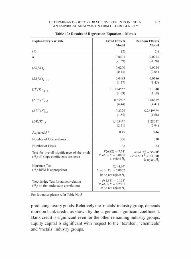
DETERMINANTS OF CORPORATE INVESTMENTS IN INDIA: 107 AN EMPIRICAL ANALYSIS ON FIRM HETEROGENEITY
producing luxury goods. Relatively the ‘metals’ industry group, depends more on bank credit, as shown by the larger and significant coefficient. Bank credit is significant even for the other remaining industry groups. Equity capital is significant with respect to the ‘textiles’, ‘chemicals’ and ‘metals’ industry groups.
Table 13: Results of Regression Equation – Metals
Explanatory Variable Fixed Effects Model
Random Effects Model
(1) (2) (3)α -0.0401
(-1.39)-0.0273 (-1.28)
0.0200 (0.43)
0.0024 (0.05)
0.0493 (1.27)
0.0386 (1.45)
0.1824*** (1.69)
0.1340 (1.18)
0.6599* (4.44)
0.6683* (4.41)
0.2329 (1.55)
0.2649*** (1.68)
1.4034** (2.41)
1.2805* (2.94)
Adjusted 0.47 0.46
Number of Observations 330 330
Number of Firms 33 33
Test for overall significance of the model (H0: all slope coefficients are zero)
a: reject H0
d: reject H0
Hausman Test (H0: REM is appropriate)
b: do not reject H0
Wooldridge Test for autocorrelation (H0: no first order auto correlation)
c: do not reject H0
For footnotes please refer Table No.5

108 RESERVE BANK OF INDIA OCCASIONAL PAPERS
Accelerator variables have an expected right sign for all four industry groups considered for analysis. However, these are significant only in the case of the ‘chemicals’ industry group (result is consistent with Athey and Laumas 1994).
Table 14: Results of Regression Equation – Electrical Machinery
Explanatory Variable Fixed Effects Model
Random Effects Model
(1) (2) (3)α -0.0224
(-0.57)0.0004 (0.002)
0.0185 (1.31)
0.0183 (1.19)
0.0040 (0.18)
0.0193 (0.82)
0.2016** (2.30)
0.1100 (1.67)
0.1943*** (1.95)
0.1966** (2.05)
1.9138 (1.29)
2.0187 (1.46)
0.5267 (0.54)
0.2529 (0.45)
Adjusted 0.20 0.21
Number of Observations 140 140
Number of Firms 14 14
Test for overall significance of the model (H0: all slope coefficients are zero)
a: reject H0
d: reject H0
Hausman Test (H0: REM is appropriate)
b: do not reject H0
Wooldridge Test for autocorrelation (H0: no first order auto correlation)
c: do not reject H0
For foot note please see Table 5.

DETERMINANTS OF CORPORATE INVESTMENTS IN INDIA: 109 AN EMPIRICAL ANALYSIS ON FIRM HETEROGENEITY
Section IV Conclusion
The results confirm heterogeneity across size-classes and industry groups in the link between investment and financial indicators (internal funds, bank credit, equity capital). Our results suggest that relatively large firms depend more on bank credit and equity capital for financing their investments. Results for small firms indicate that bank credit plays a significant positive role in determining their investments in fixed assets. In other words, the finding suggests that bank credit channelized to small firms through directed credit policies has a significant impact on determining their investments (result consistent with Eastwood and Kohli 1999). Further, as expected, the results confirm that small firms appear to face information problems in raising funds from capital markets; accordingly equity capital turns out to be insignificant for these firms.
Results across industry groups suggest that internal funds are statistically significant in the case of the ‘textiles’ and ‘chemicals’ industry groups. On the contrary, internal funds are unimportant for industry groups ‘metals’ and ‘electrical machinery’. Bank credit is significant for all four industry groups. However, relatively speaking industry groups ‘metals’ and ‘textiles’ depend more on bank credit. Lastly, the coefficient of equity capital is significant for three out of the four industry groups considered for the analysis.
Our results pertaining to small firms reveal that bank credit plays an important role in stepping-up their investments in fixed assets. As small scale firms form an important segment of the Indian economic system with a sizeable share in nation’s output policymakers need to formulate policies to further inject credit into this sector for increasing its overall output in the country. Further, although the stock market liberalization process may be able to mobilize financial resources for firms to a great extent, our results lend support to the fact that small firms still suffer to raise funds from stock markets. This might have unfavourable implications when these firms need to address higher investment demands. Therefore, policymakers need to sketch policies so that these firms are not wiped out from raising funds through stock markets.

110 RESERVE BANK OF INDIA OCCASIONAL PAPERS
References
Athey, M. J. and P. S. Laumas (1994), ‘Internal Funds and Corporate Investment in India’, Journal of Development Economics 45: 287-303.
Athey, M. J. and W. D. Reeser (2000), ‘Asymmetric Information, Industrial Policy and Corporate Investment in India’, Oxford Bulletin of Economics and Statistics 62 (2): 267-92.
Athukorala, P. C. and Kunal Sen (2002), Saving, Investment, and Growth in India. India: Oxford University Press.
Bhattacharyya, S. (2008), ‘Determinants of Corporate Investment: Evidence from Indian Manufacturing Firms’, Journal of Quantitative Economics 6 (1 and 2).
Bilsborrow, E. R. (1977), ‘The Determinants of Fixed Investment by Manufacturing Firms in a Developing Country’, International Economic Review 18 (3): 697-717.
Bond, S. and C. Meghir (1994), ‘Dynamic Investment Models and the Firm’s Financial Policy’, The Review of Economic Studies 61 (2): 197–222.
Eastwood and R. Kohli (1999), ‘Directed Credit and Investment in Small-Scale Industry in India: Evidence from Firm-Level Data 1965-78’, Journal of Development Studies 35 (4): 42-63.
Fazzari, M. S. and M. J. Athey (1987), ‘Asymmetric Information, Financing Constraints and Investment’, Review of Economics and Statistics 69 (3): 481-87.
Fazzari, M. S. R., Glenn Hubbard and B. C. Peterson (1988), ‘Financing Constraints and Corporate Investment’, Brookings Papers on Economic Activity 1: 141-206.
Harris, J. R., F. Schianterelli and M. G. Siregar (1994), ‘The Effect of Financial Liberalization on the Capital Structure and Investment Decisions of Indonesian Manufacturing Establishments’, World Bank Economic Review 8 (1): 17-47.

DETERMINANTS OF CORPORATE INVESTMENTS IN INDIA: 111 AN EMPIRICAL ANALYSIS ON FIRM HETEROGENEITY
Karim, Z. A. (2010), ‘Monetary Policy and Firm’s Investment in Malaysia: A Panel Evidence’, IIUM Journal of Economics and Management 18 (2): 221-53.
Krishnamurty, K. and D. U. Sastry (1975), Investment and Financing in the Corporate Sector in India. New Delhi: Tata McGraw-Hill.
Kumar, A. G., K. Sen and R. R. Vaidya (2001), ‘Outward Orientation, Investment and Finance Constraints: A Study of Indian Firms’, Journal of Development Studies 37 (4): 133-49.
Kumar, A. G., K. Sen and R. R. Vaidya (2002), ‘Does the Source of Financing Matter? Financial Markets, Financial Intermediaries and Investment in India’, Journal of International Development 14 (2): 211-28.
Oliner, S.D. and G.D. Rudebusch (1992), ‘Sources of Financing Hierarchy for Business Investment’, Review of Economic and Statistics 74 (4): 643-54.
Reserve Bank of India (2006), Report on Currency and Finance: 2004-05. Mumbai: RBI.
Salinger, M. and L. Summers (1983), ‘Tax Reforms and Corporate Investment’, in M. Feldstein (ed.), Behavioral Simulation Methods in Tax Policy Analysis. Chicago: University of Chicago Press, pp. 247-81.
Sancak, C. (2002), ‘Financial Liberalization and Real Investment: Evidence from Turkish firms’, IMF Working Paper No. 02/100.

112 RESERVE BANK OF INDIA OCCASIONAL PAPERS
Reserve Bank of India Occasional Papers
Vol. 34, No. 1 & 2: 2013
What Explains Credit Inequality Across Indian States? An Empirical Analysis
Snehal Herwadkar and Saurabh Ghosh*
The phenomenon of heterogeneous credit distribution across Indian states is well documented in literature. This study contributes to existing research by evaluating whether this diversity can be attributed to the risk-return profile of the states. In particular, it evaluates whether credit inequality across Indian states can be explained by state specific factors representing credit demand and supply and infrastructure facilities. Evaluating data for 22 Indian states for 2004-12, this paper concludes that the differences in credit distribution can be explained by factors such as financial deepening and physical infrastructure development. This indicates that states which garner higher deposits, have better banking networks and score high on infrastructure availability attract more credit as compared to other states. These results highlight that from the policy perspective, while the role of financial inclusion is important, the states can also contribute towards this goal by providing better infrastructure facilities that would enhance the investment climate in the states. Policy efforts, therefore, should focus on these issues as well as on promoting the spread of the formal banking channel.
JEL Classification : R1, G210Keywords : Emerging Market Economies, India, Credit, Regional Diversity,
Financial and Physical Infrastructure.
Introduction
The relationship between credit and economic growth and development has fascinated academics and practitioners alike. An old question continues to engage the economics profession deeply: does financial development promote growth or does economic growth propel financial development or is it both ways? (Patrick 1966, Gurley and Shaw 1967, Goldsmith 1969, Mckinnon 1973, Jung 1986, King and Levine 1993).
* Snehal Herwadkar and Saurabh Ghosh are Assistant Advisers in the Monetary Policy Department and Department of Economic and Policy Research respectively in the Reserve Bank of India. The authors are thankful to Dr M.D. Patra, Executive Director, RBI, an anonymous referee, Dr Charan Singh and participants at the Third DEPR Researchers’ conference for comments on an earlier draft. The authors take responsibility for errors, if any.

WHAT EXPLAINS CREDIT INEQUALITY ACROSS INDIAN STATES? 113 AN EMPIRICAL ANALYSIS
This paper contributes to this still unsettled debate by asking: does higher economic growth and better banking, social and physical infrastructure attract more credit to a particular region relative to others? It draws heavily on the wider discussion in literature on the phenomenon of uneven credit distribution across regions in the context of development (Samolyk 1989 and Hassan et al. 2011 provide a comprehensive review). Ruling orthodoxies in the evolution of ideas on this theme – ranging from the neo-classical profit-driven redistribution approach to the productive sector hypothesis (Mydral 1957) to the Keynesian liquidity preference approach – assign a passive role to financial intermediation. By contrast, policymakers across developed and emerging market economies (EMEs) are increasingly analysing the contribution of factors like the maturity of the banking sector and developmental indicators in studying credit distribution across regions (Jayaratne and Strahan 1996). Can policy interventions influence regional credit distribution patterns? This paper attempts to shed light on this question by evaluating the Indian experience.
Among EMEs, India provides an interesting test case given its heterogeneity in terms of geographic, economic, developmental and demographic characteristics across states. Using a large panel of 22 states and data for nine years (2004-12), we analyse the differences in credit distribution. The central question that we attempt to answer is: why does credit distribution differ so much across Indian states? Our hypothesis is that financial flows track highest risk-adjusted returns on investment. These returns differ across states due to various factors: availability of deposits, state of financial development, investment climate in the state, availability of infrastructure and transaction costs and ease of doing business, etc. The challenge of representing these factors through appropriate proxy variables is a multi-layered one because it is difficult to capture qualitative factors through quantifiable variables. Moreover, long time series for quantifiable variables are not always readily available. Notwithstanding these difficulties, we narrowed down to a set of key indicators which we think would adequately represent the unique characteristics of each state to carry out our analysis. These include: (i) state specific cyclical factors (that is,

114 RESERVE BANK OF INDIA OCCASIONAL PAPERS
1 Railway route length can be defined as the length of the railway routes open for traffic at the end of each year. In calculating the route length, double or more than double lines are counted only once. It is possible that some routes are shut down temporarily for maintenance or have been closed permanently as on the date of reporting. This can lead to overall fluctuations in the railway route length.
gross state domestic product –GSDP) and structural factors characterizing the state (that is, share of agriculture and services sectors in GSDP), (ii) major factors representing financial intermediation and deepening, for example, supply of credit (deposits from the state) or banking network proxied by bank centres, and (iii) proxies for existing infrastructure facilities and the law and order situation in a state, for instance rail density,1 electricity generation and criminal activities in the state. Empirical estimates employ an array of alternative models while adjusting for state specific effects. Our results suggest that apart from state GDP, financial networks and the availability of infrastructure are the major factors influencing credit disbursements across Indian states.
The rest of the paper is organized as follows. Section II gives an overview of international and Indian literature. Section III elaborates on the data used in the study while Section IV describes empirical results and the main inferences. The final section summarizes the results, discusses the policy implications and indicates the way forward.
Section II Literature Survey
Economics and finance literature is replete with studies investigating the inter-relationship between economic growth and credit. Authors like Mckinnon (1973), King and Levine (1993) Levine et al. (2000) and Rajan and Zingales (1998) have argued that financial development leads to more efficient allocation of resources, which ultimately translates into higher economic growth. On the other hand, authors like Gurley and Shaw (1967), Goldsmith (1969) and Jung (1986) have argued that higher economic growth creates demand for a better and more efficient financial sector and the financial sector merely fulfils this demand. Some authors have also found evidence of bi-directional

WHAT EXPLAINS CREDIT INEQUALITY ACROSS INDIAN STATES? 115 AN EMPIRICAL ANALYSIS
causality (Blackburn and Huang 1998, Khan 2001 and Hassan et al. 2011). In the Indian context, Demetriades and Luintel (1996) have documented bi-directional causality while Chakraborty (2010) has found evidence that banking sector development promotes economic growth. As the causality between growth and financial development has been adequately explored in literature, we attempt to empirically quantify credit dispersion and factors such as fund supply and availability of financial and physical infrastructure that could help in explaining this diversity.
International Experience
The neo-classical theory postulates that free movement of factors of production will automatically result in an exodus of labour from an underdeveloped region to a developed region, while financial resources in pursuit of higher returns will seek more profitable opportunities available in an underdeveloped region. In such a system, banks may fail to allocate resources among different regions due to imperfect or asymmetric information or due to barriers to inter-regional movement of financial flows like transaction costs or policy requirements. This neo-classical postulation has been challenged by Myrdal (1957) and Prebisch (1962). Both the Myrdal’s ‘cumulative causation theory’ and Prebisch’s ‘dependence theory’ suggest that yields of productive factors may vary between regions and the risk adjusted profitability of capital is higher in developed regions. This results in the developed regions not only utilizing and exhausting all their financial resources, but also in attracting capital from less developed regions. In both the neo-classical and Myrdal-Prebisch postulations, financial intermediation and the banking sector play only a limited role, which is confined to garnering deposits and deploying these funds as credit.
Later research in the theory of development phases of the financial system challenged the passive role assigned to the financial sector (Chick and Dow 1988 and Dow 1990). These theories indicate that as the banking system becomes more mature, it develops an ability to create credit in certain regions without reducing it in others. In this development phase, the decisions of the banking system to finance

116 RESERVE BANK OF INDIA OCCASIONAL PAPERS
development activities in one region are independent of deposits at its disposal. Samolyk (1992) developed a regional credit model and its empirical application for the US, which suggested that local banking sector problems may constrain economic activity in financially distressed regions, whereas no such link was evident in financially sound regions.
Gonzalez and Sales (2001) added to this strand of literature by highlighting the role of expectations about the number and magnitude of investment projects, which in turn determine the demand for financing or credit availability. The authors also found that in Spain the introduction of regional banks resulted in relatively low inter-regional differences. A study by the same authors done earlier found that the preference for liquidity was greater in the relatively lesser developed regions and in those that had a less promising economic outlook, which resulted in relatively lesser creation of credit for the region and an outflow of capital to more advanced regions. Lima and Resende (2008) found evidence among the EMEs of inequality in deposits translating into local credit for Brazilian states; moreover their study highlighted the role of bank group-wise differences (public versus private banks) in such an inequality pattern. There is hardly any study that explicitly analyses the role of infrastructure in analysing the credit disbursement pattern, at best it has been implicitly assumed in per capita income.
Banos et. al (2011) studied the relationship between regional banking and economic development in the Philippines and found a positive link between regional indicators of economic development and banking development with a specific influence of rural banking mainly in the intermediate‐developed regions. For the less developed regions however, they found no evidence of commercial, thrift or rural banks contributing significantly to the economic development.
Indian Literature
There are only a handful of studies that address spatial divergence in credit distribution in India and the empirical evidence is mixed. While Das and Maiti (1998) found no significant evidence of credit migration, Tyagarajan and Saoji (1977) observed that credit migration was largely

WHAT EXPLAINS CREDIT INEQUALITY ACROSS INDIAN STATES? 117 AN EMPIRICAL ANALYSIS
restricted to four major metropolitan cities. Pai (1970) showed that for industrially developed states, credit expansion was at a higher rate as compared to the deposit growth rate while the vice versa was true in case of industrially backward states.
Chatterjee et al. (1997) observed that migration of credit in the major states had become more uniform between 1974 and 1994. Singh and Srinivasan (2006) analysed data on 14 Indian states for 1990-91 to 1998-99 and found that per capita bank credit was an important determinant of growth. They also found that credit deposit ratios and FDI approvals per capita had a positive impact on growth. Finally, they observed that C-D ratios (a proxy for the internal movement of capital) had both become more varied across states and more closely related with GSDP per capita over the period. They concluded that capital, both foreign and domestic, flows to regions where it can be more effectively used, namely in higher income states.
This result is also corroborated by Chakravorty (2003) who found that there was a correlation between investment and determinants of profitability such as measures of physical infrastructure and distance to market area and to shipping hubs. In another strand of literature, Dhal (2012) found evidence which broadly corroborated asymmetry in credit and the bank lending channel of monetary policy transmission across different states. His findings suggest that poor states are likely to be more affected by a tight monetary policy.
Contribution of the Present Study
While the issue of inequality in the spatial distribution of credit is neither unique to India, nor a new concern, our study attempts to add to literature in two distinct ways. First, most of earlier studies have documented the regional disparity in credit but done little analysis of the macroeconomic factors behind the regional disparity in credit. To explain variations in credit distribution across states, taking a cue from the recently available literature, we include a large number of variables in our empirical analysis that have not been used in the Indian context.
Second, earlier studies relating to India on this subject selected bigger

118 RESERVE BANK OF INDIA OCCASIONAL PAPERS
states, completely ignoring the smaller ones. However, since this study is about explaining asymmetry in credit distribution, it is important not to exclude small states out of the sample, as that could distort the analysis. We, therefore, use a large number of states (22); only some union territories and certain states in the north-eastern region could not be covered in the study due to non-availability of consistent time series data.
Section III Data
Our study employs panel data on 22 Indian states2 for the period 2004-12. As most of the variables are available only with an annual frequency our study uses annual data. Data for this study was culled from a variety of sources. State-wise time series data on outstanding deposits and credit and bank centres of scheduled commercial banks were taken from the Basic Statistical Returns (BSR) dataset of the Reserve Bank of India. Variables like gross state domestic product, state per capita income, fiscal deficit to GDP ratio of states, share of non-industry, agriculture and services in state domestic product, factories in operation, infrastructure facilities and proxies for law and order situation in state (such as electricity generation, power deficit, crime rate, conviction rate and rail and road density) were taken from the Centre for Monitoring Economy (CMIE) database on the states of India. Non-availability of data on infrastructure facilities before 2004 has constrained the time period under consideration. A summary and definitions of all the variables is presented in Annexure I.
Credit growth across Indian states has varied substantially in terms of average growth rates and their time path (Chart I and V). An analysis of the share of states in all-India credit points to stark contrasts (Chart II and VI). We also considered a third variable, the credit to GSDP ratio to represent state credit distribution as a percentage of economic activity
2 The states include Andhra Pradesh, Assam, Bihar, Chhattisgarh, Delhi, Gujarat, Goa, Haryana, Himachal Pradesh, Jammu and Kashmir, Jharkhand, Karnataka, Kerala, Madhya Pradesh, Maharashtra, Odisha, Punjab, Rajasthan, Tamil Nadu, Uttarakhand, Uttar Pradesh and West Bengal.

WHAT EXPLAINS CREDIT INEQUALITY ACROSS INDIAN STATES? 119 AN EMPIRICAL ANALYSIS
to take care of the size of the state. Here again, only a few states showed high credit to GSDP ratio, but most of the states had low levels of the ratio (Chart III and VII). As is evident from these charts the variables representing credit distribution did not follow a similar path across states and their locus varied considerably over time.
Section IV Empirical Estimation and Analysis
i) Credit growth convergence
Before analysing the factors explaining credit divergence across states we attempt to evaluate whether there has been a convergence in credit growth across states over the years. To empirically investigate the presence of credit disparity across Indian states, the β-convergence method was used. The fixed effect panel regression consisted of 22 major states for 2004-12 with nine year average credit growth as a dependent variable and the base period credit growth as an independent variable. The coefficient of β was found to be positive and statistically insignificant at the conventional level. This finding suggests no statistically significant evidence of convergence of credit growth across states over time.
ii) Panel regressions
Having established significant divergence in credit off-take across states and insignificant convergence in them, we now attempt to identify some of the factors that could help in explaining the persisting divergence across Indian states. The list of variables used to explain credit divergence across states and their economic rationale is now discussed.
In line with the arguments extended by various authors including Gurley and Shaw (1967), Goldsmith (1969) and Jung (1986), we examine whether the high growth of a particular state helps in attracting more bank credit to that particular state and vice versa. Second, amongst the three sectors of agriculture, industry and services, the share of industry in non-food credit in India has always remained the highest. However, since there have been studies relating the industrial sector to credit

120 RESERVE BANK OF INDIA OCCASIONAL PAPERS
distribution and in view of the recent emphasis on financial inclusion and SMEs, we considered the share of the non-industrial sector in gross state domestic product to represent the comparative size of the agriculture and services sectors in a state.
Further, state deposit is taken as a proxy representing the resources available to the financial sector for its lending activities in line with the argument proposed by Beck et al. (2009) and Resende (2008). In today’s world of a technology driven banking sector, deposits garnered from a particular region need not be a constraint in extending credit to that particular region. However, the deposit base of a particular region can also be taken as a proxy of the presence of the banking sector in the region. It is clear that higher the penetration of the banking sector in a region, greater would be the credit extended through formal channels. We also considered banking centres which are taken as representative of the level of financial deepening in the state.
One of the key features of this paper is the introduction of infrastructure proxies as explanatory variables for state credit. The crucial role played by infrastructure in economic development has been well established in academic literature for a long time (Hirschman 1958 and Rostow 1960). Better infrastructure facilities like transport, communication and power help in enhancing the productivity of investment in that region, which in turn propels competitiveness. Availability of trade infrastructure like ports, highway corridors and railroads reduce transportation costs, facilitate smoother mobility of people and products and help in easing productivity constraints. These gains are often experienced over a long period of time rather than in the short term. Thus a state which has created an enabling environment through infrastructure facilities is likely to attract more investment and in turn more credit, notwithstanding its present growth or level of GDP. Taking into account infrastructure factors, we account for the expectations about the number and magnitude of investment projects, which in turn determine the demand for financing or credit availability in line with the argument extended by Gonzalez and Sales (2001).
We employ a generic panel data model with credit (or its transformation)

WHAT EXPLAINS CREDIT INEQUALITY ACROSS INDIAN STATES? 121 AN EMPIRICAL ANALYSIS
as a dependent variable and function of gross state domestic product, share of non-industry, deposit accumulation, bank centres, railway, electricity generation and crime as independent variables. All the explanatory variables have been suitably standardized taking into account the size of the state. The equations are:
G(credit)it = f(GSDP(t-1), share_nonindustryit, depositit, bank_centreit, railit, electricityit, crimeit)+ αi + λt + εit
Where G(.),f(.) are functions such as log, difference or ratios, while εit is assumed to follows normal distribution.
Before analysing data for panel regression, we consider evaluating their properties, by running Levin-Lin-Chu Test (LLC) test, which tests the hypothesis H0: each time series contains a unit root against H1: each time series is stationary. The finding of this procedure is reported in Table 1.
In the following section, we use different indicators of state-wise
Table 1: Panel Unit Root: Levin, Lin & Chu Test (Null: unit root)
Statistic Prob. sections Obs
Log(credit) -8.89 0 22 154log(deposit) -3.91 0 22 154log(bank_centres)* 16.15 1 22 154log(Rail)* 0.07 0.54 18 126log(electicity) -0.66 0.25 22 153Power_Deficit -7.17 0 21 121log(crime) -7.23 0 22 154
Note: *: variables found to be difference stationary.
outstanding credit (both in levels and in standardized form). We start with level of credit (as it was found stationary) and estimate coefficients of deposit, banking network and other infrastructure variables. We controlled for gross state domestic product (GSDP) for the size and cycles of economic activity in the state. However we used one period lagged value of GSDP to avoid an endogeneity problem. The model with cross-section and period fixed effect was chosen on the basis of the

122 RESERVE BANK OF INDIA OCCASIONAL PAPERS
F-statistics and redundant fixed effect chi-square test statistics. The estimated coefficients are reported in Table 2 (Model-1).
As some of the variables (for example, bank centres, railways and electricity generation) were found to be unit root process, we replace them by first difference (D(Rail) and D(bank_centres)) and by power_def. The cross-section and period fixed effect model was identified by the redundant fixed effect likelihood ratio test; their coefficients are reported in Table 3 (Model-2). In both of these estimates, the coefficient diagnostics clearly rejected the null of redundancy of financial inclusion variables and infrastructure variables; the coefficient and their significance indicate a strong positive relationship between credit with deposit mobilization and change in the number of banking centres in line with Beck et al. (2009) and Resende (2008). Further, among the infrastructure variables, increase in railway operational routes had a positive coefficient (Model-2). Power deficit had a positive coefficient,
Table 2: Panel Estimates Explaining Credit Disbursement
Variable Coefficient Prob. Coefficient Prob. Coefficient Prob.
Cross & Time Fixed
Cross & Time Fixed
Panel GMM
Model-1 Model-2 Model-3
log(credit(-1) 0.28 0.42C 4.72 0.04 0.75 0.71L_DEPOSIT 0.13 0.09 0.19 0.08 0.42 0.35LOG(BANK_CENTERS) 0.74 0.00DLOG(BANK_CENTERS) 0.71 0.05 2.85 0.19L_SDP(-1) 0.19 0.07 0.69 0.00 1.26 0.04SHARE_NonIND 0.001 0.65 0.003 0.43 0.01 0.42LOG(RAIL) -0.67 0.00LOG(ELECTRICITY) 0.07 0.06LOG(CRIME) -0.01 0.69DLOG(RAIL) 0.26 0.05 0.01 0.97POWER_DEF 0.003 0.10 -0.003 0.74CONVICTION_RATE -0.0003 0.68 0.01 0.11R2 0.97 0.98 0.20Arellano Bond AR(2)M-stat 0.01

WHAT EXPLAINS CREDIT INEQUALITY ACROSS INDIAN STATES? 123 AN EMPIRICAL ANALYSIS
which could indicate increase in the cost of production in the deficit states; however it is only significant at the 10 per cent level.
To evaluate the persistence of credit flows or lag dependence of the state credit factor, we included first lag of credit in the equation and estimated this dynamic model in the Panel GMM framework, using the Arellano–Bond two-step procedure. Here 2-period lagged value of credit was used as an instrument for GMM estimation. However, the estimation results indicate (Table 3, Model-3) that the coefficient of the lagged credit variable was not significantly different from zero, the R-square value was low and finally the Arellano-Bond second lag autocorrelation was found to be serially correlated, indicating that the dynamic panel is not a good fit in this context.
Indian states vary considerably in terms of their size, population and sectoral activities. So it is expected that the absolute level of credit disbursement would be different across states. Empirically, in the fixed effect panel regression, the state specific scale effect is likely to be addressed by cross-section fixed dummies. However, to address the scale effect explicitly we used different transformations of credit disbursement, which include state credit as a ratio of all India credit (credit_ai), state credit as a ratio to state GDP (credit_gsdp) and credit growth rate (Gr_credit).3 The deposit and GSDP was appropriately standardized. For instance, for estimating credit_ai, credit_gsdp and credit_gr we used state deposit to the all-India deposit ratio, state deposit to GSDP ratio and deposit growth respectively. Using each of credit_ai, credit_sdp and credit_gr as dependent variables and appropriately normalized set of independent variables, we estimated three sets of panel regressions (Table 3).
The results indicate that deposit mobilization and the banking network play an important role in credit creation in a particular state. This emphasizes the role of financial sector inclusion and development in credit creation and is in line with the findings of Love (2003). The coefficients of increase in rail network remain positive (except for credit growth equation), state power deficit has a positive coefficient, and
3 These variables were found to be stationary.

124 RESERVE BANK OF INDIA OCCASIONAL PAPERS
conviction rate has a positive and significant coefficient (Model-6). The positive coefficient of power deficit (Model-4) though counter-intuitive could indicate shortage of power in the credit-starved industrial states or increase in the cost of production due to power shortage; in either case it calls for more infra-investment in the power sector.
The share of the non-industrial sector seems to have a positive influence (Model-5) on share of credit to state GDP indicating that the states with a larger share of agriculture and services sectors attract more credit relative to their GSDP. One reason could be that in the recent period the services sector has emerged as the engine of growth for the Indian economy.
In the equation explaining credit to GSDP, fiscal deficit as a per cent of GSDP had a negative and significant coefficient indicating the adverse impact of a large state deficit on credit distribution. In line with research by Blejer and Khan (1984), this result suggests that the higher level of
Table 3: Panel Estimate Explaining Credit Dispersion Ratios
Variable State Credit to all India Credit
State Credit to GSDP
State Credit Growth
Coefficient Prob. Coefficient Prob. Coefficient Prob.
Cross & Time Fixed
Time Fixed Effect
Time Fixed Effect
Model-4 Model-5 Model-6
C 0.24 0.47 -0.42 0.00 11.76 0.01LOG(DEP_AI) 0.22 0.07DEP_GSDP 0.68 0.00DEP_Growth 0.20 0.04DLOG(BANK_CENTERS) 0.90 0.02 2.21 0.00 17.29 0.43GSDP_AI(-1) 0.15 0.00GR_GSDP(-1) 0.06 0.53FD_GSDP -0.04 0.00SHARE_NonIND 0.0004 0.92 0.01 0.00 0.03 0.58DLOG(RAIL) 0.27 0.06 -0.09 0.74 -33.53 0.00POWER_DEF 0.01 0.02 0.0003 0.87 0.09 0.13CONVICTION_RATE -0.0001 0.24 0.0001 0.86 0.04 0.01R-square 0.97 0.84 0.46
Note: Models selected on the basis of Redundant Fixed effect likelihood ratio test.
WHAT EXPLAINS CREDIT INEQUALITY ACROSS INDIAN STATES? 125 AN EMPIRICAL ANALYSIS
fiscal deficit may be ‘crowding out’ private investment. Finally, in almost all of the estimated equations, coefficients of the one- period lagged GSDP variable are positive and significant indicating the positive impact of state GDP on credit disbursements.4
All estimated models include year dummies to control for year specific effect, including that of business cycles, interest rate movements or global financial crises that uniformly affect bank credit disbursement across states. A plot of these time dummy coefficients, which were found to be jointly significant, clearly indicates two phases of credit cycle with a break around the global financial crisis (Chart IV). The residual diagnostics confirmed normal distribution of the panel regression errors.
In an attempt to test the robustness of our findings and address the possibility of some of the important variables of interest being omitted, we attempted modeling with a large number of alternative variables. These variables include corporate profit, new investment and per capita income as reported in the Annual Survey of Industries (ASI) and the National Accounts Statistics (NAS) database. We also included infrastructure facilities like telecom and road infrastructure in a state as also the existence of port (dummy) in a state. However, these variables either had a multi-collinearity problem, as indicated by a near-singular matrix inversion problem or were found to be statistically insignificant in the omitted variable likelihood ratio test.
The non-availability of longer time series especially relating to physical and social infrastructure constrains our analysis. Specifically, data on power deficit and conviction rate are available from 2004 onwards, which necessitated that the present analysis be restricted to nine years. A longer time series on these variables will be helpful in extending the analysis more fruitfully.
A note of caution is also in order while interpreting these results. Some of the state specific variables showed substantial volatility across time and across states. A more robust dataset would be helpful in further strengthening the results.
4 Lagged value of GSDP was included in the specification to avoid the possibility of any endogeneity problem leading to a biased estimate of the coefficients.

126 RESERVE BANK OF INDIA OCCASIONAL PAPERS
Section V Conclusions
Heterogeneity of credit distribution across regions has been attracting considerable academic and policy attention for a long time. While the studies so far have only documented credit heterogeneity across Indian states, our main objective was to examine factors that may explain some of the observed divergence. India provides a natural laboratory for studying heterogeneity given the considerable regional differences in terms of income, financial inclusion and infrastructure development.
Using data from a large number of Indian states from 2004 to 2012, after appropriately controlling for cross-section and time specific effects, empirical evidence suggests availability of funds (deposits) and the banking network as the most important variables explaining heterogeneity of credit disbursement. Among infrastructure facilities, rail and power deficit emerge as factors that affect credit disbursement. State GDP and fiscal deficit are also found to be important factors influencing credit disbursements.
These results motivate a few important policy implications. First, financial deepening is crucial, which not only helps in garnering more resources from the state but also helps in channelizing more resources to the state. The Reserve Bank’s recent policy initiatives such as setting up differentiated banks (such as payments banks) with a primary focus on the provision of basic financial services using new technologies could be helpful in achieving greater financial inclusion. The policy vision is to promote the spread of the formal banking channel, which will give impetus to formal credit lines, thus providing support to the growth aspirations of all the states. The government’s Jan Dhan Yojana to provide a bank account for each poor Indian family, where each account would include a debit card, accident and life insurance coverage and an overdraft facility is also a major step in this direction.
Second, this paper also emphasizes the importance of infrastructure in explaining credit diversity across states. Providing better infrastructure to create an investor friendly environment and reining in the fiscal deficit of the state at the same time are factors that play an important role.

WHAT EXPLAINS CREDIT INEQUALITY ACROSS INDIAN STATES? 127 AN EMPIRICAL ANALYSIS

128 RESERVE BANK OF INDIA OCCASIONAL PAPERS

WHAT EXPLAINS CREDIT INEQUALITY ACROSS INDIAN STATES? 129 AN EMPIRICAL ANALYSIS
Cha
rt V
: Cre
dit g
row
th a
cros
s sta
tes o
ver
time
15
C
hart
V: C
redi
t gro
wth
acr
oss
stat
es o
ver
time
16182022242628
0405
0607
0809
1011
12
1
101520253035
0405
0607
0809
1011
12
2
481216202428
0405
0607
0809
1011
12
3
1520253035
0405
0607
0809
1011
12
4
16202428
0405
0607
0809
1011
12
5
16202428
0405
0607
0809
1011
12
6
10152025
0405
0607
0809
1011
12
7
15202530354045
0405
0607
0809
1011
12
8
8121620242832
0405
0607
0809
1011
12
9
-1001020304050
0405
0607
0809
1011
12
10
1216202428
0405
0607
0809
1011
12
11
1015202530
0405
0607
0809
1011
12
12
1216202428
0405
0607
0809
1011
12
13
510152025
0405
0607
0809
1011
12
14
5101520253035
0405
0607
0809
1011
12
15
8121620242832
0405
0607
0809
1011
12
16
1620242832
0405
0607
0809
1011
12
17
1620242832
0405
0607
0809
1011
12
18
15.0
17.5
20.0
22.5
25.0
27.5
30.0
0405
0607
0809
1011
12
19
14161820222426
0405
0607
0809
1011
12
20
1216202428
0405
0607
0809
1011
12
21
1520253035
0405
0607
0809
1011
12
22
GR
_CR
EDIT

130 RESERVE BANK OF INDIA OCCASIONAL PAPERS
Cha
rt V
I: S
tate
’s sh
are
in a
ll In
dia
cred
it
16
Chart V
I: State’s share in all India cred
it
Chart V
II: Ratio of credit to state’s do
mestic
produ
ct

WHAT EXPLAINS CREDIT INEQUALITY ACROSS INDIAN STATES? 131 AN EMPIRICAL ANALYSIS
Cha
rt V
II: R
atio
of c
redi
t to
stat
e’s d
omes
tic p
rodu
ct
17
Tab
le 1
: Sum
mar
y St
atis
tics
of th
e V
aria
bles
Dep
ende
nt V
aria
bles
D
efin
ition
So
urce
M
ean
Med
ian
Max
imum
M
inim
um
Std
. Dev
. S
kew
ness
K
urto
sis
CR
EDIT
O
utst
andi
ng c
redi
t of S
CB
s(R
s.
Bill
ion)
B
SR, R
BI
1143
.43
464.
95
1404
6.74
22
.81
1952
.92
3.8
20.0
L_C
RED
IT
Log
of c
redi
t A
utho
rs’
calc
ulat
ions
13
.0
13.0
16
.5
10.0
1.
4 0.
1 2.
4
CR
EDIT
_AI
Shar
e of
sta
te in
all
Indi
a cr
edit
(per
cen
t)
Aut
hors
’ ca
lcul
atio
ns
4.5
2.4
33.5
0.2
6.7
3.0
12.2

132 RESERVE BANK OF INDIA OCCASIONAL PAPERS
Depe
nden
t Var
iabl
esDe
finiti
onSo
urce
Mea
n M
edia
n M
axim
umM
inim
um S
td. D
ev.
Ske
wnes
sK
urto
sis
CRED
ITOu
tstan
ding
cred
it of
SCB
s (`
Bill
ion)
BSR,
RBI
1143
.43
464.
9514
046.
7422
.81
1952
.92
3.8
20.0
L_CR
EDIT
Log
of cr
edit
Auth
ors’
calcu
latio
ns13
.013
.016
.510
.01.
40.
12.
4
CRED
IT_A
ISh
are o
f stat
e in
all In
dia c
redi
t (p
er ce
nt)
Auth
ors’
calcu
latio
ns4.
52.
433
.50.
26.
73.
012
.2
CRED
IT_S
DPCr
edit
to st
ate G
DP ra
tioAu
thor
s’ ca
lculat
ions
0.5
0.3
2.3
0.1
0.4
2.8
11.0
GR_C
REDI
TCr
edit
Grow
thAu
thor
s’ ca
lculat
ions
20.6
20.3
41.6
-3.1
6.6
-0.3
4.8
Expl
anat
ory V
aria
bles
DEPO
SIT
Outst
andi
ng D
epos
it o
f SCB
s (`
Bill
ion)
BSR,
RBI
1547
.51
869.
8415
298.
6710
4.94
2169
.65
3.7
20.0
BANK
_CEN
TERS
Cent
res w
ith at
least
one b
ranc
hBS
R, R
BI15
64.3
1474
.054
97.0
67.0
1124
.51.
25.
0GS
DPGr
oss
State
Do
mes
tic
Prod
uct
CMIE
, SOI
1870
461.
013
5405
510
8275
13.0
8819
4.0
1719
398.
01.
98.
2SH
ARE_
NONI
NDSh
are o
f agr
icultu
re an
d se
rvice
s se
ctor i
n ne
t stat
e dom
estic
pr
oduc
t
CMIE
, SOI
RAIL
Oper
ation
al Ra
ilway
rout
e len
gth
in K
MCM
IE, S
OI27
.421
.713
8.5
0.4
24.7
2.9
12.4
ELEC
TRIC
ITY
Elec
tricit
y Ge
nera
tion
(Mkw
h)CM
IE, S
OI30
512.
623
828.
097
008.
027
7.0
2570
4.1
0.8
2.7
CRIM
ECo
gniza
ble C
rime u
nder
IPC
(nos
./mill
ion)
CMIE
, SOI
4854
.531
79.0
2036
9.0
879.
039
08.4
1.4
4.5
POW
ER_D
EFPo
wer d
eficit
(per
cent
)CM
IE, S
OI-7
.4-4
.93.
4-2
9.0
6.9
-1.1
3.3
CONV
ICTI
ON_
RATE
Conv
ictio
n ra
te (IP
C) (p
er ce
nt)
CMIE
, SOI
61.6
66.5
100.
06.
029
.5-0
.21.
6
Tabl
e 1: S
umm
ary
Stat
istics
of t
he V
aria
bles

WHAT EXPLAINS CREDIT INEQUALITY ACROSS INDIAN STATES? 133 AN EMPIRICAL ANALYSIS
Depe
nden
t Var
iabl
esDe
finiti
onSo
urce
Mea
n M
edia
n M
axim
umM
inim
um S
td. D
ev.
Ske
wnes
sK
urto
sis
Tran
sform
ed V
aria
bles
DEP_
AISh
are o
f dep
osit
in al
l Ind
iaAu
thor
s’ ca
lculat
ions
1.0
0.6
10.1
0.1
1.4
3.7
20.0
DEP_
SDP
Ratio
of D
epos
it to
state
net
dom
estic
pro
duct
Auth
ors’
calcu
latio
ns0.
80.
62.
90.
30.
53.
012
.5
GR_D
EPGr
owth
of d
epos
itsAu
thor
s’ ca
lculat
ions
16.9
17.0
31.3
-6.7
5.2
-0.5
5.2
GR_S
DPGr
owth
of s
tate d
omes
tic p
rodu
ctAu
thor
s’ ca
lculat
ions
14.3
13.8
26.2
0.6
4.6
-0.1
3.3
FD_S
DPRa
tio o
f fisc
al de
ficit
to st
ate
dom
estic
pro
duct
CMIE
, SOI
3.6
3.2
11.3
0.5
1.8
1.4
5.7
Tabl
e 1: S
umm
ary
Stat
istics
of t
he V
aria
bles
(Con
cld.)

134 RESERVE BANK OF INDIA OCCASIONAL PAPERS
ReferencesBaños, J., C. Crouzille, E. Nys and A. Sauviat (2011), ‘Banking Industry Structure and Economic Activities: A Regional Approach for the Philippines’, Philippine Management Review (Special Issue) 18: 97-113.
Beck, T., A. Demirguc-Kunt and R. Levine (2009), ‘Financial Institutions and Markets across Countries and over Time: Data and Analysis’, Policy Research Working Paper 4943. The World Bank, May.
Blackburn, K. and V. Huang (1998), ‘A Theory of Growth, Financial
Development and Trade’, Economica 65(257): 107-24.
Blejer, M. and M. Khan (1984), ‘Government Policy and Private Investment in Developing Countries’, IMF Staff Papers 31 (2): 379-403.
Chakraborty, I. (2010), ‘Financial Development and Economic Growth in India: An Analysis of the post-reform period’, South Asia Economic Journal 11 (2): 287–308.
Chakravorty, S. (2003), ‘Industrial location in post-reform India: Patterns of inter-regional divergence and intra-regional convergence’, The Journal of Development Studies 40 (2): 120-152.
Chatterjee, A, K. Bhattacharya and S. Gayen (1997), ‘Migration of Credit Across States: An Empirical Investigation with Some New Measures’, Banking Statistics Division, Department of Statistical Analysis and Computer Services, Reserve Bank of India, Mumbai (mimeo).
Chick, V. and S.C. Dow (1988), ‘A post-Keynesian Perspective on the Relation between Banking and Regional Development’, in P. Arestis (ed.), Post Keynesian Monetary Economics: New Approaches to Financial Modelling: 219-50, UK:Edward Elgar.
Das, P. K. and P. Maiti (1998), ‘Bank credit, output and bank deposits in West Bengal and Selected States’, Economic and Political Weekly 33(47/48): 3081+3083-3088.

WHAT EXPLAINS CREDIT INEQUALITY ACROSS INDIAN STATES? 135 AN EMPIRICAL ANALYSIS
Demetriades, P. and K. B. Luintel (1996), ‘Financial Development, Economic Growth and Banking Sector Controls: Evidence from India’, The Economic Journal 106(435): 359-74.
Dhal, S. (2012), ‘A Disaggregated Analysis of Monetary Transmission Mechanism- Evidence from the Dispersion of Bank credit to Indian States’, in Deepak Mohanty (ed.), Regional Economy of India. Reserve Bank of India, Academic Foundation, New Delhi: 247-278.
Dow, S. (1990), Financial Markets and Regional Economic Development: The Canadian Experience. Gower Publishers: Aldershot.
Goldsmith, R.W. 1969. Financial structure and development, Yale University Press.
Gonzalez, M. and Sales, J. 2001. ‘‘The spatial Distribution of Credit: The Case of Spanish Savings Banks’’. The Service Industries Journal, Vol. 21(4), pp.62-82.
Gurley, J. and E. Shaw. 1967. ‘‘Financial Structure and Economic Development’’. Economic Development and Cultural Change, Vol. 15 (3), pp. 257-68.
Hassan, M. K, B. Sanchez and J. Yu (2011), ‘Financial Development and Economic Growth: New Evidence from Panel Data’, The Quarterly Review of Economics and Finance 51 (1): 88-104.
Hirschman, A. (1958), The Strategy of Economic Development. Yale University Press, Yale Studies in Economics.
Jayaratne, J. and P. Strahan (1996), ‘The finance-growth nexus: Evidence from bank branch deregulation’,. The Quarterly Journal of Economics 111(3): 639–70.
Jung, W. (1986), ‘Financial Development and Economic Growth: International Evidence’, Economic Development and Cultural Change, 34(2): 333-46.
Khan, A. (2001), ‘Financial Development and Economic Growth’, Macroeconomics Dynamics 5(3): 413-33.

136 RESERVE BANK OF INDIA OCCASIONAL PAPERS
King, R. and R. Levine (1993), ‘Finance and growth: Schumpeter might be right’, Quarterly Journal of Economics 108 (3): 717-37.
Levine, R., L. Norman and T. Beck (2000), ‘Financial intermediation and growth: Causality and causes’, Journal of Monetary Economics, 46(1): 31-77.
Lima, M. and M. Resende (2008), ‘Banking and Regional Inequality in Brazil: An Empirical Note’, Brazilian Journal of Political Economy 28 (4): 669-77.
Love, I. (2003), ‘Financial development and financing constraints: Evidence from the structural investment model’, Review of Financial Studies 16(3): 765-91.
McKinnon, R. I. (1973), Money and Capital in Economic Development. Washington, DC: The Brookings Institution.
Myrdal, G. (1957), Economic Theory and Underdeveloped Regions. London: University Paperbacks, Methuen.
Pai, G. A. (1970), ‘Regional Distribution of Bank Credit: A Critical View’, Economic and Political Weekly 5(41): 1691+1695-1699.
Patrick, H.T. (1966), ‘Financial Development and Economic Growth in Underdeveloped Countries’, Economic Development and Cultural Change 14 (2): 174-89.
Prebisch, R. (1962), ‘The Economic Development of Latin America and its Principal Problems’, Economic Bulletin for Latin America 7(1): 1-22.
Rajan, R. and L. Zingales (1998), ‘Financial dependence and growth’, American Economic Review 88 (3): 559-86.
Resende, M.L.M. (2008), ‘Banking and regional inequality in Brazil: an empirical note’, Brazilian Journal of Political Economy 28 (4): 669-77.
Rostow, W.W. (1960), The Stages of Economic Growth: A Non- Communist Manifesto. Cambridge: Cambridge University Press.

WHAT EXPLAINS CREDIT INEQUALITY ACROSS INDIAN STATES? 137 AN EMPIRICAL ANALYSIS
Samolyk, K. (1989), ‘The Role of Banks in Influencing Regional Flows of Funds’, Working Paper No. 9204, Federal Reserve Bank of Cleveland.
Samolyk, K. (1992), ‘Bank Performance and Regional Economic Growth: Evidence of a Regional Credit Channel’, Working Paper No.9204, Federal Reserve Bank of Cleveland.
Singh N. and T.N. Srinivasan (2006), ‘Indian Federalism, Economic Reform and Globalization’, in Jessica S. Wallack and T. N. Srinivasan (eds), Federalism and Economic Reform: International Perspectives. New York: Cambridge UP, pp. 301-63.
Tyagarajan, M. and S.H. Saoji (1977), ‘Migration of Credit: An Aspect of Banking in Metropolitan Centres’, Reserve Bank of India Bulletin (December), pp. 802-13.

138 RESERVE BANK OF INDIA OCCASIONAL PAPERS
Reserve Bank of India Occasional Papers
Vol. 34, No. 1 & 2: 2013
SME Financing through IPOs – An Overview
R. K. Jain, Avdhesh Kumar Shukla and Kaushiki Singh*
The new initiative of capital financing of SMEs through IPOs has been quite encouraging and the secondary market performance of SME IPOs has also been very good. However, it seems that this is risky for investors, as there is not enough liquidity and the turnover is also low. Considering these problems, market regulator SEBI has issued guidelines to keep away small investors from investing in SME IPOs. In order to make the market liquid, SEBI guidelines stipulate that merchant bankers should act as market makers in such stocks for three years. However, after the stipulated period of three years, the stocks may face the problem of liquidity again. In order to avoid such a scenario, the present paper suggests the need for more transparency and increased institutional participation in companies listed on SME platforms. Also, stock exchanges where these companies are listed should provide sustained handholding to the managements of these companies.
JEL Classification : G1, G18, Y10Keywords : SME IPOs, BSE SME IPO Index, Liquidity, Exchange, SME Platform,
Market Maker
Introduction
Small and medium enterprises (SMEs) play an important role in the socio-economic development of India due to their vital contribution to GDP, industrial growth, employment and exports. However, this sector is beset with challenges including lack of availability of adequate and timely credit and limited access to equity capital (SIDBI 2013). SMEs have primarily relied on bank finance to meet their working capital requirements, but equity capital has to be brought in by the promoters of the enterprises. Till recently, institutional arrangements for equity and risk capital were provided only by the Small Industries Development Bank of India (SIDBI) under the Growth Capital and Equity Assistance Scheme for MSMEs (GEMS) (SIDBI 2013). In order to
* R.K. Jain, Avdhesh Kumar Shukla and Kaushiki Singh are Director, Assistant Adviser and Research Officer, respectively in the Department of Economic and Policy Research. The views expressed in the paper are personal and not of the institution that they are working with. Usual disclaimers apply.

SME FINANCING THROUGH IPOS – 139 AN OVERVIEW
provide a market based solution for equity resource mobilization by SMEs, the need for having a separate exchange/platform for SMEs has been felt for a long time (RBI 2008). Though efforts were made in the past to cater to the needs of small companies through initiatives such as OTC Exchange of India (OTCEI) set up in 1990 and the INDO NEXT Platform of the BSE launched in 2005, these experiments could not achieve desired results (SEBI 2008). Finally, efforts to provide an alternative source of equity funding to SMEs fructified with the launch of the BSE SME platform by BSE on March 12, 2012 and the SME platform ‘Emerge’ by NSE in September 2012.
This paper makes an attempt to review the performance of SME platforms in India. In addition to the introduction, the rest of the paper is divided in six sections. Section II highlights the international experience of SME exchanges. Section III covers the policy framework related to equity resource mobilization by SMEs through IPOs. Section IV throws light on the performance of primary market in terms of resource mobilization by SMEs on recently launched SME platforms. Secondary market performance of companies listed on the SME platforms is outlined in Section V, while Section VI provides financial and non-financial information related to these companies. Section VII sums up the paper.
Section II International Scenario
Globally, adequate flow of equity finance to SMEs has been recognized as policy priority. In order to achieve this, both developed and developing countries have set up alternative stock exchanges for SMEs. In fact, the need for an alternative stock exchange for SMEs has been so acutely felt in the countries that the International Organization of Securities Commissions (IOSCO) has identified promotion of such exchanges as one of the areas for mutual cooperation (IOSCO 2012). Presently, separate exchanges/platforms dedicated to equity financing of SMEs are functioning in more than 24 countries (Yoo 2007). Their main features, listing norms and performances, are now briefly discussed.

140 RESERVE BANK OF INDIA OCCASIONAL PAPERS
The London Stock Exchange’s Alternative Investment Market (AIM), which was set up in 1995, has succeeded in attracting a large number of small-sized companies globally, including a few Indian ones. AIM facilitates easy entry and less onerous disclosure requirements, but it has in place an appropriate level of regulation for smaller companies. It also provides a faster admission process and no pre-vetting by the regulator (SEBI 2008). So far, firms have raised almost 30 billion pounds via IPOs on AIM with companies coming from 37 sectors, 90 sub-sectors and 26 countries (AIM 2014). The National Stock Exchange (NSX) in Australia, a fully operational and regulated main board stock exchange, is focused on listing SMEs. NSX operates Australia’s two premier alternative stock exchanges. The NSX Corporate Exchange specializes in the listing of SMEs and the NSX Alternative Exchange has attracted the listing of community based organizations such as community banks. Both of these exchanges are able to support the listing of regional enterprises (Symon 2007).
An alternative exchange for SMEs in South Africa (Altx) was set up in October 2003. The Shenzhen Stock Exchange in South China’s Guandong Province officially inaugurated a board for SMEs in May 2004. Similarly, Egypt launched its SME Exchange (NILEX) in October 2007 where companies with capital ranging from EGP 500,000 to EGP 25 million could be listed (Ministry of Finance, Egypt 2008).
Other SME exchanges are GEM (Growth Enterprise Market) in Hong Kong and the Market of the High-Growth and Emerging Stocks (MOTHERS) in Japan (both started in 1999). Unlike AIM and MOTHERS, which are trading platforms of their respective main stock exchanges, GEM is a separate dedicated stock exchange. GEM functions on the philosophy of ‘buyers beware’ and ‘let the market decide’ based on a strong disclosure regime. The rules and requirements are designed to foster a culture of self compliance by the listed issuers in the discharge of their responsibilities (Stock Exchange of Hong Kong 2014). In the case of MOTHERS, the emerging companies applying there must have the potential for high growth though there are no specific numerical

SME FINANCING THROUGH IPOS – 141 AN OVERVIEW
criteria for determining the growth potential. Further, the applicant company is mandated to make a public offering of at least 500 trading units. At the time of listing, it should have at least 2,000 trading units and the market capitalization of its listed shares should be more than 1 billion yen. The applicant
must also have a continuous business record of not less than one year dating back from the day on which it made the listing application (SEBI 2008, TSE 2014).
Other initiatives include TSX Ventures Exchange (TSX-V) in Canada, Catalist in Singapore, KOSDAQ in the Republic of Korea and MESDAQ in Malaysia. As a matter of fact, NASDAQ also started as an SME Exchange and provides special facilities for listing of small and medium enterprises. In 2013, the Nigerian Stock Exchange inaugurated the Alternative Securities Market (ASEM), which is a platform for small businesses and SMEs in Nigeria to trade their equities on the Nigerian Stock Exchange. Similarly, the Rwanda Stock Exchange (RSE) has also started an initiative for small and medium enterprises’ (SMEs) listing on the alternative market segment of the bourse. The Istanbul Stock Exchange (ISE) in Turkey has a particular segment catering to the funding requirements of SMEs.
An analysis of listing norms of SME exchanges indicates that nearly all new markets adopt looser listing and maintenance requirements than the main market, typically allowing more relaxed criteria on operating history, minimum number of shareholders, past financial performance and the number of free-float shares. However, Brazil’s Novo Mercado is an exception: it sets higher standards for listed firms than the main market, emphasizing gaining investor trust over relaxing constraints (Yoo 2007). In terms of secondary market liquidity, globally SME exchanges have varied experiences. In order to ensure sufficient liquidity, most of the exchanges have put in place alternative arrangements such as market makers for liquidity. In India, while framing policies related to the SME Exchange, some of the global practices have been followed.

142 RESERVE BANK OF INDIA OCCASIONAL PAPERS
Section III Policy Framework on Listing of SMEs in India
In India, policies relating to SME platforms were formulated after taking into account learnings from the global experience, domestic capital market realties, difficulties faced by SMEs and OTCEI’s experience1
(BSE 2011). As per SEBI guidelines, SME exchanges should be set up as corporatized entities (bodies with a structure found in publicly traded firms) with minimum net worth of `1,000 million. These guidelines stipulate that an issuer with post issue face value of up to `100 million will be invariably covered under the SME exchange whereas issuers with post issue face value capital between `100 million and `250 million may get listed either on the SME exchange or on the main board (Table 1). SEBI has relaxed norms for listing on the SME Exchange as
Table 1: Listing Criteria – Main Board and SME Exchange
Parameters Main Board SME Exchange
Post-issue paid up capital (face value)
Not less than `100 million
Not exceeding `250 million
Minimum number of allotees 1000 50IPO Application Size `10,000 - `15,000 Minimum `1 lakhObservation on draft red herring prospectus (DRHP)
By SEBI By Exchange
Track record Three years track record of profitability
Relaxed norms for track record
IPO Underwriting Mandatory (however, not required when 50% of the issue offered
for subscription to Qualified Institutional Buyers (QIB)
Mandatory (100% underwritten, out of which 15% compulsorily by
merchant banker)
Market Making Not mandatory Mandatory (All market makers in scrip will provide two way quotes for 75% time during a trading day)
Time frame for listing 6-8 months 2-3 monthsReporting requirements Quarterly Half yearly
Source : SEBI and BSE.
1 There are two important distinguishing attributes between OTCEI and present SME exchanges: 1) Unlike OTCEI, which was standalone, present day SME exchanges are completely integrated with the respective main exchange and there is a provision for migration from the SME platform to the main exchange and vice versa. 2) There is a provision of 100 per cent underwriting of the issue and market maker for three years after the listing to provide liquidity (SME World 2014).

SME FINANCING THROUGH IPOS – 143 AN OVERVIEW
issuers do not need to have a track record of distributable profits for three years as in the case of listing on the main board.
The present guidelines have a three-pronged approach: a) to safeguard the interest of investors by keeping larger lot sizes, so that only informed investors are able to participate, b) maintaining sufficient liquidity by provision of market making and c) reducing the time involved in the processing of the issue by allowing a merchant banker to file RHP with due diligence certificate with the exchange and treating approval of the exchange sufficient (BSE 2011).
Section IV Performance of SME Platforms in terms of
Equity Resource Mobilization
Since the launch of SME platforms (from April 2012 to May 2014), 64 companies have got listed on SME platforms. Of these 64 companies, 61 are listed on the BSE SME platform and three on the NSE Emerge. These companies have mobilized total resources of `5.9 billion from the capital market, which is around two per cent of `281.0 billion overall equity mobilization by stock exchanges during the same period (from April 2012 to May 2014) (Table 2). When compared with bank credit to the small scale sector, the funds mobilized through SME platforms appear even more insignificant. During 2012-13, bank credit deployed to small scale industries was `480 billion as compared to `2.4 billion mobilized through SME platforms. In percentage terms, equity resources mobilized through SME platforms was only 0.5 per cent of the bank credit to this sector during 2012-13. However, it is
Table 2: Equity Resource Mobilization: SME Platform versus Overall(` Billion)
Year Equity Resource Mobilisation through
SME Platforms
Overall Equity Resource Mobilisation through
Stock Exchanges$
2012-13 2.4 138.82013-14 3.2 132.62014-15 (Up to May) 0.4 9.5
Note: $: Excludes offer for sale issues. Source: Calculated by authors from SEBI Data.

144 RESERVE BANK OF INDIA OCCASIONAL PAPERS
still encouraging, as the amount of `2.4 billion mobilized during financial year 2012-13 through equity issues is higher than equity related assistance aggregating `1.5 billion extended by SIDBI during the financial year 2012-132. Therefore, though this route is still in a nascent stage, it is an encouraging initiative and the initial responses may be termed as satisfactory.
Sectoral distribution of the 64 companies which mobilized resources from the market (up to end May 2014) indicates that 14 of these companies were engaged in the financial services sector (including NBFCs and securities firms), seven in ‘Textile and Apparel’ and six each in ‘construction and real estate’ and ‘agro and food processing’ sectors (Chart 1). Further, a majority of the companies were from the services sector, mostly from the financial services sector. Nevertheless, they were significantly diversified. Sectoral diversification of listed firms is crucial from the risk management perspective of SME platforms as well as for investors.
2 Corresponding data for 2013-14 from SIDBI are not available for comparison.

SME FINANCING THROUGH IPOS – 145 AN OVERVIEW
Section V Performance of SME IPOs in the Secondary Market
Besides the SME platform, BSE has also launched a Barometer Index -- the BSE SME IPO to track the performance of SME IPOs in the secondary market. The BSE SME IPO Index is calculated with free float methodology in line with other BSE indices. The number of scrips included in the index are variable. However, at any point of time a minimum of 10 companies should be maintained in the index. All new listed companies are compulsorily included in the index and a company which has completed three years after listing is automatically excluded from it. However, if there are less than 10 companies on account of possible exclusion after three years, the exclusion of such companies should be delayed till such time new inclusion is made in the index.3 Since its launch on December 14, 2012, the index up to June 24, 2014 witnessed a huge rally of about 601.3 per cent which is significantly higher than gains in other stock indices in India (Chart 2).
A scrip-wise analysis of the movement of share prices (as on June 24, 2014) of companies listed on the BSE SME platform indicates that sixteen companies recorded more than 100 per cent increase over the
3 http://www.bseindia.com/indices/sme_ipo.aspx?page=531BB8D5-6CB9-4ABC-8791-378F12A70B60.

146 RESERVE BANK OF INDIA OCCASIONAL PAPERS
offer price and seven companies between 50 to 100 per cent increase, while seventeen companies recorded negative returns over the offer price (Chart 3).
Though a majority of the companies listed on the SME platform recorded positive returns, most of these scrips had very low liquidity. However, SEBI guidelines stipulate that merchant bankers should act as market makers in the stock for three years. This means that the appointed market makers will provide two-way quotes for the stock for 75 per cent time of the day. They will hold a certain number of shares of the company and facilitate trading in that security by becoming the counter party to a buyer or a seller in the stock. It is expected that in due course liquidity will increase in this segment.
Section VI Some Financial Attributes of the Companies
Listed on SME Platforms
The major financial attributes of companies listed on SME platforms have been analysed as:
a) Profitability: Profit and loss data of 56 out of the 64 companies are available for the three-year period preceding the issue. Out of these 56 companies, 40 companies recorded profits in all the three years

SME FINANCING THROUGH IPOS – 147 AN OVERVIEW
of their operations prior to the issue. Out of these 40 companies, 24 witnessed a sustained rise in their profits. Six companies recorded losses in the year preceding the issue and one company did not earn any profit during the three-year period prior to issue. Hence, as far as profitability is concerned, these companies had a mixed track record.
b) Price-earnings ratio: A comparison of the price-earnings (P-E) ratio of SME companies at the time of listing in the exchange with their peer group companies indicates that out of 39 companies forwhich comparable data are readily available, 19 had P/E ratios higher than the industry average, whereas 20 companies had P-E ratios lower than industry peer group average. On the basis of P-E ratios, it can be inferred that these stocks are not cheaply priced.
c) Institutional Holdings: Institutional holdings of the enterprises show that in most of these companies, the promoters held on an average 52 per cent of the stakes. Institutional holdings were very small in some and absent in most companies. A higher holding by financial institutions ensures better governance and higher accountability, which seems to be absent in most of the enterprises. Participation by institutional investors who take investment decisions after a critical analysis of the business prospects of the issuers will encourage a larger number of individual investors to gain confidence about investing in SME issues (NSE 2013).
d) Utilization of Resources Raised by Firms: Most of the companies that had mobilized resources through equity issues aimed to deploy them for meeting working capital requirements, augmenting capital base, general corporate purposes, enhancement of margin requirements and expansion of businesses. Five enterprises raised capital in order to repay their debts.
e) Expenses on Public Issues: An analysis of expenses on public issue floatations as percentage of issue proceeds indicates that the cost of floatation by the SME companies was significantly higher than those companies which were listing on the main exchanges.

148 RESERVE BANK OF INDIA OCCASIONAL PAPERS
Chart 4 shows that out of 58 enterprises, 31 spent 5-10 per cent, 13 spent 10-15 per cent, three spent 15-20 per cent and two spent 20-25 per cent of the total gross mobilization on issue expenses. Issue related expenses for the companies on main exchanges were on an average about 5 per cent during 2012-13 and 2013-14. A higher share of issue floatation expenses was on account of high underwriting fees charged by the underwriters. High underwriting fees was mainly on account of the expanded role that merchant bankers played in case of SME IPOs vis-à-vis main exchange IPOs. In the case of SME IPOs, merchant bankers are also entrusted with the responsibility of market making of the security for three years in addition to underwriting the issue 100 per cent. While in a normal IPO, the role of a merchant banker ends once the issue process is over in the case of a SME IPO because of his market making responsibilities a merchant banker has to stay involved with the company for three years after completion of the issue process. In order to discharge the function of market making, a merchant banker has to keep some securities with him, which raises his capital requirement. As a result, the fee charged by a merchant banker increases and thereby the cost of equity resource raising by the SME companies from the SME Exchange goes up.

SME FINANCING THROUGH IPOS – 149 AN OVERVIEW
On the basis of this analysis of the publicly available financial attributes, it is difficult to conclude that the financial attributes of companies listed on SME platforms are the major drivers of the strong increase in the stock prices of these companies in the secondary market. One possible explanation for the strong rise in stock prices of SME companies in the secondary market could be the high weightage attached to the management of these companies by investors. However, in such a scenario, companies’ managements should be encouraged to increase transparency and provide more accurate information about their functioning for informed price discovery. Exchanges may also provide handholding to the companies listed with them. They may also provide research updates on the financial performance of these companies on a regular basis which will reduce information asymmetry about them.4
Section VII Summing up
Given the importance of SMEs in the Indian economy, an adequate flow of financial resources is a priority for the government and regula-tory authorities. The stock exchanges have launched a new platform for meeting the equity funding requirements of SMEs. An analysis of SME issues listed on SME platforms indicates that in terms of amount of equity resource mobilization, their initial performance is encourag-ing. However, issue floatation costs of these companies are significantly higher.
A sharp rally in the BSE SME IPO Index, despite a not so encouraging scenario in the overall secondary market, low liquidity and low volume of trading add to the caution list about the performance of these issues. Though at present only informed investors who have risk taking appetites are expected to participate in SME platforms, managements of the listed companies should be encouraged to increase financial transparency for fair pricing. In order to tackle problem of illiquidity, SEBI has made it compulsory for the underwriter to act as the market maker for a period of three years in order to facilitate trading. However,
4 Though BSE provides research notes on the financial performance of the companies listed on its platform, at present it is not provided on a regular basis.

150 RESERVE BANK OF INDIA OCCASIONAL PAPERS
after the completion of the stipulated three years, given the illiquidity in these scrips, the performance of the index might pose a problem.
Over reliance on underwriters for market making puts a huge responsibility on merchant bankers. It increases their capital commitments. A high capital commitment discourages reputed merchant bankers to participate in the market which in turn raises the cost for the issuer. Low participation of institutional investors in SME platforms is another weak link of this segment. In order to make SME platforms sustainable exchanges and regulators should look into these weaknesses and try to remove these weak links by enhancing financial transparency and handholding.
References:
Arthapedia (2013), ‘SME Exchange / Platform’, available at: http://www.arthapedia.in/index.php?title=SME_Exchange_/_Platform.
AIM. (2014), Available at: http://www.aimlisting.co.uk/index.php/page /The-Aim-Market.
Bombay Stock Exchange (2011), available at: http://www.bsesme.com/downloads/ BSE_SME_EBOOK.pdf.
International Council of Securities Association (2013), Financing of SMEs through Capital Markets in Emerging Market Countries’, ICSA Emerging Markets Committee, February 2013.
International Organization of Securities Commissions (2012), Media Release, November 20, 2012, available at: https://www.iosco.org/media_room/?subsection=media_releases.
Ministry of Finance (Egypt) (2008), ‘Past, Present and Future: SME Policy in Egypt’, Conference Report, Ministry of Finance, Canadian International Development Agency (CIDA) and International Development Research Centre (IDRC), January 15-16, 2008.
Modak, Samie (2012), ‘IPOs a costly affair for small companies’, Business Standard. Mumbai, September27, 2012, available at: http:// www.business-standard.com/article/markets/ipos-a-costly-affair-for- small-companies-112092700074_1.html.

SME FINANCING THROUGH IPOS – 151 AN OVERVIEW
Nandi, Suresh (2012), ‘SME exchanges: New opp for small cos’, Deccan Herald, April 1, 2012.
National Stock Exchange (2013), ‘Emerge: NSE’s Platform for SME Listing, Indian Securities Market, A review (ISMR)’, National Stock Exchange, India, available at: http://www.nseindia.com/emerge/sme_brochure.pdf.
Organisation for Economic Co-operation and Development (2009), ‘The Impact of the Global Crisis on SME and Entrepreneurship Financing and Policy Responses’, Contribution to the OECD Strategic Response to the Financial and Economic Crisis, Centre for Entrepreneurship, SMEs and Local Development, OECD.
Reserve Bank of India (2008), ‘Report on Currency and Finance 2006-08’ Vol. II, September.
Respective Prospectus of all the listed SMEs downloaded from SEBI
website at: www.sebi.gov.in.
Securities and Exchange Board of India (2008), ‘Discussion paper on developing a market for Small and Medium Enterprises in India, India’, available at: http://www.sebi.gov. in/commreport/sme.pdf.
Small Industries Development Bank of India (2013), Annual Report, Small Industries Development Bank of India, India.
SME World (2014), Available at: http://smeworld.org/story/sme- exchange/sme-exchange-launched.php.
Stock Exchange of Hong Kong (2014), Available at: http://www.hkgem. com/aboutgem/e_default.htm?ref=7%3A .
Symon, Richard (2007), ‘Developing Regional Stock Exchanges’, EDA Paper No. 07, Summer, Economic Development Australia.
Tokyo Stock Exchange (2014), Available at: http://www.tse.or.jp/english/rules/mothers/.
Yoo, JaeHoon (2007), ‘Financing Innovation: How To Build an Efficient Exchange for Small Firms’, The World Bank Group, Note Number 315, March.

152 RESERVE BANK OF INDIA OCCASIONAL PAPERS
Reserve Bank of India Occasional Papers
Vol. 34, No. 1 & 2: 2013
Beautiful Minds: The Nobel Memorial Prize in Economics
Saibal Ghosh*
That time of the year when decisions relating to the Nobel memorial prize in economics are announced is gradually coming closer. This study lists the earlier recipients and highlights certain interesting facts that could act as a guide for conjecturing potential winners.
JEL Classification : A10, B31Keywords : Economics, Nobel Prize, Theory, Policy, Relative Achievement
Introduction
This is that time of the year when the economics fraternity is abuzz with the news of potential winners of the prestigious prize in economics, the Nobel Memorial Prize. This will be the 45th year of award of the prize. This article looks into the history of the Nobel Prize in Economics and attempts to elicit certain interesting facets.
A Swedish chemist and engineer, Alfred Nobel (1833-96), made a fortune from the manufacture of explosives. He left most of the money in trust and according to the terms of the Nobel Will (hereafter, Will):
the capital, invested in safe securities by my executors, shall constitute a fund, the interest on which shall be annually distributed in the form of prizes to those who, during the preceding year, shall have conferred the greatest benefit on mankind (extracted from Nobel Foundation website, hereafter NFW).
The Will further reiterated that five prizes would be awarded to the persons who shall have: (a) made the most important discovery or invention within the field of physics, (b) made the most important
* Assistant Adviser, Department of Economic and Policy Research, Reserve Bank of India, Central Office Building, Fort, Mumbai 400001. I would like to thank, without implicating, an anonymous referee for the comments on an earlier draft. The article was written prior to the Nobel prize announcement in October 2014. The views expressed and the approach pursued in the paper is strictly personal. E-mail: saibalghosh@ rbi.org.in.

BEAUTIFUL MINDS: 153 THE NOBEL MEMORIAL PRIZE IN ECONOMICS
chemical discovery or improvement; (c) made the most important discovery within the domain of physiology or medicine; (d) produced in the field of literature the most outstanding work in an ideal direction; and (e) done the most or the best work for fraternity between nations, for the abolition or reduction of standing armies and for the holding and promotion of peace congresses. The Will further remarked:
The prizes for physics and chemistry shall be awarded by the Swedish Academy of Sciences; that for physiological or medical work by the Caroline Institute in Stockholm; that for literature by the Academy in Stockholm, and that for champions of peace by a committee of five persons to be elected by the Norwegian Storting (extracted from NFW).
The executors of the Will established a private institution, the Nobel Foundation, to manage the bequest and coordinate the work of the various prize-awarding institutions. The five original Nobel Prizes – in Physics, Chemistry, Physiology/Medicine, Literature and Peace – have been awarded annually since 1901.
It was not until 1968 that the Sveriges Riksbank (Bank of Sweden), as part of its tercentenary celebrations, instituted a sixth award: the Bank of Sweden Prize in Economic Sciences in Memory of Alfred Nobel. The Economics Prize is, therefore, not technically a Nobel Prize, as it was not part of the Will; it is rather a Nobel Memorial Prize funded by the Bank of Sweden. This prize, popularly known as the Nobel Prize in Economics, is awarded annually by the Royal Swedish Academy of Sciences in line with the basic principles of the original five prizes. According to the statutes ‘the Prize shall be awarded annually to the person who has carried out a work in economic science of the eminent significance expressed in the Will of Alfred Nobel drawn up on November 27, 1895’.
Section II Nomination and Selection Process
The work of handling nominations is undertaken primarily by the Royal Swedish Academy of Sciences (see NFW for details). The people/institutions that are qualified to nominate for this award include: (a)
International Scenario

154 RESERVE BANK OF INDIA OCCASIONAL PAPERS
Swedish and foreign members of the Royal Swedish Academy of Sciences, (b) members of the Prize Committee for the Bank of Sweden Prize in economic sciences, (c) prize winners in economic sciences, (d) permanent professors in relevant subjects at the universities and colleges in Sweden, Denmark, Finland, Iceland and Norway, (e) holders of corresponding chairs in at least six universities or colleges, selected for the relevant year by the Academy of Sciences with a view to ensuring the appropriate distribution between different countries and their seats of learning, and (f) other scientists from whom the Academy may see fit to invite proposals. As regards (e) and (f), the decisions as to the selection of the teachers and scientists are taken each year before the end of September (NFW).
The Academy receives over 200 nominations every year. The economics prize selection committee of the Academy (with five members and several adjunct members with same voting rights as the members) commissions expert studies of the most outstanding candidates. These studies are usually conducted by experts with international reputation from other countries. They might also be experts from Sweden. The Prize Committee presents its award proposal to the social science class of the Academy as a report which contains a detailed survey of the potential candidates who are shortlisted for the prize. The report advances arguments in support of the proposal, incorporating observations from all the solicited expert studies. After carefully analysing the information, the social science class suggests a Laureate (or a shared prize between two or, at most, three Laureates) following the committee’s proposal. Finally, the Academy meets, usually in October, to take a final decision on the award. The deliberations and votes of the Academy are kept secret. Table 1 highlights the process.
The annual presentation of the award, along with the original five prizes, is made at a formal ceremony at the Stockholm Concert Hall on 10 December, the anniversary of Alfred Nobel’s death. At the award ceremony, the recipient receives a diploma, the Nobel medal and the prize amount. Until 1968, in principle, more than three persons could share the Nobel Prize in an area, but this never happened in practice.

BEAUTIFUL MINDS: 155 THE NOBEL MEMORIAL PRIZE IN ECONOMICS
The previous wording of the statutes governing the prize was altered in 1968 to read ‘in no case may a prize be divided between more than three persons’.
Section III The Nobel Memorial Prize in Economics
Since its inception in 1969, 74 economists have been awarded the prize till 2014. Single awards were made on 22 occasions. Annexure I provide the year wise details. In what follows, we attempt to glean certain interesting facts about the recipients of the Nobel Memorial Prize in Economics.
III.1 Areas
A useful starting point, following Lindbeck (1985) would be to ascertain the areas in which the Nobel prizes have been awarded. However, in view of the ‘multidimensional nature of scientific contributions’
Table 1: Process of Selection of Winners of the Nobel Memorial Prize in Economics
Month Process
September Nomination forms sent out by Prize Committee to around 3,000 persons.February Deadline for submission. The filled-in forms need to reach the committee not
later than 31 January of the following year. Around 250-350 names are submitted.March-May Consultation with experts. The names of short-listed candidates sent to
especially appointed experts for their assessment of the candidates’ work.June-August Writing of the report. The Prize Committee puts together the report with
recommendations to be submitted to the Academy. All members of the committee sign the report.
September Committee submits recommendations. The Prize Committee submits its report with recommendations on the final candidates to Academy members. The report is subsequently discussed at two meetings of the economics section of the Academy.
October The Academy of Sciences selects the economics prize winners through a majority vote. The decision is final and no appeal can be made against it. The names of the prize winners are then announced.
December Winners receive their prizes. The prize award ceremony takes place on 10 December in Stockholm when the winners receive the economics prize consisting of a medal, diploma and a document confirming the prize amount.
Note: Figures in the second row for September pertain to year t, information for other months pertain to year t+1.

156 RESERVE BANK OF INDIA OCCASIONAL PAPERS
(Lindbeck, NFW), any adopted classification could prove arbitrary.1
Based on hindsight, we adopt a more disaggregated classification, in line with courses typically taught at university levels: microeconomics (Stigler, 1972), macroeconomics (Friedman, 1976; Lucas, 1995; Kydland and Prescott, 2004), public economics (Buchanan, 1986), financial economics (Merton and Scholes, 1997), development economics (Schultz and Lewis, 1979), international economics (Ohlin and Meade, 1977), growth economics (Solow, 1987), macroeconometrics (Klein, 1980), econometrics (Heckman and McFadden, 2000), game theory (Aumann and Schelling, 2005), information economics (Akerlof, Spence and Stiglitz 2001)
2 and economic history (Fogel and North 1993). Needless to state, even such a disaggregated classification could be arbitrary, since there is often an overlap between the identified fields and contributions often span multiple fields. Alternately, certain fields of study could be subsumed within broader categories, substantially downsizing our classification. Keeping these caveats in view, the broad distribution (with subject areas in alphabetical order) is set out in Table 2.
Clearly, microeconomics and game theory are at the very top of the ladder, accounting for 25 (over one-third) of the economists who have received the prize.
III.2 Affiliation
At the time of the award, the laureates were affiliated with some of the most prestigious universities in the world. Only 12 universities have been associated with three or more awards. These include: University of Chicago (12), Harvard University (5), University of Cambridge
1 Assar Lindbeck (1985), Chairman of the Economics prize committee for over a decade till the mid-1990s, employed a five-fold classification (basic economic theory, theoretical contributions concerning specific sectors, new methods of economic analysis, pure empirical research and non-formalized innovative thinking). Subsequently, Lindbeck (NFW) adopted a more generic classification (general equilibrium, macroeconomics, microeconomics, interdisciplinary research and new methods of economic analysis).2 Incidentally, the maximum number of awards was also in 2001, when 15 personalities (3 each in Chemistry, Economics, Medicine and Physics), 2 in Peace and 1 in Literature were awarded Nobel prizes.

BEAUTIFUL MINDS: 157 THE NOBEL MEMORIAL PRIZE IN ECONOMICS
(4), University of California, Berkeley (5), Columbia University (4), Princeton University (6), MIT (4), Stanford University (3) and Yale University (3). An important point of note is, at the time of the award, 58 of the 74 (or 78 per cent) Nobel recipients were affiliated to US universities, highlighting the leading role of the US in pioneering economic research since its inception.
III.3 Doctorates
Another important point of note is that the Nobel laureates have been trained in some of the highly reputed universities. Of the 74 recipients, 55 received their doctorates from 15 universities. These 15 universities which have imparted doctoral training to two or more laureates (names and earliest year of doctorate in that order) include: University of Chicago (Stigler 1938; Simon 1943; Buchanan 1948; Markowitz 1954; Aumann 1955; Becker 1955; Lucas 1964; Fama1964; Scholes 1969), Harvard University (Samuelson 1941; Tobin 1947; Schelling 1951; Solow 1951; Smith 1955; Sargent 1968; Sims 1968; Spence 1972; Maskin 1976; Myerson 1976), MIT (Klein 1944; Mundell 1956; Diamond 1963; Akerlof 1966; Stiglitz 1967; Merton 1970;
Table 2: Distribution of Nobel Prizes in Economic Sciences
Area N.recipients
Percent to total
AverageAge (YRS)
Average wordsin citation
Development economics 2 2.7 70.5 17Economic governance 2 2.7 76.5 12Economic history 2 2.7 70 22Econometrics 5 6.8 65 12.2Financial economics 8 10.8 62.1 8.9Game theory 10 13.5 71.6 11.6Growth economics 2 2.7 66.5 17.5Information economics 5 6.8 63.8 10International economics 4 5.4 67.5 15Labour economics 3 4.1 68 8Macroeconomics 10 10.8 67.5 18.4Microeconomics 15 20.3 65.9 14.9Macro econometrics 4 5.4 68 13.3Monetary economics 1 1.4 64 23Public economics 1 1.4 67 17asdasd 74 100 67 13.9

158 RESERVE BANK OF INDIA OCCASIONAL PAPERS
Shiller 1972; Krugman 1977); Columbia University (Kuznets 1926; Friedman 1946; Vickery 1948; Arrow 1951), Princeton University (Nash 1950; Shapley 1953; Heckman 1971); Carnegie Mellon University (Williamson 1963; Prescott 1967; Kydland 1973); University of Minnesota (McFadden 1962; Hansen 1978) Johns Hopkins University (Miller 1952; Fogel 1963), University of California, Berkeley (North 1952; Kahnemann 1961); University of Cambridge (Stone 1935; Sen 1959; Mirrlees 1963), University of Leiden, Netherlands (Tinbergen 1929; Koopmans 1936), University of London (Lewis 1942; Coase 1951), University of Oslo (Frisch 1926; Haavelmo 1946), University of Paris (Allais 1949; Debreu 1956) and University of Stockholm (Ohlin 1924; Myrdal 1927).3
III.4 Single versus Joint Winners
Joint awards have been made on 26 occasions. In the case of joint awards, the prize has been shared between two economists on 20 occasions and between three economists i n six i n s t a n c e s (1990, 1994, 2001, 2007, 2010 and 2013). In fact, in the first year itself, the Nobel Memorial Prize was shared between two economists.
III.5 Theory versus Policy
In its citation, the award typically cites the contribution of the recipient in the concerned area of economics. While it is often difficult to make a watertight demarcation between theory and policy, in only six instances, the word ‘policy’ (the winner and year of prize in that order) explicitly figures in the prize citation (Friedman 1976; Klein 1980; Lucas 1995; Mundell 1999; Kydland 2004; Prescott 2004; Phelps 2006). Except for 2004, the rest of them were single prize winners in those years. On the other hand, the word ‘theory’ was explicitly mentioned in as many as 23 instances (including 11 instances when there were multiple awardees), presumably hinting at the dominance of theoretical research. Only in one
3 Best known for his paper titled Theory of the Firm based on a lecture delivered when he was 21 years old, Ronald Coase expired on 2 September 2013 at the age of 102 years. A couple of months prior to that, Robert Fogel, co-winner (along with Douglass North) of the 1993 Economics Nobel Prize, expired on 11 June 013.More recently, Gary Becker expired in May 2014.

BEAUTIFUL MINDS: 159 THE NOBEL MEMORIAL PRIZE IN ECONOMICS
instance (Friedman 1976), the words ‘theory’ and ‘policy’ both find place in the prize citation.
III.6 Empirics
In only seven instances, does the word ‘empirical’ appear in the citations. It was first mentioned in 1971 (in case of Kuznets), and subsequently in 1984 (in case of R. Stone) and more recently in 2011 (Sargeant and Sims) and 2013 (Fama, Hansen and Shiller).
III.7 Prize Citation
The prize citation underscores the pioneering contribution of the winner in the concerned area. The longest citation (26 words) were in 1971 (Kuznets) and 1974 (Myrdal and Hayek), followed closely by Samuelson (1970; 25 words); the shortest citation (six words) was for A. Sen, who received the prize in 1998; the average number of words per citation has been 13.9 (See Table 1). In 37 instances, the number of words in the citation exceeded 12.5 (the median number of citation words). Typically, in the case of joint winners, there is a uniform citation highlighting the contribution of the winners in the concerned area. In three instances (2000, 2003 and 2009), the joint citation was different for each winner.
III.8 Criteria for Awards
When considering a valuable contribution, as Lindbeck (NFW) has observed, the selection committee looks, in particular, at the originality of the contribution, its scientific and practical importance, and its impact on scientific work (italics in original). To some extent, the committee also takes cognizance of its impact on society at large, including its influence on public policy (Lindbeck NFW). Many a times, the relevance of new results might only be transient, therefore having much less generality than was initially conjectured. Therefore, only when a substantial amount of time elapses since the contribution and its scientific value becomes firmly established does the committee take a call while deciding on the awardees.
III.9 Does Age Matter?Following from the earlier point, unlike other Nobel prizes, in economics, recipients receive the prize after sufficient time has elapsed

160 RESERVE BANK OF INDIA OCCASIONAL PAPERS
since their contribution in the concerned area. This is reflected in the average age of Nobel recipients being 67 years (median age of 67 years); the youngest Nobel winner was Arrow (1972; 51 years) and the oldest till date has been Hurwicz (2007; 90 years).4 Apart from Arrow, 14 other laureates who were 60 years or younger include, in ascending order of age: Merton (53 years), Samuelson and Krugman (55 years), Heckman, Scholes, Sharpe and Myerson (56 years), Mishkin (57 years), Lucas, Spence and Stiglitz (58 years) and Klein and Mirrlees (60 years).5 Across disciplines, the youngest winners, on average, are in financial economies (average age of 62.1 years) whereas the oldest are in economic governance with an average age of roughly 76.5 years (Table 1). Usually, it takes a longer time in areas like game theory to ascertain if a new contribution has enduring relevance or is just a fad. On the other hand, the applicability of ideas in financial economics is presumably much more widespread and quickly and easily testable; it therefore takes relatively less time to identify the import of an idea.III.10 Awarded Contributions
The growing emphasis on mathematical techniques have been strongly reflected in the awards, important examples being the prizes to Samuelson, Hicks, Arrow, Koopmans, Kantorovich, Debreu, Allais, Phelps as well as laureates in financial economics and game theory.
Another important emerging trend has been the growing importance of quantitative methods including systematic statistical testing or estimation. This development is reflected in the awards to several economists early in the history of the Nobel Prize: Frisch, Tinbergen, Leontief, Klein, Stone (up to the mid-1980s) and subsequently, Heckman, McFadden, Engle, Granger, Sargent and Sims, Fama and Hansen (post-1999), to name a few.4 Compare this: in Physics, the youngest Nobel Prize winner was 25 years, in Chemistry 35 years, in Medicine/Physiology 32 years, in Literature 42 years and in Peace 32 years.5 The Nobel Prize in Economic Sciences also provides the case of the oldest Nobel Prize winner at 90 years. The list includes four more octogenarians, Shapley, who received the prize at 89 years, Thomas Schelling (84 years), William Vickery (82 years) and Ronald Coase (81 years). It may also be stated that Schelling retired in 2003 as Professor at the University of Maryland and was planning to learn a computer to finish research on racial segregation that he had started long back. After the Nobel Prize, the University of Maryland un-retired him to raise funds (Harford 2005).

BEAUTIFUL MINDS: 161 THE NOBEL MEMORIAL PRIZE IN ECONOMICS
The awards also illustrate the important role of macroeconomics during the post-war period. Prizes to recipients such as Friedman, Klein, Tobin, Modigliani, Solow, and more recently, to Lucas, Kydland, Prescott and Phelps bear testimony to this fact. Innovative ways of exploring the complexities of economic systems have been recognized, as reflected in the awards in the areas of information economics, human capital and game theory as well as the role of economic governance.
III.11 Woman Awardee
It was as late as 2009 that Elinor Ostrom became the first woman recipient of the Nobel Prize in Economics. Contextually, it may be mentioned that between 1969 (first year of t he Nobel Prize in Economics) and 2012, the Nobel Prize has been awarded 29 times; the maximum number of women awardees have been in the areas of peace (12) and medicine (9); the earliest awardee (since 1969, the first year of Nobel Prize in Economics) was in 1976.
III.12 John Bates and Nobel
Important indicators of potential Nobel winners include high citation counts (Quandt 1976) and prior award of prestigious honours. In the latter case, a number of recipients of t h e John Bates Clark Medal have subsequently been awarded the Nobel Prize in Economics. The Medal (named after American economist John Bates Clark 1847-1938) was instituted in 1947 by the American Economic Association and is awarded every two years to an American economist under the age of 40 who is adjudged to have made ‘a significant contribution to economic thought and knowledge’. To date, 35 economists have been awarded the Medal (no award was given in 1953) and 12 of them went on to become subsequent winners of the Nobel Memorial Prize. These include (with year of medal and Nobel Prize respectively, in that order): Samuelson (1947, 1970); Friedman (1951, 1976); Tobin (1955, 1981); Arrow (1957, 1972); Klein (1959, 1980); Solow (1961, 1987); Becker (1967, 1992); McFadden (1975, 2000); Stiglitz (1979, 2001); Spence (1981, 2001), Heckman (1983, 2000) and Krugman (1991, 2008). The shortest time gap between the two awards was for Arrow (15

162 RESERVE BANK OF INDIA OCCASIONAL PAPERS
years) and the longest (26 years) was in case of Tobin (1981) and Solow (1987).6
This evidence appears to suggest that, on average, there is a time lag of just over two decades between receipts of these two awards. It would, therefore, be of interest to see which other Medal winners since the mid-1970s (Feldstein 1977; Hausman 1985; Grossman 1987; Kreps 1989; Summers 1993; Card 1995; Murphy 1997; Shleifer 1999, Rabin 2001; Levitt 2003; Acemoglu 2005) among others, go on to win the Nobel Prize. This, however, does not preclude earlier living winners of the Medal -- Nerlove (1969), Jorgensen (1971) and Franklin Fisher (1973) – from receiving the Nobel Prize.
III.13 American Economic Review and Nobel
A committee of top economists was selected by Robert Moffitt, erstwhile Chief Editor of American Economic Review to choose the top 20 articles published in that journal over the 100 years of its existence (See, Arrow et al. 2011). The list included 26 economists, including 12 (or, 46 per cent) of them who have been awarded the Nobel Prize.7
III.14 Post-crisis world
In 2011, The Economist conducted a poll among experts in economics by invitation. The two most important questions that experts were asked to address were: (a) which economist was most influential over the past decade and (b) which economists have the most important ideas in the post-crisis world? As regards the first, Bernanke topped the list with seven nominations, followed by Keynes (four nominations), Sachs, Minky nd Krugman (with three nominations each) and Adam Smith,
6 The American Economic. Association (AEA) instituted the Francis A Walker Medal in 1947, named after the First President of AEA (1886-92), awarded every five years ‘to the living American economist who in the judgment of the awarding body has during his/her career made the greatest contribution to economics’. It was discontinued in 1981 after the Nobel Prize made it superfluous. Finally, in the 1960s, the AEA instituted the Richard T. Ely Lecture, named after Richard T Ely, the first Secretary of AEA and erstwhile President (1900-01), under which renowned economists give their address at the yearly AEA Conference. Since 2009, the John Bates Clark Prize is awarded on an annual basis.7 These include, in alphabetical order of surnames: Arrow, Friedman, Krugman, Kuznets, Lucas, Miller, Mirrlees, Modigliani, Mundell, Stiglitz, Von Hayek and Shiller.

BEAUTIFUL MINDS: 163 THE NOBEL MEMORIAL PRIZE IN ECONOMICS
Lucas, Stiglitz, Von Hayek and Greenspan (with two nominations each). Among the names cited here, four have already been awarded the Nobel Prize in Economics. As for the latter, the leaders were Raghuram Rajan, Robert Shiller and Kenneth Rogoff (with three nominations each) and Barry Eichengreen and Nouriel Roubini (with two nominations each).
Section IV Achievement and Fame: A Clue to Future Winners?
In this section, we focus on potential Nobel Prize winners by estimating their achievements from their fame. We follow Claes and De Cuester (2013) and Simkin and Roychowdhary (2011) and specify for economist j the relation between achievement (A) and fame (F) by expression (1):8
(1)
In order to eliminate (the unknown) β, it becomes useful to focus on relative achievement in equation 1, by scaling the achievement of economist j by the maximum achievement reached by any economist (Amax), yielding expression (2):
(2)
Finally, to arrive at a tractable solution for (2), we substitute C by the minimum fame obtained by the potential winners, in order to prevent the possibility of (Fj /C) falling below unity (and consequently, its natural log from becoming negative). This leads us to expression (3):
(3)
8 In their study of fame of World War-I fighter pilots, Simkin and Roychowdhary (2006) found the relation between fame (F) and achievement (A) to be of the form: . The 2011 paper by the same authors turned the question upside down, yielding expression (1) as above.

164 RESERVE BANK OF INDIA OCCASIONAL PAPERS
In this process, the fame proxy is rescaled to a relative achievement scale. This normalized scale is bounded in the unit interval. This procedure provides us with a crude proxy for estimating the relative achievements of potential Nobel winners.
We select 30 economists for our analysis. We proxy fame by the number of ‘citations’ on Microsoft Academic Search. However, fame can be a noisy estimate, simply because the fame of a person can also be because of the fame of namesake(s). To minimize this noise, we searched the intersection of the specific name format for the economist (as provided in Table 3) and the field of study ‘economics and business’. Owing to this, the number of hits got severely restricted. Given this constraint, this ensured a uniform restriction for every chosen individual.
On 2 June 2014, we searched Microsoft Academic Search using this criteria and found that Andrei Ikjkl Shleifer led the ranking with nearly 45,000 citations (i.e, Fmax). At the other end of the list is Anne Krueger (i.e, Fmin).
9 Chart 1 shows the histogram of Ln(Fame). The number of ‘hits’ appears to be skewed. In other words, a unit of extra achievement leads to a disproportionate increase in fame.
10 The
9 The reported number of ‘hits’ can change over time, even perhaps within a day. As a result, we specify the given day on which the information was accessed.10 To see this, note that Andrei Shleifer generates nearly 2-times more citations than the number two in the list and roughly 3-times the number as the individual placed third in the list.
10
8
6
4
2
0
Freq
uenc
y
Figure 1: Histogram of natural logarithm of fame
7 8 9 10 11Ln (Fame)

BEAUTIFUL MINDS: 165 THE NOBEL MEMORIAL PRIZE IN ECONOMICS
table of relative achievements appears to suggest that a significant number of those in the list are those with influence well beyond the realms of academia (Table 3).
Section V Controversies
Several criticisms have been labeled of the Nobel Memorial Prize. First, concerns have been voiced that the Chicago School has been the most favoured. More than ten economists (Becker, Coase, Fogel, Fama, Friedman, Hansen, Heckman, Lucas, Miller, Myerson, Schultz and
Table 3: Relative Achievements of Potential Nobel Prize Winners
No. Name Citations Relative achievement
1 Andrei Ikjkl Shleifer 44,758 1.0002 Robert J Barro 25,406 0.8493 Peter Charles Bonest Phillips 16,832 0.7394 Alan B Krueger 15,829 0.7225 Jeffrey Sachs 15,194 0.7116 Kenneth S Rogoff 14,009 0.6897 Lawrence H Summers 13,378 0.6778 Gene M Grossman 12,140 0.6519 Angus Deaton 11,813 0.644
10 David Card 10,824 0.62011 Jerry A Hausman 10,742 0.61812 Douglas W Diamond 9,445 0.58413 Ben Bernanke 8,461 0.55514 Barry J Eichengreen 8,341 0.55115 Matthew Rabin 8,084 0.54216 John B Taylor 7,972 0.53917 Mohammed Hashem Pesaran 7,951 0.53818 David F Hendry 6,802 0.49619 Stanley Fischer 6,398 0.48020 Martin S Feldstein 6,079 0.46621 Richard A Posner 5,241 0.42722 Gordon Tullock 4,849 0.40623 Jagdish N Bhagwati 4,707 0.39824 Sam Peltzman 2,721 0.25125 Kevin M Murphy 2,667 0.24626 Stephen Ross Yeaple 2,320 0.20927 Franklin M Fischer 2,303 0.20728 Dale W Jorgensen 2,084 0.18029 Marc Nerlove 2,084 0.18030 Anne O Krueger 1,063 …

166 RESERVE BANK OF INDIA OCCASIONAL PAPERS
Stigler) were faculty members of this university and several others (Becker, Buchanan, Fama, Lucas, Markovitz, Scholes, Simon and Stigler) received their doctoral training from this university. All in all, 16 out of 74 (or, one-fifth) of the economists were, directly or indirectly, attached to the University of Chicago, highlighting the important role of this university in the institutional pecking order.
Second, it is often felt that the Academy needed to clear the ‘backlog’ of specific achievements after its inception. This is echoed in Lindbeck (NFW) who remarked: ‘during the first decade of the Economics Prize, the Committee largely had the task of working with a heavy backlog of rather obvious candidates’ (emphasis added). However, this backlog could not be fully eliminated, either because several of them expired before the award was instituted (Keynes 1883-1946) or before their contribution could possibly be honoured (Joan Robinson 1903-1983) since post-1974, the statutes of the Nobel Foundation stipulated that the award cannot be given posthumously (Snowdon and Vane, 1999).
There have also been criticisms labeled against specific winners, for example, against John Nash for his alleged mental illness. This controversy led to a change in the governing committee: members were subsequently appointed for a 3-year term (instead of an unlimited term, as earlier) and the scope of the prize expanded to include interface with areas such as political science, psychology and sociology. Way back in 1976 when Milton Friedman was awarded the prize, there were international protests, ostensibly because of Friedman’s brief association with a Chilean dictator. More recently in 2008, after Krugman won the Nobel Prize, charges were labeled with headlines such as ‘Bush critic wins Nobel Prize in economics’ (Ringstrom et al. 2008).
Additionally, concerns have been voiced that given the prestige involved in the prize and the status it affords to affiliated universities, it often leads to a competitive race. Franco Modigliani, the 1985 Laureate, remarked ‘Nobel Prize winners are to the scientific establishment what cardinals are to the church. They are figures who command reverence and benevolence’ (quoted in Snowdon and Vane 1999). In one debate, J. Bhagwati, Professor at Columbia University went in and told Stiglitz

BEAUTIFUL MINDS: 167 THE NOBEL MEMORIAL PRIZE IN ECONOMICS
‘Joe, don’t use your Nobel prize as a weapon of mass destruction’ (quoted in Panagariya 2013).
Section VI Concluding Remarks
In conclusion, what does one take away from this analysis? Without delving into intricacies, the analysis enables us to make the following broad inferences. First, the awarded laureates are located primarily in the US. As well, the analysis suggests that the list of awardees is skewed towards universities located in the US. Third, the awardees had received doctoral training in one of the 15 select universities with a distinguished track record, out of which, eight are in the US. Finally, without loss of generality, game theory and microeconomics appears to dominate the awardee list, although of late macroeconomics and empirical applications have been gaining importance.
ReferencesArrow, J.K., B.D. Bernheim, M.Feldstein, D.L.Mcfadden, J Poterba and R.Solow. 2011. “100 years of American Economic Review: The top 20 articles”. American Economic Review, Vol. 101 (1), pp.1-8.Claes, A. G. P. and M. J. K. De Cuester. 2013. “Estimating the economics Nobel prize laureates achievement from their fame”. Applied Economics Letters, Vol. 20(9), pp. 884-88.Harford, T. 2005. “Thomas Schelling: Man with a strategy for games of life”. Financial Times, December 17-18.Indian Express. 2013. Interview with Arvind Panagariya (July 30). Lindbeck, A. 1985. “ The prize in economic science in memory ofAlfred Nobel”. Journal of Economic Literature, Vol. 23(1), pp.134-45.Lindbeck, A. The Sveriges Riksbank prize in economic science in memory of Alfred Nobel 1969-2004 <accessed from Nobel Foundation website>Nobel Foundation. Official web site http:// www. nobelprize.orgQuandt, R. 1976. “Some quantitative aspects of the economics journal literature”. Journal of Political Economy, Vol. 84(4), pp.741-55.

168 RESERVE BANK OF INDIA OCCASIONAL PAPERS
Ringstrom, A., S. Nordenstam and J. Hurdle. 2008. Reuters (October 13)
Simkin, M. V., and V. P. Roychowdhury. 2006. “Theory of aces: Fame by chance or merit?”. Journal of Mathematical Sociology, Vol. 30 (1), pp. 33-42.
Simkin, M. V., and V. P. Roychowdhury. 2011. “Von Richthofen, Einstein and the AGA: Estimating Achievements from Fame”. Significance, Vol.8, pp.22-26.
Snowdon, B and H. Vane. 1999. Conversations with leading economists, Edward Elgar Publishing.
The Economist. 2011. Economics’ most influential people. February 1, The Economist: London.

BEAUTIFUL MINDS: 169 THE NOBEL MEMORIAL PRIZE IN ECONOMICS
Ann
ex 1
: The
Nob
el m
emor
ial p
rize
in e
cono
mic
s – 1
969-
2013
Year
Laur
eate
(s)/
Year
of b
irth
Citiz
ensh
ipDo
ctor
al d
egre
e (U
niv.)
Affil
iatio
n at
tim
e of
awa
rdBr
oad
area
of s
tudy
Nobe
l Priz
e Cita
tion
1969
R Fr
isch
(189
5)No
rway
Univ.
of O
sloUn
iv. o
f Oslo
Mac
roec
onom
etrics
for
havi
ng d
evelo
ped
and
appl
ied d
ynam
ic m
odels
fo
r th
e an
alysis
of
ec
onom
ic pr
oces
ses
J Tin
berg
en (1
903)
Neth
erlan
dsUn
iv. o
f Leid
enNe
ther
lands
Sch
ool
of E
cono
mics
1970
P A S
amue
lson
(191
5)US
AHa
rvar
d Un
iv.M
ITM
icroe
cono
mics
for
the
scien
tific
work
thr
ough
whi
ch h
e de
mon
strate
d sta
tic a
nd d
ynam
ic ec
onom
ic th
eory
and
activ
ely co
ntrib
uted
to ra
ising
the
level
of an
alysis
in ec
onom
ic sc
ience
1971
S Ku
znets
(190
1)US
ACo
lum
bia U
niv.
Harv
ard
Univ.
Econ
omic
grow
thfo
r his
empi
ricall
y fo
unde
d in
terpr
etatio
n of
ec
onom
ic gr
owth
whi
ch h
as le
d to
new
and
de
epen
ed i
nsig
hts
into
the
eco
nom
ic an
d so
cial s
tructu
re an
d pr
oces
s of d
evelo
pmen
t
1972
J R H
icks (
1904
)UK
BA (U
niv.
of
Oxfo
rd)
Univ.
of O
xfor
dM
icroe
cono
mics
for t
heir
pion
eerin
g co
ntrib
utio
ns to
gen
eral
econ
omic
equi
libriu
m t
heor
y an
d we
lfare
th
eory
K J A
rrow
(192
1)US
ACo
lum
bia U
niv.
Harv
ard
Univ.
1973
W L
eont
ief (1
906)
USA
Univ.
of B
erlin
Harv
ard
Univ.
Appl
ied ec
onom
icsfo
r th
e de
velo
pmen
t of
the
inp
ut-o
utpu
t m
ethod
and
its
appl
icatio
n to
im
porta
nt
econ
omic
prob
lems
1974
G M
yrda
l (18
98)
Swed
enUn
iv. o
f St
ockh
olm
Univ.
of S
tock
holm
Mac
roec
onom
icsfo
r th
eir p
ione
erin
g wo
rk i
n th
e th
eory
of
m
oney
an
d ec
onom
ic flu
ctuati
ons
and
for
their
pen
etrati
ng a
naly
sis o
f th
e in
terde
pend
ence
of
econ
omic,
soc
ial a
nd
insti
tutio
nal p
heno
men
a
F Vo
n Ha
yek
(189
9)Au
stria
Univ.
of V
ienna
Univ.
of F
reib
urg

170 RESERVE BANK OF INDIA OCCASIONAL PAPERS
Year
Laur
eate
(s)/
Year
of b
irth
Citiz
ensh
ipDo
ctor
al d
egre
e (U
niv.)
Affil
iatio
n at
tim
e of
awa
rdBr
oad
area
of s
tudy
Nobe
l Priz
e Cita
tion
1975
L V
Kant
orov
ich
(191
2)Ru
ssia
Leni
ngra
d St
ate
Univ.
Acad
emy
of
Scien
ces,
Mos
cow
Micr
oeco
nom
icsfo
r th
eir
cont
ribut
ion
to
the
theo
ry
of
optim
um al
loca
tion
of re
sour
ces
T C
Koop
man
s (1
910)
USA
Univ.
of L
eiden
Yale
Univ.
1976
M F
riedm
an (1
912)
USA
Colu
mbi
a Uni
v.Un
iv. o
f Chi
cago
Mon
etary
econ
omics
for
his
achi
evem
ents
in
the
field
s of
co
nsum
ptio
n an
alysis
, m
oneta
ry
histo
ry
and
theo
ry a
nd fo
r his
dem
onstr
ation
of t
he
com
plex
ity o
f stab
ilisa
tion
polic
y
1977
B Oh
lin (1
899)
Swed
enUn
iv. o
f St
ockh
olm
Stoc
khol
m S
choo
l of
Econ
omics
Inter
natio
nal
econ
omics
for
their
path
-bre
akin
g co
ntrib
utio
n to
the
th
eory
of in
terna
tiona
l tra
de an
d int
erna
tiona
l ca
pital
mov
emen
tsJ E
Mea
de (1
907)
UKUn
iv. o
f Oxf
ord
Univ.
of C
ambr
idge
1978
H A
Sim
on (1
916)
USA
Univ.
of C
hica
goCa
rneg
ie M
ellon
Un
iv.M
icroe
cono
mics
for
his
pion
eerin
g re
sear
ch
into
th
e de
cisio
n-m
akin
g pr
oces
s wi
thin
eco
nom
ic or
gani
satio
ns
1979
T W
Sch
ultz
(190
2)US
AUn
iv. o
f W
iscon
sinUn
iv. o
f Chi
cago
Deve
lopm
ent
econ
omics
for t
heir
pion
eerin
g re
sear
ch in
to e
cono
mic
deve
lopm
ent
rese
arch
wi
th
parti
cular
co
nsid
erati
on o
f the
pro
blem
s of d
evelo
ping
co
untri
esW
A L
ewis
(191
5)UK
Univ.
of L
ondo
nPr
ince
ton
Univ.
1980
L R
Klein
(192
0)US
AM
ITUn
iv. o
f Pe
nnsy
lvan
iaM
acro
econ
ometr
icsfo
r the
cre
ation
of e
cono
metr
ic m
odels
and
th
e ap
plica
tion
to th
e an
alysis
of e
cono
mic
fluctu
ation
s and
econ
omic
polic
y
Ann
ex 1
(Con
td...
)

BEAUTIFUL MINDS: 171 THE NOBEL MEMORIAL PRIZE IN ECONOMICS
Year
Laur
eate
(s)/
Year
of b
irth
Citiz
ensh
ipDo
ctor
al d
egre
e (U
niv.)
Affil
iatio
n at
tim
e of
awa
rdBr
oad
area
of s
tudy
Nobe
l Priz
e Cita
tion
1981
J Tob
in (1
918)
USA
Harv
ard
Univ.
Yale
Univ.
Mac
roec
onom
icsfo
r hi
s an
alysis
of
finan
cial
mar
kets
and
their
re
latio
ns
to
expe
nditu
re
decis
ions
, em
ploy
men
t, pr
oduc
tion
and
price
s
1982
G J S
tigler
(191
1)US
AUn
iv. o
f Chi
cago
Univ.
of C
hica
goM
icroe
cono
mics
for
his
sem
inal
studi
es
of
indu
strial
str
uctu
res,
func
tioni
ng of
mar
kets
and c
ause
s an
d ef
fects
of p
ublic
regu
latio
n
1983
G De
breu
(192
1)US
AUn
iv. o
f Par
isUn
iv. o
f Cali
forn
ia at
Berk
eley
Micr
oeco
nom
icsfo
r ha
ving
in
corp
orate
d ne
w an
alytic
al m
ethod
s in
to e
cono
mic
theo
ry a
nd f
or h
is rig
orou
s re
form
ulati
on o
f th
e th
eory
of
gene
ral e
quili
briu
m
1984
R St
one (
1913
)UK
Univ.
of
Cam
brid
geUn
iv. o
f Cam
brid
geAp
plied
econ
omics
for h
avin
g m
ade
fund
amen
tal c
ontri
butio
ns
to th
e de
velo
pmen
t of
syste
ms
of n
ation
al ac
coun
ts an
d he
nce
grea
tly i
mpr
oved
the
ba
sis fo
r em
piric
al ec
onom
ic an
alysis
1985
F M
odig
liani
(191
8)US
ANe
w Sc
hool
of
Socia
l Res
earc
h,
USA
MIT
Mac
roec
onom
icsfo
r hi
s pi
onee
ring
analy
sis o
f sa
ving
and
fin
ancia
l mar
kets
1986
J M B
ucha
nan
(191
9)US
AUn
iv. o
f Chi
cago
Geor
ge M
ason
Uni
v.Pu
blic
econ
omics
for
his
deve
lopm
ent
of c
ontra
ctual
and
cons
titut
iona
l ba
ses
for
the
theo
ry
of
econ
omic
and
polit
ical d
ecisi
on-m
akin
g
1987
R M
Sol
ow (1
924)
USA
Harv
ard
Univ.
MIT
Grow
th ec
onom
icsfo
r hi
s co
ntrib
utio
ns
to
the
theo
ry
of
econ
omic
grow
th
Ann
ex 1
(Con
td...
)

172 RESERVE BANK OF INDIA OCCASIONAL PAPERS
Year
Laur
eate
(s)/
Year
of b
irth
Citiz
ensh
ipDo
ctor
al d
egre
e (U
niv.)
Affil
iatio
n at
tim
e of
awa
rdBr
oad
area
of s
tudy
Nobe
l Priz
e Cita
tion
1988
M A
llais
(191
1)Fr
ance
Univ.
of P
aris
Ecol
e Nati
onale
Su
periu
re d
es M
ines
, Fr
ance
Micr
oeco
nom
icsfo
r hi
s pi
onee
ring
cont
ribut
ions
to
th
e th
eory
of m
arke
ts an
d ef
ficien
t util
isatio
n of
re
sour
ces
1989
T Ha
avelm
o (1
911)
Norw
ayUn
iv. o
f Oslo
Univ.
of O
sloEc
onom
etrics
for h
is cla
rifica
tion
of th
e pr
obab
ility
theo
ry
foun
datio
ns of
econ
ometr
ics an
d his
analy
ses
of si
mul
taneo
us ec
onom
ic str
uctu
res
1990
H M
Mar
kovi
tz (1
927)
USA
Univ.
of C
hica
goCi
ty U
niv.
of N
ew
York
Fina
ncial
econ
omics
for
their
pio
neer
ing
work
in th
e th
eory
of
finan
cial e
cono
mics
M H
Mill
er (1
923)
USA
John
s Hop
kins
Un
iv.Un
iv. o
f Chi
cago
W F
Sha
rpe (
1934
)US
AUn
iv. o
f Ca
lifor
nia,
Los
Ange
les
Stan
ford
Uni
v.
1991
R H
Coas
e (19
10)
UKUn
iv. o
f Lon
don
Univ.
of C
hica
goM
icroe
cono
mics
for
his
disc
over
y an
d cla
rifica
tion
of t
he
signi
fican
ce of
tran
sacti
on co
sts an
d pro
perty
rig
hts
for
the
insti
tutio
nal
struc
ture
and
fu
nctio
ning
of t
he ec
onom
y
1992
G S
Beck
er (1
930)
USA
Univ.
of C
hica
goUn
iv. o
f Chi
cago
Micr
oeco
nom
icsfo
r ha
ving
ex
tende
d th
e do
main
of
m
icroe
cono
mic
analy
sis to
a w
ide
rang
e of
hu
man
beh
avio
r an
d in
terac
tion,
inc
ludi
ng
non-
mar
ket b
ehav
ior
Ann
ex 1
(Con
td...
)

BEAUTIFUL MINDS: 173 THE NOBEL MEMORIAL PRIZE IN ECONOMICS
Year
Laur
eate
(s)/
Year
of b
irth
Citiz
ensh
ipDo
ctor
al d
egre
e (U
niv.)
Affil
iatio
n at
tim
e of
awa
rdBr
oad
area
of s
tudy
Nobe
l Priz
e Cita
tion
1993
R W
Fog
el (1
926)
USA
John
s Hop
kins
Un
iv.Un
iv. o
f Chi
cago
Econ
omic
histo
ryfo
r ha
ving
ren
ewed
res
earc
h in
eco
nom
ic hi
story
by
appl
ying
eco
nom
ic th
eory
and
qu
antit
ative
meth
ods
in o
rder
to
expl
ain
econ
omic
and
insti
tutio
nal c
hang
eD
C No
rth (1
920)
USA
Univ.
of
Calif
orni
a at
Berk
eley
Was
hing
ton
Univ.
, St
.Lou
is
1994
J C H
arsa
nyi (
1920
)US
AUn
iv. o
f Bu
dape
stUn
iv. o
f Cali
forn
ia at
Berk
eley
Gam
e the
ory
for t
heir
pion
eerin
g an
alysis
of e
quili
bria
in
the t
heor
y of
non
-coo
pera
tive g
ames
J F N
ash
(192
8)US
APr
ince
ton
Univ.
Prin
ceto
n Un
iv.
R Se
lten
(193
0)Ge
rman
yUn
iv. o
f Fr
ankf
urt
Rhein
ische
Fr
iedric
h-W
ilhelm
s Un
iver
sitat,
Bon
n
1995
R E
Luca
s (19
37)
USA
Univ.
of C
hica
goUn
iv. o
f Chi
cago
Mac
roec
onom
icsfo
r ha
ving
de
velo
ped
and
appl
ied
the
hypo
thes
is of
ra
tiona
l ex
pecta
tions
, an
d th
ereb
y tra
nsfo
rmed
m
acro
econ
omic
analy
sis a
nd d
eepe
ned
our u
nder
stand
ing
of
econ
omic
polic
y
1996
J A M
irrlee
s (19
36)
UKUn
iv. o
f Ca
mbr
idge
Univ.
of C
ambr
idge
Info
rmati
on
econ
omics
for
their
fu
ndam
ental
co
ntrib
utio
ns
to
the
econ
omic
theo
ry o
f in
cent
ives
und
er
asym
metr
ic in
form
ation
W V
icker
y (1
914)
USA
Colu
mbi
a Uni
v.Co
lum
bia U
niv.
1997
R C
Mer
ton
(194
4)US
AM
ITHa
rvar
d Un
iv.Fi
nanc
ial ec
onom
icsfo
r a n
ew m
ethod
to d
eterm
ine
the
valu
e of
de
rivati
ves
M S
Sch
oles
(194
1)US
AUn
iv. o
f Chi
cago
Stan
ford
Uni
v.
Ann
ex 1
(Con
td...
)

174 RESERVE BANK OF INDIA OCCASIONAL PAPERS
Year
Laur
eate
(s)/
Year
of b
irth
Citiz
ensh
ipDo
ctor
al d
egre
e (U
niv.)
Affil
iatio
n at
tim
e of
awa
rdBr
oad
area
of s
tudy
Nobe
l Priz
e Cita
tion
1998
A Se
n (1
933)
Indi
aUn
iv. o
f Ca
mbr
idge
Univ.
of C
ambr
idge
Micr
oeco
nom
icsfo
r his
cont
ribut
ions
to w
elfar
e eco
nom
ics
1999
R A
Mun
dell
(193
2)Ca
nada
MIT
Colu
mbi
a Uni
v.In
terna
tiona
l ec
onom
icsfo
r his
analy
sis o
f mon
etary
and
fisca
l pol
icy
unde
r di
ffere
nt e
xcha
nge
rate
regi
mes
and
hi
s ana
lysis
of o
ptim
um cu
rrenc
y ar
eas
2000
J J H
eckm
an (1
944)
USA
Prin
ceto
n Un
iv.Un
iv. o
f Chi
cago
Econ
ometr
icsfo
r his
deve
lopm
ent o
f the
ory
and
meth
ods
of an
alyzin
g se
lectiv
e sam
ples
D L
McF
adde
n (1
937)
USA
Univ.
of
Min
neso
taUn
iv. o
f Cali
forn
ia at
Berk
eley
for h
is de
velo
pmen
t of t
heor
y an
d m
ethod
s of
analy
zing
disc
rete
choi
ce
2001
G A
Aker
lof (
1940
)US
AM
ITUn
iv. o
f Cali
forn
ia at
Berk
eley
Info
rmati
on
econ
omics
for t
heir
analy
ses o
f mar
kets
with
asym
metr
ic in
form
ation
A M
Spe
nce (
1943
)US
AHa
rvar
d Un
iv.St
anfo
rd U
niv.
J E S
tiglit
z (19
43)
USA
Colu
mbi
a Uni
v.Co
lum
bia U
niv.
2002
D Ka
hnem
an (1
934)
USA/
Israe
lUn
iv. o
f Ca
lifor
nia a
t Be
rkele
y
Prin
ceto
n Un
iv.M
icroe
cono
mics
for
havi
ng
integ
rated
in
sight
s fro
m
phyc
holo
gica
l re
sear
ch
into
ec
onom
ic sc
ience
, es
pecia
lly
conc
erni
ng
hum
an
judg
emen
t an
d de
cisio
n-m
akin
g un
der
unce
rtain
tyV
L Sm
ith (1
927)
USA
Harv
ard
Univ.
Geor
ge M
ason
Uni
v.
2003
R F
Engl
e (19
42)
USA
Corn
ell U
niv.
New
York
Uni
v.Ec
onom
etrics
for
meth
ods
of a
naly
zing
econ
omic
time
serie
s with
tim
e var
ying
vol
atilit
y (A
RCH)
C W
J Gr
ange
r (19
34)
UKUn
iv. o
f No
tting
ham
Univ.
of C
alifo
rnia,
Sa
n Di
ego
for
meth
ods
of a
naly
zing
econ
omic
time
serie
s with
com
mon
tren
ds (c
oint
egra
tion)
Ann
ex 1
(Con
td...
)

BEAUTIFUL MINDS: 175 THE NOBEL MEMORIAL PRIZE IN ECONOMICS
Year
Laur
eate
(s)/
Year
of b
irth
Citiz
ensh
ipDo
ctor
al d
egre
e (U
niv.)
Affil
iatio
n at
tim
e of
awa
rdBr
oad
area
of s
tudy
Nobe
l Priz
e Cita
tion
2004
F E
Kydl
and
(194
3)No
rway
Carn
egie
Mell
on
Univ.
Carn
egie
Mell
on
Univ.
Mac
roec
onom
icsfo
r th
eir
cont
ribut
ions
to
dy
nam
ic m
acro
econ
omics
: th
e tim
e co
nsist
ency
of
econ
omic
polic
y an
d th
e dr
ivin
g fo
rces
be
hind
bus
ines
s cyc
lesE
C Pr
esco
tt (1
940)
USA
Carn
egie
Mell
on
Univ.
Arizo
na S
tate U
niv.
/Fed
. Res
erve
Ban
k of
Min
neap
olis
2005
R J A
uman
n (1
930)
Israe
l/USA
MIT
Cent
re fo
r Ra
tiona
lity,
Hebr
ew
Univ.
of J
erus
alem
Gam
e the
ory
for
havi
ng
enha
nced
ou
r un
derst
andi
ng
of c
onfli
ct an
d co
oper
ation
thr
ough
gam
e th
eory
analy
sis
T C
Sche
lling
(192
1)US
AHa
rvar
d Un
iv.Un
iv. o
f Mar
ylan
d,
Colle
ge P
ark
2006
Edm
und
Phelp
s (1
933)
USA
Yale
Univ.
Colu
mbi
a Uni
v.M
acro
econ
omics
for h
is an
alysis
of i
nter
tempo
ral t
rade
offs
in
mac
roec
onom
ic po
licy
2007
Leon
id.H
urwi
cz
(191
7)US
AW
arsa
w Un
iv.
(LL.
M)
Univ.
of M
inne
sota
Gam
e the
ory
For h
avin
g laid
the f
ound
ation
s of m
echa
nism
de
sign
theo
ry
Eric.
Mish
kin
(195
0)US
AHa
rvar
d Un
iv.Pr
ince
ton
Univ.
Gam
e the
ory
Roge
r Mye
rson (
1951
)US
AHa
rvar
d Un
iv.Un
iv. O
f Chi
cago
Gam
e the
ory
2008
Paul
Kru
gman
(195
3)US
AM
ITPr
ince
ton
Inter
natio
nal t
rade
for h
is an
alysis
of t
rade
patt
erns
and
loca
tion
of ec
onom
ic ac
tivity
2009
Elin
or O
strom
(193
3)US
AUn
iv. o
f Ca
lifor
nia a
t Los
An
geles
Indi
ana U
niv.
Econ
omic
gove
rnan
cefo
r he
r an
alysis
of
econ
omic
gove
rnan
ce,
espe
cially
the c
omm
ons
Oliv
er E
Will
iamso
n (1
932)
USA
Carn
egie
Mell
on
Univ.
Univ.
of C
alifo
rnia
at Be
rkele
yEc
onom
ic go
vern
ance
for
his
analy
sis o
f ec
onom
ic go
vern
ance
, es
pecia
lly th
e bou
ndar
ies o
f the
firm
Ann
ex 1
(Con
td...
)
176 RESERVE BANK OF INDIA OCCASIONAL PAPERS
Year
Laur
eate
(s)/
Year
of b
irth
Citiz
ensh
ipDo
ctor
al d
egre
e (U
niv.)
Affil
iatio
n at
tim
e of
awa
rdBr
oad
area
of s
tudy
Nobe
l Priz
e Cita
tion
2010
Peter
Diam
ond
(194
0)US
AM
ITM
ITLa
bor E
cono
mics
for
their
ana
lysis
of
mar
kets
with
sea
rch
fricti
ons
Dale
T M
orten
sen
(193
9)US
ACa
rneg
ie M
ellon
Un
iv.No
rthwe
stern
Uni
v.La
bor E
cono
mics
Chris
toph
er
Piss
arid
es (1
948)
UK/ C
ypru
sLo
ndon
Sch
ool
of E
con.
Lond
on S
choo
l of
Econ
.La
bor E
cono
mics
2011
Thom
as S
arge
nt
(194
3)US
AHa
rvar
d Un
iv.Ne
w Yo
rk U
niv.
Mac
roec
onom
etrics
for
their
em
piric
al re
sear
ch o
n ca
use
and
effe
ct on
the m
acro
econ
omy
Chris
toph
er S
ims
(194
2)US
AHa
rvar
d Un
iv.Pr
ince
ton
Univ.
Mac
roec
onom
etrics
2012
Alvi
n Ro
th (1
951)
USA
Stan
ford
Uni
v.Ha
rvar
d Un
iv.Ga
me t
heor
yfo
r the
theo
ry o
f stab
le all
ocati
ons
and
the
prac
tice o
f mar
ket d
esig
nLl
oyd
Shap
ley (1
923)
USA
Prin
ceto
n Un
iv.Un
iv. o
f Cali
forn
ia at
Los A
ngele
sGa
me t
heor
y
2013
Euge
ne F
ama (
1939
)US
AUn
iv. o
f Chi
cago
Univ.
of C
hica
goFi
nanc
ial ec
onom
icsfo
r the
ir em
piric
al an
alysis
of a
sset
price
s
Lars
P Ha
nsen
(195
2)US
AUn
iv. o
f M
inne
sota
Univ.
of C
hica
goFi
nanc
ial ec
onom
ics
Robe
rt Sh
iller
(194
6)US
AM
ITYa
le Un
iv.Fi
nanc
ial ec
onom
ics
Ann
ex 1
(Con
td...
)

GLOBAL FINANCIAL CONTAGION 177
Reserve Bank of India Occasional PapersVol. 34, No. 1 & 2: 2013
Global Financial Contagion: Building a Resilient World Economy after the Subprime Crisis, by Shalendra D. Sharma (Cambridge University Press), 2014, US$ 36.99
Six years after the great financial crash shook the world in 2008 its after-effects continue to be felt as the global economy struggles to regain its lost momentum. The depth and impact of the great crash was unlike anything the world had seen since the Great Depression, and it is therefore not surprising that scholars continue to debate the reasons that led to the crisis, and the way out of it.
The profound impact of the crisis has led several scholars to grapple with its causes and to identify remedies that will prevent a repeat of such an event. In his recent book, Global Financial Contagion: Building a Resilient Economy after the Subprime Crisis, Shalendra D. Sharma, a professor in the Department of Politics at the University of San Francisco, provides a lucid summary of the origins of the crisis, its aftermath and the way forward. The author examines the evidence presented by a broad cross-section of economists on the economic crisis and sheds light on the economics and political roots of many of the economic problems. He expresses his ideas and views in ten well- organized and well-linked chapters. In these chapters he examines in detail how the economies – Eurozone, Russia, China, India, East Asia and the Middle East – have been impacted, what their responses w e r e and what will be G20’s role in this direction.
The origins of the crisis and the US response
Sharma points out that the three decade long period of great moderation in the US led to complacencies and lax policies which fuelled the financial crisis. The deregulation of financial markets accompanied by easy monetary policy led to excessive risk-taking by financial
institutions. The benign macroeconomic environment led to hubris among policymakers who turned a blind eye to the growing risks.

178 RESERVE BANK OF INDIA OCCASIONAL PAPERS
According to macroeconomist John Taylor, interest rates were held far too low for far too long, fuelling asset bubbles, particularly in the housing industry.
As Altunbas (2010) of BIS has shown using quarterly balance sheet data of banks in the US and EU, a loose monetary policy can affect risk- taking in at least two ways: (i) through their impact on valuations, incomes and cash flows which in turn can modify how banks measure risk and (ii) through a more intensive search for a yield process, especially when nominal return targets are in place. These two ways may be amplified if agents perceive that monetary policy will be relaxed in the case of decreasing asset prices in a financial downturn (the so-called insurance effect) causing a classic ‘moral hazard problem’.
The problem of moral hazard was aggravated because of the bailouts during the loans and savings crisis of the 1980s and the subsequent bailout of Long Term Capital Management, orchestrated by the Federal Reserve of New York a decade ago. These bailouts set the wrong precedent, creating a belief that the Fed would ‘send in the cavalry’ to rescue the financial sector whenever financial institutions faced a liquidity squeeze. ‘The unqualified optimism or the “ irrational exuberance” that such a promiscuous culture spawned took the underestimation of both risk and risk taking to new heights by inducing banks, non-bank financial institutions, and institutional and individual investors to increase their leverage and take increasingly aggressive (and risky) gambles,’ writes Sharma.
As if these trends were not egregious enough, regulators went a step further and repealed the Glass-Steagall Act of 1933 which had maintained clear walls between the transparent and regulated world of commercial banking and the less regulated world of investment banking, and which had been a bedrock of financial stability since the Great Depression. Under the old regime, commercial banks, investment banks and insurance companies had divergent interests and their lobbying efforts tended to offset each other. But its repeal led to the creation of huge financial behemoths with convergent interests, giving the financial industry disproportionate clout in shaping the country’s political and economic agenda, the author argues.

GLOBAL FINANCIAL CONTAGION 179
There were several political roots of the economic crisis. The growing clout of the financial industry and the consequent policy environment of light-touch regulation was one cause of excessive risk taking. The other problem arose from the political agenda of inclusiveness in home- ownership. There was a great deal of bi-partisan support in the US for the excluded to own homes, leading to relaxation in under-writing standards of mortgages, creating the initial conditions for a perfect storm in the housing market. The growth of the securitization industry and its increasing opacity meant that there was no way to price risks accurately.
It was ultimately these structural problems, including the lack of transparency, that led to the banking panic. As Gary Gorton argued in a 2007 research paper, it was not the case that all bank assets became toxic all of a sudden but the bursting of the housing bubble which was evident in rising foreclosures and the illiquidity in the corporate repo-market (which was at the heart of the links between the traditional and parallel banking systems) w h i c h led to a crisis of confidence. The fact that it was impossible to identify the precise location or magnitude of the risk and hence to price it, especially for the CDO and CDO-squared’s made all securitized transactions look toxic to investors causing a hurried exit from the repo market, accompanied by distress sales. The panic also led to a multiplier effect on the fall in home prices as mortgage-sellers discovered that there were few takers at the going prices as the reality of the credit excesses of the past sunk in.
There were profound political changes underlying the economic transformation in the US. The author documents the rising campaign contributions of the financial industry in the years leading up to the crisis and argues that the nexus between financial and political elites made such excessive financialization and deregulation possible, which might have aided growth in the short term but ended up creating the crisis. The other consequence of such an arrangement was a neglect of the anxieties of the lower and middle classes, who were increasingly feeling left out in the new economy. A palliative came in the form of

180 RESERVE BANK OF INDIA OCCASIONAL PAPERS
easy credit which worked in the short-run but ended up creating long-term problems. Sharma also cites Prasad and Rajan to buttress his case. According to Prasad (2012), the US has long promoted consumption-driven growth as an alternative to a welfare state. Hence, easy credit has served as an alternative to the country’s poorly developed social welfare system. Rajan (2010) has argued that the political response to growing inequality in the US was in the form of easy credit, which provided the immediate gratification of greater consumption and jobs while postponing paying the inevitable bill to the future.
Sharma argues that the US response to the crisis was unimaginative, and the bailout packages of the Bush and Obama administrations were built on a false ‘Keynesian’ hope that state backed stimulus packages could lift the economy. The author is also critical of the Obama administration’s efforts to correct historical inequalities by spending on education and universal healthcare though he does not outline what the alternative could be. Sharma writes that spending by the US treasury has failed to boost the economy to a sustained growth path. While it could be true that some of the spending has been wasteful, the author fails to examine the counter-factual: what the state of the US economy would have been in the absence of the stimulus packages.
The contagion effect
The rapid pace of globalization of the financial and real economy over the past few decades led to a contagion effect across continents, writes the author. Europe’s economy was most vulnerable because of its deep linkages with the US, similar financial and real estate problems as the US and also because of the high levels of sovereign debt in peripheral European economies such as Greece and Portugal. As credit markets froze following the great cash, the vulnerabilities of the peripheral economies and the contradictions within the European Union came to the fore. Despite adopting similar stimulus packages as in the US, it has been even more difficult for Europe to stabilize its economy.
The monetary compact of the European Union (EU) without a similar fiscal compact has proved to be its weak spot. The difficulties of

GLOBAL FINANCIAL CONTAGION 181
coordination among economies that are recovering at different speeds within the union has only exacerbated risks and raised costs of funding for sovereigns with weak balance sheets. The author is of view that the chances of a breakup still remain and the future of the EU does not appear bright without deeper fiscal integration.
The author suggests ‘Although confidence has improved (that is, risk aversion has been tempered) since the ECB (European Central Bank) offered to buy the bonds of struggling economies, namely Spain and Italy, the bloc must continue to improve investor confidence by aggressively pursuing and building on the gains of the past three years.’
The financial crisis not only impacted Europe but also left a deep scar on the rest of the world. Although the origins of the Great Recession and its rapid transmission lay in the financial sector, world trade was not immune for very long, writes Sharma. Emerging economies experienced twin shocks --- first, a sudden stop of capital inflows driven by global deleveraging (and the resultant unwinding of positions), and second, a collapse in export demand. Countries with poor or limited global financial linkages were mainly impacted through the trade channel, whereas countries with deeper financial linkages were impacted via the financial channel. The ones most adversely impacted were economies with high current account deficits, high levels of indebtedness, low foreign exchange reserves and imprudent credit growth. Most developing economies were negatively impacted because of large-scale drops in commodity prices, deterioration in their terms of trade and the tightening of global credit.
Sharma highlights two key factors behind the sharp contraction in global trade. The first is expanding vertical specialization, where countries specialize in a particular stage of a good’s manufacture or assembly, causing increased dependency on global supply chains. The rationale is that intermediate goods typically cross borders several times before being assembled into a final product, and any disruption of product inputs negatively impacts all, especially countries ‘downstream’ or at the later phases of production as they have the higher imported content

182 RESERVE BANK OF INDIA OCCASIONAL PAPERS
in their exports. Second, since international trade requires various types of financing, the extremely tight credit conditions and the resultant shortage of liquidity (especially US dollars), coupled with rising cost of trade finance, contributed to a sharp fall in economic activity.
The global response and its limitations
The author argues that the global crisis has created a crisis of confidence in the market-driven economy and led the world to seek alternatives that can yield greater stability: ‘In the aftermath of the crisis, the view that markets are inherently volatile, unpredictable, and prone to booms and busts, and thus require the guiding hand of a benevolent state to repair wrecked economies and protect average citizens from the corrosive impact of crises and crashes, they had no role in creating, seems to be again ascendant.’
The author also hypothesizes that this shift towards activist states that make important interventions in the economy may reflect ‘only a fleeting and ephemeral pendulum swing’ rather than a paradigm shift. He is doubtful that an activist Keynesian state can be the solution to today’s problems. The solution, in his view, lies in the design of improved political institutions that can allow market economies to function efficiently, while tempering the excesses that markets and self- interested behaviour can sometimes lead to. In order to more effectively balance regulation and risk, the author suggests generating a creative synergy of markets and government, or what the ‘varieties of capitalism’ school has described as ‘institutional complementarities’.
The importance of credible and effective institutions at a global level is as much as it is at the domestic level albeit it is much more difficult to put in place such institutions or even a credible framework at the global level. Like previous episodes, this crisis has also led to calls for a new international financial architecture that is resilient to financial shocks and is more equitable and sustainable. But the author is not very hopeful about progress on this front, nor does he see a decisive agenda for change backed by key economies.

GLOBAL FINANCIAL CONTAGION 183
The author quotes economic historian Charles Kindleberger to drive home his point that the absence of a powerful hegemony in today’s world has led to a state of flux, with little progress towards rebuilding the global financial architecture and putting the global growth engine back on track.
‘The conspicuous absence today of a global leader is again making the painstaking work of stabilising the international order exceedingly difficult,’ writes Sharma. However, in the absence of a hegemony or concert of powers, a multilateral body such as the G20 can be expected to find a way out of the global mess but the author is not very optimistic about the grouping. He argues that after an initial phase of decisiveness and joint action in the immediate aftermath of the crisis, the cohesiveness within the group has disappeared and it is unable to make headway in addressing core issues of global imbalances.
Sharma also points out that the initial response to the crisis in the form of a coordinated global stimulus by major economies was a panic reaction driven more by self interest than anything else. As the economic recovery began proceeding at different speeds in different major economies, fissures surfaced within the G20. The widening distance between national and global interests meant that coordination became increasingly difficult. This was particularly so in relation to monetary policy. While the US tried to isolate China within the forum for failing to rebalance its economy and recalibrate its currency, Washington’s own pursuit of self-interest by driving an expansionary monetary policy which endangered the fragile recoveries of emerging markets, was called into question.
Even in areas where the G20 agreed such as on the new Basel norms, implementation was delayed. The G20 has very little to show in terms of actual outcomes after that initial spark of bonhomie in the immediate aftermath of the crisis, contends Sharma. However, it is rightly pointed out that the institutional weakness of the G20 has prevented it from playing a truly decisive role in reshaping the world economy. The G20 lacks a formal adjudicating and enforcement system. It even

184 RESERVE BANK OF INDIA OCCASIONAL PAPERS
lacks a formal voting system so it is not possible to ascertain different members’ views, and all agreements are those which are agreed upon by consensus. Its utility has diminished steadily since the crisis as argued by the author.
In Global Financial Contagion, Sharma may not be presenting a novel or original insight into the problems plaguing the global economy, but he manages to provide an accessible account of what went wrong in the run-up to the crisis and how efforts at global coordination have faltered since then. The book also exposes the problems with multilateral structures that are supposed to lead the way out of the current mess, and ends on quite a pessimistic note on the future of the global financial architecture and the global economy.
Devasmita Jena*
* The author is Research Officer, Department of Economic and Policy Research, Reserve Bank of India, Mumbai.

IN BED WITH WALL STREET 185
Reserve Bank of India Occasional PapersVol. 34, No. 1 & 2: 2013
In Bed with Wall Street: The Conspiracy Crippling Our Global Economy by Larry Doyle. New York: Palgrave Macmillan, 2014. Price: US$ 18.76
In the book In Bed with Wall Street: The Conspiracy Crippling Our Global Economy, the author uncovers the weaknesses of the financial regulatory system which left immense scope for politicians and the financial industry and its regulators to work hand in hand and promote their own interests rather than those of the public.
When I started reading this book by an ex-Wall Street gentleman professing to write with the sole aim of pursuit of truth, I feared it would turn out to be as vindictive as it can get. Luckily it doesn’t get that bad. Divided into 12 chapters, the book highlights glaring errors on the part of politicians and regulators -- not in a whiny tone, but with a questioning tone – seeking answers on behalf of the general populace, sometimes with a wry sense of humour.
Doyle loves Wall Street, obviously -- the pace, the people, the whiff of money-- everything. Vigorous, robust markets are the need of the hour. However, when these become manipulated and twisted then not just Wall Street, but the basic premise of capitalism loses its sheen.
The book starts with ‘Pillow Talk’ tracing the history of the panic of 1873, the Alsrich Vreeland Act of 1908, Owens Glass Federal Reserve Act of 1913, the Securities Exchange Act of 1934, the establishment of SEC and the Maloney Act of 1938 to regulate the OTC markets and moves right down to 2008 which was all about survival. Here the author traces the efforts made to induce structural changes that could lead to meaningful recovery in the US.
Post 2008, people felt robbed not just of their hard earned savings, but also the faith that they had reposed in the fairness of the financial system and its regulators. As in any relationship, before trust can be rebuilt and integrity restored, questions need to be asked and the truth revealed.

186 RESERVE BANK OF INDIA OCCASIONAL PAPERS
The author’s dogged pursuit of Financial Industry Regulatory Authority’s (Wall Street’s Non-profit Self-Regulatory Organization) role /failure in the crisis, questions regarding its investment (USD 650 million) in Auction-Rate Securities (ARS), its sudden and complete withdrawal from the ARS market just a few days before it crashed and the very labeling of ARS as cash equivalent investment all become pertinent in the light of the losses that a common investor has faced. Thus, the author questions the role of SROs during the crisis. The only positive spin to SROs is that they save the government money and direct accountability, but at what cost?
The excessive hidden fees and expenses, shortchanging of investors by manipulation of the benchmark rate (LIBOR), the Kangaroo Court arbitration process at Wall Street, the mere USD150/institution premium for the coveted Securities Investor Protection Corporation (SIPC) stamp (which promises an investor an insurance of USD 500,000) and the anointment of FINRA’s head Mary Schapiro to the Securities and Exchange Commission (SEC) in spite of a previously not so great record are critical questions. People say an act is the solution to all evils but Dodd and Frank had themselves benefitted from the very financial trough which they were eventually appointed to reform.
Mary Schapiro has assets valued at almost 42 million USD making her one of the wealthiest people in the Obama administration, despite the fact that she has spent her career largely in not-for-profit enterprises. The author’s personal contributions to the Angelides Commission, far from being pursued were not even acknowledged by a rubber stamp, making him wonder about the true desire of the commission to actually solve the problems at hand.
The author also makes a valid point when he states that the mere fact that an individual is wealthy does not necessarily mean that he will fully understand the risks of complex products. Financial education is not always the core competency of the wealthy. On one end, the financial inclusion drive in India focuses on the four basic products and bringing the populace under the organized financial market umbrella, whereas on the other hand, in developed countries like the US where more than 50

IN BED WITH WALL STREET 187
per cent of the population is into market investments, the risk emanates from mis-selling of complex products.
Big money buys legalized victimization of the general population, especially of those naïve enough to place their trust in the system. The six largest banks hold assets valued at close to two-third of the US GDP aka big muscle to wriggle out of anything. The author provides insights wherein ‘the too big to fail’ banks are not just ‘too big to regulate’ but also ‘too big to prosecute’. Lack of adequate regulatory and legislative structures propel a systemic cronyism between Wall Street and Washington to achieve profit maximization which is ultimately reflected in the widening income disparity in the US.
The book emphasizes the need for regulators to not merely write parking tickets, but to be true watchdogs in the real sense of the term. The goal should never be less or more regulation, but better regulation-- words that ring not so hollow in light of the recent FSLRC recommendations. The author’s admiration for Harry Markopolos (the Madoff whistleblower) and his likes is genuine. Of course, he does not fail to point out that only five people have actually received payments under the SEC Whistle Blower Program in the last 20 years.
The web of inter linkages at the institution and individual levels is so intricate and strong that by the author’s own admission it sounds like the plot of a cheap novel. Conflict of interest becomes a joke. He laments that running for re-election has become more important than running the country. The pursuit of power makes sense only if one can ultimately use it for public good. The clamour for seats on the Congressional finance and banking committees and the chart for the moolah received by politicians of all hues from Wall Street firms over the years highlight the nexus.
The author warns of former government officials who are the ultimate revolving door. And then he makes us think of the dangers of inviting market players as regulators as they bring along not just varied knowledge or on the field experience but a payoff centric culture and the burden of relationships made under all sorts of circumstances. It is

188 RESERVE BANK OF INDIA OCCASIONAL PAPERS
true that certain people are so disillusioned that they are ready to declare anarchy and a few have gone to the other extreme and embraced socialism. However, huge deviations aside, the sweet spot of true and fair capitalism is the place where we all wish to be.
At the end, recognizing the need for reviving the confidence and trust of the public in institutions, politicians and markets, Doyle recommends a few reforms ranging from the simplistic full disclosure supplement with each offering, reinstitution of the Glass Steagall Act, shift from rule based to principle based regulation to the utopian- formation of the Financial Regulatory Review Board. Considering his background of 30 years in the labyrinths of Wall Street, one really expected suggestions with more teeth that promote the ethical practice of free market capitalism. However, as we all know, there is no easy quick fix or one liner solution to these problems. It is only a concerted effort by all regulatory agencies involved and considerable political will that investor protection can truly achieve what it professes. Overall a good read for all his efforts at pursuing the truth. Doyle has succeeded; goading us to wear our thinking hats to find the way out of the beds we should not have been in the first place.
Sakshi Parihar*
* The author is Manager in the Trade Division of Foreign Exchange Department of the Reserve Bank of India. She may be contacted at: [email protected].