Leaning against persistent financial cycles with occasional crises

NORGES BANKRESEARCH

11 | 2021

THORE KOCKEROLS,ERLING MOTZFELDT KRAVIK ANDYASIN MIMIR

WORKING PAPER

NORGES BANK

WORKING PAPERXX | 2014

RAPPORTNAVN

2

Working papers fra Norges Bank, fra 1992/1 til 2009/2 kan bestilles over e-post: 111facility@norges-bank.no

Fra 1999 og senere er publikasjonene tilgjengelige på www.norges-bank.no Working papers inneholder forskningsarbeider og utredninger som vanligvis ikke har fått sin endelige form. Hensikten er blant annet at forfatteren kan motta kommentarer fra kolleger og andre interesserte. Synspunkter og konklusjoner i arbeidene står for forfatternes regning.

Working papers from Norges Bank, from 1992/1 to 2009/2 can be ordered by e-mail:FacilityServices@norges-bank.no

Working papers from 1999 onwards are available on www.norges-bank.no

Norges Bank’s working papers present research projects and reports (not usually in their final form) and are intended inter alia to enable the author to benefit from the comments of colleagues and other interested parties. Views and conclusions expressed in working papers are the responsibility of the authors alone.

ISSN 1502-8190 (online) ISBN 978-82-8379-206-5 (online)

Leaning against persistent financial cycles with occasional crises∗

Thore Kockerols

Norges Bank

Erling Motzfeldt Kravik

Norwegian Ministry of Finance

Yasin Mimir

Norges Bank

October 2021

Abstract

Should central banks use leaning against the wind (LAW)-type monetary or macro-

prudential policy to address risks to financial stability? We first assess LAW as

a one-off (nonsystematic) policy using an estimated large-scale dynamic stochastic

general equilibrium (DSGE) model with empirically plausible persistent financial

cycles and a stylised regime-switching (RS) framework of occasional crises. We then

evaluate policy-rule based (systematic) LAW using an endogenous RS version of our

DSGE model with financial crises, effective lower bound (ELB) on interest rates, and

an asymmetric LAW policy. Our findings do not support LAW by monetary policy

because the costs of depressing the economy in normal times far outweigh the benefits

of a less likely and less severe crisis. LAW increases inflation volatility significantly as

it amplifies the effects of supply shocks on inflation. It also leads to higher long-run

output costs in the case of nonsystematic policy and to a lower mean inflation rate in

the case of systematic policy. The latter also results in more frequent ELB episodes

due to the lower mean inflation rate it induces. We find that LAW is only advisable if

the policymaker cares more about output stability relative to inflation stability or if

financial cycles are less persistent, exclusively under systematic LAW. Higher long-run

capital requirements in normal times address risks to financial stability better as they

reduce the fluctuations in inflation and output considerably.

JEL: E52, E58, G01

Keywords: leaning against the wind, monetary policy, financial cycle, macroprudential policy∗We thank SeHyoun Ahn, Karsten Gerdrup, Tord Krogh, Junior Maih, Lars E.O. Svensson, and participantsat the 55th Annual Conference of the Canadian Economics Association, the 2021 EEA-ESEM Congress, 52ndAnnual Conference of the Money, Macro and Finance Society, the European Central Bank, the Federal ReserveBoard, Norges Bank, the OECD, and Statistics Norway for valuable discussions and comments. This WorkingPaper should not be reported as representing the views of Norges Bank or the Norwegian Ministry of Finance.The views expressed are those of the authors and do not necessarily reflect those of Norges Bank or the NorwegianMinistry of Finance. Any errors are our own. Email: thore.kockerols@norges-bank.no, emk@fin.dep.no,yasin.mimir@norges-bank.no.

Introduction

The long-term economic fallout from the Covid-19 pandemic is still uncertain and central banks

will most likely keep stimulus measures in place for some time to come. The previous period of

relatively low interest rates in most major economies after the Global Financial Crisis (GFC)

and the continuation of expansionary monetary policy following the pandemic beg the question

of whether these policies increased financial imbalances, thereby laying the seeds of the next

financial crisis. Eventually the question is, should monetary policy take financial imbalances

into account and raise interest rates above the levels implied by their current mandates?1 If not,

should the competent authorities deploy macroprudential policies to counteract the buildup of

financial vulnerabilities?

The answers to these questions are far from obvious. For more than 20 years, both the academic

and central banking communities have been questioning whether LAW is on the whole beneficial

and how to insure the economy against the next crash. In addition to fulfilling their price stability

mandates, should central banks try to prevent a potential financial crisis despite the economic

costs this involves?

Taking stock of these considerations, this paper revisits leaning against the wind policies using

two distinct approaches. In particular, we differentiate between nonsystematic LAW policy,

where the policymaker implements the policy as a one-off surprise, and systematic policy, where

LAW policy is implemented in a rule-based way so that economic agents fully incorporate the

policymaker’s intentions. Furthermore, these LAW policies can be either monetary policy in the

form of a policy rate above the rate implied by the mandate, or macroprudential policy in the

form of capital requirements.

We evaluate nonsystematic and systematic LAW policies in two distinct frameworks with the

same underlying DSGE model. In particular, we employ Norwegian Economy MOdel (NEMO), a

large-scale New Keynesian (NK) DSGE model of a small open economy estimated on Norwegian

data with Bayesian methods (Kravik and Mimir (2019)).2 The model features a housing sector as

in Iacoviello (2005) and a banking sector as in Gerali et al. (2010). It also incorporates a number1Reserve Bank of New Zealand has been tasked to explicitly consider house prices in its monetary policy decisionseffective from March 1, 2021. See https://www.rbnz.govt.nz/monetary-policy/about-monetary-policy/monetary-policy-framework for more details.

2See Appendix D for a model overview and Kravik and Mimir (2019) for comprehensive documentation. Themodel is extensively used for monetary and macroprudential policy analyses at Norges Bank.

1

of real and nominal rigidities such as external habit formation, investment adjustment costs,

variable capacity utilisation as well as price and wage adjustment costs. Moreover, it includes

credit constraints on households and entrepreneurs in the form of loan-to-value restrictions,

thereby providing a role for the collateral channel. Important features of the model with regards

to our question are long-term debt and partly backward-looking expectations regarding house

prices to generate persistent cycles in household credit and house prices as observed in the data

(Gelain et al., 2013).

The framework for nonsystematic LAW is inspired by Svensson (2017a). In essence, it is a

combination of a stylised Markov switching setup where the economy is represented by the

dynamics of a DSGE model in normal times and an additional constant shock in crisis times. In

order to understand the impact of nonsystematic policy, we only need to look at the response of

the economy modelled in the DSGE part of the framework to the implementation of LAW policies.

Furthermore, we let the policy intervention coincide with a shock, which increases measures

of financial imbalances and suggests an imminent crisis. Last but not least, we determine the

optimal size and direction of the policy interventions evaluated over 40 quarters.

Regarding systematic policy, we enrich the previously mentioned DSGE model to include seven

more regimes.3 The regimes represent an occasionally binding ELB, an endogenous financial

crisis calibrated on past crisis episodes, and asymmetric LAW policy. The combination of these

ingredients is a novelty and allows us to address more detailed aspects of the question at hand.

We then search for the optimal level of systematic LAW, i.e. the response coefficient to a positive

real house price gap in the model with the possibility of crises, taking as given the optimal simple

rule (OSR) that mimics optimal monetary policy in the model with no possibility of crises.4

Given the calibrated framework, we find that nonsystematic monetary policy LAW is not

advisable because the benefits of lower crisis probability and severity are smaller than the costs

of depressing the economy due to a higher policy rate. Our setup differs in one important aspect

from the one in Svensson (2017a). In our main calibration, we have persistent financial cycles by3We solve the Markov RS DSGE model using the Rationality In Switching Environments (RISE) toolbox developedby Junior Maih. RISE is an object-oriented Matlab toolbox for solving and estimating nonlinear RS DSGEmodels. The toolbox is freely available for downloading at https://github.com/jmaih/RISE_toolbox.

4Following Gelain et al. (2013) and Gourio et al. (2017), we want to conduct a policy exercise that requires amoderate change from the existing monetary policy rule to an augmented rule that now includes a response to afinancial variable. We do not consider it to be realistic for the policymakers to significantly change their currentreaction to inflation and output under a shift to an augmented policy rule.

2

including hybrid house price expectations. We argue for the inclusion of this feature based on the

findings by Gelain et al. (2013). They find that hybrid house price expectations are empirically

relevant and able to capture the long cycles in house prices and credit. Using standard rational

expectations, we find that nonsystematic LAW is still not advisable, but to a lesser extent. The

difference can be explained by the fact that monetary policy shocks have a stronger impact

on inflation relative to output under persistent financial cycles. Thus, nonsystematic policy

generates larger costs. In the case of systematic LAW policy, we find that neither leaning with

nor against the wind reduces the central bank’s loss so that ignoring asset prices is optimal.

The result that nonsystematic LAW is not optimal but systematic LAW is closer to zero leads us

to conclude that systematic LAW changes economic agents’ decision rules in a way that reduces

the central bank’s loss for any positive degree of LAW. No systematic leaning either way is

optimal because any degree of LAW policies creates excessive inflation volatility under persistent

financial cycles, leading to higher central bank loss. This increase in loss is not compensated

by lower crisis probability and severity. In particular, inflation is more volatile because LAW

has a countercyclical effect on housing collateral and thereby adds to inflation volatility given

supply shocks to the economy. Under less persistent financial cycles, the magnifying effect of

LAW policies on the value of housing collateral is not as strong, limiting the impact of those

policies on inflation.

Our framework also allows us to isolate the effect of the possibility of a crisis, and we find that

systematic LAW is not optimal under persistent financial cycles even when a crisis never occurs.

This means that the benefits of lower crisis probability and severity due to LAW are more than

compensated for by the detrimental effect of LAW on agents’ behaviour in normal times in terms

of higher inflation volatility and lower mean inflation. The dynamics of inflation and output in

normal times prove to be crucial for the main results because the model economy spends 76%

of its time in a no-crisis, no-ELB regime. This result stands in contrast to Gambacorta and

Signoretti (2014), which find that LAW is optimal because it reduces both output and inflation

volatility due to credit supply considerations. Their finding potentially results from the absence

of persistent financial cycles, which lead to inflation volatility given LAW policies.

Our analysis is related to a substantial body of literature on LAW policies. More closely related

to our contributions are papers exploring the trade-offs in a model setting. Initially the focus was

3

on the financial accelerator. Cúrdia and Woodford (2016) show that it is optimal for systematic

monetary policy to react to financial frictions, which are modelled in reduced form. Gambacorta

and Signoretti (2014) build on this finding and argue in favour of systematic LAW using a

macro-financial DSGE model with a more elaborate financial sector as in Gerali et al. (2010).

They find that supply shocks are amplified by the financial sector, in particular via asset prices,

and a response of monetary policy to the latter lowers inflation volatility. Their model setup

does not differentiate between normal and crisis times, does not feature persistent financial cycles

as we do in our paper, and compares optimised Taylor rules of systematic policy. Caballero and

Simsek (2020) analyzes prudential monetary policy in a stylized, three-period model with asset

price booms and financial speculation. Their results show that monetary policy LAW can be

beneficial in the case of an imperfect macroprudential policy setting. Similarly, in a stylized,

three-period model of boom-bust financial cycles, Farhi and Werning (2021) study monetary and

macroprudential LAW policies. In the absence of a macroprudential policy instrument and under

non-rational, extrapolative expectations, they find support for monetary policy LAW. However,

neither of these models features supply shocks, which play a crucial role in our framework in

amplifying the fluctuations in inflation under LAW, leading to higher inflation volatility and

rendering LAW suboptimal. Boissay et al. (2021) investigate LAW-type monetary policy rules in a

NK-DSGE model with endogenous micro-founded financial crises and rational expectations about

house prices. They find that systematic LAW is optimal and timing is crucial for nonsystematic

LAW to achieve financial stability. Although their results are consistent with our findings,

their framework does not feature hybrid expectations about house prices and hence persistent

financial cycles, which render systematic LAW not favourable in our benchmark model. Adam

and Woodford (2021) study optimal systematic LAW by monetary policy in an NK model with

a housing sector and their results show that LAW is optimal under non-rational expectations.

Another influential study is Svensson (2017a). The paper evaluates nonsystematic LAW by

monetary policy in a stylised Markov switching model of crises and normal times (governed by

a large-scale DSGE model for Sweden). LAW changes the probability, and severity of a crisis

and has an impact on the economy in normal times. The paper concludes that LAW is not

advisable, because the costs (of implementing policy) are far larger than the benefits. One of

the contributions we make is that we reconcile the previous two approaches and look at the

contribution of nonsystematic and systematic policy in isolation and combination across normal

4

and crisis times. The contribution by Svensson (2017a) sparked further research into systematic

LAW in Markov switching environments. Filardo and Rungcharoenkitkul (2016) and Ajello

et al. (2019) use very stylised Markov switching NK models with minimalist representations of

endogenous financial cycles and find LAW to be slightly beneficial. Nonetheless, the insights are

limited by the reduced form modelling. Adding some more structure to the real economy side of

the model but still using only an exogenous financial block, Gerdrup et al. (2017a) implement

an OSR that generates (small) net benefits. While these three models do take into account the

possibility of a crisis, the (absence of) modelling of the financial sector in these three models, is

akin to assuming no financial frictions, shown to be crucial in Gambacorta and Signoretti (2014).

Svensson (2017b) summarises the criticism of DSGE models used to evaluate LAW policies. He

highlights that these models do not incorporate: (i) the presence of the ELB; (ii) an explicit

modelling of the financial sector, and (iii) the empirical moments and impulse responses observed

in the data. Another of our contributions is that we respond to all of these criticisms. We set up

a model with a fully fledged financial sector, building on Gerali et al. (2010), and endogenous

crisis within the DSGE model calibrated to match historical crisis trajectories. Given this more

realistic set up, and under rational house price expectations, we come to the same conclusion as

the previously mentioned studies. If we do assume persistent financial cycles, we find no evidence

in favour of systematic LAW. In a small-scale DSGE model with credit booms and financial

crises, Gourio et al. (2018) investigates LAW-type monetary policy rules. They argue that in

the presence of financial shocks and endogenous financial crises depending on credit, LAW by

monetary policy is optimal. However, their model does not feature persistent financial cycles via

hybrid expectations about house prices, which proves to be important for the optimality of LAW

policies.

An alternative to monetary policy addressing risks to financial stability can be the use of macro-

prudential policy. A quantitative assessment of macroprudential policy and nonsystematic LAW

by monetary policy was conducted in Kockerols and Kok (2021). They find that macroprudential

policy is much better placed to address risks to financial stability and that LAW by (nonsys-

tematic) monetary policy is not advisable, using a similar framework as Svensson (2017a) and a

calibration for the euro area. Gertler et al. (2020) study LAW by macroprudential policy in a

model with credit booms and crises, and they find that countercyclical capital buffers can be

successfully deployed to prevent financial crises. We further contribute to these findings that

5

under systematic policy, releasing capital buffers in crisis times is beneficial and benefits increase

with higher capital buffers in normal times. Although higher long-run capital requirements

slightly reduce the time spent in crisis episodes, they mitigate crisis severity and lead to a faster

recovery from crises. This result is in line with the empirical results in Jordà et al. (2021)

and Schularick et al. (2020). Furthermore, we find that higher long-run capital requirements

significantly lower the probability of a binding ELB by bringing the mean inflation rate closer to

the inflation target.

The importance of the financial cycle is recognised and considered in Filardo and Rungcharoenkitkul

(2016) and Kockerols and Kok (2021). The latter study also evaluates its influence on the results

when assessing LAW policies and finds that considering the financial cycle attenuates the costs

but concludes that LAW by monetary policy is not advisable. Our contribution here is that we

implement persistent financial cycles by including hybrid house price expectations under system-

atic policy. Our results show that policymakers have to consider whether their interventions are

systematic or nonsystematic and how persistent the financial cycle is. LAW is optimal only in

the case of a less persistent financial cycle and a systematic policy.

Last but not least, we contribute to the literature by assessing LAW policies in the face of the

ELB and by considering LAW including asymmetric implementations. The interaction of LAW

and the ELB has so far not been explored and we find that the presence of the ELB increases

output and asset price volatility but reduces inflation volatility. One potential reason behind the

latter is that, in an open economy, being forced to keep the policy rate higher at the ELB during

crises helps the real exchange rate remain stronger, limiting depreciation pressures and hence the

inflation volatility. Regarding asymmetric LAW policies, we find that it is not a driving factor

behind the results.

The rest of the paper is structured as follows. Section 1 presents the framework to analyze

nonsystematic LAW by monetary policy including the calibration of crisis probability and severity

as well as the results with and without hybrid house price expectations. In Section 2, we turn

our attention to systematic LAW. First, we lay out our definition of optimal policy in the single

regime DSGE model. Next, we characterise the crisis regime, the ELB implementation, and the

OSR through the cycle (across regimes). We then investigate the quantitative properties of the

RS DSGE model. Having laid the ground, we conduct the actual assessment of systematic LAW.

6

Beyond the main result, we also investigate to what extent the persistence of financial cycles

matters as well as the trade-off between responding to output vs. house prices. Finally, we assess

LAW by means of capital requirements. Section 3 concludes and robustness checks can be found

in Appendix Section B.

1 Nonsystematic LAW policy

1.1 Framework

The nonsystematic LAW framework is inspired by Svensson (2017a) and is based on the assump-

tion that a crisis can occur but agents in the economy including the policymaker do not foresee

it. Furthermore, any policy action beyond the mandate of the policymaker in response to the

possibility of a crisis is a surprise for economic agents, including the policymaker.5 This policy,

which we interpret as nonsystematic LAW, is evaluated using a quadratic loss function. LAW by

monetary policy, for example, means setting the interest rate higher than implied by the central

bank mandate, which in turn imposes costs in terms of depressing the economy in normal times

and going into the crisis. The benefits of LAW are lower crisis probability and severity. The

crisis can occur at any point in time in the future, is modelled as a constant recessionary shift in

the economy, and lasts for a predetermined amount of time.6

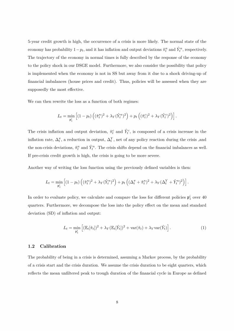
The loss function used to evaluate LAW policies is:

Lt = minpi1

[(πt)2 + λY (Yt)2

],

with, πt, being the inflation deviation from steady state (SS), Yt being the output deviation from

SS, and λY being the weight on output. The policymaker chooses policy, pi1, to minimise the

loss, Lt.

Introducing the crisis regime, we consider that when the economy is in a crisis state with

probability pt, it has inflation and output deviations, denoted by πct and Y ct , respectively. The

probability of a crisis depends on the financial imbalances in the economy. More specifically, if5We model policy as an exogenous, unanticipated shock.6Although the average duration of a typical crisis episode is calibrated to be eight quarters to be consistent withthe most empirical evidence, its impact lasts longer due to the scarring effects of financial crises on outputdocumented in the literature.

7

5-year credit growth is high, the occurrence of a crisis is more likely. The normal state of the

economy has probability 1−pt, and it has inflation and output deviations πnt and Y nt , respectively.

The trajectory of the economy in normal times is fully described by the response of the economy

to the policy shock in our DSGE model. Furthermore, we also consider the possibility that policy

is implemented when the economy is not in SS but away from it due to a shock driving-up of

financial imbalances (house prices and credit). Thus, policies will be assessed when they are

supposedly the most effective.

We can then rewrite the loss as a function of both regimes:

Lt = minpi1

[(1− pt)

((πnt )2 + λY (Y n

t )2)

+ pt((πct )2 + λY (Y c

t )2)].

The crisis inflation and output deviation, πct and Y ct , is composed of a crisis increase in the

inflation rate, ∆πt , a reduction in output, ∆Y

t , net of any policy reaction during the crisis ,and

the non-crisis deviations, πnt and Y nt . The crisis shifts depend on the financial imbalances as well.

If pre-crisis credit growth is high, the crisis is going to be more severe.

Another way of writing the loss function using the previously defined variables is then:

Lt = minpi1

[(1− pt)

((πnt )2 + λY (Y n

t )2)

+ pt((∆π

t + πnt )2 + λY (∆Yt + Y n

t )2)].

In order to evaluate policy, we calculate and compare the loss for different policies pi1 over 40

quarters. Furthermore, we decompose the loss into the policy effect on the mean and standard

deviation (SD) of inflation and output:

Lt = minpi1

[(Et[πt])2 + λY (Et[Yt])2 + var(πt) + λY var(Yt)

]. (1)

1.2 Calibration

The probability of being in a crisis is determined, assuming a Markov process, by the probability

of a crisis start and the crisis duration. We assume the crisis duration to be eight quarters, which

reflects the mean unfiltered peak to trough duration of the financial cycle in Europe as defined

8

in Schüler et al. (2015).7

Schularick and Taylor (2012), Jordà et al. (2013), and Mian and Taylor (2021) argue that credit

developments increase both the probability and severity of crises. We also rely on five-year

credit growth as a proxy for both the probability and severity of a crisis, and this choice is

empirically supported by Arbatli-Saxegaard et al. (2020), who find that five-year credit growth

has the most significant effect on downside risks to output growth in Norway. Underlying

the quarterly probability of a crisis start is a logistic function that links the policy impact

via five-year cumulative growth in real household credit to the probability of a crisis start.8

We use an estimated logistic regression for the (quarterly) probability of a crisis start, qt:

qt = 1− 11+exp(4.792−2.232D∆5Y

t ) , on five-year cumulative growth in real household credit, D∆5Yt ,

based on a sample of twenty Organisation for Economic Co-operation and Development (OECD)

countries over the period 1975Q1 - 2014Q2 (Gerdrup et al., 2017a). We also conduct a robustness

check by using an estimated crisis start probability function that depends on five-year cumulative

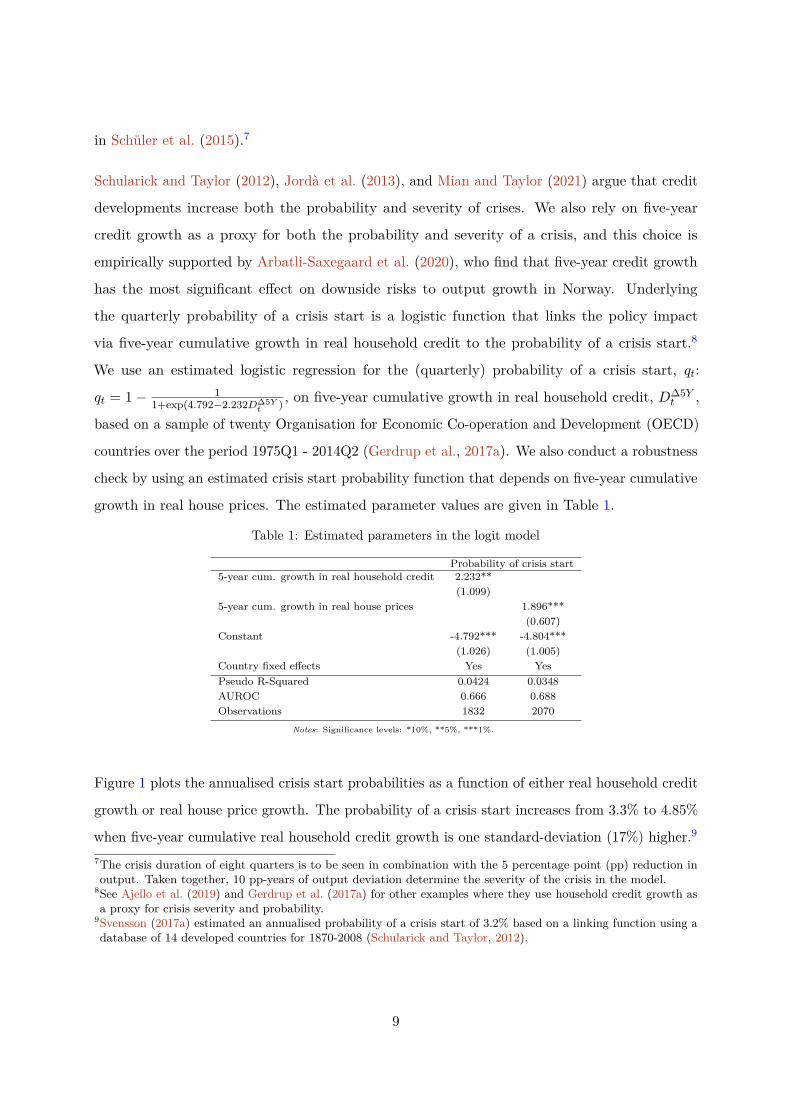
growth in real house prices. The estimated parameter values are given in Table 1.

Table 1: Estimated parameters in the logit model

Probability of crisis start5-year cum. growth in real household credit 2.232**

(1.099)5-year cum. growth in real house prices 1.896***

(0.607)Constant -4.792*** -4.804***

(1.026) (1.005)Country fixed effects Yes YesPseudo R-Squared 0.0424 0.0348AUROC 0.666 0.688Observations 1832 2070

Notes: Significance levels: *10%, **5%, ***1%.

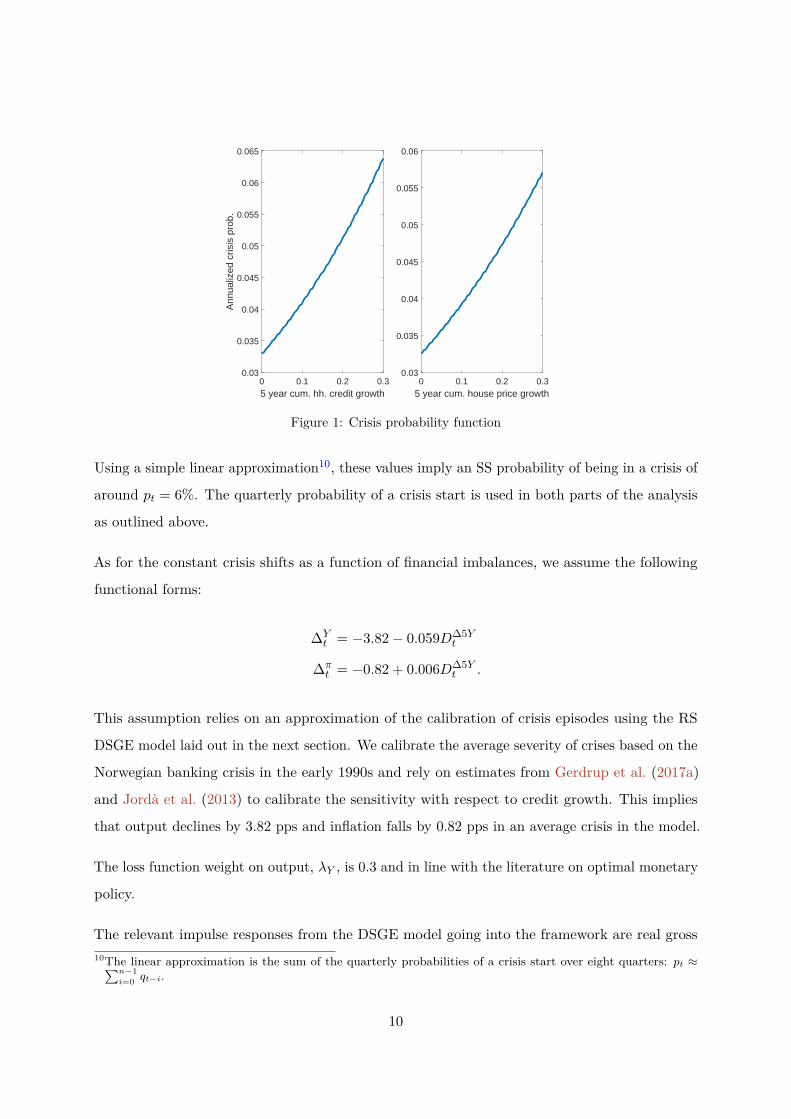
Figure 1 plots the annualised crisis start probabilities as a function of either real household credit

growth or real house price growth. The probability of a crisis start increases from 3.3% to 4.85%

when five-year cumulative real household credit growth is one standard-deviation (17%) higher.9

7The crisis duration of eight quarters is to be seen in combination with the 5 percentage point (pp) reduction inoutput. Taken together, 10 pp-years of output deviation determine the severity of the crisis in the model.

8See Ajello et al. (2019) and Gerdrup et al. (2017a) for other examples where they use household credit growth asa proxy for crisis severity and probability.

9Svensson (2017a) estimated an annualised probability of a crisis start of 3.2% based on a linking function using adatabase of 14 developed countries for 1870-2008 (Schularick and Taylor, 2012).

9

0 0.1 0.2 0.35 year cum. hh. credit growth

0.03

0.035

0.04

0.045

0.05

0.055

0.06

0.065

Ann

ualiz

ed c

risis

pro

b.

0 0.1 0.2 0.35 year cum. house price growth

0.03

0.035

0.04

0.045

0.05

0.055

0.06

Figure 1: Crisis probability function

Using a simple linear approximation10, these values imply an SS probability of being in a crisis of

around pt = 6%. The quarterly probability of a crisis start is used in both parts of the analysis

as outlined above.

As for the constant crisis shifts as a function of financial imbalances, we assume the following

functional forms:

∆Yt = −3.82− 0.059D∆5Y

t

∆πt = −0.82 + 0.006D∆5Y

t .

This assumption relies on an approximation of the calibration of crisis episodes using the RS

DSGE model laid out in the next section. We calibrate the average severity of crises based on the

Norwegian banking crisis in the early 1990s and rely on estimates from Gerdrup et al. (2017a)

and Jordà et al. (2013) to calibrate the sensitivity with respect to credit growth. This implies

that output declines by 3.82 pps and inflation falls by 0.82 pps in an average crisis in the model.

The loss function weight on output, λY , is 0.3 and in line with the literature on optimal monetary

policy.

The relevant impulse responses from the DSGE model going into the framework are real gross10The linear approximation is the sum of the quarterly probabilities of a crisis start over eight quarters: pt ≈∑n−1

i=0 qt−i.

10

domestic product (GDP) and inflation deviation [pp] for the path in normal times, and real

household debt growth [%] for the probability and severity of a crisis.

Last but not least, the baseline scenario without policy is that a shock increases financial

imbalances (house prices and credit). The dynamics of the economy following a shock to housing

preferences can be seen in Figure 2. House prices increase, giving households more collateral and

thus allowing them to take out more debt and triggering a slight boom while inflation is barely

impacted.

1.3 Analysis of monetary policy

We find the optimal degree of LAW by monetary policy by minimising the central bank loss.

We define LAW as the policymaker holding the policy rate at a constant higher level than the

otherwise model-implied optimal policy rate (in the case of the single regime DSGE model

without the possibility of a crisis) for four quarters. If there is no other shock present, Figure 3

shows the trajectory of the economy for a positive degree of LAW.

Inflation [%] Output [%]

5−year credit growth [%] 5−year house price growth [%]

0 10 20 30 40 0 10 20 30 40

0 10 20 30 40 0 10 20 30 40−3

−2

−1

0

1

2

3

0.000

0.025

0.050

0.075

−1

0

1

2

−0.010

−0.005

0.000

0.005

0.010

Figure 2: SS deviations for a shock to housingpreferences

Interest rate gap [%] Output [%]

5−year credit growth [%] Inflation [%]

0 10 20 30 40 0 10 20 30 40

0 10 20 30 40 0 10 20 30 40−0.100

−0.075

−0.050

−0.025

0.000

−0.3

−0.2

−0.1

0.0

−1

0

1

−0.25

0.00

0.25

0.50

0.75

1.00

Figure 3: SS deviations for monetary policy - 1pp increase for 4 quarters

The policymaker holds the policy rate 1 pp above the SS level for 4 quarters, which depresses

output, inflation, and credit growth simultaneously.11 The reduction in credit growth is beneficial

due to the implied lower crisis probability (see Figure 4) and severity. Yet, the reduced output

and inflation is a cost to the economy independent of the crisis occurring or not.11We construct Figure 3 by computing the trajectories of inflation, output and 5-year credit growth in response tomonetary policy shocks that are extracted to obtain a conditional forecast of the policy rate being fixed for thefirst four quarters followed by endogenous monetary policy rule.

11

Probability of crisis start [%]

0 20 40 60 80

0.79

0.80

0.81

0.82

0.83

0.84

Figure 4: Probability of a crisis start over 80 quarters for monetary policy - 1 pp increase for 4quarters

Figure 5 shows the cumulated loss over 40 quarters with varying degrees of LAW by monetary

policy coinciding with a shock to housing preferences that generate a credit and house price

boom. The lowest loss and thereby the optimal degree of LAW is for the policymaker to reduce

the policy rate by about 0.5 pps for 4 quarters. In other words, if the policymaker acts at the

same time that a shock stimulates house prices and drives credit growth, he should lean with the

wind and further support the economy instead of leaning against the wind. On the one hand,

leaning with the wind means the economy benefits from the additional stimulus in normal times

and also going into the crisis. On the other hand, it means that asset prices are further inflated,

credit growth is even stronger and the probability and severity of a crisis are even higher. Taking

both effects together, this appears to be the optimal strategy.

We can conduct the same exercise without the coinciding shock driving up house prices. This

scenario would represent an unmotivated “naive” policy action. Figure 6 shows that the optimal

degree of LAW is even more negative in this case. In other words, if there is no buildup of

financial imbalances to lean against, then it is even less advisable to do so.

9.0

9.1

9.2

9.3

9.4

9.5

−1.0 −0.5 0.0 0.5 1.0Degree of leaning [policy rate x pp above SS for 4 quarters]

Cum

ulat

ed L

oss

over

40

quar

ters

Figure 5: Loss and degree of LAW forcoinciding shock to housing preferences

9.2

9.4

9.6

−1.0 −0.5 0.0 0.5 1.0Degree of leaning [policy rate x pp above SS for 4 quarters]

Cum

ulat

ed L

oss

over

40

quar

ters

Figure 6: Loss and degree of LAW in SS

12

Figures 7 and 8 show the loss decomposed into the means and SD’s of inflation and output (see

Equation (1)) for the case of LAW coinciding with higher credit and house prices. Figure 7 shows

that the higher the degree of LAW, the lower the mean output level and the mean inflation rate

are. In particular, the impact on the mean output level increases the loss substantially. Figure 8

shows that the SD of inflation is lowest when there is no leaning either way, while for output the

lowest SD is for a positive degree of LAW. Combined with the fact that the weight on inflation

in the loss function is nearly three times as much as the weight on output, we can conclude that

the loss due to the depressed mean of output contributes the most to the cost of LAW.

−0.25

−0.20

−0.15

−0.10

−0.05

0.00

−1.0 −0.5 0.0 0.5 1.0Degree of leaning [policy rate x pp above SS for 4 quarters]

Mea

n ga

p ov

er 4

0 qu

arte

rs [%

]

Inflation Output

Figure 7: Mean gaps under different degrees ofLAW

0.05

0.10

0.15

−1.0 −0.5 0.0 0.5 1.0Degree of leaning [policy rate x pp above SS for 4 quarters]

Sta

ndar

d de

viat

ion

over

40

quar

ters

Inflation Output

Figure 8: SDs under different degrees of LAW

1.3.1 Analysis without hybrid expectations

One of the criticisms laid out in BIS (2016) of the framework proposed in Svensson (2017a)

was that it does not take into account the persistence of the financial cycle. A way to include

persistent financial cycles is to use hybrid expectations in house prices (Gelain et al., 2013). In

fact, the DSGE model underlying our analysis features hybrid expectations in house prices. The

inclusion is motivated by the findings of Gelain et al. (2013) that hybrid expectations enable the

model to better capture the long cycles in house prices and household debt observed in the data.

In other words, the model exhibits more persistent financial cycles similar to Farhi and Werning

(2021).

Hybrid expectations are modelled as in Gelain et al. (2013). A share bsa of households expects

house prices to follow a moving average process (i.e. partly backward-looking expectations),

13

whereas a share (1− bsa) has rational expectations (in log-gap form):

Et[PHt+1

]= bsaXH

t + (1− bsa)PHt+1 (2)

where denotes gap-form and the moving average process is defined as:

XHt = λsaPHt−1 + (1− λsa)XH

t−1. (3)

Figure 9 shows that under rational expectations, 5-year credit growth is less persistent and

reacts much less to the the same 1 pp increase in the policy rate for four quarters. In other

words, the variable linked to the benefits of LAW does not move as much while the costs in terms

of output and inflation are about the same.

The optimal degree of LAW under rational expectations can be found in Figure 10. Also in this

case, LAW is not advisable. However, compared to the case of hybrid expectations, the degree of

leaning with the wind is lower. LAW has a weaker impact on the economy and on debt levels

compared to the case with hybrid expectations.

Interest rate gap [%] Output [%]

5−year credit growth [%] Inflation [%]

0 10 20 30 40 0 10 20 30 40

0 10 20 30 40 0 10 20 30 40

−0.09

−0.06

−0.03

0.00

−0.2

−0.1

0.0

−0.2

−0.1

0.0

0.1

0.2

0.00

0.25

0.50

0.75

1.00

Figure 9: SS deviations for monetary policywithout hybrid expectations - 1 pp increase for 4

quarters

9.1

9.2

9.3

9.4

−1.0 −0.5 0.0 0.5 1.0Degree of leaning [policy rate x pp above SS for 4 quarters]

Cum

ulat

ed L

oss

over

40

quar

ters

Figure 10: Loss and degree of LAW formonetary policy without hybrid expectationsand a coinciding shock to housing preferences

These findings are in line with the findings in Svensson (2017a), which also uses a DSGE model

without persistent financial cycles. Another way to capture the effects of persistent financial

cycles is to use a linking function based on early-warning models for the probability of a crisis

start that captures the gradual building up of imbalances (Kockerols and Kok, 2021). Nonetheless,

14

this approach with a calibration for the euro area also reaches the conclusion that LAW is not

beneficial.

2 Optimal systematic LAW in a regime-switching DSGE model

Having analysed nonsystematic LAW policy, we now turn our attention to systematic LAW

policy. The main components of the model are the same as for nonsystematic policy, but now we

conduct the experiment within the endogenous RS-DSGE framework with an ELB for the policy

rate, financial crises and asymmetric LAW in order to capture the effect of the changed decision

rules of economic agents in the model as a result of systematic LAW policies. We further assume

that the policymaker is aware of the possibility of a crisis and of how his actions can change the

probability of the economy entering a crisis. The other economic agents underestimate the crisis

probability.

We first describe what we mean by optimal monetary policy in the model, how we model a

financial crisis, how we model the ELB and search for the optimal LAW policies given the

possibility of crisis, and describe its quantitative properties.12 We then present the main results

of our analysis of LAW policies. We show that two model ingredients prove to be crucial for

the optimality of LAW among the many alternatives we considered in the section on robustness

checks, B. The first one is the persistence of financial cycles while the second one is the response

to output in the monetary policy rule. Finally, we evaluate LAW by altering long-run capital

requirements in this framework.

2.1 Optimal monetary policy in normal times: the “mimicking” policy rule

The DSGE model we use in this work, NEMO, has been extensively used for monetary policy

analyses and forecasting in Norway and it is solved under optimal monetary policy with discretion.

However, when we conduct the analysis on LAW by monetary and macroprudential policy, we

use a “mimicking” policy rule that replicates the empirical properties of the baseline model

without the possibility of crises under optimal policy. The reason is that solving optimal policy

is computationally expensive in the endogenous RS version of a large-scale DSGE model such

as NEMO with eight different regimes. We show below that the mimicking policy rule we use12For details about the baseline DSGE model underlying the analysis in this section and in Section 1 we refer thereader to Appendix D.

15

provides a very good approximation to actual model dynamics under optimal policy.

The mimicking rule is an interest-rate feedback rule and a function of a number of variables such

as price inflation, wage inflation, output, the real exchange rate, the money market premium and

the lagged value of the nominal policy rate.13 We employ an impulse response matching procedure

to find the mimicking rule that replicates optimal policy. In particular, we find the response

coefficients in the mimicking rule by matching impulse responses of a subset of variables14 to a

subset of shocks15 under optimal policy for 10 periods.

The simple rule and the resulting response coefficients from impulse response matching are

displayed in equation (4) and Table 2, respectively.16 The variables in the mimicking rule

include (in gap terms) annual inflation (πt), expected annual inflation one quarter ahead (πt+1),

wage inflation (πWt ), output (YNAT,t), the real exchange rate (St), the money market premium

(Zprem,t), the foreign monetary policy rate (R∗t ), a monetary policy shock (ZRN3M,t) and a lagged

term. When estimating the mimicking rule, we put higher weights on matching the responses on

output, inflation and the policy rate to a monetary policy shock and an international oil price

shock.RP,t = ωRRP,t−1 + (1− ωR)

(ωP πt + ωP1πt+1 + ωW π

Wt + ωY YNAT,t

+ωSSt + ωPREM Zprem,t + ωRF R∗t

)+ ZRN3M,t.

(4)

Table 2: Estimated mimicking rule

ωR ωP ωP1 ωW ωY ωS ωPREM ωRF0.74 0 1.45 0.82 0.30 0.02 -0.25 0

Note: Estimation results from an estimated policy rule that mimics optimal policy. Theestimation hits the boundaries for ωP and ωRF .

Figure 11 shows impulse responses to a monetary policy shock under optimal policy and

the mimicking rule. The latter replicates arguably well the optimal monetary policy under13The mimicking rule was originally developed for estimation purposes since using optimal policy in the estimationprocess would be too time-consuming and computationally demanding.

14The evaluated variables are household credit, corporate credit, inflation, business investment, housing investment,oil investment, hours worked, imports, exports, output, house prices, the exchange rate, real wages and thepolicy rate.

15The shocks that are used in the impulse response matching comprise the monetary policy shock, money marketpremium shock, oil price shock, price markup shock, trading partner demand shock, risk premium shock, wagemarkup shock, labour supply shock, foreign marginal cost shock and foreign interest rate shock.

16The estimated mimicking rule in this paper slightly deviates from the one in Kravik and Mimir (2019) since weallow for a negative response to the money market premium in the current formulation.

16

discretion.17

Household credit gap (in percent)

5 10 15 20 25 30 35 40

0 0Corporate credit gap (in percent)

5 10 15 20 25 30 35 40

0 0

Consumption gap (in percent)

5 10 15 20 25 30 35 40

0 0

Imported inflation gap (in quarterly ppts.)

5 10 15 20 25 30 35 40

0 0

Domestic inflation gap (in quarterly ppts.)

5 10 15 20 25 30 35 40

0 0

Wage inflation gap (in quarterly ppts.)

5 10 15 20 25 30 35 40

0 0

Inflation gap (in annual ppts.)

5 10 15 20 25 30 35 40

0 0

Corporate investment gap (in percent)

5 10 15 20 25 30 35 40

0 0

Housing investment gap (in percent)

5 10 15 20 25 30 35 40

0 0

Hours gap (in percent)

5 10 15 20 25 30 35 40

0 0

Oil investment gap (in percent)

5 10 15 20 25 30 35 40

0

0.5

0

0.5Import gap (in percent)

5 10 15 20 25 30 35 40

0

0.1

0

0.1

Intermediate export gap (in percent)

5 10 15 20 25 30 35 40

0

0.1

0

0.1Mainland output gap (in percent)

5 10 15 20 25 30 35 40

0 0

Real house price gap (in percent)

5 10 15 20 25 30 35 40

0

0.5

0

0.5

Real exchange rate gap (in percent)

5 10 15 20 25 30 35 40

0 0

Real wage gap (in percent)

5 10 15 20 25 30 35 40

0

0.1

0

0.1Policy rate gap (in annualized ppts.)

5 10 15 20 25 30 35 40

0

0.5

1

0

0.5

1

OPTIMAL POLICY MIMICKING POLICY RULE

Figure 11: Impulse responses after a monetary policy shock under optimal policy and the estimatedmimicking rule

The coefficients in Table 2 show that the estimated mimicking rule puts a relatively high weight

on wage inflation. This finding is consistent with Levin et al. (2006) who find that an interest rule

responding to wage inflation yields a welfare outcome that nearly matches that under optimal

policy, as well as Justiniano et al. (2011), who show that output gap stability is consistent with

a significant reduction in the volatility of price and, especially, wage inflation.

2.2 Crisis regime

Normal and crisis times are governed by a Markov process in the model. The probability and

severity of crises are driven by household credit developments as in Section 1.2. Contrary to17We also obtain similar results for the other structural shocks that are used in the impulse response matchingexercise.

17

the modelling of crises under nonsystematic LAW policy in the previous section, the crisis path

under systematic LAW policy is dynamic rather than a simple constant shift of the economy as

in Section 1. It is driven by a combination of shocks scaled by the size of financial imbalances

and structural changes in the housing and financial sector.

2.2.1 The severity of a crisis

The crisis regime is calibrated to obtain a financial crisis that is similar to the macroeconomic

scenario used in macroprudential stress-testing exercises at central banks. We replicate the

dynamic paths of several macroeconomic and financial aggregates that are expected to take

place in a typical domestic financial recession. Furthermore, crisis episodes are also characterised

by structural changes in the domestic economy: (i) money market and external risk premiums

become more sensitive to changes in banks’ capital positions; (ii) risk weights on household and

business loans increase, and (iii) house prices and housing investment become more volatile.

We achieve this by translating the narrative to shocks hitting the economy in a crisis. Shocks to

bank capital are used to capture credit supply shocks motivated by loan losses and asset write-

downs observed during financial crises. Credit demand shocks, modelled using shocks to housing

preferences, are motivated by the decline in household credit demand due to the fall in house

prices and hence collateral values of houses. Shocks to domestic consumption demand are used to

represent aggregate demand shocks. Last but not least, business investment-specific technology

shocks replicate aggregate supply shocks motivated by a productivity slowdown observed during

financial crises. Furthermore, we also consider the possibility that the Countercyclical Capital

Buffer (CCyB) is fully released in a crisis (set from 2.5% to 0%). The release of the CCyB reduces

crisis severity by increasing banks’ capacity to extend credit to households and non-financial

firms during downturns.

We assume that financial imbalances accumulated before the crisis amplified crisis shocks. The

latter gradually unravels during the crisis regime. Therefore, the shock innovations for the

structural shock processes outlined above consist of typical business cycle innovations and a crisis

innovation following Gerdrup et al. (2017a):

log(Zit) = (1− ρZi)log(Ziss) + ρZilog(Zit−1) + εiZ,t − βZ

ilog(crisist) (5)

18

where Zit is a generic business cycle shock, Ziss is the SS level of the shock process, ρZ is the

persistence parameter, εiZ,t is the shock innovation, βZi is a scale factor for each crisis shock

innovation, crisist is a shock, which is only active once the economy enters a crisis, and follows

log(crisist) = ρcrisislog(crisist−1) + Ωκt (6)

where ρcrisis is the persistence of the crisis shock. Ω is a crisis indicator variable. In normal

times we have Ω = 0, and in crisis times Ω = 1. κt is a variable that captures the severity of

crises. The severity, κt, is a function of credit imbalances, B5yh,t:

κt = (1− Ω)(γ + γBhB5yh,t) + ρκΩκt−1 (7)

where B5yh,t is five-year cumulative real household credit growth, γ governs a constant effect of

credit imbalances on the respective crisis shock and γBh governs the effect of the initial level

of credit imbalances on crisis severity. βZi , ρcrisis, γ, and γBh are calibrated to match the

asymmetric effect of a crisis on each crisis shock, the persistence of crisis shocks, the baseline

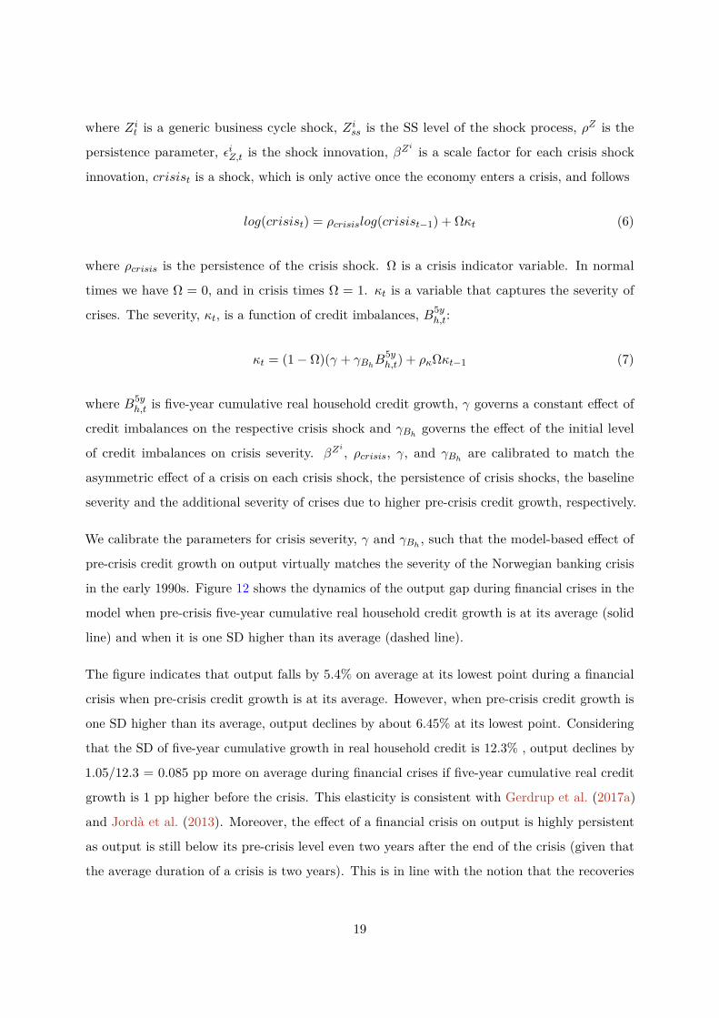
severity and the additional severity of crises due to higher pre-crisis credit growth, respectively.

We calibrate the parameters for crisis severity, γ and γBh , such that the model-based effect of

pre-crisis credit growth on output virtually matches the severity of the Norwegian banking crisis

in the early 1990s. Figure 12 shows the dynamics of the output gap during financial crises in the

model when pre-crisis five-year cumulative real household credit growth is at its average (solid

line) and when it is one SD higher than its average (dashed line).

The figure indicates that output falls by 5.4% on average at its lowest point during a financial

crisis when pre-crisis credit growth is at its average. However, when pre-crisis credit growth is

one SD higher than its average, output declines by about 6.45% at its lowest point. Considering

that the SD of five-year cumulative growth in real household credit is 12.3% , output declines by

1.05/12.3 = 0.085 pp more on average during financial crises if five-year cumulative real credit

growth is 1 pp higher before the crisis. This elasticity is consistent with Gerdrup et al. (2017a)

and Jordà et al. (2013). Moreover, the effect of a financial crisis on output is highly persistent

as output is still below its pre-crisis level even two years after the end of the crisis (given that

the average duration of a crisis is two years). This is in line with the notion that the recoveries

19

0 2 4 6 8 10 12 14 16Number of quarters from start of crisis

-7

-6

-5

-4

-3

-2

-1

Per

cent

age

poin

ts

Average depth of crisisEffect of 1 std. higher pre-crisis 5-year credit growth

Figure 12: Dynamics of output gap during financial crises

after financial crises are very slow due to the scarring effects of these types of crises on the real

economy.

While the calibration is similar between the approach taken here and in the previous section for

the probability of a crisis, the paths for the severity of a crisis differ. In the case of nonsystematic

LAW, the economy is expected to contract by about 10%, which is about the same maximum

decline in output obtained in the model with systematic policy. The less severe crisis in the case

of systematic policy diminishes the attractiveness of LAW policies because the benefits of LAW

that will be reaped in the case of a crisis are not as large given the convex loss function.

2.2.2 The probability of a crisis start

We rely on the linking function outlined in Section 1.2 with one important modification. When

we simulate the model, we truncate the probability of a crisis such that the economy does not

enter into a crisis when five-year cumulative credit growth (or house price growth) is below

zero.18 We also conduct a robustness check using five-year cumulative real house price growth as18In order to match the estimated SS annual probability of a crisis start of 3.3% in our model on average whiletruncating the probability of a crisis, we re-calibrated the constant term in the estimated logit function that isused in the model and we set it to -4.25.

20

an input into the crisis probability function.

The setup of the probability of a crisis for optimal systematic and for nonsystematic policy are

virtually identical and imply an annualised probability of a crisis start of 3.3% and a probability

of being in a crisis of 7%.

2.3 Optimal simple rule through the cycle, ELB on nominal interest rates

and asymmetric LAW

We assume that the central bank has the following operational loss function when setting the

policy rate:

minRP,t

Et∞∑t=s

βt−s[(πt − π∗)2 + λyy

2t + λdr (4RP,t)2

](8)

where β is the household’s discount factor, πt is the inflation rate, π∗ is the inflation target,

yt is the output gap, 4RP,t is the change in the nominal policy rate, λy is the weight on the

output gap, and λdr is the weight on the change in the nominal interest rate.19 Note that the

loss function presented here includes the interest rate while the loss function in Section 1 does

not. This difference is negligible due to the low variability and weight on the interest rate.

Monetary policy rules we consider incorporate the possibility of an ELB and asymmetric LAW.

The ELB is modelled as a regime switch where the switching parameter is governed by a Markov

chain (Ωzlb) with two regimes, a positive policy rate regime and an ELB regime, given by

RP,t = (1− Ωzlb)RshadowP,t + ΩzlbRzlbP,t (9)

where RP,t is the actual policy rate, RshadowP,t is the shadow rate given by the estimated mimicking

rule modified to respond to real house prices as well and RzlbP,t is the ELB interest rate, which we

set to 1.

The probability of switching to an ELB regime is a function of the distance between the shadow

policy rate and the policy rate at the ELB and is given by a step function. When the shadow

policy rate is greater than the policy rate at ELB, the probability of switching is zero and equal

to one otherwise. The way we implement ELB resembles that in Aruoba et al. (2017). When the19λy = 0.30 and λdr = 0.40 are the corresponding weights in the loss function. The optimal policy weights in theoperational loss function calibrated to achieve reasonable responses and trade-offs between, e.g. output andinflation stabilisation, when the economy is hit by different shocks.

21

economy switches to an ELB regime, we assume that the new regime has a zero SS inflation rate

compared to a 2% SS inflation rate in a positive policy rate regime.20 We choose to model the

ELB in this way since we think it is empirically consistent with the persistently lower inflation

observed in most major advanced economies after the GFC. We also find it reasonable to assume

lower SS inflation in the ELB since we do not consider unconventional monetary policy within

the model and the central bank has no other tools to raise the inflation rate in this deflationary

state of the world.

We evaluate systematic LAW by augmenting the mimicking rule to include a response to the

real house price gap. The reason why we use real house prices is based on Svensson (2013),

who argues that the stock of debt (especially mortgages with long maturities) has substantial

inertia and monetary policy has little effect on it whereas it has more effect on the growth of

house prices. However, we also conduct a robustness check using real household credit gap in the

mimicking rule.

RshadowP,t = ωRRshadowP,t−1 + (1− ωR)

(ωP πt + ωP1πt+1 + ωW π

Wt +

ωY YNAT,t + ωSSt + ωPREM Zprem,t + ωRF R∗t

)+ (1− Ω)1

Ph,t>0ωPH PH,t + ZRN3M,t

(10)

where RshadowP,t denotes the shadow rate gap, and 1Ph,t>0 is an indicator function which reflects

asymmetric LAW.

We consider an asymmetric interest rate rule that responds to a real house price gap only when

the gap is positive following Gerdrup et al. (2017a). The motivation behind it is that LAW

policies are usually implemented when financial imbalances are high. Monetary policy is tighter

than what is consistent with inflation and output stability when credit imbalances are higher

than a certain threshold value, which is assumed to be zero.21 We also assume that monetary

policy does not respond to house prices during crises. Asymmetric LAW is implemented as20Implementing an ELB in a DSGE model introduces an interesting non-linear problem in an open economyframework due to the asymmetry it induces in interest rates in the domestic economy and abroad. In particular,a fixed nominal interest rate (of zero) violates the uncovered interest parity (UIP) condition in SS that thedomestic real interest rate must be identical to the real interest rate abroad (conditioned on a zero risk premiumin SS). Instead of having a lower SS inflation rate in the ELB regime, two alternative ways of solving thischallenge include either a) to introduce a non-zero risk premium in SS, or b) also letting the nominal interestrate abroad go to zero in the SS. Our choice of implementing the ELB here does not drive our results. Binningand Maih (2016) discuss various ways of implementing an ELB within a simple closed-economy RS DSGE model.

21We also conduct robustness checks by changing the threshold value of reacting to a real house price gap in themimicking rule from zero to positive values but it does not change the main results of the paper.

22

another regime, with the indicator function 1Ph,t>0 governing the Markov process. Note that

this regime switch interacts with the switching parameter Ω for the crisis regime such that LAW

is only relevant when the economy is not in a crisis and the real house price gap is positive.

Overall, the model features eight regimes, each a combination of three two-state Markov chains:

normal vs. crisis times, positive policy rate vs. ELB and no LAW vs. LAW. We then choose

ωPH to minimise the operational loss function defined in equation (8) in the model including all

components mentioned above, holding all other response coefficients fixed at their previously

estimated levels. We only optimise over ωPH since we want our interest rate rule to reflect

the actual monetary policy stance of the central bank and not to deviate too much from its

current inflation and output stabilisation objectives following Gelain et al. (2013) and Gourio

et al. (2018). Moreover, we assume that all the economic agents in the model are aware of the

possibility of switching to the ELB and LAW regimes but they underestimate the probability of

crisis regime, meaning that they attach a zero probability to switching to a crisis regime. The

only exception is the central bank since it is aware of the possibility of crises at all times, and it

decides whether to respond to real house prices to prevent financial crises from happening.

At this stage, it should become clearer that the approach taken here goes beyond the approach

in the first part on multiple fronts. First, policy adheres to an OSR. Second, we consider the

possibility of the ELB and thereby make the effectiveness of LAW state-dependent. Second,

the asymmetric policy rule is an important component, which is impossible to capture in the

framework of the first part of the paper. Last but not least, the trade-offs between inflation and

output stabilisation are fully incorporated. Furthermore, in Section B, we explore the individual

contributions of asymmetric LAW and the ELB by doing the same analysis without them among

many other robustness checks we consider.

2.4 Quantitative properties of the regime-switching DSGE model

2.4.1 Time spent in different regimes

The benchmark model with the possibility of crises and ELB features four regimes: No crisis-No

ELB, No crisis-ELB, Crisis-No ELB and Crisis-ELB. In order to compute the time spent in each

regime over the business cycle, we simulate the model for 100,000 periods. We find that the

economy spends 72% of the time in No crisis-No ELB regime. The simulations also show that

23

21% of the time is spent in No crisis-ELB regime. This number is close to the unconditional

probability of being in the ELB regime estimated for the U.S. economy by Aruoba et al. (2017).

Moreover, we observe that the economy spends 3% of the time in Crisis-No ELB regime and 4%

of the time in Crisis-ELB regime.

2.4.2 Downside risks to output

-12 -10 -8 -6 -4 -2 0 2 4 6Output gap (%)

0

0.05

0.1

0.15

0.2

0.25

0.3

0.35No-crisisCrisis

Figure 13: Downside risks to GDP:No-Crisis vs. Crisis

0 2 4 6 8 10 12Policy rate (in ann. ppts.)

0

0.05

0.1

0.15

0.2

0.25

0.3

0.35

0.4

0.45No-crisisCrisis

Figure 14: Downside risks to policy rate:No-Crisis vs. Crisis

Figures 13 and 14 show the distributions (kernel densities) of the output gap and policy rate

in the models with and without crisis (solid red and blue lines, respectively). In both models,

the ELB may bind. As expected when using linearisation, the distribution of the output gap

in the model with no-crisis is virtually symmetric around zero, indicating no asymmetric tail

risks either for the upside or for the downside. The left fat tail in the distribution under crisis

displays significant downside risks to GDP while there are no upside risks. This is expected

given the negative asymmetric crisis shocks and RS structural parameters in the housing and

banking sectors. The results are also in line with the Growth-at-Risk (GaR) literature pioneered

by Adrian et al. (2019). They show how current financial conditions can affect downside risks to

future GDP growth. Finally, the distribution of the policy rate in the models with and without

crises shows that the ELB binds more often in the model with crisis due to more downside risks

in inflation and output (see Figure 13).

2.4.3 Dynamics of financial crises

Figure 15 shows the distribution of the behaviour of main macroeconomic and financial variables

when the economy enters into a crisis. We simulate the model for 100,000 periods and collect

the dynamics of the variables of interest in crisis regime. We obtain 836 crisis episodes with an

24

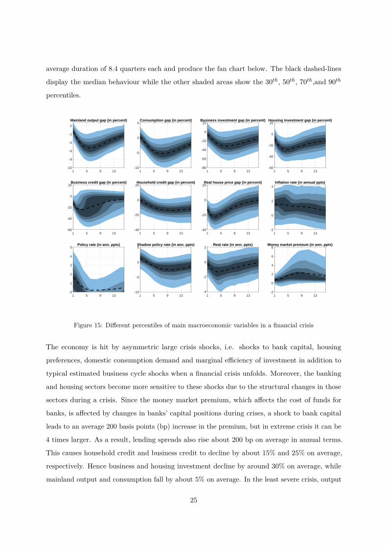
average duration of 8.4 quarters each and produce the fan chart below. The black dashed-lines

display the median behaviour while the other shaded areas show the 30th, 50th, 70th,and 90th

percentiles.

Mainland output gap (in percent)

1 5 9 13-10

-8

-6

-4

-2

0

Consumption gap (in percent)

1 5 9 13-10

-5

0

5Business investment gap (in percent)

1 5 9 13-80

-60

-40

-20

0

20Housing investment gap (in percent)

1 5 9 13-60

-40

-20

0

20

Business credit gap (in percent)

1 5 9 13-60

-40

-20

0

20Household credit gap (in percent)

1 5 9 13-40

-20

0

20Real house price gap (in percent)

1 5 9 13-40

-20

0

20Inflation rate (in annual ppts)

1 5 9 13-2

0

2

4

Policy rate (in ann. ppts)

1 5 9 130

1

2

3

4

5Shadow policy rate (in ann. ppts)

1 5 9 13-10

-5

0

5Real rate (in ann. ppts)

1 5 9 13-4

-2

0

2Money market premium (in ann. ppts)

1 5 9 13-2

0

2

4

6

8

Figure 15: Different percentiles of main macroeconomic variables in a financial crisis

The economy is hit by asymmetric large crisis shocks, i.e. shocks to bank capital, housing

preferences, domestic consumption demand and marginal efficiency of investment in addition to

typical estimated business cycle shocks when a financial crisis unfolds. Moreover, the banking

and housing sectors become more sensitive to these shocks due to the structural changes in those

sectors during a crisis. Since the money market premium, which affects the cost of funds for

banks, is affected by changes in banks’ capital positions during crises, a shock to bank capital

leads to an average 200 basis points (bp) increase in the premium, but in extreme crisis it can be

4 times larger. As a result, lending spreads also rise about 200 bp on average in annual terms.

This causes household credit and business credit to decline by about 15% and 25% on average,

respectively. Hence business and housing investment decline by around 30% on average, while

mainland output and consumption fall by about 5% on average. In the least severe crisis, output

25

falls by about 2% at the peak, while it declines by around 8% in the most severe crisis. The

inflation rate decreases by 1.5 pp to 0.7% on average but there are crisis episodes where inflation

can be negative. The shadow policy rate declines by 3 pp in annualised terms, going into negative

territory. Due to the ELB on the nominal policy rate, the actual rate stays in the positive region,

putting a drag on the economy, which we show in B. In that section, we also present how the

release of the CCyB during a crisis mitigates the adverse effects of crises on macroeconomic and

financial variables.

2.4.4 Model moments under different regimes

Table 3 displays the second moments of some selected model variables, loss values relative to the

benchmark model (the model with crises and ELB imposed), and annualized frequencies of crisis

for the models with crisis and ELB imposed, with crisis, ELB imposed and CCyB relaxed, with

crisis and no-ELB and with no-crisis and ELB imposed under the baseline mimicking policy rule.

Table 3: Model moments with and without crisis under baseline mimicking rule

Moments (%) Crisis (ELB) Crisis (ELB and CCyB released) Crisis (No-ELB) No-crisis (ELB)SD Annual inflation 1.11 1.11 1.14 1.08SD Output gap 1.89 1.84 1.79 1.25SD Interest rate (Ann. %) 1.31 1.31 2.21 1.44SD Real exchange rate 5.34 5.27 5.38 4.97SD Household credit 12.3 12.1 11.9 12.0SD Real house prices 13.2 12.9 12.9 11.9Relative Loss 100 99.7 98.7 96.0Prob. of crisis start (Ann. %) 3.34 3.33 3.27 0.00Notes: Model SDs and the frequency of financial crises are computed from 100,000 simulations. The loss function is

given by equation (8). We take β = 0.99 and the weights on the output gap and the change in the nominal interest rate isλy = 0.30 and λi = 0.40, respectively.

A comparison of the second and the fifth columns shows that incorporating financial crises into

the model increases the volatilities of macroeconomic and financial variables as expected. The

crisis regime has the largest effect on output, house prices and the real exchange rate. The

presence of the ELB in the models with crises increases the volatilities of all variables except

inflation and the real exchange rate. The loss value is also higher when the ELB binds. Moreover,

the CCyB release contributes to more stable output, house prices, household credit and real

exchange rate.

26

2.5 Optimal systematic LAW-type monetary policy under persistent finan-

cial cycles

In this section, we investigate the effect of different degrees of systematic LAW by monetary

policy in the model outlined above. To this end, we run a discrete grid search over the response

coefficient of the real house price gap in the estimated mimicking rule (ωpH in equation (10))

over the interval [-0.02 0.05], using a step-size of 0.0025. We hold all other response coefficients

in the mimicking rule constant at their previous estimated values in the model without the

possibility of crises. Holding the other coefficients constant allows us to compare the outcome for

different degrees of LAW. It would be close to impossible to isolate the effect if all coefficients

were to change. For each of the 29 grid points, we simulate the economy for 100,000 periods. We

evaluate the optimal degree of LAW by minimising the loss function shown in equation (8).

Different values of ωpH translate into different levels of LAW in the monetary policy stance. For

example, ωpH = 0.05 would mean that, all else equal, a positive real house price gap of 10% on

average would increase the annualised policy rate by 200 bp on average. Our grid point step-size

corresponds to 10 bp, given an average positive real house price gap of 10%.

-0.02 0 0.02 0.04

Degree of LAW, pH

100

120

140

160

180

200

220

Rel

ativ

e lo

ss v

alue

Figure 16: Relative loss values for differentdegrees of LAW

-0.02 0 0.02 0.04Degree of LAW,

pH

100

120

140

160

180

200

Rel

ativ

e lo

ss v

alue

Figure 17: Relative loss values for differentdegrees of LAW in the model without crisis

Figure 16 shows the loss values corresponding to different degrees of LAW (different ωpH coefficient

values) relative to the loss in the model without LAW. We obtain the lowest loss value when

ωpH = 0, i.e. no LAW. The loss value substantially increases with a higher degree of LAW.

This result is not trivial because we start from a policy rule mimicking optimal policy in the

single regime case. The addition of 7 more regimes makes it unlikely to be optimal and our

results suggest that contrary to our prior idea, it remains optimal not to lean against the wind

27

even when a crisis and the ELB are included.

Figure 17 shows the relative loss when there is no crisis regime. We still find that LAW is not

optimal. Although the relative loss values are lower overall in the model without the possibility

of crises, as expected, a positive degree of LAW is still not preferred.

Combining these results with the results for nonsystematic LAW policy we can conjecture that

the change in decision rules due to the fact that crisis and the ELB can occur tilts the balance

from LAW not being advisable back to a neutral position. In either of the two cases, any positive

degree of LAW is not advisable.

2.5.1 Understanding the results

We can decompose the central bank loss function into expected gaps and variances of inflation,

output and policy rate changes as follows.

Lt =∞∑t=s

βt−s(

(Et[πt − π∗])2 + λy (Et[yt])2 + λdr (Et[4RP,t])2

+Vart[πt] + λyVart[yt] + λdrVart[4RP,t]) (11)

The first three terms in equation (11) denote the expected gaps of inflation, output and policy

rate changes. The expected central bank loss is higher under larger gaps in these variables. The

last three terms are the variances of inflation, output and policy rate changes. This means that

higher volatilities in these variables lead to greater central bank loss. We evaluate how LAW-type

monetary policy rules change these different components of the central bank loss function.

-0.02 0 0.02 0.04

Degree of LAW, pH

-1

-0.5

0

0.5

Mea

n (%

)

-1

-0.5

0

0.5

Mea

n (%

)

Output gap Inflation gap

Figure 18: Expected gaps under differentdegrees of LAW

-0.02 0 0.02 0.04

Degree of LAW, pH

1

1.2

1.4

1.6

1.8

2

St.d

ev o

f var

iabl

es (

%)

Output gap Inflation (annualized)

Figure 19: SDs under different degrees ofLAW

28

Figure 18 shows how the expected inflation gap and output gap change under different degrees of

leaning. We do not depict the expected change in the policy rate gap since it is relatively small

and will not substantially change the central bank loss. The figure indicates that the expected

inflation gap falls with a higher degree of LAW. The expected output gap also decreases but

only to a limited extent. An increase in the policy rate due to a positive degree of LAW leads

to a decline in both inflation and output, contributing to higher losses in terms of the first two

terms in (11). The figure also shows that when the degree of LAW is zero, the expected inflation

gap is virtually zero while the expected output gap is already negative.22 This results from

the downside risks to output stemming from financial imbalances, which is also depicted in the

left-skewed distribution of output depicted in Figure 14. The results indicate that the gains in

terms of higher output due to lower downside risks under LAW-type monetary policy are not

enough to compensate for the decline in output in normal times due to higher interest rates.

Figure 19 shows how inflation and output volatility change with varying degrees of LAW. Inflation

volatility increases significantly while the output volatility falls only slightly under higher degrees

of leaning. This result stands in contrast to Alpanda and Ueberfeldt (2016), who find that both

output and inflation volatility decrease with positive degrees of LAW. Although LAW policies

reduce the downside risks to the economy, the fall in these risks due to LAW-type monetary

policy is highly limited, resulting in a small reduction in the output volatility. This finding

also indicates that the inflation variability is the main driver of higher losses. To get a deeper

understanding of the results, it is fruitful to study the costs and benefits of leaning separately.

Benefits of LAW The main benefits of leaning potentially involve lower crisis probability and

reduced crisis severity. Figure 20 shows how much time the economy spends in the Crisis-No

ELB, Crisis-ELB, and crisis regimes.

The figure shows that the time the model economy spends in Crisis-No ELB regime declines

under higher degrees of LAW, while the time spent in the Crisis-ELB regime increases. The

increase in time spent in Crisis-ELB regime is due to the fact that higher degrees of LAW lead

to an initially higher interest rate, pushing down inflation and the interest rate with it until it22The effects of crises on inflation are not as clear as their unambiguously adverse impact on output because whileinflation may fall due to lower domestic demand in crises, it may also rise due to the exchange rate depreciationin these episodes. Figure 15 shows that it is equally likely that inflation can be either positive or negative,depending on the strength of these two opposing forces.

29

-0.02 -0.01 0 0.01 0.02 0.03 0.04 0.05Degree of LAW,

pH

0

1

2

3

4

5

6

7

8

Tim

e sp

ent i

n ea

ch r

egim

e (%

)

Crisis-No ZLBCrisis-ZLB

Total time spent in crises

Figure 20: Time spent in crisis regime

reaches the ELB.

The total time spent in crisis regime declines slightly with higher degrees of LAW. For nonsys-

tematic LAW, we also found that the probability of a crisis start moves only to a small extent

and it decreases only slightly on average over a longer term horizon (see Figure 4). Therefore,

we conclude that the additional effect of changed decision rules due to systematic policy does

not substantially change the effect on the probability of a crisis start.

-0.02 -0.01 0 0.01 0.02 0.03 0.04 0.05Degree of LAW,

pH

-0.2

-0.15

-0.1

-0.05

0

0.05

0.1

0.15

0.2

Mea

n of

5y

real

hh.

cre

dit g

row

th g

ap (

%)

Figure 21: Mean of 5-year credit growthgap and degree of LAW in normal times

-0.02 0 0.02 0.04Degree of LAW,

pH

11.5

12

12.5

13

Std

. dev

. of 5

y re

al h

h. c

redi

t gro

wth

(%

)

Figure 22: SD of 5-year credit growth anddegree of LAW in normal times.

Remember that crisis probability depends on pre-crisis 5-year cumulative real household credit

growth. Figures 21 and 22 show how the mean and SD of 5-year cumulative real household credit

growth gap change in normal times as the degree of LAW increases. They indicate that higher

degrees of LAW reduce both the mean and the volatility of financial imbalances measured by

5-year credit growth but the reduction is quite limited. This explains why the probability of

crisis falls only slightly under higher degrees of leaning.

30

Mainland output gap (in percent)

1 3 5 7 9 11 13 15

No-LAW LAW

Figure 23: Average behaviour of output gap in financial crises. With LAW (orange line, ωpH = 0.05) andwithout LAW (blue line, ωpH = 0). Percentage change compared to time of crisis start.

Figure 23 displays the average dynamics of the output gap during financial crises in the model

simulations under no-LAW (blue solid line) and LAW (orange solid line). We choose a response

coefficient of 0.05, which corresponds to a 200 bp higher policy rate on average if the real house

price is 10% higher than its SS value. The figure shows that LAW effectively limits the drop in

the output gap during crises (i.e. output during crisis compared to time of crisis start). Output

falls by 5% after six quarters without LAW while it declines by a little more than 4% with LAW.

Although the average crisis duration is 8.4 quarters, it takes even longer for the output to recover

to its pre-crisis levels under no-LAW due to the longer-lasting effects of crises.

A comparison between systematic and nonsystematic policy is difficult because there is no way

to compare the scale of the respective degrees of LAW under these two policies. However, in

both cases, LAW mitigates the adverse effects of crises on the economy.

Costs of LAW The main costs of LAW-type monetary policy are lower levels of inflation and

output in normal times, higher inflation volatility and a higher likelihood of hitting the ELB.

The latter potentially results from lower average inflation leading to a lower nominal policy rate

in the long-run. It also contributes to higher inflation volatility in the model.

Figures 24 and 25 display the means of inflation rate and output level in normal times for

various degrees of LAW. In the case of nonsystematic policy, we already understood the negative

31

-0.02 0 0.02 0.04

Degree of LAW, pH

0

0.5

1

1.5

2M

ean

infla

tion

rate

(%

)

Figure 24: Inflation in normal times.

-0.02 0 0.02 0.04

Degree of LAW, pH

99.7

99.8

99.9

100

Mea

n ou

tput

leve

l (no

rmal

ized

)

Figure 25: Output in normal times.

marginal contribution of LAW in terms of lower output in normal times. What is different for

systematic LAW is that the effect of LAW on inflation is stronger than the effect of LAW on

output, relative to its respective effect under nonsystematic LAW. The reason is the amplification

of supply shocks over the business cycle under systematic LAW, which we elaborate below.

-0.02 0 0.02 0.04

Degree of LAW, pH

1

1.2

1.4

1.6

1.8

2

Vol

atili

ty o

f inf

latio

n (%

)

Figure 26: SD of inflation in normal times.

-0.02 0 0.02 0.04

Degree of leaning, pH

1

1.2

1.4

1.6

1.8

2

Vol

atili

ty o

f out

put (

%)

Figure 27: SD of output in normal times.

Figures 26 and 27 display the inflation and output volatility for different degrees of LAW in

normal times. As per higher degrees of LAW, the inflation volatility increases substantially while

output volatility falls only marginally. The former significantly contributes to higher loss values,

making the optimal degree of LAW zero.

The decomposition of the effects of LAW on inflation and output volatility into those in normal

times only (see Figures 26 and 27),and those in normal plus crisis times (see Figure 19) shows

that the overall effect is driven by higher inflation volatility in normal times.

Figure 28 shows how the time spent in ELB periods alters under different degrees of LAW. A

higher response coefficient makes the economy more vulnerable to the ELB since it reduces the

32

-0.02 0 0.02 0.04

Degree of LAW, pH

25

30

35

40

45

50

55

Tim

e sp

ent i

n Z

LB r

egim

e (%

)

Figure 28: Time spent in ELB episodes for various degrees of LAW

mean nominal policy rate through lowering the mean inflation rate. The time spent at the ELB

increases from about 28% to nearly 50% under an aggressive LAW policy. A higher probability

of hitting the ELB also contributes to higher inflation volatility, increasing losses further.

In order to get a better understanding of the increase in the inflation volatility due to LAW, we

plot the impulse responses to one SD wage markup and import demand shocks in Figures 29

and 30. These two shocks explain significant fractions of the variations in inflation and output

over the business cycle, respectively. The impulse responses belong to normal times since the

economy spends 76% of the time there.

Under the baseline mimicking policy rule, a negative wage markup shock lowers the market

power of employees and leads to workers being able to exercise less market power generating

downward pressure on wages. The drop in wages causes firms’ marginal costs and prices to

fall. In response to the decline in inflation, the central bank lowers the short-term policy rate.

Despite a temporary decrease in real wages, consumption increases due to lower interest rates.

The latter also causes investment expenditures to go up, increasing aggregate demand. The drop

in the policy rate also generates a real exchange rate depreciation. This results in higher export

volumes. Although the real exchange rate depreciation is expected to decrease imports, higher

consumption demand dominates this effect and leads to higher imports. Credit and house prices

increase alongside the overall favourable macroeconomic environment.

As expected, the LAW-type policy rule dampens real house prices compared with the baseline

mimicking rule. This provides less collateral value for households and hence dampens the increase

in household credit and in consumption. It also prevents both business and housing investment

33

from rising as much as is the case under the baseline policy rule. Therefore, the increase in

output is not as strong. However, this restraining effect on domestic demand of LAW policies

also results in more negative responses in inflation, and hence worsens the trade-off between

inflation and output stabilisation. When we search for the optimal LAW policy, this trade-off is

resolved in favour of not leaning neither way. A similar line of reasoning also applies under the

import demand shock, where the increase in the inflation rate under LAW is more pronounced

compared with very limited output stabilisation.

2.6 Optimal LAW-type monetary policy under less persistent financial cycles

In the following, we redo the previous experiment but this time with rational expectations in

house prices (by setting bsa = 0 in equation (2)). We first estimate the mimicking rule in the

baseline constant-parameter version of NEMO with rational expectations in house prices. We

then search for the optimal response coefficient to real house prices in the RS version of the

model with the same rational expectations by holding all other response coefficients fixed at their

previously estimated levels as we did in the previous section.

Figure 31 displays the relative loss values for various degrees of LAW in the model without

hybrid expectations in house prices. We obtain the lowest value when the response coefficient

to real house prices is 0.015, meaning that the optimal LAW policy is to keep the policy rate

60 bp higher on average when real house prices are 10% higher on average than their long-run

value. Figure 32 shows the relative loss in the model without crisis. LAW is optimal even if no

crisis can occur but given the ELB and asymmetric LAW. This result is in line with studies of

model economies with normal times only such as Gambacorta and Signoretti (2014) and Cúrdia

and Woodford (2016), but we can go further. The optimal degree of LAW is slightly lower if no

crisis is possible compared to the case with crisis. This means that in crisis times an even higher

response coefficient to house prices is optimal, and the dynamics in crisis times contribute more

to the overall result under rational house price expectations.

This result is in line with the findings in other studies of LAW using systematic policy and

less persistent financial cycles (see e.g. Filardo and Rungcharoenkitkul (2016) and Gerdrup

et al. (2017a)). The results from the nonsystematic case combined with these results allow us to

conclude that the changed decision rules under less persistent financial cycles tilt the balance

more in favour of LAW.

34

5 10 15 20 25 30 35 400

0.01

0.02

0.03

0.04

0.05

Consumption (%)

5 10 15 20 25 30 35 400

0.05

0.1

0.15

Business investment (%)

5 10 15 20 25 30 35 400

0.1

0.2

0.3

Housing investment (%)

5 10 15 20 25 30 35 40

0

0.2

0.4

Oil investment (%)

5 10 15 20 25 30 35 40

0

0.02

0.04

0.06

Imports (%)

5 10 15 20 25 30 35 40-0.04

-0.02

0

0.02

0.04

0.06

Exports (%)

5 10 15 20 25 30 35 400

0.02

0.04

0.06

0.08

0.1

Mainland output (%)

5 10 15 20 25 30 35 40

-0.05

-0.04

-0.03

-0.02

-0.01

0

Imported inflation (quarterly ppts.)

5 10 15 20 25 30 35 40

-0.05

-0.04

-0.03

-0.02

-0.01

0

Domestic inflation (quarterly ppts.)

5 10 15 20 25 30 35 40

-0.2

-0.15

-0.1

-0.05

0

Aggregate inflation (annual ppts.)

5 10 15 20 25 30 35 400

0.1

0.2

0.3

Real house prices (%)

5 10 15 20 25 30 35 40

-0.05

0

0.05

0.1

0.15Real exchange rate (%)

5 10 15 20 25 30 35 400

0.1

0.2

0.3

0.4

Real household credit (%)

5 10 15 20 25 30 35 40

0

0.05

0.1

Real business credit (%)

5 10 15 20 25 30 35 40

-0.1

-0.05

0

Foreign debt by banks (%)

5 10 15 20 25 30 35 40

-0.25

-0.2

-0.15

-0.1

-0.05

0

Policy rate (annual ppts.)

Hybrid Exp.Hybrid Exp. and LAW

Figure 29: Impulse responses after a one SD wage markup shock with and without LAW under hybridexpectations in house prices

10 20 30 40

-0.1

-0.05

0

Consumption (%)

10 20 30 40

-0.2

-0.1

0

0.1

0.2Business investment (%)

10 20 30 40

0

0.2

0.4

Housing investment (%)

10 20 30 400

0.2

0.4

Oil investment (%)

10 20 30 40

0

0.2

0.4

0.6

0.8Imports (%)

10 20 30 400

0.05

0.1

0.15

Exports (%)

10 20 30 40

-0.3

-0.2

-0.1

0Mainland output (%)

10 20 30 400

0.01

0.02

0.03

0.04

Imported inflation (quarterly ppts.)

10 20 30 40

0

0.01

0.02

0.03Domestic inflation (quarterly ppts.)

10 20 30 400

0.05

0.1Aggregate inflation (annual ppts.)

10 20 30 40

0

0.2

0.4

Real house prices (%)

10 20 30 400

0.2

0.4

Real exchange rate (%)

10 20 30 40

-0.2

-0.1

0

0.1

0.2

Real household credit (%)

10 20 30 40

-0.05

0

0.05

0.1

0.15

Real business credit (%)

10 20 30 400

0.1

0.2

0.3

0.4Foreign debt by banks (%)

10 20 30 40

-0.1

-0.05

0

0.05

0.1Policy rate (annual ppts.)

Hybrid Exp.Hybrid Exp. and LAW

Figure 30: Impulse responses after a one SD import demand shock with and without LAW under hybridexpectations in house prices

35

-0.02 0 0.02 0.04Degree of LAW,

pH

99

99.5

100

100.5

101

101.5

102R

elat

ive

loss

val

ue

Figure 31: Relative loss values for differentdegrees of LAW under rational house price

expectations

-0.02 0 0.02 0.04Degree of LAW,

pH

99

99.5

100

100.5

101

101.5

102

Rel

ativ

e lo

ss v

alue

Figure 32: Relative loss values for differentdegrees of LAW under rational house price

expectations and without crisis

-0.02 0 0.02 0.04Degree of LAW,

pH

-0.5

0

0.5

Mea

n (%

)

-0.5

0

0.5

Mea

n (%

)

Output gap Inflation gap

Figure 33: Expected gaps under differentdegrees of LAW and rational house price

expectations

-0.02 0 0.02 0.04Degree of LAW,

pH

1.35

1.4

1.45

1.5S

td. d

ev. o

f out

put (

%)

0.85

0.9

0.95

Std

. dev

. of i

nfla

tion

(%)Output gap Inflation (annualized)

Figure 34: SDs under different degrees ofLAW and rational house price expectations

Figure 33 shows that the expected gaps of inflation and output for higher degrees of LAW

both fall but the reduction in the expected inflation gap is much lower compared to the model

with hybrid expectations. Since the loss is a function of the squared mean deviations, the loss

contribution from mean output increases with a higher response coefficient and the minimum

loss contribution for mean inflation is around a response coefficient of 0.05. Figure 34 indicates

that the volatility of inflation falls while that of output increases. This shows a trade-off between

inflation and output stabilisation in the opposite direction of the previous section where inflation

volatility increases while output volatility falls under higher degrees of leaning.

This result highlights an interesting trade-off and a potential policy lesson for central banks.

Trying to mitigate persistent financial cycles by implementing systematic monetary policy leads to

higher inflation volatility, making the LAW-type policies not advisable. Addressing the build up

of financial stability risks by nonsystematic LAW is not advisable irrespective of the assumptions

36

about the persistence of financial cycles. When considering policy options, policymakers should

consider their view on the extent to which policy is systematic and how persistent financial

cycles are. Only in the case of less persistent financial cycles and systematic policy, would it be

advisable to use LAW policies.

We also conduct impulse response analyses, as in the previous section, to understand why the

absence of hybrid expectations in house prices overturns the main results about optimal LAW

policy. Figures 35 and 36 show the impulse responses after one SD positive wage markup and

import demand shocks with and without LAW under rational expectations in house prices. The

results indicate that the trade-off between inflation and output stabilisation is not as pronounced

as in the model with hybrid expectations or persistent financial cycles. Especially under wage

markup and import demand shocks, the volatility of inflation is not amplified to the same extent

as in the previous section under the same degree of LAW. Hence, the trade-off is resolved in

favour of a positive optimal LAW response coefficient.

2.7 LAW by macroprudential policy: Optimal long-run capital requirements

In this section, we study optimal LAW-type macroprudential policy in the form of optimal

long-run bank capital regulation that minimises the central bank loss23. Since we would like

to evaluate the effects of macroprudential policy in isolation, we use the baseline estimated

mimicking rule that does not respond to real house prices. We also use the same central bank

loss function that reflects the same preferences of inflation and output stabilisation as in the

previous section. We do not consider an additional financial stability mandate since we would

like to conduct a comparable policy experiment to the one above regarding monetary policy.

In order to find the optimal bank capital regulation in normal times, we conduct a grid search

over the different values of SS capital requirements from 11.3% to 18.2% with equally-sized grid

points of 0.5%. We then investigate how long-run bank capital requirements affect the benefits

and costs of LAW.

Figure 37 displays the relative central bank loss values with respect to the level of bank capital

requirements. The results suggest that losses fall with higher bank capital requirements in normal23We also investigate the optimal time-varying CCyB rules that respond to real house prices or real householdcredit using the same central bank loss function as in the monetary policy experiment. The rules we studyfluctuate around a long-run CCyB value of 2.5%. We find that although higher degrees of LAW by usingtime-varying CCyB lead to lower loss values, the reduction is negligible.

37

5 10 15 20 25 30 35 400

0.02

0.04

0.06

Consumption (%)

5 10 15 20 25 30 35 400

0.1

0.2

0.3

Business investment (%)

5 10 15 20 25 30 35 400

0.05

0.1

0.15Housing investment (%)

5 10 15 20 25 30 35 40

0

0.2

0.4

0.6Oil investment (%)

5 10 15 20 25 30 35 400

0.02

0.04

0.06

Imports (%)

5 10 15 20 25 30 35 40

0

0.05

0.1Exports (%)

5 10 15 20 25 30 35 400

0.05

0.1

Mainland output (%)

5 10 15 20 25 30 35 40

-0.03

-0.02

-0.01

0

Imported inflation (quarterly ppts.)

5 10 15 20 25 30 35 40

-0.04

-0.03

-0.02

-0.01

0

Domestic inflation (quarterly ppts.)

5 10 15 20 25 30 35 40-0.15

-0.1

-0.05

0

Aggregate inflation (annual ppts.)

5 10 15 20 25 30 35 40

0

0.05

0.1

0.15

0.2

Real house prices (%)

5 10 15 20 25 30 35 40

0

0.05

0.1

0.15

0.2

Real exchange rate (%)

5 10 15 20 25 30 35 40

0

0.05

0.1

0.15

0.2

Real household credit (%)

5 10 15 20 25 30 35 400

0.05

0.1

0.15

Real business credit (%)

5 10 15 20 25 30 35 40

-0.1

-0.05

0

Foreign debt by banks (%)

5 10 15 20 25 30 35 40

-0.25

-0.2

-0.15

-0.1

-0.05

0

Policy rate (annual ppts.)

No-Hybrid Exp.No-Hybrid Exp. and LAW

Figure 35: Impulse responses under a one SD wage markup shock with and without LAW under rationalexpectations in house prices

10 20 30 40

-0.1

-0.05

0

Consumption (%)

10 20 30 40

-0.2

-0.1

0

0.1

0.2

Business investment (%)

10 20 30 40

-0.1

-0.05

0

0.05

0.1Housing investment (%)

10 20 30 400

0.2

0.4

Oil investment (%)

10 20 30 40

0

0.2

0.4

0.6

0.8Imports (%)

10 20 30 400

0.05

0.1

0.15

0.2

Exports (%)

10 20 30 40-0.3

-0.2

-0.1

0Mainland output (%)

10 20 30 40

0

0.01

0.02

0.03

0.04

Imported inflation (quarterly ppts.)

10 20 30 400

5

10

10-3Domestic inflation (quarterly ppts.)

10 20 30 400

0.02

0.04

0.06

Aggregate inflation (annual ppts.)

10 20 30 40

-0.1

0

0.1

0.2Real house prices (%)

10 20 30 400

0.2

0.4

0.6Real exchange rate (%)

10 20 30 40

-0.1

-0.05

0

Real household credit (%)

10 20 30 40

0

0.1

0.2Real business credit (%)

10 20 30 400

0.1

0.2

0.3

Foreign debt by banks (%)

10 20 30 40

-0.1

-0.05

0

0.05Policy rate (annual ppts.)

No-Hybrid Exp.No-Hybrid Exp. and LAW

Figure 36: Impulse responses under a one SD import demand shock with and without LAW underrational expectations in house prices

38

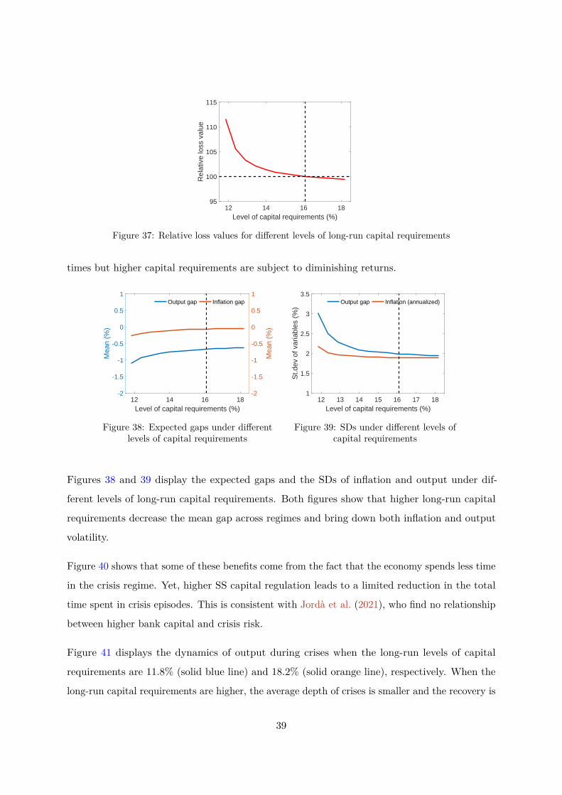
12 14 16 18Level of capital requirements (%)

95

100

105

110

115

Rel

ativ

e lo

ss v

alue

Figure 37: Relative loss values for different levels of long-run capital requirements

times but higher capital requirements are subject to diminishing returns.

12 14 16 18Level of capital requirements (%)

-2

-1.5

-1

-0.5

0

0.5

1

Mea

n (%

)

-2

-1.5

-1

-0.5

0

0.5

1

Mea

n (%

)

Output gap Inflation gap

Figure 38: Expected gaps under differentlevels of capital requirements

12 13 14 15 16 17 18Level of capital requirements (%)

1

1.5

2

2.5

3

3.5S

t.dev

of v

aria

bles

(%

)Output gap Inflation (annualized)

Figure 39: SDs under different levels ofcapital requirements

Figures 38 and 39 display the expected gaps and the SDs of inflation and output under dif-

ferent levels of long-run capital requirements. Both figures show that higher long-run capital

requirements decrease the mean gap across regimes and bring down both inflation and output

volatility.

Figure 40 shows that some of these benefits come from the fact that the economy spends less time

in the crisis regime. Yet, higher SS capital regulation leads to a limited reduction in the total

time spent in crisis episodes. This is consistent with Jordà et al. (2021), who find no relationship

between higher bank capital and crisis risk.

Figure 41 displays the dynamics of output during crises when the long-run levels of capital

requirements are 11.8% (solid blue line) and 18.2% (solid orange line), respectively. When the

long-run capital requirements are higher, the average depth of crises is smaller and the recovery is

39

12 13 14 15 16 17 18Level of capital requirements (%)

0

1

2

3

4

5

6

7

8

Tim

e sp

ent i

n ea

ch r

egim

e (%

)

Crisis-No ZLBCrisis-ZLB

Total time spent in crises

Figure 40: Time spent in crisis regime underdifferent levels of capital requirements

Mainland output gap (in percent)

1 3 5 7 9 11 13 15

Long-run capital req. of 11.8%

Long-run capital req. of 18.2%

Figure 41: Dynamics of output during financialcrises under different levels of capital requirements

faster. This finding is also in line with Jordà et al. (2021), who argue that recovery from financial

crises is faster for countries with banking sectors that are better capitalised. This benefit is more

important in magnitude than its effect on crisis probability.

12 14 16 18Level of capital requirements (%)

1.7

1.75

1.8

1.85

1.9

1.95

2

Mea

n in

flatio

n ra

te (

%)

Figure 42: Mean inflation rate in normaltimes

12 14 16 18Level of capital requirements (%)

99.9

100

100.1

100.2

Mea

n ou

tput

leve

l (no

rmal

ized

)

Figure 43: Mean output level in normaltimes

Figures 42 and 43 display the means of inflation rate and output level in normal times for various

levels of capital requirements. Higher capital requirements increase the mean inflation rate and

brings it closer to the 2 percent inflation target since they reduce the frequency of ELB episodes.

Under higher capital requirements, the banking sector and hence the economy is more resilient

to macroeconomic and financial shocks. Therefore, the negative shocks of the same magnitude

do not lead to deflationary effects. However, negative shocks reduce the mean level of output

after around 13 percent of capital requirement. After that point, the adverse effects of higher

capital requirements that raise credit spreads and hence the cost of funding start to dominate

40

the stabilising effects of capital requirements.

Figure 44 shows how much time the model economy spends in ELB episodes under different

levels of capital requirements. The figure indicates that higher long-run capital requirements

substantially reduce the probability of hitting the ELB by increasing the mean inflation rate, as

shown in Figure 42.

12 13 14 15 16 17 18Level of capital requirements (%)

25

30

35

Tim

e sp

ent i

n Z

LB r

egim

e (%

)

Figure 44: Time spent in ELB episodes for different levels of capital requirements

The benefits of lower inflation and output volatility, higher mean inflation and output in crisis

times, and lower crisis probability and severity clearly outweigh the costs of lower output in

normal times. The reaction of inflation and output is markedly different compared to LAW by

monetary policy and this begs the question of whether a combination of both policies might be

optimal. This question is beyond the scope of the current paper and is left for future research.

2.7.1 Trade-off between responding to house prices vs. to output

The benchmark model uses the estimated mimicking rule that replicates the optimal monetary

policy under discretion in normal times. When we study the optimal LAW-type monetary policy

rules, we fix all other response coefficients in the mimicking rule including the output response

at their estimated levels and only search for the optimal response to real house prices. Our main

motivation is not to deviate too much from the policy rule that broadly reflects applied monetary

policy. One may argue that by responding to output, the policy rule essentially responds to

house prices. Therefore, when we fix the output response, obtaining a positive response to real

house prices may be less likely.

41

Table 4: Simple correlations in the data

Variables Mainland output Real household credit Real house pricesMainland output 1 - -Real household credit 0.45 1 -Real house prices 0.42 0.70 1

Notes: The data sources are Norges Bank and Statistics Norway. The sample period is from 2001Q1 to 2020Q1.Mainland output is computed as the cyclical deviation from its long-run trend. Real household credit and realhouse prices are computed as 5-year cumulative growth rates.

Table 4 suggests that positive credit/house price developments tend to build up with higher

output gaps. House prices tend to lead household credit and are contemporaneously correlated

with output. This seems to support the idea that an increased weight on the output gap in

monetary policy may also help stabilise credit/house price developments. In order to test this

hypothesis, we jointly search for the optimal response coefficients to house prices and output,

which minimise the central bank loss. The other response coefficients in the mimicking are held

fixed at their previously estimated levels.24

0 20 40 60 80 100 120 140 160

Standardized response to output in ann. bps

-10

-5

0

5

10

15

20

25

30

35

Sta

ndar

dize

d re

spon

se to

rea

l hou

se p

rices

in a

nn. b

ps

Figure 45: Trade-off between responding to house prices vs. output

Figure 45 displays the optimal policy frontier that shows the relationship between responding to

output vs. house prices. We standardise the monetary policy responses by the SDs of output and

real house price gaps in the model simulations. Any pair of policy responses on the solid red line24The results underline why it is important to keep all other coefficients fixed. The collinearities are prohibitivefor identification of any effect by LAW.

42

gives the minimum central bank loss. The negative relationship clearly shows the trade-off. If

the policy rule features an output response of 120 bp, which is the current output response in the

mimicking rule, the optimal house price response is null. If the policy rule features a house price

response of 30 bp, then the optimal output response is zero. We then explore whether the loss

can be further minimised under a different combination of responses to house prices and output.

Figure 46: Loss values under different responses to output and house prices

Figure 46 displays the loss values against different degrees of LAW and output responses. In the

baseline model with an output response of 0.3, the loss is minimised when monetary policy does

not lean against the wind. However, a combination of a lower response to output of 0.15 than

the current one of 0.3 and a positive response to house prices of 0.0025 (displayed by the yellow

line) achieves an even lower loss than the baseline case. Therefore, LAW policies significantly

depend on the policymaker’s preference for output stabilisation.

We also conduct a battery of robustness checks in our framework in Section B regarding different

magnitudes of crisis probability and severity, different financial variables that monetary policy

can respond to, when the ELB constraint is removed or the CCyB is not released during crises.

43

The main results of the paper are robust to these assumptions and modifications.

3 Conclusion

This paper investigates to what extent monetary or macroprudential policy should consider

financial imbalances. We differentiate between nonsystematic policy, where the policymaker

implements the policy as a one-off intervention, and systematic policy in which the policymaker

implements policy in a systematic way and everybody is aware of the policymaker’s intention.

Furthermore, we explore to what extent the persistence of financial cycles and the ELB matter

in the policy evaluation. Last but not least, we evaluate different ways of implementing LAW

policies, such as symmetric and asymmetric policy.

For nonsystematic policy, we use a framework inspired by Svensson (2017a) and Kockerols and

Kok (2021). In essence, it is a combination of a Markov switching model where the economy is

represented by the dynamics of a linearised, large scale, small open economy, macro-financial

DSGE model with persistent financial cycles in normal times and an additional constant shock in

crisis times. We find that nonsystematic LAW is not advisable independent of the assumptions

about the persistence of the financial cycle.

Regarding systematic LAW, we augment the large scale DSGE model by adding regimes for the

ELB, endogenous crisis, and asymmetric LAW and search for the OSR. We find no evidence

supporting LAW by monetary policy in our main scenario. A monetary policy that attempts to

systematically tame the persistent financial cycle leads to excessive inflation volatility. Only in

the case that policymakers act in a systematic way and financial cycles are not persistent would

LAW be advisable. In this case LAW dampens house price volatility and is countercyclical in

response to supply shocks. The countercyclical effect of house prices acts through the collateral

channel and manifests itself in higher inflation volatility under persistent financial cycles. Under

rational house price expectations, the same collateral channel leads to a decrease in output

volatility. A side effect of systematic LAW policies is that the economy spends more time at the

ELB. Macroprudential policy in the form of long-run bank capital requirements is better suited

to addressing risks to financial stability, and the benefits increase with higher requirements in

normal times. Capital requirements lower both output and inflation volatility, and are thereby a

natural complement to LAW by monetary policy. We leave the optimal combination of monetary

44

and macroprudential policies in this framework of endogenous financial crises and the ELB as

well as the cleaning up afterwards-type policies for future research.

45

ReferencesAdam, K. and M. Woodford (2021): “Robustly Optimal Monetary Policy in a New KeynesianModel with Housing,” Journal of Economic Theory, forthcoming.

Adolfson, M., S. Laséen, L. Christiano, M. Trabandt, and K. Walentin (2013):“Ramses II - Model Description,” Occasional Paper Series 12, Sveriges Riksbank.

Adrian, T., N. Boyarchenko, and D. Giannone (2019): “Vulnerable Growth,” AmericanEconomic Review, 109, 1263–89.

Ajello, A., T. Laubach, D. Lopez-Salido, and T. Nakata (2019): “Financial stabilityand Optimal Interest Rate Policy,” International Journal of Central Banking, 15, 279–326.

Alpanda, S. and A. Ueberfeldt (2016): “Should Monetary Policy Lean Against HousingMarket Booms?” Staff Working Papers 16-19, Bank of Canada.

An, S. and F. Schorfheide (2007): “Bayesian Analysis of DSGE Models,” EconometricReviews, 26, 113–172.

Andrle, M. and J. Benes (2013): “System Priors; Formulating Priors about DSGE Models’Properties,” IMF Working Papers 13/257, International Monetary Fund.

Arbatli-Saxegaard, E., K. R. Gerdrup, and R. M. Johansen (2020): “Financial imbal-ances and medium-term macroeconomic tail risks in Norway,” Staff memo 5, Norges Bank.

Aruoba, S. B., P. Cuba-Borda, and F. Schorfheide (2017): “Macroeconomic DynamicsNear the ZLB: A Tale of Two Countries,” The Review of Economic Studies, 85, 87–118.

Bergholt, D., V. H. Larsen, and M. Seneca (2019): “Business cycles in an oil economy,”Journal of International Money and Finance, 96, 283 – 303.

Binning, A. and J. Maih (2016): “Implementing the zero lower bound in an estimatedregime-switching DSGE model,” Working Paper 2016/3, Norges Bank.

BIS (2016): “IV. Monetary Policy: more accommodation, less room,” 86th Annual Report, Bankfor International Settlements.

Boissay, F., F. Collard, J. Galí, and C. Manea (2021): “Monetary policy and endogenousfinancial crises,” .

Caballero, R. J. and A. Simsek (2020): “Prudential monetary policy,” Tech. rep., NationalBureau of Economic Research.

Corsetti, G. and L. Dedola (2005): “A macroeconomic model of international price discrim-ination,” Journal of International Economics, 67, 129–155.

Cúrdia, V. and M. Woodford (2016): “Credit Frictions and Optimal Monetary Policy,”Journal of Monetary Economics, 84, 30–65.

Del Negro, M. and F. Schorfheide (2008): “Forming priors for DSGE models (and how itaffects the assessment of nominal rigidities),” Journal of Monetary Economics, 55, 1191–1208.

46

Devereux, M. B. and C. Engel (2003): “Monetary policy in the open economy revisited:Price setting and exchange-rate flexibility,” The Review of Economic Studies, 70, 765–783.

Diez, F., D. Leigh, and S. Tambunlertchai (2018): “Global Market Power and its Macroe-conomic Implications,” IMF Working Papers 18/137, International Monetary Fund.

Dorich, J., M. K. Johnston, R. R. Mendes, S. Murchison, and Y. Zhang (2013):“ToTEM II: An Updated Version of the Bank of Canada’s Quarterly Projection Model,”Technical Reports 100, Bank of Canada.

Farhi, E. and I. Werning (2021): “Taming a Minsky Cycle,” .

Filardo, A. and P. Rungcharoenkitkul (2016): “A quantitative case for leaning againstthe wind,” BIS Working Papers 594, Bank for International Settlements.

Gambacorta, L. and F. M. Signoretti (2014): “Should monetary policy lean against thewind?” Journal of Economic Dynamics and Control, 43, 146–174.

Gelain, P., K. J. Lansing, and C. Mendicino (2013): “House Prices, Credit Growth,and Excess Volatility: Implications for Monetary and Macroprudential Policy,” InternationalJournal of Central Banking, 9, 219–276.

Gelain, P., K. J. Lansing, and G. J. Natvik (2017): “Leaning Against the Credit Cycle,”Working Paper Series 2017-18, Federal Reserve Bank of San Francisco.

Gerali, A., S. Neri, L. Sessa, and F. M. Signoretti (2010): “Credit and Banking in aDSGE Model of the Euro Area,” Journal of Money, Credit and Banking, 42, 107–141.

Gerdrup, K. R., F. Hansen, T. Krogh, and J. Maih (2017a): “Leaning Against the WindWhen Credit Bites Back,” International Journal of Central Banking, 13, 287–320.

Gerdrup, K. R., E. M. Kravik, K. S. Paulsen, and Ørjan Robstad (2017b): “Documen-tation of NEMO - Norges Bank’s core model for monetary policy analysis and forecasting,”Staff Memo 8, Norges Bank.

Gertler, M., N. Kiyotaki, and A. Prestipino (2020): “Credit booms, financial crises,and macroprudential policy,” Review of Economic Dynamics, 37, S8–S33, the twenty-fifthanniversary of “Frontiers of Business Cycle Research".

Gourio, F., A. K. Kashyap, and J. Sim (2017): “The Tradeoffs in Leaning Against theWind,” NBER Working Papers 23658, National Bureau of Economic Research, Inc.

Gourio, F., A. K. Kashyap, and J. W. Sim (2018): “The Trade offs in Leaning Against theWind,” IMF Economic Review, 66, 70–115.

Hafstead, M. and J. Smith (2012): “Financial shocks, bank intermediation, and monetarypolicy in a DSGE model,” Unpublished.

Iacoviello, M. (2005): “House Prices, Borrowing Constraints, and Monetary Policy in theBusiness Cycle,” American Economic Review, 95, 739–764.

Iacoviello, M. and S. Neri (2010): “Housing Market Spillovers: Evidence from an EstimatedDSGE Model,” American Economic Journal: Macroeconomics, 2, 125–64.

47

Jordà, O., B. Richter, M. Schularick, and A. M. Taylor (2021): “Bank Capital Redux:Solvency, Liquidity, and Crisis,” The Review of Economic Studies, 88, 260–286.

Jordà, O., M. Schularick, and A. M. Taylor (2013): “When Credit Bites Back,” Journalof Money, Credit and Banking, 45, 3–28.

Justiniano, A., G. E. Primiceri, and A. Tambalotti (2011): “Is there a trade-off betweeninflation and output stabilization?” Working Paper 17071, National Bureau of EconomicResearch.

Kim, J. (2000): “Constructing and estimating a realistic optimizing model of monetary policy,”Journal of Monetary Economics, 45, 329–359.

Kockerols, T. and C. Kok (2021): ““Leaning Against the Wind”, Macroprudential Policyand the Financial Cycle,” International Journal of Central Banking, forthcoming.

Kravik, E. M. and Y. Mimir (2019): “Navigating with NEMO,” Staff Memo 5, Norges Bank.

Kravik, E. M., Y. Mimir, and K. S. Paulsen (n.d.): “A complete documentation of NorgesBank’s policy model NEMO,” Tech. rep., Norges Bank, http://www.norges-bank.no/en/Monetary-policy/Models-for-monetary-policy-analysis-and-forecasting/NEMO/,continuously updated.

Levin, A. T., A. Onatski, J. Williams, and N. M. Williams (2006): “Monetary PolicyUnder Uncertainty in Micro-Founded Macroeconometric Models,” in NBER MacroeconomicsAnnual 2005, Volume 20, MIT Press, 229–312.

Mian, A. and A. Taylor (2021): “Financial crises: A survey,” Tech. Rep. 29155, NationalBureau of Economic Research.

Rees, D. M., P. Smith, and J. Hall (2016): “A Multi-sector Model of the AustralianEconomy,” Economic Record, 92, 374–408.

Rotemberg, J. J. (1982): “Sticky Prices in the United States,” Journal of Political Economy,90, 1187–1211.

Schmitt-Grohé, S. and M. Uribe (2003): “Closing small open economy models,” Journal ofInternational Economics, 61, 163–185.

Schularick, M. and A. M. Taylor (2012): “Credit booms gone bust: Monetary policy,leverage cycles, and financial crises, 1870-2008,” American Economic Review, 102, 1029–61.

Schularick, M., L. Ter Steege, and F. Ward (2020): “Leaning against the wind and crisisrisk,” CEPR Discussion Papers 14797, C.E.P.R. Discussion Papers.

Schüler, Y. S., P. Hiebert, and T. A. Peltonen (2015): “Characterising the financialcycle: a multivariate and time-varying approach,” Working Paper No 1846, European CentralBank.

Svensson, L. (2013): “Leaning Against the Wind Leads to Higher (Not Lower) HouseholdDebt-to-GDP Ratio,” Tech. rep., Stockholm School of Economics.

Svensson, L. E. (2017a): “Cost-benefit analysis of leaning against the wind,” Journal ofMonetary Economics, 90, 193 – 213.

48

——— (2017b): “Leaning Against the Wind: Costs and Benefits, Effects on Debt, Leaning inDSGE Models, and a Framework for Comparison of Results,” International Journal of CentralBanking, 50.

49

Appendices

A The effects of the ELB and CCyB on the evolution of financial

crises

A.1 The effects of the ELB on the dynamics of financial crises

Mainland output gap (in percent)

1 3 5 7 9 11 13 15

Consumption gap (in percent)

1 3 5 7 9 11 13 15

0 0

Business investment gap (in percent)

1 3 5 7 9 11 13 15

Housing investment gap (in percent)

1 3 5 7 9 11 13 15

Business credit gap (in percent)

1 3 5 7 9 11 13 15

0 0Household credit gap (in percent)

1 3 5 7 9 11 13 15

0 0

Real house price gap (in percent)

1 3 5 7 9 11 13 15

0 0

Inflation (in annual ppts.)

1 3 5 7 9 11 13 15

1

2

3

1

2

3

Policy rate (in ann. ppts.)

1 3 5 7 9 11 13 15

0

2

0

2Shadow policy rate (in ann. ppts.)

1 3 5 7 9 11 13 15

0

2

0

2Real rate (in ann. ppts.)

1 3 5 7 9 11 13 15

0 0Money market premium (in ann. ppts.)

1 3 5 7 9 11 13 15

0.5

1

1.5

2

0.5

1

1.5

2

ZLB imposed No-ZLB

Figure 47: Main crisis scenario under ELB versus No-ELB

Figure 47 displays the average effect of imposing the ELB on the nominal policy rate on the

dynamics of the main macroeconomic variables during crises. In the case of no-ELB, the policy

rate could fall below -2% at its trough and the real rate could decline to about -4%. The level

of the money market premium under ELB is higher compared to the no-ELB case and but the

difference is smaller than the one in the policy rate. As a consequence, the lending rate is higher

in the case of the ELB and credit and output lower. Consumption remains virtually unchanged.

The rise in the inflation rate is higher in the no-ELB regime due to both a higher SS inflation

rate and a lower policy rate.

50

A.2 The effects of a CCyB release on the dynamics of financial crises

Mainland output gap (in percent)

1 3 5 7 9 11 13 15

Consumption gap (in percent)

1 3 5 7 9 11 13 15

0 0

Business investment gap (in percent)

1 3 5 7 9 11 13 15

Housing investment gap (in percent)

1 3 5 7 9 11 13 15

Business credit gap (in percent)

1 3 5 7 9 11 13 15

Household credit gap (in percent)

1 3 5 7 9 11 13 15

0 0Real house price gap (in percent)

1 3 5 7 9 11 13 15

0 0Inflation (in annual ppts.)

1 3 5 7 9 11 13 15

0.8

1

1.2

1.4

0.8

1

1.2

1.4

Policy rate (in ann. ppts.)

1 3 5 7 9 11 13 150

0.5

1

1.5

0

0.5

1

1.5

Shadow policy rate (in ann. ppts.)

1 3 5 7 9 11 13 15

0

1

0

1

Real rate (in ann. ppts.)

1 3 5 7 9 11 13 15

0 0Money market premium (in ann. ppts.)

1 3 5 7 9 11 13 150

1

2

0

1

2

CCyB constant CCyB released

Figure 48: Main crisis scenario under a 2.5% CCyB versus a zero CCyB (ELB is imposed)

Figure 48 shows how the relaxation of the CCyB to zero from 2.5% during crises affects the

average behaviour of main macro aggregates during crises. Since the relaxation of the CCyB

lowers the pressure to generate profits in order to retain earnings and build up bank capital,

the increase in the money market premium is lower compared with the constant CCyB. Lower

funding costs for the banking sector lead to higher lending to businesses and households, reducing

the fall in business and housing investment, hence the decline in output. Inflation and the policy

rate are also higher under a zero CCyB. However, we note that the macroeconomic effects of

relaxing the CCyB during crises are not large.

B Robustness

The analysis in the previous two sections allowed us to evaluate systematic and nonsystematic

LAW by monetary and macroprudential policy with and without persistent financial cycles. For

51

the purpose of doing these experiments in a realistic setting, we introduced a range of modelling

features whose quantitative impact on the dynamics we have already demonstrated. But in this

section we also want to see to what extent their presence or absence changes the results of our

analysis.

In the following we will conduct robustness tests regarding the: (i) magnitude of crisis shocks;

(ii) sensitivity of crisis severity to excess credit; (iii) persistence of financial crises; (iv) magnitude

of crisis probability; (v) sensitivity of crisis probability to excess credit; (vi) exogenous crisis

probability; (vii) use of house prices instead of household credit as the variable driving crisis

probability and severity; (viii) removal of the ELB; (ix) removal of the CCyB release; (x) symmetric

LAW; (xi) monetary policy reacting to household credit instead of house prices, and (xii) trade-off

between house prices and output response. These robustness tests concern the case of systematic

policy with persistent financial cycles.

These additional experiments will allow us to test the robustness of our results but also to identify

the contributions of certain modelling choices.

B.1 Crisis severity

B.1.1 The magnitude of crisis shocks

In order to gauge the effect of a higher crisis shock, we increase the magnitude of crisis shocks

such that we obtain a fall in output that doubles the decline in the benchmark model (a little

more than 10%) by raising the constant term (γ) in the crisis severity function described in

equation (7) from 0.3 to 0.55. In general, larger crisis shocks should make LAW more favourable

because the central bank will then have more incentive to prevent an even more severe crisis.

Comparing the loss as a function of the response coefficient across the specification with a higher

crisis shock (see Figure 49) and our benchmark specification (see Figure 16), we find that the

point of lowest loss is the same (LAW=0) but the loss increases more strongly as soon as one

implements LAW policies. In other words, the marginal loss is larger with a higher crisis shock.

This leads us to conclude that for higher crisis shocks the changed decision rules as a result

of systematic policy have negative effects which just about compensate for the positive effects

of implementation. Because agents understand that the central bank implements LAW-type

policies, they change their behaviour such that the economy is more volatile and ultimately

52

central bank losses are higher due to this effect in isolation.

B.1.2 The sensitivity of crisis severity to excess credit

Another way of assessing the impact of higher crisis severity is to change the sensitivity of crisis

severity to excess household credit growth. To that end, we raise the slope term (γBh) in the

crisis severity function (7) from 1 to 3. The effect and logic should be the same as for the previous

robustness test.

We come to the same conclusion here as for the previous robustness test. The optimal degree of

LAW is 0 and the marginal effect only from the implementation is positive, meaning that the

changed decision rules have a negative impact which offsets the other effect. Figure 50 shows

that higher degrees of LAW still increase the central bank loss values even under higher crisis

severity.

-0.02 0 0.02 0.04

Degree of LAW, pH

100

150

200

250

Rel

ativ

e lo

ss v

alue

Figure 49: Relative loss values for differentdegrees of LAW under higher crises

severity

-0.02 0 0.02 0.04

Degree of LAW, pH

100

150

200

250

Rel

ativ

e lo

ss v

alue

Figure 50: Relative loss values for differentdegrees of LAW under higher sensitivity of

crisis severity to excess credit

B.1.3 The persistence of financial crises

The persistence of financial crises is a key parameter in the costs-benefit analysis of LAW. The

cost of a crisis increases substantially the longer it lasts, which makes LAW-type policies more

favourable. In order to test it, we increase the persistence of the crisis shocks (ρcrisis) from 0.7

to 0.95. We also recalibrate the probability (constant term in the logit function as −4.395) and

the severity of crises (γ = 0.1, and γBh = 0.47) such that we obtain the same maximum decline

in output during crises. Figure 51 indicates that a higher response to real house prices still leads

to an increase in loss values even under more persistent financial crises.

53

B.2 Crisis probability function

B.2.1 The magnitude of crisis probability

We increase the constant term in the probability of crisis function from -4.25 to -3.25 to obtain

an annual probability of a crisis start of 6% in the long run. Giving more importance to the

crisis regime, any measures preventing or mitigating the crisis should be more important. The

results show that they do not change the conclusion from the benchmark case (see Figure 52).

-0.02 0 0.02 0.04

Degree of LAW, pH

100

150

200

250

Rel

ativ

e lo

ss v

alue

Figure 51: Relative loss values for differentdegrees of LAW under more persistent

financial crises

-0.02 0 0.02 0.04

Degree of LAW, pH

100

150

200

250

Rel

ativ

e lo

ss v

alue

Figure 52: Relative loss values for differentdegrees of LAW under higher crisis

probability

B.2.2 The sensitivity of crisis probability to excess credit

We increase the slope term in the probability of crisis function from 0.0223 to 0.0523. Thus, the

sensitivity of crisis probability to excess household credit is more than doubled, and again LAW

should be more effective given the larger effect on crisis probability. This might increase the

policymaker’s incentive to curb excess credit more using LAW policies to prevent crises from

happening. Figure 53 shows that our main result remains robust to this alternative specification

of the crisis probability function. Higher degrees of LAW still raise the central bank loss values,

and the higher inflation volatility is the root cause of higher losses.

B.2.3 Exogenous crisis probability

We also investigate whether the fact that the probability of crises endogenously depends on

excess household credit growth has any effect on the optimality of LAW policies. This might

reduce the policymaker’s willingness to mitigate excess credit growth and to deploy LAW policies.

In effect, this only leaves the effect on the economy in normal times and crisis severity. Since

54

most of the time is spent in the normal regime, it is not surprising that the results do not change

and it is not advisable to respond to house prices (see Figure 54).

-0.02 0 0.02 0.04

Degree of LAW, pH

100

150

200

250

Rel

ativ

e lo

ss v

alue

Figure 53: Relative loss values for differentdegrees of LAW under higher sensitivity of

crisis probability to excess credit

-0.02 0 0.02 0.04

Degree of LAW, pH

100

150

200

250

Rel

ativ

e lo

ss v

alue

Figure 54: Relative loss values for differentdegrees of LAW under exogenous crisis

probability

B.3 Five-year cumulative house price growth in crisis severity and probabil-

ity

We use five-year cumulative real household credit growth in both the probability and the severity

of crises in our main analyses of systematic policy. One may question the plausibility of this

assumption and ask whether the main findings change if we were to use an alternative indicator

of financial imbalances in crisis probability and severity such as five-year cumulative real house

price growth. The latter is also shown to be an important indicator of financial vulnerabilities in

the literature. We rely on the estimate in Table 1 and find that LAW is not advisable even if we

use house prices instead of household credit (see Figure 55).

B.4 No ELB on policy rate

Our benchmark model of systematic policy incorporates an endogenous ELB on the policy rate,

which limits the ability of monetary policy to counteract large negative macroeconomic shocks

and hence to maintain inflation and output stabilisation. This feature impacts LAW because

higher degrees of LAW reduce the mean inflation rate, in turn leading to a lower average policy

rate and to an increased probability of hitting the ELB. Then again, Table 3 shows that inflation

volatility increases without the ELB, and output volatility decreases slightly. Removing the ELB

as a constraint on monetary policy may lower the costs of LAW, yet the results show that it does

not change the main result (see Figure 56). In other words, the ELB is not the driving factor

55

behind the results.

-0.02 0 0.02 0.04

Degree of LAW, pH

100

150

200

250

Rel

ativ

e lo

ss v

alue

Figure 55: Relative loss values for differentdegrees of LAW when house price growthis in the probability and severity of crises

-0.02 0 0.02 0.04

Degree of LAW, pH

100

150

200

250

Rel

ativ

e lo

ss v

alue

Figure 56: Relative loss values for differentdegrees of LAW under no ELB constraint

B.5 No CCyB release during crises

In the benchmark model, we assume that the CCyB is released from its long-run value of 2.5% to

0% during financial crises. The release gives banks relief in crisis times and reduces crisis severity.

Removing the release will magnify crisis severity slightly as we have seen the effect of the CCyB

to be small (see Figure 48). We suspect that the more severe crisis tilts the balance in favor

of LAW but, as we have already seen previously, changes in crisis severity did not change the

main result. Figure 57 indicates that our main finding remains unchanged under this alternative

assumption.

B.6 Monetary policy response

B.6.1 Symmetric LAW

We consider asymmetric LAW policies in the benchmark systematic policy model since we think

it is more reasonable to assume that the central bank responds to the real house price gap or

household credit growth when they are positive. One may argue that the central bank may want

to reap the benefits of stable house prices or household credit growth in normal times by also

responding to these variables when they fall. The monetary authority can reduce the policy rate

in response to a decline in house prices in normal times to stabilise the housing market. This

can potentially contribute to a better performance of the economy in normal times by reducing

the fluctuations in inflation and output. Figures 58 suggests that the symmetry of LAW does

not change the main result and it is not an assumption which drives the results.

56

-0.02 0 0.02 0.04

Degree of LAW, pH

100

150

200

250R

elat

ive

loss

val

ue

Figure 57: Relative loss values for differentdegrees of LAW when CCyB is not

released during crises

-0.02 0 0.02 0.04

Degree of LAW, pH

100

120

140

160

180

200

Rel

ativ

e lo

ss v

alue

Figure 58: Relative loss values for differentdegrees of LAW under symmetric LAW

B.6.2 Response to real household credit gap

In this section, we consider an alternative financial variable that monetary policy can respond to,

the real household credit gap instead of real house prices. Although monetary policy is considered

to be less effective in mitigating household credit due to its substantial inertia, the central bank

may want to respond directly to household credit since it is the main source of the frictions in

the economy, i.e. both the probability and the severity of crises are functions of household credit.

-0.02 0 0.02 0.04

Degree of LAW, pH

100

200

300

400

500

Rel

ativ

e lo

ss v

alue

Figure 59: Relative loss values for differentdegrees of LAW when monetary policy

responds to the real household credit gap

In fact, the optimal response coefficient is not zero when responding to household credit instead

of house prices. LAW is optimal with a small coefficient of 0.005 (see Figure 59). Responding

to the variable that we assume to directly influence crisis probability and severity proves to be

beneficial. One has to bear in mind that monetary policy is less effective in influencing the highly

persistent financial cycle (in the form of stocks of debt), whereas house prices are more elastic

57

with respect to changes in monetary policy and thereby more practical to target.

C Abbreviations

bp basis points

CCyB Countercyclical Capital Buffer

CES constant elasticity of substitution

DSGE dynamic stochastic general equilibrium

ELB effective lower bound

GaR Growth-at-Risk

GDP gross domestic product

GFC Global Financial Crisis

GPFG Government Pension Fund Global

LAW leaning against the wind

LTV loan-to-value

MGDP mainland gross domestic product

NEMO Norwegian Economy MOdel

NK New Keynesian

OECD Organisation for Economic Co-operation and Development

OSR optimal simple rule

pp percentage point

RS regime-switching

SD standard deviation

SS steady state

UIP uncovered interest parity

58

Online Appendix for “Leaning against persistent financial cycles

with occasional crises”-Not intended for publication

Thore Kockerols

Norges Bank

Erling Motzfeldt Kravik

Norwegian Ministry of Finance

Yasin Mimir

Norges Bank

October 2021

Abstract

This online appendix describes detailed mathematical derivations of optimality condi-

tions, explains the data sources and targeted empirical moments in the calibration of

the steady-state of the model, and describes the Bayesian estimation of the baseline

model in the main text.

JEL: E52, E58, G01

Keywords: leaning against the wind, monetary policy, financial cycle, macroprudential policy∗We thank SeHyoun Ahn, Karsten Gerdrup, Tord Krogh, Junior Maih, Lars E.O. Svensson, and participantsat the 55th Annual Conference of the Canadian Economics Association, the 2021 EEA-ESEM Congress, 52ndAnnual Conference of the Money, Macro and Finance Society, the European Central Bank, the Federal ReserveBoard, Norges Bank, the OECD, and Statistics Norway for valuable discussions and comments. This WorkingPaper should not be reported as representing the views of Norges Bank or the Norwegian Ministry of Finance.The views expressed are those of the authors and do not necessarily reflect those of Norges Bank or the NorwegianMinistry of Finance. Any errors are our own. Email: thore.kockerols@norges-bank.no, emk@fin.dep.no,yasin.mimir@norges-bank.no.We thank SeHyoun Ahn, Karsten Gerdrup, Tord Krogh, Junior Maih, Lars E.O. Svensson, and participantsat the 55th Annual Conference of the Canadian Economics Association, the 2021 EEA-ESEM Congress, 52ndAnnual Conference of the Money, Macro and Finance Society, the European Central Bank, the Federal ReserveBoard, Norges Bank, the OECD, and Statistics Norway for valuable discussions and comments. This WorkingPaper should not be reported as representing the views of Norges Bank or the Norwegian Ministry of Finance.The views expressed are those of the authors and do not necessarily reflect those of Norges Bank or the NorwegianMinistry of Finance. Any errors are our own. Email: thore.kockerols@norges-bank.no, emk@fin.dep.no,yasin.mimir@norges-bank.no.

D Theoretical framework: NEMO

NEMO is a large-scale DSGE open-economy New Keynesian model and is the core model used

by Norges Bank for monetary policy and forecasting. The model was launched in 2006 and has

continuously been updated and extended along several dimensions.

In this section we summarize the main features of the constant-parameter version of the model.

We give a short overview of the model’s structure, go through the calibration of the steady state

and the estimation of dynamic parameters, as well as show model moments and compare them

to their empirical counterparts. Lastly, we discuss how monetary policy is conducted in NEMO.

D.1 Model structure

The economy consists of households, domestic (traditional) firms, an oil sector, a government

sector and the monetary authority. In addition, there are separate production sectors for housing

and non-housing capital goods as well as a banking sector. All agents have rational, or model-

consistent, expectations with respect to all prices and quantities, except for households’ house

price expectations, which are partly backward-looking.

NEMO features several real and nominal rigidities. This includes habit persistence, investment

adjustment costs, variable capacity utilization and price and wage stickiness. The model also

includes collateral constraints based on loan-to-value ratios, long-term mortgage debt contracts,

incomplete interest rate pass-through and capital requirements in the banking sector.

Figure 60 provides a schematic illustration of the model and displays how the different sectors

and agents are linked to each other.

Final goods producers bundle goods from domestic intermediate firms (Q) and imports (M).

The final goods are used for household consumption (C), corporate investment (IC), housing

investment (IH), government expenditures (G) and as inputs to the oil sector (QO). Intermediate

goods producers employ labour supplied by households (LI), rent capital from entrepreneurs (KI)

and sell their goods to the final goods producers (Q) and as export (M∗). The oil sector uses

labour (LO), capital (KO) and final goods (QO) to produce oil supply goods that are exported

(MO∗) or sold to the domestic rig producers (IOF ). The rig producers invest in oil rigs (FO)

in order to extract oil (YO) that in turn is exported in full. The profits are invested in the

60

Government

Finalgoods

producers

Housinginvestment

Households

Bankingsector

Capitalproducer

Interm.goods

producers

Oil supplysector

Foreign oil extractors

Rigproducers

Oilextractors

Oil fund

Foreign sector

Risk premium

G

IH

H

Bh D

LI

LO

KI

KO

Be

IC

MO∗

IOF

FO

M∗

YO

B∗B∗

BF

M

Q

QO

C

Figure 60: A bird’s eye view of NEMO

Government Pension Fund Global (GPFG), called the “Oil fund” in Figure 60.

Households consume (C), work in the intermediate goods sector (LI) and in the oil sector (LO),

buy housing services (H), and interact with banks through borrowing (Bh) and savings through

deposits (D) (households obtain utility from holding deposits).

The banking sector lends to households (Bh) and entrepreneurs (Be), and is funded through

deposits (D), foreign borrowing (B∗) and equity (KB). A UIP relationship together with the

country’s net foreign debt position (private borrowing, B∗, minus government claims on foreigners,

BF ) tie down the debt-elastic risk premium to ensure stationarity.1

D.2 Syntax and notation

Throughout this document, PXt denotes the nominal price of real variable X in period t. The

final good is the numeraire and has the price Pt. WX,t is the nominal wage rate in sector X.

Moreover, RXt ≡ 1 + rXt is the “gross interest rate” associated with sector or variable X, where

rXt is the net interest rate. All other variables are expressed in real terms unless otherwise stated.1This is one of the standard ways of solving the unit problem inherent in small open economy models withincomplete markets (see Schmitt-Grohé and Uribe (2003)).

61

Exogenous labour augmenting technological growth in the intermediate sector makes the economy

grow at rate πzt . The housing sector is assumed to have a weaker technology growth rate of πzt /πhtto reflect increasing house prices relative to consumer prices observed in data. The stationary

version of the model is available in Kravik et al. (n.d.). We use the notation Xss to indicate

variable X in steady state.

D.3 Households

Each household supplies a differentiated labour input to the intermediate goods-producing firms

and the oil supply sector. Wages are set by households under the assumption of monopolistic

competition. Households obtain utility from consumption, leisure, housing services and deposits.

Direct utility from deposits ensures that households are both gross lenders and gross borrowers.

Preferences are additively separable. We have also separated the household’s problem into two

maximisation problems: that of the households and that of the entrepreneurs. We do this to

simplify the maximisation problem and to clarify the decision-making by the households in the

model. The entrepreneurs’ part of the problem is covered in Section D.6.

D.3.1 The household maximization problem

Lifetime expected utility of household j at time s is represented as

Us (j) = Es

∞∑t=s

βt−s [u (Ct (j)) + d(Dt (j)) + w(Ht (j))− v(Lt (j))] , (12)

where β is the discount factor, Ct denotes consumption, Dt is deposits, Ht is the housing stock2

and Lt is supply of labour. The in-period utility functions are defined as:

u (Ct (j)) = zut

(1− bc

πzss

)ln[Ct (j)− bcCt−1

1− bc/πzss

], (13)

d (Dt (j)) = zd(

1− bd

πzss

)ln[Dt (j)− bdDt−1

1− bd/πzss

], (14)

2The terms housing, housing services and housing stock are used interchangeably throughout this paper. In thesame way as in Iacoviello and Neri (2010), one can think of Ht as both housing services and as the housing stockrequired to produce housing services. Consider a simple housing technology producing housing services, H = Hκt

t ,where κt is a time-varying elasticity of housing services to the housing stock. In such a setup, the total effectsfrom the housing stock to the utility of the consumer will be captured both through the housing technology shockκt and the housing preference shock zht . Hence, as we do not include κt in our model, the housing preferenceshock captures both pure preference shocks and changes in housing service technology.

62

v (Lt (j)) = 1− bl

1 + ζ

[Lt (j)− blLt−1

1− bl

]1+ζ

, (15)

w(Ht (j)) = zht

(1− bhπhss

πzss

)ln[Ht (j)− bhHt−11− bhπhss/πzss

], (16)

where zt’s are preference parameters, of which zut and zht are shocks that follow AR(1) processes.3

The b-parameters govern habit persistence, and the πzss denotes the exogenous steady-state

(labour augmenting) technology growth rate.4 As stated above, the housing sector is assumed to

have a weaker technology growth rate that is equal to πzss/πhss in the steady state (implying that

real house prices grow with the value πhss in the steady state). The inverse of the Frisch elasticity

of labour supply is given by ζ > 0. The Frisch elasticity captures the elasticity of hours worked

to the wage rate. The log in-period utility functions for consumption, deposits and housing imply

an intertemporal elasticity of substitution equal to 1, which secures a balanced growth path.

PtCt (j) + PtDt (j) + PHt Ht (j) +(rFt−1 + δBt (j)

)Pt−1Bh,t−1 (j)

= Wt(j)Lt (j) [1− γt(j)] + PtIB,t (j) +Rdt−1Pt−1Dt−1 (j) (17)

+ (1− δH)PHt Ht−1 (j) +DIVt (j)− TAXt (j) ,

where Pt is the price level of final goods, PHt is the price level of housing services, rFt is the

nominal net mortgage interest rate faced by households, Rdt is the gross interest on household’s

deposits, δBt (j) denotes household j’s amortisation rate (mortgage repayment share), Bh,t(j) is

real household borrowing (or mortgage), Wt(j) is the nominal wage rate (in both the intermediate

goods sector and the oil sector) set by household j, γt(j) is the wage adjustment cost (defined

below in (22)), Lt (j) is the total amount of hours worked (in both the intermediate goods sector

and the oil sector), IB,t(j) indicates new real loans by household j, δH denotes the depreciation

rate of the housing stock and DIVt(j) and TAXt(j) are dividends5 (in nominal terms) disbursed

to household j and lump-sum taxes payed by household j, respectively. Hence, equation (17)

states that expenditures on consumption, deposits, housing services as well as interest and3Most shock processes are modelled as log-deviations from their steady state.4Including a habit formation parameter on hours worked turns out to have very limited impact on the propertiesof the model.

5Including any entrepreneurial surplus (see Section D.6).

63

principal on the mortgage, need to be equal to the sum of labour income (net of adjustment

costs), new mortgage, deposits from the previous period with interest income, undepreciated

housing stock plus any dividends (and other lump-sum income) less taxes.

Household borrowing follows the process:

Bh,t (j) =(1− δBt (j)

) Pt−1Pt

Bh,t−1 (j) + IB,t (j) . (18)

Similar to Iacoviello (2005) and Gelain et al. (2017), we assume that households are credit

constrained. Specifically, we assume that household j’s new loans, IB,t, are constrained by

the expected housing wealth (the expected household’s housing stock in the next period less

mortgage), assumed to always be binding:6

IB,t (j) = φtEt

[PHt+1Pt+1

Pt+1Pt

Ht (j)−Bh,t (j)], (19)

where φt is the collateral coefficient that governs the constraint on new household loans. It

follows an AR(1) process and can be interpreted as a shock to the loan-to-value (LTV) ratio for

household borrowing. As house prices increase, the collateral values of houses rise. This expands

households’ capacity to borrow more and thus create a demand for mortgages, the proceeds of

which are spent on consumption goods, housing and deposits. In the steady-state solution of the

model, Kravik et al. (n.d.) derives the relationship between φt and the LTV in the steady state.

We follow Gelain et al. (2017) in that the loan principal repayment share follows from an

(approximated) annuity loan repayment formula:

δBt+1 (j) =(

1− IB,t (j)Bh,t (j)

)(δBt (j)

)αh+ IB,t (j)Bh,t (j)

(1− αh

)κh, (20)

where αh and κh are exogenous parameters that govern the dynamics of amortisation rate. In

the case of αh equal to 0, δBt (j) = 1 for all t, i.e. Bh,t (j) = IB,t (j), but if αh > 0, the above

repayment formula captures the fact that the amortisation rate is low during the first years after

taking up a mortgage when interest payments are high and increases thereafter. We calibrate αh

and κh to capture the repayment schedule of a typical mortgage contract of 30 years.6Our setup is inspired by and very similar to Gelain et al. (2017) except that the latter study assumes that thehouseholds refinance a fixed fraction of the mortgage in every period, collateralised by the same fraction of theirhousing wealth.

64

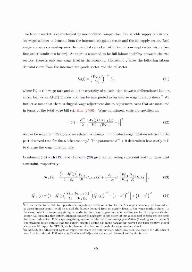
The labour market is characterised by monopolistic competition. Households supply labour and

set wages subject to demand from the intermediate goods sector and the oil supply sector. Real

wages are set as a markup over the marginal rate of substitution of consumption for leisure (see

first-order conditions below). As there is assumed to be full labour mobility between the two

sectors, there is only one wage level in the economy. Household j faces the following labour

demand curve from the intermediate goods sector and the oil sector:

Lt(j) =(Wt(j)Wt

)−ψtLt, (21)

where Wt is the wage rate and ψt is the elasticity of substitution between differentiated labour,

which follows an AR(1) process and can be interpreted as an inverse wage markup shock.7 We

further assume that there is sluggish wage adjustment due to adjustment costs that are measured

in terms of the total wage bill (cf. Kim (2000)). Wage adjustment costs are specified as:

γt(j) = φW

2

[Wt (j) /Wt−1 (j)Wt−1/Wt−2

− 1]2

. (22)

As can be seen from (22), costs are related to changes in individual wage inflation relative to the

past observed rate for the whole economy.8 The parameter φW > 0 determines how costly it is

to change the wage inflation rate.

Combining (18) with (19), and (18) with (20) give the borrowing constraint and the repayment

constraint, respectively:

Bh,t (j) =

(1− δBt (j)

)1 + φt

Pt−1Pt

Bh,t−1 (j) + φt1 + φt

Et

[PHt+1Pt+1

Pt+1Pt

Ht (j)], (23)

δBt+1 (j) =(1− δBt (j)

) Pt−1Pt

Bh,t−1 (j)Bh,t (j)

[(δBt (j)

)αh−(1− αh

)κh]+(1− αh

)κh. (24)

7For the model to be able to replicate the importance of the oil sector for the Norwegian economy, we have addeda direct impact from the oil price and the labour demand from oil supply firms to the wage markup shock. InNorway, collective wage bargaining is conducted in a way to promote competitiveness for the export-orientedsector, i.e. meaning that export-oriented industries negotiate before other labour groups and thereby set the normfor other industries. This wage bargaining system is referred to as Frontfagsmodellen (“leading sector model”).Frontfagsmodellen entails that the export-oriented sector has more bargaining power than their relative labourshare would imply. In NEMO, we implement this feature through the wage markup shock.

8In NEMO, the adjustment costs of wages and prices are fully indexed, which has been the case in NEMO since itwas first introduced. Different specifications of adjustment costs will be explored in the future.

65

Maximizing utility, (12), subject to the budget constraint, (17); the borrowing constraint, (23)

and the repayment constraint, (24), letting ωt and µt be the Lagrangian multipliers associated

with (23) and (24), gives the first-order conditions with respect to real borrowing, Bh,t (25);

deposits, Dt (26); the wage rate, Wt (27); housing, Ht (28); and repayments, δBt (29) (defining

the stochastic discount factor as ∆t+1 ≡ β u′(Ct+1)u′(Ct)

PtPt+1

and suppressing household indicator j):

1− Et[∆t+1]RFt −ωt

u′ (Ct)

+Et

[ωt+1

u′ (Ct+1)∆t+1(1− δBt+1)1 + φt+1

]

− µtu′ (Ct)

Bh,t−1B2h,t

Pt−1Pt

(1− δBt )[(δBt

)αh− (1− αh)κh

]

+Et

[µt+1

u′ (Ct+1)∆t+1(1− δBt+1)Bh,t+1

[(δBt+1

)αh− (1− αh)κh

]]= 0,

(25)

Et [∆t+1]Rdt − 1 = − d′(Dt)u′ (Ct)

, (26)

v′ (Lt)u′ (Ct)

ψtPtWt

=[(ψt − 1) (1− γt) + φW

(Wt/Wt−1Wt−1/Wt−2

− 1)

Wt/Wt−1Wt−1/Wt−2

]−Et

[∆t+1

Lt+1Lt

φW(Wt+1/Wt

Wt/Wt−1− 1

) (Wt+1/Wt)2

Wt/Wt−1

],

(27)

w′(Ht)u′ (Ct)

= PHtPt− (1− δH)Et

[∆t+1

PHt+1Pt

]− ωtu′ (Ct)

φt1 + φt

Et

[PHt+1Pt+1

Pt+1Pt

], (28)

−µt−1 + µtβBh,t−1Bh,t

Pt−1Pt

[αh(δBt

)αh−1(1− δBt )−

(δBt

)αh+ (1− αh)κh

]−ωtβ

[Bh,t−11 + φt

Pt−1Pt

]= 0.

(29)

In the special case of δBt = 1, i.e. when the full mortgage is rolled over in every period, the

first-order condition with respect to Bh,t, equation (25), would simply collapse to the first three

terms: Et[∆t+1]RFt = 1− ωtu′(Ct) , i.e. households would borrow up to a point where the effective

cost of borrowing is equal to the shadow marginal benefit of mortgage. When δBt < 1, the

fourth term in (25) captures that an increased mortgage in the current period also increases the

66

mortgage in future periods (due to the long-term debt contracts). The last two terms control how

the path of the amortisation rate changes when the size of the mortgage increases marginally.

The optimality condition for deposits, equation (26), states that the marginal rate of substitution

between deposits and consumption must be equal to the marginal benefit of holding deposits

(the interest rate). Compared with a canonical DSGE model, household faces an additional

opportunity cost of consuming in the current period in the form of lost utility from deposits.

Equation (27) is the first-order equation with respect to the wage rate, which is set by households

subject to the demand function in (21). In the special case without any wage adjustment costs,

φW = γt = 0 (see equation (22)), (27) will simply be reduced to WtPt

= ψtψt−1

v′(Lt)u′(Ct) , i.e., the real

wage rate will be set as a markup over the marginal rate of substitution between leisure and

consumption. The second term on the right-hand side of (27) captures the adjustment costs of a

change in wages, whereas the last term reflects that increasing wages today reduces the need to

increase wages in the future. Thus, the latter term means that households consider the full path

of future labour demand when setting the current wage level.

The first-order condition with respect to housing, (28), equalises the marginal rate of substitution

between housing and consumption with the effective price of housing. The first term on the

right-hand side is the real house price, the second part is the net-of-depreciation continuation

value, and the last term captures that the increase in the household’s collateral from more housing

induces the household to take up more mortgage debt (from equation (19)). The increase in

collateral is valued at the shadow value of additional mortgage debt.

Equation (29) is the first-order condition with respect to mortgage repayments, δBt . The second

term shows the impact on the amortisation dynamics when the current repayment rate is increased

marginally, whereas the last term includes the indirect effects through the behaviour of the

mortgage.

D.3.2 House price expectations

Agents in NEMO are forward-looking and have model-consistent expectations. For instance,

workers decide on wages and labour supply not only based on today’s consumer prices and labour

demand curves, but also based on all future expected prices and demand curves. The same is

true for all agents of the model, regarding all prices. A noteworthy exception is house price

67

expectations, where we introduce so-called hybrid expectations as in Gelain et al. (2013). We

assume that a share bsa of households expects house prices to follow a moving average process

(i.e. partly backward-looking expectations), whereas a share (1− bsa) has rational expectations

(in log-gap form). This generates house price cycles more in line with empirical observations:

Et[PHt+1

]= bsaXH

t + (1− bsa)PHt+1, (30)

where denotes gap-form and the moving average process is defined as

XHt = λsaPHt−1 + (1− λsa)XH

t−1. (31)

D.4 Intermediate goods sector

A continuum of firms in the intermediate goods sector uses capital and labour to produce a

differentiated intermediate good which is sold under monopolistic competition to the final goods

producers at home and abroad as an export. Firms choose labour and capital services to minimise

factor outlays, taking wages and rental rates of capital as given. As firms in the intermediate

goods sector enjoy market power, they set prices as a markup over marginal costs, and they

charge different prices at home and abroad.9 Firms are assumed to face so-called Rotemberg

adjustment costs when changing nominal prices (Rotemberg, 1982), which lead firms to change

their prices less in response to shocks than they otherwise would have done, i.e. prices are sticky.

This assumption contributes to the non-neutrality of monetary policy. Since changing prices

is costly, firms must take into account future developments when deciding on today’s prices.

Hence, inflation expectations influence today’s inflation. Finally, capital is produced by capital

producers (see Section D.7).

D.4.1 The maximisation problem

The intermediate firm n sells good Qt(n) to the final goods sector and exports the amountM∗t (n),

where Tt(n) = Qt(n) + M∗t (n)). It has the following constant elasticity of substitution (CES)

production function:

Tt(n) =[(1− α)

1ξ (ZtzLt LI,t(n))1− 1

ξ + α1ξKI,t(n)1− 1

ξ

] ξξ−1

, (32)

9Hence, we assume “local currency pricing” as in Devereux and Engel (2003) and Corsetti and Dedola (2005).

68

where α ∈ [0, 1] determines the capital share and ξ denotes the elasticity of substitution between

labour and capital. The variables LI,t (n) and KI,t (n) denote, respectively, hours and effective

capital used by firm n in period t. There are two exogenous shocks to productivity in the model:

Zt refers to an exogenous permanent labour augmenting process, which grows at the gross rate

πzt , whereas zLt denotes a temporary (stationary) shock to productivity (or labour utilisation)

that follows an AR(1) process.

Total labour input to firm n is an index over used labour from all households j, i.e.

LI,t(n) =

1∫0

LI,t(n, j)1− 1

ψt dj

ψtψt−1

, (33)

where ψt denotes the elasticity of substitution between differentiated labour types.

Let WI,t be the wage rate, which is equal to Wt due to perfect labour mobility, and let RKI,t be

the rental rate of capital equal to RK,t due to perfect capital mobility. Minimising total factor

outlays gives rise to the following conditional factor demand functions:10

LI,t = (1− α)(WI,t

MCt

)−ξTt(ZtzLt )ξ−1, (34)

KI,t = α

(RKI,tMCt

)−ξTt, (35)

where we have used that marginal costs can be shown to be:

MCt =

(1− α)(WI,t

ZtzLt

)1−ξ

+ αR1−ξKI,t

11−ξ

. (36)

This means, for example, that higher real wages will reduce labour demand and increase the

demand for capital for a given level of production. A proportional increase in both real wages

and rental prices will have no impact on the demand for labour and capital. Firms face the10Note that in symmetric equilibrium all firms make the same decisions, hence LI,t(n) = LI,t, and similarly forthe capital demand.

69

following price adjustments costs in the domestic and foreign markets, respectively:

γPQ,t(n) ≡ φPQ

2

[PQt (n) /PQt−1 (n)

PQt−1/PQt−2

− 1]2

, (37)

γPM∗,t(n) ≡ φPM∗

2

[PM

∗t (n) /PM∗t−1 (n)PM

∗t−1/P

M∗t−2

− 1]2

, (38)

where PQt and PM∗t are the prices in the domestic and the foreign market (in foreign currency),

respectively. The costs of changing prices are governed by the parameters φPQ and φPM∗ .11 One

can show that the firms face the following demand functions from the final goods sector and

from abroad, respectively:

Qt(n) =(PQt (n)PQt

)−θHtQt, (39)

M∗t (n) =

PM∗t (n)PM

∗t

−θF∗

M∗t , (40)

where θHt is the elasticity of substitution between domestic goods produced by different firms

in the intermediate goods sector and follows an AR(1) process, which can be interpreted as a

domestic price (inverse) markup shock. Correspondingly, θF ∗ is the elasticity of substitution

across export goods.

Profit maximisation gives rise to the following first-order condition for price-setting in the

domestic market, PQt :

Qt − θHt Qt +MCtθHt

Qt

PQt− φPQ

[PQt /P

Qt−1

PQt−1/PQt−2− 1

]PQt /P

Qt−1

PQt−1/PQt−2

Qt

+Et

∆t+1φ

PQ

[PQt+1/P

Qt

PQt /PQt−1− 1

](PQt+1/P

Qt )2

PQt /PQt−1

Qt+1

= 0,

(41)

In the absence of adjustment costs, φPQ = 0, prices would simply be set as a markup over

marginal costs in every period PQt = θHtθHt −1MCt (where θHt > 1). The fourth term captures the

adjustment costs of the price change, whereas the last term reflects that increasing the price in

the current period reduces the need to increase prices more in the future. Hence, the latter term11Similar to wage adjustment costs, price adjustment costs are related to changes in inflation for firm n relative tothe past observed rate for the whole economy.

70

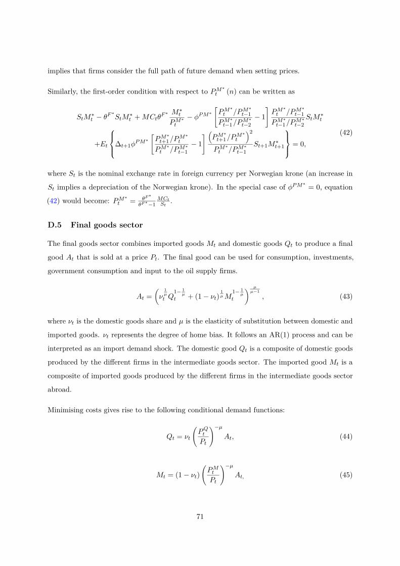
implies that firms consider the full path of future demand when setting prices.

Similarly, the first-order condition with respect to PM∗t (n) can be written as

StM∗t − θF

∗StM

∗t +MCtθ

F ∗ M∗t

PM∗

t

− φPM∗[PM

∗t /PM

∗t−1

PM∗

t−1/PM∗t−2− 1

]PM

∗t /PM

∗t−1

PM∗

t−1/PM∗t−2

StM∗t

+Et

∆t+1φPM∗

[PM

∗t+1/P

M∗t

PM∗

t /PM∗

t−1− 1

] (PM

∗t+1/P

M∗t

)2

PM∗

t /PM∗

t−1St+1M

∗t+1

= 0,(42)

where St is the nominal exchange rate in foreign currency per Norwegian krone (an increase in

St implies a depreciation of the Norwegian krone). In the special case of φPM∗ = 0, equation

(42) would become: PM∗t = θF∗

θF∗−1MCtSt

.

D.5 Final goods sector

The final goods sector combines imported goods Mt and domestic goods Qt to produce a final

good At that is sold at a price Pt. The final good can be used for consumption, investments,

government consumption and input to the oil supply firms.

At =(ν

1µ

t Q1− 1

µ

t + (1− νt)1µM

1− 1µ

t

) µµ−1

, (43)

where νt is the domestic goods share and µ is the elasticity of substitution between domestic and

imported goods. νt represents the degree of home bias. It follows an AR(1) process and can be

interpreted as an import demand shock. The domestic good Qt is a composite of domestic goods

produced by the different firms in the intermediate goods sector. The imported good Mt is a

composite of imported goods produced by the different firms in the intermediate goods sector

abroad.

Minimising costs gives rise to the following conditional demand functions:

Qt = νt

(PQtPt

)−µAt, (44)

Mt = (1− νt)(PMtPt

)−µAt, (45)

71

where Pt ≡[νt(PQt )1−µ + (1− νt)(PMt )1−µ

] 11−µ is the numerator of the model.

D.6 Entrepreneurs

D.6.1 The maximisation problem

In this sector we focus on the maximisation problem for entrepreneurs. Entrepreneurs are

households, but this section considers a separate part of households’ budget constraint to simplify

the exposition.12 We could alternatively have modelled this sector as a firm owned by households.

Entrepreneurs rent capital to the intermediate goods sector and the oil sector gaining the

rental rate RK,t (= RKI,t = RKO,t due to perfect capital mobility). They rent out KI,t to the

intermediate goods sector and KO,t to the oil supply sector. Kt is then the aggregate utilised

capital rented out by entrepreneurs. At the beginning of period t they sell the undepreciated

capital (1− δ)Kt−1 at price PKt to the capital producers. The latter combine it with investment

goods to produce Kt to be sold back to entrepreneurs at the same price. To finance their activity,

entrepreneurs borrow Be,t (referred to as corporate credit) from banks at gross rate Ret , providing

capital goods as collateral. They enter into a multi-period loan contract. Finally, entrepreneurs

also decide the capital utilisation rate ut.

We define effective capital input in period t as

Kt = utKt−1. (46)

Entrepreneurs are subject to the following real budget constraint:

RK,tPt

Kt + PKtPt

(1− δ)Kt−1 + IeB,t =

PKtPt

Kt + (ret−1 + δet )Pt−1Pt

Be,t−1 + γ (ut)Kt−1 + Ct + 1Pt

Ξt,(47)

where the first term is the income from renting out capital to the intermediate goods sector and

the oil supply sector, the second term is the income generated from the sale of undepreciated

capital to the capital producers (see Section D.7), and IeB,t is new loans. The first term on the

expenditure side of (47) is capital bought back from the capital producers, the second term12We suppress index j in this section.

72

represents the interest and principal payments to banks on outstanding debt, the third term

are costs associated with a given level of the utilisation rate of capital (see below), and Ct

is household consumption. The last term, Ξt, represents all other terms that enter into the

household budget constraint (17).13

The unit utilisation cost is defined as

γ (ut) = RK,ssPssφu

[eφu(ut−1) − 1

], (48)

where φu governs the cost of adjusting the utilisation rate, and the subscript ss denotes steady-

state values. Note that total utilised capital rented out must be equal to the utilised capital

demanded by the intermediate goods sector and by the oil supply sector, Kt = KI,t +KO,t.

Whereas households used housing capital as collateral, the entrepreneurs can borrow against

their real capital (1− δ)Kt. Similar to the household constraint (23) and (24), we have:

Be,t = (1− δet )1 + φentt

Pt−1Pt

Be,t−1 + φentt

1 + φentt

Et

[PKt+1Pt+1

Pt+1Pt

(1− δ)Kt

], (49)

δet+1 = (1− δet )Pt−1Pt

Be,t−1Be,t

[(δet )

αe − (1− αe)κe]

+ (1− αe)κe

, (50)

where φentt is the collateral coefficient that governs the constraint on new corporate debt. It

follows an AR(1) process and can be interpreted as a shock to the LTV ratio for business credit.

δet is the loan repayment share and αe and κe are exogenous parameters that govern entrepreneurs’

annuity loan repayment formula (analogous to the household case in equation (20)).

Maximising utility (equation (12)) subject to (47), (49) and (50) with respect to Kt, Bet , δet and

ut gives the following first-order conditions (where ωet and µet are the Lagrangian multipliers

associated with (49) and (50), respectively):

PKtPt

= Et

[ωet

u′ (Ct)φentt

1 + φentt

PKt+1Pt+1

Pt+1Pt

(1− δ)]

+Et

[∆t+1

Pt+1Pt

(PKt+1Pt+1

(1− δ) + RK,t+1Pt+1

ut+1 − γ (ut+1))]

,

(51)

13Since households and entrepreneurs technically are the same, one can think of all terms in (47) (except Ct andΞt) as part of DIVt in (17).

73

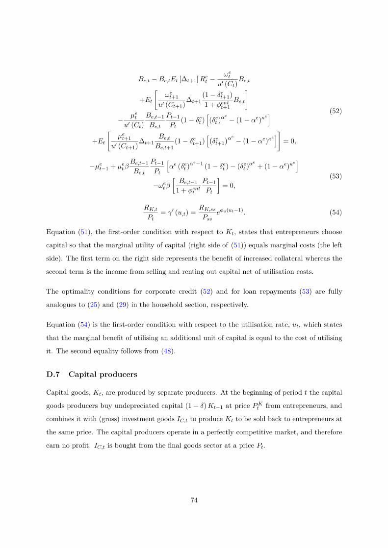
Be,t −Be,tEt [∆t+1]Ret −ωet

u′ (Ct)Be,t

+Et

[ωet+1

u′ (Ct+1)∆t+1(1− δet+1)1 + φentt+1

Be,t

]

− µetu′ (Ct)

Be,t−1Be,t

Pt−1Pt

(1− δet )[(δet )

αe − (1− αe)κe]

+Et

[µet+1

u′ (Ct+1)∆t+1Be,tBe,t+1

(1− δet+1)[(δet+1

)αe − (1− αe)κe]]

= 0,

(52)

−µet−1 + µetβBe,t−1Be,t

Pt−1Pt

[αe (δet )

αe−1 (1− δet )− (δet )αe + (1− αe)κe

]−ωetβ

[Be,t−1

1 + φentt

Pt−1Pt

]= 0,

(53)

RK,tPt

= γ′ (u,t) = RK,ssPss

eφu(ut−1). (54)

Equation (51), the first-order condition with respect to Kt, states that entrepreneurs choose

capital so that the marginal utility of capital (right side of (51)) equals marginal costs (the left

side). The first term on the right side represents the benefit of increased collateral whereas the

second term is the income from selling and renting out capital net of utilisation costs.

The optimality conditions for corporate credit (52) and for loan repayments (53) are fully

analogues to (25) and (29) in the household section, respectively.

Equation (54) is the first-order condition with respect to the utilisation rate, ut, which states

that the marginal benefit of utilising an additional unit of capital is equal to the cost of utilising

it. The second equality follows from (48).

D.7 Capital producers

Capital goods, Kt, are produced by separate producers. At the beginning of period t the capital

goods producers buy undepreciated capital (1− δ)Kt−1 at price PKt from entrepreneurs, and

combines it with (gross) investment goods IC,t to produce Kt to be sold back to entrepreneurs at

the same price. The capital producers operate in a perfectly competitive market, and therefore

earn no profit. IC,t is bought from the final goods sector at a price Pt.

74

The representative capital producer h maximises the following function

maxIC,t(h)

[PKt Kt(h)− PKt (1− δ)Kt−1(h)− PtIC,t(h)

],

s.t. the capital accumulation equation:

Kt(h) = (1− δ)Kt−1(h) + κt(h)Kt−1(h). (55)

The last term, κt(h)Kt−1(h), can be thought of as “net investment”, i.e. investment net of

adjustment costs:

κt(h) = IC,t(h)Kt−1(h) −

φI12

[IC,t(h)Kt−1(h) −

IC,ssπzss

KsszI,t

]2− φI2

2

[IC,t(h)Kt−1(h) −

IC,t−1Kt−2

]2. (56)

The parameters φI1 and φI2 govern the degree of adjustment costs, and zI,t is a shock to

investment adjustment costs, that follows an AR(1) process. Note that there are two terms in

the adjustment cost equation. The first cost term stems from the deviation of today’s level of

investment from its (stationary) steady-state value (where πzss is steady-state technology growth

(see page 63)), whereas the second cost term originates from the deviation of today’s level of

investment from the level in the previous period (for the whole economy). Because of these

adjustment costs, net investment is smaller than gross investment, κtKt−1 ≤ IC,t (holds with

equality in the steady state).

Maximisation with respect to IC,t gives the following first-order condition, suppressing indicator

h:PKtPt

=

1− φI1[IC,tKt−1

− IC,ssπzss

KsszI,t

]− φI2

[IC,tKt−1

− IC,t−1Kt−2

]−1. (57)

Based on the movements in the adjustment costs in the two bracketed terms in (57), the real

price of capital fluctuates around its steady-state level of 1.

D.8 Housing producers

The housing producers’ production function and housing capital accumulation constraint are

similar to those of the capital producers. At the beginning of period t, the housing producers

buy the undepreciated housing stock (1− δH)Ht−1 at price PHt from households, and combine

it with housing investment goods IH,t to produce Ht to be sold back to households at the same

75

price. The housing producers also operate in a perfectly competitive market and earn no profit.

IH,t is bought from the final goods sector at a price Pt.

Consistent with the historical trend in real house prices, the housing sector is assumed to have a

weaker technology growth rate than the rest of the economy of πzt /πht , where πzt ≡ Zt/Zt−1 and

πht ≡ Zht /Zht−1.

The representative housing producer f maximises

maxIH,t(f)

[PHt Ht(f)− PHt (1− δH)Ht−1(f)− PtIH,t(f)

],

s.t. the housing accumulation equation:

Ht(f) = (1− δH)Ht−1(f) + γH,t(f)Ht−1(f), (58)

where γH,t(f)Ht−1(f) is “net housing investment” and γH,t(f) is defined as

γH,t(f) = IH,t(f)Ht−1(f)Zht

− φH12

[IH,t(f)

Ht−1(f)Zht− IH,ssπ

zss

HssπhsszIH,t

]2

−φH22

[IH,t(f)

Ht−1(f)Zht− IH,t−1Ht−2Zht−1

]2

.

(59)

The parameters φH1 and φH2 govern the degree of adjustment costs, and zIH,t is a shock to

housing investment adjustment costs, that follows an AR(1) process. The interpretation of the

investment adjustment cost function is similar to the one in the previous section.

The first-order condition with respect to IH,t becomes, analogously to (57) (suppressing index

f):

PHtPt

= Zht

(1− φH1

[IH,t

Ht−1Zht− IH,ssπ

zss

HssπhsszIH,t

]− φH2

[IH,t

Ht−1Zht− IH,t−1Ht−2Zht−1

])−1

. (60)

D.9 Banking sector

The structure of the banking sector builds on Gerali et al. (2010). There is an infinite number

of banks in the economy, indexed by i ∈ [0, 1]. Each bank consists of two retail branches and a

wholesale branch. One retail branch is responsible for providing differentiated loans to households

76

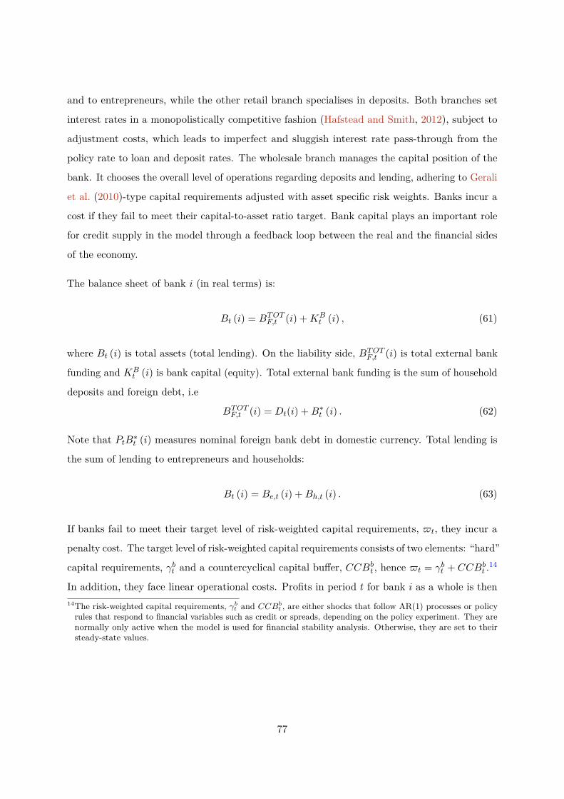
and to entrepreneurs, while the other retail branch specialises in deposits. Both branches set

interest rates in a monopolistically competitive fashion (Hafstead and Smith, 2012), subject to

adjustment costs, which leads to imperfect and sluggish interest rate pass-through from the

policy rate to loan and deposit rates. The wholesale branch manages the capital position of the

bank. It chooses the overall level of operations regarding deposits and lending, adhering to Gerali

et al. (2010)-type capital requirements adjusted with asset specific risk weights. Banks incur a

cost if they fail to meet their capital-to-asset ratio target. Bank capital plays an important role

for credit supply in the model through a feedback loop between the real and the financial sides

of the economy.

The balance sheet of bank i (in real terms) is:

Bt (i) = BTOTF,t (i) +KB

t (i) , (61)

where Bt (i) is total assets (total lending). On the liability side, BTOTF,t (i) is total external bank

funding and KBt (i) is bank capital (equity). Total external bank funding is the sum of household

deposits and foreign debt, i.e

BTOTF,t (i) = Dt(i) +B∗t (i) . (62)

Note that PtB∗t (i) measures nominal foreign bank debt in domestic currency. Total lending is

the sum of lending to entrepreneurs and households:

Bt (i) = Be,t (i) +Bh,t (i) . (63)

If banks fail to meet their target level of risk-weighted capital requirements, $t, they incur a

penalty cost. The target level of risk-weighted capital requirements consists of two elements: “hard”

capital requirements, γbt and a countercyclical capital buffer, CCBbt , hence $t = γbt + CCBb

t .14

In addition, they face linear operational costs. Profits in period t for bank i as a whole is then14The risk-weighted capital requirements, γbt and CCBbt , are either shocks that follow AR(1) processes or policyrules that respond to financial variables such as credit or spreads, depending on the policy experiment. They arenormally only active when the model is used for financial stability analysis. Otherwise, they are set to theirsteady-state values.

77

given by:

Jt (i) = rFt (i)Bh,t (i) + ret (i)Be,t (i)− rdt (i)Dt (i)

−([

1− γB∗t]R∗t

St+1St− 1

)B∗t (i)− χoBt(i)−

χc2

[KBt (i)

BRWt (i)

−$t

]2

KBt (i),

(64)

where rFt (i) is the net interest rate on loans to households, ret (i) is the net interest rate on loans to

entrepreneurs and rdt (i) is the net deposit interest rate. The bank pays a risk premium on foreign

funding. The “full” net interest rate for foreign funding hence becomes[1− γB∗t

]R∗t

St+1St− 1,

where 1− γB∗t is the debt-elastic risk premium. R∗t is the foreign money market rate and St is

the nominal exchange rate. χo governs the operational costs, and χc governs the capital target

costs. BRWt (i) denotes risk-weighted assets:

BRWt (i) = ςeBe,t + ςhBh,t, (65)

where ςe and ςh are the risk weights associated with credit to entrepreneurs and households,

respectively. Bank capital accumulates according to:

KBt (i) = (1− δb)Pt−1

PtKBt−1 (i) + Pt−1

PtJt−1 (i) , (66)

where δb is the dividend share of the bank capital paid out to shareholders (households).

D.9.1 The wholesale branch

The wholesale branch lends to the loan branch at the interest rate Rb,et (i) = 1 + rb,et (i) for

corporate credit (entrepreneurial loans) and Rb,ht (i) = 1+rb,ht (i) for household loans. It is funded

through borrowing from the deposit branch and from abroad. The “wholesale deposit rate” is

assumed to be equal to the money market rate Rt = 1 + rt, which follows from a no-arbitrage

condition since we assume that banks have access to unlimited financing at the money market

rate. The foreign funding rate,[1− γB∗t

]R∗t

St+1St

, is explained above.

The wholesale branch takes these funding costs as given and solves the following profit maximisa-

78

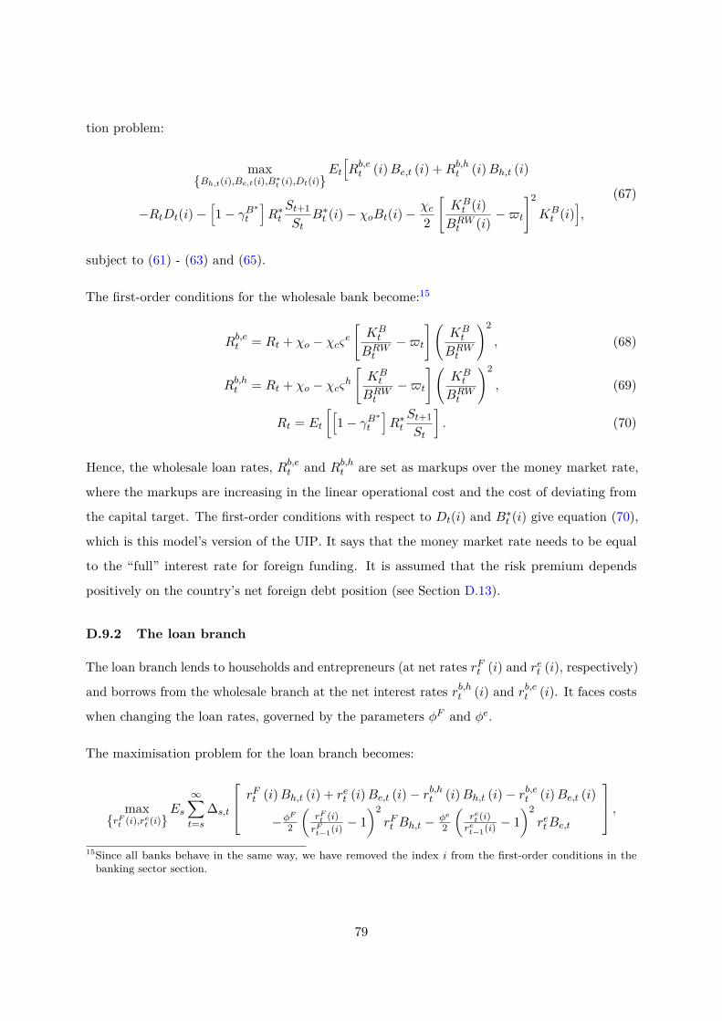
tion problem:

maxBh,t(i),Be,t(i),B∗t (i),Dt(i)

Et[Rb,et (i)Be,t (i) +Rb,ht (i)Bh,t (i)

−RtDt(i)−[1− γB∗t

]R∗t

St+1St

B∗t (i)− χoBt(i)−χc2

[KBt (i)

BRWt (i)

−$t

]2

KBt (i)

],

(67)

subject to (61) - (63) and (65).

The first-order conditions for the wholesale bank become:15

Rb,et = Rt + χo − χcςe[KBt

BRWt

−$t

](KBt

BRWt

)2

, (68)

Rb,ht = Rt + χo − χcςh[KBt

BRWt

−$t

](KBt

BRWt

)2

, (69)

Rt = Et

[[1− γB∗t

]R∗t

St+1St

]. (70)

Hence, the wholesale loan rates, Rb,et and Rb,ht are set as markups over the money market rate,

where the markups are increasing in the linear operational cost and the cost of deviating from

the capital target. The first-order conditions with respect to Dt(i) and B∗t (i) give equation (70),

which is this model’s version of the UIP. It says that the money market rate needs to be equal

to the “full” interest rate for foreign funding. It is assumed that the risk premium depends

positively on the country’s net foreign debt position (see Section D.13).

D.9.2 The loan branch

The loan branch lends to households and entrepreneurs (at net rates rFt (i) and ret (i), respectively)

and borrows from the wholesale branch at the net interest rates rb,ht (i) and rb,et (i). It faces costs

when changing the loan rates, governed by the parameters φF and φe.

The maximisation problem for the loan branch becomes:

maxrFt (i),ret (i)

Es

∞∑t=s

∆s,t

rFt (i)Bh,t (i) + ret (i)Be,t (i)− rb,ht (i)Bh,t (i)− rb,et (i)Be,t (i)

−φF

2

(rFt (i)rFt−1(i) − 1

)2rFt Bh,t −

φe

2

(ret (i)ret−1(i) − 1

)2retBe,t

,15Since all banks behave in the same way, we have removed the index i from the first-order conditions in thebanking sector section.

79

subject to

Bt (i) = Be,t (i) +Bh,t (i) , (71)

Bh,t (i) =(rFt (i)rFt

)−θIHtBh,t, (72)

Be,t (i) =(ret (i)ret

)−θetBe,t. (73)

Equations (72) and (73) are the demand functions from households and entrepreneurs respectively,

and θIHt > 0 and θet > 0 are the elasticities of substitution between household loans and corporate

credit from all loan branches. They follow AR(1) processes and can be interpreted as markup

shocks to the lending rates for household and business loans, respectively.

The first-order condition for the loan rate to households reads as (suppressing i):

1− θIHt + θIHtrb,htrFt− φF

(rFtrFt−1

− 1)

rFtrFt−1

+Et

∆t+1φF

(rFt+1rFt− 1

)(rFt+1rFt

)2Pt+1Pt

Bh,t+1Bh,t

= 0.

(74)

In the absence of adjustment costs, φF = 0, the mortgage loan rate collapses to a markup over

the wholesale lending rate (which is again a markup over the money-market rate (see (68))),

rFt = θIHtθIHt −1r

b,ht . The third term in (74) ensures that the loan branch also takes into account

future prices when setting today’s price.

In a similar fashion, the first-order condition for the loan rate to entrepreneurs, ret (i), becomes:

1− θet + θetrb,etret−φe

(retret−1

− 1)

retret−1

+Et

[∆t+1φ

e(ret+1ret− 1

)(ret+1ret

)2 Pt+1Pt

Be,t+1Be,t

]= 0. (75)

D.9.3 The deposit branch

The deposit branch lends to the wholesale branch at money market net rate rt and pays out

interest on household deposits at rate rdt (i). It faces costs when changing the deposit rate,

governed by parameter φD. The maximization problem becomes

maxrdt (i)

Es

∞∑t=s

∆s,t

rtDt (i)− rdt (i)Dt (i)− φD

2

(rdt (i)rdt−1 (i)

− 1)2

rdtDt

,

80

subject to deposit demand from households:

Dt (i) =(rdt (i)rdt

)θDtDt, (76)

where θD > 0 is the elasticity of substitution between deposit services.

The first-order condition with respect to rdt (i) becomes:

−(1 + θD) + θDrt

rdt− φD

(rdtrdt−1

− 1)

rdtrdt−1

+ Et

∆t+1φD

(rdt+1rdt− 1

)(rdt+1rdt

)2Pt+1Pt

Dt+1Dt

= 0.

(77)

In the absence of adjustment costs the deposit rate collapses to a mark-down on the money-market

rate (rdt = θD

1+θD rt).

D.10 Oil sector

To take into account the significance of the oil sector for the Norwegian economy, an explicit

oil sector is incorporated in NEMO. The oil sector builds on Bergholt et al. (2019). The

sector consists of supply firms as well as a domestic and a foreign extraction firm. The supply

firms combine labour, capital and final goods to produce oil supply goods that are used for oil

investment by the domestic extraction firm and are exported to a foreign oil extraction firm.

The representative domestic oil extraction firm undertakes two activities: (i) it invests in rigs,

using solely oil supply goods as inputs, and (ii)) it extracts and exports oil, using rigs and oil in

the ground as inputs.

D.10.1 Supply firms

A continuum of oil supply firms, indexed r, combines final goods QO,t(r) (priced at PQOt = Pt),

labour from households LO,t(r) and capital rented from entrepreneurs KO,t(r) to produce a

good YR,t(r) that is used for oil investment by an extraction firm and exports to a foreign oil

extraction firm. The wage earned by households working in the oil supply sector is WO,t, equal

to Wt because of perfect labour mobility, while the rental price of utilized capital is RKO,t, equal

to RK,t due to perfect mobility of capital.

81

The production function for supply firm r is:

YR,t(r) = ZRQαqO,t(r)(ZtLO,t(r))

αlK1−αq−αlO,t (r), (78)

where ZR is oil supply productivity, αq is the final goods share in production, αl is the labour

share and 1− αq − αl is the capital share in production. Including final goods as inputs ensures

that imports indirectly enter the production function. Minimizing costs, subject to (78), gives

rise to the following conditional demand functions and marginal cost function:

QO,t(r) = αq

(PQOtMCR,t

)−1

YR,t(r), (79)

LO,t(r) = αl

(WO,t

MCR,t

)−1

YR,t(r), (80)

KO,t(r) = (1− αq − αl)(RKO,tMCR,t

)−1

YR,t(r), (81)

MCR,t = 1ZR

(PQOtαq

)αq (WO,t

αl

)αl ( RKO,t1− αq − αl

)1−αq−αl. (82)

Oil supply firms sell their goods under monopolistic competition. Each firm r charges different

prices at home and abroad, PRt (r) in the domestic market and PR∗t (r) abroad, where the latter

is denoted in foreign currency. Dividends (which are paid out to households) becomes:

Ψt (r) = PRt (r) IOF,t(r) + PR∗t (r)StMO∗,t(r)−MCR,tYR,t(r), (83)

where IOF,t(r) are goods delivered to the domestic extraction firm, M∗O,t(r) are supply goods

for exports and St is the nominal exchange rate. Total production of supply goods must satisfy:

YR,t = IOF,t(r) +MO∗,t(r).

It can be shown that supply firm r faces the following demand functions from the domestic and

82

foreign extraction sectors, respectively:

IOF,t(r) =(PRt (r)PRt

)−θRIOF,t, (84)

MO∗,t(r) =(PR∗t (r)PR∗t

)−θR∗MO∗,t, (85)

where θR and θR∗ are the elasticities of substitution between goods in the two markets respectively.

Additionally, the costs of adjusting prices in the domestic and the foreign markets are given by:

γPR,t(r) ≡φPR

2

[PRt (r) /PRt−1 (r)PRt−1/P

Rt−2

− 1]2

, (86)

γPR∗,t(r) ≡φPR

∗

2

[PR

∗t (r) /PR∗t−1 (r)PR

∗t−1/P

R∗t−2

− 1]2

, (87)

respectively, where φPR and φPR∗ govern the costs of adjusting prices.

Profit maximisation with respect to PRt and PR∗t leads to the following first-order conditions in

symmetric equilibrium (index r removed), respectively:

IOF,t − θRIOF,t +MCR,tθR IOF,tPRt

− φPR[PRt /P

Rt−1

PRt−1/PRt−2− 1

]PRt /P

Rt−1

PRt−1/PRt−2

IOF,t

+Et

∆t+1φ

PR

[PRt+1/P

Rt

PRt /PRt−1− 1

](PRt+1/P

Rt )2

PRt /PRt−1

IOF,t+1

= 0,

(88)

StMO∗,t − θR∗StMO∗,t +MCR,tθ

R∗MO∗,tPR

∗t

− φPR∗[PR

∗t /PR

∗t−1

PR∗

t−1/PR∗t−2− 1

]PR

∗t /PR

∗t−1

PR∗

t−1/PR∗t−2

StMO∗,t

+Et

∆t+1φPR∗

[PR

∗t+1/P

R∗t

PR∗

t /PR∗

t−1− 1

] (PR

∗t+1/P

R∗t

)2

PR∗

t /PR∗

t−1St+1MO∗,t+1

= 0.(89)

Because of the adjustment costs, the supply firms take into account the full future path of expected

prices when setting current prices. In the case without any adjustment costs, prices would be set

as markups over marginal costs in every period: PRt = θR

θR−1MCR,t and PR∗

t = θR∗

θR∗−11StMCR,t.

83

D.10.2 The domestic extraction firm

Domestic oil extraction (YO,t) requires oil reserves (Ot) and oil rig services (FO,t) so that

YO,t = ZOFαoO,tO

1−αot , (90)

where ZO is oil extraction productivity and αo is the rigs share. As we abstract from issues of

depletion and discovery of new oil fields, Ot is treated as a parameter, Ot = O. Hence, αo ∈ [0, 1)

implies decreasing returns to scale. Effective oil rig services are determined by oil rig capacity,

FO,t−1, and a utilisation rate of that capacity, UF,t:

FO,t = FO,t−1UF,t. (91)

In (91) it is assumed that the rig capacity for period t is set in period t− 1. Hence, to increase

effective oil production in period t, the oil extraction firm must increase the utilisation rate, which

comes at a cost. Due to this endogenous utilisation rate, there will be a tradeoff between raising

the utilisation rate to increase production in the current period, or to increase investment that

will increase production capacity in future periods. The unit cost of increasing the utilisation

rate in terms of oil supply goods is represented by the function a(UF,t):

a(UF,t) = γO(UF,t − 1) + γOφuf

2 (UF,t − 1)2. (92)

The cost of changing the utilisation rate is governed by the parameters γO and φuf .16 The

extraction firm can invest in rig capacity, using oil supply goods as the investment good. Hence,

the dynamics of oil rig capacity is characterised by:

FO,t = (1− δO)FO,t−1 + ZIOIL,t

[1−ΨO

(IO,tIO,t−1

)]IO,t, (93)

where δO is the rigs depreciation rate and ΨO( IO,tIO,t−1

) = φRI

2 ( IO,tIO,t−1

− πzt )2 represents the costs of

changing investment levels, governed by the parameter φRI . The parameter πzt is the growth rate

of the economy and ZIOIL,t is an oil-specific technology shock, that follows an AR(1) process.

A positive innovation leads to more operative oil rigs in future periods for any given level of16By using UF,ss = 1, it can easily be shown that γO = a′(UF,ss). Kravik et al. (n.d.) show in their steady-statesolution (by combining steady-state versions of equation (95) and (97)) that γO = a′(UF,ss) = (δO + πz

ssβ− 1).

84

investment activity in the current period. Total demand for supply goods from the domestic

extraction firms is given by the sum of gross investments and the cost associated with the

utilisation rate of rigs: IOF,t = IO,t + a(UF,t)FO,t−1.

Oil production is given by YO,t, which is exported at a price PO∗t in foreign currency. Consequently,

the oil price in domestic currency is given by StPO∗t , where St is the nominal exchange rate. The

extraction firm maximises the discounted expected stream of cash flows, subject to extraction

technology and rig accumulation:

maxFO,t,IO,t,UF,t

∞∑t=s

∆s,t

[StP

O∗t YO,t − PRt IOF,t

], (94)

where ∆s,t is the stochastic discount factor between period s and t.

The intertemporal first-order conditions with respect to FO,t and IO,t become:17

ΩO,t = E[∆t+1

(αoSt+1P

O∗t+1YO,t+1F

−1O,t − P

Rt+1a(UF,t+1) + (1− δO)ΩO,t+1

)], (95)

PRt = ΩO,tZIOIL,t

[1−Ψ′O

(IO,tIO,t−1

)IO,tIO,t−1

−ΨO

(IO,tIO,t−1

)]

+E

∆ΩO,t+1ZIOIL,t+1Ψ′O

(IO,t+1IO,t

)(IO,t+1IO,t

)2 . (96)

Equation (95) determines the present marginal value of oil rig capacity, ΩO,t (the shadow price

of rig capacity). The first term on the right-hand side is the net income from installing more rigs

at the margin. The second term is the utilisation cost associated with more rigs, while the third

term represents the net-of-depreciation continuation value.

Equation (96) aligns the marginal cost of new investment (PRt ) with the marginal gain from

increased rig capacity. The first term on the right is the marginal gain from more capacity, net of

adjustment costs. The second term reflects that more investment in period t reduces the need for

costly investment adjustments in the future. The optimality conditions imply the oil company

bases its investment decisions on the entire expected future oil price path.17These are identical to equation (8) and (9) in Bergholt et al. (2019).

85

The first-order condition with respect to the utilisation rate UF,t becomes:

αoStPO∗t

YO,tUF,t

= PRt a′(UF,t)FO,t−1. (97)

In the optimum case, the marginal revenues from a higher rig utilisation rate is equated to the

marginal utilisation costs.

D.10.3 The foreign extraction firm

The foreign extraction firm is modelled in a simpler fashion. It extracts oil, YO∗,t, invests, IO∗,t,

and imports oil supply goods from the home country’s oil supply sector, MO∗,t, with the following

production function:18

YO∗,t = Mαo∗O∗,tI

αio∗O∗,t(O∗)

1−αio∗−αo∗ . (98)

O∗ is oil in the ground abroad, set to a constant and αo∗ is the share of domestically produced

oil supply goods used as inputs. Maximising profits leads to the following demand function for

oil supply goods from abroad:

MO∗,t = αo∗

(PR

∗t

PO∗t

)−1

YO∗,t. (99)

Note that YO∗,t follows an AR(1) process and can be interpreted as a foreign oil production shock

in the model (making IO∗,t, O∗ and αio∗ superfluous and not determined).

D.10.4 The GPFG

In Norway, the Government Pension Fund Act stipulates that the government’s cash flow from

the petroleum industry shall be transferred to the GPFG. A fiscal rule specifies that the transfers

from the GPFG to the central government’s fiscal budget shall follow the expected real return

on the GPFG over time. In NEMO, this relationship is simplified, as the GPFG and fiscal policy

are independently treated. The full sales revenue is transferred to the GPFG in every period.

Hence, the GPFG, BF,t, accumulates according to:

BF,t = (1− ρGF )[R∗t−1

Pt−1Pt

StSt−1

BF,t−1

]+ St

PO∗tPt

YO,t, (100)

18One can think of the product Mαo∗O∗,tI

αio∗O∗,t as the foreign rigs production function, corresponding to Fαo

O,t in (90).

86

where the amount (in real terms) transferred from the GPFG is given by:

GF,t = ρGF

[R∗t−1

Pt−1Pt

StSt−1

BF,t−1

]. (101)

The transfer, GF,t, ensures that the GPFG, BF,t is stationary. For instance, following an oil price

shock, the fund will never return back to its steady state when ρGF = 0.

In the model, we assume that the transfer from the fund goes to the banking sector (and not

to the government sector). This assumption is deemed necessary to be able to replicate (in the

steady state of the model) the fact that mainland Norway has positive net imports as well as a

negative (private) asset position (held by the banking sector) (see Section D.13 for the mainland

debt accumulation equation (B∗t ) and further details).

D.11 Foreign sector

The foreign sector in NEMO is split into two parts. The first part derives the optimality condition

for the price setting of the imported good that enters into the final good sector as well as export

demand for the domestic intermediate good. The second part, starting with (104) below, is a

block exogenous system of equations based on a standard New Keynesian model that links foreign

output, foreign money market rates, foreign inflation and the international oil price. We adopt

the small open economy assumption, implying that the foreign economy (rest of the world) is

fully exogenous from the point of view of the Norwegian economy. Hence, economic developments

in Norway have no effects on its trading partners. The two parts are linked since export demand

depends on trading partners’ output level.

The intermediate sector abroad is assumed to be symmetric to the domestic intermediate sector.

Foreign exporters enjoy market power and face price adjustment costs. The optimal price setting

rule for the imported price PMt in domestic currency (that enters into the domestic final good

sector as inputs) will therefore be (cf. (42)):

Mt − θFMt + StMC∗t θF Mt

PMt− φPM

[πMtπMt−1

− 1]πMtπMt−1

Mt

+Et

∆∗t+1φ

PM

[πMt+1πMt

− 1]

(πMt+1)2

πMtMt+1

StSt+1

= 0, (102)

87

where ∆∗t+1 is the foreign stochastic discount factor (assumed equal to (R∗t )−1 for simplicity),

φPM is a parameter that captures the cost of changing the price of imported goods, MC∗t denotes

foreign marginal costs that follow a shock process and θF is the substitution elasticity between

imported goods. Note that we have defined πMt ≡ PMt /PMt−1. In the absence of adjustment

costs, φPM = 0, prices would simply be set as a markup over marginal costs in every period

PMt = θF

θF−1StMC∗t with full exchange rate pass-through.

Turning to exports, the export demand for the intermediate good is given by (symmetric to (45)):

M∗t = (1− ν∗t )(PM∗t

P ∗t

)−µ∗Y ∗NAT,t, (103)

where ν∗t follows an AR(1) process and can be interpreted as an export demand shock. Y ∗NAT,t is

output abroad.

The second part of the foreign sector is modelled as a block-exogenous set of equations, linking

the foreign inflation gap, the foreign output gap, the foreign interest rate gap and the oil price

gap.19 Moreover, the foreign sector is divided into two groups: trading partners and non-trading

partners. The former is a group of Norway’s largest export and import partners; the latter

is the foreign sector minus trading partners. The model for the foreign sector is based on a

standard New Keynesian model, with a dynamic IS curve representing the relationship between

output and the real interest rate and a Phillips curve linking inflation to output, both with added

backward-looking terms to add more dynamics and realism.

The oil price has been added to the system of equations to negatively affect trading partners’

output and positively affect their rate of inflation. A rise in global demand will increase

international oil prices, but oil prices can also increase due to reduced international supply. The

effects of a demand-driven change in the oil price are stronger on the Norwegian economy than

the effects of a supply-driven change, since the latter weakens exports from the domestic non-oil

sector, dampening the positive effect on GDP. The effects of oil prices on the Norwegian economy

are further discussed in Gerdrup et al. (2017b).

Output for trading partners is given by equation (104) and (105), the latter being the traditional19In the remainder of this section, all variables are in gap form (deviation from steady state). The gap indicator is suppressed for readability.

88

IS curve (with the parameter ψR∗ relating the real interest rate to output):

Y ∗NAT,t = φY ∗Y ∗NAT,t−1 + (1− φY ∗)Y ∗FNAT,t − φO∗PO∗t + φY NTP∗Y NTPNAT,t + zU∗,t, (104)

where Y ∗FNAT,t is defined as:

Y ∗FNAT,t = Y ∗FNAT,t+1 − ψR∗(R∗t − π∗t+1). (105)

Trading partners’ output is affected negatively by the oil price gap, PO∗t , as Norway’s trading

partners are net oil importers, and positively by the output gap among non-trading partners,

Y NTPNAT,t. φO∗ and φY NTP∗ are positive parameters. φY ∗ is the lag operator, and zU∗,t follows an

AR(1) process and can be interpreted as a trading partner demand shock.

The output gap for non-trading partners, Y NTPNAT,t, is assumed to follow:

Y NTPNAT,t = λY NTPY Y NTP

NAT,t−1 − φONTPPO∗t + φY NTPY ∗NAT,t + zY NTP,t, (106)

where zY NTP,t can be interpreted as a global demand shock (equal to its innovation as there is

no corresponding persistence parameter), and λY NTP , φONTP and φY NTP are parameters. Total

global output is given by a weighted sum of trading partners’ and non-trading partners’ output:

Y GLOBNAT,t = αGLOBY ∗NAT,t + (1− αGLOB)Y NTP

NAT,t, (107)

where αGLOB is the trading partners’ output share of total global output.

Inflation for trading partners is given by equations (108) and (109), the latter being the traditional

Phillips curve:

π∗t = φP∗π∗t−1 + (1− φP∗)π∗F,t + φOP∗PO∗t , (108)

where π∗F,t is defined as:

π∗F,t = αP∗π∗F,t+1 + αY ∗Y ∗NAT,t + zθH∗,t. (109)

αY ∗ is the traditional Phillips curve parameter, whereas φOP∗ is a positive parameter picking up

the positive effect of real oil prices on marginal costs for trading partner firms. φP∗ is the lag

89

operator and zθH∗,t is a foreign price markup shock following an AR(1) process.

The oil price is forward-looking and assumed positively affected by global demand:

PO∗t = βOPO∗t+1 + κOY GLOBNAT,t + zPO∗,t, (110)

where zPO∗,t can be interpreted as an international oil supply shock, following an AR(1) process,

and βO and κO are parameters.

Lastly, the foreign monetary policy rate (equal to the foreign money market rate) is given by a

simple policy rule with smoothing:

R∗t = ωR∗R∗t−1 + (1− ωR∗)[ωP∗π∗t + ωY ∗Y ∗NAT,t

]+ zR∗,t, (111)

where zR∗,t follows an AR(1) process and can be interpreted as a trading partner monetary policy

shock, the parameter ωR∗ governs interest rate smoothing, and ωP∗ and ωY ∗ are weights on

inflation and output, respectively.

D.12 Market clearing conditions

The following set of equilibrium conditions needs to hold in order to close the model. In the

intermediate goods market, total production needs to equal goods for domestic use and exports:

Tt = Qt +M∗t . (112)

Total production of final goods needs to equal the sum of the following demand components:

Consumption, investment, housing investment, government expenditure and inputs into the oil

supply sector:

At = Ct + IC,t + IH,t +Gt +QO,t. (113)

Total investments must equal the sum of business and housing investment (note that it does note

include oil supply investment):

It = IC,t + IH,t. (114)

90

Total production of capital goods must equal capital usage in the oil and traditional sector

combined:

Kt = KO,t +KI,t. (115)

Equilibrium in the labour market is characterised by:

Lt = LO,t + LI,t. (116)

For the oil supply firms, total production must equal use by the domestic extraction firm and oil

supply exports.

YR,t = IOF,t +MO∗,t. (117)

Lastly, we define output for mainland Norway as:

YNAT,t =(Ct +Gt + It + PRt IO,t + StP

M∗t M∗t + StP

R∗t MO∗,t − PMt Mt

) 1log(zx,t)

, (118)

where the first four terms on the right hand side are household and government consumption,

investment and oil supply investment, respectively. The following two terms are traditional

and oil supply exports and PMt Mt represents imports. Finally, zx,t is an inventory shock to the

mainland economy that follows an AR(1) process. Total output is given by:

Y TOTALNAT,t = YNAT,t + StP

O∗t Y ∗O,t, (119)

i.e. mainland output plus production from oil extraction (which is exported).

D.13 Resource constraints, UIP and the current account

The division of the Norwegian economy into a mainland share and a non-mainland share entails

that foreign debt for the country as a whole is equal to mainland private foreign debt (held by

banks) less government claims:

BTOT∗t = B∗t −BF,t. (120)

Taking the household budget constraint as the point of departure and inserting for profits,

dividends and lump-sum taxes, it is possible to derive mainland Norway’s resource constraint,

91

i.e. the private foreign debt accumulation equation, as:

B∗t = Pt−1Pt

Rt−1B∗t−1 +

[PMtPt

Mt − StPR∗tPt

MO∗,t − StPM∗t

PtM∗t −

PRtPtIOF,t −GF,t

], (121)

where the bracketed term is the current account for mainland Norway, i.e. positive net imports

imply increased external debt for mainland Norway. The first term in the brackets is imports,

the second term is oil supply exports, the third term is traditional exports and the fourth term

is “exports” of oil supply goods from mainland Norway to non-mainland Norway.20 The fifth

term, GF,t, represents transfers from the GPFG to the mainland economy.

The accumulation equation for government claims and the size of transfers (GF,t) were derived

in Section D.10.4. Note that GF,t is included both in B∗t and BF,t and hence cancels out (except

for the interest rate differential (see equation (100))). In reality, the annual transfers from the

GPFG go to the government. As this mechanism is not modelled in NEMO and we do not wish

transfers from the GPFG to drive banking sector net worth, we set GF,t to its steady-state value

in (121) when we operate the model.

The uncovered interest rate parity was derived in Section D.9.1 and is repeated here:

Et

[[1− γB∗t

]R∗t

St+1St

]= Rt. (122)

In (122), 1− γB∗t is the debt-elastic risk premium, R∗t is the foreign money market rate and St is

the nominal exchange rate (NOK per foreign currency unit). It is assumed that the risk premium

depends positively on the country’s net foreign debt position (BTOT∗t ) and the anticipated growth

rate of the exchange rate:21

1− γB∗t = exp[φB(BTOT∗

t −BTOT∗ss )− φS(EtSt+1St − S2

ss)]

+ zBt , (123)

where zBt is an exogenous exchange rate risk premium shock following an AR(1) process and φB

and φS are non-negative parameters.

The assumption of a financial friction is necessary to ensure stationarity in small open economy20The latter term is ignored in the model file, in accordance with the national accounts.21Technically, the risk premium is defined in terms of stationary variables. Hence, in equation (123) the BTOT∗t

refers to the stationary version and St is the real exchange rate.

92

models like NEMO. Augmenting the risk premium with the anticipated growth rate of the

exchange rate tend to give a more hump-shaped exchange rate response following a risk premium

shock (see Adolfson et al. (2013) for a discussion).22

The relationship between the net foreign asset position, the risk premium and the UIP is

summarised in Figure 61.

UIP Risk premium

Net foreign asset position

Private foreign debt

(Mainland net imports)

Oil fund (Oil exports)

Fixed

transfer

Figure 61: The relationship between the net foreign asset position, the risk premium and the UIP inNEMO.

D.14 Monetary policy

The central bank controls the policy rate (RP,t), equal to the money market rate divided by the

exogenous money market risk premium (Rt = RP,tZprem,t), where Zprem,t is the risk premium and

a shock (following an AR(1) process). The central bank conducts optimal monetary policy, i.e.

setting the interest rate to minimise a loss function. The loss function consists of the discounted

(weighted) sum of future expected quadratic deviations from steady-state values of inflation,

output, the level of the policy rate and changes in the policy rate. More specifically, the central

bank minimises the following loss function, using the policy rate as instrument (either under

commitment or discretionary policies), where xt denotes variable x’s log-deviation from the

steady state:

minRP,t

∞∑t=s

βt−sp

[(πpol,t)2 + λy

(YNAT,t

)2+ λdr (4RP,t)2 + λlr

(RY EARP,t

)2], (124)

where βp is the central bank’s discount factor, RP,t is the policy rate gap, YNAT,t is the mainland

output gap (defined in Section D.12), πpol,t is four quarter consumer price inflation as a deviation

from the inflation target, 4RP,t is the annualised change in the policy rate and RY EARP,t is the22φS is weakly identified in the model and set to 0.

93

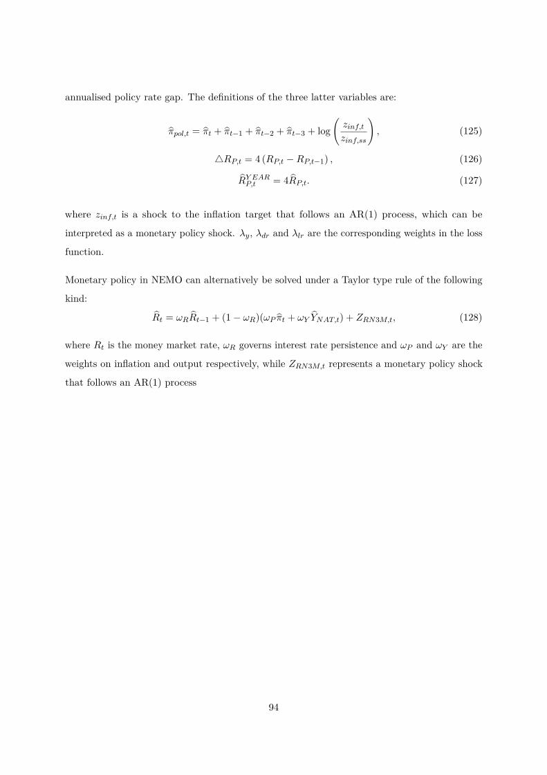
annualised policy rate gap. The definitions of the three latter variables are:

πpol,t = πt + πt−1 + πt−2 + πt−3 + log(zinf,tzinf,ss

), (125)

4RP,t = 4 (RP,t −RP,t−1) , (126)

RY EARP,t = 4RP,t. (127)

where zinf,t is a shock to the inflation target that follows an AR(1) process, which can be

interpreted as a monetary policy shock. λy, λdr and λlr are the corresponding weights in the loss

function.

Monetary policy in NEMO can alternatively be solved under a Taylor type rule of the following

kind:

Rt = ωRRt−1 + (1− ωR)(ωP πt + ωY YNAT,t) + ZRN3M,t, (128)

where Rt is the money market rate, ωR governs interest rate persistence and ωP and ωY are the

weights on inflation and output respectively, while ZRN3M,t represents a monetary policy shock

that follows an AR(1) process

94

E Calibration and estimation of NEMO

E.1 Calibration of the steady state

The steady-state solution of the model is derived recursively and is publicly available in Kravik

et al. (n.d.). We calibrate the steady state of the model by matching real and financial “great

ratios”. Specifically, we aim at matching 14 macroeconomic aggregates and 12 financial targets.

Our sample period is 2010-2016. Table 6 lists the empirical ratios and the model’s steady-state

counterparts.

Reflecting the assumption of a small open economy, the nominal interest rate in Norway in the

steady state is determined by the foreign sector and the inflation target in Norway. We set both

the inflation target and the nominal policy rate to 2 percent on an annual basis in the domestic

economy and abroad, implying a real policy rate of 0 percent. This is in line with data over the

sample period for Norway. The low nominal policy rate is important to reflect the implications

of the ELB in the model experiments. The money market premium is set to 0.5 percent on an

annual basis in Norway and abroad. The money market rate is therefore 2.5 percent. Parameters

determining interest rate markups are set to match market spreads from the data, i.e. 2.37

percent, 2.12 percent, and 0.5 percent for the business credit spread, the mortgage credit spread

and money market-deposit rate spread, respectively on an annual basis. The foreign sector and

Norway are assumed to share a steady-state productivity growth rate of 1 percent on annual

basis, which is in line with recent estimates for the Norwegian economy.

We treat the final good as the model’s numerator good and accordingly set the price of this good

to 1. The price of the intermediate good and the import good are also set to 1 in the steady state.

Although markups internationally have shown an increasing trend (Diez et al., 2018), we set

markups for the domestic good, the imported good and the exported good to 1.2, following the

standard calibration in the literature. In order to match the observed capital-to-mainland gross

domestic product (MGDP) ratio of 1.66, we set the capital share parameter, α, to 0.256 and the

elasticity of substitution between capital and labour, ξ, to 0.929. This gives a labour income

share of about 67 percent both for the intermediate goods sector and for the total mainland

economy in the steady state. This is on the lower side of what is found in the data of around 70

to 75 percent for Norway.

95

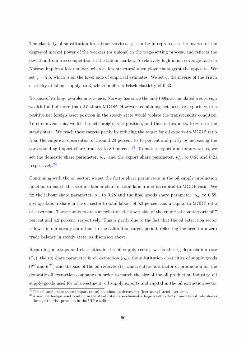
The elasticity of substitution for labour services, ψ, can be interpreted as the inverse of the

degree of market power of the workers (or unions) in the wage-setting process, and reflects the

deviation from free competition in the labour market. A relatively high union coverage ratio in

Norway implies a low number, whereas low structural unemployment suggest the opposite. We

set ψ = 2.5, which is on the lower side of empirical estimates. We set ζ, the inverse of the Frisch

elasticity of labour supply, to 3, which implies a Frisch elasticity of 0.33.

Because of its large petroleum revenues, Norway has since the mid-1990s accumulated a sovereign

wealth fund of more than 2.5 times MGDP. However, combining net positive exports with a

positive net foreign asset position in the steady state would violate the transversality condition.

To circumvent this, we fix the net foreign asset position, and thus net exports, to zero in the

steady state. We reach these targets partly by reducing the target for oil exports-to-MGDP ratio

from the empirical observation of around 20 percent to 16 percent and partly by increasing the

corresponding import share from 34 to 39 percent.23 To match export and import ratios, we

set the domestic share parameter, νss, and the export share parameter, ν∗ss, to 0.65 and 0.21

respectively.24

Continuing with the oil sector, we set the factor share parameters in the oil supply production

function to match this sector’s labour share of total labour and its capital-to-MGDP ratio. We

fix the labour share parameter, αl, to 0.28 and the final goods share parameter, αq, to 0.69,

giving a labour share in the oil sector to total labour of 5.3 percent and a capital-to-MGDP ratio

of 4 percent. These numbers are somewhat on the lower side of the empirical counterparts of 7

percent and 4.2 percent, respectively. This is partly due to the fact that the oil extraction sector

is lower in our steady state than in the calibration target period, reflecting the need for a zero

trade balance in steady state, as discussed above.

Regarding markups and elasticities in the oil supply sector, we fix the rig depreciation rate

(δO), the rig share parameter in oil extraction (αo), the substitution elasticities of supply goods

(θR and θR∗) and the size of the oil reserves (O, which enters as a factor of production for the

domestic oil extraction company) in order to match the size of the oil production industry, oil

supply goods used for oil investment, oil supply exports and capital in the oil extraction sector23The oil production share (import share) has shown a decreasing (increasing) trend over time.24A zero net foreign asset position in the steady state also eliminates large wealth effects from interest rate shocksthrough the risk premium in the UIP condition.

96

to MGDP. Due to the lower oil extraction share in the steady state compared to data, the

sub-targets also become a little lower than their empirical counterparts.

Turning to the banking sector, we use the regulatory capital risk weights of 0.4 and 0.8 on

household and corporate loans, respectively. In accordance with Norwegian financial regulations,

we set capital requirements for banks to 15.6 percent, of which 2 percent is the countercyclical

capital buffer. The internal rates of the banking sector are determined by the linear cost parameter

χo. We calibrate this and the dividend parameter δb to jointly achieve the empirical observation

of a return on equity in the Norwegian banking sector at around 10 percent. Households’ principal

repayments are assumed to follow from an approximated annuity loan repayment formula (see

equation (20) in Appendix D.3). The amortisation rate dynamics parameters αh and κh are

set in order to capture the repayment schedule of a 30-year mortgage contract, in line with

Norwegian household mortgage data. We set the collateral constraint parameter, φss, to match

a household debt-to-MGDP ratio of 105 percent. This gives an average loan-to-value (LTV)

ratio for households of 84.5 percent in the model, which is broadly consistent with a 15 percent

downpayment requirement in Norway. For corporate credit demand, we assume that loans are

rolled over in every period (αe = 0).

To match the corporate credit-to-MGDP ratio at 85 percent, we set the entrepreneurial collat-

eral constraint parameter, φentss , to 0.9917 in steady state, giving a loan-to-value rate for the

entrepreneurs at around 50 percent. We use the household deposit preference parameter, zd, to

match the deposit ratio.

House prices have over time grown more rapidly than other prices in Norway. We capture this

by assuming a negative technology trend growth in housing production of 3.4 percent annually,

matching the observed real house price growth rate of 1.046 annually.

The quarterly capital depreciation rate, δ, is set to 0.0108 in order to match the business

investment-to-MGDP ratio of 9 percent. We set the housing depreciation rate, δH , to target the

housing stock-to-MGDP ratio of about 124 percent. This gives a housing investment-to-MGDP

ratio of 7 percent – the empirical target being 6.15 percent.

Table 6 lists the empirical ratios (averages over the period 2010-2016) and the model’s steady-state

counterparts.

97

E.2 Estimation of dynamic parameters

We estimate the parameters of NEMO using Bayesian techniques, as outlined in An and

Schorfheide (2007). Computations are done using the RISE toolbox25 and NB Toolbox.26. In

this chapter we describe the data used for the estimation, give an account of how the model’s

steady state is calibrated and report on our prior and posterior distributions.

E.3 Data

The data set used for estimation of NEMO is quarterly and runs from 2001Q1, the year Norges

Bank officially introduced (flexible) inflation targeting, to 2017Q4. The macroeconomic time series

cover Norwegian and international variables. Real domestic variables include GDP, consumption,

exports, imports, government expenditure, investment and hours worked. Financial variables

include household and corporate credit. Price variables include wages, consumer prices, house

prices, lending rates to households, lending rates to corporations, money market interest rates

and the policy rate. Lastly, international variables include the exchange rate, the international

oil price and foreign GDP, money market rates and inflation. The data sources include Statistics

Norway, Norges Bank’s own calculations, and international sources, particularly the IMF and

Thomson Reuters. The data for the real variables are at constant prices from the national

accounts, whereas credit and house prices are deflated by consumer prices. In total, there are 26

observable variables used in the estimation of NEMO.

E.3.1 Data transformation and the steady state

NEMO is linearised around a steady state when solved. As with most DSGE models, NEMO

assumes that the economy has one balanced-growth path and that the different demand compo-

nents of GDP grow at the same pace over time.27 There is also a close relationship between the

steady-state real interest rate and the balanced-growth path. However, actual data are not as

well-behaved. Different variables exhibit different trends within the time span we have available,

but we have to choose only one set of steady-state values that are both deemed relevant for the

recent past and the economy going forward and that in addition are model-consistent.25“Rationality In Switching Environments” (RISE) is an object-oriented Matlab toolbox for solving and estimatingnonlinear Regime-Switching DSGE models. The toolbox was developed by Junior Maih and is freely availablefor downloading at https://github.com/jmaih/RISE_toolbox.

26NB Toolbox has been internally developed at Norges Bank. It will be released for public use in the future.27NEMO has a separate growth rate for the housing sector.

98

Even though business cycle dynamics can be influenced by the calculated gradients around the

steady state, most of the business cycles dynamics are determined by the dynamic parameters

and shock processes in the model. Consequently, since the model is too simple to explain

multiple, time-varying trends in the data, we use pre-filtered gap series (i.e. log-deviations from

trend) when we estimate dynamic parameters, estimate shock processes, calculate business cycle

moments, do shock decomposition and perform variance decompositions. There are therefore

no data transformations taking place within NEMO and no measurement equations. A future

goal is to solve the model around multiple time-varying states, so as to bring the model closer to

actual trend developments in the data.

For the demand components (consumption, housing investment, business investment, oil invest-

ment, government consumption, imports, traditional exports and oil supply exports) we use

the model DORY28 to filter the series and create the gaps. DORY ensures that the demand

component gaps sum to the output gap. Statistical filters (e.g. the Hodrick-Prescott filter) and

sector expert judgement are used to estimate the trend for hours worked, house prices, credit

variables, the oil price and foreign output. For some series, a three-quarter central moving

average procedure is utilised in order to remove noise.

Inflation is detrended by the inflation target of 2.5 percent.29 The trend in imported inflation is

assumed to be lower than that in overall inflation because of the continuous terms of trade gains

from low import price inflation that Norway has enjoyed over the sample period. These gains

have been slightly smaller in the latter years and are expected to remain so going forward. An

upward trend shift in imported inflation is therefore assumed after 2012.

Due to lower growth rates of trend productivity in recent years, downward shifts in the trend

growth rate of real wages were added in 2012 and 2013.30 The trend shifts in the money market

rate are consistent with Norges Bank’s published estimates of the neutral interest rate (see Norges

Bank’s Monetary Policy Report (MPR) 3/16, MPR 1/14, MPR 1/12 and MPR 1/10). Norges

Bank’s estimates are usually expressed as intervals, but NEMO requires point estimates in order28DORY has been developed by Ørjan Robstad and Kenneth S. Paulsen and will be documented in a forthcomingpaper in Norges Bank’s Staff Memo series.

29The inflation target was reduced in March 2018 to 2 percent. However, as we calibrate and estimate the modelusing historical data from 2001 to 2017, the new target is not considered in the detrending exercise.

30See the Special Feature on low productivity growth in Norges Bank’s Monetary Policy Report (MPR) 2/16.All Norges Bank’s Monetary Policy Reports are available at http://www.norges-bank.no/en/Published/Publications/Monetary-Policy-Report-with-financial-stability-assessment/.

99

to compute the interest rate gap. The point estimate in NEMO has been in the lower end of the

estimated interval for the neutral interest rate in recent years.

The neutral foreign money market rate is assumed to be 0.5 percentage point lower than in

Norway, reflecting the differences in the inflation target between Norway and our main trading

partners in the sample period. The neutral level of market interest rates is calculated based on

Norges Bank’s internal estimates of various risk premiums.

E.4 Choice of priors

In total, we estimate 89 parameters, of which 24 are domestic dynamic non-shock-related

parameters, 16 are non-shock-related parameters in the foreign block sector, 25 are shock

standard errors (of which 5 are in the foreign block), and finally there are 24 shock-persistence

parameters. Computations are done using the RISE toolbox (see footnote 25). We use two types

of priors in estimating the model: system priors and marginal priors.

E.4.1 System priors

The RISE toolbox allows for augmenting marginal priors (below) with system priors.31 In

contrast to marginal priors that deal with parameters independently, system priors are priors

about the model’s features and behavior as a system and are modelled with a density function

conditional on the model parameters. In theory, the system priors can either substitute or be

combined with marginal priors. In our estimation setup, we choose to augment our marginal

priors with specific beliefs about the variances of the observed variables. Specifically, we specify

our system priors as normal distributions over the variances of the observed variables, N(µ, σ),

where we set µ equal to the second-order moment from the data set that is used in the estimation,

and a not too restrictive standard deviation (given the magnitude of the variances of the observed

variables), σ, equal to 0.01. We did not set prior beliefs about co-variances. The standard

deviations of the observables are listed in Table ?? in Section ??.31This is somewhat similar to the framework laid out in Andrle and Benes (2013) and Del Negro and Schorfheide(2008). See the RISE website (https://github.com/jmaih/RISE_toolbox) for the particular codes.

100

E.4.2 Marginal priors

We use a mixed approach in setting the marginal priors. For some parameters, we use the existing

literature, empirical analysis and comparable models to find suitable prior values. Additionally,

for some parameters, we calibrate the model to match the targeted model moments referred to

in the previous section on system priors and set these values as the prior means. Finally, as

NEMO is primarily a tool for conducting monetary policy and forecasting, some priors are set

based on model users’ and sector experts’ assessments and judgements of the model’s properties,

including impulse responses to specific shocks, correlation patterns, and the overall forecasting

abilities of the model. This is especially true for the foreign block of the model, where several of

the parameters were only weakly identifiable. Table 7 and 8 display the marginal priors.

We choose a beta distribution for the habit persistence parameters with a prior mean of 0.5 and

a standard deviation of 0.2. For the habit formation parameter in consumption, we set a tighter

prior around 0.8 due to the low consumption volatility observed in the data.

We calibrate the parameters regarding house price expectations and housing investment ad-

justment costs in order to match the volatilities of housing investment and household credit

and to get empirically relevant effects of a monetary policy shock on house prices and housing

investment. Similarly, we calibrate the prior mean on investment adjustment costs parameters to

match investment volatility. As in Adolfson et al. (2013), we set the prior mean of the curvature

parameter in the capital utilisation cost, φu, to 0.2 to allow for a varying degree of utilisation of

the capital stock. Prior means for price and wage adjustment costs are calibrated to be broadly

in line with the moments on price and wage inflation rates, but prior standard deviations are set

to give room for flexibility in the estimation.

In the banking sector, we estimate the adjustment costs related to changing the deposit, mortgage

and corporate lending rates. We calibrate the prior means to match interest pass-through observed

in Norwegian data, i.e. close to 1-to-1 for deposit rates and 1-to-0.8 for corporate and household

lending rates.

The oil sector in NEMO builds on Bergholt et al. (2019) which forms the basis for our oil-related

parameter priors. In particular, we set the prior mean of the rig investment adjustment cost

parameter to 6 and the curvature parameter in the rig utilisation cost to 18, both being close

101

to posterior modes in Bergholt et al. (2019). To create sluggishness in the price setting of oil

supply goods, we augment the model with adjustment costs. We set high prior means and large

standard deviations.

DSGE models tend to be sensitive to external debt-elastic risk premium parameters in the sense

that small changes in these parameters can have large effects on the model’s behaviour. We

estimate φB based on a tight prior that was set to obtain empirically relevant effects of a shock

to real oil prices on the dynamics of the real exchange rate and the Norwegian economy in

general. The second risk premium parameter, φS , was excluded from our estimation due to

the low identification strength. We set φS to 0 to be consistent with the empirically observed

response of the real exchange rate to a monetary policy shock.

Shocks There are 26 shocks in NEMO, equal to the number of observable variables. All shocks

are assumed to follow first-order autoregressive processes, except for the non-trading-partner

output shock which is a pure innovation. Hence, there are 25 persistence parameters.

All shocks are assumed to have an inverse gamma distribution with a standard deviation of 2.

Most shocks have a prior mean of 0.01, but some prior means have been somewhat calibrated to

better fit some moments. Due to the wide priors on the standard deviations, the shock calibration

is expected to have limited impact on the estimation result. The persistence parameters are

given a beta distribution with a prior mean of 0.5 and a standard deviation of 0.2.

There is one exception to the above paragraph. The model showed some tendencies in giving

the price markup shock “too high” an explanatory power in explaining inflation in the historical

shock decomposition. To push the model to use other shocks, we tighten the prior standard

deviations of this particular shock and its persistence parameter.

E.5 Posterior results

Table 7 and 8 summarise the estimation results.

The posterior modes show strong habit persistence in consumption (0.94) and housing (0.99),

reflecting a large degree of inertia in these variables (although the housing habit parameter is only

weakly identifiable). The parameters regarding Rotemberg price adjustment costs have increased

compared to the earlier versions of NEMO, indicating a flatter Phillips curve. A relatively flat

102

Phillips curve is also found in the estimation of other DSGE models (see e.g. Adolfson et al.

(2013), Dorich et al. (2013) and Rees et al. (2016)).

The posterior modes on the parameters regarding corporate and housing investment adjustment

costs move relatively little compared to their prior means in spite of relatively loose prior

distributions. This is likely to be a sign of some identification issues (but it may also be due to

prior means that correspond well with data and the system priors). In the banking sector, the

posterior modes of the interest rate adjustment costs indicate a somewhat lower pass-through of

corporate and household interest rates and a higher pass-through for deposit rates, compared to

prior means.

Foreign sector parameters move relatively little compared to their prior means. As mentioned

above, this is expected as most of these parameters were only weakly identified in the identification

analysis and we set quite tight priors.

Most shock persistence parameters came out on the high side. Important exceptions include the

price markup shock (for which we set a tight prior) and the wage markup shock, the latter being

a sign of wage fluctuations being more transitory than other shocks. Interestingly, similar to

the finding in Rees et al. (2016), the foreign inflation shock is much more transitory (0.05) than

shocks to foreign output (0.78) and foreign monetary policy (0.32).

We use 30 Markov chains, each of which contains 2,400,000 draws generated by the Random

Walk Metropolis-Hastings algorithm with an acceptance rate tuned to 0.25. After thinning by a

factor of 10 (i.e. keeping every 10th draw), posterior moments were computed from 7,200,000

draws, where the first 1,200,000 were used as burn-in.32

We thin again to keep every remaining 100th draw before calculating the potential scale reduction

factor (PSRF) for each parameter as well as the so-called multivariate potential scale reduction

factor (MPSRF). The PSRFs for almost all estimated parameters are close to 1, implying that

convergence is achieved. The MPSRF is close to 1.4.

32To cover a large part of the surface of the log-likelihood function and to obtain the needed variation in theposterior draws, we used 900 Markov chains. Each of the 900 chains included 80000 draws. We then concatenatedthese different chains to obtain 30 chains with 2.4 million draws each. The resulting posterior densities lookedwell-behaved.

103

Table 6: Data targets and steady-state calibration values

Target Dataa Steady state

Macroeconomic aggregatesConsumption to MGDP 0.51 0.52Corporate investment toMGDP 0.09 0.09Housing investment to MGDP 0.06 0.07Oil investment to MGDP 0.08 0.06Government spending to MGDP 0.34 0.34Traditional exports to MGDP 0.16 0.16Oil supply exports to MGDP 0.07 0.07Imports to MGDP 0.34 0.39Physical capital to MGDP 1.66 1.66Physical capital in oil supply sector to MGDP 0.04 0.04Physical capital in oil extraction sector to MGDP 0.42 0.28Housing capital to MGDP 1.24 1.25Labour in oil sector to total labour 0.07 0.05Oil production to MGDP 0.20 0.16

Financial sectorHousehold lending to total assets 0.55 0.56Corporate lending to total assets 0.45 0.44Household deposits to total assets 0.51 0.49Foreign funding to total assets 0.42 0.42Bank capital to total assets 0.07 0.09Total assets to MGDP 1.90 1.90Bank capital to risk-weighted assets 0.16 0.16Real return on bank equity 0.10 0.10Average business credit spread (%) 2.37 2.37Average mortgage credit spread (%) 2.12 2.12Average money market-deposit rate spread (%) 0.5 0.5Average money market premium (%) 0.5 0.5a Averages over the period 2010-2016.

104

Table 7: Marginal prior and posterior distributions, dynamic parameters

Prior Posterior

Distr. Mean S.d. Mode Mean 5% 95%

Habit formationsbc Consumption β 0.8 0.05 0.938 0.945 0.93 0.957bh Housing β 0.5 0.2 0.987 0.989 0.987 0.99bl Labour β 0.5 0.2 0.586 0.57 0.535 0.605bd Deposits β 0.5 0.2 0.481 0.389 0.278 0.49

Adjustment costs etc.bsa House price expect. β 0.65 0.025 0.639 0.621 0.606 0.635λsa House price expect. β 0.9 0.05 0.949 0.964 0.95 0.98φPM Importsa Γ 9 1 8.301 7.966 7.585 8.334φPM

∗Exportsa Γ 3 1 2.856 2.883 2.693 3.054

φPQ Domestic goodsa Γ 12 1 6.69 6.767 6.7 6.863φW Wage inflationb Γ 0.7 0.1 0.667 0.68 0.646 0.713φu Capital util., entrep. Γ 0.2 0.075 0.219 0.22 0.201 0.24φI1 Business investment Γ 10 2 12.543 12.714 11.838 13.57φI2 Business investment Γ 170 10 165.662 163.034 158.858 166.972φH1 Housing investment Γ 60 5 60.728 61.748 59.614 63.98φH2 Housing investment Γ 200 10 199.655 196.241 187.099 205.43φD Deposit rate Γ 0.1 0.05 0.073 0.087 0.076 0.099φe Loan rate, entrep. Γ 15 2 18.501 19.581 18.149 21.096φF Loan rate, househ. Γ 15 2 18.36 18.661 17.828 19.525φRI Oil investment Γ 6 1 8.215 8.149 7.639 8.624φuf Oil rigs util. Γ 18 2 17.795 17.27 16.752 17.71φPR Oil supply, dom.b Γ 2 1 1.246 1.182 1.061 1.292φPR

∗Oil supply, abr.b Γ 2 1 1.723 1.468 0.827 2.167

φB Risk Prem. N 0.0015 0.0002 0.00156 0.00159 0.00153 0.00166

Foreign blockφY ∗ Lag, output N 0.5 0.05 0.615 0.619 0.596 0.643ψR∗ IS curve N 1 0.2 0.757 0.724 0.615 0.832ωR∗ Lag, Taylor β 0.8 0.05 0.841 0.812 0.787 0.835ωP∗ Infl. weight, Taylor N 1.5 0.1 1.461 1.408 1.366 1.444ωY ∗ Outp. weight, Taylor N 0.03 0.01 0.04 0.046 0.039 0.054αP∗ Infl. Expectations N 0.15 0.01 0.15 0.15 0.149 0.15αY ∗ Infl. ← output N 0.15 0.05 0.046 0.046 0.039 0.053φP∗ Lag, inflation N 0.8 0.2 0.886 0.884 0.873 0.894φOP∗ Infl. ← oil price N 0.003 0.001 0.001 0 0 0.001φO∗ Output ← oil price N 0.005 0.001 0.005 0.005 0.004 0.005φY NTP∗ Output ← NTP output N 1 0.2 1.099 1.137 1.04 1.244λY NTP Lag, NTP output N 0.9 0.2 0.926 0.947 0.914 0.971φONTP NTP output ← oil price N 0.002 0.001 0.001 0.002 0.001 0.003φY NTP NTP output ← output N 0.01 0.002 0.011 0.011 0.011 0.012βO Oil price expectations N 0.2 0.02 0.203 0.202 0.197 0.206κO Oil price demand N 4 0.1 4.003 3.998 3.983 4.015

Note: After thinning by a factor of 10, posterior moments are computed from 7,200,000 draws generatedby the Random Walk Metropolis-Hastings algorithm using 30 chains with an acceptance rate tuned to 0.25,where the first 1,200,000 are used as burn-in.a Parameter is multiplied by 100 in the model.b Parameter is multiplied by 1000 in the model.

105

106

Table 8: Marginal prior and posterior distributions, shock parameters

Prior Posterior

Distr. Mean S.d. Mode Mean 5% 95%

Shock persistenceλB Risk prem. β 0.5 0.2 0.737 0.732 0.686 0.774λG Gov. exp. β 0.5 0.2 0.914 0.948 0.933 0.964λh Househ. pref. β 0.5 0.2 0.694 0.658 0.599 0.711λIH Housing investment β 0.5 0.2 0.861 0.869 0.849 0.888λIOIL Oil investment β 0.5 0.2 0.834 0.853 0.806 0.894λI Business investment β 0.5 0.2 0.646 0.661 0.618 0.703λzL Productivity (temp.) β 0.5 0.2 0.804 0.815 0.794 0.835λMC∗ Marginal costs, abr. β 0.5 0.2 0.097 0.065 0.034 0.094λν Import share β 0.5 0.2 0.934 0.964 0.949 0.976λν∗ Export share β 0.5 0.2 0.924 0.927 0.9 0.953λφ LTV, househ. β 0.5 0.2 0.783 0.716 0.646 0.776λφent LTV, entrep. β 0.5 0.2 0.91 0.884 0.836 0.927λprem Money market risk prem. β 0.5 0.2 0.817 0.837 0.806 0.868λψ Wage markup β 0.5 0.2 0.28 0.241 0.2 0.279λθe Lending rate, entrep. β 0.5 0.2 0.964 0.966 0.957 0.974λθH Price markup β 0.3 0.02 0.435 0.432 0.428 0.434λθIH Lending rate, househ. β 0.5 0.2 0.89 0.874 0.848 0.898λu Consump. pref. β 0.5 0.2 0.725 0.691 0.641 0.739λwedge Inventories β 0.5 0.2 0.838 0.868 0.824 0.912λY O∗ Oil prod., abroad β 0.5 0.2 0.746 0.741 0.716 0.767λPO∗ Oil price β 0.9 0.02 0.874 0.872 0.865 0.879λR∗ Mon. pol., TP β 0.5 0.2 0.322 0.342 0.283 0.408λθH∗ Price markup, TP β 0.5 0.2 0.052 0.066 0.033 0.104λU∗ Demand, TP β 0.5 0.2 0.782 0.816 0.782 0.85

Shock st.dev. (multiplied by 100)σB Risk prem. Γ−1 5 200 0.618 0.633 0.519 0.767σG Gov. exp. Γ−1 10 200 0.381 0.401 0.381 0.44σh Household pref. Γ−1 1 200 28.677 47.065 36.776 57.85σIH Housing investment Γ−1 1 200 2.575 2.522 2.356 2.688σIOIL Oil investment Γ−1 1 200 2.612 2.507 2.021 3.08σI Business investment Γ−1 1 200 23.018 24.665 22.951 26.403σzL Productivity (temp.) Γ−1 1 200 0.598 0.587 0.545 0.631σMC∗ Marg. costs, abr. Γ−1 10 200 34.629 37.145 34.876 39.747σν Import share Γ−1 1 200 0.428 0.485 0.417 0.565σν∗ Export share Γ−1 1 200 4.238 4.419 3.825 5.101σφent LTV, entrep. Γ−1 1 200 2.59 2.757 2.377 3.203σφ LTV, househ. Γ−1 1 200 25.423 26.756 23.2 30.894σprem Money market risk prem. Γ−1 0.05 200 0.037 0.037 0.035 0.038σψ Wage markup Γ−1 200 200 63.31 52.133 46.675 57.846σθe Lending rate, entrep. Γ−1 1 200 84.858 97.346 84.03 112.26σθH Price markup Γ−1 20 0.1 20.145 20.155 20.13 20.183σθIH Lending rate, househ. Γ−1 1 200 167.942 185.12 174.699 196.939σu Consump. pref. Γ−1 1 200 3.021 3.356 2.847 3.91σwedge Inventories Γ−1 0.1 200 0.184 0.19 0.18 0.201σY O∗ Oil prod., abroad Γ−1 6 200 3.409 3.31 3.052 3.546σPO∗ Oil price Γ−1 7 200 7.918 8.055 7.864 8.253σR∗ Mon. pol., TP Γ−1 0.1 200 0.084 0.086 0.08 0.093σθH∗ Price markup, TP Γ−1 1 200 0.833 0.822 0.797 0.844σU∗ Demand, TP Γ−1 1 200 1.115 1.104 0.991 1.229σY NTP Global demand Γ−1 1 200 0.183 0.198 0.17 0.231

Otherρffm Oil price ← wage bargaining N 0.5 0.05 0.527 0.532 0.516 0.55

Note: See notes to Table 7.

107