Remote Sensing of Environment 127 (2012) 341–356

Contents lists available at SciVerse ScienceDirect

Remote Sensing of Environment

j ourna l homepage: www.e lsev ie r .com/ locate / rse

Observation uncertainty of satellite soil moisture products determined withphysically-based modeling

Niko Wanders a,⁎, Derek Karssenberg a, Marc Bierkens a,b, Robert Parinussa c, Richard de Jeu c,Jos van Dam d, Steven de Jong a

a Department of Physical Geography, Faculty of Geosciences, Utrecht University, Utrecht, The Netherlandsb Deltares, Unit Soil and Groundwater Systems, Utrecht, The Netherlandsc Department of Hydrology and Geo-environmental Sciences, Faculty of Earth and Life Sciences, VU University Amsterdam, Amsterdam, The Netherlandsd Soil Physics, Ecohydrology and Groundwater Management Group, Wageningen University, Wageningen, The Netherlands

⁎ Corresponding author. Tel.: +31 30 253 2988.E-mail address: n.wanders@uu.nl (N. Wanders).

0034-4257/$ – see front matter © 2012 Elsevier Inc. Allhttp://dx.doi.org/10.1016/j.rse.2012.09.004

a b s t r a c t

a r t i c l e i n f o

Article history:Received 21 March 2012Received in revised form 29 August 2012Accepted 7 September 2012Available online xxxx

Keywords:Soil moistureMicrowave remote sensingSatellite uncertaintyASCATAMSR-ESMOSSWAP-model

Accurate estimates of soil moisture as initial conditions to hydrological models are expected to greatly in-crease the accuracy of flood and drought predictions. As in-situ soil moisture observations are scarce,satellite-based estimates are a suitable alternative. The validation of remotely sensed soil moisture productsis generally hampered by the difference in spatial support of in-situ observations and satellite footprints.Unsaturated zone modeling may serve as a valuable validation tool because it could bridge the gap of differ-ent spatial supports. A stochastic, distributed unsaturated zone model (SWAP) was used in which the spatialsupport was matched to these of the satellite soil moisture retrievals. A comparison between point observa-tions and the SWAP model was performed to enhance understanding of the model and to assure that theSWAP model could be used with confidence for other locations in Spain. A timeseries analysis was performedto compare surface soil moisture from the SWAP model to surface soil moisture retrievals from three differ-ent microwave sensors, including AMSR-E, SMOS and ASCAT. Results suggest that temporal dynamics arebest captured by AMSR-E and ASCAT resulting in an averaged correlation coefficient of 0.68 and 0.71, respec-tively. SMOS shows the capability of capturing the long-term trends, however on short timescales the soilmoisture signal was not captured as well as by the other sensors, resulting in an averaged correlation coeffi-cient of 0.42. Root mean square errors for the three sensors were found to be very similar (±0.05m3m−3).The satellite uncertainty is spatially correlated and distinct spatial patterns are found over Spain.

© 2012 Elsevier Inc. All rights reserved.

1. Introduction

Soil moisture is an important variable inmany applications and en-vironmental studies, such as numerical weather prediction (Drusch,2007), global change modeling (Henderson-Sellers, 1996), predictingsurface runoff (Brocca et al., 2010), drought monitoring (Sheffield &Wood, 2007) and modeling evaporation (Miralles, Holmes, et al.,2010). In small catchments (700 km2) soil moisture assimilation hasbeen shown to improve discharge simulation (Brocca et al., 2010);the impact in larger scale river basins remains unknown. At thislarge scale, ground based soil moisture measurements are relativelyscarce and therefore lack sufficient spatial density to be accuratelyup-scaled to improve flood forecasting for large river basins. Soil mois-ture is highly variable in space and time and thus a high spatial andtemporal resolution of observations is required to retrieve good esti-mates of the actual soil moisture content (Western et al., 2002).

rights reserved.

A possible solution to obtain spatially averaged soil moisture forlarge river basins is the use of soil moisture retrievals from spacebornsensors measuring in the microwave frequencies. For several yearspassive and active microwave observations have been used for the re-trieval of soil moisture from the Earth's surface. The current Soil Mois-ture and Ocean Salinity (SMOS) mission observes the Earth's surfacein the L-band (1.41 GHz) frequency (Wigneron et al., 1995), becausesuch low frequency observations are most sensitive to soil moisture.SMOS is the first dedicated satellite observing soil moisture fromspace and was launched in November 2009. In the past, several pas-sive microwave sensors, such as the Advanced Microwave ScanningRadiometer-EOS (AMSR-E), have been used to retrieve soil moistureusing multi-channel observations obtained at higher microwave fre-quencies (e.g. Njoku et al., 2003; Owe et al., 2008). AMSR-E, onboardNASA's Aqua satellite was launched in 2002 and was recently (October2011) switched off due to rotation problems with its antenna. Also,several active microwave sensors, such as the Advanced Scatterometer(ASCAT) onboard ESA's MetOp satellite, were used for the samepurpose. Backscatter measurements at three different azimuth anglesare converted to surface soil moisture (Naeimi et al., 2009). Microwave

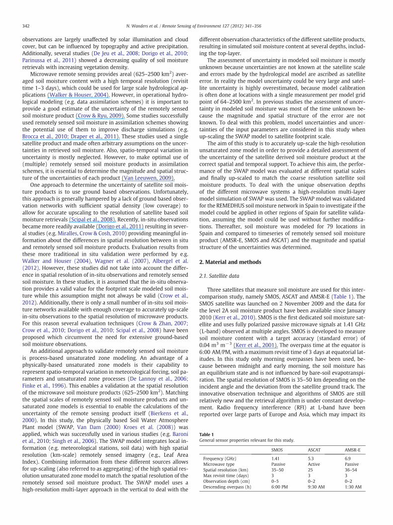
Table 1General sensor properties relevant for this study.

SMOS ASCAT AMSR-E

Frequency (GHz) 1.41 5.3 6.9Microwave type Passive Active PassiveSpatial resolution (km) 35–50 25 36–54Max revisit time (days) 3 3 3Observation depth (cm) 0–5 0–2 0–2Descending overpass (h) 6:00 PM 9:30 AM 1:30 AM

342 N. Wanders et al. / Remote Sensing of Environment 127 (2012) 341–356

observations are largely unaffected by solar illumination and cloudcover, but can be influenced by topography and active precipitation.Additionally, several studies (De Jeu et al., 2008; Dorigo et al., 2010;Parinussa et al., 2011) showed a decreasing quality of soil moistureretrievals with increasing vegetation density.

Microwave remote sensing provides areal (625–2500 km2) aver-aged soil moisture content with a high temporal resolution (revisittime 1–3 days), which could be used for large scale hydrological ap-plications (Walker & Houser, 2004). However, in operational hydro-logical modeling (e.g. data assimilation schemes) it is important toprovide a good estimate of the uncertainty of the remotely sensedsoil moisture product (Crow & Ryu, 2009). Some studies successfullyused remotely sensed soil moisture in assimilation schemes showingthe potential use of them to improve discharge simulations (e.g.Brocca et al., 2010; Draper et al., 2011). These studies used a singlesatellite product and made often arbitrary assumptions on the uncer-tainties in retrieved soil moisture. Also, spatio-temporal variation inuncertainty is mostly neglected. However, to make optimal use of(multiple) remotely sensed soil moisture products in assimilationschemes, it is essential to determine the magnitude and spatial struc-ture of the uncertainties of each product (Van Leeuwen, 2009).

One approach to determine the uncertainty of satellite soil mois-ture products is to use ground based observations. Unfortunately,this approach is generally hampered by a lack of ground based obser-vation networks with sufficient spatial density (low coverage) toallow for accurate upscaling to the resolution of satellite based soilmoisture retrievals (Scipal et al., 2008). Recently, in-situ observationsbecamemore readily available (Dorigo et al., 2011) resulting in sever-al studies (e.g. Miralles, Crow & Cosh, 2010) providing meaningful in-formation about the differences in spatial resolution between in situand remotely sensed soil moisture products. Evaluation results fromthese more traditional in situ validation were performed by e.g.Walker and Houser (2004), Wagner et al. (2007), Albergel et al.(2012). However, these studies did not take into account the differ-ence in spatial resolution of in-situ observations and remotely sensedsoil moisture. In these studies, it is assumed that the in-situ observa-tion provides a valid value for the footprint scale modeled soil mois-ture while this assumption might not always be valid (Crow et al.,2012). Additionally, there is only a small number of in-situ soil mois-ture networks available with enough coverage to accurately up-scalein-situ observations to the spatial resolution of microwave products.For this reason several evaluation techniques (Crow & Zhan, 2007;Crow et al., 2010; Dorigo et al., 2010; Scipal et al., 2008) have beenproposed which circumvent the need for extensive ground-basedsoil moisture observations.

An additional approach to validate remotely sensed soil moistureis process-based unsaturated zone modeling. An advantage of aphysically-based unsaturated zone models is their capability torepresent spatio-temporal variation in meteorological forcing, soil pa-rameters and unsaturated zone processes (De Lannoy et al., 2006;Finke et al., 1996). This enables a validation at the spatial resolutionof the microwave soil moisture products (625–2500 km2). Matchingthe spatial scales of remotely sensed soil moisture products and un-saturated zone models is essential to enable the calculations of theuncertainty of the remote sensing product itself (Bierkens et al.,2000). In this study, the physically based Soil Water AtmospherePlant model (SWAP, Van Dam (2000) Kroes et al. (2008)) wasapplied, which was successfully used in various studies (e.g. Baroniet al., 2010; Singh et al., 2006). The SWAP model integrates local in-formation (e.g. meteorological stations, soil data) with high spatialresolution (km-scale) remotely sensed imagery (e.g., Leaf AreaIndex). Combining information from these different sources allowsfor up-scaling (also referred to as aggregating) of the high spatial res-olution unsaturated zone model to match the spatial resolution of theremotely sensed soil moisture product. The SWAP model uses ahigh-resolution multi-layer approach in the vertical to deal with the

different observation characteristics of the different satellite products,resulting in simulated soil moisture content at several depths, includ-ing the top-layer.

The assessment of uncertainty in modeled soil moisture is mostlyunknown because uncertainties are not known at the satellite scaleand errors made by the hydrological model are ascribed as satelliteerror. In reality the model uncertainty could be very large and satel-lite uncertainty is highly overestimated, because model calibrationis often done at locations with a single measurement per model gridpoint of 64–2500 km2. In previous studies the assessment of uncer-tainty in modeled soil moisture was most of the time unknown be-cause the magnitude and spatial structure of the error are notknown. To deal with this problem, model uncertainties and uncer-tainties of the input parameters are considered in this study whenup-scaling the SWAP model to satellite footprint scale.

The aim of this study is to accurately up-scale the high-resolutionunsaturated zone model in order to provide a detailed assessment ofthe uncertainty of the satellite derived soil moisture product at thecorrect spatial and temporal support. To achieve this aim, the perfor-mance of the SWAP model was evaluated at different spatial scalesand finally up-scaled to match the coarse resolution satellite soilmoisture products. To deal with the unique observation depthsof the different microwave systems a high-resolution multi-layermodel simulation of SWAP was used. The SWAP model was validatedfor the REMEDHUS soil moisture network in Spain to investigate if themodel could be applied in other regions of Spain for satellite valida-tion, assuming the model could be used without further modifica-tions. Thereafter, soil moisture was modeled for 79 locations inSpain and compared to timeseries of remotely sensed soil moistureproduct (AMSR-E, SMOS and ASCAT) and the magnitude and spatialstructure of the uncertainties was determined.

2. Material and methods

2.1. Satellite data

Three satellites that measure soil moisture are used for this inter-comparison study, namely SMOS, ASCAT and AMSR-E (Table 1). TheSMOS satellite was launched on 2 November 2009 and the data forthe level 2A soil moisture product have been available since January2010 (Kerr et al., 2010). SMOS is the first dedicated soil moisture sat-ellite and uses fully polarized passive microwave signals at 1.41 GHz(L-band) observed at multiple angles. SMOS is developed to measuresoil moisture content with a target accuracy (standard error) of0.04 m3 m−3 (Kerr et al., 2001). The overpass time at the equator is6:00 AM/PM, with a maximum revisit time of 3 days at equatorial lat-itudes. In this study only morning overpasses have been used, be-cause between midnight and early morning, the soil moisture hasan equilibrium state and is not influenced by bare-soil evapotranspi-ration. The spatial resolution of SMOS is 35–50 km depending on theincident angle and the deviation from the satellite ground track. Theinnovative observation technique and algorithms of SMOS are stillrelatively new and the retrieval algorithm is under constant develop-ment. Radio frequency interference (RFI) at L-band have beenreported over large parts of Europe and Asia, which may impact its

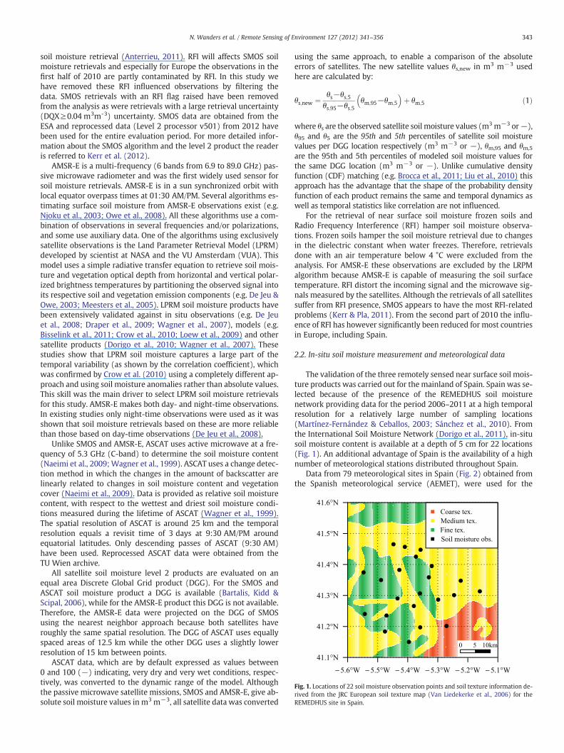
Fig. 1. Locations of 22 soil moisture observation points and soil texture information de-rived from the JRC European soil texture map (Van Liedekerke et al., 2006) for theREMEDHUS site in Spain.

343N. Wanders et al. / Remote Sensing of Environment 127 (2012) 341–356

soil moisture retrieval (Anterrieu, 2011). RFI will affects SMOS soilmoisture retrievals and especially for Europe the observations in thefirst half of 2010 are partly contaminated by RFI. In this study wehave removed these RFI influenced observations by filtering thedata. SMOS retrievals with an RFI flag raised have been removedfrom the analysis as were retrievals with a large retrieval uncertainty(DQX≥0.04 m3m-3) uncertainty. SMOS data are obtained from theESA and reprocessed data (Level 2 processor v501) from 2012 havebeen used for the entire evaluation period. For more detailed infor-mation about the SMOS algorithm and the level 2 product the readeris referred to Kerr et al. (2012).

AMSR-E is a multi-frequency (6 bands from 6.9 to 89.0 GHz) pas-sive microwave radiometer and was the first widely used sensor forsoil moisture retrievals. AMSR-E is in a sun synchronized orbit withlocal equator overpass times at 01:30 AM/PM. Several algorithms es-timating surface soil moisture from AMSR-E observations exist (e.g.Njoku et al., 2003; Owe et al., 2008). All these algorithms use a com-bination of observations in several frequencies and/or polarizations,and some use auxiliary data. One of the algorithms using exclusivelysatellite observations is the Land Parameter Retrieval Model (LPRM)developed by scientist at NASA and the VU Amsterdam (VUA). Thismodel uses a simple radiative transfer equation to retrieve soil mois-ture and vegetation optical depth from horizontal and vertical polar-ized brightness temperatures by partitioning the observed signal intoits respective soil and vegetation emission components (e.g. De Jeu &Owe, 2003; Meesters et al., 2005). LPRM soil moisture products havebeen extensively validated against in situ observations (e.g. De Jeuet al., 2008; Draper et al., 2009; Wagner et al., 2007), models (e.g.Bisselink et al., 2011; Crow et al., 2010; Loew et al., 2009) and othersatellite products (Dorigo et al., 2010; Wagner et al., 2007). Thesestudies show that LPRM soil moisture captures a large part of thetemporal variability (as shown by the correlation coefficient), whichwas confirmed by Crow et al. (2010) using a completely different ap-proach and using soil moisture anomalies rather than absolute values.This skill was the main driver to select LPRM soil moisture retrievalsfor this study. AMSR-E makes both day- and night-time observations.In existing studies only night-time observations were used as it wasshown that soil moisture retrievals based on these are more reliablethan those based on day-time observations (De Jeu et al., 2008).

Unlike SMOS and AMSR-E, ASCAT uses active microwave at a fre-quency of 5.3 GHz (C-band) to determine the soil moisture content(Naeimi et al., 2009;Wagner et al., 1999). ASCAT uses a change detec-tion method in which the changes in the amount of backscatter arelinearly related to changes in soil moisture content and vegetationcover (Naeimi et al., 2009). Data is provided as relative soil moisturecontent, with respect to the wettest and driest soil moisture condi-tions measured during the lifetime of ASCAT (Wagner et al., 1999).The spatial resolution of ASCAT is around 25 km and the temporalresolution equals a revisit time of 3 days at 9:30 AM/PM aroundequatorial latitudes. Only descending passes of ASCAT (9:30 AM)have been used. Reprocessed ASCAT data were obtained from theTU Wien archive.

All satellite soil moisture level 2 products are evaluated on anequal area Discrete Global Grid product (DGG). For the SMOS andASCAT soil moisture product a DGG is available (Bartalis, Kidd &Scipal, 2006), while for the AMSR-E product this DGG is not available.Therefore, the AMSR-E data were projected on the DGG of SMOSusing the nearest neighbor approach because both satellites haveroughly the same spatial resolution. The DGG of ASCAT uses equallyspaced areas of 12.5 km while the other DGG uses a slightly lowerresolution of 15 km between points.

ASCAT data, which are by default expressed as values between0 and 100 (−) indicating, very dry and very wet conditions, respec-tively, was converted to the dynamic range of the model. Althoughthe passive microwave satellite missions, SMOS and AMSR-E, give ab-solute soil moisture values in m3 m−3, all satellite data was converted

using the same approach, to enable a comparison of the absoluteerrors of satellites. The new satellite values θs,new in m3 m−3 usedhere are calculated by:

θs;new ¼ θs−θs;5θs;95−θs;5

θm;95−θm;5

� �þ θm;5 ð1Þ

where θs are the observed satellite soil moisture values (m3m−3 or−),θ95 and θ5 are the 95th and 5th percentiles of satellite soil moisturevalues per DGG location respectively (m3 m−3 or −), θm,95 and θm,5

are the 95th and 5th percentiles of modeled soil moisture values forthe same DGG location (m3 m−3 or −). Unlike cumulative densityfunction (CDF) matching (e.g. Brocca et al., 2011; Liu et al., 2010) thisapproach has the advantage that the shape of the probability densityfunction of each product remains the same and temporal dynamics aswell as temporal statistics like correlation are not influenced.

For the retrieval of near surface soil moisture frozen soils andRadio Frequency Interference (RFI) hamper soil moisture observa-tions. Frozen soils hamper the soil moisture retrieval due to changesin the dielectric constant when water freezes. Therefore, retrievalsdone with an air temperature below 4 °C were excluded from theanalysis. For AMSR-E these observations are excluded by the LRPMalgorithm because AMSR-E is capable of measuring the soil surfacetemperature. RFI distort the incoming signal and the microwave sig-nals measured by the satellites. Although the retrievals of all satellitessuffer from RFI presence, SMOS appears to have the most RFI-relatedproblems (Kerr & Pla, 2011). From the second part of 2010 the influ-ence of RFI has however significantly been reduced for most countriesin Europe, including Spain.

2.2. In-situ soil moisture measurement and meteorological data

The validation of the three remotely sensed near surface soil mois-ture products was carried out for the mainland of Spain. Spain was se-lected because of the presence of the REMEDHUS soil moisturenetwork providing data for the period 2006–2011 at a high temporalresolution for a relatively large number of sampling locations(Martínez-Fernández & Ceballos, 2003; Sánchez et al., 2010). Fromthe International Soil Moisture Network (Dorigo et al., 2011), in-situsoil moisture content is available at a depth of 5 cm for 22 locations(Fig. 1). An additional advantage of Spain is the availability of a highnumber of meteorological stations distributed throughout Spain.

Data from 79 meteorological sites in Spain (Fig. 2) obtained fromthe Spanish meteorological service (AEMET), were used for the

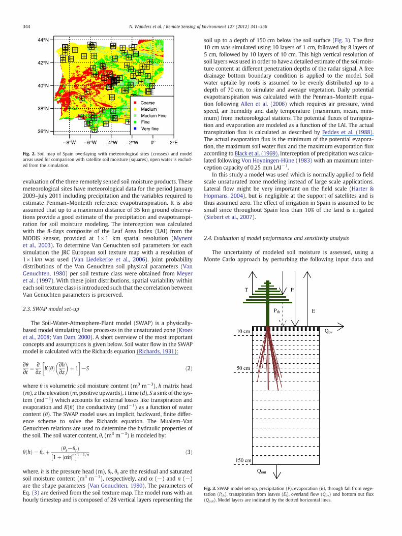
Fig. 2. Soil map of Spain overlaying with meteorological sites (crosses) and modelareas used for comparison with satellite soil moisture (squares), open water is exclud-ed from the simulation.

10 cm

50 cm

150 cm

Qout

EPth

PT

Qov

Fig. 3. SWAP model set-up, precipitation (P), evaporation (E), through fall from vege-tation (Pth), transpiration from leaves (Ei), overland flow (Qov) and bottom out flux(Qout). Model layers are indicated by the dotted horizontal lines.

344 N. Wanders et al. / Remote Sensing of Environment 127 (2012) 341–356

evaluation of the three remotely sensed soil moisture products. Thesemeteorological sites have meteorological data for the period January2009–July 2011 including precipitation and the variables required toestimate Penman–Monteith reference evapotranspiration. It is alsoassumed that up to a maximum distance of 35 km ground observa-tions provide a good estimate of the precipitation and evapotranspi-ration for soil moisture modeling. The interception was calculatedwith the 8-days composite of the Leaf Area Index (LAI) from theMODIS sensor, provided at 1×1 km spatial resolution (Myneniet al., 2003). To determine Van Genuchten soil parameters for eachsimulation the JRC European soil texture map with a resolution of1×1km was used (Van Liedekerke et al., 2006). Joint probabilitydistributions of the Van Genuchten soil physical parameters (VanGenuchten, 1980) per soil texture class were obtained from Meyeret al. (1997). With these joint distributions, spatial variability withineach soil texture class is introduced such that the correlation betweenVan Genuchten parameters is preserved.

2.3. SWAP model set-up

The Soil-Water-Atmosphere-Plant model (SWAP) is a physically-based model simulating flow processes in the unsaturated zone (Kroeset al., 2008; Van Dam, 2000). A short overview of the most importantconcepts and assumptions is given below. Soil water flow in the SWAPmodel is calculated with the Richards equation (Richards, 1931):

∂θ∂t ¼

∂∂z K θð Þ ∂h

∂z

� �þ 1

� �−S ð2Þ

where θ is volumetric soil moisture content (m3 m−3), h matrix head(m), z the elevation (m, positive upwards), t time (d), S a sink of the sys-tem (md−1) which accounts for external losses like transpiration andevaporation and K(θ) the conductivity (md−1) as a function of watercontent (θ). The SWAP model uses an implicit, backward, finite differ-ence scheme to solve the Richards equation. The Mualem–VanGenuchten relations are used to determine the hydraulic properties ofthe soil. The soil water content, θ, (m3 m−3) is modeled by:

θ hð Þ ¼ θr þθs−θrð Þ

1þ αhj jn� 1−1=n ð3Þ

where, h is the pressure head (m), θr, θs are the residual and saturatedsoil moisture content (m3 m−3), respectively, and α (−) and n (−)are the shape parameters (Van Genuchten, 1980). The parameters ofEq. (3) are derived from the soil texture map. The model runs with anhourly timestep and is composed of 28 vertical layers representing the

soil up to a depth of 150 cm below the soil surface (Fig. 3). The first10 cm was simulated using 10 layers of 1 cm, followed by 8 layers of5 cm, followed by 10 layers of 10 cm. This high vertical resolution ofsoil layerswas used in order to have a detailed estimate of the soil mois-ture content at different penetration depths of the radar signal. A freedrainage bottom boundary condition is applied to the model. Soilwater uptake by roots is assumed to be evenly distributed up to adepth of 70 cm, to simulate and average vegetation. Daily potentialevapotranspiration was calculated with the Penman–Monteith equa-tion following Allen et al. (2006) which requires air pressure, windspeed, air humidity and daily temperature (maximum, mean, mini-mum) from meteorological stations. The potential fluxes of transpira-tion and evaporation are modeled as a function of the LAI. The actualtranspiration flux is calculated as described by Feddes et al. (1988).The actual evaporation flux is the minimum of the potential evapora-tion, the maximum soil water flux and the maximum evaporation fluxaccording to Black et al. (1969). Interception of precipitation was calcu-lated following Von Hoyningen-Hüne (1983) with an maximum inter-ception capacity of 0.25 mm LAI−1.

In this study a model was used which is normally applied to fieldscale unsaturated zone modeling instead of large scale applications.Lateral flow might be very important on the field scale (Harter &Hopmans, 2004), but is negligible at the support of satellites and isthus assumed zero. The effect of irrigation in Spain is assumed to besmall since throughout Spain less than 10% of the land is irrigated(Siebert et al., 2007).

2.4. Evaluation of model performance and sensitivity analysis

The uncertainty of modeled soil moisture is assessed, using aMonte Carlo approach by perturbing the following input data and

345N. Wanders et al. / Remote Sensing of Environment 127 (2012) 341–356

parameters of SWAP: precipitation (P), evapotranspiration (E), LAIand soil properties. Since P, E, LAI and soil physical parameters arefound to have the largest influence on the simulation of near surfacesoil moisture (De Lannoy et al., 2006; Finke et al., 1996) other param-eters were kept constant and are assumed to have a negligible effecton the uncertainty of modeled soil moisture. The structural errorwas also not taken into account since is was assumed to be subordi-nate to errors in the model forcing and parameters.

Three error models were used to add uncertainty to the input dataand parameters of the SWAP model (Table 2). In the ContinuousSpatial Uncertainty Model (CSUM), variogram models and observa-tions were used to create realizations of meteorological variables con-ditioned to observed values at the meteorological stations, Pobs(x,t).For precipitation (P(x,t),mm) it is assumed that:

P x; tð Þ ¼ Z x; tð Þ2 ð4Þ

where Z(x,t) is a Gaussian distribution variable with spatial index x(Schuurmans et al., 2007). The spatial correlation of Z(x,t) (mm0.5)is given by a linear variogram:

γ hð Þ ¼ s−nð Þ hrþ n ð5Þ

where γ(h) is the variance as a function of the lag h (m), the sill s(mm), the nugget n (mm), and the range r (m), of the variogram.The variogram was computed with observations from all 79 stationsover a period of 2.5 years without making any distinction betweenthe different seasons or different spatial scale of the precipitationevents. Since the required data to create variogrammodels for individ-ual precipitation events is not available it was decided to use a singlevariogram model. With this variogram a Gaussian random simulationconditioned to the observations pobs(t)(mm), was performed, ob-taining realizations of maps of precipitation, P(t)(mm), for each dayof the simulation. Following the same approach a variogram modelwas fitted to the Penman–Monteith reference evapotranspiration cal-culated at the station locations. Evapotranspiration was not trans-formed and was assumed to have a Gaussian distribution with alinear variogram (Eq. 5). This model was used to simulate possiblefields of evapotranspiration for the reference locations, in order to as-sess the effects of evapotranspiration uncertainty.

The Continuous Local Uncertainty Model (CLUM) is used to intro-duce uncertainty in LAI values and is given by:

LAIn tð Þ ¼ LAIo tð Þ⋅X μ;σð Þ ð6Þ

where LAIn is a random variable (m2 m−2), LAIo is the observedMODIS LAI value (m2 m−2), X(μ,σ) is a Gaussian random variablewith mean, μ, and standard deviation, σ. In this study μ (−) is set to1 and σ (−) was based on a study from (Yang et al., 2006) and isset to 0.1 introducing random error in the LAI used for the calcula-tions of the SWAP model.

Table 2Description of variables and used uncertainty model for each perturbed parameter ofthe SWAP model. Error models given are the Discrete Local Uncertainty Model(DLUM), Continuous Spatial Uncertainty Model (CSUM) and Continuous Local Uncer-tainty Model (CLUM).

Var Description Source Error model

θs Saturated soil moisture (Meyer et al., 1997) DLUMθr Residual soil moisture (Meyer et al., 1997) DLUMK(θ) Unsaturated conductivity (Meyer et al., 1997) DLUMn Van Genuchten n-parameter (Meyer et al., 1997) DLUMα Van Genuchten α-parameter (Meyer et al., 1997) DLUMP Precipitation Meteo station CSUME Evapotranspiration Meteo station CSUMLAI Leaf Area Index MODIS satellite CLUM

The Discrete Local Uncertainty Model (DLUM) is applied for thesoil physical parameters and uses local properties to add uncertaintyto parameters. With the DLUM the soil texture of a location is condi-tionally changed for 20% of the locations. Since errors in soil texturemaps are not uncommon (Hengl & Toomanian, 2006) this 20% errorwas introduced to account for the effect of misclassification. Realiza-tions of soil texture were created by randomly changing the soiltexture of cells. In creating a realization, for each cell, the probabilityof a newly selected soil class (c) is calculated as:

Pr cð Þ ¼ nc;i

N−nc;jð7Þ

where nc,i and nc,j are the relative occurrences of the perturbed andobserved soil texture over Spain respectively and N is the total num-ber of pixels on the 1×1 km soil texture map. If a misclassification oc-curs, the soil texture is changed and will not be ascribed to j againresulting in newly assigned texture classes.

The predictive QQ-plot as described by Laio and Tamea (2007)was used to determine if the model uncertainties and combineduncertainty of the input data could explain the variation betweendifferent points of the REMEDHUS network. The predictive QQ-plotis a measure to check whether the obtained Monte Carlo simulationresults in a probability density function (PDF) that corresponds tothe PDF of the model prediction errors. In the predictive QQ-plotthe probability integral transforms to:

zi ¼ ∫x−∞ f xið Þdx ð8Þ

where f(xi) is the PDF of model outputs obtained from the uncertaintyanalysis (Monte Carlo simulation), xi is the value at observation loca-tion i and zi the associated cumulative probability. Thus, zi gives theprobability of the observed values with respect to the distribution ofpredicted values from the Monte Carlo simulation. The zi values areplotted against their cumulative density function, Ranki(xi), which isproduced from the observation rank rank(xi):

Ranki xið Þ ¼ rank xið Þnþ 1

ð9Þ

where n is the total number of xi values. When the zi plotted againstthe Ranki are on the 1:1 line, the PDF from the uncertainty analysiscorrectly represents the prediction errors and the predictions areunbiased. The non-parametric Kolmogorov–Smirnov test is used toevaluate whether the results are within the 95% confidence intervalof the 1:1 line. More details of the predictive QQ-plot are given inLaio and Tamea (2007).

The performance of the SWAP model at the REMEDHUS site wasevaluated using the Pearson correlation (R, Eq. A.1), Root MeanSquare Error (RMSE, Eq. A.2) and model bias, biasm(m3m−3):

biasm ¼ μo−μm ð10Þ

where μo and μm respectively are the average observed and modeledsoil moisture over the entire simulation period (m3 m−3) where anegative value indicates an underestimation of the soil moisture. TheREMEDHUS sitewas not used for calibration of themodel, only to eval-uate the model and to determine the errors in the modeled soil mois-ture and input data. Soil moisture was simulated for the entire periodfrom 2006 to 2010. In total 2000 simulations were done withperturbed parameters and input data for the REMEDHUS site inorder to accurately capture the full probability density functions ofall parameters and input data. This high number of simulations alsoallowed to accurately calculate the model uncertainty and study themodel sensitivity to the full range of possible parameters sets.

For all selected 79 meteorological stations, a Monte Carlo ap-proach (150 realizations) was used to determine the overall modeled

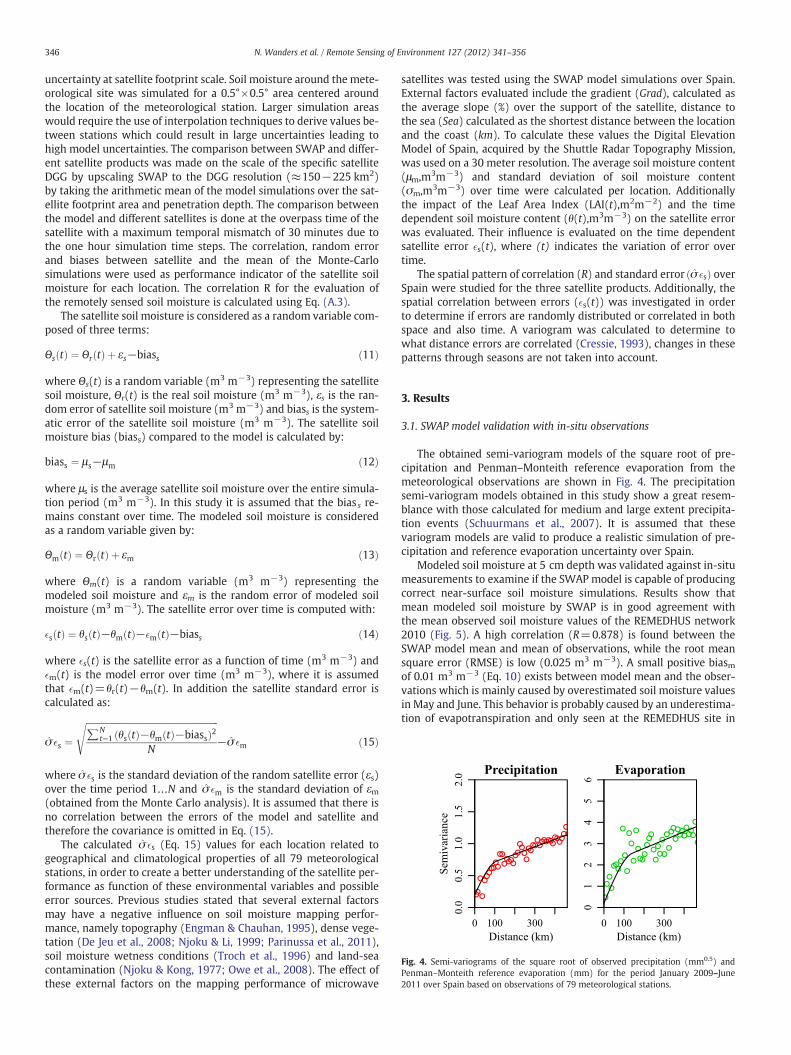
Fig. 4. Semi-variograms of the square root of observed precipitation (mm0.5) andPenman–Monteith reference evaporation (mm) for the period January 2009–June2011 over Spain based on observations of 79 meteorological stations.

346 N. Wanders et al. / Remote Sensing of Environment 127 (2012) 341–356

uncertainty at satellite footprint scale. Soil moisture around the mete-orological site was simulated for a 0.5°×0.5° area centered aroundthe location of the meteorological station. Larger simulation areaswould require the use of interpolation techniques to derive values be-tween stations which could result in large uncertainties leading tohigh model uncertainties. The comparison between SWAP and differ-ent satellite products was made on the scale of the specific satelliteDGG by upscaling SWAP to the DGG resolution (≈150−225 km2)by taking the arithmetic mean of the model simulations over the sat-ellite footprint area and penetration depth. The comparison betweenthe model and different satellites is done at the overpass time of thesatellite with a maximum temporal mismatch of 30 minutes due tothe one hour simulation time steps. The correlation, random errorand biases between satellite and the mean of the Monte-Carlosimulations were used as performance indicator of the satellite soilmoisture for each location. The correlation R for the evaluation ofthe remotely sensed soil moisture is calculated using Eq. (A.3).

The satellite soil moisture is considered as a random variable com-posed of three terms:

Θs tð Þ ¼ Θr tð Þ þ εs−biass ð11Þ

where Θs(t) is a random variable (m3 m−3) representing the satellitesoil moisture, Θr(t) is the real soil moisture (m3 m−3), εs is the ran-dom error of satellite soil moisture (m3 m−3) and biass is the system-atic error of the satellite soil moisture (m3 m−3). The satellite soilmoisture bias (biass) compared to the model is calculated by:

biass ¼ μs−μm ð12Þ

where μs is the average satellite soil moisture over the entire simula-tion period (m3 m−3). In this study it is assumed that the bias s re-mains constant over time. The modeled soil moisture is consideredas a random variable given by:

Θm tð Þ ¼ Θr tð Þ þ εm ð13Þ

where Θm(t) is a random variable (m3 m−3) representing themodeled soil moisture and εm is the random error of modeled soilmoisture (m3 m−3). The satellite error over time is computed with:

�s tð Þ ¼ θs tð Þ−θm tð Þ−�m tð Þ−biass ð14Þ

where �s(t) is the satellite error as a function of time (m3 m−3) and�m(t) is the model error over time (m3 m−3), where it is assumedthat �m(t)=θr(t)−θm(t). In addition the satellite standard error iscalculated as:

σ̂ �s ¼ffiffiffiffiffiffiffiffiffiffiffiffiffiffiffiffiffiffiffiffiffiffiffiffiffiffiffiffiffiffiffiffiffiffiffiffiffiffiffiffiffiffiffiffiffiffiffiffiffiffiffiffiffiffiffiffiffiffiffiffi∑N

t¼1 θs tð Þ−θm tð Þ−biassð Þ2N

s−σ̂ �m ð15Þ

where σ̂ �s is the standard deviation of the random satellite error (εs)over the time period 1…N and σ̂ �m is the standard deviation of εm(obtained from the Monte Carlo analysis). It is assumed that there isno correlation between the errors of the model and satellite andtherefore the covariance is omitted in Eq. (15).

The calculated σ̂ �s (Eq. 15) values for each location related togeographical and climatological properties of all 79 meteorologicalstations, in order to create a better understanding of the satellite per-formance as function of these environmental variables and possibleerror sources. Previous studies stated that several external factorsmay have a negative influence on soil moisture mapping perfor-mance, namely topography (Engman & Chauhan, 1995), dense vege-tation (De Jeu et al., 2008; Njoku & Li, 1999; Parinussa et al., 2011),soil moisture wetness conditions (Troch et al., 1996) and land-seacontamination (Njoku & Kong, 1977; Owe et al., 2008). The effect ofthese external factors on the mapping performance of microwave

satellites was tested using the SWAP model simulations over Spain.External factors evaluated include the gradient (Grad), calculated asthe average slope (%) over the support of the satellite, distance tothe sea (Sea) calculated as the shortest distance between the locationand the coast (km). To calculate these values the Digital ElevationModel of Spain, acquired by the Shuttle Radar Topography Mission,was used on a 30 meter resolution. The average soil moisture content(μm,m3m−3) and standard deviation of soil moisture content(σm,m3m−3) over time were calculated per location. Additionallythe impact of the Leaf Area Index (LAI(t),m2m−2) and the timedependent soil moisture content (θ(t),m3m−3) on the satellite errorwas evaluated. Their influence is evaluated on the time dependentsatellite error �s(t), where (t) indicates the variation of error overtime.

The spatial pattern of correlation (R) and standard error σ̂ �sð Þ overSpain were studied for the three satellite products. Additionally, thespatial correlation between errors (�s(t)) was investigated in orderto determine if errors are randomly distributed or correlated in bothspace and also time. A variogram was calculated to determine towhat distance errors are correlated (Cressie, 1993), changes in thesepatterns through seasons are not taken into account.

3. Results

3.1. SWAP model validation with in-situ observations

The obtained semi-variogram models of the square root of pre-cipitation and Penman–Monteith reference evaporation from themeteorological observations are shown in Fig. 4. The precipitationsemi-variogram models obtained in this study show a great resem-blance with those calculated for medium and large extent precipita-tion events (Schuurmans et al., 2007). It is assumed that thesevariogram models are valid to produce a realistic simulation of pre-cipitation and reference evaporation uncertainty over Spain.

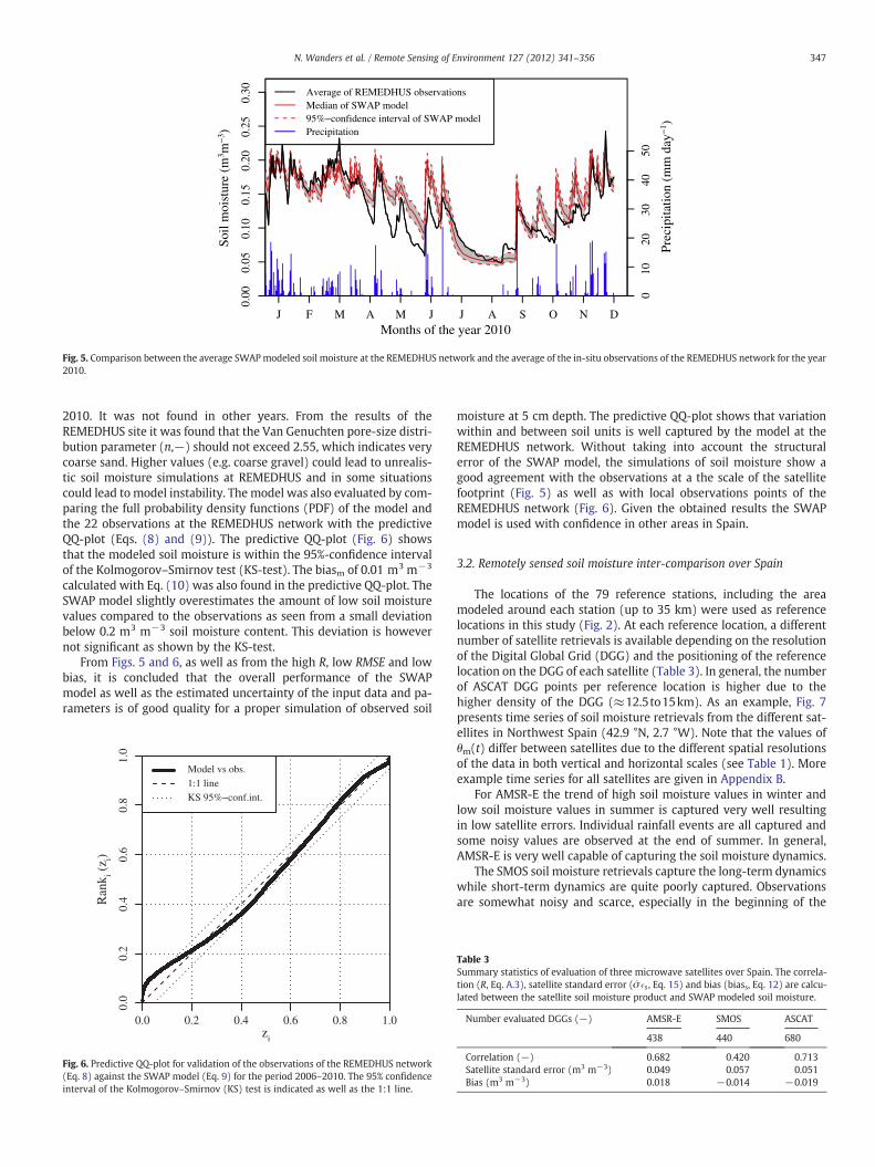
Modeled soil moisture at 5 cm depth was validated against in-situmeasurements to examine if the SWAP model is capable of producingcorrect near-surface soil moisture simulations. Results show thatmean modeled soil moisture by SWAP is in good agreement withthe mean observed soil moisture values of the REMEDHUS network2010 (Fig. 5). A high correlation (R=0.878) is found between theSWAP model mean and mean of observations, while the root meansquare error (RMSE) is low (0.025 m3 m−3). A small positive biasmof 0.01 m3 m−3 (Eq. 10) exists between model mean and the obser-vations which is mainly caused by overestimated soil moisture valuesin May and June. This behavior is probably caused by an underestima-tion of evapotranspiration and only seen at the REMEDHUS site in

Months of the year 2010

Soil

moi

stur

e (m

3 m−

3 )

J F M A M J J A S O N D

0.00

0.05

0.10

0.15

0.20

0.25

0.30 Average of REMEDHUS observations

Median of SWAP model95%−confidence interval of SWAP modelPrecipitation

010

2030

4050

Prec

ipita

tion

(mm

day

−1 )

Fig. 5. Comparison between the average SWAPmodeled soil moisture at the REMEDHUS network and the average of the in-situ observations of the REMEDHUS network for the year2010.

347N. Wanders et al. / Remote Sensing of Environment 127 (2012) 341–356

2010. It was not found in other years. From the results of theREMEDHUS site it was found that the Van Genuchten pore-size distri-bution parameter (n,−) should not exceed 2.55, which indicates verycoarse sand. Higher values (e.g. coarse gravel) could lead to unrealis-tic soil moisture simulations at REMEDHUS and in some situationscould lead to model instability. The model was also evaluated by com-paring the full probability density functions (PDF) of the model andthe 22 observations at the REMEDHUS network with the predictiveQQ-plot (Eqs. (8) and (9)). The predictive QQ-plot (Fig. 6) showsthat the modeled soil moisture is within the 95%-confidence intervalof the Kolmogorov–Smirnov test (KS-test). The biasm of 0.01 m3 m−3

calculated with Eq. (10) was also found in the predictive QQ-plot. TheSWAP model slightly overestimates the amount of low soil moisturevalues compared to the observations as seen from a small deviationbelow 0.2 m3 m−3 soil moisture content. This deviation is howevernot significant as shown by the KS-test.

From Figs. 5 and 6, as well as from the high R, low RMSE and lowbias, it is concluded that the overall performance of the SWAPmodel as well as the estimated uncertainty of the input data and pa-rameters is of good quality for a proper simulation of observed soil

0.0 0.2 0.4 0.6 0.8 1.0

0.0

0.2

0.4

0.6

0.8

1.0

zi

Ran

k i (z i)

Model vs obs.1:1 lineKS 95%−conf.int.

Fig. 6. Predictive QQ-plot for validation of the observations of the REMEDHUS network(Eq. 8) against the SWAP model (Eq. 9) for the period 2006–2010. The 95% confidenceinterval of the Kolmogorov–Smirnov (KS) test is indicated as well as the 1:1 line.

moisture at 5 cm depth. The predictive QQ-plot shows that variationwithin and between soil units is well captured by the model at theREMEDHUS network. Without taking into account the structuralerror of the SWAP model, the simulations of soil moisture show agood agreement with the observations at a the scale of the satellitefootprint (Fig. 5) as well as with local observations points of theREMEDHUS network (Fig. 6). Given the obtained results the SWAPmodel is used with confidence in other areas in Spain.

3.2. Remotely sensed soil moisture inter-comparison over Spain

The locations of the 79 reference stations, including the areamodeled around each station (up to 35 km) were used as referencelocations in this study (Fig. 2). At each reference location, a differentnumber of satellite retrievals is available depending on the resolutionof the Digital Global Grid (DGG) and the positioning of the referencelocation on the DGG of each satellite (Table 3). In general, the numberof ASCAT DGG points per reference location is higher due to thehigher density of the DGG (≈12.5to15km). As an example, Fig. 7presents time series of soil moisture retrievals from the different sat-ellites in Northwest Spain (42.9 °N, 2.7 °W). Note that the values ofθm(t) differ between satellites due to the different spatial resolutionsof the data in both vertical and horizontal scales (see Table 1). Moreexample time series for all satellites are given in Appendix B.

For AMSR-E the trend of high soil moisture values in winter andlow soil moisture values in summer is captured very well resultingin low satellite errors. Individual rainfall events are all captured andsome noisy values are observed at the end of summer. In general,AMSR-E is very well capable of capturing the soil moisture dynamics.

The SMOS soil moisture retrievals capture the long-term dynamicswhile short-term dynamics are quite poorly captured. Observationsare somewhat noisy and scarce, especially in the beginning of the

Table 3Summary statistics of evaluation of three microwave satellites over Spain. The correla-tion (R, Eq. A.3), satellite standard error (σ̂ �s , Eq. 15) and bias (biass, Eq. 12) are calcu-lated between the satellite soil moisture product and SWAP modeled soil moisture.

Number evaluated DGGs (−) AMSR-E SMOS ASCAT

438 440 680

Correlation (−) 0.682 0.420 0.713Satellite standard error (m3 m−3) 0.049 0.057 0.051Bias (m3 m−3) 0.018 −0.014 −0.019

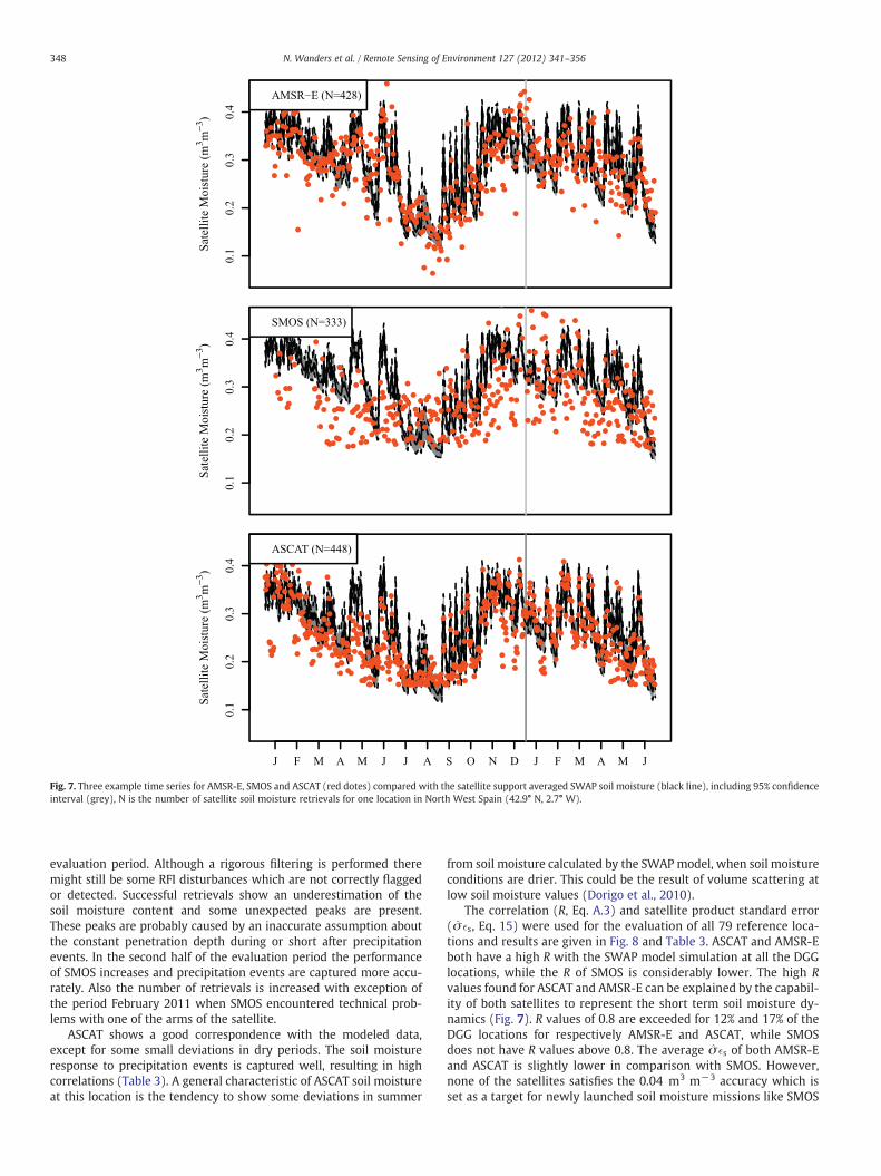
Fig. 7. Three example time series for AMSR-E, SMOS and ASCAT (red dotes) compared with the satellite support averaged SWAP soil moisture (black line), including 95% confidenceinterval (grey), N is the number of satellite soil moisture retrievals for one location in North West Spain (42.9° N, 2.7° W).

348 N. Wanders et al. / Remote Sensing of Environment 127 (2012) 341–356

evaluation period. Although a rigorous filtering is performed theremight still be some RFI disturbances which are not correctly flaggedor detected. Successful retrievals show an underestimation of thesoil moisture content and some unexpected peaks are present.These peaks are probably caused by an inaccurate assumption aboutthe constant penetration depth during or short after precipitationevents. In the second half of the evaluation period the performanceof SMOS increases and precipitation events are captured more accu-rately. Also the number of retrievals is increased with exception ofthe period February 2011 when SMOS encountered technical prob-lems with one of the arms of the satellite.

ASCAT shows a good correspondence with the modeled data,except for some small deviations in dry periods. The soil moistureresponse to precipitation events is captured well, resulting in highcorrelations (Table 3). A general characteristic of ASCAT soil moistureat this location is the tendency to show some deviations in summer

from soil moisture calculated by the SWAPmodel, when soil moistureconditions are drier. This could be the result of volume scattering atlow soil moisture values (Dorigo et al., 2010).

The correlation (R, Eq. A.3) and satellite product standard error(σ̂ �s, Eq. 15) were used for the evaluation of all 79 reference loca-tions and results are given in Fig. 8 and Table 3. ASCAT and AMSR-Eboth have a high R with the SWAP model simulation at all the DGGlocations, while the R of SMOS is considerably lower. The high Rvalues found for ASCAT and AMSR-E can be explained by the capabil-ity of both satellites to represent the short term soil moisture dy-namics (Fig. 7). R values of 0.8 are exceeded for 12% and 17% of theDGG locations for respectively AMSR-E and ASCAT, while SMOSdoes not have R values above 0.8. The average σ̂ �s of both AMSR-Eand ASCAT is slightly lower in comparison with SMOS. However,none of the satellites satisfies the 0.04 m3 m−3 accuracy which isset as a target for newly launched soil moisture missions like SMOS

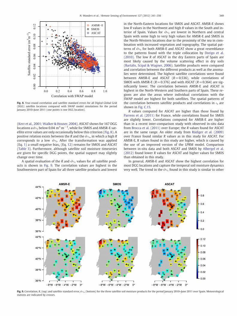
Fig. 8. Year-round correlation and satellite standard errors for all Digital Global Grid(DGG) satellite locations compared with SWAP model simulations for the periodJanuary 2010–June 2011 (one points is one DGG location).

349N. Wanders et al. / Remote Sensing of Environment 127 (2012) 341–356

(Kerr et al., 2001;Walker & Houser, 2004). ASCAT shows for 167 DGGlocations a σ̂ �s below 0.04 m3 m−3, while for SMOS and AMSR-E sat-ellite error values are only occasionally below this criterion (Fig. 8). Apositive relation exists between the R and the σ̂ �s, in which a high Rcorresponds to a low σ̂ �s. After the transformation was applied(Eq. 1) a small negative biass (Eq. 12) remains for SMOS and ASCAT(Table 3). Furthermore, although satellite soil moisture timeseriesare given for specific DGG points, the spatial support may slightlychange over time.

A spatial evaluation of the R and σ̂ �s values for all satellite prod-ucts is shown in Fig. 9. The correlation values are highest in theSouthwestern part of Spain for all three satellite products and lowest

Fig. 9. Correlation, R, (top) and satellite standard error, σ̂ �s , (bottom) for the three satellite sostations are indicated by crosses.

in the North-Eastern locations for SMOS and ASCAT. AMSR-E showslow R values in the Northwest and high R values in the South and in-terior of Spain. Values for σ̂ �s are lowest in Northern and centralSpain with some high to very high values for AMSR-E and SMOS inthe North-Western locations due to the proximity of the sea in com-bination with increased vegetation and topography. The spatial pat-terns of σ̂ �s for both AMSR-E and ASCAT show a great resemblanceto the patterns found with the triple collocation by Dorigo et al.(2010). The low R of ASCAT in the dry Eastern parts of Spain aremost likely caused by the volume scattering effect in dry soils(Bartalis, Scipal & Wagner, 2006). Satellite products were comparedand correlation between the different products as well as the anoma-lies were determined. The highest satellite correlations were foundbetween AMSR-E and ASCAT (R=0.536), while correlations ofSMOS with AMSR-E (R=0.376) and with ASCAT (R=0.364) are sig-nificantly lower. The correlation between AMSR-E and ASCAT ishighest in the North-Western and Southern parts of Spain. These re-gions are also the areas where individual correlations with theSWAP model are highest for both satellites. The spatial patterns ofthe correlation between satellite products and correlations in �s areshown in Fig. C.15.

R values computed for ASCAT are higher than those found byParrens et al. (2011) for France, while correlations found for SMOSare slightly lower. Correlations computed for AMSR-E are higherthan in a recent inter-comparison study with observed in-situ datafrom Brocca et al. (2011) over Europe; the R values found for ASCATare in the same range. An older study from Rüdiger et al. (2009)over France found similar R values as in this study for ASCAT. ForAMSR-E, R values found in this study are higher, which is caused bythe use of an improved version of the LPRM model. Comparisonbetween in-situ data and both ASCAT and SMOS by Albergel et al.(2012) found lower R values for ASCAT and higher values for SMOSthan obtained in this study.

In general, AMSR-E and ASCAT show the highest correlation formost DGG locations and capture the temporal soil moisture dynamicsvery well. The trend in the σ̂ �s found in this study is similar to other

il moisture products for the period January 2010–June 2011 over Spain. Meteorological

0 5 10 15

0.02

0.04

0.06

0.08

0.10

Gradient (%)

Sate

llite

err

or (

m3 m

−3 )

Sate

llite

err

or (

m3 m

−3 )

AMSR−ESMOSASCAT

Distance to sea (km)

0 50 100 150 200 250 300

Leaf Area Index (m2m−2)

2 4 6 8

0.04 0.06 0.08 0.10

0.02

0.04

0.06

0.08

0.10

Standard deviation (m3m−3) Average content (m3m−3)

0.20 0.22 0.24 0.26 0.28 0.30

Actual content (m3m−3)

0.1 0.2 0.3 0.4

Fig. 10. Satellite standard error of satellite soil moisture for different factors in comparison with SWAPmodel for the period January 2010–June 2011 over Spain. The satellite error isσ̂ �s (Eq. 15) is given for: the gradient (Grad), distance to the sea (Sea), standard deviation (σm) and μm. For the Leaf Area Index (LAI(t)) and actual content (θ(t)) the bin-averagetime dependent satellite error is s(t) (Eq. 14) is shown.

350 N. Wanders et al. / Remote Sensing of Environment 127 (2012) 341–356

studies (e.g. Albergel et al., 2012; Brocca et al., 2011; Parrens et al.,2011). However, a direct comparison is hampered by the fact thatthese studies did not incorporate model errors. Our approach ac-counts for model uncertainty and therefore gives a more correctestimation of the σ̂ �s of satellite soil moisture products and the per-formance of space-born sensors.

3.3. Satellite error characterization

The effect of several external factors on the satellite standard errorσ̂ �sð Þ is evaluated over Spain for all reference locations. The averageslope of the location (Grad) is found to have negligible influence onthe σ̂ �s (Fig. 10), leading to the conclusion that gradients at the refer-ence locations in Spain are too small to have a negative impact on σ̂ �s.However, with an increase in the distance to the sea (Sea), σ̂ �s forAMSR-E and SMOS decrease. Above a distance of 100 to 150 km theinfluence of the sea is absent. An increase in the Leaf Area Index(LAI(t)) over time does influence the time dependent satellite error(�s, Eq. 14) in a negative way, �s increases with an increase in vegeta-tion. The performance of SMOS is most affected by the average stan-dard deviation of soil moisture (σm), where SMOS might havedifficulties with highly dynamic soil moisture due to the high signalto noise ratio compared to AMSR-E and ASCAT. Over the entiremodeling period (Jan 2010–Jun 2011), the average soil moisture con-tent (μm) does not significantly influence the satellite performance,while the actual soil moisture content (θ(t)) does have a large influ-ence on the temporal performance of ASCAT. Both passive microwavesatellites show a small increase in the �s for θ(t) between 0.1 and0.2 m3 m−3 and decrease thereafter. ASCAT shows an unambiguousincrease in the �s with increasing θ(t). This could be the result of thestrong response of ASCAT to precipitation events, while this responseis less profound for AMSR-E and SMOS (Fig. 7). Correlations were

most affected by changes in the average footprint soil moisture con-tent (μm) and the distance to the sea (Sea) of all external factors un-derstudy (not shown). In this study no strong relationship is foundbetween the σ̂ �s and the Grad. Based on previous studies (e.g.Engman & Chauhan, 1995) it was expected that the satellite perfor-mance was related to these properties. A relationship was found forSea, LAI(t), σm, μm and θ(t) with σ̂ �s. This finding is confirmed byother studies (e.g. De Jeu et al., 2008; Njoku & Kong, 1977; Njoku &Li, 1999; Owe et al., 2008; Parinussa et al., 2011; Troch et al., 1996).

Finally, the error for all the remotely sensed soil moisture productsis spatially correlated. Ranges of the variogram of correlation arebetween 100 and 220 km, for the three satellites products (Fig. 11).The correlation ranges, sill and nugget of the variogram are almostequal for all satellite products indicating that soil moisture errorshave an almost identical spatial error pattern for AMSR-E, SMOS andASCAT.

4. Conclusions

The soil moisture mapping accuracy of three satellite sensors wasevaluated in this study. Satellites used in this study are passive micro-wave satellites AMSR-E and SMOS and the active microwave satelliteASCAT. Satellite soil moisture products were compared with thephysically-based high resolution SWAP model. Soil moisture wasmodeled at a high vertical and horizontal resolution and averagedover the support of each satellite. A validation of the high-resolutionSWAP model was performed on the REMEDHUS network situated inSpain. The mean modeled soil moisture from SWAP has a high corre-lation (R=0.878) and low RMSE (0.025m3m−3) with the median ofobservations at the REMEDHUS site. From the predictive QQ-plot itwas concluded that the SWAP model was able to capture the fullprobability density function in both space and time for this site. The

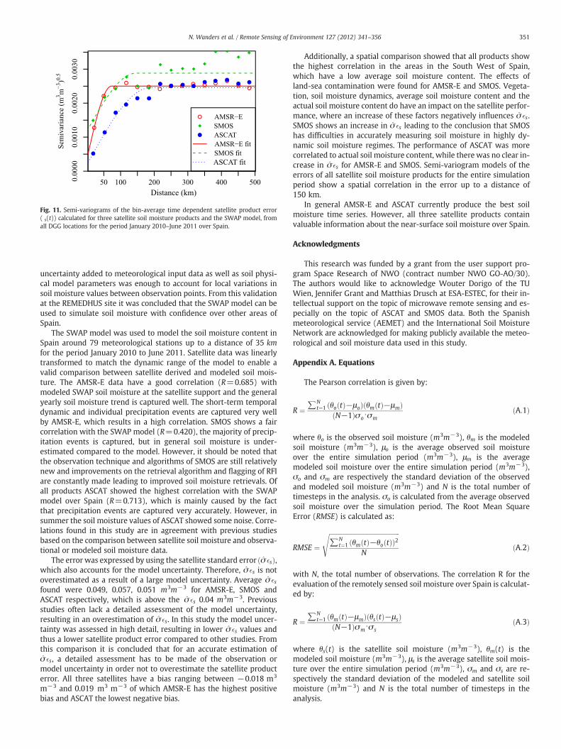
Fig. 11. Semi-variograms of the bin-average time dependent satellite product error( s(t)) calculated for three satellite soil moisture products and the SWAP model, fromall DGG locations for the period January 2010–June 2011 over Spain.

351N. Wanders et al. / Remote Sensing of Environment 127 (2012) 341–356

uncertainty added to meteorological input data as well as soil physi-cal model parameters was enough to account for local variations insoil moisture values between observation points. From this validationat the REMEDHUS site it was concluded that the SWAP model can beused to simulate soil moisture with confidence over other areas ofSpain.

The SWAP model was used to model the soil moisture content inSpain around 79 meteorological stations up to a distance of 35 kmfor the period January 2010 to June 2011. Satellite data was linearlytransformed to match the dynamic range of the model to enable avalid comparison between satellite derived and modeled soil mois-ture. The AMSR-E data have a good correlation (R=0.685) withmodeled SWAP soil moisture at the satellite support and the generalyearly soil moisture trend is captured well. The short-term temporaldynamic and individual precipitation events are captured very wellby AMSR-E, which results in a high correlation. SMOS shows a faircorrelation with the SWAP model (R=0.420), the majority of precip-itation events is captured, but in general soil moisture is under-estimated compared to the model. However, it should be noted thatthe observation technique and algorithms of SMOS are still relativelynew and improvements on the retrieval algorithm and flagging of RFIare constantly made leading to improved soil moisture retrievals. Ofall products ASCAT showed the highest correlation with the SWAPmodel over Spain (R=0.713), which is mainly caused by the factthat precipitation events are captured very accurately. However, insummer the soil moisture values of ASCAT showed some noise. Corre-lations found in this study are in agreement with previous studiesbased on the comparison between satellite soil moisture and observa-tional or modeled soil moisture data.

The error was expressed by using the satellite standard error σ̂ �sð Þ,which also accounts for the model uncertainty. Therefore, σ̂ �s is notoverestimated as a result of a large model uncertainty. Average σ̂ �sfound were 0.049, 0.057, 0.051 m3m−3 for AMSR-E, SMOS andASCAT respectively, which is above the σ̂ �s 0.04 m3m−3. Previousstudies often lack a detailed assessment of the model uncertainty,resulting in an overestimation of σ̂ �s. In this study the model uncer-tainty was assessed in high detail, resulting in lower σ̂ �s values andthus a lower satellite product error compared to other studies. Fromthis comparison it is concluded that for an accurate estimation ofσ̂ �s, a detailed assessment has to be made of the observation ormodel uncertainty in order not to overestimate the satellite producterror. All three satellites have a bias ranging between −0.018 m3

m−3 and 0.019 m3 m−3 of which AMSR-E has the highest positivebias and ASCAT the lowest negative bias.

Additionally, a spatial comparison showed that all products showthe highest correlation in the areas in the South West of Spain,which have a low average soil moisture content. The effects ofland-sea contamination were found for AMSR-E and SMOS. Vegeta-tion, soil moisture dynamics, average soil moisture content and theactual soil moisture content do have an impact on the satellite perfor-mance, where an increase of these factors negatively influences σ̂ �s.SMOS shows an increase in σ̂ �s leading to the conclusion that SMOShas difficulties in accurately measuring soil moisture in highly dy-namic soil moisture regimes. The performance of ASCAT was morecorrelated to actual soil moisture content, while there was no clear in-crease in σ̂ �s for AMSR-E and SMOS. Semi-variogram models of theerrors of all satellite soil moisture products for the entire simulationperiod show a spatial correlation in the error up to a distance of150 km.

In general AMSR-E and ASCAT currently produce the best soilmoisture time series. However, all three satellite products containvaluable information about the near-surface soil moisture over Spain.

Acknowledgments

This research was funded by a grant from the user support pro-gram Space Research of NWO (contract number NWO GO-AO/30).The authors would like to acknowledge Wouter Dorigo of the TUWien, Jennifer Grant and Matthias Drusch at ESA-ESTEC, for their in-tellectual support on the topic of microwave remote sensing and es-pecially on the topic of ASCAT and SMOS data. Both the Spanishmeteorological service (AEMET) and the International Soil MoistureNetwork are acknowledged for making publicly available the meteo-rological and soil moisture data used in this study.

Appendix A. Equations

The Pearson correlation is given by:

R ¼ ∑Nt¼1 θo tð Þ−μoð Þ θm tð Þ−μmð Þ

N−1ð Þσo⋅σmðA:1Þ

where θo is the observed soil moisture (m3m−3), θm is the modeledsoil moisture (m3m−3), μo is the average observed soil moistureover the entire simulation period (m3m−3), μm is the averagemodeled soil moisture over the entire simulation period (m3m−3),σo and σm are respectively the standard deviation of the observedand modeled soil moisture (m3m−3) and N is the total number oftimesteps in the analysis. σo is calculated from the average observedsoil moisture over the simulation period. The Root Mean SquareError (RMSE) is calculated as:

RMSE ¼ffiffiffiffiffiffiffiffiffiffiffiffiffiffiffiffiffiffiffiffiffiffiffiffiffiffiffiffiffiffiffiffiffiffiffiffiffiffiffiffiffiffiffiffiffi∑N

t¼1 θm tð Þ−θo tð Þð Þ2N

sðA:2Þ

with N, the total number of observations. The correlation R for theevaluation of the remotely sensed soil moisture over Spain is calculat-ed by:

R ¼ ∑Nt¼1 θm tð Þ−μmð Þ θs tð Þ−μsð Þ

N−1ð Þσm⋅σ sðA:3Þ

where θs(t) is the satellite soil moisture (m3m−3), θm(t) is themodeled soil moisture (m3m−3), μs is the average satellite soil mois-ture over the entire simulation period (m3m−3), σm and σs are re-spectively the standard deviation of the modeled and satellite soilmoisture (m3m−3) and N is the total number of timesteps in theanalysis.

352 N. Wanders et al. / Remote Sensing of Environment 127 (2012) 341–356

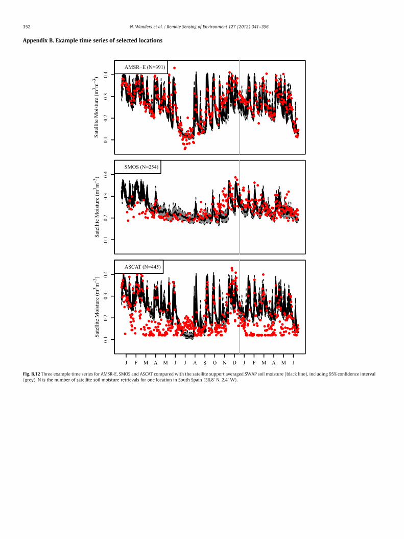
Appendix B. Example time series of selected locations

Fig. B.12 Three example time series for AMSR-E, SMOS and ASCAT compared with the satellite support averaged SWAP soil moisture (black line), including 95% confidence interval(grey), N is the number of satellite soil moisture retrievals for one location in South Spain (36.8∘ N, 2.4∘ W).

Fig. B.13. Three example time series for AMSR-E, SMOS and ASCAT compared with the satellite support averaged SWAP soil moisture (black line), including 95% confidence interval(grey), N is the number of satellite soil moisture retrievals for one location in Northeast Spain (42.8∘ N, 1.6∘ W).

353N. Wanders et al. / Remote Sensing of Environment 127 (2012) 341–356

Fig. B.14. Three example time series for AMSR-E, SMOS and ASCAT compared with the satellite support averaged SWAP soil moisture (black line), including 95% confidence interval(grey), N is the number of satellite soil moisture retrievals for one location in central Spain (41.7∘ N, 4.8∘ W).

354 N. Wanders et al. / Remote Sensing of Environment 127 (2012) 341–356

355N. Wanders et al. / Remote Sensing of Environment 127 (2012) 341–356

Appendix C. Spatial correlation between satellites

Fig. C.15. Correlation between satellite soil moisture products (top, R) and correlation between the satellite product errors (bottom, s(t)) of different satellite products for the pe-riod January 2010–June 2011 over Spain, meteorological stations are indicated by crosses.

References

Albergel, C., Rosnay, P., Gruhier, C., Muñoz Sabater, J., Hasenauer, S., Isaksen, L., et al.(2012). Evaluation of remotely sensed and modelled soil moisture productsusing global ground-based in situ observations. Remote Sensing of Environment,118(15), 215–226.

Allen, R., Pereira, L., Raes, D., & Smith, M. (2006). FAO irrigation and drainage paper no.56 — Crop evapotranspiration. Food and Agriculture Organization.

Anterrieu, E. (2011). On the detection and quantification of RFI in L1a signals providedby SMOS. IEEE Transactions on Geoscience and Remote Sensing, 49(10), 3986–3992.

Baroni, G., Facchi, A., Gandolfi, C., Ortuani, B., Horeschi, D., & van Dam, J. C. (2010). Un-certainty in the determination of soil hydraulic parameters and its influence on theperformance of two hydrological models of different complexity. Hydrology andEarth System Sciences, 14(2), 251–270.

Bartalis, Z., Kidd, R., & Scipal, K. (2006). Development and implementation of a discreteglobal grid system for soil moisture retrieval using the metop ascat scatterometer.1st EPS/MetOp RAO Workshop. Frascati, Italy: ESA SP-618.

Bartalis, Z., Scipal, K., & Wagner, W. (2006). Azimuthal anisotropy of scatterometer mea-surements over land. IEEE Geoscience and Remote Sensing Society, 44(8), 2083–2092.

Upscaling and downscaling methods for environmental research. Bierkens, M. F. P.,Finke, P. A., & De Willigen, P. (Eds.). (2000). Developments in Plant and SoilSciences, Vol. 88, : Kluwer Academic Publishers.

Bisselink, B., van Meijgaard, E., Dolman, A. J., & De Jeu, R. A. M. (2011). Initializing a re-gional climate model with satellite-derived soil moisture. Journal of Geophysical Re-search, 116(D2), D02121.

Black, T. A., Gardner, W. R., & Thurtell, G. W. (1969). The prediction of evaporation,drainage, and soil water storage for a bare soil. Soil Science Society of America Pro-ceedings, 33(5), 655–660.

Brocca, L., Hasenauer, S., Lacava, T., Melone, F., Moramarco, T., Wagner, W., et al.(2011). Soil moisture estimation through ascat and amsr-e sensors: An inter-comparison and validation study across europe. Remote Sensing of Environment,115(12), 3390–3408.

Brocca, L., Melone, F., Moramarco, T., Wagner, W., Naeimi, V., Bartalis, Z., et al. (2010).Improving runoff prediction through the assimilation of the ascat soil moistureproduct. Hydrology and Earth System Sciences, 14(10), 1881–1893.

Cressie, N. A. C. (1993). Statistics for spatial data. Wiley series in Probability and math-ematical statistics.

Crow, W. T., Berg, A. A., Cosh, M. H., Loew, A., Mohanty, B. P., Panciera, R., de Rosnay, P.,Ryu, D., & Walker, J. P. (2012). Upscaling sparse ground-based soil moisture obser-vations for the validation of coarse-resolution satellite soil moisture products. Re-views of Geophysics, 50, RG2002. http://dx.doi.org/10.1029/2011RG000372.

Crow, W. T., Miralles, D. G., & Cosh, M. H. (2010). A quasi-global evaluation system forsatellite-based surface soil moisture retrievals. IEEE Transactions on Geoscience andRemote Sensing, 48(6), 2516–2527.

Crow, W. T., & Ryu, D. (2009). A new data assimilation approach for improving runoffprediction using remotely-sensed soil moisture retrievals. Hydrology and Earth Sys-tem Sciences, 13(1), 1–16.

Crow, W. T., & Zhan, X. (2007). Continental-scale evaluation of remotely sensed soilmoisture products. IEEE Geoscience and Remote Sensing Letters, 4, 451–455.

De Jeu, R. A. M., & Owe, M. (2003). Further validation of a newmethodology for surfacemoisture and vegetation optical depth retrieval. International Journal of RemoteSensing, 24, 4559–4578.

De Jeu, R. A. M., Wagner, W., Holmes, T. R. H., Dolman, A. J., Van de Giesen, N. C., &Friesen, J. (2008). Global soil moisture patterns observed by space borne micro-wave radiometers and scatterometers. Surveys in Geophysics, 28, 399–420.

De Lannoy, G. J. M., Houser, P. R., Pauwels, V. R. N., & Verhoest, N. E. C. (2006). Assess-ment of model uncertainty for soil moisture through ensemble verification. Journalof Geophysical Research, 111, D10101.

Dorigo, W. A., Scipal, K., Parinussa, R. M., Liu, Y. Y., Wagner, W., de Jeu, R. A. M., et al.(2010). Error characterisation of global active and passive microwave soil moisturedatasets. Hydrology and Earth System Sciences, 14(12), 2605–2616.

Dorigo, W. A.,Wagner, W., Hohensinn, R., Hahn, S., Paulik, C., Xaver, A., et al. (2011). Theinternational soil moisture network: A data hosting facility for global in situ soilmoisture measurements. Hydrology and Earth System Sciences, 15(5), 1675–1698.

Draper, C., Mahfouf, J. -F., Calvet, J. -C., Martin, E., & Wagner, W. (2011). Assimilation ofASCAT near-surface soil moisture into the sim hydrological model over France. Hy-drology and Earth System Sciences, 15(12), 3829–3841.

Draper, C., Walker, J. P., Steinle, P. J., De Jeu, R. A. M., & Holmes, T. R. H. (2009). An eval-uation of amsr-e derived soil moisture over Australia. Remote Sensing of Environ-ment, 113, 703–710.

Drusch, M. (2007). Initializing numerical weather predictionmodels with satellite-derivedsurface soil moisture: Data assimilation experiments with ECMWF's integrated fore-cast system and the TMI soil moisture data set. Journal of Geophysical Research,112(D3), D03102.

Engman, E. T., & Chauhan, N. (1995). Status of microwave soil moisture measurementswith remote sensing. Remote Sensing of Environment, 51(1), 189–198.

Feddes, R. A., Kabat, P., Van Bakel, P. J. T., Bronswijk, J. J. B., & Halbertsma, J. (1988).Modelling soil water dynamics in the unsaturated zone — State of the art. Journalof Hydrology, 100(1–3), 69–111.

Finke, P. A., Wösten, J. H. M., & Jansen, M. J. W. (1996). Effects of uncertainty in majorinput variables on simulated functional soil behaviour. Hydrological Processes,10(5), 661–669.

Harter, T., & Hopmans, J. (2004). Unsaturated-zone modeling: Progress, challenges, andapplications. Role of vadose-zone flow processes in regional-scale hydrology: review,opportunities and challenges (pp. 179–208). Wageningen, The Netherlands, Ch.:Wageningen University.

Henderson-Sellers, A. (1996). Soil moisture: A critical focus for global change studies.Global and Planetary Change, 13, 3–9.

356 N. Wanders et al. / Remote Sensing of Environment 127 (2012) 341–356

Hengl, T., & Toomanian, N. (2006). Maps are not what they seem: representing uncer-tainty in soilproperty maps. In M. Caetano, & M. Painho (Eds.), 7th InternationalSymposium on Spatial Accuracy Assessment in Natural Resources and EnvironmentalSciences.

Kerr, Y., Pla, J., 2011. SMOS mission: description and radio frequency interference issue.retrieved on 01–02–2012. URL.

Kerr, Y. H., Waldteufel, P., Richaume, P., Wigneron, J. P., Ferrazzoli, P., Mahmoodi, A., AlBitar, A., Cabot, F., Gruhier, C., Juglea, S. E., Leroux, D., Mialon, A., & Delwart, S.(2012, May). The SMOS soil moisture retrieval algorithm. Geoscience and RemoteSensing, IEEE Transactions, 50(5), 1384–1403. http://dx.doi.org/10.1109/TGRS.2012.2184548

Kerr, Y., Waldteufel, P., Wigneron, J., Delwart, S., Cabot, F., Boutin, J., et al. (2010). Thesmos mission: New tool for monitoring key elements ofthe global water cycle.Proceedings of the IEEE, 98(5), 666–687.

Kerr, Y., Waldteufel, P., Wigneron, J. -P., Martinuzzi, J., Font, J., & Berger, M. (2001). Soilmoisture retrieval from space: The Soil Moisture and Ocean Salinity (SMOS) mis-sion. IEEE Transactions on Geoscience and Remote Sensing, 39(8), 1729–1735.

Kroes, J. G., van Dam, J. C., Groenendijk, P., Hendriks, R. F. A., & Jacobs, C. M. J. (2008).SWAP version 3.2 — Theory description and user manual. Wageningen: Alterra.

Laio, F., & Tamea, S. (2007). Verification tools for probabilistic forecasts of continuoushydrological variables. Hydrology and Earth System Sciences, 11(4), 1267–1277.

Liu, Y. Y., Parinussa, R. M., Dorigo, W. A., De Jeu, R. A. M., Wagner, W., Van Dijk, A. I. J. M.,et al. (2010). Developing an improved soil moisture dataset by blending passiveand active microwave satellite-based retrievals. Hydrology and Earth SystemSciences Discussions, 7(5), 6699–6724.

Loew, A., Holmes, T. R. H., & De Jeu, R. A. M. (2009). The European heat wave 2003:Early indicators from multisensoral microwave remote sensing? Journal ofGeophysical Research, 114, D05103.

Martínez-Fernández, J., & Ceballos, A. (2003). Temporal stability of soil moisture in alarge-field experiment in Spain. Soil Science Society of America Journal, 67,1647–1656.

Meesters, A. G. C. A., De Jeu, R. A. M., & Owe, M. (2005). Analytical derivation of the veg-etation optical depth from the microwave polarization difference index. IEEE Geo-science and Remote Sensing Letters, 2, 121–123.

Meyer, P. D., Rockhold, M. L., & Gee, G. W. (1997). Uncertainty analyses of infiltrationand subsurface flow and transport for SDMP sites. Tech. Rep. NUREG/CR-6565PNNL-11705. Washington: U.S. Nuclear Regulatory Commission Office of NuclearRegulatory Research.

Miralles, D. G., Crow, W. T., & Cosh, M. H. (2010). Estimating spatial sampling errors incoarse-scale soil moisture estimates derived from point-scale observations. Journalof Hydrometeorology, 11(6), 1423–1429.

Miralles, D. G., Holmes, T. R. H., De Jeu, R. A. M., Gash, J. H., Meesters, A. G. C. A., &Dolman, A. J. (2010). Global land-surface evaporation estimated fromsatellite-based observations. Hydrology and Earth System Sciences Discussions,7(5), 8479–8519.

Myneni, R., Knyazikhin, Y., Glassy, J., Votava, P., & Shabanov, N. (2003). User's GuideFPAR, LAI (ESDT: MOD15A2) 8-day Composite NASA MODIS Land Algorithm. NASA -Terra MODIS Land Team.

Naeimi, V., Scipal, K., Bartalis, Z., Hasenauer, S., & Wagner, W. (2009). An improved soilmoisture retrieval algorithm for ERS and METOP scatterometer observations. IEEETransactions on Geoscience and Remote Sensing, 47(7), 1999–2013.

Njoku, E., Jackson, T. J., Lakshmi, V., Chan, T., & Nghiem, S. (2003). Soil moisture retriev-al from AMSR-E. IEEE Transactions on Geoscience and Remote Sensing, 41(2),215–229.

Njoku, E. G., & Kong, J. A. (1977). Theory for passive microwave remote sensing ofnear-surface soil moisture. Journal of Geophysical Research, 82(20), 3108–3118.

Njoku, E. G., & Li, L. (1999). Retrieval of land surface parameters using passive micro-wave measurements at 6-18 GHz. IEEE Transactions on Geoscience and Remote Sens-ing, 37(1), 79–93.

Owe, M., De Jeu, R. A. M., & Holmes, T. R. H. (2008). Multisensor historical climatologyof satellite-derived global land surface moisture. Journal of Geophysical Research,113, F01002.

Parinussa, R. M., Meesters, A. G. C. A., Liu, Y. Y., Dorigo, W. A., Wagner, W., & de Jeu, R. A.M. (2011). Error estimates for near-real-time satellite soil moisture as derivedfrom the land parameter retrieval model. IEEE Geoscience and Remote SensingLetters, 8(4), 779–783.

Parrens, M., Zakharova, E., Lafont, S., Calvet, J. C., Kerr, Y., Wagner, W., et al. (2011).Comparing soil moisture retrievals from SMOS and ASCAT over France. Hydrologyand Earth System Sciences Discussions, 8(5), 8565–8607.

Richards, L. (1931). Capillary conduction of liquids through porous mediums. Physics, 1,318.

Rüdiger, C., Calvet, J. C., Gruhier, C., Holmes, T. R. H., De Jeu, R. A. M., & Wagner, W.(2009). An intercomparison of ERS-Scat and AMSR-E soil moisture observationswith model simulations over France. Journal of Hydrometeorology, 10(2), 431–447.

Sánchez, N., Martínez-Fernández, J., Calera, A., Torres, E., & Pérez-Gutiérrez, C. (2010).Combining remote sensing and in situ soil moisture data for the application andvalidation of a distributed water balance model (hidromore). Agricultural WaterManagement, 98(1), 69–78.

Schuurmans, J. M., Bierkens, M. F. P., Pebesma, E. J., & Uijlenhoet, R. (2007). Automaticprediction of high-resolution daily rainfall fields for multiple extents: The potentialof operational radar. Journal of Hydrometeorology, 8, 1204–1224.

Scipal, K., Drusch, M., & Wagner, W. (2008). Assimilation of a ERS scatterometer de-rived soil moisture index in the ECMWF numerical weather prediction system. Ad-vances in Water Resources, 31(8), 1101–1112.

Sheffield, J., & Wood, F. (2007). Characteristics of global and regional drought,1950–2000: Analysis of soil moisture data from off-line simulation of the terrestri-al hydrologic cycle. Journal of Geophysical Research, 112, D17115.

Siebert, S., Döll, P., Feick, S., Hoogeveen, J., Frenken, K., 2007. Global map of irrigationareas version 4.0.1. Map.

Singh, R., Kroes, J. G., van Dam, J. C., & Feddes, R. A. (2006). Distributed ecohydrologicalmodelling to evaluate the performance of irrigation system in sirsa district, India: I.Current water management and its productivity. Journal of Hydrology, 329(3–4),692–713.

Troch, P. A., Vandersteene, F., Su, Z., Hoeben, R., &Wuethrich, M. (1996). Estimating mi-crowave observation depth in bare soil through multi-frequency scatterometry.Proceedings of the First EMSL User Workshop. Ispra, Italy: SAI, JRC.

Van Dam, J. C., 2000. Field scale water flow and solute transport. SWAPmodel concepts,parameter estimation and case studies. Ph.D. thesis, Wageningen University.

Van Genuchten, M. T. (1980). A closed-form equation for predicting the hydraulic con-ductivity of unsaturated soils. Soil Science Society of America Journal, 44, 892–898.

Van Leeuwen, P. J. (2009). Particle filtering in geophysical systems. Monthly WeatherReview, 137(12), 4089–4114.

Van Liedekerke, M., Jones, A., & Panagos, P. (2006). 1km raster version of the Europeansoil database (v. 2.0). Tech. Rep. EUR 19945 EN. European Soil Bureau Network &European Commission.

Von Hoyningen-Hüne, J. (1983). Die interception des niederschlags in land-wirtschaftlichen pflanzenbeständen. Schriftenreihe des Deutschen Verbandes fürWasserwirtschaft und Kulturbau, 57, 17898.

Wagner, W., Blöschl, G., Pampaloni, P., Calvet, J. C., Bizzarri, B., Wigneron, J. P., et al.(2007). Operational readiness of microwave remote sensing of soil moisture forhydrologic applications. Nordic Hydrology, 30(1), 1–20.

Wagner, W., Lemoine, G., & Rott, H. (1999). A method for estimating soil moisture fromERS scatterometer and soil data. Remote Sensing of Environment, 70(2), 191–207.

Walker, J. P., & Houser, P. R. (2004). Requirements of a global near-surface soil moisturesatellite mission: Accuracy, repeat time, and spatial resolution. Advances in WaterResources, 27(8), 785–801.

Western, A. W., Grayson, R. B., & Bloschl, G. (2002). Scaling of soil moisture: A hydro-logic perspective. Annual Review of Earth and Planetary Sciences, 30, 149–180.

Wigneron, J. P., Chanzy, A., Calvet, J. C., & Bruguier, N. (1995). A simple algorithm to re-trieve soil moisture and vegetation biomass using passive microwave measure-ments over crop fields. Remote Sensing of Environment, 51(3), 331–341.

Yang, W., Tan, B., Huang, D., Rautiainen, M., Shabanov, N., Wang, Y., et al. (2006). Modisleaf area index products: From validation to algorithm improvement. IEEE Transac-tions on Geoscience and Remote Sensing, 44(7), 1885–1898.