arX

iv:1

105.

2326

v4 [

astr

o-ph

.HE

] 21

Sep

201

1

Observation of Anisotropy in the Arrival Directions of Galactic Cosmic Rays

at Multiple Angular Scales with IceCube

IceCube Collaboration: R. Abbasi1, Y. Abdou2, T. Abu-Zayyad3, J. Adams4, J. A. Aguilar1,

M. Ahlers5, D. Altmann6, K. Andeen1, J. Auffenberg7, X. Bai8, M. Baker1, S. W. Barwick9,

R. Bay10, J. L. Bazo Alba11, K. Beattie12 , J. J. Beatty13,14, S. Bechet15, J. K. Becker16,

K.-H. Becker7, M. L. Benabderrahmane11, S. BenZvi1, J. Berdermann11, P. Berghaus8,

D. Berley17, E. Bernardini11, D. Bertrand15, D. Z. Besson18, D. Bindig7, M. Bissok6,

E. Blaufuss17, J. Blumenthal6, D. J. Boersma6, C. Bohm19, D. Bose20, S. Boser21, O. Botner22,

A. M. Brown4, S. Buitink20, K. S. Caballero-Mora23, M. Carson2, D. Chirkin1, B. Christy17,

J. Clem8, F. Clevermann24, S. Cohen25, C. Colnard26, D. F. Cowen23,27, M. V. D’Agostino10,

M. Danninger19, J. Daughhetee28, J. C. Davis13, C. De Clercq20, L. Demirors25, T. Denger21,

O. Depaepe20, F. Descamps2, P. Desiati1, G. de Vries-Uiterweerd2, T. DeYoung23,

J. C. Dıaz-Velez1 , M. Dierckxsens15, J. Dreyer16, J. P. Dumm1, R. Ehrlich17, J. Eisch1,

R. W. Ellsworth17, O. Engdegard22, S. Euler6, P. A. Evenson8, O. Fadiran29, A. R. Fazely30,

A. Fedynitch16, J. Feintzeig1 , T. Feusels2, K. Filimonov10, C. Finley19, T. Fischer-Wasels7,

M. M. Foerster23, B. D. Fox23, A. Franckowiak21, R. Franke11, T. K. Gaisser8, J. Gallagher31,

L. Gerhardt12,10, L. Gladstone1, T. Glusenkamp6, A. Goldschmidt12, J. A. Goodman17,

D. Gora11, D. Grant32, T. Griesel33, A. Groß4,26, S. Grullon1, M. Gurtner7, C. Ha23,

A. Hajismail2, A. Hallgren22, F. Halzen1, K. Han11, K. Hanson15,1, D. Heinen6, K. Helbing7,

P. Herquet34, S. Hickford4, G. C. Hill1, K. D. Hoffman17, A. Homeier21, K. Hoshina1, D. Hubert20,

W. Huelsnitz17, J.-P. Hulß6, P. O. Hulth19, K. Hultqvist19, S. Hussain8, A. Ishihara35,

J. Jacobsen1, G. S. Japaridze29, H. Johansson19, J. M. Joseph12, K.-H. Kampert7, A. Kappes36,

T. Karg7, A. Karle1, P. Kenny18, J. Kiryluk12,10, F. Kislat11, S. R. Klein12,10, J.-H. Kohne24,

G. Kohnen34, H. Kolanoski36, L. Kopke33, S. Kopper7, D. J. Koskinen23, M. Kowalski21,

T. Kowarik33, M. Krasberg1, T. Krings6, G. Kroll33, N. Kurahashi1, T. Kuwabara8, M. Labare20,

S. Lafebre23, K. Laihem6, H. Landsman1, M. J. Larson23, R. Lauer11, J. Lunemann33,

B. Madajczyk1, J. Madsen3, P. Majumdar11, A. Marotta15, R. Maruyama1, K. Mase35,

H. S. Matis12, K. Meagher17, M. Merck1, P. Meszaros27,23, T. Meures15, E. Middell11, N. Milke24,

J. Miller22, T. Montaruli1,37, R. Morse1, S. M. Movit27, R. Nahnhauer11, J. W. Nam9,

U. Naumann7, P. Nießen8, D. R. Nygren12, S. Odrowski26, A. Olivas17, M. Olivo16,

A. O’Murchadha1, M. Ono35, S. Panknin21, L. Paul6, C. Perez de los Heros22, J. Petrovic15,

A. Piegsa33, D. Pieloth24, R. Porrata10, J. Posselt7, C. C. Price1, P. B. Price10,

G. T. Przybylski12, K. Rawlins38, P. Redl17, E. Resconi26, W. Rhode24, M. Ribordy25, A. Rizzo20,

J. P. Rodrigues1, P. Roth17, F. Rothmaier33, C. Rott13, T. Ruhe24, D. Rutledge23, B. Ruzybayev8,

D. Ryckbosch2, H.-G. Sander33, M. Santander1, S. Sarkar5, K. Schatto33, T. Schmidt17,

A. Schonwald11, A. Schukraft6, A. Schultes7, O. Schulz26, M. Schunck6, D. Seckel8, B. Semburg7,

S. H. Seo19, Y. Sestayo26, S. Seunarine39, A. Silvestri9, A. Slipak23, G. M. Spiczak3, C. Spiering11,

M. Stamatikos13,40, T. Stanev8, G. Stephens23, T. Stezelberger12, R. G. Stokstad12, A. Stossl11,

S. Stoyanov8, E. A. Strahler20, T. Straszheim17, M. Stur21, G. W. Sullivan17, Q. Swillens15,

H. Taavola22, I. Taboada28, A. Tamburro3, A. Tepe28, S. Ter-Antonyan30, S. Tilav8,

– 2 –

P. A. Toale41, S. Toscano1, D. Tosi11, D. Turcan17, N. van Eijndhoven20, J. Vandenbroucke10,

A. Van Overloop2, J. van Santen1, M. Vehring6, M. Voge21, C. Walck19, T. Waldenmaier36,

M. Wallraff6, M. Walter11, Ch. Weaver1, C. Wendt1, S. Westerhoff1, N. Whitehorn1, K. Wiebe33,

C. H. Wiebusch6, D. R. Williams41, R. Wischnewski11, H. Wissing17, M. Wolf26, T. R. Wood32,

K. Woschnagg10, C. Xu8, X. W. Xu30, G. Yodh9, S. Yoshida35, P. Zarzhitsky41, and M. Zoll19

– 3 –

1Dept. of Physics, University of Wisconsin, Madison, WI 53706, USA

2Dept. of Physics and Astronomy, University of Gent, B-9000 Gent, Belgium

3Dept. of Physics, University of Wisconsin, River Falls, WI 54022, USA

4Dept. of Physics and Astronomy, University of Canterbury, Private Bag 4800, Christchurch, New Zealand

5Dept. of Physics, University of Oxford, 1 Keble Road, Oxford OX1 3NP, UK

6III. Physikalisches Institut, RWTH Aachen University, D-52056 Aachen, Germany

7Dept. of Physics, University of Wuppertal, D-42119 Wuppertal, Germany

8Bartol Research Institute and Department of Physics and Astronomy, University of Delaware, Newark, DE 19716,

USA

9Dept. of Physics and Astronomy, University of California, Irvine, CA 92697, USA

10Dept. of Physics, University of California, Berkeley, CA 94720, USA

11DESY, D-15735 Zeuthen, Germany

12Lawrence Berkeley National Laboratory, Berkeley, CA 94720, USA

13Dept. of Physics and Center for Cosmology and Astro-Particle Physics, Ohio State University, Columbus, OH

43210, USA

14Dept. of Astronomy, Ohio State University, Columbus, OH 43210, USA

15Universite Libre de Bruxelles, Science Faculty CP230, B-1050 Brussels, Belgium

16Fakultat fur Physik & Astronomie, Ruhr-Universitat Bochum, D-44780 Bochum, Germany

17Dept. of Physics, University of Maryland, College Park, MD 20742, USA

18Dept. of Physics and Astronomy, University of Kansas, Lawrence, KS 66045, USA

19Oskar Klein Centre and Dept. of Physics, Stockholm University, SE-10691 Stockholm, Sweden

20Vrije Universiteit Brussel, Dienst ELEM, B-1050 Brussels, Belgium

21Physikalisches Institut, Universitat Bonn, Nussallee 12, D-53115 Bonn, Germany

22Dept. of Physics and Astronomy, Uppsala University, Box 516, S-75120 Uppsala, Sweden

23Dept. of Physics, Pennsylvania State University, University Park, PA 16802, USA

24Dept. of Physics, TU Dortmund University, D-44221 Dortmund, Germany

25Laboratory for High Energy Physics, Ecole Polytechnique Federale, CH-1015 Lausanne, Switzerland

26Max-Planck-Institut fur Kernphysik, D-69177 Heidelberg, Germany

27Dept. of Astronomy and Astrophysics, Pennsylvania State University, University Park, PA 16802, USA

28School of Physics and Center for Relativistic Astrophysics, Georgia Institute of Technology, Atlanta, GA 30332,

USA

29CTSPS, Clark-Atlanta University, Atlanta, GA 30314, USA

30Dept. of Physics, Southern University, Baton Rouge, LA 70813, USA

31Dept. of Astronomy, University of Wisconsin, Madison, WI 53706, USA

– 4 –

ABSTRACT

Between May 2009 and May 2010, the IceCube neutrino detector at the South

Pole recorded 32 billion muons generated in air showers produced by cosmic rays with a

median energy of 20 TeV. With a data set of this size, it is possible to probe the southern

sky for per-mille anisotropy on all angular scales in the arrival direction distribution

of cosmic rays. Applying a power spectrum analysis to the relative intensity map of

the cosmic ray flux in the southern hemisphere, we show that the arrival direction

distribution is not isotropic, but shows significant structure on several angular scales.

In addition to previously reported large-scale structure in the form of a strong dipole

and quadrupole, the data show small-scale structure on scales between 15 and 30.

The skymap exhibits several localized regions of significant excess and deficit in cosmic

ray intensity. The relative intensity of the smaller-scale structures is about a factor of 5

weaker than that of the dipole and quadrupole structure. The most significant structure,

an excess localized at (right ascension α = 122.4 and declination δ = −47.4), extends

over at least 20 in right ascension and has a post-trials significance of 5.3σ. The origin

of this anisotropy is still unknown.

Subject headings: astroparticle physics — cosmic rays

1. Introduction

The IceCube detector, deployed 1450 m below the surface of the South Polar ice sheet, is

designed to detect upward-going neutrinos from astrophysical sources. However, it is also sensitive

to downward-going muons produced in cosmic ray air showers. To penetrate the ice and trigger

the detector, the muons must possess an energy of at least several hundred GeV, which means they

32Dept. of Physics, University of Alberta, Edmonton, Alberta, Canada T6G 2G7

33Institute of Physics, University of Mainz, Staudinger Weg 7, D-55099 Mainz, Germany

34Universite de Mons, 7000 Mons, Belgium

35Dept. of Physics, Chiba University, Chiba 263-8522, Japan

36Institut fur Physik, Humboldt-Universitat zu Berlin, D-12489 Berlin, Germany

37also Universita di Bari and Sezione INFN, Dipartimento di Fisica, I-70126, Bari, Italy

38Dept. of Physics and Astronomy, University of Alaska Anchorage, 3211 Providence Dr., Anchorage, AK 99508,

USA

39Dept. of Physics, University of the West Indies, Cave Hill Campus, Bridgetown BB11000, Barbados

40NASA Goddard Space Flight Center, Greenbelt, MD 20771, USA

41Dept. of Physics and Astronomy, University of Alabama, Tuscaloosa, AL 35487, USA

– 5 –

are produced by primary cosmic rays with energies in excess of several TeV. Simulations show that

the detected direction of an air shower muon is typically within 0.2 of the direction of the primary

particle, so the arrival direction distribution of muons recorded in the detector is also a map of the

cosmic ray arrival directions between about 1 TeV and several 100 TeV. IceCube is currently the

only instrument that can produce such a skymap of cosmic ray arrival directions in the southern

sky. It records several 1010 cosmic ray events per year, which makes it possible to study anisotropy

in the arrival direction distribution at the 10−4 level and below.

It is believed that charged cosmic rays at TeV energies are accelerated in supernova remnants

in the Galaxy. It is also expected that interactions of cosmic rays with Galactic magnetic fields

should completely scramble their arrival directions. For example, the Larmor radius of a proton

with 10 TeV energy in a µG magnetic field is approximately 0.01 pc, orders of magnitude less

than the distance to any potential accelerator. Nevertheless, multiple observations of anisotropy

in the arrival direction distribution of cosmic rays have been reported on large and small angular

scales, mostly from detectors in the northern hemisphere. These deviations from isotropy in the

cosmic ray flux between several TeV and several hundred TeV are at the part-per-mille level,

according to data from the Tibet ASγ array (Amenomori et al. 2005, 2006), the Super-Kamiokande

Detector (Guillian et al. 2007), the Milagro Gamma Ray Observatory (Abdo et al. 2008, 2009),

ARGO-YBJ (Vernetto et al. 2009), and EAS-TOP (Aglietta et al. 2009). Recently, a study of

muons observed with the IceCube detector has revealed a large-scale anisotropy in the southern

sky that is similar to that detected in the north (Abbasi et al. 2010b).

In this paper, we present the results of a search for cosmic ray anisotropy on all scales in

the southern sky with data recorded between May 2009 and May 2010 with the IceCube detector

in its 59-string configuration. An angular power spectrum analysis reveals that the cosmic ray

skymap as observed by IceCube is dominated by a strong dipole and quadrupole moment, but it

also exhibits significant structure on scales down to about 15. This small-scale structure is about

a factor 5 weaker in relative intensity than the dipole and quadrupole and becomes visible when

these large-scale structures are subtracted from the data. A comprehensive search for deviations

of the cosmic ray flux from isotropy on all angular scales reveals several localized regions of cosmic

ray excess and deficit, with a relative intensity of the order of 10−4. The most significant structure

is located at right ascension α = 122.4 and declination δ = −47.4 and has a significance of 5.3σ

after correcting for trials. A comparison with data taken with fewer strings in the two years prior

to this period confirms that these structures are a persistent feature of the southern sky.

The paper is organized as follows. In this section, we give a short summary of previous

observations, almost exclusively in the northern hemisphere, of anisotropy in the cosmic ray arrival

skymap at TeV energies. After the description of the IceCube detector and the data set used for

this analysis (Section 2), the analysis techniques and results are presented in Section 3. In Section 4,

we show the outcome of several systematic checks of the analysis. The results are summarized and

compared to Milagro results in the northern hemisphere in Section 5.

– 6 –

1.1. Past Observations of Large- and Small-Scale Anisotropy

The presence of a large-scale anisotropy in the distribution of charged cosmic rays can be

caused by several effects. For example, configurations of the heliospheric magnetic field and other

fields in the neighborhood of the solar system may be responsible. In this case, it is expected that

the strength of the anisotropy should weaken with energy due to the increasing magnetic rigidity of

the primary particles. The present data cannot unambiguously support or refute this hypothesis.

Measurements from the Tibet ASγ experiment indicate that the anisotropy disappears above a few

hundred TeV (Amenomori et al. 2006), but a recent analysis of EAS-TOP data appears to show

an increase in the amplitude of the anisotropy above 400 TeV (Aglietta et al. 2009).

Existing data sets have also been searched for a time-dependent modulation of the anisotropy,

which could be due to solar activity perhaps correlated with the eleven-year solar cycle. Results

are inconclusive at this point. Whereas the Milagro data exhibit an increase in the mean depth of a

large deficit region in the field of view over time (Abdo et al. 2009), no variation of the anisotropy

with the solar cycle has been observed in Tibet ASγ data (Amenomori et al. 2010). If these results

are confirmed with more data recorded over longer time periods, different structures might show a

different long-term behavior.

A large-scale anisotropy can also be caused by any relative motion of the Earth through the rest

frame of the cosmic rays. The intensity of the cosmic ray flux should be enhanced in the direction of

motion and reduced in the opposite direction, causing a dipole anisotropy in the coordinate frame

where the direction of motion is fixed. However, the Earth’s motion through space is complex and

a superposition of several components, and the rest frame of the cosmic ray plasma is not known.

If we assume the cosmic rays are at rest with respect to the Galactic Center, then a dipole of

amplitude 0.35 % should be observed due to the solar orbit about the Galactic Center. Such a

dipole anisotropy, which would be inclined at about 45 with respect to the celestial equator, was

first proposed by Compton & Getting (1935). Although the effect is strong enough to be measured

by modern detectors, it has not been observed. This null result likely indicates that galactic cosmic

rays co-rotate with the local Galactic magnetic field (Amenomori et al. 2006).

The motion of the Earth around the Sun also causes a dipole in the arrival directions of cosmic

rays. The dipole is aligned with the ecliptic plane, and its strength is expected to be of order

10−4. This solar dipole effect has been observed by the Tibet ASγ experiment (Amenomori et al.

2004) and Milagro (Abdo et al. 2009) and provides a sensitivity test for all methods looking for

large-scale anisotropy in equatorial coordinates.

In addition to the large-scale anisotropy, data from several experiments in the northern hemi-

sphere indicate the presence of small-scale structures with scales of order 10. Using seven years

of data, the Milagro collaboration published the detection of two regions of enhanced flux with

amplitude 10−4 and a median energy of 1 TeV with significance > 10σ (Abdo et al. 2008). The

same excess regions also appear on skymaps produced by ARGO-YBJ (Vernetto et al. 2009).

– 7 –

Small-scale structures in the arrival direction distribution may indicate nearby sources of

cosmic rays, although the small Larmor radius at TeV energies makes it impossible for these

particles to point back to their sources unless some unconventional propagation mechanism is

assumed (Malkov et al. 2010). Diffusion from nearby supernova remnants, magnetic funneling

(Drury & Aharonian 2008), and cosmic ray acceleration from magnetic reconnection in the solar

magnetotail (Lazarian & Desiati 2010) have all been suggested as possible causes for the small-scale

structure in the northern hemisphere.

1.2. Analysis Techniques

While the presence of large-scale structure in the southern sky has already been established

using IceCube data (Abbasi et al. 2010b), there has not been a search of the southern sky for

correlations on smaller angular scales. In this paper, we present a comprehensive study of the

cosmic ray arrival directions in IceCube which includes, but is not limited to, the search for small-

scale structures.

Large and small-scale structure have traditionally been analyzed with very different meth-

ods. The presence of a large-scale anisotropy is usually established by fitting the exposure-

corrected arrival direction distribution in right ascension to the first few elements of a harmonic

series (Amenomori et al. 2006). While essentially a one-dimensional method, the procedure can

be applied to the right ascension distribution in several declination bands to probe the strength

of dipole and quadrupole moments as a function of declination (Abdo et al. 2009). To search for

small-scale structure, the estimation for an isotropic sky is compared to the actual arrival direction

distribution to find significant deviations from isotropy (Abdo et al. 2008; Vernetto et al. 2009).

Since both the large and small-scale structure in the cosmic ray data are currently unexplained,

it is not obvious whether a “clean” separation between large and small scales is the right approach.

The anisotropy in the arrival direction distribution might be a superposition of several effects, with

the small-scale structure being caused by a different mechanism than the large-scale structure, or

it might be the result of a single mechanism producing a complex skymap with structure on all

scales.

The analysis presented in this paper makes use of a number of complementary methods to

study the arrival direction distribution without prior separation into searches for large and small-

scale structure. The basis of this study is the angular power spectrum of the arrival direction

distribution. A power spectrum analysis decomposes the skymap into spherical harmonics and

provides information on the angular scale of the anisotropy in the map. The power spectrum

indicates which multipole moments ℓ = (0, 1, 2, . . .) in the spherical harmonic expansion contribute

significantly to the observed arrival direction distribution. To produce a skymap of the contribution

of the ℓ ≥ 3 multipoles, the strong contributions from the dipole (ℓ = 1) and quadrupole (ℓ = 2)

have to be subtracted first. The residual map can then be studied for structure on angular scales

– 8 –

corresponding to ℓ ≥ 3. This is the first search for structure at these scales in the arrival direction

distribution of TeV cosmic rays in the southern sky.

2. The IceCube Detector

IceCube is a km3-size neutrino detector frozen into the glacial ice sheet at the geographic South

Pole. The ice serves as the detector medium. High-energy neutrinos are detected by observing the

Cherenkov radiation from charged particles produced by neutrino interactions in the ice or in the

bedrock below the detector.

The Cherenkov light is detected by an array of Digital Optical Modules (DOMs) embedded in

the ice. Each DOM is a pressure-resistant glass sphere that contains a 25 cm photomultiplier tube

(PMT) (Abbasi et al. 2010a) and electronics which digitize, timestamp, and transmit signals to the

data acquisition system (Abbasi et al. 2009b). The IceCube array contains 5160 DOMs deployed

at depths between 1450 m and 2450 m below the surface of the ice sheet. The DOMs are attached

to 86 vertical cables, or strings, which are used for deployment and to transmit data to the surface.

The horizontal distance between strings in the standard detector geometry is about 125 m, while

the typical vertical spacing between consecutive DOMs in each string is about 17 m. Six strings are

arranged into a more compact configuration, with smaller spacing between DOMs, at the bottom of

the detector, forming DeepCore, designed to extend the energy reach of IceCube to lower neutrino

energies. On the ice surface sits IceTop, an array of detectors dedicated to the study of the energy

spectrum and composition of cosmic rays with energies between 500 TeV and 1 EeV, several orders

of magnitude larger in energy than the cosmic rays studied in this analysis. All data used in this

work comes from the IceCube in-ice detector only.

Construction of IceCube has recently been completed with all 86 strings deployed. The detector

has been operating in various configurations since 2005 (Achterberg et al. 2006). Between 2007 and

2008, it operated with 22 strings deployed (IC22), between 2008 and 2009 with 40 strings (IC40),

and between 2009 and 2010 with 59 strings (IC59).

IceCube is sensitive to all neutrino flavors. Muon neutrinos, identified by the “track-like” signa-

ture of the muon produced in a charged-current interaction, form the dominant detection channel.

Muons produced by astrophysical neutrinos are detected against an overwhelming background of

muons produced in cosmic ray air showers in the atmosphere above the detector. IceCube searches

are most sensitive to neutrino sources in the northern hemisphere, where the Earth can be used as

a filter against atmospheric muons (Abbasi et al. 2009a).

While atmospheric muons are a background for neutrino astrophysics, they are a valuable tool

in the analysis of the cosmic rays that produce them. The downgoing muons preserve the direction

of the cosmic ray air shower, and thus the cosmic ray primary, and can be used to study the arrival

direction distribution of cosmic rays at energies above roughly 10 TeV.

– 9 –

2.1. DST Data Set

The trigger rate of downgoing muons is about 0.5 kHz in IC22, 1.1 kHz in IC40, and 1.7 kHz in

IC59. This rate is of order 106 times the neutrino rate, and too large to allow for storage of the raw

data. Instead, downgoing muon events are stored in a separate Data Storage and Transfer (DST)

format suitable for recording high-rate data at the South Pole. The DST format is used to store

the results of an online reconstruction performed on all events that trigger the IceCube detector.

Most of the data are downward-going muons produced by cosmic ray air showers. Because of the

high trigger rate, the DST filter stream is used to save a very limited set of information for every

event. Basic event parameters such as energy estimators are stored, while digitized waveforms are

only transmitted for a limited subset of events. The data are encoded in a compressed format

that allows for the transfer of about 3 GB per day via the South Pole Archival and Data Exchange

(SPADE) satellite communication system.

The main trigger used for physics analysis in IceCube is a simple majority trigger which

requires coincidence of 8 or more DOMs hit in the deep ice within a 5 µs window. In order to

pass the trigger condition, those hits have to be in coincidence with at least one other hit in the

nearest or next-to-nearest neighboring DOM within ±1µs (local coincidence hits). Triggered events

are reconstructed using two fast on-line algorithms (Ahrens et al. 2004). The first reconstruction

is a line-fit algorithm based on an analytic χ2 minimization. It produces an initial event track

from the position and timing of the hits and the total charge, but it does not account for the

geometry of the Cherenkov cone and the scattering and absorption of photons in the ice. The

second algorithm is a maximum likelihood-based muon track reconstruction, seeded with the line-

fit estimate of the arrival direction. The likelihood reconstruction is more accurate, but also more

computationally expensive, so it is applied only when at least ten optical sensors are triggered by

the event. The analysis presented in this work uses only events reconstructed with the maximum

likelihood algorithm.

In addition to particle arrival directions, the DST data also contain the number of DOMs and

hits participating in the event, as well as the total number of triggered strings, and the position of

the center of gravity of the event. The number of DOMs in the event can be used as a measure of the

energy of the primary cosmic ray. Above 1 TeV, the energy resolution is of order of 0.5 in ∆(log(E)),

where E is the energy of the primary cosmic ray. Most of the uncertainty originates in the physics

of the air shower. In this energy range, we are dominated by air showers containing muons with

energies near the threshold necessary to reach the deep ice. Fluctuations in the generation of these

muons are the main contribution to the uncertainty in the determination of the energy of the

primary cosmic ray.

– 10 –

]°LLH Zenith angle [0 10 20 30 40 50 60 70 80 90

]° [Ψ∆

1

10

210

]°Zenith angle [0 10 20 30 40 50 60 70 80

Med

ian

prim

ary

ener

gy [T

eV]

1

10

210

310 MC track

LLH reconstruction

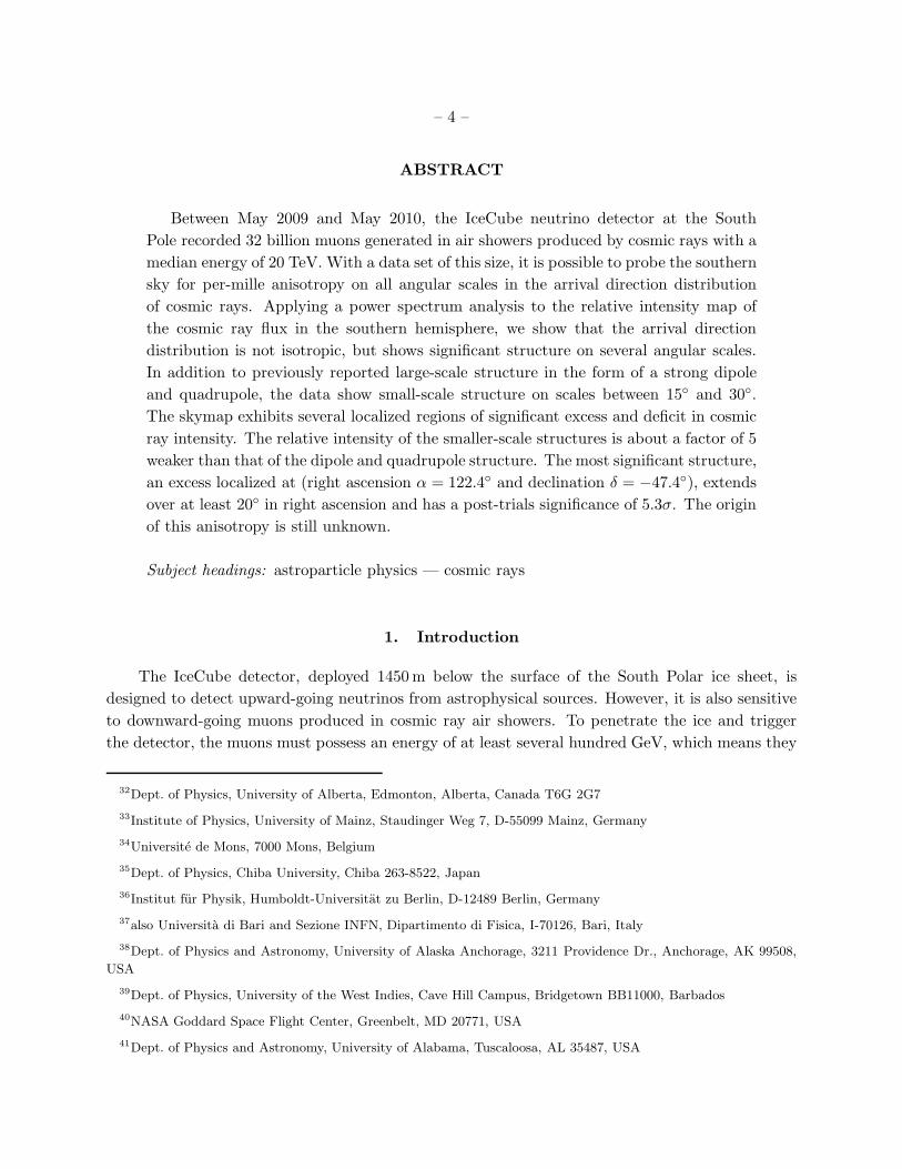
Fig. 1.— Median angular resolution (left) and median energy (right) as a function of zenith angle for

simulated cosmic ray events. The error bars on the left plot and the hatched regions on the right one

correspond to a 68% containing interval. The median primary energy is shown both as a function

of the true zenith angle (MC track) and the reconstructed zenith angle (LLH reconstruction), while

the median angular resolution (left) is shown as a function of the reconstructed zenith angle only.

The dotted vertical line at θ = 65 indicates the cut in zenith angle performed in this work.

2.2. Data Quality Cuts, Median Energy and Angular Resolution

The analysis presented in this paper uses the DST data collected during IC59 operations

between 2009 May 20 and 2010 May 30. The data set contains approximately 3.4×1010 muon events

detected with an integrated livetime of 334.5 days. A cut in zenith angle to remove misreconstructed

tracks near the horizon (see below) reduces the final data set to 3.2 × 1010 events.

Simulated air showers are used to evaluate the median angular resolution of the likelihood

reconstruction and the median energy of the downgoing muon DST data set. The simulated data

are created using the standard air shower Monte Carlo program CORSIKA1 (Heck et al. 1998).

The cosmic ray spectrum and composition are simulated using the polygonato model of Horandel

(2003), and the air showers are generated with the SIBYLL model of high-energy hadronic inter-

actions (Ahn et al. 2009).

The simulations show that, for zenith angles smaller than 65, the median angular resolution

is 3. This is not to be confused with the angular resolution of IceCube for neutrino-induced tracks

(better than 1), where more sophisticated reconstruction algorithms and more stringent quality

cuts are applied. The resolution depends on the zenith angle of the muon. Fig. 1 (left) shows the

median angular resolution as a function of zenith angle. The resolution improves from 4 at small

zenith angles to about 2.5 near 60. The larger space angle error at small zenith angles is caused

1COsmic Ray SImulations for KAscade: http://www-ik.fzk.de/corsika/

– 11 –

by the detector geometry, which makes it difficult to reconstruct the azimuth angle for near-vertical

showers. Consequently, with the azimuth angle being essentially unknown, the angular error can

be large. For zenith angles greater than 65, the angular resolution degrades markedly. The reason

is that more and more events with apparent zenith angle greater than 65 are misreconstructed

tracks of smaller zenith angle and lower energy. The energy threshold for muon triggers increases

rapidly with slant depth in the atmosphere and ice, and the statistics at large zenith angle become

quite poor. We restrict our analysis to events with zenith angles smaller than 65. Within this

range, the angular resolution is roughly constant and much smaller than the angular size of arrival

direction structure we are trying to study.

Using simulated data, we estimate that the overall median energy of the primary cosmic rays

that trigger the IceCube detector is 20 TeV. Simulations show that at this energy the detector is

more sensitive to protons than to heavy nuclei like iron. The median energy increases monoton-

ically with the true zenith angle of the primary particle (Fig. 1 (right)) due to the attenuation

of low-energy muons with increasing slant depth of the atmosphere and ice. The median energy

also increases as a function of reconstructed zenith angle. Near the horizon, the large fraction of

misreconstructed events causes the median energy to fall.

3. Analysis

The arrival direction distribution of cosmic rays observed by detectors like IceCube is not

isotropic. Nonuniform exposure to different parts of the sky, gaps in the uptime, and other detector-

related effects will cause a spurious anisotropy in the measured arrival direction distribution even

if the true cosmic ray flux is isotropic. Consequently, in any search for anisotropy in the cosmic ray

flux, these detector-related effects need to be accounted for. The first step in this search is therefore

the creation of a “reference map” to which the actual data map is compared. The reference map

essentially shows what the skymap would look like if the cosmic ray flux was isotropic. It is not

in itself isotropic, because it includes the detector effects mentioned above. The reference map

must be subtracted from the real skymap in order to find regions where the actual cosmic ray flux

deviates from the isotropic expectation.

In this section, we first describe the construction of the reference map for the subsequent

analysis. The reference map is then compared to the actual data map, and a map of the relative

cosmic ray intensity is produced. We then perform several analyses to search for the presence of

significant anisotropy in the relative intensity map.

3.1. Calculation of the Reference Level

For the construction of a reference map that represents the detector response to an isotropic

sky, it is necessary to determine the exposure of the detector as a function of time and integrate it

– 12 –

over the livetime. We use the method of Alexandreas et al. (1993) to calculate the exposure from

real data. This technique is commonly used in γ-ray astronomy to search for an excess of events

above the exposure-weighted isotropic reference level.

The method works as follows. The sky is binned into a fine grid in equatorial coordinates

(right ascension α, declination δ). Two sky maps are then produced. The data map N(α, δ) stores

the arrival directions of all detected events. For each detected event that is stored in the data

map, 20 “fake” events are generated by keeping the local zenith and azimuth angles (θ, φ) fixed and

calculating new values for right ascension using times randomly selected from within a pre-defined

time window ∆t bracketing the time of the event being considered. These fake events are stored in

the reference map with a weight of 1/20. Using 20 fake events per real event, the statistical error

on the reference level can be kept small.

Created in this way, the events in the reference map have the same local arrival direction

distribution as the real events. Furthermore, this “time scrambling” method naturally compensates

for variations in the event rate, including the presence of gaps in the detector uptime. The buffer

length ∆t needs to be chosen such that the detector conditions remain stable within this period.

Due to its unique location at the South Pole, the angular acceptance of IceCube is stable over long

periods. The longest ∆t used in this analysis is one day, and the detector stability over this time

period has been verified by χ2-tests comparing the arrival direction distributions at various times

inside the window. The IceCube detector is, in fact, stable over periods longer than 24 hours.

Deviations from isotropy are known to bias estimates of the reference level produced by this

method. In the vicinity of a strong excess, the method can create artificial deficits, as the events

from the excess region are included in the estimation of the reference level. Similarly, there can be

artificial excesses near strong deficits. In searches for point sources, the effect is usually negligible,

but it can become significant in the presence of extended regions of strong excess or deficit flux.

Since the Earth rotates by 15 every hour, the right ascension range of the scrambled data

is 15/hour × ∆t, so any structure in the data map that is larger than 15/hour × ∆t will also

appear in the reference map and therefore be suppressed in the relative intensity map ∆N/〈N〉.

For example, ∆t = 2 hr will suppress structures larger than 30 in the relative intensity map. To

be sensitive to large-scale structure such as a dipole, a time window of 24 hours (or higher) must

be used.

3.2. Relative Intensity and Significance Maps

Once the data and reference maps are calculated, deviations from isotropy can be analyzed by

calculating the relative intensity

∆Ni

〈N〉i=

Ni(α, δ) − 〈Ni(α, δ)〉

〈Ni(α, δ)〉. (1)

– 13 –

4 6 8 10 12 14

(N/N) [10

4]

90

80

70

60

50

40

30

20

decl

inati

on

[

]

Uncertainty in IC59 Relative Intensity

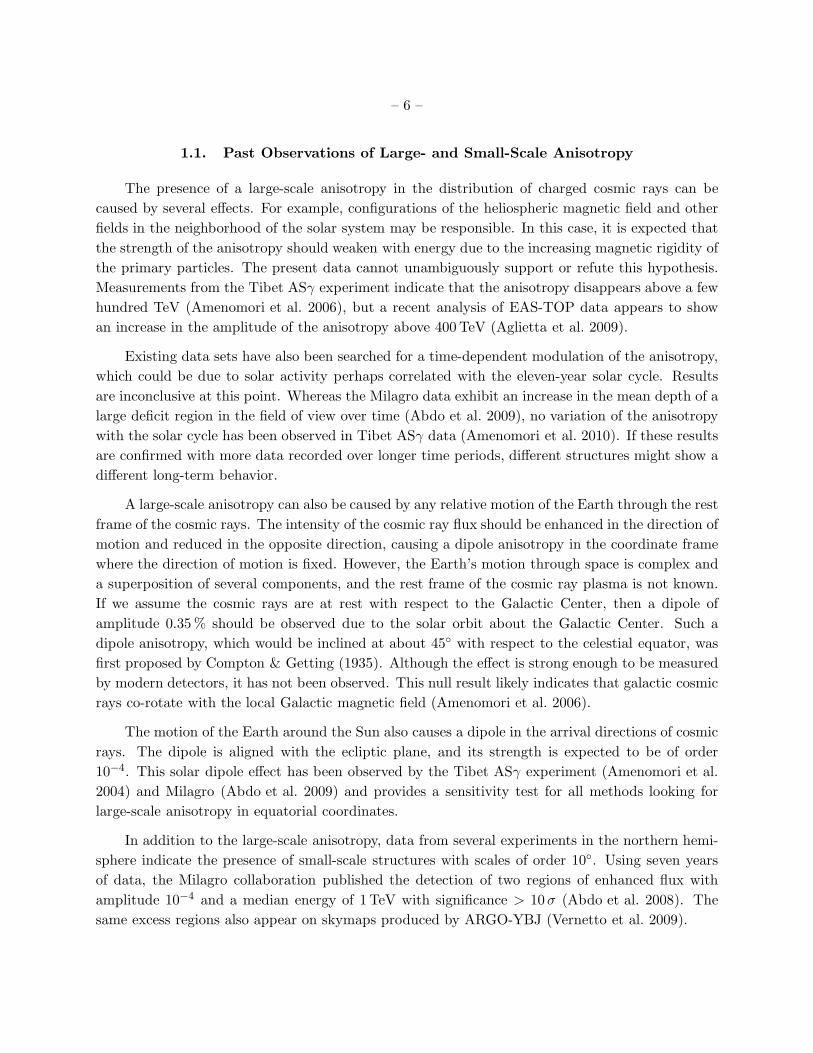
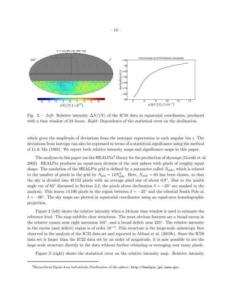
Fig. 2.— Left: Relative intensity ∆N/〈N〉 of the IC59 data in equatorial coordinates, produced

with a time window of 24 hours. Right: Dependence of the statistical error on the declination.

which gives the amplitude of deviations from the isotropic expectation in each angular bin i. The

deviations from isotropy can also be expressed in terms of a statistical significance using the method

of Li & Ma (1983). We report both relative intensity maps and significance maps in this paper.

The analyses in this paper use the HEALPix2 library for the production of skymaps (Gorski et al.

2005). HEALPix produces an equal-area division of the unit sphere with pixels of roughly equal

shape. The resolution of the HEALPix grid is defined by a parameter called Nside, which is related

to the number of pixels in the grid by Npix = 12N2side. Here, Nside = 64 has been chosen, so that

the sky is divided into 49 152 pixels with an average pixel size of about 0.9. Due to the zenith

angle cut of 65 discussed in Section 2.2, the pixels above declination δ = −25 are masked in the

analysis. This leaves 14 196 pixels in the region between δ = −25 and the celestial South Pole at

δ = −90. The sky maps are plotted in equatorial coordinates using an equal-area homolographic

projection.

Figure 2 (left) shows the relative intensity when a 24-hour time window is used to estimate the

reference level. The map exhibits clear structures. The most obvious features are a broad excess in

the relative counts near right ascension 105, and a broad deficit near 225. The relative intensity

in the excess (and deficit) region is of order 10−3. This structure is the large-scale anisotropy first

observed in the analysis of the IC22 data set and reported in Abbasi et al. (2010b). Since the IC59

data set is larger than the IC22 data set by an order of magnitude, it is now possible to see the

large scale structure directly in the data without further rebinning or averaging over many pixels.

Figure 2 (right) shows the statistical error on the relative intensity map. Relative intensity

2Hierarchical Equal-Area isoLatitude Pixelization of the sphere: http://healpix.jpl.nasa.gov.

– 14 –

]σsignificance [-6 -4 -2 0 2 4 6

coun

t

1

10

210

310

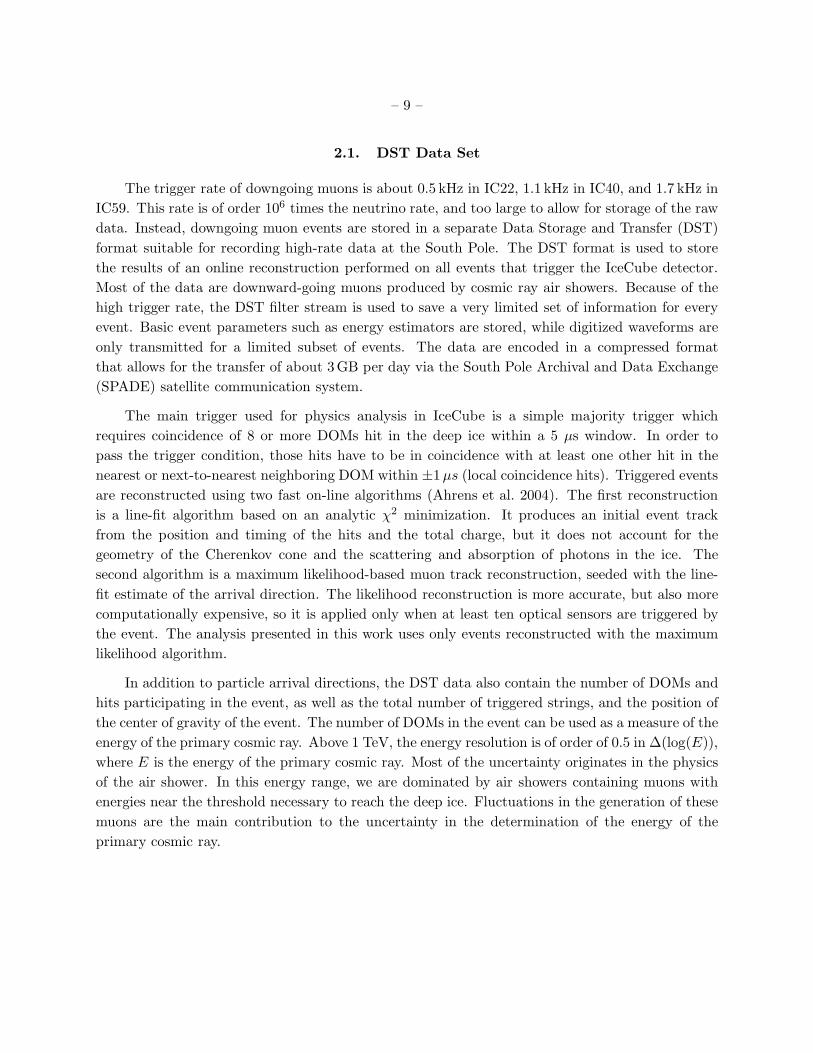
Fig. 3.— Left: Significance sky map of the IC59 data in equatorial coordinates, produced using a

time window of 24 hours. Right: 1d-distribution of the significance values together with the best-fit

(black solid line) performed with a Gaussian function. For comparison, a Gaussian function of mean

zero and unit variance (red dashed line), expected from an isotropic sky, has been superimposed.

skymaps have declination-dependent statistical uncertainties due to the fact that the detector

acceptance decreases with larger zenith angle. Since IceCube is located at the South Pole, the

relative intensity exhibits large fluctuations near the horizon, corresponding to declinations δ >

−30 . Such edge effects are not as severe for skymaps of the significance of the fluctuations,

though one must note that the location of structures with large (or small) significance may not

coincide with regions of large (or small) relative intensity.

Fig. 3 (left) shows the significance map corresponding to the relative intensity map shown in

Figure 2. The right panel also shows a distribution of the significance values in each bin. In an

isotropic skymap, the distribution of the significance values should be normal (red dashed line).

However, the best Gaussian fit to the distribution (black solid line) exhibits large deviations from

a normal distribution caused by the large-scale structure.

3.3. Angular Power Spectrum Analysis

To observe correlations between pixels at several angular scales, we calculate the angular power

spectrum of the relative intensity map δI = ∆N/〈N〉 described in Section 3.2. The relative intensity

can be treated as a scalar field which we expand in terms of a spherical harmonic basis,

δI(ui) =

∞∑ℓ=1

ℓ∑m=−ℓ

aℓmYℓm(ui) (2)

– 15 –

aℓm ∼ Ωp

Npix∑i=0

δI(ui)Y∗

ℓm(ui) . (3)

In Eqs. (2) and (3), the Yℓm are the Laplace spherical harmonics, the aℓm are the multipole coeffi-

cients of the expansion, Ωp is the solid angle observed by each pixel (which is constant across the

sphere in HEALPix), ui = (αi, δi) is the pointing vector associated with the ith pixel, and Npix is

the total number of pixels in the skymap. The power spectrum for the relative intensity field is

defined as the variance of the multipole coefficients aℓm,

Cℓ =1

2ℓ + 1

ℓ∑m=−ℓ

|aℓm|2 . (4)

The amplitude of the power spectrum at some multipole order ℓ is associated with the presence

of structures in the sky at angular scales of about 180/ℓ. In the case of complete and uniform

sky coverage, a straightforward Fourier decomposition of the relative intensity maps would yield

an unbiased estimate of the power spectrum. However, due to the limited exposure of the detector,

we only have direct access to the so-called pseudo-power spectrum, which is the convolution of

the real underlying power spectrum and the power spectrum of the relative exposure map of the

detector in equatorial coordinates. In the case of partial sky coverage, the standard Yℓm spherical

harmonics do not form an orthonormal basis that we can use to expand the relative intensity field

directly. As a consequence of this, the pseudo-power spectrum displays a systematic correlation

between different ℓ modes that needs to be corrected for.

The deconvolution of pseudo-power spectra has been a longstanding problem in CMB astron-

omy, and there are several computationally efficient tools available from the CMB community.

(For a discussion on the bias introduced by partial sky coverage in power spectrum estimation

and a description of several bias removal methods, see Ansari & Magneville (2010).) To calculate

the power spectrum of the IC59 data, we use the publicly available PolSpice3 software package

(Szapudi et al. 2001; Chon et al. 2004).

In PolSpice, the correction for partial sky bias is performed not on the power spectrum itself,

but on the two-point correlation function of the relative intensity map. The two-point correlation

function ξ(η) is defined as

ξ(η) = 〈δI(ui) δI(uj)〉 , (5)

where δI(uk) is the observed relative intensity in the direction of the kth pixel. Note that ξ(η)

depends only on the angle η between any two pixels. The two-point correlation function can be

expanded into a Legendre series,

ξ(η) =1

4π

∞∑ℓ=0

(2ℓ + 1) Cℓ Pℓ(cos η) , (6)

3PolSpice website: http://prof.planck.fr/article141.html.

– 16 –

where the Cℓ are the coefficients of the angular power spectrum and the Pℓ are the Legendre

polynomials. The inverse operation

Cℓ = 2π

∫ 1

−1

ξ(η) Pℓ(cos η) d(cos η) (7)

can be used to calculate the angular power spectrum coefficients from a known two-point correlation

function.

In order to obtain an unbiased estimator of the true power spectrum, PolSpice first calculates

the aℓm coefficients of both the relative intensity map and the relative exposure map doing a spher-

ical harmonics expansion equivalent to that shown in Eq.(3). Pseudo-power spectra for both maps

are computed from these coefficients using Eq.(4), and these spectra are subsequently converted

into correlation functions using Eq.(6). An unbiased estimator ξ(η) of the true correlation function

of the data is computed by taking the ratio of the correlation functions of the relative intensity map

and the relative exposure map. An estimate Cℓ of the true power spectrum can then be obtained

from the corrected two-point correlation function using the integral expression shown in Eq.(7).

This process reduces the correlation between different ℓ modes introduced by the partial sky

coverage. Minor ringing artifacts associated with the limited angular range over which the corre-

lation function is evaluated are minimized by applying an apodization function to the correlation

function in η-space as described in Chon et al. (2004). The cosine apodization scheme provided

by PolSpice and used in this work allows the correlation function to fall slowly to zero at large

angular scales where statistics are low, minimizing any ringing artifacts that could arise from the

calculation of the power spectrum from the corrected correlation function using Eq.(7).

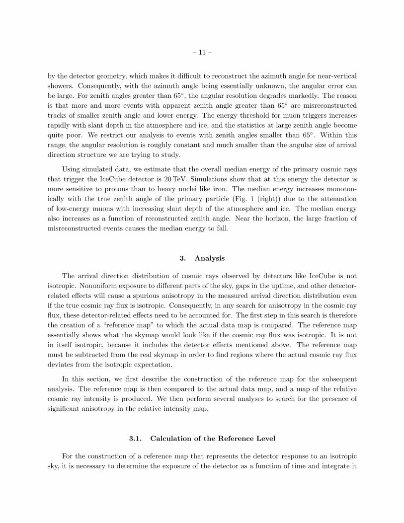
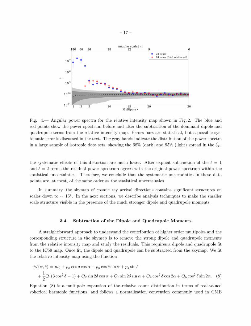
Fig. 4 (blue points) shows the angular power spectrum for the IC59 relative intensity map from

Fig. 2. In addition to a strong dipole and quadrupole moment (ℓ = 1, 2), higher order terms up to

ℓ = 12 contribute significantly to the skymap. The error bars on the Cℓ are statistical. The gray

bands indicate the 68% and 95% spread in the Cℓ for a large number of power spectra for isotropic

data sets (generated by introducing Poisson fluctuations in the reference skymap). As the Cℓ are

still not entirely independent (even after the correction for partial sky coverage is performed), a

strong dipole moment in the data can lead to significant higher order multipoles, and it is important

to study whether the structure for 3 ≤ ℓ ≤ 12 is a systematic effect caused by the strong lower order

moments ℓ = 1, 2. Fig. 4 (red points) shows the angular power spectrum after the strong dipole and

quadrupole moments are removed from the relative intensity map by a fit procedure described in

the next section. The plot illustrates that after the removal of the lower order multipoles, indicated

by the drop in Cℓ for ℓ = 1, 2 (both are consistent with 0 after the subtraction), most of the higher

order terms are still present. Only the strength of C3 and C4 is considerably reduced (the former

to a value that is below the range of the plot).

Regarding systematic uncertainties, for ℓ = 3 and ℓ = 4 the effects of the strong dipole and

quadrupole suggest that there is significant coupling between the low-ℓ modes. Therefore, we

cannot rule out that C3 and C4 are entirely caused by systematic effects. For the higher multipoles,

– 17 –

180 60 36 18 12 9 6Angular scale [ ]

10-11

10-10

10-9

10-8

10-7C

1 3 5 10 15 20 30Multipole

24 hours24 hours (D+Q subtracted)

Fig. 4.— Angular power spectra for the relative intensity map shown in Fig. 2. The blue and

red points show the power spectrum before and after the subtraction of the dominant dipole and

quadrupole terms from the relative intensity map. Errors bars are statistical, but a possible sys-

tematic error is discussed in the text. The gray bands indicate the distribution of the power spectra

in a large sample of isotropic data sets, showing the 68% (dark) and 95% (light) spread in the Cℓ.

the systematic effects of this distortion are much lower. After explicit subtraction of the ℓ = 1

and ℓ = 2 terms the residual power spectrum agrees with the original power spectrum within the

statistical uncertainties. Therefore, we conclude that the systematic uncertainties in these data

points are, at most, of the same order as the statistical uncertainties.

In summary, the skymap of cosmic ray arrival directions contains significant structures on

scales down to ∼ 15. In the next sections, we describe analysis techniques to make the smaller

scale structure visible in the presence of the much stronger dipole and quadrupole moments.

3.4. Subtraction of the Dipole and Quadrupole Moments

A straightforward approach to understand the contribution of higher order multipoles and the

corresponding structure in the skymap is to remove the strong dipole and quadrupole moments

from the relative intensity map and study the residuals. This requires a dipole and quadrupole fit

to the IC59 map. Once fit, the dipole and quadrupole can be subtracted from the skymap. We fit

the relative intensity map using the function

δI(α, δ) = m0 + px cos δ cosα + py cos δ sinα + pz sin δ

+1

2Q1(3 cos2 δ − 1) + Q2 sin 2δ cosα + Q3 sin 2δ sinα + Q4 cos2 δ cos 2α + Q5 cos2 δ sin 2α. (8)

Equation (8) is a multipole expansion of the relative count distribution in terms of real-valued

spherical harmonic functions, and follows a normalization convention commonly used in CMB

– 18 –

Fig. 5.— Fit of Eq. (8) to the IC59 relative intensity distribution ∆N/〈N〉 shown in Fig. 2.

physics (Smoot & Lubin 1979). The quantity m0 is the “monopole” moment of the distribution, and

corresponds to a constant offset of the data from zero. The values (px, py, pz) are the components

of the dipole moment, and the quantities (Q1, . . . , Q5) are the five independent components of the

quadrupole moment.

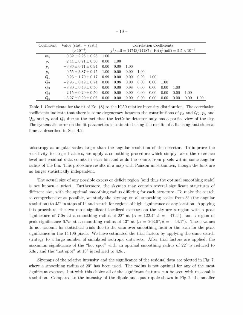
The two-dimensional harmonic expansion of Eq. (8) was fit to the 14 196 pixels in the IC59

relative intensity map that lie between the celestial South Pole and declination δ = −25. The

best-fit dipole and quadrupole coefficients are provided in Table 1, and the corresponding sky

distribution is shown in Fig. 5. By themselves, the dipole and quadrupole terms can account for

much of the amplitude of the part-per-mille anisotropy observed in the IceCube data. We note that

the quadrupole moment is actually the dominant term in the expansion, with a total amplitude

that is about 2.5 times larger than the dipole magnitude. However, the χ2/ndf = 14743/14187

corresponds to a χ2-probability of approximately 0.05%, so while the dipole and quadrupole are

dominant terms in the arrival direction anisotropy, they do not appear to be sufficient to explain

all of the structures observed in the angular distribution of ∆N/〈N〉. This result is consistent with

the result of the angular power spectrum analysis in Sec. 3.3, which also indicates the need for

higher-order multipole moments to describe the structures in the relative intensity skymap.

Subtraction of the dipole and quadrupole fits from the relative intensity map shown in Fig. 2

yields the residual map shown in Fig. 6. The fit residuals are relatively featureless at first glance,

and the significance values are well-described by a normal distribution, which is expected when no

anisotropy is present. However, the bin size in this plot is not optimized for a study of significant

– 19 –

Coefficient Value (stat. + syst.) Correlation Coefficients

(×10−4) χ2/ndf = 14743/14187 : Pr(χ2|ndf) = 5.5 × 10−4

m0 0.32 ± 2.26 ± 0.28 1.00

px 2.44 ± 0.71 ± 0.30 0.00 1.00

py −3.86 ± 0.71 ± 0.94 0.00 0.00 1.00

pz 0.55 ± 3.87 ± 0.45 1.00 0.00 0.00 1.00

Q1 0.23 ± 1.70 ± 0.17 0.99 0.00 0.00 0.99 1.00

Q2 −2.95 ± 0.49 ± 0.74 0.00 0.98 0.00 0.00 0.00 1.00

Q3 −8.80 ± 0.49 ± 0.50 0.00 0.00 0.98 0.00 0.00 0.00 1.00

Q4 −2.15 ± 0.20 ± 0.50 0.00 0.00 0.00 0.00 0.00 0.00 0.00 1.00

Q5 −5.27 ± 0.20 ± 0.06 0.00 0.00 0.00 0.00 0.00 0.00 0.00 0.00 1.00

Table 1: Coefficients for the fit of Eq. (8) to the IC59 relative intensity distribution. The correlation

coefficients indicate that there is some degeneracy between the contributions of px and Q2, py and

Q3, and pz and Q1 due to the fact that the IceCube detector only has a partial view of the sky.

The systematic error on the fit parameters is estimated using the results of a fit using anti-sidereal

time as described in Sec. 4.2.

anisotropy at angular scales larger than the angular resolution of the detector. To improve the

sensitivity to larger features, we apply a smoothing procedure which simply takes the reference

level and residual data counts in each bin and adds the counts from pixels within some angular

radius of the bin. This procedure results in a map with Poisson uncertainties, though the bins are

no longer statistically independent.

The actual size of any possible excess or deficit region (and thus the optimal smoothing scale)

is not known a priori. Furthermore, the skymap may contain several significant structures of

different size, with the optimal smoothing radius differing for each structure. To make the search

as comprehensive as possible, we study the skymap on all smoothing scales from 3 (the angular

resolution) to 45 in steps of 1 and search for regions of high significance at any location. Applying

this procedure, the two most significant localized excesses on the sky are a region with a peak

significance of 7.0σ at a smoothing radius of 22 at (α = 122.4, δ = −47.4), and a region of

peak significance 6.7σ at a smoothing radius of 13 at (α = 263.0, δ = −44.1). These values

do not account for statistical trials due to the scan over smoothing radii or the scan for the peak

significance in the 14 196 pixels. We have estimated the trial factors by applying the same search

strategy to a large number of simulated isotropic data sets. After trial factors are applied, the

maximum significance of the “hot spot” with an optimal smoothing radius of 22 is reduced to

5.3σ, and the “hot spot” at 13 is reduced to 4.9σ.

Skymaps of the relative intensity and the significance of the residual data are plotted in Fig. 7,

where a smoothing radius of 20 has been used. The radius is not optimal for any of the most

significant excesses, but with this choice all of the significant features can be seen with reasonable

resolution. Compared to the intensity of the dipole and quadrupole shown in Fig. 2, the smaller

– 20 –

]σsignificance [-6 -4 -2 0 2 4 6

coun

t

1

10

210

310

Fig. 6.— Left: Residual of the fit of Eq. (8) to the relative intensity distribution shown in Fig. 2.

Right: Distribution of pixel significance values in the skymap before (solid black line) and after

(dashed red line) subtraction of the dipole and quadrupole. Gaussian fits to the data yield a mean

of (−0.20 ± 1.05) × 10−2 and a width of 1.23 ± 0.01 before the dipole and quadrupole subtraction,

and (0.28 ± 0.89) × 10−2 and 1.02 ± 0.01 after.

structures are weaker by about a factor of 5.

Table 2 contains the location and optimal smoothing scales of all the regions in the IC59

skymap which have a pre-trials significance beyond ±5σ. The data also exhibit additional regions

of excess and deficit. It is possible that the deficits are at least in part artifacts of the reference

level estimation procedure, which can produce artificial deficits around regions of significant excess

counts (or in principle, excesses in the presence of strong physical deficits). While several of the

deficit and excess regions are observed at large zenith angles near the edge of the IC59 exposure

region, we do not believe these features are statistical fluctuations or edge effects. As we will show

in Section 4.3, the features are also present in IC22 and IC40 data, and grow in significance as the

statistics increase.

Fig. 8 shows the significance maps with regions with a pre-trial significance larger than ±5σ

indicated according to the numbers used in Table 2. Since the optimal scales vary from region

to region and no single smoothing scale shows all regions, we show the maps with two smoothing

scales, 12 (left), and 20 (right).

The angular power spectrum of the residual map is shown in red in Fig. 4. As expected, there

is no significant dipole or quadrupole moment left in the skymap, and the ℓ = 3 and ℓ = 4 moments

have also disappeared or have been weakened substantially. However, the moments corresponding

to 5 ≤ ℓ ≤ 12 are still present at the same strength as before the subtraction, and indicate the

presence of structure of angular size 15 to 35 in the data. The excesses and deficits in Fig. 7

– 21 –

Fig. 7.— Left: Residual intensity map plotted with 20 smoothing. Right: Significances of the

residual map (pre-trials), plotted with 20 smoothing.

correspond in size to these moments.

region right ascension declination optimal scale peak significance post-trials

1 (122.4+4.1−4.7)

(−47.4+7.5−3.2)

22 7.0σ 5.3σ

2 (263.0+3.7

−3.8) (−44.1+5.3

−5.1) 13 6.7σ 4.9σ

3 (201.6+6.0−1.1)

(−37.0+2.2−1.9)

11 6.3σ 4.4σ

4 (332.4+9.5

−7.1) (−70.0+4.2

−7.6) 12 6.2σ 4.2σ

5 (217.7+10.2

−7.8 ) (−70.0+3.6

−2.3) 12 −6.4σ −4.5σ

6 (77.6+3.9−8.4)

(−31.9+3.2−8.6)

13 −6.1σ −4.1σ

7 (308.2+4.8

−7.7) (−34.5+9.6

−6.9) 20 −6.1σ −4.1σ

8 (166.5+4.5−5.7)

(−37.2+5.0−5.7)

12 −6.0σ −4.0σ

Table 2: Location and optimal smoothing scale for regions of the IC59 skymap with a pre-trials

significance larger than ±5σ. The errors on the equatorial coordinates indicate the range over

which the significance drops by 1σ from the local extremum.

– 22 –

Fig. 8.— Left: Significances of the IC59 residual map plotted with 12 smoothing. Right: Sig-

nificances of the IC59 residual map plotted with 20 smoothing. The regions with a pre-trial

significance larger than ±5σ are indicated according to the numbers used in Table 2.

– 23 –

180 60 36 18 12 9 6Angular scale [ ]

10-11

10-10

10-9

10-8

10-7

C

1 3 5 10 15 20 30Multipole

2 hours

3 hours

4 hours

6 hours

8 hours

12 hours

24 hours

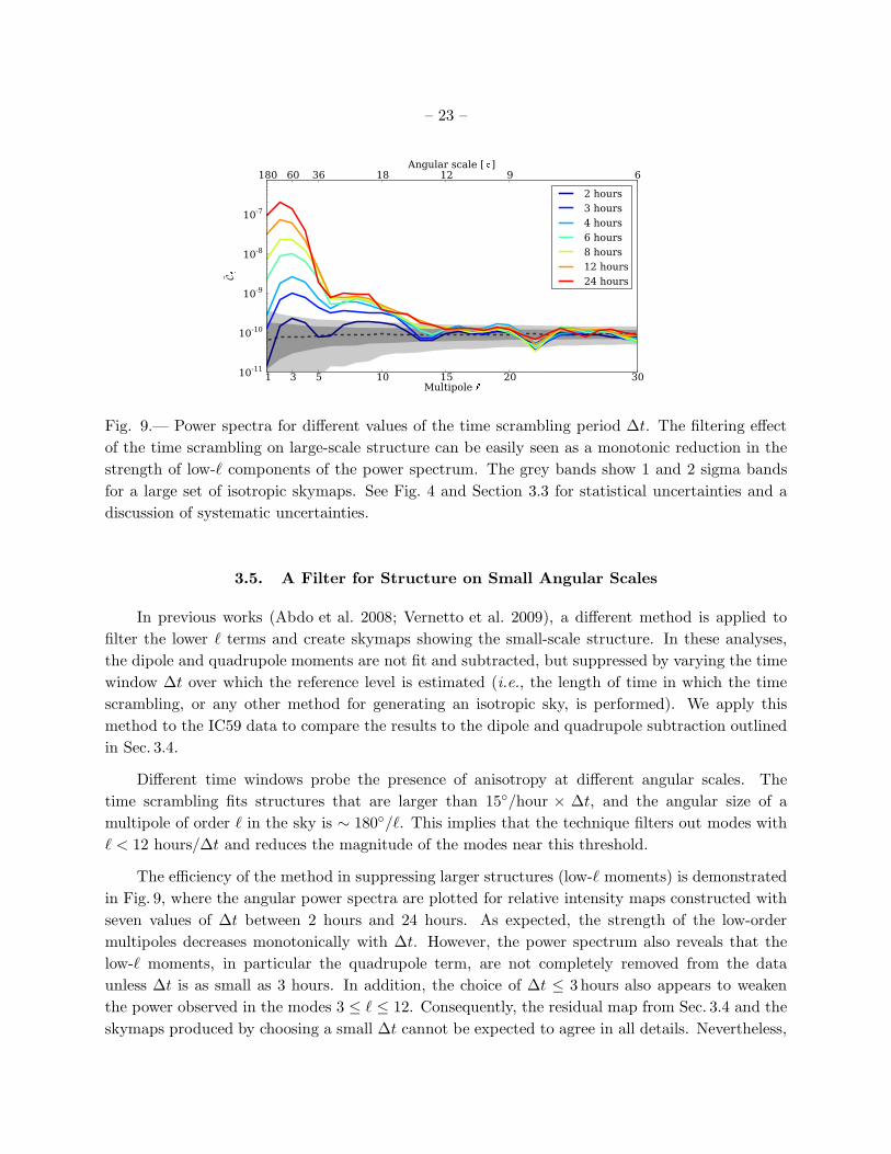
Fig. 9.— Power spectra for different values of the time scrambling period ∆t. The filtering effect

of the time scrambling on large-scale structure can be easily seen as a monotonic reduction in the

strength of low-ℓ components of the power spectrum. The grey bands show 1 and 2 sigma bands

for a large set of isotropic skymaps. See Fig. 4 and Section 3.3 for statistical uncertainties and a

discussion of systematic uncertainties.

3.5. A Filter for Structure on Small Angular Scales

In previous works (Abdo et al. 2008; Vernetto et al. 2009), a different method is applied to

filter the lower ℓ terms and create skymaps showing the small-scale structure. In these analyses,

the dipole and quadrupole moments are not fit and subtracted, but suppressed by varying the time

window ∆t over which the reference level is estimated (i.e., the length of time in which the time

scrambling, or any other method for generating an isotropic sky, is performed). We apply this

method to the IC59 data to compare the results to the dipole and quadrupole subtraction outlined

in Sec. 3.4.

Different time windows probe the presence of anisotropy at different angular scales. The

time scrambling fits structures that are larger than 15/hour × ∆t, and the angular size of a

multipole of order ℓ in the sky is ∼ 180/ℓ. This implies that the technique filters out modes with

ℓ < 12 hours/∆t and reduces the magnitude of the modes near this threshold.

The efficiency of the method in suppressing larger structures (low-ℓ moments) is demonstrated

in Fig. 9, where the angular power spectra are plotted for relative intensity maps constructed with

seven values of ∆t between 2 hours and 24 hours. As expected, the strength of the low-order

multipoles decreases monotonically with ∆t. However, the power spectrum also reveals that the

low-ℓ moments, in particular the quadrupole term, are not completely removed from the data

unless ∆t is as small as 3 hours. In addition, the choice of ∆t ≤ 3 hours also appears to weaken

the power observed in the modes 3 ≤ ℓ ≤ 12. Consequently, the residual map from Sec. 3.4 and the

skymaps produced by choosing a small ∆t cannot be expected to agree in all details. Nevertheless,

– 24 –

Fig. 10.— Relative intensity (left) and significance (right) map in equatorial coordinates for ∆t =

4 hours and an integration radius of 20.

a comparison of the skymaps produced with the two methods provides an important crosscheck.

To best compare this analysis to the results of Section 3.4, the reference level is calculated

using a scrambling time window of ∆t = 4 hours. This choice of ∆t is motivated by the angular

power spectrum in Fig. 9. With ∆t = 4 hours, the spectrum shows the strongest suppression of the

dipole and quadrupole while still retaining most of power in the higher multipole moments.

Skymaps of the relative intensity and significance for ∆t = 4 hours are shown in Fig. 10. The

maps have been smoothed by 20 to allow for a direct comparison with Fig. 7. The most prominent

features of the map are a single broad excess and deficit, with several small excess regions observed

near the edge of the exposure region. The broad excess is centered at α = (121.7+4.8−7.1) and

δ = (−44.2+12.1−7.8 ), at the same position as Region 1 in Table 2. The optimal smoothing scale of

the excess is 25, with a pre-trials significance of 9.6σ. A second significant excess is observed

at α = (341.7+1.4−5.6) and δ = (−34.9+3.6

−6.8) with a peak significance of 5.8σ at a smoothing scale

of 9. This feature does not appear to have a direct match in Fig. 7, but is roughly aligned in

right ascension with the excess identified in Table 2 as Region 4. We also note that the second-

largest excess in Table 2, Region 2, is visible near α = 263.0 in Fig. 10, but with a pre-trials peak

significance of 4.5σ after smoothing by 13.

The differences in significance between Figs. 7 and 10 can be attributed to the fact that some

contributions from the low-ℓ moments are still present in this analysis. The broad excess observed

here is co-located with the maximum of the large-scale structure shown in Fig. 5, enhancing its

significance. By comparison, the excess in Region 2 is close to the minimum of the large-scale

structure, weakening its significance. The leakage of large-scale structure into the ∆t = 4 hour

skymap also explains the large deficit near α = 220; due to its co-location with the minimum of

the dipole and quadrupole, the size of the deficit is enhanced considerably.

– 25 –

050100150200250300350Right Ascension [ ]

0.0010

0.0005

0.0000

0.0005

0.0010

N/

N

IC59 Relative Intensity

Dipole + quadrupole fit residualst=24 hours

t=4 hours

Fig. 11.— Relative intensity in the declination band −45 < δ < −30. The blue points show the

result after subtracting the dipole and quadrupole moments. The black points correspond to ∆t

=24 hours and show the large-scale structure, the red points correspond to ∆t = 4 hours. The error

boxes represent systematic uncertainties.

This effect is illustrated in Fig. 11, which shows the relative intensity for the declination range

−45 < δ < −30, projected onto the right ascension axis. This declination range is chosen

because it contains some of the most significant structures of the skymaps. The blue points show

the relative intensity corresponding to Fig. 7, i.e., the skymap after subtraction of dipole and

quadrupole moments. The black and red points show the relative intensity for skymaps obtained

with the method described in this section; the black points correspond to ∆t = 24 hours, the red

points to ∆t = 4 hours. In the case of ∆t = 24 hours, the large scale structure dominates. For

∆t = 4 hours, the large scale structure is suppressed, and the smaller features become visible. The

blue and red curves show excesses and deficits at the same locations, but with different strengths. As

the red curve still contains some remaining large scale structure, maxima and minima are enhanced

or weakened depending on where they are located with respect to the maximum and minimum of

the large-scale structure. The systematic error for the relative intensity values in Fig. 11 is taken

from the analysis of the data in anti-sidereal time as described in the next section.

Finally, we note that the presence of the small-scale structure can be verified by inspection of

the raw event counts in the data. Figure 12 shows the observed and expected event counts for de-

clinations −45 < δ < −30, projected onto the right ascension axis. The seven panels of the figure

contain the projected counts for seven time scrambling windows ∆t = 2, 3, 4, 6, 8, 12, 24 hours.

For small values of ∆t, the expected counts agree with the data; for example, when ∆t = 2 hours,

the data exhibit no visible deviation from the expected counts. For larger values of ∆t, the expected

– 26 –

count distribution flattens out as the technique to estimate the reference level no longer over-fits

the large structures. When ∆t = 24 hours, the reference level is nearly flat, and the shape of the

large-scale anisotropy is clearly visible from the raw data.

– 27 –

050100150200250300350Right Ascension [ ]

43.25

43.30

43.35

43.40co

un

ts

106

DataReference level for t=2 hours

050100150200250300350Right Ascension [ ]

43.25

43.30

43.35

43.40

cou

nts

106

DataReference level for t=3 hours

050100150200250300350Right Ascension [ ]

43.25

43.30

43.35

43.40

cou

nts

106

DataReference level for t=4 hours

050100150200250300350Right Ascension [ ]

43.25

43.30

43.35

43.40

cou

nts

106

DataReference level for t=6 hours

050100150200250300350Right Ascension [ ! ]

43.25

43.30

43.35

43.40

cou

nts

"

106

DataReference level for #t=8 hours

050100150200250300350Right Ascension [ $ ]

43.25

43.30

43.35

43.40

cou

nts

%

106

DataReference level for &t=12 hours

050100150200250300350Right Ascension [ ' ]

43.25

43.30

43.35

43.40

cou

nts

(

106

DataReference level for )t=24 hours

Fig. 12.— Number of events (red) and reference level (black), with statistical uncertainties, as

a function of right ascension for the declination range −45 < δ < −30. The reference level is

estimated in different time windows, from 2 hours (top-left) to 24 hours (bottom). Each plot has

been created using independent 15δ × 2 bins in right ascension.

– 28 –

4. Systematic Checks

Several tests have been performed on the data to ensure the stability of the observed anisotropy

and to rule out possible sources of systematic bias. Among the influences that might cause spurious

anisotropy are the detector geometry, the detector livetime, nonuniform exposure of the detector

to different regions of the sky, and diurnal and seasonal variations in atmospheric conditions. Due

to the unique location of the IceCube detector at the South Pole, many of these effects play a lesser

role for IceCube than for detectors located in the middle latitudes. The southern celestial sky is

fully visible to IceCube at any time, and changes in the event rate tend to affect the entire visible

sky. Seasonal variations are of order ± 10% (Tilav et al. 2009), but the changes are slow and the

reference level estimation technique is designed to take these changes into account. This is also true

for any effects caused by the asymmetric detector response due to the geometrical configuration of

the detector. In this section, we test the accuracy of these assumptions.

4.1. Solar Dipole Analysis

As mentioned in Section 1.1, any observer moving through a plasma of isotropic cosmic rays

should observe a difference in intensity between the direction of the velocity vector and the opposite

direction. Therefore, cosmic rays received on Earth should exhibit a dipole modulation in solar

time caused by the Earth’s orbital velocity around the Sun. The expected change in the relative

intensity is given by∆I

〈I〉= (γ + 2)

v

ccos ρ , (9)

where I is the cosmic ray intensity, γ = 2.7 the power law index of the cosmic ray energy spectrum,

v/c the ratio of the Earth’s velocity with respect to the speed of light, and ρ the angle between the

cosmic ray arrival direction and the direction of motion (Gleeson & Axford 1968). With a velocity

of v = 30 km s−1, the expected amplitude is 4.7×10−4. Note that the power law spectral index has

a systematic uncertainty (see for example Biermann et al. (2010) for a discussion) and the Earth’s

velocity is not precisely constant, but both of these uncertainties are too small to be relevant in

our comparison of the predicted dipole strength to the measured strength. The solar dipole effect

has been measured with several experiments (Amenomori et al. 2004, 2008; Abdo et al. 2009) and

provides an important check of the reliability of the analysis techniques presented earlier, as it

verifies that the techniques are sensitive to a known dipole with an amplitude of roughly the same

size as the structures in the equatorial skymap.

In principle, the solar dipole is not a cause of systematic uncertainties in the analysis of cosmic

ray anisotropy in sidereal time (equatorial coordinates). The solar dipole is visible only when the

arrival directions are plotted in a frame where the Sun’s position is fixed in the sky. A signal in

this coordinate system averages to zero in sidereal time over the course of one year. However, any

seasonal variation of the solar dipole can cause a spurious anisotropy in equatorial coordinates. The

effect works both ways: a seasonal variation in the sidereal anisotropy will affect the solar dipole.

– 29 –

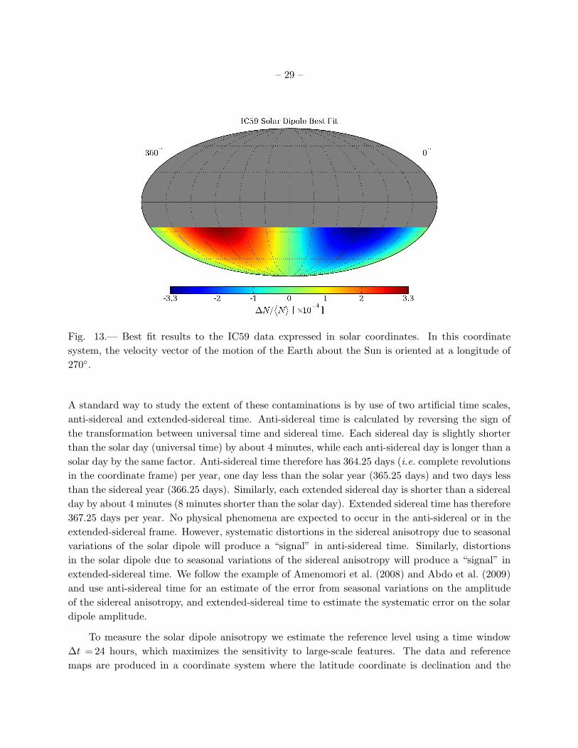
Fig. 13.— Best fit results to the IC59 data expressed in solar coordinates. In this coordinate

system, the velocity vector of the motion of the Earth about the Sun is oriented at a longitude of

270.

A standard way to study the extent of these contaminations is by use of two artificial time scales,

anti-sidereal and extended-sidereal time. Anti-sidereal time is calculated by reversing the sign of

the transformation between universal time and sidereal time. Each sidereal day is slightly shorter

than the solar day (universal time) by about 4 minutes, while each anti-sidereal day is longer than a

solar day by the same factor. Anti-sidereal time therefore has 364.25 days (i.e. complete revolutions

in the coordinate frame) per year, one day less than the solar year (365.25 days) and two days less

than the sidereal year (366.25 days). Similarly, each extended sidereal day is shorter than a sidereal

day by about 4 minutes (8 minutes shorter than the solar day). Extended sidereal time has therefore

367.25 days per year. No physical phenomena are expected to occur in the anti-sidereal or in the

extended-sidereal frame. However, systematic distortions in the sidereal anisotropy due to seasonal

variations of the solar dipole will produce a “signal” in anti-sidereal time. Similarly, distortions

in the solar dipole due to seasonal variations of the sidereal anisotropy will produce a “signal” in

extended-sidereal time. We follow the example of Amenomori et al. (2008) and Abdo et al. (2009)

and use anti-sidereal time for an estimate of the error from seasonal variations on the amplitude

of the sidereal anisotropy, and extended-sidereal time to estimate the systematic error on the solar

dipole amplitude.

To measure the solar dipole anisotropy we estimate the reference level using a time window

∆t = 24 hours, which maximizes the sensitivity to large-scale features. The data and reference

maps are produced in a coordinate system where the latitude coordinate is declination and the

– 30 –

Coefficient Value (stat. + syst.)

(×10−4)

m0 −0.03 ± 0.06 ± 0.02

px 0.02 ± 0.14 ± 0.97

py −3.66 ± 0.14 ± 0.17

pz −0.03 ± 0.07 ± 0.01

Table 3: Coefficients of a dipole and constant offset fit to the IC59 solar coordinate data. The

systematic error on the fit parameters is estimated using the results of a fit using extended-sidereal

time as described in the text.

longitude coordinate represents the angular distance from the Sun in right ascension, defined as

the difference between the right ascension of each event and the right ascension of the Sun. In this

coordinate system the Sun’s longitude is fixed at 0 and we expect, over a full year, an excess in

the direction of motion of the Earth’s velocity vector (at 270) and a minimum in the opposite

direction.

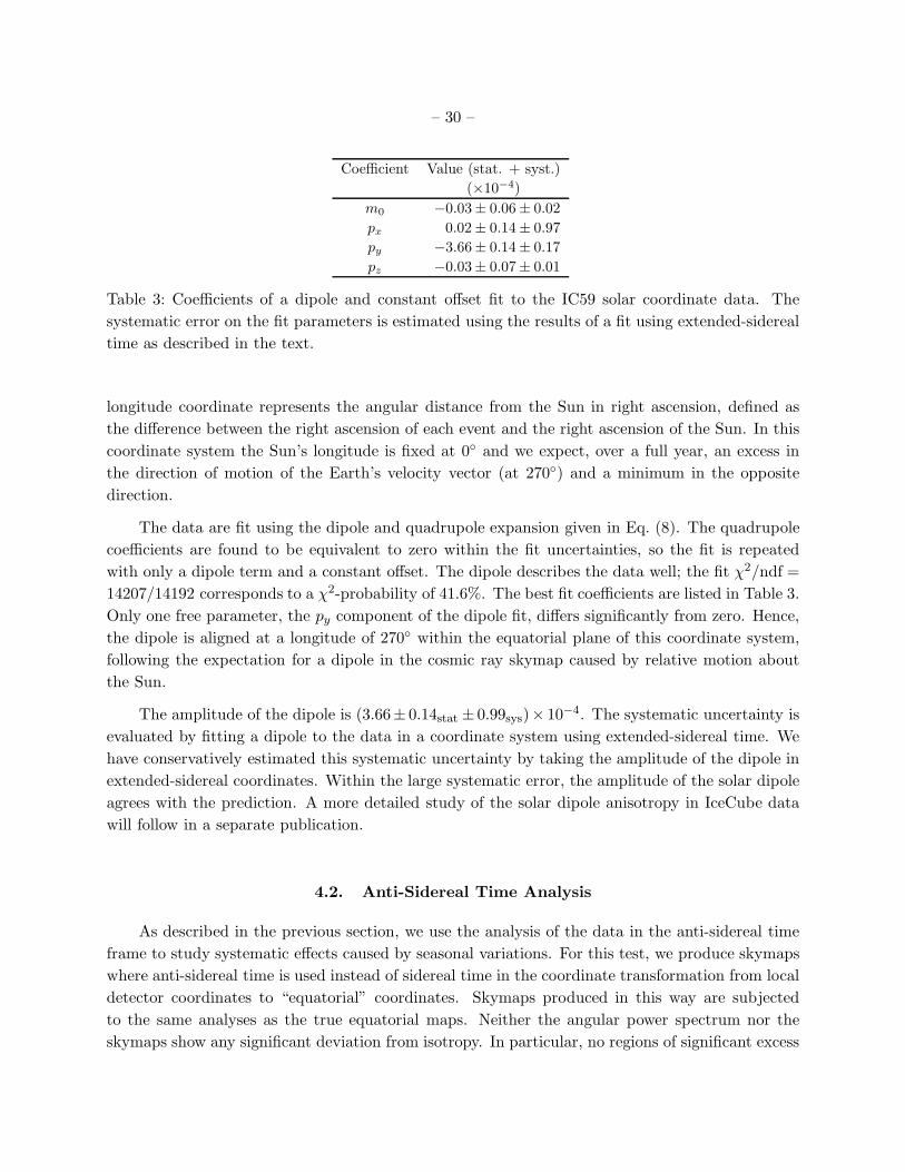
The data are fit using the dipole and quadrupole expansion given in Eq. (8). The quadrupole

coefficients are found to be equivalent to zero within the fit uncertainties, so the fit is repeated

with only a dipole term and a constant offset. The dipole describes the data well; the fit χ2/ndf =

14207/14192 corresponds to a χ2-probability of 41.6%. The best fit coefficients are listed in Table 3.

Only one free parameter, the py component of the dipole fit, differs significantly from zero. Hence,

the dipole is aligned at a longitude of 270 within the equatorial plane of this coordinate system,

following the expectation for a dipole in the cosmic ray skymap caused by relative motion about

the Sun.

The amplitude of the dipole is (3.66± 0.14stat ± 0.99sys)× 10−4. The systematic uncertainty is

evaluated by fitting a dipole to the data in a coordinate system using extended-sidereal time. We

have conservatively estimated this systematic uncertainty by taking the amplitude of the dipole in

extended-sidereal coordinates. Within the large systematic error, the amplitude of the solar dipole

agrees with the prediction. A more detailed study of the solar dipole anisotropy in IceCube data

will follow in a separate publication.

4.2. Anti-Sidereal Time Analysis

As described in the previous section, we use the analysis of the data in the anti-sidereal time

frame to study systematic effects caused by seasonal variations. For this test, we produce skymaps

where anti-sidereal time is used instead of sidereal time in the coordinate transformation from local

detector coordinates to “equatorial” coordinates. Skymaps produced in this way are subjected

to the same analyses as the true equatorial maps. Neither the angular power spectrum nor the

skymaps show any significant deviation from isotropy. In particular, no regions of significant excess

– 31 –

180 60 36 18 12 9 6Angular scale [ *]

10-11

10-10

10-9

10-8

10-7

C +

1 3 5 10 15 20 30Multipole ,

24 hours

180 60 36 18 12 9 6Angular scale [ -]

10-11

10-10

10-9

10-8

10-7

C .

1 3 5 10 15 20 30Multipole /

24 hours

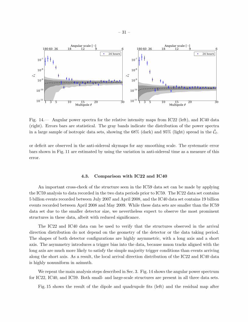
Fig. 14.— Angular power spectra for the relative intensity maps from IC22 (left), and IC40 data

(right). Errors bars are statistical. The gray bands indicate the distribution of the power spectra

in a large sample of isotropic data sets, showing the 68% (dark) and 95% (light) spread in the Cℓ.

or deficit are observed in the anti-sidereal skymaps for any smoothing scale. The systematic error

bars shown in Fig. 11 are estimated by using the variation in anti-sidereal time as a measure of this

error.

4.3. Comparison with IC22 and IC40

An important cross-check of the structure seen in the IC59 data set can be made by applying

the IC59 analysis to data recorded in the two data periods prior to IC59. The IC22 data set contains

5 billion events recorded between July 2007 and April 2008, and the IC40 data set contains 19 billion

events recorded between April 2008 and May 2009. While these data sets are smaller than the IC59

data set due to the smaller detector size, we nevertheless expect to observe the most prominent

structures in these data, albeit with reduced significance.

The IC22 and IC40 data can be used to verify that the structures observed in the arrival

direction distribution do not depend on the geometry of the detector or the data taking period.

The shapes of both detector configurations are highly asymmetric, with a long axis and a short

axis. The asymmetry introduces a trigger bias into the data, because muon tracks aligned with the

long axis are much more likely to satisfy the simple majority trigger conditions than events arriving

along the short axis. As a result, the local arrival direction distribution of the IC22 and IC40 data

is highly nonuniform in azimuth.

We repeat the main analysis steps described in Sec. 3. Fig. 14 shows the angular power spectrum

for IC22, IC40, and IC59. Both small- and large-scale structures are present in all three data sets.

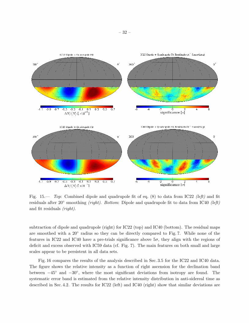
Fig. 15 shows the result of the dipole and quadrupole fits (left) and the residual map after

– 32 –

Fig. 15.— Top: Combined dipole and quadrupole fit of eq. (8) to data from IC22 (left) and fit

residuals after 20 smoothing (right). Bottom: Dipole and quadrupole fit to data from IC40 (left)

and fit residuals (right).

subtraction of dipole and quadrupole (right) for IC22 (top) and IC40 (bottom). The residual maps

are smoothed with a 20 radius so they can be directly compared to Fig. 7. While none of the

features in IC22 and IC40 have a pre-trials significance above 5σ, they align with the regions of

deficit and excess observed with IC59 data (cf. Fig. 7). The main features on both small and large

scales appear to be persistent in all data sets.

Fig. 16 compares the results of the analysis described in Sec. 3.5 for the IC22 and IC40 data.

The figure shows the relative intensity as a function of right ascension for the declination band

between −45 and −30, where the most significant deviations from isotropy are found. The

systematic error band is estimated from the relative intensity distribution in anti-sidereal time as

described in Sec. 4.2. The results for IC22 (left) and IC40 (right) show that similar deviations are

– 33 –

050100150200250300350Right Ascension [ 0 ]

10.0010

10.0005

0.0000

0.0005

0.0010

2

N/3

N

4

IC22 Relative Intensity

5t=24 hours

5t=4 hours

050100150200250300350Right Ascension [ 6 ]

70.0010

70.0005

0.0000

0.0005

0.0010

8

N/9

N

:

IC40 Relative Intensity

;t=24 hours

;t=4 hours

Fig. 16.— Relative intensity in the declination band between −45 and −30 for ∆t = 4 hours for

data from IC22 (left) and IC40 (right). Statistical and systematic uncertainties are shown, with

systematics calculated from the relative intensity distribution in anti-sidereal coordinates.

present in the IC22, IC40, and IC59 data, again with increasing significance due to the increasing

size of the data sets.

The stability of the results over several years of data taking and three different detector con-

figurations indicates that the anisotropy is not produced by the geometry of the detector. Since

the temporal distribution of detector livetime is also different for all three data sets, the stability of

the results indicates that the anisotropy is not affected by nonuniformities in the detector livetime.

As expected, the time scrambling method accounts for this effect.

5. Conclusions

Using 32 billion events recorded with the partially-deployed IceCube detector between May

2009 and May 2010, we have shown that the arrival direction distribution of cosmic rays with a

median energy of 20 TeV exhibits significant anisotropy on all scales up to ℓ = 12 in the angular

power spectrum. The power spectrum is dominated by a dipole and quadrupole moment, but also

indicates the presence of significant structure on angular scales down to about 15. These struc-

tures become visible in the skymap when the dominant dipole and quadrupole moments are either

subtracted or suppressed. The residual skymap shows both significant excesses and deficits, with

the most important excess reaching a post-trial significance of 5.3σ in IC59. The relative intensity

of the smaller-scale structures are about a factor of 5 weaker than the dipole and quadrupole struc-

ture. A study of data taken with the smaller IC22 and IC40 detectors in previous years confirms

that these deviations from an isotropic flux are consistently present in all data sets.

– 34 –

Fig. 17.— Combined map of significances in the cosmic ray arrival direction distribution observed

by Milagro in the northern hemisphere (Abdo et al. 2008) and IceCube in the southern hemisphere

(this analysis). Both maps have been smoothed with a 10 radius.

Together with data from the γ-ray experiments in the northern hemisphere, we now have an

almost complete cosmic ray map of the entire sky at TeV energies. Fig. 17 shows the combined

IceCube and Milagro skymaps of small-scale anisotropy. For this map, all available IceCube data

(IC22, IC40, and IC59) have been used, with a total of 5.6 × 1010 events, and the analysis is

performed using the method described in Sec. 3.5 with a smoothing radius of 10 to match the

Milagro analysis. The combined skymap shows significant excess regions in both hemispheres. It

is possible that the structure around right ascension 120 spans both hemispheres, as the drop

in significances around declination δ = 0 could be an artifact of the smaller exposure of both

detectors near δ = 0, which corresponds to a region close to the horizon for both detectors.

There is currently no explanation for these local enhancements in the cosmic ray flux. We

note that the two most significant excess regions in the southern sky (regions 1 and 2 in Tab. 2)

are both located near the Galactic plane. In addition, the position of one of the excess regions

(region 1) coincides with the location of the Vela pulsar at (α = 128.8, δ = −45.2). At a distance

of about 300 pc (Caraveo et al. 2001), Vela is one of the closest known supernova remnants, and

– 35 –

has long been considered a candidate source for Galactic cosmic ray acceleration. However, the

Larmor radius of 10 TeV protons in a µG magnetic field is approximately 0.01 pc, many orders of

magnitude smaller than the distance to Vela, and unless unconventional propagation mechanisms

are assumed, charged particles from Vela will have lost all directional information upon their arrival

at Earth.

Recently, several authors have investigated the extent to which the stochastic nature of nearby

supernova remnants can lead to spatial and temporal variations in the cosmic ray flux (Ptuskin et al.

2006; Blasi & Amato 2011). The random nature of the sources makes quantitative predictions

difficult, and can lead to bumps and dips in the amplitude of the anisotropy as a function of

energy that depend on the specific source distribution used in the simulation of the cosmic ray flux.

Qualitatively, the models make specific predictions for the energy dependence of the amplitude of

the cosmic ray anisotropy.

In the TeV-PeV range, the energy resolution of IceCube is poor for cosmic ray events (see

Sec. 2.1). However, given the large rate of cosmic ray triggers, it is possible to isolate a sufficiently

large subset of showers with a median energy of several hundred TeV which is not significantly

contaminated by low energy events. A paper focusing on this study is currently in preparation.

The study of cosmic ray arrival directions at TeV energies will continue to be a major ongoing

research effort in IceCube. IceCube and the future High Altitude Water Cherenkov (HAWC) γ-ray

observatory (Sinnis et al. 2004) under construction in Mexico can be used to monitor the southern

and northern hemisphere, respectively, with high sensitivity. The combined data sets will soon

allow for all-sky power spectra and the analysis of the entire sky at all angular scales.

Over the next few years, with the IceCube detector now operating in its complete 86-string

configuration, our data set will increase at a rate of about 45 × 109 muon events per year. With

this level of statistics we will also be able to study possible time dependencies of the anisotropy in

the southern hemisphere and compare to similar studies performed with data from instruments in

the northern hemisphere (Abdo et al. 2009; Amenomori et al. 2010).

6. Acknowledgments

We would like to thank Eric Hivon for helpful comments and suggestions about the angular

power spectrum analysis, and the Milagro Collaboration for providing us with their data to produce

the combined skymap in Fig. 17.

Some of the results in this paper have been derived using the HEALPix (Gorski et al. 2005)

and the PolSpice (Szapudi et al. 2001; Chon et al. 2004) software libraries.

We acknowledge the support from the following agencies: U.S. National Science Foundation-

Office of Polar Programs, U.S. National Science Foundation-Physics Division, University of Wiscon-

sin Alumni Research Foundation, the Grid Laboratory Of Wisconsin (GLOW) grid infrastructure

– 36 –

at the University of Wisconsin - Madison, the Open Science Grid (OSG) grid infrastructure; U.S.

Department of Energy, and National Energy Research Scientific Computing Center, the Louisiana

Optical Network Initiative (LONI) grid computing resources; National Science and Engineering Re-

search Council of Canada; Swedish Research Council, Swedish Polar Research Secretariat, Swedish

National Infrastructure for Computing (SNIC), and Knut and Alice Wallenberg Foundation, Swe-

den; German Ministry for Education and Research (BMBF), Deutsche Forschungsgemeinschaft

(DFG), Research Department of Plasmas with Complex Interactions (Bochum), Germany; Fund

for Scientific Research (FNRS-FWO), FWO Odysseus programme, Flanders Institute to encour-

age scientific and technological research in industry (IWT), Belgian Federal Science Policy Office

(Belspo); University of Oxford, United Kingdom; Marsden Fund, New Zealand; Japan Society for

Promotion of Science (JSPS); the Swiss National Science Foundation (SNSF), Switzerland; A. Groß

acknowledges support by the EU Marie Curie OIF Program; J. P. Rodrigues acknowledges support

by the Capes Foundation, Ministry of Education of Brazil.

REFERENCES

Abbasi, R., et al. 2009a, Astrophys. J., 701, L47

—. 2009b, Nucl. Instrum. Meth., A601, 294

—. 2010a, Nucl. Instrum. Meth., A618, 139

—. 2010b, Astrophys. J., 718, L194

Abdo, A. A., et al. 2008, Phys. Rev. Lett., 101, 221101

—. 2009, Astrophys. J., 698, 2121

Achterberg, A., et al. 2006, Astropart. Phys., 26, 155

Aglietta, M., et al. 2009, Astrophys. J. Lett., 692, L130

Ahn, E.-J., et al. 2009, Phys. Rev., D80, 094003

Ahrens, J., et al. 2004, Nucl. Instrum. Meth., A524, 169

Alexandreas, D. E., et al. 1993, Nucl. Instrum. Meth., A328, 570

Amenomori, M., et al. 2004, Phys. Rev. Lett., 93, 061101

—. 2005, Astrophys. J., 626, L29

—. 2006, Science, 314, 439

—. 2008, Astrophys. J., 672, L53

– 37 –

—. 2010, Astrophys. J., 711, 119

Ansari, R., & Magneville, C. 2010, Mon. Not. Roy. Astron. Soc., 405, 1421

Biermann, P. L., et al. 2010, Astrophys. J., 725, 184

Blasi, P., & Amato, E. 2011, submitted to JCAP, arXiv:1105.4529v1

Caraveo, P., et al. 2001, Astrophys. J., 561, 930

Chon, G., et al. 2004, Mon. Not. Roy. Astron. Soc., 350, 914

Compton, A. H., & Getting, I. A. 1935, Phys. Rev., 47, 817

Drury, L., & Aharonian, F. 2008, Astropart. Phys., 29, 420

Gleeson, L., & Axford, W. 1968, Astrophysics and Space Science, 2, 431, 10.1007/BF02175919

Gorski, K. M., et al. 2005, Astrophys. J., 622, 759

Guillian, G., et al. 2007, Phys. Rev. D, 75, 062003

Heck, D., et al. 1998, Forschungszentrum Karlsruhe Report FZKA 6019

Horandel, J. R. 2003, Astropart. Phys., 19, 193

Lazarian, A., & Desiati, P. 2010, Astrophys. J., 722, 188

Li, T.-P., & Ma, Y.-Q. 1983, Astrophys. J., 272, 317

Malkov, M. A., et al. 2010, Astrophys. J., 721, 750

Ptuskin, V., Jones, F., Seo, E., & Sina, R. 2006, Advances in Space Research, 37, 1909

Sinnis, G., Smith, A., & McEnery, J. E. 2004, in Tenth Marcel Grossman Meeting, Rio de Janeiro,

Brazil, 1068–1088

Smoot, G. F., & Lubin, P. M. 1979, Astrophys. J., 234, L83

Szapudi, I., Prunet, S., Pogosyan, D., Szalay, A. S., & Bond, J. R. 2001, Astrophys. J., 548, L115

Tilav, S., et al. 2009, in Proc. 31st ICRC, Lodz, Poland

Vernetto, S., et al. 2009, in Proc. 31st ICRC, Lodz, Poland

This preprint was prepared with the AAS LATEX macros v5.2.