IceCube Preliminary Design DocumentOctober 11, 2001/ Revision: 1.24The IceCube Collaboration

Simulated interactions of a 10 TeV �� (top left), 375 TeV �e (top right),

and 1 PeV �� (bottom) in IceCube.

1

The IceCube Collaboration

J. Ahrens12, J.R. Alonso8, J.N. Bahcall6, X. Bai1, T. Becka12, K.-H. Becker2, D. Berley13, D. Bertrand3,

D.Z. Besson, A. Biron5, B. Bless16, S. B�oser5, C. Bohm21, O. Botner20, A. Bouchta5;23, S. Carius7,

J. Cavin18, A. Chen17, W. Chinowsky8, D. Chirkin10;2, J. Conrad20, J. Cooley17, C.G.S. Costa3, D.F. Cowen15,

C. De Clercq22, T. DeYoung17, P. Desiati5, J.-P. Dewulf3, B. Dingus17, P. Doksus17, P.A. Evenson1,

A.R. Fazely9, T. Feser12, J.-M. Fr�ere3, T.K. Gaisser1, J. Gallagher16, M. Gaug5, A. Goldschmidt8, A. Hallgren20,

F. Halzen17, K. Hanson15, R. Hardtke17, T. Hauschildt5, M. Hellwig12, P. Herquet14, G.C. Hill17, P.O. Hulth21,

K. Hultqvist21, S. Hundertmark11, J. Jacobsen8, G.S. Japaridze4, A. Karle17, R. Koch18, L. K�opke12,

M. Kowalski5, J.I. Lamoureux8, H. Leich5, M. Leuthold5, P. Lindahl7, J. Madsen19, P. Marciniewski20,

H.S. Matis8, C.P. McParland8, P. Mio�cinovi�c10, R. Morse17, T. Neunh�o�er12, P. Niessen5;22, D.R. Nygren8,

H. Ogelman17, Ph. Olbrechts22, R. Paulos17, C. P�erez de los Heros20, P.B. Price10, G.T. Przybylski8, K. Rawlins17,

W. Rhode2, M. Ribordy5, S. Richter17, H.-G. Sander12, T. Schmidt5, D. Schneider17, D. Seckel1, M. Solarz10,

L. Sparke16, G.M. Spiczak1, C. Spiering5, T. Stanev1, D. Steele17, P. Ste�en5, R.G. Stokstad8, O. Streicher5,

P. Sudho�5, K.-H. Sulanke5, I. Taboada15, C. Walck21, C. Weinheimer12, C.H. Wiebusch5;23, R. Wischnewski5,

H. Wissing5, K. Woschnagg10

(1) Bartol Research Institute, University of Delaware, Newark, DE 19716, USA

(2) Fachbereich 8 Physik, BUGH Wuppertal, D-42097 Wuppertal, Germany

(3) Universit�e Libre de Bruxelles, Science Faculty CP230, Boulevard du Triomphe, B-1050 Brussels, Belgium

(4) CTSPS, Clark-Atlanta University, Atlanta, GA 30314, USA

(5) DESY-Zeuthen, D-15735 Zeuthen, Germany

(6) Institute for Advanced Study, Princeton, NJ 08540, USA

(7) Dept. of Technology, Kalmar University, S-39182 Kalmar, Sweden

(8) Lawrence Berkeley National Laboratory, Berkeley, CA 94720, USA

(9) Department of Physics, Southern University and A&M College, Baton Rouge, LA 70813, USA

(10) Dept. of Physics, University of California, Berkeley, CA 94720, USA

(11) Dept. of Physics and Astronomy, University of California, Irvine, CA 92697, USA

(12) Institute of Physics, University of Mainz, Staudinger Weg 7, D-55099 Mainz, Germany

(13) Dept. of Physics, University of Maryland, College Park, MD 20742, USA

(14) University of Mons-Hainaut, 7000 Mons, Belgium

(15) Dept. of Physics and Astronomy, University of Pennsylvania, Philadelphia, PA 19104, USA

(16) Dept. of Astronomy, University of Wisconsin, Madison, WI 53706, USA

(17) Dept. of Physics, University of Wisconsin, Madison, WI 53706, USA

(18) SSEC, University of Wisconsin, Madison, WI 53706, USA

(19) Physics Department, University of Wisconsin, River Falls, WI 54022, USA

(20) Division of High Energy Physics, Uppsala University, S-75121 Uppsala, Sweden

(21) Fysikum, Stockholm University, S-11385 Stockholm, Sweden

(22) Vrije Universiteit Brussel, Dienst ELEM, B-1050 Brussel, Belgium

(23) Present address: CERN, CH-1211, Gen�eve 23, Switzerland

2

Contents

1 Document Overview 9

2 Executive Summary 10

3 Science Motivation for Kilometer-Scale Detectors 12

3.1 High-Energy Neutrinos Associated with Cosmic Particle Accelerators . . . . . . . 13

3.1.1 Energy Considerations . . . . . . . . . . . . . . . . . . . . . . . . . . . . . 14

3.1.2 Estimates Based on Models . . . . . . . . . . . . . . . . . . . . . . . . . . 17

3.1.3 Neutrinos as a Diagnostic of TeV Gamma-Ray Sources . . . . . . . . . . . 17

3.2 Other Science Opportunities . . . . . . . . . . . . . . . . . . . . . . . . . . . . . . 18

3.2.1 WIMPs and Other Sources of Sub-TeV �� . . . . . . . . . . . . . . . . . . 18

3.2.2 Atmospheric Neutrinos . . . . . . . . . . . . . . . . . . . . . . . . . . . . . 20

3.2.3 PeV and EeV Neutrinos . . . . . . . . . . . . . . . . . . . . . . . . . . . . 20

3.2.4 Tau Neutrino Detection . . . . . . . . . . . . . . . . . . . . . . . . . . . . 21

3.2.5 Neutrinos from Supernovae . . . . . . . . . . . . . . . . . . . . . . . . . . 23

3.3 Summary . . . . . . . . . . . . . . . . . . . . . . . . . . . . . . . . . . . . . . . . 24

4 Status of High Energy Neutrino Astronomy 26

4.1 Status of AMANDA . . . . . . . . . . . . . . . . . . . . . . . . . . . . . . . . . . 29

4.1.1 Atmospheric Neutrinos . . . . . . . . . . . . . . . . . . . . . . . . . . . . . 29

4.1.2 Pointing Resolution . . . . . . . . . . . . . . . . . . . . . . . . . . . . . . 32

4.1.3 Search for a di�use high energy neutrino ux . . . . . . . . . . . . . . . . 33

4.1.4 Point Sources . . . . . . . . . . . . . . . . . . . . . . . . . . . . . . . . . . 33

4.1.5 Gamma-Ray Bursts . . . . . . . . . . . . . . . . . . . . . . . . . . . . . . 36

4.1.6 WIMPs . . . . . . . . . . . . . . . . . . . . . . . . . . . . . . . . . . . . . 37

4.1.7 Supernovae . . . . . . . . . . . . . . . . . . . . . . . . . . . . . . . . . . . 38

4.1.8 Magnetic Monopoles . . . . . . . . . . . . . . . . . . . . . . . . . . . . . . 38

4.1.9 Summary of AMANDA Status . . . . . . . . . . . . . . . . . . . . . . . . 39

5 Expected IceCube Performance 40

5.1 Introduction . . . . . . . . . . . . . . . . . . . . . . . . . . . . . . . . . . . . . . . 40

5.2 Atmospheric Neutrinos . . . . . . . . . . . . . . . . . . . . . . . . . . . . . . . . . 40

5.3 Muon-Neutrino-Induced Muons . . . . . . . . . . . . . . . . . . . . . . . . . . . . 40

5.3.1 Simulation . . . . . . . . . . . . . . . . . . . . . . . . . . . . . . . . . . . 40

5.3.2 Reconstruction and Background Rejection . . . . . . . . . . . . . . . . . . 42

5.3.3 Sensitivity to Di�use Sources of Muon Neutrinos . . . . . . . . . . . . . . 47

5.3.4 Sensitivity to Muon Neutrino Point Sources . . . . . . . . . . . . . . . . . 49

5.3.5 Sensitivity to Muon Neutrinos from Gamma-Ray Bursts . . . . . . . . . . 49

5.3.6 Possible Improvements . . . . . . . . . . . . . . . . . . . . . . . . . . . . . 54

5.4 Electromagnetic and Hadronic Cascades . . . . . . . . . . . . . . . . . . . . . . . 56

5.4.1 Simulation . . . . . . . . . . . . . . . . . . . . . . . . . . . . . . . . . . . 56

3

5.4.2 Reconstruction . . . . . . . . . . . . . . . . . . . . . . . . . . . . . . . . . 58

5.4.3 E�ective Volume . . . . . . . . . . . . . . . . . . . . . . . . . . . . . . . . 61

5.4.4 Sensitivity to Atmospheric � . . . . . . . . . . . . . . . . . . . . . . . . . 63

5.4.5 Sensitivity to Point Sources . . . . . . . . . . . . . . . . . . . . . . . . . . 64

5.4.6 Sensitivity to Di�use �e Sources . . . . . . . . . . . . . . . . . . . . . . . 64

5.4.7 Sensitivity to GRBs . . . . . . . . . . . . . . . . . . . . . . . . . . . . . . 64

5.4.8 Possible Improvements . . . . . . . . . . . . . . . . . . . . . . . . . . . . . 68

5.5 Tau Neutrinos . . . . . . . . . . . . . . . . . . . . . . . . . . . . . . . . . . . . . . 68

5.5.1 Tau Neutrino Event Rates . . . . . . . . . . . . . . . . . . . . . . . . . . . 71

5.5.2 Tau Neutrino Simulations . . . . . . . . . . . . . . . . . . . . . . . . . . . 71

5.6 Neutrino Flavor Di�erentiation with Waveform Digitization . . . . . . . . . . . . 71

5.6.1 Photon Flux Distribution Generated by High Energy Cascades . . . . . . 73

5.6.2 �� Event Signatures . . . . . . . . . . . . . . . . . . . . . . . . . . . . . . 79

5.6.3 Summary . . . . . . . . . . . . . . . . . . . . . . . . . . . . . . . . . . . . 79

5.7 Lower Energy Phenomena and Exotica . . . . . . . . . . . . . . . . . . . . . . . . 87

5.7.1 Muon Neutrinos from WIMP annihilation . . . . . . . . . . . . . . . . . . 87

5.7.2 Neutrino oscillations . . . . . . . . . . . . . . . . . . . . . . . . . . . . . . 90

5.7.3 MeV Neutrinos from Supernovae . . . . . . . . . . . . . . . . . . . . . . . 90

5.7.4 Relativistic magnetic monopoles . . . . . . . . . . . . . . . . . . . . . . . 92

5.7.5 Slowly moving, bright particles . . . . . . . . . . . . . . . . . . . . . . . . 95

5.8 IceCube Con�guration Flexibility . . . . . . . . . . . . . . . . . . . . . . . . . . . 96

5.9 Calibration of High-Level Detector Response Variables . . . . . . . . . . . . . . . 96

5.9.1 Geometry Calibration . . . . . . . . . . . . . . . . . . . . . . . . . . . . . 96

5.9.2 Calibration of Angular Response . . . . . . . . . . . . . . . . . . . . . . . 99

5.9.3 Calibration of Vertex Resolution . . . . . . . . . . . . . . . . . . . . . . . 99

5.9.4 Energy Calibration . . . . . . . . . . . . . . . . . . . . . . . . . . . . . . . 99

5.10 IceTop . . . . . . . . . . . . . . . . . . . . . . . . . . . . . . . . . . . . . . . . . . 100

5.10.1 Tagged Muon Bundles . . . . . . . . . . . . . . . . . . . . . . . . . . . . . 100

5.10.2 IceTop as a Veto . . . . . . . . . . . . . . . . . . . . . . . . . . . . . . . . 100

5.10.3 Cosmic-ray Physics . . . . . . . . . . . . . . . . . . . . . . . . . . . . . . . 103

6 Experimental Requirements 104

6.1 Time Resolution . . . . . . . . . . . . . . . . . . . . . . . . . . . . . . . . . . . . 104

6.2 Waveforms . . . . . . . . . . . . . . . . . . . . . . . . . . . . . . . . . . . . . . . 105

6.3 Dynamic Range and Linearity . . . . . . . . . . . . . . . . . . . . . . . . . . . . . 105

6.4 Absolute Amplitude Calibration and Stability . . . . . . . . . . . . . . . . . . . . 107

6.5 Dead time . . . . . . . . . . . . . . . . . . . . . . . . . . . . . . . . . . . . . . . . 107

6.6 Sensitivity of optical modules . . . . . . . . . . . . . . . . . . . . . . . . . . . . . 107

6.7 Noise Rate and Noise Rate Stability . . . . . . . . . . . . . . . . . . . . . . . . . 107

6.8 Failure Rate . . . . . . . . . . . . . . . . . . . . . . . . . . . . . . . . . . . . . . . 108

6.9 IceTop . . . . . . . . . . . . . . . . . . . . . . . . . . . . . . . . . . . . . . . . . . 108

4

7 Design and Description of IceCube 110

7.1 Overview . . . . . . . . . . . . . . . . . . . . . . . . . . . . . . . . . . . . . . . . 110

7.2 Digital Optical Module . . . . . . . . . . . . . . . . . . . . . . . . . . . . . . . . . 115

7.2.1 Pressure Housing . . . . . . . . . . . . . . . . . . . . . . . . . . . . . . . . 118

7.2.2 Optical Sensor . . . . . . . . . . . . . . . . . . . . . . . . . . . . . . . . . 118

7.2.3 PMT HV Generator . . . . . . . . . . . . . . . . . . . . . . . . . . . . . . 121

7.2.4 Optical Beacon . . . . . . . . . . . . . . . . . . . . . . . . . . . . . . . . . 121

7.2.5 Signal Processing Circuitry . . . . . . . . . . . . . . . . . . . . . . . . . . 122

7.2.6 Local/Global Time Transformation . . . . . . . . . . . . . . . . . . . . . . 128

7.2.7 Cable Electrical Length Measurement . . . . . . . . . . . . . . . . . . . . 136

7.2.8 Data Flow and Feature Extraction . . . . . . . . . . . . . . . . . . . . . . 136

7.2.9 Local Coincidence . . . . . . . . . . . . . . . . . . . . . . . . . . . . . . . 138

7.2.10 System Design Aspects . . . . . . . . . . . . . . . . . . . . . . . . . . . . 140

7.3 Network . . . . . . . . . . . . . . . . . . . . . . . . . . . . . . . . . . . . . . . . . 141

7.3.1 Copper Links . . . . . . . . . . . . . . . . . . . . . . . . . . . . . . . . . . 141

7.3.2 Time-Base Distribution . . . . . . . . . . . . . . . . . . . . . . . . . . . . 142

7.4 Surface DAQ . . . . . . . . . . . . . . . . . . . . . . . . . . . . . . . . . . . . . . 143

7.4.1 Overview . . . . . . . . . . . . . . . . . . . . . . . . . . . . . . . . . . . . 143

7.4.2 DOM Hub . . . . . . . . . . . . . . . . . . . . . . . . . . . . . . . . . . . . 145

7.4.3 String Processor . . . . . . . . . . . . . . . . . . . . . . . . . . . . . . . . 146

7.4.4 IceCube and IceTop System Integration . . . . . . . . . . . . . . . . . . . 147

7.4.5 Experiment and Con�guration Control . . . . . . . . . . . . . . . . . . . . 148

7.4.6 Security Environment . . . . . . . . . . . . . . . . . . . . . . . . . . . . . 151

7.4.7 DAQ Components . . . . . . . . . . . . . . . . . . . . . . . . . . . . . . . 152

7.4.8 Calibration Operations . . . . . . . . . . . . . . . . . . . . . . . . . . . . . 155

7.4.9 DAQ and Online Monitoring . . . . . . . . . . . . . . . . . . . . . . . . . 156

7.4.10 DAQ Computing Environment . . . . . . . . . . . . . . . . . . . . . . . . 157

7.5 AMANDA Data Transmission Techniques . . . . . . . . . . . . . . . . . . . . . . 159

8 Data Handling 163

8.1 System Elements . . . . . . . . . . . . . . . . . . . . . . . . . . . . . . . . . . . . 163

8.1.1 Software Management . . . . . . . . . . . . . . . . . . . . . . . . . . . . . 164

8.1.2 System Engineering . . . . . . . . . . . . . . . . . . . . . . . . . . . . . . 164

8.1.3 Development Environment . . . . . . . . . . . . . . . . . . . . . . . . . . 165

8.1.4 Analysis Framework . . . . . . . . . . . . . . . . . . . . . . . . . . . . . . 165

8.1.5 Database . . . . . . . . . . . . . . . . . . . . . . . . . . . . . . . . . . . . 165

8.1.6 Visualization . . . . . . . . . . . . . . . . . . . . . . . . . . . . . . . . . . 167

8.1.7 Development Interfaces . . . . . . . . . . . . . . . . . . . . . . . . . . . . 167

8.1.8 Integration at Pole . . . . . . . . . . . . . . . . . . . . . . . . . . . . . . . 168

8.1.9 Hardware . . . . . . . . . . . . . . . . . . . . . . . . . . . . . . . . . . . . 168

8.1.10 Data Distribution . . . . . . . . . . . . . . . . . . . . . . . . . . . . . . . 170

8.2 O�ine Data Flow . . . . . . . . . . . . . . . . . . . . . . . . . . . . . . . . . . . . 171

5

8.3 Data Model . . . . . . . . . . . . . . . . . . . . . . . . . . . . . . . . . . . . . . . 174

8.3.1 High Multiplicity . . . . . . . . . . . . . . . . . . . . . . . . . . . . . . . . 174

8.3.2 Upgoing Tracks . . . . . . . . . . . . . . . . . . . . . . . . . . . . . . . . . 175

8.3.3 Cascades/Taus . . . . . . . . . . . . . . . . . . . . . . . . . . . . . . . . . 175

8.3.4 GRB Downgoing Muons . . . . . . . . . . . . . . . . . . . . . . . . . . . . 176

8.3.5 Icetop . . . . . . . . . . . . . . . . . . . . . . . . . . . . . . . . . . . . . . 176

8.3.6 Supernova . . . . . . . . . . . . . . . . . . . . . . . . . . . . . . . . . . . . 176

8.3.7 Prescaled Raw Data . . . . . . . . . . . . . . . . . . . . . . . . . . . . . . 176

8.3.8 Monitor . . . . . . . . . . . . . . . . . . . . . . . . . . . . . . . . . . . . . 176

8.3.9 Calibration . . . . . . . . . . . . . . . . . . . . . . . . . . . . . . . . . . . 177

8.3.10 Full-Sky Summary Histograms . . . . . . . . . . . . . . . . . . . . . . . . 177

8.3.11 Un�ltered Raw . . . . . . . . . . . . . . . . . . . . . . . . . . . . . . . . . 177

8.4 Data Sample Organization . . . . . . . . . . . . . . . . . . . . . . . . . . . . . . . 177

8.5 Latency . . . . . . . . . . . . . . . . . . . . . . . . . . . . . . . . . . . . . . . . . 178

8.6 Schedule . . . . . . . . . . . . . . . . . . . . . . . . . . . . . . . . . . . . . . . . . 179

8.7 Summary . . . . . . . . . . . . . . . . . . . . . . . . . . . . . . . . . . . . . . . . 179

9 Data Analysis 180

9.1 Introduction . . . . . . . . . . . . . . . . . . . . . . . . . . . . . . . . . . . . . . . 180

9.2 Analysis Infrastructure . . . . . . . . . . . . . . . . . . . . . . . . . . . . . . . . . 180

9.2.1 Calibration Analysis and Data Quality Working Group . . . . . . . . . . 180

9.2.2 Simulation Working Group . . . . . . . . . . . . . . . . . . . . . . . . . . 181

9.2.3 Reconstruction Working Group . . . . . . . . . . . . . . . . . . . . . . . . 181

9.3 Computing Infrastructure . . . . . . . . . . . . . . . . . . . . . . . . . . . . . . . 181

9.4 Physics Analysis . . . . . . . . . . . . . . . . . . . . . . . . . . . . . . . . . . . . 182

9.5 Internal Review Procedure . . . . . . . . . . . . . . . . . . . . . . . . . . . . . . . 183

9.5.1 Introduction . . . . . . . . . . . . . . . . . . . . . . . . . . . . . . . . . . 183

9.5.2 Procedure . . . . . . . . . . . . . . . . . . . . . . . . . . . . . . . . . . . . 183

9.6 Prerequisites and Schedule . . . . . . . . . . . . . . . . . . . . . . . . . . . . . . . 184

10 Drilling, Deployment and Logistics 185

10.1 Drilling . . . . . . . . . . . . . . . . . . . . . . . . . . . . . . . . . . . . . . . . . 185

10.1.1 Introduction . . . . . . . . . . . . . . . . . . . . . . . . . . . . . . . . . . 185

10.1.2 Evolution of AMANDA Drills . . . . . . . . . . . . . . . . . . . . . . . . . 186

10.1.3 Performance Criteria and Design of the EHWD . . . . . . . . . . . . . . . 186

10.2 Deployment . . . . . . . . . . . . . . . . . . . . . . . . . . . . . . . . . . . . . . . 190

10.2.1 Overview . . . . . . . . . . . . . . . . . . . . . . . . . . . . . . . . . . . . 190

10.2.2 AMANDA Experience . . . . . . . . . . . . . . . . . . . . . . . . . . . . . 190

10.2.3 AMANDA Deployment . . . . . . . . . . . . . . . . . . . . . . . . . . . . 192

10.2.4 IceCube Deployment Overview . . . . . . . . . . . . . . . . . . . . . . . . 196

10.2.5 IceCube String Deployment Procedure . . . . . . . . . . . . . . . . . . . . 196

10.2.6 IceCube Indoor Deployment . . . . . . . . . . . . . . . . . . . . . . . . . . 201

6

10.2.7 IceCube Drill Hole Requirements . . . . . . . . . . . . . . . . . . . . . . . 208

10.2.8 Quality Assurance . . . . . . . . . . . . . . . . . . . . . . . . . . . . . . . 209

10.2.9 Practice Deployments . . . . . . . . . . . . . . . . . . . . . . . . . . . . . 211

10.2.10Surface Cable Installation . . . . . . . . . . . . . . . . . . . . . . . . . . . 212

10.3 Logistics . . . . . . . . . . . . . . . . . . . . . . . . . . . . . . . . . . . . . . . . . 214

10.3.1 Introduction . . . . . . . . . . . . . . . . . . . . . . . . . . . . . . . . . . 214

10.3.2 Documentation . . . . . . . . . . . . . . . . . . . . . . . . . . . . . . . . . 214

10.3.3 Personnel and Taskings . . . . . . . . . . . . . . . . . . . . . . . . . . . . 215

10.3.4 Medical/Dental Examinations . . . . . . . . . . . . . . . . . . . . . . . . . 217

10.3.5 Airline Travel . . . . . . . . . . . . . . . . . . . . . . . . . . . . . . . . . . 217

10.3.6 Weights and Cubes . . . . . . . . . . . . . . . . . . . . . . . . . . . . . . . 217

10.3.7 Cargo Transport . . . . . . . . . . . . . . . . . . . . . . . . . . . . . . . . 218

11 Quality Assurance 221

12 Relationship of AMANDA and IceCube 224

7

Contacts/Authors of this Document

Section 1: D. Cowen (Penn)Section 2: T. Gaisser (Bartol), F. Halzen (UW-Madison)Section 3: T. Gaisser (Bartol), F. Halzen (UW-Madison)Section 4: T. Gaisser (Bartol)Section 5: D. Cowen (Penn), K. Hanson (Penn),

G. Hill (UW-Madison), A. Karle (UW-Madison)Section 6: C. Spiering (DESY)Section 7: J. Jacobsen (LBNL), A. Karle (UW-Madison),

C. McParland (LBNL), D. Nygren (LBNL)Section 8: D. Cowen (Penn), P. Herquet (Mons), J. Lamoureux (LBNL),

C. McParland (LBNL), D. Schneider (UW-Madison)Section 9: P.O. Hulth (Stockholm)Section 10: A. Karle (UW-Madison), B. Morse (UW-Madison)Section 11: E. Richards (UW-Madison)Section 12: P.O. Hulth (Stockholm)

8

1 Document Overview

This document describes a conceptual design for the proposed IceCube Neutrino Observatory

at the South Pole. An Executive Summary is provided in section 2. Section 3 gives the scienti�c

motivation for constructing a kilometer-scale device optimized for detection of cosmological

neutrinos with ultrahigh energies in the TeV to PeV range. Section 4 brie y reviews the current

status of the �eld of neutrino astronomy, and section 5 details the expected performance of the

IceCube neutrino telescope, with emphasis on the scienti�c goals outlined in section 3.

Most of the remainder of the document focuses on technical aspects of the IceCube detector.

Section 6 lists the technical requirements the IceCube detector must meet in order to attain the

desired scienti�c goals, and section 7 gives a complete conceptual description of the IceCube

detector itself. Section 8 describes how the data produced by this detector will be processed and

made available for high-level analysis, and section 9 shows how the collaboration will organize

itself to perform these analyses.

An explanation of how drilling, deployment and the associated logistics will be handled is

given in section 10. Section 11 describes what quality assurance procedures will be implemented

to ensure initial and continued success in deployment, data acquisition and data processing. Fi-

nally, section 12 shows how the AMANDA and IceCube detectors will be integrated to maximize

the overall science output.

This and other documents are on the Web at http://www.ssec.wisc.edu/a3ri/icecube/.

9

2 Executive Summary

The IceCube Project at the South Pole is a logical extension of the research and development

work performed over the past several years by the AMANDA Collaboration. The optical proper-

ties of ice deep below the Pole have been established, and the detection of high-energy neutrinos

has been demonstrated with the existing detector. This accomplishment represents a proof of

concept for commissioning a new instrument, IceCube, with superior detector performance and

an e�ective telescope size at or above the kilometer-scale.

IceCube scienti�c goals require that the detector have an e�ective area for muons generated

by cosmic neutrinos of one square kilometer. The detector will utilize South Pole ice instru-

mented at depth with optical sensors that detect the Cherenkov light from secondary particles

produced in interactions of high-energy neutrinos inside or near the instrumented volume.

The design for the IceCube neutrino telescope is an array of 4800 photomultiplier tubes

(PMTs) each enclosed in a transparent pressure sphere to comprise an optical module (OM)

similar to those in AMANDA. In the IceCube design, 80 strings are regularly spaced by 125 m

over an area of approximately one square kilometer, with OMs at depths of 1.4 to 2.4 km below

the surface. Each string consists of OMs connected electrically and mechanically to a long cable,

which brings OM signals to the surface. The array is deployed one string at a time. For each

string, a hot-water drill creates a hole in the ice to a depth of about 2.4 km. The drill is then

removed from the hole and a string with 60 OMs spaced by 17 m is deployed before the water

freezes. The signal cables from all the strings are brought to a central location, which houses

the data acquisition electronics, other electronics, and computing equipment.

Each OM contains a PMT that detects individual photons of Cherenkov light generated

in the optically clear ice by muons and electrons moving with velocities near the speed of

light. Signal events consist primarily of upgoing muons produced in neutrino interactions in

the bedrock or the ice. In addition, the detector can discriminate electromagnetic and hadronic

showers (\cascades") from interactions of �e and �� inside the detector volume provided they are

suÆciently energetic (a few 100 TeV or higher). Background events are mainly downward-going

muons from cosmic ray interactions in the atmosphere above the detector. The background is

monitored for calibration purposes by the IceTop air shower array covering the detector.

Signals from the optical modules are digitized and transmitted to the surface such that

a photon's time of arrival at an OM can be determined to within a few nanoseconds. The

electronics at the surface determines when an event has occurred (e.g., that a muon traversed

or passed near the array) and records the information for subsequent event reconstruction and

analysis.

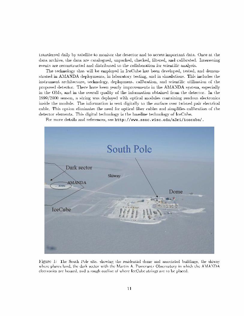
At the South Pole site (see �g. 1), a computer system accepts the data from the event

trigger through the data acquisition system. The event rate, which is dominated by down-going

cosmic ray muons, is estimated to be 1{2 kHz. This will produce a large amount of data and

requires �ltering and compression of this data stream at the South Pole. There are two ways

for the data to be transported to the Northern Hemisphere. The �rst and preferred method is

via satellite transmission. The second method is by hand-carrying the data tapes north once

the station reopens in the austral summer. Even in this case, a reduced set of data must be

10

transferred daily by satellite to monitor the detector and to access important data. Once at the

data archive, the data are catalogued, unpacked, checked, �ltered, and calibrated. Interesting

events are reconstructed and distributed to the collaboration for scienti�c analysis.

The technology that will be employed in IceCube has been developed, tested, and demon-

strated in AMANDA deployments, in laboratory testing, and in simulations. This includes the

instrument architecture, technology, deployment, calibration, and scienti�c utilization of the

proposed detector. There have been yearly improvements in the AMANDA system, especially

in the OMs, and in the overall quality of the information obtained from the detector. In the

1999/2000 season, a string was deployed with optical modules containing readout electronics

inside the module. The information is sent digitally to the surface over twisted-pair electrical

cable. This option eliminates the need for optical �ber cables and simpli�es calibration of the

detector elements. This digital technology is the baseline technology of IceCube.

For more details and references, see http://www.ssec.wisc.edu/a3ri/icecube/.

Figure 1: The South Pole site, showing the residential dome and associated buildings, the skiway

where planes land, the dark sector with the Martin A. Pomerantz Observatory in which the AMANDA

electronics are housed, and a rough outline of where IceCube strings are to be placed.

11

3 Science Motivation for Kilometer-Scale Detectors

The construction of neutrino telescopes is overwhelmingly motivated by their discovery potential

in astronomy, astrophysics, cosmology and particle physics. To maximize this potential, one

must design an instrument with the largest possible e�ective telescope area to overcome the

small neutrino cross section with matter, and the best possible angular and energy resolution

to address the wide diversity of possible signals. A well-designed neutrino telescope can

� search for high energy neutrinos from transient sources like Gamma Ray Bursts (GRB) or

Supernova bursts;

� search for steady and variable sources of high energy neutrinos, e.g. Active Galactic Nuclei

(AGN) or Supernova Remnants (SNR);

� search for the source(s) of the cosmic-rays;

� search for Weakly Interacting Massive Particles (WIMPs) which may constitute dark mat-

ter;

� search for neutrinos from the decay of superheavy particles related to topological defects;

� search for magnetic monopoles and other exotic particles like strange quark matter;

� monitor our Galaxy for MeV neutrinos from supernova explosions and operate within the

worldwide SNEWS triangulation network;

� search for unexpected phenomena.

In practice, the observed uxes of cosmic-rays and gamma rays set the scale of a neutrino

telescope. With minimal model-dependence, one can estimate the very high energy cosmic

neutrino uxes by scaling to the observed energy density in high-energy cosmic-rays, or to the

measured uxes of non-thermal high-energy gamma rays. The basic assumption in calculating

the expected neutrino uxes is that some fraction of cosmic-rays will interact in their sources to

produce neutrinos.

Although they are not yet identi�ed, the sources of the highest energy cosmic radiation very

likely involve extremely dense regions with exceptional gravitational forces such as supermas-

sive black holes, collapse of massive stars or mergers of black holes and neutron stars. With

accretion and intense radiation �elds as ingredients, some fraction of the particles accelerated

in such environments will likely produce pions in hadronic collisions with ambient gas and/or

by photoproduction. In either case, the neutral pions decay to photons, while charged pions

include neutrinos among their decay products with spectra related to the observed gamma-ray

spectra. In the �rst part of this section, we discuss estimates based on this relationship and

conclude that a km-scale detector is needed to observe neutrino signals from known classes of

high energy astrophysical sources.

12

The baseline design of the detector maximizes sensitivity to ��-induced muons from below

with energies in the TeV to PeV range, where the acceptance is enhanced by the increasing

neutrino cross section and muon range but the Earth is still largely transparent to neutrinos.

Good angular resolution is required to distinguish possible point sources from background, while

energy resolution is needed to enhance the signal from astrophysical sources, which are expected

to have atter energy spectra than that of the atmospheric neutrino background.

A standard technique to search for high energy neutrinos of astrophysical origin is to look

for upgoing muons induced by �� that have penetrated the Earth. The signal is given by the

convolution

Signal � AreaR�NA �� �� ; (1)

where R� is the muon range in g/cm2 and NA is Avogadro's number. The range and cross

section both increase linearly with energy into the TeV region, after which the rate of increase

slows. Neutrinos with E� < 100 TeV are not strongly attenuated by the Earth, and much of

the solid angle away from the nadir remains accessible up to 1 PeV [16]. Thus the optimum

range for ��-induced upgoing muons is from a TeV to a PeV. Also in this energy range the muon

energy loss is greater than minimum ionizing, which is a potential way to discriminate against

the background of atmospheric neutrinos, which have a steeply falling spectrum. We will return

to the importance of energy measurement further on.

The generic cosmic accelerator is believed to produce neutrinos in the ux ratio �e : �� : �� ::

1 : 2 : 0. With neutrino oscillations, however, at the detection point this ratio becomes 1 : 1 : 1.

This is especially interesting for neutrino telescopes because the �� is not absorbed in the Earth

like the �e and �� due to the charged current regeneration e�ect (as discussed below). Instead,

�� 's with energies exceeding roughly 1 PeV pass through the Earth and emerge with an energy

of roughly 1 PeV. IceCube is well-suited to detecting neutrinos in this energy range and will

have full 4� sensitivity to this potential signal.

In the second part of this section we discuss several other important scienti�c goals which

depend on the sensitivity of the detector to neutrinos of much higher energies and of much lower

energies. On the one hand, we will discuss detecting and measuring the energy of PeV{EeV �e,

�� and �� interactions. On the other, we will consider the detection of low energy muon-neutrinos

from the annihilation of dark matter particles and the detection of MeV electron-antineutrinos

from galactic supernovae. We describe how the baseline design can address these objectives as

well.

3.1 High-Energy Neutrinos Associated with Cosmic Particle Accelerators

We estimate the range of possible neutrino signals in three ways: �rst on the basis of an energetics

argument, second by referring to some particular models, and third by comparing to known

sources of TeV photons.

13

3.1.1 Energy Considerations

Models for the origin of the highest energy cosmic-rays typically predict associated neutrino

uxes. A requirement on the sources is that they must provide suÆcient power to supply

the observed energy in the galactic or extragalactic component of the cosmic radiation. The

assumption that comparable amounts of energy go into high-energy neutrinos allows an estimate

of the corresponding neutrino signal that is independent of the speci�c nature of the sources,

but which depends only on their distribution in the universe.

In the case of galactic cosmic-rays, the energy ux carried by neutrinos is much lower than

that carried by the parent cosmic-rays because the charged particles are trapped locally as

they propagate di�usively in the turbulent galactic magnetic �elds. Thus an observer inside

the galaxy has several chances to see a given cosmic ray particle, but only one chance to see a

neutrino that passes directly out of the galaxy. Nevertheless, there is a chance that some nearby

galactic sources could be visible in neutrinos in a km-scale detector. Examples will be discussed

in the next section.

In contrast, the neutrino energy ux for a cosmological distribution of sources can be com-

parable to or larger than the observed cosmic-ray energy ux. The ux depends on how the

sources have evolved over cosmological time scales{provided that the fraction of accelerated pro-

tons that interact near the source is large. One natural scenario that gives comparable energy in

neutrinos and cosmic rays occurs when protons remain trapped in the acceleration region until

they su�er inelastic collisions, while secondary neutrons escape and decay to become cosmic-ray

protons. It is generally believed that sources of the ultra-high energy cosmic-rays are indeed

extragalactic, or at least not con�ned to the plane of the galaxy. There is some evidence for

a transition from one particle population to another somewhere above 1018 eV as well as for a

trend from heavy toward lighter composition. Measurements of the cosmic-ray spectrum above

1017 eV are summarized in �g. 2.

We now wish to estimate the neutrino signal expected if the energy in neutrinos is comparable

to the energy in the extra-galactic component of the cosmic radiation. The �rst step is to

determine what fraction of the observed spectrum is the extra-galactic component. It is generally

assumed that the acceleration processes produce a power-law spectrum / E�� with di�erential

index � = 2 or slightly higher [8, 10]. But the measured spectrum has an index close to � = 3,

so it is not clear just how to normalize with an extra-galactic component with a much harder

spectrum.

As an illustration, the lower heavy line in �g. 2 shows a spectrum with � = 2 and an ex-

ponential cuto� at 5 � 1019 eV to represent the Greisen-Zatsepin-Kuzmin (GZK) e�ect [11].

Particles with energies above the GZK cuto� have interaction lengths in the microwave back-

ground of order 50 Mpc or less and must therefore be from a local or exotic component (indicated

by Super-GZK in the �gure), which we do not consider for the moment. If the excess of data

above the curve for E < 1019 eV in �g. 2 is attributed to the tail of the galactic cosmic-ray

spectrum, then the energy in a universal component of the cosmic radiation may be estimated.

Integrating the energy content under the � = 2 curve gives for the energy density in cosmic

rays of extragalactic origin, �EG � 2 � 10�19 eV. The estimated power calculated from �EG is

14

0.01

0.1

1

10

1017 1018 1019 1020 1021

E2.

7 dN/d

E

(cm

-2sr

-1s-1

GeV

1.7 )

E (eV / nucleus)

All-particle spectrum

α=2.25

α=2.0 Super-GZK

Akeno [16]MSU [17]

AGASA [18]Haverah Park [19]

Yakutsk [20]Fly’s Eye (mono) [21]Fly’s Eye (stereo) [6]

Figure 2: The high energy cosmic-rays spectrum. See text for explanation of curves. Data are

from Refs. [1, 2, 3, 4, 5, 6, 7]

consistent with that observed from AGN and GRBs.

Shifting the normalization point lower (or higher) by half a decade in energy would increase

(decrease) this estimate by roughly a factor of two. This is comparable to the systematic di�er-

ences among the di�erent measurements of the spectrum. If the spectrum is steeper (indicated

by the upper solid curve in �g. 2, as expected for acceleration by relativistic shocks [12, 13, 14])

then the energy content will be somewhat [15] larger.

Using our estimate of the energy in the extragalactic component of the cosmic-ray spectrum

and assuming a spectral index � � 2:0 for the neutrinos as well as the cosmic-rays, one predicts

a neutrino event rate of f � 30 events/km2/yr [17], where f is the eÆciency for production

of neutrinos relative to cosmic rays. For f = 0:3 this estimate gives a di�use ux at the

level of E2�dN=dE� � 10�8 GeVcm�2sr�1, which is comparable to the \upper bound" estimate

of Waxman & Bahcall [8] before accounting for the likely e�ect of evolution of sources over

cosmological times.

In a sense, this estimate is conservative, and there are several ways in which the neutrino

ux could be larger:

� When cosmological evolution is included, estimates based on association with sources of

15

ultrahigh energy cosmic-rays would be expected to be a factor of �ve higher if the sources

are assumed to evolve similarly to the rate of star formation [8, 9, 18]. This is because the

ultrahigh energy protons from high redshift would be attenuated by photoproduction and

pair production while the neutrinos would not. Thus the neutrino ux would be greater

for a given cosmic-ray ux at the normalization point.

� If the spectrum of extragalactic cosmic-rays to which the normalization is made has � >

2:0, then the corresponding estimated neutrino ux and signal in the TeV to PeV range

could also be larger.

� If the sources are not transparent and the cosmic-rays are partially absorbed in the source,

the neutrino ux could be larger (assuming there is suÆcient power in the sources).

� If, for a class of sources, the particular sources that produce the highest energy cosmic-rays

are di�erent from the ones that produce the highest neutrino uxes.

The above discussion is summarized in Fig. 3.

ICECUBE

AMANDA B10

Upper Limits

obscured

transparent

atmospheric

Figure 3: Cosmic-ray bounds on extragalactic neutrino uxes. The generic bound obtained by

Mannheim, Protheroe and Rachen [18] for the optically thin (�n < 1) and thick case (�n � 1)

are shown together with the limit inferred from Waxman and Bahcall [8] with and without

source evolution. They are compared to the present AMANDA limit and to the limit expected

from three years of IceCube operation.

16

3.1.2 Estimates Based on Models

We may summarize the previous paragraphs by saying that an argument based on energetics

coupled with a natural association between cosmic particle accelerators and their secondary

neutrino beams suggests that a km-scale detector will be needed to see the neutrinos. A similar

conclusion is reached by relating the neutrino ux to the source of the highest energy cosmic-rays

in the context of speci�c models.

In a recent review [19] Learned and Mannheim have summarized recent work on models of

AGN, GRB and other sources of high energy astrophysical neutrinos. As relevant examples, we

quote here just two new papers that appeared since ref. [19]. Schuster, Pohl and Schlickeiser [20]

work out the consequences of a model of AGN blazars [21] in which the TeV -rays come from

decay of neutral pions produced in proton-proton collisions as a relativistic cloud of dense plasma

plows into the ambient interstellar medium of the host galaxy. In this picture, there is a similar

ux of TeV neutrinos from decay of charged pions. They conclude that the neutrino ux from a

typical bright TeV -blazar would be detectable at the 3 � level above atmospheric background

in an exposure of a km2-year. During an extended are, such as occurred for Mrk501 from

March to September of 1997 [22, 23, 24], the rate would be correspondingly higher in this model

(see below).

The frequently quoted estimates [25, 26] of neutrino production in GRB sources by collisions

of extremely energetic protons with MeV photons in the gamma-ray jets typically produces

� 100 TeV neutrinos at a level suÆcient to produce a few events per km2-year. Now M�esz�aros

and Waxman [27] argue that in gamma-ray bursts that involve collapse of massive progenitors,

there will be an earlier phase of production of multi-TeV neutrinos from collisions of energetic

protons with X-rays as the jet pushes through the envelope of the progenitor. They predict

that there may also be a class of collapses so massive that the jets do not emerge. These would

not appear as visible gamma-ray bursts but would generate neutrino bursts. The event rates

estimated range from a few hundred to a thousand per year over the whole sky, depending on the

ratio of \choked" to \bursting" �reballs. The northern hemisphere bursts would be detectable

by IceCube.

3.1.3 Neutrinos as a Diagnostic of TeV Gamma-Ray Sources

The question whether the intriguing sources of TeV -rays such as Markarian 421, 501 are

cosmic proton accelerators has not yet been answered. Most experts argue that the photons are

produced by radiative processes from accelerated electrons. There are, however, some hints that

this may not be the case. For example, the spectrum of Mrk501 during the extended (six month)

are in 1997 [22] entends to above 20 TeV, which strains the electronic models because of the

short synchrotron loss time for electrons. However, only neutrinos can provide incontrovertible

evidence of proton acceleration.

For the case of the Mrk501 are, it is possible to estimate the associated neutrino ux and

signal that would be expected if the observed photons are produced from decay of neutral pions.

The neutrino ux is closely related to the photon ux at the source. If the pion production

17

mechanism is photoproduction by protons, then the energy in muon neutrinos will be about 1/4

the energy in photons. If the pions are produced in proton-gas collisions, then the energy in

muon neutrinos and the energy in photons will be comparable. To obtain the source spectrum

of photons, it is necessary �rst to account for the attenuation of photons during propagation

through the infrared background radiation. This has been estimated by Konopelko et al. [28].

They �nd a source photon spectrum that extends from below a TeV to above 20 TeV with a

power law di�erential spectral index of � = 2. Starting from the six-month average ux in

Ref. [22] and correcting for the infra-red absorption, one would expect 10{100 �� events per km2

of e�ective area in four months, depending on the origin of the produced pions (photo-production

or proton-gas interactions).

In principle, high-energy neutrino astronomy has the potential to discriminate between

hadronic and electromagnetic origin of the TeV emission from objects as diverse as supernova

remnants, gamma-ray bursts and active galactic nuclei. The uxes are likely to be low, however.

Estimates for a variety of sources show that reasonable expectations are at the level of a few

events per km2-year. Moreover, the estimates depend on how many interactions the photons

experience in the source as well as whether all observed photons are hadronic in origin. As an

example of the latter point, the hadronic model of Bednarek and Protheroe [29] for the CRAB

nebula attributes only the high-energy end of the photon spectrum to decay of neutral pions.

For a range of parameters their model predicts a signal from < 1 to as much as 4 events per

km2�yr with E� > 1 TeV. The corresponding rate from atmospheric background within a 1Æ

cone is � 0:4.

3.2 Other Science Opportunities

So far we have focussed on detection of muons from below the horizon produced by muon

neutrinos in the TeV-PeV regime, such as may be associated with GRB sources, AGN or other

cosmic accelerators observed as TeV gamma-ray emitters. Neutrinos of both higher and lower

energies can also be measured with IceCube. This capability will allow us to address other

science that ranges from WIMP annihilation and supernova explosions to �� appearance to

neutrinos from topological defects of supermassive relic particles.

3.2.1 WIMPs and Other Sources of Sub-TeV ��

So far we have assumed an IceCube energy threshold of 0.4 TeV or higher. It is important to note

that it will be possible to detect muon-neutrinos of signi�cantly lower energy. If the track of the

secondary muon is close to an individual string, its length can be deduced from the arrival times

of Cherenkov photons detected by nearby PMTs. A good measurement requires nanosecond

timing in several modules. Requiring, conservatively, signals in �ve modules separated by 17 m,

the minimum tracklength is � 70 m for a muon energy of � 15 GeV. Requiring further that

the distance from the string to the track is signi�cantly less than the scattering length, 10 m

for instance, yields a detection volume of 25 megaton with a threshold of less than 20 GeV for

a source directly below the detector, in particular for neutrinos from annihilation of WIMPS

18

trapped in the center of the Earth. For other directions the energy threshold is higher and the

eÆciency for a given energy is correspondingly lower. The cuts on track-length and proximity

to a string can be relaxed if the detector would be exposed to an accelerator beam. During the

short beam spills the detector is free of background and requirements on track measurement can

be reduced thus increasing the target volume. On the other hand, the neutrino beam would be

at some angle to the strings, depending on the location of the accelerator, which would reduce

the acceptance.

Several science missions would bene�t from a reduced threshold in a limited volume, e.g.

the search for dark matter. If Weakly Interacting Massive Particles (WIMPs) make up the dark

matter of the universe, they would also populate the galactic halo of our own Galaxy. They

would be captured by the Earth or the Sun where they would annihilate pairwise, producing

high-energy muon neutrinos that can be detected by neutrino telescopes. A favorite WIMP can-

didate is the lightest neutralino which arises in the Minimal Supersymmetric Model (MSSM).

In general, IceCube's reach as a dark matter detector is complementary to that of direct search

detectors because of its good sensitivity to larger neutralino masses, typically higher than a few

hundred GeV. In addition, the rates depend on the capture and annihilation rates of the WIMPs

in the Earth or Sun rather than their cross sections for interaction in the detector. High energy

neutrinos produced in the annihilation of galactic neutralino dark matter have characterisitic

energies of 1=4 � 1=6 the mass of the parent particles. A reduction in neutrino threshold there-

fore results in increased sensitivity to lower masses. The standard IceCube geometry presents an

e�ective area of 0.7 km2 for WIMPs with mass > 50 GeV annihilating in the core of the Earth.

For WIMPS in the Sun, because of the less favorable geometry, the e�ective area increases

from � :01 km2 for mW = 50 GeV and approaches 0:7 km2 for TeV WIMPS. The situation is

most favorable for WIMPS above the threshold for decay into weak intermediate bosons, where

IceCube is competitive with specialized future detectors such as GENIUS and CRESST in the

search for neutralino dark matter anticipated in supersymmetric theories [45].

Another reason for maintaining sensitivity to � 10 GeV neutrinos is that these may be

produced in GRBs along with high energy neutrinos. Bahcall and Meszaros [46] have argued

that a gamma-ray burst \�reball" is likely to contain an admixture of neutrons, in addition to

protons, in essentially all progenitor scenarios. Inelastic collisions between protons and neutrons

in the �reball produce muon neutrinos (antineutrinos) of �10 GeV energy as well as electron

neutrinos (antineutrinos) of �5 GeV, which could produce �7 events/year in km-scale detectors,if the neutron abundance is comparable to that of protons. With a reduced threshold and

exploiting coincidence in timing with the GRB, this ux may be observable.

A low threshold also preserves the capability discussed in connection with AMANDA (see

sec. 12) to detect secondary muons from TeV-energy gamma rays produced in the atmosphere

above the detector. These are guaranteed uxes, calculable from the observed uxes. The

technique could be particularly revealing in GRB studies.

19

3.2.2 Atmospheric Neutrinos

Neutrinos produced locally by interactions of cosmic-rays in the atmosphere constitute the fore-

ground for neutrinos of astrophysical origin. They are both background and calibration source.

The energy spectrum of atmospheric neutrinos is steep, falling approximately like E�3 and

steepening to E�3:7 for E � 1 TeV. Above � 10 GeV the ux of �e falls even more quickly,

and above � 100 e�ects of oscillations are also negligible. Thus atmospheric muon-neutrinos

are a known calibration source up to a TeV and beyond. There is a characteristic factor of two

excess of neutrinos from near the horizontal as compared to the vertical. Measuring the rate and

angular dependence of atmospheric ��-induced muons is therefore a benchmark measurement

for IceCube.

The component of \prompt" �� from charm decay has a harder spectrum than the component

from decay of charged kaons and pions. It is expected to become the dominant source of

atmospheric neutrinos above an energy of perhaps 100 TeV. The exact level of the prompt

component is rather poorly known, and it could present a signi�cant background for di�use

astrophysical neutrinos. If it is suÆciently large, it could be measured by IceCube as a hardening

the neutrino energy spectrum by one power of the energy.

With a suÆciently low energy threshold, IceCube could also play a role in con�rming the

compelling indications that atmospheric neutrinos oscillate. Studies of systematics and back-

grounds show, however, that signi�cant progress would require smaller spacing of OMs along

a string than presently planned. Such a specialized e�ort would be warranted only if ongoing

experiments fail to prove oscillation of atmospheric neutrinos before IceCube construction.

3.2.3 PeV and EeV Neutrinos

The interactions of neutrinos with PeV energies and higher will have spectacular signatures

in IceCube. (The simulated 6 PeV neutrino in �g. 16 illustrates this point.) Since the Earth

becomes increasingly opaque to neutrinos with energy in the PeV range and higher, it is necessary

to use events from horizontal and downgoing neutrinos. Fortunately, setting an energy threshold

in the PeV energy region is high enough to be above atmospheric backgrounds. In this energy

region the observed muon events in IceCube will be dominated by muon neutrinos interacting in

the ice or atmosphere above the detector and near the horizon. PeV cascades from �e interactions

in the detector volume also contribute at a somewhat lower rate. Tau neutrinos will also show

up as cascades, as described below. Upgoing neutrinos are suppressed by an order of magnitude.

Due to the Earth's opacity, the zenith angle distribution of neutrinos associated with EeV signals

will have a striking signature. For a detailed discussion, see [36, 38].

With a threshold for cascades below the PeV region, IceCube will be complementary to

detectors such as Auger, OWL and RICE which have thresholds of 10 EeV and higher. The

lower threshold means that comparable event rates may be possible with IceCube even though

its e�ective volume is much smaller.

The high-energy capability of IceCube will allow us to attack a major scienti�c problem,

the existence of particles whose energy apparently exceeds the GZK cuto�. Speculations re-

20

garding their origin include heavy relics from the early Universe and topological defects which

are remnant cosmic structures associated with phase transitions in grand uni�ed gauge theo-

ries [30, 31, 32]. Interactions of ultra-high energy neutrinos with massive neutrinos in the galactic

halo is also a possibility [33]. Such models would predict a sizeable ux of neutrinos in a much

higher range of energy than the neutrinos associated with the GRB and AGN models mentioned

above. Some limits on the highest predictions of neutrino uxes are emerging from analysis of

horizontal air showers, but there is still considerable phase space for exploration. Detection of

neutrinos produced in interactions leading to the GZK cuto� is also a possibility, although their

level is relatively low. Speci�c examples include:

� generic topological defects with grand-uni�ed mass scale MX of order 1015 GeV and a

particle decay spectrum consistent with all present observational constraints[30] might

yield 10 events/year;

� neutrinos produced by superheavy relics whose decay products include highest energy

cosmic-rays[35], also 10 events/year;

� superheavy relics [31, 32], which we normalize to the Z-burst scenario[33] where the ob-

served cosmic-rays with �1020 eV energy, and above, are locally produced by the interac-

tion of super-energetic neutrinos with the cosmic neutrino background could give as many

as 30 events/year;

� the ux of neutrinos produced in the interactions of cosmic rays with the microwave

background[37]. This ux, which originally inspired the concept of a km-scale neutrino

detector, would only give one or two events per year, or less depending on how the sources

evolve over cosmological time scales.

3.2.4 Tau Neutrino Detection

Interest in detection of � neutrinos is motivated by the evidence for neutrino oscillations from

SuperKamiokande [39] and SNO [40]. Production of �� in hadronic interactions or photoproduc-

tion is suppressed relative to �e and �� by several orders of magnitude. In the absence of new

physics, �� of astrophysical origin would therefore be virtually undetectable. If, however, there

is large mixing in the �� $ �� channel, then over astrophysical distances uxes of �� would be

comparable to ��.

Tau neutrinos of suÆciently high energy can in principle be identi�ed in several ways in

a km-scale neutrino detector. Perhaps the most striking signature would be the characteristic

double bang events [41] in which the production and decay of a � lepton would be seen as two

separated bursts in the detector. It may also be possible to identify \lollipop" events in which a

�� with energy >PeV creates a long minimum-ionizing track that enters the detector and ends

in a huge burst as the � lepton decays to a �nal state with hadrons or an electron. The entering

� , because of its large mass, would emit fewer bremsstrahlung photons than a muon of similar

energy. Such events would be detected from above or near the horizontal since the Earth is

opaque to neutrinos with energies at or above the PeV region.

21

At still higher energies, the Earth becomes completely opaque to �e and �� uxes but it

remains transparent to �� ux [42]. In essence, �� charged current interactions create a tau

lepton, which decays before losing all its energy, and which always has a �� as one of its decay

products. This ultimately results in an upgoing �� ux in the 100 TeV energy range. In what

follows we discuss only the \double-bang" signature, which gives a conservative estimate of

possible rates.

In a charged current �� deep inelastic scattering (DIS) interaction with a nucleus, a � lepton

of energy (1� y)E�� is produced as well as a hadronic shower of energy yE�� which is initiated

in the fragmentation of the nucleus. Here y is the fraction of energy transferred to the hadronic

vertex in the interaction. The � lepton travels on average a distance R� along the medium before

decaying given by:

R� =E�

m�ct0 =

(1� y)E��

m�ct0 (2)

where E� and m� are the energy and mass of the � respectively and t0 is its rest lifetime. In its

decay it produces another �� and an electromagnetic or hadronic shower � 82% of the times.

Assuming a typical detector dimension D, there are several conditions that have to be ful�lled

for the detection of a double bang event induced by a �� :

� The �� has to interact through a charged current DIS interaction producing a hadronic

shower contained inside the instrumented volume of the detector (� D3).

� The � lepton must decay inside the detector to a �nal state that produces an electromag-

netic or hadronic shower which again has to be contained inside the device.

� R� has to be large enough so that both showers are suÆciently separated from each other

to be distinguished.

� The showers have to be energetic enough to trigger the detector.

Using these criteria we can estimate the probability of detecting a double bang event in a

neutrino telescope of linear dimension D = 1 km such as IceCube using a simple Monte Carlo.

We take the energy threshold for detecting showers to be Eshower � 1 TeV and �x 250 m as the

minimum distance the � has to travel to distinguish the Cherenkov light from both showers.

This (conservative) number is mainly determined by the 125 m separation between strings since

detection by separated strings is needed to establish the double burst for a horizontal event. This

distance corresponds to a minimum energy of � 5 PeV for the � lepton. The requirement that

both bursts occur inside the detector sets an upper limit of � 20 PeV. With these constraints,

one would expect at most a few events per year given current limits on neutrino uxes from

AMANDA. This conclusion is consistent with the result of Athar et al. [43], who �nd some tens

of double bang events per year in the original AGN model [44] which is somewhat above current

limits.

22

3.2.5 Neutrinos from Supernovae

A high energy neutrino telescope in deep Antarctic ice is sensitive to the stream of low en-

ergy neutrinos produced by a galactic supernova Although 10-20 MeV energy is far below the

AMANDA/IceCube trigger threshold, a supernova would be detected by higher counting rates

in individual PMTs over a time window of 5-10 s. The enhancement in rate of a single PMT is

buried in PMT dark noise. However, by summing the signals from all PMTs a signi�cant excess

would be observed. Limits obtained with AMANDA have been submitted for publication [47].

Relatively low background counting rates in ice (relative to water) make this possible.

Most of the energy released by a supernova is liberated in a burst lasting about ten sec-

onds. Roughly equal energies are carried by each neutrino species with a thermal spectrum

of temperature 2{4 MeV. Since the ��e cross-section on protons in the detector is signi�cantly

larger than the interaction cross sections for the other neutrino avors, ��e events dominate the

signal by a large factor after detection eÆciency is taken into account. In this reaction, free

protons absorb the antineutrino to produce a neutron and a positron which is approximately

isotropically emitted with an energy close to that of the initial neutrino. A thermal spectrum of

temperature 4 MeV, when folded with an inverse beta decay cross section which increases with

the square of the neutrino energy, yields an observed positron energy distribution which peaks

in the vicinity of 20 MeV. The track-length of a 20 MeV positron in ice is roughly 12 centimeters

and therefore over 3000 Cherenkov photons are produced.

AMANDA and IceCube can contribute to the SuperNova Early Warning Network [48]. A

recent analysis [47] shows that 70% of the galatic disk can be monitored for a supernova like

SN1987A using a selected set of low noise AMANDA PMTs. Given a known template for time

evolution of the pulse, the resulting accuracy in timing could be 14 ms for AMANDA-II and

as good as 1-3 ms for IceCube. The resulting angular resolution depends on the orientation of

the triangulation grid with respect to the supernova. The three detectors SuperK, SNO and

IceCube will achieve typical resolution of 5 to 20 degrees. This is to be compared with the

accuracy of about 5Æ achieved from the measured electron direction in a detector like SuperK.

Simultaneous detection of high energy and lower energy MeV neutrinos from a supernova is

an exciting capability of a high energy neutrino telescope with supernova sensitivity. Loeb and

Waxman [49] have shown that when a type II supernova shock breaks out of its progenitor star,

it becomes collisionless and may accelerate protons to TeV-energy or higher. Inelastic nuclear

collisions of these protons produce a �1 hr long ash of TeV neutrinos about 10 hr after the

thermal neutrino burst from the cooling neutron star. A Galactic supernova in a red supergiant

star would produce a neutrino ux of � 10�4 erg=cm2 s. A km2 neutrino detector will detect

�100 muons, thus allowing one to constrain both supernova models and neutrino properties.

All these opportunities will be greatly enhanced by a low threshold associated with short tracks

detected by individual strings.

23

3.3 Summary

The main goal of the IceCube project is the detection of extraterrestrial sources of very high

energy neutrinos [19, 50, 51].

� IceCube will reach a sensitivity for di�use uxes of a few 10�9 � E�2 GeV�1 cm�2 s�1,

which is more than one order of magnitude below conservative \upper bounds" derived

from cosmic-ray observations, and three orders of magnitude below bounds derived from

gamma ray observations alone. The published AMANDA limit has already improved

previous experimental limits by more than a factor 10 and will be improved by AMANDA-

II and IceCube by roughly an additional 1.0 and 2.5 orders of magnitude, respectively.

Within this range of sensitivity, models predict between \several" and thousands of events

per year.

� Point source searches will reach a sensitivity of at least 10�12 cm�2 s�1 for energies greater

than about 10 TeV. This is nearly two orders of magnitude below the observed Mrk501

TeV gamma-ray ux during its aring phase. Predictions for some steady or quasi-steady

sources reach a few tens of events per year.

� Supernova models predict 10-100 events shortly before and after the SN burst.

� Gamma Ray Bursts are expected to yield 10-100 events per year.

� IceCube has also signi�cant EeV capabilities. Event numbers predicted by top-down sce-

narios (like topological defects) lead to 1-30 events per year, comparable to expectations

for dedicated EeV experiments.

� IceCube has a realistic chance to identify tau neutrinos via \double-bang" events, with up

to 100 events per year expected for certain topological defect models.

IceCube is a multi-purpose detector. Beside high energy neutrino astronomy, it can be used

to investigate a series of other questions:

� Magnetic monopoles: Present limits for the ux of relativistic monopoles can be improved

by two orders of magnitude. This is a factor of 1000 below the Parker bound [52]. One

also can search for slow monopoles catalyzing proton decay, or for strange quark matter.

� Neutrinos from WIMP annihilation: IceCube can play a complementary role to future

direct detection experiments, particularly for high WIMP masses. The instrument is

unique for TeV dark matter.

� MeV neutrinos from supernova bursts: IceCube will detect a supernova burst over the

whole Galaxy, and as far as the Magellanic clouds.

� As a by-product, neutrino oscillations, physics (and gamma-ray astronomy) with downgo-

ing muons, or even questions of glaciology can be investigated.

24

Discovery of any single one of the high energy signals listed above would unquestionably make

IceCube a resounding success. However, as a detector one hundred times larger than AMANDA

and one thousand times larger than any underground detector, IceCube will be opening a new

window on the universe, and as such holds out even greater promise: the exciting discovery of

unanticipated phenomena.

25

4 Status of High Energy Neutrino Astronomy

The science of high energy neutrino astronomy is compelling. The main challenge is therefore to

develop a reliable, expandable and a�ordable detector technology. The diagram in �g. 4 shows

1210

Det

ecto

r m

ass

(to

ns)

������������������������������������������������������������������������������������������������������������������������������������������������������������������������������������

������������������������������������������������������������������������������������������������������������������������������������������������������������������������������������

10

10

10

1010 1012 10 10 10

9

6

3

0

9 15 18 21

Underground

Acoustic,Radio,Air Shower

Underwater/ice

E (eV)ν

Figure 4: Schematic representation [70] of the physics reach of various types of detectors in detector

mass versus neutrino energy space.

schematically the range of various detectors in the space of volume vs. neutrino energy. IMB and

Kamioka are so far the only detectors that have observed neutrinos from outside the solar system,

with the detection of SN1987A. With its large volume and great sensitivity, Super-Kamiokande

has pushed the frontiers of the study of atmospheric neutrinos in the sub-GeV and multi-GeV

energy range, SNO and Super-Kamiokande have done the same with solar neutrinos, with SNO

recently providing the �rst clear evidence of solar neutrino oscillations. There is signi�cant

activity with several underground detectors, including Borexino and KamLand, pushing toward

lower energy and higher energy resolution on the solar neutrino frontier. Super-Kamiokande,

along with Frejus, MACRO and Soudan, have also provided important limits on uxes of high

energy neutrinos.

With the termination of the pioneering DUMAND experiment, the e�orts in water are, at

present, spearheaded by the Baikal experiment [71]. The Baikal Neutrino Telescope is deployed

in Lake Baikal, Siberia, 3.6 km from shore at a depth of 1.1 km. An umbrella-like frame holds

8 strings, each instrumented with 24 pairs of 37-cm diameter QUASAR photomultiplier tubes

(PMT). Two PMTs in a pair are switched in coincidence in order to suppress background from

natural radioactivity and bioluminescence. Operating with 144 optical modules since April 1997,

the NT-200 detector has been completed in April 1998 with 192 optical modules (OM). The

Baikal detector is well understood, and the �rst atmospheric neutrinos have been identi�ed.

The Baikal site is competitive with deep oceans, although the smaller absorption length

26

0

5

10

-1 -0.8 -0.6 -0.4 -0.2 0

Cos(

Eve

nts

MC expected - 31 events

Exp. - 35 events

)

θ

Figure 5: Angular distribution of muon tracks in the Lake Baikal NT-200 experiment after all �nal cuts

have been applied [73].

of �Cerenkov light in lake water requires a somewhat denser spacing of the OMs. This does,

however, result in a lower threshold which may be a de�nite advantage, for instance for oscillation

measurements and WIMP searches. They have shown that their shallow depth of 1 km does not

represent a serious drawback. By far the most signi�cant advantage is the site with a seasonal

ice cover which allows reliable and inexpensive deployment and repair of detector elements from

a stable platform.

With data taken with the Baikal NT-200 detector, the Baikal collaboration has shown that

atmospheric muons can be reconstructed with suÆcient accuracy to identify atmospheric neu-

trinos, as illustrated in �g. 5. The neutrino events are isolated from the cosmic ray muon

background by imposing a restriction on the chi-square of the �Cerenkov �t, and by requiring

consistency between the reconstructed trajectory and the spatial locations of the OMs reporting

signals.

In the following years, NT-200 will be operated as a neutrino telescope with an e�ective

area between 103 � 5� 103 m2, depending on energy. Presumably too small to detect neutrinos

from extraterrestrial sources, NT-200 will serve as the prototype for a larger telescope. For

instance, with 2000 OMs, a threshold of 10 � 20 GeV and an e�ective area of 5� 104 � 105 m2,

an expanded Baikal telescope would �ll the gap between present underground detectors and

planned high threshold detectors of km3 size. Its key advantage would be low threshold.

27

The Baikal experiment represents a proof of concept for deep ocean projects. These have

the advantage of larger depth and optically superior water. Their challenge is to �nd reliable

and a�ordable solutions to a variety of technological challenges for deploying a deep underwa-

ter detector. Several groups are confronting the problem; both NESTOR and ANTARES are

developing rather di�erent detector concepts in the Mediterranean.

The NESTOR collaboration [74], as part of a series of ongoing technology tests, is testing

the umbrella structure which will hold the OMs. They have already deployed two aluminum

\ oors," 34 m in diameter, to a depth of 2600 m. Mechanical robustness was demonstrated by

towing the structure, submerged below 2000 m, from shore to the site and back. These tests

should soon be repeated with fully instrumented oors. The actual detector will consist of a

tower of 12 six-legged oors vertically separated by 30 m. Each oor contains 14 OMs with four

times the photocathode area of the commercial 8 inch photomultipliers used by AMANDA and

ANTARES.

The detector concept is patterned along the Baikal design. The symmetric up/down orien-

tation of the OMs will result in uniform angular acceptance and the relatively close spacings in

a low threshold. NESTOR does have the advantage of a superb site o� the coast of Southern

Greece, possibly the best in the Mediterranean. The detector can be deployed below 3.5 km

relatively close to shore. With the attenuation length peaking at 55 m near 470 nm the site is

optically superior to that of all other deep water sites investigated for neutrino astronomy.

The ANTARES collaboration [72] is investigating the suitability of a 2400 m-deep Mediter-

ranean site o� Toulon, France. The site is a trade-o� between acceptable optical properties of

the water and easy access to ocean technology. Their detector concept indeed requires remotely

operated vehicles for making underwater connections. First results on water quality are very

encouraging with an attenuation length of 40 m at 467 nm and a scattering length exceeding

100 m. Random noise exceeding 50 khz per OM is eliminated by requiring coincidences between

neighboring OMs, as is done in the Lake Baikal design. Unlike other water experiments, they

will point all photomultipliers sideways in order to avoid the e�ects of biofouling. The problem is

signi�cant at the Toulon site, but only a�ects the upper pole region of the OM. Relatively weak

intensity and long duration bioluminescence results in an acceptable deadtime of the detector.

They have demonstrated their capability to deploy and retrieve a string, and have reconstructed

down-going muons with 8 OMs deployed on the test string.

With the study of atmospheric neutrino oscillations as a top priority, they had planned

to deploy in 2001-2003 10 strings instrumented over 400 m with 100 OMs. After study of

the underwater currents they decided that they can space the strings by 100 m, and possibly

by 60 m. The ANTARES detector will consist of 13 strings, each equipped with 30 storeys

and 3 PMTs per storey. The large photocathode density of the array will allow the study of

atmospheric neutrino oscillations in the range 255 < L=E < 2550 kmGeV�1 with neutrinos in

the energy range 5 < E� < 50 GeV. This detector will have an area of about 3 � 104m2 for

1 TeV muons{similar to AMANDA-II{and is planned to be fully deployed by the end of 2003.

A new R&D initiative based in Catania, Sicily has been mapping Mediterranean sites, study-

ing mechanical structures and low power electronics. One must hope that with a successful

pioneering neutrino detector of 10�3 km3 in Lake Baikal, a forthcoming 10�2 km3 detector near

28

Toulon, the Mediterranean e�orts will converge on a 10�1 km3 detector possibly at the NESTOR

site.

As in many other �elds, high energy neutrino astronomy would ideally have two or more

independent experiments sensitive to the same energy regime. Such redundancy allows one

to perform vital crosschecks and (hopefully) discovery veri�cation. It is therefore in the best

interests of the community that projects other than AMANDA and IceCube succeed. In addition,

a detector in the northern hemisphere would provide the community with full TeV{PeV neutrino

sky coverage, while at the same time having considerable coverage overlap regions.

4.1 Status of AMANDA

The AMANDA-B10 results presented below provide a proof-of-concept for a high energy neutrino

telescope at the South Pole. We focus �rst on the detection of neutrinos and compare them to

the predicted ux of atmospheric neutrinos. Possible backgrounds will be discussed. We then

apply the results to the search for high energy neutrinos of astrophysical origin, such as a di�use

ux of HE neutrinos, point-like sources and gamma-ray bursts.

It is important to note that due to its size and shape, AMANDA-B10 is not highly sensitive

to high energy neutrino uxes expected from sources such as AGN and GRBs. The much larger

AMANDA-II detector has signi�cantly more sensitivity, and data from this device is currently

being analyzed. However, only with IceCube will the sensitivity levels be high enough to reach

predicted high energy neutrino ux levels.

4.1.1 Atmospheric Neutrinos

The results presented here are based on data taken during the austral winter of 1997. The

e�ective livetime has been determined to be 130.1 days for the selected data. The method

of calibration and the characteristics of the optical sensors are very similar to the 4 string

prototype array described in ref. [53]. Simulations predict a rate of a few tens of events per day

from atmospheric neutrinos above a threshold of 30-50 GeV, compared to 6 � 106 events from

cosmic ray muons, as shown in �g. 6.

The analysis of the atmospheric neutrino sample with the AMANDA-B10 array has been

performed independently by two working groups in the collaboration. Both groups come to very

similar and statistically consistent results while the methods are quite di�erent and partially

independent. The �gures and the method presented here are based on one analysis [56].

Neutrinos are identi�ed by looking for upward going muons. We use a maximum likelihood

method [57], incorporating a detailed description of the scattering and absorption of photons

in the ice, to reconstruct muon tracks from the measured photon arrival times. Events are

reconstructed with a Bayesian method [58], in which the likelihood function is multiplied by a

prior probability function. The prior function contains the zenith angle information in �g. 6. By

accounting in the reconstruction for the fact that the ux of downgoing muons from cosmic rays

is more than 5 orders of magnitude larger than that of upgoing neutrino-induced muons, the

number of downgoing muons that are misreconstructed as upgoing is greatly reduced. A small

29

cos(θ)

10 2

10 3

10 4

10 5

10 6

10 7

10 8

-1 -0.8 -0.6 -0.4 -0.2 0 0.2 0.4 0.6 0.8 1cos(θ)

Data

Atmospheric ν MC

0

5

10

15

20

25

30

35

40

-1 -0.9 -0.8 -0.7 -0.6 -0.5 -0.4 -0.3 -0.2 -0.1 0

Figure 6: Left: The zenith angle distribution of AMANDA triggers. The solid line represents triggers

from downgoing cosmic ray muons. The dashed line shows triggers produced by atmospheric neutrinos.

Right: The zenith angle distribution of upward reconstructed events. The size of the hatched boxes

indicates the statistical precision of the atmospheric neutrino simulation.

Data

Atmospheric ν MC

Downgoing µ MC

Quality Cut

Eve

nts

Pas

sing

10-1

1

10

10 2

10 3

10 4

0 2.5 5 7.5 10 12.5 15 17.5 20 22.5 25

11.33 / 14A0 0.5789 0.4693E-01

Event Quality

Dat

a / Σ

MC

0

1

2

3

4

5

6

0 2.5 5 7.5 10 12.5 15 17.5 20 22.5 25

Figure 7: Event quality. Left: Passing rates of events above a certain quality level is shown for back-

ground MC, atmospheric neutrino MC and experimental data. Right: Di�erential presentation of the

ratio data/MC.

30

fraction of the downgoing muons (5 � 10�6) are reconstructed as upward and form a background

to the neutrino-induced events. This background is removed by applying quality criteria to the

time pro�les of the observed photons as well as to their spatial distribution in the array. A

measure of the event quality has been de�ned by combining six quality variables into a single

parameter. A high event quality is reached when the values of all six parameters agree with

the characteristics of a correctly reconstructed muon track. By making increasingly stringent

cuts on the event quality the background of a total of 1:2 � 109 events is reduced by a factor

of approximately 108, while retaining about 5% of the neutrino signal. The distribution of the

single quality parameter for experimental data and for a Monte Carlo simulation of atmospheric

neutrinos is shown in �g. 7. It compares the number of events passing various levels of cuts; i.e.,

the integral number of events above a given quality. At low qualities, the data set is dominated

by misreconstructed downgoing muons, most of which are reproduced in the Monte Carlo. At

higher cut levels, the passing rates of data closely track the simulated neutrino events, and the

predicted background contamination is very low.

Figure 8: Neutrino sky of upgoing events as seen with AMANDA-B10. The background of non neutrino

events is estimated to less than 10%.

We can investigate the agreement between data and Monte Carlo more systematically by

31

Experimental Data MC: Atmospheric Neutrinos

Triggered 1:2 � 109 4600

Reconstructed upward 5 � 103 571

Upward going 204 279

Table 1: Event numbers are given at various cutlevels: Experimental data and atmnospheric neutrino

Monte Carlo.

comparing the di�erential number of events, rather than the total number of events passing

various levels of cuts. This is done in �g. 7 (right), where the ratios of the number of events

observed to those predicted from the combined signal and background simulations are shown.

One can see that at low quality levels there is an excess in the number of misreconstructed

events observed. This is mainly due to instrumental e�ects such as cross talk which are not

well described in the detector Monte Carlo. There is also an excess, though statistically less

signi�cant, at very high quality levels, which is caused by slight inaccuracies in the description

of the optical parameters of the ice. Nevertheless, over the bulk of the range there is close

agreement between the data and the simulations, apart from an overall normalization factor. In

the range where the line is shown the ratio of Data/MC is about 0.6. Counting all events above

the quality cut (7.0) this ratio is 0.70. It should be emphasized that the quality parameter is a

combination of all six quality parameters, and so the at line in �g. 7 demonstrates agreement

not only in individual cut parameters but also quantitative agreement in the correlations between

cut parameters.

The zenith angle distribution for the 204 events is shown in �g. 6, and compared to that for

the signal simulation. In the �gure the Monte Carlo events were normalized to the observed

events. The achieved agreement in the absolute ux of atmospheric neutrinos is consistent with

the systematic uncertainties of the absolute sensitivity and the ux of high energy atmospheric

neutrinos. The shape of the zenith distribution of data is statistically consistent with the

prediction from atmospheric neutrinos. The zenith distribution re ects the angular acceptance

of the narrow but tall detector. A skyplot of these events is shown in �g. 8. 223 events were

found in an independent analysis. The overlap of 119 events with the sample presented here is

within expectations. The observation of atmospheric neutrinos at a rate consistent with Monte

Carlo prediction establishes AMANDA-B10 as a neutrino telescope.

4.1.2 Pointing Resolution

In order to establish AMANDA as a neutrino telescope, one more step is needed. That is

the veri�cation that AMANDA does indeed reconstruct the direction of events correctly in sky

coordinates. This is done by analyzing events that are measured coincidently by AMANDA in

the deep ice and by surface air shower detectors. In the 1997 data set we have three independent

detectors at the surface in operation: the SPASE-1 air shower array, the SPASE-2 array, and

the GASP air cherenkov detector. All three experiments agree on the average absolute pointing

32

of the AMANDA array to within 1{2 degrees (sky coordinates) [55]. A full agreement with the

true direction is achieved in azimuth, and a small o�est of order 1 degree is observed in the in

the zenith angle (data and Monte Carlo). The o�set is relatively small compared to the size of

a search bin (� 5 degrees half angle) for point sources. These instruments were also used to

verify the angular resolution (median angular error) of about 3 degrees.

The observation of atmospheric neutrinos together with the veri�cation of the angular res-

olution establishes AMANDA as a functioning neutrino telescope. From here we search the

neutrino sky for various sources. Depending on the type of the investigated neutrino signal

hypothesis (di�use ux, point sources, GRB, WIMPs, etc.), we re-optimize the background

rejection strategy.

4.1.3 Search for a di�use high energy neutrino ux

The search for a di�use neutrino ux of astronomical origin follows naturally from the observation

of a di�use ux of neutrinos generated in the atmosphere. Neutrinos from generic astrophysical

sources are expected to extend to higher energies while the energy spectrum of atmospheric neu-

trinos falls o� steeply with increasing energy. A very simple and robust measure of the energy

of the observed muons is the number of optical modules (OM) that observed at least one photo-

electron in a given event. Figure 9 shows the energy distribution of events that pass the neutrino

�lter as predicted for a) atmospheric neutrinos and b) an assumed energy spectrum for astro-

physical neutrinos following a power law of dN=dE� = 10�5E�2� cm�2 s�1 sr�1GeV�1. When

using the number of �red OMs as a measure of energy we obtain the distributions given in �g. 9.

The assumed astronomical neutrino ux would generate a signi�cant excess at high multiplicities

of �red photomultipliers. A preliminary analysis does not show such an excess. This leads to a

preliminary upper limit [65] (90%C.L.) of dN=dE� � 10�6E�2� cm�2 s�1 sr�1GeV�1. However,

the systematics of this analysis with respect to the high energy sensitivity is still subject to

further investigation. A re-analysis with an updated version of the Monte Carlo simulation is

underway.

This sensitivity on the di�use neutrino ux is below previously stated upper limits by ex-

periments such as BAIKAL [71], SPS-DUMAND [66], AMANDA-A [67], and FREJUS [68], and

comparable to a limit presented by BAIKAL [75].

It is comparable to the AGN prediction by Salamon and Stecker [63] and approaches the

prediction of Protheroe [69].

4.1.4 Point Sources

The search for point sources allows us to measure the background o�-source. Searches have been

performed for speci�c point sources as well as all sky searches. The median angular resolution

of the AMANDA-B10 array is 3 degrees. Thus, one hemisphere consists of 319 bins. Again

the search strategy is optimized for the expected energy spectrum. The size of the search bins,

the e�ective area and the livetime of the array enter the calculation of a neutrino ux limit.

In absence of a signal we calculate upper limits to a neutrino ux from point sources. The

33

log neutrino energy

No.

of e

vent

s

Atmos. MC

10 E

05

1015202530354045

1 2 3 4 5 6 7

50

40

30

20

10

00 10 20 30 40 50 60 70 80 90 100

Atmospheric MC

E±2

spectrum MC

Number of Channels

Figure 9: Left: Monte Carlo simulation of the energy spectrum of atmospheric neutrinos shown in the

skyplot in �g. 8. Also shown is the energy spectrum of neutrinos generated by a neutrino ux of a

E�2� -type energy spectrum (see text).

34

103 104 105 106

10–10

10–8

10–6

10–4

5

1

2

3

4

7

8

Point Source Limits

E2 (

dN/d

E) ν

(G

eV c

m–2

s–1

)

Eν (GeV)

AMANDA B-10

IceCube3 years

6

Figure 10: Predictions of high energy ��+ ��� uxes from astrophysical sources are shown. Also shown

are the preliminary average upper limit as obtained with AMANDA-B10 (3), as well as the sensitivity of

the proposed IceCube array after three years of operation. The atmospheric neutrino ux [59] in 2 � 2

degree bin is given as reference: (1) horizontal, (2) vertical. Models: (4) 3C273 pp neutrinos [60], (5)

Crab Nebula [61], (6) Coma Cluster [62], (7) 3C273 p neutrinos [63], (8) Supernova IC443 [64].

35

preliminary average neutrino ux limits are at a level of dN=dE� � 10�6E�2� cm�2 s�1GeV�1.

The limit in case of Mrk501 is of particular interest. Here our neutrino ux limit is only

about a factor of 10 above the gamma emission of this blazar, during its high state in 1997. The

sensitivity of the AMANDA array is thus beginning to approach observed uxes of gamma rays.

Figure 10 shows the expected neutrino uxes from various sources, together with the current

preliminary AMANDA upper limit (90% C.L.). The atmospheric neutrino background is given

for a 2� 2 degree bin. Detailed simulations have been performed of IceCube, the proposed km-

scale neutrino array. The achievable upper limit for an assumed E�2-type spectrum for point

sources is indicated in the �gure.

4.1.5 Gamma-Ray Bursts

According to the relativistic �reball model, gamma-ray bursts (GRBs) are expected to be astro-

physical sources of high energy neutrinos. The expected neutrino event rate in AMANDA has

been determined from a full MC simulation of the GRB signal and the detector. GRB neutrinos

are generated following a broken power law energy-spectrum [78]. Figure 11 shows the energy

spectrum of Monte Carlo events that triggered events in the AMANDA array. The search strat-

egy has been optimized for this hypothetical signal. The number of expected events depends

strongly on the assumed Lorentz factor. This scenario predicts event rates ranging from 10�4

events (� = 1000) to 1 event (� = 100) for the given data sample.

GRB spectrum at trigger level - Γ=300

10-9

10-8

10-7

10-6

10-5

10-4

10-3

10-2

1 2 3 4 5 6 7 8log(Energy) [GeV]

dRat

e/dl

og(E

nu)

[yea

r-1 •

Gev

-1 •

2π]

Figure 11: The energy spectrum of a neutrino ux as expected from gamma ray bursts triggered by

AMANDA (Monte Carlo simulation).

With � 1=3 sky coverage, the BATSE satellite instrument detected 304 gamma-ray bursts

in 1997. AMANDA data for 78 gamma-ray northern hemisphere bursts detected on-board the

BATSE satellite were examined for coincident neutrino emission. Because the time window of

36

coincidence is rather short, typically of order 10 seconds per burst, there is very little background

from cosmic rays and atmospheric neutrinos. No excess of neutrinos has been found above a

background of 17.2 events for all 78 bursts.

4.1.6 WIMPs

AMANDA can be used to search for non-baryonic dark matter in the form of weakly interacting

massive particles (WIMPs). The non observation of an excess of vertically upgoing muons has

been used to set a limit on the ux of neutrinos from WIMP annihilations in the center of the

Earth [79]. With only 132 days of exposure in 1997, AMANDA has reached a sensitivity in the

region of high WIMP masses (� 500GeV) that begins to constrain the theoretically allowed

parameter space. It is comparable in sensitivity to other detectors with much longer livetimes.

Figure 12 shows the present AMANDA limit after 132 days observation time in comparison

with the limits obtained from long-year exposure of MACRO, Baksan and SuperK [80]. Note

that the AMANDA limit is determined including (currently) large systematic uncertainties (the

other experiments did not include their comparatively small uncertainties).

Ethµ = 1 GeV

Neutralino Mass (GeV)

Muo

n flu

x fr

om th

e E

arth

(km

-2 y

r-1)

BAKSANMACRO

AMANDA

SUPER-K

BAIKAL *)

1

10

10 2

10 3

10 4

10 5

10 6

10 102

103

104

Figure 12: Upper limits on the ux of upgoing muons from WIMP annihilation in the Earth obtained

in AMANDA, Baksan, Macro, Super-K and and Baikal (normalized to 1 GeV threshold). (Note: The

Baikal limit is a muon ux limit from the center of the Earth, without MSSM model assumptions.)

37

4.1.7 Supernovae

By monitoring bursts of low energy neutrinos AMANDA can be used to detect the gravitational

collapse of supernovae in the galaxy. This method takes advantage of the low noise characteristics

(300{1500 Hz/PMT) of the optical sensors in the deep ice.

Figure 13 shows, for 215 days of live time in 1997/98 and all stable AMANDA-B10 PMTs,

the distribution of the deviation �� of the average noise rate from its mean value. Each data

point is the average over a 10 s interval. Accepting every 10 s interval with �� > 4 Hz (see the

vertical line) as a supernova event, would result in one fake alarm per year. This corresponds

to a 90% eÆciency for a SN-1987A-like supernova event loacted at a distance of 9.8 kpc (the

distance to center of Galaxy is about 8 kpc). A robust on-line monitor could be operated with a

slightly higher threshold covering about 70% of the Galaxy. With AMANDA-II and an improved

supression of non-Poissonian noise we will monitor more than 90% of the Galaxy.

1

10

10 2

10 3

10 4

-10 -5 0 5 10 15 20 ∆µ [Hz]

Num

ber

of 1

0 se

c in

terv

als

90% of SNaeat 9.8 kpc

8 σ

Figure 13: Distribution of the deviation �� of the average noise rate from its mean value, for 215 days

of live time. The vertical line is set at the level where we get a rate of one background event per year.

90% of the supernova neutrino bursts located at 9.8 kpc distance would be seen above that cut.

4.1.8 Magnetic Monopoles

A magnetic monopole with unit magnetic Dirac charge and a velocity of � close to 1 would emit

Cherenkov light along its path, exceeding that of of a bare relativistic muon by a factor of 8300.

From the non-observation of events with this clear signature, a limit of 0:62 �10�16 cm�2 s�1 sr�1for highly relativistic monopoles has been derived. This limit, illustrated in �g. 53, is a factor

of 20 below the Parker bound and a factor of four below other best limits.

38

4.1.9 Summary of AMANDA Status

The detection of atmospheric neutrinos in agreement with expectation and the calibration of

downgoing muons with surface detectors establish AMANDA-B10 as a neutrino telescope. Since

February 2000, the signi�cantly larger and improved AMANDA-II array has been collecting data.

Its e�ective area for high energy neutrinos is about three times that of the AMANDA-B10 array.

At the same time improved angular resolution and background rejection potential are available.

The analysis of these data is under way and will improve the given results signi�cantly.

39

5 Expected IceCube Performance

5.1 Introduction

In this section we describe how well the IceCube detector will perform and show that it will

reach the scienti�c goals described in Section 3. This performance depends crucially on signal

detection eÆciency, background rejection, and calibration of the detector response to high-level

variables such as energy and direction and low-level variables such as hit times and amplitudes.

Therefore, estimates of IceCube signal sensitivities and limit levels for a variety of potential

signals are given, as well as descriptions of techniques for high-level calibration of the detector

response (low-level calibrations are discussed separately in section 7). We also describe studies

of the detector con�guration in order to maximize detector performance.

5.2 Atmospheric Neutrinos

The largest contribution to the � ux from non-transient sources in the energy range of several

hundreds of MeV to at least several hundreds of TeV is atmospheric neutrinos. The atmospheric

� ux is dominated by the muon component, increasing from a 2:1 �� : �e ratio at low energies

E� � 1 GeV to 30:1 at E� � 100 TeV so that the atmospheric � \background" to UHE

cascades is somewhat smaller than for UHE muons. The following sections will address the

use of atmospheric neutrinos as a calibration source at lower energies, and their rejection as a

background source at higher energies.

5.3 Muon-Neutrino-Induced Muons

5.3.1 Simulation

Muon events have been generated with the neutrino simulation package nusim [133, 134]. Neu-

trinos, sampled from an E�1� spectrum, are propagated through the earth, taking full account of

the earth's density pro�le. Neutral current regeneration of the neutrinos is treated exactly using

a recursive propagation algorithm. Simulation of a generic E�1� spectrum allows for the �nal

events to be re-weighted to any desired neutrino source spectrum, whether it be an atmospheric

neutrino spectrum (E�3:7� ), a generic E�2� spectrum for AGN neutrinos, or any other spectrum

predicted in the literature.

The absorption of neutrinos in the Earth is an important e�ect, see �g. 14. For energies

below a few tens of TeV, the full lower hemisphere is visible, whereas at energies above a few

PeV the angular acceptance is reduced to zenith angles smaller than 30 degrees below horizon.

Neutrinos have been generated up to a maximum energy of 100 PeV which was set by

technical limitations. Eight million events from downgoing muons which constitute the main

source of background have been simulated and are used to demonstrate eÆcient background

rejection. Muons were propagated with full simulation of stochastic energy loss. The detector

40

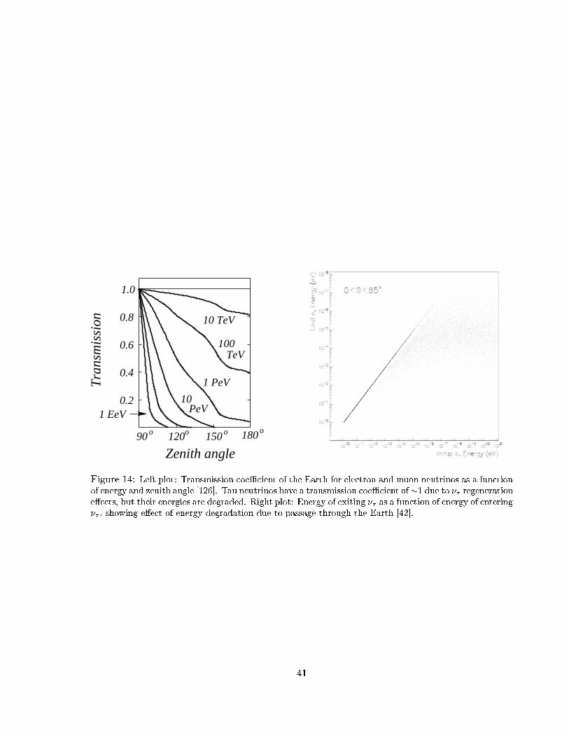
100 TeV

Zenith angle

10 TeV

1 PeV

10 PeV1 EeV

90 120 150 180

0.2

0.4

0.6

0.8

1.0

o o o o

Tra

nsm

issi

on

Figure 14: Left plot: Transmission coeÆcient of the Earth for electron and muon neutrinos as a functionof energy and zenith angle [126]. Tau neutrinos have a transmission coeÆcient of�1 due to �� regeneratione�ects, but their energies are degraded. Right plot: Energy of exiting �� as a function of energy of entering

�� , showing e�ect of energy degradation due to passage through the Earth [42].

41

simulation was performed with the AMANDA simulation package amasim. Ice inhomogenities

have been neglected for this study but will be included in the future. We simulated PMTs of

10 in diameter but did not take into account the possible increase in light collection eÆciency

due to a proposed wavelength shifter coating applied to the outer OM surfaces. The noise of

the PMTs has been conservatively assumed to be 500 Hz (i.e. higher than the design goal of

300 Hz). A trigger was de�ned by the condition of at least 5 hits in a local coincidence. A local

coincidence is de�ned with respect to the four nearest neighbors, and for a time window of 1 �s.

Signal Monte Carlo muon events are shown in �gs. 15 and 16, where the muon energies are

10 TeV and 6 PeV, respectively.

Figure 15: A simulated 10 TeV muon track in IceCube. Colored circles represent hit channels, with red

circles hit earliest and violet circles latest. Circle size corresponds to number of detected photons.

5.3.2 Reconstruction and Background Rejection

The reconstruction was done in several steps using the AMANDA reconstruction package recoos.

The start values for the full �t are obtained from two simple fast approximations called line-�t

and dipole-�t (see [151] for details). As a �rst reduction step with respect to downgoing muons,

relatively weak cuts on the zenith angle obtained from these fast approximations have been

applied. These cuts have passing rates of 0.91, 0.78 and 0.04 with respect to the sample from

AGN neutrinos, atmospheric neutrinos and downgoing muons, respectively.

Next, a full likelihood �t was performed (see [150] and [151]). This �t yields a series of

parameters which can be used for selecting events with high quality reconstruction and for

further reduction of background. The cuts chosen are the following:

� zenith angle � obtained from the likelihood �t larger than 85Æ, and � logL < 10, where L

is the likelihood;

42

Figure 16: A simulated 6 PeV muon track in IceCube. Colored circles represent hit channels, with red

circles hit earliest and violet circles latest. Circle size corresponds to number of detected photons.

43

� � 5 hits with a time residual between {15 ns and +150 ns (\direct hits"), where the photon

did not undergo many scattering interactions);

� length of the projection of the direct-hit OMs to the reconstructed track larger than 150 m;

� di�erence between the zenith angles obtained from line �t and likelihood �t smaller than

10 degrees;

� the absolute value of the smoothness, smaller than 0.5.1

Note that the standard cuts listed above result in a passing rate of 53% for AGN neutrinos

and reduce the background from downgoing muons by 3 � 10�6. As shown in �g. 17, this

background is concentrated close to the horizon. It can be easily rejected by a further zenith

cut (if lower energies should be accepted), or by cuts on the number of channels (if one focuses

to the separation of higher energies). Figure 17 also shows the background from uncorrelated

coincident air showers (bottom right) which can produce two hit clusters, and earlier one at the

bottom and a later one at the top of the array. Such events are not rejected by a simple angular

cut, giving the relatively high passing rate after angular cuts compared to muons from single

air showers. However, these events are easily identi�ed by the subsequent cuts, in particular the

cut on the smoothness.

Results are shown for the \standard con�guration" (triangular pattern, 16 m vertical spac-

ing2, 125 m interstring distance). Numbers at the top corner give the number of events and

the passing rates. For AGN neutrinos, a ux of 2� 10�7 �E�2 GeV�1 cm�2 s�1 sr�1 has beenassumed, resulting in 4265 events.3

We have investigated the physics performance of the IceCube detector for di�erent con�g-

urations, starting from the default con�guration and going into the direction of both smaller

and larger spacings [139]. Early results on similar IceCube simulations have been presented

in [124, 125]. Whereas in [139] only con�gurations with about 5000 OMs and equidistant spac-

ing are considered [124, 125] cover also options with twice or half the number of OMs, and nested

con�gurations.

The basic pattern is shown in �g. 18. Apart from the triangular pattern, we also simulated

rectangular patterns, which yield similar results. The circle in �g. 18 indicates an area of one

square kilometer. The con�guration includes 80 strings and 60 OMs per string. For a vertical

spacing of 16 m, this results in an instrumented length of 944 m. The top layer of OMs was

assumed to be at a depth of 1400 m. Table 2 summarizes the studied con�gurations.

The two following tables give the number of triggered and accepted events per year for the

various con�gurations. Table 3 gives results for atmospheric neutrinos. Numbers in table 4 are

for AGN neutrinos, again assuming a ux of 2 � 10�7 � E�2 GeV�1 cm�2 s�1 sr�1. The upper1The smoothness S measures the homogenity of the distribution of hits along the track. Exactly equidistant

hits would give S = 0, all hits at the starting point of the track S = +1 and all hits at the endpoint S = �1.2The 16 m vertical spacing was chosen for this study before 17 m became the baseline design.3An AGN neutrino ux of roughly 10�7 �E�2GeV�1 cm�2 s�1 sr�1 is roughly the ux to which AMANDA is

sensitive. It is otherwise arbitrary.

44

vertical / horizontal 100 m 125 m 150 m 175 m

12 m X X X -

16 m X X X -

20 m X X X X

Table 2: Simulated con�gurations. Columns indicate di�erent string spacings, rows di�erent spacings of

OMs along a string. An \X" indicates that the particular con�guration was simulated.

10-1

1

10

10 2

10 3

10 4

10 5

0 50 100 15010

-1

1

10

10 2

10 3

10 4

10 5

0 50 100 150

10 210 310 410 510 610 710 810 9

10 1010 1110 12

0 50 100 150

reco-zenith / o

even

ts/y

ear

AGN ν

reco-zenith / o

even

ts/y

ear

Atm ν

reco-zenith / o

even

ts/y

ear

Single Events

reco-zenith / o

even

ts/y

ear

Double Events

10 210 310 410 510 610 710 810 9

10 1010 1110 12

0 50 100 150

Figure 17: Distribution of the reconstructed zenith angle after trigger (full upper line), and the 3 cuts

on the zenith angles (dashed line), the remaining four quality cuts (dotted line). The shaded histogram

gives the energy spectrum after an additional cut on the number of hit PMTs at Nch > 50. The dark

histogram corresponds to a cut at Nch > 180. The bottom histograms show the background expected

from single air showers (left) and from accidentally coinciding air showers (right). Note that neutrinos

have been generated only between 80 and 180 degrees, hence the cut-o� at 80 degrees after quality cuts.

45

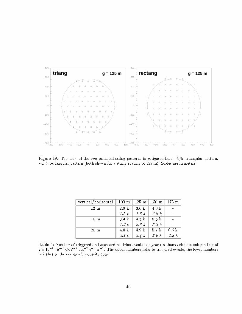
triang g = 125 m rectang g = 125 m

Figure 18: Top view of the two principal string patterns investigated here. left: triangular pattern,

right: rectangular pattern (both shown for a string spacing of 125 m). Scales are in meters.

vertical/horizontal 100 m 125 m 150 m 175 m

12 m 2.9 k 3.6 k 4.3 k -

1.5 k 1.8 k 2.2 k -

16 m 3.4 k 4.3 k 5.5 k -

1.9 k 2.3 k 2.5 k -

20 m 4.0 k 4.9 k 5.7 k 6.5 k

2.1 k 2.4 k 2.6 k 2.8 k

Table 4: Number of triggered and accepted neutrino events per year (in thousands) assuming a ux of

2 � 10�7 � E�2 GeV�1 cm�2 s�1 sr�1. The upper numbers refer to triggered events, the lower numbers

in italics to the events after quality cuts.

46

numbers refer to triggered events, the lower numbers (in italics) to events after reconstruction

and quality cuts.

vertical/horizontal 100 m 125 m 150 m 175 m

12 m 600 k 620 k 640 k -

140 k 130 k 120 k -

16 m 590 k 600 k 620 k -

140 k 130 k 110 k -

20 m 580 k 590 k 600 k 560 k

140 k 110 k 90 k 60 k

Table 3: Number of triggered and accepted events per year for atmospheric neutrinos (in thousands).

The upper numbers refer to triggered events, the lower numbers in italics to the events after quality cuts.

Clearly, larger spacing is preferable for the AGN case but tends to suppress more atmospheric

neutrinos after quality cuts. Going from 125 m string spacing to 150 m gives a 10% increase

in accepted AGN events. The rectangular con�guration gives a 5% increase in events rate.

Decreasing the spacing to 12 m/100 m gives 30% loss in AGN neutrinos, but a slight increase

for atmospheric neutrinos. The angular resolution for all con�gurations is � 1 degree.

5.3.3 Sensitivity to Di�use Sources of Muon Neutrinos

We calculate the sensitivity of the detector to di�use uxes of neutrinos with a generic E�2

spectrum, expected for sources such as active galactic nuclei (AGN). For the purposes of

these calculations we assume a source strength for muon-neutrinos and antineutrinos of a

level E2dN=dE = 10�7GeV cm�2 s�1 sr�1. We use the Model Rejection Potential formal-

ism [132, 135], and the associated \model rejection factor" (MRF), to optimize the limit analysis.

Figure 19 shows the results of the minimization of the MRF for the hit multiplicity (Nch) cut

and an exposure time of three years. The top left �gure shows the di�erential numbers of

events expected for both the E�2 spectrum (blue solid line) and for the atmospheric neutrinos

(red dashed line). The top right plot shows the same quantities as an integral distribution. Also

shown is the Feldman-Cousins 90% con�dence level average upper limit. As the background falls

toward zero, this classical average upper limit converges toward a value of 2.44. The best limit

is obtained where the model rejection factor, (��(nb)=ns), is minimised (bottom left plot).This

occurs for a cut of 168 channels, where 120.9 signal events would be expected upon a background

of 17.2. The average upper limit for this background is 8.4, leading to a MRF = 6:9 � 10�2,

and therefore to a ux limit of E2dN=dE = 6:9 � 10�7GeV cm�2 s�1 sr�1. The bottom right

plot shows the parent neutrino energy distribution for those events with multiplicity above the

optimal cut of 168 channels. The multiplicity cut corresponds to a minimum energy of about

30 TeV, and to a typical neutrino energy of 1 PeV. Table 5 summarises the results of the MRF

optimization for exposure times of one and three years.

47

time (yrs) Nch cut S(� Nch) B(� Nch) ��(B(� Nch)) limit (= E�2dN=dE � ��S)

1 175 53.1 5.4 5.3 1:0� 10�8

3 221 93.1 3.2 4.5 4:8� 10�9

Table 5: IceCube model rejection factor for an E2dN=dE = 10�7cm�2s�1sr�1GeV2 ux as a function

of exposure time.

Figure 19: Model rejection potential optimization for a di�use ux: Top left: di�erential Nch distribution

for atmospheric neutrinos (dashed histogram) and AGN neutrinos (full histogram), assuming a ux of

10�7�E�2 GeV�1 cm�2 s�1 sr�1 for AGN neutrinos. Top right: integralNch distribution, with the average

upper limit shown as a solid line. Bottom left: Model rejection factor. Bottom right: Distribution of

neutrino energies for those events with hit multiplicity Nch greater than the optimal cut. We see that

the Nch cut corresponds to neutrino energies greater than � 30 TeV and that the detector is sensitive to

di�use E�2 neutrinos of energy of order 1 PeV (solid blue line). The red dashed line shows the energies

of the atmospheric neutrinos that pass the cuts.

48

5.3.4 Sensitivity to Muon Neutrino Point Sources

The sensitivity of IceCube for point sources of neutrinos has been assessed. Since the background

may be greatly reduced by cutting to a small angular region about the direction of the point

source, the multiplicity cut (Nch) can be relaxed. The sensitivity has been checked in two ways,

�rst by averaging the sensitivity over the upward going hemisphere, and second by looking at a

point source from a speci�c zenith angle.

For each exposure time tested, we optimise in both angular bin size and Nch. Figure 20

shows the pointing accuracy of the array. Ninety percent of events reconstruct to within 4Æ

of the true direction, and 60% to within 1Æ. The MRF results from varying angular bin and

exposure time are shown in table 6. These show that a signal strength of the level dN=dE =

10�7cm�2s�1sr�1GeV2 would produce a very signi�cant signal in IceCube, and in its absence,

very constrained upper limits would be obtained. For both exposure times, the best choice of

angular cut is about 1Æ, but the limit is ultimately not very sensitive to the choice of angular

cut, suggesting that a smaller cut, to enhance the signi�cance of a possible observation, may be

warranted. Although the cuts have been optimised to minimise the MRF, thereby optimising

the limit setting potential of the detector, we can make some basic estimates of the level of

a point source ux needed to give a signi�cant detection of a signal in the exposure time. A

chance probability of � 10�7 for a background uctuation corresponds roughly to a \5 sigma"

observation. For any quoted background level, we can calculate the number of events needed

to get this chance probability. For the case of 1 year exposure with a 1Æ angular bin, the

expected background is 0.53 events. If 8 events were observed, this would give the required

chance probability of � 10�7. A signal strength of 8 � 0:5 = 7:5 events is about 1/5 of the

number of events expected from the dN=dE = 10�7cm�2s�1sr�1GeV2 ux, therefore a point

source of level dN=dE � 2� 10�8cm�2s�1sr�1GeV2 would be required to produce a \5 sigma"

observation in one year of live time. Of course, this analysis assumes that we only look at a

single candidate source. If we do a full sky search, we must pay a penalty for statistical trials.

There are about 6500 bins of 1Æ radius in a half sky (upgoing neutrino) search, so a signi�cance

of � 10�9 would be needed for an unknown point source to give a � 10�7 result after the trials

are accounted for. This requires that about 10 events are observed (the chance probability to

observe 10 or more events from a backgrpound of 0.53 is 3 � 10�10), increasing the required

signal strength by about 30%.

Table 7 shows the MRF results for a point source at a zenith angle of 130Æ. The limit setting

potential is slightly less than the average seen in table 6. Figure 21 shows the model rejection

potential optimization for a point source.

5.3.5 Sensitivity to Muon Neutrinos from Gamma-Ray Bursts

Recently, Waxman and Bahcall [94] have proposed that gamma-ray bursts (GRBs) might be

sources of neutrinos. The search for neutrinos from GRBs is simpli�ed over that of a point

source, due to the time stamp available from satellite observations of the gamma rays from the

burst. In the Waxman-Bahcall model the neutrinos are expected to arrive within approximately

49

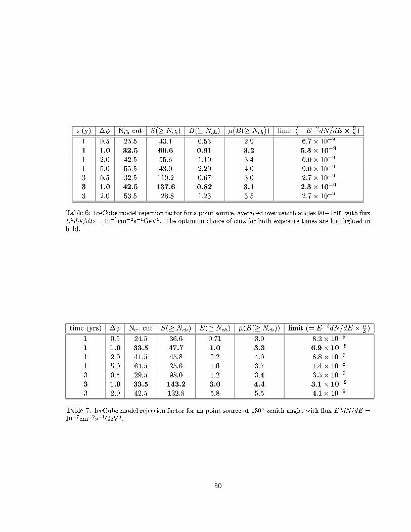
t (y) � Nch cut S(� Nch) B(� Nch) ��(B(� Nch)) limit (= E�2dN=dE � ��S)

1 0.5 25.5 43.1 0.53 2.9 6:7� 10�9

1 1.0 32.5 60.6 0.91 3.2 5:3� 10�91 2.0 42.5 55.6 1.10 3.4 6:0� 10�9

1 5.0 55.5 43.9 2.20 4.0 9:0� 10�9

3 0.5 32.5 110.2 0.67 3.0 2:7� 10�9

3 1.0 42.5 137.6 0.82 3.1 2:3� 10�93 2.0 53.5 128.8 1.25 3.5 2:7� 10�9

Table 6: IceCube model rejection factor for a point source, averaged over zenith angles 90�180Æ with uxE2dN=dE = 10�7cm�2s�1GeV2. The optimum choice of cuts for both exposure times are highlighted in

bold.

time (yrs) � Nch cut S(� Nch) B(� Nch) ��(B(� Nch)) limit (= E�2dN=dE � ��S )

1 0.5 24.5 36.6 0.71 3.0 8:2� 10�9

1 1.0 33.5 47.7 1.0 3.3 6:9� 10�91 2.0 41.5 45.8 2.2 4.0 8:8� 10�9

1 5.0 64.5 25.6 1.6 3.7 1:4� 10�8

3 0.5 29.5 98.0 1.2 3.4 3:5� 10�9

3 1.0 33.5 143.2 3.0 4.4 3:1� 10�93 2.0 42.5 132.8 5.8 5.5 4:1� 10�9

Table 7: IceCube model rejection factor for an point source at 130Æ zenith angle, with ux E2dN=dE =

10�7cm�2s�1GeV2.

50

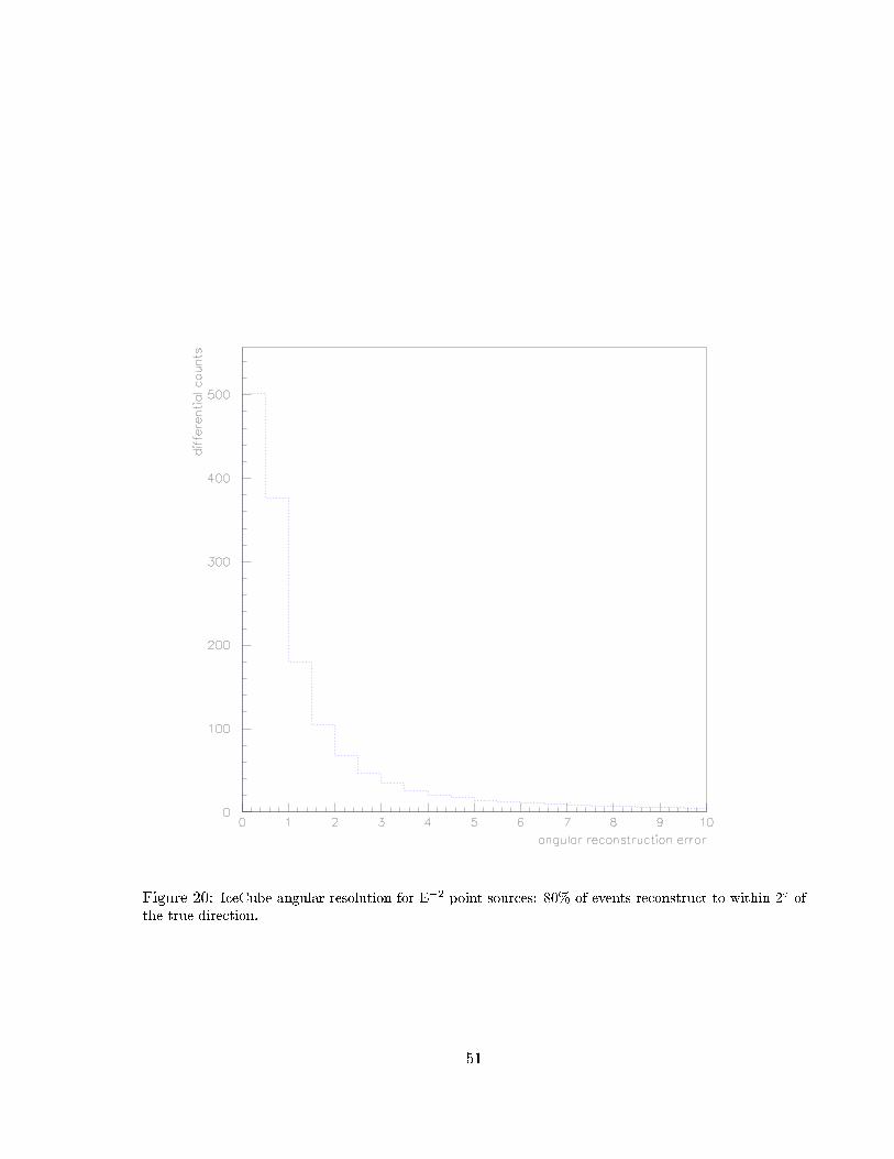
Figure 20: IceCube angular resolution for E�2 point sources: 80% of events reconstruct to within 2Æ of

the true direction.

51

Figure 21: Model rejection potential optimization for a point source: Top left: di�erential Nch distri-

bution for atmospheric neutrinos (dashed histogram) and AGN neutrinos (full histogram), assuming a

ux of 10�7 � E�2 GeV�1 cm�2 s�1 sr�1 for AGN neutrinos. Top right: integral Nch distribution. Solid

line { average upper limit Bottom left: Model rejection factor. Bottom right: Distribution of neutrino

energies for those events with hit multiplicity Nch greater than the optimal cut. We see that the Nch

cut corresponds to neutrino energies greater than � 1 TeV and that the detector is sensitive to di�use

E�2 neutrinos of energy of order 100 TeV (solid blue line). The red dashed line shows the energies of the

atmospheric neutrinos that pass the cuts.

52

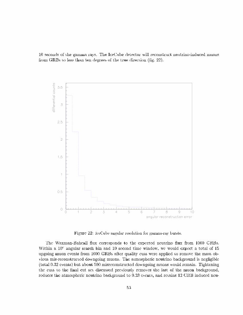
10 seconds of the gamma rays. The IceCube detector will reconstruct neutrino-induced muons

from GRBs to less than ten degrees of the true direction (�g. 22).

Figure 22: IceCube angular resolution for gamma-ray bursts.

The Waxman-Bahcall ux corresponds to the expected neutrino ux from 1000 GRBs.

Within a 10Æ angular search bin and 10 second time window, we would expect a total of 15

upgoing muon events from 1000 GRBs after quality cuts were applied to remove the most ob-

vious mis-reconstructed downgoing muons. The atmospheric neutrino background is negligible

(total 0.32 events) but about 500 misreconstructed downgoing muons would remain. Tightening

the cuts to the �nal cut set discussed previously removes the last of the muon background,

reduces the atmospheric neutrino background to 0.23 events, and retains 12 GRB induced neu-

53

trino events. It should be noted that more Monte-Carlo simulations are needed to further check

the belief that the background of mis-reconstructed downgoing muons is indeed zero.

Optimising the Nch cut leads to a cut of Nch = 12:5 and model rejection factor of 0.22, a severe

constraint on the Waxman-Bahcall model. Since the GRB search is essentially background free,

the improvement in the limit goes nearly linearly with the increasing number of GRBs searched.

This behaviour is shown in table 8. It is interesting that the observation of only 210 GRBs is

enough to rule out the Waxman-Bahcall model at 90% classical con�dence.

Since the angular cut and time window search can be made so tight, the GRB searches are

close to background-free. Then the observation of even a few events would be very signi�cant.

For 300 GRBs searched, and a 2Æ, window, the Waxman-Bahcall model predicts about 3 events,

on an atmospheric neutrino background of 0.003. The chance probability of observing 3 or

greater events given a background of 0.003 is about 5� 10�9.

Table 8 shows that the MRF is insensitive to the choice of angular bin size. In this case, a

choice of a smaller search window would be preferred, in order to reduce the background (for

limited signal loss) and give a more signi�cant observation of a potential signal. Ultimately

however, the uncertainty in the knowledge of the GRB direction (from the satellite observation)

will limit how small the angular search bin can be made. Figure 23 shows the model rejection

potential optimization for GRBs.

nbursts � Nch cut S(� Nch) B(� Nch) ��(B(� Nch)) limit (= E�2dN=dE � ��S )

100 2.0 1.5 0.98 0.001 2.4 2.49

5.0 1.5 1.13 0.005 2.4 2.16

10.0 1.5 1.19 0.02 2.46 2.06

20.0 1.5 1.20 0.086 2.51 2.07

30.0 12.5 1.22 0.19 2.60 2.12

210 10 1.5 2.50 0.045 2.49 0.99

300 2.0 1.5 2.94 0.003 2.44 0.829

5.0 1.5 3.40 0.016 2.45 0.721

10.0 1.5 3.51 0.065 2.46 0.70

20.0 1.5 3.66 0.26 2.66 0.72

1000 2.0 1.5 9.81 0.009 2.45 0.249

5.0 1.5 11.34 0.05 2.48 0.219

10.0 12.5 11.9 0.215 2.62 0.22

20.0 20.5 11.3 0.471 2.83 0.25

Table 8: IceCube model rejection factor for a Gamma-ray burst search.

5.3.6 Possible Improvements

The sensitivities given above could change in reality. We estimate that uncertainties in ice

modelling might change them by up to 50%{in either direction. Use of an energy estimator

54

Figure 23: Model rejection potential optimization for gamma-ray bursts: Top left: di�erential Nch

distribution for atmospheric neutrinos (dashed histogram) and WB GRBs (full histogram). Top right:

integral Nch distribution. Dotted line { average upper limit. Bottom left: model rejection factor. Bottom

right: Distribution of neutrino energies for those events with hit multiplicity Nch greater than the optimal

cut. We see that the Nch cut corresponds to neutrino energies greater than � 1 TeV and that the detector

is sensitive to di�use E�2 neutrinos of energy of order 100 TeV (dashed blue line). The red dashed line

shows the energies of the atmospheric neutrinos that pass the cuts.

55

better than Nch may result in an improvement of up to 30%. Use of wavelength shifter could

enhance the sensitivity of the OMs by up to 35% and result in higher signal eÆciency and

improved background rejection. The application of reconstruction methods which make use

of the full waveform instead of using only the time of the �rst arriving photon will lead to a

better angular reconstruction, in particular for high-energy events (see Section 5.6). We hope

to reach an accuracy of about 0.5 degrees for moderate cuts, resulting in a slightly better point

source sensitivity. Neutrinos with >100 PeV have not been taken into account in the present

simulation. Their inclusion will also result in a better limit. Other lines of improvement are

selection of cuts with a better passing rate for for AGN neutrinos (giving possibly a 10{15%

e�ect), and a change of the con�guration to larger spacing, which is discussed in section 5.8.

5.4 Electromagnetic and Hadronic Cascades

The charged current interaction of UHE electron neutrinos and the neutral current interactions

of UHE neutrinos of all active avors will produce large localized depositions of energy in the

IceCube detector. The signature of these electromagnetic or hadronic showers (cascades) is a

bright, pointlike source of �Cerenkov light4 as shown in �g. 24. To be detected, cascades must

occur near or within the active detector volume, and consequently the e�ective volume for their

detection is substantially smaller than that of muons. However, cascades have the advantage

that their energies can be measured more accurately than muon events, making it easier to

separate UHE cascades from background. This is especially true for �e charged current and

\double bang" �� interactions, where the resulting cascades give a fairly accurate measure of

the energy of the parent neutrino.

5.4.1 Simulation

Cascade events were generated using one of three generators depending on the study:

� Reconstruction studies and e�ective volume calculations were performed using a very sim-

ple Perl script which throws isotropic cascade vertices uniformly throughout a cylindrical

volume 1.5 km tall and 1.5 km in radius surrounding the detector. These events are

generated with a E�1cas energy spectrum from 100 GeV to 1 EeV.

� The atmospheric neutrino signal was generated by casim, a weighted Monte Carlo pack-

age which produces cascade events with a E�1cas spectrum from 10 GeV to 100 TeV. The

atmospheric neutrino ux is taken from Lipari [95]. The weight of each event is recorded

to allow biasing back to the physical energy spectrum.

� The expected signal for ultrahigh-energy cascades from di�use sources or GRBs was sim-

ulated using code which propagates a given neutrino ux through the Earth, taking into

4The pointlike approximation for cascades holds to very high energies as the logitudinal development of the

shower is only logarithmically dependent on the shower energy.

56

Figure 24: A 375 TeV cascade in IceCube. Colored circles represent hit channels, with red circles hit

earliest and violet circles latest. Circle size corresponds to number of detected photons.

57

account both neutrino absorption and neutral-current regeneration and generates neutrino-

nucleus interaction vertices in a homogeneous volume of ice surrounding the detector over

the full 4� steradians of solid angle. In order to realistically simulate the overburden of

material in the upper hemisphere, the simulation code models the south polar ice as a

spherical cap on the Earth. This package generates unweighted events. Several energy

spectra were sampled for 100 GeV < E� < 1 EeV, each corresponding to a distinct astro-

physical source models. They are dealt with in �ner detail in the appropriate sections.

These vertices are then passed to the detector simulation package, amasim, which generates

PMT hits in the array and builds them into events. Triggers were generated on a coincidence of

�ve hits in 2.5 �s. Additionally, a feature of amasim was enabled that preserves pulse amplitude

information for each pulse in the event that a single OM receives multiple hits. 5 This additional

information approximated waveform readout in IceCube.

5.4.2 Reconstruction

Applying algorithms developed for AMANDA on simulated IceCube data, we have estimated

the vertex, direction, and energy resolutions of cascades in IceCube. We have also estimated

these resolutions using newly developed algorithms tailored to IceCube data. Estimates using

AMANDA algorithms are conservative since they rely primarily on the arrival times of the �rst

photons in each PMT, while in IceCube we will have access to much more detailed waveform

information. Estimates using new algorithms are also conservative since we anticipate using the

waveform information in a more complete manner than presented here.

The AMANDA algorithm for reconstructing the vertex position and time is based on a

model of the scattering and absorption of �Cerenkov light in the ice. It maximizes a likelihood

function which depends on a parametrization of the probability distribution of observing one

photon with a given time delay at some distance from the source. The AMANDA algorithm for

reconstructing direction and energy is also a maximum likelihood �t which uses a parametrization

of the expected number of photons at each PMT as a function of cascade energy and the relative

cascade-PMT direction.

Applying these algorithms to simulated IceCube cascades with contained vertex positions

(vertices at least 100 m from the edge of the detector), resulted in energy and zenith angle

resolutions which were better than in AMANDA. The resolutions are as follows:

� Energy: 11% in log10E (AMANDA: >40%)

� Zenith: 27Æ in zenith angle (AMANDA: 27Æ)

� Vertex: 3 m in x; y; 2 m in z (AMANDA: 6.4 m in x; y; 5.3 m in z)

These resolutions are illustrated in �g. 25.

5In AMANDA, the peak ADC hardware only records a single peak value per ADC gate, and thus, normally,

the multiple pulse information is suppressed in amasim.

58

X/Y Vertex Resolution

0

20

40

-20 0 20

14.94 / 18Constant 39.39Mean 0.5255Sigma 3.062

∆X (m)

Eve

nts

Z Vertex Resolution

0

20

40

60

-20 0 20

45.20 / 18Constant 58.16Mean -0.2785E-01Sigma 1.865

∆Z (m)

Eve

nts

θ Resolution

0

10

20

30

-100 -50 0 50 100

27.65 / 32Constant 21.17Mean -0.4598Sigma 26.60

∆θ (degrees)

Eve

nts

4

6

8

4 6 8 10

ECAS v ERECO

log 10(ERECO/GeV)

’log

10(E

CA

S/G

eV)

Energy Resolution 1 TeV < E < 1 PeV

0

10

20

-1 -0.5 0 0.5 1

11.22 / 8Constant 18.44Mean -0.6736E-02Sigma 0.9227E-01

log 10(ECAS/EREC)

Eve

nts

Energy Resolution 1 PeV < E < 1 EeV

0

10

20

30

-1 -0.5 0 0.5 1

12.58 / 18Constant 24.63Mean -0.7194E-02Sigma 0.1225

log 10(ECAS/EREC)

Eve

nts

Figure 25: Vertex, direction, and energy resolutions for simulated IceCube cascades, using AMANDA

multiphoton reconstruction algorithms. These reconstructions are evaluated after all cuts which are listed

later in the subsection 5.4.2 on background rejection.

59

Ultimately, we anticipate that we will construct a likelihood function which uses the full

waveform information from each PMT, maximizing the probability that each PMT observed

a particular waveform as a function of cascade (~r,t,E,~d). Moreover, waveform readout will

dramatically increase the dynamic range of the PMTs. Cascade reconstructions in particular

would bene�t from this enhancement due to the nature of the cascade signal: OMs very close

to the cascade vertex are expected to receive thousands of �Cerenkov s, but simultaneously

the detector must be able to resolve the single hits at large distances for accurate energy

reconstruction.

Techniques for suppressing the cosmic ray muon events in IceCube have been borrowed from

AMANDA cascade analyses. The very large instrumented volume of IceCube makes cosmic-ray

muon rejection very eÆcient using quick algorithms based on event topology and total charge

information. Once these fast �lters have reduced the data volume down to manageable levels,

maximum likelihood �ts are performed to reconstruct the cascade vertex, direction, and energy

and further cuts are made on these output quantities.

It should be noted that these cuts were contructed to optimize HE events (E > 10 TeV) and

consequently, they are not eÆcient at passing the lower energy atmospheric neutrinos. In fact,

in a search for high energy galactic or extragalactic neutrinos, atmospheric neutrinos themselves

constitute a background.

The selection criteria are now explained. First, the tensor of inertia is evaluated about the

center of gravity of the hits and is diagonalized to �nd its eigenvalues. The ratio of the smallest

eigenvalue to the sum of the eigenvalues, L1=PLi, provides an estimate of the sphericity of

the event: muons tend towards enlongated hit patterns while cascades produce hits more or less

spherically symmetric about their centers. Next, a line �t is performed. The line �t is an analytic

approximation that all hits lie along a straight line moving at the speed of light. This heuristic

provides a measure of the time ow of the hits in an event. Cascades and muons separate

into two clearly distinct populations via the parameter jvLF j, the velocity of the line�t. Monte

Carlo simulations indicate that cuts on these two variables suppress much of the background

and accept most of the cascade signal.

While the above criteria reduce the background by almost two orders of magnitude there still

remain at least four orders before the level of the signals is approached. An additional cut on

the total charge generated by the detected photoelectrons,PQ, is applied which reduces even

the high-energy Corsika-generated cosmic-ray muons almost another two orders of magntiude at

the expense of loss of signal sensitivity below about 10 TeV. A cut was applied on the likelihood

of the cascade reconstruction, Lcas < 6, eliminating all but two events of the (admittedly small)

simulated high energy background sample. Finally, a containment cut was made which required

the center of gravity of the hits, weighted with ADC amplitude, to fall within a cylindrical

volume centered on the detector center, 750 m in height, 450 m in radius (0.48 km3). This

eliminates all background events in the sampled sets.

Background was estimated using two di�erent physics generators for cosmic ray muons:

the basiev program generates proton primaries up to energies of 1 PeV. Beyond that, heavier

elements constitute a large portion of the cosmic-ray primaries and the Corsika air shower package

is used which accurately simulates the composition of the cosmic-ray primaries and the high-

60

energy interactions up to very high energies, exceeding 1020 eV. The calculated live times of the

atmospheric muon samples are 80 seconds and 16 hours, respectively for the basiev and Corsika

sets. Therefore, background was estimated for higher cut levels which left no background in the

sample sets. This was done by �tting background versus a cut variable well below threshold

and integrating the extrapolated variable above threshold. Clearly, a more thorough study

necessitates additional background sampling. The results of the background suppression cuts

on these data sets as well as signal acceptance on di�use (E�2) and atmospheric neutrino uxes

are presented in table 9.

Cut Level Di�use ATM � basiev Corsika

Signal Signal ECR < 1PeV ECR > 1PeV

Trigger 981 22500 1:17� 1011 2:22� 108

L1=PL 842 10650 8:03� 108 7:76� 106

jvLF j 676 5470 1:47� 108 2:34� 106PQ 461 470 13 5:68� 104

Lmpe < 6 447 397 � 0 1:96� 103

� < 450m; jzj < 375m 180 217 � 0 � 50

Table 9: Event rates of various sources of signal and background versus cut level. The numbers quoted

are in units of expected events per year. In the case of the di�use neutrino ux, the rate is scaled for a

ux of E2�� = 10�7 (GeV � cm � s � sr)�1.

There is also the possibility for strong cosmic-ray muon background suppression with the

surface array, IceTop. In the high-energy region where muon bremsstrahlung begins to look like

a signal the surface array becomes relevant in two ways. Air showers with energy in the PeV

range and above will trigger the surface array with high eÆciency, and this trigger can be used

to veto and study this source of background. At higher energy the surface array will also have

some veto power for showers with cores outside the physical boundary of the array.

5.4.3 E�ective Volume

The e�ective trigger volume, Veff , is de�ned as the equivalent volume in which the detector

achieves 100% eÆciency and is calculated from a simulation of cascades thrown in a much larger

volume, Vgen, by

Veff (Ecas) =ntrig(Ecas)

ngen(Ecas)� Vgen

and ranges from about 1 km3 at 1 TeV to 4 km3 at 100 PeV (see �g. 26). A more realistic

e�ective volume has been calculated that takes into account the background rejection criteria

discussed in the previous section. \Background Rejection I" refers to cuts made that remove

background that is expected to remain after vetoing cosmic-ray events that trigger the IceTop

surface array. The e�ective volume drops to zero below about 1 TeV because of a high charge

61

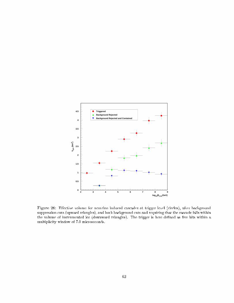
0

0.5

1

1.5

2

2.5

3

3.5

4

4.5

2 3 4 5 6 7 8 9

Triggered

Background Rejected

Background Rejected and Contained

log 10(ECAS/GeV)

VE

FF (

km3 )

Figure 26: E�ective volume for neutrino induced cascades at trigger level (circles), after background

suppression cuts (upward triangles), and both background cuts and requiring that the cascade falls within

the volume of instrumented ice (downward triangles). The trigger is here de�ned as �ve hits within a

multiplicity window of 7.0 microseconds.

62

requirement, reaches 1 km3 at 10 TeV, and grows to about 2.5 km3 at 100 PeV. \Background

Rejection II" cuts further require that the center of gravity of the hits be contained well inside

the detector instrumented volume. This additional cut reduces cosmic-ray muon background to

zero independent of any IceTop veto at the cost of reducing the �ducial volume to � 0:5 km3.

5.4.4 Sensitivity to Atmospheric �

Examination of table 9 shows that there is a very prominent signal of atmospheric � (ATM �) at

trigger level (�g. 27). Since they are produced with a much softer spectrum than the expected

spectra of extragalactic neutrinos, most of this signal populates the medium and high energy

regions from the lower energy threshold of IceCube (� 100 GeV to several tens of TeV) and is

reduced by more than 90% by thePQ cut. It may possible to recover some of this lost signal by

tuning the cuts for low energy neutrinos. For example, the high charge cut could be lowered and

supplemented with a cut on the zenith angle of the muon reconstruction to reject downgoing

fakes.

10-1

1

10

10 2

10 3

2 2.5 3 3.5 4 4.5 5 5.5 6

Trigger Level

After HE Cuts

log 10(ECAS)

Eve

nts

per

year

Figure 27: Triggers versus energy and events passing background rejection cuts versus energy for atmo-

spheric neutrinos (Lipari ux [95].)

63

5.4.5 Sensitivity to Point Sources

With present reconstruction techniques, the poor angular resolution of �-induced cascades in the

IceCube detector makes it diÆcult to perform a point source search in these channels. However,

new reconstruction techniques which take advantage of waveform information may improve upon

this situation.

5.4.6 Sensitivity to Di�use �e Sources

Earth absorption plays a signi�cant role in the UHE neutrino ux at the IceCube detector.

Figure 28 shows the zenith angle dependence on the event rate and demonstrates the e�ect:

Earth shadowing begins attenuating the event rate below the horizon at several tens of TeV.

The shadowing steepens with energy until, above energies E� > 10 PeV, the earth is almost

totally opaque to neutrinos. Fold into this the fact that the target volume for � ! cascade,

being closer to the detector than for � ! � vertices, is symmetrically distributed both above

and below the detector so that cascades do not su�er a reduced amount of target material for

downgoing events. These two observations together imply that the upper hemisphere is especially

important for the detection of UHE �-induced showers and the ability to cleanly separate UHE

neutrino-induced showers from cosmic-ray muon background is another trump held by cascade

analyses. The di�erential event rate of UHE cascades in IceCube versus energy for a ux of

E2�� = 10�7 (GeV � cm � s � sr)�1 is shown in �g. 29. The squares represent the trigger rate and

the triangles represent the event rate after all background rejection cuts have been applied.

5.4.7 Sensitivity to GRBs

GRBs are another hypothesized source of UHE extragalactic neutrinos. For these sources,

Waxman and Bahcall [127, 128] propose a ux that is very soft, falling as E�1 until a break

energy of several hundred TeV when the spectrum turns down to fall as E�2. Folding in the �

cross-section, one obtains the result of an increasing interaction rate (in logE) until the break

energy, and thus a very high-energy source of �-induced cascades in the detector visible above

the background (�g. 30). The authors also predict that the � and bursts are very closely

correlated in time so that the IceCube detector can restrict searches to time windows centered on

burst events observed by one of the several gamma-ray satellites. However, if the GRB uence

is close to the W&B prediction, IceCube could still detect a cluster of cascade events from such

a burst without \triggering" on satellite observations.

A GRB search in the cascade channel has a distinct advantage over the muon channel search

which o�sets the smaller e�ective volume of high-energy cascades versus muons: background

rejection is based on event topology. That is, cascades do not look like atmospheric muons,

therefore the upper hemisphere does not need to be excluded from a cascade GRB search,

making IceCube sensitive to both northern and southern hemisphere GRBs.

64

1

10

10 2

10 3

-1 -0.8 -0.6 -0.4 -0.2 0 0.2 0.4 0.6 0.8 1

cos θ

Eve

nts

per

year

Figure 28: Distribution of UHE �-induced cascades versus zenith angle at generator level for a generic

E�2 ux. The assumed source ux is E2� = 10�7 (GeV � cm � s � sr)�1.

65

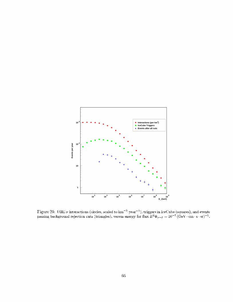
1

10

10 2

10 3

103

104

105

106

107

108

109

Interactions (per km 3)IceCube TriggersEvents after all cuts

Eν (GeV)

Eve

nts

per

year

Figure 29: UHE � interactions (circles, scaled to km�3 �year�1), triggers in IceCube (squares), and eventspassing background rejection cuts (triangles), versus energy for ux E2��+�� = 10�7 (GeV � cm � s � sr)�1.

66

10-3

10-2

10-1

103

104

105

106

107

108

109

Γ=100Eν (GeV)

Eve

nts

Γ=100

10-4

10-3

10-2

10-1

103

104

105

106

107

108

109

Γ=300Eν (GeV)

Eve

nts

Γ=300

Figure 30: GRB �-induced cascade event rate predictions following the Waxman-Bahcall model for two

choices of the Lorentz factor, �. The y-axis is in units of s�1 making the integrated expected rate of

events in a km3 detector about 0.5 Hz and 0.9 Hz for the choices � = 100 and � = 300, respectively.

67

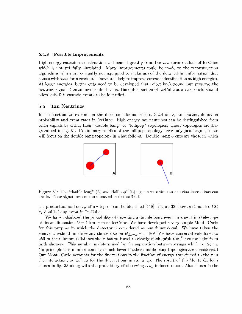
5.4.8 Possible Improvements

High energy cascade reconstruction will bene�t greatly from the waveform readout of IceCube

which is not yet fully simulated. Many improvements could be made to the reconstruction

algorithms which are currently not equipped to make use of the detailed hit information that

comes with waveform readout. These are likely to improve cascade identi�cation at high energies.

At lower energies, better cuts need to be developed that reject background but preserve the

neutrino signal. Containment cuts that use the outer portion of IceCube as a veto shield should

allow sub-TeV cascade events to be identi�ed.

5.5 Tau Neutrinos

In this section we expand on the discussion found in secs. 3.2.4 on �� kinematics, detection

probability and event rates in IceCube. High energy tau neutrinos can be distinguished from

other signals by either their \double bang" or \lollipop" topologies. These topologies are dia-

grammed in �g. 31. Preliminary studies of the lollipop topology have only just begun, so we

will focus on the double bang topology in what follows. Double bang events are those in which

A B

Figure 31: The \double bang" (A) and \lollipop" (B) signatures which tau neutrino interactions can

create. These signatures are also discussed in section 5.6.1.

the production and decay of a � lepton can be identi�ed [118]. Figure 32 shows a simulated CC

�� double bang event in IceCube.

We have calculated the probability of detecting a double bang event in a neutrino telescope

of linear dimension D = 1 km such as IceCube. We have developed a very simple Monte Carlo

for this purpose in which the detector is considered as one dimensional. We have taken the

energy threshold for detecting showers to be Eshower � 1 TeV. We have conservatively �xed to

250 m the minimum distance the � has to travel to clearly distinguish the �Cerenkov light from

both showers. This number is determined by the separation between strings which is 125 m.

(In principle this number could go much lower if other double bang topologies are considered.)

Our Monte Carlo accounts for the uctuations in the fraction of energy transferred to the � in

the interaction, as well as for the uctuations in its range. The result of the Monte Carlo is

shown in �g. 33 along with the probability of observing a ��-induced muon. Also shown is the

68

Figure 32: A double-bang �� event with an energy of a few PeV in IceCube. Colored circles represent

hit channels, with red circles hit earliest and violet circles latest. Circle size corresponds to number of

detected photons.

69

probability of observing a double bang event as obtained in [119] using the expression:

P� (E;Emin� ) = �NA

Z 1�Emin

�E

dy[D �R� ]d�CC(E; y)

dy; (3)

where � is the density of the medium and NA is Avogadro's number. Emin� is the minimum

energy of the � , it is automatically �xed imposing that R� � 250 m. This expression uses

average values for R� and hence at E�� � Emin� the probability of observing a double bang

vanishes since the average range of the � is smaller than 250 m. The probability calculated

with this expression has a broad maximum which is determined by the condition that R� has

to be larger than 250 m but smaller than the size of the detector. Assuming an average value of

y � 0:25 at these energies and using eq. 2 this corresponds to E�� between roughly 7 PeV and

27 PeV.

Figure 33: Probability of detecting �� induced double bang events in IceCube obtained with Monte

Carlo simulation and using the analytic expression given by of [119] (Eq.2). The probability is shown for

R� = 100 m and 250 m. Also shown is the probability of detecting a ��-induced muon.

70

Due to uctuations in R� , even �� 's with energy below Emin� are going to produce � 's that

travel more than 250 m. This explains why our probability doesn't vanish at E�� < Emin� as

happens to the one given by eq. (3). It also has a longer tail at high energies because uctuations

in the � range and in its energy prevent a fraction of high energy �� 's from producing a � that

travels a distance larger than the dimension of the detector.

5.5.1 Tau Neutrino Event Rates

We calculate the number of �� events in the standard way [93], convoluting the probability of

observing the double bang events with the �� + ��� ux:

Nevents = Ae�

Z���+��� (E�� )P��! double bang(E�� )dE�� (4)

where we will take Ae� = 1 km2. P��! double bang is the probability of observing a double bang

event as shown in �g. 33.

By far the largest uncertainty in this expression is the �� + ��� ux. Tau neutrino production

is expected to be very small in most astrophysical scenarios where �'s are produced in pp or

p collisions. Several calculations suggest a ratio [119] F��=�� � 10�5. Oscillation scenarios

in which ��'s convert themselves into �� 's may be the most promising sources of �� 's. Making

the assumption that F��=�� = 0:5 we obtain the number of events in table 10 for representative

��+��� uxes in the literature. In �g. 34 we also show the energy distribution of the events. They

all resemble the shape of the probability function of �g. 33. For more details and references, see

reference [83].

It is important to note that with neutrino oscillations a generic cosmic accelerator which

produces neutrinos in the ux ratio �e : �� : �� :: 1 : 2 : 0 will result in neutrinos in the ux ratio

of 1 : 1 : 1 at the detection point. With a 1 : 1 : 1 ratio the numbers of double bang events in

table 10 would grow by a factor of two.

5.5.2 Tau Neutrino Simulations

Although tau neutrinos are clearly a promising analysis to pursue, at present no IceCube simula-

tions of tau neutrinos have been run, due to lack of time and manpower. Many of the simulation

tools used for muons and cascades are applicable, so it is anticipated that this de�cit will be

remedied in the near future.

5.6 Neutrino Flavor Di�erentiation with Waveform Digitization

Waveform digitization will provide a wealth of information which undoubtedly will lead to

improvements in many aspects of event reconstruction. Since work in this area has only just

begun, this section presents a qualitative picture of what can be achieved with waveforms, with

a focus on neutrino avor di�erentiation. The signatures produced by electron, muon and tau

neutrinos are as follows:

71

Table 10: Double bang events per km2 per year in 2� stereoradian for representative �� + ��� uxes in

the literature assuming F��=�� = 0:5. Attenuation has been taken into account to calculate �� events

but not for �� events. The GRB event rate takes into account uctuations in distance, gamma factor

and energy of the GRB's normalizing to 1000 GRB's/year. The TD's models correspond to maximal

predictions of �g.2 in reference [103]. The neutrino ux from the decay of Superheavy Relics is taken

from reference [104]. The numbers of double bang events grow by a factor of two if one takes into account

recent neutrino oscillation results and uses instead F��=�� = 1.

Flux Double Bang events �� + ��� (upgoing) events

10�6 E�2(cm2 s sr)�1 6 10,779

GRB (Fluctuation model) � 1 43

TD, MX = 1014 GeV, Q0 = 6:31� 10�35, p=0 146 58,665

TD, MX = 1014 GeV, Q0 = 6:31� 10�35, p=1 6� 10�2 12

TD, MX = 1014 GeV, Q0 = 6:31� 10�35, p=2 1:5� 10�2 3

TD, MX = 1015 GeV, Q0 = 1:77� 10�34, p=0 120 48,605

TD, MX = 1015 GeV, Q0 = 1:58� 10�34, p=1 5:5� 10�2 9

TD, MX = 1015 GeV, Q0 = 1:12� 10�34, p=2 1:1� 10�2 2

Superheavy Relics MX = 1014 GeV 3� 10�2 4� 10�4

Figure 34: Di�erential �� induced double bang event rates for di�erent uxes assuming F��=�� = 0:5.

The upper lines at 107 GeV for the Topological Defect models correspond to MX = 1014 GeV and the

lower ones to MX = 1015 GeV.

72

� Charged current electron neutrino interactions and neutral current neutrino interactions

produce an electromagnetic and/or hadronic shower at the point of interaction. The

cascade generated in this reaction will, depending on energy, extend from a few to more

than 10 m, a scale small compared to the spacings of IceCube strings. Therefore, cascades

will be treated as pointlike events in what follows. As seen in �g. 24, cascades produce a

characteristic spherical pattern.

� Charged current muon neutrino interactions produce an initial hadronic shower, which

may or may not be detected, and a muon. At energies exceeding roughly 500 GeV, the

muon loses substantial amounts of energy stochastically in radiative processes.

� Tau events can have the characteristic \double bang" signature, which originates from the

production and then decay of a tau particle. The �rst shower comes from the charged

current interaction of the �� with a nucleon. The products of this interaction are a tau

lepton and a hadronic shower. The dissipation of the energy in the hadronic shower

produces the �rst \bang."

The second shower happens when the tau travels a short distance and then decays into a

tau neutrino. This reaction also causes a hadronic shower. The dissipation of this shower

is what produces the second \bang." This energy range at which these event signatures

are generated are from a few PeV to a few tens of PeV.

Alternatively, tau events can have the characteristic \lollipop" signature, which is created

when the �rst bang described above is not detected but the tau lepton and the second

bang caused by its decay are. These events can be distinguished from muons by the lower

level of light produced by the heavier tau lepton in ight.

The energy regimes best-suited to the detection of each neutrino avor are illustrated in �g. 35.

Figure 36 shows the average photoelectron density observed at an OM as a function of the

distance of closest approach of the muon track. Stochastic energy losses have been excluded

from the calculation. As expected, the closer the muon is to an OM, the more photoelectrons

the OM sees.

Figure 37 shows the photoelectron density as a function of the distance between an OM and

the high energy cascade vertex. In this case, the shower has inital energy of 1 PeV. Again, the

closer the shower occurs to an OM, the more photoelectrons that module will see. At distances

greater than 150 m, the photon ux drops by about one order of magnitude every 60 m.

5.6.1 Photon Flux Distribution Generated by High Energy Cascades

In this section we discuss the spatial photon ux density distribution as generated by high

energy cascades. The light pro�le of electromagnatic and hadronic cascades can be assumed to

be identical as shown by [105]. Simulations in this report are based on electromagnetic cascades.

Hadronic cascades di�er only in the absolute light output, which is roughly 20% lower than for

electromagnetic cascades. The simulations include the orientation of the optical sensor. The

73

νe

νµ

ντ

νe

log(Energy/eV)6 9 12 15 18 21

Figure 35: Energy regimes best-suited to the detection of each neutrino avor.

74

Figure 36: Average photoelectron density observed at an OM as a function of the distance of closest

approach of the muon track. Stochastic energy losses are excluded. The number of photoelectrons is

based on the �Cerenkov radiation of the relativistic charged particle in the medium ice.

75

1 PeV Shower

Distance Profilem

phot

oele

ctro

ns

1

10

10 2

10 3

10 4

10 5

10 6

10 7

0 50 100 150 200 250

Figure 37: Average photoelectron density as a function of the distance from the vertex of an electro-

magnetic cascade of 1 PeV energy.

76

Figure 38: Integrated number of photoelectrons over a 2.5 �s period from a 1 PeV cascade as seen by

downward facing OMs.

quantum eÆciency is assumed to be 20% and the diameter of the PMT 25 cm. The spectral

sensitivity is based on the Hamamatsu datasheet. The glass transmission of the pressure housing

is based on the instrument housings manufactured by Benthos Co. which are currently in use

by AMANDA.

In the following we focus on the integrated number of photoelectrons observed by an optical

sensor in 2.5 �s of recording time. The time window of 2.5 �s is long enough to integrate over the

full length of the expected pulses for cascades in the energy range discussed in this document (up

to 100 PeV). (N.B.: The integrated number of photoelectrons scales linearly with the cascade

energy.)

Figure 38 shows the spatial distribution of the integrated number of photoelectrons over

a 2.5 �s time period. The light emission generated by the 1 PeV cascade is assumed to be

cylindrically symmetric. Therefore we can project the density pro�le in a two dimensional graph,

using cylindrical coordinates (rho, zet). In this and the following �gures the light emission occurs

at the origin (0,0). The shower itself is assumed to be pointlike. The direction of the shower

points to the right (positive z). Thus the density is peaked in the forward direction. However,

due to scattering of photons in the ice, the light is eventually distributed in all directions. On

a scale of 400 m by 800 m as shown in the �gure, which is very large compared to the e�ective

scattering length of the ice (24 m) the emission becomes approximately spherical.

One can see that the symmetry of the light distribution is shifted in the forward direction

by about one scattering length. The OMs are pointing downward in this simuation. A grid of

OMs has been marked in the �gure with a horizontal spacing of 125 m and a vertical spacing of

17 m, corresponding to the IceCube baseline design.

Figure 39 shows the maximum number of photoelectrons to strike a downward-facing OM

77

Figure 39: Expected peak photocathode current or the maximum number of photoelectrons/ns from a

1 PeV cascade as seen by downward facing OMs.

78

per 10 ns bin for a 1 PeV shower. This �gure can be used to derive the regions in which the

PMT will saturate. For events relevant for IceCube the saturation depends primarily on the

photocathode current. The �gure gives the peak cathode current (in photoelectrons and ns). A

dynamic range of 150 pe/ns can be used.

Figures 40, 41 and 42 show how pulse shapes increase with distance from the OM for a

100 TeV, 1 PeV and 100 PeV cascade. Therefore the peak amplitude (max pe) drops less

strongly than the integrated number of photoelectrons. As these plots clearly show, waveforms

will provide us with richly detailed information from which quantities such as cascade energy

and direction can be estimated. IceCube OMs will be linear up to at least 150 pe per 10 ns bin,

which means that a 100 TeV (1 PeV) cascade can be recorded linearly from distances as close

as 30 m (50 m).

5.6.2 �� Event Signatures

Tau neutrinos can produce distinctive \double bang" and \lollipop" signatures in IceCube,

as described earlier in section 5.5. Waveform information is particularly well matched to the

extraction of these signatures. Although detailed reconstruction algorithms have not yet been

written, the following �gures should make it clear that suÆciently energetic tau neutrinos can

in principle be reconstructed and extracted from IceCube data.

Figure 43 shows the integrated number of photoelectrons from a double bang tau event of

about 10 PeV primary energy as seen by downward facing OMs. The decay length of the tau

lepton was 225 m. Figure 44 depicts the leading edge times of pulses from a tau lollipop event.

Note how the incoming tau leaves a small but clearly distinguishable set of early pulses prior to

its decay in to a large cascade. Figure 45 shows the pulse shapes as a function of time generated

at various OMs for a double bang 10 PeV tau event. Note the distinctive double-peaked structure

in OMs at z = 125 m from the �rst vertex: the �rst peak is from the interaction of the �� ; the

second from the tau lepton decay. Figure 46 shows a tau event where the decay length of the

tau was 300 m. At this distance, no single OM receives signi�cant pulses from the two cascades,

but timing measurements still show quite clearly that two distinct cascades were detected. Note

that in �gs. 43-46 the tau was generated travelling horizontally. That makes this analysis a

conservative one because the horizontal orientation is the least favorable one for reconstructing

such events.

5.6.3 Summary

The studies of individual events gives insight in the variety of pulse shapes that are expected in

IceCube. The waveforms depend strongly on the following parameters:

� Energy: The integral of a given pulse shape depends strictly linearly on the energy of a

given event.

� Distance: The width of the pulse shape increases in an unambiguous way as a function of

position and orientation of the sensor with respect to the event. The distance of the event

79

Figure 40: Pulse shapes generated by a 100 TeV cascade as observed by optical sensors in the positions

marked in �g. 38. The amplitudes are given in photoelectrons per 10 ns interval, as seen by a 100 Msps

waveform digitizer.

80

Figure 41: Pulse shapes generated by a 1 PeV cascade as observed by optical sensors in the positions

marked in �g. 38. The amplitudes are given in photoelectrons per 10 ns interval, as seen by a 100 Msps

waveform digitizer.

81

Figure 42: Pulse shapes generated by a 100 PeV cascade as observed by optical sensors in the positions

marked in �g. 38. The amplitudes are given in photoelectrons per 10 ns interval, as seen by a 100 Msps

waveform digitizer. The pulses on strings 3 and 4 exceed the dynamic range of the photomultiplier. Only

at larger distances there will be many sensors that are outside the region of saturation.

82

Figure 43: Top: Integrated number of photoelectrons from a tau event of about 10 PeV primary energy

as seen by downward facing OMs. Bottom: Same, but for upward facing OMs. The energy of the tau

was about 10 PeV and its decay length was 225 m.

83

Figure 44: Leading edge times of pulses from a tau \lollipop" event of about 10 PeV primary energy

as seen by downward facing OMs. The times are color-coded and shown as a function of � versus z.

Note that the earliest times (in yellow, cyan and green) are due to the minimum ionizing tau, and the

remaining hits in the event at later times are due to the cascade from the tau decay.

84

Figure 45: Pulse shapes generated by a tau event of about 10 PeV primary energy, similar to that in

�g. 43. The amplitudes are given in photoelectrons per 10 ns interval. The tau decay length was 225 m.

85

Figure 46: Pulse shapes generated by a tau event of about 10 PeV primary energy, similar to that in

�g. 45, but the decay length of the tau lepton was 300 m. At this decay length, single OMs do not have

double peaked pulse shapes as at 225 m, but it is still clear from the timing pro�les that two cascades

occurred in the detector.

86

is the dominant parameter to determine the width of the pulse.

� Lepton avor: Muon tracks generated by ��, cascades as generated by �e or neutral cur-

rent interaction, and �nally �� interactions generated di�erent waveforms. the complex

waveforms that can occur �� event suggest that the waveform can play a substantial role

in the particle identi�cation.

� Orientation: The pulse shape depends to some extent on the orientation of a cascade.

Reconstruction methods that exploit this rich information are yet to be developed. However,

based on the above simulations, we conclude that the characteristics of the pulse shapes show a

strong correlation with fundamental physical parameters. It should therefore be a goal to record

the pulse shapes with a precision suÆcient to extract the important features.

It should be noted that the sampling depth of 4 �s can be exceeded in very rare cases

(e.g., time pro�les of tau events). Also, the dynamic range of existing large area PMTs will be

exceeded if either the energy of the event is very high or the PMT is very close to the event.

An increased dynamic range remains desirable. However, one should keep in mind that the

detection volume at larger distances from the event is very large in these cases. For example, in

case of 100 PeV energy cascades or higher, the PMTs will be saturated up to distances of more

than 200 m. However there remains a very large shell of detector volume where hundreds of

PMT will sample waveforms. This will compensate to a large extent the limited signal quality

at closer distances.

5.7 Lower Energy Phenomena and Exotica

5.7.1 Muon Neutrinos from WIMP annihilation

If Weakly Interacting Massive Particles (WIMPs) make up the dark matter of the universe, they

would also populate the galactic halo of our own Galaxy. They would get captured by the Earth

or the Sun where they would annihilate pairwise, producing high-energy muon neutrinos that

can be searched for by neutrino telescopes. A favorite WIMP candidate is the lightest neutralino

which arises in the Minimal Supersymmetric Model (MSSM).

The typical energy of the neutrino-induced muons would be of the order of � 25% of the

neutralino mass. Since the muon threshold for IceCube is expected to be fairly high (� 100 GeV),

we expect IceCube to be sensitive mainly to neutralinos heavier than about 400 GeV.

In [121] the performance of IceCube was studied for two con�gurations, a 9 string � 9 string

pattern with 125 m string spacing and a detector consisting of eight sub-modules of 10 strings

each, with string spacing of 70 { 90 m within the sub-detectors (see �g. 47).

The e�ective area for WIMP detection depends on the WIMP mass as well as on the typical

decay channel (\soft" channels from WIMP decays into many secondaries, \hard" channels from

decays into a few secondaries only). Figure 48 shows e�ective volumes and e�ective areas for the

rectangular pattern (\standard" geometry, left) and the modular pattern (right), separately for

neutrinos from the Sun and the center of the Earth, and for soft and hard spectra, respectively.

87

-600

-400

-200

0

200

400

600

-600 -400 -200 0 200 400 600

x (meters)

y (m

eter

s) Standard IceCube geometry

-600

-400

-200

0

200

400

600

-600 -400 -200 0 200 400 600

x (meters)

y (m

eter

s) IceCube geometry with submodules

Figure 47: Con�gurations studied in [121]

88

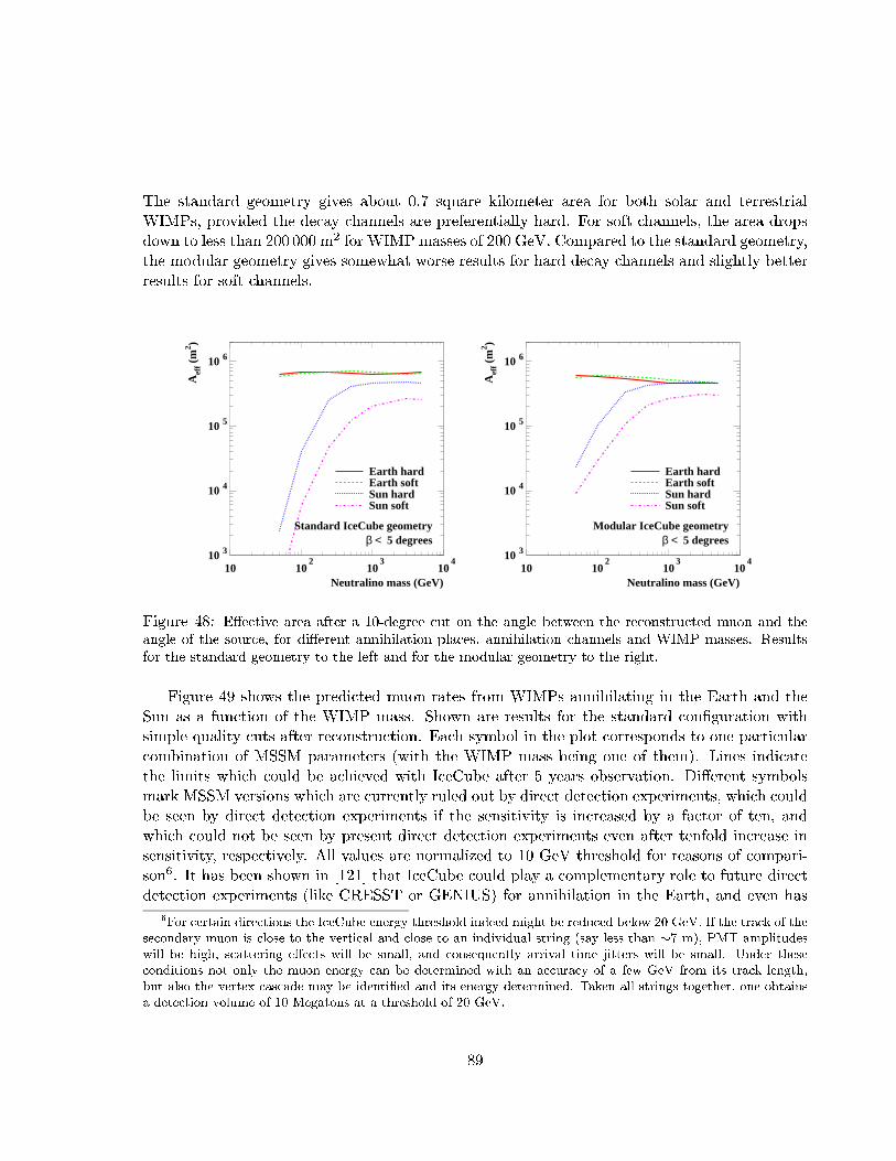
The standard geometry gives about 0.7 square kilometer area for both solar and terrestrial

WIMPs, provided the decay channels are preferentially hard. For soft channels, the area drops

down to less than 200 000 m2 for WIMP masses of 200 GeV. Compared to the standard geometry,

the modular geometry gives somewhat worse results for hard decay channels and slightly better

results for soft channels.

10 3

10 4

10 5

10 6

10 102

103

104

Neutralino mass (GeV)

Aef

f (m

2 )

Earth hardEarth softSun hardSun soft

β < 5 degreesStandard IceCube geometry

10 3

10 4

10 5

10 6

10 102

103

104

Neutralino mass (GeV)

Aef

f (m

2 )

Earth hardEarth softSun hardSun soft

β < 5 degreesModular IceCube geometry

Figure 48: E�ective area after a 10-degree cut on the angle between the reconstructed muon and the

angle of the source, for di�erent annihilation places, annihilation channels and WIMP masses. Results

for the standard geometry to the left and for the modular geometry to the right.

Figure 49 shows the predicted muon rates from WIMPs annihilating in the Earth and the

Sun as a function of the WIMP mass. Shown are results for the standard con�guration with

simple quality cuts after reconstruction. Each symbol in the plot corresponds to one particular

combination of MSSM parameters (with the WIMP mass being one of them). Lines indicate

the limits which could be achieved with IceCube after 5 years observation. Di�erent symbols

mark MSSM versions which are currently ruled out by direct detection experiments, which could

be seen by direct detection experiments if the sensitivity is increased by a factor of ten, and

which could not be seen by present direct detection experiments even after tenfold increase in

sensitivity, respectively. All values are normalized to 10 GeV threshold for reasons of compari-

son6. It has been shown in [121] that IceCube could play a complementary role to future direct

detection experiments (like CRESST or GENIUS) for annihilation in the Earth, and even has

6For certain directions the IceCube energy threshold indeed might be reduced below 20 GeV. If the track of the

secondary muon is close to the vertical and close to an individual string (say less than �7 m), PMT amplitudes

will be high, scattering e�ects will be small, and consequently arrival time jitters will be small. Under these

conditions not only the muon energy can be determined with an accuracy of a few GeV from its track length,

but also the vertex cascade may be identi�ed and its energy determined. Taken all strings together, one obtains

a detection volume of 10 Megatons at a threshold of 20 GeV.

89

a slight advantage over direct detection experiments for certain low-mass WIMP models and

annihilation in the Sun.

5.7.2 Neutrino oscillations

With a 10 Megaton detector of 20 GeV threshold, IceCube may also play a role in con�rming

the compelling indications that atmospheric neutrinos oscillate. Studies of systematics and

backgrounds have revealed that signi�cant progress requires much smaller spacing of OMs along

a string than presently planned (namely 4-6 meters). For reduction of the threshold toward the

horizon also a considerably smaller string spacing would be necessary. Such specialized e�ort

is only warranted if ongoing experiments fail to conclusively prove the oscillation hypothesis.

In that case one would consider to create a densely equipped region for detection of low-energy

contained events as one part of IceCube. This region would be nested in the full array which

acts as veto against through-going tracks. A possible solution would be to �ll AMANDA-II

with additional strings with small OM spacing. Note that interpretation of the feeble angular

dependent oscillation e�ects at high neutrino energies require an extremely good understanding

of the detector systematics.

In recent papers [122], the possibility is discussed to direct a neutrino beam to IceCube -

either a WBB beam or a beam from a neutrino factory. The short duty time of an accelerator

would allow to relax the cuts for background suppression since during the short spill times the

detector is nearly free of background. The aim would be to measure mixing angle �13 and the

sign of �m231, even though it is not possible to discriminate between charges. However, it has has

to be investigated how well discrimination between muon tracks and ccascades at low energies

would work.

5.7.3 MeV Neutrinos from Supernovae

Although the MeV-level energies of supernova neutrinos are far below the AMANDA/IceCube

trigger threshold, a supernova could be detected by observing higher counting rates of individual

PMTs over a time window of 5-10 s. The enhancement in rate of one PMT will be buried

in dark noise signals of that PMT. However, summing the signals from all PMTs over 10 s,

signi�cant excesses can be observed. With background rates more than 10 times lower than

ocean experiments, AMANDA and IceCube have the potential to see a supernova and to generate

an alarm signal.

IceCube, with low-potassium glass spheres (40K decays in the glass sphere are the main

source of external noise), might barely reach the the Large Magellanic Cloud.

AMANDA is oÆcially, and will actively be in the near future, a member of the Supernova

Early Warning System (SNEWS) [154]. The role of AMANDA will be to yield one of several

coincident alarm signals from di�erent detectors like Super-K, LVD and SNO (Macro being shut

down in the mean time). On top of that, IceCube might participate in the goal to estimate the

supernova direction by triangulation [153].

Figure 50 shows the increase in counting rate as seen in AMANDA-II and IceCube. Given

90

10-4

10-3

10-2

10-1

1

10

10 2

10 3

10 4

10 5

10 6

10 7

10 102

103

104

σSI > σSIlim

σSIlim > σSI > 0.1σSI

lim

0.1σSIlim > σSI

Ethµ = 10 GeV

Standard IceCube Geometry

Neutralino Mass (GeV)

Muo

n ra

te fr

om th

e E

arth

(km

-3 y

r-1)

Hard

Soft

10-4

10-3

10-2

10-1

1

10

10 2

10 3

10 4

10 5

10 6

10 7

10 102

103

104

σSI > σSIlim

σSIlim > σSI > 0.1σSI

lim

0.1σSIlim > σSI

Ethµ = 10 GeV

Standard IceCube Geometry

Neutralino Mass (GeV)

Muo

n ra

te fr

om th

e S

un (

km-3

yr-1

)

Hard

Soft

Figure 49: The predicted muon rates from WIMPs annihilating in the Earth (left) and the Sun (right)

as a function of the WIMP mass. Each symbol in the plot corresponds to one particular combination

of MSSM parameters. Lines indicate the limits which could be achieved with IceCube after 5 years

observation. Di�erent symbols mark MSSM versions which are currently ruled out by direct detection

experiments (dots), which can be seen by direct detection experiments if the sensitivity is increased by a

factor of ten (+), and which could not be seen by present direct detection experiments even after tenfold

increase in sensitivity (�), respectively.

91

a known template for time evolution of the pulse, the resulting accuracy in timing could be

14 ms for AMANDA-II and as good as 1-3 ms for IceCube. The resulting angular resolution

depends on the orientation of the triangulation grid with respect to the supernova. For the

three detectors Super-K, SNO and IceCube it would between typical values of 5 to 20 degrees.

Figure 51 shows the �2-contours of reconstructed supernova direction for a randomly choosen

supernova event.

With dedicated detectors like Super-K, one can determine the neutrino direction from elec-

tron direction measurement in � e� interaction with an accuracy of about 5Æ.

Figure 50: Simulated count rate data for a supernova at the center of the Galaxy, for AMANDA-II (left)

and IceCube (right). The lines correspond to the simulation input.

5.7.4 Relativistic magnetic monopoles

Several theories predict the existence of magnetic monopoles with a magnetic charge which

obeys the Dirac quantization rule g = n � e=(2�) with n = 1; 2; 3; ::: and � = 1=137. A magnetic

monopole with unit magnetic Dirac charge g = 137=2 � e and a velocity � close to 1 would emit�Cerenkov radiation along its path, exceeding that of a bare relativistic muon by a factor of

8300 for � = 1. The value 8300 is obtained from (137=2)2 multiplied with n2r, with nr = 1:33

being the refractive index of water. This is a rather unique signature. Figure 52 shows the light

emission from a monopole as a function of �. Note that due to the production of Æ electrons,

the monopole produces light even below its own �Cerenkov threshold.

92

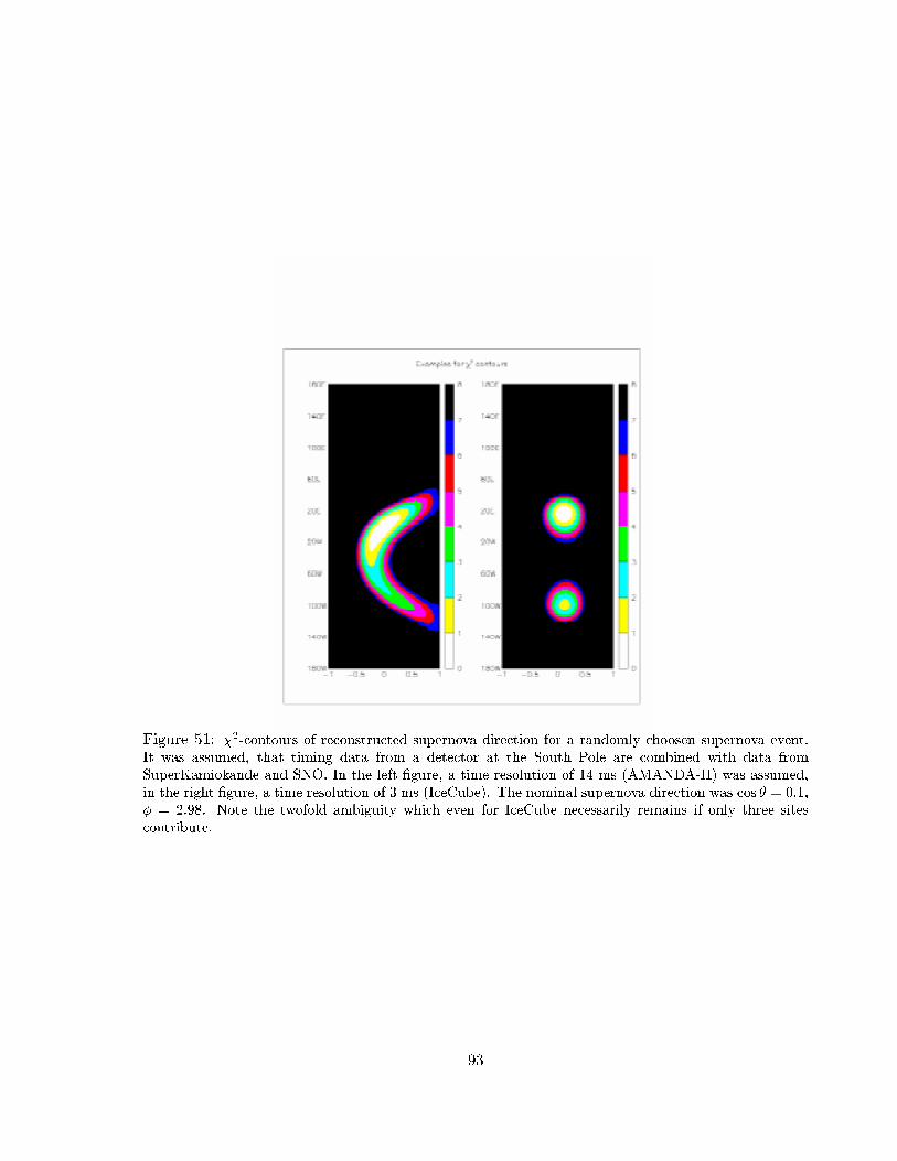
Figure 51: �2-contours of reconstructed supernova direction for a randomly choosen supernova event.

It was assumed, that timing data from a detector at the South Pole are combined with data from

SuperKamiokande and SNO. In the left �gure, a time resolution of 14 ms (AMANDA-II) was assumed,

in the right �gure, a time resolution of 3 ms (IceCube). The nominal supernova direction was cos � = 0:1,

� = 2:98. Note the twofold ambiguity which even for IceCube necessarily remains if only three sites

contribute.

93

dn /

dx ,

cm-1

bare

0.4 0.6 0.8 1.0

β

10

10

10

10

10

10

107

6

5

4

3

2

1

0

10

monopole

δ

muon

Figure 52: �Cerenkov light emission from magnetic monopoles in water (in photons per cm) as a function

of velocity. The curve labeled \Æ" represents the light produced by delta electrons which are generated

by the monopole below its �Cerenkov threshold.

94

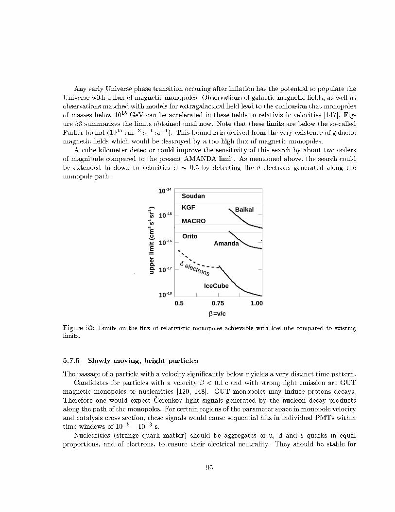
Any early Universe phase transition occuring after in ation has the potential to populate the

Universe with a ux of magnetic monopoles. Observations of galactic magnetic �elds, as well as

observations matched with models for extragalactical �eld lead to the conlcusion that monopoles

of masses below 1015 GeV can be accelerated in these �elds to relativistic velocities [147]. Fig-

ure 53 summarizes the limits obtained until now. Note that these limits are below the so-called

Parker bound (1015 cm�2 s�1 sr�1). This bound is is derived from the very existence of galactic

magnetic �elds which would be destroyed by a too high ux of magnetic monopoles.

A cube kilometer detector could improve the sensitivity of this search by about two orders

of magnitude compared to the present AMANDA limit. As mentioned above, the search could

be extended to down to velocities � � 0:5 by detecting the Æ electrons generated along the

monopole path.

-1-1

10-14

-2

IceCube

10

10

10

-15

-16

-17

-18100.5 0.75 1.00

Soudan

Baikal

β =v/c

KGF

uppe

r lim

it (c

m s

sr

)

Orito

MACRO

Amanda

electrons

δ

Figure 53: Limits on the ux of relativistic monopoles achievable with IceCube compared to existing

limits.

5.7.5 Slowly moving, bright particles

The passage of a particle with a velocity signi�cantly below c yields a very distinct time pattern.

Candidates for particles with a velocity � < 0:1 c and with strong light emission are GUT

magnetic monopoles or nuclearities [120, 148]. GUT monopoles may induce protons decays.

Therefore one would expect �Cerenkov light signals generated by the nucleon decay products

along the path of the monopoles. For certain regions of the parameter space in monopole velocity

and catalysis cross section, these signals would cause sequential hits in individual PMTs within

time windows of 10�5 { 10�3 s.

Nuclearities (strange quark matter) should be aggregates of u, d and s quarks in equal

proportions, and of electrons, to ensure their electrical neutrality. They should be stable for

95

all baryon numbers in the range between ordinary nuclei and neutron stars (A � 1057). They

could have been produced in the primordial Universe or in violent astrophysical processes. See

for recent reviews [148, 149].

The most relevant upper limits on the ux of these particles come from track etch experiments

or liquid scintillator experiments (both e.g. represented by MACRO). The Baikal experiment

has searched for enhanced counting rates over time intervals of 500 �s and deduced upper limits

on the ux of GUT monopoles and strange quark matter [120]. The search technique relies on

detectors with a low counting rate. In the Baikal case a rate as low as 100 Hz is achieved by

local coincidences. With a counting rate per OM of 300 Hz (compared to typically 1 kHz for

AMANDA), also IceCube may look for corresponding phenomena.

5.8 IceCube Con�guration Flexibility

The default IceCube con�guration is optimized for the TeV{PeV neutrino energy region. In the

scenario where a potential signal is seen at PeV energies or above, but the IceCube array has not

yet been fully deployed, the IceCube design permits considerable exibility. String deployments

can be modi�ed to increase subsequent interstring spacings, expanding the geometrical area

at little added �nancial expense. Since muons at these energies are brighter, one crossing the

array would experience no \blind" corridors. Of course, performance at lower energies would

su�er with increasing interstring spacing. Conversely, if a signal is detected at the lower end of

the TeV{PeV energy scale, the detector can be \back�lled" using as-yet-undeployed DOMs to

increase the overall pixel density. This would enhance sensitivity to lower energy neutrinos.

5.9 Calibration of High-Level Detector Response Variables

Detector geometry, angular response, vertex resolution and energy response can be calibrated

using in situ light sources, IceTop-tagged or untagged downgoing cosmic-ray muons, and atmo-

spheric neutrinos. Examples of in situ light sources include blue and UV LEDs, lasers buried in

the ice or placed on the surface and connected via optical �ber to di�using elements placed in

the ice, buried DC light sources, etc. Lower-level parameters like cable lengths will be calibrated

online by the DAQ system and can be veri�ed by adapting some of the techniques described

below.

5.9.1 Geometry Calibration

IceCube simulations indicate that downgoing muons can be used to determine the relative posi-

tions of the OMs to an accuracy of less than 1 m, which is suÆcient for accurate reconstruction of

neutrino-induced muons and cascades. The algorithm entails using �tted downgoing cosmic-ray

muon tracks and calculating the probability for a photon from the track to arrive at each of a

number of imaginary spatial grid points surrounding the putative OM position. Averaging over

many tracks, each set of grid points around each OM describes a paraboloid whose maximum

can be used to estimate the true OM position. Using these new position estimates for each OM

we can then repeat the entire procedure until the iterative procedure converges.

96

-2

-1.5

-1

-0.5

0

0.5

1

1.5

2

0 1 2 3 4 5 6 7 8 9

Y S

hift

[m]

Iteration

OM Displaced in Y by 1.5 m

OM 700

Figure 54: Calculated correct position of a single OM. The OM was intentionally displaced from its true

position by 1.5 m The procedure demonstrates that convergence occurs in three iterations.

97

-2

-1

0

1

2

680 700 720 740

OM Channel

∆X (

m)

0

5

10

-2 -1 0 1 2

8.278 / 11

Constant 8.994

Mean -0.6125E-01Sigma 0.2568

∆X (m)

Ent

ries

-2

-1

0

1

2

680 700 720 740

OM Channel

∆Y (

m)

0

2.5

5

7.5

10

-2 -1 0 1 2

7.148 / 11Constant 7.510

Mean -0.5408E-01

Sigma 0.3174

∆Y (m)

Ent

ries

-2

-1

0

1

2

680 700 720 740

OM Channel

∆Z (

m)

0

2.5

5

7.5

10

-2 -1 0 1 2

11.51 / 12

Constant 6.658

Mean -0.2859Sigma 0.2987

∆Z (m)

Ent

ries

Figure 55: Left plots: Intentional displacements of OMs (straight lines), all applied at the same time,

and their calibrated positions (dots connected by lines). Right plots: Calibrated OM positions relative

to original correct values. The left plots demonstrate that the calibration procedure can cope with string

displacements which are larger than what the IceCube drill is designed to deliver. The right plots show

that the resolution of the calibration is roughly 30 cm. The o�set in �Z is believed to be an artifact of

inaccuracies in the Monte Carlo parameterization of the photon arrival times.

98

Tests using simulated data have shown that the procedure converges quickly enough that it

can be used to determine geometry positions of OMs almost immediately after deployment. A

plot showing the convergence of the procedure for a single OM, whose position was intentionally

displaced from its correct position by 1.5 m, is shown in �g. 54. Figure 55 shows how well the

procedure calibrates the correct OM positions after intentional three-dimensional displacements

of a string's position. This procedure will be a useful high-level test of the success of the

deployment at the full-string level, and will permit the running of subsequent calibrations which

require detector geometry as input. More computationally intensive re�nements of the technique

can be used to �ne-tune the positions for use by the online �lters and downstream data analyses.

(Bright in situ light sources may also be useful for geometry calibrations, and indeed this is how

the AMANDA geometry has been calibrated. However, IceCube's larger interstring spacing may

limit the e�ectiveness of this techinque.)

5.9.2 Calibration of Angular Response

Events simultaneously triggering IceTop and IceCube constitute a data sample which can be

used to calibrate IceCube's angular response. A similar technique has been used successfully

by AMANDA with SPASE-2 triggers, where only a limited solid angle was available for study.

With substantially larger solid angle coverage, IceTop should enable IceCube to calibrate its

angular response more completely and accurately.

Over a smaller solid angle, IceTop can provide a tagged single muon beam for calibration of

IceCube response to single muons and their direction reconstruction. This will require a denser

subarray component, either in the center or perhaps also at one or more other locations on the

surface, that triggers at a much lower threshold for showers with energies of roughly 10 TeV

that are most likely to have only zero or one high energy muon capable of reaching IceCube.

5.9.3 Calibration of Vertex Resolution

The vertex resolution for cascades can be studied with pulsed in situ light sources located at

known positions in the ice. Varying the intensity of these sources provides a way to study

the vertex resolution as a function of energy. In AMANDA, sources have been determined to

produce light outputs equivalent to a cascade event with several hundred TeV of energy.

5.9.4 Energy Calibration

The IceCube energy response can be calibrated using a number of independent techniques.

Atmospheric neutrinos provide a test-beam with a known energy spectrum against which Ice-

Cube can be calibrated. Downgoing muons may also be of use here, although often such events

are composed of mulitple muons. (This may be addressed by IceTop, as discussed below.)

Bremsstrahlung events from downgoing muons provide an energy calibration for cascades at the

lower end of the energy scale, up to several hundred GeV. In situ light sources, preferably with

precisely controllable output intensities, o�er a way to calibrate IceCube energy response to

cascades at higher energies, up to roughly 500 TeV.

99

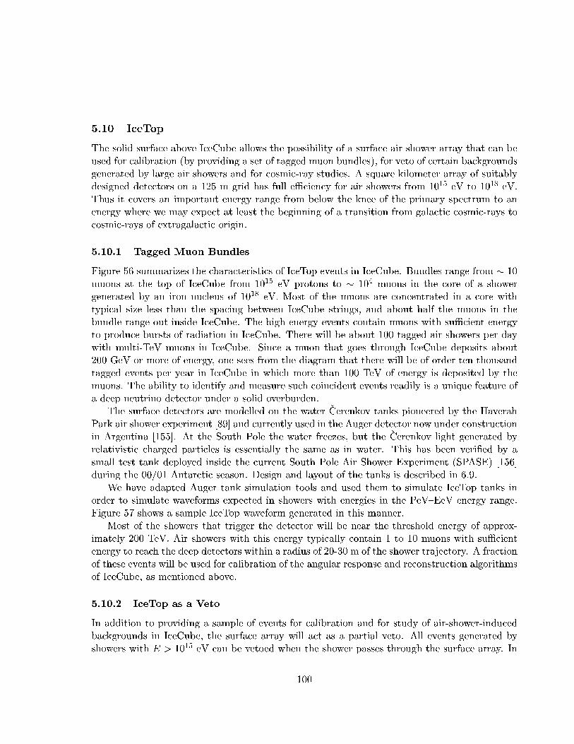
5.10 IceTop

The solid surface above IceCube allows the possibility of a surface air shower array that can be

used for calibration (by providing a set of tagged muon bundles), for veto of certain backgrounds

generated by large air showers and for cosmic-ray studies. A square kilometer array of suitably

designed detectors on a 125 m grid has full eÆciency for air showers from 1015 eV to 1018 eV.

Thus it covers an important energy range from below the knee of the primary spectrum to an

energy where we may expect at least the beginning of a transition from galactic cosmic-rays to

cosmic-rays of extragalactic origin.

5.10.1 Tagged Muon Bundles

Figure 56 summarizes the characteristics of IceTop events in IceCube. Bundles range from � 10

muons at the top of IceCube from 1015 eV protons to � 104 muons in the core of a shower

generated by an iron nucleus of 1018 eV. Most of the muons are concentrated in a core with

typical size less than the spacing between IceCube strings, and about half the muons in the

bundle range out inside IceCube. The high energy events contain muons with suÆcient energy

to produce bursts of radiation in IceCube. There will be about 100 tagged air showers per day

with multi-TeV muons in IceCube. Since a muon that goes through IceCube deposits about

200 GeV or more of energy, one sees from the diagram that there will be of order ten thousand

tagged events per year in IceCube in which more than 100 TeV of energy is deposited by the

muons. The ability to identify and measure such coincident events readily is a unique feature of

a deep neutrino detector under a solid overburden.

The surface detectors are modelled on the water �Cerenkov tanks pioneered by the Haverah

Park air shower experiment [89] and currently used in the Auger detector now under construction

in Argentina [155]. At the South Pole the water freezes, but the �Cerenkov light generated by

relativistic charged particles is essentially the same as in water. This has been veri�ed by a

small test tank deployed inside the current South Pole Air Shower Experiment (SPASE) [156]

during the 00/01 Antarctic season. Design and layout of the tanks is described in 6.9.

We have adapted Auger tank simulation tools and used them to simulate IceTop tanks in

order to simulate waveforms expected in showers with energies in the PeV{EeV energy range.

Figure 57 shows a sample IceTop waveform generated in this manner.

Most of the showers that trigger the detector will be near the threshold energy of approx-

imately 200 TeV. Air showers with this energy typically contain 1 to 10 muons with suÆcient

energy to reach the deep detectors within a radius of 20-30 m of the shower trajectory. A fraction

of these events will be used for calibration of the angular response and reconstruction algorithms

of IceCube, as mentioned above.

5.10.2 IceTop as a Veto

In addition to providing a sample of events for calibration and for study of air-shower-induced

backgrounds in IceCube, the surface array will act as a partial veto. All events generated by

showers with E > 1015 eV can be vetoed when the shower passes through the surface array. In

100

10-4

10-3

10-2

10-1

100

101

102

103

104

10-1 100 101 102

Nµ(

>E

µ)

per

sho

wer

with

E0

Eµ (TeV at production)

Energy spectra of muon bundles in IceCube

TopBottom

of IceCube

Burst regime

Rate per yr

50

5000

5*105

5*107

>109

E0=1018 eV

1017

1016

1015

1014

Figure 56: Diagram showing the energy spectra of muon bundles in IceCube associated with air showers

(proton primaries) that can be measured with IceTop. Each curve is labelled at the left by the primary

energy of the associated shower and on the right by the number of events per logarithmic energy interval

that strike the surface array within the solid angle determined by IceTop and IceCube. The surface

array is fully eÆcient for showers above 1015 eV. The arrows indicate muon energy at production in the

atmosphere needed to reach the top and the bottom of IceCube. Muons above � 3 TeV will tend to

produce bursts of radiation in IceCube.

101

Figure 57: The upper panel shows the waveform of the signal at 300 m from the shower core for a

proton-initiated shower of 100 PeV. The simulation is for an 8 in PMT at the center of the tank viewing

photons re ected from the bottom and sides of the ice tank. The lining of the cover is black. The

marks at the top of the �gure indicate the arrival time at the top of the ice of muons (top set of marks),

electrons (middle set of marks) and -rays (bottom set of marks). The lower panel shows the the muon

contribution to the waveform. In both panels the amplitude is plotted as a function of time at the output

of the base of the PMT. Most of the delay is due to the drift time of electrons in the PMT.

102

addition, higher energy events, which are a potential source of background for neutrino-induced

cascades, can be vetoed even by showers passing a long distance outside the array. In particular,

showers with E > 1017 eV and cores a km outside the array will produce a minimal trigger near

the boundary of the array.

5.10.3 Cosmic-ray Physics

The IceCube-IceTop coincidence data will cover the energy range from below the knee of the

cosmic-ray spectrum to > 1018 eV. Each event will contain a measure of the shower size at

the surface and a signal from the deep detector produced by muons with E� > 300 GeV at

production. At the high elevation of the South Pole, showers will be observed near maximum

so that shower size will give a relatively good measure of primary energy. The ratio of the

muon-induced signal in IceCube as a function of primary energy (as determined by shower size

at the surface) will give a new measure of primary composition over three orders of magnitude

in energy. In particular, if the knee is due to a steepening of the rigidity spectrum, a steepening

of the spectrum of protons around 3 � 1015 eV should be followed by a break in the spectrum

of iron at 8� 1016 eV.

103

6 Experimental Requirements

In this section we discuss the requirements on IceCube technologies dictated by science. The

most important requirements can be summarized as follows:

� time resolution of � 5 ns rms,

� waveform digitization with � 200 Msps (�rst 400 ns) and � 33 Msps (thereafter),

� waveform sampling depth of 4 �s,

� dynamic range of � 200 PE/15 ns,

� dead time of � 1%,

� gain variation of � 2% per week,

� OM noise rate � 500 Hz,

� overall permanent channel failure rate of < 5%.

While extensive simulations of the IceCube detector and its performance have been done,

ongoing studies of improved analysis techniques using the operating AMANDA-II detector may

still suggest changes in these requirements.

6.1 Time Resolution

From operation and Monte Carlo simulations of the AMANDA detector we have learned that

event rates and angular resolution of atmospheric neutrinos, as well as the eÆciency for rejecting

the background of atmospheric muons, do not depend on the accuracy of time calibration (t0)

and on time resolution (�t) provided they do not exceed 10 ns. Deterioration of the detector

performance becomes apparent only above 15 ns because below this scale scattering in the bulk

ice is the dominant e�ect. For the higher energy PeV{EeV neutrino signals in IceCube, the

requirement may even be looser because the average distances over which photons are collected

are increased and so are the e�ects of scattering. For electromagnetic showers, waveform digi-

tization will be important, but a timing accuracy similar to the one required for muon tracks

should be adequate.

A resolution of � 5 ns is a well-motivated requirement. Better resolution results in better

performance in rare cases. For instance, science requiring low thresholds, or the detection of

short muon tracks very close to strings, may bene�t from better time resolution because the

e�ect of scattering is suppressed. Examples are the detection of neutrinos from the annihilation

of dark matter particles in the center of the Earth (producing short, nearly vertical muons) and

the detection of oscillating beams from an accelerator at a northern site. One may also be able

to argue for improved time resolution on the basis of better reconstruction of the direction of

electromagnetic showers induced by electron-neutrinos, or to separate close showers from the

production and decay of tau-neutrinos (double bang events). One should keep in mind that time

resolution is ultimately limited by the PMT at 1{2 ns for multi-PE signals.

104

6.2 Waveforms

Experience with the AMANDA detector for observing electromagnetic showers and high-energy

showering muons has demonstrated the signi�cant advantages of using the presently available

\reduced" waveform information, like amplitude and time-over-threshold (TOT) rather than

amplitude alone. Light scattering results in strong signal dispersion over large distances. This

e�ect dilutes information (namely the precise arrival time of the �rst photon), but also adds

information: The length of the light signal recorded by a single PMT indicates the distance to the

light source. Therefore the combination of amplitude and time structure allows one to distinguish

between close, dim light sources and distant, bright light sources. The reconstruction of distant

tracks and very large high energy showers will therefore require full waveform digitization. For

instance, simulations based on TOT alone have demonstrated very poor angular resolution for

electromagnetic showers.

Waveforms should be recorded at a rate of � 200 Msps for the �rst 400 ns in order to obtain

good timing and double pulse resolution. For longer times, a lower sampling rate of � 33 Msps

is suÆcient to tease out structure due to secondary light pulses such as those due to double

bangs from �� events.

The waveform sampling depth should be roughly 4 �s, long enough to capture full waveform

information from most (but not all) double bang events.

6.3 Dynamic Range and Linearity

The basic requirement is a dynamic range of 200 PEs per 15 ns. The interval 15 ns represents

the typical time duration of a single PE pulse. This requirement is mostly driven by the recon-

struction of energy and direction of very high-energy showers, typically 1 PeV. These produce

measurable light over times of several hundreds of nsec. The amplitude and the waveform of

the light pulses at the OM carry information on the position, the directionality and the energy

of the shower. Figure 58 shows AMANDA-II PMT pulses from an in situ N2 laser pulse with

a light output equivalent to a 1 PeV shower. The oscilloscope pulses shown are from OMs at

three distances between 45 and 167 m.

Because of scattering of the photons in the ice, the shape of the photon pulse broadens with

increasing distance from the point of emission. For example, at a distance of 60 m (about half

the string spacing in IceCube) a 1 PeV shower will generate a PMT pulse of 1000 (200) PEs

with a FWHM of 100 ns (150 ns) in forward (backward) direction of the shower. The example

illustrates the directionality information contained in these data. Such an event will be observed

by hundreds of OMs up to distances of more than 250 m from the interaction. The maximum

current in this event reaches 12 PE/ns, or 180 PE/15 ns. Because of the greatly enhanced cross-

section at 6.4 PeV (Glashow resonance), events at this energy may be preferentially observed,

despite a falling spectrum. For these events, the peak input signal is more than 1000 PE/15 ns

(at a distance of 60 m).

The non-spherical shape of the initial light pattern can be exploited for good directional

and energy reconstruction. While the number of PMTs that saturate increases with higher

105

Figure 58: PMT signals from a 335 nm nitrogen laser signal simulating a 1 PeV shower (about 1010

photons). The light is detected by AMANDA-II optical modules with �ber-optic readout at distances of

approximately 45 m (black trace), 115 m (red trace), and 167 m (cyan trace).

106

energies (10 PeV and higher), the total number of PMT that observe a signal grows by an

even larger number. Based on evaluations of simulated waveforms, we conclude that a dynamic

range of about 15 PE/ns would be suÆcient for an accurate reconstruction of the relevant event

parameters (energy, direction), even though OMs nearest the shower will saturate.

PMTs that are very close to the shower core will saturate at the maximum anode current

that a PMT is able to sustain. In the case of the Hamamatsu 10 in PMT, which is a prime

candidate for IceCube, the anode current is limited to 80 mA, which sets an upper limit on the

dynamic range in PE that depends on the gain. The operating conditions of IceCube suggest

a gain of � 107, corresponding to a theoretical peak of 500 PE/15 ns. It seems reasonable to

expect that the PMT can sustain anode currents of 200 PE per 15 ns for intervals of about

100{200 ns. Recognizing the limitations on the dynamic range set by the PMT, and accepting

a saturation of the 10% of the OMs near the shower core, we set the physics requirement for the

dynamic range to 200 PE/15 nsec.

6.4 Absolute Amplitude Calibration and Stability

The absolute calibration of OMs should be known to better than 5%. The absolute calibration

and measurement of the angular acceptance of the instrument will be performed by observing

known signals from LEDs and from cosmic ray muon tracks. The measurement of shower pro�les

requires good calibration of individual OMs; see above. The dependence of the muon e�ective

area of the operating AMANDA-B10 detector is close to, but less than linear.

6.5 Dead time

We aim for a deadtime for muon triggers as low as 1%, assuming a trigger rate of 100 Hz.

Actually, one might consider to lower certain thresholds of the hardware triggers, e.g. in order

to cover low energy tracks. This might increase the trigger rate and �nally lead to a slightly

higher deadtime.

6.6 Sensitivity of optical modules

Maximum light collection is of highest importance. In particular, it helps to lower the detection

threshold for low energy muons and increases the detection sensitivity for supernovae. For high

energy muons or cascades, it might allow for an increase in the string spacing. Compared to

Amanda-II, the light collection will be improved by the use of PMTs with diameter 10 in or larger,

giving about 40% better light collection than the present 8 in PMTs. If a sound technological

solution is found, wavelength shifter coatings should be applied to the glass spheres. Present

results indicate that this may result in a 20{35% better light conversion.

6.7 Noise Rate and Noise Rate Stability

Ice is a very low noise medium; the noise is dominated by radioactivity introduced by the OM

itself. The noise rate in individual OMs is required to be less than 0.5 kHz (compared to typically

107

1 kHz in the present AMANDA array). For that aim, glass spheres with very low radioactivity

content (< 0:05% potassium content) should be chosen. Rates for all OMs should be recorded

for optimal sensitivity and detector monitoring.

For the muon trigger, this level of noise is readily eliminated by the use of local coincidences

(a pair of OMs that are adjacent or separated by no more than one OM report).

Supernova detection is based on the identi�cation of rate excesses over a few seconds. It

is made possible by the low noise rates and becomes impossible if the rates are as high as

2 kHz. With 300 Hz noise rates, IceCube could monitor not only our own Galaxy, but also the

Magellanic cloud.

Rates have to be recorded every ms with 10 bit dynamic range, with the possibility to adjust

arti�cial dead time between 0 and 1 ms in 10�s steps.

6.8 Failure Rate

IceCube Monte Carlo studies have shown that the quality of muon and cascade reconstructions

are rather resilient to permanent channel failure rates as high as 10%. (A permanent channel

failure is one which cannot be repaired, e.g., a broken in-ice connector.) For muons, only the

di�erence between the true and reconstructed space angle shows some degradation, but only by

roughly 3%; for cascades there is essentially no degradation at all. These results can be extended

qualitatively to tau events as well.

The main impact of such failures would be to reduce the detector sensitivity. This reduction

is energy-dependent and is more pronounced at lower energies. For example, a 10% failure rate

results in the loss at trigger level of 40% of muons with energies between 400 and 500 GeV, but

only 5% of muons with energies between 8 and 10 TeV. Above about 30 TeV there is no loss. A

10% loss would therefore not dramatically a�ect ultrahigh energy muon neutrino physics, but

it would adversely impact IceCube atmospheric muon neutrino physics, and the usefulness of

these neutrinos as an IceCube calibration tool.

Under the reasonable assumption that sensitivity loss varies roughly linearly with the per-

manent failure rate, requiring the permanent channel failure rate to be below 5% reduces the

impact of such losses on atmospheric muon neutrino physics. At the same time, a 5% failure

rate is a realistic goal.

6.9 IceTop

The IceTop array should trigger at near the 90% level for air showers above 500 TeV, which

will require stations of roughly 7 m2 area located near the top of each string. The tanks should

have a dynamic range of � 104 to cover the PeV{EeV energy range without saturation over the

full lateral extent of the showers. This will likely require using separate low gain and high gain

modules within each tank.

To reduce the background rate each station should consist of two tanks, each roughly 3.5 m2

in area. A local coincidence should be implemented between neighboring tanks to eliminate

single muon events as well as reduce the likelihood of triggering on random electron and photon

108

hits not associated with larger air showers. The separation of these individual tanks should be

large enough to keep the number of local triggers to a level that can be handled by the DOM

communications, perhaps several meters.

A denser subarray within IceTop should consist of smaller tanks on the order of 1 m2 area

separated by 10 m so that they will have a much lower threshold near 10 TeV to trigger on

showers most likely to contain only one high energy muon. This subarray could be composed

of the present SPASE array with an embedded standard IceTop station. The subarray should

record only a fraction of the data that triggers depending on what is needed for calibration and

most acceptable for the DAQ.

In addition, it is possible that we will decide to record as much of this low energy data as

DOM communications will allow, storing several days of data in a disk cache at the Pole. This

cache should be accessed when interesting IceCube events come in over that same time, when

all low energy surface array data from a wide time window on each side of the interesting events

should be separated out and stored for later investigations.

109

7 Design and Description of IceCube

7.1 Overview

In the IceCube baseline design, 80 strings are regularly spaced by 125 m over an area of ap-

proximately one square kilometer, with OMs at depths of 1.4 to 2.4 km below the surface, as

shown in �g. 59. In sections 5 and 6 the performance criteria and experimental requirements

for this device have been distilled from the scienti�c goals. In addition to explicit technical

requirements, however, the instrumental design concept must incorporate many additional fac-

tors such as system cost, software/hardware integration issues, engineering risks, lowest practical

power dissipation, noise rejection, noise generation, thermal and physical shock, data ow, Mean

Time Before Failure (MTBF) of components, production Quality Assurance (QA), deployment,

constraints on commissioning personnel, remote intervention capabilities, calibration, cost of

operations, as well as disparate factors such as safety and educational values. The process of

optimization involving all these disparate issues has led to an innovative approach, with many

attractive features. Nevertheless, no exotic, high speed, brute force, or unproven elements are

needed in this concept.

There are three fundamental elements in this architecture, common to both IceCube and

IceTop:

� The Digital Optical Module (DOM), which captures the signals induced by physical

processes and preserves the information quality through immediate conversion to a digital

format using an innovative ASIC, the Analog Transient Waveform Digitizer (ATWD);

� A Network, which connects the highly dispersed array of optical modules to the surface

data acquisition system (DAQ) and provides power to them;

� A Surface DAQ, which maintains a master clock time-base and provides all messaging,

data ow, �ltering, monitoring, calibration, and control functions. Many design features

have been realized in the AMANDA string 18, as discussed below.

The instrument design is based on a decentralized digital architecture [157]. The motivation

for this approach arises primarily from the need to acquire, from a km-scale instrument, quite

complex information in the presence of substantial backgrounds.

Roughly 1.5 kHz of downgoing cosmic ray muons penetrate the geometric volume of IceCube,

about six orders of magnitude more than muons induced by neutrinos. The �Cerenkov radiation

cones generate complex optical signals that are further complicated by scattering in the ice

before detection. Parent directionality is not uniquely determined by simple time di�erences {

a horizontal muon generates equal quantities of upgoing and downgoing light. In most cases,

neutrino-induced upgoing muons are distinguishable from backgrounds only with sophisticated

�ts using global space-time correlations.

Given the high background/signal ratio and event complexity, it would be imprudent to �lter

out the atmospheric muons with tight trigger logic at an early stage. In addition, the downgoing

muons o�er an ever-present and copious calibration source, as well as a potential arena for the

110

AMANDA-II

SPASESouthPole

IceCubeRunway

Figure 59: A top view of the IceCube detector, showing the locations of the 80 IceCube strings as well

as the AMANDA-II array, the SPASE array, the airplane runway and the South Pole.

111

detection of subtle astrophysical processes, or possibly even signatures of extreme energy release

events in the cosmos.

As noted in section 5, data and simulations show that, for both neutrino-induced and back-

ground events, the information content at the photomultiplier (PMT) ranges from single photons

arriving over a span of about 1 �s to many hundreds (even thousands) of photons arriving within

15 ns. Extremely high-energy events may generate many thousands of photoelectrons in a con-

tinuum of complex patterns lasting several microseconds.

Figure 60 shows a fairly typical raw waveform obtained from a DOM operated in coincidence

mode to capture signals induced by a down-going muon. In this �gure, the �rst photon to be

detected appears in the ATWD record at about sample 20. Somewhat later, a larger number

of detected photons appears, possibly the result of a shower process at some distance from the

direct path of �Cerenkov light, or possibly the result of multiple muons passing nearby. From

a study of these waveforms it is clear that the arriving signals are frequently complex, in the

range of 15% for muon-induced signals. Because of the optical scattering, all photons must be

included in the analysis to determine the nature of the event.

A measure of the parent muon neutrino energy comes primarily from the capability to record

very large energy losses producing electromagnetic showers along a muon trajectory. For electron

neutrinos, the showers occur in isolation, requiring for identi�cation that no muon trajectory

is present. Tau neutrinos at extreme energies can produce two showers separated by a short

distance. The earlier parts of the shower-induced waveforms vary most rapidly and reach the

highest amplitudes. The most useful information about shower direction is found here, imposing

challenging technical requirements.

Time measurement of these signals over the km-scale volume must be established and main-

tained with a resolution and accuracy of �5 ns. The capture of this highly variable complex

information requires high-speed (�200 Msps), high dynamic range (�14 bits) waveform record-

ing. These technically challenging desiderata provide the impetus for an innovative instrument

design.

The architecture makes use of modern ideas that rely on time-stamps applied very early to

each datum. This approach reduces the amount of real-time circuitry to a remarkably small level

relative to traditional DAQ concepts. Correspondingly, data ow is built on conventional net-

working techniques using messages that may contain either data or control content. Advantages

of the architecture based on the DOM include:

� High dynamic range and signal purity since PMT signals are captured and digitized

in proximity and isolation.

� Low system power consumption due to an innovative custom ASIC, the Analog Tran-

sient Waveform Digitizer (ATWD).

� Fully automated remote commissioning and calibration procedures, minimizing

South Pole personnel, an extremely important consideration during South Pole modern-

ization .

112

Figure 60: An observed waveform due to muon(s) passing near a DOM pair, operated in coincidence.

113

� No low-level analog signal processing in the counting house o�ers more predictablelarge-scale system behavior.

� Absence of optical �bers in the system reduces system cost substantially, eliminates �30 plane ights, simpli�es and shortens deployment procedures, and maximizes reliability

since all connectivity is carried by copper wire pairs.

� Minimal real-time circuitry within the DAQ, made possible by time-stamped data

and message-based architecture.

� Network-based DAQ organization requires only one custom hardware design (the

DOM Hub).

� Use of commercial o�-the-shelf components reduces costs, shortens development

time, and enhances test facility realization.

� Year-round regular operation provided by robustness against noise at surface due to

drilling and pole operations, even during commissioning of new strings.

� Operational exibility is provided by programmable logic and CPU located within

DOM, permitting changes stimulated by data or new ideas.

The discussion of the Instrument Design elaborated below will bene�t from a brief description

of the performance obtained with a string of 41 Digital Optical Module (DOM) prototypes

deployed in January 2000 by the AMANDA Collaboration. These DOMs were intended to serve

two purposes:

1. Contribute to the regular AMANDA data stream by delivering real-time analog PMT

signals via optical �bers to the AMANDA counting room. Because these signals appear

identical to the signals of other strings, string 18 contributes to the scienti�c goals of

AMANDA without compromise.

2. Demonstrate the advantages and feasibility of a purely digital technical approach, in which

PMT signals are captured and digitized locally, within the optical module. The digital

data were transmitted to the surface using the twisted pair copper conductors that also

bring power and control signals to the DOMs.

Both of these purposes were achieved, despite challenging schedule and �nancial constraints.

The DOM prototypes of AMANDA string 18 were designed, built, and deployed in about 14

months, and strong support throughout the collaboration during this period was essential for the

ultimate success of the e�ort. Because schedule pressures were so severe, little attention could

be given to the issues of reliability and QA. Nevertheless, most of the DOMs of string 18 have

delivered extremely stable performance throughout the nearly two year period of operation. One

DOM board seems to have developed an internal problem; PMT HV can still be set so that this

module continues to contribute to AMANDA data. Two PMT HV bases appear to have failed,

114

indicating that re-engineering to enhance QA for this subsystem may be needed. There appears

to be an intermittent electrical connection in the main cable for another DOM. The remainder

of the 41 DOMs have operated continuously with no glitches, crashes, or other indications of

instability.

During CY 2000, the DOMs were equipped with a simple surface DAQ that could control

PMT HV, set other operating parameters, and return housekeeping data and occasional wave-

forms to the surface. In January 2001, a subset of four DOMs was equipped with a more complete

surface DAQ based on single-channel Test-Boards, designed initially for commissioning of DOM

boards. With the four-channel Test-Board DAQ, time synchronization is possible, permitting

data from di�erent DOMs to be correlated to a few nanoseconds, and even demonstrating the

detection of downgoing muons. Most of the technical results described in this section come from

an analysis of data obtained with the Test-Board DAQ.

The successful operation of AMANDA string 18 has proven not only the feasibility of the

digital system architecture, it has also shown that the associated software is both straightforward

to design and stable in operation. Much of the software framework that has enabled these

technical results will serve as a springboard for subsequent IceCube e�orts.

The block diagram of the Test-Board DAQ is shown in �gure 61. For reference, the various

approaches used by AMANDA are described in section 7.5.

7.2 Digital Optical Module

The Digital Optical Module (DOM) is a self-contained data acquisition platform that is

capable of capturing and digitizing real-time PMT pulses, storing data internally, and, when

requested, transmitting them to a surface data acquisition (DAQ) system. It contains its own

processor, memory, ash �le system, and real-time operating system (RTOS). The DOM is

capable of scheduling background communications tasks while acquiring data from a local wave-

form digitizer. All calibration functions needed to interpret data for physical content may be

invoked under software control; some operate as scheduled tasks without interfering with data

acquisition, and others require dedicated control of state.

A Field-Programmable Gate Array (FPGA) is used to implement most low-level logical func-

tions of the DOM, facilitating fully programmable and exible implementation of performance

features. The FPGA is programmed automatically from a con�guration �le that the CPU re-

trieves from ash memory in the DOM after power-up and self-boot has occurred. The FPGA

design and CPU programs can be replaced at will subsequent to deployment to enhance func-

tionality. This capability has been exploited already in the AMANDA string 18 (DOMs only),

using the satellite link to the south pole from the northern hemisphere.

The basic elements of the DOM are the optical sensor for �Cerenkov light, an electronic

circuit board for processing signals, a HV generator for the optical sensor, an optical beacon for

calibration purposes, and the glass pressure housing. The general physical layout of a generic

DOM is shown in �g. 62.

115

ControllerCPU

(Single−BoardLinux

Computer)

FPGA

PLD TB Power

Supply

High Pass FilterTwistedPair

(to DOM)Low Pass Filter

Communications

ADC

Communications

DAC

Communications

Disc.

8b

DAC

Test DAQ Board LayoutMain Components Diagram

Deployed for Time Calibrations, 2001.

PLLT.B.4

5b

33.6 MHz

PLLT.B.3

PLLT.B.1

PLLT.B.2

PLL(T.B.1)

GPS

10 MHz

16.8 MHz

(3 Othe

r Te

st Boa

rds)

PC−104RelaySwitch

80 VDOMPowerSupply

(3 Other T

est Boards)

16.8 MHz Clock Signalsto Multiple Components

Figure 61: Block diagram of the \Test-Board" used in the AMANDA DOM string DAQ system.

116

Photocathode

gel

Schematic view of OM with Digital and Optical Analog Capability

DOM PCB

LED Flasher PCB

PMT HV Power Supply PCB

Pulse Xfmr

PMT Anode signal cable

Electrical Cable

8.0"

Photocathode

Figure 62: Schematic pro�le view of a generic Digital Optical Module, showing pressure sphere, optical

coupling gel, PMT, signal processing electronics board, LED asher board, PMT base, and electrical

penetrator.

117

7.2.1 Pressure Housing

The spherical glass pressure housings are standard, well-proven items of commerce, used in

numerous oceanographic and maritime applications. For IceCube, the most important qualities

are mechanical reliability, cost, optical transmission, and potassium content. Commonly known

in the US as Benthospheres, a trade-name of Benthos, Inc., the dominant US supplier, these

simple devices have an excellent record for reliability. Over 700 of these, from both Billings

and Benthos, in various implementations and sizes, have been deployed in AMANDA without

evidence of a single implosive failure. To ensure reliability against implosion, care must be taken

not to chip either the surfaces of the hemispherical rims that form the equatorial ground-glass

seal, or the holes that permit penetrators to carry signals and power across the boundary. Costs

for standard pressure-tested Benthospheres are modest, in the range of $350.

For IceCube, a 13 in diameter sphere is the optimum size. While larger spheres are available

that could a accommodate larger optical sensor, the costs for drilling larger diameter holes (with

an appropriate margin of safety during deployment) rise very quickly, making larger sizes a poor

overall trade-o�.

Because the �Cerenkov radiation mechanism produces the greatest intensity at ever-smaller

wavelengths, limited ultimately by self-absorption, it is of interest to push the optical transmis-

sion limit of the glass to a value below the quantum eÆciency limit of the PMT. For processing

and mechanical strength, the manufacturers use a borosilicate glass that limits transmission to

about 350 nm, well above the expected �220 nm limit for deep polar ice. It is conceivable that

an exterior surface layer of an appropriate wavelength shifter for the component shorter than

350 nm could increase the e�ective light yield, and this is being explored.

The potassium content of the typical borosilicate glass includes a naturally occurring fraction

of 40K. The � particle from the decay of this isotope produces �Cerenkov radiation at a level that

dominates the observed PMT noise rate, unless steps are taken to reduce the overall potassium

content of the glass. At the request of IceCube collaborators, manufacturers have been able to

produce glass with substantially lowered potassium content without compromise to important

processing, mechanical, or optical qualities. It is anticipated that IceCube optical modules will

display noise rates very close to those of isolated dark-adapted PMTs.

7.2.2 Optical Sensor

The optical sensor is a medium-size (�10 inch diameter) hemispherical 10-stage photomulti-

plier tube (PMT), made by Hamamatsu. PMTs very similar to the intended device have been

deployed within AMANDA with generally excellent experience. These large PMTs o�er surpris-

ingly good time-resolution, as indicated by a transit-time-spread (TTS) for single photo-electron

(SPE) pulses of about 2.5 ns rms. Despite their large photocathode area, these PMTs, in total

equilibrated darkness, generate only �300 Hz or less of spontaneous noise pulses at temperaturesless than 0Æ. Photocathode sensitivity extends well into the UV, limited by the optical trans-

mission of the glass pressure sphere at 350 nm. For each detected photon, the PMT produces

SPE pulses that have characteristic rise (fall) times of 7 (11) ns.

118

Due to the stochastic nature of the electron multiplication process, SPE pulses display sig-

ni�cant variations in pulse shape and amplitude. The measured pulse area distribution of DOM

#1 (the deepest), acquired over a period of 10 days, is shown in �g. 63. The histogram is

formed by adding together consecutive ATWD samples for the pulses that rise above a digital

threshold, and subtracting a measured pedestal. This simple method works well enough if the

discriminator threshold that launches the ATWD is suÆciently low that nearly all SPE pulses

result in a trigger. It should be noted that a fair fraction of the PMTs in string 18 do not have

such good peak to valley ratios, and the spectrum shown in �g. 63 is better than most.

SPE Spectrum

Figure 63: Measured pulse area distribution of DOM #1 measured over a period of 10 days in CY 2001.

Most of the histogram is SPE noise pulses. The stochastic nature of the electron ampli�cation process

leads to a very broad distribution such that some SPE signals fall below threshold.

To de�ne a measure of gain, the peak region of spectra such as that shown in �g. 63 are

119

�t to a simple a Gaussian form. From the �t parameters, an average gain can be extracted.

Repeated measurements taken over 180 days in CY 2000 have demonstrated that the combined

PMT + DOM signal processing electronics provide excellent gain stability. These results are

shown in �g. 64. Because PMT gains were set to optimize the optical signal paths, which

had wide variations, and because some PMTs displayed poor peak-to-valley ratios, high quality

�ts could be obtained for less than half of the deployed ensemble of DOMs. The mean of

the distribution, � �2:8% per year corresponds to drifts of 0.05% per week, far below the

experimental requirement of 2% per week; none of this subset comes close to 2% per week.

Gain Drifts DOMs Percentage/Yr from ATWD

Figure 64: Measured distribution of a subset of DOM gains, recorded over a period of 250 days in CY

2000. The mean in this ensemble is less than 3% per year, with none approaching the experimental

requirement of �2%/week.

At a gain of 107, a typical SPE pulse will have an amplitude of �8 mV into a 50 load.

120

Under these conditions, the signal displays some nonlinearity at around 2 V, reaching complete

saturation at �4 V. The e�ective dynamic range under these conditions is approximately 500 PE.The PMT maximum output current at the anode is limited by space charge e�ects in the dynode

chain. As signal size increases, the space charge e�ects appear �rst at the last dynode, then at

the next to last, and so forth. Not only does the pulse amplitude display a non-linear relationship

to the input photon signal, but the pulse shape begins to stretch out considerably. The e�ective

dynamic range may, in principle, be increased by lowering the PMT gain below 107. At some

point in the range of a few millivolts, intrinsic electronic noise will degrade performance at the

SPE level.

With careful circuit design and layout, however, ultimate performance may exceed 500 PE

signi�cantly. It seems feasible to utilize a dynode tap to obtain a signal that could extend the

dynamic range at least another order of magnitude beyond what can be practically achieved

from the anode signal. This general idea has been used in many past experiments, and should

be practical for IceCube. This possibility is being explored actively.

7.2.3 PMT HV Generator

The PMT HV generator, known familiarly as the PMT base, is a multi-stage voltage multiplier,

or Cockroft-Walton circuit, with an oscillator running at a few tens of kHz. The base must

meet a number of important requirements, in particular, high reliability, high stability and low

induced noise. A voltage multiplier has certain potential advantages since the voltage steps

are smaller than that of a single stage multiplier. If arranged correctly, the base will naturally

supply the most current to the dynode stages near the anode, where the pulse loading occurs.

This produces an attractive low power design. On the other hand, there are more parts, which

could a�ect MTBF.

The IceCube PMT base will have two separate sections. One section, supplying the potential

di�erence between the photocathode and the �rst dynode, will be �xed at a voltage near the

manufacturer's indicated maximum. This produces a uniform transit-time among the DOMs,

and produces the best peak-to-valley ratio for the SPE pulse-height spectrum. The second

section will be variable under software control, to obtain the desired 1 � 107 gain. Experience

with AMANDA string 18 shows that reliability is an issue, as two bases appear to have failed. All

HV designs involving semiconductors must be based on conservative design practices, since even

extremely rare discharge mechanisms can be fatal. Induced noise also appears to be present,

at least in the timing measurements, which give better results with the PMT HV o�. The

re-engineering of the PMT base to improve reliability is recognized as an important task.

7.2.4 Optical Beacon

The string 18 DOMs are each equipped with six GaN LEDs, which emit predominantly in the

near-UV at 380 nm. The luminous intensity and the pulsing rate may be varied over a wide

range under software control. At their brightest, these beacons can be seen by OMs 200 m

distant. Due to their high intrinsic capacitance, LEDs are not easy to pulse at ns speeds; the

121

pulse width is �5 ns. The LEDs are broad angular emitters, spaced at 60Æ around a vertical axis,and are canted over to produce a roughly hemispherical source. Some AMANDA analog OMs

have been equipped with similar optical beacon boards using GaN LEDs emitting at 450 nm;

these have also proved to be useful for test purposes. The PMT HV must be turned down at

the emitting DOM to avoid potentially harmful pulses.

The optical beacons can be used to knit together a highly over-constrained measure of relative

DOM positions within the array. They can also be used to study optical properties of the ice at

these wavelengths.

7.2.5 Signal Processing Circuitry

The block diagram of the DOM signal processing circuitry is shown in �g. 65. The principal

logical and functional elements are:

� State control;

� Waveform capture and digitization;

� Local time generation;

� Local/master clock time transformation;

� Cable length measurement for timing o�sets;

� Data ow;

� Local coincidence capability;

� Control and glue logic, provided by an FPGA;

� A low-power 32-bit ARM CPU for higher level operations;

� Power conversion and �ltering;

� Monitoring and calibration;

� Message handling - send/receive .

State Control The DOM is operated as a slave in a master/slave relationship with the surface

DAQ. Upon power-up, it enters a wait state for an interval of a few seconds, to permit down-

loading of new �rmware or software. If no messages are received before time-out, the DOM will

boot from Flash memory and await commands. Normal operation of the DOM is dominated by

a data-taking state.

In addition, a local-time calibration process is periodically invoked, so that the local DOM

time may be ultimately transformed to master clock time with nanosecond accuracy. The time

calibration process appears as separately scheduled thread, with no deleterious impact upon

122

ATWD

CPUBoot ROM

LookbackSRAM

FPGA

FASTADC

CPU

SRAM

ApplicationFlash

BootFlash

PLD PMTBase

PowerSupply

High Pass FilterTwistedPair

(to Surface)Low Pass Filter

Communications

ADC

Communications

DAC

Communications

Disc.

SPE/MPEDisc.

8b

8b

10b

10b

Flashers

DAC

DAC

DACAnode, First Dynode

Digital Optical ModuleMain Components Diagram

First Prototype, Deployed 2000.

ToyocomOscillator

(16.8 MHz)

PLL(frequencydoubling)

Digital Clock Signalsto Multiple Components

Delay Line

Figure 65: Block diagram of the digital optical module signal processing circuitry.

123

the data-taking state. Other active threads are message receive/send and data transmission,

also invisible to the data-taking process. There are several calibration modes, such as running

optical beacons, cable length measurement, etc., during which normal data-taking is presumably

inactive.

Information Capture The DOM is equipped with innovative circuitry that is well-matched

to the PMT pulse characteristics and dynamic range. The capture of waveforms with �300 MHz

14 bit resolution is a daunting technical challenge if only conventional ash ADCs are considered.

Power dissipation for the ensemble of FADCs would be several watts, imposing an undesirable

operating condition; noise due to the large amount of digital activity and data ow presents an

inhospitable engineering environment. Instead, the DOM concept takes advantage of the fact

that, most of the time, nothing is happening: �t between pulses is more than 106 ns. Circuit

activity need occur only when pulses appear.

The waveform capture capability is realized through a custom Application Speci�c Inte-

grated Circuit (ASIC) designed at Lawrence Berkeley National Laboratory (LBNL), the Analog

Transient Waveform Digitizer (ATWD). The ATWD has four channels, each with 128 samples,

that synchronously record di�erent input waveforms. For IceCube, three of the channels will

capture the PMT signal presented at three di�erent gain settings. This arrangement provides an

elegant multi-range linear PMT signal capture method. With three channels operating at �15,�3, and �0.5 gains, the ATWD provides the rough equivalent of a �14 bit 200{800 MHz ADC.

Due to schedule pressures, the DOM prototypes in string 18 were equipped with only �10 and�2 gain channels. The third channel was, instead, routed to an analog multiplexer that could

connect to various internal signals for diagnostic purposes.

The fourth ATWD channel in string 18 DOMs is permanently connected to the DOM internal

clock, to calibrate/monitor ATWD sampling speed. Experience with string 18 has shown that

the ATWD sample speed is extremely stable. In IceCube, the fourth channel will be connected

to an analog multiplexer to permit that channel to share more than one function. The ATWD

sampling speed needs to be calibrated and monitored, but only rarely after initial calibrations

are completed and the system is stable. As noted above, some other internal signals that have

diagnostic value also need only infrequent interrogation. Most of the time, �99.9%, the fourthchannel is available to capture a dynode tap signal that could increase the PMT signal e�ective

dynamic range by at least another order of magnitude. The goal is to reach at least 5000 PE,

a capability that will enhance the reconstruction of EHE events, should they occur within the

volume of IceCube.

The capture process is initiated by a \launch" signal derived from a discriminator connected

to the high-gain signal path. The capture process stores waveforms as analog voltages on four

internal linear capacitor arrays. The sampling action is generated by an active delay line within

the ATWD, with \look-ahead" to create a sampling gate of width suÆcient to obtain adequate

settling on a capacitor before the gate switch opens, e�ectively closing that sampling window.

With the ATWD, waveform capture occurs at sampling speeds that may be varied at will

from �200 Msps to more than 1 Gsps, corresponding to capture intervals of 640{128 ns. It

124

appears that capture at �300 MHz (3.3 ns/sample) is appropriate for our scienti�c goals. The

higher speed capture is useful for characterizing PMT signal shape and other diagnostic purposes,

but is not needed to extract timing information from a typical waveform. A single DC current

controls the sampling speed. All channels within an ATWD sample synchronously, with aperture

variations between channels measured to be less than 10 ps.

The ATWD performance combination of �GHz sampling and very low power dissipation,

�100 mW is unmatched by any single commercial device for transient waveform capture. The

sampling action is controlled by an active delay line internal to the ATWD. No ultra-high speed

logic/clocks are needed in the DOM, a highly desirable engineering situation. The maximum

frequency in the string 18 DOMs is the local clock frequency, a very comfortable 33.6 MHz. For

IceCube, this frequency may be higher, but will likely not exceed 40 MHz.

Two ATWDs, arranged with alternate selection logic, permit capture of longer waveforms,

and also serve to reduce dead-time. For waveforms exceeding the ATWD capture interval,

sampling at a lower frequency is suÆcient to capture relevant information at later times. For

this purpose, The DOM is equipped with a 10-bit low-power FADC, operating at the DOM local

clock frequency. The PMT signal in this path is reshaped to match the lower sampling rate.

The ATWD has two distinct functions{transient waveform capture, and digitization of cap-

tured signal. These two functions are separately controlled, so that a captured signal sub-

sequently judged uninteresting may be ignored. This feature minimizes dead-time, and also

facilitates a true local coincidence capability (see sec. 7.2.9) between neighboring DOMs, in

which only time- and space-associated signals are digitized. The immediate conversion to a

digital format preserves data quality during subsequent DAQ data ow processes.

For interesting events, waveform capture in the ATWD is followed by 10-bit simultaneous

conversion of all 128 samples/channel by an internal common-rampWilkinson ADC. The internal

scalers count on both positive and negative clock transitions. At 33.6 MHz, complete digitization

requires about 15 �s. Because of natural CMOS manufacturing variations that create o�sets in

the internal comparators, there exists uctuations in the baseline, or pedestal, of the captured

waveform. These pedestal variations are in the range of 5{15 counts; they are quite stable and

are easily subtracted away during data processing.

A single ATWD digitizing waveforms at the nominal noise trigger rate of 300 Hz, will in-

troduce deadtime of �0.5%. To this, an additional deadtime of about 0.1% must be included

for readout of data via a 10-bit parallel bus. With two ATWDs operating in ping-pong mode,

deadtime due to random noise hits is less than 1� 10�4.

The ATWD is currently designed for a 1.2 �m CMOS process with double polysilicon ca-

pacitors. This manufacturing process may not be available inde�nitely, as new CMOS processes

with ever-smaller feature size and other characteristics supplant older ones. The ATWD should

be updated by not only choosing an appropriate one of these processes, but by increasing sample

depth to perhaps 256 instead of 128, and adding new features such as a built-in DAC to reduce

ADC pedestal o�sets to an insigni�cant level. For IceCube, no aggressive design steps would be

contemplated, only those for which substantial experience already exists in other ASICs.

125

Local Time Generation Each PMT hit must be time-stamped such that correlated hits

throughout IceCube meet the relative timing accuracy requirement of 5 ns rms. This is accom-

plished within the DOM using a two-stage method that produces a coarse time-stamp and a

�ne time-stamp, both in local time units. Once data reach the surface, the local time units are

transformed to master clock units, and ultimately linked to GPS.

Although timing accuracy and resolution are in the few nanosecond range, no high-speed

clocks are needed anywhere in the system for the time measurement process. The current string

18 DOM design maintains a 54-bit local clock running at the DOM 33.6 MHz clock frequency.

The 33.6 MHz is obtained by frequency-doubling a free-running Toyocom 16.8 MHz quartz

oscillator. For IceCube, as noted earlier, the local clock frequency may be higher.

This oscillator product displays exceptionally stable behavior: measured drifts (Allan vari-

ance) taken in the laboratory are typically Æt � 0:06 ns/s, i.e. Æf=f � 60 � 10�12, as shown

by the histogram of 46 of 49 tested oscillators in �g. 66. The three oscillators not included in

the histogram were markedly worse, but still within the manufacturer's speci�cations. A test

program will select the best 90{95% of the devices. Each point in the histogram represents the

analysis of 720 measurements taken consecutively over an hour (5 s intervals). The samples in

this histogram were taken after a stabilization period of a few days, as it is well known that

quartz oscillators will display asymptotically better stability after an initial run-in to shake o�

dust, relieve strain, etc. This extraordinary stability obviates the need (and perhaps even the

practical possibility!) for a phase-locked loop connecting the local and master clocks. Such short-

term stability is only an order of magnitude or so worse than that of high quality commercial

rubidium stabilized clocks. The cost of the Toyocom oscillator is �$25.The coarse time-stamp process begins as a PMT signal triggers the discriminator. The

discriminator pulse is then resynchronized to the next DOM clock transition edge. The resyn-

chronized pulse provides the ATWD \launch" signal. In other words, the synchronous launching

of the ATWD causes the PMT signal to arrive within a one-cycle wide region of the ATWD

capture window. The clock value at the instant of ATWD launch is recorded in an appropriate

FPGA register. The \coarse time-stamp" is de�ned as the clock value recorded in this register.

At 33.6 MHz, this coarse time-stamp provides a time quantization �� of �29.76 ns (at 40 MHz,

�� is 25 ns). Because the register is loaded by the same signal that launches the ATWD, the

connection between coarse-time stamp and ATWD launch is robust.

Clearly, the coarse time-stamp does not provide the desired �5 ns resolution. However, theleading edge of the PMT signal waveform within the ATWD record will occur somewhere within

this particular 29.76 ns interval. The \�ne time-stamp" is de�ned as the waveform position

within the ATWD record. The measure of the �ne time-stamp must be extracted from the

ATWD record by an algorithmic method. A simple extrapolation to baseline of the waveform

leading edge can serve as the measure of the �ne time-stamp, although more sophisticated

methods can be easily envisaged. Even with the small SPE signals, the contribution to timing

resolution due to all electronic noise sources and digitization is expected to be less than 1 ns rms,

smaller than the PMT transit time jitter of 2.5 ns rms.

For all this to work, the PMT signal must be delayed suÆciently such that the leading edge

of the signal always appears well after the ATWD sampling action has begun. An overall delay

126

0

5

10

15

0 50 100 150 200

Best analysis result

Cou

nts

Allan Variance in parts per trillion

Toyocom Model 909F 15.36 MHz oscillators.Each data point represents one hour (720 pt) test

46 of 49

Figure 66: Histogram of measured Allen variance for 46 Toyocom oscillators, measured at 5 s intervals

relative to a good frequency standard. Some of the outliers above 100 ppt later stabilized to fall within

the trend.

127

of about 75 ns is needed to accommodate both the coarse time-stamp �� random delay and the

propagation delay of the circuitry. In string 18 DOM prototypes, a coil of coaxial cable (�50 ft)was employed for this purpose, an e�ective but bulky solution. For IceCube DOMs, a lumped

delay line may be chosen. These provide adequate performance and o�er an attractively compact

solution; of course, reliability of this device (as well as all other parts) at low temperatures must

be demonstrated.

Our observations con�rm that standard commercial GPS clocks are subject to much larger

short-term drifts than the Toyocom devices themselves. Figure 67 shows measured drifts of

one DOM local clock (in the ice) showing a 3.5 ns short-term variance between measurements

taken at 2.6 s intervals relative to GPS. In comparison, the Toyocom oscillators displayed about

50 times better stability than this during laboratory measurements taken relative to a good

frequency standard (a Stanford Research Systems Loran system). Clearly, standard commercial

rubidium clocks, which typically o�er Æf=f �2 x 10�12 per 100 s, are a much superior choice

for the master clock. The link from master clock to GPS can be easily made once per second

with standard hardware and software.

7.2.6 Local/Global Time Transformation

All DOM data, recorded in association with the free-running local clocks, must be transformed to

IceCube master clock units in order to reconstruct events. Because drift is negligibly small over

a period of seconds, a simple linear transformation between local and master time is suÆcient.

This could be performed within the DOM or, more likely, at the surface within the DAQ. In

either case, this transformation requires continuously updated knowledge of local clock frequency

and phase, relative to the master clock. Because the Toyocom oscillators are so stable, the

local/master clock calibration process needs to be invoked only a few times/min per DOM.

Consequently, this vital function requires only a tiny fraction of the network bandwidth.

The master clock units are linked to GPS time once per second in the online DAQ to

permit the connection of IceCube events with other detectors, and o�ine comparison with

potentially interesting astrophysical occurrences. Interpolation within the one second interval

is expected to be better than �1 ns rms. Synchronization of event time with other laboratory

detectors, terrestrial or non-terrestrial, will require detailed accounting of delays throughout the

as-installed IceCube DAQ and master clock system. The ultimate accuracy for inter-laboratory

timing cannot now be speci�ed but may reasonably be expected to fall in the range of �10 ns.The calibration process involves a periodic transmission to a DOM by the surface DAQ of

a simple bipolar time-mark signal, perhaps 5 �s between edges, synchronized precisely to the

master clock. These time-mark signals, however sharply de�ned at the moment of generation,

experience degradation while propagating down the twisted pair cables due to dispersion and

attenuation. Propagation over 2{3 km of cable results in rise-times of roughly 1.8{2.4 �s. These

values depend somewhat on the de�nition of rise-time, since the 1/t asymptotic approach is

very slow. The propagation of signals such as step functions over cables such as these is very

well understood. In most respects, they can be modeled as delay lines with �10:1 ratio for

delay/rise-time. This is schematically illustrated in �gure 68.

128

Clock Drift

1-Frequency Ratio(DOM/GPS)

3.4 ns, rms

2.6 sec intervals, over 15 minutes

Figure 67: Measurement of Toyocom/GPS frequency ratio at 2.6 second intervals for 15 minutes. The

�3.4 ns rms is the product of the distribution sigma value times the measurement interval, i.e., 1.3 x

10�9 x 2.6 seconds dominated by short term drifts in the GPS unit.

129

SurfaceFront-EndElectronics

GPS (UTC)

∆t (delay)

ADC

DOM

Free-runningoscillator

DOM Time-Synchronization Method

Figure 68: Transmission of a bipolar time-mark signal synchronized to the master clock by the surface

DAQ to the DOM provides the connection between local and master clock time.

130

The challenge is to exploit the very stable behavior of the cables and clocks to extract a

timing measure with a relative accuracy not exceeding 5 ns. The term \relative" is essential,

since an o�set due to method, common to all DOMs within the required resolution, is irrelevant.

The other essential conceptual element is a simple relationship between voltage noise during

measurement and time resolution:

Æt = ÆV=(dV=dt) (5)

The dV/dt of signals arriving at the DOM fall in the range of � 106 V/s. If voltage measurement

noise is on the order of 1 mV, then timing resolution will be in the range of 1 ns. Clearly,

environmental noise can signi�cantly degrade time resolution, and must be controlled for this to

work well. In the laboratory, using a simple discriminator and �lter, resolutions less than 1 ns

are easily achieved. However, this simple approach contains an undesirable aw due to random

errors in device thresholds, which may be several millivolts. According to the above equation,

shifts of several nanoseconds may occur among an ensemble of DOMs because of unknown

threshold o�sets. The threshold o�sets can in principle be measured by pulse injection, but

questions linger as to validity of method due to concerns such as the integrative behavior of the

discriminator coupling pulse rise-time and width to e�ective threshold.

On the other hand, it is completely straightforward to employ a conventional FADC and

measure the entire waveform of interest, including baseline just before the pulse arrives. Digital

o�sets from one FADC to another become irrelevant. Most noise sources are very e�ectively

suppressed because the baseline is measured just before the pulse appears. Defective or distorted

waveforms, for whatever reason, may be recognized and rejected. A 10-bit FADC running at

the local clock frequency samples the leading edge and the immediately preceding baseline, as

well as subsequent features such as the zero-crossing point. About 16 samples of each feature is

more than suÆcient. Figure 69 shows the actual received waveform after � 2 km of cable.

The measure of timing may be chosen in various ways by focussing on various parts (or

perhaps all) of the waveform, with di�ering systematic impact. The two most illustrative ap-

proaches focus on the leading edge or the zero-crossing point of the received bipolar time-mark

waveform. Although dV/dt is higher for the zero-crossing point, this measure is prone to greater

error since the extrapolation to baseline is less immediate, and the instant of zero-crossing de-

pends on circuit component values and on the risetime of the pulse, which depends on cable

length. The zero-crossing method, although o�ering somewhat better precision for tracking os-

cillator frequency, is not as suitable for establishing the local-master time transformation, which

also includes phase. A leading-edge method is a simpler and more appropriate choice.

The presently used leading-edge algorithm simply extrapolates to baseline using a few sam-

ples above a threshold. Bene�ts from using more sophisticated �tting to the waveforms surely

exist, but remain to be explored. The leading edge measurement algorithm, in whatever form it

takes, must be sophisticated enough to avoid excursions into the very �rst part of the waveform

during which the �rst and second derivatives have the same sign, or it must permit a suÆciently

complex spline form that spans accurately the somewhat asymmetric point of in ection. In any

case, the results show that the desired time resolution can be obtained, even with the most

simple approach.

131

Time Tick ADC Waves at DOM

Figure 69: Time-mark waveforms measured at the digital optical module, after traveling through 2+km

of twisted pair.

132

The extrapolation-to-baseline algorithm de�nes the instant that the waveform was received,

in local DOM time units. At the surface, the moment of transmission is precisely de�ned by the

master clock time distribution subsystem. Repeated measurements of this type serve to measure

the frequency and phase of the DOM local clock very accurately. The stability of the Toyocom

oscillators will permit, with bene�cial e�ect, �ts that include measurements made over several

minutes.

Figure 70 presents the results obtained with DOMs deployed in the ice. This �gure needs

some explanation to extract the intrinsic resolutions of the DOM and Test-Board DAQ. Each

point in the one-way histograms is based on two consecutive measurements; the rms of each

measurement is 1/p2 smaller. The di�erences between up-going resolution (7.8 ns) and down-

going resolution (4.5 ns) is thought to be due to a noisier environment in the counting room

(where the Test-Board DAQ is located) than in the DOM. The round trip resolution involves

one up-going and one down-going measurement, and is observed to be approximately the sum of

the individual resolutions taken in quadrature. In the future, resolutions should be better, since

a GPS clock would not be used directly as a master clock, and steps would be taken to reduce

or eliminate environmental noise in IceCube. The time resolution measured in the laboratory

using a Toyocom oscillator as reference was indeed signi�cantly better, �3 ns rms, supporting

this hypothesis.

The measurement of the local clock phase, however, contains an O�set due to the di�ering

physical lengths of the twisted quads throughout the detector. The di�ering physical lengths,

twists, and stretches introduce di�erences in the propagation time for signals to pass from one

end of a cable to the other. The signal propagation time, or cable electrical length, can vary by

a large amount, up to �5000 ns from the top of the IceCube string to the bottom.

The traditional way to measure cable electrical lengths is known as Time Domain Re ec-

tometry (TDR). Simply put, the TDR method sends a short pulse into a cable and measures the

time between input and a return signal from the end of the cable; however, the TDR method

requires either an unterminated or a shorted end point to re ect electrical energy. Neither condi-

tion is permitted in our case, since the cable must serve as a fairly high-bandwidth network and

deliver power as well. In addition, the return pulse shape is very di�erent due to dispersion and

attenuation in the cable during the round trip, complicating the de�nition of time measurement

at the level of accuracy that we require. More relevant than the electrical lengths themselves,

however, are the di�erences in these electrical lengths. The cable electrical lengths must be

measured in a way that provides accurate relative values of the cable lengths. There is an easy

way to do this, known as the Reciprocal Active Pulsing (RAP) method (see next section) [158].

Since our approach is novel, we present in some detail how timing precision and accuracy of

�3{5 ns is obtained throughout a simple copper-based km-scale network. We emphasize that

every critical functionality regarding time-base integrity has already been demonstrated in the

AMANDA string 18 DOM ensemble.

133

Time Resolution with Leading Edge

7 ns

4.5 ns

7.8 ns

Figure 70: Time resolution results obtained with the digital optical modules currently deployed in the ice.The resolutions displayed here are �

p2 larger than the individual resolutions because two consecutive

measurements are used to generate each point in the histograms. GPS clock drift, digitization noise, and

environmental noise in the counting house dominate the resolutions.

134

DOM Time SynchronizationOffset Measurement

SurfaceElectronics

∆t (down)

ADC

∆t (up)

DAC

GPS (t1)

For identical electronics: ∆t (down) = ∆t (up) = 1/2( Tround-trip-δt)

2

DOM

SurfaceElectronics

s

GPS (t2)

Tround-trip = t2 - t1

δt

ReciprocalActivePulsing

1

Figure 71: General concept of the RAP method for measurement of the electrical length of the twisted

quads.

135

7.2.7 Cable Electrical Length Measurement

The RAP method employs a timing strategy identical to the local/master clock time-base cal-

ibration, but adds symmetric round-trip measurement with identical bipolar time-mark pulses

that are sent/received in both directions. The return pulse is separated by a known, pro-

grammable wait interval. The wait interval is chosen to allow the pulse energy in the cable to

dissipate, so that the �rst pulse has a negligible impact on measurement of the second. By using

circuitry, �rmware, and software identical to that used for local time calibration in both DOM

and Surface DAQ, the measurement of cable length provides high relative accuracy in cable

length measurements, even though the rise-times vary somewhat due to di�ering cable lengths.

The RAP method may be used with either the DOM or the DAQ as the initiator of the �rst

pulse; consistent results are obtained in either case. The RAP method is, of course, invoked by

software, with no need for manual intervention. The general idea is illustrated in �g. 71.

The de�nition of cable length is simply one half of the total delay between initiating pulse

and received responding pulse, minus one half of the wait interval. Although a common o�set

exists in this method, taking the relative di�erences among the ensemble of cable lengths reduces

this source of error to a negligible level.

Measurements of the deployed AMANDA string 18 cables were made from the northern

hemisphere using the satellite link to the South Pole to download relevant code and commands.

The results, shown in �g. 72, are completely consistent with expectations. The statistical error

bars, �1 ns, are much smaller than the points. The RAP process may be invoked repeatedly,

leading to a measurement value for each DOM with negligible statistical errors; it may also be

invoked automatically at periodic intervals, to monitor system stability, without interfering with

normal data acquisition.

7.2.8 Data Flow and Feature Extraction

The raw representation of a digitized waveform would include 128 10-bit samples and the 54-bit

time stamp, requiring at least 170 bytes in an unreduced format. Waveforms exceeding the

maximum digitization value of 1023 would initiate digitization of the next (lower) gain channel,

resulting in additional 1280 bits of data, etc. Without �ltering or compression, a DOM with

300 Hz noise would generate 50 kB/s, or more, most of which is uninteresting noise hits with

long pedestals. Such a data rate would overtax the network capacity.

Feature extraction, local coincidence, and zero-suppression o�er useful methods to reduce

the bandwidth burden on the network. Feature extraction o�ers a powerful means to reduce

transmission rate since most of the hits, perhaps more than 95%, are simple SPE pulses. The

feature extraction process for SPE events reduces the waveform information to amplitude and

timing information only. After extraction, an SPE hit should require only 8 bytes to characterize,

including coarse and �ne time-stamps. What is critical is that the algorithmic procedure that

makes the determination whether a given waveform is an SPE or not be robust, since detailed

information is permanently lost after extraction. It seems reasonable to set the cut such that

typical SPE waveforms pass occasionally to the surface.

136

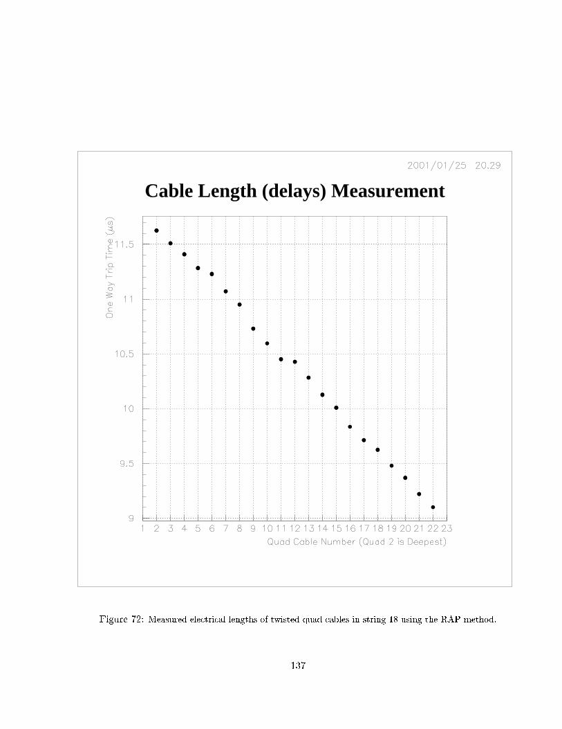
Cable Length (delays) Measurement

Figure 72: Measured electrical lengths of twisted quad cables in string 18 using the RAP method.

137

In any case, the bandwidth requirement for SPE waveforms will drop by a factor of 20 with

feature extraction. This leads to a data rate/DOM for SPE pulses of �2.3 kB/s, assuming a

300 Hz noise rate. Feature extraction is included in the baseline DOM capabilities because it

provides such a large data compression factor.

For multiple photoelectron events, the \non-SPE" waveforms, perhaps the full 170 bytes/event

are needed. Assuming 5% of the 300 Hz hit rate fall into this category, another 2.5 kB/s are

generated. While zero-suppression can reduce the unneeded pedestal data for this category, the

factor of reduction here may be only a factor of �2. Zero-suppression may also complicate eventformatting, and its role in DOM data transmission may not be prominent.

7.2.9 Local Coincidence

Conventional experimental design traditions bring all real-time signals to the counting-house,

within which various trigger logic arrays impose �lters to retain only events of interest. For

IceCube, the architecture is quite di�erent, and real-time functions play a limited role in the

DAQ. Information arrives at the \counting house" in the form of time-stamped data packets.

Since the vast majority of PMT pulses are noise hits, it is reasonable to ask what is the impact

of noise on system design and cost, and on physics.

The noise rates of the PMTs are interesting for scienti�c purposes such as SN/GRB searches

and for diagnostic purposes such as PMT gain stability. However, the DOM noise rate is

approximately 100 times greater than the rate induced by high-energy particles. The question

naturally arises whether it is necessary to transmit all the noise pulses individually to the surface

DAQ. Unlike hits due to high energy particles, noise hits appear randomly, primarily as isolated

hits, with no correlation to neighboring or nearby DOMs. Isolated hits are de�ned as those

hits falling within a loose timing window, �1 �s, but separated by two or more unhit DOMs

between. In AMANDA, such isolated hits have been relentlessly \cleaned out" during an early

stage of analysis. From the standpoint of event �tting, an isolated hit is more than 100 times

more likely to be noise than signal.

Given that �5% of the PMT hits are non-SPE events, and that feature extraction is in

operation for the remainder, the data rate per DOM is �5 kB/s, without local coincidence.

Evidence from string 18 suggests that �15% of the coincidence events are non-SPE in character.

The expected coincidence rate is �5 Hz, including random coincidences. At this rate, each

DOM would generate only �500 bytes/s, about one order of magnitude lower than without

coincidence. With local coincidence, data processing resources needed at the surface become

smaller by a comparable factor as well.

The question turns next to whether some simple local coincidence requirement, imposed in

the ice, selects essentially all interesting hits for transmission to surface. Early work on this

topic, including both analytical and Monte Carlo studies based on an IceCube-like geometry,

but using an AMANDA-like trigger criterion, suggest that a local coincidence requirement does

eliminate a small fraction, �1{3%, of real events [159, 160, 161], depending on the tightness of

timing cuts. These isolated hits may add some useful information about energy, but likely add

very little to tracking precision.

138

It should be noted that event �ltering in IceCube is likely to be quite di�erent than that

of AMANDA. The digital system architecture permits much greater exibility in the design of

�lters, due to software implementation rather than hardware. Studies have not yet been made

to determine whether IceCube would or would not su�er a loss of eÆciency, and hence whether

the instrument would be operated with some form of local coincidence. If the conclusion is yes,

local coincidence will be used, then isolated hits would not be present in the output data, except

as they contribute to the noise rate histograms for SN/GRB searches. In either case, the DOM

design will include the local coincidence capability. IceTop, discussed elsewhere, will employ

local coincidence operation to mitigate the uninteresting but copious ux of low-energy muons

at the surface. For IceCube, the use of local coincidence is an option that can be turned on or

o�.

Each DOM communicates with its nearest neighbors by means of a dedicated copper wire

pair about 20 m in length. This link is thus capable of propagating short pulses, �50 ns, with

good edge characteristics. The DOM is capable of sending and receiving these short signals in

a full duplex mode. It is therefore straightforward to arrange logic within the FPGA such that

digitization occurs only when some coincidence requirement has been met. Once a DOM has

triggered an ATWD, it sends signals to each of its neighbors and also starts a count-down from

a predetermined number of clock cycles. While the count-down is active, a DOM is receptive

to pulses from either or both of its neighbors. Should this occur, the DOM will digitize, store,

and subsequently transmit the time-stamped data to surface. Meanwhile, the neighboring DOM

will have started a count-down period to initiate a period of receptivity, even if it has not yet

been triggered. If the neighboring DOM had been triggered prior to receiving a pulse, it will

initiate digitization as well. This logic ensures that the local coincidence will capture events

independent of which DOM is hit �rst.

In this way, a local coincidence requirement of programmable width has been implemented

in AMANDA string 18 and has worked awlessly. For the future, it is intended to augment

this capability such that a DOM which receives pulses from each of its neighbors during the

programmed interval, which itself has not yet been triggered, will transmit pulses back to both

so that they will initiate digitization. This will realize next-to-nearest neighbor coincidence.

A somewhat more sophisticated approach is also possible, in which a triggered DOM trans-

mits a pulse to each of its neighbors, as before, but which is now a pulse of predetermined

length, say three clock cycles. A neighboring DOM that has not triggered will observe this pulse

and transmit it onward but with only two cycles in length; each untriggered DOM in this chain

will transmit the pulse onward, shortening it until it reaches zero length. In this manner, a

correlation length for the local coincidence requirement can be introduced that extends beyond

next-to-nearest neighbor. It remains to be determined whether such a scheme adds to physical

content.

The cost for implementation is fairly modest, as a minimal amount of circuitry is needed to

generate and receive these pulses, in any scenario. The penetrator must have six pins, rather

than two. The cable connecting DOMs is more complicated since it must support six wires.

However, by using a short cable to connect four DOMs to just one main cable breakout, a

simpli�cation has been achieved in the main cable construction; costs for the main cable are

139

reduced signi�cantly.

The PMT noise rate can be recorded properly by the DOM, and transmitted periodically to

the surface DAQ as time-ordered histograms, so that the supernova/GRB search capability is

retained. Programmable dead-time for the histogramming scalers can be included to alleviate

statistical degradation due to after-pulsing; this requires only a small amount of FPGA logic

to implement. Assuming that the histogramming intervals for detection are 10 ms, the average

count is only 3. Allocating 8-bit (maximum count: 255) scalers for the GRB/SN search adds

only 100 bytes/s, an insigni�cant burden. These 10 ms, 8-bit, scalers are unlikely to over ow,

even for a very nearby SN.

In addition, however, the DOM can maintain a circular bu�er of many seconds (even minutes,

if needed) depth, �lled with the stream of coarse time-stamps, rounded o� to �0.1 ms. This

provides a detailed record of any anomalous rate development, should a nearby SN occur. The

interval of interest could be requested in the event that a global sum of the 10 ms data indicates

the onset of a signi�cant upward rate uctuation.

7.2.10 System Design Aspects

Control Logic An Altera 10K50 FPGA provides the glue logic between circuit elements and

handles all real-time activities, i.e., those operations for which nanosecond timing is required.

The FPGA handles the synchronized launch of the ATWD, loads data into memory, receives

messages from the surface and transmits the requested response message. The FPGA will be the

site for the SPE feature extraction process. For an FPGA implementation, algorithms involving

only integer arithmetic are desirable; this does not appear to impose a limitation for accuracy,

robustness or execution speed.

ARM CPU The string 18 DOM state is controlled by a low-power Cirrus logic 32-bit CPU

targeted toward the hand-held market. The choice of an ARM device was deliberate, in the

reasonable hope that this general architecture would remain viable in the market-place at least

for the duration of the IceCube production phase. The particular CPU employed in AMANDA

string 18 is certain to be replaced by similar but more powerful devices on a yearly time-scale;

nevertheless, software compatibility is expected to be high. A product from another vendor may

be chosen for IceCube.

The CPU runs a Real-Time Executive, a thin version of a Real-Time Operating System

(RTOS). This facilitates interrupt response and message handling. The CPU boots from ash

memory upon power-up, and runs at 16.8 MHz in string 18. It o�ers the rough performance

equivalent of a 31 MHz 486, with a power dissipation of only 50 mW. Higher level functions

requiring code unsuitable for FPGA implementation will be realized in the ARM CPU. Since

the string 18 DOMs were designed, new FPGA products that o�er embedded ARM CPUs (hard

or soft) have become available. Such integrated devices may provide an attractive simpli�cation

through the elimination of one complex component.

140

Slow Control, Calibration, and Self-Test Features Each DOM is responsible for con-

trolling critical data taking parameters. These include setting local PMT high voltage levels,

discriminator threshold levels, ATWD digitizer control voltages, and even selection and load-

ing of appropriate FPGA programs. Since none of these operations is performed during actual

data acquisition, they are deemed part of the slow control system. All adjustments capable of

a�ecting the quality and quantity of data produced by the DOM are controlled from within the

DOM itself. Therefore, all slow control requests, regardless of their origin (user interface, auto-

mated experiment control sequences, etc.) are �nally serviced within the DOM and its resident

software.

Each DOM is also capable of carrying out extensive self-test sequences. In addition to

verifying correct operation of the digital platform and peripherals within the DOM, these pro-

grams can test analog electronics for the presence of increased noise, or spurious discriminator

or ATWD behavior. Upon initiation, these tests are carried out under the control of the local

DOM processor and results are reported back to surface electronics upon their completion.

One of the most important of these self-test features is uniqueness. Each DOM has its own

serial number, most likely and elegantly implemented via a preprogrammed serial memory chip

on the PC board. Upon booting up, this identi�cation number is transmitted to surface DAQ,

which can then verify that the channel number in the DAQ corresponds correctly to the deployed

sequence along the string. Thus, cockpit errors that can easily lead to reversed connections or

misplaced channels are instantly located.

There are many DOM parameters, measurable either with scheduled tasks in the DOM CPU,

or via command messages from anywhere, that must be included in the calibration database.

The primary scheduled task is the local-master clock transformation calibration process. Other

tasks that should not require frequent activation are the ATWD capture speed calibration, the

ATWD trigger discriminator threshold scan, the PMT SPE pulse-height distribution/average,

and ATWD transfer characteristics such as sample pedestal values, gain and linearity. The

transit time of photoelectrons through the PMT can be measured using a built-in triggerable

weak light source (not the optical beacon board).

7.3 Network

The km-scale network supporting the signal detection elements must be robust, cost-e�ective,

and transparent, in the sense that data quality and operational exibility are not compromised.

Despite the challenging technical requirements for data quality, a simple all-copper network can

suÆce.

7.3.1 Copper Links

All timing calibration, control, and communications signals between a given DOM and the sur-

face DAQ are provided by one conventional twisted pair of �1 mm diameter copper conductors

insulated with PVC. The impedance is in the range of 100 . This pair also supplies power to the

DOM. The resulting network is both cost-e�ective and robust, since the number of connections

141

(i.e., two) needed for all functionality is minimal. The twisted pairs are assembled �rst in double

pairs, as \twisted quads," and enclosed in a common sheath. The required number of twisted

quads are then wrapped around a Kevlar strength member and covered with a protective sleeve.

Breakouts of individual quads to facilitate connections to the DOMs are periodically introduced

at the appropriate positions.

Cable bulk and cost are reduced by planned operation of two DOMs per twisted pair. This

means that two neighboring DOMs are ganged together at depth, with a simple network at the

junction point to distribute power and transmit impedance-matched signals. DOM operation

employs alternate interrogation of each member of the DOM pair to obtain unambiguous and

uncon icted data ow. The data rates per DOM are anticipated to be �5 kB/s. Even with

two DOMs/twisted pair, the bandwidth of the copper links is suÆcient to support easily the

expected traÆc level of 10 kB/s, or equivalently, 80 kbits/s. Fast base-band communication

over twisted pair links of 2{3 km can reach 400 kbits/s or signi�cantly higher, depending on

protocol. Nevertheless, it should be noted that the margins here are only a factor of �4, andany action that would increase the PMT noise rate or data/hit will reduce the margin of safety

against network saturation, increasing the motivation to utilize the local coincidence feature.

Data transmission to the surface DAQ occurs by alternate interrogation of the DOMs sharing

a twisted pair. Di�erential send/receive results in very low levels of cross-talk for these digital

signals, measured to be less than 1% using the deployed AMANDA string 18 cables. Deployment

operations are also simpli�ed substantially, since only a single electrical connector needs to be

mated and veri�ed.

The use of an all-copper wire network eliminates the need for the optical �bers that have

been used in AMANDA. Optical �bers are obviously capable of transporting analog information

at the bandwidth needed, but the copper network can meet this goal with digital transport of

information. In the rather unorthodox AMANDA mode of optical �ber use, i.e., being frozen

in while supporting large vertical gravitational forces and freeze-in force gradients, failure or

degradation of signal was commonly observed, typically in the range of 5{15% of channels. This

pattern presents an unacceptable level of loss for an instrument of the scale of IceCube. The

actual causes of failure or degradation have remained a subject of speculation, since realistic

testing of ideas and possible remedies does not appear feasible. Combined with the goals to save

costs, eliminate dozens of plane ights, simplify and shorten deployment procedures, the history

of reliability problems generates ample motivation to develop an instrument design based on an

all-copper network.

7.3.2 Time-Base Distribution

While the all-copper network plausibly meets the goals of robustness and cost-e�ectiveness, it

may seem less apparent that such a network could meet the goal of a distributed time base at

the few nanosecond level. As noted earlier, dispersion and attenuation lead to a substantial

degradation of pulse rise-time in copper links of this length (� 2�s for 2.5 km). Nevertheless,

the realization of local) master clock time transformation with a relative accuracy of 3 ns over

a km-scale array is remarkably straightforward, requiring only a tiny fraction of bandwidth and

142

minimal circuitry for this purpose. The exceptional stability of the DOM local oscillators facil-

itates this process. Preliminary results with the four DOMs in string 18 in AMANDA operated

by the Test-Board DAQ give values for time \synchronization" of �5 ns rms, in agreement with

expectations, and with clear prospects for further improvement by algorithmic modi�cations.

The measurement and calibration of timing o�sets introduced by di�erences in twisted-pair

cable lengths has been performed automatically and remotely via satellite links by system oper-

ators in the Northern Hemisphere. No manual interventions by pole personnel are necessary at

any time for this purpose. The Reciprocal Active Pulse (RAP) technique exploits the capabilities

of the DOM to measure o�sets with a statistical precision of �1 ns as discussed in section 7.2.7.

7.4 Surface DAQ

7.4.1 Overview

The general concept for the surface system DAQ is shown in �g. 73. The proposed DAQ design

revolves around three separate phases of event creation:

1. Within a string, the collection of hits into \string coincidence events."

2. The collection of string coincidences and the decision to form a global event trigger.

3. The gathering of hits on all strings which belong to global events, and the recording of the

complete event information on disk and tape.

These tasks can be laid out in more detail by enumerating the messages that are exchanged

on the various networks of the DAQ. The following items are also summarized in the �gure.

Since 100BaseT networking is assumed, bandwidth requirements are shown to be comfortably

less than 8 MB/sec in each case.

One notable feature about this design is the prevalence of o�-the-shelf computing and net-

working hardware from the earliest possible point in the data ow diagram. It should be further

noted that the focus is on commercial hardware and software found in the world of e-commerce

and Web services industry as opposed to process control. Furthermore, there is a clear emphasis

on the use of commercial Ethernet networking protocols and hardware in place of more tra-

ditional bus-based architectures such as VME or CPCI. Both of these features are intentional

and represent our belief that, given both the expected data rates and the diÆcult maintenance

environment at the South Pole, these choices represent the best solutions for both system per-

formance and stability. A corollary of the emphasis on o�-the-shelf hardware products is that

most of the e�ort in DAQ is software.

The system consists of an interconnected set of hardware components and software tasks.

While this design does allow for a great deal of exibility in how these components are grouped

together and mapped onto various networks and processors, the overall system performance goals

dictate that certain aspects of this grouping are �xed. In the following discussion, the distinction

between system software processes and actual CPUs within the system should be noted. For

143

F

DOMPair

20 k /sec

StringProcessor

N x 20 kB/sec

All Hits -0.6 MB/sec

0 Strings

String Subsystem:60 DOMs

pairs

Event A100 aseT

Total traffic: 1.6 M /secString

CoincidenceMessages

GlobalTrigger Event Triggers /

Lookback Requests forall Strings - 0.8 MB/sec

Eventuilder

Built events ~ 1 MB/sec(all event builders)

Data HandlingDisk Cache

DOMHU

Lookback Requests

String CoincidenceMessages - 170 kB/sec

Fulfill Lookback Messages 0.6 MB/sec

FulfillLookbackMessages

Online A100 aseT

Total traffic: 1M /sec

String A100 aseT

Total traffic: 0.6 M /sec

DataHandling

CPU Cluster

Tape

Satellite

5 CPUs

2 - 5 Units

Figure 73: Conceptual illustration of DAQ system organization.

144

example, a complete string of optical modules is said to terminate in a single processor, called

the string processor.

For the purposes of system design, it has been important to decide that, since an optical

module string represents a logical grouping of data for triggering purposes, all data from one

string will always ow to a single processor and will not be distributed across multiple CPU's.

While, for the purposes of this document, it is easiest to discuss the string processing program as

executing on a single processor, namely the string processor, the system design does not require

that each string be handled by a separate processor. It does, however, require that all data

from all DOMs in a string are routed to a single system process that can deal with them in an

eÆcient and complete manner.

7.4.2 DOM Hub

At the surface, the twisted pairs from DOM pairs on a string are connected to a DOM Hub.

Each twisted pair connected to the DOM Hub is de�ned as a channel. It is appropriate to design

the Hub such that the number of channels per Hub is a factor of the number of DOM pairs on

a string, i.e. 30. For example, if the DOM Hub accommodates six channels, �ve DOM Hubs

are needed to service an entire string. If the DOM Hub accommodates ten channels, then only

three DOM Hubs are needed (similarly, two DOM Hubs will suÆce if a Hub has 15 channels).

The functions of the DOM Hub include power distribution and control for each DOM pair,

message control, data ow management from the DOMs, downloading of software, �rmware,

and operating parameters, and generation of time calibration signals. The DOM Hub design is

derived from the single-channel Test-Board used to read out string 18, and is the only signi�cant

piece of custom hardware awaiting realization. It is conceivable (and likely) that the design and

layout of the DOM Hub will accommodate more than six channels. In what follows, however,

we assume a conservative default of six channels per DOM Hub (12 DOMs).

The DOM Hub design is centered on an embedded processor that provides low level com-

munications services between the surface and the DOM and provides high level communications

services (i.e. TCP/IP) to the string processor. The DOM Hub will consist of 1U rack-mounted

chassis with front-end electronics including FPGAs and FADCs for 12 DOMs, an embedded CPU

daughter card for processing and communications functions, and a power supply capable of pro-

viding power for all attached DOMs. The back panel of the chassis contains connectors for direct

attachment to DOM deployment cables, master clock distribution, and a standard 10/100BT

network connector. The embedded processor is a credit-card-sized 200 MHz StrongARM CPU

running Linux.

The DOM Hub will support TCP/IP protocol and will deliver data streams for each DOM to

the string processor using the standard socket programming model. Furthermore, the DOM Hub

will provide transparent web-based communications with individual DOMs so that maintenance

and minimal testing functions may be performed remotely without the need of the full data

acquisition system.

All real-time functions in the surface DAQ that depend on nanosecond-level timing are con-

tained within the DOM Hub. Data transferred from the DOM Hub to downstream elements in

145

the surface DAQ are time-stamped messages; subsequent processing needs only to ensure ade-

quate data ow. The latencies of network operation do not introduce synchronization problems.

The DOM Hub receives a carefully distributed 40 MHz master clock. This master clock

will be linked ultimately to GPS, providing a universal time reference to other GPS-linked data

sets to � 40 ns. The DOM Hub maintains a register capable of assigning a unique time-stamp

for at least one day (44 bits). Although runs will likely not extend more than one day, it is

straightforward to track time perhaps for as much as a year (51 bits). Test functions will be

incorporated to ensure that every DOM Hub has exactly the same master time. These test

functions will operate as separate, scheduled threads that will not interfere with normal data

acquisition.

Assuming a PMT noise rate of 300 Hz, 60 DOMs per string, a fraction of 5% of hits needing

full waveforms, 170 bytes per waveform and 8 bytes per non-waveform hit, one obtains a DOM

data rate of about 5 kb/s and 0.3 MB/s per string. Because these data ow rates are modest,

the surface DAQ can be network-based rather than a more traditional crate/backplane/bus

implementation. Of course, with local coincidence, these rates would drop an order of magnitude

further.

Data from each DOM is requested periodically, at a rate of �10 Hz. This provides adequatelysmall latency for data streaming purposes, and maintains a reasonable transmission burst of 0.5{

1 kb/request. Each request for data includes the time-mark signal as the �rst pulse. The DOM

will ignore most of these, using them only as frequently as local clock drift characteristics require.

DOM data packets with local time-stamps are locally bu�ered in the DOM Hub. For each

string, hits from DOMs connected to �ve DOM Hubs are sent over a String LAN (one 100BaseT

network switch) to a String Processor (SP).

7.4.3 String Processor

Data bu�ered in the DOM Hub is block-transferred periodically, �10 Hz, to the String Processor(SP). The SP is expected to be a standard PC CPU running a Linux OS. Here, data is converted

to master time units. The desired space-time correlations characteristic of physics, traditionally

de�ned with real-time electronic trigger systems and called \triggers," are found in our case

through software algorithms in the SP. Simulations have shown that only about 5% of available

CPU cycles of a 1 GHz PC are needed to perform typical coincidence algorithms for a 60-DOM

string.

Each String Processor is also connected to a global Event LAN. String coincidences are

reported by each String Processor to the Global Event Trigger on the Event LAN. The Global

Event Trigger is envisioned as a single processor on the Event LAN, which is also connected to

a set of processors that serve as Event Builders. Assuming a string coincidence rate of 60 Hz

per string, an average of 4 hits per coincidence event, and 60 DOMs per string, one obtains a

total data rate for all 80 strings of less than 0.2 MB/s for these messages.

When trigger conditions for a particular event type are ful�lled, the global event trigger

informs the String Processor to tag all hits that occurred near enough in time to the global

trigger time. If one assumes a global aggregate trigger rate for all trigger types of 1 kHz,

146

10 bytes per message, and 80 string processors, these \Look-back Requests" require an average

bandwidth of 0.8 MB/s.

The String Processor sends the data for the tagged hits to one of a set of Event Builder CPUs.

This also occurs over the Event LAN. Assuming 20 random noise hits per event, 12 muon hits

per event, and the above values for the average number of bytes per hit and for the global event

rate, one obtains an average bandwidth of 0.6 MB/s. This brings the total bandwidth usage on

the Event LAN to about 1.6 MB/s, well within the capabilities of 100BaseT switches.

It may turn out that the waveform data retrieval task for the look-back requests may be just

as easily handled by sending all waveform data associated with the string coincidence trigger

messages, since the amount of data arriving at the SP is roughly the same as the look-back

request traÆc. This software architecture would eliminate the look-back process, yielding a

data ow diagram without loops at this level. In this scenario, however, the destination of

the waveform data needs to be considered carefully to ensure arrival at the appropriate Event

Builder target CPU.

The Event Builder CPUs send fully constructed events to a disk server over the Online LAN.

The disk server will write events to disk. Since the bulk of the event data is in the hits, the

bandwidth on this network will be not signi�cantly more than 0.6 MB/s. 1 MB/sec is a safe

number to assume, well within the 100BaseT limits. In addition to the Event Builder processors

and the disk server, the Online LAN also is connected to the processors that constitute the

online �ltering and data archiving system. Events are still represented in master clock time

units, but also have the associated GPS times linked to each.

This design is attractive, in part, due to its high degree of modularity and exibility. Thus

to create a minimal test stand for DOM production and quality control, one can simply work

with a single DOM Hub attached to one or more DOMs (or DOM pairs). Functionality for a

whole string can be achieved by networking the DOM Hubs to an o�-the-shelf String Processor

CPU and installing the requisite software. In an international collaboration where hardware

production, software development, testing and deployment will be carried out on multiple con-

tinents, this is a key advantage. Finally, with the proposed \network-heavy" scheme, IceCube

will bene�t from a tremendous amount of community experience and publicly-available tools

for TCP and UDP-based networking, which far outstrips the resources available for bus-based

architectures such as VME or Compact PCI.

7.4.4 IceCube and IceTop System Integration

The DOM and its associated DOM Hub design will accommodate the technical requirements

of both IceTop and IceCube, with di�erences con�ned to �rmware, software, and operating

conditions. Within the counting house, the di�erences would be apparent only in the network

con�guration.

Each IceCube string requires 15 quads for the 60 DOMs. Unlike IceCube, the IceTop DOMs

will not share a twisted quad with a neighboring DOM since the expected rates are higher than

those of IceCube. The four IceTop DOMs thus require two quads, for a total number of 17 DOM

twisted quads/string. In addition, there will be ancillary devices added to the string, such as

147

pressure sensors used during deployment and freeze-back, so the expected total number of quads

will be at least 18 per string, perhaps more. The fraction of counting house resources needed

for IceTop is �15% relative to IceCube.

IceCube The 80 strings of IceCube will require 400 (240, 160) DOM Hubs in the counting

house under the assumptions that a DOM Hub has 6 (10, 15) channels (two DOMs per channel

in IceCube) and is housed in 1U mechanics. The DOM Hubs and 80 (perhaps less) associated

String Processors will require something like 10 (6, 4) oor-to-ceiling racks. The space-saving

that would be obtained with the 10- or 15-channel version is substantial, and provides ample

motivation for high design density.

IceTop IceTop, described in detail elsewhere in this document, will consist of an ensemble of

frozen water tanks situated just below the surface, and located near each of the 80 strings. Each

string will have two tanks separated by a few meters to suppress single muon events, yielding

a total of 160 tanks. To extend the dynamic range, each tank will be viewed by two DOMs

operated at substantially di�erent gain settings. This facilitates the capture of extremely high-

energy air showers. The local coincidence requirement will be operational between the high-gain

DOMs in the two tanks. The coincidence requirement will reduce to an acceptable level the

rate induced by the relatively copious ux of uninteresting single muons penetrating the tank

volume.

With 160 tanks and two DOMs/tank, IceTop's 320 DOMs will bring 320 twisted pairs (in

160 twisted quads) into the IceCube/IceTop counting house. These IceTop quads will plug into

54 (32, 22) DOM Hubs dedicated to IceTop, if the DOM Hub supports 6 (10, 15) channels.

The IceTop DOM Hubs will connect to a dedicated IceTop Global Trigger CPU and Event

Builder, with a LAN architecture analogous to IceCube. The output data stream will be linked

to IceCube by both master clock times and GPS time units for online and o�ine analysis.

7.4.5 Experiment and Con�guration Control

The system design described in this document is based on a loosely-coupled collection of sub-

systems whose operations are, for the most part, decoupled. One advantage of such a design is

that it allows some independence in the design and implementation of individual sub-systems.

However, in order to co-ordinate these elements into a single, coherent system, some degree of

overall control is required. This function is provided by the experiment control system.

The IceCube detector can, at any given moment, be described as being in one of several

operational states. These states serve as short, meaningful descriptions of just what operations

are being performed by the detector. By enumerating which operations are allowed in which

detector states, this state model also serve as a mechanism to control and co-ordinate operations

of separate detector sub-systems.

148

Scope of Experiment Control The detector, as a whole, can be though of as being in one

of the following states: \idle," \entering data-taking state," \running," \paused," \exiting data-

taking state," \calibrating" or in one of several \testing" states. Each of these states has certain

implications for the operations of each sub-system. For example, if the detector is taking data,

the DOM string control sub-system should not be able to alter PMT high voltage settings on an

active OM. Similarly, although it is permissible to alter individual settings for an inactive DOM

(i.e. an DOM not included in the global trigger's list of active DOMs), it should not be possible

to initiate LED beacons on this particular DOM since resulting light would a�ect data taking

activities. Therefore, all sub-systems refer to experiment control as the single indicator of the

system's current aggregate operational state. Each sub-system is responsible for designing its

internal operations and states to be consistent with the overall detector behavior described by

experiment control's current state.

Common Component Control Model In addition to providing all sub-systems with a

consistent indication of the detector's overall state, experiment control must, in order to initiate

and control data taking, be able to request sub-systems to perform certain actions. Depending

on a particular sub-system's role in the detector's operation, these actions can be relatively

simple or fairly complex. For example, when beginning data taking, DOM string control will be

required to log current DOM parameter settings to a local database and change its state from

\idle" to \data taking." The fact that the DOM string control sub-system is in the \data taking"

mode implies that it will be unresponsive to user requests to reset critical DOM parameters.

Other sub-systems may require more complex responses to experiment control commands.

To the extent that the complexity of these operations is only of concern to the sub-system

itself, the details of these operations should remain concealed within the sub-system's operation.

Each sub-system should be able to accept a high-level request from experiment control to move

into a new state. Following this request, each sub-system will respond with its new state and

status. Successful transitions of each sub-system into the appropriate state will lead experiment

control to indicate that the detector has taken on the desired �nal state (e.g. \running"). The

failure of any sub-system to appropriately move to the desired target state will indicate a system

problem and will cause experiment control to bring all sub-systems back to a consistent and safe

state.

It should be noted that with the loosely-coupled system described here, individual control

operations are best handled directly by those sub-systems involved. That is, commands and

requests for monitoring and status information will be processed by the sub-systems themselves,

not by some single intervening agent (e.g. experiment control). The advantage of such a design

is that additions and alterations to sub-system controls and interfaces need only be implemented

in one place -the sub-system itself. They do not have to be further integrated into additional

supervisory programs or levels.

However, it should be pointed out that, with this implementation model, it is possible for

there to be a wide and confusing variety of user interfaces for each sub-system. Even with

experiment control properly playing its detector-wide coordinating role, it will be possible to

149

implement sub-system user interfaces in many di�erent and potentially awkward styles. A

certain degree of discipline in design and implementation of individual sub-system user interfaces

will be required in order to produce a consistent overall look and feel. Given the breadth of

functions requiring user interfaces and the necessity for e�ective remote (albeit secure) access,

the adoption of a web-based user interface model is preferred.

DAQ Con�guration Database The DOM string control sub-system will be responsible for

keeping an accurate database of DOM-related parameters for each data taking session. While

this list of DOM parameters and operational settings is not yet complete, it is safe to assume

that, during any given data taking session, each DOM participating in the detector array will

have 50 to 100 parameters that describe its intended operation. These will include static �ducial

information such as serial number, string and position location, �rmware version number, etc. It

will also include per session information such as PMT high voltage, trigger threshold level, and,

if some level of waveform capture is included in the DOM, parameters that describe operation

of waveform capture and feature extraction algorithms.

This same database will also be used to control which DOMs are actually participating in

data acquisition operations for detector array and, if required, insure that unused DOMs are

powered down and/or not contributing unwanted triggers to string processor trigger processors.

This same database will be used by the Global Trigger and Event Builder sub-system to control

operations of the String Trigger processor algorithm.

Component Discovery and Self Con�guration The IceCube detector will be deployed

over a period of several years. Furthermore, during the summer deployment season, optical

module strings will be deployed, tested and integrated at rates far in excess of that experienced

by the current collaboration. While the physical logistics for drilling, deploying and cabling

detector strings are critical to the success of this timetable, the speed with which the data

acquisition system can adapt and re-con�gure to the addition or deletion of new optical module

strings will be of equal importance.

Each sub-system located at the South Pole must be aware of its environment and capable of

determining whether needed hardware and software components are available. This operation

can be performed automatically when individual sub-systems are started or can be the result

of an explicit re-con�guration command. The most basic example of such an operation is

enabling the experiment control sub-system to locate, via a set well-de�ned network operations,

and establish communications with all other operating sub-systems. A more complex, but

conceptually similar, con�guration operation enables the DOM string control sub-system to

determine which strings are present and which optical modules are in an operable state. This

resource discovery scheme can be extended to on-line sub-systems as well by enabling the �lter

farm manager to discover which individual processors are available to participate in its operation.

If this technique is consistently applied across all sub-systems and is combined with accu-

rate and complete documentation of the experiment cable plant, it becomes relatively simple to

incorporate both additional DOM strings and computing resources as they are installed. The

150

presence or absence of portions of the hardware and software system become apparent to opera-

tors as each sub-system reports its success or failure during a \con�gure" operation. In addition

to speeding integration of new portions of the detector, this capability allows fast and e�ective

resolution of complex system-wide equipment problems. This capability can also provide critical

equipment status information when recovering from an unscheduled power loss.

Just as it is critical to be able to automatically incorporate new DOM strings and computing

components as they are installed, it is also important to be able, under computer control, to

mark portions of the system as o�-line or \non-participating." The most obvious need for such a

facility is during system debugging. It is often useful to remove elements from the system in order

to investigate their role in generating speci�c error conditions. Unfortunately, it is not always

convenient or possible to electrically disconnect or power down suspected hardware or software

components. Some data acquisition problems may require this sort of system de-population for

correct diagnosis and repair. If these problems occur during the winter season, the ability to

remove some components from the system, via remote access, will be of great advantage.

7.4.6 Security Environment

\Security" can cover a wide range of capabilities and protections. It is worth reviewing the

current use of the term in computing and communications systems. In current computing

usage, the term security is based on four principles: authentication, authorization, privacy, and

non-repudiation. Brie y, authentication involves the veri�cation that a user has the identity

they claim to have, authorization veri�es that a given user has the authorization or privilege

to perform a requested operation, privacy assures users that messages and data exchanged

with another user will be private to only those two parties, and non-repudiation stipulates that

requests received from a user cannot be repudiated at a later date (e.g. electronic transfer of

funds). Each of these principal functions can be implemented separately and each with varying

degrees of completeness. Furthermore, several di�erent technologies can be used to achieve some

or all of this functionality. While simple open password schemes are not considered to provide

any real level of security, suitable software mechanisms, such as DES, Kerberos, and PKI (Public

Key Infrastructure), exist and are readily available.

An exact statement of IceCube security requirements does not, as yet, exist. However, based

on past AMANDA experience and reasonable projections of IceCube operations, several needs

are obvious. Regardless of what network access level protections may be implemented upstream,

such as screening of requestor IP addresses, it is important that all control commands be veri�ed

and screened by a security service at the South Pole site. This service should provide, at a

minimum, strong authentication and authorization functions. These would basically regulate

who would have access to data acquisition and on-line control and monitoring information and

which speci�c capabilities would be allowed on an individual basis. While privacy and non-

repudiation functions do not appear to have any role in experiment control and monitoring

at present, any suitable security service will allow their implementation at a later date. In

discussing security in the context of experiment control, it is assumed that a certain level of

robust security is provided by the underlying operating system and network environment. It is

151

assumed, for example that unauthorized access to system accounts has been eliminated and that

network routers and their control ports have been made suitably safe. The following discussion

centers on the application design decisions that will enhance this low-level security and protect

the resulting system from unauthorized or inadvertent use.

One mechanism used in designing secure control systems is to create a �nite number of

\roles" that users can take on when logged onto a system. These roles are typically descriptive

in nature (e.g. \operator," \implementers," \maintenance technician," \super-user"). Users

requesting access to the data acquisition or on-line sub-systems at the South Pole will present

their name, security credentials, and intended operational role to the security service. After

authenticating user identity, the security service determines whether a user is authorized to take

on the requested operational role. If these security checks are successful, the user then has all

the privileges associated with that operational role.

One of the advantages of this scheme is that it creates a clean partition between security ser-

vices and system operations. Security mechanisms can be centralized into a single point of access.

Individual sub-systems are then able to treat all commands as having been issued by authen-

ticated users acting in an authorized capacity (i.e. role). In addition to these implementation

eÆciencies, this scheme also clari�es overall system design and operation. Although commands

to sub-systems will carry the identity, as well as the acting role, of the requestor, the design

becomes one primarily driven by the requestor's role. The act of describing the set of all possible

user operational roles implicitly describes all possible modes of system operation. For exam-

ple, since each sub-system di�erentiates between normal operations allowed by an \operator"

and those privileged commands reserved for \implementers," lists of permissible \operator" and

\implementer" functions take on detector-wide meaning and signi�cance. Furthermore, since,

at the sub-system implementation level, every command must be checked against the role of the

requestor, sub-system behavior becomes both well-organized, easily described and, hopefully,

documented.

7.4.7 DAQ Components

Slow Control The DOM string control sub-system will consist of a central control program

and co-operating tasks executing on each string's dedicated control processor. Since the detector

will grow by the addition of DOMs organized as strings and since the only electrical and logical

path for communicating with a particular OM is through its string processor and cable, this

design is a natural �t for the detector's topology.

The central slow control program will be responsible for all user and experiment control

interface functions to the optical modules and will be responsible for all DOM-related interactions

with the detector con�guration database. These database interactions will include queries of

DOMs currently active in the detector, setting and recording of internal DOM parameters for

data taking, and recording of individual DOM calibration information acquired during low level

calibration operations. Most DOM string control operations will be synchronous command or

monitoring requests.

At present, there are only a small number of possible states for the DOM string control sub-

152

system. These states should be suÆcient to indicate the following DOM string control activities:

o�-line or idle, performing self-con�guration and string discovery, performing one or more local

DOM calibration functions, on-line and able to accept operator commands, and on-line but only

accepting monitoring requests (as during normal data taking). Additional states can be added

as needs arise. It should be noted that these states, as well as those of other sub-systems, will

not correspond exactly to those of the experiment control program. They do, however, represent

a list of possible sub-system behaviors that are consistent with the overall detector operation.

The central control program will also be responsible for discovering via their associated string

processors, all DOMs presently in the detector. Once connected to the local area network, newly

added strings will be incorporated into the central control program through a single \recon�gure"

command. This same operation will allow strings temporarily removed from the detector for

purposes of test or electronics repair to be marked as \non participating strings" and their

respective DOMs recorded as \o� line."

String Data Handling Each DOM in a string produces a stream of hits and waveforms that,

via the String LAN, ultimately reaches the string processor. All operations surrounding data

transfer, sorting and interactions with other system components (e.g. the global trigger) are

the responsibility of the string data handling process. The �rst phase of its operations center

on the delivery of string level hit information to the global trigger process. Upon reception of

data from one or more DOMs, its initial task to sort this data into structures that allow quick,

eÆcient determination of local coincidence during a sliding time window (typically 8 �s). When

all coincidences for a given time period have been found, they are properly formatted and passed

on to the global trigger process.

The second phase begins when the global trigger process responds with a list of time intervals

of interest. It is then the string data handler's task to collect raw data from all DOMs for each

of the time intervals of interest and forward the resulting data set to the appropriate Event

Builder. In practice, these two phases will overlap and provision must be made to have several

such operations in progress at any one time.

There are only a small number of possible states for the string handler process. These

states should be suÆcient to indicate the following activities: o�-line or idle, performing self-

con�guration and DOM discovery, processing normal data triggers, paused due to operator

request or error condition, and performing string speci�c tests. Additional states can be added

as needs arise.

Global Trigger As described above, the global trigger is responsible for generating lists in-

dicating the occurrence of detector-wide events of interest. It consumes the list of hits as

determined by the string data handling process in each string processor and emits a list of

UTC-based times that bracket hits considered to be possible events. The global trigger behaves

synchronously with the aggregate collection of on-line string processors. That is, the global trig-

ger waits until all string processors that are con�gured and active to report their contributions

for a given time interval. Only when all string contributions are present, can the global trigger

153

begin the process of determining what events might have occurred. Once this determination is

complete, the Global Trigger selects an Event Builder for the current data sequence and passes

a list of UTC time intervals to both the selected Event Builder and all string handling processes.

During normal operation, all 80 string processors will remain synchronized within the re-

porting period speci�ed when data taking was initiated. This period can range from as low as

�100 ms to perhaps a few seconds, without degradation of system performance or compromise

of data integrity. Several global triggers may be found within one reporting period. As described

above, for each reporting period, ALL string processors must forward string-level local coinci-

dences, or their absence, to the global trigger in order to initiate the global triggering process.

In the absence of such a report, the global trigger will re-synchronize all string processors and

forward, to the Event Builder an indication of what reporting periods were discarded. Persistent

failure of a string processor program or CPU will cause the global trigger manager to enter a

non-operating error state. Experiment control will detect, during periodic system scans, this

state change and force an abnormal end of run sequence for all data acquisition sub-systems.

Co-ordination activities and generation of global triggers are performed by a single global trig-

ger process executing on a dedicated processor. Since this activity requires the exchange of

multiple messages between this process and each string's data handling process during each

reporting period, high speed, low latency network connections between these processors is of

great importance.

There are only a small number of possible states for the global trigger sub-system. These

states should be suÆcient to indicate the following activities: o�-line or idle, performing self-

con�guration and string processor discovery, processing normal data triggers, paused due to

operator request or error condition, and performing global trigger speci�c tests. Additional states

can be added as needs arise. As with other sub-systems, it should be noted that these states

need not correspond exactly to those of the experiment control program. They do, however,

represent a list of possible sub-system behaviors that are consistent with the overall detector

operation.

Event Builder The I/O requirements for IceCube are not very demanding, opening up many

possible approaches to event building. We opt for a simple yet exible approach based on

commercial hardware. Its main elements are a farm of the order of �ve \event worker" PCs con-

nected via a switched ethernet network and a control PC that manages the farm and distributes

the work. This asynchronous approach o�ers a redundant, fault-tolerant, reliable and scalable

solution that should work with minimal maintenance e�ort. The amount of CPU time needed

for event building has not yet been studied in detail but is estimated not to be the de�ning

factor for the size of the farm. The number of PCs is rather determined by the requirement of

redundancy. To exploit the CPU capacity, several tasks will be incorporated in addition. We

currently envision the following set of tasks:

� Asynchronous merging of data from 80 string-wise sources (event building);

� Low level monitoring, data consistency checks and online calibration;

154

� Feature extraction from digitized pulse shapes.

A special control PC is used to control event building by selecting speci�c event worker PCs

that are ready to accept data, usually in a round-robin way. In addition it will be used for

con�guration, system and data supervision and will host a graphical user interface. If a PC has

crashed, the load is taken over by the other PCs in a dynamic way and the PC is question is

automatically rebooted. All event working PCs 's have identical functionality. Their number is

completely scalable and can be adjusted according to needs. The bu�ered string-wise data will

be "pushed" to an idle event worker PCs roughly every 10{100 s. The Control PC also provides

a list of links to data belonging to the same trigger time stamp. In this way only pointers are

modi�ed and the PCs are running in an \I/O-free" mode. The data are actually only moved in

the last step before writing the data to disk. Such a farm can be built based on today's standard

networking equipment.

7.4.8 Calibration Operations

Calibrations serve a crucial and central role in the operation of the IceCube detector. They

must, to the greatest extent possible, be automated. The present digital design allows calibra-

tions to be carried out without any physical intervention to the data acquisition system. That

is, all calibrations can be performed without disconnecting cables or physically re-con�guring

DOM electrical data paths. However, while this is a necessary condition for fully automated,

unattended calibration operations, it is not a suÆcient one. Further design and detailed descrip-

tions of operational sequences are still required for automated operations to become a reality.

While the following framework should allow such operations to take place, further discussions

are needed in order to insure their successful operations within the current design.

DAQ Calibration Operations The primary calibration operation carried out within the

DAQ system is that of synchronizing time bases for all DOMs with the GPS clock. This operation

will take place automatically once every 5 to 10 seconds. The actual nanosecond-level signaling

operations are performed by the DOM Hub and DOMs themselves. The DAQ's only role is

in enabling such operations and supervising the dissemination of the calculated clock o�sets

for each DOM to both the DAQ con�guration data base and, through an as yet unspeci�ed

mechanism, the Online system. The primary DAQ component involved at the supervisory level

is the string processor. Since all data leaving the string processor is corrected to UTC, this is

the rational point at which to control and implement needed time base corrections. All other

calibration IceCube calibration operations are based on analysis of data collected by a carefully

con�gured, but normally operating DAQ. Therefore, these calibration operations fall outside the

scope and capability of the DAQ and are, more properly, Online functions.

Online Calibration Operations In addition to the time base synchronization calibration

performed by the DAQ system, additional calibration operations are required for successful

detector operation. These include, but are not limited to, determination of individual PMT

155

high voltage settings, determination of proper PMT trigger thresholds and measurement of

cable delays for all DOMs. As noted above, all of these calibration tasks are based on speci�c

data analysis applied to the detector data stream. Therefore, these calibration operations are

primarily operating in the Online domain. In fact, they can all be considered to be part of a

special subset of normal data taking operations. It should be noted that some of these Online

calibration operations will produce data required for correct operations within the DAQ system.

In these cases, mechanisms must be in place for inserting these calibration values into the DAQ

con�guration data base.

In practice, these operations can be automated and orchestrated by the main supervisory

program, experiment control. Experiment control can select a particular DAQ con�guration

and instruct DAQ to begin operations. It can then select a particular Online con�guration and

instruct Online to begin operation. With a suitable level of exibility at the experiment control

level, fairly complex sequences of calibrations can be carried out in an automated manner.

7.4.9 DAQ and Online Monitoring

Operations and Error Logging The design described in this document partitions system

behavior into a number of low-level tasks and assigns them to individual sub-systems. Further-

more, these sub-systems are organized together through a single experiment control sub-system

that is able to orchestrate their operations into a single co-ordinated activity. While such a

design has been proven to be both exible and reliable, when problems do occur, the relatively

\loose" connection between subsystems can make proper diagnosis diÆcult. A well-designed

operations log is a key tool in allowing rapid discovery and correction of individual sub-system

problems.

All sub-systems will be able to log messages to a single, system wide operations log. Each

message will be tagged with the name of the sub-system as well as the time of entry. Each

message will also include numerical and text �elds to describe error conditions as well as global

state information such as experiment control run number and state. While there will be provision

for one or more free form text areas, the format will include mandatory �xed format �elds to

facilitate automated searching in one of several modes. At a minimum, the log will be searchable

by sub-system, time and global run number. In practice, this operations log may be built on

existing open-source or commercial database technology.

DAQ and Operations Monitoring It is anticipated that, at least for purposes of detector

and data acquisition system monitoring, there will be a number of groups interested in having

independent and uncoordinated access to one or more software sub-systems at the South Pole.

As described earlier, design distinctions between monitoring requests and control commands will

allow the use of robust, commercial-grade web server programs for a large portion of these user

interactions. Routing requests for monitoring data through a web server concentrates most of

the interactive data ow through a well-debugged program that acts as a bu�er between o�-

site data requests and data acquisition and on-line sub-system programs. Unfortunately, this

mechanism is still subject to periodic and occasionally unscheduled communications outages

156

between the northern hemisphere and the South Pole. Given the wide distribution of local time

zones within the IceCube collaboration, this can create limited or, at a minimum, inconvenient

access to monitoring data.

With the interposition of a northern hemisphere server/cache gateway system, much of the

data acquisition and on-line sub-system monitoring data can be made available to collaboration

members at their home institutions during reasonable day-time hours. This gateway system

would be con�gured to refresh its cache from sources at the south pole during times of expected

communications availability and serve these monitoring data �les in response to browser and

client requests. During times of communications blackout between the south pole and northern

hemisphere, collaboration members would be able to direct their browsers and client programs

to the gateway system and obtain current, within 24 hr, detector and sub-system status. Fur-

thermore, if it were deemed necessary to restrict general collaboration access to South Pole

systems, this architecture would provide a straight forward mechanism for distributing detector

monitoring information. Thus, up-to-date detector and data acquisition system performance

data is made available collaboration-wide on a best-e�ort basis.

Portions of the monitoring and operational information will be needed for correct interpre-

tation of data during later analysis. This can include current and cumulative trigger rates for all

trigger types as well as Event Builder statistics and gross DOM data rates on a string by string

basis. There must be a mechanism for identifying and passing monitoring data from the DAQ

system to the Online system. This may consist of a separate data stream, or even the periodic

inclusion of monitoring data in normal data streams.

Online Components The Online system is essentially a carefully organized portion of the

O�ine environment that has been targeted for execution at the data acquisition site under the

control of the experiment control sub system. It has three primary responsibilities. First, it is

the sole component responsible for copying the DAQ event stream from the shared disk system,

located on the Online LAN, to both archive storage (i.e. tape) and, via satellite, to the northern

hemisphere. As such, it is capable of reformatting and repackaging data from the Event Builder

into those forms best consumed by o�ine analysis tasks. Secondly, it provides the framework

and control mechanisms for executing any online �lter operations used to analyze, reduce or

reject data from any of the data streams emitted by event builders. And thirdly, as described

above, the Online system contains �lters and or programs that perform all calibration functions

beyond those of DOM time base synchronization performed by the DAQ system

7.4.10 DAQ Computing Environment

COTS Hardware and Software Components There has been a real e�ort, during the

design of both the DAQ and Online systems, to maximize the potential for using commercial,

o� the shelf (COTS) hardware and software components. At a minimum, this includes use of

open source operating systems (namely, Linux), standards-based network and communications

software and PC-based computing platforms. Of course, we feel it also should allow for the

purchase of standards-based components as required. This can, for example, include purchase

157

of PC clusters that have well engineered cooling and maintenance features or disk systems that

have extensive space management and diagnostic software packages.

String LAN Components As noted earlier, each string terminates in its own private net-

work. In practice, this network consists of a set of DOM Hubs and a single processor connected

to an o�-the-shelf switched Ethernet hub. This design nicely encapsulates the entire string be-

hind each string processor, which serves as the complete interface to the string. Based on system

performance, we may choose to have two or more strings share the same string processor. If so,

we need only increase the number of Ethernet attachments required for the commercial switched

hub.

String, Global Trigger, and Event Builder Processors Depending upon the degree to

which multiple OM strings can be accommodated on a single string LAN and processor, the

IceCube DAQ, when fully implemented, may have on the order of 50 to 100 processors. By

any measure, this is a substantial number of systems to house and maintain. When designing

a system with such a large number of processors, several factors besides basic unit processor

cost must be considered, such as operation in a low humidity and low pressure environment

with an occasionally unreliable power source. Many vendors have addressed the ancillary issues

involved in con�guring, operating, and maintaining large clusters of PC-based Linux systems-

most notably for use in the e-commerce industry. For these markets, vendors have addressed

such issues as increased packing density (e.g. one processor per 1U rack space), improved

ventilation and temperature monitoring, improved, tool-free, modular repair capabilities, and

network-based remote diagnosis and control of individual processors. These systems typically

have a full, but limited set of disk, communications, and PCI resources. In determining the

functionality and interconnections needed to implement both the DAQ and Online systems,

care has been taken to stay within the physical and logical constraints presented by these PC

cluster implementations.

Event LAN The data rates presently anticipated indicate that the communications network

used to connect all OM string processors with the single global trigger processor and multiple

Event Builder processors can be adequately serviced by conventional data network (100BT or

Gigabit Ethernet). As with the String LANs, this network is well bounded and only requires a

local switch-based infrastructure.

If these data rate projections grow beyond the capabilities of either 100BT or Gigabit Ether-

net technologies, alternate, o�-the-shelf solutions can be inserted into this architecture without

major perturbations to the system design. In particular, we have investigated the Myricom

switched fabric inter-processor network as a potential solution.

Storage Systems and Online LAN As with network infrastructure, storage systems rep-

resent an area where system data rates dictate the technical solution. The primary storage

facility shown in this design is that which provides the exible data bu�er between the DAQ

158

and Online system partitions. This system design e�ectively increases performance by providing

parallel computing resources for those paths with the highest data throughput rates. At the

juncture of the DAQ and Online systems, this implies a shared network-based storage system

with multiple access paths to both Event Builder and online processors. The current aggregate

data rates indicate that a 100BT based commercial SAN (Storage Area Network) system will

meet the necessary storage and throughput requirements. As with the selection of processors,

storage system selection should not be based solely on hardware costs. Most modern commercial

systems include system level features such as automatic mirroring, local automated backup and

remote fault diagnosis and con�guration tools. These facilities should receive high consideration

in vendor and system selection.

As with the Event Builder LAN, the technical solutions are sensitive to the ultimate data

rates expected within the system. If the current projected data rates prove inadequate, con-

sideration will be given to their e�ect on the I/O bandwidth requirements of the shared disk

system. Alternate solutions with substantially higher throughput rates do exist - most notably

�ber channel based SAN arrays. Since these storage systems use individual PCI interfaces and

a separate switched fabric interconnect for all disk related data, the costs - as well as the data

throughput - increase dramatically.

7.5 AMANDA Data Transmission Techniques

For historical reference, we present here the data transmission techniques used in the past by the

AMANDA detector. The present AMANDA II detector has been deployed over several seasons,

with a stepwise implementation of detectors with improved data transmission techniques. An

array of four strings (AMANDA-B4) was installed in 1995/96, with the OMs connected to the

surface by an electrical coaxial cable that transmits both the HV and the analog anode signal;

see �g. 74, left. PMTs are operated at a gain of 109 to drive the pulses over 2 km of coaxial

cable without in-situ ampli�cation. Hamamatsu R5912-2 PMTs with 14 dynodes are used to

achieve the high gain; they require positive high voltage (HV) at the anode. The signal at the

surface is picked up via a DC blocking high-pass �lter. The time-o�set t0 is measured by sending

a laser-generated light pulse through an optical �ber from the surface to a di�user ball close

to the OM. The anode signal is considerably attenuated and dispersed by the 2 km cable, with

typical time over threshold of 550 ns and rise time of 180 ns. A correction for the amplitude-

dependent o�set of the time when the signal exceeds a �xed threshold (time slewing correction)

is applied o�-line, resulting in a time jitter of roughly 5 ns. Coaxial cables have been replaced

by twisted-pair cables for the 216 OMs deployed on six strings (strings 5-10) in 1996/97. Both

attenuation and dispersion were signi�cantly reduced compared to coaxial cables. The rise time

decreased from 180 ns to 100 ns. Some test-OMs were instrumented to transmit analog optical

signals through the laser calibration �bers.

In 1997/98 the array was expanded by 3 test strings (strings 11-13) that used optical �bers on

all OMs, both for calibration and for analog transmission of the PMT pulses. The main goal was

to evaluate this technology under realistic conditions and to compare various optical �bers and

optical connectors. Electrical transmission was installed as a backup. The PMTs were operated

159

at a gain near 109. Figure 74 shows the functionality of these OMs. The �ber transmitting the

calibration signal from the surface penetrates the OM. The light is directed to the di�user ball

via an optical splitter. The PMT anode current is converted into an infrared signal by an LED

operating at 1300 nm, which is transmitted to the surface where it arrives essentially without

dispersion. Optical �bers, connectors and penetrators are more vulnerable to the high pressures

when the hole refreezes than their electrical counterparts. For electrical connectors, the losses

were close to 10% for string 1-4 but, after using penetrators with an appropriate shape, this

value was reduced to 3% for strings 5-10. The failures of the optical connections have been, and

still are, about 10%, although half of these operate satisfactorily with attenuated amplitudes.

The advantages of the optical analog transmission compared to the electrical analog technique

are:

� High bandwidth (rise time of 5 ns);

� Good double pulse resolution;

� Higher dynamic range due to lower HV;

� No correction for amplitude-dependent time slewing needed and, therefore, easier calibra-

tion;

� No pickup of electromagnetic noise, no cross-talk;

� Operation during drilling operations is possible.

The analog �ber optic signal transmission became the default technology for the expansion

to AMANDA II.

Experience with AMANDA II has shown that before establishing analog �ber optical trans-

mission as an adequate technology for IceCube, the following improvements are required: 1)

the light transmitter, whether LED or laser diode, has to be operated with an independent and

adjustable bias current, and local electronics in the OM must provide that function, and 2) a

higher current-to-light conversion factor must be achieved. This resulted in the dAOM (digi-

tally controlled Analog Optical Module) concept. An alternate technical approach is the DOM

(Digital Optical Module), which represents a departure from traditional AMANDA techniques

because the digitization of the PMT signal is performed under ice. The right part of �g. 74 gives

a functional description of both. Both technologies were deployed and tested with the 1999/00

completion of AMANDA II.

The dAOM concept is depicted as second from right. A DC/DC converter in the OM

converts the 60V-supply voltage to the low voltage required to operate a microprocessor and

other integrated circuits. The HV is generated by a Cockcroft-Walton generator, which is

implemented in the PMT base. Voltages between the cathode and the �rst dynode, and between

the �rst dynode and the anode, can be set separately. Slow control and reply signals are

exchanged over the electrical cable. Also, an electrical analog signal is transmitted as a backup

to prevent a complete loss of signal in case of damage to the optical �ber.

160

HV

100 ns

t0

HV

0t

100 ns

control

0t

60 ns

60 V+

control

100 V+

synchropulses

localcoinc.

opticalelectrical

Figure 74: AMANDA OMs (from left to right): electrical signal transmission, passive optical signal

transmission, active optical signal transmission (dAOM) and digital signal transmission (DOM).

161

Rightmost, the DOM is shown, which makes use of the same HV generator as the dAOM.

The waveforms are digitized in the OM and transmitted to the surface via the electrical cable.

Determination of the t0 o�set and the synchronization between clocks at the surface and the

OM are done using the electrical cable. There is no need for a �ber cable, which results in

a savings of approximately $1.8k hardware costs per channel; other signi�cant but less direct

savings, such as �30 fewer plane ights, deployment simpli�cations, etc., are also realized.In the 1999/2000 season six strings (strings 14-19) with 42 (41) OMs each were deployed. Of

the 251 OMs, 189 use an improved passive, analog optical transmission system (with electrical

back-up). The PMT anode current that drives the LEDs is now ampli�ed in the OM by a

transformer circuit. The HV is supplied from the surface. The rest of the OMs use DC/DC

conversion inside the OM. Twenty-three OMs were of the dAOM type, with 10 using LED trans-

mitters and 13 using Laser Diode (LD) transmitters. Forty-one modules are of the DOM type.

The DOM modules have been equipped with LEDs and �ber optic read-out for implementation

in the AMANDA II DAQ. Both the dAOM and the DOM are operated at considerably lower

voltages than the standard analog OMs. They did not show any signi�cant gain loss during the

year 2000.

162

8 Data Handling

Data from the IceCube sensors will be selected, reconstructed, �ltered and analyzed to achieve

the scienti�c goals of the project. The software used in this endeavor extends from �rmware

deep in the ice, through the DAQ, to the Data Handling, and �nally into the analysis. In this

section, we describe the Data Handling software and associated computing hardware.

The location of IceCube at the South Pole places special demands on what would otherwise

be a straightforward software system. First, the Data Handling software must provide robust,

fast and accurate �ltering of the data in an essentially online environment. This is because

IceCube's high data rate from downgoing muons results in a large data volume in spite of a small

individual event size, and the satellite bandwidth for uploading data to the northern hemisphere

is much too small to permit full raw data transfers. Second, the harsh environment of the South

Pole and its inaccessibility for about nearly 3/4 of the year mean that \winter-overs" must be

employed to maintain the detector. Since winter-overs will often not have expertise in all aspects

of the detector, the interfaces used to control and monitor the Data Handling system at the Pole

must be simple, user friendly, and battle-tested, and the associated computing hardware systems

must be reliable and fault-tolerant. Third, in the absence of a centralized laboratory facility, and

since the collaboration cannot meet as frequently as one might wish, it is crucial that interfaces

between various subsystems are very well de�ned to allow for independent software development.

In sec. 8.1 we describe the general features of a Data Handling software system for the

IceCube detector, and demonstrate that these features are available in existing software packages,

or require no special techniques to custom build. O�ine data ow is covered in sec. 8.2. The

various streams into which we divide the data are discussed in sec. 8.3, and the way it is organized

in sec. 8.4. Data latency requirements are described in sec. 8.5, and sec. 8.6 gives an outline of

the schedule for implementation of the Data Handling system.

8.1 System Elements

IceCube data is similar to that of other high-energy and astrophysics experiments. In particular,

the concept of uncorrelated triggered events allows us to reuse many of the tools and concepts

of other projects. More generally, the IceCube data handling system can be built with current

technology. The main elements of the Data Handling system are:

� software management;

� system engineering;

� development environment;

� analysis framework;

� database;

� visualization;

163

� development interface;

� integration at the Pole;

� hardware;

� data distribution.

These elements are discussed in the following subsections.

8.1.1 Software Management

The complexity of IceCube software and the dispersed nature of the IceCube collaboration

strongly suggest the use of standard software management practices to organize communication,

manpower, money, and project reviews. Industry software project management practices will

be followed to implement the IceCube software.

Project-wide software management has several broad areas including oversight of:

� the DAQ real-time system,

� the Data Handling framework and database tools,

� the development of simulation, trigger and �lter algorithms.

A common development environment and software architecture will be most eÆcient for both

implementation and long-term maintenance.

Interfaces will be de�ned between subsystems and testing procedures established. Software

professionals will be employed to build the database and network programs. Physicists will

likely implement many of the procedures. To ensure robust operation, software consultants will

be involved at every stage{the design phase, a construction or development phase, and �nally

a maintenance phase{and perform regular reviews of the code. The data will be stored for

many years, and the analysis is anticipated to continue for up to 15 years. Long-term software

maintenance must be considered.

8.1.2 System Engineering

System engineering involves identifying the most logical set of subsystems and specifying com-

pletely all interfaces between them. In broad strokes this de�nes the structure of the software

project. Subsystem speci�cation will then occur in parallel by people with appropriate software

skills. The speci�cations will be reviewed to ensure overall system integrity.

A uni�ed architecture minimizes the number of people needed for development and more

importantly, long term maintenance. The main cost of architecture is in the initial stage of

system engineering. Common interfaces will be used by all subsystems. Single implementations

are easier to maintain and more exible to replacement. In long-term projects, exible applica-

tion program interfaces (APIs) can be re-implemented as commercial products become old and

better options become available.

164

8.1.3 Development Environment

A development environment is used to support the software development. Design tools, de-

buggers, etc. are needed in all stages of software development. In addition, both code and

documentation need to be added, removed, and modi�ed in an organized fashion by all devel-

opers. It is especially important for developers in di�erent subsystems to be able to discuss the

meaning of the speci�cation and modify it as needed in a rational system. To save in overhead

a common development environment will be used to implement IceCube software.

Design packages such as Rational Rose [162] or SourceForge [163] provide visual modeling

tools which are useful for creating a blueprint of the software architecture, a critical �rst step in

the design of a complex software system. We will evaluate such tools to determine which, if any,

might suit our needs. If we opt for a tool that the collaboration is not familiar with, it will be

important to provide training in its use. The freeware GNU debugger GDB, the GNU compilers

for FORTRAN, C and C++, the source code manager CVS and the release management and

distribution system based on RPMs are all standard in the physics community, currently in

use in AMANDA, and meet our requirements for ease of use and e�ectiveness. Tracking and

distribution of important design and technical documents can be accomplished with existing

packages, such as the commercial EDMS system used at CERN [164].

8.1.4 Analysis Framework

The framework is used to de�ne how users interact with pieces of data. It is a set of rules and

methods for selecting data, applying algorithms and adding new information to the dataset.

Several frameworks are under consideration including the CERN packages Gaudi, LHC++ and

Root [165]. Importantly, these packages will be supported over the lifetime of IceCube.

Implementation of the framework for IceCube will include a exible API to event, calibration

and monitor data. Time correlation of these types of data will also be provided by the framework.

For example, this allows an analyzer to correlate measurements of the South Pole environment

with physics data. Data objects are stored in memory so that all algorithms act on the same

data. The input data is protected from corruption by making copies of it as deemed necessary.

The framework also supports an arbitrary number of modular algorithms through a standard

API. Algorithms may add or remove data from the data stream. A standard set of options is

made available to select needed operational modes.

A users manual including documentation to the APIs is provided to ensure optimal user

access to the data. Except for visualization components, all components support execution via

batch mode.

8.1.5 Database

Organizational elements in the data sample are supported by one or several databases. Cali-

bration, �le/stream organization, and possibly event data are organized using database tools.

The calibration and monitoring database contains all the information needed for reconstruc-

tion, simulation and analysis (like geometry, PMT gain, and OM status) but also slow control

165

information, hardware con�guration, trigger status, and an electronic logbook. This database

requires and is optimized for fast access through APIs by the software on the basis of the event

time stamp. Quantities needed, for instance to de�ne an OM status and calibration, are de�ned

by a starting time and a validity time range. Its size, which depends on system stability and our

chosen time granularity, is small enough to work on local copies regularly distributed to slave

nodes. Access to the master copy is, of course, write-restricted. Multiple calibrations can be

performed and checked with possibility for rollback.

A similar approach has been successfully developed and implemented for AMANDA-II using

MySQL. Relational databases are well-suited for this kind of conditional (temporal) database.

Many database managers using SQL exist and are well-tested. Commercial products like Oracle

provide in addition a high level of security, advanced developing and managing tools and permit

object-oriented interfaces to user software.

The �le/stream organization database contains the complex data sample/stream organiza-

tion. The large number of chunks into which data are sliced requires a database (most probably

relational) to speed up random access of events. Placing the full sample of events in a large

database is under consideration. For this kind of application, object oriented database man-

agement systems (ODBMS) like Objectivity are probably best suited and are used by large

HEP experiments in the US (Babar) and Europe (the current choice of all LHC experiments at

CERN). However, one must keep in mind that IceCube has a large number of events of small

size and a simple event and detector structure. As a consequence, requirements are quite dif-

ferent from those needed for accelerator/general purpose detectors. ANTARES, which is quite

similar to IceCube, uses Oracle, a relational database management system (RDBMS), instead

of Objectivity. Yet another possible option is one of the object-relational database management

systems (ORDBMS), like Oracle 9i.

The strong points of the ODBMS approach are: the database mirrors the structure of events

and objects in the software, links and relations between objects are easier to modify, a lot of

tools have already been developed by the HEP community, the user does not need to know

where the data are physically located, and physics is done by event tagging instead of the usual

miniDST/Ntuple strategy. On the other hand, there are also strong drawbacks to an approach

that relies heavily on network performance and introduces large overheads which do not scale

with the database size. Large-scale realistic tests are necessary to check that for IceCube where

simple, well-tested solutions exist for event handling, this kind of ODBMS solution would confer

a true bene�t.

The database is designed so that it can be interfaced to and used for online, o�ine and

Monte Carlo reconstruction and analysis. In any case, the physical organization of the database

(internal tables, physical location on disk/tape) is designed to optimize data access. Graphical

user interfaces and histogramming facilities to display and study database contents are pro-

vided. An adapter layer of software is used to plug the database into the analysis framework.

Improvements in commercial databases and the support of a few carefully chosen �le formats

are expected to result in several database implementations and adapters. The framework and

user interface are isolated from changes in the details of the database implementation via the

adapters.

166

Benchmark tests were performed (using Linux on a 700 MHz PII and using TrueUnix on

a 500 MHz Alpha) using a simple relational data base manager like MySQL with a 300 MB condi-

tional (temporal) data base (corresponding to about six years of IceCube calibration/monitoring).

Mean access time, based on a user key like \instant of validity" ranged from 0.5 to 5 ms for

random search on randomly generated data depending on the cache state, demonstrating the

feasibility of this approach. If it is decided that the full event sample is also stored in a database,

the size of the sample may reach many terabytes (even after selection of a given physics stream).

Even if careful organization of the data structure can keep the space overhead small, time over-

head and data transfer time can become very large. Since database managers like Objectivity

do not scale simply with the size of the data sample, large scale tests have to be performed

before adopting such a solution.

Projected sizes of the individual database components are as follows:

� Calibration: 4800 OMs � 200 bytes � 5 calibration types � 5 times/year: 25 Mbytes/year.

� Monitoring: About 10 of AMANDA's 700 OMs change status each day. Extrapolating

to IceCube with 4800 OMs, conservatively assuming that OM stability does not improve,

about 50 will change status each day. Assuming a status change is described by 60 bytes:

2 MB/year.

� Slow control, con�guration, trigger status: 1MB/year.

� Electronic logbook: 10 MB/year.

� File handling management: 200 bytes to describe �le � 160 �les � 360 days: 11 MB/year.

8.1.6 Visualization

Software tools will be provided to display the data in several forms:

� Dump events to screen in text format.

� Plot statistical distributions (PAW style).

� 3-D event visualization.

� Monitor plots showing trends in time.

8.1.7 Development Interfaces

Collaborators are anticipated to interact with the software at some level either as algorithm/�lter

developers or as users of the visualization packages. Developer physicists will have access to user

manuals and local experts to aid in their work. Visualization packages will have user manuals,

and commercial products will be used whenever possible to minimize the amount of specialized

knowledge needed to work with the data.

167

8.1.8 Integration at Pole

Operation of the detector at the pole requires all processes be directed by an experimental control

process. The online �lters, trigger, disk, tape and satellite bandwidth need to be implemented

within this system. Embedding the framework modules and data access (not necessarily natively)

into the South Pole system is crucial to the smooth operation of the detector.

8.1.9 Hardware

Computers and storage are needed both at the Pole and in the northern hemisphere. A cluster

of roughly 50 CPUs (with 1 GHz processors) is needed to satisfy the peak demand for quick

turnaround post-deployment calibrations, and the steady-state demand for reconstructing and

�ltering 1.5 kHz of events. This cluster provides suÆcient peak processing power to keep pace

with deployments, and allows an ample 33 ms/event of processing to reduce the data by a

factor of 30 down to 50 Hz. Several additional machines are needed at the Pole for satellite

transfer, tape backup and disk cleanup. Four terabytes of disk is needed at the Pole for storage

of thirty days' worth of raw �les. A total of 500 tapes (at 100 GB/tape) is needed to store

the full raw data sample each year, and 50 additional tapes for backing up the �ltered data.

In the northern hemisphere, the �ltered and raw data are stored for > 15 years at 2 TB/year

and 50 TB/year, respectively. A disk archive of 60 TB will be needed to cache 15 years' worth

of �ltered and simulated data. Several clusters totaling 300 CPUs (with 1 GHz processors)

are needed to support the o�ine analysis. This cluster is used for data reorganization for the

archive long-term access, additional reconstructions and �lters, and simulations of background

and signals.

The data from the Digital Optical Modules (DOMs) is transferred to standard 100BaseT

network hardware once reaching the surface. From this point on requirements for computing,

networking, and storage can be met by commercial hardware. The design of data ow in the

hardware is modular, allowing for scalability and maximizing robustness. It is possible to make

estimates of upper limits on data ow rates, and it is found that presently available commercial

hardware will be adequate.

Once the data signals from the OMs are being transferred to a standard network, a cascading

design of switches with redundant paths will be used. At 10 Tb/day transfer rate current 1 Gb

Ethernet has orders of magnitude higher capacity than what we anticipate IceCube will require

on average (tested using the NFS protocol).

The operating conditions at the South Pole dictate that certain measures are taken to ensure

performance equal to a more standard working environment. The IceCube system is operated on

UPS (Uninteruptable Power Supply) systems. This protects against transient power anomalies,

and provides a grace period for controlled system shutdown if a power outage lasts longer than

a user-speci�ed period of time. Due to the high altitude at the South Pole, the e�ectiveness

of air cooling systems is reduced. Most computer components are not speci�ed to operate at

this altitude. Also the very dry environment results in large static build up. Experience has

shown that by using more aggressive cooling systems, careful anti-static handling techniques,

168

and routine discharging by numerous grounding strips, the same level of performance can be

achieved as in a normal working environment.

Because of the physical isolation of South Pole for almost 3/4 of the year, and the limited

personnel available during this period, the standardization of hardware with the support con-

tractor to NSF is essential to obtaining the maximum level of mutual technical support, and

eÆciency in stocking spare components. This attitude has already been adopted by AMANDA

and has been shown to provide many advantages not only to the science project, but South Pole

support crew.

Storage The choices for large data storage are expanding rapidly with options such as Snap

�le servers, IDE RAID, FireWire disks arrays, and the more traditional SCSI RAID disk arrays.

The system most suitable for IceCube is the SCSI RAID array. This system provides adequate

storage size, reliability, and transfer speeds. A major advantage is that the main components, the

SCSI disks, are standard throughout the whole systems. With the introduction of the Ultra 160

72 GB disks, arrays of 8 disks giving an overall size of 500 GB (access rates greater than 10 MB

per sec through an NFS mount), or 4 days of uncompressed raw data. Two such arrays would

be adequate for storage of raw and �ltered data. Arrays such as these are highly reliable with

hot swappable disks and power supplies resulting in operation being continuous even through

hardware failures. Another advantage of using SCSI is that the tape drives have access to the

data on the same bus, resulting in very high data transfer rates. Similar units are used as caches

along the data ow chain to guard against data loss if the data ow is interrupted. All Data

Handling hardware, including CPU, disk and tapedrives, �ts into three standard-size racks.

Due to the unreliable nature of the satellites available for use at the South Pole, all �ltered

data is backed up on tape in the unlikely event that this data will need to be physically transferred

north. Also, to guard against the possibility that a future technique requires re-�ltering, tape

copies of the raw data are made. Currently available tape technology such as SDLT (Quantum

SDLT, 110 GB raw data at 22 MB/sec) is adequate for the maximum expected data rate of

130 GB per day. Using an array of 4 tape drives gives roughly one week between operator

interventions. The �ltered data and raw data are stored on separate tapes.

CPU Cluster Once built events are on disk storage they need to be �ltered. This requires

large amounts of CPU power and a means of controlling the priority of the �ltering and other

important tasks. This is a problem that the High Performance Computing community has

been addressing for many years and a number of batching and load equalization systems are

available. A system that is widely used, and which suits this situation well, is PBS (Portable

Batch System). This is a very exible system with a very large user base. It will give priority

control over jobs, as tasks such as post-deployment calibrations and monitoring are given high

priority, and ensures optimal use of the CPU resources. A large cluster such as this is accessed

via one control node, with the rest of the system being easily expanded as required by the

expansion of the detector, and or the use of more advanced �ltering techniques. Very powerful,

compact and inexpensive clusters are now available using dual CPU 1U rack mount machines.

169

The long period over which IceCube is installed and operated means the consequences of

technology advances need to be considered. Such advances in the past have resulted in increased

system performance at reduced cost, and size. More recently there has been a strong focus on

increased energy eÆciency and robustness. Thus, all future advances in technology work in the

favor of IceCube, and restraints imposed by current hardware speci�cation will only be relaxed

and limited resources such as power and space will not be greater than what is estimated

now. By standardizing on speci�c vendors early, upgrading hardware will be feasible and as

straightforward as possible.

Hardware Monitoring Monitoring of the performance of the detector can be divided into

two sections, the hardware health, and the state of physical characteristics of each device. The

hardware layout of the detector is very modular, with only a few basic units being used. The

characteristics of these basic units depends on their function. Disk storage has characteristics

such as total storage used and available, and rate of change. The performance of networking

devices can be measured by connectivity and response times. CPU nodes have characteristics

of both a storage and a network device.

Modern hardware has the ability to monitor the physical health of a device, usually through

a system monitoring bus. The Linux OS has software written to access this information, making

it possible to quickly monitor CPU loads, temperatures, cooling systems, and power supply

voltages. Other devices such as network switches use messaging protocols such as the traditional

UNIX syslog system to make this information available.

As with other monitor information, the hardware status information will be entered into the

data stream. A hardware monitoring process, as part of the overall monitoring package for the

detector, will extract these packets of monitoring information from the data stream and display

them in a graphical manner. Many such graphical systems already exist with features such as

visual highlighting of system states and problems. During the hours of network connectivity

to the South Pole, users will be able to examine the state of the detector as a function of

time. This information will be regularly synchronized with a server which is always available for

detailed examination both at the Pole and elsewhere. On-site users will be immediately noti�ed

of problems through an email pager system.

With the implementation of IceCube being over a period of years, it will be possible to test

performance estimates of the system as it is scaled up. This will allow for adjustments and

corrections before full operational mode is reached.

8.1.10 Data Distribution

Filtered data is transferred via satellite to a single location in the northern hemisphere. From

there it is automaticaly copied via the internet to a designated IceCube institution in the US,

where one or more backup copies are made and a standard set of data quality checks are

performed. Checks are made to ensure that all the data from the Pole has been transferred

completely and correctly, e.g., through use of checksums. Further tests investigate the quality

of the data itself. Some of these tests are exactly the same as those performed at the Pole

170

to further check the integrity of the �ltered data transfer. Other more detailed tests are also

performed (these tests have not yet been de�ned).

The data is then copied via the internet to a few designated distribution centers in the US

and Europe and additional tape backup copies are made. Ultimately, all the �ltered data, at

2 TB/yr, reside on disk at each institution (or at centralized facilities shared by a small group

of institutions).

The tapes of raw data are shipped north from the Pole at the beginning of each season to

a location where at least one full copy is made. Each copy is stored at a di�erent locations in

Europe or the US for added safety.

8.2 O�ine Data Flow

The DAQ system depicted in �g. 73 deposits data of several di�erent origins into a disk cache

at the South Pole. Triggered events with a size of about 1.0 kB are collected at roughly 1.5 kHz

and are intermingled with monitor and calibration data. Triggered events are dominated by

downgoing atmospheric muons. These �gures can be used to estimate the total data from the

detector: 130 GB/day or 50 TB/year. Since the satellite bandwidth is 12 GB/day, we must

reduce the data volume by roughly an order of magnitude at the Pole. This reduction will

be accomplished with specialized �lters. The hardware required to implement these �lters is

described in sec. 8.1.9. In addition to the �ltered data, we will also send monitor data and

calibration data over the satellite. A sketch of the Data Handling system is provided in �g. 75.

Note that during the six-string �rst year, all raw data will be delivered to the northern

hemisphere over the satellite for analysis and �lter development, and taping at the Pole will

only be used for data backup. The required bandwidth is estimated from the fraction of strings

relative to the full IceCube detector and the estimated IceCube un�ltered raw data rate: 6=80�130 ' 10 GB/day. (AMANDA-II will also require satellite bandwidth of about 2 GB/day; the

total required bandwidth remains below 12 GB/day.) Transferring the entire un�ltered raw data

the �rst year gives the software developers additional time to develop a coherent system, and in

particular to develop the robust online �lters which will be required in all subsequent years.

A pre-�lter raw data cache will hold 2 days' data so that correlations with GRBs and other

external triggers can be studied. The post-�lter cache needs to hold at least a week of data to

handle failed transfers and satellite down times smoothly. We will avoid continuously saturating

the bandwidth every day to further ensure that the transfer process can catch up with the

data taking in a reasonable amount of time. Prioritizing data for transfer may be useful during

recovery period.

After transfer, the �ltered data will be cached for the inde�nite future in a mass archive.

Expected data size is 2 TB/year plus a comparable amount of simulated data. Additional

processing will be provided as necessary to support the analysis working groups' access needs

and use of the data. The CPU requirements for IceCube simulations are estimated from the

desire to simulate a reasonable fraction of the background (e.g., 20%), and from an estimated

1 s/event IceCube simulation time. Table 11 lists bandwidth, CPU and diskspace requirements

for IceCube. Data which is not transferred over the satellite will take over a year to receive

171

Process approx. output 1-GHz CPU

bandwidth requirements

event builder 1.0 MB/s 1

Pole �lter 50 kB/s 45

online calibration 25 MB/yr 5

satellite transfer 12 GB/day 1

simulation n/a 300

o�ine processing < 50 kB/s 50

Cache (cache type) cache size

30-day raw (FIFO) 4 TB

30-day �ltered (FIFO) 330 GB

�ltered data archive (permanent) 2 TB/year

simulated data archive (permanent) 2 TB/year

Table 11: Bandwidth, cache and CPU requirements for IceCube data handling. Note that the

online calibration uses 5 CPUs only for the deployment period.

172

4 TBCache

Raw Data

InterfaceMonitoring

ControlSystemRaw Data

Tape Backup

Iridium access

Non-continuous fastsatellite and slow 24/7

Calibration, GRBFMCG: Filter, Monitor,

DataBase

Str

ing

Pro

cess

ors

Trigger

for Calib. & FilteringCluster130 GB/day

11 GB/day

CPU

~50GHz of CPU

Tape BackupFMGC Data

330GB

SatelliteDataFMCG

TX Control

SN, GRB, Ext. Trigger

Event Builder

Figure 75: Diagram of the IceCube Data Handling system at the Pole. Arrows indicate direction of

primary data ow, with data ow volume as indicated. The raw data is cached for �lter processing and

to permit extraction of raw data coincident with GRB (and other external) triggers. External triggers

may arrive at any time if Iridium access is available. Raw data is permanently recorded to tape. Filter,

monitor, GRB and calibration (FMGC) data are bu�ered to a small disk cache and transferred via

satellite link to the northern hemisphere. With Iridium access, monitor data can also be uploaded to the

northern hemisphere. FMGC data is also backed up to tape at the Pole. (See �g. 73 for a diagram of

the upstream DAQ system.)

173

from the Pole, archive and �lter. Since it is highly desirable and certainly feasible to perform

�ltering at the Pole, we are concentrating our e�orts on such a system. There are several bene�ts

which accrue from this decision. First, the data analysis can begin essentially right after data is

taken, more than a year sooner than otherwise. Second, priority is placed on looking at the data

immediately so that problems are detected and �xed promptly. Finally, we are concentrating our

e�orts on a single system from the start. To avoid having to re�lter this data, it is imperative that

this system works reliably. Note that the scenario in which �ltering occurs only in the northern

hemisphere has its own serious downside beyond its inherently longer latency: computing needs

grow overwhelmingly large if we demand reasonably fast �ltering turnaround times.

Tapes are used at the Pole to backup �ltered data in order to deal with possible long-term

satellite outages. Tapes are also used at the Pole to make copies of all the un�ltered raw data.

All data written to tape is checksummed to help ensure data integrity.

In the northern hemisphere, the computing constraints are similar to those for any large

computing project. Data samples of about 2 TB/yr are archived in a mass storage system for

access. Distributed data needs to �t on user's facilities at their home institutions. Processing

power needs to be somewhat centralized for big projects and otherwise distributed for accessi-

bility to the analysis. Expensive software tools or licenses need to be purchased in such a way

that all collaborating institutions can participate fully in the data analysis.

8.3 Data Model

The signal data will be separated with good eÆciency from the downgoing muons using just a

few selection criteria. These criteria are desiged to include overlaps between the �ltered data

sets to ensure that no valid data is lost. Table 12 lists a set of tagged data samples that are to be

extracted at high eÆciency from the downgoing muon background and the approximate satellite

bandwidth required for each one. A short description of these samples follows in order to give

correspondence between the data samples and the analysis topics. The purpose of describing

the samples is not to solidify their description, but rather to indicate the level of background

reduction we believe is necessary for this data model to work. Final available satellite bandwidth

will not be known precisely for some time, and event size and event rate can only be estimated

at this stage, but table 12 is suÆciently accurate to guide design work.

8.3.1 High Multiplicity

The IceCube trigger system will probably include some sort of majority trigger in which some

numberN of time-coincident hits �re the trigger. For someM > N , the trigger rate is suÆciently

low to �t within the satellite budget. This sample is otherwise un�ltered. It supports the search

for new physics at the highest energies accessible to IceCube. The other physics samples are

devoted to the lower-energy analyses.

174

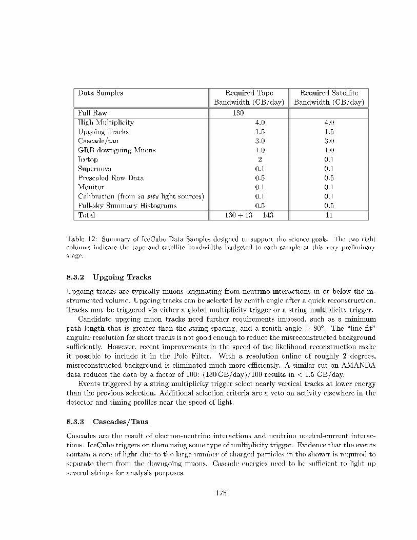
Data Samples Required Tape Required Satellite

Bandwidth (GB/day) Bandwidth (GB/day)

Full Raw 130

High Multiplicity 4.0 4.0

Upgoing Tracks 1.5 1.5

Cascade/tau 3.0 3.0

GRB downgoing Muons 1.0 1.0

Icetop 2 0.1

Supernova 0.1 0.1

Prescaled Raw Data 0.5 0.5

Monitor 0.1 0.1

Calibration (from in situ light sources) 0.1 0.1

Full-sky Summary Histograms 0.5 0.5

Total 130 + 13 = 143 11

Table 12: Summary of IceCube Data Samples designed to support the science goals. The two right

columns indicate the tape and satellite bandwidths budgeted to each sample at this very preliminary

stage.

8.3.2 Upgoing Tracks

Upgoing tracks are typically muons originating from neutrino interactions in or below the in-

strumented volume. Upgoing tracks can be selected by zenith angle after a quick reconstruction.

Tracks may be triggered via either a global multiplicity trigger or a string multiplicity trigger.

Candidate upgoing muon tracks need further requirements imposed, such as a minimum

path length that is greater than the string spacing, and a zenith angle > 80Æ. The \line �t"

angular resolution for short tracks is not good enough to reduce the misreconstructed background

suÆciently. However, recent improvements in the speed of the likelihood reconstruction make

it possible to include it in the Pole Filter. With a resolution online of roughly 2 degrees,

misreconstructed background is eliminated much more eÆciently. A similar cut on AMANDA

data reduces the data by a factor of 100: (130GB=day)=100 results in < 1:5 GB/day.

Events triggered by a string multiplicity trigger select nearly vertical tracks at lower energy

than the previous selection. Additional selection criteria are a veto on activity elsewhere in the

detector and timing pro�les near the speed of light.

8.3.3 Cascades/Taus

Cascades are the result of electron-neutrino interactions and neutrino neutral-current interac-

tions. IceCube triggers on them using some type of multiplicity trigger. Evidence that the events

contain a core of light due to the large number of charged particles in the shower is required to

separate them from the downgoing muons. Cascade energies need to be suÆcient to light up

several strings for analysis purposes.

175

Cuts on the spatial extent of the charged core may be used provided tau detection eÆciency

remains high. The high energy cascades, one of which is displayed in �g. 24, are of suÆcient

energy to be included in the high multiplicity sample. This sample is dedicated to the lower-

energy cascade analysis.

8.3.4 GRB Downgoing Muons

To study Southern Hemisphere GRBs, one needs to keep all downgoing muons for a 10 min

period around the GRB time. At the South Pole it takes a day or two to receive the GRB

trigger times from other experiments, so the raw data needs to be cached for a minimum of

2 days. One external GRB trigger per day and saving 10 min of raw IceCube centered around

the external trigger time corresponds to 1 GB/day required bandwidth out of the Pole.

It will be some time before another satellite is launched to provide these data as frequently

as once per day. The next generation experiment may have a higher GRB noti�cation rate. For

the �rst few years, therefore, we expect the IceCube GRB bandwidth requirements to be much

less than 1 GB/day.

A recent paper by Waxmann suggests that once every 40 years a supernova is close enough

to produce about 100 muons in IceCube shortly after the event. Presumably this event would

be very bright and we could search for it in the same way that we search for GRB.

8.3.5 Icetop

The IceTop array detects high energy cosmic ray shower events. These events typically have

high multiplicity and are expected to include waveforms. Their estimated raw data rate is

1{2 GB/day, reduced to 0.1 GB/day after �ltering.

8.3.6 Supernova

Supernova are expected to produce a large number of low energy neutrinos. The experimental

signal is an increase in all the PMTs of about 100 photons over a 10 s period. This analysis

requires us to record the PMT noise rates in 10 s bins for the duration of the experiment. This

adds up to about 0.1 GB/day.

8.3.7 Prescaled Raw Data

A minimum bias sample of prescaled downgoing muons can be used for geometry and timing

calibrations, to monitor detector stability, and as a test of background rejection algorithms used

in other analyses. Taking this data at 4 Hz yields a data sample of 0.5 GB/day.

8.3.8 Monitor

Monitor data is used to measure the quality of the data and verify the stability of the detector

over the lifetime of the experiment. Types of monitor data that we considered are: trigger, �lter,

176

and reconstruction rates, temperature sensors, DOM RAP jitter, PMT gain, risetime, peak-to-

valley, occupancies and noise rates, network activities, system deadtime, building power, UPS

status, local weather conditions, and station parameters such as satellite status, drilling, and

airplane landings. Measuring the DAQ related quantities once every 10 min seemed suÆcient

and contributes about 1.5 MB/day for each item monitored on 4800 PMTs. The 1 GB/day

bandwidth allows us to measure 600 such quantities. Many quantities are recorded much less

often, and some have fewer than 4800 channels.

There is no reason to limit the monitor data to activities at the Pole. The software is also

designed to include monitor data from any post-processing �lters as well. We will build on the

AMANDA experience to implement a web-based monitoring interface and electronic logbook

for IceCube.

8.3.9 Calibration

This sample consists of data from in situ light sources. This kind of data is triggered event

data, although several di�erent triggers may contribute. Triggering either from the light pulse

or with coincident hits is possible. Our other calibration source is downgoing muons which will

be available in the prescaled raw data.

Other calibrations, such as PMT gain and eÆciency, may be generated in real time in the

DOM �rmware, and as such will already exist in the data stream. These calibrations need to

be extracted and analyzed o�ine.

From various sources, calibration constants are compiled and stored for use by the recon-

struction. Since constants may be modi�ed as the analysis improves, a database implementation

is the obvious preferred choice with version numbers to keep track of what has been done.

8.3.10 Full-Sky Summary Histograms

High energy photons are predicted to send showers deep into the ice, triggering the IceCube

detector. Since this analysis requires sifting through every downgoing muon that triggers the

detector, it would be too cumbersome to achieve without a prede�ned histogramming of the data.

Full-sky summary histograms are therefore created every few minutes, resulting in 0.5 GB/day.

From these histograms energetic point sources in the Southern Hemisphere may be discovered.

8.3.11 Un�ltered Raw

After the �rst year, all un�ltered raw data is written to tape at the Pole, hand-carried out of

the Pole at station re-opening each November, copied and stored in at least two locations in the

northern hemisphere. The limitations on the use of the raw data are described in sec. 8.4.

8.4 Data Sample Organization

Several tagged samples will be bundled into one \physics" stream. The physics stream includes

the monitor, high multiplicity, upgoing tracks and cascade/tau data. They are distinguished

177

from one another by virtue of, for example, a set of bits in each data record's header. An actual

data event, for example, may have both the bits corresponding to the high multiplicity and

cascade/tau tags set. Monitor information has the monitor bit set, etc. It is a requirement

that data from one of the above streams can be time-correlated with data from any other of the

above streams. One possible way to implement this is to have all the data time-ordered and

resident in one �le, but other implementations are certainly possible. Time slicing may prove

valuable as well. In this scenario, the data are sliced into chunks representing a short length

of time (something like 10 s or 10 min). A database can then catalog the chunks, speeding up

random access to the events.

Several obvious advantages accrue from this \bundled data" scenario:

� Monitor data is available at analysis time from within the same program used to analyze

data, so one can imagine plotting not only (say) zenith angle of selected events, but also

noise rates measured at roughly the same time the event occurred in the detector.

� There are not multiple types of �les which need to be transferred from pole; the system is

simpler overall.

� Prescaled raw data is also available at analysis time, making background estimation and

monitoring detector performance with downgoing muons easier.

The size of the �les is dominated by tagged physics events, so the additional data volume of the

monitor data, prescaled raw data, etc. does not substantially increase overall �le size.

An important point here is that we are saving the full raw data stream. In the six-string

�rst year, the raw data are transferred over satellite for analysis and �lter checkout. After that

it grows too large for the satellite bandwidth, and we plan to copy it at the Pole onto tape.

The estimated size of this sample is 50 TB/yr. The tapes are mainly envisioned as an insurance

policy and we are only allocating resources for their archiving and no additional resources for

their use. If a collaborator comes up with a compelling new analysis idea which requires data

not present in the various �ltered data sets, the �rst step will be to develop a new �lter and

install it at the Pole. In this way, current data is used to validate the new idea. After the new

idea passes this test, the collaboration may decide to obtain the signi�cant additional resources

needed to re�lter all the raw tapes.

8.5 Latency

Latency is de�ned as the time between when an event is triggered and when it arrives on an

analyzer's disk. Data from the main analysis tags (high multiplicity, upgoing track, cascade/tau)

should have a 1-2 week latency, which includes possible further processing/�ltering in the north.

Monitor data should have a latency of less than 24 hrs. Supernova data should have as close to

zero latency as possible. One way to implement a very short latency time is to use the Iridium

system (if it remains available). Data volumes for supernova triggers are small enough to make

this feasible. IceCube can then be a full- edged participant in SNEWS, the Supernova Early

Warning System [48].

178

Possible uses of 24/7 low-bandwidth coverage beyond SNEWS include IceCube monitor data.

This would have the clear advantage of allowing us to keep close track of detector performance,

including during times when the winter-overs would be sleeping. This coverage would also be

very handy for small system maintenance tasks and for sending alarms to to the winterovers.

Obviously, the South Pole becomes much less remote with this kind of coverage.

After the �rst six-string year, the full raw data has a latency of at least a year, corresponding

to the movement of tapes from the Pole to the north. For IceCube design purposes, the latency

of this data sample should be considered in�nite since the resources needed to use it are not in

the current budget.

Another latency issue arises due to calibration constants (e.g., geometry) which will be

needed by the Pole �lters. We envision three categories of constants:

� initial constants: Within 2 days of deployment, crude constants should be available for the

operation of the string. An example of this would be OM locations from drill logs.

� on-line constants: Within a week or two of deployment, the results of in situ light sources

and downgoing muons need to be included for stable data taking.

� o�ine constants: As the analysis requires, constants need to be included in the database.

Multiple sets can be supported with the use of version numbers.

8.6 Schedule

IceCube construction will take a number of years. A simpli�ed �rst-light data model is used

consisting of only a multiplicity stream, calibration and monitor data. The multi-sample modes

and full online �ltering machinery are realized in the second year of operation as more strings

are deployed and the un�ltered raw data rate outstrips the available satellite bandwidth.

Software subsystem development must be prioritized, so that the �rst year's data is handled

without having to deviate dramatically from the overall system design. We need to develop

much of the infrastructure in the �rst year. De�ning APIs completely enables us to produce

needed subsystems without recoding later.

8.7 Summary

The IceCube Data Handling software system, though far from trivial, can be constructed using

existing software tools and methods, and it can be realized using existing commercial hardware.

To fully design and implement a reliable and robust system in time to analyze the data from the

�rst six IceCube strings will require a substantial software design e�ort which is best managed

by professional software engineers with experience in large scale projects like IceCube.

179

9 Data Analysis

9.1 Introduction

The main goal of the IceCube data analysis organization is to bring analyses to publication as

quickly as possible while maintaining the highest possible scienti�c standards. To achieve this

goal, the organization strives to ensure the infrastructure needed for analysis is provided and

maintained, to use analysis manpower resources in an eÆcient and fair manner, and to oversee

and streamline a rigorous internal analysis review process. Analysis infrastructure includes the

three broad areas of detector calibration and data quality, signal and background simulation,

and event reconstruction, and three working groups are formed to oversee these areas. Analy-

sis infrastructure also includes computational resources, and large and small computer clusters

are employed for data distribution, analysis and simulation purposes. Analysis manpower is

organized into �ve separate working groups, each of which contains several separate but related

analyses, so that ideas and methods can be shared easily among similar analyses. An Analy-

sis Coordinator oversees the activities of all the working groups. The internal review process

is managed by the Analysis Coordinator who, in consultation with the Collaboration Board,

appoints a small committee responsible for bringing an analysis from the �rst draft stage to

publication readiness and collaboration-wide approval.

9.2 Analysis Infrastructure

The analysis infrastructure is designed, constructed and maintained by three working groups,

each led by its own Working Group Coordinator (WGC). The coordinators are responsible for

ensuring that his/her group's responsibilities are ful�lled and for maintaining communications

with one another and with the Analysis Coordinator. These working groups are as follows:

� The detector calibration and data quality working group;

� The simulation working group;

� The event reconstruction working group.

Given the vital importance of these tasks, both for performing viable analyses and for engender-

ing a deep understanding of the IceCube detector, the associated workload is shared across the

collaboration, and each institution is obliged to contribute manpower to one or more of these

groups.

9.2.1 Calibration Analysis and Data Quality Working Group

The responsibility of this group is to collect, validate and install all detector-related constants

needed for data analysis, and to continuously measure and help maintain data quality. This

work includes, for example, the generation of detector geometry constants, measurement of ice

parameters, and studies of detector response using in situ light sources, followed by installation

of the resulting constants into the database. This work also includes the measurement and

180

analysis of quantities which track and improve data quality, such as the number of hot or dead

PMTs, PMT noise rates, possible drifts in various online calibrations, and checks of overall data

quality using downgoing muons.

Much of the output of this group is in the form of entries to the database. This database,

described in sec. 8.1.5, is accessed by both the reconstruction and the simulation codes, and this

group provides the appropriate software to make such access straightforward.

9.2.2 Simulation Working Group

The simulation working group is responsible for writing, supporting and documenting all required

simulation programs. The group develops the software which simulates the response of the

detector to charged particles emitting �Cerenkov light, including but not limited to the simulation

of ice parameters, photons passing through the ice, the PMT response, the DOM electronics,

and the trigger. The simulation package is compared to data whenever possible to ensure that

it is as close an approximation to reality as possible. This group also provides Monte Carlo

generators for the basic science topics covered by the Physics Working Groups (see below).

9.2.3 Reconstruction Working Group

The reconstruction working group is responsible for writing, supporting and documenting the

reconstruction programs for single muon tracks, multimuons, cascades, taus, contained events

and the energy reconstruction. The reconstruction programs are created within the software

framework provided by the Data Handling group.

9.3 Computing Infrastructure

Computing resources are needed for data distribution, data analysis and simulation. Two copies

of all �ltered data reside on disk in two post-�lter clusters, one in the US and the other in

Europe. This data amounts to roughly 2 TB/yr. In addition to the servers needed to control

these disk caches, permitting ready access to all members of the collaboration, each cache also

has an associated �50 GHz of CPU to perform additional �ltering and/or reconstruction tasks.

This cluster is built up in stages to match the rate at which data is acquired and to minimize

the total expense.

Each FTE in data analysis is provided with a small \local" computing cluster (on the order

of four machines with ample disk space and some peripherals, replaced every three years) for

use in analyzing data. These clusters reside at each user's home institution, and are probably

ganged together when multiple FTEs in data analysis are at the same institution.

Acquisition of a large cluster for simulating IceCube and IceTop data is also planned. The

cluster also �lters and caches this data. The nominal goal is to keep pace with the actual data

rate. Assuming roughly 0.5 s/event/GHz-CPU for generation and simulation, this translates to

a need for 800 GHz CPU power for the full detector. As with the post-�lter cluster, this cluster

is also built up in stages.

181

9.4 Physics Analysis

There are �ve physics data analysis working groups focussing on the scienti�c topics listed below.

The divisions between the di�erent working groups are not absolute and it will almost certainly

be necessary to have collaboration between di�erent groups. Each of these working groups

is led by a Working Group Coordinator (WGC). The WGC is responsible for organizing the

analysis work within his/her group, for scheduling and leading regular intra-group discussions,

for overseeing the internal review of analyses, and for communicating regularly with the Analysis

Coordinator.

� Physics Working Group 1

{ Atmospheric muons

{ Icetop

This group develops the tools and the �lters for analyzing muons coming from cosmic-

ray interactions in the atmosphere. The use of the IceTop detector is very important for

geometry and eÆciency calibration of the IceCube detector. In addition IceTop is used as

a veto detector for downgoing atmospheric muons. The group also does general air shower

physics analyses.

� Physics Working Group 2

{ Atmospheric neutrinos

{ Neutrino oscillations

{ WIMPs

This group analyzes the low energy charged-current muon neutrino interactions, including

the atmospheric neutrinos, neutrino oscillations, and neutrinos from WIMP annihilations

in the Sun and the Earth.

� Physics Working Group 3

{ High energy muon neutrinos (di�use)

{ High energy muon neutrinos (point sources)

{ GRB muon neutrinos

{ Relativistic monopoles

This group concentrates on analyzing the high energy charged-current muon neutrino

interactions inside and outside the detector. It searches for high energy neutrinos from

di�use sources, point sources, GRBs and relativistic monopoles.

� Physics Working Group 4

{ Isolated cascades

182

{ Electron neutrinos

{ GRB electron neutrinos

{ NC events

{ Tau neutrinos

This group analyzes high energy cascade events which could be due to electron neutrino

interactions, neutral current neutrino interactions or tau neutrino interactions.

� Physics Working Group 5

{ Supernova

{ Seasonal muon rate variations

This working group analyzes the Supernova data and Seasonal muon rate variations.

Certain general rules are followed to reduce experimenter bias in the analysis of data. Man-

power permitting, analyses are done in parallel and independently by two or more groups. The

collaboration may decide to insist that a particularly important analysis be done in this manner.

Each analysis uses only a fraction of the available data to tune selection criteria, and only looks

at the full data set when all selection criteria have been �nalized. Certain analyses should also

be \blind" such that the analyzer cannot tune selection criteria to enhance known source direc-

tions or times. For example, in a point source search one could alter reconstructed directions in

a deterministic but hidden way, and only after the analysis is �nalized are the true directions

used.

The Analysis Coordinator presents a report at each collaboration meeting giving an overview

of the status of each working group and its analysis work. Working Group Coordinators may

also be requested to give reports depending on the circumstances.

9.5 Internal Review Procedure

9.5.1 Introduction

Analysis results produced in the di�erent working groups should be approved for submission

to refereed journals and presentation at conferences with a minimum of administrative delays,

while at the same time rigorously checked to ensure the highest possible quality. The Analysis

Coordinator has the primary responsibility for this important task.

9.5.2 Procedure

The �rst venue in which a data analysis is discussed is within the appropriate Working Group.

This discussion is led by the WGC, and eventually results in the production of a document

detailing all aspects of the analysis. The level of detail should be such as to enable anyone in

the collaboration to repeat the analysis, with all systematic studies described and presented in

183

detail. All documentation produced in the Working Groups is made available to everyone in the

collaboration.

For parallel analyses where disagreement arises, or in other instances of disagreement, the

WGC attempts to resolve the issue. If the WGC cannot, the Analysis Coordinator tries to do

so. Ultimately, the Collaboration Board may be asked to intervene.

The next step is production of a �rst draft for publication. At this point, the Analysis

Coordinator appoints a paper committee. This committee consists of a small number of collab-

orators, preferably including some from outside the Working Group in question, to conduct the

internal review of the analysis and to shepherd it from �rst draft to publication readiness. The

Analysis Coordinator also appoints one or more primary authors if there is no obvious person

for the task.

Once the paper committee is satis�ed with the quality of the analysis and paper draft, the

draft is submitted to the collaboration for criticism and, eventually, approval for submission to a

refereed journal. Final approval for submission to a refereed journal is given by the Collaboration

Board.

9.6 Prerequisites and Schedule

IceCube data analysis obviously requires �ltered data, which depends on numerous aspects of

the data handling machinery to be in place, and on geometry and other low level constants

placed into a functioning database. The analysis framework software must be functioning. The

post-�lter clusters must be operating. The simulation framework and generation software must

be capable of simulating background and signal events, and the simulation cluster must be

operating. Basic monitoring information is required to permit veri�cation of data quality. The

data analysis management structure should be in place.

Initial analysis e�orts will focus on verifying overall detector performance in order to demon-

strate clearly that IceCube is a functioning neutrino telescope. With this in mind, analysis of

atmospheric muons, especially in conjunction with IceTop, and analyses of atmospheric electron

and muon neutrinos, would all be a high priority.

Subsequent e�ort will focus on those analysis topics that do not require substantial numbers

of strings to get started, such as searches for WIMPs, monopoles, supernovae, and extremely

high energy cascades. Analysis topics relying on more strings, like searches for ultrahigh energy

muons and cascades from point sources and di�use sources, searches for ultrahigh energy tau

neutrino interactions, and IceTop composition studies would follow.

184

10 Drilling, Deployment and Logistics

10.1 Drilling

10.1.1 Introduction

For decades glaciologists have used hot water drilling for rapid access to the inner workings of

glaciers. Though both hardware and energy intensive, hot water drilling provides the fastest and

most eÆcient way to access the deep ice. Water is also the ideal drilling uid for the IceCube

application. It is readily available, the hole is self-healing since the ice returns to essentially

its original condition after the deployment of the detectors, and its optical properties meet the

experimental requirements. Importantly, this technique is the only drilling method capable of

meeting the hole straightness requirement. Finally, components used to operate the system are

standard, reliable, and readily available from industrial outlets.

IceCube holes will be drilled with the Enhanced Hot Water Drill (EHWD). The EHWD

represents an evolution of the AMANDA drill, which was a research tool, to a production drill

capable of drilling 16 holes per season with 60 cm diameter to a depth of 2450 m. We have used

data gathered from drilling 23 holes for the AMANDA project to depths varying from 1000 to

2400 m to design a drill enabling us to drill and instrument a hole every 3.5 days.

Conceptually, hot-water drilling is as simple as it sounds. Water is pumped at high pressure

through a heating system and heated to near boiling temperature. The water is then forced

through a drill nozzle that directs a high-velocity stream of hot water against the ice in the hole,

melting it. The drill is steered by gravity.

Hot-water drilling is energy intensive because of the large amount of energy associated with

the ice-to-water phase change. This distinguishes hot-water drilling from the more energy-

eÆcient, but much slower ice-coring method.

A hole with a 60 cm diameter and, for instance, a 1 m depth has a volume of 78 gallons.

With South Pole ice at -40ÆC, an equal volume of 100ÆC water is required to melt this volume

of ice. To achieve this in one minute, or drill at a rate of 1 m/min, requires 2 MW of heat. After

accounting for heat losses to the ice surrounding the hole, we conclude that a 5 MW system is

required to drill at an average rate of 1.5 m per minute. With this rate the EWHD can deliver

IceCube holes to 2400 m depth in 40 hours with 7000 gallons of fuel. This can be seen as follows:

� One gallon of fuel can produce enough heat to produce about 80 gals of hot water at

100ÆC. When burner eÆciencies of 80% and the eÆciency of conversion to electrical power

are included, this the number reduces to 50 gal of water per gallon of fuel.

� A 2450 m deep hole contains 190,000 gallons of water. To melt this amount of ice at 50

gallons of water per gallon of fuel requires about 4000 gallons of fuel. Since the overall

eÆciency of the drilling process is 35% (half of the heat escapes into the surrounding ice

without melting it), we calculate that a hole will require 7000 gallons of fuel to drill. The

drilling time is 40 hours.

185

The relevant drilling parameters are pressure, ow and temperature. The heat delivered is the

product of ow and temperature. For constant pressures this ow varies as (hose diameter)8=3

and therefore this important parameter drives the performance of the EHWD system.

The conclusions presented above are buttressed by the wealth of data acquired with experi-

mental AMANDA drills.

While hot-water drilling is conceptually simple, meeting the power requirements for safe

and reliable drilling operations can be quite challenging. Drilling holes at the rate proposed to

2400 m depth requires the design, construction and operation of a major industrial complex in

a hostile environment. We list below the salient features of a hot-water drill system meeting our

requirements.

10.1.2 Evolution of AMANDA Drills

Initially, the AMANDA drill was designed to provide holes to 1000 m depth for the deployment

of 10 in bathyspheres and the 1.5 in diameter cable connecting them to the surface. This

was accomplished with 1 MW of heat delivered through the largest commercial synthetic hose

available (1.25 in). Drilling time was about 70 hr using 4500 gallons of fuel per hole.

The current AMANDA drill was designed to drill to 2000 m. It requires three hose reels

to hold hose reaching this depth. The heat input to this drill was increased to 2 MW. While

drilling in the upper portion of the hole with only one reel of hose connected into the system,

high ow rates and rapid drilling rates were achieved. Even though the ice is about 25ÆC warmer

near the bottom of the hole, the ow rate decreases signi�cantly due to friction with the hose

wall. With reduced ow rate, most of the heat is lost through the hose wall before reaching the

drill head. Thus, in the lower part of the hole, drilling is very slow as a result of the delivery of

low-pressure cool water to the drill nozzle. To drill eÆciently, the heat delivery to the drill head

at 2450-m depth should be comparable to the heat delivered by the drill at the top of the hole.

Three holes were drilled to 2450 m with substantially increased fuel consumption and drilling

times. Drilling to 2400 m required 120 hours and 13,000 gallons of fuel, demonstrating that the

drill had reached a practical limit. In summary, the current AMANDA drill system is capable

of drilling only four of these holes per season at these fuel consumption rates and would require

150 hours of drilling time per hole. The current drill also requires several weeks to build-up and

build-down each season, limiting actual drilling to about six weeks per season.

10.1.3 Performance Criteria and Design of the EHWD

Requiring that the heat input achieved with the AMANDA drill is doubled and a constant

water ow is maintained through the entire drilling process, both of which are possible only

with a single-reel design, one can extrapolate from drill data collected during the �rst 1000 m

of AMANDA drilling. This extrapolation indicates that drilling to a depth of 2400 m can

be achieved in 40 hrs while consuming about 7000 gallons of fuel per hole, corresponding to

a savings of about 400,000 gallons of fuel for IceCube's planned 80 holes. Note that faster

drilling is inherently more eÆcient because less time is spent warming surrounding ice. This

186

extrapolation matches our earlier estimate based on the thermodynamics of the problem.

To deliver the required heat without increasing pressure, the hose size must be increased from

1.5 in to 2.5 in diameter. The hose must be mounted on a single large hose reel to eliminate

the 8 hr hose reel changes currently required for each hole during drilling and drill extraction.

The drill components are housed in mobile drilling structures that can be quickly towed into

place and integrated, so that the drill build-up and build-down time must be reduced to a total

of about three weeks, permitting the drilling of 16 holes during an approximately 75 day �eld

season.

To improve fuel consumption we need to drill the holes quickly, particularly in cold ice. This

requires more heat at the drill nozzle. The amount of heat delivered to the drill nozzle is a

function of the hose diameter (given the desire to avoid hose pressures greater than 1000 psi).

The velocity of the water in the hose must be kept above 10 ft/s to avoid losing too much heat

through the hose wall.

The discussion of the requirements above shows that, relative to the present AMANDA drill

system, the general design criteria of the EHWD are:

� Higher eÆciency

� Higher heat generating capacity

� Greater heat delivery capability

Additional design criteria are set by the need to:

� Drill 16 holes per season (IceCube proposal requirement)

� Reduce fuel consumption to 7000 gallons or less per hole

Other objectives are:

� Increase eÆciency to minimize fuel consumption

� Increased reliability

� Decrease the work load for the drill crew

� Decrease the time to set up and take the drill apart

� Improve mobility to cover the square kilometer array

� Maintain a high degree of safety

To achieve a drill design that meets these requirements, each major subsystem must be

designed accordingly. The major subsystems of the drill are:

� Power Generation Subsystem

� Preheating Subsystem

187

� Main Heating Subsystem

� High-Pressure Pumps Subsystem

� Heat Delivery Subsystem

� Drill Head

The ways in which these drill subsystems will meet the various eÆciency, speed, and heating

generation and delivery requirements are detailed below.

Power Generation Subsystem

� EÆciency: Two eÆcient (12 kWh per gallon of JP-8) 400 kW generators (one on line,

one in standby) will provide all electric power for the drill during drilling and deployment

operations; two 60 kW generators will provide all electrical power during non-drilling

operations. By comparison, the AMANDA generators produce only about 7 kWh per

gallon of fuel. Thus, the new generators are about 54% higher in eÆciency. Waste heat

recovery for supplementing preheating plant and Rodriguez well heat requirements are

included in the design. Waste heat recovery is expected to save eight gallons of fuel per

hour.

� Faster Build-up and Build-Down: The generators will be sled-mounted and will have

fuel, water and electrical quick-connects for rapid integration during build-up and reduced

build-down time.

� Greater heat generating capability: Waste heat recovery will recover about eight gallons

of JP-8 equivalent per hour of drill time.

� Greater heat delivery capability: not directly applicable. However, the main generators are

sized to provide the additional power required to electrically drive two new high-pressure

pumps added to the high-pressure pumps subsystem, as well as replace the two diesel

drives on the two current AMANDA high-pressure pumps. This more than doubles the

generator output requirements of AMANDA.

Preheating Subsystem

� EÆciency: The Preheating plant provides about 25% of the total heat generation of the

drill. Waste-heat recovery heat will supplement the heat generated by high eÆciency (80%)

fuel-�red heaters.

� Faster Build-Up and Build-Down: The Preheating subsystem will be located in sled-

mounted Mobile Drilling Structures having fuel, water and electrical quick-connects for

rapid integration during build-up and reduced build-down time.

188

� Greater heat generating capability: The Preheating Plant will provide enough heat gen-

erating capability to increase the 200 gallons/min return and makeup water from near-

freezing to approximately 70ÆF. This is approximately double the AMANDA capability.

� Heat Delivery: The pumping capacity of circulator and transfer pumps will move about

twice as much water per minute as in the AMANDA drill. About 200 gallons/min of 70ÆF

water will be supplied to the suction side of the high-pressure pumps.

Main Heating Subsystem

� EÆciency: The design requirement is 80% minimum. Reusable AMANDA heaters will be

refurbished as necessary to achieve this design eÆciency.

� Faster Build-Up and Build-Down: The Main Heating subsystem will be located in four

sled-mounted Mobile Drilling Structures having fuel, water and electrical quick-connects

for rapid integration during build-up and reduced build-down time.

� Greater heat generating capability: The EHWD must heat 200 gallons of 70ÆF water to

190ÆF per minute, twice as much as the AMANDA drill. The EHWD has twice as many

heaters as AMANDA's main heating plant.

� Heat delivery: The inlet and outlet plumbing has been increased from 1.5 in to 2.5 in to

accommodate the increased ow.

High Pressure Pumps Subsystem

� EÆciency:The high-pressure pumps are the same as AMANDA's, but four will be required

instead of two for AMANDA. However, the ineÆcient diesel drives (about 7 kWh per gallon

of fuel) will be replaced with electric drives. Since the new generators will deliver about

12 kWh per gallon of fuel and assuming an electric drive eÆciency of 90%, the eÆciency

is expected to improve by about 54%.

� Faster Build-Up and Build-Down: The High-Pressure Pumps subsystem will be located in

a sled-mounted Mobile Drilling Structure having water and electrical quick-connects for

rapid integration during build-up and reduced build-down time.

� Heat delivery: The number of pumps will be doubled and the inlet and outlet plumbing

must be increased from 1.5 in to 2.5 in to accommodate the increased ow.

Heat Delivery Subsystem The Heat Delivery Subsystem includes the high-pressure hose

and the hose reel.

� EÆciency: The hose is increased from 1.5 in inside diameter to 2.5 in to accommodate the

increased ow and decrease the heat loss through the hose wall.

189

� Faster Build-Up and Build-Down: a single hose reel will hold the hose between the drill

head and hose reel (about 10,000 ft) instead of three for AMANDA. This reduces the

number of sled-mounted components by two.

� Heat delivery: The hose is increased from 1.5 in to 2.5 in to accommodate the increased

ow.

Drill Head

� Faster Build-Up and Build-Down: housing to be constructed of aluminum for lighter weight

and easier handling.

� Heat delivery: The nozzle size is increased to accommodate the increased ow.

10.2 Deployment

10.2.1 Overview

The installation of optical modules (OMs) in the ice is referred to as string deployment. In a

wider sense the string deployment includes the preparation of the string hardware at the South

Pole and the termination of the string in the IceCube counting house. Once the borehole of

approximately 50 cm diameter is drilled (melted) into the ice, the drill is removed from the hole

and the site is available for the string deployment. From that moment on, the water column of

2400 m depth begins to refreeze. The refreeze process is complete after about 5 days. However,

already after about 24 hrs the diameter of the water column shrinks to a diameter comparable

to the size of the OMs. The OMs must reach their �nal position before the water column

becomes too narrow. Figure 76 shows an image taken with a TV camera, which was deployed

with an AMANDA string. The glass sphere shown in the �gure was deployed for demonstration

purposes only. Its diameter was 10 in, which is less than the 13 in spheres used for the OMs.

Nonetheless, it can be seen that in this case the water column was much larger than needed, and

therefore that more fuel was used to drill the hole than necessary. An engineering project called

Smart Drill is underway to optimize the drilling by maintaining an adequate hole diameter while

minimizing fuel consumption.

The deployment coordinator must decide how much time is needed for the deployment.

The drill team must provide a hole that meets certain requirements. These requirements and

the protocol of the hand-over are discussed later. Once the hole is released for deployment

the countdown starts. After this moment the time constraints for the string deployments are

absolute and unforgiving. In the worst case scenario a string can get stuck in the ice at a shallow

depth where it is of little or no scienti�c value.

10.2.2 AMANDA Experience

AMANDA deployed a total of 23 strings to depths between 1000 and 2350 m. The chronology

of deployments is listed in table 13. The importance of the experience and expertise obtained in

190

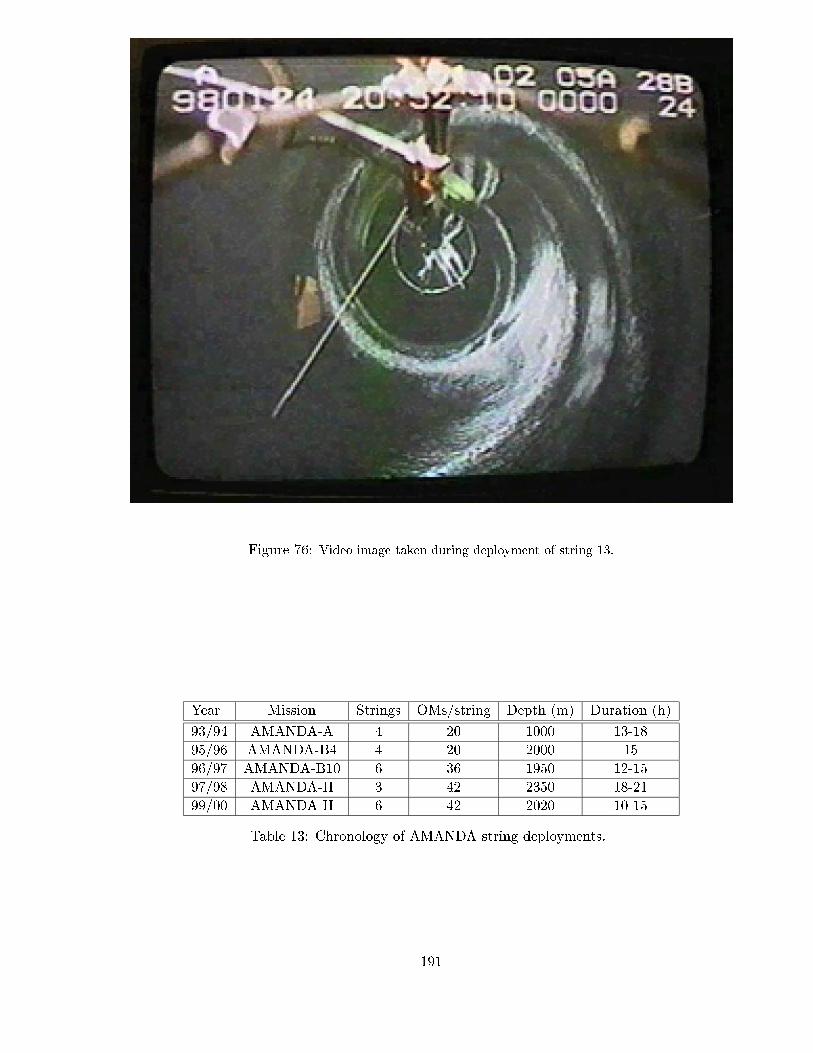
Figure 76: Video image taken during deployment of string 13.

Year Mission Strings OMs/string Depth (m) Duration (h)

93/94 AMANDA-A 4 20 1000 13-18

95/96 AMANDA-B4 4 20 2000 15

96/97 AMANDA-B10 6 36 1950 12-15

97/98 AMANDA-II 3 42 2350 18-21

99/00 AMANDA-II 6 42 2020 10-15

Table 13: Chronology of AMANDA string deployments.

191

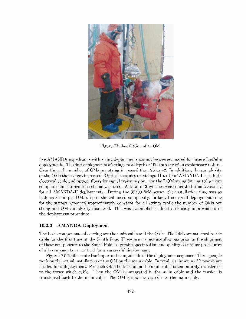
Figure 77: Installation of an OM.

�ve AMANDA expeditions with string deployments cannot be overestimated for future IceCube

deployments. The �rst deployments of strings to a depth of 1000 m were of an exploratory nature.

Over time, the number of OMs per string increased from 20 to 42. In addition, the complexity

of the OMs themselves increased. Optical modules on strings 11 to 19 of AMANDA-II use both

electrical cable and optical �bers for signal transmission. For the DOM string (string 18) a more

complex connectorization scheme was used. A total of 3 winches were operated simultaneously

for all AMANDA-II deployments. During the 99/00 �eld season the installation time was as

little as 8 min per OM, despite the enhanced complexity. In fact, the overall deployment time

for the strings remained approximately constant for all strings while the number of OMs per

string and OM complexity increased. This was accomplished due to a steady improvement in

the deployment procedure.

10.2.3 AMANDA Deployment

The basic components of a string are the main cable and the OMs. The OMs are attached to the

cable for the �rst time at the South Pole. There are no test installations prior to the shipment

of these components to the South Pole, so precise speci�cation and quality assurance procedures

of all components are critical for a successful deployment.

Figures 77-79 illustrate the important components of the deployment sequence. Three people

work on the actual installation of the OM on the main cable. In total, a minimum of 7 people are

needed for a deployment. For each OM the tension on the main cable is temporarily transferred

to the tower winch cable. Then the OM is integrated in the main cable and the tension is

transferred back to the main cable. The OM is now integrated into the main cable.

192

Figure 78: An OM ready to be lowered into the drill hole.

193

Figure 79: An OM being lowered into the drill hole.

194

String 16 - deployment

0

250

500

750

1000

1250

1500

1750

2000

0 2 4 6 8 10 12

OM deployment dropT

V c

amer

a do

wn

the

hole

New

Yea

r’s

cele

brat

ion

1999

2000

time [hours]

dept

h [m

we]

17 m

/min

8 min/O

M

8 min/O

M

shif

t cha

nge

Average OM deployment: 12 min/OM

Average drop speed: 13 m/min

Figure 80: Deployment of AMANDA string 16. The depth, as measured by a pressure sensor, is plotted

versus time. For this string the OM installation time was less than 10 hrs. The drop takes about 2 hrs.

195

Figure 80 shows the progress of the deployment with time. A pressure sensor mounted to

the bottom of the string monitors the depth of the string. The drill hole is �lled with water up

to a level of about 50 m below the snow surface. The pressure begins to increase strongly after

the sensor reaches the water level. The pressure sensor is the primary measure of the absolute

depth of the string. Other measures are cable marks and possibly a secondary pressure sensor.

Each stop corresponds to the installation of on OM. The deployment reached speeds of 8 min

per OM. Once all OMs are installed the pressure corresponds to about 350 m water equivalent

pressure (the length of the instrumented portion of the string minus 50 m at the top). Now the

\drop" begins. The string is lowered to its target depth at a speed of approximately 15 m/min.

10.2.4 IceCube Deployment Overview

A diagram of the full IceCube deployment setup, depicting the counting house, the surface cable,

an IceTop detector module and the down-hole cable, is shown in �g. 81.

The mechanical installation of the OM is illustrated in �g. 82. The OMs are attached to the

main cable below and above as shown. A chain with a shortening clutch allows adjusting the

length to a precision of 1 in. This design is identical to that used on AMANDA strings 14 to 19

and is well understood.

Each OM is connected electrically to the cable via twisted quad cable breakouts at every

fourth OM position as shown in �g. 83. Each twisted quad cable consists of 2 twisted pairs.

Each twisted pair provides 2 OMs with power and communication from the surface. Figure 84

illustrates how 4 OMs are connected to the main cable. The OMs are spaced by 17 m. Thus,

there will be a breakout of a quad cable every 68 m. A wiring harness will be used as an interface

between the twisted quad breakout on the main cable and the OM.

10.2.5 IceCube String Deployment Procedure

The requirement to deploy 16 strings with 60 OMs each in a single season, particularly in view of

South Pole population constraints, requires a further improvement of the deployment operation.

During the AMANDA deployments, the shortest time between the start of two subsequent

deployments was 120 hr. For IceCube the average deployment cycle time will be 84 hr for a

period of about 60 days, excluding 5 days of down time. The increase in the eÆciency is possible

by optimizing every single element of the deployment procedures, in particular in the pre- and

post-deployment activities.

The digital signal transmission based on the design of the DOM allows a signi�cant change

and simpli�cation of the deployment procedure of IceCube strings. No optical �ber cables will

be required. Thirty twisted pair cables will provide power and signal transmission for 60 OMs.

The absence of optical �bers reduces the cargo by about 9000 lb per string, and simpli�es test

procedures prior to and during the deployment. (During deployments of AMANDA strings 11-

13, problems were encountered when the breakouts of �ber cables and electrical cables did not

match up. These phasing problems were one of the reasons why the deployment times were

196

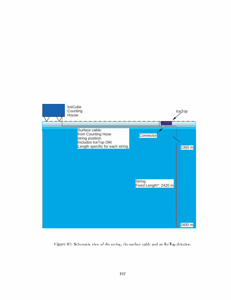
1350 m

2400 m

IceTopIceCube CountingHouse

ConnectorSurface cable:from Counting Hosestring position.Includes IceTop OM.Length specific for each string.

String:Fixed Length*: 2420 m

Figure 81: Schematic view of the string, the surface cable and an IceTop detector.

197

1)

2)

3)

180

cm

Diameter of "string"

Figure 82: Mechanical integration of OM into the main cable.

198

spacing to nextcable stop: 17 m

ICECUBE CABLE: BREAKOUT SCHEMATIC S

Albrecht KarleDec. 13, 2000Breakout schematics

(NOT TO SCALE)

0.6 m

0.9 m

0.9 m

Breakout

Cable Stopdown

Cable Stop up

0.9 m

0.9 m

No Breakout

Cable Stopdown

Cable Stop up

0.9 m

0.9 m

Cable Stopdown

Cable Stop up

spacing to nextcable stop: 17 m

Breakout on every fourth OM position: 4, 8, 12, ... -counting from top.

No Breakout

Figure 83: Breakout schematics on main cable. Pre-installed cable stops are used to mount the OMs.

A twisted quad is broken out at every fourth OM position.

199

Twisted pair cable for power and communication

6 pin connector

2 pin, male

2 pin, female

4 pin

6 pin connector

6 pin connector

6 pin connectorSplitter box, pressure resistant 10,000 psi-60 Csize of PCB: TBD(est.: 3x10 cm2)

Breakoutmain cable

Main cable

Twisted pair cable for local coincidence

feedthrough for triple twisted pair

optical module

Wiring Harness

Figure 84: A group of four OMs is operated through a single twisted quad.

200

particularly high for strings 11-13. The phasing problems were solved in the 99/00 campaign.

The deployment with a single cable, of course, means such phasing problems cannot occur.)

The phases of string deployment are as follows:

1. Install weights (600 lb);

2. Install 60 OMs;

3. Lower string to its target position at 2403 m.

Several pressure sensors on the string are used to monitor the correct motion of the string.

Communications and power to the pressure sensors and to the newly connected OM is provided

through a slip ring mounted at the cable winch. The actual payout of cable will be measured

at the surface. The measured payout at the surface and the pressure increase at the bottom of

the string will be monitored for consistency. The correct electrical connection of each OM is

veri�ed at time of installation. A short electronic test sequence of no more than a few minutes

is performed at this time. Additional communication tests to the recently installed OMs can

continue for a few more minutes.

10.2.6 IceCube Indoor Deployment

The shelter at the deployment site is very important for high quality OM installation at a rate

of 2 strings per week. In the past, these shelters consisted of simple wind shields or a tent

structure. Figures 85 and 86 show the dome structure that was used for AMANDA string 14-19

deployments.

For IceCube a heated building (see �gs. 87{90) coupled to the drilling apparatus will be

used as a deployment facility. This approach will improve the work conditions for the deployers

substantially. All deployers work indoors. The electronics control room is inside this building

but separated by a wall with large windows. The building is large enough to bring all or at least

most of the OMs inside prior to the deployment. A furnace will replace noisy bullet heaters

and eliminate exhaust near the work site. The ceiling may be partially transparent to take

advantage of solar power and light. This building will also serve as a drilling shelter during the

drill operation.

201

Figure 85: Setting up a shelter for AMANDA deployments. The setup time of 3 hours is too long for

IceCube.

202

Figure 86: Completed shelter used for AMANDA deployments. This is type of shelter is not adequate

for IceCube.

203

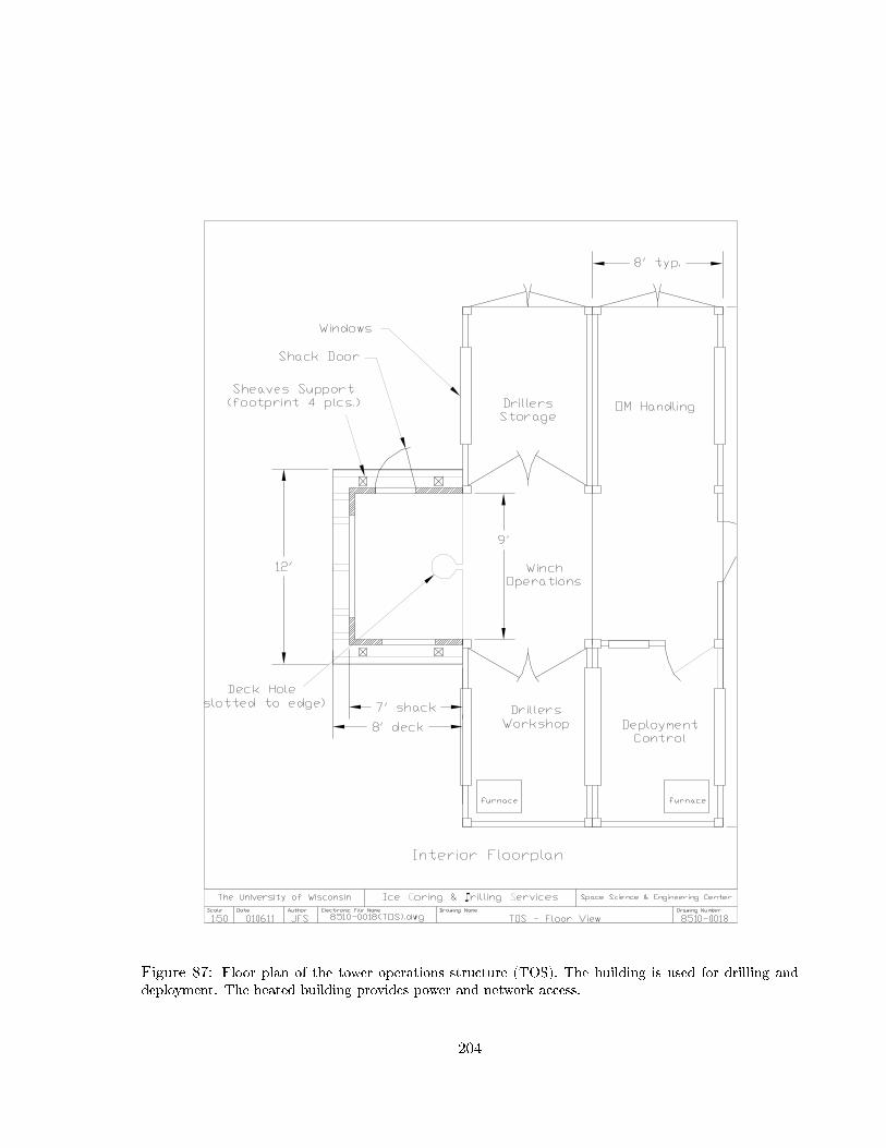
Figure 87: Floor plan of the tower operations structure (TOS). The building is used for drilling and

deployment. The heated building provides power and network access.

204

Figure 88: Roof plan of the tower operations structure (TOS).

205

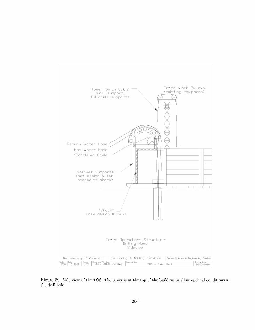
Figure 89: Side view of the TOS. The tower is at the top of the building to allow optimal conditions at

the drill hole.

206

Figure 90: The sheave is detachable from the main structure for transportation purposes.

207

Diameter 43.0 cm

Depth 2410 m

Lifespan of 1st hole per season 32:00 hr

Lifespan of subsequent holes 29:30 hr

Table 14: Requirements which the drill hole must meet at the time of handover to the deployment

team.

Deployment phase Allocated Time (hr)

Nominal Contingency Total

Preparation 1:00 1:00 2:00

Weights, pressure sensor 0:40 0:20 1:00

OM installation 14:00 6:00 20:00

Drop 2:30 2:00 4:30

Finish and secure string 1:00 1:00 2:00

Total 19:10 10:20 29:30

Table 15: Breakdown of deployment phases and allocated times.

10.2.7 IceCube Drill Hole Requirements

The drill hole needs to be of a minimum diameter and depth for at least the time required for the

string deployment. The minimal diameter is determined by the size of the OM (36 cm, including

the harness) plus the cable (4 cm). The tolerances on the OM size are 0.8 cm. The tolerance

on the cable diameter is 0.7 cm. We add an additional 1.5 cm for tapes and cable ties. The

maximum diameter of the string is 43.0 cm. The drill hole requirements are listed in table 14.

The speci�ed duration contains contingency time for the deployment operation. The nominal

total deployment time is estimated to 19 hr. This allows for more than 10 hr of contingency.

The nominal depth is 2403 m. We allocate 7 m of contingency.

The deployment operation begins when the drill hole is accessible for the deployers. At this

time the drill and the downhole pump have been removed from the hole. In addition it is required

that the area behind the tower be accessible to position the winch with the IceCube cable. Once

these conditions are met the hole is handed over from the drilling to the deployment command.

A breakdown of the di�erent phases of the string deployment operation and the estimated time

for each phase is given in table 15. Contingency times are based on experience and possible

failure mechanisms. Possible failure scenarios include power, winch control, winch drive, tower

winch, computer and unexpected situations.

208

Release hole N for deployment

Receive hole from drillingteam

Deploymentof string N

Transfer of mobile equipment(Hose winch, other winches, building, tower,...)

Drilling of hole N+1

Deploymentof string N+1

0h 12h 24h 36h 48h 60h 72h 84h

OM testing,deployment preparation,Move string deployment room,checkout at counting houseIceTop deployment, etc.

Time

Release hole N+1 for deployment

Figure 91: Time schedule of a single drilling and deployment sequence. The projected time for a single

cycle is 84 hours.

Figure 91 gives an overview of the major operations during a single drilling and deployment

cycle of 84 hr, and �g. 92 shows a schematic view of arrangement of drilling and deployment

infrastructure in the course of drilling �ve holes.

10.2.8 Quality Assurance

Optical modules and associated components are all tested at various stages leading up to and

including deployment. Tests which are done at McMurdo and the South Pole are described

below.

McMurdo Test Stand All OMs undergo a detailed test procedure and burn-in operation

before they are shipped to the South Pole. OM tests concern the integrity of the hardware after

the transportation. Most OMs will be shipped by vessel. They arrive in January in McMurdo

and stay there until about October of the same year. From here they are sent by air to the

South Pole. The infrastructure at McMurdo permits extensive testing of OMs there. Therefore,

only a very brief test sequence will be required at the Pole. (The details of the tests will be

described elsewhere.) It is a fundamental concept of the test procedures that they do not require

unpacking the OMs from the shipping crates. The crates are therefore light-tight. It is planned

to wire the OMs inside the crate to a patch panel, which is accessible from the outside.

Only in the �rst season (FY04) will all OMs be shipped by air to McMurdo. In the following

seasons an increasing fraction of OMs will be shipped by vessel. This requires that up to 1000

209

“Base Camp:Central drilling structures (6 units for heaters, pumps, Rodrigues Well,...)

deployment winch 1

Time: 0Hole 1: String in operationHole 2: Deployment in progress Hole 3: Drilling in preparation Hole 4: Firn hole drilledHole 5: Firn hole drilled

Drill controlCenter(DCC)

OM DCTOS

Hose winch

water return TOW

OM DCTOS

Central Deployment Lab

OMs

StringCables

deployment winch 2

(CDL)

1 2 3 4 5

IceTopIceTop IceTop IceTop IceTop

String 1 in operation

Surface cables to strings

Drilling and Deployment Field Camp

Figure 92: A schematic view of the drilling and deployment infrastructure with �ve drill holes is given.

210

OMs be stored in McMurdo, and hence a similar number need to be tested there each season.

This is done with a DAQ system with 500 channels to test the all the OMs in two batches. The

duration of the tests is 2{3 months. The DAQ hardware can be shipped to the pole with the

last batch of OMs in the last year of string deployments and used for the main DAQ.

South Pole Test Stand The deployment infrastructure at the pole can be divided in three

categories:

1. The central deployment lab;

2. The string deployment room;

3. A room allocated for deployment support in the IceCube counting house.

All OMs are delivered to the central deployment lab. Here they undergo a �nal test sequence

of not more than 60 min per OM. Again, the OMs are tested in the crates. The crates must be

light-tight such that the OM can be powered up and noise pulses and cosmic-rays observed.

A test DAQ is available to operate up to 100 OMs at a time. The test DAQ is very similar to

systems used at various locations during the OM production and shipping. The tests are short

in duration, ranging from 10 min to not more than 60 min. The tests are pass/fail and executed

in software. OMs that fail the Q/A procedure are rejected for deployment and sent back. Only

minor mechanical problems are �xed at the South Pole. OMs that show electronic problems are

not opened for repair at the Pole, instead they are sent back to McMurdo.

About 60 OMs will be tested at a time. Fifteen twisted quad cables (or 30 twisted pairs) need

to be connected to the crates waiting for tests. The time to wire up all the crates is estimated to

be 1{2 hr. While the test runs no longer than one hour, the time for debugging and evaluation

may take several hours. In total we allocate 24 hr of labor per string at the central deployment

lab.

After this test the OMs are powered o� and the crates are opened for the �rst time since

shipment from the northern hemisphere. The content of the crates is checked for completeness

of all mechanical components. At this time the pressure inside the OMs is checked to make

sure there are no leaks. Once the OMs are certi�ed the crates will be marked and sent the next

deployment site.

Once the OMs are certi�ed for deployment they can be moved to the string deployment

site. Sixty OMs plus about eight spares are loaded into the deployment room and partially

unpacked. During the deployment a �nal continuity and communications test is performed.

This test requires at most a few minutes and can be performed in parallel with the mechanical

installation. The OMs are connected in groups of four. Once connected the deployment DAQ

veri�es the continuity and runs some basic electronic and communications tests.

10.2.9 Practice Deployments

Experience has shown that the �rst string deployment in each season is particularly challenging

due to lack of experience of most of the team members. Two strategies are planned to optimize

211

Year FY04 FY05 FY06 FY07 FY08 FY09

baseline schedule 6 12 16 16 16 14

possible range 3-6 8-14 15-17 15-18 15-18 14-18

Table 16: Schedule for string deployments. The numbers indicate the how many strings are to be

deployed in each season in the baseline schedule and the possible range in the number of strings deployed

each year, as described in the text.

the performance during the �rst deployment. A pre-deployment workshop of about two weeks

is planned and budgeted for all deployers. This is an opportunity to familiarize the team with

the procedure and the instruments used. Unexpected situations can be discussed. Particular

responsibilities can be de�ned. A test stand will be available to practice the actual OM in-

stallation. The full deployment team must be at the South Pole two weeks prior to the �rst

deployment to begin with the preparations, test procedures, and the setup of the instruments

and labs. A practice hole of about 50 m depth together with the full deployment infrastructure

(tower, string deployment shelter, etc.) will allow deployers to practice the deployment on the

site. A subset of the deployment team needs to arrive at least three weeks prior to the �rst

IceCube deployment to prepare the new infrastructure.

10.2.10 Surface Cable Installation

Deployment Sequence and Cable Plan Table 16 shows the deployment sequence during

the IceCube construction period, and �g. 93 illustrates this sequence. The baseline schedule

calls for six strings to be installed in FY04, followed by 12 in FY05, then 16 for FY06{FY08

and �nally 14 strings in FY09. In FY04, the chief goal is to achieve an end-to-end test of all

detector systems, a goal which is best achieved with a minimum of three strings, as indicated

by the �rst number in the \possible range" row in Table 16. Similarly, in subsequent years the

�rst number represents the minimum number of strings to be deployed, and the second number

the maximum, subject to the constraint that the sum over all years equals 80. Experience

gained in earlier years may permit even larger numbers of strings to be deployed in later years

than indicated in the table. For any year in which the number of strings deployed exceeds the

baseline schedule, there are production, logistics, and schedule implications which have not yet

been addressed. It is possible that an accelerated schedule, using contingency funds in earlier

years, will result in an overall savings to the project.

The addition of 12 strings in FY05 will embed the AMANDA array in IceCube strings.

The SPASE-2 array will be embedded only in FY09. A few SPASE-2 stations will have to be

relocated then, assuming that it is still in full operation. Trenches are used to bury the cables

at depths which will keep them secure for � 15 yr.

Cable Trenches The separation of the main cable in a surface cable and an in-ice cable allows

for a very exible cable management. The surface cables will be laid and trenched independent

212

AMANDA-II

AMANDA- B

SPASE-2

Old Pole Station line (line of death)

Runway

Old Pole Station line (line of death)

IceCube layout

Dome

Gridnorth

100 m

PoleSouth

FY04:6

FY05:12FY06:16

FY07:16

FY08:16 FY09:14

ICECUBE: CABLE PLAN

Figure 93: The deployment sequence.

213

of the exact timing of the drilling and deployment. In this design, the surface cable will be

trenched before the drilling starts. Ideally the surface cable is already wired up in the counting

house by the time the string is deployed. As soon as the string is deployed it will be connected

to the surface cable and the string will be operated from the counting house hours after the

deployment is completed. Another advantage is that the valuable time during November will be

used to do the cable trenching. There is no need to wait for the strings to be deployed �rst. The

cables will be trenched starting from the counting house. This avoids the pile-up of excess cable

in its vicinity. The small amount of excess cable, a few tens of meters, will be buried together

with the IceTop tank in the snow. This is where the connection between the in-ice cable and

the surface cable will be located. Cable trenching is done by the NSF contractor.

10.3 Logistics

10.3.1 Introduction

A South Pole Experimental Deployment is a highly detailed operation requiring the e�orts

of many groups at the NSF and the Support Contractor as well as detailed planning of the

experimental group. This planning starts with the Operational Research Worksheet (ORW)

which describes the full long-term requirements of the experiment. It is supplemented each

year with the Support Information Package (SIP), and later with direct meetings between the

experimenters, the NSF, and the Support Contractors so that all can agree on the exact level of

�eld-support the experimenters can plan on being delivered by the NSF and the Contractor.

10.3.2 Documentation

The ORW is submitted along with the experimental proposal to the NSF, and it is reviewed

by the contractor to assess whether the experimental proposal can be adequately supported to

meet the needs of the experimenters. This document serves to outline the annual support an

experiment will require during the entire lifetime of the experiment.

The type of information required for both the ORW and SIP is listed below.

� PI and co-PI Contacts

� Project Description: Locations and Scienti�c Opjectives

� Personnel: Proposed time period at the pole and speci�c job-tasking, medical/dental

examinations and clearances. Travel arrangements.

� Safety Environment and Health Issues: Ice coring, use of heavy equipment, placement of

probes. use of radioactive materials, hazardous waste, etc.

� Cargo: A complete listing of all of the cargo items one expects to ship.

� Construction and Fabrication Required

� Computers and Communications: Connectivity, system maintenance, on-site support

214

� Laboratory/Observatory Requirements

� Aircraft Support

� Vehicle Support

� Global Positioning (GPS) Support

Experience with AMANDA has shown us that the best way to keep the NSF and Contractor

up to date concerning South Pole population levels and personnel medical/dental and travel sta-

tus is to maintain a Deployment WWW-page. Both personnel and cargo movement information

is presented in spreadsheet formats (presently using EXCEL). These formatted personnel and

cargo spread-sheets are also forwarded electronically to the contractor.

10.3.3 Personnel and Taskings

South Pole population levels are highly restricted, mainly due to station size limitations. In the

past AMANDA has been forced to cap its population to about 12-15 people at any time. The

�eld-season generally runs from November 1st to about February 15th each year. This 15 week

period is generally divided into 3-4 project periods of 4-5 weeks duration. This generally matches

with the period of time that people spend on the pole so that in any season we may have as

many as 35-45 people working at the pole during some period. Generally a task will involve 3-4

people and we generally schedule in 3-4 parallel tasks at any one period. This generally means

that anywhere from 12-15 speci�c tasks invoving 3-4 people for 3-5 weeks will get done during

a �eld-season

The labor hours required for the deployment of a single string and the associated IceTop

detector is given in table 17. The total population required to perform these tasks follows from

the labor required per string. Almost 40% of the deployment time is required for the actual

string deployment operation.

The basic string deployment operation requires 7 people during the core deployment opera-

tion. 24 hours are allocated for the deployment operation. This is almost 5 hours more than the

nominal deployment time to ensure the readiness of the team at the time of the hand-over from

drilling. Including the IceTop deployment, we plan on a total population of 16 people during

times of full capacity string deployments. Three people are allocated for the IceTop deployment.

The IceTop deployment personnel requirements are the most diÆcult to estimate due to lack of

experience.

As shown in table 18, the projected population reaches a maximum of 44 in all years. The

drilling population is higher in the �rst year, due to the drill construction. The AMANDA

and SPASE population is higher in the �rst 4 weeks of FY04. The \Science" population is the

personnel required for the installations of the electronics and software in the counting house

and in the B2 science lab. This group will commission and operate the detector during the

summer. As soon as the deployment operation is phased down by the end of January, the science

population is increased to accelerate the commissioning of the last strings and to increase the

e�orts on data handling operations.

215

Operation Time allocated (h)

Cable drag 52

Deployment (24*7) 168

Site. Preparation 16

Cable unpack and prep 20

OM Testing 24

Documentation 10

PTS prep 15

Logistical and other support 20

IceTop 84

General assistance 20

Total: String 429

Total: Week 858

Number of 54 hour shifts/week 15.9

Table 17: Labor hours required for a single string.

Person days: Total/season Population during deployment periods:

(Maximum/day)

Year FY 04 FY 05 FY 06 - 09 FY 04 FY 05 FY 06 - 09

Drilling 1509 1308 1307 18 15 15

Deployment 796 1334 1316 15 16 16

Science 676 905 1032 8 10 11

A-II/S-2 611 392 238 3 3 2

Sum 3592 3939 3893 44 44 44

Table 18: Population required for the �scal years FY04 to FY09. The population is broken down

in drilling personnel, deployment personnel, science personnel for IceCube and science personnel

for the subsystems AMANDA-II and SPASE-2. The total number of person days during a South

Pole summer is given on the left. On the right the number of people is given during the periods

of highest population.

216

Item Weight (lb) Volume (ft3)

Cable 10560a 307a

60 OM 3300b 270b

Mechanical 400c 4c

Weights 600c 6c

IceTop unit 1200c 120c

Total: single string 16060 7070

Total: 16 strings 25690 11310

Table 19: Breakdown of weights and cubes per string and total for a single string and 16 strings.

(Quantities come from RK quotes (a), Ho�man (b) and Karle (c).)

10.3.4 Medical/Dental Examinations

All personnel deploying to the South Pole have to pass a medical and dental examination. This

can be complicated and time consuming so the process is started in the May-June time period.

The contractor sends out the medical/dental packets and they also view the results of the tests

and make the decision if a South Pole candidate is medically quali�ed. Di�erences in European

and American dental standards have caused problems in the past. Medical quali�cation is a

precondition to Antarctic travel.

10.3.5 Airline Travel

All U.S. experimenters have their airline tickets purchased by the contractor. These tickets

provide travel between their university location and Christchurch, New Zealand. Foreign par-

ticipants have to provide transportation at their own costs to Christchurch. At that point all

participants are provided transportation at no cost to them, from Christchurch to Antarctica.

The experimenters are expected to pay for their lodging and food from their research con-

tracts. Once in Antarctica there are no costs, since both food and lodging is provided.

10.3.6 Weights and Cubes

The main elements of a string are the cable and the OMs. Smaller mechanical components

are needed for the installation of the sensors. Weights are used at the bottom to keep the

string under tension. The weights and cubes for each string are listed in table 19. We group

the cargo in three categories: Cables, OMs, and miscellaneous, where miscellaneous stands for

mechanical components, the weights and for the IceTop tank for each string. The following

cargo movements are required:

1. All incoming cargo is delivered to the central deployment lab as it arrives.

217

2. The equipment used for each string is transported to the exact location near the deploy-

ment site of a given string. The equipment is requested at the deployment site before the

drilling starts. This will be approximately 48 hours before the deployment begins.

3. Remaining packing materials are transferred to South Pole waste management.

10.3.7 Cargo Transport

Estimates of total mass and volume of material (\weights and cubes") required by IceCube over

its lifetime are given in the tables below. There are three ways that cargo can get to the South

Pole site, by \vessel," \Comm-Air" and \Kilo-Air."

The vessel is the cheapest means of transport, but requires the most advance planning. Cargo

leaves Port Hueneme, CA by vessel on about December 15 and arrives in McMurdo, Antarctica

about 6 weeks later on January 25. The cargo is then own in C-130 Hercules aircraft to the

pole or it winters in McMurdo and is is own at the beginning of the next season. Either way

the cargo is only available for use at the pole the following season. The vessel requires that

equipment be ready one year before it will be needed at the pole.

Kilo-Air is the most common way to ship items. Under this plan, items are shipped from

Port Hueneme to Christchurch NZ by vessel about September 15. From Christchurch they are

own down to McMurdo, and then from McMurdo to the pole. This means that cargo usually

has to be ready about 60-70 days before it is needed at South Pole.

Comm-Air is the fastest and most expensive way to ship cargo to the pole and it requires

NSF approval. Items travel from Port Hueneme to Christchurch by commercial air-cargo. From

Christchurch to Antarctica they travel the same way as Kilo-Air.

All Antarctic cargo orginating in the U.S. is shipped from the NSF facility in Port Hueneme,

CA. Cargo originating in Europe is generally shipped to the NSF facility in Christchurch, NZ.

During the course of the IceCube deployment it is expected that about 1300K lbs of detector

components and 650K lbs of drilling equipment will be shipped to the South Pole via vessel. We

also plan to ship about 100K lbs of detector components and 100K lbs of drilling equipment via

Kilo-Air.

The tables 20 10.3.7 10.3.7 10.3.7 10.3.7 list the cargo to be shipped by the various means

listed above. In these tables, \ROS" stands for \Required On Site" and \N" is the current

year's string count minus one. The cargo is given in two categories that describe the mode of

transportation: Kilo-Air and Vessel. The cargo is broken down further in 3 categories of string

equipment: Optical Modules (OM), Cables, Miscellaneous.

218

FY Strings Weight (lbs) Cubes (ft3) ROS

04 6+1 23100 1890 12-13-03+N�5 days05 6 19800 1620 11-20-04+N�3 days06 4 13200 1080 11-16-05+N�3 days07 0 0 0 0

08 0 0 0 0

09 0 0 0 0

Table 20: Optical Modules to be shipped by \Kilo Air."

FY Weight (lbs) Cubes (ft3) ROS

04 4000 1890 12-15-03

05 6000 1620 12-15-04

06 4000 1080 12-15-05

07 4000 0 12-15-06

08 1000 0 12-15-07

09 1000 0 12-15-08

Table 21: Miscellaneous hardware to be shipped by \Kilo Air."

FY Strings Weight (lbs) Cubes (ft3) ROS

04 0 0 0 12-13-03+N�5 days05 6+2 26,400 2160 11-20-04+N�3 days06 12+2 46,200 3780 11-16-05+N�3 days07 16+1 56,100 4590 11-16-06+N�3 days08 16+1 56,100 4590 11-16-07+N�3 days09 14 46,200 3780 11-16-08+N�3 days

Table 22: Optical modules to be shipped by vessel.

FY Strings Weight (lbs) Cubes (ft3) ROS

04 6 13200 720 12-13-03+N�5 days05 12+2 30800 1680 11-20-04+N�3 days06 16+2 39600 2160 11-16-05+N�3 days07 16+1 37400 2040 11-16-05+N�3 days08 16+1 37400 2040 11-16-05+N�3 days09 14 30800 1680 11-16-05+N�3 days

Table 23: Miscellaneous hardware to be shipped by vessel.

219

FY Strings Weight (lbs) Cubes (ft3) ROS

04 6 63,350 1842 12-13-03

05 12 126,700 3685 11-20-04+N�3 days06 16 168,900 4913 11-16-05+N�3 days07 16 168,900 4913 11-16-05+N�3 days08 16 168,900 4913 11-16-05+N�3 days09 14 147,800 4299 11-16-05+N�3 days

Table 24: Cables to be shipped by vessel.

220

11 Quality Assurance

The IceCube project oÆce will implement a quality plan meeting the requirements of ANSI/ISO/ASQC

Q9001-2000 (ISO 9000). The UW Space Science and Engineering Center (SSEC) is in the pro-

cess of implementing a Quality Management System (QMS) meeting the requirements of ISO

9000 and eventual registration.

The IceCube Quality Plan will de�ne the overall project policy, the processes to be controlled

and how they interact, and the procedures to be used. The plan will include, but not be limited

to, addressing the following areas:

1. The overall scope of the Quality Plan, the standards (ISO 9000, etc.) it is designed to

meet, and the management commitment to the plan. Exclusions, if any, will be listed. The

plan will make it clear how each element of the program is a�ected by the quality plan,

who is responsible, how each requirement is to be met, and how we verify the e�ectiveness

of the plan.

2. Control of documents: who approves, how released and distributed, lists of documents,

change procedures, how users are assured they have the latest documentation, and how

obsolete documentation is removed from the system. The document control system will

use on-line databases with web access to simplify the process, reduce paper handling and

the time and e�ort needed to make changes, and make the latest information available to

all project elements without delay.

3. Control of customer and supplier documentation: How such documentation is received,

logged, and stored. The process for assuring such documentation is the latest and correct

version is also described.

4. Procurement controls: how requirements are passed to suppliers and collaborators, what

information and documentation is required, how material is veri�ed upon receipt, what

records are generated and kept. The nature of the quality requirements that are to passed

on to suppliers and collaborators will be described.

5. How the quality system is planned, maintained, improved, and veri�ed. Management

review process, internal audits, corrective and preventive actions will be included and

will follow the ISO 9000 standard model. The essence of the system is to make our

processes clear and understandable so they can be reliably executed. The processes must be

suÆciently clear and veri�able so that de�ciencies can be readily identi�ed and corrected,

ideally before problems arise.

6. The quality organization: who is responsible for what. Internal communication processes,

management roles and responsibilities, the nature of the management reviews, internal

audits, and how these processes are carried out.

221

7. Awareness and training, certi�cation, assuring personnel have the appropriate skills and

experience, the records required for these elements, the process for verifying the e�ective-

ness of training, and how de�ciencies are corrected.

8. Design and development process: inputs and outputs, design reviews, design documents

required by phase, the purpose of the reviews, who is involved, the speci�c items needed

for the review, the process for documenting review actions and closeout, the points of the

project where reviews are required, major and minor reviews (formal and informal)

9. Reliabilility guidelines: assembly standards, parts program (standards, testing, screening),

parts derating guidelines, traceability requirements, vendor documentation, receiving in-

spection, certi�cations, parts documentation and how tied to assembled items. Spares

logistics and parts guidelines relating to spares.

10. Manufacturing planning: How manufacturing and assembly processes are planned, con-

trolled, and veri�ed. How in-process material is identi�ed and what records are kept. This

includes the traceability documentation (parts lists, lot numbers, serial numbers, etc.),

how inspections are handled, by whom, the process for documenting non-conformances,

how the documentation and actual hardware are processed, test procedures, how test data

is kept, and what happens to the �nal records after the item is complete.

11. Veri�cation: Inspection and tests: standards, records, test procedures, integration pro-

cesses, calibration of test equipment and associated records, integration logbooks, record

retention, con�guration identi�cation lists, and test procedures.

12. Non-conformance control: Identi�cation of non-conforming articles, disposition processes,

rework, repair, MRB, and associated records. How repairs are planned and documented,

rework vs repair and how each are handled, Who determines what levels of disposition of

non conforming articles and why.

13. Service, �eld support, logistics: spares, records of failures and malfunctions, con�guration

management, con�guration records, maintaining con�guration records of items deployed,

maintaining spares and support for deployed items and items subject to con�guration

control that are changed.

14. Internal audit plans and procedures, management reviews, schedules, personnel, training

for audits, audit follow up

15. Analysis of data for determining status and trends of product quality, customer satis-

faction, supplier performance, areas needing attention for continual improvement and/or

corrective and preventive action and how this all relates to the management review process.

The details of the plan will resemble plans appropriate for spacecraft instrumentation because

IceCube must operate reliably in a remote and harsh environment, is a large and complex system,

222

once deployed cannot be returned for repair, and represents a major investment. The quality plan

must therefore be rigorous and fully integrated in the management and development process.

The ISO 9000 standard is process based using a \plan, do, check, act" model. The plan

begins with identi�cation of the processes necessary to control quality. The de�nition and doc-

umentation of those processes are done to the extent required to achieve the desired results.

The QMS emphasizes the process of continuous improvement via internal audits, corrective and

preventive action, and management review. The system is based on the heritage of assurance

programs meeting NASA requirements for spacecraft instrument development projects which

SSEC has implemented within a university based research and development organization. The

quality aspects of the project are designed and built-in from the beginning, rather than \tested

in" after the fact. This approach makes quality assurance part of the management and engi-

neering process thereby increasing eÆciency, improving results, and minimizing errors.

The key documents de�ning the IceCube Quality Plan are:

1. American National Standard ANSI/ISO/ASA Q9001-2000 (and referenced documents).

These de�ne the standards we are intending to meet.

2. The SSEC Quality Management System (QMS) Plan (in development). This describes

the UW-Madison SSEC Quality Management System policies and procedures.

3. The IceCube Quality Plan. This plan will detail the quality plan for the IceCube project.

The application of the SSEC QMS for this project and any special needs of IceCube will

be described in this document

4. Supporting Procedures, Speci�cations, and Instructions. Some of these will be created for

the project, others will documents used by other projects.

223

12 Relationship of AMANDA and IceCube

The AMANDA-II detector will continue to take data during the construction phase of IceCube.

During and after this period, members of the AMANDA-II (and IceCube) collaborations will be

writing theses and publications based on analyses of AMANDA-II data. Since some members

of the AMANDA-II collaboration are not members of IceCube, AMANDA-II will continue to

produce an independent data stream. Also, since AMANDA-II needs to digitize its PMT signals

within a few microseconds, it must be running and triggering independent of IceCube.

During the 2001/2002 and 2002/2003 seasons the AMANDA-II detector will be upgraded

with waveform recording of its channels with optical readout. The DAQ system will in the

same period be upgraded in order to increase data capacity and reduce dead time. No signi�-

cant further upgrades of AMANDA-II are foreseen after the 2002/2003 season. Thereafter, the

AMANDA-II detector will mainly need maintenance and calibration, and as such it will take

data with minimal investment in personnel.

The AMANDA-II detector will be surrounded by IceCube strings (see �g. 59), permitting the

two detectors to be run in coincidence. As the number of deployed IceCube strings increases, data

taken from a combination of the two detectors will provide a useful testing ground for IceCube

software, an important calibration tool for IceCube, and accelerate the ability of IceCube to

produce scienti�c results.

Coincident triggering of AMANDA-II and IceCube is feasible at several levels. One could

treat AMANDA-II and IceCube as completely independent entities at trigger level and write out

the triggered data in two independent output streams. Selecting coincidence events can then

be done o�ine, or in the IceCube event builder, using each detector's GPS timestamps. This

scheme is simple, but it has the (perhaps unimportant) drawback that it will miss parts of those

events which are below trigger threshold in one detector but not the other. It will also miss

coincident events which are below threshold in both detectors.

It is possible to correlate events earlier in the data stream. The global trigger in the IceCube

DAQ system receives hit information via ethernet and the global trigger software runs on a

standard computer (see Sec. 7 for details). By sending similar information from AMANDA-II to

the IceCube global trigger, a search for correlations between the two detector systems can easily

be done, without the need for any new hardware. The timestamps for AMANDA-II hits would

have to be corrected by the measured signal delays due to the down-hole optical �bers, but this

can be accomplished with a straightforward look-up table in the global trigger software.

The information that both detectors have correlated hits can be sent to both systems and

agged in their respective data structures. This will make o�ine analysis easier. It is also

possible to write out a data stream with fully combined data information from AMANDA-II

and IceCube.

The information coming from AMANDA-II will di�er in format and content from IceCube

data (with the partial exception of the DOMs in AMANDA-II string 18). The channels in

AMANDA-II which have only electrical read out will have no waveform information, only time,

TOT and ADC information. The AMANDA-II channels with optical readout will have waveform

information, but with di�erent sampling frequency than that of IceCube. Data format trans-

224

lation and the ability of the IceCube o�ine analysis software to handle disparate information

content are therefore required.

The tasks outlined above require some IceCube software e�ort, but that e�ort should not be

substantial in the context of a well-designed IceCube software system. Further e�ort to maintain

and calibrate AMANDA-II is also needed, and will be part of the winter-over responsibilities,

with oversight and calibration analysis work done by IceCube and AMANDA-II physicists.

Overall, the e�ort to integrate AMANDA-II and IceCube is not large, and the returns on the

e�ort will substantially outweigh the investment.

225

References

[1] M. Nagano et al. J. Phys. G10 (1984) 1295.

[2] Yu. A. Fomin et al., Proc. 22nd Int. Cosmic Ray Conf. (Dublin) vol. 2 (1991) 85.

[3] M. Takeda et al., Phys. Rev. Lett. 81 (1998) 1163.

[4] M.A. Lawrence, R.J.O. Reid & A.A. Watson, J. Phys. G17 (1991) 733.

[5] M.I. Pravdin et al., Proc. 26th Int. Cosmic Ray Conf. (Salt Lake City, 1999) vol. 3, p. 292.

[6] D.J. Bird et al., Astrophys. J. 424 (1994) 491.

[7] D.J. Bird et al., Phys. Rev. Letters 71 (1993) 3401.

[8] E. Waxman & J. Bahcall, Phys. Rev. D 59 (1999) 023002.

[9] J. Bahcall & E. Waxman, Phys. Rev. D 64 (2001) 023002.

[10] G.R. Farrar & T. Piran, Phys. Rev. Letters 84 (2000) 3527.

[11] K. Griesen, Phys. Rev. Lett. 16 (1966) 748; G.T. Zatsepin and V.A. Kuzmin, JETPh Lett.

4 (1966) 78.

[12] A. Achterberg in High Energy Gamma-Ray Astronomy, (A.I.P. Conf. Proc. 558, ed. Felix

A. Aharonian & Heinz J. V�olk, 2000) 392.

[13] J. Bednarz & M. Ostrowski, Phys. Rev. Letters 80 (1998) 3911.

[14] J.G. Kirk, A.W. Guthmann, Y.A. Gallant & A. Achterberg, Ap.J. 542 (2000) 235.

[15] T. K. Gaisser, in Observing Ultra-high energy Cosmic Rays from Space and Earth (A.I.P.

Conf. Proc. 566, ed. Humberto Salazar, Luis Villase~nor & Arnulfo Zepeda, Metepec, Puebla,

Mexico, August 9-12, 2000), p. 238.

[16] R. Gandhi, C. Quigg, M.H. Reno & I. Sarcevic, Astropart. Phys. 5 (1996) 81.

[17] T.K. Gaisser, astro-ph/9707283.

[18] Mannheim, Protheroe & Rachen, astro-ph/9812398; J.P. Rachen, R.J. Protheroe & K.

Mannheim, astro-ph/9908031.

[19] J. Learned & K. Mannheim, Ann. Revs. Nuclear and Particle Physics.

[20] C. Schuster, M. Pohl & R. Schlickeiser, submitted to Astronomy and Astrophysics.

[21] M. Pohl & R. Schlickeiser, Astron. & Astrophys. 354 (2000) 395.

226

[22] F.A. Aharonian et al., Astron. Astrophys. 349 (1999) 11.

[23] F.W. Samuelson et al., Ap.J. 501 (1998) L17.

[24] A. Djannati-Atai et al. Astron. Astrophys. 350 (1999) 17.

[25] Eli Waxman & John Bahcall, Phys. Rev. Letters 78 (1997) 2292.

[26] J. Rachen & P. M�esz�aros, Phys. Rev. D58 (1998) 123005.

[27] P. M�esz�aros & E. Waxman, astro-ph/0103275.

[28] A.K. Konopelko, J.G. Kirk, F.W. Stecker & A. Mastichiadis, Ap.J. 518 (1999) L13.

[29] W. Bednarek & R.J. Protheroe, Phys. Rev. Letters 79 (1997) 2616.

[30] R.J. Protheroe and T. Stanev, Phys. Rev. Lett. 77, 3708 (1996) and Erratum 78, 3420

(1997).

[31] G. Gelmini and A. Kusenko, Phys. Rev. Lett. 84, 1378 (2000).

[32] M. Birkel and S. Sarkar, Astropart. Phys. 9, 297 (1998).

[33] T. Weiler, Astropart. Phys. 11, 303 (1999); D. Fargion, B. Mele and A. Salis,

Astrophys. J. 517, 725 (1999).

[34] D. Cline and F.W. Stecker, contributed to OWL/AW Neutrino Workshop on Observing

Ultrahigh Energy Neutrinos, Los Angeles, California, Nov. 1999, astro-ph/0003459.

[35] V. Berezinsky, M. Kachelrei� and A. Vilenkin, Phys. Rev. Lett. 79, 4302 (1997).

[36] J. Alvarez-Mu~niz and F. Halzen, Phys. Rev. D 63, 037302 (2001).

[37] F.W. Stecker et al., Phys. Rev. Lett., 66, 2697 (1991).

[38] J. Alvarez-Mu~niz and F. Halzen, First International Workshop on Radio Detection of High-

Energy Particles (RADHEP 2000), Los Angeles, California, astro-ph/0102106

[39] Super-Kamiokande Collaboration, Y. Fukuda et al., Phys. Rev. Lett. 81 (1998) 1562.

[40] Sudbury Neutrino Observatory (SNO) Collaboration, Q.R. Ahmad et al., submitted to

Phys. Rev. Lett. (nucl-ex/0106015).

[41] J.G. Learned and S. Pakvasa, Astrop. Phys. 3 (1995) pp 267-274.

[42] F. Halzen & D. Saltzberg, Phys. Rev. Letters 81 (1998) 4305.

[43] H. Athar, G. Parente & E. Zas, Phys. Rev. D62 (2000) 093010.

[44] A.P. Szabo & R.J. Protheroe, Astropart. Phys. 2 (1994) 375.

227

[45] J. Edsjo, WIMP searches with IceCube, Amanda Internal report, Jan.7, 2000.

[46] J. Bahcall and P. Meszaros, hep-ph/0004019.

[47] AMANDA supernova search paper, A. Bouchta et al.

[48] see K.Scholberg, Nucl.Phys.Proc.Suppl. 91 (2000) 331-337.

[49] A. Loeb and E. Waxman, astro-ph/0007049.

[50] T.K. Gaisser, F. Halzen, T. Stanev, Phys. Rep. 258 (1995) 173.

[51] F.W. Stecker, O.C. de Jager, Astron. Astrophys. 334, L85 (1998).

[52] E.N. Parker, Astrophys. J. 160 (1970) 383.

[53] E. Andr�es et al. (AMANDA Collaboration), Astropart. Phys. 13 (2000) 1{20.

[54] E. Andr�es et al. (The AMANDA Collaboration), Nature 410 (2001) 441.

[55] Bai et al., Proceedings of 27th Int. Conf. on Cosmic Rays, Hamburg 2001.

[56] T. R. DeYoung, Observation of atmospheric neutrinos with AMANDA, Dissertation, Uni-

versity of Wisconsin-Madison, April 2001

[57] Ch. Wiebusch, Muon Reconstruction with AMANDA, DESY-PROC 1999-01, July 1999

[58] G. C. Hill, proceedings of the XXXVIth Recontres de Moriond, Electroweak Interactions

and Uni�ed Theories, March 2001.

[59] V. Agrawal, T. Gaisser, P. Lipari, and T. Stanev, Phys. Rev. D53 (1996) 1314.

[60] Nellen, L., Mannheim, K., & Biermann, P.L. Neutrino Production through Hadronic Cas-

cades in AGN Accretion Disks. Phys. Rev. D47, 5270-5274 (1993).

[61] W. Bednarek and R. J. Protheroe, Mon. Not. Roy. Astro. Soc. 287(1997) 560.

[62] S. Colafrancesco, and P. Blasi, Astropart. Physics 9 (1998) 219

[63] Stecker, F.W. & Salamon, M.H. High-Energy Neutrinos from Quasars. Space Sci. Rev. 75,

341-355 (1996).

[64] T.K. Gaisser, R.J. Protheroe, and T. Stanev, Ap. J. 492 (1998) 219.

[65] E. Andr�es et al. (The AMANDA Collaboration), Proceedings of Neutrino 2000 Conference,

Sudbury, e-print: astro-ph/0009242.

[66] Bolesta J.W. et al., Proc. 25-th ICRC, Durban South Africa, 7:29 (1997)

[67] Porrata et al., Proc. 25-th ICRC, Durban South Africa, 7:9 (1997)

228

[68] Rhode W. et al. (Frejus-Coll.), AstroPart. Phys. 4:217 (1996)

[69] Protheroe RJ, astro-ph/9809144 (1998)

[70] C.Spiering, Nucl.Phys.Proc.Suppl. 91 (2000) 445-452.

[71] Balkanov,V.A. et al., Astropart. Phys. 14, 61-67 (2000). See also http://www-

zeuthen.desy.de/baikal/baikalhome.html.

[72] Nucl.Phys.Proc.Suppl. 87 (2000) 436-438. See also http://antares.in2p3.fr/.

[73] G.V.Domogatsky (for BAIKAL Collaboration), Nucl. Phys. Proc. Suppl. 91 (2000) 438-444.

[74] See http://www.nestor.org.gr/.

[75] Zh.-A. Dzhilkibaev (for BAIKAL Collaboration), these proceedings, Int. Conf. on Neutrino

Telesopes, Venice, 2001, astro-ph/0105269.

[76] Waxman, E. & Bahcall, J.N. High-Energy Neutrinos from Cosmological Gamma Ray Burst

Fireballs. Phys. Rev. Lett. 78, 2292-2295 (1997).

[77] Waxman, E. & Bahcall, J.N. High Energy Neutrinos from Astrophysical Sources: An Upper

Bound. Phys. Rev. D59, 023002 (1999).

[78] E. Waxman and J.N. Bahcall, Phys. Rev. Lett. 78, 2292 (1997).

[79] AMANDA Collaboration (Bai et al.), Sep 2000. 7pp. Contrib. to the proc. of 3rd Int.

Workshop on the Identi�cation of Dark Matter (IDM2000), York, England, 18-22 Sep 2000.

e-Print: astro-ph/0012285

[80] Paper in preparation.

[81] Ahrens et al. (AMANDA collaboration), Search for Supernova Neutrino Bursts with the

AMANDA detector, accepted for publication, AstroParticle Physics, April 2001.

[82] http://www-zeuthen.desy.de/nuastro/publications/others/proposal.shtml

[83] http://www.ssec.wisc.edu/a3ri/icecube/proposal/

[84] http://www-zeuthen.desy.de/nuastro/

[85] The Origin of Cosmic Rays, V.L. Ginzburg & S.I. Syrovatskii (Pergamon Press, 1964).

[86] M. Nagano et al. J. Phys. G10 (1984) 1295.

[87] Yu. A. Fomin et al., Proc. 22nd Int. Cosmic Ray Conf. (Dublin) vol. 2 (1991) 85.

[88] M. Takeda et al., Phys. Rev. Lett. 81 (1998) 1163.

229

[89] M.A. Lawrence, R.J.O. Reid & A.A. Watson, J. Phys. G17 (1991) 733.

[90] M.I. Pravdin et al., Proc. 26th Int. Cosmic Ray Conf. (Salt Lake City, 1999) vol. 3, p. 292.

[91] D.J. Bird et al., Astrophys. J. 424 (1994) 491.

[92] E.G. Berezhko & H.J. V�olk, Astroparticle Phys. 7 (1997) 183.

[93] T.K. Gaisser, F. Halzen, T. Stanev, Phys. Rep. 258 (1995) 173.

[94] E. Waxman & J. Bahcall, Phys. Rev. D 59 (1999) 023002.

[95] P.Lipari, Astropart. Phys. 1 (1993) 195-227.

[96] G.R. Farrar & T. Piran, Phys. Rev. Letters 84 (2000) 3527.

[97] T. K. Gaisser, to be published in Proceedings of the International Workshop on Observing

Ultra-high energy Cosmic Rays from Space and Earth (Metepec, Puebla, Mexico, August

9-12, 2000), astro-ph/0011525.

[98] T.K. Gaisser, Talk given at the OECD Megascience Forum Workshop, Taormina, Sicily,

22/23 May, 1997, astro-ph/9707283.

[99] Mannheim, Protheroe & Rachen, Phys.Rev. D63 (2001) 023003, astro-ph/9812398; J.P.

Rachen, R.J. Protheroe & K. Mannheim, Comment presented at the 19th Texas Sympo-

sium, Paris, December 1998, astro-ph/9908031.

[100] J. Alvarez-Mu~niz and F. Halzen, Phys. Rev. D 63, 037302 (2001).

[101] L.V. Volkova, Yad. Fiz. 31, 1510 (1980) [Sov. J. Nucl. Phys. 31, 784 (1980)].

(1999).

[102] D. Cline and F.W. Stecker, science white paper from UCLA Workshop on High Energy

Neutrino Astrophysics, astro-ph/0003459.

[103] R.J. Protheroe and T. Stanev, Phys. Rev. Lett. 77, 3708 (1996) and Erratum 78, 3420

(1997).

[104] G. Gelmini and A. Kusenko, Phys. Rev. Lett. 84, 1378 (2000).

[105] The Detection of Faint Light in Deep Underwater Neutrino Telescopes, C. Wiebusch, Ph.D.

Thesis, PITHA 95/37, RWTH Aachen, Dec. 1995.

[106] M. Birkel and S. Sarkar, Astropart. Phys. 9, 297 (1998).

[107] Supernova Neutrino-Burst Detection with the AMANDA Detector, to be published.

[108] F. Halzen, J.E. Jacobsen: Possibility that High Energy Neutrinos Telescopes could detect

Supernovae, Phys. Rev. D49, 1758 (1994).

230

[109] K. Scholberg, SNEWS: the Supernova Early Warning System, Conference proceedings

paper of the 3rd Amaldi Conference on Gravitational Waves, astro-ph/9911359.

[110] Christian Weinheimer and Lutz K�opke, AMANDA internal note 20000203.

[111] Marc Hellwig et al., AMANDA internal note 20010301.

[112] T. Neunh�o�er for the AMANDA Collaboration, contributed paper to ICRC 2001.

[113] P. Bauleo et al., UV-enhancement of photomultiplier response, a study of wavelength

shifters for the AMANDA/IceCube detector, August 99.

[114] J.F. Beacom and P. Vogel, Phys. Rev. D60, 33007 (1999).

[115] T. Weiler, Astropart. Phys. 11, 303 (1999); D. Fargion, B. Mele and A. Salis,

Astrophys. J. 517, 725 (1999).

[116] V. Berezinsky, M. Kachelrei� and A. Vilenkin, Phys. Rev. Lett. 79, 4302 (1997).

[117] F.W. Stecker et al., Phys. Rev. Lett., 66, 2697 (1991).

[118] J.G. Learned and S. Pakvasa, Astrop. Phys. 3 (1995) pp 267-274.

[119] H. Athar, G. Parente and E. Zas, in preparation.

[120] I.Belolaptikov et al., Astropart.Phys. 7 (1997) 263.

[121] J.Edsjo, WIMP searches with IceCube, Amanda Internal report, Jan.7, 2000.

[122] K.Dick et al., Nucl.Phys. B588 (2000) 101-109 and Nucl.Phys. B598 (2001) 543-553.

[123] J.G.Learned,K.Mannheim, High Energy Neutrino Astrophysics, Ann.Rev.Nucl.Phys.

(2000).

[124] M.Leuthold, Proc.Simulation and Analysis Methods for Large Neutrino Telescopes, DESY

Zeuthen, 1998, DESY-PROC-1999-01 (ed. C.Spiering), 484.

[125] M.Leuthold, IceCube Performance Studies, Amanda Internal Report, Nov.1999.

[126] J.Krabi, C.Spiering et al., preprint PHE 91-03, Zeuthen 1991.

[127] E. Waxman & J. Bahcall, Phys. Rev. Lett. 78 (1997) 2292.

[128] E. Waxman & J. Bahcall, Phys. Rev. D 59 (1999) 023002.

[129] C.Hettlage and K.Mannheim, to appear in the Proceedings of the XXIst Moriond Work-

shop Very High Energy Phenomena in the Universe, Les Arcs, France, January 20-27 2001,

astro-ph/0103499

231

[130] T.Gaisser, to be published in Proceedings of the International Workshop on Observing

Ultra-high energy Cosmic Rays from Space and Earth (Metepec, Puebla, Mexico, August

9-12, 2000), astro-ph/0011525.

[131] P. L. Biermann et al., Nucl. Phys. Proc. Suppl. 87 (2000) 417, astro-ph/0008063

[132] G.C. Hill, K. Rawlins, Amanda Internal Report

[133] G.C. Hill Astropart. Phys. 6 (1997) 215.

[134] G.C. Hill. PhD thesis, University of Adelaide (1996)

[135] G.C. Hill &. K. Rawlins Presentation at NSF Hartill Icecube Review, June 2000

[136] A.Hillas et al., Astrophys.J. 503, 744.

[137] T.Weekes, to be included in proceedings of the International Symposium on High Energy

Gamma-Ray Astronomy, Heidelberg, June 2000, astrop-ph/0010431.

[138] K.Wang et al., A survey of the Northern sky for TeV point sources, astro-ph/0103353

[139] M.Leuthold, C.Spiering, H.Wissing, Amanda Internal Report.

[140] G.Feldman, J.Cousins, Phys.Rev. D57 (1998) 3873.

[141] S.Barwick, HENAP meeting (Venice, Feb. 2001), Amanda collaboration meeting in March

2001.

[142] S.Hundertmark, Amanda collaboration meeting in Oct. 2000.

[143] P.Meszaros and E.Waxman, astro-ph/0103275.

[144] D.Guetta, Review talk, to appear in the Proc. of the XXIst Rencontres de Moriond "Very

High Energy Phenomena in the Universe", Les Arcs, France, Jan. 20-27 (2001), astro-

ph/0104045.

[145] C.Schuster, M.Pohl, R.Schlickeiser, Neutrinos from AGN as diagnostic tool, submitted to

A&A

[146] E.Waxman, submitted to PRL, astro-ph/0102317.

[147] T.Weiler, submitted to Astro. Part. Phys, astro-ph/0001233.

[148] D.Bakari et al., hep-ex/0004019.

[149] G.Giacomelli and L.Patrizii, Lecture at the Fifth School on Non-Accelerator Particle As-

trophysics, Trieste, 29 June - 10 July 1998, hep-ex/0002032.

[150] E.Andres et al., Astropart.Phys.13 (2000) 1.

232

[151] see report on neutrino analysis on Zeuthen IceCube webpage.

[152] C.Spiering, Nucl.Phys.Proc.Suppl. 91 (2000) 445-452.

[153] L.K�opke and C.Weinheimer, Amanda Internal report.

[154] K.Scholberg, Nucl.Phys.Proc.Suppl. 91 (2000) 331-337.

[155] Pierre Auger Observatory, see http://www.auger.org/.

[156] J.E. Dickinson et al., NIM A440 (2000) 95.

[157] D. Nygren et al., Digital Optical Module & System Design for a km-Scale Neutrino De-

tector in Ice, LBNL INPA Internal Report, March 20, 1998.

[158] R. G. Stokstad, RAP - A Method for Absolute Time Calibration of a Large Array based

on a digital Optical Module System, LBNL-43200, October 9, 1998.

[159] R. G. Stokstad, Consequences of a Local Coincidence for a Large Array in Ice, LBNL-

41476, May 1998.

[160] J. Jacobsen and R. G. Stokstad, Consequences of a Local Coincidence for a Large Array

in Ice II: Local Coincidences in AMANDA B-10 1997 Data, LBNL INPA Internal Report,

October 9, 1998.

[161] J. Jacobsen and R. G. Stokstad, Consequences of a Local Coincidence for a Large Array

in Ice III: Monte Carlo Simulations, LBNL INPA Internal Report, October 24, 1998.

[162] See http://www.rational.com/products/rose for details about the Rational Rose

model-driven software development system.

[163] See http://www.sf.net for details about the Sourceforge software development system.

[164] See http://cedar.web.cern.ch/CEDAR/ for details about the EDMS document handling

system.

[165] For Gaudi documentation, see http://proj-gaudi.web.cern.ch/proj-gaudi.

233