THE ASTROPHYSICAL JOURNAL, 524 :1105È1121, 1999 October 201999. The American Astronomical Society. All rights reserved. Printed in U.S.A.(

OBSERVATION AND MODELING OF THE SOLAR TRANSITION REGION. I. MULTI-SPECTRAL SOLARTELESCOPE ARRAY OBSERVATIONS

HAKEEM M. OLUSEYI

Department of Physics and Center for Space Sciences and Astrophysics, Stanford University, Stanford, CA 94305-4060 ; Hakeem=banneker.stanford.edu

A. B. C. WALKER IIDepartments of Physics and of Applied Physics, Stanford University, Stanford, CA 94305-4060 ; walker=banneker.stanford.edu

JASON PORTER AND RICHARD B. HOOVER

Space Sciences Laboratory, NASA Marshall Space Flight Center, Huntsville, AL 35812 ; Jason.Porter=msfc.nasa.gov, Richard.Hoover=msfc.nasa.gov

AND

TROY W. BARBEE, JR.Chemistry and Materials Science Department, Lawrence Livermore National Laboratory, Livermore, CA; barbee2=llnl.gov

Received 1998 December 3 ; accepted 1999 May 13

ABSTRACTWe report on observations of the solar atmosphere in several extreme-ultraviolet and far-ultraviolet

bandpasses obtained by the Multi-Spectral Solar Telescope Array, a rocket-borne spectroheliograph, onÑights in 1987, 1991, and 1994, spanning the last solar maximum. Quiet-Sun emission observed in the171È175 bandpass, which includes lines of O V, O VI, Fe IX, and Fe X, has been analyzed to testA�models of the temperatures and geometries of the structures responsible for this emission. Analyses ofintensity variations above the solar limb reveal scale heights consistent with a quiet-Sun plasma tem-perature of K. The structures responsible for the quiet-Sun EUV emission are500,000¹T

e¹ 800,000

modeled as small quasi-static loops. We submit our models to several tests. We compare the emissionour models would produce in the bandpass of our telescope to the emission we have observed. We Ðndthat the emission predicted by loop models with maximum temperatures between 700,000 and 900,000 Kare consistent with our observations. We also compare the absolute Ñux predicted by our models in atypical upper transition region line to the Ñux measured by previous observers. Finally, we present apreliminary comparison of the predictions of our models with diagnostic spectral line ratios from pre-vious observers. Intensity modulations in the quiet Sun are observed to occur on a scale comparable tothe supergranular scale. We discuss the implications that a distribution of loops of the type we modelhere would have for heating the local network at the loopsÏ footpoints.Subject headings : Sun: chromosphere È Sun: transition region È Sun: UV radiation

1. INTRODUCTION

Solar plasmas in the temperature range D20,000È1,000,000 K, intermediate between the temperature of thechromosphere and that of the corona, are referred to as the““ transition region.ÏÏ As the name implies, early models ofthe solar atmosphere (Giovanelli 1949) assumed that theseplasmas, which radiate most strongly in the far-ultraviolet(FUV) and extreme-ultraviolet (EUV) lines of ions such asH I, He IÈII, C IIÈIV, N IIÈV, O IIÈVI, Ne IIÈVIII, Mg IIIÈIX, SiIIIÈIX, S IIIÈIX, and Fe VIÈIX, are physically interposedbetween coronal structures and the chromosphere.However, models of large-scale coronal loops (Vesecky,Antiochos, & Underwood 1979), the structures that containthe coronal plasma with T [ 1,000,000 K, have shown thatthe emission measure of the plasma at their footpoints,where a transition to chromospheric temperatures occurs, isinsufficient to explain the magnitude of the EUV and FUVemission of the solar atmosphere (Athay 1981a, 1981b,1984 ; Rabin & Moore 1984 ; Dowdy, Emslie, & Moore1987).

A number of structures have been proposed as the site ofthe ““ transition region ÏÏ plasma. In the model of Gabriel(1976), transition-region plasma is magnetically supportedby the Ðeld associated with the supergranular network(hereafter called the network) and is connected to thenetwork by magnetic funnels having unipolar conÐgu-rations. In GabrielÏs model, the transition-region plasma

should show a strong correlation with the magnetic struc-ture of the network, but it is also connected to plasmas atcoronal temperatures. Rabin (1991) has analyzed the energybalance in coronal funnels such as those postulated byGabriel. Rabin concludes that the structure of funnels withpeak temperature greater than 1,000,000 K can account forthe emission measure necessary to generate the hottertransition-region emission in lines such as O VI and Ne VII,but, like loops with peak temperatures above 1,000,000 K,cannot account for the magnitude or temperature distribu-tion of the emission generated below 100,000 K. RabinÏsanalysis does not exclude the possibility that funnels with alower peak temperature may contribute to the transition-region plasma.

In a series of papers, Feldman (1983, 1987) suggested thatthe features observed by the High Resolution TelescopeSpectrograph (HRTS) instrument in lines emitted between40,000 and 500,000 K represent the structures responsiblefor transition-region emission. He concludes that thesestructures must be thermally and magnetically isolatedfrom both the chromosphere and the corona. He referred tothe structures responsible for this emission as ““ unresolvedÐne structure.ÏÏ Focusing more narrowly on the linesemitted by the lower transition region, Dowdy, Rabin, &Moore (1986) and Antiochos & Noci (1986) have proposedthat low-lying small (\10,000 km) ““ cool ÏÏ loops withmaximum temperature K, located in the mag-T

m\ 100,000

1105

1106 OLUSEYI ET AL. Vol. 524

netic lanes of the network, might contain the lower tran-sition region plasma. If they were found to exist, these coolloops would presumably not be thermally connected to thematerial in the much hotter coronal loops. In support ofthis hypothesis, Antiochos & Noci developed models sug-gesting that in addition to the solutions that describe thewell known hot coronal loops with K, low-T

m[ 1,000,000

lying loops with K would also be stable. BothTm

\ 100,000groups of authors suggested that cool loops might be thesource of the lower transition region EUV emission in linessuch as C IV and He II, and of the emission in the strongestline, H Lya, which, according to Fontenla, Avrett, & Loeser(1990, 1991, 1993), is emitted from plasmas in the tem-perature range of 20,000È70,000 K. However, Cally & Robb(1991) have argued that cool loops are not stable, and areeither rapidly heated to T [ 250,000 K or cooled toT D 20,000 K, depending on the relationship between theirmass and the energy dissipated in the loop. The analysis ofCally & Robb does permit the existence of loops with

K. In the present paper, we will250,000\Tm

\ 1,000,000explore the possible contribution of such loops, which werefer to as ““ lukewarm loops,ÏÏ to upper transition region

K) emission, and the contribution these(105\ Te\ 106

loops would make to lower transition region (20,000 \K) emission via thermal conduction. We noteT

e¹ 100,000

that recently, Fludra et al. (1997) have argued that themajority of the EUV emission excited in the temperaturerange from D80,000 to 800,000 K comes from loops andother unresolved structures that do not reach coronal tem-peratures (T [ 1,000,000 K).

One of the characteristics of the magnetic structure of thenetwork cited by Dowdy et al. (1986) and Dowdy (1993) insupport of their suggestion that cool loops are present inthe network is that the discrete magnetic elements thatmake up the network include both polarities in close prox-imity. At the time that Dowdy et al. (1986) and Dowdy(1993) made their proposals, loops with their footpointsembedded in the network had not been observed. Recently,Kankelborg et al. (1996, 1997) have analyzed FUV obser-vations of lower transition region structures in the emissionof H Lya (1216 and EUV and soft X-ray observations ofA� )coronal structure in narrow wavelength bands dominatedby the emission of Fe IX/X (171È175 Fe XII (186È200A� ), A� ),Fe XIV (206È216 and Si XII (43.5È45 obtained by theA� ), A� ),Multi-Spectral Solar Telescope Array (MSSTA), a rocket-borne spectroheliograph (Walker et al. 1990a). Kankelborg

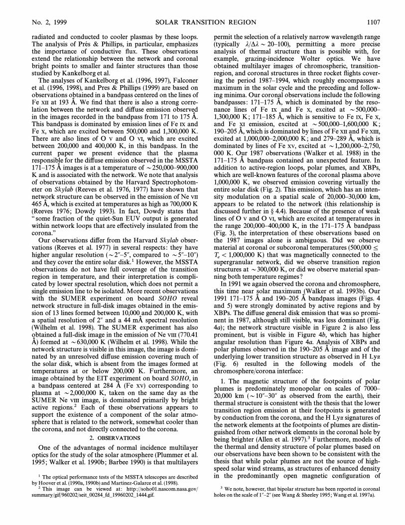
et al. (1996, 1997) observed 26 small loops in the soft X-rayimages ; the footpoints of all 26 loops coincide with networkelements that are brighter than average in the H Lyaimages. The footpoints of 18 of these loops are coincidentwith magnetic bipoles in the Kitt Peak magnetogram taken4 hr before the launch of the MSSTA. The magnetic con-Ðguration of the footpoints of the other eight loops is diffi-cult to determine because they are close to the limb. Atypical loop and its footpoints are shown in Figure 1. Ananalysis of these loops, which vary in size from 7000 to70,000 km, shows that the maximum loop temperature, T

m,

is typically 1,200,000 to 2,000,000 K, permitting Kankel-borg et al. (1996, 1997) to identify them as ““ coronal X-raybright points ÏÏ (XBPs ; Golub 1980). Kankelborg et al. havedeveloped loop models for the 26 XBPÏs they observed,which show that for a typical XBP the thermal Ñux con-ducted below the 100,000 K isotherm (approximately 50%of the energy dissipated in the loop) is sufficient to supplythe energy radiated in the H Lya line by the local network.Less than 1% of the bright elements that form the networkin H Lya emission are at the footpoints of XBPÏs ; theseelements, however, are the brightest elements, and arelocated over the most intense magnetic Ðelds in thenetwork. In a series of papers, Fontenla, Avrett, & Loeser(1990, 1991, 1993 ; hereafter FAL) have considered the struc-ture of the lower transition region (LTR). Their modelsshow that conductive heat Ñuxes compatible with thosefound by Kankelborg et al. can be dissipated by radiativelosses in the lower transition region, with H Lya as theprinciple energy-loss mode. In their analyses, FAL assumethat the top of the LTR (taken to be 105 K) is the interfaceof the chromosphere with coronal plasmas with T [ 106 K.It is possible, however, that the LTR modeled by FAL is theinterface of chromospheric material with plasma at sub-coronal temperatures, since the only constraint on theplasma lying above 105 K is that the heat Ñux from theseplasmas match that of the FAL models.

Recently, Falconer et al. (1996, 1998) have reported onobservations by the SOHO EUV Imaging Telescope (EIT)experiment of ““ microcoronal bright points,ÏÏ less than 10A(D7000 km) in size, that are rooted in small-scale magneticbipoles in the network. Pres & Phillips (1999) also usedobservations by the SOHO EIT experiment to explore therelationship of XBPs to the dynamics of small-scale mag-netic bipoles in the quiet Sun, and suggest that the dissi-pation of magnetic energy can account for the energy

FIG. 1.ÈL eft : Coronal X-ray bright point observed in the emission of Fe XII (D193 by the MSSTA in 1991. Middle : Lower transition footpoints of theA� )bright point observed in H Lya. Right : Line-of-sight magnetic Ðeld observed by the Kitt Peak magnetograph 4.5 hr before the MSSTA launch. Themagnetogram has been rotated to compensate for the time di†erence in the observations. (From Kankelborg et al. 1996.)

No. 2, 1999 SOLAR TRANSITION REGION 1107

radiated and conducted to cooler plasmas by these loops.The analysis of & Phillips, in particular, emphasizesPre� sthe importance of conductive Ñux. These observationsextend the relationship between the network and coronalbright points to smaller and fainter structures than thosestudied by Kankelborg et al.

The analyses of Kankelborg et al. (1996, 1997), Falconeret al. (1996, 1998), and Pres & Phillips (1999) are based onobservations obtained in a bandpass centered on the lines ofFe XII at 193 We Ðnd that there is also a strong corre-A� .lation between the network and di†use emission observedin the images recorded in the bandpass from 171 to 175 A� .This bandpass is dominated by emission lines of Fe IX andFe X, which are excited between 500,000 and 1,300,000 K.There are also lines of O V and O VI, which are excitedbetween 200,000 and 400,000 K, in this bandpass. In thecurrent paper we present evidence that the plasmaresponsible for the di†use emission observed in the MSSTA171È175 images is at a temperature of D250,000È900,000A�K and is associated with the network. We note that analysisof observations obtained by the Harvard Spectrophotom-eter on Skylab (Reeves et al. 1976, 1977) have shown thatnetwork structure can be observed in the emission of Ne VII

465 which is excited at temperatures as high as 700,000 KA� ,(Reeves 1976 ; Dowdy 1993). In fact, Dowdy states that““ some fraction of the quiet-Sun EUV output is generatedwithin network loops that are e†ectively insulated from thecorona.ÏÏ

Our observations di†er from the Harvard Skylab obser-vations (Reeves et al. 1977) in several respects : they havehigher angular resolution (D2AÈ5A, compared to D5AÈ10A)and they cover the entire solar disk.1 However, the MSSTAobservations do not have full coverage of the transitionregion in temperature, and their interpretation is compli-cated by lower spectral resolution, which does not permit asingle emission line to be isolated. More recent observationswith the SUMER experiment on board SOHO revealnetwork structure in full-disk images obtained in the emis-sion of 13 lines formed between 10,000 and 200,000 K, witha spatial resolution of 2A and a 44 spectral resolutionmA�(Wilhelm et al. 1998). The SUMER experiment has alsoobtained a full-disk image in the emission of Ne VIII (770.41

formed at D630,000 K (Wilhelm et al. 1998). While theA� )network structure is visible in this image, the image is domi-nated by an unresolved di†use emission covering much ofthe solar disk, which is absent from the images formed attemperatures at or below 200,000 K. Furthermore, animage obtained by the EIT experiment on board SOHO, ina bandpass centered at 284 (Fe XV) corresponding toA�plasma at D2,000,000 K, taken on the same day as theSUMER Ne VIII image, is dominated primarily by brightactive regions.2 Each of these observations appears tosupport the existence of a component of the solar atmo-sphere that is related to the network, somewhat cooler thanthe corona, and not directly connected to the corona.

2. OBSERVATIONS

One of the advantages of normal incidence multilayeroptics for the study of the solar atmosphere (Plummer et al.1995 ; Walker et al. 1990b ; Barbee 1990) is that multilayers

1 The optical performance tests of the MSSTA telescopes are describedby Hoover et al. (1990a, 1990b) and Martinez-Galarce et al. (1998).

2 This image can be viewed at : http ://soho01.nascom.nasa.gov/summary/gif/960202/seit–00284–fd–19960202–1444.gif.

permit the selection of a relatively narrow wavelength range(typically j/*jD 20È100), permitting a more preciseanalysis of thermal structure than is possible with, forexample, grazing-incidence Wolter optics. We haveobtained multilayer images of chromospheric, transition-region, and coronal structures in three rocket Ñights cover-ing the period 1987È1994, which roughly encompasses amaximum in the solar cycle and the preceding and follow-ing minima. Our coronal observations include the followingbandpasses : 171È175 which is dominated by the reso-A� ,nance lines of Fe IX and Fe X, excited at D500,000È1,300,000 K; 171È185 which is sensitive to Fe IX, Fe X,A� ,and Fe XI emission, excited at D500,000È1,600,000 K;190È205 which is dominated by lines of Fe XII and Fe XIII,A� ,excited at 1,000,000È2,000,000 K; and 279È289 which isA� ,dominated by lines of Fe XV, excited at D1,200,000È2,750,000 K. Our 1987 observations (Walker et al. 1988) in the171È175 bandpass contained an unexpected feature. InA�addition to active-region loops, polar plumes, and XBPs,which are well-known features of the coronal plasma above1,000,000 K, we observed emission covering virtually theentire solar disk (Fig. 2). This emission, which has an inten-sity modulation on a spatial scale of 20,000È30,000 km,appears to be related to the network (this relationship isdiscussed further in ° 4.4). Because of the presence of weaklines of O V and O VI, which are excited at temperatures inthe range 200,000È400,000 K, in the 171È175 bandpassA�(Fig. 3), the interpretation of these observations based onthe 1987 images alone is ambiguous. Did we observematerial at coronal or subcoronal temperatures (500,000 ¹

K) that was magnetically connected to theTe\ 1,000,000

supergranular network, did we observe transition regionstructures at D300,000 K, or did we observe material span-ning both temperature regimes?

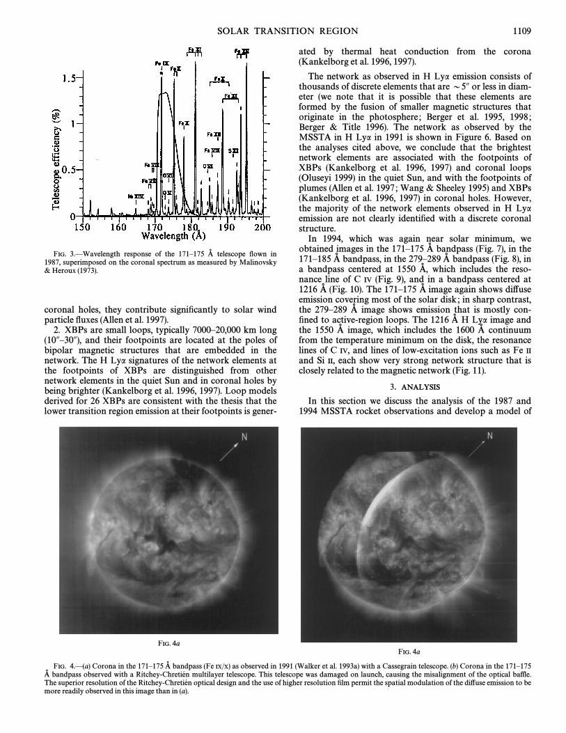
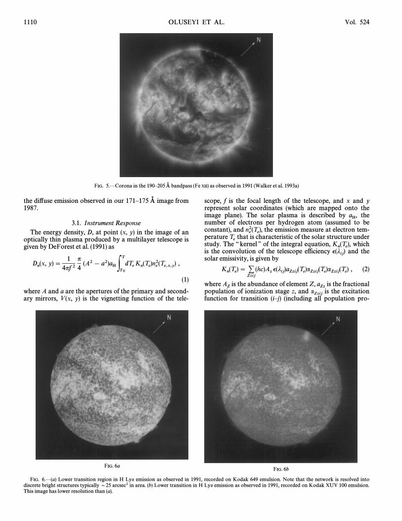
In 1991 we again observed the corona and chromosphere,this time near solar maximum (Walker et al. 1993b). Our1991 171È175 and 190È205 bandpass images (Figs. 4A� A�and 5) were strongly dominated by active regions and byXBPs. The di†use general disk emission that was so promi-nent in 1987, although still visible, was less dominant (Fig.4a) ; the network structure visible in Figure 2 is also lessprominent, but is visible in Figure 4b, which has higherangular resolution than Figure 4a. Analysis of XBPs andpolar plumes observed in the 190È205 image and of theA�underlying lower transition structure as observed in H Lya(Fig. 6) resulted in the following models of thechromosphere/corona interface :

1. The magnetic structure of the footpoints of polarplumes is predominately monopolar on scales of 7000È20,000 km (D10AÈ30A as observed from the earth), theirthermal structure is consistent with the thesis that the lowertransition region emission at their footpoints is generatedby conduction from the corona, and the H Lya signatures ofthe network elements at the footpoints of plumes are distin-guished from other network elements in the coronal hole bybeing brighter (Allen et al. 1997).3 Furthermore, models ofthe thermal and density structure of polar plumes based onour observations have been shown to be consistent with thethesis that while polar plumes are not the source of high-speed solar wind streams, as structures of enhanced densityin the predominantly open magnetic conÐguration of

3 We note, however, that bipolar structure has been reported in coronalholes on the scale of 1AÈ2A (see Wang & Sheeley 1995 ; Wang et al. 1997a).

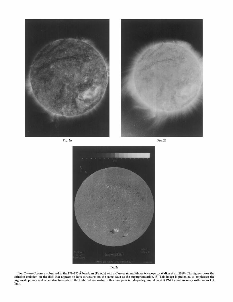
FIG. 2a FIG. 2b

FIG. 2c

FIG. 2.È(a) Corona as observed in the 171È175 bandpass (Fe IX/X) with a Cassegrain multilayer telescope by Walker et al. (1988). This Ðgure shows theA�di†usion emission on the disk that appears to have structures on the same scale as the supergranulation. (b) This image is presented to emphasize thelarge-scale plumes and other structures above the limb that are visible in this bandpass. (c) Magnetogram taken at KPNO simultaneously with our rocketÑight.

SOLAR TRANSITION REGION 1109

FIG. 3.ÈWavelength response of the 171È175 telescope Ñown inA�1987, superimposed on the coronal spectrum as measured by Malinovsky& Heroux (1973).

coronal holes, they contribute signiÐcantly to solar windparticle Ñuxes (Allen et al. 1997).

2. XBPs are small loops, typically 7000È20,000 km long(10AÈ30A), and their footpoints are located at the poles ofbipolar magnetic structures that are embedded in thenetwork. The H Lya signatures of the network elements atthe footpoints of XBPs are distinguished from othernetwork elements in the quiet Sun and in coronal holes bybeing brighter (Kankelborg et al. 1996, 1997). Loop modelsderived for 26 XBPs are consistent with the thesis that thelower transition region emission at their footpoints is gener-

ated by thermal heat conduction from the corona(Kankelborg et al. 1996, 1997).

The network as observed in H Lya emission consists ofthousands of discrete elements that are D5A or less in diam-eter (we note that it is possible that these elements areformed by the fusion of smaller magnetic structures thatoriginate in the photosphere ; Berger et al. 1995, 1998 ;Berger & Title 1996). The network as observed by theMSSTA in H Lya in 1991 is shown in Figure 6. Based onthe analyses cited above, we conclude that the brightestnetwork elements are associated with the footpoints ofXBPs (Kankelborg et al. 1996, 1997) and coronal loops(Oluseyi 1999) in the quiet Sun, and with the footpoints ofplumes (Allen et al. 1997 ; Wang & Sheeley 1995) and XBPs(Kankelborg et al. 1996, 1997) in coronal holes. However,the majority of the network elements observed in H Lyaemission are not clearly identiÐed with a discrete coronalstructure.

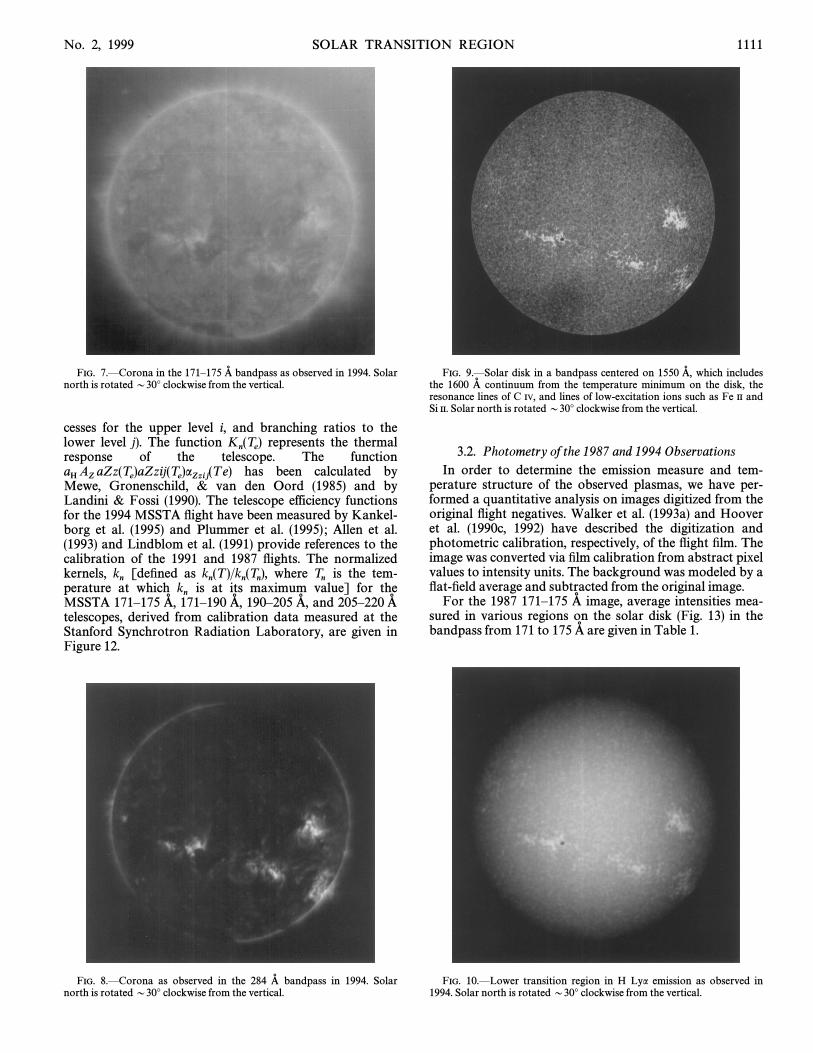
In 1994, which was again near solar minimum, weobtained images in the 171È175 bandpass (Fig. 7), in theA�171È185 bandpass, in the 279È289 bandpass (Fig. 8), inA� A�a bandpass centered at 1550 which includes the reso-A� ,nance line of C IV (Fig. 9), and in a bandpass centered at1216 (Fig. 10). The 171È175 image again shows di†useA� A�emission covering most of the solar disk ; in sharp contrast,the 279È289 image shows emission that is mostly con-A�Ðned to active-region loops. The 1216 H Lya image andA�the 1550 image, which includes the 1600 continuumA� A�from the temperature minimum on the disk, the resonancelines of C IV, and lines of low-excitation ions such as Fe II

and Si II, each show very strong network structure that isclosely related to the magnetic network (Fig. 11).

3. ANALYSIS

In this section we discuss the analysis of the 1987 and1994 MSSTA rocket observations and develop a model of

FIG. 4aFIG. 4a

FIG. 4.È(a) Corona in the 171È175 bandpass (Fe IX/X) as observed in 1991 (Walker et al. 1993a) with a Cassegrain telescope. (b) Corona in the 171È175A�bandpass observed with a multilayer telescope. This telescope was damaged on launch, causing the misalignment of the optical baffle.A� Ritchey-Chretie� n

The superior resolution of the optical design and the use of higher resolution Ðlm permit the spatial modulation of the di†use emission to beRitchey-Chretie� nmore readily observed in this image than in (a).

1110 OLUSEYI ET AL. Vol. 524

FIG. 5.ÈCorona in the 190È205 bandpass (Fe XII) as observed in 1991 (Walker et al. 1993a)A�

the di†use emission observed in our 171È175 image fromA�1987.

3.1. Instrument ResponseThe energy density, D, at point (x, y) in the image of an

optically thin plasma produced by a multilayer telescope isgiven by DeForest et al. (1991) as

Dn(x, y)\ 1

4nf 2n4

(A2[ a2)aHPT0

TdT

eK

n(T

e)n

e2(T

e,x,y) ,

(1)

where A and a are the apertures of the primary and second-ary mirrors, V (x, y) is the vignetting function of the tele-

scope, f is the focal length of the telescope, and x and yrepresent solar coordinates (which are mapped onto theimage plane). The solar plasma is described by theaH,number of electrons per hydrogen atom (assumed to beconstant), and the emission measure at electron tem-n

e2(T

e),

perature that is characteristic of the solar structure underTestudy. The ““ kernel ÏÏ of the integral equation, whichK

n(T

e),

is the convolution of the telescope efficiency and thev(jij)

solar emissivity, is given by

Kn(T

e) \ ;

Zzij(hc)A

zv(j

ij)a

Zzij(T

e)a

Zzij(T

e)a

Zzij(T

e) , (2)

where is the abundance of element Z, is the fractionalAZ

aZzpopulation of ionization stage z, and is the excitationa

Zzijfunction for transition (iÈj) (including all population pro-

FIG. 6aFIG. 6b

FIG. 6.È(a) Lower transition region in H Lya emission as observed in 1991, recorded on Kodak 649 emulsion. Note that the network is resolved intodiscrete bright structures typically D25 arcsec2 in area. (b) Lower transition in H Lya emission as observed in 1991, recorded on Kodak XUV 100 emulsion.This image has lower resolution than (a).

No. 2, 1999 SOLAR TRANSITION REGION 1111

FIG. 7.ÈCorona in the 171È175 bandpass as observed in 1994. SolarA�north is rotated D30¡ clockwise from the vertical.

cesses for the upper level i, and branching ratios to thelower level j). The function represents the thermalK

n(T

e)

response of the telescope. The functionhas been calculated byaH A

ZaZz(T

e)aZzij(T

e)a

Zzij(T e)

Mewe, Gronenschild, & van den Oord (1985) and byLandini & Fossi (1990). The telescope efficiency functionsfor the 1994 MSSTA Ñight have been measured by Kankel-borg et al. (1995) and Plummer et al. (1995) ; Allen et al.(1993) and Lindblom et al. (1991) provide references to thecalibration of the 1991 and 1987 Ñights. The normalizedkernels, [deÐned as where is the tem-k

nkn(T )/k

n(T

n), T

nperature at which is at its maximum value] for theknMSSTA 171È175 171È190 190È205 and 205È220A� , A� , A� , A�

telescopes, derived from calibration data measured at theStanford Synchrotron Radiation Laboratory, are given inFigure 12.

FIG. 8.ÈCorona as observed in the 284 bandpass in 1994. SolarA�north is rotated D30¡ clockwise from the vertical.

FIG. 9.ÈSolar disk in a bandpass centered on 1550 which includesA� ,the 1600 continuum from the temperature minimum on the disk, theA�resonance lines of C IV, and lines of low-excitation ions such as Fe II andSi II. Solar north is rotated D30¡ clockwise from the vertical.

3.2. Photometry of the 1987 and 1994 ObservationsIn order to determine the emission measure and tem-

perature structure of the observed plasmas, we have per-formed a quantitative analysis on images digitized from theoriginal Ñight negatives. Walker et al. (1993a) and Hooveret al. (1990c, 1992) have described the digitization andphotometric calibration, respectively, of the Ñight Ðlm. Theimage was converted via Ðlm calibration from abstract pixelvalues to intensity units. The background was modeled by aÑat-Ðeld average and subtracted from the original image.

For the 1987 171È175 image, average intensities mea-A�sured in various regions on the solar disk (Fig. 13) in thebandpass from 171 to 175 are given in Table 1.A�

FIG. 10.ÈLower transition region in H Lya emission as observed in1994. Solar north is rotated D30¡ clockwise from the vertical.

1112 OLUSEYI ET AL. Vol. 524

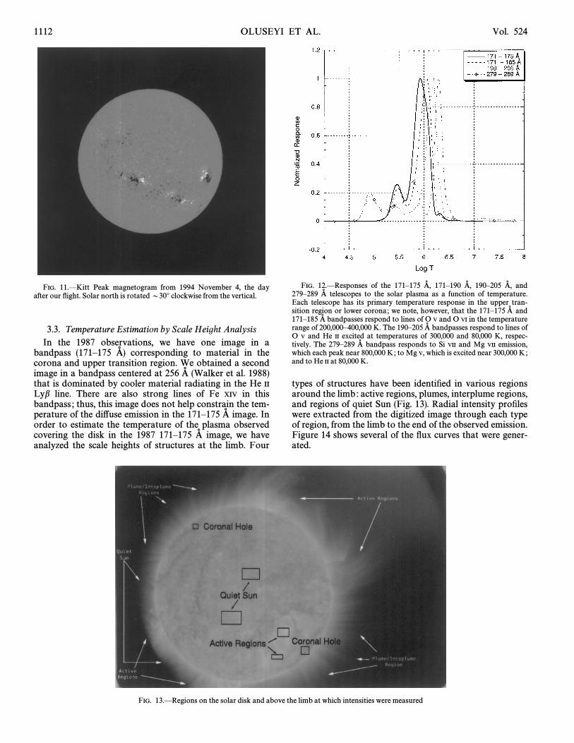
FIG. 11.ÈKitt Peak magnetogram from 1994 November 4, the dayafter our Ñight. Solar north is rotated D30¡ clockwise from the vertical.

3.3. Temperature Estimation by Scale Height AnalysisIn the 1987 observations, we have one image in a

bandpass (171È175 corresponding to material in theA� )corona and upper transition region. We obtained a secondimage in a bandpass centered at 256 (Walker et al. 1988)A�that is dominated by cooler material radiating in the He II

Lyb line. There are also strong lines of Fe XIV in thisbandpass ; thus, this image does not help constrain the tem-perature of the di†use emission in the 171È175 image. InA�order to estimate the temperature of the plasma observedcovering the disk in the 1987 171È175 image, we haveA�analyzed the scale heights of structures at the limb. Four

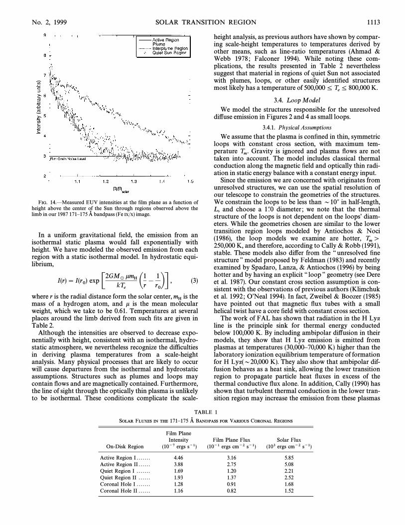
FIG. 12.ÈResponses of the 171È175 171È190 190È205 andA� , A� , A� ,279È289 telescopes to the solar plasma as a function of temperature.A�Each telescope has its primary temperature response in the upper tran-sition region or lower corona ; we note, however, that the 171È175 andA�171È185 bandpasses respond to lines of O V and O VI in the temperatureA�range of 200,000È400,000 K. The 190È205 bandpasses respond to lines ofA�O V and He II excited at temperatures of 300,000 and 80,000 K, respec-tively. The 279È289 bandpass responds to Si VII and Mg VII emission,A�which each peak near 800,000 K; to Mg V, which is excited near 300,000 K;and to He II at 80,000 K.

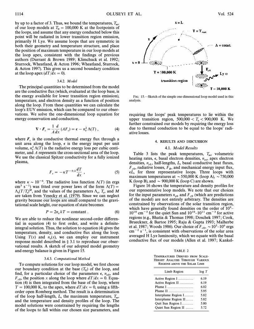
types of structures have been identiÐed in various regionsaround the limb: active regions, plumes, interplume regions,and regions of quiet Sun (Fig. 13). Radial intensity proÐleswere extracted from the digitized image through each typeof region, from the limb to the end of the observed emission.Figure 14 shows several of the Ñux curves that were gener-ated.

FIG. 13.ÈRegions on the solar disk and above the limb at which intensities were measured

No. 2, 1999 SOLAR TRANSITION REGION 1113

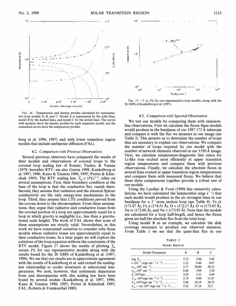
FIG. 14.ÈMeasured EUV intensities at the Ðlm plane as a function ofheight above the center of the Sun through regions observed above thelimb in our 1987 171È175 bandpass (Fe IX/X) image.A�

In a uniform gravitational Ðeld, the emission from anisothermal static plasma would fall exponentially withheight. We have modeled the observed emission from eachregion with a static isothermal model. In hydrostatic equi-librium,

I(r)\ I(r0) expC2GM

_kmH

kTe

A1r[ 1

r0

BD, (3)

where r is the radial distance form the solar center, is themHmass of a hydrogen atom, and k is the mean molecularweight, which we take to be 0.61. Temperatures at severalplaces around the limb derived from such Ðts are given inTable 2.

Although the intensities are observed to decrease expo-nentially with height, consistent with an isothermal, hydro-static atmosphere, we nevertheless recognize the difficultiesin deriving plasma temperatures from a scale-heightanalysis. Many physical processes that are likely to occurwill cause departures from the isothermal and hydrostaticassumptions. Structures such as plumes and loops maycontain Ñows and are magnetically contained. Furthermore,the line of sight through the optically thin plasma is unlikelyto be isothermal. These conditions complicate the scale-

height analysis, as previous authors have shown by compar-ing scale-height temperatures to temperatures derived byother means, such as line-ratio temperatures (Ahmad &Webb 1978 ; Falconer 1994). While noting these com-plications, the results presented in Table 2 neverthelesssuggest that material in regions of quiet Sun not associatedwith plumes, loops, or other easily identiÐed structuresmost likely has a temperature of K.500,000¹T

e¹ 800,000

3.4. L oop ModelWe model the structures responsible for the unresolved

di†use emission in Figures 2 and 4 as small loops.

3.4.1. Physical Assumptions

We assume that the plasma is conÐned in thin, symmetricloops with constant cross section, with maximum tem-perature Gravity is ignored and plasma Ñows are notT

m.

taken into account. The model includes classical thermalconduction along the magnetic Ðeld and optically thin radi-ation in static energy balance with a constant energy input.

Since the emission we are concerned with originates fromunresolved structures, we can use the spatial resolution ofour telescope to constrain the geometries of the structures.We constrain the loops to be less than D10A in half-length,L , and choose a diameter ; we note that the thermal1A.0structure of the loops is not dependent on the loopsÏ diam-eters. While the geometries chosen are similar to the lowertransition region loops modeled by Antiochos & Noci(1986), the loop models we examine are hotter, T

m[

250,000 K, and therefore, according to Cally & Robb (1991),stable. These models also di†er from the ““ unresolved Ðnestructure ÏÏ model proposed by Feldman (1983) and recentlyexamined by Spadaro, Lanza, & Antiochos (1996) by beinghotter and by having an explicit ““ loop ÏÏ geometry (see Dereet al. 1987). Our constant cross section assumption is con-sistent with the observations of previous authors (Klimchuket al. 1992 ; OÏNeal 1994). In fact, Zweibel & Boozer (1985)have pointed out that magnetic Ñux tubes with a smallhelical twist have a core Ðeld with constant cross section.

The work of FAL has shown that radiation in the H Lyaline is the principle sink for thermal energy conductedbelow 100,000 K. By including ambipolar di†usion in theirmodels, they show that H Lya emission is emitted fromplasmas at temperatures (30,000È70,000 K) higher than thelaboratory ionization equilibrium temperature of formationfor H Lya(D20,000 K). They also show that ambipolar dif-fusion behaves as a heat sink, allowing the lower transitionregion to propagate particle heat Ñuxes in excess of thethermal conductive Ñux alone. In addition, Cally (1990) hasshown that turbulent thermal conduction in the lower tran-sition region may increase the emission from these plasmas

TABLE 1

SOLAR FLUXES IN THE 171È175 BANDPASS FOR VARIOUS CORONAL REGIONSA�

Film PlaneIntensity Film Plane Flux Solar Flux

On-Disk Region (10~7 ergs s~1) (10~1 ergs cm~2 s~1) (103 ergs cm~2 s~1)

Active Region I . . . . . . . 4.46 3.16 5.85Active Region II . . . . . . 3.88 2.75 5.08Quiet Region I . . . . . . . 1.69 1.20 2.21Quiet Region II . . . . . . 1.93 1.37 2.52Coronal Hole I . . . . . . . 1.28 0.91 1.68Coronal Hole II . . . . . . 1.16 0.82 1.52

1114 OLUSEYI ET AL. Vol. 524

by up to a factor of 3. Thus, we bound the temperatures, Tm,

of our loop models at K at the footpoints ofT0\ 100,000the loops, and assume that any energy conducted below thispoint will be radiated in lower transition region emission,primarily H Lya. We assume loops that are symmetric inboth their geometry and temperature structure, and placethe position of maximum temperature in our loop models atthe loop apex, consistent with the Ðndings of previousauthors (Durrant & Brown 1989 ; Klimchuck et al. 1992 ;Sturrock, Wheatland, & Acton 1996 ; Wheatland, Sturrock,& Acton 1997). This gives us a second boundary conditionat the loop apex (dT /dx \ 0).

3.4.2. Model

The principal quantities to be determined from the modelare the conductive Ñux (which, evaluated at the loop base, isthe energy available for lower transition region emission),temperature, and electron density as a function of positionalong the loop. From these quantities we can calculate theloopÏs EUV emission, which can be compared to our obser-vations. We solve the one-dimensional loop equation forenergy conservation and conduction,

$ Æ Fc\ 1

Addx

(AFc)\ v[ n

e2"(T ) , (4)

where is the conductive thermal energy Ñux through aFcunit area along the loop, v is the energy input per unit

volume, is the radiative energy loss per cubic centi-ne2"(T )

meter, and A represents the cross-sectional area of the loop.We use the classical Spitzer conductivity for a fully ionizedplasma,

Fc\ [iT ~5@2 dT

dx, (5)

where i D 10~6. The radiative loss function "(T ) (in ergscm3 s~1) was Ðtted over power laws of the form "(T ) \

and the values of the parameters and M"s(T /T

s)M, "

s, T

s,

are taken from Vesecky et al. (1979). Since we can neglectgravity because our loops are small compared to the gravi-tational scale height, our equation of state becomes

P\ 2nekT \ constant . (6)

We are able to reduce the nonlinear second-order di†eren-tial in equation (4) to Ðrst order, and write a deÐnite-integral solution. Thus, the solution to equation (4) gives thetemperature, density, and conductive Ñux along the loop.Using T (x) and we can employ our instrumentn

e(x),

response model described in ° 3.1 to reproduce our obser-vational results. A sketch of our adopted model geometryand energy balance is given in Figure 15.

3.4.3. Computational Method

To compute solutions for our loop model, we Ðrst chooseour boundary condition at the base of the loop, and(T0)Ðnd, for a particular choice of the parameters v, andn

e0,the position x along the loop where dT /dx \ 0. Equa-Fc0,tion (4) is then integrated from the base of the loop, where

T \ 100,000 K, to the apex, where dT /dx \ 0, using a Ðfth-order open Romberg method. The result is a determinationof the loop half-length, L , the maximum temperature, T

m,

and the temperature and density proÐles of the loop. Themodel solutions were constrained by requiring the lengthsof the loops to fall within our chosen size parameters, and

FIG. 15.ÈSketch of the simple one-dimensional loop model used in thisanalysis.

requiring the loopsÏ peak temperatures to lie within theupper transition region, K. We500,000\T

e\ 900,000

further constrained our models by requiring the energy lossdue to thermal conduction to be equal to the loopsÏ radi-ative losses.

4. RESULTS AND DISCUSSION

4.1. Model ResultsTable 3 lists the peak temperatures, volumetricT

m,

heating rates, v, basal electron densities, apex electronneo

,densities, half-lengths, L , basal conductive heat Ñuxes,n

eL,

radiative losses, and mechanical energy input Ñux,Fc0, F

R,

vL , for three representative loops. Three loops withmaximum temperatures at D550,000 K (loop A), D750,000K (loop B), and D 900,000 K (loop C) are shown.

Figure 16 shows the temperature and density proÐles forour representative loop models. We note that our choicesfor the input parameters and (which are predictionsn

e0 Fc0of the model) are not entirely arbitrary. The densities are

constrained by observations of the solar transition region,which have generally found densities on the order of 109È1010 cm~3 for the quiet Sun and 1010È1011 cm~3 for activeregions (e.g., Bhatia & Thomas 1998 ; Doschek 1997 ; Cook,Brueckner, & Bartoe 1995 ; Raju & Gupta 1993 ; Malherbeet al. 1987 ; Woods 1986). Our choice of D105È106 ergsF

c0,cm~2 s~1, is consistent with observations of the solar areaaveraged H Lya luminosity, which we equate with the basalconductive Ñux of our models (Allen et al. 1997 ; Kankel-

TABLE 2

TEMPERATURES DERIVED FROM SCALE-HEIGHT ANALYSIS THROUGH VARIOUS

REGIONS ABOVE THE SOLAR LIMB

Limb Region log T

Active Region I . . . . . . . . . . . . 6.19Active Region II . . . . . . . . . . . 6.19Plume I . . . . . . . . . . . . . . . . . . . . . 6.02Plume II . . . . . . . . . . . . . . . . . . . . 5.95Interplume Region I . . . . . . . 5.82Interplume Region II . . . . . . 5.82Quit Sun Region I . . . . . . . . . 5.80Quiet Sun Region II . . . . . . 5.72

No. 2, 1999 SOLAR TRANSITION REGION 1115

FIG. 16.ÈTemperature and density proÐles calculated for representa-tive loop models A, B, and C. Model A is represented by the solid lines,model B by the dashed lines, and model C by the dotted lines. The curveswith markers show the density proÐles for each respective model, and theunmarked curves show the temperature proÐles.

borg et al. 1996, 1997) and with lower transition regionmodels that include ambipolar di†usion (FAL).

4.2. Comparison with Previous ObservationsSeveral previous observers have compared the results of

their models and observations of coronal loops to thecoronal loop scaling law of Rosner, Tucker, & Vaiana(1978 ; hereafter RTV; see also Garcia 1998 ; Kankelborg etal. 1997, 1996 ; Kano & Tsuneta 1996, 1995 ; Porter & Klim-chuk 1995). The RTV scaling law, relies onT

mP (PL )1@3,

several assumptions. First, their boundary condition at thebase of the loop is that the conductive Ñux vanish there.Second, they assume that radiation and the classical Spitzerconductivity are the only energy-loss mechanisms in theloop. Third, they assume that LTE conditions prevail fromthe corona down to the chromosphere. From these assump-tions, they argue that radiative and conductive losses fromthe coronal portion of a loop are approximately equal for aloop in which gravity is negligible (i.e., less than a gravita-tional scale height). The work of FAL shows that none ofthese assumptions are strictly valid. Nevertheless, in thiswork we have constrained ourselves to consider only thosemodels whose radiative losses are approximately equal totheir conductive losses. In a later paper we will explore thesolutions of the loop equation without the constraints of theRTV model. Figure 17 shows the results of plotting T

mversus PL for our representative models along with theresults found for the 26 XBPs of Kankelborg et al. (1997,1996). We see that our results are in approximate agreementwith the results of Kankelborg et al. and extend the scaling-law relationship to cooler structures at subcoronal tem-peratures. We note, however, that systematic departuresfrom and discrepancies with this scaling law have beenfound by several studies (Kankelborg et al. 1997, 1996 ;Kano & Tsuneta 1996, 1995 ; Porter & Klimchuk 1995 ;FAL; Roberts & Frankenthal 1980).

FIG. 17.ÈT vs. PL for our representative loop models, along with the26 XBPs of Kankelborg et al. (1997).

4.3. Comparison with Spectral ObservationWe test our models by comparing them with emission-

line observations. First we calculate the Ñuxes these modelswould produce in the bandpass of our 1987 173 telescopeA�and compare it with the Ñux we measure in our image (seeTable 2). This permits us to determine the number of loopsthat are necessary to explain our observations. We comparethe number of loops required by our model with thenumber of network elements observed in our 1550 image.A�Next, we calculate temperature-diagnostic line ratios forLi-like ions excited most efficiently at upper transitionregion temperatures and compare them with previousobservations. Finally, we calculate the absolute Ñuxes inseveral lines excited at upper transition region temperaturesand compare them with measured Ñuxes. We believe thatthese three comparisons together provide a robust test ofour models.

Using the Landini & Fossi (1990) line emissivity calcu-lations, we have calculated the luminosities (ergs s~1) thateach model would produce in the six strongest lines in ourbandpass for a 1A cross section loop (see Table 4) : Fe IX

(171.07 Fe X (174.51 O V (172.17 O VI (173.03A� ), A� ), A� ), A� ),Ne IV (172.60 and Ne V (173.93 Note that the modelsA� ), A� ).are calculated for a loop half-length, and hence the Ñuxesgiven are half the absolute Ñux from the total loop.

Using model B as an example, we calculate the diskcoverage necessary to produce our observed emission.From Table 1 we see that the quiet-Sun Ñux in our

TABLE 3

MODEL RESULTS

Model Parameter A B C

log Tm

. . . . . . . . . . . . . . . . . . . . . . . . . . . . . . . . 5.75 5.88 5.95v (10~3 ergs cm~3 s~1) . . . . . . . . . . . . 1.22 8.46 6.87ne0 (109 cm~3) . . . . . . . . . . . . . . . . . . . . . . 2.71 30.00 30.12

neL

(109 cm~3) . . . . . . . . . . . . . . . . . . . . . . 0.48 3.99 3.38L (108cm) . . . . . . . . . . . . . . . . . . . . . . . . . . . . 4.29 3.21 4.69Fc0 (105ergs cm~2 s~1) . . . . . . . . . . . . 2.74 9.00 11.67

FR

(105ergs cm~2 s~1) . . . . . . . . . . . . . 2.48 18.16 20.53Fm

\ vL (105 ergs cm~2 s~1) . . . . . . 5.22 27.16 32.2

1116 OLUSEYI ET AL. Vol. 524

bandpass is measured to be D2.0È2.5] 103 ergs cm~2 s~1at the Sun. From Table 4 we have calculated the emission inour bandpass that would be produced from model B to be6.88] 1019 ergs s~1. Dividing by the maximum projectedarea of the loop (2.25 ] 1016 cm2) gives us 3.06] 103 ergscm~2 s~1. The ratio of our measured Ñux, D2.0È2.5] 103ergs cm~2 s~1, and our calculated Ñux, 3.06] 103 ergscm~2 s~1, implies that this model would match ourobserved data with D65%È80% disk coverage. Thisamount of coverage is in good agreement with the observedcoverage in our 1987 171È175 image. Using this amountA�of coverage, we can calculate the area on the solar disk thatthese loops must cover. Dividing this number by the pro-jected area of a single loop gives us the number of loopsrequired to cover this fraction of the solar disk. Table 5summarizes the data for each of our representative models.

From Table 5 we see that models B and C withK can yield good matches to our700,000¹T

m¹ 900,000

observed data with reasonable disk coverages. We note thatbecause of the limited spatial resolution of our instrument,unresolved structures would be smeared ; thus, a range ofcoverages may constitute an acceptable model until obser-vations with better spatial resolution are available. Conse-quently, the parameters of our model, which include theelectron densities and cross sections of the loops, are notstrongly constrained. Hence, the number of loops requiredto satisfy our observed intensity is not strongly constrained,except by the number of network elements observed inlower transition region lines such as C IV and H Lya. Wehave performed a count of the number of network elementsin a unit area observed in our 1994 1550 image andA�extrapolated this number to the number of elements thatshould be on the entire solar disk. The total number ofnetwork elements inferred is approximately 25,000È50,000.We see that the models that we have calculated assuming a1A loop cross section predict on the order of 100,000 loopsto satisfy our observations. Since the cross sections we havechosen are somewhat arbitrary, we can decrease the numberof loops required by increasing the loopsÏ cross sections,which increases their volumes and hence their emissionmeasures. For example, if we double the cross-sectionalarea of our loops to 2A, we quadruple the loopsÏ luminosities

and double their projected areas. Consequently, a smallernumber of loops would be required to satisfy our obser-vations. On the other hand, the number of loops that wecalculate to satisfy our observations may very well be con-sistent with the number of network elements that we countif we do not assume that each loop has a unique set offootpoints. High-resolution observations by the T RACEsatellite have revealed that what at lower resolution appearto be single loops may be resolved into several individualloops sharing common footpoints. In order to make ourmodels consistent with both our EUV (at 173 and FUVA� )(at 1550 observations, it would be necessary to resolveA� )the structures in each regime. Nevertheless, we concludethat the number of loops that we calculate from our EUVobservations is not incompatible or inconsistent with thenumber of network elements we count in our FUV image.

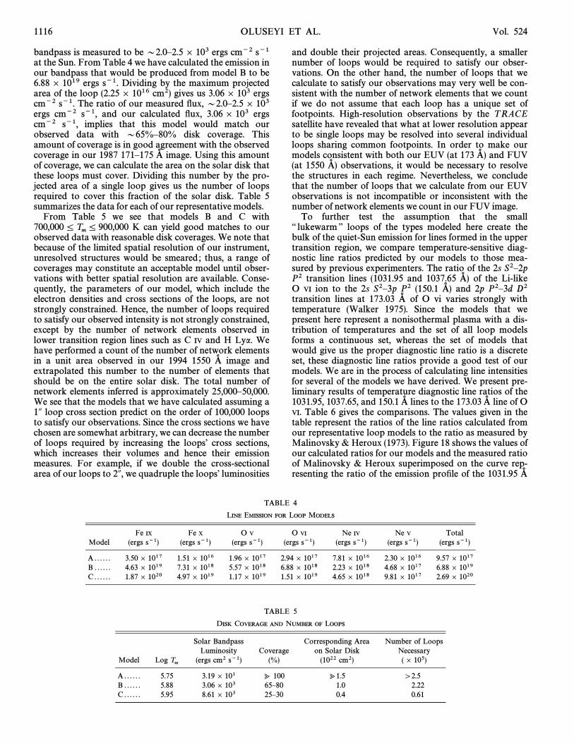
To further test the assumption that the small““ lukewarm ÏÏ loops of the types modeled here create thebulk of the quiet-Sun emission for lines formed in the uppertransition region, we compare temperature-sensitive diag-nostic line ratios predicted by our models to those mea-sured by previous experimenters. The ratio of the 2s S2È2pP2 transition lines (1031.95 and 1037.65 of the Li-likeA� )O VI ion to the 2s S2È3p P2 (150.1 and 2p P2È3d D2A� )transition lines at 173.03 of O vi varies strongly withA�temperature (Walker 1975). Since the models that wepresent here represent a nonisothermal plasma with a dis-tribution of temperatures and the set of all loop modelsforms a continuous set, whereas the set of models thatwould give us the proper diagnostic line ratio is a discreteset, these diagnostic line ratios provide a good test of ourmodels. We are in the process of calculating line intensitiesfor several of the models we have derived. We present pre-liminary results of temperature diagnostic line ratios of the1031.95, 1037.65, and 150.1 lines to the 173.03 line of OA� A�VI. Table 6 gives the comparisons. The values given in thetable represent the ratios of the line ratios calculated fromour representative loop models to the ratio as measured byMalinovsky & Heroux (1973). Figure 18 shows the values ofour calculated ratios for our models and the measured ratioof Malinovsky & Heroux superimposed on the curve rep-resenting the ratio of the emission proÐle of the 1031.95 A�

TABLE 4

LINE EMISSION FOR LOOP MODELS

Fe IX Fe X O V O VI Ne IV Ne V TotalModel (ergs s~1) (ergs s~1) (ergs s~1) (ergs s~1) (ergs s~1) (ergs s~1) (ergs s~1)

A . . . . . . 3.50] 1017 1.51] 1016 1.96] 1017 2.94] 1017 7.81] 1016 2.30] 1016 9.57] 1017B . . . . . . 4.63] 1019 7.31] 1018 5.57] 1018 6.88] 1018 2.23] 1018 4.68] 1017 6.88] 1019C . . . . . . 1.87] 1020 4.97] 1019 1.17] 1019 1.51] 1019 4.65] 1018 9.81] 1017 2.69] 1020

TABLE 5

DISK COVERAGE AND NUMBER OF LOOPS

Solar Bandpass Corresponding Area Number of LoopsLuminosity Coverage on Solar Disk Necessary

Model Log Tm

(ergs cm2 s~1) (%) (1022 cm2) (] 105)

A . . . . . . 5.75 3.19] 101 ? 100 ?1.5 [2.5B . . . . . . 5.88 3.06] 103 65È80 1.0 2.22C . . . . . . 5.95 8.61] 103 25È30 0.4 0.61

No. 2, 1999 SOLAR TRANSITION REGION 1117

FIG. 18.ÈRatio of the emissivity functions of the Li-like ions of O VI at1032 and 173.03 Horizontal lines indicate the values of the ratiosA� .derived from our models.

line to the 173.03 line. Referring to Table 6, we note thatA�our models overestimate the value of the ratio of the1031.95 and 1037.65 line to the 173.03 line. This resultA� A�is not unexpected. The Malinovsky & Heroux (1973) mea-surements are full-disk Ñuxes. The presence of elevated tem-peratures and densities of active regions on the disk wouldtend to decrease the ratio of the 1031.95 and 1037.65 linesA�to the 173.03 line. We conclude then that the ratios calcu-A�lated from our models are in rough agreement with themeasured ratio of Malinovsky & Heroux.

We can explore the e†ect of active regions on the full-diskÑuxes mentioned above by comparing the absolute Ñuxfrom the cooler emission lines of O VI at 1031.95 and1037.65 Table 7 gives the Ñuxes calculated for the emis-A� .sion lines of O VI at 1031.95 and 1037.65 from our modelsA�and the Ñuxes as measured by Malinovsky & Heroux(1973). We note that the Malinovsky & Heroux measure-ments were made on 1969 April 4, which was near solarmaximum, while our measurements were made on 1987October 23, near solar minimum. Rugge & Walker (1970)showed that the 2800 MHz solar Ñux is an excellent proxyfor the solar EUV for X-ray Ñuxes. By comparing the 2800MHz Ñux for the date of the Malinovsky & Heroux Ñight

TABLE 6

COMPARISON OF CALCULATED TEMPERATURE-SENSITIVE

DIAGNOSTIC LINE RATIOS FOR O VI TO THE MEASUREMENTS

OF MALINOVSKY & HEROUX NORMALIZED TO

THE 173.3 LINEA�

Model 1037.65 A� 1031.95 A� 173.10 A� 150.10 A�

M&H . . . . . . 8.13 17.43 1.00 0.83A . . . . . . . . . . . 11.73 22.63 1.00 0.55B . . . . . . . . . . . 14.33 27.60 1.00 0.56C . . . . . . . . . . . 13.68 26.37 1.00 0.55

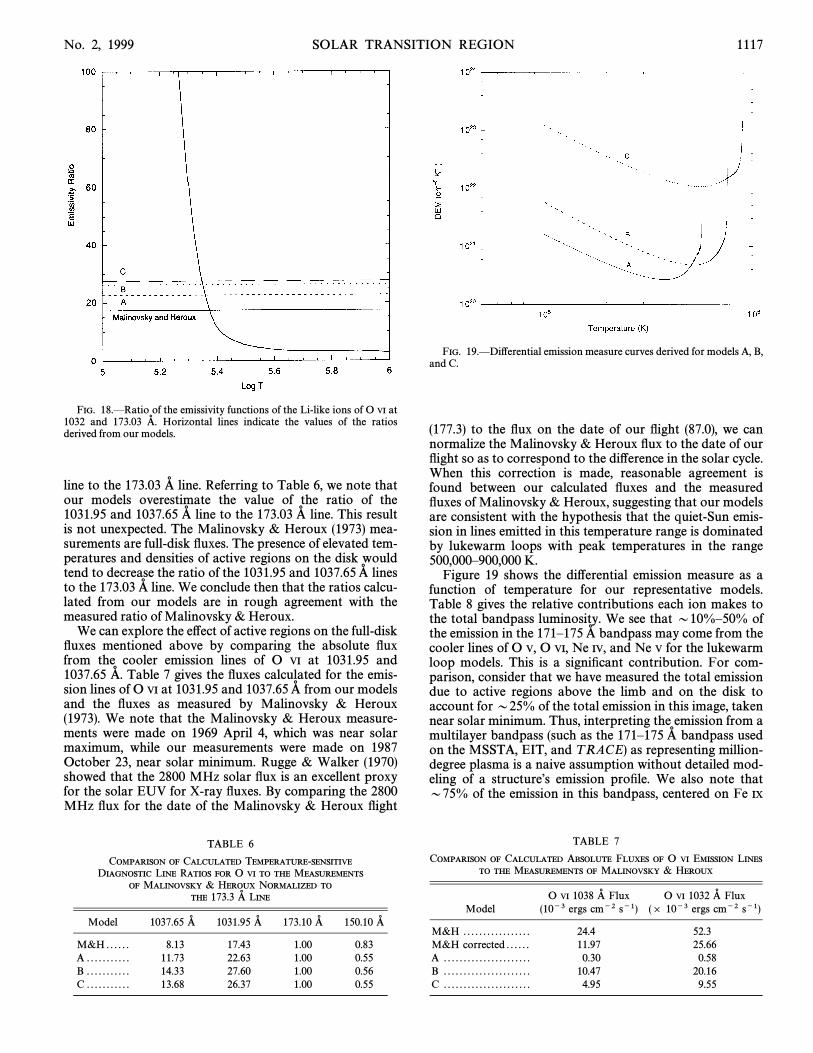
FIG. 19.ÈDi†erential emission measure curves derived for models A, B,and C.

(177.3) to the Ñux on the date of our Ñight (87.0), we cannormalize the Malinovsky & Heroux Ñux to the date of ourÑight so as to correspond to the di†erence in the solar cycle.When this correction is made, reasonable agreement isfound between our calculated Ñuxes and the measuredÑuxes of Malinovsky & Heroux, suggesting that our modelsare consistent with the hypothesis that the quiet-Sun emis-sion in lines emitted in this temperature range is dominatedby lukewarm loops with peak temperatures in the range500,000È900,000 K.

Figure 19 shows the di†erential emission measure as afunction of temperature for our representative models.Table 8 gives the relative contributions each ion makes tothe total bandpass luminosity. We see that D10%È50% ofthe emission in the 171È175 bandpass may come from theA�cooler lines of O V, O VI, Ne IV, and Ne V for the lukewarmloop models. This is a signiÐcant contribution. For com-parison, consider that we have measured the total emissiondue to active regions above the limb and on the disk toaccount for D25% of the total emission in this image, takennear solar minimum. Thus, interpreting the emission from amultilayer bandpass (such as the 171È175 bandpass usedA�on the MSSTA, EIT, and T RACE) as representing million-degree plasma is a naive assumption without detailed mod-eling of a structureÏs emission proÐle. We also note thatD75% of the emission in this bandpass, centered on Fe IX

TABLE 7

COMPARISON OF CALCULATED ABSOLUTE FLUXES OF O VI EMISSION LINES

TO THE MEASUREMENTS OF MALINOVSKY & HEROUX

O VI 1038 A� Flux O VI 1032 A� FluxModel (10~3 ergs cm~2 s~1) (] 10~3 ergs cm~2 s~1)

M&H . . . . . . . . . . . . . . . . . 24.4 52.3M&H corrected . . . . . . 11.97 25.66A . . . . . . . . . . . . . . . . . . . . . . 0.30 0.58B . . . . . . . . . . . . . . . . . . . . . . 10.47 20.16C . . . . . . . . . . . . . . . . . . . . . . 4.95 9.55

FIG

.20

.ÈC

entr

alpo

rtio

nof

the

171È

175

imag

efrom

the

1987

Ñigh

t,sp

anni

ngab

out1

sola

rra

dius

from

top

tobo

ttom

and

abou

tso

larra

dius

from

side

toside

.The

EU

Vim

age,

obta

ined

atU

TA�

11 318

:09

on19

87O

ctob

er23

,is

show

nin

the

red-

whi

teco

lor

scal

e.Su

perim

pose

don

this

are

phot

osph

eric

mag

netic

Ñux

conc

entr

atio

ns,f

rom

the

KittP

eak

mag

neto

gram

take

nth

atda

y(b

egin

ning

atU

T17

:25

and

cont

inui

ngfo

rab

out1

hr).

Pos

itiv

eÑu

xis

show

nin

blue

and

nega

tive

Ñux

issh

own

ingr

een.

The

dark

ersh

ades

corr

espo

ndto

Ðeld

stre

ngth

sof

30G

orm

ore

(pix

elsw

ere

binn

edto

4Are

solu

tion

).T

helig

hter

shad

esre

pres

entÐ

eld

stre

ngth

sof

14È2

9G

.

SOLAR TRANSITION REGION 1119

(which radiates most strongly at 106 K), arises not fromactive regions but from the quiet Sun. This indicates that atsolar minimum there is enough material present with

K for the Fe IX emission fromD500,000¹Te\ 900,000

these plasmas to dominate the Fe IX emission from thehotter active region plasmas, despite the fact that Fe IX isemitted less efficiently at these cooler temperatures.

We recognize that these results do not conclusivelydemonstrate that the unresolved structures responsible forthe quiet-Sun emission in our 1987 170È175 image orig-A�inate from the lukewarm loops we postulate, or that thestructures are loops at all ; we can say, however, that wehave illustrated that solutions exist for the models presentedhere that are consistent with our observations.

4.4. Association with the NetworkOur model of the structures that generate the EUV emis-

sion observed by our 171È175 bandpass telescope postu-A�lates a number of small loops with a projected area of D20arcsec2 or less each. These loops must have footpoints in thenetwork, which raises the question of whether there is evi-dence for the existence of such loops in chromospheric andlower transition region images and in magnetograms. Webegin this discussion by noting that our models are reason-ably well constrained in temperature by our observations,but are constrained in density only by a relatively smallnumber of observations (from other observers) that utilizedensity-sensitive line ratios to study material at transition-region temperatures. This material may or may not corre-spond to the structures that we have modeled (see, e.g.,Doschek et al. 1998). Since the luminosity of a loop varies asthe square of density, the predicted fractional coverage ofthe solar surface by the loops we model is also not stronglyconstrained. Although our images suggest that more than50% of the solar surface is covered by structures thatradiate in the 171È175 bandpass, if the structuresA�responsible for this emission have at least one dimensionthat is smaller than the resolution of our images, then thecoverage of the solar surface may well be smaller than 50%.The number of loops necessary to generate the Ñux levels weobserve is on the order of 100,000 loops (see Table 5). In ourprevious studies of polar plumes and XBPs (Allen et al.1997 ; Kankelborg et al. 1996, 1997), we were able to relatecoronal structures to the local network structures at theirbases as observed in H Lya. Unfortunately, we do not havean FUV image of lower transition region or chromosphericmaterial from our 1987 Ñight. We do, however, have a mag-netogram image corresponding to the time of our Ñight.

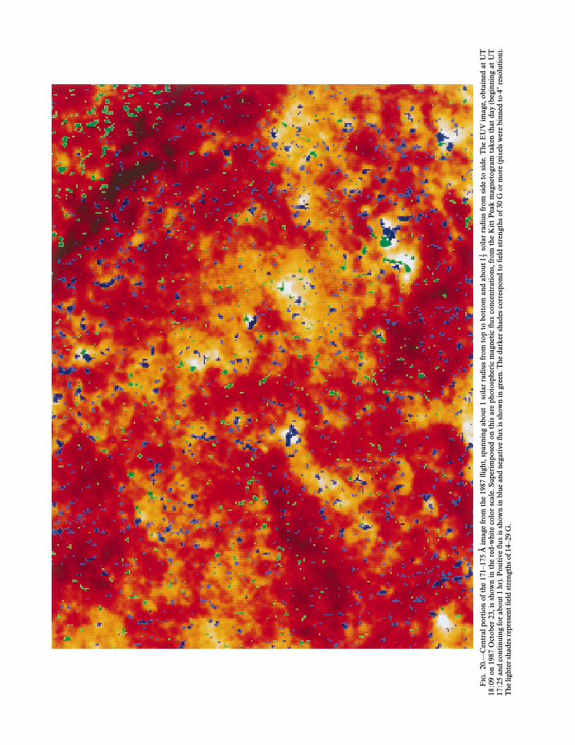
Figure 20 shows the central portion of the 171È175 A�image from the 1987 Ñight, spanning about 1 solar radiusfrom top to bottom and about solar radius from side to113

side (solar north is up). The EUV network is partiallymasked in some areas by bright larger-scale di†use emis-sion, but over most of the large area shown, there is a clearcorrespondence between the magnetic network andenhanced emission in the 171È175 bandpass. (Note thatA�some care must be taken in comparing magnetic and emis-sion features near the edges of the image, since projectione†ects shift the EUV features limbward of their photo-spheric counterparts.) The magnetic Ñux concentrations arescattered along bright rings of EUV emission, so that mostof them are embedded in bright halos of emission. The emis-sion enhancements are generally strongest over the strong-est bipoles. Owing to the 14 G cuto† and 4A pixel binning inthe magnetogram, many more bipoles must be present thanare revealed by this image. As Wang & Sheeley (1995) note,even when the network Ðeld conÐguration appears to beunipolar on the scales probed by the Kitt Peak NationalObservatory magnetograms, there is evidence that bipolarstructures exists on scales of a few arcseconds. These small-scale magnetic bipoles may provide one possible explana-tion for the larger scale di†use emission that exists in theinteriors of the network cells. Small dynamic loops overlay-ing small-scale magnetic bipoles emerging in cell centers,consistent with the ““ magnetic carpet ÏÏ model of Schrijver etal. (1997), could produce the di†use emission of the cellcenters seen in Figure 19. We note that other possible expla-nations for the di†use emission of the cell centers includefunnels of the type postulated by Gabriel (1976) and longlow-density loops crossing several cells (C. J. Schrijver 1997,private communication). Previous authors have alsopointed out the spatial correspondence between the mag-netic network and the network as observed in the chromo-sphere and transition region (Dowdy 1993 ; Athay 1981a). Itfollows then that the emission we have observed, which wepostulate originates from lukewarm loops, corresponds spa-tially with the network.

Observations of the lower transition region networkshow thousands of discrete network structures that areD5AÈ10A or less in size. One interpretation of the natureof these structures, observed for example by the SOHOSUMER experiment at 1406 (S VI) and 937.8 (H Lyv)A�(Lemaire et al. 1997), and by the SOHO CDS experiment at584.33 (He I), 303.78 (He II), 525.80 (O III), 554.51A� A� A� A�(O IV), 629.73 (O V), 562.8 (Ne VI), 313.74 (Mg VII),A� A� A�319.83 (Si VIII), 368.07 (Mg IX), and 624.95 (Mg X)A� A� A�(Gallagher et al. 1998) and by the MSSTA in bands thatinclude 1550 (C IV) and 1216 (H Lya), is that they areA� A�the footpoints of magnetic Ñux tubes connected to hottermaterial. If this interpretation is correct, these network ele-ments could well be the footpoints of the ““ lukewarm ÏÏ loopsthat we have postulated as the source of the quiet-Sun EUV

TABLE 8

RELATIVE PERCENTAGES OF LINE EMISSION TO TOTAL BANDPASS LUMINOSITY

log Tm

Model (K) Fe IX (171.07 A� ) Fe X (174.51 A� ) O V (172.17 A� ) O VI (173.03 A� ) Ne IV (172.60 A� ) Ne V (173.93 A� )

Bandpass throughputnormalized to peak response . . . . . . 1 0.385 0.808 0.615 0.615 0.538A . . . . . . . . . . . . . . . . . . . . . . . . . . . . . . . . . . . . . 5.75 46 1 21 24 6 2B . . . . . . . . . . . . . . . . . . . . . . . . . . . . . . . . . . . . . 5.88 78 5 8 7 2 0.4C . . . . . . . . . . . . . . . . . . . . . . . . . . . . . . . . . . . . . 5.95 82 8 4 4 1 0.2

1120 OLUSEYI ET AL. Vol. 524

radiation. We note that the network pattern is visible, withlittle change, in lines formed at temperatures up toD800,000 K (Gallagher et al. 1998). At coronal tem-peratures, however, the network pattern begins to disap-pear and only the bright coronal structures are visible. Thiswould seem to indicate, as Dowdy (1993) has pointed out,that there are structures in the network that never reachcoronal temperatures. These subcoronal structures couldvery well be the lukewarm loops we postulate. This pointhighlights one di†erence between the model of Gabriel(1976) and the model assumed in our analysis. GabrielÏsmodel appears to require that network plasma is alwaysassociated with the plasmas at coronal temperatures ; in ourmodel, the network plasmas are only associated withcoronal plasmas if larger, hotter loops, XBPs, or polarplumes are present. Gabriel assumes that large areas of thenetwork are unipolar, and that Ñux tubes in the network arenot twisted helically. There is evidence that, at least in thequiet network, neither assumption is strictly true. Ourmodel appears to best explain observations taken near solarminimum. At solar maximum, the increased presence ofhotter active-region loop systems may obscure the““ transition region ÏÏ plasmas associated with the network.In the next section, we ask the question, ““ what is therelationship between our lukewarm loops and the emissiongenerated in lines formed at lower transition region tem-peratures? ÏÏ

4.5. Heating of the L ower Transition RegionIt is interesting to calculate the energy available for lower

transition emission from our models. The total radiativeÑux from the lower transition region, including H Lya, isobserved to be 5 ] 105 ergs cm~2 s~1 (Timothy 1977 ;Vidal-Madjar 1977). Athay (1985) estimates the conductiveenergy Ñux parallel to magnetic Ðeld lines between 105 and106 K to be D1 ] 106 ergs cm~2 s~1. Using the conductiveÑux values from Table 3, the calculated disk coverages fromTable 5, and correcting for active regions, we Ðnd thatmodel B would conduct D6 ] 105 ergs cm~2 s~1 into thelower transition region. These conductive Ñux levels areconsistent with the total heat Ñuxes at 100,000 K derived byFAL in their lower transition region models, which includeambipolar di†usion. Previous lower transition regionmodels, which did not include ambipolar di†usion, predict-ed substantially lower heat Ñuxes, leading to the conclusionthat lower transition region emission could not be gener-ated by conduction from hotter plasmas (presumablycoronal plasmas). While our results do not exclude thepossibility of other energy sources for lower transitionregion emission, they do suggest a signiÐcant role for con-duction from plasmas at subcoronal temperatures. Thelukewarm loops could provide, then, a signiÐcant fractionof the energy radiated as quiet-Sun lower transition regionemission in the local lower transition network at their foot-points.

4.6. Chromospheric InterfaceAyres & Rabin (1996) have suggested that the chromo-

sphere is only present in magnetic Ñux tubes, and that thechromosphere typically covers D20% of the solar surface.Their model is based on infrared observations that indicatethat material cooler than the temperature minimum, associ-

ated with emission due to the CO molecule, is present overmost of the solar surface. The chromosphere, in their model,is associated only with plasma in magnetic Ñux tubes. Atleast some of the plasma at chromospheric temperatures4000È20,000 K, if we wish to associate chromospheric emis-sion with the Ca I and Mg II emission (see Vernazza, Avrett,& Loeser 1983), must be at the footpoints of the lukewarmÑux tubes that we have modeled.

4.7. ConclusionsWe have presented evidence that the unresolved struc-

tures responsible for much of the quiet-Sun emission in our1987 and 1994 171È175 images are at subcoronal tem-A�peratures (T \ 106 K). This is an important conclusion,since it directly impacts the interpretation of the tem-perature structure of features imaged with multilayer optics.We have calculated the Ñux our models would produce inthe bandpass of our 173 1987 telescope. Loop modelsA�with peak temperatures between 700,000 and 900,000 Kmatch the observational data well. A preliminary compari-son of Li-like O VI emission-line ratios calculated from ourloop models agree well with the measured ratio of Malin-ovsky & Heroux (1973). The absolute Ñuxes in typical FUVupper transition region lines have also been calculated fromour models and compared with observations ; good agree-ment is found. Our energy balance calculations also indi-cate that the lukewarm loops that we model may impartenough energy through classical thermal conduction intothe lower transition region to account for a signiÐcant frac-tion of the quiet-Sun lower transition region emission. Wehave pointed out previously (Allen et al. 1997 ; Kankelborget al. 1996, 1997) that the chromosphere/corona interface atthe footpoints of polar plumes and XBPs may make a sig-niÐcant, perhaps dominant, contribution to the energyemitted by the local network in the lower transition region,contrary to the views expressed by a number of authors. Inthe present paper we show that it is possible that the inter-face between structures at subcoronal temperatures and thechromosphere can make a signiÐcant contribution to theenergy emitted by the local lower transition region networkin the quiet Sun.

This research was supported by NASA grant NSG-5131at Stanford and NASA/MSFC; Troy W. Barbee, Jr. wassupported by DOE contract W-7405-Eng-48. We wish tothank the team at the Stanford Synchrotron RadiationLaboratory and the SURF-II team at National Institute forStandards and Technology for their assistance during cali-bration measurements at their respective laboratories. Theauthors would like to thank Ron Moore of NASA/MSFCfor discussions of the correspondence of the EUV and mag-netic networks, David Santiago of Stanford University andCharles Kankelborg of Montana State University for dis-cussions of our numerical models, and Paul Boerner ofStanford University for numerous enlightening conversa-tions. We would like to thank David Falconer of NASA/MSFC for help with the presentation of Figure 19 andMark Vande Hei and Carmel Levitan of Stanford Uni-versity for help with the presentation of Figure 17 andTable 6. We are extremely grateful to NSO/Kitt Peak forthe magnetograms used in Figures 1 (right), 2c, 11, and 20.

No. 2, 1999 SOLAR TRANSITION REGION 1121

REFERENCESAhmad, I. A., & Webb, D. F. 1978, Sol. Phys., 58, 323Allen, M. J., Oluseyi, H. M., Walker, A. B. C., II, Hoover, R. B., & Barbee,

T. W. 1997, Sol. Phys, 174, 367Allen, M. J., Willis, T. D., Kankelborg, C. C., OÏNeal, R. H., Martinez-

Galarce, D. S., DeForest, C. E., Jackson, L. R., Plummer, J. E., &Walker, A. B. C. 1993, Proc. SPIE, 2011, 381

Antiochos, S. K., & Noci, G. 1986, ApJ, 301, 440Athay, R. G. 1981a, ApJ, 249, 340ÈÈÈ. 1981b, ApJ, 250, 709ÈÈÈ. 1984, ApJ, 287, 412ÈÈÈ. 1985, Sol. Phys., 100, 257Ayres, T. R., & Rabin, D. 1996, ApJ, 460, 1042Barbee, T. W., Jr. 1990, Opt. Eng., 29, 711Berger, T. E., Lofdahl, M. G., Shine, R. S., & Title, A. M. 1998, ApJ, 495,

973Berger, T. E., Shine, R. S., Title, A. M., Tarbull, T. D., & Sharmer, G. 1995,

ApJ, 454, 531Berger, T. E., & Title, A. M. 1996, ApJ, 463, 365Bhatia, A. K., & Thomas, R. J. 1998, ApJ, 497, 483Cally, P. S. 1990, ApJ, 355, 693Cally, P. S., & Robb, T. D. 1991, ApJ, 372, 329Cook, J. W., Keenan, F. P., Dufton, P. L., Kingston, A. E., Pradhan, A. K.,

Zhang, H. L., Doyle, J. G., & Hayes, M. A. 1995, ApJ, 444, 936DeForest, C. E., et al. 1991, Opt. Eng., 30, 1125Dere, K. P., Bartoe, J. F., Brueckner, G. E., Cook, J. W., & Socker, D. G.

1987, Science, 238, 1267Doschek, G. A. 1997, ApJ, 476, 730Doschek, G. A., Laming, J. M., Feldman, U., Wilhelm, K., Lemaire, P.,

U., & Hassler, D. M. 1998, ApJ, 504, 573Schu� le,Dowdy, J. F. 1993, ApJ, 411, 406Dowdy, J. F., Emslie, A. G., & Moore, R. L. 1987, Sol. Phys., 112, 255Dowdy, J. F., Rabin, D., & Moore, R. L. 1986, Sol. Phys., 105, 35Durrant, C. J., & Brown, S. F. 1989, Proc. Astron. Soc. Australia, 8, 137Falconer, D. A. 1994, NASA Tech. Mem. 104616 (Washington : NASA)Falconer, D. A., Moore, R. L., Porter, J. G., Gary, G. A., & Shimizu, T.

1996, ApJ, 482, 519Falconer, D. A., Moore, R. L., Porter, J. G., & Hathaway, D. H. 1998, ApJ,

501, 386Feldman, U. 1983, ApJ, 275, 367ÈÈÈ. 1987, ApJ, 320, 426Fludra, A., Brekke, P., Harrison, R. A., Mason, H. E., Pike, C. D., Thomp-

son, W. T., & Young, P. R. 1997, Sol. Phys., 175, 487Fontenla, J. M., Avrett, E. H., & Loeser, R. 1990, ApJ, 355, 700ÈÈÈ. 1991, ApJ, 377, 712ÈÈÈ. 1993, ApJ, 406, 319Gabriel, A. H. 1976, Philos. Trans. R. Soc. London, A281, 339Gallagher, P. T., Phillips, K. J. H., Harra-Murnion, L. K., & Keenan, F. P.

1998, A&A, 335, 733Garcia, H. A. 1998, ApJ, 504, 1051Giovanelli, R. G. 1949, MNRAS, 109, 372Golub, L. 1980, Philos. Trans. R. Soc. London, A297, 595Hoover, R. B., Barbee, T. W., Walker, A. B. C., Lindblom, J. F., OÏNeal,

R. H., & Baker, P. C. 1990a, Opt. Eng., 29, 1281Hoover, R. B., et al. 1990b, Proc. SPIE, 1343, 189Hoover, R. B., Walker, A. B. C., DeForest, C. E., Allen, M. J., Lindblom,

J. F., OÏNeal, R. H., Paris, E. S., & DeWan, A. 1990c, Proc. SPIE, 1343,175

Hoover, R. B., Walker, A. B. C., DeForest, C. E., Watts, R. N., & Tarrio, C.1992, Proc. SPIE, 1742, 549

Kankelborg, C. C., et al. 1995, Proc. SPIE, 2515, 436Kankelborg C. C., Walker, A. B. C., & Hoover, R. B. 1997, ApJ, 491, 952Kankelborg, C. C., Walker, A. B. C., Hoover, R. B., & Barbee, T. W. 1996,

ApJ, 466, 529

Kano, R., & Tsuneta, S. 1995, ApJ, 454, 934ÈÈÈ. 1996, Publ. Astron. Soc. Japan, 48, 535Klimchuk, J. A., Lemen, J. R., Feldman, U., Tsuneta, S., & Uchida, Y. 1992,

PASJ, 44, L181Landini, M., & Fossi, B. C. 1990, A&AS, 82, 229Lemaire, P., et al. 1997, Sol. Phys., 170, 105Lindblom, J., OÏNeal, R. H., Walker, A. B. C., Powell, F. R., Barbee, T. W.,

Hoover, R. B., & Powell, S. 1991, Proc. SPIE, 1343, 544Malherbe, J. M., Schmieder, B., Simon, G., Mein, P., & Mein, P. 1987, Sol.

Phys., 112, 233Malinovsky, M., & Heroux, M. 1973, ApJ, 181, 1009

D. S., Walker, A. B. C., II, Gore, D. B., Kankelborg,Mart•� nez-Galarce,C. C., Hoover, R. B., & Barbee, T. W. 1998, Opt. Eng., submitted

Mewe, R., Gronenschild, E. H. B. M., & van den Oord, G. H. J. 1985,A&AS, 62, 197

Oluseyi, H. M., & Walker, A. B. C., II. 1999, in preparationOÏNeal, R. H. 1994, Ph.D. thesis, Stanford UniversityPlummer, J. E., et al. 1995, Proc SPIE, 2515, 565Porter, L. J., & Klimchuk, J. A. 1995, ApJ, 454, 499Pres, P., & Phillips, K. 1999, ApJ, 510, L73Rabin, D. 1991, ApJ, 383, 407Rabin, D., & Moore, R. 1984, ApJ, 285, 359Raju, P. K., & Gupta, A. K. 1993, Sol. Phys., 145, 241Reeves, E. M. 1976, Sol. Phys., 46, 53Reeves, E. M., Huber, M. C. E., & Timothy, J. G. 1977, Appl. Optics, 16,

837Reeves, E. M., Vernazza, J. E., & Withbroe, G. L. 1976, Philos. Trans. R.

Soc. London, A281, 319Roberts, B., & Frankenthal, S. 1980, Sol. Phys., 68, 103Rosner, R., Tucker, W. H., & Vaiana, G. S. 1978, ApJ, 220, 643 (RTV)Rugge, H. R., & Walker, A. B. C. 1970, Sol. Phys., 15, 372Schrijver, C. J., Title, A. M., Van Ballegooijen, A. A., Hagenaar, H. J., &

Shine, R. A. 1997, ApJ, 487, 424Spadaro, D., Lanza, A. F., & Antiochos, S. K. 1996, ApJ, 462, 1011Sturrock, P. A., Wheatland, M. S., & Acton, L. W. 1996, ApJ, 461, L115Timothy, J. G. 1977, in The Solar Ouput and Its Variations, ed. O. R.

White (Boulder : Univ. Colorado), 237Vernazza, J. E., Avrett, E. H., & Loeser, R. 1981, ApJS, 45, 635Vesecky, J. F., Antiochos, S. K., & Underwood, J. H. 1979, ApJ, 233, 987Vidal-Madjar, A. 1977, in The Solar Ouput and Its Variations, ed. O. R.

White (Boulder : Univ. Colorado), 213Walker, A. B. C., Jr. 1975, in Solar Gamma, X, and EUV Radiation, ed.

S. R. Kane (Dordrecht : Reidel)Walker, A. B. C., Jr., Barbee, T. W., Jr., Hoover, R. B., & Lindblom, J. F.

1988, Science, 241, 1781Walker, A. B. C., Jr., DeForest, C. E., Hoover, R. B., & Barbee, T. W.

1993a, Sol. Phys., 148, 239Walker, A. B. C., Jr., Hoover, R. B., & Barbee, T. W. 1993b, in Physics of

Solar and Stellar Coronae, ed. J. Linsky (Dordrecht : Kluwer), 83Walker, A. B. C., Jr., Lindblom, J. F., OÏNeal, R. H., Allen, M. J., Barbee,

T. W., Jr., & Hoover, R. B. 1990a, Opt. Eng., 29, 581Walker, A. B. C., Jr., Lindblom, J. F., OÏNeal, R. H., Hoover, R. B., &

Barbee, T. W., Jr. 1990b, Phys. Scr., 41, 1053Wang, Y.-M., & Sheeley, N. R. 1995, ApJ, 452, 457Wang, Y.-M., et al. 1997, ApJ, 484, L75Wheatland, M. S., Sturrock, P. A., & Acton, L. W. 1997, ApJ, 482, 510Wilhelm, K., Lemaire, P., Dammasch, I. E., Hollandt, J., Schuehle, U.,

Curdt, W., Kucera, T., Hassler, D. M., & Huber, M. C. E. 1998, A&A,334, 685

Woods, D. T. 1986, Ph.D. thesis, National Center for AtmosphericResearch

Zweibel, E. G., & Boozer, A. H. 1985, ApJ, 295, 642