Object Detection and Tracking with Side Cameras and ...
120
Master Thesis at the Institute of Computer Science of Freie Universität Berlin in Cooperation with Hella Aglaia Mobile Vision GmbH Object Detection and Tracking with Side Cameras and RADAR in an Automotive Context Peter Hofmann Student Number: 4491321 [email protected] Supervisor: Dr. Andreas Tewes Submitted to: Prof. Dr. Raul Rojas Berlin September 9, 2013
-
Upload
khangminh22 -
Category
Documents
-
view
1 -
download
0
Transcript of Object Detection and Tracking with Side Cameras and ...

Master Thesis at the Institute of Computer Science of Freie Universität Berlin inCooperation with Hella Aglaia Mobile Vision GmbH
Object Detection and Tracking with Side Camerasand RADAR in an Automotive Context
Peter HofmannStudent Number: [email protected]
Supervisor: Dr. Andreas TewesSubmitted to: Prof. Dr. Raul Rojas
BerlinSeptember 9, 2013

Zusammenfassung
Deutsche Version:
Auf der Basis von RADAR-Sensoren entwickelt Hella Aglaia unter anderemFahrerassistenzsysteme zur Vorhersage potentieller Auffahr– und Seitenaufpral-lunfälle. Da in letzter Zeit vor allem durch Einparksysteme vermehrt Kamerasauch im Seitenbereich Einzug in die Serienproduktion erhalten, bietet es sich andiese auch für andere Aufgaben zu verwenden. Besonders für die Vorhersage vonUnfällen in Kreuzungsbereichen oder Ausparkszenarios müssen Fahrzeuge im Sei-tenbereich zuverlässig detektiert werden können. Im Rahmen dieser Masterarbeitwird untersucht, inwieweit durch zusätzliche Kameras mit Weitwinkelobjektivenim Seitenbereich RADAR-Trackingergebnisse von Längs- und Seitenverkehr ver-bessert werden können. Dafür wird ein Versuchsfahrzeug mit entsprechenden Ka-meras ausgestattet. Dies umfasst die Auswahl der Kameras sowie deren Kalibrie-rung und die Abstimmung mit den anderen Komponenten des Versuchsträgers.Dafür wurde ein Standard Pin-Hole Kameramodell mit mehreren Verzerrungspa-rametern mit dem aktuelleren Scaramuzza-Kameramodell verglichen. Weiterhinwerden Algorithmen zur Verbesserung von RADAR-Objekt-Tracks auf Basis vonDeformable Model Fitting und der Vorhersage von optischem Fluss untersuchtund weiterentwickelt. Zudem wird eine Methode vorgestellt, mit der es möglichist künstliche Daten für das Testen einzelner Module der RADAR-Warnsystemevon Hella Aglaia zu erzeugen um so den Test- und den Entwicklungsprozess zuvereinfachen.
Abstract
English Version:
Hella Aglaia develops, amongst others, driving assistance systems based onRADAR sensors for the prediction of potential rear and side crash accidents.Within the last years, more cameras have been built into production vehicles -especially for assisted parking systems. Certainly, these cameras could be used forother tasks as well. Particularly in situations when backing out of parking spacesor at crossroads, side traffic should be reliably detected. In the scope of this the-sis, ways are explored in which additional side cameras equipped with wide angleoptics can be exploited to enhance and refine RADAR tracking results. For thispurpose a test bed vehicle is set up. This includes the choice of suitable cameras,their calibration and the set up of the software framework. For the process of cam-era calibration, a standard pin-hole camera model with distortion parameters andthe more recent Scaramuzza camera model are compared and evaluated. Further-more, approaches for optimization and refinement of RADAR object tracks basedon deformable model fitting and optical flow prediction are examined, evaluatedand further developed. Additionally a method for creating artificial data for thetesting of specific modules of Hella Aglaia’s RADAR based warning systems isdemonstrated which simplifies the testing and development process.

Eidesstattliche Erklärung
Ich versichere hiermit an Eides statt, dass diese Arbeit von niemand anderem alsmeiner Person verfasst worden ist. Alle verwendeten Hilfsmittel wie Berichte, Bü-cher, Internetseiten oder ähnliches sind im Literaturverzeichnis angegeben, Zitateaus fremden Arbeiten sind als solche kenntlich gemacht. Die Arbeit wurde bisherin gleicher oder ähnlicher Form keiner anderen Prüfungskommission vorgelegt undauch nicht veröffentlicht.
9. September 2013
Peter Hofmann

Acknowledgement
First and foremost I offer my sincerest gratitude to my supervisor at Hella Aglaia,Dr. Andreas Tewes, who has supported me throughout my thesis with his patienceand knowledge. Additionally, I would like to thank Prof. Dr. Rojas for supervisingmy thesis from the side of Freie Universität Berlin.
My sincere thanks also go to all other colleagues at Hella Aglaia as well as tomy friends who supported me throughout the time of my thesis.
Last but not the least, I would like to thank my family, especially my parentsfor giving birth to me in the first place and supporting me throughout my life.

Contents
1 Introduction 1
1.1 Motivation . . . . . . . . . . . . . . . . . . . . . . . . . . . . . . . . 1
1.2 Sensor Fusion . . . . . . . . . . . . . . . . . . . . . . . . . . . . . . 2
1.3 Preliminaries . . . . . . . . . . . . . . . . . . . . . . . . . . . . . . 5
1.3.1 Mathematical Notations . . . . . . . . . . . . . . . . . . . . 5
1.3.2 Coordinate Systems . . . . . . . . . . . . . . . . . . . . . . . 6
1.4 State of the Art . . . . . . . . . . . . . . . . . . . . . . . . . . . . . 10
1.4.1 RADAR-based Tracking Approaches . . . . . . . . . . . . . 10
1.4.2 Camera-based Approaches . . . . . . . . . . . . . . . . . . . 10
1.4.3 Sensor Fusion Approaches . . . . . . . . . . . . . . . . . . . 12
2 Test Bed Setup 15
2.1 Hella RADAR Sensors and Applications . . . . . . . . . . . . . . . 15
2.2 Video & Signal Processing Framework Cassandra . . . . . . . . . . 16
2.3 Choice of Cameras . . . . . . . . . . . . . . . . . . . . . . . . . . . 17
iii

2.4 Camera Calibration and Evaluation of Camera Models . . . . . . . 20
2.4.1 Intrinsic Calibration . . . . . . . . . . . . . . . . . . . . . . 21
2.4.2 Extrinsic Calibration . . . . . . . . . . . . . . . . . . . . . . 29
2.4.3 Results . . . . . . . . . . . . . . . . . . . . . . . . . . . . . . 33
2.5 Hardware Setup . . . . . . . . . . . . . . . . . . . . . . . . . . . . . 36
2.5.1 Sensor Mounting . . . . . . . . . . . . . . . . . . . . . . . . 36
2.5.2 Telematics and Data Flow . . . . . . . . . . . . . . . . . . . 37
2.6 Recording and Replaying of Data . . . . . . . . . . . . . . . . . . . 39
3 Sensor Fusion of Radar and Camera for Object Tracking 41
3.1 Image Correction . . . . . . . . . . . . . . . . . . . . . . . . . . . . 41
3.2 Extracting Regions of Interest . . . . . . . . . . . . . . . . . . . . . 44
3.3 Image Segmentation Based on Predicted Optical Flow . . . . . . . . 45
3.3.1 Prediction of Optical Flow . . . . . . . . . . . . . . . . . . . 47
3.3.2 Comparison of Predicted and Lucas Kanade Optical Flow . 50
3.4 3D Model Fitting . . . . . . . . . . . . . . . . . . . . . . . . . . . . 54
3.4.1 The 3D Vehicle Model . . . . . . . . . . . . . . . . . . . . . 55
3.4.2 Edge Distance Error Measurement . . . . . . . . . . . . . . 56
3.4.3 Iterative Cost Minimization Based on Edge Distance . . . . 59
3.4.4 Motion Similarity-based Edge Weighting . . . . . . . . . . . 62
3.4.5 Motion Similarity Centroid-based Position Correction . . . . 62
3.5 Results and Conclusion . . . . . . . . . . . . . . . . . . . . . . . . . 66
3.6 Future Work . . . . . . . . . . . . . . . . . . . . . . . . . . . . . . . 68
4 Synthetic Ground Truth Data Generation for Radar Object Track-ing 70
4.1 User Interface . . . . . . . . . . . . . . . . . . . . . . . . . . . . . . 72
4.2 Implementation and Utilized Libraries . . . . . . . . . . . . . . . . 74
4.3 Car Dynamics Models . . . . . . . . . . . . . . . . . . . . . . . . . 75
4.3.1 Bicycle Model . . . . . . . . . . . . . . . . . . . . . . . . . . 78
4.3.2 Single Track Model with Tire Slip . . . . . . . . . . . . . . . 79
4.3.3 Single Track Model with Over and Understeer . . . . . . . . 80
4.4 Ground Truth Data Output Formats . . . . . . . . . . . . . . . . . 81
4.4.1 Internal Data Format . . . . . . . . . . . . . . . . . . . . . . 82
4.4.2 PCR and FSR Formats . . . . . . . . . . . . . . . . . . . . . 83
4.4.3 RawDataSynthesis Format for synthetic Radar Raw TargetGeneration . . . . . . . . . . . . . . . . . . . . . . . . . . . 84
4.5 Results and Conclusion . . . . . . . . . . . . . . . . . . . . . . . . . 86
5 Conclusion 87
List of Figures 88
List of Tables 92

Abbreviations 93
Appendix 99
A Sensor Mounting Positions 99
B Calibration Errors of OpenCV and Scaramuzza Camera Models 101
C Cassandra Graphs 104
D A lazy Approach for Extrinsic Wide Angle Camera Calibration 108
D.1 Finding a Link between two Pattern Reference Systems . . . . . . . 109
D.2 Putting it all together . . . . . . . . . . . . . . . . . . . . . . . . . 110
Chapter 1
Introduction
1.1 Motivation
Hella Aglaia is a company that develops, amongst others, driving assistance sys-tems based on Radio Detection And Ranging (RADAR) sensors. Those RADARsystems track surrounding vehicles and add additional safety through warningmechanisms to warn the driver in the case of potential accidents. Currently,the Sensor Solutions group provides several RADAR based products. Pre-CrashRear (PCR) is an application which provides a warning system for potential rear-end collisions. Car producing companies can use the output of this system to senda direct warning to the driver or to prepare the car for a potential impact, e.g. bywarning the driver or tightening the safety belts. The second product – Front/-Side RADAR (FSR) – provides a similar system for potential side impacts whichimproves safety especially at cross roads. Hella Aglaia has strong backgrounds incamera based driving assistance systems in its history as well. However, the FSRproject at Hella Algaia allows vehicle tracking solely based on RADAR measure-ments. Car manufactures tend to build an increasing number of sensors into theircars, e.g. cameras, short range and long range RADAR systems or ultrasound sen-sors. These sensors have become standards even in mid-range priced cars. With awider availability of different sensors, it is reasonable to explore ways of combiningthese sensors and improve the performance of applications. Thus, one goal of thisthesis is to set up a test bed vehicle which allows the fusion of side RADAR andside camera data in the FSR context. This includes the identification of require-
1
1.2 Sensor Fusion
ments of the hardware and the respective evaluation of different camera sensorsand optics.
Sensor fusion in general exploits advantages of different sensors by compensat-ing disadvantages with information from other sensors. The advantages of RADARsensors are good velocity and distance measurements with rather limited angularresolution which come at the cost of imprecise lateral extent estimation. Monoc-ular cameras, on the other side, allow good estimation of the width and heightof an object if the distance is known. Based on the test bed, fusion methods forcombining the advantages of both sensors are explored to improve the performanceof the RADAR tracker of FSR.
Additionally, the performance of the warning systems is mainly evaluated basedon scenarios of a test catalog with given specifications how the system shouldreact under certain circumstances. For example, a test scenario defines the ego cardriving with a specific velocity on a turn in the road. If another vehicles overtakesthe ego vehicle, the warning system should not execute. Some of the describedmaneuvers require advanced driving skills and consume a lot of time to recordproperly. Instead, a simpler method to generate the data which would be acquiredfrom test drives is preferable for development and testing. However, the data hasto be physically reasonable and consistent with the test catalog. Therefore, thethesis explores and implements a way to intuitively generate artificial ground truthdata that can be used for development and module tests of warning systems.
1.2 Sensor Fusion
Over the last three decades there have been several architectures and methodsto fuse sensor data. The idea of sensor fusion is not very new and can be foundin nature and humans. For humans, even basic tasks, e.g. grabbing an object,require processing input from several sensors. Information from the eyes as well asmotor sensory feedback is used to find an optimal grip on the object. The generalconcept combines advantages of different sensors by compensating their respectivedisadvantages. A definition of Sensor Fusion can be found in The Handbook ofMultisensor Data Fusion.
Data fusion techniques combine data from multiple sensors and relatedinformation to achieve more specific inferences than could be achievedby using a single, independent sensor. [HL01]
2

1.2 Sensor Fusion
Especially with new sensor types emerging in affordable price ranges and higherprocessing power, fusion concepts become more important. Abstractly, one candefine three main methods of sensor fusion that are used and adopted in a widerange of applications. In [HL01] these are referenced as Data Level Fusion, FeatureLevel Fusion and Declaration Level Fusion. In this context, a few terms have tobe defined. A sensor is a device which provides information of the environment inany form of raw data. Feature extraction is defined as the process of extractingmeaningful information from the raw data of a sensor, e.g. points that representcorners in a camera image. State estimation describes the current state based onthe given input, e.g. the position of a tracked vehicle.
Data Level Fusion
Sensor 1
Sensor 2
Sensor n
Feature Extraction
State Estimation
State
...
Figure 1.1: Sensor fusion at data level (Low Level Sensor Fusion)
Data Level Fusion or Low Level Sensor Fusion (Figure 1.1) describes a methodof combining raw data from different sensors with each other, e.g. having a cali-brated camera and a calibrated Time-of-Flight (ToF) depth-sensor which createsa depth map of the environment, each camera pixel can be mapped to a distancemeasurement of the ToF sensor and vice versa.
In Feature Level Fusion (Figure 1.2) or Mid-Level Fusion, the sensor data ispresented via feature vectors which describe meaningful data extracted from theraw data. These feature vectors build the base for fusion. This method can befound in 3D-reconstruction for example. In this approach image features fromdifferent cameras are extracted to identify corresponding points in each image ofdifferent camera views.
3

1.2 Sensor Fusion
Sensor 1
Sensor 2
Sensor n
Feature Extraction
Feature Level Fusion
Feature Extraction
Feature Extraction
State Estimation
State
...
Figure 1.2: Sensor fusion at feature level (Mid-Level Sensor Fusion)
Sensor 1
Sensor 2
Sensor n
Feature Extraction
Feature Extraction
Feature Extraction
State Estimation
State 1
State Estimation
State Estimation
State 2
State n
DeclarationFusion
State
...
Figure 1.3: Sensor fusion at declaration level (High Level Sensor Fusion)
4
1.3 Preliminaries
Declaration Level Fusion or High Level Fusion (Figure 1.3) is the combinationof independent state hypotheses from different sensors. All sensors estimate thestate individually. The final state is a fusion of all state hypotheses from thedifferent sensors. The most famous implementation of this approach is probablythe Kalman Filter [KB61]. Each state from the individual sensors with theirrespective error covariance is used for correcting the state estimate in the KalmanFilter. The error covariance represents the trust in the state estimation, e.g. acamera image is reliable for estimating the width of objects but distance or speedmeasurements are very inaccurate. In contrast a RADAR sensor provides veryaccurate distance and velocity measurements. Thus, in the final state estimate,velocity information and distance will be closer to the RADAR measurements,while the size would be closer to the measurements from the camera which, intheory, should result in a better final state estimate.
1.3 Preliminaries
Working with different sensors involves different types of coordinate systems that,at some point, have to be transformed into each other. The following pages intro-duce mathematical notations and coordinate systems used in this thesis.
1.3.1 Mathematical Notations
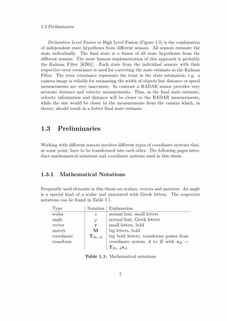
Frequently used elements in this thesis are scalars, vectors and matrices. An angleis a special kind of a scalar and annotated with Greek letters. The respectivenotations can be found in Table 1.1.
Type Notation Explanationscalar s normal font, small lettersangle ϕ normal font, Greek lettersvector v small letters, boldmatrix M big letters, boldcoordinatetransform
TB←A big bold letters, transforms points fromcoordinate system A to B with xB =TB←AxA
Table 1.1: Mathematical notations
5

1.3 Preliminaries
Homogeneous Coordinates and Coordinate Transforms
Coordinate representations of n-dimensional space can be defined as homogeneouscoordinates, which represent lines in n + 1-dimensional space by adding 1 as aconstant to the vector. xy
z
7→xyz1
(1.1)
This allows combining rotations and translations in a more compact way. Thesecoordinate transforms are annotated as TB←A and can be used for arbitrary trans-formations from n-dimensional coordinate system A to d-dimensional coordinatesystem B but usually define a transformation matrix containing a rotation matrixR and a translation vector t (eq. (1.2)) that is used to transform homogeneouscoordinates.
TB←A =(
R t0 0 0 1
)=
r11 r12 r13 t1r21 r22 r23 t2r31 r32 r33 t30 0 0 1
(1.2)
xB = TB←AxA (1.3)
Transformations can be concatenated if the resulting dimensions match. The trans-formation chain can be recognized by reading the indices from right to left, e.g.:
xC = TC←BTB←AxA (1.4)
A point xA in coordinate frame A is first transformed to coordinate system Bfollowed by a transformation from B to the final coordinate system C.
1.3.2 Coordinate Systems
Several coordinate systems are used in the thesis. A world coordinate system isused as a general reference. The ego vehicle coordinate system defines a localcoordinate system which is carried along with the motion of the vehicle. Cameramodels make use of two other coordinate frames – the 3-dimensional camera coor-dinate frame and the image frame which references to pixel coordinates. RADARsensors utilize polar coordinates to reference to detected targets. These coordinatesystems are explained in detail in the following.
6
1.3 Preliminaries
World Coordinate System
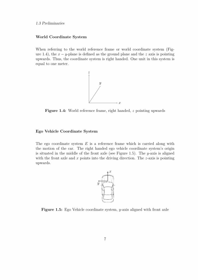
When referring to the world reference frame or world coordinate system (Fig-ure 1.4), the x− y-plane is defined as the ground plane and the z axis is pointingupwards. Thus, the coordinate system is right handed. One unit in this system isequal to one meter.
x
y
z
Figure 1.4: World reference frame, right handed, z pointing upwards
Ego Vehicle Coordinate System
The ego coordinate system E is a reference frame which is carried along withthe motion of the car. The right handed ego vehicle coordinate system’s originis situated in the middle of the front axle (see Figure 1.5). The y-axis is alignedwith the front axle and x points into the driving direction. The z-axis is pointingupwards.
x
y
Figure 1.5: Ego Vehicle coordinate system, y-axis aligned with front axle
7
1.3 Preliminaries
Camera Coordinate System
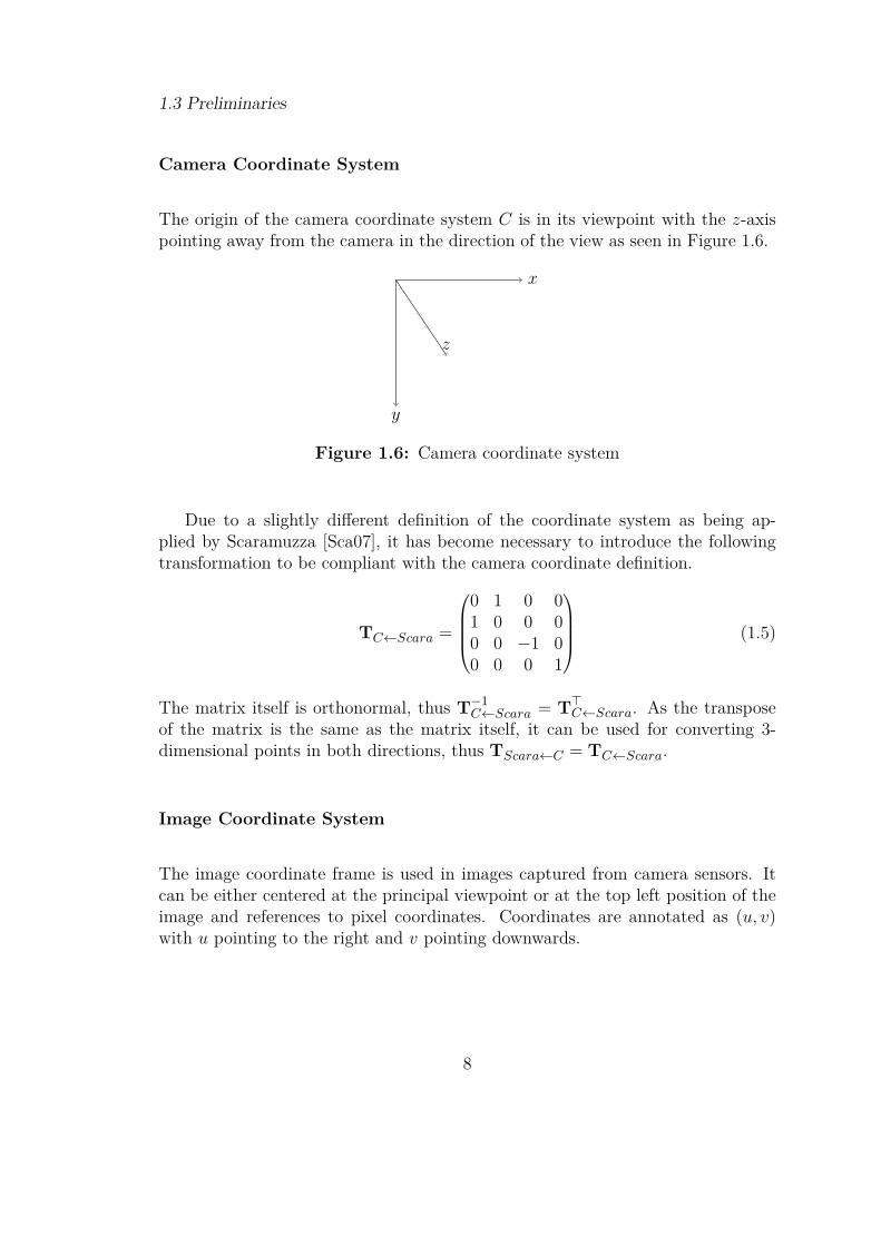
The origin of the camera coordinate system C is in its viewpoint with the z-axispointing away from the camera in the direction of the view as seen in Figure 1.6.
x
y
z
Figure 1.6: Camera coordinate system
Due to a slightly different definition of the coordinate system as being ap-plied by Scaramuzza [Sca07], it has become necessary to introduce the followingtransformation to be compliant with the camera coordinate definition.
TC←Scara =
0 1 0 01 0 0 00 0 −1 00 0 0 1
(1.5)
The matrix itself is orthonormal, thus T−1C←Scara = T>C←Scara. As the transpose
of the matrix is the same as the matrix itself, it can be used for converting 3-dimensional points in both directions, thus TScara←C = TC←Scara.
Image Coordinate System
The image coordinate frame is used in images captured from camera sensors. Itcan be either centered at the principal viewpoint or at the top left position of theimage and references to pixel coordinates. Coordinates are annotated as (u, v)with u pointing to the right and v pointing downwards.
8
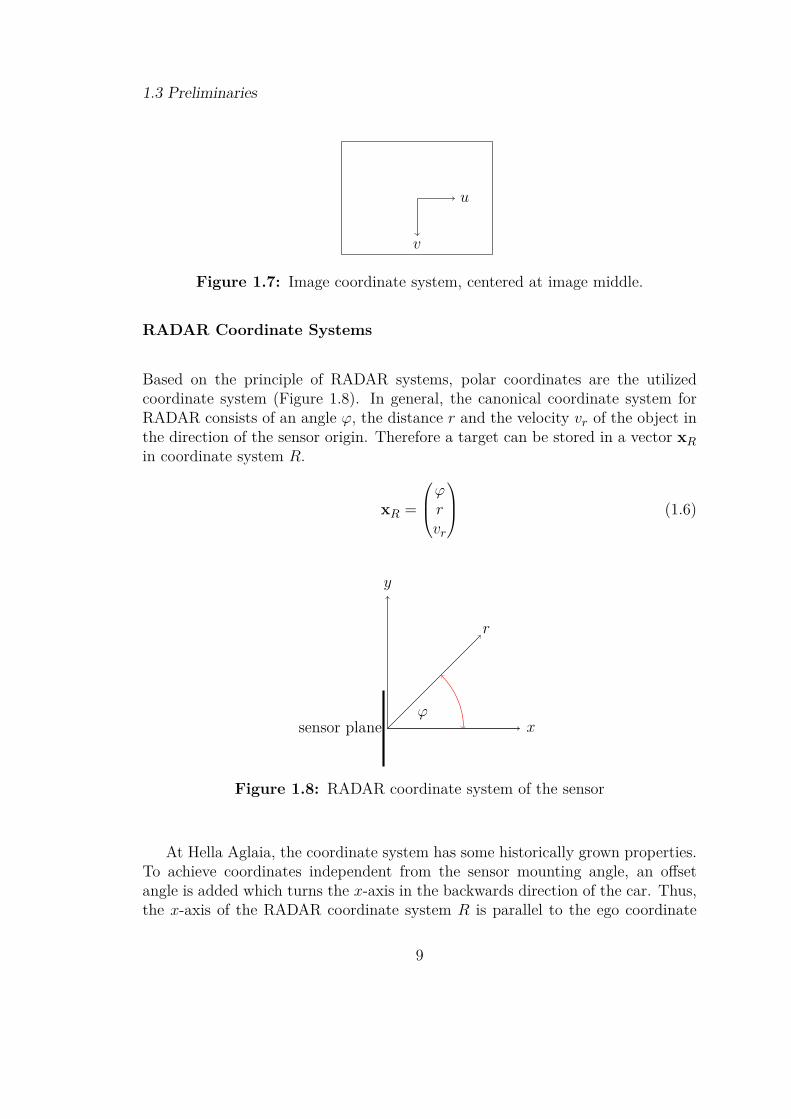
1.3 Preliminaries
u
v
Figure 1.7: Image coordinate system, centered at image middle.
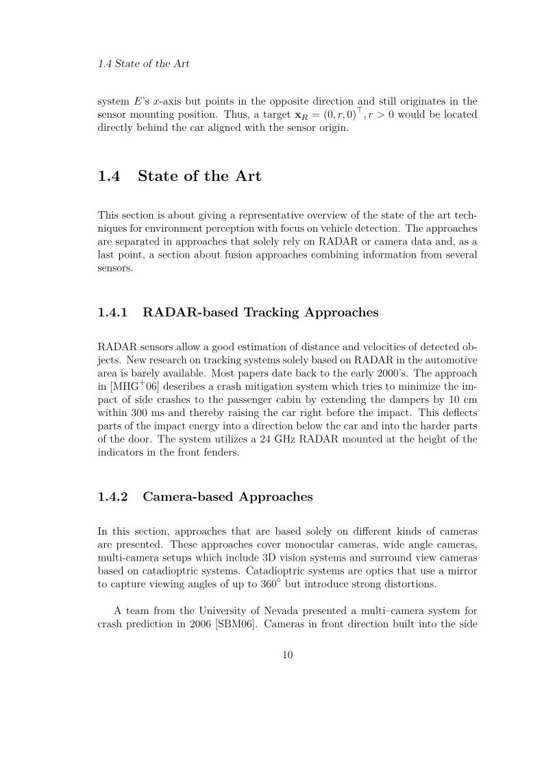
RADAR Coordinate Systems
Based on the principle of RADAR systems, polar coordinates are the utilizedcoordinate system (Figure 1.8). In general, the canonical coordinate system forRADAR consists of an angle ϕ, the distance r and the velocity vr of the object inthe direction of the sensor origin. Therefore a target can be stored in a vector xRin coordinate system R.
xR =
ϕrvr
(1.6)
y
xsensor plane
r
ϕ
Figure 1.8: RADAR coordinate system of the sensor
At Hella Aglaia, the coordinate system has some historically grown properties.To achieve coordinates independent from the sensor mounting angle, an offsetangle is added which turns the x-axis in the backwards direction of the car. Thus,the x-axis of the RADAR coordinate system R is parallel to the ego coordinate
9
1.4 State of the Art
system E’s x-axis but points in the opposite direction and still originates in thesensor mounting position. Thus, a target xR = (0, r, 0)>, r > 0 would be locateddirectly behind the car aligned with the sensor origin.
1.4 State of the Art
This section is about giving a representative overview of the state of the art tech-niques for environment perception with focus on vehicle detection. The approachesare separated in approaches that solely rely on RADAR or camera data and, as alast point, a section about fusion approaches combining information from severalsensors.
1.4.1 RADAR-based Tracking Approaches
RADAR sensors allow a good estimation of distance and velocities of detected ob-jects. New research on tracking systems solely based on RADAR in the automotivearea is barely available. Most papers date back to the early 2000’s. The approachin [MHG+06] describes a crash mitigation system which tries to minimize the im-pact of side crashes to the passenger cabin by extending the dampers by 10 cmwithin 300 ms and thereby raising the car right before the impact. This deflectsparts of the impact energy into a direction below the car and into the harder partsof the door. The system utilizes a 24 GHz RADAR mounted at the height of theindicators in the front fenders.
1.4.2 Camera-based Approaches
In this section, approaches that are based solely on different kinds of camerasare presented. These approaches cover monocular cameras, wide angle cameras,multi-camera setups which include 3D vision systems and surround view camerasbased on catadioptric systems. Catadioptric systems are optics that use a mirrorto capture viewing angles of up to 360◦ but introduce strong distortions.
A team from the University of Nevada presented a multi–camera system forcrash prediction in 2006 [SBM06]. Cameras in front direction built into the side
10
1.4 State of the Art
mirrors and windshield are used to detect front and side traffic, while a camerain the rear window is used for rear traffic. The cameras are especially optimizedfor night vision. In the first step the camera image is low pass filtered using aGaussian filter. In the second step horizontal and vertical edges are extractedfrom scaled versions of the input image and the peaks are used to generate carhypotheses. The group evaluates several features and classifiers for the verificationstep. Images representing cars are used to estimate an Eigen space to minimize thefeature space of a potential vehicle image as proposed in [TP91]. The largest Eigenvectors of this space are used to generate feature vectors. Other sets of featuresare haar wavelets and truncated haar wavelet sets (removed the wavelets withthe smallest coefficients). Furthermore, Gabor features (used for edge detection)are extracted. Additionally, a combination of Gabor and Haar features has beentested. The acquired feature vectors are used to train a neural network and aSupport Vector Machine (SVM) classifier. The combination of wavelet and Gaborfeatures classified by an SVM showed the best results.
DaimlerChrysler presented an approach for object recognition and crash avoid-ance based on stereo camera systems in 2005 [FRBG05]. The cameras record thefront view of the vehicle. The ego motion is subtracted from the optical flow of thevideo stream. Moving objects are eventually segmented using 3D information andoptical flow annotations. These moving objects are tracked with Kalman filters[KB61]. As Kalman filters are prone to inaccurate initialization parameters, foreach object three filters are set up. The three filters are initialized with v1 = 0m/sand v2,3 = ±10m/s. The quality of the estimations is finally compared with thefollowing measurement of position and speed. This quality is expressed in theMahalanobis distance between prediction and measurement and used for weight-ing each filter. The three filters are then combined to a single prediction basedon their weight. According to the paper, the combined multi-hypothesis Kalmanfilter converges faster than choosing a single filter.
The approach of fitting deformable 3-dimensional object models by projectingthem into 2-dimensional images is not new, however, a recent attempt has beenpresented by [LM09]. The method estimates a model parameter set which de-scribes the shape, orientation and position of the model in 3-dimensional spaceby fitting the projected model edges to edges in the camera image. The authorsargument that the approach of fitting a simple car model is about 20 years old.The original approach itself can be found in [Low91]. With increased comput-ing power and increased image resolution, it is possible to fit complexer models.Thus, they use several car type specific CAD models with different polygon countswith 12 to 80.000 faces. A vehicle model consists of a 3D mesh describing the
11
1.4 State of the Art
general appearance, 2D polygons which describe the appearance of parts of themodel and a mapping which maps these onto said 3D model. To reduce the pa-rameter space of a general deformable model based on their model database, theyuse Principle Component Analysis (PCA) and reduce the parameter space to mmodel parameters represented by the largest Eigen values. On the assumption ofa known ground plane, the parameter space is represented by a (x, y)-translationand a yaw angle rotation θ as well as m shape parameters deduced by PCA. Thecorresponding 2D-projection of the model’s initial pose is fit to edges found in theCanny filtered input image [Can86]. Within multiple iterations the distance to thedetected edges is minimized. The group was able to fit 6 different vehicle typesbut fitting required good initial poses which are acquired by manually placing themodel on the vehicle in the image.
In [LTH+05], the same model fitting approach is used. There is no assumptionof camera motion. Thus, object hypotheses are obtained by motion changes inthe camera image. Additionally, the detected models are tracked through severalframes by an Extended Kalman filter with an underlying bicycle model.
DaimlerChrysler also showed a bird view system which allows a driver to havea top view of his surroundings on a monitor on his dashboard [ETG07]. Two om-nidirectional cameras on the top rear corners of a truck capture the surroundingsof the vehicle. These catadioptric systems based on a camera pointing on a con-vex mirror achieve an opening angle of 360◦. As a result, two of these camerasrender sufficient to capture the rear environment. The image is back projectedon the ground plane around the car which eventually renders a bird view of theenvironment as seen from the top of the car.
1.4.3 Sensor Fusion Approaches
Sensor fusion approaches are the most recent developments in the area of environ-ment perception. The fusion of several sensors allows to combine advantages ofdifferent sensors, e.g. distance and velocity measurements of RADAR and classi-fication abilities of cameras, and reduce disadvantages at the same time. Currentresearch mostly focuses on sensors which provide 3-dimensional information of theenvironment. Thus, papers that focus on camera-RADAR fusion are rather rare.
One of the recent approaches which utilize sensor fusion is [ZXY12]. The ap-proach combines a Light Detection And Ranging (LIDAR) sensor with camera
12
1.4 State of the Art
data. LIDAR sensors measure the time light travels to a certain object point tomeasure its distance. This allows high resolution distance maps. These mapsprovide good information for obstacle detection but less for classification. Thedistance map is used to classify parts of the image to ground plane or obstaclesusing RANSAC and 3D adjacency. At the same time the image patches are clas-sified to different classes by evaluating color histograms, texture descriptors fromGaussian and Garbor filtered images as well as local binary patterns. Resultingin 107 features, each patch is classified by a Multi-Layer-Perceptron to differentcategories. The size of the object determined by the LIDAR obstacle estimationas well as labels from the image analysis are passed into a fuzzy logic frameworkwhich returns three labels – environment, middle high or obstacle. The fusionapproach reaches better classification results than the individual sensors.
In [VBA08] a framework for self-location and mapping is presented. This ap-proach is based on an occupancy grid that is used to fuse information from RADARand LIDAR. An occupancy grid discretizes the environment space into small twodimensional grid tiles. The LIDAR sensor is used to estimate a probability of agrid cell to be occupied. A high probability means there is an obstacle in the re-spective grid cell. Moving objects are detected through changes in the occupancyof grid cells. Basically, if a cell is occupied at a time point, and in the next timestep, the adjacent cell is detected to be occupied, this is assumed as a motion. AsRADAR data is relatively sparse compared to LIDAR measurements, it is used toverify or reject motion estimations based on LIDAR data.
A similar method of fusing short range RADAR and laser measurements isproposed in [PVB+09]. The system covers more performance optimizations than[VBA08]. Instead of estimating a probability representation, the grid cells areeither occupied or empty based on the number of measurements of the laser scannerfor the respective cell. Adjacent cells that are occupied are merged to an object.A Kalman filter [KB61] is used to track the detected objects. Unfortunately thefusion process of RADAR and laser data is not described in detail.
The approach proposed in [ABC07] shows a fusion of RADAR and camerain which the camera is used to verify and optimize RADAR object tracks. Thecamera is oriented to the front. The center points of RADAR objects are pro-jected into the image based on the camera calibration. The symmetry of imagesections around the projected point is estimated. Ideally, the symmetry is largearound the RADAR hypothesis as front views and rear views of vehicles are sym-metric. Searching for higher symmetry values in a predefined environment aroundthe RADAR hypothesis is used to correct the position estimate. However, this
13

1.4 State of the Art
approach does only work for scenarios in which vehicles are viewed from the rearor front.
14
Chapter 2
Test Bed Setup
This chapter describes the general hard- and software setup of the test bed vehicle.The test bed is an Audi A8 equipped with an industry computer and several sen-sors. These include a front camera and two RADAR sensors mounted at the frontbumper observing front and side traffic. Furthermore, side short range ultrasoundsensors are mounted to observe the sides near the doors.
Cassandra, the used software framework for prototyping of algorithms, record-ing and replaying of test drive data, is presented in section 2.2. The processof choosing appropriate cameras for the project is demonstrated in section 2.3.Section 2.4 introduces the calibration process of camera systems and compares apin-hole model with distortion parameters with the more recent Scaramuzza cam-era model [SMS06a]. Finally, the hardware interconnections and the recording andreplaying of test drive data in the Cassandra Framework is explained.
2.1 Hella RADAR Sensors and Applications
Hella is one of the biggest global suppliers of automotive electronics and lightingsolutions. One of their products is a low-cost 24 GHz RADAR sensor [HEL12]. Thesensor allows the detection of targets in a distance of up to 100 m with velocities of±70 m/s in cycles of 50 ms. The maximum field of view is 165◦. Not only does Hellaprovide the sensor itself, but also several driver safety system applications. Thesesystems are in use at several OEMs. Blind Spot Detection (BSD) warns drivers of
15

2.2 Video & Signal Processing Framework Cassandra
unsafe conditions when trying to change lanes. Traveling on the highway is madesafer by the Lane Change Assistant (LCA), which allows warning distances of 70m when changing lanes. A similar application - Rear Pre-Crash (RPC) - observesrear traffic and detects potential collisions. This information can be used by OEMsto prepare for impacts. Safety measures that could be executed are for examplethe fastening of seat belts or further preparations of air bags. Rear Cross TrafficAlert (RCTA) secures situations in which the driver backs out of parking spacesand warns the driver about oncoming rear traffic.
2.2 Video & Signal Processing Framework Cas-sandra
Cassandra is a C++ development environment developed at Hella Aglaia [Hel13].It supports both rapid prototyping and product development. It has been releasedfor external use in 2013. The framework will be used throughout the whole thesisto implement most of the concepts explained. Its main focus is computer vision inthe automotive area. It supports a variety of cameras and video input, as well asController Area Network (CAN) hardware for capturing and sending CAN mes-sages. Furthermore a lot of OpenCV’s [Its13b] functionality is already available.OpenCV is an open source computer vision library written in C and C++ thatprovides optimized algorithms in the area of computer vision and machine learning.
Instead of implementing the whole processing chain of computer vision algo-rithms at once, Cassandra allows to break up the processing chain into replaceableand reusable blocks called stations. A station can contain input ports for inputdata, e.g. CAN messages or single images from a video, and output ports forthe processed data. Cassandra also provides several predefined stations for cam-era calibration and image processing based on OpenCV. Each station has severaladjustable parameters for the algorithm it represents.
A simple example of such a processing chain is an edge detection algorithm.The input is a RGB video stream from a Logitech Webcam Pro 9000, thus, it hasto be converted to uint8 gray scale and then fed into the Canny edge detectionalgorithm [Can86]. The simplest approach to achieve this is to use a player stationwhich sends out the video one frame at a time to the Canny filter station. Thefinal output is a binary image that highlights edges.
16
2.3 Choice of Cameras
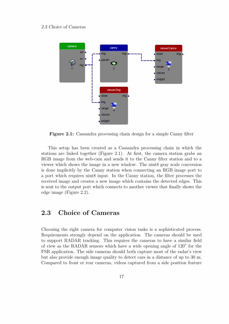
Figure 2.1: Cassandra processing chain design for a simple Canny filter
This setup has been created as a Cassandra processing chain in which thestations are linked together (Figure 2.1). At first, the camera station grabs anRGB image from the web-cam and sends it to the Canny filter station and to aviewer which shows the image in a new window. The uint8 gray scale conversionis done implicitly by the Canny station when connecting an RGB image port toa port which requires uint8 input. In the Canny station, the filter processes thereceived image and creates a new image which contains the detected edges. Thisis sent to the output port which connects to another viewer that finally shows theedge image (Figure 2.2).
2.3 Choice of Cameras
Choosing the right camera for computer vision tasks is a sophisticated process.Requirements strongly depend on the application. The cameras should be usedto support RADAR tracking. This requires the cameras to have a similar fieldof view as the RADAR sensors which have a wide opening angle of 120◦ for theFSR application. The side cameras should both capture most of the radar’s viewbut also provide enough image quality to detect cars in a distance of up to 30 m.Compared to front or rear cameras, videos captured from a side position feature
17
2.3 Choice of Cameras
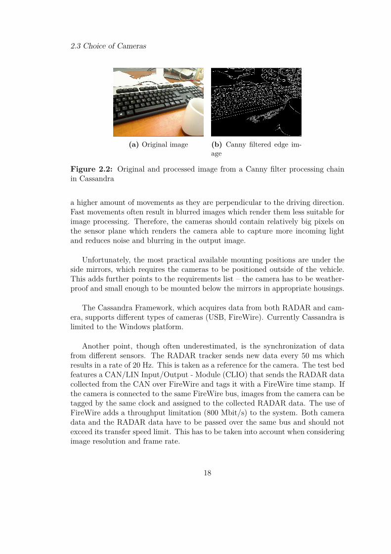
(a) Original image (b) Canny filtered edge im-age
Figure 2.2: Original and processed image from a Canny filter processing chainin Cassandra
a higher amount of movements as they are perpendicular to the driving direction.Fast movements often result in blurred images which render them less suitable forimage processing. Therefore, the cameras should contain relatively big pixels onthe sensor plane which renders the camera able to capture more incoming lightand reduces noise and blurring in the output image.
Unfortunately, the most practical available mounting positions are under theside mirrors, which requires the cameras to be positioned outside of the vehicle.This adds further points to the requirements list – the camera has to be weather-proof and small enough to be mounted below the mirrors in appropriate housings.
The Cassandra Framework, which acquires data from both RADAR and cam-era, supports different types of cameras (USB, FireWire). Currently Cassandra islimited to the Windows platform.
Another point, though often underestimated, is the synchronization of datafrom different sensors. The RADAR tracker sends new data every 50 ms whichresults in a rate of 20 Hz. This is taken as a reference for the camera. The test bedfeatures a CAN/LIN Input/Output - Module (CLIO) that sends the RADAR datacollected from the CAN over FireWire and tags it with a FireWire time stamp. Ifthe camera is connected to the same FireWire bus, images from the camera can betagged by the same clock and assigned to the collected RADAR data. The use ofFireWire adds a throughput limitation (800 Mbit/s) to the system. Both cameradata and the RADAR data have to be passed over the same bus and should notexceed its transfer speed limit. This has to be taken into account when consideringimage resolution and frame rate.
18
2.3 Choice of Cameras
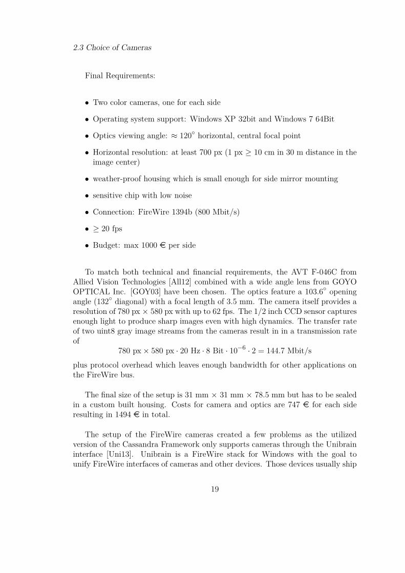
Final Requirements:
• Two color cameras, one for each side
• Operating system support: Windows XP 32bit and Windows 7 64Bit
• Optics viewing angle: ≈ 120◦ horizontal, central focal point
• Horizontal resolution: at least 700 px (1 px ≥ 10 cm in 30 m distance in theimage center)
• weather-proof housing which is small enough for side mirror mounting
• sensitive chip with low noise
• Connection: FireWire 1394b (800 Mbit/s)
• ≥ 20 fps
• Budget: max 1000 e per side
To match both technical and financial requirements, the AVT F-046C fromAllied Vision Technologies [All12] combined with a wide angle lens from GOYOOPTICAL Inc. [GOY03] have been chosen. The optics feature a 103.6◦ openingangle (132◦ diagonal) with a focal length of 3.5 mm. The camera itself provides aresolution of 780 px × 580 px with up to 62 fps. The 1/2 inch CCD sensor capturesenough light to produce sharp images even with high dynamics. The transfer rateof two uint8 gray image streams from the cameras result in in a transmission rateof
780 px× 580 px · 20 Hz · 8 Bit · 10−6 · 2 = 144.7 Mbit/s
plus protocol overhead which leaves enough bandwidth for other applications onthe FireWire bus.
The final size of the setup is 31 mm × 31 mm × 78.5 mm but has to be sealedin a custom built housing. Costs for camera and optics are 747 e for each sideresulting in 1494 e in total.
The setup of the FireWire cameras created a few problems as the utilizedversion of the Cassandra Framework only supports cameras through the Unibraininterface [Uni13]. Unibrain is a FireWire stack for Windows with the goal tounify FireWire interfaces of cameras and other devices. Those devices usually ship
19
2.4 Camera Calibration and Evaluation of Camera Models
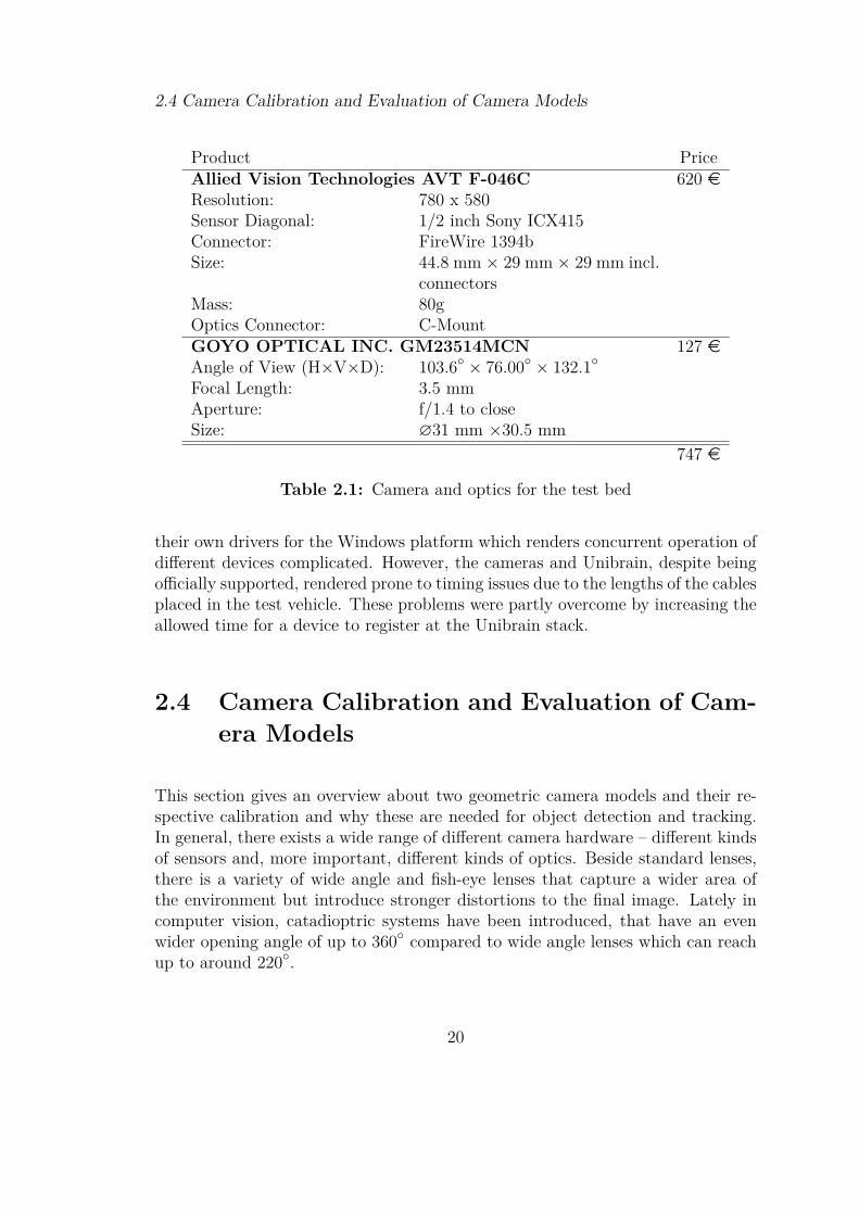
Product PriceAllied Vision Technologies AVT F-046C 620 eResolution: 780 x 580Sensor Diagonal: 1/2 inch Sony ICX415Connector: FireWire 1394bSize: 44.8 mm × 29 mm × 29 mm incl.
connectorsMass: 80gOptics Connector: C-MountGOYO OPTICAL INC. GM23514MCN 127 eAngle of View (H×V×D): 103.6◦ × 76.00◦ × 132.1◦Focal Length: 3.5 mmAperture: f/1.4 to closeSize: ∅31 mm ×30.5 mm
747 e
Table 2.1: Camera and optics for the test bed
their own drivers for the Windows platform which renders concurrent operation ofdifferent devices complicated. However, the cameras and Unibrain, despite beingofficially supported, rendered prone to timing issues due to the lengths of the cablesplaced in the test vehicle. These problems were partly overcome by increasing theallowed time for a device to register at the Unibrain stack.
2.4 Camera Calibration and Evaluation of Cam-era Models
This section gives an overview about two geometric camera models and their re-spective calibration and why these are needed for object detection and tracking.In general, there exists a wide range of different camera hardware – different kindsof sensors and, more important, different kinds of optics. Beside standard lenses,there is a variety of wide angle and fish-eye lenses that capture a wider area ofthe environment but introduce stronger distortions to the final image. Lately incomputer vision, catadioptric systems have been introduced, that have an evenwider opening angle of up to 360◦ compared to wide angle lenses which can reachup to around 220◦.
20

2.4 Camera Calibration and Evaluation of Camera Models
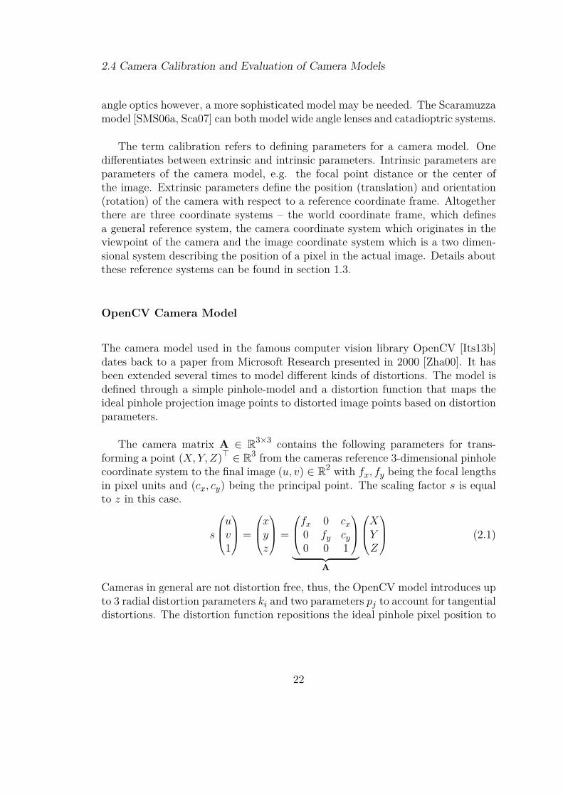
Especially when trying to identify objects in such images, distortions intro-duced by the optics can interfere with the actual detection process, e.g. straightlines in the real environment become bent in the images captured by the camera.Additionally, the form of an object in the might look different through the distor-tions. Distortions are geometric projection errors that are generated by the opticsof the system. Hence, for object detection, knowing the geometries that causesuch distortions to undistort images and remove the influence of the distortionscan greatly improve detection performance. This process is also called rectification.Most camera lenses introduce two kinds of distortions, radial distortions emittingfrom the center of the image and tangential distortions. Radial distortions are
Figure 2.3: Radial barrel distortion around the image center
radially symmetric around the image center as most lenses are manufactured ra-dially symmetric. Especially for wide angle lenses the zoom level in the middle ofthe image is usually higher than at the borders which is called barrel distortion(Figure 2.3). Tangential distortions, for example, can be seen in images takenfrom a camera which is positioned behind the windshield of a car. The bottompart of the image might exhibit a higher zoom level than the upper part becauseof the different distances to the windshield and the different ways the light raystake through the glass.
2.4.1 Intrinsic Calibration
A camera model defines a geometric system that describes how a ray of light hitsthe camera sensor. Most of the models require a single viewpoint which means,that all incoming light rays, restricted by the geometries of the optics, intersect ina defined point, the view point or focal point. In the following pages two modelswill be explained in detail. The standard pinhole model with radial distortionparameters available in OpenCV [Its13b] can be used for most cameras. With wide
21
2.4 Camera Calibration and Evaluation of Camera Models
angle optics however, a more sophisticated model may be needed. The Scaramuzzamodel [SMS06a, Sca07] can both model wide angle lenses and catadioptric systems.
The term calibration refers to defining parameters for a camera model. Onedifferentiates between extrinsic and intrinsic parameters. Intrinsic parameters areparameters of the camera model, e.g. the focal point distance or the center ofthe image. Extrinsic parameters define the position (translation) and orientation(rotation) of the camera with respect to a reference coordinate frame. Altogetherthere are three coordinate systems – the world coordinate frame, which definesa general reference system, the camera coordinate system which originates in theviewpoint of the camera and the image coordinate system which is a two dimen-sional system describing the position of a pixel in the actual image. Details aboutthese reference systems can be found in section 1.3.
OpenCV Camera Model
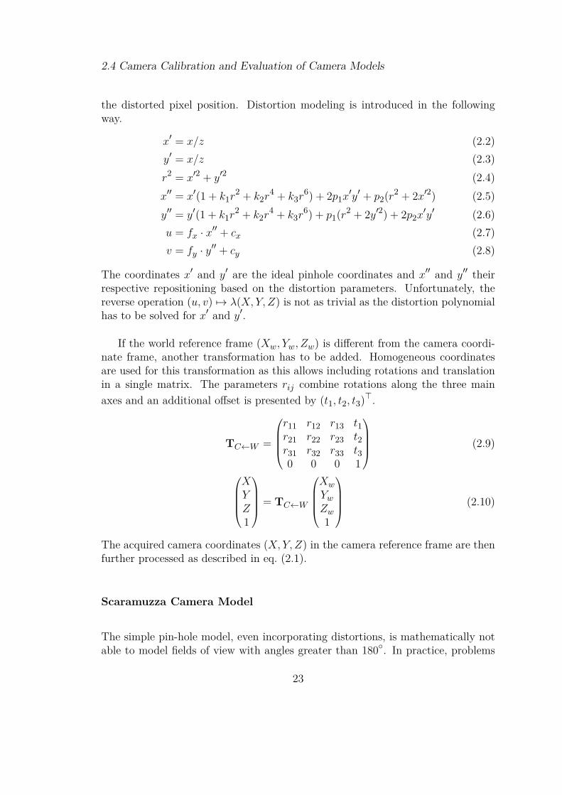
The camera model used in the famous computer vision library OpenCV [Its13b]dates back to a paper from Microsoft Research presented in 2000 [Zha00]. It hasbeen extended several times to model different kinds of distortions. The model isdefined through a simple pinhole-model and a distortion function that maps theideal pinhole projection image points to distorted image points based on distortionparameters.
The camera matrix A ∈ R3×3 contains the following parameters for trans-forming a point (X, Y, Z)> ∈ R3 from the cameras reference 3-dimensional pinholecoordinate system to the final image (u, v) ∈ R2 with fx, fy being the focal lengthsin pixel units and (cx, cy) being the principal point. The scaling factor s is equalto z in this case.
s
uv1
=
xyz
=
fx 0 cx0 fy cy0 0 1
︸ ︷︷ ︸
A
XYZ
(2.1)
Cameras in general are not distortion free, thus, the OpenCV model introduces upto 3 radial distortion parameters ki and two parameters pj to account for tangentialdistortions. The distortion function repositions the ideal pinhole pixel position to
22
2.4 Camera Calibration and Evaluation of Camera Models
the distorted pixel position. Distortion modeling is introduced in the followingway.
x′ = x/z (2.2)y′ = x/z (2.3)r2 = x′2 + y′2 (2.4)x′′ = x′(1 + k1r
2 + k2r4 + k3r
6) + 2p1x′y′ + p2(r2 + 2x′2) (2.5)
y′′ = y′(1 + k1r2 + k2r
4 + k3r6) + p1(r2 + 2y′2) + 2p2x
′y′ (2.6)u = fx · x′′ + cx (2.7)v = fy · y′′ + cy (2.8)
The coordinates x′ and y′ are the ideal pinhole coordinates and x′′ and y′′ theirrespective repositioning based on the distortion parameters. Unfortunately, thereverse operation (u, v) 7→ λ(X, Y, Z) is not as trivial as the distortion polynomialhas to be solved for x′ and y′.
If the world reference frame (Xw, Yw, Zw) is different from the camera coordi-nate frame, another transformation has to be added. Homogeneous coordinatesare used for this transformation as this allows including rotations and translationin a single matrix. The parameters rij combine rotations along the three mainaxes and an additional offset is presented by (t1, t2, t3)>.
TC←W =
r11 r12 r13 t1r21 r22 r23 t2r31 r32 r33 t30 0 0 1
(2.9)
XYZ1
= TC←W
Xw
YwZw1
(2.10)
The acquired camera coordinates (X, Y, Z) in the camera reference frame are thenfurther processed as described in eq. (2.1).
Scaramuzza Camera Model
The simple pin-hole model, even incorporating distortions, is mathematically notable to model fields of view with angles greater than 180◦. In practice, problems
23
2.4 Camera Calibration and Evaluation of Camera Models
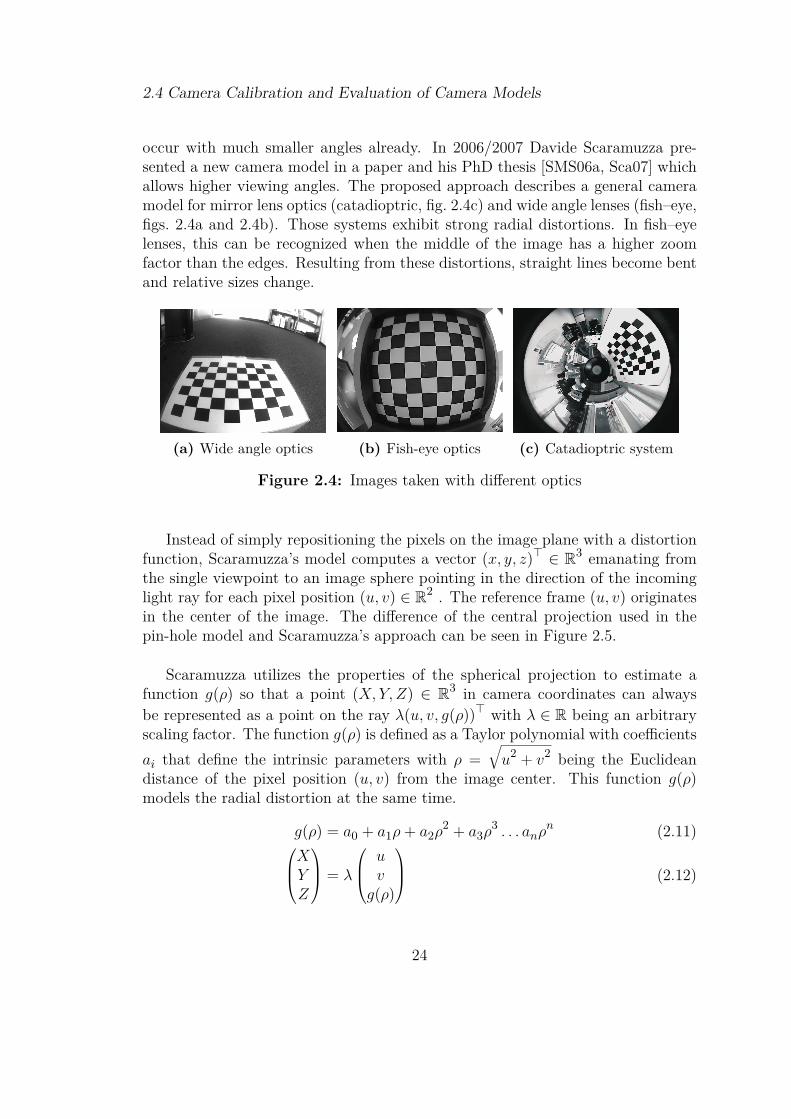
occur with much smaller angles already. In 2006/2007 Davide Scaramuzza pre-sented a new camera model in a paper and his PhD thesis [SMS06a, Sca07] whichallows higher viewing angles. The proposed approach describes a general cameramodel for mirror lens optics (catadioptric, fig. 2.4c) and wide angle lenses (fish–eye,figs. 2.4a and 2.4b). Those systems exhibit strong radial distortions. In fish–eyelenses, this can be recognized when the middle of the image has a higher zoomfactor than the edges. Resulting from these distortions, straight lines become bentand relative sizes change.
(a) Wide angle optics (b) Fish-eye optics (c) Catadioptric system
Figure 2.4: Images taken with different optics
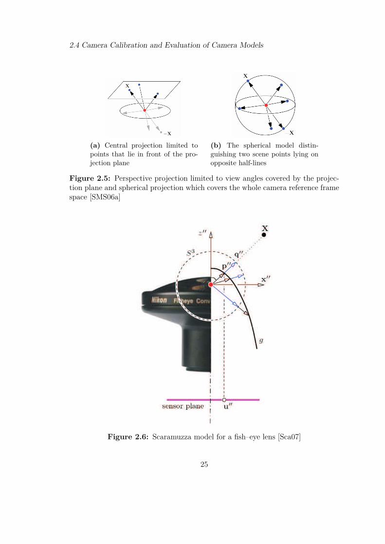
Instead of simply repositioning the pixels on the image plane with a distortionfunction, Scaramuzza’s model computes a vector (x, y, z)> ∈ R3 emanating fromthe single viewpoint to an image sphere pointing in the direction of the incominglight ray for each pixel position (u, v) ∈ R2 . The reference frame (u, v) originatesin the center of the image. The difference of the central projection used in thepin-hole model and Scaramuzza’s approach can be seen in Figure 2.5.
Scaramuzza utilizes the properties of the spherical projection to estimate afunction g(ρ) so that a point (X, Y, Z) ∈ R3 in camera coordinates can alwaysbe represented as a point on the ray λ(u, v, g(ρ))> with λ ∈ R being an arbitraryscaling factor. The function g(ρ) is defined as a Taylor polynomial with coefficientsai that define the intrinsic parameters with ρ =
√u2 + v2 being the Euclidean
distance of the pixel position (u, v) from the image center. This function g(ρ)models the radial distortion at the same time.
g(ρ) = a0 + a1ρ+ a2ρ2 + a3ρ
3 . . . anρn (2.11)XY
Z
= λ
uvg(ρ)
(2.12)
24
2.4 Camera Calibration and Evaluation of Camera Models
(a) Central projection limited topoints that lie in front of the pro-jection plane
(b) The spherical model distin-guishing two scene points lying onopposite half-lines
Figure 2.5: Perspective projection limited to view angles covered by the projec-tion plane and spherical projection which covers the whole camera reference framespace [SMS06a]
Figure 2.6: Scaramuzza model for a fish–eye lens [Sca07]
25

2.4 Camera Calibration and Evaluation of Camera Models
Certainly, to project a point (X, Y, Z) in camera coordinates onto the image,eq. (2.12) has to be solved for u and v which requires solving the polynomial ofg(ρ). As this is computational inefficient, Scaramuzza estimates an inverse Taylorpolynomial f(θ) which describes the radial positioning on the image plane basedon the angle θ of a light ray to the z axis.
f(θ) = b0 + b1θ + b2θ2 + b3θ
3...bnθn (2.13)
r =√X2 + Y 2 (2.14)
θ = atan(Z/r) (2.15)
u = X
rf(θ) (2.16)
v = Y
rf(θ) (2.17)
The model applied on a fish-eye lens can be seen in Figure 2.6. Further detailsof the model can be found in [SMS06a, Sca07, SMS06b]. During the calibrationprocess, several parameters are estimated (Table 2.2).
Description Parameters
Scaling of sensor to im-age plane
c, d, e with(u′
v′
)=(c de 0
)(uv
)
Taylor polynomial g aiImage projection Taylorpolynomial
bi
Image center (xc, yc)
Table 2.2: Parameters of an intrinsic Scaramuzza calibration
Calibration with OpenCV
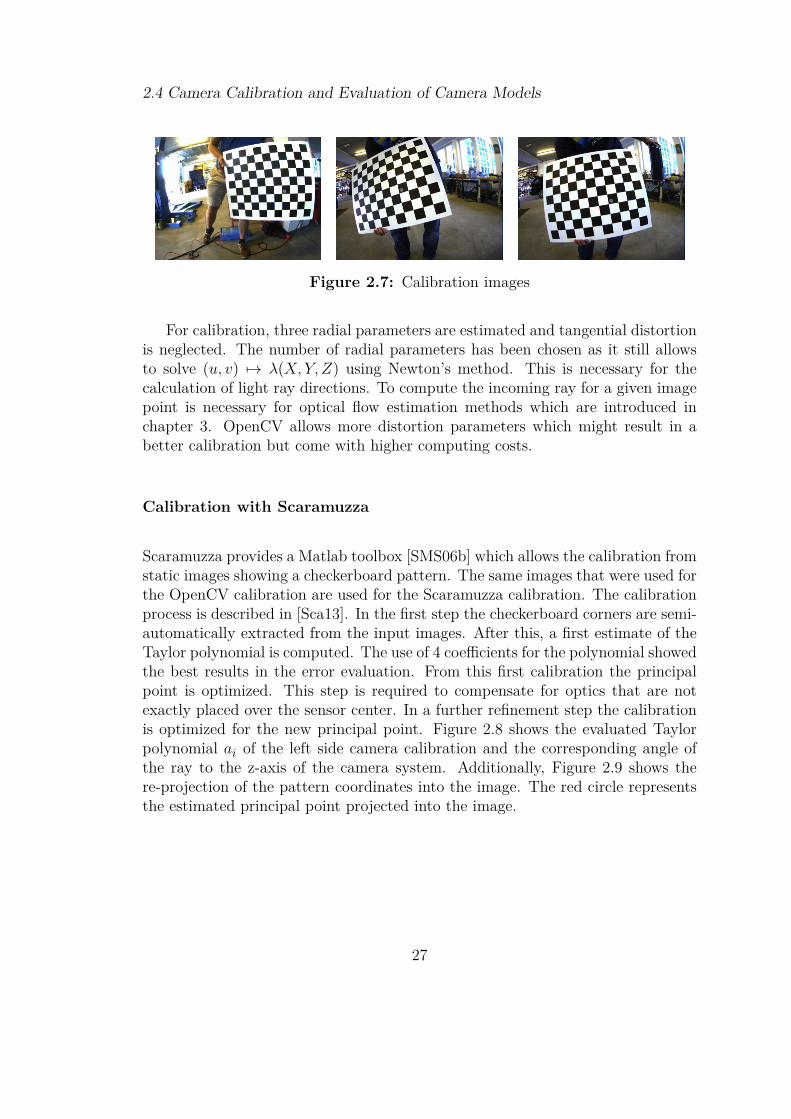
The calibration process of OpenCV is fairly automated and requires only XML filesthat describe which model parameters to be used and images or a video streamof the chosen pattern in different poses. Both circle patterns and checkerboardpatterns are supported by OpenCV. The process is described in detail in [Its13a].The pattern which is used to calibrate the camera is a checkerboard pattern with5 cm × 5 cm squares. The calibration was done on 30 static images showing thecheckerboard pattern in different poses (Examples in Figure 2.7).
26
2.4 Camera Calibration and Evaluation of Camera Models
Figure 2.7: Calibration images
For calibration, three radial parameters are estimated and tangential distortionis neglected. The number of radial parameters has been chosen as it still allowsto solve (u, v) 7→ λ(X, Y, Z) using Newton’s method. This is necessary for thecalculation of light ray directions. To compute the incoming ray for a given imagepoint is necessary for optical flow estimation methods which are introduced inchapter 3. OpenCV allows more distortion parameters which might result in abetter calibration but come with higher computing costs.
Calibration with Scaramuzza
Scaramuzza provides a Matlab toolbox [SMS06b] which allows the calibration fromstatic images showing a checkerboard pattern. The same images that were used forthe OpenCV calibration are used for the Scaramuzza calibration. The calibrationprocess is described in [Sca13]. In the first step the checkerboard corners are semi-automatically extracted from the input images. After this, a first estimate of theTaylor polynomial is computed. The use of 4 coefficients for the polynomial showedthe best results in the error evaluation. From this first calibration the principalpoint is optimized. This step is required to compensate for optics that are notexactly placed over the sensor center. In a further refinement step the calibrationis optimized for the new principal point. Figure 2.8 shows the evaluated Taylorpolynomial ai of the left side camera calibration and the corresponding angle ofthe ray to the z-axis of the camera system. Additionally, Figure 2.9 shows there-projection of the pattern coordinates into the image. The red circle representsthe estimated principal point projected into the image.
27

2.4 Camera Calibration and Evaluation of Camera Models
0 50 100 150 200 250 300 350 400
−400
−350
−300
Distance ρ from the image center in pixels
g(ρ
)
Forward projection function
0 50 100 150 200 250 300 350 400−100
−80
−60
−40
−20
Distance ρ from the image center in pixels
Degrees
Angle of optical ray as a function of distance from circle center (pixels)
Figure 2.8: Scaramuzza calibration results of the left camera calibration: g(ρ)and the angle of the rays from the z-axis in relation to the distance ρ from theimage center
28

2.4 Camera Calibration and Evaluation of Camera Models
Figure 2.9: Re-projection of the extracted 3–dimensional corner world coordi-nates back into the image. Red crosses represent the detected corner points andgreen circles their respective re-projection
2.4.2 Extrinsic Calibration
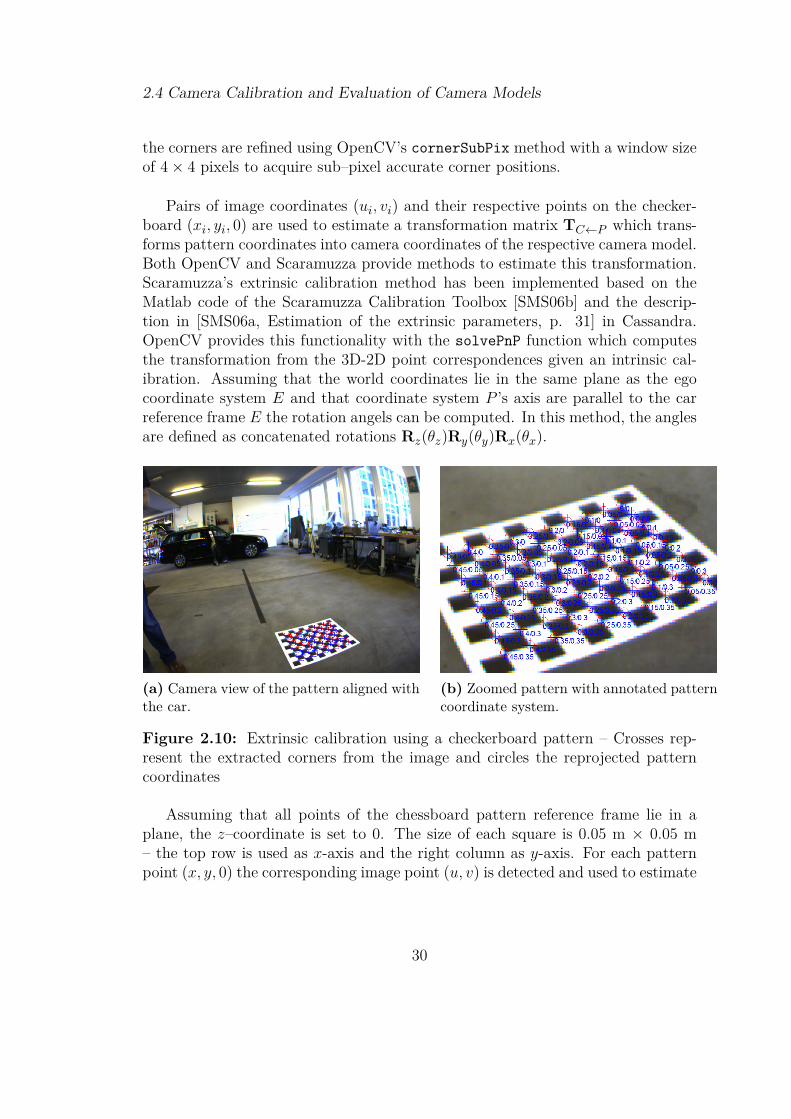
The translation of the camera can be roughly measured with standard measure-ment tools. The rotation of the camera, however, is computed by estimating thetransformation to a reference coordinate system. Both the OpenCV and Scara-muzza model provide functions to estimate a transformation from given worldcoordinates in reference system P and corresponding image coordinates I to thecamera coordinate system C based on the camera model. The reference frame P isrepresented by a checkerboard aligned with the ground plane. Its axes are parallelto the vehicle’s ego coordinate system (Figure 2.10).
The algorithms for estimating extrinsic parameters from a pattern have beenimplemented in Cassandra. In the first step the image coordinates and correspond-ing checkerboard coordinates are extracted. The method findChessBoardCornersfor automatic checkerboard detection provided by OpenCV is robust but fails insome cases. However, to detect the checkerboard patterns in the distorted imagesof the cameras, the algorithm for automatic detection of checkerboards on blurredand distorted images from [RSS08] has been used. This approach performs betterin areas of stronger distortions. After extracting the corner points of the pattern,
29
2.4 Camera Calibration and Evaluation of Camera Models
the corners are refined using OpenCV’s cornerSubPix method with a window sizeof 4× 4 pixels to acquire sub–pixel accurate corner positions.
Pairs of image coordinates (ui, vi) and their respective points on the checker-board (xi, yi, 0) are used to estimate a transformation matrix TC←P which trans-forms pattern coordinates into camera coordinates of the respective camera model.Both OpenCV and Scaramuzza provide methods to estimate this transformation.Scaramuzza’s extrinsic calibration method has been implemented based on theMatlab code of the Scaramuzza Calibration Toolbox [SMS06b] and the descrip-tion in [SMS06a, Estimation of the extrinsic parameters, p. 31] in Cassandra.OpenCV provides this functionality with the solvePnP function which computesthe transformation from the 3D-2D point correspondences given an intrinsic cal-ibration. Assuming that the world coordinates lie in the same plane as the egocoordinate system E and that coordinate system P ’s axis are parallel to the carreference frame E the rotation angels can be computed. In this method, the anglesare defined as concatenated rotations Rz(θz)Ry(θy)Rx(θx).
(a) Camera view of the pattern aligned withthe car.
(b) Zoomed pattern with annotated patterncoordinate system.
Figure 2.10: Extrinsic calibration using a checkerboard pattern – Crosses rep-resent the extracted corners from the image and circles the reprojected patterncoordinates
Assuming that all points of the chessboard pattern reference frame lie in aplane, the z–coordinate is set to 0. The size of each square is 0.05 m × 0.05 m– the top row is used as x-axis and the right column as y-axis. For each patternpoint (x, y, 0) the corresponding image point (u, v) is detected and used to estimate
30
2.4 Camera Calibration and Evaluation of Camera Models
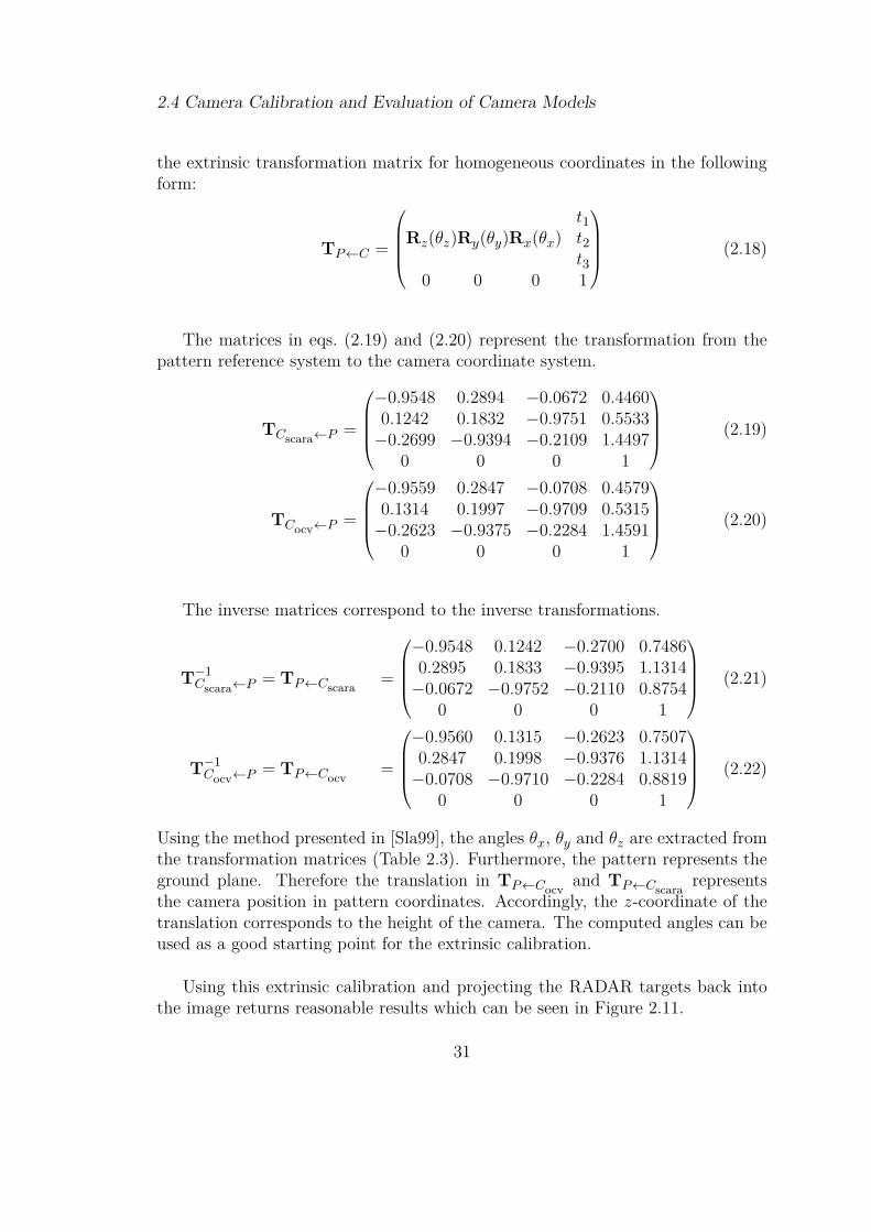
the extrinsic transformation matrix for homogeneous coordinates in the followingform:
TP←C =
t1
Rz(θz)Ry(θy)Rx(θx) t2t3
0 0 0 1
(2.18)
The matrices in eqs. (2.19) and (2.20) represent the transformation from thepattern reference system to the camera coordinate system.
TCscara←P =
−0.9548 0.2894 −0.0672 0.44600.1242 0.1832 −0.9751 0.5533−0.2699 −0.9394 −0.2109 1.4497
0 0 0 1
(2.19)
TCocv←P =
−0.9559 0.2847 −0.0708 0.45790.1314 0.1997 −0.9709 0.5315−0.2623 −0.9375 −0.2284 1.4591
0 0 0 1
(2.20)
The inverse matrices correspond to the inverse transformations.
T−1Cscara←P = TP←Cscara =
−0.9548 0.1242 −0.2700 0.74860.2895 0.1833 −0.9395 1.1314−0.0672 −0.9752 −0.2110 0.8754
0 0 0 1
(2.21)
T−1Cocv←P = TP←Cocv =
−0.9560 0.1315 −0.2623 0.75070.2847 0.1998 −0.9376 1.1314−0.0708 −0.9710 −0.2284 0.8819
0 0 0 1
(2.22)
Using the method presented in [Sla99], the angles θx, θy and θz are extracted fromthe transformation matrices (Table 2.3). Furthermore, the pattern represents theground plane. Therefore the translation in TP←Cocv and TP←Cscara representsthe camera position in pattern coordinates. Accordingly, the z-coordinate of thetranslation corresponds to the height of the camera. The computed angles can beused as a good starting point for the extrinsic calibration.
Using this extrinsic calibration and projecting the RADAR targets back intothe image returns reasonable results which can be seen in Figure 2.11.
31

2.4 Camera Calibration and Evaluation of Camera Models
OpenCV Scaramuzzaθz 76.76◦ 77.79◦θy 16.34◦ 16.31◦θx 4.06◦ 3.85◦Z 0.8819 0.8754 mZ measured 0.905 mY measured 0.97 mX measured −0.79 m
Table 2.3: Extrinsic parameters computed from a single image with OpenCVand Scaramuzza Camera models
Figure 2.11: A bicycle tracked by radar visualized in the camera image, thinlines represent the car’s ego coordinate system projected into the image
32
2.4 Camera Calibration and Evaluation of Camera Models
The Cassandra graph that computes transformations based on detected pat-terns for both Scaramuzza and OpenCV can be found in Figure C.1 in the appendixon page 104.
2.4.3 Results
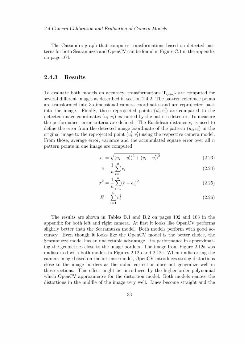
To evaluate both models on accuracy, transformations TC←P are computed forseveral different images as described in section 2.4.2. The pattern reference pointsare transformed into 3-dimensional camera coordinates and are reprojected backinto the image. Finally, these reprojected points (u′i, v′i) are compared to thedetected image coordinates (ui, vi) extracted by the pattern detector. To measurethe performance, error criteria are defined. The Euclidean distance ei is used todefine the error from the detected image coordinate of the pattern (ui, vi) in theoriginal image to the reprojected point (u′i, v′i) using the respective camera model.From those, average error, variance and the accumulated square error over all npattern points in one image are computed.
ei =√
(ui − u′i)2 + (vi − v′i)2 (2.23)
e = 1n
n∑i=1
ei (2.24)
σ2 = 1n
n∑i=1
(e− ei)2 (2.25)
E =n∑i=1
e2i (2.26)
The results are shown in Tables B.1 and B.2 on pages 102 and 103 in theappendix for both left and right camera. At first it looks like OpenCV performsslightly better than the Scaramuzza model. Both models perform with good ac-curacy. Even though it looks like the OpenCV model is the better choice, theScaramuzza model has an unelectable advantage – its performance in approximat-ing the geometries close to the image borders. The image from Figure 2.12a wasundistorted with both models in Figures 2.12b and 2.12c. When undistorting thecamera image based on the intrinsic model, OpenCV introduces strong distortionsclose to the image borders as the radial correction does not generalize well inthese sections. This effect might be introduced by the higher order polynomialwhich OpenCV approximates for the distortion model. Both models remove thedistortions in the middle of the image very well. Lines become straight and the
33

2.4 Camera Calibration and Evaluation of Camera Models
(a) Original distorted image from cam-era
(b) Undistorted image from OpenCVwhich introduces new distortions nearthe image borders
(c) Undistorted image from Scara-muzza which is distortion free.
Figure 2.12: Comparison of undistorted images from Scaramuzza and OpenCVmodel
34

2.4 Camera Calibration and Evaluation of Camera Models
fish-eye effect is removed. When looking at the buildings in the top right corner,it is notable that the Scaramuzza approach fixes the outer parts significantly bet-ter while OpenCV introduces mirroring and strong distortions in the outer parts.This can be overcome by using more radial distortion parameters (k4 − k6). Thisis supported by OpenCV but makes the calculation of the direction of a light rayeven more computational inefficient. The Scaramuzza approach, however, allowsefficient transformations from image space to camera space and from camera spaceto image space. Furthermore it is already used internally in other projects at HellaAglaia and supports the potential switch to optics with an even wider angle as wellas catadioptric systems. Therefore, this model is used for all further work.
Overall both models have their advantages and disadvantages which are sum-marized in the following.
OpenCV Advantages
• Automatic calibration process on both video and static images with a varietyof supported pattern types, e.g. checkerboards or circle boards
• C/C++ implementations available
• Models tangential distortion parameters
OpenCV Disadvantages
• Does not generalize well in border regions for wide angle lenses if only usedwith 3 radial distortion parameters
• No computing-efficient way to estimate the direction of the light ray whichhits the image plane
• Generally restricted to opening angles less than 180◦
Scaramuzza Advantages
• Both transformations image to camera coordinates and camera to image areefficiently computable
• Good generalization near image borders on wide angle lenses
35

2.5 Hardware Setup
• C implementation for basic transforms available
Scaramuzza Disadvantages
• Only semi-automatic calibration process on static images in Matlab availablewhich requires a license of the Matlab Optimization Toolbox
• No tangential distortion modeling
2.5 Hardware Setup
This section describes the general setup of the hardware as well as the intercon-nections between processing units and sensors. Furthermore, the sensor mountingsare explained.
2.5.1 Sensor Mounting
(a) Camera with housingmounted to mirror
(b) Camera with housingmounted to mirror
(c) Side radar sensormounted to bumper
Figure 2.13: Sensor mountings
Protecting the cameras from bad weather conditions is crucial. This fact madeit necessary to build custom housings which have been attached to metal platesmounted to the bottom of the side mirrors. The housings were made from PVCand sealed with silicone which can be seen in figs. 2.13a and 2.13b. The RADARsensors are attached to the front bumper 75◦ to the left and right as shown infig. 2.13c. They cover an area of 120◦. The exact mounting parameters of theRADAR sensors are shown in Table 2.4.
36
2.5 Hardware Setup
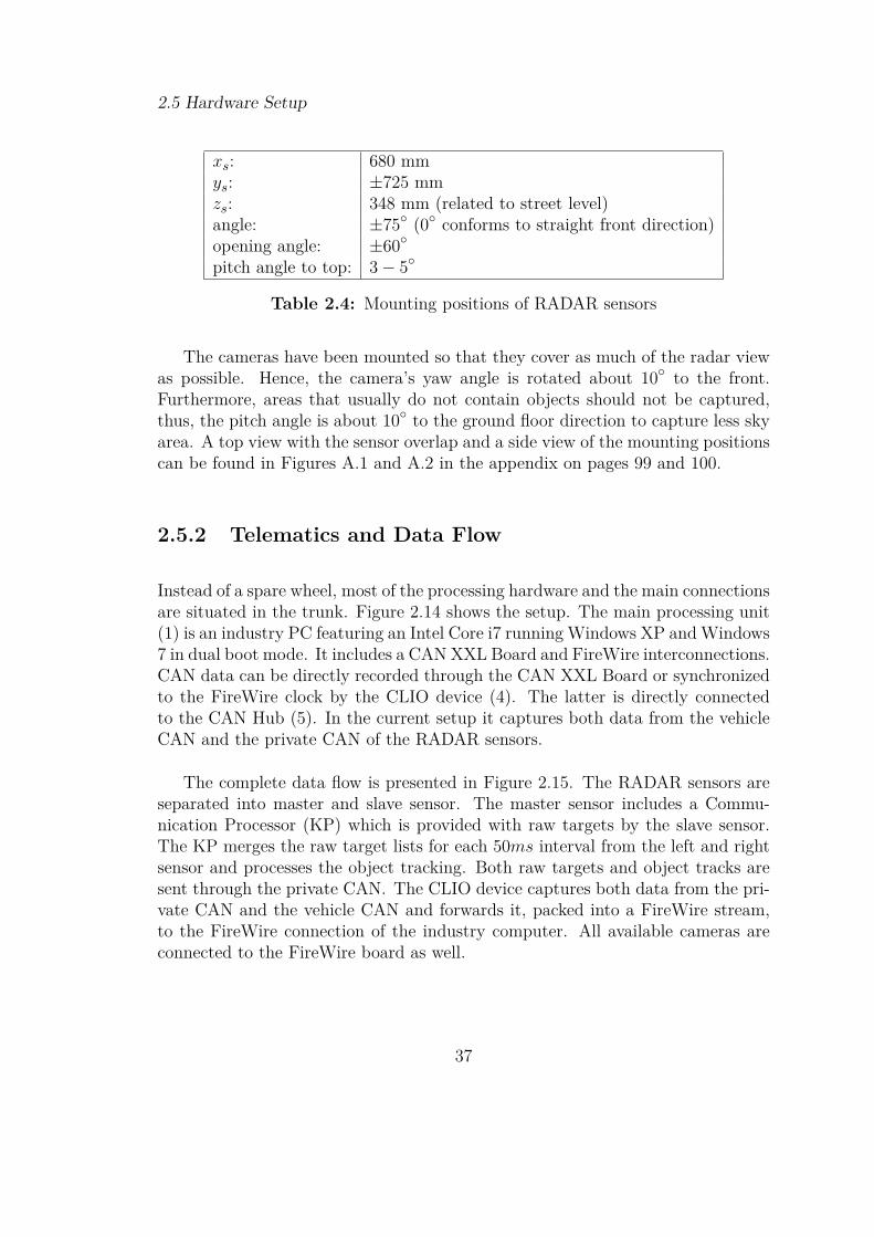
xs: 680 mmys: ±725 mmzs: 348 mm (related to street level)angle: ±75◦ (0◦ conforms to straight front direction)opening angle: ±60◦pitch angle to top: 3− 5◦
Table 2.4: Mounting positions of RADAR sensors
The cameras have been mounted so that they cover as much of the radar viewas possible. Hence, the camera’s yaw angle is rotated about 10◦ to the front.Furthermore, areas that usually do not contain objects should not be captured,thus, the pitch angle is about 10◦ to the ground floor direction to capture less skyarea. A top view with the sensor overlap and a side view of the mounting positionscan be found in Figures A.1 and A.2 in the appendix on pages 99 and 100.
2.5.2 Telematics and Data Flow
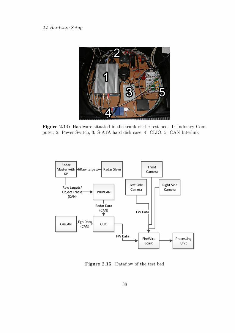
Instead of a spare wheel, most of the processing hardware and the main connectionsare situated in the trunk. Figure 2.14 shows the setup. The main processing unit(1) is an industry PC featuring an Intel Core i7 running Windows XP andWindows7 in dual boot mode. It includes a CAN XXL Board and FireWire interconnections.CAN data can be directly recorded through the CAN XXL Board or synchronizedto the FireWire clock by the CLIO device (4). The latter is directly connectedto the CAN Hub (5). In the current setup it captures both data from the vehicleCAN and the private CAN of the RADAR sensors.
The complete data flow is presented in Figure 2.15. The RADAR sensors areseparated into master and slave sensor. The master sensor includes a Commu-nication Processor (KP) which is provided with raw targets by the slave sensor.The KP merges the raw target lists for each 50ms interval from the left and rightsensor and processes the object tracking. Both raw targets and object tracks aresent through the private CAN. The CLIO device captures both data from the pri-vate CAN and the vehicle CAN and forwards it, packed into a FireWire stream,to the FireWire connection of the industry computer. All available cameras areconnected to the FireWire board as well.
37
2.5 Hardware Setup
Figure 2.14: Hardware situated in the trunk of the test bed. 1: Industry Com-puter, 2: Power Switch, 3: S-ATA hard disk case, 4: CLIO, 5: CAN Interlink
Radar Master with
KPRadar SlaveRaw targets
CLIO
PRIVCANRaw targets/Object Tracks
(CAN)
Radar Data(CAN)
FireWireBoard
FW Data
CarCANEgo Data
(CAN)
Left Side Camera
Front Camera
Right Side Camera
FW Data
Processing Unit
Figure 2.15: Dataflow of the test bed
38

2.6 Recording and Replaying of Data
2.6 Recording and Replaying of Data
Offline processing of data is a necessary need for development as the test bedvehicle is not always available and repeated testing of algorithms on the samedata is crucial. Cassandra allows to continuously record sensor data and save it tovideo streams and CAN data files. Cassandra offers a DriveRecorder module forthis purpose. The DriveRecorder provides an internal buffer to avoid frame dropsand writes the video streams from the left and right camera to uncompressedAudio Video Interleave (AVI) files. The CAN data is continuously stored in *.recfiles which also synchronize the camera frames to the internal clock. This results intwo video streams for the two side cameras and two *.rec files for private CAN andvehicle CAN. This process requires high throughput, therefore the data streamsare stored on an SSD to avoid data loss.
The Cassandra Graph for storing the data can be found in the appendix onpage 105. At first the CAN data is collected from the CLIO and captured bythe clio station which forwards it to the ClioDemuxer station that demuxes theprivate and the vehicle CAN messages to two different message streams whichare connected to the two message ports of the DriveRecorder station. The twocamera stations (avt_left and avt_right) capture uint8 gray scale images fromthe cameras at 20 Hz and forward it to the respective ports of the DriveRecorderstation. There is no further processing of the input data. The DriveRecorderstation stores the data streams in a memory buffer to avoid frame drops due tohard disk latency and subsequently writes the data to the SSD.
A minimal graph for replaying the data within the Cassandra framework canbe found in Figure C.3 on page 106. The player station has to be instructed whichstream to play at which port. Therefore, for each record a *.scene file is createdthat contains the names of files which are associated to the recording (listing 2.1).As previously mentioned, there are two files for the captured video data and twoCAN message files.
1 img1=RADAR_20130604_125156_1 . av imsg1=RADAR_20130604_125156_1 . r ec
3 img2=RADAR_20130604_125156_2 . av imsg2=RADAR_20130604_125156_2 . r ec
Listing 2.1: *.scene file
After loading such a file in the player, the left video stream is sent through portimg1 and the right through img2. CAN messages captured from the private CAN
39
2.6 Recording and Replaying of Data
are forwarded at the msg1 port and the vehicle messages can be found at port msg2of the Player station.
The data captured from the CAN bus has to be decoded for further processingwhich is done in the FSR sub graph. This sub graph also fetches information fromthe SensorSystem station which allows to enter extrinsic parameters of the masterand slave RADAR sensors. This information is needed to transform coordinatesfrom the RADAR sensor’s local coordinate frame to the ego vehicle reference frame.The mounting position in the ego coordinate frame and the respective alignmentare summarized in Table 2.4 on page 37.
The FSR sub macro (Figure C.4 on page 107 in the appendix) decodes theCAN messages from the private CAN and translates it to a list of tracked ob-jects and a list of respective RADAR raw targets for a given measurement cycle.In detail, the raw CAN messages are sent to the msg port of the msg2data sta-tion which decodes the data based on a database file and transforms it into ageneric data message format of the Cassandra Framework which is then passed tothe P-CAN-Interface station. This station collects messages containing raw tar-gets of the master (targetList_0) and slave sensor (targetList_1) and the finalobject tracks (objList). In the last step the corresponding raw target lists aresynchronized and merged into a combined list and forwarded with the respectiveobject list for further processing.
40

Chapter 3
Sensor Fusion of Radar andCamera for Object Tracking
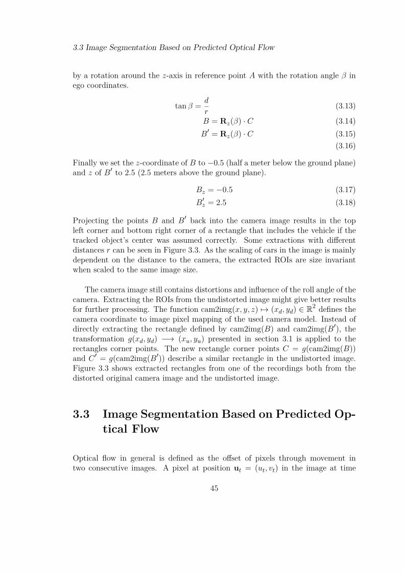
This chapter introduces a sensor fusion concept for side RADAR and side camerasensors. Features and methods usually utilized for classification and detectionof vehicles in front or rear cameras are not sufficient for the processing of imagesfrom wide angle side cameras. Vehicles appear in different angles which renders thesymmetry assumptions of front views and rear views inapplicable. Therefore othermethods are explored in this chapter. Pre-processing methods and the definitionof Regions of Interest (ROIs) are introduced in the first part. Following fromthis, a method to predict optical flow in an image sequence based on RADARmeasurements is explained. Section 3.4 describes an optimization process to fit 3-dimensional vehicle models to position hypotheses acquired from RADAR sensors.This process is refined by exploiting the prediction of optical flow based on RADARvelocity and position information of moving objects in the last part.
3.1 Image Correction
The side camera images exhibit strong radial distortions which can influence per-formance of classification algorithms. These distortions can be removed by geo-metric transforms based on the camera model. This process is called rectificationor undistortion. Mappings between the pixels of the undistorted and distorted im-age and vice versa are needed to identify ROIs in both images. OpenCV already
41
3.1 Image Correction
provides methods for realizing geometric transforms by remapping pixel coordi-nates and interpolating between them from a source image (src) to a destinationimage (dst) in the form
dst(x, y) = src(fx(x, y), fy(x, y)) (3.1)
Thus, the two mappings fx(x, y) and fy(x, y) which map the pixel coordinates ofthe undistorted image (xu, yu) to pixel coordinates in the distorted source image(xd, yd) have to be created.
Undistortion can be realized by imitating a pin-hole camera and projecting thecamera image to a plane parallel to the sensor plane in the camera coordinatesystem with an arbitrary but fixed focal length f . The images have width wand height h. The roll angle α, resulting from the mounting of the camera, is alsopartly corrected with the help of a rotation of the plane around the z-axis in the 3Dcamera coordinate system. The resulting 3D points are then projected back fromcamera coordinates to the image plane by the camera model’s cam2img functionwhich is a transformation R3 7→ R2 (see section 2.4.1 for details). Rz ∈ R3x3 isthe rotation matrix around the z-axis.
f(xu, yu) −→ (xd, yd) : (3.2)
p =
xu − w/2yu − h/2w/f
(3.3)
p′ = Rz(α)p (3.4)(xd, yd) = cam2img(p′) (3.5)
The resulting image does not show the barrel distortions. Lines that are straightin the real world are straight in the captured image as well (Figure 3.1).
The reverse mapping g(xd, yd) 7→ (xu, yu) which maps pixels of the distortedimage (xd, yd) to pixels in the undistorted image (xu, yu) is achieved by calculatingthe intersection of the light ray falling into pixel (xd, yd) with the virtual pin-holeplane previously constructed.
42
3.1 Image Correction
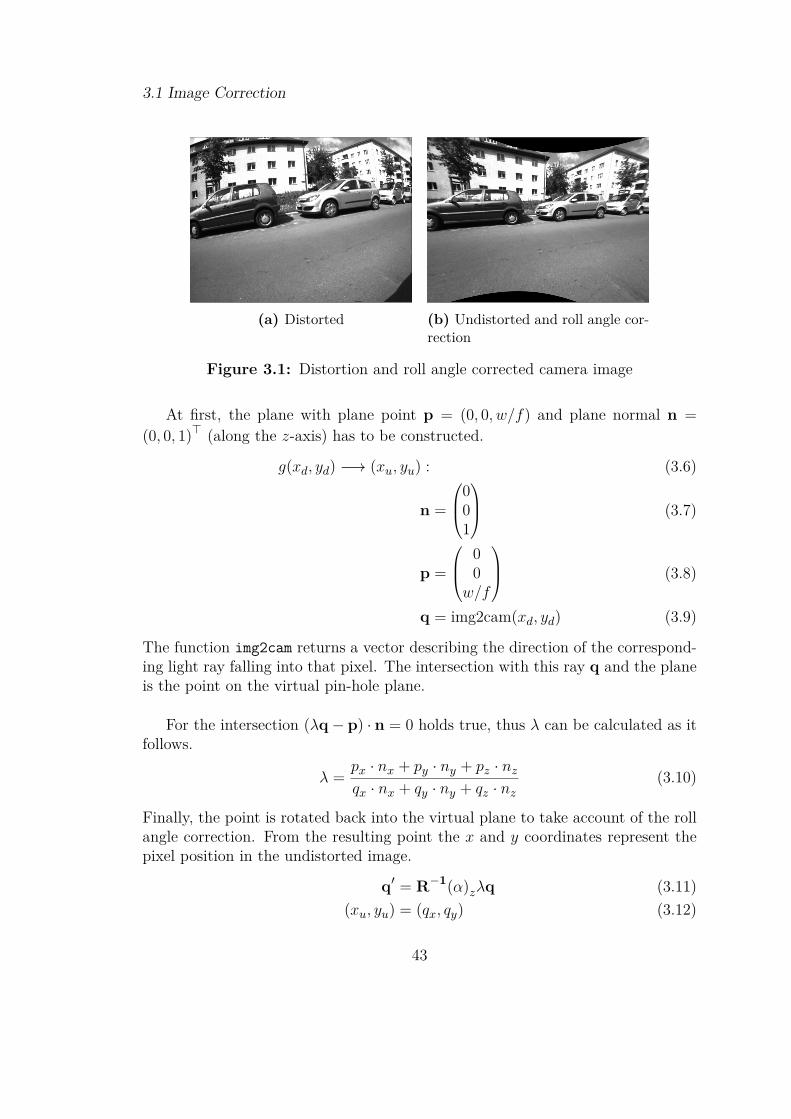
(a) Distorted (b) Undistorted and roll angle cor-rection
Figure 3.1: Distortion and roll angle corrected camera image
At first, the plane with plane point p = (0, 0, w/f) and plane normal n =(0, 0, 1)> (along the z-axis) has to be constructed.
g(xd, yd) −→ (xu, yu) : (3.6)
n =
001
(3.7)
p =
00
w/f
(3.8)
q = img2cam(xd, yd) (3.9)
The function img2cam returns a vector describing the direction of the correspond-ing light ray falling into that pixel. The intersection with this ray q and the planeis the point on the virtual pin-hole plane.
For the intersection (λq− p) · n = 0 holds true, thus λ can be calculated as itfollows.
λ =px · nx + py · ny + pz · nzqx · nx + qy · ny + qz · nz
(3.10)
Finally, the point is rotated back into the virtual plane to take account of the rollangle correction. From the resulting point the x and y coordinates represent thepixel position in the undistorted image.
q′ = R−1(α)zλq (3.11)(xu, yu) = (qx, qy) (3.12)
43
3.2 Extracting Regions of Interest
3.2 Extracting Regions of Interest
The RADAR tracker provides position information in coordinates (x, y, 0)> ∈R3 in the ego coordinate system. With extrinsic and intrinsic calibration, thesecoordinates can be transformed into image coordinates. The region in the imagethat is occupied by a vehicle largely depends on the distance to the camera. ROIsshould include the vehicle and avoid capturing too much unnecessary environment.The following heuristics rendered useful for achieving reasonable ROIs.
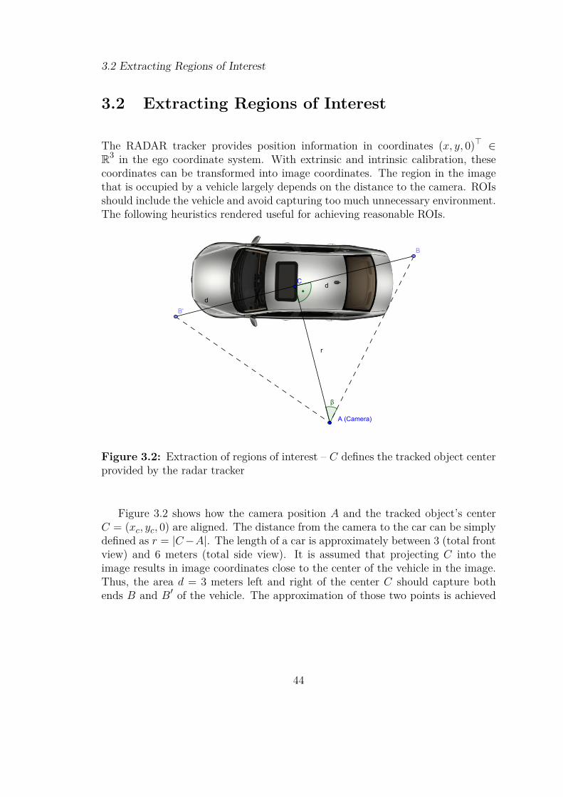
Figure 3.2: Extraction of regions of interest – C defines the tracked object centerprovided by the radar tracker
Figure 3.2 shows how the camera position A and the tracked object’s centerC = (xc, yc, 0) are aligned. The distance from the camera to the car can be simplydefined as r = |C−A|. The length of a car is approximately between 3 (total frontview) and 6 meters (total side view). It is assumed that projecting C into theimage results in image coordinates close to the center of the vehicle in the image.Thus, the area d = 3 meters left and right of the center C should capture bothends B and B′ of the vehicle. The approximation of those two points is achieved
44
3.3 Image Segmentation Based on Predicted Optical Flow
by a rotation around the z-axis in reference point A with the rotation angle β inego coordinates.
tan β = d
r(3.13)
B = Rz(β) · C (3.14)B′ = Rz(β) · C (3.15)
(3.16)
Finally we set the z-coordinate of B to −0.5 (half a meter below the ground plane)and z of B′ to 2.5 (2.5 meters above the ground plane).
Bz = −0.5 (3.17)B′z = 2.5 (3.18)
Projecting the points B and B′ back into the camera image results in the topleft corner and bottom right corner of a rectangle that includes the vehicle if thetracked object’s center was assumed correctly. Some extractions with differentdistances r can be seen in Figure 3.3. As the scaling of cars in the image is mainlydependent on the distance to the camera, the extracted ROIs are size invariantwhen scaled to the same image size.
The camera image still contains distortions and influence of the roll angle of thecamera. Extracting the ROIs from the undistorted image might give better resultsfor further processing. The function cam2img(x, y, z) 7→ (xd, yd) ∈ R2 defines thecamera coordinate to image pixel mapping of the used camera model. Instead ofdirectly extracting the rectangle defined by cam2img(B) and cam2img(B′), thetransformation g(xd, yd) −→ (xu, yu) presented in section 3.1 is applied to therectangles corner points. The new rectangle corner points C = g(cam2img(B))and C ′ = g(cam2img(B′)) describe a similar rectangle in the undistorted image.Figure 3.3 shows extracted rectangles from one of the recordings both from thedistorted original camera image and the undistorted image.
3.3 Image Segmentation Based on Predicted Op-tical Flow
Optical flow in general is defined as the offset of pixels through movement intwo consecutive images. A pixel at position ut = (ut, vt) in the image at time
45
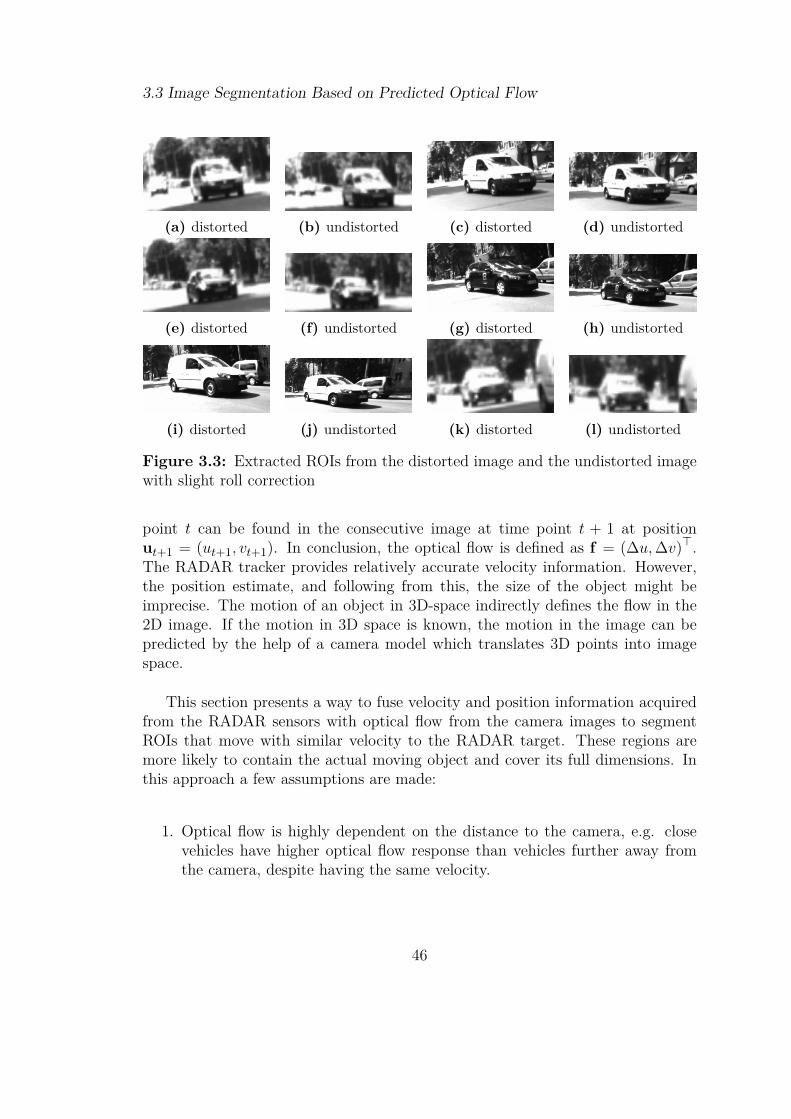
3.3 Image Segmentation Based on Predicted Optical Flow
(a) distorted (b) undistorted (c) distorted (d) undistorted
(e) distorted (f) undistorted (g) distorted (h) undistorted
(i) distorted (j) undistorted (k) distorted (l) undistorted
Figure 3.3: Extracted ROIs from the distorted image and the undistorted imagewith slight roll correction
point t can be found in the consecutive image at time point t + 1 at positionut+1 = (ut+1, vt+1). In conclusion, the optical flow is defined as f = (∆u,∆v)>.The RADAR tracker provides relatively accurate velocity information. However,the position estimate, and following from this, the size of the object might beimprecise. The motion of an object in 3D-space indirectly defines the flow in the2D image. If the motion in 3D space is known, the motion in the image can bepredicted by the help of a camera model which translates 3D points into imagespace.
This section presents a way to fuse velocity and position information acquiredfrom the RADAR sensors with optical flow from the camera images to segmentROIs that move with similar velocity to the RADAR target. These regions aremore likely to contain the actual moving object and cover its full dimensions. Inthis approach a few assumptions are made:
1. Optical flow is highly dependent on the distance to the camera, e.g. closevehicles have higher optical flow response than vehicles further away fromthe camera, despite having the same velocity.
46

3.3 Image Segmentation Based on Predicted Optical Flow
2. Knowing position xC = (x, y, z)> and velocity vC = (vx, vy, vz)> in cam-era coordinates, the optical flow of the corresponding image point can bepredicted for the next frame.
3. Moving vehicles have a good response to optical flow based on Kanade-Lucas-Tomasi Tracker (KLT Tracker) feature tracking method [TK91] because theycontain a high amount of structure compared to most environments.
3.3.1 Prediction of Optical Flow
The RADAR tracker returns a radar object state as a vector containing the position(xe, ye, 0) ∈ R3 and its velocity (ve,x, ve,y, 0) ∈ R3 in the ego vehicle coordinatesystem E. These are transformed into the camera reference frame C by the helpof the extrinsic calibration of the camera. The velocity vector vE is only rotatedand not translated. To skip the translation in homogeneous coordinates the lastentry of the vector is set to 0.
xC = TC←ExE = TC←E
xeye01
(3.19)
vC = RC←EvE = TC←E
ve,xve,y00
(3.20)
The prediction of the optical flow of a point xt = (xc,x, yc,y, zc,z)> in cam-era coordinates moving with vt = (vc,x, vc,y, vc,z)> can be achieved by linear for-ward motion with the estimated velocity for the time difference of two consecutiveframes. Both RADAR and camera generate data with a frequency f = 20Hzin the current setup. Therefore, the time difference of two consecutive frames is1f = 0.05s. Thus, the new position xt+1 of an object in the consecutive frame isestimated as it follows.
f = 20Hz (3.21)
xt+1 = xt + 1f
vt =
xt + 1
f vt,xyt + 1
f vt,yzt + 1
f vt,z
(3.22)
47

3.3 Image Segmentation Based on Predicted Optical Flow
Using the chosen camera model, both xt and xt+1 in camera coordinates aretransformed into image coordinates ut = (ut, vt) and ut+1 = (ut+1, vt+1). Thus,the predicted optical flow ft = (∆u,∆v)> is the difference of both image coordi-nates.
ut = cam2img(xt) (3.23)ut+1 = cam2img(xt+1) (3.24)
ft =(
∆u∆v
)= ut+1 − ut =
(ut+1 − utvt+1 − vt
)(3.25)
The prediction of optical flow for arbitrary points of the image based on a singleRADAR object is achieved by placing a 3-dimensional plane d parallel to theprojection plane of the camera in the camera reference frame. This plane is fixedin the RADAR object’s position x = (x, y, z)> with a plane normal n = (0, 0, 1)>.The whole plane is moved with velocity vC for one time cycle. For each imagepixel u = (u, v) in the image at time point t a ray originating in the camera’sviewpoint is pointed to the plane d and the intersection point ht is computed.This 3-dimensional intersection point ht is then forward predicted to time pointt+1 through a motion for one time step with velocity vC as described in eq. (3.22).Figure 3.4 visualizes this approach.
xc
yc
zc
Fc
x
y
v
d
x
Figure 3.4: Prediction of optical flow through a plane d originating in theRADAR object’s position x in camera coordinates and moving this plane withvelocity v for one time frame
To find the points on the virtual plane d for time frame t, the light rays ofthe camera model have to be intersected with the plane. The Scaramuzza camera
48

3.3 Image Segmentation Based on Predicted Optical Flow
model defines the direction of a light ray λq, λ ∈ R,q ∈ R3 falling into the camera’sviewpoint for each image coordinate u = (u, v) by the function img2cam(u, v)which maps the image coordinate to a 3-dimensional vector that represents thedirection of the light ray u = (u, v) ∈ R2 7→ q = (x, y, z) ∈ R3. The intersectionof this light ray λq with the virtual plane d is a potential object position for whichthe predicted flow is calculated. The following equations show the algorithm foran arbitrary image point u and RADAR object position x.
n =
001
(3.26)
x =
xyz
RADAR target in camera coordinates (3.27)
q = img2cam(u) light ray for pixel position u (3.28)
The intersection point can be calculated by solving the plane’s normal form (λq−x) · n = 0 for λ. Thus, the corresponding potential object point ht on the plane dis λq.
λ =xx · nx + xy · ny + xz · nzqx · nx + qy · ny + qz · nz
(3.29)
ht = λq (3.30)
The optical flow for the camera coordinate point ht can be predicted as describedin eq. (3.22). Figure 3.5 shows a dense field of the predicted optical flow for a given
(a) Camera image which contains amoving object tracked by RADAR
(b) Predicted optical flow field forthe whole image
Figure 3.5: Predicted flow based on RADAR tracked object
RADAR object. The following section shows how such a field can be exploited tonarrow a ROI of a moving object in the camera image.
49
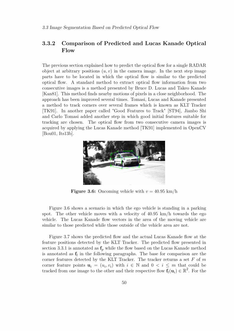
3.3 Image Segmentation Based on Predicted Optical Flow
3.3.2 Comparison of Predicted and Lucas Kanade OpticalFlow
The previous section explained how to predict the optical flow for a single RADARobject at arbitrary positions (u, v) in the camera image. In the next step imageparts have to be located in which the optical flow is similar to the predictedoptical flow. A standard method to extract optical flow information from twoconsecutive images is a method presented by Bruce D. Lucas and Takeo Kanade[Kan81]. This method finds nearby motions of pixels in a close neighborhood. Theapproach has been improved several times. Tomasi, Lucas and Kanade presenteda method to track corners over several frames which is known as KLT Tracker[TK91]. In another paper called "Good Features to Track" [ST94], Jianbo Shiand Carlo Tomasi added another step in which good initial features suitable fortracking are chosen. The optical flow from two consecutive camera images isacquired by applying the Lucas Kanade method [TK91] implemented in OpenCV[Bou01, Its13b].
Figure 3.6: Oncoming vehicle with v = 40.95 km/h
Figure 3.6 shows a scenario in which the ego vehicle is standing in a parkingspot. The other vehicle moves with a velocity of 40.95 km/h towards the egovehicle. The Lucas Kanade flow vectors in the area of the moving vehicle aresimilar to those predicted while those outside of the vehicle area are not.
Figure 3.7 shows the predicted flow and the actual Lucas Kanade flow at thefeature positions detected by the KLT Tracker. The predicted flow presented insection 3.3.1 is annotated as fp while the flow based on the Lucas Kanade methodis annotated as fl in the following paragraphs. The base for comparison are thecorner features detected by the KLT Tracker. The tracker returns a set F of mcorner feature points ui = (ui, vi) with i ∈ N and 0 < i ≤ m that could betracked from one image to the other and their respective flow fl(ui) ∈ R2. For the
50
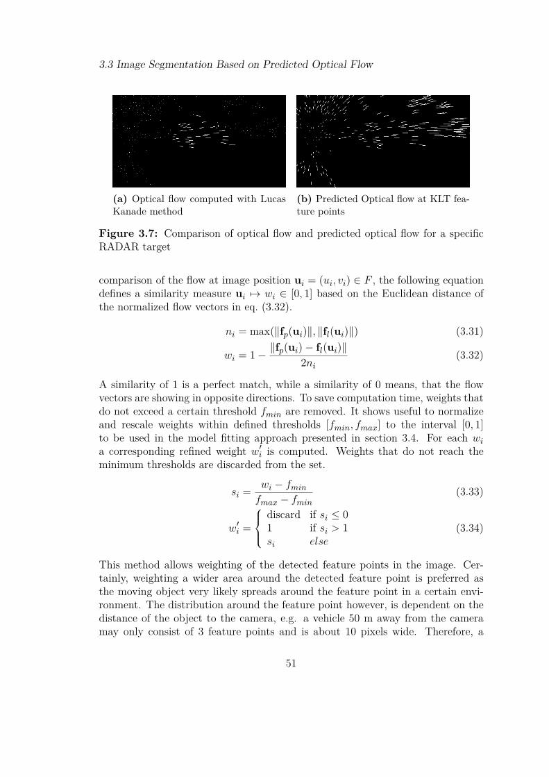
3.3 Image Segmentation Based on Predicted Optical Flow
(a) Optical flow computed with LucasKanade method
(b) Predicted Optical flow at KLT fea-ture points
Figure 3.7: Comparison of optical flow and predicted optical flow for a specificRADAR target
comparison of the flow at image position ui = (ui, vi) ∈ F , the following equationdefines a similarity measure ui 7→ wi ∈ [0, 1] based on the Euclidean distance ofthe normalized flow vectors in eq. (3.32).
ni = max(‖fp(ui)‖, ‖fl(ui)‖) (3.31)
wi = 1−‖fp(ui)− fl(ui)‖
2ni(3.32)
A similarity of 1 is a perfect match, while a similarity of 0 means, that the flowvectors are showing in opposite directions. To save computation time, weights thatdo not exceed a certain threshold fmin are removed. It shows useful to normalizeand rescale weights within defined thresholds [fmin, fmax] to the interval [0, 1]to be used in the model fitting approach presented in section 3.4. For each wia corresponding refined weight w′i is computed. Weights that do not reach theminimum thresholds are discarded from the set.
si = wi − fminfmax − fmin
(3.33)
w′i =
discard if si ≤ 01 if si > 1si else
(3.34)
This method allows weighting of the detected feature points in the image. Cer-tainly, weighting a wider area around the detected feature point is preferred asthe moving object very likely spreads around the feature point in a certain envi-ronment. The distribution around the feature point however, is dependent on thedistance of the object to the camera, e.g. a vehicle 50 m away from the cameramay only consist of 3 feature points and is about 10 pixels wide. Therefore, a
51

3.3 Image Segmentation Based on Predicted Optical Flow
Gaussian function with a standard deviation depending on the distance to thecamera is introduced.
fi(u, v) = w′i · e(ui−u)2+(vi−v)2
2σ2 (3.35)
The standard deviation estimation in eq. (3.38) has shown to return reasonableestimates supported by several experiments. The vector xe = (x, y, 0, 1)> definesthe object’s position in homogeneous ego coordinates taken from the RADARmeasurement. It is transformed into the camera coordinate system to calculate itsdistance d to the camera center.
xc = TC←Exe (3.36)d = ‖xc‖ (3.37)
σ = 15 · 11 + 0.1d (3.38)
To define weights for every pixel of the image. two weighting methods have beenexplored that showed reasonable results during experiments. The example imagesshow the weight maps for the scenario introduced previously (Figure 3.6). Theego vehicle stands still and another vehicle is coming from the left with a velocityof 40.95 km/h.
Weight Distribution Method 1:
(a) Weight distribution with annotatedROI of the detected vehicle
(b) Weight distribution multiplied withthe input image
Figure 3.8: Optical flow based weight method 1
As aforementioned, the distribution of w′i around the detected corner featurepoint (ui, vi) is approximated by a Gaussian-like function fi(u, v). At intersectionsof two or more distributions, the highest weight is chosen.
w(u, v) = maxi
(fi(u, v)) (3.39)
52
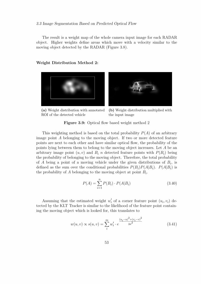
3.3 Image Segmentation Based on Predicted Optical Flow
The result is a weight map of the whole camera input image for each RADARobject. Higher weights define areas which move with a velocity similar to themoving object detected by the RADAR (Figure 3.8).
Weight Distribution Method 2:
(a) Weight distribution with annotatedROI of the detected vehicle
(b) Weight distribution multiplied withthe input image
Figure 3.9: Optical flow based weight method 2
This weighting method is based on the total probability P (A) of an arbitraryimage point A belonging to the moving object. If two or more detected featurepoints are next to each other and have similar optical flow, the probability of thepoints lying between them to belong to the moving object increases. Let A be anarbitrary image point (u, v) and Bi n detected feature points with P (Bi) beingthe probability of belonging to the moving object. Therefore, the total probabilityof A being a point of a moving vehicle under the given distributions of Bi, isdefined as the sum over the conditional probabilities P (Bi)P (A|Bi). P (A|Bi) isthe probability of A belonging to the moving object at point Bi.
P (A) =n∑i=1
P (Bi) · P (A|Bi) (3.40)
Assuming that the estimated weight w′i of a corner feature point (ui, vi) de-tected by the KLT Tracker is similar to the likelihood of the feature point contain-ing the moving object which is looked for, this translates to
w(u, v) ∝ s(u, v) =m∑i
w′i · e(ui−u)2+(vi−v)2
2σ2 (3.41)
53

3.4 3D Model Fitting
Certainly, this process is neither continuous nor normalized anymore. This couldbe normalized such that the integral over the entire image area equals one, thoughthis is of no use for the further processing. The weight map presents a goodheuristic for the likelihood if an area of the image belongs to the moving object.The summed up Gaussian values might exceed the desired weight interval [0, 1].Therefore a rescaling is needed. This can be achieved by a division by the finalmaximum value of the weight map. This scales the weight map w(u, v) to [0, 1] ineq. (3.42).
w(u, v) = s(u, v)max(s) (3.42)
An example map is presented in Figure 3.9. The weights are distributed smootherover the image compared to the first weighting method. The comparison of opticalflow and the derived weight maps allows to find regions in the image that movewith similar velocity as the vehicle tracked by the RADAR tracker.
3.4 3D Model Fitting
A relatively old approach for object detection and tracking is deformable modelfitting. First papers date back in the early 90’s [Low91], but the idea has beenrevived in several new papers as well, e.g. [LM09, LTH+05]. A model in thiscase is a three dimensional model of the object which is looked for. In generalthe approach tries to fit the projected edges of the model to edges found in thecamera image. In the first step, hypotheses are generated which estimate a ROIand initial parameter sets. In the second step an error measurement is evaluated,e.g. distance of reprojected points to edges in the image. This error is used foran optimization step that incrementally optimizes the parameters of the model tofit to the extracted edges in the image. Both papers assume a very simple cameramodel which does not model distortions. Furthermore, the camera is assumed to bestatic. In the following sections, the approach will be tested on strongly distortedimages utilizing the Scaramuzza camera model [SMS06a] on the test bed’s wideangle camera optics. Additionally, approaches to compensate for camera motionand inaccurate starting hypotheses based on RADAR are presented.
54
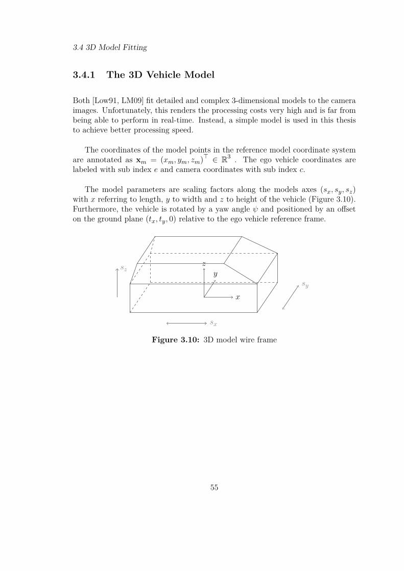
3.4 3D Model Fitting
3.4.1 The 3D Vehicle Model
Both [Low91, LM09] fit detailed and complex 3-dimensional models to the cameraimages. Unfortunately, this renders the processing costs very high and is far frombeing able to perform in real-time. Instead, a simple model is used in this thesisto achieve better processing speed.
The coordinates of the model points in the reference model coordinate systemare annotated as xm = (xm, ym, zm)> ∈ R3 . The ego vehicle coordinates arelabeled with sub index e and camera coordinates with sub index c.
The model parameters are scaling factors along the models axes (sx, sy, sz)with x referring to length, y to width and z to height of the vehicle (Figure 3.10).Furthermore, the vehicle is rotated by a yaw angle ψ and positioned by an offseton the ground plane (tx, ty, 0) relative to the ego vehicle reference frame.
x
y
sx
sy
szz
Figure 3.10: 3D model wire frame
55
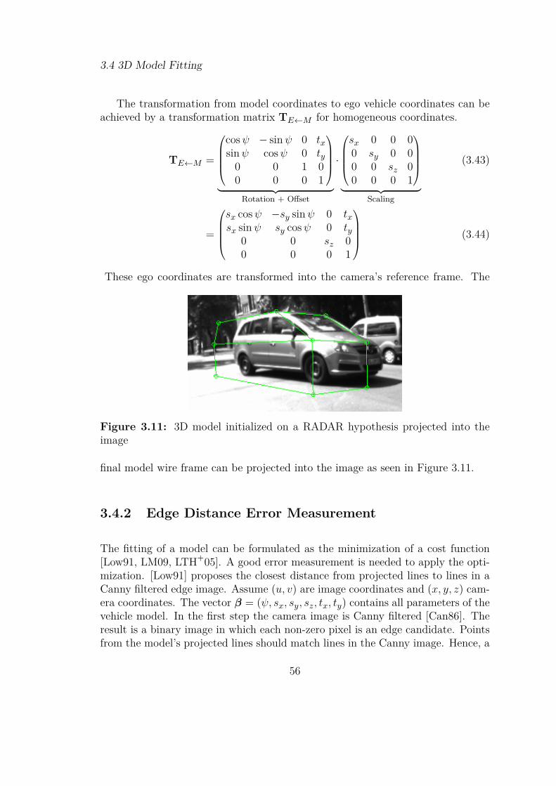
3.4 3D Model Fitting
The transformation from model coordinates to ego vehicle coordinates can beachieved by a transformation matrix TE←M for homogeneous coordinates.
TE←M =
cosψ − sinψ 0 txsinψ cosψ 0 ty
0 0 1 00 0 0 1
︸ ︷︷ ︸
Rotation + Offset
·
sx 0 0 00 sy 0 00 0 sz 00 0 0 1
︸ ︷︷ ︸
Scaling
(3.43)
=
sx cosψ −sy sinψ 0 txsx sinψ sy cosψ 0 ty
0 0 sz 00 0 0 1
(3.44)
These ego coordinates are transformed into the camera’s reference frame. The
Figure 3.11: 3D model initialized on a RADAR hypothesis projected into theimage
final model wire frame can be projected into the image as seen in Figure 3.11.
3.4.2 Edge Distance Error Measurement
The fitting of a model can be formulated as the minimization of a cost function[Low91, LM09, LTH+05]. A good error measurement is needed to apply the opti-mization. [Low91] proposes the closest distance from projected lines to lines in aCanny filtered edge image. Assume (u, v) are image coordinates and (x, y, z) cam-era coordinates. The vector β = (ψ, sx, sy, sz, tx, ty) contains all parameters of thevehicle model. In the first step the camera image is Canny filtered [Can86]. Theresult is a binary image in which each non-zero pixel is an edge candidate. Pointsfrom the model’s projected lines should match lines in the Canny image. Hence, a
56
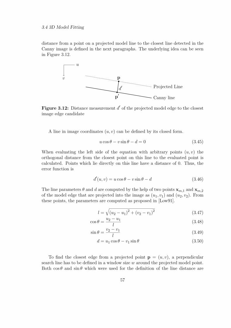
3.4 3D Model Fitting
distance from a point on a projected model line to the closest line detected in theCanny image is defined in the next paragraphs. The underlying idea can be seenin Figure 3.12.
u
v
Projected Line
p
d′
Canny linep′
Figure 3.12: Distance measurement d′ of the projected model edge to the closestimage edge candidate
A line in image coordinates (u, v) can be defined by its closed form.
u cos θ − v sin θ − d = 0 (3.45)
When evaluating the left side of the equation with arbitrary points (u, v) theorthogonal distance from the closest point on this line to the evaluated point iscalculated. Points which lie directly on this line have a distance of 0. Thus, theerror function is
d′(u, v) = u cos θ − v sin θ − d (3.46)
The line parameters θ and d are computed by the help of two points xm,1 and xm,2of the model edge that are projected into the image as (u1, v1) and (u2, v2). Fromthese points, the parameters are computed as proposed in [Low91].
l =√
(u2 − u1)2 + (v2 − v1)2 (3.47)
cos θ = u2 − u1l
(3.48)
sin θ = v2 − v1l
(3.49)
d = u1 cos θ − v1 sin θ (3.50)
To find the closest edge from a projected point p = (u, v), a perpendicularsearch line has to be defined in a window size w around the projected model point.Both cos θ and sin θ which were used for the definition of the line distance are
57

3.4 3D Model Fitting
also utilized to define a perpendicular line segment to the projected model lineintersecting at p.
p1 =(px − sin θ · wpy + cos θ · w
)p2 =
(px + sin θ · wpy − cos θ · w
)(3.51)
The image points p1 and p2 define a line segment through image points which areperpendicular to the projected model edge. The distance algorithm checks for theclosest non-zero point in the Canny filtered image and returns the distance to pas the error. A very accurate and fast way to sample pixels on the line segmentbetween p1 and p2 is the Bresenham algorithm [Bre65], which returns a set Bwith all pixels (u, v) on the search line. These pixels are checked for the closestpixel to p which contains an edge in the Canny filtered image. A simple pseudocode version of the algorithm is presented in algorithm 1. Points with errors equal
Algorithm 1 Finding the closest edge point to a projected model point1: Input: px, py2: Output: e
3: p1 =(px − sin θ · wpy + cos θ · w
)
4: p2 =(px + sin θ · wpy − cos θ · w
)5: e :=∞6: B ← bresenham(p1,p2)7: for all b = (u, v) ∈ B do8: edge← canny(u, v)9: if egde > 0 then10: Calculate distance to edge point:11: dist← u sin θ − v cos θ − db12: if ||dist|| < ||e|| then13: e← dist14: end if15: end if16: end for17: return e
to ∞ should be discarded and not taken into account for the final solution.
58
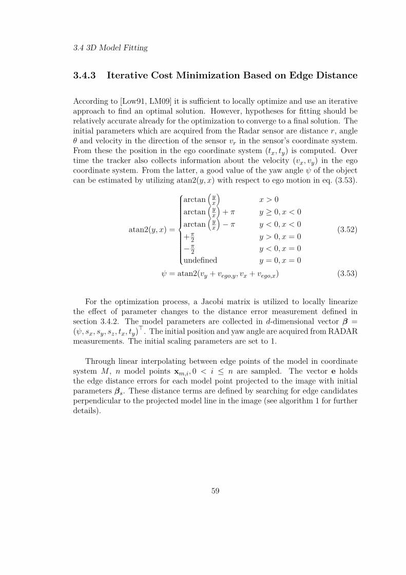
3.4 3D Model Fitting
3.4.3 Iterative Cost Minimization Based on Edge Distance
According to [Low91, LM09] it is sufficient to locally optimize and use an iterativeapproach to find an optimal solution. However, hypotheses for fitting should berelatively accurate already for the optimization to converge to a final solution. Theinitial parameters which are acquired from the Radar sensor are distance r, angleθ and velocity in the direction of the sensor vr in the sensor’s coordinate system.From these the position in the ego coordinate system (tx, ty) is computed. Overtime the tracker also collects information about the velocity (vx, vy) in the egocoordinate system. From the latter, a good value of the yaw angle ψ of the objectcan be estimated by utilizing atan2(y, x) with respect to ego motion in eq. (3.53).
atan2(y, x) =
arctan(yx
)x > 0
arctan(yx
)+ π y ≥ 0, x < 0
arctan(yx
)− π y < 0, x < 0
+π2 y > 0, x = 0−π2 y < 0, x = 0undefined y = 0, x = 0
(3.52)
ψ = atan2(vy + vego,y, vx + vego,x) (3.53)
For the optimization process, a Jacobi matrix is utilized to locally linearizethe effect of parameter changes to the distance error measurement defined insection 3.4.2. The model parameters are collected in d-dimensional vector β =(ψ, sx, sy, sz, tx, ty)>. The initial position and yaw angle are acquired from RADARmeasurements. The initial scaling parameters are set to 1.
Through linear interpolating between edge points of the model in coordinatesystem M , n model points xm,i, 0 < i ≤ n are sampled. The vector e holdsthe edge distance errors for each model point projected to the image with initialparameters βs. These distance terms are defined by searching for edge candidatesperpendicular to the projected model line in the image (see algorithm 1 for furtherdetails).
59
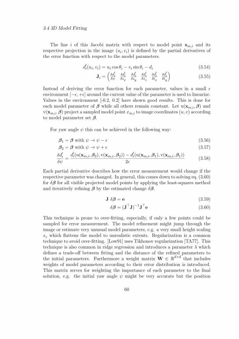
3.4 3D Model Fitting
The line i of this Jacobi matrix with respect to model point xm,i and itsrespective projection in the image (ui, vi) is defined by the partial derivatives ofthe error function with respect to the model parameters.
d′i(ui, vi) = ui cos θi − vi sin θi − di (3.54)
Ji =(δd′i
δψδd′i
δsx
δd′i
δsy
δd′i
δsz
δd′i
δtx
δd′i
δty
)(3.55)
Instead of deriving the error function for each parameter, values in a small εenvironment [−ε,+ε] around the current value of the parameter is used to linearize.Values in the environment [-0.2, 0.2] have shown good results. This is done foreach model parameter of β while all others remain constant. Let u(xm,i,β) andv(xm,i,β) project a sampled model point xm,i to image coordinates (u, v) accordingto model parameter set β.
For yaw angle ψ this can be achieved in the following way:
β1 = β with ψ → ψ − ε (3.56)β2 = β with ψ → ψ + ε (3.57)δd′iδψ
=d′i(u(xm,i,β2), v(xm,i,β2))− d′i(u(xm,i,β1), v(xm,i,β1))
2ε (3.58)
Each partial derivative describes how the error measurement would change if therespective parameter was changed. In general, this comes down to solving eq. (3.60)for δβ for all visible projected model points by applying the least-squares methodand iteratively refining β by the estimated change δβ.
J δβ = e (3.59)δβ = (J>J)−1J>e (3.60)
This technique is prone to over-fitting, especially, if only a few points could besampled for error measurement. The model refinement might jump through theimage or estimate very unusual model parameters, e.g. a very small height scalingsz which flattens the model to unrealistic extents. Regularization is a commontechnique to avoid over-fitting. [Low91] uses Tikhonov regularization [TA77]. Thistechnique is also common in ridge regression and introduces a parameter λ whichdefines a trade-off between fitting and the distance of the refined parameters tothe initial parameters. Furthermore a weight matrix W ∈ Rd×d that includesweights of model parameters according to their error distribution is introduced.This matrix serves for weighting the importance of each parameter to the finalsolution, e.g. the initial yaw angle ψ might be very accurate but the position
60
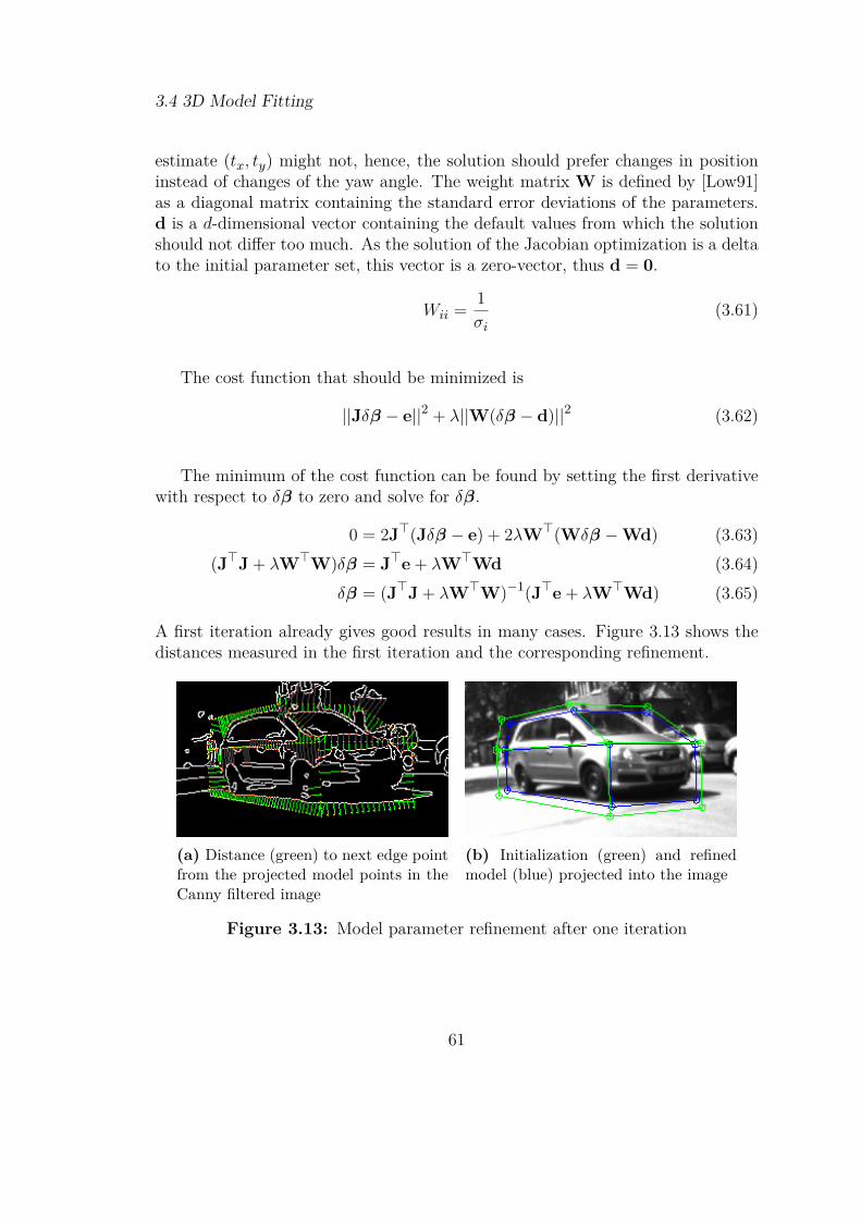
3.4 3D Model Fitting
estimate (tx, ty) might not, hence, the solution should prefer changes in positioninstead of changes of the yaw angle. The weight matrix W is defined by [Low91]as a diagonal matrix containing the standard error deviations of the parameters.d is a d-dimensional vector containing the default values from which the solutionshould not differ too much. As the solution of the Jacobian optimization is a deltato the initial parameter set, this vector is a zero-vector, thus d = 0.
Wii = 1σi
(3.61)
The cost function that should be minimized is
||Jδβ − e||2 + λ||W(δβ − d)||2 (3.62)
The minimum of the cost function can be found by setting the first derivativewith respect to δβ to zero and solve for δβ.
0 = 2J>(Jδβ − e) + 2λW>(Wδβ −Wd) (3.63)(J>J + λW>W)δβ = J>e + λW>Wd (3.64)
δβ = (J>J + λW>W)−1(J>e + λW>Wd) (3.65)
A first iteration already gives good results in many cases. Figure 3.13 shows thedistances measured in the first iteration and the corresponding refinement.
(a) Distance (green) to next edge pointfrom the projected model points in theCanny filtered image
(b) Initialization (green) and refinedmodel (blue) projected into the image
Figure 3.13: Model parameter refinement after one iteration
61

3.4 3D Model Fitting
3.4.4 Motion Similarity-based Edge Weighting
The presented approach already provides good results with good starting hypothe-ses. Unfortunately, the starting hypothesis acquired from the RADAR are not al-ways a good estimate and are too far away from the actual position in the image.This often results in model edges fitting to environment edges like parked cars onthe side of the road. Section 3.3 described how the prediction of optical flow in twoconsecutive camera images is compared to the actual optical flow to find regions inan image that move with a given velocity in a given distance to the camera. Thissection is about using the computed weight map to optimize the position estimateof a RADAR tracker object.
It is a reasonable assumption that areas in the camera image that move withthe same velocity as the RADAR tracker object contain edges that belong tosaid object. Therefore, fitting to these edges should return better results. Letgi = (gi, hi) ∈ R2 be the image coordinate of the edge point which was detectedwhen evaluating the distance measure function d’i(u, v) at image position (ui, vi)for the Jacobian row Ji. Furthermore let w(u, v) be the flow weight map presentedin section 3.3. Higher weights relate to a higher probability of the image pointbeing part of the moving object detected by RADAR.
The importance of this row to the final solution should factor in the weightof the edge point. The row of the Jacobian and the corresponding error shouldtherefore be changed to include the weight of the edge point in the following way.
w = 1 + w(gi, hi) (3.66)
J′i =(wδd′i
δψ wδd′i
δsxwδd′i
δsywδd′i
δszwδd′i
δtxwδd′i
δty
)(3.67)
e′i = w · ei (3.68)
This method reduces edge fitting to parked vehicles or shadows of trees.
3.4.5 Motion Similarity Centroid-based Position Correc-tion
The cameras are aligned perpendicular to the street. Distances of objects are nottrivial to measure with mono cameras. However, lateral measurements can bedone precisely. This section shows how the optical flow prediction and similarity
62

3.4 3D Model Fitting
measurement presented in Section 3.3 is exploited to refine the position of a vehicleinitialized from a RADAR track. Section 3.2 presented a method to extract regionsof interest from starting hypotheses. Furthermore section 3.4.4 showed how aweight map based on optical flow similarity between predicted flow and actualflow in the image can be created.
In this section a method is proposed that refines the position of the trackedvehicle (x, y, 0) in the ego vehicle coordinate system based on the centroid of thedetected optical flow motion. Within the defined ROI the centroid of the flow sim-ilarity distribution is estimated (see section 3.2 for the method of ROI estimation).The left upper point of the ROI is given as (ru, rv) in image coordinates as wellas the height rh and width rw. The centroid is estimated based on the weights inthe flow similarity image in the ROI.
n =ru+rw∑u=ru
rv+rh∑v=rv
w(u, v) (3.69)
cu = 1n
ru+rw∑u=ru
rv+rh∑v=rv
w(u, v) · u (3.70)
cv = 1n
ru+rw∑u=ru
rv+rh∑v=rv
w(u, v) · v (3.71)
cf =(cucv
)(3.72)
This centroid defines the centroid of the optical flow weights in the given ROI. Inconclusion, it defines the middle point of the moving object in image coordinates.In section 3.4.1 a 3D wire frame model is presented which is used for the optimiza-tion based on edge fitting. The centroid of this model in model coordinates M iscm = (0, 0, hm2 )> with hm being the height of the model. With the transformationsdescribed in section 3.4.1, this model centroid is transformed into image coordi-nates ch = (ch,u, ch,v)> based on an initial parameter set β = (ψ, sx, sy, sz, tx, ty)>.
ch = cam2img(TC←Mcm) (3.73)
Based on the assumption that the optical flow centroid cf defines the centroid ofthe moving vehicle in the image, a new error term is introduced to the Jacobian.The error term defines the distance from the hypothesis centroid ch to the flowcentroid cf . The distance in the v (height) axis of the image is neglected as itvaries strongly based on the height of the vehicle. Thus, the error measurementbecomes d(cf , ch).
d(cf , ch) = cf,u − ch,u (3.74)
63

3.4 3D Model Fitting
The scaling parameters sx, sy, sz and yaw angle ψ are not suitable for optimizationusing this error measurement as these are independent from the position of thecentroid. The centroid is mainly dependent on the two parameters tx and ty. Anew row is added to the Jacobian matrix to include the optimization based on thecentroid distance. This row only contains two entries for tx and ty and the othersare set to zero.
Ji =(0 0 0 0 δd
δtx
δdδty
)(3.75)
The partial derivatives are calculated similarly to the partial derivatives foredge distances. β = (ψ, sx, sy, sz, tx, ty)> contains the initial hypothesis parame-ters. An ε environment of [-0.2, 0.2] showed reasonable results.
Partial derivative for parameter tx:
β1 = β with tx → tx − ε (3.76)β2 = β with tx → tx + ε (3.77)δd
δtx=d(cf , ch(β1))− d(cf , ch(β2))
2ε (3.78)
Partial derivative for parameter ty:
β1 = β with ty → ty − ε (3.79)β2 = β with ty → ty + ε (3.80)δd
δty=d(cf , ch(β1))− d(cf , ch(β2))
2ε (3.81)
The scenario in Figure 3.14 shows a driveway onto a bigger street. The Mer-cedes on the left is turning into the street. The ego vehicle is moving with relativelylow velocity into the driveway. The optical flow centroid of the Mercedes is markedwith a big X. The green RADAR hypothesis is relatively far off the actual vehicle.Fitting solely based on edge distance fits the front but fails in the back of the vanas there is no structure near the model edges. The blue model uses both weightingof edges based on flow as well as flow centroid fitting. The flow centroid is veryfar from the RADAR hypothesis (green cross). Accordingly, the model is movedin the direction of the flow centroid and fits to the edges of the vehicle nearlyperfect.
64

3.4 3D Model Fitting
(a) Green: initial hypothesis, red: Model fitting without flow information, blue: Modelfitting with flow centroid and flow weights, yellow: estimated flow centroid
(b) Canny edge image with annotated fitting distances of the red model
(c) Flow weight image (d) Input image multiplied with flowweights
Figure 3.14: Model refinement using optical flow information
65
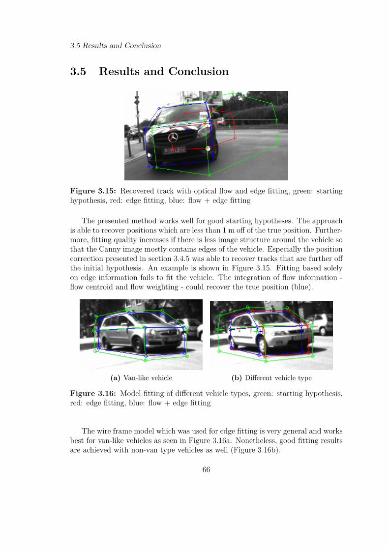
3.5 Results and Conclusion
3.5 Results and Conclusion
Figure 3.15: Recovered track with optical flow and edge fitting, green: startinghypothesis, red: edge fitting, blue: flow + edge fitting
The presented method works well for good starting hypotheses. The approachis able to recover positions which are less than 1 m off of the true position. Further-more, fitting quality increases if there is less image structure around the vehicle sothat the Canny image mostly contains edges of the vehicle. Especially the positioncorrection presented in section 3.4.5 was able to recover tracks that are further offthe initial hypothesis. An example is shown in Figure 3.15. Fitting based solelyon edge information fails to fit the vehicle. The integration of flow information -flow centroid and flow weighting - could recover the true position (blue).
(a) Van-like vehicle (b) Different vehicle type
Figure 3.16: Model fitting of different vehicle types, green: starting hypothesis,red: edge fitting, blue: flow + edge fitting
The wire frame model which was used for edge fitting is very general and worksbest for van-like vehicles as seen in Figure 3.16a. Nonetheless, good fitting resultsare achieved with non-van type vehicles as well (Figure 3.16b).
66
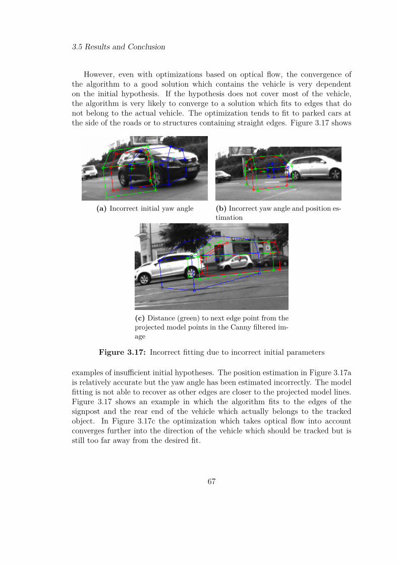
3.5 Results and Conclusion
However, even with optimizations based on optical flow, the convergence ofthe algorithm to a good solution which contains the vehicle is very dependenton the initial hypothesis. If the hypothesis does not cover most of the vehicle,the algorithm is very likely to converge to a solution which fits to edges that donot belong to the actual vehicle. The optimization tends to fit to parked cars atthe side of the roads or to structures containing straight edges. Figure 3.17 shows
(a) Incorrect initial yaw angle (b) Incorrect yaw angle and position es-timation
(c) Distance (green) to next edge point from theprojected model points in the Canny filtered im-age
Figure 3.17: Incorrect fitting due to incorrect initial parameters
examples of insufficient initial hypotheses. The position estimation in Figure 3.17ais relatively accurate but the yaw angle has been estimated incorrectly. The modelfitting is not able to recover as other edges are closer to the projected model lines.Figure 3.17 shows an example in which the algorithm fits to the edges of thesignpost and the rear end of the vehicle which actually belongs to the trackedobject. In Figure 3.17c the optimization which takes optical flow into accountconverges further into the direction of the vehicle which should be tracked but isstill too far away from the desired fit.
67

3.6 Future Work
Another reason for inaccurate fitting is the generality of the chosen vehiclemodel. Even though the actual fit covers the vehicle, it does not correctly fit toit as seen in Figure 3.18. The truck does not fit to the model, and the varianceallowed in height and length for the scaling factors is not large enough. However,the flow weighting allows the algorithm to fit to edges which are outside of theinitial parameter set, so that the length scaling factor is increased. The modelfitted to the vehicle in Figure 3.18b does not cover the hood part. Thus, it fitspartly to the hood and partly to the A-pillar.
(a) Vehicle type does not match the ab-stract vehicle model
(b) The abstract vehicle model does notcover the hood of the vehicle
Figure 3.18: Incorrect fitting due to abstraction in the chosen vehicle model
In conclusion, advantages of the approach are the computing performance com-pared to pattern based approaches and the lack of a training phase. With accuratestarting hypotheses, the algorithm is able to converge to an accurate refinementof the initial parameters. The optical flow based weighting has shown to improvethe fitting process and the flow centroid estimation increases the probability tofit to the actual vehicles if starting hypotheses are further away from the optimalsolution. Even though the technique showed good results in many cases, it requiresgood edge extractions and accurate initial hypotheses.
3.6 Future Work
Vehicle detection and tracking in side cameras is an area less explored than thedetection in front and rear cameras. Therefore there are a lot of opportunities andresearch questions.
68

3.6 Future Work
The presented approach relies on an accurate extrinsic camera calibration.The current calibration stand at Hella Aglaia however, focuses on front and rearcamera calibration. A thought experiment for a simple and inexpensive solutionto extend the calibration stand with a side camera calibration has been presentedin the appendix on page 108. Additionally, approaches to dynamically adapt theextrinsic calibration while driving may be another area of research.
Certainly, a goal is to include the refined positions of the camera in the RADARtracker. This should lead to better initial hypotheses as the camera information isfused back into the tracker. The fitting approach converges to inaccurate solutionssometimes, therefore a reasonable outlier detection has to be implemented.
Another area of research which might increase the accuracy of fitting is thechoice of features, e.g. a separate wheel detection might return a set of potentialwheel positions to fit the model to. Furthermore [LM09] uses complexer 3D-modelswhich generalize better to different vehicle types. As more computing power willbe available in up-coming production vehicles, this approach should be taken intoconsideration as well.
69
Chapter 4
Synthetic Ground Truth DataGeneration for Radar ObjectTracking
This chapter describes an intuitive method to generate artificial test data forRADAR-based crash warning algorithms developed at Hella Aglaia. At the mo-ment, two warning algorithms are in development – FSR and PCR. Each of thesesystems has special requirements that have to be fulfilled. Driving scenarios withdefined behavior of the warning algorithms are compiled into a test catalog (ex-ample: Figure 4.1). Some of the described maneuvers require advanced drivingskills and consume a lot of time to record properly. Instead, a simpler methodto generate the data which would be acquired from test drives is preferable fordevelopment. However, the data has to be physically reasonable and consistentwith the test catalog.
The data flow of the warning systems consists of three main processing steps.At first raw targets from the RADAR sensors are collected and classified. Inthe second step these RADAR targets are grouped together, filtered and trackedas moving objects. The moving objects from the tracker are used to estimatecrash probabilities in the warning algorithm by forward prediction of movements(Figure 4.2).
There are several possibilities for the generation of test data in the whole pro-cess. One could either generate raw targets for the tracking algorithm or generate
70
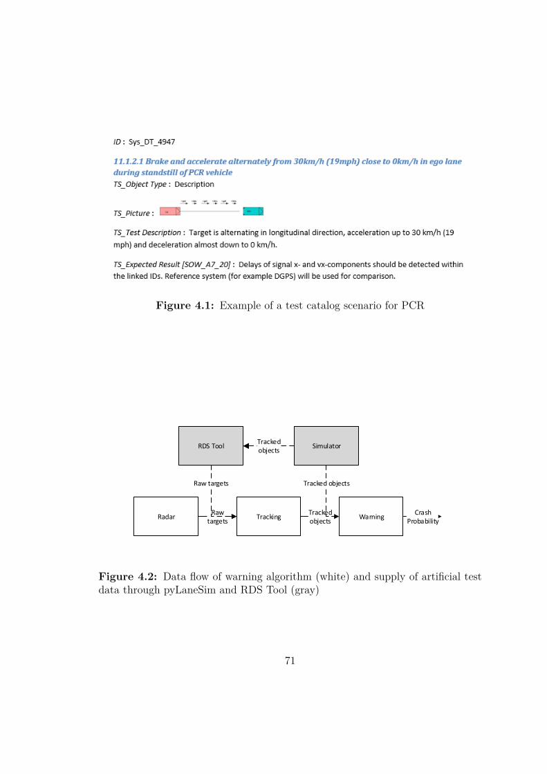
Figure 4.1: Example of a test catalog scenario for PCR
RadarRaw
targetsTracking
Trackedobjects
WarningCrash
Probability
Simulator
Raw targets
Tracked objects
RDS Tool
Tracked objects
Figure 4.2: Data flow of warning algorithm (white) and supply of artificial testdata through pyLaneSim and RDS Tool (gray)
71

4.1 User Interface
tracking objects for the actual warning algorithm. Having test data at eitherstep, it is possible to create independent module tests. This chapter will focuson generating ground truth data for the tracker, i.e. positions and velocities ofmoving vehicles in the environment as well as other physical properties which areusually generated by the RADAR tracker. Additionally, Hella also develops theRawDataSynthesis (RDS) Tool which is able to simulate radar sensor data giveninformation about objects in the environment. It models the physical process ofelectromagnetic waves traveling and reflecting in the environment to generate rawdata for the sensor itself. In the last section an interface between the simulator andthe RDS Tool is presented. Thus, it is possible to create test data for the trackermodule based on the scenarios designed in the simulator (Figure 4.2). This ren-ders a form of development possible in which development of one module, e.g. thewarning algorithm is not dependent on the availability of the preceding modules.Thus, tracker and warning algorithm development could be started at the sametime without necessity of the output of the tracking algorithm as artificial testdata could be supplied through the simulator.
4.1 User Interface
(a) Old interface of the simulator (b) Current interface
Figure 4.3: Interface development of the simulator
A first prototype features a 2–dimensional top view interface with mouse sup-port in which the trajectories of cars can be created by simple clicks on theground plane. Additionally these paths can be annotated with acceleration in-formation (Figure 4.3a). The resulting trajectories might be physically unreason-able, e.g. a hairpin turn with 40 km/h. Such being the case, a car dynamics
72

4.1 User Interface
Figure 4.4: Set up of the driving simulator
model (see section 4.3) is introduced and a Proportional-Integral-Derivative con-troller (PID-controller) connected to the steering angle which keeps the vehicle onthe trajectory. The PID-controller returned a steering angle based on the normaldistance of the car to the trajectory. The parameters for the controller were chosenby intelligently searching the parameter space using the Twiddle algorithm pre-sented in Sebastian Thrun’s Stanford online lecture "How To Build A Robotic car"[Thr13]. The annotated acceleration information at the trajectory points are fedinto said model which tries to follow the predefined trajectory. Unfortunately, thisapproach renders inconvenient for more complex scenarios that involve multiplecars. Many repetitions and refinements are needed to achieve precise timing.
The second prototype features a 3-dimensional interface and lets the user con-trol cars from a cockpit or world view (Figure 4.3b). The most intuitive way toacquire data from driving scenarios is to actually drive. Thus, the new interfacefeatures steering wheel and pedal or keyboard input if no driving wheel is present(Figure 4.4). Cars and street parts can be freely positioned in the environment onthe ground plane. Cars and their properties can be defined freely and controlledone after another by rerunning the simulation for each car.
The test cases usually define the environment as well, e.g. a crossroad or a fourlane high way. The information about the environment does not influence the testdata itself but is used for visualization. Therefore the simulator supports basicenvironment mapping with predefined map tiles aligned on a virtual grid. Thesemap tiles can be positioned on the ground plane by mouse and connected to each
73
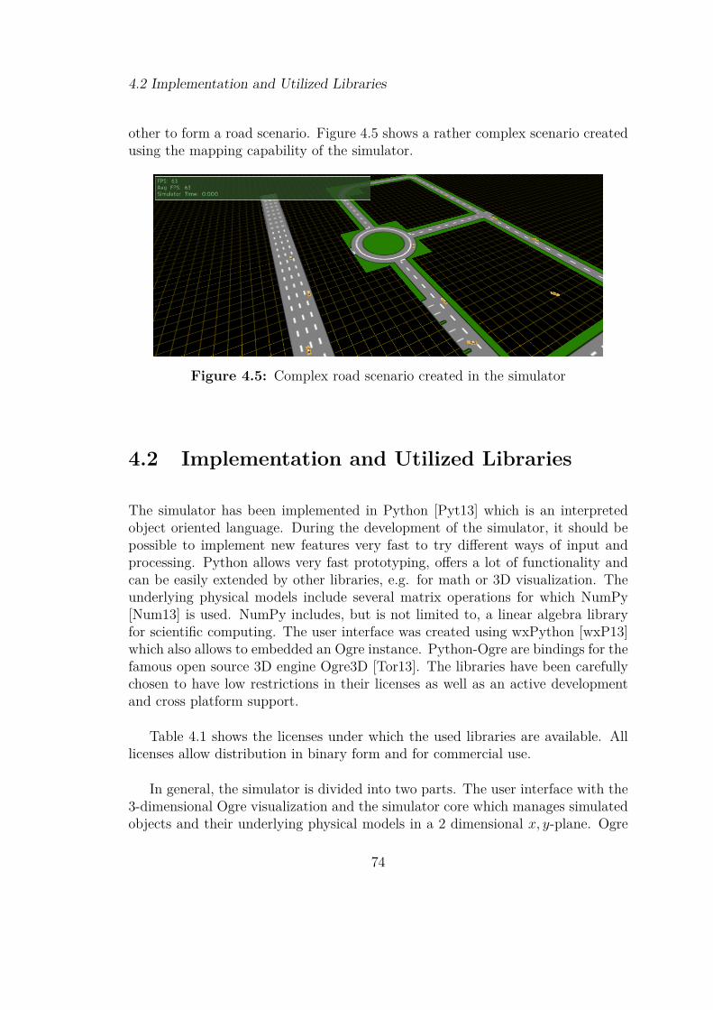
4.2 Implementation and Utilized Libraries
other to form a road scenario. Figure 4.5 shows a rather complex scenario createdusing the mapping capability of the simulator.
Figure 4.5: Complex road scenario created in the simulator
4.2 Implementation and Utilized Libraries
The simulator has been implemented in Python [Pyt13] which is an interpretedobject oriented language. During the development of the simulator, it should bepossible to implement new features very fast to try different ways of input andprocessing. Python allows very fast prototyping, offers a lot of functionality andcan be easily extended by other libraries, e.g. for math or 3D visualization. Theunderlying physical models include several matrix operations for which NumPy[Num13] is used. NumPy includes, but is not limited to, a linear algebra libraryfor scientific computing. The user interface was created using wxPython [wxP13]which also allows to embedded an Ogre instance. Python-Ogre are bindings for thefamous open source 3D engine Ogre3D [Tor13]. The libraries have been carefullychosen to have low restrictions in their licenses as well as an active developmentand cross platform support.
Table 4.1 shows the licenses under which the used libraries are available. Alllicenses allow distribution in binary form and for commercial use.
In general, the simulator is divided into two parts. The user interface with the3-dimensional Ogre visualization and the simulator core which manages simulatedobjects and their underlying physical models in a 2 dimensional x, y-plane. Ogre
74
4.3 Car Dynamics Models
Software LicensePython PSF LicenseNumPy BSD LicensewxPython wxWindows License (similar to LGPL)Python-Ogre LGPL
Table 4.1: Licenses of used libraries in the simulator
itself manages its 3-dimensional objects in a tree structure. The root node is theworld reference frame. Each sub node is positioned in the parent’s reference frameand has its own reference frame which can be rotated, scaled or moved. An easyexample is the implementation of a cockpit view for one of the simulated cars. Atfirst a CarNode is created for the car which contains the 3-dimensional model inan Ogre compatible format. The node is freely positioned as a sub node of theworld node (root node) in the x, y-plane and updates itself in each render cycle byfetching the (x, y) position and yaw angle ψ from the respective simulator object.Instead of recalculating the cockpit camera position each time, a CameraNode isadded as a sub node of the CarNode and positioned in its reference frame. TheOgre tree automatically updates the positions of the sub nodes if the higher nodesare changed.
Each CarNode holds a reference to a SimulatorObject which represents theunderlying physical model. A Simulator instance holds references to all availableSimulatorObjects and manages them with respect to the current simulation time.Each SimulatorObject has to implement a few general methods to be manageableby the Simulator. These methods return information about current position andorientation as well as speed. Currently, there is one concrete implementation – theDriveCar – which represents the dynamics of the underlying vehicle model.
This design is visualized as an UML class diagram in Figure 4.6. The diagramis simplified to the most important methods and classes for the sake of clarity.
4.3 Car Dynamics Models
To achieve physically-reasonable results for the dynamics of vehicles in the sim-ulator, a dynamics model is introduced which models the behavior of cars basedon steering information from the steering wheel or keyboard input. The simulator
75

4.3 Car Dynamics Models
SimulatorObject
name
+getName()+getSpeed()+getOrientation()+getX()+getY()+simulate(dt)+reset()
Simulator
+simulate(dt)-memberName
11
*0
DriveCar
-x-steeringInfo
-_bycicle(self, x, u, dt)-_singletracksideslip(self, x, u)-_singletrack(self, x, u)+static fromXMLNode(carnode)+toXMLNode()
CarNode
-car
+update()
1
11
1
OgreRootNode
-children
...
11
*0
CameraNode
...
...
11
11
Figure 4.6: Simplified UML representation of the simulator structure
runs in a loop calculating the state x of each dynamic object every 25ms takingthe current state and new steering information into account.
In the following, the dynamics models implemented in the simulator are ex-plained. A single track model which models tire slip, as well as over- and understeercan be seen in Figure 4.7. Each of these models assumes the world to be flat, thus,the position of a car is limited to a position within the x − y-plane and its yawangle. Roll and pitch information are discarded. The coordinate systems usedare explained in section 1.3 Preliminaries. The world coordinate system is a righthanded reference system in which the ground plane is represented by the x − y-plane and the z-axis points upwards. The dynamics models define their own righthanded ego reference frame with the x-axis aligned with the vehicle’s length axispointing into the driving direction and the y-axis positioned on the front axle. Thez-axis points upwards.
The model contains several parameters and physical properties. These containthe current position (xw, yw) of the object in world coordinates. ψ defines the yawangle (orientation) while ψ defines the respective change rate. ψ + β is the anglein which the actual motion is directed to. This angle differs to the yaw angle ψif under- or oversteer are present which is represented by the slip angle β. Thevehicle’s mass is annotated as m.
76
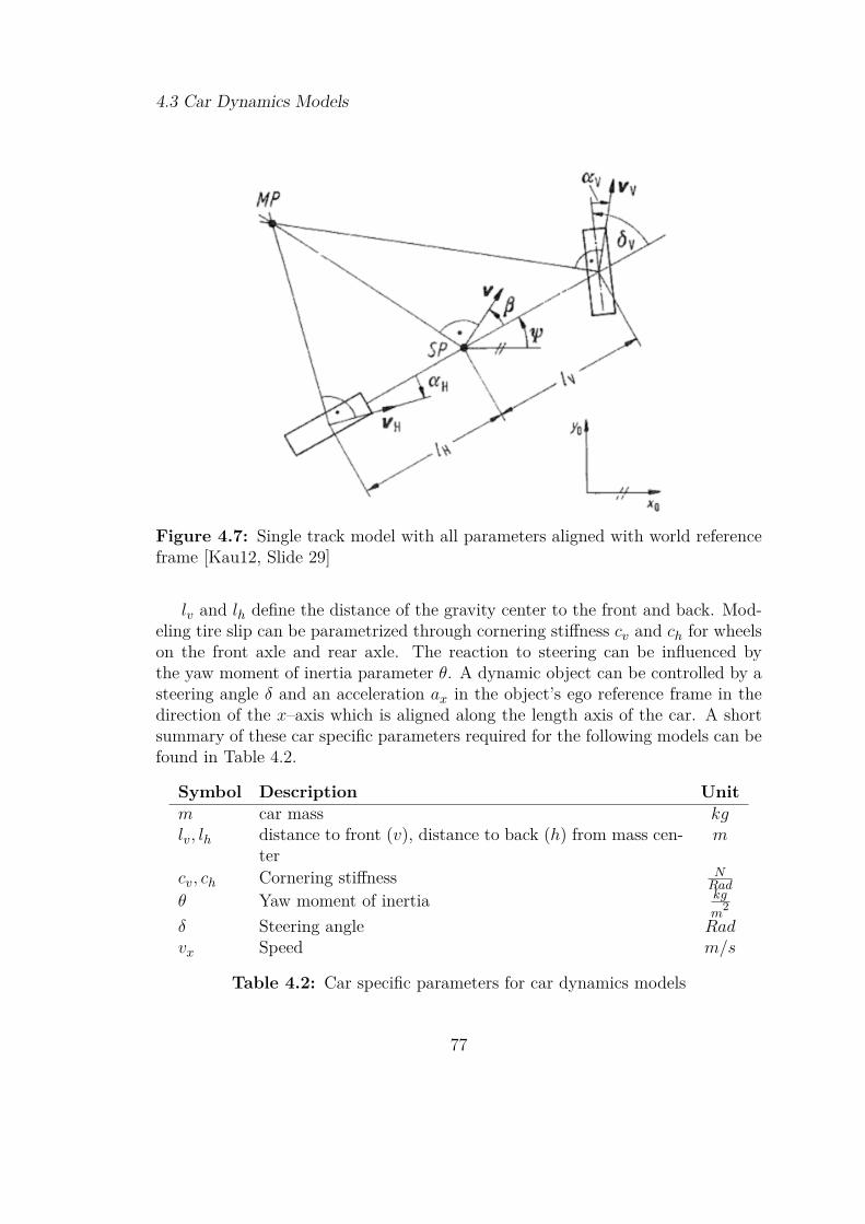
4.3 Car Dynamics Models
Figure 4.7: Single track model with all parameters aligned with world referenceframe [Kau12, Slide 29]
lv and lh define the distance of the gravity center to the front and back. Mod-eling tire slip can be parametrized through cornering stiffness cv and ch for wheelson the front axle and rear axle. The reaction to steering can be influenced bythe yaw moment of inertia parameter θ. A dynamic object can be controlled by asteering angle δ and an acceleration ax in the object’s ego reference frame in thedirection of the x–axis which is aligned along the length axis of the car. A shortsummary of these car specific parameters required for the following models can befound in Table 4.2.
Symbol Description Unitm car mass kglv, lh distance to front (v), distance to back (h) from mass cen-
term
cv, ch Cornering stiffness NRad
θ Yaw moment of inertia kg
m2
δ Steering angle Radvx Speed m/s
Table 4.2: Car specific parameters for car dynamics models
77
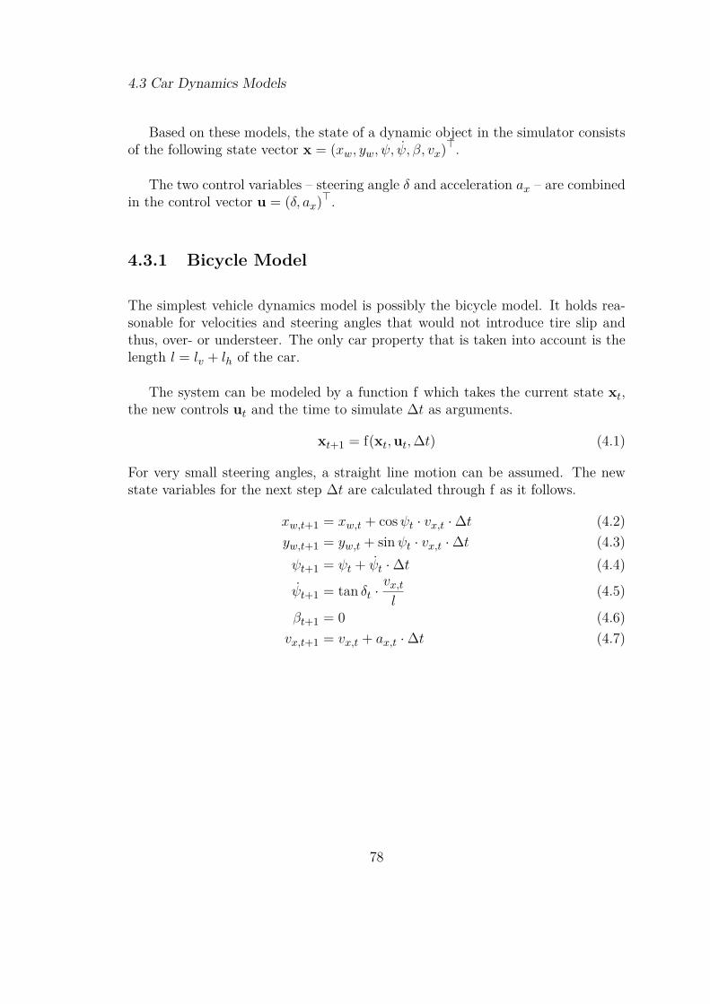
4.3 Car Dynamics Models
Based on these models, the state of a dynamic object in the simulator consistsof the following state vector x = (xw, yw, ψ, ψ, β, vx)>.
The two control variables – steering angle δ and acceleration ax – are combinedin the control vector u = (δ, ax)>.
4.3.1 Bicycle Model
The simplest vehicle dynamics model is possibly the bicycle model. It holds rea-sonable for velocities and steering angles that would not introduce tire slip andthus, over- or understeer. The only car property that is taken into account is thelength l = lv + lh of the car.
The system can be modeled by a function f which takes the current state xt,the new controls ut and the time to simulate ∆t as arguments.
xt+1 = f(xt,ut,∆t) (4.1)
For very small steering angles, a straight line motion can be assumed. The newstate variables for the next step ∆t are calculated through f as it follows.
xw,t+1 = xw,t + cosψt · vx,t ·∆t (4.2)yw,t+1 = yw,t + sinψt · vx,t ·∆t (4.3)ψt+1 = ψt + ψt ·∆t (4.4)
ψt+1 = tan δt ·vx,tl
(4.5)
βt+1 = 0 (4.6)vx,t+1 = vx,t + ax,t ·∆t (4.7)
78

4.3 Car Dynamics Models
For larger steering angles, the motion is estimated by the actual bicycle model.In the first step, the radius of the curve which would be driven with the givensteering angle δ is computed. From this, the new position can be calculated.
r = l
tan δt(4.8)
xw,t+1 = xw,t + r(− sinψt + sin(ψt + ψt ·∆t)) (4.9)yw,t+1 = yw,t + r(cos(psit − cos(ψt + ψt ·∆t)) (4.10)ψt+1 = ψt + ψt ·∆t (4.11)
ψt+1 = tan δt ·vx,tl
(4.12)
βt+1 = 0 (4.13)vx,t+1 = vx,t + ax,t ·∆t (4.14)
4.3.2 Single Track Model with Tire Slip
The bicycle model does not contain more properties of the vehicle’s physics thanthe length. However, the behavior of the car dynamics, especially in situationswith higher velocities and strong cornering, depends on the distribution of mass.Thus, two new parameters lv which is the distance of the center of gravity to thefront of the car and lh which is the distance to the back of the car are introduced.The model assumes the car to be a rigid body and shifts the center of gravity toan arbitrary position along the length axis of the car.
Instead of analytically solving the state from one time point to the next, alinearized model for a given time point t is utilized assuming that the state changex can be approximated linearly for a small time frame ∆t. Hence, the derivativex of the state is linearized as it follows.
xt+1 = xt + xt ·∆t (4.15)
79

4.3 Car Dynamics Models
A simple linearized form of the Single track model was taken from the Daimler Au-tonomous Systems lecture [Bre12, Slide 43]. ELG is defined as the steer gradientand depends on the geometry of the car.
ELG = m · ch · lh − cv · lvcv · ch · l
(4.16)
x =
xwywψ
ψ
βax
=
vx · cosψvx · sinψ
δ·vl+ELG·v2
x
00ax
(4.17)
4.3.3 Single Track Model with Over and Understeer
The previous model already gave a good idea of the behavior of a car depending onits physical properties. A more refined model which includes under- or oversteercan be found in [SHB10]. Even though the system models the behavior of a car inmore detail than the other models, it also comes with more restrictions. In generalthe model is valid for constant velocities and small steering angle changes. Thesystem is modeled through a linearized system matrix A ∈ R6×6, which defines thesystem itself, and a control matrix B ∈ R6×2 which takes the influence of steeringinformation into account. The state change can be expressed in the following way.
xt = Axt + But (4.18)xt+1 = xt + xt ·∆t (4.19)
[SHB10] describes the state only as (β, ψ), thus the matrices A and B have to beextended for the other state variables which can be expressed as it follows.
A =
0 0 0 0 0 cos(ψ + β)0 0 0 0 0 sin(ψ + β)0 0 0 1 0 00 0 0 −1
v ·cv ·l
2v+ch·l
2h
θ −cv ·lv−ch·lhθ 00 0 0 −1− 1
v2 ·
cv ·lv−ch·lhm −1
v ·cv+chm 0
0 0 0 0 0 0
(4.20)
80
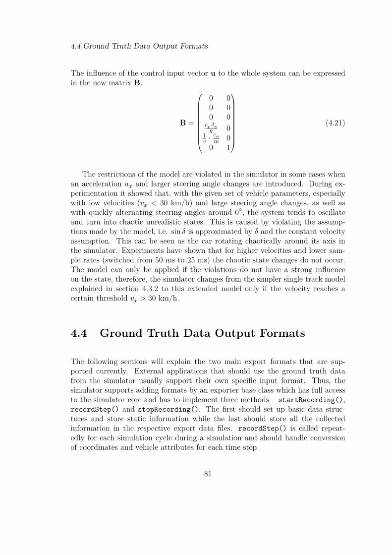
4.4 Ground Truth Data Output Formats
The influence of the control input vector u to the whole system can be expressedin the new matrix B.
B =
0 00 00 0
cv ·lvθ 0
1v ·
cvm 0
0 1
(4.21)
The restrictions of the model are violated in the simulator in some cases whenan acceleration ax and larger steering angle changes are introduced. During ex-perimentation it showed that, with the given set of vehicle parameters, especiallywith low velocities (vx < 30 km/h) and large steering angle changes, as well aswith quickly alternating steering angles around 0◦, the system tends to oscillateand turn into chaotic unrealistic states. This is caused by violating the assump-tions made by the model, i.e. sin δ is approximated by δ and the constant velocityassumption. This can be seen as the car rotating chaotically around its axis inthe simulator. Experiments have shown that for higher velocities and lower sam-ple rates (switched from 50 ms to 25 ms) the chaotic state changes do not occur.The model can only be applied if the violations do not have a strong influenceon the state, therefore, the simulator changes from the simpler single track modelexplained in section 4.3.2 to this extended model only if the velocity reaches acertain threshold vx > 30 km/h.
4.4 Ground Truth Data Output Formats
The following sections will explain the two main export formats that are sup-ported currently. External applications that should use the ground truth datafrom the simulator usually support their own specific input format. Thus, thesimulator supports adding formats by an exporter base class which has full accessto the simulator core and has to implement three methods – startRecording(),recordStep() and stopRecording(). The first should set up basic data struc-tures and store static information while the last should store all the collectedinformation in the respective export data files. recordStep() is called repeat-edly for each simulation cycle during a simulation and should handle conversionof coordinates and vehicle attributes for each time step.
81
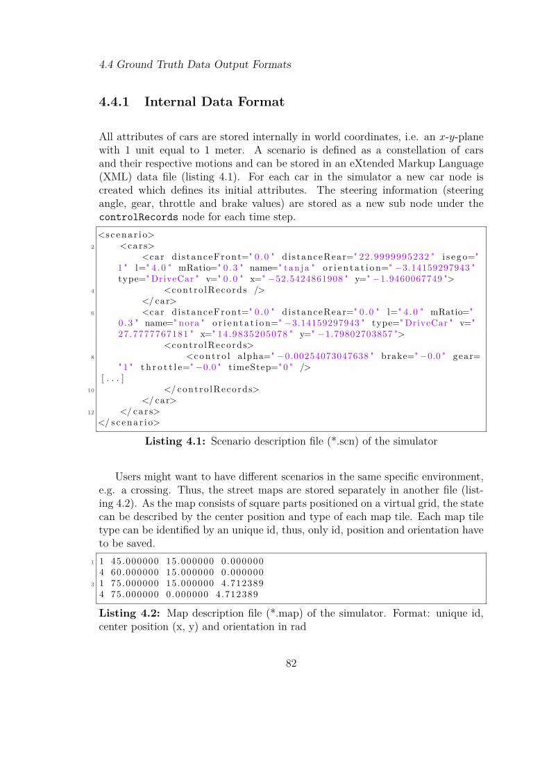
4.4 Ground Truth Data Output Formats
4.4.1 Internal Data Format
All attributes of cars are stored internally in world coordinates, i.e. an x-y-planewith 1 unit equal to 1 meter. A scenario is defined as a constellation of carsand their respective motions and can be stored in an eXtended Markup Language(XML) data file (listing 4.1). For each car in the simulator a new car node iscreated which defines its initial attributes. The steering information (steeringangle, gear, throttle and brake values) are stored as a new sub node under thecontrolRecords node for each time step.<scena r i o>
2 <car s><car d i s tanceFront=" 0 .0 " d i s tanceRear=" 22.9999995232 " i s e g o="
1 " l=" 4 .0 " mRatio=" 0 .3 " name=" tan ja " o r i e n t a t i o n=" −3.14159297943 "type=" DriveCar " v=" 0 .0 " x=" −52.5424861908 " y=" −1.9460067749 ">
4 <contro lRecords /></ car>
6 <car d i s tanceFront=" 0 .0 " d i s tanceRear=" 0 .0 " l=" 4 .0 " mRatio="0 .3 " name=" nora " o r i e n t a t i o n=" −3.14159297943 " type=" DriveCar " v="27.7777767181 " x=" 14.9835205078 " y=" −1.79802703857 ">
<contro lRecords>8 <con t r o l alpha=" −0.00254073047638 " brake="−0.0 " gear=
" 1 " t h r o t t l e="−0.0 " timeStep=" 0 " />[ . . . ]
10 </ contro lRecords></ car>
12 </ car s></ s c ena r i o>
Listing 4.1: Scenario description file (*.scn) of the simulator
Users might want to have different scenarios in the same specific environment,e.g. a crossing. Thus, the street maps are stored separately in another file (list-ing 4.2). As the map consists of square parts positioned on a virtual grid, the statecan be described by the center position and type of each map tile. Each map tiletype can be identified by an unique id, thus, only id, position and orientation haveto be saved.
1 1 45.000000 15.000000 0.0000004 60.000000 15.000000 0.000000
3 1 75.000000 15.000000 4.7123894 75.000000 0.000000 4.712389
Listing 4.2: Map description file (*.map) of the simulator. Format: unique id,center position (x, y) and orientation in rad
82
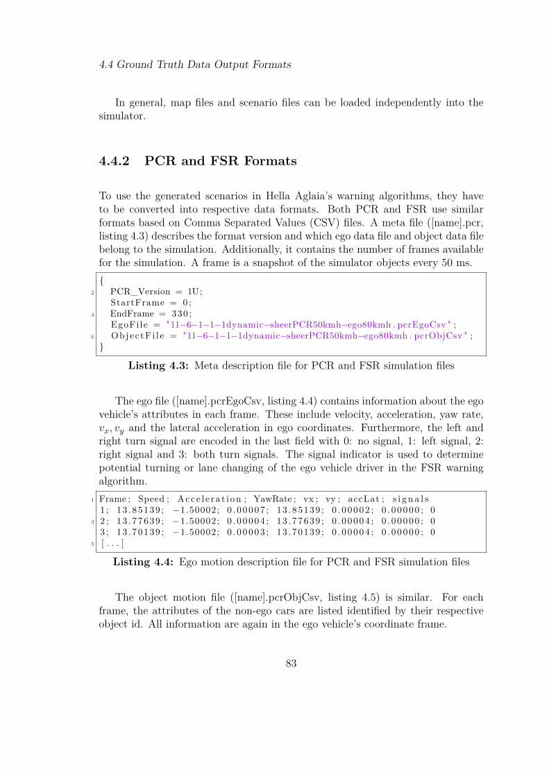
4.4 Ground Truth Data Output Formats
In general, map files and scenario files can be loaded independently into thesimulator.
4.4.2 PCR and FSR Formats
To use the generated scenarios in Hella Aglaia’s warning algorithms, they haveto be converted into respective data formats. Both PCR and FSR use similarformats based on Comma Separated Values (CSV) files. A meta file ([name].pcr,listing 4.3) describes the format version and which ego data file and object data filebelong to the simulation. Additionally, it contains the number of frames availablefor the simulation. A frame is a snapshot of the simulator objects every 50 ms.{
2 PCR_Version = 1U;StartFrame = 0 ;
4 EndFrame = 330 ;EgoFi le = "11−6−1−1−1dynamic−sheerPCR50kmh−ego80kmh . pcrEgoCsv " ;
6 Objec tF i l e = "11−6−1−1−1dynamic−sheerPCR50kmh−ego80kmh . pcrObjCsv " ;}
Listing 4.3: Meta description file for PCR and FSR simulation files
The ego file ([name].pcrEgoCsv, listing 4.4) contains information about the egovehicle’s attributes in each frame. These include velocity, acceleration, yaw rate,vx, vy and the lateral acceleration in ego coordinates. Furthermore, the left andright turn signal are encoded in the last field with 0: no signal, 1: left signal, 2:right signal and 3: both turn signals. The signal indicator is used to determinepotential turning or lane changing of the ego vehicle driver in the FSR warningalgorithm.
1 Frame ; Speed ; Acce l e r a t i on ; YawRate ; vx ; vy ; accLat ; s i g n a l s1 ; 13 . 85139 ; −1.50002; 0 . 00007 ; 13 . 85139 ; 0 . 00002 ; 0 . 00000 ; 0
3 2 ; 13 . 77639 ; −1.50002; 0 . 00004 ; 13 . 77639 ; 0 . 00004 ; 0 . 00000 ; 03 ; 13 . 70139 ; −1.50002; 0 . 00003 ; 13 . 70139 ; 0 . 00004 ; 0 . 00000 ; 0
5 [ . . . ]
Listing 4.4: Ego motion description file for PCR and FSR simulation files
The object motion file ([name].pcrObjCsv, listing 4.5) is similar. For eachframe, the attributes of the non-ego cars are listed identified by their respectiveobject id. All information are again in the ego vehicle’s coordinate frame.
83
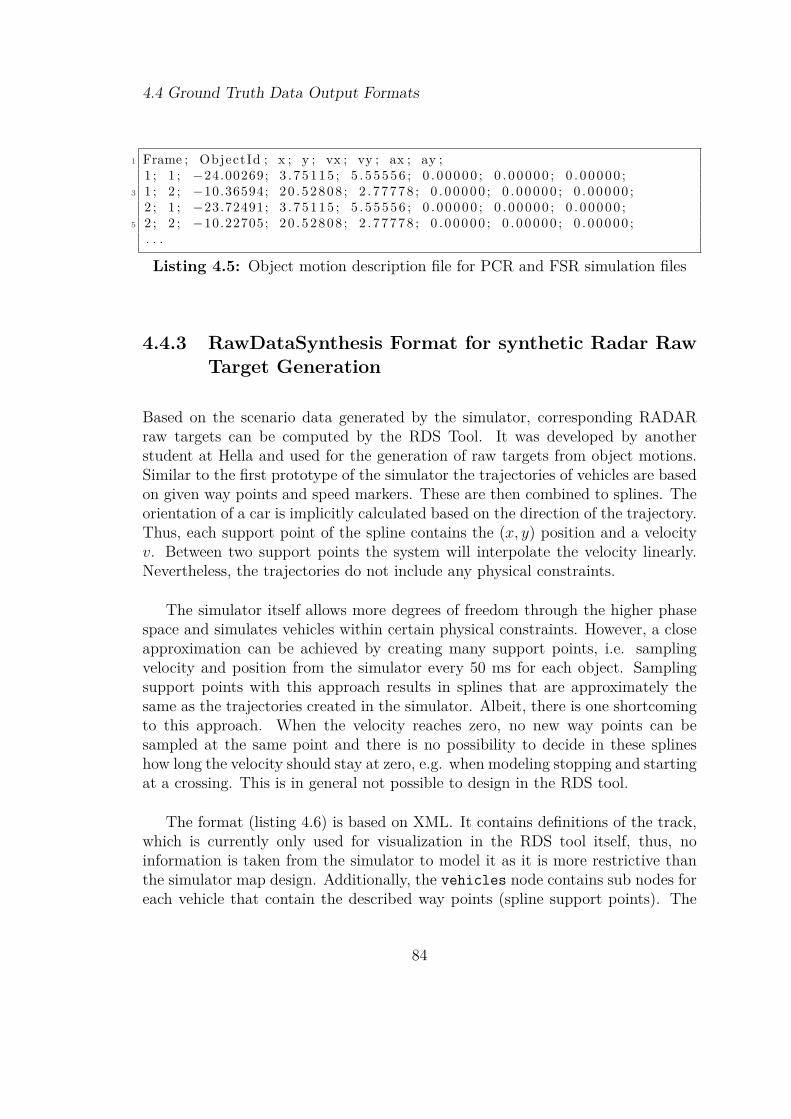
4.4 Ground Truth Data Output Formats
1 Frame ; ObjectId ; x ; y ; vx ; vy ; ax ; ay ;1 ; 1 ; −24.00269; 3 . 75115 ; 5 . 55556 ; 0 . 00000 ; 0 . 00000 ; 0 . 00000 ;
3 1 ; 2 ; −10.36594; 20 . 52808 ; 2 . 77778 ; 0 . 00000 ; 0 . 00000 ; 0 . 00000 ;2 ; 1 ; −23.72491; 3 . 75115 ; 5 . 55556 ; 0 . 00000 ; 0 . 00000 ; 0 . 00000 ;
5 2 ; 2 ; −10.22705; 20 . 52808 ; 2 . 77778 ; 0 . 00000 ; 0 . 00000 ; 0 . 00000 ;. . .
Listing 4.5: Object motion description file for PCR and FSR simulation files
4.4.3 RawDataSynthesis Format for synthetic Radar RawTarget Generation
Based on the scenario data generated by the simulator, corresponding RADARraw targets can be computed by the RDS Tool. It was developed by anotherstudent at Hella and used for the generation of raw targets from object motions.Similar to the first prototype of the simulator the trajectories of vehicles are basedon given way points and speed markers. These are then combined to splines. Theorientation of a car is implicitly calculated based on the direction of the trajectory.Thus, each support point of the spline contains the (x, y) position and a velocityv. Between two support points the system will interpolate the velocity linearly.Nevertheless, the trajectories do not include any physical constraints.
The simulator itself allows more degrees of freedom through the higher phasespace and simulates vehicles within certain physical constraints. However, a closeapproximation can be achieved by creating many support points, i.e. samplingvelocity and position from the simulator every 50 ms for each object. Samplingsupport points with this approach results in splines that are approximately thesame as the trajectories created in the simulator. Albeit, there is one shortcomingto this approach. When the velocity reaches zero, no new way points can besampled at the same point and there is no possibility to decide in these splineshow long the velocity should stay at zero, e.g. when modeling stopping and startingat a crossing. This is in general not possible to design in the RDS tool.
The format (listing 4.6) is based on XML. It contains definitions of the track,which is currently only used for visualization in the RDS tool itself, thus, noinformation is taken from the simulator to model it as it is more restrictive thanthe simulator map design. Additionally, the vehicles node contains sub nodes foreach vehicle that contain the described way points (spline support points). The
84

4.4 Ground Truth Data Output Formats
ego vehicle is stored explicitly with more information about sensor mountings andcalibration.<?xml ve r s i on=" 1 .0 " encoding=" utf−8" ?>
2 <Scenar io simulateADCValues="True " simulateRawTargets="True "><Track>
4 <TrackPart guardRailType=" S ing l e " guardRai l s=" " laneWidth="3 .8 " l ane s=" 4 " l ength=" 1000 " rad iu s=" 0 " /></Track>
6 <Veh i c l e s><Vehic l e>
8 <Waypoints><Waypoint speed=" 16.6666660309 " x=" 1.27323913574 " y="
−20.3797801494 " />10 <Waypoint speed=" 16.6666660309 " x=" 1.27326160847 " y="
−19.5464468482 " />[ . . . ]
12 </Waypoints><VehicleData name=" nora ">
14 <Vehic leDimensions l ength=" 4 .0 " width=" 1 .8 "><Axis x=" 0 .8 " />
16 <Axis x=" 3 .6 " /></Vehic leDimensions>
18 </VehicleData></Vehic l e>
20 </Veh i c l e s><EgoVehicle>
22 <Waypoints><Waypoint speed=" 0 .0 " x=" 1.84082021713 " y=" 43.444070816 "
/>24 </Waypoints>
<VehicleData name=" tan ja ">26 <Vehic leDimensions l ength=" 4 .0 " width=" 1 .8 ">
<Axis x=" 0 .8 " />28 <Axis x=" 3 .6 " />
</Vehic leDimensions>30 <Sensors>
[ De f i n i t i o n o f Sensor c a l i b r a t i o n and mountingp o s i t i o n s ]
32 </Sensors></VehicleData>
34 </EgoVehicle></ Scenar io>
Listing 4.6: Export format of RDS Tool (*.rds)
85
4.5 Results and Conclusion
4.5 Results and Conclusion
The PCR test catalog consists of 155 test cases for the PCR warning algorithm(example: Figure 4.1). This catalog is used as a basis to evaluate the usability ofthe simulator. Altogether it took 3 days for a single person to recreate the testcatalog in the simulator and save a scenario file for each test case.
Every scenario of the test catalog has been exported to FSR and PCR warningalgorithm formats as well as to the RDS tool. With the latter it is even possible totest the system at the raw target level. Both PCR and FSR delivered reasonableresults when running the synthetic scenarios from the test catalog. Albeit, RDSshowed problems in situations that include a full stop of a vehicle followed byan acceleration which cannot be modeled in the tool as already mentioned andexplained in section 4.4.3. This special case appeared only in one test case, andtherefore can be neglected.
The simulator is a valuable tool to cut down both time and costs for thegeneration of reasonable test data. It can be extended to support further exportformats by adding or adjusting exporter classes. Additionally, the simulation ofother objects, e.g. motor bikes or pedestrians, can be achieved by implementingmore simulatorObject classes with other underlying physical models.
As an outlook into the future, the raw data synthesis from the RDS tool couldbe merged directly into the simulator to skip the export and import step. Thiswould eliminate the restrictions of RDS induced by velocities of 0 km/h as well.
86

Chapter 5
Conclusion
The results and conclusions for each topic are placed in detail at the end of eachrespective chapter. Altogether, three main topics have been processed.
In Chapter 2, the choice of a reasonable camera system and the setup of aworking framework to collect data from test drives with the test bed have beenpresented. Cameras from AVT have been chosen and successfully calibrated usingthe Scaramuzza camera model [SMS06a]. This model proved practical in all casesand for all further applications.
In Chapter 3, a sensor fusion approach utilizing camera and RADAR informa-tion has been presented. This approach showed an improvement of the accuracy ofthe RADAR object tracks if the initial RADAR hypotheses are relatively accurateestimates of the true position. The approach has been successfully extended tointegrate optical flow information.
The last part of this thesis discusses a method for intuitive generation of testdata for RADAR warning systems. Instead of collecting information from testdrives equipped with the warning system, data can be acquired from a drivingsimulator. Next to the development of an intuitive interface, the data had tobe physically reasonable. Therefore, vehicle dynamics have been modeled in thesimulator which ensure this level of data quality. Combined with another projectat Hella, the output of the simulator can be used to test warning system modulesboth at pre-processing as well as warn algorithm level.
87

List of Figures
1.1 Sensor fusion at data level (Low Level Sensor Fusion) . . . . . . . . 3
1.2 Sensor fusion at feature level (Mid-Level Sensor Fusion) . . . . . . . 4
1.3 Sensor fusion at declaration level (High Level Sensor Fusion) . . . . 4
1.4 World coordinate system . . . . . . . . . . . . . . . . . . . . . . . . 7
1.5 Ego vehicle coordinate system . . . . . . . . . . . . . . . . . . . . . 7
1.6 Camera coordinate system . . . . . . . . . . . . . . . . . . . . . . . 8
1.7 Image coordinate system . . . . . . . . . . . . . . . . . . . . . . . . 9
1.8 RADAR coordinate system . . . . . . . . . . . . . . . . . . . . . . . 9
2.1 Cassandra processing chain design for a simple Canny filter . . . . . 17
2.2 Canny filter processing chain . . . . . . . . . . . . . . . . . . . . . . 18
2.3 Radial barrel distortion around the image center . . . . . . . . . . . 21
2.4 Images taken with different optics . . . . . . . . . . . . . . . . . . . 24
2.5 Perspective and spherical projection . . . . . . . . . . . . . . . . . . 25
2.6 Scaramuzza model for a fish–eye lens . . . . . . . . . . . . . . . . . 25
88
List of Figures
2.7 Calibration images . . . . . . . . . . . . . . . . . . . . . . . . . . . 27
2.8 Scaramuzza calibration results . . . . . . . . . . . . . . . . . . . . . 28
2.9 Re-projection of the Scaramuzza model . . . . . . . . . . . . . . . . 29
2.10 Extrinsic calibration using a checkerboard pattern . . . . . . . . . . 30
2.11 A bicycle tracked by radar visualized in the camera image . . . . . 32
2.12 Undistorted images from Scaramuzza and OpenCV . . . . . . . . . 34
2.13 Sensor mountings . . . . . . . . . . . . . . . . . . . . . . . . . . . . 36
2.14 Test bed hardware . . . . . . . . . . . . . . . . . . . . . . . . . . . 38
2.15 Dataflow of the test bed . . . . . . . . . . . . . . . . . . . . . . . . 38
3.1 Distortion and roll angle corrected camera image . . . . . . . . . . 43
3.2 Extraction of regions of interest . . . . . . . . . . . . . . . . . . . . 44
3.3 ROI extraction from distorted and undistorted images . . . . . . . . 46
3.4 Prediction of optical flow based on RADAR velocity . . . . . . . . . 48
3.5 Predicted flow based on RADAR tracked object . . . . . . . . . . . 49
3.6 Oncoming vehicle . . . . . . . . . . . . . . . . . . . . . . . . . . . . 50
3.7 Comparison of optical flow and predicted optical flow . . . . . . . . 51
3.8 Optical flow based weight method 1 . . . . . . . . . . . . . . . . . . 52
3.9 Optical flow based weight method 2 . . . . . . . . . . . . . . . . . . 53
3.10 3D model wire frame . . . . . . . . . . . . . . . . . . . . . . . . . . 55
3.11 3D model initialized on a RADAR hypothesis . . . . . . . . . . . . 56
89

List of Figures
3.12 Distance error measurement . . . . . . . . . . . . . . . . . . . . . . 57
3.13 Model parameter refinement after one iteration . . . . . . . . . . . 61
3.14 Model refinement using optical flow information . . . . . . . . . . . 65
3.15 Recovered track with optical flow and edge fitting . . . . . . . . . . 66
3.16 Model fitting of different vehicle types . . . . . . . . . . . . . . . . 66
3.17 Incorrect fitting due to incorrect initial parameters . . . . . . . . . 67
3.18 Incorrect fitting due to abstraction in the chosen vehicle model . . . 68
4.1 Example of a test catalog scenario for PCR . . . . . . . . . . . . . . 71
4.2 Warning algorithm data flow . . . . . . . . . . . . . . . . . . . . . . 71
4.3 Interface development of the simulator . . . . . . . . . . . . . . . . 72
4.4 Set up of the driving simulator . . . . . . . . . . . . . . . . . . . . . 73
4.5 Complex road scenario created in the simulator . . . . . . . . . . . 74
4.6 Simplified UML representation of the simulator structure . . . . . . 76
4.7 Single track model . . . . . . . . . . . . . . . . . . . . . . . . . . . 77
A.1 Sensor overlap . . . . . . . . . . . . . . . . . . . . . . . . . . . . . . 99
A.2 Back view of the camera position . . . . . . . . . . . . . . . . . . . 100
C.1 Extrinsic calibration graph in Cassandra . . . . . . . . . . . . . . . 104
C.2 DriveRecorder Graph in Cassandra . . . . . . . . . . . . . . . . . . 105
C.3 Basic Graph for replaying recorded data . . . . . . . . . . . . . . . 106
90

List of Figures
C.4 FSR sub graph for decoding CAN messages . . . . . . . . . . . . . 107
D.1 Calibration stand . . . . . . . . . . . . . . . . . . . . . . . . . . . . 108
91
List of Tables
1.1 Mathematical notations . . . . . . . . . . . . . . . . . . . . . . . . 5
2.1 Camera and optics for the test bed . . . . . . . . . . . . . . . . . . 20
2.2 Parameters of an intrinsic Scaramuzza calibration . . . . . . . . . . 26
2.3 Extrinsic parameters . . . . . . . . . . . . . . . . . . . . . . . . . . 32
2.4 Mounting positions of RADAR sensors . . . . . . . . . . . . . . . . 37
4.1 Licenses of used libraries in the simulator . . . . . . . . . . . . . . . 75
4.2 Car specific parameters for car dynamics models . . . . . . . . . . . 77
B.1 Calibration errors of the left camera . . . . . . . . . . . . . . . . . . 102
B.2 Calibration errors of the right camera . . . . . . . . . . . . . . . . . 103
D.1 Reference frames used for calibration . . . . . . . . . . . . . . . . . 109
92

Abbreviations
AVI Audio Video Interleave (Audio and video container format) . . . . . . . . . . . . . 39
CAN Controller Area Network . . . . . . . . . . . . . . . . . . . . . . . . . . . . . . . . . . . . . . . . . . . . . . 16
CLIO CAN/LIN Input/Output - Module (Device which translates CAN messagesto FireWire and tags the data with FireWire timestamps) . . . . . . . . . . . . . . .18
CSV Comma Separated Values . . . . . . . . . . . . . . . . . . . . . . . . . . . . . . . . . . . . . . . . . . . . . . 83
FSR Front/Side RADAR (Tracking and warning system mainly for cross sections)1
KP Communication Processor . . . . . . . . . . . . . . . . . . . . . . . . . . . . . . . . . . . . . . . . . . . . . . . 37
LIDAR Light Detection And Ranging . . . . . . . . . . . . . . . . . . . . . . . . . . . . . . . . . . . . . . . 12
KLT Tracker Kanade-Lucas-Tomasi Tracker . . . . . . . . . . . . . . . . . . . . . . . . . . . . . . . . 47
PCA Principle Component Analysis . . . . . . . . . . . . . . . . . . . . . . . . . . . . . . . . . . . . . . . . . 12
PCR Pre-Crash Rear (Warning system for rear crashes). . . . . . . . . . . . . . . . . . . . . . .1
PID-controller Proportional-Integral-Derivative controller . . . . . . . . . . . . . . . . . . 73
93

List of Tables
RADAR Radio Detection And Ranging . . . . . . . . . . . . . . . . . . . . . . . . . . . . . . . . . . . . . . 1
RDS RawDataSynthesis (tool for generating raw RADAR targets from objecttracks) . . . . . . . . . . . . . . . . . . . . . . . . . . . . . . . . . . . . . . . . . . . . . . . . . . . . . . . . . . . . . . . . . .72
ROI Region of Interest . . . . . . . . . . . . . . . . . . . . . . . . . . . . . . . . . . . . . . . . . . . . . . . . . . . . . . 41
SVM Support Vector Machine (Classifier) . . . . . . . . . . . . . . . . . . . . . . . . . . . . . . . . . . . 11
ToF Time-of-Flight (used in sensors for distance measurement). . . . . . . . . . . . . . . .3
XML eXtended Markup Language . . . . . . . . . . . . . . . . . . . . . . . . . . . . . . . . . . . . . . . . . . . 82
94

Bibliography
[ABC07] Giancarlo Alessandretti, Alberto Broggi, and Pietro Cerri. Vehicle andguard rail detection using radar and vision data fusion. IEEE Transac-tions on Intelligent Transportation Systems, 8(1):95–105, March 2007.
[All12] Allied Vision Technologies. Data sheet AVT Guppy Pro, September2012.
[Bou01] Jean-Yves Bouguet. Pyramidal implementation of the affine lucas kanadefeature tracker description of the algorithm. 2001.
[Bre65] Jack E Bresenham. Algorithm for computer control of a digital plotter.IBM Systems journal, 4(1):25–30, 1965.
[Bre12] Dr. Gabi Breuel. Grundlagen autonomer Fahrzeuge - Situationsanalye,2012.
[Can86] John Canny. A computational approach to edge detection. PatternAnalysis and Machine Intelligence, IEEE Transactions on, (6):679–698,1986.
[ETG07] Tobias Ehlgen, Markus Thom, and Markus Glaser. Omnidirectionalcameras as backing-up aid. In Computer Vision, 2007. ICCV 2007.IEEE 11th International Conference on, page 1–5, 2007.
[FRBG05] Uwe Franke, Clemens Rabe, Hernán Badino, and Stefan Gehrig. 6d-vision: Fusion of stereo and motion for robust environment perception.Pattern Recognition, page 216–223, 2005.
[GOY03] GOYO OPTICAL INC. GM23514MCN data sheet, June 2003.
[HEL12] HELLA. Driver assistance systems radar 24Ghz, 2012.
95

Bibliography
[Hel13] Hella Aglaia. Cassandra vision - rapid prototyping for image process-ing with OpenCV, July 2013. http://www.cassandra-vision.com/accessed: 2013-07-07.
[HL01] David L. Hall and James Llinas. Handbook of Multisensor Data Fusion.CRC Press, June 2001. Published: Hardcover.
[Its13a] Itseez. Camera calibration with OpenCV — OpenCV 2.4.6.0 documen-tation, September 2013. http://docs.opencv.org/doc/tutorials/calib3d/camera_calibration/camera_calibration.html accessed:2013-09-07.
[Its13b] Itseez. OpenCV, July 2013. http://opencv.org/ accessed: 2013-07-07.
[Kan81] Bruce D. Lucas Takeo Kanade. An iterative image registration techniquewith an application to stereo vision. 81:674–679, 1981.
[Kau12] Eberhard Kaus. Grundlagen autonomer Fahrzeuge - Fahrzeugsteuerung– putting it all together, 2012.
[KB61] Rudolph E. Kalman and Richard S. Bucy. New results in linear filteringand prediction theory. Journal of Basic Engineering, 83(3):95–108, 1961.
[LM09] Matthew J. Leotta and Joseph L. Mundy. Predicting high resolutionimage edges with a generic, adaptive, 3-d vehicle model. In ComputerVision and Pattern Recognition, 2009. CVPR 2009. IEEE Conferenceon, page 1311–1318, 2009.
[Low91] David G. Lowe. Fitting parameterized three-dimensional models to im-ages. IEEE Transactions on Pattern Analysis and Machine Intelligence,13(5):441–450, 1991.
[LTH+05] Jianguang Lou, Tieniu Tan, Weiming Hu, Hao Yang, and S.J. May-bank. 3-d model-based vehicle tracking. IEEE Transactions on ImageProcessing, 14(10):1561–1569, October 2005.
[MHG+06] Marc-Michael Meinecke, Raimond Holze, Mark Gonter, ThomasWohllebe, Ralph Mende, and Rajko Petelka. Side-pre-crash sendingsystem for automatic vehicle height level adaptation. In Proc. 3rd Int.Workshop Intell. Transp., Hamburg, Germany, 2006.
[Num13] Numpy developers. NumPy, July 2013. http://www.numpy.org/ ac-cessed: 2013-07-25.
96
Bibliography
[PVB+09] Sylvia Pietzsch, Trung Dung Vu, Julien Burlet, Olivier Aycard, ThomasHackbarth, Nils Appenrodt, Jürgen Dickmann, and Bernd Radig. Re-sults of a precrash application based on laser scanner and short-rangeradars. Intelligent Transportation Systems, IEEE Transactions on,10(4):584–593, 2009.
[Pyt13] Python Software Foundation. Python programming language, July 2013.http://python.org/ accessed: 2013-07-25.
[RSS08] Martin Rufli, Davide Scaramuzza, and Roland Siegwart. Automatic de-tection of checkerboards on blurred and distorted images. In IntelligentRobots and Systems, 2008. IROS 2008. IEEE/RSJ International Con-ference on, page 3121–3126, 2008.
[SBM06] Zehang Sun, George Bebis, and Ronald Miller. Monocular precrash ve-hicle detection: features and classifiers. Image Processing, IEEE Trans-actions on, 15(7):2019–2034, 2006.
[Sca07] Davide Scaramuzza. Omnidirectional vision: from calibration to robotmotion estimation. PhD thesis, Citeseer, 2007.
[Sca13] Davide Scaramuzza. OCamCalib: omnidirectional camera calibrationtoolbox for matlab - davide scaramuzza, September 2013. https://sites.google.com/site/scarabotix/ocamcalib-toolbox accessed:2013-09-07.
[SHB10] Dieter Schramm, Manfred Hiller, and Roberto Bardini. Modellbildungund Simulation der Dynamik von Kraftfahrzeugen. Springer, Berlin; NewYork, 2010.
[Sla99] Gregory G. Slabaugh. Computing euler angles from a rotation matrix.1999.
[SMS06a] Davide Scaramuzza, Agostino Martinelli, and Roland Siegwart. A flexi-ble technique for accurate omnidirectional camera calibration and struc-ture from motion. In Computer Vision Systems, 2006 ICVS’06. IEEEInternational Conference on, page 45–45, 2006.
[SMS06b] Davide Scaramuzza, Agostino Martinelli, and Roland Siegwart. Atoolbox for easily calibrating omnidirectional cameras. In IntelligentRobots and Systems, 2006 IEEE/RSJ International Conference on, page5695–5701, 2006.
97

Bibliography
[ST94] Jianbo Shi and Carlo Tomasi. Good features to track. In Computer Vi-sion and Pattern Recognition, 1994. Proceedings CVPR’94., 1994 IEEEComputer Society Conference on, page 593–600, 1994.
[TA77] AN Tikhonov and V Ya Arsenin. Solutions of ill-posed problems. WHWinston, Washington, DC, 330, 1977.
[Thr13] Sebastian Thrun. Artificial intelligence: How to build a robot - udacity,September 2013. https://www.udacity.com/course/cs373 accessed:2013-09-07.
[TK91] Carlo Tomasi and Takeo Kanade. Detection and tracking of point fea-tures. School of Computer Science, Carnegie Mellon Univ., 1991.
[Tor13] Torus Knot Software. OGRE – open source 3D graphics engine, July2013. http://www.ogre3d.org/ accessed: 2013-07-18.
[TP91] Matthew Turk and Alex Pentland. Eigenfaces for recognition. Journalof cognitive neuroscience, 3(1):71–86, 1991.
[Uni13] Unibrain. Unibrain.com - global leader in FireWire development.,September 2013. http://www.unibrain.com/ accessed: 2013-09-08.
[VBA08] Trung-Dung Vu, Julien Burlet, and Olivier Aycard. Grid-based local-ization and online mapping with moving objects detection and track-ing: new results. In Intelligent Vehicles Symposium, 2008 IEEE, page684–689, 2008.
[wxP13] wxPROs. wxPython, July 2013. http://www.wxpython.org/ accessed:2013-07-25.
[Zha00] Zhengyou Zhang. A flexible new technique for camera calibration.Pattern Analysis and Machine Intelligence, IEEE Transactions on,22(11):1330–1334, 2000.
[ZXY12] Gangqiang Zhao, Xuhong Xiao, and Junsong Yuan. Fusion of velodyneand camera data for scene parsing. In Information Fusion (FUSION),2012 15th International Conference on, page 1172–1179, 2012.
98

Appendix A
Sensor Mounting Positions
Figure A.1: Overlap of camera (mounted on side mirror) and radar (mountedon front bumper)
99
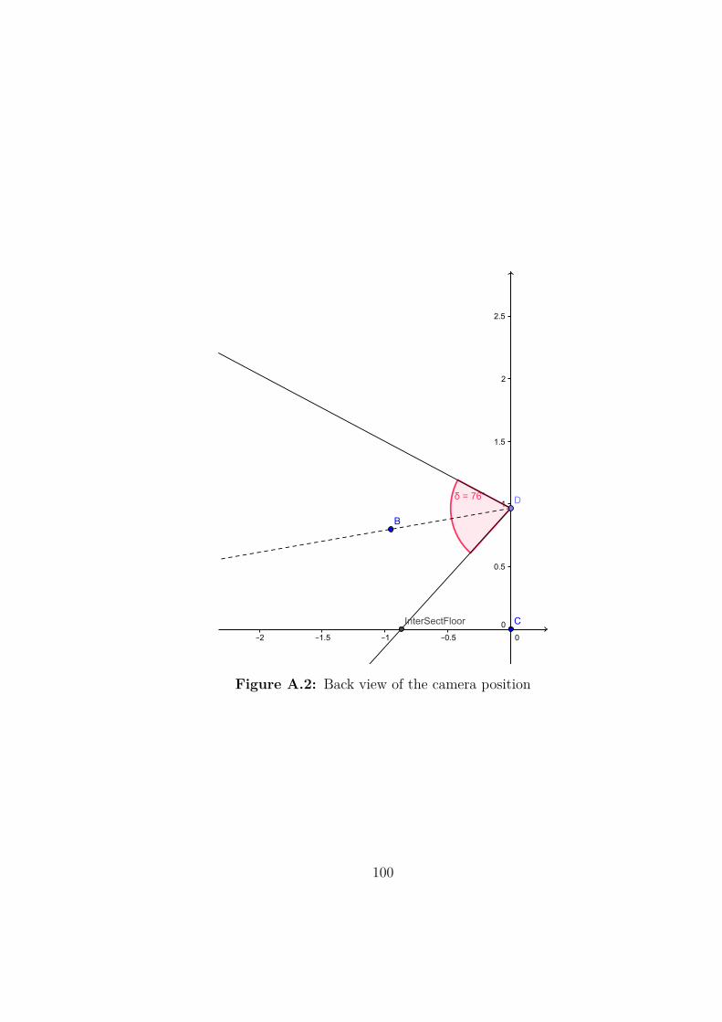
Figure A.2: Back view of the camera position
100
Appendix B
Calibration Errors of OpenCVand Scaramuzza Camera Models
101

Scaramuzza OpenCVFile e σ2 E e σ2 E
002.bmp 0.370435 0.0231854 12.8326 0.275795 0.0217404 7.82427003.bmp 0.185568 0.0112573 3.65543 0.247968 0.0184889 6.39818004.bmp 0.365633 0.0306408 13.1463 0.221599 0.0118968 4.88025005.bmp 0.165362 0.00743389 2.78228 0.186114 0.0133489 3.83899006.bmp 0.394953 0.0232965 14.3427 0.333362 0.02819 11.1456007.bmp 0.261203 0.0151738 6.67208 0.227663 0.0316865 5.34436008.bmp 0.279649 0.0186588 7.74898 0.281389 0.110866 8.86929009.bmp 0.300676 0.0152974 8.45626 0.250963 0.0161416 6.32993010.bmp 0.259342 0.0126064 6.38917 0.257811 0.0156026 6.56552011.bmp 0.483464 0.0522302 22.8774 0.32991 0.0283378 10.9743012.bmp 0.497691 0.0483012 23.6798 0.188713 0.0170201 4.21061013.bmp 0.301386 0.0146236 8.43658 0.215351 0.0101641 4.52322014.bmp 0.387718 0.0244953 13.9856 0.309064 0.0227157 9.45891015.bmp 0.300167 0.0185536 8.6923 0.162572 0.00817829 2.76863016.bmp 0.487956 0.0624943 24.0476 0.321132 0.0270494 10.414017.bmp 0.239249 0.0101859 5.39406 0.184098 0.00587861 3.18165018.bmp 0.115092 0.00284178 1.28703 0.112031 0.00426226 1.34506019.bmp 0.211512 0.00992366 4.37286 0.103195 0.0037201 1.14954020.bmp 0.271937 0.0101612 6.72889 0.241402 0.0241196 6.59156021.bmp 0.2419 0.0262558 6.78173 0.213922 0.0109082 4.53366022.bmp 0.372876 0.0403377 14.3499 0.336342 0.0213889 10.7612
Table B.1: Calibration errors for Scaramuzza and OpenCV camera models cali-brated for the left side camera
102

Scaramuzza OpenCVFile e σ2 E e σ2 E
001.bmp 0.284246 0.0338398 9.17084 0.595858 0.146288 40.1068002.bmp 0.271896 0.0175099 7.31501 0.280599 0.0324063 8.89137004.bmp 0.486398 0.0662387 24.2258 0.516561 0.094324 28.8927005.bmp 0.55324 0.0529232 28.7198 0.687035 0.109714 46.5386006.bmp 0.186948 0.0133088 3.86066 0.157153 0.00907199 2.70152007.bmp 0.286031 0.0215893 8.27223 0.158952 0.00617741 2.51546008.bmp 0.307392 0.01705 8.92321 0.326994 0.026876 10.7041009.bmp 0.350017 0.0249989 11.8009 0.300778 0.0358878 10.1084010.bmp 0.309961 0.0353365 10.513 0.611178 0.117948 39.3189011.bmp 0.210369 0.0113743 4.45034 0.257688 0.0243119 7.25722012.bmp 0.418896 0.038353 17.1061 0.308436 0.0347724 10.3924013.bmp 0.606872 0.0433953 32.9351 0.433804 0.0856371 21.9058014.bmp 0.421563 0.028635 16.508 0.379008 0.050028 15.494015.bmp 0.353267 0.0193904 11.5351 0.287304 0.0254661 8.64078016.bmp 0.445758 0.0384478 18.9719 0.57627 0.115505 35.8074017.bmp 0.600672 0.160608 41.7132 0.243548 0.107525 13.3472018.bmp 0.398316 0.042942 16.1278 0.576793 0.128176 36.8693019.bmp 0.324004 0.037779 11.4206 0.514831 0.0899744 28.402020.bmp 0.349709 0.023557 11.6682 0.459687 0.0877708 23.9267021.bmp 0.220668 0.00816057 4.5484 0.333378 0.0503491 12.9192022.bmp 0.196176 0.00997511 3.70659 0.249798 0.0205774 6.73778
Table B.2: Calibration errors for Scaramuzza and OpenCV camera models cali-brated for the right side camera
103
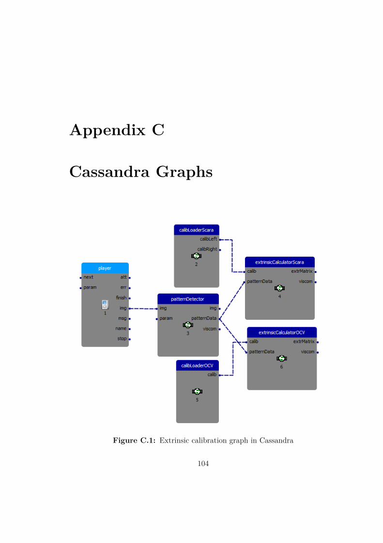
Appendix C
Cassandra Graphs
Figure C.1: Extrinsic calibration graph in Cassandra
104
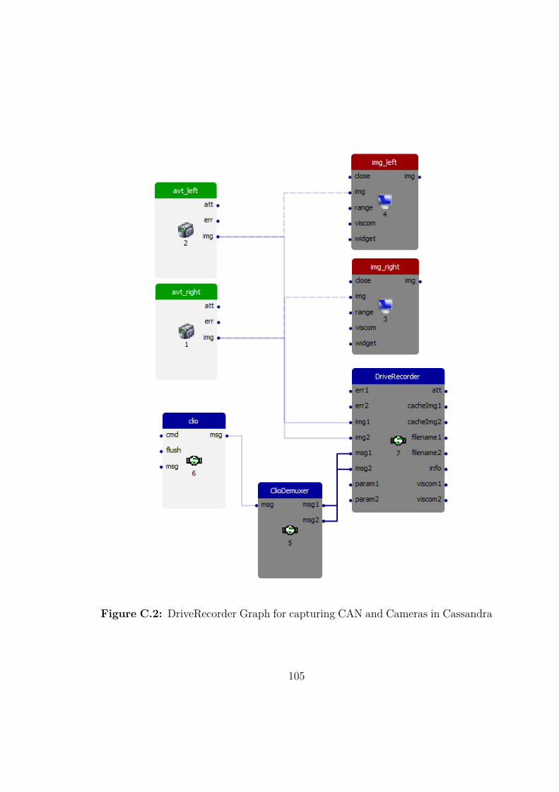
Figure C.2: DriveRecorder Graph for capturing CAN and Cameras in Cassandra
105

Figure C.3: Basic Graph for replaying recorded data
106
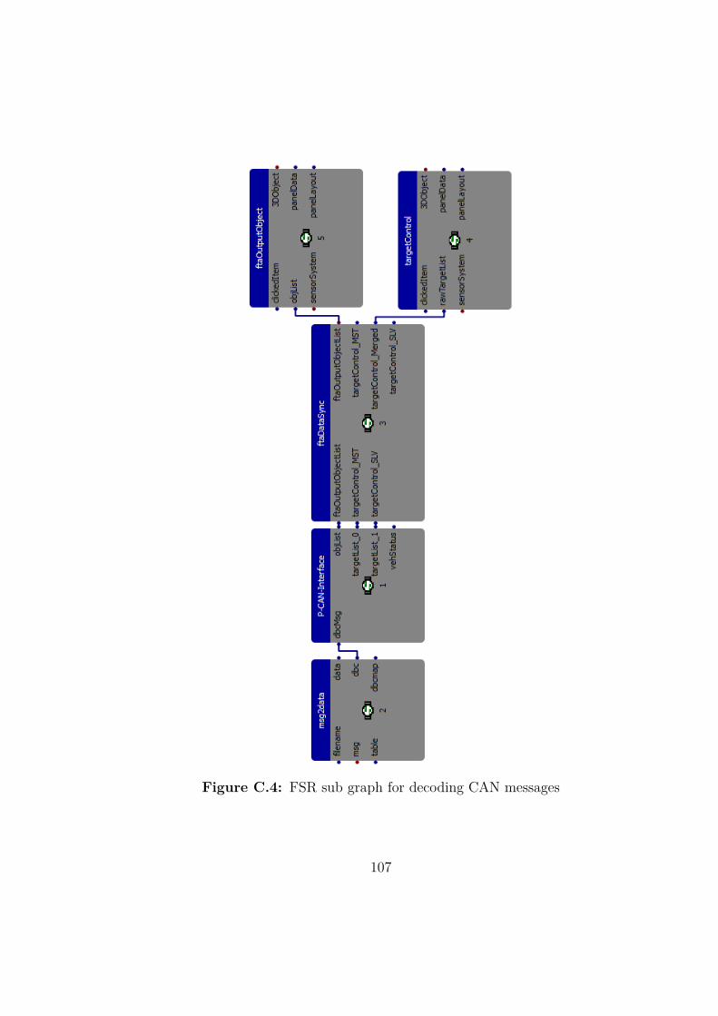
Figure C.4: FSR sub graph for decoding CAN messages
107

Appendix D
A lazy Approach for ExtrinsicWide Angle Camera Calibration
This is a thought experiment for the calibration of side cameras if a complete frontcamera calibration is available. The setup at Hella Aglaia for camera calibrationsupports front or back cameras with narrow opening angles. The following sectionspropose a method for the calibration of the side cameras used in the test bed. Theproposal utilizes the already calibrated front camera. The standard setup forcalibration is shown in Figure D.1.
Figure D.1: Calibration stand
108
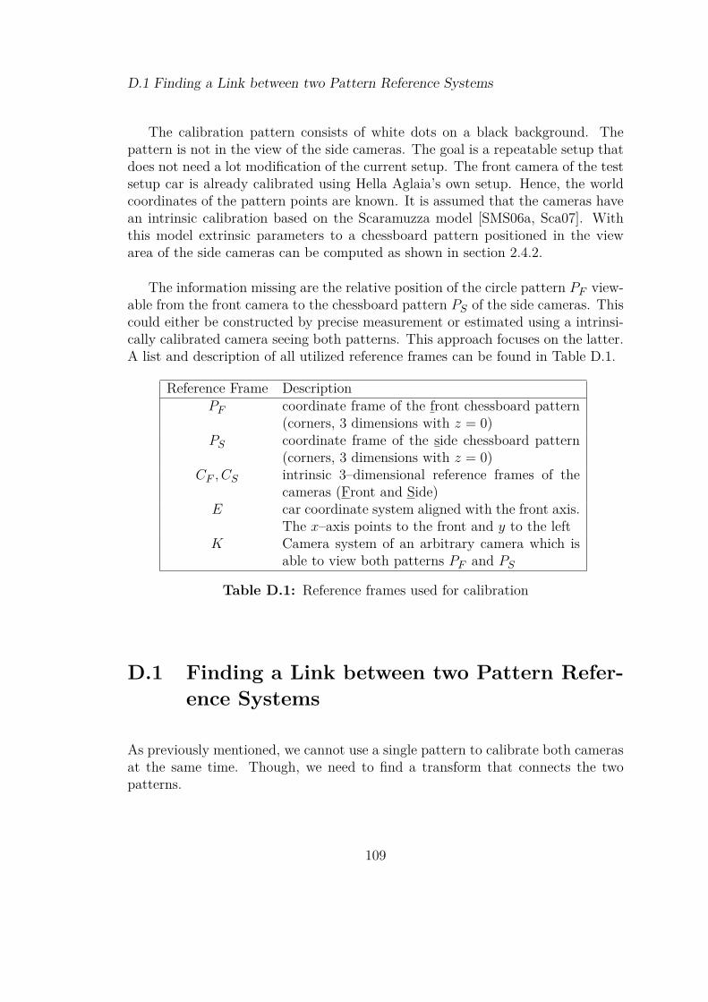
D.1 Finding a Link between two Pattern Reference Systems
The calibration pattern consists of white dots on a black background. Thepattern is not in the view of the side cameras. The goal is a repeatable setup thatdoes not need a lot modification of the current setup. The front camera of the testsetup car is already calibrated using Hella Aglaia’s own setup. Hence, the worldcoordinates of the pattern points are known. It is assumed that the cameras havean intrinsic calibration based on the Scaramuzza model [SMS06a, Sca07]. Withthis model extrinsic parameters to a chessboard pattern positioned in the viewarea of the side cameras can be computed as shown in section 2.4.2.
The information missing are the relative position of the circle pattern PF view-able from the front camera to the chessboard pattern PS of the side cameras. Thiscould either be constructed by precise measurement or estimated using a intrinsi-cally calibrated camera seeing both patterns. This approach focuses on the latter.A list and description of all utilized reference frames can be found in Table D.1.
Reference Frame DescriptionPF coordinate frame of the front chessboard pattern
(corners, 3 dimensions with z = 0)PS coordinate frame of the side chessboard pattern
(corners, 3 dimensions with z = 0)CF , CS intrinsic 3–dimensional reference frames of the
cameras (Front and Side)E car coordinate system aligned with the front axis.
The x–axis points to the front and y to the leftK Camera system of an arbitrary camera which is
able to view both patterns PF and PS
Table D.1: Reference frames used for calibration
D.1 Finding a Link between two Pattern Refer-ence Systems
As previously mentioned, we cannot use a single pattern to calibrate both camerasat the same time. Though, we need to find a transform that connects the twopatterns.
109
D.2 Putting it all together
For this, another internally calibrated camera K is needed which is able to seeboth patterns in a single image. Using a method to extract extrinsic parameters foreach pattern from an image with both patterns visible, the transforms from eachpattern coordinate system (PS and PF ) to the camera coordinate system K can beestimated. The transforms will be noted as TK←PS and TK←PF which transforma point on the pattern (x, y, 0) into the internal camera coordinate system K.The transform from one pattern coordinate system into the other then becomes asimple linear algebra exercise with the help of the coordinate system K.
To calculate the coordinates of pattern points from PS in reference frame PF ,the points from pattern PS are transformed into K. From K the inverse trans-form to PF can be used. Hence, we get the following new transforms (eqs. (D.1)and (D.2))
TPF←PS = TPF←K︸ ︷︷ ︸T−1K←PF
TK←PS (D.1)
TPS←PF = TPS←K︸ ︷︷ ︸T−1K←PS
TK←PF (D.2)
With our new transforms we can switch between the two reference frames of thepatterns.
xPF = TPF←PSxPS (D.3)xPS = TPS←PF xPF (D.4)
D.2 Putting it all together
Based on our previous calculations, we can estimate the positions of both patterns,even though only one pattern is visible at a time. We fix the car in the calibrationstand and calibrate the front camera with the help of the front pattern and theusual setup of the calibration stand. In the next step, we estimate the transformsbetween the two camera coordinate systems of the front and side cameras. At thispoint, in each camera only one of the patterns is visible. Pattern PS is visible inthe side camera CS while pattern PF is only visible in the front camera.
With both cameras we estimate the extrinsic parameters of the patterns andobtain the transforms TCS←PS and TCF←PF , i.e. the transforms to transform
110

D.2 Putting it all together
points from the pattern coordinate system into the camera coordinate system. Inthe previous section we estimated the transforms TPF←PS and TPS←PF , which wewill now use as a bridge between the two camera coordinate frames in eqs. (D.5)and (D.6).
TCS←CF = TCS←PSTPS←PF TPF←CF︸ ︷︷ ︸T−1CF←PF
(D.5)
TCF←CS = TCF←PFTPF←PS TPS←CS︸ ︷︷ ︸T−1CS←PS
(D.6)
As the front camera calibration setup already provides us with a transform thatallows us to convert between the front camera coordinate system and the car coor-dinate system E, we can derive the side camera transforms into the car coordinatesystem eq. (D.7) and vice versa eq. (D.8).
TE←CS = TE←CFTCF←CS (D.7)TCS←E = TCS←CFTCF←E (D.8)
111