Nutritional and Economic Analysis of Small-Scale Agriculture ...

Utah State University Utah State University

DigitalCommons@USU DigitalCommons@USU

All Graduate Theses and Dissertations Graduate Studies

5-2013

Nutritional and Economic Analysis of Small-Scale Agriculture in Nutritional and Economic Analysis of Small-Scale Agriculture in

Imbabura, Ecuador Imbabura, Ecuador

Jake Erickson Utah State University

Follow this and additional works at: https://digitalcommons.usu.edu/etd

Part of the Agricultural and Resource Economics Commons, and the Agricultural Economics

Commons

Recommended Citation Recommended Citation Erickson, Jake, "Nutritional and Economic Analysis of Small-Scale Agriculture in Imbabura, Ecuador" (2013). All Graduate Theses and Dissertations. 1468. https://digitalcommons.usu.edu/etd/1468

This Thesis is brought to you for free and open access by the Graduate Studies at DigitalCommons@USU. It has been accepted for inclusion in All Graduate Theses and Dissertations by an authorized administrator of DigitalCommons@USU. For more information, please contact [email protected].

https://digitalcommons.usu.edu/

https://digitalcommons.usu.edu/etd

https://digitalcommons.usu.edu/gradstudies

https://digitalcommons.usu.edu/etd?utm_source=digitalcommons.usu.edu%2Fetd%2F1468&utm_medium=PDF&utm_campaign=PDFCoverPages

http://network.bepress.com/hgg/discipline/317?utm_source=digitalcommons.usu.edu%2Fetd%2F1468&utm_medium=PDF&utm_campaign=PDFCoverPages



https://digitalcommons.usu.edu/etd/1468?utm_source=digitalcommons.usu.edu%2Fetd%2F1468&utm_medium=PDF&utm_campaign=PDFCoverPages

mailto:[email protected]

http://library.usu.edu/

http://library.usu.edu/

NUTRITIONAL AND ECONOMIC ANALYSIS OF SMALL-SCALE

AGRICULTURE IN IMBABURA, ECUADOR

by

Jake Erickson

A thesis submitted in partial fulfillment of the requirements for the degree

of

MASTER OF SCIENCE

in

Applied Economics

Approved:

Dr. DeeVon Bailey Major Professor

Dr. Ruby Ward Committee Member

Dr. Karin Allen Committee Member

Dr. Roger Kjelgren Committee Member

Dr. Mark McLellan Vice President of Research and

Dean of the School of Graduate Studies

UTAH STATE UNIVERSITY Logan, Utah

2012

ii ABSTRACT

Nutritional and Economic Analysis of Small-Scale Agriculture in Imbabura, Ecuador

by

Jake Erickson, Master of Science

Utah State University, 2012

Major Professor: Dr. DeeVon Bailey Department: Applied Economics

Last year over $130 billion were distributed to developing countries to help

eradicate extreme hunger and poverty. A body of literature has emerged challenging the

effectiveness of development aid. Economic interventions habitually pursue income

maximization through projects that develop economies of scale, share technology and

science improvements, facilitate access to capital, conduct best management practice

insemination, and/or grant access to markets. The end goal of such interventions is

usually to create the revenue stream to externally purchase items needed to overcome

malnutrition factors.

The critical view of aid stems from the separation of initiatives that exists only to

address a portion of the equation. Intervention projects normally aim to satisfy either the

nutritional needs of a group, or advancing the economic stability, but not both. One of

the many issues that may arise by narrowly focusing and creating an aid program is that

although a group may be fed, they are not equipped to mitigate risks that will arise after

project completion and thus continue or revert back to a malnourished state. A bridge is

iii required to join the economic and nutritional interventions to create aid interventions that

are sustainable past the point of donor separation.

Merging economic and nutrition interventions as pursued in this thesis required

the first step to be the creation of economic information for a typical small-scale farm.

A comprehensive set of estimated cost and return (enterprise) budgets for small-

scale agricultural crops that could be grown by the representative farm family used in this

analysis was developed. Utilizing these enterprise budgets, a linear programming model,

and nutritional information, such as is done in this study, could help in planning rural

development interventions as the income maximization and least-cost diet models are

integrated into one within the resource and management constraints of the representative

small-scale farm.

(222 pages)

iv PUBLIC ABSTRACT

Nutritional and Economic Analysis of Small-Scale Agriculture in Imbabura, Ecuador

Intervention projects in the developing world normally aim to satisfy either the

nutritional needs of a group, or advancing the economic stability, but not both. One of

the many issues that may arise by narrowly focusing and creating an aid program is that

although a group may be fed, they are not equipped to mitigate risks that will arise after

project completion and thus continue or revert back to a malnourished state. A bridge is

required to join the economic and nutritional programs to create aid interventions that are

sustainable past the point of donor separation.

This paper proposes the creation of a linear program model to assess the

effectiveness and sustainability of such intervention programs.

Investigating the effects of merging economic and nutrition interventions as

pursued in this report required the first step to be the creation of economic information

for a typical small-scale farm. The region of Cochas, Imbabura, Ecuador was selected as

the study area in which data would be collected for a representative sample of production

and living circumstances of a poor, rural, and small-scale farmer.

A comprehensive set of estimated cost and return (enterprise) budgets for small-


analysis was developed. This was accomplished via data collected in rural Ecuador by

Jake Erickson, a Master’s student in the department of Applied Economics at Utah State

University. Of the supervisory committee, daily interaction occurred with Dr. DeeVon

v Bailey, project supervisor, and Dr. Ruby Ward, linear program specialist, whom were

crucial in project completion.

Various scenarios of the linear program were run with variations to the selection

of nutritional requirements, off-farm income, and allowing food purchases off the family

farm. Each of these scenarios was pursued as they mimic circumstances in which

families may struggle to exist within the developing world. The results of each run are

compared across the set of results to help understand what assumptions need to exist to

validate an intervention’s approach to improving the standard of living or nutrition of the

world’s poor, rural, small-scale farmers.

This model is a preliminary attempt at assessing the sustainability of merging

common intervention approaches and it should be recognized that further development is

needed to create a more encompassing model. Utilizing enterprise budgets, a linear

programming model, and nutritional information, such as is done in this study, can help

in planning rural development interventions as the income maximization and least-cost

diet models are integrated into one within the resource and management constraints of the

representative small-scale farm.

vi DEDICATION

This thesis is dedicated to my advisors, Dr. DeeVon Bailey and Dr. Ruby Ward. I

am deeply indebted to them. Without their help, I would not have come this far. Their

knowledge, experience, and insights paved the way for the completion of my research.

Thank you for believing in me.

vii ACKNOWLEDGMENTS

I would like to thank Dr. DeeVon Bailey and the Utah Agricultural Experiment

Station for making available to me the funding for this project under the 2011 UAES

Grants Program. I would especially like to thank my committee members, Dr. DeeVon

Bailey, Dr. Ruby Ward, Dr. Karin Allen, and Dr. Roger Kjelgren, for their support and

assistance throughout the entire process.

I give special thanks to my wife for her encouragement, moral support, and

patience as I worked my way through this project. Her perpetual love was my strength

through all our journeys that were required for completion of this final document. I could

not have done it without her love.

Jake Erickson

viii CONTENTS

Page

ABSTRACT ........................................................................................................................ II

PUBLIC ABSTRACT ...................................................................................................... IV

DEDICATION .................................................................................................................. VI

ACKNOWLEDGMENTS ............................................................................................... VII

LIST OF TABLES ............................................................................................................ XI

LIST OF FIGURES ....................................................................................................... XIV

INTRODUCTION ...............................................................................................................1

REVIEW OF THE LITERATURE ...................................................................................11

Food Aid .....................................................................................................................11

Emergency Food Aid ..............................................................................................12 Program Food Aid .................................................................................................13 Project Food Aid ....................................................................................................13

Shift in Policy and Purpose Relative to Food Aid ......................................................13 React, Rather than Prevent .........................................................................................15 Nutrition ......................................................................................................................16 Disease ........................................................................................................................19 Economic Considerations Relative to the Rural Poor ................................................21 The Need for Interventions .........................................................................................25 Health ..........................................................................................................................26

Sanitation ...............................................................................................................26 Vaccines .................................................................................................................27 Supplementation and Fortification ........................................................................28

Farm Focus .................................................................................................................30

Cash cropping ........................................................................................................31 Storage ...................................................................................................................32 Infrastructure .........................................................................................................33

Financial .....................................................................................................................34 Microfinance ...............................................................................................................35

ix Beneficial Impacts of Microfinance .......................................................................36 Negative Impacts of Microfinance .........................................................................36 Mixed Evidence about Microfinance .....................................................................37

Savings and Investment by the Rural Poor .................................................................39 Insurance .....................................................................................................................40 Importance of Trans-Disciplinary Integration ............................................................41

METHODOLOGY ............................................................................................................43

The Study Area ...........................................................................................................46 Process of Gathering Data for the Study ....................................................................49 Enterprise Budgets ......................................................................................................53

Revenue ..................................................................................................................55 Operating Expenses ...............................................................................................57 Return to Land, Labor, and Management ..............................................................60 Labor ......................................................................................................................60 Returns to Land and Management .........................................................................61 Percentages ............................................................................................................62

Summary of Enterprise Budgets .................................................................................62 Crop Calendar .............................................................................................................63 Linear Programming ...................................................................................................64 Nutrient Requirements ................................................................................................67 MyPlate .......................................................................................................................67 Genesis ........................................................................................................................69 Parameters Used in the LP ..........................................................................................69

Family Labor .........................................................................................................69 Pantry Items ...........................................................................................................70 School Expenses .....................................................................................................71 Expenses for Utilities .............................................................................................72 Medical ..................................................................................................................72

Creation of the LP .......................................................................................................73 LP Model Scenarios ....................................................................................................76

Scenario 1 ..............................................................................................................78 Scenario 2 ..............................................................................................................78 Scenario 3 ..............................................................................................................79 Scenario 4 ..............................................................................................................79 Scenario 5 ..............................................................................................................80 Scenario 6 ..............................................................................................................80 Scenario 7 ..............................................................................................................81 Scenario 8 ..............................................................................................................81 Scenario 9 ..............................................................................................................82

x Scenario 10 ............................................................................................................82 Scenario 11 ............................................................................................................83

RESULTS ..........................................................................................................................84

Scenario 1 ...................................................................................................................85 Scenario 2 ...................................................................................................................91 Scenario 3 ...................................................................................................................93 Scenario 4 ...................................................................................................................95 Scenario 5 ...................................................................................................................99 Scenario 6 .................................................................................................................102 Scenario 7 .................................................................................................................104 Scenario 8 .................................................................................................................107 Scenario 9 .................................................................................................................111 Scenario 10 ...............................................................................................................114 Scenario 11 ...............................................................................................................118 Synthesis of Scenarios ..............................................................................................121

CONCLUSIONS..............................................................................................................127

REFERENCES ................................................................................................................132

APPENDICES .................................................................................................................151

Appendix A ...............................................................................................................152 Appendix B ...............................................................................................................179 Appendix C ...............................................................................................................182 Appendix D ...............................................................................................................190 Appendix E ...............................................................................................................193 Appendix F ...............................................................................................................195

xi LIST OF TABLES

Table Page

1 Estimated Costs & Returns for One Hectare of Quinoa in Imbabura, Ecuador .........54

2 List of All Enterprise Budgets Created for Cochas, Ecuador .....................................56

3 Pantry Items Purchased In All Scenarios Expressed In 100 Gram Increments For Each Month .......................................................................................71

4 List of Average Individual School Expenses ..............................................................72

5 General Linear Programming Model, Small-Scale Farm in Cochas, Ecuador ...........77

6 List of Scenarios Run With Brief Description ............................................................77

7 Summary of Expenses and Revenues .........................................................................86

8 Total Amount of Food Purchased for the Year in 100 Gram Portions .......................86

9 The Amount of Crops Selected for Consumption in 100 Gram Portions for the Year .................................................................................................................87

10 Total Kilograms of Crops Sold for the Year ...............................................................87

11 Number of Animal Enterprises Selected for the Year ................................................88

12 Total Square Meters of Crops Grown for the Year.....................................................88

13 Estimated Costs & Returns for One Hectare of Barley in Cochas, Ecuador ............153

14 Estimated Costs & Returns for One Square Meter of Beets in Cochas, Ecuador .......................................................................................................154

15 Estimated Costs & Returns for One Square Meter of Broccoli in Cochas, Ecuador .......................................................................................................155

16 Estimated Costs & Returns for One Square Meter of Carrots in Cochas, Ecuador .......................................................................................................156

17 Estimated Costs & Returns for One Square Meter of Cauliflower in Cochas, Ecuador ...................................................................................................157

xii 18 Estimated Costs & Returns for One Square Meter of Celery in Cochas, Ecuador .......................................................................................................158

19 Estimated Costs & Returns for One Square Meter of Chard in Cochas, Ecuador .......................................................................................................159

20 Estimated Costs & Returns for One Hectare of Chocho in Cochas, Ecuador .......................................................................................................160

21 Estimated Costs & Returns for One Hectare of Maize in Cochas, Ecuador .............161

22 Estimated Costs & Returns for One Square Meter of Green Cabbage in Cochas, Ecuador ...................................................................................................162

23 Estimated Costs & Returns for One Square Meter of Green Onion in Cochas, Ecuador ...................................................................................................163

24 Estimated Costs & Returns for One Square Meter of Lettuce in Cochas, Ecuador ...................................................................................................164

25 Estimated Costs & Returns for One Hectare of Oats in Cochas, Ecuador ...............165

26 Estimated Costs & Returns for One Hectare of Potatoes in Cochas, Ecuador .........166

27 Estimated Costs & Returns for One Hectare of Quinoa in Cochas, Ecuador ...........167

28 Estimated Costs & Returns for One Square Meter of Radish in Cochas, Ecuador ...................................................................................................168

29 Estimated Costs & Returns for One Square Meter of Red Cabbage in Cochas, Ecuador ...................................................................................................169

30 Estimated Costs & Returns for One Square Meter of Spinach in Cochas, Ecuador ...................................................................................................170

31 Estimated Costs & Returns for One Square Meter of Tomato in Cochas, Ecuador ...................................................................................................171

32 Estimated Costs & Returns for One Square Meter of Chinese Turnip in Cochas,Ecuador ........................................................................................................172

33 Estimated Costs & Returns for One Hectare of Wheat in Cochas, Ecuador ............173

34 Estimated Costs & Returns for One Square Meter of White Onion in Cochas, Ecuador .......................................................................................................174

xiii 35 Estimated Costs & Returns for One Square Meter of Zucchini in Cochas, Ecuador .......................................................................................................175

36 Estimated Costs & Returns for Small Poultry Flock in Cochas, Ecuador ................176

37 Estimated Costs & Returns for a Heifer During 13 Months in Cochas, Ecuador .......................................................................................................177

38 Estimated Costs & Returns for Guinea Pig in Cochas, Ecuador ..............................178

39 Summary of Practiced Planting and Harvest Schedule for Field and Vegetable Crops in Cochas, Ecuador ................................................................180

40 Summary of Practiced Planting and Harvest Schedule for Field and Vegetable Crops in Cochas, Ecuador ................................................................181

41 Summary of Nutrient Content Provided By 100 Grams of All Foodstuffs Utilized for Selection in Model ..............................................................183

42 Summary of Nutrient Content Provided By 100 Grams of All Foodstuffs Utilized for Selection in Model (continued) ..........................................184






48 Recommended Dietary Allowances and Adequate Intakes of Macronutrients, Vitamins, Minerals, and Trace Elements By Age and Sex ......................................191

49 Recommended Dietary Allowances and Adequate Intakes of Macronutrients, Vitamins, Minerals, and Trace Elements By Age and Sex (continued) ...................192

50 Yearly RDA Values For Macronutrients,Vitamins, Minerals, Trace Elements for a Family of Six in Cochas, Ecuador ...................................................................194

xiv LIST OF FIGURES

Figure Page

1 Wheat Monthly Price in US Dollars Per Metric Ton ....................................................3

2 Corn Monthly Price in US Dollars Per Metric Ton ......................................................3

3 Rice Monthly Price in US Dollars Per Metric Ton .......................................................3

4 Summary of Official Development Statistics Contributions in US Dollars .................5

5 FAO Nominal and Real Food Price Index ..................................................................24

6 Map of General Survey Area of Cochas, Ecuador ......................................................46

7 Example of MyPlate Illustration .................................................................................68

CHAPTER 1

INTRODUCTION

In 2005, the World Bank (WB) estimated that 985 million were living below the

international poverty line as of 2004. The WB revised this number upward in 2008

saying that an additional 400 million people worldwide were actually living below the

poverty line in 2008 than in 2004. These new numbers demonstrated that over the past 25

years global poverty has been more widespread than previously believed. In addition, the

cost of living in the developing world is higher than previously estimated due to data

revisions provided by the World Bank’s Development Research Group.

In the light of this information, the WB’s estimates of poverty in the developing

world have increased since 1981 and the number of persons living in poverty continues to

climb (WB, 2012). The full scope of global poverty has yet to be completely measured

as many of the Middle East and North African countries do not report this information

publicly. Even if accurate estimates of poverty could be made, lags in survey data

availability would mean that new estimates would not yet reflect the potentially large

impact on poor people of rising food and fuel prices experienced since 2005. One thing

is certain, about 100 million more people were pushed into the ranks of the world’s

hungry in 2011 compared to 2010 due to increased world food prices (Vishwanath and

Serajuddin, 2012).

The most current data indicate that nearly half the world’s population lives on less

than $2 per day. More than one billion people in the developing world live on less than

$1 per day. There are currently at least 1.4 billion people in the world living in extreme

poverty, and an estimated 75% of the world’s poor and hungry live in rural areas and

2 depend directly or indirectly on agriculture. This is based on the fact that over 80 percent

of rural households farm to some extent (IFAD, 2011). These poor, rural farmers in the

developing world typically farm very small plots of land. They are often disconnected

from markets, producing rather largely for their own family’s consumption and selling

only a small share of their harvest.

Many development economists have taken the view that low prices for

agricultural commodities conflict with poverty relief in developing countries. This is

based on the idea that low-income nations generate a majority of their total economic

output through agriculture. Consequently, when rising prices are mitigated by food aid

programs the effect is a reduction in household income for these small-scale farmers who

otherwise would have benefited from higher prices and likely expanded their production.

Many of the poorest people in developing countries depend on agriculture and higher

food prices would tend to reduce poverty for this part of the population (Aksoy and

Hoekman, 2010).

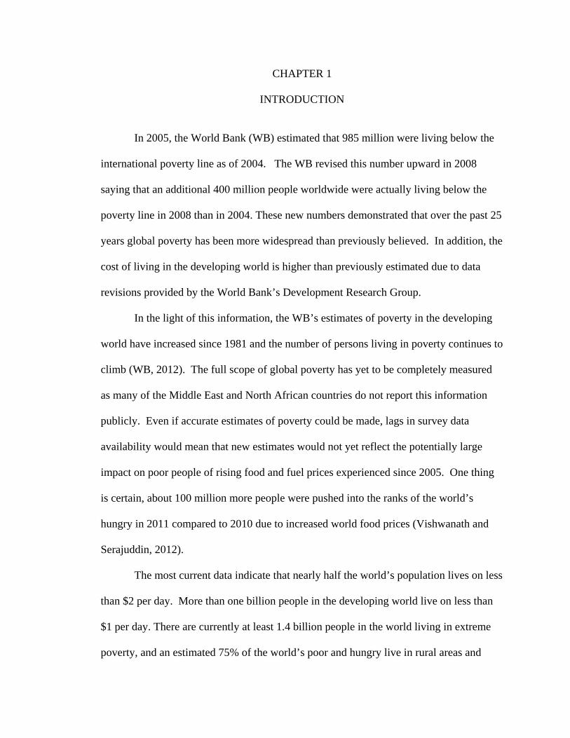
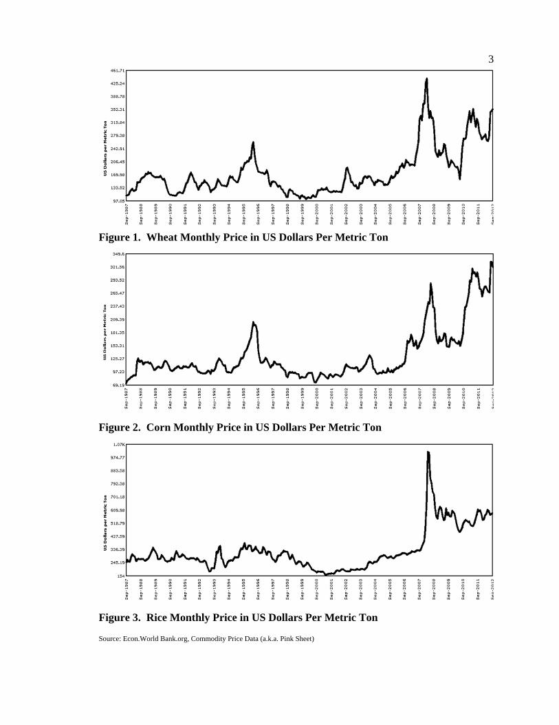
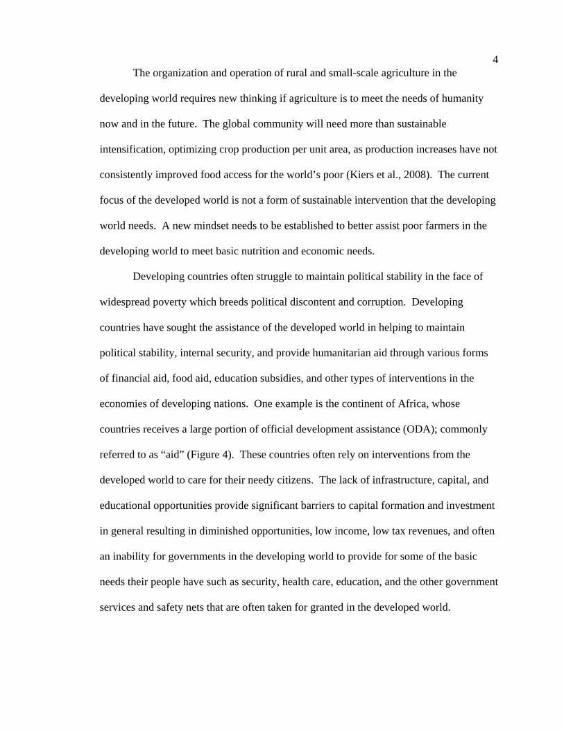
Increases in world food prices, especially for staple foods (figures 1 - 3), have

raised concerns about food security for poor households in the developing world. Food

prices in international markets increased dramatically during 2007 and 2008. The FAO

World Food Price Index rose from 100 in 1980 to 140 at the end of 2004, and reached a

climax of 282 in 2008. Even more recently, the FAO Food Price Index continues with a

high average of 216 points in September 2012 (figure 1.4) (FAO, 2012). Despite the

normalization of domestic food price inflation, domestic food prices in developing

countries remain 25 percent higher relative to non-food consumer prices than they were

at the beginning of 2005 (WB, 2012).

3

Figure 1. Wheat Monthly Price in US Dollars Per Metric Ton

Figure 2. Corn Monthly Price in US Dollars Per Metric Ton

Figure 3. Rice Monthly Price in US Dollars Per Metric Ton

Source: Econ.World Bank.org, Commodity Price Data (a.k.a. Pink Sheet)

4 The organization and operation of rural and small-scale agriculture in the

developing world requires new thinking if agriculture is to meet the needs of humanity

now and in the future. The global community will need more than sustainable

intensification, optimizing crop production per unit area, as production increases have not

consistently improved food access for the world’s poor (Kiers et al., 2008). The current

focus of the developed world is not a form of sustainable intervention that the developing

world needs. A new mindset needs to be established to better assist poor farmers in the

developing world to meet basic nutrition and economic needs.

Developing countries often struggle to maintain political stability in the face of

widespread poverty which breeds political discontent and corruption. Developing

countries have sought the assistance of the developed world in helping to maintain

political stability, internal security, and provide humanitarian aid through various forms

of financial aid, food aid, education subsidies, and other types of interventions in the

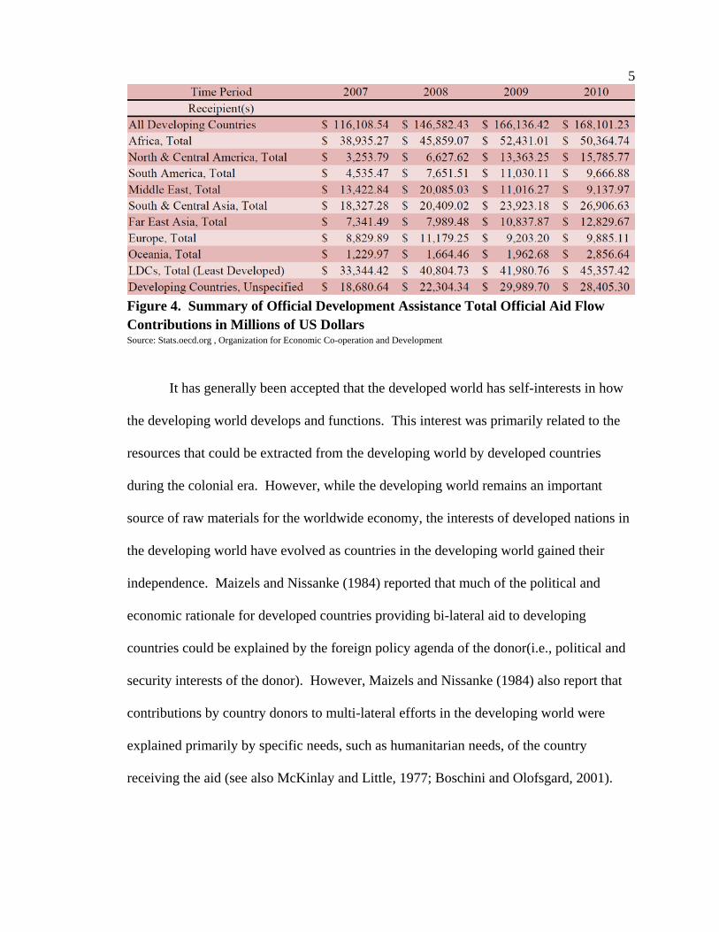
economies of developing nations. One example is the continent of Africa, whose

countries receives a large portion of official development assistance (ODA); commonly

referred to as “aid” (Figure 4). These countries often rely on interventions from the

developed world to care for their needy citizens. The lack of infrastructure, capital, and

educational opportunities provide significant barriers to capital formation and investment

in general resulting in diminished opportunities, low income, low tax revenues, and often

an inability for governments in the developing world to provide for some of the basic

needs their people have such as security, health care, education, and the other government

services and safety nets that are often taken for granted in the developed world.

5

Figure 4. Summary of Official Development Assistance Total Official Aid Flow Contributions in Millions of US Dollars Source: Stats.oecd.org , Organization for Economic Co-operation and Development

It has generally been accepted that the developed world has self-interests in how

the developing world develops and functions. This interest was primarily related to the

resources that could be extracted from the developing world by developed countries

during the colonial era. However, while the developing world remains an important

source of raw materials for the worldwide economy, the interests of developed nations in

the developing world have evolved as countries in the developing world gained their

independence. Maizels and Nissanke (1984) reported that much of the political and

economic rationale for developed countries providing bi-lateral aid to developing

countries could be explained by the foreign policy agenda of the donor(i.e., political and

security interests of the donor). However, Maizels and Nissanke (1984) also report that

contributions by country donors to multi-lateral efforts in the developing world were

explained primarily by specific needs, such as humanitarian needs, of the country

receiving the aid (see also McKinlay and Little, 1977; Boschini and Olofsgard, 2001).

6 Others argue for the involvement of the developed world in the developing world

based on moral obligation. For example, Singer (1972) presented the argument that those

of the developed world, can and ought to do more for the developing nations. He

expressed his disgust regarding the suffering caused by lack of food, shelter, and

healthcare in the developing world. Singer (1972) professed that if the developed world

can prevent one of these “bad” things from happening without sacrificing something of

comparable moral importance, then the affluent people of the developed world are

morally obligated to transfer large amounts of resources to the poor people in the

developing world. Singer’s (1972) conclusion was that interventions need to be made by

the developed world in the developing world to eradicate poverty of the poor until doing

so harms the Developing World more than it benefits them.

The developed world has also provided immense amounts of aid to the developing

world in the form of health (medical or nutrition) programs. While much of this type of

intervention could be considered humanitarian, Howson, Fineberg, and Bloom (1998)

point out that health risk cannot be adequately addressed within traditional national

boundaries. They state:

These risks include emerging infectious diseases, resulting in part from

increased prevalence of drug-resistant pathogens; exposure to dangerous

substances, such as contaminated foodstuffs, and banned and toxic substances;

and violence, including chemical and bioterrorist attack. By investing in global

health, industrialized countries will not only benefit populations in desperate and

immediate need of assistance, but also themselves—through protecting their

7 people, improving their economies, and advancing their international interests. (p.

586)

Intervention often comes in forms of programs aimed at development and poverty

reduction. Sustainability, democracy, capabilities, and woman’s rights have all received

immense attention in recent years, but interventions historically and currently are

commonly manifested as humanitarian aid (e.g., food or health) or development

assistance. For present purposes, consider humanitarian aid to be resources provided to

relieve immediate suffering, and development assistance as resources provided in order to

reduce an insufficiency over the long term. Health aid will be considered as medical and

nutrition interventions including educational activities related to preventative care and

improving nutrition.

A range of policies and programs exist to address household food insecurity and

malnutrition at the local level.1 The International Fund for Agricultural Development

(IFAD) (2011)suggests that nutrition-based aid should address nutrition security by

developing conditions that foster access to a stable supply of food. This narrow focus

usually stems from undernutrition, nutrient deficiencies, and malnutrition.

Undernutrition is one of the major problems in the developing world today. A large

proportion of the world's population does not have enough food to lead healthy and

productive lives. An even larger number of people is at risk of specific nutrient

deficiencies because people are too poor to acquire foods containing essential vitamins

and minerals. Malnutrition is the result from a complex set of interacting elements.

1 Food security was defined by the World Food Summit in 1996 as existing “when all people at all times have access to sufficient, safe, nutritious food to maintain a healthy and active life” (World Health Organization, 2012).

8 These include but are not limited to cultural, social, biological, political, and economic

environments. Thus the argument for different forms of economic intervention is created.

Economic interventions habitually pursue income maximization through projects

that develop economies of scale, share technology and science improvements, facilitate

access to capital, conduct best management practice insemination, and/or grant access to

markets. The end goal of such interventions is usually to create the revenue stream to

externally purchase items needed to overcome malnutrition factors.

Malnutrition cannot be overcome by solely improving access to an adequate diet.

Infections, disease, poor maternal health, and child care practices may be as important a

cause of malnutrition as is inadequate food intake (Unsystem.org, 1992). Therefore,

although food aid by itself can make a significant contribution to relieving hunger, it

cannot be expected to solve a complex problem such as malnutrition. It is when food aid

is combined with other inputs, such as health care, education, improved agricultural

technology and so on, that it can be most effective in overcoming poverty and

malnutrition. This thesis assumes that economic and nutritional interventions need to be

integrated to create a balanced model for aid that will be more sustainable.

A body of literature has emerged challenging the effectiveness of development

aid. Much of this literature has been produced by people in the development and

intervention community who care deeply about poverty reduction (Clement, 2011). The

critical view of aid stems from the separation of initiatives that exists only to address a

portion of the equation. Intervention projects normally aim to satisfy either the nutritional

needs of a group, or advancing the economic stability, but not both. One of the many

issues that may arise by narrowly focusing and creating an aid program is that although a

9 group may be fed, they are not equipped to mitigate risks that will arise after project

completion and thus continue or revert back to a malnourished state. A bridge is required

to join the economic and nutritional interventions to create aid interventions that are

sustainable past the point of donor separation.

Merging economic and nutrition interventions as pursued in this thesis required

the first step to be the creation of economic information for a typical small-scale farm.

The location of the farm was in northern Ecuador, but the basic analysis presented here

could be adjusted and used in similar circumstances in any location in the developing

world. A comprehensive set of estimated cost and return (enterprise) budgets for small-


analysis were developed. This produced a means for comparing crop data to estimate

projected costs, revenue, and net returns for a single enterprise to assess feasibility and

profitability of potential enterprises. These enterprise budgets could also be a planning

tool to test out new ideas and compare enterprises to identify “best” ones as they permit a

comparison of income across different enterprises. Utilizing these enterprise budgets, a

linear programming model, and nutritional information, such as is done in this study,

could help in planning rural development interventions as the income maximization and

least-cost diet models are integrated into one within the resource and management

constraints of the representative small-scale farm.

This model could develop assistance and interventions which consider a broader

range of resources and constraints than analyses of isolated nutritional or economic

interventions. The result could offer additional insights about how nutritional, economic,

and agronomic interventions might act together to reduce poverty and increase health of

10 the rural poor over the long term. The perpetual intergenerational cycle of poverty and

hunger is interdependent and directly related to poor health, which translates into lack of

readiness for school, which harbors poor academic performance, which then positions the

individual to be inadequately prepared for economic opportunities. Supporting surveys

and data sets used in this analysis are composed of information gathered from rural small

scale subsistence farmers in the community of Cochas, within the Imbabura Province of

Ecuador, South America.

11 CHAPTER 2

REVIEW OF THE LITERATURE

The objective of this study was to integrate economic, nutrition, and agronomic

principles into a mathematical-programming, decision-making framework. The reason

this is important is that so much effort and money are expended trying to help the world’s

rural poor, but are often targeted at specific interventions that do not take into full

account the complex interactions of economics, nutrition, and agronomy that determine

whether an intervention is sustainable or not. This chapter presents a review of the

literature about different types of interventions designed to assist the rural poor, their

rationale, contributions, and potential weaknesses. A case is then made for why an

integrated approach makes a contribution to this literature.

Food Aid

Food aid is a difficult subject to summarize because of its intertwining themes. In

general, food aid deals with providing food and related assistance to combat hunger.

Principally food aid is designed for emergency situations (short-term interventions) or to

help reduce severe hunger over the long term by achieving food security. Food security

refers to the availability of food that an individual has access to while starvation is the

severe deficiency in vitamin, nutrient, and caloric intake (FAO, 2012). In 1960, food aid

constituted over 20 percent of all global aid flows in terms of dollar value but now it is

less than five percent (WB, 2010). Although food aid has decreased, this does not signal

that the problem of hunger is becoming less severe. Food aid is still important because of

the prevalence of world hunger and the increase in food emergencies in the past decade

12 (WFP, 2007 and 2012). The decline of food aid as well as the way in which it is

delivered and used, therefore remain very important.

Food aid as a modern policy measure had its start in the 1950s with the United

States together with Canada accounting for over 90 percent of global food aid until the

1970s when the United Nations World Food Program (WFP) became a major player

(Usaid.gov, 2012). International food aid is largely driven by donors and international

institutions. In 1967, the Food Aid Convection (FAC) provided a set of policies for

donor countries and is monitored by the Consultative Sub-Committee on Surplus

Disposal (CSSD) (Foodaidconvention.org, 2010). The CSSD’s primary purpose is to

ensure that food aid does not affect commercial imports and local production recipient

countries (FAO, 2001). In effect, the CSSD ensures food aid does not displace trade.

Food aid is typically separated into three groups to categorize the international

flows that come in the form of food or cash to purchase food in support of food assistance

programs. The three types are program, project, and emergency/humanitarian.

Emergency Food Aid

Emergency food aid, commonly referred also as relief aid, is typically for

emergency situations, such as cases of war, conflict, or natural disaster. Deliveries of

food are provided by a developed country (such as the United States or United Kingdom)

to government and non-government agencies (GO and NGO) responding to crisis in an

affected country or countries where the food is distributed without charge. However, a

number of countries facing some forms of chronic food insecurity have also become

permanent recipients of this form of aid (Mousseau, 2005).

13 Program Food Aid

Program aid often is a form of “in-kind aid” whereby food is grown in the donor

country for distribution or sale abroad. This is typically a government-to-government

transfer which includes deliveries of food to a central government that subsequently sells

the food and uses the proceeds for whatever purpose (not necessarily food assistance).

Rather than being free food as such, recipient countries typically purchase the food with

money borrowed at lower than market interest rates (USDA, 2009). Program food aid

provides budgetary and balance of payments relief for recipient governments.

Project Food Aid

Project aid provides support to field-based projects in a specific area of chronic

need through deliveries of food, usually at no charge, to a GO or NGO that either uses it

directly to promote agricultural or economic development or nutrition and food security,

such as food for work and school feeding programs. At times, this type of food aid is

monetized (sold at market value) to allow the organization to use the proceeds for project

activities. Program and Project Food Aid makes up the majority of aid for the United

States (USDA, 2012).

Shift in Policy and Purpose Relative to Food Aid

Emergency aid used to be a minor form of aid until the 1990’s when it shifted to

being the dominant form of aid provided by the U. S. to developing countries signifying

both an increase in the number of food emergencies and the end of the Cold War (i.e.,

after the Cold War food aid as a political tool for the donor seemed to become less

important) (Mousseau, 2005). As with relief aid, project food aid is typically distributed

by the WFP, NGOs, and occasionally by government institutions (FAO, 2009).

14 The European Common Agricultural Policy (CAP), created in 1962, is geared

towards increasing agricultural productivity and food self-sufficiency (European

Commission, 2011). Through a combination of farm price supports and barriers to food

imports, the CAP generated massive surpluses, especially wheat and animal products,

which made the European Union (EU) and its member countries major actors in

international food trade and food aid (European Farmers Coordination, 2003).

In the 1950s, the Food and Agriculture Organization of the United Nations (FAO)

had warned of the potentially harmful effects of food aid on local agriculture (Oxfam,

2005). Cheap imports from developed countries, including through food aid, often

undermines local agricultural production because it distorts the market and does not

provide local farmers with the opportunity to receive higher prices and expand production

when food supplies in a local area are tight. Food aid drives down food prices and

encourages increased consumption of wheat and dairy. This, in turn, adversely affects

the livelihoods of rural populations and drives the “non-competitive” local farmers out of

agriculture.

As noted earlier, current food aid has seen some changes during the past decade.

Europe, for example, has generally moved away from in-kind food aid, preferring to

purchase locally in the affected country or help facilitate local purchases instead. There

has also been a shift away from long-term development to short-term humanitarian relief.

This has increased the role of NGOs and relief organizations and led to a prioritization by

donors on nations that actually need assistance. This is partly in contrast to the past when

food aid was often targeted towards countries that provided a strategic interest for the

donor, i.e., a “friendly” nation during periods like the Cold War.

15 The EU has shifted towards local and “triangular” purchases. These are food aid

purchases or exchanges in one developing country for use as food aid in another country.

Many argue this type of food aid will lead to more efficient distribution of food and better

support for agriculture, trade, and development in the developing nations. Frederic

Mousseau (2005) of the Oakland Institute summarizes Europe’s shift:

The shift from the export of surpluses to more purchases from within

southern countries has been strongly promoted by a number of NGOs and

researchers over the last twenty years.… Overall, in 2004, 1.6 out of a total of 7.5

million tons of food aid was obtained through local or triangular purchases in

developing countries. The EU officially adopted this policy standpoint in 1996

and adapted its food aid programs accordingly through a progressive increase in

the share of cash assistance for triangular and local purchases and more attention

for non-food interventions. As a result, a major share of EU food aid—90 percent

in 2004—is now procured in developing countries (this figure is only

approximately 1 percent for the US). (p. 11)

However, Europe is not functioning on a completely united front either. While

the EU itself has made this policy modification, some nations such as Italy and France

have lagged by maintaining a flow of in-kind food aid instead of the contractual path

which represents nearly 70 percent of their food aid (Clay, 2006).

React, Rather than Prevent

Relief aid, by definition reacts to emergencies, rather than to prevent them. It is

short-term aid, whereas going to the roots of hunger (e.g. poverty, debt) is more

complicated and leads to problems such as the ones that have been previously discussed

16 with program aid. Emergency food relief therefore goes to fixing disasters that could

have been addressed much earlier with better policies. So both natural disasters, where

emergency food aid is undoubtedly an appropriate and needed response, and human-

made, preventable disasters compete for relief aid (Tearfund, 2005).

Whether organized by a GO or NGO, interventions in the developing world seem

to follow the path outlined by the Millennium Development Goals (MDG) that the United

Nations (UN) have set forth. The first goal (MDG 1) calls to eradicate extreme poverty

and hunger and claims that this goal’s achievement is crucial for national progress and

development (UN, 2010). One of the ways that progress is assessed toward achieving

MDG 1 is the prevalence of underweight children under the age of 5 (UNICEF, 2012a).

Since the MDGs were adopted in 2000, an improved knowledge of the causes and

consequences of under nutrition has been achieved. Reducing the rate of underweight

children depends on the correct design and subsequent implementation of large-scale

nutrition and health programs that provide appropriate food and health care for children

in a country (Vander Meulen and Mucha, 2012). Failure to realize MDG 1 endangers the

achievement of the other MDGs which include improving maternal health, reducing child

mortality, and achieving universal primary education (UN, 2010).

Nutrition

Healthy eating and being physically active are particularly important for children

and adolescents. This is because the nutrition and lifestyle of children influence their

wellbeing, growth, development, and general health throughout their lives. The

nutritional requirements of children and adolescents are high in relation to their size

because of the nutritional demands for growth for children beyond that needed for body

17 maintenance and physical activity (WHO, 2008). Recent evidence makes it clear that

children under the age of five are in the period of high vulnerability to nutritional

deficiencies. Specifically, the period beginning with the woman pregnancy and

continuing till the child is two is when children are at their greatest vulnerability in terms

of the effects of malnutrition. It is during this period that nutritional deficiencies have the

greatest impact on child survival and growth (Engle et al., 2007; UNICEF, 2012a).

Nutritional deficiencies over a period of time lead to diminished or stunted

growth. In the developing world there is a high degree of nutritional stunting, defined as

linear growth failure caused by inadequate caloric intake. Stunting may be intensified by

various infections accompanied by malnutrition (Deboer et al., 2012). Once children are

stunted it is difficult for them to achieve average height, as stunting is considered “the

irreversible outcome of chronic nutritional deficiency during the first one thousand days

of a child’s life” (Unicefchina.org, 2012).

The global burden of stunting is far greater than the burden of children who are

underweight. UNICEF shows that in the developing world, the number of children under

five years old who are stunted is close to 200 million. The children under five years and

underweight are about 130 million (Unicef.org, 2009). Specifically, undernutrition in

early life for girls before they give birth or during early childhood can have perpetual

effects because their future babies are likely to be born with low birth weight which then

leads to undernutrition as those children grow (Langley-Evans, A. and Langley-Evans, S.

2003). This creates a vicious cycle of under nutrition repeating itself generation after

generation due to heritable changes in gene expression (Schoendorfer et al., 2010).

Developmental origins of health problems and disease suggest that developing fetuses

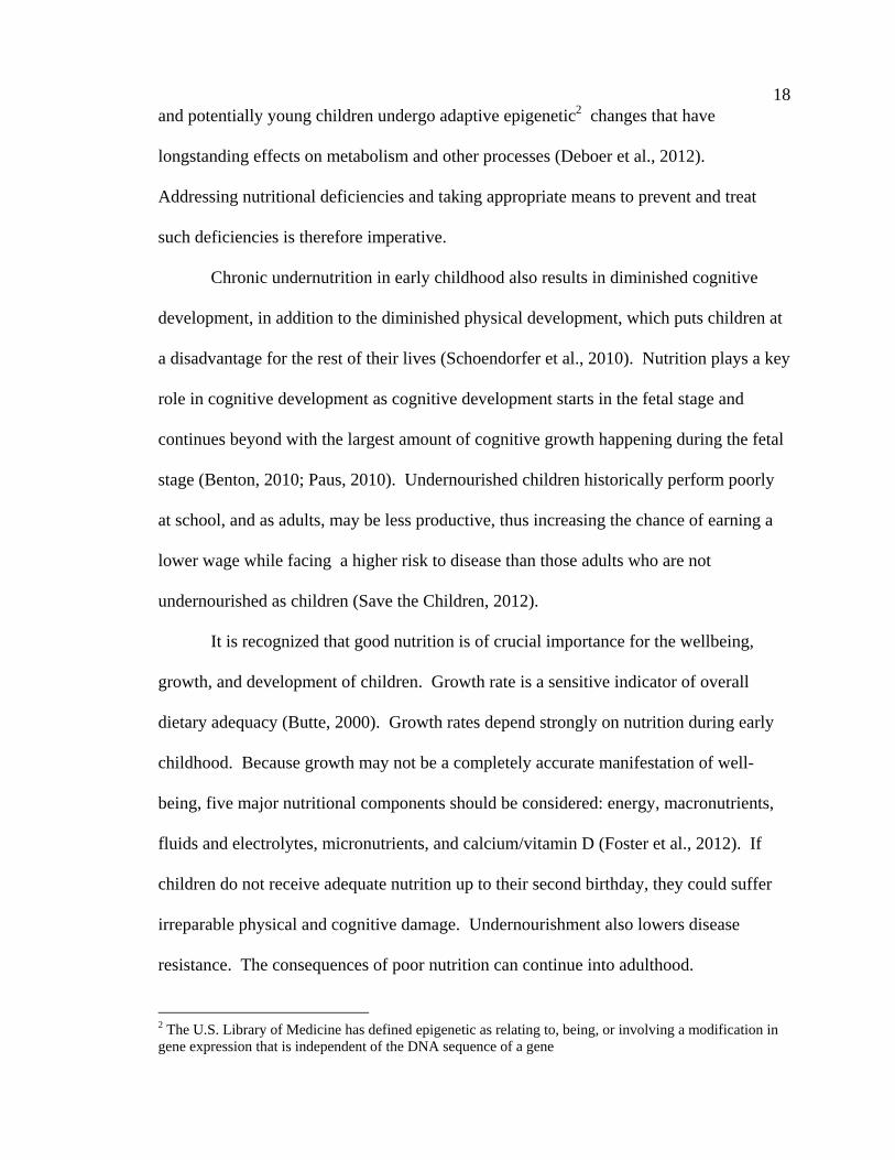
18 and potentially young children undergo adaptive epigenetic2 changes that have

longstanding effects on metabolism and other processes (Deboer et al., 2012).

Addressing nutritional deficiencies and taking appropriate means to prevent and treat

such deficiencies is therefore imperative.

Chronic undernutrition in early childhood also results in diminished cognitive

development, in addition to the diminished physical development, which puts children at

a disadvantage for the rest of their lives (Schoendorfer et al., 2010). Nutrition plays a key

role in cognitive development as cognitive development starts in the fetal stage and

continues beyond with the largest amount of cognitive growth happening during the fetal

stage (Benton, 2010; Paus, 2010). Undernourished children historically perform poorly

at school, and as adults, may be less productive, thus increasing the chance of earning a

lower wage while facing a higher risk to disease than those adults who are not

undernourished as children (Save the Children, 2012).

It is recognized that good nutrition is of crucial importance for the wellbeing,

growth, and development of children. Growth rate is a sensitive indicator of overall

dietary adequacy (Butte, 2000). Growth rates depend strongly on nutrition during early

childhood. Because growth may not be a completely accurate manifestation of well-

being, five major nutritional components should be considered: energy, macronutrients,

fluids and electrolytes, micronutrients, and calcium/vitamin D (Foster et al., 2012). If

children do not receive adequate nutrition up to their second birthday, they could suffer

irreparable physical and cognitive damage. Undernourishment also lowers disease

resistance. The consequences of poor nutrition can continue into adulthood.

2 The U.S. Library of Medicine has defined epigenetic as relating to, being, or involving a modification in gene expression that is independent of the DNA sequence of a gene

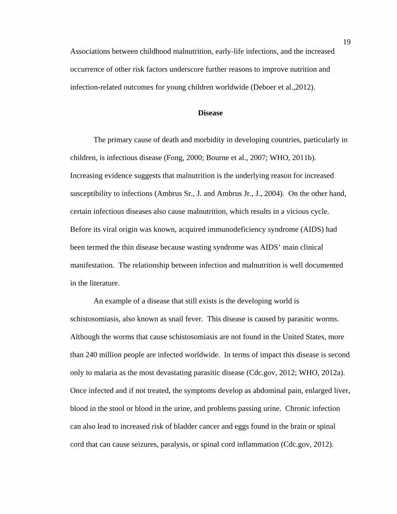
19 Associations between childhood malnutrition, early-life infections, and the increased

occurrence of other risk factors underscore further reasons to improve nutrition and

infection-related outcomes for young children worldwide (Deboer et al.,2012).

Disease

The primary cause of death and morbidity in developing countries, particularly in

children, is infectious disease (Fong, 2000; Bourne et al., 2007; WHO, 2011b).

Increasing evidence suggests that malnutrition is the underlying reason for increased

susceptibility to infections (Ambrus Sr., J. and Ambrus Jr., J., 2004). On the other hand,

certain infectious diseases also cause malnutrition, which results in a vicious cycle.

Before its viral origin was known, acquired immunodeficiency syndrome (AIDS) had

been termed the thin disease because wasting syndrome was AIDS’ main clinical

manifestation. The relationship between infection and malnutrition is well documented

in the literature.

An example of a disease that still exists is the developing world is

schistosomiasis, also known as snail fever. This disease is caused by parasitic worms.

Although the worms that cause schistosomiasis are not found in the United States, more

than 240 million people are infected worldwide. In terms of impact this disease is second

only to malaria as the most devastating parasitic disease (Cdc.gov, 2012; WHO, 2012a).

Once infected and if not treated, the symptoms develop as abdominal pain, enlarged liver,

blood in the stool or blood in the urine, and problems passing urine. Chronic infection

can also lead to increased risk of bladder cancer and eggs found in the brain or spinal

cord that can cause seizures, paralysis, or spinal cord inflammation (Cdc.gov, 2012).

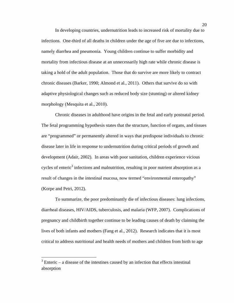
20 In developing countries, undernutrition leads to increased risk of mortality due to

infections. One-third of all deaths in children under the age of five are due to infections,

namely diarrhea and pneumonia. Young children continue to suffer morbidity and

mortality from infectious disease at an unnecessarily high rate while chronic disease is

taking a hold of the adult population. Those that do survive are more likely to contract

chronic diseases (Barker, 1990; Almond et al., 2011). Others that survive do so with

adaptive physiological changes such as reduced body size (stunting) or altered kidney

morphology (Mesquita et al., 2010).

Chronic diseases in adulthood have origins in the fetal and early postnatal period.

The fetal programming hypothesis states that the structure, function of organs, and tissues

are “programmed” or permanently altered in ways that predispose individuals to chronic

disease later in life in response to undernutrition during critical periods of growth and

development (Adair, 2002). In areas with poor sanitation, children experience vicious

cycles of enteric3 infections and malnutrition, resulting in poor nutrient absorption as a

result of changes in the intestinal mucosa, now termed “environmental enteropathy”

(Korpe and Petri, 2012).

To summarize, the poor predominantly die of infectious diseases: lung infections,

diarrheal diseases, HIV/AIDS, tuberculosis, and malaria (WFP, 2007). Complications of

pregnancy and childbirth together continue to be leading causes of death by claiming the

lives of both infants and mothers (Fang et al., 2012). Research indicates that it is most

critical to address nutritional and health needs of mothers and children from birth to age

3 Enteric – a disease of the intestines caused by an infection that effects intestinal absorption

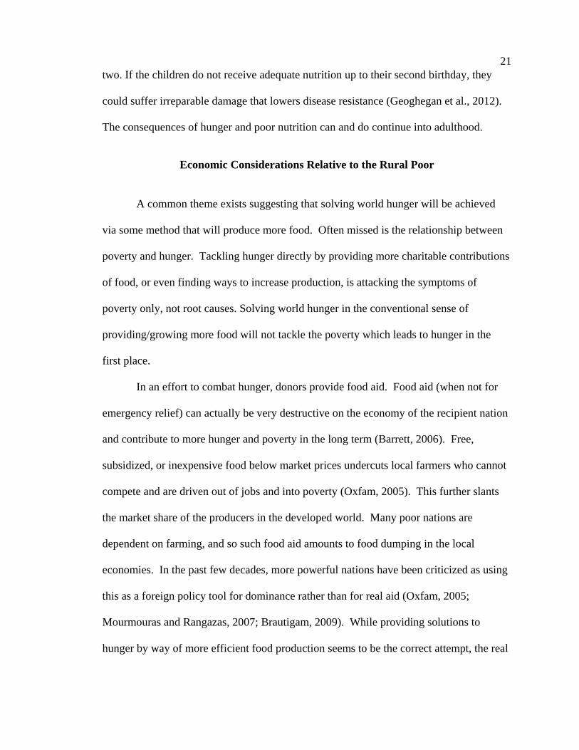
21 two. If the children do not receive adequate nutrition up to their second birthday, they

could suffer irreparable damage that lowers disease resistance (Geoghegan et al., 2012).

The consequences of hunger and poor nutrition can and do continue into adulthood.

Economic Considerations Relative to the Rural Poor

A common theme exists suggesting that solving world hunger will be achieved

via some method that will produce more food. Often missed is the relationship between

poverty and hunger. Tackling hunger directly by providing more charitable contributions

of food, or even finding ways to increase production, is attacking the symptoms of

poverty only, not root causes. Solving world hunger in the conventional sense of

providing/growing more food will not tackle the poverty which leads to hunger in the

first place.

In an effort to combat hunger, donors provide food aid. Food aid (when not for

emergency relief) can actually be very destructive on the economy of the recipient nation

and contribute to more hunger and poverty in the long term (Barrett, 2006). Free,

subsidized, or inexpensive food below market prices undercuts local farmers who cannot

compete and are driven out of jobs and into poverty (Oxfam, 2005). This further slants

the market share of the producers in the developed world. Many poor nations are

dependent on farming, and so such food aid amounts to food dumping in the local

economies. In the past few decades, more powerful nations have been criticized as using

this as a foreign policy tool for dominance rather than for real aid (Oxfam, 2005;

Mourmouras and Rangazas, 2007; Brautigam, 2009). While providing solutions to

hunger by way of more efficient food production seems to be the correct attempt, the real

22 problems lie in distribution, land ownership, inefficient use of land, and politics with its

accompanying power plays.

There are important issues with the identification of the poor and how they

survive. First, computing the poverty line utilizes purchasing power parity exchange

rates which have been criticized as being inadequate, infrequently updated, and

inapplicable to the consumption of the extremely poor (Deaton, 2006). Coupled with

incomplete data collection and reporting within the developing world, it is challenging to

properly define and measure this subset of the global population. It is certain though that

the percentage living in poverty is growing and is faced with insurmountable food prices.

Food prices are typically considered to be higher in urban than rural areas. A

further review indicates that in rural areas, the poor may pay different prices than

everyone else (typically higher) due to the lack of competition. Subsequently, families

that depend on small-scale agriculture are at a greater disadvantage than those who are

not as the prices paid for inputs and later received in payment for crops are commonly not

at the “going rate”. The small-scale farmer pays more for inputs and does not receive full

farm-gate price when it is time to sell the harvest (Banderjee and Duflo, 2006).

Structural Adjustment Programs (SAP) have been implemented in most

developing countries over the past two decades. They have generally led to the

elimination of public intervention in the agricultural sector, including state-led

institutions such as marketing boards, which in the past supported small-scale farmers

through credit, inputs, and facilitation of market access (WHO, 2012b). SAPs have also

encouraged the concentration of agricultural trade and production, which excludes small-

scale farmers from business and growth (Mousseau, 2005).

23 In a small restricted market, price and yield tend to offset one another. The

smaller the local harvest, the greater the price per unit received and vice versa since

supply and demand are largely determined by the harvest itself. Within a world market

however, this nexus between local harvest and price is broken and the world price varies

more or less independently of local supply (Scott, 1976). Accepting that the world

operates on a competitive market, the farmers in developing countries are producing in a

global market and thus must compete with all the other farmers in the world to produce

and sell their crop. Producers in a competitive market cannot control price so they must

produce at or below market price to remain in business in the long run. Generally, any

cost advantage small-scale agriculture in developing countries have is through labor costs

(Ward and Bailey, 2012). Farmers and supporting agricultural laborers work for very

small amounts of money. One major disadvantage small-scale farmers compared to

larger-scale farmers have is scale. Small-scale limits access to capital purchases and

achieving economies needed for discounts and sales. This implies that the labor

advantage of small-scale farmers in the developing world is their competitive edge. The

problem is that labor prices are rising in some parts of the developed world such as China

and India suggesting that this advantage may be shrinking except for the poorest of the

poor (Sharma, 2009).

The area of the world that receives the most attention regarding the existence of

hunger and related aid is Africa. Until the food price alarm went off in recent years,

discussions on how to reduce hunger and malnutrition in Africa took place in an

environment of declining food prices with estimates indicating that real food prices

declined by about 75 percent between 1974 and 2005 (Economist, 2007). Since then,

24 strong upward trends in global food prices occurred in 2007–2008, in late-2010, and

again in mid-2012 (figure 5). This created the concern that hunger and poverty will

increase across the world as the access to affordable food to the poor is reduced. People

are hungry not due to lack of availability of food or the ability to produce food

worldwide, but because people do not have high enough income to purchase the

nutritious food they need and because distribution of food is not equitable. In addition,

politics also influence how food is produced, who it is produced by with subsequent

benefits, and for what purposes the food is produced; such as for exporting rather than for

the hungry and feedstuffs within a food-deficit country.

Figure 5. FAO Nominal and Real Food Price Index

If efforts are only directed at providing food, or improving food production or

distribution, then the structural root causes that create hunger, poverty and dependency,

would still remain. This is not to say that research aimed at increasing food production

should not be done, it is to illustrate that attacking the roots of poverty that cause hunger

would allow better use of resources in the long term. Not fighting root causes of poverty

25 and only fighting hunger will be costly in the long run as people will continue to be

hungry and resources will be continually diverted to remedy hunger in a superficial

manner without addressing its cause. Agricultural sectors need to be provided with the

right investments and incentives to produce sufficient food and lay the basis for broad-

based and sustainable economic growth.

The Need for Interventions

Poverty traps call for external intervention because no spontaneous mechanism

exists to stop the eternal round of poverty. Several contributory factors such as poverty,

lack of purchasing power, household food insecurity, and limited general knowledge

about appropriate nutritional practices increase the risk of individuals in developing

countries. External support in either government or non-government forms can help

alleviate the physical and economic challenges that the world’s poor confront on a daily

basis. Many different interventions have been created to help the suffering populations of

the world secure a better quality of life while trying to disrupt the vicious cycle that

accounts for the high mortality and morbidity rate in these countries. Some of the

interventions and reasons they are implemented are:

Vaccinations- to help control disease/infection Supplements- to help provide the nutrients needed for healthy growth and support

the immune system to reduce infection Sanitation- eliminate disease and infection through controllable aspects of life Micronutrient/Macronutrient Crops- provide a source to create a balanced diet,

least cost ration Education- provide individuals with learning to succeed Storage- provide food security Cash Cropping- create cash flow Marketing- create access to markets Technology and Science- allow farmers to better compete, be efficient with time

26 Best Management Practices- insemination best management practices by way of

classroom lessons and on farm teaching

This study serves to review a portion of the more dominant aid and intervention

programs that have been implemented and are summarized into the sections of 1) Health,

2) Farm, and 3) Finance.

Health

Interventions designed to improve health are in effect designed to improve the

quality of life of those who participate. Health interventions have multiplier effects as

they contribute to “sustained population and economic gains in poor countries” (Bhalotra

and Pogge, 2012). As morbidity and mortality decrease, mothers tend to have fewer

births as offspring and potential offspring become more likely to survive. This lowers the

growth of population while contributing to a greater economic growth (Galor and Weil,

2000). To reduce morbidity and mortality, the most prolific interventions are sanitation

programs, vaccines/immunizations, and supplements.

Sanitation

Creating a clean environment can reduce exposure to infectious disease. In the

developing world, many health problems are directly related to fecal-oral contact by food

or water (Cairncross, 2003). Cholera, e-coli, hepatitis A, rotavirus, giardia, and

tapeworm are common infections contracted and spread through poor sanitation (Gerba et

al., 2009). To insure a greater level of sanitation, interventions provide disinfectant hand

rub, latrine construction, teach hand washing practices, point of use water filtration, and

also provide water access projects such as drinking water wells (Rodgers et al., 2007;

Allegranzi et al., 2010; Ngondi et al., 2010; Kaewchana et al., 2012).

27 Vaccines

The World Health Organization claims that 2-3 million deaths are averted

annually by vaccination. Yet, only 20 percent of children who need antibiotics receive

them (WHO, 2010a). Whether it be the developed world or the developing, the evidence

is clear about the need for vaccines and immunizations to prevent many diseases. Within

the literature, the terms immunization and vaccine are used interchangeably even though

in the medical profession there is a specific use and definition for each of these terms

(Dorlands.com, 2012).

Strong evidence exists that interventions using vaccinations are an effective

means to assist in lifting the world’s poor from poverty. One trial involving de-worming

in Kenyan schools estimates that treatment generated 2–3 additional years of schooling

and a 21–29% increase in income (Baird et al., 2011). Other studies using cohort data on

large-scale historical interventions arrive at remarkably similar estimates. A

retrospective analysis estimates that malaria eradication in the Americas increased wage

income by 15–27 percent (Bleakley, 2010). Immunization programs within developing

countries have been shown to decrease disease transfer creating better health within

households and communities, thus fostering economic growth (Bhalotra and Rawlings,

2012). Although vaccine interventions may come with relatively high costs, the cost

benefit analysis shows returns anywhere from .59 to over 22 times the savings for every

unit invested in vaccines and immunizations (Bloom et al., 2005). The benefits produced

by vaccine interventions are estimated to be even greater over the span of a generation

(Bhalotra and Rawlings, 2010). The continued push for vaccination-based interventions

28 is centered on the fact that infectious diseases can only be eliminated if high levels of

vaccination are achieved and maintained (Campbell, 2006)

Supplementation and Fortification

In 1989, Stephen DeFelice coined the term and defined nutraceutical as any

substance that is a food or a part of food that provides medical or health benefits,

including the prevention and/or treatment of disease (Nutraceuticals World, 2011). The

generally accepted terms within the world of nutrition are supplementation and

fortification (SF). Such products may be categorized as dietary supplements, specific

diets, herbal products, or processed foods such as cereals, soups, and beverages. Dietary

supplements can be extracts or concentrates and are found in many forms, including

tablets, capsules, liquids, and powders. Vitamins, minerals, herbs, or isolated bioactive

compounds are only a few examples of dietary ingredients in the products. Functional

foods are designed as enriched foods close to their natural state, providing an alternative

to dietary supplements manufactured in liquid or capsule form (Adelaja and Schilling,

1999; Whitman, 2001; Azizi, 2012). Generally, the SFs used in developing countries are

in pill or liquid form.

Supplements are a popular form of a supplementation program to help achieve

better nutrition because of the minimal cost, often $1 or less per individual per year,

associated with treating nutritional deficiencies (Chow et al., 2010; Hki.org, 2008).

Vitamins such as vitamin C, vitamin E, and vitamin A are the common forms of

supplements (Clark et al., 2008; Hki.org, 2011). However, there are many SFs and even

more interventions that employ the use of them. This is based on previous studies which

show the improved benefits to health resulting from taking these supplements. It should

29 be noted that SF interventions are not always based on previous studies completed about

SFs benefits specific to individual antioxidant nutrients (Sun, 2005). Interventions are

often based on studies of the foods rich in these nutrients and related benefits (Chao et al.,

2012).

Continued support for SFs is created as more studies of previous interventions

prove they have been successful in achieving nutritional goals for the poor. Between

1969 and 1977, one intervention supplied protein shakes with other micronutrients to

persons in four villages in Guatemala (Habicht et al., 1995). Thirty years later, the

International Food Policy Research Institute (IFPRI) conducted a study to investigate the

long-term effects of the supplied nutraceutical. The study found that participants of the

original intervention did not suffer growth failure, completed more schooling, scored

higher on cognitive skill tests, and earned higher wages than others not receiving the

supplements. Specifically, the results for women participants were they had fewer

pregnancies, and lower risk of miscarriages and stillbirths (Hoddinott et al., 2011).

Although supplements are shown to be beneficial, governments are recognizing

that these types of programs are not sustainable. They are turning to food crops to solve

the issues that the concentrated forms of macro and micro nutrients have not been able to

sufficiently address. Examples include Bangladesh and the Philippines who have joined

the cause of Golden Rice (Irri.org, 2011). Most famous for its failure due to its intense

orange color resulting from it having 23 times more beta carotene than “normal” rice,

Golden Rice is seen as a sustainable solution to providing millions with adequate intake

of vitamin A (Mayer, 2005). India has recognized that the previous decades of vitamin A

supplementation programs have not been effective on a large enough scale. As a result,

30 India has begun to stress that the avenue to prevent deficiency should be through better

food rather than with pills (Palmer and West, 2010; Indianexpress, 2012; UNICEF,

2012b).

Helen Keller International (HKI) is a leading global health organization that has

been instrumental in reducing vitamin A deficiency in the developing world. HKI’s first

effort toward blindness prevention and treatment was the distribution of vitamin A

capsules in the Asia-Pacific area and Central America in 1960-1970. Since then HKI has

expounded its effort for achieving vitamin A nutrition through continuing to gift vitamin

A capsules, creating dietary diversification through homestead gardens and husbandry to

provide vitamin A rich foods, directing initiatives to fortify commonly used food such as

cooking oil with vitamin A, and promoting the consumption and production of orange-

fleshed sweet potatoes that have been bred with higher levels of beta carotene (a

precursor to vitamin A) (Hki.org, 2011).

Farm Focus

Seventy-five percent of the world’s poor live in rural areas and most are involved

in agriculture. According to the WB (2012), agriculture remains fundamental to

economic growth, poverty alleviation, and environmental sustainability. Rural

industrialization is very limited so smallholder agriculture continues to be the source of

growth while improving the lives of the rural (Berdegué and Fuentealba, 2011). To meet

the challenge of improving incomes in rural areas, a transformation is needed from the

low-input, low-productivity, semi-subsistent system that characterizes the majority of

rural farming within the developing world (Govereh et al., 1999). The transformation is

normally pursued through integration of cash cropping.

31 Cash cropping

A cash crop is one that is produced for sale. From the perspective of the small-

scale farmer, the cash crop can be food or non-food use because its purpose is to generate

revenue rather than to be consumed by the family. A subset of cash crops is export crops

which are particular cash crops that are ultimately exported from the country. Political

interventions promoting particular crops are typically focused on export agreements

while micro level aid looks at supporting small-scale agriculture.

When reviewing the efforts of NGO’s, the focus on cash cropping is to assist

farmers in creating a crop for local markets. It deals with everything from teaching

individuals with vacant land how to efficiently prepare a crop large enough to sell to

helping change a farmer’s crop selection so that the crop generates more income than

what has been grown by the farmer in the past.

The most common commercialization in rural small-scale agriculture is the

production of marketable surplus foodstuffs over what is needed for own consumption

(Gebre-ab, 2006). This is because staple food crops have traditionally been produced

under the subsistence system so it is believed that the smallholders have adequate

knowledge and experience in these commodities (Jaleta et al., 2009). Interventions at the

farm level are aimed at introducing new yield-enhancing technologies for subsistence

crops to generate a surplus to be sold at market. This is seen as increasing household

income at a lower risk while still improving the level of food security for poor farm

families (Fafchamps, 1992). Small-scale farmers are typically risk adverse so different

modes of production targeting high-value non-traditional commodities that could help

farm households generate more income per unit of resources used are not commonly

32 pursued because of the higher production and market risk that usually accompanies these

strategies (Jayne, 1994).

The yield-enhancing technology most commonly used for cash crops is the

application of fertilizers (Duflo et al., 2006; Banful, 2011). When the land area permits,

development strategies may use mechanization to boost production levels allowing

farmers to work larger amounts of land within planting and harvesting time periods

(Singh, 2006). On a limited scale, crop interventions will implement hybrid seed

programs. These programs are very minimal as a historical practice for subsistence

farmers is to save seed for the following crop which becomes impossible with the

majority of genetically modified seed varieties (Goldman, 2001).

Storage

When harvest comes, small-scale farmers typically sell their crop without storing

it often due to their lack of storage facilities. In the absence of government price supports

such as exist in the United States, most small-scale farmers sell their crops at harvest but

often at a price that is lower than the seasonal average, all other things being equal. This

problem (plunging prices at harvest) could possibly be reduced if farmers could wait past

the end of harvest and sell (store the crop) when the price started to climb as supplies

began to dwindle. In addition to cash crop storage for sale later, a need may be present

for the household to hold inventories of staple foods they have raised (store) for later

consumption. For these reasons, interventions have been devised to train small-scale

farmers in improved handling and storage hygiene, using hermetically sealed bags, and

construction of bulk storage devices such as silos (FAO, 1994; Baoua et al., 2012;

Murdoch, 2012). In effect, better storage directly equates to greater food security.

33 Savings and warehousing can help farmers improve their bargaining power and

provide greater returns to help lift them out of poverty. Providing a means for storing

crops not only benefits the farmer through potentially increased revenue, it also helps

minimize loss of crop and the aggravation resulting from the loss of the inputs invested in

growing the crop such as irrigation water, human labor, and expensive fertilizer.

Creating ways for small-scale farmers to save staple foods efficiently minimizes

their reliance on local markets for basic food items when producing foods for the farm

family’s own consumption may be less expensive than purchasing the food in local

markets. In addition, storage may allow rural households to create stocks of food as a

contingency against supply disruptions in food products sold at local markets.

Infrastructure

Once a surplus of crop is accumulated, the next challenge, in the case of a cash

crop, is to get it to market. At the macro level this means that intervention designed to

facilitate marketing may come by way of creating, improving, and/or expanding market

infrastructure. Infrastructure is a key to farmers’ bargaining power (Bond et al., 2012).

Limited infrastructure brings condition where intermediaries dictate the price in the

village, simply because they know farmers cannot afford to sell elsewhere (Joshi et al.,

2007).

Current investments in infrastructure in the rural developing world now are

appearing not to be under the umbrella of aid, but under the influence of agricultural

outsourcing. The majority of the world's remaining cultivatable land lies in developing

countries (Cotula et al., 2009). Current studies show that about 95 percent of Asia’s

croplands have been utilized which is forcing countries such as China to look elsewhere

34 to feed their growing population. (Faostat.fao.org, 2012). The cheap and abundant

farmlands in developing nations, particularly in Africa, drive capital rich nations to

consider outsourcing their food production to these locations (Cotula et al., 2009). As of

2011, over 20 Chinese companies had been in negotiation with African and Latin

American countries to invest in agriculture, food, forestry, fishery and biofuels activities

(Afripol.org, 2010; Cobo et al., 2011; Saturnino et al., 2011). Africa and Latin America

are where foreign investors are already creating access to arable land (Kye-Woo et al.,

2012).

Currently China is at the forefront of the developed or semi-developed countries

in developing infrastructure in the developing world; financing some of the largest

infrastructure projects in the developing world. In eastern Africa, the Chinese are

building a massive highway that is 16 lanes wide in some places that will help connect

Ethiopia and Kenya (Langfit, 2011). In northern Africa, China and Japan are working

together to build a 745-mile east-west highway across Algeria which will connect the

country with Tunisia and Morocco (Newsmax.com, 2011). In Columbia, China is

looking to build a 136-mile railway to compete with the Panama Canal and connect the

Caribbean with the Pacific Ocean (Time.com, 2012).

Financial

Access to financial services for rural farmers is necessary as a means to increase

their productivity including purchasing better inputs such as fertilizer and investing in

better production and marketing methods. There is a huge need for financial tools to

ensure the day- to-day operation of farms and to assist in their development (Mahajan and

Vasumathi, 2010). This huge demand is faced with the very limited supply of credit in

35 rural areas of the developing world, so few rural areas in the developing world benefit

from access to credit facilities (Gine and Yang, 2009). Traditional and formal sources of

capital funds are typically geared to be offered to large-scale rather than small-scale

farmers so new financial tools have been designed to facilitate growth related to small-

scale farming in the developing world.

Microfinance

Microfinance has often been described as a powerful tool in fighting poverty,

specifically in very impoverished areas. Those who support microfinance efforts often

refer to micro-credit programs as development initiatives that empower people to help

themselves. Others highlight the “pay-for-itself” benefits of microfinance. In its infancy,

microfinance issued the promise that it could provide a way to lift millions out of poverty

with programs that would pay for themselves. Now that the novelty of microfinance has

faded, microfinance has come under increasing scrutiny as aid organizations,

development practitioners, and development partners continue to create microfinance

interventions. Critics argue that the promised benefits of microfinance programs are not

what they seem and that this financial vehicle rather causes harm to those it is was

created to help (Bauchet et al., 2011).

The microfinance model is designed to provide poor people with access to capital

which is supposed to increase investment in the short and long term by increasing cash

flow in impoverished areas. Theoretically, the additional cash flow in these areas would

lead to the acquisition of production assets, improve health and nutrition, and increase the

level of education for household members (Pitt et al., 2006). Investments would then

improve the households’ capabilities to respond to shocks and enhance their scope for

36 putting in place preventative measures which would eventually assist them in lifting

themselves out of poverty and reduce the risk of returning to it.

The evidence of the impact of microfinance reviewed for this project has revealed

a much more complex picture exposing positive and negative impacts which suggests that

there are some components of microfinance which must be addressed if microfinance is

to serve the poor.

Beneficial Impacts of Microfinance

There is a large literature which finds beneficial socio-economic impacts as the

result of microfinance. The recurring final effects reported in the literature are indicated

as being income stability and growth, reduced income inequality, reduced vulnerability,

employment, nutrition and health improvements, school attendance, strengthened social

networks, and women’s empowerment (Barnes, 1996; Schuler et al., 1997; UNICEF

1997; Barnes and Keogh, 1999; Wright, 2000; Khandker, 2001; Afrane, 2002; Beck et

al., 2004; Hietalahti and Linden, 2006; Hossain and Knight, 2008; Coppock et al., 2011).

One study specifically highlights that female micro-credit clients are more likely to invest

in their children’s nutrition and health expenses than those that do not participate in

microfinance (Doocy et al., 2005).

Negative Impacts of Microfinance

It is equally easy to find studies alluding to potential negative impacts associated

with microfinancing. The claimed unfavorable consequences resulting from

microfinancing indicted in the literature included effects such as the exploitation of

women, increased income inequality, creating dependencies, increased workloads, high

interest rates, unchanged poverty levels, and creating barriers to sustainable local

37 economic and social development (Adams and Von Pischke, 1992; Goetz and Sen Gupta,

1996; Rogaly, 1996; Buckley, 1997; Kabeer, 1998; Copestake et al., 2002; Bateman and

Chang, 2009). A potential negative impact of microfinance interventions related to

education was reported in Shimamura and Lastarria-Cornhiel’s assessment (2010) of

micro-credit initiatives in rural Malawi. The study was to evaluate the impact of

agriculture credit on children’s school attendance and found a correlation with the

increased of time required in the fields by the adults and the decrease of female children’s

attendance at school as a result of the parents being involved in microfinance activities

(2010). This was further supported by Barnes who reported that extended periods of

borrowing reduce children’s school enrollment (Barnes et al., 2001).

Mixed Evidence about Microfinance

Not all studies on microfinance are conclusive. For example, some evaluations

show benefits for the poor but not for the poorest of the poor (Hulme and Mosley, 1996;

Mosley and Hulme, 1998; Murdoch, 1998; Copestake et al., 2001). One particular study

found that microfinance was effective in helping the poor to better manage the money

they have (Rutherford 1996) but did not sufficiently enough to increase income (Husain

et al., 2010). Karnani (2007) argues that money spent on microfinance interventions

could be better used for other interventions, like supporting large, labor-intensive

industries for job creation.

There is also literature arguing that a single intervention (such as microfinance) is

less effective as an anti-poverty resource than simultaneous efforts combining

microfinance, health, and education (Lipton, 1996). Another study of micro-credit in

Ghana found initial mixed results for microfinance programs at the household and

38 business levels in four districts. However, the longer the clients participated in the

program, the more negligible the impact became in all four districts, compared to control

groups (Nanor, 2008). This suggests that past examinations of microfinance program

may have been carried out prematurely and may not provide accurate results to fully

understand the long-term effects of these programs. This creates the argument that the

success and failures of other interventions may have been greatly influenced by the

timeframe in which results were collected.

In summary, the definition of “development” used influences how microfinance

interventions are assessed in terms of success or failure. If the ultimate aim of

microfinance is expanded beyond just increasing household or business income,

microfinance interventions are generally judged to be more successful than if income is

the only indicator of success for the program. Other indicators such as positive outcomes

related to health and education tend to support the finding that microfinancing programs

are successful (Roodman, 2012). Detailed analyses of income and expenditure at the

household level appear to provide a more accurate indication of how microfinance

interventions impact actual recipients and their family rather than analyses examining

only the income generated by the business endeavors (e.g., expenditures on education,

health care, and better food). However, focusing on non-wealth outcomes, such as health

and education, without assessing financial indicators or considering both short- and long-

term outcomes would also potentially provide misleading information. As indicated in

the literature, families could increase their education and health expenses in the short

term as a result of microfinancing programs, but fail to realize significant sustainable

financial improvements for their households. Research focusing solely on non-financial

39 outcomes might show an increase in education expenditure, without recognizing that

there has been a reduction in overall income. Therefore, a careful analysis of all links

between microfinance interventions and their connections to wealth and non-wealth

outcomes is necessary to avoid distorted evaluations of microfinance interventions.

Savings and Investment by the Rural Poor

The poor save all the time. Savings are often the only way the poor can manage to

pay for 1) a major life event such as a marriage or funeral, 2) survive a natural disaster, or

3) take advantage of a business opportunity. The poor rarely have access to voluntary

deposit services offered by formal or semi-formal institutions. Instead, they are obliged to

save informally.

The poor will convert their cash into livestock purchases, hide cash at home,

employ their neighbors to collect it, or participate in rotating savings and credit

associations. These informal savings devices can be categorized as being high risk,

illiquid, and indivisible (Rim and Rouse, 2002). A cow, for example, can die of disease

or must be sold as a whole to obtain cash (are lumpy in terms of economics). The

opportunity does not exist for the farmer to sell just the rear quarters to pay for his child’s

schooling. The entire investment has to be converted to cash when a need arises.

Additionally, the transaction incurs time and financial costs. Credit often serves the same

purposes as savings for the poor even though it poses more risk and is typically more

expensive. When electing to save, the poor are often willing to pay to do so (Banerjee and

Duflo, 2006). Savings are arguably more important than credit in helping the poor to

raise incomes and reduce risk. It can be argued, however, that the income impact may

take longer to realize with savings (Cgap.org, 2006).

40 Insurance

The investment decisions of small‐scale farmers in developing countries are

conditioned by their financial environment. Borrowing constraints in the market and

scarce insurance can reduce investment in activities with high expected profits. Increased

insurance is associated with riskier production choices in agriculture (Karlan et al., 2012).

Intervention programs have encouraged the use of inputs such as hybrid seeds and

fertilizers to boost cash crop yields with their supporting evidence of high expected

returns but continually coordinators are faced with opposition from subsistence farmers

not wanting to diverge. The social gains from solving the risk problem could be

substantial. If risk discourages the investment and the marginal return on investment is

high, the returns to removing risk could be high (Dercon and Christiaensen,2011; Carter

and Barrett, 2012).

When provided with insurance against the major risk they face, farmers are able

to find resources to increase expenditure on their farms (Cai et al., 2010). When farmers

have more capital, access to it, or available insurance, their production decisions are not

as likely to reflect the bias of eating preference (Karlan et al., 2012). The opposite holds

true when markets lack insurance and access to capital, the separation of the decisions of

production and consumption does not exist. Interventions that communicate benefits

from increased expenditure on fertilizer, land preparation by way of mechanization, and

hired labor would do well to couple the program with a product such as insurance to

lower vulnerability to shock thus increase adoption rate (Karlan et al., 2012). Subsistence

farmers need access to insurance to take risks when they are so close to the poverty line.

41 Importance of Trans-Disciplinary Integration

The microfinance literature points out succinctly that a broad approach is called

for when analyzing the impact of different possible interventions for the rural poor. This

includes not only short-term impacts on income, but also household decisions to invest in

education and health care. The literature also demonstrates the crucial role nutrition

plays in the overall wellbeing of the rural poor in terms of their performance at work and

school. Integrating household decisions and wellbeing into analyses is an important step

to more fully understanding the complex interactions between economics, nutrition, and

agronomy that determine whether or not any particular intervention can have both short-

term and long-term beneficial results. Obviously, other factors such as culture,

sociology, infrastructure, and disabilities affect the wellbeing of households. However,

the focus of this study is on these components (economics, nutrition, and agronomy) as

an initial step at integrating some of the general features of a household contributing to

the sustainability of various potential interventions.

Understanding the impact of different interventions on several different

dimensions of poor rural households provides a broader perspective of tradeoffs existing

in the household in terms of how well-intended interventions may lack sustainability if

they are not able to achieve objectives that result in better outcomes for the household

that are independently integrated into the household’s way of life. The model presented

in this study consists of a mathematical linear program (LP) which incorporates the

nutritional, economic, and agronomic characteristics of a typical agricultural household in

northern Ecuador. The LP allows for the observation of how these dimensions

(economics, nutrition, and agronomy) affect decisions made by the household and how

42 some targeted interventions may or may not achieve the best outcomes in these three

areas. It is anticipated that tradeoffs exist when considering different interventions and

the LP sharpens and contrasts competition and complementarity between and among

different goals that may be pursued with different interventions.

Successful interventions must achieve not only short-term but also the long-term

positive outcomes for the household if they are to be fully integrated into the household

way of life. In terms of economics, this would mean achieving goals such as permanent

increases in average income and reduction of economic risks. For nutrition, it might

mean assuring that children have enough nourishment to avoid long-term health problems

and to be able to do well in school. For agronomy, it may mean being able to achieve

better yields or better crop rotations. Taken separately, each of these goals would result

in a positive outcome for the family. However, the goals may in fact be in conflict with

each other. For example, changing crop rotations could result in more variety and

availability of nutritious foods for the farm family but could result in a substantial loss in

cash income. Consequently, interventions should not be considered in isolation but

should also account for potential impact of other aspects of the farm family’s life.

Many well-intended interventions focus solely on one aspect of need for the rural

poor, such as nutrition. The thesis of this study is that combining several decisions faced

by the farm family into a single, integrated model will provide additional insights

regarding how different aspects of the farm family’s lives interact. The result should be

an increased understanding of how interventions may be designed to take into account

more aspects relating to these households than just one.

43 CHAPTER 3

METHODOLOGY

A major underlying question and potential problem faced by sustainable

agriculture and development efforts has been how to address the need for increased food

production to coincide with increases in population while maintaining and preserving the

earth’s resources and environment (Economist, 2011). This is difficult given an expected

global population of over nine billion by 2050 with approximately 80 percent of the surge

in population expected to occur within developing countries (UN, 2012). NGOs and GOs

are providing aid and implementing other interventions while looking toward options for

improving agricultural production and welfare of some of the world’s poorest farmers,

the small-scale farmer. But, one of the easiest ways to accomplish this is with

technologies such as fertilizer and chemicals that could harm the environment.

In 2011, over $130 billion was spent worldwide by mostly developed countries on

development assistance and aid with over $41 billion going to the low-income countries

(World Bank, 2010a). Recent estimates say that there are about 40,000 NGOs in the

world in addition to other community-based organizations which number in the hundreds

of thousands. Consequently, huge amounts of effort and resources are being expended in

various good causes, including attempting to raise the world’s poor out of poverty.

Obviously, the problem of rural poverty is large, complex, and persistent. Many

alternative goals and approaches to reducing rural poverty are being pursued by GOs and

NGOs and certainly the majorities of these various efforts accomplish many good things

and help people to have better lives.

44 This study recognizes that planning interventions to help the rural poor should

take into account the interconnectedness of the financial, agronomic, and nutritional

decisions of the rural poor who are often small-scale farmers. The approach taken is to

develop an initial integrated model capable of measuring the impact of potential

interventions on whole-farm decisions by small-scale farmers. The purpose of this model

is to provide some initial illustrations of how those attempting to provide assistance to

small-scale farmers might consider the impacts of these interventions on several facets of

the farm family and their operation. The model proposed in this study provides an

addition instrument which can be used to evaluate proposed and current economic,

nutritional and agronomy-based programs (interventions) for their potential viability.

Economics is an important consideration in programs designed to help small-scale

farmers and their families because if basic economic rules are violated, say that a

proposed intervention does not improve overall economic viability for the small-scale

farm, then it is highly likely that the intervention will not be sustainable and will cease to

function (be used by the farm family) once funding ceases. The sustainability of

interventions is, of course a primary concern for the assistance/aid community. Many

programs in the past have enjoyed initial success and participation by small-scale farmers

and other members of the rural poor, only to essentially disappear when funding was no

longer made available to support the efforts of these programs.

Unsustainability (interventions which are unable to sustain themselves) may

happen due to changes in focus by the government entities specifying the target of dollars

going to aid. It also occurs when interventions depend on the grace of third-party donors

and those donors move on to other projects or stop funding the current NGO. It may

45 even be the original design of the intervention to end because it is implemented as a

temporary trial with a planned expiration date. Often aid programs are rightly criticized

for creating a dependence, a paternal aspect, on external participation so when the

intervention ceases for whatever reason, the effort related to that intervention in the local

area crumbles (FAO, 2006).

Nothing is free, but goods and services may be provided at no cost to the recipient

of the goods and services provided by interventions. There is always an opportunity cost

which is the next highest-valued alternative use of that resource. For the developing

world, the idea of opportunity cost might be manifested in the time invested taking care

of a new crop that could have been used instead to work at an unskilled job in a city.

Although the intervention may be well-intended, those who implement the intervention

may fail to assess the opportunity cost that the program creates. It is arguable that an

intervention that makes a gift of inputs, such as vegetable seed, to small-scale farm

families helps them to create a family garden which can lead to improved nutrition of the

family. However, the intervention may have overlooked that the time spent caring for the

garden could have produced income that could have purchased more food than was

produced in the garden by working off the farm and then purchasing the same food in the

market.

This thesis is an initial attempt to bring together agronomic, nutritional, and

economic aspects to examine how different interventions in small-scale agriculture

interact with these aspects of the farm. This is accomplished by using a LP model

designed to maximize the income of a small-scale farm family in northern Ecuador while

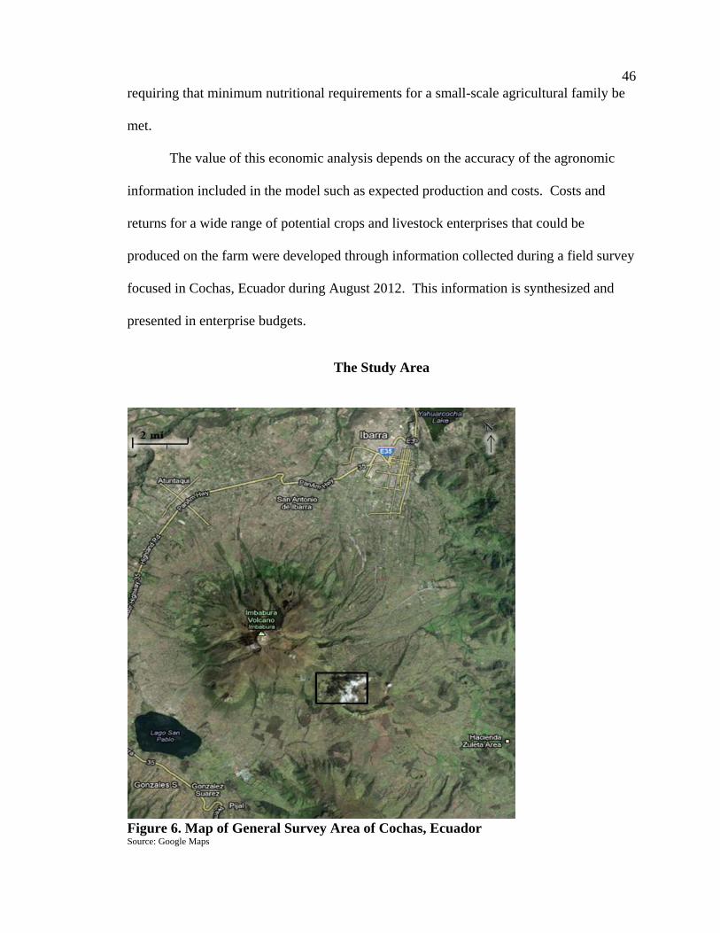
46 requiring that minimum nutritional requirements for a small-scale agricultural family be

met.

The value of this economic analysis depends on the accuracy of the agronomic

information included in the model such as expected production and costs. Costs and

returns for a wide range of potential crops and livestock enterprises that could be

produced on the farm were developed through information collected during a field survey

focused in Cochas, Ecuador during August 2012. This information is synthesized and

presented in enterprise budgets.

The Study Area

Figure 6. Map of General Survey Area of Cochas, Ecuador Source: Google Maps

47 The community of Cochas La Merced is located within the province of Imbabura

Ecuador near the Peruvian border. It sits on the Andes mountain range at about 2,800

meters above sea level. It takes approximately three hours to drive to the capital of

Ecuador, Quito, and about one hour to drive to the local city of Ibarra.

The current community was a part of the Fraile plantation. When the last Fraile

family member passed away, the land was given to the workers and their families. The

land was divided into sections called “huasipungos” which is a Quichua word for a small

portion of land for personal use. The divisions of land divided in this manner average

between 1-2 hectares. The land is controlled by force meaning that few families are

registered owners (have actual deeds) of the property on which they work. No written

documents or descriptive coordinates that perfects a family’s claim to land exist. It is

possible to receive “escritura” (proven ownership) but the cost and know-how to do so

are major inhibitors to these families doing so.

This community became the study area for this research. The study area was

selected based on existing contacts with people and organizations operating programs in

this part of Ecuador. Key contacts included the Institute for Self-Reliant Agriculture

(SRA) and Capital Seed. The Ezra Taft Benson Institute has had programs in Ecuador

for a number of years. SRA has close connections to the Benson Institute and has been

operating programs as follow-ons to Benson Institute activities in this part of Ecuador.

The Managing Director and Partner of Capital Seed, Mr. Justin Perry, was instrumental in

setting up contacts for information and surveys in the study area. These connections and

the fact that a number of different NGOs have operated in this part of Ecuador for a long

time made this location a good choice in terms of the ability to gather the necessary

48 agronomic, economic, and nutritional information that was required to complete the

study.

Homes in the study area are built from bricks made with local clay and are sun

dried. Floors are dirt, and walls are without windows. Roofs are fastened from straw,

branches, and corn stalks. The local people wash their clothes by hand outside, and have

minimal power requirements. Some of the people have a small gas cooktop. As of

August 2012, the community census showed that the community had 196 homesteads and

that all of them have water service. The potable water source is a natural reservoir located

higher in the Andes on the side of an extinct volcano adjacent to the community. This

reservoir is replenished by rain and snowfall each year.

Families that were contacted to provide information for this study and responded

to questions in a survey that will be described later. The families participating in the

survey ranged in size from single individuals to families of 12 or more. Some families

living in the community may be even larger due to multi-generations living on the same

sector of land. Average family size considered for this study was six and was composed

of three children, both parents, and a grandparent. The household fathers in the area

typically work in the town of Ibarra traveling each day to and from work by bus from

home. Often though, fathers and older sons work for extended periods of time in Quito

(performing manual labor) and returning home every eight to 22 days to help with harvest

or to bring their earned money home.

Family farms in the study area have historically focused on producing field crops

for cash market sale and daily consumption. The typical farmer engages in harvesting

potatoes, corn, wheat, quinoa, and barley. The daily diets of the farm family have

49 consisted primarily of these same food stuffs with sporadic consumption of vegetables

purchased at local markets. But, vegetables are not considered staple parts of the average

diet in the study area. SRA has recently become involved in the community in facilitating

small-scale farmers in the incorporation of family gardens into their farm plan.

This community, like many rural small-scale and poor areas of the world, has a

nonmarket orientation being they are subsistence farmers. They face abundant

limitations in learning new production techniques, acquiring and use of technology, and

do not depend on the local market to supply their food needs.

Process of Gathering Data for the Study

Primary data were collected through a survey in the study area during the month

of August, 2012. The survey4 was created with the goal of gathering the specific data

needed to create enterprise budgets for different crops and also to create the social

backdrop needed to better understand accepted agricultural practices as well as family

characteristics.

The survey included sections designed to collect information needed to express

the typical family through farm design and practices, and capture the economic situation

that these families lived in (sample survey in Appendix F). All interviews were

conducted in Spanish. An initial pilot survey was developed and administered to six

families. This first survey was designed to test my proficiency in Spanish and to confirm

the question formation. Spanish is not the only language spoken in this rural community.

4 The survey procedures received the necessary approvals from the Internal Review Board at Utah State University.

50 I was blessed with having a local guide to accompany me to facilitate the translation into

Quichua should the need arise.

Within the first few surveys, it became evident that classical Spanish terms would

not be appropriate in all questions. An example was the questions in the survey referring

to fertilizer. In classic Spanish, the translation is “fertilizante” but the local term used is

“abono.” Not only did this term and several others need to be changed, the actual

formation of the questions had to be updated to mirror the sentence structure used in local

conversation. Corrections were made based on what was learned in the initial survey and

a final review practice survey was conducted with the local guide to verify the efficiency

of the survey in collecting the data needed. The final draft of the survey was conducted

with 20 families. Under the direction of the community president, Luis Alberto Anrrango

Lechón, and treasurer, Maria Fabiola Churuchumbi Sandoval (also my town guide), 20

families were selected that she considered would reflect the over-all average family and

farming practices within the community.

Each of the surveys was completed by the researcher to ensure integrity of

answers and to clarify any misconceptions about what the questions we were attempting

to ask. The surveys were carried out over six days. I would meet the available family

members at their home at a designated time, with the assistance of the community guide.

Most frequently we would be sitting underneath a shade tree or overhang of one of the

houses to escape the scorching heat, while being in view of the crops area to facilitate the

answering questions. Each survey averaged one hour to complete.

On arrival at the home, time typically needed to be spent earning the family’s

trust. This culture requires relationships first before details of a private nature about the

51 family and the farm are willing to be shared. The culture requires that the researcher and

the family spend time getting to know each other before any information will be shared

by the family. Due to the personal and sensitive information that the survey questions

imposed, on the average, I spent an additional hour to an hour and a half creating the

confidence needed to proceed with the interview. This additional time was not entirely

focused at the beginning of each survey, but the need manifested itself within each survey

when it was evident that time was needed away from the direct questions so that we could

simply converse with the participants. Eventually the conversation would lead back to

the focus of formulated survey questions.

After arrival and once the transition from small talk to the survey questions had

occurred, the first portions of questionnaire were asked in fairly quick fashion. The

conversation would then soon morph into a more informal conversation with the sharing

of personal stories on the part of both parties with the survey questions being imbedded

into the conversation. I believe this method allowed the interviewees to feel more

relaxed as did I. I base this on the contrast between the frigid feelings which existed

while administering the practice surveys during the previous days compared to the warm

feelings which existed when a more informal conversation was pursued in the course of

the survey with the respondents.

In addition to investing the six days in survey data collection, I participated in

local events which supplied me with many supporting details. Within the events such as

a class given on how to use a grain grinder, a town hall meeting, and a local farmer

market; I was able to gain an increased relationship of trust within the local community.

52 I believe this contributed to the excellent and very specific information the last six

families shared with me during the final round of surveys.

Besides the group events, I was invited multiple times to family meals and

invested six hours rolling bread dough in preparation for the harvest festival. The

discussions that occurred over the meal table and around campfires allowed me to better

understand the dynamics of the relationships within this rural small-scale agricultural

community. It was within these cherished opportunities that the culture became more

evident to me by way of individuals expressing to me the trials that they face on a

personal or family level. These intimate conversations partly influenced the selection of

certain intervention studies that were reviewed in the literature section of this thesis.

Knowing what the local people were experiencing and what outsiders had tried to do for

them in the past helped me better comprehend what might or might not be an effective

and sustainable intervention for the poor, rural farmers in this and other similar

communities. This equipped me with the knowledge of possible available solutions that

are specific to the rural poor throughout the world.

The surveys were successful in collecting the data needed to describe the typical

agronomic, family, and economic situation used to develop the enterprise budgets and

supporting tables. In addition to the surveys that were conducted, I was able to have

conversations with family members from the majority of the households in Cochas during

other events (there are a total of 198 households in Cochas). Pictures and videos were

also recorded to facilitate recall of families and conversations. The locations of these

interviews were also marked by GPS coordinates and recorded on the family surveys to

53 facilitate information recall by providing me with photos of each area surveyed and to

eliminate confusion between plots.

Enterprise Budgets

Enterprise Budgets estimate the costs and returns for an activity (enterprise) such

as raising livestock, producing grain, or growing vegetables for a given production period

(e.g., one year). Thus, enterprise budgets are frequently titled “estimated costs and

returns.” Decision makers can use enterprise budgets to evaluate options before

committing resources to carrying out a particular activity. Enterprise budgets can help

determine breakeven yields or prices and facilitate the calculation of potential returns on

an investment. This level of itemization will ideally provide support in identifying profit

and cost centers within the business. Enterprise budgets also provide critical input for

whole-farm planning; including the potential income for a particular farm, the size of

farm needed to achieve a given potential return, and anticipated cash flows during the

year.

Enterprise budgets present information on the projected returns and costs

associated with a particular crop or livestock enterprise. The information in an enterprise

budget is presented in different sections (see Table 1 for an example of an enterprise

budget used in this study). The first section of an enterprise budget reports anticipated

revenue for the enterprise, the second section anticipated out-of-pocket (variable) costs,

the third section non-cash costs such as unpaid family labor and depreciation on

equipment and buildings. The final section of an enterprise budget describes the

anticipated returns above costs that are projected for the enterprise.

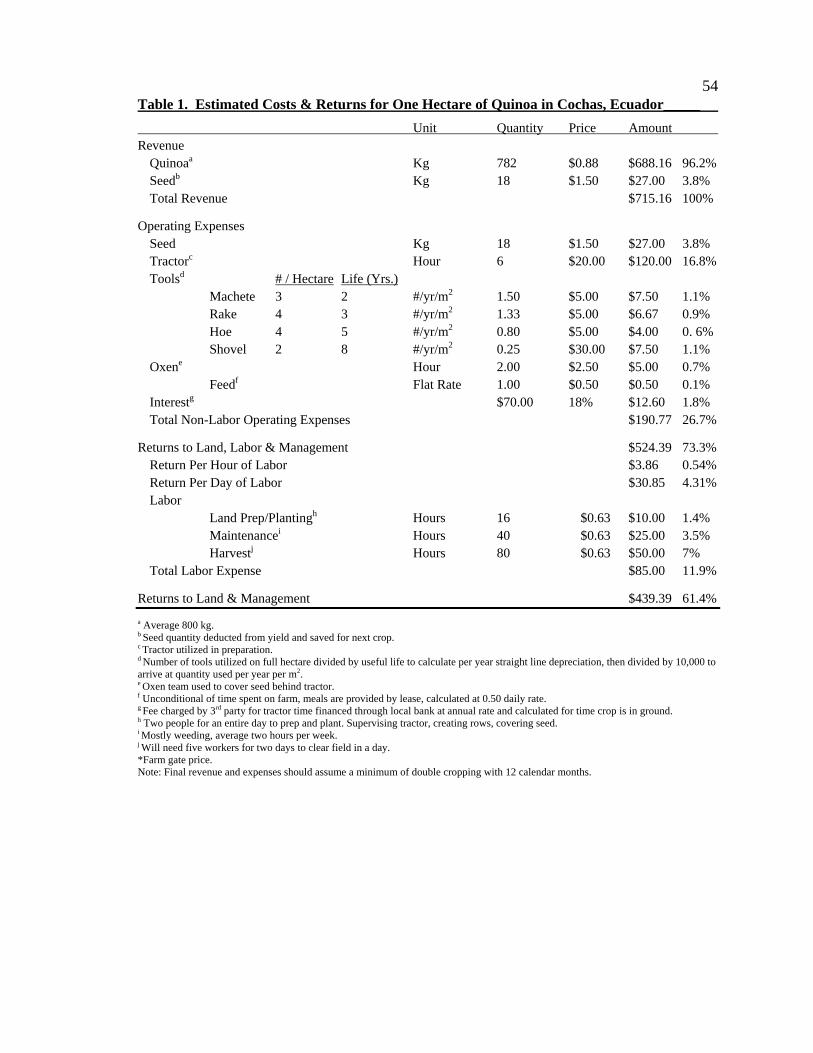
54 Table 1. Estimated Costs & Returns for One Hectare of Quinoa in Cochas, Ecuador_____

Unit Quantity Price Amount Revenue Quinoaa Kg 782 $0.88 $688.16 96.2% Seedb Kg 18 $1.50 $27.00 3.8% Total Revenue $715.16 100%

Operating Expenses Seed Kg 18 $1.50 $27.00 3.8% Tractorc Hour 6 $20.00 $120.00 16.8% Toolsd # / Hectare Life (Yrs.) Machete 3 2 #/yr/m2 1.50 $5.00 $7.50 1.1% Rake 4 3 #/yr/m2 1.33 $5.00 $6.67 0.9% Hoe 4 5 #/yr/m2 0.80 $5.00 $4.00 0. 6% Shovel 2 8 #/yr/m2 0.25 $30.00 $7.50 1.1% Oxene Hour 2.00 $2.50 $5.00 0.7% Feedf Flat Rate 1.00 $0.50 $0.50 0.1% Interestg $70.00 18% $12.60 1.8% Total Non-Labor Operating Expenses $190.77 26.7%

Returns to Land, Labor & Management $524.39 73.3% Return Per Hour of Labor $3.86 0.54% Return Per Day of Labor $30.85 4.31% Labor Land Prep/Plantingh Hours 16 $0.63 $10.00 1.4% Maintenancei Hours 40 $0.63 $25.00 3.5% Harvestj Hours 80 $0.63 $50.00 7% Total Labor Expense $85.00 11.9%

Returns to Land & Management $439.39 61.4%

a Average 800 kg. b Seed quantity deducted from yield and saved for next crop. c Tractor utilized in preparation.

d Number of tools utilized on full hectare divided by useful life to calculate per year straight line depreciation, then divided by 10,000 to arrive at quantity used per year per m2. e Oxen team used to cover seed behind tractor. f Unconditional of time spent on farm, meals are provided by lease, calculated at 0.50 daily rate. g Fee charged by 3rd party for tractor time financed through local bank at annual rate and calculated for time crop is in ground. h Two people for an entire day to prep and plant. Supervising tractor, creating rows, covering seed. i Mostly weeding, average two hours per week. j Will need five workers for two days to clear field in a day. *Farm gate price. Note: Final revenue and expenses should assume a minimum of double cropping with 12 calendar months.

55

Revenue

The revenue stream created by selling agricultural products produced by the

enterprise is located in the “Revenue” section of an enterprise budget (see Table 1).

Revenue involves calculating the value as the product of price and the amount of

agricultural product that would be available to be sold.

Enterprise budgets were developed for this study for a wide range of field crops,

vegetables, and livestock enterprises. This was done as a method to benchmark crops and

livestock that could be produced small-scale farmers in the study area. The enterprise

budgets also became the basis for the economic portion of the LP model which selected

which agricultural enterprises the farm should pursue to achieve its objectives.

Developing the enterprise budget required assuming some basic information about the

farm. This information was developed through the surveys. For example, the land area

considered for the farm was one hectare, a fairly typical land area for a farm in the study

area.

Field crop (see Table 2) yields were collected from over 20 families and

synthesized to create average yields expected for each of the given enterprises. The full

list of enterprise budgets created from the surveys is found in table 2. The full enterprise

budgets compose Appendix A. Each field crop enterprise contains a footnote stating the

average field size that was measured with corresponding yields. Because garden-type

crops, such as vegetables, are grown on small plots of land, costs and returns were

developed for them on a per square meter basis. Costs and returns were then scaled up to

the hectare level assuming a linear transformation on prices, i.e., costs and returns per

hectare were 10,000 times what they were on a square meter.

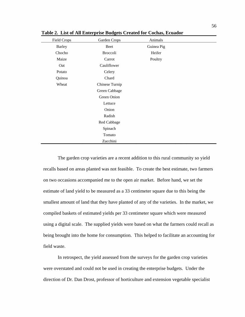
56

Table 2. List of All Enterprise Budgets Created for Cochas, Ecuador

Field Crops Garden Crops Animals

Barley Beet Guinea Pig

Chocho Broccoli Heifer

Maize Carrot Poultry

Oat Cauliflower

Potato Celery

Quinoa Chard

Wheat Chinese Turnip

Green Cabbage

Green Onion

Lettuce

Onion

Radish

Red Cabbage

Spinach

Tomato

Zucchini

The garden crop varieties are a recent addition to this rural community so yield

recalls based on areas planted was not feasible. To create the best estimate, two farmers

on two occasions accompanied me to the open air market. Before hand, we set the

estimate of land yield to be measured as a 33 centimeter square due to this being the

smallest amount of land that they have planted of any of the varieties. In the market, we

compiled baskets of estimated yields per 33 centimeter square which were measured

using a digital scale. The supplied yields were based on what the farmers could recall as

being brought into the home for consumption. This helped to facilitate an accounting for

field waste.

In retrospect, the yield assessed from the surveys for the garden crop varieties

were overstated and could not be used in creating the enterprise budgets. Under the

direction of Dr. Dan Drost, professor of horticulture and extension vegetable specialist

57 for Utah State University, a more realistic yield was calculated based on averages in the

United States.5 This assumed, of course, that yields in Ecuador would not exceed those

in the United States. The data to construct the potential yield was derived from the

National Agricultural Statistics Service datasets and case studies conducted by other

universities (Molinar et al., 2005; Kolota et al., 2010; Smith et al., 2011; Ucdavis.edu,

2012; USDA, 2012). The seeding rate developed from the surveys also presented a

potential inaccuracy in the enterprise budges so these rates were reduced to reflect the

information associated with yields in the USDA and university published datasets that

were used to develop the yields used in the enterprise budgets. Dr. Drost, who has

extensive experience working on issues related to vegetable crops not only in the United

States but also in this part of South America, confirmed the validity of the adjusted yields

and seeding rates used in the enterprise budgets.

Besides revenue from harvest, the budgets also include a line for seed income (see

Table 1). The field crops include seed planted that is typically saved from previous

harvest. Although no cash or credit was extended to supply the seed, it is included in the

revenue as all inputs have a market value even when produced on the farm. This is to

reflect the opportunity cost as they would be sold or eaten if not used in production.

Operating Expenses

The sum of variable costs and fixed costs make up the total cost of producing any

farm commodity. Variable costs are the costs of inputs used during one production

period and are variable because the total dollar value of operating inputs is a function of

the amount used and amount of the commodity produced. Labor was excluded from this

5 Using U. S. yields likely overstated perspective yields for the garden crop varieties, but was more realistic that what was generated using the method described earlier.

58 section of the enterprise budget (see Table 1) and accounted for in the third section of the

enterprise budget to facilitate a comparison across enterprises of what the various

enterprises could “afford” to pay for labor (based on income above out-of-pocket costs).

This provided an estimate of the opportunity cost of labor when used to produce the

various crops or livestock. That is, crops and livestock enterprises with the largest

returns above out-of-pocket costs offered the highest economic “opportunities” for labor

(farm family or hired labor).

Tractors are used in field preparation and seeding for some of the larger field

crops. The tractor is rented from a nearby hacienda and the rental rate for the tractor

includes a trained driver. Tractors are only used when the family cannot supply an

adequate number of labor hours for planting within the designated time of the planting

calendar. A planting calendar is a yearly schedule that designates the opportune time for

planting with expected harvesting dates to create the greatest yields. The planting of field

crops in this area of Ecuador is highly correlated with rainfall since no large scale

irrigation is used with minimal considerations due to cold weather and adjustments

accounted for being positioned along the equator. A crop calendar comprised of average

planting dates for this community can be found in Appendix B.

Fixed costs are prorated over the expected life of the asset, based on straight-line

depreciation, typically over a period of years. Fixed costs are not affected by short-term

decisions and are associated with the normal wear-and-tear on tools and other equipment

that are itemized under “tools” (see Table 1). The tools listed on the enterprise budget

represent the average number and type of tools used by the surveyed farmers along with

59 their average useful life.6 The fixed costs listed in the budges are for the hand tools used

to produce both the field crops and garden crops. Garden crops incur additional fixed

costs associated with enclosure that must be built to keep out pests, such as rabbits, and

irrigation system. The enterprise budgets for vegetable crops reflect the design of the

typical garden areas managed by farmers in the survey. The participants in the survey

who had gardens were gifted the enclosure materials by an NGO operating in the local

area. The enclosures around the gardens consisted of landscape fabric for walls and

fallen trees as posts for anchors. This was to protect the garden against extreme winds

and wild predators. Drip irrigation systems used in these gardens were also gifted as part

of an intervention program of the NGO.

Interest expenses for the garden crops is calculated in the enterprise budgets on

direct expenses such as the seed, water, and drip system repair per square meter of garden

(see Table 1). Field crop interest is assessed on tractor fees for preparing and planting

and is charged based on the amount of time between the land is prepared and the crop is

harvested and ready for market. An interest rate of 18 percent per annum was available

for borrowed capital in the local town and this is the rate that was used to calculate

interest expenses in the enterprise budgets. This rate may be low though compared to

other areas in the developing world where it is reported that interest rates may be as high

as 18 percent per month, resulting in interest rates in the hundreds of percent per annum

(source). Total non-labor operating expenses are added and then subtracted from total

revenue to arrive at the amount that would be available to pay the other non-cash inputs

used in production.

6 The metal component of each tool may last longer than indicated and replacement handles may be made from tree branches.

60 Return to Land, Labor, and Management

The return to land, labor, and management summarizes the residual amount of

revenue left after subtracting operating expenses (see Table 1). Essentially, return to

land, labor and management must pay for family labor and other family resources

devoted to producing the crop or livestock enterprise. If only returns above operating

costs are used as the basis for judging the profitability of a particular intervention, it must

be recognized that this assumes that family labor would be provided at no cost. Again, a

basic rule of economics is that nothing is free. Opportunity costs for labor may be very

low, especially in isolated areas of the developing world. In such cases, it may be

justifiable to consider that labor, especially family labor, requires only a very small return

when calculating the returns to any particular intervention. However, if family members

have other potential opportunities, say to work off of the farm, then the return to land,

labor, and management become extremely important because this return must compete

with the other opportunities available to the farm family. Proposed interventions must

account for the opportunity cost of the family’s labor when calculating the potential

benefits to the family. Otherwise, returns for the intervention may be overstated resulting

in the probable unsustainability of the intervention once the donor ceases to provide

funding for the intervention.

Labor

The return per hour of labor is calculated by summing the hours of labor needed

in the time frame (length of the production period such as a year or six months) required

for the enterprise and divided the sum into the previous line of returns to land, labor, and

management. The “return per day of labor” is calculated by multiplying the “return per

61 hour of labor” by eight hours. The daily pay in the area for a “peon,” day laborer, is

$5.00. The average amount of the day that a worker is in the field is eight hours.

Paid workers will typically spend the entire day working the land with lunch and

supper provided. An 8-hour work day at $5 equates to $0.625 per hour and this rate is

used to calculate the expense for the different subareas of “labor” in the enterprise

budgets (see Table 1). Wage rates off the farm tend to be higher than for on-farm work.

However, caution should be exercised when comparing the wage for hired labor on the

farm to the wage that could be earned off of the farm. On-farm productivity, and hence,

the return on hired farm labor are dependent on how productive and profitable different

crop or livestock enterprises are. Conversely, even though off-farm wage rates might be

higher than on-farm wage rates, one must also subtract from the off-farm wage rate any

costs associated with working off of the farm such as travel to and from work and the

cost of meals away from home when at work. The labor expense for producing the

enterprise at the $0.625 hourly rate is summed and presented by “total labor expense” in

the enterprise budget (see Table 1).

Returns to Land and Management

In enterprise budgets when no land charge is included, returns should be

interpreted as being returns to land and management. In the community of Cochas, land

has no direct cost (see study area section). Positive returns above total operating costs

indicate that the enterprise is self-supporting and generates enough revenue to cover all

variable costs and all, or at least some portion, of fixed costs. If an enterprise can cover

its costs, including opportunity costs, it creates a scenario where producing more of the

profitable crop or livestock enterprise would result in higher returns for the farm family.

62 In other words, the enterprise could be scaled up and the farm family would make more

profit after covering expenses. This would also reward the operator financially for

managerial skills. However, if returns to an enterprise are negative, the enterprise is not

generating enough revenue to cover costs and eliminating this enterprise will increase

profits or minimize losses by decreasing losses in the overall operation.

Percentages

Each enterprise budget developed for this study includes a column on its far right

illustrating the percentage of each line item compared to total revenue (see Table 1). For

example, revenue streams percentages indicate what proportion each activity contributes

to total revenue. For expenses, the percentage specifies what proportion amount of gross

revenue is consumed (expended) on that component of costs to produce the enterprise.

Summary of Enterprise Budgets

The enterprise budgets presented in this study are designed to provide a

framework for making projections about the short- and long-range sustainability of

various interventions based on an economic analysis of agriculture production. The

enterprise budgets will assist in understanding the costs and returns of different

production activities, identifying potential sources of risk, and evaluating alternatives.

Knowledge of the data used to create the estimated costs and returns will assist producers

in making sound business decisions and we believe this is the first time formal estimates

of costs and returns for these various enterprises have been completed for the study area.

When producing vegetables on a small scale (or any other enterprise or scale for that

matter), it is important to know costs. These enterprise budgets should be used as a

benchmark for understanding the components of costs and returns for these enterprises in

63 the study area. As such, they serve as the basis for the economic portion of the analysis

using the integrated LP which will be described later in this chapter.

Crop Calendar

The selection of food to be grown and purchased depends heavily upon the

availability of each of the food stuffs on the family farm. A crop calendar for this

community was derived from responses to the survey as well as from conversations

conducted during a community farmers market held at the community office (Appendix

B). The community market provided a large amount of input regarding crop schedules

with minimal time consumed compared to the time required to obtain such information

through the surveys. I estimate that over 40 families contributed information about

cropping dates to facilitate the creation of the calendar.

For the field crops, most families followed planting dates of close proximity with

correlated harvest ranges but no such “typical” selection of planting dates existed for

garden crops. The general consensus provided by the farm families was that any of the

garden varieties could be planted at any time of the year. This coincided with what they

had been instructed by a NGO. This seemed to be supported in practice in that different

farmers had similar garden plots planted but the range of planting dates varied widely

from farmer to farmer. The crop calendar in Appendix B provides multiple planting

dates for many of the crops reflecting actual practice. This allows the model to select

different periods to plant based on need and available land. The families did state though

that there were better times of the year to plant certain garden and field varieties because

the different crops required different amounts of water. However, temperatures were not

stated as the limiting factor in determining when to plant garden crops. A separate table

64 consisting of average time accruing between planting and harvest is included in Appendix

B. A common practice of the surveyed families was to leave the crop in the field or

garden longer than the calendar states because it provided an alternative method to store

the food and reduce spoilage.

April is the month with the heaviest rainfall in the study area and June through

September are the driest months. Because this area of Ecuador is considered tropical, one

might assume that it receives rainfall throughout the year with some months being drier,

but not completely dry. However, this area of Ecuador receives no rainfall typically

during the dry months even though the national weather station located about 18 miles

away claims it does (Inamhi.gob.ec, 2012). The residents were very proud of their

volcanic soil and said they rely on it retaining water to grow potatoes and keep their

maize (corn) alive in the dry months. The gardens were supported via drip irrigation

system to provide adequate amounts and a consistent source of water.

Linear Programming

A mathematical technique that determines the best way to use available resources

is linear programming. Essentially, LP optimizes an objective function that is subject to a

number of constraints. For example, the objective function of a farm family might be to

maximize income. However, the family is subject to numerous constraints such as the

amount of land they have, the amount of family labor available, and access to resources

such as fertilizer. The concept of LP is to solve this problem mathematically such that

the constraints faced by the farm family are met or accounted for while at the same time

using their resources (land, labor, and capital) in the best way to increase their income.

For example, crops and/or livestock enterprises that are best suited to the land and labor

65 endowment while offering the highest returns of the alternative enterprises that could be

produced will be selected and reported by the LP. LP allows for interacting of the

various constraints when arriving at the “optimal” solution. Consequently LP does a

relatively good job of accounting for the complexities presented by the various

constraints on resources but still can produce relatively straight-forward solutions to these

complex problems.

While LP can provide analyses of the profitability of different agricultural

strategies and enterprises based on a given set of economic constraints, it is also well

suited for solving mathematical problems related to nutritional requirements and

nutritional uptake. This is especially relevant for the nutritional issues faced by poor,

rural families. Given available foods and food prices, LP can solve for the least cost

combination of foods in a given time period to meet nutritional goals such as minimum

calorie intake, minimum protein, intake, and other nutritional intake targets. In summary,

LP can assess the possibility of satisfying nutritional intakes in a poor rural area, the price

for the most nutritionally feasible diet, and can integrate nutritional requirements into

whole-farm planning for profit while satisfying the nutritional needs of the farm family.

Darmon et al. (2002) made use of LP to find the manner and probability that rural

preschool children in Malawi achieve a nutrient dense diet. As in Malawi, the diets of

children in other poor countries are frequently deficient in key nutrients such as vitamin

C, vitamin A, iron, zinc, calcium, and riboflavin (B6) (Riddoch et al., 1998; Bekaert et

al., 2008; Fleige et al., 2010; Verkaik-Kloosterman et al., 2012). These deficiencies can

be explained by either a shortage of micronutrient-dense foods which are foods with high

concentrations of nutrients relative to energy (carbs and starches). Darmon et al. (2002)

66 found that although nutrition improves due to educating people on increased consumption

of fruits and vegetables, nutritional inadequacy will persist due to availability of these

foods. Depending on the source of deficiency, availability or selection, the possibilities

have different programmatic implications. Availability suggests that the deficiency can

only be improved by increasing the readiness of nutrient-rich foods, either through food

fortification or agricultural programs that introduce new crop varieties. A deficiency due

to poor menu selection suggests that nutrition education programs that focus on the best

use of locally available foods should be given priority.

LP can be applied to identify a nutritionally adequate diet at the lowest cost. This

approach is facilitated by the relationship of price and nutrient contents as they are

linearly related to food weight. Conforti and D’Amicis (2000) utilized LP in studying the

diet consumption structure and expenditure in Italy. The goal was to compare current

diets and associated costs with nutritional prescriptions that follow recommended daily

allowances. The findings claim that an adaption of a nutritionally adequate diet in the

developed world is unlikely to increase food expenditure. For the developing world,

Andre Briend (2003) of the Scientific and Technical Institute of Nutrition and Food

advances the argument in using linear programming. He argues that linear programming

can create a least cost diet and eliminate expert guessing and the trial and error approach.

Field crop production is a major component of the small-scale farm family

economy. The large body of literature that now exists on the use of LP in crop selection

and farm production analysis focuses on large-scale commercial farming and very little

on small-scale farms in developing countries. The models are generic in providing

suggestions to maximize profit given a set of inputs. In 2003, Adejobi et al. employed

67 LP in the savannah of Nigeria to reveal the optimal crop enterprise. They show that only

a mix of cropping enterprises is feasible when a constraint of supplying food for

consumption is applied in addition to maximizing profit. Generally, LPs suggest the best

management practice would be monocropping. Monocropping is synonymous with

modern agriculture and is widely implemented in the developing world (Bazaraa and

Bouzaher, 1981). Its advocates claim the need for economies of scale while being the

most efficient (Madeley, 2002).

Nutrient Requirements

The set of nutrient reference standards, dietary reference intakes (DRIs), for the

United States and Canada were consulted to create nutritional constraints. These values

are the recommendations from the United States National Academy of Science’s Institute

of Medicine (IOM). DRIs consist of Estimated Average Requirements (EAR), Adequate

Intake (AI), Recommended Dietary Allowance (RDA), and Tolerable Upper Intake Level

(UL). RDAs were chosen to form the constraints as they are sufficient to meet the

nutrient requirements of nearly all healthy individuals in a group, 97-98 percent, thus

presenting a low risk of inadequacy (Beaton, 2006). Where RDAs were not available,

AIs were substituted which was the case for infants zero to 12 months. A summary of the

recommended dietary allowances (RDAs) and adequate intakes (AIs) is found in

Appendix D.

MyPlate

MyPlate is an illustration based way to approach satisfying nutritional

requirements. It depicts the five food groups, fruits, vegetables, grains, protein foods,

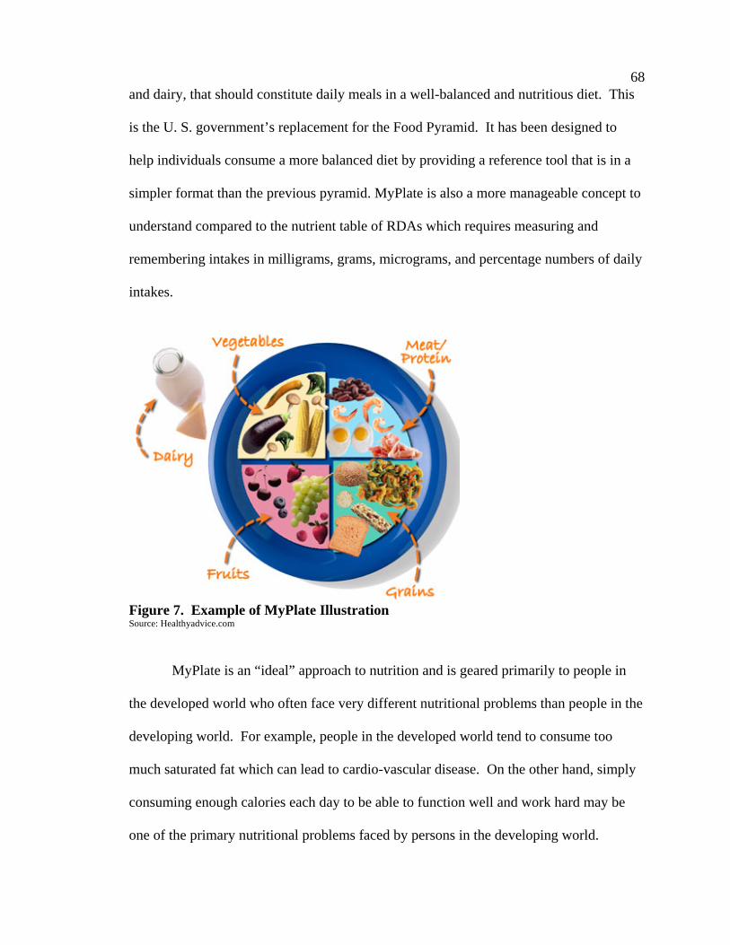
68 and dairy, that should constitute daily meals in a well-balanced and nutritious diet. This

is the U. S. government’s replacement for the Food Pyramid. It has been designed to

help individuals consume a more balanced diet by providing a reference tool that is in a

simpler format than the previous pyramid. MyPlate is also a more manageable concept to

understand compared to the nutrient table of RDAs which requires measuring and

remembering intakes in milligrams, grams, micrograms, and percentage numbers of daily

intakes.

Figure 7. Example of MyPlate Illustration Source: Healthyadvice.com

MyPlate is an “ideal” approach to nutrition and is geared primarily to people in

the developed world who often face very different nutritional problems than people in the

developing world. For example, people in the developed world tend to consume too

much saturated fat which can lead to cardio-vascular disease. On the other hand, simply

consuming enough calories each day to be able to function well and work hard may be

one of the primary nutritional problems faced by persons in the developing world.

69 Consequently, MyPlate may or may not fit well with the nutritional realities faced by

poor people in the study area. However, it is used as one point of reference in

understanding some of the basic differences in nutritional issues between the developing

and the developed world.

Genesis

The automated software service called Genesis was used to find estimated

nutritional content for different food values used in the LP model. The software manages

a database of over 50,000 food items with full nutrient values supplied by over 1700

reputable sources (Esha.com, 2012). Each food that was considered in the LP as a

possible food source for the farm family in the study area, was selected from the USDA

Standard Reference database and then had its nutritional content was calculated. A

nutrient summary of all foodstuffs is provided in Appendix C. In addition to supplying

raw food nutritional data, the Genesis analyzes the nutrient content of food and calculates

yields from moisture, fat, cooking, and processing gains and losses. One hundred gram

portions (considered to be one portion of each food) were used to measure available

nutrients that a food provides and that the model may select to satisfy nutritional

constraints.

Parameters Used in the LP

Family Labor

The family’s labor constraint established for the LP was developed off of the

available the husband in the household would be able to work whether off- or on-farm.

To match the planting calendar that was developed based on half-month cropping periods

70 throughout the year (24 cropping periods total), family labor availability was calculated

in the same fashion and the husband was assumed to have 100 hours in available work

time available during each one-half-month period. This estimate is based on working a

40-hour week plus allowing an additional ten hours of work, beyond a normal 5-day

week, that could be completed on the weekend. In surveying farm families in Cochas,

questions covered the efficiency of work that is carried out by members of the family,

other than the father, in terms of how long it took each other member of the family to

complete a task in the same amount of time as the father. The averages reported by the

surveys suggest that the mother, grandma, and daughter would be able to complete 60,

40, and 50 percent respectively, of the task that the father would accomplish in an hour.

With these percentages, the mother was allowed 60 hours per week of work, the grandma

40 hours, and the daughter only 40 in an attempt to adjust for hours while the daughter is

at school for nine months of the year and unavailable to work on the farm. The son was

not included in available labor but is recognized that typical practice in this area was to

allow younger children to help with weed removal, penning smaller animals, and

collecting crops from the field but the overall contribution of son to total family labor is

considered minimal.

Pantry Items

Certain food items were included (set by determination) in the diets of all

families; pepper, salt, oil, brown sugar, and eggs. During initial runs of the model, these

items would either not appear in the results as satisfying any nutritional requirements or

would be included in an enormous amount due to the least-cost ration feature of the LP

using large amounts to supply a particular micronutrient. To eliminate unrealistic results

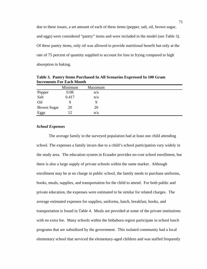
71 due to these issues, a set amount of each of these items (pepper, salt, oil, brown sugar,

and eggs) were considered “pantry” items and were included in the model (see Table 3).

Of these pantry items, only oil was allowed to provide nutritional benefit but only at the

rate of 75 percent of quantity supplied to account for loss in frying compared to high

absorption in baking.

Table 3. Pantry Items Purchased In All Scenarios Expressed In 100 Gram Increments For Each Month

Minimum MaximumPepper 0.08 n/a Salt 0.417 n/a Oil 9 9 Brown Sugar 20 20 Eggs 12 n/a

School Expenses

The average family in the surveyed population had at least one child attending

school. The expenses a family incurs due to a child’s school participation vary widely in

the study area. The education system in Ecuador provides no-cost school enrollment, but

there is also a large supply of private schools within the same market. Although

enrollment may be at no charge in public school, the family needs to purchase uniforms,

books, meals, supplies, and transportation for the child to attend. For both public and

private education, the expenses were estimated to be similar for related charges. The

average estimated expenses for supplies, uniforms, lunch, breakfast, books, and

transportation is found in Table 4. Meals are provided at some of the private institutions

with no extra fee. Many schools within the Imbabura region participate in school lunch

programs that are subsidized by the government. This isolated community had a local

elementary school that serviced the elementary-aged children and was staffed frequently

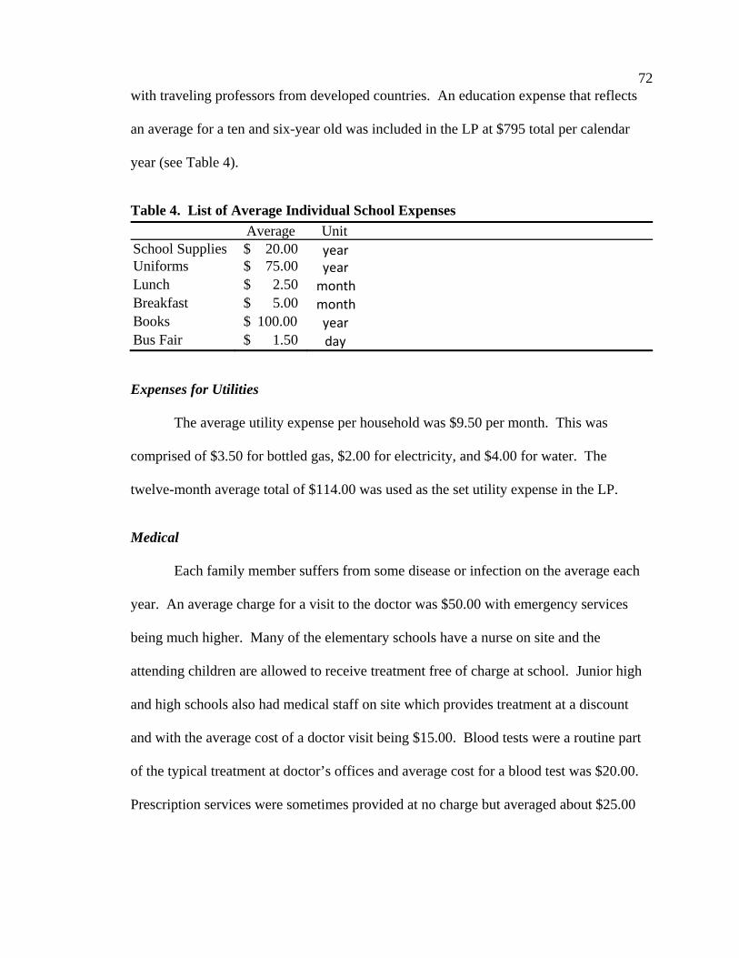
72 with traveling professors from developed countries. An education expense that reflects

an average for a ten and six-year old was included in the LP at $795 total per calendar

year (see Table 4).

Table 4. List of Average Individual School Expenses

Average UnitSchool Supplies $ 20.00 yearUniforms $ 75.00 year Lunch $ 2.50 month Breakfast $ 5.00 month Books $ 100.00 year Bus Fair $ 1.50 day

Expenses for Utilities

The average utility expense per household was $9.50 per month. This was

comprised of $3.50 for bottled gas, $2.00 for electricity, and $4.00 for water. The

twelve-month average total of $114.00 was used as the set utility expense in the LP.

Medical

Each family member suffers from some disease or infection on the average each

year. An average charge for a visit to the doctor was $50.00 with emergency services

being much higher. Many of the elementary schools have a nurse on site and the

attending children are allowed to receive treatment free of charge at school. Junior high

and high schools also had medical staff on site which provides treatment at a discount

and with the average cost of a doctor visit being $15.00. Blood tests were a routine part

of the typical treatment at doctor’s offices and average cost for a blood test was $20.00.

Prescription services were sometimes provided at no charge but averaged about $25.00

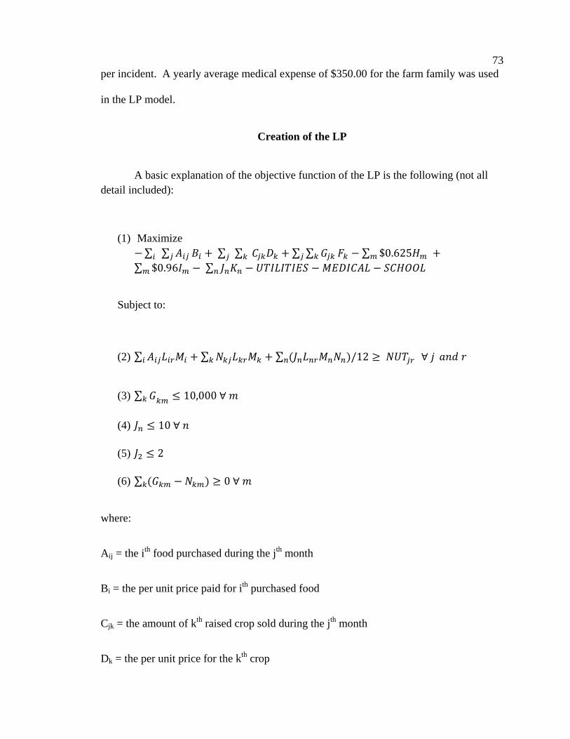
73 per incident. A yearly average medical expense of $350.00 for the farm family was used

in the LP model.

Creation of the LP

A basic explanation of the objective function of the LP is the following (not all detail included):

(1) Maximize ∑ ∑ ∑ ∑ ∑ ∑ ∑ $0.625

∑ $0.96 ∑

Subject to:

(2) ∑ ∑ ∑ /12 ∀

(3) ∑ 10,000∀

(4) 10∀

(5) 2

(6) ∑ 0∀

where:

Aij = the ith food purchased during the jth month

Bi = the per unit price paid for ith purchased food

Cjk = the amount of kth raised crop sold during the jth month

Dk = the per unit price for the kth crop

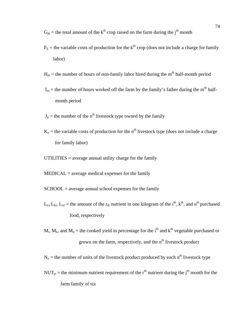
74 Gjk = the total amount of the kth crop raised on the farm during the jth month

Fk = the variable costs of production for the kth crop (does not include a charge for family

labor)

Hm = the number of hours of non-family labor hired during the mth half-month period

Im = the number of hours worked off the farm by the family’s father during the mth half-

month period

Jn = the number of the nth livestock type owned by the family

Kn = the variable costs of production for the nth livestock type (does not include a charge

for family labor)

UTILITIES = average annual utility charge for the family

MEDICAL = average medical expenses for the family

SCHOOL = average annual school expenses for the family

Lir, Lkr, Lnr = the amount of the rth nutrient in one kilogram of the ith, kth, and nth purchased

food, respectively

Mi, Mk, and Mn = the cooked yield in percentage for the ith and kth vegetable purchased or

grown on the farm, respectively, and the nth livestock product

Nn = the number of units of the livestock product produced by each nth livestock type

NUTjr = the minimum nutrient requirement of the rth nutrient during the jth month for the

farm family of six

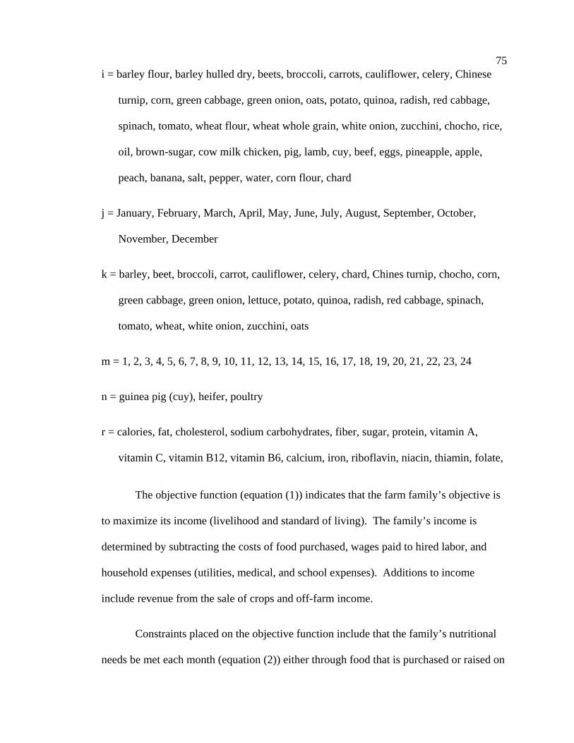
75 i = barley flour, barley hulled dry, beets, broccoli, carrots, cauliflower, celery, Chinese

turnip, corn, green cabbage, green onion, oats, potato, quinoa, radish, red cabbage,

spinach, tomato, wheat flour, wheat whole grain, white onion, zucchini, chocho, rice,

oil, brown-sugar, cow milk chicken, pig, lamb, cuy, beef, eggs, pineapple, apple,

peach, banana, salt, pepper, water, corn flour, chard

j = January, February, March, April, May, June, July, August, September, October,

November, December

k = barley, beet, broccoli, carrot, cauliflower, celery, chard, Chines turnip, chocho, corn,

green cabbage, green onion, lettuce, potato, quinoa, radish, red cabbage, spinach,

tomato, wheat, white onion, zucchini, oats

m = 1, 2, 3, 4, 5, 6, 7, 8, 9, 10, 11, 12, 13, 14, 15, 16, 17, 18, 19, 20, 21, 22, 23, 24

n = guinea pig (cuy), heifer, poultry

r = calories, fat, cholesterol, sodium carbohydrates, fiber, sugar, protein, vitamin A,

vitamin C, vitamin B12, vitamin B6, calcium, iron, riboflavin, niacin, thiamin, folate,

The objective function (equation (1)) indicates that the farm family’s objective is

to maximize its income (livelihood and standard of living). The family’s income is

determined by subtracting the costs of food purchased, wages paid to hired labor, and

household expenses (utilities, medical, and school expenses). Additions to income

include revenue from the sale of crops and off-farm income.

Constraints placed on the objective function include that the family’s nutritional

needs be met each month (equation (2)) either through food that is purchased or raised on

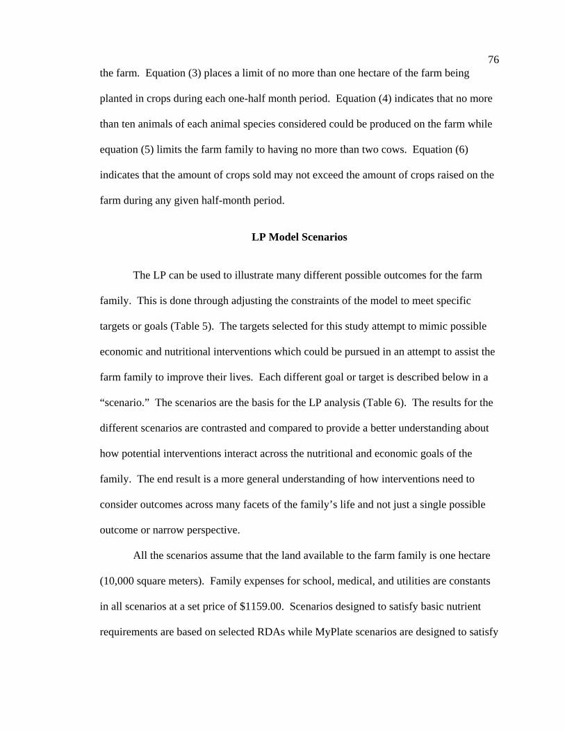
76 the farm. Equation (3) places a limit of no more than one hectare of the farm being

planted in crops during each one-half month period. Equation (4) indicates that no more

than ten animals of each animal species considered could be produced on the farm while

equation (5) limits the farm family to having no more than two cows. Equation (6)

indicates that the amount of crops sold may not exceed the amount of crops raised on the

farm during any given half-month period.

LP Model Scenarios

The LP can be used to illustrate many different possible outcomes for the farm

family. This is done through adjusting the constraints of the model to meet specific

targets or goals (Table 5). The targets selected for this study attempt to mimic possible

economic and nutritional interventions which could be pursued in an attempt to assist the

farm family to improve their lives. Each different goal or target is described below in a

“scenario.” The scenarios are the basis for the LP analysis (Table 6). The results for the

different scenarios are contrasted and compared to provide a better understanding about

how potential interventions interact across the nutritional and economic goals of the

family. The end result is a more general understanding of how interventions need to

consider outcomes across many facets of the family’s life and not just a single possible

outcome or narrow perspective.

All the scenarios assume that the land available to the farm family is one hectare

(10,000 square meters). Family expenses for school, medical, and utilities are constants

in all scenarios at a set price of $1159.00. Scenarios designed to satisfy basic nutrient

requirements are based on selected RDAs while MyPlate scenarios are designed to satisfy

77

Table 5. General Linear Programming Model, Small-Scale Farm in Cochas, Equador Activities

Constraints Buy Food

Eat Crops

Sell Crops

Sell Veg

Store Crops

Grow Crops

Raise Livestock

Hire Labor

Work Off

Farm Family

Expenses RHS OBJ - + + - - - + - Maximize Nutrition Min. + + + >= Min. Nutrition Req. Max Food + + + <= Max. Weight of Food Max Select Foods + <= UL Select Foods Min Food Req. + + >= Min. Food Req. Land Use + <= 10,000 m2 Sell Vegetables + <= 0 Max Livestock + <= Max Livestock Balance Crops + + + +/- - <= 0 Balance Labor + + - + <= Family Labor Supply

Table 6. List of Scenarios Run With Brief Description Scenario 1 Satisfying RDA of Nutrients by allowing food purchases, allowing off-farm income, no hired labor Scenario 2 Satisfying RDA of Nutrients by allowing food purchases, no off-farm income, no hired labor Scenario3 Satisfying RDA of Nutrients without purchasing food, no off-farm income, no hired labor Scenario 4 Satisfying RDA of Nutrients without purchasing foods, allowing off-farm income, no hired labor Scenario 5 Satisfying RDA of Nutrients by allowing food purchases, allowing off-farm income, hired labor Scenario 6 Satisfying MyPlate servings by allowing food purchases, allowing off-farm income, no hired labor Scenario 7 Satisfying MyPlate servings by allowing food purchases, no off-farm income, no hired labor Scenario 8 Satisfying MyPlate servings without allowing food purchases, allowing off-farm income, no hired labor Scenario 9 Satisfying RDA of Nutrients by allowing food purchases, with off-farm income, no hired labor, no heifer Scenario 10 Satisfying RDA of Nutrients by allowing food purchases, no off-farm income, no hired labor, no heifer Scenario 11 Satisfying MyPlate servings by allowing food purchases with off-farm income, no hired labor, no heifer

78

the number of portions of the different food groups as specified in MyPlate. Some of the

scenarios are designed to illustrate how farm choice change based on opportunity costs.

This is modeled by comparing farm family choices when assuming or relaxing

constraints of the amount of 1) family labor available and 2) the opportunities for off-

farm employment (see Table 6 for list of scenarios).

Scenario 1

The base scenario for this model is set to fulfill the basic nutrition requirements of

the family of six through food that is either produced on farm or purchased in market.

The father is allowed to work off-farm (up to 100 hours during each half-month period)

but also limits the family to not hiring labor. Field crops (e.g., potatoes and corn) may be

sold but garden crop varieties are limited to be only for family consumption (cannot be

sold). Products produced by animal enterprises (e.g., eggs, milk) are also allowed to be

used only for family consumption (not sold) with the exception of the heifer’s calves

which may be sold. This scenario illustrates a small-scale agricultural family in which

the father has the opportunity to work off-farm and transfers the labor requirement to

operate the farm mostly to remaining family members if the father works off of the farm.

The base scenario will be referred to as scenario 1 (S1).

Scenario 2

The second scenario (S2) is designed to fulfill nutritional requirements of the

family of six through food either produced on the farm or purchased at the market. Field

crops may be sold but garden crop varieties are limited to family consumption. Products

produced by animal enterprises are only used for family consumption with the exception

of selling the heifer’s calves. No members of the family are allowed to work-off farm

79

and the farm family is also assumed to not be able to hire non-family labor. This scenario

reflects a farm family that depends on field crops to create a revenue source to pay off-

farm expenses and the family is responsible in providing all labor required for

production.

Scenario 3

The third scenario (S3) is designed to fulfill basic nutritional requirements for the

family of six through food produced only on the farm. Field crops may be sold but

garden crops varieties are limited to family consumption. Products from animal

enterprises are consumed only by the family with the exception of selling the heifer’s

calves. No members of the family are allowed to work-off farm and they also cannot hire

non-family labor. This forces the model to grow crops to satisfy family consumption

while providing the opportunity to sell field crops to create revenue to pay for off-farm

expenses. The farm is limited to the existing number of family work hours to satisfy

production needs without hiring labor in an effort to be self-sufficient.

Scenario 4

The fourth scenario (S4) is designed to fulfill nutritional requirements for the

family of six through food produced only on the farm. Field crops may be sold but

garden crop varieties are limited to family consumption. Products from animal

enterprises are only for family consumption with the exception of selling the heifer’s

calves. The father is allowed to work off-farm but non-family labor is not allowed to be

hired. This scenario illustrates a family that is attempting to eliminate food purchases

and be self-sufficient or a family that is located in an area that does not have a local

market to purchase food. If satisfying nutritional requirements is impossible with on-

80

farm food production, the model allows food purchases at a premium and allows the

model to solve. This scenario will also provide a comparison of crop selections in S3

when the available family labor is reduced while producing a higher standard of living.

Scenario 5

The fifth scenario (S5) is designed to fulfill nutritional requirements of the family

of six through food either produced on farm or purchased at the market. The father is

allowed to work off-farm and the family is also allowed to hire non-family labor. Field

crops may be sold but garden crop varieties are limited to family consumption. Products

produced by animal enterprises are used only for family consumption with the exception

of selling the heifer’s calves. This scenario illustrates an entrepreneurial family where

the father could work off-farm while the family employs replacement labor to satisfy

production demand.

Scenario 6

The sixth scenario (S6) for this model is designed to fulfill MyPlate servings

requirements for the family of six through food either produced on farm or purchased at

the market. The father is allowed to work off-farm but non-farm labor is not allowed to

be hired. Field crops may be sold but garden crop varieties are limited only to family

consumption. Products produced by animal enterprises are used only for family

consumption with the exception of selling the heifer’s calves. This scenario illustrates a

small-scale agricultural family in which the father has the opportunity to work off-farm

and when he does the farm labor previously provided by the father is shifted to the

remaining family members. This places a strain on on-farm production, but provides an

81

alternative source of cash from the off-farm job taken by the father. It is a mirror of S1

except that the equation is satisfying servings of food instead of the specific RDAs.

Scenario 7

The seventh scenario (S7) is designed to fulfill MyPlate servings requirements for

the family of six through food either produced on farm or purchased in market. Field

crops may be sold but garden crop varieties are limited only to family consumption.

Products produced by animal enterprises are used only for family consumption with the

exception of selling the heifer’s calves. No members of the family are allowed to work-

off farm and the family cannot hire non-family labor either. This scenario is set to reflect

a family that depends on field crops to create a revenue source to pay off-farm expenses.

The family is solely responsible to provide all labor required for production. It is a

mirror of S2 except that the equation is satisfying servings of food instead of the specific

RDAs.

Scenario 8

The eighth scenario (S8) is designed to fulfill MyPlate servings requirements for

the family of six through food produced on farm but limiting food purchased in the

market by artificially inflating retail price by 90 times. This allows the family to

purchase food at a premium if it is impossible to satisfy nutrient requirements with only

family-grown food in a period. Field crops may be sold but garden crop varieties are

limited only to family consumption. Products produced by animal enterprises are only

for used for family consumption with the exception of selling the heifer’s calves. No

members of the family are allowed to work-off farm the family cannot hire non-family

labor either. This forces the model to grow crops to satisfy family consumption while

82

providing the opportunity to sell field crops to create revenue and pay for off-farm

expenses. The farm family is limited to using only family work hours to satisfy

production needs without hiring non-family labor. It is a mirror of S3 except that the

equation is satisfying servings of food instead of the specific RDAs.

Scenario 9

The ninth scenario (S9) for this model is designed to fulfill nutritional

requirements for the family of six through food either produced on farm or purchased at

the market. The father is allowed to work off-farm but the family hires no non-family

labor. Field crops may be sold but garden crop varieties are limited only to family

consumption. Products produced from animal enterprises are used only for family

consumption and this scenario eliminates the heifer from the farm animal set. This

scenario illustrates a small-scale agricultural family in which the father has the

opportunity to work off-farm and transfers the labor requirement to run the farm to

remaining family members which strains on-farm production but provides an alternative

source of cash from the father’s off-farm job. This scenario illustrates a family that does

not possess or have access to the capital required to purchase a lactating cow that births

one calf a year. The family also does not have sufficient cash flow to purchase a calf and

maintain her till producing age. This scenario mirrors S1 except that the heifer is not an

animal that the family can choose to produce.

Scenario 10

The tenth scenario (S10) is designed to fulfill nutritional requirements for the

family of six through food either produced on farm or purchased at the local market.

Field crops may be sold but garden crop varieties are limited only to family consumption.

83

Products produced by animal enterprises are used only for family consumption and this

scenario also eliminates the heifer from the farm animal set. No members of the family

are allowed to work-off farm the family also cannot hire non-family labor. This scenario

reflects a family that depends on field crops to create a revenue source to pay off-farm

expenses and is responsible for providing all the labor required for production. This

scenario illustrates a family that does not possess or have access to the capital required to

purchase a lactating cow that births one calf a year, or have sufficient cash flow to

purchase a calf and maintain her till producing age. This run mirrors S2 except that the

heifer is not an animal that the family can choose to produce.

Scenario 11

The eleventh scenario (S11) for this model is designed to fulfill MyPlate servings

requirements for the family of six through food either produced on farm or purchased in

the local market. The father is allowed to work off-farm and but the family is unable to

hire non-family labor. Field crops may be sold but garden crop varieties are limited only

to family consumption. Products produced by animal enterprises are used only for family

consumption and this scenario also eliminates the heifer from the farm animal set. This

scenario illustrates a small-scale agricultural family in which the father has the

opportunity to work off-farm and transfers the labor requirement to run the farm to

remaining family members which strains on-farm production but provides an alternative

source of cash for the family through the father’s off-farm job. This scenario is similar to

S1 except that the equation is satisfying servings of food instead of the specific RDAs

while eliminating the milk that a heifer would provide the family. This run also mirrors

S6 except that the heifer is not an animal that the family can choose to produce.

84

CHAPTER 4

RESULTS

The LP model was designed to illustrate the highest returns the family could

expect if they followed the decisions outlined in each of the different scenarios given

their initial resource endowment and opportunities to work off the farm and/or to hire

labor to work on the farm. Because the basic constraints faced by the family were the

resource endowment and the necessity to provide for the family’s nutritional

requirements. The family depicted in the study is representative for the study area. Costs

and returns for the farming operation are based on estimates depicted in the enterprise

budgets discussed earlier. Family household expenses (i.e, utilities, health care, and

school) are also typical for the study area for a family and is similar to the representative

family used for the analysis. Assumptions about the ability to work off the farm or to

hire farm labor are specific to the different scenarios considered, but are consistent with

conditions in the study area.

This LP is not designed to necessarily be descriptive of what a family currently

does in terms of precisely what crops or livestock enterprises are produced. Rather, the

scenarios are designed to facilitate observation of changes in optimal practices suggested

by the model under a specific set of reasonable (achievable outcomes in the study area)

circumstances assumed in each of the scenarios.

The quantities, costs, and returns for each scenario as determined by the LP are

used to show the degree in which the value of the objective varies depending on which of

the scenarios is being considered. The changes in these numbers for the different

scenarios show the impact of the different decisions by the family on their potential

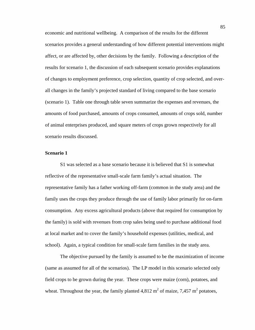
85

economic and nutritional wellbeing. A comparison of the results for the different

scenarios provides a general understanding of how different potential interventions might

affect, or are affected by, other decisions by the family. Following a description of the

results for scenario 1, the discussion of each subsequent scenario provides explanations

of changes to employment preference, crop selection, quantity of crop selected, and over-

all changes in the family’s projected standard of living compared to the base scenario

(scenario 1). Table one through table seven summarize the expenses and revenues, the

amounts of food purchased, amounts of crops consumed, amounts of crops sold, number

of animal enterprises produced, and square meters of crops grown respectively for all

scenario results discussed.

Scenario 1

S1 was selected as a base scenario because it is believed that S1 is somewhat

reflective of the representative small-scale farm family’s actual situation. The

representative family has a father working off-farm (common in the study area) and the

family uses the crops they produce through the use of family labor primarily for on-farm

consumption. Any excess agricultural products (above that required for consumption by

the family) is sold with revenues from crop sales being used to purchase additional food

at local market and to cover the family’s household expenses (utilities, medical, and

school). Again, a typical condition for small-scale farm families in the study area.

The objective pursued by the family is assumed to be the maximization of income

(same as assumed for all of the scenarios). The LP model in this scenario selected only

field crops to be grown during the year. These crops were maize (corn), potatoes, and

wheat. Throughout the year, the family planted 4,812 m2 of maize, 7,457 m2 potatoes,

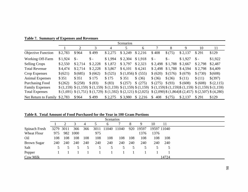
86

Table 7. Summary of Expenses and Revenues

Scenarios 1 2 3 4 5 6 7 8 9 10 11 Objective Function $ 2,783 $ 964 $ 499 $ 2,275 $ 3,249 $ 2,216 $ 408 $ (75) $ 2,137 $ 291 $129

Working Off-Farm $ 1,924 $ - $ - $ 1,994 $ 2,304 $ 1,918 $ - $ - $ 1,927 $ - $1,922 Selling Crops $ 2,550 $ 2,714 $ 2,228 $ 1,872 $ 3,797 $ 2,323 $ 2,498 $ 1,788 $ 2,667 $ 2,798 $2,487 Total Revenue $ 4,474 $ 2,714 $ 2,228 $ 3,867 $ 6,101 $ 4,241 $ 2,498 $ 1,788 $ 4,594 $ 2,798 $4,409 Crop Expenses $ (621) $ (685) $ (662) $ (525) $ (1,056) $ (555) $ (620) $ (576) $ (679) $ (730) $(608) Animal Expenses $ 351 $ 351 $ 175 $ 175 $ 351 $ (36) $ (36) $ (36) $ (11) $ (11) $(397) Purchasing Food $ (262) $ (258) $ (83) $ (83) $ (257) $ (275) $ (275) $ (93) $ (608) $ (608) $ (2,115)Family Expenses $ (1,159) $ (1,159) $ (1,159) $ (1,159) $ (1,159) $ (1,159) $ (1,159)$ (1,159)$ (1,159) $ (1,159) $ (1,159)Total Expenses $ (1,691) $ (1,751) $ (1,729) $ (1,592) $ (2,121) $ (2,025) $ (2,090)$ (1,864)$ (2,457) $ (2,507) $ (4,280)

Net Return to Family $ 2,783 $ 964 $ 499 $ 2,275 $ 3,980 $ 2,216 $ 408 $ (75) $ 2,137 $ 291 $129

Table 8. Total Amount of Food Purchased for the Year in 100 Gram Portions Scenarios 1 2 3 4 5 6 7 8 9 10 11 Spinach Fresh 3279 3011 366 366 3011 11040 11040 920 19597 19597 11040 Wheat Flour 975 982 1000 975 1376 1376 Oil 108 108 108 108 108 108 108 108 108 108 108 Brown Sugar 240 240 240 240 240 240 240 240 240 240 240 Salt 5 5 5 5 5 5 5 5 5 5 5Pepper 1 1 1 1 1 1 1 1 1 1 1Cow Milk 14724

87

Table 9. The Amount of Crops Selected for Consumption in 100 Gram Portions for the Year Scenarios 1 2 3 4 5 6 7 8 9 10 11 Wheat Flour 439 421 336 338 440 414 414 414 619 619 414 Corn Flour 46 46 58 58 46 46 46 46 63 63 46 Cauliflower Cooked 190 Carrots Fresh 110 68 94 Spinach Fresh 29 29 92 Tomato Fresh 31 31 94 Celery Fresh 97 Red Cabbage Fresh 14 204 204 188 Broccoli Cooked Corn Cooked

11 11 11 767

Potato Cooked 801 844 95 95 95 95

Table 10. Total Kilograms of Crops Sold for the Year

Scenarios 1 2 3 4 5 6 7 8 9 10 11

Corn 1402 1130 1444 1976 1582 1318 779 1059 839 1457 Potato 5965 6690 5004 3486 10849 5145 5894 4374 6621 7203 5733

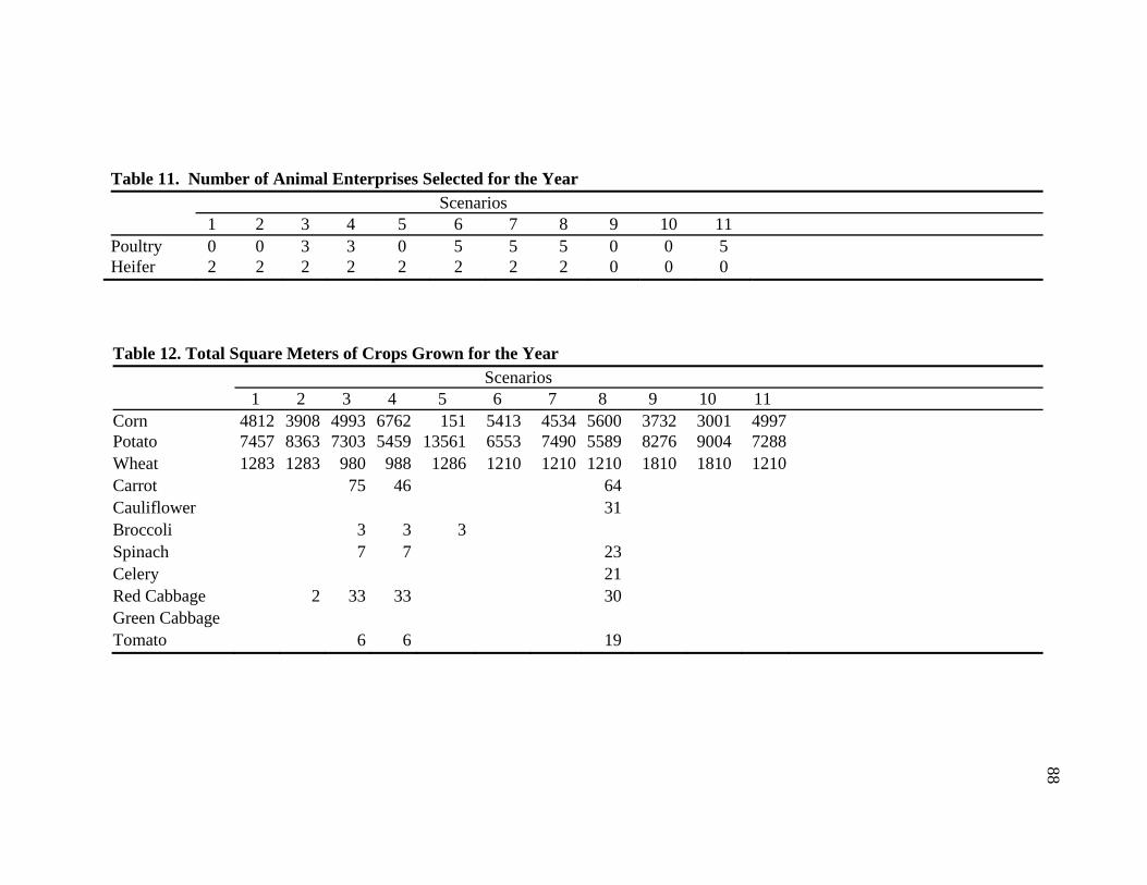
88

Table 11. Number of Animal Enterprises Selected for the Year

Scenarios 1 2 3 4 5 6 7 8 9 10 11 Poultry 0 0 3 3 0 5 5 5 0 0 5 Heifer 2 2 2 2 2 2 2 2 0 0 0

Table 12. Total Square Meters of Crops Grown for the Year

Scenarios 1 2 3 4 5 6 7 8 9 10 11 Corn 4812 3908 4993 6762 151 5413 4534 5600 3732 3001 4997 Potato 7457 8363 7303 5459 13561 6553 7490 5589 8276 9004 7288 Wheat 1283 1283 980 988 1286 1210 1210 1210 1810 1810 1210 Carrot 75 46 64 Cauliflower Broccoli

3

3

3

31

Spinach 7 7 23 Celery 21 Red Cabbage Green Cabbage Tomato

2 33

6

33

6

30

19

89

and 1,283 m2 of wheat. The farm was at full capacity, in terms of its land constraint,

with all 10,000 m2 having crops in the ground in the beginning of January, end of March,

and end of December. An out-of-pocket expense of $621.00 was incurred to grow these

crops. At harvest, the family chose to sell 1,402 kg of maize and 5,965 kg of potatoes.

But, the family initially retained (stored) all of the wheat it produced. Selling these crops

created total revenue of $2,550 for the farm family (table 6). Maize that was not sold was

processed into flour and consumed in March. The wheat was selected to be stored and

converted into flour for consumption from April through December.

To provide the family with protein and calcium that was not provided through the

consumption of the crops the family produced, the model selected 0.14 poultry and 2.0

heifers. The model selected 0.14 poultry which is the equivalent to one chicken (a full

unit of poultry consists of seven chickens). One chicken produces on average 24 eggs per

month creating an excess above constraint (a minimum of 12 eggs were assumed to be

consumed by the family each month through either buying them in the market or

producing them though raised chickens). The two heifers supplied milk for consumption

required by the family to meet calcium needs. The heifers also produce a revenue stream

during the year in which each heifer produces a calf that is sold.

During both January and February, the model selected the purchase of 49 kg of

wheat flour from the market. The crops grown on the family farm did not satisfy all

nutrition requirements. Consequently, during each of the 12 months, the model also

purchased spinach at an average of 27 kg with a spike of 31 kg in only March. Spinach

was the “low-cost” source of a number of nutrients not provided from other raised or

purchased sources. While the amount of spinach purchased seems unreasonable for the

90

family’s diet, it is representative of purchasing low-cost sources of missing nutrients. So,

even if a constraint were placed on the amount of spinach purchased, the model would

have simply selected the next cheapest source of these nutrients and “over consumed”

that source also. As a result, the amount of spinach should not be considered necessarily

what would be consumed by the family but rather as a representation of expenditures on

the next cheapest source of the missing nutrients.

The results in Table 6 show that the father would chooses to work off-farm if the

opportunity presented itself and would earn $1924 net take-home pay for doing so. This

assumes that the potential employment is located within a reasonable distance for him to

make the round-trip on the bus in three hours or less each day.7 This demonstrates that it

is advantageous for the father to work off-farm and to purchase food in the market. Food

purchased in the market compensates for any decreased production that may have

occurred by reducing family labor by the 100 hours each half-month spent in off-farm

employment by the father. Even though off-farm employment was available, the father

chose to work off-farm only 21 hours in the beginning of April, and 82 hours in the end

of December. The decrease in April illustrates the greater return to helping the family

plant potatoes than to work off of the farm at that time of the year. The December

decrease in hours worked off the farm by the father is related to the labor needed on farm

to plant maize that also provides a greater return than the $0.96/hour earned in off-farm

employment at that particular point in the year. The family labor was fully consumed in

the end of March, a surplus of 21 hours in the beginning of April, and entire amount

again in all of June.

7 Recall that the gross monthly salary was assumed to be $300.

91

Scenario 2

This scenario removed the opportunity for the father to work off the farm

compared to S1 in which the father could work off the farm. The field crop for selections

for S2 remained the same for maize, potatoes, and wheat as they were in S1. However,

S2 added a small amount of production for one of the garden varieties, red cabbage.

Over the year, the family would have planted 3,908 m2 of maize, 8,363 m2 of potatoes,

1,283 m2 of wheat, and 2 m2 of red cabbage.

The farm was at full capacity, in terms of its land constraint, with all 10,000 m2

having crops in the ground at the beginning of January, end of March, and end of

December; the same as for S1. All other half-month production periods remained similar

to S1 except for April, November, and the beginning of December where about 900 m2

more cropland was planted for S2 than for S1. These additional meters are attributed to

the increase in maize and potatoes planted compared to S1.

An out-of-pocket expense of $685 was incurred to grow the crops specified in S2;

an increase of about $64 over out-of-pocket expenses for S1. At harvest, the family

would choose to sell 1,130 kg of maize and 6,690 kg of potatoes. The family initially

retains (stores) all of the wheat it produced. Selling these crops created total revenue of

$2,714 for the farm family (Table 7). The quantity of maize not sold in the market but

consumed by the family remains the same as for S1. The maize consumed by the family

was processed into flour and consumed in March. The quantity of wheat that was

selected to be stored and converted into flour for consumption from April through

December did not change for S2 compared to S1.

92


consumption of the crops the family produced, the model continued to select 0.14 poultry

and 2.0 heifers just as it had done for S1.

The wheat purchased by the family only increased in January by the amount of

700 grams compared to S1. The crops grown on the family farm in S2 still did not satisfy

all nutrition requirements as was the case with S1. The addition of red cabbage to the

portfolio of the crops grown by the family replaced the spinach originally purchased in

January in S1. But, the purchase of spinach in all the other months remained the same as

it was in S1.

This scenario limited the father from working off-farm. In S1, food purchased in

the market compensated for any decreased production occurring as a result of the father

working off the farm for up to 100 hours each half-month. The decrease in off-farm

employment in April illustrated in S1 the greater return to helping the family plant

potatoes than to work off-farm at that time of the year. In this scenario (S2), planting

decisions do not change much from S1, but the value of the objective function was only

$964 because of the reduction in off-farm income. The increase in revenue from crops

sold, and the increased expense of growing the different spread of crops in S2 than in S1

demonstrates the ability of the family to grow primarily cash crops and to continue to

meet its nutritional needs. This is shown by the fact that the family’s decisions about

what and when to plant only marginally changed in S2 compared to S1. However, the

family’s standard of living, in terms of its income, decreased dramatically for S2

compared to S1.

93

These results demonstrate two points. First, if cash crops can be sold at the

average prices specified in the model, the family will continue to choose to sell primarily

cash crops and to buy food. This is because the cash crops generate enough income to

buy food in the market. Second, there is a large incentive to work off of the farm if

possible because the family’s income will be increased dramatically compared to if no

off-farm income is available to the family.

Scenario 3

This scenario removed the opportunity for the father to work-off farm and limited

the food that would be purchased in the marketplace by artificially increasing the cost of

purchased food by 90 times compared to S1. The field crop selection for S3 remained the

same as in S1 for maize, potatoes, and wheat. However, more garden crop varieties came

into the mix in S3 than in S1 with the addition of carrots, broccoli, spinach, red cabbage,

and tomatoes (for quantities see Table 11). The increase in maize production and the

addition of the garden crops occurred at the cost of reducing the land utilized by wheat

and potatoes (compared to S1). The farm was at full capacity, in terms of its land

constraint, in the same three periods as S1. Land utilization in all of the other half-month

periods remained similar to S1.

The farm family’s expenses to grow the crops indicated in S3 increased $42 from

S1 while the revenue from crops sold decreased by $325 compared to S1. The choice of

and the quantity of maize to be sold remained similar to S1 while potatoes became a

storable food (not stored in S1) selection alongside wheat (stored in both S1 and S3).

The potatoes were then subsequently consumed by the farm family during January

through April, and again in July and December. The entire wheat harvest that the family

94

had stored for S3 continued to provide for consumption in the form of flour for the family

during April through December. But, the amount of wheat flour consumed by the farm

family in S3 was less than for S1 because less land was dedicated by the farm family for

wheat production in S3 than S1. Vegetables were grown throughout the year providing a

wider menu selection while also providing the nutrients required by the family (see crop

calendar Appendix B).


consumption of the crops the family produced, the model continued to select the

maximum heifers at two, but increased the production of chickens 18 times or to 2.5 units

of poultry. The extra expense to raise the chickens reduced the animal income by half

compared to S1.

The pantry constraint (purchase of brown sugar, cooking oil, salt, and pepper)

continued to be satisfied at standard market prices (market price was not inflated for

pantry items). The additional of garden crops grown replaced the need to purchase

spinach in all periods except in February when the model actually selected 36 kg of

spinach at the increased cost. The crops grown on the family farm continued to not

satisfy all nutritional requirements for the family in all periods thus forcing this purchase.

The labor constraint for the farm family was a binding (all available farm family

labor used) in the end of March, end of June, and beginning of November. The period in

the beginning of April was just 18 hours short of using all family labor available during

that period. However, the use of family labor in all other half-month time periods was

the same as for S1. The labor required to plant the larger amounts of garden crop varieties

was provided by sacrificing the growing of field crops. That is, the increased production

95

of garden crops, which tend to be more labor intensive than cash crops on a m2 basis,

forced the transfer of family labor away from cash crops to garden types.

The standard of living for the family, as indicated by the value of the objective

function, was reduced by more than $2200 (compared to S1) as a result of lost off-farm

income and the need to select garden crop varieties rather than cash crops as a way to

replace the purchased food allowed by S1. This scenario (S3) presents the possibility for

introducing more intensive gardening methods to impoverished small-scale farmers to

allow them to utilize all available family labor. This may also further support the use of

genetically modified seed varieties that can be grown /planted in earlier or later periods

which would allow a family like this to make better use of idle land. However, it also

demonstrates that when off-farm employment is available that this strategy still does not

offer a higher standard of living to the farm family than S1.

Scenario 4

This scenario provided the opportunity for the father to work-off farm but limited

food purchases at the market by artificially increasing the price of purchased food by 90

times compared to S1. The LP model in this scenario selected field crops and garden

crops to be grown during the year. The field crop selection for S4 remained the same as

S1 consisting of maize, potatoes, and wheat. However, the planted areas for these crops

were different than for S1 and were 6,762 m2 , 5,459 m2 , and 988 m2 for maize, potatoes,

and wheat, respectively.

Garden crop varieties came into the mix for S4 with the addition of carrots,

broccoli, spinach, red cabbage, and tomatoes (for quantities see Table 12). The increase

in maize production and the addition of garden crop varieties was made possible by

96

reducing the amount of land, compared to S1, that was dedicated to growing wheat and

potatoes. The farm was at full capacity, in terms of its land constraint (10,000 m2), at the

end of March and approached the limit in January. The amount of land utilized for S4

was similar to the amount of land utilized under S1 for all other periods.

An out-of-pocket expense of $525 was incurred for S4 to grow the crops

described above. At harvest, the family chooses to sell 1,976 kg of maize and 3,486 kg

of potatoes but initially stores all of the wheat it produced for later consumption. The

selling of cash crops generates total revenue of $1,872 for the farm family (Table 7).

Maize that was not sold at harvest was stored and processed into corn flour that was

consumed in March. Potatoes became a storable food selection for S4 alongside wheat

and were subsequently consumed during January through April, and again in July,

October, and December.

Wheat was selected to be stored and converted into flour for consumption also

during April through December. The farm family’s expenses to grow the crops decreased

$96.00 compared to S1 while the revenue from crops sold decreased by $378 compared

to S1. The choice to grow and the amount of maize sold was significantly higher for S4

than for S1 (almost 2,000 m2 more) which was land used to grow potatoes and wheat in

S1. For S4, vegetables were grown throughout the year presenting a wider menu

selection for the family than other scenarios while providing the nutrients required for the

family. The selection of vegetables for S4 was similar to the quantities and selection for

S3, except for carrots which had only half as many produced under S4 as under S3.


consumption of the crops the family produced, the model continued to select the

97

maximum number of heifers at two, but increased the production of chickens by 18 times

compared to S1 or 2.5 poultry units. The extra expense to raise the chickens reduced the

animal income by half of what it was for S1.

The pantry constraint continued to be satisfied at standard market prices (the

inflated prices for purchased food did not apply to pantry items which could continue to

be purchased at regular market prices). The garden crops that were grown under S4

replaced the previously purchased spinach (e.g. S1) in all periods except during February.

The model selected 36 kg of spinach even at the greatly inflated cost. The crops grown

on the family farm simply did not satisfy all nutritional requirements for all periods for

the family thus forcing the model to purchase spinach.

The results in table 7 for S4 show that the father would chooses to work off-farm

if the opportunity presented itself and would earn $1994 net annual take-home pay for

doing so. Even though off-farm employment was available, the father continued to

choose to work off-farm only 48 hours in the beginning of March, 81 hours in the

beginning of April, three hours in the beginning of June, no hours at the end of June, and

46 hours in the end of December. The choice to decrease off-farm labor hours in April

and June illustrates that there was a greater return to helping the family plant potatoes

than there was to work off-farm at that time of the year. The March and December

decrease in hours worked off-farm by the father is related to the labor needed on farm to

plant maize indicating that labor spent planting maize also provides a greater return than

the $0.96/hour earned in off-farm employment at that particular point in the year. Even

though the father chose to work on-farm during many of the half-month periods, family

labor was constrained only in the month of June. This suggests that the necessary farm

98

work is able to be completed by the family members except during the times mentioned

above when the father helps with planting and harvesting of cash crops.

This demonstrates that it is advantageous for the father to work off-farm even

when the ability to purchase food in the market is limited. This is a scenario in which a

family is striving to be self-sufficient in what they produce which would limit the

dependence on the local market. The standard of living has been reduced by $508

compared to S1 because the family is forced to grow the food the family needs which

cannot be purchased in the market for a reasonable price. When facing an increased need

to satisfy the family nutritional needs from crops grown on the farm, the family’s choice

appears to favor cash crops that require the less amounts of labor compared to other

crops. Potatoes may produce a higher return, but require more labor while not satisfying

nutritional constraints in the same way that maize does.

This scenario illustrates a family that is attempting to eliminate food purchases

and be self-sufficient on their small-scale farm. It could also be viewed as a scenario

representing a family that is located in an area that does not have a local market to

purchase food at a reasonable price, but the father does have the ability to work at a job

off the farm that generates a reasonable income (could be honey harvesting, charcoal

making, or another income generating activity in a rural area as well as commuting to

work for wages in a nearby small city). If satisfying nutritional requirements is

impossible with on-farm food production, the model allows food purchases at premium

prices which allows the model to solve (i.e., satisfy all constraints including the

nutritional constraints of the family). This scenario also provides a comparison of crop

99

selections to S3 when the available on-farm family labor is reduced while producing a

higher standard of living than for S3 while being more self-sufficient.

Scenario 5

This scenario allowed the father to work off farm and also allowed the farm

family to hire labor should the need arise. Food was allowed to be purchased at regular

market prices to meet nutritional needs if food produced and consumed on the farm was

not sufficient to meet nutritional needs (less expensive sources of food to meet nutritional

needs could be purchased than if it were raised on the farm).

The LP model in this scenario selected the same field crops to be grown as S1 did.

However, the amount of field crops produced by the farm family changed quite

drastically from S1 in terms of the number of m2 planted. Throughout the year, the

family planted only 151 m2 of maize, but there was an immense increase in potatoes

produced (compared to S1) to 13,561 m2 potatoes. The amount of wheat planted, 1,286

m2, was similar to S1. The model also selected a small amount of broccoli to be

produced on the farm (similar to S3 and S4). The land on the farm was planted to near its

full capacity throughout the year with all 10,000 m2 having crops in the ground in every

period except during the period from the end of January through the beginning of March

(only about half of the available land is used during that particular part of the year).

An out-of-pocket expense of $1056 was incurred to grow the crops specified

above for this scenario. The family was able to sell almost 11,000 kg of potatoes and

consumed the small maize harvest they had during March in the form of corn flour. The

level of consumption and storage of wheat produced for S5 mirrored that of S1. Selling

the potatoes harvested created total revenue of $3,797 for the farm family (Table 7). To

100

provide the family with protein and calcium that was not provided through the

consumption of the crops the family produced, the model continued to select 0.14 poultry

and 2.0 heifers just as it had for S1.

During both January and February, the model selected to purchase 49 kg of wheat

flour from the market as it had for S1. The crops grown on the family farm did not

satisfy all nutrition requirements of the family. Consequently, the model also purchased

spinach at an average of 27 kg per month, a spike of 31 kg in only March, and no spinach

in September. In S1, purchased spinach was the “low-cost” source of a number of

nutrients not provided from other raised or purchased sources. However, broccoli

became the low-cost source of missing nutrients when family labor is reduced because of

off-farm employment but non-family labor can be hired at $0.625/hr.

The results in Table 6 show that the father would choose to work off-farm if the

opportunity presented itself and would earn $2304 net take-home pay for doing so. Since

the father receives a higher wage than what replacement labor costs, the LP has the father

working off farm in all periods in this scenario and the family has hired labor to satisfy

the increased labor needs presented by expanding their potato crop. The hired labor

expense was $732 but resulted in contributing to an increase in crop revenue of $1,247

compared to S1. Allowing the family to hire non-family labor also allowed the father to

work additional hours off-farm compared to S1 which provided the family with $380

more income than S1 thus contributing to a better standard of living for the family. This

demonstrates that it is advantageous for the father to work off-farm with the assumption

that the hired worker would be able to complete the tasks with at least the same efficiency

as the father and that the labor provided by other family members would not be reduced

101

to satisfy due to the need for family members other than the father taking over managerial

responsibilities.

Food purchased in the market for S5 is equal to S1, except in September. Spinach

was not purchased as it was in S1 due to nutritional requirements being satisfied with

broccoli that was grown on the farm instead. Previously it was stated that it is beneficial

to hire labor that the father cannot provide (because he is working off of the farm) to

assist in producing field crops that are sold for cash. However, it appears that it may also

be advantageous for the farm family to grow at least a few vegetables, in this case

broccoli, to satisfy the family’s nutritional requirements.

This scenario illustrates an entrepreneurial family where the father could work

off-farm while the family employs replacement labor to satisfy on-farm production needs.

The family situation described in this scenario may reflect opportunities in the

community of Cochas, but these practices described in the scenario are not generally

practiced by farmers in the community. It is possibly due to the capital and credit

restraint that producing such a cash crop requires from inputs and increased labor which a

cash poor rural family rarely has access to. From the information gathered in

conversations with farm families in Cochas, the absence of this type of entrepreneurial

small-scale farm activity may be a function of the families being extremely risk adverse

and who do not desire to transfer so much risk to one crop (potatoes).

The results for this scenario demonstrate the important tradeoffs which exist

between working off the farm and subsistence farming (growing primarily for the farm

family’s own consumption). While higher standards of living can be achieved by

emphasizing cash crops and also working off the farm, there may also be risks associated

102

with this strategy. Observation within the community of Cochas seems to support the

idea of a mixed strategy where people choose to diversify activities as well as work off

farm. This is consistent with portfolio theory but also suggests that risk-reducing

activities such as better infrastructure, irrigation systems, and fertilizer would tend to

raise living standards in the study area.

Scenario 6

The sixth scenario is designed to fulfill MyPlate serving requirements in lieu of

the “normal” nutritional constraint. It is a mirror of S1 except that the nutritional

constraint equation in the LP is set to satisfying servings of food groups instead of the

specific RDAs used in S1-S5.

The LP model in this scenario continued to select only field crops to be grown

during the year as it had for S1. These crops were the same as S1; maize, potatoes, and

wheat. The farm family planted 5,413 m2 of maize, 6,553 m2 potatoes, and 1,210 m2 of

wheat. This equates to an increase, compared to S1, in maize production at the expense

of potato and wheat production.

The farm’s field capacity, in terms of how much land was in production during

each one-half month production period in this scenario, was similar to S1 for all 12

months. An out-of-pocket expense of $555 was incurred in this scenario to grow these

crops; $66 less than in S1. At harvest, the family chose to sell 1,582 kg of maize and

5,145 kg of potatoes. The family maintained, as it is in S1, the practice of initially

storing all the wheat produced on the farm. The crops that were sold in this scenario

created total revenue of $2,322 for the farm family, a reduction of $227 compared to S1

(Table 7). The maize that was not sold but was rather processed into flour for

103

consumption in March remained the same for S6 as it was for S1. The selection of wheat

to be stored and converted later into flour for consumption during April through

December was reduced by 3 kg monthly compared to S1.

To provide the family with the number of servings needed to satisfy MyPlate, the

model selected 5.33 poultry and 2.0 heifers. The selected 5.33 poultry is the equivalent

to 37 chickens (a full unit of poultry consists of seven chickens). One chicken produces

on the average 24 eggs per month. Consequently, approximately 1,000 eggs were

produced each month from the 37 chickens, which were used to create a least-cost ration

to satisfy the number of meat/protein servings specified in MyPlate. The high level of

chicken production in this scenario reduced the income from animals reported for S1 and

now shows an expense for S6 of $36. The calves are still being sold, but the increased

cost of the poultry enterprise has more than depleted the revenue from the heifer

enterprise.

Wheat flour was eliminated from food purchases (compared to S1) but the crops

grown on the family farm did not satisfy the MyPlate serving requirements. During each

of the twelve months, the model purchased 92 kg of spinach, 3.4 times what the model

selected for S1 (regular RDA nutritional constraints). The amount of spinach purchased

is unreasonable for the family’s diet and it must be remembered that it is representative of

purchasing low-cost sources of missing nutrients. Should a constraint be placed that

limited these types of purchases, it would only increase the cash outlay by the family and

further reduce their standard of living.

The results in Table 7 depict that the father would choose to work off-farm if the


104

is very similar to S1 and is only less due to the difference in S6 by a few additional hours

that were selected by the model for on-farm work to support increased maize production

(after accounting for the decrease in potato production).

Subjecting a farm family in the developing world to the nutritional guidelines

presented in MyPlate would decrease the standard of living for the family. The estimated

reduction to the standard of living is $560 compared to S1. This suggests that the

MyPlate guidelines are not well suited for a developing world situation. North American

diets tend to over consume certain food groups resulting in too much saturated fat and

carbohydrates in diets. In the developing world, this is much less of a problem because

nutrition targets seem less complex, i.e., enough calories and enough protein, compared

to North American diets where incomes are larger and diet problems are different than in

the developing world.

Scenario 7

This scenario removed the opportunity for the father to work-off farm (S6 allowed

the father to work off of the farm) while maintaining the diet constraint of MyPlate. As

such, this scenario is the same as S2 except for the MyPlate requirements imposed on S7

compared to the RDA nutritional requirements imposed on S2.

The LP’s field crop selections remained the same as for S2 and S6 with maize,

potatoes, and wheat being produced by the farm family. However, this scenario did not

incorporate the small amount of red cabbage that was produced on the farm in S2.

Throughout the year in this scenario, the family planted 4,534 m2 of maize, 7,490 m2 of

potatoes, and 1,210 m2 of wheat. These are comparable changes in production rates from

S6 and mirror the percentage changes in production from S1 to S2 production levels.

105

The land planted on the farm was at full capacity, in terms of its land constraint,

with all 10,000 m2 having crops in the ground in the beginning of January, end of March,

and end of December; the same as for S1 and S6. An out-of-pocket expense of $621 was

incurred to grow these crops, an increase of about $66 above the same expense for S6 but

equal to S1. At harvest, the farm family chose to sell 1,318 kg of maize and 5,894 kg of

potatoes. But, the family initially retained (stored) all of the wheat it produced. Selling

these crops created total revenue of $2,714 for the farm family (Table 6). The quantity of

unsold (stored) maize remained the same and it was processed into flour and consumed

by the farm family in March. The quantity of wheat that was selected to be stored and

converted into flour for consumption from April through December did not change from

S6.


model selected 5.33 poultry units and 2.0 heifers. The increased level of chicken

production reduced the income from animals compared to S1, and now shows the

expense of $36.00 which is equal to S6. The calves are still being sold, but the increased

cost of the poultry enterprise has depleted the revenue as in S6.

Wheat flour was not purchased from the market but the crops grown on the family

farm continued, just as in S6, not to satisfy serving requirements specified in MyPlate for

the farm family. During each of the twelve months, the model purchased 92 kg of

spinach, 3.4 times what the model selected under nutritional constraints (S2). The

amount of spinach purchased is unreasonable for the family’s diet and it must be

remembered that it is representative of purchasing low-cost sources of missing nutrients.

106

Should a constraint be put in place that limited these types of purchases, it would only

increase the cash outlay by the family and further reduce their standard of living.

In this scenario (S7), planting decisions do not change much from S1, but the

value of the objective function was only $408 compared to $2,216 for S6. This was due

primarily to the reduction in off-farm income compared to S6. The relationship of

changes in crops planted, sold, and consumed between S7 and S6 is approximately equal

to the changes between S2 and S1. The increase in revenue from crops sold, and the

increased expense of growing the different spread of crops in S7 compared to S1

demonstrates the ability of the family to grow primarily cash crops and to continue to

meet its nutritional needs. This supports the notion that the farm family can have a

higher standard of living, even with no off-farm income, if it can sell cash crops and buy

food rather than raising vegetables for on-farm consumption only. This is shown by the

fact that the family’s decisions about what and when to plant only marginally changed in

S7 compared to S1. However, the family’s standard of living, in terms of its income,

decreased dramatically for S7 compared to S1.

The drastic change in the objective function from S1 to S7 can be explained by

the removal of off-farm in S7 compared to S1 and the reduction in crop revenue in S7

compared to S1 due to the “MyPlate Tax” (the need to meet MyPlate serving

requirements is more expensive for the family than simply meeting RDA requirements).

Even though the family had the more costly constraint of MyPlate to satisfy in S7

compared to S1 (simple RDA requirements), the family continued to select field crops

which require less labor than the garden crop varieties that tend to be more labor

intensive on a m2 basis than field crops. The revenue from the sale of field crops is able

107

to satisfy the different constraints (food purchase needed) on food groups specified in

MyPlate while also providing a cash crop to create revenue for the family to purchase

other foods in the market when allowed.

The results for this scenario illustrate that, given reasonable risks; it pays the farm

family to grow cash crops rather than producing vegetables and livestock products only

for on-farm consumption. This seems to suggest that as long as a reasonably well-

functioning market exists it may be difficult to recruit farm families into interventions

that attempt to emphasize vegetable production for on-farm consumption. Of course,

price risk for cash crops is an important consideration. Consequently, it is likely best for

vegetable-oriented interventions to start slowly with farm families in the study area by

encouraging them to plant only small plots of vegetables rather than expecting farm

families to convert a significant amount of land currently devoted to field crops into

diversified vegetable production for on-farm consumption.

Scenario 8

In addition to replacing the nutrition constraint (RDAs) with MyPlate, this

scenario does not allow father to work-off farm and limited food purchases in the

marketplace by artificially inflating the cost to purchase most food items by 90 times

compared to S1. The LP’s selection of field crops produced for S8 remained the same as

for S1 and included maize, potatoes, and wheat.

In response to the model limiting off-farm food purchases, and having a greater

supply of family labor available due to the father not working off-farm, the quantities of

field crops changed from S6 and S7. In general fewer potatoes are produced (with the

exception of S4) but lightly more corn (again with the exception of S4) compared to the

108

other scenarios already discussed. Maize production was selected to increase by 788 m2

while potatoes decreased by 1,868 m2 compared to S1. Wheat only marginally changed

compared to S1 (down to 1,210 in S7 compared to 1,283 in S1) as occurred in the other

MyPlate scenarios (S6, S7).

Garden crop varieties are significantly expanded compared to the other scenarios

with S8 devoting the largest land area to garden crops of any of the scenarios considered.

This included additional carrots, cauliflower, spinach, celery, red cabbage, and tomatoes

(for quantities see Table 12). The increase in maize production and the additional garden

crops occurred at the cost of reducing the land utilized by wheat and potatoes (compared

to S1). The farm was at full capacity, in terms of its land constraint, in only the half-

month period of the end of March which is when the planting season for both maize and

potatoes co-exist. Land utilization in all of the other half-month periods was reduced on

the average compared to those in S1. The farm family sells its excess corn and potato

production.

The farm family’s expenses to grow the crops indicated in S8 decreased $45 from

S1 while the revenue from crops sold decreased by $762 compared to S1. The choice of

and the quantity of maize and potatoes to be sold were reduced but a larger quantity of

these crops was stored than in any of the other scenarios considered.

This was the first scenario in which the model chose to store any amount of maize

and it selected to store a relatively large amount of maize; 1,544 kg. Stored potatoes

were subsequently consumed by the farm family during January, while the maize was

available July through November to be converted into corn flour and consumed by the

farm family. The entire wheat harvest that the family had stored for S8 continued to

109

provide for consumption in the form of flour during the period of April through

November. But, the amount of wheat flour consumed by the farm family in S8 was less

than for S1 because less land was dedicated by the farm family for wheat production in

S8 than S1. Vegetables were grown throughout the year providing a wider menu

selection while also providing the nutrients required by the family (see crop calendar

Appendix B).

To provide the family with the number of servings needed to satisfy MyPlate in

terms of protein/meat, the model selected 5.33 poultry units and 2.0 heifers. The selected

5.33 poultry units is equivalent to 37 chickens (a full unit of poultry consists of seven

chickens). One chicken produces on average 24 eggs per month, or 1,000 eggs from 37

chickens, meaning that eggs produced on the farm were a least-cost form of meat/protein

servings available to meet the requirements specified in MyPlate. The increased level of

egg production in S8 reduced animal income compared to S1 (shows an expense of $36).

The calves are still being sold, but the increased cost of the poultry enterprise has more

than depleted the revenue generated by the heifer enterprise.

The pantry constraint (purchase of brown sugar, cooking oil, salt, and pepper)

continued to be satisfied at standard market prices (market price was not inflated for

pantry items). Wheat flour was eliminated from the foods purchased (S1) in the market,

but the crops grown on the family farm continued not to be able to fully satisfy serving

requirements specified by MyPlate.

The additional of garden crops grown by the farm family under S8 replaced the

need to purchase spinach in all periods except in February when the model purchased 92

kg of spinach, 3.4 times more than what the model selected under nutritional constraints

110

(RDAs) for the same period in S1. The amount of spinach purchased is unreasonable for

the family’s diet and it must be remembered that it is representative of purchasing low-

cost sources of missing nutrients. Should a constraint be put in place that limited these

types of purchases, it would only increase the cash outlay by the family and further

reduce their standard of living.

The labor constraint for the farm family was binding (all available farm family

labor used) in the end of March, end of June, and beginning of November. The period in

the beginning of April was just 13 hours short of using all family labor available during

that period. However, the use of family labor in all other half-month time periods was

less on the average than what the farm family could provide. The labor required to plant

the larger amounts of garden crop varieties selected in S8 compared to the other scenarios

was provided by sacrificing the growing of field crops. That is, the increased production

of garden crops, which tend to be more labor intensive than cash crops on a m2 basis,

forced the transfer of family labor away from cash crops to garden crop types.

The standard of living for the family, as indicated by the value of the objective

function, was reduced by more than $2800 (compared to S1) as a result of lost off-farm

income and the need to select garden crop varieties rather than cash crops as a way to

replace the purchased food allowed by S1. This scenario (S8) presents the possibility for

introducing more intensive gardening methods to impoverished small-scale farmers to

allow them to utilize all available family labor. This may also further support the use of

genetically modified seed varieties that can be grown /planted in earlier or later periods

which would allow a family like this to make better use of idle land. However, it also

111

demonstrates that when off-farm employment is available that this strategy still does not

offer a higher standard of living to the farm family than S1.

This scenario suggests that farm families in the study area could almost achieve

the MyPlate nutritional requirements if they are forced to do so (no off-farm income and

no access to reasonably-priced food). However, they would be able to do so only by

accepting a greatly reduced standard of living if normal opportunity costs are assumed

(i.e., ability to work off the farm for wages). This implies that opportunity costs are

extremely important to consider when developing interventions involving switching field

crops production to expanded vegetable production for on-farm family consumption. It

also suggests that such interventions will likely best be suited for areas that are at a

considerable distance from urban center where off-farm employment might be available.

Also, other types of off-farm income (e.g., honey harvesting, charcoal production) also

must be limited for farm families to be willing to switch out field crops for significant

amounts of vegetable production for on-farm consumption.

Scenario 9

Scenario 9 is meant to illustrate a family that does not possess or have access to

the capital required to purchase a lactating cow that births one calf per year, or a family

that does not have sufficient cash flow to purchase a calf and maintain her till producing

age. This scenario mirrors S1 except that the heifer is not an animal that the family can

choose to produce. It also means that the nutrients provided by the milk from the cow are

not available for on-farm consumption by the family.

The LP model in this scenario selected only field crops to be grown during the

year (no garden crop varieties selected to be grown in this scenario). The crops selected

112

to be produced on the farm were maize, potatoes, and wheat. During the year, the family

planted 3,732 m2 of maize, 8,276 m2 potatoes, and 1,810 m2 of wheat.


having crops in the ground for the same half-month periods as S1. Each half-month

period had more m2 planted than in S1 except the half-month periods during the end of

January through the end of March with each of these periods having 266 m2 or less

planted. This is in direct relation to the additional potato crops planted throughout the

year, specifically the 266 m2 planted in June and harvested in the beginning of January.

An out-of-pocket expense of $679 was incurred to grow these crops, $59 more than S1.

At harvest, the family chose to sell 1,059 kg of maize and 6,621 kg of potatoes.

The family initially retained (stored) all of the wheat it produced as in S1 even though the

family planted 527 m2 more in S9 than for S1. Selling these crops created total revenue

of $2,667 for the farm family (Table 7). Maize that was not sold was processed into flour

and consumed in March; the same as for S1. The wheat was selected to be stored and

converted into flour for consumption from April through December which also was the

case in S1. But, S8 produced larger quantities of wheat than the other scenarios due to

the increased harvested area for wheat (largest wheat area harvested of all the scenarios).

In S1, the model selected 0.14 poultry and 2.0 heifers to provide the family with

protein and calcium that was not provided through the consumption of the crops the

family produced. Without the option of selecting a heifer, the poultry selection and

quantity remained unchanged in S8 from S1. However, without the heifer the farm

family did not have access to an inexpensive source of calcium nor the revenue stream

113

generated during the year from the heifer’s calves being sold. Thus, the animal expense

for the year was only $11 and went toward raising the chicken.

During both January and February, the model selected the purchase of 69 kg of

wheat flour from the market, 20 kg more than in S1. The crops grown on the family farm

did not satisfy all nutrition requirements. With all other constraints held constant except

for eliminating the heifer from S1, the S8 model purchased spinach at an average of 162

kg per month. Spinach was the “low-cost” source of a number of nutrients not provided

from other raised or purchased sources. Without milk, spinach proves to be a lower-cost

source of calcium than purchasing milk from the store. While the amount of spinach is

unreasonable for the family’s diet, it is representative of purchasing low-cost sources of

missing nutrients. So, even if a constraint were placed on the amount of spinach

purchased, the model would have simply selected the next cheapest source of these

nutrients and “over consumed” that source also. As a result, the amount of spinach

should not be considered necessarily what would be consumed by the family but rather as

a representation of expenditures on the next cheapest source of the missing nutrients.

The results in Table 7 show that the father would choose to work off-farm if the


minimal increase in income compared to S1 is due to the labor hours saved on farm from

not caring for the heifers but instead is utilized to grow cash crops. S8 continues to

demonstrate that it is advantageous for the father to work off-farm and to purchase food

in the market as in S1. The family labor was fully consumed in the same half-month

periods as S1.

114

Although a family may dedicate more time to growing cash crops when not

required to care for a heifer, the decrease in the standard of living compared to S1

(objective function value is $646 less for S9 than for S1) cannot be offset by selling more

cash crops. In addition, the food expenditure was over 2.5 times the expenditures on food

projected for S1. This scenario supports what Heifer International has done for years in

providing a low-cost and relatively low input source of calcium that could also provide

revenue streams if their model did not dictate gifting the born calves to neighbors or

family members.

This scenario provides strong evidence for the importance of raised animal

protein and calcium sources that are raised on the farm. Most farm families in the study

area have cows and chickens. The results for this scenario underscore the important role

animals play in the nutritional and economic wellbeing of these farm families.

Scenario 10

This scenario removed the opportunity for the father to work off the farm

compared to S1 in which the father could work off the farm. This scenario also

eliminates the heifer from the farm animal set. This are the only difference in S10’s (no

heifer) constraints compared to S2.

The LP’s selection of field crops for S10 remained the same as the other scenarios

by selecting maize, potatoes, and wheat to be produced on the farm. However, S2 added

a small amount of production for red cabbage which S10 did not. No garden crop

varieties were selected although S10 shares the constraints of S2 of not allowing the

father to work off-farm. However, food products may be purchased at the local market at

regular market prices.

115

Over the year, the S10 farm family would have planted 3,001 m2 of maize, 9,004

m2 of potatoes, 1,810 m2 of wheat. The S10 quantities selected of maize are 1,811 m2

less than S1, and 907 m2 less than S2 quantities. Potatoes were produced in the largest

amount of all scenarios thus far considered that did not allow for the hiring of non-family

labor.8 This scenario (S10) selected 1,547 m2 of potato production more than S1 and 641

m2 more than S2 (S2 is the next highest in potato production). Wheat production levels

are equal to S9 with 1,810 m2 being produced (also exceeds the amount of wheat

produced in S1).


having crops in the ground at the beginning of January, end of March, and end of

December; the same as projected for S1 and S2. Each half-month period in S10 had

more m2 planted than in the same periods corresponding to S1 with the exception of the

half-month periods from the end of January through the end of March (this was the same

pattern observed in S9 compared to S1 which illustrates a greater use of land for all the

year when no heifer is on the farm).

An out-of-pocket expense of $730 was incurred to grow the crops specified in

S10; an increase of about $109 over out-of-pocket expenses for S1. At harvest, the

family would choose to sell 839 kg of maize and 7,203 kg of potatoes. The farm family

initially retained (stored) all of the wheat it produced (same as in S1) even though the

family planted 527 m2 more in S10 than S1; the same practice was evident in S9.

Selling these crops generated total revenue of $2,798 for the farm family (table 7).

The quantity of maize not sold in the market but consumed by the family remains the

8 Recall that only scenario 5 allowed the hiring of off-farm labor for production for an entrepreneurial family.

116

same as for S1. The maize consumed by the family was processed into flour and

consumed in March. The farm family elected to store the wheat it produced which was

subsequently converted into flour for consumption during the period of April through

December (same practice as in S1 but S10 had the family produce more wheat than it did

for S1).

In S1, the model selected 0.14 poultry units (one chicken) and 2.0 heifers to

provide the family with protein and calcium that was not provided through the

consumption of the crops the family produced. Without the option of selecting a heifer,

the poultry selection and quantity remained unchanged in S10 from S1. Without the

heifer, the family did not have access to an inexpensive source of calcium nor the revenue

stream during the year from the heifers’ calves being sold. Thus, the animal expense for

the year was $11 used only to raise the chicken.

As in S9 (also no heifers on the farm) in both January and February the model

selected the purchase of 69 kg of wheat flour from the market; 20 kg of wheat more than

in S1. The crops grown on the family farm did not satisfy all nutrition requirements.

With all other constraints held constant except for eliminating the heifers from S1 and not

allowing off-farm income, the S10 model purchased spinach at an average of 162 kg per

month, with a spike of 181 kg in March which also occurred in S9. Without the milk

production on farm, spinach proves to be a lower-cost source of calcium than purchasing

milk from the store with a selected quantity in S10 over six times the quantities selected

in S1. The amount of spinach should not be considered what would be consumed by the

family but rather as a representation of expenditures on the next cheapest source of the

missing nutrients. This simply means that without the milk produced by the cow that the

117

farm family will seek to purchase the next lowest-cost source of calcium and protein, in

this case spinach.

This scenario limited the father from working off-farm. In S1, food purchased in

the market compensated for any decreased production occurring as a result of the father

working off the farm for up to 100 hours each half-month. The decrease in off-farm

employment in April illustrated in S1 the greater return to helping the family plant

potatoes than to work off-farm at that time of the year. In this scenario (S10), planting

decisions changed drastically for the cash crops compared to S1, but the value of the

objective function was only $290 (compared to $2,783 for S1) because of the reduction in

off-farm income in S10 compared to S1 and the increase in purchased food expenditures

in S10 compared to S1 because no milk is produced on the farm.

The increase in revenue from crops sold, and the increased expense of growing

the different spread of crops in S10 than in S1 demonstrates the ability of the farm family

to grow primarily cash crops to meet its nutritional needs. This is shown by the fact that

the family’s decisions about what and when to plant only marginally changed in S10

compared to S1, while the quantities of crops produced changed greatly. However, the

family’s standard of living, in terms of its income, decreased dramatically for S10

compared to S1.

If cash crops can be sold at the average prices specified in the model, the family

will continue to choose to sell primarily cash crops and to buy food rather than to greatly

expand the amount of vegetables it goes for on-farm consumption. This is because the

cash crops generate enough income to buy food in the market. Second, there is a large

incentive to work off of the farm if possible because the family’s income will be

118

increased dramatically (S1) compared to if no off-farm income is available to the family

(S10).

Scenario 11

The eleventh and final scenario considered is similar to S1 except that the

nutritional constraint used in the LP satisfies the serving requirements for food groups as

specified in MyPlate, instead of the specific RDAs used in S1-S5. This scenario mirrors

S6 except that the heifer is not an animal that the family can choose to produce.

The LP model in this scenario continued to select, as with S10, only field crops to

be produced during the year (no garden crop varieties selected). S11 field crop plantings

were only marginal different from those planted in S1. The field crops for S11 were the

same as for S1; maize, potatoes, and wheat. Under S11, the farm family planted 4,997

m2 of maize, 7,288 m2 potatoes, and 1,210 m2 of wheat. This equates to an increase,

compared to S1, in maize production at the expense of potato and wheat production. This

is a similar shift in crop selection as when S1 was compared to S6. However, the shift

was a bit greater for S6 than for S11.

The farm’s field capacity, in terms of how much land was in production during

each one-half month production period in this scenario, was similar to S1 for all 12

months. This further establishes the tradeoff stated earlier between corn production with

potatoes and wheat. An out-of-pocket expense of $608 was incurred in this scenario to

grow these crops; $13 less than in S1. At harvest, the family chose to sell 1,457 kg of

maize and 5,733 kg of potatoes. The family maintained, as it did in S1, the practice of

initially storing all the wheat produced on the farm.

119

The crops sold in this scenario created total revenue of $2,487 for the farm family,

a reduction of $63 compared to S1 (Table 7). The maize that was not sold but was rather

processed into flour for consumption in March remained the same for S11 as it was for

S1 and S6. The selection of wheat to be stored and converted later into flour in S11 is the

same as S6 with a reduction of 3 kg monthly compared to S1 during April through

December.


model selected 5.33 poultry units. The 5.33 poultry units are the equivalent of about 37

chickens (a full unit of poultry consists of seven chickens). S11 mirrors S6 in that the

model selected the same level of chickens. The 37 chickens produce about 1,000 eggs

which were used by the farm family to create a least-cost ration to satisfy the number of

meat/protein servings specified in MyPlate. The high level of chicken production in this

scenario, compared to many of the other scenarios, reduced income from animals

compared to S1 (now an expense of about $11 per chicken). Without the presence of the

heifers in the model that produce revenue by selling the calves, the increased cost of the

poultry enterprise has created another financial strain on the family when it is forced to

satisfy the MyPlate constraint.

Wheat flour was eliminated from food purchases (compared to S1) but the crops

grown on the family farm did not satisfy the MyPlate serving requirements. During each

of the twelve months, the model purchased 92 kg of spinach, 3.4 times what the model

selected for S1 (regular RDA nutritional constraints were assumed for S1). The amount

of spinach purchased is unreasonable for the family’s diet and it must be remembered that

it is representative of purchasing low-cost sources of missing nutrients. Should a

120

constraint be placed that limited these types of purchases, it would only increase the cash

outlay by the family and further reduce their standard of living.

Without the milk producing heifer, and if the family is subjected to meeting a

required daily intake of the dairy food group in MyPlate, the model selects 123 kg of

purchased milk (about 120 liters) each month which increased the food expense to $2115

for the year. This is over double what the families in the surveyed area reported as their

budget for purchased food was.

The results in table 6 depict that the father would choose to work off-farm if the


is very similar to S1 and is a value only less than S1 as a result of S11 using a few

additional hours (compared to S1) to support increased maize production (after

accounting for the decrease in potato and wheat production).

Subjecting a farm family in the developing world to the nutritional guidelines

presented in MyPlate would decrease the standard of living for the family. The estimated

reduction to the standard of living is $2654 compared to S1 which is accredited to the

elimination in the model of the milk producing heifer while continuing to require the

farm family in Ecuador to consume dairy products at a developed world rate. This

suggests that the MyPlate guidelines are not well suited for a developing world situation.

North American diets tend to over consume certain food groups resulting in too much

saturated fat and carbohydrates in diets. In the developing world, this is much less of a

problem because nutrition targets seem less complex, i.e., enough calories and enough

protein, compared to North American diets where incomes are larger and diet problems

are different than in the developing world.

121

The results for S11 reinforce the importance of livestock, and especially heifers in

this case, to the overall nutritional and economic wellbeing of families in the study area.

Opportunity costs, in terms of the ability to work off of the farm are also demonstrated to

be a very important consideration when considering interventions in the study area.

Synthesis of Scenarios

The results demonstrate clearly the need to integrate different aspects of a small-

scale farm family’s lives into whole-farm decision making frameworks. The different

scenarios provided illustrate how the economics of the farm family have ties to

nutritional goals and vice versa.

Observation by the author in the study area showed that the generally accepted

practice of farm families there is have the father work off farm. However, when planting

and harvesting of cash crops is taking place on the farm, the father will work more hours

on the farm and fewer hours off of the farm than typical. They do this because the farm

families perceived it to be more beneficial than working off the farm all of the time. This

implies essentially that the value of cash crops to the family is high enough that it pays to

work fewer hours off the farm during planting and harvest to care for these crops rather

than relying solely on off-farm income for the family’s livelihood. However, it is clear

that off-farm income is extremely important to the standard of living these families are

able to achieve. The return to labor of off-farm income has in no way attempted to adjust

for social dimensions or risk that may be associated with the father working away from

the family farm for extended periods of time

The entrepreneurial family (S5) illustrates that even on a small scale that it is

better for the father to work off-farm and pay a day laborer to complete the work he

122

would have done by staying home. It is interesting that even if the father does not work

off of the farm that there are not large changes in the types of crops produced unless the

amount of food purchased in the market is severely limited. This demonstrates the

importance of cash (field) crops to the farm family. It also shows that there are only a

few times during the year when the farm family’s labor constraint is reached (all

available family labor is used). So, essentially, much of the father’s time spent working

off the farm is relatively slack with the exception of when planting and harvesting are

taking place for the field crops (especially potatoes and maize). During those busy

periods, the father will choose to work on the farm rather than off the farm for short

periods illustrating again the importance of the cash crops to the farm family.

Even in the scenarios when no off-farm income is available, the increased supply

of 100 hours each half-month of family labor gained by the father not working off the

farm is not used to greatly expand the amount of crops that are grown. This is related to

the fact that the farm is mostly at its planting capacity with or without off-farm income,

so just increasing the amount of family labor available does not lead to much more crop

production on the part of the farm family. This suggests a relatively low opportunity cost

exists for the father to work off of the farm, but conversely, that a relatively high

opportunity cost exists for the father’s off-farm labor.

When a family is forced to grow the food they need due to inflated market prices

for purchased food, the farm family will increase the types and amounts of vegetables it

produces on the farm. However, the family’s standard of living (measured by cash

income) will be greatly reduced compared to if the family concentrates on producing and

selling field crops while purchasing any needed food. Each scenario supports the claim

123

that it is better to work off-farm than staying home, especially if staying home means

attempting to create a self–sufficient farming operation.

Diverting resources away from producing field crops to producing small-scale

garden crop varieties is only justifiable if virtually no opportunity costs for farm family

labor exist (no off-farm employment opportunities) and if food cannot be purchased at a

reasonable price. This is also true if cash crops can be planted, harvested, and sold

instead of focusing on garden crops for on-farm consumption. A higher standard of

living can be achieved for the farm family in this case (focus on field crops rather than

vegetables for on-farm consumption) even if no off-farm income is available.

The results imply that opportunity costs are extremely important to consider when

developing interventions involving switching field crop production to any other

enterprise. This is particularly relevant when considering expanded vegetable production

for on-farm family consumption. It also suggests that such interventions (switching field

crops for vegetable crops) will likely best be suited for areas where farmers are a

considerable distance from urban centers (no off-farm employment opportunities

available) or where field crop producers face large price or production risks. However,

even in isolated locations other types of off-farm income (e.g., honey harvesting, charcoal

production) may improve livelihoods of poor farm families more than striving to become

self-sufficient in crop production for consumption. This is a testable hypothesis, of

course.

The results demonstrate how important animals are in achieving nutritional goals

for the farm family. Cows in general are considered the most inefficient animal when

measuring feed conversion to meat yield, but when one contemplates adding a milk

124

producing heifer to a poor rural farmer, the results of this study suggest it is a benefit to

the farm family. The cow provides a food source that requires minimal amounts of labor

(at least in this study area) because it can be sustained with crop residue and wild-

growing forage. The results for the scenarios that had animal enterprises available as

compared to those in which the heifer was eliminated underscored the important role

animals play in the nutritional and economic wellbeing of these farm families.

The results indicate that, on the average, the representative farm family in this

rural, small-scale farming community can achieve the nutritional goals of the family with

their current resource endowment. This, of course, assumes that there is not tremendous

production or price risk associated with field crop production. The scenarios suggest that

achieving the basic RDAs for nutrition could be done by continuing to support the

practice of planting the field crops. However, diversifying by growing more vegetable

varieties in place of field crops also provides the farm family with the ability to meet its

nutritional needs, but with a lower standard of living than if the farm family focuses on

growing field crops. Again, if market or production volatility is high in the study area, it

may be better to grow the food for on-farm consumption as a method to reduce

nutritional risks faced by the family. This would be especially true if no off-farm labor

opportunities exist.

The MyPlate scenarios suggest that the guidelines the developed world is

attempting to employ to improve health through better eating choices are probably not

well suited for a developing world situation. This suggests that modifying the “ideals”

for dietary guidelines is appropriate in developing world situations. MyPlate is a feasible

125

diet for this community; however, basing diets on MyPlate guidelines rather than RDAs

could only be done by farm families accepting a greatly reduced standard of living.

The area of Cochas is a good place to conduct this type of an analysis. The area

has an ideal climate to grow crops year around, fertile soils, and access to water. Some

locations in other developing countries may not be as fortunate and the tradeoffs

associated with growing vegetables rather than field crops would probably be different

than what is presented here. Even in this ideal setting, the model continued to select

spinach for purchase because the family could not grow a crop that satisfied nutrition in

all periods. This would likely be a worse problem in locations that do not have a wide

selection of garden varieties and that have a more limited crop calendar (e.g., weather

does not permit year around production).

The results could support the need for intensive gardening methods to be taught to

impoverished small-scale farmers if land is available and not all available family labor is

being used. The results presented here may also further support the use of genetically

modified seed varieties that can be grown/planted in earlier or later periods which would

allow a farm family to better use idle land and family time. However, it also

demonstrates that when off-farm employment is available that being self-sufficient still

does not offer a higher standard of living to the farm family compared to if some off-farm

income is generated.

While higher standards of living can be achieved by emphasizing cash crops and

also working off the farm than by emphasizing growing vegetable crops for on-farm

consumption, there may also be risks associated with this strategy. Observation within

the community of Cochas seems to support the idea that a mixed strategy be

126

implemented. This means that small-scale farmers will likely emphasize field crop

production, but may also choose to have gardens plots as a method to spread risks to

some degree. This is consistent with portfolio theory but also suggests that risk-reducing

activities such as better infrastructure, irrigation systems, and fertilizer would tend to

raise living standards in the study area.

127

CHAPTER 5

CONCLUSIONS

Within the global health debate a new focus has been placed on the important role

played by agriculture in alleviating some of the suffering existing in the developing

world. The objective of this study was to integrate economic, nutrition, and agronomic

principles into a mathematical-programming, decision making framework which

considers a broader range of resources and constraints for analysis. Based on primary

data gathered in surveys, a representative small-scale rural poor family situation in

northern Ecuador was simulated by a linear programming model. The LP assumed that

the overall goal of the farm family was to maximize discretionary cash at the end of the

year after satisfying all basic nutritional and economic family needs. We examined how

the availability of family labor and hired, non-family labor affect the family’s decisions.

We also examined how the availability of off-farm employment affects the family’s

decision as to what to plant/produce on the farm. We also observed how different

nutritional requirements for the farm family affect results (farm family decisions).

The model results demonstrated that a higher standard of living for the farm

family is not necessarily reached with a more self-sufficient family farm. Farming as a

primary source of income has failed to guarantee sufficient livelihoods for small-scale

farm household in the study area, as evidenced by most adult male family members

seeking employment off-farm as well as working on the farm. Past macro agricultural

developmental policies employed by NGOs and GOs in this study area have largely

produced little improvement in this part of Ecuador and diversification into off-farm

activities has become the norm.

128

This study supports that notion that involvement in off-farm income-generating

activities may lead to these farm families deciding to produce less on the farm due to the

generally higher return to labor in off-farm employment than in on-farm farming

activities. Although on-farm production may be reduced because of off-farm

employment, the scenarios explored in this report conclude that able fathers should chose

to work off-farm when the opportunity exists if they wish to increase their family’s

standard of living as measured by household income. This study also presents a scenario

which indicates that returns to the farm family can be increased even more when the

father works off the farm if the family hires replacement labor for the family’s father.

In areas that have an established field crop practice, this model indicates that

diversifying resources away from producing these cash crops is only justifiable if low

opportunity costs exist for the family labor and if replacement food cannot be purchased

for reasonable prices. A higher standard of living would be produced by focusing on the

field crop production than focusing on small-scale garden crop varieties for on-farm

consumption.

The results imply that when developing interventions that accounting for

opportunity costs is tremendously important to consider when creating programs with the

intention that these programs will be self-sustaining once donor funding ends. At the

time of the survey, solutions to the development problems of the area were being sought

with remarkable disregard for the constraints and opportunity costs, particularly those

associated with farm family labor, faced by the farm families.

This thesis also dedicated considerable effort to develop an initial set of enterprise

budgets for a representative small-scale farm in the study area. These budgets will

129

hopefully help facilitate analyses undertaken by NGOs and GOs who are considering

various interventions to assist farm families in the study area. A careful analysis of the

estimated costs and returns associated with different interventions can aid agencies and

donors in familiarizing themselves with potential inputs, input prices, yields,

management practice, and expected income specific to the study area. These estimated

costs and returns may also provide a basis for further in-depth study of the components

contributing to farm estimated income including such things as actions affecting yields

(e.g., fertilizer, rainfall, and species or varieties) and market prices (price risk, prices net

of marketing costs, market information, and market infrastructure issues) when building

models and conducting assessments of risks and other factors affecting outcomes for the

farm family. The model developed for this study could benefit from additional

information being incorporated about nutritional requirements of the rural poor, optional

labor saving practices for on-farm activities, and the use of enhanced seed varieties.

The MyPlate scenarios raise the argument that nutritional programs developed to

address the problems of overweight people in the developed world are not always

applicable in the developing world. The nutritional constraint used in this model was

composed of RDAs from the developed world. The daily rituals and labor practices

observed in the study are not typical of the population for which the RDAs were devised.

This model could benefit from a more applicable dietary constraint applicable to the

study area. These periods could then be comprised of specific dietary needs for the

nutrient levels demanded for the actual level of physical activity experienced by members

of the farm family. This new dietary constraint would account for idle time as well as for

130

nutritional needs during intense periods of planting and harvest which are typical of these

small-scale farmers.

The model was limited in family labor placement to being employed on or off the

farm. A more dynamic variable could be constructed that allowed selection of

mechanized preparation of land and harvest activities with the associated costs and labor

saving attributes. Other farm technologies that existed in this region of Ecuador but were

not studied within this thesis were seed spreaders, harvesting machines, and other tractor

implements. A better understanding of the efficiencies gained by using more mechanized

cropping practice than considered in this study may produce a different selection of

enterprises and farming practices that were considered here. It may also provide insight

to whether or not the study area has a competitive advantage in the crops it grows due to

low-cost labor (especially when accounting for opportunity cost).

In the data collection for the enterprise budgets, it was found that genetically-

modified (GM) seed varieties were available for the types of field crops that this area

grows but none were being used by farmers in Cochas. The community continues to

practice saving seeds and was unaware of the possible benefits that GM seed strains

might provide such as reducing the time a crop is in the ground, higher yields, or lower

water requirements. If this model had incorporated the option to select modified (GM)

varieties with their increased costs and benefits for either the field and/or garden crops, it

is possible that better alternatives for the farm family than described in the scenarios

considered could have been achieved. For example, these enhanced seed varieties may

facilitate greater yields which would in effect achieve the same benefit as increasing the

amount of land farmed by the family.

131

Some of the most important constraints faced by the rural small-scale farmer are

land, labor, and nutrition. The means used to assist in creating a better standard of living

for these rural poor while providing adequate nutrition may also vary across different

cultures. An important concept that agricultural and economic programs should have at

the forefront of the intervention planning process is that the intervention should be self-

sustaining if possible. For aid programs to be sustainable, and thus truly effective, the

programs need to take into account the specific circumstances that may be idiosyncratic

to the locality in which are operating. Essentially, planned interventions also need to

reflect the structure and functions of the local culture. Hopefully the model described in

this study provides the means to begin to objectively evaluate an intervention program in

an integrated, whole-farm decision-making framework.

“There is bad aid and there is good aid. The bad aid is that one which creates

dependencies, but good aid is that which is targeted to create capacities in people so that

they are able to live on their own activities,” Paul Kagame, The President of Rwanda

(YouTube, 2007).

132

REFERENCES

Adair, L. 2002. Chapter 7: Early nutrition conditions and later risk of disease. In Caballero, B. and Popkin, B., eds. The Nutrition Transition: Diet and Disease in the Developing World. 1st ed. London: Academic Press, p.129–145.

Adams, D., and Von Pischke, J.D. 1992. Micro-enterprise credit programs: déjà vu. World Development 20(10): 1463–1470. Available through: USAid http://pdf.usaid.gov/pdf_docs/PNABK705.pdf [Accessed: 1 November 2012].

Adejobi, A. et al. 2003. Optimal Crop Combinations under Limited Resource Conditions -- Application of Linear Goal Programming Model to Smallholder Farmers in the Drier Savannah Zone of Nigeria. [online] Available through: International Research on Food Security, Natural Resource Management, and Rural Development http://www.tropentag.de/2003/proceedings/node98.html [Accessed: 1 December 2012].

Adelaja, A., and Schilling, B. 1999. Nutraceuticals, Choices: The Magazine Of Food, Farm & Resource Issues, 14, 4, p. 35, Academic Search Premier, EBSCOhost, [Accessed: 14 November 2012].

Afrane, S. 2002. Impact assessment of microfinance interventions in Ghana and South Africa: a synthesis of major impacts and lessons. Journal of Microfinance , 4 (1), p.37-58. Available at: https://ojs.lib.byu.edu/spc/index.php/ESR/article/view/1423 [Accessed: 15 September 2012].

Afripol.org 2010. Following China-US and India plan food security in Africa. http://www.afripol.org/afripol/item/184-following-china-us-and-india-plan-food-security-inafrica.html [Accessed: 8 October 2012].

Allegranzi, B. et al. 2010. Successful implementation of the World Health Organization hand hygiene improvement strategy in a referral hospital in Mali, Africa, Infection Control & Hospital Epidemiology, 31, 2, pp. 133-141, CINAHL, EBSCOhost, [Accessed: 14 November 2012].

Aksoy, A., and Hoekman, B. 2010. Food Prices and Rural Poverty. [online] Washington, DC: The World Bank. Available through: The International Bank for Reconstruction and Development http://siteresources.worldbank.org/INTRANETTRADE/Resources/Pubs/Food_Prices_Rural_Poverty.pdf [Accessed: 13 October 2012].

Almond, D. et al. 2010. Human Capital Development before Age Five. NBER Working Paper No. 15827', National Bureau of Economic Research, ERIC, EBSCOhost, [Accessed: 26 August 2012].

133

Ambrus Sr., J., and Ambrus Jr., J. 2004. Nutrition and Infectious Diseases in Developing Countries and Problems of Acquired Immunodeficiency Syndrome. Experimental Biology and Medicine EBM, 229 p.464-472. Available at: http://ebm.rsmjournals.com/content/229/6/464.full.pdf+html, [Accessed: 03 November 2012].

Azizi, R. 2010. Supplementing the DSHEA: Congress Must Invest the FDA with Greater Regulatory Authority over Nutraceutical Manufacturers by Amending the Dietary Supplement Health and Education Act, California Law Review, 98, 2, pp. 439-479, Legal Collection, EBSCOhost, [Accessed: 11 October 2012].

Baird, S. et al. 2011. Worms and Work: Long-Run Impacts of Child Health Gains. [online] Available through: University of California, Berkley http://elsa.berkeley.edu/~emiguel/pdfs/miguel_wormsatwork.pdf, [Accessed: 22 September 2012].

Banderjee, A., Duflo, E. 2006. The Economic Lives of the Poor. Cambridge, Massachusetts. : Massachusetts Institute of Technology. p.2-30. http://economics.mit.edu/files/530.

Banful, A. 2011. Old Problems in the New Solutions? Politically Motivated Allocation of Program Benefits and the “New” Fertilizer Subsidies, World Development, 39, 7, pp. 1166-1176, Business Source Premier, EBSCOhost, [Accessed: 13 November 2012].

Baoua, I. et al. 2012. Comparative evaluation of six storage methods for postharvest preservation of cowpea grain, Journal of Stored Products Research, 49, pp. 171-175, Business Source Premier, EBSCOhost, [Accessed; 23 November 2012].

Barker, D. 1990. The fetal and infant origins of adult disease. BMJ, 301 p.1111. Available at: http://www.bmj.com/highwire/filestream/331964/field_highwire_article_pdf/0/1111, [Accessed: 9 September 2012].

Barnes, C. 1996. Assets and The Impact of Microenterprise Finance Programs. [online] USAid. Available through: AIMS http://www.eldis.org/vfile/upload/1/document /0708/DOC2042.pdf, [Accessed: 11 November 2012].

Barnes, C., and Keogh, E. 1999. An assessment of the impact of Zambuko’s micro-enterprise program in Zimbabwe: baseline findings. [online] Available through: USAid http://pdf.usaid.gov/pdf_docs/PNACF380.pdf, [Accessed: 11 November 2012].

Barnes, C. et al. 2001. The Impact of Three Microfinance Programs in Uganda. [online] Available through: USAid http://pdf.usaid.gov/pdf_docs/PNACL035.pdf, [Accessed: 11 November 2012].

134

Barrett, C. 2006. Food Aid's Intended and Unintended Consequences. [online] The Food and Agriculture Organization of the United Nations. p.3-8. ftp://ftp.fao.org/docrep/fao/009/ag301e/ag301e00.pdf, [Accessed: 15 November 2012].

Bateman, M., and Chang, H. 2009. The Microfinance Illusion. [online] Available through: Cambridge http://www.econ.cam.ac.uk/faculty/chang/pubs/ Microfinance.pdf, [Accessed: 21 November 2012].

Bauchet, J. et al. 2011. Latest Findings from Randomized Evaluations of Microfinance. [online] CGAP. Available through: Poverty Action Lab http://www.povertyactionlab.org/publication/latest-findings-randomized-evaluations-microfinance, [Accessed: 7 November 2012].

Bazaraa, M., and Bouzaher, A. 1981. A Linear Goal Programming Model for Developing Economies with an Illustration. Management Science, 27 (4), p.396-413. Available at: http://content.ebscohost.com/pdf19_22/pdf/1981/MGS/01Apr81/7350360.pdf?T=P&P=AN&K=7350360&S=R&D=buh&EbscoContent=dGJyMNHr7ESeqLU4yNfsOLCmr0ueprFSr664SbaWxWXS&ContentCustomer=dGJyMPPq34Dx6vNT69fnhrnb5ofx6gAA, [Accessed: 27 July 2012].

Beaton, G. 2006. When is an individual an individual versus a member of a group? An issue in the application of the Dietary Reference Intakes, Nutrition Reviews, 64, 5 Part 1, pp. 211-225, CINAHL, EBSCOhost, [Accessed: 27 November 2012].

Beck, T. et al. 2004. Finance, inequality and poverty: cross-country evidence . [online] World Bank. Available through: National Bureau of Economic Research http://www.nber.org/papers/w10979, [Accessed: 25 September 2012].

Bekaert, S. et al. 2008. Folate biofortification in food plants, Trends In Plant Science, 13, 1, pp. 28-35, Academic Search Premier, EBSCOhost, [Accessed 03 December 2012].

Benton, D. 2010. Neurodevelopment and neurodegeneration: are there critical stages for nutritional intervention?. Nutrition Reviews, 68 p.S6-S10. Available at: http://onlinelibrary.wiley.com/doi/10.1111/j.1753-4887.2010.00324.x/pdf, [Accessed: 17 September 2012].

Berdegué, J., and Fuentealba, R. 2011. Latin America: The State of Smallholders in Agriculture. [online] Available through: IFAD http://www.ifad.org/events/agriculture/doc/papers/berdegue.pdf, [Accessed: 15 October 2012].

Bhalotra, S., and Pogge, T. 2012. Ethical and Economic Perspectives on Global Health Interventions. [online] Yale University. p.2-18. http://ssrn.com/abstract=2003947, [Accessed: 10 October 2012].

135

Bhalotra, S., and Rawlings, S. 2010. Intergenerational persistence in health in developing countries. [online] Available through: University of Bristol http://www.efm.bris.ac.uk/ecsrb/papers/LevelsIntergen.pdf, [Accessed: 12 October 2012].

Bhalotra, S., and Rawlings, S. 2012. Gradients of the Intergenerational Transmission of Health in Developing Countries. The Review of Economics and Statistics, forthcoming Available at: http://www.mitpressjournals.org/ doi/abs/10.1162/REST_a_00263?journalCode=rest, [Accessed: 22 October 2012].

Bleakley, H. 2013. Comment. NBER Macroeconomics Annual, 23 (1), p.205-220. Available at: http://www.jstor.org/stable/10.1086/593085, [Accessed: 17 October 2012].

Bloom, D. et al. 2005. The Value Of Vaccination. World Economics, 6 (3), p.15-34. Available at: http://www.who.int/immunization_supply/financing/value_ vaccination_bloom_canning _weston.pdf, [Accessed: 18 November 2012].

Boschini, A., and Olofsgard, A. 2001. Foreign Aid: an Instrument for Fighting Poverty or Communism?. [online] Available through: World Bank http://info.worldbank .org/etools/docs/voddocs/155/336/olofsgard.pdf, [Accessed: 28 August 2012]

Bond, D. et al. 2012. Financing small-scale infrastructure investments in. [online] Available through: United Nations http://www.un.org /esa/desa/papers/2012/wp114_2012.pdf, [Accessed: 22 November 2012].

Bourne, L. et al. 2007. Addressing malnutrition in young children in South Africa. Setting the national context for pediatric food-based dietary guidelines, Maternal & Child Nutrition, 3, 4, pp. 230-238, Academic Search Premier, EBSCOhost, [Accessed 13 October 2012].

Brautigam, D. 2009. The dragon's gift: the real story of China in Africa. Journal of the Washington Institute of China Studies, 5 (1), p.65-69. Available at: http://wics-usa.org/journal/Papers/Summer_2010/06_dragon_gift.pdf, [Accessed: 23 October 2012].

Briend, A. 2003. Trial and error methods, "expert" guessing or linear programming?. [online] Available through: Nutrition Surveys and Calculations http://www.nutrisurvey.de/lp/lp_scn.pdf, [Accessed: 3 December 2012].

Butte, N. 2000. Fat intake of children in relation to energy requirements. American Journal of Clinical Nutrition, 72 (5), p.124-125. Available at: http://www.ncbi.nlm.nih.gov/pubmed/11063466, [Accessed: 17 october 2012].

Buckley, G. 1997. Microfinance in Africa: is it either the problem or the solution?. World Development, 25 p.1081-1093. Available at: http://www.sciencedirect.com/science/article/B6VC6-3SX0M1V-6/2/94dc0c8d1ad144e6c3e60c5adf2cc80d, [Accessed: 24 October 2012].

136

Cai, H. et al. 2010) The Effect of Microinsurance on Economics Activities: Evidence from a Randomized Natural Field Experiment, University of Pennsylvania working paper. www.econ.upenn.edu/~hfang/WorkingPaper/sow/insurance11.pdf

Cairncross, S. 2003. Sanitation in the developing world: current status and future solutions, International Journal of Environmental Health Research, 13, pp. S123-S131, Academic Search Premier, EBSCOhost, [Accessed: 13 November 2012].

Campbell, S. 2006. Increasing immunization coverage in developing countries, Primary Health Care, 16, 1, pp. 25-29, Academic Search Premier, EBSCOhost, [Accessed: 23 November 2012].

Carter, M., and Barrett, C. 2012. The Economics Of Poverty Traps And Persistent Poverty. [online] Available through: University of California http://www.google.com/url?sa=t&rct=j&q=&esrc=s&frm=1&source=web&cd=4&ved=0CF0QFjAD&url=http%3A%2F%2Feconomics.ucr.edu%2Fspring12%2FBarrett%2520paper%2520for%25205%252024%252012%2520seminar.pdf.docx&ei=sLMEUe-rDuiviQLtmICoDw&usg=AFQjCNH_A3n5p9wMeKlluSSFUV UhXAbj6Q&bvm=bv.41524429,d.cGE, [Accessed: 11 November 2012].

Cdc.gov 2012. CDC - Schistosomiasis Parasites. [online] Available at: http://www.cdc.gov/parasites/schistosomiasis/, [Accessed: 11 Nov 2012].

Cgap.org 2006. Helping to Improve Donor Effectiveness in Microfinance. [online] Available through: Consultative Group to Assist the Poorest http://www.cgap.org/sites/default/files/CGAP-Donor-Brief-Savings-Are-as-Important-as-Credit-Deposit-Services-for-the-Poor-Jun-2002.pdf ,[Accessed: 17 November 2012].

Chao, J. et al. 2012. Nutraceuticals and their preventive or potential therapeutic value in Parkinson's disease, Nutrition Reviews, 70, 7, pp. 373-386, Academic Search Premier, EBSCOhost, [Accessed: 14 November 2012].

Chow, J. et al. 2010. Cost-Effectiveness of “Golden Mustard” for Treating Vitamin A Deficiency in India. [online] Available through: PloSOne http://10.0.5.91/journal.pone.0012046, [Accessed: 15 November 2012].

Clarke, M., Burnett, J., and Croft, K. 2008. Vitamin E in Human Health and Disease, Critical Reviews In Clinical Laboratory Sciences, 45, 5, pp. 417-450, Academic Search Premier, EBSCOhost, [Accessed: 14 November 2012].

Clay, E. 2006. Food Aid and the Doha Development Round: Building on the Positive. [online] p.3. Available through: Overseas Development Institute, http://www.odi.org.uk/sites/odi.org.uk/files/odi-assets/publications-opinion-files/3045.pdf, [Accessed: 20 September 2012].

137

Clement, D 2011., 'Esther Duflo', Region (10453369), 25, 4, pp. 12-22, Academic Search Premier, EBSCOhost, [Accessed: 14 November 2012].

Cobo, L. et al. 2011. Can Latin America Feed China?. Latin Business Chronicle, [online] 9 November 2011. Available at: http://www.latinbusinesschronicle.com /app/article.aspx?id=5221, [Accessed: 30 October 2012].

Conforti, P., and D'amicis, A. 2000. What is the cost of a healthy diet in terms of achieving RDAs?. Public Health Nutrition, 3 (3), p.367-373. Available at: http://journals.cambridge.org/download.php?file=%2FPHN%2FPHN3_03%2FS1368980000000410a.pdf&code=b30b5f6ec03a305b6dc05fe2f918880a, [Accessed: 3 December 2012].

Coppock, D. 2011. Capacity Building Helps Pastoral Women Transform Impoverished Communities in Ethiopia, Science, 334, 6061, pp. 1394-1398, Academic Search Premier, EBSCOhost, [Accessed: 12 November 2012].

Copestake, J. et al. 2001. Assessing the impact of micro-credit: a Zambian case study. . Development Studies, 37 (4), p.81-100. Available at: http://www.tandfonline.com/ doi/abs/10.1080/00220380412331322051#preview, [Accessed: 18 October 2012].

Copestake, J. et al. 2002. Impact assessment of micro-finance: towards a new protocol for collection and analysis of qualitative data . [online] Available through: The Institute of Development Studies http://ageconsearch.umn.edu/bitstream/23746/1/wp020007.pdf ,[Accessed: 18 October 2012].

Cotula, L. et al. 2009. Land grab or development opportunity? Agricultural Investment and International Land Deals in Africa. www.ifad.org/pub/land/land_grab.pdf, [Accessed; November 2011].

Darmon, N. et al. 2002. Linear and nonlinear programming to optimize the nutrient density of a population's diet: an example based on diets of preschool children in rural Malawi, American Journal Of Clinical Nutrition, 75, 2, pp. 245-253, CINAHL, EBSCOhost, [Accessed: 27 October 2012].

Deaton, A. 2006. Purchasing power parity exchange rates for the poor: using household surveys to construct PPPs. [online] Princeton University. Available through: World Bank http://siteresources.worldbank.org/INTKNOWLEDGEFORCHANGE/Resources/491519-1199818447826/Deaton_PPPExchangeRatesforthePoor_Aug06.pdf, [Accessed: 1 September 2012].

Deboer, M. et al. 2012. Early childhood growth failure and the developmental origins of adult disease: do enteric infections and malnutrition increase risk for the metabolic syndrome?. Nutrition Reviews [serial online]. November 2012; 70(11):642-653. Available from: Academic Search Premier, Ipswich, MA., [Accessed: November 19, 2012].

138

Dercon, S., and Christiaensen, L. 2011. Consumption risk, technology adoption and poverty traps: Evidence from Ethiopia. Journal of Development Economics, 96 (2), p.159-173. Available at: http://ac.els-cdn.com/S0304387810000878/1-s2.0-S0304387810000878-main.pdf?_tid=9ebe8398-6844-11e2-a42b-00000aacb35f&acdnat=1359265650_5677bca8b00cab601fc0c0a16588206d, [Accessed: 20 November 2012].

Doocy, S. et al. 2005. Credit program outcomes: coping capacity and nutritional status in the food insecure context of Ethiopia. Social Science & Medicine, 60 (10), p.2371-2382. Available at: http://www.sciencedirect.com /science/article/pii/S0277953604005295, [Accessed: 12 October 2012].

Dorlands.com 2012. Dorlands Medical Dictionary. The First and Last Word in Medicine for Over 100 Years. [online] Available at: http://www.dorlands.com, [Accessed: 12 Nov 2012].

Duflo, E. et al. 2006. Understanding Technology Adoption: Fertilizer in Western Kenya. [online] Berkeley.http://emlab.berkeley.edu/users/webfac/saez/e231_s06/ esther.pdf, [Accessed: 10 October 2012].

Econ.worldbank.org 2012. Prospects - Commodity Markets. [online] Available at: http://econ.worldbank.org/WBSITE/EXTERNAL/EXTDEC/EXTDECPROSPECTS/0,,contentMDK:21574907~menuPK:7859231~pagePK:64165401~piPK:64165026~theSitePK:476883,00.html ,[Accessed: 10 Oct 2012].

Economist 2011. The 9 billion-people question. [online] Available at: http://www.economist.com/node/18200618, [Accessed: 29 Nov 2012].

Economist 2007. The end of cheap food. [online] Available at: http://www.economist.com/node/10252015, [Accessed: 13 August 2012].

Engle, P. et al. 2007. Strategies to avoid the loss of developmental potential in more than 200 million children in the developing world. The Lancet, 369 (9557), p.229-242. Available at:http://www.sciencedirect.com/science/article/pii/S01406736076 01123#, [Accessed: 2 October 2012].

Esha.com 2012. Database Information | ESHA Research. [online] Available at: http:// www.esha.com/nutrition/database-information, [Accessed: 8 September 2012].

European Farmers Coordination 2003. Animal Feed: A Key Common Agricultural Policy Issue. [online] AEFPR. Available through: Institute for Agriculture and Trade Policy http://iatp.org/documents/animal-feed-a-key-common-agricultural-policy-issue-0, [Accessed: 09 October 2012].

European Commission 2011. Common Agriculture Policy Towards 2020. [online] Brussels: European Commission. p.10-12. Available through: Europa EC http://ec.europa.eu/agriculture/analysis/perspec/cap-2020/impact-assessment/full-text_en.pdf, [Accessed: November 5 2012].

139

Fafchamps, M. 1992. Cash crop production, food price volatility, and rural market integration in the thrid world. American Journal of Agricultural Economics, 74 (1), p.90-99. Available at: http://www.jstor.org/stable/1242993?origin=JSTOR-pdf&, [Accessed: 10 October 2012].

Fang, Y, et al. 2012., The Immediate Economic Impact of Maternal Deaths on Rural Chinese Households, Plos One, 7, 6, pp. 1-7, Academic Search Premier, EBSCOhost, [Accessed: 21 November 2012].

FAO 1994. Agricultural engineering in development - Table of Contents. [online] Available at: http://www.fao.org/docrep/T0522E/T0522E00.htm, [Accessed: 13 Nov 2012].

FAO 2001. Reporting Procedures and Consultative Obligations Under the FAO Principles of Surplus Disposal. [online] Food and Agriculture Organization. p.6. Available through: FAO ftp://ftp.fao.org/docrep/fao/007/y1727e/y1727e00.pdf, [Accessed: November 6 2012]

FAO 2006. The State of Food and Agriculture 2006. [online] FAO. p.32-46. ftp://ftp .fao.org/docrep/fao/009/a0800e/a0800e03.pdf, [Accessed: 18 October 2012].

FAO 2009. Global Agriculture Towards 2050. [online] Food and Agriculture Organization. p.1-4. Available at: http://www.fao.org/fileadmin/templates/wsfs/docs/Issues_papers/HLEF2050_Global_Agriculture.pdf, [Accessed: 6 November 2012].

FAO 2012. The State of Food Insecurity in the World 2012. [online] Available at: http:// www.fao.org/docrep/016/i3027e/i3027e00.htm, [Accessed: 26 October 2012].

Faostat.fao.org 2012. FAOSTAT. [online] Available at: http://faostat3.fao.org /home/index.html#SEARCH_DATA, [Accessed: 27 October 2012].

Fleige, L. et al. 2010. Recommendations for optimization of fortified and blended food aid products from the United States, Nutrition Reviews, 68, 5, pp. 290-315, Academic Search Premier, EBSCOhost, [Accessed: 03 December 2012].

Foodaidconvention.org 2010. Contributing to World Food Security. [online] Available at: http://www.foodaidconvention.org/en/index/aboutthefac.aspx, [Accessed: 6 Nov 2012].

Fong, I. 2000. Emerging relations between infectious diseases and coronary artery disease and atherosclerosis, CMAJ: Canadian Medical Association Journal, 163, 1, pp. 49-56, Academic Search Premier, EBSCOhost, [Accessed: 13 November 2012].

Foster, B. et al 2012., Nutrition in infants and very young children with chronic kidney disease, Pediatric Nephrology, 27, 9, pp. 1427-1439, Academic Search Premier, EBSCOhost, [Accessed: 26 August 2012].

140

Galor, O., and Weil, D. 2000. Population, Technology, and Growth: From Malthusian Stagnation to the Demographic Transition and Beyond. American Economic Review, Volume 90 (4): 806-828.

Gebre-Ab, N. 2006. Commercialization of smallholder agriculture in Ethiopia. [online] Available through: Policy Dialogue http://policydialogue.org/files/events/Gebre-ab_Commercialization_of_smallholder_agriculture_in_Ethiopia.pdf [Accessed: 7 October 2012].

Gerba, C. et al. 2009. Environmental Microbiology. 2nd ed. San Diego: Elsevier Inc, p.445-484.

Geoghegan, T. et al. 2012. Nutrition in the First 1,000 Days. State of the World's Mothers. [online] Westport, CT: Save the Children International. p.4-11. http://www.savethechildren.org/atf/cf/%7B9def2ebe-10ae-432c-9bd0-df91d2eba74a%7D/STATE-OF-THE-WORLDS-MOTHERS-REPORT-2012-FINAL.PDF, [Accessed: 15 November 2012].

Gine, X., and Yang, D. 2009. Insurance, Credit, and Technology Adoption: Field Experimental Evidence from Malawi. Journal of Development Economics, 89 p.1-11. Available at: http://siteresources.worldbank.org/INTFR/Resources/GineYang-InsuranceMalawi.pdf, [Accessed: 3 Ocotber 2012].

Goetz, A., and Gupta, R. 1996. Who Takes the Credit? Gender, Power and Control Over Loan Use in Rural Credit Programs in Bangladesh. World Development, 24 p.45-63. Available at: http://www.sciencedirect.com/science/article/pii/030575 0X9500124U, [Accessed: 27 Ocotber 2012].

Goldman, M. 2001. Constructing an Environmental State: Eco-governmentality and other Transnational Practices of a 'Green' World Bank. Social Problems, 48 (4), p.499-523. Available at: http://encore.lib.usu.edu:50080/jstor/stable/pdfplus/10.15 25/sp.2001.48.4.499. pdf?acceptTC=true, [Accessed: 10 October 2012].

Govereh, J. et al. 1999. Smallholder Commercialization, Interlinked Markets and Food Crop Productivity. [online] United States Agency for International Development. p.2-36. http://libra.msra.cn/Publication/11730187 /smallholder-commercialization-interlinked-markets-and-food-crop-productivity-cross-country, [Accessed: 15 November 2012].

Habicht, J. et al. 1995. Nutritional Impact of Supplementation in the INCAP Longitudinal Study: Analytic Strategies and Inferences. Journal of Nutrition 125 (4S): 1042S–1050S.

Healthy Advice. 2011. Hello MyPlate: The Basics. [online] Available at: http://www. healthyadvice.com/nutrition-eating/hello-myplate-basics, [Accessed: 5 Dec 2012].

141

Hietalahti, J., and Linden, M. 2006. Socio-economic impacts of microfinance and repayment performance: a case study of the Small Enterprise Foundation, South Africa. [online] Sage. Available through: Sage Publications http://pdj.sagepub.com/content/6/3/201.full.pdf, [Accessed: 19 November 2012].

Hki.org 2011. Helen Keller International | Preventing Blindness | Reducing Malnutrition | Food Fortification | Vitamin A Supplementation. [online] Available at: http://www.hki.org/, [Accessed: 15 Nov 2012].

Hki.org 2008. Reducing Malnutrition | Helen Keller International Reduces Malnutrition. [online] Available at: http://www.hki.org/reducing-malnutrition/, [Accessed: 15 Nov 2012].

Hoddinott, J. et al. 2011. The Consequences of Early Childhood Growth Failure over the Life Course. [online] Available through: International Food Policy Research Institute http://www.ifpri.org/publication/consequences-early-childhood-growth-failure-over-life-course, [Accessed: 15 October 2012].

Hossain, F., and Knight, T. 2008. Financing the poor: can micro-credit make a difference? Empirical observations from Bangladesh . [online] Available through: University of Manchester http://www.bwpi.manchester.ac.uk/ resources/Working-Papers/bwpi-wp-3808.pdf, [Accessed: 26 Ocotber 2012].

Howson, C. et al. 1998. The pursuit of global health: The relevance of engagement for developed countries, The Lancet, 351, 9102, p. 586, Academic Search Premier, EBSCOhost, [Accessed: 26 November 2012].

Hulme, D., and Mosley, P. 1996. Finance against the poor. London: Routledge http://books.google.com/books?id=7iAlB6e0j2QC&printsec =frontcover#v=onepage&q&f=false

Husain, Z. et al. 2010. Self Help Groups and empowerment of women: Self-selection or actual benefits?. [online] Available through: Munich Personal RePEc Archive http://mpra.ub.uni-muenchen.de/20765/, [Accessed: 22 October 2012].

IFAD 2011. Rural Poverty Report. [online] Rome, Italy: IFAD. Available through: International Fund for Agricultural Development http://www.ifad.org/rpr2011/report/e/rpr2011.pdf, [Accessed: 15 October 2012].

Inamhi.gob.ec 2012. Red de Estaciones. [online] Available at: http://www. inamhi.gob.ec/index.php/red-de-estaciones, [Accessed: 27 October 2012].

Indianexpress.com 2012. In battle against vitamin A deficiency, push for better food rather than pills - Indian Express. [online] Available at: http://www.indianexpress.com/news/in-battle-against-vitamin-a-deficiency-push-for-better-food-rather-than-pills/939012, [Accessed: 16 Nov 2012].

142

Irri.org 2011. Vitamin A Deficiency. [online] Available at: http://www.irri.org/index.php?option=com_k2&view=item&layout=item&id=10227&Itemid=100570&lang=en, [Accessed: 15 Nov 2012].

Jaleta, M. et al. 2009. Smallholder commercialization: processes, determinants and impact . [online] International Livestock Research Institute. p.1-9. http://hdl.handle.net/10568/27, [Accessed: 15 November 2012].

Jayne, T. 1994. Do High Food Marketing Costs Constrain Cash Crop Production? Evidence from Zimbabwe. [online] USAID. p.2,4,6. http://pdf.usaid.gov/pdf_docs/pnabt297.pdf, [Accessed: 22 October 2012].

Johnston, P. 2012. Cuy Production Information. Interviewed by DeeVon Bailey [by phone] Logan, Utah, 19 November 2012.

Joshi, P. et al. 2007. Agricultural diversification in India: Status, natureand pattern. In: Joshi PK, Gulati A and Cummings R (eds), Agricultural diversification and small holders in South Asia. Academic Foundation, New Delhi, India. pp. 219–242.

Junshi, C., and Wenhua, Z. 2012. Nutrition and Chronic Disease in Mainland China. Journal of Food & Drug Analysis [serial online]. April 2, 2012; 20:222-225. Available from: Academic Search Premier, Ipswich, MA. [Accessed: 19 November 2012.

Kabeer, N. 1998. Money can’t buy me love? Re-evaluating gender, credit and empowerment in rural Bangladesh. [online] Available through: Institute of Development Studies http://www.ids.ac.uk/files/Dp363.pdf [Accessed: 27 Ocotber 2012].

Kaewchana, S. et al. 2012.. Effect of intensive hand washing education on hand washing behaviors in Thai households with an influenza-positive child in urban Thailand, Asia-Pacific Journal Of Public Health, 24, 4, pp. 577-585, PsycINFO, EBSCOhost, [Accessed: 15 November 2012].

Karlan, D. et al. 2012. Agricultural Decisions after Relaxing Credit and Risk Constraints. [online] Cambridge, MA: National Bureau Of Economic Research. p.3,4,19,20,28. http://www.nber.org/papers/w18463.pdf?new_window=1, [Accessed:15 November 2012].

Karnani, A. 2007. Microfinance Misses Its Mark. [online] Available through: Stanford Social Innovation Review http://nbis.org/nbisresources/sustainable_development_ equity/microfinance_misses_its_mark_kamani.pdf, [Accessed: 20 October 2012].

Kiers, T. et al. 2008. Agriculture at a Crossroads. Science, 320 (5874), p.320-321. Available at: http://www.sciencemag.org/content/320/5874/320.summary, [Accessed: 18 September 2012].

143

Kolota, E. et al. 2010. Yield and Nutritional Value of Swiss Chard. Journal of Agricultural Science, 2 (4), p.120-126. Available at: http://www.researchgate .net/publication/228863169_Yield_and_Nutritional_Value_of_Swiss_Chard_Grown_for_Summer_and_Autumn_Harvest, [Accessed: 26 November 2012].

Khandker, S. 2001. Does Micro-finance Really Benefit the Poor?. [online] Available through: University of New York http://www.google.com/url?sa=t&rct=j&q=&esrc=s&frm=1&source=web&cd=1&ved=0CC8QFjAA&url=http%3A%2F%2Feconomia.uniandes.edu.co%2Fcontent%2Fdownload%2F44316%2F379232%2Ffile%2FKhandker.pdf&ei=r0QHUd_UEcvwiQLdp4GwBg&usg=AFQjCNEJiaOFmIQzNF4MbqTcaKsMqWsFiw&bvm=bv.41642243,d.cGE, [Accessed: 3 September 2012].

Korpe, P., and Petri, W. 2012. Environmental enteropathy: critical implications of a poorly understood condition. Trends in Molecular Medicine, 18 (6), p.328-336. Available at: http://dx.doi.org/10.1016/j.molmed.2012.04.007, [Accessed: 11 November 2012].

Kye-Woo, L. et al. 2012. Can the Current Aid to Latin America Contribute to Economic Growth and Poverty Alleviation?, Asian Journal of Latin American Studies, 25, 2, pp. 83-114, Academic Search Premier, EBSCOhost, [Accessed: 20 October 2012.

Langfitt, F. 2011. Will Kenyan Superhighway Also Benefit China? : NPR. [online] Available at: ttp://www.npr.org/2011/06/21/137185048/will-kenyan-superhighway-also-benefit-china, [Accessed: 14 Nov 2012].

Langley-Evans, A., and Langley-Evans, S. 2003) Relationship between maternal nutrient intakes in early and late pregnancy and infants weight and proportions at birth: prospective cohort study . [online] Sage. Available through: Sage Publications http://rsh.sagepub.com/content/123/4/210, [Accessed: 12 September 2012].

Lanjouw, P., and Ravallion, M. 1994. Poverty and Household Size. [online] World Bank. http://www.wds. worldbank.org/external/default/WDSContentServer /IW3P/IB/1994/08/01/000009265_3970716141454/Rendered/PDF/multi0page.pdf, [Accessed: 2 October 2012].

Lipton, M. 1996. Successes in antipoverty. [online] International Institute of Labour Studies. Available through: Sussex University http://www.ilo.int/wcmsp5/groups/public/@ed_emp/documents/publication/wcms_123434.pdf, [Accessed: 15 October 2012].

Madeley, J. 2002. Food for All: The need for a new agriculture. London: Zed Books, p.27-31.

Mahajan, V., and Vasumathi, K. 2010. Innovations in Rural and Agriculture Finance. [online] Available through: IFPRI http://www.ifpri.org/sites/default/ files/publications/focus18_13.pdf, [Accessed: 13 November 2012].

144

Maizels, A., and Nissanke, M. 1984. Motivations for Aid to Developing Countries. World Development, 12 (9), p.879-900. Available at: http://ac.els-cdn.com /0305750X84900469/1-s2.0-0305750X84900469-main.pdf? _tid=38dfa72a-6671-11e2-9acf-00000aacb35e&acdnat=1359064904_8e0270f7cb653 092f9434f81f749f243, [Accessed: 12 October 2012].

Mayer, J. 2005. The Golden Rice Controversy: Useless Science or Unfounded Criticism?. BioScience, 55 (9), p.726-727. Available at: http://www.jstor. org/stable/10.1641/0006-3568%282005%29055%5B0726% 3ATGRCUS%5D2.0.CO%3B2, [Accessed: 17 November 2012].

Mckinlay, R., and Little, R. 1977. A Foreign Policy Model of U.S. Bilateral Aid Allocation. World Politics, 30 (1), p.58-86. Available at: http://dx.doi.org/10.2307/2010075 [Accessed: 18 September 2012].

Mesquita, F. et al. 2010. Maternal undernutrition and the offspring kidney: from fetal to adult life. Braz J Med Biol Res. vol.43, n.11 [cited 2012-11-16], pp. 1010-1018 . Epub Oct 29, 2010 ISSN 1414-431X. http://dx.doi.org/10.1590/S0100-879X2010007500113.

Molinar, R. et al. 2005. Sample Costs to Produce Daikon. [online] p.1-13. http:// coststudies.ucdavis.edu/files/daikonvs2005.pdf, [Accessed: 26 November 2012].

Morduch, J. 1998. Does microfinance really help the poor? Evidence from flagship programs in Bangladesh. [online] Harvard University. Available through: New York University http://www.nyu.edu/projects/morduch/documents/microfinance /Does_Microfinance_Really_Help.pdf, [Accessed: 20 September 2012].

Mosley, P., and Hulme, D. 2013. Microenterprise finance: is there a conflict between growth and poverty alleviation?. World Development, 26 (5), p.783-790. Available at: http://www.sciencedirect.com/science/article /pii/S0305750X98000217, [Accessed: 19 September 2012].

Mourmouras, A., Rangazas, P. 2007. Foreign Aid Policy and Sources of Poverty. IMF Staff Papers, 54 (1), p.59-90. Available at: http://www.jstor.org/stable/30036003, [Accessed: 12 October 2012].

Mousseau, F. 2005. Food Aid or Food Sovereignity?. [online] Oakland Institute. p.42-47. http://www.oaklandinstitute.org/sites/oaklandinstitute.org/files/fasr.pdf, [Accessed: 5 November 2012].

Murdoch, L. 2012. A new way to bag weevils, Machine Design, 84, 5, p. 26, Business Source Premier, EBSCOhost, [Accessed: 23 November 2012].

145

Nanor, M. 2008. Microfinance and Its Impact on Selected Districts in Eastern Region of Ghana. [online] Available through: Microfinance Gateway http://www.microfinancegateway.org/gm/document-1.9.44584/Microfinance%20and%20Its%20Impact%20on%20Selected%20Districts%20in%20Eastern%20Region%20of%20Ghana.pdf, [Accessed: 9 September 2012].

Newsmax.com 2011. China Wins Friends at Breakneck Speed. [online] Available at: http://www.newsmax.com/deBorchgrave/China-RobertZoellick-WorldBank-Bahamas/2011/04/19/id/393436, [Accessed: 27 October 2012].

Ngondi, J., et al. 2010., Effect of a community intervention with pit latrines in five districts of Amhara, Ethiopia, Tropical Medicine & International Health, 15, 5, pp. 592-599, Academic Search Premier, EBSCOhost, [Accessed: 13 November 2012].

Nutraceuticals World 2011. An Interview with Dr. Stephen DeFelice. [online] Available at: http://www.nutraceuticalsworld.com/contents/view_health-e-insights/2011-10-28/an-interview-with-dr-stephen-defelice/, [Accessed: 25 November 2012].

Oxfam 2005. Food Aid or Hidden Dumping. [online] Oxfam. p.15-23. Available through: pdf http://www.oxfam.org/en/policy/food-aid-or-hidden-dumping, [Accessed: 1 November 2012].

Palmer, A., and West, K. 2010. A Quarter of a Century of Progress to Prevent Vitamin A Deficiency Through Supplementation, Food Reviews International, 26, 3, pp. 270-301, Academic Search Premier, EBSCOhost, [Accessed: 14 November 2012].

Paus, T. 2010. A primer for brain imaging: a tool for evidence-based studies of nutrition?. Nutrition Reviews, 68 Available at: http://onlinelibrary.wiley.com/doi/10.1111/j.1753-4887.2010.00327.x/pdf [Accessed: 13 November 2012].

Pitt, M. et al. 2006. Empowering Women with Micro Finance: Evidence from Bangladesh. [online] University of Chicago. Available through: Brown University https://repository.library.brown.edu/fedora/objects/bdr:5946/ datastreams/PDF/content [Accessed: 12 September 2012].

Riddoch, C. et al. 1998. An evaluation of germinating beans as a source of vitamin C in refugee foods, European Journal Of Clinical Nutrition, 52, 2, p. 115, Academic Search Premier, EBSCOhost, [Accessed: 13 December 2012].

Rim, J., and Rouse, J. 2002. The group savings resource book. [online] Food and Agriculture Organization of the United Nations. p.8-12. ftp://ftp.fao.org/docrep/fao/005/y4094E/y4094E00.pdf, [Accessed: 18 November 2012].

146

Rogaly, B. 1996. Micro-finance evangelism, destitute women and the hard selling of a new anti-poverty formula. Development in Practice, 6 (2), p.100-112. Available at: http://www.jstor.org/discover/10.2307/4028973?uid=3739552&uid=2129&uid=2&uid=70&uid=4&uid=3739256&sid=21101598523481, [Accessed: 4 September 2012].

Rodgers, A. et al. 2007. Characteristics of latrine promotion participants and non-participants; inspection of latrines; and perceptions of household latrines in Northern Ghana, Tropical Medicine & International Health, 12, 6, pp. 772-782, Academic Search Premier, EBSCOhost, [Accessed: 13 November 2012].

Roodman, D. 2012. Due Diligence: An Impertinent Inquiry into Microfinance. [online] Washington, D.C.: Available through: Center for Global Development http://www.cgdev.org/files/1425842_file_Roodman_Due_Diligence_brief_FINAL.pdf, [Accessed: 6 September 2012].

Rutherford, S. 1996. A critical typology of financial services for the poor. [online] ActionAid and Oxfam. Available through: Microfinance Lessons http://media.microfinancelessons.com/resources/Critical_Typology_Section1.pdf, [Accessed: 27 September 2012].

Saturnino Jr., M. et al. 2011. Land grabbing in Latin America and the Caribbean viewed from broader international perspectives. [online] FAO. Available through: Transnational Institute http://www.tni.org/sites/www.tni.org/files/download/ borras_franco_kay__spoor_land_grabs_in_latam__caribbean_nov_2011.pdf, [Accessed: 4 October 2012].

Save The Children 2012. Nutrition in the First 1,000 Days. [online] Available through: Savethechildren.org http://www.savethechildren.org/atf/cf/%7B9def2ebe-10ae-432c-9bd0-df91d2eba74a%7D/State-Of-The-Worlds-Mothers-Report-2012-Final.PDF [Accessed: 20 August 2012].

Schoendorfer, N. et al. 2010. Micronutrient adequacy and morbidity: paucity of information in children with cerebral palsy. Nutrition Reviews [serial online]. December 2010;68(12):739-748. Available from: Academic Search Premier, Ipswich, MA., [Accessed: 15 November 2012].

Schuler, S. et al. 1997. The influence of women’s changing roles and status in Bangladesh’s fertility transition: evidence from a study of credit programs and contraceptive use. World Development, 25 (4), p.563-575. Available at: http://www.sciencedirect.com/science/article/pii/S0305750X96001192, [Accessed: 10 September 2012].

Scott, J. 1976. The Moral Economy of the Peasant: Rebellion and Subsistence in Southeast Asia. Yale University Press, p.57-60.

147

Segrt , A. 2009. Food Aid or Hidden Dumping?. [online] Oxford: Oxfam Internation. Available through: http://www.oxfam.org/sites/www.oxfam.org/files/bp71 _food_aid.pdf , [Accessed: 15 October 2012].

Sharma, W. 2009. India, China to Lead 2010 Salary Increases in Asia, Hewitt Says. Available online at http://www.bloomberg.com/apps/news?pid=newsarchive &sid=amibCRUx.baE. Dated October 21, 2009. [Accessed 26 November 2012].

Shimamura, Y., and Lastarria-Cornhiel, S. 2010. Credit Program Participation and Child Schooling in Rural Malawi. World Development, 38 (4): 567–80. http://www.sciencedirect.com/science/article/B6VC6-4XY4B89-1/2/13d740f1bea523f227c34f3a4c2a3500

Singer, P. 1972. Famine, Affluence, and Morality. Philosophy and Public Affairs, 1 (3), p.229-243. Available at: http://faculty.www.umb.edu/steven.levine/courses/Fall% 202012/MS%20folder/Singer.pdf, [Accessed: 1 October 2012].

Singh, G. 2006. Estimation of a Mechanisation Index and Its Impact on Production and Economic Factors—a Case Study in India. Biosystems Engineering, 93 (1), p.99-106. Available at: http://bsesrv214.bse.vt.edu/Grisso/Ethiopia/Books_Resources/Tillage/Estimation%20of%20a%20Mechanisation%20Index.pdf, [Accessed: 23 November 2012].

Smith, R. et al. 2011. Green Onion Production in California. [online] p.1-4. http://anrcatalog.ucdavis.edu/pdf/7243.pdf, [Accessed: 26 November 2012].

Stats.oecd.org 2012. QWIDS - Query Wizard for International Development Statistics. [online] Available at: http://stats.oecd.org/qwids/, [Accessed: 24 October 2013].

Sun, Y., et al. 2005. Effects of Antioxidant Vitamin Supplements on Helicobacter pylori-induced Gastritis in Mongolian Gerbils, Helicobacter, 10, 1, pp. 33-42, Academic Search Premier, EBSCOhost, [Accessed: 14 November 2012].

Tearfund 2005. One Disaster Too Many. [online] Available through: Tearfund.org http://www.tearfund.org/webdocs/Website/Campaigning/Policy%20and%20research/BDS%20Kobe%20Jan%202005.pdf, [Accessed: 18 September 2012].

Time.com 2012. Breaking News, Analysis, Politics, Blogs, News Photos, Video, Tech Reviews - TIME.com. [online] Available at: http://www.time.com/time/world/article/0,8599,2049645,00.html, [Accessed: 14 Nov 2012].

Ucdavis.edu 2012. Summer Squash Production In California. [online] Available at: http://sfp.ucdavis.edu/crops/squash1/, [Accessed: 20 November 2012].

United Nations 2010. United Nations Millennium Development Goals. [online] Available at: http://www.un.org/millenniumgoals/bkgd.shtml, [Accessed: 08 Oct 2012].

148

United Nations 2012. World Population to Exceed 9 Billion by 2050. [online] United Nations. p.1. www.un.org/esa/population/publications/wpp2008/pressrelease.pdf, [Accessed: 29 November 2012].

UNICEF 1997. Give us credit: How access to loans and basic social services can enrich and empower people. [online] Available through: UNICEF http://www.unicef.org/credit/credit.pdf, [Accessed: 2 October 2012].

UNICEF 2009. Tracking progress on child and maternal nutrition: A survival and development priority. [online] New York: p.15-20. Available through: Unicef.org http://www.unicef.org/publications/files/Tracking_Progress_on_Child_and_Maternal_Nutrition_EN_110309.pdf, [Accessed: 17 September 2012].

UNICEF 2012. UNICEF - Early Childhood - Why Early Childhood Development?. [online] Available at: http://www.unicef.org/earlychildhood/index_40748.html, [Accessed: 10 Nov 2012].

UNICEF 2012. UNICEF - India -. [online] Available at: http://www.unicef.org/infobycountry/india_latest.html, [Accessed: 15 Nov 2012].

Unicefchina.org 2012. Lifelong effects of infant malnutrition - News - UNICEF China Protecting children's rights. [online] Available at: http://www.unicefchina.org/en/index.php?m=content&c=index&a=show&catid=48&id=784, [Accessed: 27 August 2012].

Unsystem.org 1992. Nutritional Issues in Food Aid. [online] Available at: http://www.unsystem.org/scn/archives/npp12/ch3.htm, [Accessed: 26 September 2012].

Usaid.gov 2012. Quick Facts | U.S. Agency for International Development. [online] Available at: http://www.usaid.gov/what-we-do/agriculture-and-food-security/food-assistance/quick-facts, [Accessed: 6 November 2012].

USDA 2009. USDA Food Aid Programs. [online] Available at: http://www. fas.usda.gov/info/factsheets/foodaid.asp, [Accessed: 6 November 2012].

USDA 2012. Food Aid | USDA Foreign Agriculture Service . [online] Available at: http://www.fas.usda.gov/food-aid.asp, [Accessed: 6 November 2012].

USDA 2012. Vegetables 2011 Summary. [online] USDA, national Agricultural Statistics Service. p.8-11. http://usda01.library.cornell.edu/usda/current/VegeSumm/VegeSumm-01-26-2012.pdf, [Accessed: 20 November 2011].

Vander Meulen, R., and Mucha, N. 2012. Linking Nutrition and Health: Progress and Opportunities. [online] Washington, DC: Bread for the World. p.2,5-7. Available through: pdf http://www.bread.org/institute/papers/briefing-paper-14.pdf, [Accessed: 14 November 2012].

149

Verkaik-Kloosterman, J. et al. 2012. Vitamins and minerals: issues associated with too low and too high population intakes, Food & Nutrition Research, 56, pp. 1-8, Academic Search Premier, EBSCOhost, [Accessed: 3 December 2012].

Vishwanath, T., and Serajuddin, U. 2012. Poverty in MENA: Advances and Challenges. [online] Available through: World Bank http://siteresources.worldbank. org/INTMENA/Resources/QN64.pdf, [Accessed: 10 September 2012].

Ward, R. A., and Bailey, D. 2012. "Economics and Decisions for Small-Scale Agriculture." Book Chapter in Feeding the Forgotten: Agricultural Development for the World's Small-Holder Farmer. Allen C. Christensen editor. Forthcoming.

WFP 2007. Hunger Stats | WFP | United Nations World Food Programme - Fighting Hunger Worldwide. [online] Available at: http://www.wfp.org/hunger/stats, [Accessed: 20 October 2012].

WFP 2012. Responding to Emergencies | WFP | United Nations World Food Program - Fighting Hunger Worldwide. [online] Available at: http://www.wfp.org/emergencies, [Accessed: 19 October 2012].

Whiteman, M. 2001. 'Understanding the Perceived Need for Complementary and Alternative Nutraceuticals: Lifestyle Issues', Clinical Journal of Oncology Nursing, 5, 5, pp. 1-5, Academic Search Premier, EBSCOhost, [Accessed: 14 November 2012].

World Health Organization 2008. Children Are Not Little Adults. [online] Available through: World Health Organization http://www.who.int/ceh/capacity /Children_are_not_little_adults.pdf, [Accessed: 19 November 2012].

World Health Organization 2012a. WHO | Schistosomiasis. [online] Available at: http://www.who.int/schistosomiasis/en/, [Accessed: 19 November 2012].

World Health Organization 2011b. WHO | The top 10 causes of death. [online] Available at: http://www.who.int/mediacentre/factsheets/fs310/en/index.html, [Accessed: 13 November 2012].

World Health Organization 2012. WHO | Structural Adjustment Programmes (SAPs). [online] Available at: http://www.who.int/trade/glossary/story084/en/index.html, [Accessed: 04 November 2012].

World Health Organization 2010. Global Burden of Disease. [online] Available at: http://www.who.int/healthinfo/global_burden_disease/GBD_2005_study/en/index.html, [Accessed: 27 October 2012].

World Bank 2005. Global Monitoriing Report. [online] Washington, D.C.: International Monetary Fund and World Bank. p.170-179. http://siteresources.worldbank.org/GLOBALMONITORINGEXT/Resources/complete.pdf, [Accessed: 26 November 2012].

150

World Bank 2010a. Net official development assistance and official aid received (current US$) | Data | Table. [online] Available at: http://data.worldbank.org/ indicator/DT.ODA.ALLD.CD/countries, [Accessed: 10 November 2012].

World Bank 2011. Malnutrition prevalence, weight for age (% of children under 5) | Data | Table. [online] Available at: http://data.worldbank.org/indicator/SH.STA.MALN.ZS/countries, [Accessed: 10 November 2012].

World Bank 2012. Rural population (% of total population) | Data | Table. [online] Available at: http://data.worldbank.org/indicator/SP.RUR.TOTL.ZS/countries, [Accessed: 10 November 2012].

World Bank. 2010b. Designing and implementing a rural safety net in a low income setting. [online] World Bank. p.2. http://siteresources.worldbank.org/SAFETYNETSANDTRANSFERS/Resources/EthiopiaPSNPLessonsLearnedLite.pdf, [Accessed: November 6, 2012].

Wright, G. 2000. Microfinance systems: designing quality financial services for the poor. International Development, 13 (8), p.1194-1195. Available at: http:// onlinelibrary.wiley.com/doi/10.1002/jid.836, [Accessed: 7 September 2012].

Young, R. 2012. Nutrient and Iron Deficiency: Focus on Fetal Brain Development and Beyond. International Journal of Childbirth Education [serial online]. October 2012;27(4):65-69. Available from: CINAHL, Ipswich, MA. [Accessed: 10 November 2012.

YouTube 2007. The Entrepreneur President, Paul Kagame of Rwanda - Part 2/2.[online] Available at: http://youtu.be/2nq4Hzac-1I, [Accessed: 9 December 2012].

151

APPENDICES

152

Appendix A

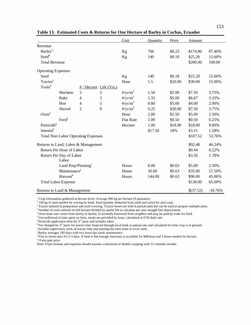
153

Table 13. Estimated Costs & Returns for One Hectare of Barley in Cochas, Ecuador

Unit Quantity Price Amount Revenue Barleya Kg 760 $0.23 $174.80 87.40% Seedb Kg 140 $0.18 $25.20 12.60% Total Revenue $200.00 100.00

Operating Expenses Seed Kg 140 $0.18 $25.20 12.60% Tractorc Hour 1.5 $20.00 $30.00 15.00% Toolsd # / Hectare Life (Yrs.) Machete 3 2 #/yr/m2 1.50 $5.00 $7.50 3.75% Rake 4 3 #/yr/m2 1.33 $5.00 $6.67 3.33% Hoe 4 5 #/yr/m2 0.80 $5.00 $4.00 2.00% Shovel 2 8 #/yr/m2 0.25 $30.00 $7.50 3.75% Oxene Hour 2.00 $2.50 $5.00 2.50% Feedf Flat Rate 1.00 $0.50 $0.50 0.25% Pesticideg Hectare 1.00 $18.00 $18.00 9.00% Interesth $17.50 18% $3.15 1.58% Total Non-Labor Operating Expenses $107.52 53.76%

Returns to Land, Labor & Management $92.48 46.24% Return Per Hour of Labor $0.44 0.22% Return Per Day of Labor $3.56 1.78% Labor Land Prep/Plantingi Hours 8.00 $0.63 $5.00 2.50% Maintenancej Hours 56.00 $0.63 $35.00 17.50% Harvestk Hours 144.00 $0.63 $90.00 45.00% Total Labor Expense $130.00 65.00%

Returns to Land & Management $(37.52) -18.76%

a Crop information gathered at hectare level. Average 900 kg per hectare (9 quintales). b 140 kg of seed needed for sowing by hand. Seed quantity deducted from yield and saved for next crop. c Tractor utilized in preparation and seed covering. Tractor hours not sold in partial units but can be used to prepare multiple plots. d Number of tools utilized on full hectare divided by useful life to calculate per year straight line depreciation. e Oxen lease rate varies from family to family. Is normally borrowed from neighbor and may be paid by trade for food. f Unconditional of time spent on farm, meals are provided by lease, calculated at 0.50 daily rate. g Pesticide application done by 3rd party and includes labor. h Fee charged by 3rd party for tractor time financed through local bank at annual rate and calculated for time crop is in ground. i Includes supervisory work of tractor time and running the oxen team to cover seed. j Barley averages 180 days with two hours per week maintenance. k Five to seven days for 2-3 days. If land is flat enough, harvester is available for $40/hour and 2 hours needed for hectare. * Farm gate price Note: Final revenue and expenses should assume a minimum of double cropping with 12 calendar months.

154

Table 14. Estimated Costs & Returns for One Square Meter of Beets in Cochas, Ecuador

Unit Quantity Price Amount Revenue Beetsa Kg 6.73 $0.30 $2.02 100% Seedb Gram 0 $0.04 $ -- 0% Total Revenue $2.02 100%

Operating Expenses Seed Gram 1.68 $0.04 $0.07 4% Water Days 100.00 $0.001 $0.10 5% Toolsc # / Hectare Life (Yrs.) Machete 3 2 #/yr/m2 0.00015 $5.00 $0.00075 0% Rake 4 3 #/yr/m2 0.00013 $5.00 $0.00067 0% Hoe 4 5 #/yr/m2 0.00008 $5.00 $0.00040 0% Shovel 2 8 #/yr/m2 0.00003 $30.00 $0.00075 0% Drip Systemd 1 5 price/yr/ha 1 $0.03 $0.03 2% Repairse per mt2 1 $0.02 $0.02 1% Garden Enclosuref 5 meters/area/yr 0.06 $2.10 $0.13** 6% Interest $0.19 18% $0.03 2% Total Non-Labor Operating Expenses $0.39 19%

Returns to Land, Labor & Management $1.63 81% Return Per Hour of Labor $0.08 4% Return Per Day of Labor $0.68 33% Labor Land Prep/Planting Hours 1.65 $0.63 $1.03 51% Maintenance Hours 5.89 $0.63 $3.68 182% Harvest Hours 0.25 $0.63 $0.16 8% Total Labor Expense $4.87 241%

Returns to Land & Management $(3.24) -160%

a Beet yield measured per 33cm2 producing 1.333 kg initially. b Assume no saving of seed and purchasing seed each season. c Number of tools utilized on full hectare divided by useful life to calculate per year straight line depreciation, then divided by 10,000 to arrive at quantity used per year per m2. d Drip irrigation kit for hectare is $65 for valves/diverters, $1500 for tubing. Five year depreciation. Same style of kit is $43 for garden crop area of 20x10 meters or 200m2. e Repairs begin year 2 at $4 through year 5 for 200 m2. Scaled to hectare. f Most efficient garden plan assumed utilizing minimal square area. Netting not used for small gardens. Utilization of wind break and security netting at larger scale will depend on geography and size of plot. g Interest calculated on direct expenses, i.e. seed, water, drip system repair. h Worker can prepare and plant a row that has 33cm bed, spaced 60cm on center, and 8m long; total area 4.8m2. i Maintenance needed calculated by water days divided by 7 for weeks. Each row requires 4 hours every other week for weeding/maintaining. j Harvest as crop becomes ripe. Common practice to leave crop in field for storage until needed. *Garden variety crop value derived using half of market price. **Garden enclosure amount should be calculated by linear meters needed divided by area encompassed and then divided by useful life which is multiplied by netting price per linear meter. Note: Final revenue and expenses should assume a minimum of double cropping with 12 calendar months. Garden crop planted in rows 60cm on center with a 33cm wide bed.

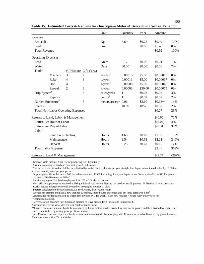
155

Table 15. Estimated Costs & Returns for One Square Meter of Broccoli in Cochas, Ecuador

Unit Quantity Price Amount Revenue Broccoli Kg 3.69 $0.25 $0.92 100% Seed Gram 0 $0.06 $ -- 0% Total Revenue $0.92 100%

Operating Expenses Seed Gram 0.17 $0.06 $0.01 1% Water Days 60.00 $0.001 $0.06 7% Toolsa # / Hectare Life (Yrs.) Machete 3 2 #/yr/m2 0.00015 $5.00 $0.00075 0% Rake 4 3 #/yr/m2 0.00013 $5.00 $0.00067 0% Hoe 4 5 #/yr/m2 0.00008 $5.00 $0.00040 0% Shovel 2 8 #/yr/m2 0.00003 $30.00 $0.00075 0% Drip Systemb 1 5 price/yr/ha 1 $0.03 $0.03 3% Repairsc per mt2 1 $0.02 $0.02 2% Garden Enclosured 5 meters/area/yr 0.06 $2.10 $0.13** 14% Interest $0.09 18% $0.02 2% Total Non-Labor Operating Expenses $0.27 29%

Returns to Land, Labor & Management $(0.66) 71% Return Per Hour of Labor $(0.04) 4% Return Per Day of Labor $(0.31) 34% Labor Land Prep/Planting Hours 1.65 $0.63 $1.03 112% Maintenance Hours 3.54 $0.63 $2.21 240% Harvest Hours 0.25 $0.63 $0.16 17% Total Labor Expense $3.40 369%


a Broccoli yield measured per 33cm2 producing 0.73 kg initially. b Assume no saving of seed and purchasing seed each season. c Number of tools utilized on full hectare divided by useful life to calculate per year straight line depreciation, then divided by 10,000 to arrive at quantity used per year per m2. d Drip irrigation kit for hectare is $65 for valves/diverters, $1500 for tubing. Five year depreciation. Same style of kit is $43 for garden crop area of 20x10 meters or 200m2. e Repairs begin year 2 at $4 through year 5 for 200 m2. Scaled to hectare. f Most efficient garden plan assumed utilizing minimal square area. Netting not used for small gardens. Utilization of wind break and security netting at larger scale will depend on geography and size of plot. g Interest calculated on direct expenses, i.e. seed, water, drip system repair. h Worker can prepare and plant a row that has 33cm bed, spaced 60cm on center, and 8m long; total area 4.8m2. i Maintenance needed calculated by water days divided by 7 for weeks. Each row requires 4 hours every other week for weeding/maintaining. j Harvest as crop becomes ripe. Common practice to leave crop in field for storage until needed. *Garden variety crop value derived using half of market price. **Garden enclosure amount should be calculated by linear meters needed divided by area encompassed and then divided by useful life which is multiplied by netting price per linear meter. Note: Final revenue and expenses should assume a minimum of double cropping with 12 calendar months. Garden crop planted in rows 60cm on center with a 33cm wide bed.

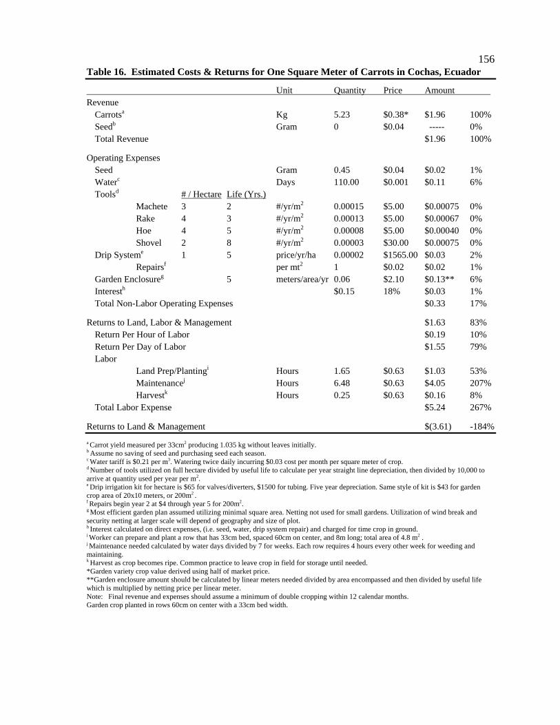
156

Table 16. Estimated Costs & Returns for One Square Meter of Carrots in Cochas, Ecuador

Unit Quantity Price Amount Revenue Carrotsa Kg 5.23 $0.38* $1.96 100% Seedb Gram 0 $0.04 ----- 0% Total Revenue $1.96 100%

Operating Expenses Seed Gram 0.45 $0.04 $0.02 1% Waterc Days 110.00 $0.001 $0.11 6% Toolsd # / Hectare Life (Yrs.) Machete 3 2 #/yr/m2 0.00015 $5.00 $0.00075 0% Rake 4 3 #/yr/m2 0.00013 $5.00 $0.00067 0% Hoe 4 5 #/yr/m2 0.00008 $5.00 $0.00040 0% Shovel 2 8 #/yr/m2 0.00003 $30.00 $0.00075 0% Drip Systeme 1 5 price/yr/ha 0.00002 $1565.00 $0.03 2% Repairsf per mt2 1 $0.02 $0.02 1% Garden Enclosureg 5 meters/area/yr 0.06 $2.10 $0.13** 6% Interesth $0.15 18% $0.03 1% Total Non-Labor Operating Expenses $0.33 17%

Returns to Land, Labor & Management $1.63 83% Return Per Hour of Labor $0.19 10% Return Per Day of Labor $1.55 79% Labor Land Prep/Plantingi Hours 1.65 $0.63 $1.03 53% Maintenancej Hours 6.48 $0.63 $4.05 207% Harvestk Hours 0.25 $0.63 $0.16 8% Total Labor Expense $5.24 267%


a Carrot yield measured per 33cm2 producing 1.035 kg without leaves initially. b Assume no saving of seed and purchasing seed each season. c Water tariff is $0.21 per m3. Watering twice daily incurring $0.03 cost per month per square meter of crop. d Number of tools utilized on full hectare divided by useful life to calculate per year straight line depreciation, then divided by 10,000 to arrive at quantity used per year per m2. e Drip irrigation kit for hectare is $65 for valves/diverters, $1500 for tubing. Five year depreciation. Same style of kit is $43 for garden crop area of 20x10 meters, or 200m2 . f Repairs begin year 2 at $4 through year 5 for 200m2. g Most efficient garden plan assumed utilizing minimal square area. Netting not used for small gardens. Utilization of wind break and security netting at larger scale will depend of geography and size of plot. h Interest calculated on direct expenses, (i.e. seed, water, drip system repair) and charged for time crop in ground. i Worker can prepare and plant a row that has 33cm bed, spaced 60cm on center, and 8m long; total area of 4.8 m2 . j Maintenance needed calculated by water days divided by 7 for weeks. Each row requires 4 hours every other week for weeding and maintaining. k Harvest as crop becomes ripe. Common practice to leave crop in field for storage until needed. *Garden variety crop value derived using half of market price. **Garden enclosure amount should be calculated by linear meters needed divided by area encompassed and then divided by useful life which is multiplied by netting price per linear meter. Note: Final revenue and expenses should assume a minimum of double cropping within 12 calendar months.

Garden crop planted in rows 60cm on center with a 33cm bed width.

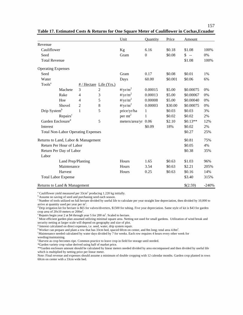
157

Table 17. Estimated Costs & Returns for One Square Meter of Cauliflower in Cochas,Ecuador

Unit Quantity Price Amount Revenue Cauliflower Kg 6.16 $0.18 $1.08 100% Seed Gram 0 $0.08 $ -- 0% Total Revenue $1.08 100%




a Cauliflower yield measured per 33cm2 producing 1.220 kg initially. b Assume no saving of seed and purchasing seed each season. c Number of tools utilized on full hectare divided by useful life to calculate per year straight line depreciation, then divided by 10,000 to arrive at quantity used per year per m2. d Drip irrigation kit for hectare is $65 for valves/diverters, $1500 for tubing. Five year depreciation. Same style of kit is $43 for garden crop area of 20x10 meters or 200m2. e Repairs begin year 2 at $4 through year 5 for 200 m2. Scaled to hectare. f Most efficient garden plan assumed utilizing minimal square area. Netting not used for small gardens. Utilization of wind break and security netting at larger scale will depend on geography and size of plot. g Interest calculated on direct expenses, i.e. seed, water, drip system repair. h Worker can prepare and plant a row that has 33cm bed, spaced 60cm on center, and 8m long; total area 4.8m2. i Maintenance needed calculated by water days divided by 7 for weeks. Each row requires 4 hours every other week for weeding/maintaining. j Harvest as crop becomes ripe. Common practice to leave crop in field for storage until needed. *Garden variety crop value derived using half of market price. **Garden enclosure amount should be calculated by linear meters needed divided by area encompassed and then divided by useful life which is multiplied by netting price per linear meter. Note: Final revenue and expenses should assume a minimum of double cropping with 12 calendar months. Garden crop planted in rows 60cm on center with a 33cm wide bed.

158

Table 18. Estimated Costs & Returns for One Square Meter of Celery in Cochas, Ecuador

Unit Quantity Price Amount Revenue Celery Kg 4.69 $0.25 $1.17 100% Seed Gram 0 $0.13 $ -- 0% Total Revenue $1.17 100%

Operating Expenses Seed Kg 0.22 $0.13 $0.03 3% Water Days 90.00 $0.00 $0.09 8% Toolsa # / Hectare Life (Yrs.) Machete 3 2 #/yr/m2 0.00015 $5.00 $0.00075 0% Rake 4 3 #/yr/m2 0.00013 $5.00 $0.00067 0% Hoe 4 5 #/yr/m2 0.00008 $5.00 $0.00040 0% Shovel 2 8 #/yr/m2 0.00003 $30.00 $0.00075 0% Drip Systemb 1 5 price/yr/ha 1 $0.03 $0.03 3% Repairsc per mt2 1 $0.02 $0.02 2% Garden Enclosured 5 meters/area/yr 0.06 $2.10 $0.13** 11% Interest $0.14 18% $0.03 2% Total Non-Labor Operating Expenses $0.32 28%



a Celery yield measured per 33cm2 producing 0.929 kg initially. b Assume no saving of seed and purchasing seed each season. c Number of tools utilized on full hectare divided by useful life to calculate per year straight line depreciation, then divided by 10,000 to arrive at quantity used per year per m2. d Drip irrigation kit for hectare is $65 for valves/diverters, $1500 for tubing. Five year depreciation. Same style of kit is $43 for garden crop area of 20x10 meters or 200m2. e Repairs begin year 2 at $4 through year 5 for 200 m2. Scaled to hectare. f Most efficient garden plan assumed utilizing minimal square area. Netting not used for small gardens. Utilization of wind break and security netting at larger scale will depend on geography and size of plot. g Interest calculated on direct expenses, i.e. seed, water, drip system repair. h Worker can prepare and plant a row that has 33cm bed, spaced 60cm on center, and 8m long; total area 4.8m2. i Maintenance needed calculated by water days divided by 7 for weeks. Each row requires 4 hours every other week for weeding/maintaining. j Harvest as crop becomes ripe. Common practice to leave crop in field for storage until needed. *Garden variety crop value derived using half of market price. **Garden enclosure amount should be calculated by linear meters needed divided by area encompassed and then divided by useful life which is multiplied by netting price per linear meter. Note: Final revenue and expenses should assume a minimum of double cropping with 12 calendar months. Garden crop planted in rows 60cm on center with a 33cm wide bed.

159

Table 19. Estimated Costs & Returns for One Square Meter of Chard in Cochas, Ecuador

Unit Quantity Price Amount Revenue Chard Kg 5.05 $0.13 $0.63 100% Seed Gram 0 $0.04 $ -- 0% Total Revenue $0.63 100%




a Chard yield measured per 33cm2 producing 1 kg initially. b Assume no saving of seed and purchasing seed each season. c Number of tools utilized on full hectare divided by useful life to calculate per year straight line depreciation, then divided by 10,000 to arrive at quantity used per year per m2. d Drip irrigation kit for hectare is $65 for valves/diverters, $1500 for tubing. Five year depreciation. Same style of kit is $43 for garden crop area of 20x10 meters or 200m2. e Repairs begin year 2 at $4 through year 5 for 200 m2. Scaled to hectare. f Most efficient garden plan assumed utilizing minimal square area. Netting not used for small gardens. Utilization of wind break and security netting at larger scale will depend on geography and size of plot. g Interest calculated on direct expenses, i.e. seed, water, drip system repair. h Worker can prepare and plant a row that has 33cm bed, spaced 60cm on center, and 8m long; total area 4.8m2. i Maintenance needed calculated by water days divided by 7 for weeks. Each row requires 4 hours every other week for weeding/maintaining. j Harvest as crop becomes ripe. Common practice to leave crop in field for storage until needed. *Garden variety crop value derived using half of market price. **Garden enclosure amount should be calculated by linear meters needed divided by area encompassed and then divided by useful life which is multiplied by netting price per linear meter. Note: Final revenue and expenses should assume a minimum of double cropping with 12 calendar months. Garden crop planted in rows 60cm on center with a 33cm wide bed.

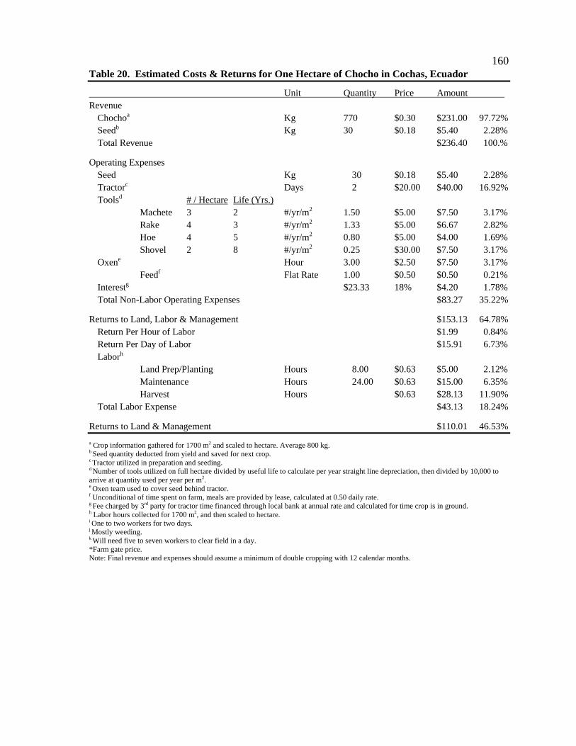
160

Table 20. Estimated Costs & Returns for One Hectare of Chocho in Cochas, Ecuador

Unit Quantity Price Amount Revenue Chochoa Kg 770 $0.30 $231.00 97.72% Seedb Kg 30 $0.18 $5.40 2.28% Total Revenue $236.40 100.%

Operating Expenses Seed Kg 30 $0.18 $5.40 2.28% Tractorc Days 2 $20.00 $40.00 16.92% Toolsd # / Hectare Life (Yrs.) Machete 3 2 #/yr/m2 1.50 $5.00 $7.50 3.17% Rake 4 3 #/yr/m2 1.33 $5.00 $6.67 2.82% Hoe 4 5 #/yr/m2 0.80 $5.00 $4.00 1.69% Shovel 2 8 #/yr/m2 0.25 $30.00 $7.50 3.17% Oxene Hour 3.00 $2.50 $7.50 3.17% Feedf Flat Rate 1.00 $0.50 $0.50 0.21% Interestg $23.33 18% $4.20 1.78% Total Non-Labor Operating Expenses $83.27 35.22%

Returns to Land, Labor & Management $153.13 64.78% Return Per Hour of Labor $1.99 0.84% Return Per Day of Labor $15.91 6.73% Laborh Land Prep/Planting Hours 8.00 $0.63 $5.00 2.12% Maintenance Hours 24.00 $0.63 $15.00 6.35% Harvest Hours $0.63 $28.13 11.90% Total Labor Expense $43.13 18.24%


a Crop information gathered for 1700 m2 and scaled to hectare. Average 800 kg. b Seed quantity deducted from yield and saved for next crop. c Tractor utilized in preparation and seeding. d Number of tools utilized on full hectare divided by useful life to calculate per year straight line depreciation, then divided by 10,000 to arrive at quantity used per year per m2. e Oxen team used to cover seed behind tractor. f Unconditional of time spent on farm, meals are provided by lease, calculated at 0.50 daily rate. g Fee charged by 3rd party for tractor time financed through local bank at annual rate and calculated for time crop is in ground. h Labor hours collected for 1700 m2, and then scaled to hectare. i One to two workers for two days. j Mostly weeding. k Will need five to seven workers to clear field in a day. *Farm gate price. Note: Final revenue and expenses should assume a minimum of double cropping with 12 calendar months.

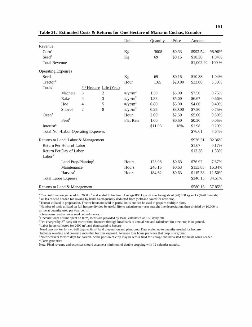
161

Table 21. Estimated Costs & Returns for One Hectare of Maize in Cochas, Ecuador

Unit Quantity Price Amount Revenue Corna Kg 3008 $0.33 $992.54 98.96% Seedb Kg 69 $0.15 $10.38 1.04% Total Revenue $1,002.92 100 %

Operating Expenses Seed Kg 69 $0.15 $10.38 1.04% Tractorc Hour 1.65 $20.00 $33.08 3.30% Toolsd # / Hectare Life (Yrs.) Machete 3 2 #/yr/m2 1.50 $5.00 $7.50 0.75% Rake 4 3 #/yr/m2 1.33 $5.00 $6.67 0.66% Hoe 4 5 #/yr/m2 0.80 $5.00 $4.00 0.40% Shovel 2 8 #/yr/m2 0.25 $30.00 $7.50 0.75% Oxene Hour 2.00 $2.50 $5.00 0.50% Feedf Flat Rate 1.00 $0.50 $0.50 0.05% Interestg $11.03 18% $1.98 0.20% Total Non-Labor Operating Expenses $76.61 7.64%

Returns to Land, Labor & Management $926.31 92.36% Return Per Hour of Labor $1.67 0.17% Return Per Day of Labor $13.38 1.33% Laborh Land Prep/Plantingi Hours 123.08 $0.63 $76.92 7.67% Maintenancej Hours 246.15 $0.63 $153.85 15.34% Harvestk Hours 184.62 $0.63 $115.38 11.50% Total Labor Expense $346.15 34.51%


a Crop information gathered for 2600 m2 and scaled to hectare. Average 800 kg with max being about (20) 100 kg sacks (8-20 quintals). b 40 lbs of seed needed for sowing by hand. Seed quantity deducted from yield and saved for next crop. c Tractor utilized in preparation. Tractor hours not sold in partial units but can be used to prepare multiple plots. d Number of tools utilized on full hectare divided by useful life to calculate per year straight line depreciation, then divided by 10,000 to arrive at quantity used per year per m2. e Oxen team used to cover seed behind tractor. f Unconditional of time spent on farm, meals are provided by lease, calculated at 0.50 daily rate. g Fee charged by 3rd party for tractor time financed through local bank at annual rate and calculated for time crop is in ground. h Labor hours collected for 2600 m2, and then scaled to hectare i Need two worker for two full days to finish land preparation and plant crop. Data scaled up to quantity needed for hectare. j Includes weeding and covering roots that become exposed. Average four hours per week that crop is in ground. k Need workers for two days for harvest. Some portion of crop may be left in field for storage and harvested for meals when needed. * Farm gate price Note: Final revenue and expenses should assume a minimum of double cropping with 12 calendar months.

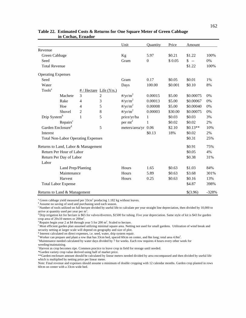
162

Table 22. Estimated Costs & Returns for One Square Meter of Green Cabbage in Cochas, Ecuador

Unit Quantity Price Amount Revenue Green Cabbage Kg 5.97 $0.21 $1.22 100% Seed Gram 0 $ 0.05 $ -- 0% Total Revenue $1.22 100%




a Green cabbage yield measured per 33cm2 producing 1.182 kg without leaves. b Assume no saving of seed and purchasing seed each season. c Number of tools utilized on full hectare divided by useful life to calculate per year straight line depreciation, then divided by 10,000 to arrive at quantity used per year per m2. d Drip irrigation kit for hectare is $65 for valves/diverters, $1500 for tubing. Five year depreciation. Same style of kit is $43 for garden crop area of 20x10 meters or 200m2. e Repairs begin year 2 at $4 through year 5 for 200 m2. Scaled to hectare. f Most efficient garden plan assumed utilizing minimal square area. Netting not used for small gardens. Utilization of wind break and security netting at larger scale will depend on geography and size of plot. g Interest calculated on direct expenses, i.e. seed, water, drip system repair. h Worker can prepare and plant a row that has 33cm bed, spaced 60cm on center, and 8m long; total area 4.8m2. i Maintenance needed calculated by water days divided by 7 for weeks. Each row requires 4 hours every other week for weeding/maintaining. j Harvest as crop becomes ripe. Common practice to leave crop in field for storage until needed. *Garden variety crop value derived using half of market price. **Garden enclosure amount should be calculated by linear meters needed divided by area encompassed and then divided by useful life which is multiplied by netting price per linear meter. Note: Final revenue and expenses should assume a minimum of double cropping with 12 calendar months. Garden crop planted in rows 60cm on center with a 33cm wide bed.

163

Table 23. Estimated Costs & Returns for One Square Meter of Green Onion in Cochas, Ecuador

Unit Quantity Price Amount Revenue Oniona Kg 1.35 $0.26 $0.35 100% Seedb Gram 0 $0.11 $ -- 0% Total Revenue $0.35 100%


Returns to Land, Labor & Management $(0.01) -2% Return Per Hour of Labor $(0.00) 0% Return Per Day of Labor $(0.00) -1% Labor Land Prep/Planting Hours 1.65 $0.63 $1.03 293% Maintenance Hours 5.89 $0.63 $3.68 1047% Harvest Hours 0.25 $0.63 $0.16 44% Total Labor Expense $4.87 1384%


a Green onion yield measured per 33cm2 producing 0.268 kg initially. b Assume no saving of seed and purchasing seed each season. c Number of tools utilized on full hectare divided by useful life to calculate per year straight line depreciation, then divided by 10,000 to arrive at quantity used per year per m2. d Drip irrigation kit for hectare is $65 for valves/diverters, $1500 for tubing. Five year depreciation. Same style of kit is $43 for garden crop area of 20x10 meters or 200m2. e Repairs begin year 2 at $4 through year 5 for 200 m2. Scaled to hectare. f Most efficient garden plan assumed utilizing minimal square area. Netting not used for small gardens. Utilization of wind break and security netting at larger scale will depend on geography and size of plot. g Interest calculated on direct expenses, i.e. seed, water, drip system repair. h Worker can prepare and plant a row that has 33cm bed, spaced 60cm on center, and 8m long; total area 4.8m2. i Maintenance needed calculated by water days divided by 7 for weeks. Each row requires 4 hours every other week for weeding/maintaining. j Harvest as crop becomes ripe. Common practice to leave crop in field for storage until needed. *Garden variety crop value derived using half of market price. **Garden enclosure amount should be calculated by linear meters needed divided by area encompassed and then divided by useful life which is multiplied by netting price per linear meter. Note: Final revenue and expenses should assume a minimum of double cropping with 12 calendar months. Garden crop planted in rows 60cm on center with a 33cm wide bed.

164

Table 24. Estimated Costs & Returns for One Square Meter of Lettuce in Cochas, Ecuador

Unit Quantity Price Amount Revenue Lettuce Kg 3.05 $0.20 $0.61 100% Seed Gram 0 $0.07 $ -- 0% Total Revenue $0.61 100%




a Lettuce yield measured per 33cm2 producing 0.603 kg initially. b Assume no saving of seed and purchasing seed each season. c Number of tools utilized on full hectare divided by useful life to calculate per year straight line depreciation, then divided by 10,000 to arrive at quantity used per year per m2. d Drip irrigation kit for hectare is $65 for valves/diverters, $1500 for tubing. Five year depreciation. Same style of kit is $43 for garden crop area of 20x10 meters or 200m2. e Repairs begin year 2 at $4 through year 5 for 200 m2. Scaled to hectare. f Most efficient garden plan assumed utilizing minimal square area. Netting not used for small gardens. Utilization of wind break and security netting at larger scale will depend on geography and size of plot. g Interest calculated on direct expenses, i.e. seed, water, drip system repair. h Worker can prepare and plant a row that has 33cm bed, spaced 60cm on center, and 8m long; total area 4.8m2. i Maintenance needed calculated by water days divided by 7 for weeks. Each row requires 4 hours every other week for weeding/maintaining. j Harvest as crop becomes ripe. Common practice to leave crop in field for storage until needed. *Garden variety crop value derived using half of market price. **Garden enclosure amount should be calculated by linear meters needed divided by area encompassed and then divided by useful life which is multiplied by netting price per linear meter. Note: Final revenue and expenses should assume a minimum of double cropping with 12 calendar months. Garden crop planted in rows 60cm on center with a 33cm wide bed.

165

Table 25. Estimated Costs & Returns for One Hectare of Oats in Cochas, Ecuador

Unit Quantity Price Amount Revenue Oatsa Kg 800 $0.25 $200.00 88.11% Seedb Kg 150 $0.18 $27.00 11.89% Total Revenue $227.00 100%

Operating Expenses Seed Kg 150 $0.18 $27.00 11.89% Tractorc Hour 1.5 $20.00 $30.00 13.22% Toolsd # / Hectare Life (Yrs.) Machete 3 2 #/yr/m2 1.50 $5.00 $7.50 3.30% Rake 4 3 #/yr/m2 1.33 $5.00 $6.67 2.94% Hoe 4 5 #/yr/m2 0.80 $5.00 $4.00 1.76% Shovel 2 8 #/yr/m2 0.25 $30.00 $7.50 3.30% Oxene Hour 3.00 $2.50 $7.50 3.30% Feedf Flat Rate 1.00 $0.50 $0.50 0.22% Interestg $10.00 18% $1.80 0.79% Total Non-Labor Operating Expenses $92.47 40.73%

Returns to Land, Labor & Management $134.53 59.27% Return Per Hour of Labor $0.48 0.21% Return Per Day of Labor $3.84 1.69% Labor Land Prep/Plantingh Hours 8.00 $0.63 $5.00 2.20% Maintenancei Hours 104.00 $0.63 $65.00 28.63% Harvestj Hours 168.00 $0.63 $105.00 46.26% Total Labor Expense $175.00 77.09%

Returns to Land & Management $(40.47) -17.83%

a Average between 900 to 1000 kg. b Seed quantity deducted from yield and saved for next crop. c Tractor utilized in preparation and seeding. d Number of tools utilized on full hectare divided by useful life to calculate per year straight line depreciation, then divided by 10,000 to arrive at quantity used per year per m2. e Oxen team used to help evenly spread seed and cover seed behind tractor. f Unconditional of time spent on farm, meals are provided by lease, calculated at 0.50 daily rate. g Fee charged by 3rd party for tractor time financed through local bank at annual rate and calculated for time crop is in ground. h Includes supervisory work and running oxen team. i Mostly weeding, average four hours per week. j Will need five to seven workers for two to three days to clear, or harvester runs $40/hour and takes 2 hours per hectare. *Farm gate price. Note: Final revenue and expenses should assume a minimum of double cropping with 12 calendar months.

166

Table 26. Estimated Costs & Returns for One Hectare of Potatoes in Cochas, Ecuador

Unit Quantity Price Amount Revenue Potatoa Kg 8000 $0.35 $2,800 87.04% Seedb Kg 1000 $0.42 $417 12.96% Total Revenue $3,217.00 100%

Operating Expenses Seed Kg 1000 $0.42 $417.00 12.96% Tractorc Hour 10 $25.00 $250.00 7.77% Toolsd # / Hectare Life (Yrs.) Machete 3 2 #/yr/m2 1.50 $5.00 $7.50 0.23% Rake 4 3 #/yr/m2 1.33 $5.00 $6.67 0.21% Hoe 4 5 #/yr/m2 0.80 $5.00 $4.00 0.12% Shovel 2 8 #/yr/m2 0.25 $30.00 $7.50 0.23% Oxene Hour 20.00 $2.50 $50.00 1.55% Feedf Flat Rate 1.00 $0.50 $0.50 0.02% Interestg $145.83 18% $26.25 0.82% Total Non-Labor Operating Expenses $769.42 23.92%

Returns to Land, Labor & Management $2,447.58 76.08% Return Per Hour of Labor $1.25 0.04% Return Per Day of Labor $9.99 0.31% Laborh Land Prep/Plantingi Hours 1200.00 $0.625 $750.00 23.31% Maintenancej Hours 280.00 $0.625 $175.00 5.44% Harvestk Hours 480.00 $0.625 $300.00 9.33% Total Labor Expense $1,225.00 38.08%

Returns to Land & Management $1,222.58 38.00%

a Crop information gathered for 1000 m2 and scaled to hectare. Average 900 kg. b Seed potatoes needed for sowing by hand. Seed quantity deducted from yield and saved for next crop. c Tractor utilized in preparation. Plot plowed multiple times for soil preparation d Number of tools utilized on full hectare divided by useful life to calculate per year straight line depreciation, then divided by 10,000 to arrive at quantity used per year per m2. e Oxen team utilized in addition to tractor to continue plowing/disking to break up soil. f Fee charged by 3rd party for tractor time financed through local bank at annual rate and calculated for time crop is in ground. g Labor hours collected for 1000 m2, and then scaled to hectare.

h Five workers for three full days to finish land preparation and plant crop. Majority of time spent in cutting/planting potatoes. i Mostly weeding. j Will need five to seven workers to clear a field in a day. * Farm gate price Note: Final revenue and expenses should assume a minimum of double cropping with 12 calendar months.

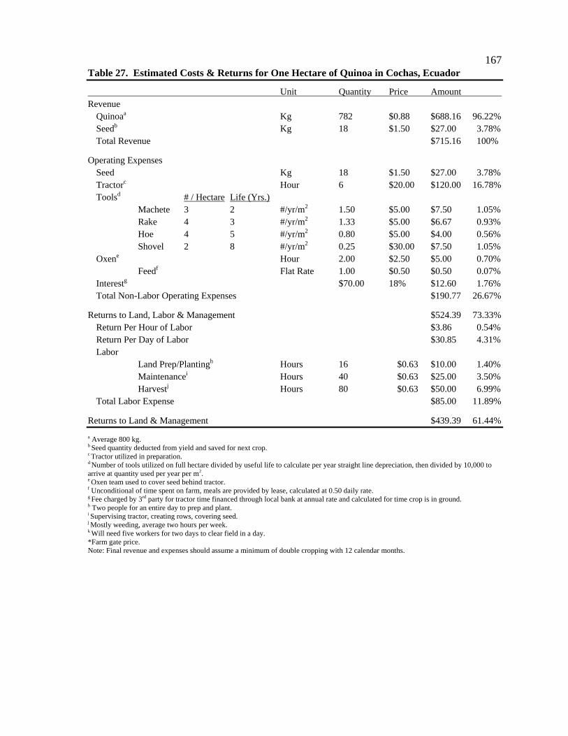
167

Table 27. Estimated Costs & Returns for One Hectare of Quinoa in Cochas, Ecuador

Unit Quantity Price Amount Revenue Quinoaa Kg 782 $0.88 $688.16 96.22% Seedb Kg 18 $1.50 $27.00 3.78% Total Revenue $715.16 100%

Operating Expenses Seed Kg 18 $1.50 $27.00 3.78% Tractorc Hour 6 $20.00 $120.00 16.78% Toolsd # / Hectare Life (Yrs.) Machete 3 2 #/yr/m2 1.50 $5.00 $7.50 1.05% Rake 4 3 #/yr/m2 1.33 $5.00 $6.67 0.93% Hoe 4 5 #/yr/m2 0.80 $5.00 $4.00 0.56% Shovel 2 8 #/yr/m2 0.25 $30.00 $7.50 1.05% Oxene Hour 2.00 $2.50 $5.00 0.70% Feedf Flat Rate 1.00 $0.50 $0.50 0.07% Interestg $70.00 18% $12.60 1.76% Total Non-Labor Operating Expenses $190.77 26.67%

Returns to Land, Labor & Management $524.39 73.33% Return Per Hour of Labor $3.86 0.54% Return Per Day of Labor $30.85 4.31% Labor Land Prep/Plantingh Hours 16 $0.63 $10.00 1.40% Maintenancei Hours 40 $0.63 $25.00 3.50% Harvestj Hours 80 $0.63 $50.00 6.99% Total Labor Expense $85.00 11.89%


a Average 800 kg. b Seed quantity deducted from yield and saved for next crop. c Tractor utilized in preparation.

d Number of tools utilized on full hectare divided by useful life to calculate per year straight line depreciation, then divided by 10,000 to arrive at quantity used per year per m2. e Oxen team used to cover seed behind tractor. f Unconditional of time spent on farm, meals are provided by lease, calculated at 0.50 daily rate. g Fee charged by 3rd party for tractor time financed through local bank at annual rate and calculated for time crop is in ground. h Two people for an entire day to prep and plant. i Supervising tractor, creating rows, covering seed. j Mostly weeding, average two hours per week. k Will need five workers for two days to clear field in a day. *Farm gate price. Note: Final revenue and expenses should assume a minimum of double cropping with 12 calendar months.

168

Table 28. Estimated Costs & Returns for One Square Meter of Radish in Cochas, Ecuador

Unit Quantity Price Amount Revenue Radish Kg 0.77 $1.04 $0.80 100% Seed Gram 0 $0.03 $ -- 0% Total Revenue $0.80 100%




a Radish yield measured per 33cm2 producing 0.152 kg initially. b Assume no saving of seed and purchasing seed each season. c Number of tools utilized on full hectare divided by useful life to calculate per year straight line depreciation, then divided by 10,000 to arrive at quantity used per year per m2. d Drip irrigation kit for hectare is $65 for valves/diverters, $1500 for tubing. Five year depreciation. Same style of kit is $43 for garden crop area of 20x10 meters or 200m2. e Repairs begin year 2 at $4 through year 5 for 200 m2. Scaled to hectare. f Most efficient garden plan assumed utilizing minimal square area. Netting not used for small gardens. Utilization of wind break and security netting at larger scale will depend on geography and size of plot. g Interest calculated on direct expenses, i.e. seed, water, drip system repair. h Worker can prepare and plant a row that has 33cm bed, spaced 60cm on center, and 8m long; total area 4.8m2. i Maintenance needed calculated by water days divided by 7 for weeks. Each row requires 4 hours every other week for weeding/maintaining. j Harvest as crop becomes ripe. Common practice to leave crop in field for storage until needed. *Garden variety crop value derived using half of market price. **Garden enclosure amount should be calculated by linear meters needed divided by area encompassed and then divided by useful life which is multiplied by netting price per linear meter. Note: Final revenue and expenses should assume a minimum of double cropping with 12 calendar months. Garden crop planted in rows 60cm on center with a 33cm wide bed.

169

Table 29. Estimated Costs & Returns for One Square Meter of Red Cabbage in Cochas, Ecuador

Unit Quantity Price Amount Revenue Red Cabbage Kg 6.17 $0.20 $1.26 100% Seed Gram 0 $0.05 $ -- 0% Total Revenue $1.26 100%




a Red cabbage yield measured per 33cm2 producing 1.221 kg initially. b Assume no saving of seed and purchasing seed each season. c Number of tools utilized on full hectare divided by useful life to calculate per year straight line depreciation, then divided by 10,000 to arrive at quantity used per year per m2. d Drip irrigation kit for hectare is $65 for valves/diverters, $1500 for tubing. Five year depreciation. Same style of kit is $43 for garden crop area of 20x10 meters or 200m2. e Repairs begin year 2 at $4 through year 5 for 200 m2. Scaled to hectare. f Most efficient garden plan assumed utilizing minimal square area. Netting not used for small gardens. Utilization of wind break and security netting at larger scale will depend on geography and size of plot. g Interest calculated on direct expenses, i.e. seed, water, drip system repair. h Worker can prepare and plant a row that has 33cm bed, spaced 60cm on center, and 8m long; total area 4.8m2. i Maintenance needed calculated by water days divided by 7 for weeks. Each row requires 4 hours every other week for weeding/maintaining. j Harvest as crop becomes ripe. Common practice to leave crop in field for storage until needed. *Garden variety crop value derived using half of market price. **Garden enclosure amount should be calculated by linear meters needed divided by area encompassed and then divided by useful life which is multiplied by netting price per linear meter. Note: Final revenue and expenses should assume a minimum of double cropping with 12 calendar months. Garden crop planted in rows 60cm on center with a 33cm wide bed.

170

Table 30. Estimated Costs & Returns for One Square Meter of Spinach in Cochas, Ecuador

Unit Quantity Price Amount Revenue Spinach Kg 3.94 $0.09 $0.35 100% Seed Gram 0 $0.04 $ -- 0% Total Revenue $0.35 100%


Returns to Land, Labor & Management $(0.01) -1% Return Per Hour of Labor $(0.00) 0% Return Per Day of Labor $(0.00) -1% Labor Land Prep/Planting Hours 1.65 $0.63 $1.03 291% Maintenance Hours 5.30 $0.63 $3.31 935% Harvest Hours 0.25 $0.63 $0.16 44% Total Labor Expense $4.50 1270%


a Spinach yield measured per 33cm2 producing 0.780 kg initially. b Assume no saving of seed and purchasing seed each season. c Number of tools utilized on full hectare divided by useful life to calculate per year straight line depreciation, then divided by 10,000 to arrive at quantity used per year per m2. d Drip irrigation kit for hectare is $65 for valves/diverters, $1500 for tubing. Five year depreciation. Same style of kit is $43 for garden crop area of 20x10 meters or 200m2. e Repairs begin year 2 at $4 through year 5 for 200 m2. Scaled to hectare. f Most efficient garden plan assumed utilizing minimal square area. Netting not used for small gardens. Utilization of wind break and security netting at larger scale will depend on geography and size of plot. g Interest calculated on direct expenses, i.e. seed, water, drip system repair. h Worker can prepare and plant a row that has 33cm bed, spaced 60cm on center, and 8m long; total area 4.8m2. i Maintenance needed calculated by water days divided by 7 for weeks. Each row requires 4 hours every other week for weeding/maintaining. j Harvest as crop becomes ripe. Common practice to leave crop in field for storage until needed. *Garden variety crop value derived using half of market price. **Garden enclosure amount should be calculated by linear meters needed divided by area encompassed and then divided by useful life which is multiplied by netting price per linear meter. Note: Final revenue and expenses should assume a minimum of double cropping with 12 calendar months. Garden crop planted in rows 60cm on center with a 33cm wide bed.

171

Table 31. Estimated Costs & Returns for One Square Meter of Tomato in Cochas, Ecuador

Unit Quantity Price Amount Revenue Tomato Kg 4.84 $0.38 $1.81 100% Seed Gram 0 $0.16 $ -- 0% Total Revenue $1.81 100%




a Tomato yield measured per 33cm2 producing 0.958 kg initially. b Assume no saving of seed and purchasing seed each season. c Number of tools utilized on full hectare divided by useful life to calculate per year straight line depreciation, then divided by 10,000 to arrive at quantity used per year per m2. d Drip irrigation kit for hectare is $65 for valves/diverters, $1500 for tubing. Five year depreciation. Same style of kit is $43 for garden crop area of 20x10 meters or 200m2. e Repairs begin year 2 at $4 through year 5 for 200 m2. Scaled to hectare. f Most efficient garden plan assumed utilizing minimal square area. Netting not used for small gardens. Utilization of wind break and security netting at larger scale will depend on geography and size of plot. g Interest calculated on direct expenses, i.e. seed, water, drip system repair. h Worker can prepare and plant a row that has 33cm bed, spaced 60cm on center, and 8m long; total area 4.8m2. i Maintenance needed calculated by water days divided by 7 for weeks. Each row requires 4 hours every other week for weeding/maintaining. j Harvest as crop becomes ripe. Common practice to leave crop in field for storage until needed. *Garden variety crop value derived using half of market price. **Garden enclosure amount should be calculated by linear meters needed divided by area encompassed and then divided by useful life which is multiplied by netting price per linear meter. Note: Final revenue and expenses should assume a minimum of double cropping with 12 calendar months. Garden crop planted in rows 60cm on center with a 33cm wide bed.

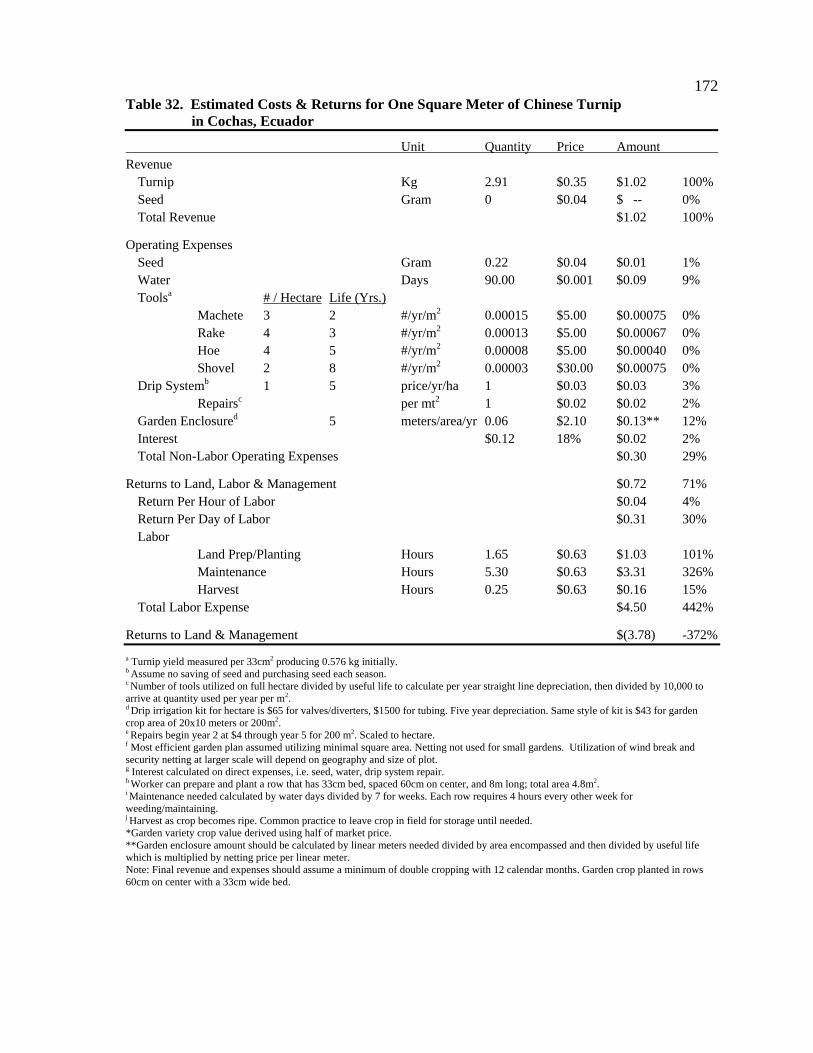
172

Table 32. Estimated Costs & Returns for One Square Meter of Chinese Turnip in Cochas, Ecuador

Unit Quantity Price Amount Revenue Turnip Kg 2.91 $0.35 $1.02 100% Seed Gram 0 $0.04 $ -- 0% Total Revenue $1.02 100%




a Turnip yield measured per 33cm2 producing 0.576 kg initially. b Assume no saving of seed and purchasing seed each season. c Number of tools utilized on full hectare divided by useful life to calculate per year straight line depreciation, then divided by 10,000 to arrive at quantity used per year per m2. d Drip irrigation kit for hectare is $65 for valves/diverters, $1500 for tubing. Five year depreciation. Same style of kit is $43 for garden crop area of 20x10 meters or 200m2. e Repairs begin year 2 at $4 through year 5 for 200 m2. Scaled to hectare. f Most efficient garden plan assumed utilizing minimal square area. Netting not used for small gardens. Utilization of wind break and security netting at larger scale will depend on geography and size of plot. g Interest calculated on direct expenses, i.e. seed, water, drip system repair. h Worker can prepare and plant a row that has 33cm bed, spaced 60cm on center, and 8m long; total area 4.8m2. i Maintenance needed calculated by water days divided by 7 for weeks. Each row requires 4 hours every other week for weeding/maintaining. j Harvest as crop becomes ripe. Common practice to leave crop in field for storage until needed. *Garden variety crop value derived using half of market price. **Garden enclosure amount should be calculated by linear meters needed divided by area encompassed and then divided by useful life which is multiplied by netting price per linear meter. Note: Final revenue and expenses should assume a minimum of double cropping with 12 calendar months. Garden crop planted in rows 60cm on center with a 33cm wide bed.

173

Table 33. Estimated Costs & Returns for One Hectare of Wheat in Cochas, Ecuador

Unit Quantity Price Amount Revenue Wheata Kg 4050 $0.16 $647.94 98.04% Seedb Kg 68 $0.19 $12.95 1.96% Total Revenue $660.89 100%

Operating Expenses Seed Kg 68.00 $0.19 $12.95 1.96% Tractorc Hour 1.5 $20.00 $30.00 4.54% Toolsd # / Hectare Life (Yrs.) Machete 3 2 #/yr/m2 1.50 $5.00 $7.50 1.13% Rake 4 3 #/yr/m2 1.33 $5.00 $6.67 1.01% Hoe 4 5 #/yr/m2 0.80 $5.00 $4.00 0.61% Shovel 2 8 #/yr/m2 0.25 $30.00 $7.50 1.13% Oxene Hour 2.00 $2.50 $5.00 0.76% Feedf Flat Rate 1.00 $0.50 $0.50 0.08% Interestg $17.50 18% $3.15 0.48% Total Non-Labor Operating Expenses $77.26 11.69%

Returns to Land, Labor & Management $583.63 88.31% Return Per Hour of Labor $6.55 0.99% Return Per Day of Labor $52.38 7.93% Laborh Land Prep/Plantingi Hours 16 $5.00 $80.00 12.10% Maintenancej Hours 17 $0.63 $10.71 1.62% Harvestk Hours 56 $5.00 $280.00 42.37% Total Labor Expense $370.71 56.09%


a Crop information gathered for 1700 m2 and scaled to hectare. Average 800 kg. b Seed quantity deducted from yield and saved for next crop. c Tractor utilized in preparation and seeding. d Number of tools utilized on full hectare divided by useful life to calculate per year straight line depreciation, then divided by 10,000 to arrive at quantity used per year per m2. e Oxen team used to cover seed behind tractor. f Unconditional of time spent on farm, meals are provided by lease, calculated at 0.50 daily rate. g Fee charged by 3rd party for tractor time financed through local bank at annual rate and calculated for time crop is in ground. h Labor hours collected for 1700 m2, and then scaled to hectare. i One to two workers for two days. j Mostly weeding. k Will need five to seven workers to clear field in a day. *Farm gate price. Note: Final revenue and expenses should assume a minimum of double cropping with 12 calendar months.

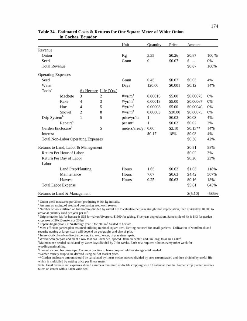
174

Table 34. Estimated Costs & Returns for One Square Meter of White Onion in Cochas, Ecuador

Unit Quantity Price Amount Revenue Onion Kg 3.35 $0.26 $0.87 100 % Seed Gram 0 $0.07 $ -- 0% Total Revenue $0.87 100%




a Onion yield measured per 33cm2 producing 0.664 kg initially. b Assume no saving of seed and purchasing seed each season. c Number of tools utilized on full hectare divided by useful life to calculate per year straight line depreciation, then divided by 10,000 to arrive at quantity used per year per m2. d Drip irrigation kit for hectare is $65 for valves/diverters, $1500 for tubing. Five year depreciation. Same style of kit is $43 for garden crop area of 20x10 meters or 200m2. e Repairs begin year 2 at $4 through year 5 for 200 m2. Scaled to hectare. f Most efficient garden plan assumed utilizing minimal square area. Netting not used for small gardens. Utilization of wind break and security netting at larger scale will depend on geography and size of plot. g Interest calculated on direct expenses, i.e. seed, water, drip system repair. h Worker can prepare and plant a row that has 33cm bed, spaced 60cm on center, and 8m long; total area 4.8m2. i Maintenance needed calculated by water days divided by 7 for weeks. Each row requires 4 hours every other week for weeding/maintaining. j Harvest as crop becomes ripe. Common practice to leave crop in field for storage until needed. *Garden variety crop value derived using half of market price. **Garden enclosure amount should be calculated by linear meters needed divided by area encompassed and then divided by useful life which is multiplied by netting price per linear meter. Note: Final revenue and expenses should assume a minimum of double cropping with 12 calendar months. Garden crop planted in rows 60cm on center with a 33cm wide bed.

175

Table 35. Estimated Costs & Returns for One Square Meter of Zucchini in Cochas, Ecuador

Unit Quantity Price Amount Revenue Zucchini Kg 1.94 $0.18 $0.34 100% Seed Gram 0 $0.16 $ -- 0% Total Revenue $0.34 100%


Returns to Land, Labor & Management $(0.06) -17% Return Per Hour of Labor $(0.00) -1% Return Per Day of Labor $(0.03) -8% Labor Land Prep/Planting Hours 1.65 $0.63 $1.03 304% Maintenance Hours 4.42 $0.63 $2.76 814% Harvest Hours 0.25 $0.63 $0.16 46% Total Labor Expense $3.95 1164%


a Zucchini yield measured per 33cm2 producing 2.304 kg with 6 week harvest initially. b Assume no saving of seed and purchasing seed each season. c Number of tools utilized on full hectare divided by useful life to calculate per year straight line depreciation, then divided by 10,000 to arrive at quantity used per year per m2. d Drip irrigation kit for hectare is $65 for valves/diverters, $1500 for tubing. Five year depreciation. Same style of kit is $43 for garden crop area of 20x10 meters or 200m2. e Repairs begin year 2 at $4 through year 5 for 200 m2. Scaled to hectare. f Most efficient garden plan assumed utilizing minimal square area. Netting not used for small gardens. Utilization of wind break and security netting at larger scale will depend on geography and size of plot. g Interest calculated on direct expenses, i.e. seed, water, drip system repair. h Worker can prepare and plant a row that has 33cm bed, spaced 60cm on center, and 8m long; total area 4.8m2. i Maintenance needed calculated by water days divided by 7 for weeks. Each row requires 4 hours every other week for weeding/maintaining. j Harvest as crop becomes ripe. Common practice to leave crop in field for storage until needed. *Garden variety crop value derived using half of market price. **Garden enclosure amount should be calculated by linear meters needed divided by area encompassed and then divided by useful life which is multiplied by netting price per linear meter. Note: Final revenue and expenses should assume a minimum of double cropping with 12 calendar months. Garden crop planted in rows 60cm on center with a 33cm wide bed.

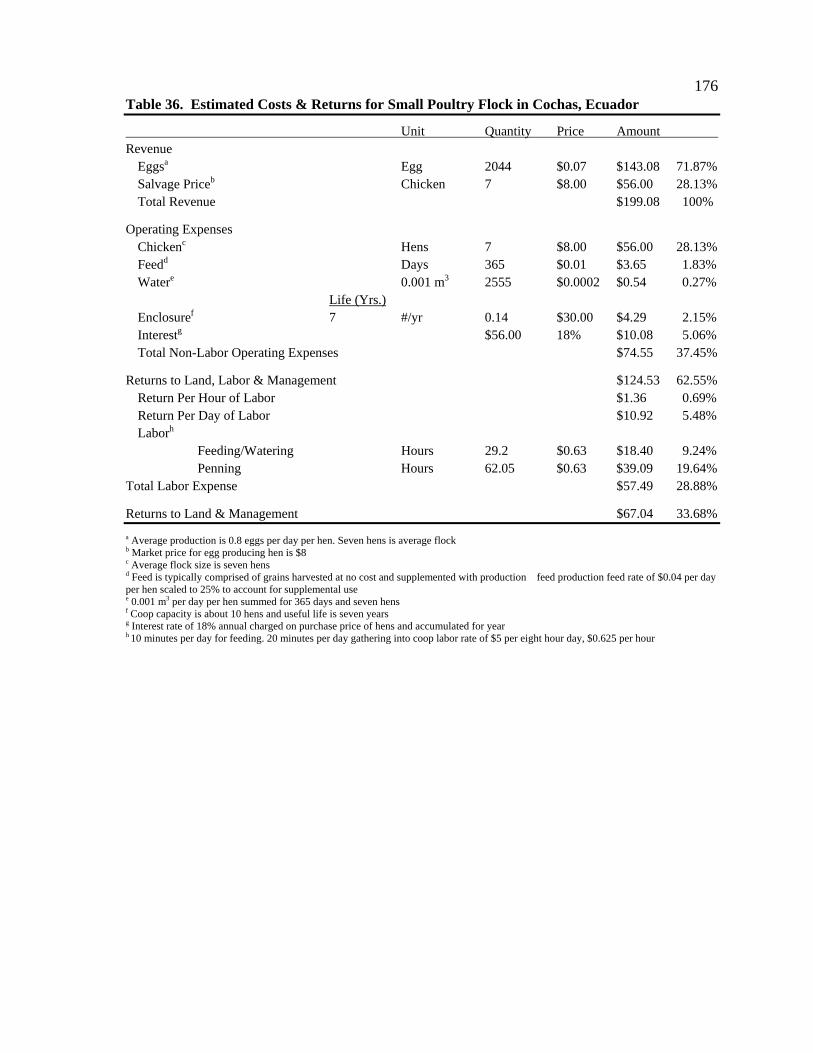
176

Table 36. Estimated Costs & Returns for Small Poultry Flock in Cochas, Ecuador

Unit Quantity Price Amount Revenue Eggsa Egg 2044 $0.07 $143.08 71.87% Salvage Priceb Chicken 7 $8.00 $56.00 28.13% Total Revenue $199.08 100%

Operating Expenses Chickenc Hens 7 $8.00 $56.00 28.13% Feedd Days 365 $0.01 $3.65 1.83% Watere 0.001 m3 2555 $0.0002 $0.54 0.27% Life (Yrs.) Enclosuref 7 #/yr 0.14 $30.00 $4.29 2.15% Interestg $56.00 18% $10.08 5.06% Total Non-Labor Operating Expenses $74.55 37.45%

Returns to Land, Labor & Management $124.53 62.55% Return Per Hour of Labor $1.36 0.69% Return Per Day of Labor $10.92 5.48% Laborh Feeding/Watering Hours 29.2 $0.63 $18.40 9.24% Penning Hours 62.05 $0.63 $39.09 19.64% Total Labor Expense $57.49 28.88%


a Average production is 0.8 eggs per day per hen. Seven hens is average flock b Market price for egg producing hen is $8 c Average flock size is seven hens d Feed is typically comprised of grains harvested at no cost and supplemented with production feed production feed rate of $0.04 per day per hen scaled to 25% to account for supplemental use e 0.001 m3 per day per hen summed for 365 days and seven hens f Coop capacity is about 10 hens and useful life is seven years g Interest rate of 18% annual charged on purchase price of hens and accumulated for year h 10 minutes per day for feeding. 20 minutes per day gathering into coop labor rate of $5 per eight hour day, $0.625 per hour

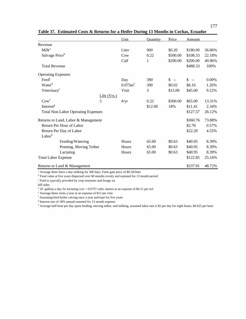
177

Table 37. Estimated Costs & Returns for a Heifer During 13 Months in Cochas, Ecuador

Unit Quantity Price Amount Revenue Milka Liter 900 $0.20 $180.00 36.86% Salvage Priceb Cow 0.22 $500.00 $108.33 22.18% Calf 1 $200.00 $200.00 40.96% Total Revenue $488.33 100%

Operating Expenses Feedc Day 390 $ -- $ -- 0.00% Waterd 0.075m3 390 $0.02 $6.16 1.26% Veterinarye Visit 3 $15.00 $45.00 9.22% Life (Yrs.) Cowf 5 #/yr 0.22 $300.00 $65.00 13.31% Interestg $12.68 18% $11.41 2.34% Total Non-Labor Operating Expenses $127.57 26.12%

Returns to Land, Labor & Management $360.76 73.88% Return Per Hour of Labor $2.78 0.57% Return Per Day of Labor $22.20 4.55% Laborh Feeding/Watering Hours 65.00 $0.63 $40.95 8.39% Penning, Moving Tether Hours 65.00 $0.63 $40.95 8.39% Lactating Hours 65.00 $0.63 $40.95 8.39% Total Labor Expense $122.85 25.16%

Returns to Land & Management $237.91 48.72% a Average three liters a day milking for 300 days. Farm gate price of $0.20/litter b Final value at five years dispersed over 60 months evenly and summed for 13 month period c Feed is typically provided by crop remnants and forage on hill sides d 20 gallons a day for lactating cow = 0.0757 cubic meters at an expense of $0.21 per m3 e Average three visits a year at an expense of $15 per visit f Assuming bred heifer calving once a year and kept for five years g Interest rate of 18% annual summed for 13 month expense h Average half hour per day spent feeding, moving tether, and milking, assumed labor rate is $5 per day for eight hours, $0.625 per hour

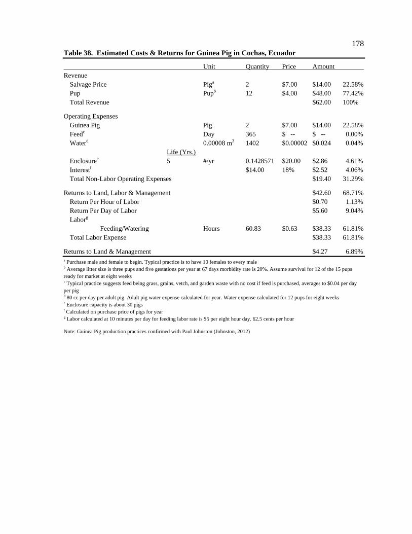
178

Table 38. Estimated Costs & Returns for Guinea Pig in Cochas, Ecuador

Unit Quantity Price Amount Revenue Salvage Price Piga 2 $7.00 $14.00 22.58% Pup Pupb 12 $4.00 $48.00 77.42% Total Revenue $62.00 100%

Operating Expenses Guinea Pig Pig 2 $7.00 $14.00 22.58% Feedc Day 365 $ -- $ -- 0.00% Waterd 0.00008 m3 1402 $0.00002 $0.024 0.04% Life (Yrs.) Enclosuree 5 #/yr 0.1428571 $20.00 $2.86 4.61% Interestf $14.00 18% $2.52 4.06% Total Non-Labor Operating Expenses $19.40 31.29%

Returns to Land, Labor & Management $42.60 68.71% Return Per Hour of Labor $0.70 1.13% Return Per Day of Labor $5.60 9.04% Laborg Feeding/Watering Hours 60.83 $0.63 $38.33 61.81% Total Labor Expense $38.33 61.81%

Returns to Land & Management $4.27 6.89% a Purchase male and female to begin. Typical practice is to have 10 females to every male b Average litter size is three pups and five gestations per year at 67 days morbidity rate is 20%. Assume survival for 12 of the 15 pups ready for market at eight weeks c Typical practice suggests feed being grass, grains, vetch, and garden waste with no cost if feed is purchased, averages to $0.04 per day per pig d 80 cc per day per adult pig. Adult pig water expense calculated for year. Water expense calculated for 12 pups for eight weeks e Enclosure capacity is about 30 pigs f Calculated on purchase price of pigs for year g Labor calculated at 10 minutes per day for feeding labor rate is $5 per eight hour day. 62.5 cents per hour

Note: Guinea Pig production practices confirmed with Paul Johnston (Johnston, 2012)

179

Appendix B

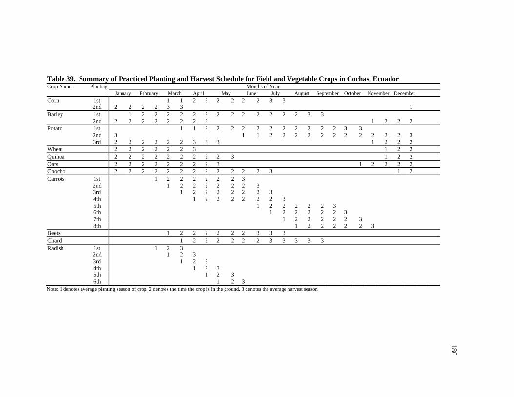
180

Table 39. Summary of Practiced Planting and Harvest Schedule for Field and Vegetable Crops in Cochas, Ecuador Crop Name Planting Months of Year January February March April May June July August September October November December

Corn 1st 1 1 2 2 2 2 2 2 3 3 2nd 2 2 2 2 3 3 1Barley 1st 1 2 2 2 2 2 2 2 2 2 2 2 2 2 3 3 2nd 2 2 2 2 2 2 2 3 1 2 2 2Potato 1st 1 1 2 2 2 2 2 2 2 2 2 2 2 3 3 2nd 3 1 1 2 2 2 2 2 2 2 2 2 2 2 3 3rd 2 2 2 2 2 2 3 3 3 1 2 2 2Wheat 2 2 2 2 2 2 3 1 2 2Quinoa 2 2 2 2 2 2 2 2 2 3 1 2 2Oats 2 2 2 2 2 2 2 2 3 1 2 2 2 2Chocho 2 2 2 2 2 2 2 2 2 2 2 2 3 1 2Carrots 1st 1 2 2 2 2 2 2 3 2nd 1 2 2 2 2 2 2 3 3rd 1 2 2 2 2 2 2 3 4th 1 2 2 2 2 2 2 3 5th 1 2 2 2 2 2 3 6th 1 2 2 2 2 2 3 7th 1 2 2 2 2 2 3 8th 1 2 2 2 2 2 3 Beets 1 2 2 2 2 2 2 3 3 3 Chard 1 2 2 2 2 2 2 3 3 3 3 3 Radish 1st 1 2 3 2nd 1 2 3 3rd 1 2 3 4th 1 2 3 5th 1 2 3 6th 1 2 3 Note: 1 denotes average planting season of crop. 2 denotes the time the crop is in the ground. 3 denotes the average harvest season

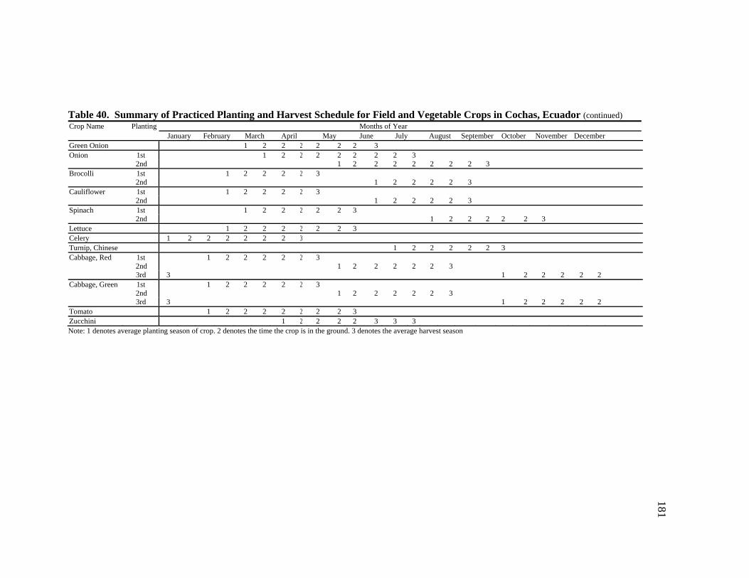
181

Table 40. Summary of Practiced Planting and Harvest Schedule for Field and Vegetable Crops in Cochas, Ecuador (continued)

Crop Name Planting Months of Year January February March April May June July August September October November DecemberGreen Onion 1 2 2 2 2 2 2 3 Onion 1st 1 2 2 2 2 2 2 2 3 2nd 1 2 2 2 2 2 2 2 3 Brocolli 1st 1 2 2 2 2 3 2nd 1 2 2 2 2 3 Cauliflower 1st 1 2 2 2 2 3 2nd 1 2 2 2 2 3 Spinach 1st 1 2 2 2 2 2 3 2nd 1 2 2 2 2 2 3 Lettuce 1 2 2 2 2 2 2 3 Celery 1 2 2 2 2 2 2 3 Turnip, Chinese 1 2 2 2 2 2 3 Cabbage, Red 1st 1 2 2 2 2 2 3 2nd 1 2 2 2 2 2 3 3rd 3 1 2 2 2 2 2 Cabbage, Green 1st 1 2 2 2 2 2 3 2nd 1 2 2 2 2 2 3 3rd 3 1 2 2 2 2 2 Tomato 1 2 2 2 2 2 2 2 3 Zucchini 1 2 2 2 2 3 3 3 Note: 1 denotes average planting season of crop. 2 denotes the time the crop is in the ground. 3 denotes the average harvest season

182

Appendix C

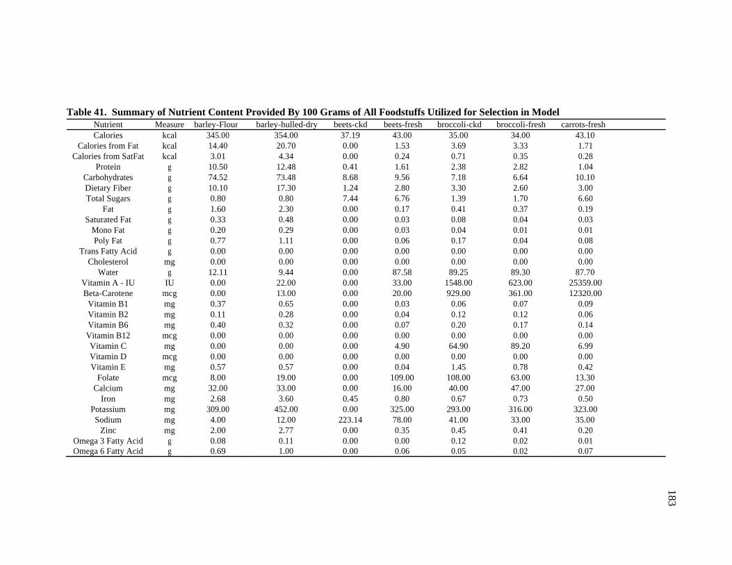
183

Table 41. Summary of Nutrient Content Provided By 100 Grams of All Foodstuffs Utilized for Selection in Model Nutrient Measure barley-Flour barley-hulled-dry beets-ckd beets-fresh broccoli-ckd broccoli-fresh carrots-freshCalories kcal 345.00 354.00 37.19 43.00 35.00 34.00 43.10

Calories from Fat kcal 14.40 20.70 0.00 1.53 3.69 3.33 1.71Calories from SatFat kcal 3.01 4.34 0.00 0.24 0.71 0.35 0.28

Protein g 10.50 12.48 0.41 1.61 2.38 2.82 1.04Carbohydrates g 74.52 73.48 8.68 9.56 7.18 6.64 10.10Dietary Fiber g 10.10 17.30 1.24 2.80 3.30 2.60 3.00Total Sugars g 0.80 0.80 7.44 6.76 1.39 1.70 6.60

Fat g 1.60 2.30 0.00 0.17 0.41 0.37 0.19Saturated Fat g 0.33 0.48 0.00 0.03 0.08 0.04 0.03

Mono Fat g 0.20 0.29 0.00 0.03 0.04 0.01 0.01Poly Fat g 0.77 1.11 0.00 0.06 0.17 0.04 0.08

Trans Fatty Acid g 0.00 0.00 0.00 0.00 0.00 0.00 0.00Cholesterol mg 0.00 0.00 0.00 0.00 0.00 0.00 0.00

Water g 12.11 9.44 0.00 87.58 89.25 89.30 87.70Vitamin A - IU IU 0.00 22.00 0.00 33.00 1548.00 623.00 25359.00Beta-Carotene mcg 0.00 13.00 0.00 20.00 929.00 361.00 12320.00

Vitamin B1 mg 0.37 0.65 0.00 0.03 0.06 0.07 0.09Vitamin B2 mg 0.11 0.28 0.00 0.04 0.12 0.12 0.06Vitamin B6 mg 0.40 0.32 0.00 0.07 0.20 0.17 0.14Vitamin B12 mcg 0.00 0.00 0.00 0.00 0.00 0.00 0.00Vitamin C mg 0.00 0.00 0.00 4.90 64.90 89.20 6.99Vitamin D mcg 0.00 0.00 0.00 0.00 0.00 0.00 0.00Vitamin E mg 0.57 0.57 0.00 0.04 1.45 0.78 0.42

Folate mcg 8.00 19.00 0.00 109.00 108.00 63.00 13.30Calcium mg 32.00 33.00 0.00 16.00 40.00 47.00 27.00

Iron mg 2.68 3.60 0.45 0.80 0.67 0.73 0.50Potassium mg 309.00 452.00 0.00 325.00 293.00 316.00 323.00Sodium mg 4.00 12.00 223.14 78.00 41.00 33.00 35.00

Zinc mg 2.00 2.77 0.00 0.35 0.45 0.41 0.20Omega 3 Fatty Acid g 0.08 0.11 0.00 0.00 0.12 0.02 0.01Omega 6 Fatty Acid g 0.69 1.00 0.00 0.06 0.05 0.02 0.07

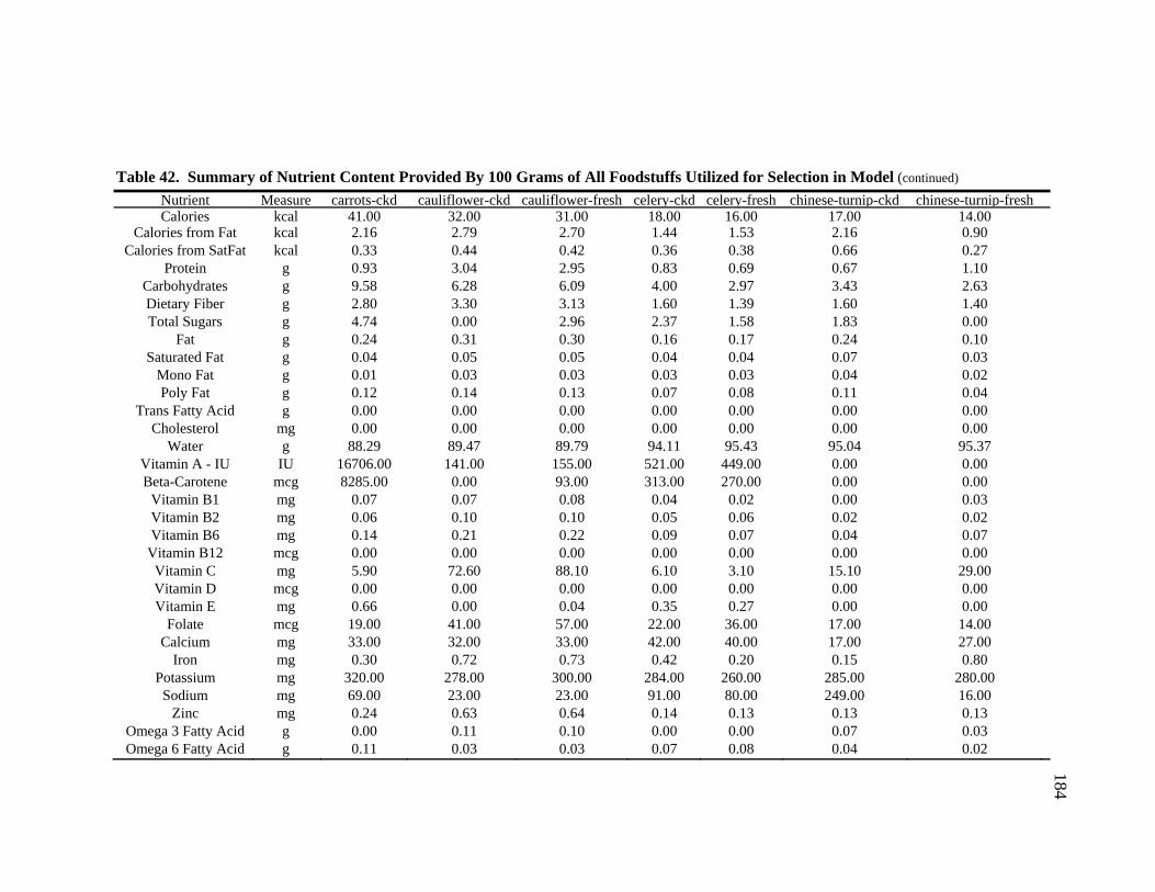
184

Table 42. Summary of Nutrient Content Provided By 100 Grams of All Foodstuffs Utilized for Selection in Model (continued)

Nutrient Measure carrots-ckd cauliflower-ckd cauliflower-fresh celery-ckd celery-fresh chinese-turnip-ckd chinese-turnip-freshCalories kcal 41.00 32.00 31.00 18.00 16.00 17.00 14.00

Calories from Fat kcal 2.16 2.79 2.70 1.44 1.53 2.16 0.90Calories from SatFat kcal 0.33 0.44 0.42 0.36 0.38 0.66 0.27

Protein g 0.93 3.04 2.95 0.83 0.69 0.67 1.10Carbohydrates g 9.58 6.28 6.09 4.00 2.97 3.43 2.63Dietary Fiber g 2.80 3.30 3.13 1.60 1.39 1.60 1.40Total Sugars g 4.74 0.00 2.96 2.37 1.58 1.83 0.00

Fat g 0.24 0.31 0.30 0.16 0.17 0.24 0.10Saturated Fat g 0.04 0.05 0.05 0.04 0.04 0.07 0.03

Mono Fat g 0.01 0.03 0.03 0.03 0.03 0.04 0.02Poly Fat g 0.12 0.14 0.13 0.07 0.08 0.11 0.04

Trans Fatty Acid g 0.00 0.00 0.00 0.00 0.00 0.00 0.00Cholesterol mg 0.00 0.00 0.00 0.00 0.00 0.00 0.00

Water g 88.29 89.47 89.79 94.11 95.43 95.04 95.37Vitamin A - IU IU 16706.00 141.00 155.00 521.00 449.00 0.00 0.00Beta-Carotene mcg 8285.00 0.00 93.00 313.00 270.00 0.00 0.00

Vitamin B1 mg 0.07 0.07 0.08 0.04 0.02 0.00 0.03Vitamin B2 mg 0.06 0.10 0.10 0.05 0.06 0.02 0.02Vitamin B6 mg 0.14 0.21 0.22 0.09 0.07 0.04 0.07

Vitamin B12 mcg 0.00 0.00 0.00 0.00 0.00 0.00 0.00Vitamin C mg 5.90 72.60 88.10 6.10 3.10 15.10 29.00Vitamin D mcg 0.00 0.00 0.00 0.00 0.00 0.00 0.00Vitamin E mg 0.66 0.00 0.04 0.35 0.27 0.00 0.00

Folate mcg 19.00 41.00 57.00 22.00 36.00 17.00 14.00Calcium mg 33.00 32.00 33.00 42.00 40.00 17.00 27.00

Iron mg 0.30 0.72 0.73 0.42 0.20 0.15 0.80Potassium mg 320.00 278.00 300.00 284.00 260.00 285.00 280.00Sodium mg 69.00 23.00 23.00 91.00 80.00 249.00 16.00

Zinc mg 0.24 0.63 0.64 0.14 0.13 0.13 0.13Omega 3 Fatty Acid g 0.00 0.11 0.10 0.00 0.00 0.07 0.03Omega 6 Fatty Acid g 0.11 0.03 0.03 0.07 0.08 0.04 0.02

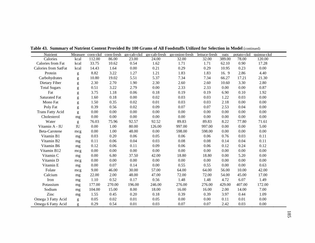
185


Nutrient Measure corn-ckd corn-fresh gn-cab-ckd gn-cab-fresh gn-onion-fresh lettuce-fresh oats potato-ckd quinoa-ckdCalories kcal 112.00 86.00 23.00 24.00 32.00 32.00 389.00 78.00 120.00

Calories from Fat kcal 33.75 10.62 0.54 1.62 1.71 1.71 62.10 0.90 17.28 Calories from SatFat kcal 14.43 1.64 0.00 0.21 0.29 0.29 10.95 0.23 0.00

Protein g 8.82 3.22 1.27 1.21 1.83 1.83 16. 9 2.86 4.40 Carbohydrates g 10.80 19.02 5.51 5.37 7.34 7.34 66.27 17.21 21.30 Dietary Fiber g 2.30 2.70 1.90 2.30 2.60 2.60 10.60 3.30 2.80 Total Sugars g 0.51 3.22 2.79 0.00 2.33 2.33 0.00 0.00 0.87

Fat g 3.75 1.18 0.06 0.18 0.19 0.19 6.90 0.10 1.92 Saturated Fat g 1.60 0.18 0.00 0.02 0.03 0.03 1.22 0.03 0.00

Mono Fat g 1.50 0.35 0.02 0.01 0.03 0.03 2.18 0.00 0.00 Poly Fat g 0.39 0.56 0.02 0.09 0.07 0.07 2.53 0.04 0.00

Trans Fatty Acid g 0.00 0.00 0.00 0.00 0.00 0.00 0.00 0.00 0.00 Cholesterol mg 0.00 0.00 0.00 0.00 0.00 0.00 0.00 0.00 0.00

Water g 76.03 75.96 92.57 92.52 89.83 89.83 8.22 77.80 71.61 Vitamin A - IU IU 0.00 1.00 80.00 126.00 997.00 997.00 0.00 0.00 5.00 Beta-Carotene mcg 0.00 1.00 48.00 0.00 598.00 598.00 0.00 0.00 0.00

Vitamin B1 mg 0.03 0.20 0.06 0.05 0.06 0.06 0.76 0.03 0.11 Vitamin B2 mg 0.11 0.06 0.04 0.03 0.08 0.08 0.14 0.04 0.11 Vitamin B6 mg 0.12 0.06 0.11 0.09 0.06 0.06 0.12 0.24 0.12

Vitamin B12 mcg 0.00 0.00 0.00 0.00 0.00 0.00 0.00 0.00 0.00 Vitamin C mg 0.00 6.80 37.50 42.00 18.80 18.80 0.00 5.20 0.00 Vitamin D mcg 0.00 0.00 0.00 0.00 0.00 0.00 0.00 0.00 0.00 Vitamin E mg 0.00 0.07 0.14 0.00 0.55 0.55 0.00 0.00 0.63

Folate mcg 9.00 46.00 30.00 57.00 64.00 64.00 56.00 10.00 42.00 Calcium mg 22.00 2.00 48.00 47.00 72.00 72.00 54.00 45.00 17.00

Iron mg 1.10 0.52 0.17 0.56 1.48 1.48 4.72 6.07 1.49 Potassium mg 177.00 270.00 196.00 246.00 276.00 276.00 429.00 407.00 172.00 Sodium mg 104.00 15.00 8.00 18.00 16.00 16.00 2.00 14.00 7.00

Zinc mg 1.55 0.45 0.20 0.18 0.39 0.39 3.97 0.44 1.09 Omega 3 Fatty Acid g 0.05 0.02 0.01 0.05 0.00 0.00 0.11 0.01 0.00 Omega 6 Fatty Acid g 0.29 0.54 0.01 0.03 0.07 0.07 2.42 0.03 0.00

186

Table 44. Summary of Nutrient Content Provided By 100 Grams of All Foodstuffs Utilized for Selection in Model (continued) Nutrient Measure radishes-fresh rd-cab-ckd rd-cab-fresh spinach-ckd spinach-fresh tomato-fresh wheat-flour wheat-whl-grainCalories kcal 16.00 29.00 31.00 23.00 23.00 23.00 339.00 339.00

Calories from Fat kcal 0.90 0.81 1.44 7.02 3.51 1.80 16.83 22.23 Calories from SatFat kcal 0.29 0.10 0.19 0.00 0.57 0.25 2.90 4.09

Protein g 0.68 1.51 1.43 2.98 2.86 1.20 13.70 13.68 Carbohydrates g 3.40 6.94 7.37 2.71 3.63 5.10 72.57 71.13 Dietary Fiber g 1.57 2.60 2.10 2.10 2.20 1.10 12.20 13.00 Total Sugars g 1.83 3.32 3.83 0.00 0.42 4.00 0.41 0.00

Fat g 0.10 0.09 0.16 0.78 0.39 0.20 1.87 2.47 Saturated Fat g 0.03 0.01 0.02 0.00 0.06 0.03 0.32 0.45

Mono Fat g 0.02 0.01 0.01 0.00 0.01 0.03 0.23 0.34 Poly Fat g 0.05 0.04 0.08 0.00 0.16 0.08 0.78 0.98

Trans Fatty Acid g 0.00 0.00 0.00 0.00 0.00 0.00 0.00 0.00 Cholesterol mg 0.00 0.00 0.00 0.00 0.00 0.00 0.00 0.00

Water g 95.27 90.84 90.39 92.50 91.40 93.00 10.27 10.94 Vitamin A - IU IU 7.00 33.00 1116.00 1158.00 9377.00 642.00 9.00 0.00 Beta Ca otene mcg 4.00 20.00 670.00 0.00 5626.00 346.00 5.00 0.00

Vitamin B1 mg 0.01 0.07 0.06 0.11 0.08 0.06 0.45 0.42 Vitamin B2 mg 0.04 0.06 0.07 0.13 0.19 0.04 0.22 0.12 Vitamin B6 mg 0.07 0.22 0.21 0.09 0.19 0.08 0.34 0.42

Vitamin B12 mcg 0.00 0.00 0.00 0.00 0.00 0.00 0.00 0.00 Vitamin C mg 14.80 34.40 57.00 5.90 28.10 23.40 0.00 0.00 Vitamin D mcg 0.00 0.00 0.00 0.00 0.00 0.00 0.00 0.00 Vitamin E mg 0.00 0.12 0.11 0.00 2.03 0.38 0.82 0.00

Folate mcg 25.00 24.00 18.00 114.00 194.00 9.00 44.00 43.00 Calcium mg 25.00 42.00 45.00 124.00 99.00 13.00 34.00 34.00

Iron mg 0.34 0.66 0.80 1.48 2.71 0.51 3.88 3.52 Potassium mg 233.00 262.00 243.00 256.00 558.00 204.00 405.00 431.00

Sodium mg 39.00 28.00 27.00 55.00 79.00 13.00 5.00 2.00 Zinc mg 0.28 0.25 0.22 0.30 0.53 0.07 2.93 4.16

Omega 3 Fatty Acid g 0.03 0.02 0.04 0.00 0.14 0.00 0.04 0.05 Omega 6 Fatty Acid g 0.02 0.02 0.03 0.00 0.03 0.08 0.74 0.93

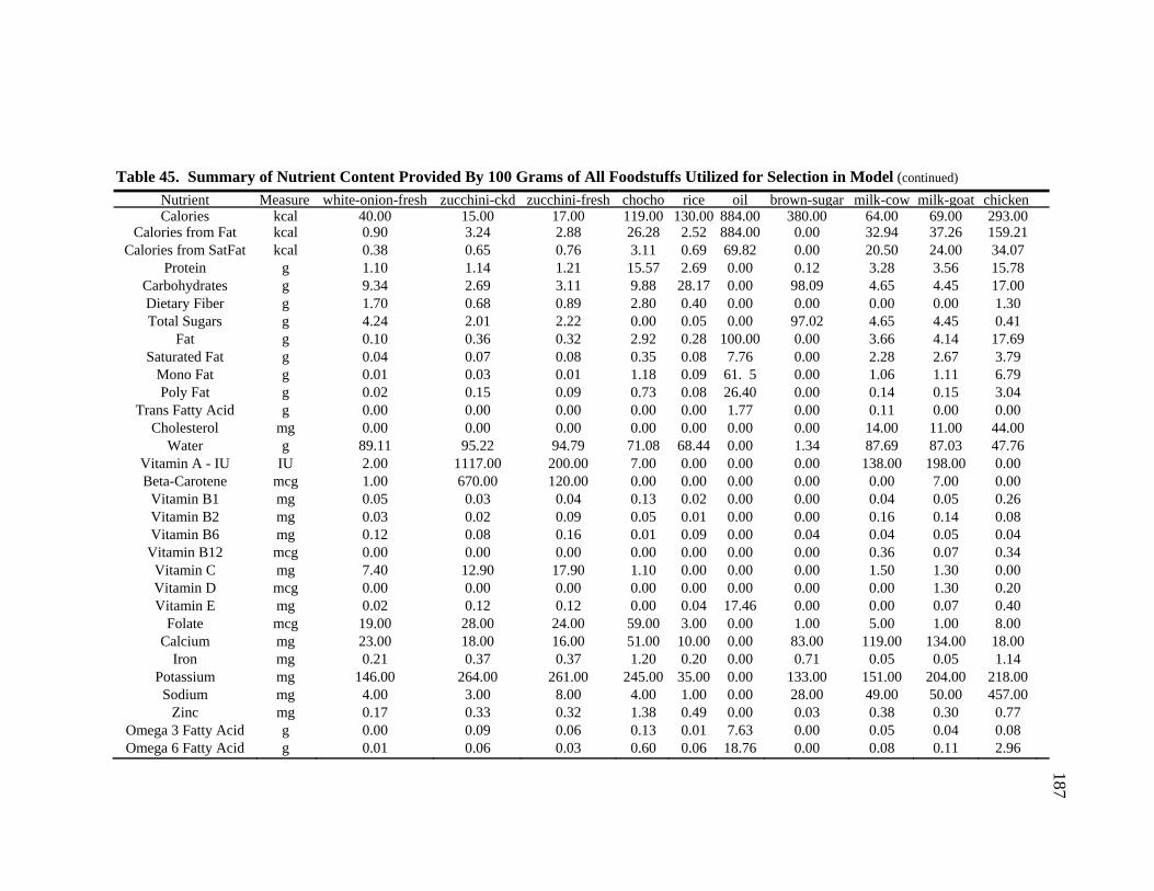
187


Nutrient Measure white-onion-fresh zucchini-ckd zucchini-fresh chocho rice oil brown-sugar milk-cow milk-goat chickenCalories kcal 40.00 15.00 17.00 119.00 130.00 884.00 380.00 64.00 69.00 293.00

Calories from Fat kcal 0.90 3.24 2.88 26.28 2.52 884.00 0.00 32.94 37.26 159.21Calories from SatFat kcal 0.38 0.65 0.76 3.11 0.69 69.82 0.00 20.50 24.00 34.07

Protein g 1.10 1.14 1.21 15.57 2.69 0.00 0.12 3.28 3.56 15.78Carbohydrates g 9.34 2.69 3.11 9.88 28.17 0.00 98.09 4.65 4.45 17.00Dietary Fiber g 1.70 0.68 0.89 2.80 0.40 0.00 0.00 0.00 0.00 1.30Total Sugars g 4.24 2.01 2.22 0.00 0.05 0.00 97.02 4.65 4.45 0.41

Fat g 0.10 0.36 0.32 2.92 0.28 100.00 0.00 3.66 4.14 17.69Saturated Fat g 0.04 0.07 0.08 0.35 0.08 7.76 0.00 2.28 2.67 3.79

Mono Fat g 0.01 0.03 0.01 1.18 0.09 61. 5 0.00 1.06 1.11 6.79Poly Fat g 0.02 0.15 0.09 0.73 0.08 26.40 0.00 0.14 0.15 3.04

Trans Fatty Acid g 0.00 0.00 0.00 0.00 0.00 1.77 0.00 0.11 0.00 0.00Cholesterol mg 0.00 0.00 0.00 0.00 0.00 0.00 0.00 14.00 11.00 44.00

Water g 89.11 95.22 94.79 71.08 68.44 0.00 1.34 87.69 87.03 47.76Vitamin A - IU IU 2.00 1117.00 200.00 7.00 0.00 0.00 0.00 138.00 198.00 0.00Beta-Carotene mcg 1.00 670.00 120.00 0.00 0.00 0.00 0.00 0.00 7.00 0.00

Vitamin B1 mg 0.05 0.03 0.04 0.13 0.02 0.00 0.00 0.04 0.05 0.26Vitamin B2 mg 0.03 0.02 0.09 0.05 0.01 0.00 0.00 0.16 0.14 0.08Vitamin B6 mg 0.12 0.08 0.16 0.01 0.09 0.00 0.04 0.04 0.05 0.04

Vitamin B12 mcg 0.00 0.00 0.00 0.00 0.00 0.00 0.00 0.36 0.07 0.34Vitamin C mg 7.40 12.90 17.90 1.10 0.00 0.00 0.00 1.50 1.30 0.00Vitamin D mcg 0.00 0.00 0.00 0.00 0.00 0.00 0.00 0.00 1.30 0.20Vitamin E mg 0.02 0.12 0.12 0.00 0.04 17.46 0.00 0.00 0.07 0.40

Folate mcg 19.00 28.00 24.00 59.00 3.00 0.00 1.00 5.00 1.00 8.00Calcium mg 23.00 18.00 16.00 51.00 10.00 0.00 83.00 119.00 134.00 18.00

Iron mg 0.21 0.37 0.37 1.20 0.20 0.00 0.71 0.05 0.05 1.14Potassium mg 146.00 264.00 261.00 245.00 35.00 0.00 133.00 151.00 204.00 218.00

Sodium mg 4.00 3.00 8.00 4.00 1.00 0.00 28.00 49.00 50.00 457.00Zinc mg 0.17 0.33 0.32 1.38 0.49 0.00 0.03 0.38 0.30 0.77

Omega 3 Fatty Acid g 0.00 0.09 0.06 0.13 0.01 7.63 0.00 0.05 0.04 0.08Omega 6 Fatty Acid g 0.01 0.06 0.03 0.60 0.06 18.76 0.00 0.08 0.11 2.96

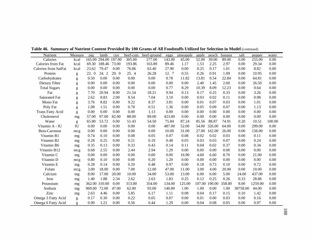
188


Nutrient Measure pig lamb cuy beef-cuts beef-ground eggs pineapple apple peach banana salt pepper waterCalories kcal 165.00 294.00 197.00 305.00 277.00 143.00 45.00 52.00 39.00 89.00 0.00 255.00 0.00

Calories from Fat kcal 69.30 188.46 73.00 193.86 163.89 89.46 1.17 1.53 2.25 2.97 0.00 29.34 0.00Calories from SatFat kcal 23.62 79.47 0.00 76.86 63.40 27.90 0.00 0.25 0.17 1.01 0.00 8.82 0.00

Protein g 22. 0 24. 2 29. 0 25. 4 26.28 12. 7 0.55 0.26 0.91 1.09 0.00 10.95 0.00Carbohydrates g 0.50 0.00 0.00 0.00 0.00 0.78 11.82 13.81 9.54 22.84 0.00 64.81 0.00Dietary Fiber g 0.00 0.00 0.00 0.00 0.00 0.00 0.00 2.40 1.45 2.60 0.00 26.50 0.00Total Sugars g 0.00 0.00 0.00 0.00 0.00 0.77 8.29 10.39 8.09 12.23 0.00 0.64 0.00

Fat g 7.70 20.94 8.00 21.54 18.21 9.94 0.13 0.17 0.25 0.33 0.00 3.26 0.00Saturated Fat g 2.62 8.83 2.00 8.54 7.04 3.10 0.00 0.03 0.02 0.11 0.00 0.98 0.00

Mono Fat g 3.76 8.82 0.00 9.22 8.37 3.81 0.00 0.01 0.07 0.03 0.00 1.01 0.00Poly Fat g 1.08 1.51 0.00 0.78 0.51 1.36 0.00 0.05 0.09 0.07 0.00 1.13 0.00

Trans Fatty Acid g 0.00 0.00 0.00 0.00 1.13 0.00 0.00 0.00 0.00 0.00 0.00 0.00 0.00Cholesterol mg 57.00 97.00 82.00 88.00 89.00 423.00 0.00 0.00 0.00 0.00 0.00 0.00 0.00

Water g 65.80 53.72 0.00 51.43 54.50 75.84 87.24 85.56 88.87 74.91 0.20 10.51 100.00Vitamin A - IU IU 0.00 0.00 0.00 0.00 0.00 487.00 52.00 54.00 326.00 64.00 0.00 299.00 0.00Beta-Carotene mcg 0.00 0.00 0.00 0.00 0.00 10.00 31.00 27.00 162.00 26.00 0.00 156.00 0.00

Vitamin B1 mg 0.74 0.10 0.00 0.08 0.05 0.07 0.08 0.02 0.02 0.03 0.00 0.11 0.00Vitamin B2 mg 0.28 0.25 0.00 0.21 0.19 0.48 0.03 0.03 0.03 0.07 0.00 0.24 0.00Vitamin B6 mg 0.35 0.13 0.00 0.33 0.43 0.14 0.11 0.04 0.02 0.37 0.00 0.34 0.00

Vitamin B12 mcg 0.68 2.55 0.00 2.44 2.94 1.29 0.00 0.00 0.00 0.00 0.00 0.00 0.00Vitamin C mg 0.00 0.00 0.00 0.00 0.00 0.00 16.90 4.60 6.60 8.70 0.00 21.00 0.00Vitamin D mcg 0.80 0.10 0.00 0.00 0.20 1.20 0.00 0.00 0.00 0.00 0.00 0.00 0.00Vitamin E mg 0.28 0.14 0.00 0.20 0.48 0.97 0.00 0.18 0.73 0.10 0.00 0.72 0.00

Folate mcg 3.00 18.00 0.00 7.00 12.00 47.00 11.00 3.00 4.00 20.00 0.00 10.00 0.00Calcium mg 8.00 17.00 20.00 10.00 34.00 53.00 13.00 6.00 6.00 5.00 24.00 437.00 0.00

Iron mg 1.40 1.88 2.34 2.62 2.63 1.83 0.25 0.12 0.25 0.26 0.33 28.86 0.00Potassium mg 362.00 310.00 0.00 313.00 354.00 134.00 125.00 107.00 190.00 358.00 8.00 1259.00 0.00Sodium mg 969.00 72.00 47.00 62.00 93.00 140.00 1.00 1.00 0.00 1.00 38758.00 44.00 0.00

Zinc mg 2.63 4.46 0.00 5.85 6.17 1.11 0.08 0.04 0.17 0.15 0.10 1.42 0.00Omega 3 Fatty Acid g 0.17 0.30 0.00 0.22 0.05 0.07 0.00 0.01 0.00 0.03 0.00 0.16 0.00Omega 6 Fatty Acid g 0.90 1.21 0.00 0.56 0.44 1.29 0.00 0.04 0.08 0.05 0.00 0.97 0.00

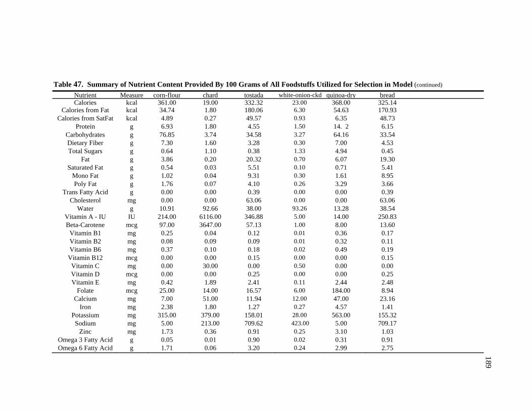
189


Nutrient Measure corn-flour chard tostada white-onion-ckd quinoa-dry breadCalories kcal 361.00 19.00 332.32 23.00 368.00 325.14

Calories from Fat kcal 34.74 1.80 180.06 6.30 54.63 170.93Calories from SatFat kcal 4.89 0.27 49.57 0.93 6.35 48.73

Protein g 6.93 1.80 4.55 1.50 14. 2 6.15Carbohydrates g 76.85 3.74 34.58 3.27 64.16 33.54Dietary Fiber g 7.30 1.60 3.28 0.30 7.00 4.53Total Sugars g 0.64 1.10 0.38 1.33 4.94 0.45

Fat g 3.86 0.20 20.32 0.70 6.07 19.30Saturated Fat g 0.54 0.03 5.51 0.10 0.71 5.41

Mono Fat g 1.02 0.04 9.31 0.30 1.61 8.95Poly Fat g 1.76 0.07 4.10 0.26 3.29 3.66

Trans Fatty Acid g 0.00 0.00 0.39 0.00 0.00 0.39Cholesterol mg 0.00 0.00 63.06 0.00 0.00 63.06

Water g 10.91 92.66 38.00 93.26 13.28 38.54Vitamin A - IU IU 214.00 6116.00 346.88 5.00 14.00 250.83Beta-Carotene mcg 97.00 3647.00 57.13 1.00 8.00 13.60

Vitamin B1 mg 0.25 0.04 0.12 0.01 0.36 0.17Vitamin B2 mg 0.08 0.09 0.09 0.01 0.32 0.11Vitamin B6 mg 0.37 0.10 0.18 0.02 0.49 0.19

Vitamin B12 mcg 0.00 0.00 0.15 0.00 0.00 0.15Vitamin C mg 0.00 30.00 0.00 0.50 0.00 0.00Vitamin D mcg 0.00 0.00 0.25 0.00 0.00 0.25Vitamin E mg 0.42 1.89 2.41 0.11 2.44 2.48

Folate mcg 25.00 14.00 16.57 6.00 184.00 8.94Calcium mg 7.00 51.00 11.94 12.00 47.00 23.16

Iron mg 2.38 1.80 1.27 0.27 4.57 1.41Potassium mg 315.00 379.00 158.01 28.00 563.00 155.32Sodium mg 5.00 213.00 709.62 423.00 5.00 709.17

Zinc mg 1.73 0.36 0.91 0.25 3.10 1.03Omega 3 Fatty Acid g 0.05 0.01 0.90 0.02 0.31 0.91Omega 6 Fatty Acid g 1.71 0.06 3.20 0.24 2.99 2.75

190

Appendix D

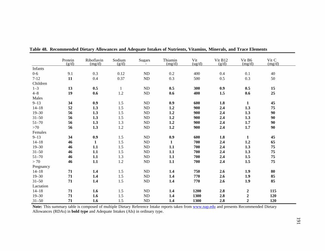
191

Table 48. Recommended Dietary Allowances and Adequate Intakes of Nutrients, Vitamins, Minerals, and Trace Elements

Protein

Riboflavin

Sodium

Sugars

Thiamin

Vit

Vit B12

Vit B6

Vit C

(g/d) (mg/d) (g/d) ‐ (mg/d) (ug/d) (g/d) (mg/d) (mg/d) Infants 0‐6 9.1 0.3 0.12 ND 0.2 400 0.4 0.1 40 7‐12 11 0.4 0.37 ND 0.3 500 0.5 0.3 50 Children 1–3 13 0.5 1 ND 0.5 300 0.9 0.5 15 4–8 19 0.6 1.2 ND 0.6 400 1.5 0.6 25 Males 9–13 34 0.9 1.5 ND 0.9 600 1.8 1 45 14–18 52 1.3 1.5 ND 1.2 900 2.4 1.3 75 19–30 56 1.3 1.5 ND 1.2 900 2.4 1.3 90 31–50 56 1.3 1.5 ND 1.2 900 2.4 1.3 90 51–70 56 1.3 1.3 ND 1.2 900 2.4 1.7 90 >70 56 1.3 1.2 ND 1.2 900 2.4 1.7 90 Females 9–13 34 0.9 1.5 ND 0.9 600 1.8 1 45 14–18 46 1 1.5 ND 1 700 2.4 1.2 65 19–30 46 1.1 1.5 ND 1.1 700 2.4 1.3 75 31–50 46 1.1 1.5 ND 1.1 700 2.4 1.3 75 51–70 46 1.1 1.3 ND 1.1 700 2.4 1.5 75 > 70 46 1.1 1.2 ND 1.1 700 2.4 1.5 75 Pregnancy 14–18 71 1.4 1.5 ND 1.4 750 2.6 1.9 80 19–30 71 1.4 1.5 ND 1.4 770 2.6 1.9 85 31–50 71 1.4 1.5 ND 1.4 770 2.6 1.9 85 Lactation 14–18 71 1.6 1.5 ND 1.4 1200 2.8 2 115 19–30 71 1.6 1.5 ND 1.4 1300 2.8 2 120 31–50 71 1.6 1.5 ND 1.4 1300 2.8 2 120

Note: This summary table is composed of multiple Dietary Reference Intake reports taken from www.nap.edu and presents Recommended Dietary Allowances (RDAs) in bold type and Adequate Intakes (AIs) in ordinary type.

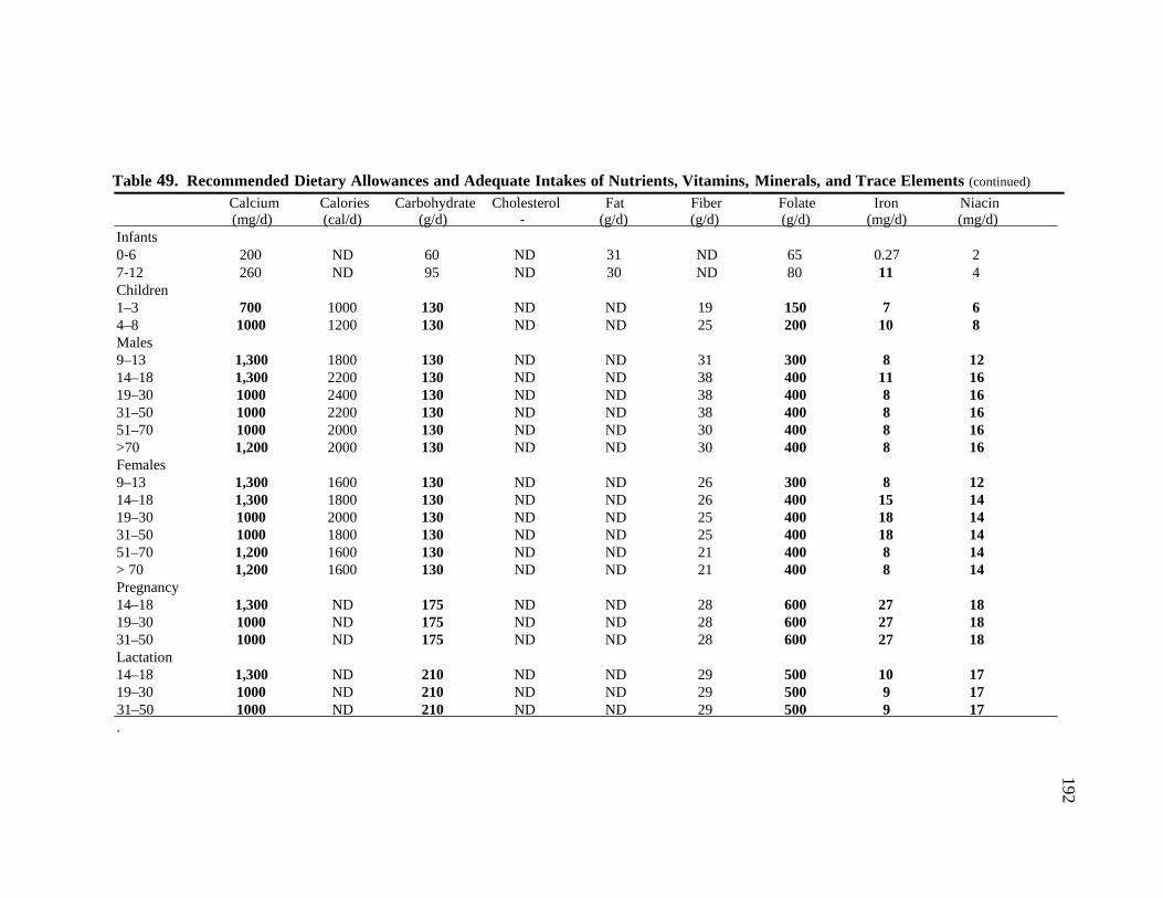
192

Table 49. Recommended Dietary Allowances and Adequate Intakes of Nutrients, Vitamins, Minerals, and Trace Elements (continued)

Calcium Calories Carbohydrate Cholesterol Fat Fiber Folate Iron Niacin (mg/d) (cal/d) (g/d) ‐ (g/d) (g/d) (g/d) (mg/d) (mg/d) Infants 0‐6 200 ND 60 ND 31 ND 65 0.27 2 7‐12 260 ND 95 ND 30 ND 80 11 4 Children 1–3 700 1000 130 ND ND 19 150 7 6 4–8 1000 1200 130 ND ND 25 200 10 8 Males 9–13 1,300 1800 130 ND ND 31 300 8 12 14–18 1,300 2200 130 ND ND 38 400 11 16 19–30 1000 2400 130 ND ND 38 400 8 16 31–50 1000 2200 130 ND ND 38 400 8 16 51–70 1000 2000 130 ND ND 30 400 8 16 >70 1,200 2000 130 ND ND 30 400 8 16 Females 9–13 1,300 1600 130 ND ND 26 300 8 12 14–18 1,300 1800 130 ND ND 26 400 15 14 19–30 1000 2000 130 ND ND 25 400 18 14 31–50 1000 1800 130 ND ND 25 400 18 14 51–70 1,200 1600 130 ND ND 21 400 8 14 > 70 1,200 1600 130 ND ND 21 400 8 14 Pregnancy 14–18 1,300 ND 175 ND ND 28 600 27 18 19–30 1000 ND 175 ND ND 28 600 27 18 31–50 1000 ND 175 ND ND 28 600 27 18 Lactation 14–18 1,300 ND 210 ND ND 29 500 10 17 19–30 1000 ND 210 ND ND 29 500 9 17 31–50 1000 ND 210 ND ND 29 500 9 17 .

193

Appendix E

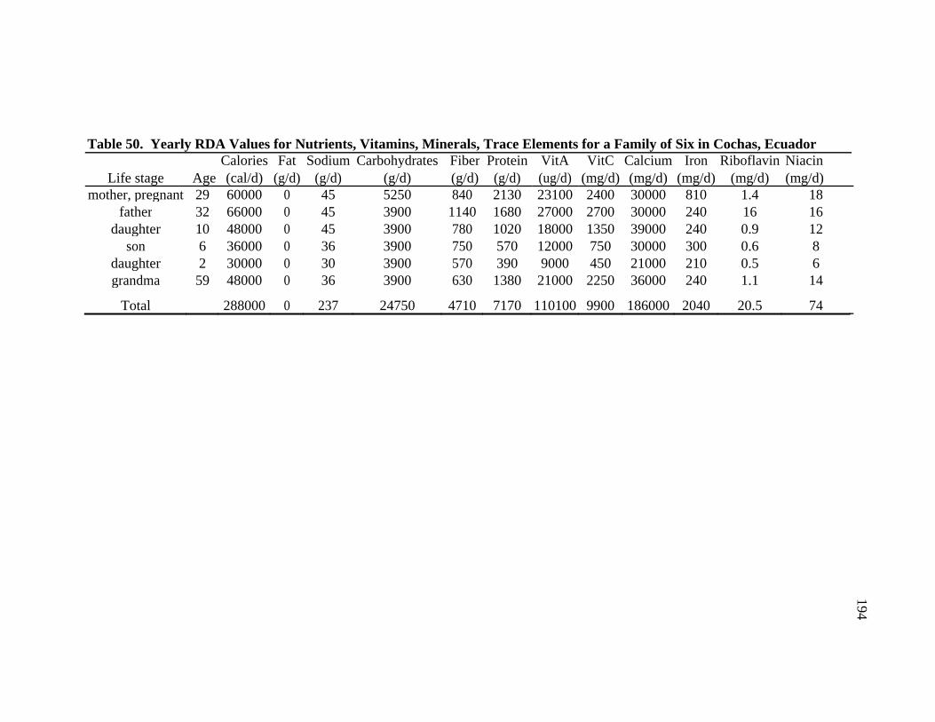
194

Table 50. Yearly RDA Values for Nutrients, Vitamins, Minerals, Trace Elements for a Family of Six in Cochas, Ecuador Calories Fat Sodium Carbohydrates Fiber Protein VitA VitC Calcium Iron Riboflavin Niacin

Life stage Age (cal/d) (g/d) (g/d) (g/d) (g/d) (g/d) (ug/d) (mg/d) (mg/d) (mg/d) (mg/d) (mg/d)mother, pregnant 29 60000 0 45 5250 840 2130 23100 2400 30000 810 1.4 18

father 32 66000 0 45 3900 1140 1680 27000 2700 30000 240 16 16daughter 10 48000 0 45 3900 780 1020 18000 1350 39000 240 0.9 12

son 6 36000 0 36 3900 750 570 12000 750 30000 300 0.6 8daughter 2 30000 0 30 3900 570 390 9000 450 21000 210 0.5 6grandma 59 48000 0 36 3900 630 1380 21000 2250 36000 240 1.1 14

Total 288000 0 237 24750 4710 7170 110100 9900 186000 2040 20.5 74

195

Appendix F

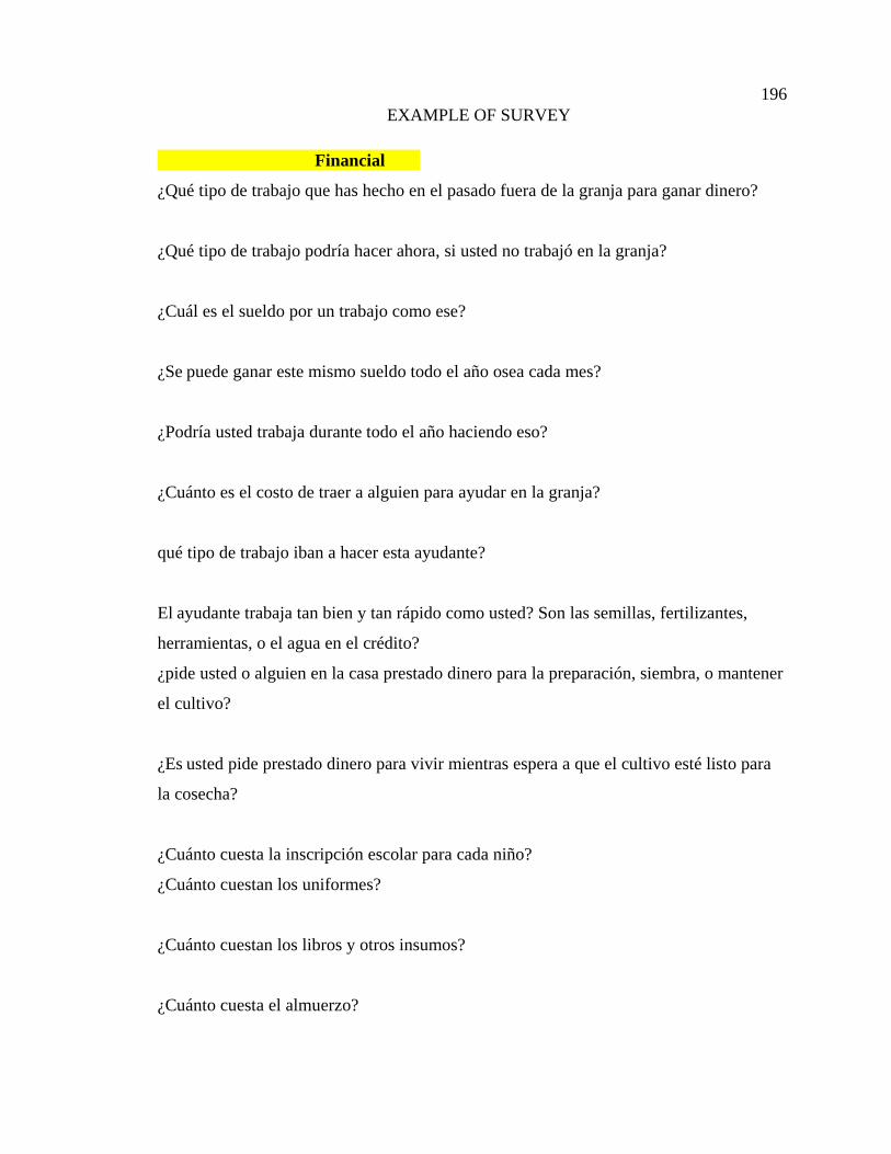
196

EXAMPLE OF SURVEY

Financial

¿Qué tipo de trabajo que has hecho en el pasado fuera de la granja para ganar dinero?

¿Qué tipo de trabajo podría hacer ahora, si usted no trabajó en la granja?

¿Cuál es el sueldo por un trabajo como ese?

¿Se puede ganar este mismo sueldo todo el año osea cada mes?

¿Podría usted trabaja durante todo el año haciendo eso?

¿Cuánto es el costo de traer a alguien para ayudar en la granja?

qué tipo de trabajo iban a hacer esta ayudante?

El ayudante trabaja tan bien y tan rápido como usted? Son las semillas, fertilizantes,

herramientas, o el agua en el crédito?

¿pide usted o alguien en la casa prestado dinero para la preparación, siembra, o mantener

el cultivo?

¿Es usted pide prestado dinero para vivir mientras espera a que el cultivo esté listo para

la cosecha?

¿Cuánto cuesta la inscripción escolar para cada niño?

¿Cuánto cuestan los uniformes?

¿Cuánto cuestan los libros y otros insumos?

¿Cuánto cuesta el almuerzo?

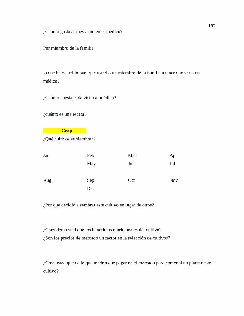
197

¿Cuánto gasta al mes / año en el médico?

Por miembro de la familia

lo que ha ocurrido para que usted o un miembro de la familia a tener que ver a un

médico?

¿Cuánto cuesta cada visita al médico?

¿cuánto es una receta?

Crop

¿Qué cultivos se siembran?

Jan Feb Mar Apr

May Jun Jul

Aug Sep Oct Nov

Dec

¿Por qué decidió a sembrar este cultivo en lugar de otros?

¿Considera usted que los beneficios nutricionales del cultivo?

¿Son los precios de mercado un factor en la selección de cultivos?

¿Cree usted que de lo que tendría que pagar en el mercado para comer si no plantar este

cultivo?

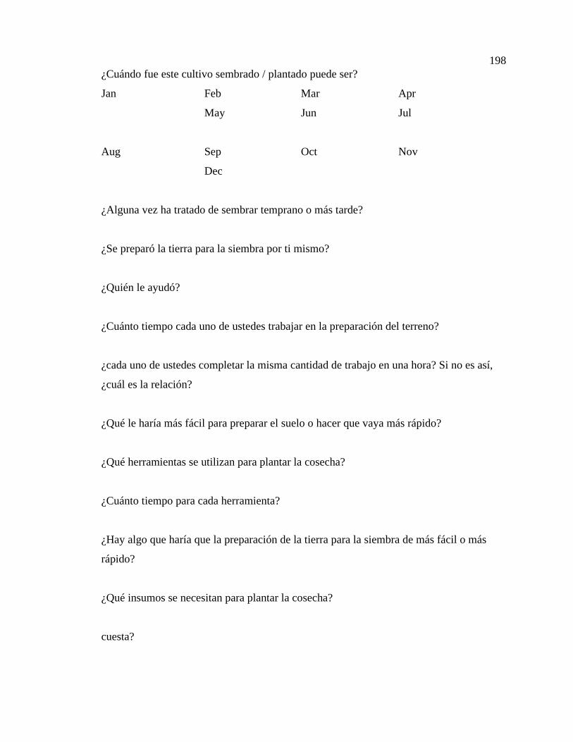
198

¿Cuándo fue este cultivo sembrado / plantado puede ser?

Jan Feb Mar Apr

May Jun Jul

Aug Sep Oct Nov

Dec

¿Alguna vez ha tratado de sembrar temprano o más tarde?

¿Se preparó la tierra para la siembra por ti mismo?

¿Quién le ayudó?

¿Cuánto tiempo cada uno de ustedes trabajar en la preparación del terreno?

¿cada uno de ustedes completar la misma cantidad de trabajo en una hora? Si no es así,

¿cuál es la relación?

¿Qué le haría más fácil para preparar el suelo o hacer que vaya más rápido?

¿Qué herramientas se utilizan para plantar la cosecha?

¿Cuánto tiempo para cada herramienta?

¿Hay algo que haría que la preparación de la tierra para la siembra de más fácil o más

rápido?

¿Qué insumos se necesitan para plantar la cosecha?

cuesta?

199

agua

¿Qué herramientas se utilizaron?

¿De cuánto tiempo fue dedicado al uso de cada una de las herramientas para plantar la

cosecha?

¿Hizo usted plantar la cosecha de si mismo?

¿Quién le ayudó?

¿Cuánto tiempo cada uno de ustedes trabajar en la plantación?

¿Qué podría hacer la plantación ir más rápido o más fácil?

costos asociados?

Una vez que se sembró el cultivo, el tiempo de cuánto se gasta por día o semana el

mantenimiento de la cosecha?

Deshierbe

Riego

Difusión de los Fertilizantes

Otro

¿Usa los pesticidas?

¿Cuánto?

200

¿Cuánto tiempo se necesita para aplicarlo?

¿Qué se utiliza para aplicarla?

¿De dónde obtiene el agua necesaria para su cultivo?

¿Tiene algún costo? ¿Cuánto? Los derechos de agua?

¿Con qué frecuencia regar el cultivo?

¿Cuánta agua se utiliza cada vez? Cantidad o tiempo?

¿Qué herramientas o suministros se necesitan para obtener el agua para su cultivo?

¿Cuándo es la cosecha?

una cosecha?

¿Cuál es el rendimiento de este cultivo?

¿qué crees que afecta el rendimiento de la mayoría?

el agua?

los fertilizantes?

¿se almacena alguna de la cosecha?

¿Por qué no?

¿Cómo se almacena?

201

¿Cuánto se pierde al mez?

Debido a la descomposición / las ratas?

cuánto tiempo hace que el almacenamiento de alimentos les perdura?

¿Cuánta tierra se utiliza para sembrar este cultivo?

Groceries

24-hora recordatorio de alimentos

Entre comidas

¿Cuál es su lista de compras típico?

¿Cuál es su presupuesto semanal / mensual de los alimentos?

Oxen

¿Es usted dueño del buey?

¿Cuánto fue el buey?

¿Se arriende el buey a los demás?

¿Cuál es el cargo?

¿Cuánto cuesta pedir prestado?

¿Por cuánto tiempo tomarlo prestado por?

¿Qué edad tiene el animal?

¿Que le da al buey de alimento?

202

¿Cree usted que sería saludable si usted le dio más de buey para comer?

¿Cultiva la alimentación? ¿Cuánto de ello?

¿Qué cantidad de tierra que se necesita para la que se alimentan?

¿A cuánto cuesta las facturas del veterinario de ano?

¿Qué otros cobras se incurre al tener el buey?

los derechos de pastoreo?

¿Cuántos años es un buey para el arado buena?

¿Qué se hace con ella después de que se es demasiado viejo?

¿Cuánto es el arnés?

¿Cuánto es el arado?

¿Cuántos años son el arnés y el arado bueno?

¿Qué tipo de reparaciones son necesarias en el arado o el arnés?

¿Cuánto cuesta este costo promedio por temporada / cultivos / año?

¿Por qué no utilizar un tractor?

Tractor

¿Es usted dueño del tractor?

¿Cuánto fue el tractor?

¿Cuanto les pide a los vecinos para arrendar al tractor?

203

¿Cuánto cuesta pedir prestado?

¿Por cuánto tiempo tomarlo prestado por?

¿Qué edad tiene el tractor?

¿Cuántos años le sirve un tractor para arar?

¿Qué se hace con el tractor después de que es demasiado viejo?

¿Cuánto es el arnés?

¿Cuánto es el arado?

¿Cuántos años son el arnés y el arado bueno para utilizar?

¿Qué tipo de reparaciones o mantenimiento que se necesita el tractor cada mes /

temporada / año?

¿cuánto cuesta esto?

¿Qué tipo de reparaciones son necesarias del arado o el arnés?

¿Cuánto cuesta este costo promedio por temporada / cultivos / año?

¿Cuánto gasta de combustible por mes / temporada / año?

¿Por qué no utilizar un buey?

Water

Lo que afecta el suministro de agua?

204

¿Cuáles son las interrupciones?

¿Qué hacer cuando no podía conseguir agua cuando sea necesario para regar el cultivo?

¿Qué meses normalmente tienen suficiente lluvia para los cultivos?

Jan Feb Mar Apr May Jun Jul Aug

Sep Oct Nov Dec

¿Qué meses no tienen suficiente lluvia para los cultivos?

Jan Feb Mar Apr May Jun Jul Aug

Sep Oct Nov Dec

¿Ha notado la pauta de las precipitaciones está cambiando?

¿Cómo?

Es la temporada de lluvias empezando mas tarde? Es la temporada de lluvias terminando

más tarde?

¿Como cree usted que es la lluvia más o menos en comparación con hace 5 años?

¿Es posible utilizar el agua del llave para regar los cultivos?

¿Has pensado en formas de almacenar el agua de lluvia?

¿Ha tratado de almacenar agua para la temporada seca?

Incluso si usted tenía un poco de agua almacenada, ¿crees que se podría almacenar agua

suficiente para superar el suelo seco y el sol caliente?

¿Crees que tus cultivos sería mejor si tuviera alguna fuente de agua que se puede utilizar

para regar sus cultivos sobre una base regular en lugar de depender de la lluvia?

205

Chicken

¿Tiene alguna gallina?

¿cuántos?

¿Cuánto cuesta comprar?

¿Qué edad tenían?

¿Qué les das de comer a las gallinas?

¿Cuántos huevos se puede conseguir de un día / mes?

Hay meses cuando las gallinas se les dan mas huevos? Cuales son?

Cuantos?

¿Cuánto tiempo espera antes de comer las gallinas?

¿Dónde los guarda?

¿Cuánto fue el recinto?

¿De cuánto tiempo se necesita para reparar la caja por mes / año?

¿Con qué frecuencia se muere o ser comido por otro animal?

Cuy

¿Tiene algún cuy?

¿cuántos?

206


¿Qué edad tenían al comprarlo?

¿Qué les das de comer?

¿Cuánto tiempo espera antes de comerlas?

¿Dónde las guarda?


¿De cuánto tiempo se necesita para reparar la caja por mes / año?

¿Con qué frecuencia se muere o ser comido por otro animal?

¿Cuánta carne tiene uno?

Dairy Goat

¿Tiene algún cabras?

¿cuántos?




¿Cuándo empiezan a lactantes?

la cantidad de leche se puede conseguir cada mes dia?

cuales son los mejores meses

207

peores meses

¿Cuánto tiempo espera antes de comerlas?



¿De cuánto tiempo se necesita para reparar el recinto por mes / año?

¿Con qué frecuencia uno morir / ser comido por otro animal?

Pig

¿Tiene usted un cerdo?

¿cuántos?

¿Cuánto cuesta cada cerdo para comprar?

¿Qué edad tiene el cerdo normalmente cuando usted lo compra?


¿Qué edad tienen cuando se los comen?

¿Qué edad tienen cuando se llevan al mercado a vender? A cuanto se lo venden?





Cow

208

¿Tiene algún vacas?

¿cuántos?




¿Cuándo empiezan a lactantes?

la cantidad de leche se puede conseguir cada mes / día?

mejores meses/ día peores meses o día

¿Qué edad tienen cuando se llevan al mercado a vender? A cuanto se lo venden?

Si usted va a comer a la vaca, ¿cuánto tiempo se mantendrá antes de comerlas? Sabe la

cantidad de carne se puede conseguir de una vaca?





Nutritional and Economic Analysis of Small-Scale Agriculture ...

Documents

Transcript of Nutritional and Economic Analysis of Small-Scale Agriculture ...