at point B. The pressure attained at point A in this schematic is only due to pre-compression

caused by a hammer shock. In the sections ahead, re-injection of the hot combusted gas is

presented as a potentially viable method to enhance pre-compression.

1.2 Organization of dissertation

This dissertation is a compilation of various numerical simulations aimed at obtaining the

best operating points out of the Wave Disk Engine. Chapter 2 discusses the numerical

scheme and special considerations for turbulence and combustion simulations. The first

feature discussed is the combustion time. Chapter 3 details combustion simulations which

study combustion inside a closed chamber. An accurate estimation of combustion time

is crucial in determining the angular speed at which the WDE can operate. If extremely

high combustion times (1-2 ms) are not realizable, it is necessary pressurize the charge by

means other than a hammer shock. Re-injection of combusted mixture into fresh charge

is presented as an option, and numerical simulations are performed. The final challenge in

the success of the WDE is power extraction. The extraction in the rotor itself may not be

sufficient. Alternate techniques are presented. Chapter 4 discusses some additional features

added to the basic Wave Disk Engine configuration. Chapter 5 details efforts to arrive at

the thermodynamic cycle followed by the working fluid in the Wave Disk Engine. Chapter

6 provides conclusions based on these studies and recommendations for future work.

4

Chapter 2

Numerical simulations

This thesis is an exclusively numerical study of Wave Disk Engine processes.

2.1 Numerical Scheme

The commercial computational fluid dynamics(CFD) code, Ansys Fluent was used in this

analysis to examine various aspects of the problem at hand in two dimensions(2D) . The

compressible Navier-Stokes equations were solved using a pressure-velocity coupling scheme,

with first-order accuracy in time and space. The “Semi Implicit method for Pressure-Linked

Equations”(SIMPLE) algorithm was used for this purpose. Transfer of flow data between

the rotating (rotor) and stationary(intake and exit ports) parts of the flow field was realized

using the interface technique. Species transport equations were additionally solved to model

mixing and reaction. Viscosity was modeled using the Sutherland law. The convergence of

the simulations was checked by ensuring that the residuals of the continuity, momentum,

energy, and species transport equations were below 0.001.

2.2 Turbulence

In the combustion simulations, no turbulence model was used. In cases involving simulations

of an entire rotor with no combustion, turbulence was modeled using the Spalart-Allmaras

5

turbulence model with the turbulence intensity at the inlet equal to 5% and a length scale

of 1% of the inlet width. Some simulations were also performed using the k-ω turbulence

model.

2.3 Combustion

Species transport equations were solved for the gas mixing and the chemical reactions of

combustion in the channel. A finite-rate model was used to compute the chemical source

terms in the species transport equations using Arrhenius kinetic expressions, and ignoring

the influences of turbulent fluctuations on the reaction rates.

Two detailed simulations were performed using the 235-step San Diego chemical kinetic

mechanism for CH4 combustion in air. Since we resolve the influences of compressibility

(propagation of pressure waves) as well as solve 235 transport equations at each time step for

the different chemical species, this was a computationally intensive simulation. This detailed

simulation allows the resolution of the flame front in detail, with approximately 5 grid points

over the flame thickness (taken to be approximately O(1 mm) on average). In addition, and

perhaps of greater value to the investigation, the results from the 235-step simulation can

be used as a reference for comparing results obtained from simpler and shorter reduced

mechanisms with and without resolution of pressure waves and associated compressibility

phenomena.There are approximately 500 grid points in the longitudinal direction and 50

cells in the transverse direction. This gives a mesh size of approximately 0.1 mm. The mesh

size remains constant throughout the simulations. There are approximately 5 computational

cells across a flame sheet.

6

Chapter 3

Combustion studies

3.1 Introduction

In constant volume combustion devices, it is important to minimize the time required for

complete combustion of a fuel and air mixture. This study was motivated by the need for

an assessment of the burning process and the required combustion time in a wave rotor or

a wave disk engine. These devices achieve compression of a combustible mixture by the

sudden closing of one port and power extraction when another port opens. Details on the

mechanical and thermal operation of such devices can be found in Refs. [1] - [4].

It is commonly observed that a flame propagating from one end to the other in a narrow

channel starts off with a parabolic or “mushroom” shape flame, which evolves into a concave

(toward the burned combustion products)“finger” shaped flame that later interacts in a com-

plicated manner with its self-generated flow to evolve into a “tulip” shaped convex flame.

The “tulip” flame has been observed and studied for nearly a century beginning with the

1928 work of Ellis [16]. More recently, thorough discussions of the essential research, along

with numerous references, are found in Refs. [17]-[19]. Kratzel et al. [20] have performed

experiments and numerical simulations that demonstrate this tulip flame formation. Gon-

zalez et al.[21] have carried out numerical simulations of flame propagation in a closed tube

ignited at one end. These simulations used laminar flow, one-step chemistry and a comput-

ing procedure based on the finite volume technique that was restricted to two-dimensional,

7

compressible, reacting flows.

The tulip flame phenomenon has, to date, been chiefly attributed to the Darrieus-Landau

instability, in which small perturbations of an initially flat flame front lead to wrinkling and

unstable growth of the flame surface. The subsequent acceleration of the flame is mitigated

by the formation of the convex or tulip shape, thus flames propagating in the tulip stage of

combustion display relatively constant velocities and mass consumption rates. A detailed

theoretical examination of the tulip flame is found in Refs. [22] and [23]. Recent work

by Hariharan et al. [24],[25] has determined that the apparent instability that leads to

the formation of the tulip flame is the consequence of the movement of a stagnation (or,

more precisely, saddle) point that forms after ignition (called the mushroom flame stage)

and subsequent flame motion (called the finger flame stage), behind the flame. As this

stagnation or saddle point propagates closer to the flame front from the rear of the flame

(since the saddle point starts in the combustion product gases behind the propagating flame

front) the flame flattens, which reduces the curvature until it finally becomes zero when the

flame becomes planar. The saddle point passes through the flame front when it is exactly

planar. Once it has passed through, the saddle point remains in front of the propagating

flame at a fixed distance from it. In this stage of combustion the flame shape becomes convex

toward the ignition side, which yields the classical tulip shape discussed in the literature,

see Refs. [16]-[25]. The flame evolution described in Refs. [24],[25] emphasizes the fact that

the process is not one of stability or instability but rather a basic interaction between flame

and flow morphology. Instead of becoming “unstable”, the flame front shape and structure

evolves in response to changing local and global conditions and constraints.

For the practical problem of the wave disk engine the fundamental considerations of tulip

shapes and possible instabilities and their evolution are not as important as is the reduction

8

of burn time while maintaining completeness of combustion. In the actual operation of an

engine, the initial conditions prior to the ignition of a combustible mixture in a wave disk

engine cylinder (i.e., a constant volume combustion device) are anything but quiescent. The

opening and closing of the inlet and exhaust ports, along with the ingestion of fresh oxidizer

and fuel produces an abundance of pressure waves which propagate rapidly back and forth

through the channel, serving to dramatically alter the structure of the initial spark flame

kernel and the subsequent flame front.

The subject of premixed flame and flow interaction has a lengthy and complicated history.

In areas related to the current investigation, Markstein examined the generation of vortices

when a weak shock passes over a premixed flame in a shock tube [28]. The vortices thus

formed interact with the flame to further alter its shape. Renard et al. [29] presented a review

of the progress in theoretical, experimental and numerical investigations of flame/vortex

interactions. Picone et al.[30] have discussed the theory behind the generation of vorticity

in great detail. Other important work in this area is attributed to Batley et al.[31], Lee

and Tsai[32], and Ju et al.[33]. We should note here that the work of Hariharan et al.

[24],[25] also is, essentially, a flame-vortex interaction study since the stagnation point that

is instrumental to the evolution of the flame shape cannot exist, or even translate along the

axis of symmetry in the channel, if the requisite fundamental vortices were not present in

the flow. Until these counter-rotating vortices are generated and modify the character of the

local flow field near the flame through the formation of local nodes and saddle points in the

flow field, the flame front shape cannot be substantively altered.

The present study examines numerical simulations of combustion in a closed rectangular

channel with and without an initial pressure field generated by opening and closing of the end

walls. The end walls serve as inlet and outlet ports for the engine. The opening and closing

9

process pre-loads the channel with distributed vorticity that influences the subsequent flame

propagation and burning rate process.

The equations and initial/boundary conditions are specified in Section 3.2. In Section

3.3 the numerical solutions are presented. In Section 3.4 these solutions are analyzed and

discussed in fundamental terms.

3.2 Physical Problem and Equations

3.2.1 Physical problem

Figure 3.1: Geometry used in numerical simulations. The channel is rectangular, serving asa model for the actual engine channels, which are curved.

A rectangular channel of length 5cm and width 1/2cm (Fig. 3.1) was chosen as the

computational domain for the numerical simulations. This choice was made not because

channels of this size are used in the engine (the actual engine channels were larger) but

primarily because the establishment of a numerical solution grid required that the channel

domain should not be extremely large if the required O(10) aspect ratio (note: AR =

5/(1/2) = 10) was retained and efficient computability was required. In the initial state, the

channel is bounded on all sides by adiabatic walls and contains air at high pressure (7atm)

and high temperature (2200K). This initial state can be considered to correspond to a fully

10

combusted methane-air mixture from the previous cycle.

Actual engine channels in prototype wave rotor and wave disk engines employ a curved

channel structure for combustion. These channels are narrower at one end than the other

and hence they are not, strictly speaking, rectangular. The rectangular channel configura-

tion employed here is for modeling and examining the important processes occurring in the

combustion segment of the engine cycle. The following events occur in sequence:

1. Outlet port CD opens: The right boundary CD changes from a wall to a pressure

outlet. Outside the channel is air at ambient temperature and pressure. As the air

inside the channel rushes out (Fig. 3.14) a leftward-propagating expansion wave is

generated which moves towards boundary AB while lowering the pressure behind it

(Fig. 3.2). Once this expansion wave strikes the wall AB, it turns and propagates

oppositely towards the right as the pressure continues to drop. Just before this reflected

expansion wave has reached CD, the channel pressure is below the ambient pressure

(Fig. 3.14). The lowest pressure inside the channel is approximately 0.4atm below

ambient.

2. Inlet port AB opens: Once the expansion wave has decreased the pressure inside the

channel below the ambient pressure by approximately 40%, boundary AB is changed

into a pressure inlet (Fig. 3.3). The stagnation pressure at this boundary is maintained

at 1.1atm along with temperature 300K. The gas entering the channel from this inlet

is premixed stoichiometric methane/air. The pressure gradient created by events 1

and 2 forces the fresh methane-air mixture into the channel at a high velocity of

approximately 150 m/s, hence a first estimate for the time required to fill the channel

is approximately 5cm/150m/s = 3.3E − 4s. A direct computation of the fill-up time

11

gives 5.3E − 4s because the inlet gases do not flow uniformly into the channel with

velocity 150 m/s. The effective fill-up velocity is therefore 94.3 m/s

3. Outlet port CD closes: The outlet port CD at the far end of the channel is changed

from a pressure outlet to a wall just prior to the instant at which the methane-air

mixture reaches CD, see Fig. 3.4. It is advantageous to close the wall early to capture

the high momentum of the flow leaving CD. The ram effect of the sudden stoppage

of the flow produces an instantaneous pressure rise at the right end of the channel. If

the incoming fluid momentum is sufficiently high, this can produce a shock akin to the

rupturing of a diaphragm in a shock tube. A pressure wave subsequently travels left

toward the near wall, AB.

4. Inlet port AB closes: The inlet port AB is changed from a pressure inlet boundary

to a wall just before the pressure wave generated by event (3) reaches AB. The

combustible mixture is confined inside the closed (and now constant-volume) chamber

at an elevated pressure of approximately 1.3 atm. The elevated pressure helps to

produce faster burning of the trapped reactant mixture. The total time required for

processes (1)-(4) is 5.7ms

5. Trapped mixture is ignited: The computational domain contains a circle of radius

1 mm, which is of the order of one laminar flame thickness, δL. This region, which is

along the channel centerline with its center at exactly 2 mm from the inlet port AB is

employed in this article as the ignition source for the premixed combustible gas. After

the events (1)− (4) are completed, the circumference of this ring is instantly converted

into a heat source by raising its temperature to 2500 K along with a high heat con-

duction coefficient (k ∼ 1E6W/m−K), see Fig. 3.5. This thermal process simulates

12

a spark kernel having energy deposition ka(2πδL.w)∆T/δL ∼ 1.1 kW , where w is the

depth of the ring, taken here as unity, and where ka is the thermal conductivity of the

gas mixture (taken as air) having average temperature 1650K(= ((2500 + 800)/2)),

ka = 10.25E − 2 W/mK. In addition, ∆T = 2500− 800 = 1700 K is the temperature

difference between the fictitious surface and the 800 K pre-heated reactant mixture.

The spark time is approximately 1 ms which yields a total spark energy of approx-

imately 1J . In response to this concentrated application of energy, the immediate

vicinity of the spark attains a high temperature and subsequently, a chemical reac-

tion is initiated. A flame is generated which travels in a highly stochastic manner

unlike a laminar flame in a still medium. The time history of propagation of this flame

described in the following sections is seen to be influenced by events (1)-(4).

Figure 3.2: Outlet CD opens. Expansion wave travels to the left.

3.2.2 Equations and Numerical Scheme

The commercial computational fluid dynamics (CFD) code Ansys Fluent was used to ana-

lyze the two-dimensional channel problem. The compressible Navier-Stokes equations were

13

Figure 3.3: Inlet AB opens. Fresh mixture moves in.

Figure 3.4: Outlet CD closes. Generates hammer shock.

14

Figure 3.5: Ignition after inlet closes.

solved using a pressure-velocity coupling scheme, with first-order accuracy in time and space.

Species transport equations were solved for the gas mixing and the chemical reactions of com-

bustion in the channel. A finite-rate model was used to compute the chemical source terms

in the species transport equations using Arrhenius kinetic expressions, and ignoring the in-

fluences of turbulent fluctuations on the reaction rates. The gas viscosity was modeled using

the Sutherland law. The governing transport equations were solved until their error residuals

decreased below 1E − 3 at every time step.

One detailed simulation was performed using the 235−step San Diego chemical kinetic

mechanism for CH4 combustion in air. Since we resolve the influences of compressibility

(propagation of pressure waves) as well as solve 235 transport equations at each time step

for the different chemical species, this was a computationally intensive simulation. This

detailed simulation allows the resolution of the flame front in detail, with approximately 5

grid points over the flame thickness (understood to be approximately O(1 mm) on average).

The shear layers formed at the side walls by events 1,2,3 of Sec 3.2.1 are approximately

3 cells wide. In addition, and perhaps of greater value to the investigation, the results

15

from the 235−step simulation can be used as a reference for comparing results obtained

from simpler and shorter reduced mechanisms with and without resolution of pressure waves

and associated compressibility phenomena.There are approximately 500 grid points in the

longitudinal direction and 50 cells in the transverse direction. This gives a mesh size of

approximately 0.01 mm2. The mesh size remains constant throughout the simulations.

3.3 Numerical Simulation Results

3.3.1 Regime 1(ignition and initial flame propagation)

After the spark is ignited, the mixture around it burns, forming a C-shaped flame front

extending toward CD. This ballooning front is often referred to as a mushroom shape in the

quiescent initiation case that leads to a tulip flame ([24],[25]). The location of the flame front

is delineated by tracking the contours of the radical species CH+ and OH− (see Fig. 3.6).

The temperature distribution in the channel shows that a high burned-gas temperature of

approximately 2000 K is attained within this C-shaped boundary.

Pressure waves arising from the ignition event proceed outward from the spark. These

pressure waves are reflected by the walls on the opposite ends of the channel. As they

propagate rapidly back and forth, the pressure in the channel rises. In this regime the speed

of sound in the amalgamated gaseous mixture of reactants and combustion products was

approximately 550 m/s so that a complete traversal of the pressure wave from any fixed

point back to itself (one complete period) required 10cm/(550m/s) = 2E − 4 s. In contrast

with the results obtained for an initially quiescent mixture ([24],[25]), the shape of the initial

flame front is found to be dictated by the velocity field that pre-exists in the channel and

by the placement of the spark kernel inside the channel. Thus, the combustion process

16

is dependent on the detailed inflow and outflow processes described in Sec. 3.2.1. Our

simulation shows that the arms of the C-shaped flame front stretch forward as time passes,

and that they subsequently coalesce into one coherent front. The coalescence event heralds

the end of regime 1 burning.

3.3.2 Regime 2(flame propagation of statistical appearance)

The coherent flame front at the end of regime 1 splits into many small flame fragments at

approximately 1ms. Contours of CH+ and OH− radicals in this phase are shown in Fig. 3.7.

There is no distinct flame front and the flame appears as though it is turbulent. Although the

closing of the ports prior to the initial spark caused the bulk flow to cease, we believe that the

high initial flow through with large Reynolds number of order (150m/s)(1/2E−2m)/(1.5E−

5m2/s) ∼ 5E4 was sufficient to produce turbulence in the channel which generates a flame

that presents as a statistical process. This value of Re is 12.5 times as large as the turbulent

transition value of Re in a duct(Retrans ' 4E3). The visible flame propagates to half the

channel length by 2.8 ms after ignition, which is approximately 40% of the total burn time

of about 7ms.

3.3.3 Regime 3(coalesced flame front propagation)

In regime 3, which begins at approximately t ∼ 1.5 ms, the irregular or statistical combustion

process of regime 2 subsides as the various combusted regions coalesce into one single block

of burnt gas. In this regime, combustion is found to occur for the 235 step scheme in the

vicinity of the right end of the channel near CD. This phenomenon arises because high

temperature combustible gas that was trapped after closing the exit port CD is finally self-

17

ignited, producing a flame that propagates leftward into the unburned mixture from the

right end of the channel. Pressure waves continue to traverse the channel due to reflection

from the end walls, causing the flame front to oscillate in the horizontal direction. Between

t ∼ 1.5ms and t ∼ 5ms the speed of sound in the composite mixture is approximately

565m/s.

The visual combustion process proceeds more slowly from the mid-point onwards: it

requires slightly more than 7 ms for complete combustion of the entire mixture in the channel,

and the difference between the beginning of this regime (at approximately 2.8 ms) and

extinction (at approximately 7ms ) is about 4.2ms or 60% of the total burn time. Figure 3.8

shows CH+ and OH− radical concentrations in the immediate vicinity of the flame front

during the latter part of regime 3.

3.3.4 Regime 4(extinction)

In this stage of combustion, which begins for the 235-step scheme at approximately t ∼ 5.5

ms, the flame has nearly reached the far (right hand) wall CD and is being extinguished by

heat losses (for the case of the isothermal wall) and by reactant depletion. The extinction

regime is especially apparent in some of the simulations.

3.4 Analysis

In this section discuss two sets of numerical simulations are discussed. One set, Sec 4.1,

examines the case with initial flow through as described in Sec 3.2.1. Both multi-step and

one-step chemistry is examined. The second set of simulations, Sec 3.4.2, examines the case

without any initial flow-through, i.e., an initially quiescent zero-initial-vorticity situation.

18

3.4.1 Flow-Through Case with Initial Vorticity

The different combustion regimes described in Sec. 3 do not concern only the variation

in flame shape and flame position. More importantly, the rate at which fuel is consumed

differs in each regime. Figure 3.9 shows the temporal variation of methane mass fraction

YCH4in the channel. In regime 1, which is a short regime, the magnitude of dYCH4

/dt is

large(−18/s) and the CH4 is consumed rapidly. There follows a fast transition to regime 2,

where the CH4 consumption rate remains essentially identical(−22.5/s). Centered around

1.5ms, there is change in the slope of the CH4 consumption rate. This coincides with the

time when the various stretched flamelets recombine. Combustion then proceeds at a slower

rate in regime 3(−5.3/s) as indicated by the visual location of the flame and principally by

the diminished slope of the methane mass fraction versus time.

3.4.1.1 Vorticity and Flame Area

The mechanism by which the flame shape and morphology change [13, 14] and the manner

in which the flame is sheared and split apart, and later recombined, is related to the creation

and destruction of vorticity in the channel. Figure 3.12 shows a plot of the temporal evolution

of the volume integral of vorticity magnitude in the channel. There is a sharp increase in

the overall vorticity in the channel immediately after ignition. The higher vorticity ushers in

the “chaotic” regime 2 where fuel is burned at a fast rate; dYCH4/dt ' −18/s in regime 1,

and dYCH4/dt ' −22.5/s in regime 2, as stated previously. The slope of this plot attains a

lower value starting around 1.5 ms in regime 3. The integrated or total vorticity magnitude

has a fluctuating component that is superposed onto a decreasing trend. This fluctuating

amplitude correlates with the pressure waves that travel back and forth in the longitudinal

direction after reflection from the end walls.

19

The generation and evolution of vorticity is linked to the initial steps for loading the

channel described in Sec. 2. As the hot combusted mixture leaves the channel (steps 1, 2 of

Sec. 2.1), the velocity at the far end is very high. The sudden closing of the outlet (step 3 of

Sec. 2.1) causes the flow to turn on itself, which creates large vortices. In addition, intense

vorticity is generated in the shear layers near the walls of the channel in the flow-through

stages 1,2 of Sec. 2.1. Once the mixture is ignited, the behavior of the “churned” fluid inside

the channel primarily determines the resultant flame shape. Figure 3.10 shows the velocity

vectors and CH+ radical concentration around the spark. There are two large vortices above

and below the spark which stretch the flame into a C-shape. The apparent “chaos” of regime

2 is in part caused by vorticity generation, predominantly through the baroclinicity of the

fluid near the flame. The pressure gradient always points in the longitudinal direction due

to the reflections from the end walls. The density gradient points toward diverse directions

around the flame, from the burnt to the unburned gas. The pressure and density contours

in Fig. 3.11 show this baroclinicity. The gradient mismatch generates vorticity through

~∇ρ× ~∇p. Many small vortices are created which stretch and eventually break the front from

a coherent front into several parts that form the bulk of flame “brush” propagation in regime

2.

The breakup of the flame front leads to a rise in the flame area, producing faster com-

bustion. The intermediate species CH+ exists where combustion occurs, i.e., at the flame

location. The concentration of CH+ in the channel is taken as a measure of flame area.

Figure 3.13 shows the volume average of CH+ mass fraction in the channel versus time.

When the mixture ignites, a large quantity of CH+ is created. As the flame is sheared and

fractured in regime 2 the CH+ concentration assumes an approximate value of 8E − 8 until

regime 3 is entered where the average value is approximately 1.2E − 8, about 20/3 times

20

smaller. In regime 3, the flame is almost flat and has a near constant area, thus the burn

rate is correspondingly slower.

3.4.1.2 Relationship between mass consumption rate and flame area

It is important to attempt to quantify the difference between flame area and mass consump-

tion rate, if any. Ideally, the two concepts are interchangeable but in reality, although there

is significant overlap the correspondence is not complete. To see this, we first evaluate the

mass consumption rate, noting that dmCH4/dt = mdYCH4

/dt where the total mass in the

channel is constant throughout combustion. From Fig. 3.9, dYCH4/dt = −22.5/ s in regime

2 and dYCH4/dt = −5.3s−1 in regime 3(Fig.3.9). This yields a ratio of 4.2 for the burn rate

of CH4 in the two regimes. We compare this to the flame surface area computation which

yields a mass fraction of CH+ = 7.93E − 08 in regimes 1 and 2 and 1.20E − 08 in regime 3.

We treat the CH++ mass fraction as an indicator of the flame area, and the ratio across the

two regimes is 6.6 which is of the order of magnitude of the CH4 consumption rate ratio of

4.2. Although an increased flame area is correlated with a higher burn rate, correspondence

between these two measures is not one-to-one. Possible causes of discrepancy are inaccurate

determinations of the flame surface area using the CH+ mass fraction measure or the CH4

mass consumption rate, or both. Regardless of the actual reasons for the discrepancy, it is

sufficient to notice that in practice the specification of “flame surface area” is a difficult and

elastic concept that is unlikely to constitute a viable combustion measure in any but the

simplest problems. The mass consumption rate of reactant (CH4) appears as a much more

reliable and robust measure of the overall reaction rate.

21

3.4.1.3 Vorticity scaling

The vorticity field in the channel is examined in order to determine its characteristic scaling

and also to find where the regions of high vorticity are primarily concentrated. The vorticity

in the channel is generated in two dominant ways, first by the initial high speed flow-

through and the creation of two intense shear layers during the loading of the channel with

combustible mixture and second, by the flame sheet once ignition has taken place. In this

simplified scaling analysis only magnitudes, not directions of the vorticity will be discussed.

The surface or boundary layer generated vorticity is |~ωflow| = |~∇ × ~V | ∼ V/δ where

δ is the average boundary layer thickness in the channel during flow-through. The total

integrated vorticity in the channel becomes∫vol |~ωflow| dτ =

∫vol |~∇× ~V | dτ ∼ O[(V/δ)τflow]

where τ designates volume. Since the volume occupied by the boundary layers on the

upper and lower surfaces of the channel is 2δLw we find for the integrated flow vorticity

∫vol |~ωflow| dτ ∼ O[2V Lw]. Substituting V = 150 m/s for the initial flow through velocity,

L = 5E−2 m for the length of the channel and w = 1 m (unit depth) gives∫vol |~ωflow| dτ ∼

15 m3/s.

The scaling of the flame generated vorticity is achieved by examining the equation

D~ω/Dt = (~∇ρ× ~∇p)/ρ2 to obtain

|~ωflame| ∼ (t/ρ2)(∆ρ/δF )(∆p/δF ), (3.1)

where the density and pressure gradients are calculated across the flame sheet of thickness

δF (to be specified later). In our scaling we estimate ∆ρ ∼ ρ0, ∆p ∼ ρ0S2, ρ ∼ ρ0, where

S is the flame speed and ρ0 is a reference value of the gas density, to find |~ωflame| ∼

tS2/δ2F . Integrating this result over the entire channel volume yields∫vol |~ωflame| dτ ∼

22

O[(tS2/δ2F )τflame], where τflame = δFAflame, and the flame area Aflame scales with the

channel cross section, hw, so we write Aflame = λhw, where the factor λ accounts for the

fact that the actual flame area is usually approximately O(10) times larger than the cross

section hw. We take the characteristic time scale in this expression as the time required for

a particle to traverse the flame sheet, t ∼ δF /S. The result is∫vol |~ωflame| dτ ∼ O[λShw].

Consequently, the ratio Ω of total flow-to-flame generated vorticity in the channel scales as

follows:

Ω ≡∫vol |~ωflow| dτ∫vol |~ωflame| dτ

∼ 2L

λh

V

S(3.2)

Using the values for L and h, V = 150 m/s, S ∼ 5 m/s and λ ∼ 10(because the mixture

burns in O(10ms) over a 5 cm channel length) in Eq. 4.2 yields Ω ∼ 60. Since the flow

generated total vorticity was estimated as 15 m3/s the flame generated vorticity is estimated

to scale as 0.25 m3/s. We take this to be one fluctuation, hence the total amplitude for the

flame generated vorticity fluctuation is approximately twice this value or 0.5 m3/s which

generally agrees with the order of magnitude of the fluctuations shown in Fig. 3.17.

These estimates of the scale of the vorticity in the channel during combustion can be

used to filter the total vorticity numerically as follows. The estimated value of the instan-

taneous, local vorticity produced by the shear flow is |~ωflow| ∼ V/δ , where δ ∼ 0.21L/Re

is the average turbulent boundary layer thickness (which is derived using the well-known

turbulent boundary layer correlation δ/x = 0.382(Rex)−1/2 for Rex < 1E7). Our numerical

parameters yield |~ωflow| ∼ 1.3E5s−1 as a characteristic magnitude of the vorticity in this

stage. If we use the simpler correlation δ/x = 5(Rex)−1/2 we find |~ωflow| ∼ 2.2E5s−1.

For the flame vorticity we use |~ωflame| ∼ tS2/δ2F ∼ S2/α and find an order of magnitude

23

|~ωflame| ∼ 8E4 s−1. Thus the local flow generated vorticity is only about three times as

large as the local flame generated vorticity. This should become apparent in a filtering pro-

cess in which smaller cut-offs are used to visualize the local vorticity levels in the channel,

see Figs.3.14a - 3.14d.

3.4.1.4 Tracking physical properties at a point in the flow field

The center point of the channel was selected in order to track several flow field properties as

the flame passes over it.The center-point of the flow field was selected to track several flow-

field properties as a flame passes over it. Figure 3.15 shows the evolution of density, pressure

and temperature around this time. Pressure follows a cyclical rise and fall corresponding to

the reflection of pressure waves off the end walls of the channel. There is, however, a general

rise in the pressure as more mixture gets burned and the overall temperature in the channel

rises. Density and temperature can be seen to occupy two different steady values before and

after the flame front has passed over the point.

The value of p follows a cyclical rise and fall corresponding to the reflecting pressure

waves from the opposite side walls of the channel. There is, however, a general and con-

tinuous rise in p as more mixture gets burned and the overall temperature in the channel

rises. The quantities ρ and T occupy two different steady values before and after the flame

front has passed over the test point. The specific entropy at a point in the flow field is

constant before and after the flame spreads across it. From elementary thermodynamics

the quantities p/ργ and T γ/(γ−1)/p are constant when entropy is constant. Figure 3.16

shows these quantities at a point plotted against time as the flame brush passes over it.

The entropy increases from one nearly constant value to a higher constant value. From

these figures the entropy jump is given by s2 − s1 = R[ln(θ2/θ1)]; θ = T γ/(γ−1)/p, which

24

leads to s2 − s1 = 0.287kJ/kgK[ln(θ2/θ1)]T . Using this value we see that for the entire

mixture of mass m = 2.8E − 4kg we have the heat generation Q = T∆S = mT (s2 − s1) =

mRTln(θ2/θ1) = (2.8E − 4kg)(0.287kJ/kg − K)([2250K + 800K]/2)ln(1316770/36909) =

0.44kJ , which is close to the value Q = 0.37 kJ obtained from the global energy balance in

Sec. 3.4.1.9.

It is interesting to note the variation of p and vorticity magnitude at this fixed point

(Fig. 3.17). Between t = 2.5 and 3.5 ms the average period of vorticity fluctuations is

0.09 ms, while the average period of pressure fluctuations is 0.18 ms, giving a numerical

pressure-to-vorticity frequency ratio of 2. From the vorticity equation we see that D~ω/Dt ∝

(1/ρ2)(~∇ρ × ~∇p) and hence for fluctuations in which density is proportional to pressure

in the gas and D~ω′/Dt ∝ (1/ρ20)(~∇ρ′ × ~∇p′) for the fluctuating components we see that

the substitutions p′ ∝ exp(iωt) and ρ′ ∝ exp(iωt) give ω′ ∝ exp(2iωt)so that the vorticity

oscillation is twice as fast as the pressure oscillation. It is evident from this computation

that in this burning stage the vorticity is generated by the baroclinic torque term.

3.4.1.5 Vorticity and the mass burning rate relationship

The rapid (V = 150 m/s) initial flow-through and the sudden closure of end walls AB

and CD(Fig.3.1) produces an initial total or integrated vorticity level of approximately

O(20m3/s) in the channel(see Fig. 3.12). Then the ignition event and the subsequent

baroclinic torque produce an additional approximately 4− 5 m3/s(Fig. 3.12 at ∼ 0.75ms).

This series of events, which we refer to as regime 1(ignition) occurs approximately between

0− 0.75ms, see Fig. 3.12, during which time interval the integrated total vorticity increases

from about 18 m3/s to 22.5 m3/s. After 0.75ms the total vorticity monotonically decreases

except for the small-amplitude oscillations, and any distinctions between regimes 2 and 3

25

are not evident. In fact, the decay of total vorticity follows an exponential decay, which can

be described by the function 4.8exp[−0.49× (t− 1.5)]) where t is in ms for t > 1.5ms.

By contrast, the mass burning rate shown in Fig.3.9 produces three distinct stages

in which the CH4 consumption rate follows three distinct burning rates. In regime 1,

dYCH4/dt = −18/s, in regime 2, dYCH4

/dt = −22.5/s, and in regime 3, dYCH4/dt =

−5.3/s. Functionally, total vorticity increases while total CH4 mass decreases in regime 1,

thus the relationship is of inverse kind. In regimes 2 and 3 however, both total vorticity and

total CH4 mass decrease, hence the relationship is of direct kind. The decay of total vorticity

is exponential, whereas the decay of CH4 follows two distinct straight-line slopes(excepting

the oscillations for both sets of curves). Consequently the functional relation, though direct,

cannot be one of proportionality: mass consumption rate and total vorticity are not pro-

portional to one another, not in the “ decaying turbulence stage”(regime 3) and especially

not in the “growing turbulence stage”(regime 1)where the former decreases while the latter

increases. We believe this result, in regime 3 at least, is partly the consequence of pre-loading

the channel with intense flow vorticity prior to combustion. This pre-loading(whose level is

arbitrary, since V can be altered)destroys any potentially simple relationship between total

vorticity and mass consumption.

3.4.1.6 One-step chemistry

Additional simulations were performed using a one-step model for CH4 combustion. The

same distinct phases are observed as in for multi-step chemistry. These stages are shown

in figure 3.18 which display the contours of methane concentration. Since this is a one-step

model, no intermediate radicals can be displayed. The major difference in these results from

those previously is that there is no flame proceeding from the right side toward the left in

26

the channel. This is explained by the absence of any reactive radicals near the end CD.

This phenomenon, however, drastically increases the time for complete combustion of the

reactants in the channel. The time for complete combustion is now 20ms, approximately

three times as long as for the multi-step chemistry case.

3.4.1.7 Correspondence of one-step and multi-step chemistry

It was necessary to establish, if possible, a level of correspondence between the one step

and multi-step chemistry simulations. A complete correspondence is of course not possible

since there are various features of the multi-step model that are inaccessible to the single-

step simplified model. One of the most prominent of these is the absence in the one-step

model of pressure induced far field chemical reactions that ignite and sustain a flame in the

multi-step case (see Fig. 3.11a and the discussion in Sec. 3). However, several global or

overall parameters and measures should exhibit a strong correspondence. Two of these are

the overall mass consumption rate and the vorticity level, both normalized to the maximum

values appropriate to each.

Shown in Fig. 3.19 is a plot of YCH4versus normalized combustion time t = t/tmax,

where tmax is the maximum burn time and is different for the one-step and multi-step

cases(by a factor of 3). Similarities in the figure are the overall slopes in regimes 1,2 and

regime 3, and essentially identical normalized transition times t ' 0.2 between regime 2 and

regime 3 combustion. Of course, absolute values differ by about 20% in regime 3 and the

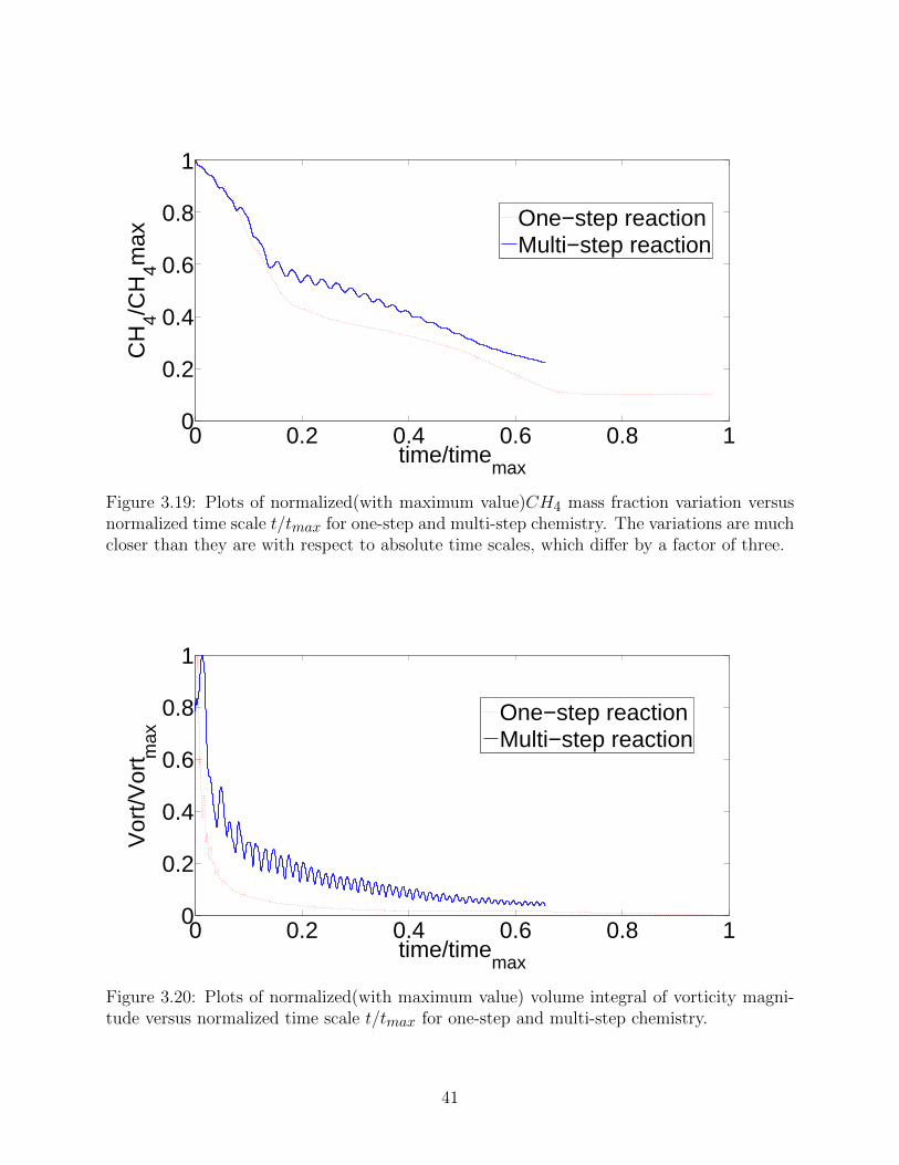
one-step case does produce the oscillations. Shown in Fig. 3.20 is a plot of the normalized

volume integral of the vorticity magnitude, where normalization is with the maximum value,

versus t. The agreement is not complete, but the overall trend is very similar except for the

lack of oscillations in the one-step case.

27

These plots indicate that even though various details may be substantially different,

there are nevertheless important points of agreement that permit the discussion of the one-

step mechanism and render its predictions adequate for the purposes of understanding and

describing various features of the problem.

3.4.1.8 Adiabatic and constant temperature walls

The simulations shown so far have assumed adiabatic walls, thus there was no heat loss

from the domain. A single one-step simulation was performed with the walls at constant

temperature 800 K. The constant temperature walls do not change the overall burn time by

a significant amount.

Figure 3.21 compares the two boundary conditions of constant temperature walls and

adiabatic walls. The two curves are generally similar with respect to the location of the three

burning regimes. The only substantial difference appears between t ∼ 6ms and t ∼ 11ms.

3.4.1.9 Global (first law) energy balance

The first law of thermodynamics, Q = ∆U gives the heat released by the combustion reaction

as Q = m∫ 21 cv(T ) dT = m[uair(2250K) − uair(800K)], where we use the total mass m =

2.8E − 4 kg and the internal energy values for air as a reasonable proxy for the burned

and unburned gases. This yields Q ∼ 2.8E − 4kg(1921.3− 592.3)kJ/kg = 0.37kJ , which is

reasonably close to the value estimated using the entropy balance in Sec 4.1.4. The overall

heat release during the combustion event is approximately 0.4kJ , which is about 400 times

larger than the ignition energy of 1J(see Sec. 2.1). It can be concluded that the ignition

event has no influence on the energetics of the combustion process, although it may alter

the geometric evolution of the flame as will be discussed later in this article.

28

3.4.1.10 Higher temperature of spark

A separate simulation was performed with the spark given a temperature of 3000K. There

did not appear to be a significant change in the flame shape or the total time of combustion.

Figure 3.22 shows mass fraction contours of methane during Regime 2 of combustion. The

flame shape is entirely different from the previous cases, but is still has a stochastic nature.

Like the previous cases we still have 3 distinct regimes of combustion. The total time of

combustion was however not significantly changed.

29

(a) Contours of CH+ radical mass fraction in Regime 1.

(b) Contours of OH− radical mass fraction in Regime 1.

Figure 3.6: Flame propagation in regime 1 using CH+ and OH− as the markers. Note theformation of the C-shaped fronts. The OH− appears to track the flame front and the high-Tcombustion products.

30

(a) Contours of CH+ radical mass fraction in Regime 2.

(b) Contours of OH− radical mass fraction in Regime 2.

Figure 3.7: Flame propagation in regime 2, which ends when the separate flames havecoalesced. In regime 2 the flame brush is highly fragmented.

31

(a) Contours of CH+ radical mass fraction in Regime 3.

(b) Contours of OH− radical mass fraction in Regime 3.

Figure 3.8: Flame propagation in regime 3. This regime corresponds qualitatively, with the“tulip” flame stage for initially quiescent fixed-volume combustion in a rectangular channel.

32

0 1 2 3 4 5 6x 10

−3

0.01

0.02

0.03

0.04

0.05

0.06

Time (s)

Mas

s fr

actio

n of

CH

4

Slope ~ −5.3/s

Regime 3

Regime 2

Slope ~ −22.5/s

Regime 1

Figure 3.9: Volume average of CH4 in the channel with time. The slope changes near 0.75ms and at 1.5 ms.

33

(a) CH+ mass fraction showing flame location.

(b) Velocity vectors showing vortices which shape the flame.

Figure 3.10: Comparison of velocity vectors and CH+ radical concentrations which trackthe flame front.

34

(a) Pressure contours in the channel near the spark.

(b) Density contours near the spark after some fuel has burnt.

Figure 3.11: Comparison of pressure and density contours concentrations at the same instant.The baroclinicity in the fluid is clearly visible. Density and pressure gradients are not alignedat several points.

35

0 0.5 1 1.5 2 2.5 3 3.5 4 4.5 5 5.5 6x 10

−3

0

5

10

15

20

25

Time(s)

Vor

ticity

mag

nitu

de v

olum

e in

tegr

al (

m3 /s

)

Regime 3

Regime 2

Regime 1

Figure 3.12: Volume integral of vorticity magnitude in the channel with time. Shown arethe three regimes of combustion.

0 1 2 3 4 5 6x 10

−3

0

1

2

3

4

5x 10−7

Time (s)

Mas

s fr

actio

n of

CH

+ r

adic

al

average ~ 8E−08

average ~ 1.2E−08

Figure 3.13: Volume average of CH+ in the channel with time. The ratio of average valuesis 8E − 8/1.2E − 8 ' 6.7.

36

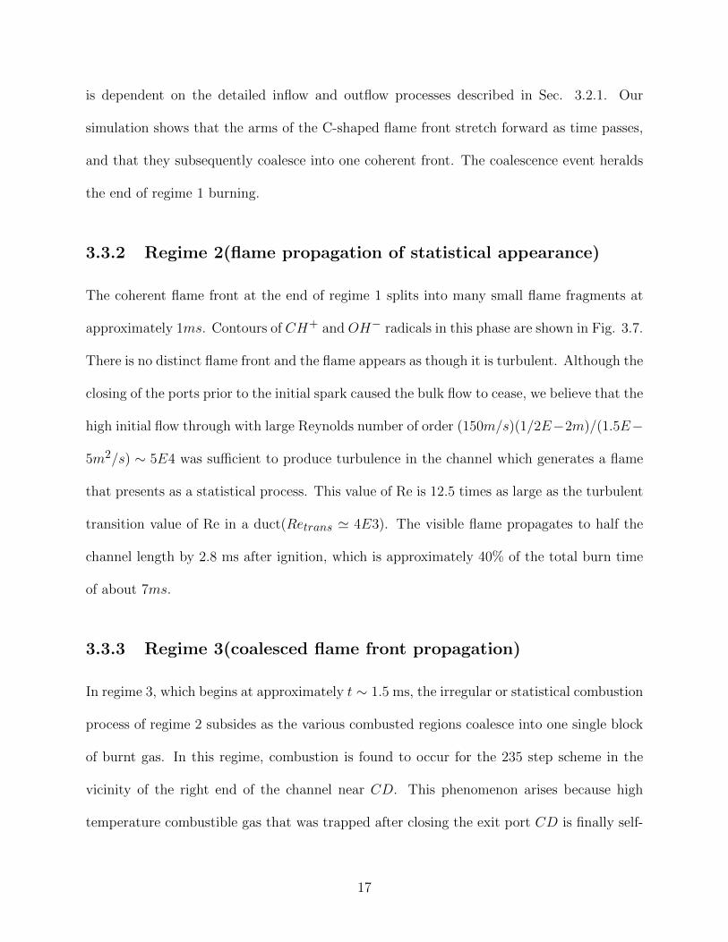
(a) The case 5E4 < |~ω| < 1.5E5/s. This isthe highest range of vorticity magnitude.This scale is concentrated near the walls.

(b) The case 1E4 < |~ω| < 1E5/s. This isthe second highest range of vorticity mag-nitude showing a lot of flame vorticity andalso a little flow vorticity near the walls.

(c) The case 1E3 < |~ω| < 1E4/s. In thisrange the vorticity is almost exclusivelyflame vorticity.

(d) The case 1E2 < |~ω| < 1E3/s. This isthe lowest range of vorticity magnitude.

Figure 3.14: Four different filters applied to the vorticity field to show where the differentscales of vorticity magnitude are located.

37

012

Den

sity

(kg

/m3 )

33.5

4x 105

Pre

ssur

e (P

a)

2.5 3 3.5x 10

−3

1000

2000

Time (s)Tem

pera

ture

(K)

Figure 3.15: Density, pressure and temperature at the center-point of the channel as a flamepasses over it.

2.5 3 3.5x 10

−3

0

2

4

6

8

10

Time(seconds)

ln(φ

)

T*γ/(γ−1)/p*

p*/ρ*γ

Figure 3.16: The burnt and unburnt mixture at different entropy levels. The y-axis showsthe log of a quantity θ which is supposed to remain constant in an isentropic process. Twosuch values of θ are chosen, namely p/ργ and T γ/(γ−1)/p.

38

2.5 2.6 2.7 2.8 2.9 3 3.1 3.2 3.3 3.4 3.5x 10

−3

1

1.5

2

2.5

3

3.5

4

Time(seconds)

Pre

ssur

e(ba

rs)/

V

ortic

ity m

agni

tude

(m

3 /s)

Pressure

Volume integral of vorticity magnitude

Figure 3.17: Pressure and vorticity magnitude at a point in the flow field. Between t = 2.6and 3.3 ms there are eight vorticity oscillations giving the period T ' 0.875ms. Between2.65 and 3.35ms there are four pressure oscillations giving T ' 0.4375 ms, for a ratio of 2.0.

39

(a) CH4 mass fraction contours during regime 1.

(b) CH4 mass fraction contours during regime 2.

(c) CH4 mass fraction contours during regime 3.

Figure 3.18: CH4 mass fraction contours at different stages of combustion using one-stepchemistry. Red represents stoichiometric mixture and blue represents complete absence ofmethane.

40

0 0.2 0.4 0.6 0.8 10

0.2

0.4

0.6

0.8

1

time/timemax

CH

4/CH

4max

One−step reactionMulti−step reaction

Figure 3.19: Plots of normalized(with maximum value)CH4 mass fraction variation versusnormalized time scale t/tmax for one-step and multi-step chemistry. The variations are muchcloser than they are with respect to absolute time scales, which differ by a factor of three.

0 0.2 0.4 0.6 0.8 10

0.2

0.4

0.6

0.8

1

time/timemax

Vor

t/Vor

t max

One−step reactionMulti−step reaction

Figure 3.20: Plots of normalized(with maximum value) volume integral of vorticity magni-tude versus normalized time scale t/tmax for one-step and multi-step chemistry.

41

0 0.005 0.01 0.015 0.020

0.02

0.04

0.06

Time (s)

Mas

s fr

actio

n of

CH

4

Walls at 800 KAdiabatic walls

Figure 3.21: Comparison of one-step chemistry burning rate of CH4 in the channel for thecases with constant temperature and adiabatic walls. Except for a small middle portionbetween 0.006 and 0.01s the CH4 mass consumption rates are essentially identical.

Figure 3.22: Methane mass fraction distribution in channel during Regime 2 using one-stepchemistry and a higher temperature of spark.

42

3.4.1.11 Two sparks

A large difference was found with two sparks instead of one, each having a temperature of

2500 K. The statistical regime of combustion lasted longer and the entire channel achieved

complete combustion in around 3 ms. For one-step chemistry this is a nearly seven-fold

increase in the overall burning rate. Figures 3.23 and 3.24 show methane mass fraction

contours at the beginning and end of combustion.

Figure 3.23: Methane mass fraction distribution in channel at the start of combustion usingtwo sparks and one-step chemistry.

Figure 3.24: Methane mass fraction distribution in channel at the end of combustion usingtwo sparks and one-step chemistry.

This method of using two sparks located at different locations clearly appears to be a

potentially very useful method of utilizing the vorticity generation mechanism for enhancing

the burning rate discussed earlier. The seven-fold reduced combustion time is a result of

the stochastic regime of combustion occurring in two different locations rather than by the

deposition of more energy into the channel.

43

3.4.2 End Walls Permanently Closed(No Initial Vorticity)

A separate set of simulations was performed without the opening and closing of end walls

as mentioned in Sec. 2. The San Diego mechanism was used with all parameters remaining

the same as before. Once again, four distinct regimes were observed. In this case, however,

overall combustion is much slower.

3.4.2.1 Mass consumption rate and flame area

Figure 3.25 shows the variation with elapsed time of the volume average of the mass fraction

of CH4 in the channel. In the fast regime we have dYCH4/dt ' −11.6s−1. The slope of

this plot shows two separate temporal regimes of fast and slow burning. After about 5ms ,

the slope of the graph becomes low and the time to burn the remaining CH4 in the channel

is > 10ms . In the slow regime we find dYCH4/dt ' −3.3s−1. Thus, the ratio of CH4

consumption rates in the fast to the slow regimes is −11.6/− 3.3 ' 3.5, which is close to the

value 4.2 calculated for the initial flow-through case (see Sec. 4.1.2). The plots of CH+ (Fig.

3.26) and volume integral of vorticity magnitude (Fig. 3.27), respectively, versus time, shed

light on this behavior. As for the flow-through case, the ignition process initiates pressure

waves which reflect off the channel walls AB and CD and wherever there are misaligned

pressure and density gradients in the channel, vortices are created which twist the flame

front and split it into many parts. This is apparent in the rise in vorticity magnitude as well

as mass fraction of CH+ in the channel. The vorticity magnitude, however, never attains

the high values observed in the previous simulations(maximum magnitude ∼ 23m3/s in Fig.

3.12). In Fig. 3.27 the maximum integrated vorticity is approximately 4.5m3/s which is

smaller than the flow-through case by approximately the factor 23/4.5 ∼ 5. Note that the

value of ∼ 4m3/s is of the order of the rise in vorticity between t = 0.5 and 0.75ms in Fig.

44

7, suggesting that ∼ 4m3/s is the integrated vorticity associated with flame initiation.

0 2 4 6 8x 10

−3

0.01

0.02

0.03

0.04

0.05

0.06

Time (s)

Mas

s fr

actio

n of

CH

4

Slope ~ −11.6/s

Slope ~ −3.2/sRegime 2

Regime 3

Regime 1

Figure 3.25: Volume average of CH4 in the channel with time(walls always closed). Usesthe San Diego mechanism(full chemistry) to describe the flame chemistry.

3.4.2.2 Vorticity scaling

Analogous to the flow-through scaling of Sec. 4.1.3, the flame-generated baroclinic torque

vorticity scales as Eq. 4.1, where the time t is now measured from the start of combustion.

We scale the various quantities in Eq. 4.1 as follows: ∆ρ ∼ ρ0, ∆p ∼ ρ0S2, ρ ∼ ρ0,

δF ∼ (α/S) . Here α is the gas thermal diffusivity and S is the flame speed in the initial

burning regime. The result is |~ωflame| ∼ t(S4/α2). In order to obtain the total or integrated

vorticity we now evaluate the quantity∫vol |~ωflame| dτ ∼ t(S2/α2)δFhw = t(S3/α)hw. This

enables writing the integrated initial vorticity variation in Fig.3.27 as |~ωflame|.τflame =

|~ωflame|0 .τflame+t(S3/α)hw, where the first term on the RHS is the initial value of the total

vorticity produced by the ignition of the spark: from Fig. 3.12 it has the value 2 m3/s. Note

that except for the fluctuations this variation is linear in t. From the preceding relationship,

45

0 2 4 6 8x 10

−3

0

1

2

3x 10−7

Time (s)

Mas

s fr

actio

n of

CH

+ r

adic

al

Average ~ 1.23E−07

Average ~ 1.71E−08

Figure 3.26: Volume average of CH+ in the channel with time(walls always closed). Anapproximate average value for 0 < t < 3ms is 1.23E − 7, for t > 3ms it is ' 1.71E − 08 fora ratio of 1.23/1.7 ' 7.2.

a mathematical expression for the flame speed is deduced:

S =

[α

hw

d

dt

(|~ωflame|.τflame

)]1/3. (3.3)

In Fig. 3.12 the slope of the linear rise is d[|~ωflame|.τflame

]/dt = [(3.752)m3/s]/(2.9E−

3s) = 600m3/s2. Therefore using α = 3E−4m2/s, h = 0.5E−2m and w = 1m (unit depth)

in Eq. 3.3 gives S ∼ 3.3m/s. Multiplying this by the elapsed time of 2.9E − 3 s in this

stage indicates that the flame has propagated a distance of approximately 1cm. The total

burn time is 20ms, hence the ratio 5cm(3ms/20ms) yields a flame propagation distance of

approximately 0.75cm, which is of the same order of magnitude as the scaling estimate of

1cm.

46

0 2 4 6 8x 10

−3

0

1

2

3

4

5

Time (s)

Vor

ticity

mag

nitu

de

volu

me

inte

gral

(m3 /s

)

Figure 3.27: Volume integral of vorticity magnitude in the channel with time(walls alwaysclosed). Uses full multi-step San Diego mechanism.

3.4.2.3 Vorticity decay

The growth of vorticity in the channel cannot continue indefinitely. During the entire growth

process, viscous decay is present according to ∂~ω/∂t ∼ ν∇2~ω which simplifies to ∂|~ω|/∂t ∼

−ν|~ω|/l2 for a homogeneous turbulence. Here l is a characteristic vorticity decay length

scale, which can be estimated from the solution |~ω|/||~ω0| = exp[−(ν/l2)(t − t0)] where

t0 = 2.9ms and |~ω|0L.h.w = 3.9 m3/s. The vorticity decay approximately follows the

function 3.9exp[−0.187× (t−2.9)] where t is in ms.The vorticity scale is therefore a fraction

of a millimetre.

47

Chapter 4

Enhancement features

4.1 Re-injection of combusted gas mixture for com-

pression of fresh gas mixture

The overall thermodynamic efficiency of this device, which employs the Humphrey ther-

modynamic cycle, increases with increased pressure inside the combustion channel prior to

combustion. One possible way of achieving pre-compression in a combustion channel is to

re-inject combusted gas from the previous cycle, before it is expanded. However, this pre-

compression in one channel comes at the cost of a loss of pressure and temperature in another

channel, which is to be expanded for power production. In this chapter, an attempt is made

to derive optimum working conditions, which would maximize overall cycle efficiency, using

analytical and computational methods.

The combusted mixture generates torque when it is expelled over the rotor channels and

through the exit port of the wave disk engine. The gas extraction from the high pressure

combustion channel reduces both the pressure and mass of gas available for torque generation,

which hampers the power production. Re-injection dilutes the combustible mixture and

may affect ignition and subsequent combustion characteristics. The unsteady flow processes

developed inside the re-injection passage demands careful modeling and analysis of the same.

The variable parameters considered here are the rotating speed of the engine and the diameter

48

of the re-injection passage. These two parameters control the total mass of gas that is

transferred from the high pressure combustion channel to the low pressure one, thereby

altering the level of pre-compression achieved and ultimately the overall thermal efficiency.

This section describes two-dimensional computational fluid dynamic simulations for dif-

ferent angular speeds of the engine and widths of the re-injection passage. A balance is

sought between loss of mass and enthalpy in a high pressure combustion channel and the

gain in pressure and enthalpy in the low pressure channel, such that we maximize overall

cycle efficiency.

4.1.1 Thermodynamics of pre-compression

The effect of pre-compression by combustion gas re-injection on thermal efficiency has been

calculated with the following assumptions and input parameters: external compressor pres-

sure ratio of 1.1, specific heat ratio (γ) of 1.4, and combustor temperature ratio Tfinal/Tinitial

of 6. The heat addition process is treated as constant volume. The pressure drop in the high

pressure channel due to mass bleeding for re-injection is calculated according to equation

4.1:

∆p high pressure channel = 1.4×∆p low pressure channel + 18500 (4.1)

where ∆p high pressure channel is the pressure drop in the high pressure channel due to mass

loss via the re-injection tube, ∆p low pressure channel is the pressure rise in the low pressure

channel due to mass gain via the re-injection port. The following equation was taken from

figure 4.2, which correlates ∆p high pressure channel and ∆p low pressure channel for a variety

of RPMs and re-injection passage widths.

49

Figure 4.1: Thermodynamic state points of a pressure-gain WDE, utilizing hot gas re-injection for combustible mixture pre-compression.

50

With the notations in Figure 4.1,

P2 = P1 × PRcompressor (4.2)

T2T1

=P2P1

γ−1γ

(4.3)

P2′ = P1 × PRHammershock (4.4)

T2′T2

=P2′P2

γ−1γ

(4.5)

PA = P2′ × PRRe−inject (4.6)

TAT2′

=PAP2′

γ−1γ

(4.7)

TB = TA × TRcombustor (4.8)

PB = TB ×PATA

(4.9)

Using the correlation found in Figure 4.2,

P3′ = PB −(1.4× (PA − P2′) + 18500

)(4.10)

51

T3′TB

=P3′PB

γ−1γ

(4.11)

T4T3′

=P4P3′

γ−1γ

(4.12)

ηth =Wnet

Hin=WTurbine −WCompressor

Hin=mTurbine × (h4 − h3′)− mCompressor × (h2 − h1)

mCombustor × (hB − hA)

(4.13)

It is to be noted that mTurbine = mCompressor, ∆hTurbine = CpdT , ∆hCompressor =

CpdT , and ∆uCombustor = CvdT , which gives

ηth =mTurbine

mCombustor× γ ×

(T3′ − T4)− (T2 − T1)

(TB − TA). (4.14)

The first term in Equation 4.14 (ratio of mass supplied into the turbine to that sup-

plied into the combustor) is evaluated according to figure 4.3 where the re-injection pre-

compression ratio was plotted against the amount of mass lost in the high pressure channel.

The thermal efficiency presented in Figure 4.4 has been calculated using exchange of mass

between the low pressure channel and the high pressure channel. The efficiency is multiplied

by γ (=1.4) to account for the constant volume heat addition and constant pressure external

compression and expansion works. The thermal efficiency shown in Figure 4.4 is calculated

using Equations 4.2-4.14 for 100% component efficiencies and assuming that the gas expands

to atmospheric pressure in the turbine after power extraction. The efficiencies involved in

the conversion of thermal energy into kinetic energy in the turbine, for power production is

neglected in this calculation. The high thermal efficiency values shown in figure 4.4 should

52

not be viewed as possible values attainable by any device explained in this paper. In line

with the objective of this paper, only the trends are to be extracted. Figure 4.4 is used only

to show that thermal efficiency can be increased by re-injecting burned gas from one channel

to another which is yet to burn, in a WDE. The trends shown in Figure 4.4 are expected

to hold, even with realistic component and process efficiencies introduced. The magnitude

of thermal efficiencies given in figure 4.4 will change to accommodate these inefficiencies.

The thermal efficiency can be seen to increase when the pre-compression ratio due to gas

re-injection increases up to a value of 2. Beyond this, the decrease in thermal efficiency is due

to the decrease of the mass ratio in Equation 4.14. The decrease of thermal efficiency due

to mass loss supersedes the increase of thermal efficiency due to pre-compression. The tran-

sient nature of the mass addition into the low pressure channel (and mass loss from the high

pressure channel) via the re-injection tube is neglected when calculating the thermodynamic

state points. Equilibrium states are assumed at each state point. For example, the compres-

sion and expansion processes in the channels due to re-injection, are transient processes of

pressure rise/loss and mass gain/loss. However the simple analytical analysis used in cal-

culating the thermal efficiency (4.2-4.14) neglects these transient processes. The numerical

analysis has taken these complex transient processes into account in its predictions.

53

Figure 4.2: Pressure rise in the low pressure channel vs. pressure drop in the high pressurechannel.

54

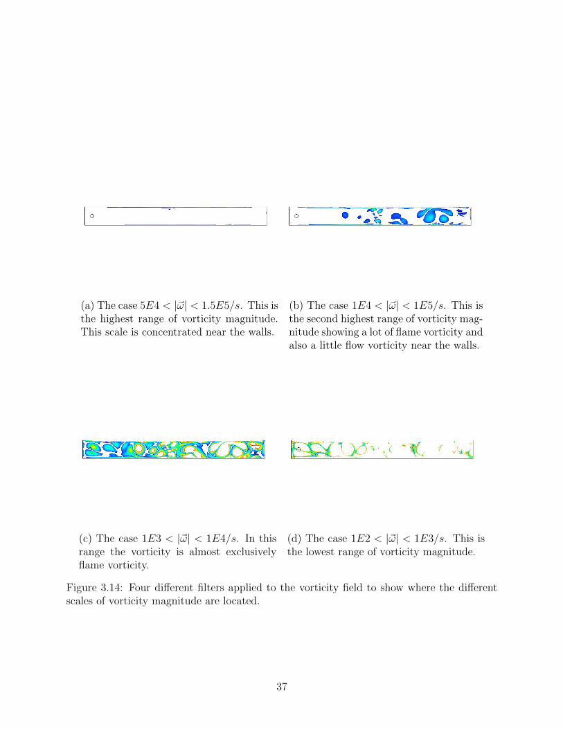
Figure 4.3: Plot of ratio of mass in turbine over mass in combustor to reinjection pressuregain.

55

Figure 4.4: Thermal efficiency increase with gas re-injection for pre-compression.

4.2 Numerical simulations

4.2.1 Simulation Methodology

The objective of this study was to investigate the thermal efficiency increase due to pre-

compression for various re-injection passage widths and combustion channel speeds. The

size and shape of the combustion channels were not varied. Any variation in the dimensions

and shape of the channels can have a further impact on the predictions which is not studied

in this paper. The basic geometry used in the simulations is shown in Figure 4.5. One

combustion channel on either side of a rectangular re-injection passage is shown in two di-

mensions. The shape and length of the combustion channels were arbitrarily chosen based on

56

prior numerical and experimental studies and does not correspond to any optimized values

for an actual WDE. The re-injection passage is kept stationary and an angular velocity is

imparted to the combustion channels. The rotation direction is shown also shown in Figure

4.5. Several numerical simulations were carried out with different widths of the re-injection

passage and different rotating speeds of the combustion channels. Initial set of simulations

were run with the re-injection passage interacting with one high pressure combustion channel

and one low pressure combustion channel (Preliminary Analysis 1: Section III A). However

these predictions were biased from the initial conditions supplied. To eliminate the influence

of initial conditions, the simulations were repeated with two channels on either side of the

reinjection passage (Preliminary Analysis 2: Section III B), and a few selected complete cycle

simulations using 20 combustion channels. The preliminary analyses were used to quantify

the pressure gain in low pressure combustion channels as a function of mass, enthalpy and

pressure loss in the high pressure combustion channels at a lower computational cost. Com-

bustion was not modeled in these preliminary analyses and only gas mixing and subsequent

pressure exchange was looked into. The complete cycle analyses performed were detailed nu-

merical simulations with combustion turned on, on a full Wave Disk Engine equipped with

a re-injection passage. Predictions from preliminary analysis 2 were compared against the

complete cycle analysis to see the viability of using preliminary analysis 2 as a design tool

for WDE design, which are simple and lower in computational cost, compared to complete

cycle analyses.

4.2.2 Numerical Scheme

The commercial computational fluid dynamics(CFD) code, Ansys Fluent was used in this

paper to analyze the problem at hand in two spatial dimensions. The compressible Navier-

57

Stokes equations were solved using a pressure-velocity coupling scheme, with first-order

accuracy in time and space. Transfer of flow data between the rotating (rotor) and stationary

(intake and exit ports) parts of the flow field was handled using sliding meshes, wherein nodes

move rigidly in a dynamic mesh zone without any distortion to the computational cells.

Multiple cell zones are connected with each other through non-conformal interfaces. As the

mesh motion is updated in time, the non-conformal interfaces are likewise updated to reflect

the new positions of each zone [7] . Turbulence was modeled using the Spalart-Allmaras

turbulence model[7] with the turbulence intensity at the inlet equal to 5% and a turbulence

length scale of 1% of the inlet width. Species transport equations were additionally solved

to model gas mixing and chemical reactions. A laminar finite-rate model [7] was used to

compute the chemical source terms in the species transport equations using Arrhenius kinetic

expressions, and ignoring the effects of turbulent fluctuations on reaction rates. This model

is known to predict the laminar flames with acceptable accuracy, but is generally inaccurate

for turbulent flames due to highly non-linear Arrhenius chemical kinetics [7]. The specific

heat capacity at constant pressure for each component was allowed to vary with temperature

according to experimental correlations[6]. Viscosity was modeled using Sutherland law [6].

The governing transport equations were solved until their residuals went below 0.001 at every

time step.

58

4.3 Results

4.3.1 Preliminary analysis 1 : One channel on either side of re-

injection passage

The initial simulations used a re-injection passage connecting two channels at different pres-

sures. The objective was to analyze the flow patterns developed after the re-injection process

was completed (after the two channels rotate past the re-injection passage). The initial con-

ditions used are shown in Figures 4.5 and 4.6 with the high pressure combustion channel at

a pressure of 11 bars and a temperature of 2260 K. These values correspond to state variable

values used in the analytical analysis (Equations 4.2-4.14). The re-injection passage was ini-

tialized with the same conditions as the high pressure channel. The low pressure combustion

channel was initialized with a pressure of 1 bar and a temperature of 300 K. In the case

shown in Figures 4.5-4.8, the re-injection passage width is one-fifth of the inner width of the

channels. The channels were rotated at 5000 RPM anti-clockwise 4.5. The state after the

exchanger-injection process is given in Figures 4.7 and 4.8. Transient wave motions were

observed during the re-injection process.

The re-injection passage is opened and closed gradually into the combustion channels

as it rotate past them, which gives rise to compression and expansion waves within the

passage. These waves ensure that the next channel coming in alignment with the re-injection

passage will experience conditions significantly different to those faced by the first channel.

Consequently, predictions which are significantly less biased due to initial conditions can be

obtained by using two combustion channels on either side of the re-injection passage.

59

Figure 4.5: Initial pressure contours for preliminary analysis 1.

4.3.2 Preliminary analysis 2 : Two channels on either side of re-

injection passage

The influence of unsteady effects is more effectively captured by using two channels on either

side of the re-injection passage. In this way, the second set of combustion channels (both

low and high pressure) that are exposed to the re-injection passage, faces more realistic flow

conditions which are less biased from the initial conditions. This is a simple and approximate

way of studying the flow physics of the re-injection process without the need of carrying out

60

Figure 4.6: Initial temperature contours for preliminary analysis 1.

several simulations of the entire engine cycle which is computationally expensive. Figures

4.9 - 4.14 show the flow conditions before and after the re-injection process for a rotor

speed of 5000 RPM and a re-injection tube of width three-fifth of the inner width of the

channels. Several speed and re-injection passage width combinations were studied to see

which combination provides maximum pre-compression at a minimal level of dilution of the

unburned combustible mixture (Table 4.1 ). To analyze the level of mixing of the gases in

the two channels, the high pressure channels and the re-injection passage were filled with

nitrogen (to represent burned gas) and the low-pressure channels were filled with ethane (to

represent unburned combustible mixture). Combustion was not modeled in these simulations

and only gas mixing was looked into. Ethane mass fraction contours (for 5000 RPM and

re-injection passage width equal to three-fifth of the combustion channel width) at the end

of the re-injection process (4.14) show that the combustible mixture gets diluted with the

61

Figure 4.7: Final pressure contours for preliminary analysis 1.

burned gas for the particular rotating speed and the re-injection passage width shown in

Figures 4.9 - 4.14. This would result in a very lean combustible mixture which might not be

desirable for combustion. This shows that, the particular combination of re-injection passage

width and angular speed discussed above (5000 RPM and re-injection passage width equal to

three-fifth of the combustion channel width) would not result in desirable working conditions

to maximize cycle efficiency.

The same initial conditions in the channels were applied to different re-injection passage

width and rotating speed combinations (Tables 4.2 - 4.4). The ratio of mass lost in the

high-pressure channels and the ratio of mass gained in the low-pressure channels during the

re-injection process are listed in Table 4.2. For wider re-injection passage widths and lower

rotor speeds, the high-pressure channel loses more mass to the low-pressure channel, which

is undesirable for cycle efficiency maximization. The resulted change in mixture enthalpy in

62

Figure 4.8: Final temperature contours for preliminary analysis 1.

combustion channels, due to re-injection, for varying re-injection passage widths and rotor

speeds are also tabulated in Table 4.1. The change in pressure experienced by combustion

channels due to re-injection, for varying re-injection passage widths and rotor speeds is

tabulated in Tables 4.1. The tabulated quantities in Table 1 are calculated according to

Equations 4.15-4.18.

Pressure gain in low pressure channel =(PLf − PLi)

PLi(4.15)

Pressure loss in high pressure channel =(PHi − PHf )

PHi(4.16)

63

Figure 4.9: Initial pressure contours for preliminary analysis 2.

Fraction of enthalpy lost in high pressure channel =(HHi −HHf )

HHi(4.17)

Fraction of mass lost in high pressure channel =(MHi −MHf )

MHi(4.18)

The pressure-gain in the low-pressure channel is plotted against the pressure loss in

the high pressure channel in Figure 4.15 for different re-injection passage widths and rotor

speeds. Each marker shape represents a distinct re-injection passage width (expressed as

a fraction of combustion channel width), while the size of the marker represents different

rotor speeds. The biggest marker size is used for 20000 RPM, the medium size for 10000

RPM and the smaller size for 5000 RPM. It can be seen that the variation of pressure in

the combustion channels gets independent of the re-injection passage width when it gets

smaller than one-fifth of the combustion channel width. For re-injection passage widths

smaller than this, only rotor speed seems to affect the pressure exchange process between

64

Figure 4.10: Initial temperature contours for preliminary analysis 2.

the combustion channels. This is due to the fact that the flow from the re-injection channel

into the low pressure channel gets sonic for passage widths of one-fifth and smaller as shown

in Figure 4.19. The pressure exchange process is seen to be affected by both re-injection

passage width and the rotor speed, for re-injection passage widths larger than one-fifth of

the combustion channel width, This behavior is further seen by plotting the pressure-gain

in the low-pressure combustion channel against rotor speed (4.15), where the pressure gain

does not vary significantly for smaller re-injection widths beyond one-fifth of the combustion

channel width. As expected, pressure gain is inversely proportional to rotor speed in that

more pressure gain is obtained at lower speeds for a given re-injection passage width.

The pressure-gain in the low-pressure channel against enthalpy and mass loss in the high

pressure channel are shown in Figures 4.17 and 4.18 respectively. Each curve represents

a different reinjection passage width (expressed as fraction of combustion channel width)

while data points show the rotor speeds. The variation is once again linear showing similar

behavior as was seen in Figure 4.15 .

65

Figure 4.11: Initial ethane mass fraction contours for preliminary analysis 2.

Figure 4.12: Final pressure contours for preliminary analysis 2.

66

Figure 4.13: Final temperature contours for preliminary analysis 2.

Figure 4.14: Final ethane mass fraction contours for preliminary analysis 2.

67

Table 4.1: A table showing change in mass, enthalpy and pressure in the combustion channelsafter the reinjection process for preliminary analysis 2.

Width ofre-injectionport(fractionof channel)

RPM Pressuregainin LPchannel

Mass lossin HPchannel

Pressurelossin HPchannel

Enthalpylossin HPchannel

One-seventh 5000 2.35 0.18 0.22 0.2310000 1.57 0.06 0.08 0.0920000 1.33 0.04 0.05 0.05

One-sixth 5000 2.58 0.20 0.26 0.2710000 1.68 0.07 0.10 0.1020000 1.39 0.05 0.06 0.07

One-fifth 5000 2.89 0.24 0.30 0.3210000 1.82 0.10 0.12 0.1320000 1.47 0.06 0.07 0.08

Two-fifth 5000 4.61 0.43 0.51 0.5310000 2.94 0.19 0.24 0.2520000 2.00 0.12 0.15 0.16

Three-fifth 5000 5.86 0.54 0.63 0.6610000 4.02 0.29 0.35 0.3720000 2.59 0.17 0.22 0.23

0 0.2 0.4 0.6 0.81

2

3

4

5

6

Pressure loss in high pressure channel

Pre

ssur

e ga

in

in lo

w p

ress

ure

chan

nel

One−seventh, 5000 RPMOne−seventh, 10000 RPMOne−seventh, 20000 RPMOne−sixth, 5000 RPMOne−sixth, 10000 RPMOne−sixth, 20000 RPMOne−fifth, 5000 RPMOne−fifth, 10000 RPMOne−fifth, 20000 RPMTwo−fifth, 5000 RPMTwo−fifth, 10000 RPMTwo−fifth, 20000 RPMThree−fifth, 5000 RPMThree−fifth, 10000 RPMThree−fifth, 20000 RPM

Figure 4.15: Comparison of pressure gain in low pressure channel against pressure loss inhigh pressure channel for different widths of re-injection passage.

68

Table 4.2: A table showing the fraction of mass lost from the high pressure channel duringthe re-injection process for preliminary analysis 2.

Widthof re-injectiontube (frac-tion ofchannelwidth)

RPM Mass in low-pressure channel(kg)

Mass in high-pressure channel(kg)

Fraction ofmass lostin high-pressurechannel

Before After Before AfterOne-seventh

5000 1.96E-005 2.44E-005 2.64E-005 2.18E-005 0.175

10000 1.96E-005 2.16E-005 2.64E-005 2.47E-005 0.06320000 1.96E-005 2.08E-005 2.64E-005 2.53E-005 0.041

One-sixth 5000 1.96E-005 2.52E-005 2.64E-005 2.10E-005 0.20410000 1.96E-005 2.20E-005 2.64E-005 2.44E-005 0.07520000 1.96E-005 2.10E-005 2.64E-005 2.51E-005 0.049

One-fifth 5000 1.96E-005 2.64E-005 2.64E-005 2.00E-005 0.24310000 1.96E-005 2.26E-005 2.64E-005 2.39E-005 0.09520000 1.96E-005 2.13E-005 2.64E-005 2.49E-005 0.058

Two-fifth 5000 1.96E-005 3.24E-005 2.64E-005 1.51E-005 0.42610000 1.96E-005 2.60E-005 2.64E-005 2.14E-005 0.18920000 1.96E-005 2.31E-005 2.64E-005 2.33E-005 0.117

Three-fifth 5000 1.96E-005 3.56E-005 2.64E-005 1.22E-005 0.53910000 1.96E-005 2.99E-005 2.64E-005 1.88E-005 0.28720000 1.96E-005 2.51E-005 2.64E-005 2.18E-005 0.173

69

Table 4.3: A table showing the pressure gain ratio in the low-pressure channel and pressureloss ratio in the high-pressure channel during the re-injection process for preliminary analysis2.

Width ofre-injectiontube(fractionof channelwidth)

RPM Volume aver-age of Pressurein low-pressurechannel(Pa)

Volume aver-age of Pressurein high-pressurechannel(Pa)

Pressuregainin low-pressurechannel

Pressureloss inhigh-pressurechannel

Before After Before AfterOne-seventh

5000 1.01E+5 2.38E+5 1.10E+6 8.58E+5 1.351 0.221

10000 1.01E+5 1.59E+5 1.10E+6 1.01E+6 0.566 0.08120000 1.01E+5 1.35E+5 1.10E+6 1.05E+6 0.333 0.050

One-sixth 5000 1.01E+5 2.62E+5 1.10E+6 8.19E+5 1.585 0.25710000 1.01E+5 1.70E+5 1.10E+6 9.96E+5 0.676 0.09520000 1.01E+5 1.40E+5 1.10E+6 1.03E+6 0.386 0.063

One-fifth 5000 1.01E+5 2.92E+5 1.10E+6 7.68E+5 1.886 0.30310000 1.01E+5 1.84E+5 1.10E+6 9.69E+5 0.817 0.12020000 1.01E+5 1.49E+5 1.10E+6 1.02E+6 0.466 0.075

Two-fifth 5000 1.01E+5 4.67E+5 1.10E+6 5.37E+5 3.611 0.51310000 1.01E+5 2.98E+5 1.10E+6 8.42E+5 1.938 0.23620000 1.01E+5 2.02E+5 1.10E+6 9.38E+5 0.997 0.148

Three-fifth 5000 1.01E+5 5.94E+5 1.10E+6 4.03E+5 4.864 0.63410000 1.01E+5 4.08E+5 1.10E+6 7.12E+5 3.024 0.35420000 1.01E+5 2.63E+5 1.10E+6 8.61E+5 1.594 0.218

70

Table 4.4: A table showing the fraction of enthalpy lost from the high pressure channelduring the re-injection process for preliminary analysis 2.

Width of re-injection tube(fraction ofchannel width)

RPM Mass-weighted inte-gral of Enthalpy inlow-pressure chan-nel(J)

Mass-weighted in-tegral of Enthalpyin high-pressurechannel(J)

Fraction of En-thalpy lost inhigh-pressurechannel

Before After Before AfterOne-seventh 5000 0.064 12.979 61.731 47.369 0.233

10000 0.064 4.863 61.731 56.449 0.08620000 0.064 2.809 61.731 58.491 0.052

One-sixth 5000 0.064 15.141 61.731 45.086 0.27010000 0.064 5.754 61.731 55.514 0.10120000 0.064 3.205 61.731 57.625 0.067

One-fifth 5000 0.064 18.030 61.731 42.098 0.31810000 0.064 7.586 61.731 53.907 0.12720000 0.064 4.171 61.731 56.868 0.079

Two-fifth 5000 0.064 32.815 61.731 28.772 0.53410000 0.064 16.191 61.731 46.465 0.24720000 0.064 8.680 61.731 52.115 0.156

Three-fifth 5000 0.064 40.502 61.731 21.191 0.65710000 0.064 25.347 61.731 38.868 0.37020000 0.064 13.597 61.731 47.561 0.230

0 0.1 0.2 0.3 0.4 0.5 0.61

2

3

4

5

6

Mass loss in high pressure channel

Pre

ssur

e ga

in

in lo

w p

ress

ure

chan

nel

One−seventh, 5000 RPMOne−seventh, 10000 RPMOne−seventh, 20000 RPMOne−sixth, 5000 RPMOne−sixth, 10000 RPMOne−sixth, 20000 RPMOne−fifth, 5000 RPMOne−fifth, 10000 RPMOne−fifth, 20000 RPMTwo−fifth, 5000 RPMTwo−fifth, 10000 RPMTwo−fifth, 20000 RPMThree−fifth, 5000 RPMThree−fifth, 10000 RPMThree−fifth, 20000 RPM

Figure 4.16: Comparison of pressure gain in low pressure channel against RPM for differentwidths of re-injection tube.

71

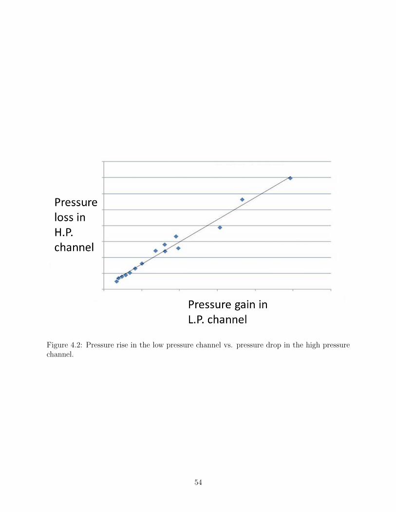
0 0.1 0.2 0.3 0.4 0.5 0.6 0.71

2

3

4

5

6

Enthalpy loss in high pressure channel

Pre

ssur

e ga

in

in lo

w p

ress

ure

chan

nel

One−seventh, 5000 RPMOne−seventh, 10000 RPMOne−seventh, , 20000 RPMOne−sixth, 5000 RPMOne−sixth, 10000 RPMOne−sixth, 20000 RPMOne−fifth, 5000 RPMOne−fifth, , 10000 RPMOne−fifth, 20000 RPMTwo−fifth, 5000 RPMTwo−fifth, 10000 RPMTwo−fifth, 20000 RPMThree−fifth, 5000 RPMThree−fifth, 10000 RPMThree−fifth, 20000 RPM

Figure 4.17: Comparison of pressure gain in low pressure channel against enthalpy loss inhigh pressure channel for different widths of re-injection passage.

5000 10000 15000 200001

2

3

4

5

6

RPM

Pre

ssur

e ga

in in

low

−pr

essu

re c

hann

el

One seventhOne sixthOne fifthTwo fifthThree fifth

Figure 4.18: Comparison of pressure gain in low pressure channel against mass loss in highpressure channel for different widths of re-injection tube.

72

Figure 4.19: Mach number of flow field as the reinjection passage meets the low pressurechannel

For the re-injection passage width which is three-fifth of the combustion channel width,

a pre-compression pressure gain of 1.6(at 20000 RPM) to 4.9 (at 5000 RPM)can be obtained

by making the high and low pressure channels traverse in and out of alignment with a re-

injection passage. The pre-compression pressure gain is related to re-injection pressure ratio

(PRreinject) of Equation 4.6 , by the following relation.

PRreinject = PA/P2

73

Pre− compression pressure gain = (PA − P2)/P2 = PRreinject − 1

where P2 is pressure in the low-pressure channel before pre-compression, and PA is the

pressure in low-pressure channel after pre-compression

Hence for this particular re-injection passage width, re-injection pressure ratios of 2.6 to

5.9 can be obtained, which corresponds to thermal efficiencies of 68% to 42% (Figure 4.4)

neglecting any pre-compression by the hammer shock. The power extraction from the WDE

is maximized at higher rotational speeds and hence 20000 RPM is a more desirable operating

point to the WDE than 5000 RPM. It can be seen in figure 4.4 , that pre-compression pressure

ratios of 1.5 - 2.5 produce the maximum thermal efficiency which is attainable by using a

re-injection passage width of 3/5th of the combustion channel and operating at 20,000 RPM.

4.3.3 Complete cycle analysis(preliminary model prediction vali-

dation)

As a method to validate the previous simplified numerical simulations, in the absence of

experimental data, a complete WDE with 20 combustion channels were simulated with a re-

injection system as shown in Figure 4.20 . The location and sizes of the ports shown in here

were chosen according to gas dynamic phenomena explained in Section 1B, although they

are not experimentally validated. A re-injection passage of width three-fifth of the channel

width and an angular velocity of 20,000 RPM was used for this 360 simulation, based on

the findings of preliminary analysis 2. At these conditions a pre-compression pressure gain

of 2.5 was obtained with only 20% pressure loss in the high-pressure channel (Table 4.1 ),

74

based on the preliminary analysis. Correspondingly, the thermal efficiency increases to 68%

(from 65% at no pre-compression) for a shock pre-compression of 1.0. The angular velocity

was chosen as 20,000 RPM because the unsteady effects of hammer shock formation and

expansion waves are most significant at higher RPMs. Pressure gain in the low pressure

channel and the pressure loss in the high pressure channel were found to be independent of

reinjection passage widths less than one-fifth of the width of the combustion channels as was

found in the preliminary analyses. A stoichiometric mixture of ethane and air is supplied

to the inlet of the WDE, at a pressure of 1.1 bar. The combustible mixture is ignited by a

spark plug which supplies an instantaneous temperature of 3000 K to a small circular region

of radius 1 mm within each channel after it is pre-compressed by exhaust gas re-injection.

4.3.3.1 Mixture ignited with spark

The simulation was run for 6 complete revolutions of the WDE. Every combustion channel

was ignited after it was pre-compressed by re-injection of exhaust gas. Figure 4.20 shows

the pressure contours after 6 revolutions. The initial pressure of 11 bars assumed in the

preliminary analysis seems too high for the high-pressure side. After 4 revolutions, the

pressure in all channels after combustion has reached a steady value of 4.5 bars (figure

4.20). The pressure just before the exhaust(after the re-injection process) was 3 bar. The

intake and exhaust ports were sized and positioned to purge the burnt exhaust gas completely

from the exit port and to fill each channel completely with the combustible mixture from the

intake without any spillage from the exit (figure 4.22). The combustible mixture is introduced

into the channel at the optimum time which allows the mixture to reach the opposite end of

the channel while avoiding any spillage through the exhaust port. The re-injected gas, which

was at a high enough temperature (figure 4.21), ignited the mixture in addition to the spark

75

plug. Hence the re-injection passage was seen to act as an ignition source as well. Ignition

by a jet of hot combustion products has been found to be a viable source of ignition for other

types of wave combustors ( [10], [12]). This type of ignition method has been found aiding

in igniting very lean combustible mixtures which are generally not ignitable using a spark

plug. This is attractive in the current WDE situation where a certain level of combustible

mixture dilution takes place during pre-compression. However, the ignition of the mixture

by the re-injection port should take place after the gas has been pre-compressed by it, to

achieve the enhanced thermal efficiency. The gases were seen to get pre-compressed, before

they are ignited (figure 4.25) as desired.

Figure 4.20: Pressure contours for complete cycle analysis after 6 revolutions.

76

Figure 4.21: Temperature contours for complete cycle analysis after 6 revolutions.

Figure 4.22: Ethane mass fraction contours for complete cycle analysis after 6 revolutions.

77

4.3.3.2 Removing the ignitors

After the 6th revolution, the spark plug which was modeled using a high instantaneous

temperature of 3000 K is removed. It was observed that the combustion was self sustaining

and all the charge was getting burned, as can be seen in Figure 4.27. The ignition was

initiated via the hot gas re-injection passage. The pressure reached in the engine was still as

high at 4.5 bars, as seen in Figure 4.23 . The combustion channel pressure was monitored

closely during the re-injection process to see if the gas was getting pre-compressed prior to

its ignition. The pressure contours shown in Figure 4.23 provide necessary verification that

the combustible mixture was in fact getting pre-compressed prior to ignition.

Figure 4.23: Pressure contours for complete cycle analysis after removing ignitors.

78

Figure 4.24: Temperature contours for complete cycle analysis after removing ignitors.

4.3.3.3 Comparison with preliminary analyses

The main departure from the complete cycle analysis shown above from the preliminary

analyses is in the pressure chosen for the high pressure combustion channel before the rein-

jection process. The preliminary analyses were initialized with a pressure of 11 bars at the

high pressure side, while the full cycle simulations show that a pressure of around 4.5 bars

was resulted after combustion in the high pressure channels. In order to directly compare

the two methods, preliminary analysis 2 was repeated with initial conditions which are more

representative of the flow conditions prevailing in the full cycle analysis. Due to the fact that

the pressure rise in the low pressure channels of the full cycle simulation is affected by both

79

Figure 4.25: Pressure (right) and fuel mass fraction (left) contours which show that themixture is pre-compressed before ignition. At the time instance shown, the reaction frontstarts forming at 1 channel width into the channel, while the pressure wave has traveled 3channel widths.

combustion and re-injection, combustion was also modeled in the new preliminary analysis

2 simulations. Figure 4.26 shows pressure contours after the reinjection process is complete.

The second low pressure channel has an average pressure of 3.21 bars after the reinjection

process. This value was 3.85 bars in the full cycle simulation. The difference of 17% is quite

acceptable considering the simplifications done in the preliminary analysis 2, compared to

the full cycle simulation.

80

Figure 4.26: Pressure contours for a fresh analysis with two channels on either side ofreinjection passage.

81

Figure 4.27: Ethane mass fraction contours for complete cycle analysis after removing igni-tors.

The low efficiency recorded here is one of the major challenges to the suitability of a

device like this. If we have complete combustion, as we strive to do through the calculations

presented in Chapter 3, we at least numerically have high pressure and high temperature

gas which can impart mechanical energy to a shaft. The low efficiency is because only a

small part of the internal energy of the exhaust gas is being extracted by expansion through

the channels of the rotor. Figure 4.24 shows that even the exhaust is at a temperature of

around 2000 K. In figure 4.28, we can see that the expelled gas also has a velocity of around

82

900 m/s. It is necessary to examine ways to harness the energy of this high temperature and

high velocity stream.

Figure 4.28: Velocity vectors for complete cycle analysis after 6 revolutions.

4.4 Combining re-injection and external turbine ex-

traction

The previous section shows that re-injection of combusted gas is useful tool for pre-compression

and ignition. The hot gas generated after the combustion process is however not completely

83

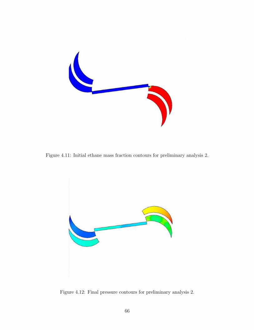
expanded in the rotor channels. A separate set of simulations was done to investigate the

benefits of adding an external row of turbine blades to a Wave Disk Engine system that has

been equipped with a re-injection passage. Figures 4.29 -4.31 show the pressure, ethane mass

fraction and temperature contours inside the system. There are some other minor modifica-

tions. The rotor channels with high aspect ratio and constant cross section are used to be

more conducive to shock formation. Re-injected gas is extracted from the inner side of an

H.P. channel and supplied at the outer side of an L.P. channel. This is done to further reduce

mixing of the fresh combustible mixture and the reinjected stream. The power extracted

in this case turns out to be 8.27kW and the efficiency is 5.5%. The temperature contours

show that even with the external row of blades, the exhaust gas is not fully expanded. This

indicates the need for several turbine stages, but that would make the Wave Disk Engine

lose its compactness.

Figure 4.29: Pressure contours for a Wave Disc Engine with a re-injection passage andexternal turbine blades.

84

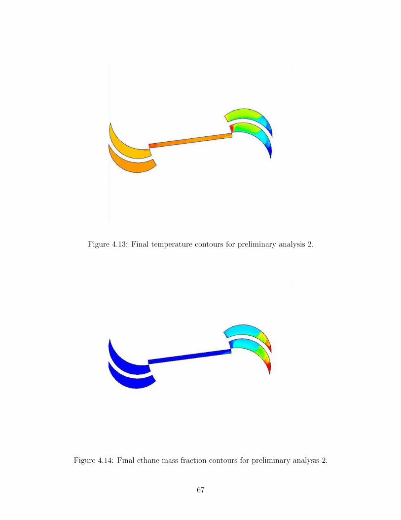
Figure 4.30: Ethane mass fraction contours for a Wave Disc Engine with a re-injectionpassage and external turbine blades

Figure 4.31: Temperature contours for a Wave Disc Engine with a re-injection passage andexternal turbine blades

85

4.5 Wave Disk Engine with external combustion cham-

ber

The Wave Disc Engines that have been manufactured so far employ a design in which the

compression, combustion and expansion of fuel and air is achieved within the wave disc

itself. Originally, the wave disc was envisioned as a compressor which could compress a

fuel-air mixture by inducing shock waves within its channels. It is important to also try to

combust this mixture outside the wave disc channels, to see if we can generate more power.

The original WDE proposal included wave disc engines made from ceramic materials. It was

believed that a WDE design with external combustion would be very suitable for ceramic

materials because combustion chambers made from ceramic materials are commonplace.

Extremely high temperatures can be reached without much distortion of the parts. A lot

of the ideas for this design were provided by Dr. Janusz Piechna, Warsaw University of

Technology, Warsaw, Poland.

4.5.1 Numerical simulations

CFD simulations were performed on a two-layered design, with one layer only serving as a

combustion chamber and the other layer being a rotor which is used primarily for compression

and expansion. Figures 4.32 - 4.34 show the pressure, temperature and fuel distribution

within this design after 15 revolutions. The rotor turned at an angular velocity of 20,000

RPM and the ignition was through a line given a high temperature (3000K) within the

combustion chamber. This would imitate a high temperature coil within the combustion

chamber. Fresh mixture undergoes a compression process by a hammer shock and is supplied

to the combustion chamber where it combusts and reaches a high pressure. This high pressure

86

gas again squeezes out of the channels through a converging-diverging nozzle. The velocity

at the outlet is shown in detail in Figure 4.35.

Figure 4.32: Pressure contours for a Wave Disc Engine with external combustion.

In these simulations, the rotor continuously rotates at 20, 000RPM . The torque acting

on the rotor goes from negative to positive when the engine starts generating power. This is

because the the combusted gas from the combustion chamber takes time to reach the rotor

and expand. The power rises steadily and becomes constant after 10 rotations. The mean

power after 5 rotations is 26.3kW . Over the 15th revolution the mean power is 39.26kW .

There are however, a few qualifying factors to consider here. The inlet pressure is very high.

It is 2 bars more than atmospheric. The pressure reached inside the device is still a lot more

87

Figure 4.33: Temperature contours for a Wave Disc Engine with external combustion (K).

than this. It varies from 7−9 bars inside the combustion chamber. Because the inlet and one

of the outlets are facing each other, and the inlet pressure is high, most of the combustible

mixture goes out of this outlet without burning. Because of the amount of fuel flowing out,

the efficiency was extremely low.

4.5.2 Ceramic Wave Disc Engine manufacturing

Some steps were taken towards manufacturing a Wave Disc Engine using ceramics with a two-

layered design and external combustion. Figure 4.36 shows a three-dimensional model based

on the two-dimensional CFD simulations discussed in the previous section. Fully-stabilized

88

Figure 4.34: Methane mass fraction contours for a Wave Disc Engine with external combus-tion.

zirconia was chosen as the ceramic powder which would be compacted and sintered. Figures

4.37 and 4.38 show the die connected to a press and the ceramic powder in the die. The

die was prepared with allowance for dimensional changes while sintering. The compaction

experiments were not very successful. It proved very difficult to compress the ceramic powder,

without the die distorting or the powder escaping from some orifice. Generally, compaction

molding of ceramics is done for smaller sizes than our purpose, and we need a better mold

design to make parts for the Wave Disc Engine. The investment required was deemed too

large before a satisfactory numerical model could be arrived at.

89

Figure 4.35: Velocity vectors at the outlet for a Wave Disk Engine with external combustion.

Figure 4.36: Three dimensional model of Wave Disk Engine with external combustion.

90

Figure 4.37: Die prepared for manufacturing ceramic Wave Disc Engine.

Figure 4.38: Die prepared for manufacturing ceramic Wave Disc Engine with zirconia powder.

91

Chapter 5

Thermodynamic cycle of the Wave

Disk Engine

The Wave Disk Engine is expected to follow the Humphrey thermodynamic cycle to achieve

its maximum potential. This cycle includes the following steps - isentropic compression,

constant volume combustion, isentropic work extraction, and constant pressure heat release.

This is indeed an ideal cycle and losses due to friction and irreversibility will never let the

WDE attain the ideal Humphrey cycle, in the same as no gasoline engine attains the ideal

Otto cycle. We can however use a knowledge of the thermodynamic cycle followed by the

WDE in order to identify the processes during which losses can be avoided.

Sun ([13]) has analytically studied the thermodynamic cycle followed by the WDE. Figure

5.1 shows the ideal WDE cycle described by him.

Sun ([13]) further used a 1-D numerical code to track one particle and draw thermody-

namic cycle diagrams. In the tracking process, the location of the fluid particle at a future

time step was calculated based on the location at its current time step and its current ve-

locity, and the values of its properties at various time step are recorded.The diagrams were

drawn by sequencing the property values in time. Figures 5.2 and 5.3 show the T-s and p-v

diagrams for a single fluid particle.

These diagrams are still close to ideal because they are based on a 1-D study where the

92

Figure 5.1: Ideal T-s diagram for a WDE([13]).

various steps in the WDE cycle are allowed to finish completely. However, in 2-D CFD

simulations, many processes such as combustion and extraction are not always completed

and a look at the cycle followed in a 2-D simulation gives us a look at where the various

cycle inefficiencies lie.

5.1 Discrete Phase Model

The Lagrangian discrete phase model in ANSYS FLUENT follows the Euler-Lagrange ap-

proach. The fluid phase is treated as a continuum by solving the Navier-Stokes equations,

while the dispersed phase is solved by tracking a large number of particles, bubbles, or

droplets through the calculated flow field. The dispersed phase can exchange momentum,

mass, and energy with the fluid phase. This model was used to implement a particle tracking

study for the WDE.

93

Figure 5.2: T-s diagram for a WDE traced by G. Sun([13]).

Several particles of an inert substance(nitrogen) of a diameter of 10−6m were introduced

into the flow field. They represent the dispersed Langrangian phase. The mixture of fuel

and air before and after combustion represents the Eulerian phase which is treated as a con-

tinuum. The reaction, pressure exchange, and enthalpy exchange in the continuum phase is

unaffected by the presence of the nitrogen particles. The particles meanwhile get transported

by the surrounding continuum fluid and track the physical properties of the nearby fluid.

This provides a means of tracking a thermodynamic cycle followed by the working fluid in a

Wave Disk Engine.

94

Figure 5.3: p-v diagram for a WDE traced by G. Sun([13]).

5.2 Particles introduced into Wave Disc Engine with a

reinjection tube

The WDE simulations with a reinjection tube were very promising in terms of power extrac-

tion and efficiency, and are hence considered a good test case where we might be closer to

a desired thermodynamic cycle. Ten particles were introduced near the inlet and observed

over two complete rotations of the rotor. Figures 5.4 and 5.5 show the particles at different

stages of the cycle colored by temperature.

T-s and p-v diagrams can be drawn from these simulations as shown below. Figures 5.6

and 5.7 show T-s and p-v diagrams respectively for all 10 particles on the same plot. It is

evident that there is a very wide variation in the cycle followed by each particle. An average

on the basis of all 10 particles gives us a better perspective in figures 5.8 and 5.9.

95

Figure 5.4: 10 particles introduced into a WDE equipped with a reinjection tube.

It is clear that the cycle followed by every particle is different but distinct compression,

combustion, and extraction phases can be seen. Figure (5.10) shows the average pressure

attained by the different particles at various troughs and crests of the plot. The pressure

rises from 1.24 bars to 4.67 bars after compression, pre-compression by reinjection, and

combustion. The particles, however, leave the WDE at an average pressure of 2.6 bars.

Thus, the biggest hurdle in reaching an ideal Humphrey cycle is the poor extraction. The

extraction stage is clearly very close to isentropic.

96

Figure 5.5: Location of particles at a later stage in a WDE equipped with a reinjection tube.

5.3 Particles introduced into Wave Disc Engine at tested

conditions

The WDE configuration tested most often at Michigan State University’s Turbomachinery

laboratory has given us complete combustion but low efficiency at a low RPM. A set of simu-

lations were performed to see where the inefficiencies may lie. Ten particles were introduced

near the inlet and observed over two complete rotations of the rotor. Figures 5.11 and 5.12

Figures T-s and p-v diagrams can be drawn from these simulations as shown below. Figure

5.13 and 5.14 shows T-s and p-v diagrams respectively for all 10 particles on the same plot.

A wide variation in cycles is also evident here.

97

0 1000 2000 30000

1000

2000

3000

Specific Entropy (J/kg.K)

Tem

pera

ture

(K

)

particle 1particle 2particle 3particle 4particle 5particle 6particle 7particle 8particle 9particle 10

Figure 5.6: Superimposed T-s diagram for 10 particles introduced into a WDE with a rein-jection tube.

5.4 Discussion

In both of the WDE configurations shown in this chapter, expansion of the combusted gas

mixture has not been complete so far. The fact that only a portion of the enthalpy of the

combusted mixture is used, limits the efficiency. This re-emphasizes the point mentioned in

Chapter 4 about the benefit of having several turbine stages. The ideal Humphrey/Atkinson

cycle expected in the WDE cycle is distorted by pressure waves inside the channels. There

are several small compression and expansion processes which form a part of the four major

processes in the cycle. This should not be considered a drawback in itself.

98

0 2 4 6 80

2

4

6x 105

Specific volume (m3/kg)

Pre

ssur

e (P

a)

particle 1particle 2particle 3particle 4particle 5particle 6particle 7particle 8particle 9particle 10

Figure 5.7: Superimposed p-v diagram for 10 particles introduced into a WDE with a rein-jection tube

−1000 0 1000 2000 30000

1000

2000

3000

Entropy(J/kg.K)

Tem

pera

ture

(K)

Figure 5.8: Average T-s diagram for 10 particles introduced into a WDE with a reinjectiontube.

99

0.5 1 1.5 2 2.5 3 3.50

2

4

6x 105

Specific volume(m3/kg)

Pre

ssur

e(P

a)

Figure 5.9: Average p-v diagram for the 10 particles introduced into a WDE with a reinjec-tion tube.

−1000 0 1000 2000 30000

1000

2000

3000

Entropy(J/kg.K)

Tem

pera

ture

(K)

1.24 bars

4.32 bars

4.67 bars

2.6 bars

Figure 5.10: Average T-s diagram for the 10 particles introduced into a WDE with a rein-jection tube (average pressure labeled).

100

Figure 5.11: 10 particles introduced into the tested WDE near the inlet.

Figure 5.12: Location of previously introduced particles into the tested WDE.

101

0 1000 2000 3000 40000

1000

2000

3000

4000

Specific entropy (J/kg.K)

Tem

pera

ture

(K

)

particle 1particle 2particle 3particle 4particle 5particle 6particle 7particle 8particle 9particle 10

Figure 5.13: Superimposed T-s diagram for 10 particles introduced into the tested WDE.

0 2 4 6 8 100

1

2

3

4

5x 105

Specific volume (m3/kg)

Pre

ssur

e (P

a)

particle 1particle 2particle 3particle 4particle 5particle 6particle 7particle 8particle 9particle 10

Figure 5.14: Superimposed p-v diagram for 10 particles introduced into the tested WDE.

102

Chapter 6

Conclusions

This study outlines computational analysis and solutions to various challenges faced in the

design and testing of the Wave Disk Engine, a radial engine prototype utilizing compression

by pressure waves, constant volume combustion and isentropic work extraction in a small

rotating disk.

The first problem to be investigated was the nature of combustion of a fuel-air mixture

trapped in a rectangular chamber. Based on our numerical simulations, we can make some

remarks about the important phenomena involved in the combustion process. First, we are

able to identify the various distinct combustion regimes 1-4. Second, we have demonstrated

that the parameter which enables the combustion regimes to be clearly identified is the

mass consumption of fuel, which may or may not correspond to the nominal value of the

flame surface area. Events and processes which lead to an increase in flame area serve to

increase the mass consumption rate of fuel in the chamber although the correspondence has

been shown in Sec. 4.1 not to be one-to-one, since dYCH4/dt, which measures the mass

consumption rate, does not correlate exactly with the flame surface area (as measured by

total mass fraction of CH+). Between regimes 2 and 3, for example, the mass consumption

rate decreases by a factor of 4.21 while the surface area (measured by the CH+ mass fraction)

decreases by a factor of 6.6. The numerical correspondence is therefore 64%.

In this problem, the only way to increase the flame area is by distorting the flame front.

The distortion of the flame front is a result of vorticity that exists prior to ignition and

103

additional vorticity generation inside the channel by the flame front: the former is nearly an

order of magnitude larger than the latter. Vortices created inside the channel help in swirling

the interface between the burnt and unburnt gases and breaking the flame into several small

flame fragments. This, along with the vorticity produced by the initial flow through shear

layers, leads to the period of fastest burning in regimes 1, 2. As fuel is consumed, and the

flame structure (brush) becomes aware of the far wall CD and the distinctly finite volume

available for combustion, the flamelets recombine and a single flame front is formed. This

is the start of regime 3 of combustion in the channel. The vortices inside the channel settle

down (in regime 3) with time, and the mass consumption rate of fuel attains a nearly steady,

lower value. The mass consumption rate in this slower stage of burning (regime 3) is found

to be about 4 times slower than the initial combustion regimes 1 and 2.

Vorticity generation happens for three primary reasons. The first is before ignition and

occurs due to the opening and closing of end walls prior to through flow. As the fluid

moving at a high velocity (about 150 m/s) strikes a suddenly closed wall, it reflects and

large vortices are created. The shear layers at the channel side walls generate concentrated

vorticity, which we refer to herein as flow vorticity. The third way in which vorticity is

generated, after ignition, is by misaligned local pressure and velocity gradients at the flame

surface. The pressure gradient is longitudinal and fluctuates as pressure waves move back

and forth across the length of the channel with a period of approximately 3.3E − 4 s. The

density gradient points from the unburnt to the burnt fluid. Thus, the flame surface is subject

to baroclinic torques acting in different directions at various locations along the flame front

in the channel. This contribution to the total vorticity is referred to as flame vorticity.

When the flame becomes stable and assumes the form of a single front, the pressure

and density gradients are aligned, therefore the above mechanism for vorticity generation

104

is suppressed. The density gradient points from left to right. Pressure waves also travel

back and forth from left to right and, thus, barely any additional vorticity is generated after

the initial stochastic regime of combustion. Indeed, regime 3 is one of largely continual and

monotonic decay of overall vorticity.

There is one feature of the solution generated in this article that does not align with

previous studies of the “tulip” flame phenomenon, see Refs. [17]-[25]. In our numerical solu-

tions, even when the channel walls are completely closed for the entire numerical experiment

(Sec. 4.2), significant levels of vorticity are generated in the flow field and, in addition, the

flame never evolves into the classical tulip shape during the latter part of the burn. Since the

only difference between this analysis and the others is spark placement, we hypothesize that

the heat generated by the 1mm spark, whose center is located 2mm from the wall AB (see

Fig. 3.1), generates the initial flow that produces the C-shaped fronts which later morph

into the flame brush. Consequently, ignition is a crucially important process that can, and

does, alter the fundamental structure of the propagating flame.

In the channel it is clear that when there is a high level of mixing the rate of burning is

highest. By contrast, once the mixture has “settled” the rate of fuel consumption decreases to

approximately one-fourth of its maximum value in regime 2 (see Fig. 3.9). This diminishment

is found even when the two end walls are always closed and the mixture has no initial vorticity

generated by flow-through(see Fig. 3.25). This work confirms the long-known fact that in

order to burn fast the combustible mixture in the channel should be continually as well

mixed as possible. This work serves in part as an indication of what happens to the burning

rate when that initial level of mixedness is not maintained at its high value and instead

diminishes. If the mixture were to burn entirely at the initial rate, in which the first half of

the mixture burns at four times the rate of the second half, the overall combustion time would

105

decrease by 60%. We note also that the burning rate, though usually strongly dependent

upon mixing and vorticity, is not proportional to the latter. In fact, the relationship is not

one of proportionality even when the two quantities follow the same general trend because

they follow different functional forms. This was discussed in Sec. 4.1.5 and is illustrated in

Figs. 3.9 and 3.12.

It was demonstrated that the ignition energy is approximately 1 J whereas the total

energy released by combustion (∼ 0.4kJ) is 400 times larger. It is unlikely that the energetics

of ignition influences the subsequent course of the combustion event. As discussed above,

however, the placement of the ignition source is crucial for the flow that is generated in the

channel.

The next feature studied is reinjection of combusted gas into fresh combustible mixture

as a means of enhancing thermal efficiency of the WDE. The thermal efficiency was seen

to increase for re-injection pressure gains up to a value of 2, assuming complete expansion

of gas in the power generation turbine to atmospheric conditions and ideal component ef-

ficiencies. A series of flow simulations were performed to ascertain whether such beneficial

reinjection configurations were possible in a compact device. A simplified geometry with

only two combustion channels on either side of a reinjection passage was used to compare

reinjection pressure gain with mass, enthalpy and pressure loss of combusted gas at a reduced

computational cost. The potential to use simplified geometry simulations is highly advan-

tageous when trying to identify several geometry and angular velocity combinations where

reinjection can be used effectively to enhance thermal efficiency. It was found that there

are indeed practically viable combinations of re-injection passage widths and combustion

channel speeds where reinjection can lead to enhanced thermal efficiency. This procedure

was however highly dependent on initial conditions and limited full cycle simulations were

106

performed to get realistic initial conditions. It was found that with similar initial conditions,

the complete cycle and simplified simulations (with only two combustion channels on either

side of the re-injection passage) lead to very similar results. Reinjection also served as a

means to ignite fresh mixture. The exact dimensions of a reinjection passage which can

improve thermal efficiency of such wave engine devices are strongly dependent on a number

of factors including geometry, and completeness of combustion. There is thus a lot more

that can be done in this regard.

Incomplete extraction of power within the wave disk has been partially addressed by

a second row of turbine blades. A WDE with a reinjection passage as well as a second

row of turbine blades has given us the highest efficiency in simulation. There are a lot of

creative refinements possible which can help in extracting even more enthalpy out of the

combusted mixture. The problem of seizing of rotor and housing of the WDE was studied

and a two-layer design made of ceramic was considered a reasonable solution.

The thermodynamic cycle followed by the WDE was studied using a system of tracking

particles of an inert gas introduced into the WDE. The study revealed that the expansion

process of the WDE was only partially completed within the rotor.

107

BIBLIOGRAPHY

108

BIBLIOGRAPHY

[1] Piechna, J., and Dyntar, D., Two-dimensional Numerical Analysis of the Wave JetMicro-Engine Operation, Proc. PowerMEMS 2007, Freiburg, Germany, 2007.

[2] Piechna, J., and Dyntar, D., Numerical Investigation of the Wave Disk Micro-EngineConcept , International Journal of Gas Turbine, Propulsion and Power Systems, De-cember 2008, Volume 2, Number 1, 208.

[3] Piechna, J., Micro Ring-Engine Numerical Fluid Dynamics Analysis , Proc. Power-MEMS 2008, Sendai, Japan, 2008.

[4] Piechna, J., Akbari, P., Iancu, F., and Mueller, N., Radial-flow wave rotor concepts,unconventional designs and applications Proc. IMECE 2004, IMECE2004-59022 Ana-heim, California, 2004.

[5] Iancu, F., Piechna, J., Dempsey, E., Mueller, N., Ultra-Micro Wave Rotor Investiga-tions , Proc. PowerMEMS 2005, pp. 93-96, Nov. 28-30, Tokyo, Japan, 2005

[6] ANSYS, Inc., ANSYS FLUENT User’s Guide , Southpointe, 275 Technology DriveCanonsburg, PA 15317, Release 14.0, November 2011

[7] ANSYS, Inc., ANSYS FLUENT Theory Guide , Southpointe, 275 Technology DriveCanonsburg, PA 15317, Release 14.0, November 2011

[8] Weber, H. E., Shock Wave Engine Design , J. Wiley, New York, 1994

[9] Snyder,P.H, Alparslan, B., Nalim, M.R., Gas Dynamic Analysis of the Constant Vol-ume Combustor, A Novel Detonation Cycle, 38th AIAA/ASME/SAE/ASEE JointPropulsion Conference & Exhibit, Indianapolis, IN, 2002.

[10] Matsutomi, Y., Meyer, S., Wijeyakulasuriya, S.D., Izzy, Z., Nalim, M.R., Shimo,M., Kowalkowski, M., and Snyder, P.H. Experimental Investigation on the WaveRotor Constant Volume Combustor, 46th AIAA/ASME/SAE/ASEE Joint PropulsionConference & Exhibit, Nashville, TN, 2010.

[11] Elharis, T.M., Wijeyakulasuriya, S.D., Nalim, M.R. Wave Rotor CombustorAerothermodynamic Design and Model Validation based on Initial Testing, 46th

109

AIAA/ASME/SAE/ASEE Joint Propulsion Conference & Exhibit, Nashville, TN,2010

[12] Wijeyakulasuriya, S. D., Transient and Translating Gas Jet Modeling for PressureGain Combustion Applications, Ph.D. Dissertation, School of Mechanical Engineer-ing, Purdue University, West Lafayette, IN, 2011.

[13] Sun, G., Numerical Study of the Aerodynamic Characteristics of a Wave Disc Engine,Ph.D. Dissertation, Department of Mechanical Engineering, Michigan State Univer-sity, East Lansing, IN, 2012.

[14] Perera, U. I., Wijeyakulasuriya, S. D., Nalim, M. R.,Hot Jet Ignition Delay Timeand Localization Analysis for Ethylene-Air, 49th AIAA Aerospace Sciences Meeting,Orlando, FL, 2011.

[15] Perera, U.I.,Experimental Investigation into Combustion Torch Jet Ignitionof Methane-Air, Ethylene-Air, and Propane-Air Mixtures,M.S.Thesis, IndianaUniversity-Purdue University Indianapolis, Indianapoils, IN, 2010.

[16] Ellis, O.C De C., Flame movement in gaseous explosive mixtures, Fuel in Science andPractice, (1928) pp. 502.

[17] Dunn-Rankin, D., Sawyer, R. F., Tulip flames: Changes in shapes of premixed flamespropagating in closed tubes, Experiments in Fluids, 24:130-140 (1998).

[18] Searby, G., Instability Phenomena during Flame Propagation, Combustion Phenom-ena, CRC Press (2009).

[19] Clanet, C. and Searby, G., On the “Tulip Flame Phenomenon, Combustion andFlame, Vol. 105, pp. 225-238 (1996).

[20] Kratzel, T., Pantow, E., and Fischer, M., On the transition from a highly turbulentcurved flame into a tulip flame, Int. J. Hydrogen Energy, Vol. 23, No. 1(1998), pp.45-51.

[21] Gonzalez, M., Borghi, R., and Saouab,A., Interaction of a Flame Front with Its Self-Generated Flow in an Enclosure: The ”Tulip Flame” Phenomenon, Combustion andFlame 88 (1992) pp. 201-220.

[22] McGreevy, J. L., Premixed Flame Propagation in Closed Tubes, Ph. D. thesis, North-western University, Evanston, IL (1993).

110

[23] Matalon, M., McGreevy, J. L., The initial development of a tulip flame,CombustionSymposium, (1994) pp. 1407-1413 .

[24] Hariharan, A., Wichman, I. S., and Mueller, N., Experimental study of premixedmethane-air flame propagation in a rectangular constant volume combustion chamber,Proceedings of the Combustion Institute - Central States Section Spring TechnicalMeeting, Dayton, OH, April 22-24, 2012.

[25] Hariharan, A., Wichman, I. S., and Mueller, N., Premixed flame propagation andmorphology in a constant volume rectangular combustion chamber, submitted to Com-bustion and Flame (2013).

[26] Kiran, R., Wichman, I. S., and Mueller, N., Numerical investigation of premixedflame propagation in a closed channel with a fluctuating pressure and velocity field,Proceedings of the Combustion Institute - Central States Section Spring TechnicalMeeting, Dayton, OH, April 22-24, 2012.

[27] Kiran, R., Wichman, I. S., and Mueller, N., On combustion in a closed rectangularchannel with initial vorticity, submitted to Combustion Theory and Modelling (2013).

[28] Markstein, G.H., A shock tube study of the flame front-pressure wave interaction, 6thInternational Symposium on Combustion (Reinhold, New York, 1957), pp. 387-398.

[29] Renard,P.-H., Thevenin, D., Rolon, J.C., and Candel, S. Dynamics of flame/vortexinteractions, Progress in Energy and Combustion Science 26 (2000), pp. 225-282.

[30] Picone, J. M., Oran, E. S., Boris, J. P. and Young, Jr.,T. R., Theory of vorticitygeneration by shock wave and flame interaction, Dynamics of Shock Waves, Explo-sions, and Detonations, edited by J. R. Bowen, N. Manson, A. K. Oppenheim, andR. I. Soloukhin, Progress in Astronautics and Aeronautics Vol. 94 (AIAA, New York,1985), Chap. IV, pp. 429-448.

[31] Batley,G.A., McIntosh, A.C., and Brindley, J. Baroclinic Distortion of LaminarFlames, Proceedings: Mathematical, Physical and Engineering Sciences, Vol. 452,No. 1945, (Feb.8, 1996), pp. 199-221, published by The Royal Society.

[32] Lee, S.T., and Tsai, C.H., Numerical Investigation of Steady Laminar Flame Propa-gation in a Circular Tube, Combustion and Flame 99 (1994) pp. 484-490.

[33] Ju, Y., Shimano, A., and Inoue, O., Vorticity Generation and Flame Distortion in-duced by Shock Flame Interaction, Twenty-Seventh Symposium (International) onCombustion/The Combustion Institute (1998), pp. 735-741.

111

[34] Kiran, R., Wijeyakulasuriya, S., Piechna, J., Mueller, N.,Thermodynamic cycle ef-ficiency enhancement in a Wave Disk Engine by re-injection of combusted gas forpre-compression, AIAA/ASME/SAE/ASEE Joint Propulsion Conference and Exhibit(Atlanta, Georgia, July 2012).

112