Numerical simulation of the stress field in California:implications for the stress perturbation by Big Bend

and Garlock Fault

Abstract: 2D finite element modelling is used to analyze the state of stress in and around the SanAndreas Fault System (SAFS) taking the whole area of California. In this study we focus on the stateof stress at the general seismogenic depth of 12 km, imposing elastic rheology. The purpose of the pres-ent study is to simulate the regional stress field and also to find the stress perturbation due to Big Bendand Garlock Fault. Although in nature there is lateral and vertical variation in rheology, our highly sim-plified domain properties have simulated results comparable with the observed data. Our imposedboundary condition (fixed North American plate, Pacific plate motion along N34W vector up tonorthern terminus of the San Andreas faults and N50E vector motion for the subducting Gorda plate)simulated the present day regional Hmax orientation and velocity vector. Simulated results show local

effect on the stress field and displacement vector by the Big Bend and is further enhanced by theGarlock Fault, which may have significant impact on fault slip, stress, and hence deformation in thesurrounding region.

Keywords: San Andreas Fault System (SAFS), 2D finite element modelling, Big Bend, Garlock Fault,σHmax, velocity vector.

Simulation Tectonics Laboratory, Faculty of Science, University of the Ryukyus, Okinawa, 903-0213, Japan.

*e-mail: matrikakoirala@gmail.com

M. P. KOIRALA* AND D. HAYASHI

Trabajos de Geología, Universidad de Oviedo, 30 : 350-360 (2010)

The San Andreas Fault System (SAFS), a complex sys-tem of faults that display predominantly large-scalestrike slip displacement, is part of an even more com-plex system of faults, isolated segments of the EastPacific Rise, and scraps of plates lying east of the EastPacific Rise that collectively separate the NorthAmerican plate from the Pacific plate (Wallace,1990). The SAFS is mainly a right-lateral strike slipfault. It has many other small faults, some are left-lat-eral, some are thrusts and some normal faults.Present-day plate kinematics of the Pacific and NorthAmerican plates reveals that the Pacific plate is mov-ing towards NW with respect to North Americanplate. The motion of the plate is approximately 3.4-6cm a-1 on a N34W vector approximately (Atwater,1970; Minster and Jordan, 1978; DeMets et al.,1994; Argus and Gordon, 2001; Savage et al., 2004;d’Alessio et al., 2005). At its north end, the San

Andreas Fault joins the Mendocino Fracture Zone ata high angle, and there the Gorda plate and Juan deFuca plate are being subducted under the NorthAmerican plate. The Juan de Fuca plate currentlysubducts under the North American plate with a gen-eralized vector motion of N50E (Swanson et al.,1989) and with a velocity of 3 cm a-1 (Noson et al.,1988). The Gorda plate subducts with a similar direc-tion, but at an average velocity of 1.8 cm a-1 (Woodand Kienle, 1990). Generally, it is said that the SAFSis a fault oblique to the compression direction.However, it is not so simple, if it is considered that inthe area very near to the main fault the state of stressis fault oblique compression and away from the faultthe state of stress is fault perpendicular compression(as shown by fold axes parallel to the fault strike). Italso depends on the depth where we are measuringthe maximum horizontal stress. In the present study,

we calculated the stress at the seismogenic crust (at 12km depth) of the whole California area and tried toanalyze the effect of the Big Bend and Garlock Faulton the stress field and displacement vector. For this,we use simple but powerful FE plain stress modelling.

The objectives of the present study are: 1) evaluate the stateof stress along and around the SAFS, California; 2) deci-pher the stress perturbations due to the big bend andGarlock Fault on the SAFS; and 3) unravel the deflectionin displacement vector by the Big Bend and Garlock Fault.

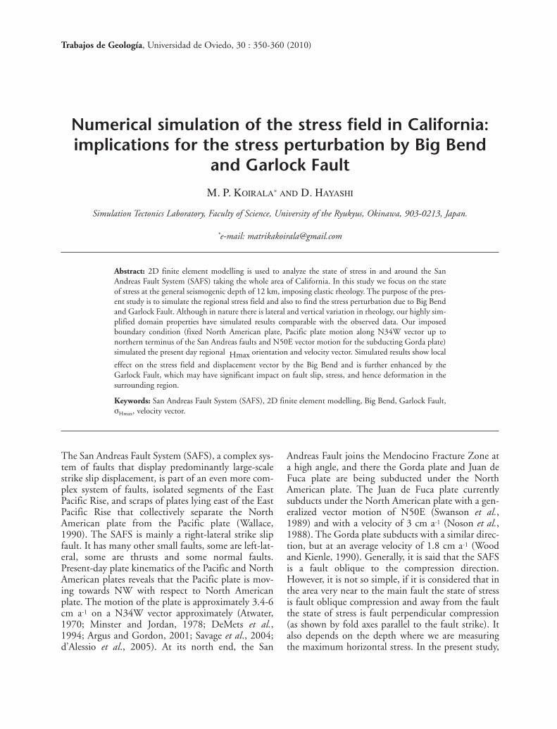
Figure 1. Simplified geological map of California (modified after Irwin, 1990 and references therein).

351STRESS FIELD PERTURBATIONS BY BIG BEND AND GARLOCK FAULT, CALIFORNIA

Elastic plane stress FE models are created to analyzethe state of the stress on the whole California region,especially along and around the SAFS (Hayashi,2008). Different domains are created in the modelthrough variation of the domain properties. The sim-plified geological map of California modified afterIrwin (1990) is taken as the base map (Fig. 1).

Model description

Models are created to analyze the state of stress alongand around the SAFS. The simplified geological mapof California (Fig. 1) is taken as the base map.

The FE software has been used in order to solve theelastic equations and for that we have to define thegeometry of the models and the correct boundaryconditions to apply to it. For the FEM calculation,the Young’s modulus (E), Poisson’s ratio (υ) and thedensity (ρ) are needed. The values selected are basedon the available published literature (Bird and Kong,1994; Cai and Wang, 2001; Chery et al., 2001; Lynch

and Richards, 2001; Malservisi et al., 2003; Parsons,2006; Flesch et al. 2007).

Elastic behaviour of crust is assumed for the modelledarea and this is justifiable since rheology changes fromelastic to viscous at depths greater than 16 km depthin the study area (Fuis and Mooney, 1990). Recentstudies of Becken et al. (2008) also show that the elas-tic (seismogenic) crust extends at least up to 12-15km depth. Realistic boundary conditions have beenapplied to match the present-day plate kinematics inthe Western North America and Pacific boundary.

Model geometry

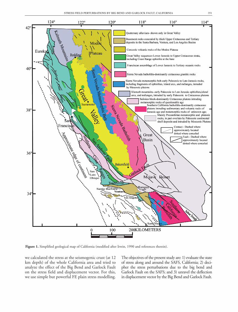
The model covers the entire California area and con-sists of 1638 triangular elements and 879 nodes inplane stress condition. There are three types of models:(A) a first model consisting in whole California as ahomogeneous one domain, (B) a second model withthree domains (Pacific plate, North American plateand San Andreas Fault Zone), and (C) a third model

Figure 2. Geometry and boundary condition of: (A) single domain model, (B) three domains model, and (C) four domains model.

352 M. P. KOIRALA AND D. HAYASHI

with four domains consisting of the Garlock Faultzone as fourth domain and the other three domainsbeing the same as in the second model. The Fault zoneboundary is made somewhat zigzag to mimic the actu-al fault geometry. Obviously, the width of the faultzone is slightly different at different places (Fig. 2).

Boundary condition

The boundary condition imposed represents the pres-ent-day plate kinematics of the Pacific plate, remnantsof the Farallon plate and North American plate in theWestern North America. In all models, the displace-ment boundary condition is given (Fig. 2). Thedomain west of the San Andreas Fault is considered aspart of the Pacific plate and east of San Andreas isconsidered as the North American plate. In themodel, the Pacific plate is driven by a displacementvector parallel to N34W vector and the NorthAmerican plate is fixed. Fault-oblique displacement isimposed progressively from 0 m to 250 m, 500 m and1000 m. In the northeastern portion of the model

after the San Andreas bends offshore to theMendocino fracture zone (Figs. 1 and 2), obliqueconvergence boundary condition is imposed, wherethe Gorda plate and further north the Juan de Fucaplate descend below the North American plate. As theconvergent rate of the Gorda plate and the Juan deFuca plate is less than that of the Pacific plate, only60% of the displacement rates imposed for the Pacificplate are applied to this boundary along the N50Evector. The northern part of the model is free to movein any direction (Fig. 2).

Rock domain properties

Rock domain properties, geometry, model dimen-sions and the imposed displacement strongly influ-ence the results of the numerical modelling. Selectionof the suitable rock properties for each domain is cru-cial. In this calculation, the model is highly simpli-fied, so that the properties of the upper crustal rocksare chosen for the calculation. The parameters takento constrain the rock domain properties are density,

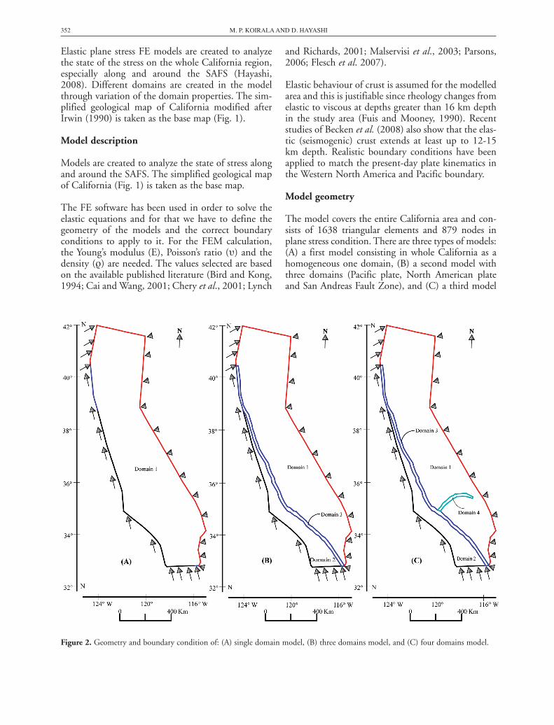
Figure 3. Stress distribution at 250 m displacement for models (A), (B), and (C) respectively; each pair of perpendicular lines repre-sents σHmax (long lines) and σHmin (short lines) in the stress field, and the red bar shows the tension.

353STRESS FIELD PERTURBATIONS BY BIG BEND AND GARLOCK FAULT, CALIFORNIA

Young’s modulus, and Poisson’s ratio. The parametersfor the rock domains are taken as follows. The Pacificplate and the North American plate are simulatedwith a Young’s modulus of 80 GPa, density of 2800kg m-3 and a Poisson ratio of 0.25. The fault zones aresimulated with a Young modulus of 1 GPa, density of2000 kg m-3 and Poisson ratio of 0.25. For all thedomains the depth is considered to be 12 km.

Modelling results

As discussed above, the simulation of California isbased on a simplified geological map. Three models arecreated as mentioned above and the general propertiesof the upper crustal layer are taken to constrain theelastic models. Progressive oblique displacement alongthe fault is imposed in all models as mentioned already.

Stress field

The stress field for the three models with increasingdisplacement is shown in figures 3, 4 and 5. Long linesare the maximum horizontal principal stress σHmax and

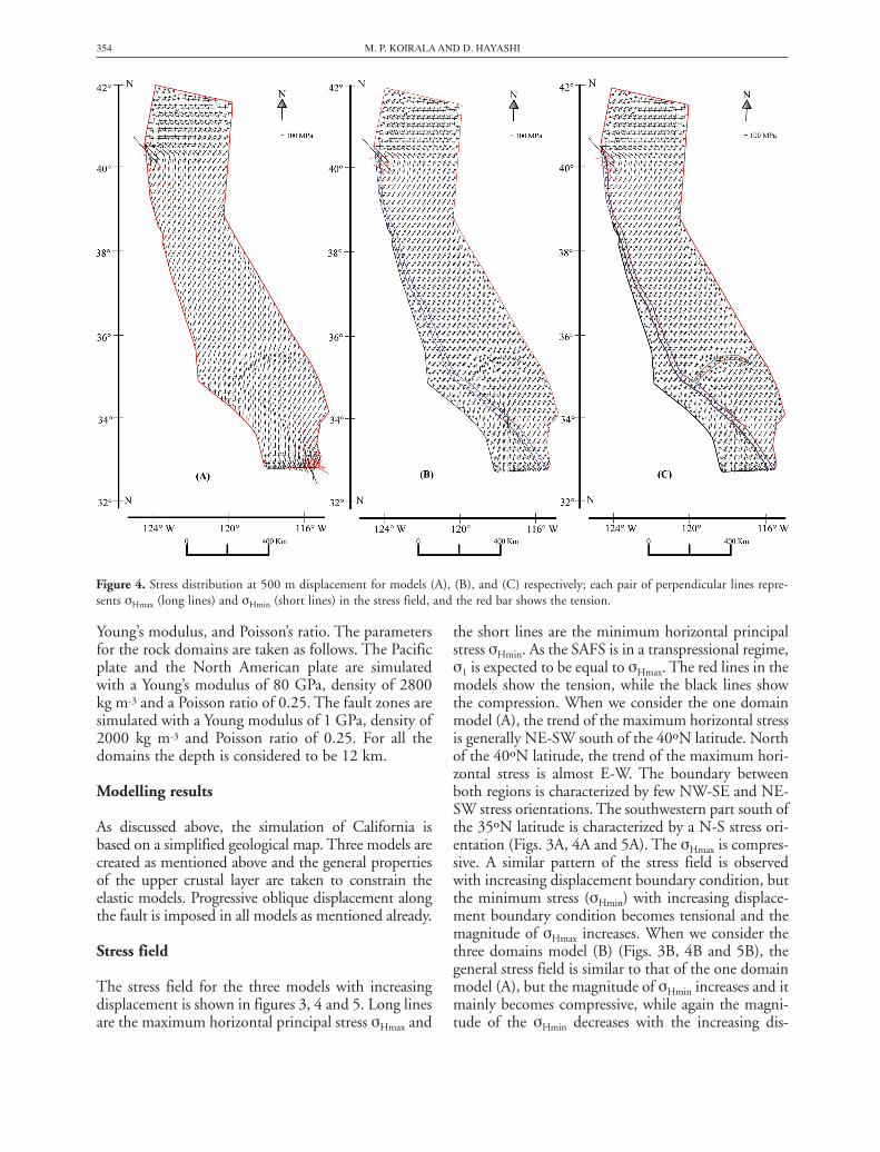
the short lines are the minimum horizontal principalstress σHmin. As the SAFS is in a transpressional regime,σ1 is expected to be equal to σHmax. The red lines in themodels show the tension, while the black lines showthe compression. When we consider the one domainmodel (A), the trend of the maximum horizontal stressis generally NE-SW south of the 40ºN latitude. Northof the 40ºN latitude, the trend of the maximum hori-zontal stress is almost E-W. The boundary betweenboth regions is characterized by few NW-SE and NE-SW stress orientations. The southwestern part south ofthe 35ºN latitude is characterized by a N-S stress ori-entation (Figs. 3A, 4A and 5A). The σHmax is compres-sive. A similar pattern of the stress field is observedwith increasing displacement boundary condition, butthe minimum stress (σHmin) with increasing displace-ment boundary condition becomes tensional and themagnitude of σHmax increases. When we consider thethree domains model (B) (Figs. 3B, 4B and 5B), thegeneral stress field is similar to that of the one domainmodel (A), but the magnitude of σHmin increases and itmainly becomes compressive, while again the magni-tude of the σHmin decreases with the increasing dis-

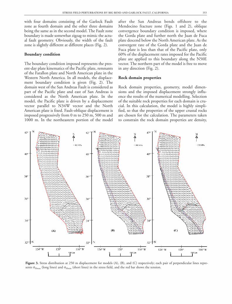
Figure 4. Stress distribution at 500 m displacement for models (A), (B), and (C) respectively; each pair of perpendicular lines repre-sents σHmax (long lines) and σHmin (short lines) in the stress field, and the red bar shows the tension.

354 M. P. KOIRALA AND D. HAYASHI

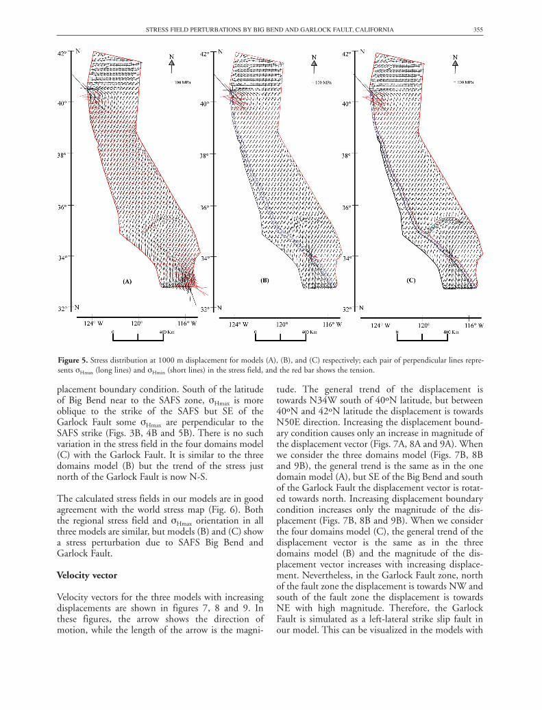
placement boundary condition. South of the latitudeof Big Bend near to the SAFS zone, σHmax is moreoblique to the strike of the SAFS but SE of theGarlock Fault some σHmax are perpendicular to theSAFS strike (Figs. 3B, 4B and 5B). There is no suchvariation in the stress field in the four domains model(C) with the Garlock Fault. It is similar to the threedomains model (B) but the trend of the stress justnorth of the Garlock Fault is now N-S.

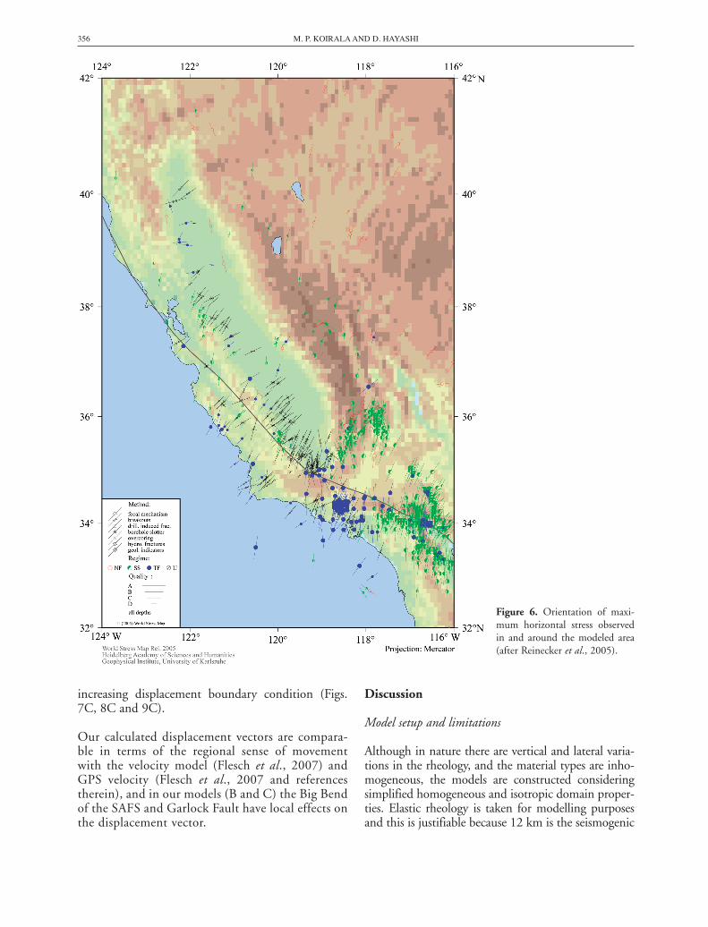
The calculated stress fields in our models are in goodagreement with the world stress map (Fig. 6). Boththe regional stress field and σHmax orientation in allthree models are similar, but models (B) and (C) showa stress perturbation due to SAFS Big Bend andGarlock Fault.

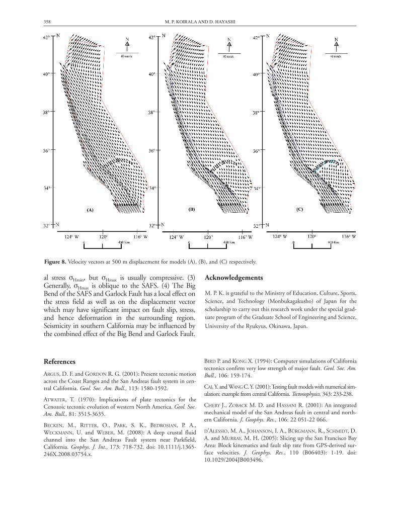
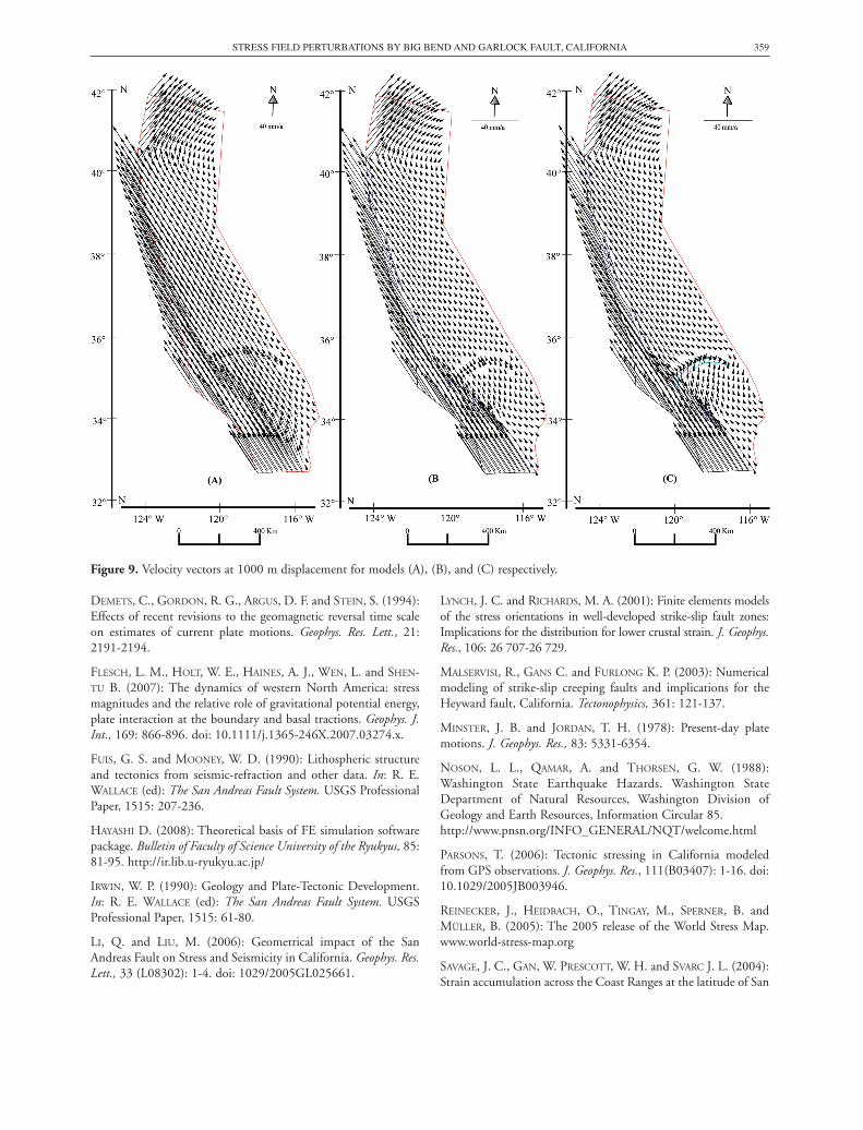
Velocity vector

Velocity vectors for the three models with increasingdisplacements are shown in figures 7, 8 and 9. Inthese figures, the arrow shows the direction ofmotion, while the length of the arrow is the magni-

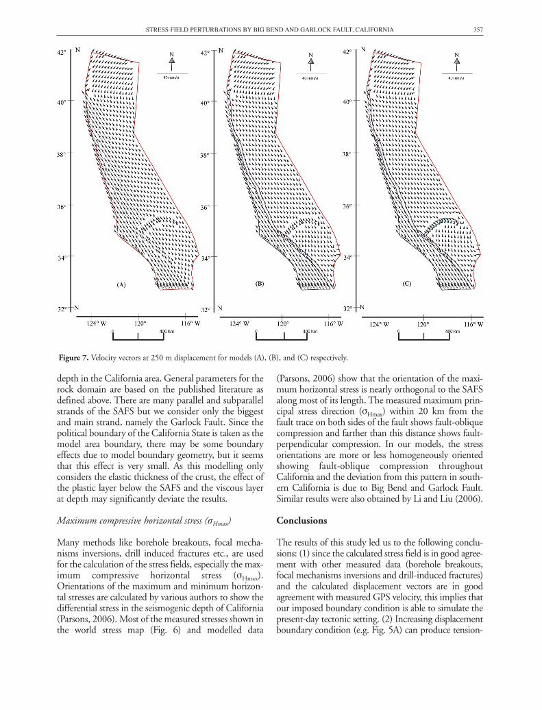
tude. The general trend of the displacement istowards N34W south of 40ºN latitude, but between40ºN and 42ºN latitude the displacement is towardsN50E direction. Increasing the displacement bound-ary condition causes only an increase in magnitude ofthe displacement vector (Figs. 7A, 8A and 9A). Whenwe consider the three domains model (Figs. 7B, 8Band 9B), the general trend is the same as in the onedomain model (A), but SE of the Big Bend and southof the Garlock Fault the displacement vector is rotat-ed towards north. Increasing displacement boundarycondition increases only the magnitude of the dis-placement (Figs. 7B, 8B and 9B). When we considerthe four domains model (C), the general trend of thedisplacement vector is the same as in the threedomains model (B) and the magnitude of the dis-placement vector increases with increasing displace-ment. Nevertheless, in the Garlock Fault zone, northof the fault zone the displacement is towards NW andsouth of the fault zone the displacement is towardsNE with high magnitude. Therefore, the GarlockFault is simulated as a left-lateral strike slip fault inour model. This can be visualized in the models with

Figure 5. Stress distribution at 1000 m displacement for models (A), (B), and (C) respectively; each pair of perpendicular lines repre-sents σHmax (long lines) and σHmin (short lines) in the stress field, and the red bar shows the tension.

355STRESS FIELD PERTURBATIONS BY BIG BEND AND GARLOCK FAULT, CALIFORNIA

increasing displacement boundary condition (Figs.7C, 8C and 9C).

Our calculated displacement vectors are compara-ble in terms of the regional sense of movementwith the velocity model (Flesch et al., 2007) andGPS velocity (Flesch et al., 2007 and referencestherein), and in our models (B and C) the Big Bendof the SAFS and Garlock Fault have local effects onthe displacement vector.

Discussion

Model setup and limitations

Although in nature there are vertical and lateral varia-tions in the rheology, and the material types are inho-mogeneous, the models are constructed consideringsimplified homogeneous and isotropic domain proper-ties. Elastic rheology is taken for modelling purposesand this is justifiable because 12 km is the seismogenic

Figure 6. Orientation of maxi-mum horizontal stress observedin and around the modeled area(after Reinecker et al., 2005).

356 M. P. KOIRALA AND D. HAYASHI

depth in the California area. General parameters for therock domain are based on the published literature asdefined above. There are many parallel and subparallelstrands of the SAFS but we consider only the biggestand main strand, namely the Garlock Fault. Since thepolitical boundary of the California State is taken as themodel area boundary, there may be some boundaryeffects due to model boundary geometry, but it seemsthat this effect is very small. As this modelling onlyconsiders the elastic thickness of the crust, the effect ofthe plastic layer below the SAFS and the viscous layerat depth may significantly deviate the results.

Maximum compressive horizontal stress (σHmax)

Many methods like borehole breakouts, focal mecha-nisms inversions, drill induced fractures etc., are usedfor the calculation of the stress fields, especially the max-imum compressive horizontal stress (σHmax).Orientations of the maximum and minimum horizon-tal stresses are calculated by various authors to show thedifferential stress in the seismogenic depth of California(Parsons, 2006). Most of the measured stresses shown inthe world stress map (Fig. 6) and modelled data

(Parsons, 2006) show that the orientation of the maxi-mum horizontal stress is nearly orthogonal to the SAFSalong most of its length. The measured maximum prin-cipal stress direction (σHmax) within 20 km from thefault trace on both sides of the fault shows fault-obliquecompression and farther than this distance shows fault-perpendicular compression. In our models, the stressorientations are more or less homogeneously orientedshowing fault-oblique compression throughoutCalifornia and the deviation from this pattern in south-ern California is due to Big Bend and Garlock Fault.Similar results were also obtained by Li and Liu (2006).

Conclusions

The results of this study led us to the following conclu-sions: (1) since the calculated stress field is in good agree-ment with other measured data (borehole breakouts,focal mechanisms inversions and drill-induced fractures)and the calculated displacement vectors are in goodagreement with measured GPS velocity, this implies thatour imposed boundary condition is able to simulate thepresent-day tectonic setting. (2) Increasing displacementboundary condition (e.g. Fig. 5A) can produce tension-

Figure 7. Velocity vectors at 250 m displacement for models (A), (B), and (C) respectively.

357STRESS FIELD PERTURBATIONS BY BIG BEND AND GARLOCK FAULT, CALIFORNIA

al stress σHmin, but σHmax is usually compressive. (3)Generally, σHmax is oblique to the SAFS. (4) The BigBend of the SAFS and Garlock Fault has a local effect onthe stress field as well as on the displacement vectorwhich may have significant impact on fault slip, stress,and hence deformation in the surrounding region.Seismicity in southern California may be influenced bythe combined effect of the Big Bend and Garlock Fault.

Acknowledgements

M. P. K. is grateful to the Ministry of Education, Culture, Sports,Science, and Technology (Monbukagakusho) of Japan for thescholarship to carry out this research work under the special grad-uate program of the Graduate School of Engineering and Science,

University of the Ryukyus, Okinawa, Japan.

Figure 8. Velocity vectors at 500 m displacement for models (A), (B), and (C) respectively.

References

ARGUS, D. F. and GORDON R. G. (2001): Present tectonic motionacross the Coast Ranges and the San Andreas fault system in cen-tral California. Geol. Soc. Am. Bull., 113: 1580-1592.

ATWATER, T. (1970): Implications of plate tectonics for theCenozoic tectonic evolution of western North America. Geol. Soc.Am. Bull., 81: 3513-3635.

BECKEN, M., RITTER, O., PARK, S. K., BEDROSIAN, P. A.,WECKMANN, U. and WEBER, M. (2008): A deep crustal fluidchannel into the San Andreas Fault system near Parkfield,California. Geophys. J. Int., 173: 718-732. doi: 10.1111/j.1365-246X.2008.03754.x.

BIRD P. and KONG X. (1994): Computer simulations of Californiatectonics confirm very low strength of major fault. Geol. Soc. Am.Bull., 106: 159-174.

CAI, Y. and WANG C. Y. (2001): Testing fault models with numerical sim-ulation: example from central California. Tectonophysics, 343: 233-238.

CHERY J., ZOBACK M. D. and HASSANI R. (2001): An integratedmechanical model of the San Andreas fault in central and north-ern California. J. Geophys. Res., 106: 22 051-22 066.

D’ALESSIO, M. A., JOHANSON, I. A., BÜRGMANN, R., SCHMIDT, D.A. and MURRAY, M. H. (2005): Slicing up the San Francisco BayArea: Block kinematics and fault slip rate from GPS-derived sur-face velocities. J. Geophys. Res., 110 (B06403): 1-19. doi:10.1029/2004JB003496.

358 M. P. KOIRALA AND D. HAYASHI

DEMETS, C., GORDON, R. G., ARGUS, D. F. and STEIN, S. (1994):Effects of recent revisions to the geomagnetic reversal time scaleon estimates of current plate motions. Geophys. Res. Lett., 21:2191-2194.

FLESCH, L. M., HOLT, W. E., HAINES, A. J., WEN, L. and SHEN-TU B. (2007): The dynamics of western North America: stressmagnitudes and the relative role of gravitational potential energy,plate interaction at the boundary and basal tractions. Geophys. J.Int., 169: 866-896. doi: 10.1111/j.1365-246X.2007.03274.x.

FUIS, G. S. and MOONEY, W. D. (1990): Lithospheric structureand tectonics from seismic-refraction and other data. In: R. E.WALLACE (ed): The San Andreas Fault System. USGS ProfessionalPaper, 1515: 207-236.

HAYASHI D. (2008): Theoretical basis of FE simulation softwarepackage. Bulletin of Faculty of Science University of the Ryukyus, 85:81-95. http://ir.lib.u-ryukyu.ac.jp/

IRWIN, W. P. (1990): Geology and Plate-Tectonic Development.In: R. E. WALLACE (ed): The San Andreas Fault System. USGSProfessional Paper, 1515: 61-80.

LI, Q. and LIU, M. (2006): Geometrical impact of the SanAndreas Fault on Stress and Seismicity in California. Geophys. Res.Lett., 33 (L08302): 1-4. doi: 1029/2005GL025661.

LYNCH, J. C. and RICHARDS, M. A. (2001): Finite elements modelsof the stress orientations in well-developed strike-slip fault zones:Implications for the distribution for lower crustal strain. J. Geophys.Res., 106: 26 707-26 729.

MALSERVISI, R., GANS C. and FURLONG K. P. (2003): Numericalmodeling of strike-slip creeping faults and implications for theHeyward fault, California. Tectonophysics, 361: 121-137.

MINSTER, J. B. and JORDAN, T. H. (1978): Present-day platemotions. J. Geophys. Res., 83: 5331-6354.

NOSON, L. L., QAMAR, A. and THORSEN, G. W. (1988):Washington State Earthquake Hazards. Washington StateDepartment of Natural Resources, Washington Division ofGeology and Earth Resources, Information Circular 85.http://www.pnsn.org/INFO_GENERAL/NQT/welcome.html

PARSONS, T. (2006): Tectonic stressing in California modeledfrom GPS observations. J. Geophys. Res., 111(B03407): 1-16. doi:10.1029/2005JB003946.

REINECKER, J., HEIDBACH, O., TINGAY, M., SPERNER, B. andMÜLLER, B. (2005): The 2005 release of the World Stress Map.www.world-stress-map.org

SAVAGE, J. C., GAN, W. PRESCOTT, W. H. and SVARC J. L. (2004):Strain accumulation across the Coast Ranges at the latitude of San

Figure 9. Velocity vectors at 1000 m displacement for models (A), (B), and (C) respectively.

359STRESS FIELD PERTURBATIONS BY BIG BEND AND GARLOCK FAULT, CALIFORNIA

Francisco, 1994-2000. J. Geophys. Res., 109(B03413): 1-11. doi:10.1029/2003JB002612.

SWANSON D. A., CAMERON K. A., EVARTS R. C., PRINGLE P. T.and VANCE J. A. (1989): Cenozoic Volcanism in the CascadeRange and Columbia Plateau, Southern Washington, andNorthernmost Oregon. AGU Field Trip Guidebook,T106.http://vulcan.wr.usgs.gov/Volcanoes/PacificNW/AGUT106/hood.html#mounthood

WALLACE, R. E. (1990): General Features and GeomorphicExpression. In: R. E. WALLACE (ed): The San Andreas FaultSystem. USGS Professional Paper, 1515: 3-21.

WOOD, C. A. and KIENLE, J. (1990): Volcanoes of North America:U.S. and Canada. Cambridge University Press, 354 pp. ISBN

052143811X, 9780521438117.

M. P. KOIRALA AND D. HAYASHI360