Numerical simulation of passive-active cells with

microperforated plates or porous veils

A. Bermudez∗,a, P. Gamallob, L. Hervella-Nietoc, A. Prietoa,d

aDepartamento de Matematica Aplicada, Universidade de Santiago de Compostela, 15782

Santiago de Compostela, SpainbTecnologıas Avanzadas Inspiralia SL, 28034 Madrid, Spain

cDepartamento de Matematicas, Universidade da Coruna, 15071 A Coruna, SpaindApplied and Computational Mathematics, California Institute of Technology, MC 217-50,

1200 East California Blvd., CA 91125, United States

Abstract

The main goal of this work consists in the numerical simulation of a multichannel

passive-active noise control system based on devices involving a particular kind

of cells. Each cell consists of a parallelepipedic box with all their faces rigid,

except one of them, where a porous veil or a rigid micro-perforated plate (MPP)

is placed. Firstly, the frequency response of a single passive cell is computed,

when it is surrounded by an unbounded air domain (an anechoic room) and

harmonic excitations are imposed. For the numerical solution of this three-

dimensional problem, the original unbounded domain is truncated by using

exact Perfectly Matched Layers (PML) and the resulting partial differential

equation (PDE) is discretized with a standard finite element method. Secondly,

the passive cells are transformed into active by assuming that the opposite face

to the passive one may vibrate like a piston in order to reduce noise. The

corresponding multichannel active control problem is stated and analyzed in

the framework of the optimal control theory. A numerical method is proposed

to assess and compare different control configurations.

Key words: Active control of sound, Microperforated plate, Porous veil,

∗Corresponding author.Email addresses: alfredo.bermud@usc.es (A. Bermudez), pablo.gamallo@itav.es (P.

Gamallo), luis.hervella@udc.es (L. Hervella-Nieto), andres.prieto@usc.es,maprieto@acm.caltech.edu (A. Prieto)

Preprint submitted to Journal of Sound and Vibration January 21, 2010

Perfectly Matched Layer, Finite Element Method

Notation

List of Symbols

aj Half of the j-th spatial dimension of the fluid domain

a⋆j Half of the j-th spatial dimension of the computational domain

b Projection vector of the passive observation on the active ones

c Sound speed

δa Dirac’s delta supported at point a

ei Vector of the canonical basis associated to the i-th coordinate

η Fluid viscosity

f Frequency

Γ Porous veil boundary

Γ0 Rigid part of the cell boundary

ΓD Outer PML boundary

ΓI Interface boundary between the fluid and the PML domain

ΓL Inner cell face opposite to the porous veil

Γl Rectangular patch corresponding to the l-th loudspeaker

g Volumic acoustic source

γj Complex-valued PML coefficient

I Identity matrix

J Cost function

Jn Bessel function of first kind and order n

NL Number of loudspeakers

NS Number of sensors

n Unit outward normal vector on the porous veil face

ν Unit outward normal vector on the rigid cell boundary

ν Control effort weighting factor

Ω Parallelepipedic passive cell

ΩF Fluid domain

2

ΩA PML domain

ω Angular frequency

pin Pressure field in the interior of the cell

pout Pressure field in the exterior of the cell

φ MPP perforation ratio

r0 Radius of the MPP holes

ρ Fluid mass density

s MPP thickness

σj PML absorbing function in the j-th Cartesian direction

Uad Convex set of admisible controls

u Vector of control variables

ul Normal displacement of the l-th speaker

uop Optimal control vector

Z Transfer matrix of the control problem

xj Cartesian coordinate in the j-th direction

xj Spatial coordinates of the j-th sensor

y Vector of particle velocity values at sensor points

Z0 Fluid characteristic impedance

Zω Impedance of the porous veil or the MPP

z Pressure observations at sensor points

z0 Passive pressure observations at sensor points

zi Active pressure observations at sensor points associated to the

i-th loudspeaker

List of Subscripts

h Finite element discretization

M Impedance matching control

R Pressure release control

3

1. INTRODUCTION

An important field of work in many industrial and practical acoustical appli-

cations is the design of cells for the control of noise in open or closed enclosures.

Obviously, these cells should include some passive method for sound absorption,

but it is well-known that the use of these kind of methods in the low frequency

range is inefficient because large sizes and/or weights of bulky sound-absorbing

materials would be required to achieve acceptable performances (see [1]). In

contrast, in the last decades active noise control techniques have become very

popular thanks to the development of fast digital signal processors (DSP) and

because they prove to work well in the low frequency range (see [2]). However,

hybrid strategies come from the notion of active absorption in the early fifties

in [3], and were later validated experimentally [4].

Concerning the passive control, two different possibilities are considered:

a porous veil or a microperforated plate (MPP). Both of them are modeled

by means of a surface impedance condition which, in addition to simplify the

numerical code, is expected to provide a good performance from the simulation

viewpoint in the same way as it does for viscoelastic panels (this was shown

in [5]). Acoustic absorbing panels involving MPP systems has been analyzed

experimentally in noise barriers [6], as part of a transparent window system [7],

coupled with flexible plates [8] or combining two MPPs with different perforation

scale [9]. In all those cases and also in this work, the complex-valued impedance

associated to the MPP is based on the Maa’s formula (see [10]).

For the cells under study, the sound absorption properties can be improved

in the low frequency range by using active control techniques. These techniques

are based on the principle of destructive interference and thus restricted to

linear systems. The aim is to adjust the total field by tuning a secondary field

generated by some actuators and superposed to the primary field (see [2]).

Obviously, the configuration of the active cell, which depends on the scheme

to minimize the reflected sound and the geometric position of sensors and loud-

speakers, leads to a different cost function in the optimal control problem. More

4

precisely, two different control criteria are stated and analyzed: pressure release

(see [11]) and impedance matching (see [12]).

The actuators considered in this paper consists of planar loudspeakers lo-

cated at the top of the cells whose amplitudes can be adjusted (see Figure 3);

these amplitudes will be the control variables of the active system. The ref-

erence sensors, required to provide the error signals, will be placed inside the

cell. Such geometrical configuration of the passive-active cells mimics that used

in the experimental setup of the passive-active cells done by Cobo et al. in

[13, 14, 15].

With the purpose of the mathematical modelling of the problem, firstly the

equations governing the active cell, i.e. the state equations of the system, are

introduced. Secondly, the active control problem corresponding to each criterion

is settled in the framework of the theory of optimal control systems governed

by partial differential equations (see [16]). In both cases, although the state

equation is a partial differential equation, the optimal control problem reduces

to a discrete quadratic programming problem due to the fact that the control

variable is discrete (a finite set of amplitudes). However, the need of numerical

methods for solving the state equation will result in an approximate optimal

control problem.

In order to have a method covering a broader range of applications (interior

as well as exterior problems), we tackle also the possibility of placing the passive-

active cell in an unbounded domain (see [17] for an underwater application of

active control problems in unbounded domains). In this way, the acoustic prop-

agation in large enclosures (airport terminals, train stations, public buildings,

etc.) can be simulated numerically and also real experiments performed in ane-

choic rooms. With this purpose, the problem is stated in an unbounded domain

and solved by means of the combination of a Perfectly Matched Layer (PML)

and a Finite Element Method (FEM). The PML technique was introduced by

Berenger (see [18]) for electromagnetic wave problems, but it has been soon

extended to other fields, such as acoustics, which require also the simulation of

wave propagation in unbounded media. Recently, an improvement of PML for

5

Helmholtz equation has been proposed by using unbounded absorbing functions

(see [19]). This new PML technique is used in this work.

In summary, the main contribution of this work is to study a numerical sim-

ulation methodology for the design and assessment of passive-active cells for

noise control. It comprises three main points: a) The mathematical modelling

of porous veils and microperforated plates impinged upon by an arbitrary three-

dimensional acoustic pressure field, which extend the current mathematical anal-

ysis done in one-dimensional models by using harmonic plane waves with normal

or oblique incidence (see for instance [8] or [15]); b) The numerical simulation

of three-dimensional passive-active cells in general geometrical configurations,

including both interior and exterior problems, by using a combination of a finite

element method and possibly a PML technique; c) The numerical evaluation of

the noise absorption of the passive-active cells described above, comparing dif-

ferent noise control strategies in a three-dimensional model, where not only the

MPP acoustic properties but also the entire geometrical configuration of the cell

is taken into account.

The outline of the paper is as follows: in Section 2 the acoustic propagation

equations of a single passive cell in an unbounded domain are introduced. In

Section 3 a PML technique is used to truncate the unbounded domain. In

Section 4 the different active control strategies, based on passive-active cells, are

posed in the mathematical framework of the optimal control theory. In Section

5, a finite element method is proposed for solving numerically the state equation

and an approximate control problem is established. In Section 6 some numerical

results are presented to show the performance of the proposed methodology

when applied to real situations. Finally, in Section 7 the capabilities and the

possible applications of the implemented numerical method are discussed.

6

2. THE PASSIVE CELL: STATEMENT OF THE ACOUSTIC PROP-

AGATION PROBLEM

The system in hand consists of a parallelepipedic passive cell, denoted by Ω,

filled with an acoustic fluid (e.g. air). The face of the cell where a porous veil or

a MPP is placed is denoted by Γ and the rest of the faces, which are assumed to

be rigid, by Γ0 (see Figure 1). In what follows, we suppose a harmonic regime of

angular frequency ω, a real and positive number. Moreover, it is assumed that

there is a noise source acting outside the cell Ω. Since neither the porous veil

nor the MPP preserve pressure continuity through the face Γ, the pressure in

the interior and in the exterior of Ω will be denoted by pin and pout, respectively.

Ω

Γ0

Rigid walls

Γn

ν

ν

Passive cell

R3 \ Ω

x1

x3

Porous veil or MPP

Figure 1: Vertical cut of the three-dimensional passive cell domain.

The source problem for this passive cell is governed by the following math-

ematical model:

Given an angular frequency ω > 0 and an acoustic source g acting outside the

7

cell Ω, find the pressure fields pin and pout satisfying

−ω2

c2pin − Δpin = 0 in Ω, (1)

−ω2

c2pout − Δpout = g in R

3 \ Ω, (2)

∂pin

∂n=

∂pout

∂non Γ, (3)

pin − pout = Zω

1

iωρ

∂pin

∂non Γ, (4)

∂pin

∂ν

= 0,∂pout

∂ν

= 0 on Γ0, (5)

lim|x|=r→∞

r

�

∂pout

∂r− i

ω

cpout

�

= 0 in R3, (6)

where Zω is the impedance of the porous veil or the MPP, and n and ν are the

unit outward normal vectors on Γ and Γ0, respectively (see Figure 1).

The proof of the existence and uniqueness of solution to the above problem

follows from the Fredholm’s Alternative (see, for instance, [20]) but it is beyond

the scope of this paper.

3. PERFECTLY MATCHED LAYER

Let us remark that the computational domain of problem (1)-(6) is un-

bounded. This is why the Sommerfeld radiation condition (6) has been consid-

ered. For numerical solution a PML technique is proposed herein to truncate

the unbounded domain (see [18, 21]). The PML works as a buffer zone which

is designed in a way that any wave entering the PML zone is not reflected and

it is damped out when propagating within it.

Let us assume that the cell is contained in the domain

ΩF = (−a1, a1) × (−a2, a2) × (−a3, a3),

and focus our attention on computing the pressure field given by (1)-(6) only

inside the domain ΩF. The domain where the absorbing PML layers are located

8

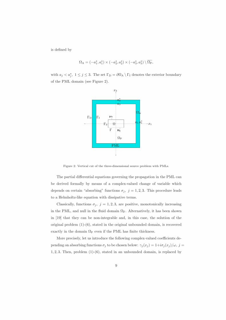
is defined by

ΩA = (−a⋆1, a

⋆1) × (−a⋆

2, a⋆2) × (−a⋆

3, a⋆3) \ ΩF,

with aj < a⋆j , 1 ≤ j ≤ 3. The set ΓD = ∂ΩA \ΓI denotes the exterior boundary

of the PML domain (see Figure 2).

PML

ΩF

ΓD

Γ0

Γ n

ΓI

Ω

ν

ΩA

x1

x3

a∗

3

a3

a∗

1a1

Figure 2: Vertical cut of the three-dimensional source problem with PMLs.

The partial differential equations governing the propagation in the PML can

be derived formally by means of a complex-valued change of variable which

depends on certain “absorbing” functions σj , j = 1, 2, 3. This procedure leads

to a Helmholtz-like equation with dissipative terms.

Classically, functions σj , j = 1, 2, 3, are positive, monotonically increasing

in the PML, and null in the fluid domain ΩF. Alternatively, it has been shown

in [19] that they can be non-integrable and, in this case, the solution of the

original problem (1)-(6), stated in the original unbounded domain, is recovered

exactly in the domain ΩF even if the PML has finite thickness.

More precisely, let us introduce the following complex-valued coefficients de-

pending on absorbing functions σj to be chosen below: γj(xj) = 1+iσj(xj)/ω, j =

1, 2, 3. Then, problem (1)-(6), stated in an unbounded domain, is replaced by

9

the following modified problem in the bounded domain ΩF ∪ ΩA:

Given an angular frequency ω > 0 and an acoustic source g acting outside Ω,

find pressure fields pin and pout satisfying

−ω2

c2pin − Δpin = 0 in Ω, (7)

−ω2

c2pout −

3�

j=1

1

γj

∂

∂xj

�

1

γj

∂pout

∂xj

�

= g in (ΩA ∪ ΩF) \ Ω, (8)

∂pin

∂n=

∂pout

∂non Γ, (9)

pin − pout = Zω

1

iωρ

∂pin

∂non Γ, (10)

∂pin

∂ν

= 0,∂pout

∂ν

= 0 on Γ0, (11)

pout = 0 on ΓD. (12)

The key point here is that, by considering suitable non-integrable absorbing

functions σj , j = 1, 2, 3, null in the fluid bounded domain ΩF, the solutions

of problems (1)-(6) and (7)-(12) are exactly the same in ΩF. This result was

rigorously proved for a case with uniform PML layers in polar coordinates, in

[22].

4. THE PASSIVE-ACTIVE CELL: OPTIMAL CONTROL PROB-

LEM

In this section, going a step further, the passive cell is complemented with

an active control system. More precisely, it is assumed that the wall of the cell

in front of the porous veil (or the MPP) consists of several patches, each of them

vibrating like a piston (planar loudspeaker) so radiating acoustic waves. The

aim is to reduce the reflected field by means of the secondary fields generated

by the loudspeakers, by adjusting their amplitudes in an appropriate way.

Two different control criteria will be considered in this work: pressure release

and impedance matching (see for instance [14]). Note that the extension of the

simulation method to other control criteria is straightforward.

10

4.1. Modelling the passive-active cell

Let us denote by ΓL the planar face of the parallelepipedic cell opposite to

the porous veil (or the MPP). Let us consider a partition of ΓL consisting of NL

rectangular patches, {Γl}, l = 1, . . . , NL, representing the planar loudspeakers

(see Figure 3).

PML

ΩF

ΓD

Γ0

Γ n

ΓI

Γ2Γ1

ΓL

ν

ΩA

x3

x1

a∗

3

a3

a1 a∗

1

Planar loudspeaker

Figure 3: Vertical cut of the computational domain with the PMLs, corresponding to a three-dimensional source problem with two loudspeakers.

The motion of each loudspeaker is characterized by its normal displacement

ul, l = 1, . . . , NL. Thus, the mathematical model for the acoustic behaviour of

the active cell can be written as follows:

Given an angular frequency ω > 0 and an acoustic source g acting outside Ω,

11

find pressure fields pin and pout satisfying

−ω2

c2pin − Δpin = 0 in Ω, (13)

−ω2

c2pout −

3�

j=1

1

γj

∂

∂xj

�

1

γj

∂pout

∂xj

�

= g in ΩA ∪ ΩF, (14)

∂pin

∂n=

∂pout

∂non Γ, (15)

pout − pin = Zω

1

iωρ

∂pin

∂non Γ, (16)

∂pin

∂ν

= 0 on Γ0 \ ΓL,1

iωρ

∂pin

∂ν

= ul on Γl, l = 1, . . . , NL, (17)

∂pout

∂ν

= 0 on Γ0, (18)

pout = 0 on ΓD. (19)

4.2. Active control techniques: optimal control problems

In this section the active noise control problem is stated as an optimal control

problem, in the framework of the theory developed in [16]. It is defined by the

following elements:

• Control variable: in the active cell, the normal displacement of each of

its NL loudspeakers can be set freely and therefore the control variable is

a complex-valued vector (amplitude and phase) defined by these normal

displacements:

u = (u1, . . . , uNL) ∈ C

NL .

In general, due to technological constraints, the loudspeakers amplitudes

are bounded and so they must belong to a convex set of admissible controls

Uad ⊂ CNL .

• State of the system: it is given by the pressure fields (pin, pout) satisfying

equations (13)-(19); notice that it depends on the control u.

• Observation: it will be defined, in general, as a linear combination of the

pressure and the particle velocity (projected on a certain direction) at NS

12

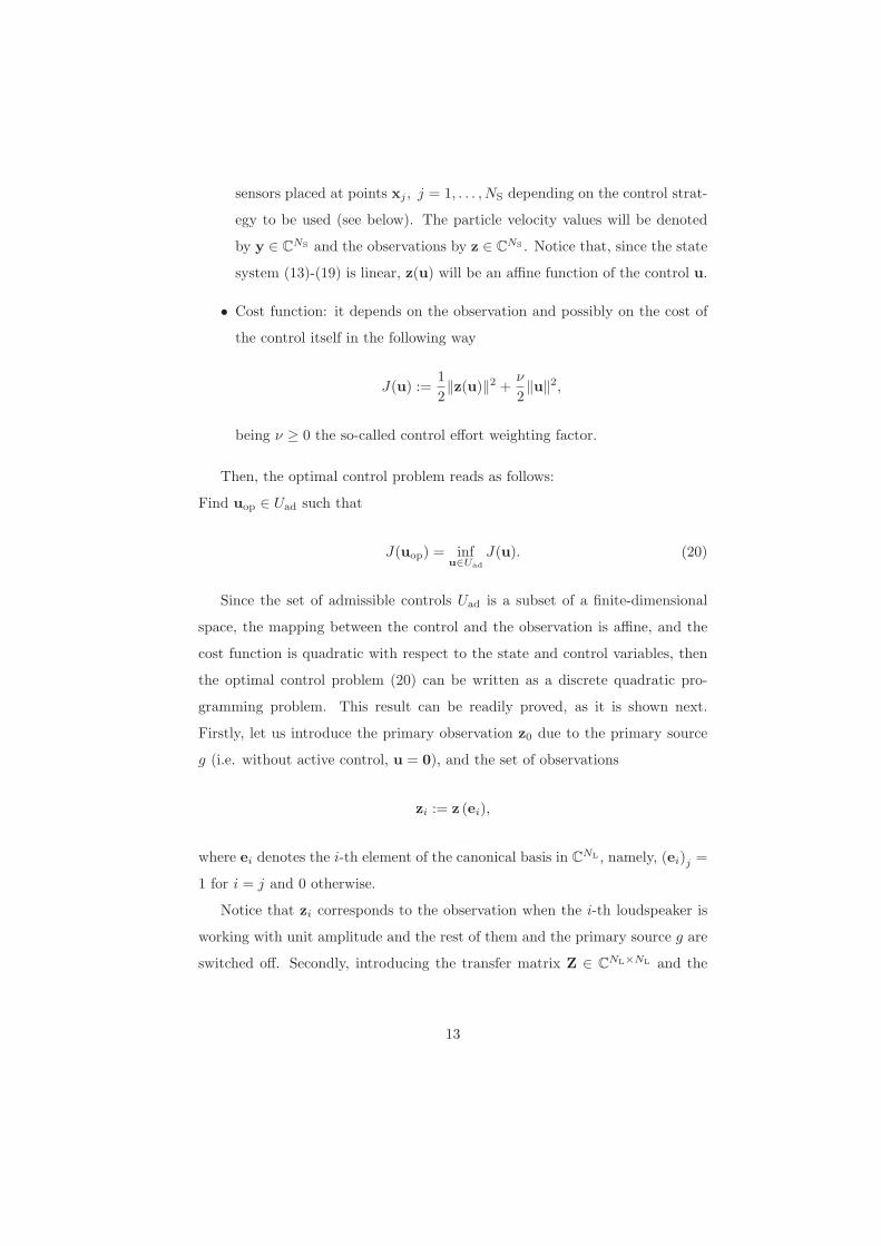
sensors placed at points xj , j = 1, . . . , NS depending on the control strat-

egy to be used (see below). The particle velocity values will be denoted

by y ∈ CNS and the observations by z ∈ C

NS . Notice that, since the state

system (13)-(19) is linear, z(u) will be an affine function of the control u.

• Cost function: it depends on the observation and possibly on the cost of

the control itself in the following way

J(u) :=1

2�z(u)�2 +

ν

2�u�2,

being ν ≥ 0 the so-called control effort weighting factor.

Then, the optimal control problem reads as follows:

Find uop ∈ Uad such that

J(uop) = infu∈Uad

J(u). (20)

Since the set of admissible controls Uad is a subset of a finite-dimensional

space, the mapping between the control and the observation is affine, and the

cost function is quadratic with respect to the state and control variables, then

the optimal control problem (20) can be written as a discrete quadratic pro-

gramming problem. This result can be readily proved, as it is shown next.

Firstly, let us introduce the primary observation z0 due to the primary source

g (i.e. without active control, u = 0), and the set of observations

zi := z (ei),

where ei denotes the i-th element of the canonical basis in CNL , namely, (ei)j =

1 for i = j and 0 otherwise.

Notice that zi corresponds to the observation when the i-th loudspeaker is

working with unit amplitude and the rest of them and the primary source g are

switched off. Secondly, introducing the transfer matrix Z ∈ CNL×NL and the

13

vector b ∈ CNL by

(Z)ij = (zi, zj), i, j = 1, . . . , NL, (21)

(b)i = (z0, zj), j = 1, . . . , NL, (22)

where (·, ·) is the standard scalar product in CNL , the observation is given

by z(u) = Zu + b. Finally, straightforward calculations show that problem

(20) can be written as the following constrained finite-dimensional quadratic

programming problem:

Find uop ∈ Uad such that

J(uop) = infu∈Uad

�

1

2(u, (Z + νI)u) + (u,b) +

1

2�z0�

2

�

. (23)

It can be easily shown that, provided that ν > 0, or ν ≥ 0 and z(u) is an

injective mapping, the above optimal control problem has a unique solution (see

for instance [23] for a similar problem). Moreover, the optimal control uop is

the solution of the following variational inequality (optimality condition):

(v − uop, (Z + νI)uop) ≥ − (v − uop,b) ∀v ∈ Uad. (24)

When the set of admissible controls Uad is the whole space, i.e., if there are no

constraints on the control variable, the above condition reduces to the Euler

equation,

(Z + νI)uop = −b. (25)

Let us remark that, if the control effort is null and the number of observation

points, NS, is less or equal than the number of planar loudspeakers, NL, then

J(uop) = 0, i.e., the pressure field is cancelled at the observation points when

the control is optimal.

Two different standard noise control strategies will be analyzed in this work

corresponding to two different observations (see [12]):

• Pressure release: the observation to be minimized is the pressure at the

14

center point of the interior side of the porous veil (or the MPP) of each

cell; more precisely, it is the scalar

zR(u) := (pin(x1), . . . , pin(xNS

)), (26)

so the cost function reads

JR(u) =1

2

NS�

i=1

|pin(xi)|2 +

ν

2�u�2.

• Impedance matching: the goal is that the normal input impedance to the

cell matches the characteristic impedance of the medium, Z0, at the center

point of the external side of the porous veil (or the MPP) f each cell. In

other words, we want to annulate the observation which corresponds to

the i-th cell,

(zM(u), ei) := pout(xi) + Z01

iωρ

∂pout

∂n(xi), i = 1, . . . , NS, (27)

by minimizing the cost function

JM(u) =1

2�zM(u)�2 +

ν

2�u�2. (28)

From a practical point of view, it is preferable to place the error sensor

inside the cell rather than outside. For this reason, the observation is

obtained indirectly from the pressure and the (normal) particle velocity

at the center of the interior side of the porous veil (or the MPP). Thus,

taking into account equations (15) and (16) defining the pressure jump

across the porous veil (or the MPP), we obtain

(zM(u), ei) = pin(xi) + (Z0 − Zω)1

iωρ

∂pin

∂n(xi), i = 1, . . . , NS.

15

5. NUMERICAL SOLUTION: DISCRETIZATION PROCEDURE

5.1. Description of the Finite Element Method (FEM)

A standard FEM is used to solve numerically the state equations. Let us

consider hexaedral meshes of the two regions, Ω and (ΩF ∪ ΩA)\Ω, of the compu-

tational domain. Although it is not necessary to have meshes matching on their

common interface ΓI, all the numerical examples below have been performed

with compatible meshes. As usual, h denotes the mesh-size. Approximations

pinh and pout

h of pin and pout, respectively, are computed by using bilinear hexae-

dral finite elements. Let us recall that the degrees of freedom defining the finite

element solution are the values of pinh and pout

h at the vertices of the hexaedra.

Regarding the boundary condition on the outer boundaries of the PMLs,

a prescribed null pressure is imposed (see equation (12)). Hence, pouth does

not have any degrees of freedom on this outer boundary. This condition is

essential for the resulting discrete problem to be well posed when non-integrable

absorbing functions are used (see [19]).

Let us remark again that, inside the fluid domain ΩF, the absorbing functions

γj are equal to one, for j = 1, 2, 3, because functions σj are taken to be null

there.

As proposed in [19], in the PML these functions are chosen of the following

form

σj (xj) =c

a∗j − xj

, xj ∈�

aj , a∗j

�

,

for j = 1, 2, 3. Notice that they are unbounded as xj goes to a∗j and also non

integrable in the interval�

aj , a∗j

�

corresponding to the j-th PML (see Figure 3).

However, straightforward computations show that the coefficients of the finite

element matrices are bounded, in spite of the singularity of σj on ΓD (see [19]).

Let us remark that the complex matrices arising from this finite element

discretization, although non-Hermitian, are complex symmetric matrices which

allows us to reduce the memory storage when a direct solver is used for solving

the linear system. Finally, it is worth mentioning that all the matrix entries

16

have been computed by means of a standard quadrature rule of eight points per

hexahedron.

5.2. The discrete optimal control problem

A discrete optimal control problem is obtained when replacing the solution

of the original state equation by the FEM approximation of the boundary value

problem (13)-(19) involving the PMLs. Let us denote by (pinh , pout

h ) the FEM

solution corresponding to the mesh size h and by zh(u) the corresponding ap-

proximation of the observation.

Thus, an approximate cost function is obtained

Jh(u) :=1

2�zh(u)�2 +

ν

2�u�2

leading to the approximate optimal control problem

Jh(uoph) = inf

u∈Uad

Jh(u). (29)

From a mathematical point of view, the above optimal control problem is anal-

ogous to the exact one. In particular, a similar inequality to (24), characterizes

the approximate optimal control uoph, namely

�

v − uoph, (Zh + νI)uop

�

≥ −�

v − uoph,bh

�

, ∀v ∈ Uad. (30)

where Zh ∈ CNL×NL and bh ∈ C

NL are the approximations of transfer matrix

Z and vector b given by

(Zh)ij = (zhi, zhj), i, j = 1, . . . , NL, (31)

(bh)j = (zh0, zhj), j = 1, . . . , NL. (32)

In [23, 24] it is proven that, provided the matrix Z + νI is positive definite,

17

i.e., if there exists a positive constant α > 0 such that

(v, (Z + νI)v) ≥ α�v�2, ∀v ∈ Uad,

and the mesh size h is small enough, the error of the optimal control is bounded

by the error on the transfer matrix and the vector b through

�uop − uoph� ≤

2

α

�

�b�

α�Z − Zh� + �b − bh�

�

.

Certainly, the error in the observation, and thus the error in the optimal con-

trol, will depend on the order of the FEM discretization and the choice of the

observation.

6. NUMERICAL RESULTS

First, the implementation of numerical method described above is validated

by comparing the obtained numerical solution with an explicit exact solution.

With this purpose, a normal plane wave propagation problem is chosen.

In order to assess the performance of the passive-active cells introduced in

this work for noise control, the acoustic attenuation produced by an isolated cell

and surrounded by air is computed. The pressure release and the impedance

matching control strategies are taking into account in two different cell config-

urations. Then, we consider a real-life application where the ceiling of a room

is covered with an array of 6 × 5 passive-active cells.

6.1. Validation

In what follows, the implementation of the numerical method is validated

by computing the solution of a normal plane wave propagation problem in

the passive case. Let us assume the parallelepipedic computational domain

(−0.75, 0.75) × (−0.75, 0.75) × (−0.5, 0.75) where all the boundary faces are

rigid except those perpendicular to the x3-axis.

18

A porous veil is placed at plane x3 = 0m and a PML domain of thickness

0.25m is situated between the planes x3 = 0.75m and x3 = 0.5m. The ampli-

tude of the incoming pressure plane wave is fixed to 1N/m2, which is imposed

on a boundary condition on the face of plane x3 = −0.5 m.

The following physical data are considered: the thickness of the passive

fluid cell is 0.15m and the air properties are c = 343m/s, ρ = 1kg/m3. The

complex-valued impedance associated to the porous veil is given by Zω = Z0(1−

i) kg/(m2s).

The exact solution of the previous problem is a plane wave which depends

only on the spatial coordinate x3, i.e.,

p(x3) =

−Zω

2 − Zω

e−i ω

c(x3+0.5) + ei ω

c(x3−0.5) if x3 ∈ (−0.5.0),

2

2 − Zω

e−i ω

c(x3−0.5) if x3 ∈ (0, 0.5),

x3 + 0.75

0.25

2

2 − Zω

e−i ω

c(x3−0.5) if x3 ∈ [0.5, 0.75).

For f = 100Hz and using a uniform finite element mesh with 6137 vertices,

the real and imaginary parts of the approximate pressure field has been com-

puted and shown in Figure 4. In addition, the real and imaginary part of the

exact solution are also shown in the same plots with the purpose of comparison.

From these plots it can be verified that: on one hand, the pressure field

has a discontinuity at the point where the porous veil is placed; on the other

hand, the velocity field, which depends on the derivatives of the pressure field,

is continuous. Let us remark that the boundary between the physical and the

PML domain is marked with a dash-dot line in both plots.

In order to check the convergence order of the numerical method described in

the previous sections, different uniform finite element meshes with 2028, 6137,

13750, 43808, and 100842 vertices have been used to compute the approximate

solution. As it is checked in Figure 5, where the L2-relative error is plotted ver-

sus the mesh-size, the optimal order of convergence is achieved for the piecewise

bilinear elements used in the finite element discretization.

19

(a) (b)

−0.4 −0.2 0 0.2 0.4 0.6−0.2

0

0.2

0.4

0.6

0.8

1

1.2

1.4

x3

Rea

l par

t

Approx. sol

Exact. sol

−0.4 −0.2 0 0.2 0.4 0.6

−0.2

0

0.2

0.4

0.6

0.8

1

1.2

1.4

x3

Imag

inar

y pa

rt

Approx. sol

Exact. sol

Figure 4: Plane wave solution for f = 100Hz on line x1 = x2 = 0: (a) real part, (b) imaginarypart.

0.025 0.05 0.075 0.1 0.1510

−2

10−1

100

h2

h (mesh−size)

L2 Rel

. err

or (%

)

Figure 5: L2-relative error (in percentage) computed in the plane wave propagation problem.

6.2. One active cell configuration

In order to determine the impedance associated with the MPP on Γ, the

Maa’s formula for micro-perforated plates (see [10]) is taken into account, namely

Zω =iωρs

φ

�

1 −2

y(ω)

J1(y(ω))

J0(y(ω))

�−1

, (33)

20

where s is the thickness of the rigid plate, φ the perforation ratio and y(ω) =

r0

�

−iωρ/η, being r0 the radius of the holes and η the fluid viscosity. Jn(·) is

the Bessel functions of first kind and order n.

For the numerical simulations, the following physical data are considered:

the size of the passive fluid cell is 0.6m × 0.6m × 0.15m, the air properties are

c = 343m/s, ρ = 1kg/m3 and η = 1.789 × 10−5 kg/m s. The geometrical data

characterizing the MPP are s = 10−3 m, φ = 0.1, r0 = 4 × 10−3 m.

Concerning the dimension of the computational domain of interest and the

PML domain, we consider the following (in meters):

ΩF = (−0.5, 0.5) × (−0.5, 0.5) × (−0.925, 0.925),

ΩA = [(−0.7, 0.7) × (−0.7, 0.7) × (−1.125, 1.125)] \ ΩF.

To represent the primary field produced by the acoustic source, a pointwise

monopole source is located at point a = (0, 0,−0.725) with unitary volume

velocity and a complex amplitude depending linearly on the angular frequency

and the mass density, i.e., g = iωρδa, where δa is the Dirac’s delta supported at

point a.

Two different configurations has been taking into account. First, a unique

loudspeaker is placed covering the back face of the active cell and the pressure

observation is done at the inner center point of the porous veil (0, 0,−0.15).

Second, the orignal active cell is split into two smaller parts. Each one has a

unique loudspeaker as described above. In this case, two observation points are

located at (0, 0.17,−0.15) and (0,−0.17,−0.15). In both cases a null control

effort weighting factor (ν = 0) is assumed.

To compare the pressure level with and without control, the attenuation

level is defined by

Attenuation (dB) = 10 log

�

|pop|2

|p|2

�

,

where p and pop are the computed pressure at the observation point without

21

control and with the optimal control, respectively.

For the pressure release scheme, in Figure 6 the attenuation fields for the

frequencies f = 100Hz and f = 400Hz are shown. Analogous graphs for the

impedance matching scheme are shown in Figure 7.

It can be checked from the plots above that, for a frequency of 100Hz,

the attenuation field achieved by the impedance matching strategies reaches

−5 dB nearby the cell whereas the pressure release only gets −3 dB. Moreover,

the attenuation field does not show any local maximum in the computational

domain at this frequency.

However, if the frequency is fixed to 400Hz, the attenuation field obtained

with both control strategies reaches a reinforcement of 20 dB in a unique cen-

tered region with respect to the passive-active cell and a noise attenuation about

−10 dB with minima periodically distributed in the perpendicular direction to

the MPP face of the passive-active cell.

Notice that for both frequencies and the two control strategies considered,

the one-loudspeaker configurarion provides larger attenuation in the neighbourg-

hood of the active cell. Nevertheless, the two-loudspeaker configuration allows

us to reduce the area of reinforcement obtained in front of the active cell at

400Hz.

6.3. Real-life application

Next, the optimal passive-active control of noise in a room whose ceiling has

been completely covered with thirty active cells, is computed. The size of each

active cell is 0.45m × 0.45m × 0.03m and they are arranged in an 5 × 6 array

with a separation of 0.05m among them. The dimensions of the walls, the door

and the window of the room are indicated in Figure 8.

It is worth noting that this problem (or a very similar one) has practical

interest and, in fact, it has been the object of previous research, as it can be

seen in [25, 26].

The door and the window has been modelled by means of impedance bound-

ary conditions. On the one hand, the door is assumed to be open so the classical

22

(a) (b)

(c) (d)

Figure 6: Pressure release scheme: attenuation field with one sensor and one actuator at100Hz and 400 Hz (plots (a) and (b), respectively); attenuation field with two sensors andtwo actuators at 100Hz and 400Hz (plots (c) and (d), respectively).

first order radiation boundary condition is considered, namely,

∂pout

∂n− i

ω

cpout = 0.

23

(a) (b)

(c) (d)

Figure 7: Impedance matching scheme: attenuation field with one sensor and one actuatorat 100Hz and 400 Hz (plots (a) and (b), respectively); attenuation field with two sensors andtwo actuators at 100Hz and 400Hz (plots (c) and (d), respectively).

On the other hand, we set a harmonic vibration of unit amplitude incoming

through the window (primary field). This has been modelled by the non-

24

Figure 8: Three-dimensional geometry of the room with a door (on the left) and a window(on the right).

homogeneous Robin boundary condition

∂pout

∂n− i

ω

cpout = 1.

The remaining walls and the floor are assumed to be rigid, i.e., ∂pout/∂n = 0.

For the discretization procedure, a conforming mesh on the cell/room inter-

faces has been used, with approximately 13×103 elements and 86×103 degrees

of freedom. Let us remark that the motion of each loudspeaker is possibly dif-

ferent in each cell and depends globally on the value of the observations in the

cell array.

Figure 9 shows the modulus of the passive and the active pressure fields,

for the cell and the two control strategies described in previous sections taking

f = 100Hz. In both strategies, the thirty cells are active. The pressure field

has been plotted on planes x1 = 1.75m, x2 = 3m, and x3 = 0m, located inside

the room and the active cells.

From the point of view of real-life feasibility of the active control system, it

25

(a) (b)

(c)

Figure 9: Amplitude of the pressure field for f = 100Hz for: (a) the passive case, (b) pressurerelease control, and (c) impedance matching control.

should be guaranteed a uniform pressure level reduction in the low frequency

range. Figure 10 shows the L2-norm of pressure (in dB) inside the room versus

frequency for the different control strategies with thirty active cells.

It can be observed that the pressure norm reduction achieved for the impedance

matching control scheme is much more stable for the whole range of frequencies

than the pressure release one. However, the latter yields better reduction in the

low frequency range between 0 and 40 Hz. Notice that if thirty cells are used

with the impedance matching strategy, the reduction of the L2-norm pressure

is pronounced and the peaks corresponding to the resonant frequencies almost

vanish.

26

(a) (b)

50 100 150 200 250−50

0

50L2 −n

orm

of p

ress

ure

(dB

)

Frequency (Hz)

PassivePressure releaseImpedance matching

50 100 150 200 250−10

0

10

20

30

40

50

L2 −nor

m o

f pre

ssur

e (d

B)

Frequency (Hz)

PassivePressure releaseImpedance matching

Figure 10: L2-norm of pressure (dB) inside the room: (a) with thirty active cells, (b) withfour active cells.

The performance when only four cells are active is also included on the right-

hand side of Figure 10. In terms of practical implementation, the same four cell

configuration has been fixed for the full frequency range. They have been chosen

by localizing the four maximal frequency-average of the entries of the transfer

matrix. Clearly, despite using any of the active control strategies, the pressure

reduction is far from the optimal one computed when thirty cells are active.

7. CONCLUSIONS

Two control strategies (pressure release and impedance matching) have been

simulated numerically to assess the performance of passive-active cells as sound

absorbers. The acoustic effect of a porous veil or a MPP has been included by

means of a locally reacting surface impedance model (see [10]).

The discretization procedure for solving the three-dimensional sound prop-

agation model combines a standard FEM and an exact PML technique. The

proposed numerical methodology could be used to analyze the performance of

potential isolated configurations or the noise absorption of real-life installations

as noise barriers [6], absorbers in acoustic window systems [7] or noise reduction

devices in flow ducts applications [27].

27

By using this numerical method, the simulation of a passive-active cell in an

anechoic room has been done following as guidance the geometrical setup de-

scribed in [14]. Overcoming the restrictions that a harmonic plane wave mathe-

matical analysis (at normal or oblique incidence) has, the proposed methodology

allows us to evaluate the pressure and attenuation field at any point of the com-

putational domain (see Figures 6 and 7).

Moreover, the numerical evaluation of the noise absorption of a 6×5 matrix

of passive-active cells in a real-life installation has been shown. As it can be

checked from the results in the previous section, the proposed methodology

based on a finite element code and on the implementation of the active noise

reduction problem in the framework of an approximate optimal control problem

[16], allows us to evaluate the acoustic attenuation.

ACKNOWLEDGEMENTS

The work of A. Bermudez was partially supported by Ministerio de Edu-

cacion y Ciencia of Spain under grant MTM2008-02483 and Xunta de Galicia

grant 2006/98.

The work of P. Gamallo was partially supported by Ministerio de Educacion

y Ciencia of Spain under grants MTM2008-02483 and 18-08-463B-750, and by

Xunta de Galicia under grant PGIDIT07PXIB105257PR.

The work of L. Hervella-Nieto was partially supported by Ministerio de Edu-

cacion y Ciencia of Spain under grants MTM2008-02483 and MTM2007-67596-

C02-01 and by Xunta de Galicia under grant PGIDIT07PXIB105257PR.

The work of A. Prieto was partially supported by Ministerio de Educacion y

Ciencia of Spain under grant MTM2008-02483 and by Xunta de Galicia under

grant PGIDIT07PXIB105257PR and program Angeles Alvarino 2007/AA-076.

References

[1] L. L. Beranek, I. L. Ver (eds.), Noise and vibration control engineering:

principles and applications, John Wiley & Sons, Hoboken, New Jersey,

28

2006.

[2] P. A. Nelson, S. J. Elliot, Active Control of Sound, Academic Press, New

York, 1992.

[3] H. F. Olson, E. G. May, Electronic sound absorber, Journal of the Acous-

tical Society of America 25 (6) (1953) 1130–1136.

[4] D. Guicking, E. Lorenz, An active sound absorber with porous plate, Jour-

nal of Vibration and Acoustics 106 (3) (1984) 389–392.

[5] A. Bermudez, L. M. Hervella-Nieto, A. Prieto, R. Rodrıguez, Validation of

acoustic models for time-harmonic dissipative scattering problems, Journal

of Computational Acoustics 15 (1) (2007) 95–121.

[6] F. Asdrubali, G. Pispola, Properties of transparent sound-absorbing panels

for use in noise barriers, Journal of the Acoustical Society of America 121

(1) (2007) 214–221.

[7] J. Kang, M. W. Brocklesby, Feasibility of applying micro-perforated ab-

sorbers in acoustic window systems, Applied Acoustics 66 (6) (2005) 669-

689.

[8] T. Dupont, G. Pavic, B. Laulagnet, Acoustic properties of lightweight

micro-perforated plate systems, Acta Acustica united with Acustica 28 (2)

(2003) 201–212.

[9] J. Pfretzschner, P. Cobo, F. Simon, M. Cuesta, A. Fernandez, Microper-

forated insertion units: An alternative strategy to design microperforated

panels, Applied Acoustics 67 (1) (2006) 62-73.

[10] D. Y. Maa, Microperforated-panel wideband absorbers, Noise Control En-

gineering Journal 29 (3) (1987) 77-84.

[11] M. Furstoss, D. Thenail, M. A. Galland, Surface impedance control for

sound absorption: direct and hybrid passive/active strategies, Journal of

Sound and Vibration 203 (2) (1997) 219–236.

29

[12] S. Beyene, R. A. Burdisso, A new hybrid passive–active noise absorption

system, Journal of the Acoustical Society of America 101 (3) (1997) 1512–

1515.

[13] P. Cobo, J. Pfretzschner, M. Cuesta, D. K. Anthony, Hybrid passive-active

absorption using microperforated panels, Journal of the Acoustical Society

of America 116 (4) (2004) 2118–2125.

[14] P. Cobo, A. Fernandez, Hybrid passive-active absorption of broadband

noise using MPPs, Noise & Vibration Worldwide 37 (5) (2006) 19–23.

[15] P. Cobo, M. Cuesta, Measuring hybrid passive-active sound absorption of a

microperforates liner at oblique incidence, Journal of the Acoustical Society

of America 125 (1) (2009) 185–190.

[16] J. L. Lions, Optimal Control of Systems Governed by Partial Differential

Equations, Springer-Verlag, Berlin, 1971.

[17] Z. Zhang, Y. Chen, X. Yin, H. Hua, Active vibration isolation and under-

water sound radiation control, Journal of Sound and Vibration 318 (4-5)

(2008) 725–736.

[18] J.P. Berenger, A perfectly matched layer for the absorption of electromag-

netic waves, Journal of Computational Physics 114 (2) (1994) 185–200.

[19] A. Bermudez, L. M. Hervella-Nieto, A. Prieto, R. Rodrıguez, An opti-

mal perfectly matched layer with unbounded absorbing function for time-

harmonic acoustic scattering problems, Journal of Computational Physics

223 (2) (2007) 469–488.

[20] J.C. Nedelec, Acoustic and electromagnetic equations: integral representa-

tions for harmonic problems, Springer, New York, 2001.

[21] A. Bermudez, L. M. Hervella-Nieto, A. Prieto, R. Rodrıguez, Perfectly

matched layers, in: S. Marburg and B. Nolte (Eds.), Computational Acous-

tics of Noise Propagation in Fluids. Springer-Verlag, Berlin Heidelberg,

2008, pp. 167–196 (Chapter 6).

30

[22] A. Bermudez, L. M. Hervella-Nieto, A. Prieto, R. Rodrıguez, An exact

bounded perfectly matched layer for time-harmonic scattering problems,

SIAM Journal on Scientific Computing 30 (1) (2007/08) 312–338.

[23] A. Bermudez, P. Gamallo, R. Rodrıguez, Finite element methods in local

active control of sound, SIAM Journal on Control and Optimization 43 (2)

(2004) 437–465.

[24] P. Gamallo, Contribucion al estudio matematico de problemas de simu-

lacion elastoacustica y control activo del ruido (in Spanish), Contribution

to the mathematical study of elastoacoustic simulation and active control of

sound problems, PhD Thesis, University of Santiago de Compostela, 2002.

[25] M. Tarabini, A. Roure, Modeling of influencing parameters in active noise

control on an enclosure wall, Journal of Sound and Vibration 311 (3-5)

(2008) 1325–1339.

[26] M. Tarabini, A. Roure, C. Pinhede, Active control of noise on the source

side of a partition to increase its sound isolation, Journal of Sound and

Vibration 320 (4-5) (2009) 726–743.

[27] N. Sellen, M. Cuesta, M.-A. Galland, Noise reduction in a flow duct: Im-

plementation of a hybrid passive/active solution, Journal of Sound and

Vibration 297 (3-5) (2006) 492–511.

31