Numerical analysis of the Burgers’ equation in the presence of uncertainty

Journal of Computational Physics xxx (2009) xxx–xxx

ARTICLE IN PRESS

Contents lists available at ScienceDirect

Journal of Computational Physics

journal homepage: www.elsevier .com/locate / jcp

Numerical analysis of the Burgers’ equation in the presence of uncertainty

Per Pettersson a,b,*, Gianluca Iaccarino a, Jan Nordström b,c,d

a Department of Mechanical Engineering, Stanford University, Stanford, CA 94305, USAb Department of Information Technology, Uppsala University, SE-75105 Uppsala, Swedenc Department of Aeronautics and Systems Integration, FOI, The Swedish Defense Research Agency, SE-16490 Stockholm, Swedend School of Mechanical, Industrial and Aeronautical Engineering, University of the Witwatersrand, Johannesburg, WITS 2050, South Africa

a r t i c l e i n f o a b s t r a c t

Article history:Received 16 November 2008Received in revised form 17 July 2009Accepted 15 August 2009Available online xxxx

Keywords:Uncertainty quantificationHyperbolic problemsPolynomial chaosNumerical stability

0021-9991/$ - see front matter � 2009 Elsevier Incdoi:10.1016/j.jcp.2009.08.012

* Corresponding author. Address: Department of M7232535.

E-mail addresses: [email protected] (P. Pet

Please cite this article in press as: P. PetterssonPhys. (2009), doi:10.1016/j.jcp.2009.08.012

The Burgers’ equation with uncertain initial and boundary conditions is investigated usinga polynomial chaos (PC) expansion approach where the solution is represented as a trun-cated series of stochastic, orthogonal polynomials.

The analysis of well-posedness for the system resulting after Galerkin projection is pre-sented and follows the pattern of the corresponding deterministic Burgers equation. Thenumerical discretization is based on spatial derivative operators satisfying the summationby parts property and weak boundary conditions to ensure stability. Similarly to the deter-ministic case, the explicit time step for the hyperbolic stochastic problem is proportional tothe inverse of the largest eigenvalue of the system matrix. The time step naturallydecreases compared to the deterministic case since the spectral radius of the continuousproblem grows with the number of polynomial chaos coefficients. An estimate of theeigenvalues is provided.

A characteristic analysis of the truncated PC system is presented and gives a qualitativedescription of the development of the system over time for different initial and boundaryconditions. It is shown that a precise statistical characterization of the input uncertainty isrequired and partial information, e.g. the expected values and the variance, are not suffi-cient to obtain a solution. An analytical solution is derived and the coefficients of the infi-nite PC expansion are shown to be smooth, while the corresponding coefficients of thetruncated expansion are discontinuous.

� 2009 Elsevier Inc. All rights reserved.

1. Introduction

In many physical problems our knowledge is limited by our ability to measure, our bias in the observations and, in gen-eral, by an incomplete understanding of the physical processes. When we attempt to simulate the problem numerically, wemust account for those limitations, and in addition we must identify the possible limitations of the numerical techniques andphenomenological models employed. In a general sense, we distinguish between errors and uncertainty simply by saying thaterrors are recognizable deficiencies not due to lack of knowledge, whereas uncertainties are potential and directly related to lackof knowledge [1]. This definition clearly identifies errors as deterministic quantities and uncertainties as stochastic in nature;uncertainty estimation is, therefore, typically treated within a probabilistic framework.

Numerical simulations are subject to uncertainty in boundary or initial conditions, model parameter values and even inthe geometry of the physical domain of the problem (input uncertainty); this results in uncertainty in the output data that

. All rights reserved.

echanical Engineering, Stanford University, Stanford, CA 94305, USA. Tel.: +1 650 7232177; fax: +1 650

tersson), [email protected] (G. Iaccarino), [email protected] (J. Nordström).

et al., Numerical analysis of the Burgers’ equation in the presence of uncertainty, J. Comput.

http://dx.doi.org/10.1016/j.jcp.2009.08.012

mailto:[email protected]



http://www.sciencedirect.com/science/journal/00219991

http://www.elsevier.com/locate/jcp


2 P. Pettersson et al. / Journal of Computational Physics xxx (2009) xxx–xxx

ARTICLE IN PRESS

must be clearly identified and quantified. Uncertainty quantification is also a fundamental step towards validation and cer-tification of numerical methods to be used for critical decisions. Fields of application of uncertainty quantification includebut are not limited to turbulence, climatology [19], turbulent combustion [20], flow in porous media [8], fluid mixing[30] and computational electromagnetics [6].

An example of the need for uncertainty quantification in applications related to methods and problems studied here is theinvestigation of the aerodynamic stability properties of an airfoil. Uncertainty in physical parameters such as structural fre-quency and initial pitch angle, affect the characteristics of limit cycle oscillations. One approach in particular, the polynomialchaos method [10], has been used to obtain a statistical characterization of the stability limits and to calculate the risk forsystem failure [26,2]; this approach will be studied in detail.

There are several approaches to propagate the input uncertainty in numerical simulations; the simplest one is the MonteCarlo method where a vast number of simulations are performed to compute the output statistics. Conversely in the poly-nomial chaos approach, the solution is expressed as a truncated series and only one simulation is performed. The dimensionof the resulting system of equations grows with the number of the terms retained in the series (the order of the polynomialchaos expansion) and the dimension of the stochastic input.

An increased number of Monte Carlo simulations implies a solution with better converged statistics; on the other hand, inthe polynomial chaos approach, one single simulation is sufficient to obtain a complete statistical characterization of thesolution. However, the accuracy of this solution is dependent on the order of polynomials considered, and therefore onthe truncation in the PC expansion. Also, convergence requires the solution to be smooth with respect to the parametersdescribing the input uncertainty [24].

Although of limited practical use in fluid mechanics applications, the Burgers’ equation is an interesting and highly non-linear model problem and many results can be extended to other hyperbolic systems, such as the Euler equations. In thispaper, a detailed uncertainty quantification analysis is performed for the Burgers’ equation; we employ a spectral represen-tation of the solution in the form of a polynomial chaos expansion. The equation is stochastic as a result of the uncertainty inthe initial and boundary values. Galerkin projection results in a coupled, deterministic system of hyperbolic equations fromwhich the expected values and variance of the solution can be determined.

Previous uncertainty analyses have been performed on the location of the transition layer of a shock discontinuity arising insimulations of the Burgers’ equation with non-zero viscosity. Small one-sided perturbations imply large variation in the locationof the transition layer, so-called supersensitivity [29], which is a problem in deterministic as well as stochastic simulations. Theresults from the polynomial chaos approach were accurate and the method was faster than the Monte Carlo method [28,29].Burgers’ equation with a stochastic forcing term has also been investigated and compared to standard Monte Carlo methods [13].

In this work we perform a fundamental analysis of the Burgers’ equation and develop a numerical framework to study theeffect of uncertainty of the boundary conditions. By assuming that the boundary data uncertainty has a Gaussian distributionwe allow the occurence of unbounded solutions. Assuming that the boundary data resemble the Gaussian distribution butare bounded to a sufficiently large range does not alter the numerical results. Another reason for allowing unboundedparameter range of the stochastic variable is that the problem becomes more interesting from a mathematical point of view.Convergence is proved by a suitable choice of functional space.

In order to ensure stability of the discretized system of equations, summation by parts operators and weak imposition ofboundary conditions [17,18,5] are used to obtain energy estimates. The system is expressed in a split form that combines theconservative and non-conservative formulation [16]. A particular set of artificial dissipation operators [15] and the simulta-neous approximation term (SAT) technique [4] for boundary treatment are used to enhance the stability close to the shock.The discretization method is based on a fourth order central difference operator in space and the fourth order Runge–Kuttamethod in time. The summation by parts operators ensure stable solutions but the allowed time step decreases with increas-ing order of the PC expansion as a result of the eigenvalues growing with the polynomial order (i.e. the size of the system).

An analytical solution is derived for a discontinuous and uncertain initial condition: the expectation and variance of thesolution are shown to be smooth functions while the coefficient of truncated polynomial chaos expansions are discontinu-ous. An analysis of the characteristics of the truncated system also shows that the boundary values are time-dependent andsuggest a way of imposing accurate boundary conditions.

2. Polynomial chaos expansion

The theoretical foundation underlying polynomial chaos was first formulated in [25,10]. The solution to a partial differ-ential equation characterized by input uncertainty (for simplicity we consider only one uncertain parameter, n, defined onthe probability space Xprob) is expressed as a spectral expansion:

PleasePhys.

uðx; t; nÞ ¼X1i¼0

uiðx; tÞWiðnÞ; ð1Þ

with the inner product

hu; vi ¼Z

Xprob

uvf ðnÞdn; ð2Þ

cite this article in press as: P. Pettersson et al., Numerical analysis of the Burgers’ equation in the presence of uncertainty, J. Comput.(2009), doi:10.1016/j.jcp.2009.08.012


P. Pettersson et al. / Journal of Computational Physics xxx (2009) xxx–xxx 3

ARTICLE IN PRESS

where f ðnÞ is the probability density function. The solution is subject to the constraint

PleasePhys.

kuk2 ¼Z

Xprob

u2f ðnÞdn <1; ð3Þ

i.e. it is a second-order random field (finite variance).The expected value EðuÞ and variance VarðuÞ can be expressed as functions of the polynomial chaos coefficients. We have

EðuÞ ¼Z

Xprob

X1i¼0

uiWif ðnÞdn ¼ u0

ZXprob

f ðnÞdnþZ

Xprob

X1i¼1

uiWif ðnÞdn ¼ u0; ð4Þ

and

r2 ¼ VarðuÞ ¼ E½u2� � ðE½u�Þ2 ¼Z

Xprob

X1i¼0

u2i W

2i f ðnÞdn� u2

0 ¼X1i¼1

u2i hW

2i i: ð5Þ

The basis functions WiðnÞ are orthogonal polynomials of the stochastic variable n, and thus

hWi;Wji ¼ dijci; ð6Þ

where ci is a constant depending on the polynomial basis. The relations between different polynomial bases is described bythe Askey scheme; for further reading, see for instance [27]. Here it is sufficient to notice that the optimal basis in terms ofconvergence is Hermite polynomials if n is distributed according to a Gaussian measure.

2.1. Polynomial chaos expansion of Burgers’ equation

The polynomial chaos representation uðx; t; nÞ ¼P1

i¼0uiWiðnÞ is inserted into the Burgers’ equation,

ut þ uux ¼ 0; 0 6 x 6 1; ð7Þ

which yields

X1i¼0

@ui

@tWiðnÞ þ

X1j¼0

ujWjðnÞ ! X1

i¼0

@ui

@xWiðnÞ

!¼ 0: ð8Þ

A stochastic Galerkin projection is performed by multiplying (8) by WkðnÞ for non-negative integers k and integrating overthe probability domain X. The orthogonality of the basis polynomials then yields a system of deterministic equations. Bytruncating the series (1) to a finite order M, the solution is projected onto a finite dimensional deterministic space. The resultis a symmetric system of equations.

@uk

@thW2

ki þXM

i¼0

XM

j¼0

ui@uj

@xhWiWjWki ¼ 0 for k ¼ 0;1; . . . ;M: ð9Þ

2.2. Modeling the solution with Hermite polynomials

The probabilistic version of the Hermite polynomial basis functions is used since it is the most intuitive choice with re-gard to weight function and calculation of expected value and variance. The weight function of the inner products is theprobability density function of the Gaussian distribution. This means that the inner product of two variables u and v coin-cides with the expected value of their product

hu;vi ¼Z

Xprob

uvf ðnÞdn ¼ EðuvÞ:

For probabilistic Hermite polynomials HðnÞ of a Gaussian variable n the double inner product defined in (6) is given by

hHiHji ¼ diji!: ð10Þ

The triple inner product can be derived from a formula in [23]:

hHiHjHki ¼0 if iþ jþ k is odd or max ði; j; kÞ > s;

i!j!k!ðs�iÞ!ðs�jÞ!ðs�kÞ! otherwise;

(ð11Þ

where s ¼ ðiþ jþ kÞ=2.




ARTICLE IN PRESS

2.3. Derivation of an analytical solution

By the Cameron–Martin theorem [3] the solution converges in the L2 sense; in a probabilistic sense this implies meansquare convergence, that is

PleasePhys.

limM!1

E u�XM

i¼1

uiWi

��

224 35 ¼ 0:

In order to allow piecewise continuous solutions to the Burgers’ equation we follow [9] and broaden the concept of solutionsto the class of functions equivalent to u, denoted Cu, and define a normed space that does not require its elements to besmooth functions. We consider u belonging to the space

L2wðXÞ ¼ Cuju measurable;

ZXprob

u2fdn <1( )

;

where the weight function f is the probability density function of n.Consider Burgers’ Eq. (7) with stochastic boundary and initial conditions of the form

uðx; 0; nÞ ¼uL ¼ 1þ 0:1n if x < x0;

uR ¼ �1þ 0:1n if x > x0;

�uð0; t; nÞ ¼ uL; uð1; t; nÞ ¼ uR;

n 2 Nð0;1Þ;

ð12Þ

where we assume an initial shock location x0 2 ½0;1�. In all experiments performed, x0 ¼ 0:5. For a fixed n the initial discon-tinuity will travel with the shock speed s ¼ 0:1n. For any given shock location xs at a time ts, a unique ns given by

nsðx; tÞ ¼xs � x0

0:1tsð13Þ

exists. Using the relation (13), the analytical solution to the problem (7) and (12) is given by

uðx; t; nÞ ¼uL ¼ 1þ 0:1n if n > ns;

uR ¼ �1þ 0:1n if n < ns:

�
The boundary conditions are time-dependent but for short simulation times these can be assumed constant with negligiblelack of accuracy. The solution clearly belongs to L2
wðXÞ and thus

limM!1

ku�Pf ;MukL2wðXÞ¼ 0;

where Pf ;M is the projection operator to the space of Hermite polynomials of order M.Since the analytical solution is known, the coefficients of the complete PC expansion ðM !1Þ can be calculated for any

given i; x and t. We have

uiðx; tÞ ¼1hW2

i i

Z 1

�1uðx; t; nÞWiðnÞf ðnÞdn ¼ di0 þ 0:1di1 �

2hW2

i i

Z ns

�1Wif ðnÞdn: ð14Þ

Using the recursion relation

WiðnÞ ¼ nWi�1ðnÞ �W0i�1ðnÞ;

(14) can be written

uiðx; tÞ ¼ di0 þ 0:1di1 þffiffiffiffi2p

rWi�1ðnsÞe�n2

s =2

i!; ð15Þ

for i P 1. Differentiating (15) with respect to x and t results in

@ui

@x¼ @ui

@ns

@ns

@x¼ �2

i!Wiðnsðx; tÞÞf ðnsðx; tÞÞ

10:1t

and

@ui

@t¼ @ui

@ns

@ns

@t¼ 2

i!Wiðnsðx; tÞÞf ðnsðx; tÞÞ

x� x0

0:1t2

from which it is clear that uiðx; tÞ is continuous in x and t for x 2 ½0;1� and t > 0. (The same is true for u0.) With an appropriatechoice of initial function, the coefficients would be continuous also for t ¼ 0. For the treatment of a similar case of smoothcoefficients of a discontinuous solution, see [7].




ARTICLE IN PRESS

The solution to the truncated problem will be compared to the expected value and the variance of the analytical solution,given by

PleasePhys.

EðuÞ ¼ 1� 2Z nsðx;tÞ

�1

e�n2=2ffiffiffiffiffiffiffi2pp dn ð16Þ

and

VarðuÞ ¼ 0:01þ 0:4e�n2

s =2ffiffiffiffiffiffiffi2pp þ 4

Z ns

�1

e�n2=2ffiffiffiffiffiffiffi2pp dn� 4

Z ns

�1

e�n2=2ffiffiffiffiffiffiffi2pp dn

!2

: ð17Þ

These expressions can be generalized for different boundary conditions and polynomial bases.

2.4. Truncated PC system for Burgers’ equation

The system of equations resulting from the stochastic Galerkin projection can be written in non-conservative matrix formas

But þ AðuÞux ¼ 0; ð18Þ

where B is a positive definite constant diagonal matrix with the inner products of the basis polynomials and AðuÞ is a sym-metric matrix depending on u. As an illustration, the 3� 3 system given by truncating the expansion (1) to M ¼ 2 with aHermite polynomial basis for Burgers’ equation is

1 0 00 1 00 0 2

0B@1CA u0

u1

u2

0B@1CA

t

þu0 u1 2u2

u1 u0 þ 2u2 2u1

2u2 2u1 2u0 þ 8u2

0B@1CA u0

u1

u2

0B@1CA

x

¼ 0; ð19Þ

or the equivalent non-symmetric form used in the simulations

u0

u1

u2

0B@1CA

t

þu0 u1 2u2

u1 u0 þ 2u2 2u1

u2 u1 u0 þ 4u2

0B@1CA u0

u1

u2

0B@1CA

x

¼ 0: ð20Þ

From the system of equations it is clear that if no uncertainty is introduced in the polynomial chaos expansion of the initialand boundary conditions, all coefficients ui ¼ 0; 8i P 1 and the system is reduced to the scalar, deterministic Burgers’ equa-tion. The deterministic Burgers’ equation is thus a special case of the stochastic Burgers’ equation.

2.5. Conservation form

Burgers’ Eq. (7) should be expressed in conservation form to obtain correct shock speed, i.e.

ut þ@

@xf ðuÞ ¼ 0; ð21Þ

where f ðuÞ ¼ u2=2. Both the conservative and the non-conservative formulations will be studied in the following sections.Using the conservative form (21), a stochastic Galerkin projection on the polynomial chaos expansion truncated to M

terms gives

hW2ki@uk

@tþ @

@x12

XM

i¼0

XM

j¼0

uiujhWiWjWki ¼ 0; ð22Þ

for k ¼ 0;1; . . . ;M. In matrix form with the matrices A and B defined as before, (22) can be written

But þ@

@xf ðuÞ ¼ 0; f ðuÞ ¼ 1

2AðuÞu: ð23Þ

As a comparison, the system ut þ uux ¼ 0 lead to (18). Note that the matrix A ¼ AðuÞ occurs in both the conservative and non-conservative form.

2.6. Diagonalization

For various purposes, such as analysis of well-posedness, design of dissipation operators and analysis of characteristics,the system (18) is diagonalized. A and B are both positive definite and symmetric matrices and it can be shown that B�1A hasreal valued eigenvalues and eigenvectors. See [11] for further details and proof.




ARTICLE IN PRESS

Assuming A constant, let K denote a diagonal matrix with the eigenvalues ki of B�1A on the main diagonal and V a matrixwhere the columns are the linearly independent eigenvectors. Eq. (18) is rewritten as

PleasePhys.

wt þKwx ¼ 0; ð24Þ

where w ¼ V�1u.Assuming non-zero eigenvalues, K can be split according to the sign of its eigenvalues as K ¼ Kþ þK�. Introducing the

split scheme into the system of equations gives

wt þKþwx þK�wx ¼ 0: ð25Þ

This form will be used in the following sections.

3. Well-posedness

A problem is well-posed if the solution exists, is unique and depends continuously on the problem data. An initial–bound-ary-value problem given by

ut þHðx; t; @@xiÞu ¼ Fðx; tÞ x 2 Xphys t P 0;

u ¼ f ðxÞ x 2 Xphys t ¼ 0;Lu ¼ gðtÞ x 2 Cphys t P 0

ð26Þ

is strongly well-posed if the solution exists, is unique and is subject to the estimate

kuk2XphysþZ t

0kuk2

Cphysds 6 Kcegc t kfk2

XphysþZ t

0kFk2

Xphysþ kgk2

Cphysds

� �: ð27Þ

Kc and gc are independent of F; f and g. See [12,16] for more details.The solution of (26) requires initial and boundary data. The data depend on the expected conditions and the distribution

of the uncertainty introduced; the stochastic Galerkin procedure is again used to determine the polynomial chaos coeffi-cients for the initial and boundary values. In this section we will show that the truncated system resulting from a truncatedPC expansion is well-posed if correct boundary conditions are given.

In the rest of this section, we assume u to be smooth. Consider the continuous problem in split form [21]:

But þ b@

@xA2

u� �

þ ð1� bÞAux ¼ 0; 0 6 x 6 1:

Multiplication by uT and integration over the spatial domain Xphys ¼ ½0;1� yields
Z 1
0uT Butdxþ b

Z 1

0uT @

@xðA2

uÞdxþ ð1� bÞZ 1

0uT Auxdx ¼ 0:

Integration by parts and the observation that B is positive definite gives

12@

@tkuk2

B ¼ �b2½uT Au�x¼1

x¼0 þb2

Z 1

0uT

x Audx� ð1� bÞZ 1

0uT Auxdx: ð28Þ

We choose b such that

b2� ð1� bÞ ¼ 0() b ¼ 2

3;

which is inserted into (28), yielding

@

@tkuk2

B ¼ �23½uT Au�x¼1

x¼0 ¼23

wT0 Kþ0 þK�0� �

w0 �wT1 Kþ1 þK�1� �

w1� �

: ð29Þ

where AðuÞ has been diagonalized at the boundaries according to Section 2.6. Boundary conditions are imposed on the result-ing incoming characteristic variables which correspond to Kþ for x ¼ 0 and K� for x ¼ 1. On the left boundary, the conditionsare set such that

ðw0Þi ¼ ðV�1uðx ¼ 0ÞÞi ¼ ðg0Þi if ki > 0

and on the right boundary

ðw1Þi ¼ ðV�1uðx ¼ 1ÞÞi ¼ ðg1Þi if ki < 0:

The boundary norm is defined as

kwk2Cphys¼ wTKþw�wTK�w ¼ wTðKþ þ jK�jÞw ¼ wT jKjw for x ¼ 0;1:




ARTICLE IN PRESS

Inserting the boundary conditions and integrating Eq. (29) over time gives

PleasePhys.

kuk2Xphysþ 2

3

Z t

0kw0k2

Cphysþ kw1k2

Cphysds 6 kfk2

Xphysþ 4

3

Z t

0kg0k

2Cphysþ kg1k

2Cphys

ds: ð30Þ

Since kwk 6 kV�1kkuk 6 Ckuk for some C <1, the estimate (30) is in the form of Eq. (27).Uniqueness follows directly from (30). Assume u and v are two different solutions to the Burgers’ equation with given

conditions. Then u� v is a solution to the homogeneous system. The energy estimate (30) with zero data shows that thissolution equals zero everywhere and therefore u ¼ v and the solution is unique. Since existence is trivial in this case (ahyperbolic problem with correct number of boundary conditions), we have shown well-posedness.

Remark. The assumption that u is smooth is actually true for an infinite number of terms of the polynomial chaos expansionand t > 0.

4. Energy estimates for stability analysis

Although the problems of interests are stochastic, the problem that arises from the stochastic Galerkin projection isstrictly deterministic. For such a problem, well-known numerical techniques can be used to ensure stable and accuratesolutions.

4.1. Summation by parts operators

Summation by parts (SBP) is the discrete equivalent to integration by parts. A difference operator P�1Q has the SBP prop-erty if it has the characteristic form

Q þ QT ¼

�1 00

. ..

00 1

0BBBBBB@

1CCCCCCA and P ¼ PT > 0: ð31Þ

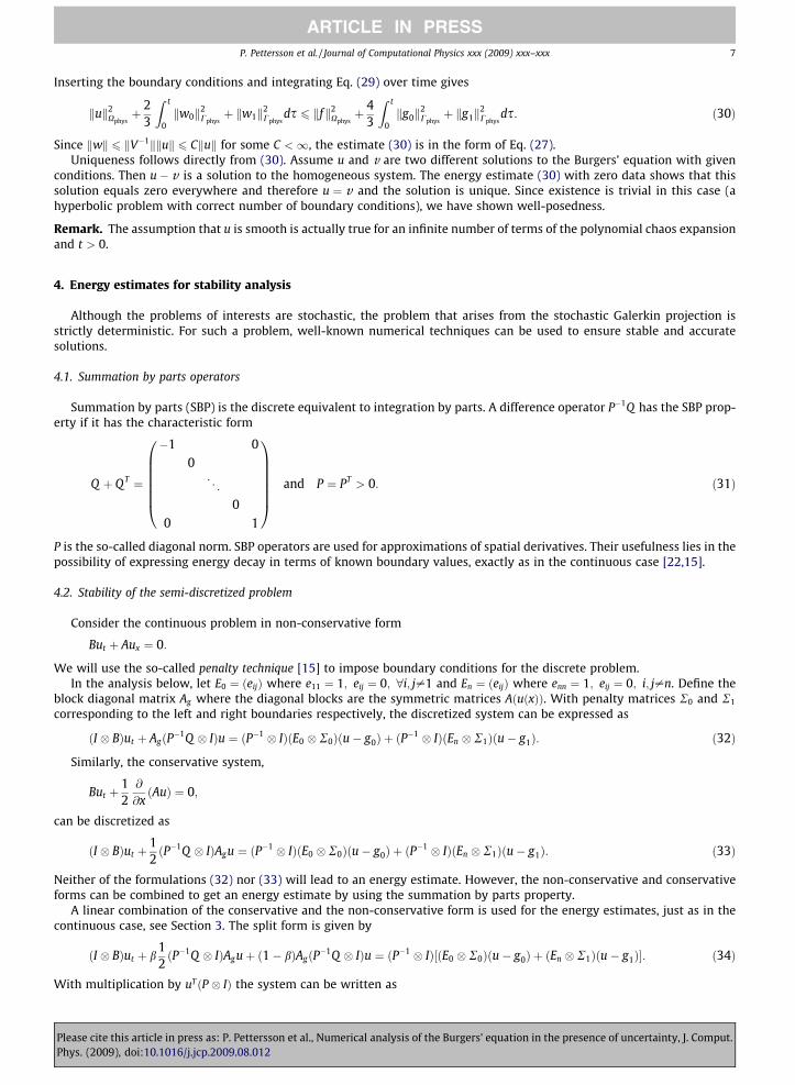
P is the so-called diagonal norm. SBP operators are used for approximations of spatial derivatives. Their usefulness lies in thepossibility of expressing energy decay in terms of known boundary values, exactly as in the continuous case [22,15].

4.2. Stability of the semi-discretized problem

Consider the continuous problem in non-conservative form

But þ Aux ¼ 0:

We will use the so-called penalty technique [15] to impose boundary conditions for the discrete problem.In the analysis below, let E0 ¼ ðeijÞ where e11 ¼ 1; eij ¼ 0; 8i; j–1 and En ¼ ðeijÞ where enn ¼ 1; eij ¼ 0; i; j–n. Define the

block diagonal matrix Ag where the diagonal blocks are the symmetric matrices AðuðxÞÞ. With penalty matrices R0 and R1

corresponding to the left and right boundaries respectively, the discretized system can be expressed as

ðI � BÞut þ AgðP�1Q � IÞu ¼ ðP�1 � IÞðE0 � R0Þðu� g0Þ þ ðP�1 � IÞðEn � R1Þðu� g1Þ: ð32Þ

Similarly, the conservative system,

But þ12@

@xðAuÞ ¼ 0;

can be discretized as

ðI � BÞut þ12ðP�1Q � IÞAgu ¼ ðP�1 � IÞðE0 � R0Þðu� g0Þ þ ðP�1 � IÞðEn � R1Þðu� g1Þ: ð33Þ

Neither of the formulations (32) nor (33) will lead to an energy estimate. However, the non-conservative and conservativeforms can be combined to get an energy estimate by using the summation by parts property.

A linear combination of the conservative and the non-conservative form is used for the energy estimates, just as in thecontinuous case, see Section 3. The split form is given by

ðI � BÞut þ b12ðP�1Q � IÞAguþ ð1� bÞAgðP�1Q � IÞu ¼ ðP�1 � IÞ½ðE0 � R0Þðu� g0Þ þ ðEn � R1Þðu� g1Þ�: ð34Þ

With multiplication by uTðP � IÞ the system can be written as




ARTICLE IN PRESS

PleasePhys.

uTðP � BÞut þb2

uTðQ � IÞAguþ ð1� bÞuTðP � IÞAgðP�1Q � IÞu ¼ uTðE0 � R0Þðu� g0Þ þ uTðEn � R1Þðu� g1Þ: ð35Þ

We will use the commutativity property

Ag ¼ ðP � IÞAgðP�1 � IÞ: ð36Þ

We add the transpose to (35) and use (36) to get

@

@tkuk2

ðP�BÞ þb2

uT ðQ � IÞAg þ AgðQ T � IÞ

uþ ð1� bÞuTðAgðQ � IÞ þ ðQT � IÞAgÞu

¼ 2uTðE0 � R0Þðu� g0Þ þ 2uTðEn � R1Þðu� g1Þ: ð37Þ

As before, we choose b such that

b2¼ 1� b() b ¼ 2

3:

By the summation by parts property (31) this yields the desired form

@

@tkuk2

ðP�BÞ ¼23

uTx¼0Aux¼0 � uT

x¼1Aux¼1� �

þ 2uTx¼0R0ðux¼0 � g0Þ þ 2uT

x¼1R1ðux¼1 � g1Þ: ð38Þ

Restructuring (38) yields

@

@tkuk2

ðP�BÞ ¼ uTx¼0

23

Aþ 2R0

� �ux¼0 � 2uT

x¼0R0g0 � uTx¼1

23

A� 2R1

� �ux¼1 � 2uT

x¼1R1g1: ð39Þ

Stability is achieved by a proper choice of the penalty matrices R0 and R1. For that purpose A is split according to the sign ofits eigenvalues as

A ¼ Aþ þ A� where Aþ ¼ xTKþx and A� ¼ xTK�x: ð40Þ

Choose R0 and R1 such that 23 Aþ þ 2R0 ¼ � 2

3 Aþ () R0 ¼ � 23 Aþ and 2

3 A� � 2R1 ¼ 23 A� () R1 ¼ 2

3 A�. We now get the energyestimate

@

@tkuk2

ðP�BÞ ¼ �23ðux¼0 � g0Þ

T Aþðux¼0 � g0Þ þ23

uTx¼0A�ux¼0 þ gT

0Aþg0

� �� 2

3uTðx¼1ÞA

þuðx¼1Þ þ gT1A�g1

h iþ 2

3ðuðx¼1Þ

� g1ÞT A�ðuðx¼1Þ � g1Þ; ð41Þ

which shows that the system is stable.

Remark. In the numerical calculations we use (33) for correct shock speed, see [14].

5. Artificial dissipation operators

An artificial dissipation operator is a discretized even order derivative which is added to the system to allow stable andaccurate solutions to be obtained in the presence of solution discontinuities. The artificial dissipation is designed to trans-form the global discretization into a one-sided operator close to the shock location. Depending on the accuracy of the dif-ference scheme, this require one or more dissipation operators. The accuracy of the difference approximation is chosen ashigh as possible within the computational stencil of the difference approximation of the system matrix. All dissipation oper-ators used here are of the form

A2k ¼ �DxP�1 eDTk Bw

eDk; ð42Þ

where P�1 is the diagonal norm of the first derivative as before, eD is an approximation of ðDxÞk@k=@xk and Bw is a diagonalpositive definite matrix. In most cases here, Bw is replaced by a single constant bw. An appropriate choice of dissipation con-stant results in an upwind scheme, suitable for problems where shocks evolve. For further reading about the design of arti-ficial dissipation operators we refer to [15].

The complete difference approximation (33) augmented with artificial dissipation is given by

ðP � BÞut þ12ðQ � IÞAgu� ðE0 � R0Þðu� g1Þ � ðEn � R1Þðu� g1Þ ¼ �Dx

Xk

ðeDTk � BÞBw;kðeDk � IÞu; ð43Þ

where Bw;k is a possibly non-constant weight matrix to be determined and k ¼ 1;2 for the fourth order accurate SBP operator.Determining Bw in (42) requires estimates of the eigenvalues kj of B�1A for j ¼ 0; . . . ;M; the largest eigenvalue is typically

sufficient. For the system of equations generated by polynomial chaos expansion of Burgers’ equation, max jkj is not alwaysknown. Since the only non-zero polynomial coefficients on the boundaries are u0 and u1 and since the polynomial chaosexpansion converges in the L2 sense, a reasonable approximation of the maximum eigenvalue of B�1A is




ARTICLE IN PRESS

PleasePhys.

jkjmax � ju0j þMju1j; ð44Þ

where M is the order of polynomial chaos expansion. This estimate is justified by the eigenvalue analysis performed in thenext section as well as by computational results. For the dissipation operators A2 and A4 in the simulations, we use

Bw;2 ¼ diagðju0j þMju1jÞ

6Dx

� �; Bw;4 ¼ diag

ðju0j þMju1jÞ24Dx

� �: ð45Þ

The second order dissipation operator is only applied close to discontinuities.

6. Time integration

The increase in simulation cost associated with higher order systems is due to a number of factors. The size of the systemdepends both on the number of terms in the truncated polynomial chaos expansion and the spatial mesh size.

For the Kronecker product A� B the relation

ki;jA�B ¼ ki

AkjB ð46Þ

holds, where the indices i; j denotes all the eigenvalues of A and B respectively. This enables a separate analysis of the eigen-values corresponding to the polynomial chaos expansion and the eigenvalues of the total spatial difference operator D.Assuming constant coefficients, the maximum system eigenvalue is limited by

kmax 6 ðmax kDÞðmax kB�1AÞ: ð47Þ

The estimate (47) in combination with (44) will be used in order to obtain estimates of the time step constraint.

6.1. Eigenvalue approximation

Analytic eigenvalues for the matrix B�1A can only be obtained for a small number of polynomial chaos coefficients andtherefore approximations are needed. Even though most eigenvalues of interest in this report can be calculated exactlyfor every particular case, a general estimate is of interest. The approximation of the largest eigenvalue of the scaled systemmatrix B�1A is calculated from solution values on the boundaries, which are the only values known a priori. For smooth solu-tions with boundary conditions where the polynomial chaos coefficients ui are equal to 0 for i > 1, the higher order coeffi-cients tend to remain small compared to lower order coefficients (strong probabilistic convergence). For solutions where ashock is developing, higher order polynomial chaos coefficients might grow and the approximation of the largest eigenvaluebased on boundary values is likely to be a less accurate estimate.

To get estimates of the eigenvalues, the system of equations can be written

ut þ B�1XM

i¼0

AiðuiÞ !

ux ¼ 0; ð48Þ

where AðuÞ ¼ Aiui is a linear combination of the polynomial chaos coefficients. The eigenvalue approximation used here isgiven by

max kB�1A ¼maxxTðB�1PAiuiÞx

xT x6

Xi

maxxT

i B�1Aixi

xTi xi

juij ¼X

i

juijmax jkij: ð49Þ

Since B�1A0ðu0Þ ¼ u0I, this approximation coincides with the exact eigenvalue for boundary value with ui ¼ 0 for i > 1. Thiscan be seen by observing that if x1 is an eigenvector with corresponding eigenvalue k for the matrix B�1A1 then B�1A1x ¼ kxand

B�1ðA1u1 þ A0u0Þx ¼ u1kxþ u0Ix ¼ ðu1kþ u0Þx; ð50Þ

so u1kþ u0 and x1 are eigenvalue and eigenvector to the matrix B�1ðA0u0 þ A1u1Þ ¼ B�1A. This shows that (44) is an appro-priate eigenvalue approximation for problems where only u0 and u1 are non-zero on the boundaries.

For a given boundary condition, the maximum eigenvalue of A0 corresponding to the deterministic part of the conditiondoes not change with increasing number of polynomial chaos coefficients. However, the largest eigenvalue contribution fromA1 grows with the number of polynomial chaos coefficients.

The eigenvalue approximation (44) is in general of the same order of magnitude as the largest eigenvalue in the interior ofthe domain but might have to be adjusted to remove all oscillations. The exact value is problem specific and an estimatebased on the interior values requires knowledge about the solution of the problem.

6.2. Efficiency of the polynomial chaos method

The convergence of the polynomial chaos expansion is investigated by measuring the discrete Euclidean error norm of thevariance and the expected value. For a discretization with m spatial grid points, we have



Table 1Convergence to (16) and (17) with the Monte Carlo method, m ¼ 400; t ¼ 0:3.

N 10 50 100 400 1600

k�Expk 0.122 0.0374 0.0344 0.0257 0.0151k�Vark 0.127 0.0589 0.0426 0.0283 0.0189T (s) 240 1180 2390 9350 38,460

Table 2Convergence to (16) and (17) with the polynomial chaos method, m ¼ 400; t ¼ 0:3.

M 2 4 6 8

k�Expk 0.113 0.0544 0.0164 0.0150k�Vark 0.147 0.122 0.0409 0.0630T (s) 126 636 4180 10,900

Fig. 1. The first four PC coefficients, t ¼ 0:3; M ¼ 5 and M ¼ 3;m ¼ 400.


ARTICLE IN PRESS

PleasePhys.

k�Expk2 ¼ 1m� 1

Xm

i¼1

ðE½u�m � E½uref �mÞ2

and



Table 3Norms

M

k�Exp

k�Var


ARTICLE IN PRESS

PleasePhys.

k�Vark2 ¼ 1m� 1

Xm

i¼1

ðVar½u�m � Var½uref �mÞ2;

where uref denotes the analytical solution. Consider the model problem (12); the problem is solved with the Monte Carlomethod and PC until time t ¼ 0:3. Accuracy (measured as the norm of the difference between the actual solution and theanalytical solution) and simulation cost are shown in Table 1 for the Monte Carlo method and Table 2 for the PC expansions.

For this highly non-linear and discontinuous problem, the polynomial chaos method is more efficient than the Monte Car-lo method with low accuracy requirements. The convergence properties of these solutions are affected by the spatial gridsize and the accuracy of imposed artificial dissipation and no general conclusion of the relative performances of the twomethods will be drawn here. As will be further illustrated in the section on analysis of characteristics, the solution coeffi-cients of the truncated system are discontinuous approximations to the analytical coefficients which are smooth. Eventhough the PC results do converge for this problem, the low order expansions are qualitatively very different from the ana-lytical solution, see for instance Fig. 1. Also, note that excessive use of artificial dissipation is likely to produce a solutioncloser to the analytical solution for lower order expansions. Note that, as expected spatial grid refinement leads to conver-gence to the true solution of the truncated system but does not get any closer to the analytical solution.

The use of artificial dissipation proportional to the largest eigenvalue makes the solutions of large order expansions dis-sipative and spatial grid refinement is needed for an accurate solution. This can be seen in Table 2, where the accuracy of thevariance decreases with large M.

6.3. Numerical convergence

The convergence of the computed polynomial chaos coefficients, the expected value and the variance of the truncatedsystem is investigated and comparisons to the analytical solution derived in Section 2.3 are presented.

As mentioned earlier, the numerical results obtained for a small number of expansion terms is expected to be a poorapproximation to the analytical solution; this is confirmed by the mesh refinement study reported in Fig. 1 for M ¼ 5. In thisparticular application, the analytical solution admits continuous (smooth) coefficients in spite of the discontinuous initialcondition; on the other hand, the coefficients of the truncated system are discontinuous.

Interestingly, the difference between the computed coefficients corresponding to a finite PC expansion (ui for i 6 M) andthe analytical ðM ¼ 1Þ coefficients indicates that a poorly resolved numerical solution with excessive dissipation might be

Fig. 2. Dissipative solution on coarse grid ðm ¼ 200Þ, computed for M ¼ 3 and non-dissipative solution for M ¼ 4.

of errors for dissipative and non-dissipative solutions.

3 3 (dissipative) 4

k 0.0354 0.0173 0.0374k 0.0918 0.0370 0.0723




ARTICLE IN PRESS

qualitatively closer to the analytical solution than a grid converged solution to the truncated system. Fig. 2 and Table 3 illus-trates this phenomenon of illusory convergence.

The discrepancy between the truncated solution for M ¼ 3 and the analytical solution is also illustrated in Fig. 3. The coef-ficients do not converge to the analytical solution when the spatial grid is refined (Fig. 3(a), left). Instead the coefficients con-verge numerically to a reference solution corresponding to a numerical solution obtained with a large number of gridpoints(Fig. 3(a), right). For the 7th order expansion, the solution is sufficiently close the solution of the analytical problem to exhibitspatial numerical convergence of the first four coefficients to the analytical coefficients (Fig. 3(b)).

The variance calculated for M ¼ 7 appears to converge to a function that is close but not equal to the analytical variancegiven by (17), see Fig. 4.

Fig. 3. Convergence of the first chaos coefficients. Note the different scales in the figures.

Please cite this article in press as: P. Pettersson et al., Numerical analysis of the Burgers’ equation in the presence of uncertainty, J. Comput.Phys. (2009), doi:10.1016/j.jcp.2009.08.012



ARTICLE IN PRESS

7. Theoretical results and interpretation

7.1. Analysis of characteristics: disturbed cosine wave

In this section, the characteristics of the stochastic Burgers’ equation with M ¼ 1 (truncated to 2� 2 system) will beinvestigated to give a qualitative measure of the time development of the solution. The system is given by

Fig. 4.(right).

PleasePhys.

u0

u1

� �t

þu0 u1

u1 u0

� �u0

u1

� �x

¼ 0: ð51Þ

With w1 ¼ u0 þ u1 and w2 ¼ u0 � u1, (51) can be diagonalized and rewritten

w1

w2

� �t

þw1 00 w2

� �w1

w2

� �x

¼ 0: ð52Þ

Eq. (52) is the original Burgers’ equation for w1;w2 and the shock speeds are given by

sw1 ¼½f ðw1Þ�½w1�

¼ w1R þw1L

2¼ �u0 þ �u1 ð53Þ

and

sw2 ¼½f ðw2Þ�½w2�

¼ w2R þw2L

2¼ �u0 � �u1; ð54Þ

where we have introduced the mean over the shock, �ui ¼ ðuiL þ uiRÞ=2. Double brackets [] denotes the jump in a quantity overa discontinuity. Similarly to (53) and (54), with the non-diagonalized system in conservation form, the propagation speeds ofdiscontinuities in u0;u1 are given by

su0 ¼u2

0 þ u21

� �=2

� �½u0�

¼ �u0 þ �u1½u1�½u0�

ð55Þ

and

su1 ¼½u0u1�½u1�

¼ �u0 þ �u1½u0�½u1�

: ð56Þ

The analysis of characteristics w1 and w2 describes the behavior and emergence of discontinuities in the coefficients u0 andu1 of the truncated system. However, the coefficients of the solution to the problem given by the infinite PC expansion aresmooth (except for t ¼ 0 for the Riemann problem). Diagonalization of large systems is not feasible but we can obtainexpressions for the shock speeds of the coefficients. For instance, the expression (55) for the shock speed in u0 can begeneralized for expansions of order M as

M ¼ 7. Convergence of the variance. Norm of the error relative to the analytical variance (left) and error relative to the finest grid variance, m ¼ 800




ARTICLE IN PRESS

PleasePhys.

su0 ¼XM

i¼0

�ui½ui�½u0�

i! ð57Þ

In the assumption that only one Gaussian variable n is introduced, and the uncertainty is (linearly) proportional to n only alimited number of different values of the correlation coefficient between the left and right state can occur. Since we are alsoassuming the same model for the left and right state uncertainties, only a few combinations of covariance matrices describ-ing their correlation are realizable. With the assumptions made here, the dependence between the two states is determinedby the correlation coefficient qLR, which for these cases is either 1 or �1.

Ex 1:1 Ex 1:2

uðx; 0; nÞ ¼uL ¼ 1þ r̂n x < x0;

uR ¼ �1� r̂n x < x0;

�uðx;0; nÞ ¼

uL ¼ 1þ r̂n x < x0;

uR ¼ �1þ r̂n x < x0;

�uðx; 0Þ ¼ cosðpxÞð1þ r̂nÞ; uðx;0Þ ¼ cosðpxÞ þ r̂n;

n 2 Nð0;1Þ; n 2 Nð0;1Þ;qLR ¼ �1: qLR ¼ 1:

Fig. 5. Development of variance of the perturbed cosine wave. t ¼ 0:5 for M ¼ 3; m ¼ 400.




ARTICLE IN PRESS

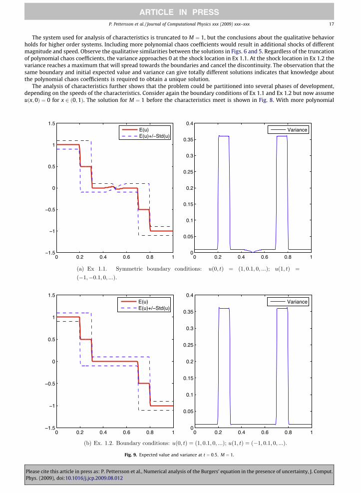
The problems are similar in terms of expected value and variance at the boundary, but the difference in correlation betweenthe left and right states completely change the behavior over time. The difference in initial variance in the interior of thedomain has only a limited impact on the time-dependent difference between the solutions; this has been checked by varyingthe initial functions. Note that Ex 1.1 is included to show the importance of the sign of the stochastic variable, but is a specialcase of a more general phenomenon of superimposition of discontinuities exhibited by Ex 1.2 and further explained and ana-lyzed below. Fig. 5 shows the two cases at time t ¼ 0:5 for M ¼ 3. We use r̂ ¼ 0:1 and x0 ¼ 0:5.

Fig. 7. Variance of Ex 1.1 and Ex 1.2 for M ¼ 1, calculated from w1; w2 using (59).

Fig. 6. Characteristics of the two perturbed cosine waves (Ex 1.1 and Ex 1.2) for M ¼ 1.




ARTICLE IN PRESS

To explain the differences between the solutions depicted in Fig. 5, we turn to analysis of the characteristics for the trun-cated system with M ¼ 1. The polynomial chaos coefficients of the boundaries are given by

PleasePhys.

u0 ¼ 1u1 ¼ 0:1

x ¼ 0;

u0 ¼ �1u1 ¼ �0:1

x ¼ 1 ðEx1:1Þ

and

u0 ¼ 1u1 ¼ 0:1

x ¼ 0;

u0 ¼ �1u1 ¼ 0:1

x ¼ 1 ðEx1:2Þ;

respectively.Note that with more polynomial chaos coefficients included, the higher order coefficients are zero at the boundaries. The

expected boundary values as well as the boundary variance are the same for Ex 1.1 and Ex 1.2. In order to relate the conceptsof characteristics with expected value and variance, we will use the fact that the expected value at each point is the averageof the characteristics,

EðuÞ ¼ u0 ¼w1 þw2

2ð58Þ

and that the variance depends on the distance between the characteristics,

VarðuÞ ¼ u21 ¼

w1 �w2

2

2: ð59Þ

To explain the qualitative differences between the two cases Ex 1.1 and Ex 1.2, consider the decoupled system (52). Theboundary values for u0 and u1 are inserted into the characteristic variables w1 and w2; discontinuities emerge when the char-acteristics meet.

For Ex 1.1 we have w1ðx ¼ 0Þ ¼ �w1ðx ¼ 1Þ and w2ðx ¼ 0Þ ¼ �w2ðx ¼ 1Þ. Inserting these values in (53) and (54) gives theshock speeds sw1 ¼ sw2 ¼ 0, corresponding to two stationary shocks (of different magnitude) at x ¼ 0:5, which can be seen inFig. 6(a). Inserting the characteristic values (can be evaluated in Fig. 6) into Eq. (59) result in uniform variance except aroundthe discontinuity, Fig. 7(a). Since the characteristic solution is propagating from the boundaries, this interval shrinks withtime and collapses at x ¼ 0:5.

In Ex 1.2, the characteristics are w1ðx ¼ 0Þ ¼ 1:1 > �w1ðx ¼ 1Þ ¼ 0:9 and w2ðx ¼ 0Þ ¼ 0:9 < �w2ðx ¼ 1Þ ¼ 1:1. Evaluating(53) and (54) when the characteristics cross yields sw1 ¼ 0:1 and sw2 ¼ �0:1. The discontinuity when the characteristics meetwill then split and propagate as two moving shocks in u0 and u1, located equidistantly from the mid-point x ¼ 0:5. In w1 andw2 there will still be a single shock. The shock speeds are given by the expressions (53)–(56). The vertical gap between thecharacteristics at x ¼ 0:5 in Fig. 6(b) corresponds to the variance peak at this location in Fig. 5(b).

Fig. 8. Characteristics at t ¼ 0:5; M ¼ 1.




ARTICLE IN PRESS

The system used for analysis of characteristics is truncated to M ¼ 1, but the conclusions about the qualitative behaviorholds for higher order systems. Including more polynomial chaos coefficients would result in additional shocks of differentmagnitude and speed. Observe the qualitative similarities between the solutions in Figs. 6 and 5. Regardless of the truncationof polynomial chaos coefficients, the variance approaches 0 at the shock location in Ex 1.1. At the shock location in Ex 1.2 thevariance reaches a maximum that will spread towards the boundaries and cancel the discontinuity. The observation that thesame boundary and initial expected value and variance can give totally different solutions indicates that knowledge aboutthe polynomial chaos coefficients is required to obtain a unique solution.

The analysis of characteristics further shows that the problem could be partitioned into several phases of development,depending on the speeds of the characteristics. Consider again the boundary conditions of Ex 1.1 and Ex 1.2 but now assumeuðx;0Þ ¼ 0 for x 2 ð0;1Þ. The solution for M ¼ 1 before the characteristics meet is shown in Fig. 8. With more polynomial

Fig. 9. Expected value and variance at t ¼ 0:5; M ¼ 1.



Fig. 10. Characteristics at t ¼ 4 for M ¼ 1.


ARTICLE IN PRESS

chaos coefficients, the sharp edges in the solution will disappear. At time t ¼ 0:5, the solutions to the two problems are stillsimilar, with two variance peaks at the shocks that are traveling towards the middle of the domain.

For comparison, Fig. 9 shows the expected value and variance calculated from the characteristics in Fig. 8.Asymptotically in time, the symmetric problem (Ex 1.1) will result in a stationary shock. The variance will equal the initial

boundary variance except for a peak at the very location of the shock. The boundary conditions are independent of time. Thisproperty is illustrated in Fig. 10(a), where the solution has reached steady state.

The time development of the solution of Ex 1.2 is not consistent with the stationary boundary conditions stated in theproblem formulation. The characteristics are transported from one boundary to the other (see Fig. 10(b)), thus changingthe boundary data. The boundary conditions of Ex 1.2 must therefore be time-dependent (and can be calculated exactly from(14) for this example). Unlike the continuously varying boundary conditions of the full polynomial chaos expansion problem,the boundary conditions for the truncated system of Fig. 10(b) will change discontinuosly from the initial boundary condi-tion to zero at the moment the characteristics reach the boundaries. In a general hyperbolic problem, the imposition of cor-rect time-dependent boundary conditions might become one of the more significant problems with the PC method. Adetailed investigation is necessary to identify an approach to specify time-dependent stochastic boundary data, especiallyfor the higher order moments. Special non-reflecting boundary conditions will be required. In the case studied here, analyt-ical boundary conditions have been derived and can be correctly imposed for any time and order of chaos expansions.

8. Summary and conclusions

The polynomial chaos approach, together with finite difference methods, is used to solve the Burgers’ equation underuncertain initial and boundary conditions. Stable difference schemes are obtained by the use of artificial dissipation, differ-ence operators satisfying the summation by parts property and a weak imposition of characteristic boundary conditions.

A number of mathematical properties of the deterministic Burgers’ equation hold for the hyperbolic problem that resultsfrom the Galerkin projection of the truncated PC expansions. The system is symmetric and a split form combining conser-vative and non-conservative formulations is used to obtain an energy estimate. The truncated linearized problem is shown tobe well-posed. The system eigenvalues cannot be computed analytically and this makes the choice of the time step difficult;moreover, this affects the accuracy of the methods since the dissipation operators are eigenvalue dependent. An eigenvalueestimate is provided.

Even though the solution of the Burgers’ equation is discontinuous for a particular value of the uncertain (stochastic) var-iable, the polynomial chaos coefficient functions are in general continuous for the Riemann problems investigated. The solu-tion coefficients of the truncated system are discontinuous and can be treated as a superimposition of a finite number ofdiscontinuous characteristic variables. This has been shown explicitly for the 2� 2-case. The discontinuous coefficients con-verge with the number of polynomial chaos coefficients to continuous functions.

Examples have shown the need to provide time-dependent boundary conditions that might include higher order mo-ments. Stochastic time-dependent boundary conditions have been derived for the Burgers’ equation.




ARTICLE IN PRESS

References

[1] Guide for the Verification and Validation of Computational Fluid Dynamics Simulations, No. AIAA-G-077-1998, American Institute of Aeronautics andAstronautics, Reston, VA, 1998.

[2] P.S. Beran, C.L. Pettit, D.R. Millman, Uncertainty quantification of limit-cycle oscillations, Journal of Computational Physics 217 (1) (2006) 217–247.[3] R.H. Cameron, W.T. Martin, The orthogonal development of non-linear functionals in series of Fourier–Hermite functionals, The Annals of Mathematics

48 (2) (1947) 385–392.[4] M.H. Carpenter, D. Gottlieb, S. Abarbanel, Time-stable boundary conditions for finite-difference schemes solving hyperbolic systems: methodology and

application to high-order compact schemes, Journal of Computational Physics 111 (1994) 220–236.[5] M.H. Carpenter, J. Nordström, D. Gottlieb, A stable and conservative interface treatment of arbitrary spatial accuracy, Journal of Computational Physics

148 (1999) 341–365.[6] C. Chauvière, J.S. Hesthaven, L. Lurati, Computational modeling of uncertainty in time-domain electromagnetics, SIAM Journal on Scientific Computing

28 (2) (2006) 751–775.[7] Q.-Y. Chen, D. Gottlieb, J.S. Hesthaven, Uncertainty analysis for the steady-state flows in a dual throat nozzle, Journal of Computational Physics 204

(2005) 378–398.[8] M. Christie, V. Demyanov, D. Erbas, Uncertainty quantification for porous media flows, Journal of Computational Physics 217 (1) (2006) 143–158.[9] D. Funaro, Polynomial approximation of differential equations, Springer-Verlag, New York, 1992.

[10] R. Ghanem, P. Spanos, Stochastic Finite Elements: A Spectral Approach, Springer-Verlag, New York, 1991.[11] G.H. Golub, C.F. van Loan, Matrix Computations, second ed., Johns Hopkins University Press, Baltimore, 1989.[12] B. Gustafsson, H.-O. Kreiss, J. Oliger, Time Dependent Problems and Difference Methods, Wiley, 1995.[13] T.Y. Hou, W. Luo, B. Rozovskii, H.-M. Zhou, Wiener chaos expansions and numerical solutions of randomly forced equations of fluid mechanics, Journal

of Computational Physics 216 (2) (2006) 687–706.[14] R. LeVeque, Numerical Methods for Conservation Laws, second ed., Birkhäuser, Basel, 2006.[15] K. Mattsson, M. Svärd, J. Nordström, Stable and accurate artificial dissipation, Journal of Scientific Computing 21 (1) (2004) 57–79.[16] J. Nordström, Conservative finite difference formulations, variable coefficients, energy estimates and artificial dissipation, Journal of Scientific

Computing 29 (3) (2006) 375–404.[17] J. Nordström, M.H. Carpenter, Boundary and interface conditions for high-order finite-difference methods applied to the Euler and Navier–Stokes

equations, Journal of Computational Physics 148 (1999) 621–645.[18] J. Nordström, M.H. Carpenter, High-order finite difference methods, multidimensional linear problems and curvilinear coordinates, Journal of

Computational Physics 173 (2001) 149–174.[19] S.V. Poroseva, J. Letschert, M.Y. Hussaini, Application of evidence theory to quantify uncertainty in forecast of Hurricane path, in: Proceedings of the

18th Conference on Probability and Statistics, The American Meteorological Society 86th Annual Meeting, Atlanta, GA, 2006.[20] M.T. Reagan, H.N. Najm, R.G. Ghanem, O.M. Knio, Uncertainty quantification in reacting-flow simulations through non-intrusive spectral projection,

Combustion and Flame 132 (3) (2003) 545–555.[21] R.D. Richtmyer, K.W. Morton, Difference Methods for Initial-Value Problems, second ed., Interscience Publishers, New York, 1967.[22] B. Strand, Summation by parts for finite difference approximations for d/dx, Journal of Computational Physics 110 (1994) 47–67.[23] G. Szegö, Orthogonal Polynomials, fourth ed., American Mathematical Society, Providence, 1975.[24] X. Wan, G.E. Karniadakis, Long-term behavior of polynomial chaos in stochastic flow simulations, Computer Methods in Applied Mechanics and

Engineering 195 (41–43) (2006) 5582–5596.[25] N. Wiener, The homogeneous chaos, American Journal of Mathematics 60 (4) (1938) 897–936.[26] J. Witteveen, S. Sarkar, H. Bijl, Modeling physical uncertainties in dynamic stall induced fluid–structure interaction of turbine blades using arbitrary

polynomial chaos, Computers and Structures 85 (2007) 866–878.[27] D. Xiu, G.E. Karniadakis, The Wiener–Askey polynomial chaos for stochastic differential equations, SIAM Journal on Scientific Computing 24 (2) (2002)

619–644.[28] D. Xiu, G.E. Karniadakis, Modeling uncertainty in flow simulations via generalized polynomial chaos, Journal of Computational Physics 187 (1) (2003)

137–167.[29] D. Xiu, G.E. Karniadakis, Supersensitivity due to uncertain boundary conditions, International Journal for Numerical Methods in Engineering 61 (2004)

2114–2138.[30] Y. Yu, M. Zhao, T. Lee, N. Pestieau, W. Bo, J. Glimm, J.W. Grove, Uncertainty quantification for chaotic computational fluid dynamics, Journal of

Computational Physics 217 (1) (2006) 200–216.



Numerical analysis of the Burgers’ equation in the presence of uncertainty

Documents

Transcript of Numerical analysis of the Burgers’ equation in the presence of uncertainty