Numerical analysis of a screen mesh wick heat pipe with Cu/water nanofluid

This article appeared in a journal published by Elsevier. The attachedcopy is furnished to the author for internal non-commercial researchand education use, including for instruction at the authors institution

and sharing with colleagues.

Other uses, including reproduction and distribution, or selling orlicensing copies, or posting to personal, institutional or third party

websites are prohibited.

In most cases authors are permitted to post their version of thearticle (e.g. in Word or Tex form) to their personal website orinstitutional repository. Authors requiring further information

regarding Elsevier’s archiving and manuscript policies areencouraged to visit:

http://www.elsevier.com/authorsrights

http://www.elsevier.com/authorsrights

Author's personal copy

Numerical analysis of a screen mesh wick heat pipe with Cu/waternanofluid

A. Brusly Solomon, K. Ramachandran ⇑, L. Godson Asirvatham, B.C. PillaiCentre for Research in Material Science and Thermal Management, School of Mechanical Sciences, Karunya University, Coimbatore 641114, India

a r t i c l e i n f o

Article history:Received 21 December 2013Received in revised form 2 April 2014Accepted 3 April 2014Available online 6 May 2014

Keywords:Heat pipesNanofluidsNumerical analysisCapillary pressurePore sizeDryout

a b s t r a c t

A two-dimensional transient numerical model is developed to predict the vapor core, wall temperatures,vapor pressure, vapor velocity and liquid velocity in the screen mesh wick heat pipe. The mass, momen-tum and energy equations are solved numerically for liquid and vapor regions. The effect of Cu–waternanofluid on the heat transfer performance of heat pipe is studied using the developed model and thesame is compared with that of the DI water. The transient profiles of vapor and liquid velocities in thewick region and the location of dry-out in the evaporator section of the heat pipe are also obtained usingthe developed model. It is found that the addition of nanoparticles leads to the reduction in wall temper-ature, operating pressure, vapor temperature and total resistance of the heat pipe; thereby, increasing theheat transfer of the heat pipe at the same heat load. Interestingly, the liquid and vapor velocities of theheat pipe charged with 0.1 wt% of Cu-water nanofluid is found to be 20% higher when compared with thatof the heat pipe with DI water at the same operating conditions. It is also observed that the decreasedpore size of the wick due to the addition of nanoparticles increases the effective thermal conductivityof the wick structure which acts as a coating layer and enhances the heat transfer capability of the heatpipe.

� 2014 Elsevier Ltd. All rights reserved.

1. Introduction

Heat pipes are hollow metal enclosures partly filled with aliquid coolant that moves heat from one end to another continu-ously by evaporation and condensation of the liquid due tocapillary pressure. After the invention of heat pipe much advance-ment have been taken place during the past few decades withrespect to the design construction and operating fluid etc. specificto the application. Recently, Faghri [1] reviewed the advances inheat pipe technology including various types of heat pipes, heatpipe analysis and simulations. Heat pipes have been used in severalapplications such as electronic cooling [2], heat recovery in renew-able energy [3], and heat exchangers [4], etc. Modern develop-ments in coolant fluid such as a nanofluid led to furtheradvancement in heat pipe technology in the field of electronic cool-ing applications. Kakac and Pramuanjaroenkij [5] reviewed theflow and heat transfer characteristics of nanofluids under freeand forced convection modes. This study showed that thenanofluids significantly improved the heat transfer capability ofconventional fluids such as oil and water. It is also reported that

the reason for enhancement is due to the higher thermal conduc-tivity of the suspended nanoparticles in the base fluids. Followingthat many experimental studies [6–10] have been carried out tostudy the effect of nanofluids on the heat transfer performance ofheat pipes. In a study [11] various types of nanofluids (silver, cop-per, Al2O3, gold, diamond) used in heat pipes and the mechanismfor the heat transfer enhancement are presented. It is observedthat the enhancement in heat transfer is not only by the thermophysical properties of nanofluids but also by the nature of thesurface formed during boiling process in the evaporator section.Similarly, many numerical studies have also been performed topredict the heat transfer enhancement of nanofluid by conven-tional numerical methods and new Lattice Boltzmann Method(LBM) [12]. Though the mechanism for heat transfer enhancementis understood to an extent, still there are lots of issues taking placein the micro level are unclear. Hence more numerical studies arenecessary to get more insights on the heat transfer enhancementmechanism.

Tien and Rohani [13] analyzed the effects of vapor pressurevariation on the vapor temperature distribution, evaporation andcondensation rates, and the overall performance of the heat pipe.Chen and Faghri [14] analyzed the heat conduction between thewall and liquid-wick interface and the compressibility effects.Huckaby et al. [15] performed a one dimensional analysis using a

http://dx.doi.org/10.1016/j.ijheatmasstransfer.2014.04.0070017-9310/� 2014 Elsevier Ltd. All rights reserved.

⇑ Corresponding author. Address: Department of Physics, Bharathiar University,Coimbatore, India. Tel.: +91 422 2614439; fax: +91 422 2615615.

E-mail address: [email protected] (K. Ramachandran).

International Journal of Heat and Mass Transfer 75 (2014) 523–533

Contents lists available at ScienceDirect

International Journal of Heat and Mass Transfer

journal homepage: www.elsevier .com/locate / i jhmt


collocation-spectral method to compute the dynamic behavior ofthe vapor flow in a heat pipe. Two-dimensional, heat pipe transientanalysis model (HPTAM) is developed and benchmarked by Tour-nier et al. [16] using transient experimental data for cumulativeoperations of fully-thawed heat pipes. Tournier and El-Genk [17]developed free-molecular, transition and continuum vapor flowmodel, based on the dusty gas model, incorporated in HPTAM, toanalyze the startup of a radiatively-cooled sodium heat pipe froma frozen state. Legierski et al. [18] conducted a study on the model-ing and measurements of heat and mass transfer in heat pipes usingthe FLUENT commercial code. Alizadehdakhel et al. [19] studied agas/liquid two-phase flow and the simultaneous evaporation andcondensation phenomena by using the volume of the fluid model(VOF) technique in a thermosyphon using FLUENT code.

Vadakkan et al. [20] developed a numerical model to analyzethe transient performance of flat heat pipes for high heat fluxesand high wick conductivity. In another study, Vadakkan et al.[21] developed a three-dimensional model to analyze the transientand steady-state performance of the flat heat pipe with multipleheating sources. Ranjan et al. [22] developed a micro scale evapo-ration model for thin-film evaporation in capillary wick structures.This micro scale evaporation model is coupled with the general(macro) model to include the microstructure effects in the liquid/vapor interface [23]. The meniscus curvature at every locationalong the wick is calculated as a result of this coupling. This cou-pled model is used to predict the thermal transport in heat pipesand vapor chambers. Carbajal et al. [24] developed a quasi-3Dnumerical model to analyze the flat heat pipe. Rice and Faghri[25] performed a complete numerical analysis of heat pipes includ-ing flow in the wick. Wang et al. [26] simulated the two-phase flowin vapor chamber and compared the simulation results withexperimental test data. Xiao and Faghri [27] developed a three-dimensional model to analyze the thermal hydrodynamicbehaviors of flat heat pipes without empirical correlations. Chenet al. [28] performed a mathematical analysis for a whole set ofthermal module which consists of a plate-fin heat sink embedded

with a vapor chamber. Aghvami et al. [29] developed a simplifiedanalytical thermal-fluid model including the wall, and both liquidand vapor flows for flat heat pipes and vapor chambers withdifferent heating and cooling configurations.

Shafahi et al. [30] developed an analytical model to investigatethe thermal performance of rectangular and disk-shaped heatpipes with nanofluids as working fluid. The pressure and velocityprofile of liquid, temperature distribution of the heat pipe wall,temperature gradient along the heat pipe are obtained. Also, ther-mal resistance at various heat loads is obtained for the flat-shapedheat pipes. Do et al. [31] studied the effect of water-based Al2O3

nanofluids on the thermal performance of a flat micro-heat pipewith a rectangular grooved wick. One dimensional conductionequation for the wall and Young–Laplace equation for the phasechange process were solved to predict the axial variations of thewall temperature, the evaporation and condensation rates. Thethermo physical properties of nanofluids, the surface characteris-tics formed by nanoparticles such as a thin porous coating are alsoconsidered in this model. Shafahi et al. [32] performed a two-dimensional analysis to study the thermal performance of a cylin-drical heat pipe utilizing nanofluids. Three of the most commonnanoparticles, namely Al2O3, CuO, and TiO2 are considered as theworking fluid. Based on the review of literatures mentioned above,most of the numerical analysis on heat pipe have been carried outonly with conventional working fluids. Also it is clearly observedthat most of the investigations (numerical analysis & model devel-opment) have been reported in the open literature that uses themetallic oxides nanoparticles for predicting the liquid and vaporvelocities in the evaporator and condenser sections. However nonumerical analysis and model development has been made topredict the liquid and vapor velocities in the evaporator and con-denser sections by using low weight concentrations of pure metal-lic nanoparticles. Hence in the present study, an attempt is made tonumerically analyze the effect of Cu–water nanofluids in the heatpipe for predicting the liquid and vapor velocities in the evaporatorand condenser sections. Also the effect of heat input on the axial

Nomenclature

u x directional velocity (m/s)v y directional velocity(m/s)P pressure (Pa)K permeability (m2)CE Ergun coefficientC specific heat (J/kg K)k thermal conductivity (W/m-K)T temperature (K)N number of layersd diameter (m)q heat flux (W/m2)L length (m)h heat transfer coefficient (W/m2-K)x axial distance (m)A area (m2)_m mass flow rate (kg/s)

m00i mass flux (kg/m2s)M molecular weight (g/mol)M mass (kg)R gas constant (J/kg-K)R Resistance (�C/W)hfg heat of vaporization (J/kg)~V velocity vector (m/s)Vcell volume of the cell (m3)t time (s)

r wire radius (m)

Symbolse porosityq density (kg/m3)l viscosity (Nm-s)x wirer accommodation coefficient

Subscriptseff effectives solidl liquidm meani interfacee evaporatora adiabaticc condenser, capillaryw wick, wallv vaporo stagnationop operatingsat saturationP center of the computational cell

524 A.B. Solomon et al. / International Journal of Heat and Mass Transfer 75 (2014) 523–533


wall temperature distribution, axial velocity profile, system pres-sure variation and pressure drop in the liquid/vapor interface arestudied. In addition, the pore size of wick structure is obtainedfor the heat pipe with DI water and nanofluids.

2. Experimental setup

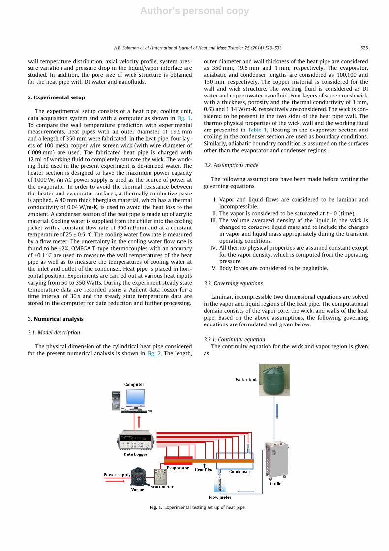
The experimental setup consists of a heat pipe, cooling unit,data acquisition system and with a computer as shown in Fig. 1.To compare the wall temperature prediction with experimentalmeasurements, heat pipes with an outer diameter of 19.5 mmand a length of 350 mm were fabricated. In the heat pipe, four lay-ers of 100 mesh copper wire screen wick (with wire diameter of0.009 mm) are used. The fabricated heat pipe is charged with12 ml of working fluid to completely saturate the wick. The work-ing fluid used in the present experiment is de-ionized water. Theheater section is designed to have the maximum power capacityof 1000 W. An AC power supply is used as the source of power atthe evaporator. In order to avoid the thermal resistance betweenthe heater and evaporator surfaces, a thermally conductive pasteis applied. A 40 mm thick fiberglass material, which has a thermalconductivity of 0.04 W/m-K, is used to avoid the heat loss to theambient. A condenser section of the heat pipe is made up of acrylicmaterial. Cooling water is supplied from the chiller into the coolingjacket with a constant flow rate of 350 ml/min and at a constanttemperature of 25 ± 0.5 �C. The cooling water flow rate is measuredby a flow meter. The uncertainty in the cooling water flow rate isfound to be ±2%. OMEGA T-type thermocouples with an accuracyof ±0.1 �C are used to measure the wall temperatures of the heatpipe as well as to measure the temperatures of cooling water atthe inlet and outlet of the condenser. Heat pipe is placed in hori-zontal position. Experiments are carried out at various heat inputsvarying from 50 to 350 Watts. During the experiment steady statetemperature data are recorded using a Agilent data logger for atime interval of 30 s and the steady state temperature data arestored in the computer for date reduction and further processing.

3. Numerical analysis

3.1. Model description

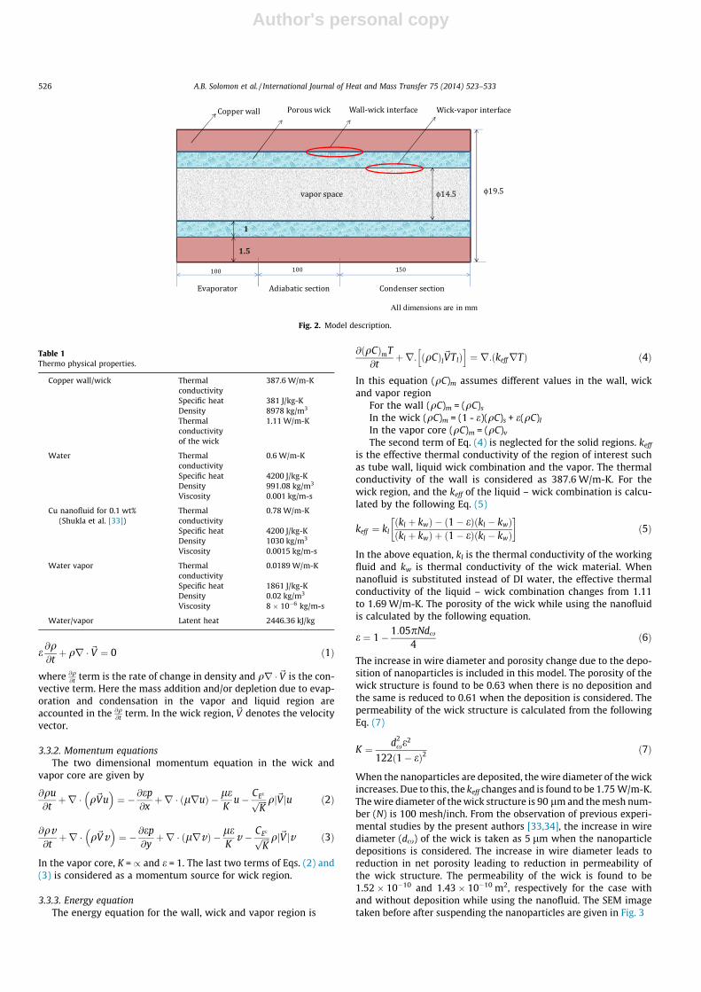
The physical dimension of the cylindrical heat pipe consideredfor the present numerical analysis is shown in Fig. 2. The length,

outer diameter and wall thickness of the heat pipe are consideredas 350 mm, 19.5 mm and 1 mm, respectively. The evaporator,adiabatic and condenser lengths are considered as 100,100 and150 mm, respectively. The copper material is considered for thewall and wick structure. The working fluid is considered as DIwater and copper/water nanofluid. Four layers of screen mesh wickwith a thickness, porosity and the thermal conductivity of 1 mm,0.63 and 1.14 W/m-K, respectively are considered. The wick is con-sidered to be present in the two sides of the heat pipe wall. Thethermo physical properties of the wick, wall and the working fluidare presented in Table 1. Heating in the evaporator section andcooling in the condenser section are used as boundary conditions.Similarly, adiabatic boundary condition is assumed on the surfacesother than the evaporator and condenser regions.

3.2. Assumptions made

The following assumptions have been made before writing thegoverning equations

I. Vapor and liquid flows are considered to be laminar andincompressible.

II. The vapor is considered to be saturated at t = 0 (time).III. The volume averaged density of the liquid in the wick is

changed to conserve liquid mass and to include the changesin vapor and liquid mass appropriately during the transientoperating conditions.

IV. All thermo physical properties are assumed constant exceptfor the vapor density, which is computed from the operatingpressure.

V. Body forces are considered to be negligible.

3.3. Governing equations

Laminar, incompressible two dimensional equations are solvedin the vapor and liquid regions of the heat pipe. The computationaldomain consists of the vapor core, the wick, and walls of the heatpipe. Based on the above assumptions, the following governingequations are formulated and given below.

3.3.1. Continuity equationThe continuity equation for the wick and vapor region is given

as

Fig. 1. Experimental testing set up of heat pipe.

A.B. Solomon et al. / International Journal of Heat and Mass Transfer 75 (2014) 523–533 525


e@q@tþ qr � ~V ¼ 0 ð1Þ

where @q@t term is the rate of change in density and qr � ~V is the con-

vective term. Here the mass addition and/or depletion due to evap-oration and condensation in the vapor and liquid region areaccounted in the @q

@t term. In the wick region, ~V denotes the velocityvector.

3.3.2. Momentum equationsThe two dimensional momentum equation in the wick and

vapor core are given by

@qu@tþr � q~Vu

� �¼ � @ep

@xþr � lruð Þ � le

Ku� CEeffiffiffiffi

Kp qj~V ju ð2Þ

@qv@tþr � q~Vv

� �¼ � @ep

@yþr � lrvð Þ � le

Kv � CEeffiffiffiffi

Kp qj~V jv ð3Þ

In the vapor core, K = / and e = 1. The last two terms of Eqs. (2) and(3) is considered as a momentum source for wick region.

3.3.3. Energy equationThe energy equation for the wall, wick and vapor region is

@ðqCÞmT@t

þr: ðqCÞl~VTlÞh i

¼ r:ðkeffrTÞ ð4Þ

In this equation (qC)m assumes different values in the wall, wickand vapor region

For the wall (qC)m = (qC)s

In the wick (qC)m = (1 - e)(qC)s + e(qC)l

In the vapor core (qC)m = (qC)v

The second term of Eq. (4) is neglected for the solid regions. keff

is the effective thermal conductivity of the region of interest suchas tube wall, liquid wick combination and the vapor. The thermalconductivity of the wall is considered as 387.6 W/m-K. For thewick region, and the keff of the liquid – wick combination is calcu-lated by the following Eq. (5)

keff ¼ klðkl þ kwÞ � ð1� eÞðkl � kwÞðkl þ kwÞ þ ð1� eÞðkl � kwÞ

� �ð5Þ

In the above equation, kl is the thermal conductivity of the workingfluid and kw is thermal conductivity of the wick material. Whennanofluid is substituted instead of DI water, the effective thermalconductivity of the liquid – wick combination changes from 1.11to 1.69 W/m-K. The porosity of the wick while using the nanofluidis calculated by the following equation.

e ¼ 1� 1:05pNdx

4ð6Þ

The increase in wire diameter and porosity change due to the depo-sition of nanoparticles is included in this model. The porosity of thewick structure is found to be 0.63 when there is no deposition andthe same is reduced to 0.61 when the deposition is considered. Thepermeability of the wick structure is calculated from the followingEq. (7)

K ¼ d2xe2

122ð1� eÞ2ð7Þ

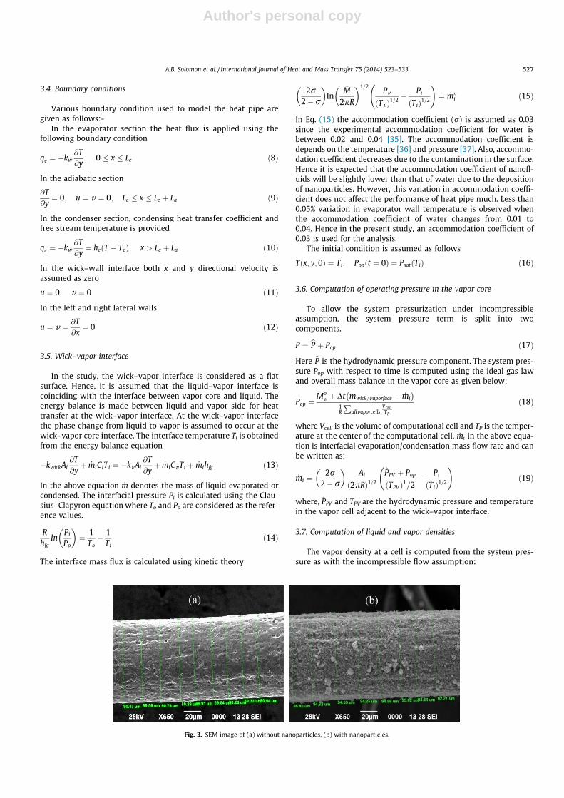
When the nanoparticles are deposited, the wire diameter of the wickincreases. Due to this, the keff changes and is found to be 1.75 W/m-K.The wire diameter of the wick structure is 90 lm and the mesh num-ber (N) is 100 mesh/inch. From the observation of previous experi-mental studies by the present authors [33,34], the increase in wirediameter (dx) of the wick is taken as 5 lm when the nanoparticledepositions is considered. The increase in wire diameter leads toreduction in net porosity leading to reduction in permeability ofthe wick structure. The permeability of the wick is found to be1.52 � 10�10 and 1.43 � 10�10 m2, respectively for the case withand without deposition while using the nanofluid. The SEM imagetaken before after suspending the nanoparticles are given in Fig. 3

φ φ

Fig. 2. Model description.

Table 1Thermo physical properties.

Copper wall/wick Thermalconductivity

387.6 W/m-K

Specific heat 381 J/kg-KDensity 8978 kg/m3

Thermalconductivityof the wick

1.11 W/m-K

Water Thermalconductivity

0.6 W/m-K

Specific heat 4200 J/kg-KDensity 991.08 kg/m3

Viscosity 0.001 kg/m-s

Cu nanofluid for 0.1 wt%(Shukla et al. [33])

Thermalconductivity

0.78 W/m-K

Specific heat 4200 J/kg-KDensity 1030 kg/m3

Viscosity 0.0015 kg/m-s

Water vapor Thermalconductivity

0.0189 W/m-K

Specific heat 1861 J/kg-KDensity 0.02 kg/m3

Viscosity 8 � 10�6 kg/m-s

Water/vapor Latent heat 2446.36 kJ/kg



3.4. Boundary conditions

Various boundary condition used to model the heat pipe aregiven as follows:-

In the evaporator section the heat flux is applied using thefollowing boundary condition

qe ¼ �kw@T@y

; 0 � x � Le ð8Þ

In the adiabatic section

@T@y¼ 0; u ¼ v ¼ 0; Le � x � Le þ La ð9Þ

In the condenser section, condensing heat transfer coefficient andfree stream temperature is provided

qc ¼ �kw@T@y¼ hcðT � TcÞ; x > Le þ La ð10Þ

In the wick–wall interface both x and y directional velocity isassumed as zero

u ¼ 0; v ¼ 0 ð11Þ

In the left and right lateral walls

u ¼ v ¼ @T@x¼ 0 ð12Þ

3.5. Wick–vapor interface

In the study, the wick–vapor interface is considered as a flatsurface. Hence, it is assumed that the liquid–vapor interface iscoinciding with the interface between vapor core and liquid. Theenergy balance is made between liquid and vapor side for heattransfer at the wick–vapor interface. At the wick–vapor interfacethe phase change from liquid to vapor is assumed to occur at thewick–vapor core interface. The interface temperature Ti is obtainedfrom the energy balance equation

�kwickAi@T@yþ _miClTi ¼ �kvAi

@T@yþ _miCvTi þ _mihfg ð13Þ

In the above equation _m denotes the mass of liquid evaporated orcondensed. The interfacial pressure Pi is calculated using the Clau-sius–Clapyron equation where To and Po are considered as the refer-ence values.

Rhfg

InPi

Po

� �¼ 1

To� 1

Tið14Þ

The interface mass flux is calculated using kinetic theory

2r2� r

� �In

�M2p�R

� �1=2Pv

ðTvÞ1=2 �Pi

ðTiÞ1=2

!¼ _m00i ð15Þ

In Eq. (15) the accommodation coefficient (r) is assumed as 0.03since the experimental accommodation coefficient for water isbetween 0.02 and 0.04 [35]. The accommodation coefficient isdepends on the temperature [36] and pressure [37]. Also, accommo-dation coefficient decreases due to the contamination in the surface.Hence it is expected that the accommodation coefficient of nanofl-uids will be slightly lower than that of water due to the depositionof nanoparticles. However, this variation in accommodation coeffi-cient does not affect the performance of heat pipe much. Less than0.05% variation in evaporator wall temperature is observed whenthe accommodation coefficient of water changes from 0.01 to0.04. Hence in the present study, an accommodation coefficient of0.03 is used for the analysis.

The initial condition is assumed as follows

Tðx; y;0Þ ¼ Ti; Popðt ¼ 0Þ ¼ PsatðTiÞ ð16Þ

3.6. Computation of operating pressure in the vapor core

To allow the system pressurization under incompressibleassumption, the system pressure term is split into twocomponents.

P ¼ bP þ Pop ð17Þ

Here bP is the hydrodynamic pressure component. The system pres-sure Pop with respect to time is computed using the ideal gas lawand overall mass balance in the vapor core as given below:

Pop ¼Mo

v þ Dt mwick=vaporface � _mi

1R

Pallvaporcells

VcellTP

ð18Þ

where Vcell is the volume of computational cell and TP is the temper-ature at the center of the computational cell. _mi in the above equa-tion is interfacial evaporation/condensation mass flow rate and canbe written as:

_mi ¼2r

2� r

� �Ai

ð2pRÞ1=2

P̂PV þ Pop

ðTPV Þ1=2� Pi

ðTiÞ1=2

!ð19Þ

where, P̂PV and TPV are the hydrodynamic pressure and temperaturein the vapor cell adjacent to the wick–vapor interface.

3.7. Computation of liquid and vapor densities

The vapor density at a cell is computed from the system pres-sure as with the incompressible flow assumption:

(a) (b)

Fig. 3. SEM image of (a) without nanoparticles, (b) with nanoparticles.



qp ¼Pop

RTPð20Þ

Similarly, the mean liquid density is computed in order to conservethe liquid mass appropriately:

dMl

dt¼

Xwick=vaporfaces

_ml; ql ¼Ml

eVlð21Þ

The liquid mass Ml is computed during every time step and themean liquid density is computed.

In this study very fine mesh is used to predict the heat transfercharacteristics of heat pipes. In the axial direction, 350 cells areused in the wall, wick and vapor regions. In the radial direction,15 and 10 cells are used in the wall and wick, respectively for bothsides of the vapor. In the vapor region 145 cells are used in theradial direction.

4. Results and discussion

Numerical analysis is performed by solving the governing Eqs.(1)–(4)with the boundary conditions (Eqs. (8)–(15)) and initialconditions (Eq. (16)). The operating pressure of the heat pipe is cal-culated using Eq. (17). Computations are carried out for the heatpipe with the input powers of 250 and 350 W. The experimentalheat transfer coefficient applied at the condenser section of theheat pipe is 1070 and 1872 W/m2-K for 250 and 350 W, respec-tively. The initial temperature and pressure of the computationaldomain is assumed as 297.9 K and 3778 Pascal, respectively. Thecoolant fluid temperature or the free stream (Tc) is assumed as297.9 K. The effective thermal conductivity (keff) of the wick is cal-culated by Eq. (5) and is found to be 1.11 and 1.69 W/m-K, respec-tively for DI water and nanofluids (0.1 wt%) without consideringthe deposition of nanoparticles. (keff) is 1.75 W/m-K when deposi-tion of nanoparticles on the wick is considered.

To establish a suitable time step, varieties of tests are performedwith five different time steps varying between 0.2 and 4 s. Theevaporator temperature at different time step is shown in Fig. 4.An experimental study by Hajian et al. [35] reported that theresponse time of the heat pipe is one of the characteristics of tran-sient and steady states while using the nanofluid as a workingfluid. To predict the variation in different operating parametersduring transient and steady states a lower time step is needed.Hence in the present study a time step of 1 s is considered eventhough the variation of temperature at the evaporator is negligible,the time step is varied from 0.2 to 4 s. As the heat flux increases thepressure inside the heat pipe increases, in order to set the requiredpressure level in the vapor domain, a transient computationalmodel is essential. However the Navier–Stokes equation only givesthe pressure gradient with respect to time, and finding the rise inthe pressure level with time is not possible with the use of steadyincompressible analysis. Therefore the present study reports atransient analysis with incompressible fluid assumption has beenmade to predict the rise in the pressure level with at each timestep. The present numerical results are validated against the pub-lished work by Vadakkan et al. [20]. It was clearly observed thatthe present numerical results agree well with the results reportedby Vadakkan et al. [20] with the average deviation of ±0.1% (Fig. 5).Further the present numerical results also showed good agreementwith the present experimental results.

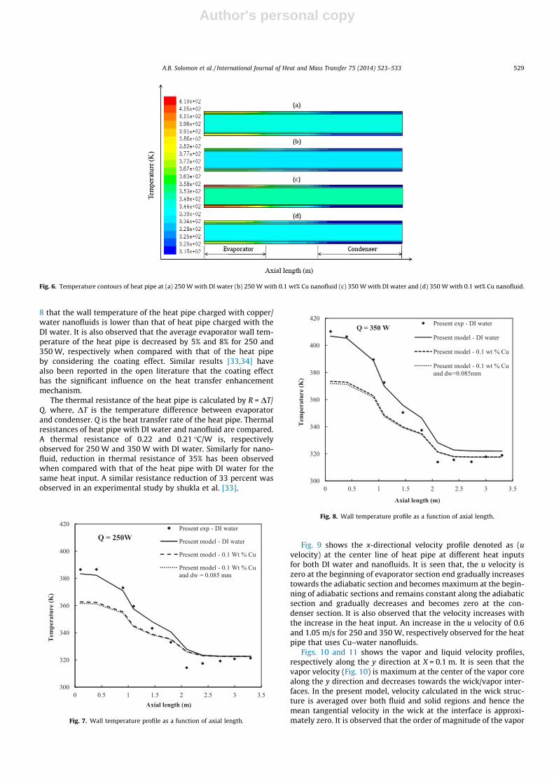
A typical temperature contour of the heat pipe simulated at 250and 350 W for water and nanofluids are shown in Fig. 6. It is seenthat the evaporator temperature of the heat pipe is found to behigher than that of the adiabatic and condenser sections for thesame heat input. It is also observed that the temperature gradientof the heat pipe decreases along the axial distance of the heat pipe

leading towards the condenser section. Further it is noted that thetemperature distribution of the heat pipe filled with nanofluid(Fig. 6 b and d) is lower than that of the heat pipe filled with DIwater (Fig. 6 a and c). Further, there is a strong temperature gradi-ent in the wick region is observed. Due to the addition of nanopar-ticles the temperature profile is flattened throughout the length ofthe heat pipe; and thereby enhancing the heat transfer capabilityof the heat pipe when nanofluid is used as the working fluid.

The Figs. 7 and 8 shows the comparison between the predictedand experimental wall temperatures of the heat pipe charged withDI water and with Cu-water nanofluids with and without coating ispresented for two different heat inputs namely 250 W and 350 W,respectively. From the obtained results it is clearly seen that thepredicted results agree well with the experimental results. A max-imum temperature deviation between the predicted and experi-mental data is found to be ±0.4% and ±1.5% at the evaporator andcondenser sections, respectively. The higher deviation in the con-denser section is caused due to the non uniform cooling effectpresent in the condenser section. The reason for this behavior isattributed because a constant heat transfer coefficient is appliedas one of the boundary conditions in the numerical model. How-ever in practical, the heat transfer coefficient along the condensersection will vary. After validating the experimental and numericalresults, the thermo-physical properties of nanofluids are incorpo-rated into the model and the effect nanofluids on the performanceof the heat pipe is analyzed. It is also observed from the Figs. 7 and

300

310

320

330

340

350

360

370

380

390

0 25 50 75 100 125 150 175 200

Eva

pora

tor

Tem

pera

ture

(K)

Time (s)

0.2 sec0.5 sec1 sec1.5 sec4 sec

Fig. 4. Evaporator wall temperature profile as a function of time.

288

293

298

303

308

313

0 0.01 0.02 0.03 0.04 0.05 0.06 0.07 0.08 0.09

Tem

pera

ture

(K)

Axial length (m)

Present modelPrevious model (Vadakkan,2004)

Fig. 5. Axial wall temperature of flat heat pipe at 30 W heat input (Vaddakan et al.[20]).



8 that the wall temperature of the heat pipe charged with copper/water nanofluids is lower than that of heat pipe charged with theDI water. It is also observed that the average evaporator wall tem-perature of the heat pipe is decreased by 5% and 8% for 250 and350 W, respectively when compared with that of the heat pipeby considering the coating effect. Similar results [33,34] havealso been reported in the open literature that the coating effecthas the significant influence on the heat transfer enhancementmechanism.

The thermal resistance of the heat pipe is calculated by R = DT/Q. where, DT is the temperature difference between evaporatorand condenser. Q is the heat transfer rate of the heat pipe. Thermalresistances of heat pipe with DI water and nanofluid are compared.A thermal resistance of 0.22 and 0.21 �C/W is, respectivelyobserved for 250 W and 350 W with DI water. Similarly for nano-fluid, reduction in thermal resistance of 35% has been observedwhen compared with that of the heat pipe with DI water for thesame heat input. A similar resistance reduction of 33 percent wasobserved in an experimental study by shukla et al. [33].

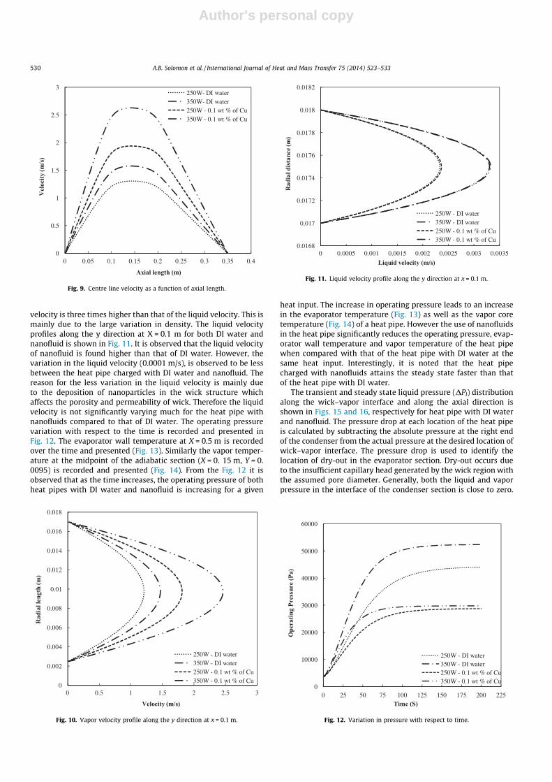
Fig. 9 shows the x-directional velocity profile denoted as (uvelocity) at the center line of heat pipe at different heat inputsfor both DI water and nanofluids. It is seen that, the u velocity iszero at the beginning of evaporator section end gradually increasestowards the adiabatic section and becomes maximum at the begin-ning of adiabatic sections and remains constant along the adiabaticsection and gradually decreases and becomes zero at the con-denser section. It is also observed that the velocity increases withthe increase in the heat input. An increase in the u velocity of 0.6and 1.05 m/s for 250 and 350 W, respectively observed for the heatpipe that uses Cu–water nanofluids.

Figs. 10 and 11 shows the vapor and liquid velocity profiles,respectively along the y direction at X = 0.1 m. It is seen that thevapor velocity (Fig. 10) is maximum at the center of the vapor corealong the y direction and decreases towards the wick/vapor inter-faces. In the present model, velocity calculated in the wick struc-ture is averaged over both fluid and solid regions and hence themean tangential velocity in the wick at the interface is approxi-mately zero. It is observed that the order of magnitude of the vapor

Fig. 6. Temperature contours of heat pipe at (a) 250 W with DI water (b) 250 W with 0.1 wt% Cu nanofluid (c) 350 W with DI water and (d) 350 W with 0.1 wt% Cu nanofluid.

300

320

340

360

380

400

420

0 0.5 1 1.5 2 2.5 3 3.5

Tem

pera

ture

(K)

Axial length (m)

Present exp - DI water

Present model - DI water

Present model - 0.1 Wt % Cu

Present model - 0.1 Wt % Cu and dw = 0.085 mm

Q = 250W

Fig. 7. Wall temperature profile as a function of axial length.

300

320

340

360

380

400

420

0 0.5 1 1.5 2 2.5 3 3.5

Tem

pera

ture

(K)

Axial length (m)

Present exp - DI water

Present model - DI water

Present model - 0.1 wt % Cu

Present model - 0.1 wt % Cu and dw=0.085mm

Q = 350 W

Fig. 8. Wall temperature profile as a function of axial length.



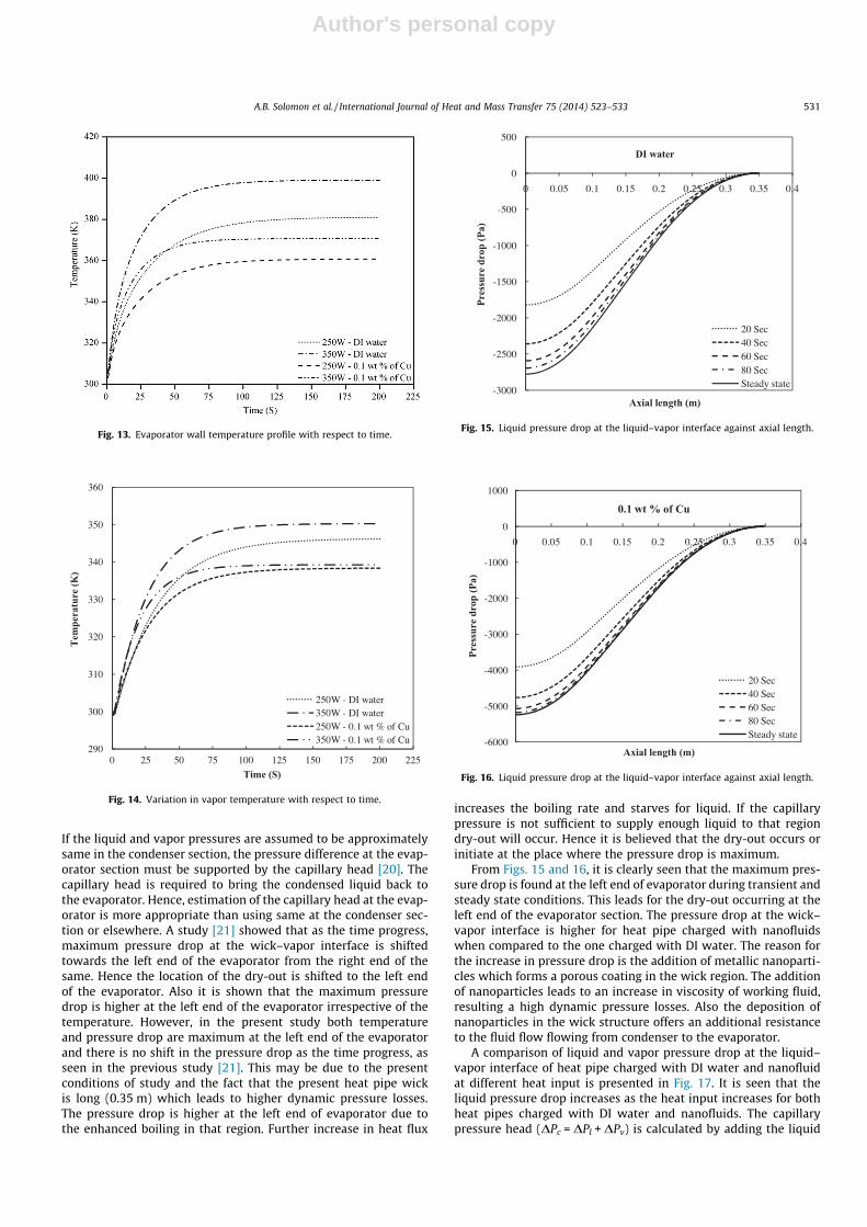
velocity is three times higher than that of the liquid velocity. This ismainly due to the large variation in density. The liquid velocityprofiles along the y direction at X = 0.1 m for both DI water andnanofluid is shown in Fig. 11. It is observed that the liquid velocityof nanofluid is found higher than that of DI water. However, thevariation in the liquid velocity (0.0001 m/s), is observed to be lessbetween the heat pipe charged with DI water and nanofluid. Thereason for the less variation in the liquid velocity is mainly dueto the deposition of nanoparticles in the wick structure whichaffects the porosity and permeability of wick. Therefore the liquidvelocity is not significantly varying much for the heat pipe withnanofluids compared to that of DI water. The operating pressurevariation with respect to the time is recorded and presented inFig. 12. The evaporator wall temperature at X = 0.5 m is recordedover the time and presented (Fig. 13). Similarly the vapor temper-ature at the midpoint of the adiabatic section (X = 0. 15 m, Y = 0.0095) is recorded and presented (Fig. 14). From the Fig. 12 it isobserved that as the time increases, the operating pressure of bothheat pipes with DI water and nanofluid is increasing for a given

heat input. The increase in operating pressure leads to an increasein the evaporator temperature (Fig. 13) as well as the vapor coretemperature (Fig. 14) of a heat pipe. However the use of nanofluidsin the heat pipe significantly reduces the operating pressure, evap-orator wall temperature and vapor temperature of the heat pipewhen compared with that of the heat pipe with DI water at thesame heat input. Interestingly, it is noted that the heat pipecharged with nanofluids attains the steady state faster than thatof the heat pipe with DI water.

The transient and steady state liquid pressure (DPl) distributionalong the wick–vapor interface and along the axial direction isshown in Figs. 15 and 16, respectively for heat pipe with DI waterand nanofluid. The pressure drop at each location of the heat pipeis calculated by subtracting the absolute pressure at the right endof the condenser from the actual pressure at the desired location ofwick–vapor interface. The pressure drop is used to identify thelocation of dry-out in the evaporator section. Dry-out occurs dueto the insufficient capillary head generated by the wick region withthe assumed pore diameter. Generally, both the liquid and vaporpressure in the interface of the condenser section is close to zero.

0

0.5

1

1.5

2

2.5

3

0 0.05 0.1 0.15 0.2 0.25 0.3 0.35 0.4

Vel

ocity

(m/s

)

Axial length (m)

250W- DI water350W- DI water250W - 0.1 wt % of Cu350W - 0.1 wt % of Cu

Fig. 9. Centre line velocity as a function of axial length.

0

0.002

0.004

0.006

0.008

0.01

0.012

0.014

0.016

0.018

0 0.5 1 1.5 2 2.5 3

Rad

ial l

engt

h (m

)

Velocity (m/s)

250W - DI water350W - DI water250W - 0.1 wt % of Cu350W - 0.1 wt % of Cu

Fig. 10. Vapor velocity profile along the y direction at x = 0.1 m.

0.0168

0.017

0.0172

0.0174

0.0176

0.0178

0.018

0.0182

0 0.0005 0.001 0.0015 0.002 0.0025 0.003 0.0035

Rad

ial d

ista

nce

(m)

Liquid velocity (m/s)


Fig. 11. Liquid velocity profile along the y direction at x = 0.1 m.

0

10000

20000

30000

40000

50000

60000

0 25 50 75 100 125 150 175 200 225

Ope

ratin

g Pr

essu

re (P

a)

Time (S)


Fig. 12. Variation in pressure with respect to time.



If the liquid and vapor pressures are assumed to be approximatelysame in the condenser section, the pressure difference at the evap-orator section must be supported by the capillary head [20]. Thecapillary head is required to bring the condensed liquid back tothe evaporator. Hence, estimation of the capillary head at the evap-orator is more appropriate than using same at the condenser sec-tion or elsewhere. A study [21] showed that as the time progress,maximum pressure drop at the wick–vapor interface is shiftedtowards the left end of the evaporator from the right end of thesame. Hence the location of the dry-out is shifted to the left endof the evaporator. Also it is shown that the maximum pressuredrop is higher at the left end of the evaporator irrespective of thetemperature. However, in the present study both temperatureand pressure drop are maximum at the left end of the evaporatorand there is no shift in the pressure drop as the time progress, asseen in the previous study [21]. This may be due to the presentconditions of study and the fact that the present heat pipe wickis long (0.35 m) which leads to higher dynamic pressure losses.The pressure drop is higher at the left end of evaporator due tothe enhanced boiling in that region. Further increase in heat flux

increases the boiling rate and starves for liquid. If the capillarypressure is not sufficient to supply enough liquid to that regiondry-out will occur. Hence it is believed that the dry-out occurs orinitiate at the place where the pressure drop is maximum.

From Figs. 15 and 16, it is clearly seen that the maximum pres-sure drop is found at the left end of evaporator during transient andsteady state conditions. This leads for the dry-out occurring at theleft end of the evaporator section. The pressure drop at the wick–vapor interface is higher for heat pipe charged with nanofluidswhen compared to the one charged with DI water. The reason forthe increase in pressure drop is the addition of metallic nanoparti-cles which forms a porous coating in the wick region. The additionof nanoparticles leads to an increase in viscosity of working fluid,resulting a high dynamic pressure losses. Also the deposition ofnanoparticles in the wick structure offers an additional resistanceto the fluid flow flowing from condenser to the evaporator.

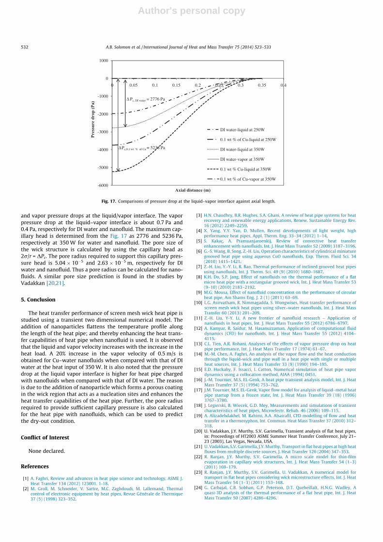
A comparison of liquid and vapor pressure drop at the liquid–vapor interface of heat pipe charged with DI water and nanofluidat different heat input is presented in Fig. 17. It is seen that theliquid pressure drop increases as the heat input increases for bothheat pipes charged with DI water and nanofluids. The capillarypressure head (DPc = DPl + DPv) is calculated by adding the liquid

Fig. 13. Evaporator wall temperature profile with respect to time.

290

300

310

320

330

340

350

360

0 25 50 75 100 125 150 175 200 225

Tem

pera

ture

(K)

Time (S)


Fig. 14. Variation in vapor temperature with respect to time.

-3000

-2500

-2000

-1500

-1000

-500

0

500

0 0.05 0.1 0.15 0.2 0.25 0.3 0.35 0.4

Pres

sure

dro

p (P

a)

Axial length (m)

20 Sec40 Sec60 Sec80 SecSteady state

DI water

Fig. 15. Liquid pressure drop at the liquid–vapor interface against axial length.

-6000

-5000

-4000

-3000

-2000

-1000

0

1000

0 0.05 0.1 0.15 0.2 0.25 0.3 0.35 0.4

Pres

sure

dro

p (P

a)

Axial length (m)

20 Sec40 Sec60 Sec80 SecSteady state

0.1 wt % of Cu

Fig. 16. Liquid pressure drop at the liquid–vapor interface against axial length.



and vapor pressure drops at the liquid/vapor interface. The vaporpressure drop at the liquid–vapor interface is about 0.7 Pa and0.4 Pa, respectively for DI water and nanofluid. The maximum cap-illary head is determined from the Fig. 17 as 2776 and 5236 Pa,respectively at 350 W for water and nanofluid. The pore size ofthe wick structure is calculated by using the capillary head as2r/r = DPc. The pore radius required to support this capillary pres-sure head is 5.04 � 10�5 and 2.63 � 10�5 m, respectively for DIwater and nanofluid. Thus a pore radius can be calculated for nano-fluids. A similar pore size prediction is found in the studies byVadakkan [20,21].

5. Conclusion

The heat transfer performance of screen mesh wick heat pipe isstudied using a transient two dimensional numerical model. Theaddition of nanoparticles flattens the temperature profile alongthe length of the heat pipe; and thereby enhancing the heat trans-fer capabilities of heat pipe when nanofluid is used. It is observedthat the liquid and vapor velocity increases with the increase in theheat load. A 20% increase in the vapor velocity of 0.5 m/s isobtained for Cu–water nanofluids when compared with that of DIwater at the heat input of 350 W. It is also noted that the pressuredrop at the liquid vapor interface is higher for heat pipe chargedwith nanofluids when compared with that of DI water. The reasonis due to the addition of nanoparticle which forms a porous coatingin the wick region that acts as a nucleation sites and enhances theheat transfer capabilities of the heat pipe. Further, the pore radiusrequired to provide sufficient capillary pressure is also calculatedfor the heat pipe with nanofluids, which can be used to predictthe dry-out condition.

Conflict of Interest

None declared.

References

[1] A. Faghri, Review and advances in heat pipe science and technology, ASME J.Heat Transfer 134 (2012) 123001. 1-18.

[2] M. Groll, M. Schneider, V. Sartre, M.C. Zaghdoudi, M. Lallemand, Thermalcontrol of electronic equipment by heat pipes, Revue Générale de Thermique37 (5) (1998) 323–352.

[3] H.N. Chaudhry, B.R. Hughes, S.A. Ghani, A review of heat pipe systems for heatrecovery and renewable energy applications, Renew. Sustainable Energy Rev.16 (2012) 2249–2259.

[4] X. Yang, Y.Y. Yan, D. Mullen, Recent developments of light weight, highperformance heat pipes, Appl. Therm. Eng. 33–34 (2012) 1–14.

[5] S. Kakaç, A. Pramuanjaroenkij, Review of convective heat transferenhancement with nanofluids, Int. J. Heat Mass Transfer 52 (2009) 3187–3196.

[6] G.-S. Wang, B. Song, Z.-H. Liu, Operation characteristics of cylindrical miniaturegrooved heat pipe using aqueous CuO nanofluids, Exp. Therm. Fluid Sci. 34(2010) 1415–1421.

[7] Z.-H. Liu, Y.-Y. Li, R. Bao, Thermal performance of inclined grooved heat pipesusing nanofluids, Int. J. Therm. Sci. 49 (9) (2010) 1680–1687.

[8] K.H. Do, S.P. Jang, Effect of nanofluids on the thermal performance of a flatmicro heat pipe with a rectangular grooved wick, Int. J. Heat Mass Transfer 53(9–10) (2010) 2183–2192.

[9] M.G. Mousa, Effect of nanofluid concentration on the performance of circularheat pipe, Ain Shams Eng. J. 2 (1) (2011) 63–69.

[10] L.G. Asirvatham, R. Nimmagadda, S. Wongwises, Heat transfer performance ofscreen mesh wick heat pipes using silver–water nanofluids, Int. J. Heat MassTransfer 60 (2013) 201–209.

[11] Z.-H. Liu, Y-Y. Li, A new frontier of nanofluid research – Application ofnanofluids in heat pipes, Int. J. Heat Mass Transfer 55 (2012) 6786–6797.

[12] A. Kamyar, R. Saidur, M. Hasanuzzaman, Application of computational fluiddynamics (CFD) for nanofluids, Int. J. Heat Mass Transfer 55 (2012) 4104–4115.

[13] C.L. Tien, A.R. Rohani, Analyses of the effects of vapor pressure drop on heatpipe performance, Int. J. Heat Mass Transfer 17 (1974) 61–67.

[14] M.-M. Chen, A. Faghri, An analysis of the vapor flow and the heat conductionthrough the liquid-wick and pipe wall in a heat pipe with single or multipleheat sources, Int. J. Heat Mass Transfer 33 (9) (1990) 194–195.

[15] E.D. Huckaby, F. Issacci, I. Catton, Numerical simulation of heat pipe vapordynamics using a collocation method, AIAA (1994) 0451.

[16] J.-M. Tournier, M.S. EL-Genk, A heat pipe transient analysis model, Int. J. HeatMass Transfer 37 (5) (1994) 753–762.

[17] J.M. Tournier, M.S. EL-Genk, Vapor flow model for analysis of liquid–metal heatpipe startup from a frozen state, Int. J. Heat Mass Transfer 39 (18) (1996)3767–3780.

[18] J. Legierski, B. Wiecek, G.D. Mey, Measurements and simulations of transientcharacteristics of heat pipes, Microelectr. Reliab. 46 (2006) 109–115.

[19] A. Alizadehdakhel, M. Rahimi, A.A. Alsairafil, CFD modelling of flow and heattransfer in a thermosyphon, Int. Commun. Heat Mass Transfer 37 (2010) 312–318.

[20] U. Vadakkan, J.Y. Murthy, S.V. Garimella, Transient analysis of flat heat pipes,in: Proceedings of HT2003 ASME Summer Heat Transfer Conference, July 21–23 (2003), Las Vegas, Nevada, USA.

[21] U. Vadakkan, S.V. Garimella, J.Y. Murthy, Transport in flat heat pipes at high heatfluxes from multiple discrete sources, J. Heat Transfer 126 (2004) 347–353.

[22] R. Ranjan, J.Y. Murthy, S.V. Garimella, A micro scale model for thin-filmevaporation in capillary wick structures, Int. J. Heat Mass Transfer 54 (1–3)(2011) 169–179.

[23] R. Ranjan, J.Y. Murthy, S.V. Garimella, U. Vadakkan, A numerical model fortransport in flat heat pipes considering wick microstructure effects, Int. J. HeatMass Transfer 54 (1–3) (2011) 153–168.

[24] G. Carbajal, C.B. Sobhan, G.P. Peterson, D.T. Queheillalt, H.N.G. Wadley, Aquasi-3D analysis of the thermal performance of a flat heat pipe, Int. J. HeatMass Transfer 50 (2007) 4286–4296.

-6000

-5000

-4000

-3000

-2000

-1000

0

1000

0 0.05 0.1 0.15 0.2 0.25 0.3 0.35 0.4

Pres

sure

dro

p (P

a)

Axial distance (m)

DI water-liquid at 250W

0.1 wt % of Cu-liquid at 250W

DI water-liquid at 350W

DI water-vapor at 350W

0.1 wt % Cu-liquid at 350W

0.1 wt % of Cu-vapor at 350W

Pc, DI water = 2776 Pa

Pc,0.1 wt % of Cu = 5236 Pa

Δ

Δ

Fig. 17. Comparisons of pressure drop at the liquid–vapor interface against axial length.



[25] J. Rice, A. Faghri, Analysis of screen wick heat pipes, including capillary dry-outlimitations, J. Thermophys. Heat Transfer 21 (3) (2007) 475–486.

[26] B.-J Wang, C.-R. Chen, J.-R. Tsai, Two-phase flow simulation in heat pipe, AIAA(2007) 4838.

[27] B. Xiao, A. Faghri, A three-dimensional thermal-fluid analysis of flat heat pipes,Int. J. Heat Mass Transfer 51 (2008) 3113–3126.

[28] Y.-S. Chen, K.-H. Chien, T.-C. Hung, C.-C. Wang, Y.-M. Ferng, B.-S. Pei, Numericalsimulation of a heat sink embedded with a vapor chamber and calculation ofthe effective thermal conductivity of a vapor chamber, Appl. Therm. Eng. 29(2009) 2655–2664.

[29] M. Aghvami, A. Faghri, Analysis of flat heat pipes with various heating andcooling configurations, Appl. Therm. Eng. 31 (14–15) (2011) 2645–2655.

[30] M. Shafahi, V. Bianco, K. Vafai, O. Manca, An investigation of the thermalperformance of cylindrical heat pipes using nanofluids, Int. J. Heat MassTransfer 53 (2010) 376–383.

[31] K.H. Do, H.J. Ha, S.P. Jang, Thermal resistance of screen mesh wick heat pipesusing the water-based Al2O3 nanofluids, Int. J. Heat Mass Transfer 53 (2010)5888–5894.

[32] M. Shafahi, V. Bianco, K. Vafai, O. Manca, Thermal performance of flat-shapedheat pipes using nanofluids, Int. J. Heat Mass Transfer 53 (2010) 1438–1445.

[33] K.N. Shukla, A.B. Solomon, B.C. Pillai, M. Ibrahim, Thermal performance ofcylindrical heat pipes using nanofluids, J. Thermophys. Heat Transfer 24 (4)(2010) 796–802.

[34] A.B. Solomon, K. Ramachandran, B.C. Pillai, Thermal performance of heat pipewith nanoparticles coated wick, Appl. Therm. Eng. 36 (2012) 106–112.

[35] R. Hajian, M. Layeghi, K.A. Sani, Experimental study of nanofluid effects on thethermal performance with response time of heat pipe, Energy Convers.Manage. 56 (2012) 63–68.

[36] G. Barnes, Insoluble monolayers and evaporation coefficient of water, J. ColloidInterface Sci. 65 (2) (1978) 567–572.

[37] V.K. Badam, V. Kumar, F. Durst, D. Danov, Experimental and theoreticalinvestigations on interfacial temperature jumps during evaporation, Exp.Therm. Fluid Sci. 32 (2007) 276–292.


Numerical analysis of a screen mesh wick heat pipe with Cu/water nanofluid

Documents

Transcript of Numerical analysis of a screen mesh wick heat pipe with Cu/water nanofluid