arX

iv:h

ep-l

at/0

3030

19v2

4 M

ar 2

005

Nucleon electromagnetic form factors on the lattice and in chiral

effective field theory

M. Gockeler,1, 2 T.R. Hemmert,3 R. Horsley,4 D. Pleiter,5

P.E.L. Rakow,6 A. Schafer,2 and G. Schierholz5, 7

(QCDSF collaboration)

1Institut fur Theoretische Physik, Universitat Leipzig, D-04109 Leipzig, Germany

2Institut fur Theoretische Physik, Universitat Regensburg, D-93040 Regensburg, Germany

3Physik-Department, Theoretische Physik,

Technische Universitat Munchen, D-85747 Garching, Germany

4School of Physics, University of Edinburgh, Edinburgh EH9 3JZ, UK

5John von Neumann-Institut fur Computing NIC,

Deutsches Elektronen-Synchrotron DESY, D-15738 Zeuthen, Germany

6Theoretical Physics Division, Department of Mathematical Sciences,

University of Liverpool, Liverpool L69 3BX, UK

7Deutsches Elektronen-Synchrotron DESY, D-22603 Hamburg, Germany

(Dated: February 7, 2008)

Abstract

We compute the electromagnetic form factors of the nucleon in quenched lattice QCD, using

non-perturbatively improved Wilson fermions, and compare the results with phenomenology and

chiral effective field theory.

PACS numbers: 11.15.Ha; 12.38.Gc; 13.40.Gp

Keywords: Lattice QCD; effective field theory; chiral extrapolation; nucleon electromagnetic form factors

1

I. INTRODUCTION

The measurements of the electromagnetic form factors of the proton and the neutron

gave the first hints at an internal structure of the nucleon, and a theory of the nucleon

cannot be considered satisfactory if it is not able to reproduce the form factor data. For a

long time, the overall trend of the experimental results for small and moderate values of the

momentum transfer q2 could be described reasonably well by phenomenological (dipole) fits

Gpe(q

2) ∼ Gpm(q2)

µp∼ Gn

m(q2)

µn

∼(

1 − q2/m2D

)

−2,

Gne (q2) ∼ 0 (1)

with mD ∼ 0.84 GeV and the magnetic moments

µp ∼ 2.79 , µn ∼ −1.91 (2)

in units of nuclear magnetons. Recently, the form factors of the nucleon have been studied

experimentally with high precision and deviations from this uniform dipole form have been

observed, both at very small q2 [1] and in the region above 1 GeV2 [2, 3].

It is therefore of great interest to derive the nucleon form factors from QCD. Since form

factors are typical low-energy quantities, perturbation theory in terms of quarks and gluons

is useless for this purpose and a non-perturbative method is needed. If one wants to avoid

additional assumptions or models, one is essentially restricted to lattice QCD and Monte

Carlo simulations. In view of the importance of nucleon form factors and the amount of

experimental data available, it is surprising that there are only a few lattice investigations

of form factors in the last years [4, 5].

In this paper we give a detailed account of our results for the nucleon form factors ob-

tained in quenched Monte Carlo simulations with non-perturbatively O(a)-improved Wilson

fermions. We shall pay particular attention to the chiral extrapolation and compare with for-

mulae from chiral effective field theory previously used for studies of the magnetic moments.

The plan of the paper is as follows. After a few general definitions and remarks in the next

section we describe the lattice technology that we used in Sec. III. After commenting on our

earlier attempts to perform a chiral extrapolation in Sec. IV, we investigate the quark-mass

dependence of the form factors in more detail on a phenomenological basis in Sec. V. We

2

find that our data are in qualitative agreement with the recently observed deviations [2, 3]

from the uniform dipole parametrization of the proton form factors. In Sec. VI we collect

and discuss formulae from chiral effective field theory, which are confronted with our Monte

Carlo results in Sec. VII. Our conclusions are presented in Sec. VIII. The Appendixes

contain a short discussion of the pion mass dependence of the nucleon mass as well as tables

of the form factors and of the corresponding dipole fits.

II. GENERALITIES

Experimentally, the nucleon form factors are measured via electron scattering. Because

the fine structure constant is so small, it is justified to describe this process in terms of

one-photon exchange. So the scattering amplitude is given by

Tfi = e2ue(k′

e, s′

e)γµue(ke, se)1

q2〈p′, s′|Jµ|p, s〉 (3)

with the electromagnetic current

Jµ =2

3uγµu− 1

3dγµd+ · · · . (4)

Here p, p′ are the nucleon momenta, ke, k′

e are the electron momenta, and s, s′, . . . are the

corresponding spin vectors. The momentum transfer is defined as q = p′ − p. With the help

of the form factors F1(q2) and F2(q

2) the nucleon matrix element can be decomposed as

〈p′, s′|Jµ|p, s〉 = u(p′, s′)

[

γµF1(q2) + iσµν qν

2MNF2(q

2)

]

u(p, s) (5)

where MN is the mass of the nucleon. From the kinematics of the scattering process, it can

easily be seen that q2 < 0. In the following, we shall often use the new variable Q2 = −q2.

We have F1(0) = 1 (in the proton) as J is a conserved current, while F2(0) measures the

anomalous magnetic moment in nuclear magnetons. For a classical point particle, both form

factors are independent of q2, so deviations from this behavior tell us something about the

extended nature of the nucleon. In electron scattering, F1 and F2 are usually re-written in

terms of the electric and magnetic Sachs form factors

Ge(q2) = F1(q

2) +q2

(2MN )2F2(q

2) ,

Gm(q2) = F1(q2) + F2(q

2) , (6)

3

as then the (unpolarized) cross section becomes a linear combination of squares of the form

factors.

Throughout the whole paper we assume flavor SU(2) symmetry. Hence we can decompose

the form factors into isovector and isoscalar components. In terms of the proton and neutron

form factors the isovector form factors are given by

Gve(q

2) = Gpe(q

2) −Gne (q2) ,

Gvm(q2) = Gp

m(q2) −Gnm(q2) (7)

such that

Gvm(0) = Gp

m(0) −Gnm(0) = µp − µn = µv = 1 + κv (8)

with µv (κv) being the isovector (anomalous) magnetic moment ∼ 4.71 (3.71). In the actual

simulations we do not work directly with these definitions when we calculate the isovector

form factors. We use the relation

〈proton|(

23uγµu − 1

3dγµd

)

|proton〉 − 〈neutron|(

23uγµu− 1

3dγµd

)

|neutron〉

= 〈proton|(

uγµu− dγµd)

|proton〉 (9)

and compute the isovector form factors from proton matrix elements of the current uγµu−dγµd instead of evaluating the proton and neutron matrix elements of the electromagnetic

current separately and then taking the difference. Similarly one could use the isoscalar

current uγµu+ dγµd for the computation of isoscalar form factors, but we have not done so,

since in the isoscalar sector there are considerable uncertainties anyway due to the neglected

quark-line disconnected contributions.

III. LATTICE TECHNOLOGY

Using the standard Wilson gauge field action we have performed quenched simulations

with O(a)-improved Wilson fermions (clover fermions). For the coefficient cSW of the

Sheikholeslami-Wohlert clover term we chose a non-perturbatively determined value cal-

culated from the interpolation formula given in Ref. [6]. The couplings β = 6/g2 and cSW ,

the lattice sizes and statistics, the values of the hopping parameter κ (not to be confused

with an anomalous magnetic moment) and the corresponding pion and nucleon masses (in

4

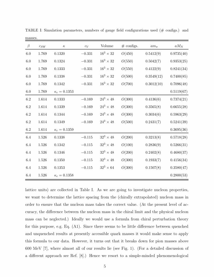
TABLE I: Simulation parameters, numbers of gauge field configurations used (# configs.) and

masses.

β cSW κ cV Volume # configs. amπ aMN

6.0 1.769 0.1320 −0.331 163 × 32 O(450) 0.5412(9) 0.9735(40)

6.0 1.769 0.1324 −0.331 163 × 32 O(550) 0.5042(7) 0.9353(25)

6.0 1.769 0.1333 −0.331 163 × 32 O(550) 0.4122(9) 0.8241(34)

6.0 1.769 0.1338 −0.331 163 × 32 O(500) 0.3549(12) 0.7400(85)

6.0 1.769 0.1342 −0.331 163 × 32 O(700) 0.3012(10) 0.7096(48)

6.0 1.769 κc = 0.1353 0.5119(67)

6.2 1.614 0.1333 −0.169 243 × 48 O(300) 0.4136(6) 0.7374(21)

6.2 1.614 0.1339 −0.169 243 × 48 O(300) 0.3565(8) 0.6655(28)

6.2 1.614 0.1344 −0.169 243 × 48 O(300) 0.3034(6) 0.5963(29)

6.2 1.614 0.1349 −0.169 243 × 48 O(500) 0.2431(7) 0.5241(39)

6.2 1.614 κc = 0.1359 0.3695(36)

6.4 1.526 0.1338 −0.115 323 × 48 O(200) 0.3213(8) 0.5718(28)

6.4 1.526 0.1342 −0.115 323 × 48 O(100) 0.2836(9) 0.5266(31)

6.4 1.526 0.1346 −0.115 323 × 48 O(200) 0.2402(8) 0.4680(37)

6.4 1.526 0.1350 −0.115 323 × 48 O(300) 0.1933(7) 0.4156(34)

6.4 1.526 0.1353 −0.115 323 × 64 O(300) 0.1507(8) 0.3580(47)

6.4 1.526 κc = 0.1358 0.2800(53)

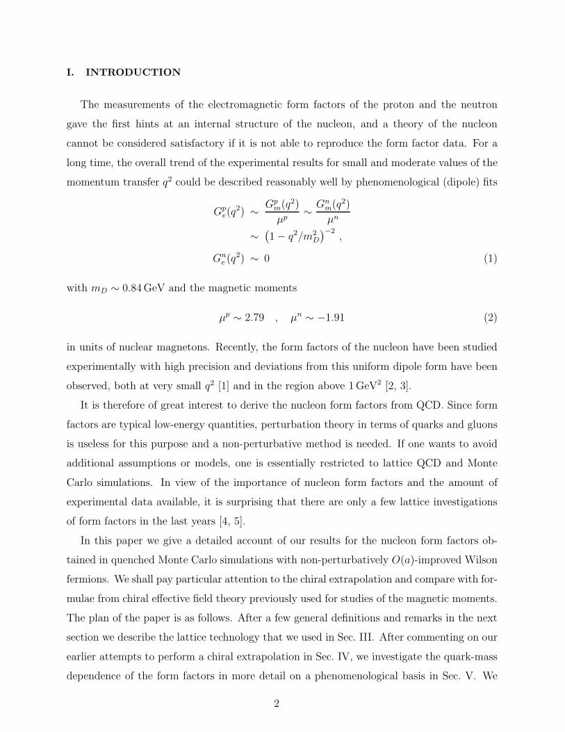
lattice units) are collected in Table I. As we are going to investigate nucleon properties,

we want to determine the lattice spacing from the (chirally extrapolated) nucleon mass in

order to ensure that the nucleon mass takes the correct value. (At the present level of ac-

curacy, the difference between the nucleon mass in the chiral limit and the physical nucleon

mass can be neglected.) Ideally we would use a formula from chiral perturbation theory

for this purpose, e.g. Eq. (A1). Since there seems to be little difference between quenched

and unquenched results at presently accessible quark masses it would make sense to apply

this formula to our data. However, it turns out that it breaks down for pion masses above

600 MeV [7], where almost all of our results lie (see Fig. 1). (For a detailed discussion of

a different approach see Ref. [8].) Hence we resort to a simple-minded phenomenological

5

procedure extrapolating our masses by means of the ansatz

(aMN )2 = (aM0N )2 + b2(amπ)2 + b3(amπ)3 (10)

for each β. This ansatz provides a very good description of the data [9]. The nucleon masses

extrapolated to the critical hopping parameter κc in this way (on the basis of a larger set of

nucleon masses) are also given in Table I. Whenever we give numbers in physical units the

scale has been set by these chirally extrapolated nucleon masses.

In the last years it has become more popular to set the scale with the help of the force

parameter r0 [10]. While this choice avoids the problems related to the chiral extrapolation

of the nucleon mass, it has the disadvantage that the physical value of r0 is less precisely

determined than the physical nucleon mass. Furthermore, as the present paper deals ex-

clusively with nucleon properties it seemed to us more important to have the correct value

in physical units for the mass of the particle studied when evaluating other dimensionful

quantities like, e.g., radii. It is however interesting to note that the dimensionless product

r0M0N is to a good accuracy independent of the lattice spacing. Indeed, taking r0 from

Ref. [11] and multiplying by the chirally extrapolated nucleon masses given in Table I one

finds r0M0N = 2.75, 2.72, and 2.73 for β = 6.0, 6.2, and 6.4, respectively. Thus the scaling

behavior of our results is practically the same for both choices of the scale.

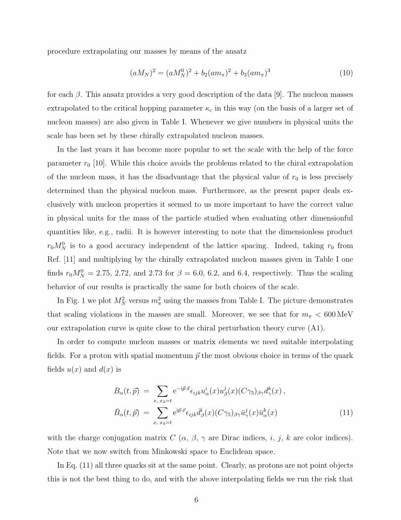
In Fig. 1 we plot M2N versus m2

π using the masses from Table I. The picture demonstrates

that scaling violations in the masses are small. Moreover, we see that for mπ < 600 MeV

our extrapolation curve is quite close to the chiral perturbation theory curve (A1).

In order to compute nucleon masses or matrix elements we need suitable interpolating

fields. For a proton with spatial momentum ~p the most obvious choice in terms of the quark

fields u(x) and d(x) is

Bα(t, ~p) =∑

x, x4=t

e−i~p·~xǫijkuiα(x)uj

β(x)(Cγ5)βγdkγ(x) ,

Bα(t, ~p) =∑

x, x4=t

ei~p·~xǫijkdiβ(x)(Cγ5)βγ u

jγ(x)u

kα(x) (11)

with the charge conjugation matrix C (α, β, γ are Dirac indices, i, j, k are color indices).

Note that we now switch from Minkowski space to Euclidean space.

In Eq. (11) all three quarks sit at the same point. Clearly, as protons are not point objects

this is not the best thing to do, and with the above interpolating fields we run the risk that

6

0.0 0.2 0.4 0.6 0.8 1.0 1.2 1.4

m2

[GeV2]

0.0

0.5

1.0

1.5

2.0

2.5

3.0

3.5

4.0

MN

2[G

eV2 ]

= 6.40= 6.20= 6.00

FIG. 1: Nucleon mass squared versus pion mass squared from the data in Table I. The dotted curve

shows our phenomenological chiral extrapolation (Eq. (10)) for β = 6.4. The full curve corresponds

to the chiral extrapolation derived from chiral perturbation theory (Eq. (A1)) with the parameters

given in Appendix A.

the amplitudes of one-proton states in correlation functions might be very small making the

extraction of masses and matrix elements rather unreliable. Therefore we employ two types

of improvement: First we smear the sources and the sinks for the quarks in their time slices,

secondly we apply a “non-relativistic” projection.

Our smearing algorithm (Jacobi smearing) is described in Ref. [12]. The parameters

Nsmear, κsmear used in the actual computations and the resulting smearing radii are given in

Table II. A typical rms nucleon radius is about 0.8 fm, our smearing radii are about half

that size.

The “non-relativistic” projection means that we replace each spinor by

ψ → ψNR = 12(1 + γ4)ψ , ψ → ψNR = ψ 1

2(1 + γ4) . (12)

This replacement leaves quantum numbers unchanged, but we would expect it to improve the

overlap with baryons. Practically this means that for each baryon propagator we consider

only the first two Dirac components. So we only have 2 × 3 inversions to perform rather

7

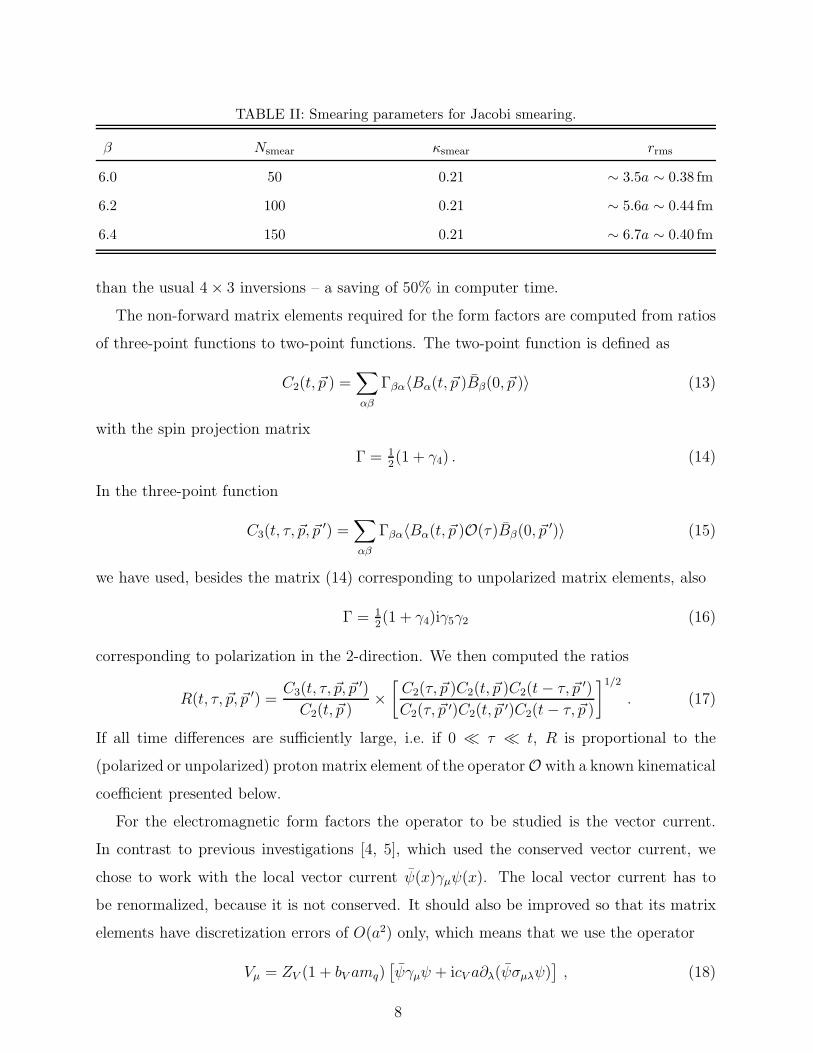
TABLE II: Smearing parameters for Jacobi smearing.

β Nsmear κsmear rrms

6.0 50 0.21 ∼ 3.5a ∼ 0.38 fm

6.2 100 0.21 ∼ 5.6a ∼ 0.44 fm

6.4 150 0.21 ∼ 6.7a ∼ 0.40 fm

than the usual 4 × 3 inversions – a saving of 50% in computer time.

The non-forward matrix elements required for the form factors are computed from ratios

of three-point functions to two-point functions. The two-point function is defined as

C2(t, ~p ) =∑

αβ

Γβα〈Bα(t, ~p )Bβ(0, ~p )〉 (13)

with the spin projection matrix

Γ = 12(1 + γ4) . (14)

In the three-point function

C3(t, τ, ~p, ~p′) =

∑

αβ

Γβα〈Bα(t, ~p )O(τ)Bβ(0, ~p ′)〉 (15)

we have used, besides the matrix (14) corresponding to unpolarized matrix elements, also

Γ = 12(1 + γ4)iγ5γ2 (16)

corresponding to polarization in the 2-direction. We then computed the ratios

R(t, τ, ~p, ~p ′) =C3(t, τ, ~p, ~p

′)

C2(t, ~p )×

[

C2(τ, ~p )C2(t, ~p )C2(t− τ, ~p ′)

C2(τ, ~p ′)C2(t, ~p ′)C2(t− τ, ~p )

]1/2

. (17)

If all time differences are sufficiently large, i.e. if 0 ≪ τ ≪ t, R is proportional to the

(polarized or unpolarized) proton matrix element of the operator O with a known kinematical

coefficient presented below.

For the electromagnetic form factors the operator to be studied is the vector current.

In contrast to previous investigations [4, 5], which used the conserved vector current, we

chose to work with the local vector current ψ(x)γµψ(x). The local vector current has to

be renormalized, because it is not conserved. It should also be improved so that its matrix

elements have discretization errors of O(a2) only, which means that we use the operator

Vµ = ZV (1 + bV amq)[

ψγµψ + icV a∂λ(ψσµλψ)]

, (18)

8

where mq is the bare quark mass:

amq =1

2κ− 1

2κc. (19)

We have taken ZV and bV from the parametrizations given by the ALPHA collabora-

tion [13] (see also Ref. [14]). The improvement coefficient cV has also been computed

non-perturbatively [15]. The results can be represented by the expression [9]

cV = −0.012254

3g21 − 0.3113g2

1 − 0.9660g2, (20)

from which we have calculated cV (see Table I). In the limit g2 → 0 it agrees with perturba-

tion theory [16]. Computing all these additional contributions in our simulations, we found

the improvement terms to be numerically small. Note that the improvement coefficient cCV C

for the conserved vector current is only known to tree level so that a fully non-perturbative

analysis would not be possible had we used the conserved vector current.

In order to describe the relation between the ratios we computed and the form factors let

us call the ratio R for the µ-component of the renormalized vector current more precisely

Rµ. Furthermore we distinguish the unpolarized case (spin projection matrix (14)) from the

polarized case (spin projection matrix (16)) by a superscript. The (Minkowski) momentum

transfer is given by

q2 = −Q2 = 2(

M2N + ~p · ~p ′ − EN(~p )EN(~p ′)

)

(21)

with the nucleon energy

EN(~p ) =√

M2N + ~p 2 . (22)

Using the abbreviation

A(~p, ~p ′)−1 = (−Q2 − 4M2N)

√

EN(~p )(MN + EN(~p ))EN (~p ′)(MN + EN (~p ′)) (23)

we have

Runpol4 (t, τ, ~p, ~p ′) = A(~p, ~p ′)

[

Ge(Q2)MN

(

EN (~p ) + EN (~p ′))

×(

~p ′ · ~p− (MN + EN(~p ))(MN + EN (~p ′)))

+Gm(Q2)(

(~p ′ · ~p )2 − ~p 2~p ′2)

]

, (24)

9

Rpol4 (t, τ, ~p, ~p ′) = A(~p, ~p ′)i(p′1p3 − p′3p1)

[

Ge(Q2)MN

(

EN (~p ) + EN (~p ′))

+Gm(Q2)(

~p ′ · ~p− (MN + EN(~p ))(MN + EN (~p ′)))

]

, (25)

and for j = 1, 2, 3

Runpolj (t, τ, ~p, ~p ′) = A(~p, ~p ′)i

[

Ge(Q2)MN

(

pj + p′j)(

(MN + EN (~p ))(MN + EN(~p ′)) − ~p ′ · ~p)

+Gm(Q2)(

pj(EN(~p )~p ′2 −EN (~p ′)~p ′ · ~p ) + p′j(EN(~p ′)~p 2 −EN (~p )~p ′ · ~p ))

]

, (26)

Rpolj (t, τ, ~p, ~p ′) = A(~p, ~p ′)

[

Ge(Q2)MN

(

pj +p′

j

)(

p′1p3−p′3p1

)

+Gm(Q2)(

MN (p2+p′2)(~p′×~p)j

+(

(MN + EN(~p ))(MN + EN(~p ′)) − ~p ′ · ~p)

3∑

k=1

ǫj2k(p′

kEN (~p ) − pkEN (~p ′)))

]

. (27)

Analogous expressions for the computation of the form factors F1 and F2 are obtained by

inserting the definitions (6) in the above equations.

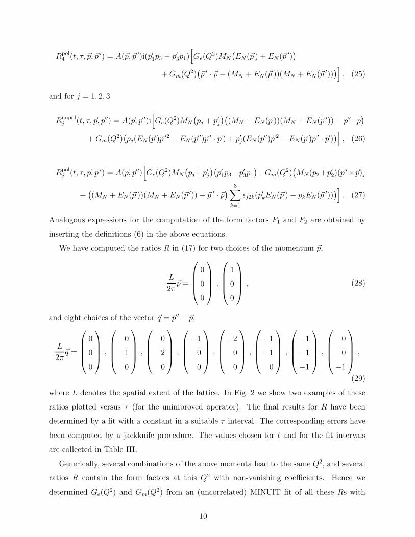
We have computed the ratios R in (17) for two choices of the momentum ~p,

L

2π~p =

0

0

0

,

1

0

0

, (28)

and eight choices of the vector ~q = ~p ′ − ~p,

L

2π~q =

0

0

0

,

0

−1

0

,

0

−2

0

,

−1

0

0

,

−2

0

0

,

−1

−1

0

,

−1

−1

−1

,

0

0

−1

,

(29)

where L denotes the spatial extent of the lattice. In Fig. 2 we show two examples of these

ratios plotted versus τ (for the unimproved operator). The final results for R have been

determined by a fit with a constant in a suitable τ interval. The corresponding errors have

been computed by a jackknife procedure. The values chosen for t and for the fit intervals

are collected in Table III.

Generically, several combinations of the above momenta lead to the same Q2, and several

ratios R contain the form factors at this Q2 with non-vanishing coefficients. Hence we

determined Ge(Q2) and Gm(Q2) from an (uncorrelated) MINUIT fit of all these Rs with

10

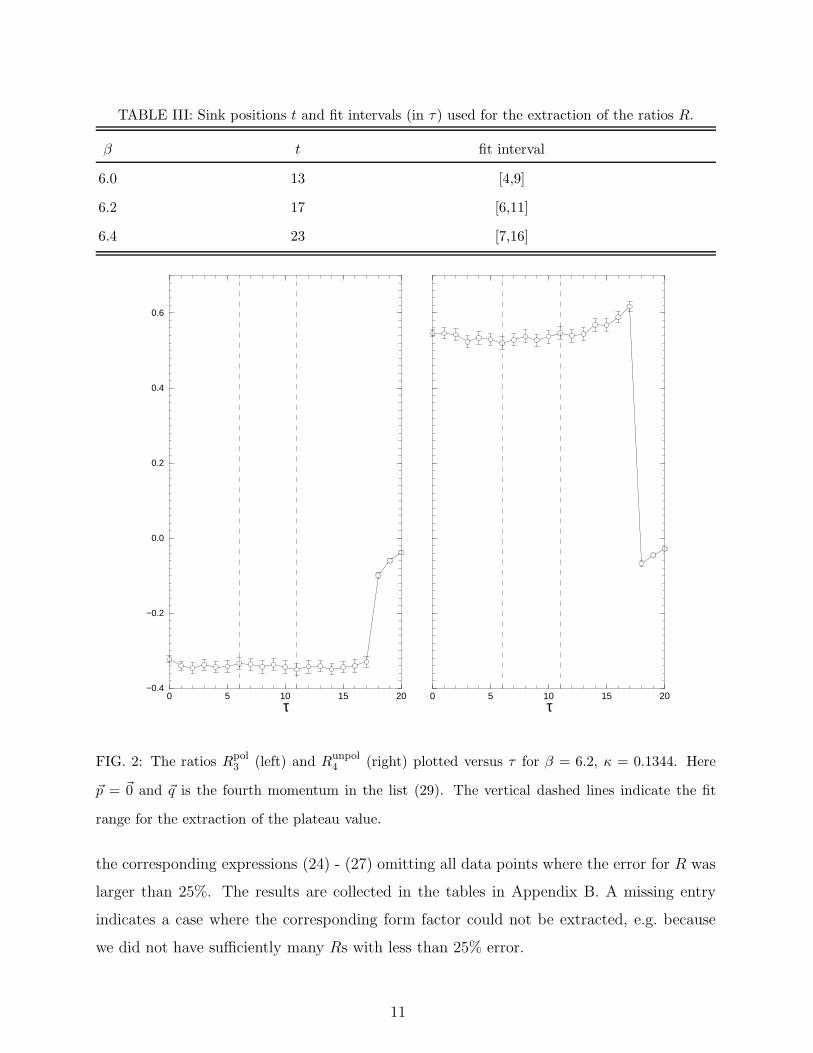
TABLE III: Sink positions t and fit intervals (in τ) used for the extraction of the ratios R.

β t fit interval

6.0 13 [4,9]

6.2 17 [6,11]

6.4 23 [7,16]

0 5 10 15 20τ

−0.4

−0.2

0.0

0.2

0.4

0.6

0 5 10 15 20τ

FIG. 2: The ratios Rpol3 (left) and Runpol

4 (right) plotted versus τ for β = 6.2, κ = 0.1344. Here

~p = ~0 and ~q is the fourth momentum in the list (29). The vertical dashed lines indicate the fit

range for the extraction of the plateau value.

the corresponding expressions (24) - (27) omitting all data points where the error for R was

larger than 25%. The results are collected in the tables in Appendix B. A missing entry

indicates a case where the corresponding form factor could not be extracted, e.g. because

we did not have sufficiently many Rs with less than 25% error.

11

The nucleon masses used can be found in Table I. The corresponding errors were, however,

not taken into account when computing the errors of the form factors. Varying the nucleon

masses within one standard deviation changed the form factors only by fractions of the

quoted statistical error.

In general, the nucleon three-point functions consist of a quark-line connected contribu-

tion and a quark-line disconnected piece. Unfortunately, the quark-line disconnected piece

is very hard to compute (for some recent attempts see Refs. [17, 18, 19]). Therefore it is

usually neglected, leading to one more source of systematic uncertainty. However, in the case

of exact isospin invariance the disconnected contribution drops out in non-singlet quantities

like the isovector form factors. That is why the isovector form factors (Tables VIII - X)

are our favorite observables. Nevertheless, we have also computed the proton form factors

separately ignoring the disconnected contributions. The results are given in Tables XI -

XIII. Regrettably, meaningful values of the electric form factor of the neutron could not be

extracted from our data (for a more successful attempt see Ref. [20]). The results for the

neutron magnetic form factor are collected in Tables XIV - XVI. Note that the isovector

form factors have been computed directly (cf. Eq. (9)) and not as the difference of the proton

and neutron form factors.

IV. CHIRAL EXTRAPOLATION: A FIRST ATTEMPT

The quark masses in our simulations are considerably larger than in reality leading to

pion masses above 500 MeV. Hence we cannot compare our results with experimental data

without performing a chiral extrapolation. In a first analysis of the proton results (see

Refs. [21, 22]) we assumed a linear quark-mass dependence of the form factors. More pre-

cisely, we proceeded as follows.

Schematically, the relation between a ratio R (three-point function/two-point function)

and the form factors Ge, Gm can be written in the form

R = 〈p′|J |p〉 + · · · = ceGe + cmGm (30)

with known coefficients ce, cm for each data point characterized by the momenta, the quark

mass, the spin projection and the space-time component of the current. Assuming a linear

12

quark-mass dependence of Ge and Gm we performed a 4-parameter fit,

R = ceae(amq) + cebe + cmam(amq) + cmbm , (31)

of all ratios R belonging to the same value of Q2 in the chiral limit. The resulting form

factors in the chiral limit are typically larger than the experimental data. They can be

fitted with a dipole form, but the masses from these fits are considerably larger than their

phenomenological counterparts [21, 22].

What could be the reason for this discrepancy? Several possibilities suggest themselves:

finite-size effects, quenching errors, cut-off effects or uncertainties in the chiral extrapolation.

The length L of the spatial boxes in our simulations is such that the inequality mπL >

4 holds in all cases. Previous experience suggests that in the quenched approximation

this is sufficient to exclude considerable distortions of the results due to the finite volume.

This assumption is confirmed by simulations with Wilson fermions, where we have data

on different volumes. Quenching errors are much more difficult to control. However, first

simulations with dynamical fermions indicate that – for the rather heavy quarks we can deal

with – the form factors do not change very much upon unquenching [22]. Having Monte

Carlo data for three different lattice spacings (see Table I) we can test for cut-off effects in

the chirally extrapolated form factors, but we find them to be hardly significant. So our

chiral extrapolation ought to be reconsidered. Indeed, the chiral extrapolation of lattice

data has been discussed intensively in the recent literature (see, e.g., Refs. [19, 20, 23, 24,

25, 26, 27, 28]) and it has been pointed out that the issue is highly non-trivial. Therefore

we shall examine the quark-mass dependence of our form factors in more detail.

Ideally, one would like to identify a regime of parameters (quark masses in particular)

where contact with chiral effective field theory (ChEFT) can be made on the basis of results

like those presented for the nucleon form factors in Ref. [29]. Once the range of applicability

of these low-energy effective field theories has been established, one can use them for a

safe extrapolation to smaller masses. However, these schemes do not work for arbitrarily

large quark masses (or pion masses), nor for arbitrarily large values of Q2. In particular,

the expressions for the form factors worked out in Ref. [29] can be trusted only up to

Q2 ≈ 0.4 GeV2 (see the discussion in Sec. VIA below) . Unfortunately, from our lattice

simulations we only have data for values of Q2 which barely touch the interval 0 < Q2 <

0.4 GeV2. Therefore we shall try to describe the Q2 dependence of the lattice data for each

13

quark mass by a suitable ansatz (of dipole type) and then study the mass dependence of the

corresponding parameters. The fit ansatz will also serve as an extrapolation of the magnetic

form factor down to Q2 = 0. Since we cannot compute Gm(0) directly, such an extrapolation

is required anyway to determine the magnetic moment. (For a different method, which does

not require an extrapolation, see Ref. [5].) In Sec. VII we shall come back to a comparison

with ChEFT.

V. INVESTIGATING THE QUARK-MASS DEPENDENCE

The analysis of our form factor data sketched in Sec. IV yielded results in the chiral limit

without much control over the approach to that limit. In this section we want to study the

quark-mass dependence of the form factors more thoroughly. As already mentioned, to this

end we have to make use of a suitable description of the Q2 dependence.

Motivated by the fact that the experimentally measured form factors at small values of

Q2 can be described by a dipole form (cf. Eq. (1)) we fitted our data with the ansatz

Gl(Q2) =

Al

(1 +Q2/M2l )2

, l = e,m ,

Fi(Q2) =

Ai

(1 +Q2/M2i )2

, i = 1, 2 . (32)

In the case of the form factors Ge (F1) we fixed Ae = 1 (A1 = 1). Note that we do

not require the dipole masses in the two form factors to coincide. Thus our ansatz can

accomodate deviations of the ratio Gm(0)Ge(Q2)/Gm(Q2) from unity as they have been

observed in recent experiments [1, 2, 3].

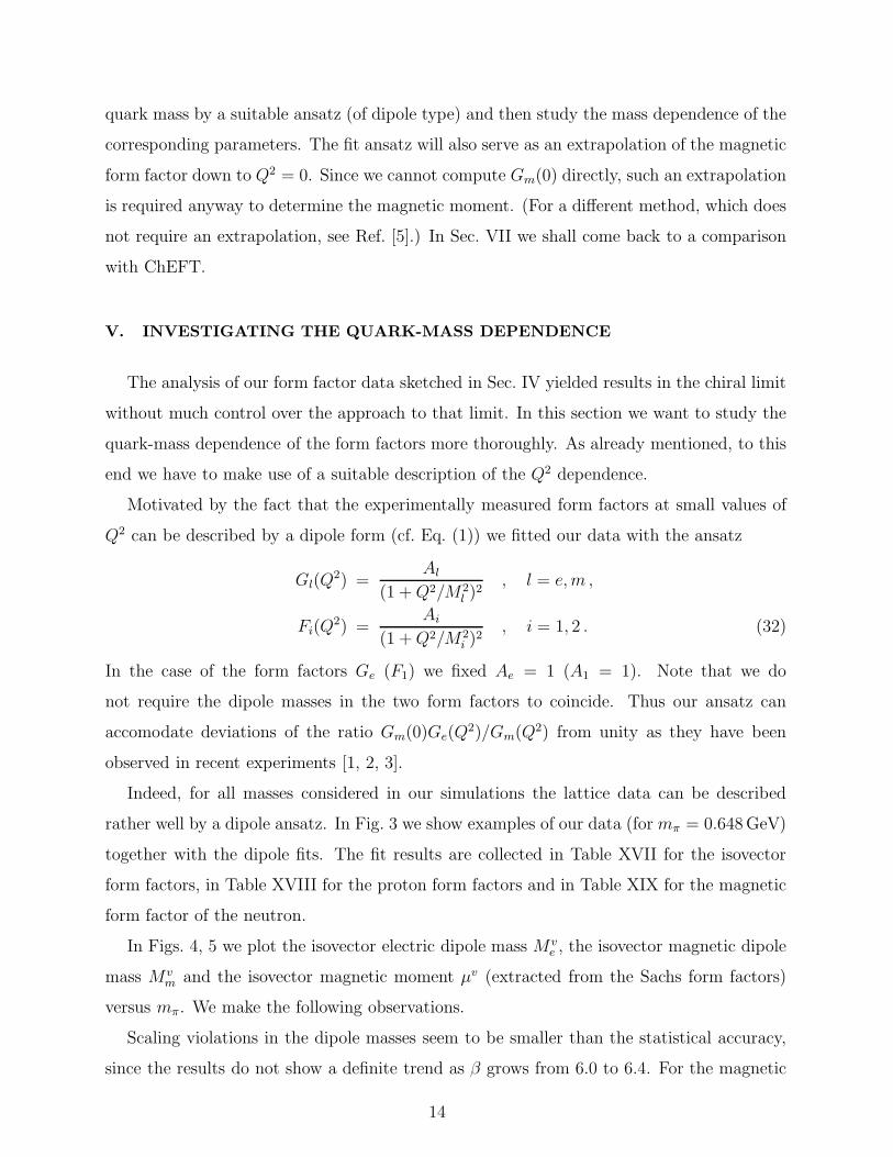
Indeed, for all masses considered in our simulations the lattice data can be described

rather well by a dipole ansatz. In Fig. 3 we show examples of our data (for mπ = 0.648 GeV)

together with the dipole fits. The fit results are collected in Table XVII for the isovector

form factors, in Table XVIII for the proton form factors and in Table XIX for the magnetic

form factor of the neutron.

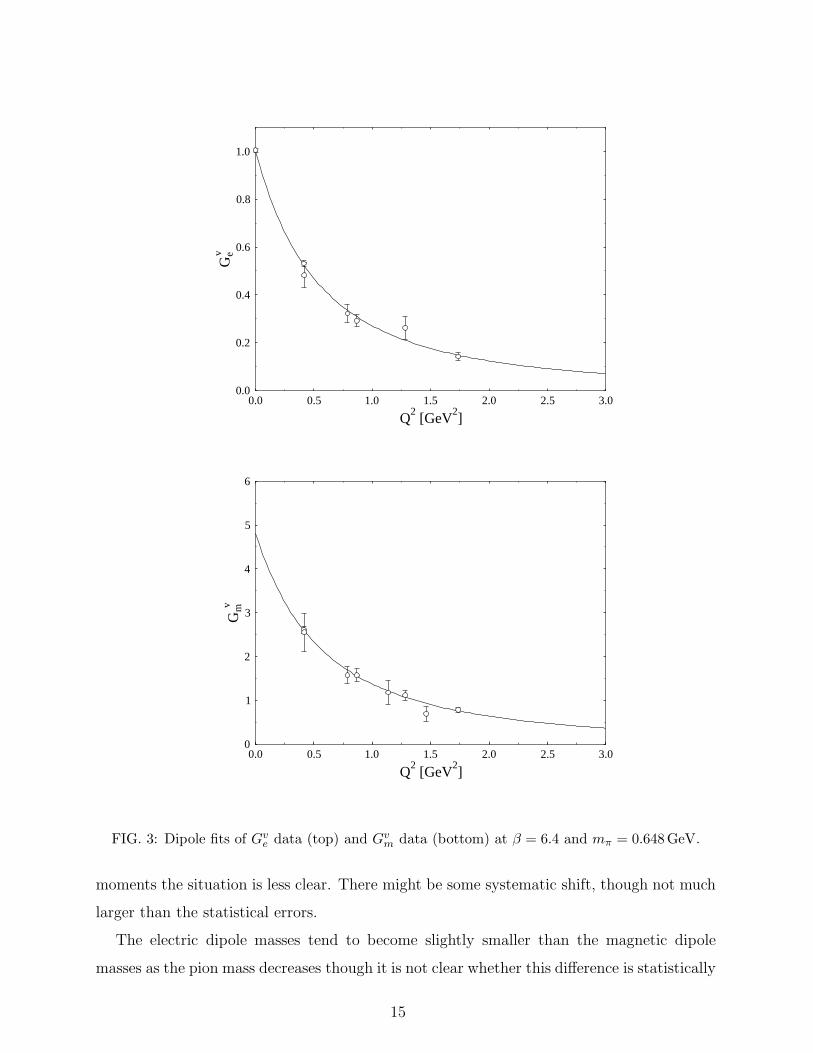
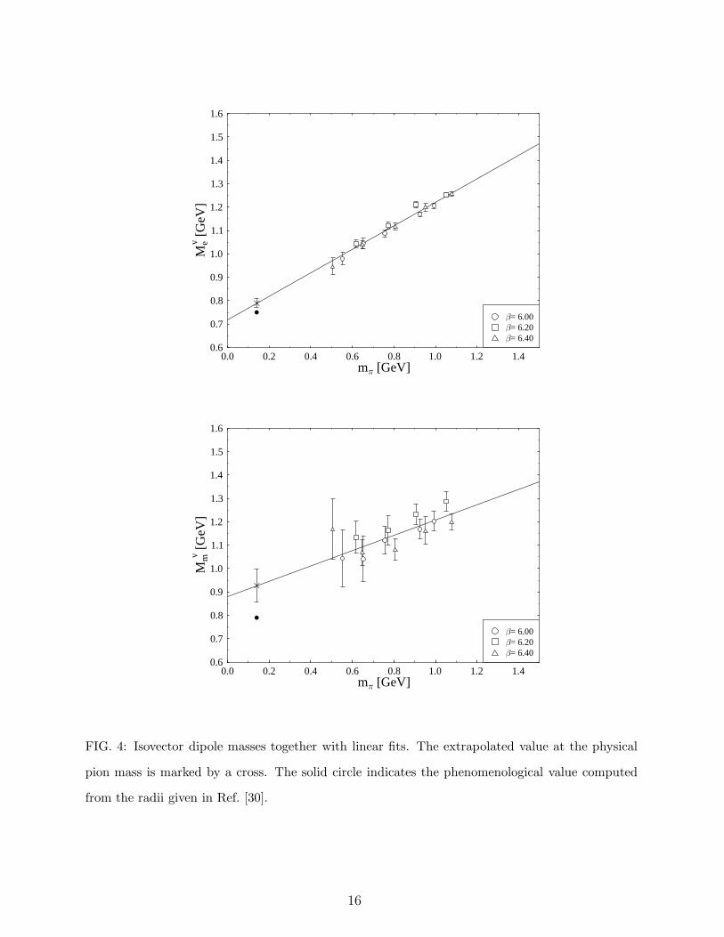
In Figs. 4, 5 we plot the isovector electric dipole mass Mve , the isovector magnetic dipole

mass Mvm and the isovector magnetic moment µv (extracted from the Sachs form factors)

versus mπ. We make the following observations.

Scaling violations in the dipole masses seem to be smaller than the statistical accuracy,

since the results do not show a definite trend as β grows from 6.0 to 6.4. For the magnetic

14

0.0 0.5 1.0 1.5 2.0 2.5 3.0

Q2

[GeV2]

0.0

0.2

0.4

0.6

0.8

1.0

Gev

0.0 0.5 1.0 1.5 2.0 2.5 3.0

Q2

[GeV2]

0

1

2

3

4

5

6

Gmv

FIG. 3: Dipole fits of Gve data (top) and Gv

m data (bottom) at β = 6.4 and mπ = 0.648GeV.

moments the situation is less clear. There might be some systematic shift, though not much

larger than the statistical errors.

The electric dipole masses tend to become slightly smaller than the magnetic dipole

masses as the pion mass decreases though it is not clear whether this difference is statistically

15

0.0 0.2 0.4 0.6 0.8 1.0 1.2 1.4m [GeV]

0.6

0.7

0.8

0.9

1.0

1.1

1.2

1.3

1.4

1.5

1.6

Mev

[GeV

]

= 6.40= 6.20= 6.00

0.0 0.2 0.4 0.6 0.8 1.0 1.2 1.4m [GeV]

0.6

0.7

0.8

0.9

1.0

1.1

1.2

1.3

1.4

1.5

1.6

Mmv

[GeV

]

= 6.40= 6.20= 6.00

FIG. 4: Isovector dipole masses together with linear fits. The extrapolated value at the physical

pion mass is marked by a cross. The solid circle indicates the phenomenological value computed

from the radii given in Ref. [30].

16

0.0 0.2 0.4 0.6 0.8 1.0 1.2 1.4m [GeV]

0

1

2

3

4

5

6

v

= 6.40= 6.20= 6.00

FIG. 5: Isovector magnetic moment together with a linear fit. The extrapolated value at the

physical pion mass is marked by a cross. The solid circle indicates the experimental value.

significant. This behavior agrees qualitatively with the recent JLAB data [2, 3] for Ge/Gm

in the proton (see Fig. 6 below).

The data for the electric dipole masses suggest a linear dependence on mπ. Therefore

we could not resist temptation to perform linear fits of the dipole masses and moments

(extracted from the Sachs form factors) in Tables XVII - XIX in order to obtain values

at the physical pion mass. Of course, at some point the singularities and non-analyticities

arising from the Goldstone bosons of QCD must show up and will in some observables lead

to a departure from the simple linear behavior. It is however conceivable that this happens

only at rather small pion masses (perhaps even only below the physical pion mass) and thus

does not influence the value at the physical pion mass too strongly. One can try to combine

the leading non-analytic behavior of chiral perturbation theory with a linear dependence on

m2π as it is expected at large quark mass in order to obtain an interpolation formula valid

both at small and at large masses. Fitting our form factor data with such a formula one

ends up remarkably close to the experimental results [28].

We performed our fits separately for each β value as well as for the combined data from

17

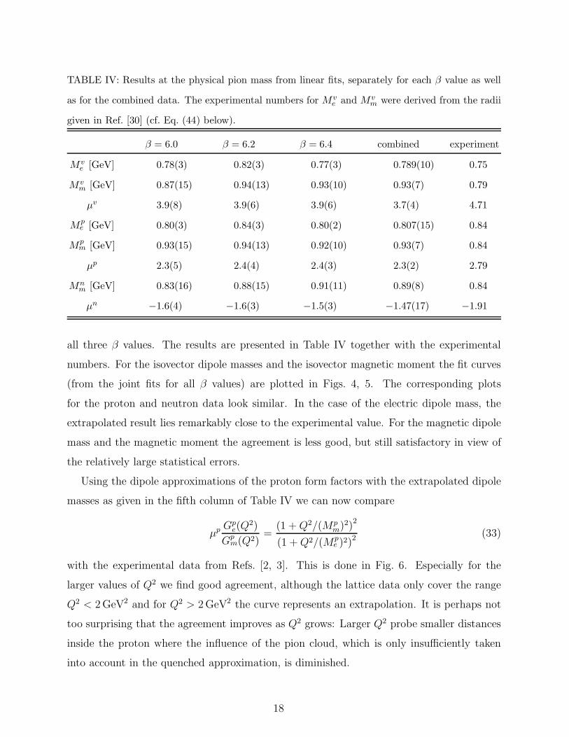
TABLE IV: Results at the physical pion mass from linear fits, separately for each β value as well

as for the combined data. The experimental numbers for Mve and Mv

m were derived from the radii

given in Ref. [30] (cf. Eq. (44) below).

β = 6.0 β = 6.2 β = 6.4 combined experiment

Mve [GeV] 0.78(3) 0.82(3) 0.77(3) 0.789(10) 0.75

Mvm [GeV] 0.87(15) 0.94(13) 0.93(10) 0.93(7) 0.79

µv 3.9(8) 3.9(6) 3.9(6) 3.7(4) 4.71

Mpe [GeV] 0.80(3) 0.84(3) 0.80(2) 0.807(15) 0.84

Mpm [GeV] 0.93(15) 0.94(13) 0.92(10) 0.93(7) 0.84

µp 2.3(5) 2.4(4) 2.4(3) 2.3(2) 2.79

Mnm [GeV] 0.83(16) 0.88(15) 0.91(11) 0.89(8) 0.84

µn −1.6(4) −1.6(3) −1.5(3) −1.47(17) −1.91

all three β values. The results are presented in Table IV together with the experimental

numbers. For the isovector dipole masses and the isovector magnetic moment the fit curves

(from the joint fits for all β values) are plotted in Figs. 4, 5. The corresponding plots

for the proton and neutron data look similar. In the case of the electric dipole mass, the

extrapolated result lies remarkably close to the experimental value. For the magnetic dipole

mass and the magnetic moment the agreement is less good, but still satisfactory in view of

the relatively large statistical errors.

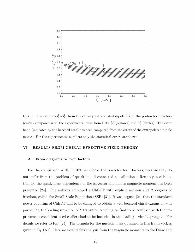
Using the dipole approximations of the proton form factors with the extrapolated dipole

masses as given in the fifth column of Table IV we can now compare

µp Gpe(Q

2)

Gpm(Q2)

=(1 +Q2/(Mp

m)2)2

(1 +Q2/(Mpe )2)

2 (33)

with the experimental data from Refs. [2, 3]. This is done in Fig. 6. Especially for the

larger values of Q2 we find good agreement, although the lattice data only cover the range

Q2 < 2 GeV2 and for Q2 > 2 GeV2 the curve represents an extrapolation. It is perhaps not

too surprising that the agreement improves as Q2 grows: Larger Q2 probe smaller distances

inside the proton where the influence of the pion cloud, which is only insufficiently taken

into account in the quenched approximation, is diminished.

18

0.0 0.5 1.0 1.5 2.0 2.5 3.0 3.5

Q2

[GeV2]

0.0

0.2

0.4

0.6

0.8

1.0

1.2

1.4

1.6

1.8

2.0

pG

ep/G

mp

FIG. 6: The ratio µpGpe/G

pm from the chirally extrapolated dipole fits of the proton form factors

(curve) compared with the experimental data from Refs. [2] (squares) and [3] (circles). The error

band (indicated by the hatched area) has been computed from the errors of the extrapolated dipole

masses. For the experimental numbers only the statistical errors are shown.

VI. RESULTS FROM CHIRAL EFFECTIVE FIELD THEORY

A. From diagrams to form factors

For the comparison with ChEFT we choose the isovector form factors, because they do

not suffer from the problem of quark-line disconnected contributions. Recently, a calcula-

tion for the quark-mass dependence of the isovector anomalous magnetic moment has been

presented [24]. The authors employed a ChEFT with explicit nucleon and ∆ degrees of

freedom, called the Small Scale Expansion (SSE) [31]. It was argued [24] that the standard

power-counting of ChEFT had to be changed to obtain a well-behaved chiral expansion – in

particular, the leading isovector N∆ transition coupling cV (not to be confused with the im-

provement coefficient used earlier) had to be included in the leading-order Lagrangian. For

details we refer to Ref. [24]. The formula for the nucleon mass obtained in this framework is

given in Eq. (A1). Here we extend this analysis from the magnetic moments to the Dirac and

19

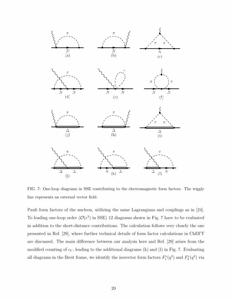
N�(a) N�(b) N� �( )NN �

(d) N�

N (e) N�N� (f)��(g) ��(h) �� �(i)

� � �(j) N � �(k) � � N(l)FIG. 7: One-loop diagrams in SSE contributing to the electromagnetic form factors. The wiggly

line represents an external vector field.

Pauli form factors of the nucleon, utilizing the same Lagrangians and couplings as in [24].

To leading one-loop order (O(ǫ3) in SSE) 12 diagrams shown in Fig. 7 have to be evaluated

in addition to the short-distance contributions. The calculation follows very closely the one

presented in Ref. [29], where further technical details of form factor calculations in ChEFT

are discussed. The main difference between our analysis here and Ref. [29] arises from the

modified counting of cV , leading to the additional diagrams (k) and (l) in Fig. 7. Evaluating

all diagrams in the Breit frame, we identify the isovector form factors F v1 (q2) and F v

2 (q2) via

20

the O(ǫ3) relation for the proton matrix element

〈p2|(

uγµu− dγµd)

|p1〉Breit =e

N1N2

uv(r2)

[(

F v1 (q2) +

q2

4(M0N )2

F v2 (0) + O(ǫ4)

)

vµ

+1

M0N

(

F v1 (0) + F v

2 (q2) + O(ǫ4))

[Sµ, Sν] qν

]

uv(r1) (34)

written in Minkowski space notation. Here M0N is the nucleon mass in the chiral limit

and uv(ri) denotes a nucleon spinor with the normalization Ni as given in Ref. [29]. The

quantity Sµ denotes the Pauli-Lubanski spin-vector, Sµ = i2γ5σµνv

ν . The four-vector vµ

(v2 = 1) is connected to the usual four-momentum vector pµ = M0Nv

µ + rµ, where rµ is a

soft momentum. Further details regarding calculations in this non-relativistic ChEFT can

be found in Ref. [31].

Nevertheless we have to discuss some subtleties behind Eq. (34) to be able to compare the

ChEFT results to lattice data. In (lattice) QCD a change in the quark mass does not only

lead to a change in µv and κv, but at the same time also to a change in the nucleon mass.

However, this variation of the nucleon mass – corresponding to a quark-mass dependent

“magneton” – is not accounted for at the order in ChEFT we are working at, as can be

seen from the presence of the nucleon mass in the chiral limit M0N in Eq. (34). Hence,

before comparing with the lattice results, we have to eliminate this effect. We do so by

defining “normalized” magnetic moments which are measured relative to the physical mass

of the nucleon MphysN and so are given in units of “physical” magnetons. These normalized

magnetic moments can then be matched to the formulae from ChEFT with M0N replaced by

MphysN .

We define the normalized magnetic moment by

µvnorm := µv

lattice

MphysN

M latticeN

=Mphys

N

M latticeN

+ κlatticev

MphysN

M latticeN

, (35)

Correspondingly, we take for the normalized anomalous magnetic moment

κnormv := κlattice

v

MphysN

M latticeN

(36)

such that

µvnorm =

MphysN

M latticeN

+ κnormv . (37)

At higher orders in the chiral expansion, the quark-mass dependence of the nucleon mass will

manifest itself in the matrix element (34), and the fits will have to be modified accordingly.

21

B. Form factors at O(ǫ3)

For the isovector Dirac form factor we obtain

F v1 (q2) = 1 +

1

(4πFπ)2

{

q2

(

68

81c2A − 2

3g2

A − 2B(r)10 (λ)

)

+ q2

(

40

27c2A − 5

3g2

A − 1

3

)

log[mπ

λ

]

+

∫ 1

0

dx

[

16

3∆2c2A +m2

π

(

3g2A + 1 − 8

3c2A

)

− q2x(1 − x)

(

5g2A + 1 − 40

9c2A

)]

log

[

m2

m2π

]

+

∫ 1

0

dx

[

32

9c2Aq

2x(1 − x)∆ logR(m)√

∆2 − m2

]

−∫ 1

0

dx32

3c2A∆

[

√

∆2 −m2π logR(mπ) −

√∆2 − m2 logR(m)

]

}

+ O(ǫ4) . (38)

To the same order one finds

F v2 (q2) = κv(mπ) − g2

A

4πMN

(4πFπ)2

∫ 1

0

dx[√

m2 −mπ

]

+32c2AMN∆

9(4πFπ)2

∫ 1

0

dx

[

1

2log

[

m2

4∆2

]

− log[mπ

2∆

]

+

√∆2 − m2

∆logR(m) −

√

∆2 −m2π

∆logR(mπ)

]

(39)

for the isovector Pauli form factor, where we have used the abbreviations

R(m) =∆

m+

√

∆2

m2− 1 , m2 = m2

π − q2x(1 − x) . (40)

Furthermore, the isovector anomalous magnetic moment κv(mπ) appearing in Eq. (39) is

given by

κv(mπ) = κ0v −

g2AmπMN

4πF 2π

+2c2A∆MN

9π2F 2π

{√

1 − m2π

∆2logR(mπ) + log

[mπ

2∆

]

}

− 8E(r)1 (λ)MNm

2π +

4cAcV gAMNm2π

9π2F 2π

log

[

2∆

λ

]

+4cAcV gAMNm

3π

27πF 2π∆

− 8cAcV gA∆2MN

27π2F 2π

{

(

1 − m2π

∆2

)3/2

logR(mπ) +

(

1 − 3m2π

2∆2

)

log[mπ

2∆

]

}

(41)

to O(ǫ3). As already mentioned, to this order the nucleon mass MN is a fixed number

in the above expression, independent of the quark mass, and we shall later identify it with

MphysN . Note that Eq. (41) corresponds to case C in the terminology of Ref. [24]. Of course, it

agrees with the result obtained in Ref. [24] because the magnetic moments are automatically

contained in a calculation of the form factors, as can be seen from the diagrams of Fig. 7.

22

TABLE V: Empirical values of the parameters.

Parameter Empirical value

gA 1.267

cA 1.125

Fπ 0.0924 GeV

MN 0.9389 GeV

∆ 0.2711 GeV

κphysv 3.71

κphyss −0.12

The expressions (38) and (39) contain a number of phenomenological parameters: the pion

decay constant Fπ, the leading axial N∆ coupling cA (denoted by gπN∆ in Ref. [29]), the ax-

ial coupling of the nucleon gA, the nucleon mass MN and the ∆(1232)-nucleon mass splitting

∆ = M∆ −MN . In addition, there is one parameter not directly related to phenomenol-

ogy, B(r)10 (λ). This counterterm at the renormalization scale λ parametrizes short-distance

contributions to the Dirac radius discussed in the next subsection. Further parameters are

encountered in the expression (41) for κv(mπ): the isovector anomalous magnetic moment of

the nucleon in the chiral limit κ0v, the leading isovector N∆ coupling cV and the counterterm

E(r)1 (λ), which leads to quark-mass dependent short-distance contributions to κv.

The only difference of the above results for the form factors compared to the formulae

given in Ref. [29] lies in the mass dependence of κv(mπ), as the two additional diagrams

(l) and (k) of Fig. 7 do not modify the momentum dependence at O(ǫ3). The authors of

Ref. [29] were only interested in the physical point mπ = mphysπ . Hence they fixed κv(m

physπ )

to the empirical value κphysv = 3.71. In addition, one may determine the counterterm B

(r)10

such that the phenomenological value of the isovector Dirac radius rv1 is reproduced. This

leads to B(r)10 (600 MeV) = 0.34. Using for the other parameters the phenomenological values

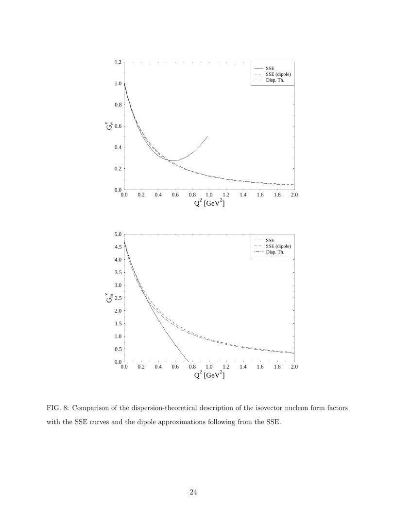
as given in Table V and inserting (38) and (39) in (6) one gets a rather good agreement with

the experimental Sachs form factors for values of Q2 up to about 0.4 GeV2, as exemplified

in Fig. 8 by a comparison with the dispersion-theoretical description [30] of the isovector

form factors. In addition we show in Fig. 8 the dipole approximations derived from the SSE

formulae, which will be explained in Sec. VIC.

23

0.0 0.2 0.4 0.6 0.8 1.0 1.2 1.4 1.6 1.8 2.0

Q2

[GeV2]

0.0

0.2

0.4

0.6

0.8

1.0

1.2

Gev

Disp. Th.SSE (dipole)SSE

0.0 0.2 0.4 0.6 0.8 1.0 1.2 1.4 1.6 1.8 2.0

Q2

[GeV2]

0.0

0.5

1.0

1.5

2.0

2.5

3.0

3.5

4.0

4.5

5.0

Gmv

Disp. Th.SSE (dipole)SSE

FIG. 8: Comparison of the dispersion-theoretical description of the isovector nucleon form factors

with the SSE curves and the dipole approximations following from the SSE.

24

Here we want to study the quark-mass dependence of the form factors. Strictly speaking,

in such a study all the parameters should be taken in the chiral limit. To order ǫ3 in the

SSE, the mπ dependence of F1 and F2 is then given by the expressions (38), (39), (41). For

comparison we note that in Ref. [29] a function κv(mπ) was found which corresponds to

scheme B in the language of Ref. [24]. In this latter paper, scheme B was however shown to

be insufficient to describe large-mass lattice data while scheme C turned out to work much

better. Another recent calculation [32] of the nucleon form factors utilizes a relativistic

framework for baryon chiral perturbation theory. However, as demonstrated in Ref. [24], it

is not able to describe the mass dependence of the lattice data for κv. Therefore we shall

not consider it for our fits.

Unfortunately, for most of the parameters the values in the chiral limit are only poorly

known. That is why we shall usually work with the phenomenological numbers as given in

Table V with the notable exception of the anomalous magnetic moment.

C. Form factor radii

From our lattice simulations we only have data for values of Q2 which barely touch the

interval 0 < Q2 < 0.4 GeV2. Therefore a direct comparison with (38) and (39) does not

make sense (although the Q2 range in which the leading one-loop results of Eqs. (38) and

(39) are applicable could depend on mπ) and we have to resort to another procedure, which

exploits the dipole fits of our lattice form factors (see Sec. VII).

The dipole masses of the form factors are closely related to the radii ri defined by the

Taylor expansion of Fi around q2 = 0:

Fi(q2) = Fi(0)

[

1 +1

6r2i q

2 + O(q4)

]

. (42)

If one describes the Sachs form factors by the dipole formulae

Ge(q2) =

1

(1 +Q2/M2e )2

,

Gm(q2) =Gm(0)

(1 +Q2/M2m)2

, (43)

the masses Me and Mm are related to the above radii by

1

M2e

=r21

12+

κ

8M2N

,1

M2m

=r21 + κ r2

2

12(1 + κ). (44)

25

We note again that we do not demand the two dipole masses to be equal. Hence violations

of the uniform dipole behavior can be accounted for.

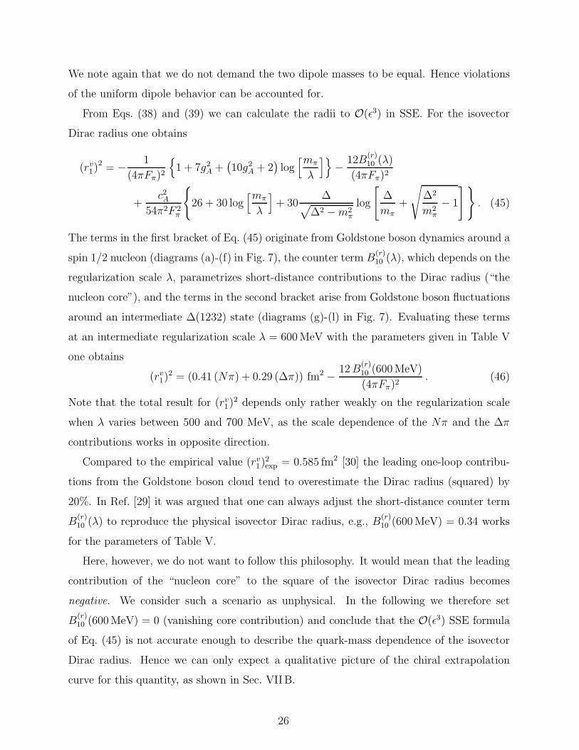
From Eqs. (38) and (39) we can calculate the radii to O(ǫ3) in SSE. For the isovector

Dirac radius one obtains

(rv1)

2 = − 1

(4πFπ)2

{

1 + 7g2A +

(

10g2A + 2

)

log[mπ

λ

]}

− 12B(r)10 (λ)

(4πFπ)2

+c2A

54π2F 2π

{

26 + 30 log[mπ

λ

]

+ 30∆

√

∆2 −m2π

log

[

∆

mπ

+

√

∆2

m2π

− 1

] }

. (45)

The terms in the first bracket of Eq. (45) originate from Goldstone boson dynamics around a

spin 1/2 nucleon (diagrams (a)-(f) in Fig. 7), the counter term B(r)10 (λ), which depends on the

regularization scale λ, parametrizes short-distance contributions to the Dirac radius (“the

nucleon core”), and the terms in the second bracket arise from Goldstone boson fluctuations

around an intermediate ∆(1232) state (diagrams (g)-(l) in Fig. 7). Evaluating these terms

at an intermediate regularization scale λ = 600 MeV with the parameters given in Table V

one obtains

(rv1)

2 = (0.41 (Nπ) + 0.29 (∆π)) fm2 − 12B(r)10 (600 MeV)

(4πFπ)2. (46)

Note that the total result for (rv1)

2 depends only rather weakly on the regularization scale

when λ varies between 500 and 700 MeV, as the scale dependence of the Nπ and the ∆π

contributions works in opposite direction.

Compared to the empirical value (rv1)

2exp = 0.585 fm2 [30] the leading one-loop contribu-

tions from the Goldstone boson cloud tend to overestimate the Dirac radius (squared) by

20%. In Ref. [29] it was argued that one can always adjust the short-distance counter term

B(r)10 (λ) to reproduce the physical isovector Dirac radius, e.g., B

(r)10 (600 MeV) = 0.34 works

for the parameters of Table V.

Here, however, we do not want to follow this philosophy. It would mean that the leading

contribution of the “nucleon core” to the square of the isovector Dirac radius becomes

negative. We consider such a scenario as unphysical. In the following we therefore set

B(r)10 (600 MeV) = 0 (vanishing core contribution) and conclude that the O(ǫ3) SSE formula

of Eq. (45) is not accurate enough to describe the quark-mass dependence of the isovector

Dirac radius. Hence we can only expect a qualitative picture of the chiral extrapolation

curve for this quantity, as shown in Sec. VIIB.

26

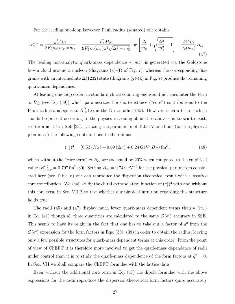
For the leading one-loop isovector Pauli radius (squared) one obtains

(rv2)

2 =g2

AMN

8F 2πκv(mπ)πmπ

+c2AMN

9F 2πκv(mπ)π2

√

∆2 −m2π

log

[

∆

mπ+

√

∆2

m2π

− 1

]

+24MN

κv(mπ)Bc2 .

(47)

The leading non-analytic quark-mass dependence ∼ m−1π is generated via the Goldstone

boson cloud around a nucleon (diagrams (a)-(f) of Fig. 7), whereas the corresponding dia-

grams with an intermediate ∆(1232) state (diagrams (g)-(k) in Fig. 7) produce the remaining

quark-mass dependence.

At leading one-loop order, in standard chiral counting one would not encounter the term

∝ Bc2 (see Eq. (39)) which parametrizes the short-distance (“core”) contributions to the

Pauli radius analogous to B(r)10 (λ) in the Dirac radius (45). However, such a term – which

should be present according to the physics reasoning alluded to above – is known to exist,

see term no. 54 in Ref. [33]. Utilizing the parameters of Table V one finds (for the physical

pion mass) the following contributions to the radius:

(rv2)

2 =(

0.53 (Nπ) + 0.09 (∆π) + 0.24 GeV3Bc2

)

fm2 , (48)

which without the “core term” ∝ Bc2 are too small by 20% when compared to the empirical

value (rv2)

2exp = 0.797 fm2 [30]. Setting Bc2 = 0.74 GeV−3 for the physical parameters consid-

ered here (see Table V) one can reproduce the dispersion theoretical result with a positive

core contribution. We shall study the chiral extrapolation function of (rv2)

2 with and without

this core term in Sec. VIIB to test whether our physical intuition regarding this structure

holds true.

The radii (45) and (47) display much fewer quark-mass dependent terms than κv(mπ)

in Eq. (41) though all three quantities are calculated to the same O(ǫ3) accuracy in SSE.

This seems to have its origin in the fact that one has to take out a factor of q2 from the

O(ǫ3) expression for the form factors in Eqs. (38), (39) in order to obtain the radius, leaving

only a few possible structures for quark-mass dependent terms at this order. From the point

of view of ChEFT it is therefore more involved to get the quark-mass dependence of radii

under control than it is to study the quark-mass dependence of the form factors at q2 = 0.

In Sec. VII we shall compare the ChEFT formulae with the lattice data.

Even without the additional core term in Eq. (47) the dipole formulae with the above

expressions for the radii reproduce the dispersion-theoretical form factors quite accurately

27

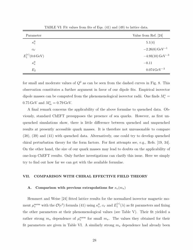
TABLE VI: Fit values from fits of Eqs. (41) and (49) to lattice data.

Parameter Value from Ref. [24]

κ0v 5.1(4)

cV −2.26(6)GeV−1

E(r)1 (0.6GeV) −4.93(10)GeV−3

κ0s −0.11

E2 0.074GeV−3

for small and moderate values of Q2 as can be seen from the dashed curves in Fig. 8. This

observation constitutes a further argument in favor of our dipole fits. Empirical isovector

dipole masses can be computed from the phenomenological isovector radii. One finds Mve =

0.75 GeV and Mvm = 0.79 GeV.

A final remark concerns the applicability of the above formulae to quenched data. Ob-

viously, standard ChEFT presupposes the presence of sea quarks. However, as first un-

quenched simulations show, there is little difference between quenched and unquenched

results at presently accessible quark masses. It is therefore not unreasonable to compare

(38), (39) and (41) with quenched data. Alternatively, one could try to develop quenched

chiral perturbation theory for the form factors. For first attempts see, e.g., Refs. [19, 34].

On the other hand, the size of our quark masses may lead to doubts on the applicability of

one-loop ChEFT results. Only further investigations can clarify this issue. Here we simply

try to find out how far we can get with the available formulae.

VII. COMPARISON WITH CHIRAL EFFECTIVE FIELD THEORY

A. Comparison with previous extrapolations for κv(mπ)

Hemmert and Weise [24] fitted lattice results for the normalized isovector magnetic mo-

ment µnormv with the O(ǫ3) formula (41) using κ0

v, cV and E(r)1 (λ) as fit parameters and fixing

the other parameters at their phenomenological values (see Table V). Their fit yielded a

rather strong mπ dependence of µnormv for small mπ. The values they obtained for their

fit parameters are given in Table VI. A similarly strong mπ dependence had already been

28

0.0 0.2 0.4 0.6 0.8 1.0 1.2 1.4m [GeV]

0

1

2

3

4

5

6

vnorm

= 6.40= 6.20= 6.00

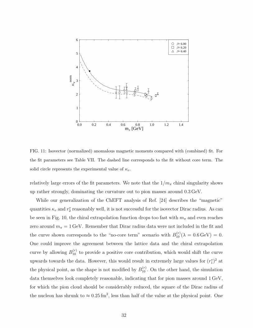
FIG. 9: Our results for the isovector (normalized) magnetic moments compared with the SSE

extrapolation curve of Ref. [24]. The solid circle represents the experimental value of µv.

observed in Refs. [25, 26] for the magnetic moments of the proton and the neutron. In

Fig. 9 we plot our data together with the curve corresponding to the fit of Ref. [24]. The

comparison indicates that the data used in Ref. [24] lie somewhat below ours.

B. Combined fits

The results of Ref. [24] show that using the SSE it is possible to connect the experimental

value of the magnetic moment with the lattice data. This raises the question whether one

could not obtain a similarly good description of the radii by fitting the SSE expression to

the simulation results. From the point of view of ChEFT the mass dependence of the Dirac

and Pauli radius is much simpler to discuss than that of the analogous Sachs quantities.

Hence we shall base our analysis on rv1 and rv

2 instead of Mve and Mv

m. Note, however, that

the numerical data in the following discussion are taken from the dipole fits of the Sachs

form factors.

Because cut-off effects seem to be small we fitted the results from all three β values

together taking into account all data points with mπ < 1 GeV. We kept Fπ, MN , cA and ∆

29

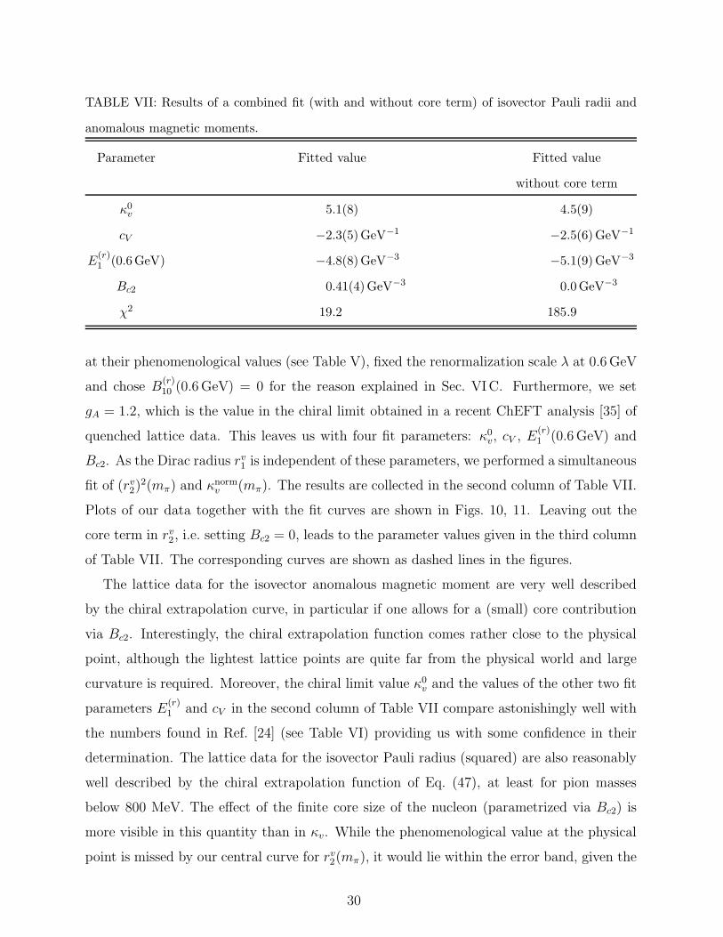
TABLE VII: Results of a combined fit (with and without core term) of isovector Pauli radii and

anomalous magnetic moments.

Parameter Fitted value Fitted value

without core term

κ0v 5.1(8) 4.5(9)

cV −2.3(5)GeV−1 −2.5(6)GeV−1

E(r)1 (0.6GeV) −4.8(8)GeV−3 −5.1(9)GeV−3

Bc2 0.41(4)GeV−3 0.0GeV−3

χ2 19.2 185.9

at their phenomenological values (see Table V), fixed the renormalization scale λ at 0.6 GeV

and chose B(r)10 (0.6 GeV) = 0 for the reason explained in Sec. VIC. Furthermore, we set

gA = 1.2, which is the value in the chiral limit obtained in a recent ChEFT analysis [35] of

quenched lattice data. This leaves us with four fit parameters: κ0v, cV , E

(r)1 (0.6 GeV) and

Bc2. As the Dirac radius rv1 is independent of these parameters, we performed a simultaneous

fit of (rv2)

2(mπ) and κnormv (mπ). The results are collected in the second column of Table VII.

Plots of our data together with the fit curves are shown in Figs. 10, 11. Leaving out the

core term in rv2, i.e. setting Bc2 = 0, leads to the parameter values given in the third column

of Table VII. The corresponding curves are shown as dashed lines in the figures.

The lattice data for the isovector anomalous magnetic moment are very well described

by the chiral extrapolation curve, in particular if one allows for a (small) core contribution

via Bc2. Interestingly, the chiral extrapolation function comes rather close to the physical

point, although the lightest lattice points are quite far from the physical world and large

curvature is required. Moreover, the chiral limit value κ0v and the values of the other two fit

parameters E(r)1 and cV in the second column of Table VII compare astonishingly well with

the numbers found in Ref. [24] (see Table VI) providing us with some confidence in their

determination. The lattice data for the isovector Pauli radius (squared) are also reasonably

well described by the chiral extrapolation function of Eq. (47), at least for pion masses

below 800 MeV. The effect of the finite core size of the nucleon (parametrized via Bc2) is

more visible in this quantity than in κv. While the phenomenological value at the physical

point is missed by our central curve for rv2(mπ), it would lie within the error band, given the

30

0.0 0.2 0.4 0.6 0.8 1.0 1.2 1.4m [GeV]

0.0

0.1

0.2

0.3

0.4

0.5

0.6

0.7

0.8

0.9

1.0

(r1v )2

[fm

2 ]

= 6.40= 6.20= 6.00

0.0 0.2 0.4 0.6 0.8 1.0 1.2 1.4m [GeV]

0.0

0.1

0.2

0.3

0.4

0.5

0.6

0.7

0.8

0.9

1.0

(r2v )2

[fm

2 ]

= 6.40= 6.20= 6.00

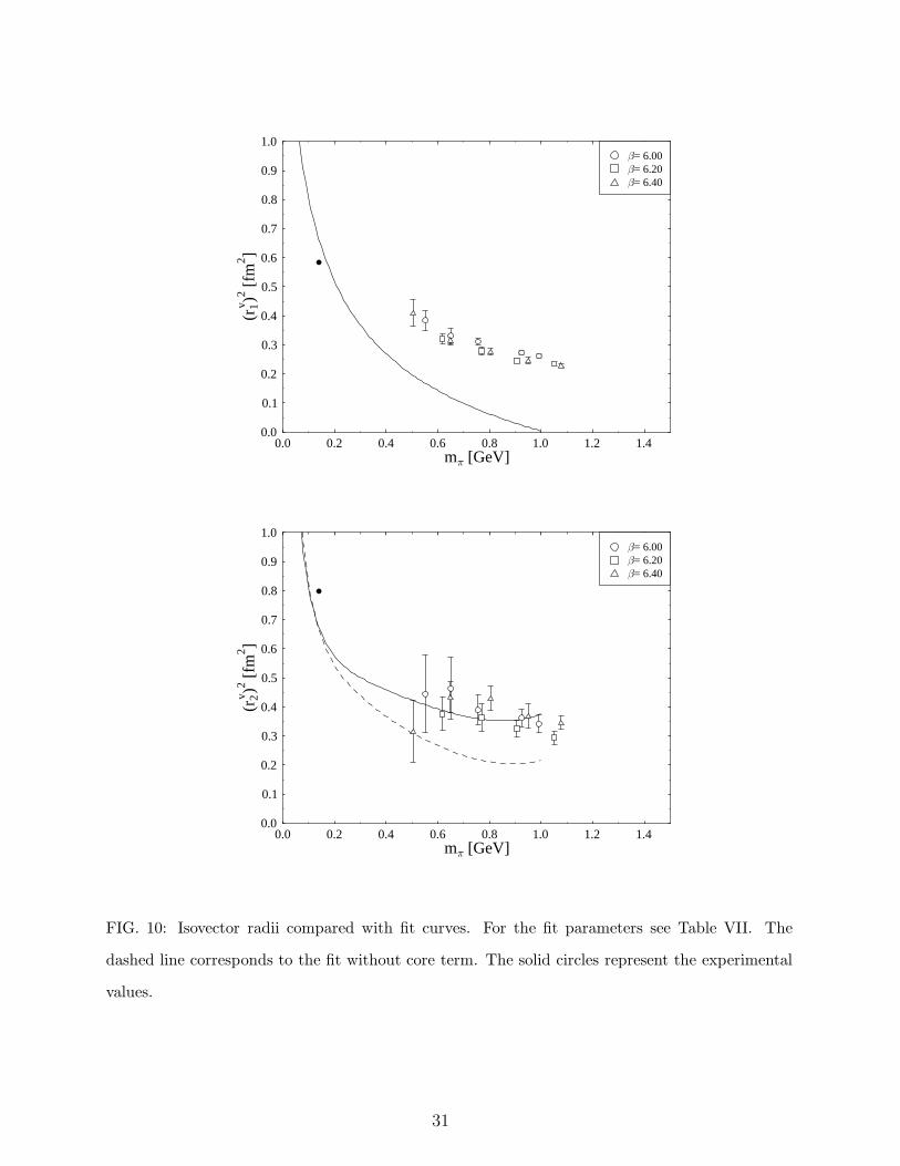
FIG. 10: Isovector radii compared with fit curves. For the fit parameters see Table VII. The

dashed line corresponds to the fit without core term. The solid circles represent the experimental

values.

31

0.0 0.2 0.4 0.6 0.8 1.0 1.2 1.4m [GeV]

0

1

2

3

4

5

6

vnorm

= 6.40= 6.20= 6.00

FIG. 11: Isovector (normalized) anomalous magnetic moments compared with (combined) fit. For

the fit parameters see Table VII. The dashed line corresponds to the fit without core term. The

solid circle represents the experimental value of κv.

relatively large errors of the fit parameters. We note that the 1/mπ chiral singularity shows

up rather strongly, dominating the curvature out to pion masses around 0.3 GeV.

While our generalization of the ChEFT analysis of Ref. [24] describes the “magnetic”

quantities κv and rv2 reasonably well, it is not successful for the isovector Dirac radius. As can

be seen in Fig. 10, the chiral extrapolation function drops too fast with mπ and even reaches

zero around mπ = 1 GeV. Remember that Dirac radius data were not included in the fit and

the curve shown corresponds to the “no-core term” scenario with B(r)10 (λ = 0.6 GeV) = 0.

One could improve the agreement between the lattice data and the chiral extrapolation

curve by allowing B(r)10 to provide a positive core contribution, which would shift the curve

upwards towards the data. However, this would result in extremely large values for (rv1)

2 at

the physical point, as the shape is not modified by B(r)10 . On the other hand, the simulation

data themselves look completely reasonable, indicating that for pion masses around 1 GeV,

for which the pion cloud should be considerably reduced, the square of the Dirac radius of

the nucleon has shrunk to ≈ 0.25 fm2, less than half of the value at the physical point. One

32

reason for this failure of Eq. (45) might lie in important higher order corrections in ChEFT

which could soften the strong mπ dependence originating from the chiral logarithm.

Nevertheless, one should also not forget that here we are dealing with a quenched simu-

lation. Given that (rv1)

2 at the physical point is nearly completely dominated by the pion

cloud (for low values of λ, cf. Eq. (46)) it is conceivable that the Dirac radius of the nucleon

might be sensitive to the effects of (un)quenching. We therefore conclude that especially for

rv1 a lot of work remains to be done, both on the level of ChEFT, where the next-to-leading

one-loop contributions need to be evaluated, as well as on the level of the simulations, where

a similar analysis as the one presented here has to be performed based on fully dynamical

configurations.

Of course, one can think of alternative fit strategies, which differ by the choice of the

fixed parameters. For example, one might leave also cA and ∆ free in addition to the four

parameters used above. In this (or a similar) way it is possible to force the fit through the

data points for (rv1)

2 also, but then the physical point is missed by a considerable amount.

So we must conclude that at the present level of accuracy the SSE expression for the Dirac

radius is not sufficient to connect the Monte Carlo data in a physically sensible way with

the phenomenological value.

C. Beyond the isovector channel

While ChEFT (to the order considered in Ref. [24]) yields the rather intricate expression

(41) for the quark-mass dependence of the isovector anomalous magnetic moment, the anal-

ogous expression for the isoscalar anomalous magnetic moment κs = κp + κn of the nucleon

is much simpler,

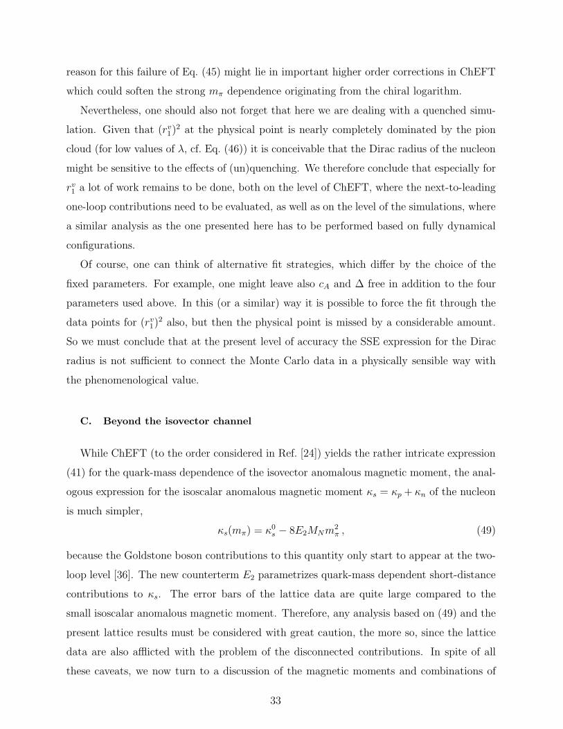
κs(mπ) = κ0s − 8E2MNm

2π , (49)

because the Goldstone boson contributions to this quantity only start to appear at the two-

loop level [36]. The new counterterm E2 parametrizes quark-mass dependent short-distance

contributions to κs. The error bars of the lattice data are quite large compared to the

small isoscalar anomalous magnetic moment. Therefore, any analysis based on (49) and the

present lattice results must be considered with great caution, the more so, since the lattice

data are also afflicted with the problem of the disconnected contributions. In spite of all

these caveats, we now turn to a discussion of the magnetic moments and combinations of

33

0.0 0.2 0.4 0.6 0.8 1.0 1.2 1.4m [GeV]

-0.6

-0.4

-0.2

0.0

0.2

0.4

0.6

snorm

= 6.40= 6.20= 6.00

FIG. 12: Isoscalar (normalized) anomalous magnetic moments compared with SSE fit. The solid

circle represents the experimental value of κs. The cross with the attached error bar shows the

value at mphysπ .

them which are not purely isovector quantities.

In Fig. 12 we present the normalized values of κs together with a fit using Eq. (49). The

values of κs have been computed as κp + κn from the proton and neutron dipole fits of Gm,

and the errors have been determined by error propagation. We obtain κ0s = −0.04(15) and

E2 = −0.004(25) GeV−3. These numbers are to be compared with the fit parameters from

Ref. [24] given in Table VI. The large statistical errors make definite statements difficult.

Having determined κv(mπ) as well as κs(mπ) we can now discuss the chiral extrapolation

of proton and neutron data separately. For κ0v, cV , E

(r)1 , Bc2 we choose the values given in

the second column of Table VII together with gA = 1.2, while for κ0s and E2 we take the

numbers given above and the remaining parameters are fixed at their physical values (see

Table V).

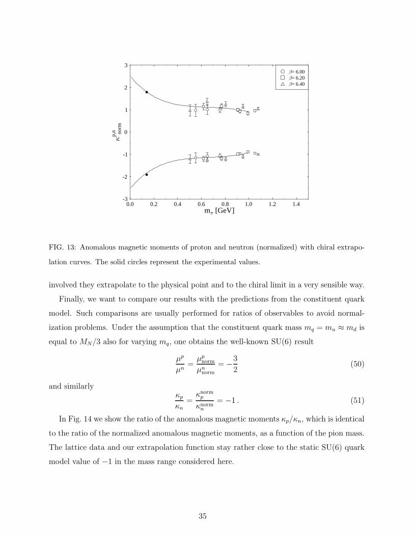
In Fig. 13 we compare the resulting extrapolation functions with the lattice results for the

anomalous magnetic moments. The extrapolation functions are surprisingly well behaved.

Despite the large gap between mphysπ and the lowest data point and the substantial curvature

34

0.0 0.2 0.4 0.6 0.8 1.0 1.2 1.4m [GeV]

-3

-2

-1

0

1

2

3

p,n no

rm

= 6.40= 6.20= 6.00

FIG. 13: Anomalous magnetic moments of proton and neutron (normalized) with chiral extrapo-

lation curves. The solid circles represent the experimental values.

involved they extrapolate to the physical point and to the chiral limit in a very sensible way.

Finally, we want to compare our results with the predictions from the constituent quark

model. Such comparisons are usually performed for ratios of observables to avoid normal-

ization problems. Under the assumption that the constituent quark mass mq = mu ≈ md is

equal to MN/3 also for varying mq, one obtains the well-known SU(6) result

µp

µn=µp

norm

µnnorm

= −3

2(50)

and similarlyκp

κn=κnorm

p

κnormn

= −1 . (51)

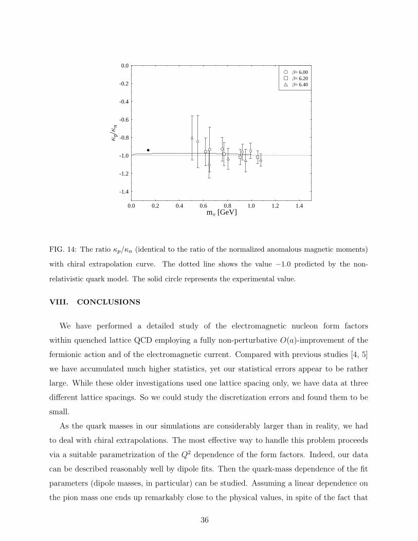
In Fig. 14 we show the ratio of the anomalous magnetic moments κp/κn, which is identical

to the ratio of the normalized anomalous magnetic moments, as a function of the pion mass.

The lattice data and our extrapolation function stay rather close to the static SU(6) quark

model value of −1 in the mass range considered here.

35

0.0 0.2 0.4 0.6 0.8 1.0 1.2 1.4m [GeV]

-1.4

-1.2

-1.0

-0.8

-0.6

-0.4

-0.2

0.0

p/n

= 6.40= 6.20= 6.00

FIG. 14: The ratio κp/κn (identical to the ratio of the normalized anomalous magnetic moments)

with chiral extrapolation curve. The dotted line shows the value −1.0 predicted by the non-

relativistic quark model. The solid circle represents the experimental value.

VIII. CONCLUSIONS

We have performed a detailed study of the electromagnetic nucleon form factors

within quenched lattice QCD employing a fully non-perturbative O(a)-improvement of the

fermionic action and of the electromagnetic current. Compared with previous studies [4, 5]

we have accumulated much higher statistics, yet our statistical errors appear to be rather

large. While these older investigations used one lattice spacing only, we have data at three

different lattice spacings. So we could study the discretization errors and found them to be

small.

As the quark masses in our simulations are considerably larger than in reality, we had

to deal with chiral extrapolations. The most effective way to handle this problem proceeds

via a suitable parametrization of the Q2 dependence of the form factors. Indeed, our data

can be described reasonably well by dipole fits. Then the quark-mass dependence of the fit

parameters (dipole masses, in particular) can be studied. Assuming a linear dependence on

the pion mass one ends up remarkably close to the physical values, in spite of the fact that

36

the singularities arising from the Goldstone bosons of QCD must show up at some point

invalidating such a simple picture. Nevertheless, the difference between the electric and the

magnetic dipole mass which we obtain at the physical pion mass is in (semi-quantitative)

agreement with recent experimental results [2, 3].

Ideally, the chiral extrapolation should be guided by ChEFT. However, most of the

existing chiral expansions do not take into account quenching artefacts and are therefore,

strictly speaking, not applicable to our data. But first simulations with dynamical quarks

indicate that at the quark masses considered in this paper quenching effects are small so

that quenched chiral perturbation theory is not required. While in this respect the size of

our quark masses might be helpful, it leads on the other hand to doubts on the applicability

of ChEFT. Indeed, only a reorganisation of the standard chiral perturbation theory series

allowed Hemmert and Weise [24] to describe with a single expression the phenomenological

value of the isovector anomalous magnetic moment of the nucleon as well as (quenched)

lattice data. For a different approach to the same problem see Refs. [25, 26, 28].

We have extended the analysis of the magnetic moments of the nucleon of Ref. [24] to

the general case of nucleon electromagnetic form factors. Given that these calculations are

reliable only for Q2 < 0.4 GeV2, no direct comparison with our lattice data, taken at higher

values of Q2, could be performed. Instead we have converted the dipole masses extracted

from our simulations into form factor radii, which could then be compared with the ChEFT

formulae. Larger lattices allowing smaller values of Q2 would be required, if one aims at a

direct comparison with the ChEFT results for the form factors.

As low-order (one-loop) ChEFT is insufficient to simultaneously account for the quark-

mass dependence of the nucleon mass and the form factors in the current matrix elements,

we were forced to “normalize” the magnetic moments computed on the lattice before fitting

them with the ChEFT formulae. Higher-order calculations in ChEFT, at least at the two-

loop level, would be required to avoid this necessity.

In the isovector channel a combined fit of κv(mπ) and the Pauli radius rv2(mπ) yielded

extrapolation functions which describe the lattice data quite well and extrapolate (albeit

with large error bar) close to the physical point. For the isovector Dirac radius rv1(mπ) no

chiral extrapolation function could be obtained that is consistent both with the lattice data

and known phenomenology at the physical point. Further studies are needed to resolve this

discrepancy, both in ChEFT regarding higher order corrections and on the simulation side

37

investigating quenching effects. (For an alternative view see Ref. [27].) The parameters

obtained in the fits are well consistent with those found in Ref. [24]. In particular, we find

κ0v = 5.1± 0.8 as the chiral limit value for the isovector anomalous magnetic moment of the

nucleon.

The isoscalar sector is plagued by large uncertainties in the lattice data. The chiral

dynamics contributing to extrapolation functions in this sector seems to be dominated by

analytic terms. Quantitative studies can only be performed once the statistics of the data

is improved and disconnected contributions are taken into account. The ratio κp/κn could

be well described by our chiral extrapolation and was found in remarkable agreement with

the constituent quark model.

The leading one-loop calculation in the SSE is found to describe the quark-mass depen-

dence of magnetic quantities quite well. Unfortunately, at the moment we do not have a

ChEFT with appropriate counting scheme that simultaneously describes the quark-mass

dependence in all four quantities κv, κs, rv1 , r

v2 at leading one-loop order. It remains to be

seen whether the discrepancies found in rv1(mπ) can be resolved in a next-to-leading one-

loop SSE calculation of the form factors. The figures in this paper show that ChEFT often

predicts large effects at values of mπ lighter than those we used in our lattice simulations. In

order to confirm the predictions of ChEFT, and in order to extrapolate reliably to physical

quark masses, we need simulations at much smaller values of mπ. Moreover, it would be

desirable to compute the quark-line disconnected contributions. Important progress is also

to be expected from the ongoing simulations with dynamical fermions.

Acknowledgments

This work has been supported in part by the European Community’s Human Poten-

tial Program under contract HPRN-CT-2000-00145, Hadrons/Lattice QCD, by the DFG

(Forschergruppe Gitter-Hadronen-Phanomenologie) and by the BMBF. Discussions with V.

Braun and W. Weise are gratefully acknowledged, as well as the constructive remarks of the

referee. TRH thanks the Institute for Theoretical Physics of the University of Regensburg

and DESY Zeuthen for their kind hospitality.

The numerical calculations were performed on the APE100 at NIC (Zeuthen) as well as

on the Cray T3E at ZIB (Berlin) and NIC (Julich). We wish to thank all institutions for

38

their support.

APPENDIX A

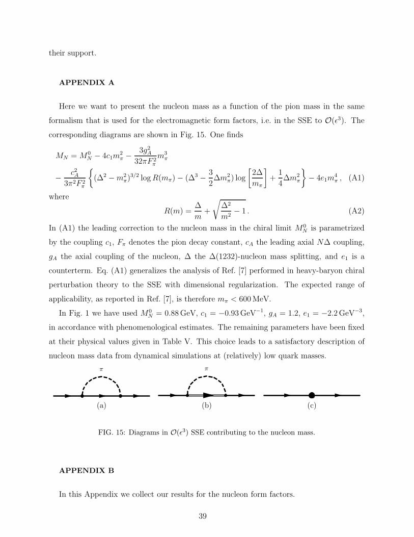
Here we want to present the nucleon mass as a function of the pion mass in the same

formalism that is used for the electromagnetic form factors, i.e. in the SSE to O(ǫ3). The

corresponding diagrams are shown in Fig. 15. One finds

MN = M0N − 4c1m

2π − 3g2

A

32πF 2π

m3π

− c2A3π2F 2

π

{

(∆2 −m2π)3/2 logR(mπ) − (∆3 − 3

2∆m2

π) log

[

2∆

mπ

]

+1

4∆m2

π

}

− 4e1m4π , (A1)

where

R(m) =∆

m+

√

∆2

m2− 1 . (A2)

In (A1) the leading correction to the nucleon mass in the chiral limit M0N is parametrized

by the coupling c1, Fπ denotes the pion decay constant, cA the leading axial N∆ coupling,

gA the axial coupling of the nucleon, ∆ the ∆(1232)-nucleon mass splitting, and e1 is a

counterterm. Eq. (A1) generalizes the analysis of Ref. [7] performed in heavy-baryon chiral

perturbation theory to the SSE with dimensional regularization. The expected range of

applicability, as reported in Ref. [7], is therefore mπ < 600 MeV.

In Fig. 1 we have used M0N = 0.88 GeV, c1 = −0.93 GeV−1, gA = 1.2, e1 = −2.2 GeV−3,

in accordance with phenomenological estimates. The remaining parameters have been fixed

at their physical values given in Table V. This choice leads to a satisfactory description of

nucleon mass data from dynamical simulations at (relatively) low quark masses.

π π

(a) (b) (c)

FIG. 15: Diagrams in O(ǫ3) SSE contributing to the nucleon mass.

APPENDIX B

In this Appendix we collect our results for the nucleon form factors.

39

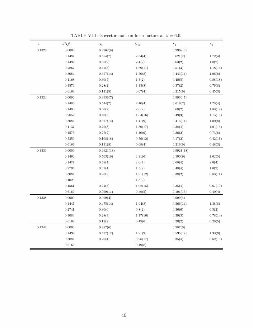
TABLE VIII: Isovector nucleon form factors at β = 6.0.

κ a2Q2 Ge Gm F1 F2

0.1320 0.0000 0.9962(6) 0.9962(6)

0.1484 0.554(7) 2.34(4) 0.621(7) 1.72(4)

0.1492 0.56(2) 2.4(2) 0.63(2) 1.8(2)

0.2867 0.42(3) 1.69(17) 0.51(3) 1.18(16)

0.3084 0.357(14) 1.50(8) 0.443(14) 1.06(8)

0.4168 0.30(5) 1.3(2) 0.40(5) 0.88(18)

0.4576 0.28(2) 1.13(8) 0.37(2) 0.76(8)

0.6169 0.141(9) 0.67(4) 0.215(9) 0.45(3)

0.1324 0.0000 0.9936(7) 0.9936(7)

0.1480 0.544(7) 2.40(4) 0.619(7) 1.78(4)

0.1488 0.60(2) 2.6(2) 0.68(2) 1.88(19)

0.2852 0.40(3) 1.64(16) 0.49(3) 1.15(15)

0.3084 0.327(14) 1.41(9) 0.415(14) 1.00(8)

0.4137 0.26(3) 1.39(17) 0.38(4) 1.01(16)

0.4573 0.27(2) 1.10(9) 0.36(2) 0.73(8)

0.5350 0.108(18) 0.59(12) 0.17(2) 0.42(11)

0.6169 0.131(8) 0.69(4) 0.216(9) 0.48(3)

0.1333 0.0000 0.9921(18) 0.9921(18)

0.1463 0.503(10) 2.21(6) 0.590(9) 1.62(5)

0.1477 0.58(4) 2.6(4) 0.68(4) 2.0(4)

0.2796 0.37(4) 1.5(2) 0.48(4) 1.0(2)

0.3084 0.28(2) 1.21(12) 0.38(2) 0.83(11)

0.4029 1.3(2)

0.4561 0.24(5) 1.02(15) 0.35(4) 0.67(13)

0.6169 0.099(11) 0.59(5) 0.191(13) 0.40(4)

0.1338 0.0000 0.999(4) 0.999(4)

0.1447 0.475(14) 1.94(8) 0.566(14) 1.38(8)

0.2741 0.30(6) 0.8(2) 0.36(6) 0.5(2)

0.3084 0.28(3) 1.17(16) 0.39(3) 0.78(14)

0.6169 0.12(2) 0.49(6) 0.20(2) 0.29(5)

0.1342 0.0000 0.987(6) 0.987(6)

0.1439 0.437(17) 1.91(9) 0.535(17) 1.38(9)

0.3084 0.26(4) 0.98(17) 0.35(4) 0.62(15)

0.6169 0.49(8)

40

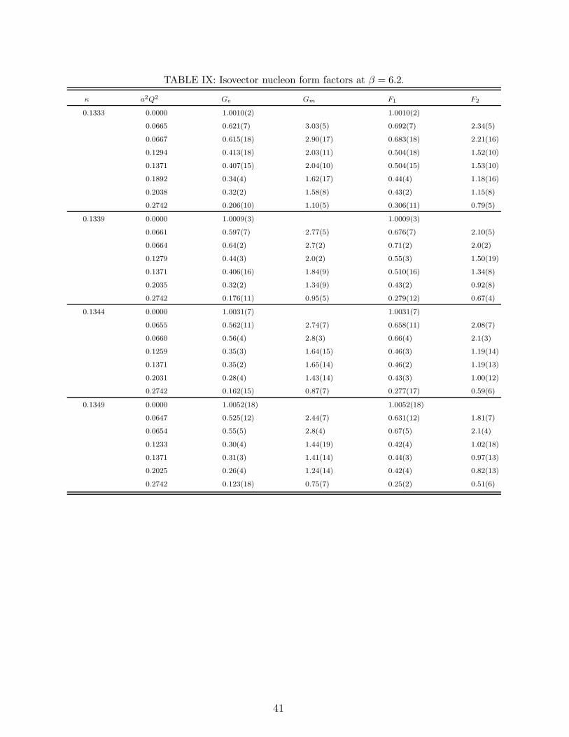
TABLE IX: Isovector nucleon form factors at β = 6.2.

κ a2Q2 Ge Gm F1 F2

0.1333 0.0000 1.0010(2) 1.0010(2)

0.0665 0.621(7) 3.03(5) 0.692(7) 2.34(5)

0.0667 0.615(18) 2.90(17) 0.683(18) 2.21(16)

0.1294 0.413(18) 2.03(11) 0.504(18) 1.52(10)

0.1371 0.407(15) 2.04(10) 0.504(15) 1.53(10)

0.1892 0.34(4) 1.62(17) 0.44(4) 1.18(16)

0.2038 0.32(2) 1.58(8) 0.43(2) 1.15(8)

0.2742 0.206(10) 1.10(5) 0.306(11) 0.79(5)

0.1339 0.0000 1.0009(3) 1.0009(3)

0.0661 0.597(7) 2.77(5) 0.676(7) 2.10(5)

0.0664 0.64(2) 2.7(2) 0.71(2) 2.0(2)

0.1279 0.44(3) 2.0(2) 0.55(3) 1.50(19)

0.1371 0.406(16) 1.84(9) 0.510(16) 1.34(8)

0.2035 0.32(2) 1.34(9) 0.43(2) 0.92(8)

0.2742 0.176(11) 0.95(5) 0.279(12) 0.67(4)

0.1344 0.0000 1.0031(7) 1.0031(7)

0.0655 0.562(11) 2.74(7) 0.658(11) 2.08(7)

0.0660 0.56(4) 2.8(3) 0.66(4) 2.1(3)

0.1259 0.35(3) 1.64(15) 0.46(3) 1.19(14)

0.1371 0.35(2) 1.65(14) 0.46(2) 1.19(13)

0.2031 0.28(4) 1.43(14) 0.43(3) 1.00(12)

0.2742 0.162(15) 0.87(7) 0.277(17) 0.59(6)

0.1349 0.0000 1.0052(18) 1.0052(18)

0.0647 0.525(12) 2.44(7) 0.631(12) 1.81(7)

0.0654 0.55(5) 2.8(4) 0.67(5) 2.1(4)

0.1233 0.30(4) 1.44(19) 0.42(4) 1.02(18)

0.1371 0.31(3) 1.41(14) 0.44(3) 0.97(13)

0.2025 0.26(4) 1.24(14) 0.42(4) 0.82(13)

0.2742 0.123(18) 0.75(7) 0.25(2) 0.51(6)

41

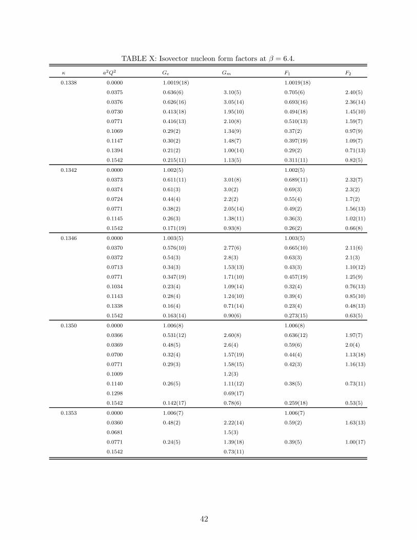
TABLE X: Isovector nucleon form factors at β = 6.4.

κ a2Q2 Ge Gm F1 F2

0.1338 0.0000 1.0019(18) 1.0019(18)

0.0375 0.636(6) 3.10(5) 0.705(6) 2.40(5)

0.0376 0.626(16) 3.05(14) 0.693(16) 2.36(14)

0.0730 0.413(18) 1.95(10) 0.494(18) 1.45(10)

0.0771 0.416(13) 2.10(8) 0.510(13) 1.59(7)

0.1069 0.29(2) 1.34(9) 0.37(2) 0.97(9)

0.1147 0.30(2) 1.48(7) 0.397(19) 1.09(7)

0.1394 0.21(2) 1.00(14) 0.29(2) 0.71(13)

0.1542 0.215(11) 1.13(5) 0.311(11) 0.82(5)

0.1342 0.0000 1.002(5) 1.002(5)

0.0373 0.611(11) 3.01(8) 0.689(11) 2.32(7)

0.0374 0.61(3) 3.0(2) 0.69(3) 2.3(2)

0.0724 0.44(4) 2.2(2) 0.55(4) 1.7(2)

0.0771 0.38(2) 2.05(14) 0.49(2) 1.56(13)

0.1145 0.26(3) 1.38(11) 0.36(3) 1.02(11)

0.1542 0.171(19) 0.93(8) 0.26(2) 0.66(8)

0.1346 0.0000 1.003(5) 1.003(5)

0.0370 0.576(10) 2.77(6) 0.665(10) 2.11(6)

0.0372 0.54(3) 2.8(3) 0.63(3) 2.1(3)

0.0713 0.34(3) 1.53(13) 0.43(3) 1.10(12)

0.0771 0.347(19) 1.71(10) 0.457(19) 1.25(9)

0.1034 0.23(4) 1.09(14) 0.32(4) 0.76(13)

0.1143 0.28(4) 1.24(10) 0.39(4) 0.85(10)

0.1338 0.16(4) 0.71(14) 0.23(4) 0.48(13)

0.1542 0.163(14) 0.90(6) 0.273(15) 0.63(5)

0.1350 0.0000 1.006(8) 1.006(8)

0.0366 0.531(12) 2.60(8) 0.636(12) 1.97(7)

0.0369 0.48(5) 2.6(4) 0.59(6) 2.0(4)

0.0700 0.32(4) 1.57(19) 0.44(4) 1.13(18)

0.0771 0.29(3) 1.58(15) 0.42(3) 1.16(13)

0.1009 1.2(3)

0.1140 0.26(5) 1.11(12) 0.38(5) 0.73(11)

0.1298 0.69(17)

0.1542 0.142(17) 0.78(6) 0.259(18) 0.53(5)

0.1353 0.0000 1.006(7) 1.006(7)

0.0360 0.48(2) 2.22(14) 0.59(2) 1.63(13)

0.0681 1.5(3)

0.0771 0.24(5) 1.39(18) 0.39(5) 1.00(17)

0.1542 0.73(11)

42

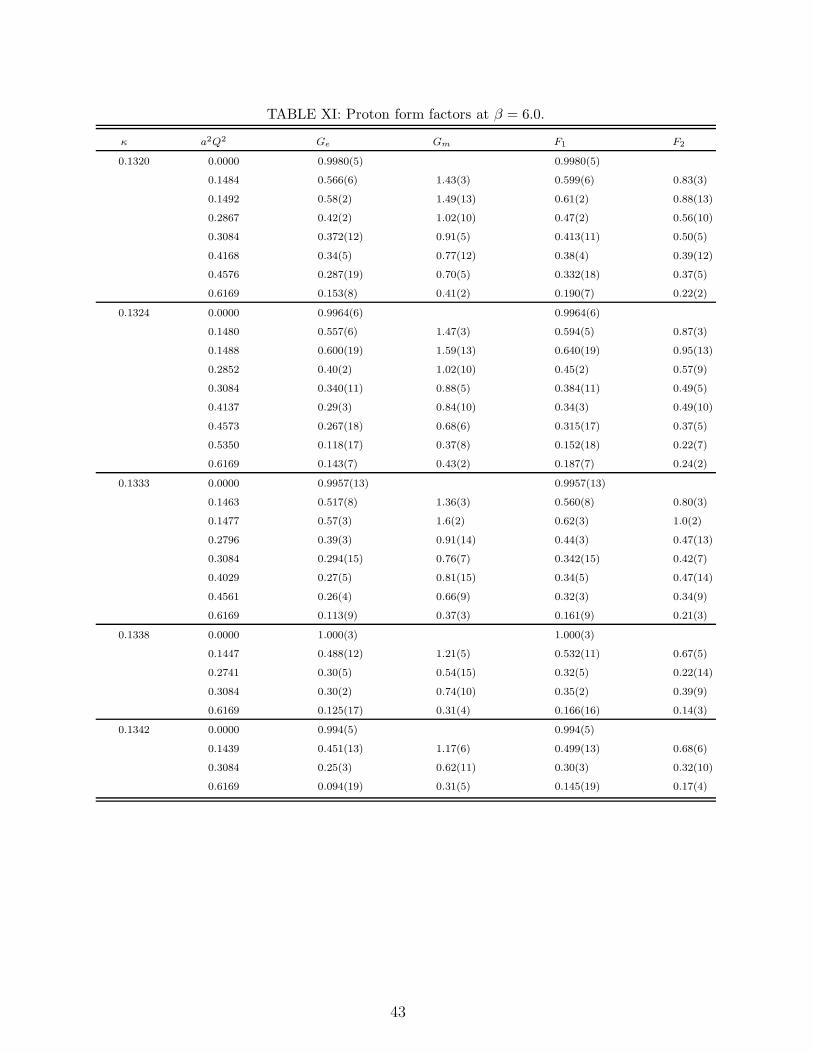
TABLE XI: Proton form factors at β = 6.0.

κ a2Q2 Ge Gm F1 F2

0.1320 0.0000 0.9980(5) 0.9980(5)

0.1484 0.566(6) 1.43(3) 0.599(6) 0.83(3)

0.1492 0.58(2) 1.49(13) 0.61(2) 0.88(13)

0.2867 0.42(2) 1.02(10) 0.47(2) 0.56(10)

0.3084 0.372(12) 0.91(5) 0.413(11) 0.50(5)

0.4168 0.34(5) 0.77(12) 0.38(4) 0.39(12)

0.4576 0.287(19) 0.70(5) 0.332(18) 0.37(5)

0.6169 0.153(8) 0.41(2) 0.190(7) 0.22(2)

0.1324 0.0000 0.9964(6) 0.9964(6)

0.1480 0.557(6) 1.47(3) 0.594(5) 0.87(3)

0.1488 0.600(19) 1.59(13) 0.640(19) 0.95(13)

0.2852 0.40(2) 1.02(10) 0.45(2) 0.57(9)

0.3084 0.340(11) 0.88(5) 0.384(11) 0.49(5)

0.4137 0.29(3) 0.84(10) 0.34(3) 0.49(10)

0.4573 0.267(18) 0.68(6) 0.315(17) 0.37(5)

0.5350 0.118(17) 0.37(8) 0.152(18) 0.22(7)

0.6169 0.143(7) 0.43(2) 0.187(7) 0.24(2)

0.1333 0.0000 0.9957(13) 0.9957(13)

0.1463 0.517(8) 1.36(3) 0.560(8) 0.80(3)

0.1477 0.57(3) 1.6(2) 0.62(3) 1.0(2)

0.2796 0.39(3) 0.91(14) 0.44(3) 0.47(13)

0.3084 0.294(15) 0.76(7) 0.342(15) 0.42(7)

0.4029 0.27(5) 0.81(15) 0.34(5) 0.47(14)

0.4561 0.26(4) 0.66(9) 0.32(3) 0.34(9)

0.6169 0.113(9) 0.37(3) 0.161(9) 0.21(3)

0.1338 0.0000 1.000(3) 1.000(3)

0.1447 0.488(12) 1.21(5) 0.532(11) 0.67(5)

0.2741 0.30(5) 0.54(15) 0.32(5) 0.22(14)

0.3084 0.30(2) 0.74(10) 0.35(2) 0.39(9)

0.6169 0.125(17) 0.31(4) 0.166(16) 0.14(3)

0.1342 0.0000 0.994(5) 0.994(5)

0.1439 0.451(13) 1.17(6) 0.499(13) 0.68(6)

0.3084 0.25(3) 0.62(11) 0.30(3) 0.32(10)

0.6169 0.094(19) 0.31(5) 0.145(19) 0.17(4)

43

TABLE XII: Proton form factors at β = 6.2.

κ a2Q2 Ge Gm F1 F2

0.1333 0.0000 1.00196(17) 1.00196(17)

0.0665 0.633(5) 1.85(3) 0.669(5) 1.18(3)

0.0667 0.626(15) 1.82(11) 0.662(15) 1.16(10)

0.1294 0.426(15) 1.24(7) 0.472(15) 0.77(6)

0.1371 0.423(12) 1.24(6) 0.471(12) 0.77(6)

0.1892 0.37(4) 1.00(11) 0.42(4) 0.58(10)

0.2038 0.333(18) 0.97(5) 0.387(17) 0.58(5)

0.2742 0.219(10) 0.67(3) 0.269(9) 0.40(3)

0.1339 0.0000 1.0020(3) 1.0020(3)

0.0661 0.607(6) 1.70(3) 0.646(6) 1.05(3)

0.0664 0.637(19) 1.71(13) 0.676(19) 1.04(12)

0.1279 0.45(3) 1.22(12) 0.50(3) 0.72(12)

0.1371 0.414(13) 1.13(6) 0.466(13) 0.66(5)

0.2035 0.33(2) 0.83(5) 0.380(19) 0.45(5)

0.2742 0.184(10) 0.58(3) 0.237(9) 0.34(3)

0.1344 0.0000 1.0037(5) 1.0037(5)

0.0655 0.576(8) 1.67(4) 0.624(8) 1.05(4)

0.0660 0.56(3) 1.8(2) 0.62(3) 1.1(2)

0.1259 0.37(2) 1.02(9) 0.42(2) 0.60(9)

0.1371 0.368(18) 1.00(8) 0.424(18) 0.57(8)

0.1823 0.29(7)

0.2031 0.30(3) 0.88(8) 0.38(3) 0.50(8)

0.2742 0.174(13) 0.53(4) 0.232(13) 0.30(4)

0.1349 0.0000 1.0054(12) 1.0054(12)

0.0647 0.535(9) 1.49(5) 0.588(9) 0.91(4)

0.0654 0.55(4) 1.8(3) 0.62(4) 1.2(3)

0.1233 0.34(3) 0.86(12) 0.39(3) 0.47(11)

0.1371 0.34(2) 0.85(8) 0.392(19) 0.46(8)

0.2025 0.27(4) 0.76(9) 0.34(3) 0.41(8)

0.2742 0.133(13) 0.47(4) 0.199(13) 0.27(3)

44

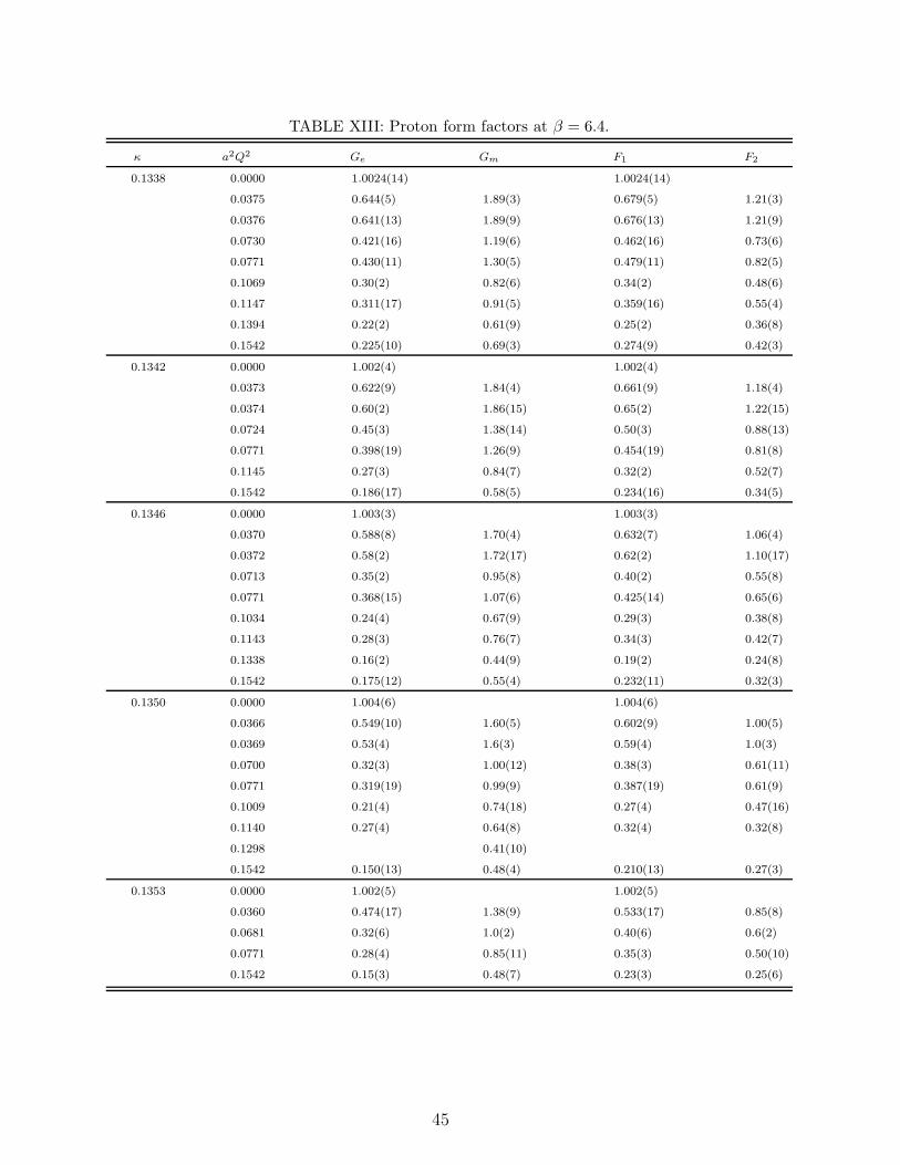
TABLE XIII: Proton form factors at β = 6.4.

κ a2Q2 Ge Gm F1 F2

0.1338 0.0000 1.0024(14) 1.0024(14)

0.0375 0.644(5) 1.89(3) 0.679(5) 1.21(3)

0.0376 0.641(13) 1.89(9) 0.676(13) 1.21(9)

0.0730 0.421(16) 1.19(6) 0.462(16) 0.73(6)

0.0771 0.430(11) 1.30(5) 0.479(11) 0.82(5)

0.1069 0.30(2) 0.82(6) 0.34(2) 0.48(6)

0.1147 0.311(17) 0.91(5) 0.359(16) 0.55(4)

0.1394 0.22(2) 0.61(9) 0.25(2) 0.36(8)

0.1542 0.225(10) 0.69(3) 0.274(9) 0.42(3)

0.1342 0.0000 1.002(4) 1.002(4)

0.0373 0.622(9) 1.84(4) 0.661(9) 1.18(4)

0.0374 0.60(2) 1.86(15) 0.65(2) 1.22(15)

0.0724 0.45(3) 1.38(14) 0.50(3) 0.88(13)

0.0771 0.398(19) 1.26(9) 0.454(19) 0.81(8)

0.1145 0.27(3) 0.84(7) 0.32(2) 0.52(7)

0.1542 0.186(17) 0.58(5) 0.234(16) 0.34(5)

0.1346 0.0000 1.003(3) 1.003(3)

0.0370 0.588(8) 1.70(4) 0.632(7) 1.06(4)

0.0372 0.58(2) 1.72(17) 0.62(2) 1.10(17)

0.0713 0.35(2) 0.95(8) 0.40(2) 0.55(8)

0.0771 0.368(15) 1.07(6) 0.425(14) 0.65(6)

0.1034 0.24(4) 0.67(9) 0.29(3) 0.38(8)

0.1143 0.28(3) 0.76(7) 0.34(3) 0.42(7)

0.1338 0.16(2) 0.44(9) 0.19(2) 0.24(8)

0.1542 0.175(12) 0.55(4) 0.232(11) 0.32(3)

0.1350 0.0000 1.004(6) 1.004(6)

0.0366 0.549(10) 1.60(5) 0.602(9) 1.00(5)

0.0369 0.53(4) 1.6(3) 0.59(4) 1.0(3)

0.0700 0.32(3) 1.00(12) 0.38(3) 0.61(11)

0.0771 0.319(19) 0.99(9) 0.387(19) 0.61(9)

0.1009 0.21(4) 0.74(18) 0.27(4) 0.47(16)

0.1140 0.27(4) 0.64(8) 0.32(4) 0.32(8)

0.1298 0.41(10)

0.1542 0.150(13) 0.48(4) 0.210(13) 0.27(3)

0.1353 0.0000 1.002(5) 1.002(5)

0.0360 0.474(17) 1.38(9) 0.533(17) 0.85(8)

0.0681 0.32(6) 1.0(2) 0.40(6) 0.6(2)

0.0771 0.28(4) 0.85(11) 0.35(3) 0.50(10)

0.1542 0.15(3) 0.48(7) 0.23(3) 0.25(6)

45

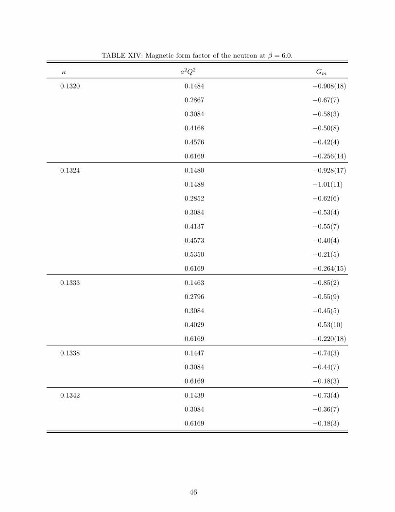
TABLE XIV: Magnetic form factor of the neutron at β = 6.0.

κ a2Q2 Gm

0.1320 0.1484 −0.908(18)

0.2867 −0.67(7)

0.3084 −0.58(3)

0.4168 −0.50(8)

0.4576 −0.42(4)

0.6169 −0.256(14)

0.1324 0.1480 −0.928(17)

0.1488 −1.01(11)

0.2852 −0.62(6)

0.3084 −0.53(4)

0.4137 −0.55(7)

0.4573 −0.40(4)

0.5350 −0.21(5)

0.6169 −0.264(15)

0.1333 0.1463 −0.85(2)

0.2796 −0.55(9)

0.3084 −0.45(5)

0.4029 −0.53(10)

0.6169 −0.220(18)

0.1338 0.1447 −0.74(3)

0.3084 −0.44(7)

0.6169 −0.18(3)

0.1342 0.1439 −0.73(4)

0.3084 −0.36(7)

0.6169 −0.18(3)

46

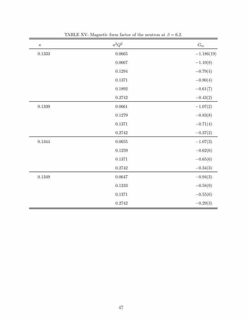
TABLE XV: Magnetic form factor of the neutron at β = 6.2.

κ a2Q2 Gm

0.1333 0.0665 −1.186(19)

0.0667 −1.10(8)

0.1294 −0.79(4)

0.1371 −0.80(4)

0.1892 −0.61(7)

0.2742 −0.43(2)

0.1339 0.0661 −1.07(2)

0.1279 −0.83(8)

0.1371 −0.71(4)

0.2742 −0.37(2)

0.1344 0.0655 −1.07(3)

0.1259 −0.62(6)

0.1371 −0.65(6)

0.2742 −0.34(3)

0.1349 0.0647 −0.94(3)

0.1233 −0.58(9)

0.1371 −0.55(6)

0.2742 −0.29(3)

47

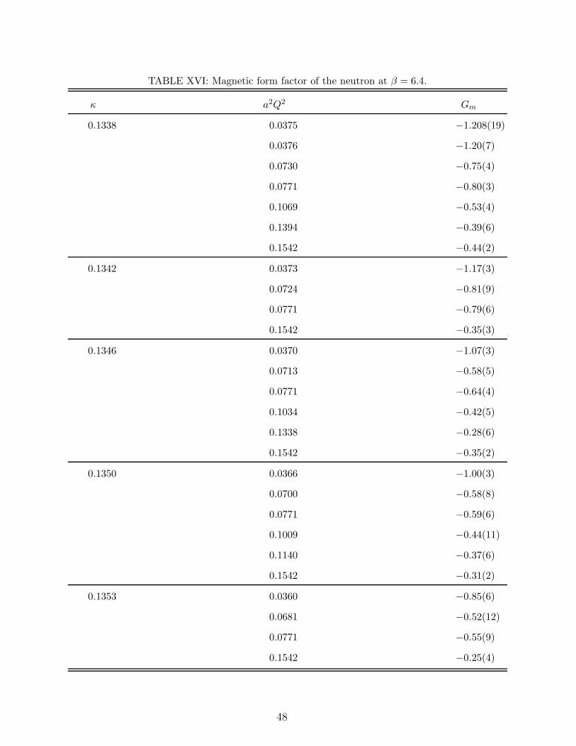
TABLE XVI: Magnetic form factor of the neutron at β = 6.4.

κ a2Q2 Gm

0.1338 0.0375 −1.208(19)

0.0376 −1.20(7)

0.0730 −0.75(4)

0.0771 −0.80(3)

0.1069 −0.53(4)

0.1394 −0.39(6)

0.1542 −0.44(2)

0.1342 0.0373 −1.17(3)

0.0724 −0.81(9)

0.0771 −0.79(6)

0.1542 −0.35(3)

0.1346 0.0370 −1.07(3)

0.0713 −0.58(5)

0.0771 −0.64(4)

0.1034 −0.42(5)

0.1338 −0.28(6)

0.1542 −0.35(2)

0.1350 0.0366 −1.00(3)

0.0700 −0.58(8)

0.0771 −0.59(6)

0.1009 −0.44(11)

0.1140 −0.37(6)

0.1542 −0.31(2)

0.1353 0.0360 −0.85(6)

0.0681 −0.52(12)

0.0771 −0.55(9)

0.1542 −0.25(4)

48

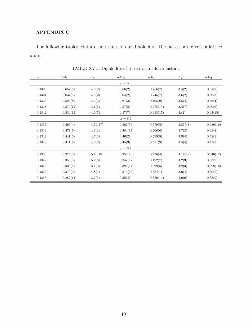
APPENDIX C

The following tables contain the results of our dipole fits. The masses are given in lattice

units.

TABLE XVII: Dipole fits of the isovector form factors.

κ aMe Am aMm aM1 A2 aM2

β = 6.0

0.1320 0.657(6) 4.3(2) 0.66(2) 0.756(7) 3.4(2) 0.61(3)

0.1324 0.637(5) 4.5(2) 0.64(2) 0.745(7) 3.6(2) 0.60(3)

0.1333 0.593(8) 4.3(3) 0.61(3) 0.705(9) 3.5(4) 0.56(4)

0.1338 0.570(12) 4.1(6) 0.57(5) 0.675(14) 3.4(7) 0.50(6)

0.1342 0.534(14) 4.0(7) 0.57(7) 0.633(17) 4.(2) 0.44(15)

β = 6.2

0.1333 0.493(4) 4.79(17) 0.507(16) 0.579(5) 3.87(18) 0.480(19)

0.1339 0.477(5) 4.6(2) 0.484(17) 0.566(6) 3.7(2) 0.45(2)

0.1344 0.441(6) 4.7(3) 0.46(2) 0.539(8) 3.9(4) 0.42(3)

0.1349 0.411(7) 4.3(3) 0.45(3) 0.511(9) 3.5(4) 0.41(3)

β = 6.4

0.1338 0.375(3) 5.16(18) 0.358(10) 0.436(4) 4.19(19) 0.340(12)

0.1342 0.358(5) 5.2(3) 0.347(17) 0.422(7) 4.2(3) 0.33(2)

0.1346 0.333(4) 5.1(3) 0.322(14) 0.399(5) 4.2(3) 0.299(16)

0.1350 0.310(5) 4.8(4) 0.319(16) 0.384(7) 3.9(4) 0.30(2)

0.1353 0.282(11) 3.7(5) 0.35(4) 0.350(14) 2.9(9) 0.33(9)

49

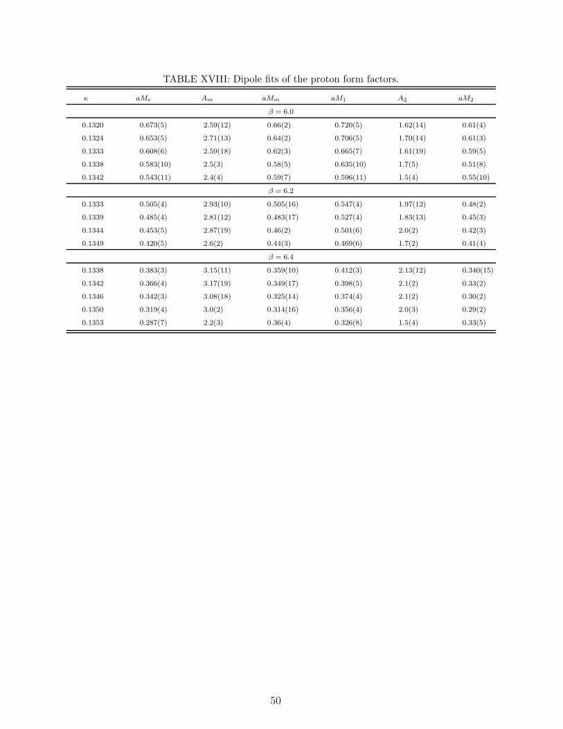
TABLE XVIII: Dipole fits of the proton form factors.

κ aMe Am aMm aM1 A2 aM2

β = 6.0

0.1320 0.673(5) 2.59(12) 0.66(2) 0.720(5) 1.62(14) 0.61(4)

0.1324 0.653(5) 2.71(13) 0.64(2) 0.706(5) 1.70(14) 0.61(3)

0.1333 0.608(6) 2.59(18) 0.62(3) 0.665(7) 1.61(19) 0.59(5)

0.1338 0.583(10) 2.5(3) 0.58(5) 0.635(10) 1.7(5) 0.51(8)

0.1342 0.543(11) 2.4(4) 0.59(7) 0.596(11) 1.5(4) 0.55(10)

β = 6.2

0.1333 0.505(4) 2.93(10) 0.505(16) 0.547(4) 1.97(12) 0.48(2)

0.1339 0.485(4) 2.81(12) 0.483(17) 0.527(4) 1.83(13) 0.45(3)

0.1344 0.453(5) 2.87(19) 0.46(2) 0.501(6) 2.0(2) 0.42(3)

0.1349 0.420(5) 2.6(2) 0.44(3) 0.469(6) 1.7(2) 0.41(4)

β = 6.4

0.1338 0.383(3) 3.15(11) 0.359(10) 0.412(3) 2.13(12) 0.340(15)

0.1342 0.366(4) 3.17(19) 0.349(17) 0.398(5) 2.1(2) 0.33(2)

0.1346 0.342(3) 3.08(18) 0.325(14) 0.374(4) 2.1(2) 0.30(2)

0.1350 0.319(4) 3.0(2) 0.314(16) 0.356(4) 2.0(3) 0.29(2)

0.1353 0.287(7) 2.2(3) 0.36(4) 0.326(8) 1.5(4) 0.33(5)

50

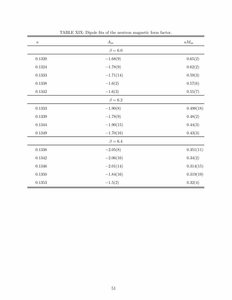
TABLE XIX: Dipole fits of the neutron magnetic form factor.

κ Am aMm

β = 6.0

0.1320 −1.68(9) 0.65(2)

0.1324 −1.78(9) 0.62(2)

0.1333 −1.71(14) 0.59(3)

0.1338 −1.6(2) 0.57(6)

0.1342 −1.6(3) 0.55(7)

β = 6.2

0.1333 −1.90(8) 0.498(18)

0.1339 −1.78(9) 0.48(2)

0.1344 −1.90(15) 0.44(3)

0.1349 −1.70(16) 0.43(3)

β = 6.4

0.1338 −2.05(8) 0.351(11)

0.1342 −2.06(16) 0.34(2)

0.1346 −2.01(14) 0.314(15)

0.1350 −1.84(16) 0.319(19)

0.1353 −1.5(2) 0.32(4)

51

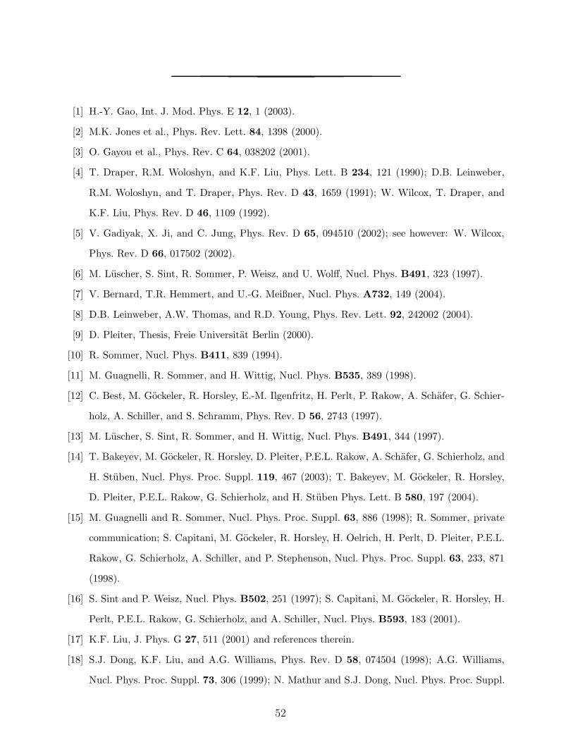
[1] H.-Y. Gao, Int. J. Mod. Phys. E 12, 1 (2003).

[2] M.K. Jones et al., Phys. Rev. Lett. 84, 1398 (2000).

[3] O. Gayou et al., Phys. Rev. C 64, 038202 (2001).

[4] T. Draper, R.M. Woloshyn, and K.F. Liu, Phys. Lett. B 234, 121 (1990); D.B. Leinweber,

R.M. Woloshyn, and T. Draper, Phys. Rev. D 43, 1659 (1991); W. Wilcox, T. Draper, and

K.F. Liu, Phys. Rev. D 46, 1109 (1992).

[5] V. Gadiyak, X. Ji, and C. Jung, Phys. Rev. D 65, 094510 (2002); see however: W. Wilcox,

Phys. Rev. D 66, 017502 (2002).

[6] M. Luscher, S. Sint, R. Sommer, P. Weisz, and U. Wolff, Nucl. Phys. B491, 323 (1997).

[7] V. Bernard, T.R. Hemmert, and U.-G. Meißner, Nucl. Phys. A732, 149 (2004).

[8] D.B. Leinweber, A.W. Thomas, and R.D. Young, Phys. Rev. Lett. 92, 242002 (2004).

[9] D. Pleiter, Thesis, Freie Universitat Berlin (2000).

[10] R. Sommer, Nucl. Phys. B411, 839 (1994).

[11] M. Guagnelli, R. Sommer, and H. Wittig, Nucl. Phys. B535, 389 (1998).

[12] C. Best, M. Gockeler, R. Horsley, E.-M. Ilgenfritz, H. Perlt, P. Rakow, A. Schafer, G. Schier-

holz, A. Schiller, and S. Schramm, Phys. Rev. D 56, 2743 (1997).

[13] M. Luscher, S. Sint, R. Sommer, and H. Wittig, Nucl. Phys. B491, 344 (1997).

[14] T. Bakeyev, M. Gockeler, R. Horsley, D. Pleiter, P.E.L. Rakow, A. Schafer, G. Schierholz, and

H. Stuben, Nucl. Phys. Proc. Suppl. 119, 467 (2003); T. Bakeyev, M. Gockeler, R. Horsley,

D. Pleiter, P.E.L. Rakow, G. Schierholz, and H. Stuben Phys. Lett. B 580, 197 (2004).

[15] M. Guagnelli and R. Sommer, Nucl. Phys. Proc. Suppl. 63, 886 (1998); R. Sommer, private

communication; S. Capitani, M. Gockeler, R. Horsley, H. Oelrich, H. Perlt, D. Pleiter, P.E.L.

Rakow, G. Schierholz, A. Schiller, and P. Stephenson, Nucl. Phys. Proc. Suppl. 63, 233, 871

(1998).

[16] S. Sint and P. Weisz, Nucl. Phys. B502, 251 (1997); S. Capitani, M. Gockeler, R. Horsley, H.

Perlt, P.E.L. Rakow, G. Schierholz, and A. Schiller, Nucl. Phys. B593, 183 (2001).

[17] K.F. Liu, J. Phys. G 27, 511 (2001) and references therein.

[18] S.J. Dong, K.F. Liu, and A.G. Williams, Phys. Rev. D 58, 074504 (1998); A.G. Williams,

Nucl. Phys. Proc. Suppl. 73, 306 (1999); N. Mathur and S.J. Dong, Nucl. Phys. Proc. Suppl.

52

94, 311 (2001); W. Wilcox, Nucl. Phys. Proc. Suppl. 94, 319 (2001).

[19] R. Lewis, W. Wilcox, and R.M. Woloshyn, Phys. Rev. D 67, 013003 (2003).

[20] A. Tang, W. Wilcox, and R. Lewis, Phys. Rev. D 68, 094503 (2003).

[21] S. Capitani, M. Gockeler, R. Horsley, B. Klaus, H. Oelrich, H. Perlt, D. Petters, D. Pleiter,

P.E.L. Rakow, G. Schierholz, A. Schiller, and P. Stephenson, Nucl. Phys. Proc. Suppl. 73, 294

(1999).

[22] M. Gockeler, R. Horsley, D. Pleiter, P.E.L. Rakow, and G. Schierholz, in: Lepton Scattering,

Hadrons and QCD, eds. W. Melnitchouk, A.W. Schreiber, A.W. Thomas, and P.C. Tandy

(World Scientific, Singapore, 2001), hep-ph/0108105.

[23] C. Bernard, S. Hashimoto, D.B. Leinweber, P. Lepage, E. Pallante, S.R. Sharpe, and H.

Wittig, Nucl. Phys. Proc. Suppl. 119, 170 (2003) and references therein.

[24] T.R. Hemmert and W. Weise, Eur. Phys. J. A 15, 487 (2002).

[25] D.B. Leinweber, D.H. Lu, and A.W. Thomas, Phys. Rev. D 60, 034014 (1999).

[26] D.B. Leinweber, A.W. Thomas, and R.D. Young, Phys. Rev. Lett. 86, 5011 (2001).

[27] E.J. Hackett-Jones, D.B. Leinweber, and A.W. Thomas, Phys. Lett. B 494, 89 (2000); G.V.

Dunne, A.W. Thomas, and S.V. Wright, Phys. Lett. B 531, 77 (2002).

[28] J.D. Ashley, D.B. Leinweber, A.W. Thomas, and R.D. Young, Eur. Phys. J. A 19, 9 (2004).

[29] V. Bernard, H.W. Fearing, T.R. Hemmert, and U.-G. Meißner, Nucl. Phys. A635, 121 (1998);

A642, 563(E) (1998).

[30] P. Mergell, U.-G. Meißner, and D. Drechsel, Nucl. Phys. A596, 367 (1996).

[31] T.R. Hemmert, B.R. Holstein, and J. Kambor, J. Phys. G 24, 1831 (1998).

[32] B. Kubis and U.-G. Meißner, Nucl. Phys. A679, 698 (2001).

[33] N. Fettes, U.-G. Meißner, M. Mojzis, and S. Steininger, Ann. Phys. 283, 273 (2000); 288,

249(E) (2001).

[34] D.B. Leinweber, Nucl. Phys. Proc. Suppl. 109A, 45 (2002); D.B. Leinweber, Phys. Rev. D

69, 014005 (2004); M.J. Savage, Nucl. Phys. A700, 359 (2002).

[35] T.R. Hemmert, M. Procura, and W. Weise, Phys. Rev. D 68, 075009 (2003).

[36] V. Bernard, N. Kaiser, and U.-G. Meißner, Nucl. Phys. A611, 429 (1996).

53