
NPSS User Guide - Wolverine Ventures
362
Numerical Propulsion System Simulation Consortium NPSS TM User Guide Software Release: NPSS TM _2.3.0 Doc. #: NPSS TM –User Doc Revision: 2 Revision Date: July 7, 2010 © Copyright 2008, 2009, 2010. The Ohio Aerospace Institute, on behalf of the NPSSTM Consortium. All rights reserved. Controlled Distribution Further distribution requires written approval of the Ohio Aerospace Institute, Cleveland, OH. Neither title nor ownership of the software is hereby transferred. NPSSTM software Version 2.3.0 and related documentation is export controlled with an Export Control Classification Number(ECCN)of 9D991, controlled for Anti-Terrorism reasons, under U.S. Export Administration Regulations 15 CFR 730-774. It may not be transferred to a country checked under anti-terrorism on the Commerce Country Chart structure or to foreign nationals of those countries in the U.S. or abroad without first obtaining a license from the Bureau of Industry and Security, United States Department of Commerce. Violations are punishable by fine, imprisonment, or both. Disclaimer: This software is provided “as is” without any warranty of any kind, either expressed, implied, or statutory. In no event shall NPSSTM Consortium member organizations, the Ohio Aerospace Institute., or OAI’s contractors or subcontractors, be held liable for any damages, including, but not limited to, direct, indirect, special, or consequential damage.
-
Upload
khangminh22 -
Category
Documents
-
view
2 -
download
0
Transcript of NPSS User Guide - Wolverine Ventures

Numerical Propulsion System Simulation Consortium
NPSSTM User Guide
Software Release: NPSSTM
_2.3.0 Doc. #: NPSS
TM–User
Doc Revision: 2
Revision Date: July 7, 2010
© Copyright 2008, 2009, 2010. The Ohio Aerospace Institute, on behalf of the NPSSTM Consortium. All rights reserved.
Controlled Distribution
Further distribution requires written approval of the Ohio Aerospace Institute, Cleveland, OH. Neither title nor ownership of the
software is hereby transferred.
NPSSTM software Version 2.3.0 and related documentation is export controlled with an Export Control Classification Number(ECCN)of
9D991, controlled for Anti-Terrorism reasons, under U.S. Export Administration Regulations 15 CFR 730-774. It may not be transferred
to a country checked under anti-terrorism on the Commerce Country Chart structure or to foreign nationals of those countries in the U.S.
or abroad without first obtaining a license from the Bureau of Industry and Security, United States Department of Commerce. Violations
are punishable by fine, imprisonment, or both.
Disclaimer: This software is provided “as is” without any warranty of any kind, either expressed, implied, or statutory. In no event shall
NPSSTM Consortium member organizations, the Ohio Aerospace Institute., or OAI’s contractors or subcontractors, be held liable for any
damages, including, but not limited to, direct, indirect, special, or consequential damage.

Doc. #: NPSSTM User Guide REL: 2.3 Date: 7/7/10
Contents i
Table of Contents
Preface ............................................................................................................................ ix
Overview of Chapters .................................................................................................. ix
Part 1: User Guide .................................................................................................................................. ix
Part 2: Reference ................................................................................................................................... ix
Text Conventions .......................................................................................................... x
Font Conventions ..................................................................................................................................... x
Variable Naming Rules ................................................................................................. x
Other Conventions ....................................................................................................... xi Requests for Bug Fixes and Enhancements ........................................................................................... xi
Getting Help .................................................................................................................. xi
Part 1: User Guide ........................................................................................................ xii
1 Overview .................................................................................................................... 1
1.1 Introduction ......................................................................................................... 1
1.2 Input Files ............................................................................................................ 1
1.3 Object Orientation ............................................................................................... 2
1.4 Air Breathing Thermodynamic Gas Properties ................................................ 2
1.5 Model Definition .................................................................................................. 2
1.5.1 Elements, Sockets, Subelements, Functions, and Tables .......................................................... 4
1.5.2 Ports and Links ............................................................................................................................ 4
1.5.3 Assemblies .................................................................................................................................. 5
1.5.4 Executives ................................................................................................................................... 5
1.5.5 The Solver ................................................................................................................................... 5
1.5.6 Output Data Viewers ................................................................................................................... 6
1.6 Distributed Modeling Via CORBA ...................................................................... 6
1.7 Running the Model .............................................................................................. 6
1.7.1 Batch Mode ................................................................................................................................. 6
1.7.2 Interactive Mode .......................................................................................................................... 6
2 Syntax Guide ............................................................................................................. 7
2.1 Command Line Syntax ....................................................................................... 7
2.2 General NPSS Input Syntax................................................................................ 9
2.2.1 Introduction to the Input ............................................................................................................... 9
2.2.2 Some General Features of the Input ........................................................................................... 9
2.2.3 Preprocessor Commands .......................................................................................................... 12
2.2.4 Variables .................................................................................................................................... 14
2.2.5 Programming Constructs ........................................................................................................... 32
2.2.6 Functions ................................................................................................................................... 38
2.2.7 Tables ........................................................................................................................................ 43
2.3 Interactive Mode Syntax ................................................................................... 51
2.3.1 Introduction to Interactive Mode Syntax .................................................................................... 51
2.3.2 Entering Interactive Mode ......................................................................................................... 52
2.3.3 Breakpoints................................................................................................................................ 53
2.3.4 Interactive Debugging Commands ............................................................................................ 56
3 Acquiring Components in NPSS ............................................................................ 58
3.1 Interpreted Component Load on Demand (ICLOD) ........................................ 58
3.2 Overview of Dynamically Loadable Modules (DLMs) ..................................... 59
3.3 DLM Component Load on Demand (DCLOD) ................................................. 60

Doc. #: NPSSTM User Guide REL: 2.3 Date: 7/7/10
Contents ii
3.4 How NPSS Uses CMFs ..................................................................................... 60
3.5 Component Creation Query Function findResource() ................................... 61
3.6 Metadata ............................................................................................................ 61
4 Common Tasks ........................................................................................................ 62
4.1 Thermodynamics Packages ............................................................................. 62
4.2 Elements ............................................................................................................ 63
4.3 Ports ................................................................................................................... 64
4.3.1 Creating Ports ........................................................................................................................... 65
4.3.2 Linking Ports .............................................................................................................................. 66
4.3.3 DataPorts................................................................................................................................... 67
4.3.4 FilePorts .................................................................................................................................... 68
4.4 Subelements ...................................................................................................... 69
4.5 Sockets .............................................................................................................. 70
4.5.1 Socket Attributes ....................................................................................................................... 71
4.5.2 Determining Allowable Socket/Subelement Combinations ....................................................... 72
4.5.3 Inserting Subelements into Sockets .......................................................................................... 73
4.5.4 Inserting Functions and Tables into Sockets ............................................................................ 73
4.5.5 list() Function and Sockets ........................................................................................................ 74
4.6 Assemblies ........................................................................................................ 75
4.6.1 Order of Execution in Assemblies ............................................................................................. 76
4.7 Bleed Usage....................................................................................................... 79
4.7.1 Compressor Element Bleed Extraction ..................................................................................... 79
4.7.2 Turbine Element Bleed Entry .................................................................................................... 80
4.7.3 Bleed Element Extraction and Entry ......................................................................................... 80
4.7.4 Linking Bleed Flows .................................................................................................................. 81
4.7.5 Bleed User Functions ................................................................................................................ 81
4.8 Solver Setup ...................................................................................................... 82
4.8.1 Basics ........................................................................................................................................ 83
4.8.2 Critiquing Solver Setup .............................................................................................................. 84
4.8.3 Adding to the Automatic Solver Setup ...................................................................................... 85
4.8.4 Saving and Restoring A Solver Setup ....................................................................................... 87
4.8.5 Solvers and Assemblies ............................................................................................................ 88
4.9 Input and Output ............................................................................................... 88
4.9.1 File Streams .............................................................................................................................. 88
4.9.2 DataViewers .............................................................................................................................. 93
4.10 Basic Model Running ...................................................................................... 105
4.11 Moving and Deleting Objects ......................................................................... 107
4.12 Adding or Removing Elements from a Model ............................................... 108
4.13 Prepass, Preexecute and Postexecute Functions ........................................ 110
4.14 Error Handling and Messages........................................................................ 112
4.14.1 ESO (Engineering Status Objects) .......................................................................................... 112
4.14.2 ESORegistry ............................................................................................................................ 112
4.14.3 ESORegistry: Identification Attributes (Unchangeable) ......................................................... 112
4.14.4 ESORegistry: Changeable Attributes ..................................................................................... 113
4.14.5 ESORegistry Functions .......................................................................................................... 114
4.14.6 ESO Convenience Functions ................................................................................................. 115
4.14.7 errHandler Object Behavior ..................................................................................................... 115
4.14.8 errHandler Variables ............................................................................................................... 116
4.14.9 errHandler Functions ............................................................................................................... 117
4.14.10 ESO: Examples ...................................................................................................................... 118
4.15 Data Matching and Analysis........................................................................... 119

Doc. #: NPSSTM User Guide REL: 2.3 Date: 7/7/10
Contents iii
5 Building a Model .................................................................................................... 121
5.1 Study Executive File ....................................................................................... 122
5.1.1 Define Thermo Package .......................................................................................................... 122
5.1.2 Include Standard NPSS Utilities and Components ................................................................. 122
5.1.3 Include Special Utilities and Components ............................................................................... 122
5.1.4 Include Model Definition .......................................................................................................... 123
5.1.5 Model Case Description Files.................................................................................................. 123
5.2 Model File ........................................................................................................ 123
5.2.1 Header ..................................................................................................................................... 123
5.2.2 Instantiating Model Components ............................................................................................. 124
5.2.3 Linking Elements ..................................................................................................................... 132
5.2.4 Solver Setup ............................................................................................................................ 134
5.3 Case Input File ................................................................................................. 136
5.3.1 Design Point ............................................................................................................................ 136
5.3.2 Offdesign Steady-state Points ................................................................................................. 137
5.3.3 Transient Points ...................................................................................................................... 138
5.4 fanjet Source Files .......................................................................................... 138
5.4.1 fanjet.run .................................................................................................................................. 138
5.4.2 Transient.view ......................................................................................................................... 139
5.4.3 fanjet.mdl ................................................................................................................................. 139
5.4.4 fanE3.map ............................................................................................................................... 148
5.4.5 IpcE3.map ............................................................................................................................... 148
5.4.6 hpcE3.map .............................................................................................................................. 148
5.4.7 hptE3.map ............................................................................................................................... 148
5.4.8 IptE3.map ................................................................................................................................ 149
5.4.9 Controls.cmp ........................................................................................................................... 149
5.4.10 desOD.case ............................................................................................................................. 152
5.4.11 viewOut .................................................................................................................................... 154
5.4.12 tout ........................................................................................................................................... 157
6 Solver ..................................................................................................................... 158
6.1 Introduction ..................................................................................................... 158
6.2 Basic Theory of Solver Operation ................................................................. 158
6.3 General Structure of the NPSS Solver .......................................................... 161
6.4 Creating a Solver ............................................................................................. 161
6.5 Independent Variables .................................................................................... 162
6.6 Dependent Conditions .................................................................................... 163
6.7 Solver Setup .................................................................................................... 166
6.8 Constraint Handling ........................................................................................ 169
6.8.1 Constraint Definition and Usage ............................................................................................. 169
6.8.2 Adding Constraints Dependents to Target Dependents ......................................................... 171
6.8.3 Constraint Groups ................................................................................................................... 174
6.8.4 Removing Constraints ............................................................................................................. 175
6.8.5 Temporarily Disabling Constraints .......................................................................................... 175
6.8.6 Resolving Constraint Slope Conflicts ...................................................................................... 176
6.8.7 Resolving Min/Max Constraint Conflicts .................................................................................. 177
7 Transient Simulation ............................................................................................. 178
7.1 Introduction ..................................................................................................... 178
7.2 Running a Basic Transient Simulation .......................................................... 182
7.2.1 Basic Setup ............................................................................................................................. 182
7.2.2 Output ...................................................................................................................................... 182
7.2.3 Initial Conditions ...................................................................................................................... 183

Doc. #: NPSSTM User Guide REL: 2.3 Date: 7/7/10
Contents iv
7.2.4 Transient Executive ................................................................................................................. 183
7.2.5 Integration Method .................................................................................................................. 184
7.2.6 Setup of Transient Mode ......................................................................................................... 184
7.2.7 Time Step ................................................................................................................................ 185
7.2.8 Termination Criteria ................................................................................................................. 185
7.2.9 Running the Transient ............................................................................................................. 186
7.3 Variable Time-Step Computation ................................................................... 187
7.3.1 Adaptive Time Stepping .......................................................................................................... 187
7.3.2 User-Defined Time-Step Computations .................................................................................. 188
7.4 Controlling Termination of a Transient Run ................................................. 189
7.5 TransientExecutive Attributes ....................................................................... 191
7.6 Integrators ....................................................................................................... 193
7.6.1 Implicit Integration ................................................................................................................... 193
7.6.2 Explicit Integration ................................................................................................................... 194
7.6.3 Switching Individual Integrators to Steady-State .................................................................... 194
8 Hierarchical Data Format (HDF) Guide ................................................................ 196
8.1 Overview .......................................................................................................... 196
8.2 Syntax .............................................................................................................. 196
8.3 User-accessible Functions ............................................................................. 199
Part 2: Reference ........................................................................................................ 201
9 Assembly Attributes.............................................................................................. 202
10 Units .................................................................................................................... 203
10.1 Units Functions ............................................................................................... 203
10.2 Valid Unit Strings ............................................................................................ 205
11 Function Summary ............................................................................................. 210
11.1 User-Accessible Member Functions ............................................................. 210
11.1.1 Functions for All NPSS Objects (Elements, Subelements, Assemblies, DataViewers, Solver, Ports, Stations, Sockets) and Variables ............................................................................................... 210
11.1.2 Array Functions ....................................................................................................................... 213
11.1.3 Assembly Functions ................................................................................................................ 214
11.1.4 BleedInPort/BleedOutPort Functions ...................................................................................... 214
11.1.5 DataViewer Functions ............................................................................................................. 215
11.1.6 Dependent Functions .............................................................................................................. 215
11.1.7 Element, Assembly, and Subelement Functions..................................................................... 215
11.1.8 errHandler Functions ............................................................................................................... 216
11.1.9 External Component Attributes and Functions ........................................................................ 216
11.1.10 FlowStation Functions ............................................................................................................. 217
11.1.11 Independent Functions ............................................................................................................ 225
11.1.12 InFileStream Functions ........................................................................................................... 226
11.1.13 Linear Model Generator Functions .......................................................................................... 226
11.1.14 Link Functions ......................................................................................................................... 227
11.1.15 msgHandler Functions ............................................................................................................ 227
11.1.16 OutFileStream Functions ......................................................................................................... 227
11.1.17 Port Functions ......................................................................................................................... 228
11.1.18 Socket Functions ..................................................................................................................... 228
11.1.19 Solver Functions ...................................................................................................................... 228
11.1.20 Table Functions ....................................................................................................................... 228
11.1.21 Time Discrete Model Objects .................................................................................................. 230
11.1.22 Transient Executive Functions ................................................................................................ 230
11.1.23 User-Supplied Subelement Functions ..................................................................................... 230
11.1.24 VariableContainer Functions ................................................................................................... 230

Doc. #: NPSSTM User Guide REL: 2.3 Date: 7/7/10
Contents v
11.2 Global Functions ............................................................................................. 230
11.2.1 Bitwise Functions .................................................................................................................... 230
11.2.2 ESORegistry Functions ........................................................................................................... 231
11.2.3 Units Functions ........................................................................................................................ 231
11.2.4 Miscellaneous Global Functions ............................................................................................. 232
11.3 Interactive Mode Functions ............................................................................ 235
11.4 Macros ............................................................................................................. 236
11.4.1 Bleed Macro ............................................................................................................................ 236
11.4.2 Print Macro .............................................................................................................................. 237
11.4.3 Solver Macro ........................................................................................................................... 237
11.4.4 runSequence Macro ................................................................................................................ 238
11.5 Block Diagram Generator ............................................................................... 238
11.6 System/Scripting Functions ........................................................................... 238
11.6.1 General Functions ................................................................................................................... 238
11.6.2 SSH/SCP Support ................................................................................................................... 243
11.6.3 External Component Server Support ...................................................................................... 243
11.7 NPSS Built-in Math Functions ........................................................................ 247
11.8 NPSS String Handling Capabilities ................................................................ 247
11.8.1 String functions ........................................................................................................................ 248
11.8.2 Tokenizer Class ....................................................................................................................... 252
12 DataViewer Reference Sheets ........................................................................... 255
12.1 Data Viewer Common Characteristics .......................................................... 255
12.2 CaseColumnViewer/CaseRowViewer ............................................................ 256
12.3 PageViewer ...................................................................................................... 257
12.4 Text Blocks ...................................................................................................... 257
12.4.1 SimpleBlock ............................................................................................................................. 258
12.4.2 DColTBlock, LinkColTBlock and DRowTBlock ....................................................................... 258
12.4.3 GroupBlock .............................................................................................................................. 260
12.4.4 EmptyTextBlock ...................................................................................................................... 260
12.4.5 UserTextBlock ......................................................................................................................... 260
12.4.6 VarDumpViewer ...................................................................................................................... 260
13 Stream Reference Sheets .................................................................................. 261
13.1 Common Attributes ......................................................................................... 261
13.2 Output Streams ............................................................................................... 262
13.3 Input Streams .................................................................................................. 262
14 The NPSS Solver Reference .............................................................................. 263
14.1 Solver (NPSSSteadyStateSolver class) ......................................................... 263
14.1.1 Solver Definition Syntax Example ........................................................................................... 263
14.1.2 Solver Input/Commands .......................................................................................................... 263
14.1.3 The preconvergence Function ................................................................................................ 264
14.1.4 Solver User Input Attributes .................................................................................................... 265
14.1.5 Solver Output (Calculated) Attributes ...................................................................................... 270
14.2 Independent (NCPIndependent Class) .......................................................... 272
14.2.1 Independent Definition Example ............................................................................................. 272
14.2.2 Independent Limits .................................................................................................................. 273
14.2.3 Independent Input/Commands ................................................................................................ 273
14.2.4 Independent User Input Attributes .......................................................................................... 273
14.2.5 Lock Attributes for Independents ............................................................................................ 275
14.2.6 Independent Output (Calculated) Attributes ............................................................................ 275
14.3 Dependent (NCPDependent class) ................................................................ 276

Doc. #: NPSSTM User Guide REL: 2.3 Date: 7/7/10
Contents vi
14.3.1 Examples of Dependent Definition .......................................................................................... 276
14.3.2 Dependent Input/Commands .................................................................................................. 277
14.3.3 Dependent User Input Attributes ............................................................................................. 278
14.3.4 Lock Attributes for Dependents ............................................................................................... 280
14.3.5 Dependent Output (Calculated) Attributes .............................................................................. 281
14.4 ConstraintGroups (ConstraintGroup class).................................................. 282
14.4.1 ConstraintGroup Input/Commands ......................................................................................... 282
14.4.2 ConstraintGroup User Input Attributes .................................................................................... 282
14.4.3 ConstraintGroup Output (Calculated) Attributes ..................................................................... 282
14.5 DiscreteStateVariable (DSV) .......................................................................... 282
14.5.1 Nested vs. Simultaneous DSV Solution .................................................................................. 283
14.5.2 Controlling Movement through the Allowed State Values ....................................................... 284
14.5.3 Controlling Repetition of Previously Failed Iterations ............................................................. 284
14.5.4 Example Definitions of DiscreteStateVariables ....................................................................... 285
14.5.5 Using a DSV in a Model .......................................................................................................... 286
14.5.6 DSV Input Commands ............................................................................................................. 287
14.5.7 DSV User Input Attributes ....................................................................................................... 287
14.5.8 DSV Output (Calculated) Attributes ........................................................................................ 289
14.6 Advanced Solver Member Functions ............................................................ 289
14.7 Solver Diagnostic Output ............................................................................... 292
14.7.1 Searching Diagnostic Output................................................................................................... 293
14.7.2 Grepable Output ...................................................................................................................... 293
14.7.3 Interactive Debug Output Functions ........................................................................................ 294
14.7.4 userReport: User-defined Solver Output Function .................................................................. 295
14.7.5 projectionReport: User-defined Solver Output Function ......................................................... 297
14.7.6 dxLimitAll: User-defined Solver Output Function .................................................................... 297
14.8 Solver Diagnostic and Trouble-Shooting Reference .................................. 298
14.9 Solver Terms ................................................................................................... 299
15 Transient Reference Guide ................................................................................ 302
15.1 Transient (TransientExecutive class) ............................................................ 302
15.1.1 Initial Model State Assumptions .............................................................................................. 302
15.1.2 Initialization of the Time Update Loop ..................................................................................... 302
15.1.3 Time Update Loop ................................................................................................................... 303
15.1.4 Independent variable predictions ............................................................................................ 309
15.1.5 Time Step Computation ........................................................................................................... 310
15.1.6 Utility Functions ....................................................................................................................... 312
15.1.7 TransientExecutive Functions ................................................................................................. 313
15.1.8 Transient User Input Attributes................................................................................................ 314
15.1.9 Transient Output (Calculated) Attributes ................................................................................. 316
15.2 Integrator (NCPStateIntegrator class) ........................................................... 317
15.2.1 Creating an Integrator ............................................................................................................. 317
15.2.2 Implicit Integration ................................................................................................................... 317
15.2.3 Explicit Integration ................................................................................................................... 319
15.2.4 Integrator Functions ................................................................................................................ 319
15.2.5 Integrator Input Attributes ........................................................................................................ 320
15.2.6 Locking Attributes for Integrator .............................................................................................. 320
15.2.7 Integrator Output (Calculated) Attributes ................................................................................ 321
15.2.8 State Substitution Variables .................................................................................................... 321
15.3 Example Program ............................................................................................ 322
15.3.1 Model File ................................................................................................................................ 322
15.3.2 First Order Lag Test File ......................................................................................................... 323
15.3.3 Test Output File ....................................................................................................................... 331
15.4 Functions for Time-Discrete Model Objects ................................................. 332

Doc. #: NPSSTM User Guide REL: 2.3 Date: 7/7/10
Contents vii
15.4.1 Time Discrete Example Test File ............................................................................................ 333
15.4.2 Time Discrete Test Output File................................................................................................ 335
16 Glossary .............................................................................................................. 336
Index ............................................................................................................................. 339

Doc. #: NPSSTM User Guide REL: 2.3 Date: 7/7/10
Contents viii
List of Figures
Figure 1. Engine Model ................................................................................................................................................... 3
Figure 4. Time March Executive Event Sequence ....................................................................................................... 305
Figure 5. Time Sequence - Step 2 ................................................................................................................................ 306
Figure 6. Time Sequence - Step 3 ................................................................................................................................ 306
Figure 7. Time Sequence - Step 4 ................................................................................................................................ 307
Figure 8. Time Line ..................................................................................................................................................... 308

Doc. #: NPSSTM User Guide REL: 2.3 Date: 7/7/10
Preface ix
Preface
This TUser Guide Tis for engineers who will be using NPSS. This includes those who run the code, those who modify and edit its input files, and those who develop complete models. Part 1 is designed to provide complete explanations of the NPSS features used by most users for the majority of their performance-related work. Chapters 1-5 contain basic information about the system, its syntax, and the structure of a model. Chapters 6 and 14 contain more detailed information about the NPSS systems that solve steady-state and transient problems. Chapters 1-6 make occasional reference to information for more advanced users contained in the TDeveloper GuideT. The content of chapters 1-6 should be considered prerequisite for the material in the TDeveloper GuideT. Chapters 9-16 constitute part 2 of the Guide. Part 2 is intended to give complete reference information on important parts of the NPSS system. For example, a discussion of the most commonly used solver features is given in Part 1 (Chapter 6), but a complete list of all features is given in Part 2 (Chapter 14).
Overview of Chapters
Part 1: User Guide 1 Overview introduces the model structure and presents basic information about the input file. It introduces terms
and presents a general view of the system discussed in detail in later chapters. 2 Syntax Guide explains (1) the command line syntax, (2) the general NPSS syntax used to create input files, and
(3) interactive mode syntax. It provides the basic fundamentals of how to run the system. 3 Acquiring Components in NPSS provides information on Creation Method Facilities (CMFs), which are
important for using pre-written NPSS components–either supplied with NPSS or written at a particular site. 4 Common Tasks provides information on the practical tasks involved in using NPSS syntax to construct and use
models. 5 Building a Model shows how to build a model using the concepts in Chapters 1–4. It presents a complete,
working NPSS model of a turbofan gas turbine engine. 6 Solver introduces the basic theory and structure of the solver. It discusses setting up the solver for steady-state
runnng and using constraints. 7 Transient Simulation provides information on setting up and running transient simulations. 8 The Hierarchical Data Format (HDF) Guide discusses a basic implementation of HDF file format for binary
data storage.
Part 2: Reference 9 Assembly Attributes contains attributes specific to an assembly. 10 Units is a list of unit strings accepted by the system. 11 Function Summary provides the member functions for the various objects, global functions, interactive mode
functions, suites of functions, and built-in math functions. 12

Doc. #: NPSSTM User Guide REL: 2.3 Date: 7/7/10
Preface x
DataViewer Reference Sheets lists characteristics common to all data viewers and variables specific to certain types of data viewers. 13 Stream Reference Sheets provides attributes on input and output streams. 14 The NPSS Solver Reference contains all the commands and attributes for the solver classes, sections on output
and troubleshooting, and solver terms. It contains commands for more advanced users. 15 Transient Reference Guide provides Transient Executive and Integrator attributes and functions, and functions
for Time-Discrete Model Objects. 16 Glossary contains some basic terminology (excluding solver-specific terms, which are included in the solver
reference chapter).
Text Conventions
Font Conventions The font conventions below are followed in this document.
Font Used For Times New Roman Body of the document
Times New Roman Bold Emphasizes text
TTimes New Roman ItalicT Titles of Documents Emphasizes the introduction of new terms and concepts
TCourier New (constant width)T Examples of code, file contents, and program output
TCourier New or Times New Roman ItalicT Items for which the user must supply context-specific information. For example, the variable TVar1T would be replaced by an actual variable name supplied by the user.
Variable Naming Rules When you create variable names for the new components you want to add, please use the variable naming rules that were followed for the NPSS built-in components. These naming conventions are provided below.
Naming Conventions • The first and second words in the name alternate case of the starting letter; remaining words all start with upper
case followed by lower case.
• Names start with lower case letters except for common usage names: A, P, T, C, F, RNI
• Axxx : Area associated with xxx
• P: pressure
• T: temperature
• Cxxx: Coefficient of xxx
• Fxxx: thrust
• Fluid Ports start with Fl_
• Fuel Ports start with Fu_
• Sockets start with S_
• Tables start with TB_
• Shafts start with Sh_
• adders start with a_
• scalars start with s_
• Subscripts for "total" and "static" are always lower case: t, s
• Base added to the end of a variable name refers to a variable that is passed from a socket.
• Map added to the end of a variable name refers to variables used to read a table.
• hx added to the end of a variable is associated with heat transfer.

Doc. #: NPSSTM User Guide REL: 2.3 Date: 7/7/10
Preface xi
• All option switches begin with switch.
• Two letters abbreviate familiar ratios: PR, AR, TR (i.e., pressure ratio, area ratio, and temperature ratio)
• eff is always assumed adiabatic efficiency; if polytropic, label as effPoly.
• errXxx : error in Xxx
• expXxx : exponent on Xxx
• fracXxx : fraction of xxx
Other Conventions As noted above TitalicsT are used in generic examples to indicate that the user must substitute a specific name. A generic example might be:
Tsolver_nameT.addIndependent("Tindependent_nameT");
In real use, the user would supply specific names for the items in TitalicsT, such as:
solver.addIndependent("HPSpeedIndep");
In general, examples are indented. However, some long sections of code have not been indented. Throughout this document the reader may notice occasional names that include the letters "NCP," for example, "NCPDependent." Earlier versions of NPSS were known as NCP so the system's code still contains references to it.
Requests for Bug Fixes and Enhancements If you have a question, a defect, or an enhancement you want addressed, check with your site representative first, since you may have a problem related to your site's installation of NPSS. If your problem is an NPSS problem that has not been addressed, your site representative can enter a change request (CR) in the Web Site Change Request Tracking System or contact the NPSS Software Configuration Manager (SCM) who will enter the request for them. If you have a question that your contact person cannot answer, that person is responsible for contacting the appropriate person at Wolverine Ventures, Inc. You may also receive help via email. Please see the following section.
Getting Help Check with your local expert, then if there are further question that requires assistance, you can send an e-mail to the following address:
Your e-mail must include the following information. Please Udouble spaceU between these items. 1. The category of the request for help: question or problem 2. The submitter of the problem, bug, etc., so the person can be contacted when the issue is resolved. 3. The version of the system you are running: npss –v 4. The platform on which you are running the system. 5. A detailed description of the question/problem. Explain exactly what you were doing or what action you
completed when the problem occurred. You may want to include the path where the problem occurred. 6. A copy of the input file you were working with when you encountered a problem. To expedite the process,
please delete from the input file any information that does not pertain to your problem or question. Send the pared down copy of the input file with your email. You may send it as an attachment.
7. The error message you received. Please provide the exact wording of the message.

Doc. #: NPSSTM User Guide REL: 2.3 Date: 7/7/10
Divider xii
Part 1: User Guide

Doc. #: NPSSTM User Guide REL: 2.3 Date: 7/7/10
1 Overview 1
1 Overview
1.1 Introduction NASA Glenn Research Center, in conjunction with the U.S. aeropropulsion industry and the Department of Defense, developed technologies capable of supporting detailed aerothermomechanical computer simulations of complete aircraft engines. This project is called the Numerical Propulsion System Simulation (NPSS). NPSS can realistically model the physical interactions that take place throughout an engine, accelerating the concept-to-production development time and reducing the need for expensive full-scale tests and experiments. Its architecture supports implementing one-, two-, and three-dimensional models of the engine flow field and structure, and reconciling them with zero-dimensional component-based models. At its foundation, NPSS is a component-based object-oriented engine cycle simulator designed to perform cycle design, steady-state and transient off-design performance prediction, test data matching, and many other traditional tasks of engine cycle simulation codes. Like traditional codes, an NPSS engine model is assembled from a collection of interconnected components, and controlled through the implementation of an appropriate solution algorithm. Historically, limited computer resources restricted component representations used in these simulations to be simple characterizations of empirical test results, or the results of more sophisticated component models run separately. NPSS, however, is capable of calling upon more sophisticated component models directly. Using the computer industry's Common Object Request Broker Architecture (CORBA) communication standard, NPSS can interact with external codes running on other computers distributed across a network. The advanced system architecture designed into NPSS will allow the marriage of design tools at varying levels of dimensional fidelity across multiple technology disciplines. The initial focus of NPSS was on the aerothermodynamic cycle simulation process, which includes the following:
• All model definition through input file(s)
• NIST (National Institute of Standards and Technology) compliant thermodynamic gas-properties package
• A sophisticated solver with auto-setup, constraints, and discontinuity handling
• Steady-state and transient system simulation
• Flexible report generation
• Built-in object-oriented programming language for user-definable components and functions
• Support for distributed running of external code(s) via CORBA
• Support for test data matching and analysis This chapter presents a brief introduction to the system and its features.
1.2 Input Files An NPSS engine model may be completely defined in one or more input files. No alteration of NPSS source code is required. Input files may be created and modified using any text editor. Input files contain commands and directives that do the following:
• Identify what thermodynamic gas-properties package to use.
• Define a model's components and component linkages, tell NPSS what calculations to perform, and specify what output to generate.
• Initiate the solution of specified cases. NPSS input syntax is a full-featured programming language modeled after C++. It allows definition of real (floating point), integer, and string variables, up to three-dimensional arrays, "if…else if…else" (branching) constructs, looping controls, and conditional preprocessing directives. Floating point variables can be assigned units, and a facility exists to automatically convert variables and expressions from one set of units to another.
Refer to Chapter 2, Syntax Guide, and Chapter 4, Common Tasks, for detailed information on the NPSS input language, and how to use it to define a model. Chapter 5, Building a Model, presents a complete example.

Doc. #: NPSSTM User Guide REL: 2.3 Date: 7/7/10
1 Overview 2
1.3 Object Orientation NPSS is an Tobject-orientedT program, and its input reflects this. Object orientation means that the program's structure revolves around TobjectsT of various TtypesT, each of which has a set of TattributesT accessible by other objects, and certain TfunctionsT–a set of actions particular to the object that can be performed at the request of other objects. See 2.2.2.1 for more information on object orientation.
1.4 Air Breathing Thermodynamic Gas Properties Several thermodynamic gas property packages are supplied with NPSS to support air breathing engine analysis (aircraft and industrial gas turbine engines). Their modular design allows a user to select the desired package at run
time. One package ("Janaf") offers flexibility and matches the NIST standard (NIST−JANAF, Revision 3) at the expense of some computational speed. A second package ("GasTbl"), created by Pratt & Whitney and based on NASA's "Therm," includes humidity calculations as well as some chemical equilibrium capabilities. The "CEA" thermo is an implementation of the NASA chemical equilibrium code. "allFuel," from General Electric, contains both gas properties and fuel properties. It is generally consistent with the NASA TP-1908 thermo but specific agreement varies with the fuel and working fluid options selected. A fluid property table “FPT” package is also available. It allows users to define NPSS tables and/or functions to describe the thermodynamic properties of the fluid. Section 4.1 discusses declaration of thermodynamics packages.
1.5 Model Definition Before using NPSS, one should be familiar with the structure of the model and with some terminology. Figure 1 graphically depicts a simple model using phrases described in this section. Briefly stated, a model will encapsulate a variety of component TelementsT, some of which may have TsocketsT connected to TsubelementsT, TfunctionsT, or TtablesT, and TportsT connected by links to other elements. Elements may be grouped into TassembliesT, and each assembly may have a dedicated TsolverT. In addition, the model definition will include specifications for generating formatted output using one or more Tdata viewersT.

Doc. #: NPSSTM User Guide REL: 2.3 Date: 7/7/10
1 Overview 3
Figure 1. Engine Model
Data Viewer(s)
Simple Conceptual
Engine Model
Inlet Element
FlightConditions1 Element
Fluid Port
Duct Element
Nozzle Element
Bleed
FlowEnd Element
Compressor
Element
Shaft Port
FuelStart Element
Fuel Port
Burner Element
Shaft Element
Turbine Element
Socket
CompressorMap
Subelement
Element
Compressor
F P
Solver
Assembly
F P
F P
F P
F P
F P
F P
F P
F P
F P
F P
F P
F P
F P
F P
F P
Fluid Port
Fluid Port
Fuel Port
Shaft Port
Shaft Port
S P
S P
Model

Doc. #: NPSSTM User Guide REL: 2.3 Date: 7/7/10
1 Overview 4
1.5.1 Elements, Sockets, Subelements, Functions, and Tables TElementsT are the main building blocks of an engine model in NPSS and generally represent the major components of the engine (e.g., compressors, combustors, turbines). Elements contain TvariablesT, also called TattributesT. These represent quantities appropriate for a given component, such as physical characteristics, scale factors, and gas properties. Some element variables may be Toption variablesT, which have a limited set of values that may be assigned to them (e.g., "DESIGN" and "OFFDESIGN"). These are typically used to control the behavior of the element. Section 2.2.4 discusses variables in detail. The attributes associated with each element (and with other NPSS objects) are given in the TNPSS Reference SheetsT. Some elements contain TsocketsT. Sockets are a software vehicle to "plug in" calculations needed by the element. For example an element modeling a compressor might have a socket through which the compressor map information is provided. The most common socket plug-ins are TsubelementsT: element-like objects designed to support the object to which they are attached. In the example above, a subelement would perform the compressor map lookups to be supplied through a socket to the compressor element. Some subelements also have sockets that can accept other subelements. In general, wherever interchangeable computational approaches are required for an element, one or more subelements will be available. Each socket is of a distinct type, and each subelement must meet the requirements of that socket type in order to "fit." This checking prevents a turbine map subelement from being plugged into a compressor element, for example. Elements are discussed further in Section 4.2, and subelements in Section 4.4. Section 4.5 discusses sockets and their use. NPSS comes with a standard set of elements and subelements that fulfill many modeling needs. Users may, however, create additional customized elements and subelements. This can be done entirely through normal input files if desired. For improved execution speed, it is also possible to run user-written elements and subelements through a separate conversion utility that changes the NPSS syntax into C++. The object definition can then be compiled and made available to any model as if it were a native part of NPSS. These topics are covered in the TDeveloper GuideT rather than in this document. In addition to using components written in NPSS's native syntax, NPSS can use components written in other languages, such as FORTRAN or C. Compiled components can be added to the standard NPSS executable to produce a custom executable or a customer deck, or they can be compiled into TDynamically Loadable ModulesT (DLMs) and loaded at run time by an existing NPSS executable. NPSS can also use external components accessed through the Common Object Request Broker Architecture (CORBA). Information on loading components at run time is given in Chapter 3. Creating such components is discussed in the TDeveloper's GuideT. Special calculations can also be specified through TfunctionsT and TtablesT. Functions are like program subroutines that can be called by direct command, or by objects such as elements, subelements, and other functions. Tables are special functions that perform table lookups. Many subelements either require or provide the opportunity for the user to supply information through tables. NPSS comes with many preprogrammed functions for various tasks, and the user can readily write new ones using NPSS syntax. Every element and subelement may have a user-supplied prePass function, Tpreexecute functionT and Tpostexecute functionT attached to them. These provide users with the ability to override variable values and compute extra attributes not computed by the element or subelement. Functions are discussed more fully in Section 2.2.6. The use of prePass and pre- and postexecute functions in particular is discussed in Section 4.13. Tables are discussed in Section 2.2.7. Sockets can also be designed to accept plug-in functions and tables, but this is covered in the TDeveloper's GuideT.
1.5.2 Ports and Links Elements communicate with other elements through input and output TportsT that manage the flow of data through TlinksT. Elements may have zero to many ports, depending on their needs. Ports can be categorized by the type of information communicated and the direction of information flow. NPSS ensures that a port is linked with another port of the same type and opposite direction. For example, a Compressor element could have three ports: a FluidInputPort linked to an Inlet element's FluidOutputPort, a FluidOutputPort

Doc. #: NPSSTM User Guide REL: 2.3 Date: 7/7/10
1 Overview 5
linked to a Burner element's FluidInputPort, and a ShaftOutputPort linked to a Shaft element's ShaftInputPort. In addition, a Compressor element may have any number of InterStageBleedOutPorts. A variety of port types is available. Fluid ports transfer primary-gas flow properties between elements (e.g., flow rate, total temperature and pressure, molecular constituents); special fluid ports are available for bleeds and leakages. Similarly, fuel ports are used to transfer fuel properties from a FuelStart element into a Burner. Shaft ports transfer mechanical properties such as torque and rotational speed between rotating components. DataPorts transfer a single numerical value, such as an engine measurement. FilePorts transfer one or more files. Ports are discussed in detail in Section 4.3.
1.5.3 Assemblies A set of connected elements may be grouped as an Tassembly.T The assembly is then treated by the rest of the model as if it were a single element. Selected element ports within the assembly are generally TpromotedT to the assembly boundary so they may be connected with other elements and assemblies. Each assembly may have its own dedicated solver. An assembly can contain other assemblies. In fact, the entire model constitutes the Ttop-level
assemblyT; any other assemblies are contained within it. The top-level assembly is the only assembly that must have an Executive. The use of assemblies is discussed further in Section 4.6.
1.5.4 Executives An object that may exist inside an Assembly or Element, which is responsible for the accounting for and running of executionSequences (and possible solving) is an Executive. The Executive class contains string array variables preExecutionSequence, executionSequence, and postExecutionSequence, which are explained further in Section
4.6.1. Classes derived from Executive may be solvers, but are not necessarily so. The NPSSSteadyStateSolver
class and the NPSSTransientSolver class are both classes derived from Executive.
1.5.5 The Solver The TsolverT is the part of NPSS that drives the model to a valid solution. The top-level assembly always contains a solver, which is created for the user. This solver receives a TrunT command and is responsible for iteratively adjusting the values of the model Tindependent variablesT in order to satisfy the Tdependent conditionsT in the system. If convergence cannot be achieved within a specified number of iterations, an error is returned for that case. For transient simulations, the solver also controls the progression of time within the run, providing a converged solution at each point in time. More details about the solver's operation are presented in Chapter 6. Transient simulation is specifically discussed in Chapter 7. Many Elements contain predefined independents and/or dependents. Should the user choose the "default" solver setup, this information is automatically used to solve the cycle. User-defined independents and dependents may also be added to, or used instead of, the defaults provided. Further, cTonstraintsT may be imposed on the solver's solution. Basic solver setup is discussed in Section 4.8. The use of constraints is discussed in Section 6.8. Any assembly in an NPSS model may contain its own solver. When an assembly with a solver is run, its solver attempts to converge that assembly by recursively calling any other assemblies it contains, and so on down to the bottom of the assembly tree. If an assembly does not have a solver, the independents and dependents in that assembly are handled by the solver in the assembly containing it. If an assembly has a solver, its independent variables are varied to satisfy its dependent conditions before control is returned to its parent assembly. A model may therefore contain a hierarchy of nested solvers, each responsible for solving a successively smaller portion of the model. The solver in the top level of the model is always responsible for controlling the time-step for transient simulations. The use of solvers in subassemblies is discussed in Section 4.8.5. Each assembly may define one "pre-solve" sequence of objects that is executed once before every converged point, an "inner-loop" solve sequence that is run during the solution process, and a "post-solve" sequence that is run after the point is converged. If an assembly does not have a solver, the pre-, inner-, and post-solve sequences are executed sequentially, once, and the flow of control is returned to the calling level.

Doc. #: NPSSTM User Guide REL: 2.3 Date: 7/7/10
1 Overview 6
1.5.6 Output Data Viewers TData viewersT provide the mechanism for generating formatted output. Viewers are available for presenting model output in columnar format (i.e., one column per "case"), row format, full-page layout, and others. For each viewer, which data values are presented, how they are labeled, and where they appear is entirely under user control. Data "views" are defined in the model, and the viewers are called as needed while case running progresses. Information on constructing and using data viewers is found in Section 4.9.2. A data viewer is connected to an output TstreamT, which defines the output destination. Streams can be directed to a monitor, a disk file, or a connected printer. Output messages can also be generated and directed to a stream without the use of a data viewer. For example, progress messages can be directed to the monitor through the predefined stream "cout" (connected to the operating system's "standard output"), or user-generated warnings can be directed to "cerr" (connected to "standard error"). Input streams can also be set up to read information from sources outside NPSS. Input and output streams are discussed in Section 4.9.1.
1.6 Distributed Modeling Via CORBA NPSS supports Tdistributed computingT. This means an NPSS model running on one computer can access components or complete NPSS models running on other computers. For example, an NPSS model running on a UNIX workstation could obtain its high-pressure compressor definition from a multi-stage 3D computational fluid dynamics program running on a supercomputer, accessed via the internet. NPSS uses CORBA (Common Object Request Broker) as the agent to support distributed components and models. To aid in developing distributed components, a CORBA Component Developer's Kit is provided with the system.
1.7 Running the Model After the model definition is complete, cases may be run. Option variables may be set, element variables adjusted, solver goals established, and a TrunT command issued to process the point. After point convergence is achieved, output may be processed and a new setup established for the next case. More details can be found in Section 4.10.
1.7.1 Batch Mode TBatch modeT operation is the default mode of running NPSS. Input files contain not only all model definition information, but also all case-running directives. When NPSS is executed, the model definition is processed and all cases are run. Output files collect the results of model running, as defined by the data viewers, and any appropriate errors and warnings are conveyed to the user. In this mode, execution stops when an Tend-of-fileT or an explicit TquitT command is encountered.
1.7.2 Interactive Mode TInteractiveT execution is also available in NPSS. In interactive mode the system presents the user with a command-line prompt. Individual commands may be typed directly into the system and executed immediately, after which the user is presented with another prompt. This mode can be triggered by a command-line option, or by commands inserted the input files. All of the features available for batch mode running are available in interactive mode. Command-line editing capability is provided, as well as previous command recall. This mode is primarily intended for debugging purposes, but it is not limited to that task. It is discussed in detail in Section 2.3.

Doc. #: NPSSTM User Guide REL: 2.3 Date: 7/7/10
2 Syntax Guide 7
2 Syntax Guide
This chapter is divided into three major sections:
Command Line Syntax How to execute NPSS from a command line General NPSS Input Syntax How to construct NPSS input files Interactive Mode Syntax Special commands and features available in interactive mode
The middle section on General NPSS Input Syntax focuses on the basic building blocks of the NPSS input language: the preprocessor, variables, programming constructs, functions, and tables. To actually build and run a model, these items must be used, together with special NPSS commands, to create and connect more complex objects such as elements, subelements, and assemblies. These topics, and other topics of interest in constructing practical NPSS models, are discussed in Chapter 4, Common Tasks. Many of these concepts are illustrated in the discussion of a complete, working NPSS model in Chapter 5, Building a Model.
2.1 Command Line Syntax NPSS is executed from a command line using the following syntax:
TnpssT [-v] [-D TvarName[T=TvalueT]] [-trace] [-debug] [-I TdirnameT] [-i]
[-l TdlmModuleT] [-log] [-corba] [-ns TnsRefT] [-iclodfirst] [-nodclod] [-noiclod]
[-h] [-X customAssemblyType] [-E customExecutiveType] [-nosolver] Tfile1T]T
T[Tfile2T] …
where: TnpssT is the name of the NPSS executable
Tfile1T, Tfile2T, etc., are input files [ ] indicate optional items The command line options are presented in Table 1 below. The meaning of some of these options is made clearer by material later in the TUser GuideT.
Table 1. Command Line Options
Command Line Option
Description
T-vT Prints the NPSS program version and copyright information. Also reports whether this build is a DEBUG and/or OPTIMIZED build, and the CORBA implementation in use.
Format is T"(ORB::TTorbNameTT)"T, where TorbNameT is either TVisiBrokerT, TOrbixT, or
TMICOT. If NPSS was not built with CORBA support, "T(CORBA disabled)T" is displayed.
T-D TTvarNameTT=TTvalueT Defines a preprocessor variable named TvarNameT with an optional TvalueT (see Section
2.2.3.2). White space is optional between T–DT and TvarNameT. For example:
-D THERMO=Janaf
This defines preprocessor variable TTHERMOT and assigns it the value "TJanafT". No white space is allowed around the equals sign. Notice that the variable value is not quoted.
-DprintDiagnostics
This defines preprocessor variable TprintDiagnosticsT but assigns it no value.
T-traceT Causes the system to generate a trace output to the screen of all interpreted statements
and function calls. Also see command TtraceT in Section 2.3.4 and the traceExecution() global function.

Doc. #: NPSSTM User Guide REL: 2.3 Date: 7/7/10
2 Syntax Guide 8
Command Line Option
Description
T-debugT Runs in debug mode (breakPoints are active). See Section 2.3.3. Also enters interactive mode. (-i)
T-I TTdirnameT Adds the directory specified by TdirnameT to the NPSS Tinclude pathT (see Section 2.2.3.1). For example:
npss –I /NPSS/dev/AirBreathing/include –I../myDir myFile
A space after the –I is optional. Use a separate T–I for each directory to be added to the include path.
The NPSS include path can also be defined using the NPSS_PATH environment variable, defined by a command before NPSS is executed.
In UNIX, directory pathnames in the TNPSS_PATHT variable are separated by colons. Different UNIX shells use different syntax for defining environment variables. Under the C shell, the syntax is:
setenv NPSS_PATH "/NPSS/dev/AirBreathing/include:../myDir"
Under the Bourne shell, the syntax is:
NPSS_PATH="/NPSS/dev/AirBreathing/include:../myDir"
export NPSS_PATH
In Windows, directory pathnames in the NPSS_PATH variable are separated by semicolons. To set an environment variable the syntax is:
set NPSS_PATH=\NPSS\dev\AirBreathing\include;..\myDir
If paths are defined in NPSS_PATH and more paths are defined on the command line
using –I, the command line paths are added before those in NPSS_PATH, and in the
order given on the command line. Chapter 3 discusses other environment variables
used by NPSS and their relationship to NPSS_PATH.
T-iT Enters interactive mode after reading and executing all input files specified (see Section 2.3).
T-l TTdlmModuleT Dynamically loads the specified DLM module on startup (see Section 3.2).
T-logT Creates a log file of interactive commands (see Section 2.3). The file is named
Tnpss.logT, and is placed in the same directory from which NPSS was launched.
T-iclodfirstT Tells the NPSS to use TICLODT (Interpreted Component Load on Demand) before TDCLODT (DLM Component Load on Demand) when searching for components. When both ICLOD and DCLOD are active (the default), DCLOD will search for the component first unless this option is used (see Section 3.4).
T-nodclodT Disables automatic use of the DCLOD (DLM Component Load on Demand) facility (see Sections 3.3 and 3.4)
T-noiclodT Disables automatic use of the ICLOD (Interpreted Component Load on Demand) facility (see Sections 3.1 and 3.4)
T-hT Displays a summary of these command line arguments.
-X assemblyName Runs NPSS with an instance of the user-specified type assemblyName as the top-level object.

Doc. #: NPSSTM User Guide REL: 2.3 Date: 7/7/10
2 Syntax Guide 9
Command Line Option
Description
-nosolver
Runs NPSS without its default NPSSSteadyStateSolver and NPSSTransientSolver, and instead places a default Executive instance named “executive” in the top-level Assembly. This Executive contains and is able to run all of the execution sequences.
-E executiveName Runs NPSS with the an instance of the user-specified Executive executiveName as the Executive in the top-level Assembly. The instance is named “solver” by default.
Each time an NPSS execution ends, an exit status is returned. If any errors or exceptions occurred during execution, the status will be set to –1; otherwise, it will be 0.
2.2 General NPSS Input Syntax
2.2.1 Introduction to the Input NPSS is usually executed with at least one input file. NPSS input files are plain ASCII files that can be prepared with standard text editors such as vi or xemacs. The input file or files define the engine model, the calculations that are to be performed, and any output that is to be generated. This section describes the syntax used to create these files. Later chapters ( such as Chapter 4 and Chapter 5) will show more specifically how this syntax is used to define and run a simulation.
NPSS input is actually a programming language. Readers familiar with C++ will notice many similarities between that language and the language of NPSS. No prior knowledge of C++ is necessary, however, to understand this or any other chapter in the TUser GuideT.
2.2.2 Some General Features of the Input Five general features affect all NPSS input:
• object orientation
• case sensitivity
• statement terminators
• blocks
• comments
2.2.2.1 Object Orientation
As mentioned in Section 1.3, object orientation means that the program's structure revolves around TobjectsT of various TtypesT that have TattributesT accessible by other objects and TfunctionsT that can be performed at the request of other objects. An object may be a simple entity, such as a variable, or a complex entity, such as a solver. An object TtypeT is a pattern or blueprint defining the attributes and functions that all objects of that type will have.
The NPSS program has been written by defining various object types, and creating specific objects of those types so that they can interact with each other. Likewise, the user builds a model in NPSS and controls what it does by creating specific instances of NPSS object types, and causing them to interact with one another and with other NPSS objects created for the user. Creating a specific example or instance of an object type is called instantiation. In addition to instantiating objects of predefined object types, and using objects instantiated automatically, the user can also utilize the NPSS language to define new object types having whatever attributes and functions are useful. Objects can be instantiated from user-defined types just as objects of predefined types can be. Whenever an object is instantiated, it is given a unique name by which it is referenced thereafter.
The attributes and functions of an object are generally accessed using "dot" notation. For example, suppose
thrust is an instance of an NPSS TvariableT (an NPSS object type), and therefore has an attribute (as will be

Doc. #: NPSSTM User Guide REL: 2.3 Date: 7/7/10
2 Syntax Guide 10
discussed in Section 2.2.4.1) called units. One could set the units attribute of variable thrust by using the following notation:
thrust.units = "lbf";
Similarly, suppose TncpViewT is an object instantiated from the NPSS TDataViewerT type. As discussed in Section
4.9.2, NPSS DataViewer objects have a function called Tdisplay()T. To instruct object TncpViewT to execute its
Tdisplay()T function, use the following notation:
ncpView.display();
NPSS objects are ThierarchicalT: it is common for one object to be contained inside another, which may be contained inside another, and so on. "Dot" notation is again used to specify the TpathT to a specific object. Suppose
TCmpHT is an object instantiated from an NPSS TCompressorT type. The NPSS TCompressorT type is an example of a
kind of NPSS types called TelementsT. Elements can contain TsubelementsT. The TCompressorT element in particular
can contain a subelement object of type TCompressorMapT. In our example, suppose the TCmpHT element contains a
CompressorMap subelement named TS_mapT. An object of type TCompressorMapT automatically contains a variable
named TPRdesT that specifies the design pressure ratio of the compressor. One could set the value of this variable using the following notation:
CmpH.S_map.PRdes = 25.0;
Another NPSS TCompressorT element named TCmpLT might also contain a TCompressorMapT subelement named
TS_mapT which itself contains a variable named TPRdesT. This variable would be set using the following notation:
CmpL.S_map.PRdes = 1.8;
Both subelements and both variables have the same name, but they are not confused with each other because they are in different places in the NPSS object hierarchy (they have different paths). As will be discussed later, it is not always necessary to specify the complete path to an NPSS object. It is important to understand at this point, however, the hierarchical nature of NPSS objects.
The simplest path is a dot placed before the name of an object to indicate an object directly under the top-level assembly (see Section 1.5.3). As will be discussed further in Section 2.2.4.3, this is often called Tglobal scopeT.
An object that contains another object can be referred to as that object's TparentT. In the first example above,
Compressor element CmpH is the parent of TCompressorMapT subelement TS_mapT. Similarly, subelement TS_mapT
could be described as the child of TCompressorT element TCmpHT. Subelement TS_mapT is also the parent of variable
TPRdesT, and variable TPRdesT is the child of subelement TS_mapT.
2.2.2.2 Case Sensitivity
All NPSS input is case sensitive. This means that name1 and Name1 refer to two distinct objects. This gives the user more flexibility in naming objects. It also means, however, that the user must carefully note the case of each letter in predefined NPSS objects and commands.
To simplify matters for the user, NPSS commands, keywords, and predefined variables follow certain rules regarding case:
• Basic commands (such as TifT and TelseT), basic data types (such as TintT and TrealT), and other keywords
(such as TclassT and TextendsT) are in lower case.
• Complex data types (such as TAssemblyT and TElementT) begin with a capital letter.
• If a name is a concatenation of multiple words, all words after the first begin with a capital letter. An example
is TDataViewerT, which begins with a capital because it is a complex data type. Most predefined variable
names begin with a lower case letter, such as TeRamBaseT.

Doc. #: NPSSTM User Guide REL: 2.3 Date: 7/7/10
2 Syntax Guide 11
2.2.2.3 Statement Terminators
NPSS input is composed of TstatementsT: syntactical units that instruct NPSS to instantiate an object, access an attribute of an existing object, or execute a function in an existing object. In general, each statement must end with
the NPSS Tstatement terminatorT which is the semi-colon (T;T). Thus,
A = B + C
would not be recognized as an NPSS statement, whereas
A = B + C;
would be. Although it is customary to place one statement per line, the user must remember that the line feed/carriage return does not terminate an NPSS statement. (Interactive mode provides an exception to this rule – see Section 2.3.1.1.) In NPSS input files, the semi-colon is necessary. The semi-colon as a statement terminator allows the user to put two or more statements on a single line. Placing one statement per line, however, usually makes for input that is easier to understand and more pleasing to the eye. The user also has the freedom to break a single long statement into two or more lines in order to make it easier to read.
2.2.2.4 Blocks
A TblockT is a set of statements that are grouped together as a unit. Certain features of the NPSS language, such as conditional branching, require blocks. The statements constituting a block are always enclosed within Tcurly
bracesT: T{}T. Curly braces must always be used in pairs; a common error is to open a block with a left "curly" but fail to close it with a right "curly." As the examples in the TUser GuideT will show, consistent use of indentation can help the user keep curly braces properly matched in pairs.
In many respects, a block is treated as a single, compound statement. Syntactically, however, a block does not need to be terminated by a semi-colon; the closing curly brace is sufficient. Individual statements within the block, however, do require the semi-colon to terminate them. For example:
Element Inlet Inl {
eRamBase = 0.995;
} // END Inl
The first line instantiates an object of Element type Inlet, which is named Inl (see Section 2.2.2.1 for more information on instantiating elements). The left curly brace opens a block. It is not the end of a statement, so no semi-colon appears. A single statement appears within the block, assigning the value of 0.995 to the variable eRamBase. This statement must be terminated by a semi-colon as shown. The statement is indented simply to remind the reader that it is part of a block. The block is closed by a right curly brace, after which no semi-colon is necessary. The closing "curly" is placed on its own line with the same indentation as the line that opened the block to assist the reader in identifying the extent of the block. This practice also helps the user remember the closing brace. The text "// END Inl" is an optional comment, as discussed in the next section (2.2.2.5).
When objects are instantiated, it is always possible to place a block (enlosed in curly braces) after the object name to immediately define items pertaining to the object. This block, such as the one in the example above, is called an object's instantiation block. After an object's instantiation, another block can be associated with it by giving the object's name followed by the block (again, enlosed in curly braces). For example:
Inl {
a_eRamAud = 0.0;
s_eRamAud = 1.0;
}
The examples above simply assign values to variables instantiated for the user by NPSS. It is also possible to instantiate objects such as variables (Section 2.2.4), functions (Section 2.2.6), tables (Section 2.2.7), and subelements (Section 4.4) within a block associated with an object. Objects instantiated within a block associated
with another object become the UchildrenU of that object. The importance of this will be more clearly seen as the hierarchy of objects in an NPSS model is discussed further (especially, for example, Sections 2.2.4.3, 2.2.6.2, and 0 through 4.6).

Doc. #: NPSSTM User Guide REL: 2.3 Date: 7/7/10
2 Syntax Guide 12
2.2.2.5 Comments
Every bit of text in an NPSS input file is not necessarily processed as an instruction by NPSS. The user can denote certain text as a TcommentT, in which case, it is ignored by NPSS. Two devices are available for marking text as a
comment. Any text following a pair of slashes, T//T, to the end of the line is treated as a comment. For example:
// Component design operating characteristics
Amb.W = 47.8194; // CmpH WcDes = 124 lbm/sec
As in the first line above, if the two slashes are the first non-blank characters on the line, the entire line is a comment. As in the second line, comment text can also be added at the end of a line containing input to be interpreted by NPSS.
Another way to mark a segment of input as a comment is to enclose it between these delimiters: /* … */. For example:
/*
Element Compressor CmpL {
#include "CmpL.map"
} //END CmpL
*/
This "comments out" the entire object instantiation. This is a useful technique for removing items from the model that might be desired in a later run. Alternatively, double slashes could have been added at the start of each line. As shown in the example, the two comment methods can be combined. Multi-line comments delimited by /* … */ can also be nested (unlike C and C++).
The user is encouraged to liberally introduce comments in NPSS input files to provide visual markers separating major sections of the input and to document important features of the input.
2.2.3 Preprocessor Commands Before the instructions in the input files are processed by NPSS, they are scanned by a TpreprocessorT. The user can insert commands to the preprocessor in the input files. Preprocessor commands always begin with the pound sign:
T#T. These commands allow the user to include other files, define preprocessor variables, and perform conditional preprocessing. A preprocessor command can appear anywhere on a line, but must be the only thing on the line except for comment text. A preprocessor command need not be terminated with a semi-colon.
2.2.3.1 Including Other Files
T#include "TTfilenameTT"T or T#include <TTfilenameTT>T instructs the preprocessor to insert the entire contents of the
named file in place of the T#includeT command. For example:
Element Compressor CmpH {
#include "hpc.map"
} //END CmpH
In the example, the "map" defining the operating characteristics of compressor CmpH is located in a separate file
named Thpc.mapT. Its contents are included within the block instantiating this compressor object just as if they had
been typed there. By using T#includeT commands, the user can divide the NPSS input among several files in a logical fashion.
If the file name appears between quotation marks, as above, the preprocessor first searches the current directory for the file. (Of course, filename could be a path to a file located in another directory.) If the file is not found, the preprocessor searches the NPSS include path (combination of NPSS_PATH and –I command line args). If the file name appears between angle brackets, <>, the preprocessor performs the same search but in the opposite sequence, searching the NPSS include path first and then the current directory. For example:
#include <ncp.view> //default page viewer

Doc. #: NPSSTM User Guide REL: 2.3 Date: 7/7/10
2 Syntax Guide 13
This facilitates including standard pieces of input located in "library" directories, which are made part of the include path. See Section 2.1 for information on using the command line –I option and the NPSS_PATH environment variable to specify the include path.
A given file can be included any number of times by other NPSS input files. However, users should avoid inadvertently including a file more than once. A particularly bad error is causing a file to include itself. For example:
file_1: T#include file_2T
file_2: T#include file_3T
file_3: T#include file_1T
This "self-inclusion" of a file is currently undetected in NPSS and will result in a crash once memory is exhausted. Conditional preprocessing using preprocessor variables can avoid this error. These are the topics of the next two sections. (Prevention of multiple inclusion is specifically discussed in Section 2.2.3.3.)
The contents of one file can also be processed from within another file by using the TparseFile()T function (see Section 11.2.4 for details). Preprocessor commands cause the contents of a file to be inserted before parsing begins. The file's contents are then parsed when encountered by the parser as it processes the entire input stream.
The TparseFile()T function, on the other hand, parses the contents of the specified file immediately as it is read.
The TparseFile()T function can be useful in interactive mode (discussed in Section 2.3) in which the user
suspends normal NPSS input stream processing. Using TparseFile()T in interactive mode, the user can force immediate processing of a file's contents.
2.2.3.2 Defining Preprocessor Variables
T#define TTvariable_nameTT TTvalueT defines a preprocessor variable. The value is optional. There must not be any
comment text on the same line as a T#defineT statement (it will be taken as part of the variable's value). After its
definition, TprefixingT the preprocessor variable name with a dollar sign, T$T, directs the preprocessor to substitute
the variable's value, if there is one, in place of T$TTvariable_nameT. For example:
#define THERMO Janaf
…
setThermoPackage("$THERMO");
The last line is equivalent to TsetThermoPackage("Janaf");T. (See Section 4.1 for more information on thermodynamics packages.) Assigning a value to a preprocessor variable is useful if that value appears several
places in the input files. To change the TvalueT, the user need only change the definition of the preprocessor variable. The preprocessor takes care of placing the new value wherever it is referenced in the input files. Another use is to assign critical model values to preprocessor variables and collect the definition of these variables together in a convenient place (such as at the top of one of the first input files processed). The user can then change these critical values in a single location without having to find the places they are used in the input files.
As mentioned in Section 2.1, the values of preprocessor variables can also be defined on the command line using
the T–DT option. Any preprocessor variable defined on the command line takes precedence in the following two ways over those defined using #define in an input file:
• Any attempt to T#defineT a variable with a different value than that set on the command line will be ignored. The value set on the command line cannot be changed.
• Any attempt to T#undefT a variable (see below) defined on the command line will be ignored. Once defined on the command line, always defined.
These features can be used to force certain behavior on a given run of NPSS, overriding preprocessor variable
definitions in the input files. In the example given above, an NPSS input file uses preprocessor variable TTHERMOT to
specify TJanafT as the thermodynamics package. The value of preprocessor variable TTHERMOT can be overridden, however, on the command line as follows:
npss –D THERMO=GasTbl Tfile1T Tfile2T …

Doc. #: NPSSTM User Guide REL: 2.3 Date: 7/7/10
2 Syntax Guide 14
This provides a convenient way to run the same model with any thermodynamics package without having to change any of the model's files.
Preprocessor variables can also be T"TundefinedT"T as follows:
#undef variable_name
As far as the preprocessor is concerned, Tvariable_nameT no longer exits. The principal reason to T"TundefineT"T a preprocessor variable is in certain cases where it is used in a conditional preprocessor statement (discussed in the following section).
2.2.3.3 Conditional Preprocessing
Four conditional preprocessing commandsare available:
Table 2. Conditional Preprocessing Commands
Command Description #ifdef variable_name (T"Tif definedT"T) True if variable_name is defined.
#ifndef variable (T"Tif not definedT"T) True if variable_name is not defined.
#else Used in logical constructs.
#endif Used to end a logical construct.
T#ifdefT and T#ifndefT test only for the definition of a preprocessor variable (i.e. whether or not it exists), not if it has a value associated with it. For example:
#ifdef PPVAR
… // These commands processed if PPVAR is defined.
#else
… // These commands processed if PPVAR is not defined.
#endif
A T#endifT must always follow a T#ifdefT or a T#ifndefT. The T#elseT section is optional. A T#elseT can follow
either a T#ifdefT or a T#ifndefT.
One use for such conditionals is to prevent a file from being included more than once. For example, an object type
named TEngPerfT might be defined in a file named TEngPerf.cmpT. The definition of the object type in file
TEngPerf.cmpT should be bracketed by conditional preprocessor commands as follows:
#ifndef ENGPERF_CMP
#define ENGPERF_CMP
… // Definition
#endif
After the object type has first been defined in the model through a T#include "EngPerf.cmp"T statement,
preprocessor variable TENGPERF_CMPT is defined. The object will not be erroneously defined twice even if
T#include "EngPerf.cmp"T appears elsewhere in the model.
2.2.4 Variables The most basic objects in the NPSS language are TvariablesT. Their primary purpose is to hold data values–either
numbers or text. TVariablesT may be integers, real numbers, or text strings, and they may be either scalars or arrays. All in all, there are ten types of NPSS variables. These variable types and the data values they hold are:

Doc. #: NPSSTM User Guide REL: 2.3 Date: 7/7/10
2 Syntax Guide 15
Table 3. Variable Types
Variable Type Description TintT scalar integer value Tint[]T 1D array of integer values int[][] 2D array of integer values TrealT scalar real (T"Tfloating pointT"T) value Treal[]T 1D array of real values Treal[][]T 2D array of real values Treal[][][]T 3D array of real values TstringT scalar text string Tstring[]T 1D array of text strings string[][] 2D array of text strings TOptionT one of a set of allowable text strings TFunctVariableT references to a TgetFunctionT and TsetFunctionT (see Section 2.2.4.8) TMatrixT a matrix of real values
Ordinary scalar variable types (TintT, TrealT, and TstringT) are discussed in Section 2.2.4.4. Array types (Tint[]T,
.int[][], Treal[]T, Treal[][]T, Treal[][][]T, and Tstring[]T) are discussed in Section 2.2.4.5. Some special features of string scalars and string arrays are covered in Section 2.2.4.6. Option variables are discussed in Section 2.2.4.7. Section 2.2.4.8 covers FunctVariables.
There will be occasional references later in this Guide to TBoolean integersT. These are not a separate NPSS variable
type, but simply a way to interpret a variable of type TintT. When an integer variable has a value of zero, and is
interpreted as a Boolean, it is interpreted to mean T"Tfalse.T"T When an integer, interpreted as a Boolean, has a
nonzero value (either positive or negative), it is taken to indicate T"Ttrue.T"T Boolean integers are usually given the
value T"T1T"T to indicate T"Ttrue.T"T
2.2.4.1 Variable Attributes
Different types of variables have different properties and capabilities; however, all variable types allow the user to
define the attributes shown in Table 4. Only the variable's TvalueT is required; setting the other attributes is optional.
Table 4. Variable Attributes
Variable Attribute Description TvalueT The variable's data value. The variable's type (Table 3) determines the kind of
information its TvalueT attribute holds. The default is zero or a null string. See the following information.
TdescriptionT A short text string describing the variable's meaning (i.e., why it exists). The default is a null string. See the following information.
TiDescriptionT A short text string describing the variable's value (i.e. why it has the value it does). The default is a null string. See the following information.
TunitsT A text string identifying the variable's units. The units attribute can be set for any NPSS variable type; however, units are meaningful only for real variables. The default is a null string. See the following information.
TIOstatusT A text string indicating the variable's current input/output status. Allowable values are given and discussed in the information that follows.
TtriggerT
TTRUET or TFALSET, indicating whether a change in the variable is registered with its parent component. This is discussed further in information that follows.

Doc. #: NPSSTM User Guide REL: 2.3 Date: 7/7/10
2 Syntax Guide 16
Uvalue
A variable's value is set by default when the assignment operator (=) is used, as in
CmpH.S_map.PRdes = 25.0;
This is equivalent TtoT TCmpH.S_map.PRdes.value = 25.0;T.
Variables of type TrealT hold floating point numbers; variables of type TintT hold integers. Integer values can be
assigned to real variables. If a TrealT value is assigned to an TintT variable, the TintT variable will be assigned only the integral part of the real number (i.e. the truncation of the real number). The real number is not rounded.
Values of string variables must be enclosed in Tdouble quotation marksT, as in
Brn.switchBurn = "TEMPERATURE";
Numerical values cannot be directly assigned to TstringT variables, nor TstringT values to variables of types TrealT
and TintT. Functions are provided, however, to accomplish these conversions (see Section 11.8.1).
Udescription and iDescription
These attributes receive string values. For variables, attribute TdescriptionTis intended to explain why the variable exists. This is particularly useful for new variables created by the user, but can also explain the particular
purpose to which a standard NPSS variable is applied. Attribute TiDescriptionT is intended to explain why the variable has been given its particular value. For example:
CmpH.S_map.effDes.description = "Development goal adiabatic efficiency";
CmpH.S_map.effDes.iDescription = "Value from rig test of similar machine";
Attributes TdescriptionT and TiDescriptionT also exist for more complex objects such as elements and
subelements. For such objects, TdescriptionT is intended to explain the general purpose of the object type, and is
usually given a predefined default value by the element writer. Attribute TiDescriptionT is intended to explain the purpose of a specific instance of a type. It can be supplied by the user to help document a model.
Uunits
The TunitsT attribute receives a string value, as in the following example:
thrust.units = "lbf";
NPSS recognizes certain units strings given in Chapter 10. These can be used to affect units conversions as discussed in Section 2.2.5.3.
UIOstatus
The TIOstatusT attribute is a string value that the user may access but will normally not set when using NPSS
components. The TIOstatusT attribute identifies the role of the variable in the current Toperating modeT of the object
that contains the variable. NPSS contains certain predefined TOptionT variables that control the mode of operation
of certain objects. (TOptionT variables are discussed in more detail in Section 2.2.4.7.) For example, several
element and subelement types include an TOptionT variable named TswitchDesT. When TswitchDes = "DESIGN"T, the object calculates scale factors to make its output match specified design values. The variables representing the
design values are TinputsT to the object, and the scale factors are ToutputsT. When TswitchDes = "OFFDESIGN"T, the object assumes the scale factors are already defined (they are now inputs), and it calculates its other output
variables using them. The variables representing design values may be inactive in this case. The TIOstatusT attribute can take on the values shown in the following table.

Doc. #: NPSSTM User Guide REL: 2.3 Date: 7/7/10
2 Syntax Guide 17
Table 5. IOstatus Values
IOstatus Value Description TinputT The variable is an input to its parent component.
ToutputT The variable is an output from its parent component.
TconstT The variable's value cannot be changed; it is a constant. See note below.
TinactiveT The variable is not used in the current operating mode.
TunsetT Either the variable's role has not been determined, or it is not calculated in the current operating mode. Most likely the variable is an output in some other operating mode. A variable's default IOstatus is unset.
readonly The variable is an output from its parent component and can only be read, not modified.
If a variable is to be a constant, all its other attributes should be set before its TIOstatusT attribute is set to TconstT.
Once a variable's TIOstatusT attribute equals TconstT, nothing about the variable can be changed. Even its
TIOstatusT cannot be reassigned to another value.
Utrigger
The TtriggerT attribute is an integer value interpreted as a TBooleanT (0 is false, nonzero is true). For clarity, NPSS
provides named constant TTRUET, which is a substitue for integer 1, and TFALSET, which is a substitute for integer 0. If
a variable's TtriggerT attribute is nonzero (TTRUE)T, then whenever the variable's value is set, the variable calls the
TvariableChanged()T function of its parent component. The function in the parent component can be written to take certain actions whenever critical variables within it change. See the TDeveloper GuideT for more information.
Most variables have their TtriggerT attribute equal to TFALSET by default. Option variables (see Section 2.2.4.7)
have their TtriggerT attribute equal to TTRUET by default.
2.2.4.2 Variable Naming
As with all NPSS objects, a variable must be given a name, and this name must be unique within the TscopeT of the variable (see Section 2.2.4.3). Follow these rules when naming any NPSS object, including variables:
• Use only alphabetic characters, digits, and the underscore character, _. Names cannot include spaces, dots (periods), hyphens, or any other punctuation marks or special characters.
• Do not begin the name with a digit. It can begin with an alphabetic character or the underscore character.
• Make the name meaningful–there is no limit on name length.
• Remember that the name is case sensitive.
• Do not use an NPSS keyword (summarized below). NPSS TkeywordsT, which cannot be used as object names, are as follows.

Doc. #: NPSSTM User Guide REL: 2.3 Date: 7/7/10
2 Syntax Guide 18
Table 6. NPSS Keywords
Control Structures
TifT
TelseT
TdoT
TforT
TwhileT
TbreakT
TcontinueT
Simple Data Types
TintT
TrealT
TstringT
TvoidT
TOptionT
TFunctVariableT
TanyT
Other Keywords TclassT
TextendsT
TexternT
Although usually permissible, it is generally unwise to name objects after standard NPSS complex object types (such as Element, Subelement, Table, etc.). Such names can make an input file confusing to read. A fairly
complete list of names to avoid can be obtained from the output of function TlistKnownTypes()T (see Section 11.2.4).
2.2.4.3 Variable Scope
A variable's scope is that part of the input where the variable can be referenced by Tname onlyT, without a path. The scoping rules for variables in NPSS are as follows:
• If the user creates a variable, the scope of that variable is limited to the block in which it is defined and any
blocks or objects contained within that block.
• Similarly, variables created by NPSS for the user are scoped to the object to which they belong and to that
object's children. This means that if a variable name appears without a path attached to it, NPSS first looks for the definition of that variable within the block in which the name appears, or within the object where the name is referenced. If it fails to find the variable there, it looks in the parent block or object, and so forth up the hierarchy until Tglobal scopeT is reached (the scope of the top-level assembly – see Section 1.5.3). If the variable cannot be found there, an error is reported. To access variables in the child of an object, a path must be given. That path, however, need not be an absolute path (beginning with objects in the top-level assembly). The path can begin with objects under that in which the variable is being referenced. Consider the following example.
real effGoal = 0.832;
CmpH {
S_map.effDes = effGoal;
real required_PR = 25.0;
S_map.PRdes = required_PR;
}
The first line instantiates or declares a new variable of type real named effGoal. The next lines constitute a block defining variables belonging to object CmpH which was instantiated earlier as an object of type Compressor (not evident from the code fragment given). Object CmpH contains a subelement named S_map which in turn contains a variable named effDes. To reference this variable from within the block belonging to CmpH, a path must be given. The path does not, however, need to be CmpH.S_map.effDes. Paths inside a block belonging to an object need only begin with children of that object. Consequently, the path is simply S_map.effDes. This variable is

Doc. #: NPSSTM User Guide REL: 2.3 Date: 7/7/10
2 Syntax Guide 19
assigned the value of effGoal. Variable effGoal does not exist within the block in which it is referenced, so NPSS seeks it (and finds it) in the next level up. Within the block belonging to CmpH, another new variable is declared, required_PR, and assigned a value. No path need be given to this variable when it is used to assign a value to S_map.PRdes.
As mentioned in Section 2.2.2.1, the simplest path is a dot placed before the name of an object to indicate that it belongs directly to the top-level assembly (is in global scope). A variable without a path is sought in successively higher level scopes until global scope is reached. But if a variable by the same name as that desired in global scope exists in one of the intervening scopes, it will be found and used first. In cases where the user must be certain that the global variable is used, prepending a dot as a path insures safety. In the following example, element CmpH contains a subelement named S_map. Separate variables each named here are placed in global scope and in the scope of each object.
int here = 1;
CmpH {
int here = 2;
S_map {
int here = 3;
int a = here; // a = 3
int c = .here; // c = 1
int d = parent.here; // d = 2
}
}
The assignment of ThereT to T"TTaTT"T uses the variable named ThereT in the local scope of the assignment. The
reference to T.hereT, however, refers to the variable bearing that name in global scope. Thus T"TTcTT"T is assigned the
value 1. The variable named ThereT belonging to object TCmpHT can only be reached from the scope of object TS_mapT by using the path CmpH.here.
UThe extern keyword
Use the extern keyword to specify either the type of an out-of-scope variable or the return type of an out-of-scope function. When interpreted component files are converted, out-of-scope variables/functions are attributed to be from a parent, and no type is assumed. This can cause operational ambiguities in the C++ code that's created by the converter. If, however, a user makes the variables/functions they are using external, then the variable type may be given and conversion problems will be reduced. For example: Textern int x; //when x used, evaluate as an int
extern string y; //when y used, evaluate as a string
extern int testFunct(); //call to testFunct() will evaluate to an int.
Extern is used only as a way to specify type ahead of time, so users may not attempt to initialize an extern. The following are examples that won't work with extern: extern real x { some init block;} //must not attempt to init.
extern int x = 5; //must not attempt to init
extern string testFunct() { return "Hi";} //don't try to def. Funct body
See the Developer's Guide, Chapter 8, for information about the NPSS to C++ Converter and its -ext flag.
2.2.4.4 Scalars
A variable is instantiated (or TdeclaredT) by first giving its type, then giving its name, then (optionally) initializing
the variable with a value. A simple assignment to the variable name always sets the variable's value attribute. Other attributes of the variable must be referenced explicitly. Some examples follow.
real var1; // single declaration without initialization
real var2, var3; // multiple declaration without initialization
int counter = 2; // declaration with value initialization
string label_1 = "xyz";

Doc. #: NPSSTM User Guide REL: 2.3 Date: 7/7/10
2 Syntax Guide 20
var3.IOstatus = "output"; // subsequent attribute assignment
real duct_length { // declaration with full initialization
value = 10.3;
units = "in";
description = "Length of transition duct";
iDescription = "From print 1234567-89, rev. B";
IOstatus = "input";
trigger = TRUE;
}
In the final example, notice that curly braces inclose a TblockT (see Section 2.2.2.4) associated with variable
duct_length, and that no semicolon is required after the closing curly brace of the block. A semicolon is required, however, after each statement in the block.
2.2.4.5 Arrays
As given in Table 3, the allowable array types in NPSS are:
• real (1D, 2D, and 3D)
• int (1D and 2D)
• string (1D and 2D)
A one-dimensional TintT array called TiaT can be created and initialized as follows:
int ia[] = { 1, 2, 3 };
In this table variable array types were indicated by placing a pair of square brackets after the variable type. This was only shorthand, however. When arrays are instantiated, the fact that the variable as an array is indicated by placing one or more pairs of square brackets after the variable name as in the example above. Array values are supplied between curly braces. Since three initial entries were supplied, the initial size of this array is three. Note that a semicolon is required after the closing curly brace. The initial array values do not constitute a block of statements. The initialization is a simple statement, and must be terminated with a semicolon as all simple statements must.
Entries of an array are addressed using an index number. The index number of the first entry in an array is zero, not one, as shown in the following example.
int i;
i = ia[0]; // i = 1
i = ia[1]; // i = 2
i = ia[2]; // i = 3
i = ia[3]; // Won't work! ia[] currently has only 3 entries.\
Alternatively, the array could be created with an initial size, in which case it is automatically initialized to all zeros:
real ra1[3];
An array must either be given a set of initial entries or an initial size. The following example produces an error:
real ra2[];
ra2[0] = 1; // Won't work!
An NPSS array will change size when reinitialized.
string sa[] = { "A", "B", "C" }; // sa[] has 3 entries.
sa = { "D", "E", "F", "G" }; // sa[] now has 4 entries.

Doc. #: NPSSTM User Guide REL: 2.3 Date: 7/7/10
2 Syntax Guide 21
NPSS array objects have some useful member functions. Calling a member function using dot notation was mentioned in Section 2.2.2.1. Functions are discussed in detail in Section 2.2.6.
To simply add entries to an array, use the append() function.
sa.append( "H" ); // sa[] now equals { "D", "E", "F", "G", "H" }
To find the number of entries currently in an array, use the entries() function, which returns an integer.
int e;
e = sa.entries(); // e = 5
Other variable attributes, such as description and units, pertain to the entire array. They cannot be set or
accessed through individual entries.
real ra3[] = { 1.1, 2.2, 3.3 };
ra3.units = "ft";
If one tried ra3[0].units = "ft"; an error would result.
As mentioned previously, real arrays can be two- or three-dimensional. A 2D array is a 1D array of 1D arrays.
real ra5[][] = { { 0.0, 0.1, 0.2 }, { 1.0, 1.1 } };
Notice that the subarrays can differ in size. If the initial size of a multidimensional array is specified, its subarrays are initialized to the same size:
real ra6[2][3];
Array ra6 can be thought of as a 1D array of two 1D arrays, each of which contain three elements. Since no initial values were given, all the elements (2x3=6 total) are automatically initialized to zero.
Indices are evaluated from left to right with the leftmost index indicating the position in the topmost 1D array. Indices to the right indicate positions in the subarrays. Thus, ra5[0][1] corresponds to the first 1D array (index 0 indicates the first position), and the second entry of that array (1 indicates the second position). In the example above, ra5[0][1] equals 0.1. If the second index were omitted, the reference would be to an entire array:
real ra7[] = ra5[1]; // Array ra7 now equals { 1.0, 1.1 }
Three-dimensional arrays are handled similarly. A 3D array is a 1D array of 2D arrays, each of which is itself a 1D array of 1D arrays.
real ra8[][][] = { { { 000, 001 }, { 010, 011 } },
{ { 100, 101 }, { 110, 111 } },
{ { 200, 201 }, { 210, 211 } } };
Notice again that a semicolon is required to terminate the array initialization statement.
Function Tappend()T can be used to add arrays to multidimensional arrays. The function only appends to the top-
level 1D array. Thus, when appending to a 3D array, Tappend()T requires a 2D array as its argument. When
appending to a 2D array, Tappend()T requires a 1D array. These arrays must have been assigned to separate variable objects.
real app2[][] = { { 300, 301 }, { 310, 311 } };
ra8.append( app2 ); // This works.
ra8.append( { { 300, 301 }, { 310, 311 } } ); // This fails.
As mentioned above function Tappend()T will only add an entity to the topmost 1D array.
real app1[] = { 120, 121, 122 };
ra8[1].append( app1 ); // This fails.

Doc. #: NPSSTM User Guide REL: 2.3 Date: 7/7/10
2 Syntax Guide 22
For convenience, nD array append() can also take an nD argument. This is treated as a sequence of normal
append() calls with an (n-1)D argument.
The entries() function returns only the number of subarrays contained in the topmost 1D array. After the successful append illustrated earlier, ra8.entries() equals 4 (ra8[] contains four 2D subarrays).
URange to Array Assignment
A range of values may be assigned to an array. A range of values is a one-dimensional array containing a set of values the user would like to assign to an array starting at a predefined array index. The index may contain no more than one operator, i.e., a[x + y]. Using more than one operator (+,-,*,/) will result in an error. To use the returned integer value from a function as an index, the user will need to assign the returned value to an integer variable such as:
int myIndex = MyFunct();
where MyFunct() returns an integer value. The index would then look like this: a[myIndex]
A range of strings and integers can be assigned to one-dimensional arrays only. Reals can be assigned to one-, two-, and three-dimensional arrays. Examples of the syntax for range assignments are as follow: Strings:
string str[10];
str[0]={"one","two","three"};
returns: str = {"one","two","three",” “,” “, “ “,” “,” “,” “,” “}
str[2] = {"four","five"};
returns: str = {"one","two","four",”five “,” “, “ “,” “,” “,” “,” “}
Integers:
one dimension: int MyInt1D[] = {0,1,2,3,4,5,6,7};
MyInt1D[2] = {9,8,7};
returns: MyInt1D = {0,1,9,8,7,5,6,7}
two dimensions: int MyInt2D[][]={{0,1,2},{3,4,5}};
MyInt2D[0][1]={5,3,1};
returns MyInt2D = {{0,5,3},{1,4,5}}
Reals:
one dimension: real MyReal1D[]= { 0., 1., 4.2, 5.0, 6.5};
MyReal1D[0]={1.,2.,3.};
returns: MyReal1D = {1, 2, 3, 5, 6.5}
MyReal1D[1]={2.2,4.4};
returns: MyReal1D = {1, 2.2, 4.4, 5, 6.5}
two dimensions: real MyReal2D[][]={{0.,1.0,2.0},{3.0,4.0,5.0}};
MyReal2D[0][1]={5.0,3.0,1.0};
returns MyReal2D = {{0.,5.0,3.0},{1.0,4.0,5.0}}
three dimensions: real MyReal3D[][][] = { { {1.,2.,3.}, {4.,5.,6.} }, { {7.,8.,9.}, {10., 11.,12. } },

Doc. #: NPSSTM User Guide REL: 2.3 Date: 7/7/10
2 Syntax Guide 23
{ {13., 14., 15.}, {16., 17., 18.} } };
MyReal3D[0][1][0]={15., 14., 13., 12., 11., 10., 9., 8., 7., 6., 5., 4.};
returns MyReal3D = { { {1.,2.,3.}, {15.,14.,13.} }, { {12.,11.,10.}, {9., 8.,7. } },
{ {6., 5., 4.}, {16., 17., 18.} } }
2.2.4.6 String Variables
A few special points pertain to string variables. Strings are always enclosed in double quotes for assignment to string variables.
string s = "This is a string.";
Sometimes strings contain commands or expressions (discussed in Section 2.2.5.2). Sometimes these expressions must themselves contain quotes. A common example is expressions using the cout object for writing information to the screen:
cout << "s = " << s << endl;
Briefly, however, the characters "<<" are used to send information to cout which displays it on the screen. If a string is sent, cout displays the string. If a number is sent, cout displays it with an appropriate format. If an array is sent (Section 2.2.4.5), cout displays the entire array in an appropriate format. In the example above, string "s = " is first sent, followed by string variable s itself, followed by predefined global variable endl (see Section 2.2.4.10) which produces a carriage return and line feed. The result is:
s = This is a string.
If the cout command given above needed to be stored as a string, the quotation marks that are part of the command must be separated from the quotation marks that enclose the string. This is done by escaping the quotation marks within the string by preceding them with a backslash ("\").
string command = "cout << \"s = \" << s << endl;";
Scalar string variables have a special member function named length() that returns the number of characters in the string. For example, s.length() returns the integer 17. The individual characters of a scalar string variable can be accessed with notation resembling that used for arrays. Each character is numbered, left to right beginning with zero, and is accessed by giving the string variable name followed by the character number enclosed in square brackets. For example, s[1] holds the character "h". Other functions for the manipulation of scalar strings are discussed in Section 11.8.
String arrays have five special member functions: contains(), insertAt(), insertByName(), replaceByName(), and remove() (see Section 11.1.2). Suppose variable sa is a string array defined as follows:
sa = { "A", "B", "D", "13", "E" };
You can test if a string is contained in the array by:
int foundD = sa.contains(“D”);
A new string can be inserted to occupy index location 2 (the third element of the array) as follows:
sa.insertAt( 2, "C" );
String sa now equals { "A", "B", "C", "D", "13", "E" }. Notice that no entries were lost, only shifted. Entries can be removed as follows:
sa.remove( "13" );
The user need not know the position in the array of the entry to be removed. Function remove() finds the entry, if it exists, removes it, and shifts the remaining entries as needed. After the command above, string sa equals { "A", "B", "C", "D", "E" }.

Doc. #: NPSSTM User Guide REL: 2.3 Date: 7/7/10
2 Syntax Guide 24
Two-dimensional string arrays can be created in the following manner: string sa2[][] = { {“A”, “B”}, {“C”, “D”} }
When working with two-dimensional string arrays, remember that each entry in the array is a one-dimensional string array, and the operations on these arrays take that into account. So,when using the two-dimensional array above, one could, for instance, append a regular string array (as opposed to a single string) as follows:
string sa[] = {“E”, “F”};
sa2.append(sa);
That would change sa2 to look be { {“A”, “B”}, {“C”, “D”}, {“E”,”F”} } The other
functions for two-dimensional string arrays tend to follow accordingly.
2.2.4.7 Option Variables
An Toption variableT is a scalar string variable that can take on only certain values. For example, many NPSS
objects of type Element contain an option variable named TswitchDesT that has two allowable values: T"DESIGN"T and "OFFDESIGN".
The user can create new option variables using the Option keyword, as in the following example:
Option compressor_name;
compressor_name.allowedValues = { "CmpFSec", "CmpL", "CmpH" };
The allowable values for an option variable are defined by setting its allowedValues attribute. It is good practice to set this attribute immediately after declaring the variable. Once created, Option variables can be set just like ordinary string variables:
switchDes = "DESIGN";
compressor_name = "CmpL";
If the user attempts to set the variable to a value that is not listed in its allowedValues attribute, an error results. However, The user may append a new value to the allowedValues list by using the append function:
compressor_name.append = { "BypassFan" };
As noted in Table 4, all NPSS variables have an attribute named trigger that for option variables is set to TRUE by default. This means that changes to the variable's value generate a call to function variableChanged() in the variable's parent object. The variableChanged() functions built into NPSS are written to recognize changes to built-in NPSS option variables such as switchDes. These functions do not recognize new user-created option variables such as compressor_name in the example above. Therefore changes to such variables will generate a non-fatal error that the variableChanged() function did not know how to handle the variable's change. To avoid these messages, set trigger to FALSE:
compressor_name.trigger = FALSE;
UInteger Associations
Each allowable string value is also associated with an integer value. By default, the allowable strings are associated from left to right with consecutive integers beginning with zero. Thus, in the examle above,
"CmpFSec" is associated with 0, "CmpL" with 1, and "CmpH" with 2.
The integer value associated with the current string value of an option variable is held in attribute intValue.
Thus, in the example above, the assignment of string value "CmpL" to compressor_name caused
compressor_name.intValue to take on the value 1. Setting attribute intValue also sets the string value of an option variable:
compressor_name.intValue = 0; // Sets compressor_name to "CmpFSec"

Doc. #: NPSSTM User Guide REL: 2.3 Date: 7/7/10
2 Syntax Guide 25
Thus integer associations provide a second way for the user to set the value of an option variable. An error results if the user attempts to assign intValue a value not associated with one of the allowable string values.
When an option variable is created, the user may assign integer values other than the defaults to the allowable string values of the variable. This is illustrated in the following example:
Option days;
days.allowedValues = { "TU=3", "SU=1", "MO=2.6", "WE", "TH", "FR", "SA" };
Any integer values can be assigned – they need neither be consecutive nor ascending. If a real value is provided, it is truncated to an integer ("MO" is associated with integer 2). If integer values are not explicitly assigned to some string values, consecutive default integers are assigned, left to right, beginning with one greater than the largest integer explicitly assigned. Thus "WE" is associated with 4, "TH" with 5, "FR" with 6, and "SA" with 7.
Note that the option variable itself is a string. Thus printing variable days will print a string, not an integer. The value of days can only be compared with operators == or != (see Section 2.2.5.1) to another string, not to an integer.
UallowedStrings and allowedInts
In addition to allowedValues and intValue, option variables have two other special attributes accessible to the user. Each of these is an array, and can only be read by the user (not written to).
allowedStrings String values to which the option variable may be set.
allowedInts Integer values associated with the allowable string values (and to which attribute intValue may be set).
In the example above, days.allowedStrings = { "TU", "SU", "MO", "WE", "TH", "FR", "SA" } and days.allowedInts = { 3, 1, 2, 4, 5, 6, 7 }.
rewritableValues
The rewritableValues attribute controls whether the allowedValues attribute may be rewritten. By default this attribute is TRUE. If set FALSE, the allowedValues attribute is constant. This will enable a converter optimization when comparing option variables with constant strings (the converter is a tool used to translate from NPSS syntax to C++, see the Developer’s Guide). Once set FALSE, you cannot reset the rewritableValues attribute back to TRUE.
Function setOption()
NPSS provides the function setOption() to set all option variables with a given name in and below the scope in which the setOption() function is called. The function can be called in the following two ways:
setOption( "option_variable_name", "value" );
setOption( "option_variable_name", intValue);
If setting the option variable's name to a string, the desired value must appear in quotes, as shown in the first line above.
Calling setOption() instructs NPSS to look throughout the scope from which setOption() was called for an option variable with the name specified. If one exists, NPSS will set its value as specified, assuming that the specification is one of the variable's allowable settings. NPSS will then look in all the scopes contained in the scope from which setOption() was called for other option variables with the name specified. All such variables found will also be set as specified. This process continues recursively through all scopes below that in which setOption() was originally called. For example, if the following appeared in global scope:
setOption( "switchDes", "OFFDESIGN" );
then all switchDes option variables in the entire NPSS model would be set to "OFFDESIGN."

Doc. #: NPSSTM User Guide REL: 2.3 Date: 7/7/10
2 Syntax Guide 26
The setOption() function is a member function of all elements and subelements, and most other NPSS object types (see Section 11.1.1). Therefore, if CmpH is a Compressor object, then
CmpH.setOption("switchDes", "OFFDESIGN");
would set the switchDes option variable in just the CmpH object and its children to "OFFDESIGN".
NPSS functions are discussed in more detail in Section 2.2.6.
2.2.4.8 FunctVariables
Note: This section requires knowledge of NPSS programming constructs (Section 2.2.5) and functions (Section 2.2.6). Upon first reading, the reader may wish to skip this section and return to it after covering the sections just mentioned. This section is located here, with the discussion of other variable types, to facilitate easier reference by experienced users.
A TFunctVariableT is used when other actions should always accompany the getting or setting of the variable's value. A FunctVariable has special attributes that associate it with two functions: a TsetFunctionT and a getFunction. The setFunction assigns the value of a variable associated with the FunctVariable, and can perform other actions as well (called Tside effectsT). The getFunction returns the value of a variable associated with the FunctVariable, and can also produce other side effects. A FunctVariable that lacks a setFunction is said to be read-
only.
The user may create new FunctVariables using the FunctVariable keyword, as in the following example:
FunctVariable fv {
setFunction = "fvSet";
getFunction = "fvGet";
}
Notice that setFunction and getFunction are attributes of the FunctVariable. The functions themselves have the names specified by the attributes. If a value is assigned to attribute setFunction or getFunction, the user must implement the named function, and the function must be accessible from the scope in which the FunctVariable is referenced. These functions may be implemented before or after the instantiation of the FunctVariable, but before it is referenced.
The setFunctions and getFunctions should normally be written according to the following rules:
• The setFunction should not return a value, and must receive exactly one argument representing the value to be returned by the getFunction, or from which that value can be calculated.
• The setFunction should assign a value to an existing variable accessible from the scope in which the FunctVariable is to be referenced.
• The getFunction must receive no arguments, and should return the value of the variable set by the setFunction.
An example of these functions appears below, using the definition of FunctVariable fv given above.
real fvVal = 0.;
int fvAccess = 0;
void fvSet( real newval ) {
fvAccess = fvAccess + 1;
if ( newval >= 0. ) {
fvVal = newval;
}
else {
fvVal = 0.;
}
}
real fvGet() {
fvAccess = fvAccess + 1;
return fvVal;

Doc. #: NPSSTM User Guide REL: 2.3 Date: 7/7/10
2 Syntax Guide 27
}
The setFunction above (fvSet()) insures that the value associated with FunctVariable fv is non-negative. Writing setFunctions to insure valid values is one use of FunctVariables. In the example above, a side effect of the setFunction and getFunction is counting the number of times the FunctVariable is accessed.
A FunctVariable is accessed with syntax like that of an ordinary variable. For example:
fv = 13.7;
NPSS effectively replaces this statement with:
fvSet(13.7);
Likewise, the statement,
var1 = fv;
is effectively replaced with:
var1 = fvGet();
Note that the FunctVariable itself does not hold the value assigned to it. The setFunction assigns values to other variables, the getFunction accesses those variables. References to the FunctVariable simply trigger calls to those
functions. Accessing the value attribute of a FunctVariable, as in
var1 = fv.value;
fv.value = var1;
simply results in calls to the getFunction and the setFunction.
The value supplied to the setFunction is stored in attribute setValue of the FunctVariable. Thus in the example,
fv = -10.2;
var1 = fv;
variable var1 will have the value 0 (because of the way function fvSet() was written), but fv.setValue will
have the value –10.2. Recall that fv = -10.2 is equivalent to fvSet(-10.2). The value supplied to fvSet() is
copied into fv.setValue before fvSet() is executed. The user cannot directly assign a value to the setValue attribute.
Note: In the special case on the Windows platform, where a user defines a large number of FunctVariables and variables, the compiler may fail due to a stack overflow. If this occurs, the user will need to add the /Zm compiler option to the compiler command line. This option will increase the size of the memory used by the Windows compiler. The allowed values to the /Zm option are as follows: /Zm10 = 5.0MB, /Zm100 = 50MB (default), /Zm200 = 100MB, /Zm1000 = 500MB, and /Zm2000 = 1000MB.
2.2.4.9 Matrix Variables
Matrix is another NPSS variable type. A Matrix can be declared in any of the following ways:
Matrix A,B;
real[] and real[][] expressions may be assigned to a Matrix directly without explicit conversion, for example:
Matrix A = {{1,2},{3,4}};
Another option for declaring a Matrix is:
Matrix A
{
value = {{1,2},{3,4}};

Doc. #: NPSSTM User Guide REL: 2.3 Date: 7/7/10
2 Syntax Guide 28
description = "a matrix!";
units = "in";
}
A Matrix may also be the return type of a function or a function argument, for example:
Matrix matMult(Matrix A, Matrix B)
{
return A*B;
}
The following standard operations are supported: A*B // multiply A+B // add A-B // subtract n*A or A*n // scalar multiply A/n // scalar divide A[1][2] // member access
UMatrix Functions
Matrix A.transpose()
Returns a Matrix that is the transpose of A.
real A.determinant()
Returns the determinant of A.
Matrix A.inverse()
Returns a Matrix that is the inverse of A.
Matrix A.eigenvalues()
Returns a diagonal matrix with eigenvalues along diagonal.
Matrix A.eigenvectors()
Returns a matrix with eigenvectors as column vectors.
real[] A.toR1D()
Returns a real[] representation of A (if A is a row or column vector).
real[][] A.toR2D()
Returns a real [][] representation of A (if A is a row or column vector).
Matrix A.getRow(int)
Returns a row vector (a Matrix) of the given row.
Matrix A.getCol(int)
Returns a column vector (a Matrix) of the given column.
string A.format()
Writes the matrix with fixed-width columns to a string, for example:
cout << A.format();
1.000000 2.000000
3.000000 4.000000

Doc. #: NPSSTM User Guide REL: 2.3 Date: 7/7/10
2 Syntax Guide 29
2.2.4.10 Automatically Created Global Variables
When launched, NPSS automatically creates the following variables, which exist in the top-level assembly (i.e., they have global scope).
Table 7. Automatically Created Global Variables
Name Type Initial Value Description
TAUTHORT TstringT "" Available to hold the author's name.
TbackgroundT TstringT "" Available to document the top-level assembly. Not normally used.
TbaseTypeT TstringT "Element" Identifies the base object type of the top-level assembly. Not normally used.
byteSwapIO
int 0 The default value used for the byteSwap attribute of a stream when created. Only affects binary files.
TCASET TintT 0 Available for use as a numerical case identifier. CASE is not automatically incremented; the user must set its new value at the beginning of each new case. See Section 4.10.
cpuTimeC
cpuTime real (run dependent) User and system CPU time accumulated by the process (seconds).
TdateT TstringT (run dependent) The current date in format MM/DD/YY.
TDCLODPATHST TstringT array
(run dependent) Directories searched by DCLOD (Section 3.3).
defaultHideLevel
int 0 Sets the initial hide level for all new
objects. It eliminates the need to call the hide() function explicitly on a large number of objects to hide them.
TdescriptionT TstringT "" Available to describe the top-level assembly. Not normally used.
TET TrealT 2.71828 Base of natural logarithms (to approximately 20 digits).
TendlT TstringT "\n" Line feed string. Commonly used when producing output with cout or cerr. See Section 2.2.4.6.
TFALSET TintT 0 Used to make logical tests and Boolean arguments clearer.
TICLODPATHST TstringT array
(run dependent) Directories searched by ICLOD (Section 3.1).

Doc. #: NPSSTM User Guide REL: 2.3 Date: 7/7/10
2 Syntax Guide 30
Name Type Initial Value Description
TiDescriptionT TstringT "" Available to describe the top-level assembly. Not normally used.
TINCLUDEPATHST TstringT array
(run dependent) Directories searched by the preprocessor, and, by default, Creation Method Facilities. See Sections 2.1, 2.2.3.1, 3.1, and 3.3.
TinputFileListT TstringT array
(run dependent) List of all input files, in the order they were loaded.
TMODELNAMET TstringT T""T Available to hold the model name.
TNaNT TrealT TNaNT Can be used to indicate the result of an invalid mathematical operation ("Not a Number").
TNPSSTerminationSequenc
eT
Tstring
arrayT
T{}T List of objects executed in order after NPSS exits. Items placed in this sequence would be for cleanup or for generating output. Functions must be no argument functions.
TPIT TrealT T3.14159T Ratio of a circle's circumference to its diameter (to approximately 20 digits).
TpostsolverSequenceT TstringT array
{} List of objects executed in order after the solver exits. Object names are commonly placed here by the user to cause them to be executed once after the solver converges. This is actually an alias to the current Executive’s postExecutionSequence, kept for backward compatibility.
TpresolverSequenceT TstringT array
{} List of objects executed in order before the solver assumes control of execution. This is actually an alias to the current Executive’s preExecutionSequence, kept for backward compatibility.
sstringSorting
Sstrin g
string “IgnoreCase” Type of comparison used during sorting for operations like list(). Valid values are “Exact”, “IgnoreCase”, “AlphaNumeric”, and “AlphaNumericIgnoreCase”

Doc. #: NPSSTM User Guide REL: 2.3 Date: 7/7/10
2 Syntax Guide 31
Name Type Initial Value Description
TsolutionModeT TstringT "ONE_PASS" Identifies the mode of operation of the top-level assembly. This variable is not very important since the mode of operation of the solver is determined by its local solutionMode attribute (e.g., solver.solutionMode). See Chapters 6 and 6. Allowable values are "STEADY_STATE," "TRANSIENT," and "ONE_PASS." The initial mode for solver objects is "STEADY_STATE." The value of this variable will determine which Executive object is used, either the one referenced by steadyStateExecutiveName or transientExecutiveName.
TsolverSequenceT TstringT array
{} List of objects executed in order during each solver pass. This is actually an alias to the current Executive’s executionSequence, kept for backward compatibility.
TswitchDesT TstringT "DESIGN" Option variable determining the mode of operation of the top-level assembly (but not necessarily the objects within it). Allowable values are "DESIGN" and "OFFDESIGN". This switch is normally set for all the objects in a model using function setOption() called from global scope. See Section 4.8.1.
TTHERMPACKAGET TstringT "" The currently selected thermodynamics package. This attribute should not be set directly by the user. The thermodynamics package is set using command setThermoPackage() (see Section 4.1).
TtimeT TrealT 0 The time in seconds during a transient run. See Chapter 6.
TtimeOfDayT TstringT (run dependent) The current wall clock time (24 hour) in format HH:MM:SS.
TtimeStepT TrealT 0.05 The current time step in seconds used in a transient run. See Chapter 6.
TtitleT TstringT "" Available to hold a title for the model.
TTRUET TintT 1 Used to make logical tests and Boolean arguments clearer.
TUsageNotesT TstringT "" Available to document the top-level assembly. Not normally used.

Doc. #: NPSSTM User Guide REL: 2.3 Date: 7/7/10
2 Syntax Guide 32
Name Type Initial Value Description
TUSERT TstringT (run dependent) The user's UNIX full name, or login name, if no full name is defined.
TVERSIONT TstringT (run dependent) The program version.
wallTime
real
(run dependent) Time since some epoch (typically
system boot time) with sub-second resolution.
2.2.5 Programming Constructs The NPSS language provides ToperatorsT with which the user can combine the values of variables and constants into a single value in constructs called TexpressionsT. Keywords also exist which allow construction of Tconditional
branchesT and TloopsT.
2.2.5.1 Operators
The following table gives the NPSS operators in the order in which they are executed. The "precedence" column indicates this order. If two operators appear in the same statement, the operator with the lower "precedence" value will be executed first. If two operators with equal precedence appear in the same statement, they are executed left
to right. Unless otherwise stated, the operands are of type TintT or TrealT.
Table 8. Operator Precedence
Symb Name Example Prec Description T->T indirect membership TA->BT 0
TBT is an attribute, object, or function that belongs to the
object whose name is given by the value of string TAT. See Section 2.2.6.5.
T-T unary minus T-AT 1 Returns the value with the opposite sign of A. The
value of A is not changed.
T!T logical negation T!AT 1 = 0 if TAT is nonzero.
= 1 if TAT is zero.
T++T increment prefix T++AT 1 First increases the value of TAT by 1, then returns this new value.
T--T decrement prefix T--AT 1 First decreases the value of TAT by 1, then returns this new value.
T++T increment suffix TA++T 2 First returns the value of TAT, then increases the value of
TAT by 1.
T--T decrement suffix TA--T 2 First returns the value of TAT, then decreases the value of
TAT by 1.
~ unary bitwise negation
~A 2 a.k.a. ones-compliment. The result is an integer in which all 1s in A are changed to 0 and vice versa.
:> bitwise right shift A :> b 3 Returns an integer in which all bits in A are shift right
by b places. Equivalent to A / (2**b), truncated (not rounded) to an integer.
<: bitwise left shift A <: b 3 Returns an integer in which all bits in A are shift left by b places. Equivalent to A * (2**b).
& bitwise TANDT
A & B 3 For each bit, result is 1 if both operand bits are 1, 0 otherwise.

Doc. #: NPSSTM User Guide REL: 2.3 Date: 7/7/10
2 Syntax Guide 33
Symb Name Example Prec Description ^ bitwise exclusiveT ORT
A ^ B 3 For each bit, result is 1 if the one or the other operand bit is 1, but 0 if both bits are 1 or 0.
| bitwiseT ORT
A | B 3 For each bit, result is 1 if either operand bit is 1, 0 otherwise.
T**T exponentiation TA**BT 4 Raises TAT to the TBT power. If TBT is TrealT and has a
fractional part, TAT must be non-negative. (C++ users will notice that this operator is an addition to the C++ operator set.)
T*T multiplication TA*BT 5 Multiplies TAT and TBT.
T/T division TA/BT 5 Divides TAT by TBT. TBT must be nonzero. If both TAT and TBT
are type TintT, a type TintT is returned by truncating any fractional part of the quotient.
T%T modulus TA%BT 5 Evaluates to the remainder of dividing TAT by TBT. Both TAT
and TBT must be type TintT.
T+T addition TA+BT 6 Adds TAT and TBT. If TAT and TBT are both type TstringT, the
result is the concatenation of TAT and TBT.
T-T subtraction TA-BT 6 Subtracts TBT from TAT.
T<T less than TA<BT 8 Evaluates to 1 (TTRUET) if TAT is less than TBT. Evaluates to
0 (TFALSET) otherwise.
T>T greater than TA>BT 8 Evaluates to 1 (TTRUET) if TAT is greater than TBT. Evaluates
to 0 (TFALSET) otherwise.
T<=T less than or equal to TA<=BT 8 Evaluates to 1 (TTRUET) if TAT is less than or equal to TBT.
Evaluates to 0 (TFALSET) otherwise.
T>=T greater than or equal to TA>=BT 8 Evaluates to 1 (TTRUET) if TAT is greater than or equal to
TBT. Evaluates to 0 (TFALSET) otherwise.
T==T equal to TA==BT 9 Evaluates to 1 (TRUE) if A is equal to B. Evaluates to 0 (FALSE) otherwise. Can be used to compare strings as well as reals and integers.
T!=T not equal to TA!=BT 9 Evaluates to 1 (TTRUET) if TAT is not equal to TBT. Evaluates
to 0 (TFALSET) otherwise. Can be used to compare strings as well as reals and integers.
T&&T logical AND TA<B &&
B<CT
13 Evaluates to 1 (TTRUET) if both expressions evaluate to
nonzero (TTRUET). Evaluates to 0 (TFALSET) otherwise.
T||T logical OR TA<B ||
A>CT
14 Evaluates to 1 (TTRUET) if either expression evaluates to
nonzero (TTRUET). Evaluates to 0 (TFALSET) otherwise.
T=T assignment TA=BT 14 Assigns the value of TBT to TAT.
T+=T add and assign TA+=BT 14 Equivalent to TA = A + BT. Just like the T+T operator,
this operator performs a concatenation if TAT and TBT are
both of type TstringT.
T-=T subtract and assign TA-=BT 14 Equivalent to TA = A – BT
T*=T multiply and assign TA*=BT 14 Equivalent to TA = A * BT
T/=T divide and assign TA/=BT 14 Equivalent to TA = A / BT

Doc. #: NPSSTM User Guide REL: 2.3 Date: 7/7/10
2 Syntax Guide 34
Symb Name Example Prec Description %= modulus and assign A%=B 14 Equivalent to A = A % B
&= bitwise AND and assign
A&=B 14 Equivalent to A = A & B
|= bitwise OR and assign A|=B 14 Equivalent to A = A | B
^= bitwise XOR and assign
A^=B 14 Equivalent to A = A ^ B
As with other programming languages, parentheses can be used to give an operation higher precedence than it would otherwise have. For example:
var1 = 5 + 3 * 2; // var1 equals 11
var1 = (5 + 3) * 2; // var1 equals 16
Use of these operators is illustrated in much of the material in the following sections. The indirect membership operator (->) is discussed in more detail in Section 2.2.6.5. These operators are evaluated in pairs from left to right, such that in the expression A & B | C, A & B is evaluated first and the result ORed with C. The operands are assumed to be INTEGER values.
2.2.5.2 Expressions
TExpressionsT are formed by applying operators to variables or constants. An expression evaluates to a single value
and can appear in a statement anywhere a variable or constant can appear. In the following example, Tsin()T is a
function (Section 2.2.6) that requires a single TrealT value within its parentheses representing an angle in radians. Variable var2 represents an angle in degrees. Variable PI is an automatically created global variable (Table 7).
var1 = 2. * sin( var2 * PI / 180. );
2.2.5.3 Expressions with Units
A string (enclosed in quotation marks) can follow an expression to indicate the units of the expression result. NPSS can perform some units conversions for the user. For example:
real inletP = 14.696;
real dPoP = 0.05;
real exitP_SI { units = "kpa"; } // kilopascals
exitP_SI = inletP * (1-dPoP) "psia"; // pounds per square inch, absolute
In the example above, the result of multiplying TinletPT by the quantity T1-dPoPT is a value known to the user to
have units of pounds per square inch. The user indicates this to NPSS by adding the string T"psia"T after the
expression. The expression result is to be assigned to the variable TexitP_SIT. NPSS checks to see if the TunitsT
attribute of TexitP_SIT is defined. In this case it is, and is set to T"kpa"T. NPSS compares this unit to the indicated units of the expression. If they match, the simple assignment is made. If they do not match, as in the case above,
NPSS checks to see if it knows how to convert T"psia"T into T"kpa"T. Since these units are compatible, NPSS will
perform the conversion so that the value stored in variable TexitP_SIT really does have units of T"kpa"T. Had the units of the expression and the units of the assignment variable been incompatible, an error would have been issued.
Unitless parameters can be declared with their TunitsT attribute equal to T"none"T. This prevents dimensional quantities being assigned to them. Valid units strings are given in Chapter 10.
Note that NPSS does not do units arithmetic. In the following example,
real force { value = 1000; units = "lbf"; } // pounds force
real area { value = 10; units = "in2"; } // square inches
real pressure;
pressure = force / area;

Doc. #: NPSSTM User Guide REL: 2.3 Date: 7/7/10
2 Syntax Guide 35
NPSS does not know that the units of the expression Tforce / areaT are pounds per square inch. It must be told:
pressure = force / area "psia";
The specified units of the expression are not automatically copied into the units attribute of the variable on the
left-hand side of the equals sign. In the example above, pressure.units is undefined.
Even in very simple cases, no units conversion will be performed unless NPSS is explicitly told the units of the right-hand-side of an assignment statement:
real P_US {value = 14.696; units = "psia"; }
real P_SI { units = "kpa"; }
P_SI = P_US; // no units conversion; the numerical value in P_SI is
// not in units of "kpa".
P_SI = P_US "psia"; // units conversion is performed.
2.2.5.4 Conditional Branches
A Tconditional branchT is a construct in which a test is made and a different set of statements executed depending
on the outcome of the test. NPSS provides two keywords for constructing conditional branches: TifT and TelseT. An
TifT construct has the following form:
if ( Tconditional_expressionT ) {
T body_statementsT;
}
NPSS conditional expressions evaluate to numerical results that are interpreted as TBoolean valuesT (see Section 2.2.4). A variable or expression whose value is nonzero (either positive or negative) is interpreted as "true." A variable or expression whose value is zero is interpreted as "false." Normally Boolean values are integers, but in this case real expressions are interpreted the same way. If the Tconditional expressionT above evaluates to nonzero ("true"), the Tbody statementsT are executed. Any number of body statements can be given; they are identified by being grouped together in a block (enclosed within a pair of curly braces). The curly braces must be included even if there is only one body statement. If the conditional expression evaluates to zero ("false"), the body statements are skipped, and execution continues with whatever statement follows the body statement block.
The following examples are based on solving the quadratic equation in the form
A*(ans**2) + B*ans + C = 0
with A, B, C, and ans being NPSS real variables, and A being nonzero. An integer soln will be used to indicate the number of unique real solutions (0, 1, or 2).
A simple if construct can avoid the error due to a negative square root.
real ans1, ans2, det;
int soln;
det = B**2 – 4*A*C;
if ( det > 0 ) {
ans1 = ( -B + sqrt(det) ) / (2*A);
ans2 = ( -B – sqrt(det) ) / (2*A);
soln = 2;
}
Function Tsqrt()T is a built-in NPSS math function. (See Section 11.7.)
The else keyword can be used to provide a block of statements to be executed if the original conditional
expression evaluates to 0 (TFALSET). If the expression is TTRUET, the TifT block is executed; if it is TFALSET, the TelseT block is executed.
if ( det > 0 ) {
ans1 = ( -B + sqrt(det) ) / (2*A);
ans2 = ( -B – sqrt(det) ) / (2*A);

Doc. #: NPSSTM User Guide REL: 2.3 Date: 7/7/10
2 Syntax Guide 36
soln = 2;
}
else {
soln = 0;
}
The else keyword can also be followed by another if block.
if ( det > 0 ) {
ans1 = ( -B + sqrt(det) ) / (2*A);
ans2 = ( -B – sqrt(det) ) / (2*A);
soln = 2;
}
else if ( det == 0 ) {
ans1 = -B / (2*A);
ans2 = ans1;
soln = 1;
}
else {
soln = 0;
}
As many elseT ifT constructs can be used as are necessary to handle the relevant cases. The final TelseT block is
optional. If included, it handles any cases not covered by the preceding TifT tests.
It is permissible to nest if – else if – else constructs inside others.
if ( det >= 0 ) {
ans1 = ( -B + sqrt(det) ) / (2*A);
if ( det > 0 ) {
ans2 = ( -B – sqrt(det) ) / (2*A);
soln = 2;
}
else {
ans2 = ans1;
soln = 1;
}
}
else {
soln = 0;
}
The conditional expression can be a compound set of expressions using the && and || operators, or it can be as simple as a test on the value of a single variable.
if ( !det ) {
soln = 1;
}
2.2.5.5 Loops
A TloopT is a construct in which one or more statements are executed repeatedly until some terminating condition is met. Each repetition is called an TiterationT. Five keywords in the NPSS language allow the construction of loops: Tfor, TwhileT, do, breakT, and TcontinueT.
The for loop is the most general and has the following form:
for ( Tinitialization_statementT; Tconditional_expressionT; Tincrement_statementT ) {
T body_statementsT; }

Doc. #: NPSSTM User Guide REL: 2.3 Date: 7/7/10
2 Syntax Guide 37
The Tinitialization statementT is generally used to set a loop counter to an initial value. This statement is executed only once. The Tconditional expressionT is generally used to compare the loop counter to a limiting value. It is evaluated every iteration. If the expression evaluates to nonzero ("true"), the loop continues by first executing the Tbody statementsT and then by executing the Tincrement statementT. If the expression evaluates to zero ("false"), the loop terminates and execution resumes with whatever statement follows the body statement block. The Tincrement
statementT is generally used to increase or decrease the loop counter initialized by the initialization statement. The increment statement is executed once per iteration, and is the last thing executed before the conditional expression is evaluated again. The body statements constitute a block (enclosed in curly braces) and are executed once per
iteration. In the following example, the model's altitude (in feet) is set by assigning a value to variable alt
belonging to element AMB (as in Section 5.2.2.1). Function run() executes the model.
real altitude[] = { 0, 10000, 20000, 30000 }; // Array of desired altitudes.
int ialt;
for ( ialt = 0; ialt < altitude.entries(); ialt++ ) {
Amb.alt = altitude[ialt]; // Set the model's ambient condition to each
// altitude in the array.
CASE++;
run(); // Run the model at each specified altitude.
}
Note that in a loop designed to access all the elements of an array, the array index ranges from 0 to 1 less than the
number of entries (in the example, ialt ranges from 0 to 3 for an array with 4 entries). See Section 2.2.4.5 for details on array indexing. C++ users should note that, unlike C++, variable declarations cannot be made in the initialization statement. Loop counters must be declared outside the loop as in the example above. The variable used in the initialization statement, conditional expression, and increment statement need not be merely a counter. The same result accomplished by the loop above could be done as follows:
for ( Amb.alt = 0; Amb.alt <= 30001; Amb.alt+=10000 ) {
CASE++;
run();
}
Variable AMB.alt is a real number, not an integer. Care should be exercised when indexing a real value since real arithmetic is not as precise as integer arithmetic. The conditional expression in the example above is written to allow for accumulated round-off error in the real variable.
The initialization statement and increment statement can be made into compound statements by separating individual statements with commas. In this way, a single for loop can change two or more variables at once. In the following example, the model's Mach number is set using variable AMB.MN.
for ( Amb.alt = 0, Amb.MN = 0;
Amb.alt <= 30001 && Amb.MN <= 0.61;
Amb.alt+=10000, Amb.MN+=0.20 ) {
CASE++;
run();
}
The line breaks in the example above are purely to improve readability. The TforT statement is very flexible. It is not necessary for the same variable or variables to appear in the initialization statement, conditional expression, and increment statement. Nor is it necessary for the conditional expression to be the comparison of two or more values; it could be an arithmetic expression, or even a single variable. A successful loop results whenever each iteration changes something that eventually causes the

Doc. #: NPSSTM User Guide REL: 2.3 Date: 7/7/10
2 Syntax Guide 38
conditional expression to evaluate to 0 ("false"). For more complicated examples, see texts on C or C++ programming.
A TwhileT loop is a simpler version of the TforT loop. Its syntax includes only the conditional expression. The user must handle initialization outside the loop and handle incrementing within the body statements. For example:
Amb.alt = 0;
while ( Amb.alt <= 30001 ) {
CASE++;
run();
Amb.alt += 10000;
}
A loop constructed with the do statement, often called a "do-while" loop, is just like a while loop except the conditional expression comes last rather than first. This means the body statements are always executed at least once.
Amb.alt = 0;
do {
CASE++;
run();
Amb.alt += 10000;
} while ( Amb.alt <= 30001 );
The final TwhileT statement in a do-while loop is a single statement and can appear on its own line. However,
placing it on the same line as the close of the do block, as in the example above, improves readability by avoiding
the appearance of the while statement initiating a while loop rather than completing a do-while loop. The TbreakT statement causes execution to jump out of any of these loop constructs. In the following example, the
ambient temperature in degrees Rankine is stored in variable AMB.Ts.
for ( Amb.alt = 0; Amb.alt <= 30001; Amb.alt+=10000 ) {
CASE++;
run();
if ( Amb.Ts < 450. ) {
break;
}
}
Since the ambient temperature at 20000 ft altitude is less than 450°R, the loop terminates before the 30000 ft altitude condition is run. The continue statement causes execution to skip the remainder of the body statements and start the next iteration.
for ( Amb.alt = 0; Amb.alt <= 30000; Amb.alt+=10000 ) {
if ( Amb.alt >= 19999 && Amb.alt <= 20001 ) {
continue;
}
CASE++;
run();
}
This logic runs the model at altitudes of 0 and 10000, skips the run() statement when altitude is 20000, but continues the loop to run the model at an altitude of 30000. Again, notice allowance for imprecise indexing of real values.
2.2.6 Functions As mentioned in Section 1.5.1, the user may define functions in the input file. An NPSS function accepts zero or more arguments, whose types must be specified, and TreturnsT a value, whose type must be also be specified. In addition to the types discussed in Section 2.2.4, two additional possibilities are available for use with functions:

Doc. #: NPSSTM User Guide REL: 2.3 Date: 7/7/10
2 Syntax Guide 39
• A function TargumentT can be specified as type TanyT, in which case, any of the allowable variable types is accepted.
• The function can be specified to TreturnT type TvoidT, in which case no value is returned.
TOptionT variables cannot be returned by functions. An TOptionT variable can be used as an argument to a function
but is declared and treated as an ordinary TstringT variable by the function.
The statements that make up the function (the function body) constitute a block (Section 2.2.2.4) and are therefore enclosed in curly braces, {}. The value returned by the function is specified by a return statement. Some examples follow.
real Tstd(int alt) { // This function is named Tstd, returns a
// real value, and accepts a single int argument.
real T;
T = 518.67 – 0.0035662 * alt;
return T;
}
real[] extract(real arr[][], int nsub) {
// This function is named extract,
// returns a single-dimensioned, real array,
// and accepts two arguments: the first is a double-
// dimensioned real array, the second is an int.
return arr[nsub];
}
string TF(any val) { // This function is named TF, returns a
// string value, and accepts a single
// argument of any type.
if (val) {
return "True";
}
else {
return "False";
}
}
void setGuesses() { // This function is named setGuesses,
// returns no value, and accepts no arguments.
CmpH.S_map.RlineMap = 2.0;
ShH.Nmech = 9025.078;
}
A function can be defined with global scope or within the scope of any object other than another function. This means function definitions cannot be nested. Functions can, however, be called from within other functions. (See Function Summary in Section 11 for lists for functions.)
2.2.6.1 Using Functions
A function is called by supplying its name followed by a set of parentheses containing its arguments (or empty parentheses if there are no arguments). If the function returns a value, the function call itself is treated just like the value it returns and can be used in expressions or other statements. The examples that follow use the functions defined in Section 2.2.6 above.
real Ts;
Ts = Tstd(10000) + 36;
string det_check;
det_check = TF( B**2 – 4*A*C );

Doc. #: NPSSTM User Guide REL: 2.3 Date: 7/7/10
2 Syntax Guide 40
setGuesses();
If a function returns an array, the result of the function call should be assigned to an array variable in order to use
the functionality of NPSS arrays. Function entries() in the example below was introduced in Section 2.2.4.5.
real matrix[][] = { {00, 01}, {10, 11, 12, 13} };
real vector[];
real scalar;
int num;
vector = extract(matrix,0); // See the definition of function extract above.
scalar = vector[1]; // extract(matrix,0)[1] won't work.
num = vector.entries(); // extract(matrix,0).entries() won't work.
A function can only return a variable's TvalueT, not its other attributes.
real setVane() {
real alpha {
value = 5.;
units = "deg";
description = "Variable geometry vane angle";
}
return alpha;
}
real VaneAngle;
VaneAngle = setVane();
Any attempt to access TVaneAngle.unitsT or TVaneAngle.descriptionT will fail. These attributes are not defined by the call to the function.
Function arguments become variables within the function body, and their scope is limited to the function itself. When a function is called, its arguments (if any) receive their initial values from the variables in the calling sequence (the variables within the parentheses following the function name). When the function terminates, however, the values of its arguments are not passed back to the variables in the calling sequence. This means that arguments changed in a function are not changed in the block from which the function was called. (Programmers recognize this as Tcall by valueT rather than Tcall by referenceT. NPSS functions are like C++ functions in this regard.).
void DoNothing(real arg) {
arg += 1;
}
A = 5;
DoNothing(A);
// Variable A still equals 5.
Within function DoNothing, variable arg initially equals 5, then is changed to equal 6. In the calling block, however, after the function call, variable A still equals 5.
This means that functions can be used to change variable values in only two ways:
• Return the desired new value.
• Set a variable whose scope is beyond that of the function.
For example:
real Bump_general(real arg) {
return arg + 1;
}
A = 5;
A = Bump_general(A);
After calling Bump_general, A will equal 6.

Doc. #: NPSSTM User Guide REL: 2.3 Date: 7/7/10
2 Syntax Guide 41
void Bump_specific() {
outsideVar += 1;
}
real outsideVar = 5;
Bump_specific();
When function Bump_specific is called, NPSS will first look for variable outsideVar within the function. Not finding it there, it will look in the function's parent. Finding it there, it will increase its value by 1. Therefore, after the call to Bump_specific, the value of outsideVar will be 6. The setGuesses() function in Section 2.2.6 above is an example of using a function to set specific variable values whose path is specified.
Special syntax that allows a function to access variables in its parent is discussed in Section 2.2.6.3.
2.2.6.2 Function Scope
Functions and Variables in NPSS are scoped in the same fashion. A function name without a specified path is first sought in the block in which it is referenced and then successively in blocks enclosing that block until the top-level assembly (global scope) is reached.
2.2.6.3 Accessing a Function's Parent's Variables
A function can access its parent's objects (such as variables or functions) by placing "parent." in front of the object's name. The following example adds another function to subelement S_dP from Section 2.2.6.2. The cout object is used to display information to the screen (see Section 2.2.4.6).
void Diffuser.S_dP.subFunct2() {
string s = "Diffuser.S_dP.subFunct2()";
cout << "s is in " << s << endl;
cout << "parent.s is " << parent.s << endl;
parent.subFunct();
}
The last line of the example above executes function subFunct2(). Its output is as follows:
s is in Diffuser.S_dP.subFunct2()
parent.s is Diffuser.S_dP.s
The reference to parent.subFunct() from within Diffuser.S_dP.subFunct2() correctly executes Diffuser.S_dP.subFunct(), but that function generates no output.
The "parent" feature can be used to access functions NPSS automatically creates for the user. For example, a function can obtain its parent's name using parent.getName(), or check for the existence of an object in its parent using parent.exists() (see Section 13.1.1 for more information on these functions).
It should be noted that the "parent." notation is a general syntax for accessing objects one level up in the hierarchy and works from the scope of any NPSS object. Combining multiple "parent."s together will allow access to objects more than one level up, for example:
x.y.z {
cout << "top description = " << parent.parent.parent.description << "\n";
}
2.2.6.4 Built-in Functions
NPSS provides a number of built-in functions which behave just like user-written functions (TgetName()T and
Texists()T were mentioned above). Some of the built-in functions have global scope; others are Tmember functionsT

Doc. #: NPSSTM User Guide REL: 2.3 Date: 7/7/10
2 Syntax Guide 42
of particular objects (they are part of the local scope of that object). In still other cases, functions with the same
name are defined in global scope as well as in the local scope of each element (functions Tlist()T and
TsetOption()T are examples). The system's built-in functions are summarized in Chapter 11. The same scoping rules apply to built-in functions as to user-written functions.
2.2.6.5 Functions Using the Indirect Membership Operator
As noted in Table 8, the indirect membership operator, ->, is used as follows:
A->B
where TAT is a string variable whose value is the name of an NPSS object, and TBT is an attribute or function of that
object. The T->T operator is used just like "dot" notation. When the name of the object is directly given, use "dot"
notation; when the name of the object is indirectly given through the value of a TstringT variable, use T->T notation.
CmpH.S_map.NcDes = 1.; // "dot" notation
string subelement_name = "CmpH.S_map";
subelement_name->NcDes = 1.; // "->" notation
The indirect membership operator can be used only when its left operand is a string and its right operand is the actual name of an object. Consider the following example:
VariableContainer foo {
VariableContainer bar {
int ii=-1;
}
string subelement_name = "bar";
}
string element_name = "foo";
element_name->subelement_name->ii = 3;
This dual indirect membership operation works because both "element_name" and "subelement_name" are strings, and "subelement_name" is resolvable in the scope of the object named in "element_name". Objects found outside of the enclosing scope where the -> operator appears are treated as read-only, so an error will be reported if the -> operation containing the out-of-scope object appears on the left-hand side of an expression, for example:
VariableContainer jj { // enclosing scope is jj
element_name->subelement_name->ii = 1; // Won't work: 'foo' is read-only
}
cout << endl;
When a path name must be assembled from the contents of several strings, the strings may also be concatenated together into a single string before using the indirect membership operator.
(element_name+"."+subelement_name)->ii = 1;
This method, like the method using multiple -> operators to indicate the path, is also limited by the restriction that out-of-scope objects are read-only, so the following will not work:
VariableContainer jj {
(element_name+"."+subelement_name)->ii =2; // Won't work: 'foo' is read-only
}
Use of the indirect membership operator allows the user to write powerful functions. Consider the following example which iterates over an array of variable names, printing the name, description, iDescription, value, units, and IOstatus of each.
void dumpVarArray(string names[]) {
int i;
for (i=0; i<names.entries(); i++) {
cout << "name = " << names[i] << endl;
cout << " descr = " << names[i]->description << endl;

Doc. #: NPSSTM User Guide REL: 2.3 Date: 7/7/10
2 Syntax Guide 43
cout << " iDescr = " << names[i]->iDescription << endl;
cout << " value = " << names[i]->value;
cout << ", units = " << names[i]->units;
cout << ", IOstatus = " << names[i]->IOstatus << endl;
}
}
In the TforT statement, the number of entries in the actual array variable named "TnamesT" is required; therefore "dot"
notation is used to access the array's Tentries()T function: Tnames.entries()T. However, to print the attributes
of the variables whose names are stored in array names, the indirect membership operator T->T must be used, as in
the last five TcoutT statements above.
2.2.7 Tables TTablesT return a TrealT value or array that is interpolated from tabulated values involving one or more independent variables. Tables are actually a special kind of function, and can be defined and called anywhere a function can be defined or called. Whereas functions can optionally return a value, tables always return a value, and this value is
always of type TrealT. As with functions, the type of each table argument must be specified. Tables can be defined with a minimum of 1 and a maximum of 6 arguments.
2.2.7.1 Defining Tables
UAn example of a one-dimensional table follows:
Table Ratings1( real PLA ) {
PLA = { 10.0, 30.0, 50.0 }
BOT = { 1756.7, 2374.6, 2800.0 }
}
The single argument to this table is a TrealT variable known to the table as TPLAT. The body of the table defines TPLAT
as an array whose elements have one-to-one correspondence with the elements of another array, in this case TBOTT.
The table definition thus establishes TBOTT as a function of TPLAT by defining several (in this case, 3) ordered pairs of
TPLAT and TBOTT. PLA gives the independent values, and BOT gives the corresponding dependent values. When the
table is called, a value of TBOTT will be determined by interpolating between these ordered pairs based on the value
supplied for TPLAT. The default interpolation method is linear, but second- and third-order interpolation is also available (how to select interpolation methods will be discussed in Section 2.2.7.7). The array of independent
variables (TPLAT in the example) must be monotonic.
In the example, the name of the dependent array (BOT) has a different name than the table itself (Ratings1). It is permissible for the same name to be specified for each, and it is often good practice to do so.
Tables can be more than one-dimensional. Suppose BOT is a function of both TPLAT and altitude:
Table Ratings2( real alt, int PLA ) {
alt = 0. {
PLA = { 10, 30, 50 }
BOT = { 1756.7, 2374.6, 2800.0 }
}
alt = 10000. {
PLA = { 10, 20, 30, 40, 50 }
BOT = { 1702.0, 2066.0, 2317.6, 2545.8, 2797.9 }
}
}
For each value of TaltT, a TsubtableT was specified giving TBOTT as a function of TPLAT for that value of TaltT. Notice
that these subtables need not use the same values of TPLAT, and can even have different numbers of ordered pairs.
As many values of TaltT as desired can be given, but they must be specified in a monotonic order. Notice also that
although tables always return real values, their arguments need not be real.

Doc. #: NPSSTM User Guide REL: 2.3 Date: 7/7/10
2 Syntax Guide 44
A three-dimensional table would be formed by adding a third independent parameter as an argument to the table and defining a two-dimensional subtable for each tabulated value of the third parameter. Each two-dimensional subtable, of course, would consist of a set of one-dimensional subtables. There is no limit to the number of dimensions a table can have.
If a multidimensional table is specified, and one or more of its subtables use the same independent array as the subtable preceding it, a shortened syntax is available, as follows:
Table Ratings2a( real alt, int PLA ) {
alt = 0. {
PLA = { 10, 30, 50 }
BOT = { 1756.7, 2374.6, 2800.0 }
}
alt = 10000. {
PLA = { 10, 20, 30, 40, 50 }
BOT = { 1702.0, 2066.0, 2317.6, 2545.8, 2797.9 }
}
alt = 20000. {
PLA = *;
BOT = { 1578.9, 1916.8, 2151.0, 2362.5, 2597.8 }
}
}
In the above example, the asterisk indicates that the PLA values of {10.0, 20.0, 30.0, 40.0, 50.0} be used for an alt of 20000.
A table's arguments are not required to be in the same order as their arrays appear in the table definition. In the above example, the positions of real alt and real PLA could be transposed, despite the fact that alt comes before PLA in the table definition.
Additionally, if there is a need to pass into a table more arguments than are actually used, extraneous arguments will be ignored. Consider a version of the table above, only including an extra argument:
Table Ratings2b( int PLA, string UNUSED, real alt ) {
alt = 0. {
PLA = { 10, 30, 50 }
BOT = { 1756.7, 2374.6, 2800.0 }
}
alt = 10000. {
PLA = { 10, 20, 30, 40, 50 }
BOT = { 1702.0, 2066.0, 2317.6, 2545.8, 2797.9 }
}
alt = 20000. {
PLA = *;
BOT = { 1578.9, 1916.8, 2151.0, 2362.5, 2597.8 }
}
}
This would not produce any type of error, or calculation side effects, as TUNUSEDT is dealt with internally and is essentially ignored.
2.2.7.2 Minimum Table Definition
A certain minimum number of independent variable values must be specified for each dimension of an NPSS table. This minimum number depends on the order of interpolation specified, which is discussed in Section 2.2.7.7. The default order of interpolation is linear, which requires at least two independent variable values. For a one-dimensional table, then, the following would be a minimum table definition:
Table Ratings0( int PLA ) {
PLA = { 10, 50 }
BOT = { 1756.7, 2800.0 }

Doc. #: NPSSTM User Guide REL: 2.3 Date: 7/7/10
2 Syntax Guide 45
}
Sometimes it is desirable to return a constant dependent value for all values of the independent variable. To accomplish this, the user must specify the same dependent value for at least two values of the independent variable, for example:
Table Ratings0a( int PLA ) {
PLA = { 10, 50 }
BOT = { 2800.0, 2800.0 }
}
An alternative is to define a function that returns a constant value:
real Ratings0b( int PLA ) {
return 2800.0;
}
2.2.7.3 Calling Tables
Once a table has been defined, it may be called in the same way a function is called. The following example calls table Ratings2a() defined above in Section 2.2.7.1.
Amb.alt = 15000.;
real BrnTemp = Ratings2a( Amb.alt, 45 );
A table definition can be part of a function definition. This allows a function like the following, which makes a
one-dimensional table look like a two-dimensional table for special cases when the extra independent variable is not needed.
real Ratings2c( real alt, int PLA ) {
Table Ratings1( real PLA ) {
PLA = { 10, 30, 50 }
BOT = { 1756.7, 2374.6, 2800.0 }
}
return Ratings1(PLA); // Variable alt is ignored.
}
2.2.7.4 Scaling Tables
UScaling Return Values
All tables have two attributes that can be used to scale the value returned by the table. The value resulting from the
table lookup is first multiplied by Ts_rtnT, and then Ta_rtnT is added to the result. The default values (Ts_rtn =
1.0T, Ta_rtn = 0.0T) perform no scaling. As with all objects belonging to a parent object, these variables can be set outside the table's definition block using "dot" notation.
Table Ratings1a( int PLA ) {
PLA = { 10, 30, 50 }
BOT = { 1756.7, 2374.6, 2800.0 }
}
real Rat_unscaled = Ratings1a(30); // Rat_unscaled will equal 2374.6
Ratings1a.s_rtn = 1.05;
Ratings1a.a_rtn = 14.2;
real Rat_scaled = Ratings1a(30); // Rat_scaled will equal 2507.53
UScaling Independent Values
All tables have two variables that can be used to scale the independent values in the table. During evaluation, each
independent value is first multiplied by s (the scalar); then to that product, a (the adder) is added. This calculation
will not overwrite the original table values; it only occurs during evaluation. The default values (s = 1.0, a =
0.0) perform no scaling. The value of s must be greater than zero.

Doc. #: NPSSTM User Guide REL: 2.3 Date: 7/7/10
2 Syntax Guide 46
If a user wants to actually change the independent values within the table, the function applyIndepMods() (see Section 11.1.20) will apply the scalar and adder to all of the independent entries, overwriting the previous values.
As with all objects belonging to a parent object, these variables can be set outside the table's definition block using "dot" notation.
2.2.7.5 Inverse Lookups
Tables can perform TinverseT lookups in which the dependent and independent variables are swapped. Do this by
using member functions TevalYX()and evalYXiter()Tas in the following examples:
real P_angle = Ratings1a.evalYX(2700.); // P_angle will equal 45.2985 real P_angle = Ratings1a.evalYXiter(2700.);
The difference between evalYX() and evalYXiter() is that evalYX() reverses the independents and
dependents and does a normal table read while evalYXiter() will do a normal table read while iterating on the independent value to force the dependent value to match. Due to differences in the interpolation, the values from
evalYX() will not give the same independent when put back into the table while evalYXiter() will. Consider the following example:
real ind0 = 8100;
real Mline0 = 0.0824282;
real dep0 = TB_WcMap( ind0, Mline0 );
real ind1 = TB_WcMap.evalYX( dep0, Mline0 );
real ind2 = TB_WcMap.evalYXiter( dep0, Mline0 );
Since ind1 is determined from evalYX() it will not be 8100. It be slightly different to interpolating in reverse
order. Since evalYXiter() maintains the interpolation order, it will be 8100.
Refer to the definition of table Ratings1a in Section 2.2.7.4 above, before scaling was applied. Notice that even
though PLA in TtableT Ratings1a is of type int, the answer returned is 45.2985. Functions evalYX() and
evalYXiter() treat PLA as the dependent array, and internally promote its values to reals. Functions TevalYX()T
and evalYXiter() only work when both the independent and dependent arrays are monotonic.
For multidimensional tables, evalYX() evalYXiter() swap the independent and dependent arrays in the lowest level of one-dimensional subtables. For example:
Table Ratings2d( real alt, real PLA ) {
alt = 0. {
PLA = { 10, 30, 50 }
BOT = { 1756.7, 2374.6, 2800.0 }
}
alt = 10000. {
PLA = { 10, 20, 30, 40, 50 }
BOT = { 1702.0, 2066.0, 2317.6, 2545.8, 2797.9 }
}
}
BrnTemp = Ratings2d(10000, 20); // Standard: BrnTemp = 2066.0
P_angle = Ratings2d.evalYX(10000, 2317.6); // Inverse: P_angle = 30.
The altitude variable is an independent variable in either case; there is no way to use this table to find altitude as a
function of PLA and TBOTT.
2.2.7.6 Stacked Tables
Tables can also be "stacked": they can return multiple dependent values as an array. To do this, first specify several uniquely named dependent arrays, all of which have the same number of values as their corresponding
independent array. Then use member function evalStacked():
Table Ratings1b( real PLA ) {
PLA = { 10.0, 30.0, 50.0 }

Doc. #: NPSSTM User Guide REL: 2.3 Date: 7/7/10
2 Syntax Guide 47
BOT = { 1756.7, 2374.6, 2800.0 }
Fn = { 2232.3, 6697.5, 11162.0 }
}
real Rated_values[2];
Rated_values = Ratings1b.evalStacked( 40. );
Rated_values[0] will hold the interpolated value of BOT; Rated_values[1] will hold the interpolated value of Fn.
The following points pertain to stacked tables:
• Inverse lookups using TevalYX()T cannot be performed on stacked tables.
• The scale factors Ts_rtnT and Ta_rtnT are applied to each entry of the array returned by a call to a stacked table.
• If a stacked table is called as a normal table (i.e., without using TevalStacked()T ), it returns a single value that is the result of interpolating the first dependent array given in the table.
2.2.7.7 Controlling Interpolation and Extrapolation
Each table independent variable has attributes which control the degree of interpolation and extrapolation. The interpolation attribute is accessed by:
Tindep_variable_nameT.interp
The extrapolation attribute is accessed by:
Tindep_variable_nameT.extrap
The allowable values for these variables are shown as follows, along with the minimum number of tabulated points required for each.
Table 9. Table Interpolation and Extrapolation Attributes
Attribute Allowable Values Minimum Number of Points
TinterpT
T"linear"T (default) 2
T"lagrange2"T 3
T"lagrange3"T 4
"akima" 4
"hermite" 4
T"discrete"T 2
“none” TextrapT
T"linear"T (default) 2
T"lagrange2"T 3
T"lagrange3"T 4
"akima" 4
"hermite" 4
T"discrete"T 2
T"none"T extrapHigh same as above same as above
extrapLow same as above same as above
If T"none"T or T"discrete" Tis specified for interp or TextrapT, the edge value is used whenever extrapolation is necessary. Several of the other options above are illustrated in the following example.

Doc. #: NPSSTM User Guide REL: 2.3 Date: 7/7/10
2 Syntax Guide 48
Table Ratings2( real alt, int PLA ) {
alt = 0. {
PLA = { 10, 30, 50 }
BOT = { 1756.7, 2374.6, 2800.0 }
}
alt = 10000. {
PLA = { 10, 20, 30, 40, 50 }
BOT = { 1702.0, 2066.0, 2317.6, 2545.8, 2797.9 }
}
}
Ratings2.PLA.interp = "lagrange2";
Ratings2.PLA.extrap = "linear";
Ratings2.alt.interp = "linear";
Ratings2.alt.extrap = "none";
The interpolation and extrapolation settings could also have been included within the block defining the table.
The effect of these options is summarized as follows:
alt PLA Action Taken 5000 25 A second-order interpolation on TBOTT will be performed at TPLAT = 25 for TaltT = 0
and for TaltT = 10000 since TPLA.interp = "lagrange2"T.
Then these results will be linearly interpolated to TaltT = 5000 since
Talt.interp = "linear"T.
5000 55 A linear extrapolation on TBOTT will be performed at TPLAT = 55 for TaltT = 0 and
for TaltT = 10000 since TPLA.extrap = "linear"T.
Then these results will be linearly interpolated to TALTT = 5000 since
TALT.interp = "linear"T.
20000 25 A second order interpolation on TBOTT will be performed at PLA = 25 and TaltT =
10000. Since TALT.extrap = "none"T, the edge value (i.e., the value at alt = 10000) is used.
If TPLA.interp = "lagrange3"T were specified, an error would be generated since one of the subtables using
TPLAT as an independent variable has less than 4 points. Likewise, if Talt.interp = "lagrange2"T were
specified, an error would be generated since only 2 values of TaltT have been tabulated.
Setting the interp attribute to discrete causes the table to return the value of the dependent corresponding to the closest independent value. Suppose the example above were modified as follows:
Ratings2.PLA.interp = "discrete";
Consider for the sake of example, interpolations on the first subtable, with alt = 0. If PLA = 10, the table will
return 1756.7. If PLA = 11, the table will again return 1756.7, because 11 is nearest to the tabulated independent
value of 10 to which the dependent value of 1756.7 corresponds. If PLA = 21, the nearest tabulated independent
value is 30, and the table will return 2374.6. If PLA = 20, midway between the tabulated values of 10 and 30, the larger independent value is chosen, so that the table would again return 2374.6.
In certain cases it may be desirable set extrapolation methods of a table to different techniques based on the independent values being either off the high or low end of the table. NPSS provides the capability to change extrapolation methods based on this, which use the same allowed values as the general .extrap variable.
These extrapolation attributes are accessed by:
Tindep_variable_nameT.extrapHigh
Tindep_variable_nameT.extrapLow

Doc. #: NPSSTM User Guide REL: 2.3 Date: 7/7/10
2 Syntax Guide 49
As noted earlier, setting the extrap attribute to discrete has the same effect as setting it to none.
An example of using these features is as follows. Utilizing the following table for engine inlet pressure recovery (ERAM) data may only be provided for a certain range of tested airflows. However if the engine model is desired to run transiently, operations outside the available data range may occur during engine start or transient overshoots. By utilizing some features of NPSS tables, we can better handle these conditions with existing table.
Table ERAM( real WC020 ) {
WC2 = { 200., 300., 400., 500. }
ERAM = { .98, .88, .86, .8 }
}
ERAM.WC2.interp = "lagrange2";
ERAM.WC2.extrapLow = "none";
ERAM.WC2.extrapHigh = "linear";
The above settings would keep the ERAM value from going greater than 1 in the airflow region from 0 to 200, by capping it at the .98 discrete point. Since the table has some curvature in the actual data range the Lagrange method is used, while for data above the 500 point the table will linearly extrapolate, continuing the trend of the data.
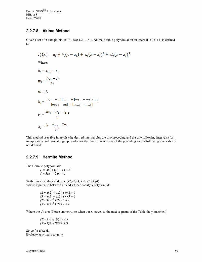
Doc. #: NPSSTM User Guide REL: 2.3 Date: 7/7/10
2 Syntax Guide 50
2.2.7.8 Akima Method
Given a set of n data points, (xi,fi), i=0,1,2,…,n-1. Akima’s cubic polynomial on an interval (xi, xi+1) is defined as
Where:
This method uses five intervals (the desired interval plus the two preceding and the two following intervals) for interpolation. Additional logic provides for the cases in which any of the preceding and/or following intervals are not defined.
2.2.7.9 Hermite Method
The Hermite polynomials: y = ax3 + ax2 + cx + d y' = 3ax2 + 2ax + c
With four ascending nodes (x1,x2,x3,x4),(y1,y2,y3,y4) Where input x, in between x2 and x3, can satisfy a polynomial:
y2 = ax23 + ax22 + cx2 + d y3 = ax33 + ax32 + cx3 + d y2'= 3ax22 + 2ax2 + c y3'= 3ax32 + 2ax3 + c
Where the y's are: (Note symmetry, so when our x moves to the next segment of the Table the y' matches)
y2' = (y3-y1)/(x3-x1) y3' = (y4-y2)/(x4-x2)
Solve for a,b,c,d. Evaluate at actual x to get y

Doc. #: NPSSTM User Guide REL: 2.3 Date: 7/7/10
2 Syntax Guide 51
Assumes two nodes on either side of the input X. Note, simple logic handles cases where there are not two nodes on either side.
2.2.7.10 Extrapolation Warnings and Errors
Each entire table has two attributes that control how extrapolations are handled. These are TprintExtrapT and
TextrapIsErrorT. Either can be set within the table definition, or otherwise outside by using:
Ttable_nameT.printExtrap or Ttable_nameT.extrapIsError
These attributes are described in the following table.
Table 10. Table Extrapolation Warning Attributes
Attribute Allowable Values Action Taken When an Extrapolation Occurs
TprintExtrapT
TFALSET (0) (default)
TTRUET (1)
No notification Notification
TextrapIsErrorT
TFALSET (default) TTRUET
Notification = Warning Notification = Error
No notification is provided if TprintExtrap = FALSET regardless of the value of TextrapIsErrorT. When
printExtrap = TRUE, any warning and error notifications issued are TprovisionalT. This means that if the fault condition exists when the solver exits, the message is issued then, and the program continues running. Provisional fault conditions that occur momentarily during the solver's iterations, but clear by the time it exits generate no messages. A solver must be present for a provisional error or warning to be printed. The example that follows will provide no messages unless it is associated with a solver.
Table Ratings1( real PLA ) {
PLA = { 10.0, 30.0, 50.0 }
BOT = { 1756.7, 2374.6, 2800.0 }
}
Ratings1.printExtrap = TRUE; // Overrides default value of FALSE.
// extrapIsError still defaults to FALSE.
Ratings1( 55. ); // PLA is extrapolated.
CASE++;
run(); // Upon solver termination, a warning message is issued.
Ratings1.extrapIsError = TRUE;
Ratings1( 55. );
CASE++;
run(); // Upon solver termination, an error message is issued.
Ratings1.printExtrap = FALSE;
Ratings1( 55. );
CASE++;
run(); // Even though extrapIsError = TRUE, no message is issued.
2.3 Interactive Mode Syntax
2.3.1 Introduction to Interactive Mode Syntax The mode of operation in view in preceding sections involves storing NPSS commands in various files that are processed by NPSS without further interaction with the user. Interactive mode allows the user to enter commands to NPSS directly from the keyboard while NPSS is active. Commands exist to control the entry into interactive mode, and to transition back and forth between interactive mode and file-based mode. Interactive mode can be a powerful tool to debug or interrogate a model.
Command line options affecting interactive mode are discussed in Sections 2.1, 2.3.2, and 2.3.3.

Doc. #: NPSSTM User Guide REL: 2.3 Date: 7/7/10
2 Syntax Guide 52
2.3.1.1 Interactive Mode Input
Interactive mode is indicated by a prompt on the user's screen of two greater-than signs, ">>", followed by a space.
When NPSS is waiting for information continued from a preceding line, the prompt changes to "more?".
Interactive mode syntax and file-based syntax require the semicolon statement terminator. In interactive mode as well as file-based syntax, one line is continued to the next simply by starting a new line without the semicolon statement terminator.
>> real ra[] = { 0.0, 1.0, 2.0, 3.0,
more? 4.0, 5.0, 6.0 };
In interactive mode, the value of any expression that is not assigned to a variable will be displayed on the terminal. For example:
>> ra;
{ 0, 1, 2, 3, 4, 5, 6 }
>>
This also allows the output of functions such as list() to be displayed easily.
>> list( "Subelement", 1 );
{ "CmpH.S_map", "CmpH.S_map.S_eff", "TrbH.S_map", "TrbH.S_map.S_eff" }
>>
All standard file-based NPSS commands are also valid in interactive mode. For example:
>> int i;
>> for ( i=0; i<ra.entries(); i++ ) {
more? Cout << ra[i] << ", ";
more? }; cout << endl;
0, 1.5, 2, 3, 4, 5, 6,
>>
2.3.1.2 Interactive Mode Command Line Editing
The arrow keys and backspace keys can be used as follows:
• Up arrow ("↑") and down arrow ("↓") scroll through a saved list of previously entered commands. A displayed command is available to be executed again, or to be edited before execution.
• Left arrow ("←") and right arrow ("→") move the cursor left and right through a displayed command.
• The backspace key deletes one character at a time to the left of the cursor position. New text can be inserted into a displayed command at the cursor location by simply typing the text. There is no overstrike mode of editing available. Once a command has been edited as desired, pressing the enter or return key executes it.
2.3.2 Entering Interactive Mode There are three ways to enter interactive mode:
1. Use the –i command line option when starting an NPSS run to enter interactive mode after all file-based processing is complete. See Section 2.1.
2. Execute function icl.start(); from within an input file. 3. Execute a TbreakpointT from within an input file.
NPSS object icl ("interactive command line") is automatically created for the user to control entrance into
interactive mode. As noted above, icl.start(); will halt normal file processing and enter interactive mode at
the place the command is encountered in an input file. The user can also define function icl.preexecute(); which will execute once at the start of each interactive mode session.

Doc. #: NPSSTM User Guide REL: 2.3 Date: 7/7/10
2 Syntax Guide 53
Breakpoints are discussed in the following section. It can be noted here, however, that the user can define
functions icl.preBreak(); and icl.postBreak(); to execute in connection with active break points.
Function icl.preBreak(); executes whenever a breakpoint executes. Function icl.postBreak(); executes
whenever processing of file-based commands is resumed using commands continue, step, stepOut, or
stepOver (see Section 2.3.4). These commands cause interactive mode to be reentered after executing one or
more file-based commands. Upon reentering interactive mode, icl.preBreak(); will be executed first, then
icl.preexecute(); .
2.3.3 Breakpoints Breakpoints are used to enter interactive mode at desired points in a model's execution. They are like icl.start(); but provide the user more power in determining the location of the start of interactive running. Breakpoints are ignored unless at least one of the following conditions is met:
• NPSS was started with the –debug command line option (see Section 2.1).
• Command debug() has been executed in the file. Only breakpoints encountered after the debug() command will be processed. See Section 11.3.
2.3.3.1 The breakPoint() command
Breakpoints are established using the breakPoint() command as follows:
breakPoint( TlocationT, TconditionT, TactionT );
All three arguments are optional, but to enter TconditionT, TlocationT must also be entered, and to enter TactionT, both
TlocationT and TconditionT must be entered. Executing breakPoint() without any arguments causes an immediate
break to interactive mode at that location, like icl.start().
ULocation
The TlocationT argument is a string (enclosed TinT double quotes) consisting of a keyword and one or more location
indicator separated by colons (":"). The syntax options are as follows:
ENTRY:Tfunction_pathnameT:Toccurrence_numberT
EXIT:Tfunction_pathnameT:Toccurrence_numberT
FILE:TfilenameT,Tline_numberT:Toccurrence_numberT
WATCH:Tparameter_name T
For keywords ENTRY:, EXIT:, and FILE:, the occurrence number is optional. If present, it is a single integer number that causes a break to interactive mode to occur only on or after the specified number of times when the break would otherwise have executed.
The keywords cause the following behavior:
• ENTRY: causes a break just before the named function is entered. For example: breakPoint( "ENTRY:CmpH.preexecute" );
• EXIT: causes a break after the last statement has been executed but before exiting the function. BreakPoint( "EXIT:CmpH.postexecute" );
• FILE: causes a break before the statement on the indicated line is executed. BreakPoint( "FILE:interactive.file,2" );
• WATCH: causes a break whenever the value of the named parameter changes. BreakPoint( "WATCH:CmpH.Fl_I.W" );
Breaks can only be made in interpreted functions. For example, all Element objects have an internal function
named calculate() that is executed every time the object is executed. However, the following breakpoint:
breakPoint( "ENTRY:CmpH.calculate" );
will have no effect unless object CmpH was created from interpreted code.
There are five exceptions to this rule. The user can set breakpoints for the following internal solver functions:

Doc. #: NPSSTM User Guide REL: 2.3 Date: 7/7/10
2 Syntax Guide 54
Table 11. Internal Solver Functions for Which a Breakpoint May Be Specified
Trun()T
runPreExecutionSequence()T T
TrunExecutionSequence()T
TrunPostExecutionSequence()T
TgenerateJacobian()T
For example, by entering the following breakpoint:
breakPoint( "EXIT:solver.generateJacobian" );
the user can examine each Jacobian matrix after it has been generated. More discussion on the
preExecutionSequence, executionSequence, and postExecutionSequence attributes of solver objects is found in 4.6.1. General solver theory and operation are discussed in Chapter 6.
Breaks in files are only made when the file is processed by the parser. For example, suppose a model includes
(using #include) file hpc.map containing subelement instantiations belonging to Compressor element CmpH. Suppose after the file has been processed, the following breakpoint is set:
breakPoint( "FILE:hpc.map,1" );
Even though the information in this file is used repeatedly in the execution of element CmpH, the file itself is not reprocessed, so the breakpoint will have no effect. The breakpoint would have to be set before the initial
#include "hpc.map" statement in order to effect a break.
Furthermore, a break in a file can only be performed at lines representing the start of complete statements. For
example, file hpc.map used in the example above would normally contain lengthy table definitions spanning many lines of the file. Attempting to break at a line in the middle of the table definition will not work, because the parser treats the entire table definition as a compound statement.
The file name specified with the FILE: keyword must be recognizable to NPSS. If in doubt about the name NPSS
associates with a file, force a break to interactive mode somewhere in the file (for example, using icl.start() ),
and issue the show command (see Section 2.3.4).
Keyword WATCH:, which looks for changes in the value of a named parameter, should be used with care because it can greatly add to execution time. It can also be difficult to determine which object produced the change if the
change occurred in compiled code (see notes under command where in Section 2.3.4). If a variable being "watched" is changed in compiled code, interactive mode will be entered sometime after the exit from that segment of code. If the variable is changed by a line of interpreted code, interactive mode will be entered after the execution of that line.
UCondition
The TconditionT argument is a string containing an expression that should evaluate to an integer value. The integer is treated as a Boolean value (0 = "false", nonzero = "true"). If the condition expression evaluates to "false," the breakpoint will be skipped. This argument defaults to "true". To force a value of "true," syntax such as the following can be used:
breakPoint( "ENTRY:solver.runExecutionSequence:5", "TRUE" );
The condition argument must always be enclosed in quotes because it is a string. In this case, the string evaluates
to the value of the automatically created global variable TRUE (see Table 7. Automatically Created Global Variables) which holds the value 1.
The following command causes a break to interactive mode at the beginning of CmpH.postexecute() if the
CmpH inlet Mach number is greater than 0.28.
breakPoint( "ENTRY:CmpH.postexecute", "CmpH.Fl_I.MN > 0.28" );

Doc. #: NPSSTM User Guide REL: 2.3 Date: 7/7/10
2 Syntax Guide 55
Uaction
The TactionT argument is also a string containing a command (or series of commands separated by semicolons) that is executed when the break is executed. A common usage for the action argument is to print a value or set of
values to the screen. Object cout is generally used for this. Strings are always enclosed in quotes, but it is often
necessary to use quotes as part of a cout command. To do this (as discussed in Section 2.2.4.6), precede any
quotation marks within the action string by a backslash ("\") as in the following example:
breakPoint( "ENTRY:solver.run", "Amb.MN > 0.5",
"cout << \"Amb.MN = \" << Amb.MN << endl;" );
This breakpoint causes an entry into interactive mode at the beginning of the solver's run() command if the ambient Mach number is greater than 0.5. When the break is executed a message is written to the screen informing the user of the magnitude of the ambient Mach number.
2.3.3.2 Breakpoint Number
Each breakpoint created in a given NPSS session is assigned a unique integer identification number, beginning with 0 and increasing sequentially. This breakpoint number is used to identify the breakpoint in the commands discussed in the following section. Once a breakpoint number has been assigned, it is never reassigned to another breakpoint, even if the original breakpoint is deleted. For example, if eight breakpoints (numbered 0-7) were created, and later all deleted, the next breakpoint created after these events would be given number 8.
2.3.3.3 Commands Used with Breakpoints
The following rules generally apply to the Tbreakpoint_numberT argument in the commands discussed in this section:
• A positive integer value selects the breakpoint of that number.
• A negative value ( -1 ) selects all breakpoints.
• Omitting the argument entirely selects the Tcurrent breakpointT. When the command is entered from interactive mode, the current breakpoint is the breakpoint that initiated the current interactive session.
The following commands can be issued either from interactive mode, or as file-based commands.
listBreak ( Tbreakpoint_numberT, Tshow_conditionT );
Returns a string array containing information about existing breakpoints. Each entry gives a breakpoint number, its location string, its status (whether active or inactive), and optionally its condition string. Argument Tshow_conditionT is a string containing an expression that should evaluate to either "true" (nonzero integer) or "false" (integer 0). It defaults to "false," and can be omitted entirely. If "true," the condition string is included in
the information returned. To list all existing breakpoints, execute listBreak( -1 ). This is a convenient way to confirm the breakpoint number assigned to each breakpoint.
The NPSS language (like C and C++) does not allow the user to omit initial arguments to a function. Thus, it is not possible to list the condition string of the current breakpoint in a single step. The user should discover the
breakpoint number of the current breakpoint by issuing listBreak() (with no arguments), and then issue the
command again using that breakpoint number, as in listBreak( 5, "TRUE" ).
suspendBreak ( Tbreakpoint_numberT );
Makes the specified breakpoint TinactiveT. Inactive breakpoints still exist, but are ignored.
activateBreak ( Tbreakpoint_numberT );
Makes the specified breakpoint active. Breakpoints are active when created, so this command is used to reactivate
breakpoints that were previously made inactive by suspendBreak().
clearBreak ( Tbreakpoint_numberT );
Deletes the specified breakpoint. Although the number associated with a deleted breakpoint is not reused, the
breakpoint no longer exists. It is not listed by listBreak(), and cannot be reactivated by activateBreak().

Doc. #: NPSSTM User Guide REL: 2.3 Date: 7/7/10
2 Syntax Guide 56
2.3.4 Interactive Debugging Commands The following commands are available only in interactive mode. They work whether interactive mode was entered
through icl.start() or through a breakpoint. They are generally used when tracing the execution of a file-based model to understand unexpected behavior.
continue
Ends the current interactive session and resumes normal file-based execution. Interactive mode will be reentered if
an active breakpoint or an icl.start() command is encountered. Compare with quit and the step commands below.
load TfilenameT
Reads and processes the contents of the specified file. This is equivalent to #include <TfilenameT> in file-based
processing. As with T#includeT, the TloadT command searches for the specified file using the NPSS include path (see Sections 2.1 and 2.2.3.1).
quit
Ends the interactive session and terminates the program. Compare with continue and the step commands.
show
Displays the absolute pathname and line number of the current file. See notes under the where command below.
step
Executes the next interpreted statement and then returns to interactive mode. If the next statement results in a call to an interpreted function, either directly or indirectly, interactive mode is activated upon entry into that function. Otherwise, interactive mode resumes after the current statement is executed.
It takes two step commands to get through a statement such as:
int x = 11;
The first step is for the declaration of TxT; the second step is for the assignment of value 11 to the variable.
Repeated executions of the step command are conveniently accomplished using the up arrow key followed by the enter or return key (see Section 2.3.1.2).
Commands step, stepOut, and stepOver only function properly if –debug has been specified on the command
line (see Section 2.1) or command debug() has been entered (see Sections 2.3.3 and 11.3).
stepOut
Completes execution of the current block of interactive code (unless an active breakpoint or icl.start() is encountered), then returns to interactive mode. The current block can be a loop (Section 2.2.5.5), a conditional (Section 2.2.5.4), or an interpreted function body (Section 2.2.6).
stepOver
Behaves the same as TstepT, except that interactive mode resumes after the current statement is executed, even if
the current statement results in a call to an interpreted function (unless an active breakpoint or icl.start() is encountered).
trace [on/off]
Command trace on turns trace on; trace off turns it off. Entering trace with no following keyword causes the system to report the status of trace (on or off).
When trace is on, the system writes to standard output a record of each interpreted statement and function call as it is executed. The value of each expression is shown in parentheses after the expression. Trace can be turned on
from the very beginning of an NPSS session using the –trace command line option (see Section 2.1). Trace can
be controlled in batch mode via the traceExecution() function.

Doc. #: NPSSTM User Guide REL: 2.3 Date: 7/7/10
2 Syntax Guide 57
where
Displays the stack trace of functions that were called. This command often does not show anything below the
global call to run(), even when interactive mode is entered in an interpreted function such as a preexecute().
Function show above is sometimes more helpful in finding the location of a break to interactive mode. When
WATCH: is being used (see Section 2.3.3.1), interactive mode may be entered at a piece of interpreted code even
when the variable change took place in compiled code. In these cases use of where and show can be misleading.

Doc. #: NPSSTM User Guide REL: 2.3 Date: 7/7/10
3 Acquiring Components 58
3 Acquiring Components in NPSS
TComponentsT include Elements, Subelements, and Assemblies – the primary building blocks of NPSS simulations. There are four ways to define NPSS components, and several ways to TacquireT them, or make them available for use in a specific simulation. These are summarized in the following table.
Table 12. Component Acquisition Methods
Component Definition
Acquisition Method
Description Further Documentation
interpreted Write component definition into an NPSS input file.
Use the NPSS input syntax already described plus some special commands to define a component with the desired functionality.
TDeveloper GuideT
interpreted #include Use the #include preprocessor command to draw a file containing an interpreted component definition into an NPSS input file. The location of the desired file must be part of the include path specified to NPSS.
Sections 2.2.3.1 and 2.1
interpreted Interpreted Component Load on Demand (ICLOD)
NPSS can automatically load interpreted component definitions when they are needed.
Section 3.1 below
Dynamically Loadable Module (DLM)
command line Use the –l command line option to specify a specially compiled piece of code called a DLM to be loaded with NPSS.
Section 2.1
DLM loadDLM() Use function loadDLM() either interactively or in an NPSS input file to load a DLM.
Section 11.2.4
DLM DLM Component Load on Demand (DCLOD)
NPSS can automatically load component definitions existing as DLMs when they are needed.
Section 3.3 below
internal Compile into the NPSS executable.
C++ code defining components can be written and compiled into NPSS.
TDeveloper GuideT
TCreation Method FacilitiesT (CMFs) are NPSS modules that search for and acquire necessary components at run
time. The available CMFs, and the order in which they are accessed, is given by function listLoadedCMFs(). NPSS currently provides three CMFs, called in the following order.
1. DLM Component Load on Demand (DCLOD) 2. Interpreted Component Load on Demand (ICLOD) 3. External Component Load on Demand (ECLOD)
ECLOD is available only when a CORBA-aware NPSS executable is called with the -corba command line option. ICLOD and DCLOD are always available unless disabled by command line options.
3.1 Interpreted Component Load on Demand (ICLOD) The TInterpreted Component Load on DemandT (TICLODT) CMF assists in finding and loading interpreted
components. ICLOD works on the principle that the file Tcomponent_nameT.int contains exactly one interpreted
component named Tcomponent_nameT. For example, Duct.int is an ASCII file containing NPSS input syntax
defining an object type named Duct. It uses this one-to-one mapping of an interpreted component name to a file name to look for and load a component.

Doc. #: NPSSTM User Guide REL: 2.3 Date: 7/7/10
3 Acquiring Components 59
When ICLOD is asked to create a component, for example Duct, it searches a given path for a file named Duct.int. If the ICLOD_PATH environment variable is set, ICLOD searches the directories specified by the contents of that variable, in the order they are specified. If the file is not found in ICLOD_PATH, ICLOD then searches the NPSS
include path. This is the combination of the environment variable NPSS_PATH and any paths specified using the -I command line option (see Section 2.1). For informational purposes, ICLOD shows the search path it is using
in variable ICLODPATHS (see Table 7). ICLODPATHS may be modified by the user by simply setting ICLODPATHS equal to a string array of desired paths, as shown in this example. ICLODPATHS = {“/NPSS/dev/CustomPath”, “/NPSS/dev/CustomPath2”};
Setting ICLODPATHS in this manner will discard any previous paths that were being held in ICLODPATHS. So if a user wants to append paths to the existing ICLODPATHS, the user may wish to incorporate a temporary string array to hold the original values, as shown here: string tempPaths [] = ICLODPATHS; //store ICLODPATHS in tempPaths
string newPaths[]={“/new/path/1”, “/new/path/2”}
tempPaths += newPaths; //combine the old and new paths
ICLODPATHS = tempPaths; //net result is appending new paths
As currently implemented, ICLOD is not active until it is used in some way. Thus, when NPSS is first started, variable ICLODPATHS does not exist, and a command like cout << ICLODPATHS will fail. Calling any function that touches ICLOD, such as listLoadedCMFs() or listKnownTypes() will activate it. If ICLOD finds a file of the name it is seeking, it then parses that file. If the file contains inappropriate code, such as a quit(), this will be executed with all its consequences. ICLOD tries to inform the user when it encounters a parsing error while reading the file, or when it successfully parses the file but does not find the appropriate component definition.
3.2 Overview of Dynamically Loadable Modules (DLMs) TDynamically Loadable ModulesT (DLMs) allow NPSS to use compiled components not statically compiled into the code. Thus, any number of components can be compiled into an entity similar to a shared library to be dynamically loaded into NPSS at run time if and when needed. DLMs can provide a wide range of functionality. "Components," then, can be taken in a very general sense: Elements, Subelements, Assemblies, thermodynamics packages, Ports, DataViewers, functions, CMFs, customer decks, compiled models, etc. It is even possible to have CORBA support be a DLM. Most users, however, will use DLMs as means to make Elements, Subelements, and Assemblies available to NPSS in a form that will execute roughly twice as fast as their interpreted code counterparts. A DLM component is created in the same way a regular compiled NPSS component is created, only using a special make procedure. See the Developer Guide for details. A DLM is strongly tied to a particular NPSS executable (more specifically to a particular version of the NPSS Executive library). If a header file in the Executive library is changed, DLMs must be recompiled to work correctly with NPSS executables built on the new library. When loading a DLM, NPSS compares the DLM version ID to its own version ID. If they differ, the load will fail and an error message will be generated. As summarized in Table 12 above, a DLM can be loaded into NPSS:
1. By passing –l TpathToDLMModuleT as an argument on the NPSS command line. For example: npss.exe –l ./MyComponents.scl Tother_arguments_to_executableT
2. By calling function loadDLM(TpathToDLMModuleT) either interactively or from an input file. For example: loadDLM("./MyComponents.scl");

Doc. #: NPSSTM User Guide REL: 2.3 Date: 7/7/10
3 Acquiring Components 60
3. By using DCLOD (discussed below).
In addition, one can call the Executive library's DM::loadDLM(const NCPString &TpathToDLMT) function from C++ code. For example,
#include <DataManagerInterface.H>
…
void someFunct(some args) {
DM::loadDLM("./MyComponents.scl");
}
This option will probably not be called from a component but will most often be called behind the scenes by, for example, a site-specific Creation Method Facility.
3.3 DLM Component Load on Demand (DCLOD) The TDLM Component Load on Demand (DCLODT) CMF assists in loading DLMs. DCLOD works on the principle
that the file named Tcomponent_nameTT.scT contains exactly one DLM component named Tcomponent_nameT. For
example, Duct.sc is a compiled DLM file defining an object type named Duct. It uses this one-to-one mapping of a DLM component name to a file name to look for and load a component.
When DCLOD is asked to create a component, for example TDuctT, it searches a given TpathT for a file named
TDuct.scT. If the TDCLOD_PATHT environment variable is set, DCLOD searches the directories specified by the contents of that variable, in the order they are specified. If the file is not found, DCLOD then searches the NPSS
include path. This is the combination of the environment variable TNPSS_PATHT and any paths specified using the T–
IT command line option (see Section 2.1). For informational purposes, DCLOD shows the search path it is using in
variable TDCLODPATHST (). This is similar to the TINCLUDEPATHST variable that lists the include paths NPSS is using.
Currently TDCLODPATHST is read only, meaning that the paths it searches cannot be modified at run time.
As currently implemented, DCLOD is not active until it is used in some way. Thus, when NPSS is first started,
variable DCLODPATHS does not exist, and a command like cout << DCLODPATHS will fail. Calling any function
that touches DCLOD, such as listLoadedCMFs() or listKnownTypes() will activate it.
If DCLOD finds a file of the name it is seeking, it then loads that file. If the file does not contain the component sought for, DCLOD throws an exception indicating that it cannot create the requested component. There is no
guarantee that the DLM does not contain inappropriate code.
3.4 How NPSS Uses CMFs As mentioned earlier, NPSS can recognize several CMFs and uses them in a specified order. Currently NPSS has three standard CMFs accessed in the following order: 1. DLM Component Load on Demand (DCLOD) 2. Interpreted Component Load on Demand (ICLOD)
3. External Component Load on Demand (ECLOD) – only if the –corba command line option is used When NPSS is asked to create a component it cannot find, it will normally ask DCLOD to find the component as a DLM. This strategy seeks to minimize execution time since DLM components execute roughly twice as fast as comparable interpreted components. As noted above, if DCLOD finds a file named as though it contains the desired component, but the file does not contain the component, an error results. If, however, DCLOD cannot find
a file of the appropriate name (Tcomponent_nameT.sc), it simply returns control to NPSS, which calls the next available CMF, namely ICLOD. Similarly, ICLOD will either find the desired component, generate an error due to
incorrect content in a file named Tcomponent_nameT.int, or fail to find the file. If NPSS exhausts all its CMFs without finding the component required, it generates an error and stops execution.
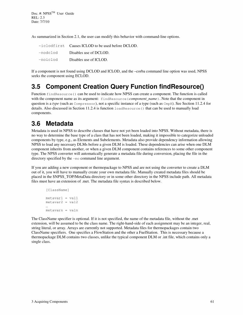
Doc. #: NPSSTM User Guide REL: 2.3 Date: 7/7/10
3 Acquiring Components 61
As summarized in Section 2.1, the user can modify this behavior with command-line options.
-iclodfirst Causes ICLOD to be used before DCLOD.
-nodclod Disables use of DCLOD.
-noiclod Disables use of ICLOD.
If a component is not found using DCLOD and ICLOD, and the –corba command line option was used, NPSS seeks the component using ECLOD.
3.5 Component Creation Query Function findResource() Function findResource() can be used to indicate how NPSS can create a component. The function is called
with the component name as its argument: findResource(Tcomponent_nameT). Note that the component in
question is a type (such as Compressor), not a specific instance of a type (such as CmpH). See Section 11.2.4 for
details. Also discussed in Section 11.2.4 is function loadResource() that can be used to manually load components.
3.6 Metadata Metadata is used in NPSS to describe classes that have not yet been loaded into NPSS. Without metadata, there is no way to determine the base type of a class that has not been loaded, making it impossible to categorize unloaded components by type, e.g., as Elements and Subelements. Metadata also provide dependency information allowing NPSS to load any necessary DLMs before a given DLM is loaded. These dependencies can arise when one DLM component inherits from another, or when a given DLM component contains references to some other component type. The NPSS converter will automatically generate a metadata file during conversion, placing the file in the
directory specified by the –mo command line argument. If you are adding a new component or thermopackage to NPSS and are not using the converter to create a DLM out of it, you will have to manually create your own metadata file. Manually created metadata files should be placed in the $NPSS_TOP/MetaData directory or in some other directory in the NPSS include path. All metadata files must have an extension of .met. The metadata file syntax is described below.
[ClassName]
metavar1 = val1
metavar2 = val2
…
metavarn = valn
The ClassName specifier is optional. If it is not specified, the name of the metadata file, without the .met extension, will be assumed to be the class name. The right-hand-side of each assignment may be an integer, real, string literal, or array. Arrays are currently not supported. Metadata files for thermopackages contain two ClassName specifiers. One specifies a FlowStation and the other a FuelStation. This is necessary because a thermopackage DLM contains two classes, unlike the typical component DLM or .int file, which contains only a single class.

Doc. #: NPSSTM User Guide REL: 2.3 Date: 7/7/10
4 Common Tasks 62
4 Common Tasks
Chapter 2 covered the basic building blocks of the NPSS input language. Chapter 3 covered how to gain access to more complex pre-written NPSS objects. This chapter covers how to use these items to create complete NPSS models. The first several sections discuss the basics of key NPSS objects: thermodynamics packages, elements, subelements, assemblies, and how to connect them together. The specification of bleeds, solver setup, and output formats are also discussed. After covering the basics of running a model, a number of special topics are treated, such as how to modify an existing model, expand the capability of existing objects, generate initial guesses, handle error messages, and match test data.
4.1 Thermodynamics Packages Calculations involving fluid properties require a Tthermodynamics packageT that models the fluid. NPSS offers the user the ability to choose the thermodynamics package to be used. Table 13 below lists the packages distributed with a standard NPSS release.
Table 13. Thermodynamics Packages
Keyword Description TCEAT Implementation of the NASA chemical equilibrium code.
TJanafT Implementation of the National Institude of Standards and Technology gas properties prepared by Honeywell.
TGasTblT Package developed by Pratt & Whitney based on Therm, but adding humidity calculations and some chemical equilibrium capabilities.
TAllFuelT Package developed by General Electric that contains gas properties and fuel properties.
TFPT Package used to define NPSS tables and/or functions that describe the thermodynamic properties of the fluid
A thermodynamics package must be specified before any elements or subelements are instantiated. Its specification, therefore, is generally among the first actions accomplished in an NPSS model. A thermodynamics package is
specified with command setThermoPackage(). For GasTbl, Janaf, allFuel, and FPT this command takes one argument defining the package. For example,
setThermoPackage( "GasTbl" );
setThermoPackage( "Janaf" );
setThermoPackage( "allFuel" );
setThermoPackage( “FPT” );
The setThermoPackage command can be executed any number of times to allow the use of more than one thermodynamics package in a single model. Care must be taken, however, since the enthalpy and entropy bases for packages often differ. The copyFlow and add functions throw a warning if the thermodynamic package is of a different type. The model developer will need to compensate for this by emulating this functionality within the component in question. See the NPSS Developer’s Guide for details on creating components. To run CEA, the user must have a CEA thermo.inp and trans.inp (if transport properties are to be calculated) in the directory where the model is running. These files can be created by running CEA off-line with a library input file. For CEA, the setThermoPackage command takes seven arguments defining the thermodynamic package and also the names of the possible reactants. The first name identifies which CEA reactant represents air. The second name identifies which CEA reactant represents water. The additional names represent the other possible reactants. They do

Doc. #: NPSSTM User Guide REL: 2.3 Date: 7/7/10
4 Common Tasks 63
not need values and can be input as blank strings. All these reactants must be defined in the thermo.lib and trans.lib files. For example,
setThermoPackage( "CEA", "Air", "H2O", "JP_7", "", "", "" );
The FPT package allows the user/developer to create tables and/or functions to describe the thermodynamic properties of a fluid. These tables and/or functions are defined in NPSS interactive format. The tables and/or functions are placed in a file with the name "fluidName.fpt." These files can be converted to C++. To use the fluid, set the composition (flowstationName.setComp(“fluidName”);) then use the flowstation as you would any other. A list of the functions available for FPT flowstations can be found in the Reference Sheets document.
4.2 Elements TElementsT are an important class of NPSS objects. As summarized earlier in Section 1.5.1, elements are used to model the basic components of an engine cycle, such as compressors, turbines, burners, ducts, and nozzles.
Element objects are instantiated using the following items in order:
1. Keyword Element (optional) 2. The specific element type 3. The object name 4. An optional block of statements (enclosed in curly braces) executed when the object is instantiated. If present,
this block is called the Tinstantiation blockT. This block of statements can instantiate other objects that become children of the element object.
For example:
Element Inlet Inl {
eRamBase = 0.995;
} // END Inl
In this case, variable eRamBase is a variable created by the system in all objects of type Inlet (the variables created by the system for each element and subelement type can be found in the TNPSS Reference SheetsT).
The instantiation block is optional. Many users prefer to include an empty set of curly braces if no instantiation block statements are required. It is also permissible, however, to terminate the statement with a semicolon after the object name.
Element Ambient Amb {
} // END Amb
Element InletStart InletStart {
AmbientName = “Amb”;
} // END InletStart
Element FuelStart Fuel;
As noted in Section 2.2.2.4, a block of statements can be associated with an object after its instantiation by giving the object name immediately before the block:
Inl {
a_eRamAud = 0.0;
s_eRamAud = 1.0;
}

Doc. #: NPSSTM User Guide REL: 2.3 Date: 7/7/10
4 Common Tasks 64
where a_eRamAud and s_eRamAud are predefined variables contained in objects of type Inlet. Everything that can be done in an object's instantiation block can also be done in a block such as that above associated with an object after its instantiation.
If users wish, when they instanitate an element they have the option of giving it a version designation, or number, using the string variable "version" as follows:
Element TESTELT elt {
…
version="Test version 1";
…
}
Note also that the attributes description and iDescription (as discussed in section 2.2.4.1) exist for complex
objects such as elements (and subelements). For such objects, description is intended to explain the general purpose of the object type, and is usually given a predefined default value by the element writer. Attribute
iDescription is intended to explain the purpose of a specific instance of a type. It can be supplied by the user to help document a model.
The order in which the NPSS solver executes elements is controlled by string array variable executionSequence.
Each time an Element object is instantiated, NPSS appends its name to executionSequence. Thus, by default,
NPSS will execute its elements in the order they are instantiated. By editing array executionSequence, the user can easily change the execution sequence, so in principle the user is free to instantiate elements in any order desired. The only restrictions are that any object must be instantiated before its internal attributes are assigned values, and before it is referenced by another object. It is good practice, however, to instantiate elements in a logical order, generally following the gas flow from inlet to exit.
In addition to using pre-written standard elements, NPSS allows the user to create entirely new element types which can then be instantiated and used in a model. Details on how to do this are found in the TDeveloper GuideT.
4.3 Ports As introduced in Section 4, NPSS elements communicate with each other via TportsT. Five kinds of ports exist in NPSS:
• fluid
• fuel
• shaft
• data
• file The presence of a port signals a collection point for properties to be shared with another element: fluid properties, fuel properties, and shaft properties. In the case of a data port, a single specified data value is shared, and for a file port, one or more files. Each port on an element is usually connected to a port on another element so that the two elements share the properties of the port as a mutual boundary condition. For example, if the core flow of a gas
turbine engine passes from the high pressure compressor diffuser (represented, say, by a TDuctT element named
TDiffuserT) to the burner (represented by a TBurnerT element named TBrnT), then the fluid output port on element
TDiffuserT would be connected to the fluid input port on element TBrnT. The fuel would be introduced to the burner
by instantiating a TFuelStartT element whose fuel output port would be connected to the fuel input port on element
TBrnT.
Most elements create the ports they need for the user. These ports are automatically named. The naming convention for fluid, fuel, and shaft ports is given in Table 14 below.

Doc. #: NPSSTM User Guide REL: 2.3 Date: 7/7/10
4 Common Tasks 65
Table 14. Port Naming Conventions
Description Name FluidInputPort Fl_I
FluidOutputPort Fl_O
FuelInputPort Fu_I
FuelOutputPort Fu_O
ShaftInputPort Sh_I
ShaftOutputPort Sh_O
Elements with multiple input and output ports are generally named Fl_I1, Fl_I2, Fl_O1, Fl_O2, etc., but consult the TNPSS Reference SheetsT to be sure. (The Splitter, for example, has primary and secondary fluid outlet ports named Fl_O1 and Fl_O2 respectively.) Shaft input ports are generally created and named by the user (see Section 4.3.1).
Ports are NPSS objects and contain a number of variables. The variables contained by fluid and fuel ports depends
somewhat on the thermodynamics package being used, which is specified by the TsetThermoPackage()T command (see Section 4.1 and the TNPSS Reference SheetsT). Port objects are children of the element on which they are created,
and their variables are children of the port. Accessing the fuel/air ratio (variable name FAR) on the fluid ouput port
of a Burner object named Brn, for example, would be done as follows:
Brn.Fl_O.FAR
4.3.1 Creating Ports Some elements either allow or require the user to create ports. Ports are created in a similar way as elements are (see Section 4.2) by giving a keyword, a port name, and an optional instantiation block. The keywords used to create ports are summarized in the following table.
Table 15. Port Creation Keywords
Keyword Port Type Typical Elements TFluidInputPortT fluid TFluidOutputPortT fluid TBleedInPortT fluid Bleed TBleedOutPortT fluid Bleed
TInterStageBleedInPortT fluid Turbine
TInterStageBleedOutPortT fluid Compressor
TFuelInputPortT fuel TFuelOutputPortT fuel TShaftInputPortT shaft Shaft
TShaftOutputPortT shaft TDataInputPortT data any
TDataOutputPortT data any
TFileInPortT files indirectly wrapped elements TFileOutPortT files indirectly wrapped elements
When using standard NPSS elements, the user does not normally need to create ports using FluidInputPort,
FluidOutputPort, FuelInputPort, FuelOutputPort, or ShaftOutputPort. Ports that would be created with these commands are created automatically by the system. The commands are included in Table 15 for completeness. These commands are often needed, however, when the user creates new element types (see the TDeveloper GuideT).
A typical example of creating ports with some of these commands is given below.
CmpH {
InterStageBleedOutPort Bld1out {
fracBldW = 0.05;
}

Doc. #: NPSSTM User Guide REL: 2.3 Date: 7/7/10
4 Common Tasks 66
InterStageBleedOutPort Bld2out, Bld3out;
Bld2out {
fracBldW = 0.002;
}
Bld3out.fracBldW = 0.003;
}
TrbH {
InterStageBleedInPort Bld1in, Bld2in, Bld3in;
Bld3in.diaPump = 1.2;
}
In the example, CmpH is assumed to be an existing Element object of type Compressor, and TrbH is an existing
Element object of type Turbine. Variable fracBldW is an attribute of all InterStageBleedOutPort objects, and sets the bleed flow as a fraction of the parent object's inlet flow (bleeds are discussed in detail in Section 4.7). Note the following points:
• Objects instantiated within a block associated with another object become children of that object (Section
2.2.2.4). Ports Bld1out, Bld2out, and Bld3out are children of element CmpH. Ports Bld1in, Bld2in, and
Bld3in are children of element TrbH.
• When no instantiation block is included, several ports can be created after the keyword by separating their names with commas and ending the statement with a semicolon.
• Attributes of existing ports can be set by associating a block with the port, or by direct assignment using dot notation.
• The user is free to name the port objects as desired, subject to the general naming rules given in Section 2.2.4.2. DataPorts are discussed further in Section 4.3.3. For information on which elements require or permit user-created ports, see the Element Reference Sheets in the TNPSS Reference SheetsT document. [Need a section that lists ports created for the user.] Some user-created ports can have an associated block of statements in which variables affecting the behavior of the port can be set. Once ports are created on an element, they must generally be linked together. This is the topic of the next section.
4.3.2 Linking Ports Ports are connected together using the TlinkPorts()Tcommand. It has the following form:
linkPorts ( "Tport_nameT", "Tport_nameT", "Tstation_nameT" );
Each link statement connects one output port to one input port, and it is customary to name the output port as the
first argument and the input port as the second. The linkPorts() command causes a TstationT to be created and assigned the given station name (more on this below). The same statement is used to link all the different types of ports. Port type and direction are checked to confirm that both ports are of the same type and output is connected to input. If an attempt is made to link two output ports, or a fluid to a mechanical port, an error message will be issued. Some examples of linking ports follow:
linkPorts( "Diffuser.Fl_O", "Brn.Fl_I", "FL36" ); // fluid ports
linkPorts( "Fuel.Fu_O", "Brn.Fu_I", "FU36" ); // fuel ports
linkPorts( "CmpH.Bld1out", "TrbH.Bld1in", "Bld1" ); // fluid ports
The first example above links a pre-defined fluid output port on element Diffuser to a pre-defined fluid input port
on element Brn, naming the resulting station "FL36". The second links a pre-defined fuel output port on element
Fuel to a pre-defined fuel input port on element Brn, naming the resulting station "FU36". The third links a user-defined fluid output port (a bleed port) to a user-defined fluid input port (another bleed port), naming the resulting
station "Bld1". See the example in Section 4.3.1 for the commands used to create the ports used in this third example. Shaft and data ports are linked in an identical fashion as the examples above.
Element objects representing rotating components, such as elements of type Compressor and Turbine, are automatically instantiated with shaft output ports (one per object). The user manually creates the required number of

Doc. #: NPSSTM User Guide REL: 2.3 Date: 7/7/10
4 Common Tasks 67
shaft input ports on an element object of type Shaft, and links the output ports of the components on the same shaft
to the input ports of a single Shaft object. For example, to connect a Compressor object named CmpH to the same
shaft as a Turbine object named TrbH, the following code would be required:
Element Shaft ShH {
ShaftInputPort CmpH_SH, TrbH_SH;
}
linkPorts( "CmpH.Sh_O", "ShH.CmpH_SH", "CmpH_SH" ); // shaft ports
linkPorts( "TrbH.Sh_O", "ShH.TrbH_SH", "TrbH_SH" ); // shaft ports
To model two compressors and a turbine on a single shaft, three shaft input ports would need to be created on the
Shaft element, and a third linkPorts() command given.
When two ports are connected, the set of fluid, fuel, shaft, or data properties at that location is called a TstationT. It too
is given a name – in the TlinkPortsT command as indicated above. The fluid, fuel, shaft, or data properties at a location can generally be accessed using the station name or either of the two port names. For example, using the
first example given above, Diffuser.Fl_O.Tt, Brn.Fl_I.Tt, and FL36.Tt all refer to the total temperature
between element Diffuser and element Brn.
For fluid, fuel, and shaft ports, the following two rules apply:
• Every port must be linked to another port. Ports that have been created but not linked are detected when one attempts to run the model, and an error is generated.
• Each port must be linked to one and only one other port. For example, a fluid output port cannot be linked to more than one fluid input port. Likewise, a fluid input port cannot be linked to more than one fluid output port. Special elements exist for splitting and combining flows (see the TNPSS Reference SheetsT).
DataPorts follow somewhat different rules, as discussed in the following section.
4.3.3 DataPorts DataPorts contain a single attribute named val that holds the value transfered by the port. The element on which the output port is created must assign a value to this attribute. Once the output port is linked to an input port (see Section 4.3.2), the attribute can be retrieved by the element on which the input port was created. An example follows:
CmpH {
DataOutputPort CDP;
DataOutputPort CDT;
void postexecute() {
CDP.val = Fl_O.Pt;
CDT.val = Fl_O.Tt;
}
}
PERF {
DataInputPort CDP;
DataInputPort CDT;
}
TrbH {
DataInputPort CDP;
}
linkPorts ( "CmpH.CDP", "PERF.CDP", "CDP1" );
linkPorts ( "CmpH.CDP", "TrbH.CDP", "CDP2" );
In the example, two Data0utputPorts are created on existing object CmpH (an element of type Compressor). Two
DataInputPorts are created on existing object PERF (a special element that collects overall cycle information). A

Doc. #: NPSSTM User Guide REL: 2.3 Date: 7/7/10
4 Common Tasks 68
DataInputPort is also created on object TrbH (an element of type Turbine). One of the CmpH DataOutputPorts
(CDP) is linked to two DataInputPorts: one on PERF, the other on TrbH. Element PERF can access the compressor
discharge pressure as CDP.val (the complete path would be PERF.CDP.val), and element TrbH can access the
value as CDP.val (the complete path would be TrbH.CDP.val). The remaining DataOutputPort on CmpH, and the
remaining DataInputPort on PERF are not linked.
The example illustrates the following special rules for DataPorts:
• No error is generated when DataPorts are not linked. Values are transmitted from one DataPort to another,
however, only if they are linked. The value in unlinked DataInputPort PERF.CDT.val is zero.
• DataOutputPorts may be linked to more than one DataInputPort. DataInputPorts, however, can be linked to only one DataOutputPort.
DataPorts are useful for writing general elements that use a piece of information that can bear different names in different models. For example, element PERF might display the overall pressure ratio of a cycle. The name and location of the last compressor's discharge varies from model to model. If DataInputPort PERF.CDP is correctly linked to a DataOutputPort on the last compressor, however, it can always access the highest pressure in the cycle using the name CDP.val.
DataOutputPorts support a user-defined preexecute() function, so that the user may collect the data just before it is to be transferred from current model contents if necessary. Similarly, DataInputPorts support a user-defined
postexecute() function which may be used to distribute data contents into the model if needed.
4.3.4 FilePorts FilePorts are used to transfer files from one component to another. They are typically used with components that wrap external codes indirectly, i.e., codes that interface with each other only through file input and output.
FilePorts contain the following attributes:
filenames[]: A list of names of files to be transferred
directory: The parent directory containing the files in filenames. Defaults to the current working directory of the process.
deleteFilesOnExit: If TRUE, the FilePort will delete the files in filenames when the port itself is deleted. Default value is FALSE.
transferType: The style of transfer, either PUSH or PULL. PUSH is the default. Typically this is only changed to handle transfers through firewalls.
conditionalRecv: (FileInputPorts) If TRUE, only invoke postexecute() if one or more files have
changed, as indicated by their modification timestamp. If FALSE, postexecute() is always invoked. Default TRUE.
newFileFlags[]: (FileInputPorts) Integer flags indicating which files in filenames have changed according to their modification timestamp.
autoExecute: (FileOutputPorts) If TRUE, always send files whenever execute() is invoked. If
FALSE, only send files when explicitly requested via the execute() method (i.e., not
via the solverSequence).
conditionalSend: (FileOutputPorts) If TRUE, only send those files which have changed, as indicated by their modification timestamp. If FALSE, always send all files. Default TRUE.
In most port types, data is pulled from the output port to the input port, but in FilePorts, files may be pushed from the FileOutPort to the FileInPort or pulled. Pushing means that the actual transfer of files occurs when the component containing the FileOutPort is executed, immediately after the component's postexecute function, if it exists. Pulling means that the actual transfer of files occurs when the component containing the FileInPort is executed, immediately after the component’s preexecute function, if it exists. FileOutPorts keep track of the modification times for their files so that they won't transfer them if they haven't changed since the last time they

Doc. #: NPSSTM User Guide REL: 2.3 Date: 7/7/10
4 Common Tasks 69
were transferred. Like DataOutputPorts, FileOutPorts may be connected to multiple FileInPorts, but each FileInPort may be connected to only one FileOutPort. It is not an error if FilePorts are not connected. If filenames in the FileInPort is not empty and the number of entries in filenames in the FileOutPort does not match the number of entries in filenames in the FileInPort, an error will be reported. The number of entries must match because the entries in filenames in the FileInPort are used as destination file names for the files being transferred from the FileOutPort. If filenames is empty in the FileInPort, the file names from the FileOutPort are used for the destination files. Also, if the filenames are the same, then directory must be different, which means that it must either be set explicitly to be different, or the two parent components that contain the FilePorts must be running in different processes with different working directories. The following is an example of FilePort usage:
// a local component
MyComponent {
FileOutPort FOP {
filenames = { "a.out", "b.out", "c.out" };
directory = "mydir";
}
}
// another local component
MyOtherComponent {
FileInPort FIP {
filenames = { "1.in", "2.in", "3.in" };
directory = "somedir"; // directory could be the same since
// filenames are different, but we'll make it
// different anyway
deleteFilesOnExit = TRUE; // clean up files when we exit
}
}
// this is an external component that is running in another process
// (with a different working directory) or on another machine, so
// we'll assume here that our working directory is different than that of
// MyComponent.FOP. We also don't set the value of filenames, so our
// filenames will be the same as MyComponent.FOP.
MyExternalComponent {
FileInPort FIP {
deleteFilesOnExit = TRUE;
}
}
linkPorts ( "MyComponent.FOP", "MyOtherComponent.FIP", "files1" );
linkPorts ( "MyComponent.FOP", "MyExternalComponent.FIP", "files2" );
Now, when MyComponent is executed, MyComponent.FOP will transfer its files to MyOtherComponent.FIP and MyExternalComponent.FIP, provided that the files have changed since the last time they were sent.
FilePorts also have a user-accessible Texecute()T function, so that the user can explicitly trigger the file transfer outside of a normal component execution.
FileOutputPorts support a user-defined preexecute() function, so that the user may create the file just before it is to be transferred from current model contents if necessary. Similarly, FileInputPorts support a user-defined
postexecute() function which may be used to read file contents into the model if needed.
4.4 Subelements As mentioned in Sections 1.5.1 and 4.2, elements are the primary building blocks used to model components such as compressors, turbines, burners, etc. Elements can reside in the top-level assembly (global scope), not being the children of any other object. TSubelementsT are always active as the children of other elements or subelements. They assist their parent object by performing certain major calculations on behalf of the parent. For example, compressor and turbine maps are implemented in NPSS using subelements.

Doc. #: NPSSTM User Guide REL: 2.3 Date: 7/7/10
4 Common Tasks 70
Subelement objects are instantiated much like element objects are, using the following items in order:
1. Keyword Subelement (optional) 2. The specific subelement type 3. The object name 4. An optional block of statements (enclosed in curly braces) executed when the object is instantiated. This block
of statements can instantiate other objects that become children of the subelement object.
Since active subelements are always the child of another element or subelement, they are usually instantiated that way. Recall (Section 2.2.2.4) that an object instantiated in a block associated with another object becomes the child of that object. For example:
Element Turbine TrbH {
Subelement TurbineNeppMap S_map {
parmGeom = 76.0;
parmGeomDes = 76.0;
Subelement TurbineEfficiencyMap S_eff {
…
} // end S_eff
} // end S_map
} //END TrbH
Notice that a Subelement object can be the child of another Subelement object (the TurbineEfficiencyMap subelement named S_eff is the child of the TurbineNeppMap subelement named S_map, which itself is the child of the Turbine element named TrbH). The parmGeom and permGeomDes variables are attributes of all TurbineNeppMap subelements, and are defined in the block of statements accompanying the instantiation of the subelement. These variables could have been defined outside the block, using their path names (e.g., TrbH.S_map.parmGeom = 76.0;). Another way to set such attributes after an element or subelement object has been instantiated is to create another block of lines associated with the object, as in the following example.
TrbH.S_map {
parmMap = 5.0;
parmMapDes = 5.0;
parmNcDes = 100.0;
effDes = 0.895;
}
If users wish, when they instanitate a subelement they may designate a version number using the string variable
"version" (as discussed in Section 4.2). Note also that the attributes description and iDescription exist for
complex objects such as subelements. For such objects, description is intended to explain the general purpose of
the object type, and is usually given a predefined default value by the subelement creator. Attribute iDescription is intended to explain the purpose of a specific instance of a type. It can be supplied by the user to help document a model.
In addition to using pre-written standard subelements, NPSS allows the user to create entirely new subelement types which can then be instantiated and used in a model. Details on how to do this are found in the TDeveloper's GuideT.
Subelements can be associated only with certain parent objects, and must be given a predetermined name in order to work properly with their parent. This is because subelements are designed to fit into TsocketsT, discussed in the next section.
4.5 Sockets Whenever an element or subelement can accept a subelement as a child object, a TsocketT exists to plug in that subelement. In the example in the preceding section, element TrbH could accept subelement S_map because all Turbine elements contain a socket that can accept a subelement of type TurbineNeppMap. It is most common to insert a subelement into a socket (as in the example above); but sockets can be designed to accept functions or tables

Doc. #: NPSSTM User Guide REL: 2.3 Date: 7/7/10
4 Common Tasks 71
as well. Sockets are created and named automatically when their parent object (an element or subelement) is instantiated.
The following points are important to keep in mind regarding sockets:
• Not all elements and subelements have sockets.
• Some elements and subelements have more than one socket, each having a unique name.
• Most sockets do not have to be filled. Sockets can be modified, however, such that they must be filled (see
attribute required in Table 16 below).
• Each socket can accept only one object, and that object must be of a specific type, which is determined by the
socket (see attribute socketType in Table 16 below).
• For sockets that accept subelements, sometimes two or more standard NPSS subelements are available for use in that socket. This affords the user a choice of more than one method to calculate the information the socket is designed to provide to its parent object.
4.5.1 Socket Attributes Sockets are themselves objects residing within their parent element or subelement. As such, all sockets have certain attributes that can be accessed by the user. The following table summarizes these attributes.
Table 16. Socket Attributes
Socket Attribute
Type User Access
Description
description TstringT set/get Describes the socket.
baseType TstringT get only Immediate base type. For sockets this is VariableContainer.
required Boolean
(TTRUET or
TFALSET)
set/get If set to TRUE, an error message is produced if the socket is empty when the model is run. Default value is FALSE.
allowedValues TstringT array
set/get Contains the names of the variables that an object in the socket is permitted to set.
argTypes TstringT array
set/get Defines the argument types required for a function or table inserted in the socket.
returnType TstringT set/get Defines the return type of a function inserted in the socket.
socketType TstringT set/get Defines what type of object can be inserted into the socket.
Attributes argTypes and returnType are discussed further in Section 4.5.4.
As will be discussed in Section 4.5.3, objects inserted into a socket are always treated as having the same name as the socket. Attributes in both the socket and the object that fills it are then accessed as parent_name.socket_name.attribute_name. If the object and the socket have identically named objects, there is potential for ambiguity. For attributes, this normally occurs only for the description and baseType attributes. NPSS handles these variables as follows:
• When a socket is empty, Tparent_nameT.Tsocket_nameT.description and
Tparent_nameT.Tsocket_nameT.baseType access attributes of the UsocketU.
• When a socket is filled, Tparent_nameT.Tsocket_nameT.description and
Tparent_nameT.Tsocket_nameT.baseType access attributes of the Uobject filling the socketU (i.e. the corresponding attributes of the socket are hidden).
• If a socket is filled with an object whose description attribute is empty, the socket's description is copied to the object's.
Notice that sockets do not have an iDescription attribute, so it always pertains to the inserted object.

Doc. #: NPSSTM User Guide REL: 2.3 Date: 7/7/10
4 Common Tasks 72
The user should not create variables named required, allowedValues, argTypes, returnType, or socketType in an object filling a socket. The naming conflicts arising between the socket and the object filling it can produce unexpected results.
A number of important member functions (those described in Section 11.1.1 for example) exist in both Socket objects and in the objects that fill sockets. Unlike attributes description and baseType, the socket member functions are not hidden once the socket is filled. Notation using ".child" is provided to distinguish the socket from the object filling it:
• Tparent_nameT.Tsocket_nameT.Tfunction_nameT accesses a member function of the UsocketU.
• Tparent_nameT.Tsocket_nameT.child.Tfunction_nameT accesses a member function of the Uobject filling the socketU.
In general, then, the following rules may be applied:
• When accessing UattributesU, the only attributes of importance after a socket has been filled are those belonging to
the object filling the socket. Access them using the simpler syntax Tparent_nameT.Tsocket_nameT.Tattribute_nameT.
• When accessing the Umember functionsU of an object inserted into a socket, use
Tparent_nameT.Tsocket_nameT.child.Tfunction_nameT.
The .child syntax is also important when using the move() command to insert an object into a socket (see Section 4.11).
Although only knowledgeable users should do so, the values of the socket attributes listed in Table 16 can be
changed by the user before an object is inserted into a socket (except for baseType, which the user can never change). These attributes are primarily used at the time a user attempts to insert an object into a socket to test the validity of the object. After an object is successfully inserted into a socket, however, the socket attributes are no longer used. The system currently allows the user to change socket attributes after the socket is filled, but these changes do not affect the interaction between the socket and the object filling it. It is recommended that the user refrain from changing socket attributes once the socket has been filled, and exercise caution in changing them before the socket is filled.
4.5.2 Determining Allowable Socket/Subelement Combinations As noted above, each socket accepts only certain objects that match its socketType attribute. Every NPSS object
has a member function named hasInterface() that accepts a single string argument. If the argument matches an
interface the object supports, hasInterface() returns integer 1 (for Boolean "true"). If the argument does not
match, hasInterface() returns integer 0 (for Boolean "false"). When a user tries to insert an object in a socket,
the socket calls that object's hasInterface() function with the socket's socketType attribute as the argument.
For example, each Turbine element has a socket named S_map. If TrbH is a Turbine element, then
TrbH.S_map.socketType equals "TURBINE_MAP". Suppose subelement TrbH_map is a subelement object of type
TurbineNeppMap. If the user tries to insert this object into socket TrbH.S_map, the socket will call
TrbH_map.hasInterface( "TURBINE_MAP" )
Only if the function returns 1, or "True," will the insertion be allowed.
The interfaces an object supports can be found by calling the object's listInterfaces() member function. For example:
TrbH_map.listInterfaces()
would return the following string array: { "TurbineNeppMap", "TURBINE_MAP", "Subelement",
"ElementBase", "VariableContainer", "VariableOnlyContainer", "VCInterface" }. Several of these items reflect the way subelements inherit properties from other NPSS objects. The significant point at hand,
however, is that the string "TURBINE_MAP" is among the interfaces supported by objects of type TurbineNeppMap.
They can therefore be inserted into Turbine element S_map sockets, which require type "TURBINE_MAP".

Doc. #: NPSSTM User Guide REL: 2.3 Date: 7/7/10
4 Common Tasks 73
A desired interface can be forced on an object by calling its addInterface() function, supplying the desired interface as a single string argument. This feature should be used with caution by experienced users only. It is often necessary when writing new subelement types as discussed in the TDeveloper GuideT.
Tables showing NPSS Element and Subelement objects, the sockets they contain, the socketType required by each socket, and the Subelement objects supporting each socket type are found in the NPSS Reference Sheets.
4.5.3 Inserting Subelements into Sockets The simplest way to insert a Subelement object into a socket is to:
1. Instantiate the Subelement object within a block associated with its intended parent.
2. Give the Subelement object the same name as its intended socket.
For example:
Element Turbine TrbH {
Subelement TurbineNeppMap S_map {
Subelement TurbineEfficiencyMap S_eff {
…
} // end S_eff
} // end S_map
} //END TrbH
Turbine elements contain a socket named S_map. Therefore, to insert a subelement of type TurbineNeppMap into
this socket, the TurbineNeppMap object is instantiated within a block associated with the Turbine object (in this
case the instantiation block), and is named S_map. Likewise, TurbineNeppMap objects contain a socket named
S_eff. To insert a subelement of type TurbineEfficiencyMap into this socket, the TurbineEfficiencyMap
object is instantiated within a block associated with the TurbineNeppMap object, and is named S_eff. As noted in Section 2.2.2.4, a block can be associated with an object after its instantiation.
There is another, more complicated, way to insert subelements into sockets using the Tmove()T functionThis is discussed in Section 4.11.
4.5.4 Inserting Functions and Tables into Sockets Functions support the following interfaces (as determined by the listInterfaces() command, Section 4.5.2):
• UserFunction
• Function
• VCInterface Tables support the following interfaces:
• Table
• Function
• VCInterface
Notice that a table supports the "Function" interface. As noted in Section 2.2.7, tables are really special functions that always return a real value.
A socket with socketType = "Function" can accept either a function or a table. A socket with socketType = "Table" can only accept a table. As noted in Table 16, sockets have two attributes that specify information about functions and tables that can be inserted into the socket. These are argTypes and returnType. Attribute argTypes is a string array containing the types ("real", "int", "string", etc.) of the arguments, in order, supplied to the function or table. Attribute returnType is a string variable that specifies the type returned by the function or table. For ordinary tables, this must be "real". For stacked tables, it must be "real[]". These attributes are used to test prospective functions or tables being inserted into the socket. They are ignored for sockets designed to accept subelements.

Doc. #: NPSSTM User Guide REL: 2.3 Date: 7/7/10
4 Common Tasks 74
Functions and tables are inserted into sockets designed to accept them in the same way subelements are. The simplest way is to define the function or table within a block associated with its intended parent object, and give it the same name as its intended socket (see Section 4.5.3). The function or table can also be created separately from the parent object, and moved to fill the socket using the move() command (see Section 4.11).
There are no standard NPSS elements or subelements that contain sockets designed to accept functions or tables. Notice that whereas the types of arguments supplied to a function or table filling a socket are specified, nowhere can the user specify the specific variable names supplied as arguments. For this reason, the user cannot take a standard NPSS element or subelement with a socket designed to accept a subelement, modify the socket attributes, and fill the socket with a function or table instead. Rather, the user must write a custom element or subelement with sockets that accept functions or tables, and logic to handle the specific functions or tables envisioned. The writing of custom elements and subelements is discussed in the Developers Guide.
4.5.5 list() Function and Sockets Function list()along with other pre-programmed functions available to the user, is discussed in Chapter 11.
Briefly, list() is a member function of all NPSS objects (including the top-level assembly) that returns a string
array of all objects contained within the object on which list() was called that match certain criteria. This section
shows how to use list() to gain information about an object's sockets.
Calling Tlist()Ton an element or subelement as follows generates a list of all the sockets in the object, and any subelements of the object.
CmpH.list( "Socket", TRUE )
In the example, CmpH is an element object of type Compressor. Typical output from this command would be a string array like the following:
{ "CmpH.S_map", "CmpH.S_map.S_eff", "CmpH.S_map.S_hum", "CmpH.S_map.S_Re",
"CmpH.S_Ng", "CmpH.S_Qhx" }
This indicates that elements of type Compressor have three sockets named S_map, S_Ng, and S_Qhx. In this
particular case, socket CmpH.S_map must be filled with a subelement, because three additional sockets were found
in that subelement: S_eff, S_hum, and S_Re. The list does not indicate whether those sockets are filled. Nor does it
indicate whether CmpH.S_Ng or CmpH.S_Qhx are filled.
Sockets have a member function (see Section 11.1.18) named isEmpty() that returns integer 1 for "true" if the socket is empty and 0 for "false" if it is filled. The following function, then, returns a string array listing the empty sockets on and below an object.
string[] findEmptySockets( string Obj ) {
string tempList[], returnList[];
tempList = Obj->list("Socket", TRUE);
int i;
returnList = {};
for ( i=0; i<tempList.entries(); i++ ) {
if ( tempList[i]->isEmpty() ) {
returnList.append(tempList[i]);
}
}
return returnList;
}
In the example above, findEmptySockets( "CmpH" ) might return { "CmpH.S_map.S_hum",
"CmpH.S_map.S_Re", "CmpH.S_Ng", "CmpH.S_Qhx" }.
Function list() could also be used in a function to find all sockets expecting a certain type of object:
string[] findSocketsOfType( string Obj, string type ) {
string tempList[], returnList[];
tempList = list("Socket", TRUE);

Doc. #: NPSSTM User Guide REL: 2.3 Date: 7/7/10
4 Common Tasks 75
int i;
returnList = {};
for ( i=0; i<tempList.entries(); i++ ) {
if (tempList[i]->socketType == type) {
returnList.append(tempList[i]);
}
}
return returnList;
}
In the example, findSocketsOfType( "CmpH", "COMPRESSOR_MAP" ) would return { "CmpH.S_map" }.
4.6 Assemblies As introduced in Section 1.5.3, an TassemblyT is a group of elements (together with any subelements or other objects that are children of those elements) that is treated by the model as though it were a single element.
Assemblies are instantiated much as ordinary elements are (see Section 4.2). In fact they are instantiated as an
element of type Assembly. The following items are provided in order:
1. Keyword Element (optional)
2. The specific element type: Assembly 3. The assembly name 4. An optional block of statements (enclosed in curly braces) executed when the assembly is instantiated. This
block of statements is usually used to instantiate the elements contained within the assembly.
The following example instantiates an assembly named Core:
Element Assembly Core {
Element Compressor CmpH {
#include "hpc.map"
}
Element FuelStart Fuel;
Element Burner Brn;
Element Turbine TrbH {
#include "hpt.map"
}
Element Shaft ShH {
ShaftInputPort CmpH_SH, TrbH_SH;
}
linkPorts( "CmpH.Fl_O", "Brn.Fl_I", "FL3" );
linkPorts( "Fuel.Fu_O", "Brn.Fu_I", "FU3" );
linkPorts( "Brn.Fl_O", "TrbH.Fl_I", "FL4" );
linkPorts( "CmpH.Sh_O", "ShH.CmpH_SH", "CmpH_SH" );
linkPorts( "TrbH.Sh_O", "ShH.TrbH_SH", "TrbH_SH" );
} // end Core
This groups together all the components and links associated with the core of a fan engine. When incorporated in the overall model, the assembly will be treated as though it were a single element.
As noted in Section 1.5.3, assemblies can contain other assemblies. In fact, "global scope" in NPSS is actually an assembly created for the user, known as the Ttop-level assemblyT. The user seldom needs to be aware of this since usually no path is necessary to access objects belonging to the top-level assembly (although one can be supplied – see Sections 2.2.2.1 and 2.2.4.3). The only special property of the top-level assembly is that it must (and always

Doc. #: NPSSTM User Guide REL: 2.3 Date: 7/7/10
4 Common Tasks 76
does) have a solver. The top-level assembly's solver is automatically instantiated for the user, but the user must set it up properly (see Section 4.8). Assemblies created inside the top-level assembly may or may not have solvers, at the user's discretion.
Like ordinary elements, assemblies need ports in order to communicate with other elements or assemblies. Normally, these ports already exist as part of elements within the assembly. To tell NPSS that an element's port is to
be considered a port on the entire assembly, that port is TpromotedT. The TpromotePort()T command has the following form:
promotePort ( "Telement_port_nameT", "Tassembly_port_nameT" );
Continuing the example above:
Core {
promotePort( "CmpH.Fl_I", "Fl_I" );
promotePort( "TrbH.Fl_O", "Fl_O" );
}
Once a port has been promoted, it can be referred to as a member object of the assembly, and connected with another element's or assembly's port using the linkPorts() command. The following example links the primary fluid output port of a Splitter element named Spl to the fluid input port of the Core assembly, and the fluid output port of the assembly to the fluid input port of a Turbine element named TrbL.
linkPorts( "Spl.Fl_O1", "Core.Fl_I", "FL21" );
linkPorts( "Core.Fl_O", "TrbL.Fl_I", "FL5" );
Note that since the promotePort() commands in the previous example above were given inside a block associated
with assembly Core, the names given to the ports (Fl_I and Fl_O) had no path given. Whenever these ports are
referenced outside the scope of the assembly, however, their path (Core.Fl_I and Core.Fl_O) must be given, as
in the linkPorts() examples immediately above. The same is true for all objects inside the assembly. Within the
assembly, compressor CmpH can be referenced as simply CmpH. Outside the assembly, it must be referenced as
Core.CmpH.
The Assembly class has a counter-function to promotePort called unpromotePort(portName), which unlinks all of
the connections to the promoted port and un-resigters the port from the Assembly to which it had previously been promoted. To unpromote the ports that had been promoted in the above example, the code would look like this:
Core{
unpromotePort(“FL_I”);
unpromotePort(“Fl_O”);
}
4.6.1 Order of Execution in Assemblies Control over order of execution was mentioned in Section 4.2. Every assembly, including the top-level assembly, has an Executive which contains three string array attributes that control the order of execution of objects within the assembly. These are summarized in the table that follows.

Doc. #: NPSSTM User Guide REL: 2.3 Date: 7/7/10
4 Common Tasks 77
Table 17. Assembly Object Sequence Variables
TpresolverSequenceT An alias for solver.preExecutionSequence , which is a list of objects to be executed, in order, before the solver executes. Defaults to empty.
TsolverSequenceT An alias for solver.executionSequence, which is a list of objects in the order they are to be executed by the solver. If there is no solver, the objects in solverSequence are executed once, in the order given. Defaults to all the elements instantiated, in the order in which they are instantiated.
TpostsolverSequenceT An alias for solver.postExecutionSequence, which is a list of objects to be executed, in order, after the solver executes. Defaults to empty.
Normally these lists contain the names of elements or assemblies. The execution of an element automatically executes all its subelements, so subelements should not be added to the lists. It is permissible, however, to add other objects such as functions or DataViewers to the lists. The execution of an assembly automatically executes the objects in its Executive’s execution sequences lists, even if it does not have a solver.
The model containing the Core assembly given as an example in Section 4.6 might have the following objects in
attribute executionSequence of its top-level assembly’s Executive.
1. "Amb" (Ambient element establishing ambient conditions)
2. “InletStart” (Connects Ambient element and initiates the flow stream)
3. "Inl" (Inlet element establishing conditions at the fan inlet)
4. "CmpFSec" (Compressor element modeling the fan)
5. "Spl" (Splitter element dividing flow between core and bypass)
6. "Core" (Assembly containing the core components)
7. "TrbL" (Turbine element modeling the low-pressure turbine)
8. "NozPri" (Nozzle element modeling the primary exhaust nozzle)
9. "FePri" (FlowEnd element terminating the flow from the primary nozzle)
10. "Bypass" (Duct element modeling the bypass duct)
11. "SecNoz" (Nozzle element modeling the secondary nozzle)
12. "FeSec" (FlowEnd element terminating the flow from the secondary nozzle)
13. "ShL" (Shaft element modeling the low-pressure shaft)
14. "PERF" (User-written element calculating overall performance measures)
Notice that the Core assembly is listed as a single element. When assembly Core is executed, even though it has no
separate solver, the objects in its executionSequence attribute will be executed, which would be as follows (see the example code in Section 4.6):
1. "CmpH" (Compressor element modeling the high-pressure compressor)
2. "Fuel" (FuelStart element establishing fuel properties)
3. "Brn" (Burner element modeling the primary burner)
4. "TrbH" (Turbine element modeling the high-pressure turbine)
5. "ShH" (Shaft element modeling the high-pressure shaft)

Doc. #: NPSSTM User Guide REL: 2.3 Date: 7/7/10
4 Common Tasks 78
The solver for the top-level assembly executes assembly Core once every pass. Thus all the objects within Core are executed once per pass, and the entire model can converge correctly.
In the example above, if element PERF calculated values to be used for final output only, it could be removed from
executionSequence and placed in postExecutionSequence instead, thus saving the time required for its
execution every pass. This is often done with DataViewer objects (see Section 4.9.2). The presence of PERF in
executionSequence, however, allows its values to be used as one of the criteria for solver convergence. For
example, the model can be run to match a desired total net thrust, calculated by PERF by summing the thrusts associated with the primary and secondary nozzles.
As element and assembly objects are instantiated, their names are added to the executionSequence array of the Executive in the assembly that contains them. The default execution sequence of an assembly, therefore, is the order in which its elements were instantiated. With some care, the user can avoid the need to manually edit the
executionSequence array. Success is generally had by insuring that output ports are executed before the input ports to which they are linked. Thus:
• As much as possible, create elements in normal flow order, following each stream from its start to its end.
• Create elements that are the source of bleeds before the elements that receive those bleeds.
• Create a FuelStart element before each burner since the FuelStart element's fuel output port must be linked to the burner's fuel input port.
• Create Shaft elements after the rotating components to be connected by the shaft. This is because the rotating
components have shaft output ports that must be linked to shaft input ports on the Shaft element.
• Create elements with data output ports before the elements with corresponding data input ports.
• Elements without ports, such as PERF in the example above, and objects such as DataViewers, should normally be executed last, after all cycle information is available.
If the user finds it necessary to alter the contents of preExecutionSequence, executionSequence, or
postExecutionSequence, the array manipulation commands mentioned in Sections 2.2.4.6 and 11.1.2 are often helpful. An example is given in Section 4.12.
The parameter autoAddToSolvSeq (defaults to TRUE) can also be set by the user. The autosolver checks this attribute to see what elements should be included in the solver sequence.
The following example illustrates the use of autoAddToSolvSeq. In element Comp, autoAddToSolvSeq has been set to FALSE. This excludes the element from the solver sequence.
setThermoPackage( "GasTbl" );
Element FlowStart S1{
W = 10;
Pt = 14;
Tt = 500;
}
Element Compressor Comp{
PR = 10;
autoAddToSolvSeq = FALSE;
}
Element FlowEnd E1{
}
Element Shaft Shaft{
ShaftInputPort Sh_I;
Nmech = 10000;
}
linkPorts( "S1.Fl_O", "Comp.Fl_I", "F1" );
linkPorts( "Comp.Fl_O", "E1.Fl_I", "F2" );

Doc. #: NPSSTM User Guide REL: 2.3 Date: 7/7/10
4 Common Tasks 79
linkPorts( "Comp.Sh_O", "Shaft.Sh_I", "link" );
Comp.Sh_O.trq = 200;
Comp.Sh_O.inertia = 100;
cout << "Execution Sequence Comp Removed: " << solver.executionSequence <<
endl;
This will produce the following output:
Execution Sequence Comp Removed: {"S1",
"E1",
"Shaft" }
Issues pertaining to solvers and assemblies are discussed in Section 4.8.5.
4.7 Bleed Usage Certain NPSS elements are designed to allow bleed flows between them. TCompressorT and TBleedT elements can be
bleed sources; TTurbineT and TBleedT elements can be bleed sinks. Bleed flows are handled the same way as primary flows: by creating bleed ports and linking them together. Any number of bleed ports can be created on an element designed to accept them. NPSS provides some built-in functions to simplify the creation of bleed flows (see Section 4.7.5).
The following sections will illustrate and describe use of some of the variables associated with bleed ports. The user should consult the NPSS TReference SheetsT, however, for complete details.
4.7.1 Compressor Element Bleed Extraction TCompressorT elements are designed to be bleed sources, and consequently permit creation of fluid output ports for
bleed flows. As illustrated previously in Section 4.3.1, bleed ports on a TCompressorT element are created using the
TInterStageBleedOutPortT command:
CmpH {
InterStageBleedOutPort Bld1out {
fracBldW = 0.05;
}
InterStageBleedOutPort Bld2out, Bld3out;
Bld2out {
fracBldW = 0.002;
}
Bld3out.fracBldW = 0.003;
}
A compressor TInterStageBleedOutPortT has three input variables:
TfracBldWT Fraction of the compressor inlet flow that is extracted as bleed.
= bleed flow / compressor inlet flow
TfracBldPT Fraction of the total pressure rise in the bleed flow. If total pressure is P, then:
= (bleed P – compressor inlet P) / (compressor exit P – compressor inlet P)
= 0 for bleed extracted from the compressor inlet
= 1 for bleed extracted from the compressor exit
TfracBldWorkT Fraction of the total enthalpy rise in the bleed flow. Analagous to fracBldP.

Doc. #: NPSSTM User Guide REL: 2.3 Date: 7/7/10
4 Common Tasks 80
4.7.2 Turbine Element Bleed Entry TTurbineT elements are designed to be bleed sinks, and consequently permit creation of fluid input ports for bleed
flows. As illustrated previously in Section 4.3.1, bleed ports on a Turbine element are created using the
TInterstageBleedInPortT command:
TrbH {
InterStageBleedInPort Bld1in, Bld2in, Bld3in;
Bld3in.diaPump = 1.2;
}
As documented in the TNPSS Reference SheetsT, a turbine TInterstageBleedInPortT has two input variables:
TPfractT Fraction of the total pressure "rise" associated with the turbine that acts as the sink pressure for the bleed.
= (bleed P– turbine exit P / (turbine inlet P– turbine exit P
= 1 for bleed introduced at the turbine inlet
= 0 for bleed introduced at the turbine exit
TdiaPumpT Effective pumping diameter used to calculate the power used to accelerate the bleed flow to the rotational speed of the turbine blades.
4.7.3 Bleed Element Extraction and Entry The TBleedT element serves as a utility element that allows the user to create bleed input and output ports. Like most
NPSS elements, the TBleedT element has one predefined fluid inlet port (named TFl_IT) and one predefined fluid
outlet port (named TFl_OT), both for the primary flow. Bleed inlet and outlet ports can be created by the user using the
TBleedInPortT and TBleedOutPortT commands illustrated below. Both kinds of ports can be created on a single
Bleed object, and multiple ports of either kind can be created on a single Bleed object.
Element Bleed DiffBld {
BleedOutPort TrbHV1out {
fracW = 0.08;
Pscale = 0.95;
hscale = 1.00;
}
}
Element Bleed TrbHV1 {
BleedInPort TrbHV1in;
}
The bleed inflow port has two input variables that are not commonly used. They are discussed in the TTurbineT element reference sheet.
The bleed outflow port has three input variables:
TfracWT Ratio of bleed flow to Bleed element inlet flow.
THscaleT Ratio of bleed enthalpy to primary flow enthalpy.
TPscaleT Ratio of bleed pressure to primary flow pressure.
In the example the bleed outflow pressure is 5% lower than the primary flow, and the bleed outflow enthalpy is equal to that of the primary flow. The pressure scaling has no effect on the primary flow. Enthalpy scaling, however, is reflected in the primary flow. Scaling the bleed enthalpy up will lower the outgoing primary stream enthalpy to satisfy conservation of energy.

Doc. #: NPSSTM User Guide REL: 2.3 Date: 7/7/10
4 Common Tasks 81
4.7.4 Linking Bleed Flows Once bleed ports have been created, they are linked just as other fluid ports are. For example:
linkPorts( "DiffBld.TrbHV1out", "TrbHV1.TrbHV1in", "TrbHV1bld" );
Only fluid output ports can be linked to fluid input ports.
4.7.5 Bleed User Functions The previous sections illustrate how to create bleeds using a three-step process:
1. Create the bleed source port. 2. Create the bleed sink port.
3. Link the two together using the linkPorts()function.
NPSS provides some functions (called TmacrosT, which are nothing more than predefined global functions the user can employ to simplify this process by creating the source and sink ports, and linking them together, all in one step.
Only two element types can be the source of bleed outflows: TCompressorT and TBleedT. Only two element types can
receive bleed inflows: TTurbineT and TBleedT. There are thus four possible bleed combinations, and four macros to handle them:
• TlinkBleedCT()T for bleeds from a TCompressorT to a TTurbineT
• TlinkBleedCB()T for bleeds from a TCompressorT to a TBleedT element
• TlinkBleedBT()T for bleeds from a TBleedT element to a TTurbineT
• TlinkBleedBB()T for bleeds from one TBleedT element to another
In order to use these functions, the file Tbleed_macros.fncT must be included in one of the NPSS input files before any of the functions is called.
#include <bleed_macros.fnc>
To create a bleed between a compressor and a turbine, use TlinkBleedCT()T as follows:
linkBleedCT("Tcompr_nameT", "Tturb_nameT", TfracBldWT, TfracBldPT, TfracBldWorkT,
TPfractT, TdiaPumpT, "Tport_nameT");
The five arguments before "Tport_nameT" are the bleed port variables discussed in sections 4.7.1 and 4.7.2. For example:
linkBleedCT("CmpH", "TrbH", 0.02, 0.85, 0.80, 0.20, 1.2, "TrbHlpBld");
To create a bleed between a compressor and a TBleedT element, use TlinkBleedCB()T as follows:
linkBleedCB("Tcompr_nameT", "Tbld_elem_nameT", TfracBldWT, TfracBldPT, TfracBldWorkT,
"Tport_nameT");
The three arguments before "Tport_nameT" are discussed in Section 4.7.1. For example:
linkBleedCB("CmpH", "TrbHV1", 0.01, 1.00, 1.00, "TrbHhpBld");
To create a bleed between a TBleedT element and a turbine, use TlinkBleedBT()T as follows:
linkBleedBT("Tbld_elem_nameT", "Tturb_nameT", TfracWT, ThscaleT, TPscaleT, TPfractT,
TdiaPumpT, "Tport_nameT");
The five arguments before "Tport_nameT" are discussed in sections 4.7.3 and 4.7.2. For example:
linkBleedBT("DiffBld", "TrbH", 0.01, 1.00, 0.95, 0.70, 1.05, "TrbHV2bld");
To create a bleed between two TBleedT elements, use TlinkBleedBB()T as follows:

Doc. #: NPSSTM User Guide REL: 2.3 Date: 7/7/10
4 Common Tasks 82
linkBleedBB("Tbld_out_nameT", "Tbld_in_nameT", TfracWT, ThscaleT, TPscaleT,
"Tport_nameT");
The three arguments before "Tport_nameT" are discussed in Section 4.7.3. For example, the bleed established between
Bleed elements DiffBld and TrbHV1 in the examples above could be established in the following single step (after
the Bleed elements themselves had been instantiated):
linkBleedBB("DiffBld", "TrbHV1", 0.08, 1.00, 0.95, "V1bld");
Each of these functions makes triple use of the name provided for "Tport_nameT":
• The bleed output port is given this name.
• The bleed input port is given this name.
• The station that results from linking these ports is given this name.
There is no collision between the names because of the NPSS hierarchy of objects. The station exists in global scope, and the ports exist as children of their respective parent elements.
The station name can be used to access variables in either fluid port. Therefore changes in bleed properties after the links have been established can be done by either using the bleed port name or the station name. In the following
example, refer to the linkBleedCT() example above. The following statements are equivalent:
CmpH.TrbHlpBld.fracBldW = 0.;
TrbHlpBld.fracBldW = 0.;
TrbH.TrbHlpBld.Pfract = 0.;
TrbHlpBld.Pfract = 0.;
For more information on the functions in Tbleed_macros.fncT see Section 11.4.1.
Another available Uer Function is the preBleed() function. The source terms for Bleed output ports (prior to being overwritten by linking) are available via the user hook "preBleed" which exists for all interStageBleeds. An example of a preBleed function definition for compressor ‘Comp’ is shown below. This example reads the initial values of Pt and Tt.
Comp {
PRdes = 2.507;
effDes = 0.8850;
NcDes = 10000.;
Sh_O.Nmech = NcDes*sqrtTheta; // initial pass not at 0 speed.
bleed1 {
Wbld = 0.1;
switchFlow = "ABSOLUTE";
fracBldP = 0.5 ;
fracBldWork = 0.5;
int initialPass = 0;
void preBleed() {
if(!initialPass) {
initialPass = 1;
cout << "Comp.bleed1.Pt = " << Comp.bleed1.Pt << endl;
cout << "Comp.bleed1.Tt = " << Comp.bleed1.Tt << endl;
}
}
}
4.8 Solver Setup As mentioned in Section 4.6, the top-level assembly of any NPSS model automatically contains a solver created by
the system. This solver is named simply solver. NPSS solver objects contain many attributes that the user can set to affect the solver's behavior. These are discussed in detail in Chapters 6 and 14. Basic solver setup, however, is quite simple.

Doc. #: NPSSTM User Guide REL: 2.3 Date: 7/7/10
4 Common Tasks 83
4.8.1 Basics The first step in solver setup is ensuring that all the required objects in the model will be executed in an acceptable
order. Each assembly, including the top-level assembly, has a string array variable named executionSequence that holds the names of objects to be executed on each solver pass, in the order in which they are to be executed. The
user can also place object names in arrays preExecutionSequence and postExecutionSequence, which by
default are empty. It is common to place TDataViewersT in postExecutionSequence to store or display the results of each converged solution (see Section 4.9.2).
Next the operating mode of the model is set as determined by Option variable switchDes.
• switchDes = "DESIGN" causes geometry and scale factors to be calculated to achieve specified performance.
• switchDes = "OFFDESIGN" uses specified geometry and scale factors to calculate resulting performance.
Variable switchDes is an attribute of many NPSS elements and subelements, allowing the user to specify some elements/subelements to run in design mode while others in the same model are in offdesign mode. For most purposes, however, it is sufficient to set all objects throughout the model in one mode or the other. Global function
setOption() is available to accomplish this in a single statement (see Section 2.2.4.7). Most models are initially run in design mode, so the following command would be issued from global scope:
setOption( "switchDes", "DESIGN" );
Some elements have additional option variables that control the specific inputs they require in either design or offdesign mode. As the user instantiates elements, he or she should consult the TNPSS Reference SheetsT for those
elements to determine the available options and necessary inputs. For example each Burner object has an option
variable named switchBurn that determines if the object uses fuel/air ratio, fuel flow, or outlet temperature as its input value. This variable, and any others like it that may pertain to other objects in the model, should be set before the solver is set up since their values may affect which quantities are regarded as independent variables by the
solver. Suppose, then, a cycle has a single Burner object named Brn. Its mode is set as follows:
Brn.switchBurn = "TEMPERATURE";
Finally, a powerful global function named autoSolverSetup() is available that normally produces a complete and correct solver setup, even when multiple solvers are involved. It is called from global scope:
autoSolverSetup();
For many situations, all that remains after this step is to define the design point condition and run the model (see Section 4.10.
Once a design point has been run, the resulting geometry and scale factors can be fixed by switching to offdesign mode.
setOption( "switchDes", "OFFDESIGN" );
It may be desired to change the operating mode of certain components, and start with appropriate initial condtions from the design point.
Brn.switchBurn = "FAR";
Brn.FAR = Brn.Fl_O.FAR;
Switching to offdesign mode necessitates a different solver setup. This is automatically handled by
autoSolverSetup(), which should be called after the call to setOption() illustrated above. Function
autoSolverSetup() clears the former solver setup before establishing the new one, so after it has been issued the model is again ready to run. More information on this function is given in Section 6.7.

Doc. #: NPSSTM User Guide REL: 2.3 Date: 7/7/10
4 Common Tasks 84
4.8.2 Critiquing Solver Setup The solver varies a number of Tindependent variablesT to satisfy an equal number of Tdependent conditionsT. Each
independent variable, and certain information on how it is handled, is specified by an object of type Independent.
Each dependent condition is similarly specified by an object of type Dependent. Information on creating
Independent and Dependent objects, and adding them to a solver, is given in Section 4.8.3 below. This section notes some ways to identify the independent variables and dependent conditions active in a solver, such as those
added automatically by autoSolverSetup().
The names of the independent objects active in a solver can be obtained by calling the list()member function of the solver:
solver.list( "Independent", FALSE );
(See Section 11.1.1 for more information on the list() function.) The second argument to the function controls
whether recursion through child objects is performed; it can always be FALSE for solver objects. Note also that a
function named list() exists in the top-level assembly. The command list( "Independent", TRUE ), called
from global scope, will list all Independent objects that exist throughout the model. As will be discussed in
Section 4.8.3, however, an Independent object must both exist and be TaddedT to a solver in order for the solver to
use it. The command given above, where the solver's list() function is called rather than the global list() function, is the correct way to determine the independent variables controlled by the solver.
The names returned by solver.list() are the names of objects of type Independent. These are not the names of the variables controlled as independents by the solver. The name of the variable actually controlled is stored in
attribute varName of the Independent object (more on this below).
Similarly, the names of the dependent objects active in a solver can be obtained as follows:
solver.list( "Dependent", FALSE );
Note, as with finding active Independent objects, that the solver's list() function must be called, not the global
list() function. Each Dependent object has two attributes, eq_lhs and eq_rhs, that hold strings indicating quantities that are to be equal when the solver converges. They may be variable names, constants, or expressions.
Independent and Dependent objects can reside within elements and subelements. The variables referenced in
varName, eq_lhs, and eq_rhs are found by beginning in the scope of the Independent or Dependent object
containing them. For example, suppose CmpH.S_map.dep_errWc is a Dependent object.
CmpH.S_map.dep_errWc.eq_lhs equals "Wc". NPSS begins looking for a variable named Wc in CmpH.S_map. In this case, it does not find it there, so in accordance with the scoping rules for variables (see Section 2.2.4.3) it looks next in the parent object. In this case it finds it there. The variable on the "left-hand side" of the dependent condition
equation, therefore, is CmpH.Wc. This situation makes it somewhat more difficult than might be expected for the user to identify the exact variables active in a solver.
The following function illustrates how to critique a solver setup. Function printSolverSetup() uses list() to
find all the active Independent and Dependent objects in a specified solver. The user must know the names of these objects to alter their attributes for special purposes (see Sections 6.5 and 6.6). The path name of each object
also indicates the scope of the variable names contained in attributes varName, eq_lhs, and eq_rhs. The function prints these attributes in a convenient format. Independent variables and dependent conditions are numbered, not because the two are paired, but to allow the user to readily grasp the size of the system being solved, and confirm that there are an equal number of independents and dependents.
void printSolverSetup ( string Sname ) {
string indeps[] = Sname->list("Independent", FALSE );
string deps[] = Sname->list("Dependent", FALSE );
cout << Sname << " Independent Variables:" << endl;
int i;
string var;
for (i=0; i<indeps.entries(); i++) {
var = indeps[i]->varName;
cout << " " << i+1 << " " << indeps[i] << ": "

Doc. #: NPSSTM User Guide REL: 2.3 Date: 7/7/10
4 Common Tasks 85
<< var << endl;
}
cout << Sname << " Dependent Conditions:" << endl;
string lhs, rhs;
for (i=0; i<deps.entries(); i++) {
lhs = deps[i]->eq_lhs;
rhs = deps[i]->eq_rhs;
cout << " " << i+1 << " " << deps[i] << ": "
<< lhs << " = " << rhs << endl;
}
} // end printSolverSetup()
For a single solver in the top-level assembly, printSolverSetup( "solver" ) will print the solver's active independent variables and dependent conditions to the screen for user inspection. The same function can be used to critique the solvers in sub-assemblies by giving the name of the solver (e.g.,
printSolverSetup("Core.solver") – see Section 4.8.5). By doing this, or manually executing the same basic steps, the user can confirm that a model's solvers are converging all the important conditions of the model.
4.8.3 Adding to the Automatic Solver Setup The user will not always want to specify burner fuel flow, fuel/air ratio, or exit temperature. In many cases he or she will want the solver to vary one of these quantities until some other condition (such as a desired net thrust) is
achieved. To do this, additional Independent and Dependent objects must be instantiated and added to a solver.
To give the solver control over a burner fuel flow, for example, an Independent object must be created. This is done by using the following items in order:
1. Keyword Independent 2. The object name 3. An optional block of statements (enclosed in curly braces) executed when the object is instantiated. Normally,
at a minimum, attribute varName will be set here. The user must assign a value to varName before the object can be used by a solver.
As an example, assume a cycle with a single Burner object named Brn.
Brn.switchBurn = "FAR";
Independent fuelAir {
varName = "Brn.FAR";
indepRef = "0.02";
}
Attribute indepRef a string variable containing a numerical value, variable name (such as a design parameter), or expression that yields a single real number, provides a Treference valueT indicating the approximate value (order of magnitude) of the independent variable. It is used by the solver when calculating partial derivatives and when
damping iterations (see sections 6.2 and 6.5). Defining indepRef is not required. If indepRef is not specified, the
reference value becomes the value of the variable specified by varName. This often proves satisfactory. More
details on this and other Independent object attributes are given in Section 6.5.
The desired operating condition must be specified in a Dependent object, which is created similarly:
Dependent RunCondition {
eq_lhs = "CmpH.S_map.NcMap";
eq_rhs = "1.0";
}
The user must assign values to eq_lhs and eq_rhs before the object can be used by a solver. In this example, the
model is run to 100% map speed on the high-pressure compressor. More details regarding Dependent objects are given in Section 6.6.

Doc. #: NPSSTM User Guide REL: 2.3 Date: 7/7/10
4 Common Tasks 86
The two objects just created do not become an active part of a solver until they are TaddedT to a solver. This is done with two solver member functions: one for independents and one for dependents. In the following example, the
objects are added to the top-level assembly solver named solver:
solver.addIndependent("fuelAir");
solver.addDependent("RunCondition");
Adding an Independent or Dependent object to the solver does not move the object in the NPSS hierarchy. In the
examples above, objects fuelAir and RunCondition were created in the top-level assembly. After being added to
solver, they still reside in the top-level assembly. They cannot be addressed as solver.fuelAir or
solver.RunCondition.
Normally the steps above would be taken after autoSolverSetup() had been run. However, both Independent
and Dependent objects have an attribute named autoSetup that, when set to TRUE (or integer 1), instructs
autoSolverSetup() to add the objects when it executes. A similar task as that above could be accomplished with the following statements:
Independent fuelAir {
varName = "Core.Brn.FAR";
indepRef = "0.02";
autoSetup = TRUE;
}
Dependent RunCondition {
eq_lhs = "CmpFSec.S_map.NcMap";
eq_rhs = "1.0";
autoSetup = TRUE;
}
autoSolverSetup();
In this example a specified fan map speed is the desired operating condition. Also, the burner object is in an
assembly named Core. Specific issues involving solvers and assemblies are discussed in Section 4.8.5.
Once a general Dependent object such as RunCondition above has been created and added to a solver, the operating condition of the model can easily be changed. For example, the following lines set the model up to
converge to a net thrust (calculated in an element named PERF). The desired thrust value is stored by the user in a
global variable named thrust.
RunCondition.eq_lhs = "PERF.Fn";
RunCondition.eq_rhs = "thrust";
solver.forceNewJacobian = TRUE;
As discussed in Section 6.2, the NPSS solver constructs a matrix called a TJacobianT matrix that records the influence of each independent variable on each dependent condtition. By default, the solver uses the Jacobian matrix from the
previous point to begin iterations on the current point. When Independent and Dependent objects are added or
removed from the solver setup, the solver sets its forceNewJacobian attribute to TRUE so that a new Jacobian is formed with the new independents and dependents before beginning iterations. However, if the user simply changes
the identity of an Independent or Dependent object already added to the solver as in the example above, the solver does not know that its current Jacobian is no longer valid. It is important to force the generation of a new
Jacobian by manually setting the forceNewJacobian attribute to TRUE as in the example. This is strictly necessary
only when the variable being controlled by an independent (specified by varName) or the variable being matched
by a dependent (normally specified by eq_lhs) is changed. If only the value of the right-hand-side of the dependent condition is changed, it is not normally necessary to force formation of a new Jacobian. Sometimes, however, forcing the initial formation of a new Jacobian can help converge a difficult point.
It is possible to remove objects from a solver using commands removeIndependent() and
removeDependent().
solver.removeIndependent( "fuelAir" );
solver.removeDependent( "RunCondition" );

Doc. #: NPSSTM User Guide REL: 2.3 Date: 7/7/10
4 Common Tasks 87
These commands do not destroy the Independent and Dependent objects; they only make them "inactive" by removing them from the solver setup. They can be added to a solver again at any time.
It is also possible to remove all objects from a solver with a single function: the clear() member function of the solver object. For example:
solver.clear();
This removes all Independent and Dependent objects from the Solver object named solver. It does not reset
any of the Solver object's attributes (see Section 6.7). It is usually unnecessary to call clear() explicitly because
autoSolverSetup() calls it automatically before constructing a new solver setup.
4.8.4 Saving and Restoring A Solver Setup The solver contains the parameters independentNames, dependentNames and DSVNames that will return or accept an array of Independent, Dependent and DSV object path names. If these parameters appear on the right hand side of an assignment statement or in output stream, the solver returns a string array containing the full path name of each of the corresponding terms. For example, if the solver contained the Independents “CmpH.S_map.ind_Rline” and “fuelAir,” then the following text
string savedIndepNames[] = solver.independentNames;
would create an 1D string array savedIndepNames whose contents are {“CmpH.S_map.ind_Rline”,
“fuelAir”}.
When these parameters appear on the left side of an assignment statement, the solver first removes all items of the given type already present in the solver and then adds each of the named objects to the solver setup. The following restores the Independents in the solver to the list saved above. Any Independents that were present in the solver prior to this are removed.
solver.independentNames = savedIndepNames;
The same applies to DSVNames. The dependentNames array has one difference. The Dependent names array returned by the solver contains only unconstrained Dependents and target Dependents. It does not contain any constraint Dependents. However, if any of the Dependents that are listed have constraint Dependents associated with them, those constraints are added to the solver along with their associated target Dependent when the
dependentNames array is assigned to the Solver. An additional attribute, constraintNames, is available in the solver that will return a string array containing the path names of all the constraint Dependents present in the solver. This attribute is intended for output use only. Assigning an array of constraint Dependent names to
constraintNames will not affect the constraints present in the solver. The only effect will be to check whether the number of names in the assigned array is equal to the number of constraints already present in the solver. An error message is issued if they are not.
The solver also contains the attributes independentValues, DSVvalues, and jacobian. The first two return and accept 1-D arrays of real numbers containing the values of the Indendents and DSVs. The jacobian attribute returns and accepts a 2-D real array containing the contents of the full rectangular Jacobian matrix (containing rows for Dependents and Constraints).
The three value arrays along with the three name arrays represents the full solver setup and state. When the names and value arrays have been set in the solver and any user input in the rest of the model has been restored to the same values as when the solver values were saved, the model is completely restored to the same converged state it was when the values were saved. This represents a very efficient way to restore a model to a previously converged point. If all inputs are reset to the same values, then a point run immediately after restoring the solver state should converge on the first pass regardless of the operating conditions prior to restoring the solver.

Doc. #: NPSSTM User Guide REL: 2.3 Date: 7/7/10
4 Common Tasks 88
4.8.5 Solvers and Assemblies By default, no solver is instantiated for assemblies created under the top-level assembly. When assemblies with no
dedicated solvers are contained within the top-level assembly, autoSolverSetup() will find the necessary independent variables and dependent conditions within the sub-assemblies, and add them correctly to the top-level assembly's solver. It is often unnecessary, then, to instantiate a solver object dedicated to a sub-assembly. When
assemblies with solvers are contained within the top-level assembly, autoSolverSetup() adds the necessary
independent variables and dependent conditions to each solver as appropriate. Function autoSolverSetup(), called once from global scope, normally produces complete and correct solver setups even when multiple solvers are involved.
When an assembly's solver executes a sub-assembly, the sub-assembly's solver (if present) will attempt to iterate to convergence before returning control to the higher level assembly's solver. Although useful for some problems, this situation can result in less stable models that take longer to converge. In general, the user should not instantiate solvers in sub-assemblies unless there is good reason to do so.
To instantiate a solver within an assembly, use the following items in order:
1. Keyword Solver 2. The solver name 3. An optional block of statements (enclosed in curly braces) executed when the solver is instantiated. See Section
6.7 for information on Solver object attributes.
Suppose a model contains an assembly named Core (see Section 4.6). A solver for this assembly would be instantiated as follows:
Core {
Solver solver;
}
There is no name collision between this solver and the solver by the same name in the top-level assembly because of the hierarchy of objects within NPSS. From global scope, the top-level assembly's solver is referenced by simply
solver; the Core assembly's solver is referenced by Core.solver. From within the Core assembly's scope, the
Core assembly's solver is referenced by simply solver.
The model with two solvers, the top-level solver and the solver in Core, can be set up and run as follows:
autoSolverSetup();
CASE++;
run();
4.9 Input and Output
4.9.1 File Streams Information flows into and out of NPSS in what are called TstreamsT. Specifying an Tinput streamT means specifying the TsourceT of information NPSS will process, such as the keyboard or a file on disk. Specifying an Toutput streamT means specifying the TdestinationT of information NPSS will produce, such as the monitor, a file on disk, or a printer. A typical NPSS model might have several streams for such things as detailed cycle sheets, data for plotting, and error or warning messages.
4.9.1.1 Input Streams
Input streams are normally used to read information that is not in NPSS input syntax. To process an NPSS input file,
simply use the preprocessor command T#includeT or command parseFile() (see Section 2.2.3.1).
By default, input streams are opened in ‘text’ mode. The binary attribute may be set TRUE to open the file in binary mode, where end-of-line translations are disabled and data values are read as binary entities rather than text.
The discussion below refers to the default mode (binary == FALSE).

Doc. #: NPSSTM User Guide REL: 2.3 Date: 7/7/10
4 Common Tasks 89
A specific input stream is established by instantiating an object of type InFileStream. This is done in a manner
similar to the instantiation of other NPSS objects. InFileStream objects contain an attribute named filename that is normally set in the instantiation block. The general syntax is:
InFileStream Tstream_nameT {
filename = "TsourceT";
}
TSourceT can either be a file name or the special source named TcinT that accepts information from standard input (by default, the keyboard). For example:
InFileStream test_data1 {
filename = "engine001.dat";
}
InFileStream keyboard {
filename = "cin";
}
An alternate syntax for declaring an input stream uses the InFileStream object's open() member function:
InFileStream Tstream_nameT;
Tstream_nameT.open("TsourceT");
For example:
InFileStream test_data2 {
test_data2.open("engine002.dat");
}
For the following examples, assume file engine001.dat, connected to input file stream test_data1 in the first example above, has the following content:
PBARO 1001 14.652
TCELL1 2001
75.332
TCELL2 2002 77.021
PT1 1021 15.077
Once an input stream has been defined, there are multiple ways to obtain information through it. The first is used to read information directly into NPSS variables of the appropriate type. This is done using the "get from" operator
"T>>T". Information can be put into any of the basic NPSS variable types (see Section 2.2.4). For example, to read a
string, an integer, and a real number from the same line in file engine001.dat:
string instName;
int instNum;
real meas;
test_data1 >> instName >> instNum >> meas;
In the input source, the string, integer, and real value must be separated by one or more spaces, and the string cannot contain spaces. Any spaces before the first character of the string will be ignored. In the example, variable
instName will equal "PBARO", instNum will equal 1001, and meas will equal 14.652.
If an end-of-line is encountered before all the variables have been read, NPSS will attempt to read from the next
line. If more information remains on a line, the next use of T>>T with that stream will resume reading from the middle of the line. For example, consider the following input statements:
test_data1 >> instName;
test_data1 >> instNum >> meas;
Variable TinstNameT will equal "TTCELL1T", TinstNumT will equal 2001 and, TmeasT , read from the following line, will
equal 75.332. The line beginning with "TTCELL2T" will not be read.

Doc. #: NPSSTM User Guide REL: 2.3 Date: 7/7/10
4 Common Tasks 90
The second way to obtain information from an input stream is to use function Tgetline()T, which is a member
function of InFileStream objects. Function getline() reads until an end-of-line is encountered. For example:
string line;
line = test_data1.getline();
With the sample content of file Tengine001.datT given above, this will give variable TlineT the content "TCELL2
2002 77.021". Any leading spaces on the line are ignored. If a previous input statement left information
remaining on a line, function Tgetline()T will pick up where the previous statement left off. For example:
test_data1 >> instName;
line = test_data1.getline();
Variable instName will equal "PT1", and line will equal "1021 15.077".
The third way to obtain information from an input stream is to use member function Tgetc()T, which reads a single character.
string char;
char = test_data1.getc();
Function Tgetc()T reads spaces and end-of-line characters just like non-blank characters. Like Tgetline()T, Tgetc()T reads its next character exactly where any previous input statement left off, even if this is in the middle of a line. The following example reads the remainder of a line into a string variable, one character at a time, stopping when an end-of-line character is detected.
Line = "";
while ( ( char = test_data1.getc() ) != endl ) {
line += char;
}
Finally, input streams include the functions getInt(), getReal(), and getString(). These are analogous to the “get from” operator, but may be invoked directly, or more typically, via the indirect reference operator.
If a read has been successful, integer variable TgoodT, an attribute of TInFileStreamT objects, will be set to 1 (or
TTRUET). If an end-of-file has been encountered, integer attribute TeofT will be set to 1 (or TTRUET). These variables allow the user to test for input problems, or for the end of an input file.
If input information is to be read from standard input, it is not necessary to create an input stream with Tfilename =
cinT (as in the second example of this section). Rather, TcinT can be used as a predefined input stream connected to standard input:
cin >> line;
line = cin.getline();
char = cin.getc();
To close an input stream, member function Tclose()T may be used:
test_data1.close();
All streams are closed automatically when NPSS terminates if they have not been closed manually as above.
Input streams have additional attributes that control aspects of their behavior. See the Stream Reference Sheet for full details (Chapter 13).
4.9.1.2 Output Streams
Output streams allow data to be sent to a monitor, a file, or a printer.
By default, output streams are opened in "text" mode. The binary attribute may be set TRUE to open the file in binary mode, where end-of-line translations are disabled and data values are written as binary entities rather than
text. The discussion below refers to the default mode (binary == FALSE).

Doc. #: NPSSTM User Guide REL: 2.3 Date: 7/7/10
4 Common Tasks 91
A specific output stream is established by instantiating an object of type OutFileStream. This is done in a manner
similar to the instantiation of other NPSS objects. Like InFileStream objects, OutFileStream objects contain an
attribute named filename that is normally set in the instantiation block. The general syntax is:
OutFileStream Tstream_nameT {
filename = "TdestinationT";
}
TDestinationT can be a file name, a printer port, or one of the special destinations TcoutT or TcerrT. Destination TcoutT is
connected to standard output; TcerrT is connected to standard error. By default, both are displayed on the monitor screen. Some examples follow:
OutFileStream diag {
filename = "model.diagnostics";
}
OutFileStream screen {
filename = "cout";
}
OutFileStream errors {
filename = "cerr";
}
An alternative syntax for declaring an output stream uses the stream's open member function:
OutFileStream Tstream_nameT;
Tstream_nameT.open("TdestinationT");
For example:
OutFileStream plotfile;
plotfile.open( "model.plt" );
Once an output stream has been defined, there are three ways to send information to it. The first is to use the "put to"
operator "T<<T". The value of any NPSS variable type can be "put to" an output stream this way, as well as quoted text
supplied by the user. A line return is written using the predefined string TendlT (see Table 7), or the quoted characters
"T\nT". The examples below use OutFileStream diag defined in the first example above, and are written to a file
named "model.diagnostics".
string str1 = "The variables are: ";
int dec = 10;
real a = 3.1415;
diag << "Variables output:\n";
diag << str1 << "dec = " << dec << ", a = " << a << endl;
diag << str1 << "dec = " << dec;
diag << ", a = " << a << "\n";
When information to an output stream is not terminated by an end-of-line character, subsequent "puts" to the stream will begin in the middle of the line where the previous statement left off. Thus, the last two lines in the example above produce a single line of output identical to that produced by the line before them, namely:
The variables are: dec = 10, a = 3.1415
OutFileStream objects use the "put to" operator to produce special formatting for entire arrays. Arrays of numerical values are written across a line, enclosed in curly braces. For example,
real realA[] = { 1.1, 2.2, 3.3, 4.4, 5.5, 6.6, 7.7 };
diag << "realA = " << realA << endl;
produces
realA = { 1.1, 2.2, 3.3, 4.4, 5.5, 6.6, 7.7 }

Doc. #: NPSSTM User Guide REL: 2.3 Date: 7/7/10
4 Common Tasks 92
String arrays are written with one entry per line, with a final end-of-line character automatically appended. For example:
string strA[] = { "A", "B" };
diag << "strA = " << strA;
produces:
strA = {"A",
"B" }
The second way to produce output using an output stream is to use the stream object's Tprint()T member function. It is used in much the same way the "put to" operator is.
Diag.print("Variables output:\n");
diag.print(str1); diag.print("dec = "); diag.print(dec);
diag.print(", a = "); diag.print(a);
diag.print(endl);
Member function print() is useful when combined with the indirect reference operator (see Section 2.2.6.5) for writing general functions that can produce output to any stream.
void varOut( string o ) {
o->print(str1); o->print("dec = "); o->print(dec);
o->print(", a = "); o->print(a);
o->print(endl);
}
varOut( "diag" );
varOut( "screen" );
The third way to produce output using an output stream is to use a TDataViewerT object. This is the topic of the next section (4.9.2).
If an output operation has been successful, integer variable good, an attribute of OutFileStream objects, will be
set to 1 (or TTRUET).
If output information is to be written to standard output or standard error, it is not necessary to create an output
stream with Tfilename = coutT or Tfilename = cerrT (as in the second and third examples of this section).
Rather, one can use TcoutT or TcerrT as predefined output streams connected to their default devices.
cout.print("Variables output:\n");
cout << str1 << "dec = " << dec << ", a = " << a << endl;
cerr << str1 << "dec = " << dec << ", a = " << a << endl;
Take special note of the middle line in the example above. Using cout in this way is a very common way to write information about a model to the screen.
To redirect the output from one of the special output objects, assign a file (or printer port) name to its filename
attribute just as with user-created OutFileStream objects. For example:
cerr.filename = "model.errors";
cerr << "This is written to the file named above." << endl;
To close an output stream, member function Tclose()T may be used:
diag.close();
All steams are closed automatically when NPSS terminates if they have not been closed manually as above.
Output streams have additional attributes that control aspects of their behavior. See the Stream Reference Sheet for full details (Chapter 13).

Doc. #: NPSSTM User Guide REL: 2.3 Date: 7/7/10
4 Common Tasks 93
The cerr and cout streams may also be individually closed by setting the output stream attribute ‘isActive’ equal to ‘0’. For example:
cout.isActive = 0;
cerr.isActive = 0;
The cerr and cout streams may be individually opened again by setting the output stream attribute ‘isActive’ equal to ‘1’. For example:
cout.isActive = 1;
cerr.isActive = 1;
4.9.1.3 LocalOutFileStream
LocalOutFileStream is a special form of OutFileStream that keeps its output local to the process that created it. In a model without remote servers, LocalOutFileStream will behave identically to OutFileStream. If a LocalOutFileStream is declared in a remote server, then any output written to it will remain local to the remote server. If a regular OutFileStream is declared in a remote server, its output will be shipped back to the main calling program. The general syntax for declaring a LocalOutFileStream is:
LocalOutFileStream Tstream_nameT {
filename = "TdestinationT";
}
4.9.1.4 Binary and Unformatted Streams
NPSS supports reading and writing binary and Fortran unformatted stream data via the binary and unformatted stream attributes, as well as special handling within the various stream functions. A binary stream is one in which the data is not stored in a human readable format. It has the advantage of being smaller than a formatted stream when handling full precision real data (8 bytes for the binary stream vs. over 17 for the formatted stream). Binary streams also are generally quicker to process, since the formatting operations can be skipped. The drawback to binary streams is that they are ”endian” specific, meaning that some machines will store the binary data in an order that doesn’t match with some other machines, rendering the file unreadable. In general, AMD/Intel-based machines
are termed “little-endian” and other machines are “big-endian.” The byteSwap attribute can be used to allow reading/writing files in the format of another machine. An unformatted stream is intended for use with a Fortran program. Fortran unformatted files are binary files with integer record-length indicators added before and after the data. NPSS directly supports reading and writing simple forms of unformatted records (i.e., scalars and individual arrays). More complicated record types can be handled by treating the stream as binary and dealing with the record length indicators in your program.
4.9.2 DataViewers NPSS provides TDataViewerT objects to simplify designing and producing output. These objects retrieve variable values from the model and display those values in some formatted way. There are three types of DataViewers:
TVarDumpViewerT, CaseViewer, and TPageViewerT. Two functions, Tdisplay()T and Tupdate()T, control the way in which a DataViewer retrieves and displays information; these functions perform different tasks with different viewers.
• A TVarDumpViewerT will simply print out an alphabetical list of variables and their values. This is done
whenever the viewer's Tdisplay()T function is called.
• A TCaseViewerT stores values and displays them all at once in either columns (TCaseColumnViewerT) or rows
(TCaseRowViewerT). In TCaseColumnViewerT output, each column represents a single case and each row
corresponds to a particular variable. A TCaseRowViewerT prints out case results so that each row represents a
single case and each column corresponds to a particular variable. The Tupdate()T function instructs a
TCaseViewerT to collect its data from the model, and store it internally. The Tdisplay()T function instructs it to output its internally stored data. Its internal storage is then cleared by default, but this behavior can be changed
by setting attribute doReset to FALSE (see Section 12.2).
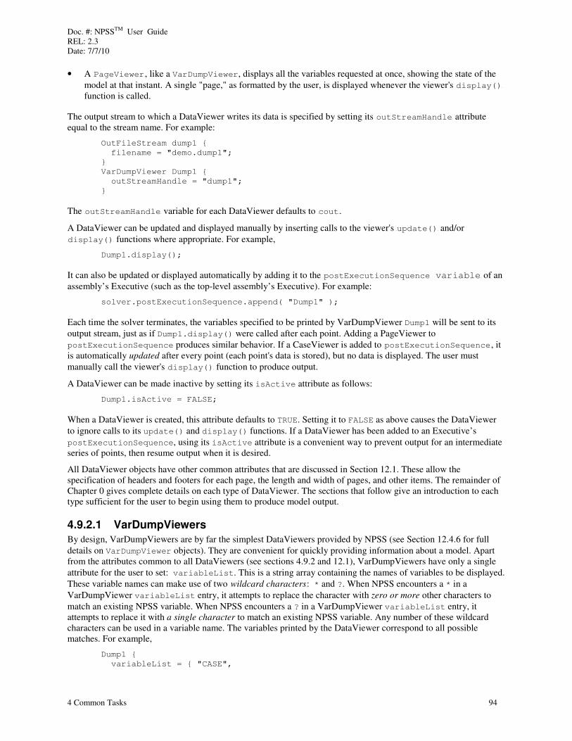
Doc. #: NPSSTM User Guide REL: 2.3 Date: 7/7/10
4 Common Tasks 94
• A TPageViewerT, like a VarDumpViewer, displays all the variables requested at once, showing the state of the
model at that instant. A single "page," as formatted by the user, is displayed whenever the viewer's Tdisplay()T function is called.
The output stream to which a DataViewer writes its data is specified by setting its ToutStreamHandleT attribute equal to the stream name. For example:
OutFileStream dump1 {
filename = "demo.dump1";
}
VarDumpViewer Dump1 {
outStreamHandle = "dump1";
}
The ToutStreamHandleT variable for each DataViewer defaults to TcoutT.
A DataViewer can be updated and displayed manually by inserting calls to the viewer's Tupdate()T and/or
Tdisplay()T functions where appropriate. For example,
Dump1.display();
It can also be updated or displayed automatically by adding it to the TpostExecutionSequence variableT of an
assembly’s Executive (such as the top-level assembly’s Executive). For example:
solver.postExecutionSequence.append( "Dump1" );
Each time the solver terminates, the variables specified to be printed by VarDumpViewer Dump1 will be sent to its
output stream, just as if Dump1.display() were called after each point. Adding a PageViewer to
postExecutionSequence produces similar behavior. If a CaseViewer is added to TpostExecutionSequenceT, it is automatically updated after every point (each point's data is stored), but no data is displayed. The user must
manually call the viewer's Tdisplay()T function to produce output.
A DataViewer can be made inactive by setting its isActive attribute as follows:
Dump1.isActive = FALSE;
When a DataViewer is created, this attribute defaults to TRUE. Setting it to FALSE as above causes the DataViewer
to ignore calls to its update() and display() functions. If a DataViewer has been added to an Executive’s
postExecutionSequence, using its isActive attribute is a convenient way to prevent output for an intermediate series of points, then resume output when it is desired.
All DataViewer objects have other common attributes that are discussed in Section 12.1. These allow the specification of headers and footers for each page, the length and width of pages, and other items. The remainder of Chapter 0 gives complete details on each type of DataViewer. The sections that follow give an introduction to each type sufficient for the user to begin using them to produce model output.
4.9.2.1 VarDumpViewers
By design, VarDumpViewers are by far the simplest DataViewers provided by NPSS (see Section 12.4.6 for full
details on VarDumpViewer objects). They are convenient for quickly providing information about a model. Apart from the attributes common to all DataViewers (see sections 4.9.2 and 12.1), VarDumpViewers have only a single
attribute for the user to set: variableList. This is a string array containing the names of variables to be displayed.
These variable names can make use of two Twildcard charactersT: * and ?. When NPSS encounters a * in a
VarDumpViewer variableList entry, it attempts to replace the character with zero or more other characters to
match an existing NPSS variable. When NPSS encounters a ? in a VarDumpViewer variableList entry, it attempts to replace it with a single character to match an existing NPSS variable. Any number of these wildcard characters can be used in a variable name. The variables printed by the DataViewer correspond to all possible matches. For example,
Dump1 {
variableList = { "CASE",

Doc. #: NPSSTM User Guide REL: 2.3 Date: 7/7/10
4 Common Tasks 95
"*.alt",
"*.dTs",
"Amb.MN",
"Amb.?amb",
"HP?.Fl_I.?t",
"Brn.FAR",
"Brn.TtCombOut",
"PERF.Fn" }
}
This specifies the following variables to be displayed: CASE (see Table 7), all variables named alt and dTs
belonging to some other object (such as a Ambient object named Amb), Amb.MN, Amb.Ps and Amb.Ts, the inlet
total quantities (such as variables Pt and Tt) of objects such as CmpH and TrbH, and variables Brn.FAR,
Brn.TtCombOut, and PERF.Fn. The output might appear as follows:
Amb.alt = 15000
Amb.dTs = 0
Amb.MN = 0.5
Amb.Ps = 8.29357
Amb.Ts = 465.178
Brn.FAR = 0.0194843
Brn.TtCombOut = 2402.94
CASE = 41
CmpH.Fl_I.ht = -11.5567
CmpH.Fl_I.kt = 81
CmpH.Fl_I.Pt = 9.78962
CmpH.Fl_I.Rt = 0.0685604
CmpH.Fl_I.Tt = 488.478
CmpH.Fl_I.ut = -45.047
TrbH.Fl_I.ht = 473.566
TrbH.Fl_I.kt = 1641
TrbH.Fl_I.Pt = 161.932
TrbH.Fl_I.Rt = 0.0685497
TrbH.Fl_I.Tt = 2303.83
TrbH.Fl_I.ut = 315.639
PERF.alt = 15000
PERF.dTs = 0
PERF.Fn = 4531.06
A simple list of variable names and values is produced. Notice that the list is in alphabetical order, not the order
given in variableList. For more control over output format, the user must use one of the other DataViewer types, which use Tformat indicatorsT as discussed below.
4.9.2.2 Format Indicators
The information output by CaseViewers and PageViewers is specified by two items:
• Lists of variable names whose values are to be output
• Corresponding Tformat indicatorsT
The number of variable names must always equal the number of format indicators provided for them.
The format indicators, in general, can consist of fixed text enclosed in quotes, and Tplace holdersT for the values of
the specified variables. Question marks ("T?T") are used to indicate place holders. The question marks are replaced by actual data values when the DataViewer produces its output. The number of question marks indicates the size of the field available for the data value. Decimal points and exponent indicators can also be included to control the
formatting of TrealT values.

Doc. #: NPSSTM User Guide REL: 2.3 Date: 7/7/10
4 Common Tasks 96
Table 18. DataViewer Format Indicators
Variable Type
Sample Format Indicator
Notes
TstringT T??????????T Text is right-justified in the field indicated by the place holder.
TintT T?????T Values are right-justified in the field indicated by the place holder.
Treal,
decimalT
T??.????T • The place holders right of the decimal point are always filled. For example, 10.24 output with the example format indicator would display as 10.2400.
• Negative values require enough question marks left of the decimal point to allow for the negative sign.
• If a real value is output using a format indicator that has no decimal point, its fractional part is dropped and it is printed as though it were an integer.
Treal,
exponentialT
T??.???E???
(UNIX)
“??.??E????”
( Windows)
• Either “E” or “e” can be used to indicate presence of an exponent.
• The number of question marks right of the “E” must always equal three (one for a sign, and two for the exponent).
• Negative values require two question marks left of the decimal point to allow for the negative sign.
real,
significant
digit
??????S??? • Values are right-justified in the field indicated by the place holder.
• A blank space is always included in the left-most column.
• The number of ‘?’ to the left of the ‘S’ (or ‘s’) indicate the number of significant digits that will be displayed.
• A decimal number will be used if it fits within the total width.
• If a decimal number does not fit, then an exponential number will be used.
• If the exponential number does not fit then the number of significant digits will be reduced as necessary to make it fit.
• If the total width of the field is insufficient to display the value then the format will be ignored and a default system exponential format will be used.
If a value will not fit in the field specified by the format indicator, a string of dashes (“-”) will be output. The only exception to this is the significant digit format. It will increase the width as needed to force the value to be displayed.
CaseViewers and objects used with PageViewers have attributes named defIntFormat, defRealFormat,
defSNFormat, and defStrFormat that set default format indicators for each variable type. See sections 12.2 and 12.4.2 for details.
4.9.2.3 CaseViewers
After VarDumpViewers, the next DataViewers in terms of complexity are the CaseViewers of which there are two
types: the CaseColumnViewer and the CaseRowViewer. As mentioned in Section 4.9.2, in CaseColumnViewer
output, each column represents a single case and each row corresponds to a particular variable. A CaseRowViewer prints out case results so that each row represents a single case and each column corresponds to a particular variable. The attributes available for each are identical.
There are three basic parts to a CaseViewer's output: the TtitleT, the TheadersT, and the Tvariable valuesT. The title is
printed once each time the viewer's display() function is executed. Attribute titleBody is a scalar string variable in which the user specifies the fixed title text and format indicators for variable values included in the title.
Attribute titleVars is a string array in which the user specifies the variables whose values are to appear in the title. For example:
OutFileStream case1 {
filename = "demo.case1";
}
CaseRowViewer Case1 {

Doc. #: NPSSTM User Guide REL: 2.3 Date: 7/7/10
4 Common Tasks 97
outStreamHandle = "case1";
titleBody = "???????????????????? Run on ???????? at ????????";
titleVars = { "VERSION", "date", "timeOfDay" }
}
Attribute titleBody can contain newline characters ("\n") to create a multi-line title. The example above will produce a title like the following:
NPSS_1.3.0 – Rev:N run on 08/17/01 at 14:03:53
A default title definition is created when a CaseViewer object is instantiated, so the user is not required to define one.
The TheadersT identify each case run. A CaseColumnViewer prints them at the top of each column, while a
CaseRowViewer prints them at the start of each row. Attributes caseHeaderBody and caseHeaderVars are used
to in an analogous fashion as titleBody and titleVars. A difference is that only single-line headers should be
produced (do not use "\n" in caseHeaderBody). Headers should normally be short. For example:
Case1 {
caseHeaderBody = "Case ???";
caseHeaderVars = { "CASE" }
}
Each header will have an appearance like "Case 42". As with titles, the user can accept a default header definition rather than defining one as described above.
The TvariablesT to be displayed and their format indicators are specified in a single string array named
variableList. More than just the format can be specified. A label or TaliasT for each variable can be specified as
well as the Toutput unitsT. Each entry of variableList should give the variable name first. If a format indicator is
provided, it should be preceded by a colon (":"). If an alias is provided, it should be preceded by an equals ("="). If
a units string is provided, it should be preceded by an "at" symbol ("@"). For example:
Case1.variableList = { "Amb.alt",
"Amb.MN:?.????",
"Amb.dTs:???.??=dTs",
"Brn.Wfuel@lbm/hr",
"Brn.TtCombOut:????.??=BOT@F",
"PERF.Fn:?????.?=Fn" };
Units strings must be among the valid strings recognized (see Section 10.2), and must be compatible with the units of the variable. Units conversion is performed for output only; the value and units stored in the variable remain the same.
The example above, used in a CaseRowViewer, will produce output like the following:
Amb.alt Amb.MN dTs Brn.Wfuel BOT Fn
Case 42 15000.000 0.5000 0.00 4500.629 1872.64 5000.0
Unless given an alias, the variable labels are the full variable names as specified in variableList. If no format indicator is given, the default is used. Units conversions are performed as specified, but no units strings are displayed.
Unlike titles and headers, no default is set up for variableList. The user must define this variable at a minimum for a CaseViewer to work properly.
Suppose the CaseRowViewer built by the examples above is used as shown below. The example assumes that an
Independent object has been added to the solver to vary a fuel flow parameter (see Section 4.8.3), that
Dependent object RunCondition has been added to the solver (see Section 4.8.3), and that variable thrust exists
in the top-level assembly. Object PERF calculates the net thrust of the engine and stores the result in PERF.Fn.
solver.postExecutionSequence.append( "Case1" );

Doc. #: NPSSTM User Guide REL: 2.3 Date: 7/7/10
4 Common Tasks 98
RunCondition.eq_lhs = "PERF.Fn";
RunCondition.eq_rhs = "thrust";
solver.forceNewJacobian = TRUE;
for ( thrust=5000.; thrust<=6001.; thrust+=500. ) {
CASE++;
run();
}
Case1.display();
for ( thrust=6500.; thrust<=7501.; thrust+=500. ) {
CASE++;
run();
}
Case1.display();
Output like the following will be produced:
NPSS_1.3.0 – Rev:N run on 08/17/01 at 14:03:53
Amb.alt Amb.MN dTs Brn.Wfuel BOT Fn
Case 42 15000.000 0.5000 0.00 4500.629 1872.64 5000.0
Case 43 15000.000 0.5000 0.00 4995.383 1947.77 5499.9
Case 44 15000.000 0.5000 0.00 5509.832 2024.37 5999.8
NPSS_1.3.0 – Rev:N run on 08/17/01 at 14:03:53
Amb.alt Amb.MN dTs Brn.Wfuel BOT Fn
Case 45 15000.000 0.5000 0.00 6069.513 2105.42 6500.0
Case 46 15000.000 0.5000 0.00 6645.594 2191.29 7000.1
Case 47 15000.000 0.5000 0.00 7262.976 2285.75 7500.1
A CaseColumnViewer with identical attribute settings would appear similarly, with columns and rows transposed.
Full details on CaseColumnViewer and CaseRowViewer objects is found in Section 12.2.
4.9.2.4 PageViewers
The most advanced formatting features are available with PageViewer objects. These are intended to provide extensive detail about a model's results on a single "page" (which could occupy more than one sheets of paper when printed) per case. PageViewers are constructed with objects called Ttext blocksT (not to be confused with a collection of statements enclosed within curly braces which is called simply a "block"). The user instantiates text block objects within a PageViewer object, and positions them in relationship to one another on the page. Several kinds of text block objects are available for use with PageViewers. These are detailed in Chapter 0, but introduced here in the sections that follow.
NPSS is distributed with a general PageViewer that is adequate for many purposes. Its use is illustrated in Chapter 5. See especially sections 5.1.2, 5.3.1, and 5.4.11.
Apart from the attributes common to all DataViewers (see sections 4.9.2 and 12.1), the only attribute belonging
directly to a PageViewer object is anchor. This is a string variable containing the name of the text block that is to appear in the upper left corner of the page. It defaults to the first text block object instantiated within the
PageViewer object. All other text blocks are positioned beginning with the anchor text block.
All text block objects have two attributes: right and bottom. Each is a string variable containing the name of
another text block object. The object named in attribute right will be placed to the right of the text block. The
object named in attribute bottom will be placed below the text block. One or both of these strings can be left empty
in a given text block, but all text blocks to be printed must be named in another text block's right or bottom attribute (except for the first text block created which is printed by default as the anchor). When objects are specified
in both right and bottom attributes of a text block, the object to the right is placed first, then the object below. A given text block can only be printed once during the execution of a PageViewer.

Doc. #: NPSSTM User Guide REL: 2.3 Date: 7/7/10
4 Common Tasks 99
USimpleBlock
This text block allows the printing of variables whose names and paths are fixed in the model. Attribute body is a scalar string variable in which the user specifies fixed text, and format indicators for variable values included in the
body. Attribute vars is a string array in which the user specifies the variables whose values are to appear in the body. For example:
SimpleBlock Title {
body = "???????????????????? Run on ???????? at ????????";
vars = { "VERSION", "date", "timeOfDay" }
}
This text block will produce output resembling the following:
NPSS_1.3.0 – Rev:N run on 08/17/01 at 17:52:14
SimpleBlock objects are much like the title (TtitleBodyT and TtitleVarsT) feature of CaseViewers (see Section 4.9.2.3). They can be used for purposes other than a title banner, however. Although a given SimpleBlock object can be displayed only once per page by a PageViewer, a PageViewer can contain and display several different
SimpleBlock objects. Full details on SimpleBlock objects is found in Section 12.4.1.
UDynamic Text Blocks
NPSS offers three Tdynamic text blocksT for use in PageViewer objects. They are TdynamicT because they query the model for all objects of a specified type and print specified attributes of all objects found. This allows the writing of general PageViewers, applicable to many models. The use of dynamic text blocks (which hereafter will be referred
to simply as "text blocks") resembles using miniature CaseViewers (Section 4.9.2.3) within a PageViewer. Instead of the rows or columns being determined by the separate cases run, they are determined by the separate objects in the model matching a specified type.
Text blocks of type DRowTBlock list attributes in rows with a column for each object to which they belong. Text
blocks of type DColTBlock list attributes in columns with a row for each object to which they belong. Text blocks
of type LinkColTBlock are like objects of type DColTBlock, but can be used to print the attributes of ports. Port
attributes cannot be written using DColTBlock or DRowTBlock objects. Like CaseViewers, the output of text blocks consists of three parts: TtitleT, TheadersT, and Tvariable valuesT. The title is
printed once at the top of the text block each time it is executed. Attribute titleBody is a scalar string variable in which the user specifies the fixed title text and format indicators for variable values included in the title. Attribute
titleVars is a string array in which the user specifies the variables whose values are to appear in the title.
The TheadersT identify the variables being printed. They appear at the left of each row in DRowTBlock objects, and at
the top of each column in DColTBlock and LinkColTBlock objects. They are automatically generated from the information provided about the variables to be printed.
The TvariablesT to be printed are specified using two text block attributes: compType and compAttr. Attribute
compType is a scalar string variable containing the name of a component type. Generally this is the name of an
element type (such as "Compressor", "Turbine", "Duct", "Burner", "Nozzle", etc.) or, for LinkColTBlock
objects, the name of a port type (such as "FluidInputPort", "FluidOutputPort", or "FuelStation"). The
complete list of object types that can be specified is the same as that for the list() command (see Section 11.1.1).
Attribute compAttr is a string array in which the user specifies the attributes (or variables) belonging to objects of
the type specified in compType that are to be printed. For example, if compType = "Compressor", the user might
wish to print Compressor object attributes "Nc" (corrected speed), "Wc" (corrected inlet flow), "PR" (pressure ratio),
and "eff" (adiabatic efficiency). The complete list of attributes in each component type is given in the TNPSS
Reference SheetsT.
Like CaseViewer attribute variableList, text block attribute compAttr can be used to specify not only the names of component attributes to be printed, but also their formats, the header text associated with each, and the
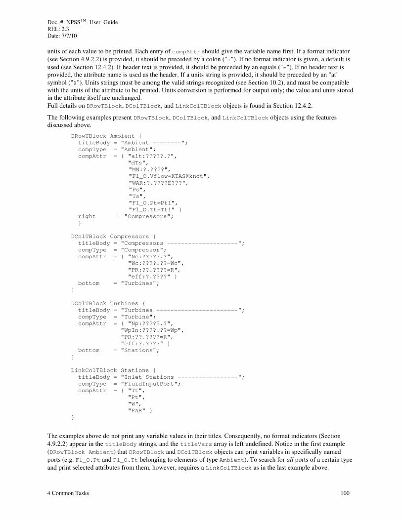
Doc. #: NPSSTM User Guide REL: 2.3 Date: 7/7/10
4 Common Tasks 100
units of each value to be printed. Each entry of compAttr should give the variable name first. If a format indicator
(see Section 4.9.2.2) is provided, it should be preceded by a colon (":"). If no format indicator is given, a default is
used (see Section 12.4.2). If header text is provided, it should be preceded by an equals ("="). If no header text is provided, the attribute name is used as the header. If a units string is provided, it should be preceded by an "at"
symbol ("@"). Units strings must be among the valid strings recognized (see Section 10.2), and must be compatible with the units of the attribute to be printed. Units conversion is performed for output only; the value and units stored in the attribute itself are unchanged.
Full details on DRowTBlock, DColTBlock, and LinkColTBlock objects is found in Section 12.4.2.
The following examples present DRowTBlock, DColTBlock, and LinkColTBlock objects using the features discussed above.
DRowTBlock Ambient {
titleBody = "Ambient --------";
compType = "Ambient";
compAttr = { "alt:?????.?",
"dTs",
"MN:?.????",
"Fl_O.Vflow=KTAS@knot",
"WAR:?.????E???",
"Ps",
"Ts",
"Fl_O.Pt=Pt1",
"Fl_O.Tt=Tt1" }
right = "Compressors";
}
DColTBlock Compressors {
titleBody = "Compressors --------------------";
compType = "Compressor";
compAttr = { "Nc:?????.?",
"Wc:????.??=Wc",
"PR:??.????=R",
"eff:?.????" }
bottom = "Turbines";
}
DColTBlock Turbines {
titleBody = "Turbines -----------------------";
compType = "Turbine";
compAttr = { "Np:?????.?",
"WpIn:????.??=Wp",
"PR:??.????=R",
"eff:?.????" }
bottom = "Stations";
}
LinkColTBlock Stations {
titleBody = "Inlet Stations -----------------";
compType = "FluidInputPort";
compAttr = { "Tt",
"Pt",
"W",
"FAR" }
}
The examples above do not print any variable values in their titles. Consequently, no format indicators (Section
4.9.2.2) appear in the titleBody strings, and the titleVars array is left undefined. Notice in the first example
(DRowTBlock Ambient) that DRowTBlock and DColTBlock objects can print variables in specifically named
ports (e.g. Fl_O.Pt and Fl_O.Tt belonging to elements of type Ambient). To search for all ports of a certain type
and print selected attributes from them, however, requires a LinkColTBlock as in the last example above.

Doc. #: NPSSTM User Guide REL: 2.3 Date: 7/7/10
4 Common Tasks 101
Suppose that DRowTBlock Ambient above is the anchor text block in a PageViewer object. It will produce a block
of output that is relatively few columns wide, but several lines high since each of the FlightConditons1 object
attributes specified will be printed on a separate line (or row). Ambient.right = "Compressors", so text block
Compressors will be printed to the right of text block Ambient. Compressors is a DColTBlock object, and will
tend to produce output that is only a few lines high but many columns wide since each Compressor object attribute
specified is printed left to right in a separate column. Compressors.bottom = "Turbines", so text block
Turbines will be printed below text block Compressors. Turbines.bottom = "Stations", so text block
Stations will be printed below text block Turbines. The output will resemble the example below. Ambient -------- Compressors --------------------
Amb Nc Wc R eff
alt 35000.0 CmpFSec 3500.0 743.95 1.5000 0.8700
dTs 0.000 Core.CmpH 9125.1 88.31 25.0014 0.8250
MN 0.8000
KTAS 461.295
WAR 0.0000E+00
Ps 3.458
Ts 393.854
Pt1 5.273
Tt1 444.410
Turbines -----------------------
Np Wp R eff
Core.TrbH 181.9 8.33 5.8373 0.8950
TrbL 78.5 40.43 2.5884 0.9000
Inlet Stations -----------------
Tt Pt W FAR
FL0 Inl.Fl_I 444.410 5.273 286.919 0.000
FL1 CmpFSec.Fl_I 444.410 5.246 286.919 0.000
FL2 Spl.Fl_I 507.230 7.870 286.919 0.000
FL21 Core.Fl_I 507.230 7.870 47.821 0.000
FL3 Core.Brn.Fl_I 1397.923 196.750 47.821 0.000
FL4 Core.TrbH.Fl_I 2460.029 186.913 48.638 1.71E-02
FL5 TrbL.Fl_I 1701.440 32.020 48.638 1.71E-02
FL7 NozPri.Fl_I 1375.156 12.371 48.638 1.71E-02
FL9 FePri.Fl_I 1375.156 12.371 48.638 1.71E-02
FL12 Bypass.Fl_I 507.230 7.870 239.097 0.000
FL17 SecNoz.Fl_I 507.230 7.870 239.097 0.000
FL19 FeSec.Fl_I 507.230 7.870 239.097 0.000
By default, the order in which objects are printed by dynamic text blocks is the order given in the
executionSequenceattribute of the Executive that exists in each assembly. It can be observed from the output
above that an assembly below the top-level assembly exists named Core that contains objects CmpH, Brn, and TrbH (see Section 4.6).
The user might have envisioned text block Turbines appearing immediately below text block Compressors,
occupying room remaining to the right of text block Ambient. Once one object has been placed to the right of another, however, objects placed below either of them will be placed below the pair considered as a group. This can result in wasted space, as in the example above. TGroupBlocksT, discussed in the next section, are the solution to this problem.
UGroupBlock
A GroupBlock object is like a miniature PageViewer within the overall PageViewer object. GroupBlocks contain
other text blocks, and can contain other GroupBlocks. Like PageViewer objects, GroupBlock objects have an attribute named anchor that specifies the name of the text block to be located in the upper left corner of the space
allocated to the block. By default, the anchor is the first text block instantiated within the GroupBlock object. Full
details on GroupBlock objects can be found in Section 12.4.3.
An example of a GroupBlock object incorporating the Compressors and Turbines dynamic text blocks is shown below.
GroupBlock RotatingComponents {

Doc. #: NPSSTM User Guide REL: 2.3 Date: 7/7/10
4 Common Tasks 102
DColTBlock Compressors {
titleBody = "Compressors --------------------";
compType = "Compressor";
compAttr = { "Nc:?????.?",
"Wc:????.??=Wc",
"PR:??.????=R",
"eff:?.????" }
bottom = "Turbines";
}
DColTBlock Turbines {
titleBody = "Turbines -----------------------";
compType = "Turbine";
compAttr = { "Np:?????.?",
"WpIn:????.??=Wp",
"PR:??.????=R",
"eff:?.????" }
}
} // end RotatingComponents
The incorporation of this GroupBlock in a complete PageViewer is shown in the PageViewer example below. It resolves the problem of wasted space.
UEmptyTextBlock
An EmptyTextBlock object is used purely to help position other text blocks. It contains only white space.
EmptyTextBlock objects have two integer attributes named height and width (see Section 12.4.4 for full
details). Attribute height gives the number of lines or rows in the block, width gives the number of columns. For example:
EmptyTextBlock EndofCase {
height = 2;
width = 0;
}
UUserTextBlock
A UserTextBlock object contains a single string array attribute named filledBlock. In it, the user specifies a
list of variables whose values are set by a user-defined update() function. These become available for other text blocks in the PageViewer to print. Details are given in Section 12.4.5.
UPageViewer Example
The following is a complete PageViewer object incorporating objects used as examples in the preceding sections.
OutFileStream page2 {
filename = "demo2.page2";
}
PageViewer Page2 {
outStreamHandle = "page2";
anchor = "Title";
SimpleBlock Title {
body = "???????????????????? Run on ???????? at ????????";
vars = { "VERSION", "date", "timeOfDay" }
bottom = "Ambient";
}
DRowTBlock Ambient {

Doc. #: NPSSTM User Guide REL: 2.3 Date: 7/7/10
4 Common Tasks 103
titleBody = "Ambient --------";
compType = "Ambient";
compAttr = { "alt:?????.?",
"dTs",
"MN:?.????",
"Fl_O.Vflow=KTAS@knot",
"WAR:?.????E???",
"Ps",
"Ts",
"Fl_O.Pt=Pt1",
"Fl_O.Tt=Tt1" }
right = "RotatingComponents";
bottom = "Stations";
}
GroupBlock RotatingComponents {
DColTBlock Compressors {
titleBody = "Compressors --------------------";
compType = "Compressor";
compAttr = { "Nc:?????.?",
"Wc:????.??=Wc",
"PR:??.????=R",
"eff:?.????" }
bottom = "Turbines";
}
DColTBlock Turbines {
titleBody = "Turbines -----------------------";
compType = "Turbine";
compAttr = { "Np:?????.?",
"WpIn:????.??=Wp",
"PR:??.????=R",
"eff:?.????" }
}
} // end RotatingComponents
LinkColTBlock Stations {
titleBody = "Inlet Stations -------------------";
compType = "FluidInputPort";
compAttr = { "Tt",
"Pt",
"W",
"FAR" }
bottom = "EndofCase";
}
EmptyTextBlock EndofCase {
height = 2;
width = 0;
}
} // end Page2
A SimpleBlock object defining a title is the anchor. Below it appears a DRowTBlock object named Ambient that
gives ambient, flight, and engine inlet conditions. To its right is a GroupBlock object named
RotatingComponents, which itself contains two DColTBlock objects displaying information about all the
Compressor and Turbine objects in the model. Below this entire grouping (as specified by Ambient.bottom) is
a LinkColTBlock object giving information at the inlet of all components in the model. Finally, an
EmptyTextBlock object produces extra space between the output for each case.

Doc. #: NPSSTM User Guide REL: 2.3 Date: 7/7/10
4 Common Tasks 104
Suppose PageViewer object Page2 was executed in a model as follows:
RunCondition.eq_rhs = "1.0";
CASE++;
run();
Page2.display();
RunCondition.eq_rhs = "0.9";
CASE++;
run();
Page2.display();
In this example, it is assumed that the solver contains an Independent object that causes a burner input parameter
(such as fuel flow) to be controlled by the solver, and that RunCondition is an active solver Dependent object defining some desired operating condition. (See Section 4.8 for information on solver setup.) The output produced by these lines will resemble the following.
NPSS_1.3.0 – Rev:N run on 08/18/01 at 11:12:26
Ambient -------- Compressors --------------------
Amb Nc Wc R eff
alt 35000.0 CmpFSec 3500.0 743.95 1.5000 0.8700
dTs 0.000 Core.CmpH 9125.1 88.31 25.0014 0.8250
MN 0.8000
KTAS 461.295 Turbines -----------------------
WAR 0.0000E+00 Np Wp R eff
Ps 3.458 Core.TrbH 181.9 8.33 5.8373 0.8950
Ts 393.854 TrbL 78.5 40.43 2.5884 0.9000
Pt1 5.273
Tt1 444.410
Inlet Stations -------------------
Tt Pt W FAR
FL0 Inl.Fl_I 444.410 5.273 286.919 0.000
FL1 CmpFSec.Fl_I 444.410 5.246 286.919 0.000
FL2 Spl.Fl_I 507.230 7.870 286.919 0.000
FL21 Core.Fl_I 507.230 7.870 47.821 0.000
FL3 Core.Brn.Fl_I 1397.923 196.750 47.821 0.000
FL4 Core.TrbH.Fl_I 2460.029 186.913 48.638 1.71E-02
FL5 TrbL.Fl_I 1701.440 32.020 48.638 1.71E-02
FL7 NozPri.Fl_I 1375.156 12.371 48.638 1.71E-02
FL9 FePri.Fl_I 1375.156 12.371 48.638 1.71E-02
FL12 Bypass.Fl_I 507.230 7.870 239.097 0.000
FL17 SecNoz.Fl_I 507.230 7.870 239.097 0.000
FL19 FeSec.Fl_I 507.230 7.870 239.097 0.000
NPSS_1.3.0 – Rev:N run on 08/18/01 at 11:12:26
Ambient -------- Compressors --------------------
Amb Nc Wc R eff
alt 35000.0 CmpFSec 3150.0 678.22 1.3750 0.8804
dTs 0.000 Core.CmpH 8820.5 77.73 20.7517 0.8480
MN 0.8000
KTAS 461.295 Turbines -----------------------
WAR 0.0000E+00 Np Wp R eff
Ps 3.458 Core.TrbH 186.0 8.32 5.9180 0.8947
Ts 393.854 TrbL 76.4 40.66 2.5939 0.9021
Pt1 5.273
Tt1 444.410
Inlet Stations -------------------
Tt Pt W FAR
FL0 Inl.Fl_I 444.410 5.273 261.569 0.000
FL1 CmpFSec.Fl_I 444.410 5.246 261.569 0.000
FL2 Spl.Fl_I 492.555 7.214 261.569 0.000
FL21 Core.Fl_I 492.555 7.214 39.151 0.000
FL3 Core.Brn.Fl_I 1268.919 149.697 39.151 0.000

Doc. #: NPSSTM User Guide REL: 2.3 Date: 7/7/10
4 Common Tasks 105
FL4 Core.TrbH.Fl_I 2135.238 142.212 39.678 1.35E-02
FL5 TrbL.Fl_I 1456.269 24.030 39.678 1.35E-02
FL7 NozPri.Fl_I 1167.513 9.264 39.678 1.35E-02
FL9 FePri.Fl_I 1167.513 9.264 39.678 1.35E-02
FL12 Bypass.Fl_I 492.555 7.214 222.418 0.000
FL17 SecNoz.Fl_I 492.555 7.214 222.418 0.000
FL19 FeSec.Fl_I 492.555 7.214 222.418 0.000
4.10 Basic Model Running As discussed in the preceding sections, the basic steps in constructing and running a model are:
1. Specify a thermodynamics package (see Section 4.1). 2. Instantiate the necessary Elements, Subelements, Ports, and Assemblies (see sections 0 through 4.7). Also
create any necessary functions and tables (see sections 2.2.6 and 2.2.7). This step may involve using preprocessor commands (Section 2.2.3) to include pre-written components distributed with NPSS, or user written components. It may also involve use of Creation Method Facilities (Chapter 3).
3. Link the model's ports (see Section 4.3.2). 4. Insure that the model's execution sequence is satisfactory, and add any necessary items to the
preExecutionSequence or postExecutionSequence attributes of each assembly’s Executive. 5. Define input and output as required (see Section 4.9). 6. Set up the model's solver or solvers (see Section 4.8). 7. Define the desired cases, and run the model, modifying the solver setup as required (see Section 4.8.3).
These steps can be accomplished in different files that are brought together by the preprocessor to make a complete model and execution definition. Chapter 5 suggests an orderly way to do this, and presents a complete example.
As mentioned above in step 2, the user will often want to access pre-written components and global functions called TmacrosT that are distributed with NPSS. One may also wish to access personal or site-specific libraries of components, functions, and tables. The Tinclude pathT is important to instruct NPSS to look in the right places for such items. As discussed in chapter 3, the include path may be used to search for DLM and Interpreted components also. Unless the user launches NPSS with a special run script, it may be necessary to add the standard locations of
DLM and Interpreted components to the include path using the –I command line option (see Section 2.1). In a
standard NPSS installation, an environment variable named NPSS_TOP will be defined that identifies the directory
under which all the NPSS program files are stored. Another environment variable, NPSS_CONFIG, will identify the
kind of system being run (such as "sun", "hp", or "sgi"). The user can insure that the paths to standard NPSS
components are part of the include path by starting NPSS with the following –I command line options.
npss –I $NPSS_TOP/InterpIncludes -I $NPSS_TOP/AirBreathing/DLMComponents/$NPSS_CONFIG
A standard NPSS installation will include a script named runnpss that the user can customize to define
environment variables like NPSS_PATH, DCLOD_PATH, and ICLOD_PATH to include necessary directories. Starting
npss using a properly configured runnpss script can save much typing over starting it with a command like that given above.
Once the first five steps above are completed, the first case run is usually a design point. This involves using
command setOption() to set attribute switchDes equal to "DESIGN" throughout the model. The TNPSS Reference
SheetsT indicate which object attributes are inputs when the object's switchDes attribute is "DESIGN". The user must
set appropriate values for all these attributes. The model is run by issuing command run() from global scope. For example:
// Design operating condtions
Amb.alt = 35000.;
Amb.dTs = 0.;
Amb.MN = 0.8;
Brn.switchBurn = "TEMPERATURE";
Brn.TtCombOut = 2460.;
// Component design operating characteristics
Amb.W = 47.8194; // CmpH WcDes = 124 lbm/sec

Doc. #: NPSSTM User Guide REL: 2.3 Date: 7/7/10
4 Common Tasks 106
Inl.eRamBase = 0.995;
CmpH.S_map.NcDes = 1.0;
CmpH.S_map.RlineMap = 2.0;
CmpH.S_map.PRdes = 25.0;
CmpH.S_map.PRdes.value = 25.0;
CmpH.S_map.effDes = 0.825;
Brn.dPqPdryBase = 0.05;
Brn.dPqPgrowthBase = 0.00;
Brn.dPqPmomBase = 0.00;
Brn.effBase = 0.98;
Brn.effChemBase = 1.0;
Brn.switchHotLoss = "input";
TrbH.S_map.parmGeom = 76.0;
TrbH.S_map.parmGeomDes = 76.0;
TrbH.S_map {
parmMap = 5.0;
parmMapDes = 5.0;
parmNcDes = 100.0;
effDes = 0.895;
}
ShH.Nmech = 9025.078; // 100% CmpH Nc = 9750.0 rpm
setOption( "switchDes", "DESIGN" );
autoSolverSetup();
CASE++;
run();
Depending on what has been added to the top-level assembly Executive’s postExecutionSequence attribute, the
user may wish to execute specific calls the display() function of DataViewer objects after the run() command.
As noted in Table 7, global variable CASE is an automatically created integer variable initialized to zero. It is a convenient way to identify various cases run. It is not automatically indexed, however, and therefore must be given a
desired value before each run() command in order to be useful. Most of the examples in this Guide index CASE by
one before calling run(), as in the example above.
Normally, offdesign points are run next. The model's design point performance can be repeated in offdesign mode with commands such as the following:
Brn.switchBurn = "FAR";
Brn.FAR = Brn.Fl_O.FAR;
setOption( "switchDes", "OFFDESIGN" );
autoSolverSetup();
CASE++;
run();
Finally, Independent and Dependent objects can be added to the solver setup to permit running the model to any desired condition. For example:
Brn.switchBurn = "FAR";
Independent fuelAir {
varName = "Brn.FAR";
indepRef = "0.02";
}
Dependent RunCondition {
eq_lhs = "CmpH.S_map.NcMap";

Doc. #: NPSSTM User Guide REL: 2.3 Date: 7/7/10
4 Common Tasks 107
eq_rhs = "1.0";
}
solver.addIndependent("fuelAir");
solver.addDependent("RunCondition");
run();
The discussion above pertains to steady-state running. Transient running is discussed more fully in Chapter 6.
4.11 Moving and Deleting Objects Users can move objects from one point to another within the model by using the move() command. In general, the
syntax of the move() command is as follows:
move( "current_location", "new_location" );
Quotation marks around object names are required. For example:
move("a.b.c", "x.y.z");
In the above example, object "c", which resides in "a.b", is moved to reside in "x.y", and is renamed "z". Object
"a.b.c" can be called the TsourceT object, and "z" can be called the TdestinationT object, with "x.y" being the parent of the destination object.
As mentioned in sections 4.5.3 and 4.5.4, the move() function can be used to insert an object into a socket. Care must be taken, however, since sockets and the objects inserted in them share the same name. For example:
move("Tsub_nameT", "Tsocket_nameT"); // Don't do this!
The command above will replace the socket with the source object rather than inserting it in the socket. To insert an
object into a socket, specify the destination object as Tsocket_nameT.child.
move("Tsub_nameT", "Tsocket_nameT.child");
For example, objects of element type Duct have a socket named S_dP that can accept subelement objects of type
dPqP. Suppose Duct object Diffuser exists. The following code creates and inserts subelement DiffuserLoss
into object Diffuser's S_dP socket.
Subelement dPqP DiffuserLoss {
Table TB_Closs ( real MN, real RNI ) {
RNI = 1.00 {
MN = { 0.0, 0.5, 1.0 }
C = { 0.05, 0.07, 0.10 }
}
RNI = 0.01 {
MN = { 0.0, 0.5, 1.0 }
C = { 0.08, 0.10, 0.13 }
}
RNI.interp = "linear";
RNI.extrap = "none";
MN.interp = "lagrange2";
MN.extrap = "none";
}
switchDes = "OFFDESIGN";
}
move( "DiffuserLoss", "Diffuser.S_dP.child" );
Even though the subelement in the example above was instantiated with a name (DiffuserLoss) other than that of
the socket into which it was inserted (S_dP), once it is inserted in the socket its attributes are accessed by the socket
name (e.g. Diffuser.S_dP.Closs). The same rules for accessing socket object attributes and functions apply as were discussed in Section 4.5.1.

Doc. #: NPSSTM User Guide REL: 2.3 Date: 7/7/10
4 Common Tasks 108
If another object occupied the Diffuser.S_dP socket before the move, it was destroyed by the move. To preserve an object inserted in a socket before replacing it with another, first move it to another location.
move( "Diffuser.S_dP.child", "OldLoss" );
After the move in the example above, socket Diffuser.S_dP is empty.
The following restrictions apply to using the move() function:
1. Both the source and destination arguments to the move() function must reside within the object from which
move() is called. For example, if object "a" has a function that calls the move() function, both arguments to
move() must be descendants of "a". It is recommended, therefore, that move() always be called from the top-level assembly (global scope), with complete path names given for the arguments. This practice should minimize confusion.
2. The source object (1P
stP argument) and the parent of the destination object must both exist before move() is
called.
Deleting objects anywhere in the model may be accomplished by using the delete() command. The syntax is as follows:
delete("a.b.c");
In this example, object "c", which currently resides in "a.b", will be deleted. To delete an object inserted in a
socket, use the .child syntax:
delete( "Diffuser.S_dP.child" );
The following restrictions apply:
1. The object being deleted must reside within the object from which delete() is called. For example, if object
"a" has a function that calls the delete() function, the argument to delete() must be a descendant of "a". It
is safe to call delete() from global scope as long as the object's complete path name is specified. 2. The object being deleted cannot be an external component or contained in an external component. 3. The object being deleted must exist.
4.12 Adding or Removing Elements from a Model Sometimes it is desirable to leave a basic model definition intact, but add or remove components for the sake of
special analyses. It is easy to instantiate new components, and the delete() command discussed in Section 4.11
can be used to remove existing components. To add or remove Element objects one must alter the linking of ports. This section discusses the steps involved.
Suppose a simple model consists of the following elements, executed in the following order as indicated by the top-
level assembly's Executive’s execution attribute:
1. Ambient Amb 2. InletStart InletStart 3. Inlet Inl 4. Compressor CmpH 5. Duct Diffuser 6. FuelStart Fuel 7. Burner Brn 8. Turbine TrbH 9. Nozzle NozPri 10. FlowEnd FePri 11. Shaft ShH
The port links for these elements is as follows:
linkPorts( "InletStart.Fl_O", "Inl.Fl_I", "FL0" ); // fluid ports
linkPorts( "Inl.Fl_O", "CmpH.Fl_I", "FL1A" ); // fluid ports
Doc. #: NPSSTM User Guide REL: 2.3 Date: 7/7/10
4 Common Tasks 109
linkPorts( "CmpH.Fl_O", "Diffuser.Fl_I", "FL2" ); // fluid ports
linkPorts( "Diffuser.Fl_O", "Brn.Fl_I", "FL36" ); // fluid ports
linkPorts( "Fuel.Fu_O", "Brn.Fu_I", "FU36" ); // fuel ports
linkPorts( "Brn.Fl_O", "TrbH.Fl_I", "FL41" ); // fluid ports
linkPorts( "TrbH.Fl_O" , "NozPri.Fl_I", "FL7" ); // fluid ports
linkPorts( "NozPri.Fl_O", "FePri.Fl_I", "FL9" ); // fluid ports
linkPorts( "CmpH.Sh_O", "ShH.CmpH_SH", "CmpH_SH" ); // shaft ports
linkPorts( "TrbH.Sh_O", "ShH.TrbH_SH", "TrbH_SH" ); // shaft ports
It is desired to insert two Element objects of type Bleed, one after the Duct object named Diffuser (to extract
compressor discharge air), and one before the Turbine object named TrbH (to simulate nonchargeable bleed introduced in the turbine nozzle before the first rotor). First, the user should instantiate these objects.
Element Bleed DiffBld {
BleedOutPort TrbHV1out {
fracW = 0.08;
Pscale = 0.95;
hscale = 1.00;
}
}
Element Bleed TrbHV1 {
BleedInPort TrbHV1in;
}
The existing station named FL36 connects element Diffuser to element Brn. This link must be broken in order to
insert element DiffBld between Diffuser and Brn. Also, the existing station named FL41 connects element Brn
to element TrbH. This link must also be broken in order to insert element TrbHV1 between Brn and TrbH. The user
accomplishes this using the unlink() command, which takes a single string argument corresponding to a station name.
unlink( "FL36" );
unlink( "FL41" );
Next, the new links should be established:
linkPorts( "Diffuser.Fl_O", "DiffBld.Fl_I", "FL35" );
linkPorts( "DiffBld.Fl_O", "Brn.Fl_I", "FL36" );
linkPorts( "Brn.Fl_O", "TrbHV1.Fl_I", "FL40" );
linkPorts( "TrbHV1.Fl_O", "TrbH.Fl_I", "FL41" );
linkPorts( "DiffBld.TrbHV1out", "TrbHV1.TrbHV1in", "TrbHV1bld" );
Notice that once a link has been broken, its name can be reused to establish a new link.
Although the desired elements now exist, and their ports are correctly linked, the model will not run correctly because the execution sequence is wrong. When new elements are instantiated, they are automatically added to the
end of the execution sequence (i.e., appended to array solver.executionSequence). The new bleed elements, then, will be executed after all the other elements in the model. To correct this, the element names should first be
removed from array solver.executionSequence (see sections 2.2.4.6 and 11.1.2 for information on function
remove() ).
solver.executionSequence.remove("DiffBld");
solver.executionSequence.remove("TrbHV1");
The new elements must now be inserted in the appropriate places. Element DiffBld should be executed
immediately after element Diffuser. Element Diffuser is the fourth entry in array
solver.executionSequence, and therefore has index 3 (array index numbers begin with 0). Element DiffBld
should therefore be inserted as index 4 (see sections 2.2.4.6 and 11.1.2 for information on function insertAt() ).

Doc. #: NPSSTM User Guide REL: 2.3 Date: 7/7/10
4 Common Tasks 110
solver.executionSequence.insertAt( 4, "DiffBld" );
Element TrbHV1 should be inserted immediately before element TrbH, which has now been pushed to be the eighth
element of array solver.executionSequence (index 7). Element TrbHV1 is inserted at index location 7, pushing
TrbH one position further down.
solver.executionSequence.insertAt( 7, "TrbHV1" );
When objects are instantiated, the default value of their switchDes attribute (if present) is usually "DESIGN". If the user desires to run in offdesign mode, this attribute should be reset in the new objects.
In the example above, the solver setup does not need to be altered since Bleed objects do not add any
Independent or Dependent objects to the solver (see the TNPSS Reference SheetsT for Bleed elements). In general, however, it is a good idea to reestablish a complete solver setup after model changes of this magnitude have been undertaken.
autoSolverSetup();
CASE++;
run();
To remove objects from a model, a similar procedure is used. Errors may result from destroying objects while their links are still present, so the order of operations should be as follows:
1. Use command unlink() to break the links that will no longer be present in the final model. 2. Move or delete the desired elements (see Section 4.11). 3. Establish the necessary links for the new model configuration. 4. Correct the execution sequence (in the case of removing elements, this will usually involve simply removing the
element names the current Executive’s executionSequence). 5. Correct the solver setup if necessary.
4.13 Prepass, Preexecute and Postexecute Functions NPSS executes an element or subelement by calling the following three member functions in the following order:
1. preexecute()(if it exists) 2. calculate()
3. postexecute()(if it exists)
In addition, at the top of the solver’s executionSequence, a prePass function can be called.
4. prePass()(if it exists)
The calculate() function contains the preprogrammed engineering calculations of the element or
subelement, designed to simulate the physics of a particular component. The prePass, preexecute(), and
postexecute() functions are available for the user to define. They perform additional calculations at the top of the solver’s executionSequence loop and either immediately before or after the normal calculations.
The prePass, preexecute, and postexecute functions are generally used for three primary purposes:
• to set parameters not otherwise calculated (such as a special performance measure),
• to modify a preprogrammed calculation (such as implementing a different definition of surge margin), and
• to set parameters used in the cycle but not calculated elsewhere (such as a customer's power extraction from a shaft, or the scaler on a compressor's efficiency due to clearance effects).
In the following example, assume object Brn has already been instantiated as type Burner, and assume functions
loadParam() and NOx() have also been defined in the top-level assembly.
Brn {
switchBurn = "FAR";
real loadP;
real NOx;

Doc. #: NPSSTM User Guide REL: 2.3 Date: 7/7/10
4 Common Tasks 111
void preexecute() {
Table Beff( real Load ) {
Load = { 0.0, 0.2, 0.4, 0.6, 0.8, 1.0 }
eff = { 1.0000, 1.0000, 0.9998, 0.9994, 0.9986, 0.9970 }
}
loadP = loadParam( Fl_I.W, Fl_I.Tt, FAR );
effBase = Beff(loadP);
}
void postexecute() {
NOx = NOxCal( FAR, Fl_O.Tt );
}
}
In this example, Burner element Brn is modified to contain two new variables: loadP representing a loading
parameter, and NOx representing a measure of Nitrous Oxide emissions. The burner is also placed in a mode in
which fuel/air ratio (FAR) is an input value. The burner efficiency depends on the loading parameter, so a
preexecute() function is written to first calculate the loading parameter, then use it to calculate the burner
efficiency. The loading parameter is calculated with function loadParam() which uses variables that are defined before the burner is executed (inlet air flow, inlet air total temperature, and fuel/air ratio). The loading parameter is
then used as the independent variable in a table lookup, the result of which is assigned to variable effBase.
Variable effBase exists in all objects of type Burner, and determines the burner efficiency. Since these
calculations are performed by the preexecute() function, the burner efficiency just set is available when the
burner's calculate() function is called. After the burner's calculate() function has executed, the burner's exit
temperature is known (Brn.Fl_O.Tt). Therefore, a postexecute() function is written to use this temperature and
the fuel/air ratio to calculate an emissions parameter found by function NOxCal(). After the model in which these
objects reside has run, the user can access variables Brn.loadP and Brn.NOx for output or further processing.
The prePass, preexecute and postexecute functions are defined just like any other function subject to the following rules:
• They must be defined within a block belonging to the object to which they pertain.
• They must not return any value (return type void) and must accept no arguments.
• They must be named "prePass" to be performed at the top of the executionSequence, "preexecute" to be
performed before the normal calculations, or "postexecute" to be performed after.
It is important to note that simple variable assignments in a block belonging to an element or subelement are performed only once, when the lines are first processed by NPSS. Consider the following code for example:
Brn {
Table Beff( real Load ) {
Load = { 0.0, 0.2, 0.4, 0.6, 0.8, 1.0 }
eff = { 1.0000, 1.0000, 0.9998, 0.9994, 0.9986, 0.9970 }
}
loadP = loadParam( Fl_I.W, Fl_I.Tt, FAR );
effBase = Beff(loadP);
}
This would set variable effBase equal to some value depending on the values Fl_I.W, Fl_I.Tt, and FAR happen to have before the solver begins to execute the elements of this model. It will make this assignment only once; it will
not be updated each time element Brn is executed. The only way to insure that loadP and effBase equal correct
values in the converged solution is to make the calculations part of a preexecute() function as in the first example above.

Doc. #: NPSSTM User Guide REL: 2.3 Date: 7/7/10
4 Common Tasks 112
4.14 Error Handling and Messages
4.14.1 ESO (Engineering Status Objects) An ESO (Engineering Status Object) is an NPSS model object class that holds information about error/warning conditions. An ESO contains many attributes that were generally not available in previous modeling systems. These include a general description, an instance description and context information (calling object, file name, line number, etc.).
Historically engine performance simulations have utilized a four-digit NSI (Numerical Status Indicator) to convey the severity, category and purpose of an error/warning condition. The purpose of an NSI is to concisely display and store, in a printout or in a database, error/warning information about each point run. This is especially important when hundreds or thousands of cases are run.
One of the ESO attributes is an eight-digit ESI (Engineering Status Indicator). The ESI is just an extension of the NSI; it utilizes two digits (instead of one) to indicate category, three digits (instead of two) to indicate purpose, and contains two additional digits to indicate ownership. This was done to help avoid collisions in larger simulations. The first digit for both an NSI and ESI indicates severity. The name was changed to ESI to avoid confusion with NSI even though the purpose of both variables is equivalent.
4.14.2 ESORegistry An ESO must be registered in NPSS before it can be utilized. At instantiation an NPSS object should register its UpotentialU ESOs. Only one registry exists. The registration system was created for the following reasons:
• To provide the user with a complete list of potential ESOs.
• To provide a mechanism for the developer to identify and avoid conflicts.
• To provide a mechanism for the developer to override the behavior associated with a potential error condition. For instance, the ESORegistry may be used to promote/demote the severity of an input syntax error. The ESORegistry holds information about a Upotential Uerror/warning condition. A description of each ESORegistry attribute follows.
4.14.3 ESORegistry: Identification Attributes (Unchangeable) The following attributes are used to uniquely identify a registered ESO entry; hence by definition these attributes cannot be changed once they have been specified.
owner – A two-digit number used to scope an ESO. Using this attribute will reduce the possibility of conflicts for large models with multiple contributors. The NPSS team must agree to the owner list if collisions are to be avoided. A starter list follows.
Table 19. ESO Owners
Entity/Company Value None 00
NASA 01 GE 02 PW 03
04
NPSS system 99
category – A two-digit number that categorizes an error/warning condition. The reserved ESO categories are shown in Table 20. The NPSS team must agree to additions/changes to the list. The names given are predefined NPSS variables holding the values shown. These variables are intended for use in functions that allow the user to generate error and warning messages.

Doc. #: NPSSTM User Guide REL: 2.3 Date: 7/7/10
4 Common Tasks 113
Table 20. ESO Categories
Name Value 00 UNDEFINED 01 SYSTEM_OTHER 02 INPUT_FILE_ACCESS 03 OUTPUT_FILE_ACCESS 04 READ 05 WRITE 06
COMPUTING_OTHER 10 ARITHMETIC_EXCEPTION 11
ENGINEERING_OTHER 20 INPUT_INVALID_BUT_RESET 21 INPUT_INVALID 22 CALC_VALUE_INVALID 23 CONSTRAINT_VIOLATED 24 CONSTRAINT_USED 25
SOLVER_OTHER 30 SOLVER_ZERO_DET 31 SOLVER_CONV_FAILURE 32 SINGLE_PT_SOLVER_FAILURE 39
THERMO_OTHER 40 THERMO_INPUT_INVALID 41 THERMO_CONV_FAILURE 42
TABLE_INDEP_OUT_OF_RANGE 51
purpose – A three-digit number used to identify a specific problem. Each owner group is free to define conventions for these values.
id – A seven-digit number that uniquely identifies an ESORegistry entry. The three attributes owner, category and
purpose are combined to form the ESO identifier. The function ESOMakeId() implements this relationship. All references to the ESO registery use this identifier.
4.14.4 ESORegistry: Changeable Attributes The model developer can modify the following ESORegistry attributes.
severity – The severity attribute serves two purposes: it controls the execution behavior when an error is encountered and it also determines the severity level that is displayed to the user via an ESI. A zero severity level will not be allowed as it introduces display problems for a resulting ESI. The severity of a registered ESO CANNOT be reduced if it is protected.
The ESO severity levels, together with predefined NPSS variables holding the numerical value corresponding to each level, are shown in the following table. It is desirable that the NPSS team reaches consensus on the warning levels, values (1-7).

Doc. #: NPSSTM User Guide REL: 2.3 Date: 7/7/10
4 Common Tasks 114
Table 21. ESO Severity Levels
Description Variable Name
Value
Kill Run KILL_RUN 99
Kill Point Error KILL_POINT 9
Error, but do not kill point ERROR 8
Warning levels, execution proceeds 1-7
Illegal values Other
provisional – The provisional attribute indicates whether the ESO is provisional or not. The default value is FALSE. If TRUE, the execution behaviors (severity=KILL_RUN or KILL_POINT) are deferred until after the last pass of a solver sequence, regardless of solver success.
active – The active attribute allows the developer to de-activate a potential ESO without changing any of the other attributes. This capability is needed in situations where the system error no longer makes any sense or where a more detailed mechanism for handling the situation is in place. A registered ESO CANNOT be inactivated if it is protected. The default value is TRUE. An example is to de-activate a solver warning that indicates a constraint was invoked.
protected – The protected attribute prevents a user from making an unauthorized reduction in severity of a registered ESO. The default value is FALSE. The developer should only set protected=TRUE for conditions where recovery from the condition is not possible. Once this attribute is set to TRUE it cannot be reset back to FALSETU. UT
description – A generic description of the potential condition.
4.14.5 ESORegistry Functions The following ESORegistry functions are available. Note that all functions begin with "ESOreg." They are global
top-level functions; they do not operate on an object. Note that only one of these functions, ESOregCreate(), actually produces an error. All the other functions indicate problems via their return values.
void ESOregCreate (int id, int severity, string description, int provisional, int
protected, int active
Adds a new ESO to the registry. The registry will be checked to see if the specified id has already been entered. If it has, then all attributes (except severity, protected, active) are compared. If they do not match, an error is generated. The last three arguments are optional; these attributes will receive default values if not specified.
int ESOregDelete(int id)
Deletes an existing entry. The decision to delete an entry should not be taken lightly. A non-existent id returns FALSE.
int ESOregExists(int id)
Checks for the existence of the specified id. A non-existent id returns FALSE.
int ESOregGetActive(int id)
Gets the active attribute. A non-existent id returns –1.
string ESOregGetDescription(int id)
Gets the description. A non-existent id returns the null string. (Note that the null string is also a legitmate value).
int ESOregGetProtect(int id)
Gets the protected attribute. A non-existent id returns –1.
int ESOregGetProvisional(int id)
This function is used to get the provisional attribute. A non-existent id returns –1.

Doc. #: NPSSTM User Guide REL: 2.3 Date: 7/7/10
4 Common Tasks 115
int ESOregGetSeverity(int id)
Gets the severity attribute. A non-existent id returns –1.
string ESOregList(int id)
Writes all the attributes for the specified id to a string. It consists of a series of attribute=value pairs. A non-existent id returns the null string.
string[] ESOregListAll()
Writes all the attributes for all of the ESOs in the registry to a string array. The first lines contain attribute names, and the following lines are the corresponding attribute values for each entry.
Int[] ESOregListIDs()
Returns a list of all ESOs ids in the registry to an int array. If no ids exist, FALSE is returned.
int ESOregSetActive(int id, int active)
Updates the active attribute. A non-existent id or invalid value returns FALSE.
int ESOregSetDescription(int id, string description)
Updates the description. A non-existent id returns FALSE.
int ESOregSetProtect(int id)
Sets the protected attribute to TRUE. Note that once an attribute is protected, it cannot be unprotected. A non-existent id returns FALSE.
int ESOregSetProvisional(int id, int immediate)
Updates the provisional attribute. A non-existent id or invalid value returns FALSE.
int ESOregSetSeverity(int id, int severity)
This function is used to update the severity attribute. A non-existent id or invalid severity returns FALSE.
4.14.6 ESO Convenience Functions The following functions do NOT access the ESORegistry. These functions are used to preserve the integrity among the various ESO identification attributes.
int ESOgetCategory(int id)
Returns an ESO category implied by the id. An invalid id returns –1.
int ESOgetOwner(int id)
Returns an ESO owner implied by the id. An invalid id returns –1.
int ESOgetPurpose(int id)
Returns an ESO purpose implied by the id. An invalid id returns –1.
int ESOmakeESI(int id, int severity)
Constructs and returns an ESI given the ESORegistry id and severity. The user may overwrite this function. The built-in function prefixes the severity to the id, yielding an eight-digit integer. Invalid inputs return –1.
int ESOmakeID(int purpose, in category, int owner)
Constructs and returns an ESORegistry id given the set of identification attributes. Invalid inputs return –1.
Id = 10,000*purpose + 100*cat + owner
4.14.7 errHandler Object Behavior In every assembly having a solver, NPSS automatically instantiates an object named errHandler to handle error/warning conditions reported to it.

Doc. #: NPSSTM User Guide REL: 2.3 Date: 7/7/10
4 Common Tasks 116
When the errHandler is informed of an error/warning condition, it logs the condition. The errHandler stores the ESOreg id, an instance description, and context information (calling object, file name, line number, etc.). The remaining information can be obtained from the ESORegistry.
Provisional messages have meaning when generated during execution of the main solver sequence. Consequently, any condition generated before or after the main solver sequence is automatically promoted to a non-provisional condition. All provisional conditions pertaining to the last execution of the main solver sequence are promoted to non-provisional status regardless of the success of the iteration—even if no iteration was performed.
void ESOreport(int id, string iDescription, int verbose)
This VC Interface function is used to inform the errHandler that a error/warning condition has been encountered.
The errHandler performs the behavior as defined in the ESORegistry for the specified id. An error is generated if id does not exist. iDescription is an instance/supplemental description of the condition. The information is also written to the appropriate stream. The final argument, verbose, determines whether or not the "general" ESORegistry error message will be displayed or not. Verbose defaults to TRUE, so you do not need to include it in most cases. When you wish to withhold the general error description and simply display the instance error message, this is the place to take that control.
void message(string msg)
This VC Interface function is only loosely related to the errHandler. The output of this function is written to the
stream identified in errHandler.msgStreamName. This information is NOT buffered in the errHandler.
4.14.8 errHandler Variables The errHandler object variables are described as follows.
Several string variables exist that control what streams are written to. These variables can be set to the names of any valid output stream (see Section 13.2 on Output Streams).
string errStreamName default="cerr" alternate="errStream"
Controls the stream that the error (severity>=9) ESO information is written to.
string msgStreamName default="cout" alternate="msgStream"
Controls the stream that the message() function writes to.
string warnStreamName default="cerr" alternate="warnStream"
Controls the stream that the warning (severity<9) ESO information is written to. The following two variables control the writing of provisional ESO information to their respective streams. They do
NOT influence the buffering of the ESO information in the errHandler object. If TRUE (1) is returned, the provisional information is displayed to the stream as it occurs. Note that the information will be displayed for every pass on which it occurs. If FALSE (0) is returned, the provisional information will be displayed only when the solver terminates. The promoted information may be out of chronological order.
int showProvErrors default=TRUE
Controls the writing of provisional errors (severity>=9) ESO information to the "errStreamName" stream.
int showProvWarnings default=TRUE
Controls the writing of provisional warnings (severity<9) ESO information to the "warnStreamName" stream.
The following variables provide information about errors and warnings.
string[] errors
The array of errors contained in the msgHandler. string[] ESIs
Eight-digit Engineering Status Indicators.

Doc. #: NPSSTM User Guide REL: 2.3 Date: 7/7/10
4 Common Tasks 117
string[] messages The array of messages contained in the msgHandler. int numCaseErrors
The number of case error conditions in the msgHandler int numCaseWarnings
The number of case warning conditions in the msgHandler int numErrors
The number of error conditions in the msgHandler int numMessages
The number of messages in the msgHandler int numProvErrors
The number of provisional errors in msgHandler int numProvWarnings
The number of provisional warnings in the MsgHandler int numWarnings
The number of warnings in the msgHandler string[] provErrors
Provisional errors string[] provWarnings
Provisional warnings
string[] warnings
The array of warnings contained in the msgHandler
4.14.9 errHandler Functions The functions that operate on the errHandler object follow. Note that the other attributes can be obtained by using the ESOreg functions.
void clear()
Function errHandler.clear()clears all the saved conditions (errors/warnings) in errHandler. All conditions,
including provisional conditions, are accumulated by errHandler until the clear() function is called. Function
errHandler.clear() is not automatically called by NPSS. Therefore, it is advisable for the user to call
errHandler.clear() after the DataViewers have updated for each case.
int ESIexists(int ESI)
Returns TRUE (1) if the ESI is found in the errHandler.
string[] getContexts()
Returns the list of context strings.
string[] getDescriptions()
Returns the list of the generic descriptions.
int[] getESIs()
Returns the list of ESIs found in the errHandler.

Doc. #: NPSSTM User Guide REL: 2.3 Date: 7/7/10
4 Common Tasks 118
int[] getIds()
Returns the list of ESOreg ids found in the errHandler.
int getNum()
Returns number of conditions in errHandler.
void postKillPoint(int sequence, int index)
This is actually an assembly function. If an NCPKillPointException is generated, the user-overwriteable
function postKillPoint is called.
The sequence specifies in which solver sequence the NCPKillPointException occurred, based on the following enumeration:
NOT_IN_SOLVER 0 PRE_SOLVER 1 SOLVER 2
POST_SOLVER 3
The index specifies in which element the NCPKillPointException occurred. This number can be helpful if attempting to continue the postExecutionSequence at the next element.
If users are overwriting postKillPoint, they must write the function signature to include the two integer
arguments. But users need not use either argument in their version of postKillPoint.
The default behavior of postKillPoint is: • If sequence is PRE_SOLVER or SOLVER, go directly to postExecutionSequence. • If sequence is POST_SOLVER, skip the current element and continue the postExecutionSequence. • Following the postExecutionSequence, run the Assembly's postexecute function. • If a second NCPKillPointException is encountered, the point is abandoned.
4.14.10 ESO: Examples Some sample code fragments follow which illustrate usage of the error handling functionality.
Example 1: Deactivating a Solver Warning
T// Solver constructor logic
// Create private class variable that holds ESO ID
int idhitConstraint = ESOMakeId( 0, CONSTRAINTUSED, 14); //owner=system=0
// register a potential ESO, make it provisional
ESOregCreate(_id_hitConstraint, WARNING,"Constraint encountered", TRUE);
// Solver constraint handling logic (report condition to errHandler object)
ESOreport(_id_hitConstraint, "Constraint="+constraint[i]+" active on dependent=
"+dependent[j]);
// Logic added to a model definition file
ESOregSetActive( 0022014, FALSE); //Deactivate constraint warning
Example 2: Limit Exceedance in Element Class Code
int idhumidtyExceed = ESOMakeId( 2, INPUTINVALIDBUTRESET, 0);
ESOregCreate(_id_humidtyExceed,WARNING, "Relative Humidity exceeds FAR25
regulation");
calculate() {
if( humidity >= WARmax ) {
ESOreport(_id_humidtyExceed, toStr(humidity) + ">=" + toStr(WARmax);
humidity = WARmax
}
}

Doc. #: NPSSTM User Guide REL: 2.3 Date: 7/7/10
4 Common Tasks 119
Example 3: Use of message() to write context information
message("Processing MPS point 2 of 4\n");
4.15 Data Matching and Analysis A common use for computational models of gas turbine engines is to match a model to measured data from a physical engine and use the resulting model to better understand both the data and the engine. Such a process can
• Reveal how engine components are performing relative to design intent.
• Provide good estimates for parameters not measured.
• Shed insight on the accuracy and reliability of measured data.
• Provide good predictions of engine performance at operating conditions other than those measured.
Three phases of the process can be identified, and are often performed sequentially:
1. Run an existing model of the physical engine to the tested operating conditions. Results from this phase can be called "predicted" results since they provide a prediction of the data measured by the test. These results can be used to guide the test during its progress.
2. Run the model to the tested operating conditions, and add independent variables and dependent conditions to the solver to adjust component performance until selected measured data are matched. Results from this phase can be called "as measured" results.
3. Lock the values of the various component performance modifiers solved for in step 2, and run the model at operating conditions other than those tested. This provides a prediction of the physical engine's performance at other conditions. It is often useful to run such a model to standard conditions, in which case the model results can be called "corrected" results. "Corrected" results from several engine tests generally provide a better basis for comparing the tests than direct use of "as measured" results.
These operations assume that the raw instrumentation values (volts, frequencies, etc.) have been converted to engineering units, and that multiple measurements representing a location in the engine have been suitably averaged into a single value that can be properly compared with the single value calculated by the model at that location. Generally these tasks are accomplished by a data acquisition and reduction system outside NPSS. If necessary, however, the powerful features of the NPSS programming language can be used to accomplish these tasks as well.
The process outlined above requires model features that are usually not included in the model used during an engine's design phase. The following steps are typically necessary:
• Add components to simulate pressure losses resulting from the instrumentation.
• Add components to represent the measurements to be matched.
• Establish a means to make the measured data available to the engine model.
The InstrumentDuct element is available for modeling instrumentation pressure losses. It is identical to the Duct element except for two features. First, it includes a switch to turn the losses on or off. This is convenient for using the same model to predict instrumented and non-instrumented performance, or for modeling different instrumentation configurations. Second, it includes an attribute specifying the number of rakes that serves as a
multiplier on the base loss. The loss due to one rake can be modeled using a subelement in the S_dP socket, and the multiplier used to obtain the total loss. This also facilitates using a single model for different instrumentation configurations. The user should refer to the TNPSS Reference SheetsT for details.
The basic model definition can be modified to include InstrumentDuct elements, or the procedure given in Section 4.12 can be used to insert the new elements in an existing model. With either method, modifications will be
necessary to the linkPorts() commands and to the solver’s executionSequence array.
The Instrument element is available to represent a measurement to be matched. It has no ports, and thus is easily
added to a model without modification to the linkPorts() commands. It is generally good practice to group
Instrument elements together as the final elements defined and executed in a model. Each Instrument element

Doc. #: NPSSTM User Guide REL: 2.3 Date: 7/7/10
4 Common Tasks 120
includes a number of sockets in which subelements can be used to adjust measured values for various inaccuracies, including total-to-static calibration and dynamic lag. The element calculates an error term between the adjusted
measurement and a specified model variable, but does not create Independent and Dependent objects for addition to the solver. This is the user's responsibility (see Section 4.8.3). Details on the element are found in the TNPSS Reference SheetsT.
The ExternalDB element is available for making measured data available to the engine model. It too has no ports
and can thus be added to a model without modification to the linkPorts() commands. It is unique in that it should
not be added to the solver.executionSequence array (although its presence there is not detrimental – it
performs no action when its run() command is called). It retrieves data from an external source when the user calls
its retrieve() member function (somewhat like calling display() on DataViewers whenever output is desired). The element relies on a file that maps parameter names in the data source with parameter names in the model. Consult the TNPSS Reference SheetsT for details. A user-written data input subelement may be required for use with
element ExternalDB, for which the user should see the TDeveloper GuideT. External data can also be read into NPSS variables by direct use of input streams (see Section 4.9.1.1).
Once a suitable model file has been constructed, an NPSS input file could be constructed to carry out the three phases of data matching and analysis listed above on a point-by-point basis.
1. Retrieve the desired data 2. Validate operating condition data and set up the solver for a prediction run. 3. Run a prediction case. 4. Validate measured cycle data and set up the solver for an "as measured" run. 5. Save the initial values of the solver independent variables. 6. Run an "as measured" case. 7. Set standard operating conditions and set up the solver for a "corrected" run. 8. Run the "corrected" case. 9. Restore the values of the solver independent variables stored before the "as measured" case was run. 10. Identify the next desired data record and repeat the process.

Doc. #: NPSSTM User Guide REL: 2.3 Date: 7/7/10
5 Building a Model 121
5 Building a Model
The following sections describe the basic building blocks of a typical engine simulation model using a two-spool fan engine. Both steady-state and transient simulations are demonstrated, although transient operation is covered in detail in Chapter 6 and in the TDeveloper GuideT.
The complete model listing is given in Section 5.4, to which the reader may wish to refer. Each part of the model is discussed in detail, together with partial listings from the model, in the sections below.
The model is read as a single continuous input stream and may be constructed in a single file. This file would contain the complete definition of model components – their inputs and how they are linked together, the tables and maps required, a definition of the output, and the inputs describing each of the conditions at which the model is to be run. The resulting file would be large. In practice, therefore, the model is sectioned into separate files
which are brought into the main model file where needed by using the #include directive (see Section 2.2.3.1). This subdivides the model into more easily readable (and editable) portions. Some of these files may be reused for several models, others may contain portions of the model that are of less concern to the general user.
When dividing model information among several files, two points are helpful to remember.
• Variable scope is determined by a variable's location in the model's object hierarchy, not by the file in which it resides. For example, variables declared inside files that are included in the model's top-level assembly have global scope. See Section 2.2.4.3 for more information about variable scope.
• The same file may be included multiple times. For example, a pressure loss table that is a function of local Mach number may be included in different ducts within the model. Sometimes including a file more than once is undesirable, and can be prevented using preprocessor commands (see Section 2.2.3.3).
The order of items within the model, the method of separating model parts into files, and the file extensions used in this document are recommendations based on the experience of the program developers. (In the past, interpreted
components used the .cmp extension and were #included into the model. The current recommendation is to use
the .int extension which will in many cases automatically load the component, or loadResource() may be used to explicitly load the component. The discussion below is based on the previous recommendations).
The model file types may be identified by their file extensions:
Table 22. Recommended File Extensions
File description Extension Example Study executive *.run fanjet.run
Model description *.mdl fanjet.mdl
Case definition *.case desOD.case
Functions *.fnc bleed_macros.fnc
Interpreted components *. int EngPerf.int, controls.int
Component maps *.map fanE3.map, hptE3.map
Tables *.tbl pressLoss.tbl, ramRecovery.tbl
Output viewers *.view ncp.view, Transient.view
A sample turbofan engine is described in the following sections:
Study file Section 5.1 Model file Section 5.2 Case input file Section 5.3

Doc. #: NPSSTM User Guide REL: 2.3 Date: 7/7/10
5 Building a Model 122
5.1 Study Executive File A Tstudy executive fileT contains references (#include) to files used to define the model and to the case files where the model execution is defined. These files may be reusable in other simulations, and this is a convenient place to view the major parts of a simulation and to make modifications.
An example of a study executive file, fanjet.run, follows. Its parts are discussed in the sections that follow.
//Hi Bypass Fanjet model
//Created: 7/2000
#ifndef THERMO
#define THERMO GasTbl
#endif
//Set the thermo package
setThermoPackage("$THERMO");
//default includes
#include "ncp.view" //default page viewer
#include "bleed_macros.fnc" //bleed macros
//local includes
#include "Transient.view" //transient viewer
//model file
#include "fanjet.mdl"
//case input files
#include "desOD.case"
5.1.1 Define Thermo Package Before any Element or Subelement objects are defined (normally done in the model file), the Tthermodynamics
packageT must be specified (see Section 4.1).
5.1.2 Include Standard NPSS Utilities and Components //default includes
#include <ncp.view> //default page viewer
#include <bleed_macros.fnc> //bleed macros
Various standard global functions, or TmacrosT, are available to the user as summarized in Chapter 11, Function
Summary. The default DataViewer included above (ncp.view) creates a 132-column-wide page of summary output arranged by component type for each case run. A sample output produced by the viewer is shown in
Section 5.4.11. The bleed macros file (bleed_macros.fnc) contains functions that can be used to set up bleed flows, as discussed in Section 4.7.5 and illustrated below in Section 5.2.3.2.
As explained in Section 2.2.3.1, the use of angle brackets around the file names in the example above causes NPSS to search the directories in its Tinclude pathT (see Section 2.1) to find the files named. See Section 4.10 for suggestions on setting environment variables used by NPSS to establish the include path, and other paths used by Creation Method Facilities (Chapter 3).
5.1.3 Include Special Utilities and Components //local includes
#include "Transient.view" //transient viewer

Doc. #: NPSSTM User Guide REL: 2.3 Date: 7/7/10
5 Building a Model 123
The use of quotation marks around the file name in the example above causes NPSS to look only in the current directory for the files named (see Section 2.2.3.1). File must therefore reside in the same directory from which NPSS is started.
In order to obtain output from NPSS, the user must generally include one or more DataViewers (see Section
4.9.2). A standard DataViewer was included earlier (ncp.view), but the user may have created his or her own special DataViewers that can be included here. It may be desirable to use several DataViewers for a single model to obtain output specialized for different uses. It is recommended that each DataViewer be defined in a separate
file with an extension of ".view".
This section of the study executive file can be used to include files defining many special objects such tables,
functions, elements, and DataViewes (such as Transient.view in the example above). Special variables can be defined here as well. Any objects defined as illustrated in the study executive file will exist in the top-level assembly and have global scope.
5.1.4 Include Model Definition //model file
#include "fanjet.mdl"
This file defines the engine cycle, and will be discussed in detail in Section 5.2. If a single engine is being simulated, including the model definition in the top-level assembly as done above is satisfactory. If multiple
engines are to be simulated, each should be included within a uniquely named assembly (e.g. Eng1 and Eng2). See Section 4.6 for more information on using assemblies.
5.1.5 Model Case Description Files //case input files
#include "desOD.case"
One or more files are included that contain solver directives, model variable inputs, run commands, and print requests. The structure of these files is described in Section 5.3.
5.2 Model File This model file contains the definition of the model geometry, including the components used, general inputs, and the connection between components. The model file roughly consists of four sections:
1. Header 2. Instantiating model components 3. Linking elements 4. Solver setup
5.2.1 Header //
//------------------------------------------------------------------------
// F A N J E T E N G I N E |
// |
// File Name: fanjet.mdl |
// Version: 1.0 |
// Date(s): 11 November 1998 |
// Author: John Doe |
// |
// This fan jet model has been developed to use as example in User
// Guide document. Model uses E3 compressor and turbine maps.

Doc. #: NPSSTM User Guide REL: 2.3 Date: 7/7/10
5 Building a Model 124
AUTHOR = "J. Doe";
MODELNAME = "fanjet";
string Model_ID = "fanjet for documentation example";
The top of the model file will contain model descriptive information and the definition of objects that require global scope. The information contained at the top of the model file should identify the model, the author, and relevant dates (such as the date of the initial build and of later revisions).
In the example, predefinded global variables AUTHOR and MODELNAME were mentioned in Section 2.2.4.10 (Table
7). Variable Model_ID is a user-created NPSS variable. Variables like this can be used to identify the model in output files.
The header comments should include notes about assumptions and modeling restrictions. A simple schematic of the model may also be included.
5.2.2 Instantiating Model Components In the study executive file, the user included definitions of standard and special objects (see Sections 5.1.2 and 5.1.3). The model file is where specific instances of these objects are created. Special tables and functions that may be used more than once in the model can be instantiated first to set them apart from other objects, and insure they have global scope. Otherwise, it is best to instantiate objects in the order of normal flow from the front of the engine to the rear. A logical order of instantiation will improve the readability of the model. It also simplifies solver setup as illustrated below in Section 5.2.4.1.
The fanjet.mdl example file is shown in its entirety in Section 5.4.2, but its main componenets will be shown and discussed in the sections that follow. To provide an overview, the element types used are listed below.
Table 23. Fanjet Element Types
Element Name(s) Element Type Description
Amb Ambient Sets ambient conditions, establishes a source of airflow into engine. (does not have an outlet port and requires the InletStart)
InletStart InletStart Sets the flow that enters a following Inlet.
Inlet Inlet Sets conditions at engine inlet, after ram recovery.
SplitFan Splitter Divides flow between the bypass stream and core stream.
CmpFSec, CmpL, CmpH Compressor Compresses flow.
FusEng FuelStart Establishes a source of fuel for the burner.
BrnPri Burner Burns fuel/air mixture.
B025, B025in, BFanOB, B041,
B042, B045
Bleed Establishes a location for bleed outflow and inflow.
TrbH, TrbL Turbine Extracts work from flow
Dfan, Duct43 Duct Defines pressure loss between components.
NozSec, NozPri Nozzle Delivers flow to the atmosphere at engine exit.
FePri, FeSec, FeFanOB FlowEnd Establishes a sink for a fluid stream.
ShH, ShL Shaft Transfers torque between rotating components.
PERF EngPerf Calculates overall performance parameters.
Refer to the TNPSS Reference SheetsT for a complete description of available elements.

Doc. #: NPSSTM User Guide REL: 2.3 Date: 7/7/10
5 Building a Model 125
5.2.2.1 Ambient, InletStart and FlowStart Elements
All fluid streams must start with either an Ambient with InletStart, FlowStart, or FuelStart element.
The Ambient element includes atmospheric tables and is usually used to identify the freestream ambient flow conditions into the inlet of an engine model. A single Ambient element may provide freestream conditions for several InletStart and Inlet streams.
Element Ambient Amb {
switchMode = "ALDTMN";
alt_in = 35000.;
dTs_in = 0.;
MN_in = 0.8;
} // END Amb
Element Ambient initiates the ambient conditions, however this element does not have
an outflow port and requires an InletStart tp initiate an airflow stream., and automatically creates
an outflow port, Fl_O, to send the stream to another element. The member variables alt, dTs, etc. will normally be redefined in the case input file. They are assigned values here to give the model an initial starting point in the
event none is supplied before a run() command is executed, and may correspond to a design condition. When
autoSolverSetup() is run in off-design the variable W is made an independent to be controlled by the solver.
A FlowStart element, as opposed to Ambient and InletStart, may be useful when modeling an isolated component or assembly.
5.2.2.2 InletStart Element InletStart InletStart{
AmbientName = "Amb";
W_in = 100.;
}
The InletStart elements begins the freestream conditions. It references ambient conditions from the named Ambient element and defines a flow in it’s fluid out port.
5.2.2.3 Inlet Element Element Inlet InEng {
eRamBase = 0.995;
} // END InEng
Once a flow representing freestream conditions has been established, the Inlet element is generally the best way to establish conditions at the engine inlet face. In this case, the engine inlet total pressure will be 0.995 times the freestream total pressure. Details on more advanced uses of the element are found in the TNPSS Reference SheetsT.
5.2.2.4 Splitter Element Element Splitter SpltFan {
BPRdes = 5.;
} // END SpltFan
The Splitter element automatically creates two output flow ports: Fl_O1 ("primary") and Fl_O2
("secondary"). Variable BPR specifies the ratio of secondary to primary flow. It is assigned a value here either as a
design condition or as an initial guess for the first case run. When autoSolverSetup() is run, BPR is made an independent to be controlled by the solver.

Doc. #: NPSSTM User Guide REL: 2.3 Date: 7/7/10
5 Building a Model 126
5.2.2.5 Modeling Compressors Element Compressor CmpFSec {
#include "fanE3.map";
S_map.PRdes = 1.5;
S_map.effDes= 0.8589;
S_map.RlineMap = 2.0;
S_map.NcDes = 1.0;
Sh_O.inertia = 10.; // slugs-ft**2.
} //END CmpFSec
As will be seen later, Compressor element CmpFSec models the tip portion of the fan and receives the secondary
flow from the splitter. Compressors CmpL and CmpH are modeled similarly. The compressor characteristics are supplied using a subelement that returns flow, pressure ratio, efficiency, and other compressor performance
parameters. The subelement is defined in file fanE3.map. Storing the compressor characteristic definition (which may be lengthy) in its own file improves the readability of the model file, and allows the characteristic to be conveniently used by other models.
5.2.2.6 Modeling a Compressor Map
The following Compressor map is an example of how the map would be constructed for a variable geometry model.
Subelement CompressorMap S_map {
// ----------------------------------------------------------------------
// | Declaration of a new subelement instance S_eff
// | that is of the type: CompressorEfficiencyMap
// ----------------------------------------------------------------------
Subelement CompressorEfficiencyMap S_eff {
RlineStall= 1.0;
Table TB_Wc(real alpha, real NcMap, real RlineMap) {
alpha = 0.0 {
NcMap = 0.4 {
RlineMap = { 1.0, 1.25, 1.5, 1.75, 2.0 }
WcMap = { 386.838, 552.308, 670.769, 762.906, 830.598 }
}
NcMap = 0.5 {
RlineMap = { 1.0, 1.25, 1.5, 1.75, 2.0 }
WcMap = { 544.786, 659.487, 766.667, 855.043, 918.974 }
}
... } //end alpha = 0.
alpha = 1.0 {
NcMap = 0.4 {
RlineMap = { 1.0, 1.25, 1.5, 1.75, 2.0 }
WcMap = { 386.838, 552.308, 670.769, 762.906, 830.598 }
}
NcMap = 0.5 {
RlineMap = { 1.0, 1.25, 1.5, 1.75, 2.0 }
WcMap = { 544.786, 659.487, 766.667, 855.043, 918.974 }
}
... } //end alpha = 1.
alpha.interp = "linear" ;
alpha.extrap = "linear" ;
NcMap.interp = "lagrange3" ;

Doc. #: NPSSTM User Guide REL: 2.3 Date: 7/7/10
5 Building a Model 127
NcMap.extrap = "linear" ;
RlineMap.interp = "lagrange3" ;
RlineMap.extrap = "linear" ;
extrapIsError = 0;
printExtrap = 0;
} //end TB_Wc
Table TB_eff(real alpha, real NcMap, real RlineMap) {
alpha = 0.0 {
NcMap = 0.4 {
RlineMap = { 1.0, 1.25, 1.5, 1.75, 2.0 }
effMap = { 0.6982, 0.8757, 0.8322, 0.4826, 0.1873 }
}
...
} //end TB_eff
Table TB_PR(real alpha, real NcMap, real RlineMap) {
alpha = 0.{
NcMap = 0.4 {
RlineMap = { 1.0, 1.25, 1.5, 1.75, 2.0 }
PRmap = { 1.091, 1.084, 1.06, 1.005, 0.9419 }
}
...
} //end TB_PR
} //end S_eff
} //end S_map
The following is an example of how the Compressor map would be constructed for a fixed geometry model.
Notice the change in the placement and as a result the scope of alpha. The tables access functions require three
parameters as arguments to each function (alpha, NcMap, RlineMap). In a fixed geometry model alpha will always be zero therefore this method allows the user to build more efficient maps by having alpha as a fixed value, global to the map.
Subelement CompressorMap S_map {
// ----------------------------------------------------------------------
// | Declaration of a new subelement instance S_eff
// | that is of the type: CompressorEfficiencyMap
// | This example map is for fixed gepmetry models.
// ----------------------------------------------------------------------
Subelement CompressorEfficiencyMap S_eff {
RlineStall= 1.0;
alpha = 0.0 //alpha is constant for this map; fixed geometry
Table TB_Wc(real alpha, real NcMap, real RlineMap) {
NcMap = 0.4 {
RlineMap = { 1.0, 1.25, 1.5, 1.75, 2.0 }
WcMap = { 386.838, 552.308, 670.769, 762.906, 830.598 }
}
NcMap = 0.5 {
RlineMap = { 1.0, 1.25, 1.5, 1.75, 2.0 }
WcMap = { 544.786, 659.487, 766.667, 855.043, 918.974 }
}
... NcMap.interp = "lagrange3" ;
NcMap.extrap = "linear" ;

Doc. #: NPSSTM User Guide REL: 2.3 Date: 7/7/10
5 Building a Model 128
RlineMap.interp = "lagrange3" ;
RlineMap.extrap = "linear" ;
extrapIsError = 0;
printExtrap = 0;
} //end TB_Wc
Table TB_eff(real alpha, real NcMap, real RlineMap) {
NcMap = 0.4 {
RlineMap = { 1.0, 1.25, 1.5, 1.75, 2.0 }
effMap = { 0.6982, 0.8757, 0.8322, 0.4826, 0.1873 }
}
... } //end TB_eff
Table TB_PR(real alpha, real NcMap, real RlineMap) {
NcMap = 0.4 {
RlineMap = { 1.0, 1.25, 1.5, 1.75, 2.0 }
PRmap = { 1.091, 1.084, 1.06, 1.005, 0.9419 }
}
... } //end TB_PR
} //end S_eff
} //end S_map
File fanE3.map defines two subelements. By including the file within a block associated with Compressor
element Fan, they become children of that element (see Section 2.2.2.4). Subelement CompressorMap must be
named S_map to fit in the socket of a Compressor element (see Section 4.5.3). It returns scaled values of compressor performance parameters. The unscaled values come from yet another subelement where the
compressor maps reside. In the example, this is a CompressorEfficiencyMap subelement, and must be named
S_eff to fit in the CompressorMap socket. The CompressorEfficiencyMap subelement uses three tables to
look up compressor map parameters: TB_Wc, TB_eff, and TB_PR, which can be given in any order. These tables follow the ordinary rules for all tables (see Section 2.2.7). Each gives its dependent parameter as a function of
three independent parameters: alpha (which can be used to represent variable geometry settings), NcMap
(corrected speed), and RlineMap (a speedline location parameter). If the maps are independent of alpha (as is
normally the case for fans), duplicate tables of flow, efficiency, and pressure ratio versus NcMap and RlineMap
must nevertheless be supplied at two arbitrary values of alpha.
Variable CmpFSec.S_map.S_eff.RlineStall identifies the RlineMap value that corresponds to the stall line to enable stall margin calculations.
A variety of scale factors are available in the CompressorMap subelement, although none appear in the example
(see the TNPSS Reference SheetsT). When autoSolverSetup() is called, the CompressorMap variable RlineMap
is made an independent to be controlled by the solver. A dependent is also created to cause the Compressor
element's inlet flow (in this case CmpFSec.Wc which is set equal to CmpFSec.S_map.Wc) to equal the flow scaled
from the comressor maps (CmpFSec.S_map.WcCalc).
5.2.2.7 Modeling Bleeds
This example will demonstrate the two ways to create a bleed flow discussed in Section 4.7. Each involves
instantiating a Bleed element at the location where bleed is either to be extracted or reintroduced. In the first
method, details about the bleed are included in the Bleed element instantiation.
Element Bleed BFanOB {
BleedOutPort BFanOB {
hscale = 1.0;
Pscale = 1.0;
fracW = .00;
}

Doc. #: NPSSTM User Guide REL: 2.3 Date: 7/7/10
5 Building a Model 129
}
Bleed elements automatically have inlet and outlet ports for the main flow (Fl_I and Fl_O respectively). To
extract a bleed, the user must create a BleedOutPort as is the example above (see Section 4.3.1). Variables
hscale and Pscale determine the enthalpy and pressure of the bleed relative to inlet values of the bleed element,
and variable fracW determines the bleed quantity as a fraction of the Bleed element inlet flow (see Section 4.7.3).
Port BFanOB must be linked to another element elsewhere in the model (see Section 5.2.3.2).
The second method accomplishes the same thing, but uses standard NPSS macros to accomplish it (see Section
4.7.5). The Bleed element must still be instantiated at the appropriate location, but no details about the bleed need be given.
Element Bleed B025in {
}
Use of the macros will be illustrated in Section 5.2.3.2. File bleed_macros.fnc was included in the study executive file to enable use of the bleed macros (see Section 5.1.2).
5.2.2.8 Nozzle Element Element Nozzle NozSec{
PsExhName = "Amb.Ps";
} //END NozSec
In this model, the bypass stream is followed to its nozzle, which is separate from the core stream nozzle (the cycle is an unmixed turbofan), before instantiating the elements corresonding to the remainder of the core stream.
Modeling the core stream nozzle is similar to modeling the bypass nozzle. Variable PsExhName is a string variable holding the name of a variable whose value is the nozzle exit static pressure (see the TNPSS Reference SheetsT). In
this case, it is the ambient static pressure as calculated by the Ambient element (named Amb). If the value of the named variable changes during the course of a simulation, the nozzle exit static pressure will be automatically changed to match.
By default, the Nozzle element calculates an ideally expanded converging-diverging nozzle. When
autoSolverSetup() is called, a dependent is created that causes the flow per unit area at the nozzle throat to equal the value required to either choke the throat or match the specified exit static pressure (depending on nozzle pressure ratio and other options).
5.2.2.9 Burner Modeling // ------------------------------
// FuelStart FusEng
// ------------------------------
Element FuelStart FusEng {
hFuel = 182.7175;
} // END FusEng
// ------------------------------
// Burner BrnPri
// ------------------------------
Element Burner BrnPri {
dPqPfBase = 0.05;
effBase = 0.98;
switchHotLoss = "input";
switchBurn = "FUEL";
Wfuel = .35;
tolRayleigh = 0.0001;

Doc. #: NPSSTM User Guide REL: 2.3 Date: 7/7/10
5 Building a Model 130
} // END BrnPri
The burner combines air and fuel, and calculates the result of burning the mixture. The burner's Fl_I port will
receive the airflow from upstream components (established originally by the Ambient element), but the fuel flow
has yet to be established. This is done using the FuelStart element as shown above. Its outlet port (Fu_O) will be
linked later to the burner's fuel inlet port (Fu_I).
The various Burner element variables are described in the TNPSS Reference SheetsT document. The variable
switchBurn determines the quantity, fuel flow, fuel/air ratio, or exit temperature; it is used as an input to the
burner calculation. In the example above, fuel flow is selected, and an initial value is supplied for Wfuel. This value is likely to be changed later in the case input file, or possibly made an independent for the solver to control.
5.2.2.10 Turbine Element Element Turbine TrbH {
#include "hptE3.map";
S_map.parmMapDes = 4.975;
S_map.parmNcDes = 100.0;
S_map.effDes = 0.89;
Subelement ThermalMass S_Qhx {
Ahx = 3574.35;
CpMat = 1.0;
ChxDes = .0003858;
massMat = 100;
wtdAvg_Fl = .5;
}
} //END TrbH
The turbine characteristics are modeled much like the compressors', and are defined in file hptE3.map. Like
compressors, two levels of subelements are used: a TurbineNeppMap subelement named S_map that supplies
scaled values, and a TurbineEfficiencyMap subelement named S_eff under it that supplies map values. This
last subelement contains two tables, TB_Wp and TB_eff, that give corrected flow and efficiency as functions of a
geometric parameter, speed, and expansion ratio. As with the CompressorMap subelement, the TurbineNeppMap
subelement creates both an independent and a dependent when autoSolverSetup() is called. The expansion ratio is put under the control of the solver as an independent, and a dependent is created such that the scaled map
flow equals the inlet flow to the Turbine element at convergence.
The example above further shows use of a ThermalMass subelement, which can also be used with compressors
(in fact it is used in the CmpH compressor object, though not discussed above). The subelement returns variable
Qhx which is used to adjust the element's exit temperature to account for heat transferred to or from a thermal mass
(such as the engine case). When autoSolverSetup() is called, the subelement makes material temperature
Tmat an independent under the control of the solver. It also creates a dependent such that the gas path temperature,
TgasPath, equals the material temperature at convergence. Details are given in the TNPSS Reference SheetsT.
5.2.2.11 Duct Element Element Duct D043 {
switchDP = "INPUT";
void preexecute() {
dPqP_in = 0.25 * Fl_I.MN * Fl_I.MN;
}
Fl_I.MNdes = 0.4;
} //END D043
Duct elements are usually used to introduce pressure losses between components. The element's principal means
of doing this is through variable dPqPbase (scale factors are also available for modification of this value).

Doc. #: NPSSTM User Guide REL: 2.3 Date: 7/7/10
5 Building a Model 131
Subelement dPqP or dPqPMach can be used to set dPqPbase, but in the example above, a preexecute()
function is used instead (see Section 4.13). Before each execution of Duct43's main calculations, dPqPbase is set
to ¼ of the inlet Mach number squared. When the duct's inlet fluid port's switchDes variable is set to "DESIGN", the area of the port will be calculated such that its Mach number equals 0.4.
5.2.2.12 FlowEnd Elements
All fluid streams must end in a FlowEnd element. The following FlowEnd elements will be linked later to terminate the core stream, bypass stream, and an overboard bleed stream.
Element FlowEnd FePri {
}
Element FlowEnd FeSec {
}
Element FlowEnd FeFanOB {
}
5.2.2.13 Shaft Elements // ------------------------------
// Shaft ShH
// ------------------------------
Element Shaft ShH {
// Mechanical Ports. These are created as needed on the shaft.
ShaftInputPort MeCmpH, MeTrbH;
Nmech = 8997.43;
inertia = .93243; //30. lbm-ft2;
} //END ShH
// ------------------------------
// Shaft ShL
// ------------------------------
Element Shaft ShL {
ShaftInputPort MeCmpFSec, MeCmpL, MeTrbL;
Nmech = 3497.40;
inertia = 2.73513; //88. lbm-ft2;
} //END ShL
The compressor components are mechanically connected to their respective turbine components by Shaft
elements. The required number of shaft input ports are created by the user on each Shaft element, and these are later linked in such a way as to connect the proper components. The names chosen for the ports above suggest that the HP turbine will drive the HP compressor, and the LP turbine will drive both the LP compressor and the fan.
The values specified for Nmech may correspond to a design condition, or provide initial values for the first case
run. When autoSolverSetup() is called, each Shaft element makes its Nmech variable an independent under
the control of the solver. When the solver is run in steady-state mode, autoSolverSetup() also causes dependents to be set up such that the net torque on each shaft is zero when the solver converges.
5.2.2.14 EngPerf Element Element EngPerf PERF {
} //END PERF

Doc. #: NPSSTM User Guide REL: 2.3 Date: 7/7/10
5 Building a Model 132
Element EngPerf calculates summary engine performance parameters such as total net thrust, total airflow, and thrust specific fuel consumption.. As shown in Section 5.2.4.1, the model will be set up to execute an object of
type EngPerf at the end of each pass through the engine model components.
The performance variables calculated in the sample EngPerf element are as follows:
Table 24. Variables Calculated in Sample EngPerf Element
Variable Description alt altitude dTs delta static temperature from standard day Fg total gross thrust Fn total net thrust Fram total ram drag MN Mach number OPR overall core engine pressure ratio TSFC thrust specific fuel consumption Vtas true airspeed WAR water to air ratio of freestream air Wtot total inlet airflow Wfuel total fuel flow (lbm/hr)
If the user wishes to define additional summary variables, a good practice is to add them in a postexecute()
function of the EngPerf element.
5.2.2.15 Control Element // ------------------------------
// Controls
// ------------------------------
#include "controls.cmp"
This model implements a simple control. File Controls.cmp (Section 5.4.9) contains interpreted code that
defines a new element of type Control, and creates an instance of it named CONTROL. When executed, this element gathers specific values from the model including ambient total temperature, fan mechanical shaft speed, and TrbH inlet total temperature. It contains a table of corrected percent fan speed versus a power lever angle,
contained in variable CONTROL.PLACS. It calculates an error, contained in variable CONTROL.ERR1, that represents the difference between the actual corrected fan speed (calculated from the model's mechanical speed
and the ambient total temperature) and the scheduled fan speed (determined from the value of CONTROL.PLACS). It modifies this error, if necessary, to accomplish three things:
• Limit the corrected fan speed to a maximum value
• Limit the mechanical fan speed to a maximum value
• Limit the TrbH inlet total temperature to a maximum value
The model will later use the solver to vary burner fuel flow such that CONTROL.ERR1 is zero. The power level of
the model will be controlled by specifying values for CONTROL.PLACS.
5.2.3 Linking Elements The declarations of the elements do not contain any connection information. All connection information is given in separate link statements. How to do this is discussed in Section 4.3.2.

Doc. #: NPSSTM User Guide REL: 2.3 Date: 7/7/10
5 Building a Model 133
5.2.3.1 Main Fluid Ports
The following are the main flow element link statements required for the fanjet example.
linkPorts( "InletStart.Fl_O", "InEng.Fl_I", "F0" );
linkPorts( "InEng.Fl_O", "SpltFan.Fl_I", "F01A" );
// Primary section
linkPorts( "SpltFan.Fl_O1", "CmpL.Fl_I", "F025" );
linkPorts( "CmpL.Fl_O", "B025.Fl_I", "F0251" );
linkPorts( "B025.Fl_O", "D025.Fl_I", "F0252" );
linkPorts( "D025.Fl_O", "CmpH.Fl_I", "F0253" );
linkPorts( "CmpH.Fl_O", "BrnPri.Fl_I", "F03" );
linkPorts( "FusEng.Fu_O", "BrnPri.Fu_I", "FU036" );
// Primary Hot Section Connect Statements:
linkPorts( "BrnPri.Fl_O", "B041.Fl_I", "F041" );
linkPorts( "B041.Fl_O", "TrbH.Fl_I", "F041a" );
linkPorts( "TrbH.Fl_O", "B042.Fl_I", "F042" );
linkPorts( "B042.Fl_O", "D043.Fl_I", "F043" );
linkPorts( "D043.Fl_O", "TrbL.Fl_I", "F044" );
linkPorts( "TrbL.Fl_O", "B045.Fl_I", "F045" );
linkPorts( "B045.Fl_O" , "NozPri.Fl_I", "F07" );
linkPorts( "NozPri.Fl_O", "FePri.Fl_I", "F09" );
// Fan duct section:
linkPorts( "SpltFan.Fl_O2", "CmpFSec.Fl_I", "F12" );
linkPorts( "CmpFSec.Fl_O", "B025in.Fl_I", "F11" );
linkPorts( "B025in.Fl_O", "Dfan.Fl_I", "F16" );
linkPorts( "Dfan.Fl_O", "BFanOB.Fl_I", "F165" );
linkPorts( "BFanOB.Fl_O", "NozSec.Fl_I", "F17" );
linkPorts( "NozSec.Fl_O", "FeSec.Fl_I", "F19" );
Note the following points:
• The splitter primary output flow (SplitFan.Fl_O1) is linked to the CmpL inlet (CmpL.Fl_I), and its
secondary output flow (SplitFan.Fl_O2) is linked to the fan inlet (Fan.Fl_I).
• The main stream input and output ports of Bleed elements (e.g. B025) are linked to other main stream components just like any other element would be.
• The burner's fluid input port (BrnPri.Fl_I) is linked to its upstream component, and its fuel input port
(BrnPri.Fu_I) is linked to the FuelStart element (FusEng.Fu_O).
• The nozzle fluid output ports are linked to the fluid input ports of FlowEnd elements.
Two special elements in the model, PERF and CONTROL, do not appear anywhere in the linkPorts() statements because they do not have ports.
5.2.3.2 Bleed Ports
Recall that Bleed element BFanOB was created with full bleed definition in the element instantiation (see Section
5.2.2.7). A BleedOutPort, also named BFanOB, was created on this element. This port is linked to another element just as any other fluid port would be. In this example, the bleed goes overboard, and therefore the port is
linked to a FlowEnd element as follows.
linkPorts( "BFanOB.BFanOB", "FeFanOB.Fl_I", "FL166");
The other bleeds are created by means of the macros found in file bleed_macros.fnc. and discussed in Section
4.7.5 Two of the macros are used in our example. Bleeds from a Compressor to a Bleed element require the
name of the Compressor object (source), the name of the Bleed object (sink), the fraction of compressor inlet flow extracted as bleed, the fractional pressure of the bleed (0 indicates the pressure at compressor inlet, 1 the pressure at compressor exit), the fractional enthalpy of the bleed (analogous to fractional pressure), and the name given to the bleed.
linkBleedCT( "CmpH", "TrbH", .10, 1., 1., 1., 0, "ca1HPT" );

Doc. #: NPSSTM User Guide REL: 2.3 Date: 7/7/10
5 Building a Model 134
linkBleedCB( "CmpH", "B042", .04, 1., 1., "ca2HPT" );
linkBleedCB( "CmpH", "B045", .01, .5, .5, "ca3HPT" );
Bleeds from one Bleed element to another require the name of the source Bleed object, the name of the sink Bleed object, the fraction of source bleed object flow extracted as bleed, the enthalpy of the bleed relative to the source bleed object inlet enthalpy, the pressure of the bleed relative to the source bleed object inlet pressure, and the name given to the bleed.
linkBleedBB( "B025", "B025in", .00, 1., 1., "surge" );
5.2.3.3 Shaft Ports
Compressor and Turbine elements have shaft outlet ports named Sh_O created automatically. The user must
connect the shaft inlet ports created on the Shaft elements to the appropriate shaft outlet ports on the other elements.
linkPorts( "CmpL.Sh_O", "ShL.MeCmpL", "MeCmpL" );
linkPorts( "CmpFSec.Sh_O", "ShL.MeCmpFSec","MeCmpFSec" );
linkPorts( "TrbL.Sh_O" , "ShL.MeTrbL", "MeTrbL" );
linkPorts( "CmpH.Sh_O", "ShH.MeCmpH", "MeCmpH" );
linkPorts( "TrbH.Sh_O", "ShH.MeTrbH", "MeTrbH" );
Notice that a port is never connected to more than one other port. Shafts are normally connected to more than one
component (in the example, the LP shaft is connected to the TrbL, the CmpL, and the fan, and the HP shaft is connected to the TrbH and the CmpH). This requires multiple ports to be created on each shaft element (see sections 4.3.1 and 5.2.2.13).
5.2.4 Solver Setup Two solver setup items are appropriate for inclusion in the model file:
• Definition of the execution sequence
• Definition of Independent and Dependent objects.
5.2.4.1 Execution Sequence
The execution sequence is the order in which a model's objects are executed. Usually only the model's elements are considered since subelements are automatically executed by the elements to which they belong. It is permissible to specify other objects, such as functions, in the execution sequence to cause them to execute every pass through the cycle. It is often possible, however, to achieve the desired end using other means.
As mentioned, the default execution sequence is the Element objects of the model in the order they were instantiated. For our example, the default sequence is:
1. Ambient element Amb 2. InletStart element InletStart
3. Inlet element Inlet
4. Splitter element SplitFan
5. Compressor element CmpFSec
6. Bleed element B025in
7. Duct element Dfan
8. Bleed element BFanOB
9. Nozzle element NozSec
10. Compressor element CmpL
11. Bleed element B025
12. Compressor element CmpH
13. FuelStart element FusEng
14. Burner element BrnPri

Doc. #: NPSSTM User Guide REL: 2.3 Date: 7/7/10
5 Building a Model 135
15. Bleed element B041
16. Turbine element TrbH
17. Bleed element B042
18. Duct element Duct43
19. Turbine element TrbL
20. Bleed element B045
21. Nozzle element NozPri
22. FlowEnd element FePri
23. FlowEnd element FeSec
24. FlowEnd element FeFanOB
25. Shaft element ShH
26. Shaft element ShL
27. EngPerf element PERF
28. Control element CONTROL
. The default execution sequence for our example does not need to be modified – a benefit of instantiating objects in a sensible order. However, had it been necessary to alter the execution sequence, string array
solver.executionSequence could have been assigned values as follows:
solver.executionSequence = { "Amb", “InletStart”, "Inlet", "SplitFan",
"CmpFSec", "B025in", "Dfan", "BFanOB", "NozSec", "CmpL ", "B025", "CmpH",
"FusEng", "BrnPri", "B041", "TrbH", "B042", "Duct43", "TrbL",
"B045","NozPri","FePri","FeSec","FeFanOB", "ShH", "ShL", "PERF", "CONTROL"};
If objects must be executed before the solver runs or after it converges, string array variables solver.preExecutionSequence and solver.preExecutionSequence can be defined similarly.
5.2.4.2 Definition of Independents and Dependents
Generally, Independent and Dependent objects should only be defined in the model file, not added to the solver. This is because different modes of operation, as defined in the case input file, may change which independents and dependents should be active.
Various elements and subelements flag certain variables to be made part of a solver Independent or Dependent
object, and added to the solver, when autoSolverSetup() is run. In our example, the following solver setup would result for the off design case.
Independents
1. InletStart.W 2. SplitFan.BPR 3. CmpFSec.S_map.RlineMap 4. CmpL.S_map.RlineMap 5. CmpH.S_map.RlineMap 6. CmpH.S_Qhx.Tmat 7. TrbH.S_map.parmMap 8. TrbH.S_Qhx.Tmat 9. TrbL.S_map.parmMap 10. ShH.Nmech 11. ShL.Nmech
Dependents
1. CmpFSec.S_map.Wc = CmpFSec.S_map.WcCalc
2. CmpL.S_map.Wc = CmpL.S_map.WcCalc
3. CmpH.S_map.Wc = CmpH.S_map.WcCalc
4. CmpH.S_Qhx.TgasPath = CmpH.Qhx.Tmat
5. TrbH.S_map.WpIn = TrbH.S_map.WpOut
6. TrbH.S_Qhx.TgasPath = TrbH.S_Qhx.Tmat

Doc. #: NPSSTM User Guide REL: 2.3 Date: 7/7/10
5 Building a Model 136
7. TrbL.S_map.WpIn = TrbL.S_map.WpOut
8. NozSec.WqAE = NozSec.WqAEdem
9. NozPri.WqAE = NozSec.WqAEdem
10. ShH.trqNet = 0
11. ShL.trqNet = 0
The number of independents equals the number of dependents, and all the physics of the model are captured, so
there is no need to create additional solver quantities. This is normally the case when autoSolverSetup() is
used (see Section 4.8.1). If a model has special features not captured by autoSolverSetup(), the additional
Independent and Dependent objects can be defined in the model file, with their autoSetup attribute set to
TRUE (see Section 4.8.3). This way, the additional quantities will be added to the solver when
autoSolverSetup() is run.
Special purpose independents and dependents, needed only for certain run cases, can be defined and added to the solver in the case input file.
5.3 Case Input File After the model has been defined the next grouping of inputs are referred to as Tcase inputT. Case input contains assignments to model parameters, calls to built-in and user defined global functions, conditional logic, and other input required to control the execution of the model. The inclusion of independents and dependents to the solver are also part of the case definition. In special situations, new elements can be instantiated, links can broken and made, and the execution sequences changed (see sections 4.11 and 4.12).
5.3.1 Design Point Our example runs the cases defined in file desOD.case (see Section 5.1.5). It begins with a design point case.
SetOption( "switchDes", "DESIGN" );
autoSolverSetup();
CASE = CASE + 1;
run();
ncpView.display();
By calling setOption()from global scope, as above, the switchDes variable in all objects throughout the model
(where it exists) is set to DESIGN (see Section 4.8.1). This mode calculates geometry and scale factors to match
specified aerothermodynamic conditions. In design mode, all gas flow stations (InletStart.Fl_O,
CmpFSec.Fl_I, etc.) will calculate an area corresponding to the value of the station's MNdes variable, if it was
specified. CompressorMap and TurbineNeppMap subelements use specified design values to calculate map
scalers. Each Nozzle element calculates a throat area to match the design point fl
As discussed in Section 4.8.1, the value of an object's switchDes variable often affects which independents and
dependents it signals to be given to the solver. Consequently, autoSolverSetup() should always be called after
the call to setOption().
The predefined global variable CASE (an integer) is often used as a numeric label for cases run (see Section 4.10). The system initializes it to zero, and it must be manually incremented by the user.
The call to run() from the top-level assembly executes the entire model, including the solver. Since no operating conditions have been defined in the case input file, those defined in the instantiation of the model will be used. These are:
• Altitude = 35000 ft, standard day (dTs = 0), Mach number = 0.8 (see Section 5.2.2.1).
• Total inlet flow of 100 lbm/sec (not changed from input value because of design mode).
• Bypass ratio of 5.0 (not changed from input value because of design mode; see Section 5.2.2.4).

Doc. #: NPSSTM User Guide REL: 2.3 Date: 7/7/10
5 Building a Model 137
• Fuel flow of 0.25 lbm/sec = 900 lbm/hr (see Section 5.2.2.9).
• HP shaft mechanical speed of 8997.43 rpm, LP shaft mechanical speed of 3497.40 rpm (not changed because of design mode; see Section 5.2.2.13).
The study executive file included file ncp.view (see Section 5.1.2). This file defines an object of type
PageViewer (see Section 4.9.2.4) named ncpView. PageViewer ncpView sends its output to OutFileStream
pvStream. File ncp.view associates this stream with file viewOut. Thus, the command ncpView.display()
causes output from the design case run to be written to a file named viewOut in the same directory from which the NPSS run was initiated (this output is shown in Section 5.4.11).
5.3.2 Offdesign Steady-state Points setOption( "switchDes", "OFFDESIGN" );
autoSolverSetup();
CASE = CASE + 1;
run();
ncpView.display();
Function setOption() is run again to change all objects to offdesign mode. Function autoSolverSetup() is
run again to make any changes to the solver necessitated by the new mode. Variable CASE is manually indexed and then the model itself is executed. Finally, the results are written to file viewOut using DataViewer ncpView.
More advanced offdesign running is accomplished next using the special element instance named CONTROL (see Section 0).
Independent FuelControl {
varName = "BrnPri.Wfuel";
}
Dependent ControlErr {
eq_lhs = "CONTROL.ERR1";
eq_rhs = "0.0";
}
solver.addIndependent( "FuelControl" );
solver.addDependent( "ControlErr" );
CONTROL.PLACS = 50;
solver.maxIterations = 50;
run();
ncpView.display();
CONTROL.PLACS = 45;
run();
ncpView.display();
CONTROL.PLACS = 40;
run();
ncpView.display();
CONTROL.PLACS = 35;
run();
ncpView.display();
CONTROL.PLACS = 30;
run();
ncpView.display();

Doc. #: NPSSTM User Guide REL: 2.3 Date: 7/7/10
5 Building a Model 138
The solver is given control of the burner fuel flow, and is instructed to converge such that CONTROL.ERR1 is zero.
Variable CONTROL.PLACS is then set to various values causing element CONTROL to seek to run to a schedule of corrected fan speed, subject to certain limits (see Section 0). After each point, the results are written to the output
file using ncpView. Since CASE was not manually indexed after each point, its value remains constant at 2.
5.3.3 Transient Points solver.removeIndependent( "FuelControl" );
solver.removeDependent( "ControlErr" );
CONTROL.PLACS = 50;
setOption( "solutionMode", "TRANSIENT");
transient.stopTime = 10;
transient.baseTimeStep = .01;
solver.postExecutionSequence = { "transientTrace" };
run();
transientTrace.display();
The solver items used with the control element in steady-state are first removed. The control element power lever
angle is then set to 50, corresponding to 100% corrected fan speed. Function setOption() is then called to set all
option variables named solutionMode throughout the model to TRANSIENT. This sets the solver to run in
transient mode (see Chapter 6). The special control element instantiated as object CONTROL also contains an option
variable named solutionMode that has TRANSIENT as a valid value. In this mode, the element changes fuel flow
over time toward the goal condition specified by CONTROL.PLACS. The transient is set to end at a time of 10 seconds, and to increase time at 0.01 second intervals.
The study executive file included a local file named Transient.view (see sections 5.1.3 and 5.4.2). It defines a
CaseColumnViewer (see Section 4.9.2.3) named transientTrace that stores time, engine inlet airflow, CmpH exit total pressure and total temperature, HP and LP shaft mechanical speeds, and CmpH material temperature in
columns whenever it is executed. When its display() function is called, its output is sent to OutFileStream
transientStream which file Transient.view connects to a file named tout. Viewer transientTrace is
made a member of string array solver.postExecutionSequence which will cause it to execute whenever the solver converges. These executions simply store the data from each converged case (each time step) specified by
the viewer. After the transient run is complete, function transientTrace.display() produces the output file (a portion of which is shown in Section 5.4.12).
5.4 fanjet Source Files The following sections contain listings of the files used in the fanjet example discussed above.
5.4.1 fanjet.run //Hi Bypass Fanjet model
//Created: 7/2000
#ifndef THERMO
#define THERMO GasTbl
#endif
//Set the thermo package
setThermoPackage("$THERMO");
//default includes
#include "nasa.view" //default page viewer

Doc. #: NPSSTM User Guide REL: 2.3 Date: 7/7/10
5 Building a Model 139
#include "bleed_macros.fnc" //bleed macros
//local includes
#include "Transient.view" //transient viewer
//model file
#include "fanjet.mdl"
//case input files
#include "desOD.case"
5.4.2 Transient.view // **** T R A N S I E N T C A S E C O L U M N V I E W E R ****
OutFileStream transientStream { filename = "tout"; }
DataViewer CaseRowViewer transientTrace {
titleBody = " ";
titleVars = { };
variableList = {
"time: ??.???? ",
"Amb.W : ???.?? = Air Flow",
"CmpH.Fl_O.Pt : ????.?? = Pt3",
"CmpH.Fl_O.Tt : ????.?? = Tt3",
"ShH.Nmech : ??????.?? = HPSpeed",
"ShL.Nmech : ??????.?? = LPspeed",
"CmpH.S_Qhx.Tmat : ????.?? = Tmat"
};
pageWidth = 132;
pageHeight = 0.;
outStreamHandle = "transientStream";
}
5.4.3 fanjet.mdl //
//------------------------------------------------------------------------
// F A N J E T E N G I N E |
// |
// File Name: fanjet.mdl |
// Version: 2.0 |
// Date(s): 11 November 1998 |
// 5 Dec 2006 - ARP5571 standard nomenclature |
// |
// This fan jet model has been developed to use as example in User
// Guide document. Model uses E3 compressor and turbine maps.
AUTHOR = " ";
MODELNAME = "fanjet";
string Model_ID = "fanjet for documentation example";
// ------------------------------
// Ambient Amb
// ------------------------------
Element Ambient Amb {

Doc. #: NPSSTM User Guide REL: 2.3 Date: 7/7/10
5 Building a Model 140
switchMode = "ALDTMN";
alt_in = 35000.;
dTs_in = 0.;
MN_in = 0.8;
} // END Amb
// ------------------------------
// InletStart InletStart
// ------------------------------
Element InletStart InletStart{
AmbientName = "Amb";
W_in = 100.;
}
// ------------------------------
// Inlet InEng
// ------------------------------
Element Inlet InEng {
eRamBase = 0.995;
} // END InEng
// ------------------------------
// Splitter SpltFan
// ------------------------------
Element Splitter SpltFan {
BPRdes = 5.;
} // END SpltFan
// ------------------------------
// Compressor CmpFSec
// ------------------------------
Element Compressor CmpFSec {
#include "fanE3.map";
S_map.PRdes = 1.5;
S_map.effDes= 0.8589;
S_map.RlineMap = 2.0;
S_map.NcDes = 1.0;
Sh_O.inertia = 10.; // slugs-ft**2.
} //END CmpFSec
// ------------------------------
// Bleed B025in
// ------------------------------
Element Bleed B025in {
}
// ------------------------------
// Duct Dfan
// ------------------------------
Element Duct Dfan {
} // END FanDuct

Doc. #: NPSSTM User Guide REL: 2.3 Date: 7/7/10
5 Building a Model 141
// ------------------------------
// Bleed BFanOB
// ------------------------------
Element Bleed BFanOB {
BleedOutPort BFanOB {
hscale = 1.0;
Pscale = 1.0;
fracW = .00;
}
}
// ------------------------------
// Nozzle NozSec
// ------------------------------
Element Nozzle NozSec {
PsExhName = "Amb.Ps";
} //END NozSec
// ------------------------------
// Compressor CmpL
// ------------------------------
Element Compressor CmpL {
#include "lpcE3.map";
S_map.PRdes = 3.0;
S_map.effDes= 0.872;
S_map.RlineMap = 2.0;
S_map.NcDes = 1.0;
Sh_O.inertia = 10.; // slugs-ft**2.
} //END CmpL
// ------------------------------
// Bleed B025
// ------------------------------
Element Bleed B025 {
}
// <<<<<<<<<<<<<<<<<<<<<<<<<<<<<<<
// Duct D025
// <<<<<<<<<<<<<<<<<<<<<<<<<<<<<<<
Element Duct D025{
switchDP="OFF";
dPqP_in=0.002;
//numRakes=1;
} // END D025
// ------------------------------
// Compressor CmpH
// ------------------------------

Doc. #: NPSSTM User Guide REL: 2.3 Date: 7/7/10
5 Building a Model 142
Element Compressor CmpH {
#include "hpcE3.map";
Subelement ThermalMass S_Qhx {
Ahx = 35743.5;
CpMat = 1.0;
ChxDes = .0003858;
massMat = 500;
wtdAvg_Fl = .5;
}
S_map.PRdes = 10.0;
S_map.effDes= 0.8522;
S_map.RlineMap = 2.0;
S_map.NcDes = 1.0;
Sh_O.inertia = 10.; // slugs-ft**2.
} //END CmpH
// ------------------------------
// FuelStart FusEng
// ------------------------------
Element FuelStart FusEng {
hFuel = 182.7175;
} // END FusEng
// ------------------------------
// Burner BrnPri
// ------------------------------
Element Burner BrnPri {
dPqPfBase = 0.05;
effBase = 0.98;
switchHotLoss = "input";
switchBurn = "FUEL";
Wfuel = .35;
tolRayleigh = 0.0001;
} // END BrnPri
// ------------------------------
// Bleed B041
// ------------------------------
Element Bleed B041 {
}
// ------------------------------
// Turbine TrbH
// ------------------------------
Element Turbine TrbH {
#include "hptE3.map";
S_map.parmMapDes = 4.975;
S_map.parmNcDes = 100.0;
S_map.effDes = 0.89;

Doc. #: NPSSTM User Guide REL: 2.3 Date: 7/7/10
5 Building a Model 143
Subelement ThermalMass S_Qhx {
Ahx = 3574.35;
CpMat = 1.0;
ChxDes = .0003858;
massMat = 100;
wtdAvg_Fl = .5;
}
} //END TrbH
// ------------------------------
// Bleed B042
// ------------------------------
Element Bleed B042 {
}
// ------------------------------
// Duct D043
// ------------------------------
Element Duct D043 {
switchDP = "INPUT";
void preexecute() {
dPqP_in = 0.25 * Fl_I.MN * Fl_I.MN;
}
Fl_I.MNdes = 0.4;
} //END D043
// ------------------------------
// Turbine TrbL
// ------------------------------
Element Turbine TrbL {
#include "lptE3.map";
S_map.parmMapDes = 4.271;
S_map.parmNcDes = 100.0;
S_map.effDes = 0.8777;
} //END TrbL
// ------------------------------
// Bleed B045
// ------------------------------
Element Bleed B045 {
}
// ------------------------------
// Nozzle NozPri
// ------------------------------
Element Nozzle NozPri {
PsExhName = "Amb.Ps";
} //END NozPri
// ------------------------------

Doc. #: NPSSTM User Guide REL: 2.3 Date: 7/7/10
5 Building a Model 144
// FlowEnds
// ------------------------------
Element FlowEnd FePri {
}
Element FlowEnd FeSec {
}
Element FlowEnd FeFanOB {
}
// ------------------------------
// Shaft ShH
// ------------------------------
Element Shaft ShH {
// Mechanical Ports. These are created as needed on the shaft.
ShaftInputPort MeCmpH, MeTrbH;
Nmech = 8997.43;
inertia = .93243; //30. lbm-ft2;
} //END ShH
// ------------------------------
// Shaft ShL
// ------------------------------
Element Shaft ShL {
ShaftInputPort MeCmpFSec, MeCmpL, MeTrbL;
Nmech = 3497.40;
inertia = 2.73513; //88. lbm-ft2;
} //END ShL
// ------------------------------
// PerfNASA Perf
// ------------------------------
Element EngPerf Perf {
} //END Perf
// ------------------------------
// Cycle Cycle
// ------------------------------
Element Cycle Cycle {
EPR_numName = "CmpH.Fl_O";
EPR_denName = "InEng.Fl_O";
FPR_numName = "CmpFSec.Fl_O";
FPR_denName = "InEng.Fl_O";
} //END Cycle
// ------------------------------
// Controls
// ------------------------------
#include "controls.cmp"

Doc. #: NPSSTM User Guide REL: 2.3 Date: 7/7/10
5 Building a Model 145
// -------------------------------
// linkPorts
// -------------------------------
linkPorts( "InletStart.Fl_O", "InEng.Fl_I", "F0" );
linkPorts( "InEng.Fl_O", "SpltFan.Fl_I", "F01A" );
// Primary section
linkPorts( "SpltFan.Fl_O1", "CmpL.Fl_I", "F025" );
linkPorts( "CmpL.Fl_O", "B025.Fl_I", "F0251" );
linkPorts( "B025.Fl_O", "D025.Fl_I", "F0252" );
linkPorts( "D025.Fl_O", "CmpH.Fl_I", "F0253" );
linkPorts( "CmpH.Fl_O", "BrnPri.Fl_I", "F03" );
linkPorts( "FusEng.Fu_O", "BrnPri.Fu_I", "FU036" );
// Primary Hot Section Connect Statements:
linkPorts( "BrnPri.Fl_O", "B041.Fl_I", "F041" );
linkPorts( "B041.Fl_O", "TrbH.Fl_I", "F041a" );
linkPorts( "TrbH.Fl_O", "B042.Fl_I", "F042" );
linkPorts( "B042.Fl_O", "D043.Fl_I", "F043" );
linkPorts( "D043.Fl_O", "TrbL.Fl_I", "F044" );
linkPorts( "TrbL.Fl_O", "B045.Fl_I", "F045" );
linkPorts( "B045.Fl_O" , "NozPri.Fl_I", "F07" );
linkPorts( "NozPri.Fl_O", "FePri.Fl_I", "F09" );
// Fan duct section:
linkPorts( "SpltFan.Fl_O2", "CmpFSec.Fl_I", "F12" );
linkPorts( "CmpFSec.Fl_O", "B025in.Fl_I", "F11" );
linkPorts( "B025in.Fl_O", "Dfan.Fl_I", "F16" );
linkPorts( "Dfan.Fl_O", "BFanOB.Fl_I", "F165" );
linkPorts( "BFanOB.Fl_O", "NozSec.Fl_I", "F17" );
linkPorts( "NozSec.Fl_O", "FeSec.Fl_I", "F19" );
// -------------------------------
// Bleed Connections
// -------------------------------
// Component to Component Bleed
linkBleedCT( "CmpH", "TrbH", .10, 1., 1., 1., 0, "ca1HPT" );
linkBleedCB( "CmpH", "B042", .04, 1., 1., "ca2HPT" );
linkBleedCB( "CmpH", "B045", .01, .5, .5, "ca3HPT" );
linkBleedBB( "B025", "B025in", .00, 1., 1., "surge" );
//Overboard bleed
linkPorts( "BFanOB.BFanOB", "FeFanOB.Fl_I", "FL166");
// -------------------------------
// Shaft Connect Statements
// -------------------------------
linkPorts( "CmpL.Sh_O", "ShL.MeCmpL", "MeCmpL" );
linkPorts( "CmpFSec.Sh_O", "ShL.MeCmpFSec","MeCmpFSec" );
linkPorts( "TrbL.Sh_O" , "ShL.MeTrbL", "MeTrbL" );
linkPorts( "CmpH.Sh_O", "ShH.MeCmpH", "MeCmpH" );
linkPorts( "TrbH.Sh_O", "ShH.MeTrbH", "MeTrbH" );
// <<<<<<<<<<<<<<<<<<<<<<<<<<<<<<<
// Instrumentation Elements
// <<<<<<<<<<<<<<<<<<<<<<<<<<<<<<<
Element Instrument HUMSE {
baseName="USERSET";
base=0.;
switchError="DELTA";
tol=1.;

Doc. #: NPSSTM User Guide REL: 2.3 Date: 7/7/10
5 Building a Model 146
measName = "DB.HUMSE";
switchSolverActive = "Never";
} // END HUMSE Instrument
Element Instrument PAMBSE {
switchError="RATIO";
tol=0.1;
baseName="Amb.Ps";
measName = "DB.PAMBSE";
indName = "Amb.alt_in";
indRef = "10000";
switchSolverActive = "Never";
} // END PAMBSE Instrument
Element Instrument TAMBSE {
switchError="DELTA";
tol=10.;
baseName="Amb.Ts";
measName = "DB.TAMBSE";
indName = "Amb.dTs_in";
switchSolverActive = "Never";
indRef = "1000";
} // END TAMBSE Instrument
Element Instrument P25SE {
switchError="RATIO";
tol=0.1;
baseName="F025.Pt";
measName = "DB.P25SE";
indName = "InEng.eRamBase";
switchSolverActive = "Never";
indRef = "1";
} // END P25SE Instrument
Element Instrument T25SE {
switchError="DELTA";
tol=20.;
baseName="F025.Tt";
measName = "DB.T25SE";
indName = "Amb.MN_in";
switchSolverActive = "Never";
indRef = "1";
} // END T25SE Instrument
Element Instrument P3SE {

Doc. #: NPSSTM User Guide REL: 2.3 Date: 7/7/10
5 Building a Model 147
switchError="RATIO";
tol=0.1;
baseName="F03.Pt";
measName = "DB.P3SE";
indName = "CmpH.S_map.S_eff.TB_Wc.s_rtn";
} // END P3SE Instrument
Element Instrument T3SE {
switchError="DELTA";
tol=20.;
baseName="F03.Tt";
measName = "DB.T3SE";
indName = "CmpH.S_map.S_eff.TB_eff.s_rtn";
} // END T3SE Instrument
Element Instrument WF36SE {
switchError="RATIO";
tol=0.15;
baseName="USERSET";
measName="DB.WF36SE";
indName = "TrbH.S_map.S_eff.TB_eff.s_rtn";
void preexecute(){
base=BrnPri.Wfuel * 3600.;
}
} // END WF36SE Instrument
Element Instrument P42SE {
switchError="RATIO";
tol=0.2;
baseName="F042.Pt";
measName = "DB.P42SE";
indName = "NozPri.CdTh_in";
} // END P42SE Instrument
Element Instrument T42SE {
switchError="DELTA";
tol=100.;
baseName="DB.T42SE";
measName="USERSET";
indName = "T42SE.a_measAdj";
indRef = "1";
void preexecute() { meas=F042.Tt; }
} // END T42SE Instrument
Element Instrument N25SE {

Doc. #: NPSSTM User Guide REL: 2.3 Date: 7/7/10
5 Building a Model 148
switchError="RATIO";
tol=0.1;
baseName="ShH.Nmech";
measName = "DB.N25SE";
indName = "BrnPri.Wfuel";
switchSolverActive = "Never";
} // END N25SE Instrument
// <<<<<<<<<<<<<<<<<<<<<<<<<<<<<<<
// DataBase Read Element
// <<<<<<<<<<<<<<<<<<<<<<<<<<<<<<<
Element ExternalDB DB {
Subelement wsfr S_ExtDB {
}
}
solver.debugLevel = "ITERATION_DETAILS";
solver.diagnosticFile = "solver.diag";
5.4.4 fanE3.map Excerpts from this file are shown and discussed in Section 5.2.2.6.
5.4.5 IpcE3.map This file is quite similar to fanE3.map exerpted and discussed in Section 5.2.2.6.
5.4.6 hpcE3.map This file is quite similar to fanE3.map exerpted and discussed in Section 5.2.2.6.
5.4.7 hptE3.map Because of the length of this file, exerpts are shown as follows.
Subelement TurbineNeppMap S_map {
parmMap = 4.984;
s_parmMap = 1.0;
a_parmMap = 0.0;
s_parmGeom = 1.0;
a_parmGeom = 0.0;
s_RNI = 1.0;
a_RNI = 0.0;
parmGeom = 76.0;
parmGeomDes = 76.0;
Subelement TurbineEfficiencyMap S_eff {
Table TB_Wp (real BETA, real RPM, real PR) {
BETA = 71.0 {
RPM = 20.0 {
PR = { 2.0, 2.5, 3.0, 3.5, 4.0, 4.5, 4.75, 4.96, 5.25, 5.5, 5.75, 6.0 }
TFF = { 19.835, 19.835, 19.835, 19.835, 19.835, 19.835, 19.835, 19.835, 19.835,
19.835, 19.835, 19.835 }
}
RPM = 30.0 {
PR = { 2.0, 2.5, 3.0, 3.5, 4.0, 4.5, 4.75, 4.96, 5.25, 5.5, 5.75, 6.0 }

Doc. #: NPSSTM User Guide REL: 2.3 Date: 7/7/10
5 Building a Model 149
TFF = { 19.835, 19.835, 19.835, 19.835, 19.835, 19.835, 19.835, 19.835, 19.835,
19.835, 19.835, 19.835 }
}
…
}
BETA = 76.0 {
RPM = 20.0 {
PR = { 2.0, 2.5, 3.0, 3.5, 4.0, 4.5, 4.75, 4.96, 5.25, 5.5, 5.75, 6.0 }
TFF = { 16.041, 16.041, 16.041, 16.041, 16.041, 16.041, 16.041, 16.041, 16.041,
16.041, 16.041, 16.041 }
}
…
}
BETA = 80.0 {
RPM = 20.0 {
PR = { 2.0, 2.5, 3.0, 3.5, 4.0, 4.5, 4.75, 4.96, 5.25, 5.5, 5.75, 6.0 }
TFF = { 11.229, 11.229, 11.229, 11.229, 11.229, 11.229, 11.229, 11.229, 11.229,
11.229, 11.229, 11.229 }
}
…
}
BETA.interp = "linear" ;
BETA.extrap = "none";
RPM.interp = "lagrange3" ;
RPM.extrap = "none" ;
PR.interp = "lagrange3" ;
PR.extrap = "linear" ;
extrapIsError = 0;
printExtrap = 0;
} // end TB_Wp
…
Table TB_eff (real BETA, real RPM, real PR) {
BETA = 71.0 {
RPM = 20.0 {
PR = { 2.0, 2.5, 3.0, 3.5, 4.0, 4.5, 4.75, 4.96, 5.25, 5.5, 5.75, 6.0 }
EFF = { 0.627, 0.593, 0.568, 0.55, 0.536, 0.524, 0.519, 0.515, 0.511,
0.507, 0.503, 0.5 } }
…
} // end TB_eff
} // end S_eff
} // end S_map
5.4.8 IptE3.map This file is quite similar to hptE3.map, exerpted in Section 5.4.7.
5.4.9 Controls.cmp class Control extends Element {
}
Element Control CONTROL {
// Variables and limits
real PLACS;
real T1ACS;
real T25CS;
real P1ACS;
real P25CS;

Doc. #: NPSSTM User Guide REL: 2.3 Date: 7/7/10
5 Building a Model 150
real PS3CS;
real T41CS;
real P7CS;
real T7CS;
real WF36CS;
real TH1A;
real T41H = 3206;
real WFEL = 430;
real PCNHR = 105;
real PCNHH = 105;
real PCNHRH;
real XN25CS;
real PCNHRS;
real EPCNHR;
real XNDHP;
real EPCNHH;
real EPNHRH;
real ET41;
real ERR1;
real XNHRD = 13000;
real WFED;
// Frame rate
real dtime = .01;
// Execute time
real execTime = 0;
real C_TSTD = 518.6700;
void variableChanged(string name, string value) {
// do nothing…
}
Option switchDes {
allowedValues = { "DESIGN", "OFFDESIGN" }
value = "DESIGN";
}
Option solutionMode {
allowedValues = { "TRANSIENT", "STEADY_STATE", "ONE_PASS" }
value = "STEADY_STATE";
}
// Get data from engine to control
void mapIn() {
XN25CS = ShL.Nmech;
T1ACS = FL0.Tt;
T25CS = FL1A.Tt;
P1ACS = FL0.Pt;
P25CS = FL1A.Pt;
PS3CS = FL3.Ps;
T41CS = F41.Tt;
P7CS = FL7.Pt;
T7CS = FL7.Tt;
WF36CS = BrnPri.Wfuel;
}
// Get data from control to engine

Doc. #: NPSSTM User Guide REL: 2.3 Date: 7/7/10
5 Building a Model 151
void mapOut() {
if ( solutionMode == "TRANSIENT" ) { BrnPri.Wfuel = WFED * BrnPri.Wfuel;}
}
void calculate() {
//steady-state mode
if ( solutionMode == "STEADY_STATE" ) {
mapIn();
steadyState();
}
}
// Steady-state
// Schedule fuel flow based on limits (from GE)
void steadyState() {
TH1A = T1ACS / C_TSTD;
if ( switchDes == "DESIGN" ) {
XNDHP = XN25CS/ sqrt( TH1A );
}
// Calculate corrected speed
TH1A = T1ACS / C_TSTD;
PCNHRS = 100 * XN25CS / sqrt( TH1A )/ XNDHP;
// Read demand fan speed from PLA
PCNHR = PC_SKED( PLACS );
// Calculate error between demand fan speed mand sensed fan speed
EPCNHR = ( PCNHR – PCNHRS )/ 100.0;
// Check max corrected fan speed limit
EPCNHH = ( PCNHH – PCNHRS )/ 100;
if ( EPCNHR > EPCNHH ) {
EPCNHR = EPCNHH;
}
// Check max corrected fan speed as a function of physical speed
PCNHRH = PCNHH * XNHRD / sqrt( TH1A )/ XNDHP;
EPNHRH = ( PCNHRH – PCNHRS )/ 100;
if ( EPCNHR > EPNHRH ) {
EPCNHR = EPNHRH;
}
// Calculate error due to T41 max
ET41 = ( T41H – T41CS )/ T41H;
ERR1 = EPCNHR;
if ( EPCNHR > ET41 ) {
ERR1 = ET41;
}
}
// Discrete calcs (done once per time step)
int runDiscreteCalcs( real time, real nextCalcTime ) {
if ( abs ( nextCalcTime – execTime ) > .000001 ) {
return FALSE;
}

Doc. #: NPSSTM User Guide REL: 2.3 Date: 7/7/10
5 Building a Model 152
// Check steady-state limits
steadyState();
real step = min( abs( ERR1 ), .005 );
WFED = ( 1 + ERR1 / abs ( ERR1 ) * step );
// Map data from control to engine
mapOut();
return TRUE;
}
// Schedule of comp speed vs power code
Table PC_SKED( real PL ) {
PL = { 25, 40, 50 }
PC_SKED = { 80, 90, 100 }
}
// Calculations performed after the cycle converges
void updateHistory( ) {
if ( abs ( time – execTime ) > .000001 ) {
return;
}
// Determine the next time this executes
execTime = execTime + dtime;
// Get the data from the engine to the control
mapIn();
}
// Intialize
void initializeHistory() {
execTime = time + dtime;
// Get the data from the engine to the control
mapIn();
}
// Tell the system at what time this thing needs to run
real nextExecTime( real currentNextTime ) {
return execTime;
}
}
5.4.10 desOD.case //-------------------------------------------------
// Run a design and off design case
//-------------------------------------------------
setOption( "switchDes", "DESIGN" );
autoSolverSetup();
CASE = CASE + 1;
run();
ncpView.display();

Doc. #: NPSSTM User Guide REL: 2.3 Date: 7/7/10
5 Building a Model 153
setOption( "switchDes", "OFFDESIGN" );
autoSolverSetup();
CASE = CASE + 1;
run();
ncpView.display();
//-------------------------------------------------
// Run a throttle hook using the controller
//-------------------------------------------------
Independent FuelControl {
varName = "BrnPri.Wfuel";
}
Dependent ControlErr {
eq_lhs = "CONTROL.ERR1";
eq_rhs = "0.0";
}
solver.addIndependent( "FuelControl" );
solver.addDependent( "ControlErr" );
CONTROL.PLACS = 50;
solver.maxIterations = 50;
run();
ncpView.display();
CONTROL.PLACS = 45;
run();
ncpView.display();
CONTROL.PLACS = 40;
run();
ncpView.display();
CONTROL.PLACS = 35;
run();
ncpView.display();
CONTROL.PLACS = 30;
run();
ncpView.display();
//-------------------------------------------------
// Transient: Control-governed snap accel to full power
//-------------------------------------------------
solver.removeIndependent( "FuelControl" );
solver.removeDependent( "ControlErr" );
CONTROL.PLACS = 50;
setOption( "solutionMode", "TRANSIENT");
transient.stopTime = 10;
transient.baseTimeStep = .01;
solver.postExecutionSequence = { "transientTrace" };
run();
transientTrace.display();

Doc. #: NPSSTM User Guide REL: 2.3 Date: 7/7/10
5 Building a Model 154
5.4.11 viewOut This file contains output from the default output viewer (see the following pages). Only the first two points (the design point and the first offdesign point) are shown.

Doc. #: NPSSTM User Guide REL: 2.3 Date: 7/7/10
5 Building a Model
*******************************************************************************
NCP NPSS_2.2.1 (Beta) model: fanjet run by:John Doe solutionMode= STEADY_STATE converge= 1 case: 1
time: 0.000 timeStep:0.0500 therm_package:GasTbl Mode: DESIGN iter/pas/Jac/Broy= 7/ 9/ 1/ 5 run: 08/12/09 09:26:26
Summary Output Data
MN alt dTs W Fg Fn SFC Wfuel WAR OPR
0.800 35000.0 0.00 100.0 4261.7 1842.6 0.6838 1260.00 0.0000 29.850
INPUT FLOW
W Pt Tt ht FAR Wc Ps Ts Aphy MN gamt
F0 InEng.Fl_I 100.00 5.269 444.23 106.32 0.0000 258.11 3.458 393.85 780.7 0.8000 1.39967
F01A SpltFan.F> 100.00 5.243 444.23 106.32 0.0000 259.41 0.000 0.00 0.0 0.0000 1.39967
F12 CmpFSec.F> 83.33 5.243 444.23 106.32 0.0000 216.17 0.000 0.00 0.0 0.0000 1.39967
F11 B025in.Fl> 83.33 7.864 508.82 121.82 0.0000 154.24 0.000 0.00 0.0 0.0000 1.39993
F16 Dfan.Fl_I 83.33 7.864 508.82 121.82 0.0000 154.24 0.000 0.00 0.0 0.0000 1.39993
F165 BFanOB.Fl> 83.33 7.864 508.82 121.82 0.0000 154.24 0.000 0.00 0.0 0.0000 1.39993
F17 NozSec.Fl> 83.33 7.864 508.82 121.82 0.0000 154.24 0.000 0.00 0.0 0.0000 1.39993
F025 CmpL.Fl_I 16.67 5.243 444.23 106.32 0.0000 43.23 0.000 0.00 0.0 0.0000 1.39967
F0251 B025.Fl_I 16.67 15.729 633.14 151.68 0.0000 17.21 0.000 0.00 0.0 0.0000 1.39806
F0252 D025.Fl_I 16.67 15.729 633.14 151.68 0.0000 17.21 0.000 0.00 0.0 0.0000 1.39806
F0253 CmpH.Fl_I 16.67 15.729 633.14 151.68 0.0000 17.21 0.000 0.00 0.0 0.0000 1.39806
F03 BrnPri.Fl> 14.17 157.287 1298.11 316.76 0.0000 2.09 0.000 0.00 0.0 0.0000 1.36240
F041 B041.Fl_I 14.52 149.423 2764.30 748.28 0.0247 3.30 0.000 0.00 0.0 0.0000 1.28631
ca1HPT TrbH.ca1H> 1.67 149.423 1298.11 316.76 0.0000 0.26 0.000 0.00 0.0 0.0000 1.36240
F041a TrbH.Fl_I 14.52 149.423 2764.30 748.28 0.0247 3.30 0.000 0.00 0.0 0.0000 1.28631
F042 B042.Fl_I 16.18 44.382 2056.75 534.68 0.0221 10.67 0.000 0.00 0.0 0.0000 1.31069
F043 D043.Fl_I 16.85 44.382 2028.78 526.06 0.0212 11.03 40.005 1979.18 52.6 0.4000 1.31230
F044 TrbL.Fl_I 16.85 42.606 2028.78 526.06 0.0212 11.49 0.000 0.00 0.0 0.0000 1.31230
F045 B045.Fl_I 16.85 13.662 1598.90 404.57 0.0212 31.82 0.000 0.00 0.0 0.0000 1.33059
F07 NozPri.Fl> 17.02 13.662 1593.18 402.90 0.0210 32.08 0.000 0.00 0.0 0.0000 1.33103
F09 FePri.Fl_I 17.02 13.662 1593.18 402.90 0.0210 32.08 3.458 1119.91 116.8 1.5583 1.33103
F19 FeSec.Fl_I 83.33 7.864 508.82 121.82 0.0000 154.24 3.458 402.41 457.5 1.1499 1.39993
FL166 FeFanOB.F> 0.00 7.864 508.82 121.82 0.0000 0.00 0.000 0.00 0.0 0.0000 1.39993
INLETS COMPRESSORS & TURBINES
eRam Afs Fram Wc PR TR efPoly eff Nc|Np pwr
InEng 0.9950 780.74 2419.2 CmpFSec 216.17 1.500 1.1454 0.8637 0.8589 3779.104 -1826.8
CmpL 43.23 3.000 1.4253 0.8888 0.8720 3779.104 -1069.6
DUCTS CmpH 17.21 10.000 2.0503 0.8900 0.8522 8143.570 -3873.1
dPqP MNin Aphy TrbH 3.30 3.367 1.2744 0.8752 0.8900 171.1 3873.2
Dfan 0.00000 0.0000 0.00 TrbL 11.49 3.118 1.2689 0.8617 0.8777 77.6 2896.3
D025 0.00000 0.0000 0.00
D043 0.04000 0.4000 52.64 MAP POINTS - COMPRESSORS & TURBINES
WcMap PRmap effMap NcMap R||parm
SPLITTERS CmpFSec 1441.71 1.677 0.8703 1.000 2.0000
BPR dP/P1 dP/P2 CmpL 187.66 1.710 0.8969 1.000 2.0000
SpltFan 5.00000 0.0000 0.0000 CmpH 123.57 24.136 0.8216 1.000 2.0000
TrbH 15.77 4.975 0.9220 100.000 76.0000
TrbL 78.56 4.271 0.9171 100.000 68.0000
BURNERS
TtOut eff dPqP LHV Wfuel FAR ADDERS AND SCALARS
BrnPri 2764.30 0.9800 0.0500 18400 0.35000 0.02471 s_WcAud a_WcAud s_effAud a_effAud
CmpFSec 1.0000 0.0000 1.0000 0.0000
NOZZLES CmpL 1.0000 0.0000 1.0000 0.0000
PR Cfg CdTh Cv Ath Vactual Fg CmpH 1.0000 0.0000 1.0000 0.0000
NozSec 2.274 1.0000 1.0000 1.0000 447.99 1130.9 2929.0 s_WpAud a_WpAud s_PRaud a_PRaud s_effAud a_effAud
NozPri 3.951 1.0000 1.0000 1.0000 95.00 2519.8 1332.7 TrbH 1.0000 0.0000 1.0000 0.0000 1.0000 0.0000
TrbL 1.0000 0.0000 1.0000 0.0000 1.0000 0.0000
SHAFTS
Nmech trqIn trqNet pwrIn HPX dNqdt BLEEDS
ShH 8997.4 2260.9 0.0549 3873.2 0.00 0.05 Wb/Win dhb/dh dPb/dP Tt ht
ShL 3497.4 4349.4 -0.1662 2896.3 0.00 -0.07 ca1HPT CmpH.ca1HPT 0.1000 1.0000 1.0000 1298.11 316.76
ca2HPT CmpH.ca2HPT 0.0400 1.0000 1.0000 1298.11 316.76
INERTIA ca3HPT CmpH.ca3HPT 0.0100 0.5000 0.5000 971.61 234.22
inertia inertiaSum
ShH 0.93 10.93
ShL 2.74 22.74
CmpFSec 10.00
CmpL 10.00
CmpH 10.00
TrbH 0.00
TrbL 0.00

Doc. #: NPSSTM User Guide REL: 2.3 Date: 7/7/10
5 Building a Model
*******************************************************************************
NCP NPSS_2.2.1 (Beta) model: fanjet run by:John Doe solutionMode= STEADY_STATE converge= 1 case: 2
time: 0.000 timeStep:0.0500 therm_package:GasTbl Mode: OFFDESIGN iter/pas/Jac/Broy= 1/ 1/ 0/ 0 run: 08/12/09 09:26:26
Summary Output Data
MN alt dTs W Fg Fn SFC Wfuel WAR OPR
0.800 35000.0 0.00 100.0 4261.7 1842.6 0.6838 1260.00 0.0000 29.850
INPUT FLOW
W Pt Tt ht FAR Wc Ps Ts Aphy MN gamt
F0 InEng.Fl_I 100.00 5.269 444.23 106.32 0.0000 258.11 3.458 393.85 780.7 0.8000 1.39967
F01A SpltFan.F> 100.00 5.243 444.23 106.32 0.0000 259.41 0.000 0.00 0.0 0.0000 1.39967
F12 CmpFSec.F> 83.33 5.243 444.23 106.32 0.0000 216.17 0.000 0.00 0.0 0.0000 1.39967
F11 B025in.Fl> 83.33 7.864 508.82 121.82 0.0000 154.24 0.000 0.00 0.0 0.0000 1.39993
F16 Dfan.Fl_I 83.33 7.864 508.82 121.82 0.0000 154.24 0.000 0.00 0.0 0.0000 1.39993
F165 BFanOB.Fl> 83.33 7.864 508.82 121.82 0.0000 154.24 0.000 0.00 0.0 0.0000 1.39993
F17 NozSec.Fl> 83.33 7.864 508.82 121.82 0.0000 154.24 0.000 0.00 0.0 0.0000 1.39993
F025 CmpL.Fl_I 16.67 5.243 444.23 106.32 0.0000 43.23 0.000 0.00 0.0 0.0000 1.39967
F0251 B025.Fl_I 16.67 15.729 633.14 151.68 0.0000 17.21 0.000 0.00 0.0 0.0000 1.39806
F0252 D025.Fl_I 16.67 15.729 633.14 151.68 0.0000 17.21 0.000 0.00 0.0 0.0000 1.39806
F0253 CmpH.Fl_I 16.67 15.729 633.14 151.68 0.0000 17.21 0.000 0.00 0.0 0.0000 1.39806
F03 BrnPri.Fl> 14.17 157.287 1298.11 316.76 0.0000 2.09 0.000 0.00 0.0 0.0000 1.36240
F041 B041.Fl_I 14.52 149.423 2764.30 748.28 0.0247 3.30 0.000 0.00 0.0 0.0000 1.28631
ca1HPT TrbH.ca1H> 1.67 149.423 1298.11 316.76 0.0000 0.26 0.000 0.00 0.0 0.0000 1.36240
F041a TrbH.Fl_I 14.52 149.423 2764.30 748.28 0.0247 3.30 0.000 0.00 0.0 0.0000 1.28631
F042 B042.Fl_I 16.18 44.382 2056.75 534.68 0.0221 10.67 0.000 0.00 0.0 0.0000 1.31069
F043 D043.Fl_I 16.85 44.382 2028.78 526.06 0.0212 11.03 40.007 1979.18 52.6 0.4000 1.31230
F044 TrbL.Fl_I 16.85 42.606 2028.78 526.06 0.0212 11.49 0.000 0.00 0.0 0.0000 1.31230
F045 B045.Fl_I 16.85 13.662 1598.90 404.57 0.0212 31.82 0.000 0.00 0.0 0.0000 1.33059
F07 NozPri.Fl> 17.02 13.662 1593.18 402.90 0.0210 32.08 0.000 0.00 0.0 0.0000 1.33103
F09 FePri.Fl_I 17.02 13.662 1593.18 402.90 0.0210 32.08 3.458 1119.90 116.8 1.5583 1.33103
F19 FeSec.Fl_I 83.33 7.864 508.82 121.82 0.0000 154.24 3.458 402.41 457.5 1.1499 1.39993
FL166 FeFanOB.F> 0.00 7.864 508.82 121.82 0.0000 0.00 0.000 0.00 0.0 0.0000 1.39993
INLETS COMPRESSORS & TURBINES
eRam Afs Fram Wc PR TR efPoly eff Nc|Np pwr
InEng 0.9950 780.74 2419.2 CmpFSec 216.17 1.500 1.1454 0.8637 0.8589 3779.104 -1826.8
CmpL 43.23 3.000 1.4253 0.8888 0.8720 3779.104 -1069.6
DUCTS CmpH 17.21 10.000 2.0503 0.8900 0.8522 8143.570 -3873.1
dPqP MNin Aphy TrbH 3.30 3.367 1.2744 0.8752 0.8900 171.1 3873.2
Dfan 0.00000 0.0000 0.00 TrbL 11.49 3.118 1.2689 0.8617 0.8777 77.6 2896.3
D025 0.00000 0.0000 0.00
D043 0.04000 0.4000 52.64 MAP POINTS - COMPRESSORS & TURBINES
WcMap PRmap effMap NcMap R||parm
SPLITTERS CmpFSec 1441.71 1.677 0.8703 1.000 2.0000
BPR dP/P1 dP/P2 CmpL 187.66 1.710 0.8969 1.000 2.0000
SpltFan 5.00000 0.0000 0.0000 CmpH 123.57 24.136 0.8216 1.000 2.0000
TrbH 15.77 4.975 0.9220 100.000 76.0000
TrbL 78.56 4.271 0.9171 100.000 68.0000
BURNERS
TtOut eff dPqP LHV Wfuel FAR ADDERS AND SCALARS
BrnPri 2764.30 0.9800 0.0500 18400 0.35000 0.02471 s_WcAud a_WcAud s_effAud a_effAud
CmpFSec 1.0000 0.0000 1.0000 0.0000
NOZZLES CmpL 1.0000 0.0000 1.0000 0.0000
PR Cfg CdTh Cv Ath Vactual Fg CmpH 1.0000 0.0000 1.0000 0.0000
NozSec 2.274 1.0000 1.0000 1.0000 447.99 1130.9 2929.0 s_WpAud a_WpAud s_PRaud a_PRaud s_effAud a_effAud
NozPri 3.951 1.0000 1.0000 1.0000 95.00 2519.8 1332.7 TrbH 1.0000 0.0000 1.0000 0.0000 1.0000 0.0000
TrbL 1.0000 0.0000 1.0000 0.0000 1.0000 0.0000
SHAFTS
Nmech trqIn trqNet pwrIn HPX dNqdt BLEEDS
ShH 8997.4 2260.9 0.0549 3873.2 0.00 0.05 Wb/Win dhb/dh dPb/dP Tt ht
ShL 3497.4 4349.4 -0.1662 2896.3 0.00 -0.07 ca1HPT CmpH.ca1HPT 0.1000 1.0000 1.0000 1298.11 316.76
ca2HPT CmpH.ca2HPT 0.0400 1.0000 1.0000 1298.11 316.76
INERTIA ca3HPT CmpH.ca3HPT 0.0100 0.5000 0.5000 971.61 234.22
inertia inertiaSum
ShH 0.93 10.93
ShL 2.74 22.74
CmpFSec 10.00
CmpL 10.00
CmpH 10.00
TrbH 0.00
TrbL 0.00

Doc. #: NPSSTM User Guide REL: 2.3 Date: 7/7/10
5 Building a Model 157
5.4.12 tout Because of the large number of transient points run, this file is lengthy. Exerpts are shown here.
Time Air Flow Pt3 Tt3 HPSpeed LPspeed Tmat
Case 2 0.0500 100.00 157.10 1298.57 8997.25 3497.28 965.63
Case 2 0.1000 100.00 156.91 1299.05 8997.07 3497.16 965.63
Case 2 0.1500 99.99 156.70 1299.62 8996.36 3496.71 965.62
Case 2 0.2000 99.98 156.49 1300.20 8995.68 3496.28 965.62
Case 2 0.2500 99.97 156.29 1300.76 8995.00 3495.85 965.62
Case 2 0.3000 99.95 156.06 1301.42 8993.86 3495.12 965.62
Case 2 0.3500 99.94 155.84 1302.08 8992.74 3494.41 965.62
Case 2 0.4000 99.92 155.62 1302.74 8991.62 3493.70 965.61
Case 2 0.4500 99.90 155.38 1303.48 8990.11 3492.74 965.61
Case 2 0.5000 99.88 155.16 1304.16 8988.73 3491.86 965.60
Case 2 0.5500 99.86 154.92 1304.92 8987.11 3490.83 965.60
Case 2 0.6000 99.84 154.67 1305.71 8985.38 3489.72 965.59
Case 2 0.6500 99.81 154.42 1306.52 8983.45 3488.49 965.59
Case 2 0.7000 99.78 154.17 1307.32 8981.53 3487.27 965.58
Case 2 0.7500 99.75 153.92 1308.11 8979.61 3486.04 965.57
Case 2 0.8000 99.72 153.66 1308.97 8977.41 3484.62 965.57
Case 2 0.8500 99.69 153.41 1309.79 8975.30 3483.27 965.56
Case 2 0.9000 99.66 153.14 1310.66 8973.02 3481.81 965.55
...
Case 2 9.0000 97.07 145.66 1322.56 8837.53 3375.61 959.66
Case 2 9.0500 97.14 145.99 1321.44 8840.80 3378.11 959.64
Case 2 9.1000 97.20 146.32 1320.32 8844.06 3380.61 959.62
Case 2 9.1500 97.27 146.65 1319.19 8847.38 3383.12 959.61
Case 2 9.2000 97.33 146.98 1318.06 8850.73 3385.64 959.59
Case 2 9.2500 97.40 147.32 1316.91 8854.09 3388.16 959.57
Case 2 9.3000 97.46 147.66 1315.77 8857.48 3390.70 959.56
Case 2 9.3500 97.53 147.99 1314.61 8860.93 3393.25 959.54
Case 2 9.4000 97.59 148.32 1313.46 8864.34 3395.79 959.53
Case 2 9.4500 97.66 148.66 1312.28 8867.83 3398.36 959.51
Case 2 9.5000 97.72 149.00 1311.10 8871.29 3400.92 959.50
Case 2 9.5500 97.79 149.34 1309.92 8874.83 3403.49 959.49
Case 2 9.6000 97.85 149.68 1308.74 8878.34 3406.06 959.48
Case 2 9.6500 97.92 150.03 1307.53 8881.92 3408.67 959.46
Case 2 9.7000 97.99 150.37 1306.33 8885.51 3411.25 959.45
Case 2 9.7500 98.05 150.71 1305.12 8889.09 3413.85 959.45
Case 2 9.8000 98.12 151.06 1303.90 8892.72 3416.46 959.44
Case 2 9.8500 98.18 151.41 1302.67 8896.37 3419.08 959.43
Case 2 9.9000 98.25 151.76 1301.43 8900.05 3421.70 959.42
Case 2 9.9500 98.31 152.11 1300.19 8903.76 3424.33 959.42
Case 2 10.0000 98.38 152.46 1298.95 8907.46 3426.93 959.41

Doc. #: NPSSTM User Guide REL: 2.3 Date: 7/7/10
6 Solver 158
6 Solver
6.1 Introduction The function of the NPSS Solver is to drive a model created with the NPSS software to a self-consistent, or TconvergedT state. Models of complex systems such as gas turbine engines generally consist of a number of interdependent equations that typically cannot be solved explicitly. An TiterativeT approach must be taken in which an initial guess at the solution is progressively refined until a satisfactory solution is obtained. This is the job of the solver.
As discussed in Section 4.8, it is often possible for a user to build and execute an NPSS model without any detailed knowledge of the solver or its operation. Some users, however, will need to customize the solver configuration for their model, and the NPSS solver was designed to provide a high degree of flexibility and user control. The following sections provide details for those users who wish to exert more control over the solver setup and its operating parameters. Complete listings of solver attributes and functions is given in Chapter 14.
The solver provides a solution to the model for each steady-state case or transient simulation time-step. Multi-point solutions, such as transient simulations, are controlled by other objects external to the solver. The
TransientExecutive object that controls transient simulations is discussed in Chapter 6.
6.2 Basic Theory of Solver Operation A set of equations can be considered to consist of a set of Tindependent variablesT, the values of which can be set however desired, and a set of Tdependent conditionsT, the state of which is completely determined by the values of the independent variables. For example, consider the following single equation:
4xP
2P – 7.25 = xP
3P + sin(x/4π)
In this case, there is one independent variable named x. For any given value of x, the value of the equation's Tleft-
hand sideT is determined (4xP
2P – 7.25), as is the value of the equation's Tright-hand sideT (xP
3P + sin(x/4�) ). The
dependent condition is that the left-hand side equal the right-hand side. It is customary to express this condition as an Terror termT whose value is zero when the condition is satisfied. For example, if the equation left-hand side is
denoted by eq_lhs and the right-hand side by eq_rhs, an error term could be defined as follows:
error = eq_lhs – eq_rhs
Some tolerance would be specified, meaning that the equation is considered satisfactorily solved when the error term is less than the tolerance value. In the example above, the tolerance specified would be called an Tabsolute
toleranceT since it is compared to the absolute difference between eq_lhs and eq_rhs. Absolute tolerances are often undesirable. If the equation were solved by its left- and right-hand sides both equalling 1, a reasonable absolute tolerance might be 10P
-5P. If, however, the equation were solved by its left- and
right-hand sides both equalling 10000, an absolute tolerance of 10P
-5P might be unattainable with the precision of the
computer being used, and in most cases would be unnecessarily tight. A tolerance of 1 might be more appropriate. Often what is desired is a tolerance expressed as a certain fraction of the converged left- and right-hand sides. This gives rise to the TfractionalT, or TnondimensionalT, error term and tolerance:
errorNonDim = ( eq_lhs – eq_rhs ) / eq_rhs
If error terms are defined this way, a single Tfractional toleranceT can be appropriate for all equations, regardless of the magnitude of the converged left- and right-hand sides. The error term definition given above is suitable for equations in which eq_rhs never equals zero. For cases in which eq_rhs may equal or approach zero, a different term should be used in the denominator of the error term

Doc. #: NPSSTM User Guide REL: 2.3 Date: 7/7/10
6 Solver 159
definition. The term in the denominator can be called the Treference termT. The error term definition can be generalized to take the following form:
errorNonDim = ( eq_lhs – eq_rhs ) / eq_Ref
If the term eq_Ref equals 1, the error term reduces to an absolute difference. If eq_Ref equals eq_rhs, the error
term is a true fractional error as discussed above. In general, eq_Ref can be any expression that is always nonzero.
Best results will be had if eq_Ref is of the same order of magnitude as the converged values of eq_lhs and
eq_rhs.
If errorNonDim is defined as a fractional error with eq_rhs as the reference term, the variation of the error term with the independent variable is as follows:
-4.5
-4.0
-3.5
-3.0
-2.5
-2.0
-1.5
-1.0
-0.5
0.0
0.5
1.0 1.2 1.4 1.6 1.8 2.0 2.2 2.4 2.6
x
err
orN
on
Dim
Suppose an initial guess of x = 1 is made. The error term is about 4.0. Newton's method of iteration calculates the
slope of the curve at this point, and finds the value of x at which the error term would equal zero if the curve were
linear (i.e., if the slope calculated at the initial x value were the same at all x values). The true error term is
calculated again at the new x value. The process is illustrated as follows:
-4.5
-4.0
-3.5
-3.0
-2.5
-2.0
-1.5
-1.0
-0.5
0.0
0.5
1.0 1.2 1.4 1.6 1.8 2.0 2.2 2.4 2.6
x
err
orN
on
Dim
Notice that if the initial guess for x had been 2.4, the next guess on x could have been a very large negative number–far from the solution. For this reason some form of TdampingT is normally applied to Newton's method. For
example, the value of x might be allowed to only change by a specified maximum fraction on each iteration.
For the sorts of general equations arising from modeling systems like gas turbine engines, it is not possible to analytically determine the slope at a guessed value of an independent variable. The slope is approximated

Doc. #: NPSSTM User Guide REL: 2.3 Date: 7/7/10
6 Solver 160
numerically, therefore, by finding the change in the error term due to a Tsmall perturbationT of the independent
variable. In the example above, a value of the error term would be found at a value of x near the initial guess. For example:
slope ≈ ( errorNonDim(1.0) – errorNonDim(0.99) ) / ( 1.0 – 0.99 )
Once a new value of x has been determined as discussed above, the procedure can be repeated to find another
value of x until the error term is less than the specified tolerance. A true Newton's method iteration recalculates the
slope of the curve at every new value of x as illustrated below.
-4.5
-4.0
-3.5
-3.0
-2.5
-2.0
-1.5
-1.0
-0.5
0.0
0.5
1.0 1.2 1.4 1.6 1.8 2.0 2.2 2.4 2.6
x
err
orN
on
Dim
This procedure converges in relatively few iterations, but each iteration can be time-consuming since the independent variable must be perturbed, the resulting value of the error term found, and the numerical slope calculated on every iteration. TModified Newton's methodT simply reuses the slope found for the initial guess of the independent variable, as follows:
-4.5
-4.0
-3.5
-3.0
-2.5
-2.0
-1.5
-1.0
-0.5
0.0
0.5
1.0 1.2 1.4 1.6 1.8 2.0 2.2 2.4 2.6
x
err
orN
on
Dim
Modified Newton's method makes each iteration fast because it avoids the overhead of recalculating slopes, but it can require many iterations to converge since the slope is never updated. TQuasi-Newton methodsT use information from each iteration to update the slope without taking the time to calculate it exactly. These methods are usually the most successful: fewer iterations are required than with modified Newton, and each iteration is faster than with pure Newton.
The methods illustrated above for a single equation can be generalized to a system of any number of equations. They are often called TNewton-Raphson methodsT in such cases. The methods can be applied when a set of n equations contains exactly n indepependent variables and n dependent conditions, which are expressed as n error

Doc. #: NPSSTM User Guide REL: 2.3 Date: 7/7/10
6 Solver 161
terms. Note that the solver must be able to vary each of the independent variables; their values must not be controlled by the model itself. There is no longer a single slope value, but rather a TmatrixT of slopes quantifying the change in each error term with respect to each independent variable perturbed individually. This matrix is called the TJacobianT matrix. It is a matrix of partial derivatives. If each partial derivative is approximated with a one-sided perturbation from the initial guess (rather than a centered difference, for example, which would require two perturbations from the initial guess), then it requires n evaluations of each equation to determine the Jacobian matrix. This makes quasi-Newton methods especially attractive over a pure Newton method for systems of several equations. A popular method for updating the Jacobian matrix on each iteration of a quasi-Newton method is TBroyden'sT method. Generally, some criterion is applied to determine when another Jacobian update is appropriate, and when a completely new Jacobian must be formed by independent variable perturbations. Some provision is also made to TdampT each iteration. More details on the normal solver algorithm are given in Section 6.7.
The following, then, are the primary areas that concern a user of a quasi-Newton solver:
• Setting up the correct set of equations defined by an equal number of independent variables and dependent conditions.
• Specifying appropriate error terms and tolerances for each dependent condition.
• Controlling the way the Jacobian matrix is formed.
• Controlling the way the Jacobian matrix is updated.
• Controlling the damping applied to each iteration.
• Controlling the conditions under which the iteration is terminated if a solution has not been found.
The most common user-controlled parameters to address these concerns are discussed in this chapter. Full details on all parameters under the user's control are given in Chapter 14.
This chapter also discusses placing TconstraintsT on the solution to a system of equations (see Section 6.8). The basic equations of the system are TequalitiesT, in which the left-hand side of each equation must equal its right-hand side. Constraints are TinequalitiesT. They express mathematically an intention such as the following: "Find an engine operating condition as specified by these equations, but do not let burner exit temperature exceed 2200º F."
Other advanced uses of the NPSS solver, such as using discrete state variables, are discussed in Chapter 14.
6.3 General Structure of the NPSS Solver The NPSS solver consists of several complementary object classes designed to achieve a solution to any given
system model. The Solver class provides central control for all independent and dependent parameters assigned
to it in the model. Each Solver object contains a single Jacobian object, which handles most of the
mathematical operations applied to the matrix. The Solver object also contains lists of pointers to the
Independent and Dependent objects distributed throughout the model. These objects perform many of the low-level calculations required by the solver, and act as the interfaces between the solver, the Jacobian and the model.
Data and methods in the solver are distributed among the various classes described above. The Solver object holds user-settable attributes that apply to all independents and dependents collectively (such as default values),
and to the central control of the solver's operation. The Independent and Dependent objects hold attributes that
apply to each of these objects separately, including override values to the defaults specified in the Solver object.
For example, the maximum allowed number of solver iterations is set in the Solver object, as is the default perturbation size for all independents. A different value of perturbation size for a specific independent variable
would be set in the appropriate Independent object, not in the Solver object.
6.4 Creating a Solver The commands used to create a solver in an assembly are discussed and illustrated in Section 4.8.5. The top-level
assembly has a Solver object named solver created automatically for the user. Each Solver object in the model
is distinct, and can have its own set of attribute values that differ from those in other Solver objects. When a Solver object is created, reasonable values for all its attributes are set by default. The user need not assign values to any attributes unless there is reason to do so. Solver attributes that are commonly given values other than their

Doc. #: NPSSTM User Guide REL: 2.3 Date: 7/7/10
6 Solver 162
defaults are discussed in Section 6.7. A solver object must exist before Independent and Dependent objects can be added to it.
6.5 Independent Variables The creation of Independent objects is discussed and illustrated in Section 4.8.3. Independent objects must
both be created and added to a specific solver to be actively controlled. Element and Subelement objects
automatically create Independent and Dependent objects likely to be needed to satisfy the physics of the model. The TUserGuide Reference SheetsT indicate which solver-related objects are created. As noted in Section
4.8.1, global command autoSolverSetup() normally adds all the Independent and Dependent objects to the appropriate solvers to satisfy the basic physics of the model. Section 4.8.2 shows how to verify this. Section 4.8.3
shows how additional Independent and Dependent objects can be created and added to a solver to satisfy
special requirements. Independent objects can be created at the assembly level, or as children of Element and
Subelement objects. As illustrated in Section 4.8.2, Independent objects created automatically by standard NPSS elements and subelements are created as children of those objects.
The user can give new values to the attributes contained in Independent objects, including those automatically
created by the system. As discussed in Section 4.8.3, the only attribute the user must set is varName, which
identifies the model variable that the Independent object puts under control of a solver. The following additional
Independent input attributes are among those most often set by users.
Table 25. Commonly Used Independent Input Attributes
Attribute Name Type Description Default Value
autoSetup Boolean integer
Determines whether or not the Independent should be automatically added to the solver
when autoSolverSetup() is called.
FALSE
dxLimit real Specifies the maximum allowable change for the independent variable on any single iteration. Whether the maximum change specified is fractional or absolute is determined
by dxLimitType. If not set, the solver default value is used.
solver.defaultDxLimit
dxLimitType Option variable
Allowable values are "FRACTIONAL" and
"ABSOLUTE". If not set, the solver default value
is used. That value defaults to "FRACTIONAL".
solver.
defaultDxLimitType
indepRef string Contains an expression (that can be simply a numeric value or a variable name) evaluated to
yield a reference value for the Independent. The result of the expression is stored in
attribute xRef. If not set, the value of the
independent variable TxT is used unless the value
of TxT is zero, then TxRefT is set to 1.0. When
specified, TindepRefT should evaluate to a value of the same order of magnitude as the converged value of the independent.
""
perturbation real Specifies the amount by which the independent variable is varied when forming a Jacobian. Whether the perturbation specified is fractional or absolute is determined by
perturbationType. If not set, the solver default value is used.
solver.
defaultPerturbation

Doc. #: NPSSTM User Guide REL: 2.3 Date: 7/7/10
6 Solver 163
Attribute Name Type Description Default Value
perturbationType Option variable
Allowable values are "FRACTIONAL" and
"ABSOLUTE". If not set, the solver default value
is usedTU. UTThat value defaults to "FRACTIONAL".
solver.
defaultPerturbationType
varName string The name of the independent variable. Variable scoping rules apply (see Section 2.2.4.3). Thus,
if the Independent object resides within the object containing the independent variable, simply the variable's name can be specified. If
the Independent object resides in global scope, the full path name of the independent variable must be specified.
""
With reference to the concepts discussed in Section 6.2:
• The formation of the Jacobian is affected by attributes indepRef, perturbation, and perturbationType
• The damping is affected by attributes indepRef, dxLimit, and dxLimitType Notice that, if desired, each independent variable in the system can have a different perturbation and damping,
although by default all of them share common values set in the Solver object.
By default, fractional perturbations are applied to each independent variable to form the Jacobian, and damping is achieved by only allowing independent variables to change a certain fractional amount per iteration. These fractions are fractions of each independent variable's Treference valueT, determined by the expression in each
Independent object's indepRef attribute. If an Independent object's indepRef expression yields a value much larger than the independent variable value, the quality of the partial derivatives involving that variable in the Jacobian will be poor because the perturbation of the variable will be large. In addition, little damping will be
applied to changes of the variable. Conversely, if the indepRef expression yields a value much smaller than the independent variable value, so much damping may be applied that a solution cannot be had in a reasonable number of iterations.
If indepRef is left blank (its default setting), the independent variable's reference value becomes the value of the independent variable unless the independent variable value is zero, in which case a value of 1.0 is used.
As indicated in Table 25, some Independent object attributes (such as dxLimit and perturbation) have
default values set by attributes in the Solver object. When the value of such an attribute is explicitly set by the
user in the Independent object, that value is Tlocked.T This means that any subsequent change to the default value
in the Solver object will not change the value explicitly set in the Independent object. Chapter 14 explains how
the value of an Independent object attribute can be unlocked so that it reverts to the default value set in the
Solver object.
Other Independent object attributes are described in Chapter 14. These options allow such actions as:
• Setting minimum and maximum limits on an independent variable so that either a warning or an error is generated if the variable is outside its limits upon solver termination.
• Establishing a mapping function between the independent variable value and the value used by the solver.
6.6 Dependent Conditions The creation of Dependent objects is discussed and illustrated in Section 4.8.3. As with Independent objects,
Dependent objects must both be created and added to a specific solver to be actively controlled. Element and
Subelement objects automatically create Dependent (as well as Independent) objects likely to be needed to satisfy the physics of the model. See the TNPSS Reference SheetsT to find which solver-related objects are created by
each Element and Subelement object. As noted in Section 4.8.1, global command autoSolverSetup()
normally adds all the Independent and Dependent objects to the appropriate solvers to satisfy the basic physics of the model, as can be verified using a procedure like that illustrated in Section 4.8.2. Section 4.8.3 shows how
additional Independent and Dependent objects can be created and added to a solver to satisfy special

Doc. #: NPSSTM User Guide REL: 2.3 Date: 7/7/10
6 Solver 164
requirements. Dependent objects can be created at the assembly level, or as children of Element and
Subelement objects. As illustrated in Section 4.8.2, Dependent objects created automatically by standard NPSS elements and subelements are created as children of those objects.
The user can give new values to the attributes contained in Dependent objects, including those automatically
created by the system. As noted in Section 4.8.3, the only attributes the user must set are eq_lhs, and eq_rhs. From these the solver forms an error term, the value of which must be less than a specified tolerance at convergence (see Section 6.2). For eq_lhs, eq_rhs and eq_Ref any valid expression that evaluates to a single real value can be given. The expression can be a simple numerical value, a variable name, an algebraic expression that can reference multiple model variables and include any supported math operator, or can even be a call to a
function which returns a real number. The following additional Dependent input attributes are among those most often set by users.
Table 26. Commonly Used Dependent Input Attributes
Attribute Name
Type Description Default Value
autoSetup Boolean integer
Determines whether or not the Dependent should be automatically added to the solver when
autoSolverSetup() is called.
FALSE
eq_lhs string Any valid expression that when evaluated yields a real value for the left-hand side of the dependent condtion.
The results of the expression evaluation are stored in y1 The expression can basically be anything that yields a real number when evaluated. This includes simple constants or single variable references. It can also be any mathematical expression referencing one or more variables. The expression can even be a function call that performs any arbitrarily complex calculations and returns a single real value.
""
eq_rhs string Any valid expression that when evaluated yields a real value for the right hand side of the dependent condition. The result of the expression evaluation is stored in
attribute y2.
""
eq_Ref string Any valid expression that when evaluated yields a real number reference value. The absolute value of the results of the expression evaluation is stored in attribute
yRef. The error term, stored as attribute errorCon, is
calculated as (y1-y2)/yRef, and is used to check
convergence. The value of yRef at the point where a
Jacobian is generated is stored in the attribute yRefLock and is used to calculate the error term errorIter. When an
expression is not given for eq_Ref (or it evaluates to
zero), the value of eq_rhs (y2) is used as the reference
value. If eq_Ref is not set and y2 is equal to zero, then a
yRef value of 1 is used.
""
tolerance real Compared with the error term each iteration to determine convergence. Whether the tolerance specified is interpreted as fractional or absolute is determined by
toleranceType. If not set, the solver default value is used.
solver.
DefaultTolerance

Doc. #: NPSSTM User Guide REL: 2.3 Date: 7/7/10
6 Solver 165
Attribute Name
Type Description Default Value
toleranceType Option variable
Allowable values are "FRACTIONAL" and "ABSOLUTE". If not set, the solver default value is used. That value
defaults to "FRACTIONAL". When toleranceType =
"FRACTIONAL", the value stored in attribute errorCon
is compared to tolerance to determine convergence.
When toleranceType = "ABSOLUTE", the given
absolute tolerance value is divided by yRef to yield a fractional tolerance for internal use. This internal tolerance is recalculated each iteration so that the convergence is to the given absolute tolerance value.
solver.
DefaultToleranceType
With reference to the concepts discussed in Section 6.2:
• The formation of the error term is affected by attributes eq_lhs, eq_rhs, eq_Ref
• The convergence tolerance is affected by attributes tolerance and toleranceType Notice that, if desired, each dependent condition in the system can have a different tolerance value and type,
although by default all of them share common values set in the Solver object.
Two fractional error terms, errorCon and errorIter, are calculated on each pass. The difference between the
two error terms is that errorCon is normalized by yRef which is recalculated from eq_Ref each iteration and
errorIter is normalized by yRefLock, which is the value of yRef when a new Jacobian matrix is generated and
remains fixed until a new matrix is generated. The errorCon value is used for convergence checking and
constraint handling. The errorIter value is used when generating a Jacobian and when using the solution of the Jacobian to calculate the updates to the independents parameters. While it is desireable to use fractional error
in the Jacobian matrix, it is important mathematically that the reference term remain constant while a given
matrix is generated and used. If eq_Ref evaluates to the same value during the iteration process, then errorCon
and errorIter will remain at the same value throughout the iteration process. If not, the two errors will start at
the same value and then differ as the value of yRef changes. This represent expected behavior and is not an error.
If eq_Ref is left blank (its default setting), the dependent condition's reference value becomes the value of the
right-hand side of the condition (as determined by eq_rhs and stored in y2). If the right-hand side of a dependent
evaluates to zero, and eq_Ref is not set, yRef is set to 1, making the error term equal the absolute difference between left- and right-hand sides. A good reference value is important to robust and stable convergence. If the
eq_rhs expression is a constant or evaluates to values that will always represents a good reference, then the
eq_Ref expression can be left blank. If however eq_rhs is zero or tends towards zero, then it makes a poor
reference and an expression yielding a good reference value should be given in eq_Ref.
As indicated -, some Dependent object attributes (such as tolerance) have default values set by attributes in the
Solver object. When the value of such an attribute is explicitly set by the user in the Dependent object, that
value is locked. This means that any subsequent change to the default value in the Solver object will not change
the value explicitly set in the Dependent object. Chapter 14 explains how the value of a Dependent object
attribute can be unlocked so that it reverts to the default value set in the Solver object.
The following table summarizes the Dependent object output attributes.

Doc. #: NPSSTM User Guide REL: 2.3 Date: 7/7/10
6 Solver 166
Table 27. Commonly Used Dependent Output Attributes
Attribute Name
Type Description
errorCon real Normalized or "non-dimensional" difference between the left- and right-hand sides of
the dependent condition divided by yRef. errorCon = (y1 – y2)/yRef
errorIter real Normalized or "non-dimensional" difference between the left- and right-hand sides of
the dependent condition divided by the locked reference value. ErrorIter = (y1-
y2)/yRefLock
y1 real Left-hand side of the dependent condition. It is the value of expression eq_lhs.
y2 real Right-hand side of the dependent condition. It is the value of expression eq_rhs.
yRef real Reference value of the error term. It is the absolute value of expression eq_Ref, if
defined and non-zero, or otherwise the current value of expression y2. If y2 is also
zero, yRef = 1. yRef is updated every pass.
yRefLock real The value of yRef at the point the current Jacobian matrix was generated. When a new matrix is generated, this attribute is updated
Other Dependent object attributes are described in Chapter 14. Most of these options have to do with the use of constraints which are discussed in Section 6.8.
6.7 Solver Setup As discussed in Section 4.8.1, function autoSolverSetup() searches the entire model for Independent and
Dependent objects that have the attribute autoSetup set to TRUE, and adds them to a solver automatically.
Function autoSolverSetup() was discussed earlier as a global function, but it actually is a member function of
every assembly. It also accepts a single Boolean integer argument that defaults to TRUE. When the argument is
omitted, or explicitly set to TRUE, autoSolverSetup() adds objects with autoSetup = TRUE to the solver at its
current level in the model, then recursively calls autoSolverSetup() in every assembly below that level. If the
argument is explicitly set to FALSE as follows:
autoSolverSetup( FALSE );
then autoSolverSetup() is called on the current assembly only. In either case, autoSolverSetup() first
removes all active Independent and Dependent objects from the solver before adding those marked by
autoSetup = TRUE.
As mentioned in sections 4.8.3, 6.5, and 6.6, a user-created Independent or Dependent object with autoSetup
= TRUE is added to a solver by autoSolverSetup() just as a system-created object is. Likewise, a system-
created Independent or Dependent object can be omitted from the automatic solver setup by explicitly setting
its autoSetup attribute to FALSE. The names of Independent and Dependent objects created by standard NPSS elements and subelements are given in the TNPSS Reference SheetsT. They can be found for an existing model using the procedure given in Section 4.8.2.
Before discussing commonly used solver input attributes, a few more details about normal solver operation are appropriate. The solver recognizes three kinds of passes, or single executions of the model. The Tfirst passT evaluates the model state before any steps are taken to converge the model. A Tperturbation passT is a pass in which one independent variable has been perturbed from its initial state to determine the resulting effect on the model's error terms. As many perturbation passes as there are independent variables are made to build the Jacobian matrix. An Titeration passT is made to determine a new model state after the solver has determined values for all the independent variables that should be closer to convergence. After each iteration pass, error terms for each
dependent condition are computed. Each Dependent object's convergent error term is compared to that object's
tolerance. If all the active Dependent objects are converged, the solver terminates. Otherwise, the Tconvergence
ratioT is examined. The convergence ratio is a measure of how much progress the iteration just completed has made toward convergence. The convergence ratio is the ratio of the square root of the sum of the squares of the

Doc. #: NPSSTM User Guide REL: 2.3 Date: 7/7/10
6 Solver 167
errorCon values for the active dependents from the current iteration to the same quantity for the same set of dependents on the previous iteration.
A convergence ratio greater than 1.0 suggests the model is diverging. If it is greater than divergenceLimit (described in the table below), a new Jacobian is formed immediately. An exception is made if the iteration is very close to convergence as measured by comparing the square root of the sum of the squares of the convergence errors to the square root of the sum of the squares of the tolerance. If the errors are within a given multiple of the
tolerances (given by divergenceCutoffMultiplier), then the divergenceLimit is ignored. This avoids generating a new Jacobian in a region where even very slight reversals in the progressive diminution of the errors can result in a comparatively large fractional increase in the total magnitude of the errors.
A convergence ratio less than 1.0 suggests the model is converging, and the smaller the value, the faster the
convergence. If the convergence ratio is greater than convergenceLimit (i.e. the most recent iteration was not very successful in reducing the model error), a counter is indexed. If a certain number of consecutive iterations
(defined by maxConvergenceFailures) fail to produce a convergence ratio less than convergenceLimit, a
new Jacobian is formed. If the convergence ratio is greater than broydenLimit, the Jacobian is updated using the
Broyden method. If a certain number of Jacobians (maxJacobians) have been formed, but convergence has not
been achieved, the solver terminates. Also, if a certain total number of iterations (maxIterations) have been performed but convergence has not been achieved, the solver terminates.
Some of the Solver object input attributes that are commonly customized are given in the following table.
Table 28. Commonly Used Solver Input Attributes
Attribute Name Type Description Default value
broydenLimit real Compared to convergenceRatio each iteration to determine if a Broyden update should be performed on the Jacobian matrix. If
the calculated value of convergenceRatio is smaller than the value of this variable, the speed of convergence is judged to be sufficiently rapid enough to forgo a Broyden update.
0.0
closeToAnswer Real Used to stop Broyden generation when all errors are close to tolerance. Uses the relation: Abs(errorCon) < closeToAnswer * getTolerance()
1.0
convergenceLimit real Compared with convergenceRatio each iteration to determine if the system is converging rapidly enough to be considered
successful. See maxConvergeFailures below. Nominal range is between zero and one.
1.0
divergenceLimit real Compared with convergenceRatio each iteration to determine if the system is
diverging. If convergenceRatio is larger than this variable, a new Jacobian matrix is generated immediately. Nominal range is greater than one.
2.0
debugLevel Option variable
Defines the amount of diagnostic output generated. (See Section 14.7 for details).
"NONE"
defaultDxLimit real Maximum allowable change for independent variables on any single iteration. Whether the maximum change specified is fractional or absolute is determined by
defaultDxLimitType.
0.10

Doc. #: NPSSTM User Guide REL: 2.3 Date: 7/7/10
6 Solver 168
Attribute Name Type Description Default value
defaultDxLimitType Option variable
Allowable values are "FRACTIONAL" and
"ABSOLUTE".
"FRACTIONAL"
defaultPerturbation real Amount by which independent variables are varied when forming a Jacobian. Whether the perturbation specified is fractional or absolute is determined by
defaultPerturbationType.
.001
defaultPerturbationType Option variable
Allowable values are "FRACTIONAL" and
"ABSOLUTE".
"FRACTIONAL"
defaultTolerance real Compared with dependent condition error terms each iteration to determine convergence. Whether the tolerance specified is fractional or absolute is determined by
defaultToleranceType.
0.0001
defaultToleranceType Option variable
Allowable values are "FRACTIONAL" and
"ABSOLUTE".
"FRACTIONAL"
maxConvergeFailures int Number of consecutive times that
convergenceRatio may exceed
convergenceLimit before an new Jacobian matrix is generated.
3
maxIterations int Number of iterations that may be attempted to converge any single point. This does not include model passes required to generate the Jacobian.
50
maxJacobians int Number of Jacobians that may be generated from scratch for any single point.
10
solutionMode Option variable
Solver mode. A value of "STEADY_STATE" attempts to converge a steady-state point. A
value of "TRANSIENT" attempts to converge each time step of a transient run (see Chapter
6). A value of "ONE_PASS" cause a single model pass with no iteration.
"STEADY_STATE"
With reference to the concepts discussed in Section 6.2:
• defaultTolerance and defaultToleranceType affect the error terms and their tolerances
• defaultPerturbation and defaultPerturbationType affect how the Jacobian is formed
• broydenLimit, convergenceLimit, divergenceLimit, maxBroydens, and
maxConvergenceFailures affect how the Jacobian is updated and when a new Jacobian is generated
• defaultDxLimit and defaultDxLimitType affect the damping of each iteration
• maxIterations and maxJacobians affect when the solver terminates.
It should be noted that defaultDxLimitType, defaultPerturbationType and defaultToleranceType have been included as "commonly used solver input attributes" for completeness in understanding other attributes.
It is strongly recommended that the user leave these default types as "FRACTIONAL" unless there is clear reason to
do otherwise. These types can be altered for individual Independent and Dependent objects when required as described in sections 6.5 and 6.6.
The following table lists some Solver object output attributes that are often of interest in examining a Solver's performance or including in DataViewer output.

Doc. #: NPSSTM User Guide REL: 2.3 Date: 7/7/10
6 Solver 169
Table 29. Commonly Used Solver Output Attributes
Attribute Name Type Description converged Boolean
integer Indicates if the model is converged. If the solver terminates and converged
= 0, something went wrong.
convergenceRatio real Current model error divided by the model error of the previous pass. See the detailed discussion earlier in this section.
determinant real Determinant of the current Jacobian matrix.
errorConverged int array Each entry is a Boolean integer (0 = false, 1 = true) indicating the convergence state of each dependent condition. The order of entries is the same as given by
solver.list( "Dependent", 0 ).
matrixSize int Number of rows and columns in the Jacobian matrix, which equals the number of independent variables, and the number of dependent conditions.
iterationCounter int Number of iterations taken to attempt convergence. This number does not include Jacobian formation passes.
passType string Type of pass being taken: "noPass," "firstPass",
"perturbationPass", or "iterationPass.".
numBroydens int Total number of Broyden updates performed during the convergence process.
numJacobians int Total number of Jacobian matrices formed from scratch during the convergence process.
passCounter int Total number of model execution passes performed during the convergence process. This includes the initial pass and all Jacobian formation passes as well as all iteration passes.
perturbationCounter int Number of the perturbation pass during the generation of a Jacobian. Starts at one. The value is zero when the pass type is anything other than “perturbationPass”.
lastPerturbationPass Boolean int
A flag to indicate that the pass is the perturbation pass for the last Independent. This is important because at the end of this pass while the pass type is still “perturbationPass”, the new Jacobian will be used to calculate a new set of updates to the Independents. This set of updates will be missed if output of Independent updates is only done when the pass type is “iterationPass”
Additional Solver object attributes, intended for advanced users, are discussed in Section 14.1.4.
6.8 Constraint Handling
6.8.1 Constraint Definition and Usage As mentioned in Section 6.2, the NPSS solver has the ability to solve TconstrainedT problems. These are problems in which the user specifies that one or more dependent conditions are to be satisfied only if certain limits are not violated. For example, one might desire an engine's thrust to equal some value, but only if the burner exit temperature is less than some limit. If the desired thrust cannot be obtained, the limiting temperature is to be achieved instead. The basic dependent conditions of a model are TequalitiesT. Constraints are TinequalitiesT: they specify the maximum or minimum value some variable or expression can have.
To constrain a solution, the user must accomplish three tasks:
• Define the constraints.
• Associate each constraint with an active dependent condition.
• Notify the solver of the presence of the constraints.
Constraints are specified as Dependent objects, just as ordinary dependent conditions are (see Sections 4.8.1 and
6.6). It is the second step noted above, associating one Dependent object with another rather than adding it

Doc. #: NPSSTM User Guide REL: 2.3 Date: 7/7/10
6 Solver 170
directly to the solver, that causes a Dependent object to be handled as a constraint (inequality) rather than as a
dependent condition (equality). Any Dependent object can be either a dependent condition or a constraint, and
can be switched from one to the other from case to case. A given Dependent object cannot be both a dependent condition and a constraint at the same time, however.
For clarity, dependents functioning as constraints will be referred to as constraint dependents, or simply constraints. A dependent with constraint dependents associated with it will be referred to as a target dependent.
Any target dependent can be constrained by one or more constraint dependents, but a given constraint can be used to constrain only one active target dependent at a time. Only the target dependents are added to the Solver. The Solver checks each Dependent as it is being added to determine if constraint Dependent have been added to it, in which case the Solver extracts the constraint information from the target Dependent and adds it to a list of auxiliary Dependents.
When, during convergence, a constraint is reached, the Solver moves the constraint Dependent to the active list of Dependents being converged (turning the constraint from an inequality condition to an equality condition) and moves the target Dependent to the inactive Dependent list. Since this is the expected behavior of the program, no
warning or error messages are generated. However, the TconstraintsActiveT flag in the Solver is set to TRUE to indicate that one or more constraint Dependents are in the active Dependent set. The target Dependents that have
been replaced by a constraint will contain the name of that constraint in its TactiveConstraintNameT attribute. This attribute will be set back to any empty string when the target is no longer constrained and is moved back onto the active Dependent list.
Each Dependent object has several special attributes that control its use of other Dependent objects as constraints. These were not discussed in Section 6.6, but are summarized in the table that follows.
Table 30. Dependent Input Attributes Used to Define Constraints
Attribute Name Type Description Default Value constraintNameList string
array The names of other Dependent objects that constrain
this object. The named Dependent objects must not themselves be dependent conditions added directly to the solver.
None
limitTypes string array
Specifies whether each Dependent object listed in
constraintNameList represents a maximum limit
("MAX") or a minimum limit ("MIN"). "MAX" and "MIN" are the only meaningful values for the entries of this array.
"MAX"
constraintPriorities int array
Priority of each constraint listed in
constraintNameList. Values should be positive integers. Negative values are allowed but not encouraged. The larger the value, the higher the priority. These priorities are used only when one or more maximum limits cannot be satisfied at the same time as one or more minimum limits. The constraint with the highest priority is satisfied to the exclusion of others it is in conflict with. More than one constraint can have the same priority. By default, all constraints have priority 1.
1
constraintSlopes int array
Slope multipliers for each Dependent object listed in
constraintNameList. It is intended that each value be either 1 or -1. By default, all values are 1. The user need not alter this default unless a solution instability is encountered.
1

Doc. #: NPSSTM User Guide REL: 2.3 Date: 7/7/10
6 Solver 171
Attribute Name Type Description Default Value resolveMinMaxConflict Option
variable Allowable values are "MAX" and "MIN". If two constraints (one a maximum limit and one a minimum limit) cannot be satisfied at the same time, and both have the same priority, the value of this attribute determines which is satisfied. If not set, the solver
default setting is used, which is "MAX".
solver.
ResolveMinMax
Conflict
useConstraints Boolean integer
If this attribute is set to FALSE in a target dependent containing constraint dependents, the target will not activate any of its constraints even if they exceed their limits. If set to FALSE in a given constraint dependent, that dependent will not become an active dependent regardless of exceeding its limit value. Changing the value does not effect whether a dependent is present in the solver configuration. Rows in the Jacobian are present for all constraint objects regardless of the value of this flag.
TRUE
A few attributes of Solver objects that affect constraints can be mentioned.
Table 31. Solver Attributes Affecting Constraints
Attribute Name Type Description Default Value
constraintHandlingOpt Boolean integer
Determines whether constraints in any Dependent object will affect the solution.
TRUE
resolveMinMaxConflict Option variable
Determines the default behavior when a maximum limit
conflicts with a minimum limit. If set to "MAX", the
maximum limit is chosen; if set to "MIN", the minimum limit is chosen. This default behavior can be overridden in individual constrained dependents.
"MAX"
constraintsActive Boolean integer
Output indicating whether a constraint affected the final solution. 0 means the solution would have been the same without constraints; 1 means the solution was constrained.
FALSE
6.8.2 Adding Constraints Dependents to Target Dependents An individual constraint dependent can be associated with a target dependent in one of two ways: through the
addConstraint member function, or by directly setting the internal storage arrays. Each method is discussed below.
For the examples in this section, assume that burner fuel/air ratio will be added to the solver as an independent
variable. Assume that a Dependent object named RunCondition will also be added to the solver as a target
dependent condition. RunCondition.eq_lhs is total net thrust, stored in variable PERF.Fn. The desired value of net thrust is stored in the variable PERF.FnTarget.

Doc. #: NPSSTM User Guide REL: 2.3 Date: 7/7/10
6 Solver 172
Dependent RunCondition {
eq_lhs = "PERF.Fn";
eq_rhs = "PERF.FnTarget";
}
Assume the variation of burner outlet temperature (BOT) and high-pressure compressor corrected speed
(CmpH.Nc) with net thrust (Fn) is as follows.
2580
2590
2600
2610
2620
2630
2640
2650
2660
2670
2680
5800 5850 5900 5950 6000 6050 6100 6150 6200
Fn
BO
T
9730
9740
9750
9760
9770
9780
9790
9800
9810
9820
9830
5800 5850 5900 5950 6000 6050 6100 6150 6200
Fn
HP
C.N
c
Suppose you want to limit BOT to 2660ºR. If the burner object is named "Brn", then the parameter to be limited is
"Brn.Fl_O.Tt". The limit value is specified by a model specific variable "TBrn.TtOutMaxT". The following
defines a Dependent object to be used as a constraint on the RunCondition target dependent:
Dependent BOTlimit {
eq_lhs = "Brn.Fl_O.Tt";
eq_rhs = "Brn.TtOutMax";
}
The addConstraint() method of the target is used to add a single constraint dependent at a time. This method takes four arguments: the name of the constraint dependent, the limit type (either "MAX" or "MIN"), the priority,
and the slope. The only attribute that must be specified is the constraint Dependent name. If the second, third and fourth arguments are not given, then default values of "MAX", 1 and 1 are used respectively. If the name of the

Doc. #: NPSSTM User Guide REL: 2.3 Date: 7/7/10
6 Solver 173
constraint Dependent doesn't make the limit-type clear, it is a good idea to specify the limit-type, even if it is the
default value. In this example we might have called the constraint Dependent "BOTmaxLimit" and made the type clear in the name.
RunCondition.addConstraint("BOTlimit", "MAX");
It does not matter if the target Dependent has been added to the Solver. If the target has already been added to the Solver, the additional constraint Dependent is automatically added to the Solver constraint list at the same time it is being added to the list of constraints held by the target. The same is true in reverse when a constraint is removed. If the target Dependent has not been added to a Solver, the constraint Dependent is simply added or removed from the targets list of constraints.
As shown in the first graph above, the example model requires a TBOTT greater than 2660 to achieve a net thrust of
6200, as requested by RunCondition (see above). The solution will therefore be limited to a BOT of 2660, producing a net thrust of only about 6142. Since this is expected behavior, no warning message is issued.
However, any time a constraint has been reached, the Tsolver.constraintsActiveT flag is set to TRUE to indicate that one or more constraints are active.
A given target dependent can be constrained by more than one constraint dependent. For example, suppose a second constraint, a limit on high-pressure compressor corrected speed, is defined. The high-pressure compressor
in our example is an object named TCmpHT, and its corrected speed is given by attribute TNcT. Further assume the
model definition contains a user-specified variable T"CmpH.NcMaxT", which is set to the desired maximum corrected speed.
Dependent CmpHNcLimit {
eq_lhs = "CmpH.Nc";
eq_rhs = "CmpH.NcMax";
}
The new limit on corrected speed is a maximum limit, as is the limit on TBOTT. To add this constraint to
RunCondition, there is no need to specify a priority relative to BOTlimit because priority values are only used to choose between conflicting maximum and minimum limits. The slope multiplier should always be set to 1
unless there is reason to do otherwise. Therefore, the new constraint can be added to RunCondition as follows:
RunCondition.addConstraint( "CmpHNcLimit", "MAX");
The plots given earlier show that TCmpH.NcT reaches 9800 at a lower net thrust than 6200, and a lower BOT than 2660. When multiple maximum or minimum limits constrain a dependent, the most severe prevails, regardless of
its priority value. A new solution constrained as above by both BOTlimit and CmpHNcLimit will run to the CmpH corrected speed limit of 9800 (and a thrust of about 6078 (less than the target) at a BOT of about 2645 (less than the limit).
Function addConstraint() can be used as many times as desired to add constraints one at a time to dependent conditions.
It is possible, though not recommended, to add constraints by directly setting the arrays in the target Dependent
used to store the constraint information. For example, the BOTlimit and CmpHNcLimit could be added to the RunCondition target as follows
RunCondition {
constraintNameList = { "BOTlimit", "CmpHNcLimit" };
limitType = { "MAX", "MAX" };
constraintPriorities = { 1, 1 };
constraintSlopes = { 1, 1 };
}
The TconstraintPrioritiesT and TconstraintSlopesT arrays will default to 1 for each constraint if it is not explicitly set. Thus the lines above that set these arrays can be omitted.

Doc. #: NPSSTM User Guide REL: 2.3 Date: 7/7/10
6 Solver 174
6.8.3 Constraint Groups The second way to add constraint dependents to a target involves using constraint groups. Sometimes groups of constraints go together. For example, one set of limits might correspond to standard engine ratings, and another set correspond to a one-engine-inoperative (OEI) condition on a twin-engine aircraft. NPSS allows related groups of constraints to be added together.
First, as always, the constraints should be defined as Dependent objects.
Dependent BOTlimitStd {
eq_lhs = "Brn.Fl_O.Tt";
eq_rhs = "2660";
}
Dependent BOTlimitOEI {
eq_lhs = "Brn.Fl_O.Tt";
eq_rhs = "2675";
}
Dependent CmpHNcLimitStd {
eq_lhs = "CmpH.Nc";
eq_rhs = "9800";
}
Dependent CmpHNcLimitOEI {
eq_lhs = "CmpH.Nc";
eq_rhs = "9850";
}
Dependent LeanBlowOut {
eq_lhs = "Brn.Wfuel";
eq_rhs = "100./3600.";
}
Next, objects of type ConstraintGroup should be created. Constraints that are to be handled as a group should
be added to the same ConstraintGroup object exactly as they would have been added directly to a Dependent object. For example:
ConstraintGroup StdLims;
StdLims.addConstraint( "BOTlimitStd", "MAX", 2);
StdLims.addConstraint( "CmpHNcLimitStd", "MAX", 2);
StdLims.addConstraint( "LeanBlowOut", "MIN", 1);
ConstraintGroup OEIlims;
OEIlims.addConstraint( "BOTlimitOEI", "MAX", 2);
OEIlims.addConstraint( "CmpHNcLimitOEI", "MAX", 2);
OEIlims.addConstraint( "LeanBlowOut", "MIN", 1);
In the example, notice that a given constraint (in this case LeanBlowOut) can be member of more than one constraint group. But the limitation that a given constraint can not be used to limit two target Dependents simultaneously still applies. Both minimum and maximum constraints are present within a group, so, to be safe, a higher priority is assigned to one set. In this case, however, there is little possibility of conflicting constraints.
Objects of type ConstraintGroup have the same attributes used to define constraints as objects of type
Dependent do. That is, ConstraintGroup objects have attributes TconstraintNameListT, TlimitTypesT,
TconstraintPrioritiesT, and TconstraintSlopesT. Dependent objects can be associated with a
ConstraintGroup object using these attributes directly rather than command addConstraint() if desired.
Individual constraints can be removed from constraint groups in the same way as they would be from Dependent
objects. The function removeConstraint() can be used (it is a member function of ConstraintGroup objects
as it is of Dependent objects).
Function containsConstraint() is a member function of ConstraintGroup objects. It takes a single
string argument that should be the name of a Dependent object. If the named dependent is a constraint in the

Doc. #: NPSSTM User Guide REL: 2.3 Date: 7/7/10
6 Solver 175
group on which containsConstraint() was called, the function returns 1 (or "TRUE"). If not, it returns 0 (or "FALSE"). For example,
StdLims.containsConstraint( "LeanBlowOut" )
returns 1 since Dependent object LeanBlowOut is part of ConstraintGroup StdLims.
The ConstraintGroup object can be added to the target Dependent using either the setConstraintGroup or
addConstraintGroup functions. These functions differ in that the setConstraintGroup function clears out any previously added constraints from the target before adding the constraints from the group, while the
addConstraintGroup function simply augments the constraints already present in the target. Any duplicates
between the constraints already present and those in the group are quietly ignored by the addConstraintGroup
function. The setConstraintGroup function is used in the example below to insure that the target contains only the constraints in the group.
RunCondition.setConstraintGroup( "StdLims" );
PERF.FnTarget = 6250;
solver.forceNewJacobian = TRUE;
CASE++;
run();
A net thrust of 6250 requires a fuel flow well above the lean blowout limit, so the minimum constraint does not
come into play. The maximum limits on BOT and TCmpH.NcT would be violated, however, so the more severe of the two is held: the solution yields an CmpH corrected speed of 9800.
Constraints can be added individually to a Dependent object in addition to those added as part of a group.
Individual constraints must be added after the group when using the setConstraintGroup method, however. Any constraints added to the target Dependent prior to adding the constraint group will be removed when the constraint group is added to the target Dependent. The following lines add an additional constraint to those in the
StdLims group added above.
Dependent CmpHNmechLim { eq_lhs = "CmpH.Sh_O.Nmech"; eq_rhs = "9320";
}
RunCondition.setConstraintGroup( "StdLims" );
RunCondition.addConstraint( "CmpHNmechLim", "MAX", 2, 1 );
6.8.4 Removing Constraints Constraints can be removed one at a time from Dependent objects using function removeConstraint(). The
function takes a single string argument: the name of the constraint to be removed. For example:
RunCondition.removeConstraint( "CmpHNcLimit" );
All the constraints can be removed from a target with the removeAllConstraints() command. For example:
RunCondition.removeAllConstraints();
The system had no function to remove all the constraints brought in by a constraint group because a constraint may have come in through more than one ConstraintGroup. It is difficult to know the user's intent. If one group is removed, should the duplicate constraint be removed, or should it remain behind because it a part of another group that is not being removed? If all the constraints from a group need to be removed, it is probably simpler and less error prone to clear all the constraints and add back in the desired ConstraintGroup(s) and individual constraints.
6.8.5 Temporarily Disabling Constraints An unconstrained solution can be found without disturbing the established constraints. All constraint handling in
the solver can be temporarily disabled using the TconstraintHandlingOptT attribute:

Doc. #: NPSSTM User Guide REL: 2.3 Date: 7/7/10
6 Solver 176
solver.constraintHandlingOpt = FALSE;
When constraintHandlingOpt is FALSE, The constraints remain on the auxiliary list of dependents and the solver is converged to the target dependents regardless of whether any of the constraints are being violated .
Unconstraining a single target Dependent can be done by setting the target Dependent object's
TuseConstraintsT attribute to FALSE:
RunCondition.useConstraints = FALSE;
CASE++;
Brn.FAR *= 1.001;
run();
This run will converge to a net thrust of 6250 as specified by the basic RunCondition dependent condition. Other target Dependents that have useConstraints equal TRUE are uneffected and will converge to a constraint Dependent if required.
To reactivate the constraints set up earlier, simply set the useConstraints flag on the target back to TRUE. No
constraints were lost by setting useConstraints to FALSE, nor was any existing Jacobian matrix affected, so the Jacobian does not need to be regenerated. Therefore,
RunCondition.useConstraints = TRUE;
run();
will again be limited by a BOT of 2675.
An individual constraint associated with a target dependent can also be disabled by setting the useConstraints
attribute in the individual constraint to FALSE. For example the LeanBlowOut constraint can be disabled for a single point.
LeanBlowOut.useConstraints = FALSE;
CASE++;
Brn.FAR *=1.001;
run();
The point will now converge to one of the other constraints or the target dependent.
Setting TconstraintHandlingT Option in the solver or TuseConstraintsT in individual targets or constraint Dependents does not effect whether the constraint(s) are present in the Solver configuration. Printing out the
content of TSolver.constraintNamesT will still list all of the constraints and there will be rows for all
constraints in the Jacobian matrix regardless of the value of TuseConstraintsT. It only effects whether the constraint(s) are adhered to in the converged solution.
6.8.6 Resolving Constraint Slope Conflicts In certain rare cases, the constraints associated with a given dependent may have incompatible slopes (changes in their error values with respect to changes in the solver independents). The algorithm used to invoke constraints requires that the slopes have the same sign (+ or -). If this is not the case, the constraint selection will tend to toggle back and forth between different constraints until the solver exceeds its iteration limits. Automatically detecting this mode of convergence failure is not simple, and its diagnosis is left to the user. The problem can be corrected by reversing the sign of the slopes of the offending constraints. When the sign of the slope is reversed,
the limit-type must also be reversed (from "MIN" to "MAX" or vice versa). If this problem arises, the user should
call invertConstraint(), which is a member function of both Dependent objects and ConstraintGroup objects. The syntax is as follows.
TDependent_nameT.invertConstraint( "Tconstraint_nameT" );
or
TConstraintGroup_nameT.invertConstraint( "Tconstraint_nameT" );
For example:

Doc. #: NPSSTM User Guide REL: 2.3 Date: 7/7/10
6 Solver 177
RunCondition.invertConstraint( "BOTlimit" );
StdLims.invertConstraint( "LeanBlowOut" );
If a constraint that is part of a ConstraintGroup object is inverted before that group is associated with a
dependent, then the inversion remains when the group is associated (i.e., when setConstraintGroup() or
addConstraintGroup() is called). If a constraint that is part of a ConstraintGroup object is inverted after that group is associated with a dependent, then the inversion is lost if the constraint or the group is removed from the dependent.
Another option to eliminate nonconvergent constraint toggling is to disable the use of Tprojected errorsT for selecting constraints. This can be done on a case by case basis if desired and is accomplished by setting
solver.maxConstraintProjections to zero. More information is given in Chapter 14.
6.8.7 Resolving Min/Max Constraint Conflicts A min/max conflict is a situation where a maximum and minimum type constraint can not both be satisfied at the same time. In other words, it is when the maximum limit value is less than the minimum limit value. In these situations it is impossible to find a value that doesn't violate both constraints. A choice has to be made as to which of the conflicting constraints is matched.
There are two ways of specifying which of the conflicting constraints is selected. The primary method is by selecting the constraint with the highest numerical value of priority. For example, recall that in the stdLims constraint group defined previously there are three constraints; BOTlimitStd, NPCNcLimitStd, and LeanBlowOut. The first two were defined as MAX type constraints and given a priority level of 2, while the third was defined as being a MIN type constraint and given a priority of 1. It is extremely unlikely that these particular constraints would ever get into a min/max conflict, but if they did, then the given priorities would mean that one of the max constraints (which ever one was most in violation) would be selected. The min constraint would be allowed to be in violation.
If the conflicting minimum and maximum constraint have the same priority level, then the secondary resolution method is to use the value of the resolveMinMaxConflict flag. The default value is stored in the Solver instance of this variable. This can be overridden by setting the value in the target dependent. Calling the
revertToDefaults() function on the target dependent allows the target to again use the default value stored in the Solver.

Doc. #: NPSSTM User Guide REL: 2.3 Date: 7/7/10
7 Transient Simulation 178
7 Transient Simulation
7.1 Introduction Chapter 6 discussed how the NPSS solver iteratively controls passes through the model until a system of equations defining the physics of the model and the requirements of the user is satisfied. The solutions in view were Tsteady-
stateT solutions in which time did not play a part. TTransientT simulations, in which the time-varying behavior of a system is sought over some time interval, are performed by finding a series of solutions at discrete time steps spanning the interval desired. The solution at each time step is similar to a steady-state solution: it is represented by a system of equations that can be solved iteratively by the methods of Chapter 6. The transient problem is unique, however, in that some of the equations to be solved represent TintegrationsT. Suppose it is desired to find the transient response of a gas turbine engine to a ramp in fuel flow.
0
0.5
1
1.5
2
2.5
3
0 0.2 0.4 0.6 0.8 1 1.2 1.4 1.6 1.8 2 2.2 2.4 2.6 2.8 3 3.2 3.4 3.6
time
Fu
el F
low
The change in HP spool speed to this event is defined by a first-order differential equation:
dtI
TNN
dtI
TdN
I
T
dt
dN
dt
dNI
IT
t
t
nettt
t
t
net
t
t
net
net
∫
∫∫
=−
=
=
=
=
2
1
12
2
1
2
1
α
TBnetB is the net torque on the shaft, I is the rotational inertia of the spool, N is the rotational speed of the spool, t is time, and the time step under consideration is from time t1 to time t2. In the following discussion we will refer to
N as the state variable and dtdN
as the state derivative, which for the shaft we know is a function of net torque,
which is in turn a function of shaft speed. Suppose that N and TBnetB are known at time t1, and it is desired to know N at t2. It is generally true that the equations arising in transient simulations can be expressed by first-order equations similar to the example above.

Doc. #: NPSSTM User Guide REL: 2.3 Date: 7/7/10
7 Transient Simulation 179
Calculation of the transient depends on the way the integral on the right-hand-side of the final equation above is evaluated. Some methods use only the information known at the previous time (t1) to determine conditions at the current time (t2). These are known as TexplicitT methods. The only explicit integration method that NPSS supports at this time is the Eulear method. The Euler method simply assumes that the integrand is constant over the interval:
( )121
12 ttdt
dNNN
t
tt −+=
( )121
12 ttI
TNN
t
nettt −+=
0
200
400
600
800
1000
1200
0.2 0.25 0.3 0.35 0.4 0.45 0.5
time
Tn
et/
I
Since explicit methods, such as Euler, only use information at the previous time to determine values at the current time, no iteration is required to perform the integration. Steady-state iteration may be required at a given time to determine the required quantities (in this case the net torque), but once that iteration is complete, the time integration can be performed directly. This may result in a significant performance improvement. Explicit methods, however, must make some sort of assumption regarding the behavior of the integrand over the time interval. As illustrated above, a poor assumption can lead to inaccurate results. The cumulative error resulting from the assumption above can be minimized by taking very small time steps. This is a typical requirement for successful use of explicit integration methods. A much more accurate integration would be had if the trapezoidal rule were used to approximate the integral.
( )122
1
21
12 ttdt
dN
dt
dNNN
tt
tt −
++=
( )122
1
21
12 ttI
T
I
TNN
t
net
t
nettt −
++=
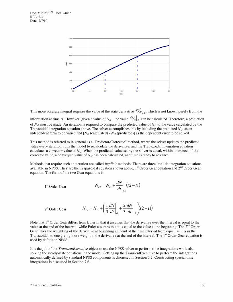
Doc. #: NPSSTM User Guide REL: 2.3 Date: 7/7/10
7 Transient Simulation 180
0
200
400
600
800
1000
1200
0.2 0.25 0.3 0.35 0.4 0.45 0.5
time
Tn
et/
I
This more accurate integral requires the value of the state derivative 2tdtdN
, which is not known purely from the
information at time t1. However, given a value of NBt2B, the value 2tdtdN
can be calculated. Therefore, a prediction
of NBt2B must be made. An iteration is required to compare the predicted value of NBt2 to the value calculated by the Trapazoidal integration equation above. The solver accomplishes this by including the predicted NBt2 as an independent term to be varied and [NBt2 (calculated) - NBt2 (predicted)] as the dependent error to be solved. This method is referred to in general as a “Predictor/Corrector” method, where the solver updates the predicted value every iteration, runs the model to recalculate the derivative, and the Trapazoidal integration equation calculates a corrector value of NBt2. When the predicted value set by the solver is equal, within tolerance, of the corrector value, a converged value of NBt2 has been calculated, and time is ready to advance. Methods that require such an iteration are called TimplicitT methods. There are three implicit integration equations available in NPSS. They are the Trapazoidal equation shown above, 1st Order Gear equation and 2nd Order Gear equation. The form of the two Gear equations is:
1st Order Gear ( )122
12 ttdt
dNNN
t
tt −+=
2st Order Gear ( )123
2
3
1
21
12 ttdt
dN
dt
dNNN
tt
tt −
++=
Note that 1st Order Gear differs from Euler in that it assumes that the derivative over the interval is equal to the value at the end of the interval, while Euler assumes that it is equal to the value at the beginning. The 2nd Order Gear takes the weighting of the derivative at beginning and end of the time interval from equal, as it is in the Trapazoidal, to one giving more weight to the derivative at the end of the interval. The 1st Order Gear equation is used by default in NPSS. It is the job of the TTransientExecutiveT object to use the NPSS solver to perform time integrations while also solving the steady-state equations in the model. Setting up the TransientExecutive to perform the integrations automatically defined by standard NPSS components is discussed in Section 7.2. Constructing special time integrations is discussed in Section 7.6.

Doc. #: NPSSTM User Guide REL: 2.3 Date: 7/7/10
7 Transient Simulation 181
Just as NPSS automatically creates a solver in the top-level assembly (see Section 4.8), it also automatically
creates a TransientExecutive object. The top-level solver is automatically named solver; the top-level
TransientExecutive is automatically named transient. Other solvers can be created in assemblies under the top-level assembly (see Section 4.8.5), but this is not the case with the TransientExecutive. The top-level TransientExecutive object controls the time step and time integration activities for the entire model, thus only one such object can exist. Users, therefore, never need to explicitly instantiate an object of type
TransientExecutive. They need only address the attributes and use the member functions belonging to the
global TransientExecutive object named transient. The variation of spool speed with time from the fuel ramp example above might be as follows:
4000
5000
6000
7000
8000
9000
10000
0 0.2 0.4 0.6 0.8 1 1.2 1.4 1.6 1.8 2 2.2 2.4 2.6 2.8 3 3.2 3.4 3.6
time
Me
ch
an
ica
l S
pe
ed
The choice of time step size in a transient simulation is important. A time step size of 0.1 seconds, for example, is adequate to resolve the variation in spool speed for the case shown above. However, one of the important parameters during an acceleration is minimum surge margin. The following plot shows the variation of surge margin with time when a time step of 0.1 seconds is used, compared with a time step of 0.02 seconds. The steady-state surge margin is also shown for reference.
0
5
10
15
20
25
30
0 0.2 0.4 0.6 0.8 1 1.2 1.4 1.6 1.8 2 2.2 2.4 2.6 2.8 3 3.2 3.4 3.6
time
Perc
en
t S
urg
e M
arg
in
dt=0.02
dt=0.10
steady

Doc. #: NPSSTM User Guide REL: 2.3 Date: 7/7/10
7 Transient Simulation 182
If a time step of 0.1 were used, one would conclude that the surge margin never drops below 7%. In reality, however, it approaches 2%. In the example presented above, even though the fuel flow increases at a constant rate over 3 seconds, it is evident that the most rapid acceleration takes place during the first 0.6 seconds after the start of the fuel flow ramp. A time step adequate for the majority of the transient is too large for this initial portion, and yet if a small enough time step is chosen to resolve the initial acceleration, many points are wasted on the remainder of the transient. NPSS includes provisions to allow the time step to vary throughout the course of a transient. This variation can either be specified by the user, or can be automatically determined by the system. Automatic time step variation, called Tadaptive time steppingT, reduces the time step as necessary to prevent excessive changes in independent variables between successive points, and increases the time step when the independent variables are changing slowly. Variable time stepping is discussed in Section 7.3. A final consideration in transient simulation is when to terminate the simulation. In the example above, since the precise timing of the item driving the transient (the fuel flow ramp) is known, the duration of the transient is reasonably clear. This is not always the case, however. For example, instead of specifying fuel flows, one might use the model to derive the fuel flows corresponding to a certain minimum allowable surge margin. In this case the duration of the acceleration is unknown. The termination criterion might be TquiescenceT, or the condition at which a steady-state has been reached, within a specified tolerance. As another example, the user might wish to terminate a simulation as soon as an unacceptable condition is reached, such as a negative surge margin. In NPSS, the user must always specify a maximum duration of a transient simulation, but has the option of specifying other criteria that can terminate the simulation sooner. How to do this is discussed in Section 7.4. In general, the user should consider the following items when constructing a transient simulation.
1. Component inputs necessary for transient running. A steady-state solution is possible with zero inertia, for example, but a transient simulation is not. The user should review each component using the TNPSS Reference
SheetsT to insure that attributes affecting time-dependent behavior are set appropriately. 2. Output 3. Initial conditions 4. Setup of the events driving the transient 5. Integration method 6. Setup of transient model 7. Time step 8. Termination criteria
These steps are summarized for a basic transient run in the following section. As mentioned periodically above, more details are given concerning options available for several of the steps in later sections.
7.2 Running a Basic Transient Simulation
7.2.1 Basic Setup The integrators necessary to correctly model the time-dependent behavior of the system are automatically created
when each component is instantiated, and are added to the solver when autoSolverSetup() is called. (Integrators are discussed in more detail in Section 7.6.) Thus, the basics necessary for transient running as well as
steady-state running are established by calling autoSolverSetup() from the top-level assembly. As mentioned in the preceding section, the first special concern of the user beyond the usual steady-state issues is to set the component attributes (such as intertias) necessary for transient running.
7.2.2 Output After setting the transient-related component attributes, the next item often addressed in setting up a transient simulation is the output desired. The most commonly used form of output for transients is the TCaseRowViewerT,
Doc. #: NPSSTM User Guide REL: 2.3 Date: 7/7/10
7 Transient Simulation 183
with a separate line (or row) for each discrete time, and a column for each variable of interest (global variable
time usually being chosen for the first column). Section 4.9.2.3 discusses the use of CaseViewers. If a
CaseViewer is added to the postExecutionSequence array of the top-level assembly’s Executive (in this case “solver”), it will be updated with information from each time step. Following is a simple example.
OutFileStream caseRow {
filename = "demo.sampleRuns";
}
CaseRowViewer CaseView {
outStreamHandle = "caseRow";
}
CaseView.variableList = { "time:??.??",
"Brn.Wfuel:??.??????=Wf",
"CmpH.Sh_O.Nmech:????.??=Nmech",
"ShH.trqNet:????.??=trqNet",
"PERF.Fn:?????.?=Fn",
"CmpH.SMN:???.??=SM" }
solver.postExecutionSequence.append("CaseView");
If output is desired on less than every time step, instead of placing the CaseViewer in postExecutionSequence,
the user should place there a function that calls the viewer's update() member function when desired. Another
option is to write a special update() function that overrides the standard one in the CaseViewer. For information on such tasks, see the TDeveloper GuideT.
7.2.3 Initial Conditions Normally a transient is initiated from steady-state conditions. (See Chapter 15 for information and a example of
initializing transients at non-steady conditions.) Global variable time holds the current simulation time in
seconds, and is updated automatically during a transient simulation. When NPSS is first launched, time is initialized to zero, but it is not reset to zero at the end of each transient run. It is the user's responsibility, then, to
set the time to the desired value before running a transient. If a steady-state point is run to establish initial conditions, this point is not repeated when the transient begins. It is recommended, therefore, that the output
desired for the transient run be set up first, the time variable initialized, and then the initial steady-state point run. This will print the steady-state point as though it were the first point of the transient, and will show the initial time as specified by the user. The following is an example, which is assumed to follow the CaseViewer setup lines given earlier (Section 7.2.2).
RunCondition.eq_lhs = "Brn.Wfuel";
RunCondition.eq_rhs = "Wf1";
solver.forceNewJacobian = TRUE;
time = 0.;
CASE++;
run();
In the example it is assumed that two steady-state points have been run previously, one at a low power setting
which yielded a burner fuel flow that was stored in global variable Wf1, and the other at a high power setting
whose fuel flow has been stored in global variable Wf2. The initial condition for the transient, which will be
considered time = 0., corresponds to a burner fuel flow of Wf1.
7.2.4 Transient Executive To simulate a transient, the model must be set up so that some specified time-varying event drives the transient response of the rest of the system (i.e. a forcing function). This event could be a change in environmental conditions simulating an aircraft maneuver, fuel flow changes resulting from simulated operator input, system

Doc. #: NPSSTM User Guide REL: 2.3 Date: 7/7/10
7 Transient Simulation 184
configuration changes simulating a mechanical failure such as a shaft break, etc. The fuel ramp example given above could be implemented as follows.
real Ramp( real time, real tstart, real duration, real Y1, real Y2 ) {
real Y, slope;
if ( duration < 0 ) {
duration = 0;
}
if ( duration ) {
slope = ( Y2 – Y1 ) / duration;
}
if ( time <= tstart ) {
Y = Y1;
}
else if ( time > tstart && time < tstart+duration ) {
Y = Y1 + ( slope * (time-tstart) );
}
else {
Y = Y2;
}
return Y;
}
RunCondition.eq_rhs = "Ramp( time, 0.2, 3.0, Wf1, Wf2 )";
Assume an Independent object is active in the solver that makes burner fuel/air ratio an independent variable.
Dependent object RunCondition is also active in the solver to allow the user a convenient means to specify some desired operating condition for steady-state solutions. It was used in the example above to establish the
initial condition. Function Ramp() is a general ramp function that returns argument Y1 for times less than tstart,
Y2 for times greater than a specified interval (duration) after tstart, and a linear interpolation between the two
for intermediate times. RunCondition is adapted for transient use by making its right-hand-side a time-varying
fuel flow returned by Ramp(). Effectively, the model fuel/air ratio is varied by the solver so that the fuel flow
matches the schedule returned by Ramp().
7.2.5 Integration Method If it is known that an integration method other than the default is desired, an appropriate time to change methods is after the solver has been set up and before switching to transient mode. The integration method can be set as follows:
Transient.integrationType = "TRAPEZOIDAL";
Some integration methods produce a different solver and TransientExecutive setup than others. For the present example, the default integration method (GEAR_1ST_ORDER) will be accepted. Other integration methods are: GEAR_2ND_ORDER TRAPEZOIDAL EULER These are discussed further in Chapter 15.
7.2.6 Setup of Transient Mode The mode of the solver is determined by its solutionMode attribute, which is an Option variable. By default this
attribute equals STEADY_STATE. Up to this point, nearly all examples have involved steady-state running, so it was unnecessary to explicitly set the attribute. After the solver has been set up for the transient in steady-state mode, it can be switched to transient mode as follows:

Doc. #: NPSSTM User Guide REL: 2.3 Date: 7/7/10
7 Transient Simulation 185
setOption( "solutionMode", "TRANSIENT" );
Function setOption() should be called from the top-level assembly (global scope) since more objects than just
the solver have a solutionMode attribute that must be set to TRANSIENT for a successful simulation. This should normally be done after all necessary independents and dependents have been set up in the solver. When the solver and TransientExecutive are switched to transient mode, the TransientExecutive retrieves configuration information from the solver, and may make some modifications to dependent conditions in the solver. The easiest way to insure a proper setup is to simply configure the solver in steady-state mode, then switch to transient mode.
If it is necessary to make changes to the solver configuration while in transient mode, take the following steps:
1. Clear the TransientExecutive setup by issuing the command transient.clear(). This reestablishes the
solver setup that existed before the switch to transient mode. Function tranient.clear()is automatically
called whenever solutionMode is switched from TRANSIENT to something else. 2. Modify the solver setup as desired, following the usual rules for solver setup changes (see Section 4.8.3 for
example). 3. Reestablish the correct solver and TransientExecutive configurations for transient running by issuing the
command transient.setup().
This procedure should also be followed if an integration method is changed to or from type EULER. The Euler integration method is an explicit method and requires a different configuration than the other methods, which are implicit. After the model has been switched to transient mode, internal storage areas used for variable histories can be initialized using the conditions established by the initial point.
initializeHistory();
The initializeHistory() function is a global function and should be called from global scope. It should only be called after the system has been switched to transient mode. It need be called only if the initial conditions for the transient to be run differ from the final conditions of the most recent transient.
7.2.7 Time Step The time step to be used can be addressed next. The simplest, and default, time stepping method uses a constant
time step throughout the duration of the simulation. The value of this time step is set by the baseTimeStep attribute of the TransientExecutive as follows. (Variable time stepping is covered in Section 7.3).
transient.baseTimeStep = 0.10;
NPSS allows for certain objects called Ttime-discrete objectsT that can directly control the time step from outside the TransientExecutive. Thus it is possible in models with such objects for the time step to vary even when constant time stepping has been selected in the TransientExecutive. The creation of time-discrete objects is an advanced topic touched upon in Chapter 15 and dealt with in more detail in the TDeveloper GuideT. There are no time-discrete objects among the standard NPSS elements and subelements.
7.2.8 Termination Criteria Finally, the user must establish termination criteria for the transient. At a minimum, the user must specify a value
of time at which the simulation will terminate. This is done using attribute stopTime belonging to the TransientExecutive:
transient.stopTime = 3.60;

Doc. #: NPSSTM User Guide REL: 2.3 Date: 7/7/10
7 Transient Simulation 186
Note that since time is not necessarily zero at the start of a transient, stopTime is not necessarily the number of
seconds simulated. The duration of the transient is stopTime less the value of variable time when the transient is initiated.
Additionally, the user can set a maximum number of iterations that can be run on a transient point. If the max limit is hit, the solver will assume convergence and move on to the next point. This is done using the attribute
maxIterations belonging to the TransientExecutive.
transient.maxIterations = 5;
The user can also limit the maximum number of iterations that can be run on a transient point by setting the Frame Rate (specified in millisecs). If the max limit is hit, the solver will assume convergence and move on to the next
point. This is done using the attribute frameRate belonging to the TransientExecutive.
transient.frameRate = 50; // Frame Rate is 50 millisecs
Establishing other criteria for termination is discussed in Section 7.4.
7.2.9 Running the Transient Once these steps have been taken, the transient is run with the usual run() command issued from global scope:
CASE++;
run();
CaseView.display();
All time steps converged as part of the transient will bear the same CASE number.
Transient simulations can be interrupted and restarted easily. The following code produces the same results as a single transient run from time = 0 to time = 3.6.
setOption( "solutionMode", "STEADY_STATE" );
RunCondition.eq_rhs = "Wf1";
solver.forceNewJacobian = TRUE;
time = 0.;
CASE++;
run();
RunCondition.eq_rhs = "Ramp( time, 0.2, 3.0, Wf1, Wf2 )";
setOption( "solutionMode", "TRANSIENT" );
initializeHistory();
transient.baseTimeStep = 0.10;
transient.stopTime = 0.60;
CASE++;
run();
transient.stopTime = 3.60;
run();
CaseView.display();
Transients driven by a different time-varying event can be set up using the transient.clear() and
transient.setup() commands discussed in Section 7.2.6, as in the following example.
real Fn1 = PERF.Fn;
real Fn2 = Fn1 * 0.80;
transient.clear();
RunCondition.eq_lhs = "PERF.Fn";
RunCondition.eq_rhs = "Ramp( time, 0.2, 2.0, Fn1, Fn2 )";
solver.forceNewJacobian = TRUE;
transient.setup();
time = 0.;
transient.stopTime = 2.40;

Doc. #: NPSSTM User Guide REL: 2.3 Date: 7/7/10
7 Transient Simulation 187
CASE++;
run();
CaseView.display();
7.3 Variable Time-Step Computation By default, the time-increment between points in any transient simulation is constant, and is equal to the
baseTimeStep attribute of the TransientExecutive object. As illustrated in Section 7.1, it is desirable in some cases to vary the time-step during a simulation. During periods in which the model states change slowly, a relatively large time step can be used. During periods in which one or more model states change rapidly, a smaller time step must be used to accurately model the event. This can be accomplished either automatically, or as specified by the user.
7.3.1 Adaptive Time Stepping When using adaptive time stepping, the user should still specify transient.baseTimeStep to be used at the beginning of the transient, as in constant time step running. The following attributes provide the most commonly used controls over adaptive time stepping:
• dxTransLimit
• dxTransLimitType
• maxTimeStep
• minTimeStep
Attribute transient.dxTransLimit specifies the maximum allowable change in an independent variable from
one time step to the next. Attribute dxTransLimitType specifies whether dxTransLimit is FRACTIONAL or
ABSOLUTE. By default it is FRACTIONAL. When the independent variables are changing slowly, large time steps,
up to the limit specified by maxTimeStep, will be taken. As necessary, small time steps, down to the limit
specified by minTimeStep, will be taken to insure that no independent variable changes more than
dxTransLimit during the step.
Adaptive time stepping is activated by setting attribute timeStepMethod equal to ADAPTIVE as in the following example.
SetOption( "solutionMode", "TRANSIENT" );
initializeHistory();
transient {
timeStepMethod = "ADAPTIVE";
baseTimeStep = 0.10;
dxTransLimit = 0.05;
maxTimeStep = 0.20;
minTimeStep = 0.01;
stopTime = 3.60;
}
CASE++;
run();
CaseView.display();
The points run by this method for the example presented in Section 7.1 are illustrated below.

Doc. #: NPSSTM User Guide REL: 2.3 Date: 7/7/10
7 Transient Simulation 188
4000
5000
6000
7000
8000
9000
10000
0 0.2 0.4 0.6 0.8 1 1.2 1.4 1.6 1.8 2 2.2 2.4 2.6 2.8 3 3.2 3.4 3.6
time
Mech
an
ical
Sp
eed
The times steps range from the minimum specified (0.01) to the maximum (0.20). The number of time steps taken is 69. A constant time step of 0.01 over the same interval would require 360 steps.
Adaptive time stepping is best suited for models that are not highly discontinuous with respect to time. If the user anticipates that the system being simulated will exhibit periods of very slow change followed immediately by periods of very abrupt change, care must be exercised to insure that the abrupt change is not skipped over. Setting
an appropriately restrictive value for maxTimeStep can insure this.
Although in some cases adaptive time stepping can shorten simulation time by greatly reducing the number of time steps taken, it can increase execution time in other cases. This is because the method takes additional passes through the model to estimate the rate of change of the independent variables. In the example above, 459 model passes were required for 69 time steps, for an average of 6.65 passes per time step. The same problem run with a constant time step of 0.01 requires 1053 model passes for 360 time steps for an average of 2.93 passes per time step – less than half that required for adaptive time stepping. In this case adaptive time stepping reduced the number of time steps by about 80%, but the number of model passes by only 56%. Adaptive time stepping, therefore, must dramatically reduce the number of time steps in order to result in a net execution time savings. It has the advantage, however, of clustering data points where they are usually most needed.
The model can be restored to constant time steps by setting timeStepMethod to "CONSTANT_DT".
The prediction passes made by the adaptive time stepping method take place before calls to Ttime-discrete objectsT. These are components that either directly manage the time step, or perform special operations at each time step. They can be useful in simulating controls. If a time-discrete object assumes that the model data available to it is from the previous time step, its logic can be corrupted by the predictor passes of the adaptive time stepping method. Care should be taken, therefore, when using time-discrete objects together with adaptive time stepping. See the TDeveloper GuideT for more information.
7.3.2 User-Defined Time-Step Computations If timeStepMethod is set to USER_DEFINED, then an expression can be placed in attribute
userTimeStepFunction that will be evaluated after each time step to determine the next time step. Normally this is a function call that contains the logic required to properly set the time step through the transient. For example:

Doc. #: NPSSTM User Guide REL: 2.3 Date: 7/7/10
7 Transient Simulation 189
real varTimeStep1() {
real dt;
if ( time < 0.195 ) { dt = 0.10; }
else if ( time < 0.595 ) { dt = 0.01; }
else if ( time < 0.995 ) { dt = 0.02; }
else { dt = 0.20; }
return dt;
}
RunCondition.eq_rhs = "Ramp( time, 0.2, 3.0, Wf1, Wf2 )";
setOption( "solutionMode", "TRANSIENT" );
initializeHistory();
transient {
timeStepMethod = "USER_DEFINED";
userTimeStepFunction = "varTimeStep1()";
baseTimeStep = 0.10;
stopTime = 3.60;
}
CASE++;
run();
CaseView.display();
Similar results may be had by setting timeStepMethod to CONSTANT_DT and directly varying the
baseTimeStep after each solver convergence:
void varTimeStep2() {
real dt;
if ( time < 0.195 ) { dt = 0.10; }
else if ( time < 0.595 ) { dt = 0.01; }
else if ( time < 0.995 ) { dt = 0.02; }
else { dt = 0.20; }
transient.baseTimeStep = dt;
}
RunCondition.eq_rhs = "Ramp( time, 0.2, 3.0, Wf1, Wf2 )";
setOption( "solutionMode", "TRANSIENT" );
initializeHistory();
transient {
timeStepMethod = "CONSTANT_DT";
baseTimeStep = 0.10;
stopTime = 3.60;
}
solver.postExecutionSequence.insertAt( 0, "varTimeStep2" );
CASE++;
run();
CaseView.display();
7.4 Controlling Termination of a Transient Run As mentioned earlier, the user must specify a value for the TransientExecutive attribute stopTime. In any event,
the transient simulation will terminate when time becomes greater than stopTime. The user may also, however,
supply an expression for attribute terminateCondition. This expression, which may be a function call, must
return an integer value, interpreted as a Boolean. If the expression evaluates to 0, and time is less than or equal to
stopTime, the transient simulation continues. If the expression evaluates to nonzero, the simulation terminates. This is useful when the exact duration of the transient is unknown.
Suppose, for example, the fuel ramp example from Section 7.1 were modified to run until 7% surge margin is obtained, then accelerate at constant 7% surge margin until the final fuel flow is obtained, then hold that fuel flow until the shaft speed is essentially steady. The fuel flow schedule corresponding to such an acceleration is desired,
as well as the time required for the acceleration. To accomplish this, functions runtoSM() and runtoWF() are

Doc. #: NPSSTM User Guide REL: 2.3 Date: 7/7/10
7 Transient Simulation 190
written to modify the solver to run either to 7% surge margin, or to constant fuel flow. Another function,
runSwitch(), is placed in solver.postExecutionSequence to control the solver switching. Finally, function
steady() is written to determine when the shaft speed is constant enough to consider the acceleration over, and a
call to this function made via terminateCondition. The complete example is as follows.
void runtoSM() {
transient.clear();
RunCondition.eq_lhs = "CmpH.SMN";
RunCondition.eq_rhs = "7.0";
solver.forceNewJacobian = TRUE;
transient.setup();
initializeHistory();
}
void runtoWF() {
transient.clear();
RunCondition.eq_lhs = "Brn.Wfuel";
RunCondition.eq_rhs = "Wf2";
solver.forceNewJacobian = TRUE;
transient.setup();
initializeHistory();
}
void runSwitch() {
if ( RunCondition.eq_lhs != "CmpH.SMN" && CmpH.SMN < 7.0 ) {
runtoSM();
}
else if ( RunCondition.eq_lhs == "CmpH.SMN" && Brn.Wfuel > Wf2 ) {
runtoWF();
}
}
real lastVal;
int steady( real tstart, string var, real tol ) {
if ( time <= tstart ) {
lastVal = var->value;
return 0;
}
real val = var->value;
int stop = 0;
if ( lastVal != 0 && abs( (val-lastVal)/lastVal ) < tol ) {
stop = 1;
}
lastVal = val;
return stop;
}
RunCondition.eq_rhs = "Ramp( time, 0.2, 3.0, Wf1, Wf2 )";
solver.executionSequence.append( "runSwitch" );
setOption( "solutionMode", "TRANSIENT" );
initializeHistory();
transient {
timeStepMethod = "CONSTANT_DT";
baseTimeStep = 0.02;
terminateCondition = "time > 0.3 && steady( 0., \"ShH.Nmech\", 1e-4 )";
stopTime = 4.00;
}
CASE++;
run();
CaseView.display();

Doc. #: NPSSTM User Guide REL: 2.3 Date: 7/7/10
7 Transient Simulation 191
The resulting mechanical speed variation is shown below.
4000
5000
6000
7000
8000
9000
10000
0 0.1 0.2 0.3 0.4 0.5 0.6 0.7 0.8 0.9 1
time
Me
ch
an
ica
l S
pe
ed
Although stopTime was set to 4 seconds, the transient is over in less than a second, and much time is saved by its terminating then.
In the example, a user-written function named steady() was used in connection with terminateCondition to determine when the simulation should stop. A built-in member function of all TransientExecutive objects named
quiescence() is also available. Function transient.quiescence() returns 1 or TRUE when the fractional
changes of all independent variables are less than attribute transient.quiescenceTolerance.
The simulation can be made to stop after each time step by setting terminateCondition simply to "1". The
transient can be advanced another time step by issuing the run() command. Such a technique can be useful for debugging transient simulations in interactive mode (Section 2.3).
7.5 TransientExecutive Attributes This section summarizes the attributes of TransientExecutive objects discussed in the preceding sections, and discusses some additional controls available to the user. Full details on the TransientExecutive and related object types is found in Chapter 15.
The variables in the table below are attributes of the TransientExecutive object, i.e. they are referenced by
transient.Tattribute_nameT. Bear in mind that two variables important to transient simulations reside in the top-
level assembly rather than in object transient: time and timeStep. Global variable time can be set by the user before a transient run is launched, but is controlled by the system during the transient. Global variable
timeStep is always an output variable, and reflects the time stepping logic of the TransientExecutive object.
The following attributes are commonly set by users in order to control transient simulations.
Table 32. Commonly Used TransientExecutive Input Attributes
Attribute Name Type Description Default Value baseTimeStep real Time step to be used unless overridden by other logic
such as adaptive time stepping, user-defined time stepping, or time-discrete objects. Units are seconds.
0.05
dxTransLimit real Maximum allowable change in an independent variable from one time step to the next under adaptive time stepping. Whether the specified change is fractional or absolute is determined by
dxTransLimitType. Used only when
timeStepMethod = "ADAPTIVE".
0.10

Doc. #: NPSSTM User Guide REL: 2.3 Date: 7/7/10
7 Transient Simulation 192
Attribute Name Type Description Default Value dxTransLimitType Option
variable Allowable values are "FRACTIONAL" and
"ABSOLUTE".
"FRACTIONAL"
integrationType Option variable
Default integration method for all integrations. This can be overridden in individual integrators.
Allowable values are "GEAR_1P
STP_ORDER",
"GEAR_2P
NDP_ORDER", "TRAPEZOIDAL", which are
implicit methods, and "EULER" which is an explicit method.
"GEAR_1P
STP_ORDER"
maxTimeStep real Maximum allowable adaptive time step. Used only
when timeStepMethod = "ADAPTIVE".
1.0
minTimeStep real Minimum allowable adaptive time step. Used only
when timeStepMethod = "ADAPTIVE".
0.0001
quiescenceTolerance real Used by member function quiescence(). If the fractional change of all state variables over a time
step is less than quiescenceTolerance,
quiescense() returns 1 or TRUE. Otherwise it
returns 0 or FALSE. Function quiescence() can be
used in attribute terminateCondition as part of a termination test.
0.01
solutionMode Option variable
Mode of the TransientExecutive object. Allowable
values are "ONE_PASS", "STEADY_STATE", and
"TRANSIENT".
"STEADY_STATE"
stopTime real Maximum value of time after which the transient simulation will be terminated.
0.0
terminateCondition string Expression that should evaluate to an integer, interpreted as a Boolean (0 = "false", nonzero = "true"). The simulation terminates when the expression evaluates to "true". The expression can include calls to other functions.
""
timeStepMethod Option variable
Time step method. Allowable values are
"CONSTANT_DT", "ADAPTIVE", and
"USER_DEFINED".
"CONSTANT_DT"
userTimeStepFunction string Expression that should evaluate to a real value giving the time step to be used. The expression can include calls to other functions. Used only when
timeStepMethod = "USER_DEFINED".
""
maxIterations int Maximum number of iterations that can be run on a transient point. If the max limit is hit, the solver will assume convergence and move on to the next point.
0
frameRate int Maximum number of millisecs allowed for iterations that can be run on a transient point. If the max limit is hit, the solver will assume convergence and move on to the next point.
0

Doc. #: NPSSTM User Guide REL: 2.3 Date: 7/7/10
7 Transient Simulation 193
Attribute Name Type Description Default Value discreteCalcsOrder Option
variable Used to determine whether the time discrete calculations are run prior to running the continuous portion of the model or after.Allowable values are
"BEFORE" and "AFTER". Note that if the switch is set
to "AFTER," the associated functions preTimeDiscretes(), runDiscreteCalcs(), and postTimeDiscretes() will all be run after the final explicit integrations but before updateHistory(). See the Developers Guide for a further description of these functions.
"BEFORE"
Table 33. Commonly Used TransientExecutive Output Attributes
Attribute Name Type Description initialized Boolean
integer Indicates whether the TransientExecutive object has been initialized. It is
initialized to zero, and is reset to zero after a call to member function clear(). If it is zero at the start of a transient run, all transient histories are initialized before time stepping commences.
stopFlag Boolean integer
Result of the expression in terminateCondition. It is initialized to zero, and is reset to zero at the start of each new transient run.
timeStepCounter int Number of time steps taken by the most recent transient run. It is reset to zero at the start of each new transient run.
7.6 Integrators Integrators are a subclass of the Dependent class. They function identically to any other Dependents during steady-state operation, but during transient operation they utilize additional attributes and methods to carry out extra responsibilities. In fact, some of the default NPSS components, such as the Shaft Element, create Integrators as part of their class definition. An integrator has all the attributes of a Dependent. It also has an attribute,
stateName, that references a state variable in the model, such as metal temperature, and an attribute,
derivativeName, that references the time derivative of this state. The state and derivative attributes hold
the values of the model parameters pointed to by the stateName and derivativeName attributes.
The Integrator class calculates two different error terms depending on the solution mode. For steady-state mode,
the error term in the Integrator is error = (y1-y2) [or (y1-y2)/yRef], the same as any other Dependent.
For transient mode, the error term changes to error = state – stateDemand [or (state –
stateDemand)/yRef], where stateDemand is the result of the integrator equation.
7.6.1 Implicit Integration There are four integration equations available that calculate the value of the state at the end of the time step using the state value at the beginning of the time step, the time step size, and the state derivative values from the beginning of the time step, the end of the time step, or both. They are 1st order Gear, 2nd order Gear, Trapazoidal or
Euler. The integrationType attribute in the transient executive sets the default type for all Integrators. However, this default can be overwritten for each Integrator, so each Integrator can use a different integration equation. These equations, save Euler, use the value of the state derivative from the end of the time step. For example the Trapazoidal equation is of the form:
dtdt
dx
dt
dxxx
tdtttdtt ∗
++=
++
2
1

Doc. #: NPSSTM User Guide REL: 2.3 Date: 7/7/10
7 Transient Simulation 194
The state derivative at the end of the time step, however, is a function of the state value at the end of the time step. This results in a dependent condition that must be iterated to solve. A guess or prediction of the value of the state at the end of the time step must be made before the derivative can be calculated. The value of the state used in the model is decoupled from the results of the integration equation by capturing the results of the integration equation
in a parameter called stateDemand. The above equation for the Trapazoidal equation then becomes:
dtdt
dx
dt
dxxx
tdtttdttdemand ∗
++=
++
2
1
The difference between the value of the state variable set before each iteration pass and the value of stateDemand calculated after the iteration pass form an error condition, called the corrector error, that must be driven to zero.
The solver varies the state variable, or state substitution variable from which the state can be calculated, to close the corrector error term in exactly the same process used to solve steady-state dependencies. And in fact, the solver is simultaneously solving the corrector error for Integrators and regular Dependent errors for non-dynamic aspects of the model, such as mass and energy continuity.
7.6.2 Explicit Integration The above discussion applies only to the implicit methods, 1st order Gear, 2nd order Gear, and Trapazoidal. The Euler equation is an explicit integration form which depends only on the derivative at the beginning of the time step, which is known without iteration, in order to calculate the end state value. Therefore, any Integrator set to Euler is removed from the list of Integrators that require iteration. The state value in the model is set directly to the
stateDemand value only once at the start of each time step, and it remains at that value for any subsequent iterations required to converge any existing error terms, including other Integrators integrated with implicit methods.
To set an Integrator to integrate using Euler, there must be an Independent object in the solver setup that points
directly to the same model parameter referenced by the stateName parameter in the Integrator. The reason is that for transient integration the Independent and Integrator are paired in a way that they are not for steady-state. For transient the Independent must vary the state variable directly or indirectly by varying a parameter that the model is set up to use for calculating the state variable (a so-called state substitution variable). If the partner Independent of an Integrator points to a state substitution variable, that means the state variable is calculated by modeling code, which is incompatible with Euler integration, which calculates the state variable value directly.
7.6.3 Switching Individual Integrators to Steady-State Individual Integrators can be switched from transient mode back to steady-state mode, while leaving the simulation as a whole in transient mode. The result is that the Integrator moves back to calculating the steady-state error term. When each time step is converged, therefore, the Integrator is at its steady-state condition. This is done when a given state very nearly reaches it steady-state value at the end of each time step. In this situation, the impact on the dynamic behavior of the model of the state associated with the Integrator is nearly zero. Setting an Integrator to steady-state reduces the number of states being tracked through time.
The number of states being integrated is referred to as the order of the system. Switching an Integrator to steady-state reduces the order of the system by one. As such, it is a very effective way to perform reduced order modeling, which seeks to determine the minimum set of states that must be integrated to provide an accurate time simulation of the sytem being modeled.
Integrators are not normally created outside the definition of an Element or Subelement class. This is because the Integrator must work with Elements and Subelements that contain state and state derivative variables, and in turn, these Elements and Subelements must have an Integrator to properly integrate the state in order for it to represent the transient behavior of its portion of the model.

Doc. #: NPSSTM User Guide REL: 2.3 Date: 7/7/10
7 Transient Simulation 195
Table 34. Integrator Input Attributes
Attribute Name Type Description Default Value derivativeName string Name of a variable holding the current value of the
time derivative of the variable named by stateName.
""
desiredDerivativeValue Real When the solutionMode is set to “SET_DERIVATIVE,” this attributes holds the derivative value at which the model is to be at convergence.
0.0
eq_RefTransient string Expression evaluated only during a transient run that yields a value of yRef. If an expression is not given, then the expression in eq_Ref is used during transient as well as steady-state operation. And if eq_Ref is not given, then eq_rhs is used to determine yRef
""
integrationType Option variable
Integration method for this integrator. Different integrators in the same system can use different integration methods. Allowable values are
"GEAR_1P
STP_ORDER", "GEAR_2P
NDP_ORDER",
"TRAPEZOIDAL", which are implicit methods, and
"EULER" which is an explicit method. If unset, the default set in the TransientExecutive is used. It
defaults to "GEAR_1P
STP_ORDER".
Transient.
IntegrationType
solutionMode Option variable
“ONE_PASS”, “STEADY_STATE”, “TRANSIENT”, “SET_DERIVATIVE.”
“STEADY_STATE”
stateName string Name of the variable whose time-varying value is to be determined by integrating the derivative specified
by derivativeName.
""
timeConstantExpr string A string containing an expression that when evaluated will yield a single real number representing the time constant value of the state
“”
Table 35. Integrator Output Attributes
Attribute Name Type Description derivative real Current derivative of the state variable, as given by derivativeName.
state real Current value of the state variable, as given by stateName.
stateDemand real Calculated value from the Integrator equation, including the Euler equation.
timeConstant real Value of the time constant of the state. If a timeConstantExpr is given, this attribute holds the results of its evaluation. If not, then the time constant is calculated by the following formula: timeConstant = fabs(state) * [(y1 – y2) / (derivative * y1)] where y1 and y2 are always the steady-state values regardless of solutionMode
As indicated in Table 34, some Integator object attributes such as integrationType have default values set by attributes in the TransientExecutive. When the value of such an attribute is explicitly set by the user in the
Integrator object, that value is TlockedT. This means that any subsequent change to the default value in the TransientExecutive will not change the value explicitly set in the integrator. Chapter 15 explains how the value of an Integrator object attribute can be unlocked so that it reverts to the default value set in the TransientExecutive. Chapter 15 also covers other attributes and topics of interest to advanced users and includes extensive examples.
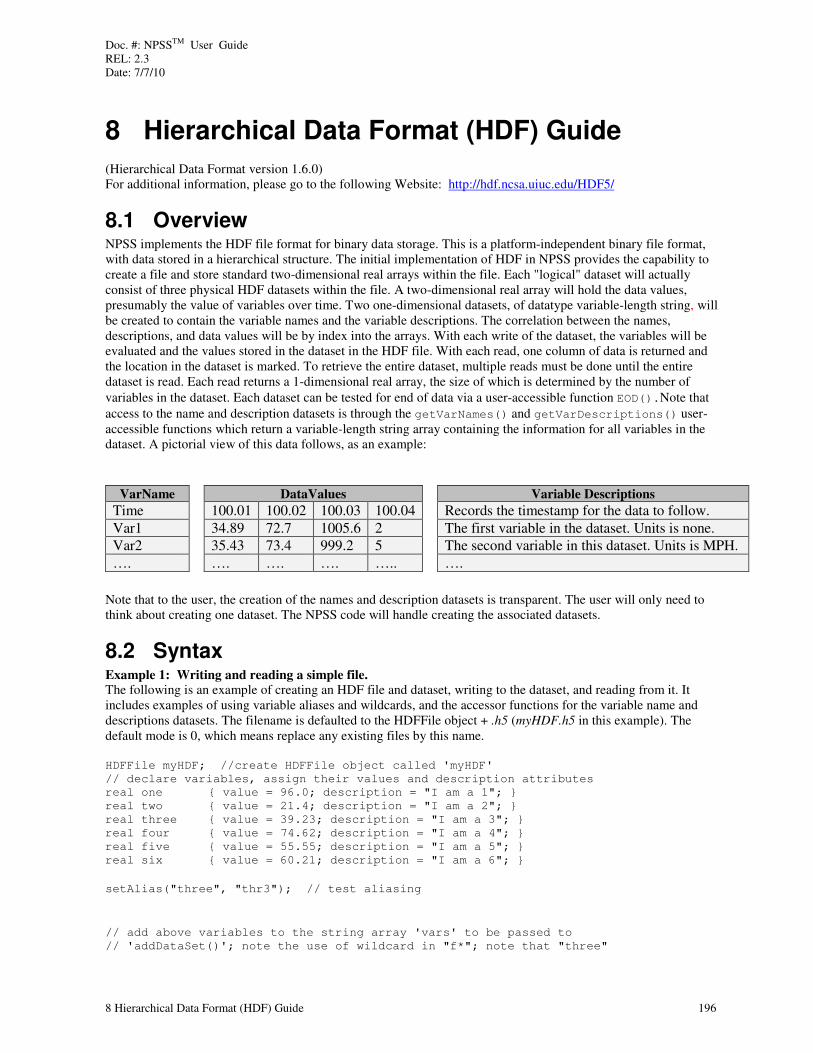
Doc. #: NPSSTM User Guide REL: 2.3 Date: 7/7/10
8 Hierarchical Data Format (HDF) Guide 196
8 Hierarchical Data Format (HDF) Guide
(Hierarchical Data Format version 1.6.0) For additional information, please go to the following Website: http://hdf.ncsa.uiuc.edu/HDF5/
8.1 Overview NPSS implements the HDF file format for binary data storage. This is a platform-independent binary file format, with data stored in a hierarchical structure. The initial implementation of HDF in NPSS provides the capability to create a file and store standard two-dimensional real arrays within the file. Each "logical" dataset will actually consist of three physical HDF datasets within the file. A two-dimensional real array will hold the data values, presumably the value of variables over time. Two one-dimensional datasets, of datatype variable-length string, will be created to contain the variable names and the variable descriptions. The correlation between the names, descriptions, and data values will be by index into the arrays. With each write of the dataset, the variables will be evaluated and the values stored in the dataset in the HDF file. With each read, one column of data is returned and the location in the dataset is marked. To retrieve the entire dataset, multiple reads must be done until the entire dataset is read. Each read returns a 1-dimensional real array, the size of which is determined by the number of
variables in the dataset. Each dataset can be tested for end of data via a user-accessible function EOD().Note that
access to the name and description datasets is through the getVarNames() and getVarDescriptions() user-accessible functions which return a variable-length string array containing the information for all variables in the dataset. A pictorial view of this data follows, as an example:
VarName
Time
Var1
Var2
….
DataValues
100.01 100.02 100.03 100.04
34.89 72.7 1005.6 2
35.43 73.4 999.2 5
…. …. …. …..
Variable Descriptions
Records the timestamp for the data to follow.
The first variable in the dataset. Units is none.
The second variable in this dataset. Units is MPH.
….
Note that to the user, the creation of the names and description datasets is transparent. The user will only need to think about creating one dataset. The NPSS code will handle creating the associated datasets.
8.2 Syntax Example 1: Writing and reading a simple file. The following is an example of creating an HDF file and dataset, writing to the dataset, and reading from it. It includes examples of using variable aliases and wildcards, and the accessor functions for the variable name and descriptions datasets. The filename is defaulted to the HDFFile object + .h5 (myHDF.h5 in this example). The default mode is 0, which means replace any existing files by this name. HDFFile myHDF; //create HDFFile object called 'myHDF'
// declare variables, assign their values and description attributes
real one { value = 96.0; description = "I am a 1"; }
real two { value = 21.4; description = "I am a 2"; }
real three { value = 39.23; description = "I am a 3"; }
real four { value = 74.62; description = "I am a 4"; }
real five { value = 55.55; description = "I am a 5"; }
real six { value = 60.21; description = "I am a 6"; }
setAlias("three", "thr3"); // test aliasing
// add above variables to the string array 'vars' to be passed to
// 'addDataSet()'; note the use of wildcard in "f*"; note that "three"

Doc. #: NPSSTM User Guide REL: 2.3 Date: 7/7/10
8 Hierarchical Data Format (HDF) Guide 197
// has been aliased to "thr3"
string vars[] = { "one", "two", "thr3", "f*", "six" };
// add a new dataset called "my data" which will record the variables
// contained in 'vars'; this will create a HDF5 file with default name
// of "myHDF.h5" and default mode = 0 (overwrite)
myHDF.addDataSet( "my data", vars);
myHDF.write(""); // perform a write to ALL datasets in "myHDF"
// (current value of all variables)
//retrieve data just written to "my data" in "myHDF.h5"
real vals[] = myHDF.read("my data");
//retrieve variable names from "my data"
string names[] = myHDF.getVarNames("my data");
//retrieve variable descriptions from variables in "my data"
string descriptions[] = myHDF.getVarDescriptions("my data");
// now print out what we have for "my data"
cout << "\n\nTEST 1 RESULTS:\n\nDataset \"my data\":\n";
int i;
for (i = 0; i < names.entries(); i++) {
cout << names[i] << "\t" << vals[i] << "\t" << descriptions[i] << endl;
}
The previous input file creates the following output:
Dataset "my data":
one 96 I am a 1
two 21.4 I am a 2
thr3 39.23 I am a 3
six 60.21 I am a 6
four 74.62 I am a 4
five 55.55 I am a 5
For the logical dataset my data, three physical datasets are actually created. My data will contain the real values of the variables. My data_Variables (a dataset that is hidden to the user) will contain the variable names. My
data_Descriptions (also hidden to the user) will contain the variable descriptions. The user need not know about these additional physical datasets, as the NPSS code handles creating and accessing them. Access to the
information in these datasets is through the user-accessible functions getVarNames() and
getVarDescriptions(). Each file can have a virtually infinite number of datasets, but the dataset names must be unique.
Note that the addDataSet function supports NPSS wildcards and aliasing in the list of variables to be added to the system. Note that variable three is known as thr3 (its alias name) by the HDF dataset. Be careful when using wildcards as you might pick up native NPSS model variables that you are not expecting. Example 2: Opening the existing file for reading and appending. This example uses the file created in example 1. A new HDFFile object is instantiated and the existing file is opened with mode = 1 (for append). The existing file information is printed out. The variables (which are expected to already exist in the current model) are updated and written to the file. The dataset is rewound so that the entire dataset can be read from the beginning. A user-function reads each record and prints it out, checking for the end-of-data condition to avoid reading past the end of the dataset. The values for the entire dataset are then printed again, showing the original data plus the appended data. //first define a fuction to read all data from a dataset
void retrieveData(string ds) {
int i = 0;
while (!myHDF2.atEOD(ds)) {

Doc. #: NPSSTM User Guide REL: 2.3 Date: 7/7/10
8 Hierarchical Data Format (HDF) Guide 198
cout << "\t Values for time = " << i++ << ":\n" << myHDF2.read(ds) << endl;
}
cout << "End of data reached for '" << ds << "'!\n\n";
}
//declare variables that were saved
real one;
real two;
real thr3;
real four;
real five;
real six;
HDFFile myHDF2; //create HDFFile object called "myHDF2"
myHDF2.openHDFFile("myHDF.h5", 1); //open existing file "myHDF.h5" for append
// Query the dataset first
//retrieve list of dataset names from "myHDF.h5"
string datasets[] = myHDF2.getDSnames();
int i, j;
for (i = 0; i < datasets.entries(); i++) {
//loop through all existing datasets (only one in this example)
cout << "\n Dataset '" << datasets[i] << "' in file '" << myHDF2.getFilename() <<
"':\n";
//retrieve variable names from "my data"
string names[] = myHDF2.getVarNames("my data");
cout << "\t Variable Names:\n" << names << endl;
//print out variable descriptions from variables in "my data"
cout << "\t Variable Descriptions:\n" << myHDF2.getVarDescriptions(datasets[i]) <<
endl;
//print out current dataset
retrieveData(datasets[i]);
//now append to dataset;
real base = 100;
for (j= 0; j < names.entries(); j++) {
names[j]->value = base+j;
cout << "Setting " << names[j] << " to " << base+j << endl;
}
//now write new values
cout << "\n\nUpdating data values and writing out to file…\n";
myHDF2.write(datasets[i]);
cout << "Rewinding dataset to read from beginning of file…\n";
myHDF2.rewindDataSet(datasets[i]);
cout << "Updated values for dataset '" << datasets[i] << "':\n";
retrieveData(datasets[i]);
}
The previous input file creates the following output: EXAMPLE 2 RESULTS:
Dataset 'my data' in file 'myHDF.h5':
Variable Names:
{"one",
"two",
"thr3",

Doc. #: NPSSTM User Guide REL: 2.3 Date: 7/7/10
8 Hierarchical Data Format (HDF) Guide 199
"six",
"four",
"five" }
Variable Descriptions:
{"I am a 1",
"I am a 2",
"I am a 3",
"I am a 6",
"I am a 4",
"I am a 5" }
Values for time = 0:
{ 96, 21.4, 39.23, 60.21, 74.62, 55.55 }
End of data reached for 'my data'!
Setting one to 100
Setting two to 101
Setting thr3 to 102
Setting six to 103
Setting four to 104
Setting five to 105
Updating data values and writing out to file…
Rewinding dataset to read from beginning of file…
Updated values for dataset 'my data':
Values for time = 0:
{ 96, 21.4, 39.23, 60.21, 74.62, 55.55 }
Values for time = 1:
{ 100, 101, 102, 103, 104, 105 }
End of data reached for 'my data'!
8.3 User-accessible Functions
HDFFile hdfObject;
Creates an empty HDFFile object. No physical file will be created until either the addDataSet() or
openHDFFile() functions are called. Note this is NOT a generic reader for HDF files; the structure imposed by NPSS is expected and is there to relieve the user from having to implement the details.
void hdfObject.openHDFFile(string filename, int mode);
Attempts to open a physical file called filename as an HDF5 file. Mode indicates how the user would like to handle existing files. Mode = 0 tells the system to delete any existing file by this name and create a new one. Mode = 1 tells the system to read in an existing file and append to any existing data. If no file exists with this name, one will be created. The user can then add new datasets to this file or add to the existing datasets. This call is unnecessary if you use the default parameter values, which are dsname = HDFFile object name +.h5 and mode = 0. If this
function is not called, the first time addDataSet() is called, the default values for these parameters are invoked and the new file is created and the dataset added.
string hdfObject.getFilename();
Returns the name of the physical file currently associated with this HDFFile object. Only one physical file can be associated with an HDFFile object for the life of the object. Example: cout << “The HDF file name is “ << myHDF.getFilename() << endl;

Doc. #: NPSSTM User Guide REL: 2.3 Date: 7/7/10
8 Hierarchical Data Format (HDF) Guide 200
void hdfObject.addDataSet(string dsname, string[] varnames);
Creates a dataset in the file called dsname which will contain the real data values for the variables in the varNames list. This dsname MUST be unique in the file or an error message will be produced. The variables contained in varnames will be checked for correct datatype, and if found to be of an invalid type or nonexistent, will NOT be added to the dataset and a warning message will be issued.
void hdfObject.write(string dsname);
Causes the current real data values of all variables in dsname to be written to the HDFFile filename. If a null string ("") is supplied, ALL datasets in the file will be written. A write will reset the end-of-data flag so that additional reads can be performed on the new data.
Real[] hdfObject.read(string dsname);
Returns a 1-D real array consisting of one write of all variables to the named dataset. The first read will read the first set of values written; consecutive reads step through file, i.e., if there are 10 variables in the dataset, a read will return a 10-element real array. If a read is done past the end of data, an error message will be returned. The isEOD() function allows the user to test this condition before performing a read.
int hdfObject.atEOD(string dsname);
Returns 0 if the dataset contains more data to be read; 1 if the end of the dataset has been reached. To reset the
read pointers to read from the beginning of the dataset, use rewindDataSet(). This function operates on a single dataset at a time.
void hdfObject.rewindDataSet(string dsname);
Resets the read pointers to allow reading from the beginning of the dataset. Can be called at any point in reading the data. A null string parameter value ("") will reset ALL datasets. Alternatively, a single dsname can be provided to operate on a single dataset.
string[] hdfObject.getDSnames();
Returns a list of the names of all datasets in the file.
string[] hdfObject.getVarNames(string dsname);
Returns a list of the variable names in dsname. If alias names were provided for any variable, those names will be returned.
string[] hdfObject.getVarDescriptions(string dsname);
Returns a list of the variable descriptions for the variables in dsnames.

Doc. #: NPSSTM User Guide REL: 2.3 Date: 7/7/10
Divider Error! Reference source not found.
Part 2: Reference

Doc. #: NPSSTM User Guide REL: 2.3 Date: 7/7/10
11 Assembly AttributesAssembly Attributes 202
9 Assembly Attributes
An assembly is a group of elements encapsulated and managed for users. An assembly has the following attributes associated with it.
Table 36. Assembly Attributes
Attribute Description Default Value
presolverSequence A list of the names of the elements and/or functions that are executed prior to the solver iteration loop. This is an alias to the Assembly’s current Executive’s preExecutionSequence.
{ }
postsolverSequence A list of the names of the elements and/or functions that are executed after the solver iteration loop. This is an alias to the Assembly’s current Executive’s postExecutionSequence.
{ }
solverSequence A list of the names of the elements and/or functions that are executed in the solver iteration loop. This is an alias to the Assembly’s current Executive’s executionSequence.
{ }
steadyStateExecutiveName
A string that holds the name of the Executive that should be set as the current Executive of this Assembly if the solutionMode OptionVariable is set to “STEADY_STATE” or “ONE_PASS.”
“solver”
transientExecutiveName
A string that holds the name of the Executive that should be set as the current Executive of this Assembly if the solutionMode OptionVariable is set to “TRANSIENT.”
“transient”
switchDes
Design mode switch indicator – equals either DESIGN or OFFDESIGN
DESIGN

Doc. #: NPSSTM User Guide REL: 2.3 Date: 7/7/10
10 Units 203
10 Units
TUnitsT track the quantity of a real value. They keep the values consistent no matter which system is used to enter them. Rather than being based on a giant lookup table, units are built on primitive base measures, which can be constructed into complex units.
. The following is an example showing how automatic conversion takes place.
real x = 10;
x.units = "mile";
cout << "x = " << x << " " << x.units << endl;
x = 10 mile
Since the unit of the variable x is mile, an assignment in feet will be converted to mile:
x = 6000 "ft";
cout << "x = " << x << " " << x.units << endl;
x = 1.13636 mile
In the units functions that follow, "left" and "right" are aliases for English and Metric. "Left" and "right" are used because they are more generic. There could be other unit systems; the units code was designed to allow a nearly
complete redefinition of unit systems. When adding a new unit, use the addUnitRelation(….)mentioned in the following section. To change from English to Metric units, for every variable used specify its unit string with its equivalent metric unit.
10.1 Units Functions The following functions are used to display, set and manipulate the units:
displayConvTables()
This function call outputs a string stream that contains the base units table, the unit relations table, and the names given to the left and right unit systems. If the user extends or resets the unit tables as described as follows, this function call will output the current tables.
resetConvTable(string leftSystem, string rightSystem)
If users want to have their own set of units, they have to destroy the old conversion table. To do that, they need to use this function. Pass in the two strings that are the names of the new conversion unit systems. For example:
resetConvTable("US", "my_system");
The purpose of the strings is to label the left and right unit systems in the new table. By default these strings are "US" and "SI". This is needed if the variable unitSystem is set in the Data Viewer definition statements.
addUnitBase (string leftUnit, string rightUnit, real conversionFactor, string type)
Unit bases are the primitives, where the actual conversions take place. All other units are complex units and will be broken down into unit bases. A conversion factor is needed to translate between two primitive base units. For example:
addUnitBase("ft","m", .3048, Q_LENGTH);
addUnitBase("sec","sec", 1, Q_TIME);
Here both feet ("ft") and meters ("m") are added as length units, with a conversion factor of .3048 between left and right units. Sec, for second, is unit system neutral but still must be defined. Argument 4 uses Q_LENGTH, Q_TIME, Q_TEMP, Q_SQRT_T, Q_MASS, Q_ANGLE, and Q_SUBSTANCE to differentiate between the

Doc. #: NPSSTM User Guide REL: 2.3 Date: 7/7/10
10 Units 204
different types of units of measure. Q_SQRT_T is for square root temperature as in SQRT_R. Two base unit entries are put in by default. They are "none" of type NONE and "+" of type WITHOFFSET. The type "none" is needed for variables that have no units. The type "+" is used so temperature conversions can be made with offsets when they are not mixed with other units. Compound unit entries, such as "1000*m", are not permitted in this function call.
After you have entered all the primitives and their conversions, use the next function to enter the unit relations.
addUnitRelation(string leftUnitName, string leftUnitRelation,
stringcorrespondingRightUnitName, string correspondingRightUnitRelation )
This function may be used to add a new unit. Some examples are:
addUnitRelation("mile", "5280.0*ft", "km", "1000*m");
addUnitRelation("ft2", "ft*ft", "m2", "m*m");
Note that ordering is important when entering these statements. NPSS must be given the definition of each item in the 2 nd and 4 th arguments before hand. For example, this statement
addUnitRelation("knot", "nmile/hr", "km/hr", "km/hr");
will cause errors unless the following are entered first:
addUnitRelation("nmile", "6076.115*ft", "km", "1000*m");
addUnitRelation("hr", "3600*sec", "hr", "3600*sec");
The default unit relations can also be expanded using the above call. Add a Unit Relation when you want to use a new, previously undefined unit of measure. All Unit Relations must be expressed in unit bases or previously defined relations. If, for example, you wish to use yards and furlongs, you must create Unit Relations as follows:
addUnitRelation("yd", "3*ft", "m", "m");
addUnitRelation("furlong", "500*yds", "km", "1000*m");
Note that the 3P
rdP and 4P
thP arguments are the closest units of measure in the rightSystem; if there is a numerical
constant, it needs to be on the left side of the multiplication sign. The 2P
ndP and 4P
thP argument's types are checked to
make sure they are the same type of quantity (i.e., length, velocity, etc.). Above, "furlong" and "kilometer" are simply aliases for the actual relations. Checks are done to make sure that the relations contain primitives from their proper systems.
A plus sign ("+") is used as a unit to tag other units. By default it means "with offset" and is used with the temperature relation:
addUnitRelation("F", "R*+", "C", "K*+");
This allows stand-alone temperature conversions with offset to be properly handled.
addUnitPref (string leftUnit, string preferredRightUnit)
The user has the option to specify preferred units for various quantities in the output conversions as a result of
using the Data Viewer UnitSystem call. For example:
addUnitPref("ft", "km");
This function is used to specify whether a user prefers feet to be converted to kilometers instead of meters, for instance. Unit Prefs are kept in a table, and all UnitPrefs are destroyed with a call to resetConvTable.
real getUnitAdder(string inUnit, string outUnit)
Returns the adder required to convert from inUnit to outUnit.
real getUnitScaler(string inUnit, string outUnit)
Returns the scaler required to convert from inUnit to outUnit.

Doc. #: NPSSTM User Guide REL: 2.3 Date: 7/7/10
10 Units 205
10.2 Valid Unit Strings The NPSS accepts the following unit strings. Numerous other combinations are also accepted, but mixing unit primitives from left and right systems in the same unit string will generate a warning.
Table 37. Valid Unit Strings
Unit String Definition “1/sec” per second “1/rpm” per revolutions per minute “A” Ampere “atm” atmosphere “bar” bar “Btu” Btu “Btu/hr” Btu per hour “Btu/(hr*ft*F)” Btu per hour per foot per degrees Fahrenheit “Btu/(hr*ft2)” Btu per hour per foot squared “Btu/(hr*ft2*F)” Btu per hour per foot squared per degrees Fahrenheit “Btu/(hr*ft3)” Btu per hour per foot cubed “Btu/lbm” Btu per pounds mass “Btu/(lbm*sec)” Btu per pound mass per second “Btu/(lbm*R)” Btu per pounds mass per degree Rankine “Btu/(lbm*R*R)” Btu per pounds mass per degree Rankine squared “Btu/R” Btu per degrees Rankine “Btu/(R*in)” Btu per Rankine per inch “Btu/sec” Btu per second “Btu/(sec*ft*R)” Btu per second per foot per Rankine “Btu/(sec*ft*R)” Btu per second feet Rankine “Btu/(sec*ft2)” Btu per second per square foot “Btu/(sec*in*R)” Btu per second inches Rankine “Btu/(sec*in2*R)” Btu per second inches squared Rankine “Btu/(sec*R)” Btu per second per Rankine “Btu*sec2/(lbm*ft2)” Btu seconds squared per pound mass foot squared “C” degrees Celsius “cm” centimeter “cm2” square centimeter “cm3” cubic centimeter “cm4” centimeters to the fourth “cm5” centimeters to the fifth “Coul” coulomb “daN” dekanewton “day” day “deg” degrees “dC” Delta degrees Celsius (no offset on conversion) “dF” Delta degrees Fahrenheit (no offset on conversion) “dK” Delta degrees Kelvin (no offset on conversion) “dR” Delta degrees Rankin (no offset on conversion) “F” degrees Fahrenheit “FD” farad “ft” feet “ft*lbf” foot-pounds force “ft*lbf/Btu” foot-pounds force per Btu “ft*lbf/(R*lbm)” foot-pounds force per degrees Rankine per pounds mass “ft*lbf/(R*lbmol)” foot-pounds force per degrees Rankine per pound mole

Doc. #: NPSSTM User Guide REL: 2.3 Date: 7/7/10
10 Units 206
Unit String Definition “ft*lbf/rad” foot-pounds force per radian “ft*lbf/(rad*sec)” foot pounds force per radians second “ft*lbf/sec” foot-pounds force per second “ft*lbf*in3/(lbm*rad2)” foot-pounds force cubic inch per pound mass per radian squared “ft*lbm/(lbf*sec2)” foot-pounds mass per pounds force per second squared “ft/sec” feet per second “ft/sec2” feet per second squared “ft2” square feet “ft2*lbm” square feet pound mass “ft2/sec2” square feet per second squared “ft2/(sec2*R)” square feet per second squared per degrees Rankine “ft3” cubic foot “ft3/lbm” cubic foot per pounds mass “g/sec” grams per second “gal” gallon “gal*in/(min*SQRT_lbf)” gallon inch per minute per square root pound force “grains” grains “H” henry “hbar” hectobar “hp” horsepower “hp/ft2” horsepower per square foot “hp*hr” horsepower hour “hr” hours “Hz” hertz “in” inches “in2” square inches “in3” cubic inch “in2*in2” inches to the fourth “in2*in2*sec2(lbm*ft)” inches to the fourth seconds squared per pound mass foot “in2*in3” inches to the fifth “in4” inches to the fourth “in4*sec2/(lbm*ft)” inches to the fourth second squared per pound mass per foot “in5” inches to the fifth “in*lbf*sec2/lbm” inch pound force second squared per pound mass “inH20” inch of water “inHg” inch of mercury “in/sec” inch per second “in2/lbf” square inch per pound force “in3*sec/rad” cubic inch second per radian “J” Joule “J/kg” Joules per kilogram “J/(kg*K)” Joules per kilogram per degrees Kelvin “J/sec” Joule per second “K” degrees Kelvin “kg” kilograms “kg/J” kilograms per Joule “kg*m/sec2” kilogram-meters per second squared “kg*m2” kilogram-square meters “kg/m3” kilograms per cubic meter “kg/(N*sec)” kilograms per Newton per second “kg/sec” kilograms per second

Doc. #: NPSSTM User Guide REL: 2.3 Date: 7/7/10
10 Units 207
Unit String Definition “kA” kilo ampere “kC” kilo coulomb “kH” kilo henry “kOhm” kilo ohm “kS” kilo siemens “kV” kilo volt “kW” kilo watts “kWb” kilo weber “kJ/kg” kilojoule per kilogram “kJ/(kg*K)” kilojoules per kilogram per Kelvin “km” kilometer “kN” kilonewton “knot” nautical miles per hour “kPa” kilopascals “kW” kilowatts “lbf” pounds force “lbf/ft2” pound force per square foot “lbf*in*sec2/lbm” pound force inch second squared per pound mass “lbf*in2” pound force square inch “lbf*in4*sec2/lbm” pound force inches to the fourth second squared per pound mass “lbf*sec/(lbm*in2)” pound force second per pound mass per square inch “lbf*sec2/(lbm*in5)” pound force second squared per pound mass per inches to the fifth
“lbf*sec2/(lbm*in2)” pound force second squared per pound mass per square inch “lbm” pounds mass “lbm/(ft*sec)” pound mass per foot per second “lbm/(ft*sec2)” pounds mass per foot per second squared “lbm/ft3” pound mass per cubic foot “lbm/(ft3*sec)” pound mass per cubic foot per second “lbm/lbm” pounds mass per pounds mass “lbm/hr” pound mass per hour “lbm/(hr*hp)” pounds mass per hour per horsepower “lbm/(hr*lbf)” pounds mass per hour per pounds force “lbm/(in*sec)” pounds mass per inch per second “lbm/in2” pounds mass per inch squared “lbm/in3” pound mass per cubic inch “lbm/(in3*sec)” pound mass per cubic inch per second “lbm/mol” pounds mass per mole “lbm/sec” pounds mass per second “lbm/(sec*ft2)” pounds mass per second per feet squared “lbm/(sec*in2)” pounds mass per second per inches squared “lbm/sec2” pounds mass per second squared “lbm*in2” pounds mass-square inches “lbm*lbm/(sec2)” pound mass squared per second squared “lbm*lbm*in2/(lbf*sec2)” pound mass squared square inch per pound force per second squared “lbm*R/sec” pound mass Rankine per second “lbm*SQRT_R/psia pounds mass square root degrees Rankine per pounds per square inch “lbmol” pound mole “liter” liters “m” meters “mA” milli ampere “mC” milli coulomb

Doc. #: NPSSTM User Guide REL: 2.3 Date: 7/7/10
10 Units 208
Unit String Definition “mFD” milli farad “mH” milli henry “mOhm” milli ohm “mS” milli siemens “mV” milli volt “mW” milli watts “mWb” milli weber “mbar” millibar “megaA” mega ampere “megaC” mega coulomb “megaH” mega henry “megaOhm” mega ohm “megaS” mega siemens “megaV” mega volt “megaW” mega watts “megaWb” mega weber “mm4” millimeters to the fourth “mm5” millimeters to the fifth “m/sec” meters per second “m/sec2” meters per second squared “m2” square meters “m3” cubic meters “mg/J” milligrams per joule “mg/(N*sec)” milligrams per newton per second “mil” 1/1000 inch (0.001*in) “mile” mile (5280 ft) “min” minute “mm” millimeters “mm2” square millimeters “mm3” cubic millimeters “mol” mole “MPa” megapascals “N” Newton “nA” nano amperes “nC” nano coulomb “nFD” nano farad “nH” nano henry “nOhm” nano ohm “nS” nano siemens “nV” nano volt “nW” nano watts “nWb” nano weber “N*m” Newton-meters “N/m2” Newtons per meter squared “none” no unit “nmile” nautical mile “ohm” ohm “Pa” Pascal “pC” pico coulomb “pFD” pico farad “pWb” pico weber

Doc. #: NPSSTM User Guide REL: 2.3 Date: 7/7/10
10 Units 209
Unit String Definition “pH” pico henry “pS” pico siemens “psia” pounds per square inch “psia/sec” pounds per square inch absolute per second “R” degrees Rankine “R/sec” degrees Rankine per second “rad” radians “rad/sec” radians per second “rev” revolution “rev/sec” revolutions per second “rpm” revolutions per minute “rpm/sec” revolutions per minute per second “rpm/SQRT_R” revolutions per minute per square root degrees Rankine “S” siemens “sec” second “sec2” second squared “sec3” second cubed “slug” slug
“slug*ft2” slug-square feet “slug/ft3” slug per foot cubed
“SQRT_lbf” square root pound force “SQRT_N” square root Newton “SQRT_R” square root degrees Rankine “uA” micro ampere “uC” micro coulomb “uFD” micro farad “uH” micro henry “uOhm” micro ohm “uS” micro siemens “uV” micro volt “uW” micro watts “uWb” micro weber “volt” volt “W” Watts “W/(m*K)” Watts per meter per degree Kelvin “W/m2” Watts per meter squared “W/(m2*K)” Watts per meter squared per degree Kelvin “W/m3” Watts per meter cubed “Wb” weber “yd” yard

Doc. #: NPSSTM User Guide REL: 2.3 Date: 7/7/10
11 Function Summary 210
11 Function Summary
11.1 User-Accessible Member Functions In the following sections, user-accessible member functions are categorized according to the object types that they operate on.
11.1.1 Functions for All NPSS Objects (Elements, Subelements, Assemblies, DataViewers, Solver, Ports, Stations, Sockets) and Variables
void create (string baseType, string type, string instanceName)
Creates an object of the given baseType and type with the given instance name. If a function: creates an object using the create() function, the newly created object resides in the function's parent. Therefore, the "parent." token must be used in front of the object name when referencing it from inside the function. For example:
void test() {
setThermoPackage("GasTbl");
create("Element", "Duct", "d1"); // Creates a Duct element named "dl"
cout << exists("d1") << endl; // d1 does NOT exist inside this
// function.
cout << parent.exists("d1") << endl; // d1 DOES exist in this
function's
// parent
}
test();
The output is as follows.
0
1
After invoking create(), instanceName.VCinit() should be called to complete the initialization of the new object.
any evalExpr(string expression)
Evaluates expression and returns the result.
cout << evalExpr(“2 + 4”) << endl; // 6
int exists(string name)
Returns 1 (TRUE) if the object exists in the model, 0 (FALSE if) it does not.
string getDataType()
Returns the object's data type such as: int, real string, void, real[], real[][], real[][][], int[], int[][], string[], any, Matrix, no_value.
real x;
cout << x.getDataType() << endl; // real
string getName()
Returns the object's local name.
int getPassType()
Returns integers 0, 1, or 2. Global integer constants NO_PASS = -1, FIRST_PASS = 0, PERTURBATION_PASS = 1, and ITERATION_PASS = 2 have been defined to allow test of the return value of this function to be more readable. This function is only available for Elements, Subelements, and Assemblies. The return values refer to

Doc. #: NPSSTM User Guide REL: 2.3 Date: 7/7/10
11 Function Summary 211
whether the current Model pass is the first pass of a convergence attempt, a matrix generation pass where an independent has been perturbed, or a pass where the solver is varying the Independent parameters in order to converge the system, or in the case of noPass, the solver is no longer in control. An example of the usage of this function is in the preexecute function of an element to determine if the current pass is the first pass of a new convergence attempt so that a guess of the independent parameters can be made.
string getPathName()
Returns the object's full pathname.
int hasInterface (string typeName)
Returns 1(TRUE) if the object is of the type specified by typeName. It also returns 1 (TRUE) if the object is inherited from the given type. For example, if object myDuct is a Duct object, which is inherited from Element, then both of the following function calls would return true:
myDuct.hasInterface("Duct"); // returns 1(TRUE) since myDuct is a Duct.
myDuct.hasInterface("Element"); // returns 1 (TRUE) since myDuct inherits
// from Element.
myDuct.hasInterface("Subelement"); // returns 0 (FALSE) because a Duct is not
// a Subelement.
int hashCollisions()
Returns the number of collisions in this VariableContainer’s instance hash table. The instance hash table is
used for finding objects within the VariableContainer. Excessive collisions (object names hashing to the same value) can impair performance in some situations.
real[] hashStats()
Returns an array of statistics for this VariableContainer’s instance and class hash tables.
string[] hashStatNames()
Returns an array of names for the statistics returned by hashStats().
int hashVal(string name)
Returns the hash value associated with name.
void hide(int flag)
This function is intended to insulate the user from parts of a model that they don't need to be aware of. Objects
marked as hidden are invisible to the list() command. Also, list() will not search inside of a hidden object unless called directly on that object. Consequently, marking a parent object as hidden effectively hides all of that
object's children, even though they are not explicitly marked as hidden. hide() can also affect the behavior of an
object if that object is converted to C++. Valid options to hide() are as follows:
flag value : result 0 : object is NOT hidden. This is the default.
1 : object is hidden. It will not be returned from any list() command unless showHidden is TRUE. 2 : object is hidden AND will not be user-accessible at all in the C++ version. showHidden is a global variable that can be used to make all hidden variables visible to the list() command. If its value is TRUE, all variables will behave as if they are not hidden. If its value is FALSE, objects marked as
hidden will not be returned from list().
showHidden=FALSE; // this is the default
To hide an object:
myObj.hide(1);
To reveal an object:

Doc. #: NPSSTM User Guide REL: 2.3 Date: 7/7/10
11 Function Summary 212
myObj.hide(0);
To make an object hidden AND prevent it from being user-accessible at all in
the C++ version of the given component:
myObj.hide(2);
To make all objects visible to the list() command:
showHidden=TRUE;
Note: a hide value of 2 should only be used with variables or functions, not with other kinds of objects, e.g., Subelements. Functions and variables are internally accessible after a component is converted to C++ regardless of whether or not they are user-accessible, but other types of objects are only accessible internally if they are user-accessible.
int hidden()
Returns 0 for visible objects, 1 for hidden objects, and 2 for objects that are hidden and will not be user-accessible when converted to C++.
string isA()
Returns the type of the object.
cout << myDuct.isA() << endl; // duct
string[] list (string type, int recurse, string expression)
Returns a list of sorted objects, each of which must match the given type and return TRUE for the given expression. The third argument, a conditional expression, is optional but must be a string that when parsed and evaluated produces a TRUE or a FALSE. Include only the first and second arguments to list UallU objects matching a given type. To list all Elements, for example: list("Element", TRUE). To narrow the list, use the conditional filtering functionality by inserting an expression as the third argument. To list all variables with an IOstatus set to "input", for example: list("Variable", TRUE, "IOstatus == \"input\""). (Note: In the previous example, to include the string "input" inside the expression, one must "escape" the quotation marks with a backward slash ("\") so that the quotation marks are not mistaken by the parser as the quotation marks which end the third argument.) Specific element and subelement types may also be listed, for example, Duct, Burner, Compressor, etc.
string[] listInterfaces()
Returns a string array. For each name that appears in the string array, hasInterface(name)on the given object will return 1 (TRUE). (Note: Use this function to list socket types.)
void reconfigureHash(real targetACL, int addAtHead, int recurse)
Reconfigures the instance and class hash tables for the specified target average chain length. A chain is a list of object names which hash to the same value. Long chains can affect performance in some situations. If
addAtHead is TRUE, then new colliding object names are added at the beginning of the chain rather than being
added at the end (the default). If recurse is TRUE, then all child VariableContainers are similarly configured as well.
int setOption(string name, any value)
This function will set the variable specified by "name" in this object and every object contained within this object. The named variable will be set only where it exists, i.e., if some child objects do not contain the named variable, they will simply be skipped. As long as there is at least one instance of the named variable somewhere in the hierarchy at or below the level where the function is called, the return value of setOption will be 1. A return value of 0 indicates that no variables matching the given name were found. Note that the specified variable can be of any type, i.e., it does not have to be an Option variable.
void showHash()
Displays the instance hash table on cout.

Doc. #: NPSSTM User Guide REL: 2.3 Date: 7/7/10
11 Function Summary 213
void showHashStats([string prefix [, string stream]])
Displays hash table statistics. Statistics lines are prefixed by prefix (default null), and written to the named
stream (default cout).
int varNameIsActiveIndep(string name)
Returns 1 (TRUE) if the specified variable is controlled by an Independent object that is part of the current Solver setup. If the variable is pointed to by an Independent object, but that Independent is not part of the set of Independents being used by the Solver when this function is called, then the function will return 0 (FALSE). The variable path name must be the full path name of the variable. This function is only available for Elements, Subelements, and Assemblies. An example usage is to determine which input variables for which it is acceptable to provide guess values. Guesses are only appropriate for variables that are controlled by an active Independent, otherwise a user input value could be overwritten by the guess value.
int verify()
Returns 1 (TRUE) if the model is valid, 0 (FALSE) if it is not. Also displays warning messages describing what is wrong.
11.1.2 Array Functions
void append(type value)
If type is the type of an array member, this function appends value to the end of the array. If type is the type of
the array, this function appends each top-level member of value to the end of the array.
int contains(type value)
Returns TRUE if there is a member of the array equal to value.
int entries()
Returns the number of entries in the array.
void getMember(int i1, [int i2], [int i3])
Accepts a minimum of 1 to a maximum of 3 int values as arguments for 1D, 2D, and 3D arrays. Returns the value of the element indexed by the argument(s).
int index(type value)
Returns the first array index at which value was found, or -1.
void insertAt(int index, type value)
Inserts value at the location specified by the index and moves all the values that follow the inserted value down. No value is deleted and the order of the values following the inserted one does not change.
void remove(type value)
Removes the first member found equal to value from the array.
void resize(int newSize)
Resizes the current array to the new size specified. To release allocated memory, you must call resize(0). Merely resizing to a smaller size does not release any memory.
void setMember(int i1, [int i2], [int i3], type val)
Accepts a minimum of 1 to a maximum of 3 int values as arguments for 1D, 2D, and 3D arrays as well as an element value argument. Type is the type of array member. It sets the element indexed by the argument(s) to the value specified by val.

Doc. #: NPSSTM User Guide REL: 2.3 Date: 7/7/10
11 Function Summary 214
UFor string arrays only:
int containsIgnoreCase(string value)
Is like contains(), but ignores case distinctions.
void insertByName(string anchor, int offset, string strToInsert)
Inserts the string strToInsert offset places from the the string anchor. A zero offset inserts the string just ahead of the anchor string. A negative offset inserts further towards to start of the array. No value is deleted and the order of the values following the inserted one does not change.
void replaceByName(string strToReplace, string strReplaceWith)
Replaces the string strToReplace with the string strReplaceWith. The number of values in the array does not change.
11.1.3 Assembly Functions
string getExecutive()
Returns the name of an Assembly’s current Executive.
void linkPorts (string port1, string port2, string stationName)
Connects port1 to port2 and labels the station with stationName.
void postKillPoint(int sequence, int index)
This function may be overwritten by the user to specify desired behavior after an NCPKillPointException has been generated. The sequence specifies in which solver sequence the exception occurred. The the index specifies in which element the exception occurred. (Please refer to Section 4.14.9 [errHandler Functions] for more detailed information).
void promotePort (string port, string newName)
Tells NPSS that an element's port (string) is to be considered a port on the specified assembly (string).
void setExecutive (string executiveName)
If executiveName is the name of an executive in the current Assembly, then it is set to be the Assembly’s current Executive.
void unpromotePort (string port)
Undoes the work of promotePort by taking the name of a port that has been promoted to the assembly level (string), unlinking that port from any connections, and un-registering it from its current Assembly.
void setupExecutive()
Sets up the current Executive in an Assembly to prepare it to be run.
11.1.4 BleedInPort/BleedOutPort Functions These functions are also used for InterStageBleedInPort and InterStageBleedOutPort.
void setBleedStation()
Sets the bleed station conditions based on current cycle conditions and bleed inputs. For optimal performance, call this function inside the verify() function.
string getStation()
Returns the station inside the bleed port.
void updateBleed ()
Calculates current station conditions; must be called after setBleedStation() has been called at least once. For optimal performance, call this function should be called inside the calculate() function.

Doc. #: NPSSTM User Guide REL: 2.3 Date: 7/7/10
11 Function Summary 215
11.1.5 DataViewer Functions
void display()
Causes the named DataViewer to print or display its data. display() is now automatically called when a DataViewer has buffered a full page of information. This cuts memory use that was taking place with
extraordinarily large buffered data. display() may be called explicitly by the user at the desired time without side effects to the automatic feature.
If the user fails to specify the pageLength of a CaseRowViewer, the page length is assumed to be infinite, but the DataViewer will display automatically once a default amount of data has been buffered. This automatic display of CaseRowViewer will not insert spaces and headers if showHeaders is set to FALSE. This way, the automatic display will save memory without ruining plotter-friendly data.
If the user fails to specify the page width of a CaseColumnViewer, the DataViewer will assume an infinitely wide page, as would be consistent with generating plotter-friendly data. Because of the way CaseColumn data is displayed, however, it cannot be displayed automatically and still remain plotter-friendly. In the case of infinite pageWidth of a CaseColumnViewer, memory use and performance will suffer, since there is no choice but to buffer all data at once. If a pageWidth is provided for CaseColumnViewer, then it will display automatically and achieve higher performance, but will likely not be plotter-friendly.
display() is also automatically called upon destruction of the DataViewer. If an explicit user call to reset() a DataViewer is made, it is assumed that the user wants to destroy the information stored in the DataViewer buffer,
and that information is UnotU automatically display()ed. An explicit display() would have to be called to clear out the buffer before a reset().
void update()
Updates the named DataViewer. Updating a DataViewer causes it to retrieve data from the model in its current state. Some types of DataViewers, for example, the VarDumpViewer, will also print the data at this point, while others, such as the CaseColumnViewer, will store the data and display it if it has accumulated enough buffered
data to force an automatic display().
11.1.6 Dependent Functions
void revertToDefaults()
Unlocks all "lockable" attributes in this dependent. This function is also available for objects derived from a Dependent, such as the Integrator.
11.1.7 Element, Assembly, and Subelement Functions
void autoSolverSetup([int recurse])
This assembly function tells the solver to retrieve the default independents and dependents from the model. Parameter recurse is optional and defaults to TRUE (non-zero). A value of FALSE (0) forces the function to set up ONLY the solver in the assembly the function is called on.
string getTextRep(int saveLevel)
Returns a string containing an ASCII text representation of the current assembly, element, or subelement. Parameter saveLevel can be set to either 1 or 0. A saveLevel of 1 gives a full save, delving into each object's children and the variables contained within. A saveLevel of 0 saves a more skeletal state representation.
void run()
Runs the given element or assembly. At the top level, runs the entire model.
Tvoid addInterface (string socketType)
Allows the Subelement to be inserted into a Socket with type socketType, even if the Subelement is not of type socketType and is not derived from a socketType class.

Doc. #: NPSSTM User Guide REL: 2.3 Date: 7/7/10
11 Function Summary 216
string[] TlistSocketTypes ()
Returns a string array containing all the socketTypes that the Subelement can be plugged into. Note:
listSocketTypes() is deprecated. Please use listInterfaces() instead.
void tree()
Displays a hierarchical view of the model presented in execution sequence. The elements are listed in the order defined in the solver sequence array. Any elements not named there will be listed next.
11.1.8 errHandler Functions Please see Section 4.14.9 for the errHandler functions. It is a subsection of 4.14, Error Handling and Messages.
11.1.9 External Component Attributes and Functions These attributes and functions are available with all external components, and are used with CORBA builds.
int proxyTraceLevel
Debug tracing level for proxy (client) side of CORBA transactions, default 0.
int proxySynchronous
Perform calculate(), parseFile(), parseString(), sendFile(), recvFile(), and send() operations synchronously, default TRUE. int proxyMaxRetries
Max CORBA::TRANSIENT retries within proxyRetryWindow, default 10.
int proxyRetryWindow
Window within which no more than proxyMaxRetries are attempted (seconds), default 600.
void parseFile(string remoteName)
Parses the file remoteName, which must exist on the external component's server. What it means to parse a file is component-dependent.
void parseString(string text)
Parses the given string. What it means to parse a string is component-dependent.
void revertToDefaults()
Revert to a default or initial state. Exact definition is component-dependent.
real getFile(string remoteName)
real getFile(string remoteName, string localName)
real getFile(string remoteName, string localName, int buffSize)
Copies a remote file to the local system (i.e., the host running NPSS). Simple binary copy, no attempt attranslation from the remote system's representation is made. The single argument form uses remoteName as the name of the local copy. The default for buffSize is 128KB. Returns the data transfer rate (bytes/sec).
real putFile(string localName)
real putFile(string localName, string remoteName)
real putFile(string localName, string remoteName, int buffSize)
Copies a local file to the remote system (i.e., the host running the server associated with the external component). Simple binary copy, no attempt at translation to the remote system's representation is made. The single argument form uses localName as the name of the remote copy. The default for buffSize is 128kB. Returns the data transfer rate (bytes/sec).

Doc. #: NPSSTM User Guide REL: 2.3 Date: 7/7/10
11 Function Summary 217
real sendFile(string localName, string dest)
real sendFile(string localName, string dest, string destName)
Send a file from the server associated with the external component to another component, dest. In this context, localName refers to a file on the server associated with the external component, not a file local to the host running NPSS. The two-argument form uses localName as the name of the destination copy. The destination component dest may be an interpreted, internal, or external component. If dest is an interpreted or internal component, it is checked for a directory attribute. If this attribute exists, it is prepended to destName, resulting in a destination path of directory/destName. Returns the data transfer rate (bytes/sec).
real recvFile(string src, string srcName)
real recvFile(string src, string srcName, string localName)
Receive a file from the server associated with another component, src. In this context, localName refers to a file on the server associated with the external component, not a file local to the host running NPSS. The two-argument form uses srcName as the name of the destination copy. The source component src may be an interpreted, internal, or external component. If src is an interpreted or internal component, it is checked for a directory attribute. If this attribute exists, it is prepended to srcName, resulting in a source path of directory/srcName. Returns the data transfer rate (bytes/sec).
void removeFile(string remoteName)
Removes the file from the remote system.
void send(string localVar, string remote) void send(string localVar, string remote, string remoteVar)
void send(string localVars[], string remote)
void send(string localVars[], string remote, string remoteVars[])
Sends one or more variables from the server associated with the external component to another external component, remote. In this context, localVar refers to a variable on the server associated with the external component, not a variable in the NPSS model. The two-argument forms use localVar(s) as the name(s) on remote. void shutdown()
Shuts down remote server. Any attempts to access a shut down server will fail.
int testReady()
Returns TRUE if the component is ready to process a new operation.
void wait()
Waits for any previous (presumably asynchronously invoked) operation to complete. Typically this function is not needed as all operations implicitly wait for the previous operation to complete before invoking the next.
11.1.10 FlowStation Functions Note: All FlowStation functions can be called from the FluidOutputPort side of a link. However, only get functions can be called from the FluidInputPort side of a link. Any other FlowStation functions called on a linked FluidInputPort will generate an error message. FluidInputPorts that are not linked have access to all FlowStation functions.
Note: Any FlowStation functions that take a TstationName Tas a string argument must NOT contain the element name as part of the string. Otherwise, NPSS will not be able to resolve the station name. For example,
DUCT.Fl_O.copyFlow("Fl_I") //right way
DUCT.Fl_O.copyFlow("DUCT.Fl_I") //wrong way
Note: Not all FlowStations use all of these functions.

Doc. #: NPSSTM User Guide REL: 2.3 Date: 7/7/10
11 Function Summary 218
void add(string stationName)
Adds the secondary stream stationName to this flow station. Keeps the total pressure the same and uses an energy balance to calculate the new temperature.
void flowStationName.burn(string fuelStationName, real efficiency)
Adds a fuel stream (fuelStationName) to the specified flow station (FlowStationName) and burns unburned fuel to the given efficiency.
void copyFlow(string stationName)
Copies flow total conditions from the specified stationName to this flow station.
void copyFlowRemote(string stationName)
Copies flow total conditions from the specified stationName outside the local scope to this flow station.
void copyFlowStatic(string stationName)
Copies total conditions and static conditions from the specified stationName to this flow station.
void copyFlowStaticRemote(string stationName)
Copies total conditions and static conditions from the specified stationName outside the local scope to this flow station.
real getExergy(real pressure, real temperature)
Set the state to the input temperature and pressure and return exergy defined as: exergy = href- _ht - _ht - Tref * ( s - s_ref ) where ref refers to the new state conditions.
real getIdealEnthalpy(real entropy)
Sets the state to a condition defined by the input entropy and current pressure and then returns the enthalpy for that state. State is returned to it’s previous value when the function returns.
real getIdealWork(real pressure)
Sets the state to a condition defined by the input pressure and current entropy and then returns the enthalpy difference between the two states.
string getStationType()
Returns the flow station type as assigned by the setThermoPackage command
virtual int haveStatic()
Returns a flag to let the user know if statics are available.
void setDryAir()
Sets the consistency of the flow to dry air. This may be called for the following thermo packages: AllFuel and FPT. The following parameters are set:
Common to all thermo packages:
The Water to Air Ratio is set to zero for the flowstation through a call to setWAR(0.0)
Additional actions specific to thermo package allFuel:
The following FlowStation parameters are set: Fraction of flow that is inlet flow = 1.0 Fraction of flow that is unburned fuel = 0.0 Fraction of flow that is burned fuel = 0.0 Fuel to Air Ratio = 0.0 Water to Air Ratio = 0.0 Status of static values = NO

Doc. #: NPSSTM User Guide REL: 2.3 Date: 7/7/10
11 Function Summary 219
setTotalTP(Tt, Pt) is called which sets the total conditions based on the total temperature and total pressure.
Additional actions specific to thermo package FPTFlowStation
Status of static values = NO The Water to Air Ratio of the FlowStation is set to 0.0. setTotalTP(Tt, Pt) is called which sets the total conditions based on the total temperature and total pressure.
void setStatic_u _rho(real u, real rho)
Set total conditions based on static input internal energy and density.
The only thermo package FlowStation that uses this set function is allFuel
The difference between the input energy and the current static energy is used in a total enthalpy solver to determine the total enthalpy, ht. The difference between the input density and the current static density is used in a total pressure solver to determine the total pressure, Pt.
void setTotal_hP(real h, real P)
Sets total conditions based on the input enthalpy and pressure.
Common to all thermo packages:
The following FlowStation parameters are set: Sets the total enthalpy to the input value. Sets the total pressure to the input value. Sets the total temperature through a call to get_T_hP(real h, real P) using the input values of h and P.
Additional actions specific to thermo package allFuel:
Sets the following FlowStation parameters: Sets the total pressure to the input value. Sets the total enthalpy to the input value. oar = har = 0.0 air = fracAir plog = log(Pt) h = ht FAR = FAR*air war = WAR*air After the following function call, additional parameters are set:
thofhc_(&h, &plog, &t, &s, &cs, &r, (char*)_jphase.data(), allFuelFlowStation::_tfuel, &FAR, &war, &air, &har, &oar)
Tt = t Rt = r gamt = cs/(cs – r) entropy = s Cp = cs Rhot = Pt*144/(Rt*Tt*C_BTUtoFT_LBF) Status of static values = NO
Additional actions specific to thermo package FPT:
Sets the following FlowStation parameters: Sets the total pressure to the input value. Sets the total enthalpy to the input value. Sets the total temperature through a call to get_T_ht().

Doc. #: NPSSTM User Guide REL: 2.3 Date: 7/7/10
11 Function Summary 220
Sets the flowstation’s entropy through a call to get_s(this). Status of static values = NO
Additional actions specific to thermo package JanafFlowStation
Sets the following FlowStation parameters: Sets the total pressure to the input value. Sets the total enthalpy to the input value. Status of static values = NO If the Fuel to Air Ratio > 0 the total temperature is determined through a Tt solver based on the input enthalpy. Otherwise, the total temperature is calculated from the input enthalpy, heat of formation, and the total fluid composition.
void setTotal_hS(real h, real S)
Sets total conditions based on the input enthalpy and entropy.
Common to all thermo packages:
Sets the following parameters: Sets the total enthalpy to the input value. Status of static values = NO A total pressure solver is used to determine the pressure that will match the input h and S. This results in setting Tt and Pt.
Additional actions specific to thermo package allFuel
Status of static values = NO The following are input parameters to the allFuel calculation function: h2 = ht = hin h = 1.0 air = fracAir FAR = FAR*air war = WAR*air p = exp((0.24*log(hin/0.24) – Sin + 0.279)/0.06855) oar = har = 0.0 herror = 0.1 plog = log(p) entropy = s = Sin The AllFuel calculation function: thofsc_(&s, &plog, &t, &h, &cs, &r, (char*)_jphase. data(), allFuelFlowStation::_tfuel,&FAR, &war, &air, &har, &oar) Output parameters from the allFuel calculation function: entropy = s Tt = t Pt = exp(plog) Rt = r gamt = cs/(cs - r) entropy = s Cp = cs rhot = _Pt * 144 /( Rt * Tt * C_BTUtoFT_LBF )

Doc. #: NPSSTM User Guide REL: 2.3 Date: 7/7/10
11 Function Summary 221
Additional actions specific to thermo package FPT:
Sets the following FlowStation parameters: Sets the total enthalpy to the input value. Sets the entropy to the input value Status of static values = NO If the total pressure or total temperature have not been previously defined, they are set to STP values. A total pressure solver is used to determine the pressure that will match the input enthalpy. The function setTotalSP(s, Pt) is called which will set the entropy, total pressure, total enthalpy, and total temperature.
void setTotal_hsPsV()
Sets the thermodynamic state based on static enthalpy, static pressure, and velocity (Mach Number).
Actions specific to thermo package allFuel:
Calculates the following FlowStation parameters: Sets the state using the given enthalpy and pressure: setTotal_hP( hin, Pin ) Calculates the enthalpy: ht = hin + 1./ 2. * get_rhot()/ C_GRAVITY / C_BTUtoFT_LBF * pow( Vf, 2 ) gams = get_gamt() A total pressure solver is used to determine the Pt using the given static pressure.
Actions specific to thermo package CEA:
Calculates the following FlowStation parameters: Sets the state using the given enthalpy and pressure: setTotal_hP( hin, Pin ) Calculates the enthalpy: ht = hin + 1./ 2. * get_rhot()/ C_GRAVITY / C_BTUtoFT_LBF * pow( Vf, 2 ) gams = get_gamt() A total pressure solver is used to determine the Pt using the given static pressure.
Actions specific to thermo package FPT:
Calculates the following FlowStation parameters: Sets the state using the given enthalpy and pressure: setTotal_hP( hin, Pin ) Calculates the enthalpy: ht = hin + 1./ 2. * fluidPtr->get_rhot(this)/ C_GRAVITY / C_BTUtoFT_LBF * pow( Vf, 2 ) gams = fluidPtr->get_gamt(this) A total pressure solver is used to determine the Pt using the given static pressure.
Actions specific to thermo package Janaf:
Calculates the following FlowStation parameters: Sets the state using the given enthalpy and pressure: setTotal_hP( hin, Pin ) Calculates the enthalpy: ht = hin + 1./ 2. * fluidPtr->get_rhot(this)/ C_GRAVITY / C_BTUtoFT_LBF * pow( Vf, 2 ) gams = fluidPtr->get_gamt(this) Rs = get_Rt() MN = Vf / sqrt( C_BTUtoFT_LBF * C_GRAVITY * gams * Rs * Ts ) A total pressure solver is used to determine the Pt using the given static pressure.
void setTotalSP(real S, real P)
Sets total conditions based on the input entropy and pressure.
Common to all thermo packages:
Sets the following FlowStation parameters:

Doc. #: NPSSTM User Guide REL: 2.3 Date: 7/7/10
11 Function Summary 222
Sets the FlowStation entropy to the input value. Sets the FlowStation total pressure to the input value Status of static values = NO
Actions specific to thermo package allFuel:
The following are input parameters to the allFuel calculation function: Pt = Pin entropy = s = Sin oar = har = 0.0 air = fracAir plog = (float)log(Pt) FAR = FAR*air war = WAR*air r = Rt The AllFuel calculation function: thofsc_(&s, &plog, &t, &h, &cs, &r, (char*)_jphase.data(), allFuelFlowStation::_tfuel, &FAR, &war, &air, &har, &oar) Output parameters from the allFuel calculation function: Tt = t Rt = r ht = h gamt = cs/(cs - r) entropy = s Cp = cs rhot = Pt * 144 /( Rt * Tt * C_BTUtoFT_LBF )
Actions specific to thermo package CEA:
Sets the following FlowStation parameters: Sets total pressure to the input pressure Sets the entropy to the input value Status of static values = NO Calculates the the total temperature: Tt = pow (( Pin / Pt ), ( gamt - 1 )/ gamt ) * Tt Calls CEA setting the state conditions to S and P: startceasp_( type, Pt, Stemp, Wreac1, _Wreac2, _Wreac3, _Wreac4, _Wreac5, _Wreac6, _Wreac7, _Wreac8, _Wreac9, _Wreac10, Aratio, rhot_r, ht_r, Tt_r, gamt_r, Vson_r, _print, transport, mu_r, k_r, Cp_r, Pr_r, R_r, _error ) Conversions are then done: mut = mu_r*6.7197e-5 rhot = rhot_r * .0022046 / .000035315 ht = ht_r * 1.798796 Cpt = Cp_r kt = k_r * 1e-3*.0671519 Prt = Pr_r Tt = Tt_r * 9 / 5 Rt = R_r gamt = gamt_r

Doc. #: NPSSTM User Guide REL: 2.3 Date: 7/7/10
11 Function Summary 223
Actions specific to thermo package FPT:
Sets the following FlowStation parameters: Sets the entropy to the input value Sets the total pressure to the input value Gets the value of the total enthalpy as a function of (s, Pt) though a call to get_h_st(this) Gets the value of the total temperature as a function of (ht, Pt) through a call to get_T_ht(this) Status of static values = NO
Actions specific to thermo package Janaf:
Sets the following FlowStation parameters: Sets the total pressure to the input value Rt = get_Rt() phiT = entropyin + Rt * log( Pt ) Calculates Tt = phi_to_t_( phiT, kGasTotal ) Calculates ht = t_to_h_ ( Tt, kGasTotal ) + formation_heat_( kGasTotal ) Status of static values = NO Recalculates these parameters if FAR > 0 and reconstitute != FROZEN through a call to: chem_equilibrium_( k_type, Pin, q_dum1, Stemp, q_t_react, q_lost_h, kGasTotal ) Rt = get_Rt() phiT = entropyin + rt * log( Pt ) Tt = q_t_react ht = t_to_h_ ( Tt, _kGasTotal ) + formation_heat_( kGasTotal )
void setTotalStaticTP(real Ts, real Ps, real MN)
Sets total and static conditions based on the input static temperature, static pressure, and Mach number.
Actions specific to thermo package Janaf:
Sets the following FlowStation parameters: Calls setMNdes(MNin) Sets the static temperature to the input value Sets the static pressure to the input value Calls setTotalTP( Tin, Pin ) hs = ht gams = get_gamt() Calculates total enthalpy: ht = hs + MNin * MNin * get_Rt() * gams * Tin / 2.0 Calulates the total pressure: Pt = Pin * pow((1.0 + (gams-1)/2 * MNin * MNin), gams/(gams-1)) Calls setTotal_hP(ht, Pt) MachOrArea = MACH Status of static values = NO MN = MNin Calls setStatic()
void setTotalTP(real Tt, real Pt)
Sets total conditions based on temperature and pressure.
Common to all thermo packages:
Sets the following FlowStation parameters: Sets the total pressure to the input value Sets the total temperature to the input value Sets the total enthalpy through the call: ht = get_h(Tin, Pin) Status of static values = NO

Doc. #: NPSSTM User Guide REL: 2.3 Date: 7/7/10
11 Function Summary 224
Actions specific to thermo package allFuel:
Sets the following FlowStation parameters: Sets the total pressure to the input value Sets the total temperature to the input value Status of static values = NO The following are input parameters to the allFuel calculation function: air = fracAir FAR = FAR*air war = WAR*air oar = har = 0.0 plog = (float)log(Pin) ts = Tin The AllFuel calculation function: thoftc_(&ts, &plog, &h, &cs, &s, &r, (char*)jphase.data(), allFuelFlowStation::_tfuel, &FAR, &war, &air, &har, &oar) Output parameters from the allFuel calculation function: ht = h Rt = r gamt = cs/(cs - r) entropy = s Cp = cs rhot = Pt * 144 /( Rt * Tt * C_BTUtoFT_LBF )
Actions specific to thermo package CEA:
Sets the following parameters: Sets the total temperature to the input value Sets the total pressure to the input value Status of static values = NO Calls CEA to calculate several parameters: startceatp_( type, Pt, Tt, _Wreac1, _Wreac2, _Wreac3, _Wreac4, _Wreac5, _Wreac6, _Wreac7, _Wreac8, _Wreac9, _Wreac10, dum, rhot_r, ht_r, S_r, gamt_r, _print, _transport, mu_r, k_r, Cp_r, Pr_r, R_r, _error ) Calculates and sets FlowStation parameters: rhot = rhot_r * .0022046 / .000035315 ht = ht_r * 1.798796 entropy = S_r gamt = gamt_r mut = mu_r*6.7197e-5 Cpt = Cp_r kt = k_r * 1e-3*.0671519 Rt = R_r Prt = Pr_r
Actions specific to thermo package FPT:
Sets the following FlowStation parameters: Sets the total pressure to the input value Sets the total temperature to the input value Calculates total enthalpy: ht = get_h_Tt(this)

Doc. #: NPSSTM User Guide REL: 2.3 Date: 7/7/10
11 Function Summary 225
Calculates entropy = get_s(this) Status of static values = NO
Actions specific to thermo package Janaf:
Sets the following FlowStation parameters: Sets the total temperature to the input value Sets the total pressure to the input value Calculates total enthalpy: ht = t_to_h_( Tt, kGasTotal ) + formation_heat_( kGasTotal ) Status of static values = NO If FAR > 0 and reconstitute != FROZEN, recomputed the composition: chem_equilibrium_( k_type, _Pt, q_dum1, q_dum2, q_t_react, q_lost_h, kGasTotal ) ht = t_to_h_( Tt, _kGasTotal ) + formation_heat_( kGasTotal )
void setTotal_u_rho()
Set total conditions based on internal energy and density
Common to all thermo packages:
Sets up a total pressure solver to calculate Pt based on rho. Sets up a total enthalpy solver to calculate ht based on internal energy. Calls: setTotal_hP(ht, Pt)
Actions specific to thermo package allFuel:
Sets up a total pressure solver to calculate Pt based on rho. Sets up a total enthalpy solver to calculate ht based on internal energy.
real getTotalComp("H2")
Returns the mass fraction of the specified species (in CEA notation).
void addEq("H2", 0.5)
Adds a specified mass flow (lbm/s) of a specified species (in CEA notation) within the flow and then recalculates equilibrium. The species must be one of the six called in the "setThermoPackage" command.
void subtractEq("H2", 0.5)
Subtracts a specified mass flow (lbm/s) of a specified species (in CEA notation) within the flow and then recalculates equilibrium. The species must be one of the six called in the "setThermoPackage" command..
void addNonEq("H2", 0.5)
Adds a specified mass flow (lbm/s) of a specified species (in CEA notation) within the flow but does not recalculate equilibrium. The species must be one of the six called in the "setThermoPackage" command.
void subtractNonEq("H2", 0.5)
Subtracts a specified mass flow (lbm/s) of a specified species(in CEA notation) within the flow but does not recalculate equilibrium. The species must be one of the six called in the "setThermoPackage" command.
11.1.11 Independent Functions
void revertToDefaults()
Unlocks all "lockable" attributes in this independent.

Doc. #: NPSSTM User Guide REL: 2.3 Date: 7/7/10
11 Function Summary 226
11.1.12 InFileStream Functions
void close()
Closes the file.
int fileExists(string filename)Returns TRUE if the specified file exists.
int getByte()
Reads a single character from the stream and returns it as an integer.
string getc()
Reads a single character from the stream and returns it as a string (The NPSS does not have a char data type).
string getline([int expected])
On formatted streams, reads from the stream until the next newline character. For binary or unformatted streams,
this just calls getString(). The optional expected argument is only used for binary or unformatted streams; it is ignored when used with a formatted stream.
int getInt([int width])
Reads an integer from the stream. If specified, at most width characters are read.
int getInt1D(string varName [, int expected [, int start]])
Reads an integer array from the stream into the variable. For formatted and binary streams, the expected
argument is required and specifies how many values are to be read. For unformatted streams, expected is
optional, and if > 0, it is checked against the read record length. The start argument is always optional. If
specified, it is the starting index in the array variable for values to be stored. If start is not specified, the first value read is stored at index 0.
real getReal([int width])
Reads a real number from the stream. If specified, at most width characters are read.
string getString([int expected])
Reads a string from the stream. For formatted streams, the optional expected argument is ignored. For binary
streams, expected is a required argument. If expected is zero, characters are read until a terminating zero. If
expected is >0, that many characters are read. For unformatted streams, the expected argument is optional. If specified and >0, it is compared against the read record length.
void open(string filename)
Opens a file, just as if assigning a function name. If you do not use the close() function to close an open file, the file will be closed automatically when you exit NPSS.
string peekc()
Returns the next character which would be returned by getc() without actually removing it from the stream.
void ungetc(string chars)
Pushes one or more characters back onto the stream. These characters will only be seen by getc() or peekc().
11.1.13 Linear Model Generator Functions See Section Error! Reference source not found. for the Linear Model Generator member functions.

Doc. #: NPSSTM User Guide REL: 2.3 Date: 7/7/10
11 Function Summary 227
11.1.14 Link Functions
string getP1Name()
Returns the name of the first of two ports held together by this link.
string getP2Name()
Returns the name of the second of two ports held together by this link.
11.1.15 msgHandler Functions Note: These functions have not been removed from the system but are OBSOLETE. Please see Section 4.14, Error Handling and Messages, for the latest information, including preferred functions.
void clear()
Clears all of the buffered errors, warnings, and informational messages and all provisionals.
void error(string errMessage, int ESI)
Generates an error message.
void message(string message, int showFullMessage)
Generates an informational message and optionally shows the file and line number information.
void provisionalError(string errMessage, int ESI)
Generates a provisional error message.
void throwError(string errMessage, int ESIcat)
Breaks flow of execution and generates an error message. If throwError() is called from interpreted code, then execution will resume on the next statement in the interpretive code.
void warning(string warningMessage, int ESI)
Generates a warning message.
11.1.16 OutFileStream Functions
To create an OutFileStream:
OutFileStream theFileOut;
void close()
Writes the file and then closes it. Using this function allows the closed file to be seen from other files.
int fileExists(string filename)Returns TRUE if the specified file exists.
void flush()
Writes any pending output to the file, "flushing" the internal buffer. Typically unnecessary, as all output is flushed upon closing, or upon each newline if autoFlush is active (the default).
void open(string filename)
Opens a file, just like assigning a function name. Explicitly opened streams always create a file, even if it is never written to (resulting in a zero-length file). If you do not use the close() function to close the file, the file will automatically be closed when you exit NPSS.
void print(any value [, string format])
Prints the given value to the stream. The optional format parameter is only used with formatted streams, and is
described in the section for the global function toStr(). It is ignored with binary and unformatted streams.
Doc. #: NPSSTM User Guide REL: 2.3 Date: 7/7/10
11 Function Summary 228
void println()
Prints a newline to a formatted stream. Ignored by binary and unformatted streams.
void println(any value [, string format])
Calls print(). With formatted streams, it then prints a newline. With binary streams and a string value, writes a
terminating zero to the stream. For unformatted streams, does nothing beyond print().
void printByte(int value)
Writes value directly to the stream. Note that some values can cause confusing results on a formatted stream,
void printVariable(string varName [, string format])
Calls print() with the given variable. More efficient with interpreted code and arrays, as it avoids copying the array to a temporary.
11.1.17 Port Functions
string PortName.isLinkedTo()
Returns the fullPathName of the Port that this Port is linked to. If the Port is not linked, returns NULL.
string[] getLinkName()
Returns the name(s) of the link(s) that this Port is attached to. If the Port is not linked, returns an empty array.
string[] getLinkedPortName()
Returns the name(s) of the remote Port(s) that this Port is attached to. If the port Is not linked , returns an empty array.
11.1.18 Socket Functions
int isEmpty()
This function is accessed from interpreted code. It returns 1 (TRUE) if the user has not instantiated a subelement to fill the given socket (i.e., the socket is "empty"), and returns 0 (FALSE) if the user has instantiated a subelement (i.e., the socket is NOT empty).
11.1.19 Solver Functions Please see Section 14.1.2 for Solver member functions. Advanced Solver functions can be found in Section 14.6.
11.1.20 Table Functions
void applyIndepMods( )
This function takes a table's modifiers (scalar and adder) and applies them to each table value. The original values are then overwritten with new scaled values. Each subtable in turn has its own modifiers applied. Finally, the scalar and adder are reset to their default values of 1 and 0, respectively.
string display()
Writes the Table definition into a string. If desired, the Table definition string can be saved to a file and read back into NPSS at a later time. The definition contains all of the Table's independent and dependent values, as well as any Table attributes that differ from default values.
real eval(real v1, real v2, ..., real vn)
Performs a table lookup and returns the resulting real value.

Doc. #: NPSSTM User Guide REL: 2.3 Date: 7/7/10
11 Function Summary 229
real[] evalStacked(real v1, real v2, ..., real vn)
Performs a table lookup on a stacked table, i.e., a table with multiple dependents, and returns an array of real values.
real evalYX(real v1, real v2, ... , real vn)
Performs an inverse table lookup, i.e., the table dependent becomes the independent and the lowest level independent becomes an independent. Note that evalXY will produce an error if the table dependents are not monotonic.
real evalYXiter(real v1, real v2, . . . real vn)
Performs an inverse table lookup while iterating on the independent value to force the dependent value to match.
The values from evalYX() will not give the same independent when put back into the table while valYXiter() (described above) will. Note that evalXY will produce an error if the table dependents are not monotonic.
string[] getDependentNames()
Returns a string array containing the names of all of the dependents in the Table. Typically there will only be one name in the array unless the Table is stacked.
string[] getIndependentNames()
Returns a string array containing the names of all of the independents in the Table. The names appear in order from outermost to innermost subtable, which is not necessarily the same order as the argument list in the Table definition.
int getIndependentCount()
Returns the number of independents in the Table.
void getIndependentArgNames(string names[])
Writes the names of all the Independent arguments in the Table definition, into the string array, names[]. The Independent argument names appear in the same order as the argument list in the Table definition.
int getIndependentArgCount()
Returns the count (or total number) of Independent arguments in the Table definition.
int getNumberDependents()
Returns the number of dependents in the Table.
int getNumberIndependents()
Returns the number of independents in the Table.
real[] getValues(string name, indep1, ..., indepN)
Returns a real array containing the values of the requested independent or dependent. The first argument is the name of the requested independent or dependent, followed by a number of independent values that is sufficient to specify which set of independent or dependent values are desired. For example, for a Table containing three independents { "z", "y", "x" } where z is the outermost subtable, the independent "z" values can be retrieved in the following way:
real vals[] = TtableNameT.getValues("z"); // no independent args needed here
To retrieve a set of "x" independent values, two independent values must be supplied in order to specify which "z" subtable and which "y" subtable to retrieve the "x" values from. For example:
vals = TtableNameT.getValues("x",1.3,4.1); // two independent args needed
Since the dependent values live in the innermost subtable, the same number of independent arguments is needed to retrieve them as is needed to retrieve the innermost independent. In this example, "x" is the innermost independent, so in order to retrieve a set of dependents (called "dep" in this example), you need two independent values to specify which dependent set that you want. For example:
Doc. #: NPSSTM User Guide REL: 2.3 Date: 7/7/10
11 Function Summary 230
depVals = TtableNameT.getValues("dep",1.3,4.1); // two indep. args needed
string getTextRep(int saveLevel)
Returns a string containing an ASCII text representation of the current table. Parameter saveLevel can be set to either 1 or 0. A saveLevel of 1 gives a full save, delving into each level of the table and the variables contained within. A saveLevel of 0 saves a more skeletal state representation.
11.1.21 Time Discrete Model Objects Section 15.4 contains the functions for time discrete model objects, which are for advanced users.
11.1.22 Transient Executive Functions Section 15.1.7 contains transient executive functions and a usage example.
11.1.23 User-Supplied Subelement Functions
NCPVal getValueFromParent (string name)
Returns the value of the named variable in the parent element or subelement.
void setValueInParent (string name, NCPVal value)
Sets the named variable i the parent to the given value.
11.1.24 VariableContainer Functions
void dump(int recurse, string wildcard)
This function writes all of the selected variables and their values to the standard output. If a wildcard string is supplied, only variables with pathnames that match the wildcard will be displayed. All output is sorted alphabetically and the names displayed are the pathnames relative to the starting scope. The “recurse” argument gives the recursion depth to report. This ranges from 0 to the number of levels to be examined. The “wildcard” string may be used for filteringing reported information.
void loadCompiledObjects(string DLMname,string objectname=””,int absolute=0)
This function can be called from any VariableContainer and will allow specific function objects or other VCInterface object instances created in the DLM to be registered in that VariableContainer. For example, given an
object called foo, calling foo.loadCompiledObjects("myfunctDLM") will load whatever objects are created in myfunctDLM.sc (UNIX) or myfunctDLM.dll (Windows). Note that this is different from a normal component DLM, which loads a CLASS. This type of DLM loads an instance or instances of class into a specific scope.
If the DLM supports it, a specific object can be loaded from the DLM if objectname is not empty. Table DLMs support this option.
If the optional argument absolute is passed as a non-zero value, the DLMname is taken literally as a filename.
Please refer to the NPSS Reference Sheets, specifically the VariableContainer Reference Sheet, for additional VariableContainer functions.
11.2 Global Functions Global functions apply to the NPSS as a whole and are not associated with any particular object.
11.2.1 Bitwise Functions Note: See Section 2.2.5.1 for bitwise operators.

Doc. #: NPSSTM User Guide REL: 2.3 Date: 7/7/10
11 Function Summary 231
int bitget(int A, int B)
Returns the Bth bit (0 to 31) of A.
A = 1089
A = 0000 0000 0000 0000 0000 0100 0100 0001
bitget(A, 6) = 1
bitget(A, 8) = 0
int bitset(int A, int B, int C)
Sets the Bth bit (0 to 31) of A to C (0 or 1) and returns the result.
bitset(A, 12, 1) = 5185
0000 0000 0000 0000 0001 0100 0100 0001
int shiftL16(int A, int B)
Shifts the bits of A to the left by B places and returns the result with the 16 MSB masked out.
shiftL16(A,7) = 8320
0000 0000 0000 0000 0010 0000 1000 0000
int shiftL32(int A, int B)
Shifts the bits of A to the left by B places and returns the result.
shiftL32(A,7) = 139392
0000 0000 0000 0010 0010 0000 1000 0000
int shiftR16(int A, int B)
Shifts the bits of A to the right by B places and returns the result with the 16 MSB masked out.
A = 139393
A = 0000 0000 0000 0010 0010 0000 1000 0001
shiftR16(A, 1) = 4160
0000 0000 0000 0000 0001 0000 0100 0000
int shiftR32(int A, int B)
Shifts the bits of A to the right by B places and returns the result.
shiftR32(B, 1) = 69696
0000 0000 0000 0001 0001 0000 0100 0000
11.2.2 ESORegistry Functions Please see Section 4.14.5 for ESORegistry functions, which are global functions. That section is a subsection of 4.14, Error Handling and Messages.
11.2.3 Units Functions Please see Section 10.1 for units functions.

Doc. #: NPSSTM User Guide REL: 2.3 Date: 7/7/10
11 Function Summary 232
11.2.4 Miscellaneous Global Functions UFunctions which interface with the Operating System:
int chdir(string path)
Changes current directory to path then returns the exit code of the function
string getcwd()
Returnd current directory.
string getenv(string environment_name)
Returns a string value for the environment name given.
int getpid()
Returns process ID.
int randomInt([int lowerBound,] int upperBound)
Returns a random integer from lowerBound to upperBound. The single-argument form returns an integer between zero and upperBound, useful for indexing an array.
real randomReal([real lowerBound, real upperBound, int closed])
Returns a random real number from lowerBound to upperBound. If closed is non-zero, the upper limit of the interval is closed. The default no-argument form returns a real number in [0..1).
void randomSeed([int seed])
Seeds the random number generator. It is not necessary for this to be called, the system will provide a constant seed value. If no seed argument is supplied the random number generator will be seeded based on the system’s time() function.
int system(string shellCommand)
Executes the given string as a shell command and returns the exit code of the command.
UFunctions which interface with NPSS:
string[] displayAliasTable()
Returns a 1-D string array containing the lines of a table showing all the alias names in the model with their corresponding model names. Note, this does not currently check security or access, so using this will allow the user to see anything that is in this table. It doesn't give them access to the objects, just the display of the names.
string getAlias(string name)
Returns the alias for the object name. If there is none, a null string is returned. See the NPSS Developer's GuideS Sfor more information.
string getModelName(string alias)
Returns the real model name for alias.
any getVal(string string_ref_name)
Returns the contents of the string ref variable or attribute, if given.
int isNaN(real val)
Boolean function which returns 1 (TRUE) if the given val is a NaN or 0 (FALSE) otherwise.
int isInf(real val)
Boolean function which returns 1 (TRUE) if the given val is infinite or 0 (FALSE) otherwise.

Doc. #: NPSSTM User Guide REL: 2.3 Date: 7/7/10
11 Function Summary 233
void NPSSTerminationSequence()
A flexible approach to shutdown is the implementation of a mechanism in which NPSS executes a user-definable sequence of objects upon termination. This sequence is called NPSSTerminationSequence (see section
2.2.4.10, Automatically Created Global Variables) and is a global string array that may contain a combination of objects, no-argument functions, and viewers that the user would like to execute upon shutdown. Using this type of structure allows the sequence to be built over time and insures that all termination requests are honored.
void parseEfile(string fileName [, string keyFile])
Reads in and executes the ENCRYPTED file specified by TfileNameT. An encryption key may be provided in a TkeyFile Tthat NPSS can use to correctly decrypt the file before parsing (i.e., the same key used for encryption). This key is generated in the CDgen program and is mainly for use with Customer Decks. If no TkeyFile Tis provided, NPSS will look for the key in a global variable, which gets set by CDgen program. If the global variable is not set and no TkeyFileT is provided, an error message is generated and execution is halted.
void parseFile(string fileName)
Reads in and executes the file specified by the user.
void parseString(string stringName)
Reads in and executes the string defined by the user.
void setAlias(string name, string alias)
Creates an alias for Tname.T Aliases can have their access type set independently of the real variable. If the alias is given "RW" permission and the real variable has "PRIV" access, the actual variable can be seen, but not written to, through the alias name. Care should be taken when setting an alias' access type different from that of the original variable. See NPSS Developer's Guide for more information.
void setVal(string string_ref_name, any value)
Assigns the string ref name or attribute, if given.
int traceExecution(int onOff)
Controls execution tracing, as described by the trace command. Returns the previous on/off state.
void quit()
Exits the NPSS instance.
void setFlowFuelStablePointers(int flag)
Set flag to 0 (default) if flow station names and types are changing. Set flag to 1 for faster processing (station name only resolved once) if station names and types are constant
UFunctions which Query the DataManager:
int canCreate(string Type)
Boolean function returns 1 (TRUE) if the executable can create the given component type, or 0 (FALSE) if it cannot. Since CMFs (Creation Method Facilities) can dynamically bring in components, a user may be able to
create a component type that was not specifically mentioned in the output of listKnownTypes().
string[] findResource(string resource)
Returns a string that indicates where the DataManager hopes to get the resource when asked to load it or create it. Resources are usually a component name, but they do not have to be. Traditionally the DataManager will either check its internal stores to see if it knows about the object, or it will ask the CMFs if they can bring this resource
into the system. If the resource is in the DataManager's internal store, findResource will return <Internally
linked> if is a compiled component or an already loaded DLM. For interpreted components that it knows about,
findResource returns the string <Internally cloned>. For CMFs, if a specific CMF can load the resource, look at that CMF's documentation to see the data returned. In particlular, DCLOD and ICLOD return the path to

Doc. #: NPSSTM User Guide REL: 2.3 Date: 7/7/10
11 Function Summary 234
the item they would load, such as /NPSS/dev/AirBreathing/DLMComponents/sun/Duct.sc for DCLOD, or /NPSS/dev/AirBreathing/InterpComponents/Duct.int for ICLOD. In the future, resources will follow the standard Universal Resource format (URL).
string[] listKnownTypes(string base, int verbose)
Returns a list of all object types that NPSS is capable of creating either internally or through ICLOD or DCLOD (ECLOD not supported yet). The "base" argument (which defaults to "") specifies a base class, allowing the user to list all known Elements or Subelements, for example. The "verbose" flag defaults to 0, causing the function to return just a list of type names. If "verbose" is not 0, then each entry in the returned string array will contain the type name, a list of interfaces for that type, and a list of CMFs that can create that type, for example:
typeName^iface1,iface2,...iface_n^CMF1,CMF2,...CMF_n
string[] listLoadedCMFs()
Returns the names of all the loaded (active) CMFs. To display the list you will probably want to send it to an
output stream, for example: cout<<listLoadedCMFs()<<endl;
string[] listThermoPackages()
Returns a list of available thermodynamic package names as long as meta data has been supplied defining them. To display the list, you must send it to an output stream. (See Section 3.6 on metadata.)
string[] listTypes(string baseType)
Returns a list of available types for the given base type. The list of available base types are: "Assembly," "DataCollector," "DataViewer," "Element," and "Subelement." To display the list, you must send it to an output
stream, for example: cout << listTypes ("Subelement").
int loadDLM (string dlmName,[string objectName])
Loads the given DLM. Returns 1 (TRUE) if the DLM was successfully loaded, 0 (FALSE ) if was not. Since there is some uncertainty in properly initializing a DLM, this function could return 1 (TRUE) and the DLM may not
have fully activated itself. The TloadDLMT command is intended for use with a path that specifies where the resource can be found. The second argument is an optional argument that explicitly states the object name to load instead of having the binary figure out the object name based on the file name. The path can be defined in one of the following three ways:
Absolute Path (searches from the top of the directory tree):
TloadDLM("/NPSS/dev/ThermoPackages/DLMComponents/sun/GasTbl.sc");
Relative Path (searches from current directory):
loadDLM("./sun/GasTbl.sc");
Default Path (searches paths defined in LD_LIBRARY_PATH):
loadDLM("GasTbl.sc");
Explicitly stating the object name:
loadDLM("/lib/object1.dll","SpecialCompressor");
int loadResource(string resource)
Returns 1 (TRUE) if the resource was successfully loaded; throws an exception if it cannot be loaded. The
loadResource command is generally more convenient to use than loadDLM. It combines a findResource
with a loadDLM. In other words, it finds the sc file for you and loads it, without needing the absolute path. Keep in
mind that loadResource checks for DLMs first, so if there is a DLM version you will get that BEFORE an int version. The equivalent loadResource call to the loadDLM (described immediately above) is:
loadResource("GasTbl");
While loadResource is clearly easier, if you need to specify where the resource is coming from, then use
loadDLM. If you use loadResource and are worried about where the resource came from, use the

Doc. #: NPSSTM User Guide REL: 2.3 Date: 7/7/10
11 Function Summary 235
findResource command. The command findResource("TwhateverT") will return the full path of where the
resource got its definition, or it will return <Internally Linked> if it was compiled in.
USecurity related functions:
void activateSecureMode()
Turns security on, thus hiding the secure portion of a model. See the NPSS Developer's Guide for more information.
string getAccess(string name)
Returns the permission status for the object name (either "RW", "RO", or "PRIV"). See NPSS Developer's Guide for more information.
string getDefaultAccess ()
Returns the current value of the static variable defaultAccess (either "RW", "RO", or "PRIV"). See NPSS Developer's Guide for more information.
void setAccess (string name, string access, int recurse)
Allows users to set a variable's permission status to Read-Write, Read-Only, or Private. It supports both wildcarding and recursion. The first parameter, TnameT, is the name of the object that you want to affect. If this name is a wildcard, all objects in the model which match the wildcard will be affected from the level at which the function is called and below. Allowable wildcard characters are the question mark (?) and the asterisk (*). In the absence of a wildcard, if the Trecursion Tparameter is set to 0, only the current object will be affected. If it is set to 1, all objects below the current object will also be affected. This action, of course, depends on the accessibility of the calling object to lower level objects. The object name can also be an alias, which will be treated as any other variable. See the NPSS Developer's Guide for more information.
void setDefaultAccess(string access)
Sets the static attribute defaultAccess (either "RW", "RO", or "PRIV"). All objects created after this will have their TaccessT attribute set to this value. See the TNPSS Developer's GuideT for more information.
UOther Global Functions:
int isRealValid(NCPReal x)
Tests the validity of a real number; it checks for Not a Number (NaN) and +/- infinity. If the number is a valid real number, the function returns a 1; otherwise the function returns zero.
11.3 Interactive Mode Functions For more information on interactive mode, see Section 2.3.
void debug(int flag)
Activates or deactivates interactive debug mode based on the value of flag. If flag=TRUE, debug mode is activated. If flag=FALSE, debug mode is deactivated. The value of flag defaults to TRUE, so calling
debug() has the same effect as calling debug(TRUE). When debug is inactive, all breakPoints will be ignored and
the where() command will not return the function call stack.
icl.preBreak()
This function executes every time an active breakPoint is encountered, but before the action specified in the breakPoint command is executed. It will also execute after a step, stepOver, or stepOut command has been issued.

Doc. #: NPSSTM User Guide REL: 2.3 Date: 7/7/10
11 Function Summary 236
icl.preexecute() { }
Executes once at the start of the interactive mode session. This function is similar to the element/subelement
preexecute() functions.
icl.postBreak()
This function executes after a step, stepOver, stepOut or continue command has been issued.
icl.start()
Starts interactive mode execution at the point in the NPSS input file where the user enters this command.
11.4 Macros The NPSS interpretive code capability allows users to create utilities that can perform repetitive tasks and/or augment model calculations. These utilities are functions, or suites of functions known as "macros."
As previously discussed in the syntax section on functions (see Section 2.2.6), one of the fundamental uses of a function is to perform repetitive calculations. A very powerful tool for this is the indirect membership operator
"->" (see Section 2.2.6.5). To reiterate the usefulness of this tool, see how it is used in the printData function below. The printData function will print all of the names and values for a list of variables passed into it via a string array.
void printData(string Names[]) {
int i;
for (i=0; i<Names.entries(); i+=1) {
// print each Name and its value
cout << Names[i] << " = " << Names[i]->value << endl;
}
cout << endl;
}
The following two methods show how the printData function may be used:
Method 1 – The user creates a list of names and calls the function.
string names[];
names = { "name1", "name2", "name3" }
printData( names );
Method 2 – The user calls the function to list all the values in the CmpH element.
printData( CmpH.list("Variable",FALSE) );
Several standard NPSS functions have been developed to facilitate non-viewer-based output, solver setup, bleed definition, and model execution. Summaries for these standard NPSS functions are contained in the following sub-sections. To access these NPSS standard function files, use #include in the input file. For example, to include the print functions:
#include <print_macros.fnc>
11.4.1 Bleed Macro File bleed_macros.fnc contains the following:
bldPumpPwr
Pump power used by the bleed impeller.
FracBldW
Fraction of the source stream flow used as bleed.

Doc. #: NPSSTM User Guide REL: 2.3 Date: 7/7/10
11 Function Summary 237
FracBldWork
Work fraction of bleed flow.
void linkBleed
Creates bleed port and link into the model.
void linkBleed(string source, string sink, real fracBldWork, real PressureFraction,
real bldPumpPwr, string name) source
Location (name) of bleed source.
name
Root name of bleed port.
Pfrac
Relative interstage pressure level for bleed introduction to turbine (=1, front; =0, back).
sink
Location (name) of bleed sink.
11.4.2 Print Macro File print_macros.fnc contains the following:
void printAll(string array)
Prints array of data names, values, units, IOstatus and description
void printData(string array)
Prints array of data names and values
void printDependents(string array)
Prints only solver dependent names and values
void printDescription(string array)
Prints array of data names, values and description
void printIndependents(string array)
Prints only solver independent names and values.
void printIOstatus(string array)
Prints array of data names, values and IOstatus
void printPride(string array)
Prints solver Indep and Dep names and values
void printUnit(string array)
Prints array of data names, values and units
void printValue(string array)
Calls printData
11.4.3 Solver Macro File solver_macros.fnc contains the following :
void restoreIndependents()
Restores the saved solver independent values to the actual model parameters.

Doc. #: NPSSTM User Guide REL: 2.3 Date: 7/7/10
11 Function Summary 238
void saveIndependents()
Saves the current solver independent names and values for later use.
11.4.4 runSequence Macro The runSequence function sends the run() command to all objects in the input string sequence. The user must ensure that only valid object names (capable of responding to the run message) are in the sequence. In most cases the user will give one of the following pre-defined sequences as the arguments in the case input. For example,
runSequence(executive.executionSequence);
File runSequence_macros.fnc contains the following:
void runSequence(string sequence[]){ }
11.5 Block Diagram Generator
string BlockDGen (string baseType, string component)
Returns a string with the diagram for the element or subelement specified in component. The string is in ASCII characters.
#include <BlockDGen.util>
... // a thermoPackage must be specified string baseT, comp;
string blockDiagram;
...
comp = "Turbine";
baseT = "Element";
blockDiagram = BlockDGen(baseT, comp);
cout << blockDiagram << endl;
11.6 System/Scripting Functions The file System.fnc defines a VariableContainer instance called sys, which implements various functions for general scripting, remote host access via ssh/scp, and managing external component servers. Since these
functions use various system resources, a sys.onNPSStermination() function is provided to release these
resources. System.fnc defines a global onNPSStermination() function by default, which simply invokes
sys.onNPSStermination(). If you need to define your own onNPSStermination() function, define the
preprocessor variable SYS_NOTERMINATION before including System.fnc.
11.6.1 General Functions These functions provide a shell-like scripting environment which can be useful for writing indirect wrappers for external codes. Unless otherwise noted, these routines return the exit status of the underlying system call, where an exit status of zero indicates success. string sys.dirSeparator
Character used to separate components of a directory path. "\" on Windows and "/" on UNIX. Option sys.errorResponse
Selects how to respond to errors in sys functions. May be set to RETURN (return an error code), REPORT (report the error and return an error code), or FATAL (report the error and terminate execution). The default is FATAL. string sys.npssConfig
Value of the NPSS_CONFIG environment variable.

Doc. #: NPSSTM User Guide REL: 2.3 Date: 7/7/10
11 Function Summary 239
string sys.pathSeparator
Character used to separate components of a search path. ";" on Windows and ":" on UNIX. string sys.tmpDir
The path to a directory for temporary files. Set from environment variables NPSS_TMP, TMP, TEMP, or just C: on Windows and from the environment variables NPSS_TMP, TMP, TMPDIR, or just /tmp on UNIX. int sys.traceLevel
Debug tracing level, 0=>off (default). string sys.tstamp
Convenience attribute which evaluates to date+" "+timeOfDay+" ". Typically used for time stamping of log messages. string sys.stdin[]
Lines to be supplied to stdin during sys.doCmd() or sys.spawn(). string sys.stdout[]
Lines retrieved from stdout during sys.doCmd() or sys.spawn(). string sys.stderr[]
Lines retrieved from stderr during sys.doCmd() or sys.spawn(). string sys.whitespace
A constant string containing the whitesspace characters newline, carriage-return, tab, and space. Typically used with sys.first(). int sys.append(string src, string dst)
Appends one file to another. string sys.basename(string path, string suffix)
Returns the file portion of path, with trailing suffix removed. void sys.broadcast(string varName)
Sends the value of varName to all known servers. int[] sys.calcSortingPermutation(real data[])
Returns a permutation array which can be used to index the data array in a sorted order. The algorithm is O(n**2), so this is not appropriate for large data sets. Can be useful for generating table data in a monotonic order. int sys.cd(string path)
Moves to a new directory path. int sys.checkDir(string path, int create)
Returns TRUE if directory path exists, create if necessary and create is non-zero. int sys.checkPID(int pid)
Returns TRUE if process pid exists. int sys.checkPIDs(int pids[])
Returns TRUE if all non-negative pids exist. int sys.chgrp(string group, string path)
Changes file group for path. Not implemented on Windows. int sys.chmod(string permissions, string path)

Doc. #: NPSSTM User Guide REL: 2.3 Date: 7/7/10
11 Function Summary 240
Changes file permissions for path. Not implemented on Windows. int sys.cp(string src, string dst)
Copies file src to dst. int sys.cpAll(string src[], string dst)
Copies all src files to directory dst. Returns number of files UnotU copied. string sys.dirname(string path)
Returns directory portion of path. int sys.doCmd(string cmdLine, int in, int out, int err)
Executes cmdLine, returning its exit status. The in, out, and err flags should be set non-zero if the
corresponding sys.stdin, sys.stdout, or sys.stderr arrays should be used for stream data. real sys.et(string t1, string t2)
Both t1 and t2 should be timeOfDay strings or tstamp strings. Returns t2-t1 in seconds. string sys.etStr(string t1, string t2)
Both t1 and t2 should be timeOfDay strings or tstamp strings. Returns t2-t1 formatted as “days hh:mm::ss”. int sys.execOK(string path)
Returns TRUE if path can be executed. Searches $PATH if path does not begin with '/'. void sys.exit(int status)
Exits with given status code. void sys.fatalError(string msg)
Prints msg and then throws a fatal error. int sys.fileExists(string path)
Returns TRUE if path exists. int sys.fileSize(string path)
Returns size of path in bytes, or -1 if it doesn't exist. string sys.fileModified(string fileName)
Returns the latest modification time of fileName. int sys.first(string str1, string str2)
Returns the index in str1 of the first instance of any character in str2, or -1 if no instance was found. string sys.getenv(string name)
Gets value of environment variable name. int sys.getpid()
Returns process ID.
int sys.groupExists(string groupName)
Returns TRUE if the specified group exists. Not implemented on Windows.
int sys.isBigEndian()
Returns TRUE if the local machine is a ‘big-endian’ architecture.
int sys.isDirectory(string path)
Returns TRUE if path is a directory.

Doc. #: NPSSTM User Guide REL: 2.3 Date: 7/7/10
11 Function Summary 241
int sys.isExecutable(string path)
Returns TRUE if path is executable. int sys.isFile(string path)
Returns TRUE if path is a regular file. int sys.isInteractive()
Returns TRUE if this is an interactive session (stdin connected to a terminal). Not implemented on Windows. int sys.isNewer(string path1, string path2)
Returns TRUE if path1 is newer than path2. The time granulatity on UNIX is one second, and currently the time granularity on Windows is one minute. int sys.kill(int pid)
Kills process pid. void sys.killAll(int pids[])
Kills all positive-valued pids. int sys.killKids(int parentPID)
Kills child process(es) of parentPID. Typically used with PIDs returned by sys.spawn(). int sys.last(string str1, string str2)
Returns the index in str1 of the last instance of any character in str2, or -1 if no instance was found. int sys.mkdir(string path)
Makes directory path, including intermediate levels. int sys.mv(string current, string new)
Moves/renames file current to new. void sys.multicast(string varName, string servers[])
Sends varName to the given servers. void sys.onNPSStermination()
Cleanup resources, to be called via NPSSTerminationSequence. string sys.popd()
Returns to a previously pushed directory. Returns new current directory or null. int sys.pushd(string path)
Moves to new directory path, pushing current directory on an internal stack. void sys.pushErrorResponse(string newResponse)
Save the current errorResponse value on a stack, and the set errorResponse to newResponse. void sys.popErrorResponse()
Restore errorResponse from the last value saved by pushErrorResponse(). string sys.pwd()
Returns current directory path. void sys.reconfigureHashTables(real targetACL)
Reconfigures all VariableContainer hash tables to the given target average chain length, reporting changes on
cout.

Doc. #: NPSSTM User Guide REL: 2.3 Date: 7/7/10
11 Function Summary 242
string sys.relpath()
Returns path of current directory relative to $HOME. Not implemented on Windows. void sys.reportError(string prefix)
Reports error via error() using data in sys.stderr. The string prefix is prepended to the error message. int sys.rm(string path)
Remove path. int sys.rmdir(string path)
Remove path and everything in it. void sys.setenv(string name, string value)
Sets environment variable name to value. int sys.showFile(string path, string stream)
Show contents of path on stream. Returns TRUE if successful.
int sys.showBinaryFile(string path, string stream, int start, int stop)
Show binary contents of path from byte start to byte stop on stream. If stop < start, contents are shown
until end of file. Thus to show the entire file use start,stop of 0,-1. Returns TRUE if successful. void sys.sleep(int secs)
Sleeps for approximately secs seconds. int sys.spawn(string cmdLine, int in, int out, int err)
Spawns a subprocess executing cmdLine, returns child PID (>=0) or error status (<0). The in, out, and err flags
should be set non-zero if the corresponding sys.stdin, sys.stdout, or sys.stderr arrays should be used for stream data. int sys.system(string cmdLine)
Executes cmdLine, returning its exit status. int sys.testReadyAllServers()
Returns TRUE if all known servers are ready. int sys.testReadyAll(string servers[])
Returns TRUE if all of the given servers are ready.
string[] sys.testReadyAnyServer()
Returns the names of all known ready servers. string[] sys.testReadyAny(string servers[])
Returns the names of the given servers which are ready.
string sys.translate(string s, string from, string to)
Translates all occurances of character from in string s to character to. The character to may be null, in which
case all from characters are deleted. void sys.unsetenv(string name)
Removes the definition of environment variable name. void sys.waitReadyAllServers()
Returns when all known servers are ready.

Doc. #: NPSSTM User Guide REL: 2.3 Date: 7/7/10
11 Function Summary 243
void sys.waitReadyAll(string servers[])
Returns when all of the given servers are ready.
string[] sys.waitReadyAnyServer()
Waits until at least one known server is ready and returns the names of all known ready servers. string[] sys.waitReadyAny(string servers[])
Waits until at least one of the given servers is ready and returns the names of the given servers which are ready.
11.6.2 SSH/SCP Support Access to remote hosts and filesystems can be accomplished via the ssh/scp commands. These functions have been tested under Windows using Cygwin, but only with UNIX hosts as the remote target. string sys.sshBinDir
If non-null, this directory is where to look for the ssh related executables. This is rarely used. string ssh.identity
If non-null, this identity file is added to the local ssh-agent. Typically used only when the user's .ssh directory is shared among multiple hosts. int sys.ssh(string user, string host, string cmdLine, int in, int out, int err)
Executes cmdLine as user on host via ssh. The in, out, and err flags should be set non-zero if the
corresponding sys.stdin, sys.stdout, or sys.stderr arrays should be used for stream data. A null user argument defaults to the local user ID. Implicitely uses the –A and –X options to ssh. int sys.scp(string src, string dst, int recurse)
Copies src to dst via scp. If recurse is TRUE, copies an entire directory tree. string sys.sshRef(string user, string host)
Convenience routine to return string of form "user@host" or just "host." string sys.scpRef(string user, string host)
Convenience routine to return string of form sys.sshRef(user, host)+":". string sys.fileRef(string user, string host, string dir, string file)
Convenience routine to return string of form sys.scpRef(user, host)+dir+"/"+file.
11.6.3 External Component Server Support
UAttributes and functions of a ServerSpec Object
Managing external component servers can be accomplished by specifying server configuration parameters in ServerSpec objects (defined in the ServerSpec.int file), where the name of the ServerSpec object matches
the name of the type of object that the server supports. A ServerSpec object contains the following attributes: string context
NamingService context to use. string domain
CORBASec security domain name, currently not used. string host
Server host name. Default is null; non-null implies a remote host to be accessed via ssh.

Doc. #: NPSSTM User Guide REL: 2.3 Date: 7/7/10
11 Function Summary 244
Option hostOS
Server host operating system type, either "Unknown," "UNIX," or "Windows." Currently a remote host is assumed
to be of type "UNIX." Local host type determined from sys.npssConfig. The hostOS attribute controls what form of command line is sent to the remote host, either Windows syntax or Bourne syntax. int port
Port to be used. Default is 0, port <= 0 implies the port should be selected by the system. string user
User ID on host. Default is $USER. string directory
Directory to run the server in. int factory
Set this TRUE (non-zero) if the server is a server "factory." This affects server name generation. Note: This special naming distinction for server factories is expected to go away in the future. int foreign
Set this TRUE (non-zero) if the server is a "Foreign" server developed with the NPSS CORBA Component
Development kit (CCDK). This affects server argument name generation (see below). Default FALSE. string command
Command to run. Note that any environment variables contained within command are expanded at the remote host, not locally. This is typically what is desired but does require that those environment variables be defined whenever a new session is started on the host. In some situations, it may be appropriate to write a small shell script which sets up the environment and runs the real command. string arguments
Arguments for the command. If foreign is true, -NPSS_name and -NPSS_nameContext will be specified
automatically. If foreign is false, the -name and -nc form for these arguments is used. int timeout
Time to wait for a server to start (seconds), default 120. int bind
Forces binding in local NamingService, default FALSE. Typically used when for some reason the server can't bind to the NamingService on its own. For example, when a server is running on a remote host which does not have a NamingService running, or the remote NamingService has not been federated with the local NamingService. After a server is launched, the following attributes have valid values: int pid
The server's process ID. If the server is remote, this is the PID of the local ssh process. string outFile
The name of the (possibly remote) output file, string fullCmd
The full command line used to launch the server. int kill()
Kills this server. Not ormally called by user code. int launch()
Launches this server. Not normally called by user code.

Doc. #: NPSSTM User Guide REL: 2.3 Date: 7/7/10
11 Function Summary 245
int start()
Starts this server. Returns TRUE if successful. int up()
Checks if this server is running. Not normally called by user code.
UAttributes and Functions of a ProxySpec Object
In certain situations (typically due to network firewalls), an NPSSProxy server is required on a host. Parameters used to connect to such proxies are contained within ProxySpec objects (defined in the ProxySpec.int file). A
ProxySpec object contains the following attributes: string host
Server host name (implies a remote host). string iorFile
IOR filename on host. string context
Local NamingService context name to bind to. int bind(string user)
Bind to local Name Service. user is used for transferring the IOR file via scp. void unbind()
Delete the entry in the local Name Service.
UAttributes and Functions in System.fnc File
The System.fnc file contains the following attributes and functions to manage servers described by ServerSpec
and ProxySpec objects: string sys.contextPrefix
Prefix applied to NamingService entries, default $USER. int sys.startServer(string serverSpec)
Start server described by serverSpec. If serverSpec refers to a host for which a ProxySpec has been
supplied, a connection to that proxy is made and it is registered with the local NamingService. Returns TRUE if the server was successfully started. Remote Windows hosts have not been tested yet. int sys.startServers(string serverSpecs[])
Start multiple servers. Returns TRUE if all servers were started. int sys.startAllServers()
Start all servers for which a ServerSpec exists. Returns TRUE if all servers were started. int sys.killServer(string serverSpec)
Kill server serverSpec. Returns TRUE if server was found and told to shut down. int sys.killServers(string serverSpecs[])
Kill multiple servers. int sys.killAllServers()

Doc. #: NPSSTM User Guide REL: 2.3 Date: 7/7/10
11 Function Summary 246
Kill all servers started by the sys object. int sys.killNPSS(string context, string name, int pid)
Kill specified server via the killnpss.$NPSS_CONFIG tool, or by directly killing pid if the tool fails. int sys.nsBind(string context, string name, string ior)
Bind server specified by ior to NamingService context and name via the nsbind.$NPSS_CONFIG tool. int sys.nsDelete(string context, string name)
Unbind/delete the specified NamingService entry via the nsdelete.$NPSS_CONFIG tool.
The sys.killServer() functions normally do not need to be invoked; sys.killAllServers() is called
within sys.onNPSStermination(), which is normally invoked at the end of a simulation. An example use of these facilities is shown below. In the example situation, two servers providing Overflow and Vulcan objects are run on a host behind a firewall, thus requiring an NPSSProxy whose IOR file has been stored at
/tmp/NPSSProxy.IOR. A third server is running on another remote host and provides an ANSYS object.
#include "System.fnc"
// IPG access configuration.
string ipgHost = "sharp.as.nren.nasa.gov";
string ipgProxyIOR = "/tmp/NPSSProxy.IOR";
ProxySpec ipgProxy {
host = ipgHost;
iorFile = ipgProxyIOR;
context = "ISTAR";
}
// Overflow configuration.
ServerSpec Overflow {
host = ipgHost;
directory = "/t/$USER/ISTAR/overflow";
command = "NPSSObjServer.$NPSS_CONFIG";
arguments = "-ns " + ipgProxyIOR + " -idle 0 -t 2";
arguments += " -I$NPSS_TOP/InterpIncludes overflow.mdl";
}
// Vulcan configuration.
ServerSpec Vulcan {
host = ipgHost;
directory = "/t/$USER/ISTAR/vulcan";
command = "NPSSObjServer.$NPSS_CONFIG";
arguments = "-ns " + ipgProxyIOR + " -idle 0 -t 2";
arguments += " -I$NPSS_TOP/InterpIncludes vulcan.mdl";
}
// ANSYS configuration.
ServerSpec ANSYS {
host = "predator";
directory = "/t/$USER/ISTAR/ansys";
command = "NPSSObjServer.$NPSS_CONFIG";
arguments = "-noreg -idle 0 -t 2";
arguments += " -I$NPSS_TOP/InterpIncludes -I. ansys.mdl";
bind = TRUE;
}
sys.startAllServers();

Doc. #: NPSSTM User Guide REL: 2.3 Date: 7/7/10
11 Function Summary 247
Overflow overflow {
...
}
Vulcan vulcan {
...
}
ANSYS ansys {
...
}
11.7 NPSS Built-in Math Functions The following functions may be called from within any NPSS expression:
real abs(real)
real acos(real)
real acosh(real)
real asin(real)
real asinh(real)
real atan(real)
real atan2(real x, real y)
- Returns a value of the arc tangent of y/x in the range of – л to л. real atanh(real)
real ceil(real)
real cos(real)
real cosh(real)
real exp(real)
real floor(real)
real log(real)
real log10(real)
real max(real, real, real, real, ...,) // accepts as many arguments as the
// user wants
real min(real, real, real, real, ...,) // accepts as many arguments as
// the user wants
real round(real)
- returns the same value of the FORTRAN nint function
real sin(real)
real sinh(real)
real sqrt(real)
real tan(real)
real tanh(real)
real truncate(real)
- returns the same value of the FORTRAN int function
11.8 NPSS String Handling Capabilities NPSS provides several user-accessible functions for manipulating strings and string variables, and for converting other data types to their string representation. These functions are toStr(), toInt(), toReal(), index(), substr(), indexing using the [] operator, and the Tokenizer class.

Doc. #: NPSSTM User Guide REL: 2.3 Date: 7/7/10
11 Function Summary 248
11.8.1 String functions
int index(string substring, [int position])
Returns the starting position in the current string where substring is found, with first position being zero. If not
found, -1 is returned. position allows the user to specify an index into string at which to start search, defaulting to zero (beginning) position.
string myStr = "Four score and seven years ago";
int s_position;
s_position = myStr.index("s");
cout << "First occurrence of 's' is at: " << s_position << endl;
s_position = myStr.index("s", s_position+1);
cout << "Second occurrence of 's' is at: " << s_position << endl;
s_position = myStr.index("s", s_position+1);
cout << "Third occurrence of 's' is at: " << s_position << endl;
s_position = myStr.index("s", s_position+1);
cout << "Fourth occurrence of 's' is at: " << s_position << endl;
Results:
First occurrence of 's' is at: 5
Second occurrence of 's' is at: 15
Third occurrence of 's' is at: 25
Fourth occurrence of 's' is at: -1
int reverseIndex(string substring)
Similar to the index string function, reverseIndex returns the starting position in the current string where substring is found. However, reverseIndex starts searching from the end of the string backwards. If not found, -1 is returned.
In the examples below, position 18 is the location in the test string of the last dot ‘.’ And position 37 is the location of the last ‘Cleveland’
Also worthy of note, when using index to find the location of a substring, for example ‘Cleveland’ the location of the character ‘C’ is returned. When using reverseIndex to find the location of the substring ‘Cleveland’ the location of the last character ‘d’ is returned, since we are searching backwards.
string bigStr, littleStr;
bigStr = "North.America.Ohio.Cleveland Cleveland Ohio";
int position = bigStr.reverseIndex(".");
cout << position << endl; // 18
littleStr = bigStr.substr(position, 1);
cout << littleStr << endl; // .
position = bigStr.reverseIndex("Cleveland");
cout << position << endl; //37
littleStr = bigStr.substr(position-8, 9);
cout << littleStr << endl; //Cleveland
Results:
18
.
37
Cleveland
string insertEscapes()
Returns a string with special characters replaced with their ‘escaped’ equivalents, for example “\t” in place of the tab character.

Doc. #: NPSSTM User Guide REL: 2.3 Date: 7/7/10
11 Function Summary 249
string removeEscapes()
Returns a string with escaped characters replaced with their special character equivalents, for example the tab character in place of “\t”.
int length()
Returns the number of characters in the variable. For example,
string text = "How long am I?";
int l = text.length(); // l = 14
string operator []
The overloaded operator [] allows access to individual characters in a string.
string S = "Hello gorld";
cout << S.index("gorld") << endl; // prints out 6
S[6] = "w";
cout << S << endl; // prints out 'Hello world'
Results:
6
Hello world
string substr(int position, int size)
This function returns the substring starting at position of length size from the original string. A size <0 implies the rest of the string.
string bigStr, littleStr;
bigStr = "The United States of America";
int position = bigStr.index("America");
cout << position << endl; // 21
littleStr = bigStr.substr(position, 7);
cout << littleStr << endl; //America
Results:
21
America
int toInt(string name)
Returns the integer value of name. name is the name of a string variable that will be converted to an integer
value. If name contains leading non-numeric characters, the return value will be zero. If name begins with
numeric characters and non-numeric characters follow, the non-numeric characters are ignored. name can also be the name of an integer variable.
string data = "127.5";
int iData = toInt(data);
cout << iData << endl; //127
Results:
127
real toReal(string name)
Returns the real value of name. name is the name of a string variable that will be converted to a real value. If
name contains leading non-numeric characters, the return value will be zero. If name begins with numeric
characters and non-numeric characters follow, the non-numeric characters are ignored. name can also be the name of a real variable.

Doc. #: NPSSTM User Guide REL: 2.3 Date: 7/7/10
11 Function Summary 250
string data = "127.5";
real rData = toReal(data);
cout << rData << endl; // 127.5
Results:
127.5
string toStr(any name[, int precision])
Returns the string representation of name. name can be the name of any type variable. The optional precision argument is used to specify the number of digits for real values, default 6.
real T1 = 103.52;
string T1Str = toStr(T1); // places the string "103.52" into string variable
// T1Str
string toStr(any name[, string format])
Returns the string representation of name. name can be the name of any type variable. The optional format argument is used to specify the formatting required. The formatting may be specified in the style used by DataViewers, or a second style allowing greater control. The DataViewer style is assumed if the first character of format is a “?”. The second style supports the following:
[arrayOrder][repeatCount] basicTypeAndFormat
[showPositive][leftJustify][lineRepeat][fill][width[.precision]]
- If the first character is “r,” 2D and 3D arrays are output in row-major (default) order. Otherwise, if the first character is “c,” 2D and 3D arrays are output in column-major (Fortran) order.
- If the next character is a digit, then digits are collected into a line repeat count. A line repeat count > zero sets the maximum numver of values printed on a single line.
- The next character sets basic data type and format:
A,a – left-justified string
E – scientific notation, upper case exponent indicator
e – scientific notation lower case exponent indicator
F - fixed point notation, upper case exponent indicator
f – fixed point notation, lower case exponent indicator
G – general real formatting, upper case exponent indicator
g – general real formatting, lower case exponent indicator
I,i – decimal integer formatting
O,o – octal integer formatting
S,s – right justified string
X,Z – upper case hexadecimal integer formatting
x,z – lower case hexadecimal integer formatting
- If the next character is “+,” then positive numbers show a leading “+.” Otherwise, if the next character is “-,” the value is left-justified.
- The next character specifies the fill character (default “ “). “0” is only used as a fill character if it preceeds a width (see below). “.” Is only used as a fill character if formatting a non-real value.

Doc. #: NPSSTM User Guide REL: 2.3 Date: 7/7/10
11 Function Summary 251
- If the next character is a digit, digits are collected into a field width. Default field width is zero, indicating that whatever width is required is used.
- If the next character is “.”, the digits following specify the number of digits after the decimal point to be displayed.
Only the basicTypeAndFormat character is required. Some examples:
Integer formatted as 8 uppercase hexadecimal digits with leading zeroes: “X08”
2D real array in Fortran order, maximum 5 values per line, scientific notation: “c5E12.5”
string toLower()
Returns the string converted to lower case.
string toUpper()
Returns the string converted to upper case.
string trim([string c])
Returns the string with leading and trailing spaces removed. The optional c argument is used to specify a character other than ‘space’ to be removed.
string trimLeft([string c])
Returns the string with leading spaces removed. The optional c argument is used to specify a character other than “space” to be removed.
string trimRight([string c])
Returns the string with trailing spaces removed. The optional c argument is used to specify a character other than “space” to be removed.
string append(string name)
Returns the string with the string name appended to the end.
int find_first_of(string substring, [int position])
Returns the first position in the current string where substring is found. If not found, -1 is returned. Optional parameter position allows the user to specify an index into string at which to start search, defaulting to zero (beginning) position.
int find_last_of(string substring, [int position])
Returns the last position in the current string where substring is found. If not found, -1 is returned. Optional parameter position allows the user to specify an index into string at which to start searching backwards, defaulting to zero (beginning) position.
myStr = "Four score and seven years ago";
cout << myStr << endl;
cout << myStr.find_first_of("r") << endl; // s/b position 3
cout << myStr.find_first_of("r",6) << endl; // s/b position 8
// Starting at position 9 and going backward, this s/b = 8
cout << myStr.find_last_of("r",9) << endl;
// Starting at position 6 and going backward, this s/b = 3
cout << myStr.find_last_of("r",6) << endl;

Doc. #: NPSSTM User Guide REL: 2.3 Date: 7/7/10
11 Function Summary 252
Four score and six years ago
3
8
8
3
int first(string substring)
Returns the first position in the current string where substring is found. If not found, -1 is returned.
int find_first_not_of(string substring, [int position])
Returns the first position in the current string where the members of substring are not found. If none are located, -1 is returned. Optional parameter position allows the user to specify an index into string at which to start search, defaulting to zero (beginning) position.
string lower_case = "abcdefghijklmnopqrstuvwxyz ,-";
string str = "this is the lower-case part, AND THIS IS THE UPPER-CASE PART";
// this s/b position 29 where the 'A' in AND is located
cout << "first non-lower-case letter in str at: " <<
str.find_first_not_of(lower_case) << endl;
first non-lower-case letter in str at: 29
remove(int position, int count)
Removes count number of characters from string, beginning at location, position.
replace(string oldString, string newString)
Replaces the oldString within str, with newString.
11.8.2 Tokenizer Class This class provides an object that can be created by users to parse a string and return substrings based on user-supplied delimiters, or the default delimiters (" \n\t\0"). The following functions are in the Tokenizer Class.
Tokenizer name;
Create Tokenizer. // name will be the Tokenizer name used to call the other functions.
string getToken([string delim [, string quote]])
This function will sequentially parse sourceString based on delim delimiter values. If no parameter is passed into this function, the default delimiters will be used (" \n\t\0"). The optional quote argument is typically used when treating quoted strings as a single token. Within a quoted section delimiters are ignored.
string S = "Now is the time"; // Creates new string
Tokenizer next; // Creates tokenizer next
next.sourceStr = S; // Sets string to be parsed
cout << "Using the default delimiters....\n";
string newStr; // Variable to hold parsed substrings
// This loop prints out "Now", "is", "the", "time", each on a different line
while ((newStr = next.getToken()) != "") {
cout << "\"" << newStr << "\"" << endl;
}
// Parse based on another delimiter
next.sourceStr = S; // Reset the string to be parsed
cout << "Using 't' as the delimiter...\n";
// This loop prints out "Now is ", "he ", "ime", each on a different line
while ((newStr = next.getToken("t")) != "") {

Doc. #: NPSSTM User Guide REL: 2.3 Date: 7/7/10
11 Function Summary 253
cout << "\"" << newStr << "\"" << endl;
}
Results: Using the default delimiter....
"Now"
"is"
"the"
"time"
Using 't' as the delimiter...
"Now is "
"he "
"ime"
sourceStr = sourceString;
Setting this variable sets the string to be parsed with sourceString.

Doc. #: NPSSTM User Guide REL: 2.3 Date: 7/7/10
13 Stream Reference Sheets 254

Doc. #: NPSSTM User Guide REL: 2.3 Date: 7/7/10
13 Stream Reference Sheets 255
12 DataViewer Reference Sheets
12 DataViewer Reference Sheets
Values obtained from the model may be looked at by using one of the following data viewers which display formatted and unformatted output. Each DataViewer Reference Sheet includes a list of variables–also known as attributes–associated with the Data Viewer, a description of the variables, and any default values, where relevant.
12.1 Data Viewer Common Characteristics All four data viewers–Variable Dump Viewer (VarDumpViewer), PageViewer, CaseColumnViewer, and CaseRow Viewer–share several attributes which are described in the following table.
Table 38. Common Attributes of DataViewers
Variable Variable Description Default Value aliases Array of "TnameT = TaliasT" strings which are used as aliases by the
data viewers.P
1P Setting this array adds, instead of replaces, the
values. Setting an empty alias causes that name to be removed from the list.P
2P
{}
coverPage When this string is not empty, a cover page will be printed. It will also force the printing of a concluding page, which is a blank page containing a pageHeader and pageFooter.
""
isActive When this attribute is set to FALSE, data viewers do not respond
to update() and display() calls.
TRUE
outStreamHandle The name of the output stream. Can also be set equal to "cout"
or "cerr," which correspond to the STDOUT and STDERR
streams on the display.
"cout"
pageBreakStr The string gets printed between pages. Setting the value to "FORMFEED" will print a form feed character.
3 line feeds
pageFooter
If this string is not empty, a footer will be printed at the bottom of each page
""
pageHeader If this string is not empty, a header will be printed at the top of each page.
""
pageHeight The height of the viewable area on a page, in characters. If set to zero (0), this attribute will be ignored.
58
pageWidth The width of the viewable area on a page, in characters. If set to zero (0), this attribute will be ignored.
76
UnitSystemP
3P The unit system used in displaying the viewers. ""
P
1P Although aliases can be added to a PageViewer, they are not used since that viewer does not print the names of its
variables.
P
2P For CaseViewers, changing an alias does not have any effect until the variableList is reset.

Doc. #: NPSSTM User Guide REL: 2.3 Date: 7/7/10
13 Stream Reference Sheets 256
P
3P The default values to be used are "US" and "SI" but may be different if the function resetConvTable(…) was used.
12.2 CaseColumnViewer/CaseRowViewer CaseColumnViewer and CaseRowViewer share the same syntax, so their reference sheets are identical. The difference between the two is that the CaseColumnViewer prints columns of cases while the CaseRowViewer prints columns of variables.
Table 39. CaseViewer Attributes
Variable Variable Description Default Value
caseHeader A shorthand for entering the caseHeaderBody and caseHeaderVars. The first element of the array is the body, the rest are vars.
{ "Case ???", "CASE" }
caseHeaderBody
A string that will be printed at the top of each column on each page. This string can
be only one line long (i.e., no "\n"
characters).
"Case ???"
caseHeaderVars
A list of variables that will be used to fill in caseHeaderBody.
{ "CASE" }
defIntFormat
This is the default format which will be used for integers.
"?????????"
defRealFormat
This is the default format which will be used for real numbers.
"?????.???"
defSNFormat
This is the default format which will be used for real numbers that do not fit into the default real format.
"??.??E???" (UNIX)
"??.??E????" (Windows)
defStrFormat
This is the default format which will be used for strings.
"?????????"
doReset
Determines whether the case viewers are reset after a display. If set to FALSE, won't reset.
TRUE
showErrors
When set to TRUE, cases with errors will be printed. If FALSE, bad cases will not be displayed().
TRUE
showHeaders
Allows you to omit header information. When set to TRUE, headers will be printed as usual. If set to FALSE, page break strings, page headers/footers, and case headers are omitted to create an output more suitable for plotter use. When set to -1, showHeaders represents ONCE, and will display the title and headers on the first page only. This variable will then revert to FALSE for subsequent pages.
TRUE

Doc. #: NPSSTM User Guide REL: 2.3 Date: 7/7/10
13 Stream Reference Sheets 257
showMarks
When set to TRUE, cases with errors and warnings will be marked when displayed.
TRUE
title A shorthand for entering the titleBody and titleVars. The first element of the array is the body, the rest are vars. Can be used with the other two.
{ "User: ????????????????????
Version: ???????????\nDate:
???????? Time: ????????",
"USER," "VERSION," "date,"
"timeOfDay" }
titleBody
The title that goes at the top of every page. Can include format strings.
"User: ????????????????????
Version: ???????????\nDate:
???????? Time: ????????"
titleVars
A list of variable names which will be used
to fill in the titleBody string.
{ "USER", "VERSION", "date",
"timeOfDay" }
variableList
A list of variables that will be stored and then displayed when needed. You MUST
set this variable during declaration. The variable name can also be followed by a colon (:) and a format string which will override the default (see below). It can also be followed by an equals sign (=) and an
alias (e.g., { "dt:???.??=Delta
Temp" } will use "???.??" As the format
and "Delta Temp" as the alternate label). The desired unit string can also be added by adding an at ("@") symbol.
{ }
12.3 PageViewer PageViewers are made up of multiple text blocks. The starting point is the anchor, which is described below.
Variable Variable Description Default Value
anchor The name of the text block that appears in the upper left corner of the page. From this starting point, all other text blocks are arranged.
The name of the first text block declared
12.4 Text Blocks All text blocks have the following two attributes in common.
Table 40. Text Block Attributes
Variable Variable Description Default Value
right The name of the text block which will be placed to the right of this text block.
""
bottom The name of the text block which will be placed below this text block.
""

Doc. #: NPSSTM User Guide REL: 2.3 Date: 7/7/10
13 Stream Reference Sheets 258
12.4.1 SimpleBlock Table 41. SimpleBlock Variables
Variable Variable Description Default Value
body
The string–with embedded format strings–which will be used as the body for the text block.
""
content A shorthand combination of the body and vars variables.
The first element of the array is the body, the rest are vars.
Can be used with the other two.
{ "" }
vars
List of the variable names to be used with the body string.
{ }
12.4.2 DColTBlock, LinkColTBlock and DRowTBlock The only difference between the row and column versions of the dynamic text blocks is the direction the attributes
are prdev/Executive/src/Modelinted in. The DColTBlocks prints attributes in columns, while DRowTBlocks
print them in rows. A specialized text block called LinkColTBlock also exists. It is used to display port data, which is treated differently from other components.
Table 42. Dynamic Text Block Variables
Variable Variable Description Default Value
title A shorthand for entering the titleBody and titleVars. The first element of the array is the body, the rest are vars.
Can be used with the other two.
{ "" }
titleBody
The string–with embedded format strings–which will be used as the title for the dynamic text block.
""
titleVars
List of the variable names to be used with the
titleBody string.
{ }
compAttr
These are the attributes that will be looked at on the
components of type compType that the model returned. The attribute name can also be followed by a colon (:) and a format string which will override the default (see below). It can also be followed by an equals sign (=) and
an alias. (e.g., { "dt:???.??=Delta Temp" } will use "???.??" As the format and "Delta Temp" as the alternate label.)
{ }
compType
This is the type name of the component which the model will be queried for.
""

Doc. #: NPSSTM User Guide REL: 2.3 Date: 7/7/10
13 Stream Reference Sheets 259
Variable Variable Description Default Value
compTypeFormat
This is the string format used when printing component names. If set to an empty string (default), the full name will be printed.
""
defIntFormat
This is the default format which will be used for integers.
"?????????"
defRealFormat
This is the default format which will be used for real numbers.
"?????.???"
defSNFormat
This is the default format which will be used for real numbers that do not fit into the default real format.
"??.??E???" (UNIX)
"??.??E????" (Windows)
defStrFormat
This is the default format which will be used for strings.
"?????????"
componentList This string array can contain a list of components to be printed (instead of always doing an automatic search based on compType). A blank “” value in this array results in a blank line being printed between the specified components. The components displayed will retain the order in which they are listed. When this array
is empty, all components matching compType will be
listed. When this array is used, excludeCompTypes and
useSolvSeqOrder are ignored in favor of the user component selection/order.
{ }
excludeCompTypes
This string array can contain component type names which will be removed from the list of components
matching the type compType. If componentList has entries, this array is ignored in favor of the user preference of components.
{ }
showColHeader
(Only in
DColTBlock and
LinkColTBlock.)
If set to FALSE, a DColTBlock and LinkColTBlock will not print the attribute names on the line below the title, allowing two blocks to be put very close together.
TRUE
useSolvSeqOrder
When set to TRUE, components are printed in the order they execute in. If a component is not in a solver sequence, then it will not be printed. If none of the components are in a solver sequence, nothing will be printed. When set to FALSE, all components are printed.
TRUE

Doc. #: NPSSTM User Guide REL: 2.3 Date: 7/7/10
13 Stream Reference Sheets 260
12.4.3 GroupBlock GroupBlocks, like PageViewers, are composed of text blocks, including other GroupBlocks.
Table 43. GroupBlock Variables
Variable Variable Description Default Value
anchor
The name of the text block that appears in the upper left corner of the page. From this starting point, all other text blocks are arranged.
The name of the first text block declared
addGutter
When set to TRUE, adds whitespace around text blocks.
TRUE
12.4.4 EmptyTextBlock
Table 44. EmptyTextBlock Variables
Variable Variable Description Default Value
height
The height of the block
0
width
The width of the block.
0
12.4.5 UserTextBlock Table 45. UserTextBlock
Variable Variable Description Default Value
filledBlock
This string array must be filled by the overloaded update() function. It contains the text which will be given to the PageViewer to be printed.
{ }
12.4.6 VarDumpViewer
Table 46. VarDumpViewer
Variable Variable Description Default Value
variableList The list of variables whose values will be displayed. They can include wildcard characters: *'s and ?'s.
{ "" }

Doc. #: NPSSTM User Guide REL: 2.3 Date: 7/7/10
13 Stream Reference Sheets 261
13 Stream Reference Sheets
NPSS streams are used to direct input data from, and output data to, an outside source.
13.1 Common Attributes The attributes listed below are common to both input and output streams.
Table 47. Common Attributes of Streams
Variable Variable Description Default Value
binary If TRUE, line termination translations are disabled, and items are read/written in a binary form rather than text. Should be set before the file is opened.
FALSE
byteSwap If TRUE, binary data is byte-swapped during read and write operations.
FALSE
filename
The name of the file to be opened for read/writing.
""
good
Used to determine if a stream is still valid. The default
value is only TRUE if the stream has been properly
initialized.
TRUE
eof
Checks whether the stream is at the end of a file.
FALSE
singlePrecision If TRUE, and binary or unformatted is TRUE, real values are read/written as single procision floating point format.
FALSE
unformatted If TRUE, leading and trailing record length indicators are processed. Implies binary.
FALSE

Doc. #: NPSSTM User Guide REL: 2.3 Date: 7/7/10
13 Stream Reference Sheets 262
13.2 Output Streams Output streams allow users to send data to output devices, i.e., a monitor, a file on disk, or a printer.
Table 48. Output Stream Variables
Variable Variable Description Default Value
append If set to TRUE, it will append a file instead of truncating it. Must be set before the file is opened.
FALSE
autoFlush If TRUE, output is flushed after every ‘bare’ newline (“\n” or endl). This can be slow on some platforms.
TRUE
width An integer value which determines the size of the field your data will be printed to.
0
precision The precision that real numbers will be printed to, i.e., the number of places (digits) to the right of the decimal point.
6
showpoint Used with the variable "precision," it will pad significant digits with zeros, e.g., 4.100 instead of 4.1.
FALSE
scientific When set to TRUE, real values will print in scientific notation. FALSE
13.3 Input Streams
Table 49. InputStreams Variables
Variable Variable Description Default Value
skipWhite If TRUE,whitespace is skipped on string input. If FALSE, string's input will contain the whitespace characters as read.
TRUE

Doc. #: NPSSTM User Guide REL: 2.3 Date: 7/7/10
14 The NPSS Solver Reference 263
14 The NPSS Solver Reference
This section gives a detailed inventory of the input/command syntax and attributes for the Solver. Where two slash marks, i.e., //, appear followed by text, the text is explanatory information or comments and not information the user must enter.
14.1 Solver (NPSSSteadyStateSolver class)
14.1.1 Solver Definition Syntax Example The following example shows how to create a solver within an assembly:
// Start definition of Engine Assembly
Element Assembly Engine {
// start definition of solver
Solver solver {
defaultTolerance = 0.01;
}
// define other parts of the assembly
// block definition of extra solver stuff
solver {
defaultPerturbation = 0.1;
defaultPerturbationType = FRACTIONAL;
defaultDxLimit = 0.01;
defaultDxLimitType = FRACTIONAL;
}
} //end of Engine
// single solver attribute override outside the engine
Engine.solver.defaultToleranceType = FRACTIONAL;
14.1.2 Solver Input/Commands The following commands are member functions of Solver, so in order to execute them, you must either add a dot
(.) and append them to the name of a solver object, e.g., solver.addDependent("myDep"), or you must call
them within the scope of a solver, for example:
solver {
addDependent("myDep");
addIndependent("myIndep");
}
USolver Member Functions
void addDependent(Tdependent_nameT)
Adds the named Dependent or Integrator (which must have been previously defined) to the solver.
void addDSV(DSV_name)
Adds the named DiscreteStateVariable (DSV) (which must have been previously defined) to the solver.
void addIndependent(independent_name)
Adds the named Independent object (which must have been previously defined) to the solver.
void clear ()
Removes all independents and dependents from the solver. The removed objects are still defined, however.

Doc. #: NPSSTM User Guide REL: 2.3 Date: 7/7/10
14 The NPSS Solver Reference 264
void removeDependent (dependent_name)
Removes the named Dependent or Integrator (which must have been previously defined) from the solver.
void removeDSV (DSV_name)
Removes the named DiscreteStateVariable (DSV) object (which must have been previously defined) from the solver.
void removeIndependent (independent_name)
Removes the named independent object (which must have been previously defined) from the solver.
void resetConstraints()
Updates the solver active and auxiliary Dependent lists, based on current constrained Dependent definitions. It is no longer necessary to call this function whenever a constraint Dependent(s) is added to or removed from a target Dependent. The target Dependent will automatically notify any solver to which it has been added of the configuration change.
void revertToDefaults()
Unlocks all "lockable" attributes in independents, dependents, etc., so that the solver defaults can be used (i.e., it resets attributes you set for specific independents, dependents, etc).
void run()
Orders the solver to solve the Model for a single point with the current input conditions.
int varNameIsActiveIndep (variable_path_name)
Determines if the given full variable path name corresponds to the model variable controlled by any of the independent objects contained by the solver. It returns TRUE/FALSE.
14.1.3 The preconvergence Function This is a user implementable function, much like the preexecute() and postexecute() functions in elements and subelements. It takes no arguments and returns void. The function is implemented in the user model input within the scope of the solver (e.g., solver { void preconvergence() {...}}). The function body can contain any code that the user wishes to have executed.
This function is called immediately before converging the continuous model. If there are no DSVs in the Solver, then this function is called only once per point. If, however, there are DSVs in the solver, then this function is called once each discontinuous iteration. When there are DSVs, it is called at a point after either the DSVs have been initialized (first discontinuous iteration) or after the DSV state values have been updated (subsequent discontinuous iterations) and immediately before the continuous model is (re)converged.
The preconvergence function can be used to perform setup/initialization/guess tasks prior to converging the model. The following is an example implementation that uses this function to guess the position of a bleed valve DSV on the first discontinuous iteration.
solver{
void preconvergence() {
if(disconIterationCounter == 1) {
if(PLA <= 35) {
CmpH.BleedValvePosition.stateInitial = “CDP”;
}
else {
CmpH.BleedValvePosition.stateInitial = “INTERSTAGE”;
}
}
}

Doc. #: NPSSTM User Guide REL: 2.3 Date: 7/7/10
14 The NPSS Solver Reference 265
14.1.4 Solver User Input Attributes
Table 50. Solver User Input Attributes
Attribute Name Description Default value
broydenLimit Compared to convergenceRatio to determine if a Broyden update should be performed on the Jacobian matrix. If the calculated value of convergenceRatio is smaller than the value of this variable, the speed of convergence is judged to be sufficiently rapid enough to forgo a Broyden update.
0.0
convergenceLimit Compared to convergenceRatio to determine if an iteration is approaching convergence rapidly enough to be considered successful. If the calculated value of convergenceRatio is larger than this variable, the failedConvergenceCounter is incremented. Nominal range is between zero and one.
1.0
constraintNames Returns or accepts a 1-D string array containing the full path names of constraint Dependents. Constraints are not added through this attribute. Instead they are added when the target Dependent with which they are associated is added to the Solver. When this attribute is on the right side of an assignment operator, it returns a 1-D string array of all the constraint Dependents currently in the Solver (in the order they appear in the Solver internal list). When it is on the left side of an assignment operator, this variable accepts a 1-D string array of constraint Dependent path names. The only effect of assignment is to check the number of names in the array being assigned against the number of constraint Dependents currently in the Solver. If they are not equal, an error message is generated.
{}
constraintHandlingOpt This option turns all constraint handling on (TRUE) or off (FALSE).
TRUE
debugLevel This defines the amount of diagnostic output generated. (See Section 14.7 for details).
"NONE"
defaultDxLimit The amount that each independent variable may be changed during each iteration toward a solution. This value may be overridden individually in each independent object.
0.10
defaultDxLimitType Defines whether the dxLimit value entered is taken as an absolute or fractional amount (compared to current independent value). Values are "FRACTIONAL" and "ABSOLUTE."
"FRACTIONAL"
defaultPerturbation The amount by which the solver independents will be varied in order to generate the Jacobian matrix. This value may be overridden in each independent object individually.
.001
defaultPerturbationType Defines whether the perturbation value entered is to be taken as the absolute or fractional amount of variation used to generate the Jacobian matrix. Values are "FRACTIONAL" and "ABSOLUTE."
"FRACTIONAL"
defaultTolerance The largest convergence error (which may be different from matrix error) which qualifies each dependent as converged.
0.0001
defaultToleranceType Defines whether the convergence tolerance is compared with the absolute or fractional error (relative to the size of the second dependent model variable) when testing convergence. Values are "FRACTIONAL" and "ABSOLUTE."
"FRACTIONAL"

Doc. #: NPSSTM User Guide REL: 2.3 Date: 7/7/10
14 The NPSS Solver Reference 266
Attribute Name Description Default value
defaultXLimitReport Provides a default xLimitReport value for Independents to determine whether or not to report xMinLimit/xMaxLimit violations or predictor cut-backs to the limit.
FALSE
dependentNames Returns or accepts a 1-D string array containing the full path names of unconstrained and target Dependents. This list does not contain the path names of any constraint Dependents. When on the right side of an assignment operator, returns a 1-D string array of all the unconstrained and target Dependents currently in the Solver, in the order they appear in the Solver internal list. When on the left side of an assignment operator, accepts a 1-D string array of Dependent path names. When an array of names is assigned, all the Dependents and Constraints currently in the solver are removed and the names in the assigned array are added. If any of the Dependents in the array have constraint Dependents associated with them, those Constraints are added along with their target Dependent. Constraints are added in the order they were added to the target Dependent and the order the target Dependents appear in this array. Assigning an array of names to this attribute invalidates any existing Jacobian
matrix; thus, the forceNewJacobian flag is set to TRUE.
{}
divergenceCutoffMultiplie
r When the square-root of the sum of the square (SQSS) of the
errors (recorded in the attribute errorMagNorm) is within a
divergenceCutoffMultiplier multiple of the SQSS of the fractional tolerances of all active Dependents, the
divergenceLimit is ignored. The purpose is to keep the
divergenceLimit from causing a new matrix to be generated when the model is very close to the answer.
10.0
broydenCutoffMultiplier Scale factor applied to iTolerance. When the absolute value of errorCon <= broydenCutoffMultiplier * iTolerance of all active Dependents, further broyden updates are not performed.
1.0
divergenceLimit Compared to convergenceRatio to determine if an iteration is causing the system to diverge above an acceptable rate. If convergenceRatio is larger a new Jacobian matrix is immediately generated. Nominal range is greater than one.
2.0
DSVnames A string array attribute that returns or accepts a 1-D string array containing the path names of DSVs. When on the right side of an assignment operator, returns a 1-D string array of all the DSVs currently in the Solver in the order they appear in the Solver internal list. When on the left side of an assignment operator, accepts a 1-D string array of DSV path names. On assignment, any DSVs currently in the solver are removed and the names in the assigned array are added.
{}
DSVvalues A string array attribute that returns or accepts a 1-D string array containing the state values of the DSVs. When on the right side of an assignment operator, returns a 1-D string array containing the state values of the DSVs currently in the Solver in the order the DSVs appear in the Solver internal list. When on the left side of an assignment operator, accepts a 1-D string array of DSV state values. The first DSV value is assigned to the first DSV in the solver list of DSVs. The
{}

Doc. #: NPSSTM User Guide REL: 2.3 Date: 7/7/10
14 The NPSS Solver Reference 267
Attribute Name Description Default value
DSV will generate an error if the state value is not contained in the DSV list of valid state values. The fact that the DSV value does appear on the list of valid DSV state values does not guarantee that the order of values in this array corresponds to the order of the DSVs since the same value may be valid for two or more DSVs. If there is any doubt about whether the order of the DSVs might have changed
between the point where the DSVvalues array was saved and
when it is restored, it is advised that the DSVnames and
DSVvalues arrays be saved and restored as a set.
executionSequence
List of objects executed in order during each solver pass. See Section 0 for more information. Aliased to solverSequence in the Assembly to support backward compatibility.
{}
firstNewJacobian Specifies whether to use the final Jacobian matrix from the previous point as the initial matrix for the current point or to immediately generate a new matrix before beginning convergence iterations. Values are "CARRY_OVER" and "CALCULATE."
"CARRY_OVER"
forceNewJacobian Setting to TRUE causes new Jacobian to be immediately generated. After generating a new matrix, this option is reset to FALSE. Based on user options (like regenNewJacobian) and on other factors in the convergence process, the Solver uses this option to specify when a new Jacobian is required. The default value at the time of solver construction is TRUE, indicating that a new Jacobian is required to use the solver.
TRUE
independentNames A string array attribute that returns or accepts a 1-D string array containing the path names of Independents. When on the right side of an assignment operator, returns a 1-D string array of all the Independents currently in the Solver in the order they appear in the Solver internal list. When on the left side of an assignment operator, accepts a 1-D string array of Independent path names. On assignment, any Independents currently in the solver are removed and the names in the assigned array are added. Assigning an array of names to this attribute invalidates any existing Jacobian matrix, thus the
forceNewJacobian flag is set to TRUE.
{}
independentValues A real array attribute that returns or accepts a 1-D real array containing the values in the independents. When on the right side of an assignment operator, returns a 1-D real array
containing the x values of the Independents currently in the Solver in the order the Independents appear in the Solver internal list. When on the left side of an assignment operator, this variable accepts a 1-D real array of values. The first
value is passed to the x value of the first Independent. If mapping functions are present in an Independent, the value of the model parameter referenced by the Independent (and
available through the xModel attribute of the Independent) will be different than the values contained in this array. The independentNames array does not have to be set in order for this array of values to be set, if the correct set of Independents is already present and in the correct order. An error will be issued if the number of Independents doesn’t match the number of values in this array. However, there is
{}

Doc. #: NPSSTM User Guide REL: 2.3 Date: 7/7/10
14 The NPSS Solver Reference 268
Attribute Name Description Default value
no way to tell if the Independents are in the same order in the solver as they were when this array of values was saved. If there is any doubt that the order of the Independents might have changed between the point where the values were saved and where they were reset into the Solver, it is best to save and restore the names and values together as a set.
jacobian A real array attribute that returns or accepts a 2-D real array containing the full rectangular Jacobian matrix. The first n rows, where n is the number of columns, will contain the rows for unconstrained and target Dependents. The order of the rows is the same as the order of the Dependents list in the Solver. Subsequent rows will contain coefficients for any constraints present in the Solver. The order of these additional rows will be the order of the constraint Dependent list in the Solver. This will be the order of the rows even if the jacobian is obtained after convergence of a point with constraints active. When on the right side of an assignment operator, a 2-D real array is returned. When on the left side of an assignment operator, this variable accepts a 2-D real array that replaces any Jacobian matrix currently in the Solver. It is assumed that the order of the rows in any matrix corresponds to the order of the Dependents and Constraints, and the order of the columns corresponds to the order of the Independents. Restoring a Jacobian matrix works best if the DSV and Independent values are also saved and restored at the same time. Restoring the Jacobian matrix through this attribute will
cause the forceNewJacobian flag to be set to FALSE.
{}
linearDependencyTolerance If the term-by-term ratios of any two rows or columns in the Jacobian matrix are all the same, plus or minus the value of this attribute, then the matrix is singular due to linear
dependency. This test is performed only if the determinant
is less than singularityTest.
1e-09
maxBroydens The maximum number of Broyden updates performed on a given Jacobian matrix before a new matrix is generated. Tested against the broydenCounter variable
25
maxConstraintProjections The maximum number of error projection iterations (within a single solver convergence iteration) performed to select constraints. Setting this attribute to zero will disable the use of projected error for selecting constraints (current error will be used instead).
3
maxConvergeFailures The number of consecutive times that the convergenceRatio may exceed the convergenceLimit before an new Jacobian matrix is generated. This counter is reset to zero if on any iteration the convergenceRatio is less than the convergenceLimit.
3
maxDisconIterations Maximum allowed number of discontinuous convergence attempts. The continuous portion of the model must also converge for each discontinuous convergence attempt.
10
maxIterations The maximum number of solution iterations allowed for any single point solution (case or time-step) of the continuous model. Does not include model passes required to generate the Jacobian.
25
maxFreeToggles Default value for DSVs active in the Solver. Controls the 0

Doc. #: NPSSTM User Guide REL: 2.3 Date: 7/7/10
14 The NPSS Solver Reference 269
Attribute Name Description Default value
number of times that DSVs may change state while converging the continuous portion of the model.
maxJacobians The maximum number of Jacobians that may be generated from scratch for any single case.
10
maxPasses The maximum allowed number of model passes, including those for Jacobian matrix generation. A value of zero signifies that any number of passes is allowed, since this is usually not a criterion dictated by the user.
0
minJacobianTerm Defines the smallest non-zero term allowed when generating a new Jacobian matrix. If the calculated term is smaller than this attribute, that term is set to zero. The default value is zero, so unless changed, this attribute has no effect.
0.0
minBroydenUpdate Defines the minimum fraction that each term in the Broyden update must change the corresponding term in the Jacobian before it is applied. If the term in the Jacobian is exactly zero, then the Broyden update term is applied if the update is greater than the (minBroydenUpdate * 1e-03). This makes sure that the update is significant. The default is zero, so this attribute has no effect unless a non-zero value is specifically set.
0.0
regenNewJacobian This option controls when the Jacobian matrix is regenerated from scratch rather than simply being updated. Options are: "WHEN_NEEDED," "WHEN_FORCED," and "EVERY_ITERATION."
"WHEN_NEEDED"
preExecutionSequence List of objects executed in order before the solver assumes control of execution. Also aliased in the Assembly as presolverSequence to support backward compatibility.
{}
postExecutionSequence List of objects executed in order after the solver exits. Object names are commonly placed here by the user to cause them to be executed once after the solver converges. Also aliased in the Assembly as presolverSequence to support backward compatibility.
{}
resolveMinMaxConflict Option which determines what constraint will be invoked if a min and a max constraint are both violated at the same priority level. Options are "MIN" and "MAX."
"MAX"
singularityTest If the Jacobian matrix determinant is less than the value of this attribute, then a detailed singularity check is performed to identify either the zero rows and/or columns or the linearly dependent rows and/or columns. Mathematically a matrix is singular only if the determinant is exactly zero. However round-off error in calculations can result in a non-zero determinant for a matrix that is indeed singular. This attribute sets the threshold.
1e-06
singularRowColTolerance If the largest absolute value in any row or column is less than this attribute, the matrix is judged to be effectively singular. If this attribute is set to zero, only matrices that are mathematically singular are flagged as such. This test is
performed only if the determinant is less than
singularityTest.
1e-10
solutionMode Options are "STEADY_STATE," "ONE_PASS," and "TRANSIENT."
"STEADY-
STATE"
testXConvergence Determines whether the iteration-to-iteration change in the independent variables is also tested (relative to tolerance
FALSE

Doc. #: NPSSTM User Guide REL: 2.3 Date: 7/7/10
14 The NPSS Solver Reference 270
Attribute Name Description Default value
value) when determining convergence of the model solver.
toleranceScaleFactor A multiplier on the tolerance of all Dependents regardless of
whether they are using the Solver TdefaultToleranceT value of a locally specified value. Setting this value does not effect either the default tolerance or any local values in individual Dependents. This variable is only functional during steady-state execution. A variable of the same name in
the TransientExecutive object TtransientT controls tolerance scaling during convergence of time steps during a transient run.
1.0
switchYRefLock Allows for different yRefLock behaviors:
("ALWAYS", "ONCE", "JACOBIAN")
ONCE
14.1.5 Solver Output (Calculated) Attributes
Table 51. Solver Output Attributes
Attribute Name Description
aDSVchangedState An integer flag which is TRUE if the TchangedStateT flag of any DSV is TRUE at the end of convergence. The DSV.changedState flag is true if the converged vale of state is not the same as stateInitial
aDSVtoggled An integer flag which is TRUE if the TtoggledT flag of any DSV is following a discrete iteration during convergence. By definition this flag will always be FALSE when the case is converged since each DSV is converged only when they have not toggled.
broydenCounter The number of Broydens performed on the current Jacobian matrix. Reset to zero when a new Jacobian is generated. Tested against maxBroydens to determine if a new Jacobian should be generated.
constraintsActive Signals whether any constraints were involved in the final solution at a given point. Values are TRUE and FALSE.
continuousConverged Convergence indicator for the continuous portion of the model.
converged Convergence indicator for the model and solver (including discontinuous model states).
convergenceRatio Ratio of the square root of the sum of the squares of the convergence errors of the current iteration to that of the previous iteration. The convergence errors are normalized by the ratio of the dependent to the default tolerance.
currentDSVlevel The DSV level value being iterated
determinant Determinant of the Jacobian matrix.
disconIterationCounter Number of discontinuous convergence attempts.
DSVbounce Integer flag. TRUE if the bounce flag of any DSV present in the Solver was set to TRUE when the Solver finished overall convergence.
dxLimited Array of delta change actually applied to the variables pointed to by the Independent objects. Resulting from dxUnlim * scaleFactor. During Jacobian generation contains all zeros except the perturbation delta for the independent being perturbed. Array zeroed out after point converged.
dxLimIndepIndex The index number, starting at 1, of the Independent that resulted in the scaleFactor used to limit the dxUnlim vector. If no scaling is required (scaleFactor = 1), this attribute is set to zero.

Doc. #: NPSSTM User Guide REL: 2.3 Date: 7/7/10
14 The NPSS Solver Reference 271
Attribute Name Description
dxLimitIndepName The full path name of the limiting Independent. If no scaling is required (scaleFactor = 1), this attribute is an empty string.
dxUnlim Array of delta changes to the variables pointed to by the Independent objects. The values are those resulting from multiplying the inverted Jacobian by the errorsActive vector. The non-linear nature of the actual model means that this vector needs to be limited in the amount the independents can move in a given iteration. Thus this vector is multiplied by the calculated value of scaleFactor to yield the dxLimited vector. During Jacobian generation contains all zeros except the perturbation delta for the independent being perturbed. Array zeroed out after point converged.
errorConRMS The root mean square value of the convergence errors of all active Dependents.
errorConverged Array of individual Jacobian error convergence status(es) flags
errorsActive Array of errorIter values for the active Dependents. Used to generate updates to the Independent variables.
errorsInactive Array of the errorIter values of the inactive Dependents
errorToleranceRatio The ratio of errorConRMS to toleranceRMS. This represents a general measure of how “close” to convergence the solution is. This is presented for user information only. It is not used to determine convergence or for any other determination. However, when this value is much greater than 1, it is clear that the model is far from the solution point and as it approaches 1 the solution as a whole is approaching convergence.
hasBeenRun Integer flag set to TRUE if at least one point ran to convergence.
iterationCounter Number of continuous-model convergence attempts.
J n x n 2-D array containing the active Jacobian, where n is the number of Independents.
Jaux m x n 2-D array containing the rows for the inactive Dependents, where m is the number of inactive Dependents and n is the number of Independents.
lastPerturbationPass Set to TRUE when the Solver is running the last perturbation pass when generating a new Jacobian matrix. This is useful information because the
passType is still perturbationPass when the newly generated Jacobian is
used to calculate the dxLimited vector to be set at the start of the next iteration
and when anything placed by the user in the userReport function is evaluated.
matrixSize Number of rows and columns in the square Jacobian matrix. Is equal to the number of Independents and active Dependents.
maxDSVlevel The maximum DSVlevel value of all DSVs currently present in the Solver
minDSVlevel The minimumDSVlevel value of all DSVs currently present in the Solver
minMaxConflict Set to TRUE if a conflict between a min and a max type constraint occurred. The resolveMinMaxConflict option variable determines which is selected.
numBroydens Number of Broyden updates performed during the convergence of the current point. This counter is not reset when a new Jacobian matrix is generated.
numJacobians Number of new Jacobian matrices generated during the convergence of the current point.
passCounter Number of model execution passes (convergence iterations + perturbation passes)
passType String containing description of the type of pass being made by the model. Possible values are: "NoPass," "firstPass," "perturbationPass," and "iterationPass."
pertubationCounter Records the number of the perturbation pass while a Jacobian matrix is being
generated. It is zero when passType is anything but perturbationPass.
scaleFactor Largest scale factor (closest to zero) found when comparing the unlimited dx for each Independent against the allowed dx for that Independent. Applying this

Doc. #: NPSSTM User Guide REL: 2.3 Date: 7/7/10
14 The NPSS Solver Reference 272
Attribute Name Description
single scalar value to the dxUnlim vector will insure that the change in each Independent variable is at or below its limit value. If scaling is required
(scaleFactor < 1.0), then the name and number of the limiting Independent is
recorded in the dxLimIndepName and dxLimIndepIndex attributes.
toleranceRMS The root mean square value of the normalized tolerance values of all the active Dependents. The normalized tolerance value is used regardless of the toleranceType in order to put all tolerance values in the same scale.
totalBroydens Number of Broyden updates performed since the beginning of execution.
totalContinuousConvergences Number of continuous model points converged since the beginning of execution. Includes reconvergence of the continuous portions of a model while converging any DSVs present
totalIterations Number of convergence iteration passes since the beginning of execution.
totalJacobians Number of Jacobian matrices generated since the beginning of execution.
totalPasses Number of model passes executed since the beginning of execution.
updateConverged Array of individual dx convergence status(es)
14.2 Independent (NCPIndependent Class)
14.2.1 Independent Definition Example Element Assembly TurbineAssembly {
// Element definitions, Solver definition, etc.
// Define independent
Independent ind_TurbinePR {
varName = "TRB041.S_map.parmMap" ;
dxLimit = 0.1 ; // Allow turbine PR to move by .1
dxLimitType = "ABSOLUTE" ;
initXFunction = "tan(xModel)"; // define mapping function
// from model to solver
xMappingFunction = "atan(x)"; // define inverse mapping function
// from solver to model
xMaxLimitWarn = 5.50 ;
xMaxLimitFail = 6.00 ;
xMinLimitWarn = 1.25 ;
xMinLimitFail = 1.02 ;
}
// more model stuff
// set the autoSetup attribute to TRUE so that the next call to
// autoSolverSetup will include this Independent in the Solver Setup.
ind_TurbinePR.autoSetup = TRUE;
// set another attribute outside the definition block
ind_TurbinePR.perturbation = 0.01;
}
// set an attribute from outside of the assembly
TurbineAssembly. ind_TurbinePR.indepRef = "2.5" ;

Doc. #: NPSSTM User Guide REL: 2.3 Date: 7/7/10
14 The NPSS Solver Reference 273
14.2.2 Independent Limits The Independent class contains two groups of limit attributes. The original set attributes (xMaxLimitWarn,
xMaxLimitFail, xMinLimitWarn and xMinLimitFail) actually do not limit the value the Independent passes to the model. Rather these attributes function to generate warning and error message if the model converges with independent values beyond the given limit values. These attributes are also single real number attributes, and so can not be defined, in and of themselves, as a function of any other parameter. A second set of attributes has been added to the Independent. The primary purpose of these parameters is to place limits on the predictor value during a transient time step and the perturbation step during Jacobian generation. These limits provide a way to safeguard the model from values that represent a condition, such as negative pressure or area, that the simulation can not recover from during subsequent iterations to converge the time step. These limits, like the original limit parameters, cannot limit the Independent during regular convergence iterations. Trying to limit the Independent value during convergence iterations will result in the allowed change to the Independent values to be zero once the limit has been reached. The result is that the scale factor on the Independent changes is zero and the Independents stop changing. So these limits, like the original set of Independent limits, only provide warnings if the limit value is exceeded at convergence. Application of the Dependent constraint system is required to keep the converged Independent value below the limit.
The xMinLimitExp and xMaxLimitExp parameters are string attributes which are assumed to contain an expression that when evaluated yields a single real number. This can be any valid NPSS expression including a
function call. The results of these expressions are saved in the xMinLimit and xMaxLimit parameters. These are
read-only parameters. Attempting to assign a value to the xMinLimit and xMaxLimit parameters will generate
an error. The integer parameter xLimitCheck controls whether either set of the limit parameters is checked. Assigning an expression to either xMinLimitExp or xMaxLimitExp will have the side-effect of setting the
xLimitCheck parameter to TRUE. The xLimitReport integer parameter controls whether cut-backs to limit values during prediction or perturbation or limit exceedence at convergence are reported or not. This parameter has
no impact on whether the limits are checked or not, only whether the user is notified or not. So an xLimitCheck set to TRUE and xLimitReport set to FALSE will still limit the predictor to the limit, but will do so silently. And
lastly the xLimitExceeded flag is an integer parameter that records whether a limit has been hit or exceeded.
This parameter is set regardless of the value of xLimitReport.
14.2.3 Independent Input/Commands
void revertToDefaults()
Unlocks all "lockable" attributes in this independent.
14.2.4 Independent User Input Attributes
Table 52. Independent User Input Attributes
Attribute Name Description Default value
autoSetup An option which determines whether or not the Independent should be automatically added to the solver when autoSolverSetup() is called (TRUE or FALSE).
FALSE
dxLimit The max allowed change for this particular independent variable. If not set, solver default value (solver.defaultDxLimit) is used.
solver.defaultDxLimit
dxLimitType The method for computing dxLimit, as an ABSOLUTE value or as a FRACTIONAL portion of
solver.

Doc. #: NPSSTM User Guide REL: 2.3 Date: 7/7/10
14 The NPSS Solver Reference 274
Attribute Name Description Default value
the xRef value. If not set, the default dxLimitType value set in the Solver is used.
indepRef An expression that is evaluated to yield a reference value for the Independent. The result of the expression is stored in the xRef output attribute. Example: "xDes"
""
initXFunction The expression for the mapping function between the model independent value and the solver value used internally. Should be the opposite in effect as expression as the xMappingFunction. For example, if xMappingFunction equals x*x, initXFunction should equal sqrt(x).
""
perturbation The perturbation size for this particular model independent variable. If not set, the solver default value (solver.defaultPerturbation) is used.
solver.defaultPerturbation
perturbationType Determines whether the perturbation value is used as an ABSOLUTE value or as a FRACTIONAL of the xRef value. If not set, the default perturbationType value set in the Solver is used.
solver.defaultPerturbationType
solutionMode Local override for the overall Model's solutionMode. This attribute cannot be locked and so will be reset whenever the setOption is used at the Model level to set the overall solutionMode. Valid options are "ONE_PASS," "STEADY_STATE," "TRANSIENT," and "SET_DERIVATIVE."
"STEADY_STATE"
varName The full path name to the independent variable in the NPSS model.
""
xLimitCheck Determines whether the limit checking on this xModel is performed.
FALSE
xLimitExceeded Set to TRUE if the predicted or final value of x exceeded either xMinLimit or xMaxLimit. The value of xLimitReport does not affect whether this flag is set.
FALSE
xLimitReport Controls reporting of whether the predicted value violated a limit and was cut back or if convergence exceeded the limits. The Solver parameter defaultXLimitReport provides a Solver wide default. If the local xLimitReport remains unset, the Solver default will be used. After setting a local value, to return to using the Solver default, the user must set the lockXLimitReport flag to FALSE.
FALSE
XMappingFunction The expression for the mapping function between the solver internal independent and the model variable (should be the inverse of initXFunction).
""
xMaxLimitFail Upper limit on model independent which will generate a provisional error indicating the value is out of bounds
0.0
xMaxLimitWarn Upper limit on model independent which will generate a provisional warning indicating the value is high
0.0
xMinLimitFail Lower limit on model independent which will generate a provisional error indicating the value is out of bounds
0.0
xMinLimitWarn Lower limit on model independent which will generate a provisional warning indicating the value is low.
0.0
xMaxLimitExp An expression that determines an actual hard maximum limit on predicted values during a transient simulation and the perturbed value when generating a matrix.
“”

Doc. #: NPSSTM User Guide REL: 2.3 Date: 7/7/10
14 The NPSS Solver Reference 275
Attribute Name Description Default value
xMaxLimit Real value resulting from evaluation of xMaxLimitExp
xMinLimitExp An expression that determines an actual hard minimum limit on predicted values during a transient simulation and the perturbed value when generating a matrix.
“”
xMinLimit Real value resulting from evaluation of xMinxLimitExp
xTolerance The value used to test the convergence of this particular independent. If not set, the solver.defaultTolerance value is used.
solver.defaultTolerance
xToleranceType Determines how xTolerance is used to test convergence of this particular independent. If not set, the solver default value (solver.defaultToleranceType) is used
solver.defaultToleranceType
s Scalar value applied to xRef via formula x*s+a. See default value of indepRef above.
1
a Adder value applied to xRef via formula x*s+a. See default value of indepRef above.
0
14.2.5 Lock Attributes for Independents The SolverExecutive sets some attribute default values for each of its associated independents. If you specifically set one of these attributes in an independent, the default value will be ignored. For each independent attribute which has a default in the SolverExecutive, the independent has a lock attribute.
When the corresponding attribute is set for a specific independent, the lock parameter is set to TRUE. When you want the default to be used again, you should set the corresponding lock attribute to FALSE again.
Note: The default value for all the "lock" variables below is FALSE.
Table 53. Independent Lock Attributes
Attribute Name Description Default value
lockDxLimit The default override lock on the dxLimit attribute. FALSE
lockDxLimitType The default override lock on the dxLimitType attribute FALSE
lockPerturbation The default override lock on perturbation attribute FALSE
lockPerturbationType The default override lock on the perturbationType attribute FALSE
lockXLimitReport The default override lock on the xLimitReport attribute FALSE
lockXTolerance The default override lock on the xTolerance attribute FALSE
lockXToleranceType The default override lock on the xToleranceType attribute FALSE
14.2.6 Independent Output (Calculated) Attributes
Table 54. Independent Output Attributes
Attribute Name Description
baselineValue Base value of the model independent for Jacobian generation
x The solver independent value
xFirst The value of x after one pass through the model (executionSequence has run once) at the start of the overall convergence attempt
xFirstErr The percent difference between xFirst and x - ((xFirst –x)/x)*100

Doc. #: NPSSTM User Guide REL: 2.3 Date: 7/7/10
14 The NPSS Solver Reference 276
Attribute Name Description
xFirstErrRef The percentage result of (xFirst/xRef –1)*100
xModel The model independent value
xModelFirst The value of xModel after one pass through the model (executionSequence has run once) at the start of the overall convergence attempt.
xModelFirstErr The percent difference between xModelFirst and xModel - ((xModelFirst –xModel)/xModel)*100
xModelFirstErrRe
f The percentage result of (xModelFirst/xRef –1)*100
xPrevious The solver independent value from the previous iteration
xRef The independent reference value. If an expression is given in indepRef, then xRef is the result of evaluating that expression. If no expression is specified, then xRef is simply set equal the current value of x, unless x equals zero, in which case xRef is set equal to 1.0.
14.3 Dependent (NCPDependent class)
14.3.1 Examples of Dependent Definition Element Assembly MainShaftAssembly {
// Element definitions, Solver definition, etc.
.
.
// define a dependent in which a single
// model parameter is driven to a constant value
ShH {
Dependent dep_netTrq {
eq_lhs = "ShH.trqNet" ; //the left-hand side of the
// Dependent equality.
eq_rhs = "0.0000"; // value defaults to zero
tolerance = 0.1 ; // Override Solver default
toleranceType = "ABSOLUTE" ; // Converged with +/- .1 ft-lb
}
}
// define a dependent in which two model variables will be
// driven equal to each other.
Dependent dep_matchSpoolSpeeds {
eq_lhs = "LP_SHAFT1.Speed";
eq_rhs = "LP_SHAFT2.Speed";
tolerance = 0.0005;
}
// more model stuff
.
.
// add the dependent to the assembly's solver
solver.addDependent("ShH.dep_netTrq");
solver.addDependent("dep_matchSpoolSpeeds");
.
.
// set another attribute outside the definition block and revert back
// to using the default tolerance and tolerance type
ShH.dep_netTrq.eq_Ref = "1000.";
ShH.dep_netTrq.revertToDefaults();
}

Doc. #: NPSSTM User Guide REL: 2.3 Date: 7/7/10
14 The NPSS Solver Reference 277
// set an attribute from outside of the assembly
MainShaftAssembly.dep_matchSpoolSpeeds.tolerance = 0.0002 ;
14.3.1.1 Example of a Dependent with Constraints
To place constraints on a target Dependent, all constraint Dependents must be defined first. Constraint Dependents should have their autoSetup attributes set to FALSE (the default), since they cannot exist in both the active and auxiliary dependents list simultaneously.
// Define the Constraint Dependents first
Dependent T4Limit {
eq_lhs = "Burner_Disch_Duct.Fl_O.Ts";
eq_rhs = "1500.*Nozzle.Fn/RatedThrust";
autoSetup = FALSE;
}
Dependent Overspeed {
eq_lhs = "ShH.Nmech";
eq_rhs = "CmpH.tipSpeedLimit";
autoSetup = FALSE;
}
// Define the constrained Dependent
Dependent ThrustTarget {
eq_lhs = "Nozzle.Fn";
eq_rhs = "RatedThrust";
constraintNameList = { "T4Limit", // list of constraint objects
"Overspeed" // associated with this target
}
constraintPriorities = {1, 2}; // T4Limit is top priority,
// then Overspeed
limitTypes = { "MAX", "MAX" }; // both constraints are MAX types
constraintSlopes = { 1, 1 }; // by default, the slope should be 1.
}
solver.addDependent("ThrustTarget"); // add target and its two constraints
// to the solver
Dependent BypassDep {
eq_lhs = "Bypass_Duct.Fl_O.Wflow";
eq_rhs = "0.01 * Inlet.Fl_O.Wflow";
autoSetup = FALSE;
}
ThrustTarget.addConstraint("BypassDep", "MIN", 3, 1); // add constraint
14.3.2 Dependent Input/Commands
void addConstraint (string name, string limitType, int priority, int slope);
Adds the named Dependent to the current Dependent's list of constraints, with the specified limit-type ("MIN" or "MAX"), priority (integer greater than 0), and slope (1 or –1).
void addConstraintGroup(string name);
Adds all of the constraint Dependent information contained in the named group to the Dependent's list of constraints. In addition to the names of the constraint, the limit-type ("MIN" or "MAX"), priority (integer greater than 0), and slope (1 or –1) specified for each is transferred from the ConstraintGroup to the internal storage in the Dependent.
string getLimitType(string name);
Returns the limitType attribute for the named constraint Dependent.

Doc. #: NPSSTM User Guide REL: 2.3 Date: 7/7/10
14 The NPSS Solver Reference 278
int getPriority(string name);
Returns the priority for the name constraint Dependent.
int getSlope(string name);
Returns the slope for the named constraint Dependent.
void invertConstraint(string name);
Changes the named constraint Dependent's limitType from "MIN" to "MAX" or vice versa and sets the associated constraint slope from 1 to –1 (or vice versa)
int removeConstraint(string name);
Removes the named constraint Dependent from the current Dependent.
void revertToDefaults();
Unlocks all "lockable" attributes in this dependent. This function is also available for objects derived from Dependent, such as the Integrator.
void setLimitType(string name, string limitType);
Sets the limitType for the named constraint to the input value ("MIN" or "MAX"). The limitTypes array elements can also be set directly by index.
void setPriority(string name, int priority);
Sets the priority for the named constraint to the input value. The constraintPriorities array elements can also be set directly by index.
void setSlope(string name, int slope);
Sets the slope for the named constraint Dependent to the input value. The constraintSlopes array elements can also be set directly by index.
14.3.3 Dependent User Input Attributes
Table 55. Dependent User Input Attributes
Attribute Name Description Default value
autoSetup An option which determines whether or not the Dependent should be automatically added to the solver when autoSolverSetup() is called (TRUE or FALSE).
FALSE
constraintNameList A list of names for Dependent objects which will act to constrain this Dependent's solution.
{ }
constraintPriorities A list of integers specifying the priority of the corresponding constraint in the constraint name list. It is used strictly to break a tie between min-limit and max-limit constraints if both types are violated at any point. If no such conflict exists, the most restrictive constraint will be invoked, regardless of priority. Higher values indicates LOWER priority. If not set, all priorities default to 1.
{ }
constraintSlopes An integer array of slope modifiers for the Dependent constraints. The elements of this array correspond to those in the constraintNameList. The assumed values of
{ }

Doc. #: NPSSTM User Guide REL: 2.3 Date: 7/7/10
14 The NPSS Solver Reference 279
Attribute Name Description Default value
the array are limited to 1 and -1, although this is not enforced through error checking. The purpose of the constraintSlopes is to invert the variation of each constraint's error value with respect to the model independents. These slopes affect only the logic for invoking constraints. Typically, when an element of this array is switched from 1 (its default) to -1, the corresponding element of the limitTypes array is switched from MIN to MAX or vice-versa. Both actions can be performed using the invertConstraint method.
eq_lhs Any valid expression that when evaluated yields a real value for the left-hand side of the dependent condition. The results of the
expression evaluation are stored in y1 The expression can basically be anything that yields a real number when evaluated. This includes simple constants or single variable references. It can also be any mathematical expression referencing one or more variables. The expression can even be a function call that performs any arbitrarily complex calculations and returns a single real value.
""
eq_rhs Any valid expression that when evaluated yields a real value for the right hand side of the dependent condition. The result of the expression evaluation is stored in attribute
y2.
""
eq_Ref Any valid expression that when evaluated yields a real number reference value. The absolute value of the results of the expression
evaluation is stored in attribute yRef. The
error term, stored as attribute errorCon, is
calculated as (y1-y2)/yRef, and is used to
check convergence. The value of yRef at the point where a Jacobian is generated is stored
in the attribute yRefLock and is used to calculate the error term errorIter. When an
expression is not given for eq_Ref (or it
evaluates to zero), the value of eq_rhs (y2)
is used as the reference value. If eq_Ref is
not set and y2 is equal to zero, then a yRef value of 1 is used.
""
limitTypes A list of constraint types (min or max) corresponding to the constraints in the
constraintNameList. Allowed values are "MIN" or "MAX".
{ }
resolveMinMaxConflict Option which determines what constraint will be invoked if a min and a max constraint are both violated at the same priority level. Options are "MIN" and "MAX."
solver.resolveMinMaxConflict

Doc. #: NPSSTM User Guide REL: 2.3 Date: 7/7/10
14 The NPSS Solver Reference 280
Attribute Name Description Default value
testRealValid If set to TRUE, then the error returned by the Dependent will always be checked to verify that it is a valid number (not an NaN or inf). If the test is performed and the error is found to be not a valid number, then the y1, y2, and yRef terms are checked to see which of these is not a valid number.
FALSE
tolerance The tolerance used to test the convergence of this dependent error term. If no value is set,
the solver.defaultTolerance value is used.
solver.defaultTolerance
toleranceType Determines how tolerance is used to determine convergence for this dependent error term. The options are "FRACTIONAL" or "ABSOLUTE." If no value is set, the solver.defaultToleranceType is used. When
toleranceType = "ABSOLUTE", the given
absolute tolerance value is divided by yRef to yield a fractional tolerance for comparison to errorCon. This fractional tolerance is recalculated each iteration so that the convergence is to the given absolute tolerance value.
solver.defaultToleranceType
useConstraints When FALSE, the constraints associated with the Dependent are disabled. This is an easy way to disable constraints without clearing the constraintNameList.
TRUE
14.3.4 Lock Attributes for Dependents The SolverExecutive sets some attribute default values for each of its associated dependents. If you specifically set one of these attributes in an dependent, the default value will be ignored. For each dependent attribute which has a default in the SolverExecutive, the dependent has a lock attribute.
When the corresponding attribute is set for a specific dependent, the lock parameter is set to TRUE. When you want the default to be used again, you should set the corresponding lock attribute to FALSE again.
Table 56. Dependent Lock Attributes
Attribute Name Description Default value
lockResolveMinMaxConflict The default override lock on resolveMinMaxConflict FALSE
lockTolerance The default override lock on tolerance FALSE
lockToleranceType The default override lock on toleranceType FALSE

Doc. #: NPSSTM User Guide REL: 2.3 Date: 7/7/10
14 The NPSS Solver Reference 281
14.3.5 Dependent Output (Calculated) Attributes
Table 57. Dependent Output Attributes
Attribute Name Description
conflictingMax When minMaxConflict is TRUE, this attribute contains the path name of the conflicting max constraint.
conflictingMin When minMaxConflict is TRUE, this attribute contains the path name of the conflicting max constraint.
constraintGroupNames 1-D string array containing the names of any constraint groups used to associate groups of constraints with the target Dependent
deltaErrorCon The difference between the errorCon on the current and previous iterations. On
the first iteration deltaErrorCon is equal to errorCon errorCon The error used to determine convergence. This error will always be the normalized
or "non-dimensional" difference between the left- and right-hand sides of the
dependent condition divided by yRef. errorCon = (y1 – y2)/yRef regardless
of the value of the Solver useNormalizedError flag. If the tolerance given is an absolute tolerance (as determined by toleranceType), the given tolerance will be normalized internally before comparison to this error.
errorConFirst The first value of errorCon. TIt does not change if a DSV changes state and the continuous model is reconverged.
errorIter The error used to form the Jacobian matrix and then during subsequent iterations with the LU decomposed Jacobian to calculate the unlimited dx values. Whether
this error is calculated as either a normalized or "non-dimensional" (errorIter =
(y1-y2)/yRefLock) or a delta (errorIter = y1 - y2) is controlled by the
Solver useNormalizedError flag. errorProjected
The error value that is anticipated at the end of the current iteration (based on current independents and Jacobian matrix). This parameter is used for constraint
selection and is calculated only when the solver maxConstraintProjections attribute is non-zero. This error is always expressed as an error normalized by
yRef, so that it can be used in the same way as errorCon to determine constraint selection.
minMaxConflict An integer flag that is set to TRUE when a min type and max type constraint associated with the given target Dependent are simultaneously violated
y1 The value of eq_lhs expression
y1First The first value of eq_lhs expression in each overall convergence. TIt does not change Tif a DSV changes state and the continuous model is reconverged.
y2 The value of eq_rhs expression
y2First The first value of eq_rhs expression. TIt does not change Tif a DSV changes state and the continuous model is reconverged.
yRef The value of the eq_Ref expression
yRefFirst The first value of eq_Ref expression. TIt does not change Tif a DSV changes state and the continuous model is reconverged.
yRefLock The value of yRef at the point the current Jacobian matrix was generated. When a new matrix is generated, this attribute is updated

Doc. #: NPSSTM User Guide REL: 2.3 Date: 7/7/10
14 The NPSS Solver Reference 282
14.4 ConstraintGroups (ConstraintGroup class)
14.4.1 ConstraintGroup Input/Commands
void addConstraint (string constraintDepName, string limitType>, int priority, int
slope)
Adds the named dependent object (which must have been previously defined) to the ConstraintGroup.
int containsConstraint(string constraintDepName)
Returns TRUE (1) if the named constraint is contained by the group. Returns FALSE (0) if the named constraint is not contained by the group.
void invertConstraint(string constraintDepName)
Reverses the limit type from MAX to MIN or the reverse, and changes the sign of the slope indicator integer associated with the named constraint.
int removeConstraint (string constraintDepName)
Removes the named dependent object from the ConstraintGroup. Returns TRUE (1) if the named constraint was found and removed from the group. Returns FALSE (0) if the named constraint was not contained by the group.
14.4.2 ConstraintGroup User Input Attributes
Table 58. ConstraintGroup User Input Attributes
Attribute Name Description Default value
constraintNam
eList 1D string array containing the path names of the constraints to be contained by the group
{ }
limitTypes 1D string array containing the limit type (either "MAX" , or "MIN") that corresponds to the constraints contained in the constraintNameList.
{ }
constraintPri
orities 1D integer array containing the priorities (positive, non-zero integers) that corresponds to the constraints contained in the constraintNameList.
{ }
constraintSlo
pes 1D integer array containing the slope indicators (either –1 or 1) that corresponds to the constraints contained in the constraintNameList.
{ }
14.4.3 ConstraintGroup Output (Calculated) Attributes There are no calculated attributes available from this class.
14.5 DiscreteStateVariable (DSV) DiscreteStateVariables (DSVs) describe aspects of the model that can only have specific values. A classic example is a bleed selector valve. When engine speed is low, and hence compressor pressure is low, the selector valve is set to draw all customer bleed air from the compressor discharge. At some point, as power is increased, the pressure at the interstage port is sufficient, and the selector valve, from a steady-state perspective, abruptly transitions to taking all bleed air from this port. There is no intermediate steady-state setting where bleed air is pulled from both stations. The bleed valve can therefore be seen to have two discrete settings, or states. DSVs are not restricted to two states. For example, for a large compressor there may be two intermediate bleed ports in addition to the discharge port.

Doc. #: NPSSTM User Guide REL: 2.3 Date: 7/7/10
14 The NPSS Solver Reference 283
Changing between discrete states causes a discontinuity in the model output. The impact of the discrete change on the performance of the model may be that it tends to drive the model back across the discontinuity, causing the model to endlessly toggle between the two states. This can make convergence difficult to achieve at or near the boundary between discrete states.
The DSV objects provide a means for the Solver to control the behavior of the model when there are discrete state variables present. The DSV object sits between the logic that calculates the demand value of the discrete state (determining where the bleed air should be drawn, for example) and the portions of the model that use the discrete
state as input (the bleed valve itself). The starting guess for the DSV state variable is set to an initial value via
the DSV stateInitial variable which can be set through user input. If the user does not set the
stateInitial, the value used is simply the converged value of the state from the previous point.
During the execution of the model the state value is calculated based on other parameters in the model. This
calculated value of the state is termed the state demand and is assigned to the DSV stateDemand variable. The
Solver compares the state value used by the model to the calculated stateDemand value. If they are the same, then the DSV is converged. Since these are discrete values, no tolerance factor is involved. If they are not the
same, the state value is set equal to the stateDemand and another iteration is run. This process continues until all DSVs and Dependents are converged or until the maximum continuous or discrete number of iterations is reached.
The DSV state can be set equal to the stateDemand either between iterations converging the continuous portion of the model (termed free toggling) or between continuous model convergences as part of an outer
discrete iteration loop. Allowing the DSV state to free toggle while trying to converge the continuous model has the potential to cause convergence stability problems. Therefore, a limit, via the Solver and/or DSV
maxFreeToggles variable, is placed on how many times a DSV can free toggle before it is locked and the state value for that particular DSV is only allowed to change outside the continuous convergence loop.
The default behavior is to not allow free toggling (maxFreeToggles defaults to zero). If free toggling is enabled, care should be taken to make sure that when the model is being converged at or near a point where the DSV changes state, that doing so doesn’t cause the model to chatter needlessly back and forth across the discontinuity.
One possible solution is a Schmidt trigger in which the logic that determines the DSV stateDemand provides for
an overlap or hysteresis band in which the calculated stateDemand has two values depending on from which
“side” the current iteration started. For the bleed valve example, the selector logic might move the stateDemand from discharge to interstage at a compressor discharge pressure of 102 psia, but not move from interstage back to compressor discharge until the pressure falls to 98 psia. The result is a 4 psia hysteresis band. If one or more DSVs hit the maximum allowed number of free toggles during continuous model convergence, or if free toggling is not permitted, then convergence of the DSVs is moved to a loop around the convergence of the continuous model. In
this situation the stateDemand value is passed through to the state value of the DSV only after the continuous
model is converged. If any DSV state value changed, the entire continuous model is reconverged with the new
state value(s). This process repeats until all the DSVs are converged. If after the maximum number of these discrete iterations the DSVs are still not converged, then the point is reported to have failed to converge, even
though the continuous portion might have successfully converged with the given state values. And of course, if the continuous model cannot find a converged solution with the given DSV state value(s), then the point also returns as failed to converge. Diagnostics are available to report the problem was in the continuous or discontinuous iterations.
14.5.1 Nested vs. Simultaneous DSV Solution A model may contain more than one DSV. The user may select a Tsimultaneous, nested or combinationT approach to solving those DSVs. A Tsimultaneous solutionT is achieved by updating the state value of all DSVs at the same time and reconverging the continuous portion of the model with the new set of discrete state values, checking to see if
all the DSVs are converged (state equals stateDemand), and continuing to iterate if they are not. However, updating all the DSVs at once may introduce instabilities to the convergence process. The nested solution approach is designed to address this situation.

Doc. #: NPSSTM User Guide REL: 2.3 Date: 7/7/10
14 The NPSS Solver Reference 284
In the pure TnestedT approach, each DSV is assigned its own solution level, using the level attribute in each DSV. When the Solver attempts to converge the discrete portions of the model, it begins iterating the lowest level DSV. If needed, it updates the state value, reconverges the continuous model and checks the DSV for convergence. If the DSV is converged, the Solver moves to the next higher level DSV and checks to see if it too is converged. If it is not, the Solver updates the state value with the demand value, resets lower level DSVs using their
TstateInitial Tvalue, and begins again at the lowest level DSV and recoverges each level. This continues until the DSVs at all levels are converged. Since each discrete iteration requires a complete convergence of the continuous model, the computational requirements to converge a single operating point grows exponentially with each additional DSV level. The Solver can accommodate a TcombinationT of nested and simultaneous discrete solutions. If more than one DSV exists at the same solution level, the Solver will only move on to the next higher level when all the DSVs at a given level are converged.
14.5.2 Controlling Movement through the Allowed State Values The default behavior is to allow the state value to move directly to the stateDemand value when instructed by the Solver to do so. However, at times it may be advantageous to restrict the movements through the possible state
value to be sequential. The sequential attribute in each DSV object controls this behavior. When set to TRUE,
the state value of the DSV will only move to the next higher or lower value in the list of allowed state values.
The stateDemand value is then only used to determine which direction to move.
14.5.3 Controlling Repetition of Previously Failed Iterations When the DSVs are configured in the Solver in a nested solution structure with only one DSV per level, it is unproductive for any DSV to go back to a value that has already been attempted during a specific convergence attempt of that DSV. For example, if a DSV has state values of "A", "B", "C" and "D", and a solution with a value of "B" has already been attempted without success, then "B" will not yield a solution if tried again. When this happens, the solution is said to be "bouncing" back to "B". The ability to detect and accommodate this bounce condition has been built into each DSV. This is not true when trying to reconverge a lower level DSV when a higher level DSV has changed state and all lower level DSVs are being reconverged. Then it is acceptable for the
TstateT to have values that were tried in previous convergences.
Before updating the state value, the new value is checked against the list of previous values attempted during the current convergence attempt. The previous values are stored in the attribute DSVPath. If the new value is has
already been tried, the bounce attribute is set to TRUE. The input attribute controlBounce is checked to
determine if any action should be done if a bounce is detected. If controlBounce is TRUE, then the option
attribute resolveBounce is used to determine how to resolve the situation. Until the DSV is reset, all attempts to
change the stateT Tvalue will be ignored. Also a DSV in a bounce situation will report that it is converged in the hope that an iteration of a higher level DSV will help resolve the repeating loop the current DSV is caught in. The
Solver will not, however, report the discrete portion of the model as converged as long as the bounce attribute of any of the DSVs is still TRUE. This basically is a last attempt to find convergence for a model that is clearly going in circles.
Controlling this type of bounce situation is only compatible when DSVs are being solved in the nested style of solution as discussed in section 14.5.1. The simultaneous solution methodology couples the solution of the discrete and continuous portions of the model. It is not possible to determine if a DSV is bouncing because the continuous portion on which it depends is still not converged.
Further bounce control requires that only one DSV be present at each level. If there are two or more DSVs at a given level, that level is “bouncing back” to a previously tried solution only if the combination of states for each of the DSVs at that level have been tried previously. Currently there is no built-in way to detect this repetition of multiple states, though user code placed in the userReport function might be an avenue to detect the repetition of multiple states.

Doc. #: NPSSTM User Guide REL: 2.3 Date: 7/7/10
14 The NPSS Solver Reference 285
14.5.4 Example Definitions of DiscreteStateVariables A DSV can be created individually at any point in the model. It can also be defined as part of an element or subelement class definition. As part of a class, a DSV is created for each instance of the class created in a model. To function, a DSV, like Independents and Dependents, has to be added to the Solver. This is done manually using
the addDSV function on the Solver. Alternatively, the TautoSetupT flag in the DSV can be set to TRUE, in which
case the DSV will automatically be added to the Solver each time the autoSolverSetup function is run.
// Create a DSV at the top level outside the scope of any Element
DSV checkValveState {
allowedValues = { "OPEN", "CLOSED" }
autoSetup = FALSE;
}
// Manually add this DSV to the Solver
solver.addDSV("checkValveState");
// Creating a DSV in the scope of an element.
Element Compressor CmpH {
DSV BldValvePos {
allowedValues = { "IP1", "IP2", "CDP" }
level = 1;
controlBounce = TRUE;
autoSetup = TRUE;
}
}
// Running autoSolverSetup clears the Solver of all DSVs
// and then automatically adds those with autoSetup == TRUE
// Those DSVs with autoSetup == FALSE can be added Manually
// after autoSolverSetup() has run.
autoSolverSetup(); // Only CmpH.BldValvePos in Solver
Solver.addDSV("checkValveState"); // add back manually
// Defining a DSV as part of an element class.
class Demo extends Element {
real x, y, z;
DSV discreteVar {
allowedValues = { "TOP", "MIDDLE", "BOTTOM" }
autoSetup = TRUE;
}
void calculate() {
...
}
}
// A discreteVar DSV with the allowedValues defined in the
// class definitions is created each time an instance of
// Demo is created
Element Demo Demo1; // DSV Demo1.discreteVar now exists
Element Demo Demo2; // DSV Demo2.discreteVar now exists
autoSolverSetup(); // Demo1.discreteVar, Demo2.discreteVar
// and CmpH.BldValvePos added to Solver

Doc. #: NPSSTM User Guide REL: 2.3 Date: 7/7/10
14 The NPSS Solver Reference 286
14.5.5 Using a DSV in a Model A DSV serves to hold and control the value of a discrete state variable. It does not determine what the state value should be. Instead the model must contain logic to calculate a demand value for the discrete state. The calculated or demand value is then passed to the DSV. The logic within the DSV then determines whether or not to set the state value to the demand value, and when to do so. The following illustrates this process using a bleed valve that has three discrete settings.
The DSV is created as part of the HP compressor. The logic that utilizes the DSV state value is placed in the
preexecute function of the compressor since the active bleed port and the amount of bleed air from that port needs to be determined before the compressor is executed. The logic that determines the position of the bleed
valve is in the compressor postexecute function since the data required to make the selection is only available after the compressor has been executed. The DSV serves to pass the calculated bleed valve position from the
postexecute function to the preexecute function and to make sure that the value used is the same as the value calculated.
Element Compressor CmpH {
InterStageBleedOutPort Bld_IP1 {
fracBldWork = 0.45; fracBldP = 0.4;
}
InterStageBleedOutPort Bld_IP2 {
fracBldWork = 0.65; fracBldP = 0.6;
}
InterStageBleedOutPort Bld_CDP {
fracBldWork = 1.0; fracBldP = 1.0;
}
// The DSV has three possible states with the initial
// demand value set at creation to be "CDP".
DSV BldValvePos {
allowedValues = { "IP1", "IP2", "CDP" }
autoSetup = TRUE;
stateInitial = "CDP"; // Initial guess
sequential = TRUE;
}
// Use the state value of the DSV to determine where to pull
// customer bleed.
void preexecute() {
if(BldValvePos.state == "CDP") {
Bld_CDP.fracW = 0.04;
Bld_IP1.fracW = 0.0;
Bld_IP2.fracW = 0.0;
}
else if(BldValvePos.state == "IP2") {
Bld_CDP.fracW = 0.0;
Bld_IP1.fracW = 0.05;
Bld_IP2.fracW = 0.0;
}
else if(BldValvePos.state == "IP1") {
Bld_CDP.fracW = 0.0;
Bld_IP1.fracW = 0.00;
Bld_IP2.fracW = 0.06;
}
}
// Use the discharge pressure of the compressor to determine

Doc. #: NPSSTM User Guide REL: 2.3 Date: 7/7/10
14 The NPSS Solver Reference 287
// which bleed port should be used. This is used to set the
// demand value of the BldValvePos DSV.
void postexecute() {
if(Fl_O.Pt < 50.0) {
BldValvePos.stateDemand = "CDP";
}
else if(Fl_O.Pt < 85.0) {
BldValvePos. stateDemand = "IP2";
}
else {
BldValvePos. stateDemand = "IP1";
}
}
}
14.5.6 DSV Input Commands Other than to set attribute values and options, there are no user commands to the Discrete State Variable objects.
14.5.7 DSV User Input Attributes
Table 59. DSV User Input Attributes
Attribute Name Description Default value
allowedValues Lists the allowed discrete state values (as strings). The TallowedValuesT must be defined for every DSV created. The number and content of the strings can be different for each DSV, but they do not have to be. An error
message will be generated if the stateDemand or stateInitial are set to anything other than one of the strings in this list. The order that the
allowed values are specified is important if the movement of the state value through the allowed value is restricted to being sequential, since the
state value can only move from its current value to the adjacent values in
the allowedValue list.
{}
controlBounce Determines if action above and beyond locking the DSV should be done if the bounce flag is TRUE. If controlBounce is set to TRUE, then the
resolveBounce attribute is used to determine the action. If
controlBounce is set to FALSE, then the bounce flag is ignored and the
Solver is allowed to update the TstateT value.
FALSE
description The description field for defining a generic DSV.
“”
iDescription The description field for defining a specific DSV. “”
level An integer value that determines the solution level in which the DSV is solved. The Solver converges the DSV from the lowest level to the highest level. It is allowable to have solution levels without a DSV (e.g., a model with three DSVs can have level values of 1, 5, and 8). It is also allowable to have more than one DSV with a given level value. When there is more than one DSV at a given level, all the DSVs at that level are iterated as a group and all must be converged before convergence of the next higher level DSV(s) is (are) attempted.
0
maxFreeToggles The number of times the DSV may change state while the continuous 0

Doc. #: NPSSTM User Guide REL: 2.3 Date: 7/7/10
14 The NPSS Solver Reference 288
Attribute Name Description Default value
portion of the model is being converged before the DSV is locked and converged in the outer discrete iteration loop
resolveBounce Determines the action to take if controlBounce is TRUE and a bounce
situation is detected. "HOLD" indicates that the current TstateT value
should be retained. T"HIGH" indicates that if the TstateDemandT
value has a higher index value in the TallowedValuesT
array than the state, then the state is set to the
TstateDemandT. "LOW" indicates the converse.T T"INITAL"T
indicates that if the stateDemand is taking the state towards the
stateInitial in the array of allowed values, then set the state to the
stateDemand. Otherwise, keep the state at its current value. Movement
of the state in response to a bounce situation is still moderated by the
sequential flag. If the sequential flag is TRUE, then the state is still restricted to moving only one index location in the indicated direction.
“HOLD”
sequential Integer that controls the movement of the DSV state value through the
list of allowed values. If TRUE, the TstateT value is allowed to move only
to the next higher or lower allowed value regardless of the stateDemand
value. The stateDemand value is used to determine the direction the
state value moves. If FALSE, then the state is allowed to move directly
to the stateDemand.
FALSE
stateDemand The demand, or calculated value of the discrete state, is based on model
conditions. The stateDemand value must be in the allowedValues array
or an error message is issued. The TstateT is set to the TstateDemandT only between convergences of the continuous model. However, before doing
this, the stateDemand value is compared to the state value. If they are the same, then the DSV is considered converged.
allowedValue(0)
stateInitial Serves as a means to set an initial guess for the state value. When assigning a value to this attribute, it is first saved in this attribute, which remains the same for the rest of the convergence attempt. In addition, the
state attribute is also directly set to the given value, the bounce and
lockFlag attributes are set FALSE, and the DSVpath is cleared and the
stateInitial value inserted as the first element of a new DSVpath. The
value of the sequential flag is ignored in this situation. If the user does
not set stateInitial, then TstateInitialT is set to the converged value
of TstateT from the previous point. stateInitial can be set at any point, but care must be taken since setting this attribute short-circuits the real
purpose of DSVs, which is to control how and when the state value is set.
allowedValue(0)
or previously
converged state
value

Doc. #: NPSSTM User Guide REL: 2.3 Date: 7/7/10
14 The NPSS Solver Reference 289
14.5.8 DSV Output (Calculated) Attributes
Table 60. DSV Output Attributes
Attribute Description
bounce
A integer flag indicating that the DSV was passed a value that has already been attempted
since the DSV was locked. The controlBounce and resolveBounce attributes control how the DSV responds when a bounce condition is detected.
DSVpath A string array containing all of the state values to which the DSV was set since the DSV
was reset. A DSV is reset at the beginning of each new point, when the stateInitial value is set and when a higher level DSV is iterated. The reset path is initialized with the
value of stateInitial.
lockFlag The lockState is set to TRUE (1) by the DSV if setting the state value to (or towards) the
stateDemand value would cause the counter for the allowed value to which the state
would be set to exceed the maxFreeDisconToggles value. This check is done prior to
actually setting the state value, so the state value is not changed if doing so would violate the toggling limit. When the DSV is locked, the Solver moves the updating of the
state value from between every iteration of the continuous model to between convergences of the continuous model.
lockMaxFreeToggles
Set by automatically to TRUE when maxFreeToggles is set by the user. Manually set to FALSE to return to using the Solver default value.
numFreeToggles
The number of times the DSV changed state during continuous model convergence. If equal to the maxFreeToggles, the DSV is locked
state
The attribute that should be used by code that uses the value of the DSV as input. Attempts
to set the DSV value must go through the stateDemand attribute. The exception is that
before a point is run, setting the stateInitialValue attribute sets the state value, thus
providing a mechanism to make an initial guess of the state value. Attempts to directly set this attribute will result in an error message and the input will be ignored. The DSV
controls how and when this attribute is updated. If the lockState is FALSE, then this
attribute is updated between iterations of the continuous model. If the lockState is TRUE, the Solver updates this attribute only between convergences of the continuous model.
14.6 Advanced Solver Member Functions The following user-accessible member functions are intended for advanced users. If desired, these functions can be used to define a solution process different from that which is normally used in the NPSS. These functions comprise the basic steps used in obtaining a solution (see NPSS Software Design Document).
void calcDxLim();
Computes the updates to the independents which should (according to the current Jacobian) drive the errors to zero. Differs from updateJacobian in that it ignores constraints and does not set the model inputs to the new independent values.

Doc. #: NPSSTM User Guide REL: 2.3 Date: 7/7/10
14 The NPSS Solver Reference 290
void convergeContinuousModel(); Runs the continuous portion of the model to convergence, ignoring the movement of DSVs.
void doBroydenUpdate();
Performs a Broyden update to the Jacobian (depending on the value of toleranceBroydenScalar).
void generateJacobian();
Generates a new Jacobian matrix by direct perturbation of the model.
void initialize();
Gets the initial values of the independents from the model.
void run();
Can be used to run a single time-step (converged point) when the solutionMode is set to "TRANSIENT".
int updateDSVs();
Sets the values of the model DSVs based on model-suggested outputs. Returns TRUE if all DSVs in the model are converged (have not changed state since last invocation), FALSE otherwise.
int updateErrors();
Runs a single pass through the model and updates the error values calculated by the solver Dependents. Returns TRUE if all errors are converged, FALSE otherwise.
int updateIndependents();
Computes the updates to the independents which should (according to the current Jacobian) drive the errors to zero and set the solver-controlled inputs in the model appropriately. This function also tests for constraint violation and modifies the Jacobian accordingly. Returns TRUE if the change to independents from the previous iteration is within tolerance, FALSE otherwise.
The user cannot change how each step in the process is implemented but can modify the order in which these steps are executed and under what conditions.
UExample 1
To demonstrate the potential usefulness of this capability, consider the following example. The NPSS solver normally performs a Broyden update on every solver iteration, using the error convergence rate to determine when a new (rather than updated) Jacobian matrix must be generated. A given user may instead prefer to perform a Broyden update only when the convergence rate is unacceptable. They may prefer to generate a new Jacobian after a certain number of Broyden updates have been performed. To implement this alternative algorithm, the following function would be created by the user.
void runMySolver() {
// create a local variable to test convergence and initialize
// it to FALSE.
int errsConverged, totalBroydens ;
errsConverged = 0; totalBroydens = 0; solver.numBroydens = 0;
// generate an initial Jacobian.
solver.generateJacobian();
solver.numJacobians = 1;
// collect errors for solver to use
solver.updateErrors();
solver.iterationCounter = 0;
// begin iteration loop.

Doc. #: NPSSTM User Guide REL: 2.3 Date: 7/7/10
14 The NPSS Solver Reference 291
do {
// increment the iterationCounter.
solver.iterationCounter = solver.iterationCounter + 1;
// set the independents to drive errors to zero.
solver.updateIndependents();
// run the model and compute the errors, check to see if they
// are all converged.
errsConverged = solver.updateErrors();
if (errsConverged) {
solver.converged = TRUE;
break;}
else {
solver.converged = FALSE;
}
// check the RMS error convergence rate; if it is below a
// given threshold, update the Jacobian using the Broyden
// technique.
if (solver.rmsConvRate < 0.30) {
solver.doBroydenUpdate();
solver.numBroydens = solver.numBroydens + 1;
totalBroydens = totalBroydens + 1;
}
// after a certain number of Broyden updates have been
// performed, generate a new Jacobian from scratch.
if (numBroydens > maxBroydens) {
solver.generateJacobian();
solver.numJacobians = solver.numJacobians + 1;
solver.numBroydens = 0;
}
} while ( !errsConverged &&
solver.iterationCounter <= solver.maxIterations &&
solver.numJacobians <= solver.maxJacobians );
// end of the iteration loop
// test for conditions which terminated the process.
if (errsConverged) {
cout << "Model converged in "
<< solver.iterationCounter << " iterations, "
<< solver.numJacobians << " Jacobians, and "
<< totalBroydens
<< " total Broyden updates" << endl << endl;
}
else if (solver.iterationCounter > solver.maxIterations) {
cout << "Model failed to converge in "
<< solver.maxIterations
<< "iterations." << endl << endl;
}
else if (solver.numJacobians > solver.maxJacobians) {
cout << "Model failed to converge with "
<< solver.maxJacobians
<< " new matrix generations." << endl << endl;
}
else {
cout << "Model failed to converge but reason is unknown"
<< endl << endl;
}

Doc. #: NPSSTM User Guide REL: 2.3 Date: 7/7/10
14 The NPSS Solver Reference 292
} // end of the custom solver convergence function.
UExample 2
To run a single pass through the model, users must write a their own function (a single-pass member-function is not built into the solver). Examples of how this might be done is shown below.
void runSolverPass() {
int i;
// iterate over objects in the exeuction sequence.
for (i=0; i < executionSequence.entries(); i++) {
// execute each object in the sequence.
executionSequence[i]->execute();
}
}
void runPreSolverPass() {
int i;
// iterate over objects in the pre-execution sequence.
for (i=0; i < preExecutionSequence.entries(); i++) {
// execute each object in the sequence.
preExecutionSequence[i]->execute();
}
}
14.7 Solver Diagnostic Output The NPSS solver produces a great deal of data at every iteration of the model during the convergence process. A record of this data is often useful in troubleshooting a model that fails to converge. The volume and format of the solver diagnostic data does not easily lend itself to the report-generation functions of the NPSS, and so this capability has been built into the solver software.
As a user, you can select from several levels of diagnostic detail. Each level of detail adds information to the one
below it. The desired level is set using the Solver debugLevel attribute.
debugLevel = "ITERATION_DETAILS";
Data on individual independents, dependents, and states at each iteration, including those which have not failed convergence at each step.
debugLevel = "ITERATION_FAILURES";
Provides data on individual independents, dependents, and states including only those which fail convergence at each step.
debugLevel = "MATRIX_DETAILS";
Provides data about generation and update of the Jacobian matrix and its normalized inverse
debugLevel = "NONE";
No special solver diagnostic is generated.
debugLevel = "RUN_SUMMARY";
Provides overall statistics on the solver performance during each converged point.
debugLevel = "SETUP_DETAILS";
Provides data on solver setup The default value of debugLevel is "NONE." You may specify the name of the file you want the output sent to by setting the Solver attribute as shown below:
solver.diagnosticFile = "mySolverOutput";

Doc. #: NPSSTM User Guide REL: 2.3 Date: 7/7/10
14 The NPSS Solver Reference 293
If you do not set this attribute, the output is sent to the standard error stream.
Note: If you are using multiple solvers, each solver can have it own diagnostic output file.
14.7.1 Searching Diagnostic Output The diagnostic output contains certain keywords which can be used to file desired information using file-editing software or the UNIX "grep" command.
The following rules apply for finding information with a text-editing program:
The setup information section begins with the words "SOLVER SETUP" and ends with "END SOLVER SETUP INFORMATION."
When a Jacobian matrix is being generated from scratch, the output for that process begins with the words "JACOBIAN BEING GENERATED."
When the solver is performing a Broyden update, the output generated starts with the words "BROYDEN UPDATE."
When the constraint handling logic indicates a change in dependents, the potential changes are noted in a message containing the words "indicates that." The rest of the message includes the names of specific dependents and constraints; unless you want information about a specific ConstrainedTarget, the message is not useful for searching.
When a change has actually being made in the dependents for constraint handling, a message is output which contains the words "has been switched." The rest of the message includes the names of specific dependents and constraints, so most of it is not useful for searching unless you want information about a specific named dependent or constraint.
Information about the final state of model convergence can generally be found by searching for the words "convergeContinuousModel" or "Discontinuous convergence." If you are looking for problems, search for the word "FAILED" or "failed."
You can use any number of key phrases to find desired information in the output, and you will eventually decide on the keywords you find most useful. The rules above are intended only as a starting point.
14.7.2 Grepable Output The UNIX "grep" command is useful for finding and displaying single lines which contain a specified keyword. The perturbations and updates to the solver independents, and the dependent errors on each iteration of the convergence process are output with a coded string at the end of each line to facilitate the use of grep.
Independent perturbations include a string starting with the letters "PX," followed by the number index of the independent being perturbed. For example, the perturbation of independent 5 (the fifth independent in the list) would include the string PX5.
The dependent response to each independent perturbation also includes the letters "PY," followed by the number index of each dependent. The response of the third dependent to perturbation of the fifth independent would therefore contain the string PX5PY3.
If you perform a grep on the string "PX5," you will see the perturbation of the fifth independent, followed by the responses of all dependents to that perturbation, for every Jacobian generation in the run.
Independent updates for each iteration contain the letters "DX," followed by the number index of the independent being updated, followed by the letter "I," followed by the number of the current iteration. Therefore, the independent update of the sixth independent in the twenty-third iteration would contain the string DX6I23. If you perform a grep on the string "DX6," you will see the see the updates to the sixth independent for every iteration in the run.

Doc. #: NPSSTM User Guide REL: 2.3 Date: 7/7/10
14 The NPSS Solver Reference 294
Similarly, the variations in the dependent errors on each iteration contain the letters "DY," followed by the number index of the dependent, followed by the letter "I," followed by the number of the current iteration. For example, the output for the third dependent error in the eighth iteration would contain the string DY3I8. In each case, you must read the setup information for each run to determine the independent or dependent number you are interested in. Considering the large amount of data commonly generated for solver diagnostics, the grepable strings should help you find specific information in the output file.
14.7.3 Interactive Debug Output Functions In addition to the debugLevel described above, the user has access to several interactive functions which supply specific bits of diagnostic data on demand. These functions can be used from the interactive command line, or may be included in functions to create customized batch diagnostic output.
NCPString auxDepStats();
Returns data about the status of the auxiliary dependents (inactive target or constraints).
NCPString constraintStats();
Returns data about the status of the constrained-targets and their associated constraints.
NCPString constraintsHit();
Returns a list of constraints currently invoked by the solver.
NCPString [or string for interpreted function call] convRateInfo();
Returns convergence rate statistics for the most recent error update pass (solver iteration).
NCPString depDeltas();
Returns data showing how much the errors changed during the most recent solver iteration.
NCPString depFailStats();
Returns data about only those dependents which are currently outside their desired tolerance.
NCPString depStats();
Returns data about all dependents.
NCPString dsvFailStats();
Returns data about only those DSVs (DiscreteStateVariables) which have not converged.
NCPString dsvStats();
Returns data about all DSVs (DiscreteStateVariables).
NCPString indepDeltas();
Returns data showing how the independents were changed during the most recent solver iteration. The first line contains the value of the scaleFactor applied to the dxUnlim vector and, if this value is less than one, the name and index of the most limiting Independent are also listed, with the indexing starting at one.
NCPString indepStats();
Returns data about the independents.
NCPString setupInfo();
Returns a complete description of the current solver setup.
NCPString stats();
Returns current convergence statistics.

Doc. #: NPSSTM User Guide REL: 2.3 Date: 7/7/10
14 The NPSS Solver Reference 295
NCPString whyFailed();
Returns a description of way the most recent run failed to converge.
Each of these functions Returns an NCPString, which can be redirected to any desired output stream. For example, to output the current convergence statistics to the screen, type:
cout << solver.stats() << endl;
14.7.4 userReport: User-defined Solver Output Function A user-definable Solver function, userReport(), allows the user access at key points in the internal calculations
of the Solver that represents the true end of a Solver iteration. This function is like the preexecute and
postexecute functions for elements and subelements in that implementation is left to the user and, while nominally for Solver diagnostic output, may contain any code the user wishes. This function takes no arguments and returns void.
This method is called once during each pass after the objects in the executionSequence list have been evaluated, the dependent errors calculated, constraints checked and any updates to the independent parameters are calculated, but before those updates are applied. The information available is different for each of the pass types the Solver makes during a convergence attempt. The Solver attribute, passType, can be used to distinguish the type of pass the Solver is performing when the function is called or to specify that there is no pass.
During a first pass, no independent updates are calculated when the Jacobian is carried over from the previous point. If a Jacobian is being generated immediately, then the independent updates contain the perturbation amount of the first Independent. During an iteration pass, the function is called after the independent parameter updates have been calculated in response to the Dependent error values, but before those updates have been applied to the independent parameters. During a perturbation pass the function is called before the perturbed independent parameter is set back to its baseline value. A special case is the last perturbation pass when generating a new Jacobian matrix. After the matrix is generated a new vector of updates to the independent parameters is calculated with the new matrix and this function is called while the passType is still perturbationPass. The Solver attribute lastPerturbationPass is TRUE in this situation. Testing to see if the passType is iterationPass OR perturbationPass and lastPerturbationPass is TRUE will allow all independent update vectors to be captured and output.
The following example implementation will give a results similar to the built-in solver diagnostic output. It demonstrates how to use the individual reporting functions as building blocks. This example sends output to cerr. To send output to a file, create a output file stream in your model and modify this function to send output to that stream:
// Define the userReport function
solver {
// Add flag diagPrintFlag to control level of detail of
// printout in userReport function
int diagPrintFlag = 0;
// 0 = no print
// 1 = just convergence summary after point converges
// 2 = adds convergence rate information for each
// iteration pass
// 3 = adds Independent and Dependent stats for each
// iteration pass
// 4 = adds Independent and Dependent stats for
// perturbation passes
// 5 = adds the Jacobian matrix following generation
// jacobianGenFlag and pertPassNum are used internal
// to userReport, do not assign a value to them.

Doc. #: NPSSTM User Guide REL: 2.3 Date: 7/7/10
14 The NPSS Solver Reference 296
int jacobianGenFlag = 1;
int pertPassNum = 0;
// indepDepSummary() - userReport helper function
void indepDepSummary() {
cerr << indepStats() << depStats()
<< auxDepStats() << indepDeltas() << endl;
}
void userReport() {
if(diagPrintFlag != 0) {
if(passType == "firstPass") {
if(diagPrintFlag >= 2) {
cerr << "\n\n*********\nCASE = "
<< CASE << "\n*********"
<< "\n\n======= FIRST PASS =======\n";
}
if(diagPrintFlag >= 3) {
indepDepSummary();
}
}
if(passType == "perturbationPass" ) {
if(diagPrintFlag >= 2 && jacobianGenFlag == 1){
cerr << "\n\n======= GENERATING JACOBIAN #"
<< numJacobians
<< " =======\n";
pertPassNum = 0;
jacobianGenFlag = 0;
}
if(diagPrintFlag >= 4) {
pertPassNum += 1;
cerr << "\n\n======= PERTURBATION PASS #"
<< pertPassNum
<< " =======\n";
indepDepSummary();
}
}
if(passType == "iterationPass") {
if(diagPrintFlag >= 5 && jacobianGenFlag == 0) {
cerr << "\n\n *** NEW JACOBIAN MATRIX *** \n\n"
<< "Main Jacobian (active Dependents)\n\n"
<< J << "\n\n"
<< "Auxiliary Jacobian "
<< "(inactive constraints and targets)\n\n"
<< Jaux << "\n\n"
<< "\n\n";
}
jacobianGenFlag = 1;
if(diagPrintFlag >= 2) {
cerr << "\n\n======= ITERATION PASS #"
<< iterationCounter
<< " =======" << endl;
}
if(diagPrintFlag >= 3) {

Doc. #: NPSSTM User Guide REL: 2.3 Date: 7/7/10
14 The NPSS Solver Reference 297
indepDepSummary();
}
if(diagPrintFlag >= 2) {
cerr << convRateInfo() << endl;
}
}
if(converged) {
if(diagPrintFlag >= 1) {
cerr << stats() << endl;
}
}
}
}
}
14.7.5 projectionReport: User-defined Solver Output Function A user-definable Solver function, projectionReport(), allows the user to create a debug hook inside the error projection loop to help with the error projection analysis.
The definition syntax for the function is shown below:
solver {
void projectionReport() {
// function implementation
}
}
14.7.6 dxLimitAll: User-defined Solver Output Function A user-definable Solver function, dxLimitAll(), allows the user to add iteration dependent dxLimited bounding.
This function is like the preexecute and postexecute functions for elements and subelements in that implementation is left to the user. The developer is responsible for all variable declarations. Here are some examples of what could be in dxLimitAll():
1) Early damping: CVARGA: default=1, 0<=range<=1,
typically might be 0.0 for poorly guess models:
IITER = iterationCounter;
if(IITER<=10) DAMP = CVARGA + (1-CVARGA)*IITER/10;
dxLimited *= DAMP;
2) Late damping ""halving and quartering"":
OSCILL=1.0;
if(IITER>10 && IITER-4*(IITER/4)==0) { OSCILL=0.5; }
if(IITER>16 && IITER-4*(IITER/4)==1) { OSCILL=0.25; }
dxLimited *= OSCILL;"
The definition syntax for the function is shown below:
solver {
void dxLimitAll() {
// function implementation
}
}

Doc. #: NPSSTM User Guide REL: 2.3 Date: 7/7/10
14 The NPSS Solver Reference 298
14.8 Solver Diagnostic and Trouble-Shooting Reference The Solver Subsystem may post a number of different warnings and exceptions. The messages that are output can be used to help diagnose and fix the problems with the Solver setup. This table describes several of the most common problems related to Solver operation and suggests remedial actions that you may take to correct the problems. This list is by no means exhaustive, however. Some problems can only be diagnosed and corrected based on experience with numerical solvers, their design and operation.
Table 61. Solver Diagnostic and Trouble-Shooting Reference
Type of Error When Error Occurs
Remedial Action
User sets an illegal attribute Solver setup List solver variables or consult design documentation to identify valid attribute names
User sets an illegal option value
Solver setup List the valid options or consult design documentation to identify and set valid option values.
Attempt to add Independent, Dependent or Integrator which already exists in the Solver
addIndependent addDependent
List the independents and dependents currently defined by the model and existing in the solver. Identify independents which access the same model variable and dependents which access the same pair of model variables. Avoid adding redundant objects to solver.
Solver refers to elements or variables not in the model
verify Confirm that named elements and variables exist in the model and modify definition of solver objects accordingly.
Unequal numbers of independents and dependents in Solver
verify List the independents and dependents currently added to the solver. Identify missing or superfluous solver terms. Add or remove objects as necessary.
No mapping expressions defined
verify If mapping is supposed to be enabled for a given solver term, set a mapping expression. If mapping is not intended, make sure the
mapping expressions are set to "" (blank).
Row Singularity (named dependent object is not affected by any of the independent variables)
run-time Review the model to ensure that the dependent variables referenced in the affected dependent object are properly connected to the model and that the two variables are not trivially related to each other. Look for any limiting logic that may cause the variables to stop at some limit during Jacobian generation.
Column Singularity (named independent object does not affect any of the dependent errors)
run-time Review the model to ensure that the independent variable referenced by the solver term is correctly connected to the rest of the model. Verify that nothing in the model is setting the value of the independent variable (other than the solver). Can indicate that iteration has reached the edge of a table or map with extrapolation turned off so that the same table/map value is returned regardless of the map independent value set.
Row Linear-Dependent matrix
run-time Substitute or define a different dependent object for one identified as the source of the problem. Make sure the error term for the new dependent is not a linear function of any other in the solver. If no such dependent object can be defined, consider eliminating one of the dependents AND one of the added independent objects from the Solver.
Column Linear-Dependent matrix
run-time Substitute or define a different independent object for one of the those identified as the sources of the problem. Make sure that the new independent variable is not a linear function of any other in the solver and that it does not affect every error term in the solver in the same way as an existing independent. If no such independent object can be defined, consider eliminating one of

Doc. #: NPSSTM User Guide REL: 2.3 Date: 7/7/10
14 The NPSS Solver Reference 299
Type of Error When Error Occurs
Remedial Action
the independents AND one of the dependent objects from the Solver.
Solver fails to converge run-time * Easiest solution is to modify the initial guesses for the independent variables, or set the maxIterations attribute to a larger value. * If the convergence failed because it exceeds the maximum allowed number of Jacobian matrices, increase maxJacobians and/or maxBroydens attributes. * List errorConverged and updateConverged attributes to determine which terms failed to converge. Verify that none of these terms have excessively tight convergence tolerances. * Verify that none of the independent objects have excessively large values for dxLimit attributes. * If the user has set any attributes to non-default values, set these back to the default values.
If the diagnostic and corrective actions described above do not solve the problems encountered in execution of the model, it may be necessary to examine the solver and model data for each iteration of the model in detail. A diagnostic output report format has been designed for the Solver. This report should be included in the run input file and the results analyzed by someone experienced with both the model and the solver algorithms. In most cases, the problem will eventually be traced to limitations in the model itself, rather than the Solver. In other cases, the problems may be due to inappropriate solver option or control parameter settings.
14.9 Solver Terms The following terms or phrases are used in conjunction with the Solver.
absolute
When referring to Solver variables, this term refers to a quantity that is not to be measured relative to some base value. When the toleranceType for a given Solver Dependent is ABSOLUTE, for example, the tolerance is the actual largest allowed difference between the two sides of the equality, and not the difference relative to the size of the right-hand side value. (See fractional.)
algebraic loop Refers to an instance where the input to a given model element is used before it is calculated by a second model element. For the model solution to be valid, all algebraic loops must be resolved by the Solver.
bias Value added to a Solver Independent value in order to above floating point divide by zero exceptions and general convergence failures. A bias value should be assigned for any independent parameter which is expected to approach zero or change sign during a given run.
constraint A limit placed on a model parameter; the solution to the model should not permit any Constraint from being violated.
convergence Describes the state (or process of attaining the state) where all equations in the model are simultaneously satisfied (within some specified tolerance).
Dependent Contains references to the right and left hand sides of an equation which must be satisfied in the model (energy balance, for example). The function of the Solver is to vary the model independent variables until all such equations are satisfied.

Doc. #: NPSSTM User Guide REL: 2.3 Date: 7/7/10
14 The NPSS Solver Reference 300
DiscreteStateVariable Defines discontinuous operating regions for the model, or some portion of the model. The model should contain logic to set the DiscreteStateVariable value based on conditions in the system, and logic to use the DiscreteStateVariable value to control branching between different modes (behaviors). Using DiscreteStateVariables allows the solver to control switching between modes when the model gets caught in a loop between two model states.
DSV See DiscreteStateVariable.
dxLimit The maximum allowed change in each Solver Independent on a single convergence iteration (attempt).
error The difference between the right and left hand sides of a Dependent equation. The Solver's function is to drive all errors to zero (within some tolerance).
fractional When referring to Solver variables, this term refers to a quantity taken as a fraction of another. A fractional tolerance, for example, is the maximum allowed error, divided by some reference value (typically the right-hand-side value of a Dependent equation).
Independent A model parameter which can be varied by the Solver to achieve a converged solution.
Integrator
Calculation or method which gives the area under a function curve over a specified period of time. The function in question is typically the time-derivative of a model state (solver independent) variable. Various methods exist for making this calculation; most assume a linear approximation to the function curve over a relatively small interval of time.
iteration A single convergence attempt by the Solver. Each iteration involves the Solver setting the Independent values, running the model, and computing the new error values.
Jacobian The matrix containing the partial derivatives of all Dependent errors with respect to changes in the Independents.
locked attribute When the user sets an attribute in a specific Independent or Dependent, and if that attribute also has a default value set in the Solver, the local attribute value is TlockedT to prevent further changes in the Solver default value from changing the value specified locally by the user. In order for the default value to be used in the future, that specific Independent or Dependent attribute must be unlocked by the user.
mapping A non-linear relationship between the model independent value and the Solver Independent.
perturbation An incremental change to an Independent parameter value, used here to compute the Jacobian matrix.
Solver
The object which controls the convergence process at each steady-state point or transient time-step. The Solver varies the Independent values to drive all Dependent
errors to zero.
steady-state
A converged state of the model in which all time-derivatives are zero (all flows and forces balance). The NPSS can find this condition without having to run a transient simulation until it settles out.
tolerance The maximum allowed value of each error value in order for the model to be considered converged.

Doc. #: NPSSTM User Guide REL: 2.3 Date: 7/7/10
14 The NPSS Solver Reference 301
transient
A time-varying solution to the model. A transient run may consist of a large number of single-point model solutions, each representing the state of the system at a different value of time.

Doc. #: NPSSTM User Guide REL: 2.3 Date: 7/7/10
18 Transient Reference Guide 302
15 Transient Reference Guide
15.1 Transient (TransientExecutive class) Time-dependent or TtransientT simulation in the NPSS is performed by the TransientExecutive class. Only one TransientExecutive object with a name of "transient" is currently allowed in the simulation. It is automatically created at program start-up in the top-level assembly. The user cannot manually create a TransientExecutive in subassemblies.
The TransientExecutive has several user attributes and functions, as described briefly below.
A TransientExecutive is automatically created in the top-level Assembly. The minimum required user instructions in order to run a transient are as follows.
setOption("solutionMode", "TRANSIENT");
// set the stop time for simulation (in seconds)
transient.stopTime = Tdesired_stop_timeT;
run(); // run the transient
A specific solution process will be followed to simulate the time variation of an NPSS model. The solution process makes assumptions about the state of the model; these are stated in Section 15.1.1 below. The initialization of the transient computation, which occurs only at the beginning of the transient, is described in Section 15.1.2. The time step computations (described in Section 15.1.3) handle the computation from the start time until the user’s end criteria are met.
15.1.1 Initial Model State Assumptions Certain assumptions are made about the model state at the start of the transient solution process. It is intended, although not required, that the user will have run either a steady-state point or transient point prior to the commencement of a transient solution. The specific assumptions about the model state at the start of the transient process are:
1. The model is assumed to contain initial values for the integration states and iteration independents. The user typically sets these values by running a previously converged point.
2. If the solver setup has changed, a partial derivative matrix will be created by the solver.
3. The start time may be some value other than zero
15.1.2 Initialization of the Time Update Loop The time history vectors and discrete elements of the system must be initialized. This initialization occurs at the start of the transient only. The initialization steps, in execution order, are described here.
1. Set the initial value of time and time increment, dtbase . The time value may be explicitly input by the user, or it may be inherited from a previously stopped transient simulation.
2. Compute time dependent inputs as functions of time
3. Initialize the discrete elements of the system. The discrete elements of the system are allowed to carry out their specific initialization computations. The sensor histories of the NPSS discrete elements are initialized at this point.

Doc. #: NPSSTM User Guide REL: 2.3 Date: 7/7/10
18 Transient Reference Guide 303
4. Initialize the state integration histories
5. Initialize the solver independent histories. The solver independent histories are used to project the independent values for the next time step based on past history.
6. Set the convergence tolerance on all solver dependents to be larger (looser) by a multiplicative factor (toleranceScaleFactor), which can be set by the user.
15.1.3 Time Update Loop The time update loop is responsible for marching through time until the user’s finish criteria are achieved. Once the finish criteria are achieved, control returns to the calling object. A minimum of two passes through the model are required on each time step when adaptive time-stepping in ON. The first, the predictor pass, is used to modify the timeStep, if necessary, and the second is required to close the corrector errors. Time-discrete elements do not execute on predictor passes but should run on the first corrector pass, thus requiring at least two passes through the model. When adaptive time-stepping is not being used (user input timeStep), the predictor pass through the Model is not required, and it is possible that the time-step may succeed in a single pass.
The time-update process is described below and is summarized in Figure 6.
15.1.3.1 Compute a Time Increment
The choice of time-increment (dt) is made prior to the first convergence iteration (Solver) pass through the Model. This is done on each time step in the simulation.
1. Determine a required or forced time increment, dtforce , by querying the time-discrete objects in the model for their next required times to be called (see Section 0 for a discussion of time-discrete objects)
2. Apply limits from the forced time increment, the stopTime for the simulation and the minTimeStep:
dt dt dt dt t tbase force finish current= −max{ ,min{ , , ( )}}min
where dtbase is either input or computed by the adaptive time step logic on the previous time-step (see steps 10-11 below
3. Update the current solution time: time = time + dt
4. Predict the iteration independents at the computed time, based on their values at previous time-points, and limited by dxTranLimit (see Section 15.1.4 for a description of predictor methods).
5. Compute time-dependent inputs as functions of time.
6. Steps 7-11 below describe the default adaptive time-stepping algorithm provided with the NPSS software. If a user-defined time-stepping function is to be used instead, execute the function and then proceed to Section 15.1.3.2 below. If no time-stepping function is to be used, proceed directly to Section 15.1.3.2 below.
7. Make a single predictor pass through the preSolve and Solve sequences.
8. Compute solver error terms including state integration errors
9. Compute projected solver independent values. The Model error terms, independents and solver derivative matrix are used to compute the independents needed to achieve convergence at the current

Doc. #: NPSSTM User Guide REL: 2.3 Date: 7/7/10
18 Transient Reference Guide 304
time. These independent values should be unlimited by the independent limiting logic since they will be used to evaluate the model state movement for the time step.
10. Compute a new time-increment to limit the change in model independents, as described in Section 15.1.5.1. This computed time increment may be larger or smaller than the current time increment. The computed time increment is assigned to dtbase so it will be used on the next time step. (Note that it would be useful to have the limited time increment computed, even when fixed time steps are activated by the user.)
11. If another predictor pass is required with the time increment computed in Step 10, return to Step 2 above. Logic described in Section 15.1.5.1 is used to determine whether another pass is required. Otherwise continue to the next section.
15.1.3.2 Before the Convergence Iteration
The actual time step is known (either input directly or computed with the adaptive time step logic). The next part of the solution process focuses on calling the appropriate discrete elements to execute. At the end of these operations, the discretes will have “caught up” with the simulation time. Please refer to Section 0 for more details on the discrete objects of the system.
1. Call discrete Elements of the system to run to the value of time. The discretes will execute as many times as required to catch up with, but not exceed, the continuous model simulation time.
2. For each time the discrete needs to run, NPSS discrete elements will extrapolate from saved sensor histories and set the discrete’s “sensed” input to the extrapolated value.
3. Perform any explicit integrations assigned to the Transient Executive (not internal to the Model).
15.1.3.3 Convergence of the Model
The discrete objects of the system have run and provided their inputs to the continuously varying portion of the Model. The continuous portion of the model must be executed to convergence.
Run the model to convergence, closing on solver iteration errors and implicit state integrations (see Section 15.2.2).
15.1.3.4 Post convergence computations
1. Upon convergence (which might have required only a single model pass), an additional pass may be made through the inverse-Jacobian matrix to update the independents. This additional pass, although making only a small change in the independents, makes the predictor pass on the next time-step more accurate. This step improves the accuracy of the transient simulation, especially when the toleranceScaleFactor has been set to a value greater than 1.0 (looser tolerances). This additional independent update is performed only when the extraIndepUpdate option is set to TRUE.
2. Perform explicit integration of any state in the top-level Assembly. This refines the explicit integrations performed in Step 3 of Section 15.1.3.2 above. This can only be performed on state integrators in the top-level because integrators in lower-level assemblies may have already had their histories updated.
3. Perform an update pass through the model hierarchy. The update pass allows elements that keep time-histories to update them using converged (rather than predicted) inputs.
4. Call the postSolve execution sequence
5. Make updates to any “active” reports
6. Update state integration and iteration independent histories

Doc. #: NPSSTM User Guide REL: 2.3 Date: 7/7/10
18 Transient Reference Guide 305
7. Test for run termination conditions. These conditions may be user supplied.
8. Loop back to process the next dtbase time increment described in Step 1 of Section 15.1.3.1.
It should be noted that there is no update pass through the model after convergence at a given time step. Model elements with internal integration must use the value of time to determine when their internal updates should be performed. There will be no support in the Solver or Transient Executive for integrations performed internal to the model elements.
limit FTIME, TF= f( FTIME, MaxDT, Synced Discretes)
Discrete Assembly
Execute Continuous Elements(compute State Derivatives, DX/DT,
and continuity error terms)
Integrate State DerivativesCalculate Demand State Values Xd
SOLVERAnother PASS
Converged
Update value histories
TIME >= TF ?
TIME >= FTIME?
No
Yes
Yes=DONE
No
Discrete Element
Continuous Elements
Integrator
Integrator
Solver
FTIME
1)
5)
4)
7)
8)
9)
10)
12)
13)
Execute Discretes as required to arrive at TIME
TIME MARCH
EXECUTIVE
EVENT SEQUENCE
Call Report Writer11)
2)
Independent Predictions= F( T, history )Compute Solver errors via. single pass through continuous elements
3)
SOLVER: Compute New Independents
T = minimum( TF, TIME_OLD+dt )
TIME_OLD=TIME
Limit Time step per Independent allowed movement bandwidthdt=T-TIME; TIME=T
Update States and Continuity Independents
Solver
6)
Figure 2. Time March Executive Event Sequence

Doc. #: NPSSTM User Guide REL: 2.3 Date: 7/7/10
18 Transient Reference Guide 306
Further explanation of steps in Figure 2:
Step 1: Determine a Computational Frame Time (TF) increment by querying all the objects in the system for their next required time to be called. The closest time requirement will set the value of TF. This will ensure that the computational time doesn’t pass any object’s required time. Note that the discretes will be queried at this time, and if they are operating in a synchronized mode of operation, they will force TF to match up with their execution frequency.
Step 2: Compute a provisional time, T, as the minimum of the last time plus the previous “dt” and TF. Predict the
iteration independent values at proposed new time, TF. A prediction example is shown below of the
independent value at T(n+1).
TimeTimeTime(n-1)(n-2) (n)
Independent History
T(n+1)
Projected Independent
X
Iteration Error History
TimeTimeTime(n-1)(n-2) (n)
Err
or
Figure 3. Time Sequence - Step 2
Step 3: Compute the time dependent user inputs at T(n+1). Call continuous elements at T(n+1). The single pass
call for the continuous elements produces solver error terms at the T(n+1). The iteration independent
update diagram might now look like the following:
TimeTimeTime(n-1)(n-2) (n)
Indpendent History
T(n+1)
X
Iteration Error History
TimeTimeTime(n-1)(n-2) (n)
Err
or
T(n+1)
FirstPassErrors
Figure 4. Time Sequence - Step 3
Step 4: From the first pass computed error terms, updated values of the solver independents can be computed by
multiplying the error terms by the solver partial derivative matrix. If one or more of the independents
move more than the specified bandwidth limit (expressed as a percentage and absolute movement value),
then the time increment is pulled back to the most limiting time as indicated by intercepts of the
independent movement with the allowed bandwidth. This situation is shown below. Note that the
diagram depicts a contraction in the time step in order to maintain accuracy, it is also possible to extend
the time step (limited by TF of course) according to the same bandwidth argument. Since the time step is
now known with certainty, TIME and time increment “dt” can now both be set.
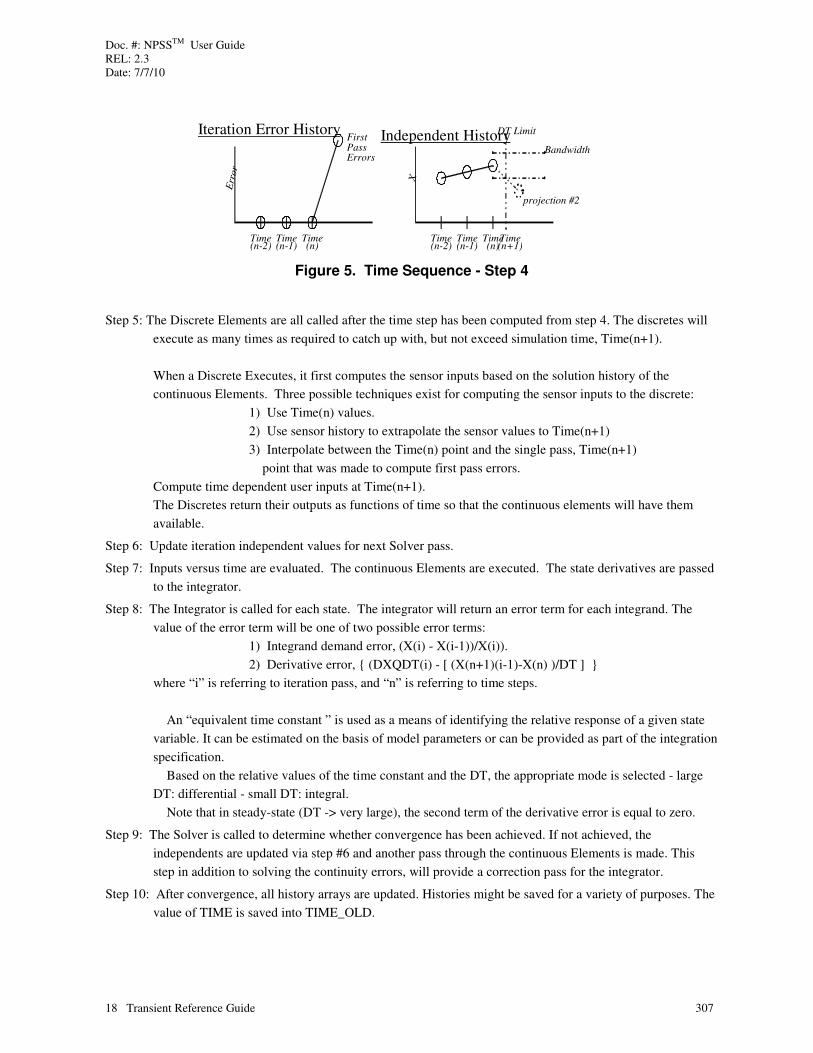
Doc. #: NPSSTM User Guide REL: 2.3 Date: 7/7/10
18 Transient Reference Guide 307
TimeTimeTime(n-1)(n-2) (n)
Independent History
Time(n+1)
Bandwidth
projection #2
DT Limit
X
Iteration Error History
TimeTimeTime(n-1)(n-2) (n)
Err
or
FirstPassErrors
Figure 5. Time Sequence - Step 4
Step 5: The Discrete Elements are all called after the time step has been computed from step 4. The discretes will
execute as many times as required to catch up with, but not exceed simulation time, Time(n+1).
When a Discrete Executes, it first computes the sensor inputs based on the solution history of the
continuous Elements. Three possible techniques exist for computing the sensor inputs to the discrete:
1) Use Time(n) values.
2) Use sensor history to extrapolate the sensor values to Time(n+1)
3) Interpolate between the Time(n) point and the single pass, Time(n+1)
point that was made to compute first pass errors.
Compute time dependent user inputs at Time(n+1).
The Discretes return their outputs as functions of time so that the continuous elements will have them
available.
Step 6: Update iteration independent values for next Solver pass.
Step 7: Inputs versus time are evaluated. The continuous Elements are executed. The state derivatives are passed
to the integrator.
Step 8: The Integrator is called for each state. The integrator will return an error term for each integrand. The
value of the error term will be one of two possible error terms:
1) Integrand demand error, (X(i) - X(i-1))/X(i)).
2) Derivative error, { (DXQDT(i) - [ (X(n+1)(i-1)-X(n) )/DT ] }
where “i” is referring to iteration pass, and “n” is referring to time steps.
An “equivalent time constant ” is used as a means of identifying the relative response of a given state
variable. It can be estimated on the basis of model parameters or can be provided as part of the integration
specification.
Based on the relative values of the time constant and the DT, the appropriate mode is selected - large
DT: differential - small DT: integral.
Note that in steady-state (DT -> very large), the second term of the derivative error is equal to zero.
Step 9: The Solver is called to determine whether convergence has been achieved. If not achieved, the
independents are updated via step #6 and another pass through the continuous Elements is made. This
step in addition to solving the continuity errors, will provide a correction pass for the integrator.
Step 10: After convergence, all history arrays are updated. Histories might be saved for a variety of purposes. The
value of TIME is saved into TIME_OLD.

Doc. #: NPSSTM User Guide REL: 2.3 Date: 7/7/10
18 Transient Reference Guide 308
Step 11: Call Report Writer. The report writer writes data to reports if it is the correct time to do so. The report
frequency may be controlled by the user in these ways:
-by time frequency (every 0.1 seconds)
-by number of time steps, (i.e. every5 time steps, write output)
-by discrete time specification (at 1.1 seconds, 1.7 seconds, etc...)
Step 12: Determine if simulation time has attained the demanded frame time, TF. If so, continue, else loop back
and compute a new proposed time step, “dt”.
Step 13: Determine if simulation time has attained the demanded final time of the simulation.
Figure 6. Time Line
Further explanation of the terms used in Figure 5:
• Discrete Element – A Discrete Element is a special type of Element that performs integrations w.r.t. time, internally in the Element Logic. These element types may Only be Called once, at a given time. (has equations of the form: X=X+DX/DT * DT)
• Synced Discrete – A Synced Discrete refers to a Discrete for which the continuous submodel is forced to compute time accurate inputs. Predictions of actuation and sensors, at times when they haven’t been computed, are provided by default.

Doc. #: NPSSTM User Guide REL: 2.3 Date: 7/7/10
18 Transient Reference Guide 309
• UnSynced Discrete – An UnSynced Discrete refers to a Discrete Element for which the continuous submodel is NOT forced to compute time accurate inputs. UnSynced Discretes use out-of-date inputs (this speeds up execution). The maximum latency of Discrete sensor input data is controlled by the Maximum Continuous DT input.
• Continuous Element – A Continuous Element is one that assumes all Integrands with respect to time, X, are passed into the Element as input. These Elements generate derivatives of the integrand w.r.t. time (has equations of the form: DX/DT = F(X)). For Steady-state, the external Solver will drive X until DX/DT = 0. For Transient, the external integrator will force X to be the integrand of DX/DT, integrated with respect to time.
• Maximum Continuous DT – A maximum allowed time step for the continuous elements forces a time step to occur, even if the time management routines don’t think one is needed.
• Minimum Continuous DT – The Solver will error out if the time step reduces below the minimum time step without a solution.
15.1.4 Independent variable predictions An important part of the transient solution process is the prediction of independent values of the model for future values of time based on known past values. Three predictor methods are provided with the NPSS: NONE, LINEAR, and LAGRANGE. The choice of method is selected by the user by setting the predictorMethod attribute. Each method is described in greater detail below. In each of these expressions, the subscripts represent the time-step, and the nth time step is the one for which predictions are being generated.
15.1.4.1 No Predictor Extrapolation
When the predictorMethod is set to NONE, the predictor value is set to the independent value on the previous time-step.
x xn n=
−1 (1)
15.1.4.2 Linear Predictor Extrapolation
When the predictorMethod is set to LINEAR, the predictor value for each independent is set according to the expression
x xx x
t tt tn n
n n
n n
n n= +−
−−
−
− −
− −
−1
1 2
1 21* ( )
(2)
15.1.4.3 Lagrange Predictor Extrapolation
When the predictorMethod is set to LAGRANGE, the independent predictions will be expressed in terms of a three point Lagrange polynomial technique. This is a standard technique for making extrapolations with arbitrarily spaced data observations. By saving a three point history of times and independent value observations within the predictor, good predictions can be made with the Lagrange formula.
The three point Lagrange extrapolation formula for a given independent, x, is:
x x P x P x Pn n n n n n n= + +− − − − − −3 3 2 2 1 1* * *
(3)
Where xn indicates independent’s value at the nth time step, and P refers to coefficients that are computed from the time history.
The formula for the three Lagrange coefficients: Pn-3 , Pn-2 , Pn-1 are expressed in terms of the times at which the three x observations were made as well as the time at which xn is desired.

Doc. #: NPSSTM User Guide REL: 2.3 Date: 7/7/10
18 Transient Reference Guide 310
( ) ( )[ ]( ) ( )[ ]
Pt t t t
t t t tn
n n n n
n n n n
−
− −
− − − −
=− −
− −3
2 1
3 2 3 1
*
*
(4a)
( ) ( )[ ]( ) ( )[ ]
Pt t t t
t t t tn
n n n n
n n n n
−
− −
− − − −
=− −
− −2
3 1
2 3 2 1
*
*
(4b)
( ) ( )[ ]( ) ( )[ ]
Pt t t t
t t t tn
n n n n
n n n n
−
− −
− − − −
=− −
− −1
3 2
1 3 1 2
*
*
(4c)
It is useful to note that for equally spaced time values(i.e. constant time increment), the three Lagrange polynomial values will be 1, -3 and 3 respectively.
15.1.4.4 Limits on Predicted Values
Setting the Independents to the predicted values and running the model entail some risk since no constraint checking is done on the predicted values before the model is executed. It is therefore possible that the predicted values are outside the range of valid values for the model, such as negative areas or pressures. The simulation may not be able to recover if it is run with the predicted values. To protect against this, attributes are available in the Independent objects that allow a minimum and maximum range to be defined. (See 14.2.2). If a predicted value is passed to the Independent, the Independent will limit the predicted value to the limit value.
15.1.5 Time Step Computation There are three basic reasons for adaptive time stepping in a transient simulation:
1. Synchronize model execution with discrete time requirements.
2. Improve model transient accuracy.
3. Improves the overall computational performance of the simulation by allowing the time increment to increase when possible.
All three factors must be considered when selecting the next simulation time for the model. A time line is shown in Figure 5 illustrating the various factors in computing the time increment. The process of adaptive time-stepping and model execution is described in detail is section 15.1.3.1 above, and is also depicted in Figure 5.
15.1.5.1 Adaptive Time Stepping.
The following expression can be used to compute a new time increment, based on an allowed change in the solver independent values, as set by the user. This expression may increase (expand) or decrease (reduce) the time increment.
( )dt
dt
dx
dxTranLimit
adapted
current
i
i predicted
i
=
max
(5)
The following process is used to determine how dtadapted is used.

Doc. #: NPSSTM User Guide REL: 2.3 Date: 7/7/10
18 Transient Reference Guide 311
1. If dtadapted is greater than current dtcurrent (i.e. if the time increment is being expanded), it may not be necessary to make another predictor pass to test the expanded time increment. The value of dtcurrent may be used on is step instead, if the following condition is satisfied.
dt dtExpandFactor dtcurrent adapted≥ * (6)
The user can control this decision by setting the value of dtExpandTolerance. In this case, the dtadapted will be used to set the dtbase in the next time-step.
dt dtbase adapted= * dtRelaxFactor (7)
The dtRelaxFactor is intended to help ensure that the dt used in the next predictor pass will be small enough to avoid another time-step reduction.
2. If dtadapted is greater than current dtcurrent (i.e. if the time increment is being expanded), but the condition in Error! Reference source not found. is not satisfied, dtcurrent may still be used for the current time-step if dtadapted exceeds dtforce or dtmax . In that case, the dtbase for the next time-step will be set according to the appropriate limit.
If dtadapted > dtforce , then
dt dt dtbase force current= −
(8)
If dtadapted < dtforce but dtadapted > dtmax , then
dt dtbase = max (9)
The user may specify the value of dtmax (maxTimeStep)
If dtadapted < dtforce and dtadapted < dtmax , then another predictor iteration is required and control is passed to step 5 below.
3. If dtadapted is less than dtcurrent (i.e. the time inclement is being reduced, then dtmin is used for the current time-step if the following condition is satisfied:
dtdt
current ≤min
dtRelaxFactor (10)
The value of dtbase for the next time-step is also set equal to dtmin The user may set a value for the dtmin (minTimeStep).
4. If dtadapted is less than dtcurrent (i.e. the time inclement is being reduced), and Error! Reference source not
found. is not satisfied, then another predictor iteration is required and control is passed to step 5 below.
5. The values of dt (see section 15.1.3.1) and dtbase are set according to Error! Reference source not found. and the process repeats at step 2 in section 15.1.3.1 above.
dt dt
dt dt
adaptive
base adaptive
=
=
dtRelaxFactor
dtRelaxFactor
*
*
(11)

Doc. #: NPSSTM User Guide REL: 2.3 Date: 7/7/10
18 Transient Reference Guide 312
15.1.5.2 Handling Synchronized Time-Discrete
An NPSS Model may include objects that must be executed at specific times. These are referred to here as synched
time-discrete objects. An Elements which contains digital control logic is one example. During the initialization of the Transient Executive, the synched time-discrete objects in the Model are identified. At each time-step, the Transient Executive must query the synched time-discrete objects to determine the next simulation time required (the earliest of all times indicated by the discrete elements). This defines the value of dtforce (as used in section 15.1.3.1 above). If the simulation is about to step past a synched time-discrete request, the dt is reduced so that the model will execute at the proper time.
15.1.5.3 Handling Unsynched Discrete Elements
Unsynched time-discrete objects are those which perform time-dependent operations (such as integration) internally. These model objects use input values from the predictor pass of the top-level assembly to compute their own internal behaviors over the entire top-level time-step.
Before the unsynched discrete elements can be run, the proper time step for the model must first be determined as described in section 15.1.3.1 above. The time-discrete objects will not be execute during the predictor passes required to determine the proper time step. In the process of determining the time-step, the time-continuous model elements are executed and their output can be used to predict input values to the time-discrete objects. If an unsynched time-discrete object has a time increment smaller than that of the top-level assembly, it may execute several points for each top-level time-step. All required internal time-steps are executed on the first iteration of the corrector convergence process (for the top-level Assembly). These objects are executed only on this pass, and should be placed in the preExecutionSequence of the Model. It is desirable to have control elements run first, for example, so that their output values will be available to the system for the current time-step.
Since the discrete control elements generally require sensor inputs from the model, predictions of these parameter values are required at each discrete time where the elements must run. These sensor values may be predicted in three ways:
1. Use sensor values from the previous converged time-step (at tn-1) for all internal sub-steps.
2. Extrapolate sensor values from a time-history of the last k converged solutions (tn-k through tn-1).
3. Interpolate sensor values between the previous converged time-step solution (at tn-1) and the predictor pass values (at tn).
It is important to point out here, however, that the choice of sensor-prediction methods and the storage of time-histories for option 2 is the responsibility of the individual time-discrete elements. This function is not performed by the Solver or Transient Executive. The iteration over multiple discrete element cycles is done within the discrete elements themselves and do not require separate calls from the system or solver software.
15.1.6 Utility Functions Certain optional utility functions have been identified that are not required in the Transient Executive source code, but which might be valuable to the users, for inclusion in their user-defined functions. Utility functions are built-in; they are compiled C++ rather than being interpreted by the NPSS. The functions are built in because they perform operations (such as sorting through arrays of pointers to other objects) which do not lend themselves to interpreted code.
The Transient Executive employs user-defined function for conditional report updates, conditional run termination, and adaptive time-stepping. The following utility functions have been identified as potentially useful.

Doc. #: NPSSTM User Guide REL: 2.3 Date: 7/7/10
18 Transient Reference Guide 313
15.1.6.1 Transient Run Quiescence Utility Function
This utility determines whether a transient run has come to a quiescent (steady) state. It does this by comparing the value of the expression
( )dxdt
x
n
n
*τ
(12)
with the user-defined threshold attribute (quiescenceTolerance). If this quantity is below the set threshold for all states on two consecutive time-steps, the quiescence conditions is considered TRUE.
15.1.7 TransientExecutive Functions The following are Transient Executive functions:
int quiescence ();
Returns TRUE (1) if the state integrators satisfy the quiescence criteria (see Section 18.1.6).
int testRunTermination ();
Returns TRUE if the transient terminateCondition is satisfied, returns FALSE otherwise.
real computeTimeStep ();
Computes the correct time increment for the next time-step, using whatever method the user has specified in transient timeStepMethod attribute.
void clear ();
Resets all solver dependent error tolerances to their steady-state solution values, puts all explicitly integrated states back in the solver, and clears the lists of pointers which the TransientExecutive keeps for the model.
void doExplicitInteg ();
Updates states associated with all explicit Integrators, based on the current time-step value.
void initializeHistory ();
Sets all independent predictor histories to the current independent values. Initializes histories for all state
Integrators. As an alternative the attribute forceInitializeHistory has been added to the transient solver. Setting this flag to TRUE will cause histories to be initialized at the top of the first time step of the next transient run. As such it represents a replacement to calling this function between two transient runs to force initialization so that the history vectors don’t carry over.
void predictorPass(real predictTime);
Performs a predictor pass on all Independents in the model. This updates the currentValue in the associated histories kept by the TransientExecutive object.
void run();
Runs a transient simulation. This function is not usually required, since the normal system run command typically invokes this function anyway.
int runTimeDiscretes(real prevTime, real nextTime);
Calls the runDiscreteCalcs function on the parent assembly, which sends that message to all objects contained in that assembly in turn. The previous and next (predicted) values of time are passed into this function through the argument list. This function should return TRUE if inputs to the model have been changed, FALSE otherwise.

Doc. #: NPSSTM User Guide REL: 2.3 Date: 7/7/10
18 Transient Reference Guide 314
Normally this function is called before the predictor pass on each time-step in a transient simulation. Predictor passes will, however, be run before this function is called if the adaptive time-stepping option is enabled.
void setup();
Obtain all required configuration information from the Solver and set up the Transient internal data structures accordingly.
void synchTimeDiscretes();
Query all Model objects for their next required execution time. Only time-discrete objects will return limiting values for the next time value. This function sets the dtForce attribute in the TransientExecutive.
All of the above messages must be sent to the TransientExecutive object, which has the name "transient" by default for any given assembly.
nextTime = currentTime + transient.computeTimeStep();
transient.predictorPass(nextTime);
// etc.
15.1.7.1 Example
The following function illustrates how the above functions might be used to create an alternative transient simulation process.
// the initializeHistory message propagates throughout model.
initializeHistory();
int terminate = FALSE;
// begin loop over time.
do {
// increment time, using transient's time-step algorithm
time = time + transient.computeTimeStep();
// must run pre-solver sequence specifically (using function
// defined previously) since solver does not run that sequence
// automatically in TRANSIENT mode.
runPreSolverPass();
// run a single converged point for the current time.
solver.run();
// update the transient histories (propagates throughout model).
// includes updates to DataViewers.
updateHistory();
terminate = transient.quiescence();
} while ( (time < transient.stopTime) &&
(!terminate) );
15.1.8 Transient User Input Attributes
baseTimeStep = 0.05;
The default timeStep selected by the user (the value set by the user may be altered by the Transient Executive as required during the simulation).
dtExpandTolerance = 0.30;
The minimum fraction that the current dt may have, relative to the adapted dt (the new dtbase), in order to be used on the current time-step.
Doc. #: NPSSTM User Guide REL: 2.3 Date: 7/7/10
18 Transient Reference Guide 315
dtRelaxFactor = 0.90;
The fraction of the adapted dt to be used in the next adaptive iteration or for the next step's dtbase. Used to ensure that the next time step reduction will be sufficiently small, allowing for non-linearities.
dxTransLimit = 0.10;
Maximum allowed change in each Solver independent over a given time increment (for adaptive time stepping). This attribute is different from the Solver dxLimit, which is the maximum allowed independent change for any given Solver convergence iteration.
dxTransLimitType = "FRACTIONAL";
Option which determines whether dxTransLimit is taken as an absolute or fractional value.
explicitIntegOrder = "BEFORE";
This attribute still exists, but is no longer has any impact on the simulation.
extraIndepUpdate = FALSE;
When TRUE, an additional update will be made to the independents (though not set in the model). This makes the predictor for the next pass more accurate, especially when the toleranceScaleFactor is greater than 1.0.
forceInitializeHistory = FALSE;
Set by the User between two back-to-back transient runs when it is not desireable to carry over history from one transient run to the next. Setting this attribute represents an alternative to calling the initializeHistory() function between runs. Calling the initializeHistory function is still valid. After initializing the history vectors at the top of the first time step, the transient solver sets this flag back to FALSE. Thus it will have to be set to TRUE before each transient run where the history vectors are to be initialized. Note that this flag does not affect the required initializations that are automatically performed any time the solutionMode changes. Any time the solutionMode changes, all histories are initialized before starting a transient run.
frameRate = 50;
The maximum number of millisecs allowed for iterations that can be run on a transient point. If the max limit is hit, the solver will assume convergence and move on to the next point.
initialized = 0;
Integer flag that indicates whether or not the TransientExecutive has been initialized. If FALSE (0), the TransientExecutive and the Model will be re-initialized and the value will be set to TRUE(1). You can use the clear() function to reset this attribute to zero.
integErrorForm = "INTEGRAL";
The form of the integration error to be used by the Solver. Valid options are INTEGRAL, DIFFERENTIAL and VARIABLE.
integrationType = "GEAR_1P
STP_ORDER";
The default integration method for all states in the system. The user may override this default by setting the integrationType attribute on each NCPStateIntegrator object individually. Valid options are GEAR_1P
STP_ORDER,
GEAR_2PNDP_ORDER, TRAPEZOIDAL, and EULER.
maxIterations = 5;
The maximum number of iterations that can be run on a transient point. If the max limit is hit, the solver will assume convergence and move on to the next point.
maxTimeStep = 1.000;
The maximum time step allowed in adaptive time stepping.
minTimeStep = 1.00e-04;
The minimum time step allowed in adaptive time-stepping.

Doc. #: NPSSTM User Guide REL: 2.3 Date: 7/7/10
18 Transient Reference Guide 316
predictorMethod = "LINEAR";
The method used to estimate the independent values on the predictor pass of each time-step. Options are NONE, LINEAR, and three-point LAGRANGE.
quiescenceTolerance = 0.01;
The maximum allowed value of (dx/dt * time-constant) (expressed as a fraction of the state value) for each state to be considered quiescent (steady with respect to time).
stopTime = 10.00;
The default finish time for a transient simulation (this value may not be reached if user-defined run-termination conditions are met during the simulation). This value MUST be entered, or an exception will be thrown. The default is zero (no run).
terminateCondition = "quiescence()";
User-defined integer expression used to determine whether the current transient run should terminate. If this expression returns TRUE, the run will terminate. The default is blank (no conditional termination, runs to stopTime).
time = 0.0000;
The current time for a transient simulation (the input value is used as the start time and is updated by the Transient Executive during the simulation).
timeStepMethod = "CONSTANT_DT";
Desired method of computing the time-increment on each point of the transient run. Valid options are CONSTANT_DT, ADAPTIVE, and USER_DEFINED. *Users should note that setting this attribute to ADAPTIVE will cause predictor passes to be performed BEFORE the runTimeDiscretes function is called. This may be undesireable for the logic of some control elements that are predicated on being the very first calculations to run on any given time-step.
toleranceScaleFactor = 1.0000;
The multiplicative factor by which the convergence tolerances are loosened for transient solutions (as compared to steady-state solutions).
userTimeStepFunction = "mySteppingFunction()";
User-defined real expression (entered as a string) used to compute the time-increment for each point in the transient run. Used only when timeStepMethod is set to USER_DEFINED. The default is blank (there IS no default).
discreteCalcsOrder = "BEFORE"; Determines whether the time discrete calculations are run prior to running the continuous portion of the model or after. The switch is set to BEFORE as a default. If the switch is set to AFTER then the associated functions preTimeDiscretes(), runDiscreteCalcs(), and postTimeDiscretes() will all be run after the final explicit integrations but before updateHistory(). See the Developers Guide for a further description of these functions.
15.1.9 Transient Output (Calculated) Attributes
dtForce
The time-step calculated from time-discrete object requests in the Model.
initialized
A Boolean flag (1 or 0, TRUE or FALSE) which indicates whether the TransientExecutive and the objects it controls have been initialized (including their transient histories). Setting this attribute to zero will have the same
effect as the initializeHistory function overall.

Doc. #: NPSSTM User Guide REL: 2.3 Date: 7/7/10
18 Transient Reference Guide 317
stopFlag
A Boolean flag (1 or 0, TRUE or FALSE) which is set to the results of testRunTermination from within the run function.
timeStep
Depending on the baseTimeStep set by the user, the adaptive time-stepping algorithm, and synchronization with time-discrete objects in the Model, the actual timeStep at any given point in the simulation is calculated.
15.2 Integrator (NCPStateIntegrator class) The Integrator class is derived from the Dependent class; it has the same functions and attributes as the Dependent class, but behaves differently when running in transient mode.
15.2.1 Creating an Integrator The minimum required information to define an Integrator is shown below.
Integrator Tintegrator_nameT {
stateName = "Tstate_variable_name_in_modelT";
derivativeName = "Tstate_derivative_name_in_modelT";
eq_lhs = "Texpr_for_lhs_of_steady-state_equalityT";
eq_rhs = "Texpr_for_rhs_of_steady-state_equalityT";
}
An example of an Integrator definition is as follows.
Integrator ShaftInertia {
stateName = "HP_SHAFT.Nmech";
derivativeName = "HP_SHAFT.dNqdt";
eq_rhs = "HP_SHAFT.trqIn";
eq_lhs = "HP_SHAFT.trqOut";
integrationType = "TRAPEZOIDAL";
}
Integrators are added to the solver as Dependents (there is no addIntegrator function in the solver).
solver.addDependent ("Manifold Pressure"); // can use addDependent
// because it is a kind of
// dependent
// (etc.)
15.2.2 Implicit Integration Implicit integration refers to a predictor-corrector method. Some integration methods, such as Gear and Trapezoidal, depend on knowing the state derivatives at the new time point. This derivative may, itself, depend on the value of the state at the new time (for example, the time-derivative of shaft speed depends on the net torque exerted on the shaft, but the torques produced by the various components depend on the speed). To resolve this circular dependence, the state independent parameters are varied until their values are consistent with the values of the state derivatives, integrated over the current time-step. This iterative process is handled by the Solver in a manner similar to algebraic balances. The predictor passes discussed previously determine an estimate for the state independent variables at the new time (tn). The corrector errors are defined (as described below) such that when they are zero, the states values will be consistent with the derivative values and integrator method used. The Solver controls the corrector iterations by which the corrector errors are driven to within a specified tolerance of zero.
In a transient simulation, the model computes the state derivative values, as well as a characteristic time-constant for the state. A generic expression for time-constant can be calculated using the expression

Doc. #: NPSSTM User Guide REL: 2.3 Date: 7/7/10
18 Transient Reference Guide 318
( )τ =
−x
dxdt
y y
y*
( )1 2
1
(13)
In this expression, x is the state value, y1 and y2 are the values of the dependent parameters which would be used to compute steady-state error (torquein and torqueout when x is the shaft-speed state, for example).
Transient models may also be run in a steady-state mode (in order to set the initial conditions for a transient run, for example). The error terms for a steady-state run are not the same as for a transient simulation, as described above. In principle, it is possible to find the steady-state condition by driving the derivative values to zero (the derivative value itself would be the error in this case). In general, however, finding the steady-state solution by driving the derivatives to zero is discouraged. Instead, the component developer should define a dependent equality between two parameters which should be enforced at a steady-state condition. For example, instead of driving the derivative of the shaft speed to zero, the steady-state solver should drive the input torque and output torque from the shaft to be equal. Of course, this condition is physically equivalent to a zero shaft speed derivative, but it is generally better in terms of solver convergence to choose a dependent equality in which neither side is zero. The steady-state dependents must therefore be chosen on a case-by-case basis (there is not standard form as described for integrators above).
The implicit integration methods supported by the NPSS are described below. Each state variable can be independently assigned a different integrationType.
15.2.2.1 Trapezoidal Integration
When used as a corrector, it's also known as the Modified Euler formula. It assumes a linear variation in the state derivative with respect to time. Integration formulae that employ past state variable derivatives introduce a spurious lead effect into the response of the model which can be shown using the z-transform analysis. When the time increment employed is large compared to the response of the state variable, an oscillatory response is noted that is eliminated when either the Gear 1st- or 2nd-order formula is used. Trapezoidal integration uses the average of the state derivatives at the previous time (tn-1) and current time (tn).
dtdt
dx
dt
dxxx
tdtttdtt ∗
++=
++
2
1 (14)
15.2.2.2 Gear First-Order Integration
The 1st order Gear integration method, sometimes refered to as the “backwards Euler” method, is the best from a warranty standpoint. Although less accurate than the 2nd order method (next section), it does not share the stability properties of the higher order methods. The continuous and discrete stability domains are the same for this formula regardless of the size of the time increment. Gear’s first-order integration method uses only the new state derivatives (at tn).
dtdt
dxxx
dtttdtt ∗+=
++ (15)
15.2.2.3 Gear Second-Order Integration
The 2nd order Gear integration method is the best multi-point compromise, at least for implicit applications. Its weakness is that there is a small region near the imaginary "z" axis and the origin of the z-plane trajectory where "false" stability can occur. This means that for small (or negative) damping ratios and large time increments, a model can appear stable when the response of the real system would oscillate or diverge. At smaller time steps, the

Doc. #: NPSSTM User Guide REL: 2.3 Date: 7/7/10
18 Transient Reference Guide 319
correct (oscillatory or divergent) response is obtained. Therefore, when a new model is created, it is important to explore the potential for significant error by running a few test cases at time increments small enough to uncover unstable parasitic effects.
dtdt
dx
dt
dxxx
tdtttdtt ∗
++=
++
3
1
3
2 (16)
15.2.3 Explicit Integration Although implicit integration methods may improve the stability and accuracy of a transient simulation, closing the corrector error requires additional Solver iterations that may significantly impact the computational performance of the simulation overall. When the transient behavior is relative linear and well-behaved in time, explicit integration methods may offer an alternative which is less computationally intensive. Explicit integration methods do not include derivative values at the new time-step, and therefore do not require an iteration with the state values.
Explicit integration of the selected states is performed at the same point as the predictor passes.
The user may which select states (none, some, or all states in the Model) are to be explicitly integrated. Explicit integration does not require the Solver to close an error term between the state and its derivative. Thus when an Integrator is set to Euler Integration, a search is made to locate a matching Independent. When one is found, the Integrator and the Independent are removed from the list of Independents and Dependents used in the iterative solution.
The Euler explicit integration method is supported in the NPSS software. NPSS does limit which Integrators can be set to Euler Integration. To switch a given Integrator to use Euler, a state substitution variable must not be used (See Section 15.2.8 for more information). The practical impact is that there must be an Independent in the current solver setup with a varName attribute that points directly to the same model variable that is referenced by the stateName attribute of the Integrator being set to Euler. This is an indirect indication that the underlaying model calculations are structured to use the state variable value directly as input, rather than using another variable as input and then calculating the state value from the input value. The latter is the case when a state substitution variable is used as the Independent.
15.2.3.1 Euler Integration
Euler integration uses the state derivative value from the beginning of the time-step to predict the state value at the end of the time step.
dtdt
dxxx
ttdtt ∗+=
+ (17)
15.2.4 Integrator Functions
The Integrator has the same functions as the Dependent class.
Note: When you add an integrator to the solver configuration, use the addDependent function. For example,
solver.addDependent("ShaftInertia");
Similarly, the removeDependent function is used to remove an integrator from the solver.

Doc. #: NPSSTM User Guide REL: 2.3 Date: 7/7/10
18 Transient Reference Guide 320
15.2.5 Integrator Input Attributes In addition to those which it inherits from the Dependent class, the Integrator has the following attributes:
Table 62. Integrator Input Attributes
Attribute Name Type Description Default Value derivativeName string Name of a variable holding the current value of the
time derivative of the variable named by stateName.
""
desiredDerivValue real The value of the derivative to be matched by the Solver when the local solutionMode is set to "SET_DERIVATIVE."
0.0000
eq_RefTransient string Expression evaluated only during a transient run that yields a value of yRef. If an expression is not given, then the expression in eq_Ref is used during transient as well as steady-state operation. And if eq_Ref is not given, then eq_rhs is used to determine yRef, and finally if eq_rhs is zero or evaluates to zero, a yRef of one is used.
“”
integrationType Option variable
Integration method for this integrator. Different integrators in the same system can use different integration methods. Allowable values are
"GEAR_1P
STP_ORDER", "GEAR_2P
NDP_ORDER",
"TRAPEZOIDAL", which are implicit methods, and
"EULER" which is an explicit method. If unset, the default set in the TransientExecutive is used. It
defaults to "GEAR_1P
STP_ORDER".
Transient.
IntegrationType
stateName string Name of the variable whose time-varying value is to be determined by integrating the derivative specified
by derivativeName.
""
timeConstantExpr string An expression used to calculate the state's time-constant (tau). If not set, the time-constant is computed internally (refer to the Transient E-Spec document for more information regarding the internally used expression).
“”
15.2.6 Locking Attributes for Integrator The SolverExecutive sets some attribute default values for each of its associated integrators. If you specifically set one of these attributes in an integrator, the default value will be ignored. In addition to those inherited from the Dependent, the Integrator has the following additional lock attributes
When the corresponding attribute is set for a specific independent, the lock parameter is set to TRUE. When you want the default to be used again, you should set the corresponding lock attribute to FALSE again.
Note: The default value for all the "lock" variables below is FALSE.

Doc. #: NPSSTM User Guide REL: 2.3 Date: 7/7/10
18 Transient Reference Guide 321
Table 63. Integrator Locking Attribute
Attribute Name Description
lockIntegrationType An attribute that determines whether the TransientExecutive's default integrationType will overwrite the current value. When lock is TRUE, the default will NOT overwrite the current value.
15.2.7 Integrator Output (Calculated) Attributes In addition to those which it inherits from the Dependent class, theIntegrator has the following output attributes.
Table 64. Integrator Output Attributes
Attribute Name Description
derivative The value of the state derivative computed by the Model.
state The value of the state variable (set by Solver).
stateDemand The value of the state variable calculated by the Integration equation.
timeConstant The current value of the state's time-constant.
15.2.8 State Substitution Variables In some cases, it is advantageous for the Solver to control a model independent variable other than the state variable itself. Consider a compressible gas volume, for example. The state variable for the gas is usually the density, whose time-derivative depends on the difference between the flows entering and leaving the volume. The flows, in turn, are dependent on the pressure of the volume, not the density. In this case, it would be easier to have the Solver control the volume pressure as the Independent, using this input to compute the volume density (state value) and the flows affecting the volume. In this case, therefore, the pressure is the Independent while the density is still the state whose derivative is referenced by the Integrator. By keeping the state Integrator and Independent separate, the NPSS makes this easy to setup.
Independent pressIndep {
varName = "volume.Pt";
}
Integrator densInteg {
stateName = "volume.density";
derivativeName = "volume.dRHOdt";
eq_lhs = "volume.Fl_I.W";
eq_rhs = "volume.Fl_O.W";
integrationType = "GEAR_2P
NDP_ORDER";
}
The only potential problem that this sort of state substitution presents is when an explicit integration method is desired. In such cases, the state itself is typically updated. In the example above, there is no easy way to update the pressure based on integrating the density. This should be taken into account when deciding whether state-substitution will be used in a model.

Doc. #: NPSSTM User Guide REL: 2.3 Date: 7/7/10
18 Transient Reference Guide 322
15.3 Example Program The following First Order Lag test program demonstrates the functions and attributes discussed in sections 15.1 and 15.2, above.
15.3.1 Model File
// First Order Lag Model
// for testing the NPSS Tranient capability
//
class InterpLag extends Element {
real x, dxdt, y, tau, localTime;
void calculate() {
dxdt = (y-x) / tau;
}
}
// analytic recursion relation for a "clamped ramp"
// to be run in the ExecutionSequence and compared to the
// implicit solution.
class AnalyticFOL extends Element {
real x, y, tau;
void calculate() {
x = y * (1.000 - (tau/timeStep)*exp(-time/tau)*(exp(timeStep/tau)-1.000));
}
}
Element InterpLag myLag { }
Element AnalyticFOL benchMark {
real theError;
void postexecute() {
theError = myLag.x - x;
}
}
OutFileStream myTransOut { filename = "cout"; append = TRUE; }
DataViewer VarDumpViewer dumper {
variableList = {"myLag.*", "solver.*", "xInteg.*", "xIndep.*"};
outStreamHandle = "myTransOut";
}
DataViewer CaseRowViewer transOut {
titleBody = "Transient Output for First-Order-Lag model";
titleVars = {};
pageWidth = 0;
pageHeight = 0;
if (getenv("NPSS_CONFIG") == "nt"){
variableList = {"time", "solver.iterationCounter: ???? = iters",
"solver.numJacobians: ???? = Jacobians",

Doc. #: NPSSTM User Guide REL: 2.3 Date: 7/7/10
18 Transient Reference Guide 323
"solver.numBroydens: ???? = Broydens",
"myLag.y: ??.?????", "myLag.x: ??.?????",
"myLag.dxdt: ??.?????", "benchMark.x: ??.????",
"benchMark.theError : ???.????E???? = benchMark.error"};
}
else {
variableList = {"time", "solver.iterationCounter: ???? = iters",
"solver.numJacobians: ???? = Jacobians",
"solver.numBroydens: ???? = Broydens",
"myLag.y: ??.?????", "myLag.x: ??.?????",
"myLag.dxdt: ??.?????", "benchMark.x: ??.?????",
"benchMark.theError : ???.????E??? = benchMark.error"};
}
outStreamHandle = "myTransOut";
}
Independent xIndep { varName = "myLag.x"; }
Integrator xInteg {
stateName = "myLag.x";
derivativeName = "myLag.dxdt";
eq_rhs = "myLag.y";
eq_lhs = "myLag.x";
}
solver.addIndependent("xIndep");
solver.addDependent("xInteg");
executionSequence = {"myLag"};
postExecutionSequence = {"benchMark", "transOut"};
15.3.2 First Order Lag Test File
#include "FirstOrderLag.mdl"
// create a function that will reset the model to initial conditions.
void resetModel ()
{
// reset the input and run once to reset the derivative (output)
myTransOut << "\n\nRun a ONE_PASS to reset derivative in model\n";
myLag.x = 0.0000;
time = 0.0000;
setOption("solutionMode", "ONE_PASS");
run();
transOut.reset();
setOption("solutionMode", "TRANSIENT");
initializeHistory();
// force it start with a new matrix
solver.forceNewJacobian = TRUE;
}
// create an element for setting the input step function.
class Input extends Element{
real stepTime, stepVal, outputVal;
void calculate() {
if (time <= stepTime)

Doc. #: NPSSTM User Guide REL: 2.3 Date: 7/7/10
18 Transient Reference Guide 324
{
outputVal = 0.0000;
}
else
{
outputVal = stepVal;
}
}
}
// create an instance of the input element
Element Input yInput {
stepVal = 5.0;
stepTime = 0.00;
void postexecute() { myLag.y = outputVal; }
}
// put the input element in the preExecutionSequence.
solver.executionSequence.remove("yInput");
solver.preExecutionSequence.append("yInput");
// set initial conditions
myLag.x = 0.0000;
myLag.tau = 0.5;
benchMark.x = 0.0000;
benchMark.tau = 0.5;
benchMark.y = yInput.stepVal;
// set the independent reference value (since x starts from zero).
xIndep.indepRef = "1.00";
// set up the baseline transient run options
setOption("solutionMode", "TRANSIENT");
transient.stopTime = 2.5000;
transient.baseTimeStep = 0.025;
// set the debug options so we can track the number of passes,
// etc. in the transient run.
solver.debugLevel = "NONE";
// optional settings to improve convergence
//solver.toleranceBroydenScalar = 1.e-10;
// Test 1.1 Baseline run to quiescence
myTransOut << "======================================================="
<< "\n TRANSIENT TESTS WITH IMPLICIT FIRST-ORDER LAG MODEL "
<< "\n======================================================="
<< "\n\nTest 1.1 Baseline Case - run to quiescence "
<< "\n(dt = 0.025)"
<< "\n--------------------------------------------\n";
//cout << "Test 1.1\n";
transient.terminateCondition = "quiescence()";
run();
//update transient output report;
myTransOut << "\n"; transOut.display();
// Test 1.2 Run Steady-state point w/o resetting
myTransOut << "\n\nTest 1.2 Run Steady-state point w/o resetting"
<< "\n-----------------------------------------------\n";

Doc. #: NPSSTM User Guide REL: 2.3 Date: 7/7/10
18 Transient Reference Guide 325
//cout << "Test 1.2\n";
setOption("solutionMode","STEADY_STATE");
run();
dumper.display();
transOut.reset();
// Test 1.3 Reset initial conditions and run to an x=.632 * 5.0
myTransOut << "\n\nTest 1.3 Reset initial conditions and run to an x=.632 *
5.0"
<< "\n-----------------------------------------------------------
---\n";
//cout << "Test 1.3\n";
resetModel();
transient.terminateCondition = "myLag.x > (0.632 * yInput.stepVal)";
myTransOut << "\n\n Now run transient ...\n";
run();
myTransOut << "\n"; transOut.display();
transient.terminateCondition = "quiescence()";
// Test 1.4 Run Steady-state point w/o resetting
myTransOut << "\n\nTest 1.4 Run Steady-state point w/o resetting"
<< "\n-----------------------------------------------\n";
//cout << "Test 1.4\n";
setOption("solutionMode","STEADY_STATE");
run();
dumper.display();
transOut.reset();
// Test 3.1.3 - Run with different time-step
myTransOut << "\n\nTest 3.1.3 - Run baseline with dt = 0.05\n"
<< "-------------------------------------------------\n";
//cout << "Test 3.1.3\n";
resetModel();
transient.baseTimeStep = 0.05;
run();
myTransOut << "\n"; transOut.display();
// Test 3.3 - run with adaptive time-stepping on
myTransOut << "\nTest 3.3 run 1.1 with timeStepMethod = ADAPTIVE\n"
<< "-------------------------------------------------\n";
//cout << "Test 3.3\n";
resetModel();
transient.baseTimeStep = 0.025;
transient.timeStepMethod = "ADAPTIVE";
run();
myTransOut << "\n"; transOut.display();

Doc. #: NPSSTM User Guide REL: 2.3 Date: 7/7/10
18 Transient Reference Guide 326
// Test 3.4.1 - change min and max time steps
myTransOut << "\nTest 3.4.1 - set minTimeStep = 0.02; and maxTimeStep =
0.05\n"
<< "------------------------------------------------------------
\n";
//cout << "Test 3.4.1\n";
resetModel();
transient.baseTimeStep = 0.025;
real oldMin = transient.minTimeStep;
real oldMax = transient.maxTimeStep;
transient.minTimeStep = .02;
transient.maxTimeStep = 0.05;
run();
myTransOut << "\n"; transOut.display();
transient.minTimeStep = oldMin;
transient.maxTimeStep = oldMax;
// Test 3.4.2 - change dxTransLimit and dxTransLimitType
myTransOut << "\nTest 3.4.2 - set dxTransLimit = 0.25 and \n"
<< "dxTransLimitType = ABSOLUTE\n"
<< "------------------------------------------------------------
\n";
//cout << "Test 3.4.2\n";
resetModel();
transient.baseTimeStep = 0.025;
real oldLimit = transient.dxTransLimit;
string oldType = transient.dxTransLimitType;
transient.dxTransLimit = 0.25;
transient.dxTransLimitType = "ABSOLUTE";
run();
myTransOut << "\n"; transOut.display();
transient.dxTransLimit = oldLimit;
transient.dxTransLimitType = oldType;
// Test 3.4.3 - change dtExpandTolerance
myTransOut << "\nTest 3.4.3 - increase dtExpandTolerance by factor of
three.\n"
<< "------------------------------------------------------------
\n";
//cout << "Test 3.4.3\n";
resetModel();
transient.baseTimeStep = 0.025;
real oldTol = transient.dtExpandTolerance;
transient.dtExpandTolerance = 3.0 * oldTol;
myTransOut << " (new dtExpandTolerance = " << transient.dtExpandTolerance
<< ")";
run();

Doc. #: NPSSTM User Guide REL: 2.3 Date: 7/7/10
18 Transient Reference Guide 327
myTransOut << "\n"; transOut.display();
transient.dtExpandTolerance = oldTol;
// Test 3.4.4 - change dtRelaxFactor
myTransOut << "\nTest 3.4.4 - set dtRelaxFactor = 1.0\n"
<< "------------------------------------------------------------
\n";
//cout << "Test 3.4.4\n";
resetModel();
transient.baseTimeStep = 0.025;
real oldRelax = transient.dtRelaxFactor;
transient.dtRelaxFactor = 1.0000;
run();
myTransOut << "\n"; transOut.display();
transient.dtRelaxFactor = oldRelax;
transient.timeStepMethod = "CONSTANT_DT";
transient.baseTimeStep = 0.025;
// run to steady-state as setup for next point.
setOption("solutionMode","STEADY_STATE");
run();
// clear viewers
dumper.reset();
transOut.reset();
// Test 4.3 Run to a SET_DERIVATIVE (for x) of 1.0
myTransOut << "\n\nTest 4.3 Run x to a SET_DERIVATIVE = 1.0"
<< "\n-----------------------------------------------\n";
//cout << "Test 4.3\n";
setOption("solutionMode", "STEADY_STATE");
// override on xInteg alone
xInteg.solutionMode = "SET_DERIVATIVE";
xInteg.desiredDerivValue = 1.0;
run();
dumper.display();
transOut.reset();
myTransOut << "\n\nContinue run from there to quiescence"
<< "\n---------------------------------------\n";
setOption("solutionMode", "TRANSIENT");
initializeHistory();
transient.stopTime = 10.;
transient.terminateCondition = "quiescence()";
run();
myTransOut << "\n"; transOut.display();
// Test 6.2.1 - Run baseline with integrationType = "GEAR_2ND_ORDER"
myTransOut << "\n\nTest 6.2.1 Run baseline case with integrationType"
<< "= GEAR_2ND_ORDER"

Doc. #: NPSSTM User Guide REL: 2.3 Date: 7/7/10
18 Transient Reference Guide 328
<< "\n----------------------------------------------------------------\n";
//cout << "Test 6.2.1\n";
resetModel();
transient.integrationType = "GEAR_2ND_ORDER";
run();
myTransOut << "\n"; transOut.display();
// Test 6.2.2 - Run baseline with integrationType = "GEAR_1ST_ORDER"
myTransOut << "\n\nTest 6.2.2 Run baseline case with integrationType"
<< "= GEAR_1ST_ORDER\n(shoutld be identical to 1.1 results)"
<< "\n----------------------------------------------------------------\n";
//cout << "Test 6.2.2\n";
resetModel();
transient.integrationType = "GEAR_1ST_ORDER";
run();
myTransOut << "\n"; transOut.display();
// Test 6.2.3 - Run baseline with integrationType = "TRAPEZOIDAL"
myTransOut << "\n\nTest 6.2.3 Run baseline case with integrationType"
<< "= TRAPEZOIDAL"
<< "\n----------------------------------------------------------------\n";
//cout << "Test 6.2.3\n";
resetModel();
transient.integrationType = "TRAPEZOIDAL";
run();
myTransOut << "\n"; transOut.display();
// Test 6.2.4.1 - Run basline with integrationType = "EULER"
myTransOut << "\n\nTest 6.2.4.1 Run baseline case to stopTime = 10."
<< "\nwith integrationType = EULER"
<< "\n----------------------------------------------------------------\n";
//cout << "Test 6.2.4.1\n";
resetModel();
transient.clear();
xInteg.integrationType = "EULER"; // this will also lock the attribute
transient.setup();
initializeHistory();
// set the termination criteria to "", since quiescence won't work
transient.terminateCondition = "";
transient.stopTime = 10.0;
run();
myTransOut << "\n"; transOut.display();
// Test 6.2.5.1 - Run baseline with integrationType = "GEAR_2ND_ORDER"
// and baseTimeStep = 2.5

Doc. #: NPSSTM User Guide REL: 2.3 Date: 7/7/10
18 Transient Reference Guide 329
myTransOut << "\n\nTest 6.2.5.1 Run baseline case with integrationType"
<< "= GEAR_2ND_ORDER\nand baseTimeStep = 2.5"
<< "\n----------------------------------------------------------------\n";
//cout << "Test 6.2.5.1\n";
resetModel();
transient.baseTimeStep = 2.5; // must set timeStep in TransientExec after
// initializeHistory is done. Otherwise, the baseTimeStep overwrites it.
transient.maxTimeStep = 3.0; // need to increase max too.
transient.terminateCondition = "";
transient.stopTime = 10.0; // run out to 10 sec.
transient.integrationType = "GEAR_2ND_ORDER";
run();
myTransOut << "\n"; transOut.display();
// Test 6.2.5.2 - Run baseline with integrationType = "TRAPEZOIDAL"
myTransOut << "\n\nTest 6.2.5.2 Run baseline case with integrationType"
<< "= TRAPEZOIDAL\nand baseTimeStep = 2.5"
<< "\n----------------------------------------------------------------\n";
//cout << "Test 6.2.5.2\n";
resetModel();
transient.integrationType = "TRAPEZOIDAL";
run();
myTransOut << "\n"; transOut.display();
// put things back to original condition
transient.baseTimeStep = .025;
transient.maxTimeStep = 1.0;
transient.integrationType = "GEAR_1ST_ORDER";
// Test 6.3.2 - Run basline with extraIndepUpdate = TRUE and
// toleranceScaleFactor = 1.0
myTransOut << "\n\nTest 6.3.2 Run baseline case to quiescence"
<< "\nwith extraIndepUpdate = TRUE and toleranceScaleFactor = 1.0"
<< "\n----------------------------------------------------------------\n";
//cout << "Test 6.3.2\n";
resetModel();
transient.extraIndepUpdate = TRUE;
transient.terminateCondition = "quiescence()";
run();
myTransOut << "\n"; transOut.display();
// Test 6.3.3 - Run basline with extraIndepUpdate = FALSE and
// toleranceScaleFactor = 10.0
myTransOut << "\n\nTest 6.3.3 Run baseline case to quiescence"
<< "\nwith extraIndepUpdate = FALSE and toleranceScaleFactor = 10.0"
<< "\n----------------------------------------------------------------\n";
//cout << "Test 6.3.3\n";
resetModel();

Doc. #: NPSSTM User Guide REL: 2.3 Date: 7/7/10
18 Transient Reference Guide 330
transient.extraIndepUpdate = FALSE;
transient.toleranceScaleFactor = 10.0;
run();
myTransOut << "\n"; transOut.display();
// Test 6.3.4 - Run basline with extraIndepUpdate = TRUE and
// toleranceScaleFactor = 10.0
myTransOut << "\n\nTest 6.3.4 Run baseline case to quiescence"
<< "\nwith extraIndepUpdate = TRUE and toleranceScaleFactor = 10.0"
<< "\n----------------------------------------------------------------\n";
//cout << "Test 6.3.4\n";
resetModel();
transient.extraIndepUpdate = TRUE;
run();
myTransOut << "\n"; transOut.display();
// Test 6.4.2 - Run baseline case to quiescence with predictorType = LAGRANGE
myTransOut << "\n\nTest 6.4.2 Run baseline case to quiescence"
<< "\nwith predictorType = LAGRANGE"
<< "\n----------------------------------------------------------------\n";
//cout << "Test 6.4.2\n";
resetModel();
transient.extraIndepUpdate = FALSE;
transient.toleranceScaleFactor = 1.0;
transient.predictorMethod = "LAGRANGE";
run();
myTransOut << "\n"; transOut.display();
// Test 6.4.3 - Run baseline case to quiescence with predictorType = NONE
myTransOut << "\n\nTest 6.4.3 Run baseline case to quiescence"
<< "\nwith predictorType = NONE"
<< "\n----------------------------------------------------------------\n";
//cout << "Test 6.4.3\n";
resetModel();
transient.predictorMethod = "NONE";
run();
myTransOut << "\n"; transOut.display();

Doc. #: NPSSTM User Guide REL: 2.3 Date: 7/7/10
18 Transient Reference Guide 331
15.3.3 Test Output File Because of its length, only selected portions of the test output file have been included below.
=======================================================
TRANSIENT TESTS WITH IMPLICIT FIRST-ORDER LAG MODEL
=======================================================
Test 1.1 Baseline Case - run to quiescence
(dt = 0.025)
--------------------------------------------
Transient Output for First-Order-Lag model
time iters Jacobians Broydens myLag.y myLag.x
myLag.dxdt benchMark.x benchMark.error
Case 0 2.50E-02 4 2 1 5.00000 0.23810 9.52381
0.12294 1.1515E-01
Case 0 5.00E-02 2 0 0 5.00000 0.46485 9.07029
0.36080 1.0405E-01
Case 0 7.50E-02 2 0 0 5.00000 0.68081 8.63838
0.58706 9.3756E-02
Case 0 1.00E-01 2 0 0 5.00000 0.88649 8.22702
0.80228 8.4210E-02
Case 0 1.25E-01 2 0 0 5.00000 1.08237 7.83526
1.00700 7.5366E-02
Case 0 1.50E-01 2 0 0 5.00000 1.26892 7.46215
1.20174 6.7179E-02
Case 0 1.75E-01 2 0 0 5.00000 1.44659 7.10681
1.38699 5.9606E-02
Case 0 2.00E-01 2 0 0 5.00000 1.61580 6.76839
1.56320 5.2608E-02
Note worthy differences between the next two runs are that: In Test 6.2.3 (integrationType = TRAPEZOIDAL) the benchmark error is much lower than in Test 6.2.4.1 (integrationType = EULER). However, in test 6.2.4.1 the number of iterations = 0 at each point.
Test 6.2.3 Run baseline case with integrationType= TRAPEZOIDAL
----------------------------------------------------------------
Run a ONE_PASS to reset derivative in model
Transient Output for First-Order-Lag model
time iters Jacobians Broydens myLag.y myLag.x
myLag.dxdt benchMark.x benchMark.error
Case 0 2.50E-02 3 1 1 5.00000 0.12195 9.75610
0.12294 -9.9123E-04
Case 0 5.00E-02 3 0 1 5.00000 0.35990 9.28019
0.36080 -8.9453E-04
Case 0 7.50E-02 2 0 0 5.00000 0.58625 8.82750
0.58706 -8.0491E-04
Case 0 1.00E-01 2 0 0 5.00000 0.80156 8.39689
0.80228 -7.2191E-04
Case 0 1.25E-01 2 0 0 5.00000 1.00636 7.98728
1.00700 -6.4508E-04
Case 0 1.50E-01 2 0 0 5.00000 1.20117 7.59766
1.20174 -5.7404E-04

Doc. #: NPSSTM User Guide REL: 2.3 Date: 7/7/10
18 Transient Reference Guide 332
Case 0 1.75E-01 2 0 0 5.00000 1.38648 7.22704
1.38699 -5.0838E-04
Case 0 2.00E-01 2 0 0 5.00000 1.56275 6.87450
1.56320 -4.4777E-04
Case 0 2.25E-01 2 0 0 5.00000 1.73042 6.53916
1.73081 -3.9186E-04
Case 0 2.50E-01 2 0 0 5.00000 1.88991 6.22018
1.89025 -3.4034E-04
Case 0 2.75E-01 2 0 0 5.00000 2.04162 5.91676
2.04192 -2.9292E-04
Case 0 3.00E-01 2 0 0 5.00000 2.18593 5.62813
2.18618 -2.4931E-04
Test 6.2.4.1 Run baseline case to stopTime = 10. with integrationType = EULER
----------------------------------------------------------------
Run a ONE_PASS to reset derivative in model
Transient Output for First-Order-Lag model
time iters Jacobians Broydens myLag.y myLag.x
myLag.dxdt benchMark.x benchMark.error
Case 0 2.50E-02 0 0 0 5.00000 0.00000 10.00000
0.12294 -1.2294E-01
Case 0 5.00E-02 0 0 0 5.00000 0.25000 9.50000
0.36080 -1.1080E-01
Case 0 7.50E-02 0 0 0 5.00000 0.48750 9.02500
0.58706 -9.9556E-02
Case 0 1.00E-01 0 0 0 5.00000 0.71313 8.57375
0.80228 -8.9153E-02
Case 0 1.25E-01 0 0 0 5.00000 0.92747 8.14506
1.00700 -7.9534E-02
Case 0 1.50E-01 0 0 0 5.00000 1.13110 7.73781
1.20174 -7.0648E-02
Case 0 1.75E-01 0 0 0 5.00000 1.32454 7.35092
1.38699 -6.2446E-02
Case 0 2.00E-01 0 0 0 5.00000 1.50831 6.98337
1.56320 -5.4882E-02
Case 0 2.25E-01 0 0 0 5.00000 1.68290 6.63420
1.73081 -4.7913E-02
Case 0 2.50E-01 0 0 0 5.00000 1.84875 6.30249
1.89025 -4.1498E-02
15.4 Functions for Time-Discrete Model Objects The functions below help manage simulation time and perform internal time-dependent operations for NPSS model objects. For more information regarding these functions, refer to the TDeveloper's GuideT.
void initializeHistory();
Sets the initial values of time-dependent history variables and vectors used to perform internal calculations.
real nextExecTime(real proposedTime);
Informs the TransientExecutive when the model must execute again in order to meet the objects functional requirements during a transient simulation.

Doc. #: NPSSTM User Guide REL: 2.3 Date: 7/7/10
18 Transient Reference Guide 333
int runDiscreteCalcs(real startTime, real endTime);
Performs calculations which must be performed only once per time step, regardless of which model sequencer the element belongs to (preExecutionSequence, executionSequence, or postExecutionSequence).
void updateHistory();
Updates internal variables and time-dependent histories after the model has converged at the current time-step.
void postconvergence() This function is called immediately after convergence in the NPSSSteadyStateSolver::run() routine. If the user does not define this function, no additional functionality is invoked. void updateDiscretes()
The user/modeler can define this function in a similar fashion to the way they can define runDiscreteCalcs().
This function has no arguments and does not return anything. As with runDiscreteCalcs() and similar
functions, it is acceptable for the user/modeler not to provide a function called updateDiscretes(). This is strictly an optional function that the user could define.This function is called at the end of the time step but prior to
calling postTimeStep() described below. void preTimeStep()
This function is called in the NPSSTransientSolver run() routine, immediately following the point where the new time and time step values are set. If the user does not define this function, no additional functionality is invoked.
void preTimeDiscretes() This function is called immediately prior to the call to runTimeDiscretes in the NPSSTransientSolver run() routine. If the user does not define this function, no additional functionality is invoked.
void postTimeDiscretes() This function is called immediately after the call to runTimeDiscretes in the NPSSTransientSolver run() routine. If the user does not define this function, no additional functionality is invoked. void postPredictors()
The location of this function would be after predictTransIndepUpdates and before any integrations in the NPSSTransientSolver run() routine. If the user does not define this function, no additional functionality is invoked.
void postTimeStep() The location of this function would be immediately prior to exiting the NPSSTransientSolver run() routine. If the user does not define this function, no additional functionality is invoked.
15.4.1 Time Discrete Example Test File The following example demonstrates the functions described above. The program preforms runs at various frequencies above and below the baseTimeStep.
class Clock extends Element {
real nextTime, prevTime, dtClock, signal, x, y, sigFreq;
void nextExecTime(real currExecTime) {
if (time < 0.4999)
{ dtClock = 0.025; }
if ((time > 0.4999) && (time < 0.9999))
{ dtClock = 0.020; }
if ((time > 0.9999) && (time < 1.9999))
{ dtClock = 0.040; }
if ((time > 1.9999) && (time < 2.4999))

Doc. #: NPSSTM User Guide REL: 2.3 Date: 7/7/10
18 Transient Reference Guide 334
{ dtClock = 0.050; }
if (time > 2.4999)
{ dtClock = 0.025; }
nextTime = prevTime + dtClock;
cout << "\nnext time to run discretes = " << nextTime << "\n";
return nextTime;
}
int runDiscreteCalcs(real start, real stop) {
if ( abs(time - nextTime) > 0.000001 ) { return FALSE; }
prevTime = time; // update the prevTime for next cycle.
signal = 1.0001 + sin(sigFreq * time);
cout << "discrete calcs run at time = " << time << " with input = "
<< signal << "\n";
return TRUE;
}
void updateHistory() { cout << "\n continuous model runs at time = "
<< time << " ... x = "
<< x << " updated\n"; }
void initializeHistory() { cout << "initialized\n"; }
void calculate() {
y = x**3.0;
}
}
MODELNAME = "testTimeDiscrete";
Element Clock myClock { sigFreq = 6.28; };
Independent xIndep {
varName = "myClock.x";
indepRef = "1.0";
}
Dependent yDep { eq_lhs = "myClock.y"; eq_rhs = "myClock.signal"; }
solver.addIndependent("xIndep");
solver.addDependent("yDep");
solver.defaultDxLimit = 0.25;
setOption("solutionMode", "TRANSIENT");
transient.baseTimeStep = 0.025;
transient.stopTime = 3.0;
transient.predictorMethod = "NONE";
cout << "====================================================\n"
<< " TEST OF TIME DISCRETE HANDLING\n"
<< "----------------------------------------------------\n"
<< " The time-discrete element sets several different \n"
<< " execution cycle periods, both smaller and larger \n"
<< " than the baseTimeStep. \n"
<< "====================================================\n\n";

Doc. #: NPSSTM User Guide REL: 2.3 Date: 7/7/10
18 Transient Reference Guide 335
run();
15.4.2 Time Discrete Test Output File Portions of the output from this test program is shown below. For time < 0.5 seconds, the execution cycle period is 0.025 seconds.
====================================================
TEST OF TIME DISCRETE HANDLING
----------------------------------------------------
The time-discrete element sets several different
execution cycle periods, both smaller and larger
than the baseTimeStep.
====================================================
initialized
next time to run discretes = 0.025
discrete calcs run at time = 0.025 with input = 1.15646
continuous model runs at time = 0.025 ... x = 1.04963 updated
next time to run discretes = 0.05
discrete calcs run at time = 0.05 with input = 1.30897
continuous model runs at time = 0.05 ... x = 1.0939 updated
next time to run discretes = 0.075
discrete calcs run at time = 0.075 with input = 1.45388
continuous model runs at time = 0.075 ... x = 1.13286 updated
next time to run discretes = 0.1
For 0.5 < time < 1.0 seconds, the execution cycle period is 0.020 seconds.
discrete calcs run at time = 0.5 with input = 1.00169
continuous model runs at time = 0.5 ... x = 1.00056 updated
next time to run discretes = 0.52
discrete calcs run at time = 0.52 with input = 0.87641
continuous model runs at time = 0.52 ... x = 0.956979 updated
next time to run discretes = 0.54
discrete calcs run at time = 0.54 with input = 0.753077
continuous model runs at time = 0.54 ... x = 0.909801 updated
next time to run discretes = 0.56
discrete calcs run at time = 0.56 with input = 0.633635
continuous model runs at time = 0.56 ... x = 0.858908 updated
next time to run discretes = 0.58
For 1.0 < time < 2.0 seconds, the execution cycle period is 0.040 seconds, and so on.

Doc. #: NPSSTM User Guide REL: 2.3 Date: 7/7/10
19 Glossary 336
16 Glossary
The following terms are relevant to the model. For terms relating specifically to the solver, see Section 14.9.
API Application. Program Interface
Assembly A collection of elements that is encapsulated and managed within NPSS. An assembly is treated by the model as though it were a single element.
Block A group of statements that are grouped together as a unit. The statements that instantiate an object must be grouped together in a block.
CMF Creation Method Facilities
Comment A segment of an input file that is ignored by NPSS. Any text following a pair of slashes (//) to the end of the line is treated as a comment. Comments may also be enclosed between these delimiters: /* … */.
conditional branch A construct in which a test is made and a different set of statements executed depending on the outcome of the test. NPSS provides two keywords for constructing conditional branches: if and else.
CORBA Common Object Request Broker Architecture. Users can write special code that
encloses existing component code and then use CORBA to register it for access at run time.
DataPorts Transfer a single numerical value, such as an engine measurement.
data reduction Refers to the process of incorporating measured test data into an engine model, adjusting the model to match those measurements, and using the adjusted model to predict results at interesting conditions.
DataViewer An object that allows users to display formatted and unformatted output. There are four kinds of data viewers: CaseColumnViewer, CaseRowViewer, Page Viewer, and VarDumpViewer. These viewers retrieve variable values and display them in the format specified in the input file.
ESO An ESO (Engineering Status Object) is an NPSS model object class that holds a complete set of information about error/warning conditions. In includes attributes such as general description, an instance description, and context information. One of the ESO attributes in an 8-digit ESI (Engineering Status Indictor).
Element The main building block of an engine model in NPSS. It is generally defined along component lines (e.g., compressor, turbine, burner, duct, and nozzle). Component elements are preprogrammed objects designed to model the thermodynamic/physical process they represent.
expressions Formed by applying operators to variables or constants. An expression evaluates to a single value and can appear in a statement anywhere a variable or constant can appear. See Section 2.2.5.2 on expressions.
Fluid Ports Contains a reference to fluid station, which actually stores the data. Data flows through the port in only one direction, from output to input port. Fluid ports transfer primary-gas flow properties between elements (e.g., flow rate, total temperature and pressure,

Doc. #: NPSSTM User Guide REL: 2.3 Date: 7/7/10
19 Glossary 337
molecular constituents). Special fluid ports are available for bleeds and leakages.
Fluid Station
Holds all the fluid information being shared between two fluid ports.
Fuel Ports Are used to transfer fuel properties from a FuelStart element into a Burner. See Section 4.3 on Ports.
functions An action that can be performed at the request of other objects. An NPSS function accepts zero or more arguments, whose types must be specified, and returns a value, whose type must be also be specified. A function is called by supplying its name and its arguments (or empty parentheses if no argument). If the function returns a value, the function call itself is treated just like the value it returns and can be used in expressions or other statements.
global functions A function that applies to NPSS as a whole and is not associated with any particular object. (The Function Summary contains some information on global functions.
initialization
statement Generally used to set a loop counter to an initial value. This statement is executed only once.
instantiation
Creating an example or instance of an object. Whenever an object is instantiated, it is given a unique name by which it is referenced thereafter.
interactive mode Allows users to enter commands while running within the NPSS framework. Users can trigger this mode by entering a command-line option when NPSS is started or by entering a keyword in the input file.
Linear Model
Generator (LMG) An optional object created at run-time that generates a linear representation of the full non-linear model about a converged point of the non-linear model. A linear model relates changes in selected state derivative and model output variables to changes to the corresponding state and selected input variables. See Section Error! Reference source
not found. on Linear Models.
link Connects two ports so data can flow between them
loop A construct in which one or more statements are executed repeatedly until some terminating condition is met. Each repetition is called an iteration.
Model The object in NPSS that contains all of the configuration information for a particular simulation.
NCP National Cycle Program. This was the name of the early versions of NPSS; hence, the code contains references to NCP.
NPSS Numerical Propulsion System Simulation. A computer simulation that realistically models the physical interactions that take place throughout an engine. The system is being designed to reduce 1) development time and 2) the need for expensive full-scale tests and experiments. Eventually, it will be able to implement one-, two-, and three-dimensional models of the engine flow field and structure and reconcile them with zero-dimensional component-based models.
object-oriented
program A program whose structure revolves around objects of various kinds, each of which has a set of attributes accessible by other objects, and certain functions—a set of actions particular to the object—that can be performed at the request of other objects.
option variable A scalar text string variable with a finite number of possible values. For example, many

Doc. #: NPSSTM User Guide REL: 2.3 Date: 7/7/10
19 Glossary 338
NPSS objects classed as Elements contain an option variable named switchDes that has two allowable values: "DESIGN" and "OFFDESIGN".
parent An object that contains another object.
Port An object that connects elements, allowing them to communicate with each other. There are fluid, fuel, shaft (mechanical), data, and file ports. A port can be created only within an element, not a subelement.
scope That part of the input where the variable can be referenced by name only, without a path.
Shaft Ports Transfer mechanical properties such as torque and rotational speed between rotating components.
Socket An object created within an element that acts as a placeholder at specific points within the element's execute() function. Users must specify where in the element execute function the socket will be called. If a socket containing an object is called, it will execute the object. Each socket is a distinctive type, and each object must meet the requirements of the socket type to "fit" into the socket. By using the socket attribute, socketType for compatibility checking, NPSS can detect when incompatible objects are called from an element.
Solver The object within NPSS software that drives any system model to a converged state.
Station Contains the state of a fluid, heat flux, or mechanical energy flux for a given point in space and time. A station also provides accessibility for reading the values of the parameters contained in the station.
statement Syntactical unit that instructs NPSS to define or instantiate an object or access an existing object's attributes or capabilities.
statement
terminator
In NPSS, the semi-colon (;) that typically ends a statement.
Subelement Objects that are used to define the behavior of certain elements. A subelement supplies element performance parameters (efficiencies, pressure ratios, etc.) to elements or other subelements. In the NPSS hierarchy, a subelement is always the child of an element.
Table An organized set of numeric data that is used to relate a desired output (dependent) to one or more input variables (independents). Tables may be of arbitrary dimensionality, from 1 to N.
variable Basic object within NPSS that holds data values (numbers or text) and is accessible through the VariableContainer API. Variables may be integers, real numbers, or text strings, and they may be either scalars or arrays.

Doc. #: NPSSTM User Guide REL: 2.3 Date: 7/7/10
339
Index
#
#define.................................................................... 13 #else ....................................................................... 14 #endif...................................................................... 14 #ifdef....................................................................... 14 #ifndef..................................................................... 14 #include ............................................................ 12, 58 #undef .................................................................... 13
A
absolute ................................................................ 299 action argument ...................................................... 55 activateBreak () ...................................................... 55 activateSecureMode() .......................................... 235 active
ESORegistry attribute ....................................... 114 adaptive time stepping ......................................... 310 add(string stationName) ....................................... 218 addConstraint () ............................................ 277, 282 addConstraint() ..................................................... 172 addConstraintGroup () .......................................... 277 addDependent () .................................................. 263 addDSV () ............................................................. 263 addEq(" ................................................................ 225 addGutter
GroupBlock variable ......................................... 260 addIndependent () ................................................ 263 addInterface (string socketType) .......................... 215 addNonEq(" .......................................................... 225 addUnitBase() ...................................................... 203 addUnitPref() ........................................................ 204 addUnitRelation() ................................................. 204 advanced solver functions .................................... 289 algebraic loop ....................................................... 299 aliases .................................................................. 255 allFuel ..................................................................... 62 allowed state values ............................................. 284 allowedInts ............................................................. 25 allowedStrings ........................................................ 25 allowedValues ........................................................ 25
DSV input attribute ........................................... 287 anchor
GroupBlock variable ......................................... 260 viewer attribute ................................................. 257
anchor text block .................................................. 101 append
output stream attribute ...................................... 262 append() ................................................................. 21 append(type value) ............................................... 213 applyIndepMods( ) ................................................ 228 array types ........................................................ 15, 20 arrays ..................................................................... 20
functions ........................................................... 213 one-dimensional ................................................. 20 three-dimensional ............................................... 21 two-dimensional ................................................. 21
assembly ........................................ 5, 58, 75, 88, 336 attributes ........................................................... 202 execution order in ............................................... 76
attributes and functions external components ........................................ 216
attributes, of variables............................................. 15 autoSetup ............................. 162, 164, 273, 278, 287 autoSolverSetup() ............. 83, 88, 162, 166, 182, 215
B
baselineValue ....................................................... 275 baseTimeStep ...................................... 187, 191, 314 batch mode ............................................................... 6 bias ....................................................................... 299 biasModel ............................................................. 162 binary data storage .......................................... ix, 196 bitwise operators .................................................... 32 bldPumpPwr ......................................................... 236 Bleed element ................................................. 80, 129 bleed extraction
Compressor element .......................................... 79 bleed macro .......................................................... 236 bleed ports ........................................ 79, 80, 133, 282
linking ................................................................. 81 bleed sinks .................................................. 79, 80, 81 bleeds ............................................................. 79, 133
creating ............................................................... 81 modeling ........................................................... 128
block ....................................... 11, 35, 36, 37, 38, 336 BlockDGen () ........................................................ 238 body
simple block attribute ........................................ 258 body statements ............................................... 35, 37 bottom
text block attribute............................................. 257 bounce
DSV output attribute ................................. 284, 289 break statement
in a loop .............................................................. 38 breakpoint number .................................................. 55 breakPoint() ............................................................ 53 breakpoints ............................................................. 53
for internal solver functions ................................. 53 breaks
in files ................................................................. 54 in interpreted functions ....................................... 53
broydenLimit ................................................. 167, 265 burn() .................................................................... 218 Burner element ..................................................... 130
C
C++ language ........................................................... 9 calcDxLim() ........................................................... 289 calculate() ..................................................... 110, 111 canCreate() ........................................................... 233 case input ............................................................. 136

Doc. #: NPSSTM User Guide REL: 2.3 Date: 7/7/10
case sensitive ......................................................... 10 CaseColumnViewer .................. 93, 96, 215, 255, 256 caseHeader .......................................................... 256 caseHeaderBody .................................................. 256 caseHeaderVars ................................................... 256 CaseRowViewer ....................... 93, 96, 215, 255, 256 CaseViewer .................................................... 96, 183 category
ESORegistry attribute ....................................... 112 CEA
running ............................................................... 62 char operator [] ..................................................... 249 child
of an object ......................................................... 10 clear () .................................................................. 263 clear() ..................................................... 87, 117, 313 clearBreak () ........................................................... 55 close()..................................................... 90, 226, 227 CMF................................................................ 60, 336 command line options .............................................. 7 comments ....................................................... 12, 336 compAttr ......................................................... 99, 258 components
acquiring ............................................................. 58 instantiating ...................................................... 124
Compressor element ............................................ 126 compressor map
modeling ........................................................... 126 compType ....................................................... 99, 258 compTypeFormat ................................................. 259 Computational Frame Time .................................. 306 computeTimeStep () ............................................. 313 condition argument ................................................. 54 conditional branches ................................ 32, 35, 336 conditional expression ............................................ 35
in a loop .............................................................. 37 conditional preprocessing commands .................... 14 constraint dependents .......................................... 171 constraint groups .................................................. 174 constraint slopes conflicts..................................... 176 constraintGroup .................................................... 287 ConstraintGroup ........................................... 174, 175
input attributes .................................................. 282 input commands ............................................... 282
constraintHandlingOpt .......................... 171, 175, 265 constraintNameList ....................... 170, 174, 278, 282 constraintNames .................................................. 265 constraintPriorities ........................ 170, 174, 278, 282 constraints ................................................ 5, 169, 299
disabling ........................................................... 176 removing ........................................................... 175
constraintsActive .......................................... 171, 270 constraintSlopes ........................... 170, 174, 278, 282 constructs ............................................................... 32 contains(type value) ............................................. 213 containsConstraint () ............................................ 282 content
simple block attribute ........................................ 258 continue
interactive debugging command ......................... 56 continue statement
in a loop .............................................................. 38 continuousConverged ........................................... 270 Control element .................................................... 132 Control Structures ................................................... 18 controlBounce ............................................... 284, 287 convergeContinuousModel() ................................. 290 converged ............................................. 158, 169, 270 convergence ..................................................... 5, 299 convergenceLimit ......................................... 167, 265 convergenceRatio ......................................... 169, 270 copyFlow() ............................................................ 218 copyFlowRemote()................................................ 218 copyFlowStatic() ................................................... 218 copyFlowStaticRemote() ....................................... 218 -corba ....................................................................... 8 CORBA ................................................ ix, 1, 4, 6, 336 coverPage ............................................................ 255 Creation Method Facilities (CMFs) ......................... 58 curly braces
to enclose a block ............................................... 11
D
-D varName=value .................................................... 7 data matching and analysis .................................. 119 data reduction ....................................................... 336 DataPorts ............................................................ 5, 68 dataset .................................................................. 196 DataViewers ............... 2, 6, 78, 83, 93, 215, 255, 336
functions ........................................................... 215 updating .............................................................. 94
DCLOD ................................................. 8, 58, 60, 233 DCLOD_PATH ..................................................... 105 DCLODPATHS ....................................................... 29 DColTBlock ..................................................... 99, 258 -debug ...................................................................... 8 debug mode .............................................................. 8 debugLevel ................................................... 167, 265 debugLevel = “ITERATION_DETAILS" ................. 292 debugLevel = “ITERATION_FAILURES" .............. 292 debugLevel = “MATRIX_DETAILS" ...................... 292 debugLevel = “NONE" .......................................... 292 debugLevel = “RUN_SUMMARY" ........................ 292 debugLevel = “SETUP_DETAILS" ........................ 292 defaultDxLimit ............................................... 167, 265 defaultDxLimitType ....................................... 168, 265 defaultPerturbation ....................................... 168, 265 defaultPerturbationType ............................... 168, 265 defaultTolerance ........................................... 168, 265 defaultToleranceType ................................... 168, 265 defaultXLimitReport .............................................. 266 defIntFormat ................................................. 256, 259 defRealFormat .............................................. 256, 259 defSNFormat ................................................ 256, 259 defStrFormat ................................................. 256, 259 delete() ................................................................. 108 deleting objects ..................................................... 108 delimiters ................................................................ 12 dependent conditions.................................. 5, 84, 158 Dependent with Constraints .................................. 277 dependentNames ................................................. 266 dependents ..................................... 85, 135, 163, 299

Doc. #: NPSSTM User Guide REL: 2.3 Date: 7/7/10
functions ........................................................... 215 input attributes .......................................... 164, 278 input attributes to define constraints ................. 170 input commands ............................................... 277 lock attributes ................................................... 280 output attributes ........................................ 166, 281
derivative .............................................................. 195 derivativeName ............................................ 195, 320 description
DSV input attribute ........................................... 287 ESORegistry attribute ....................................... 114 variable attribute ............................... 15, 16, 64, 70
design point .......................................................... 136 determinant .................................................. 169, 270 directory
adding to NPSS include path ................................ 8 disconIterationCounter ......................................... 270 discontinuity .......................................................... 283 DiscreteStateVariables (DSVs) .................... 282, 300 display() .................................................. 94, 215, 228 displayAliasTable() ............................................... 232 displayConvTables() ..................................... 203, 204 distributed simulation ............................................... ix divergenceCutoffMultiplier .................................... 266 divergenceLimit ............................................ 167, 266 DLM .................................................. 58, 60, 105, 233 DLM Component Load on Demand (DCLOD) .. 58, 60 DLM module
dynamically loading .............................................. 8 do statement ........................................................... 38 doBroydenUpdate() .............................................. 290 doExplicitInteg () ................................................... 313 doReset ................................................................ 256 dot notation ............................................................. 43 do-while loop .......................................................... 38 DRowTBlock ................................................... 99, 258 DSVnames ........................................................... 266 DSVs .................................................... 282, 284, 286
example definitions ........................................... 285 input commands ............................................... 287
DSVvalues ............................................................ 266 dtExpandTolerance .............................................. 314 dtForce ................................................................. 316 dtRelaxFactor ....................................................... 315 Duct element ........................................................ 130 dump () ................................................................. 230 dxLimIndepIndex .................................................. 270 dxLimit .......................................... 162, 163, 273, 300 dxLimited .............................................................. 270 dxLimitIndepName ............................................... 271 dxLimitType .......................................... 162, 163, 273 dxTransLimit ................................................. 191, 315 dxTransLimitType ................................. 187, 192, 315 dynamic text blocks ................................................ 99 Dynamically Loadable Modules (DLMs) ....... 4, 58, 59
E
ECLOD ................................................................... 61 elements ......................... 2, 4, 26, 58, 62, 63, 71, 336
adding or removing ........................................... 108 execution sequence of...................................... 134
else if constructs ..................................................... 36 else keyword ........................................................... 35 EmptyTextBlock ............................................ 102, 260 endl ......................................................................... 29 entries() ................................................................ 213 environment variables............................................... 8 eof
stream attribute ................................................. 261 eq_lhs ........................................................... 164, 279 eq_Ref .......................................................... 164, 279 eq_rhs ........................................................... 164, 279 errHandler ............................................................. 115
functions ........................................................... 117 variables ........................................................... 116
error dependent output attribute ........................ 166, 281 solver term ........................................................ 300
error term .............................................................. 158 errorConRMS ....................................................... 271 errorConverged ............................................ 169, 271 errorNonDim ................................................. 166, 281 errorsActive .......................................................... 271 errorsInactive ........................................................ 271 errorToleranceRatio .............................................. 271 errStreamName .................................................... 116 ESI (Engineering Status Indicator) ....................... 112 ESIexists() ............................................................ 117 ESO (Engineering Status Object) ................. 112, 336 ESO severity levels............................................... 113 ESOgetCategory() ................................................ 115 ESOgetOwner() .................................................... 115 ESOgetPurpose() ................................................. 115 ESOmakeESI() ..................................................... 115 ESOmakeID() ....................................................... 115 ESOregCreate() .................................................... 114 ESOregDelete() .................................................... 114 ESOregExists() ..................................................... 114 ESOregGetActive() ............................................... 114 ESOregGetDescription() ....................................... 114 ESOregGetProtect() ............................................. 114 ESOregGetProvisional() ....................................... 114 ESOregGetSeverity() ............................................ 115 ESORegistry ................................................. 113, 115 ESORegistry attributes ......................................... 112 ESOregList() ......................................................... 115 ESOregListAll() ..................................................... 115 ESOregListIDs() ................................................... 115 ESOregSetActive() ............................................... 115 ESOregSetDescription() ....................................... 115 ESOregSetProtect() .............................................. 115 ESOregSetProvisional() ........................................ 115 ESOregSetSeverity() ............................................ 115 ESOreport() .......................................................... 116 Euler integration ................................................... 319 evalStacked() ................................................ 228, 229 evalYX() .......................................................... 46, 229 evalYXiter() ..................................................... 46, 229 excludeCompTypes .............................................. 259 Executive .................................................................. 5 exists() .................................................................. 210 explicit integration ................................................. 319

Doc. #: NPSSTM User Guide REL: 2.3 Date: 7/7/10
explicitIntegOrder ................................................. 315 expressions .............................................. 32, 34, 336
with units ............................................................ 34 extern ............................................................... 18, 19 External Component Load on Demand (ECLOD)58, 60 external components .................................... 4, 8, 216 extraIndepUpdate ................................................. 315 extrapIsError ........................................................... 51 extrapolation ........................................................... 48 extrapolations ......................................................... 51
F
Fan element ......................................................... 126 fanjet Source Files ................................................ 138 file extensions ....................................................... 121 file types ............................................................... 121 filename
stream attribute ................................................ 261 FilePorts ................................................................. 68 filledBlock ............................................................. 260 findResource() ................................................ 61, 233 first pass ............................................................... 295 firstNewJacobian .................................................. 267 FlightConditions1 element .................................... 125 FlowEnd element .................................................. 131 FlowStart element ................................................ 125 FlowStations
functions ........................................................... 217 fluid ports .................................................... 5, 81, 336 fluid stations ......................................................... 337 for statement .......................................................... 37 forceInitializeHistory = FALSE; ............................. 315 forceNewJacobian ................................................ 267 format indicators
for DataViewers .................................................. 95 FracBldW .............................................................. 236 FracBldWork ......................................................... 237 fractional error ...................................................... 165 fractional tolerance ....................................... 158, 300 Frame Rate .......................................................... 186 frameRate ..................................................... 186, 315 fuel ports........................................................... 5, 337 FuelStart element ................................................. 125 function argument ................................................... 39 function scope ........................................................ 41 functions ............................................... 2, 38, 39, 337
bitwise .............................................................. 230 built-in ................................................................. 41 defining scope .................................................... 39 for writing indirect wrappers .............................. 238 HDF user-accessible ........................................ 199 inserting into sockets .......................................... 73
FunctVariable ............................................. 18, 26, 27
G
GasTbl ................................................................ 2, 62 Gear 2nd-order integration method ...................... 318 Gear first-order integration method ...................... 318 generateJacobian() .............................................. 290 getAccess () ......................................................... 235
getAlias() .............................................................. 232 getChar() ...................................................... 226, 227 getContexts() ........................................................ 117 getDataType() ....................................................... 210 getDefaultAccess () .............................................. 235 getDependentNames() ......................................... 229 getDescriptions() .................................................. 117 getenv() ................................................................ 232 getESIs() ............................................................... 117 getExecutive() ....................................................... 214 getFile() ................................................................ 216 getFunction
attribute of FunctVariable .............................. 26, 27 getIds() ................................................................. 118 getIndependentArgCount() ................................... 229 getIndependentArgNames(string names[]) ........... 229 getIndependentCount() ......................................... 229 getIndependentNames() ....................................... 229 getLimitType () ...................................................... 277 getLine() ............................................................... 226 getMember() ......................................................... 213 getModelName() ................................................... 232 getName() ............................................................. 210 getNum() ............................................................... 118 getNumberDependents() ...................................... 229 getNumberIndependents() .................................... 229 getPassType() ...................................................... 210 getPathName() ..................................................... 211 getpid() ......................................................... 232, 240 getPriority () .......................................................... 278 getSlope () ............................................................ 278 getStation() ........................................................... 214 getStationType() ................................................... 218 getTextRep() ................................................. 215, 230 getToken() ............................................................ 252 getTotalComp(" ..................................................... 225 getVal() ................................................................. 232 getValueFromParent() .......................................... 230 getValues () .......................................................... 229 global functions ............................................. 230, 337 global scope ........................................... 10, 185, 186 global variables ....................................................... 29 good
stream attribute ................................................. 261 grep command ...................................................... 293 GroupBlock ................................................... 101, 260
H
-h, command line option ........................................... 9 hasInterface() ................................................. 72, 211 haveStatic() .......................................................... 218 HDF ................................................................. ix, 196 HDF file
creating ............................................................. 196 HDF user-accessible functions ............................. 199 headers ................................................................... 99
in DataViewers.................................................... 97 height
empty text block variable .................................. 260 hidden ................................................................... 212 hide ............................................................... 211, 212

Doc. #: NPSSTM User Guide REL: 2.3 Date: 7/7/10
Hierarchical Data Format...................................... 196 hierarchical objects ................................................. 10
I
-I dirname ................................................................. 8 -i, command line option ............................................ 8 icl.postBreak() ...................................................... 236 icl.preBreak() ........................................................ 235 icl.preexecute() { } ............................................... 236 icl.start() ................................................................ 236 ICLOD ............................................................ 61, 233 ICLOD (Interpreted Component Load on Demand) .. 8 ICLOD_PATH ................................................. 59, 105 -iclodfirst ............................................................. 8, 61 ICLODPATHS ........................................................ 29 id
ESORegistry attribute ....................................... 113 iDescription
DSV input attribute ........................................... 287 variable attribute ..................................... 15, 16, 70 variable attribute ................................................. 64
if construct .............................................................. 35 implicit integration ................................................. 317 include path .............................................................. 8 INCLUDEPATHS .................................................... 30 increment statement
in a loop .............................................................. 37 independent variables ........................................ 5, 84 independentNames .............................................. 267 independents .................................. 85, 135, 158, 300
functions ........................................................... 225 input attributes .......................................... 162, 273 input/commands ............................................... 273 locking attributes .............................. 163, 195, 275 output attributes ................................................ 275
independentValues ............................................... 267 indepRef ....................................................... 163, 274 index
for an array ................................................... 21, 37 specifies where exception occurred.......... 118, 214
index number of an array ........................................................ 110 of an array .......................................................... 20
index() .................................................. 248, 251, 252 index(type value) .................................................. 213 indirect membership
scope of an object .............................................. 42 indirect membership operator ................................. 42 indirect wrappers .................................................. 238 initialization statement .......................................... 337
in a loop .............................................................. 37 initialization steps
of time update loop ........................................... 302 initialize() .............................................................. 290 initialized............................................................... 193
transient input attribute ..................................... 315 transient output attribute ................................... 316
initializeHistory() ................................... 185, 313, 332 initXFunction ......................................................... 274 Inlet element ......................................................... 125 input file ................................................................ 1, 9
input ports ............................. 65, 67, 68, 80, 131, 133 input stream ...................................................... 88, 89 inputFileList ............................................................ 30 insertAt() ............................................................... 213 insertEscapes() ..................................................... 248 instantiation .............................................................. 9 instantiation block ................................................... 11 InStream functions ........................................ 226, 227 integer associations ................................................ 25 integErrorForm ..................................................... 315 integration method ................................................ 184 integrationType ..................................... 195, 315, 320 integrators ............................................. 182, 300, 317
creating ............................................................. 317 functions ........................................................... 319 input attributes .......................................... 195, 320 locking attributes ............................................... 320 output attributes ........................................ 195, 321
interactive debug output functions ................................................ 294
interactive mode ................................... 6, 51, 52, 337 debugging commands ........................................ 56 functions ........................................................... 235 how to enter ........................................................ 52
Interoperable Object Reference (IOR) ...................... 8 interpolation ............................................................ 48 Interpreted Component Load on Demand (ICLOD)9, 58, 59,
60 intValue ................................................................... 25 invertConstraint () ......................................... 278, 282 IOstatus ............................................................ 15, 16 IOstatus values ....................................................... 16 isA() ...................................................................... 212 isActive ........................................................... 94, 255 isEmpty() .............................................................. 228 isNaN() ................................................................. 232 iteration ........................................... 36, 180, 300, 337 Iteration
before convergence .......................................... 304 iteration pass ........................................................ 295 iterationCounter ............................................ 169, 271 iterations ................................................................... 5
J
jacobian ................................................................ 268 Jacobian ............................................................... 300 Jacobian matrix ........ 54, 86, 161, 166, 167, 290, 292 Janaf ................................................................... 2, 62 Jaux ...................................................................... 271
K
keywords ................................................................ 17
L
-l dlmModule ............................................................. 8 lastPerturbationPass............................................. 271 left-hand side
of independent variable’s equation ................... 158 length() ................................................................. 249

Doc. #: NPSSTM User Guide REL: 2.3 Date: 7/7/10
level DSV input attribute ........................................... 287
limitTypes ..................................... 170, 174, 279, 282 linear extrapolation ................................................. 48 Linear Model Generator .............................. 337
linearDependencyTolerance ................................. 268 link functions ......................................................... 227 linkBleed() ............................................................ 237 LinkColTBlock ................................................ 99, 258 linking elements .................................................... 133 linkPorts() ....................................................... 67, 214 links .................................................................. 2, 337
breaking ............................................................ 109 list() ........................................ 42, 52, 74, 84, 99, 212 listBreak () .............................................................. 55 listInterfaces() ......................................................... 72 listKnownTypes() .................................................. 234 listLoadedCMFs() ................................................. 234 listThermoPackages()........................................... 234 listTypes() ............................................................. 234 load filename
interactive debugging command ......................... 56 loadCompiledObjects(string DLMname) ............... 230 loadDLM() ....................................................... 58, 234 loadResource() ..................................................... 234 LocalOutFileStream ................................................ 93 location argument
interactive mode ................................................. 53 lockDxLimit ........................................................... 275 lockDxLimitType ................................................... 275 locked attribute ..................................................... 300 lockPerturbation ................................................... 275 lockPerturbationType ........................................... 275 lockTolerance ....................................................... 280 lockToleranceType ............................................... 280 lockXLimitReport .................................................. 275 lockXTolerance ..................................................... 275 lockXToleranceType ............................................. 275 -log ........................................................................... 8 loops ............................................................... 36, 337
M
macros............................................................ 81, 236 mapping................................................................ 300 math functions ...................................................... 247 Matrix...................................................................... 27 Matrix Functions ..................................................... 28 matrixSize ..................................................... 169, 271 MAX to MIN .......................................................... 282 maxBroydens ....................................................... 268 maxConstraintProjections..................................... 268 maxConvergeFailures .................................. 168, 268 maxDisconIterations ............................................. 268 maxFreeToggles .................................................. 283 maxIterations ........................................ 168, 268, 315 maxJacobians .............................................. 168, 269 maxPasses ........................................................... 269 maxTimeStep ....................................... 188, 192, 315 mechanical ports .................................................. 338 member functions ............................................. 21, 41
user-accessible ................................................. 210 message() ............................................................. 116 messages ................................................... 6, 51, 298
error .................................................................. 112 provisional ........................................................ 116 warning ............................................................... 88
metadata ................................................................. 61 MIN and MAX ....................................................... 278 min/max constraint conflicts .................................. 177 minBroydenUpdate ............................................... 269 minJacobianTerm ................................................. 269 minTimeStep ................................................ 192, 315 model ................................................................ 2, 337
running .............................................................. 105 model block .......................................................... 122 model file .............................................................. 123
header .............................................................. 124 Modified Euler formula .......................................... 318 move() .................................................... 73, 107, 108 moving objects ...................................................... 107 msgStreamName .................................................. 116
N
name part of bleed macro ........................................... 237
NaN ........................................................................ 30 NCPDependent class ........................................... 276 NCPIndependent Class ........................................ 272 NCPString auxDepStats(); .................................... 294 NCPString constraintsHit(); ................................... 294 NCPString constraintStats(); ................................. 294 NCPString convRateInfo(); ................................... 294 NCPString depDeltas(); ........................................ 294 NCPString depFailStats(); .................................... 294 NCPString depStats(); .......................................... 294 NCPString dsvFailStats(); ..................................... 294 NCPString dsvStats();........................................... 294 NCPString indepDeltas(); ..................................... 294 NCPString indepStats(); ....................................... 294 NCPString setupInfo();.......................................... 294 NCPString stats(); ................................................. 294 NCPString whyFailed(); ........................................ 295 nested DSV solution ............................................. 284 Newton’s method .................................................. 159 Newton’s method, modified .................................. 160 Newton-Raphson methods ................................... 160 nextExecTime() .................................................... 332 -nodclod .............................................................. 8, 61 -noiclod ............................................................... 9, 61 Nozzle element ..................................................... 129 NPSS .................................................................... 337 NPSS installation
standard ............................................................ 105 NPSS_PATH ........................................................ 105 -ns nsRef .................................................................. 8 NSI (Numerical Status Indicator) .......................... 112 number index ........................................................ 293 numBroydens ............................................... 169, 271 Numerical Propulsion System Simulation ................. 1 numJacobians .............................................. 169, 271

Doc. #: NPSSTM User Guide REL: 2.3 Date: 7/7/10
O
object oriented .................................................. 2, 337 ObjectName.listInterfaces() .................................. 212 objects
instantiating ........................................................ 11 offdesign mode ..................................................... 137 open() ..................................................... 89, 226, 227 operator precedence .............................................. 32 operators ................................................................ 32 option variables ............................................ 4, 24, 39
definition of ....................................................... 337 output ports .............................. 64, 65, 66, 67, 68, 78 output stream ............................................... 6, 88, 91
variables ........................................................... 262 OutStream functions ............................................. 227 outStreamHandle ................................................. 255 owner
ESORegistry attribute ....................................... 112
P
pageFooter ........................................................... 255 pageHeader .......................................................... 255 pageHeight ........................................................... 255 PageViewer ...................................... 94, 98, 255, 257
example of ........................................................ 102 pageWidth ............................................................ 255 parent ................................................................... 338
of an object ......................................................... 10 parseEfile() ........................................................... 233 parseFile() .............................................. 13, 216, 233 parseString() ................................................. 216, 233 passCounter ................................................. 169, 271 passType .............................................. 169, 271, 295 PataPorts .............................................................. 336 pertubationCounter ............................................... 271 perturbation .................................. 160, 162, 274, 300
fractional ........................................................... 163 perturbation pass .................................................. 295 perturbationType .......................................... 163, 274 Pfrac ..................................................................... 237 port functions ........................................................ 228 port types ................................................................ 66 PortName.isLinkedTo()......................................... 228 ports ....................................................... 2, 64, 76, 79
bleed................................................................. 133 creating ............................................................... 65 data .................................................................... 67 file ....................................................................... 64 fluid ..................................................................... 64 fuel...................................................................... 64 functions ........................................................... 228 linking ........................................................... 66, 76 naming conventions............................................ 64 output ................................................................... 4 shaft............................................................ 64, 134
post convergence calculations ............................. 304 postexecute function ................................................ 4 postexecute() ................................................ 110, 111 postKillPoint() ............................................... 118, 214 postsolverSequence ......... 77, 83, 135, 183, 202, 238
adding DataViewers to ........................................ 94 precision ............................................................... 262 preconvergence function ...................................... 264 predictions
of independent variable values ........................ 309 predictorMethod .................................................... 316 predictorPass ........................................................ 313 preexecute function .......................................... 4, 286 preexecute() ................................... 57, 110, 111, 131 prepass function ....................................................... 4 prepass() .............................................................. 110 preprocessor commands ........................................ 12 preprocessor variables ........................................... 13
defining ............................................................... 13 presolverSequence ................... 77, 83, 135, 202, 292 print macro ............................................................ 237 print() ...................................................... 92, 227, 228 printAll() ................................................................ 237 printData() ............................................................. 237 printDependents() ................................................. 237 printDescription() .................................................. 237 printExtrap .............................................................. 51 PrintFormFeed ...................................................... 255 printIndependents()............................................... 237 printIOstatus() ....................................................... 237 printPride() ............................................................ 237 printSolverSetup() ................................................... 84 printUnit() .............................................................. 237 printValue() ........................................................... 237 promotePort() ....................................................... 214 protected
ESORegistry attribute ....................................... 114 provisional
ESORegistry attribute ....................................... 114 provisional warnings ............................................... 51 ProxySpec object
attributes of ....................................................... 245 purpose
ESORegistry attribute ....................................... 113 putFile() ................................................................ 216
Q
quiescence ........................................................... 182 quiescence () ........................................................ 313 quiescenceTolerance.................................... 192, 316 quit
interactive debugging command ......................... 56 quit() ............................................................... 59, 233
R
randomInt([int lowerBound,] int upperBound) ....... 232 randomReal([real lowerBound, real upperBound, int closed])
.......................................................................... 232 randomSeed([int seed]) ........................................ 232 range of values
assigned to array ................................................ 22 regenNewJacobian ............................................... 269 remove() ....................................................... 213, 214 removeConstraint () .............................................. 282 removeConstraint () .............................................. 278

Doc. #: NPSSTM User Guide REL: 2.3 Date: 7/7/10
removeDependent () ............................................ 264 removeDependent() ....................................... 86, 319 removeDSV () ....................................................... 264 removeEscapes() ................................................. 249 removeFile() ......................................................... 217 removeIndependent () .......................................... 264 removeIndependent() ............................................. 86 resetConstraints() ................................................. 264 resetConvTable() .................................................. 203 resolveBounce ...................................................... 288 resolveMinMaxConflict ................................. 171, 269 restoreIndependents() .......................................... 237 return type .............................................................. 39 revertToDefaults() ........ 215, 216, 217, 225, 264, 278 right
text block attribute ............................................ 257 right-hand side
of independent variable’s equation ................... 158 run() .............................................. 215, 264, 290, 313 runDiscreteCalcs() ................................................ 333 runSequence macro ............................................. 238 runTimeDiscretes() ............................................... 313
S
saveIndependents() .............................................. 238 scalar variable types ............................................... 15 scalars .................................................................... 19 scaleFactor ........................................................... 271 scientific
output stream attribute ...................................... 262 scope .................................................................... 338 scope of object
and indirect membership .................................... 42 second-order interpolation ...................................... 48 semi-colon
as statement terminator ...................................... 11 use within a block ............................................... 11
send() ................................................................... 217 sendFile() ............................................................. 217 sequence
solver sequence where exception occurred ..... 118 solver sequence where exception occurred ..... 214
sequential DSV input attribute ........................................... 288
ServerSpec object attributes of ....................................................... 243
setAccess () .......................................................... 235 setAlias() .............................................................. 233 setBleedStation() .................................................. 214 setDefaultAccess () .............................................. 235 setDryAir() ............................................................ 218 setExecutive() ....................................................... 214 setFunction
attribute of FunctVariable ................................... 26 setLimitType () ...................................................... 278 setMember() ......................................................... 213 setOption() ................................ 25, 42, 137, 185, 212 setPriority () .......................................................... 278 setSlope () ............................................................ 278 setStatic_u _rho() ................................................. 219 setThermoPackage() .............................................. 62
setTotal_hP() ........................................................ 219 setTotal_hS() ........................................................ 220 setTotal_u_rho() ................................................... 225 setTotalSP() .......................................................... 221 setTotalStaticTP() ................................................. 223 setTotalTP() .......................................................... 223 setup() .................................................................. 314 setupExecutive() ................................................... 214 setVal() ................................................................. 233 setValueInParent() ................................................ 230 severity
ESORegistry attribute ....................................... 113 Shaft Elements ..................................................... 131 shaft ports ................................................. 5, 134, 338 show
interactive debugging command ......................... 56 showColHeader .................................................... 259 showErrors ........................................................... 256 showHeaders ........................................................ 256 showHidden .......................................................... 211 showMarks ........................................................... 257 showpoint
output stream attribute ...................................... 262 showProvError ...................................................... 116 showProvWarnings ............................................... 116 Simple Data Types ................................................. 18 SimpleBlock .................................................. 103, 258 simultaneous DSV solution ................................... 283 single pass ............................................................ 292 singularityTest ...................................................... 269 singularRowColTolerance ..................................... 269 sink
part of bleed macro ........................................... 237 sockets ............................................... 2, 4, 70, 72, 73
attributes ............................................................. 71 definition of ....................................................... 338 functions ........................................................... 228
solutionMode .......... 31, 138, 168, 184, 192, 269, 274 solver .............................................. 2, 5, 9, 51, 64, 76
attributes affecting constraints .......................... 171 commands/member functions ........................... 263 creating within assembly ................................... 263 definition of ............................................... 300, 338 input attributes .......................................... 167, 265 key terms .......................................................... 299 output attributes ........................................ 168, 270 searching diagnostic output .............................. 293 setup ................................................................... 82 structure ............................................................ 161 troubleshooting ................................................. 298
solver diagnostic reference ................................... 298 solver macro ......................................................... 237 solver setup
automatic ............................................................ 85 SolverExecutive class ........................................... 263 solverSequence ........................................ 31, 77, 202 sourceStr = sourceString; ..................................... 253 Splitter element ..................................................... 125 sring variables ........................................................ 23 ssh/scp support functions ..................................... 243 state ...................................................................... 195

Doc. #: NPSSTM User Guide REL: 2.3 Date: 7/7/10
state value ............................................................ 284 state variables ...................................................... 321 stateDemand ................................................ 287, 288 stateInitialValue ............................................ 284, 287 statement terminator ...................................... 11, 338 statements ...................................................... 11, 338 stateName .................................................... 195, 320 stations ................................................................... 67
definition of ....................................................... 338 steady state107, 121, 131, 138, 168, 178, 180, 182, 183, 300 step
interactive debugging command ......................... 56 stepOut
interactive debugging command ......................... 56 stepOver
interactive debugging command ......................... 56 stopFlag........................................................ 193, 317 stopTime ............................................... 189, 192, 316 stopTime attribute ................................................. 185 streams........................................................... 88, 261
common attributes ............................................ 261 input.................................................................... 88 output ........................................................... 88, 90
string getP1Name() .............................................. 227 string getP2Name() .............................................. 227 string[] getLinkedPortName .................................. 228 string[] getLinkName() .......................................... 228 study executive file ............................................... 122 subelements ........... 2, 4, 7, 10, 26, 58, 62, 69, 70, 71
definition of ....................................................... 338 inserting into a socket ......................................... 73
substr() ................................................................. 249 subtable .................................................................. 43 subtractEq(" .......................................................... 225 subtractNonEq ...................................................... 225 suspendBreak () ..................................................... 55 switchDes ....................................................... 31, 202 synched time-discrete objects .............................. 312 synchTimeDiscretes() ........................................... 314 sys.dirSeparator ................................................... 238 sys.et(string t1, string t2) ...................................... 240 sys.etStr(string t1, string t2) .................................. 240 sys.pathSeparator ................................................ 239 sys.popErrorResponse()....................................... 241 sys.pushErrorResponse() ..................................... 241 system(string shellCommand) .............................. 232 System.fnc file
attributes and functions in ................................. 245 system/scripting functions .................................... 238
T
table ............................................................. 228, 229 table extrapolation
warning attributes ............................................... 51 tables ........................................................ 2, 4, 43, 45
controlling interpolation and extrapolation .......... 47 definition of ....................................................... 338 inserting into sockets .......................................... 73 interpolation & extrapolation attributes ............... 47 inverse lookup .................................................... 46 minimum definition.............................................. 44
one dimensional.................................................. 43 scaling independent values ................................ 45 scaling return values ........................................... 45 stacked ............................................................... 46 three-dimensional ............................................... 44
target dependents ......................... 170, 171, 173, 277 terminateCondition ....................................... 192, 316 testRealValid ........................................................ 280 testRunTermination () ........................................... 313 testXConvergence ................................................ 269 text block ................................................................ 99 TextBlock .............................................................. 257 Therm ..................................................................... 62 thermodynamics package ......... 2, 13, 31, 59, 62, 122 time
transient input attribute ..................................... 316 time discrete model objects
functions ........................................................... 332 time step ....................................................... 181, 185 time stepping
adaptive ............................................ 182, 187, 188 user defined ...................................................... 188
time update loop ................................................... 303 timeConstantExpr ................................................. 320 time-discrete objects ............................................. 185 time-increment
computing ......................................................... 303 time-sequence steps............................................. 306 timeStep ............................................................... 317 timeStepCounter ................................................... 193 timeStepMethod ........................... 187, 188, 192, 316 title
dynamic text block variable ............................... 258 viewer attribute ................................................. 257
titleBody ........................................................ 257, 258 titleVars ......................................................... 257, 258 toInt() .................................................................... 249 Tokenizer Class .................................................... 252 tolerance ....................................... 158, 164, 280, 300
absolute ............................................................ 158 fractional ........................................................... 158
toleranceRMS ....................................................... 272 toleranceScaleFactor ............................................ 316 toleranceType ............................................... 165, 280 toReal() ................................................................. 249 toStr() .................................................................... 250 -trace ........................................................................ 7 trace [on/off] ............................................................ 56 trace output ............................................................... 7 traceExecution(int onOff) ...................................... 233 transient ........................................................ 138, 302
attribute of timeStep .......................................... 317 calculating ......................................................... 179 conditions ......................................................... 183 definition of ....................................................... 301 driving ............................................................... 183 input attributes .................................................. 314 output attributes ................................................ 316 running .............................................................. 186 terminating ................................................ 185, 189
Transient Executive utility functions ...................... 312

Doc. #: NPSSTM User Guide REL: 2.3 Date: 7/7/10
transient simulations ............................................. 178 TransientExecutive ....................................... 180, 181
attributes ........................................................... 191 functions ........................................................... 313
tree() ..................................................................... 216 trigger ............................................................... 15, 17 Turbine element ................................................... 130
U
units .......................................................... 15, 16, 203 adding ............................................................... 203 conversions ........................................................ 34 functions ........................................................... 203 valid strings in NPSS ........................................ 205
UnitSystem ........................................................... 255 unlink().................................................................. 109 unpromotePort ...................................................... 214 unsynched time-discrete objects .......................... 312 update() .................................................. 94, 183, 215 updateBleed () ...................................................... 214 updateConverged ................................................. 272 updateDSVs() ....................................................... 290 updateErrors() ...................................................... 290 updateHistory() ..................................................... 333 updateIndependents() .......................................... 290 useConstraints ............................................. 171, 280 userReport() ................................................. 295, 297 UserTextBlock .............................................. 102, 260 userTimeStepFunction ................................. 192, 316 useSolvSeqOrder ................................................. 259
V
-v, command line option ........................................... 7 value
variable attribute ........................................... 15, 16 VarDumpViewer ....................... 93, 94, 215, 255, 260 variable scope ........................................................ 18 variable types ......................................................... 14 variableList ....................................... 94, 97, 257, 260 variables ............................................................. 4, 14
definition of ....................................................... 338 naming ................................................................ 17
varName ....................................................... 163, 274
varNameIsActiveIndep () ...................................... 264 varNameIsActiveIndep() ....................................... 213 vars
simple block attribute ........................................ 258 verify() ................................................................... 213 version number ................................................. 64, 70 void debug(int flag) ............................................... 235 void insertByName() ............................................. 214 void replaceByName() .......................................... 214 void revertToDefaults () ........................................ 273
W
warnStreamName ................................................. 116 where
interactive debugging command ......................... 57 while loop ................................................................ 38 width
empty text block variable .................................. 260 output stream attribute ...................................... 262
X
xFirst ..................................................................... 275 xLimitCheck .......................................................... 274 xLimitExceeded .................................................... 274 xLimitReport ......................................................... 274 XMappingFunction ................................................ 274 xMaxLimit ............................................................. 275 xMaxLimitExp ....................................................... 274 xMaxLimitFail ........................................................ 274 xMaxLimitWarn ..................................................... 274 xMinLimit .............................................................. 275 xMinLimitFail ......................................................... 274 xMode ................................................................... 276 xModelFirst ........................................................... 276 xPrevious .............................................................. 276 xRef ...................................................................... 276 xTolerance ............................................................ 275 xToleranceType .................................................... 275
Y
yRef .............................................................. 166, 281