Novel wavelet domain Wiener filtering de-noising techniques: Application to bowel sounds captured by...
42
Novel wavelet domain Wiener filtering de-noising techniques: Application to bowel sounds captured by means of abdominal surface vibrations C. Dimoulas a, * , G. Kalliris b , G. Papanikolaou a , A. Kalampakas c a Department of Electrical and Computer Engineering, Aristotle University of Thessaloniki, Thessaloniki University Campus, Thessaloniki 54124, Greece b School of Journalism and Mass Communication Media, Aristotle University of Thessaloniki, Thessaloniki University Campus, Thessaloniki 54124, Greece c Gastrenterology Department, Papageorgiou General District Hospital, Perifereiaki Odos, 56403 Thessaloniki, Greece Received 15 February 2006; received in revised form 22 June 2006; accepted 18 August 2006 Available online 17 October 2006 Abstract This work focuses on the design and evaluation of efficient and accurate de-noising algorithms that combine robust signal enhancement and minimum signal distortion. The proposed method introduces novel, frequency depended, parametric, Wiener filtering techniques that involve Discrete Wavelet Transform and Wavelet Packets. Implementations of various decomposition schemes, different mother wavelets and various thresholding options were tested, while perceptual criteria were also taken into account. The introduced de-noising approach has been extensively tested on human bowel sounds, captured by means of abdominal surface vibration recordings, in order to be further utilized as a diagnostic tool. Qualitative and quantitative analysis of the method’s performance, when applied to various types of recorded and synthetic sounds, revealed that the new approach works excellent with favourable results. # 2006 Elsevier Ltd. All rights reserved. Keywords: Wavelets; Wiener filter; De-noise; Signal enhancement; Bowel sounds; Abdominal vibrations; Gastrointestinal phonography 1. Introduction The background noise removal problem is addressed in many research directions of various scientific fields and different implementation approaches, including non-audio applications. There is a pluralism of noise reduction references in many areas of the communications domain, including speech, music, video, vibrations, bio-signals, medical imaging. A general model that addresses such problems suggests the following steps: (i) transformation (in the broad sense of the term) of the original signal to the appropriate domain that best separates signal from noise, (ii) processing of the transformed noised-signal components, aiming at noise elimination, (iii) inverse transformation of the processed components to obtain noise-free signal (Fig. 1). Many transformation and analysis– synthesis schemes have been utilized according to this general model. The basic intention of audio restoration techniques is the improvement of speech intelligibility and music quality, for speech and audio recording enhancement, respectively. The analysis of human auditory systems has allowed the introduc- tion of perceptual criteria, which have further extended the potentials of audio restoration. Critical bands analysis, audible noise suppression and elimination of audible artefacts are the key concepts for these ‘‘perceptual’’ approaches [1–8]. With respect to instrumentation and measurements, including biomedical and bioacoustics applications, it is not very common to utilize such approaches. The most common methodologies tend to use combinations of adaptive filtering techniques and decomposition–reconstruction schemes, includ- ing classical spectral subtraction [9–11]. Wavelets fall under the second sub-category, whereas most work has mainly been concentrated on seeking the ‘‘best’’ signal decomposition– reconstruction topologies, as well as the optimum threshold strategy adoption [12–19]. The current work was motivated from the de-noising demands in human bowel sounds, captured as abdominal surface vibrations, in order to be further facilitated for diagnostic purposes. Some of the key concepts and unquestionable targets of the current research, since its initiation, were robust noise cancellation, minimal signal distortion and feasible implementa- tion for long-term analysis. The implementation proposed in this www.elsevier.com/locate/bspc Biomedical Signal Processing and Control 1 (2006) 177–218 * Corresponding author. Tel.: +30 2310933868; fax: +30 2310996309. E-mail address: [email protected] (C. Dimoulas). 1746-8094/$ – see front matter # 2006 Elsevier Ltd. All rights reserved. doi:10.1016/j.bspc.2006.08.004
Transcript of Novel wavelet domain Wiener filtering de-noising techniques: Application to bowel sounds captured by...
www.elsevier.com/locate/bspc
Biomedical Signal Processing and Control 1 (2006) 177–218
Novel wavelet domain Wiener filtering de-noising techniques: Application
to bowel sounds captured by means of abdominal surface vibrations
C. Dimoulas a,*, G. Kalliris b, G. Papanikolaou a, A. Kalampakas c
a Department of Electrical and Computer Engineering, Aristotle University of Thessaloniki, Thessaloniki University Campus, Thessaloniki 54124, Greeceb School of Journalism and Mass Communication Media, Aristotle University of Thessaloniki, Thessaloniki University Campus, Thessaloniki 54124, Greece
c Gastrenterology Department, Papageorgiou General District Hospital, Perifereiaki Odos, 56403 Thessaloniki, Greece
Received 15 February 2006; received in revised form 22 June 2006; accepted 18 August 2006
Available online 17 October 2006
Abstract
This work focuses on the design and evaluation of efficient and accurate de-noising algorithms that combine robust signal enhancement and
minimum signal distortion. The proposed method introduces novel, frequency depended, parametric, Wiener filtering techniques that involve
Discrete Wavelet Transform and Wavelet Packets. Implementations of various decomposition schemes, different mother wavelets and various
thresholding options were tested, while perceptual criteria were also taken into account. The introduced de-noising approach has been extensively
tested on human bowel sounds, captured by means of abdominal surface vibration recordings, in order to be further utilized as a diagnostic tool.
Qualitative and quantitative analysis of the method’s performance, when applied to various types of recorded and synthetic sounds, revealed that
the new approach works excellent with favourable results.
# 2006 Elsevier Ltd. All rights reserved.
Keywords: Wavelets; Wiener filter; De-noise; Signal enhancement; Bowel sounds; Abdominal vibrations; Gastrointestinal phonography
1. Introduction
The background noise removal problem is addressed in
many research directions of various scientific fields and
different implementation approaches, including non-audio
applications. There is a pluralism of noise reduction references
in many areas of the communications domain, including
speech, music, video, vibrations, bio-signals, medical imaging.
A general model that addresses such problems suggests the
following steps: (i) transformation (in the broad sense of the
term) of the original signal to the appropriate domain that best
separates signal from noise, (ii) processing of the transformed
noised-signal components, aiming at noise elimination, (iii)
inverse transformation of the processed components to obtain
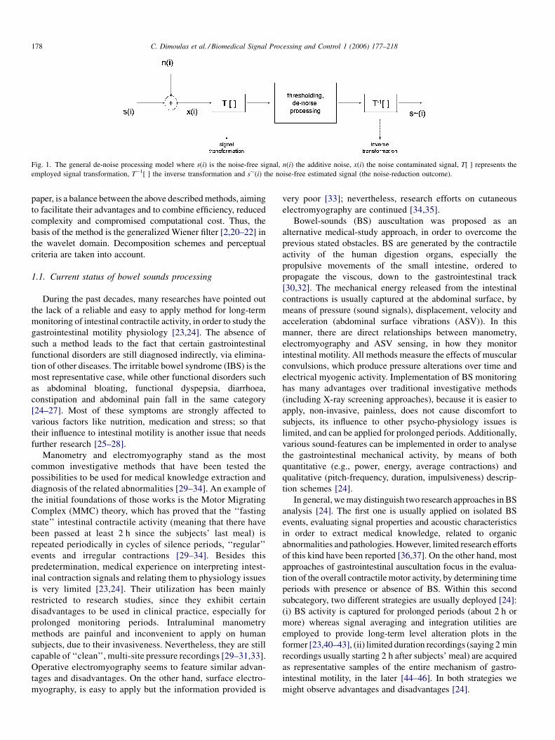
noise-free signal (Fig. 1). Many transformation and analysis–
synthesis schemes have been utilized according to this general
model.
The basic intention of audio restoration techniques is the
improvement of speech intelligibility and music quality, for
* Corresponding author. Tel.: +30 2310933868; fax: +30 2310996309.
E-mail address: [email protected] (C. Dimoulas).
1746-8094/$ – see front matter # 2006 Elsevier Ltd. All rights reserved.
doi:10.1016/j.bspc.2006.08.004
speech and audio recording enhancement, respectively. The
analysis of human auditory systems has allowed the introduc-
tion of perceptual criteria, which have further extended the
potentials of audio restoration. Critical bands analysis, audible
noise suppression and elimination of audible artefacts are the
key concepts for these ‘‘perceptual’’ approaches [1–8]. With
respect to instrumentation and measurements, including
biomedical and bioacoustics applications, it is not very
common to utilize such approaches. The most common
methodologies tend to use combinations of adaptive filtering
techniques and decomposition–reconstruction schemes, includ-
ing classical spectral subtraction [9–11]. Wavelets fall under the
second sub-category, whereas most work has mainly been
concentrated on seeking the ‘‘best’’ signal decomposition–
reconstruction topologies, as well as the optimum threshold
strategy adoption [12–19].
The current work was motivated from the de-noising demands
in human bowel sounds, captured as abdominal surface
vibrations, in order to be further facilitated for diagnostic
purposes. Some of the key concepts and unquestionable targets of
the current research, since its initiation, were robust noise
cancellation, minimal signal distortion and feasible implementa-
tion for long-term analysis. The implementation proposed in this
C. Dimoulas et al. / Biomedical Signal Processing and Control 1 (2006) 177–218178
Fig. 1. The general de-noise processing model where s(i) is the noise-free signal, n(i) the additive noise, x(i) the noise contaminated signal, T[ ] represents the
employed signal transformation, T�1[ ] the inverse transformation and s�(i) the noise-free estimated signal (the noise-reduction outcome).
paper, is a balance between the above described methods, aiming
to facilitate their advantages and to combine efficiency, reduced
complexity and compromised computational cost. Thus, the
basis of the method is the generalized Wiener filter [2,20–22] in
the wavelet domain. Decomposition schemes and perceptual
criteria are taken into account.
1.1. Current status of bowel sounds processing
During the past decades, many researches have pointed out
the lack of a reliable and easy to apply method for long-term
monitoring of intestinal contractile activity, in order to study the
gastrointestinal motility physiology [23,24]. The absence of
such a method leads to the fact that certain gastrointestinal
functional disorders are still diagnosed indirectly, via elimina-
tion of other diseases. The irritable bowel syndrome (IBS) is the
most representative case, while other functional disorders such
as abdominal bloating, functional dyspepsia, diarrhoea,
constipation and abdominal pain fall in the same category
[24–27]. Most of these symptoms are strongly affected to
various factors like nutrition, medication and stress; so that
their influence to intestinal motility is another issue that needs
further research [25–28].
Manometry and electromyography stand as the most
common investigative methods that have been tested the
possibilities to be used for medical knowledge extraction and
diagnosis of the related abnormalities [29–34]. An example of
the initial foundations of those works is the Motor Migrating
Complex (MMC) theory, which has proved that the ‘‘fasting
state’’ intestinal contractile activity (meaning that there have
been passed at least 2 h since the subjects’ last meal) is
repeated periodically in cycles of silence periods, ‘‘regular’’
events and irregular contractions [29–34]. Besides this
predetermination, medical experience on interpreting intest-
inal contraction signals and relating them to physiology issues
is very limited [23,24]. Their utilization has been mainly
restricted to research studies, since they exhibit certain
disadvantages to be used in clinical practice, especially for
prolonged monitoring periods. Intraluminal manometry
methods are painful and inconvenient to apply on human
subjects, due to their invasiveness. Nevertheless, they are still
capable of ‘‘clean’’, multi-site pressure recordings [29–31,33].
Operative electromyography seems to feature similar advan-
tages and disadvantages. On the other hand, surface electro-
myography, is easy to apply but the information provided is
very poor [33]; nevertheless, research efforts on cutaneous
electromyography are continued [34,35].
Bowel-sounds (BS) auscultation was proposed as an
alternative medical-study approach, in order to overcome the
previous stated obstacles. BS are generated by the contractile
activity of the human digestion organs, especially the
propulsive movements of the small intestine, ordered to
propagate the viscous, down to the gastrointestinal track
[30,32]. The mechanical energy released from the intestinal
contractions is usually captured at the abdominal surface, by
means of pressure (sound signals), displacement, velocity and
acceleration (abdominal surface vibrations (ASV)). In this
manner, there are direct relationships between manometry,
electromyography and ASV sensing, in how they monitor
intestinal motility. All methods measure the effects of muscular
convulsions, which produce pressure alterations over time and
electrical myogenic activity. Implementation of BS monitoring
has many advantages over traditional investigative methods
(including X-ray screening approaches), because it is easier to
apply, non-invasive, painless, does not cause discomfort to
subjects, its influence to other psycho-physiology issues is
limited, and can be applied for prolonged periods. Additionally,
various sound-features can be implemented in order to analyse
the gastrointestinal mechanical activity, by means of both
quantitative (e.g., power, energy, average contractions) and
qualitative (pitch-frequency, duration, impulsiveness) descrip-
tion schemes [24].
In general, we may distinguish two research approaches in BS
analysis [24]. The first one is usually applied on isolated BS
events, evaluating signal properties and acoustic characteristics
in order to extract medical knowledge, related to organic
abnormalities and pathologies. However, limited research efforts
of this kind have been reported [36,37]. On the other hand, most
approaches of gastrointestinal auscultation focus in the evalua-
tion of the overall contractile motor activity, by determining time
periods with presence or absence of BS. Within this second
subcategory, two different strategies are usually deployed [24]:
(i) BS activity is captured for prolonged periods (about 2 h or
more) whereas signal averaging and integration utilities are
employed to provide long-term level alteration plots in the
former [23,40–43], (ii) limited duration recordings (saying 2 min
recordings usually starting 2 h after subjects’ meal) are acquired
as representative samples of the entire mechanism of gastro-
intestinal motility, in the later [44–46]. In both strategies we
might observe advantages and disadvantages [24].
C. Dimoulas et al. / Biomedical Signal Processing and Control 1 (2006) 177–218 179
However, knowledge and interpretation of BS has advanced
little since Cannon’s pioneering work [47], so that there is a
lack of a reliable and accurate method for use in clinical
practice. Most researchers seem to agree that this is not due to
redundancy of diagnostic information of BS, but due to
insufficient scientific support [24,48]. There are many
difficulties connected with ASV sensing and BS analysis,
mainly caused by the weak nature of the produced acoustic
phenomena, as well as the peculiar characteristics of the sound
propagating medium. Satisfactory BS acquisition demands
ultra sensitive electroacoustic transducers and high amplifica-
tion signal conditioning circuits, while subjects’ safety is
critical. Thus, one of the major factors that influence the
potential of BS analysis is noise contamination [48–56]. The
noise removal process is essential for BS enhancement, for
easier and more efficient auscultation of BS from clinicians,
and unsupervised analysis of long-term ASV monitoring. Thus,
it is a necessary processing stage to all the previous BS-analysis
approaches [23,24,42,43,48–57].
There are many issues to be considered for the influence of
the interfering noise to BS analysis. First of all, the presence of
noise complicates the audible interpretation of the original
signal, resulting to problematic and tiresome auscultation.
Secondly, masking effects are possible to appear so that
detection and interpretation of low-amplitude signal-frequency
components, become tricky. In this sense, various audible
artefacts often arise. The afore-mentioned issues are likely to
lead to major estimation errors, because (i) medical analysis is
difficult to progress in supervised schemes (especially for long-
term monitoring), since clinicians’ audible interpretation of the
recorded signals is not available, (ii) signal-energy parameters
and other audio features, employed for analysis purposes, are
miscalculated, (iii) numerical analysis and automated proces-
sing can produce misclassification errors. These issues are also
dominant to all the above-mentioned strategies of BS analysis.
This is the reason that many research efforts have been recently
appeared in bibliography, focusing on robust signal enhance-
ment of the noise contaminated BS. Except of the adaptive
filtering approach of Mansy and Sandler [49], most of these de-
noising methods are dealing with the problem of additive
broadband noise elimination, employing auto threshold
estimation strategies, in combination with wavelet-statistics
[48,50,51,53], wavelets-fractal dimension [54,55] and higher
order statistics [52,56].
In fact, all the previously stated methods are based on the
initial work of Coifman and Wickerhauster [9] that employ
iterative wavelet processing in combination with best basis
selection. Hadjileontiadis and Panas [10] had initially modified
the original algorithm, keeping only the iterative structure
(without the best basis selection functionality) and providing a
new auto-threshold estimation procedure. The implemented
‘‘wavelet transform-based stationary–non stationary’’ (WTST–
NST) filter [10] was proposed for lung-sounds de-noising
processing. This parametric approach has also been imple-
mented for BS processing [48,50,51], while implementation
improvements have also been suggested [53]. The ‘‘wavelet
transform-fractal dimension-based method (WT-FD) was then
proposed by Hadjileontiadis [54,55] for lung sounds and BS de-
noising purposes, providing a novel approach in estimating
wavelet thresholds, while keeping the rest of the method intact.
The iterative processing procedure was also implemented in a
new fashion, employing higher order statistics instead of
wavelets [52,56]. The proposed Iterative Kurtosis-based
Detector (IKD) is also intended for lung sounds and bowel
sound detection and analysis [52,56].
According to the results of the previous paragraph’s research
works, all these variations of the iterative structured algorithms
are very efficient when they are applied in explosive bowel
sounds (EBS) [48,52,54–56], also referred as intestinal bursts
(IB) [57], pops, tingles and clicks [38,39,47]. However,
regularly sustained (RS) BS signals [57], with smoother
attack-release envelopes and longer durations, are also found
inside BS recordings, very frequently [38,39,47]. As a result,
the utilization of EBS de-noising algorithms is usually
problematic in the case of the RS events (also referred as
borborygmus, crepitating sounds, gurgling, rumbling, or
growling noise, including cases of whistling—musical BS),
causing either insufficient de-noising, or serious destructions of
the signals’ morphological structures [24]. Furthermore, their
implementation in automated long-term processing is risky,
producing de-noising artefacts quite often. The computational
cost of the repeated threshold estimation and the iterative
processing scheme is another serious drawback [24]. As already
stated, the current work aims to overcome the previously
described weaknesses, providing novel Wiener filtering de-
noising techniques, which can be efficiently applied on both IB
and RS patterns of BS, with compromised complexity and
computational cost.
1.2. Problem definition
A common problem to all instrumentation set-ups that
demand high amplification is the presence of the so-called,
additive broadband background noise (ABN). Some of the
reasons that cause the production of ABN are (i) ‘‘thermal’’
noise induced along the data acquisition chain, (ii) ambient
acoustic noise, (iii) quantization noise, especially in cases
where recording levels are not adjusted properly.
Let x(i) be the sampled version of a noise contaminated
signal x(t), whereas s(i) and n(i) are the sampled versions of the
‘‘clean’’ signal s(t) and the uncorrelated with the signal,
additive random noise n(t):
xðiÞ ¼ sðiÞ þ nðiÞ (1)
The aim of noise reduction techniques is to recover an
approximation s�(i) as closely as possible to the original clean
signal s(i), in order to eliminate noise components. Two of the
most famous de-noising approaches are spectral subtraction
and wavelet thresholding. Methods of the first type emphasize
minimal signal distortion. Wavelet thresholding strategies, on
the other hand, can provide rough noise reduction results,
so that they are likely to affect useful signal components
besides noise.
C. Dimoulas et al. / Biomedical Signal Processing and Control 1 (2006) 177–218180
The current approach aims at implementing an accurate and
relatively fast, universal de-noising method that can be easily
applied for long-term analysis. Elimination of time disconti-
nuities and artefact-caused misinterpretation, due to severe
noise contamination, were considered as issues of major
importance. The proposed Wavelet Domain Wiener Filter
(WDWF) method satisfies the afore-mentioned prerequisites by
combining classical Wiener filter efficiency [20–22], bark scale
wavelets flavour [58–63] and compromised computational cost
of Fast Wavelet Transform algorithms [64].
2. Material and methods
Since the proposed WDWF method is a combination of
classical spectral subtraction and wavelet domain processing, a
quick report on both signal-processing fields is necessary,
before presenting the implemented algorithms.
2.1. Spectral subtraction and parametric Wiener filter
Spectral subtraction was introduced by Boll [65] in 1979 and
still remains one of the most popular methods for background
noise reduction [66–68] or as standard reference when
evaluating other noise reduction techniques [69,70]. It is based
on filtering of the noisy signal using a time-varying filter
applied to the frequency domain. Let us turn our attention now
to the general de-noise model of Fig. 1, as it was described in
the previous section. If X(k), S(k) and N(k) are the spectra of the
noise contaminated signal x(i), the original clean signal s(i) and
the noise signal n(i), respectively, estimated using short time
spectral analysis, such as the STFT, then:
XðkÞ ¼ SðkÞ þ NðkÞ) SðkÞ ¼ XðkÞ � NðkÞ (2)
The solution to the de-noise problem is to formulate a filter
H(k) that best approaches the spectral subtraction operation
described in (2), so that we would be able to extract an
estimation S�(k) of the clean signal, which is the output of the
filter, the available signal X(k) being the input. Assuming that
the noise signal is a stationary random process, we may get an
estimation NFP(k) of the noise spectrum (noise footprint), by
applying Fourier Transform to available signal silence periods.
With this line of reasoning, the estimation of the clean signal is
given by:
S� ðkÞ ¼ XðkÞ � NFPðkÞ ¼ HðkÞ � XðkÞ (3)
The two basic short time spectral analysis noise reduction
methods are the magnitude spectral subtraction
S� ðkÞj j ¼ XðkÞj j � NFPðkÞj j; XðkÞj j> NFPðkÞj j0; otherwise
�(4)
and the power spectral subtraction
S�ðkÞj j2
¼PXðkÞ�a �PNFP
ðkÞ; PXðkÞ�a �PNFPðkÞ>b �PNFP
ðkÞb �PNFP
ðkÞ; otherwise
�(5)
where
PXðkÞ , EfjXðkÞj2g; PNFPðkÞ , EfjNFPðkÞj2g (6)
and a, b are real valued positive parameters employed to
control the amount of subtraction and the remaining noise
floor [2,6]. Thus, without further processing of the noisy signal
phase [4,6], the clean signal can be estimated from the Inverse
Fourier Transform (IFT) using the following formula:
s� ðiÞ ¼ IFTfjS� ðkÞj;]ðXðkÞÞg (7)
Another classical noise reduction technique is the para-
metric Wiener filter, which can be proved to be equivalent to the
spectral subtraction procedure, when applied to time limited
signals [20,21]. Wiener filter minimizes the mean square error
of the estimate’s time domain reconstruction for the case of
uncorrelated, zero-mean, additive noise [6]. The mathematical
expression for the transfer function HPWF of the parametric
Wiener filter is given below:
HPWFðkÞ ¼ 1� cNFPðkÞj j
XTðNFPðkÞÞj j
� �a� �b
; if cjNFPðkÞjjXTðkÞj
� �a
� 1
0; otherwise
8><>:
(8)
where a, b, c are the real valued parameters of the filter and
XT(k) is the spectrum of T duration windowed signal. NFP(k) is
again calculated as the Fourier Transform of a noise only
segment of signal (noise footprint) [2,4,6,20–22].
The noise estimation procedure as stated up to this point,
does not consider any perceptual criteria that are related with
the human auditory system. It is well known that human
response to audio stimulus is not spectrally uniform along the
range of audible frequencies. The formulation of such a
psycho-acoustic factor extended the potential of the so-called
Frequency Depended Parametric Wiener Filter [20,21].
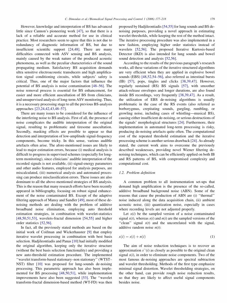
Equivalent masking noise estimation analysis [20,21,71]
has been concentrated to examine the model of pure tones
masked by white noise, as the worst case of perceiving a
desired tonal signal in the presence of broad-band acoustic
noise (Fig. 2). According to the results of those studies
[20,21,71], it could be stated that human auditory system
filters broad-band acoustic noise, according to a transfer
function given by,
Aðk � d f Þ ¼1; for k � d f � 500
k � d f
500; for k � d f > 500
8<: (9)
where df = fs/N the involved frequency resolution of the STFT.
If we include the above transfer function in the noise
estimation procedure, this would result to a frequency
depended method, simulating the perception of broad
band acoustic noise by the human ear [20,21]. The Frequency
Depended Parametric Wiener Filter is implemented
C. Dimoulas et al. / Biomedical Signal Processing and Control 1 (2006) 177–218 181
Fig. 2. Level (SPL) of test tones just masked by white noise of given density level Lwn, as a function of the test-tone frequency. The dashed curve indicates the
threshold in quiet (Source: Zwicker and Fastl [71], p. 57).
according to
HFDPWFðkÞ
¼ 1� c �AðkÞ � NFPðkÞj jXTðkÞj j
� �a� �b
; if c �AðkÞ � NFPðkÞj jXTðkÞj j
� �a
� 1
0; otherwise
8><>:
(10)
2.2. Wavelet domain de-noising techniques
The implementation of the above Wiener filter formulas
involves short-term spectral analysis, usually accomplished via
the STFT. To do so, signal is windowed to time-overlapped
sequential frames, prior to Wiener filter process. According to
Heisenberg’s principle [58,62] there is a limit to the time–
frequency resolution product:
Dt � D f � 1
4p(11)
where Dt is the time resolution and Df the frequency resolution,
depending on the STFT windowing operation, that is deter-
mined by the sampling frequency fs, the windowing function
and the window-length N [58]. The previous equation points out
that it is possible to achieve fine time resolution forcing poor
frequency resolution and vice versa, but there is no way of
achieving best resolution in both fields at the same time. Thus,
once parameters fs and N have been selected, time and fre-
quency resolutions are defined, and they are linearly expanded
over the time or the frequency axis. On the other hand, effective
representation and analysis of audio signals require fine time
resolution at high frequencies and fine frequency resolution at
low frequencies, the so-called ‘‘constant Q analysis’’. The term
‘‘constant Q analysis’’ was first introduced to filter bank
implementations, whereas the Q factor of each filter, which
is equivalent to the central frequency ( fc) divided by the
bandwidth (BW), remains constant (Q = fc/BW) [58].
2.2.1. Wavelet transforms
Wavelet transform has been introduced as a more elegant
approach to achieve the previously described prerequisite for
fine time and frequency resolution. Some of the aims and
motives of wavelet analysis was the elimination of drawbacks
appeared in filter bank processing, such as the increased amount
of data, the computational complexity and cost, issues related
with filter delay parameters. Wavelet processing offers an
alternative spectral analysis approach that features the flavour
of fine, bark scale, resolution, promising easier implementation
and lower computational complexity [58,60,62].
Wavelets are families of functions generated from a
‘‘mother’’ function, the mother wavelet, after scaling and
dilation (time shifting). The sum of the inner products of signal
and wavelet functions, the so-called wavelet coefficients,
results to the Continuous Wavelet Transform (CWT). If L2(R)
denotes the vector space of measurable, square integrable one-
dimensional functions and x(t) one-dimensional function such
as x 2 L2(R), then the following equations are valid in a Hilbert
space:
Cu;tðtÞ ¼1ffiffiffiffiffiffijuj
p � c�
t � t
u
�; u; t 2R; u 6¼ 0 (12)
CWTxðu; tÞ ¼
x;cu;t
¼Z
xðtÞ � c�u;tðtÞ d t (13)
where u, t are the scale and dilation parameters, respectively,
c(t) the mother wavelet, cu,t(t) the family of wavelet functions
and * represent the complex conjugate. An analogous expres-
sion is used for the Inverse Continuous Wavelet Transform.
Since the full analysis of the wavelet transform exceeds this
paper’s intension, we will focus our attention on the specific
topics of Discrete Wavelet Transform (DWT) and Wavelet
Packet analysis (WP) [58,60,62,72], which have been
employed in the current approach. DWT has been suggested
in an attempt to reduce wavelet coefficients by restricting
parameters u, t to some discrete values. The elimination of
C. Dimoulas et al. / Biomedical Signal Processing and Control 1 (2006) 177–218182
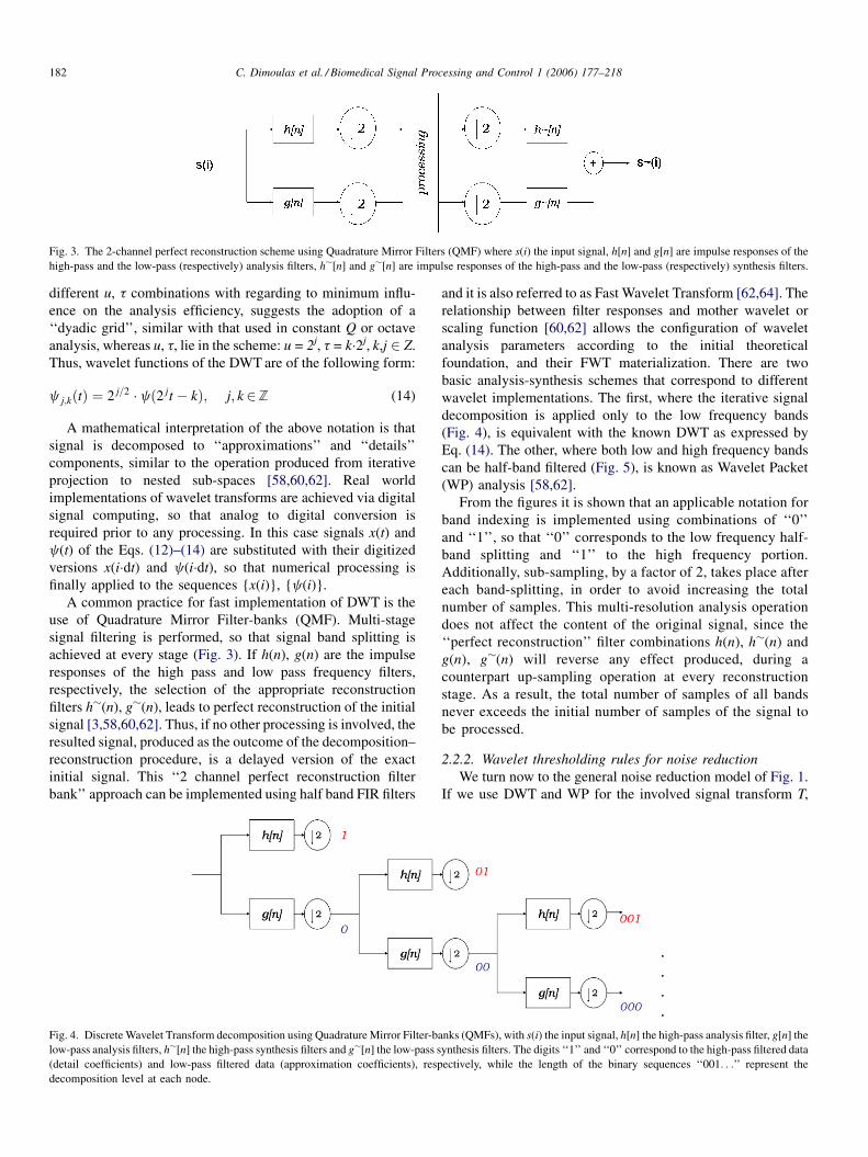
Fig. 3. The 2-channel perfect reconstruction scheme using Quadrature Mirror Filters (QMF) where s(i) the input signal, h[n] and g[n] are impulse responses of the
high-pass and the low-pass (respectively) analysis filters, h�[n] and g�[n] are impulse responses of the high-pass and the low-pass (respectively) synthesis filters.
different u, t combinations with regarding to minimum influ-
ence on the analysis efficiency, suggests the adoption of a
‘‘dyadic grid’’, similar with that used in constant Q or octave
analysis, whereas u, t, lie in the scheme: u = 2j, t = k�2j, k,j 2 Z.
Thus, wavelet functions of the DWT are of the following form:
c j;kðtÞ ¼ 2 j=2 � cð2 jt � kÞ; j; k2Z (14)
A mathematical interpretation of the above notation is that
signal is decomposed to ‘‘approximations’’ and ‘‘details’’
components, similar to the operation produced from iterative
projection to nested sub-spaces [58,60,62]. Real world
implementations of wavelet transforms are achieved via digital
signal computing, so that analog to digital conversion is
required prior to any processing. In this case signals x(t) and
c(t) of the Eqs. (12)–(14) are substituted with their digitized
versions x(i�dt) and c(i�dt), so that numerical processing is
finally applied to the sequences {x(i)}, {c(i)}.
A common practice for fast implementation of DWT is the
use of Quadrature Mirror Filter-banks (QMF). Multi-stage
signal filtering is performed, so that signal band splitting is
achieved at every stage (Fig. 3). If h(n), g(n) are the impulse
responses of the high pass and low pass frequency filters,
respectively, the selection of the appropriate reconstruction
filters h�(n), g�(n), leads to perfect reconstruction of the initial
signal [3,58,60,62]. Thus, if no other processing is involved, the
resulted signal, produced as the outcome of the decomposition–
reconstruction procedure, is a delayed version of the exact
initial signal. This ‘‘2 channel perfect reconstruction filter
bank’’ approach can be implemented using half band FIR filters
Fig. 4. Discrete Wavelet Transform decomposition using Quadrature Mirror Filter-ba
low-pass analysis filters, h�[n] the high-pass synthesis filters and g�[n] the low-pass s
(detail coefficients) and low-pass filtered data (approximation coefficients), resp
decomposition level at each node.
and it is also referred to as Fast Wavelet Transform [62,64]. The
relationship between filter responses and mother wavelet or
scaling function [60,62] allows the configuration of wavelet
analysis parameters according to the initial theoretical
foundation, and their FWT materialization. There are two
basic analysis-synthesis schemes that correspond to different
wavelet implementations. The first, where the iterative signal
decomposition is applied only to the low frequency bands
(Fig. 4), is equivalent with the known DWT as expressed by
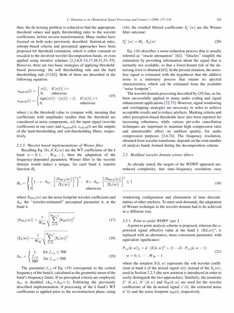
Eq. (14). The other, where both low and high frequency bands
can be half-band filtered (Fig. 5), is known as Wavelet Packet
(WP) analysis [58,62].
From the figures it is shown that an applicable notation for
band indexing is implemented using combinations of ‘‘0’’
and ‘‘1’’, so that ‘‘0’’ corresponds to the low frequency half-
band splitting and ‘‘1’’ to the high frequency portion.
Additionally, sub-sampling, by a factor of 2, takes place after
each band-splitting, in order to avoid increasing the total
number of samples. This multi-resolution analysis operation
does not affect the content of the original signal, since the
‘‘perfect reconstruction’’ filter combinations h(n), h�(n) and
g(n), g�(n) will reverse any effect produced, during a
counterpart up-sampling operation at every reconstruction
stage. As a result, the total number of samples of all bands
never exceeds the initial number of samples of the signal to
be processed.
2.2.2. Wavelet thresholding rules for noise reduction
We turn now to the general noise reduction model of Fig. 1.
If we use DWT and WP for the involved signal transform T,
nks (QMFs), with s(i) the input signal, h[n] the high-pass analysis filter, g[n] the
ynthesis filters. The digits ‘‘1’’ and ‘‘0’’ correspond to the high-pass filtered data
ectively, while the length of the binary sequences ‘‘001. . .’’ represent the
C. Dimoulas et al. / Biomedical Signal Processing and Control 1 (2006) 177–218 183
then, the de-noising problem is reduced to find the appropriate
threshold values and apply thresholding rules to the wavelet
coefficients, before inverse transformation. Many studies have
focused on both tasks previously described. Statistical rules,
entropy-based criteria and perceptual approaches have been
proposed for threshold estimation, which is either constant or
rescaled to the involved wavelet decomposition bands, or even
applied using iterative schemes [2,3,6,9–14,17,48,51,53–55].
However, there are two basic strategies of applying threshold-
based processing: the soft thresholding rule and the hard
thresholding rule [13,62]. Both of them are described in the
following equation:
xhard-thðiÞ ¼xðiÞ; if xðiÞj j> t0; otherwise
�
xsoft-thðiÞ ¼signðxðiÞÞ � ðjxðiÞj � tÞ; if jxðiÞj> t0; otherwise
� (15)
where t is the threshold value to compare with, meaning that
coefficients with amplitudes smaller than the threshold are
considered as noise components, x(i) the input signal (wavelet
coefficients in our case) and xhard-th(i), xsoft-th(i) are the outputs
of the hard-thresholding and soft-thresholding filters, respec-
tively.
2.2.3. Wavelet based implementations of Wiener filter
Recalling Eq. (8), if XkðwÞ are the WT coefficients of the k
band w ¼ 0; 1; � � � ;WXk � 1, then the adaptation of the
frequency-depended parametric Wiener filter to the wavelet
domain would induct a unique, for each band k, transfer
function Hk
Hk ¼ 1� c � Akw �hNFP-kðwÞihXkðwÞi
� �a� �b
; if c � Akw �hNFP-kðwÞihXkðwÞi
� �a
� 1
0; otherwise
8<: (16)
where NFP-kðwÞ are the noise footprint wavelet coefficients and
Akw the ‘‘wavelet-estimated’’ perceptual parameter A, at the
band k:
hNFP;kðwÞi ¼1
WNk
ffiffiffiffiffiffiffiffiffiffiffiffiffiffiffiffiffiffiffiffiffiffiffiffiffiffiffiffiffiffiXWNk�1
w¼0
½NFPðwÞ�2vuut (17)
hXkðwÞi ¼1
WXk
ffiffiffiffiffiffiffiffiffiffiffiffiffiffiffiffiffiffiffiffiffiffiffiffiffiffiffiXWXk�1
w¼0
½XkðwÞ�2vuut (18)
Akw ¼1; for f c-k � 500
f c-k
500; for f c-k > 500
((19)
The parameter fc-k of Eq. (19) corresponds to the central
frequency of the band k, calculated as the geometric mean of the
band’s frequency limits. If no perceptual criteria are employed,
Akw is disabled (Akw = Ak0 = 1). Following the previously
described implementation, if processing of the k band’s WT
coefficients is applied prior to the reconstruction phase, using
(16), the resulted filtered coefficients S�k ðwÞ are the Wiener
filter outcome:
S�k ðwÞ ¼ Hk � XkðwÞ (20)
Eq. (16) describes a noise-reduction process that is usually
referred as ‘‘oracle attenuation’’ [62]. ‘‘Oracles’’ simplify the
estimation by providing information about the signal that is
normally not available, so that a lower-bound risk of the de-
noising error is obtained [62]. In the present situation, the noise-
free signal is estimated with the hypothesis that the additive
noise is a stationary process that retains its spectral
characteristics, which can be estimated from the available
‘‘noise footprint’’.
The wavelet domain processing described by (20) has, so far,
been successfully applied to many audio coding and signal
enhancement applications [72,73]. However, signal windowing
and overlapping strategies are necessary in order to achieve
acceptable results and to reduce artefacts. Masking criteria and
other perception-based thresholds have also been reported for
increasing robustness, while various pre-echo cancellation
techniques are important to maintain high compression ratio
and unnoticeable effect on audition quality, for audio
compression purposes [3,6,74]. The frequency resolution,
obtained from wavelet transforms, depends on the total number
of analysis bands formed during the decomposition scheme.
2.3. Modified wavelet domain wiener filters
As already stated, the targets of the WDWF approach are:
reduced complexity, fine time–frequency resolution, easy
windowing configuration and elimination of time disconti-
nuities or other artefacts. To meet such demands, the adaptation
of Wiener technique to the wavelet domain had to be achieved
in a different way.
2.3.1. Point to point WDWF type I
A point to point analysis scheme is proposed, whereas the a-
powered signal effective value at the band k hX(k,w)ia, is
replaced with an alternative, more convenient parameter, with
equivalent significance:
Px;aðk;wÞjI ¼ d � jXðk;wÞja þ ð1� dÞ � Px;aðk;w� 1Þ
w ¼ 0; 1; � � � ;WXk � 1(21)
where the notation Xðk;wÞ represents the wth wavelet coeffi-
cient at band k of the noised signal x(i), instead of the XkðwÞ,used in Section 2.2.3 (the new notation is introduced in order to
easily distinguish the two approaches). Similarly, the notations
S� ðk;wÞ, N � ðk;wÞ and NFPðk;wÞ are used for the wavelet
coefficients of the de-noised signal s�(i), the extracted noise
n�(i) and the noise footprint nFP(i), respectively.
C. Dimoulas et al. / Biomedical Signal Processing and Control 1 (2006) 177–218184
Fig. 5. Wavelet Packet decomposition using Quadrature Mirror Filter-banks (QMFs).
Eq. (21) introduces an exponential moving average
estimation for the a-powered magnitude signal estimation
Px;a(k,w)jI. The real valued momentum term d is spaced in the
interval [0,1] and it is used to control the amount of memory
taken into account for the calculation. Similar approaches have
been utilized in relative, frame-based, spectral subtraction or
Wiener filtering noise cancellation applications [20,21,73,75].
With this settlement, finest time resolution is achieved, while
computational complexity is minimal. The estimated value is
sensitive to the preceded samples of the signal, which is in
accordance to the Haas precedence effect of psychoacoustics
[71], offering a potential advantage towards perceptual audio
processing. However, signal discontinuities are likely to be
produced at the initiation of the iterative process, for the 0th
sample specifically, where no previous estimation is available.
In an effort to overcome this handicap, the Eq. (21) is re-formed
as follows:
Px;aðk;wÞjI ¼jXðk;wÞja; w ¼ 0
d � jXðk;wÞja þ ð1� dÞ � Px;aðk;w� 1Þ; w ¼ 1; � � � ;WXk � 1
�(22)
With this last arrangement the proposed type-I WDWF
allows a point to point processing at every band:
HWDFWðk;wÞ ¼1� c � Akw �
PnFP;aðkÞPx;aðk;wÞ
� �� �b
; if c � Akw �PnFP;aðkÞPx;aðk;wÞ
� �� 1
0; otherwise
8><>: (23)
whereas Px;a(k,w) is the Px;a(k,w)jI estimation of Eq. (22), Akw is
still calculated from (19) and the noise estimation PnFP;a(k) is
the average of all the a-powered magnitude noise estimations
NFP;a(k,w), provided by the k-band wavelet coefficients of the
noise footprint:
PnðkÞ ¼1
WNk
XWNk�1
w¼0
jNFPðk;wÞja (24)
Thus, the wavelet domain, frequency-depended, parametric
Wiener filtering operation is described in the following
equation:
S� ðk;wÞ ¼ HWDWFðk;wÞ � Xðk;wÞ; w ¼ 0; 1; � � � ;WXk � 1
(25)
where k are all the available analysis bands produced from
DWT or WP decomposition.
The introduction of the exponential moving average scheme
for the estimation of the noised-signal coefficients power is
advantageous, over both Fourier-based short-term spectral
amplitude (STSA) approaches and classical wavelet de-
noising. It is also beneficial compared to previous exponential
moving average implementations, adapted to filter banks. Thus,
in contrast to the predecessor STFT Wiener filter, the WDWF
approach, as it is described from Eqs. (21)–(25), retains the

C. Dimoulas et al. / Biomedical Signal Processing and Control 1 (2006) 177–218 185
flavour of the logarithmic frequency resolution, instead of the
classical linear spacing. Additionally, the method features
increased time resolution, in contrast to the classical wavelet-
Wiener approaches described in Section 2.2.3, while the
reduced complexity and computational load is also profitable.
Another attribute of the proposed scheme, which places it in
advantageous position over the non-wavelet filter-bank
implementations [20,21], is the multi-resolution nature of the
wavelet transform. The length of the wavelet coefficients is kept
equal to the initial length of the input sequence, i.e., a
settlement that compromises the computational cost, in contrast
to the implementations of [20,21], where the total size of the
band-filtered sequences is multiplied by the number of the
involved analysis bands. Furthermore, the multi-resolution
scheme allows for identical filter-configuration over all wavelet
scales, where in the case of the classical filter-bank filtering
[20,21] a band-adaptation is required, mostly for the influence
of the memory term d that will be analyzed in the following
paragraphs.
In all the previous formulas of the parametric Wiener filter
implementations, parameters a, b, c are used to adjust the filter
transfer function, according to the degree of noise contamina-
tion [2,20–22]. In general, filter-response is controlled, so that
noised signals are highly compressed for low signal to noise
ratios (SNR), while the attenuation level gets smaller for higher
SNR values. In fact, the filter-magnitude curve is asymptoti-
cally approaching the 0 dB level (Hk = 1) as the SNR gets
bigger. In this context, increasing the a parameter results to
smoother filtering, since, for SNR values greater than about
2 dB the filter-magnitude response is moving closer to the 0 dB
level [2,20,21]. The exact opposite behaviour is observed for
the parameters b and c, given that a rougher filtering is initiated
when the corresponding parametric values are raised.
Specifically, the filter-response curves are bending to reach
about 60 dB attenuation at 0 dB SNR, for typical values of b = 4
and c = 1.5 [2,20,21]. In any case, the filter attenuation function
with respect to SNR changing has a characteristic exponential
curve, which starts from very large attenuation values at low
SNR (jHkj > 15–20 dB, for SNR < 5 dB) and asymptotically
reaches the 0 dB level at higher SNR (SNR > 15–20 dB). More
information about the influence of a, b and c parameters and the
related filter attenuation curves, may be found in [2,21].
As already stated, the current WDWF approach differs from
the parametric Wiener spectral subtraction [2,22], mostly due to
the exponential moving average procedure, that is used instead
of classical windowing approaches. This introduces an
additional parameter, the memory term d, which is also
involved in the filter-configuration process. However, the
influence of this parameter is not so obvious as in the cases of a,
b and c, so it is meaningful to emphasize on this aspect,
providing more information about the behaviour of the memory
term d. Exponential averaging techniques are used in various
sound pressure level estimation techniques [76], to take
advantage of the fact that most acoustic phenomena feature
similar to the exponential curves, attack-release envelopes.
Additional benefits are related to perceptual attributes [71], as
well as to their desirable operational characteristics, such as
simplicity, easy implementation and efficiency [76]. In contrast
to the classical window-based sound-level estimation, expo-
nential averaging is applied by filtering the instantaneous sound
power signal (�signal2), using a first order infinite impulse
response (IIR) filter with reverse coefficients {a0,a1} and
forward coefficients {b1}: [76]
a0 ¼ 1; a1 ¼ �e�ð1= f s�twÞ
b1 ¼ 1� e�ð1= f s�twÞ ¼ 1þ a1
(26)
In the above formulas, fs is the sampling frequency [Hz] of
the input sequence and tw the equivalent duration [s] of the
‘‘exponential windowing’’ operation [76]. Comparing Eqs. (21)
and (26), it is obvious that the filter coefficient b1 and the
memory term d are identical. Thus, the reverse and forward
coefficients of the ‘‘exponential average’’ IIR filter are {1,
d � 1} and {d}, respectively. Using Eq. (26), we are able to
calculate the equivalent windowing duration for various values
of the memory parameter d. Before we do so, let us turn our
attention to the significance of the duration tw and its influence
to the Wiener filtering process, issues that can be synopsized to
the general remarks that follow. The length of the window
should be controlled according to signal variations and its
morphological structure, meaning that a signal with abrupt
changes (usually with high frequency content) requires short
averaging lengths, while longer durations might be used for
sustained (lower frequency) signals. Thus, the shorter the
length, the more adaptive the Wiener filtering process,
especially for the cases that useful-signal is not always present
(as it happens with most natural phenomena), resulting to the
total elimination of the ‘‘noise-only’’ intervals. However, a
minimum window-length is required in order to avoid
‘‘interruptions’’, or erroneous power estimation of the useful
signal components.
The last sentence suggests that for each signal-frequency
component, the length of a full periodic circle should be at least
selected for the value of the duration tw, in order to avoid
miscalculation of the signal expected (power) values. For
example, a minimum duration of 5 ms is necessary for a 200 Hz
tonal signal, resulting to a window-length of 40 samples, in the
case of a typical sampling frequency of 8 kHz. The
corresponding exponential averaging requires a memory term
d = 0.025, as it is estimated from Eq. (26). Based on the
previous remarks, it is obvious that a variable memory term d(k)
is necessary for each frequency band k, considering a constant
sampling-frequency, as it happens with classical constant-rate
filter-bank implementations [20,21]. Table 1 represents the
band-edge frequency limits for the cases of the classical octave
and third-octave analysis [76], and the corresponding upper-
bounds of the band memory terms d(k), for the frequencies up to
4 kHz ( fs = 8 kHz).
The adoption of the wavelet analysis and the corresponding
multi-resolution scheme, equips the WDWF method with some
additional advantages related to the exponential averaging
procedure. In contrast to the previously stated cases of constant-
rate filter banks [20,21], the wavelet sub-sampling procedure
makes obsolete the individual configuration of the memory
C. Dimoulas et al. / Biomedical Signal Processing and Control 1 (2006) 177–218186
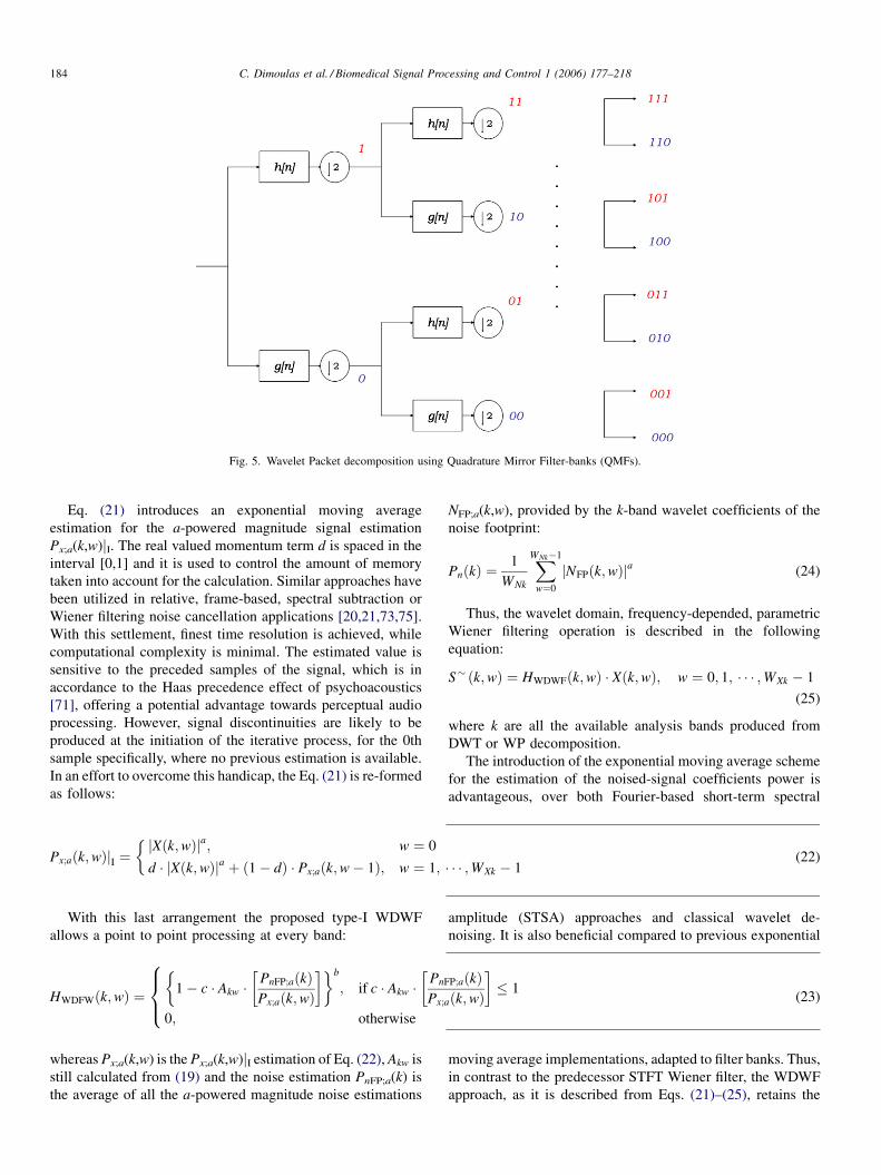
Table 1
Required exponential-averaging lengths in constant rate, spectral band analysis (octaves, third-octaves)
Octaves [k] fL [Hz] fC [Hz] fH [Hz] tw-min [ms]
(lower-bound)
d(k)
(upper-bound)
Third-
octaves [k]
fL [Hz] fC [Hz] fH [Hz] tw-min [ms]
(lower-bound)
d(k)
(upper-bound)
1 44.2 62.5 88.4 22.6 0.006 1 55.7 62.5 70.2 18.0 0.007
2 70.2 78.7 88.4 14.3 0.009
2 88.4 125 176.8 11.3 0.011 3 88.4 99.2 111.4 11.3 0.011
4 111.4 125.0 140.3 9.0 0.014
5 140.3 157.5 176.8 7.1 0.017
3 176.8 250 353.6 5.7 0.022 6 176.8 198.4 222.7 5.7 0.022
7 222.7 250.0 280.6 4.5 0.027
8 280.6 315.0 353.6 3.6 0.034
4 353.6 500 707.1 2.8 0.043 9 353.6 396.9 445.4 2.8 0.043
10 445.4 500.0 561.2 2.2 0.054
11 561.2 630.0 707.1 1.8 0.068
5 707.1 1000 1414.2 1.4 0.085 12 707.1 793.7 890.9 1.4 0.085
13 890.9 1000.0 1122.5 1.1 0.105
14 1122.5 1259.9 1414.2 0.9 0.131
6 1414.2 2000 2828.4 0.7 0.162 15 1414.2 1587.4 1781.8 0.7 0.162
16 1781.8 2000.0 2244.9 0.6 0.200
17 2244.9 2519.8 2828.4 0.4 0.245
7 2828.4 4000 4000a 0.4 0.298 18 2828.4 3174.8 3563.6 0.4 0.298
19 3563.6 4000.0 4000a 0.3 0.359
a For the given sampling rate of 8 kHz, the high bandedge frequency at the last band, k = 7 for the octave analysis and k = 19 for the third octave analysis, is equal to
4 kHz (half the sampling rate), due to the Nyquist criterion.
term d(k) for each band, due to the fact that sampling rate is
adaptively reduced to each band. Thus, careful adjustment of a
global memory term d is entirely adequate to serve the above
processing requirements for all the involved bands. With this
arrangement, the filter retains its efficiency and de-noising
capabilities, while easy configuration and reduced complexity
facilitate filter adjustment and implementation. Having those
remarks in mind, the ‘‘type-I Wavelet Domain Wiener Filter’’
(WDWFI) was configured based on empirical observations of
BS de-noising examples. The memory term was set to d = 0.2,
while the rest of the parameters were adjusted to a = 2, b = 1
and c = 3. The configuration of the parameter d for the selected
analysis–synthesis topologies (5-level DWT and 17-band WPA,
described next) is presented in Tables 2 and 3, where the
selected value satisfies all the conditions, previously discussed.
Comparing Tables 1–3, it is obvious that the WDWF
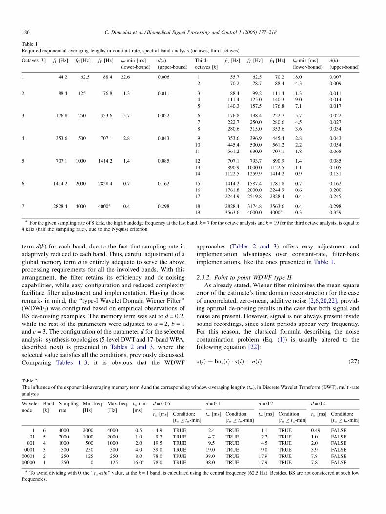
Table 2
The influence of the exponential-averaging memory term d and the corresponding w
analysis
Wavelet
node
Band
[k]
Sampling
rate
Min-freq.
[Hz]
Max-freq.
[Hz]
tw-min
[ms]
d = 0.05
tw [ms] Condition:
[tw � tw-m
1 6 4000 2000 4000 0.5 4.9 TRUE
01 5 2000 1000 2000 1.0 9.7 TRUE
001 4 1000 500 1000 2.0 19.5 TRUE
0001 3 500 250 500 4.0 39.0 TRUE
00001 2 250 125 250 8.0 78.0 TRUE
00000 1 250 0 125 16.0a 78.0 TRUE
a To avoid dividing with 0, the ‘‘tw-min’’ value, at the k = 1 band, is calculated usi
frequencies.
approaches (Tables 2 and 3) offers easy adjustment and
implementation advantages over constant-rate, filter-bank
implementations, like the ones presented in Table 1.
2.3.2. Point to point WDWF type II
As already stated, Wiener filter minimizes the mean square
error of the estimate’s time domain reconstruction for the case
of uncorrelated, zero-mean, additive noise [2,6,20,22], provid-
ing optimal de-noising results in the case that both signal and
noise are present. However, signal is not always present inside
sound recordings, since silent periods appear very frequently.
For this reason, the classical formula describing the noise
contamination problem (Eq. (1)) is usually altered to the
following equation [22]:
xðiÞ ¼ bnsðiÞ � sðiÞ þ nðiÞ (27)
indow-averaging lengths (tw), in Discrete Wavelet Transform (DWT), multi-rate
d = 0.1 d = 0.2 d = 0.4
in]
tw [ms] Condition:
[tw � tw-min]
tw [ms] Condition:
[tw � tw-min]
tw [ms] Condition:
[tw � tw-min]
2.4 TRUE 1.1 TRUE 0.49 FALSE
4.7 TRUE 2.2 TRUE 1.0 FALSE
9.5 TRUE 4.5 TRUE 2.0 FALSE
19.0 TRUE 9.0 TRUE 3.9 FALSE
38.0 TRUE 17.9 TRUE 7.8 FALSE
38.0 TRUE 17.9 TRUE 7.8 FALSE
ng the central frequency (62.5 Hz). Besides, BS are not considered at such low
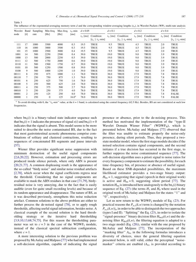
C. Dimoulas et al. / Biomedical Signal Processing and Control 1 (2006) 177–218 187
Table 3
The influence of the exponential-averaging memory term d and the corresponding window-averaging lengths (tw), in Wavelet Packets (WP), multi-rate analysis
Wavelet
node
Band
[k]
Sampling
rate
Min-freq.
[Hz]
Max-freq.
[Hz]
tw-min
[ms]
d = 0.05 d = 0.1 d = 0.2 d = 0.4
tw [ms] Condition:
[tw � tw-min]
tw [ms] Condition:
[tw � tw-min]
tw [ms] Condition:
[tw � tw-min]
tw [ms] Condition:
[tw � tw-min]
111 17 1000 3500 4000 0.3 19.5 TRUE 9.5 TRUE 4.5 TRUE 2.0 TRUE
110 16 1000 3000 3500 0.3 19.5 TRUE 9.5 TRUE 4.5 TRUE 2.0 TRUE
101 15 1000 2500 3000 0.4 19.5 TRUE 9.5 TRUE 4.5 TRUE 2.0 TRUE
1001 14 500 2250 2500 0.4 39.0 TRUE 19.0 TRUE 9.0 TRUE 3.9 TRUE
1000 13 500 2000 2250 0.5 39.0 TRUE 19.0 TRUE 9.0 TRUE 3.9 TRUE
0111 12 500 1750 2000 0.6 39.0 TRUE 19.0 TRUE 9.0 TRUE 3.9 TRUE
0110 11 500 1500 1750 0.7 39.0 TRUE 19.0 TRUE 9.0 TRUE 3.9 TRUE
0101 10 500 1250 1500 0.8 39.0 TRUE 19.0 TRUE 9.0 TRUE 3.9 TRUE
0100 9 500 1000 1250 1.0 39.0 TRUE 19.0 TRUE 9.0 TRUE 3.9 TRUE
00111 8 250 875 1000 1.1 78.0 TRUE 38.0 TRUE 17.9 TRUE 7.8 TRUE
00110 7 250 750 875 1.3 78.0 TRUE 38.0 TRUE 17.9 TRUE 7.8 TRUE
00101 6 250 625 750 1.6 78.0 TRUE 38.0 TRUE 17.9 TRUE 7.8 TRUE
00100 5 250 500 625 2.0 78.0 TRUE 38.0 TRUE 17.9 TRUE 7.8 TRUE
00011 4 250 375 500 2.7 78.0 TRUE 38.0 TRUE 17.9 TRUE 7.8 TRUE
00010 3 250 250 375 4.0 78.0 TRUE 38.0 TRUE 17.9 TRUE 7.8 TRUE
00001 2 250 125 250 8.0 78.0 TRUE 38.0 TRUE 17.9 TRUE 7.8 FALSE
00000 1 250 0 125 16.0a 78.0 TRUE 38.0 TRUE 17.9 TRUE 7.8 FALSE
a To avoid dividing with 0, the ‘‘tw-min’’ value, at the k = 1 band, is calculated using the central frequency (62.5 Hz). Besides, BS are not considered at such low
frequencies.
where bns(i) is a binary-valued state indicator sequence such
that bns(i) = 1 indicates the presence of signal s(i) and bns(i) = 0
indicates that the signal is absent. This model seems to be more
suited to describe the noise contaminated BS, due to the fact
that most gastrointestinal acoustic phenomena comprise com-
binations of solitary and clustered contractions, resulting to
sequences of concatenated BS segments and pause intervals
[57].
Wiener filter provides significant noise suppression with
minimum destruction of the useful signal components
[2,6,20,22]. However, estimation and processing errors are
produced inside silence periods, where only ABN is present
[20,21,77]. A common displeasing result is the appearance of
the so-called ‘‘birdy noise’’ and similar noise residual artefacts
[2,78], which occur when the signal coefficients regress near
the threshold. Considering that no signal components are
available to mask the ABN residues in that case [71,79], birdy-
residual noise is very annoying, due to the fact that is easily
audible (even for quite small recording levels) and because of
its random appearance and disappearance. The nature of BS, as
it was described previously, strengthens this noise reduction
artefact. Common solutions to the above problem are either to
further process the de-noised signal [78], or to apply rough
thresholds, affecting useful signal information, besides noise. A
classical example of the second solution is the hard thresh-
olding strategy or the iterative hard thresholding
[3,9,10,13,68,74,75]. For this reason the thresholding para-
meter was set to c = 3 in the case of the WDWFI module,
instead of the classical spectral subtraction configuration,
where c = 1.
A more interesting solution to the previous problem was
proposed by McAulay and Malpass [77] who had implemented
a soft-decision algorithm, capable of indicating the signal
presence or absence, prior to the de-noising process. This
method has motivated the implementation of the ‘‘type-II
Wavelet Domain Wiener Filter’’ (WDWFII), which is
presented below. McAulay and Malpass [77] observed that
the filter was unable to estimate properly the noise-only
presence, during silent periods. Thus, they proposed a two-
state modular model, where the first stage module decides if the
noised selection contains signal components, and the second
initiates if a true decision has occurred in the first stage, to
further suppress the noise contaminated sequence [77]. The
soft-decision algorithm uses a-priori signal to noise ratios for
every frequency component to estimate the possibility, for each
time–frequency bin, of presence or absence of useful signal.
Based on these SNR-depended possibilities, the maximum
likelihood estimator provides a two-stage binary output:
Hbn = 1, suggesting that signal (speech in their original work)
is active and Hbn = 0, suggesting silent period [77]. The
notation Hbn is introduced here analogously to the bns(i) binary
sequence of Eq. (27) (the terms H1 and H0 where used in the
original work of McAulay and Malpass for the states ‘‘1’’ and
‘‘0’’, respectively).
Let us now return to the WDWFI module of Eq. (23). For
practical reasons the Pa;x(k,w) term is changed by the notation
Pa;x(k,w)jI, in order to be able to distinguish the two approaches
(types I and II). ‘‘Splitting’’ the Eq. (23), in order to isolate the
‘‘signal-presence’’ binary decision filter HbnjI(k,w) and the de-
noising filter HdnjI(k,w), the filtering equation is adapted to a
two stage model (Eq. (28)), similar with the one proposed by
McAulay and Malpass [77]. The incorporation of the
‘‘masking filter’’ Akw in the following formulas introduces a
diversity of choices, since the general filtering equation
presented below, is still valid, either the perceptual ‘‘noise-
masker’’ criteria are enabled (Akw is provided according to
C. Dimoulas et al. / Biomedical Signal Processing and Control 1 (2006) 177–218188
Eq. (19)), or disabled (Akw = Ak0 = 1).
HWDFWjIðk;wÞ ¼ HbnjIðk;wÞ � HdnjIðk;wÞ;
HbnjIðk;wÞ ¼ fc � Akw � PnFP;aðkÞ � Px;aðk;wÞjIg;
HdnjIðk;wÞ ¼�
1� c � Akw ��
PnFP;aðkÞPx;aðk;wÞjI
��b(28)
It is obvious that the ‘‘signal-presence’’ binary decision
filter HbnjI(k,w) is quite sensitive to noise fluctuations,
especially for the cases of c = 1 and Akw = Ak0 = 1, since very
small random variations might be considered as signal. This
unwanted situation is also caused by the fact that ABN usually
has a quasi-stationary nature, which might result to slightly
different probability distributions or spectral profiles, than
those of the selected noise footprint. The simplest solution to
face the discussed problem is to increase the thresholding
parameter c, as it was done for the case of the WDWFI module
(c = 3). As already stated, this may have a negative impact
when suppressing useful signal components besides noise,
since the filter attenuation curve becomes sharper [2,20,21].
Another unwanted behaviour that sometimes arises is the fact
that a strong signal may cause ‘‘post-echo’’ phenomena,
meaning that noise-residue-tails might be observed for a while,
although the signal component has completed his cycle. This
issue is related to the smooth windowing operation of the
exponential averaging (related examples are presented in the
next section). Although these artefacts are hardly listened (in
most cases they are inspected visually, only), their presence
affects the morphology of the corresponding signal-curves,
which also plays an important role in automated BS analysis
[24,57].
Following the approach of McAulay and Malpass [77], a
more convenient solution to face the previously mentioned state
problems would be to use varying threshold parameters c(k,w),
or varying memory terms d(k,w), adapting their values to the
state-changes of the binary decision filter HbnjI(k,w). However,
this settlement would add more complexity during filter
implementation and adjustment, so it was abandoned. Instead
of that, we preferred to introduce an alternative, more adaptive
to signal variations, a-powered value estimation Px;a(k,w) to be
utilized in the binary decision filter Hbn(k,w). Keeping the
parametric, recursive nature of the exponential averaging
procedure, we decided to take advantage of the noise-free past
values, in order to form the ‘‘type II a-powered estimation’’:
Px;aðk;wÞjII ¼jXðk;wÞja; w ¼ 0
d � jXðk;wÞja þ ð1� dÞ � Ps� ;aðk;w� 1Þ; w ¼ 1
�where,
Ps� ;aðk;wÞ ¼ dPS � jS� ðk;wÞja þ ð1� dPSÞ � Ps� ;a k;w� 1ð Þ; wor
Ps� ;aðk;wÞ ¼ jS� ðk;wÞja; ðdPSffi 1Þ
(in the case where dPS = 1, the exponential-average-power, can
be omitted so that the second part of Eq. (30) is used, to allow
rapid adaptation).
Comparing Eqs. (22) and (29) and considering that the
contaminating noise is uncorrelated with the useful signal, we
may point out the following remarks: (i) both power-
estimations Px;a(k,w)jI and Px;a(k,w)jII contain a signal-part
and a noise-part, with the last being smaller for the case of
Px;a(k,w)jII, since the corresponding noise-part comes from the
current noised-sample jX(k,w)ja, alone, (ii) the type-II
exponential power averaging is more adaptive to the
morphological structure of the signal components, so that
the corresponding windowing operation has shorter duration (it
is less influenced by the preceding noised samples, so that it
exhibits ‘‘shorter memory’’), (iii) the type-II power estimation
is always smaller than the type-I (Px;a(k,w)jII < Px;a(k,w)jI).Replacing the Px;a(k,w)jI term in the binary decision filter, with
the Px;a(k,w)jII, we obtain the type-II signal detection filter,
HbnjII(k,w):
HbnjIIðk;wÞ ¼ fc � Akw � PnFP;aðkÞ � Px;aðk;wÞjIIg (31)
From the analysis of the Eqs. (29)–(31) it is concluded that
the HbnjII(k,w) filter estimates the possibility for the signal-
presence binary decision, predicting forthcoming states of
signal presence or absence, from the previous ones. Within this
context, it is obvious that the possibility for signal presence is
greater if the previous state was active, comparing to the
opposite, non-active, case. In other words, the binary decision
filter expresses the conditional probability for a ‘‘signal-
decision’’ state, given the condition of the previous, signal
‘‘presence’’ or ‘‘absence’’, state. This is related with the fact
that, once a signal is initiated, there must be some time for the
attack-release cycle to be completed, before a pause interval
reappears. However, to avoid erroneous estimations at the
beginning and the ending of the signal segments, current
noised-samples are combined with past clean-samples, where
the memory term d is utilized to control the corresponding
probability density functions. Nevertheless, the physical
meaning and interpretation of the parameter d in the type-II
power-estimation, is completely different from the classical
exponential-averaging. It more likely behaves as a control
parameter that balances previous clean-samples with the
current noised-ones, and compares them with the noise
footprint power, to decide for signal initiation.
; � � � ;WXk � 1(29)
¼ 1; � � � ;WXk � 1; dPS! 1
(30)
C. Dimoulas et al. / Biomedical Signal Processing and Control 1 (2006) 177–218 189
Taking the previous interpretation into account, it is easy
to form a hybrid system, consisting of the HbnjII(k,w) and
HdnjI(k,w) filters, to modify the proposition of McAulay and
Malpass [77] for the case of the Wavelet Domain Wiener
Filter. According to the earlier analysis, the type-II binary
decision filter HbnjII(k,w) is more accurate in detecting and
rejecting the noise-only silent periods. Additionally, small
signal components, usually masked by the presence of ABN,
are likely to be rejected, so that perceptual criteria are also
incorporated into the de-noising process. This approach has
similar functionality with the perceptual filter Akw, since both
are based on the following fact: ‘‘inside noised sequences,
weak signal components (maskee) are ‘‘hidden’’ from the
presence of noise (masker)’’ [4,20,21,71]. On the other hand,
the de-noising filter HdnjI(k,w) that is employed during the
signal-presence state, remains unchanged, as in the case of
WDWFI. In fact, this modification allows for lowering the
threshold parameter c (c = 1), which is also beneficial for the
following reasons. Given the presence of signal, low-level
noise residuals, resulted from the soft suppression filtering,
are very likely to be masked, so that their presence is barely
annoying and sometimes not even perceptible. Such ‘‘tricks’’
are quite common on various perceptual approaches
employed in audio compression [8,79] and audio restoration
techniques [4], with the difference that the roles between
signal components and noise residuals are reversed in this
case (in contrast to the previous perceptual approaches),
since signal is now the masker and noise the maskee.
Additionally, the utilization of softer filtering curves is also
beneficial, from a different point of view, since less signal
distortion is introduced. We will refer to this combined
method of HbnjII(k,w) and HdnjI(k,w) filters, as WDWF type
‘‘I & II’’ (WDWFI&II):
HWDFWjI&IIðk;wÞ ¼ HbnjIIðk;wÞ � HdnjIðk;wÞ (32)
where the filters HbnjII(k,w) and HdnjI(k,w) are still given by
Eqs. (31) and (28), respectively. The difference between type
I and types I and II is that parameters a, b, c, d can be
configured independently for each one of the two filters (aI,
bI, cI, dI and aII, bII, cII, dII). However, a configuration with
identical parameters of both filters was managed, based on
empirical observations, as well as considering the require-
ments (discussed in Section 2.3.1) for the memory parameter
d. The configuration for the WDWFI&II module resulted to
the selection of the following parameters: a = 2, b = 1, c = 1
and d = 0.1. The hybrid WDWFI&II system provides robust
de-noising results on both binary states (whether signal is
present or absent). However, we could consider as disadvan-
tages the fact that it introduces more parameters to be
configured, and mostly that it demands additional computa-
tions. To simplify both the filter complexity and the imple-
mentation requirements, we decided to introduce the type-II
power estimation Px;a(k,w)jII in the de-noising filter Hdn-
II(k,w), so that both filters will use similar expressions.
The resulted type-II WDWF (WDWFII) was tested and
configured based mostly on empirical observations, however,
theoretical aspects were also taken into account and will be
described in the paragraph below.
HWDFWjIIðk;wÞ ¼ HbnjIIðk;wÞ � HdnjIIðk;wÞ;
HdnjIIðk;wÞ ¼�
1� c � Akw ��
PnFP;aðkÞPx;aðk;wÞjII
��b (33)
The WDWFII module differs from the corresponding
WDWFI&II hybrid system, in the de-noising filter Hdn(k,w),
which is activated when the signal is present (the binary
decision state is true). From Eqs. (22), (28), (29) and (33), it is
obvious that the type II de-noising filter HdnjII(k,w) provides
harder suppression of the noised sequences in contrast to the
type-I HdnjI(k,w) (for identical a, b, c and d parameters), due to
the fact that Px;a(k,w)jII < Px;a(k,w)jI. Nevertheless, the pre-
sence of signal, enables signal components to have greater
influence to the overall signal power (the greatest level of the
signal determines the overall power level of the noised signal),
so that the type-II power estimation approaches the correspond-
ing type-I. Thus, type-II WDWF (with c = 1) provides softer
signal suppression compared to the type-I WDWF (c = 3) when
signal is present, but harder suppression when signal
components are not presented, or they are buried below noise
levels.
Summing up, the transfer function of the WDWF is given by
Eqs. (23) and (25) for both types I and II, but with different a-
powered signal estimations Px;a(k,w) (Eqs. (22) and (29),
respectively). Although the WDWFII module has been
empirically motivated from types WDWFI and WDWFI&II, it
features some unique attributes, since: (i) it maintains its
simplicity, for the reduced implementation complexity and the
compromised computational load, (ii) it incorporates the soft-
decision filtering, suggested by McAulay and Malpass [77],
(iii) it features perceptual criteria, eliminating the weak signal
components usually masked by noise (it completely removes
the very hardly-audible components, instead of keeping a small
portion of them with many noise residual artefacts), (iv) it
continuously (point to point) balances the filter-gain, so that no
additional smoothing is necessary to eliminate audio artefacts
[78], or to prevent signal interruptions and violent transitions
[73].
The WDWFII transfer function is a first order autoregressive
(AR) model for the a-powered signal jX(k,w)ja, since output is
produced using the current input and the exact previous output.
However, the WDWFII feedback loop results to further
shrinkage of the signal (a-powered/k-band wavelet coefficients,
in our case), a fact that eliminates the possibilities for unstable
operation, which is inherent in autoregressive models. As it has
been already made clear in the above analysis, the configuration
of the WDWFII module was based on the theoretical
justification of the WDWFI&II and the related empirical
observations, resulting to the following adjustments: a = 2,
b = 1, c = 1 and d = 0.1, which, of course, are identical to the
selections of the WDWFI&II case. Validation results, about the
efficiency of the selected configurations for both types I and II
are presented in Section 3.

C. Dimoulas et al. / Biomedical Signal Processing and Control 1 (2006) 177–218190
2.3.3. 6-Band DWT implemented WDWF
The selection of the ‘‘optimal’’ decomposition for wavelet-
based processing or analysis, is a classical problem. Avariety of
best-basis-selection strategies have been proposed both for,
DWT and WP, such as entropy, perceptual criteria and other
cost functions [3,12]. Daubechies [80] suggested that for a N
length input signal, optimal decomposition, in the sense of
DWT orthonormal base signal projection, requires a number of
M adjacent resolution scales (M-1 level of decompositions),
where:
M ¼ log2ðNÞ (34)
This suggestion has been adopted in many areas of de-noise
signal processing, including BS enhancement [48]. However,
for a single frame processing, which in our case has been
selected to nb = 2048 samples, this leads to 11 analysis bands,
or a 10-level decomposition tree. Given a sampling frequency
of 8 kHz, and calculating frequency limits of the bands
produced via the half-band splitting operation, it turns out that
almost half of the formatted bands are laid below 100 Hz,
whereas most audio signal components are unconsidered,
especially for the case of BS. From this point of view, the
adoption of M = 11 scales results to unnecessary processing
overheads, an issue that was also pointed out in [53]. Because of
the above remarks, a standard 6-level DWT has been chosen to
serve as a rough de-noise process, suitable for the long-term
frame based ASV processing [24,42]. The decomposition
scheme of this 6-band WDWF, which is presented in Fig. 6,
divides the full range of 0–4 kHz to a classical octave analysis
from 125 Hz to 4 kHz (upper frequency limits). Given that such
type of 5 level DWT processing has been implemented in many
audio applications [81], the proposed approach is best suited for
band feature analysis, such as band average power, or signal to
noise ratios [57].
Fig. 6. The 6-band DWT decomposition tree employe
The 6-band DWT configured WDWF has been tested with
various sets of parameters. As already discussed, experimenta-
tion showed that type (I) WDWF with a = 2, b = 1, c = 3 and
d = 0.2 and type (II) WDWF with a = 2, b = 1, c = 1 and d = 0.1
formulate efficient configurations for BS enhancement. Mother
wavelet Daubechies 6 proved to be the best selection for both
types. Use of the perceptual parameter Ak led to robust
enhancement with reduced artefacts, for components quite
above noise thresholds, while, desirable for prolonged analysis,
hard de-noising results were observed for noise buried signal
components.
2.3.4. 17-Band WP implemented WDWF
Although the results of the DWT implementations were very
satisfactory, an alternative decomposition topology was also
proposed. It is about a WP decomposition, where both
approximation and detail coefficients can further be band-
split. There are two basic factors that suggested this alternative
approach. Firstly, the fact that Wiener filter efficiency increases
as the frequency resolution gets finer [20,22]. Secondly, the
selection of an optimal basis, concerning critical bands for
human auditory attributes, would further extend the de-noising
and analysis capabilities of our approach [5,8,59,71]. Thus, the
new implementation would be ideal for delicate treatment, in
the case of enhancement and medical interpretation of isolated
short-term BS.
According to the bark scale rules, frequency resolution
should feature constant bandwidth (BW = 100 Hz) for fre-
quencies below 500 Hz, and bandwidth constantly equal to
20% of the central frequency (BW = 20%fc) for frequencies
above 500 Hz [8,59,71,79]. This type of semi-linear, semi-
logarithmic frequency spacing has been applied in many audio
coding applications and it has proved to be very efficient [8,79].
However, in contrast to the classical, Fourier-based, frequency
analysis methods and filter-banks, wavelets band-split analysis
d for Wavelet Domain Wiener Filtering (WDWF).
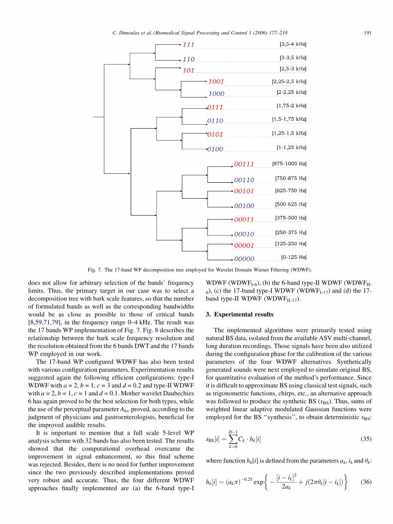
C. Dimoulas et al. / Biomedical Signal Processing and Control 1 (2006) 177–218 191
Fig. 7. The 17-band WP decomposition tree employed for Wavelet Domain Wiener Filtering (WDWF).
does not allow for arbitrary selection of the bands’ frequency
limits. Thus, the primary target in our case was to select a
decomposition tree with bark scale features, so that the number
of formulated bands as well as the corresponding bandwidths
would be as close as possible to those of critical bands
[8,59,71,79], in the frequency range 0–4 kHz. The result was
the 17 bands WP implementation of Fig. 7. Fig. 8 describes the
relationship between the bark scale frequency resolution and
the resolution obtained from the 6 bands DWT and the 17 bands
WP employed in our work.
The 17-band WP configured WDWF has also been tested
with various configuration parameters. Experimentation results
suggested again the following efficient configurations: type-I
WDWF with a = 2, b = 1, c = 3 and d = 0.2 and type-II WDWF
with a = 2, b = 1, c = 1 and d = 0.1. Mother wavelet Daubechies
6 has again proved to be the best selection for both types, while
the use of the perceptual parameter Akw proved, according to the
judgment of physicians and gastroenterologists, beneficial for
the improved audible results.
It is important to mention that a full scale 5-level WP
analysis scheme with 32 bands has also been tested. The results
showed that the computational overhead overcame the
improvement in signal enhancement, so this final scheme
was rejected. Besides, there is no need for further improvement
since the two previously described implementations proved
very robust and accurate. Thus, the four different WDWF
approaches finally implemented are (a) the 6-band type-I
WDWF (WDWFI-6), (b) the 6-band type-II WDWF (WDWFII-
6), (c) the 17-band type-I WDWF (WDWFI-17) and (d) the 17-
band type-II WDWF (WDWFII-17).
3. Experimental results
The implemented algorithms were primarily tested using
natural BS data, isolated from the available ASV multi-channel,
long duration recordings. Those signals have been also utilized
during the configuration phase for the calibration of the various
parameters of the four WDWF alternatives. Synthetically
generated sounds were next employed to simulate original BS,
for quantitative evaluation of the method’s performance. Since
it is difficult to approximate BS using classical test signals, such
as trigonometric functions, chirps, etc., an alternative approach
was followed to produce the synthetic BS (sBS). Thus, sums of
weighted linear adaptive modulated Gaussian functions were
employed for the BS ‘‘synthesis’’, to obtain deterministic sBS:
sBS½i� ¼XD�1
k¼0
Ck � hk½i� (35)
where function hk[i] is defined from the parameters ak, ik and uk:
hk½i� ¼ ðakpÞ�0:25exp
�� ½i� ik�2
2akþ jð2puk½i� ik�Þ
�(36)
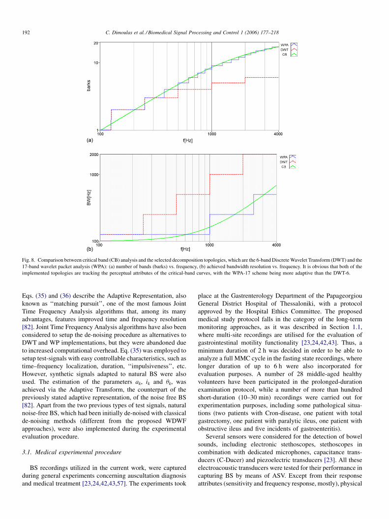
C. Dimoulas et al. / Biomedical Signal Processing and Control 1 (2006) 177–218192
Fig. 8. Comparison between critical band (CB) analysis and the selected decomposition topologies, which are the 6-band Discrete Wavelet Transform (DWT) and the
17-band wavelet packet analysis (WPA): (a) number of bands (barks) vs. frequency, (b) achieved bandwidth resolution vs. frequency. It is obvious that both of the
implemented topologies are tracking the perceptual attributes of the critical-band curves, with the WPA-17 scheme being more adaptive than the DWT-6.
Eqs. (35) and (36) describe the Adaptive Representation, also
known as ‘‘matching pursuit’’, one of the most famous Joint
Time Frequency Analysis algorithms that, among its many
advantages, features improved time and frequency resolution
[82]. Joint Time Frequency Analysis algorithms have also been
considered to setup the de-noising procedure as alternatives to
DWT and WP implementations, but they were abandoned due
to increased computational overhead. Eq. (35) was employed to
setup test-signals with easy controllable characteristics, such as
time–frequency localization, duration, ‘‘impulsiveness’’, etc.
However, synthetic signals adapted to natural BS were also
used. The estimation of the parameters ak, ik and uk, was
achieved via the Adaptive Transform, the counterpart of the
previously stated adaptive representation, of the noise free BS
[82]. Apart from the two previous types of test signals, natural
noise-free BS, which had been initially de-noised with classical
de-noising methods (different from the proposed WDWF
approaches), were also implemented during the experimental
evaluation procedure.
3.1. Medical experimental procedure
BS recordings utilized in the current work, were captured
during general experiments concerning auscultation diagnosis
and medical treatment [23,24,42,43,57]. The experiments took
place at the Gastrenterology Department of the Papageorgiou
General District Hospital of Thessaloniki, with a protocol
approved by the Hospital Ethics Committee. The proposed
medical study protocol falls in the category of the long-term
monitoring approaches, as it was described in Section 1.1,
where multi-site recordings are utilised for the evaluation of
gastrointestinal motility functionality [23,24,42,43]. Thus, a
minimum duration of 2 h was decided in order to be able to
analyze a full MMC cycle in the fasting state recordings, where
longer duration of up to 6 h were also incorporated for
evaluation purposes. A number of 28 middle-aged healthy
volunteers have been participated in the prolonged-duration
examination protocol, while a number of more than hundred
short-duration (10–30 min) recordings were carried out for
experimentation purposes, including some pathological situa-
tions (two patients with Cron-disease, one patient with total
gastrectomy, one patient with paralytic ileus, one patient with
obstructive ileus and five incidents of gastroenteritis).
Several sensors were considered for the detection of bowel
sounds, including electronic stethoscopes, stethoscopes in
combination with dedicated microphones, capacitance trans-
ducers (C-Ducer) and piezoelectric transducers [23]. All these
electroacoustic transducers were tested for their performance in
capturing BS by means of ASV. Except from their response
attributes (sensitivity and frequency response, mostly), physical

C. Dimoulas et al. / Biomedical Signal Processing and Control 1 (2006) 177–218 193
characteristics such as dimension, weight and shape, as well as
the corresponding mechanisms of operation, were also
considered as very important for the demands of the current
application. Based on the experimental observations of the
evaluation procedure, contact piezoelectric transducers were
selected as the most appropriate sensors. Piezoelectric
transducers, also referred as contact microphones or sound
Pick-Ups (PU), feature many advantages: (i) they have small
size and convenient shape, so that can be easily attached to the
objects, (ii) they are highly sensitive to the vibrations of the
contacted surfaces and less sensitive to all the other air-
propagated sounds, (iii) they are passive electric elements and
they do not require power to operate, ensuring safety conditions
for the subjects, (iv) their cost is low, in contrast to the
measuring piezoelectric accelerometers, while (v) their poor
frequency response at very low frequencies is rather beneficial,
since BS are not considered at frequencies below 100–150 Hz
[23].
The ‘‘K&K Sound’’, single-head, hot-spot piezo-transducer
pick-up was finally selected, since it features outstanding
performance characteristic and very small size. It is a round-
shaped instrument transducer having excellent linearity, listed
to the frequency range of 15 Hz to 15 kHz, with high
impedance and sensitivity. According to the manufacturer
(K&K Sound Systems, Inc.) many experimental projects have
been done with the Hot Spot, like installing pickups on the
fingertips of a glove or using them as ‘‘knocking’’ sensors in car
engines. Its small head is only 1.2 in. diameter and 1/32 in.
height and allows an unobtrusive installation. Furthermore,
small areas at the instrument can be reached and the transducer
can be mounted virtually invisibly. This low-cost transducer
was compared for its BS sensing capabilities via auscultation
experiments in combination with an electronic stethoscope
(Audioscope, Medivisio OY, Helsinki, Finland), as well as with
a high precision measurements’ accelerometer (Bruel & Kjær,
type 4506, tri-axial, miniature, high precision accelerometer).
According to the clinicians’ judgment, the transducer features
excellent sound-quality, while the very small size makes it
suitable for easy adaptation on the abdominal wall, especially
for long-term monitoring during nocturnal sleep.
Additionally, the frequency response of the sensor was
measured using the Bruel & Kjær 4809 vibration exciter and
white-noise test signals, resulting to a flat frequency response,
with variation smaller than 3 dB, in the desired frequency
area from 80 Hz to 4 kHz. A high gain (>50 dB), low noise and
low output-impedance preamplifier, with 40 Hz–50 kHz (+0/
�1 dB) frequency range, was also designed for matching
impedance and signal amplification demands. The preamplifier
was housed to a small plastic box (5 cm � 2 cm � 2 cm) and
was placed to a very small distance (<25 cm) from the sensor,
since longer distance cables, connected directly to the
transducer, would produce additional noise interferences.
The power supply for the pre-amplifier is provided through
rechargeable batteries, eliminating the possibilities for noise
interference from the power supply network (hum noises due to
ground loops), while ensuring safety operation, at the same
time. No analog filters were involved in the electroacoustic
chain, besides the high-pass AC coupling and the low-pass anti-
aliasing filters, employed from the circuitry of the recording
units.
The proposed sensor can be easily attached to the abdominal
walls, using double adhesive tape. However, a wearable
absorbing abdominal vest (WAAV), containing a thin lead-plate
(similar to those used in radiographic medical uniforms),
coated with foamy sound-absorbing material was additionally
designed to cover the sensor, aiming best adaptation to the
abdominal vibrating surface, as well as insulation of the air-
propagated ambient noise. The implemented sensors’ adapta-
tion module weights about 860gr and it has proved very useful,
since it keeps sensor(s) closely contacted to the measuring
surface, increasing the sound acquisition sensitivity, while the
presence of environmental acoustic noises is strongly
suppressed (an insertion loss of about 15 dB was measured).
Based on the experience of the clinicians that participated in the
examination procedures, the introduction of the WAAV module
facilitated the preparation of the monitoring process, while
reduced movements’ artefacts were appeared, due to the tighter
attachment of the sensors to the abdominal wall. According to
the opinions of the involved subjects, no discomfort was caused
by the use of the WAAV, since the foamy coating in
combination with the light construction made it very
convenient to adapt. Its utilization was proved very beneficial
especially in the case of mutli-channel recordings, where many
transducers had to be attached and adapted at the abdomen.
In general, any reasonable number of sensors can be
employed during BS auscultation and analysis [23,24,42,43].
The implementation of more than one sensor is enabled, in
order to overcome difficulties related with the weak-nature of
the propagated acoustic waves, selecting each time the sensor
closest to sound origination site, as well as to provide multi-site
monitoring and sound-field topographic interpretation [24].
Within this context, a 2-channel system was initially used, with
the sensors being symmetrically placed at the up-left and the
down-right abdominal quadrants [23,42,43]. The extension to
the four monitoring sensors, symmetrically distributed at the
four abdominal quadrants, was proved to serve best, both the
increased sensitivity demands and the multi-site monitoring
aspects [24]. The implemented de-noising methods were tested
using both 2-channel and 4-channel BS recordings. In addition,
the proposed methods could be also used in the case of signals,
captured by means of displacement, velocity and acceleration,
using tri-axial accelerometer. A hybrid arrangement, utilising
both contact piezoelectric transducers and tri-axial acceler-
ometers, has been recently introduced and it is currently
evaluated for sound-field visualization purposes.
In order to be able to satisfy the above recording demands, a
multi-channel sound card was selected so that signals were
directly captured in a computerised environment. Specifically,
the external card ‘‘PreSonus FIREPOD—24-bit/96K FireWire
Recording Studio’’ was selected, enabling mutli-channel
recordings from up to ten simultaneous monitoring sites.
The easily controlled level-adjustment potentiometers were
used in combination with the pre-amplifier settings, offering an
overall amplification of about 50 dB. Thus, the recording levels
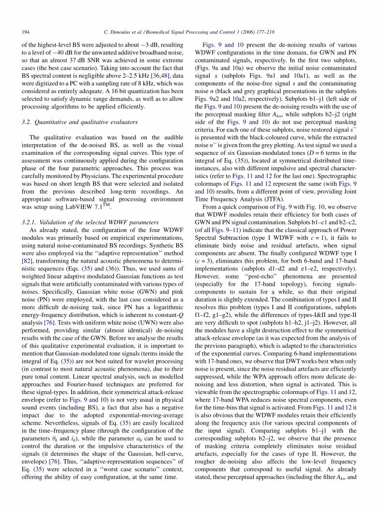
C. Dimoulas et al. / Biomedical Signal Processing and Control 1 (2006) 177–218194
of the highest-level BS were adjusted to about�3 dB, resulting
to a level of�40 dB for the unwanted additive broadband noise,
so that an almost 37 dB SNR was achieved in some extreme
cases (the best case scenario). Taking into account the fact that
BS spectral content is negligible above 2–2.5 kHz [36,48], data
were digitized to a PC with a sampling rate of 8 kHz, which was
considered as entirely adequate. A 16 bit quantization has been
selected to satisfy dynamic range demands, as well as to allow
processing algorithms to be applied efficiently.
3.2. Quantitative and qualitative evaluators
The qualitative evaluation was based on the audible
interpretation of the de-noised BS, as well as the visual
examination of the corresponding signal curves. This type of
assessment was continuously applied during the configuration
phase of the four parametric approaches. This process was
carefully monitored by Physicians. The experimental procedure
was based on short length BS that were selected and isolated
from the previous described long-term recordings. An
appropriate software-based signal processing environment
was setup using LabVIEW 7.1TM.
3.2.1. Validation of the selected WDWF parameters
As already stated, the configuration of the four WDWF
modules was primarily based on empirical experimentations,
using natural noise-contaminated BS recordings. Synthetic BS
were also employed via the ‘‘adaptive representation’’ method
[82], transforming the natural acoustic phenomena to determi-
nistic sequences (Eqs. (35) and (36)). Thus, we used sums of
weighted linear adaptive modulated Gaussian functions as test
signals that were artificially contaminated with various types of
noises. Specifically, Gaussian white noise (GWN) and pink
noise (PN) were employed, with the last case considered as a
more difficult de-noising task, since PN has a logarithmic
energy-frequency distribution, which is inherent to constant-Q
analysis [76]. Tests with uniform white noise (UWN) were also
performed, providing similar (almost identical) de-noising
results with the case of the GWN. Before we analyse the results
of this qualitative experimental evaluation, it is important to
mention that Gaussian-modulated tone signals (terms inside the
integral of Eq. (35)) are not best suited for wavelet processing
(in contrast to most natural acoustic phenomena), due to their
pure tonal content. Linear spectral analysis, such as modelled
approaches and Fourier-based techniques are preferred for
these signal-types. In addition, their symmetrical attack-release
envelope (refer to Figs. 9 and 10) is not very usual in physical
sound events (including BS), a fact that also has a negative
impact due to the adopted exponential-moving-average
scheme. Nevertheless, signals of Eq. (35) are easily localized
in the time–frequency plane (through the configuration of the
parameters uk and ik), while the parameter ak can be used to
control the duration or the impulsive characteristics of the
signals (it determines the shape of the Gaussian, bell-curve,
envelope) [76]. Thus, ‘‘adaptive-representation sequences’’ of
Eq. (35) were selected in a ‘‘worst case scenario’’ context,
offering the ability of easy configuration, at the same time.
Figs. 9 and 10 present the de-noising results of various
WDWF configurations in the time domain, for GWN and PN
contaminated signals, respectively. In the first two subplots,
(Figs. 9a and 10a) we observe the initial noise contaminated
signal x (subplots Figs. 9a1 and 10a1), as well as the
components of the noise-free signal s and the contaminating
noise n (black and grey graphical presentations in the subplots
Figs. 9a2 and 10a2, respectively). Subplots b1–j1 (left side of
the Figs. 9 and 10) present the de-noising results with the use of
the perceptual masking filter Akw, while subplots b2–j2 (right
side of the Figs. 9 and 10) do not use perceptual masking
criteria. For each one of these subplots, noise restored signal s�
is presented with the black-coloured curve, while the extracted
noise n� is given from the grey plotting. As test signal we used a
sequence of six Gaussian-modulated tones (D = 6 terms in the
integral of Eq. (35)), located at symmetrical distributed time-
instances, also with different impulsive and spectral character-
istics (refer to Figs. 11 and 12 for the last one). Spectrographic
colormaps of Figs. 11 and 12 represent the same (with Figs. 9
and 10) results, from a different point of view, providing Joint
Time Frequency Analysis (JTFA).
From a quick comparison of Fig. 9 with Fig. 10, we observe
that WDWF modules retain their efficiency for both cases of
GWN and PN signal contamination. Subplots b1–c1 and b2–c2,
(of all Figs. 9–11) indicate that the classical approach of Power
Spectral Subtraction (type I WDWF with c = 1), it fails to
eliminate birdy noise and residual artefacts, when signal
components are absent. The finally configured WDWF type I
(c = 3), eliminates this problem, for both 6-band and 17-band
implementations (subplots d1–d2 and e1–e2, respectively).
However, some ‘‘post-echo’’ phenomena are presented
(especially for the 17-band topology), forcing signals-
components to sustain for a while, so that their original
duration is slightly extended. The combination of types I and II
resolves this problem (types I and II configurations, subplots
f1–f2, g1–g2), while the differences of types-I&II and type-II
are very difficult to spot (subplots h1–h2, j1–j2). However, all
the modules have a slight destruction effect to the symmetrical
attack-release envelope (as it was expected from the analysis of
the previous paragraph), which is adapted to the characteristics
of the exponential curves. Comparing 6-band implementations
with 17-band ones, we observe that DWT works best when only
noise is present, since the noise residual artefacts are efficiently
suppressed, while the WPA approach offers more delicate de-
noising and less distortion, when signal is activated. This is
viewable from the spectrographic colormaps of Figs. 11 and 12,
where 17-band WPA reduces noise spectral components, even
for the time-bins that signal is activated. From Figs. 11 and 12 it
is also obvious that the WDWF modules retain their efficiently
along the frequency axis (for various spectral components of
the input signal). Comparing subplots b1–j1 with the
corresponding subplots b2–j2, we observe that the presence
of masking criteria completely eliminates noise residual
artefacts, especially for the cases of type II. However, the
rougher de-noising also affects the low-level frequency
components that correspond to useful signal. As already
stated, these perceptual approaches (including the filter Akw and
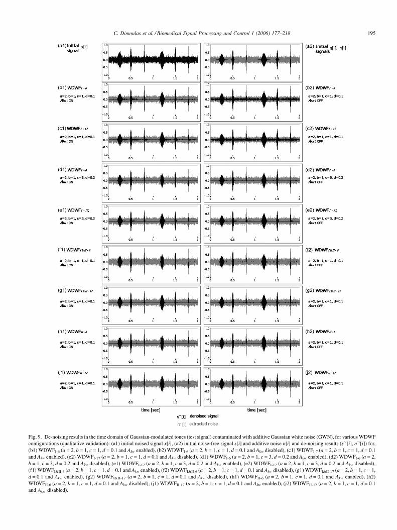
C. Dimoulas et al. / Biomedical Signal Processing and Control 1 (2006) 177–218 195
Fig. 9. De-noising results in the time domain of Gaussian-modulated tones (test signal) contaminated with additive Gaussian white noise (GWN), for various WDWF
configurations (qualitative validation): (a1) initial noised signal x[i], (a2) initial noise-free signal s[i] and additive noise n[i] and de-noising results (s�[i], n�[i]) for,
(b1) WDWFI-6 (a = 2, b = 1, c = 1, d = 0.1 and Akw enabled), (b2) WDWFI-6 (a = 2, b = 1, c = 1, d = 0.1 and Akw disabled), (c1) WDWFI-7 (a = 2, b = 1, c = 1, d = 0.1
and Akw enabled), (c2) WDWFI-17 (a = 2, b = 1, c = 1, d = 0.1 and Akw disabled), (d1) WDWFI-6 (a = 2, b = 1, c = 3, d = 0.2 and Akw enabled), (d2) WDWFI-6 (a = 2,
b = 1, c = 3, d = 0.2 and Akw disabled), (e1) WDWFI-17 (a = 2, b = 1, c = 3, d = 0.2 and Akw enabled), (e2) WDWFI-17 (a = 2, b = 1, c = 3, d = 0.2 and Akw disabled),
(f1) WDWFI&II-6 (a = 2, b = 1, c = 1, d = 0.1 and Akw enabled), (f2) WDWFI&II-6 (a = 2, b = 1, c = 1, d = 0.1 and Akw disabled), (g1) WDWFI&II-17 (a = 2, b = 1, c = 1,
d = 0.1 and Akw enabled), (g2) WDWFI&II-17 (a = 2, b = 1, c = 1, d = 0.1 and Akw disabled), (h1) WDWFII-6 (a = 2, b = 1, c = 1, d = 0.1 and Akw enabled), (h2)
WDWFII-6 (a = 2, b = 1, c = 1, d = 0.1 and Akw disabled), (j1) WDWFII-17 (a = 2, b = 1, c = 1, d = 0.1 and Akw enabled), (j2) WDWFII-17 (a = 2, b = 1, c = 1, d = 0.1
and Akw disabled).
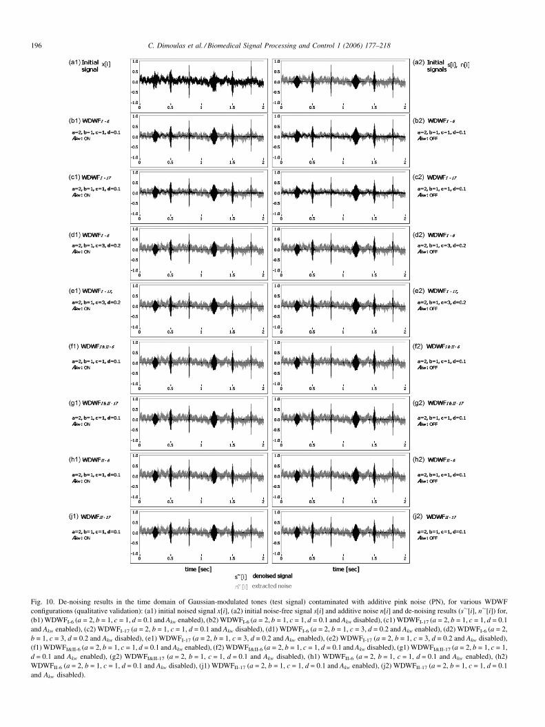
C. Dimoulas et al. / Biomedical Signal Processing and Control 1 (2006) 177–218196
Fig. 10. De-noising results in the time domain of Gaussian-modulated tones (test signal) contaminated with additive pink noise (PN), for various WDWF
configurations (qualitative validation): (a1) initial noised signal x[i], (a2) initial noise-free signal s[i] and additive noise n[i] and de-noising results (s�[i], n�[i]) for,
(b1) WDWFI-6 (a = 2, b = 1, c = 1, d = 0.1 and Akw enabled), (b2) WDWFI-6 (a = 2, b = 1, c = 1, d = 0.1 and Akw disabled), (c1) WDWFI-17 (a = 2, b = 1, c = 1, d = 0.1
and Akw enabled), (c2) WDWFI-17 (a = 2, b = 1, c = 1, d = 0.1 and Akw disabled), (d1) WDWFI-6 (a = 2, b = 1, c = 3, d = 0.2 and Akw enabled), (d2) WDWFI-6 (a = 2,
b = 1, c = 3, d = 0.2 and Akw disabled), (e1) WDWFI-17 (a = 2, b = 1, c = 3, d = 0.2 and Akw enabled), (e2) WDWFI-17 (a = 2, b = 1, c = 3, d = 0.2 and Akw disabled),
(f1) WDWFI&II-6 (a = 2, b = 1, c = 1, d = 0.1 and Akw enabled), (f2) WDWFI&II-6 (a = 2, b = 1, c = 1, d = 0.1 and Akw disabled), (g1) WDWFI&II-17 (a = 2, b = 1, c = 1,
d = 0.1 and Akw enabled), (g2) WDWFI&II-17 (a = 2, b = 1, c = 1, d = 0.1 and Akw disabled), (h1) WDWFII-6 (a = 2, b = 1, c = 1, d = 0.1 and Akw enabled), (h2)
WDWFII-6 (a = 2, b = 1, c = 1, d = 0.1 and Akw disabled), (j1) WDWFII-17 (a = 2, b = 1, c = 1, d = 0.1 and Akw enabled), (j2) WDWFII-17 (a = 2, b = 1, c = 1, d = 0.1
and Akw disabled).
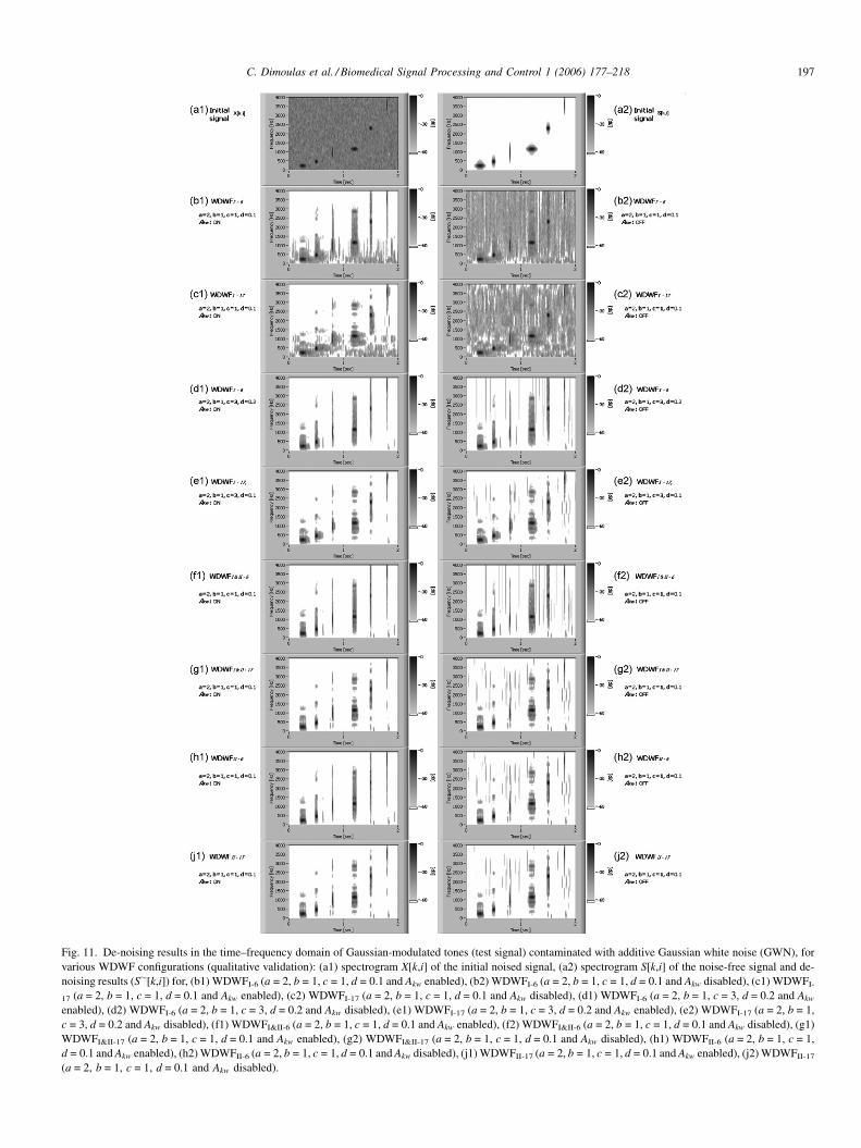
C. Dimoulas et al. / Biomedical Signal Processing and Control 1 (2006) 177–218 197
Fig. 11. De-noising results in the time–frequency domain of Gaussian-modulated tones (test signal) contaminated with additive Gaussian white noise (GWN), for
various WDWF configurations (qualitative validation): (a1) spectrogram X[k,i] of the initial noised signal, (a2) spectrogram S[k,i] of the noise-free signal and de-
noising results (S�[k,i]) for, (b1) WDWFI-6 (a = 2, b = 1, c = 1, d = 0.1 and Akw enabled), (b2) WDWFI-6 (a = 2, b = 1, c = 1, d = 0.1 and Akw disabled), (c1) WDWFI-
17 (a = 2, b = 1, c = 1, d = 0.1 and Akw enabled), (c2) WDWFI-17 (a = 2, b = 1, c = 1, d = 0.1 and Akw disabled), (d1) WDWFI-6 (a = 2, b = 1, c = 3, d = 0.2 and Akw
enabled), (d2) WDWFI-6 (a = 2, b = 1, c = 3, d = 0.2 and Akw disabled), (e1) WDWFI-17 (a = 2, b = 1, c = 3, d = 0.2 and Akw enabled), (e2) WDWFI-17 (a = 2, b = 1,
c = 3, d = 0.2 and Akw disabled), (f1) WDWFI&II-6 (a = 2, b = 1, c = 1, d = 0.1 and Akw enabled), (f2) WDWFI&II-6 (a = 2, b = 1, c = 1, d = 0.1 and Akw disabled), (g1)
WDWFI&II-17 (a = 2, b = 1, c = 1, d = 0.1 and Akw enabled), (g2) WDWFI&II-17 (a = 2, b = 1, c = 1, d = 0.1 and Akw disabled), (h1) WDWFII-6 (a = 2, b = 1, c = 1,
d = 0.1 and Akw enabled), (h2) WDWFII-6 (a = 2, b = 1, c = 1, d = 0.1 and Akw disabled), (j1) WDWFII-17 (a = 2, b = 1, c = 1, d = 0.1 and Akw enabled), (j2) WDWFII-17
(a = 2, b = 1, c = 1, d = 0.1 and Akw disabled).
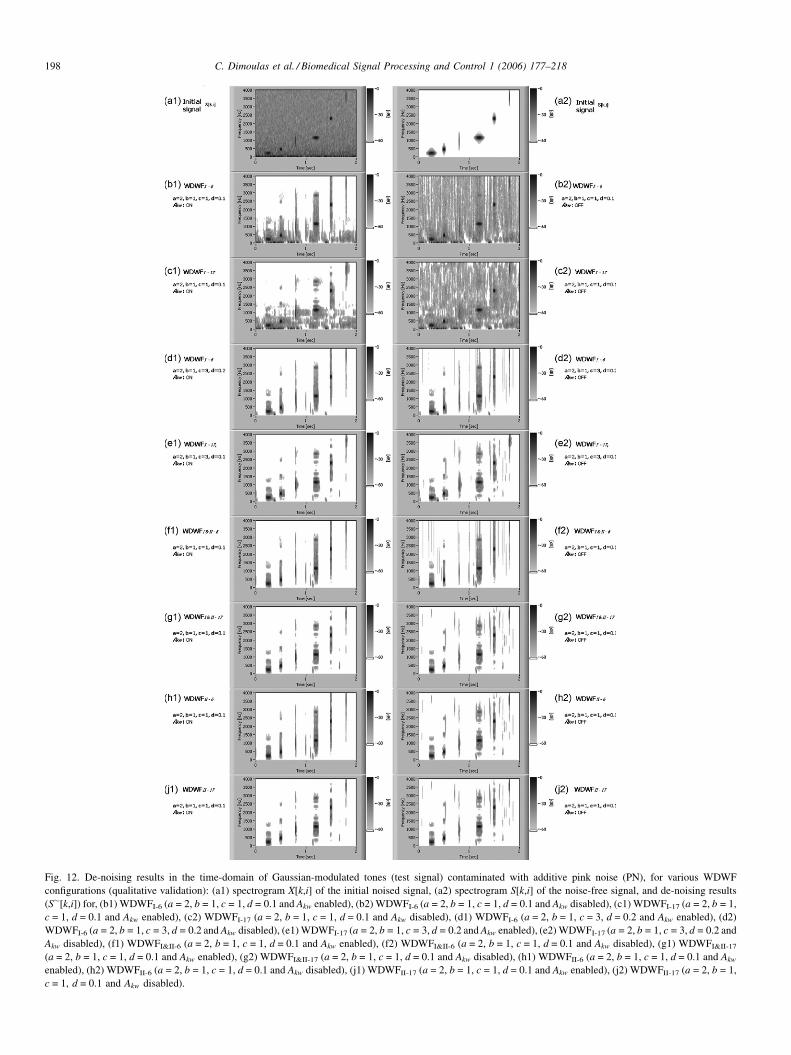
C. Dimoulas et al. / Biomedical Signal Processing and Control 1 (2006) 177–218198
Fig. 12. De-noising results in the time-domain of Gaussian-modulated tones (test signal) contaminated with additive pink noise (PN), for various WDWF
configurations (qualitative validation): (a1) spectrogram X[k,i] of the initial noised signal, (a2) spectrogram S[k,i] of the noise-free signal, and de-noising results
(S�[k,i]) for, (b1) WDWFI-6 (a = 2, b = 1, c = 1, d = 0.1 and Akw enabled), (b2) WDWFI-6 (a = 2, b = 1, c = 1, d = 0.1 and Akw disabled), (c1) WDWFI-17 (a = 2, b = 1,
c = 1, d = 0.1 and Akw enabled), (c2) WDWFI-17 (a = 2, b = 1, c = 1, d = 0.1 and Akw disabled), (d1) WDWFI-6 (a = 2, b = 1, c = 3, d = 0.2 and Akw enabled), (d2)
WDWFI-6 (a = 2, b = 1, c = 3, d = 0.2 and Akw disabled), (e1) WDWFI-17 (a = 2, b = 1, c = 3, d = 0.2 and Akw enabled), (e2) WDWFI-17 (a = 2, b = 1, c = 3, d = 0.2 and
Akw disabled), (f1) WDWFI&II-6 (a = 2, b = 1, c = 1, d = 0.1 and Akw enabled), (f2) WDWFI&II-6 (a = 2, b = 1, c = 1, d = 0.1 and Akw disabled), (g1) WDWFI&II-17
(a = 2, b = 1, c = 1, d = 0.1 and Akw enabled), (g2) WDWFI&II-17 (a = 2, b = 1, c = 1, d = 0.1 and Akw disabled), (h1) WDWFII-6 (a = 2, b = 1, c = 1, d = 0.1 and Akw
enabled), (h2) WDWFII-6 (a = 2, b = 1, c = 1, d = 0.1 and Akw disabled), (j1) WDWFII-17 (a = 2, b = 1, c = 1, d = 0.1 and Akw enabled), (j2) WDWFII-17 (a = 2, b = 1,
c = 1, d = 0.1 and Akw disabled).
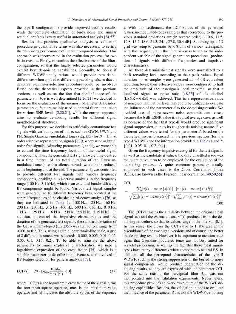
C. Dimoulas et al. / Biomedical Signal Processing and Control 1 (2006) 177–218 199
the type-II configuration) provide improved audible results,
while the complete elimination of birdy noise and similar
residual artefacts is very useful in automated analysis [24,57].
Besides the previous qualitative analysis, a validation
procedure in quantitative terms was also necessary, to certify
the de-noising performance of the four proposed modules. This
approach was incorporated in the evaluation process, for two
basic reasons. Firstly, to confirm the effectiveness of the filter-
configuration, so that the finally selected parameters would
exhibit best de-noising capabilities. Secondly, to check if
different WDWF-configurations would provide remarkable
differences when applied to different types of signals, so that an
adaptive parameter-selection procedure could be involved.
Based on the theoretical aspects provided in the previous
sections, as well as on the fact that the influence of the
parameters a, b, c is well determined [2,20,21] we decided to
focus on the evaluation of the memory parameter d. Besides,
parameters a, b, c are mainly used to control filter attenuation
for various SNR levels [2,20,21], while the current approach
aims to evaluate de-noising results for different signal
morphological structures.
For this purpose, we decided to artificially contaminate test
signals with various types of noise, such as GWN, UWN and
PN. Single Gaussian-modulated tones (Eq. (35) for D = 1, first
order adaptive representation signals [82]), where used as initial
noise free signals. Adjusting parameters ik and uk we were able
to control the time–frequency location of the useful signal
components. Thus, the generated test signals were time-centred
in a time interval of 1 s (total duration of the Gaussian-
modulated tones), so that silence periods would be introduced
at the beginning and at the end. The parameter uk was controlled
to provide different test signals with various frequency
components, enabling a 1/3-octave analysis in the frequency
range [100 Hz, 3.1 kHz], which is an extended bandwidth were
BS components might be found. Various test signal samples
were generated at 16 different frequency bins, located at the
central frequencies of the classical third-octave analysis [76], as
they are indicated in Table 1: {100 Hz, 125 Hz, 160 Hz,
200 Hz, 250 Hz, 315 Hz, 400 Hz, 500 Hz, 630 Hz, 810 Hz,
1 kHz, 1.25 kHz, 1.6 kHz, 2 kHz, 2.5 kHz, 3.15 kHz}. In
addition, to control the impulsive characteristics and the
duration of the generated test signals, the standard deviation of
the Gaussian enveloped (Eq. (35)) was forced to a range from
0.001 to 0.2. Thus, using again a logarithmic-like scale, a grid
of 8 different instances was selected: {0.002, 0.005, 0.01, 0.02,
0.05, 0.1, 0.15, 0.2}. To be able to translate the above
parameters to signal explosive characteristics, we used a
logarithmic expression of the crest factor [75], which is a
suitable parameter to describe impulsiveness, also involved in
BS feature selection for pattern analysis [57]:
LCFðsÞ ¼ 20 � log10
rmsðsÞmaxðjsjÞ ½dB� (37)
where LCF(s) is the logarithmic crest factor of the signal s, rms
the root-mean-square operator, max is the maximum-value
operator and jsj indicates the absolute values of the sequence
s. With this settlement, the LCF values of the generated
Gaussian-modulated-tones samples that correspond to the pre-
vious standard deviations are (in reverse order): {10.6, 11.5,
12.8, 15.2, 18.6, 21.3, 24.1, 27.8, 30.4 dB}. Summing up, a 2D
grid was setup to generate 16 � 8 bins of various test signals,
with the frequency and the impulsiveness to act as the inde-
pendent variable of the signal generation procedures (produc-
tion of signals with different frequencies and impulsive
characteristics).
All these deterministic test signals were normalized to a
0 dB recording level, according to their peak values. Equal
duration noise samples were generated at �6 dB equivalent
recording level; their effective values were configured to half
the amplitude of the test-signals local maxima, so that a
localized signal to noise ratio [48,55] of six decibel
(LSNR = 6 dB) was achieved. This is a representative value
of noise-contamination level that could be utilized to evaluate
the influence of the parameter d to the de-noising results. We
avoided use of more severe noise contaminations cases,
because the 6 dB LSNR value is a typical average case, as well
as because of the fact that type-II would produce significant
signal suppression, due to its rougher de-noising nature. Five
different values were tested for the parameter d, based on the
theoretical issues discussed in the previous section (for the
type-I WDWF) and the information provided in Tables 1 and 2:
{0.01, 0.05, 0.1, 0.2, 0.4}.
Given the frequency-impulsiveness grid for the test signals,
as well as the candidate d values, the only unsettled issue was
the quantitative term to be employed for the evaluation of the
de-noising process. A quite common parameter usually
employed in such cases is the Cross Correlation Index
(CCI), also known as the Pearson linear correlation [48,50,55]:
CCI
¼P
i½sðiÞ �meanfsðiÞg� � ½s� ðiÞ �meanfs� ðiÞg�ffiffiffiffiffiffiffiffiffiffiffiffiffiffiffiffiffiffiffiffiffiffiffiffiffiffiffiffiffiffiffiffiffiffiffiffiffiffiffiffiffiffiffiffiffiffiPi½sðiÞ �meanfsðiÞg�2
q�ffiffiffiffiffiffiffiffiffiffiffiffiffiffiffiffiffiffiffiffiffiffiffiffiffiffiffiffiffiffiffiffiffiffiffiffiffiffiffiffiffiffiffiffiffiffiffiffiffiffiffiffiffiffiP
i½s� ðiÞ �meanfs� ðiÞg�2q
(38)
The CCI estimates the similarity between the original clean
signal s(i) and the estimated one s�(i) produced from the de-
noising procedure, so that its values range in the interval [0,1].
In this sense, the closer the CCI value to 1, the greater the
resemblance of the two signal versions and of course, the better
the de-noising results. However, it is important to mention once
again that Gaussian-modulated tones are not best suited for
wavelet processing, as well as the fact that these ideal signal-
types have many differences when compared to natural BS. In
addition, all the perceptual characteristics of the type-II
WDWF, such as the strong suppression of the buried to noise
signal components, would produce degradation of the de-
noising results, as they are expressed with the parameter CCI.
For the same reason, the perceptual filter Akw was not
incorporated into the validation experiments. Nevertheless,
this procedure provides an overview-picture of the WDWF de-
noising capabilities. Besides, the validation intends to evaluate
the influence of the parameter d and not the WDWF de-noising
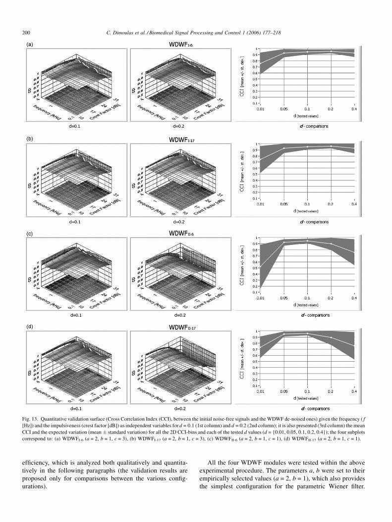
C. Dimoulas et al. / Biomedical Signal Processing and Control 1 (2006) 177–218200
Fig. 13. Quantitative validation surface (Cross Correlation Index (CCI), between the initial noise-free signals and the WDWF de-noised ones) given the frequency ( f
[Hz]) and the impulsiveness (crest factor [dB]) as independent variables for d = 0.1 (1st column) and d = 0.2 (2nd column); it is also presented (3rd column) the mean
CCI and the expected variation (mean standard variation) for all the 2D CCI-bins and each of the tested d values (d = {0.01, 0.05, 0.1, 0.2, 0.4}); the four subplots
correspond to: (a) WDWFI-6 (a = 2, b = 1, c = 3), (b) WDWFI-17 (a = 2, b = 1, c = 3), (c) WDWFII-6 (a = 2, b = 1, c = 1), (d) WDWFII-17 (a = 2, b = 1, c = 1).
efficiency, which is analyzed both qualitatively and quantita-
tively in the following paragraphs (the validation results are
proposed only for comparisons between the various config-
urations).
All the four WDWF modules were tested within the above
experimental procedure. The parameters a, b were set to their
empirically selected values (a = 2, b = 1), which also provides
the simplest configuration for the parametric Wiener filter.
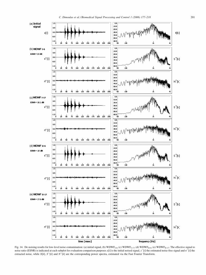
C. Dimoulas et al. / Biomedical Signal Processing and Control 1 (2006) 177–218 201
Fig. 14. De-noising results for low-level noise contamination: (a) initial signal, (b) WDWFI-6, (c) WDWFI-17, (d) WDWFII-6, (e) WDWFII-17. The effective signal to
noise ratio (ESNR) is indicated at each subplot for evaluation-comparison purposes x[i] is the initial noised signal, s�[i] the estimated noise-free signal and n�[i] the
extracted noise, while X[k], S�[k] and N�[k] are the corresponding power spectra, estimated via the Fast Fourier Transform.
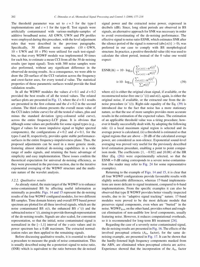
C. Dimoulas et al. / Biomedical Signal Processing and Control 1 (2006) 177–218202
The threshold parameter was set to c = 3 for the type-I
implementations and c = 1 for the type-II. Test signals were
artificially contaminated with various-multiple-samples of
additive broadband noise. All GWN, UWN and PN profiles
were employed during this procedure, with the level adjustment
rules that were described in the previous paragraphs.
Specifically, 30 different noise samples (10 � GWN,
10 � UWN and 10 � PN) were utilized for each test-signal-
bin, so that every WDWF module was implemented 30 times
for each bin, to estimate a mean CCI from all the 30 de-noising
results (per input signal). Tests with 300 noise samples were
also performed, without any significant difference in the
observed de-nosing results. As a consequence, we were able to
draw the 2D-surface of the CCI variation across the frequency
and crest-factor axes, for every tested d value. The statistical
properties of those parametric surfaces would provide the final
validation results.
In all the WDWF modules the values d = 0.1 and d = 0.2
provided the best results of all the tested values. The related
surface-plots are presented in Fig. 13, where the d = 0.1 results
are presented in the first column and the d = 0.2 in the second
column. The third column presents the overall mean value of
the CCI index (white curve) for all the tested d values, plus and
minus the standard deviation (grey-coloured solid curve),
across the entire frequency-LCF plane. It is obvious that
although some values are preferable for some signal types (e.g.,
bigger d values for more impulsive signal or higher spectral
components), the configurations d = 0.2 and d = 0.1, for the
types I and II, respectively, provides quite stable performance-
surfaces in the entire frequency-impulsiveness plane. Thus, the
proposed adjustments can be used in a more generic mode,
featuring almost identical de-noising capabilities in a wide
range of audio signals, and retaining the basic advantage of
simplicity and easy implementation. These issues confirm the
theoretical expectation for universal de-noising efficiency, as
they were presented in the previous section, due to the iterative
exponential averaging of the WDWF structure and the multi-
rate nature of the wavelet analysis.
3.2.2. Qualitative results
As already stated, the main target of the WDWF is to enhance
noise-contaminated BS by affecting useful information as
minimally as possible. Figs. 14 and 15 represent the de-noising
results of the four WDWF configured modules, for two different
BS samples. Time domain history and overall FFT-based power
spectrum are plotted for all three involved signals, which are the
noise contaminated BS x(i), the enhanced BS s�(i) and the
subtracted noise n�(i), aiming to provide thorough representation
of the de-noising results. Signals are also scaled, for convenient
representation, so that the initial, noise contaminated signal is
normalized in the [�1,1] interval of the y-axis values and its
power spectrum has a 0 dB maximum. The extracted normal-
ization rules are then applied to the remaining signals.
Before discussing qualitative results, it is essential to define
a procedure to measure the grade of noise contamination. This
is usually described using the a-posteriori signal to noise ratio,
(SNR) which is equivalent to the ratio between the de-noised
signal power and the extracted noise power, expressed in
decibels (dB). Since, long silent periods are observed in BS
signals, an alternative approach for SNR was necessary in order
to avoid overestimating of the de-noising performance. The
effective signal to noise ratio ESNR, which estimates SNR after
the silence period of the signal is removed (abs{s(i)} > 0), was
preferred in our case to comply with BS morphological
structure. In practice, a positive threshold value (th) was used to
calculate the silent period, instead of the 0 value one would
expect:
ESNRðthÞ ¼ 10 � log10
�Pi;jsðiÞj> thsðiÞ2Pi;jsðiÞj> thnðiÞ2
�
ffi 10 � log10
�Pi;sðiÞj> thsðiÞ2P
inðiÞ2
�(39)
where s(i) is either the original clean signal, if available, or the
reconstructed noise-free one (s�(i)) and n(i), again, is either the
original noise, if available, or the extracted one from the de-
noise procedure (n�(i)). Right-side equality of the Eq. (39) is
introduced due to the fact that noise has a more stationary
nature, so that the use of more samples provides more accurate
results in the estimation of the expected values. The estimation
of an applicable threshold value was a tiring procedure; how-
ever it finally successfully dealt with, by adopting the following
rule: (i) a local maximum signal region is selected and its
average power is calculated, (ii) a threshold is estimated so that
signal regions that are above �20 dB of the calculated average
power, are considered as non-silence. Exponential sound-level
averaging was proved very useful for the previously described
level estimation procedure, enabling a point to point compar-
ison mode. The coefficients {1, �0.92} and {0.08} of the IIR
filter (Eq. (26)) were experimentally selected, so that the
ESNR = 0 dB rating corresponds to a severe noise-contamina-
tion (the reader may refer to Fig. 24 for some representative
examples).
Returning to the example of Figs. 14 and 15, it is clear that
all four WDWF configurations provide favourable results with
slightly noticeable differences, whereas 17-band implementa-
tions are more delicate to signal treatment, compared to 6-band
implementations. From the specific examples it can also be
observed that type II WDWF provides better visually inspected
results, due to its ‘‘adaptive signal tracking’’ nature. 17-band
modules were proved to be the most delicate module that
preserves signal components, even when are ‘‘buried’’ in the
noise. WDWFII-6, on the other hand, provides robust and rough-
cut elimination of non-audible low level components, usually
featuring noise. However, it reduces computational overheads,
so it is recommended for long-term BS treatment [24].
Regarding the case of a severely noise contaminated signal,
the de-noising results are presented in Fig. 16. The effects of the
involved perceptual criteria (Akw factor), for the same de-
noising example, are presented in Fig. 17. It can be shown that
the hardly-listened high frequency components masked from
the ABN, are eliminated when perceptual criteria are active.
Experience showed that the incorporation of the Akw factor
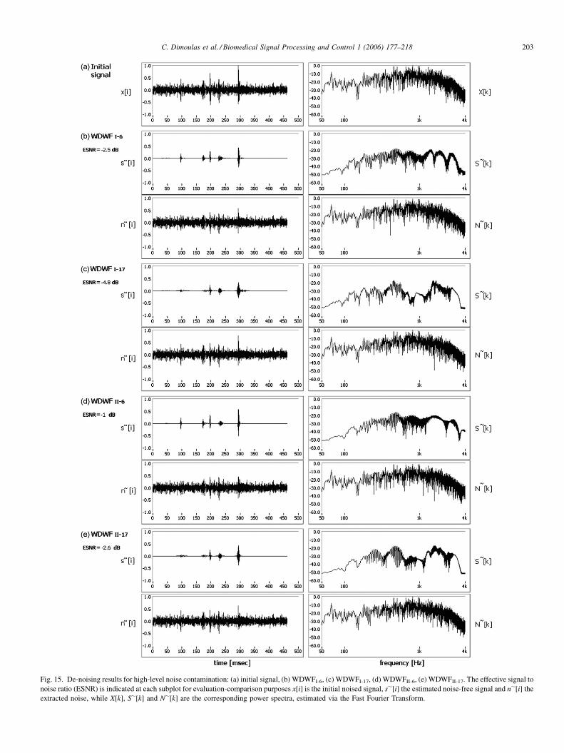
C. Dimoulas et al. / Biomedical Signal Processing and Control 1 (2006) 177–218 203
Fig. 15. De-noising results for high-level noise contamination: (a) initial signal, (b) WDWFI-6, (c) WDWFI-17, (d) WDWFII-6, (e) WDWFII-17. The effective signal to
noise ratio (ESNR) is indicated at each subplot for evaluation-comparison purposes x[i] is the initial noised signal, s�[i] the estimated noise-free signal and n�[i] the
extracted noise, while X[k], S�[k] and N�[k] are the corresponding power spectra, estimated via the Fast Fourier Transform.
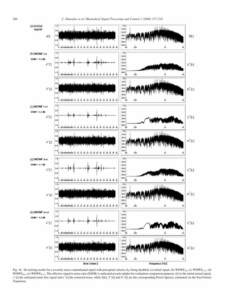
C. Dimoulas et al. / Biomedical Signal Processing and Control 1 (2006) 177–218204
Fig. 16. De-noising results for a severely noise-contaminated signal with perceptual criteria (Ak) being disabled: (a) initial signal, (b) WDWFI-6, (c) WDWFI-17, (d)
WDWFII-6, (e) WDWFII-17. The effective signal to noise ratio (ESNR) is indicated at each subplot for evaluation-comparison purposes x[i] is the initial noised signal,
s�[i] the estimated noise-free signal and n�[i] the extracted noise, while X[k], S�[k] and N�[k] are the corresponding Power Spectra, estimated via the Fast Fourier
Transform.
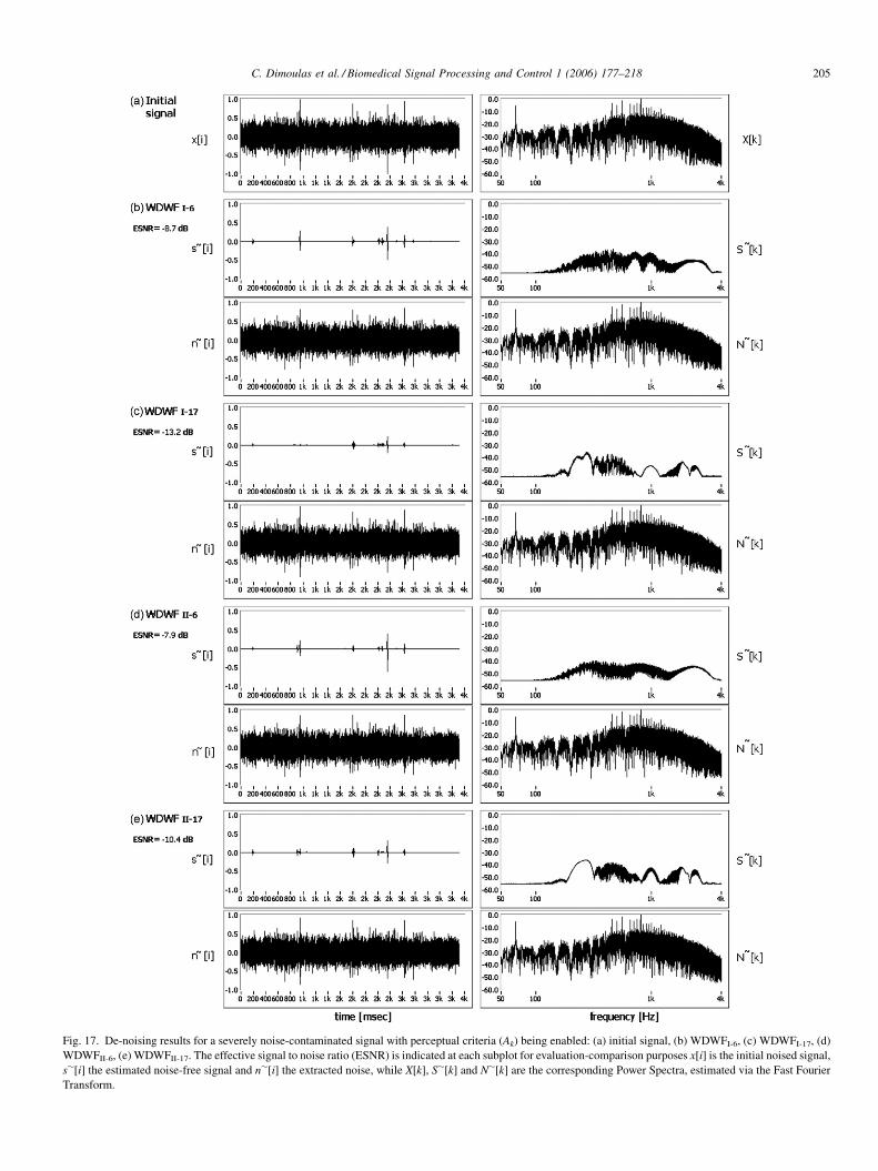
C. Dimoulas et al. / Biomedical Signal Processing and Control 1 (2006) 177–218 205
Fig. 17. De-noising results for a severely noise-contaminated signal with perceptual criteria (Ak) being enabled: (a) initial signal, (b) WDWFI-6, (c) WDWFI-17, (d)
WDWFII-6, (e) WDWFII-17. The effective signal to noise ratio (ESNR) is indicated at each subplot for evaluation-comparison purposes x[i] is the initial noised signal,
s�[i] the estimated noise-free signal and n�[i] the extracted noise, while X[k], S�[k] and N�[k] are the corresponding Power Spectra, estimated via the Fast Fourier
Transform.
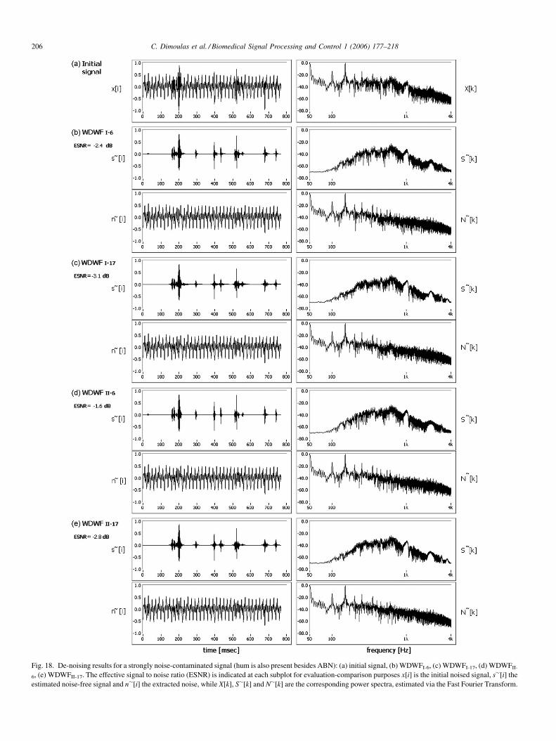
C. Dimoulas et al. / Biomedical Signal Processing and Control 1 (2006) 177–218206
Fig. 18. De-noising results for a strongly noise-contaminated signal (hum is also present besides ABN): (a) initial signal, (b) WDWFI-6, (c) WDWFI-17, (d) WDWFII-
6, (e) WDWFII-17. The effective signal to noise ratio (ESNR) is indicated at each subplot for evaluation-comparison purposes x[i] is the initial noised signal, s�[i] the
estimated noise-free signal and n�[i] the extracted noise, while X[k], S�[k] and N�[k] are the corresponding power spectra, estimated via the Fast Fourier Transform.
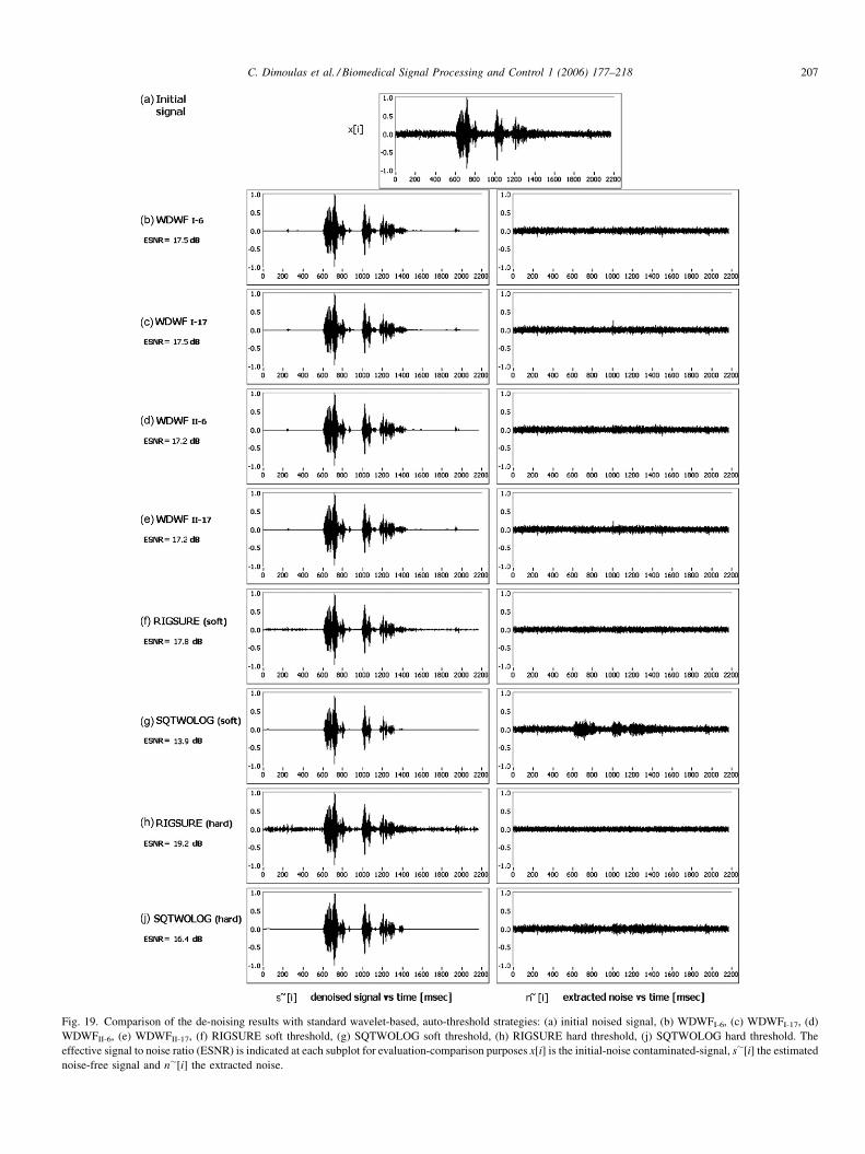
C. Dimoulas et al. / Biomedical Signal Processing and Control 1 (2006) 177–218 207
Fig. 19. Comparison of the de-noising results with standard wavelet-based, auto-threshold strategies: (a) initial noised signal, (b) WDWFI-6, (c) WDWFI-17, (d)
WDWFII-6, (e) WDWFII-17, (f) RIGSURE soft threshold, (g) SQTWOLOG soft threshold, (h) RIGSURE hard threshold, (j) SQTWOLOG hard threshold. The
effective signal to noise ratio (ESNR) is indicated at each subplot for evaluation-comparison purposes x[i] is the initial-noise contaminated-signal, s�[i] the estimated
noise-free signal and n�[i] the extracted noise.
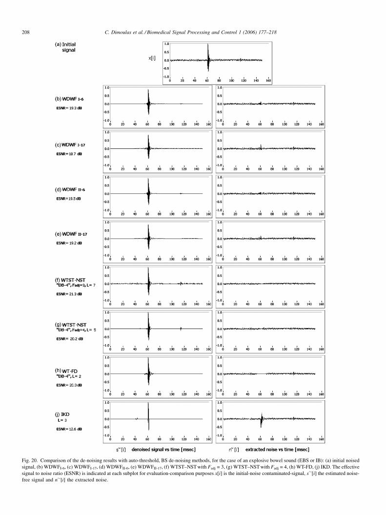
C. Dimoulas et al. / Biomedical Signal Processing and Control 1 (2006) 177–218208
Fig. 20. Comparison of the de-noising results with auto-threshold, BS de-noising methods, for the case of an explosive bowel sound (EBS or IB): (a) initial noised
signal, (b) WDWFI-6, (c) WDWFI-17, (d) WDWFII-6, (e) WDWFII-17, (f) WTST–NST with Fadj = 3, (g) WTST–NST with Fadj = 4, (h) WT-FD, (j) IKD. The effective
signal to noise ratio (ESNR) is indicated at each subplot for evaluation-comparison purposes x[i] is the initial-noise contaminated-signal, s�[i] the estimated noise-
free signal and n�[i] the extracted noise.
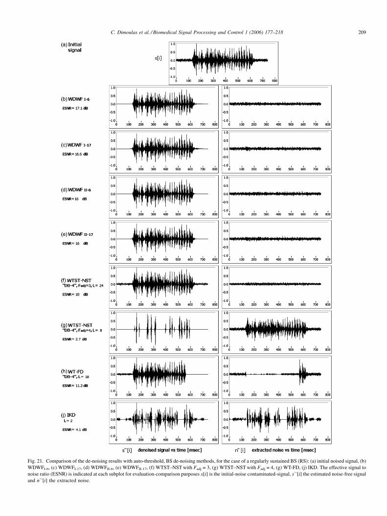
C. Dimoulas et al. / Biomedical Signal Processing and Control 1 (2006) 177–218 209
Fig. 21. Comparison of the de-noising results with auto-threshold, BS de-noising methods, for the case of a regularly sustained BS (RS): (a) initial noised signal, (b)
WDWFI-6, (c) WDWFI-17, (d) WDWFII-6, (e) WDWFII-17, (f) WTST–NST with Fadj = 3, (g) WTST–NST with Fadj = 4, (g) WT-FD, (j) IKD. The effective signal to
noise ratio (ESNR) is indicated at each subplot for evaluation-comparison purposes x[i] is the initial-noise contaminated-signal, s�[i] the estimated noise-free signal
and n�[i] the extracted noise.

C. Dimoulas et al. / Biomedical Signal Processing and Control 1 (2006) 177–218210
leads to audible improvements as well as elimination of birdy-
noise and residual artefacts, while useful information is barely
affected.
In the example of Fig. 18, the signal is also contaminated
with hum, besides ABN (not a rare incident in such
applications). The de-noising results prove the fact that the
method is capable of eliminating background noise even in
cases where broadband spectral characteristics are violated, as
long as the appropriate noise footprint is provided.
Another issue, connected with the qualitative analysis of the
method’s performance, is the comparison with standard de-
noising techniques. Two of the most famous wavelet de-noising
techniques, with automatic thresholds, were selected for this
task. The first uses the principle of Stein’s Unbiased Risk
Estimate (SURE) for threshold estimation, and the ‘‘SQTWO-
LOG’’ approach that uses the universal threshold, sqrt(2*lo-
g(length of x[i])) [13]. These reference methods were selected
from the ‘‘ready to use’’ tools of the National Instruments
Signal Processing Toolset v6.0TM [83]. For the rest of the paper,
we will use the notation ‘‘RIGSURE-(soft)’’ and ‘‘RIGUSRE-
(hard)’’ for soft and hard thresholding (Eq. (14)), respectively,
where the SURE threshold is employed [83]. Similarly the
notations ‘‘SQTWOLOG-(soft)’’ and ‘‘SQTWOLOG-(hard)’’
are defined, for the SQTWOLOG-based threshold estimation
[83]. Fig. 19 provides comparisons of de-noising results,
between the WDWF modules, and the above-mentioned
wavelet, auto-thresholding, strategies. It is clear that WDWF
approaches combine robust de-noise with bare minimum effect
on useful signal information. Experience showed that the
WDWF approach balances between the minimal signal
destruction of the RIGSURE-(soft) method and the rough
de-noising of the SQTWOLOG-(hard) method. The first
approach, suffers from the birdy noise and similar residual
artefacts, especially for low SNRs, while the second sweeps out
most of the stationary-like signal components. On the other
hand, RIGSURE-(hard) methods leaves out more noise
residuals compared to RIGSURE-(soft), while the SQTWO-
LOG-(soft) approach resolves this problem, usually affecting
useful signal components (refer to the extracted noise curve, in
Fig. 19g). In general, WDWF preserve the morphological
structure of all regularly sustained BSs, included whistling and
rumbling gastrointestinal sounds, produced by prolonged
sweep clusters of contractions [23,24], whereas most auto-
mated thresholding strategies seriously damage the shape of the
signals.
Related with the previous issue is the fact that all the
proposed auto-threshold de-noising algorithms, that have been
developed for BS processing [48,50–56], are mainly suggested
for explosive BS. However, it is interesting to compare the
WDWF modules with some of those methods, such as the
WTST–NST approach [10,48,50], which has been utilized in
various BS analysis demands [51] and received various
interpretations and implementation improvements [53], the
WT-FD method [54,55] and the IKD approach [52,56],
although the last filtering technique is mostly intended for
signal detection purposes. Since all the previous approaches
have been developed for EBS, it would be useful to evaluate and
compare them with WDWF, using such types of signals. Fig. 20
provides de-noising results of a noised explosive BS pattern
(IB), for all the WDWF modules and the standard EBS auto-
threshold de-nosing methods. It is obvious that all the tested
algorithms result to robust de-noising, with the IKD approach
to efficiently detect the signal initiation (Fig. 20j), inside a
small number of iterations (L = 3). The WTST–NST method
with Fadj = 3 (as it was proposed in its original configuration
[10,48]), results to significant signal enhancement with
minimum distortion (Fig. 20f). However, a weakness is spotted
in the presence of noise residual artefacts, problem that is
successfully dealt when Fadj = 4 (Fig. 20g). The last
modification also facilitates faster convergence, since a number
of L = 5 iterations is now required, instead of L = 7 for the case
of Fadj = 3. The WT-FD method (Fig. 20h) seems to be immune
to noise residual artefacts, where the ABN is completely
eliminated when the signal is absent. The filtering process is
softer in the opposite case, when signal components are present,
approaching noise-gate processing results, an issue that
preserves perceptual characteristics (the noise is masked by
the signal) and does not cause any spectral distortion.
Comparing all the previous results with the ones provide of
our proposed methods (Fig. 20, subplots b–e), it is important to
mention that all the four WDWF modules have outstanding
performance, with similar, if not superior, de-nosing results.
Fig. 21 provides an alternative example, where all the
candidate de-noising algorithms are compared for their ability
to be utilized in the case of clustered-contraction BS events,
referred as regularly sustained (RS) [57]. Although the auto-
threshold EBS de-noising methods are not indented for such
types of signals, this comparison is unavoidable for two basic
reasons: (i) for the completeness of the evaluation procedure
and (ii) to show up that the proposed WDWF techniques are
very efficient in these cases, where certified de-noising methods
are not available. From Fig. 21, it is obvious that all the four
WDWF modules retain their efficiency, providing robust
enhancement with accurate noise elimination (Fig. 21, subplots
b–e). This is not an incident for the case of all the other
methods, where we observe either insufficient de-noising
(Fig. 21f), or random signal distortions and morphological
destructions (Fig. 21g and h). Similarly, the IKD detection
results seem to be very confusing (Fig. 21j). These results are
quite natural, since according to the corresponding authors
[48,50–56] the proposed methods have been configured for
EBS processing demands. Thus, algorithms modifications or
alternative configuration are needed. Based on our experi-
mentation, the WTST–NST provides better results from the
other approaches, especially the original configuration
(Fig. 21f) with Fadj = 3 [10,48]. Nevertheless, a rather great
amount of noise remains in tact, after a heavy computational
workload (L = 24). The configuration with Fadj = 4 leads to
faster convergence (L = 8) and stronger noise-elimination
(Fig. 21g), an issue that causes serious morphological
destruction in most of the RS patterns. The WT-FD method
(Fig. 21h) seemed quite unstable, since very small modification
to the filter-configuration-parameters (accuracy, acc; epsilon, e;sliding window length, WL [54,55]), leads to completely
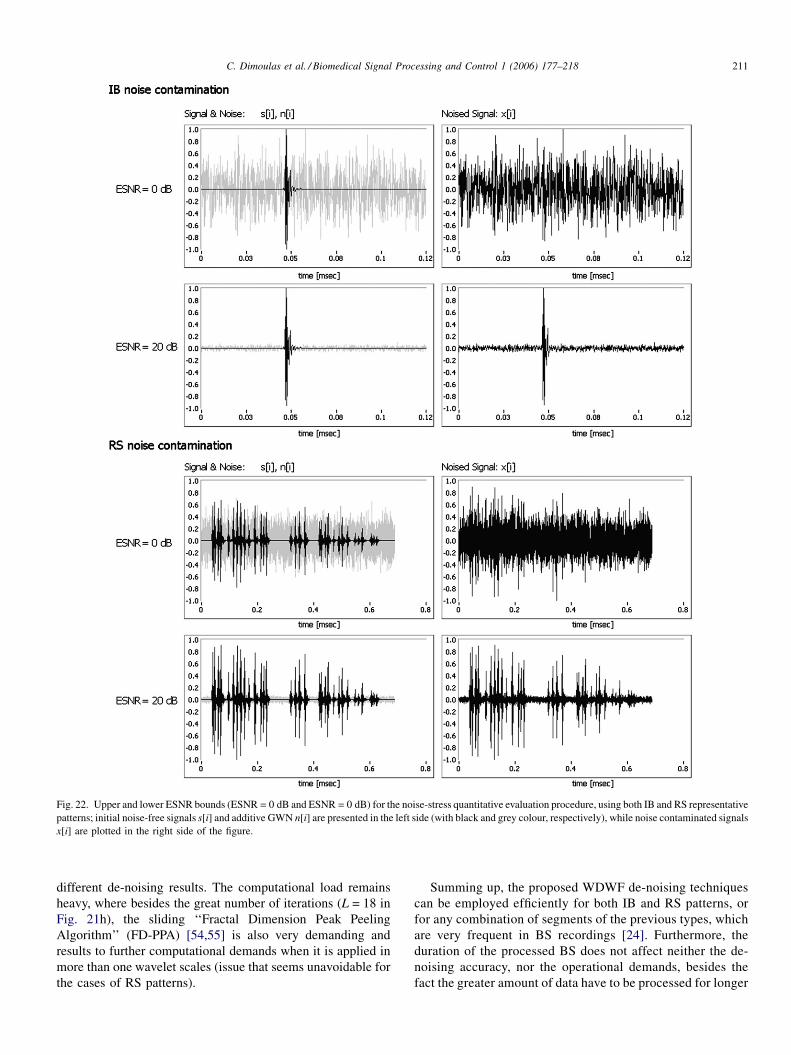
C. Dimoulas et al. / Biomedical Signal Processing and Control 1 (2006) 177–218 211
Fig. 22. Upper and lower ESNR bounds (ESNR = 0 dB and ESNR = 0 dB) for the noise-stress quantitative evaluation procedure, using both IB and RS representative
patterns; initial noise-free signals s[i] and additive GWN n[i] are presented in the left side (with black and grey colour, respectively), while noise contaminated signals
x[i] are plotted in the right side of the figure.
different de-noising results. The computational load remains
heavy, where besides the great number of iterations (L = 18 in
Fig. 21h), the sliding ‘‘Fractal Dimension Peak Peeling
Algorithm’’ (FD-PPA) [54,55] is also very demanding and
results to further computational demands when it is applied in
more than one wavelet scales (issue that seems unavoidable for
the cases of RS patterns).
Summing up, the proposed WDWF de-noising techniques
can be employed efficiently for both IB and RS patterns, or
for any combination of segments of the previous types, which
are very frequent in BS recordings [24]. Furthermore, the
duration of the processed BS does not affect neither the de-
noising accuracy, nor the operational demands, besides the
fact the greater amount of data have to be processed for longer
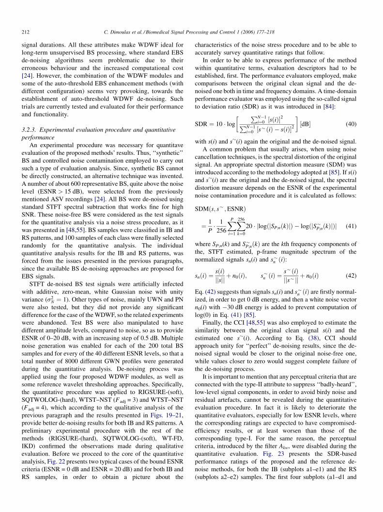
C. Dimoulas et al. / Biomedical Signal Processing and Control 1 (2006) 177–218212
signal durations. All these attributes make WDWF ideal for
long-term unsupervised BS processing, where standard EBS
de-noising algorithms seem problematic due to their
erroneous behaviour and the increased computational cost
[24]. However, the combination of the WDWF modules and
some of the auto-threshold EBS enhancement methods (with
different configuration) seems very provoking, towards the
establishment of auto-threshold WDWF de-noising. Such
trials are currently tested and evaluated for their performance
and functionality.
3.2.3. Experimental evaluation procedure and quantitative
performance
An experimental procedure was necessary for quantitave
evaluation of the proposed methods’ results. Thus, ‘‘synthetic’’
BS and controlled noise contamination employed to carry out
such a type of evaluation analysis. Since, synthetic BS cannot
be directly constructed, an alternative technique was invented.
A number of about 600 representative BS, quite above the noise
level (ESNR > 15 dB), were selected from the previously
mentioned ASV recordings [24]. All BS were de-noised using
standard STFT spectral subtraction that works fine for high
SNR. These noise-free BS were considered as the test signals
for the quantitative analysis via a noise stress procedure, as it
was presented in [48,55]. BS samples were classified in IB and
RS patterns, and 100 samples of each class were finally selected
randomly for the quantitative analysis. The individual
quantitative analysis results for the IB and RS patterns, was
forced from the issues presented in the previous paragraphs,
since the available BS de-noising approaches are proposed for
EBS signals.
STFT de-noised BS test signals were artificially infected
with additive, zero-mean, white Gaussian noise with unity
variance (s2N ¼ 1). Other types of noise, mainly UWN and PN
were also tested, but they did not provide any significant
difference for the case of the WDWF, so the related experiments
were abandoned. Test BS were also manipulated to have
different amplitude levels, compared to noise, so as to provide
ESNR of 0–20 dB, with an increasing step of 0.5 dB. Multiple
noise generation was enabled for each of the 200 total BS
samples and for every of the 40 different ESNR levels, so that a
total number of 8000 different GWN profiles were generated
during the quantitative analysis. De-noising process was
applied using the four proposed WDWF modules, as well as
some reference wavelet thresholding approaches. Specifically,
the quantitative procedure was applied to RIGSURE-(soft),
SQTWOLOG-(hard), WTST–NST (Fadj = 3) and WTST–NST
(Fadj = 4), which according to the qualitative analysis of the
previous paragraph and the results presented in Figs. 19–21,
provide better de-noising results for both IB and RS patterns. A
preliminary experimental procedure with the rest of the
methods (RIGSURE-(hard), SQTWOLOG-(soft), WT-FD,
IKD) confirmed the observations made during qualitative
evaluation. Before we proceed to the core of the quantitative
analyisis, Fig. 22 presents two typical cases of the bound ESNR
criteria (ESNR = 0 dB and ESNR = 20 dB) and for both IB and
RS samples, in order to obtain a picture about the
characteristics of the noise stress procedure and to be able to
accurately survey quantitative ratings that follow.
In order to be able to express performance of the method
within quantitative terms, evaluation descriptors had to be
established, first. The performance evaluators employed, make
comparisons between the original clean signal and the de-
noised one both in time and frequency domains. A time-domain
performance evaluator was employed using the so-called signal
to deviation ratio (SDR) as it was introduced in [84]:
SDR ¼ 10 � log
� PN�1i¼0 ½sðiÞ�
2PN�1i¼0 ½s� ðiÞ � sðiÞ�2
�½dB� (40)
with s(i) and s�(i) again the original and the de-noised signal.
A common problem that usually arises, when using noise
cancellation techniques, is the spectral distortion of the original
signal. An appropriate spectral distortion measure (SDM) was
introduced according to the methodology adopted at [85]. If s(i)
and s�(i) are the original and the de-noised signal, the spectral
distortion measure depends on the ESNR of the experimental
noise contamination procedure and it is calculated as follows:
SDMðs; s� ;ESNRÞ
¼ 1
P� 1
256
XP
i¼1
X256
k¼0
20 � jlogðjSP;nðkÞjÞ � logðjS�P;nðkÞjÞj (41)
where SP;n(k) and S�P;nðkÞ are the kth frequency components of
the, STFT estimated, p-frame magnitude spectrum of the
normalized signals sn(i) and s�n ðiÞ:
snðiÞ ¼sðiÞjjsjj þ n0ðiÞ; s�n ðiÞ ¼
s� ðiÞjjs� jj þ n0ðiÞ (42)
Eq. (42) suggests than signals sn(i) and s�n ðiÞ are firstly normal-
ized, in order to get 0 dB energy, and then a white noise vector
n0(i) with �30 dB energy is added to prevent computation of
log(0) in Eq. (41) [85].
Finally, the CCI [48,55] was also employed to estimate the
similarity between the original clean signal s(i) and the
estimated one s�(i). According to Eq. (38), CCI should
approach unity for ‘‘perfect’’ de-noising results, since the de-
noised signal would be closer to the original noise-free one,
while values closer to zero would suggest complete failure of
the de-noising process.
It is important to mention that any perceptual criteria that are
connected with the type-II attribute to suppress ‘‘badly-heard’’,
low-level signal components, in order to avoid birdy noise and
residual artefacts, cannot be revealed during the quantitative
evaluation procedure. In fact it is likely to deteriorate the
quantitative evaluators, especially for low ESNR levels, where
the corresponding ratings are expected to have compromised-
efficiency results, or at least worsen than those of the
corresponding type-I. For the same reason, the perceptual
criteria, introduced by the filter Akw, were disabled during the
quantitative evaluation. Fig. 23 presents the SDR-based
performance ratings of the proposed and the reference de-
noise methods, for both the IB (subplots a1–e1) and the RS
(subplots a2–e2) samples. The first four subplots (a1–d1 and
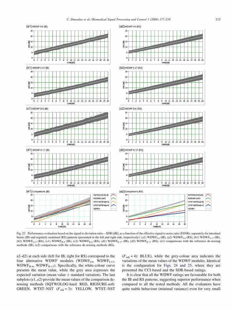
C. Dimoulas et al. / Biomedical Signal Processing and Control 1 (2006) 177–218 213
Fig. 23. Performance evaluation based on the signal to deviation ratio—SDR [dB], as a function of the effective signal to noise ratio (ESNR), separately for intestinal
bursts (IB) and regularly sustained (RS) patterns (presented in the left and right side, respectively): (a1) WDWFI-6 (IB), (a2) WDWFI-6 (RS), (b1) WDWFI-17 (IB),
(b2) WDWFI-17 (RS), (c1) WDWFII-6 (IB), (c2) WDWFII-6 (RS), (d1) WDWFII-17 (IB), (d2) WDWFII-17 (RS), (e1) comparisons with the reference de-noising
methods (IB), (e2) comparisons with the reference de-noising methods (RS).
a2–d2) at each side (left for IB, right for RS) correspond to the
four alternative WDWF modules (WDWFI-6, WDWFI-17,
WDWFII-6, WDWFII-17). Specifically, the white-colour curve
presents the mean value, while the grey area expresses the
expected variation (mean value standard variation). The last
subplots (e1, e2) provide the mean values of the comparison de-
noising methods (SQTWOLOG-hard: RED, RIGSURE-soft:
GREEN, WTST–NST (Fadj = 3): YELLOW, WTST–NST
(Fadj = 4): BLUE), while the grey-colour area indicates the
variations of the mean values of the WDWF modules. Identical
is the configuration for Figs. 24 and 25, where they are
presented the CCI-based and the SDR-based ratings.
It is clear that all the WDWF ratings are favourable for both
the IB and RS patterns, suggesting superior performance when
compared to all the tested methods. All the evaluators have
quite stable behaviour (minimal variance) even for very small

C. Dimoulas et al. / Biomedical Signal Processing and Control 1 (2006) 177–218214
Fig. 24. Performance evaluation based on the Cross Correlation Index (CCI), as a function of the effective signal to noise ratio (ESNR), separately for intestinal bursts
(IB) and regularly sustained (RS) patterns (presented in the left and right side, respectively): (a1) WDWFI-6 (IB), (a2) WDWFI-6 (RS), (b1) WDWFI-17 (IB), (b2)
WDWFI-17 (RS), (c1) WDWFII-6 (IB), (c2) WDWFII-6 (RS), (d1) WDWFII-17 (IB), (d2) WDWFII-17 (RS), (e1) comparisons with the reference de-noising methods
(IB), (e2) comparisons with the reference de-noising methods (RS).
ESNR levels. It is also observed that the type-II ratings worsen
for smaller ESNR, issue that was expected according to the
analysis of the previous paragraph. According to the results of
Fig. 24, 6-band implementations seem to have greater
performance from the 17-band ones, in the case of the IB
patterns and especially for low ESNR values. On the other
hand, 17-band modules work slightly better in the RS case, as it
is concluded from Fig. 23, when comparing subplots b1, d1
with the corresponding b2, d2. Examining Fig. 25, we observe
that type-II WDWF modules provide smaller spectral distor-
tions, due to the fact that the filter attenuation is softer. All the
modules tend to approach ‘‘perfect de-noising’’, as the ESNR
level gets higher, especially for values greater than 10 dB,
where the CCI index is about 0.95 and more.
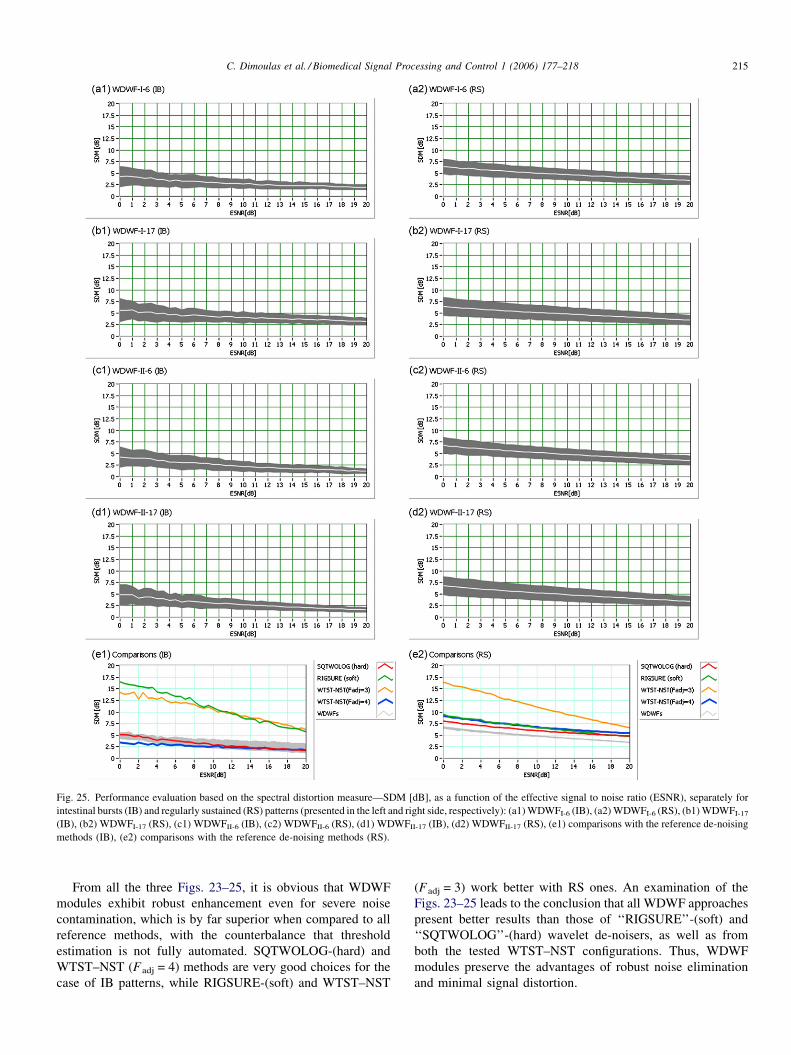
C. Dimoulas et al. / Biomedical Signal Processing and Control 1 (2006) 177–218 215
Fig. 25. Performance evaluation based on the spectral distortion measure—SDM [dB], as a function of the effective signal to noise ratio (ESNR), separately for
intestinal bursts (IB) and regularly sustained (RS) patterns (presented in the left and right side, respectively): (a1) WDWFI-6 (IB), (a2) WDWFI-6 (RS), (b1) WDWFI-17
(IB), (b2) WDWFI-17 (RS), (c1) WDWFII-6 (IB), (c2) WDWFII-6 (RS), (d1) WDWFII-17 (IB), (d2) WDWFII-17 (RS), (e1) comparisons with the reference de-noising
methods (IB), (e2) comparisons with the reference de-noising methods (RS).
From all the three Figs. 23–25, it is obvious that WDWF
modules exhibit robust enhancement even for severe noise
contamination, which is by far superior when compared to all
reference methods, with the counterbalance that threshold
estimation is not fully automated. SQTWOLOG-(hard) and
WTST–NST (Fadj = 4) methods are very good choices for the
case of IB patterns, while RIGSURE-(soft) and WTST–NST
(Fadj = 3) work better with RS ones. An examination of the
Figs. 23–25 leads to the conclusion that all WDWF approaches
present better results than those of ‘‘RIGSURE’’-(soft) and
‘‘SQTWOLOG’’-(hard) wavelet de-noisers, as well as from
both the tested WTST–NST configurations. Thus, WDWF
modules preserve the advantages of robust noise elimination
and minimal signal distortion.
C. Dimoulas et al. / Biomedical Signal Processing and Control 1 (2006) 177–218216
4. Discussion
This paper deals with the problem of additive broadband
noise in bio-acoustic signals. Four novel Wavelet Domain
Wiener Filter implementations have been successfully applied
and tested for the case of abdominal vibration recordings and
enhancement of the captured bowel sounds. The new methods
combine advantages of standard wavelet domain thresholding
strategies, such as robust noise elimination, as well as minimal
signal distortion suggested by Wiener filtering approaches.
Some of the surplus advantages of the suggested approaches,
are, (a) the fact that the method can be applied to any signal
length, with the computational overhead being the only
restriction, (b) it is also ideal for long-term, frame-based
simplified processing, avoiding to produce signal disconti-
nuities and keeping complexity to minimum. In fact, the overall
computational cost is quite affordable for the achieved de-
noising results, in contrast to other, often iterative approaches
that provide similar results. Another issue is the elimination of
the birdy noise and the related residuals, by applying slight
perceptual criteria. As a result, the enhancement operation
barely produces artefacts, while non-audible signal components
are reasonably bounded. Comparison with the related works of
auto-threshold EBS de-noising algorithms, proved that WDWF
work better for both IB and RS patterns. However, the
incorporation of some of their auto-threshold capabilities seems
very promising and the implementation of related combined
methods is currently examined. From the results, it can be said
that the proposed methods can be applied efficiently to almost
any sound signal, in contrast to previous studies of rough
wavelet-based threshold de-noising that work best for specific
signal types. Experimental results using tones, chirp-z signals,
even noise-buried speech, strengthen these prospects.
Acknowledgments
Authors wish to thank Assist. Prof. L.J. Hadjileontiadis for
his valuable contribution by providing his implemented
algorithms for comparison purposes. Authors would also like
to thank Dr. Marina Joannopoulou for carefully proofreading
and correcting the English language and style in this paper.
References
[1] X. Yang, K. Wang, S.A. Shamma, Auditory representations of acoustic
signals, IEEE Trans. Inf. Theory 38 (March (2)) (1992) 824–839.
[2] W. Etter, G. Moschytz, Noise reduction by noise adaptive spectral
magnitude expansion, J. Audio Eng. Soc. 42 (May (5)) (1994) 341–349.
[3] J. Berger, R.D. Coifman, M.J. Goldberg, Removing noise from music
using local trigonometric bases and wavelet packets, J. Audio Eng. Soc. 42
(October (10)) (1994) 808–818.
[4] D.E. Tsoukalas, J. Mourjopoulos, G. Kokkinakis, Perceptual filters for
audio signal enhancement, J. Audio Eng. Soc. 45 (January/February (1/2))
(1997) 22–36.
[5] M. Rosa, F. Lopez, P. Jarabo, S. Maldonado, N. Ruiz, A new algorithm for
translating psycho-acoustic information to the wavelet domain, Signal
Process. 81 (2001) 519–531.
[6] P.J. Wolfe, S.J. Godsill, Perceptually motivated approaches to music
restoration, J New Music Res. 30 (January (1)) (2001) 83–92.
[7] J. Yao, Y.-T. Zhang, Bionic wavelet transform: a new time–frequency
method based on auditory model, IEEE Trans. Biomed. Eng. 48 (August
(8)) (2001) 856–863.
[8] J. Johnston, Transform coding of audio signals using perceptual noise
criteria, IEEE J. Selected Areas Commun. 6 (February (2)) (1988) 314–323.
[9] R. Coifman, M.V. Wickerhauser, Adapted waveform ‘de-noising’ for
medical signals and images, IEEE Eng. Med. Biol. 14 (September/October
(5)) (1995) 578–586.
[10] L.J. Hadjileontiadis, S.M. Panas, Separation of discontinuous adventitious
sounds from vesicular sounds using a wavelet-based filter, IEEE Trans.
Biomed. Eng. 44 (December (12)) (1997) 1269–1281.
[11] L.J. Hadjileontiadis, S.M. Panas, A wavelet-based reduction of heart
sound noise from lung sounds, Int. J. Med. Inf. 52 (1998) 183–190.
[12] R. Coifman, M.V. Wickerhauster, Entropy based algorithms for best basis
selection, IEEE Trans. Inf. Theory 38 (March (2)) (1992) 713–718.
[13] D.L. Donoho, De-noising by soft-thresolding, IEEE Trans. Inf. Theory 41
(May (3)) (1995) 613–627.
[14] Adelino R. Ferreira da Silva, Bayesian wavelet denoising and evolutionary
calibration, Digital Signal Process. 14 (2004) 566–589.
[15] Y. Zheng, David B.H. Tay, L. Li, Signal extraction and power spectrum
estimation using wavelet transform scale space filtering and Bayes
shrinkage, Signal Process. 80 (2000) 1535–1549.
[16] A. Gupta, S.D. Joshi, S. Prasad, A new method for estimating wavelet with
desired features from a given signal, Signal Process. 85 (2005) 147–161.
[17] D. Leporini, J.-C. Pesquet, Bayesian wavelet denoising: Besov priors and
non-Gaussian noise, Signal Process. 81 (2001) 55–67.
[18] H. Qiu, J. Lee, J. Lin, G. Yu, Wavelet filter-based weak signature detection
method and its application on rolling element bearing prognostics, J.
Sound Vib. 289 (4–5) (2006) 1066–1090. doi:10.1016/j.jsv.2005.03.007.
[19] Y.Y. Kim, J.C. Hong, Frequency response function estimation via a robust
wavelet de-noising method, J. Sound Vib. 244 (2001) 635–649.
doi:10.1006/jsvi.2000.3509.
[20] G. Kalliris, New Techniques to Speech and Music Audio Restoration,
Ph.D. Thesis, Aristotle University of Thessaloniki, 1995.
[21] G. Kalliris, Ch. Dimoulas, G. Papanikolaou, Broad-Band Acoustic Noise
Reduction using a Novel Frequency Depended Parametric Wiener Filter:
Implementations using Filter-bank, STFT and Wavelet Analysis/Synthesis
Techniques, Audio Engineering Society Preprint, Proceedings of the 110th
AES Convetion, Amsterdam, May 2001 (Preprint 5382).
[22] S.V. Vaseghi, Advanced Digital Signal Processing and Noise Reduction,
second ed., John Wiley & Sons Ltd., New York, USA, 2000, , ISBN: 0-
471-62692-9.
[23] C. Pastiadis, G. Papanikolaou, Ch. Dimoulas, A. Kalampakas, Intestinal
Motility Recording and Analysis, Proceedings of the VIII Mediterranean
Conference on Medical and Biological Engineering and Computing
Medicon ’98, Lemesos, Cyprus, 1998.
[24] C.A. Dimoulas, G.M. Kalliris, G.V. Papanikolaou, A. Kalampakas, Long
term signal detection, segmentation and summarization using wavelets
and fractal dimension: a bioacoustics application in gastrointestinal
motility monitoring, Comput. Biol. Med. (2006) doi:10.1016/j.comp-
biomed.2006.08.013, Elsevier (special issue on wavelet-based algorithms
for medical problems), in press.
[25] D.A. Drossman, The functional gastrointestinal disorders and the Rome II
process, Gut 45 (Suppl. II) (1999) II1–II5.
[26] N.J. Talley, et al., B. Functional gastroduodenal disorders, in: D.A.
Drossman (Ed.), ROME II: The functional Gastrointestinal Disorders,
Second ed., Degnon Associates, 2000, pp. 299–350 (Chapter 6).
[27] W.G. Thompson, C. Functional bowel disorders and D. Functional
abdominal pain, in: D.A. Drossman (Ed.), ROME II: The Functional
Gastrointestinal Disorders, second ed., Degnon Associates, 2000, pp. 351–
432 (Chapter 7).
[28] G. Holtmann, P. Enck, Stress and gastrointestinal motility in humans: a
review of the literature, J. Gastrointest. Motil. 3 (4) (1991) 245–254.
[29] G. Vantrappen, J. Janssens, G. Coremans, R. Jian, Gastrointestinal motility
disorders, Dig. Dis. Sci. 31 (September (9)) (1986) 5S–25S.
[30] N.W. Weisbrodt, Motility of the small intestine, in: L.R. Johnson (Ed.),
second ed., Physiology of the Gastrointestinal Tract, vol. 1, Raven, New
York, 1987, pp. 631–663.
C. Dimoulas et al. / Biomedical Signal Processing and Control 1 (2006) 177–218 217
[31] J.E. Kellow, R.C. Gill, D.L. Wingate, Prolonged ambulant recordings of
small motility demonstrate abnormalities in the irritable bowel syndrome,
Gastroenterology 98 (May (5)) (1990) 1208–1218.
[32] B.L. Bardakjian, Gastrointestinal system, in: J.D. Bronzino (Ed.), The
Biomedical Engineering Handbook, vol. 6, IEEE Press and CRC Press
Inc., 1995, pp. 57–69.
[33] S. Sharna, in: N.W. Read (Ed.), Intestinal Manometry to Evaluate
Intestinal Motor Function, in Gastrointestinal Motility: Which Test?,
vol. 18, Wrighton Biomedical Publishing Ltd., 1989, pp. 157–166.
[34] J. Chen, B.D. Schirmer, R.W. McCallum, Measurement of electric activity
of the human small intestine using surface electrodes, IEEE Trans.
Biomed. Eng. 40 (June (6)) (1993) 598–602.
[35] J. Garcia-Casado, J.L. Martinez-de-Juan, J.L. Ponce, Non-invasive
measurement and analysis of intestinal myoelectrical activity using
surface electrodes, IEEE Trans. Biomed. Eng. 52 (June (6)) (2005)
983–991.
[36] H. Yoshino, Y. Abe, T. Yoshino, K. Oshato, Clinical application of spectral
analysis of bowel sounds in intestinal obstruction, Dis. Col. Rect. 33
(September (9)) (1990) 753–757.
[37] C. Liatsos, L.J. Hadjileontiadis, C. Mavrogiannis, D. Patch, S.M. Panas,
A.K. Burroughs, Bowel sounds analysis: a novel non-invasive method
for diagnosis of small-volume ascites, Dig. Dis. Sci. 48 (2003) 1630–
1636.
[38] D. Dalle, G. Devroede, R. Thibault, J. Perrault, Computer analysis of BS,
Comput. Biol. Med. 4 (1975) 247–256.
[39] C. Gamer, H. Ehrenreich, Non invasive topographic analysis of intestinal
activity in man on the basis of acoustic phenomena, Res. Exp. Med. (Bed.)
189 (2) (1989) 129–140.
[40] T. Tomomasa, A. Morikawa, R.H. Sandler, H.A. Mansy, H. Koneko, T.
Masahiko, P.E. Hyman, Z. Itoh, Gastrointestinal sounds and migrating
motor complex in fasted humans, Am. J. Gastroenterol. 94 (February (2))
(1999) 374–381.
[41] T. Tomomasa, A. Takahashi, Y. Nako, H. Kaneko, M. Tabata, Y. Tsuchida,
A. Morikawa, Analysis of gastrointestinal sounds in infants with pyloric
stenosis before and after pyloromyotomy, Pediatrics 104 (November (5))
(1999) e60.
[42] Ch. Dimoulas, G. Papanikolaou, G. Kalliris, C. Pastiadis, Computer aided
systems for prolonged recording and analysis of human bowel sounds, J.
Acoust. Soc. Am. 105 (February (2)) (1999) 1102 (Abstract).
[43] Ch. Dimoulas, G. Papanikolaou, G. Kalliris, C. Pastiadis, Computer aided
systems for prolonged recording and analysis of human bowel sounds, in:
Proceedings of the JOINT the ASA/EAA/DEGA MEETING ON ACOUS-
TICS, Berlin, March, 1999 (CD-ROM).
[44] B. Craine, M. Silpa, C. O’Toole, Computerized auscultation applied to
irritable bowel syndrome, Dig. Dis. Sci. 44 (9) (1999) 1887–1892.
[45] B. Craine, M. Silpa, C. O’Toole, Enterotachogram analysis to distinguish
irritable bowel syndrome from Crohn’s disease, Dig. Dis. Sci. 46 (9)
(2001) 1974–1979.
[46] B. Craine, M. Silpa, C. O’Toole, Two-dimensional positional mapping of
gastrointestinal sounds in control and functional bowel syndrome patients,
Dig. Dis. Sci. 47 (2002) 1290–1296.
[47] W.B. Cannon, Auscultation of the rhythmic sounds produced by the
stomach and intestine, Am. J. Physiol. 13 (1905) 339–353.
[48] L.J. Hadjileontiadis, C.N. Liatsos, C.C. Mavrogiannis, T.A. Rokkas, S.M.
Panas, Enhancement of bowel sounds by wavelet-based filtering, IEEE
Trans. Biomed. Eng. 47 (July (7)) (2000) 876–886.
[49] H.A. Mansy, R.H. Sandler, Bowel-sound signal enhancement using
adaptive filtering, IEEE Eng. Med. Biol. Mag. 16 (November/December
(6)) (1997) 105–117.
[50] C.N. Liatsos, L.J. Hadjileontiadis, C.C. Mavrogiannis, T.A. Rokkas, S.M.
Panas, Enhanced De-Noising of Bowel Sounds Using a Wavelet-Based
Filter, Proceedings of the VIII Mediterranean Conference on Medical and
Biological Engineering and Computing MEDICON ’98, Lemesos,
Cyprus, 1998.
[51] R. Ranta, C. Heinrich, V. Louis-Dorr, D. Wolf, F. Guillemin, Wavelet-
based bowel sounds denoising, segmentation and characterization, in:
Proceedings of 23rd Annual International Conference IEEE EMBS,
Istanbul, Turkey, October 25–28, (2001), pp. 1903–1906.
[52] L.J. Hadjileontiadis, I.T. Rekanos, Enhancement of explosive bowel
sounds using kurtosis-based filtering, in: Proceedings of 25th IEEE EMBS
2003, Cancun, Mexico, September, (2003), pp. 2479–2482.
[53] R. Ranta, C. Heinrich, V. Louis-Dorr, D. Wolf, Interpretation and
Improvement of an Iterative Wavelet-Based Denoising Method, IEEE
Signal Process. Lett. 10 (August (8)) (2003) 239–241.
[54] L.J. Hadjileontiadis, Wavelet-based enhancement of lung and bowel
sounds using fractal dimension thresholding—Part I: methodology, IEEE
Trans. Biomed. Eng. 52 (June (6)) (2005) 1143–1148.
[55] L.J. Hadjileontiadis, Wavelet-based enhancement of lung and bowel
sounds using fractal dimension thresholding—Part II: application results,
IEEE Trans. Biomed. Eng. 52 (June (6)) (2005) 1050–1064.
[56] I.T. Rekanos, L.J. Hadjileontiadis, An iterative kurtosis-based technique
for the detection of nonstationary bioacoustic signals, Signal Process. 86
(2006) 3787–3795.
[57] C. Dimoulas, G. Kalliris, G. Papanikolaou, A. Kalampakas, Abdominal
sounds pattern classification using advanced signal processing and arti-
ficial intelligence, in: Proceedings of the International Conference on
Computational Intelligence for Modelling Control and Automation
(CIMCA 2003), Vienna, February, (2003), pp. 71–82.
[58] Ol. Rioul, M. Vetterli, Wavelet and Signal Processing, IEEE Signal
Process. Mag. 8 (October (4)) (1991) 14–38.
[59] F.T. Agerkvist, A time–frequency auditory model using wavelet packets, J.
Audio Eng. Soc. 44 (January/February (1/2)) (1996) 37–50.
[60] M. Unser, T. Blu, Wavelet theory demistified, IEEE Trans. Signal Process.
51 (February (2)) (2003) 470–483.
[61] T. Gulzow, A. Engelsberg, U. Heute, Comparison of a discrete wavelet
transformation and a uniform polyphase filterbank applied to spectral
subtraction speech enhancement, Signal Process. (1997) 5–19.
[62] S. Mallat, A Wavelet Tour of Signal Processing, second ed., Academic
Press, Elsevier, USA, 1999, , ISBN: 0-12-466606-X.
[63] R.A. Wannamaker, Ed.R. Vrscay, Fractal wavelet compression of audio
signals, J. Audio Eng. Soc. 45 (July/August (7/8)) (1997) 540–553.
[64] Ol. Rioul, P. Duhamel, Fast algorithms for discrete and continuous
wavelets transforms, IEEE Trans. Inf. Theory 38 (March (2)) (1992)
569–586.
[65] S. Boll, Suppression of acoustic noise in speech using spectral subtraction,
IEEE Trans. Acoust. Speech Signal Process. ASSP-27 (April (2)) (1979)
113–120.
[66] N. Virag, Single channel speech enhancement based on masking proper-
ties of the human auditory system, IEEE Trans. Speech Signal Process. 7
(March (2)) (1999) 126–137.
[67] A. Spriet, M. Moonen, J. Wouters, Spatially pre-processed speech dis-
tortion weighted multi-channel Wiener filtering for noise reduction, Signal
Process. 84 (2004) 2367–2387.
[68] A. Spriet, M. Moonen, J. Wouters, The impact of speech detection errors
on the noise reduction performance of multi-channel filtering and general-
ized sidelob cancellation, Signal Process. 85 (2005) 1073–1088.
[69] S.Y. Yuen, C.K. Fong, K.L. Chan, Y.W. Leung, Fractal dimension
estimation and noise filtering using Hough transform, Signal Process.
84 (2004) 907–917.
[70] Jianye. Ching, Albert C. To, Steven D. Glaserb, Microseismic source
deconvolution: Wiener filter versus minimax, Fourier versus wavelets, and
linear versus nonlinear, J. Acoust. Soc. Am. 115 (June (6)) (2004) 3048–
3058.
[71] E. Zwicker, H. Fastl, Psychoacoustics Facts and Models, Springer Series
in Information Sciences, Springer-Verlag, Berlin, 1990, , ISBN: 3-540-
52600-5.
[72] A. Quinquis, A few practical applications of wavelet packets, Digital
Signal Process. 8 (1998) 49–60.
[73] C.P. Chan, P.C. Ching, T. Lee, Noisy speech recognition using de-noised
multiresolution analysis acoustic features, J. Acoust. Soc. Am. 110
(November (5)) (2001) 2567–2574.
[74] M. Sablatash, T. Cooklev, Compression of high-quality audio signals,
including recent methods using wavelet packets, Digital Signal Process. 6
(1996) 96–107.
[75] J.P. Dron, F. Bolaers, I. Rasolofondraibe, Improvement of the sensitivity of
the scalar indicators (crest factor, kurtosis) using a de-noising method by
C. Dimoulas et al. / Biomedical Signal Processing and Control 1 (2006) 177–218218
spectral subtraction: application to the detection of defects in ball bear-
ings, J. Sound Vib. 270 (2004) 61–73. doi:10.1016/S0022-460X(03)
00483-8.
[76] National Instruments Corporation, Sound and Vibration Toolkit User
Manual, Austin, Texas, USA, April 2004 edition.
[77] R.J. McAulay, M.L. Malpass, Speech enhancement using a soft-decision
noise suppression filter, IEEE Trans. Acoust. Speech Signal Process.
ASSP-28 (April (2)) (1980) 137–145.
[78] P.K. Ramarapu, R.C. Maher, Methods for reducing audible artifacts in a
wavelet based broad-band denoising system, J. Audio Eng. Soc. 46 (March
(3)) (1998) 178–190.
[79] T. Painter, A. Spanias, Perceptual coding of digital audio, Proc. IEEE 88
(April (4)) (2000) 451–515.
[80] I. Daubechies, Orthonormal bases of compactly supported wavelets,
Commun. Pure Appl. Math. 41 (1988) 909–996.
[81] N. Ruiz, M. Rosa, F. Lopez, P. Jarabo, Adaptive wavelet-packet analysis
for audio coding purposes, Signal Process. 83 (2003) 919–929.
[82] National Instruments Corporation, Joint time frequency analysis, in:
Signal Processing Toolset Reference Manual, Austin, Texas, USA,
December 2002 edition.
[83] National Instruments Corporation, Wavelet Analysis, in: Signal Proces-
sing Toolset Reference Manual, Austin, Texas, USA, December 2002
edition.
[84] M. Kazama, M. Tohyama, Estimation of speech components by acf
analysis in a noisy environment, J. Sound Vib. 241 (1) (2001) 41–52.
doi:10.1006/jsvi.2000.3275.
[85] H.W. Lou, G.R. Hu, An approach based on simplied KLT and wavelet
transformfor enhancing speech degraded by non-stationary wideband
noise, J. Sound Vib. 268 (2003) 717–729. doi:10.1016/S0022-460X
(02)01556-0.