Novel Analytical Method for Mix Design and Performance ...

Polymers 2021, 13, 900. https://doi.org/10.3390/polym13060900 www.mdpi.com/journal/polymers

Article

Novel Analytical Method for Mix Design and Performance

Prediction of High Calcium Fly Ash Geopolymer Concrete

Chamila Gunasekara 1,*, Peter Atzarakis 1, Weena Lokuge 2, David W. Law 1 and Sujeeva Setunge 1

1 School of Engineering, Royal Melbourne Institute of Technology (RMIT) University,

Melbourne, VIC 3000, Australia; [email protected] (P.A.); [email protected] (D.W.L.);

[email protected] (S.S.) 2 School of Civil Engineering and Surveying, University of Southern Queensland,

Springfield, QSL 4300, Australia; [email protected]

* Correspondence: [email protected]; Tel.: +61‐399‐251‐709; Fax: +61‐396‐390‐138

Abstract: Despite extensive in‐depth research into high calcium fly ash geopolymer concretes and a

number of proposed methods to calculate the mix proportions, no universally applicable method to

determine the mix proportions has been developed. This paper uses an artificial neural network

(ANN) machine learning toolbox in a MATLAB programming environment together with a Bayes‐

ian regularization algorithm, the Levenberg‐Marquardt algorithm and a scaled conjugate gradient

algorithm to attain a specified target compressive strength at 28 days. The relationship between the

four key parameters, namely water/solid ratio, alkaline activator/binder ratio, Na2SiO3/NaOH ratio

and NaOH molarity, and the compressive strength of geopolymer concrete is determined. The geo‐

polymer concrete mix proportions based on the ANN algorithm model and contour plots developed

were experimentally validated. Thus, the proposed method can be used to determine mix designs

for high calcium fly ash geopolymer concrete in the range 25–45 MPa at 28 days. In addition, the

design equations developed using the statistical regression model provide an insight to predict ten‐

sile strength and elastic modulus for a given compressive strength.

Keywords: high calcium fly ash; geopolymer concrete; artificial neural network; mix design;

compressive strength; regression analysis

1. Introduction

Concrete is the most widely utilised construction material in the world. It is essential

in the urbanisation of society in order to improve human living standards [1]. The expan‐

sion of urbanization and the worldwide population increase has led to a significant en‐

hancement of the current global cement production of 12% in 2019, which is predicted to

double by 2050 [2]. China is dominating the global cement market and produced 2.4 bil‐

lion tonnes in 2018, which accounted for half of the global cement demand, followed by

India at 290 million tonnes [3]. The manufacture of one ton of cement can generate 0.6 to

1.0 ton of CO2 depending on the manufacturing method employed [4–6], and is responsi‐

ble for the 5−9% of global CO2 emission [7–10].

Many researchers have been exploring alternative sustainable cementitious binders

that can reduce the dependence on Portland cement (PC) in construction [11–13]. Fly ash

geopolymer concrete is a promising alternative that can reduce CO2 emissions by 25‒45%

by utilizing waste coal combustion products [14]. High calcium fly ash is a popular mate‐

rial for the production of alkali‐activated concrete due to worldwide availability and con‐

taining sufficient quantities of reactive aluminate, silicate and calcium oxide [15,16]. Eu‐

ropean countries, such as Greece, Poland, and Spain generate the majority of the high

calcium fly ash, derived from lignite coal production [17]. Greece produces 12 million

tonnes of high calcium fly ash annually while in Asia (Thailand) generates about 3 million

Citation: Gunasekara, C.; Atzarakis,

P.; Lokuge, W.; Law, D.W.; Setunge,

S. Novel Analytical Method for Mix

Design and Performance Prediction

of High Calcium Fly Ash

Geopolymer Concrete. Polymers

2021, 13, 900. https://doi.org/10.3390/

polym13060900

Academic Editors: Enzo Martinelli

and Luciano Feo

Received: 3 February 2021

Accepted: 8 March 2021

Published: 15 March 2021

Publisher’s Note: MDPI stays neu‐

tral with regard to jurisdictional

claims in published maps and insti‐

tutional affiliations.

Copyright: © 2021 by the authors. Li‐

censee MDPI, Basel, Switzerland.

This article is an open access article

distributed under the terms and con‐

ditions of the Creative Commons At‐

tribution (CC BY) license (http://crea‐

tivecommons.org/licenses/by/4.0/).

Polymers 2021, 13, 900 2 of 21

tonnes [16]. However, more than 60% of this fly ash is being discarded in landfill, posing

serious environmental concerns [18].

Nuaklong et al. [19] investigated the compressive strength and fire‐resistance of high

calcium fly ash alkali‐activated concrete blended with rice husk ash. The results showed

that the 28‐day compressive strengths of geopolymer ranged from 36.0 to 38.1 MPa due

to an improved microstructure and denser matrix. However, the inclusion of SiO2 rich rice

husk ash had an adverse effect on the postfire residual strength. Wongsa et al. [20] exam‐

ined the fire resistance behaviours of high calcium fly ash alkali‐activated concrete incor‐

porating natural zeolite and mullite. Test results showed that the use of these additives

alone and together improved the fire resistance of concrete, which was attributed to the

presence of Ye’elimite and Wallastonite formed at high temperatures. Wong et al. [21]

illustrated that high calcium fly ash‐brick powder alkali‐activated composite can yield up

to 44.2 MPa at 28 days. However, the results indicated that brick powder replacement

beyond 10% resulted in the creation of an inhomogeneous microstructure in concrete.

Research has shown that a range of mix design parameters influence the compressive

strength of fly ash geopolymer concrete. Ling et al. [22] studied the impact of four design

parameters, namely the SiO2/Na2O ratio, the alkali activator concentration, the liquid/fly

ash ratio and curing temperature, on the setting time and compressive strength develop‐

ment of high calcium fly ash geopolymer. Test results confirmed that as the SiO2/Na2O

ratio increased, the setting time was accelerated but the compressive strength was re‐

duced. As activator concentration increased, the setting time for geopolymer mixes with

SiO2/Na2O of 1.0 and 1.5 were prolonged but were shortened when SiO2/Na2O equalled

2.0, while the compressive strength of these geopolymer mixes increased. The data also

showed that an elevated curing temperature increased the compressive strength. Zhang

and Feng [23] reported that water content, NaOH molarity and curing temperature influ‐

enced the compressive strength development of high calcium fly ash geopolymers. Ab‐

dullah et al. [24] noted that NaOH molarity, Na2SiO3/NaOH ratio, fly ash/alkaline activa‐

tor ratio and curing temperature affected the compressive strength of fly ash geopolymers.

The test results revealed that a 12 M NaOH solution and mass ratios of fly ash/alkaline

activator and Na2SiO3/NaOH of 2.0 and 2.5, respectively, yielded the highest compressive

strength. Literature [25,26] has reported that a fly ash/alkaline activator ratio of 3.3−4.0 is

required to achieve higher compressive strengths. Sathonawaphak et al. [27] stated that

geopolymers produced with fly ash/alkaline activator ratios in the range of 1.4–2.3 dis‐

played compressive strengths, ranging from 42 to 52 MPa. Their study noted that the op‐

timum Na2SiO3/NaOH ratio was 1.5. Rattanasak et al. [28] concluded that the use of a

Na2SiO3/NaOH ratio of 1.0 produced a product with a compressive strength as high as 70

MPa. However, Hardjito [29] showed that the use of a Na2SiO3/NaOH ratio of 2.5 gave the

highest compressive strength, whereas a ratio of 0.4 resulted in lower compressive

strength. In addition, researchers have reported that compressive strength increases as the

molarity of the NaOH increases from 8 to 16 M [30]. However, Palomo et al. [25] reported

that a 12 molar NaOH concentration gave higher strength than 18 M in fly ash geopolymer

concrete.

Despite the past research on performance and mix design parameters of high calcium

fly ash in geopolymers, there is no widely accepted procedure to determine the propor‐

tions to be mixed in concrete. Optimization by artificial intelligence tools with different

algorithms [31,32] has been used for the mix design of PC concrete. The artificial neural

networks (ANN) technique was used for alkali‐activated concrete and found that com‐

pressive strength can be predicted with minimal error in comparison to the experimental

results [33–35]. ANN is a statistical data modelling tool that can be trained using the

available data as inputs by changing the weights with the aim to model a complex rela‐

tionship between the inputs and the target outcome [36,37]. Lahoti et al. [34] investigated

the effect of four influential ratios (Si/Al molar, water/solid, Al/Na molar H2O/Na2O mo‐

lar) using ANN to predict the compressive strength of alkali‐activated metakaolin con‐

crete. In another study [35], ANN models with different numbers of neurons in hidden

Polymers 2021, 13, 900 3 of 21

layers were investigated and predicted the compressive range of strength of alkali‐acti‐

vated concretes based on curing time, CaO content, NaOH concentration, and H2O/Na2O

molar ratio. Researchers have been attempting to optimise the layers by using different

functions for the hidden and output layers [38]. Ling et al. [33] showed a strong correlation

between the ANN model predictions and the experimental results for compressive

strength and setting time of high calcium fly ash geopolymer concrete.

In this study, ANN was used with three algorithms and different numbers of neurons

in the hidden layer for the prediction of compressive strength of high calcium fly ash ge‐

opolymer concrete based on the data obtained from the literature. Having assessed the

available mix design parameters, the water/solid ratio, alkaline activator/fly ash ratio,

Na2SiO3/NaOH ratio and NaOH molarity were identified as the most influential parame‐

ters for compressive strength prediction. Although the curing temperature was reviewed

and analysed for the database, the strength development over time did not identify it as

an influential parameter. Based on the parameters identified, a novel standard process to

find the mix proportions for a high calcium fly ash geopolymer concrete was developed,

and the effectiveness of achieving a specified compressive strength was tested and vali‐

dated through laboratory experiments.

2. Significance of Research

Although fly ash geopolymer concrete has been used in structural members and com‐

mercialised as a construction material, the mix design process is still unclear because of

the many variables involved. Almost all the proposed methods employ different tech‐

niques specific for the particular situation and cannot be used as a standard method. The

missing link identified is that there is no unique mix design guideline for high calcium fly

ash geopolymer concrete. This research addresses the identified gap and proposes a

standard mix design procedure using a machine learning technique. The validation of the

technique demonstrates that the novel method developed can be used with confidence to

calculate mix proportions for compressive strength in the range of 25–45 MPa.

3. Geopolymer Concrete Database

A database was established using the published research/literature up to 2019 (inclu‐

sive) on high calcium fly ash geopolymer concrete scrutinising it for compressive strength

at 28 days. The database included only 100% high calcium fly ash concrete mixes and did

not consider mortar or phase mixes, and excluded the blended high calcium fly ash com‐

posites. This selection criteria was adopted to develop a mix design procedure that could

predict the standard 28‐day compressive strength for high calcium fly ash geopolymer

concrete more accurately. The present database consists of compressive strength values

obtained from 166 concrete mix designs, Table 1.

Polymers 2021, 13, 900 4 of 21

Table 1. Mix design database for high calcium fly ash geopolymer concrete.

Fly

Ash

(kg)

Aggregate (kg) Activator (kg) Added

Water

(kg)

Solid % in Na2SiO3 NaOH

Molar‐

ity

Heat Curing

[Ambient Curing]

Comp.

Strength

(MPa)

Flexural

Strength

(MPa)

Elastic

Modulus

(GPa)

Ref.

Coarse Fine NaOH Na2SiO3 SiO2 Na2O Time °C

414 1091 588 104 104 0 32.9 15.3 10 M 24 h 60 46.67 – 31.00 [16]

414 1091 588 104 104 0 32.9 15.3 15 M 24 h 60 54.40 – 37.80

414 1091 588 104 104 0 32.9 15.3 20 M 24 h 60 43.42 – 38.00

414 1091 588 69 138 0 32.9 15.3 10 M 24 h 60 40.09 – 24.20

414 1091 588 69 138 0 32.9 15.3 15 M 24 h 60 48.18 – 31.00

414 1091 588 69 138 0 32.9 15.3 20 M 24 h 60 49.50 – 31.80

414 1091 588 104 104 0 32.9 15.3 10 M 24 h [23] 39.67 – 30.40

414 1091 588 104 104 0 32.9 15.3 15 M 24 h [23] 45.34 – 34.80

414 1091 588 104 104 0 32.9 15.3 20 M 24 h [23] 37.64 – 38.40

414 1091 588 69 138 0 32.9 15.3 10 M 24 h [23] 33.80 – 23.40

414 1091 588 69 138 0 32.9 15.3 15 M 24 h [23] 39.02 – 26.80

414 1091 588 69 138 0 32.9 15.3 20 M 24 h [23] 46.69 – 35.40

523 1124 459 118 118 0 28.7 11.7 10 M 24 h [23] 36.5 5.5 22 [39]

500 1166 475 113 113 0 28.7 11.7 10 M 24 h [23] 33.0 5.3 26

478 1211 490 108 108 0 28.7 11.7 10 M 24 h [23] 26.0 4.8 24

470 1161 474 118 118 0 28.7 11.7 10 M 24 h [23] 32.5 6.1 24

450 1201 489 113 113 0 28.7 11.7 10 M 24 h [23] 32.0 5.8 24

430 1245 504 108 108 0 28.7 11.7 10 M 24 h [23] 27.5 5.6 23.9

428 1191 487 118 118 0 28.7 11.7 10 M 24 h [23] 32.0 5.9 21.5

409 1231 501 113 113 0 28.7 11.7 10 M 24 h [23] 29.9 5.1 24.5

391 1273 515 108 108 0 28.7 11.7 10 M 24 h [23] 27.5 5 24.5

392 1216 497 118 118 0 28.7 11.7 10 M 24 h [23] 25.0 4.8 24.7

375 1255 511 113 113 0 28.7 11.7 10 M 24 h [23] 21.0 4.9 27.5

359 1296 525 108 108 0 28.7 11.7 10 M 24 h [23] 20.0 4.1 22.5

523 1126 460 118 118 0 28.7 11.7 15 M 24 h [23] 35.5 6.4 27

500 1168 475 113 113 0 28.7 11.7 15 M 24 h [23] 32.5 6.3 27

478 1212 491 108 108 0 28.7 11.7 15 M 24 h [23] 31.0 5.8 20

470 1163 475 118 118 0 28.7 11.7 15 M 24 h [23] 36.0 6.3 26

Polymers 2021, 13, 900 5 of 21

450 1203 490 113 113 0 28.7 11.7 15 M 24 h [23] 34.5 6 27.5

430 1246 505 108 108 0 28.7 11.7 15 M 24 h [23] 33.0 5.8 26

428 1193 487 118 118 0 28.7 11.7 15 M 24 h [23] 32.5 6.2 27

409 1232 502 113 113 0 28.7 11.7 15 M 24 h [23] 33.0 5.9 29

391 1274 516 108 108 0 28.7 11.7 15 M 24 h [23] 32.5 5.3 25.1

392 1218 498 118 118 0 28.7 11.7 15 M 24 h [23] 18.5 5.9 19

375 1257 512 113 113 0 28.7 11.7 15 M 24 h [23] 19.0 5.2 19.5

359 1298 525 108 108 0 28.7 11.7 15 M 24 h [23] 16.0 5.1 29

390 1092 585 67 167 0 30.0 9.0 8 M 28 days [25] 23.4 – – [40]

390 1092 585 67 167 0 30.0 9.0 10 M 28 days [25] 25.0 – –

390 1092 585 67 167 0 30.0 9.0 12 M 28 days [25] 28.2 – –

390 1092 585 67 167 0 30.0 9.0 14 M 28 days [25] 31.8 – –

390 1092 585 67 167 0 30.0 9.0 16 M 28 days [25] 32.2 – –

390 1092 585 67 167 0 30.0 9.0 18 M 28 days [25] 30.3 – –

300 1684 681 51.4 129 0 29.4 14.7 14 M 24 h 60 25.8 4.81 – [41]

300 1684 681 51.4 129 0 29.4 14.7 14 M 24 h 60 23.2 4.56 –

300 1684 681 51.4 129 0 29.4 14.7 14 M 24 h 60 21.5 4.63 –

300 1684 681 51.4 129 0 29.4 14.7 14 M 24 h 60 26.8 4.69 –

300 1684 681 51.4 129 0 29.4 14.7 14 M 24 h 60 20.5 4.72 –

300 1684 681 51.4 129 0 29.4 14.7 14 M 24 h 60 22.0 4.85 –

600 1087 572 89.1 223 0 29.4 14.7 14 M 24 h 60 26.5 4.68 –

600 1087 572 89.1 223 0 29.4 14.7 14 M 24 h 60 29.0 4.65 –

600 1087 572 89.1 223 0 29.4 14.7 8 M 24 h 60 27.0 – –

600 1087 572 89.1 223 0 29.4 14.7 8 M 24 h 60 25.0 – –

600 1087 572 89.1 223 0 29.4 14.7 8 M 24 h 60 22.5 – –

600 1087 572 89.1 223 0 29.4 14.7 8 M 24 h 60 28.5 – –

600 1087 572 89.1 223 0 29.4 14.7 8 M 24 h 60 22.0 – –

600 1087 572 89.1 223 0 29.4 14.7 8 M 24 h 60 30.0 – –

494 858 691 198 198 0 30.0 15.0 14 M 72 h 60 59.5 4.48 33.63 [42]

494 858 691 198 198 0 30.0 15.0 14 M 72 h 60 52.3 4.72 34.37

494 858 691 198 198 0 30.0 15.0 14 M 72 h 60 55.9 4.3 37.10

494 858 691 198 198 0 30.0 15.0 14 M 72 h 60 80.4 5.27 42.87

494 858 691 198 198 0 30.0 15.0 14 M 72 h 60 61.4 6.23 31.44

Polymers 2021, 13, 900 6 of 21

494 858 691 198 198 0 30.0 15.0 14 M 72 h 60 39.2 4.19 19.06

494 858 691 198 198 0 30.0 15.0 14 M 72 h 60 53.7 4.43 28.91

494 858 691 198 198 0 30.0 15.0 14 M 72 h 60 36.5 3.58 26.97

494 858 691 198 198 0 30.0 15.0 14 M 72 h 60 57.2 5.27 29.44

494 858 691 198 198 0 30.0 15.0 14 M 72 h 60 42.8 5.18 22.56

494 858 691 198 198 0 30.0 15.0 14 M 72 h 60 62.2 4.83 29.89

450 1150 500 108 162 0 30.3 12.3 12 M 48 h 60 35.2 5 – [43]

450 1036 500 108 162 0 30.3 12.3 12 M 48 h 60 32.9 3.6 –

550 838 600 95 239 0 30.0 12.0 8 M 24 h 60 33.2 – – [44]

550 838 600 95 239 0 30.0 12.0 8 M 28 day [29] 35.6 – –

550 838 600 95 239 0 30.0 12.0 10 M 24 h 60 35.4 – –

550 838 600 95 239 0 30.0 12.0 10 M 28 day [29] 36.7 – –

550 838 600 95 239 0 30.0 12.0 12 M 24 h 60 42.4 – –

550 838 600 95 239 0 30.0 12.0 12 M 28 day [29] 39.7 – –

550 838 600 95 239 0 30.0 12.0 14 M 24 h 60 40.1 – –

550 838 600 95 239 0 30.0 12.0 14 M 28 day [29] 38.7 – –

550 838 600 95 239 0 30.0 12.0 8 M 24 h 60 34.7 – –

550 838 600 95 239 0 30.0 12.0 8 M 28 day [29] 36.2 – –

550 838 600 95 239 0 30.0 12.0 10 M 24 h 60 34.3 – –

550 838 600 95 239 0 30.0 12.0 10 M 28 day [29] 37.1 – –

550 838 600 95 239 0 30.0 12.0 12 M 24 h 60 41.3 – –

550 838 600 95 239 0 30.0 12.0 12 M 28 day [29] 38.9 – –

550 838 600 95 239 0 30.0 12.0 14 M 24 h 60 42.3 – –

550 838 600 95 239 0 30.0 12.0 14 M 28 day [29] 38.5 – –

550 838 600 95 239 0 30.0 12.0 8 M 24 h 60 36.3 – –

550 838 600 95 239 0 30.0 12.0 8 M 28 day [29] 35.3 – –

550 838 600 95 239 0 30.0 12.0 10 M 24 h 60 36.1 – –

550 838 600 95 239 0 30.0 12.0 10 M 28 day [29] 36.3 – –

550 838 600 95 239 0 30.0 12.0 12 M 24 h 60 42.2 – –

550 838 600 95 239 0 30.0 12.0 12 M 28 day [29] 45.3 – –

550 838 600 95 239 0 30.0 12.0 14 M 24 h 60 40.2 – –

550 838 600 95 239 0 30.0 12.0 14 M 28 day [29] 39.6 – –

550 838 600 95 239 0 30.0 12.0 8 M 24 h 60 34.4 – –

Polymers 2021, 13, 900 7 of 21

550 838 600 95 239 0 30.0 12.0 8 M 28 day [29] 36.3 – –

550 838 600 95 239 0 30.0 12.0 10 M 24 h 60 35.4 – –

550 838 600 95 239 0 30.0 12.0 10 M 28 day [29] 38.3 – –

550 838 600 95 239 0 30.0 12.0 12 M 24 h 60 43.4 – –

550 838 600 95 239 0 30.0 12.0 12 M 28 day [29] 44.3 – –

550 838 600 95 239 0 30.0 12.0 14 M 24 h 60 39.4 – –

550 838 600 95 239 0 30.0 12.0 14 M 28 day [29] 38.3 – –

550 838 600 95 239 0 30.0 12.0 8 M 24 h 60 33.1 – –

550 838 600 95 239 0 30.0 12.0 8 M 28 day [29] 33.5 – –

550 838 600 95 239 0 30.0 12.0 10 M 24 h 60 35.1 – –

550 838 600 95 239 0 30.0 12.0 10 M 28 day [29] 35.5 – –

550 838 600 95 239 0 30.0 12.0 12 M 24 h 60 42.2 – –

550 838 600 95 239 0 30.0 12.0 12 M 28 day [29] 41.5 – –

550 838 600 95 239 0 30.0 12.0 14 M 24 h 60 40.2 – –

550 838 600 95 239 0 30.0 12.0 14 M 28 day [29] 37.5 – –

550 838 600 95 239 0 30.0 12.0 8 M 24 h 60 34.2 – –

550 838 600 95 239 0 30.0 12.0 8 M 28 day [29] 35.5 – –

550 838 600 95 239 0 30.0 12.0 10 M 24 h 60 36.2 – –

550 838 600 95 239 0 30.0 12.0 10 M 28 day [29] 37.5 – –

550 838 600 95 239 0 30.0 12.0 12 M 24 h 60 41.4 – –

550 838 600 95 239 0 30.0 12.0 12 M 28 day [29] 40.5 – –

550 838 600 95 239 0 30.0 12.0 14 M 24 h 60 40.8 – –

550 838 600 95 239 0 30.0 12.0 14 M 28 day [29] 38.4 – –

310 1204 649 48.6 121.5 0 34.7 16.2 10 M 24 h 80 44.4 – – [45]

350 1250 650 41 103 0 29.8 14.7 8 M 7 day [28] 19.0 – – [46]

350 1250 650 41 103 0 29.8 14.7 8 M 7 day [28] 26.0 – –

350 1250 650 41 103 0 29.8 14.7 8 M 7 day [28] 23.5 – –

350 1250 650 41 103 0 29.8 14.7 8 M 7 day [28] 22.5 – –

350 1250 650 41 103 0 29.8 14.7 8 M 7 day [28] 17.8 – –

350 1250 650 41 103 0 29.8 14.7 8 M 7 day [28] 21.5 – –

350 1250 650 41 103 0 29.8 14.7 8 M 7 day [28] 19.0 – –

350 1250 650 41 103 0 29.8 14.7 8 M 7 day [28] 13.0 – –

350 1250 650 41 103 0 29.8 14.7 8 M 7 day [28] 12.0 – –

Polymers 2021, 13, 900 8 of 21

350 1250 650 41 103 0 29.8 14.7 8 M 24 h 60 32.5 – –

350 1250 650 41 103 0 29.8 14.7 8 M 24 h 60 33.5 – –

350 1250 650 41 103 0 29.8 14.7 8 M 24 h 60 31.0 – –

350 1250 650 41 103 0 29.8 14.7 8 M 24 h 60 24.7 – –

350 1250 650 41 103 0 29.8 14.7 8 M 24 h 60 22.0 – –

350 1250 650 41 103 0 29.8 14.7 8 M 24 h 60 25.0 – –

350 1250 650 41 103 0 29.8 14.7 8 M 24 h 60 23.5 – –

350 1250 650 41 103 0 29.8 14.7 8 M 24 h 60 16.0 – –

350 1250 650 41 103 0 29.8 14.7 8 M 24 h 60 15.0 – –

383 1379 567 54.5 137.00 0 32.4 13.5 12 M 7 day [30] 20.0 – – [44]

527 1159 522 53.3 133.33 0 32.4 13.5 12 M 7 day [30] 19.0 – –

530 1070 505 51.6 128.59 0 32.4 13.5 12 M 7 day [30] 16.0 – –

450 1200 600 80 120 0 32.4 13.5 10 M 7 day [25] 18.5 – – [47]

450 1200 600 80 120 0 32.4 13.5 12 M 7 day [25] 27.0 – –

450 1200 600 80 120 0 32.4 13.5 14 M 7 day [25] 29.3 – –

410 1143 521.8 110 120 2.3 32.4 13.5 10 M 7 day [25] 16.2 – –

410 1143 521.8 110 120 2.3 32.4 13.5 12 M 7 day [25] 25.0 – –

410 1143 521.8 110 120 2.3 32.4 13.5 14 M 7 day [25] 22.5 – –

350 1200 645 41 103 35 29.8 14.7 8 M 3 day [35] 19.0 – – [48]

350 1200 645 41 103 35 29.8 14.7 8 M 24 h 65 49.0 – –

350 1200 645 41 103 35 29.8 14.7 8 M 3 day 55 48.0 – –

500 1000 750 125 125 0 30.0 15.0 14 M 72 h 80 51.0 – – [49]

500 1000 750 125 125 0 30.0 15.0 14 M 72 h 80 53.0 – –

500 1000 750 125 125 0 30.0 15.0 14 M 72 h 80 50.0 – –

500 1000 750 125 125 0 30.0 15.0 14 M 72 h 80 50.0 – –

500 1000 750 125 125 0 30.0 15.0 14 M 72 h 80 52.0 – –

500 1000 750 125 125 0 30.0 15.0 14 M 72 h 80 44.0 – –

Polymers 2021, 13, 900 9 of 21

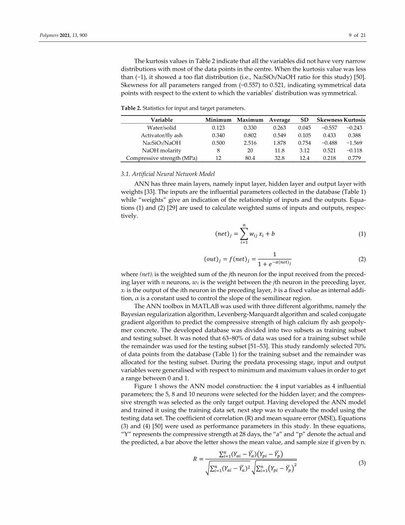
The kurtosis values in Table 2 indicate that all the variables did not have very narrow

distributions with most of the data points in the centre. When the kurtosis value was less

than (−1), it showed a too flat distribution (i.e., Na2SiO3/NaOH ratio for this study) [50].

Skewness for all parameters ranged from (−0.557) to 0.521, indicating symmetrical data

points with respect to the extent to which the variables’ distribution was symmetrical.

Table 2. Statistics for input and target parameters.

Variable Minimum Maximum Average SD Skewness Kurtosis

Water/solid 0.123 0.330 0.263 0.045 −0.557 −0.243

Activator/fly ash 0.340 0.802 0.549 0.105 0.433 0.388

Na2SiO3/NaOH 0.500 2.516 1.878 0.754 −0.488 −1.569

NaOH molarity 8 20 11.8 3.12 0.521 −0.118

Compressive strength (MPa) 12 80.4 32.8 12.4 0.218 0.779

3.1. Artificial Neural Network Model

ANN has three main layers, namely input layer, hidden layer and output layer with

weights [33]. The inputs are the influential parameters collected in the database (Table 1)

while “weights” give an indication of the relationship of inputs and the outputs. Equa‐

tions (1) and (2) [29] are used to calculate weighted sums of inputs and outputs, respec‐

tively.

𝑛𝑒𝑡 𝑤 𝑥 𝑏 (1)

𝑜𝑢𝑡 𝑓 𝑛𝑒𝑡1

1 𝑒 (2)

where (net)j is the weighted sum of the jth neuron for the input received from the preced‐

ing layer with n neurons, wij is the weight between the jth neuron in the preceding layer,

xi is the output of the ith neuron in the preceding layer, b is a fixed value as internal addi‐

tion, α is a constant used to control the slope of the semilinear region.

The ANN toolbox in MATLAB was used with three different algorithms, namely the

Bayesian regularization algorithm, Levenberg‐Marquardt algorithm and scaled conjugate

gradient algorithm to predict the compressive strength of high calcium fly ash geopoly‐

mer concrete. The developed database was divided into two subsets as training subset

and testing subset. It was noted that 63−80% of data was used for a training subset while

the remainder was used for the testing subset [51–53]. This study randomly selected 70%

of data points from the database (Table 1) for the training subset and the remainder was

allocated for the testing subset. During the predata processing stage, input and output

variables were generalised with respect to minimum and maximum values in order to get

a range between 0 and 1.

Figure 1 shows the ANN model construction: the 4 input variables as 4 influential

parameters; the 5, 8 and 10 neurons were selected for the hidden layer; and the compres‐

sive strength was selected as the only target output. Having developed the ANN model

and trained it using the training data set, next step was to evaluate the model using the

testing data set. The coefficient of correlation (R) and mean square error (MSE), Equations

(3) and (4) [50] were used as performance parameters in this study. In these equations,

“Y” represents the compressive strength at 28 days, the “a” and “p” denote the actual and

the predicted, a bar above the letter shows the mean value, and sample size if given by n.

𝑅∑ 𝑌 𝑌 𝑌 𝑌

∑ 𝑌 𝑌 ∑ 𝑌 𝑌

(3)

Polymers 2021, 13, 900 10 of 21

𝑀𝑆𝐸∑ 𝑌 𝑌

𝑛 (4)

Figure 1. Schematic diagram of artificial neural network (ANN) model.

Figure 2 shows the comparison of the model performance with a number of hidden

neurons for different algorithms. Results showed that 8 hidden neurons along with the

Bayesian regularization algorithm yielded the best correlation in the given dataset. This

gave the highest R value for training, highest R value for all and second lowest value clos‐

est to zero for mean squared error.

Polymers 2021, 13, 900 11 of 21

Figure 2. Model performance vs. number of hidden neurons for each algorithm.

The model performance with 8 hidden neurons along with the Bayesian Regulariza‐

tion algorithm is shown in Figure 3. When data points sit on the dotted straight line, it

confirms the exact correlation between the predicted and compressive strength from ex‐

perimental results, which is the desired outcome. It was observed that the training dataset

had the best correlation with the normalised actual compressive strength when compared

to the test and all plots. In addition, all three scatter plots yielded R values greater than

0.8, which meant a close relationship existed between the key mix design parameters and

the 28‐day compressive strength. The ANN model with the selected neurons and the al‐

gorithm had a MSE value of 0.0056897, closest to zero, confirming there was almost no

error present in this predictive model.

0.000

0.002

0.004

0.006

0.008

0.010

0.012

0.014

5 6 7 8 9 10

Hidden

Neurons

Hidden Layers

Bayesian Regularization Algorithm

Levenberg‐Marquardt Algorithm

Scaled Conjugate Gradient Algorithm

Mean Squared Error (MSE)

0.00

0.20

0.40

0.60

0.80

1.00

5 6 7 8 9 10

Hidden

Neurons

Hidden Layers

Training (R)

0.00

0.20

0.40

0.60

0.80

1.00

5 6 7 8 9 10

Hidden

Neurons

Hidden Layers

All (R)

Polymers 2021, 13, 900 12 of 21

Figure 3. Performance of the artificial neural network (ANN) model based on (a) the training dataset; (b) test dataset; (c)

all datasets; and (d) mean squared error for 8 hidden neurons and the Bayesian Regularization training algorithm.

4. Geopolymer Concrete Design

4.1. Contour Plots

The contour plots shown in Figure 4 demonstrate the intercorrelation of the selected

four input variables (water/solid ratio, activator/fly ash ratio, Na2SiO3/NaOH ratio and

NaOH molarity) with the target output of compressive strength. Hence, these contour

maps can be used to design mix proportions for a target 28‐day compressive strength for

high calcium fly ash geopolymer concrete.

Polymers 2021, 13, 900 13 of 21

Figure 4. Effect of input parameters on the compressive strength (Note: for instance, the selected input parameters of 45

MPa mix is illustrated). Input parameters: (a) activator/fly ash ratio and NaOH molarity; (b) water/solid ratio and NaOH

molarity; (c) water/solid ratio and activator/fly ash ratio; (d) NaOH molarity and Na2SiO3/NaOH ratio; (e) water/solid ratio

and Na2SiO3/NaOH ratio; (f) activator/fly ash ratio and Na2SiO3/NaOH ratio.

Water/solid ratio—Figure 4b,e depicts that there was an increasing trend for com‐

pressive strength with increased water/solid ratio. On the other hand, Figure 4c shows

that even with a lower water/solid ratio a higher compressive strength could be achieved

using a higher activator/fly ash ratio.

Activator/fly ash ratio—Figure 4f depicts that compressive strength had an increas‐

ing trend with an increased activator/fly ash ratio. It was possible to obtain a 20−35 MPa

concrete using an activator/fly ash ratio between 0.3 to 0.6, Figure 4a. For an activator/fly

Polymers 2021, 13, 900 14 of 21

ash ratio of 0.7 to 0.9 together with any NaOH molarity, 35–50 MPa compressive strength

could be achieved.

Na2SiO3/NaOH ratio—Figure 4f shows that when the Na2SiO3/NaOH ratio was de‐

creased, the compressive strength was increasing faster due to the increment in the acti‐

vator/fly ash ratio. Further, by increasing the Na2SiO3/NaOH ratio with decreasing NaOH

molarity, higher compressive strength could be achieved, Figure 4d.

NaOH molarity—Figure 4a illustrates that for an activator/fly ash ratio less than 0.7,

compressive strength could only achieve a maximum 40 MPa irrespective of the NaOH

molarity. Hence, in order to achieve higher strength, the activator/fly ash ratio needs to

be in the range 0.7 to 0.9 in combination with adjustment of the NaOH molarity. Figure

4b shows a similar approach, as water/solid ratio had to be increased in combination with

NaOH molarity in order to achieve higher compressive strengths.

4.2. Mix Design Calculation

For model validation, four high calcium fly ash geopolymer concrete mixes were de‐

signed with the targeted compressive strengths of 25, 30, 40 and 45 MPa at 28 days. A

detailed calculation procedure for 45 MPa concrete mix is illustrated below. The calculated

mix design variables obtained from the contour plots of Figure 4 were water/solid ratio =

0.4, activator/fly ash ratio = 0.85, Na2SiO3/NaOH ratio = 3.7 and NaOH molarity = 10 M.

The 460 kg fly ash was used which is the median of database, Table 1.

(a) Alkaline activator content:

𝐴𝑐𝑡𝑖𝑣𝑎𝑡𝑜𝑟𝐹𝑙𝑦 𝑎𝑠ℎ

0.85 ; Na SiO NaOH

𝐹𝑙𝑦 𝑎𝑠ℎNa SiO

NaOH 3.7 (5)

After solving: Na2SiO3 = 307.8 kg; NaOH = 83.2 kg

(b) Added water content:

𝑊𝑎𝑡𝑒𝑟𝑆𝑜𝑙𝑖𝑑

Na SiO NaOH Added Water

𝐹𝑙𝑦 𝑎𝑠ℎ Na SiO NaOH0.4 (6)

After solving: Added water (w) = 2.82 kg (Table 3)

Table 3. Data tabulation: calculating added water content.

Na2SiO3 NaOH Extra Water Binder Total

Solid 120.1 25.8 0 460 605.9

Water 187.7 57.4 w 0 245.1 + w

(c) Aggregate content:

𝑉 𝑉 𝑉 𝑉 𝑉 𝑉 1 (7)

𝑀

𝜌

𝑀

𝜌𝑀𝜌

𝑀

𝜌

𝑀𝜌

𝑀𝜌

1 (8)

𝑉𝑉 𝑉

0.65 (9)

After solving: 𝑀 467 kg and 𝑀 919.3 kg

Similarly, Figure 4 was used to obtain the mix proportions for 25 MPa, 30 MPa and

40 MPa concretes and these were tabulated in Table 4.

Polymers 2021, 13, 900 15 of 21

Table 4. Mix proportions of high calcium fly ash geopolymer concrete.

Mix Nota‐

tion

Target

Strength

Mix Design Variables

Water/Solid Activator/Fly Ash Na2SiO3/NaOH NaOH Molarity

M25 25 MPa 0.25 0.42 1.5 10 M

M30 30 MPa 0.28 0.50 2.0 10 M

M40 40 MPa 0.35 0.70 3.5 10 M

M45 45 MPa 0.42 0.85 4.0 8 M

Mix Nota‐

tion

Target

Strength

Mix Proportions (kg/m3)

Fly Ash Sand Aggregates Na2SiO3 NaOH Added Water

M25 25 MPa 460 500.8 985.8 115.9 77.3 93.7

M30 30 MPa 460 495.7 975.8 153.3 76.7 75.5

M40 40 MPa 460 480.3 945.5 250.5 71.5 33.1

M45 45 MPa 460 467 919.3 307.8 83.2 2.82

4.3. Experimental Procedure

The high calcium fly ash obtained from an Indonesian coal power station was used

for this study. The chemical composition of the fly ash, Table 5, was determined using

Bruker Axs S4 Pioneer X‐ray fluorescence equipment. The particle size distribution was

determined using a Malvern Mastersizer analyser and the crystalline composition with a

Bruker Axs D8 ADVANCE Wide Angle X‐ray diffraction (XRD) instrument. The XRD

analysis was performed at 40 kV, Cu Kα = 1.54178 Å wavelength, and a scanning range of

2 theta in 5–95°. Sample holders were filled using the front‐loading procedure. The data

obtained from XRD were interpreted using Bruker‐DIFFRAC.EVA software and Rietveld

analysis [54,55]. The surface area was determined using the Brunauer‐Emmett‐Teller

method by N2 absorption. The crystalline and amorphous content, specific surface area,

and particle size distribution are shown in Table 6.

Table 5. Chemical composition of high calcium fly ash.

Source Material Component (wt.%)

SiO2 Al2O3 Fe2O3 CaO P2O5 TiO2 MgO K2O SO3 MnO Na2O LOIa

Fly ash 38.7 20.8 5.3 26.6 0.15 0.45 1.5 2.6 2.1 0.5 1.2 0.1 a Loss on ignition (unburnt carbon content).

Table 6. Physical and mineralogical properties of high calcium fly ash.

Properties Investigated Fly Ash

Specific gravity 2.15

BET Surface area, (m2/kg) 2619

Fineness (%)

at 10 microns 45.2

at 20 microns 64.1

at 45 microns 85.9

Amorphous content (%) 67.1

Crystalline content (%) 32.8

Commercially available sodium hydroxide solution (8–10 M) and sodium silicate so‐

lution (Na2O = 14.7% and SiO2 = 29.4% by mass, specific gravity = 1.53) were used as alka‐

line activator in the geopolymer production. The fine aggregate and coarse aggregate

were prepared with respect to the Australian Standards, AS 1141.5 [56]. River sand in an

uncrushed form (specific gravity = 2.5 and fineness modulus = 2.8) was used as fine ag‐

gregate, and 10 mm grain size crushed granite aggregate (specific gravity = 2.65 and water

absorption = 0.74%) was used as coarse aggregate in concrete. Demineralised water was

used throughout in the mixing.

Polymers 2021, 13, 900 16 of 21

A 60 L concrete mixer was used to prepare all concrete specimens. Firstly, fly ash,

sand and coarse aggregates were mixed for 4 min followed by the addition of alkaline

activator and water with further mixing for 8 min. This provided a well‐combined, non‐

segregated concrete mix. The concrete was poured into standard cylindrical moulds (100

mm diameter × 200 mm height), then compacted using a vibration table for 1 min to re‐

move air bubbles. All prepared concrete cylinders were kept in the laboratory under am‐

bient conditions (23 °C temperature and 70% relative humidity) for 24 h. Afterwards, all

concrete specimens were heat cured at 60 °C temperature for one day. After demoulding,

all specimens were clearly labelled and stored in laboratory conditions (23 °C temperature

and 70% relative humidity) until the 28 day testing. Compressive strength testing was

undertaken in accordance with the ASTM C109/C109M standard using a Technotest con‐

crete testing machine [57]. A total of 4 specimens were tested at each interval at a loading

rate of 0.34 MPa/S until failure.

5. Experimental Results and Model Validation

The experimental results, noted in Table 7, demonstrated that the four high calcium

fly ash geopolymer concrete mixes achieved close to their relevant target compressive

strengths at 28 days. The M25 and M30 concrete mixes slightly exceeded the target

strength while both the M40 and M45 concrete mixes displayed a slightly lower value than

the expected compressive strength. Although all the mixes showed increased compressive

strength from 7 to 28 days, the percentage increment was slightly different. The M25 and

M30 geopolymer mixes obtained the highest strength development (~70%) while the other

two concrete mixes gained ~60% strength during this period. Overall, experimental obser‐

vations were in good agreement with the predicted and actual compressive strength for

high calcium fly ash geopolymer concrete indicating the reliability of the mix design pro‐

cedure described in this paper.

Table 7. Measured compressive strength (MPa).

Concrete Type 7‐day 28‐day

M25 19.0 ± 0.6 27.2 ± 0.8

M30 23.1 ± 0.9 33.1 ± 1.2

M40 22.9 ± 0.7 38.1 ± 0.5

M45 32.7 ± 0.9 44.1 ± 0.8

5.1. Relationship between Mechanical Properties

The high calcium geopolymer concrete experimental data available in Table 1 was

used in a regression analysis to explore the trends and correlations between elastic mod‐

ulus and tensile strength with compressive strength. Residual and refined R2 values for

selected regression models were used together with the least square method to obtain the

linear regression lines to match the experimental data. Each best fit line is linked with the

confidence and prediction interval bands. The prediction interval is concentrated on the

specific data point while prediction lines are the focus of the confidence interval. There is

a 95% chance that the actual regression line will be in the confidence interval band calcu‐

lated using Equation (5) [58]. Hence, there is a 95% chance that the actual value (Y) corre‐

sponding to a particular value (X0,) is located within this interval, Equation (6) [58].

𝑌 . 𝑡 .∑ 𝑌 𝑌 .

𝑛 2 .

1𝑛

𝑋 𝑋𝑆𝑆

(10)

𝑌 . 𝑡 . 1∑ 𝑌 𝑌 .

𝑛 2 . 1

1𝑛

𝑋 𝑋 𝑆𝑆

(11)

Polymers 2021, 13, 900 17 of 21

The Ypred. is the predicted Y values, t0.05 is the t critical value for 95% interval, n is the

sample size, X is the true value while 𝑋 is the mean of sample and SSx is the sum of the

squares of standard error of X values. The proposed regression model for the relationship

between compressive and flexural strength is shown in Figure 5. Relevant equations are

available in the Standards [59,60] for Portland cement concrete to evaluate the flexural

strength which are used in deflection calculations. However, these equations do not lie in

the 95% prediction interval bands of the regression model for experimental results. The

AS 3600 [59] and ACI 318 [60] equations for flexural strength are on the lower side of the

confidence interval of the proposed regression model, illustrating that the design equa‐

tions of both standards underestimate the flexural strength for high calcium fly ash geo‐

polymer concrete. Hence, the use of the current standard/code for PC concrete will achieve

a conservative design for flexural members made with high calcium fly ash based geopol‐

ymer concrete.

Figure 5. Correlation between compressive strength vs. flexural strength.

A linear regression line with prediction and confidence interval bands to demon‐

strate the relationship between compressive strength and elastic modulus is shown in Fig‐

ure 6. As the R2 value of the regression model was 0.97, this indicates that a more accurate

modulus of elasticity could be achieved if the density was also considered in the equation.

AS 3600 [59] and ACI 318 [60] also provide a similar design equation with the inclusion of

density. Contrary to the flexural strength, the AS 3600 equation for elastic modulus lies

above the upper confidence interval of proposed regression model. This implies that the

available equations for PC concrete overestimate the elastic modulus of high calcium fly

ash geopolymer concrete which leads to an underestimation of serviceability perfor‐

mance.

0

1

2

3

4

5

6

7

8

9

10

4.0 4.5 5.0 5.5 6.0 6.5 7.0 7.5 8.0 8.5 9.0

𝐶𝑜𝑚𝑝𝑟𝑒𝑠𝑠𝑖𝑣𝑒 𝑠𝑡𝑟𝑒𝑛𝑔𝑡ℎ, 𝑓 𝑀𝑃𝑎

Flex

ural

str

engt

h,f

. M

Pa

95% Confidence bands for Experimental equation95% Prediction bands for

Experimental equation

𝒇𝒄𝒕.𝒇 𝟎.𝟖𝟓 𝒇𝒄Experimental equation

𝑓 . 0.6 𝑓 AS 3600 equation

𝑓 0.62 𝑓 ACI 318 equation

R2 = 0.95

Polymers 2021, 13, 900 18 of 21

Figure 6. Correlation between compressive strength vs. elastic modulus.

6. Summary and Conclusions

1. The algorithm for the predictive model for high calcium fly ash geopolymer concrete

mix design was developed using artificial neural networks in order to determine the

relationship between the four key parameters identified, namely water/solid ratio,

alkaline activator/binder ratio, Na2SiO3/NaOH ratio and NaOH molarity, and the 28‐

day compressive strength of geopolymer concrete.

2. A new standard mix design procedure was developed for high calcium fly ash geo‐

polymer concrete using contour plots generated in the MATLAB programming en‐

vironment, and demonstrated through detailed calculation to ascertain the mix pro‐

portions for 45 MPa target compressive strength at 28 days.

3. Good correlation between the experimental results and the compressive strengths

calculated from contour plots validated the developed novel mix design method for

high calcium fly ash geopolymer concrete. Thus, the proposed method is suitable for

calculating mix proportions with confidence for a target compressive strength at 28

days in the range of 25–45 MPa.

4. A statistical regression model was developed using the database to provide new de‐

sign equations to predict tensile strength and elastic modulus of high calcium fly ash

geopolymer concrete based on the 28‐day compressive strengths obtained.

5. The design equations available in AS 3600 and ACI 318 standards for Portland ce‐

ment concrete provide a conservative design for tensile strength in high calcium fly

ash geopolymer concrete. However, AS 3600 design equation overestimates the elas‐

tic modulus for geopolymer concrete.

6. The present study suggests preliminary amendments to the available design stand‐

ards for Portland cement concrete to design high calcium fly ash geopolymer con‐

crete structural elements with better serviceability performance. However, further

investigations are required prior to implementing them in the standards/codes.

Author Contributions: Conceptualization, C.G., P.A. and W.L.; methodology & formal analysis,

C.G., P.A. and W.L.; writing—original draft preparation, C.G. and W.L.; writing—review and edit‐

ing, D.L. and S.S. All authors have read and agreed to the published version of the manuscript.

5,000

10,000

15,000

20,000

25,000

30,000

35,000

40,000

45,000

50,000

400,000 500,000 600,000 700,000 800,000 900,000 1,000,000

R2 = 0.97

95% Confidence bands for Experimental equation

Experimental equation

95% Prediction bands for Experimental equation

AS 3600 equation

5000

Polymers 2021, 13, 900 19 of 21

Funding: This research received no external funding.

Institutional Review Board Statement: Not applicable.

Informed Consent Statement: Not applicable.

Data Availability Statement: All data are included in the manuscript.

Acknowledgments: The scientific and technical assistance provided by the Civil engineering labor‐

atory in RMIT University is acknowledged. This research was conducted by the Australian Research

Council Industrial Transformation Research Hub for nanoscience‐based construction material man‐

ufacturing (IH150100006) and funded by the Australian Government.

Conflicts of Interest: The authors declare that they have no conflict of interest.

References

1. Aitcin, P.C. Cements of yesterday and today—Concrete of tomorrow. Cem. Concr. Res. 2000, 30, 1349–1359.

2. Harper, G.G. Cement Industry Initiative Releases Technology Roadmap to Cut CO2 Emissions 24% by 2050; Available online:

https://sdg.iisd.org/news/cement‐industry‐initiative‐releases‐technology‐roadmap‐to‐cut‐co2‐emissions‐24‐by‐2050/ (accessed

on 15 March 2020).

3. Bernhardt, D.; Reilly, J.F., II. Mineral Commodity Summaries (2019); Government Printing Office, US Geological Survey: Reston,

VA, USA, 2019.

4. Peng, J.X.; Huang, L.; Zhao, Y.B.; Chen, P.; Zeng, L. Modeling of carbon dioxide measurement on cement plants. Adv. Mater.

Res. 2013, 610–613, 2120–2128.

5. Li, C.; Gong, X.Z.; Cui, S.P.; Wang, Z.H.; Zheng, Y.; Chi, B.C. CO2 emissions due to cement manufacture. Mater. Sci. Forum 2011,

685, 181–187.

6. Huntzinger, D.N.; Eatmon, T.D. A life‐cycle assessment of Portland cement manufacturing: Comparing the traditional process

with alternative technologies. J. Clean. Prod. 2009, 17, 668–675.

7. Meyer, C. The greening of the concrete industry. Cem. Concr. Compos. 2009, 31, 601–605.

8. Chen, C.; Habert, G.; Bouzidi, Y.; Jullien, A. Environmental impact of cement production: Detail of the different processes and

cement plant variability evaluation. J. Clean. Prod. 2010, 18, 478–485.

9. Hasanbeigi, A.; Price, L.; Lin, E. Emerging energy‐efficiency and CO2 emission‐reduction technologies for cement and concrete

production: A technical review. Renew. Sustain. Energy Rev. 2012, 16, 6220–6238.

10. Shanks, W.; Dunant, C.F.; Drewniok, M.P.; Lupton, R.C.; Serrenho, A.; Allwood, J.M. How much cement can we do without?

Lessons from cement material flows in the UK. Resour. Conserv. Recycl. 2019, 141, 441–454.

11. Sandanayake, M.; Gunasekara, C.; Law, D.; Zhang, G.; Setunge, S.; Wanijuru, D. Sustainable criterion selection framework for

green building materials—An optimisation based study of fly‐ash Geopolymer concrete. Sustain. Mater. Technol. 2020, 25,

e00178.

12. Gunasekara, C.; Sandanayake, M.; Zhou, Z.; Law, D.W.; Setunge, S. Effect of nano‐silica addition into high volume fly ash–

hydrated lime blended concrete. Constr. Build. Mater. 2020, 253, 119205.

13. Gunasekara, C.; Law, D.W.; Setunge, S.; Burgar, I.; Brkljaca, R. Effect of Element Distribution on Strength in Fly Ash Geopoly‐

mers. ACI Mater. J. 2017, 144, 795.

14. Turner, L.K.; Collins, F.G. Carbon dioxide equivalent (CO2‐e) emissions: A comparison between geopolymer and OPC cement

concrete. Constr. Build. Mater. 2013, 43, 125–130.

15. Nuaklong, P.; Sata, V.; Chindaprasirt, P. Influence of recycled aggregate on fly ash geopolymer concrete properties. J. Clean.

Prod. 2016, 112, 2300–2307.

16. Topark‐Ngarm, P.; Chindaprasirt, P.; Sata, V. Setting time, strength, and bond of high‐calcium fly ash geopolymer concrete. J.

Mater. Civ. Eng. 2015, 27, 04014198.

17. Feuerborn, H.‐J. Calcareous ash in Europe‐a reflection on technical and legal issues. In Proceedings of the 2nd Hellenic Confer‐

ence on Utilisation of Industrial By‐Products in Construction, Aiani Kozani, Greece, 1 June 2009.

18. Hanjitsuwan, S.; Hunpratub, S.; Thongbai, P.; Maensiri, S.; Sata, V.; Chindaprasirt, P. Effects of NaOH concentrations on phys‐

ical and electrical properties of high calcium fly ash geopolymer paste. Cem. Concr. Compos. 2014, 45, 9–14.

19. Nuaklong, P.; Jongvivatsakul, P.; Pothisiri, T.; Sata, V.; Chindaprasirt, P. Influence of rice husk ash on mechanical properties

and fire resistance of recycled aggregate high‐calcium fly ash geopolymer concrete. J. Clean. Prod. 2020, 252, 119797.

20. Wongsa, A.; Wongkvanklom, A.; Tanangteerapong, D.; Chindaprasirt, P. Comparative study of fire‐resistant behaviors of high‐

calcium fly ash geopolymer mortar containing zeolite and mullite. J. Sustain. Cem. Based Mater. 2020, 9, 307–321.

21. Wong, C.L.; Mo, K.H.; Alengaram, U.J.; Yap, S.P. Mechanical strength and permeation properties of high calcium fly ash‐based

geopolymer containing recycled brick powder. J. Build. Eng. 2020, 32, 101655.

22. Ling, Y.; Wang, K.; Wang, X.; Hua, S. Effects of mix design parameters on heat of geopolymerization, set time, and compressive

strength of high calcium fly ash geopolymer. Constr. Build. Mater. 2019, 228, 116763.

23. Zhang, J.; Feng, Q. The making of Class C fly ash as high‐strength precast construction material through geopolymerization.

Min. Metall. Explor. 2020, 37, 1603–1616.

Polymers 2021, 13, 900 20 of 21

24. Abdullah, M.M.A.B.; Kamarudin, H.; Bnhussain, M.; Khairul Nizar, I.; Rafiza, A.R.; Zarina, Y. The relationship of NaOH mo‐

larity, Na2SiO3/NaOH ratio, fly ash/alkaline activator ratio, and curing temperature to the strength of fly ash‐based geopolymer.

In Advanced Materials Research; Trans Tech Publications Ltd: Geneva, Switzerland, 2011.

25. Palomo, A.; Grutzeck, M.; Blanco, M. Alkali‐activated fly ashes: A cement for the future. Cem. Concr. Res. 1999, 29, 1323–1329.

26. Swanepoel, J.; Strydom, C. Utilisation of fly ash in a geopolymeric material. Appl. Geochem. 2002, 17, 1143–1148.

27. Sathonsaowaphak, A.; Chindaprasirt, P.; Pimraksa, K. Workability and strength of lignite bottom ash geopolymer mortar. J.

Hazard. Mater. 2009, 168, 44–50.

28. Rattanasak, U.; Chindaprasirt, P. Influence of NaOH solution on the synthesis of fly ash geopolymer. Miner. Eng. 2009, 22, 1073–

1078.

29. Hardjito, D.; Wallah, S.E. On the development of fly ash‐based geopolymer concrete. Mater. J. 2004, 101, 467–472.

30. Mishra, A.; Choudhary, D.; Jain, N.; Kumar, M.; Sharda, N.; Dutt, D. Effect of concentration of alkaline liquid and curing time

on strength and water absorption of geopolymer concrete. ARPN J. Eng. Appl. Sci. 2008, 3, 14–18.

31. Lim, C.‐H.; Yoon, Y.‐S.; Kim, J.‐H. Genetic algorithm in mix proportioning of high‐performance concrete. Cem. Concr. Res. 2004,

34, 409–420.

32. Camp, C.V.; Pezeshk, S.; Hansson, H. Flexural design of reinforced concrete frames using a genetic algorithm. J. Struct. Eng.

2003, 129, 105–115.

33. Topcu, I.B.; Sarıdemir, M. Prediction of compressive strength of concrete containing fly ash using artificial neural networks and

fuzzy logic. Comput. Mater. Sci. 2008, 41, 305–311.

34. Lahoti, M.; Narang, P.; Tan, K.H.; Yang, E.H. Mix design factors and strength prediction of metakaolin‐based geopolymer.

Ceram. Int. 2017, 43, 11433–11441.

35. Nazari, A.; Torgal, F.P. Predicting compressive strength of different geopolymers by artificial neural networks. Ceram. Int. 2013,

39, 2247–2257.

36. Özcan, F.; Atiş, C.D.; Karahan, O.; Uncuoğlu, E.; Tanyildizi, H. Comparison of artificial neural network and fuzzy logic models

for prediction of long‐term compressive strength of silica fume concrete. Adv. Eng. Softw. 2009, 40, 856–863.

37. Yaprak, H.; Karacı, A.; Demir, I. Prediction of the effect of varying cure conditions and w/c ratio on the compressive strength of

concrete using artificial neural networks. Neural Comput. Appl. 2013, 22, 133–141.

38. Bondar, D. Use of a Neural Network to Predict Strength and Optimum Compositions of Natural Alumina‐Silica‐Based Geopol‐

ymers. J. Mater. Civ. Eng. 2013, 26, 499–503.

39. Phoo‐Ngernkham, T.; Phiangphimai, C.; Damrongwiriyanupap, N.; Hanjitsuwan, S.; Thumrongvut, J.; Chindaprasirt, P. A mix

design procedure for alkali‐activated high‐calcium fly ash concrete cured at ambient temperature. Adv. Mater. Sci. Eng. 2018,

2018, 2460403.

40. Chindaprasirt, P.; Chalee, W. Effect of sodium hydroxide concentration on chloride penetration and steel corrosion of fly ash‐

based geopolymer concrete under marine site. Constr. Build. Mater. 2014, 63, 303–310.

41. Muthadhi, A.; Dhivya, V. Investigating Strength Properties of Geopolymer Concrete with Quarry Dust. ACI Mater. J. 2017, 114,

355.

42. Diaz‐Loya, E.I.; Allouche, E.N.; Vaidya, S. Mechanical Properties of Fly‐Ash‐Based Geopolymer Concrete. ACI Mater. J. 2011,

108, 300–306.

43. Nuaklong, P.; Sata, V.; Wongsa, A.; Srinavin, K.; Chindaprasirt, P. Recycled aggregate high calcium fly ash geopolymer concrete

with inclusion of OPC and nano‐SiO2. Constr. Build. Mater. 2018, 174, 244–252.

44. Lavanya, G.; Jegan, J. Durability study on high calcium fly ash based geopolymer concrete. Adv. Mater. Sci. Eng. 2015, 2015,

731056.

45. Mehta, A.; Siddique, R. Sulfuric acid resistance of fly ash based geopolymer concrete. Constr. Build. Mater. 2017, 146, 136–143.

46. Embong, R.; Kusbiantoro, A.; Shafiq, N.; Nuruddin, M.F. Strength and microstructural properties of fly ash based geopolymer

concrete containing high‐calcium and water‐absorptive aggregate. J. Clean. Prod. 2016, 112, 816–822.

47. Pane, I.; Imran, I.; Budiono, B. Compressive Strength of Fly ash‐based Geopolymer Concrete with a Variable of Sodium Hy‐

droxide (NaOH) Solution Molarity. MATEC Web Conf. EDP Sci. 2018, 147, 01004.

48. Kusbiantoro, A.; Nuruddin, M.F.; Shafiq, N.; Qazi, S.A. The effect of microwave incinerated rice husk ash on the compressive

and bond strength of fly ash based geopolymer concrete. Constr. Build. Mater. 2012, 36, 695–703.

49. Kupwade‐Patil, K.; Allouche, E.N. Impact of alkali silica reaction on fly ash‐based geopolymer concrete. J. Mater. Civ. Eng. 2013,

25, 131–139.

50. Hair, J.F., Jr.; Hult, G.T.M.; Ringle, C.; Sarstedt, M. A primer on Partial Least Squares Structural Equation Modeling (PLS‐SEM); Sage

Publications, California, USA: 2016.

51. Boadu, F.K. Rock properties and seismic attenuation: Neural network analysis. Pure Appl. Geophys. 1997, 149, 507–524.

52. Kurup, P.U.; Dudani, N.K. Neural networks for profiling stress history of clays from PCPT data. J. Geotech. Geoenviron. Eng.

2002, 128, 569–579.

53. Samui, P.; Dixon, B. Application of support vector machine and relevance vector machine to determine evaporative losses in

reservoirs. Hydrol. Process. 2012, 26, 1361–1369.

54. Whitfield, P.; Mitchell, L. Quantitative Rietveld analysis of the amorphous content in cements and clinkers. J. Mater. Sci. 2003,

38, 4415–4421.

Polymers 2021, 13, 900 21 of 21

55. Font, O.; Moreno, N.; Querol, X.; Izquierdo, M.; Álvarez, E.; Diez, S.; Elvira, J.; Antenucci, D.; Nugteren, H.; Plana, F.; et al. X‐

ray powder diffraction‐based method for the determination of the glass content and mineralogy of coal (co)‐combustion fly

ashes. Fuel 2010, 89, 2971–2976.

56. Methods for sampling and testing aggregates, Method 5: Particle density and water absorption of fine aggregate; AS 1141.5‐2000; Stand‐

ards Australia Limited: Sydney, Australia, 2000; pp. 1–8.

57. Standard Test Method for Compressive Strength of Hydraulic Cement Mortars (Using 2‐in. or [50‐mm] Cube Specimens); ASTM C109 /

C109M ‐ 20b; ASTM International Press: West Conshohocken, PA, USA, 2013.

58. Brown, A.M. A step‐by‐step guide to non‐linear regression analysis of experimental data using a Microsoft Excel spreadsheet.

Comput. Methods Programs Biomed. 2001, 65, 191–200.

59. Concrete Structures; AS 3600‐2018 (2018); Standards Australia Limited: Sydney, Australia, 2018; pp. 1–208.

60. ACI Committee; International Organization for Standardization. Building Code Requirements for Structural Concrete in ACI (Amer‐

ican Concrete Institute); American Concrete Institute: Farmington Hills, MI, USA, 2008.

Novel Analytical Method for Mix Design and Performance ...

Documents

Transcript of Novel Analytical Method for Mix Design and Performance ...