
Distribution and movements of fin whales in the North Pacific Ocean
Upload
independentCategory
view
0download
0
NORTH PACIFIC RESEARCH BOARD PROJECT FINAL REPORT
BSIERP Management Strategy Evaluation
Project B73
Elizabeth Moffitt1, André E. Punt1, James N. Ianelli2, Kerim Aydin2, Ivonne Ortiz1, Kirstin Holsman1, Mike Dalton2
1 Marine Population Assessment and Population Dynamics Group, School of Aquatic and
Fishery Sciences, College of the Environment, University of Washington, 1122 NE Boat St., Box
355020, Seattle, WA, 98195 ([email protected])
2 NOAA, National Marine Fisheries Service, Alaska Fisheries Science Center, 7600 Sand Point Way, NE, Seattle, WA 98115-0070, USA ([email protected])
31st March 2014

Project B73 BSIERP Management Strategy Evaluation Final report
Abstract The aim of this project was to conduct a formal Management Strategy Evaluation (MSE) in which the FEAST model acts as an “operating model” and currently developed methods (stock assessments, MSMt, and Ecosim) act as “assessment” models. The project planned to test assessment models from the range currently available for the Bering Sea, including: single species-assessments w/ correlative recruitment indices; multi-species models; and whole ecosystem models. In addition, testing of autocorrelative biomass dynamics/network models and nonlinear correlative models would provide results for “null” models for determining the added value of the more mechanistic approaches. The metrics for evaluating the success of the “assessment” models was to be the accuracy (lack of bias) and precision (lack of variance) of key model outputs (such as recruitment and biomass, both in the past and as forecast under given management regimes) when they are fit to data generated (with observation error) from the operating (Forage/Euphausiid Abundance in Space and Time, FEAST) model. The aim of the project was to provide information about the skill of each model in determining past and current states (hindcast/nowcast) as well as the success of each model when predicting future states from current states. When combined with management decision rules, success was to be defined as the ability to keep fish populations and yields above a “best performance” reference point determined from the operating model and the ability to achieve high economic returns. However, the MSE project as planned became untenable as the project deadline approached and a FEAST hindcast with the required level of performance remained unavailable. Nevertheless, the work conducted under this project shows that it is feasible to develop a Management Strategy Evaluation system which could be based on an operating model of the complexity of FEAST. The specifications and code developed during the project could be used in any follow-up modeling work. The project conducted a stakeholder workshop which led to analyses which showed that it is feasible to develop harvest control rules which are both consistent with US federal fisheries law and can be applied using the outputs from multispecies and ecosystem models. Furthermore, the project did conduct MSE forecasts using MSM as an operating model and developed an approach for blending results from multiple models so that model projections reflect estimation error, uncertainty about future recruitment success and well as model error. The key conclusions of this study pertain primarily to the lessons learnt conducting a modeling project of this magnitude as the challenges of including and charactering uncertainty when conducting forecasts of fish systems.
Key Words: Arrowtooth flounder, climate change, Ecosim, Management strategy evaluation, Multispecies models, Pacific cod, simulation, stock assessment, walleye pollock.
Recommended Citation: Moffitt, E., Punt, A.E., Ianelli, J, Aydin, A, Ortiz, I, Holsman, K, and M. Dalton. BSIERP Management Strategy. North Pacific Research Board Final Report B73, vii+136 p
ii

Final report BSIERP Management Strategy Evaluation Project B73
Table of Contents Abstract ........................................................................................................................................... ii Table of Contents ........................................................................................................................... iii List of Tables ................................................................................................................................... v List of Figures ................................................................................................................................ vi Study Chronology ............................................................................................................................ 1 Chapter 1. Introduction .................................................................................................................... 2 Chapter 2. Objectives ...................................................................................................................... 6 Chapter 3. Use of FEAST as an operating model for MSE ............................................................. 8
3.1 Stock assessment methods ..................................................................................................... 8 3.1.1 Single-species assessments ............................................................................................. 8 3.1.2. Multi-species stock assessment model with temperature .............................................. 9 3.1.3 Ecosim .......................................................................................................................... 10
3.2 Data Generation ................................................................................................................... 11 3.2.1. Transforming FEAST age and length bins to single species assessment bins ............. 11 3.2.2 Generating simulated survey data................................................................................. 12 3.2.3 Catch estimates ............................................................................................................. 21 3.2.4 Fishery observer data .................................................................................................... 21 3.2.5 Stochastic data .............................................................................................................. 22 3.2.6 Implementation ............................................................................................................. 22
3.3 Effort Allocation .................................................................................................................. 23 3.3.1 FAMINE optimization model to apportion catches each year ..................................... 23 3.3.2 A simpler effort allocation approach ............................................................................ 25
3.4 Implementation .................................................................................................................... 27 3.5.1 Evaluation of estimation performance .......................................................................... 27 3.5.2 Evaluation of management performance ...................................................................... 29
Chapter 4. Selection of Multi-species Harvest Control Rules ....................................................... 41 4.1. Introduction ........................................................................................................................ 41
4.1.1 Background................................................................................................................... 41 4.1.2. Previous considerations ............................................................................................... 43
4.2. Material and Methods ......................................................................................................... 43 4.2.1 Candidate MBRPs to be used in multi-species control rules ........................................ 43 4.2.2 Example using predator-prey model............................................................................. 45
4.3. Results ................................................................................................................................ 46 4.4. Discussion .......................................................................................................................... 47
Chapter 5. Blended Forecasts ........................................................................................................ 56 iii

Project B73 BSIERP Management Strategy Evaluation Final report
5.1 Introduction ......................................................................................................................... 56 5.2. Overview of model averaging ............................................................................................ 57
5.2.1 Bayesian Model Averaging (BMA) ............................................................................. 57 5.2.2 Ensemble forecasting .................................................................................................... 58 5.2.3 Fisheries examples of model averaging ........................................................................ 58
5.3. Application to walleye pollock, Pacific cod and arrowtooth flounder ............................... 60 5.3.1 Alternative models ........................................................................................................ 60 5.3.2 Projections .................................................................................................................... 61
5.4. Results ................................................................................................................................ 61 5.4.1 Results by model scenario ............................................................................................ 61 5.4.2 Model averaged results ................................................................................................. 61
5.5 Discussion ........................................................................................................................... 62 Supplemental material ............................................................................................................... 76
Chapter 6. Progress Against Objectives and Lessons Learnt ........................................................ 78 6.1 Progress against objectives .................................................................................................. 78 6.2 Lessons Learnt and Bering Sea Project Connections .......................................................... 78 6.3 Management and Policy Implications ................................................................................. 80
Chapter 7. Conclusions .................................................................................................................. 81 7.1 Key conclusions .................................................................................................................. 81 7.2 Next Steps and Future Work ............................................................................................... 81
7.2.1 Simple MSE Overview ................................................................................................. 81 7.3 Integration Activities ........................................................................................................... 82
7.3.1 Meetings ....................................................................................................................... 82 7.3.2 Publications .................................................................................................................. 83 7.3.3 Presentations / posters at scientific meetings ............................................................... 83 7.3.4 Outreach/workshops ..................................................................................................... 84
Chapter 8. References .................................................................................................................... 86 Appendix A. Dates and locations of the hauls used to construct the survey data ......................... 93 Appendix B. Summary and results of the Management Strategy Evaluation Workshop (Oct. 27-28 2011) ............................................................................................................................................ 106 Appendix C. Workshop non-technical report .............................................................................. 129 Appendix D. Workshop Concise Report ..................................................................................... 135
iv

Final report BSIERP Management Strategy Evaluation Project B73
List of Tables Table 3.1. Simulated data to be generated from FEAST for the assessments. .............................. 31 Table 3.2. Diet data requirements for Ecosim (blank values denote zeros). Large and small
phytoplankton do not consume any of the species in the model. ............................... 32 Table 3.3. Biological data requirements for the Ecosim assessment model, with example inputs.34 Table 3.4. Catch data requirements for the Ecosim assessment model. (X denotes a situation in
which a sector catches a species) [CP denotes catcher-processor and CV catcher vessel] ........................................................................................................................ 35
Table 3.5. Fishery observer samples (fraction of total catch measured (#/t)) taken from the simulated FEAST data. Observer data for the single-species assessments are extracted from the listed FEAST fleets. ..................................................................... 36
Table 3.6. The seven scenarios to run in forecast for the BSIERP MSE project as decided at the MSE workshop. ......................................................................................................... 37
Table 4.1. The candidate control rules encompass both individual stock and system-wide biological reference points. ........................................................................................ 50
Table 5.1. Spawning stock biomass (SMSY: thousands of metric tons) and fishing mortality rate (FMSY: per year) associated with MSY for Georges Bank Atlantic cod (Gadus morhua) based on five stock-recruitment models. ..................................................... 65
Table 5.2 Catches (t) used in the projections................................................................................. 65 Table 5.3 Percentiles of the distributions for the spawning stock biomass for the individual
models and for the model averaged results. ............................................................... 66 Table S.5.1. Model comparison for each of the stock-assessment models. ................................... 76 Table C.1. The consensus on which scenarios to run in forecast for the MSE. The specific climate
models to be used are being finalized. ..................................................................... 133
v

Project B73 BSIERP Management Strategy Evaluation Final report
List of Figures Figure 3.1. The mean proportion of the fishery catch and survey length-composition for
arrowtooth flounder that is male by length based on data for 1981-2009 (years weighted by numbers in each annual sample). The sex-ratio was assumed to be 1:1 for the 18cm length bin for the slope survey owing to lack of data. .......................... 37
Figure 3.2. Stomach samples from the (a) shelf and (b) slope surveys by length and species. The values given are averages over surveys from 2005-2009. ......................................... 38
Figure 3.3. (a) availability to the shelf survey for pollock (Jim Ianelli pers. comm.), Pacific cod (Nichol et al., 2007), and arrowtooth flounder (Jim Ianelli pers. comm.), (b) selectivity for pollock (Jim Ianelli, AFSC, pers. comm.), Pacific cod (Stan Kotwicki, AFSC, pers. comm.), and arrowtooth flounder (Kotwicki and Weinberg, 2005) assumed for the shelf survey, (c) availability and selectivity of arrowtooth flounder to the slope survey (Stan Kotwicki pers. comm.), and (d) combined availability and selectivity for pollock to the EIT survey (Jim Ianelli pers. comm.). ......................... 39
Figure 4.1. Current single-species control rules. a) North Pacific Fishery Management Council Tier 3 harvest control rules. FABC defines the fishing rate corresponding to the maximum Acceptable Biological Catch (ABC). FOFL is the fishing mortality rate that would produce the Overfishing Limit (OFL) and is defined by FMSY. b) Pacific Fishery Management Council flatfish harvest control rules. The Overfishing Limit (OFL) is defined by FMSY (or a proxy) and estimated current biomass (B). The maximum Acceptable Biological Catch (ABC) is defined by FMSY (or a proxy), estimated current biomass (B), and an uncertainty buffer (P). .................................. 51
Figure 4.2. Predator-prey model dynamics. Equilibrium biomass (a,b) and catch (c,d) for a hypothetical predator (“cod”) and prey (“pollock”) pair under all combinations of annual fishing rates from 0 to 0.8 yr-1 in increments of 0.01yr-1. The black contour lines represent the “single-species” overfishing limit (fishing rate > F35% in Option A). Units for biomass and catch are t/km2, based on the Ecopath model by Aydin et al. (2007). ................................................................................................................... 52
Figure 4.3. Candidate multi-species control rules. Control rules modeled in this paper as a function of pollock and cod fishing mortality rates. The gray area represents the “single-species” overfishing limit (fishing rate > F35% in Option A), similar to the black lines in Fig. 4.2. ................................................................................................ 53
Figure 4.4. Comparing outcomes from candidate multi-species control rules. Biomass, catch, and fishing mortality rate for the unfished two-species model (first column), and for candidate control rules. Units for biomass and catch are t/km2, based on the Ecopath model by Aydin et al. (2007). .................................................................................... 54
Figure 5.1. The four future temperature time-series on which the MSMt projections are based. The constant temperature is the average over time for the “hindcast” (dashed line). 69
Figure 5.2. Time-trajectories of spawning stock biomass for walleye pollock, Pacific cod and arrowtooth flounder for three catch series when the projections are based on the AFSC single-species model. The bold lines are distribution medians, the light shaded areas contain 50% of the distributions and the dark shaded areas contain 90% of the distributions. .............................................................................................................. 70
Figure 5.3. Time-trajectories of spawning stock biomass for walleye pollock, Pacific cod and arrowtooth flounder (columns) for three catch series when the projections are based
vi

Final report BSIERP Management Strategy Evaluation Project B73
on the MSMtA model. The results for each temperature scenario are shown as rows: average of hindcast values (a-c), ECHO-G (d-f), CCMA (g-i), and MIROC-ESM (j-l). The bold lines are distribution medians, the light shaded areas contain 50% of the distributions and the dark shaded areas contain 90% of the distributions. ................ 71
Figure 5.4. Time-trajectories of spawning stock biomass for walleye pollock, Pacific cod and arrowtooth flounder (columns) for three catch series when the projections are based on the MSMtB model. The results for each temperature scenario are shown as rows: average of hindcast values (a-c), ECHO-G (d-f), CCMA (g-i), and MIROC-ESM (j-l). The bold lines are distribution medians, the light shaded areas contain 50% of the distributions and the dark shaded areas contain 90% of the distributions. ................ 72
Figure 5.5. Model averaged results (over climate scenarios) for time-trajectories of spawning stock biomass for walleye pollock, Pacific cod and arrowtooth flounder for three catch series. The bold lines are distribution medians, the light shaded areas contain 50% of the distributions and the dark shaded areas contain 90% of the distributions. ................................................................................................................................... 73
Figure 5.6. Model averaged results for time-trajectories of spawning stock biomass for walleye pollock, Pacific cod and arrowtooth flounder for three catch series. The bold lines are distribution medians, the light shaded areas contain 50% of the distributions and the dark shaded areas contain 90% of the distributions. .................................................. 74
Figure 5.7. Results of simple yield per-recruit as related to spawning biomass per recruit based on selectivity and mean body mass estimates used in the stand-alone pollock single species model and that used in the single species version for pollock in the MSMt model. ........................................................................................................................ 75
Figure S.5.1. Survey age selectivities for each species from the single species model (solid line), MSMtA (dashed line), and MSMtB (dotted line). ..................................................... 77
Fig. 7.1 Schematic of the MSE cycle. MSMt is first fit to historical (1979-2012) species fishery and survey catch, biomass (Bpy), age composition and diet data for the Bering Sea to estimate model parameters for the stock recruitment function (“R/S”) and the operating version of MSMt (“MSMto”; a). Downscaled IPCC climate scenarios (n=3) are then used to drive a 10km2 Regional Ocean Modeling System model coupled to a Nutrient-Phytoplankton-Zooplankton model (“ROMS/NPZ”) generation of future projections of zooplankton biomass (Zoopy) and sea surface and bottom temperatures (Tempy) for each future simulation year y (b). For each projection year MSMto generates species (p) specific survey abundance ( payN ) or biomass ( payB , catch (Cpy), and survey (s) and fishery (f) age or length composition data (Ppay or Pply, respectively) for the single species assessments, which are fit to generated data and used to derive catch (Cpy) recommendations that feed back into the next year of MSMto (c). Normal (ε) and multinomial (τ) variance is used to generate random estimates for each replicate simulation (n=7) in each year. The process is repeated for each year of the simulation and final single species estimates (i.e., emergent values) of unfished biomass (B0py), population abundance (Npa,y) and biomass (Bpa,y), fishery and survey selectivity (Spa,ys Spa,yf, respectively), mortality (Mpa,y), and recruitment (Rpy) are compared to operating model values (“true values”) for use in model evaluation (d). ............................................................................................................ 85
Figure B.1. The vertically-integrated model that will be used as the operating model in the management strategy evaluation. ............................................................................. 107
Figure B.2. Overview of a management strategy. ....................................................................... 109
vii

Project B73 BSIERP Management Strategy Evaluation Final report
Figure C.1. Schematic of a management strategy. ...................................................................... 130 Figure C.2. The vertically-integrated model that will be used as the operating model in the
management strategy evaluation. Gray arrows represent directions of model linkages. ................................................................................................................... 131
Figure C.3. A more detailed schematic of the vertically-integrated model, including the species groups in FEAST. .................................................................................................... 131
Figure C.4. The spatial scale of the MSE (tan area) in the Eastern Bering Sea, Stat 6 management areas (pink), and the 10km vertically-integrated model grid cells (small blue grid). ................................................................................................................................. 132
Figure C.5. The general plan for the MSE project as determined by the October 27-28 2011 workshop. ................................................................................................................. 134
viii

Final report BSIERP Management Strategy Evaluation Project B73
Study Chronology This was a new project, and was the first NPRB-funded project for PI André Punt. The work followed up on research which PI Punt had conducted on Management Strategy Evaluation in general, and in particular multispecies Management Strategy Evaluation (e.g., Punt and Butterworth, 1995). The award for the entire project was made to the University of Washington. It began on October, 1 2007 and ended on February 28, 2014. The project was closely related to two other BSIERP modelling projects (B70: FEAST, PI Kerim Aydin; and B71: Economic-Ecological Models of Pollock and Cod, PI Michael Dalton). The FEAST model provided the operating model for the simulations of both estimation and management performance while project B71 provided the FAMINE model which implemented the fleet dynamics model that linked the output from the assessments and harvest control rules with FEAST. Punt was the UW PI for projects B70 and B71. Semi-annual progress reports were provided to NPRB in September 2008 and during April and October from April 2009 to April 2013, covering reporting periods from October 1 to March 31, and from April 1 to September 30, respectively.
1

Project B73 BSIERP Management Strategy Evaluation Final report
Chapter 1. Introduction Federal management of US fisheries is governed by the Magnuson–Stevens Fishery Conservation and Management Act (MSA; US Public Law 104–297). At the core of the Act are ten “National Standards” which include that:
• “Conservation and management measures shall prevent overfishing while achieving, on a continuing basis, the optimum yield from each fishery” (National Standard 1),
• “Conservation and management measures shall be based upon the best scientific information available” (National Standard 2), and
• “Conservation and management measures shall, consistent with the conservation requirements of this Act, take into account the importance of fishery resources to fishing communities by utilizing economic and social data that meet the requirements of paragraph (2), in order to (A) provide for the sustained participation of such communities, and (B) to the extent practicable, minimize adverse economic impacts on such communities” (National Standard 8).
National Standards 1 and 8 are in conflict to some extent. However, with the 1996 amendment to the Act and the associated guidelines from the National Marine Fishery Service (NMFS) changed many of the requirements for how US fisheries are managed. In particular, overfishing and being in an overfished state were more formally defined and time limits were imposed on the time for developing and implementing Rebuilding Plans for overfished stocks. This has led to rebuilding of several stocks which were previously overfished, albeit at a cost to the US fishing industry (NRC, 2013).
The focus of the MSA has been on single-species considerations (although the need to minimize bycatch is recognized in National Standard 9). However, there is an increasing recognition worldwide of the need to account for factors that are ignored when conducting the single-species stock assessments on which fisheries management advice is currently based, as well as the need to take into account interactions among fisheries in scientific studies and management decision making. This has led to policy documents and statements of intent that fisheries management move to a more ecosystem-based or ecosystem-focused approach.
Management strategy evaluation (MSE: Smith, 1994; Smith et al., 1999; Goodman et al., 2002; Butterworth, 2007) involves assessing the performance of alternative candidate management strategies relative to performance measures which quantify the management (and legal) goals for the managed system. MSE involves developing a model of the system to be managed and parameterizing this model using data for the system under consideration (or hypotheses for how the system may change over time; Punt et al., in press).
Management strategies have been developed and tested using MSE for a wide range of marine renewable resources, including (a) baleen whales subject to commercial and aboriginal whaling (e.g., Punt and Donovan, 2007), (b) small pelagic fish, groundfish and tunas (e.g., De Oliveira and Butterworth, 2004; Cox and Kronlund, 2008, Rademeyer et al., 2008; de Moor et al., 2011), and (c) invertebrate stocks (e.g., Starr et al., 1997; Johnston and Butterworth, 2005). Although the focus for most previous studies has been on single-species systems, MSE has also been used to evaluate management strategies to achieve ecosystem objectives (e.g., Sainsbury et al., 2000; Fulton et al., 2007; Dichmont et al., 2008, 2013).
The steps associated with conducting an MSE have been documented frequently. Marasco et al. (2007) expanded the set of steps on which MSE is based to identify issues and processes which
2

Final report BSIERP Management Strategy Evaluation Project B73
apply specifically ecosystem-based approach to management (or more correctly fisheries management) (EAFM)1 more clearly:
1. Delineate and characterize the ecosystem, including the ecological, human, and institutional elements of the ecosystem that most significantly affect fisheries.
2. Determine and quantify management objectives that reflect societal goals. 3. Develop conceptual models for (a) the food web, and (b) the influence of oceanographic
and climatic factors. 4. Describe the habitat needs of different life history stages of plants and animals that
represent the “significant food web”, and how they are considered in conservation and management measures.
5. Expand and modify the conceptual model of the ecosystem to include life history characteristics and spatial variation.
6. Calculate total removals, including incidental mortality, and show how they relate to standing biomass, production, optimum yields, natural mortality, and trophic structure.
7. Construct a range of alternative system models (often referred to as “operating models”) based on the conceptual models.
8. Identify a set of candidate management strategies. 9. Use the management strategies to “manage” the simulated ecosystems represented by the
system models and summarize performance as defined by the management objectives.
Marasco et al. (2007) note that the results from the MSE could be used to choose amongst the selected management strategies and identify future research and monitoring goals. An additional use of the results of an MSE could be to evaluate how well existing monitoring and data analysis methods are able to reflect correctly the true status of the system (see, for example, Fulton et al. [2004] for an evaluation of ecosystem indicators). Marasco et al. (2007) also emphasize the need to continue to monitor the system following the implementation of a management strategy. Consistent with practice in, for example, the International Whaling Commission and South Africa (Punt and Donovan, 2007; Butterworth, 2007), they also emphasize the need to review and revise the MSE periodically given the outcomes from future monitoring.
The largest challenges to implementing these steps are: (a) obtaining the goals and objectives of the decision makers, and (b) developing and parameterizing an operating model. Elucidating goals and objectives (and quantifying them using metrics which can be generated using the operating model) requires considerable effort, although some success has been achieved through focused workshops (e.g. Mapstone et al., 2008). Ideally, the set of operating models should be large enough that all plausible scenarios are represented. However, given the practical limitations related to implementing and parameterizing operating models, this is rarely possible. Two basic philosophical approaches have emerged in terms of developing operating models for EAFM. One approach involves developing end-to-end operating models such as Ecopath-with-Ecosim / Ecospace (Walters et al., 1999, 2000), Atlantis (Fulton et al., 2011), and Forage/Euphausiid Abundance in Space and Time (FEAST) model (Ortiz et al., in review-a,b). This approach aims to represent all key processes and can provide performance metrics which relate to a broad range
1 Several acronyms have been proposed for an ecosystem approach to fisheries management, including EBFM (ecosystem based fisheries management). Conceptually, except for EBM (ecosystem based management) which often envisages management of sectors in addition to fisheries, all these acronyms have the same ultimate intent and we use EAFM in this paper for convenience.
3

Project B73 BSIERP Management Strategy Evaluation Final report
of goals. Given the end-to-end nature of this approach, however, they are very difficult to parameterize and frequently major data gaps have to be filled in using assumptions (or guesses).
In principle, control rules could involve monitoring a range of ecosystem indicators and modifying management practices (catch limits, effort limits, gear regulations, seasonal and spatial closures, etc.) based on whether the indicators are outside of acceptable limits,. Control rules could be based on assessment methods which include explicitly multi-species considerations. However, to date such control rules have yet to be implemented or even fully defined.
The project aimed to apply MSE in which the FEAST model acted as an “operating model” and currently developed methods (stock assessments, MSMt [Temperature specific Multi-species Stock-assessment Model], and Ecosim) acted as “assessment” models. Models from the range currently available for the Bering Sea, including: single species-assessments w/ correlative recruitment indices; multi-species models; and whole ecosystem models, could be tested using the framework. In addition, other approaches (e.g. autocorrelative biomass dynamics/network models and nonlinear correlative models) could be tested as “null” models for determining the added value of the more mechanistic approaches.
The metrics for evaluating the success of the “assessment” models should be the accuracy (lack of bias) and precision (lack of variance) of key model outputs (such as recruitment and biomass, both in the past and as forecast under given management regimes) when they are fit to data generated (with observation error) from the operating (FEAST) model. The aim would be to provide information about the skill of each model in determining past and current states (hindcast/nowcast) as well as the success of each model when predicting future states from current states. When combined with management decision rules, success could be defined as the ability to keep fish populations and yields above a “best performance” reference point determined from the operating model and the ability to achieve high economic returns. An experiment was to determine how often correlative models (including stock assessment models) need to be updated given a (simulated) “intensive field and retrospective sampling season” (in addition to standard monitoring data).
This project addresses BSIERP Hypothesis 5: Commercial and subsistence fisheries reflect climate.
4

Final report BSIERP Management Strategy Evaluation Project B73
5

Project B73 BSIERP Management Strategy Evaluation Final report
Chapter 2. Objectives This project addresses four specific objectives:
1. Use the FEAST model as an operating model to evaluate currently-developed assessment methods (single- and multi-species stock assessment methods and ECOSIM), with the aim to provide information about the skill of each assessment method in determining past and current states (hindcast/nowcast) as well as the success of each assessment method when predicting future states from current states.
2. Develop and implement an approach for conducting blended forecasts for fisheries in the North Pacific based on multiple models.
3. Use the FEAST model as an operating model to evaluate whether single- and multi-species ecosystem-based management strategies can achieve ecosystem objectives for the Eastern Bering Sea fisheries in scenarios in which the multi-species population dynamics are impacted by climate.
4. Present the results to relevant advisory bodies (e.g. Plans Teams, SSC, etc.) and the public if deemed appropriate by the NPFMC.
The MSE project as planned became untenable as the project deadline approached and the FEAST hindcast remained unavailable. Therefore, the expectations for the project were modified in April 2013 to focus on methods, recognizing that their application would not be possible within the context of this project. The objectives were consequently achieved as follows:
• Objectives 1 & 4. Specifications were developed for how the FEAST model can be linked to a set of assessment models, including single-species and multispecies / ecosystem models (Chapter 3). The work conducted under this project showed that it is feasible to develop a Management Strategy Evaluation system which could be based on an operating model of the complexity of FEAST.
• Objective 2. An approach was developed to conduct blended forecasts and this approach to blended forecasts was applied to single-species and multispecies models for three fish stocks in the Bering Sea (Chapter 5)
• Objective 3. It was not possible conduct projections using FEAST as an operating model within the context of this project. However, the project developed an approach for applying harvest control rules which are consistent with US federal fisheries management standards and can be applied to the outcomes from multispecies and ecosystem models. Development of this approach is a key first step towards using multispecies and ecosystem models to provide tactical fisheries management advice.
• Objective 4. The PIs provided several briefings to Scientific and Statistical Committee (SSC) of the North Pacific Fishery Management Council (NPFMC). The Workshop conducted during the project (Appendices B-D) involved representatives of NPFMC as well as its Plan Teams. The results of the first workshop (the 2nd having been cancelled) identified a way forward to use MSE to evaluate estimation methods and harvest control rules.
6

Final report BSIERP Management Strategy Evaluation Project B73
7

Project B73 BSIERP Management Strategy Evaluation Final report
Chapter 3. Use of FEAST as an operating model for MSE The key steps associated with using FEAST as operating model are to: (a) identify the stock assessment methods and associated harvest control rules, (b) specify how the data used by the stock assessment methods are generated by the operating model, (c) specify the specific scenarios (combinations of stock assessment methods, harvest control rules and specifications for the operating model) to be tested, and (d) specify the performance measures used to summarize estimation and management performance. Sections 3.1 and Chapter 4, Section 3.2, and Section 3.5 respectively address each of items (a) – (d).
3.1 Stock assessment methods Three classes of stock assessment method were identified as potential estimation methods and as the basis for providing the input for control rules. These include the single species methods which are used in practice by NMFS and the North Pacific Fishery Management Council along with alternatives devised which consider trophic interactions (MSMt and Ecosim),
3.1.1 Single-species assessments Single species assessments are currently used by the AFSC to provide management advice for Eastern Bering Sea (EBS) walleye pollock (e.g., Ianelli et al., 2012), Pacific cod (e.g. Thompson and Lauth, 2012), and arrowtooth flounder (e.g., Spies et al., 2012). The assessments for these stocks are based on software developed specifically for those stocks coded using AD Model Builder (Fournier et al., 2012). To streamline the assessment process for Pacific cod, data inputs based on the Stock Synthesis framework (Methot and Wetzel, 2013) were adopted to retain the essential model aspects (i.e., fit to length frequency data from fisheries and surveys) but avoid some of the complexity in generating model input and converting that to ABC values. The assessments were recompiled and transferred to the high performance computer cluster located at AFSC. All single species assessments have the following features in common:
1) They are fundamentally age-structured and use an annual time step 2) Estimates of annual fishing mortality rates are conditioned on the total catch (retained
and discards) estimates (i.e., an annual term fits the observed catch biomass precisely) 3) Fishery data (catch biomass and catch proportions at age) are aggregated over seasons
and areas within each year 4) Proportions at age from surveys and fisheries are fitted using estimated (or assumed)
multinomial sample sizes 5) Survey indices (abundance or biomass) are modeled using lognormal assumptions and
annually-specified observation errors (variances)
Other specific characteristics for each species follows.
3.1.1.1 Eastern Bering Sea pollock The assessment of EBS Pollock considers the period 1964-present. This assessment is formulated as a Bayesian assessment, with priors on all key parameters. The population dynamics model on which the assessment is based on sex-aggregated, and the fisheries for EBS pollock are combined into a single fleet with allowance made for changes over time in fishing practices by modelling fishery selectivity as time-varying. The model is fitted to fishery catch-at-age data (1979-present), index and the age-composition data from the shelf survey (1982-present), index and age-composition data from the acoustic-trawl survey (1979-present), and an index derived from acoustic data collected opportunistically on bottom-trawl survey vessels. The selectivity pattern
8

Final report BSIERP Management Strategy Evaluation Project B73
for the shelf survey is asymptotic with time-varying slope and inflection points. The numbers of age-1 animals in the acoustic trawl survey are treated separately from the data from the remaining ages. The likelihood function for the age-composition data is taken to be the robust normal for proportions distribution of Fournier et al. (1990) while the likelihood functions for the index and catch data are assumed to be lognormal (Ianelli et al., 2012).
3.1.1.2 Pacific cod The Pacific cod model commences in 1977 and is a simplified version of the stock synthesis configuration used in annual assessment process. This was required because of complexities associated with a) the growth model specification, b) converting Stock Synthesis output into a form used for model projections and harvest control rule specifications, and run/estimation time. A fixed growth model was assumed (to fit observed length frequency via a conversion matrix) and was specified to be the same as used in the 2012 assessment model (Thompson et al., 2012).
3.1.1.3 Arrowtooth flounder The arrowtooth flounder model tracks sex-specific data on length frequencies from survey and fishery observations. Where available, age compositions replace observed length frequency data. Survey data from the eastern Bering Sea shelf are used from 1982 onwards, whereas intermittent data from the deeper slope region (NMFS “Bering Sea slope” trawl survey) and the Aleutian Islands trawl survey are also used (Spies et al,. 2012).
3.1.2. Multi-species stock assessment model with temperature Temperature specific Multi-species Stock-assessment Model (MSMt) (Holsman et al., in review)is a modification of a previous multi-species age-structured statistical model that combines a catch-at-age stock assessment model with multispecies virtual population analysis (MSVPA) in a statistical framework (Jurado-Molina et al., 2005). In MSMt, weight-at-age and predation mortality vary as a function of bottom temperature, allowing MSMt to capture climatic-driven changes in growth and predation effects on biomass and attendant harvest rates. Weight-at-age is determined from temperature-specific von Bertalanffy growth functions fit to otolith-based size-at-age data (Holsman et al., in review). MSMt dynamically estimates time-varying natural mortality (i.e., 𝑀𝑀𝑝𝑝𝑝𝑝,𝑦𝑦 = 𝑀𝑀1𝑝𝑝𝑝𝑝 + 𝑀𝑀2𝑝𝑝𝑝𝑝,𝑦𝑦) based on the numerical abundance and biomass of predators and prey where 𝑀𝑀1𝑝𝑝𝑝𝑝 is the age (a) specific residual mortality for each species p, and 𝑀𝑀2𝑝𝑝𝑝𝑝,𝑦𝑦 is the annual age-specific predation mortality for each species. Predation morality in MSMt is the combined outcome of temperature-dependent predator rations estimated from bioenergetics models of consumption, and a foraging sub-model that allocates predator consumption to various species in the model. The foraging model is based on patterns of size- and species-specific prey preference that reflect the relative availability of prey species in the system and is based on trophic patterns in diet data from 1980-2012 averaged over the entire EBS.
MSMt is statistically fit to fishery and survey data (1979+) for catch biomass, survey biomass, fishery and survey size- at age-composition, length to weight relationships, predator size and species preference, bioenergetics-based temperature-specific predator rations, and maturity (Holsman et al., in prep). Published size-and temperature-specific algorithms for predator rations (Holsman et al., in review) are also used. Emergent quantities estimated by the model include biomass consumed (by predators in the model), recruitment, fishery, survey, and predator selectivity, annually varying natural mortality, age-specific abundance, population biomass, and harvest rate.
9

Project B73 BSIERP Management Strategy Evaluation Final report
3.1.3 Ecosim Ecosim (Walters 2000; Christensen and Walters, 2004) is a dynamic whole-of-ecosystem model. It simulates predator-prey relationships between functional groups, implicit refuges from predation, and time-varying diets. Unlike FEAST, Ecosim is spatially-aggregated. The mass balance model of the EBS continental shelf system is defined by the North Pacific Fishery Management Council (NPFMC) management areas between 500 and 531 (but does not include area 530), which coincide roughly with International Pacific Halibut Commission (IPHC) management areas 4C-4E in the EBS. The continental shelf and slope to approximately 1,000 m are included in the model following AFSC bottom trawl surveys. Unlike in the AI or GOA, nearshore areas of less than 50 m depth are included in the shallowest depth stratum for the EBS. Within the NPFMC management areas listed above, the area of the EBS shelf/slope covered by NMFS trawl surveys is 495,218 km2. This total shelf area was used to calculate biomass and production per unit area as model inputs.
There are ten spatial strata in the EBS model (Aydin et al., 2007): six on the EBS shelf, three on the northern Alaska Peninsula (“Horseshoe”), and one along the EBS slope. The shelf habitat types are defined as “shallowest” habitats from 0-50 m depth, “shallow” habitats from 50-100 m depth, and “middle” habitats from 100-200 m depth. The entire EBS slope habitat ranges from 2001,000 m depth. Habitats north of the Alaska Peninsula in the Horseshoe area are classified similarly to GOA and AI, with shallow, middle and deep regions referring to the 0-100 m, 100200 m, and 200-500 m depth layers, respectively.
Table 3.2 lists the species included in the model. Note that these are the model group names, which do not always correspond to single taxonomic species. Full descriptions of the species included in each of these groups are found in Appendix A of Aydin et al. (2007). Species were categorized as one of either migratory (moving specifically across model boundaries), stock (primarily contained within each model’s boundaries), complexes (stocks consisting of multiple species) or local (subpopulation/different species may occur in different subdomains of each of the three models). Further, species were modeled as either biomass pools or aged (initially split into juvenile and adult biomass accounting; this would be elaborated into a fully age-structured model during future dynamic simulations).
Juvenile groups were included to account for ontogenetic diet shifts and to represent age structure for protected pinnipeds and commercially important fish species. See Appendix A of Aydin et al. (2007) for detailed pinniped juvenile definitions. In general, “juveniles” of each major groundfish species are defined to be those individuals less than 20 cm long. This size threshold was based on observations of groundfish predator diets, where fish smaller than 20 cm were much more common in diets than those above 20 cm in length. Using a size threshold to define all juvenile groups means that the age of juveniles may vary by species. The approximate ages corresponding to juvenile groups for each species in these models are discussed in each species group description in Appendix A of Aydin et al. (2007).
Pacific salmon (Oncorhynchus spp.) represent a unique model group, as a large proportion of the critical stages in their life cycle occur outside of modeled areas, and their presence occurs in compressed bursts of migration throughout the year. These bursts represent a large component of both food supply and predation, and yet their temporal compression prevents scaling their brief in-system growth rates to the remainder of their life cycle. Therefore, outmigrating and immigrating salmon are considered to be separate (unlinked) species and treated as an input parameter rather than a state variable for dynamic simulations. The substantial catch of incoming adult salmon is included in the EBS models, although this fishery operates differently than other modeled fisheries (terminal fishery).
10

Final report BSIERP Management Strategy Evaluation Project B73
3.2 Data Generation The data used by the single species assessment models are shown in Table 3.1, which also shows which data types are used by MSMt and Ecosim. The multi-species models have additional data requirements. Both MSMt and Ecosim require diet data from the shelf and slope surveys. Diet data for pollock, Pacific cod, and arrowtooth flounder by length is required for MSMt. Ecosim requires diet data for the entire modeled food web (Table 3.2). Species groups were chosen for use with the FEAST operating model. Additional Ecosim data requirements tailored for use with the FEAST operating model are shown in Tables 3.3 and 3.4.
3.2.1. Transforming FEAST age and length bins to single species assessment bins Binning of fish length and age data was optimized in FEAST to reduce the runtime of the simulations while keeping the bins small enough to capture the dynamics of the fish in the system. The FEAST age bin [0:1:10]2 and lower length bins for walleye pollock [0:2:76], Pacific cod [0:2:102], and arrowtooth flounder [0:2:74] differ from the age and length bins that have been used in the single-species assessments for these species: walleye pollock ([1:1:15] and [25:2:35 36:1:46 48:2:62]), Pacific cod ([1:1:12] and [9:3:45 50:5:105]), and arrowtooth flounder ([1:1:21] and [10 16:2:40 43:3:70 75]). Therefore the fish data need to be transformed to the appropriate bins for the assessments, and the length bins used in the Pacific cod and arrowtooth flounder assessments were reduced to [9:3:45 50:5:100] and [10 16:2:40 43:3:70] respectively. It was necessary to transform the age and length bins for each grid cell and day from FEAST needed for the MSE.
3.2.1.1 Length data The length data from FEAST bins were first transformed to 1 cm bins. Linear interpolation was used to calculate the density of fish in 1 cm bins from the 2 or 4 cm bins in FEAST. These 1 cm bins were then used in all intermediate calculations. The final step was to aggregate the length data by 1 cm length bins into the length bins used in the assessments.
3.2.1.2 Age data Fish density at ages 1 through 9 were unchanged from the FEAST age bins, but age-10 fish needed to be extrapolated into older age bins for the single-species assessments under the assumption of an exponential decay in abundance with age. If no data were available for the years prior to the year for which age data were needed (i.e., the start year of the simulation), age-10 fish were extrapolated into older age bins using only the current run year natural and fishing mortality rates (mortality rates used were particular to each FEAST grid cell defined by the location of the haul and averaged over the year). For years in which previous years’ data were available, the historical density of age 9 fish on July 1 (the middle of the survey season) averaged over the EBS, along with the historical mean natural and fishing mortality rates, were used to determine the proportion of age 10 fish that would be expected in age bins 10 through the maximum age bin in the assessment, i.e.:
2 This vector notation refers to [minimum value: step: maximum value]. Specific values are separated by a space.
11

Project B73 BSIERP Management Strategy Evaluation Final report
, , , ,1,9 1,9
, , , , , , , ,9,9 9,9 ,10 ,10
( ), ,1,9
1( ) ( ), , , ,
, 9,910
(, ,9,9
s survey h s survey hy y
s survey h s survey h s survey h s survey hy a y a i i
y
M Fs survey hy
yM F M Fs survey h s survey h
y a y ai y a
Ms survey hy j
D e
P D e e
D e
− −
− + − +
−
− +−
−− + − +
− += − +
−− +
= ⋅
⋅
∏, , , , , , , ,
9,9 9,9 ,10 ,10
15) ( )
10
s survey h s survey h s survey h s survey hj y j i i
yaF M F
j a i y j
e+ − +
−++ − +
= = − +
∑ ∏
if 10
if 11
if
s
s
a
a x
a x
=
≤ <
=
(3.1)
where , /,s survey h
y aP is the relative density at the location of the hth haul during survey survey for
animals of species s and age a during year y, , /,
s survey hy aD is the density at the location of the hth haul
during survey survey of animals of species s and age a during year y, , /,
s survey hy aM is the rate of
natural mortality for animals of species s and age a during year y in the location where the hth haul during survey survey took place, , /
,s survey h
y aF is the fishing mortality rate for animals of species s and age a during year y at the location where the hth haul during survey survey took place, and sx is the maximum age-class for species s. The densities by age-class for survey survey for ages a > 9 were computed using the equation:
, , , , , , , ,, ,10 , ,
10/
sxs survey h s survey h s survey h s survey hy a y y a y a
aD D P P
=
= ∑ (3.2)
3.2.1.3 Condition factors Condition factors, which in the FEAST model are used to calculate weight, are defined for each FEAST age and length combination. They need to be transformed into the length and age bins used for single-species assessment. For length, the condition factor for the 1 cm bins were set equal to the condition factor of the nearest smaller FEAST length bin. The condition factors for the age bins greater than age-10 were set equal to the age-10 condition factor for each particular grid cell and day (haul).
3.2.1.4 Sex-ratios for arrowtooth flounder The single-species stock assessment for arrowtooth flounder is sex-structured owing to sex-specific differences in mortality, and hence length compositions. However, the FEAST model does not split species by sex. It was therefore necessary to split the length compositions for simulated shelf and slope surveys and the catch for arrowtooth flounder to sex. Assuming that the sex-ratio is independent of length (e.g. that 60% of all arrowtooth are female) would lose information. Consequently, the length-compositions by sex for the fishery catch, the shelf survey and the slope survey for 1981-2009 (Figure 3.1) were used to split the simulated fishery catch and survey length-compositions to sex.
3.2.2 Generating simulated survey data 3.2.2.1 Stochastic verses deterministic survey data Two types of simulated data sets are generated using FEAST: a deterministic data set and several stochastic data sets. The deterministic data set represents the expectations of the results of the shelf, slope, and Echo Integration Trawl (EIT) surveys. Given that the survey stations are pre-specified, there is no uncertainty associated with the choice of survey grid and survey stations
12

Final report BSIERP Management Strategy Evaluation Project B73
within the grid. Stochasticity is introduced into the data generation process because of subsampling (taking weight data from only a few fish from the survey catch for instance) and additional observation error so that the generated data mimic the noise associated with the observed data.
3.2.2.2 Diet data MSMt and ECOSIM require diet data collected from stomach samples. Diet data were only simulated for collections during the summer bottom trawl shelf and slope surveys because collection of diet data by observers is somewhat opportunistic and because the multispecies models do not currently use winter observer data. The AFSC diet data sampling plan does not define how many fish of each length are to be collected and examined. Therefore, these numbers were defined by the historical average from the years 2005-2009 for the shelf and slope surveys (Fig. 3.2).
3.2.2.3 Bottom trawl shelf survey Bottom trawl shelf survey data were generated for each year they were historically used in the single-species assessments and every year of the future simulations, with the hauls defined by the actual historical locations and mean dates of hauls from 1982-2009 (Appendix A.1).
For each shelf survey haul, the density and condition factor of each species by length and age was extracted from FEAST, along with bottom temperature. Density of fish was converted to numbers of fish in the haul using the historical mean area swept (4.773 ha), availability to the trawl (Figure 3.3a) and capture probability of fish available to the trawl (Figure 3.3b). The availability to the bottom trawl (those fish 0-3m off the bottom) was calculated for fish in the entire water column because fish are not vertically distributed in FEAST. Pollock larger than 9 cm were assumed to be either available to the bottom trawl survey or to the EIT survey, represented by the assumption that availability to the bottom trawl and to the EIT surveys sums to one for each length (Figures 3.3a and 3.3d).
The numbers of fish captured by the bottom trawl survey by FEAST length and age bins were converted to 1 cm length bins and assessment age bins (Sections 3.2.1.1 and 3.2.1.2). This matrix of numbers of fish and condition factor by length and age per survey haul was used in all subsequent calculations. The number of length samples taken per haul (200/species) was defined by the bottom trawl shelf survey protocol (Lauth and Acuna, 2009). The numbers of fish weighed and aged per haul (4 pollock, 3 Pacific cod) and the numbers of fish weighed per haul (4 pollock, 2 arrowtooth flounder) were selected based on the actual historical data for 2004-08.
Arrowtooth flounder otoliths are usually collected during the shelf and slope surveys. However, they are not needed for the single-species assessment and the sampled otoliths have only been aged for one year of the past 12. The multispecies assessment models require data on weight-at-age. It is likely that reading of arrowtooth flounder otoliths would be given a higher priority if multispecies assessment models were used to provide management advice. Therefore, the data generation process assumed that three arrowtooth per haul were weighed and aged (similar to current aging rates for Pacific cod in the shelf survey).
The simulated haul samples for the shelf survey were converted to aggregated EBS data for use in the stock assessments using the same methods as are used in reality (Lauth and Acuna, 2009); data were aggregated to haul and then to stratum.
13

Project B73 BSIERP Management Strategy Evaluation Final report
The expected survey CPUE (numbers per hectare) for a given haul is computed using the density of fish, availability to trawl, capture probability of fish available to the trawl, and the historical mean area swept (4.773), i.e.:
,shelf, ( ) ,shelf , ( ) ,shelf ,shelf, ,4.773s h k s h k s s
y y l a l ll a
U D V P= ∑∑ (3.3)
where ,shelf , ( )s h kyU is the expected CPUE for species s in haul h (where haul h is in survey stratum
k) during the shelf survey conducted in year y, ,shelf , ( ), ,
s h ky l aD is the density of fish of species s and
age a in length bin l at the location of haul h when the shelf survey took place during year y, ,shelfs
lV is the availability of fish of species s in length bin l to the shelf survey (Figure 3.3a), and ,shelfs
lP is the probability of capture for fish of species s in length bin l during the shelf survey (Figure 3.3b). Haul length (
Nl ) and age (
Na ) frequencies are calculated similarly:
,shelf , ( ) ,shelf , ( ) ,shelf ,shelf, , ,4.773s h k s h k s s
y l y l a l la
N D V P= ∑ (3.4a)
,shelf , ( ) ,shelf, ( ) ,shelf ,shelf, , ,4.773s h k s h k s s
y a y l a l ll
N D V P= ∑ (3.4b)
The expected length and age frequencies for species s during year y by stratum (k) are calculated as mean haul length and age frequencies weighted by haul CPUE, i.e.:
shelf shelf( ) ( ),shelf , ,shelf , ( ) ,shelf , ( ) ,shelf , ( ), ,
1 1( ) /
n k n ks k s h k s h k s h ky l y l y y
h hN N U U
= =
= ∑ ∑ (3.5a)
shelf shelf( ) ( ),shelf , ,shelf , ( ) ,shelf , ( ) ,shelf , ( ), ,
1 1( ) /
n k n ks k s h k s h k s h ky a y a y y
h hN N U U
= =
= ∑ ∑ (3.5b)
where shelf ( )n k is the number of hauls during the shelf survey in stratum k.
Stratum expected length and age frequencies are used to calculate the expected length and age frequencies for the whole Eastern Bering Sea:
,shelf, ,shelf ,, ,
s EBS s ky l y l
kN N= ∑ (3.6a)
,shelf, ,shelf,, ,
s EBS s ky a y a
kN N= ∑ (3.6b)
The expected total numbers by stratum for the shelf survey is calculated using the equation:
shelf ( ),shelf, shelf, ,shelf, ( )
shelf1
1( )
n ks k k s h ky y
hN S U
n k =
= ∑ (3.7)
14

Final report BSIERP Management Strategy Evaluation Project B73
where shelf ,kS is the area of stratum k in the shelf survey. The expected total number for the entire EBS is the sum of the stratum estimates:
,shelf, ,shelf,s EBS s ky y
kN N= ∑ (3.8)
Standard errors were calculated for the numbers estimates:
helf
,shelf,
shelf, 2 ( )2 ,shelf , ( ) ,shelf, 2
helf helf1
( ) ( )( )( ( ) 1)
s
s ky
k n ks h k s ky ys sN
h
S U Un k n k
σ=
= −− ∑ (3.9)
,shelf, ,shelf,2
s EBS s ky yN N
kσ σ= ∑ (3.10)
where ,shelf,s kyU is the mean (across haul) CPUE for stratum k during year y.
The expected biomasses by haul from the shelf survey are calculated using the FEAST condition factor for each age, length, time, and location, the length-weight relationship, and the estimated number of fish in the haul:
,shelf, ( ) ,shelf, ( ) ,shelf , ( ) ,shelf ,shelf, , , ,4.773
ss h k s h k s s h k s sy y a l l y l a l l
a lB R L D V Pεα= ∑∑ (3.11)
where ,shelf, ( ), ,
s h ky a lR is the condition factor for animals of species s and age a in length bin l at haul h
during the shelf survey in year y (weight relative the expected weight), sα and sε are the
parameters of length-weight relationship, and lL is the mean length for a fish in length bin l.
The expected CPUE in biomass is calculated for each haul from the haul biomass estimates and the mean area swept:
,shelf, ( ) ,shelf, ( ) 4.773s h k s h ky yZ B= (3.12)
where ,shelf, ( )s h kyZ is the CPUE in biomass for species s at the haul h during the shelf survey in year
y.
The expected biomass by stratum, ,shelf,s kyB , and the expected biomass for the entire EBS,
,shelf,s EBSyB and their standard errors are:
shelfshelf, ( )
,shelf, ,shelf, ( )shelf
1( )
k n ks k s h ky y
h
SB Zn k =
= ∑ (3.13a)
shelf
,shelf,
shelf, 2 ( )2 ,shelf, ( ) ,shelf, ( ) 2
shelf shelf1
( ) ( )( )( ( ) 1)s k
y
k n ks h k s h ky yB
h
S Z Zn k n k
σ=
= −− ∑ (3.13b)
15

Project B73 BSIERP Management Strategy Evaluation Final report
,shelf, ,shelf,s EBS s ky y
kB B= ∑ (3.14a)
,shelf, ,shelf,2
s EBS s ky yB B
kσ σ= ∑ (3.14b)
where ,shelf, ( )s h kyZ is the mean (across hauls) CPUE in biomass for species s for stratum k during the
shelf survey in year y.
Expected mean length-at-age (
L ) is calculated as the mean of the length-at-age (L) samples weighted by CPUE:
helf helf
,shelf, ,shelf, ,shelf, ,shelf,, ,
1 1( ) /
s sn ns EBS s h s h s hy a y y a y
h hL U L U
= =
= ∑ ∑ (3.15)
where shelfn is the number if hauls in the shelf survey, ,shelf,,
s EBSy aL is the mean length-at-age for
species s during year y during the shelf survey for the entire EBS, and ,shelf,,
s hy aL is the mean
length-at-age for species s during year y during haul h. Expected mean weights-at-age are calculated for each haul:
shelf, ( )
, , ( ) , , ( ), , ,i , , ( )shelf, ( )
1,
1 h ks
ns shelf h k s shelf h k s
y a y a a i h kh kiy a
W R Ln
εα=
= ∑
(3.16)
where , , ( ),s shelf h k
y aW is the mean weight of fish of species s and age a sampled in haul h during the
shelf survey in year y, , , ( ), ,i
s shelf h ky aR is the condition factor for ith fish of species s and age a
sampled in haul h during the shelf survey in year y, , , ( )a i h kL is the length of ith fish of species s
and age a sampled in haul h during the shelf survey in year y, shelf, ( ),
h ky an is the number of animals of
age a which were sampled in haul h during the shelf survey in year y. The mean weight-at-age for the entire EBS is given by
,shelf, ,shelf, ( ) ,shelf, ( ) ,shelf, ( ), ,( ) /s EBS s h k s h k s h k
y a y a y yh h
W W U U= ⋅∑ ∑ (3.17)
where ,shelf,,s EBS
y aW is the mean weight of fish of species s and age a in the shelf survey during year y.
The bottom temperature for the entire EBS for the shelf survey is defined by the mean haul bottom temperature weighted by the proportion of survey area it accounts for:
shelf, shelf,shelf, shelf, ( )
shelf shelf, shelf shelf,1 1( ) /
( ) ( )
k kn nEBS h k
y y k kh h
k k
S ST Tn k S n k S= =
=⋅∑ ∑∑ ∑
(3.18)
16

Final report BSIERP Management Strategy Evaluation Project B73
where shelf,EBSyT is the mean temperature during the shelf survey of year y, and shelf, ( )h k
yT is the temperature at haul h during the shelf survey in year y.
3.2.2.4 Bottom trawl slope survey Bottom trawl slope survey data were generated for each year they were historically used in the single-species assessments and for each even year of the future simulations, with the hauls defined by the actual historical locations and dates of hauls in 2008 (Appendix A.2). The density and condition factor for arrowtooth flounder by length and age was extracted from the FEAST output. Density of arrowtooth flounder was converted to number of fish in the haul using the historical mean area swept (7.487 ha), availability to trawl, and capture probability of arrowtooth (Fig. 3.3c).
The FEAST length and age bins were converted to 1 cm length bins. The number of length samples for arrowtooth flounder taken in each haul (300) was defined by the bottom trawl slope survey methods (Hoff and Britt, 2009). Similar to the shelf survey, three arrowtooth flounder per haul were assumed to be weighed and aged.
The following calculations were used to convert haul samples to aggregated EBS data for use in the stock assessments, and to follow the actual methods as outlined in Hoff and Britt (2009). The survey CPUE (numbers per hectare) for a given haul is computed using the density of fish, availability to trawl, capture probability of fish available to the trawl, and the historical mean area swept (7.487):
,slope, ( ) ,slope, ( ) ,slope ,slope, ,7.487s h k s h k s s
y y l a l ll a
U D V P= ∑∑ (3.19)
where ,slope, ( )s h kyU is the expected CPUE for species s in haul h (where haul h is in survey stratum
k) during the slope survey conducted in year y, ,slope, ( ), ,
s h ky l aD is the density of fish of species s and
age a in length bin l at the location of haul h when the slope survey takes place, ,slopeslV is the
availability of fish of species s in length bin l to the slope survey, and ,slopeslP is the probability of
capture for fish of species s in length bin l during the slope survey. Expected haul length frequencies are calculated similarly:
,slope, ( ) ,slope, ( ) ,slope ,slope, , ,7.487s h k s h k s s
y l y l a l la
N D V P= ∑ (3.20)
The expected length frequencies for species s during year y by stratum (k) are calculated as mean haul length frequencies weighted by haul CPUE:
slope slope( ) ( ),slope, ,slope, ( ) ,slope, ( ) ,slope, ( ), ,
1 1( ) /
n k n ks k s h k s h k s h ky l y l y y
h hN N U U
= =
= ∑ ∑ (3.21)
where slope ( )n k is the number of hauls during the slope survey in stratum k.
17

Project B73 BSIERP Management Strategy Evaluation Final report
Stratum expected length frequencies are used to calculate the expected length frequencies for the whole Eastern Bering Sea:
,slope, ,slope,, ,
s EBS s ky l y l
kN N= ∑ (3.22)
The expected biomass by haul from the slope survey is calculated using the FEAST condition factor for each age, length, time, and location, the length-weight relationship, and the estimated number of fish in the haul:
,slope, ( ) ,slope, ( ) ,slope, ( ) ,slope ,slope, , , ,7.487
ss h k s h k s s h k s sy y a l l y l a l l
a lB R L D V Pεα= ∑∑ (3.23)
where ,slope, ( ), ,
s h ky a lR is the condition factor for animals of species s and age a in length bin l at haul h
during the slope survey in year y (weight relative the expected weight).
The expected CPUE in biomass is calculated for each haul from the haul biomass estimates and the mean area swept:
,slope, ( ) ,slope, ( ) 7.487s h k s h ky yZ B= (3.24)
where ,slope, ( )s h kyZ is the CPUE for species s at the haul h during the slope survey in year y. The
expected stratum and EBS biomass estimates and their standard errors can be computed using:
slopeslope, ( )
,slope, ,slope, ( )slope
1( )
k n ks k s h ky y
h
SB Zn k =
= ∑ (3.25a)
slope
,slope,
slope, 2 ( )2 ,slope, ( ) ,slope, ( ) 2
slope slope1
( ) ( )( )( ( ) 1)s k
y
k n ks h k s h ky yB
h
S Z Zn k n k
σ=
= −− ∑ (3.25b)
,slope, ,slope,s EBS s ky y
kB B= ∑ (3.25c)
,slope, ,slope,2
s EBS s ky yB B
kσ σ= ∑ (3.25d)
where slope,kS is the area of stratum k in the slope survey.
3.2.2.5 Echo-integration trawl (EIT) survey The NMFS EIT survey data were generated for each year they were historically used in the single-species assessments and for each odd year for the future simulation years. The continuous transect EIT survey was converted to the discrete FEAST grid cells by defining static survey locations for which EIT data would be generated (Appendix A.3).
The density and condition factor of pollock by length and age was extracted from the FEAST output for each EIT survey station. Density of fish was converted to number of fish in the haul using the area swept (18.5822 ha), and the combined effects of availability and capture
18

Final report BSIERP Management Strategy Evaluation Project B73
probability for the survey (Fig. 3.3d). The area swept for each survey station was defined by the width of the acoustic beam at the historical mean bottom depth of the EIT survey multiplied by the historical (1994-2010) mean total length of the EIT transects in the U.S. EEZ, divided by the number of EIT survey stations in Appendix A.3. The width of the 38 kHz acoustic beam used in the AFSC EIT surveys at the average bottom depth of the survey (125 m) is about 14 m (Patrick Ressler, AFSC, pers. comm). It was necessary to make assumptions about the availability of fish in the water column to the EIT survey, which reports fish 16 m from the surface to 3 m off the bottom because fish are not distributed vertically in FEAST. The assumption was that pollock larger than 9 cm are either available to the bottom trawl survey or available to the EIT survey, is represented by the assumption that availability to the bottom trawl survey and to the EIT survey sums to one for each length (Figs 3.3a and 3.3d).
FEAST length and age bins were converted to 1 cm length bins and the bins used in the single-species stock assessments (Section 3.2.1). The numbers of samples taken for pollock length, age, and weight data each year from the EIT survey were defined by the fraction of age 3+ biomass at the start of the year that was sampled from the most recent five surveys (2002, 2004, 2006, 2007, 2008; 3.82E-03 lengths, 3.63E-04 ages, 4.29E-04 weights (numbers sampled/ton)). The total number of samples taken from the EIT survey was calculated each year as the age 3+ biomass on January 1 of that year multiplied these sampling fractions.
The following calculations were used to convert haul samples to aggregated EBS data for use in the stock assessments, and to follow the actual methods as outlined in Honkalehto et al. (2008). The expected survey CPUE (numbers per hectare) for a given haul is computed using the density of fish, availability to EIT, capture probability of fish available to the EIT, and the historical mean area swept (18.5822 ha):
,EIT, ( ) ,EIT, ( ) ,EIT ,EIT, ,18.5822s h k s h k s s
y y l a l ll a
U D V P= ∑∑ (3.26)
where ,EIT, ( )s h kyU is the expected CPUE for species s in haul h (where haul h is in survey stratum
k) during the EIT survey conducted in year y, ,EIT, ( ), ,
s h ky l aD is the density of fish of species s and age
a in length bin l at the location of haul h when the IET survey took place during year y, ,EITslV is
the availability of fish of species s in length bin l to the EIT survey, and ,EITslP is the probability
of capture for fish of species s in length bin l during the EIT survey. Expected haul length (
Nl ) and age (
Na ) frequencies are calculated similarly:
,EIT, ( ) ,EIT, ( ) ,EIT ,EIT, , ,18.5822s h k s h k s s
y l y l a l la
N D V P= ∑ (3.27)
,shelf , ( ) ,EIT, ( ) ,EIT ,EIT, , ,18.5822s h k s h k s s
y a y l a l ll
N D V P= ∑ (3.27)
The expected length and age frequencies for species s during year y by stratum (k) are calculated as the expected mean haul length and age frequencies weighted by haul CPUE:
,EIT, ,EIT, ( ), ,
s k s h ky l y l
hN N= ∑ (3.28a)
19

Project B73 BSIERP Management Strategy Evaluation Final report
,EIT, ,EIT, ( ), ,
s k s h ky a y a
hN N= ∑ (3.28b)
Expected length and age frequencies for the entire EBS are calculated from expected haul length frequencies by stratum:
Ny,ls,EIT ,EBS = Ny,l
s,EIT ,h(k )
h∑ (3.29a)
Ny,as,EIT ,EBS = Ny,a
s,EIT ,h(k )
h∑ (3.29b)
The expected biomass by haul from the IET survey is calculated using the FEAST condition factor for each age, length, time, and location, the length-weight relationship, and the number of fish by haul:
,EIT, ( ) ,EIT, ( ) ,EIT, ( ) ,EIT ,EIT, , , ,18.5822
ss h k s h k s s h k s sy y a l l y l a l l
a lB R L D V Pεα= ∑∑ (3.30)
where ,EIT, ( ), ,
s h ky a lR is the condition factor for animals of species s and age a in length bin l at haul h
during the EIT survey (weight relative the expected weight).
The expected CPUE in biomass is calculated for each haul from the haul biomass estimates and the mean area swept:
,EIT, ( ) ,EIT, ( ) 18.522s h k s h ky yZ B= (3.31)
where ,EIT, ( )s h kyZ is the expected CPUE in biomass for species s at the haul h during the EIT
survey in year y. The estimates of the EBS biomass are:
EITEIT,EBS
,EIT,EBS ,EIT, ( )EIT
1
ns s h ky y
h
SB Zn =
= ∑
(3.32)
where EIT,EBSS is the area of the EIT survey. Consistent with the assumptions of the single-species assessments for pollock, the standard error for the EIT EBS biomass estimate is assumed to be 20% of the EIT EBS biomass estimate, and ,EITs
yn is the number of fish of species s sampled for weight during the EIT survey.
The mean weights-at-age for pollock in the EBS from the EIT survey are calculated as the mean weight for each age from all samples taken from all hauls in the survey:
EIT
,EIT,EBS ,EIT, ,iEIT
1
1 ys
ns s s
y a y iiy
W R Ln
εα=
= ∑
(3.33)
20

Final report BSIERP Management Strategy Evaluation Project B73
where ,EIT,EBS,s
y aW is the mean weight of animals of species s and age a in the EIT survey during
year y, and ,EIT,i
syR is the condition factor for the ith fish of species s sampled during the EIT
survey in year y.
3.2.3 Catch estimates The single-species assessments require an estimate of catch biomass for each year. The catch for year y is not known when the assessment in year y is undertaken. For consistency with actual practice, the catch for year y is taken as the actual catch from January to October 1 of year y plus an estimate about how much additional catch would occur from October 1 to December 31, i.e:
,,Oct1,
,1
sys
y s
CC
ττ
τφ=
−
(3.34)
where ,syC τ is the (estimate of) the catch biomass for species s caught by fleet τ during year y,
,,Oct1
syC τ is the catch biomass for species s caught by fleet τ during year y from January 1 to
October 1, and ,s τφ is the average proportion of the catch of species s by fleet τ from January 1 to October 1. The values for ,s τφ are based on the average proportion of the total annual catch that was caught from October 1 to December 31 during 2003-09 (Table 3.5). If the estimate from Equation 3.34 exceeded the TAC for year y, the TAC for year y was used instead. The catch biomasses for the years before the current year are assumed to be known exactly. These catch biomasses were allocated to the fleets used in the single-species stock assessments (Table 3.5). Specifically, there were two fleets for EBS pollock, nine fleets for Pacific cod, and a single fleet for arrowtooth flounder.
3.2.4 Fishery observer data Fishery observer data were generated for each year such data were available historically and used in the single-species assessments, and every year of the projection period. Only observer data up to year y-1 are used in assessment conducted during year y for consistency with reality. The total numbers caught at-age and at-length, and the mean weight-at-age in the catch (via the condition factor) were computed using FEAST output. In addition, the observer data were reported by sex for arrowtooth flounder (see Section 3.2.1.3). The numbers of fish sampled for length, age and weight were based on the fractions of catch (numbers/t) that were actually sampled by fishery observers (2007 onwards for pollock, 2008 onwards and the previous four years for Pacific cod [years vary by fleet], and 2004-08 for arrowtooth flounder) (Table 3.5).
Expected length and age frequencies sampled from the catch were converted from FEAST bins to the bins used in the single-species stock assessments (see Section 3.2.1). Expected length and age frequencies from the catch for the entire EBS were defined as the sum over all fleets:
,catch,EBS ,catch,, ,
s sy l y lN N τ
τ
= ∑ (3.35a)
,catch,EBS ,catch,, ,
s sy a y aN N τ
τ
= ∑ (3.35b)
21

Project B73 BSIERP Management Strategy Evaluation Final report
where ,catch,EBS,
sy lN is the total catch-at-length for species s during year y , ,catch,
,sy lN τ is the catch-at-
length for species s and fleet τ during year y, ,catch,EBS,
sy aN is the total catch-at-age for species s
during year y , and ,catch,,
sy aN τ is the catch-at-age for species s and fleet τ during year y.
Expected mean weights at age (
W ) are calculated first for each fleet in the single-species stock assessments (
τ ):
catch,,
,catch, ,catch,, , , ,catch,
1,
1 y as
ns s s
y a y a i a iiy a
W R Ln
τ
τ τ ετ α
=
= ∑ (3.36)
where ,catch,τ,s
y aW is the expected mean weight of fish of species s and age a sampled in the catches by fleet τ during year y, ,catch,
, ,isy aR τ is the condition factor for ith fish of species s and age a sampled
in the catch of fleet τ during year y, ,
s
a iLε is the length of ith fish of species s and age a sampled from the catch by fleet τ during year y, catch,
,y an τ is the number of animals of age a which were
sampled from the catches by fleet τ in year y. The expected mean weight at age of the catch for the entire EBS is given by
,catch, ,catch, ,catch, ,catch,, ,( ) /s EBS s s s
y a y a y yW W C Cτ τ τ
τ τ
= ∑ ∑ (3.37)
3.2.5 Stochastic data The expected data defined in Sections 3.2.2 and 3.2.3 are stochastic in the sense that the FEAST output from all grid cells is not used – only those data from the selected grid cells during the selected days are used to construct the biomass indices and the length- and age -compositions. However, the grid cells and days are pre-specified (Appendix A) so there is no inter-simulation uncertainty due to this source of uncertainty. In contrast, Equations 3.33 and 3.36 allow for subsamping of the catch for length and age within length, while the diet data are subsampled as well3.
Although not yet implemented, the data on biomasses and numbers provided to the assessments will be log-normal with CVs chosen so that the sampling CV for the survey "matches" the actual CV. Some of the uncertainty associated with survey results is due to spatial variation. However, spatial variation under-estimates the extent of variation between the survey estimates of biomass and numbers and the outputs from single-species assessments. Rather than adding noise to the biomass and numbers estimates by haul, the “additional variation” would be added at the level the data are used in the assessment. The extent of additional variation can only be calculated once FEAST model output is available, data sets can be generated without additional variation and the single-species assessments applied.
3.2.6 Implementation FEAST model simulation results are output in netcdf files containing several days’ data. Species are defined in FEAST by density at each grid cell and time step. Key simulated FEAST data
3 Although this is yet to be coded.
22

Final report BSIERP Management Strategy Evaluation Project B73
needed for the MSE simulated surveys are then consolidated from the netcdf files into csv files using an R wrapper. The MSE code then extracts the simulated data from these csv files for each year of the model run and simulates the surveys.
3.3 Effort Allocation
3.3.1 FAMINE optimization model to apportion catches each year 3.3.1.1 Overview The spatial allocation of catch by fleet to area is based on the assumption that all players (vessel) play an optimizing (i.e., maximizing) strategy so the catches are allocated under the assumption of a Nash Equilibrium (NE). The decision rules are linear and static under the assumption that payoffs are linear-quadratic, i.e. the NE under these conditions is a Linear Complementarity Problem (LCP) or Quadratic Program (QP).
3.3.1.2 Implementation The FAMINE (Fishing effort Allocation Model In Nash Equilibrium) algorithm involves solving a QP for a system with 1, ,m M= grid cells for each fishing sector 1, ,s S= and each weekly time interval 1, ,t T= . Let stx be the vector of effort by grid for sector s during time step t. Given target (e.g., historical average) values for 0st ≥x and a general M M× symmetric positive definite weighting matrix V , the solution 0st ≥x is an M -dimensional vector that minimizes a sum-of-squared deviations ( ) ( )st st st st′− −x x V x x . Every solution to this minimization problem satisfies a linear system of constraints st st st≥A x b where stA is an L M× constraint matrix and stb is an L -dimensional vector; in particular, this system can represent non-negativity constraints 0st ≥x .
Each fishing sector disaggregates to a triple: ( , , )s i j k where {COD,PLCK,OTHR}, {HAL,POT,TWL}, {CP,CV}i j k∈ ∈ ∈ 4 . However, some of
these combinations are null (no catch), i.e., (PLCK, , ) : {HAL,POT}, {CP,CV}j k j k∈ ∈ , and (OTHR, POT,CV) . Therefore, the total number of sectors is 13S = . Total catch in each
fishing sector must satisfy an annual TAC for Pacific cod and EBS Pollock, i.e. 0ijktijktc c≤∑
and 0ijktijktp p≤∑ .Scalars 0/c
ijkt ijktr c c= and 0/pijkt ijktr p p= are taken as given and used to
allocate an annual TAC to sector s and week t . Two pollock sectors base effort stx on pollock catch 1sty for that sector divided (component by component) by its fishable biomass of pollock
1stz . In addition, twelve sectors are represented by Pacific cod and other, and these sectors base effort stx on cod catch 2sty for that sector divided (component by component) by its fishable biomass of cod 2stz
4 PLCK=pollock; COD=Pacific cod; OTHER=other species; HAL=hook and line; POT=pot gear; CP = Catcher processors; CV = Catcher vessels.
23

Project B73 BSIERP Management Strategy Evaluation Final report
The 13 QPs can be computed sequentially or simultaneously. Without loss of generality, these can be represented in order 1, ,13s = . The objective function can be expanded to get a standard representation for the QP:
( ) ( ) (2 )st st st st st st st st st st′ ′ ′ ′− − = − +x x V x x x Vx Vx x x Vx (3.38)
The first-term on the right-hand side of the equation above is a scalar constant that is superfluous in the QP minimization and is dropped from the problem. The remaining terms in the objective function are multiplied by 1/2 which also does not affect the QP minimization. Suppressing subscripts for fishing sector and time to simplify notation and letting = −g Vx and =H Vproduces a standard representation of a QP objective:
1( )2
f ′ ′= +x g x x H x .
Constraints on catch of pollock ( 1n = ) and Pacific cod ( 2n = ) must be implemented for each QP 1, ,13s = and 1, ,52t = to satisfy each TAC, A fishing sector s in week t is inactive if
0stc = or 0stp = and the trivial solution 0st =x is obtained. Otherwise, two active constraints
are implemented. These constraints depend on catch mnsty in each spatial cell 1, ,m M= for
each type of catch 1, 2n = . Each mnsty depends on the available biomass 0mntz > . An exact catch identity is assumed to hold in each cell for each type of catch, mnst mst mnty x z= , where
( , , )s i j k such that i=pollock if 1n = , and i=Pacific cod if 2n = . This identity requires
multiplying the non-target cod 2m tz in the pollock sectors by the ratio 1 2
1 2
m t m st
m st m t
z yy z
and non-target
pollock 1m tz in the cod sectors by 2 1
1 1
m t m st
m st m t
z yy z
. To express this identity in matrix notation, let
1(z , z )nt nt Mnt ′=z and form nst nt st′=y z x . The catch constraints on sector s in week t are
1st stc≤y and 2st stp≤y . Rewriting these with decision variables 0st ≥x yields
1t st stc′ ≤z x (3.39a)
2t st stp′ ≤z x (3.39b)
These constraints hold for all s and t , i.e., 2L = (excluding non-negativity constraints) such that a pair is included in each QP that is solved. In the notation of condition 39b above, the constraint vector is ( , )st st stc p ′= − −b and the L M× constraint matrix for sector s in week t is
1 2( , )st t t′ ′ ′= − −A z z . In particular, stA is the same for each sector here but this condition is easily
relaxed with sector specific selectivity coefficients for each 1, 2n = .
The approach is implemented in FAMINE by let =V I , the M M× identity matrix, such that
st =H I . The hindcast data for Pacific cod and EBS pollock 1, ,131 1 2 2 1, ,52{ , , , }s
st st st st t==y z y z
the then
24

Final report BSIERP Management Strategy Evaluation Project B73
to compute 1, ,131, ,52{ }s
st t==x
. Then, st st= −g x in the QP for each sector s and week t . FEAST
produces 1,2{ }nt n=z and FAMINE solves for 1, ,13{ , }st st s=x y
for each 1, ,52t = .
The current implementation uses IMSL subroutine QPROG. A single sector with around 6000 cells solves in about 6 minutes. This implementation is based on a dense solver that is not intended for sparse problems which is the case with FAMINE.
3.3.2 A simpler effort allocation approach 3.3.2.1 Target species The approach in Section 3.3.1, while appropriate for the problem at hand, is very slow given that it needs to be applied for each combination of time-step, future year and simulation. A simpler gravity-type model was therefore developed. For this model, the split of the catches spatially and temporally in the forecast is based on data from the historical period. Let , , , ,g r t w zC is the catch by fleet g of target species r in Stat6 area z during week w of year t (Pacific cod or pollock). Stat 6 areas are used as the spatial scale for the historical based variables for two reasons: this is the spatial scale at which fishery data were used in the hindcast; and using the 10 by 10 km FEAST grid cells as the spatial scale led to model artifacts in terms of mismatches between predicted catch and available fish biomass.
The historical relative interest (i) in week w is defined by the historical catches:
, , , , , , , , , ,1 1 1 1 1
/T Z T Z W
g r w g r t w z g r t w zt z t z w
i C C= = = = =
= ∑∑ ∑∑∑ (3.40)
where W is the number of weeks, Z is the number of Stat6 area and years 1 to T cover the years since rationalization. i distributes catch share of target species r for fleet g by week in the year. In order to distribute the catch by location, we first define the historical catch to biomass ratios f by week and Stat6 location:
, , , , , , , , , , , , , , , , , , ,1 1 1
( / ) / ( / )T T Z
g r w z g r t w z g r t w z g r t w z g r t w zt t z
f C B C B= = =
= ∑ ∑∑ (3.41)
where , , , ,g r t w zB is the biomass of species r in Stat6 z available to fleet g during week w of year t. The annual catch limits (ACLs) for pollock and Pacific cod in each future year are split into total allowable catches (TACs) for each fleet. For the deterministic run, for all future years the ACLs get split into fleet TACs based on the split of ACLs into TACs from the entire historical period.
, , , , , , , , ,1 1 1 1 1 1 1
/T W Z G T W Z
g r r g r t w z g r t w zt w z g t w z
TAC TAC C C= = = = = = =
= ∑∑∑ ∑∑∑∑ (3.42)
For the stochastic runs, in each future year ACLs are split into TACs for each fleet based on one random year t drawn from the historical period.
, , , , , , , , , ,1 1 1 1 1
/W Z G W Z
g r t r g r t w z g r t w zw z g w z
TAC TAC C C= = = = =
= ∑∑ ∑∑∑ (3.43)
25

Project B73 BSIERP Management Strategy Evaluation Final report
Once the variables based on historical data are defined, the predicted catch is set for each week
C~
for all future years t to:
C~
g,r,t,w = TACg,r,t × ig,r,w (3.44)
The weekly split of the catch is not dynamic because that would require knowledge of biomass in future weeks. There may be instances in which the predicted catch is greater than the available biomass in a grid cell for a week. In this case, 95% of the available biomass is assumed to be caught. Cases like this mean that the actual catch in a week in the forecast may be less than predicted catch. In this case, the uncaught catch is redistributed among the future weeks to create an adjusted catch for each week in the forecast year:
1, , ,
, , , , , , , , '' 1
, , ,
( )*w
g r t w Wg r t w W g r t g r t w W
wg r t w W
w
CA TAC C
C
−→
→=
→
= − ∑∑
(3.45)
For the current week in the forecast, the catch is then allocated to 10 by 10 km FEAST grid cells (x,y):
Cg,r,t,w,x,y = ˜ A g,r,t ,w
Jg,r,t ,w,x,y fg,r,w,x,yBg,r,t ,w,x,y
(Jg,r,t ,w,x,y fg,r,w,x,yBg,r,t ,w,x,y )y =1
Y
∑x =1
X
∑ (3.46)
using the exploitable biomass at the start of week w, , , , , ,g r t w x yB . , , , , ,g r t w x yJ indicates whether cell x,y is open to fishing (1=open, 0=closed) in week w of year t (due to closures and ice cover). We defined “unfishable ice cover” as a FEAST grid cell with ice cover >5% (Pfeiffer and Haynie, 2012). Notice that f has been translated from Stat6 areas to 10 by 10 FEAST grid cells (grid cells have the f value of the Stat6 area they are contained in). Noise can be added to Equation 3.46 to allow for imperfect knowledge, and, in principle, the extent of noise could be quantified using the predictions from this model relative to the historical catches spatially and temporally (sensu Punt and Kennedy, 1997).
3.3.2.2 Bycatch species All species in FEAST other the Pacific cod and pollock that are caught by fisheries are treated as bycatch in this simple effort allocation method. The biomass catch C of bycatch species s is defined as:
, , , , , , , , , , , , , , , , , ,g s t w x y g s t w x y g s x y g r t w x yC B q U= (3.47)
where U is the ratio of catch to biomass of the target species r for that fleet g, week w, and location (x,y):
Ug,r,t,w,x,y = Cg,r,t ,w,x,y /Bg,r,t,w,x,y (3.48)
26

Final report BSIERP Management Strategy Evaluation Project B73
A selectivity proxy q for a bycatch species depends on catch and biomass in the historical period, and the ratio of catch to biomass of the target species (
u ) at all Stat 6 locations for the entire historical period:
, ,, ,
, ,, , /g s z
g s zg r zg s z
Bq
B u= (3.49)
, , , , , ,/ Bg r z g r z g r zu C= (3.50)
For use in equation 3.48, q is translated from Stat6 areas to 10 by 10 FEAST grid cells (grid cells have the q value of the Stat6 area they are contained in). For each bycatch species, the associated target species must be chosen among the options (bycatch is determined by only one target species).
3.4 Implementation ADMB, Matlab, and Stock Synthesis were implemented on the BEAST computing cluster, routines were developed to communicate between the operating model and the single species assessment models, and VPN remote access was established for both computing clusters. Use of computing time on NOAA’s High Performance Computing supercomputer for FY2013 was obtained to increase the possible number of MSE model runs. All single-species assessment models have been tested on BEAST. Scripts for parsing data files and calling the models have been written in R.3.5 Selection of analyses
Management strategy evaluation is used for two main purposes: (a) evaluation of estimation performance and (b) evaluation of management performance. Evaluation of estimation performance involves using an operating model to generate data sets for which the true values of key quantities of management and scientific interest (such as biomass and fishing mortality) are known, applying a range of candidate estimation methods, and comparing the estimated values for the key quantities with the true (operating model) values. In contrast, evaluation of management performance involve iterating the process of data generation, application of estimation methods then control rules, and using the outcomes of the control rules along with an effort dynamics model to update the population dynamics represented in the operating model.
Ideally, an evaluation of estimation (or management) performance should be based on 100s or 1000s of replications of data generation followed by estimation or projection of the operating model ahead under various harvest control rules. In some cases, the computational requirements of applying estimation methods is such that it is infeasible to conduct 100s-1000s of simulations, and inference needs to be based on fewer simulations. In the case of this project, it is the operating model (FEAST) which is computationally intensive which made conducting many projections infeasible.
3.5.1 Evaluation of estimation performance Scientific advice for the management of exploited fish and invertebrate populations is usually based on the results of single-species stock assessments even when data and methods are available to conduct stock assessments which account for the impacts of predation and competition. For example, in the Bering Sea / Aleutian Islands (BSAI) region of the North Pacific, quantitative single-species stock assessments are conducted annually for 18 species or species groups. However, several models which account for predation have been developed and applied to data for species in this region. Some of these (‘minimum realistic’ models; Plagányi,
27

Project B73 BSIERP Management Strategy Evaluation Final report
2007) have focused on predation among a small number of species, but have also considered the age- or length-structure of the assessed populations (e.g., Livingston and Methot, 1998; Jurado-Molina and Livingston, 2000; Jurado-Molina et al., 2005; Kinzey and Punt, 2009), while others (‘end-to-end’ models; Plagányi, 2007) have attempted to model a much larger number of species, but without the level of detail for each species typical of single-species stock assessments (e.g., Aydin et al., 2007).
Although the results of a variety of models, as well as analyses of ecosystem indicators (e.g., Boldt and Zador, 2009), are regularly provided to the North Pacific Fishery Management Council (NPFMC), scientific management recommendations are based primarily on the results of single-species assessments. There are, however, examples where the NPFMC has used ecosystem considerations to modify the management recommendations which arise from the single-species assessments. There are several reasons for management primarily basing its decisions on single-species assessments. These include: (i) inertia within the management system, (ii) multi-species assessments seldom produce the types of information on which harvest control rules are based, and (iii) concerns that while single-species assessments may provide biased assessment outcomes, more complicated assessment methods which estimate far more parameter values than single-species assessments may lead to estimates of the quantities on which management decisions are based that have greater errors. Kinzey (2010) showed that the latter was the case for one particular multi-species model (MALMAK. Multispecies Age-Length Model).
Previous comparisons of single-species and more complex assessment methods (e.g. Kinzey, 2010) have either compared assessment outputs or assumed that one of the models which allow for time-trends in natural mortality represents ‘reality’. However, reality will always be more complicated than the models which underlie stock assessment methods. Simulation is therefore used to compare the performance of assessment methods based on single-species, minimum realistic, and end-to-end models for three species (walleye pollock Theragra chalcogramma, Pacific cod Gadus macrocephalus, and arrowtooth flounder Atheresthes stomias) in the Bering Sea in which the ‘truth’ is based on a multi-species model which operates at much finer time and spatial scales than the assessment methods (FEAST – Forage/Euphausiid Abundance in Space and Time).
As noted above the plan was to test three categories of estimation method: (a) the existing single-species stock assessments for walleye pollock, Pacific cod and arrowtooth flounder, (b) The Temperature specific Multi-species Stock-assessment Model (MSMt), and (c) EcoSim.
While each assessment method was designed to address a somewhat different question, they can all be formulated to answer a common set of questions. A first series of questions would involve assessing how well each assessment method performs in terms of its hindcast skill. These questions are addressed by applying the MSMt and the single-species assessment methods to data up to the last year included in FEAST and comparing the true (i.e. FEAST) values for biomass, recruitment and natural mortality with the estimated values. The situation for Ecosim is a little different because it requires the construction of an EcoPath model followed by projection (using EcoSim) to 2009 given the actual catches. Thus, Ecosim could be evaluated based on EcoPath models developed for 1980, 1990 and 2000. The performance of the latter models depends not only on the length of time Ecosim is projected for, but also on the amount of data which would have been available in each of these years to construct an EcoPath model.
Forecast skill would be evaluated by conducting MSMt and single-species assessments in 1980, 1990 and 2000 and projecting these forward under the known catches and comparing how well the forecast values for biomass, recruitment and natural mortality compare with the true values.
28

Final report BSIERP Management Strategy Evaluation Project B73
Given the way Ecosim is applied, the forecast and hindcast results for Ecosim are identical. Stock assessments tend to get more complicated over time (e.g. most assessments assume time-invariant fishery selectivity until data become available to change this assumption). However, MSMt and the single-species assessments would be applied using the same specifications as would be made had assessments been conducted in 2012. This should lead to higher variability for the assessment conducted in, particularly, 1980 and 1990.
There are two (major) reasons for an assessment method not to exactly replicate the FEAST output: (a) structural differences between FEAST and the assessment methods (e.g. whether and how predation is modelled, how the fishery and survey operated relative to random sampling of the fishery- and survey-selected populations), and (b) sampling error. To distinguish these two sources of error, one set of analyses would be conducted using deterministic data (no sampling or measurement error) and another set would be conducted in which sampling error is added to the data. The latter set of simulations would ideally be based on 1000 replications. 1000 replications are computationally feasible because it is not necessary run FEAST multiple times to extract the information needed to generate the data sets.
3.5.2 Evaluation of management performance The ideal use of minimum realistic or end-to-end models within US fisheries management would be as the basis for the harvest control rules, HCRs, which define overfishing levels, OFLs, and acceptable biomass catches, ABCs. However, OFLs, and hence ABCs, depend on HCRs which are a function of the fishing mortality corresponding to MSY, FMSY, (or a proxy thereof) (e.g. NPFMC, 2008) and there is no agreement on how FMSY is defined for minimum realistic and end-to-end models. Chapter 4 of this report outlines several ways in which multi-species and ecosystem models could be used implement the standard harvest control rules applied to North Pacific fish and crab stocks.
Moffitt, Punt, and Ianelli organized and hosted an MSE workshop at the AFSC October 2011 (Appendix B). Fisheries scientists, ecosystem modelers, fisheries economists, industry representatives, and NPFMC representatives (Council and SSC members as well as NPFMC staff) were present and provided input related to the choice of management strategies and scenarios to consider in the MSE and the definition of control rules for multi-species assessment (Chapter 4). The two-day workshop included presentations by modelers involved in the vertically-integrated model (Punt, Ianelli, Aydin, Ortiz, Holsman, Moffitt, Dalton, and Bond) and the MSE project, which led to discussions among the entire group focused on tactical decisions for the MSE.
The factors to consider when designing an MSE for the Bering Seas ecosystem are: (a) the available assessment methods and harvest control rules; (b) the climate models, and (c) number of simulations for each scenario (a scenario is the combination of the assessment method and harvest control rule for each species, the climate model, and the parameters which define the uncertainty associated with future data). The Workshop agreed that a full factorial design is not computationally feasible given there are three assessment methods, 10 harvest control rule options, many climate models, and a desire to conduct 50-100 runs for each scenario to enable variances to be estimated.
The workshop agreed that three climate models (Coupled Global Climate Model, t47 grid: (CCCMA_47, Model for Interdisciplinary Research on Climate model, medium-resolution version: MIROC_M and the Hamburg Atmosphere-Ocean Coupled Circulation Model: ECHO_G) which reproduced oceanographic conditions in the Bering Sea would be considered. These models respectively project large, moderate and small declines in winter ice on the Bering
29

Project B73 BSIERP Management Strategy Evaluation Final report
Sea shelf. The Workshop agreed that all projections would be conducted for the A1B emissions scenario5 to enhance comparability among scenarios. It also agreed that it was important to use the simulations to explore whether stochasticity in data or the deterministic aspects of the scenarios are more important. For example, the climate signal may be so influential that all 100 stochastic simulations will results in qualitatively identical results.
The Workshop agreed that it was necessary to run only a few simulations for each scenario to allow a broader set of scenarios to be explored. The scenarios identified (Table 3.6) explore the impact of the type of assessment method (single-species [SSA]; multi-species [MSMt], and whole-ecosystem [Ecosim]), the climate model used to drive the ROMS model and hence the dynamics of the lower trophic levels, and the impact of the 2 million t cap. It agreed that the results of the MSE should be considered primarily in a relative sense (i.e. the direction and relative amount of change in spawning biomass of pollock between scenarios will be the focus, rather than the absolute biomass). The workshop noted that fewer strategies would be examined than originally anticipated because of the time it has taken to develop the vertically-integrated model, as well as because of the time it takes to run the MSE. However, once developed, additional scenarios could be explored with relatively little additional work.
5 The A1 storyline and scenario family describes a future world of very rapid economic growth, global population that peaks in mid-century and declines thereafter, and the rapid introduction of new and more efficient technologies. Major underlying themes are convergence among regions, capacity building and increased cultural and social interactions, with a substantial reduction in regional differences in per capita income. The A1 scenario family develops into three groups that describe alternative directions of technological change in the energy system. The three A1 groups are distinguished by their technological emphasis: fossil intensive (A1FI), non-fossil energy sources (A1T), or a balance across all sources (A1B) (where balanced is defined as not relying too heavily on one particular energy source, on the assumption that similar improvement rates apply to all energy supply and end-use technologies).
30

Final report BSIERP Management Strategy Evaluation Project B73
Table 3.1. Simulated data to be generated from FEAST for the assessments.
Data source Data type Species Needed for assessment model(s)
Shelf survey Length frequency Pollock, cod, AF SSA, MSMt, ECOSIM Shelf survey Age frequency Pollock, cod, AF SSA, MSMt, Shelf survey Raw weight at age Pollock, cod, AF ECOSIM Shelf survey Mean weight at age Pollock, cod, AF SSA, MSMt Shelf survey Numbers estimate Pollock, cod, AF SSA, MSMt Shelf survey Biomass estimate Pollock, cod, AF SSA, MSMt, ECOSIM Shelf survey Bottom temperature AF SSA EIT survey Length frequency Pollock SSA EIT survey Age frequency Pollock SSA, MSMt EIT survey Numbers estimate Pollock SSA, MSMt EIT survey Biomass estimate Pollock SSA, MSMt, ECOSIM
Slope survey Length frequency Pollock, cod, AF SSA (AF only), ECOSIM Slope survey Raw weight at age Pollock, cod, AF ECOSIM Slope survey Numbers estimate AF SSA, MSMt Slope survey Biomass estimate Pollock, cod, AF SSA (AF only), MSMt,
ECOSIM Observer data Length frequency Pollock, cod, AF SSA Observer data Age frequency Pollock, cod SSA, MSMt Observer data Mean weight at age Pollock SSA
Fishery Total catch Pollock, cod, AF SSA, MSMt, ECOSIM
31

Project B73 BSIERP Management Strategy Evaluation Final report
Table 3.2. Diet data requirements for Ecosim (blank values denote zeros). Large and small phytoplankton do not consume any of the species in the model.
Predators Prey
Pollock Juveniles1
Pollock Adults1
P. Cod Juveniles1
P. Cod Adults1
Herring1
Arrowtooth Juveniles1
Arrowtooth Adults1
Squids2
Salmon returning2
Salmon outgoing2
Myctophidae2
Capelin2
Pollock Juveniles 0.01 0.05 0.01 0.03 0.24 0.54 Pollock Adults 0.09 0.31 0.22 P. Cod Juveniles 0.00 0.00 0.00 P. Cod Adults 0.00 0.01 0.00 Herring 0.00 0.00 0.01 Arrowtooth Juveniles 0.00 0.00 Arrowtooth Adults 0.00 0.00 0.00 Squids 0.00 0.00 0.00 0.01 0.25 Salmon returning 0.00 Salmon outgoing 0.03 Myctophidae 0.00 0.00 0.00 0.00 0.03 Capelin 0.00 0.00 0.00 0.01 0.01 0.03 Sandlance 0.00 0.00 0.01 0.03 0.00 0.03 Eulachon 0.00 0.00 0.02 0.03 Crab 0.00 0.00 0.00 0.16 0.00 Shrimp 0.00 0.04 0.01 0.06 0.05 0.04 OtherFEAST+ 0.21 0.06 0.88 0.16 0.00 0.46 0.03 0.05 0.25 Epifauna 0.02 0.00 0.01 0.11 0.01 0.00 Benthic Infana& 0.01 0.00 0.04 0.09 0.00 0.00 0.00 Jellies 0.00 0.00 0.00 Euphausiids 0.33 0.36 0.03 0.03 0.96 0.24 0.10 0.45 0.25 0.25 0.90 0.90 Copepods 0.43 0.39 0.01 0.00 0.04 0.00 0.00 0.36 0.25 0.75 0.10 0.10 Microzooplankton 0.00 0.00 0.00 Lg Phytoplankton Sm Phytoplankton Pelagic Detritus Benthic Detritus
1 = data sampled from FEAST; 2 = pre-specified ‘literature values’ (not sampled from FEAST); 3 = EBS ‘literature values’ simulated from FEAST & = bivalves, polychaetes, misc. worms, and benthic microbes; + = North Pacific shrimp, Benthic Amphipods, Chaetognaths, and Mysids.
32

Final report BSIERP Management Strategy Evaluation Project B73
Table 3.2 (Continued)
Predators Prey
Sandlance2
Eulachon2
Crab3
Shrimp2
OtherFEAST2
Epifauna2
Benthic Infana 2
Jellies3
Euphausiids2
Copepods2 Microzooplankton2
Pollock Juveniles 0.00 Pollock Adults P. Cod Juveniles P. Cod Adults Herring Arrowtooth Juveniles Arrowtooth Adults Squids 0.00 Salmon returning Salmon outgoing Myctophidae 0.00 Capelin 0.00 Sandlance 0.00 Eulachon 0.00 Crab 0.00 Shrimp 0.00 OtherFEAST 0.05 0.30 0.02 0.00 0.02 Epifauna 0.23 0.00 0.02 Benthic Infana 0.59 0.10 0.45 0.50 0.08 Jellies Euphausiids 0.90 0.90 0.00 0.20 0.01 0.71 Copepods 0.10 0.10 0.02 0.17 0.25 0.00 Microzooplankton 0.01 0.06 0.15 0.49 Lg Phytoplankton 0.03 0.06 0.50 0.25 Sm Phytoplankton 0.01 0.10 0.25 0.70 Pelagic Detritus 0.30 Benthic Detritus 0.14 0.40 0.46 0.49 0.89
33

Table 3.3. Biological data requirements for the Ecosim assessment model, with example inputs.
Group Biomass (t/km)
P/B1 (yr-1)
Q/B2 (yr-1)
EE3
Prod/ Cons4
Unassim5 PDF6 BDF6
Pollock Juveniles 4.49* 1.45& 8.40& 0.2 0.4 0.6 Pollock Adults 18.49& 0.67& 3.17& 0.2 0.4 0.6
P. Cod Juveniles 0.19* 1.78& 8.83& 0.2 0.4 0.6 P. Cod Adults 2.46& 0.41& 2.28& 0.2 0.4 0.6
Herring 0.61& 0.32+ 3.52+ 0.2 0.4 0.6 Arrowtooth Juveniles 0.01* 0.81& 6.14& 0.2 0.4 0.6
Arrowtooth Adults 1.00& 0.18& 1.16& 0.2 0.4 0.6 Squids 3.20 10.67 0.80 0.2 0.4 0.6
Salmon returning 0.16& 1.65+ 11.60+ 0.2 0.4 0.6 Salmon outgoing 1.28+ 13.56+ 0.80 0.2 0.4 0.6
Myctophidae 0.80 3.65 0.80 0.2 0.4 0.6 Capelin 0.80 3.65 0.80 0.2 0.4 0.6
Sandlance 0.80 3.65 0.80 0.2 0.4 0.6 Eulachon 0.80 3.65 0.80 0.2 0.4 0.6
Crab 2.94& 1.30+ 3.12+ 0.2 0.1 0.9 Shrimp 0.58 2.41 0.80 0.2 0.1 0.9
OtherFEAST 27.70& 4.12 19.44 0.2 0.12 0.88 Epifauna 18.77& 4.08 0.20 0.2 0.1 0.9
Benthic Infana 109.29& 8.77 0.31 0.29 0.1 0.9 Jellies 0.34+ 0.88 3.00+ 0.2 0.4 0.6
Euphausiids 5.48+ 0.80 0.35 0.2 0.4 0.6 Copepods 5.79+ 26.52+ 0.80 0.2 0.4 0.6
Microzooplankton 45.00+ 36.50 0.35 0.25 0.4 0.6 Lg Phytoplankton 101.79+ 0.80 0 0.4 0.6 Sm Phytoplankton 110.92+ 0.80 0 0.4 0.6 Pelagic Detritus 0 0 Benthic Detritus 0 0
1 = Production/biomass ratio; 2 = consumption/biomass ratio; 3 = ecotrophic efficiency; 4 = production/consumption; 5 = unassimilated fraction of consumption used in detritus calculations; 6 = proportions of unassimilated consumption and dead animals going into either the pelagic or benthic detritus pool.
& = data sample from FEAST; + = EBS ‘literature values’ simulated from FEAST; none = pre-specified ‘literature values’ (not sampled from FEAST)

Final report BSIERP Management Strategy Evaluation Project B73
Table 3.4. Catch data requirements for the Ecosim assessment model. (X denotes a situation in which a sector catches a species) [CP denotes catcher-processor and CV catcher vessel]
Group CP trawl CP pot CP longline CV trawl CV longline CV pot Pollock Juveniles Pollock Adults X X X X X P. Cod Juveniles P. Cod Adults X X X X X Herring Arrowtooth Juveniles Arrowtooth Adults X X X X X Squids X X X Salmon returning Salmon outgoing Myctophidae X X Capelin X X Sandlance X X Eulachon X X Crab X Shrimp X X OtherFEAST Epifauna X X X X X X Benthic Infana X X Jellies X X Euphausiids Copepods Microzooplankton Lg Phytoplankton Sm Phytoplankton Pelagic Detritus Benthic Detritus
35

Project B73 BSIERP Management Strategy Evaluation Final report
Table 3.5. Fishery observer samples (fraction of total catch measured (#/t)) taken from the simulated FEAST data. Observer data for the single-species assessments are extracted from the listed FEAST fleets.
SSA fleet splits FEAST fleets Length samples
Length / weight
samples
Age samples
Oct 1 - Dec 31 Catch
expansion (
φ)
Pollock Catcher processor vessels CP_Pol_trawl 0.287289 0.031288 0.00306 0.0255
Catcher vessels* CV_Pol_trawl 0.220611 0.024026 0.00235 0.0688 Pacific cod
Trawl Jan-May CP_Pcod_trawl, CV_Pcod_trawl 0.3177 N/A
0.0346 Trawl Jun-Aug CP_Pcod_trawl, CV_Pcod_trawl 0.2516 N/A
Trawl Sept-Dec CP_Pcod_trawl, CV_Pcod_trawl 0.2019 N/A
Hook & Line Jan-May CP_Pcod_HAL, CV_Pcod_HAL 0.5626 N/A
0.2114 Hook & Line Jun-Aug CP_Pcod_HAL, CV_Pcod_HAL 0.9294 N/A
Hook & Line Sept-Dec CP_Pcod_HAL, CV_Pcod_HAL 0.9623 N/A
Pot Season Jan-May CP_Pcod_pot, CV_Pcod_pot 0.4523 N/A
0.0840 Pot Season Jun-Aug CP_Pcod_pot, CV_Pcod_pot 0.2423 N/A
Pot Season Sept-Dec CP_Pcod_pot, CV_Pcod_pot 0.2423 N/A
Arrowtooth flounder
CP_Pol_trawl, CV_Pol_trawl, CP_Pcod_trawl, CV_Pcod_trawl, CP_Pcod_HAL, CV_Pcod_HAL, CP_Pcod_pot, CV_Pcod_pot,
CP_Other_trawl, CV_Other_trawl, CP_Other_HAL, CV_Other_HAL, CP_Other_pol, CV_Other_pot
0.1417 N/A 0.0994
* Catcher vessels include those that deliver to either mothership or shore
36

Final report BSIERP Management Strategy Evaluation Project B73
Table 3.6. The seven scenarios to run in forecast for the BSIERP MSE project as decided at the MSE workshop.
Assessment model Climate model EBS cap
SSA CCMAT47 2 million t
MSMt CCMAT47 2 million t
Ecosim CCMAT47 2 million t
SSA Miroc-M 2 million t
MSMt Miroc-M 2 million t
SSA MIUB/ECHO-G 2 million t
SSA CCMAT47 Change cap
Figure 3.1. The mean proportion of the fishery catch and survey length-composition for arrowtooth flounder that is male by length based on data for 1981-2009 (years weighted by numbers in each annual sample). The sex-ratio was assumed to be 1:1 for the 18cm length bin for the slope survey owing to lack of data.
37

Project B73 BSIERP Management Strategy Evaluation Final report
Figure 3.2. Stomach samples from the (a) shelf and (b) slope surveys by length and species. The values given are averages over surveys from 2005-2009.
38

Final report BSIERP Management Strategy Evaluation Project B73
Figure 3.3. (a) availability to the shelf survey for pollock (Jim Ianelli pers. comm.), Pacific cod (Nichol et al., 2007), and arrowtooth flounder (Jim Ianelli pers. comm.), (b) selectivity for pollock (Jim Ianelli, AFSC, pers. comm.), Pacific cod (Stan Kotwicki, AFSC, pers. comm.), and arrowtooth flounder (Kotwicki and Weinberg, 2005) assumed for the shelf survey, (c) availability and selectivity of arrowtooth flounder to the slope survey (Stan Kotwicki pers. comm.), and (d) combined availability and selectivity for pollock to the EIT survey (Jim Ianelli pers. comm.).
39

Project B73 BSIERP Management Strategy Evaluation Final report
40
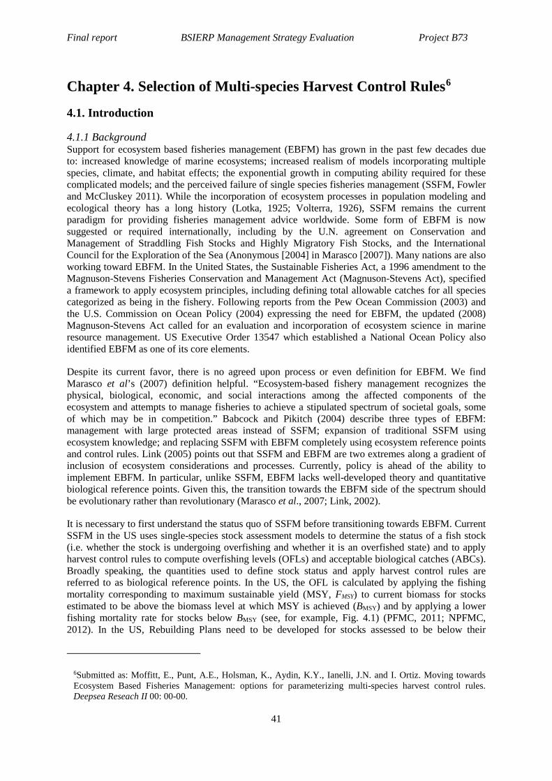
Final report BSIERP Management Strategy Evaluation Project B73
Chapter 4. Selection of Multi-species Harvest Control Rules6
4.1. Introduction
4.1.1 Background Support for ecosystem based fisheries management (EBFM) has grown in the past few decades due to: increased knowledge of marine ecosystems; increased realism of models incorporating multiple species, climate, and habitat effects; the exponential growth in computing ability required for these complicated models; and the perceived failure of single species fisheries management (SSFM, Fowler and McCluskey 2011). While the incorporation of ecosystem processes in population modeling and ecological theory has a long history (Lotka, 1925; Volterra, 1926), SSFM remains the current paradigm for providing fisheries management advice worldwide. Some form of EBFM is now suggested or required internationally, including by the U.N. agreement on Conservation and Management of Straddling Fish Stocks and Highly Migratory Fish Stocks, and the International Council for the Exploration of the Sea (Anonymous [2004] in Marasco [2007]). Many nations are also working toward EBFM. In the United States, the Sustainable Fisheries Act, a 1996 amendment to the Magnuson-Stevens Fisheries Conservation and Management Act (Magnuson-Stevens Act), specified a framework to apply ecosystem principles, including defining total allowable catches for all species categorized as being in the fishery. Following reports from the Pew Ocean Commission (2003) and the U.S. Commission on Ocean Policy (2004) expressing the need for EBFM, the updated (2008) Magnuson-Stevens Act called for an evaluation and incorporation of ecosystem science in marine resource management. US Executive Order 13547 which established a National Ocean Policy also identified EBFM as one of its core elements.
Despite its current favor, there is no agreed upon process or even definition for EBFM. We find Marasco et al’s (2007) definition helpful. “Ecosystem-based fishery management recognizes the physical, biological, economic, and social interactions among the affected components of the ecosystem and attempts to manage fisheries to achieve a stipulated spectrum of societal goals, some of which may be in competition.” Babcock and Pikitch (2004) describe three types of EBFM: management with large protected areas instead of SSFM; expansion of traditional SSFM using ecosystem knowledge; and replacing SSFM with EBFM completely using ecosystem reference points and control rules. Link (2005) points out that SSFM and EBFM are two extremes along a gradient of inclusion of ecosystem considerations and processes. Currently, policy is ahead of the ability to implement EBFM. In particular, unlike SSFM, EBFM lacks well-developed theory and quantitative biological reference points. Given this, the transition towards the EBFM side of the spectrum should be evolutionary rather than revolutionary (Marasco et al., 2007; Link, 2002).
It is necessary to first understand the status quo of SSFM before transitioning towards EBFM. Current SSFM in the US uses single-species stock assessment models to determine the status of a fish stock (i.e. whether the stock is undergoing overfishing and whether it is an overfished state) and to apply harvest control rules to compute overfishing levels (OFLs) and acceptable biological catches (ABCs). Broadly speaking, the quantities used to define stock status and apply harvest control rules are referred to as biological reference points. In the US, the OFL is calculated by applying the fishing mortality corresponding to maximum sustainable yield (MSY, FMSY) to current biomass for stocks estimated to be above the biomass level at which MSY is achieved (BMSY) and by applying a lower fishing mortality rate for stocks below BMSY (see, for example, Fig. 4.1) (PFMC, 2011; NPFMC, 2012). In the US, Rebuilding Plans need to be developed for stocks assessed to be below their
6Submitted as: Moffitt, E., Punt, A.E., Holsman, K., Aydin, K.Y., Ianelli, J.N. and I. Ortiz. Moving towards Ecosystem Based Fisheries Management: options for parameterizing multi-species harvest control rules. Deepsea Reseach II 00: 00-00.
41

Project B73 BSIERP Management Strategy Evaluation Final report
Minimum Stock Size Thresholds (MSSTs) and declared by the National Fisheries Management Service to be in an overfished state.
MSY in single-species assessment models often depends on the form of the stock-recruitment relationship, which can be difficult to estimate given available data. Consequently, “proxy” values are frequently used for FMSY and BMSY (Punt et al., in press) Common proxies for FMSY are FMAX (the fishing mortality rate which maximizes yield-per-recruit), and Fx% (the fishing mortality rate which reduces spawning biomass-per-recruit to x% of its unfished level). These levels of fishing lead to corresponding spawning biomass levels (Bx%) in which the spawning biomass is x% of the unfished biomass (B0) under the assumption that recruitment is independent of spawning biomass. For example, F35% is used as the default proxy for FMSY for crab stocks in the Bering Sea and Aleutian Islands region of Alaska (NPFMC, 2008), while F50% is the default proxy for rockfishes off the US west coast (PFMC, 2011). Common proxies for BMSY include a pre-specified fraction of the unfished biomass (e.g. Punt et al., in press), and the average biomass over a period of years when the stock was considered to be close to BMSY (NPFMC, 2008).
Several multi-species assessment models have been developed (e.g. for the North Pacific: MSVPA - Jurado-Molina and Livingston, 2002; MALMAK - Kinzey and Punt, 2009; MSM – Jurado-Molina et al., 2005; MSMt – Holsman et al., in review) which could be used to estimate stock biomass and trends. However, methods for implementing multi-species models to provide fisheries management advice within legal frameworks such as are in place in the US, have lagged behind the development of multi-species assessment models. One specific challenge is that the Magnuson-Stevens Act is framed in terms of MSY. However there is no agreement of how MSY is defined in an ecosystem context. Specifically, the “excess production” (often called “surplus production”) concept of MSY is clear in SSFMs; there is a surplus of individuals that can be harvested when the population is above its threshold for collapse and below its unfished level. However, the amount of “excess production” is not stationary in an ecosystem context, and varies with annual mortality that depends on the numbers of predators, prey, and competitors. Multi-species objectives further confound management reference points as management decisions may also include minimum biomass thresholds needed to avoid depletion of predators and prey while “achieving MSY” (e.g. Gaichas et al., 2012a).
Management advice for defining multi-species biological reference points (MBRPs) for EBFM can be developed in several ways, but using multi-species assessment models to define ABCs and OFLs for each species individually is closest to the current management paradigm. An alternative would be to define ABCs and OFLs for species in aggregate, either for several groups or for the entire ecosystem, and could include goals such as optimizing total biomass yield, optimizing total revenue, or optimizing biomass yield or revenue for a particular set of species. Additionally, it is possible to create MBRPs to manage for ecosystem-level goals or ecosystem “health”. Some precedent for EBFM management advice exists under current SSFM for Alaskan systems. The North Pacific Fisheries Management Council has specifically identified various ecosystem goals for the region such as conserving food-web resources, maintaining biodiversity, and reducing bycatch of non-target species (Livingston et al., 2011; NPFMC, 2012). These EBFM goals have led to implementation of EBFM limits such as maximum annual harvested groundfish caps (i.e., 2 and 0.7-1.4 million t for optimum yield for the eastern Bering Sea and Gulf of Alaska ecosystems, respectively) and minimum biomass thresholds (e.g., 20% of unfished spawning stock biomass for pollock in the Gulf of Alaska; A’mar et al., 2009). However, these limits are currently static. Incorporating time-varying limits into EBFM could be used to meet objectives such as conserving biodiversity, maintaining the ecosystem in a particular state, or maintaining particular ecosystem services (Link et al., 2002; Link, 2005).
The focus of this study is to outline and contrast several ways to define MBRPs (proxies for FMSY and BMSY) used in control rules, which are parameterized using output from multi-species assessment models. The discussion is focused on the legal framework for EBFM in the US, specifically how control rules are applied off the US West Coast and Alaska. However, the general principles underlying this work have broader applications, including jurisdictions such as New Zealand and
42

Final report BSIERP Management Strategy Evaluation Project B73
Australia where harvest control rules are used extensively (Ministry of Fisheries, 2008; Smith et al., 2009).
4.1.2. Previous considerations Several authors have explored the use of MBRPs for EBFM. Collie and Gislason (2001) examined the sensitivity of commonly-used biological reference points to trophic interactions in a simple two-species, predator-prey fish community. This sensitivity is expected given the outputs from multi-species production models (Larkin, 1966; Walter and Hogman, 1971). Collie and Gislason (2001) suggested that biological reference points for prey species should be defined according to the level of predation mortality. In fact, their model indicated that surplus production was zero for a fishery on a prey species when predation mortality was high. Similarly, Gamble and Link (2009) incorporated Lotka-Volterra terms for predation and competition into a surplus production model to explore whether all stocks can simultaneously reach and maintain BMSY in the face of multi-species interactions and harvesting. They found that biomass estimates differed when such interactions were ignored when both exploitation and species interactions were present, which Tyrrell et al. (2011) argued reinforces the need to take multi-species interactions into account when calculating reference points.
A naïve first step for estimating system-wide MSY involves summing the MSYs from single-species assessments. Mueter and Megrey (2006) fitted surplus production models to the time series of aggregated catch and biomass of groundfish in Alaska. They found that their estimates of ecosystem-level MSY were smaller than the sum of the single-species MSYs from recent stock assessments, and argued that including multi-species interactions may lead to different, perhaps more realistic, results. Moustahfid et al. (2009a) used a multi-species surplus production model to estimate BMSY for longshore inshore squid (Loligo pealeii) and found that BMSY was higher when multi-species interactions were taken into account. Moustahfid et al. (2009b) used a multi-species age-structured model to estimate MSY and BMSY for Atlantic mackerel (Scomber scombrus ) in the Northwest Atlantic and found that accounting for multi-species interactions led to higher estimates of both quantities compared to estimates based on single-species models. Similarly, multiple comparative analyses of single- and multi-species production models applied to 13 northern hemisphere ecosystems confirmed that system-wide MSY is less than the sum of single-species MSY (Gaichas et al., 2012a; Link et al., 2012; Holsman et al., 2012). This led to the recommendation of Link et al. (2012) that multi-species models should include considerations of common productivity, and inter-species and environmental interactions.
More recently, Kaplan et al. (In press) conducted projections of an Ecosim (Walters et al., 2000; Christensen and Walters, 2004) model for the California Current system in which system-wide unfished biomass was calculated by projecting the system forward in the absence of any exploitation and defining biological reference points by projecting the model forward with the same fishing mortality on all groups.
4.2. Material and Methods
4.2.1 Candidate MBRPs to be used in multi-species control rules Control rules are likely to be of the forms in Figure 4.1, which require values for FMSY and BMSY. Control rules to be used in EBFM fall within two separate philosophies. They can either be based on each stock’s status in relation to its MSY individually, or a system-wide MSY (or proxy) can be used. Control rules based on individual-stock reference points are more closely tied to the current philosophy of SSFM (and therefore potentially easier to implement), while system-wide control rules are more consistent with the broadest interpretation of EBFM.
One challenge is how to define unfished biomass, B0, in a multi-species context. The process is relatively straightforward if a multi-species framework is used to derive estimates for a single target species; unfished biomass is determined by projecting the model forward under average fishing mortality rate for other species in the model (or some other defined fishing mortality rate), but without
43

Project B73 BSIERP Management Strategy Evaluation Final report
fishing on the target species. However, if the multi-species model is being used to derive biological reference points for multiple species that are linked through predation, unfished biomass may be lower when fishing is simultaneously set to zero for predators and their prey than if fishing is set to zero for a subset of predators (Holsman et al., in review). For the purposes of this paper we generally (the exception being one variant of option A below) define multi-species B0 as the set of biomasses when fishing mortality is set to zero for all species simultaneously (sensu Kaplan et al. in press). As such, B0 for each species is computed by projecting the multi-species model several years forward with no fishing until the biomass values of all the species come to some relative equilibrium; B0 is then set for each species to the resulting long-term average biomass level, or the biomass level at the end of the projection period.
We developed candidate control rules (Table 4.1) for a case in which there is ongoing uncertainty about the values for the parameters of the stock-recruitment relationship, but there is information on predation relationships, as is the case for the stocks in the North Pacific region of the US. Thus, we base the candidate control rules on analogies to a spawning biomass-per-recruit proxy for FMSY, i.e. FMSY ~ Fx% and a biomass proxy for BMSY = x*B0. The value of x assumed when applying control rules differs among jurisdictions (e.g. 0.25 for flatfishes of the US West Coast; 0.4 for groundfishes off the US West Coast except flatfish, 0.35 for groundfishes and crab off Alaska).
4.2.1.1 Calculate Fx% using model simulation Conceptually, this approach involves conducting projections using a multi-species model to find the fishing mortality rates so that each species equilibrates at x*B0 (Options A-B2 in Table 4.1). In principle, this can be accomplished by solving a system of non-linear equations relating biomass of all species to fishing mortality. However, rarely will a solution for it exist. Instead, iterative approaches can be used when it is impossible to find a global solution (Option B3 in Table 4.1). The approach that is closest to single species management as it presently exists is to solve for Fx% for each species so that when fishing mortality rates for all other species are set to current average values the biomass of each species equilibrates at x*B0 (Option A in Table 4.1). Alternatively, the fishing mortality for all other species could be set to zero instead of the current average values (Option B1 in Table 4.1). Management might find it preferable that the biomass of no species drops below y*B0; in this case Option B2 (Table 4.1) could be used. In this case, the fishing mortality of all other species could be set either at current average values (Option B2a) or zero (Option B2b). If no simultaneous solution for all species can be found using Options A-B2, all of these options could be iterated several times, i.e. the fishing mortality rate would be calculated for a species, setting the fishing mortality rates for the remaining species based on a previous iteration and this process repeated for each species until convergence occurs (Option B3 in Table 4.1). However, this iteration process is not guaranteed to converge.
4.2.1.2 Calculate Fx% using a single-species model and multi-species model-generated M and B0 Options A-B could be computationally very intensive and there may not be a unique solution. A simpler alternative approach would to be replace the multi-species system with a set of single-species models in which the natural mortality rates by species are set to those derived from the multi-species model when fishing mortality is zero for all species (i.e., multi-species B0). Each single-species model would then be used to compute the Fx% (Option C in Table 4.1).
4.2.1.3 Sum of all stocks are at x% of sum of individual B0’s The biological reference points can also be defined on a system-wide level. For Option D (Table 4.1), system-wide unfished biomass ( ) would be defined as the sum of the unfished biomass over all
species (i.e., ). The fishing mortality rate for each species would then be a scalar
multiplied by a relative fishing mortality rate (e.g. where is the relative fishing
mortality rate for species i and is the scalar, the value of which is selected to maximize total yield). An intuitive way to set the relative fishing mortality rates would be to use the natural mortality
0,allB
0, 0,all ii
B B= ∑
,R iF
F
44

Final report BSIERP Management Strategy Evaluation Project B73
rates at B0. In many jurisdictions, some species are protected – the relative fishing mortality rates for these species would be set to zero.
4.2.1.4 Solve for system-wide MMSY for key species The other major way to define system-wide biological reference points involves solving for the system-wide multi-species maximum sustainable yield (MMSY; Option E in Table 4.1). This is similar to an option in Ecopath-with-Ecosim that involves estimating fishing mortality patterns to maximize a utility function (Christensen and Walters, 2004).
There are multiple ways to achieve MMSY. This simplest is to find the unconstrained theoretical mathematical solution (Option E1 in Table 4.1). Other ways, which may be more consistent with existing law, would be to constrain the optimization so that no stocks are predicted to equilibrate below y*B0 (Option E2 in Table 4.1). In this case, the sustainability of each individual stock is equally important even if that means reducing system-wide MMSY. The third option is analogous to Option D where the relative fishing mortalities are pre-specified to split the system-wide FMSY among component stocks (Option E3 in Table 4.1). System-wide MMSY weights species by their mass rather than their economic values. This approach could be generalized to maximize other measures such as system-wide profit. Such an approach would need to be adopted for jurisdictions such as Australia for which management objectives are expressed in terms of maximizing economic benefits (Rayns, 2007; Kompas et al., 2010).
4.2.2 Example using predator-prey model Consistent with how single-species management advice is provided, it is likely that any multi-species and ecosystem models used for management purposes will represent major species using age-structured models. However, a simple two-species predator-prey population dynamics (surplus production) model is used to illustrate the properties of the various options for developing biological reference points in a multi-species context:
(4.1a) (4.1b)
where P is the biomass of the prey species, Q is biomass of the predator species, αP and αQ are the intrinsic growth rates of the prey and predator species, with the density-dependent terms βP and βQ determining the rate of increase of each species in the absence of the other species (due to other species in the ecosystem), λ is the maximum per capita predation rate, µ is a term governing density-dependence of the predation rate, g is consumption efficiency parameter, FP, and FQ are the fishing mortality rates for the prey and predators, and MP, and MQ are the natural mortality rates due to predator species not in the modeled system.
For this example, the functional response forms and values chosen for parameters were based on walleye pollock (Theragra chalcogramma) and Pacific cod (Gadus macrocephalus) from the Ecosim model constructed by Aydin et al. (2007). It is important to note that the set of parameters used for this example were not fit to time-series data and the original model modelled age-structure for these species rather than aggregated biomass. So while “pollock” and “cod” are used for illustration of a predator/prey pair, the species as modeled represent a hypothetical set of parameters – actual results may differ substantially as the parameters are based on fitting Equation 4.1 to data on abundance.
To illustrate the biological reference points for this hypothetical predator/prey pair, the model was run using a full range of annual fishing rates for each species from 0 to 0.8yr-1 in increments of 0.01yr-1. The equilibrium biomass and catch levels for each species were determined for each pair of fishing rates in the form of a two-dimensional set of biomass and catch curves (Fig. 2). The results from the projections were then used to determine the target fishing mortality rates under each potential harvest control rule where the target biomass (x*B0) was taken be 40% of B0 and the level below which species should not equilibrate (y*B0) was taken to be 35% of B0, consistent with current policy for groundfish in Alaskan waters.
dP /dt = (αP P /1+ βP P) − (λPQ /1+ µQ) − MP P − FP P
dQ /dt = (αQQ /1+ βQQ) + g(λPQ /1+ µQ) − MQQ − FQQ
45

Project B73 BSIERP Management Strategy Evaluation Final report
4.3. Results Pollock biomass decreased with increasing pollock fishing rate, and increased as cod biomass is removed from the system; the latter due to lessened predation (Fig. 4.2a). Cod decreased with increases in cod fishing mortality (Fig 4.2b), and also decreased as their prey were removed through increased fishing on pollock. In terms of catch, both pollock and cod showed a “traditional” surplus production catch/fishing rate relationship, peaking at a maximum yield, but that maximum level depended on the level of the fishing mortality rate on pollock (Fig 4.2c) and cod (Fig 4.2d). The black contour lines show the “single-species” overfishing limit (fishing rate > F35% in Option A).
The control rule options considered in this paper (Table 4.1) can be illustrated as a function of fishing rates (Fig. 4.3), which can be overlain on each of the images in Fig. 4.2 to determine the biomass and catch of each species as a result of the given strategy. For control rule A (Fig. 4.3), each red line represents the F40% contour (solid for pollock, dashed for cod), where the reference value for unfished biomass B0 is calculated dependent on the biomass of the other species. The fishing rates converge at the red point on the figure. The target fishing mortality rates under Option A are shown by the red dot; the value represents an analogy to single-species management in that single-species policy involves setting natural mortality in assessment models to the prevailing (constant) value given mortality rates for all other species in the system. As such, control rule A is used in Fig. 4.3 as a proxy for overfishing limits (OFLs); the gray area in Fig. 4.3 shows the area in which one or both stocks are below B35% as defined in control rule A and is analogous to the black lines in Fig. 4.2.
For control rule B1 (blue lines and point in Fig. 4.3), each line represents the F40% contour for each species when referenced against a B0 for each species when there is no fishing in the ecosystem. The point represents the set of fishing mortality rates when both species are at B40%; this option leads to the most conservative fishing rate for cod. The target fishing mortality rates under options A and B1 in this example are below those when the two species equilibrate at 35% B0; in this case they also represent options B2a and B2b. Because our example contains only two species, the additional process of iterating by species (control rule B3) was not needed and is therefore not shown.
Control rule C is another option that could be integrated easily into the current management paradigm (light blue lines and point in Fig. 4.3). M-at-age values for each species are obtained from the multi-species model then used in a single-species context to determine the values at B0. This option leads to the most conservative fishing rate for pollock.
Control rule D is shown in green; the solid line represents the locus of fishing mortality rates corresponding to B40% for the combined (summed) cod and pollock biomasses, where B0 is the sum of cod and pollock biomass with no fishing (Fig. 4.3). The green dashed line represents the line on which Fcod = rFpollock, where r is the ratio of Mcod to Mpollock in the unfished state (in this case ~ 0.74).
Option E1 uses unconstrained optimization to solve for the system-wide BMSY (MMSY) (Fig. 4.3). Option E2 solves for system-wide BMSY with the constraint that no stocks fall below 35% of B0 (Fig. 4.3). Option E3 solves for system-wide BMSY but splits the relative fishing mortality among species in a pre-specified way – in this case proportional to M (Fig. 4.3).
The resulting equilibrium biomass, catch, and fishing mortality rates resulting from each control rule option (points in Fig. 4.3) are shown in Figure 4.4. The management implications resulting from the different control rule options are less variable for pollock than for cod (Fig. 4.4). Option A represents the control rule that is closest to current single-species management. If Option B1 is used instead, the fishing mortality rates are reduced and biomass is increased, but the catches are only slightly reduced for pollock. Option C, which takes the M-at-age vectors for all species from the multi-species model to use in single-species B0 calculations, is another option that could be easily integrated into current management. This option results in the low fishing mortality rates, and large pollock and cod biomass. However the pollock catch is only slightly decreased, and it leads to the largest cod catch (Fig. 4.4). Option D, which defines system-wide B0 as the sum over all species, imposes a higher fishing rate on cod, resulting in a lower equilibium cod biomass. Results for pollock as similar to Option A. Option
46

Final report BSIERP Management Strategy Evaluation Project B73
E1 fishes cod at the highest rate to remove the predation on pollock, which results in a higher pollock (and hence total) catch (note the differences in scale between cod in pollock in Figure 4.4). The fishing rate for pollock is similar to Option A, but with higher resulting pollock catch. Option E2 does not allow cod to be depleted below 35% B0 and results in similar outcomes to Option A. Option E3 has the highest fishing rate on pollock, resulting in the smallest biomass and a small increase in pollock catch; cod is also fished strongly (Fig. 4.4).
4.4. Discussion US Fisheries Management Councils have already started to make the transition from single-species to ecosystem based fisheries management in that they have, for example, identified essential fish habitat and in some cases protected key forage species. The North Pacific Fishery Management Council has implemented caps on optimum yield for both the eastern Bering Sea and the Gulf of Alaska. However, to date tactical management advice has not been based on assessment models that explicitly include species interactions. One reason for this has been the lack of multi-species biological reference points (MBRPs). Here we outline a framework for MBRPs that range from those that can be readily used in current SSFM frameworks to broader EBFM limits that may take years to fully implement.
Multi-species and ecosystem models can improve our understanding of the effects of fishing in such a way that it is possible to make informed and transparent decisions about when and how to limit fishery impacts. However, these methods also have intensive data, development, and computing power needs, which translate into increased costs of monitoring and assessment. Given this, it is necessary to evaluate whether the additional expenditures are worth the investment. An inherent challenge of complicated models is the complexity/predictive tradeoff: as complexity and number of parameters increase, the predictive ability (required of models used for management) is compromised (Plaganyi,2007).
The multi-species biological reference points we outline each have their own strengths and weaknesses. Option A, which solves for Fx% for each species with fishing rates for all other species set to current average rates, is the MBRP closest to the single-species control rules that are currently used. As such, Option A could be implemented the most easily into the current management process and represents a first step into the use of MBRPs. While MBRPs from Option A are set for each species when all other species are set at current fishing mortality levels, MBRPs from Option B1 are set for each species when B0 is defined when all other species are unfished. Fishing rates defined when fishing for all other species is set to zero (Option B1) will tend to be lower than those defined using Option A. This result has been cited as a fundamental tenet of multi-species management (joint control rules produce lower fishing rates than single-species control rules). However, as seen in our example, Option B1 led to similar catches compared to Option A, with lower fishing mortality rates (Fig. 4.4). If effort costs are considered, Option B1 may be an overall improvement over Option A. Options B2a and B2b are the same as Options A and B1, but with the constraint that no stock is allowed to drop below y*B0. This adds conservative limits and, in keeping with current legislation, ensures that all stock sizes exceed conventional choices for MSST. Options A, B1, and B2 implicitly involve solving the system of equations defining the multi-species model. However, an analytical solution may not exist that allows all species to be at x*B0, or there may be multiple solutions if the multi-species model has strong ecological interactions among species (Holsman et al., in review). In these cases, Option B3 can be used, and prioritization of species order in the iteration becomes an important policy discussion point.
Option C uses B0 and M-at-age values for each species resulting from the multi-species or ecosystem assessment model in single-species analysis. This method is similar to methods of stock assessment in which values for M-at-age taken from a multi-species stock assessment are assumed when conducting a single-species stock assessment (e.g. ICES, 2012). However, the M-at-age values used in the single-species analysis are taken from the ecosystem model when there is no fishing. In reality, M-at-age would be expected to change as species are selectively harvested due to ecological linkages. It is
47

Project B73 BSIERP Management Strategy Evaluation Final report
common to use yield-per-recruit methods to compute target fishing mortalities (NPFMC, 2008; PFMC, 2011). These methods ignore time-variation in weight-at-age as well as M-at-age, whereas weight-at-age varies due to temperature, ecological interactions, and/or population sizes in some multi-species models such as Atlantis and MSMt (Fulton et al., 2011; Holsman et al., in review). Option C could be readily implemented for EBFM.
Option D finds the system-wide unfished biomass (the sum of the unfished biomass over all species), similar to the approach by Mueter and Megrey (2006). This option allows flexibility in how the total fished biomass is split among species, and fishing mortality rates can be set to zero for protected species. Fishing policies based on summed biomass may be dominated by the most abundant species. In our example, the green solid line (summed B40%) is nearly identical to the red solid line (single-species) for pollock B40% (Fig. 4.3).
Options E1-3, which use MMSY calculated using a multi-species or ecosystem model, encompasses a philosophy most in keeping with EBFM. Multi-species maximum sustainable yield (MMSY) provides a metric of optimal ecosystem productivity. Option E1 uses the unconstrained mathematical solution found using the multi-species assessment model. This method may allow multiple solutions including unrealistic scenarios (e.g., harvest removals exceeding fishery capacity) and depletion of some species below their nominal Minimum Stock Size Thresholds (MSSTs), which would conflict with the US law (Link, 2002; Hilborn et al., 2004; Gamble and Link, 2009). While perhaps not directly practical for management, such scenarios allow managers to evaluate multi-species dynamics of a modeled system and serve as a comparative reference for alternative options. Any maximum based on catch biomass alone will tend to produce the answer “eliminate the predator to harvest the prey” since a prey species tends to be considerably more productive that its predators (black point in Fig. 4.3). In addition to being not feasible due to the need to keep stocks above minimum biomass levels, Option E1 includes continual fishing pressure on the predator (0.8yr-1 on cod in Fig. 4.4) for no gain in catch; this is unlikely to be cost-effective. Weighting based on economics or relative societal importance of each species can be used to balance joint maximization.
Option E2 uses the MMSY resulting from the multi-species assessment model, with the constraint that the target stock size is never less than the nominal BMSY proxy of y*B0. This is a way to use the ecosystem knowledge in terms of the maximum amount of yield to be taken out of the ecosystem, but still comply with current regulations that prevent stocks becoming overfished. Implementation of constraints when selecting a FMSY proxy (Options B2 and E2) would add conservative limits and ensure that the target stock size exceeds conventional choices for MSST. However, these control rules may sacrifice potential yield from the ecosystem in common with the other methods that prevent depleting stocks below nominal target levels (Hilborn et al., 2004; Hilborn, 2011). Similarly, Gaichas et al. (2012b) found that biomass thresholds were needed to balance yield and biodiversity objectives for species assemblages with disparate productivities. Specifically, a small reduction in overall yield prevented multiple species extinctions.
Option E3 defines the relative fishing mortality corresponding to MSY resulting from the ecosystem assessment model among component stocks based on the effort, value, or potential yield of each stock. This option includes socio-economic information in terms of how FMSY is defined, and reflects current realities of the relative importance of different stocks. However, stakeholder consensus on how fishing mortality should be allocated among stocks may prove challenging.
Care needs to be taken when considering possible multi-species control rules. Options E1 and E3 are least consistent with current management practices because MMSY could occur by depleting stocks below MSSTs (as shown in Fig. 4.3). Under the US Magnuson-Stevens Fishery Management and Conservation Act, depleting stocks below the MSST leads to designation of an “overfished” status, and initiates stock rebuilding. Options such as D and E could lead to high fishing mortality on the lower trophic levels, but the resulting yield may have lower economic value than if lower trophic levels remain unfished or under-fished relative to the true FMSY. This problem could be addressed by weighting yield by value. In general, economic considerations will be important to consider. Some
48

Final report BSIERP Management Strategy Evaluation Project B73
control rule options expected lower fishing mortality rates to achieve a similar level of catch to other options; these would likely be preferable to the options that expected fishing at a higher level but without proportional catch increases. Realities about how high fishing rates for particular species also need to be considered; high fishing rates on predator species to increase prey catch may not be practical if there is not a market or fishery for the predator species.
Proxies for FMSY and BMSY for use in single-species control rules are usually based on yield-per-recruit analysis. This approach involves following a cohort over time. The approach consequently ignores the relationship between spawning biomass and subsequently recruitment. Some multi-species models (e.g. MALMAK and MSM) are based on this assumption, while other multi-species models such as Atlantis explicitly include stock-recruitment relationships. Applications of the control rules of Table 4.1 are likely to be sensitive to the type of multi-species model used as the basis for forecasts as well as to whether and how relationships between spawning biomass and recruitment are modeled.
Quantifying uncertainty is a key component of modern fisheries stock assessment and a variety of methods such as bootstrapping and Bayesian methods have been developed to quantify the uncertainty of model outputs. This uncertainty feeds into the management process within the US because the Acceptable Biological Catch is the Overfishing Level less “scientific uncertainty”. The estimates of uncertainty from these approaches tend to underestimate the actual level of uncertainty as shown by comparisons between estimates of uncertainty for biomass from these methods and the variation in estimates of biomass among assessments (Ralston et al., 2011). Although some methods for quantifying the extent of uncertainty associated with the outputs of multi-species and ecosystem models have been developed (e.g. Gaichas et al., 2012b), quantification of uncertainty for these methods is still an area of research.
The logical next step is therefore testing of these potential multi-species harvest control rules through management strategy evaluation (MSE). MSE (Smith, 1994; Sainsbury et al., 2000; Goodman et al., 2002; Butterworth, 2007) involves assessing the performance of alternative candidate management strategies relative to performance measures which quantify the management (and legal) goals for the managed system. MSE involves developing a model of the system to be managed and parameterizing this model using data for the system under consideration (or hypotheses for how the system may change over time; Punt et al., in press). Data are then generated from the system model and used as the base for assessments of the resources in the system. The results from these assessments are then used as the basis for the harvest control rules which determine the future removals from the system. For the purposes of this paper, the assessment methods would be a range of single- and multi-species models and the control rules would include the options in Table 4.1. MSEs that focus on multi-species and ecosystem objectives have already been undertaken (e.g. Fulton et al., 2007; Dichmont et al., 2008, 2013; Plaganyi et al., 2014), but to date no MSE has applied multi-species control rules along the lines outlined in this paper.
Many multi-species assessment models have been developed, and while these methods provide estimates of biomass trends, they cannot be used for management purposes without a way to translate biomass estimates into catch limit recommendations. Using multi-species models in a management context requires the development and testing of multi-species biological reference points (MBRPs) for use in harvest control rules. Here we have outlined several options that cover the broad scope of possibilities on the spectrum from close to the single-species status quo to fully immersed in the EBFM paradigm.
49

Project B73 BSIERP Management Strategy Evaluation Final report
Table 4.1. The candidate control rules encompass both individual stock and system-wide biological reference points.
Individual stocks: Option A. Solve for Fx% by species when fishing mortality for all other species is set to
current average values. Option B1. Solve for Fx% by species when fishing mortality for all other species is set to
zero. Option B2a/b. Solve for Fx% by species when fishing mortality for all other species is set
to current average values (a) or zero (b) with the additional requirement that no stock is allowed to drop below y*B0.
Option B3a-d. Approaches A and B2a iterated by species to find a solution. Option C. Calculate Fx% when M-at-age for each species is set to the values at B0 System-wide: Option D. x*B0 would apply over all species combined. FMSY for each species would be a
scalar multiplied by M. Option E. Solve for system-wide BMSY
E1. Unconstrained optimization E2. Constrained so that no stocks fall below y*B0. E3. Unconstrained with relative fishing mortality pre-specified
50

Final report BSIERP Management Strategy Evaluation Project B73
Figure 4.1. Current single-species control rules. a) North Pacific Fishery Management Council Tier 3 harvest control rules. FABC defines the fishing rate corresponding to the maximum Acceptable Biological Catch (ABC). FOFL is the fishing mortality rate that would produce the Overfishing Limit (OFL) and is defined by FMSY. b) Pacific Fishery Management Council flatfish harvest control rules. The Overfishing Limit (OFL) is defined by FMSY (or a proxy) and estimated current biomass (B). The maximum Acceptable Biological Catch (ABC) is defined by FMSY (or a proxy), estimated current biomass (B), and an uncertainty buffer (P).
51

Project B73 BSIERP Management Strategy Evaluation Final report
Figure 4.2. Predator-prey model dynamics. Equilibrium biomass (a,b) and catch (c,d) for a hypothetical predator (“cod”) and prey (“pollock”) pair under all combinations of annual fishing rates from 0 to 0.8 yr-1 in increments of 0.01yr-1. The black contour lines represent the “single-species” overfishing limit (fishing rate > F35% in Option A). Units for biomass and catch are t/km2, based on the Ecopath model by Aydin et al. (2007).
52

Final report BSIERP Management Strategy Evaluation Project B73
Figure 4.3. Candidate multi-species control rules. Control rules modeled in this paper as a function of pollock and cod fishing mortality rates. The gray area represents the “single-species” overfishing limit (fishing rate > F35% in Option A), similar to the black lines in Fig. 4.2.
53

Project B73 BSIERP Management Strategy Evaluation Final report
Figure 4.4. Comparing outcomes from candidate multi-species control rules. Biomass, catch, and fishing mortality rate for the unfished two-species model (first column), and for candidate control rules. Units for biomass and catch are t/km2, based on the Ecopath model by Aydin et al. (2007).
54

Final report BSIERP Management Strategy Evaluation Project B73
55

Project B73 BSIERP Management Strategy Evaluation Final report
Chapter 5. Blended Forecasts
5.1 Introduction The Scientific and Statistical Committees, SSCs, of the Regional Fishery Management Councils are required to provide recommendations for overfishing levels, OFLs, and Acceptable Biological Catches, ABCs, as well as evaluate whether a stock is subject to overfishing or is in an overfished state. For most major stocks, these recommendations are based on the outcomes of quantitative stock assessment methods, which involve fitting population dynamics models to monitoring data collected during fishing and surveys. For stocks managed by the North Pacific Fishery Management Council (NPFMC 2012, PMFC 2011), the stock assessments are based on single-species models, i.e. the impacts of time-varying predation mortality are ignored (or subsumed into the variation in the estimates of recruitment, under the assumption that the majority of predation mortality which is time-varying occurs before the age-at-recruitment).
Most stock assessments involve pre-specifying the values for some of the parameters of the population dynamics model (e.g., the rate of natural mortality, M, fecundity as a function of length or age, and the survey catchability coefficient), making structural assumptions (e.g. vulnerability for a given fleet is a time-varying logistic function of length, recruitment is related to spawning stock size according to the Beverton-Holt form of the stock-recruitment relationship), choosing the data sets used when fitting the model (e.g., should fishery catch rate data be used or ignored given uncertainties regarding the relationship between catch rate and abundance), and assigning weights to the data sources which are included in the assessment. Although model fits to data may be similar, the results of stock assessments can be highly sensitive to parameter values and choices regarding model structure (e.g., Taylor and Stephens, 2013; Holsman et al. in review)
In general, fisheries management advice (and hence OFLs and ABCs) is based on a single “best” model (and hence set of assumptions), and uncertainty is quantified about that model conditioned on its assumptions being correct. Typically, uncertainty is quantified using asymptotic methods, bootstrapping, or Bayesian methods (Magnusson et al., 2013). However, many sources of uncertainty are ignored when applying these methods, so the measures of uncertainty reported to managers usually underestimate the true amount of uncertainty (Ralston et al., 2011; Punt et al., 2012). The difference between the OFL and the ABC for a stock (the “buffer”) is meant to reflect the amount of scientific uncertainty. ABCs are often set so that the probability that the ABC exceeds the true OFL equals a selected value, P* (where P*< 0.5), i.e. P(ABC>OFL)=P* (Prager et al., 2003; Shertzer et al., 2008; Prager and Shertzer, 2010). However, the true probability that the ABC exceeds the OFL will be larger than P* if uncertainty is underestimated because the uncertainty associated with assumptions regarding model structure is ignored.
The use of multispecies and ecosystem models for fisheries management is considered to be a key component of Ecosystem Based Fisheries Management (EBFM) (Marasco et al., 2007; Plagányi, 2007). However, similar to single-species stock assessment methods, projections based on two ecosystem models (or variants of one ecosystem model with alternative assumptions) often reflect uncertainty about model structure and assumptions regarding values for pre-specified parameters For example, Kaplan et al. (in press) evaluated the impacts of depleting forage species in the California Current ecosystem using Atlantis (Fulton et al., 2011; Horner et al., 2010) and Ecopath-with-Ecosim (Christensen and Walters, 2004; Field et al., 2006). However, the results from these two ecosystem models differed markedly for some ecosystem components, to the extent that it is uncertain whether reducing forage species abundance would have a negative or positive effect on some ecosystem components. In addition, Kinzey and Punt (2009) showed that the results of a multispecies stock assessment were sensitive to the choice of the relationship between predation mortality and the density of predators and prey. For example, the multispecies models examined by Kinzey and Punt (2009) predicted that Pacific cod (Gadus macrocephalus) in the Aleutian Islands could have been increasing or decreasing prior to 1990 depending on this relationship.
56

Final report BSIERP Management Strategy Evaluation Project B73
The selection of the model for providing management advice is often done informally or in discussion based council process that favors familiar, well tested, models but can impede rapid adoption of updated assessment models that incorporate ecosystem information. However, model uncertainty can be accounted for using “model averaging”. Model averaging involves integrating model outputs from multiple models taking account of the relative probability (or plausibility) of each model. This provides a means for accounting for the uncertainties in models themselves by incorporating multiple simulations from a variety of models. Model outputs can include projections of population size under alternative harvest control rules or catch scenarios as well as specific outputs such as OFLs and ABCs. Model averaging allows diverse, yet plausible, model outputs to collectively be used to guide management, and can provide estimates of uncertainty derived from both data fit (as is the case with singular models) as well as model structure and assumptions. It allows the uncertainty regarding which model is correct to be reflected in the outputs used for management purposes, along with the uncertainty conditioned on the model given that it is assumed to be correct.
Here we provide a brief review of multi-model inference for fisheries assessment applications, focusing in particular on two alternative ways to implement model averaging for EBFM. We then use model averaging to integrate the results from three classes of model (single-species, temperature-specific single-species, temperature-specific multispecies) for three scenarios regarding future catch in the eastern Bering Sea in terms of impacts on the spawning stock biomass of walleye pollock (Gadus chalcogrammus), Pacific cod and arrowtooth flounder (Atheresthes stomias).
5.2. Overview of model averaging There are two main ways to conduct model averaging: Bayesian Model Averaging (BMA) and “ensemble” forecasting. BMA requires that estimates of the posterior probability of each candidate model be available. This probability needs to be derived by fitting the model to available data. However, the probability of the model given the data cannot be derived for all models (e.g. dynamic ecosystem models such as Atlantis or the Forage/Euphausiid Abundance in Space and Time (FEAST) model) because they cannot be formally fitted to data. It is consequently impossible to apply BMA in many situations. When this is the case, “posterior probability distributions” can be approximated by “envelopes of plausibility” derived from ensemble/Monte Carlo runs of each model where each run is based on a different (yet plausible) set of parameters, with the probability assigned to each model based on expert judgment (i.e. the “Delphi method”), a process which we will term “ensemble” forecasting. Butterworth et al. (1996) proposed the following four-level scheme to assign ‘plausibility ranks’ to the hypotheses underlying alternative models which could be used to weight models when “ensemble” forecasting is conducted:
1. how strong is the basis for the hypothesis in the data for the species or region under consideration
2. how strong is the basis for the hypothesis in the data for a similar species or another region; 3. how strong is the basis for the hypothesis for any species; and 4. how strong or appropriate is the theoretical basis for the hypothesis?
For the population dynamics models typical of fisheries management, both ways of conducting model averaging fundamentally involve making projections. Each model can be projected multiple times (the outcomes will differ if there are multiple parameter choices for each model or the projections account for future stochasticity due to recruitment variability for example). The results of model averaging can be summarized by the overall mean of some quantity of management or scientific interest, the spread of results, and by individual trajectories. The mean of the projections is a form of “best estimate”, but this does not take advantage of the primary aim of conducting multiple forecasts, namely to characterize uncertainty. Ianelli et al. (2011) summarize the results of projections for multiple models by illustrating intervals containing 50% and 80% of the outcomes as well as some individual trajectories to illustrate the overall uncertainty.
5.2.1 Bayesian Model Averaging (BMA) The philosophy underlying Bayesian model averaging has been outlined by several authors (e.g. Buckland et al., 1997; Durban et al., 2005; Hoeting et al., 1999; Kass and Raftery, 1995; Raftery et
57

Project B73 BSIERP Management Strategy Evaluation Final report
al., 2005; Chimielechi and Raftery, 2011). Ideally, BMA involves fitting the range of models to the available data and computing the probability of each model given the data. This weighting of models should ideally be conducted using Bayes factors, which evaluate the credibility of a model relative to all other models (Aitkin, 1991; Kass and Raftery, 1988). However, studies have weighted alternative models, using, for example, the Deviance Information Criterion (Spiegelhalter et al., 2002), Akaike’s Information Criterion (Akaike, 1973; Burnham and Anderson, 1998), and the Bayes Information Criterion (Schwartz, 1978). The latter two weighting schemes are non-Bayesian, but are relatively easy to compute in contrast to Bayes factor and DIC which require that a Bayesian analysis be conducted, which can be computationally prohibitive even for relatively simple ecosystem models (e.g. Parslow et al., 2013).
Bayes factor, DIC, AIC, and BIC can only be computed if each model is fit to the same data set. If the models are not fit to the same data set, it is necessary to weight each model using a more ad hoc approach, such as fitting the models to a subset of the data and predicting the remaining data, aka cross-validation. In this case, the weight assigned to each model would be proportional to the inverse of the mean square error associated with its predictions.
Given probabilities for each model, the Bayesian model averaged forecast is constructed by conducting multiple projections for each model and generating the overall forecast by sampling projections with probability proportional to the probability of the model. Table 5.1 summarizes an application of Bayesian model averaging in which five models are used to predict the fishing mortality and spawning biomass corresponding to maximum sustainable yield (FMSY and SMSY) for George’s Bank haddock, Melanogrammus aeglefinus. The best model in Table 5.1 is RBH, but model RZBH is almost as likely. The model-averaged results are as expected closest to the best models, but the standard errors for the model-averaged results are larger than for either of the two best models. The weights assigned to each model in Table 5.1 are based on the Bayes factor. Bayes factors can be computed in this case because all of the models use the same data and the models are fairly simple.
5.2.2 Ensemble forecasting Ensemble forecasting involves generating multiple projections of future system state under different choices for assumptions or parameter values. In principle, both structural and parameter uncertainty can be addressed through the use of multi-model ensembles. This approach is widely used in climate modeling where uncertainty is reflected in the accuracy of the approximations to the well-known and accepted physical principles of climate, and the inherent variability of the climate system. The climate system is chaotic, and the timing and phases of major and long-lasting fluctuations are largely unpredictable beyond time-horizons of a few years. Consequently, slightly different initial conditions for a climate model can lead to markedly different outcomes 40-50 years into the future. Whether including climate in population dynamics models has major impacts on the estimated future state of the populations under investigation depends on how the dynamics of the populations are linked to climate and the strength of the associated relationships.
Probabilities can be assigned to model configurations (the underlying model equations and the values for its parameters) or entire model configurations can be considered implausible using hindcast simulations of past conditions (e.g. Overland and Wang, 2007), although past performance is not necessarily a good indicator of success in simulating future climate (Reifen and Toumi, 2009). A’mar et al. (2009) based projections on six general circulation models which were selected for both their accuracy with respect to the historical data and their predictions with respect to future climate scenarios. Specifically, these six models were in the subset of models that replicated the spatial pattern and temporal characteristics of the first principal component of sea surface temperature (SST) in the North Pacific Ocean (the PDO) observed in the latter half of the twentieth century (A’mar et al., 2009).
5.2.3 Fisheries examples of model averaging Model averaging in fisheries assessments are rare; the focus for fisheries management tending to be either selection of a best model or identification of harvest control rules that are robust to model
58

Final report BSIERP Management Strategy Evaluation Project B73
selection and parameter value uncertainty (Butterworth, 2007). However, there are a few examples of where model averaging has been applied to fisheries population dynamics models and these are reviewed here.
5.2.3.1 Bayesian Model Averaging BMA has been applied to account for uncertainty regarding the form of the stock-recruitment relationship (usually Ricker vs Beverton-Holt) and the error structure (autocorrelated or not, and the distribution for the residuals) (Patterson, 1999; Brodziak and Legault, 2005). BMA was used by Brandon and Wade (2006) to account for uncertainty regarding the form of the population dynamics model underlying a stock assessment (density-dependent or non-density-dependent, and whether the stock was at its environmental carrying capacity at the start of the modeled period) in an assessment of the Bering Sea-Chucki-Beaufort seas stock of bowhead whales, Balaena mysticetus. The weights assigned to each model by Brandon and Wade (2006) were based on Bayes factor and they developed their posterior distributions for each model using the sample-importance-resample algorithm, which allowed straightforward computation of the posterior probability of each model. Wilberg and Bence (2008) used Monte Carlo simulation to show that model averaging of alternative formulations for how fishery catchability changes over time performed better than using DIC to select a “best” model.
Brodziak and Piner (2010) used BMA to integrate uncertainty due to the form of the stock-recruitment relationship (Ricker or Beverton-Holt), the extent of autocorrelation about the stock-recruitment relationship, and two values for the steepness of the stock-recruitment relationship for striped marlin (Tetrapturus audax) in the North Pacific. Unlike Broziak and Legault (2005), Brodziak and Piner (2010) approximated the Bayes factor using BIC.
5.2.3.2 Ensemble forecasting This basic approach was used by Dick and Ralston (2009) when conducting analyses to quantify the impact of various rebuilding strategies for cowcod (Sebastes levis) off southern California. Dick and Ralston (2009) conducted forecasts for a range of assessment models, each of which was conditioned on one of a set of values for the steepness of the Beverton-Holt stock-recruitment relationship. Each projection was weighted based on a pre-specified probability distribution for steepness. Hamel (2011) conducted projections to evaluate times for Pacific Ocean Perch (Sebastes alutus) to rebuild to the proxy for the biomass at which maximum sustainable yield is achieved, BMSY for three models, given different levels of future fishing mortality and catch. Two of these models were assigned probability 0.25 and the third model was assigned a probability of 0.5. The selection of probabilities in this case was not entirely subjective because the specifications for the two models assigned probability 0.25 were developed to have approximately this probability (Hamel and Ono, 2011).
Ianelli et al. (2011) evaluated the performance of management strategies for walleye pollock in the eastern Bering Sea. Recruitment was linked to predictions of SST from 82 Intergovernmental Panel on Climate Change (IPCC) models—SST, among other environmental factors, was found by Mueter et al. (2011) to be a possible factor affecting pollock recruitment. These 82 models were selected by downscaling IPCC models to the eastern Bering Sea ecosystem and using retrospective studies to identify models that perform poorly for this system (Wang et al., 2010).
Kolody et al. (2008), Kolody (2011), and Davies et al. (2012) developed an ‘uncertainty grid’ for assessments of swordfish (Xiphias gladius) in the Indian and Pacific Oceans, and explored structural uncertainty in a balanced factorial design. The results of the assessment were presented in terms of box plots of output statistics for each level of the factors considered. Kolody et al. (2008) explored sensitivity to stock-recruitment steepness, mixing proportions, growth rate/maturity/mortality options, the extent of variation about the stock-recruitment relationship, selectivity constraints, and data weights. Of 768 model configurations, a set of 192 model configurations considered the “most plausible ensemble” were used to summarize stock status. This ensemble was selected using three metrics: the root mean square fit to the catch rate index, the effective sample sizes for the length-frequency data, and the difference between observed and model-predicted mean catch lengths (similar to method of Francis 2011). Kolody (2011) assigned weighs to each of the factors on which the
59

Project B73 BSIERP Management Strategy Evaluation Final report
uncertainty grid was based using auxiliary information and the quality of the fits to the data, which led to some factors, such as that recruitment is related deterministically to spawning biomass, being assigned zero weight.
An unusual form of ensemble modeling has been applied to calculate strike limits for the Bering-Chucki-Beaufort Seas stock of bowhead whales and the Eastern North Pacific stock of gray whales, Eschrichtius robustus. This involves calculating strike limits from two different methods and averaging them (Punt and Donovan, 2007). The philosophy underlying this approach is that each model can be wrong some of the time so averaging model results will lead to an outcome that is never very badly wrong (but is usually somewhat wrong).
5.3. Application to walleye pollock, Pacific cod and arrowtooth flounder 5.3.1 Alternative models Three classes of models formed the basis for the analysis (Table S.5.1):
1. The single species assessment models currently used by the AFSC to provide management advice for Eastern Bering Sea (EBS) walleye pollock (e.g., Ianelli et al., 2012), Pacific cod (e.g. Thompson and Lauth, 2012), and arrowtooth flounder (e.g., Spies et al., 2012). The assessments for these stocks are based on software developed specifically for those stocks coded using AD Model Builder (Fournier et al., 2012). All single species assessments have the following features in common: (a) they are fundamentally age-structured and use an annual time step. (b) estimates of annual fishing mortality rates are conditioned on the total catch (retained and discards) estimates, (c) fishery data (catch biomass and catch proportions at age) are aggregated over seasons and areas within each year, (d) proportions at age from surveys and fisheries are fitted using estimated (or assumed) multinomial sample sizes, and (e) survey indices (abundance or biomass) are modeled using lognormal assumptions and annually-specified observation errors (variances).Uncertainty in the projections based on these models reflects both parameter uncertainty, captured through MCMC sampling from the joint posterior distribution, and process error, captured through variation in recruitment about mean recruitment.
2. The Temperature-Specific Multispecies Model (MSMt; Holsman et al., in review) is an example of a “model of intermediate complexity” (Plagányi et al., 2014). The implementation of MSMt for the eastern Bering Sea includes the three focal species, models natural mortality for each species and age as the sum of a pre-specified residual natural mortality and time-varying predation mortality due to the predators included the model. Predation mortality is driven by temperature-dependent daily ration and a suitability function, which is based on observed proportions of each prey species by age in the diets of each predator species by age. Weight-at-age is also assumed to depend on temperature and varies annually. The parameters of MSMt are estimated by fitting the model to data on catch age-composition as well as survey biomass index and age-composition data. The projections of the model assume that future recruitment at age-0 is lognormal about mean recruitment. Two variants of MSMt are considered, one in which account is taken of multispecies interactions, MSMtA, and one which natural mortality is assumed to be constant over time, MSMtB. MSMtB differs from the single species models used by AFSC in that weight-at-age in MSMtB depends on temperature and some other structural simplifications (e.g., constant fishery selectivity over time). Stochasticity in future projections based on MSMtA and MSMtB account only for process error in future recruitment.
Four climate scenarios are considered for MSMtA and MSMtB because temperature influences weight-at-age and the predation mortality function in MSMt. The four scenarios are: 1) future temperature is constant and equal to the mean of historical temperatures (temperature scenario 1), and future temperature in each projection year is the mean summer water column temperature predicted from a ROMS model for the Bering Sea forced by three statistically downscaled global climate models based on the IPCC A1B climate scenario (Wang et al., 2010), including: (temperature scenario 2) ECHO-G version 4, T30 resolution model (Legutke and Voss, 1999), (temperature scenario 3) CCMA model (Canadian Centre for Climate Modelling and Analysis CGCM3-t47; Flato et al., 2000,
60

Final report BSIERP Management Strategy Evaluation Project B73
Flato and Boer 2001, Kim et al. 2002, 2003), (temperature scenario 4) MIROC 3.2 (Watanabe et al., 2011, K-1 model developers, 2004) (Fig. 5.1). A single realization of each of these three climate scenarios was used for atmospheric forcing and oceanic boundary conditions for the regional ROMS forecasts of the Bering Sea (present to 2040).
5.3.2 Projections Each projection of the 1,000 iterations for each model involved the forecast period (2013-2039). Projections were undertaken from three future catch scenarios:
1. Catches set to the mean catch over the most recent 15 years (Table 5.2). 2. Catches set to the maximum catch over the most recent 15 years (Table 5.2) 3. No future catches of any species
5.4. Results 5.4.1 Results by model scenario Figures 5.2-5.4 shows the time-trajectories of spawning stock biomass for each of three models individually when catches are removed for each of three model types. Three sets of results are shown for the MSMtA and MSMtB models, one for each climate scenario. There is relatively little difference amongst the four climate scenarios for the MSMtA and MSMtB models, although the projections when future temperature in each projection year is based on downscaled global climate projections (rows 2-4 in Figures 5.3 and 5.4) are more variable. This is unsurprising given the low variability shown by the data in Figure 5.1.
The general patterns between the two single-species models (AFSC; Figure 5.2 and MSMtB; Figure 5.4) share some qualitatively similar traits but also show some major differences. Specifically, the declines in abundance under the mean and maximum catches for pollock and Pacific cod are much greater for MSMtB. The cause of the differences between the two single-species models is unlikely to be due to temperature impacts on weight-at-age because the qualitative difference in results remains even when future temperature equals the historical mean. This is more likely due to differences in the assumptions regarding fishery selectivity in projections where MSMtB is balancing periods of selectivity shifted well to the left of maturity and the more recent selectivity trend which is more focused on older pollock, whereas the single-species model uses the assumption that the most recent 5-year average selectivity-at-age is most appropriate for projection purposes. This points out that simplifications in the MSMt models’ treatment of individual species are important to consider in evaluating projecting interactions.
The results are also markedly sensitive to whether MSMt is applied in single-species or multispecies mode (Figures 5.3 and 5.4). Specifically pollock is predicted to decline and then rebuild under all catch scenarios (including zero catch) for MSMtA (multispecies mode) whereas pollock is predicted to increase under zero catch and decline under mean and maximum catches for MSMtB (single-species mode). The difference between the single-species and multispecies predictions for cod is attributable primarily to the combined effect of cod and arrowtooth predation and pollock cannibalism in MSMtA. The abundance of Pacific cod is more robust between MSMtA and MSMtB, but the extent of decline in cod abundance is much greater under the multispecies version of the model (again reflecting a slight but important source of predation on age 1 cod). The trends in biomass of arrowtooth flounder are similar between MSMtA and MSMtB for the first few years of the projection period. However, unlike the MSMtB, MSMtA predicts stability or an increasing trend in arrowtooth abundance post 2030 (Figures 5.3 and 5.5). Because the increasing trend in arrowtooth abundance is not evident in MSMtB, this result is probably a consequence of temperature effects of weight-at-age combined with a slight decrease in predation by cod (and possibly pollock).
5.4.2 Model averaged results Figure 5.5 shows results for three model classes when results are pooled over climate scenarios for the two MSMt models. The results of the projections, including those based on model averaging, are
61

Project B73 BSIERP Management Strategy Evaluation Final report
summarized quantitatively in Table 5.3 by the median and 50% and 90% intervals for spawning biomass in 2039, the last year of the projection period.
As expected, model averaging across climate scenarios (assigning equal weight to each climate scenario) confirms that the impacts of the different climate scenarios on the model outcomes are not large (Figure 5.5). The widths of the 90% intervals in Figure 5.5 for the model-averaged results for MSMtA and MSMtB are not larger than those for the individual climate models, suggesting that variation in recruitment has a larger impact on uncertainty than the choice of climate model in this case.
Figure 5.6 and Table 5.3 show results when the AFSC single-species assessments and the model-averaged results for MSMtA and MSMtB in Figure 5.5 are model-averaged (with equal weight assigned to all three models). In this case, the widths of the 90% intervals are wider for the model-averaged results than for the results for each individual model, reflecting that between-model variation is greater than the variation due to climate scenario (models MSMtA and MSMtB), parameter uncertainty (AFSC single-species models) and recruitment variation (all three models).
5.5 Discussion Effectively capturing uncertainty is key focus for modern stock assessment science, and quantifying uncertainty in fisheries stock assessment models has been focus for stock assessment scientists for decades (e.g. Patterson, 1999; Hill et al., 2007; Magnusson et al., 2013). A full accounting for uncertainty requires adequately representing uncertainty regarding growth rates, natural mortality, the form and parameters of the stock-recruitment relationship, and how data are weighted. However, conventional approaches to quantifying uncertainty fail to capture ‘model uncertainty’, i.e. the uncertainty associated with the structural assumptions of a model. In general, single-species stock assessments make a small number of very strong assumptions (e.g. that natural mortality is independent of time) while multispecies and ecosystem models make more, but more specific assumptions (e.g. that the form of feeding functional relationship has the Holling Type II form) and often are forced to make other simplifying assumptions (e.g., constant fishery selectivity). Application of model averaging approaches (BMA or ensemble) is an appropriate way to express the full range of uncertainty, to the extent possible.
The results in Figures 5.5 and 5.6 and Table 5.3 highlight the importance of different sources of uncertainty on predictions of spawning stock biomass under different catch scenarios. In particular, variability in climate scenarios contribute less to overall uncertainty than recruitment variation for the MSMtA and MSMtB models. However, model uncertainty is a more marked source of uncertainty than parameter uncertainty, recruitment variation, and the choice of climate scenario. It is, however, noteworthy that the impact of model uncertainty depends on the particular catch scenario under investigation. It is largest for the zero catch scenario, in particular given the impact of ‘release’ of Pacific cod, a major predator of pollock in the MSMtA model. The models are more consistent in their predictions when the projections are based on the mean catch and most consistent for the projections based on the maximum catch where the biomass of predators and concomitant predation mortality is lowest (and thus differences between model parameterizations of predation mortality are lowest).
Comparing alternative models has also raised another challenge in developing more “holistic” multispecies models. As noted above, simplifications in the multispecies model (e.g., constant fisheries selectivity) can introduce substantial differences in projections. For example, considering the estimated selectivity (Figure S.5.1) and mean body mass at age (but the same natural mortality-at-age) for pollock results in substantially different yield curves between the MSMt model and the single species model used for projections (Figure 5.7). This highlights the need to compare potentially subtle demographic characteristics when comparing multispecies projections with their single-species counterparts. Nevertheless, the different ways of modeling selectivity and body mass at age are plausible and reflect alternative hypotheses. Accounting for this source of uncertainty when conducting model averaging reflects the uncertainty due to choice made by modelers in the absence of
62
Final report BSIERP Management Strategy Evaluation Project B73
definitive evidence in favor of one of the ways. Ralston et al. (2011) based their characterization of scientific uncertainty in the outputs of single-stocks species stock assessments by the extent of different assessment variation, where a key component of this uncertainty reflects choices made by analysts.
The model forecasts were assigned equal probability in constructing the model-averaged forecasts. This was because there is no way for the hindcast and forecast skills of the three models to be compared at present. The ideal of using Bayes factor (or DIC, AIC, BIC) is infeasible in this case because although the parameters of the single-species model and MSMt are estimated by fitting them to monitoring data, each model has slightly different statistical weights and/or levels of aggregation in the data sources. In principle, each model could be weighted objectively by a cross-validation-like approach. For example, one could fit the model including data only up to 2008 and using the fitted model to predict the survey estimates of abundance for 2009, 2010, 2011, etc. given the catches that actually occurred during 2009, 2010, 2011; models that fit the observations better would obtain a higher weight.
The illustrative application of this paper was based on three models. However, there are several other models that could have been included in the application. These include alternative multispecies models such as the multispecies virtual population analysis model of Jurado-Molina and Livingston (2002), and the statistical multispecies model developed by Kinzey and Punt (2009). Other models available for the Bering Sea include an Ecosim model (Aydin et al., 2007), the FEAST model, the multispecies surplus production model of Mueter and Megrey (2006), and a spatially-structured model of pollock (Hulson et al., 2013)
Future work could involve evaluating the hindcast and forecast skill of projections based on a single model as well as on a model average of multiple models (c.f. Wilberg and Bence, 2008). This could involve fitting the model to a subset of the data and conducting projections. The skill of the modeling approach could then be evaluated in terms of the percentiles of the predicted distributions in which the actual observed fell. Ideally, the percentiles associated with the data should be uniformly distributed over 0-100. Large numbers of observations in the upper and lower tails of the forecast distributions would suggest that uncertainty is underestimated while no or few observations in the tails would suggest that uncertainty is overestimated. The benefits of using single models or model-averaged results could also be evaluated using simulations in which a true model is defined and data typical of an actual situation generated. This approach has been used extensively to evaluate the performance of single-species stock assessment methods, but has only been applied in a limited capacity for multispecies and ecosystem models (Kinzey (2010) being a noteworthy exception).
Ultimately all approaches to applying model averaging involve subjective choices. These range from the initial choice of models to consider, along with a prior probability associated with each model. The latter is particularly a concern when many of the models are based on the same underlying philosophy. For example, the single-species assessments and MSMt, while different in several respects, make identical assumptions regarding many biological and fishery processes and cannot be considered to be totally independent. Similarly, MSMtA and MSMtB are identical except that the former allows for time-varying predation mortality while the latter does not.
The outcomes from this model averaging exercise are expressed in terms of time-trajectories of spawning output given a time-series of catches. However, the primary use of stock assessments is to define whether overfishing is taking place and whether the stock is in overfished stock, which, given the way fisheries management advice is provided in the US, requires a way to define the management reference points SMSY and FMSY. These reference points are well-defined for the single-species assessments (although the precision of the estimates even from single-species models can be poor). However, there are several alternative ways to define these reference points for multispecies and ecosystem models (Chapter 4). Holsman et al. (in review) illustrates how SMSY and FMSY can be calculated for a range of definitions for SMSY and FMSY. Ultimately, model averaging could be used to
63

Project B73 BSIERP Management Strategy Evaluation Final report
compute ensemble distributions for stock status relative to reference points if probabilities could be assigned to each of the definitions for SMSY and FMSY.
We suggest that model uncertainty can be as large, or even exceed, many of the types of uncertainties considered routinely in stock assessments. Use of model averaging can quantify the range of outcomes from multiple models and hence better characterize uncertainty. Given that ABCs are OFLs are often reduced based on scientific uncertainty, accounting for model uncertainty can inform buffers between OFLs and ABCs and hence an improved ability to achieve fishery goals such as avoiding overfishing and preventing stocks from becoming overfished.
64

Final report BSIERP Management Strategy Evaluation Project B73
Table 5.1. Spawning stock biomass (SMSY: thousands of metric tons) and fishing mortality rate (FMSY: per year) associated with MSY for Georges Bank Atlantic cod (Gadus morhua) based on five stock-recruitment models.
Model Posterior Probability
SMSY FMSY
RBH 0.34 193.7 (26.2) 0.21 (0.03) RABH 0.15 176.1 (39.1) 0.23 (0.05) RZBH 0.33 188.7 (33.6) 0.22 (0.02) RZABH 0.16 172.7 (34.6) 0.23 (0.03) SRK 0.01 87.5 (57.4) 0.69 (0.01) Model Average 80% credibility intervals
184.7 (38.2) (135.8, 233.6)
0.23 (0.06) (0.15, 0.31)
RBH, informative recruitment priors with uncorrelated Beverton-Holt; RABH, informative recruitment priors with autocorrelated Beverton-Holt; RZBH, informative recruitment and steepness priors with uncorrelated Beverton-Holt; RZABH, informative recruitment and steepness priors with autocorrelated Beverton-Holt; SRK, informative slope at origin priors with uncorrelated Ricker (Ricker 1954, modified from Hill et al., 2007).
Table 5.2 Catches (t) used in the projections.
Stock Mean catch over 1998-2012
Maximum catch over 1998-2012
Pollock 1,226,280 1,490,900 Pacific cod 191,938 220,134 Arrowtooth flounder 13,458 17,737
65

Project B73 BSIERP Management Strategy Evaluation Final report
Table 5.3 Percentiles of the distributions for the spawning stock biomass for the individual models and for the model averaged results.
(a) a) Zero catch scenario
Model Climate Scenario
Pollock Pacific cod Arrowtooth flounder Low
5% Low 25%
Med. 50%
Up 25%
Up 95%
Low 5%
Low 25%
Med. 50%
Up 25%
Up 95%
Low 5%
Low 25%
Med. 50%
Up 25%
Up 95%
MSMtB
Average 3,671 4,566 5,281 6,208 8,039 398 498 575 662 815 275 322 365 414 498 ECHO-G 3,827 4,764 5,509 6,471 8,391 425 532 615 708 871 237 279 317 358 434 CCMA 4,093 5,089 5,876 6,906 8,959 471 591 682 785 969 192 227 258 292 355
MIROC-ESM 3,963 4,931 5,690 6,696 8,678 449 562 649 747 920 211 250 284 321 390
MSMtA
Average 1,525 2,011 2,461 3,103 4,683 258 310 354 405 497 217 265 313 368 470 ECHO-G 1,426 1,903 2,359 3,017 4,649 261 313 357 410 510 181 221 261 308 395 CCMA 1,359 1,784 2,226 2,859 4,342 275 329 376 432 531 142 174 206 242 309
MIROC-ESM 1,500 1,975 2,412 3,056 4,566 279 334 381 438 537 163 199 237 278 352
Single species
4,042 5,144 6,269 7,806 11,616 322 398 474 564 725 412 477 529 588 691
MSMtB Averaged 3,830 4,810 5,620 6,538 8,450 432 544 628 730 902 212 260 304 357 445 MSMtA Averaged 1,458 1,894 2,378 3,022 4,616 265 324 369 421 518 161 206 251 308 411
All Averaged 1,631 2,927 5,088 6,556 9,653 294 381 478 611 812 178 254 331 476 617
66

Final report BSIERP Management Strategy Evaluation Project B73
b) Mean catch scenario
Model Climate Scenario
Pollock Pacific cod Arrowtooth flounder Low
5% Low 25%
Med. 50%
Up 25%
Up 95%
Low 5%
Low 25%
Med. 50%
Up 25%
Up 95%
Low 5%
Low 25%
Med. 50%
Up 25%
Up 95%
MSMtB
Average 0 1 644 1,919 3,794 0 0 33 121 279 183 229 272 319 406 ECHO-G 0 55 996 2,251 4,159 0 6 83 176 342 148 188 225 266 341 CCMA 0 340 1,447 2,663 4,737 0 46 143 240 423 110 144 175 208 271
MIROC-ESM 0 41 989 2,306 4,277 0 4 78 178 355 133 170 204 240 309
MSMtA
Average 145 1,609 2,773 4,160 7,149 0 0 2 36 139 174 239 299 376 507 ECHO-G 104 1,453 2,642 4,091 7,216 0 0 5 51 161 132 187 237 306 422 CCMA 44 1,312 2,532 3,929 7,130 0 0 14 69 181 91 134 175 229 322
MIROC-ESM 105 1,545 2,797 4,257 7,404 0 0 5 53 170 121 172 219 278 381
Single species
2,031 2,844 3,651 4,820 6,973 0 61 170 261 437 357 421 471 531 632
MSMtB Averaged 0 66 993 2,240 4,311 0 5 81 184 360 129 176 216 266 353 MSMtA Averaged 66 1,428 2,669 4,129 7,216 0 0 5 52 167 116 172 229 306 446
All Averaged 0 1,134 2,636 3,867 6,380 0 2 73 189 378 127 198 279 427 561
c) Maximum catch scenario
Model Climate Scenario
Pollock Pacific cod Arrowtooth flounder Low
5% Low 25%
Med. 50%
Up 25%
Up 95%
Low 5%
Low 25%
Med. 50%
Up 25%
Up 95%
Low 5%
Low 25%
Med. 50%
Up 25%
Up 95%
MSMtB
Average 0 1 644 1919 3794 0 0 33 121 279 183 229 272 319 406 ECHO-G 0 55 996 2251 4159 0 6 83 176 342 148 188 225 266 341 CCMA 0 340 1447 2663 4737 0 46 143 240 423 110 144 175 208 271
MIROC-ESM 0 41 989 2306 4277 0 4 78 178 355 133 170 204 240 309
MSMtA Average 145 1609 2773 4160 7149 0 0 2 36 139 174 239 299 376 507 ECHO-G 104 1453 2642 4091 7216 0 0 5 51 161 132 187 237 306 422
67

Project B73 BSIERP Management Strategy Evaluation Final report
CCMA 44 1312 2532 3929 7130 0 0 14 69 181 91 134 175 229 322 MIROC-
ESM 105 1545 2797 4257 7404 0 0 5 53 170 121 172 219 278 381 Single species
2031 2844 3651 4820 6973 0 61 170 261 437 357 421 471 531 632
MSMtB Averaged 0 66 993 2240 4311 0 5 81 184 360 129 176 216 266 353 MSMtA Averaged 66 1428 2669 4129 7216 0 0 5 52 167 116 172 229 306 446
All Averaged 0 1134 2636 3867 6380 0 2 73 189 378 127 198 279 427 561
68

Final report BSIERP Management Strategy Evaluation Project B73
Figure 5.1. The four future temperature time-series on which the MSMt projections are based. The constant temperature is the average over time for the “hindcast” (dashed line).
69

Project B73 BSIERP Management Strategy Evaluation Final report
Figure 5.2. Time-trajectories of spawning stock biomass for walleye pollock, Pacific cod and arrowtooth flounder for three catch series when the projections are based on the AFSC single-species model. The bold lines are distribution medians, the light shaded areas contain 50% of the distributions and the dark shaded areas contain 90% of the distributions.
70

Final report BSIERP Management Strategy Evaluation Project B73
Figure 5.3. Time-trajectories of spawning stock biomass for walleye pollock (left column), Pacific cod (center column) and arrowtooth flounder (right column) for three catch series when the projections are based on the MSMtA model. The results for each temperature scenario are shown as rows: average of hindcast values (a-c), ECHO-G (d-f), CCMA (g-i), and MIROC-ESM (j-l). The bold lines are distribution medians, the light shaded areas contain 50% of the distributions and the dark shaded areas contain 90% of the distributions.
71

Project B73 BSIERP Management Strategy Evaluation Final report
Figure 5.4. Time-trajectories of spawning stock biomass for walleye pollock (left column), Pacific cod (center column) and arrowtooth flounder (right column) for three catch series when the projections are based on the MSMtB model. The results for each temperature scenario are shown as rows: average of hindcast values (a-c), ECHO-G (d-f), CCMA (g-i), and MIROC-ESM (j-l). The bold lines are distribution medians, the light shaded areas contain 50% of the distributions and the dark shaded areas contain 90% of the distributions.
72

Final report BSIERP Management Strategy Evaluation Project B73
Figure 5.5. Model averaged results (over climate scenarios) for time-trajectories of spawning stock biomass for walleye pollock (left column), Pacific cod (center column) and arrowtooth flounder (right column) for three catch series. The bold lines are distribution medians, the light shaded areas contain 50% of the distributions and the dark shaded areas contain 90% of the distributions.
73

Project B73 BSIERP Management Strategy Evaluation Final report
Figure 5.6. Model averaged results for time-trajectories of spawning stock biomass for walleye pollock, Pacific cod and arrowtooth flounder for three catch series. The bold lines are distribution medians, the light shaded areas contain 50% of the distributions and the dark shaded areas contain 90% of the distributions.
74
Final report BSIERP Management Strategy Evaluation Project B73
Figure 5.7. Results of simple yield per-recruit as related to spawning biomass per recruit based on selectivity and mean body mass estimates used in the stand-alone pollock single species model and that used in the single species version for pollock in the MSMt model.
0.0
0.1
0.2
0.3
20% 40% 60% 80% 100%
Yiel
d pe
r rec
ruit
Spawning biomass per recruit
SS
MSMt
75

Project B73 BSIERP Management Strategy Evaluation Final report
Supplemental material Table S.5.1. Model comparison for each of the stock-assessment models.
Model Data range
Ages (pollock, P.
cod, arrowtooth) Weight at age
Age specific mortality (M)
Survey age selectivity
Single species [15,12, 21] Fixed Fixed
Variable for pollock, fixed for P. cod and
arrowtooth
MSMtA 1979-2012 [12,12, 21]
Annual varying with
temp.
Annual varying with temp. and
predator biomass Fixed
MSMtB 1979-2012 [12,12, 21]
Annual varying with
temp.
Annual varying with temp. Fixed
76

Final report BSIERP Management Strategy Evaluation Project B73
Figure S.5.1. Survey age selectivities for each species from the single species model (solid line), MSMtA (dashed line), and MSMtB (dotted line).
77

Project B73 BSIERP Management Strategy Evaluation Final report
Chapter 6. Progress Against Objectives and Lessons Learnt
6.1 Progress against objectives The MSE project as planned became untenable as the project deadline approached and the FEAST hindcast remained unavailable. Therefore, the objectives for the project were modified in April 2013. The wrap-up workshop with stakeholders was cancelled and presentations on the results of the project will either be conducted as part of AFSC activities, or to the North Pacific Fisheries Management Council and Plan team meetings.
The outcomes from the project were therefore: i) The specifications for how FEAST can be linked to the assessment models (Chapter
3) ii) The results of first workshop, focusing on multispecies harvest control rules and
chosen management strategies (Appendices B, C and D; Chapter 3). iii) An approach for applying harvest control rules which are consistent with US federal
fisheries management standards yet can be applied to the outcomes from multi-species and ecosystem models (Chapter 4).
iv) The specifications and results of the blended forecasts (Chapter 5) v) A plan to use MSMt as an operating model with temperatures from a ROMS-NPZ
forecast and a non-spatial temperature correlation model with species interaction (part of testing competing models) (see Section 7.1).
The results of the first workshop (the 2nd having been cancelled) identified a way forward to use MSE to evaluate estimation methods and harvest control rules. If future funding becomes available, the results and recommendations from that workshop should be focus of additional projections.
6.2 Lessons Learnt and Bering Sea Project Connections The Principal Investigators of the current project (Punt and Ianelli) have successfully led many Management Strategy Evaluations. However, the scope of this project involved many linkages as well as an enormously more complicated operating model, particularly the biological component of the operating model (i.e. FEAST). Many MSE studies involve a single person or group developing (a) the operating model, (b) the data generation process, (c) the model of how the fishery reacts to management regulations, and (d) the management strategies themselves. However, in this case, while considerable progress was made implementing (b) – (d) the ability to test the resulting software products and conduct additional analyses was lost because FEAST was not completed (nor fast enough) before the project concluded.
There are two potential ways to avoid the inability of an MSE study to achieve its objectives: 1) Start projects of this type in multiple phases. In particular, phase 1 would involve
developing the operating model while phase 2 would involve refining the operating model and also conducting the MSE. Phase 1 would involve steps such as a stakeholder workshop to identify the management strategies to evaluate and also the specifications of the data that are needed to apply to selected management strategies. These steps are needed so that the biological operating model is structured so that it can generate the data needed as the basis for the MSE. This approach is similar in concept to the way the GOAIERP is operating. However, to date no discussions within the GOAIERP group have taken place to check that the biological models being developed are going to be sufficient to evaluate the types of management strategy which may be of interest to stakeholder groups.
78

Final report BSIERP Management Strategy Evaluation Project B73
2) Conduct an MSE component in parallel with the development of the operating model but include development of a “simple” operating model as a component of the project so that some MSE results can be obtained no matter how long it takes to develop the full operating model. It is likely that it will be possible to show that some management strategies will be unable to achieve the management objectives even without testing using a very sophisticated operating model structure. In general, management strategies which ‘fail’ for simple operating models will ‘fail’ for more sophisticated and realistic operating models. An example of simple operating model in outlined in Section 7.1.
The integration with the alternative models was less successful than desired. This is largely attributable to the fact that the MSE was not conducted as planned. However, if a similar study is to be undertaken, funds should probably be retained “centrally” (i.e. by NPRB) to facilitate the evaluation of alternative models rather than hope that this evaluation will arise naturally.
The project was facilitated by an Ecosystem Modeling Committee (EMC). This was a large group of experts who provided ‘top down’ advice. The questions which had to be responded to by the modelers helped to design the modeling project. However, once the project was underway, the value of the EMC was less obvious. An alternative model has been adopted for the GOAIERP which involves to what amounts to an outside consultant being available to the research team when and if they need help. This “mini-EMC” also provides feedback to NPRB to assist project management staff understand progress and manage expectations. It is unclear whether an EMC along the lines of the GOIERP EMC would have avoided the delays in the project, but it is a model which should be considered seriously in future.
There was an expectation in this project (and similar projects such as the GOAIERP) that ongoing data collection would ‘feed into’ the modeling. This might be a realistic expectation if the way data are entered into the model is straightforward, in the sense of adding data to new data file and then repeating calculations, for example, a linear model analysis. However, and in keeping with the linear model analogy, adding data can lead to a change to the model structure, because the model structure is by definition tailored to the data. While it is obviously desirable to allow data collection efforts to feed into model development and parameterization, the process should not be considered routine, easy or not disruptive to the overall modeling process. Addressing the issue of how to integrate new data into modeling process needs to be addressed early on in the project design – perhaps an approach where new data are used for validation purposes in the final year of a project is a useful model.
This project was integrally linked into other aspects of the Bering Sea Project. Specifically, it was designed essentially to “value add” project B70 (FEAST) to enable management and policy implications to be understood, and management advice provided regarding strategic decision making for North Pacific fisheries, within the context of a spatial ecosystem model driven by climate. As noted above, linkage between FEAST and the MSE models was achieved. However, the lack of FEAST hindcasts meant that it was not possible to conduct the projections which were originally anticipated. This project was also closely linked to project B71 (Economic-Ecological Models of Pollock and Cod) in that the output from a management strategy is a Total Allowable Catch (TAC) as well as possibly spatial constraints on catches. However, implementation of a TAC in a complex model such as FEAST requires a way to allocate catches both spatially and temporally. It is known that the performance of management strategies can be very sensitive to how users react to management actions (e.g. Wilen et al., 2002; Grafton et al., 2006; Fulton et al., 2011). Having the FAMINE model and the simpler model of Section 3.3.2 of this report to allocate catches spatially and temporally would have been essential to providing a realistic
79

Project B73 BSIERP Management Strategy Evaluation Final report
evaluation of the performance of management strategies. The other links between project B73 and the Bering Sea Project occurred through the FEAST model which made use of many of the types of information collected during the Bering Sea Project (see Ortiz et al., in review for details).
6.3 Management and Policy Implications This project aimed to provide managers with the trade-offs amongst key management objectives achieved by alternative candidate management strategies, in particular management strategies based on population dynamics models which explicitly account for multispecies and ecosystem effects as well as climate impacts on population dynamics. In addition, it aimed to compare the estimation performance of alternative multispecies modelling frameworks.
The PIs kept the Scientific and Statistical Committee (SSC) of the North Pacific Fishery Management Council (NPFMC) informed of the progress of the project (see Section 7.3.4). This Committee evaluates the models which are used for the provision of scientific management advice and would need to endorse any changes to the models used to set OFLs and ABCs for North Pacific fisheries. However, given the inability of the MSE study to achieve its objectives, changes to the models used to provide management advice is premature.
The development of approaches for applying harvest control rules using the outcomes from multispecies and ecosystem models is a key step needed if management is to move from scientific advice based on single-species models to such advice based on multispecies and ecosystem models. Chapter 4 provides examples of such approaches. The results from Chapter 4 raise a policy implication for management, namely how to select amongst the various alternative approaches. This is a policy rather than scientific decision as it involves deciding how to rank fisheries for different species. The approach developed to blend forecasts from alternative models (Chapter 5) is a way to synthesize information from multiple models. Blended forecasts could be included the Ecosystem Considerations document provided annually to the NPFMC. However, how to synthesize and base management decisions on such forecasts is again a policy decision, albeit one which should be informed by science.
80

Final report BSIERP Management Strategy Evaluation Project B73
Chapter 7. Conclusions
7.1 Key conclusions The expectations at the start of the project were that the key conclusions would pertain to the estimation performance of various single- and multi-species assessment methods, along with the trade-offs associated with alternative management strategies. However, as noted above, the MSE project as planned became untenable as the project deadline approached and the FEAST hindcast remained unavailable. Thus the key conclusions of this study therefore pertain primarily to the lessons learnt conducting a modeling project of this magnitude (see Section 6.2). Nevertheless, the work conducted under this project shows that it is feasible to develop a Management Strategy Evaluation system which could be based on an operating model of the complexity of FEAST.
A second key conclusion of the study is that it is feasible to develop harvest control rules which are both consistent with US federal fisheries law and can be applied to using the outputs from multispecies and ecosystem models. Many multispecies model exist and there is a desire to move to an ecosystem approach to fisheries management. However, use of models for tactical management purposes requires that their outputs pertain to quantities of interest to managers and also that they can produces the type of predictions and outputs which are necessary to satisfy US federal law, in particular that stocks are not subject to overfishing nor that they are driven to a level at which they would be designated to be overfished.
It is clear from Chapter 4 that there is a range of ways to interpret the need ‘to achieve MSY’ some of which is are relative straightforward extensions of existing single-species approaches. In contrast, attempting to maximize ‘system wide’ yield could lead to outcomes (such as extirpating predator species) which would be considered illegal under the MSA. The approaches in Chapter 4 should provide a challenge to managers and their advisors regarding which trade-offs are most appropriate.
7.2 Next Steps and Future Work
7.2.1 Simple MSE Overview Model runs have been completed for the Bering Sea using a 10km2 Regional Ocean Modeling System (ROMS) model coupled to a Nutrient-Phytoplankton-Zooplankton (NPZ) model to produce detailed hindcasts for the period 1970-2009 and forecasts using downscaled IPCC scenarios through 2040. These results drive an operating version of a Temperature specific Multi-species Stock-assessment Model (MSMt) for use in a management strategy evaluation. Our approach is three part: (1) statistically fit MSMt to historical survey and catch data, (2) use annual recruitment estimated from MSM to parameterize a recruits-per-spawner (RS) function with zooplankton and temperature covariates, (3) use downscaled IPCC driven ROMS/NPZ projection estimates for future sea surface temperature (SST), bottom temperature (BT), spring and fall zooplankton biomass and indices of species overlap to project an operating version of MSMt (i.e., MSMtO) forward under three climate scenarios where catch in each projection year is determined using the single species status-quo stock assessment models.
For this approach, recruitment estimates were first derived from a multi-species stock assessment models (MSMt) fit to historical survey and fishery data. The model was run in multi-species mode, where each species is linked through a predation sub-model, as well as in single-species mode, where no predation interactions occur. ROMS/NPZ model estimates for historical mean water column temperature and spring and fall zooplankton biomass were then used as covariates on a modified Ricker stock-recruitment regression (Ricker, 1954), such that:
81

Project B73 BSIERP Management Strategy Evaluation Final report
𝑙𝑙𝑙𝑙𝑙𝑙�𝑅𝑅�𝑝𝑝,𝑦𝑦� = log�𝛼𝛼𝑅𝑅,𝑝𝑝 ∙ 𝑆𝑆𝑆𝑆𝑆𝑆𝑝𝑝,𝑦𝑦−1� − β𝑆𝑆𝑆𝑆𝑆𝑆,𝑝𝑝𝑆𝑆𝑆𝑆𝑆𝑆𝑝𝑝,𝑦𝑦−1 + �β𝑖𝑖,𝑝𝑝𝑥𝑥𝑖𝑖,𝑦𝑦
𝑘𝑘
𝑖𝑖=1
+ 𝜀𝜀
where 𝑅𝑅�𝑝𝑝,𝑦𝑦 is estimated recruitment in year y for species p, 𝑆𝑆𝑆𝑆𝑆𝑆𝑝𝑝,𝑦𝑦−1 is the spawning stock biomass from the multi-species model, β𝑖𝑖,𝑝𝑝 = (β1, … , β𝑘𝑘)𝑝𝑝 is a 𝑘𝑘 X 1 vector of unknown regression parameters and x𝑖𝑖,𝑝𝑝 = (x1, … , x𝑘𝑘)𝑦𝑦 is a vector 𝑘𝑘 regressors (or independent variables or covariates) for year y and may include spring zooplankton biomass (𝑍𝑍𝑦𝑦
𝑠𝑠𝑝𝑝𝑠𝑠) biomass, the ratio of the annual ration of the first age class of species p (𝛿𝛿𝑝𝑝,1,𝑦𝑦) to fall zooplankton biomass (i.e., index of carrying capacity; 𝛿𝛿𝑝𝑝,1,𝑦𝑦 𝑍𝑍𝑦𝑦
𝑓𝑓𝑝𝑝𝑓𝑓𝑓𝑓⁄ ), and mean summer bottom temperature (𝑇𝑇𝑦𝑦). 𝑍𝑍𝑦𝑦𝑠𝑠𝑝𝑝𝑠𝑠 and 𝑍𝑍𝑦𝑦
𝑓𝑓𝑝𝑝𝑓𝑓𝑓𝑓 are the total spring and fall zooplankton biomasses predicted from the ROMS/NPZ model for the Bering Sea, and 𝛼𝛼𝑅𝑅,𝑝𝑝, β𝑆𝑆𝑆𝑆𝑆𝑆,𝑝𝑝, β𝑖𝑖,𝑝𝑝 are fit in ADMB through maximum likelihood to recruitment from the multi-species model (𝑅𝑅𝑝𝑝,𝑦𝑦) such that 𝜀𝜀~𝑁𝑁(0,𝜎𝜎2). Model estimates were compared via Akaike information criterion (AIC) and top models for each species were selected for use in projections of MSMto under future climate scenarios (Fig. 5.1).
For each downscaled IPCC climate scenario (n=3) we used ROMS/NPZ projections of spring and fall zooplankton biomass, SST and bottom temperature, and predator overlap indices, as well as MSMt, and RS parameters fit to historical data and MSMt outputs (e.g., fishery and survey selectivity, recruitment) to project an operational version of the model (MSMtO) forward (1) without fishing to derive estimates of unfished biomass and (2) under catch rates (e.g., allowable biological catch; ABC) determined in each projection year from implementation of current single-species stock assessment models for each species (Fig. 5.1).
For each of the three climate scenarios we ran three replicate runs with random noise around recruitment and survey biomass error. Unfished biomass, abundance, weight-at-age, fishery and survey selectivity, and recruitment from MSMto and single-species models will then be compared to evaluate single-species model performance under various climate scenarios (ongoing work).
7.3 Integration Activities
7.3.1 Meetings 1. Punt and Ianelli collaborated with Aydin and Ortiz on the documentation of the FEAST
model. 2. Moffitt, Ianelli, and Punt worked with Aydin, Hermann, and Ortiz in planning the
integrated runs, and in ensuring that FEAST is able to provide the structure needed for the MSE analyses.
3. Punt and Moffitt attended the BSIERP modelers’ meeting December 10-11, 2009. This meeting led to an agreed (and revised) general timeline and agreements regarding hardware requirements for the BSIERP modeling project.
4. Moffitt met with AFSC RACE scientists in the planning of the simulation of the data needed and typically given to assessment scientists
5. Moffitt and Ianelli met with AFSC assessment scientists (T. Wilderbuer and G. Thompson) in defining appropriate survey selectivities and availabilities
6. Ianelli and Moffitt worked with Holsman and Aydin in the development of the MSMt model update
7. Moffitt, Ianelli, and Punt worked with Gaichas, Aydin, and Ortiz in the development of the Ecosim model in assessment mode
82

Final report BSIERP Management Strategy Evaluation Project B73
8. Punt, Moffitt, and Ianelli worked with Aydin, Dalton, Ortiz, and Murphy on the catch allocation module.
9. Moffitt, Punt, and Ianelli organized and hosted an MSE workshop at the AFSC during October 2011 with fisheries scientists, ecosystem modelers, fisheries economists, industry representatives, and NPFMC representatives (Council and SSC members as well as NPFMC staff). The two-day workshop included presentations by modelers involved in the vertically-integrated model (Punt, Ianelli, Aydin, Ortiz, Holsman, Moffitt, Dalton, and Bond) and the MSE project. With workshop participants, we decided how to allocate the approximately 50 MSE forecast runs in terms of management strategies and scenarios and possible options for the generation of multi-species control rules were formulated and discussed. Moffitt, Ortiz, and Punt wrote a technical report summarizing the results from the MSE workshop (Appendix B), a more accessible non-technical report (Appendix C), and a concise version (Appendix D). These were disseminated to workshop participants and the NPRB and NPFMC.
10. Ianelli presented the results from the October 2011 MSE workshop (in particular the ongoing development on multi-species harvest control rules) to the NPFMC SSC in March 2012. The technical report from the workshop and the concise version were also provided (Appendices C and D).
11. Moffitt worked with Holsman, Aydin, and Ortiz to continue to develop the multi-species harvest control rules that were conceived during the October 2011 MSE workshop for both multi-species models (MSM and Ecosim).
12. Moffitt worked with Aydin on the development and structure of the csv files produced from the R wrapper using FEAST output for the MSE
13. Punt, Ianelli, and Moffitt attended the March 2012 BSIERP PI meeting in Anchorage. Punt gave a short presentation of our progress and goals, and Punt and Moffitt met with Aydin, Ortiz, Kruse, and Hollowed to discuss the preliminary results from the development of multi-species harvest control rules.
7.3.2 Publications 1. Moffitt, E., Punt, A.E., Holsman, K., Aydin, K.Y., Ianelli, J.N. and I. Ortiz. Submitted.
Moving towards Ecosystem Based Fisheries Management: options for parameterizing multi-species harvest control rules. Deepsea Reseach II 00: 00-00.
2. Holsman, K.K., Ianelli, J., Aydin, K., A.E. Punt, A.E. and E.A. Moffit. Submitted. Comparative biological reference points estimated from temperature-specific multispecies and single species stock assessment models. Deepsea Reseach II 00: 00-00. [Contributions by Punt and Moffitt to a project primarily funded elsewhere]
3. Ianelli, J., Holsman, K., Punt, A.E. and K. Aydin. Submitted. Multi-model inference for incorporating trophic and climate uncertainty into stock assessment estimates of fishery biological reference points. Deep Sea Research II 00:00-00.
7.3.3 Presentations / posters at scientific meetings 1. Ianelli, J.N. 2013. Contributed to two talks and discussions. “The evolution of governance,
science advice and management measures for southern bluefin tuna (SBT)” and “The development of a management procedure for southern bluefin tuna” both presented at the 2013 International Seafood Sustainability Foundation’s (ISSF) Stock Assessment Workshop: Harvest Control Rules and Reference Points for Tuna RFMOs, San Diego, California, USA, March 6-8, 2013 (presentation).
2. Holsman, K.K.*, Ianelli, J.N., Aydin, K. and A.E. Punt. 2013. The influence of climate change and predation on biological reference points estimated from multispecies and single species stock assessment models. 2013 Alaska Marine Science Symposium, Anchorage, AK. January 21-25, 2013 (presentation).
83

Project B73 BSIERP Management Strategy Evaluation Final report
3. Ianelli, J., Moffit, E. And K. Holsman. 2013. Fishery Management strategy evaluations within the Bering Sea ecosystem: contrasts with other cases. 2013 Alaska Marine Science Symposium, Anchorage, AK. January 21-25, 2013 (poster).
4. Ianelli, J.N. 2012. “Patterns in Eastern Bering Sea pollock fishery catch rates relative to assessment and quota recommendations” American Institute of Fishery Research Biologists. New Bedford MA, June 25, 2012 (presentation on management strategies for eastern Bering Sea pollock—in particular the relative impact of the environment on fishing and survey/assessment conditions is a central question that the MSE can address.).
5. Moffitt, E.A. Punt, A.E., Ianelli, J.N., Holsman, K.K., Aydin, K. and I. Ortiz. 2012. Definition of multi-species control rules for the Bering Sea management strategy evaluation. 2012. Alaska Marine Science Symposium, Anchorage, AK. January 2012 (poster).
6. Ortiz, I., Aydin, K. and E.A. Moffitt. 2011. Modeling fish in a vertically integrated model, from climate to MSE. University of Washington Fisheries Think Tank, Seattle, WA. April 2011 (presentation).
7. Moffitt, E.A.*. 2010. The design and implications of marine protected areas for mobile species. University of Washington School of Aquatic & Fishery Sciences Quantitative Seminar, Seattle, WA.
8. Ianelli, J.N. 2013. Ianelli presented an invited paper at the workshop on selectivity detailing estimation and specification issues. In particular, scenarios where operating models might be specified to have a cohort-effect on selectivity (targeting high-cpue aggregations of specific year classes) was presented. La Jolla, March 11-14, 2013.
7.3.4 Outreach/workshops 1. Presentation by Jim Ianelli on management situation for North Pacific groundfish and
examples of uncertainty, use of decision tables, control rules, and how management strategy evaluations can be tied together. Workshop on risk and ABC specifications for New England’s Fishery Management Council. March 20-22, 2013.
2. Presentation by Jim Ianelli on the outcomes of the October 2011 MSE workshop and the preliminary results of the development of the multi-species harvest control rules. NPFMC SSC. March , 2012.
3. Presentation by Jim Ianelli on an update of BSIERP activities. NPFMC SSC?. Dec 5-10, 2012.
4. MSE workshop (see Appendices A, B, C). October, 27-28, 2011. 5. Dr. Ianelli hosted an informal technical workshop at the AFSC involving scientists from
AFSC, the NWFSC, and visiting scientists from Chile and Argentina during the week of June 5 2012.
6. Dr. Ianelli served as panelist for the Western Central Pacific Fisheries Commission Management objectives workshop. He participated in discussions on how management strategy evaluations should be linked with management objectives drawing from the experiences with the BSIERP project and the Northeast Pacific in general. Nov 24-30th 2012. Manila.
7. Presentation by Kerim Aydin on BSIERP modeling (FEAST and MSE). NPFMC SSC, Feb 3 2014
84

Final report BSIERP Management Strategy Evaluation Project B73
Fig. 7.1 Schematic of the MSE cycle. MSMt is first fit to historical (1979-2012) species fishery and survey catch, biomass (Bpy), age composition and diet data for the Bering Sea to estimate model parameters for the stock recruitment function (“R/S”) and the operating version of MSMt (“MSMto”; a). Downscaled IPCC climate scenarios (n=3) are then used to drive a 10km2 Regional Ocean Modeling System model coupled to a Nutrient-Phytoplankton-Zooplankton model (“ROMS/NPZ”) generation of future projections of zooplankton biomass (Zoopy) and sea surface and bottom temperatures (Tempy) for each future simulation year y (b). For each projection year MSMto generates species (p) specific survey abundance (
payN ) or biomass ( payB , catch (Cpy), and survey (s) and fishery (f) age or length composition data (Ppay or Pply, respectively) for the single species assessments, which are fit to generated data and used to derive catch (Cpy) recommendations that feed back into the next year of MSMto (c). Normal (ε) and multinomial (τ) variance is used to generate random estimates for each replicate simulation (n=7) in each year. The process is repeated for each year of the simulation and final single species estimates (i.e., emergent values) of unfished biomass (B0py), population abundance (Npa,y) and biomass (Bpa,y), fishery and survey selectivity (Spa,y
s Spa,yf , respectively), mortality (Mpa,y), and recruitment (Rpy) are compared to operating model values
(“true values”) for use in model evaluation (d).
85

Project B73 BSIERP Management Strategy Evaluation Final report
Chapter 8. References A’mar, Z.T., Punt, A.E. and M.W. Dorn. 2009. The evaluation of two management strategies for the Gulf
of Alaska walleye pollock fishery under climate change. ICES Journal of Marine Science 66: 1614-1632.
Akaike, H. 1973. Information theory and an extension of the maximum likelihood principle, in: 2nd International Symposium on Information Theory. Academiai Kiado, Budapest, pp. 267–281.
Aitkin, M. 1991. Posterior Bayes factors. Journal of the Royal Society Series B 53: 111–142. Anonymous. 2004. Report of the 13th dialogue meeting: advancing scientific advice for an ecosystem
approach to management: collaboration amongst managers, scientists and other stakeholders. ICES Coop. Res. 267.
Aydin, K., Gaichas, S., Ortiz, I., Kinzey, D. and N. Friday. 2007. A Comparison of the Bering Sea, Gulf of Alaska, and Aleutian Islands Large Marine Ecosystems Through Food Web Modeling. NOAA Tech Memo NMFSAFSC 178, 298 pp.
Babcock E.A. and E.K. Pikitch. 2004. Can we reach agreement on a standardized approach to ecosystem-based fishery management? Bulletin of Marine Science 74: 685–692.
Boldt, J. and S. Zador, S. (Eds) 2009. Ecosystem considerations for 2010. Stock Assessment and Fishery Evaluation Report for the Groundfish Resources or the Bering Sea/Aleutian Islands Regions. North Pacific Fishery Management Council, Anchorage, AK, 191 pp
Brandon, J.R. and P.R. Wade. 2006. Assessment of the Bering-Chukchi-Beaufort Seas stock of bowhead whales using Bayesian model averaging. Journal of Cetacean Research and Management 8: 225–239.
Brodziak, J. and C.M. Legault. 2005. Model averaging to estimate rebuilding targets for overfished stocks. Canadian Journal of Fisheries and Aquatic Sciences 62: 544–562.
Brodziak, J. and K. Piner. 2010. Model averaging and probable status of North Pacific striped marlin, Tetrapturus audaz. Canadian Journal of Fisheries and Aquatic Sciences 67: 793–805.
Buckland, S.T., Burnham, K.P. and N.H. Augustin. 1997. Model selection: an integral part of inference. Biometrics 53: 603–618.
Burnham, K.P. and D.R. Anderson. 1998 Model Selection and Inference: a Practical Information-theoretical Approach. Springer Verlag, New York. 353 pp.
Butterworth, D.S. 2007. Why a management procedure approach? Some positives and negatives. ICES Journal of Marine Science 64: 613–617.
Butterworth, D.S., Punt, A.E. and A.D.M. Smith. 1996. On plausible hypotheses and their weighting, with implications for selection between variants of the Revised Management Procedure. Reports of the International Whaling Commission 46: 637–640.
Chimielechi, R.M. and A.E. Raftery. 2011. Probabilistic visbility forecasting using Bayesian Model Averaging. Monthly Weather Review 139: 1626–1636.
Christensen, V. and C.J. Walters. 2004. Ecopath with Ecosim: methods, capabilities and limitations. Ecological Modelling 172: 109–130.
Collie, J.S. and H. Gislason. 2001. Biological reference points for fish stocks in a multispecies context. Canadian Journal of Fisheries and Aquatic Sciences 58: 2167–2176.
Cox, S.P. and A.R. Kronlund. 2008. Practical stakeholder-driven harvest policies for groundfish fisheries in British Columbia, Canada. Fisheries Research 94: 224–237.
Davies, N., Hoyle, S., Hampton, J., 2012. Stock assessment of striped marlin (Kajikia audax) in the southwest Pacific Ocean. WCPFC document WCPFC-SC8-2012/SA-WP-05. 90 pp.
de Moor, C.L., Butterworth, D.S. and J.A.A. De Oliveira. 2011. Is the management procedure approach equipped to handle short-lived pelagic species with their boom and bust dynamics? The case of the South African fishery for sardine and anchovy. ICES Journal of Marine Science 68: 2075–2085
De Oliveira, J.A.A., and D.S. Butterworth. 2004. Developing and refining a joint management procedure for the multispecies South African pelagic fishery. ICES Journal of Marine Science 61: 1432–1442.
Dick, E.J. and S. Ralston. 2009. Cowcod Rebuilding Analysis. Pacific Fishery Management Council, 7700 NE Ambassador Place, Portland, OR 97220. 32 pp.
Dichmont, C.M., Deng, A., Punt, A. E., Ellis, N., Venables, W. N., Kompas, T., Ye, Y., Zhou, S. and J. Bishop. 2008. Beyond biological performance measures in Management Strategy Evaluation: Bringing in economics and the effects of trawling on the benthos. Fisheries Research 94: 238–250.
86

Final report BSIERP Management Strategy Evaluation Project B73
Dichmont, C.M., Ellis, N., Bustamante, R.H., Deng, R., Rickell, S., Pascual, R., Lozano-Montes, H. and S. Griffiths. 2013. Evaluating marine spatial closures with conflicting fisheries and conservation objectives. Journal of Applied Ecology 50: 1060–1070.
Durban, J.W., Elston, D.A., Ellifrit, D.K., Dickson, E., Hammond, P.S. and P.M. Thompson. 2005. Multisite mark-recapture for cetaceans: population estimates with Bayesian model averaging. Marine Mammal Science 21: 80–92.
Field, J.C., Francis, R.C. and K. Aydin. 2006. Top-down modelling and bottom-up dynamics: linking a fisheries-based ecosystem model with climate hypotheses in the Northern California Current. Progress in Oceanography 68: 238–270.
Flato, G.M., Boer, G.J., Lee, W.G., McFarlane, N.A., Ramsden, D., Reader, M.C. and A.J. Weaver. 2000. The Canadian Centre for Climate Modelling and Analysis global coupled model and its climate. Climate Dynamics 16: 451-467.
Francis, R.I.C.C., 2011. Data weighting in statistical fisheries stock assessment models. Canadian Journal of Fisheries and Aquatic Sciences 68: 1124–1138.
Fournier, D.A., Sibert, J.R., Majkowski, J. and J, Hampton. 1990. MULTIFA: a likelihood-based methods for estimating growth parameters and age composition from multiple length frequency data sets illustrated using data for southern bluefin tuna (Thunnus maccoyii). Canadian Journal of Fisheries and Aquatic Sciences 55: 2105–2116.
Fournier, D.A., Skaug, H.J., Ancheta, J., Ianelli, J., Magnusson, A., Maunder, M.N., Nielsen, A. and J. Sibert. 2012. AD Model Builder: using automatic differentiation for statistical inference of highly parameterized complex nonlinear models. Optimization Methods and Software 27: 233–249.
Fowler, C.W. and S.M. McCluskey. 2011. Sustainability, ecosystems, and fishery management. In: Belgrano, A., Fowler, C.W., (Eds.), Ecosystem-based management for marine fisheries: an evolving perspective. Cambridge University Press, Cambridge, UK.
Fulton, E.A., Smith, A.D.M. and A.E. Punt. 2004. Which ecological indicators can robustly detect effects of fishing? ICES Journal of Marine Science 62: 540–551.
Fulton, E.A., Link, J.S., Kaplan, I.C., Savina-Rolland, M., Johnson, P., Ainsworth, C., Horne, P., Gorton, R., Gamble, R.J., Smith, A.D.M., and D.C. Smith. 2011. Lessons in modelling and management of marine ecosystems: the Atlantis experience. Fish and Fisheries 12: 171–188.
Fulton E.A., Smith, A.D.M. and D.C. Smith. 2007. Alternative management strategies for Southeastern Australian Commonwealth Fisheries: Stage 2: Quantitative Management Strategy Evaluation. Report to the Australian Fisheries Management Authority and the Fisheries Research and Development Corporation. CSIRO Marine and Atmospheric Research.
Fulton, E.A., Smith, A.D.M., Smith, D.C. and I.E. van Putten. 2011. Human behavior: the key source of uncertainty in fisheries management. Fish and Fisheries 12: 2–17.
Gaichas, S., Gamble, R., Fogarty, M., Benoît, H., Essington, T., Fu, C., Koen-Alonso, M. and J. Link. 2012a. Assembly rules for aggregate-species production models: simulations in support of management strategy evaluation. Marine Ecology Progress Series 459: 275–292.
Gaichas, S.K., Odell, G., Aydin, K.Y. and R.C. Francis. 2012b. Beyond the defaults: functional response parameter space and ecosystem-level fishing thresholds in dynamic food web model simulations. Canadian Journal of Fisheries and Aquatic Sciences 69: 2077–2094.
Gamble, R.J. and J.S. Link. 2009. Analyzing the tradeoffs among ecological and fishing effects on an example fish community: A multispecies (fisheries) production model. Ecological Modleling 220: 2570–2582.
Goodman, D., Mangel, M., Parkes, G., Quinn, T., Restrepo, V., Smith, T. and K. Stokes. 2002. Scientific review of the harvest strategy currently used in the BSAI and GOA groundfish fishery management plans. North Pacific Fishery Management Council. Anchorage, AK.
Grafton, R.Q., Arnason, R., Bjørndal, T., Campbell, D., Campbell, H.F., Clark, C.W., Connor, R., Dupont, D.P., Hannesson, R., Hilborn, R., Kirkley, J.E., Kompas, T., Lane, D.E., Munro, G.R., Pascoe, S., Squires, D., Steinshamn, S.I., Turris, B.R. and Q. Weninger. 2006. Incentive-based approaches to sustainable fisheries. Canadian Journal of Fisheries and Aquatic Sciences 63: 699–710.
Hamel, O.S. 2011. Rebuilding analysis for Pacific Ocean Perch in 2011. Pacific Fishery Management Council, 7700 NE Ambassador Place, Portland, OR 97220. 15 pp.
Hamel, O.S. and K. Ono. 2011. Stock Assessment of Pacific Ocean Perch in Waters off of the U.S. West Coast in 2011. Pacific Fishery Management Council, 7700 NE Ambassador Place, Portland, OR 97220. 165 pp.
87

Project B73 BSIERP Management Strategy Evaluation Final report
Hoff, G.R. and L.L. Britt. 2009. Results of the 2008 Eastern Bering Sea Upper Continental Slope Survey of groundfish and Inbvertebrate Resources. NOAA Technical Memorandum NMFS-AFSC-197 313 pp.
Hilborn, R. 2011. Future directions in ecosystem based fisheries management: A personal perspective. Fish. Res. 108: 235–239.
Hilborn, R., Punt, A.E. and J. Orensanz. 2004. Beyond band-aids in fisheries management: Fixing world fisheries. Bulletin of Marine Science 74: 493–507.
Hill, S.L., Watters, G.M., Punt, A.E., McAllister, M.K., LeQuere, C. and J. Turner. 2007. Model uncertainty in the Ecosystem Approach to Fisheries. Fish and Fisheries. 8: 315–336.
Holsman K.K. and K. Aydin. In review. Comparative methods for evaluating climate change impacts on the foraging ecology of Alaskan groundfish. Marine Ecology Progress Series 00: 00–00.
Holsman K.K., Ianelli, J., Aydin, K., Punt, A.E. and E.A. Moffitt. In review. Comparative biological reference points estimated from temperature-specific multispecies and single species stock assessment models. Deep Sea Research II 00:00-00.
Holsman, K.K., Essington, T., Miller, T.J., Koen-Alonso, M. and W.J. Stockhausen. 2012. Comparative analysis of cod and herring production dynamics across 13 northern hemisphere marine ecosystems. Marine Ecology Progress Series 459: 231–246.
Hoeting, J.A., Madigan, D., Raftery, A.E. and C.T. Volinsky. 1999. Bayesian Model Averaging: a tutorial. Statistical Sciences 14: 382–417.
Honkalehto, T., Williamson, N., Jones, D., Mccarthy, A. And D. McKelvery. 2008. Results of the Echo Integration-Trawl Survey of Walleye Pollock (Theragra chalcogramma) on the U.S. and Russian Bering Sea Shelf in June and July 2007. NOAA Technical Memorandum NMFS-AFSC-190 63 pp.
Horner, P.J., Kaplan, I.C., Marshall, K.N., Levin, P.S., Harvey, C.J., Hermann, A.J. and E.A. Fulton. 2010. Design and parameterization of a spatially explicit ecosystem model of the Central California Current. NOAA Technical Memorandum NMFS-NWFSC-104, NOAA, USA. 140 pp
Hulson, P-J,F., Quinn, T.J. II, Hanselman, D.H. and J.N. Ianelli. 2013. Spatial modeling of Bering Sea walleye pollock with integrated age-structured assessment models in a changing environment. Canadian Journal of Fisheries and Aquatic Sciences 70: 1402–1416.
ICES. 2012. Report of the Working Group on the Assessment of Demersal Stocks in the North Sea and Skagerrak (WGNSSK), 4 - 10 May 2011, ICES Headquarters, Copenhagen. ICES CM 2011/ACOM:13. 1197 pp.
Ianelli, J.N., Honkalehto, T., Barbeaux, S., Kotwicki, S., Aydin, K. And N. Williamson. 2012. Pg 51-155 in Stock Assessment and Fishery Evaluation Report for the Groundfish Resources for the Bering Sea/Aleutian Islands Regions. North Pacific Fishery Management Council, 605 West 4th Ave, Suite 306, Anchorage AK 99501.
Ianelli, J.N., Hollowed, A.B., Haynie, A.C., Mueter, F.J. and N.A. Bond. 2011. Evaluating management strategies for eastern Bering Sea walleye pollock (Theragra chalcogramma) in a changing environment. ICES Journal of Marine Science 68: 1297–1304.
Johnston, S.J. and D.S. Butterworth. 2005. Evolution of operational management procedures for the South African West Coast rock lobster (Jasus Ialandii) fishery. New Zealand Journal of Marine and Freshwater Research 39: 687–670.
Jurado-Molina, J. and P. Livingston. 2002. Climate-forcing effects on trophically linked groundfish populations: implications for fisheries management. Canadian Journal of Fisheries and Aquatic Sciences 59: 1941–1951.
Jurado-Molina, J., Livingston, P. and J. Ianelli. 2005. Incorporating predation interactions in a statistical catch-at-age model for a predator-prey system in the eastern Bering Sea. Canadian Journal of Fisheries and Aquatic Sciences 62: 1865–1873.
Kaplan, I.C., Brown, C.J., Fulton, E.A., Gray, I.A., Field, J.C. and A.D.M. Smith. In press. Impacts of depleting forage species in the California Current. Environmental Conservation 00: 00–00.
K-1 model developers 2004. K-1 coupled model (MIROC) description, K-1 technical report, 1, H. Hasumi and S. Emori (eds.), Center for Climate System Research, University of Tokyo, 34pp.
Kass, R.E. and A.E. Raftery. 1995. Bayes factors. Journal of the American Statistical Association 90: 773–795.
Kim, S.-J., G.M. Flato, G.J. Boer and N.A. McFarlane, 2002: A coupled climate model simulation of the Last Glacial Maximum, Part 1: transient multi-decadal response. Climate Dynamics 19: 515-537.
Kim, S.-J., G.M. Flato, and G.J. Boer, 2003: A coupled climate model simulation of the Last Glacial Maximum, Part 2: approach to equilibrium. Climate Dynamics 20: 635-661.
88

Final report BSIERP Management Strategy Evaluation Project B73
Kinzey, D. 2010. Multispecies stock assessment with predator-prey interactions. Ph.D. thesis, Univesrity of Washington, 123 pp.
Kinzey, D., and A.E. Punt. 2009. Multispecies and single-species models of fish population dynamics: comparing parameter estimates. Natural Resource Modelling 22: 167–204.
Kolody, D. 2011. An age-, sex- and spatially-structured stock assessment of the Indian Ocean swordfish fishery 1950-2009, including special emphasis on the south-west region. IOTC Document IOTC-2011-WPB-17. 75 pp.
Kolody, D., Campbell, R. and N. Davies. 2008. A MULTIFAN-CL stock assessment of southwest Pacific swordfish 1952-2007. WCPFC document WCPFC-SC4-2008/SA-WP-6 (Rev1). 90 pp.
Kompas, T., Dichmont, C.M., Punt, A.E., Deng, A., Che, T.N., Bishop, J., Gooday, P., Ye, Y. and S. Zhou. 2010. Maximizing profits and conserving stocks in the Australian Northern Prawn Fishery. Australian Journal of Agricultural and Resource Economics 54: 281–299.
Kotwicki S. and K.L. Weinberg. 2005. Estimating capture probability of a survey bottom trawl for Bering Sea skates (Bathyraja sp.) and other fish. Alaska Fishery Research Bulletin 11:135–145.
Larkin, P.A., 1966. Exploitation in a type of predator-prey relationship. Journal of Research Board of Canada 23: 349–356.
Lauth, R.R. and E. Acuna. 2009. Results of the 2008 Eastern Bering Sea Continental Shelf Bottom Trawl Survey of Groundfish and Invertebrate Resources. NOAA Technical Memorandum NMFS-AFSC-195 241 pp.
Legutke S and R. Voss. 1999. ECHO-G, the Hamburg atmosphere-ocean coupled circulation model. DKRZ technical report 18, DKRZ, Hamburg.
Link J.S. 2002. What does ecosystem-based fisheries management mean? Fisheries 27: 18–21. Link, J.S. 2005. Translating ecosystem indicators into decision criteria. ICES Journal of Marine Science
62: 569–576. Link, J.S., Brodziak, J.K.T., Edwards, S.F., Overholtz, W.J., Mountain, D., Jossi, J.W., Smith, T.D. and
M.J. Fogarty. 2002. Marine ecosystem assessment in a fisheries management context. Canadian Journal of Fisheries and Aquatic Sciences 59: 1429–1440.
Link, J.S., Gaichas, S., Miller, T.J., Essington, T., Bundy, A., Boldt, J., Drinkwater, K.F. and E. Moksness. 2012. Synthesizing lessons learned from comparing fisheries production in 13 northern hemisphere ecosystems: emergent fundamental features. Marine Ecology Progress Series 459: 293–302.
Livingston, P.A. and J. Jurado-Molina. 2000. A multispecies virtual population analysis of the eastern Bering Sea ICES Journal of Marine Science 57: 294–299.
Livingston, P.A. and R.D. Methot. 1998. Incorporation of predation into a population assessment model of eastern Bering Sea walleye pollock, (T.J. Quinn II, F. Funk, J. Heifetz, J.N. Ianelli, J.E. Powers, J.F. Schweigert, P.J. Sullivan and C.I. Zhang, eds.), Fishery Stock Assessment Models, Alaska Sea Grant College Program Report No. 98-01, 663–678.
Livingston, P.A., Aydin, K., Bolt, J.L., Hollowed, A.B. and J.M. Napp. 2011. Alaskan marine fisheries management: advances and linkages to ecosystem research. In A Belgrano and W Fowler (eds.), Ecosystem-Based Management for Marine Fisheries: An Evolving Perspective. Cambridge University Press, pp 113–152.
Lotka A.J. 1925. Elements of Physical Biology. Baltimore, MD: Williams and Wilkins. Magnusson, A., Punt, A.E. and R. Hilborn. 2013. Measuring uncertainty in fisheries stock assessment: the
delta method, bootstrap, and MCMC. Fish and Fisheries 14: 325–342. Mapstone, B.D., Little, L.R., Punt, A.E., Davies, C.R., Smith, A.D.M., Pantus, F., McDonald, A.D.,
Williams, A.J. and A. Jones. 2008. Management strategy evaluation for line fishing in the Great Barrier Reef: Balancing conservation and multi-sector fishery objectives. Fisheries Research 94: 315–329.
Marasco, R.J., Goodman, D., Grimes, C.B., Lawson, P.W., Punt, A.E. and T.J. Quinn II. 2007. Ecosystem-based fisheries management: some practical suggestions. Canadian Journal of Fisheries and Aquatic Sciences 64: 928–939.
Methot, R.D. and C.R. Wetzel. 2013. Stock Synthesis: a biological and statistical framework for fish stock assessment and fishery management. Fisheries Research 142: 86–99.
Ministry of Fisheries 2008. Harvest Strategy Standard for New Zealand Fisheries. www. http://fs.fish.govt.nz/Page.aspx?pk=113&dk=16543 {Accessed 18 January 2013}
89

Project B73 BSIERP Management Strategy Evaluation Final report
Moustahfid, H., Tyrrell, M.C. and J.S. Link. 2009a. Accounting explicitly for predation mortality in surplus production models: an application to longfin inshore squid. North American Journal of Fisheries Management 29: 1555–1566.
Moustahfid, H., Link, J.S., Overholtz, W.J. and M.C. Tyrrel. 2009b. The advantage of explicitly incorporating predation mortality into age-structured stock assessment models: an application for Atlantic mackerel. ICES Journal of Marine Science. 66: 445–454.
Mueter, F.J. and B.A. Megrey. 2006. Using multispecies surplus production models to estimate ecosystem-level maximum sustainable yields. Fisheries Research 81: 189–201.
Mueter, F.J., Bond, N.A., Ianelli, J.N. and A.B. Hollowed. 2011. Expected declines in recruitment of walleye pollock (Theragra chalcogramma) in the eastern Bering Sea under future climate change. ICES Journal of Marine Science 68: 1284–1296.
National Research Council (NRC) 2013. Report of the Committee on evaluating the effectiveness of stock rebuilding plans of the 2006 Fishery Conservation and Management Reauthorization Act. National Academies Press, Washington DC 292 pp.
Nichol, D.G., Honkalehto, T. and G.G. Thompson. 2007. Proximity of Pacific cod to the sea floor: Using archival tags to estimate fish availability to research bottom trawls. Fisheries Research 86: 129–135.
North Pacific Fishery Management Council (NPFMC). 2008. Amendment 24. Final Environmental Assessment for amendment 24 to the Fishery Management Plan for Bering Sea/Aleutian Islands King and Tanner Crabs to Revise Overfishing Definitions. North Pacific Fishery Management Council, 605 West 4th Ave, Anchorage, AK 99501.
North Pacific Fishery Management Council (NPFMC). 2012. Stock Assessment and Fishery Evaluation Report for the Groundfish Resources of the Bering Sea / Aleutian Islands Regions. North Pacific Fishery Management Council, 605 West 4th Ave, Anchorage, AK 99501.
Ortiz, I., Aydin, K., Hermann, A.J. and G. Gibson. In review Climate to fisheries: Exploring processes in the eastern Bering Sea based on a 40 year hindcast. Deep Sea Research II 00:00-00
Ortiz, I., Aydin, K. and A. Punt. In review. Forage Euphausiid in Space and Time (FEAST). NPRB BSIERP Project B70 Final Report
Overland, J.E. and M. Wang. 2007. Future climate of the North Pacific Ocean. EOS Transactions of the American Geophysical Union 88: 182.
Pacific Fishery Management Council (PFMC). 2011. Pacific Coast Groundfish Fishery Management Plan for the California, Oregon and Washington Grounfish Fishery. 7700 NE Ambassador Place NE, Portland, OR 97220
Parslow, J., Cressie, N., Campbell, E.P., Jones, E. and L. Murray. 2013. Bayesian learning and predictability in a stochastic nonlinear dynamical model. Ecological Applications 23: 679–698.
Patterson, K.R. 1999. Evaluating uncertainty in harvest control law catches using Bayesian Markov chain Monte Carlo virtual population analysis with adaptive rejection sampling and including structural uncertainty. Canadian Journal of Fisheries and Aquatic Sciences 56: 208–221.
Plagányi, É.E. 2007. Models for an ecosystem approach to fisheries. FAO Fish. Tech. Pap. 477. Rome, FAO. 108 pp.
Plagányi, É.E., Punt, A.E., Hillary, R., Morello, E.B., Thébaud, O., Hutton, T., Pillans, R.D., Thorson, J.T., Fulton, E.A., Smith, A.D.M., Smith, F., Bayliss, P., Haywood, M., Lyne, V. and P.C. Rothlisberg. 2014. Models of intermediate complexity for ecosystem assessment to support tactical management decisions in fisheries and conservation. Fish and Fisheries 15: 1-22.
Pfeiffer, L. and A.C. Haynie. 2012. The effect of decreasing seasonal sea-ice cover on the winter Bering Sea pollock fishery. ICES Journal of Marine Science 69: 1148-1159.
Prager, M.H. and K.W. Shertzer. 2010. Deriving Acceptable Biological Catch from the Overfishing Limit: Implications for Assessment Models. North American Journal of Fisheries Management 30: 289–294.
Prager, M.H., Porch, C.E., Shertzer, K.W. and J.F. Caddy. 2003. Targets and limits for management of fisheries: a simple probability-based approach. North American Journal of Fisheries Management 23: 349–361.
Punt, A.E. and D.S. Butterworth. 1995. The effects of future consumption by the Cape fur seal on catches and catch rates of the Cape hakes. 4. Modelling the biological interaction between Cape fur seals Arctocephalus pusillus pusillus and Cape hakes Merluccius capensis and M. paradoxus. South African Journal of Marine Science 16: 255-285.
Punt, A.E. and G. Donovan. 2007. Developing management procedures that are robust to uncertainty: Lessons from the International Whaling Commission. ICES Journal of Marine Science 64: 603–612.
90

Final report BSIERP Management Strategy Evaluation Project B73
Punt, A.E. and R.B. Kennedy. 1997. Population modelling of Tasmanian rock lobster, Jasus edwardsii, resources. Marine and Freshwater Research 48: 967–980.
Punt, A.E., Siddeek, M.S.M., Garber-Yonts, B., Dalton, M., Rugolo, L., Stram, D., Turnock, B.J. and J. Zheng. 2012. Evaluating the impact of buffers to account for scientific uncertainty when setting TACs: Application to red king crab in Bristol Bay, Alaska. ICES Journal of Marine Science 69: 624–634.
Punt, A.E., Smith, A.D.M., Smith, D.C., Tuck, G. and N. Klaer. In press. Selecting relative abundance proxies for BMSY and BMEY. ICES Journal of Marine Science 00: 00-00.
Rademeyer R.A., Butterworth D.S. and E.E. Plagányi. 2008. A history of recent bases for management and the development of a species-combined Operational Management Procedure for the South African hake resource. African Journal of Marine Science 30: 291–310.
Raftery, A.E., Gneiting, T., Balabdaoui, F. and M. Polakowski. 2005. Using Bayesian model averaging to calibrate forecast ensembles. Monthly Weather Review 133: 1155–1174.
Ralston, S., Punt, A.E., Hamel, O.S., DeVore, J. And R.J. Conser.2011. An approach to quantifying scientific uncertainty in stock assessment. Fishery Bulletin 109: 217–231.
Rayns, N. 2007. The Australian government's harvest strategy policy. ICES Journal of Marine Science 64: 596–598.
Reifen, C. and R. Toumi. 2009: Climate projections: Past performance no guarantee of future skill? Geophysical Research Letters 36: L13704.
Ricker, W.E. 1954. Stock and Recruitment. Journal of the Fisheries Research Board of Canada 11: 559–623.
Sainsbury, K.J., Punt, A.E. and A.D.M. Smith. 2000. Design of operational management strategies for achieving fishery ecosystem objectives. ICES Journal of Marine Science 57: 731-741.
Shertzer, C.E., Prager, M.H. and E.H. Williams. 2008. A probability-based approach to setting annual catch levels. Fishery Bulletin 106: 225–232.
Smith, A.D.M. 1994. Management strategy evaluation – the light on the hill. In Population dynamics for fisheries management, pp. 249–253. Ed. by D. A. Hancock. Australian Society for Fish Biology, Perth.
Smith, A.D.M., Sainsbury K.J. and R.A. Stevens. 1999. Implementing effective fisheries management systems – management strategy evaluation and the Australian partnership approach. ICES Journal of Marine Science 56: 967–979.
Smith, D., Punt, A., Dowling, N., Smith, A., Tuck, G. And I. Knuckey. 2009. Reconciling approaches to the assessment and management of data-poor species and fisheries with Australia’s Harvest Strategy Policy. Marine and Coastal Fisheries 1: 244–254.
Smith T.D. 1994. Scaling fisheries: the science of measuring the effects of fishing, 1855-1955. Cambridge University Press, New York, NY.
Spiegelhalter, D.J., Best, N.G., Carlin, B.P. and A, van der Linde. 2002. Bayesian measures of model complexity and fit. Journal of Royal Society B 64: 583–639.
Spies, I., Wilderbuer, T.K., Nichol, D.G. and K. Aydin. 2012. Arrowtooth flounder. Pp 895-965 in Stock Assessment and Fishery Evaluation Report for the Groundfish Resources for the Bering Sea/Aleutian Islands Regions. North Pacific Fishery Management Council, 605 West 4th Ave, Suite 306, Anchorage AK 99501.
Schwartz, G. 1978. Estimating the dimension of a model. Annals of Statistics 6: 461–464. Taylor, I.G. and A. Stephens. 2013. Stock assessment of shortspine thornyhead in 2013. Pacific Fishery
Management Council, 7700 NE Ambassador Place, Portland, OR 97220. Thompson, G.G. and R.R. Lauth. 2012. Assessment of the Pacific cod stock in the Eastern Bering Sea and
Aleutian Islands area. pp 245-254 in Stock Assessment and Fishery Evaluation Report for the Groundfish Resources for the Bering Sea/Aleutian Islands Regions. North Pacific Fishery Management Council, 605 West 4th Ave, Suite 306, Anchorage AK 99501.
Tyrrell, M.C., Link, J.S. and H. Moutsahfid. 2011. The importance of including predation in fish population models: Implications for biological reference points. Fisheries Research 108: 1–8.
Volterra V. 1936. Fluctuations in the abundance of a species considered mathematically. Nature 118: 558–560.
Walter, G.G. and W. Hogman.1971. Mathematical models for estimating changes in fish populations with application to Green Bay. Proc. Conf. Great Lakes Res. 14: 170–184.
Walters, C., Pauly, D. and V. Christensen. 1999. Ecospace: Prediction of mesoscale spatial patterns in trophic relationships of exploited ecosystems, with emphasis on the impacts of marine protected areas. Ecosystems 2: 539–554.
91

Project B73 BSIERP Management Strategy Evaluation Final report
Walters, C.J., Pauly, D., Christensen, V. and J.F. Kitchell. 2000. Respresenting density dependent consequences of life history strategies in aquatic ecosystems: EcoSim II. Ecosystems 3: 70–83.
Wang, M., Overland, J.E. and N.A. Bond. 2010. Climate projections for selected large marine ecosystems. Journal of Marine Systems 79: 258–266.
Watanabe, S., Hajima, T., Sudo, K., Nagashima, T., Takemura, T., Okajima, H., Nozawa, T., Kawase, H., Abe, M., Yokohata, T., Ise, T., Sato, H., Kato, E., Takata, K., Emori, S. and M. Kawamiya. 2011. MIROC-ESM 2010: model description and basic results of CMIP5-20c3m experiments, Geosci. Model Dev. 4: 845–872.
Wilberg, M.J. and J.R. Bence. 2008. Performance of deviance information criterion model selection in statistical catch-at-age analysis. Fisheries Research 93: 212–221.
Wilen, J.E., Smith, M.D., Lockwood, D. and L.W. Botsford. 2002. Avoiding surprises: incorporating fisherman behaviour into management models. Bulletin of Marine Science 70: 553–575.
92

Final report BSIERP Management Strategy Evaluation Project B73
Appendix A. Dates and locations of the hauls used to construct the survey data (a) Shelf survey
Eta_row Xi_row Month Day Stratum Eta_row Xi_row Month Day Stratum Eta_row Xi_row Month Day Stratum 37 116 6 3 10 51 115 6 7 10 55 81 6 12 31 38 119 6 3 10 52 118 6 7 10 58 100 6 12 31 39 112 6 3 10 53 111 6 7 10 60 104 6 12 10 40 115 6 3 10 54 114 6 7 10 61 106 6 12 10 40 122 6 3 10 55 116 6 7 10 63 110 6 12 10 41 117 6 3 10 51 101 6 8 31 64 112 6 12 10 40 108 6 4 10 52 103 6 8 31 66 115 6 12 10 43 121 6 4 10 54 107 6 8 10 67 118 6 12 10 46 119 6 4 10 55 109 6 8 10 54 85 6 13 31 47 122 6 4 10 57 112 6 8 10 55 88 6 13 31 41 110 6 5 10 58 115 6 8 10 57 91 6 13 31 43 106 6 5 31 48 95 6 9 31 69 114 6 13 10 43 113 6 5 10 49 97 6 9 31 70 116 6 13 10 44 108 6 5 31 57 105 6 9 10 72 120 6 13 10 44 116 6 5 10 58 108 6 9 10 58 93 6 14 31 46 112 6 5 31 60 111 6 9 10 59 96 6 14 31 47 114 6 5 31 61 113 6 9 10 61 99 6 14 31 48 117 6 5 10 49 90 6 10 10 62 101 6 14 31 49 120 6 5 10 51 94 6 10 31 64 105 6 14 10 44 101 6 6 10 52 96 6 10 31 66 108 6 14 10 45 104 6 6 31 54 99 6 10 31 67 110 6 14 10 47 107 6 6 31 55 102 6 10 31 70 109 6 15 10 48 109 6 6 31 63 117 6 10 10 71 111 6 15 10 50 113 6 6 31 51 87 6 11 31 73 115 6 15 10 47 100 6 7 10 52 89 6 11 31 74 117 6 15 10 48 102 6 7 31 54 92 6 11 31 77 116 6 15 20 50 106 6 7 31 55 95 6 11 31 56 83 6 16 31 51 108 6 7 31 57 98 6 11 31 58 86 6 16 31 59 76 6 16 43 80 115 6 20 20 85 102 6 25 41 59 89 6 16 31 82 118 6 20 20 88 115 6 25 20
93

Project B73 BSIERP Management Strategy Evaluation Final report
Eta_row Xi_row Month Day Stratum Eta_row Xi_row Month Day Stratum Eta_row Xi_row Month Day Stratum 64 98 6 16 31 64 76 6 21 50 91 114 6 25 20 65 100 6 16 31 65 79 6 21 50 92 116 6 25 20 67 103 6 16 10 67 82 6 21 50 71 76 6 26 50 68 106 6 16 10 68 84 6 21 50 79 91 6 26 31 73 108 6 16 10 70 88 6 21 31 80 93 6 26 31 74 110 6 16 10 70 95 6 21 31 82 97 6 26 31 76 114 6 16 10 73 101 6 21 31 83 99 6 26 41 56 76 6 17 31 74 103 6 21 10 85 110 6 26 20 58 79 6 17 50 79 105 6 21 10 86 105 6 26 20 59 81 6 17 50 71 90 6 22 31 86 112 6 26 20 61 85 6 17 32 73 94 6 22 31 88 108 6 26 20 61 92 6 17 31 74 96 6 22 31 89 110 6 26 20 62 87 6 17 31 76 99 6 22 31 90 121 6 26 20 62 94 6 17 31 80 107 6 22 20 93 119 6 26 20 70 102 6 17 31 82 111 6 22 20 73 79 6 27 50 71 104 6 17 10 83 113 6 22 20 74 82 6 27 50 64 91 6 18 31 85 117 6 22 20 76 85 6 27 50 65 93 6 18 31 77 102 6 23 31 77 87 6 27 31 67 96 6 18 31 71 83 6 24 50 94 113 6 27 20 68 99 6 18 20 73 86 6 24 50 95 115 6 27 20 61 78 6 19 50 67 75 6 25 50 97 119 6 27 20 62 80 6 20 50 68 77 6 25 50 88 101 6 28 41 64 83 6 20 50 70 81 6 25 50 89 103 6 28 20 65 86 6 20 31 74 89 6 25 31 91 107 6 28 20 67 89 6 20 31 76 92 6 25 31 92 109 6 28 20 68 91 6 20 31 77 94 6 25 31 86 98 6 29 42 71 97 6 20 31 79 98 6 25 31 97 111 6 29 20 76 106 6 20 10 80 100 6 25 31 98 114 6 29 20 77 109 6 20 10 82 104 6 25 20 99 116 6 29 20 79 112 6 20 20 83 106 6 25 20 82 89 6 30 32 83 92 6 30 32 86 84 7 3 32 98 92 7 7 42 85 95 6 30 42 88 87 7 3 42 103 102 7 7 41 87 96 6 30 42 89 85 7 3 42 104 104 7 7 41 91 100 6 30 41 90 87 7 3 42 106 108 7 7 41 92 102 6 30 41 92 95 7 3 42 94 84 7 8 42 94 106 6 30 41 89 89 7 4 42 95 87 7 8 42
94

Final report BSIERP Management Strategy Evaluation Project B73
Eta_row Xi_row Month Day Stratum Eta_row Xi_row Month Day Stratum Eta_row Xi_row Month Day Stratum 95 108 6 30 20 91 86 7 4 42 97 90 7 8 42 79 84 7 1 50 91 93 7 4 42 103 95 7 8 41 80 86 7 1 50 92 90 7 4 42 104 97 7 8 41 82 87 7 1 32 93 86 7 4 42 106 100 7 8 41 84 90 7 1 32 93 93 7 4 42 107 103 7 8 43 85 88 7 1 32 97 97 7 4 41 109 106 7 8 43 86 93 7 1 42 98 99 7 4 41 110 109 7 8 43 88 91 7 1 42 100 103 7 4 41 110 116 7 8 41 88 94 7 1 42 101 105 7 4 41 112 112 7 8 43 89 96 7 1 42 88 80 7 5 50 111 107 7 9 43 90 94 7 1 42 89 82 7 5 42 111 118 7 9 41 77 80 7 2 50 92 84 7 5 42 112 109 7 9 43 83 85 7 2 32 92 88 7 5 42 113 114 7 9 41 86 86 7 2 32 94 91 7 5 42 115 118 7 9 41 86 90 7 2 42 95 94 7 5 42 100 89 7 10 41 87 88 7 2 42 96 92 7 5 42 101 91 7 10 41 94 98 7 2 41 103 109 7 5 41 106 93 7 10 61 95 101 7 2 41 104 111 7 5 41 107 96 7 10 61 97 104 7 2 41 105 114 7 5 41 109 99 7 10 41 98 107 7 2 41 94 88 7 6 42 110 102 7 10 43
100 110 7 2 41 100 96 7 6 41 98 85 7 11 41 101 112 7 2 41 101 98 7 6 41 112 105 7 11 43 103 116 7 2 20 107 110 7 6 41 113 103 7 11 43 76 78 7 3 50 109 114 7 6 41 114 106 7 11 43 82 82 7 3 50 91 79 7 7 50 95 80 7 12 61 85 81 7 3 43 92 81 7 7 61 97 83 7 12 61
103 87 7 12 61 113 93 7 17 61 122 97 7 22 61 104 90 7 12 50 115 97 7 17 61 124 101 7 22 61 109 92 7 12 61 116 99 7 17 62 125 103 7 22 61 110 95 7 12 61 118 103 7 17 62 127 106 7 22 61 112 98 7 12 61 119 105 7 17 43 127 120 7 22 82 113 100 7 12 43 120 103 7 17 62 133 111 7 22 90 113 107 7 12 43 121 108 7 17 43 133 118 7 22 82 116 113 7 12 41 115 89 7 18 61 136 120 7 22 82 101 84 7 13 61 122 107 7 18 43 137 113 7 22 90 115 101 7 13 43 122 118 7 18 82 139 109 7 22 90
95

Project B73 BSIERP Management Strategy Evaluation Final report
Eta_row Xi_row Month Day Stratum Eta_row Xi_row Month Day Stratum Eta_row Xi_row Month Day Stratum 115 104 7 13 43 123 121 7 18 82 120 92 7 23 61 116 109 7 13 43 124 115 7 18 41 128 102 7 23 61 118 110 7 13 43 125 117 7 18 82 130 105 7 23 61 98 78 7 14 61 125 124 7 18 82 130 112 7 23 90
100 82 7 14 61 128 123 7 18 82 132 108 7 23 61 106 86 7 14 61 119 98 7 19 62 137 115 7 23 90 107 89 7 14 61 120 101 7 19 62 139 112 7 23 90 116 106 7 14 43 122 104 7 19 62 141 106 7 23 61 117 105 7 14 43 124 107 7 19 61 142 108 7 23 90 117 116 7 14 41 125 110 7 19 42 124 93 7 24 61 119 108 7 14 43 127 113 7 19 82 126 97 7 24 61 119 112 7 14 41 128 116 7 19 82 127 99 7 24 61 101 77 7 15 61 130 120 7 19 82 132 101 7 24 61 103 80 7 15 61 131 122 7 19 82 133 104 7 24 61 104 83 7 15 61 116 92 7 20 61 135 108 7 24 61 121 116 7 15 41 118 96 7 20 61 136 103 7 24 61 109 85 7 16 61 131 115 7 20 90 136 110 7 24 90 110 88 7 16 61 134 121 7 20 82 138 100 7 24 61 112 91 7 16 61 128 109 7 21 61 138 106 7 24 61 122 111 7 16 41 134 114 7 21 90 123 91 7 25 61 106 79 7 17 61 136 117 7 21 90 129 96 7 25 61 107 82 7 17 61 121 95 7 22 61 130 98 7 25 61 132 95 7 25 61 133 90 7 25 61 133 97 7 25 61 134 100 7 25 61 126 90 7 26 61 127 92 7 26 61 129 89 7 26 61 130 91 7 26 61
96

Final report BSIERP Management Strategy Evaluation Project B73
(b) Slope survey
Eta_row Xi_row Month Day Stratum Eta_row Xi_row Month Day Stratum Eta_row Xi_row Month Day Stratum 62 69 7 5 12 68 69 7 9 13 71 72 7 14 62 63 69 7 5 25 69 69 7 9 63 71 73 7 14 12 64 69 7 5 61 58 74 7 10 12 70 74 7 15 62 68 66 7 5 34 60 73 7 10 41 71 73 7 15 14 62 69 7 6 11 60 74 7 10 61 71 73 7 15 11 63 69 7 6 23 64 72 7 10 25 72 74 7 15 24 65 68 7 6 12 65 71 7 10 61 72 74 7 15 24 67 67 7 6 32 69 70 7 10 34 73 74 7 15 21 69 66 7 6 62 58 75 7 11 62 72 74 7 16 13 69 67 7 6 53 59 75 7 11 31 73 74 7 16 64 62 70 7 7 51 60 75 7 11 22 73 75 7 16 12 62 71 7 7 41 62 73 7 11 15 74 75 7 16 61 63 70 7 7 12 67 71 7 11 62 74 76 7 16 22 64 69 7 7 24 68 71 7 11 11 75 75 7 16 45 65 69 7 7 12 58 76 7 12 31 75 75 7 17 14 66 68 7 7 64 60 75 7 12 42 75 76 7 17 34 59 73 7 8 14 61 75 7 12 15 76 75 7 17 42 60 72 7 8 44 62 74 7 12 21 76 75 7 17 22 60 72 7 8 23 66 72 7 12 11 76 76 7 17 12 61 72 7 8 41 69 71 7 12 11 77 76 7 17 63 66 69 7 8 41 63 74 7 13 13 78 75 7 18 12 67 69 7 8 11 63 74 7 13 11 79 75 7 18 13 59 74 7 9 21 65 73 7 13 44 79 76 7 18 22 60 73 7 9 11 67 73 7 13 52 80 79 7 18 32 47 100 6 7 10 69 72 7 13 44 86 76 7 18 11 48 102 6 7 31 69 72 7 13 11 87 75 7 18 64 50 106 6 7 31 67 74 7 14 63 80 79 7 19 33 51 108 6 7 31 69 74 7 14 33 81 79 7 19 61 62 72 7 9 12 70 73 7 14 14 83 78 7 19 45 64 71 7 9 61 70 74 7 14 52 84 77 7 19 54 85 77 7 19 14 107 79 7 25 52 125 88 7 30 13 86 76 7 19 11 109 78 7 25 15 128 88 7 30 11 78 80 7 20 61 109 79 7 25 62 133 86 7 30 12 80 80 7 20 43 109 79 7 25 12 134 86 7 30 21
97

Project B73 BSIERP Management Strategy Evaluation Final report
Eta_row Xi_row Month Day Stratum Eta_row Xi_row Month Day Stratum Eta_row Xi_row Month Day Stratum 80 80 7 20 11 110 79 7 25 42 119 91 7 31 11 80 80 7 20 32 110 79 7 25 11 120 91 7 31 12 82 80 7 20 12 110 80 7 26 62 131 87 7 31 13 84 78 7 20 42 111 85 7 26 21 134 87 7 31 25 79 81 7 21 34 111 85 7 26 61 134 88 7 31 12 82 80 7 21 54 112 85 7 26 41 135 88 7 31 23 84 79 7 21 11 113 83 7 26 41 135 89 8 1 31 85 79 7 21 32 113 85 7 26 12 135 89 8 1 23 91 76 7 21 62 112 86 7 27 33 135 93 8 1 15 94 75 7 21 12 112 86 7 27 55 136 92 8 1 21 94 76 7 22 12 112 86 7 27 11 137 93 8 1 34 98 77 7 22 64 120 85 7 27 13 138 92 8 1 31 99 76 7 22 55 121 85 7 27 12 134 94 8 2 14 99 77 7 22 51 121 85 7 27 11 135 94 8 2 15
101 75 7 22 12 119 88 7 28 11 136 94 8 2 14 101 75 7 22 33 119 88 7 28 11 137 93 8 2 34 99 76 7 23 14 120 87 7 28 11 138 93 8 2 32 99 77 7 23 61 121 87 7 28 11 139 93 8 2 32
100 76 7 23 15 121 87 7 28 12 137 94 8 3 34 100 76 7 23 11 122 87 7 28 12 137 95 8 3 21 100 77 7 23 11 117 90 7 29 33 138 94 8 3 35 102 76 7 23 33 118 90 7 29 31 139 94 8 3 35 105 76 7 24 15 121 88 7 29 12 139 95 8 3 31 105 76 7 24 12 125 88 7 29 13 140 96 8 3 44 106 77 7 24 43 128 87 7 29 13 141 96 8 4 45 106 77 7 24 12 133 85 7 29 13 141 96 8 4 45 106 78 7 24 24 118 90 7 30 43 141 97 8 4 53 108 77 7 24 13 119 90 7 30 11 142 97 8 4 63 143 99 8 4 61 144 98 8 4 61 143 98 8 5 61 143 100 8 5 61 143 100 8 5 54 144 99 8 5 62 145 98 8 5 65 145 99 8 5 65
98

Final report BSIERP Management Strategy Evaluation Project B73
Eta_row Xi_row Month Day Stratum Eta_row Xi_row Month Day Stratum Eta_row Xi_row Month Day Stratum 141 101 8 6 41 142 101 8 6 43 143 101 8 6 55 144 100 8 6 63 144 100 8 6 65 145 101 8 6 61 142 102 8 7 42 143 103 8 7 61 144 102 8 7 61 144 104 8 7 62
99

Project B73 BSIERP Management Strategy Evaluation Final report
(c) EIT survey
Eta_row Xi_row Month Day Stratum Eta_row Xi_row Month Day Stratum Eta_row Xi_row Month Day Stratum 44 101 6 3 10 52 96 6 5 31 58 94 6 8 31 44 102 6 3 31 52 97 6 5 31 58 95 6 8 31 45 104 6 3 31 53 98 6 5 31 59 96 6 8 31 45 105 6 3 31 54 100 6 5 31 60 97 6 8 31 46 98 6 3 10 54 94 6 6 31 60 98 6 8 31 46 99 6 3 10 54 101 6 6 31 61 99 6 8 31 46 106 6 3 31 55 95 6 6 31 61 100 6 8 31 47 100 6 3 31 55 102 6 6 31 57 86 6 9 31 47 101 6 3 31 55 103 6 6 31 58 87 6 9 31 47 107 6 3 31 56 97 6 6 31 59 88 6 9 31 47 108 6 3 31 56 98 6 6 31 59 89 6 9 31 48 103 6 4 31 57 99 6 6 31 60 90 6 9 31 49 104 6 4 31 57 100 6 6 31 60 91 6 9 31 49 105 6 4 31 58 101 6 6 31 61 93 6 9 31 50 99 6 4 31 59 102 6 6 31 62 94 6 9 31 50 100 6 4 31 50 86 6 7 31 62 95 6 9 31 50 106 6 4 31 51 87 6 7 31 63 96 6 9 31 51 101 6 4 31 52 89 6 7 31 63 97 6 9 31 51 102 6 4 31 52 90 6 7 31 64 98 6 9 31 52 103 6 4 31 53 84 6 7 31 55 75 6 10 31 52 104 6 4 31 53 91 6 7 31 55 81 6 10 31 53 105 6 4 31 53 92 6 7 31 55 82 6 10 31 48 95 6 5 31 54 86 6 7 31 56 76 6 10 31 48 96 6 5 31 54 87 6 7 31 56 83 6 10 31 49 90 6 5 10 54 93 6 7 31 57 77 6 10 31 49 97 6 5 31 55 88 6 7 31 57 78 6 10 50 50 92 6 5 31 55 89 6 8 31 57 85 6 10 31 50 93 6 5 31 56 90 6 8 31 58 80 6 10 50 51 94 6 5 31 57 91 6 8 31 58 81 6 11 50 51 95 6 5 31 57 92 6 8 31 59 82 6 11 50 60 83 6 11 50 67 90 6 13 31 64 78 6 15 50 60 84 6 11 50 60 76 6 14 50 65 79 6 15 50 61 85 6 11 31 63 75 6 14 50 66 81 6 15 50 61 86 6 11 31 63 76 6 14 50 66 82 6 15 50
100

Final report BSIERP Management Strategy Evaluation Project B73
Eta_row Xi_row Month Day Stratum Eta_row Xi_row Month Day Stratum Eta_row Xi_row Month Day Stratum 62 88 6 11 31 64 77 6 15 50 67 83 6 15 50 63 89 6 11 31 64 78 6 15 50 67 84 6 15 50 63 90 6 11 31 65 79 6 15 50 68 85 6 15 50 64 91 6 11 31 66 81 6 15 50 69 86 6 15 50 64 92 6 11 31 66 82 6 15 50 69 87 6 15 31 65 93 6 11 31 67 83 6 15 50 70 89 6 15 31 65 94 6 12 31 67 84 6 15 50 70 90 6 15 31 66 96 6 12 31 68 85 6 15 50 71 91 6 16 31 67 91 6 12 31 69 86 6 15 50 72 92 6 16 31 67 97 6 12 31 69 87 6 15 31 72 93 6 16 31 67 98 6 12 31 70 89 6 15 31 73 94 6 16 31 68 92 6 12 31 70 90 6 15 31 73 95 6 16 31 68 99 6 12 31 71 91 6 16 31 74 97 6 16 31 69 93 6 12 31 72 92 6 16 31 75 98 6 16 31 69 94 6 12 31 72 93 6 16 31 75 99 6 16 31 70 96 6 12 31 73 94 6 16 31 77 95 6 16 31 70 97 6 12 31 73 95 6 16 31 78 97 6 16 31 60 77 6 13 50 74 97 6 16 31 78 98 6 16 31 61 78 6 13 50 75 98 6 16 31 70 82 6 17 50 61 79 6 13 50 75 99 6 16 31 71 83 6 17 50 62 81 6 13 50 77 95 6 16 31 71 84 6 17 50 63 82 6 13 50 78 97 6 16 31 72 85 6 17 50 63 83 6 13 50 78 98 6 16 31 72 86 6 17 50 64 84 6 13 50 70 82 6 17 50 73 87 6 17 50 64 85 6 13 50 71 83 6 17 50 73 88 6 17 31 65 86 6 13 31 63 75 6 14 50 74 90 6 17 31 66 88 6 13 31 63 76 6 14 50 75 91 6 17 31 66 89 6 13 31 64 77 6 15 50 75 92 6 17 31 76 93 6 17 31 80 86 6 21 50 89 96 6 24 42 76 94 6 17 31 80 87 6 21 32 89 97 6 24 42 66 75 6 18 50 81 88 6 21 32 90 99 6 24 41 67 76 6 18 50 81 89 6 21 32 91 100 6 24 41 67 77 6 18 50 82 90 6 21 32 91 101 6 24 41 68 78 6 18 50 82 91 6 21 32 92 102 6 24 41 69 79 6 18 50 83 93 6 21 32 93 98 6 24 41 69 80 6 18 50 84 94 6 21 32 94 99 6 24 41
101
Project B73 BSIERP Management Strategy Evaluation Final report
Eta_row Xi_row Month Day Stratum Eta_row Xi_row Month Day Stratum Eta_row Xi_row Month Day Stratum 70 75 6 19 50 84 95 6 21 42 94 100 6 24 41 71 76 6 19 50 85 96 6 21 42 86 85 6 25 32 71 77 6 19 50 75 77 6 22 50 87 86 6 25 42 72 78 6 19 50 75 78 6 22 50 88 87 6 25 42 72 79 6 19 50 76 79 6 22 50 88 88 6 25 42 73 80 6 19 50 76 80 6 22 50 89 90 6 25 42 73 81 6 19 50 77 81 6 22 50 90 91 6 25 42 74 83 6 19 50 78 82 6 22 50 90 92 6 25 42 75 84 6 19 50 78 83 6 22 50 91 93 6 25 42 75 85 6 19 50 79 77 6 22 50 91 94 6 25 42 76 86 6 19 50 79 78 6 22 50 92 95 6 25 42 77 87 6 20 31 81 81 6 23 50 93 97 6 25 42 77 88 6 20 31 82 83 6 23 50 84 80 6 26 50 78 89 6 20 31 82 84 6 23 32 85 82 6 26 31 78 90 6 20 31 83 85 6 23 32 86 77 6 26 50 79 92 6 20 31 83 86 6 23 32 86 84 6 26 32 80 93 6 20 31 84 87 6 23 32 87 79 6 26 50 80 94 6 20 31 84 88 6 23 32 87 80 6 26 50 81 95 6 20 31 85 89 6 23 32 88 81 6 26 31 81 96 6 20 31 86 91 6 23 42 89 82 6 26 42 82 98 6 20 31 86 92 6 23 42 89 83 6 26 42 85 97 6 20 42 87 93 6 24 42 90 84 6 27 42 86 98 6 20 42 88 94 6 24 42 90 85 6 27 42 79 85 6 21 50 88 95 6 24 42 92 89 6 27 42 93 90 6 27 42 91 79 6 30 61 112 106 7 2 43 93 91 6 27 42 91 80 6 30 61 105 92 7 3 41 94 92 6 27 42 92 81 6 30 61 105 93 7 3 41 94 93 6 27 42 92 82 6 30 61 106 95 7 3 41 95 94 6 27 42 93 77 6 30 61 107 96 7 3 41 96 96 6 27 41 94 78 6 30 61 107 97 7 3 41 96 97 6 27 41 95 80 6 30 61 108 98 7 3 41 97 98 6 27 41 95 81 6 30 61 108 99 7 3 41 97 99 6 28 41 96 82 6 30 61 109 100 7 3 43 98 100 6 28 41 96 83 6 30 61 110 102 7 3 43 99 101 6 28 41 97 84 7 1 61 110 103 7 3 43 99 102 6 28 41 98 85 7 1 41 111 104 7 3 43
102

Final report BSIERP Management Strategy Evaluation Project B73
Eta_row Xi_row Month Day Stratum Eta_row Xi_row Month Day Stratum Eta_row Xi_row Month Day Stratum 100 96 6 28 41 98 86 7 1 41 98 79 7 4 61 100 97 6 28 41 99 88 7 1 41 99 81 7 4 61 101 98 6 28 41 99 89 7 1 41 100 82 7 4 61 101 99 6 28 41 100 90 7 1 41 100 83 7 4 61 102 101 6 28 41 101 91 7 1 41 101 84 7 4 61 103 102 6 28 41 101 92 7 1 41 101 85 7 4 61 103 103 6 28 41 102 93 7 1 41 102 86 7 4 61 104 104 6 28 41 102 94 7 1 41 103 88 7 4 61 93 83 6 29 42 103 96 7 1 41 103 89 7 4 61 93 84 6 29 42 104 97 7 2 41 104 90 7 4 41 94 85 6 29 42 104 98 7 2 41 104 91 7 4 41 95 87 6 29 42 105 99 7 2 41 98 78 7 5 61 95 88 6 29 42 105 100 7 2 41 101 77 7 5 61 96 89 6 29 42 106 102 7 2 41 102 79 7 5 61 96 90 6 29 42 107 103 7 2 43 102 80 7 5 61 97 91 6 29 42 107 104 7 2 43 103 81 7 5 61 98 93 6 29 42 108 105 7 2 43 103 82 7 5 61 98 94 6 29 42 108 106 7 2 43 104 83 7 5 61 99 95 6 29 41 109 107 7 2 43 104 84 7 5 61 90 77 6 30 61 111 105 7 2 43 105 86 7 5 61
106 87 7 5 61 118 104 7 8 43 117 95 7 11 61 106 88 7 6 61 119 106 7 8 43 118 96 7 11 61 107 89 7 6 61 120 107 7 8 43 119 98 7 11 62 107 90 7 6 61 120 108 7 8 43 119 99 7 12 62 108 91 7 6 61 121 109 7 8 43 120 100 7 12 62 109 93 7 6 61 108 84 7 9 61 120 101 7 12 62 109 94 7 6 61 108 85 7 9 61 121 102 7 12 62 110 95 7 6 61 109 86 7 9 61 121 103 7 12 62 110 96 7 6 61 110 87 7 9 61 122 104 7 12 62 111 97 7 6 61 110 88 7 9 61 123 106 7 12 62 112 98 7 6 61 111 90 7 9 61 123 107 7 12 62 112 99 7 6 43 111 91 7 9 61 124 108 7 12 43 113 101 7 7 43 112 92 7 9 61 124 109 7 12 41 113 102 7 7 43 113 93 7 9 61 125 110 7 12 41 114 103 7 7 43 113 94 7 9 61 126 112 7 13 41 115 104 7 7 43 114 95 7 9 61 126 113 7 13 82
103

Project B73 BSIERP Management Strategy Evaluation Final report
Eta_row Xi_row Month Day Stratum Eta_row Xi_row Month Day Stratum Eta_row Xi_row Month Day Stratum 115 105 7 7 43 114 96 7 9 61 127 107 7 13 61 116 106 7 7 43 104 77 7 10 61 127 114 7 13 82 116 107 7 7 43 105 78 7 10 61 127 115 7 13 82 121 110 7 7 41 105 79 7 10 61 128 108 7 13 61 122 111 7 7 41 106 80 7 10 61 128 109 7 13 61 123 113 7 7 41 106 81 7 10 61 128 116 7 13 82 123 114 7 7 41 107 82 7 10 61 129 111 7 13 90 124 115 7 7 41 111 82 7 10 61 130 112 7 13 90 124 115 7 7 82 111 84 7 10 61 130 113 7 13 90 115 98 7 8 61 114 88 7 11 61 131 114 7 13 90 116 99 7 8 62 114 89 7 11 61 121 95 7 14 61 116 100 7 8 62 115 91 7 11 61 121 96 7 14 61 117 101 7 8 62 116 92 7 11 61 122 97 7 14 61 117 102 7 8 62 116 93 7 11 61 122 98 7 14 61 118 103 7 8 43 117 94 7 11 61 123 99 7 14 61 124 100 7 14 61 136 117 7 17 90 133 98 7 21 61 124 101 7 14 61 136 110 7 18 90 134 99 7 21 61 125 103 7 14 61 137 111 7 18 90 134 100 7 21 61 125 104 7 14 61 137 112 7 18 90 135 101 7 21 61 126 105 7 14 61 138 114 7 18 90 136 102 7 21 61 127 106 7 14 61 129 97 7 19 61 136 104 7 21 61 119 92 7 15 61 130 98 7 19 61 137 105 7 22 61 120 93 7 15 61 131 100 7 19 61 137 106 7 22 61 121 89 7 15 61 131 101 7 19 61 138 107 7 22 61 122 90 7 15 61 132 102 7 19 61 139 108 7 22 90 123 91 7 15 61 132 103 7 19 61 139 109 7 22 90 123 92 7 15 61 133 104 7 19 61 140 110 7 22 90 124 94 7 15 61 134 106 7 19 61 137 97 7 24 61 124 95 7 15 61 134 107 7 19 61 137 98 7 24 61 125 96 7 15 61 135 108 7 19 61 138 100 7 24 61 126 97 7 16 61 135 109 7 19 90 138 101 7 24 61 126 98 7 16 61 125 89 7 20 61 139 102 7 24 61 127 99 7 16 61 126 91 7 20 61 140 103 7 24 61 127 100 7 16 61 126 91 7 20 61 140 104 7 24 61 128 102 7 16 61 127 93 7 20 61 141 105 7 24 61 129 103 7 16 61 128 88 7 20 61 141 106 7 24 61
104

Final report BSIERP Management Strategy Evaluation Project B73
Eta_row Xi_row Month Day Stratum Eta_row Xi_row Month Day Stratum Eta_row Xi_row Month Day Stratum 129 104 7 16 61 128 94 7 20 61 142 108 7 24 90 130 105 7 16 61 128 95 7 20 61 132 88 7 25 61 130 106 7 16 61 129 89 7 20 61 132 89 7 25 61 131 107 7 16 61 129 90 7 20 61 133 90 7 25 61 131 108 7 16 61 129 96 7 20 61 133 91 7 25 61 132 110 7 17 61 130 91 7 20 61 136 90 7 25 61 133 111 7 17 90 130 92 7 21 61 137 91 7 26 61 133 112 7 17 90 131 94 7 21 61 140 96 7 26 61 134 113 7 17 90 131 94 7 21 61 140 97 7 26 61 134 114 7 17 90 132 96 7 21 61 141 98 7 26 61 135 115 7 17 90 133 97 7 21 61 141 99 7 26 61
105

Project B73 BSIERP Management Strategy Evaluation Final report
Appendix B. Summary and results of the Management Strategy Evaluation Workshop (Oct. 27-28 2011)
Abstract
Management strategies in the context of Management Strategy Evaluation (MSE) consist of combinations of specifications for how future data will be collected, for the stock assessment method to be applied, and for how the results of the stock assessment will be used to set Overfishing Levels (OFLs), Acceptable Biological Catches (ABCs), and Total Allowable Catches (TACs). Given the time it will take to conduct one 35-year simulation (approximately 7 days), the MSE Workshop on October 27 and 28 discussed the trade-off between the number of simulations for each scenario (more simulations will allow probabilities of particular outcomes to be quantified) versus the number of scenarios examined (more scenarios may allow the major factors influencing the performance of management strategies to be identified). The Workshop agreed to run only a few simulations for each scenario to allow a broader set of scenarios to be explored.
The scenarios identified by the Workshop explore the impact of the type of assessment method (single-species; multi-species, and whole-ecosystem), the climate model used to drive the ROMS model and hence the dynamics of the lower trophic levels, and the impact of the 2 million t cap. The Workshop noted that the results of the MSE should be considered primarily in a relative sense (i.e., the direction and relative amount of change in spawning biomass of pollock among scenarios will be the focus, rather than the absolute biomass). The Workshop noted that fewer strategies will be examined than originally anticipated because of the time it has taken to develop the vertically-integrated model, as well as because of the time it takes to run this model. However, once developed, additional scenarios could be explored with relatively little additional work.
Many multi-species and whole-ecosystem models have been developed, and several of these have been applied to the Bering Sea ecosystem. However, these models have not been used for tactical fisheries management advice, e.g. to provide advice on Acceptable Biological Catches. The Workshop identified nine possible ways in which the NPFMC control rules could be applied to multi-species and whole-ecosystem models, with the aim that these ways are as comparable as possible to how management advice is provided based on single-species models. The Workshop identified one of these ways as a baseline for further work and a second way as a possible sensitivity case, but also recommended further analyses be undertaken to check that the selected methods perform reasonably before basing simulations on them.
Presentations from the workshop can be found at: www.tinyurl.com/bsierpmse. The contents of these presentations are summarized below, but are not be duplicated.
106

Final report BSIERP Management Strategy Evaluation Project B73
A. THURSDAY OCTOBER 27, 2011
Attendees: Teresa A’mar, Kerim Aydin, Nick Bond, Bill Clark, Mike Dalton, Jane DiCosimo, Martin Dorn, Dana Hanselman, Alan Haynie, Al Hermann, Anne Hollowed, Kirstin Holsman, Jim Ianelli, Isaac Kaplan, Pat Livingston, Liz Moffitt, Ivonne Ortiz, Lisa Pfeiffer, Andre Punt, Ed Richardson, Howard Townsend, Bill Tweit, Tadayasu Uchiyama, Juan Valero, Tom Van Pelt, Francis Wiese, Farron Wallace
On WebEx: Bob Clark, Franz Mueter, Corey Niles, Mike Sigler, Diana Stram, Grant Thompson, Doug Woodby
FEAST model update – Ivonne Ortiz and Kerim Aydin
Note: The accompanying presentation can be viewed via the “FEAST model update” link on the website.
A short overview of the vertically integrated model, including the fish module FEAST, model assumptions, limitations, and progress was presented. In terms of model progress, fish movement is currently being finalized.
Figure B.1. The vertically-integrated model that will be used as the operating model in the management strategy evaluation.
Question: Are Kamchatka flounder included in the model? They are implicitly included as part of an arrowtooth/Kamchatka complex. This is because it is not possible to separate arrowtooth from Kamchatka flounder in the historical catch data used as input into FEAST.
107

Project B73 BSIERP Management Strategy Evaluation Final report
Question: Which crabs are included in the crab box? Snow crabs. Other crabs are contained in epifauna.
Question: How are fish affected by vertical temperature if they are not vertically distributed? Exposure to temperatures and environments in the vertical layer are defined by FEAST equations.
Question: Is there randomness in the fish happiness gradient? No true randomness, but fish diffuse.
Question: Do fish move through gradients of happiness (do they have knowledge of more than neighboring cells)? No, they move according to happiness of neighboring cells, but they do have knowledge of the ‘happiest’ a fish could possibly be.
Question: Is there spawning movement? Not currently.
Question: Can fish move more than one grid cell in one time step? No, not in the 10 minute time step of the lower trophic levels of the model, but they can move more than one grid cell in a day. There is the possibility of a mismatch between catches and biomasses. There may be some dynamic adjustments of catch to deal with possible mismatches.
Question: Are there fish outside the eastern Bering Sea box in the model? Yes. There is nothing stopping the fish from going outside the eastern Bering Sea (EBS). This is partially a diagnostic to see how fish move in the model.
Question: What is the explanation for the section in the movie where there is a band of low pollock biomass? These are very new results. It could be due to fishing.
Question: Are fish being modeled under the ice? Yes.
Explanation/definition of management strategy – Andre Punt
Note: The accompanying presentation can be viewed via the “Explanation/definition of management strategy” link on the website.
The concept of a management strategy was explained.
108

Final report BSIERP Management Strategy Evaluation Project B73
Figure B.2. Overview of a management strategy.
Question: Is the management strategy evaluation (MSE) external to the model? If so, how do you get the catch removals correct? Yes, the MSE is external to FEAST. FEAST is stopped weekly to calculate and then apply catch removals.
Question: Was it just convenient not to embed the MSE code into the FEAST model? Partially, but also FEAST actually doesn’t have global knowledge and needs to be stopped weekly to remove catch irrespective of how the MSE module is coded.
Question: Will all these model pieces be running on the cluster? Yes.
Question: Where is the 20% line on the pollock control rule? This is a mistake on the powerpoint slide. It should in fact be there.
Question: Were you aware the 20% rule doesn’t affect the total allowable catch (TAC)? Yes, it’s not the acceptable biological catch (ABC) control rule. But it does affect the catch limit.
Overview of evaluation of estimators and strategies, and purpose of testing – Andre Punt
Note: The accompanying presentation can be viewed via the “Overview of evaluation of estimators and strategies, and purpose of testing” link on the website.
The reason for testing different assessment models is to determine how well each does in estimating key quantities used in managing populations. The assessment models that we will be testing include: the currently used single-species stock assessment models (SSA) for walleye pollock, Pacific cod, and arrowtooth flounder; the MSMt (multi-species statistical model with time) predator-prey model which includes the three target species; and Ecosim, a food-web mass-dynamic model which includes species and groups of species in addition to the three target species. We will summarize the performance of these assessment models in terms of accuracy, precision, and bias of chosen summary statistics (which could include measures of spawning stock biomass and recruitment).
109

Project B73 BSIERP Management Strategy Evaluation Final report
Question: Is there value to being able to do more runs of the hindcast? Not really. We only need one FEAST hindcast run for the evaluation of estimators. We will be adding observation errors to the catch and survey data and so the more simulated data sets the better we are able to quantity estimation performance.
Question: You would consider both bias and precision in the MSE evaluations, correct? Yes.
Comment: Most of the mortality is during the first year and a half of life. This life stage is fundamental to stock assessment and is not really modeled in FEAST. This seems like a problem with testing assessment models here. If FEAST is reality we need to demonstrate that it gives year classes correctly. FEAST may not need to get all the years of historical year classes correct. We will judge FEAST by how well it captures reality. This is part of the process of the FEAST project. However, it shouldn’t need to match historical recruitment exactly. Rather for testing assessment methods, we need FEAST to mimic a system that behaves like the EBS.
Comments: It is critical that we spell the objectives out. The comparison of models needs to be analytical and defined in advance. It’s important to know the loss function, are you being risk averse or not, and what are the values you’re comparing? The tradeoffs you make depend on the criteria you use for comparisons. What type of measures would people want to see as an outcome? These were discussed on October 28 during the “Summary statistics for measuring assessment model performance” section.
Outline of effort allocation models: FAMINE - Michael Dalton
Note: The accompanying presentation can be viewed via the “FAMINE overview” link on the website. Also see the October 28 “Simplified recap of FAMINE” discussion.
Mike explained the quadratic method effort allocation model. An effort allocation model is needed to calculate the catches in mass by week, sector, species, and FEAST 10km by 10km grid cell. Fishable biomass is defined by FEAST, and is based on the length-based selectivity curves for each gear/species and the number of fish at age/length/condition factor in each cell. Catch for a sector/week/grid cell observed in previous years (the historical reference period) could be zero, but that does not preclude fishing there in the future (unlike the simple model described below). There is a time restriction on doing the allocations and computations using the full FEAST grid (~6,000 cells) vs. the number of stat6 areas (~220). That is, catch allocation can be optimized across 6,000 cells (FEAST 10 km2 cells) or optimized across 220 cells (stat6 areas). There is a potential constraint on computing time. Using stat6 areas and parallelizing the process will help, but it is possible that this might still not run fast enough for the MSE runs.
Question: Do you split TAC by sector before space? We solve each sector over space. Sector split comes first.
Question: Regarding the process used by the Council currently to split ABC to TAC, is that going to be used in the forecasts so there is no change in how it has been split in the past? Yes. Currently that’s what we’re starting with.
110

Final report BSIERP Management Strategy Evaluation Project B73
Question: What is the unit of effort? Fraction of exploitable biomass that has been caught during the historical period.
Question: Effort is allocated each week? Yes.
Question: Any links back to the number of vessels in the real world? No, but possibly in the future. Our computing demands are already quite high.
Question: The temporal distribution of the catch is based on the historical average? Yes.
Question: The hindcast is based on actual data? Yes.
Question: Are the grid cells you’re discussing stat6 or FEAST 10km grid cells? We developed it at the 10 km2 grid, but with 6,000 cells it takes 12 minutes to calculate the catch split for one sector. Optimizing the catch over the stat6 cells (220 cells) saves a lot of time. Then within a stat6 block we apportion the catch to the 10 km2 grid cells based on current exploitable biomass in those cells.
Question: You’re allocating all effort/catch for both pollock and cod simultaneously? Yes. The pollock and cod catches are optimized simultaneously.
Question: How many boats catch both pollock and cod? The cod fishery catches far more pollock than the pollock fishery catches cod.
Question: There are no constraints based on distance from port? That’s correct. But, it is straightforward to put distance weights into the model.
Question: You can close any cells that are covered in ice or otherwise unavailable? Yes.
Comment: The effort is a species-combined effort, which is my concern. You can’t allocate pollock and cod completely separately. You could put effort for pollock and cod separately and double the variables from 220 (with stat6) to 440.
Question: In the forecast is the maximum allowable catch defined by what was caught in the past? In terms of total ABC, no, that comes from the stock assessments. In terms of ACL split into TACs, yes. Also, in terms of the management process we need to make sure that total caught is less than the ACL.
Technical opinion: In reality, catch will always be less than ACL (and it would be best to report what that ratio is).
Question: Are you defining catch weekly because FEAST needs this or because the MSE needs this? We are serving FEAST on this. FEAST is working on a daily time step. We’re already downscaling the catch to week to save run time for FEAST. It’s a compromise between the fine scale FEAST needs and faster computing time.
Industry input: There are very different weekly fleet dynamics in both sectors and particularly catcher vessels (CVs), where the set of penalties for geographic differences are very different at the beginning of the season than late in the season. The penalty on a long trip at the beginning of the season is high when you don’t know roe quality and market price. Later in the season that penalty may be gone if prices and quality are good. That dynamic is very hard to capture.
111

Project B73 BSIERP Management Strategy Evaluation Final report
Comment: Regarding how well FEAST runs and matches reality, you’ve decided that allocating catches on a monthly time step will introduce too much inaccuracy, but having enough information to do it at weekly time steps will be interesting. The penalty in terms of geographic distance is different depending on the season. The key thing is to put catch where there are fish. That’s a lot of the reason to work at this resolution. There’s no reason why you can’t do a broader maximization, once a month or a season and use that in our historical-based calculations. The original aim was to use Alan Haynie’s more mechanistic economic model as an alternative effort allocation model. Alan’s model can explore how the fleet is behaving without the constraints of matching that to FEAST. The MSE is set up so that you can substitute effort models. The difficulty is being able to use the alternative effort models given our computing and time restrictions. Mike’s model framework is lightly parameterized at this point. In theory we can add things to this that are deemed important.
Why keep FAMINE at stat6/week? In order to keep removals in tune with fish biomass. Can use a mix: historical weekly within larger (monthly?) optimization if that matches the fleet behavior better.
Question: With regard to Alan’s model: are assumptions you make about forecast (in fleet behavior), consistent with what you see (i.e. do fishermen behave in the future as they have behaved in the past?)
Industry comment: Most of the conclusions of the MSE are going to relate more to the stock management, not the management of the fleet. On the fishing side when you look at pollock or cod, we’re rationalized and we’re probably going to catch all of the TAC. What difference does it make really to MSE to just assume that for pollock or cod all the TAC is going to be taken every year and why care about predicting spatially where it’s going to be on the shelf? To clarify, the MSE isn’t oriented to model how well the fishery behaves. We want to remove fish from FEAST in a way that is as realistic as possible. It’s not about optimizing the economics and we’re going to catch the whole TAC. We need to have fishery removals that make sense and can’t just remove the whole TAC on January 1.
Comment: It would be interesting in an analysis to remove fishery catches all uniformly over time and space and compare that to the removals tuned on history. That will help us determine how important this aspect of effort distribution is.
Question: How does the actual biomass affect the distribution of effort? The question is why do you care when and where it comes out of? It obviously has to be taken where the fish are, but why is it necessary to have this level of detail? You need to do something like this because otherwise fishing could distort the whole process. This is important with respect to growth and to spawning seasons, and we need to make an assumption regardless, we might as well do it in a way that is consistent with history.
Question: Is there anything in FEAST that’s constraining the biomass to certain locations? Can we get mismatches in predicted catch and available biomass? Yes, we can get mismatches regardless. We’re working at what spatial scales make the most sense.
Comment: This process is making the assumption that the spatial distribution of removals is more important than the temporal distribution of effort. It’s difficult to apply too many experiments with temporal distribution based on model practicality. Computing time takes that off the table.
Comment: You could do some cartoon versions of that - just start 10% later and compare that to see how much temporal variation matters.
Comment: It might be useful to plot FEAST age structure, condition of fish, etc, to see how space matters and to see how much fishing in different spots in space and time matters.
112

Final report BSIERP Management Strategy Evaluation Project B73
Comment: How realistic is it to assume a fishery can take 100% of the biomass in a grid cell? Perhaps only allow a fishery to take a maximum percentage of the total available biomass.
Question: What does a fleet need to do in FEAST? Is there a way of putting a “price” on each block so as to make it more attractive to go to a certain cell vs. another? (Mix using FAMINE with some of Alan’s data).
Technical consensus: We need to avoid spending too much time polishing any one of the models before we put them together. There is a tradeoff in terms of perfecting the models and getting runs done. There is a lot of additional research that is possible after this MSE project is finished.
Simple catch allocation model - Elizabeth Moffitt
Note: The accompanying presentation can be viewed via the “Outline of the effort allocation models” link on the website.
An alternative effort allocation model to specify catches within FEAST for the MSE runs was presented. This option should be computationally faster, allowing more MSE runs to be done. Inputs (historical distribution of effort) are the same as for FAMINE, but there are two major differences: catch for each sector is calculated independently for pollock and cod; and historically unfished cells cannot be fished in the forecasts. In FAMINE, pollock and cod are simultaneously optimized across space. With the simple catch allocation model, pollock and cod are completely independently allocated to space, given the historical TAC shares of the sector. The catch is renormalized across open cells if a cell cannot be fished in the current year due to ice cover > 5. Each sector/species is allocated independently. Bycatch will be calculated based on historical bycatch rates per bycatch/target/sector combination, biomass of target species, and biomass of bycatch species.
Question: If cod is a bycatch of pollock does that come from the pcod TAC? Yes it would. It will be necessary to determine exactly how we stay under the TAC if pollock or cod are treated as bycatch.
Technical comment: Because treating cod or pollock as bycatch would likely lead to overshooting the TAC (because we cannot use iteration due to computing time), the other option is to treat each sector as if it is targeting both pollock and cod independently based on historical rates.
Summary of current control rules - Jim Ianelli
Note: The accompanying presentation can be viewed via the “Summary of current control rules” link on the website.
Control rules currently used in single-species assessments for management of pollock, cod, and arrowtooth flounder in the Bering Sea will be used for single-species assessments in the MSE. While control rules may remain the same, the assessment of status may change (what is B0, etc.). Alaska’s conservation strategy considers multiple species in terms of the 2 million t cap for total removals.
113

Project B73 BSIERP Management Strategy Evaluation Final report
Question: What do we think would be reasonable policies for 2025 (i.e., how is Council policy changing)? For instance, what about the influence/impact of marine spatial planning? What about added demand that would change 2 million t cap? Or new technologies in fishing, new ways of how fish are captured? There are many directions the future could take. It will be impossible to predict. For instance by 2025 we could market arrowtooth flounder or better avoid bycatch. Given the difficulty in predicting the future and the limited number of runs, it makes sense to assume the past predicts the future in terms of single-species control rules.
Overview of multispecies technical interactions – Jim Ianelli
Note: The accompanying presentation can be viewed via the “Overview of multi-species technical interactions” link on the website.
The multispecies technical interactions model describes how annual catch limits (ACLs) are converted to TACs within the 2 million t biomass catch cap in the Bering Sea. Generally pollock TACs are set at their ACL for the year, with species such as arrowtooth receiving a smaller TAC than their ACL. The model describes the trade-offs and correlations between TACs across species.
Question: Can you do all of this for pollock, cod, and arrowtooth? Yes. We should be able to come up with a smart way to approximate what happens with catch and TAC for these three species.
Question: Can we use the 2 million t cap in the forecasts even if we don’t have all the species in FEAST that contribute to it in reality or do we reduce the 2 million t cap by some amount to account for this? We can do it with pollock, cod, and other species combined and we get the proportion of ABC that becomes TAC.
Question: What do we do about restrictions for marine mammals? In the future it seems reasonable that some replicates of pollock will hit the 20% rule and get shut down. We keep this in FEAST forecasts.
Summary of assessment methods – Jim Ianelli, Kirstin Holsman, Kerim Aydin
Note: The accompanying presentations can be viewed via the “MSM” and “Ecosim” links on the website.
Single species assessments:
The single species assessment models used in the MSE forecasts will be the currently used assessments for pollock, cod, and arrowtooth. These are on the cluster and running, and we have linked them to processed FEAST-generated survey data (shelf bottom trawl survey, slope bottom trawl survey, echo integration-trawl (EIT) survey, fishery-dependent data, and catch estimates).
114

Final report BSIERP Management Strategy Evaluation Project B73
Question: These three assessment models are going to be run in the full MSE sense? Thinking about simplified models...in the past the models used have been stripped down. There are checks that you do, convergence tests. How do you automate that? For the single-species assessments we’ll get something close to what’s being used in the most recent year and not mess with that. To give an example, in a FEAST run gear selectivity might change. You won’t be able to change the selectivity function at that point, which you would in reality. In the MSE project there will not be evolution of assessments. There is the personal aspect of stock assessment that will not be captured here.
Question: Stock Synthesis will be running on the cluster? Yes.
Multi Species Model (MSMt):
MSMt is a predator-prey statistical assessment model that now includes bottom temperature data. Multiple ways of predicting rations were explored and then an evaluation conducted to determine how sensitive the results from the model are to each method. There is an allometric (Wisconsin) relationship where fish were fed ad libidum, but you can set proportion of maximum consumption when you fit to data (so it’s scaled to the observed).
Question: Is ration done annually because the diet data are from the summer and we assume that applies throughout the entire year? There is an MSM version that is seasonal and we have the data to support that. We are going to be developing and testing that – seasonal rations versus annual. We are developing spatial variation in the diet data as well.
Question: How do you set M1? It is estimated within the model.
Question: Is it well determined? Usually M1 is dubious.
Comment: Perhaps values that are within observed values should be used for sensitivity analyses. Zero fishing is not very realistic. But it’s important as a reference and it will be used for multispecies FMSY calculations.
Question: Can you do projections based on catch as well as F? Yes.
Comment: It is important to consider in projections that climate will not be a mean increase. It’s will be highly variable. Yes, if we used yearly climate projections instead of means going forward the resulting projections would not likely be flat.
Question: The predation mortality shown is just from those three species. Given how small predation mortality is for cod, how helpful is it to have predation mortality on cod in the model? It might not be that important. But this model is flexible in terms of species included.
Question: Is this set up to take the output from FEAST fairly straightforwardly? Yes. The MSE project needs to take FEAST data and make it look like the diet database. There are assumptions that need to be made in things like noise on the data.
Question: Is the fitting to the diet data automated so that if we increase the diet data that can be evaluated easily? Not currently, but that can be done. We should leave the Wisconsin model side of it
115

Project B73 BSIERP Management Strategy Evaluation Final report
alone. The foraging side fitting we can make automated. We have a lot more potential to fit this than functional responses.
Question: Is it a fair comparison (MSMt versus the single species assessments) given that MSMt has some simplifications from the single species assessments? The test is how the model captures reality, the exercise is to assess what do you lose with each of the assumptions of the assessment models. It is also possible to compare the single-species assessments to the single-species option of MSMt where you turn off the trophic interactions. That can help us get at which assumptions are causing the differences.
Ecosim:
The version of Ecosim that has been developed as an assessment model contains FEAST species only – FEAST defines reality. Other species predation was converted to mortality (it was added to the “other” mortality, M0), but not modeled per se and is not dynamic. Gears are the same as in FEAST, with no flatfish, seabirds, or marine mammals. Ecosim has fixed catchability by gear type. There is variable weight at age, recruitment, and mortality based on multispecies interactions. It is developed as a C program with an R front end parallelized on the cluster.
Comment: It looks like the primary productivity base is different between your food web images. They are similarly large. They’re comparable. The benthic component in FEAST is modeled by the lower trophic level (NPZ) group and has very simplified dynamics. The Ecosim model we’ve been using the past few years has a lot more detail.
Question: How many parameters does the Ecosim assessment have? We haven’t counted for this version, but the groups we use here are in same neighborhood as MSMt.
Question: Do you see this version of the model having utility outside of this application? In terms of the small groups included here for this application with FEAST, not necessarily, but this model is used for ecosystem interactions in the Alaska Fishery Science Center (AFSC) stock assessment process.
Question: How do you get an ABC or a catch estimate? It has spawning biomass included, we can pull out the recruits - you can get the output as normal, but the question is what do you do with those reference points?
Question: Why compare a completely different Ecosim version with these reduced groups if you’re trying to use the models that are currently available? We had a lot of discussions about this, but in the context of the MSE project FEAST is reality, it doesn’t make sense to put animals in there that don’t exist in the FEAST world of “reality”.
Question: The diet data doesn’t start until 1982 or is it a snapshot? The diet data are not a snapshot, and the fit to them changes by year.
Question: How did you get a F40 if that’s what you’re trying to estimate? You can use M at an unfished state to get to F40. F=M=F40=FMSY. F/Ftarget vs Pollock B/B0, fixed M and by luck it coincides ~0.4, really lucky given it depends on the other F=M assumptions in the model for all the other species. For
116

Final report BSIERP Management Strategy Evaluation Project B73
cod, we end up with B/B0=0.2, you overshoot because you have taken away the prey (so for arrowtooth and cod it’s a bottom up effect).
Question: For forecasts 2005-2040 when will you check output (at 10-20-30-40 years)? Because the output for all forecast years will be saved, this is mostly a post processing issue, but management would probably be interested in a near term, a long- term and a mid-term.
B. FRIDAY OCTOBER 28, 2011
Attendees: Teresa A’mar, Kerim Aydin, Nick Bond, Bill Clark, Mike Dalton, Jane DiCosimo, Martin Dorn, Dana Hanselman, Alan Haynie, John Henderschedt, Al Hermann, Kirstin Holsman, Jim Ianelli, Isaac Kaplan, Heather McCarty, Liz Moffitt, Ivonne Ortiz, Lisa Pfeiffer, Andre Punt, Ed Richardson, Howard Townsend, Bill Tweit, Tadayasu Uchiyama, Juan Valero, Tom Van Pelt, Francis Wiese, Farron Wallace
On WebEx: Henry Cheng, Bob Clark, Franz Mueter, Corey Niles, Mike Sigler, Diana Stram, Grant Thompson
Recap Thursday – Andre Punt
FEAST generates output, which will be sampled by the MSE as survey and fisheries-dependent data that are used by the stock assessment models.
The effort allocation model’s aim is not to model fleet dynamics per se. This was the original idea, but computation time of FEAST now precludes this. What it needs to do now is downscale the annual TAC to the scales of FEAST (daily and by grid cell) in a reasonable way.
Simplified recap of FAMINE – Mike Dalton
Catch is reflective of the amount of biomass in each block and the historical catch to exploitable biomass ratio, with the possibility of allocating catches to a previously unfished stat6 area. It is basically a general attractiveness of fishing that distributes catch along with current biomass.
Question: What is the impact of the spatial allocation of catch to the MSE results? Depending on space and time of catch, you could get a different catch age or length structure or different bycatch rates. One of the key questions is that if we ignore this complexity, does it really matter? There are some things we shouldn’t ignore - age structure is probably one of these. However. given age structure, predation, and spatial scale, are the single-species stock assessments badly wrong and does this lead to undesirable outcomes?
Technical consensus: Conducting sensitivity analyses starting with Mike’s simple FAMINE model and incorporating Alan’s results into it makes sense. However, we have to start simply. In addition, this may have to be done outside of this MSE project given time constraints.
Summary of agreed Climate Scenarios - Nick Bond
Note: The accompanying presentation can be viewed via the “Summary of agreed climate scenarios” link on the website.
117

Project B73 BSIERP Management Strategy Evaluation Final report
Ice cover affects the cold pool in the Bering Sea, which is available habitat for temperature-driven species (such as arrowtooth). The GAM shown reproduces about 70% of the variation in the cold pool from year to year. Note that CCSM3 was not a climate model that had been included in the previously agreed 3 climate models to include in forecast, but given new analyses done by Muyin Wang (Nick Bond’s colleague), it has been added to the three originally selected, namely the CCCMA_47, MIROC-M and ECHO-G models. These models project large, moderate and small declines in winter ice on the Bering Sea shelf, respectively. It is noted that the ECHO-G is the same as the MIUB model.
Question: Is there a new generation of IPCC models? Yes. There was a lot more Arctic sea ice when these models were originally run than there is now. The new models will take into account what we know now about what’s happening in the Arctic. What happens in the Arctic seems to impact the Bering Sea in fall but not in spring.
Comment: This indirect way (GAM) to predict the cold pool is an inference of the cold pool based on two parameters. The output from ROMS/FEAST is from a fully mechanistic model. It would be important to compare the results.
Question: Which are the variables of the climate models that will force ROMS? N: From these climate models ROMS takes the subsurface oceanographic variables at the air/ocean interface (air temperature, humidity at the sea surface, surface wind speed and direction, sea level pressure, downward fluxes of longwave and shortwave radiative fluxes at the sea surface, sea surface height, and ocean temperature, salinity and currents by depth) and computes how much heat goes through. Even if these models aren’t getting the ice right, if they’re getting the input variables right that’s good for the ROMS model.
Question: With a danger of being too simplistic, for the parameters that come from the climate models that drive ROMS, what is the influence on each of those things on the resulting biology? And then how do these climate models compare in those parameters that drive the ROMS/FEAST model and what is the sensitivity of those things on sea ice, cold pool extent in your analyses? For instance if air temperature is the really important driver and then the 3 climate models we’re using are very similar for this, then we predict the ROMS results should be quite similar. Al suggested that short wave radiation would likely be the most important variable.
Question: Wouldn’t you just take the means of the many model runs (using different starting conditions) for each climate model? Well it depends on whether variability is important in the question. Variability is key to get at an environment in the future that will represent an actual system in reality.
Question: Given the variability among various simulations using the same climate model, is one realization of the climate enough to evaluate and give weights to the different models in the ensemble average? This can only be answered with multiple simulations.
Question: Getting back to Al’s comment, how do these models differ in terms of solar radiation? It’s been extremely difficult to get that. We’ve just recently gotten that quantity.
Question: How long do you take to run these climate models? If we were to take even further time, how long does your end take to do the analysis and boundary conditions? On the order of a week or two, but this is reliant on the modeling center that produces it. There would also be more time involved for Al to incorporate the changes into ROMS.
Question: Is ocean acidification included as a part of FEAST? It’s not included. We don’t have enough information to model that in the prey currently. There also is no chemistry in the climate models
118
Final report BSIERP Management Strategy Evaluation Project B73
currently. There are some pretty reasonable forecasts of what the pH is going to be like, but that’s not explicitly modeled. There is some chemistry included in the CCSM model (and possibly another one as well). Although it would be interesting to explore ocean acidification in a model such as FEAST, FEAST is missing key species for this analysis.
Summary statistics for measuring assessment model performance - Andre Punt
Note: The accompanying presentation can be viewed via the “Summary statistics for measuring assessment model performance” link on the website.
We must identify objectives to evaluate the assessment models (i.e. what outputs from the assessment models will we be comparing against the true FEAST values). For estimation performance, the quantities we could compare include biomass, natural and fishing mortalities, and recruitment (summarized by (True-Est)/True, frequency of over-estimation, and trends over time). For management performance we could compare spawning biomass, recruitment, exploitable biomass, catch, variability in catch, and profit (potentially).
Question: If we find that some strategy optimizes whatever we’re trying to optimize in management what do we care if the model is accurate or precise? Like recruitment, why do we care whether or not it is correct if we’re getting the catches correct each year? This is a deep philosophical question. NOAA wants to know whether or not the population is overfished. Our requirement is to estimate stock status, but if we’ve got a Tier 3 stock should we be happy with that or should we be working to get it to Tier 1? If we have a method that performs badly in an estimation sense, should it be off the table for management purposes?
Question: What are the features of the functions that extract the relevant information (survey info)? How well do the survey pulls from FEAST in the historical time period actually compare to real historical data? We will be pulling the 1) deterministic data and 2) subsampling (in time and space) to get to stochasticity. We may need to add more noise in the second case. We replicated the survey and catch data pulls from FEAST in a way that is consistent with how it is currently done by the AFSC, although we did simplify the methods in several aspects. This is the next generation of data generation - we are mimicking the sampling process in an MSE.
Question: What is the expectation of the survey (i.e., if the assessment doesn’t work is it the survey data that is the problem or is it the model that is not working)? Testing the survey data input is an important part of the evaluation of assessment estimators portion of the project.
Question: Can this model get at questions regarding chum salmon bycatch? The way the model is set up this is way down the list of priorities. This project is not the best way to get at this question – it is a much better structure for asking bigger questions about the performance of stock assessment methods and harvest control rules.
How far down into life history can you go with these models? No model here goes down to eggs (FEAST kind of, but not MSMt and not Ecosim, though Ecosim includes younger ages than MSMt).
Question: You don’t have profit data? No. We don’t have that on the vessel level, plus it gets tricky fast to forecast profits into the future. In other projects we have done profit forecasting, but we don’t have that for this project.
General discussion of management strategies to test
119

Project B73 BSIERP Management Strategy Evaluation Final report
The testing of estimators (assessment models) in hindcast mode takes one run of FEAST in hindcast. We will package the FEAST results to give to other groups to test other assessment methods. For hindcast testing of estimators we will consider increasing and decreasing the amount of input data (survey and catch data) and changing the start year (Ecopath set up) for Ecosim to see how this affects assessment model performance.
For the MSE forecast runs, the major factor constraining the number of management strategies we can test is computational time. We have about 8 months of computing time and current estimates of 10 layer FEAST running for a 2005-2040 year forecast is 1 week. With the timing of the project we only have about 50 forecast runs.
Note that we use “scenario” to mean management scenario and not emissions scenario. The powerpoint presentation should read “climate model” instead of “climate scenario”.
Factors to consider:
o There are three assessment models (single species, MSMt, Ecosim)
o Climate models (3 options to consider)
o Number of simulations for each scenario (depends on how much we care about uncertainty vs model structure)
To get at variance you need at least 50-100 runs. Those are not possible. Given that, it may be better to explore the universe of things that you could get. Also, we may be able to tell if stochasticity in data or the deterministic aspects of the scenarios are more important. For example, the climate signal may be so influential that you didn’t need to do 100 simulations to know that different climate models lead to different results. It can be clear with a small number of runs when a management strategy isn’t working. This could work for us. One of the problems with regime shifts are that you don’t know it’s occurring until after it’s occurred.
Given 50 forecast runs, it is likely a better choice to do fewer simulations and more scenarios so then we can start to scope out what factors influence performance – kind of like a scoping out process to determine what would need more research/runs in the future. This could be the conclusion of this project - the final phase in this experimental/development plan.
Question: What is the end process? The structure will be set up to run more simulations and so could research continue in the future? The intent is for the computers (cluster, and BEAST) to stay at the AFSC. The Gulf of Alaska (GOA) ecosystem project is hoping to use this next. Other projects may be North Pacific Research Board (NPRB) funded that may want to use it as well. This is a tradeoff between projects. It is not an impossibility to continue funding for this or similar projects.
Comment: Given that FEAST is deterministic I wonder what we’ll learn about the system. I suggest for each scenario we do one deterministic run and 4 stochastic runs to compare to the deterministic run.
Comment: I was hoping for this to be able to provide us with a sense of how vulnerable our current single species assessment (SSA) model processes are to ecosystem shifts (due to climate change or other reasons). It doesn’t even really matter where the shifts come from - it’s valuable to know how fragile or sensitive our SSA methods are to this. Also, comparing the multispecies methods to the SSA is important as well and important to see if they deal with the change better. I’m assuming we’re moving towards multispecies management, and this gives us an idea of the sense of the urgency and
120

Final report BSIERP Management Strategy Evaluation Project B73
how well we should be pushing towards that. To me this is one of the most important things we can take out of this. I’m comfortable with what you have described in terms of the scenarios (several basic scenarios with few runs).
Comment: I was impressed with the huge variability in climate projections that Nick showed. What we’re going to find out is anything is possible. I’m not sure we’ll learn anything about the future in terms of what will happen with climate because the overall trend over the next 50 years is extremely uncertain so if we’re going to pare down anything I would think it could be climate scenarios. There are variables in climate that are crucial. It might be better just to choose different climate models rather than changing realizations of climate models. The current plan is to use three climate models and one emissions scenario for them. We do want to know if there is a system that is more robust to the climate uncertainty. Dropping 1 climate scenario only gains us 2-3 runs per scenario (3 assessment models x 3 climate models = 9 scenarios --> 5-6 runs per scenario.
Question: Climate model runs show a lot of random noise which will interact with other random noise in the system. So is having that kind of variable useful for understanding what’s going on in the system? That variability is very important for the biology - recruitment for instance. In Teresa A’mar’s work that was fairly consequential. FEAST is deterministic. The only way there will be variability in FEAST is the change in the TAC from the different assessment methods and the different climate scenario/model runs used. It’s important to keep the nonlinear aspects in the climate models and not use the mean because it is not the mean that the environment interacts with and variability is important. The question is how well the assessment models and control rules react to these climate scenarios.
Question: Wouldn’t it be possible to have different stochastic climate projections? Yes, this has been done. We can do this in principle. The only danger with doing that is it gets difficult to detangle the effects. It is important to change one thing at a time so that we know what factors are important. This could be important in round 2 - taking one climate model and using different starting conditions to get closer to the impacts of climate change.
Comment: Given that the stochasticity in the model comes just from different climate models, subsampling, and additional observation error, I’m concerned that this type error is minor and you’re burning runs on the stochastic runs. We’re also adding more error to get much closer to the actual variance in the assessment input data.
Question: I am curious about the impacts of our 2 million t cap. For example, in scenarios in which we’re harvesting right to the ABC for pollock and nowhere near the ABC for arrowtooth, what are the dynamics of that? We could take the current management system and change the cap to see what that would do. There are a number of ways to design an experiment to get to that question. Whether or not we have the resources is a separate question.
Comment: We could keep it simple and explore what are the long-term effects of how we’re managing with the 2 million t cap. We don’t know if what we’re doing is successful even without climate change. We could get to this with this model. We are partially getting to that by testing the SSA against the multispecies assessment models. You could ask given a reference scenario (SSA for example), how do climate scenarios change that? A ‘default’ climate model and the SSA model plus the current 2 million t cap could be the base.
Question: Are we planning a scenario changing the 2 million t cap? It seems valuable to reduce it and see what happens. How does the cap change the harvest allocations of all the species? This is a good
121

Project B73 BSIERP Management Strategy Evaluation Final report
question and we could do this, but there are perhaps other ways to better get to that question in particular.
Question: Regarding the inshore/offshore decisions for pollock... I’d be interested in a run of the economic module with the recent pattern as a weighting system. Do pollock become more of a transboundary stock under some of these climate scenarios? How much would it stress an inshore/offshore system and how much would it stress the boundary with Russia? We could show maps of where the fish are under the base scenario and where the fish are under the other scenarios.
Comment: Getting to spatial issues of bycatch... not just salmon but halibut and crab bycatch and the protected measures that we use. There are rolling/hot spots closures that have changed over the last few years somewhat. The problem is predicting what salmon will do into the future so that it becomes possible to predict where future closures might be. Alan has a good hotspot closure program. This could be incorporated into Mike’s effort model. Salmon bycatch is probably not a good focus for this project. There are other better ways to get at salmon bycatch issues. Doing it here would be very dubious and difficult. Halibut are not in the model, but the same thing applies. It seems that the greatest value of this tool is not so much trying to model management designs we’re already developing through empirical data, but for things we have very little data on. Climate change for instance. We can’t get to that from current fisheries data. Most people would argue these big models are good for the big picture questions - model structure and specification for instance. We can get at robustness of models.
Comment: Atlantis is a food web model that is map-based with fleets that move around – in many ways it is a very light version of FEAST. Because it runs faster you can get at some of this uncertainty, some of these questions. You could do some of these climate scenarios. If I were working with pollock or arrowtooth I would change the key parameters for those species. You can’t test everything in terms of uncertainty. In terms of using these models in a strategic way, some things we could test are control rules. Under climate change you get different system behavior and it’s interesting to see what the effects of using those current control rules are under climate change.
Comment: How can FEAST give advice on management if it doesn’t match reality? It is not necessary for FEAST to be “right”. This is the main reason for focuses the results on the relative performance difference of different strategies rather than absolute numbers. By looking at relatives you’re always looking at what the impact of the changes are relative to reference strategy or scenario. We need to make sure not to look at the outcomes from the MSE work as predictions.
Comment: A group at NCAR has the same issues we have in terms of running time. They took a climate model, did a PCA and reduced the model to a few parameters. This project could get us to the parameters that are important. This is very interesting and a great proposal, but we can’t do it in this project specifically.
Comment: It would be interesting to also run the assessments with the true values for input. We are planning to do this for the Ecosim assessment model and could do this for the others.
Comment: It seems like with the way FEAST works you can get change in prey density within marine mammal and potentially bird foraging areas. The impacts for these populations could be interesting. Because FEAST does not include birds or marine mammals these effects would have to be implied outside of the model using possible changes in fish prey densities.
Question: Is FEAST something that the Plan Teams may want run each year for management input? And if so shouldn’t we want one of the scenarios to be able to apply to this? It is trivial in computing time
122

Final report BSIERP Management Strategy Evaluation Project B73
to add a year’s run to FEAST. We would think it could be informative to the Plan Team meetings. We would have to update all ROMS input and getting the oceanographic updates into it takes quite a bit of Al’s time. [Al noted that there are resources available so that adding this oceanographic data may be a bit easier. Nick noted that there is a climate model that is run out 9 months and this is run once a day. It is available, and Nick and Al have some experience using this in ROMS/FEAST]. On the other hand, tactical models are better for stock assessment purposes. If we were going to use it in this way we’d need more validation of FEAST than is necessary for this project.
Question: If you add in the oceanographic data and run that through it’s beginning to tell you at least in the FEAST world that the ecosystem is starting to behave in ways that are outside of our historical knowledge. Wouldn’t this be useful? Being able to trust those results doesn’t seem likely. Although there may be potential if we could use zooplankton data that is pretty well predicted by FEAST along with some other conditions - not using absolute pollock abundance. There’s potential value in doing this, but you want to have the discussion that we’re having in a more detailed and thought out way. But at the same time, if you’re going to see Ecosim predictions at Plan Team meetings, FEAST is an ecosystem model that could be more realistic, so there could be value in using it this way.
Question: Are we all comfortable with doing a slice and dice structure for scenarios (for example, running the three climate models with just SSA and not the other two assessment models)? I think we also want to do at least the MSMt model with a second climate model along with the SSA.
Technical consensus:
We will run only a few simulations for each scenario to allow a broader set of scenarios to be explored. The scenarios identified (Table B.1) explore the impact of the type of assessment method (single-species [SSA]; multi-species [MSMt], and whole-ecosystem [Ecosim]), the climate model used to drive the ROMS model and hence the dynamics of the lower trophic levels, and the impact of the 2 million t cap. The results of the MSE should be considered primarily in a relative sense (i.e. the direction and relative amount of change in spawning biomass of pollock between scenarios will be the focus, rather than the absolute biomass). Fewer strategies will be examined than originally anticipated because of the time it has taken to develop the vertically-integrated model, as well as because of the time it takes to run this model. However, once developed, additional scenarios could be explored with relatively little additional work.
Assessment model Climate EBS cap
SSA A 2 million t
MSMt A 2 million t
Ecosim A 2 million t
SSA B 2 million t
MSMt B 2 million t
SSA C 2 million t
SSA A Change cap
123

Project B73 BSIERP Management Strategy Evaluation Final report
Table B.1. The consensus on which scenarios to run in forecast for the MSE.
Multi-species control rules discussion (including summary of literature review and proposals based on initial discussions) – Andre Punt
This was a more scientifically technically discussion between Teresa A’mar, Kerim Aydin, Bill Clark, Mike Dalton, Martin Dorn, Dana Hanselman, Alan Haynie, Kirstin Holsman, Jim Ianelli, Isaac Kaplan, Elizabeth Moffitt, Franz Mueter, Ivonne Ortiz, Andre Punt, Ed Richardson, Grand Thompson, Howard Townsend, Tadayasu Uchiyama
The issue with multispecies control rules and reference points - conditioned on high pollock biomass, the reference point for Pacific cod might be at one level, but conditioned on low Pollock biomass, the reference point for Pacific cod could be entirely different. One way to get at a multi-species reference point is to turn off the fishing in the entire system to define B0 for each species.
Comment: There is the Walters et al 2005 paper that uses Ecosim models to estimate MSY (when all other species are held constant) and what happens when you try to fish at MSY. Also check out the papers of Smith et al, Worm, Hilborn et al paper, Alita Bundy, and Beth Fulton.
Comment: I think there are other examples of optimizing F in a multispecies context. Grant Thompson gave a talk about this type of work. He will send it along.
Comment: Fmsy for Alaska is B35%. The kink in the control rule is at B40%.
Question: Can we clarify the difference between B0 and B100%? It is the difference between the West coast and the North Pacific. For B100% you use average recruitment, and don’t worry about a stock recruitment relationship. You look at what would happen if you stop fishing under mean recruitment. This is in the North Pacific, which, in general, contains fish populations that are not heavily impacted.
Comment: When you turn off fishing to define B0, you’d have to make assumptions about environment as well as recruitment. Yes, you’d have to use mean values perhaps. If you could run FEAST in many iterations you could use this. The B0’s would probably need to be an average of several years in order to deal with the environment. Given that the number of runs is limited, it seems reasonable to take the average recruitment over the years for which it’s estimated and use that Rbar in keeping with the SSA process.
Question: Each of your multispecies models will have a different B0 with this method? Yes.
Question: what would FEAST do if you ran it forward with no catch? The ultimate cap on top is a mortality term and there is bottom up carrying capacity. It’s not going to go chaotic. But there will be variability and cycles. We would define B0 from a long term projection over when it’s somewhat stable. The objective function for getting to B35% could include species weights.
Question: The assumption is that all stocks reach their maximum production at 35% of B0? That’s what we do currently in the single species management.
Question: Kerim’s results using the Ecosim model yesterday showed that you may not be able to catch each species at the target defined by the control rule. What if it’s not realizable? Well then you want to get them as close to B35% as possible.
124

Final report BSIERP Management Strategy Evaluation Project B73
Comment: The results yesterday showed that with no fishing there was not more pollock available because Pacific cod was eating them. You would say that your target was 35% of a number that’s not that different from what it is now. The target level for pollock could be much lower than it is today. That’s part of the question. Finding out if the reference points would be lower than for the single species case.
Question: Could you do it so that your target species are 35% but then there’s a hybrid combining each run? The other species (other than pollock, cod, and arrowtooth) are set to Fbar in this exercise so we are not dealing with them and we have a better chance of getting the 3 species right.
Comment: It seems like it would be consistent to do pollock first and then set the others based on getting pollock right. You do the multispecies B0 then scale back the F’s on each species proportionately so that the system is reduced to 35% overall. But then you have to have the proportions.
Comment: Everything could get equal proportion reduction. Kirstin showed this sort of thing in the MSMt plots yesterday. If you’re fishing correctly that should work but it could also be quite unstable.
Comment: Wouldn’t there be multiple solutions for that? Yes. One solution is to reduce all three Fs proportionally.
Question: You‘re using 35% and 40% because those are the current control rules instead of just using the multispecies models to find the MSY directly? Yes, in order not to depart too far from the current paradigm used for the single species assessments.
Comment: We may have a different box/paradigm to work in if we’re only using multi-species assessments. The thought to keep in the current paradigm is to know if any differences in results are due to the different assessment models, not completely different management/control rule processes.
Comment: Maybe there’s some ratio of ‘system-wide’ Bmsy to B0 that doesn’t translate to single species.
Comment: Maybe we should do both types. One multi-species control rule within the current SSA control rules, one multi-species control rule that makes more sense outside of this box. We don’t have enough runs for this.
Question: The objective of the current control rules is to prevent doing badly, now what is the objective on that front if you always use MSM? In Europe they use multi-species models to get time trend in M, then use that in their single species assessment models. The European biomass and fishing mortality precautionary approach reference points are constant and independent of assessment. Europe’s approach would not work in Alaska given federal mandates.
Comment: In terms of getting M’s from some period of time for each model - MSMt is implicitly holding species constant, but Ecosim has some of these species explicitly in the model. We want to test how the degree of food web and species interactions inclusion matters in assessment results.
Question: With single species assessment we have a control rule that does a pretty good job of not screwing up (hopefully). If we used MSMt on its own as an assessment what is our objective then?
Comment: You’re talking about estimating a multispecies virgin biomass. You could also estimate a virgin multispecies B35% for all species? Yes. If your objective is to maximize all catch then yes you could do that. Then you’d have an M vector for each stock then calculate an F35 from that. But you wouldn’t be at those M’s when you fish it. Comment: That happens with B100% as well.
125

Project B73 BSIERP Management Strategy Evaluation Final report
Comment: We need an objective with which to come up with a proxy.
Comment: I thought the same thing. We’re trying to apply the 35% rule here as a meaningful proxy, which is based on analyses of single species stocks. It’s not really what we would want to do in a multispecies context. We should figure out what’s the appropriate percentage for a multispecies context. If you had a suite of multispecies models that is what you could do. I’m not sure how you’d do it from a single system. In SSA you’re looking at a number of stock-recruitment functions. This is an important point, but how do you get from where we are to what you’re saying?
Comment: If you want to get multispecies Fmsy with pollock as an important species then you kill all the pollock predators. You’d have to put in the negative value of arrowtooth.
Comment: If you just want maximum biomass without value, you kill all predators and harvest krill.
Comment: I see two options: you use relative F’s for each species and the overall level of system-wide biomass that you want; or you could maximize yield subject to a certain suite of relative F’s.
Comment: In SSA we don’t really worry about whether that is an equilibrium biomass. But it’s implicit if we assume R is constant.
Comment: But those are separate issues.
Comment: You might want to use B35% as a starting point, but it’s certainly questionable.
Comment: The B0’s are probably going to be quite different in a multispecies context. Right, but that’s what we’re testing.
Comment: Any maximization that has any costs on effort at all can keep us away from optimization answers that get us out of reality (i.e. driving arrowtooth down without having a fishery capable of doing that).
Comment: Historically, arrowtooth wasn’t fished much because there wasn’t halibut associated with it. Halibut is part of the picture. It constrains arrowtooth. And the 2 million t cap constrains arrowtooth. Are you saying we should include a fleet that catches arrowtooth?
Comment: Perhaps we would find that in an ideal solution we would want to increase the 2 million t cap to catch more arrowtooth.
Comment: You could set your quotas so that you don’t fall below B35% for any of the three species. Maximize the catch based on that constraint. That means that your control rule could keep you away from the actual MSY (say if it’s B20% in actuality). But this is also the case in the single species case. As an aside it might not be possible to get to B35% for all 3 species at the same time.
126

Final report BSIERP Management Strategy Evaluation Project B73
Figure B.3. A summary of the multi-species control rules with their priority given in red text.
Technical consensus:
We have identified nine possible ways in which the NPFMC control rules could be applied to multi-species and whole-ecosystem models, with the aim that these ways are as comparable as possible to how management advice is provided based on single species models. Kirstin and Kerim will run MSMt and Ecosim with 3a and 4b (Figure B.3) to see how well they do before we make a final decision on a multi-species control rule. We will put a date on the schedule by December to get a small group together to look at these results.
Note:
At their November 2011 meeting, the Bering Sea Plan Team expressed some written concern at the (strictly correct) application of the current single-species control rule and its implications for the pollock stock, and is going to recommend that Jim test some specific scenarios and reference point variations for next year. The Bering Sea Plan Team and SSC minutes (when they are finalized December 2011) should describe their recommended scenarios and/or rules. These could also be important for us to explore.
Next Steps
Disseminate results of workshop:
127

Project B73 BSIERP Management Strategy Evaluation Final report
- Technical report
- Summary for NPRB
- Summary for NPFMC Executive Report
- Presentation of multi-species control rules at AMSS January 2012
- Presentation at NPFMC SSC meeting February 2012
- Presentation at BSIERP PI meeting March 2012
We will put a date on the schedule by December to get a small group together to look at the results of the first multi-species control rule options with MSMt and Ecosim.
A second workshop will be planned for late 2012.
128

Final report BSIERP Management Strategy Evaluation Project B73
Appendix C. Workshop non-technical report The Bering Sea Integrated Ecosystem Program (http://bsierp.nprb.org/), funded by the North Pacific Research Board, is developing complex coupled oceanographic and biological models of the Eastern Bering Sea with specific focus on walleye pollock, Pacific cod, and arrowtooth flounder and their fisheries. This fully integrated model provides a unique tool to compare stock assessment methods (including applications of multi-species models). Additionally, trade-offs among different management control rules can be tested and evaluated against alternative climate scenarios.
SCOPE OF WORKSHOP
A two-day workshop was held on 27 & 28 October 2011 at the Alaska Fisheries Science Center, Seattle, with objectives:
1. Provide an update on the Forage and Euphausiid Abundance in Space and Time (FEAST) model. 2. Outline the economic and management models which can be linked to the FEAST model. 3. Identify priority management strategies for evaluation in the balance of the project. These
strategies will include methods for how stock assessments will be conducted in future, for how stock assessment outcomes are translated in Overfishing Levels, Acceptable Biological Catches and Total Allowable Catches, and for how time-area constraints will be imposed on harvest. Strategies that include assessments that take multi-species interactions into account may also be explored.
4. Review the suite of climate scenarios to explore. 5. Review approaches for applying multi-species OFL and ABC control rules.
PARTICIPANTS
The workshop was chaired by André Punt, and facilitated by Jim Ianelli and Liz Moffitt. Other presenting participants included Kerim Aydin, Nick Bond, Mike Dalton, Kirstin Holsman, and Ivonne Ortiz. NPFMC members Bill Tweit and John Henderschedt participated, as did NPRB Board member Heather McCarty. NPFMC staff participation included Jane DiCosimo and Diana Stram. Industry representatives included Ed Richardson. A full list of attendees is available on request.
BACKGROUND
Management strategies in the context of Management Strategy Evaluation (MSE) consist of combinations of specifications for how future data will be collected, for the stock assessment method to be applied and for how the results of the stock assessment will be used to set Overfishing Levels, Acceptable Biological Catches, and Total Allowable Catches (Fig. C.1).
129

Project B73 BSIERP Management Strategy Evaluation Final report
Figure C.1. Schematic of a management strategy.
This MSE project will be testing the currently-used single species assessment models for the three species of interest and the multi-species assessment models MSMt and Ecosim. MSMt is a statistical predator-prey assessment model, which includes the three species of interest: pollock, pacific cod, and arrowtooth flounder. The Ecosim model is a food web model that includes the three species of interest plus 20 other species groups.
The MSE project will use the BSIERP vertically-integrated model as the operating model (i.e., the “real world” model in the simulation). The vertically-integrated model consists of multiple linked models: climate; physical oceanography; lower and upper trophic levels; and fishing effort allocation (Fig. C.2). Although the MSE project is specifically concerned with fish species in the upper trophic level (FEAST) (Fig. C.3), these species interact and are dependent on all other modules in the vertically-integrated model. Therefore, the entire model must be run concurrently. The hindcast will be run for the years 1970-2005 and the forecast will be run for the years 2000-2050.
130

Final report BSIERP Management Strategy Evaluation Project B73
Figure C.2. The vertically-integrated model that will be used as the operating model in the management strategy evaluation. Gray arrows represent directions of model linkages.
Figure C.3. A more detailed schematic of the vertically-integrated model, including the species groups in FEAST. The scale of the vertically-integrated model consists of a 10x10km horizontal grid in the Eastern
Bering Sea (Fig. C.4). The modules below FEAST (oceanography-NPZ) are split into 60 vertical depth layers and run at a time step of 10 min. The species in FEAST operate on a daily time step.
131

Project B73 BSIERP Management Strategy Evaluation Final report
Figure C.4. The spatial scale of the MSE (tan area) in the Eastern Bering Sea, Stat 6 management areas (pink), and the 10km vertically-integrated model grid cells (small blue grid).
Fish in FEAST are subject to spatial fishing mortality (determined by the FAMINE model), size- and species-specific predation mortality, and growth via bioenergetics and location conditions. They move from cell to cell based on favourability of conditions in each location. Many oceanographic variables are modelled within the entire vertically integrated model: including air and sea temperatures; winds and tides; ice cover; and plankton blooms. Outputs specific to the fish considered in the MSE include length- and age-structure, spatial distribution, mortality rates, total fish biomass, and recruitment.
WORKSHOP OUTCOMES
Given the time it will take to conduct one 35-year simulation (approximately 7 days), the Workshop discussed the trade-off between the number of simulations for each scenario (more simulations will allow probabilities of particular outcomes to be quantified) versus the number of scenarios examined (more scenarios may allow the major factors influencing the performance of management strategies to be identified). The Workshop agreed to run only a few simulations for each scenario to allow a broader set of scenarios to be explored (Table C.1, Figure C.5).
132

Final report BSIERP Management Strategy Evaluation Project B73
Table C.1. The consensus on which scenarios to run in forecast for the MSE. The specific climate models to be used are being finalized.
Assessment model Climate model EBS cap
Single species models A 2 million t
MSMt A 2 million t
Ecosim A 2 million t
Single species models B 2 million t
MSMt B 2 million t
Single species models C 2 million t
Single species models A Change cap
The scenarios identified by the Workshop explore the impact of the type of assessment method (single-species; multi-species, and whole-ecosystem), the climate model used to drive the ROMS model and hence the dynamics of the lower trophic levels, and the impact of the 2 million t cap. The Workshop noted that the results of the MSE should be considered primarily in a relative sense (i.e. the direction and relative amount of change in spawning biomass of pollock between scenarios will be the focus, rather than the absolute biomass). The Workshop noted that fewer strategies will be examined than originally anticipated because of the time it has taken to develop the vertically-integrated model, as well as because of the time it takes to run this model. However, once developed, additional scenarios could be explored with relatively little additional work.
The Workshop noted that many multi-species and whole-ecosystem models have been developed, and several of these have been applied to the Bering Sea ecosystem. However, these models have not been used for tactical fisheries management advice, e.g. to provide advice on Acceptable Biological Catches. The Workshop identified nine possible ways in which the NPFMC control rules could be applied to multi-species and whole-ecosystem models, with the aim that these ways are as comparable as possible to how management advice is provided based using single-species assessment models. The Workshop identified one of these ways as a baseline for further work and a second way as a possible sensitivity case, but also recommended further analyses be undertaken to check that the selected methods perform reasonably before basing simulations on them. This work is currently being done.
Results from this workshop have been documented in a technical report and given in a presentation and poster at the Alaska Marine Science Symposium in January 2012.
133

Project B73 BSIERP Management Strategy Evaluation Final report
Figure C.5. The general plan for the MSE project as determined by the October 27-28 2011 workshop.
NEXT STEPS
We will continue to develop the options for multispecies harvest control rules. Further discussion on the general results of this workshop will occur at the BSIERP PI meeting in March 2012. A second workshop will be planned for late 2012.
RESOURCES
More detailed information in the form of workshop presentations is available at ftp://ftp.afsc.noaa.gov/afsc/public/plan_team/MSEworkshop/BSIERPmse.htm. For the full Technical Report or specific MSE workshop questions contact the workshop organizers André Punt ([email protected]) or Liz Moffitt ([email protected]). General questions about the integrated modelling work and/or the overall Bering Sea Project can be directed to Francis Wiese ([email protected]) or Tom Van Pelt ([email protected]).
134

Final report BSIERP Management Strategy Evaluation Project B73
Appendix D. Workshop Concise Report BACKGROUND
The Bering Sea Project (http://bsierp.nprb.org/) is developing models and tools to compare how well stock assessment methods perform, and to evaluate the trade-offs among different management objectives achieved by possible management strategies under climate change scenarios. The modelling work has now progressed to the point at which it is time to select which management strategies and scenarios to explore so that results will be available by the end of the project (December 2012).
SCOPE of WORKSHOP
A two-day workshop was held on 27 & 28 October 2011 at the Alaska Fisheries Science Center, Seattle, with objectives:
1. Provide an update on the Forage and Euphausiid Abundance in Space and Time (FEAST) model. 2. Outline the economic and management models which can be linked to the FEAST model. 3. Identify priority management strategies for evaluation in the balance of the project. These
strategies will include methods for how stock assessments will be conducted in future, for how stock assessment outcomes are translated in Overfishing Levels, Acceptable Biological Catches and Total Allowable Catches, and for how time-area constraints will be imposed on harvest. Strategies that include assessments that take multi-species interactions into account may also be explored.
4. Review the suite of climate scenarios to explore. 5. Review approaches for applying multi-species OFL and ABC control rules.
PARTICIPANTS
The workshop was chaired by André Punt, and facilitated by Jim Ianelli and Liz Moffitt. Other presenting participants included Mike Dalton, Ivonne Ortiz, and Nick Bond. NPFMC members Bill Tweit and John Henderschedt participated, as did NPRB Board member Heather McCarty. NPFMC staff participation included Jane DiCosimo and Diana Stram. Industry representatives included Ed Richardson. A full list of attendees is available on request.
BRIEF WORKSHOP SUMMARY
Management strategies in the context of Management Strategy Evaluation, MSE, consist of combinations of specifications for how future data will be collected, for the stock assessment method to be applied and for how the results of the stock assessment will be used to set Overfishing Levels, Acceptable Biological Catches, and Total Allowable Catches. Given the time it will take to conduct one 35-year simulation (approximately 7 days), the Workshop discussed the trade-off between the number of simulations for each scenario (more simulations will allow probabilities of particular outcomes to be quantified) versus the number of scenarios examined (more scenarios may allow the major factors influencing the performance of management strategies to be identified). The Workshop agreed to run only a few simulations for each scenario to allow a broader set of scenarios to be explored.
The scenarios identified by the Workshop explore the impact of the type of assessment method (single-species; multi-species, and whole-ecosystem), the climate model used to drive the ROMS model and hence the dynamics of the lower trophic levels, and the impact of the 2-million t cap. The Workshop noted that the results of the MSE should be considered primarily in a relative sense (i.e. the direction and relative amount of change in spawning biomass of pollock between scenarios will be the focus, rather
135

Project B73 BSIERP Management Strategy Evaluation Final report
than the absolute biomass). The Workshop noted that fewer strategies will be examined than originally anticipated because of the time it has taken to develop the vertically-integrated model, as well as because of the time it takes to run this model. However, once developed, additional scenarios could be explored with relatively little additional work.
The Workshop noted that many multi-species and whole-ecosystem models have been developed, and several of these have been applied to the Bering Sea ecosystem. However, these models have not been used for tactical fisheries management advice, e.g. to provide advice on Acceptable Biological Catches. The Workshop identified nine possible ways in which the NPFMC control rules could be applied to multi-species and whole-ecosystem models, with the aim that these ways are as comparable as possible to how management advice is provided based on single species models. The Workshop identified one of these ways as a baseline for further work and a second way as a possible sensitivity case, but also recommended further analyses be undertaken to check that the selected methods perform reasonably before basing simulations on them.
NEXT STEPS
The Workshop noted that the MSE team intends to provide a brief summary of the Workshop to the NPFMC for its December 2011 meeting and to give presentations to the NPFMC SSC in February 2012 and to the BSIERP PI meeting in March 2012. A second workshop will be planned for late 2012.
RESOURCES
More detailed information in the form of workshop presentations is available at ftp://ftp.afsc.noaa.gov/afsc/public/plan_team/MSEworkshop/BSIERPmse.htm. Specific MSE workshop questions can be directed to the workshop organizers André Punt ([email protected]) or Liz Moffitt ([email protected]). General questions about the integrated modelling work and/or the overall Bering Sea Project can be directed to Francis Wiese ([email protected]) or Tom Van Pelt ([email protected]).
136
Copyright © 2022 FDOKUMEN