arX

iv:c

ond-

mat

/040

2259

v1 [

cond

-mat

.sof

t] 9

Feb

200

4

Nonlinear theory of solitary waves

associated with longitudinal particle motion in lattices:

Application to longitudinal grain oscillations

in a dust crystal ∗

I. Kourakis† and P. K. Shukla‡

Institut fur Theoretische Physik IV, Fakultat fur Physik und Astronomie,

Ruhr–Universitat Bochum, D-44780 Bochum, Germany

(Dated: submitted: 17 dec. 2003, accepted: 6 jan. 2003)

The nonlinear aspects of longitudinal motion of interacting point masses in a lattice are revisited,with emphasis on the paradigm of charged dust grains in a dusty plasma (DP) crystal. Differenttypes of localized excitations, predicted by nonlinear wave theories, are reviewed and conditionsfor their occurrence (and characteristics) in DP crystals are discussed. Making use of a generalformulation, allowing for an arbitrary (e.g. the Debye electrostatic or else) analytic potential formφ(r) and arbitrarily long site-to-site range of interactions, it is shown that dust-crystals supportnonlinear kink-shaped localized excitations propagating at velocities above the characteristic DPlattice sound speed v0. Both compressive and rarefactive kink-type excitations are predicted, de-pending on the physical parameter values, which represent pulse- (shock-)like coherent structuresfor the dust grain relative displacement. Furthermore, the existence of breather-type localized oscil-lations, envelope-modulated wavepackets and shocks is established. The relation to previous resultson atomic chains as well as to experimental results on strongly-coupled dust layers in gas dischargeplasmas is discussed.

PACS numbers: 52.27.Lw, 52.35.Fp, 52.25.Vy

I. INTRODUCTION

A wide variety of linear electrostatic waves are knownto propagate in plasmas [1, 2]. It is now established thatthe inherent nonlinearity of electrostatic dispersive me-dia gives birth to remarkable new phenomena, in par-ticular related to the formation and stable propagationof long-lived nonlinear structures, when a balance be-tween nonlinearity and dispersion is possible [3, 4]. Sinceabout a decade ago, plasma wave theories have receiveda new boost after the prediction (and subsequent ex-perimental confirmation) of the existence of new oscil-latory modes, associated with charged dust-grain mo-tion in dust-contaminated plasmas, as well as the pos-sibility for an important modification of existing modesdue to the presence of charged dust grains [5, 6]. Aunique new feature associated to these dusty (or com-plex) plasmas (DP) is the existence of new strongly-coupled charged matter configurations, held responsiblefor a plethora of new phenomena e.g. phase transitions,crystallization, melting etc., and possibly even leadingto the formation of dust-layers (DP crystals) when theinter-grain potential energy far exceeds the average dust

∗Preprint; to appear in European Physics Journal B.†On leave from: U.L.B. - Universite Libre de Bruxelles, PhysiqueStatistique et Plasmas C. P. 231, Boulevard du Triomphe, B-1050Brussels, Belgium; also: Faculte des Sciences Apliquees - C.P.165/81 Physique Generale, Avenue F. D. Roosevelt 49, B-1050Brussels, Belgium;Electronic address: ioannis@tp4.rub.de‡Electronic address: ps@tp4.rub.de

kinetic energy; a link has thus been established betweenplasma physics and solid state physics [7]. These dustBravais-type quasi-lattices, which are typically formed inthe sheath region in low–temperature dusty plasma dis-charges, and remain suspended above the negative elec-trode due to a balance between the electric and grav-ity forces [8, 9, 10, 11], are known to support harmonicexcitations (acoustic modes) in both longitudinal andtransverse-shear (horizontal-plane) directions, as well asoptical-mode-like oscillations in the vertical (off-plane)direction [12, 13, 14, 15, 16, 17, 18, 19].

The longitudinal dust-lattice waves (LDLW) are rem-iniscent of waves (‘phonons’) propagating in atomicchains, which are long known to be dominated by non-linear phenomena, due to the intrinsic nonlinearities ofinter-atomic interaction mechanisms and/or on-site sub-strate potentials [20, 21, 22, 23, 24]. These phenomenahave been associated with a wealth of phenomena, e.g.dislocations in crystals, energy localization, charge andinformation transport in bio-molecules and DNA strands,coherent signal transmission in electric lines, optical pulsepropagation and many more [25, 26, 27, 28, 29]. Eventhough certain well-known nonlinear mechanisms, e.g.shock formation, electrostatic pulse propagation and in-stabilities, have been thoroughly investigated in weakly-coupled (gas-like) dusty plasmas [6, 30, 32], the theoreti-cal investigation of the relevance of such phenomena withwaves in DP crystals is still in a pre-mature stage; apartfrom the pioneering works of Melandsø[12], who first de-rived a Korteweg-DeVries (KdV) equation [31] associ-ated with longitudinal dust-lattice oscillations, Shukla[19], who predicted the formation of dust cavitons dueto lattice dynamical coupling to surrounding ions, and

2

the investigation of related nonlinear amplitude modula-tion effects by Amin et al. [33] a little later, not muchhas been done in the direction of a systematic elucidationof the relevance of dust-lattice waves being described bythe known model nonlinear wave equations. It should,however, be stressed that some recent attempts to tracethe signature of nonlinearity in experiments [34, 35, 36]have triggered an effort to interpret these results in termsof coherent structure propagation [35, 36, 37, 38], essen-tially along the physical ideas suggested in Ref. [12].

In this paper, we aim at reviewing the procedure em-ployed in the derivation of a nonlinear evolution equationfor longitudinal dust grain motion in DP lattices, and dis-cussing the characteristics of the solutions. Emphasis ismade on the methodology, in a quite exhaustive manner,in close relation with previous results on atomic chains,yet always focusing on the particular features of DP crys-tals; we will discuss, in particular:

- the physical assumptions underlying the continuumapproximation;

- the choise of truncation scheme, when departing fromthe discrete lattice picture;

- the long-range electrostatic interactions, differenti-ating DP crystals from ordinary classical atomic chains(spring models);

- the physical relation between different solutions ob-tained.Some of the results presented here are closely related towell-known previous results, yet enriched with a new an-alytical set of coefficients allowing for any assumed rangeof site-to-site interactions and any analytical form of theinteraction potential. The present study is, therefore,valid in both short and long- Debye length DP cases, andalso aims at providing a general ‘recipe’ which allows one,for instance, to assume a modified (possibly non-Debye-type) potential form and obtain the corresponding setof formulae in a straightforward manner. In specific, wehave in mind the modification of the inter-grain interac-tions due to ion flow in the sheath region surroundingthe dust layer, which may even lead to the crystal beingdestabilized, according to recent studies from first prin-ciples [39, 40].

Most of the results presented here are general and ap-ply, in principle, to a sufficiently general class of chainsof classical agents (point masses) coupled via arbitrary(and possibly long-range) interaction laws. Neverthe-less, our specific aim is to establish a first link betweenexisting nonlinear theories and the description of lon-gitudinal dust-lattice oscillatory grain motion in a DPcrystal. At a first step, our description cannot help be-ing ‘academic’, and somewhat abstract: an ideal one–dimensional DP crystal is considered, i.e. a single, unidi-mensional, infinite-sized, dust-layer of identical (in size,charge and mass) dust grains situated at spatially peri-odic sites (at equilibrium). Effects associated with crys-tal asymmetries, defects, dust charging, ion-drag, dustmass variation and multiple dust-layer coupling, are leftfor further consideration [41]. Transverse (off-plane) mo-

tion, in particular, will be addressed in a future work.

II. THE MODEL

A. Equation of motion

Let us consider a layer of charged dust grains (mass M ,charge Q, both assumed constant for simplicity) forminga Bravais lattice, of lattice constant r0. The Hamiltonianof such a chain reads

H =∑

n

1

2M

(

drn

dt

)2

+∑

m 6=n

U(rnm) ,

where rn is the position vector of the n−th grain;Unm(rnm) ≡ Q φ(x) is a binary interaction potentialfunction related to the electrostatic potential φ(x) aroundthe m−th grain, and rnm = |rn − rm| is the distancebetween the n−th and m−th grains. We shall limit our-selves to considering the longitudinal (∼ x) motion of then−th dust grain, which obeys

M

(

d2xn

dt2+ ν

dxn

dt

)

= −∑

n

∂Unm(rnm)

∂xn≡ Q E(xn),

(1)where E(x) = −∂φ(x)/∂x is the electric field; the usualad hoc damping term is introduced in the left-hand-side(lhs), involving the damping rate ν, to account for thedust grain collisions with neutrals. Note that a one-dimensional (1D) DP layer is considered here, but thegeneralization to a two-dimensional (2D) grid is straight-forward. At a first step, we have omitted the externalforce term Fext, often introduced to account for the ini-tial laser excitation and/or the parabolic confinementwhich ensures horizontal lattice equilibrium in experi-ments [35]. The analogous formulae for non-electrostatic,e.g. spring–like coupling interactions are readily obtainedupon some trivial modifications in the notation.

The additive structure of the contribution of each siteto the potential interaction force in the right-hand-side(rhs) of Eq. (1) allows us to express the electric field in(1) as:

E(x) = − ∂

∂xn

∑

m

φ(xn − xm)

= +∑

l

[

φ′(xn+l − xn) − φ′(xn − xn−l)]

=

N∑

l=1

∞∑

l′=1

1

l′!

dl′+1φ(r)

drl′+1

∣

∣

∣

∣

r=lr0

×

[

(δxn+l − δxn)l′ − (δxn − δxn−l)l′]

(2)

where l denotes the degree of vicinity, i.e. l = 1 ac-counts for the nearest-neighbour interactions (NNI) andl ≥ 2 accounts for distant- (second or farther) neighbour

3

interactions (DNI). The summation upper limit N nat-urally depends on the model and the interaction mecha-nism; even though N ‘traditionally’ equals either 1 or 2 inmost studies of atomic chains, one should consider highervalues for long-range-interactions e.g. Coulomb or De-bye (screened) electrostatic interactions (the latter caseis addressed below, in detail). In the last step, we haveTaylor-developed the interaction potential φ(r) aroundthe equilibrium inter-grain distance lr0 = |n − m|r0 (be-tween l−th order neighbours), viz.

φ(rnm) =∞∑

l′=0

1

l′!

dl′φ(r)

drl′

∣

∣

∣

∣

r=|n−m|r0

(xn − xm)l′ ,

where l′ denotes the degree (power) of nonlinearity in-volved in each contribution: l′ = 1 is the linear interac-tion term, l′ = 2 stands for the quadratic nonlinearity,

and so forth. Obviously, δxn = xn − x(0)n denotes the

displacement of the n−th grain from equilibrium, whichnow obeys

M

(

d2(δxn)

dt2+ ν

d(δxn)

dt

)

=

Q

{

φ′′(r0) (δxn+1 + δxn−1 − 2δxn)

+

N∑

l=2

φ′′(lr0) (δxn+l + δxn−l − 2δxn)

+

∞∑

l′=2

1

l′!

dφl′+1(r)

drl′+1

∣

∣

∣

∣

r=r0

×

[

(δxn+1 − δxn)l′ − (δxn − δxn−1)l′]

+

N∑

l=2

∞∑

l′=2

1

l′!

dφl′+1(r)

drl′+1

∣

∣

∣

∣

r=lr0

×[

(δxn+l − δxn)l′ − (δxn − δxn−l)l′]}

.

(3)

We have distinguished the linear/nonlinear contributionsof the first neighbors (1st/3rd lines) from the correspond-ing longer neighbor terms (2nd/4th lines, respectively).

Keeping all upper summation limits at infinity, the lastdiscrete difference equation (3) is exactly equivalent tothe complete equation (1). However, the former needs tobe truncated to a specific order in l, l′, depending on thedesired level of sophistication, for reasons of tractability.

B. Continuum approximation.

We shall now adopt the standard continuum approxi-mation often employed in solid state physics [7], tryingto be very systematic and keeping track of any inevitableterm truncation. We will assume that only small dis-

placement variations occur between neighboring sites, i.e.

δxn±l = δxn ± lr0∂u

∂x+

1

2(lr0)

2 ∂2u

∂x2

± 1

3!(lr0)

3 ∂3u

∂x3+

1

4!(lr0)

4 ∂4u

∂x4+ ... ,

i.e.

δxn+l − δxn = lr0∂u

∂x+

1

2(lr0)

2 ∂2u

∂x2

+1

3!(lr0)

3 ∂3u

∂x3+

1

4!(lr0)

4 ∂4u

∂x4+ ...

=

∞∑

m=1

(lr0)m

m!

∂mu

∂xm, (4)

and

δxn − δxn−1 = lr0∂u

∂x− 1

2(lr0)

2 ∂2u

∂x2

+1

3!(lr0)

3 ∂3u

∂x3− 1

4!(lr0)

4 ∂4u

∂x4+ ...

= −∞∑

m=1

(−1)m (lr0)m

m!

∂mu

∂xm, (5)

where the displacement δx(t) is now expressed as a con-tinuous function u = u(x, t).

Accordingly, the linear contributions (i.e. the first twolines) in (3) now give

Q

N∑

l=1

φ′′(lr0) (δxn+l + δxn−l − 2δxn)

= Q∞∑

m=1

N∑

l=1

φ′′(lr0) (lr0)2m 2

(2m)!

∂2mu

∂x2m

= Q

∞∑

m=1

2

(2m)!

[ N∑

l=1

φ′′(lr0) (lr0)2m

]

∂2mu

∂x2m

≡ M

∞∑

m=1

c2m∂2mu

∂x2m

= M

(

c2 uxx + c4 uxxxx + c6 uxxxxxx + ...

)

(6)

where the subscript in ux denotes differentiation withrespect to x, i.e. uxx = ∂2u/∂x2 and so on. We seethat only even order derivatives contribute to the linearpart; this is rather expected, since the model (for ν =0) is conservative, whereas odd-order derivatives mightintroduce a dissipative effect, e.g. via a Burgers-like (∼uxx) additional term in the KdV Eq. below [42, 43, 44].The definition of the coefficients c2m (m = 1, 2, ...) isobvious; the first term reads

c2 =Q

Mr20

N∑

l=1

φ′′(lr0) l2 ≡ v20 ≡ ω2

0,L r20 , (7)

4

which defines the characteristic second-order dispersion(‘sound’) velocity v0 [cf. vp in (6) of Ref. [38]], relatedto the longitudinal oscillation eigenfrequency ω0,L; also

c4 =1

12

Q

Mr40

N∑

l=1

φ′′(lr0) l4 ≡ v21 r2

0 ,

c6 =2

6!

Q

Mr60

N∑

l=1

φ′′(lr0) l6 , (8)

and so on. Notice that v21 = v2

0/12 for NNI, i.e. if (andonly if) one stops the summation at lmax = N = 1,like Eq. (26) in Ref. [12] [and unlike Eq. (5) in Ref.[38], whose 2nd term in the rhs is rather not correct, forl 6= 1 i.e. DNI]. See that the ‘relative weight’ of any given2m−th contribution as compared to the previous one isroughly (2m − 2)!/(2m)!, e.g. 4!/6! = 1/30 for m = 3,which somehow justifies higher (than, say, m = 2) ordercontributions often neglected in the past; nevertheless,this argument should rigorously not be taken for granted,as a given function u(x, t) and/or potential φ(x), maypresent higher numerical values of higher-order deriva-tives, balancing this numerical effect; clearly, any trun-cation in an infinite series inevitably implies loss of in-formation.

We may now treat the quadratic nonlinearity contri-bution in (3) (the last two lines for l′ = 2) in the samemanner. Making use of Eqs. (4) and (5), and also of theidentity a2 − b2 = (a + b)(a − b), one obtains

Q1

2!

N∑

l=1

φ′′′(lr0)

[

(δxn+l−δxn)2−(δxn−δxn−1)2

]

= Q

∞∑

m=1

∞∑

m′=1

2

(2m − 1)!(2m′)!×

[ N∑

l=1

φ′′′(lr0) (lr0)2(m+m′)−1

]

∂2m−1u

∂x2m−1

∂2m′

u

∂x2m′

≡ M

∞∑

m=1

∞∑

m′=1

cm,m′

∂2m−1u

∂x2m−1

∂2m′

u

∂x2m′

= M

(

c1,1 ux uxx + c1,2 ux uxxxx

+c2,1 uxx uxxx + ...

)

. (9)

The definition of the coefficients cm,m′ (m, m′ = 1, 2, ...)is obvious; the first few terms read

c1,1 =Q

Mr30

N∑

l=1

φ′′′(lr0) l3 , (10)

which defines the first nonlinear contribution [eg. B inEqs. (5) and (7) in Ref. [38]; we note that a factor 1/2

and 1/M is missing therein, respectively],

c1,2 =2

1! 4!

Q

Mr50

N∑

l=1

φ′′′(lr0) l5 ,

c2,1 =2

3! 2!

Q

Mr50

N∑

l=1

φ′′′(lr0) l5 ,

and so on.The cubic nonlinearities in (3) (the last two lines for

l′ = 3) may now be treated in the same manner. Makinguse of Eqs. (4) and (5), as well as of the identity: a3−b3 =(a − b)(a2 + ab + b2), one obtains

Q1

3!

N∑

l=1

φ′′′(lr0)

[

(δxn+l−δxn)3−(δxn−δxn−1)3

]

= Q1

3

∞∑

m=1

∞∑

m′=1

∞∑

m′′=1

1 − (−1)m′

+ (−1)m′+m′′

(2m)! m′! m′′!×

[ N∑

l=1

φ′′′′(lr0) (lr0)2m+m′+m′′

]

∂2mu

∂x2m

∂m′

u

∂xm′

∂m′′

u

∂xm′′

≡ M∞∑

m=1

cm,m′,m′′

∂2mu

∂x2m

∂m′

u

∂xm′

∂m′′

u

∂xm′′

= M

[

c1,1,1 (ux)2 uxx + (c1,1,2 + c1,2,1)ux (uxx)2

+ c1,2,2 (uxx)3 + ...

]

. (11)

The definition of the coefficients cm,m′,m′′ (m, m′, m′′ =1, 2, ...) is obvious; their form is immediately deducedupon inspection, e.g.

c1,1,1 =1

2

Q

Mr40

N∑

l=1

φ′′′′(lr0) l4 ,

c1,1,2 = −c1,2,1 =1

12

Q

Mr50

N∑

l=1

φ′′′′(lr0) l5 , (12)

and so forth. We note that the second term in Eq. (11)cancels.

Higher order nonlinearities in Eq. (3) (the last twolines therein for l′ ≥ 4), related to fifth- (or higher-) orderderivatives of the interaction potential φ, will deliberatelybe neglected in the following, since they are rather notlikely to affect the dynamics of small grain displacements.It should be pointed out that, rigorously speaking, thereis no a priori criterion of whether some truncation of theabove infinite sums is preferable to another; some ad hoc

truncation schemes, proposed in the past, should onlybe judged upon by careful numerical comparison of the

5

relevant contributions – e.g. in Eqs. (6), (9), (11) above– and/or, finally, a comparison of the analytical resultsderived to experimental ones.

Keeping the first few contributions in the above sums,one obtains the continuum analog of the discrete equationof motion

u + ν u−v20 uxx = v2

1 r20 uxxxx − p0 ux uxx + q0 (ux)2 uxx ,

(13)which is the final result of this section. Notice thatux uxx = (u2

x)x/2; also, (ux)2 uxx = (u3x)x/3. The co-

efficients

v20 ≡ c2 , v2

1 r20 ≡ c4 , p0 ≡ −c1,1 , q0 ≡ c1,1,1 ,

defined by Eqs. (7), (8), (10) and (12), respectively,should be evaluated for a given potential function φ,by truncating, if inevitable, all summations therein to agiven order lmax. Note that, quite surprisingly, the infi-nite neighbour contributions may be exactly summed up,in the case of Debye (screened) electrostatic interactions,as we shall show below. Let us point out that Eq. (13)is general; the only assumption made is the continuumapproximation. Also, should one prefer to improve theabove truncation scheme, e.g. by including more nonlin-ear terms, one may readily go back to the above formulaeand simply keep one or more extra term(s); in any case,one can find the exact form of all (retained and trun-cated) coefficients above. On the other hand, Eq. (13)generalizes the previous known results for monoatomiclattices in that it holds for an arbitrary degree of inter-site vicinity (range of interactions).

Let us point out that the above definitions of the co-efficients in Eq. (13) are inspired by the Debye–Huckel(Yukawa) potential form (whose odd/even derivatives arenegative/positive; see below), in which case they are de-fined in such a way that all of v2

0 , v21 , p0 and q0 take

positive values. Nevertheless, keep in mind that the signof these coefficients for a different potential function φis, in principle, not prescribed; indeed, analytical andnumerical studies of the nature of the inter-grain inter-actions from first principles suggest that the presence ofion flow, for instance, may result in a structural changein the form of φ, leading to lattice oscillation instabil-ity and presumably crystal melting [45]; see e.g. Refs.[39, 40]. However, our physical problem loses its mean-ing once this happens; therefore, we will assume, as aworking hypothesis in the following, that c2 and c4 bearpositive values (so that v0, v1 are real) - as a requirementfor the stability of the lattice - and that, in principle (yetnot necessarily), the same holds for p0 and q0.

We observe that, upon setting ν = 0, q0 = 0, r0 = aand l = 1 (NNI), which imply that v2

1 = v20a2/12 and

p0 = −Qa3φ′′′(a)/M ≡ γ(a)a3/M in Eq. (13), one re-covers exactly Eq. (26) in Ref. [12] [also see the definitionin Eq. (16) therein]; also cf. Ref. [33]. Equations (5) –(7) in Ref. [38] are also recovered.

In the following, we will drop the damping term [secondterm in the right-hand-side of Eq. (13)], which is purely

phenomenological; the damping effect may then be re-inserted in the analysis at any step further, by plainlyadding a similar ad hoc term to the equation(s) model-ing the grain dynamics. It may be noted that dampingcomes out to be weak, in experiments [35], so one may inpinciple proceed by including dissipation effects a poste-

riori, and then comparing theoretical or numerical resultsto experimental ones.

C. An exactly computable case - the Debyeordering

Most interestingly, the summations (in l) in the abovedefinitions of coefficients cm,m′,... above, converge andmay exactly be computed in the Debye-Huckel (Yukawa)potential case: φD(r) = Qe−r/λD/r, for any given num-ber N of neighboring site vicinity: N = 1 for the near-est neighbor interactions (NNI), N = 2 for the second-neighbor interactions (SNI) and even N equal to infinity,for an infinite chain. The details of the calculation aregiven in the Appendix, so only the final result will begiven here, for later use in this text. Note the definitionof the lattice parameter κ = r0/λD, to be extensivelyused in the following; in fact, κ is roughly of the order of(or slightly above) unity in laboratory experiments.

Truncating the summations at N = 1 (NNI), relations(7), (8), (10) and (12) give

(ω(NNI)L,0 )2 =

2Q2

Mλ3D

e−κ 1 + κ + κ2/2

κ3

= (v(NNI)0 )2/(κ2λ2

D) = 12(v(NNI)1 )2/(κ2λ2

D) , (14)

p(NNI)0 =

6Q2

MλDe−κ

(

1

κ+ 1 +

κ

2+

κ2

6

)

, (15)

q(NNI)0 =

12Q2

MλDe−κ

(

1

κ+ 1 +

κ

2+

κ2

6+

κ3

24

)

. (16)

These relations coincide with the ones in previous studiesfor NNI [12, 33].

Truncating the summations at N = 2 (SNI), relations(7), (8), (10) and (12) give

(ω(SNI)L,0 )2 =

2Q2

Mλ3D

(

e−κ 1 + κ + κ2/2

κ3+e−2κ

12 + κ + κ2

κ3

)

= v(SNI)0

2/(κ2λ2

D) , (17)

accompanied by an extended set of expressions for

v(SNI)1

2(6= (v

(SNI)0 )2/12, now, unlike in the NNI case

above), p(SNI)0 and q

(SNI)0 (see in the Appendix for de-

tails).

6

For higher lmax = N , even though the effect of addingmore neighbors is cumulative, since all extra contribu-tions are positive, these diminish fast and converge, forinfinite N , to a finite set of expressions, which can becalculated via the identities:

∑∞l=1 al = a/(1 − a) and

∑∞l=1 al/l = −ln(1 − a) (for 0 < a < 1); details can

be found in the Appendix. This procedure is similar tothe one proposed in Ref. [18] and later adopted in Refs.[35, 38]. One obtains

ω2L,0 =

2Q2

Mλ3D

1

κ3×

[

e−κ/2 κ

2csch

(

κ

2

)

+κ2

8csch2

(

κ

2

)

− ln(1 − e−κ)

]

,

(18)for the characteristic oscillation frequency ωL,0 =v0/(κλD); the result for v0 is obvious; cschx = 1/ sinhx.A numerical investigation shows that the numerical valueof the frequency in the region near r0 ≈ λD (i.e. κ ≈ 1)is thus increased by a factor of 1.5 or higher, roughly,compared to the NNI expression above (see Fig. 1), andso does the characteristic second-order dispersion veloc-ity v2

0 = ωL,0 r0 = ωL,0 λD κ (see Fig. 2). A similar effectis witnessed for the characteristic velocity v1, related tothe fourth-order dispersion

v21 =

Q2

MλD

1

96κcsch4

(

κ

2

)

×[

(κ2 + 2) coshκ + 2 (κ2 − 1 + κ sinhκ)

]

,(19)

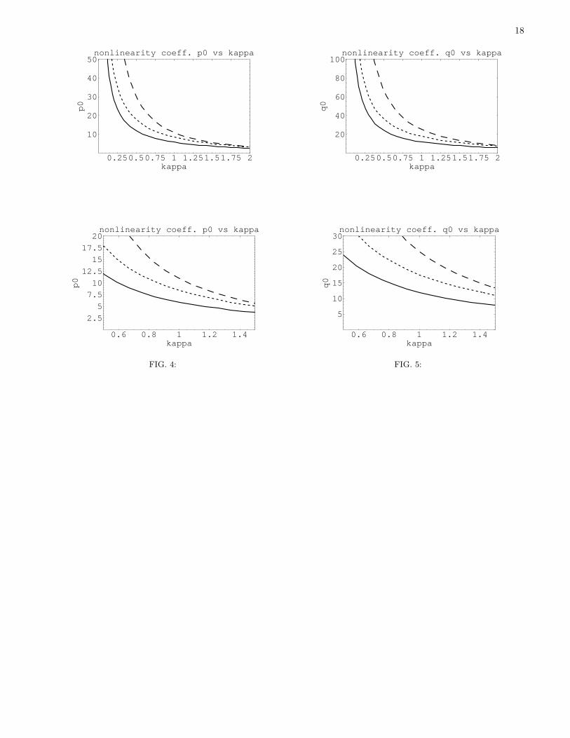
(see Fig. 3) and for the nonlinearity coefficients

p0 =Q2

MλD

{

1

(eκ − 1)3

[

6 + eκ(κ2 − 3κ − 12)

+ e2κ (κ2 + 3κ + 6)

]

− 6

κln

(

1 + sinhκ − coshκ)

}

,(20)

and

q0 =Q2

MλD

{

1

(eκ − 1)4

[

−12

+ e2κ[(κ3 + 12κ + 48) coshκ

+ 2(κ3 − 6κ− 18) + 2(κ2 − 6) sinhκ]

]

−12

κln

(

1 + sinhκ − coshκ)

}

. (21)

Upon simple inspection of Figs. 4 and 5, one deduces thatq0 takes practically double the value of p0 everywhere,and thus draws the conclusion that q0 should rather not

be omitted in Eq. (13) (cf. e.g. Refs. [12, 30, 35, 38]),for the case of the Debye potential.

III. LINEAR OSCILLATIONS

Let us first consider the linear regime in longitudinalgrain oscillations. For the sake of rigor, one may revert tothe discrete formula (3) and consider its linearized formby simply neglecting the two last (double) sums therein.Inserting the ansatz δxn ∼ exp i(nkr0 − ωt), where ω isthe phonon frequency and k = 2π/λ (respectively, λ) isthe wavenumber (wavelength), one immediately obtainsthe general dispersion relation

ω (ω + i ν) =4Q

M

N∑

l=1

φ′′(lr0) sin2 l kr0

2

=4Q

M

N∑

l=1

φ′′(lκλD) sin2 l κ (kλD)

2. (22)

One may readily verify that the standard 1D acousticwave dispersion relation ω ≈ v0 k is obtained in the smallk (long wavelength) limit: check by setting sin(l kr0/2) ≈lkr0/2 (and recalling the general definition of v0 above).Of course, taking this limit simply amounts to linearizingthe continuum equation of motion derived above (andkeeping the lowest contribution in k). As pointed outbefore (see e.g. Ref. [18]), one thus recovers the dust-acoustic wave dispersion relation obtained in the strong-coupling dusty plasma regime (upon defining the densitynd as ∼ r−3

0 , which may nevertheless appear somehowheuristic in this 1D model).

Notice that the form of the dispersion relation, in prin-ciple, depends on the value of N . However, in the caseof the Debye interactions, i.e. explicitly substitutingd2φD(x)/dx2 into (22), one obtains

ω (ω + i ν) =4Q2

Mλ3D

N∑

l=1

e−lκ 2 + 2κ + (lκ)2

(lκ)3sin2 l kr0

2.

(23)A numerical investigation, e.g. for κ = 1 (see Fig. 6),suggests that the dispersion curve quickly sums up to alimit curve, even for not so high values of N (practicallyfor N = 2 already). The values of the frequency reducewith increasing κ, as suggested by the exponential term.We see that the dispersion curve possesses a maximumat k = π/r0 = π/(κλD) for any value of κ and N .

The dispersion curves of dust-lattice waves have beeninvestigated by both experiments (see e.g. Refs. [46, 47])and ab initio numerical simulations [48]. In should never-theless be acknowledged that the results of these studiesdo not absolutely confirm the dispersion curves obtainedabove, which suggests, as poined out in Ref. [46], thatone-dimensional crystal models may be inappropriate forreal dust crystals.

7

IV. THE KORTEWEG – DE VRIES (KDV)EQUATION

In order to take into account weak nonlinearities, aprocedure which is often adopted at a first step consistsin keeping only the first nonlinear contribution in Eq.(13) (by cancelling the last term in the rhs, i.e. settingq0 = 0) and then considering excitations moving at avelocity close to the characteristic velocity v0. A Galileanvariable transformation, viz.

x → ζ = x − v0 t , t → τ = t , w = uζ , (24)

then provides the Korteweg – De Vries (KdV) Equa-tion

wτ − s a w wζ + b wζζζ = 0 , (25)

where a term uττ was assumed of higher-order and thusneglected. The coefficients are

a =|p0|2v0

, b =v21r

20

2v0, s = sgn p0 = p0/|p0| .

(26)We have introduced the parameter s (= +1/−1), denot-ing the sign of p0, which may change the form of the solu-tions (see below); as discussed above, it is equal to s = +1for the Debye-type interactions. It should be noted thatthis procedure is identical to the one initially adaptedfor dust-lattice-waves in [12] and then followed in Ref.[30, 35, 38] (for s = +1) as may readily be checked, yetthe new aspect here lies in the generalized definitions ofthe physical parameters above. Also notice that positive-oriented (∼ x) propagation was considered; adopting theabove procedure in backward (∼ −x) propagation is triv-ial, yet it should be carried out by re-iterating the ana-lytical procedure and not by plainly considering v → −v:the KdV equation is not symmetric with respect to thistransformation (also see that the velocity v appears un-der a square root in the formulae).

As a mathematical entity, the KdV Equation has beenextensively studied [3, 27, 49, 50, 51, 52, 53, 54, 55],so only necessary details will be summarized here. Itis known to possess a rich variety of solutions, includ-ing periodic (non-harmonic) solutions (cnoidal waves, in-volving elliptic integrals) [54]. For vanishing boundaryconditions, Eq. (25) can be shown (see e.g. in Refs.[27, 55]) to possess one- or more (N−) soliton localizedsolutions wN (ζ, τ) which bear all the well-known soli-ton properties: namely, they propagate at a constantprofile, thanks to an exact balance between dispersiveand nonlinear effects, and survive collisions between oneanother. The simplest (one-) soliton solution has thepulsed-shaped form

w1(ζ, τ) = −s w1,msech2

[

(ζ − vτ − ζ0)/L0

]

, (27)

where x0 is an arbitrary constant, denoting the initialsoliton position, and v is the velocity of propagation; in

principle, v may take any real value even though its rangemay be physically limited, as in our case, where v hasbeen assumed close to v0; this constraint will be relaxedbelow. A qualitative result to be retained from the solitonsolution in (27) is the velocity dependence of both solitonamplitude w1,m and width L0, viz.

w1,m = 3v/a = 6vv0/|p0| ,

L0 = (4b/v)1/2

= [2v21r

20/(vv0)]

1/2 .

We see that w1,mL20 = constant, implying that nar-

rower/wider solitons are taller/shorter and propagatefaster/slower. These qualitative aspects of dust-latticesolitons have recently been confirmed by dust-crystal ex-periments [35]. Notice that the solutions of (25) satisfyan infinite set of conservation laws [3, 55]; in particu-lar, the solitons wN carry a constant ‘mass’ M ∼

∫

wdζ(which is negative for a negative pulse), ‘momentum’P ∼

∫

w2dζ, ‘energy’ P ∼∫

(w2x/2 + u3) dζ, and so

forth (integration is understood over the entire x− axis)[52, 55]. See that the forementioned amplitude–widthdependence of the 1-soliton solution (27) is heuristicallydeduced from the soliton ‘mass’ conservation law (im-plying conservation of the surface under the bell-shapedcurved in Fig. 7): taller excitations have to be thinnerand vice versa.

Inverting back to our initial reference frame, one ob-tains, for the spatial displacement variable u(x, t), thekink/antikink (for s = −1/ + 1) solitary wave form

u1(x, t) = −s u1,m tanh

[

(x − vt − x0)/L1

]

, (28)

which represents a localized region of compres-sion/rarefaction (for s = +1/ − 1), propagating to thepositive direction of the x−axis (see Fig. 7). The am-plitude u1,m and the width L1 of this shock excitationare

u1,m =6v1r0

|p0|[

2 v0 (v − v0)]1/2

,

L1 = r0

[

2 v21

v0 (v − v0)

]1/2

=12v2

1r20

|p0|1

Am,

imposing ‘supersonic’ propagation (v > v0) for stability,in agreement with experimental results in dust crystals[35]. Notice that faster solitons will be narrower, and thusmore probable to ‘feel’ the lattice discreteness, contraryto the continuum assumption above; therefore, one mayimpose the phenomenological criterion: L ≪ r0, amount-ing to the condition v/v0 ≫ 1 + 2 v2

1/v20 [≈ 1.17 for the

Debye NNI case; see (14) above], in order for the above(continuum) solution to be sustained in the (discrete)chain. Nevertheless, supersonic wave stable propagationhas been numerically verified at a wide range of velocityvalues in atomic chains [23, 57], where Eqs. (13) and (25)

8

arise via a procedure similar to the one outlined above;also see Ref. [58] for a recent experiment in crystallinesolids. Finally, note that v0 in real DP crystals bearsvalues as low as a few tens of mm/sec [34, 35].

Remarkably, Eq. (25) is exactly solved via the InverseScattering Transform [53, 55, 56], for any given initialcondition u(ζ, 0), which is generally seen to break-up intoa number of (say N , depending on u(ζ, 0) [56]) solitonsplus a tail of background oscillations. These considera-tions, including, in particular, the two-soliton solution w2

of Eq. (25), which represents two distinct humps movingat different velocities and colliding during propagationwithout changing shape, have been postulated to be ofrelevance in the interpretation of recent dusty plasmadischarge experiments [35, 38].

The wide reputation of the KdV Equation (25) ismostly due to the exhaustive knowledge of its analyti-cal properties [3, 27, 51, 52, 53, 54, 55], in addition toits omni-presence in a variety of physical contexts, notexcluding the physics of ordinary (ideal, i.e. electron–ion) plasmas [3, 4] and, more recently, dusty plasmas[6, 30]. However, in the above dusty-plasma-crystal con-text, it has been derived under specific assumptions (lowdiscreteness and low nonlinearity effects; also, a propa-gation velocity v ≈ v0) which may be questionable, in areal DP crystal. Even if the first one is virtually impos-sible to cope with, analytically, the latter ones may besomehow relaxed via a different approach, to be outlinedbelow.

V. HIGHER-ORDER KORTEWEG–DEVRIES(EKDV) EQUATIONS

In order to derive a KdV equation from the continuumequation of motion (13), we have neglected the coeffi-cient q, which is related to the cubic nonlinearity of theinteraction potential. Nevertheless, a simple numericalinvestigation shows that this term is not small, and may,in certain cases, even dominate over the quadratic term p,as in the Debye potential case (see the discussion above).Therefore, one is tempted to find out how the dynamicsis modified if this term is taken into account.

A. The Extended Korteweg – de Vries (EKdV)Equation

Repeating the procedure which led to Eq. (25), inthe previous section, yet now keeping the fourth orderderivative coefficient q 6= 0 in Eq. (13), one obtains theEKdV Equation

wτ − s a w wζ + a w2 wζ + b wζζζ = 0 , (29)

where all coefficients are given in (26) except a =q0/(2v0); recall that a, b are positive by definition. Weshall see below that p0, q0 > 0 for Debye interactions (yet

not necessarily, in general), so that the nonlinearity co-efficients, i.e. −sa (for s = +1) and a, bear negativeand positive (respectively) values in this (Yukawa crys-tal) case.

The EKdV Eq. (29) was thoroughly studied in a clas-sical series of papers by Wadati [21], who derived it fornonlinear lattices, then obtained its travelling-wave and,separately, periodic (cnoidal wave) solutions and, finally,exhaustively studied its mathematical properties. Bothcompressional and rarefactive solitons (say, w2,±, to bedistinguished from the KdV solution w1) were found tosolve Eq. (29) (for either signs of s); adapted to ournotation here [59], they are of the form

w(1)2 (ζ,τ) = −s v/

{

C cosh2[(ζ − vτ − ζ0)/L0]

+ D sinh2[(ζ − vτ − ζ0)/L0]}

, (30)

and

w(2)2 (ζ,τ) = +s v/

{

D cosh2[(ζ − vτ − ζ0)/L0]

+ C sinh2[(ζ − vτ − ζ0)/L0]}

, (31)

where

C =a

6

(

√

1 +6av

a2+ 1

)

=1

12v0

(

√

p20 + 12q0v0v + |p0|

)

,

D =a

6

(

√

1 +6av

a2− 1

)

=1

12v0

(

√

p20 + 12q0v0v − |p0|

)

, (32)

the width L0 was defined above, and v > 0 is the propa-gation velocity. For s = +1/−1, the first expression rep-resents a propagating localized compression/rarefaction,while the second denotes a (larger, see comment below;cf. Fig. 8) rarefaction/compression, respectively. Noticethat, for q0 ∼ a = 0, the first expression recovers theKdV result obtained previously (since v/C then recoversthe KdV soliton width w1,m), while the second results ina divergent (physically unacceptable) solution [21]. Fol-lowing Wadati, we may re-arrange (30) and (31) as

w(j)2 (ζ, τ) = −s ǫj

2√

6b√a

×

∂

∂ζ

{

tan−1

[

W(j)2 tanh

(

ζ − vτ − ζ0

L0

)]}

, (33)

provided that a ∼ q0 6= 0. Here

W(j)2 =

(

√

1 + 6ava2 − ǫj

√

1 + 6ava2 + ǫj

)1/2

. (34)

Furthermore, v > 0 is the propagation velocity in the

frame {ζ, τ} and j = 1 (2) recovers w(1)2 (w

(2)2 ) above, so

9

that ǫ1 (ǫ2) is equal to +1 (−1), representing rarefactive(compressive) solutions, for s = +1 – e.g. the Debye case– and vice versa for s = −1 (which recovers Wadati’snotation). The pulse width now depends on both L0

(defined as previously) and W(j)2 . The pulse value for

s = −1 [21] satisfies:

w− ≡ −(√

a2 + 6av + a) < w(1)2 < 0 < w

(2)2

< (√

a2 + 6av − a) ≡ w+ ,

(for s = +1, one should permute the superscripts 1 and2); since |w−| > |w+|, one expects, for s = −1, a smallrarefactive and a large compressive pulse; the oppositeholds for s = +1, e.g. in a Debye crystal case: see Fig.8.

Inverting to the lattice displacement coordinate u ∼∫

wdζ, expressed in the original coordinates {x, t}, weobtain

u(j)2 (x, t) = −s ǫj 2

√

6v21

q0r0 ×

tan−1

[

W(j)2 tanh

(

x − vt − x0

L1

)]

, (35)

where

W(j)2 =

(

√

p20 + 12q0 v0 (v − v0) − ǫj |p0|

√

p20 + 12q0 v0 (v − v0) + ǫj |p0|

)1/2

, (36)

and j = 1, 2. As expected, for any given s (= ±1), thetwo different kink/antikink solutions obtained for differ-ent j (= 1 or 2) are not symmetric; cf. Figure 8. No-

tice that the maximum value now also depends on W(j)2

(j = 1, 2).In conclusion, the Extended KdV equation provides a

more complete description of the nonlinear dynamics ofthe lattice, compared to the KdV equation. In partic-ular, the EKdV compressive (rarefactive) pulse solitonobtained for s = +1 (s = −1), i.e. p0 > 0 (p0 < 0) isslightly smaller than its KdV counterpart (see Fig. 8),but the EKdV also predicts the possibility for a rarefac-tive (compressive) soliton, in either case, to form andpropagate in the same lattice. In the particular caseof Debye crystals, the net new result to be retained isthe prediction of the existence of a rarefactive new ex-citation, in addition to the rarefactive one, observed inexperiments. Nevertheless, theoretical studies on molec-ular chains seem to suggest that the additional shock-likelocalized mode predicted by the EKdV equation will notbe as stable as its (KdV–related) counterpart. This pre-diction should, therefore, be confirmed numerically (andexperimentally) before being taken for granted.

B. The Modified Korteweg – de Vries (MKdV)Equation

Note, for the sake of rigor, that upon setting p0 ∼ a = 0in Eq.(29) above, one obtains a modified KdV (MKdV)

equation (with only a cubic nonlinearity term). TheMKdV equation shares all the qualitative properties ofthe KDV Eq. and is, in fact, related to it via a Miuratransformation [55]. It has two (both negative and pos-itive, for each value of s) pulse soliton solutions whichfollow immediately from the preceding solutions (30) and(31) of the EKdV equation, upon setting p0 = 0. Theremarkable additional aspect of the MKdV equation isthat it also bears slowly oscillating solutions, namedbreathers, obtained just as rigorously via the inverse scat-tering method [22, 60]. These solutions (whose wave-length is comparable to their localized width, hence the‘breathing’ impression and the name) share the remark-able properties of solitons; in particular, they are seento survive collisions between themselves and with pulsesolitons [22]. Their analytic form can be readily foundin Refs. [22] (see §4.1 therein) and [60] and will notbe reproduced here, since their condition of existence,namely p0 ≪ q0 (cf. Ref. [22]) is rather not satisfied inthe case of Debye-interacting dust grains. Note howeverthat breather-like excitations may exist in a DP crystal,as one may see via a different (perturbative) analysis ofthe nonlinear modulation of the amplitude of longitudi-nal lattice waves. This is considered in separate work[61].

VI. THE BOUSSINESQ (BQ) ANDGENERALIZED BOUSSINESQ (GBQ)

EQUATIONS

Remember that the KdV–type equations in the preced-ing Section were obtained from the equation of motion(13) in an approximative manner, assuming near–sonicpropagation and neglecting high–order time derivatives.Those results are therefore expected to hold for veloc-ity values only slightly above v0. We shall now see howthese assumptions can be relaxed by directly relying onthe initial (nonlinear) equation .

Let us consider Eq. (13) again (for ν = 0). Uponsetting p0 = −2p, q0 = 3q, v2

1r20 = h > 0, and integrating

once, with respect to x, one exactly obtains, for w = ux,the generalized Boussinesq (GBq) Equation

w − v20 wxx = h wxxxx + p (w2)xx + q (w3)xx (37)

which, neglecting the cubic nonlinearity coefficient q [viz.q0 = 0 in (13)], reduces to the well-known Boussinesq(Bq) equation, widely studied e.g. in solid chains; see e.g.[22, 23, 57]. It possesses well-known localized solutions,whose derivation is straightforward and need not be re-produced here. The exact expressions obtained from (37)for the relative displacement w(x, t) and the longitudinaldisplacement u(x, t) are exhaustively presented and dis-cussed in Refs. [22, 23]. The analytic kink/antikink-typelocalized solutions for u(x, t) read

u3(x, t) = ∓2 sgn(h)

(

6h

q0

)1/2

×

10

tan−1

[

W3 tanhx − vt − x0

L3

]

. (38)

Here the soliton velocity is v, while the soliton widthdepends on both W3 and L3, which are

W3 =

{

[p20 + 6q0(v

2 − v20)]

1/2 ∓ |p0|[p2

0 + 6q0(v2 − v20)]

1/2 ± |p0|

}1/2

,

L3 = 2

(

h

v2 − v20

)1/2

. (39)

Recall that, for Debye interactions, h, q > 0 andp = −p0 < 0 (see above), prescribing the ‘supersonic’(v > v0) propagation of the solutions; the same was trueof the KdV solitons obtained above. Notice, however,that the expressions obtained here for the longitudinaldisplacement u represent both rarefactive and compres-sive lattice excitations even for p0 > 0 (see Table I in [23],for p = −p0 < 0); remember that this feature was absentin the KdV equation (25), where p0 > 0 i.e. s = +1 al-ways led to a compressive solution in (28). In fact, this isalso true of the Bq equation, which is obtained for q0 = 0,i.e. neglecting the last term in the continuum equationof motion (13). The exact solution then reads

uBq(x, t) = −sgn(h) sgn(p0)6[h(v2 − v2

0)]1/2

|p0|×

tanhx − vt − x0

L1, (40)

which, for positive h and p0, prescribes only compressivesupersonic kinks, pretty much like the solution u1 derivedfrom the KdV theory above (cf. Table I in [23], for h0 >0, p < 0 and q = 0).

Closing this section, one may wish to compare theGBq and Bq solutions (38) and (40), to the homologousEKdV– and KdV–related solutions (35) and (28), respec-tively, obtained previously: one may readily check thatthe former ones tend to the latter two as v tends to v0

[to see this, one may set v2 − v20 = (v + v0)(v

2 − v0) ≈2v0(v

2 − v0); recall that h = v21r

20 ]. Nevertheless, this

velocity range restriction is relaxed in the Boussinesq–related description.

VII. EXCITATIONS IN REAL DP CRYSTALS

It is now quite tempting to observe and compare thepredictions furnished by the above nonlinear models ina DP crystal in terms of excitation features, e.g. dimen-sions and form. For instance, one may substitute theexpressions for the model’s physical parameters (i.e. ω0,v0, v1, p0 and q0) derived in §II C into the definitions inthe latter three sections, in order to derive a final formfor localized excitations in a real DP crystal, in terms ofthe propagation velocity v, the lattice parameter κ and,generally, the sign s (= +1 for Debye interactions). Theinterest in this procedure is evident, since one may seek

feedback (e.g. parameter values, excitation behaviour)from experiments and then investigate the validity of theabove models by adjusting them to real DP crystal val-ues.

The final expressions for uj(x, t) [j = 1, 2, 3, cf. (28),(35) and (38), respectively] are somewhat lengthy andneed not be reported here (since they are straightfor-ward to derive). We may nevertheless summarize someinteresting numerical results.

The soliton width L1, as defined in (28), now becomesL1 = v2

0/p0u1,m: we see that the product of the displace-ment u kink’s width and maximum value remains con-stant (regulated by the cubic interaction potential non-linearity), viz. u1,m L1 = 1/p0, unlike the KdV pulsesoliton for the relative displacement w = ux which ischaracterized by w1,m L2

1 = cst.. Both the kink maxi-mum value u1,m and width L1 depend on the velocity v;as a matter of fact, faster kink excitations will be tallerand narrower - see Fig. 9 - since now

u1,m

r0=

v20

√6

p0

√M − 1 ,

L1

r0=

1√

6(M − 1). (41)

Recall that the Mach number M = v/v0 is always largerthan unity. Furthermore, the magnitude of the excitationseems to decrease with κ; see Fig.9a: nevertheless, veryhigh values (near u/r0 = 1) observed for low κ and highv are rather not to be trusted, since they contradict thecontinuum approximation u ≪ r0.

Finally, one may compare the solutions obtained fromthe above theories, for a typical value of κ, say 1.25,according with real experimental values. The KdV–,EKdV– and Boussinesq–related kink excitations, i.e. u1,u2 and u3, are depicted in Figs. 10 – 12, for three differ-ent values of M , 1.1, 1.25 and 2. We see that the EKdVand Bq models allow for both compressive and rarefac-tive structures, while the KdV description predicts a lo-calized compression, which is quite sensitive to velocitychanges. As expected (cf. the discussion above), boththe EKdV– and Bq–related compressive excitations aresimilar in magnitude to the KdV–related anti-kink fornear–sonic velocity (i.e. near M ≈ 1). Nevertheless, wesee that the KdV–related antikink becomes taller andnarrower as velocity increases, and substantially differ-entiates itself from its EKdV– and Bq–analogues. Onemay wonder whether or not the KdV picture (more fa-miliar since widely studied) is adequate for the modelingof a real DP crystal, and also whether the rarefactive ex-citations predicted by other theories can indeed be sus-tained in the crystal. These questions may be answeredby appropriate experiments and, possibly, also be inves-tigated by numerical simulations. From a purely theo-retical point of view, the Boussinesq–based descriptionappears to be more rigorous (recall that the KdV wasderived in some approximation) and valid in a more ex-tended region than both the KdV and Extended-KdVtheories.

11

VIII. DISCRETENESS EFFECTS

The above analytical solutions have been derived inthe continuum limit, i.e. for L >> r0, where L is thetypical spatial dimension (width) of the solitary excita-tion. One may therefore define the discreteness parame-ter g = r0/L, and require a posteriori that g ≪ 1. Fromthe expressions derived for the Bq equation above, oneeasily sees that g ∼ (v2 − v2

0)1/2/v1, so this requirementis indeed fulfilled for propagation velocities v ≈ v0. How-ever, for higher values of v, the (narrower) soliton willbe subject to a variety of effects e.g. shape distortion,wave radiation etc., due to the intrinsic lattice discrete-ness. These effects have been investigated in solid statephysics [62, 63] and may be considered with respect toDP crystals at a later stage. Let us briefly point out thatnarrow kink-shaped lattice excitations have been numer-ically shown to propagate with no considerable loss ofenergy, in a quite general monoatomic lattice model [62].

Also worth mentioning is the work of Rosenau [65] whoderived an improved version of the Boussinesq equation(the I-Bq Eq.) in a quasi-continuum limit. The I-Bqequation, which bears the general structure of (37) uponreplacing h uxxxx therein by h uxxtt (yet with different co-efficient definitions), is not integrable and bears solitarywave solutions which do not collide elastically; neverthe-less, it was numerically shown to be more stable than theBq equation, and was argued to model discrete lattice dy-namics more efficiently, upon comparison of theoreticalpredictions to exact numerical results [63]. Further exam-ination of such effects may be carried out in dust-lattices,once our feedback from experiments has sufficiently de-termined the relevance of the issue in real DP crystals,i.e. typical excitation width, dynamics etc.

It should be underlined that the possibility for the exis-tence of breather solitons, anticipated above, establishesa link between complex plasma ‘solid state’ modeling andthe framework of discreteness-related localized excita-tions (discrete breathers [66], intrinsic localized modes[67]), which have recently received increasing interestamong researchers in the nonlinear dynamics community.These localized modes, which are due to coupling anhar-monicity and are stabilized by lattice discreteness, havebeen shown to exist in frequency regions forbidden to or-dinary lattice waves and account for energy localizationin highly discrete real crystals, where continuum theoriesfail. The relevance of this framework to dust crystals ap-pears to be an interesting open area for investigation.

IX. ENVELOPE EXCITATIONS AND SHOCKS –OPEN ISSUES

As a final interesting issue involved in the nonlineardynamics of longitudinal lattice oscillations, let us men-tion the nonlinear modulation of the amplitude of dust-lattice waves, a well-known mechanism related to har-monic generation and, possibly, the modulational insta-

bility of waves propagating in lattices, eventually lead-ing to modulated wave packet energy localization viathe formation of envelope solitons [29]. This framework,which was recently also investigated with respect to low-frequency (dust-acoustic, dust-ion acoustic) electrostaticwaves in dusty plasmas [32], has been partly analyzed,on the basis of the Melandsø[12] model in Ref. [33]. Theauthors relied on a truncated Boussinesq equation, inthe form of (37) for q = 0, and succeeded in predict-ing the occurrence of modulational instability in LDLwaves in DP crystals and the formation of envelope struc-tures. Nevertheless, the nonlinearity coefficient q omittedtherein seems to compete with p in (37) (notice the dif-ferent signs) and is rather expected to affect significantlythe wave’s stability profile. It should be stressed thatthese localized envelope excitations result from a phys-ical mechanism which is intrinsically different from theone related to the small–amplitude excitations describedin this paper; see the discussion in Ref. [68]. An ex-tended study of this modulation nonlinear mechanism isin row and will be reported elsewhere, for clarity andconciseness.

As a final comment, we may speculate on the role ofdamping, herewith ignored, on the dynamics of dust-lattice waves. It is known that weak damping may bal-ance nonlinearity, leading to the formation of shock wavefronts, as predicted in Refs. [30, 43] and confirmed bynumerical simulations [44]. Furthermore, it was recentlyshown that the same mechanism may result in the for-mation of large-amplitude wide-shaped solitary waves,which may later break into a (gradually damped) trainof solitons or a wavepacket depending on physical pa-rameters [42]. We see that friction, yet weak, may playa predominant role in the life and death of localized ex-citations; this effect definitely deserves paying close at-tention with respect to waves propagating in dust crys-tals. Again, one would expect phenomenological theoriesfollowed by appropriately designed experiments to elu-cidate the friction mechanisms inherent in longitudinaldust-lattice wave propagation, in view of a more com-plete description than the one provided by the conserva-tive model adopted here.

X. CONCLUSIONS

This work was devoted to an investigation of the rel-evance of existing model nonlinear theories to the dy-namics of longitudinal oscillations in anharmonic chains,with emphasis on dust-lattice excitations in (strongly-coupled) complex plasma crystals. Taking into accountan arbitrary interaction potential and long-range inter-actions, we have rigorously shown that both compres-sive and rarefactive kink-shaped (shock-like) excitationsmay form and propagate in the lattice, depending basi-cally on the mechanism of interaction between grains lo-cated at each site. These excitations are effectively mod-eled by either KdV- or Boussinesq-type equations, whose

12

analytic form was presented and whose qualitative andquantitative differences were discussed. In any case, thetheory predicts coherent wave propagation above the lat-tice’s ‘sound’ speed, in agreement with previous theoreti-cal works and experimental observations (in both atomicand dust-lattices). It may be appropriate to mentionthat subsonic soliton propagation in monoatomic chainswas also numerically considered and shown to be feasiblein the past [62]. Let us point out that the model usedhere to pass from a discrete description to the continuum(long-wavelength) limit is quite generic, so possible mod-ification via refined nonlinear equations may readily beobtained from it, for future consideration.

Furthermore, we have discussed the possibility of theformation of breather modes and envelope excitations, asa consequence of modulated wave packet instability, an-ticipating their link to discrete nonlinear theories of lo-calized modes, left for future consideration; despite theiranalytical complexity, these models may, in principle, beof relevance in dust crystals due to the finite dimensionsof the chain and its intrinsic spatial discreteness. Fi-nally, the possible role played by dissipation mechanisms

has been briefly discussed.The present study relies on, and aims at extending,

previous theories on both anharmonic atomic chains anddusty plasma crystals. We hope to have succeeded in re-viewing the former (extending them to the case of long-range electrostatic interactions) and generalizing the lat-ter (which are still in an early stage). Hopefully, our pre-dictions may be confirmed by appropriately set-up exper-iments, with the ambition of throwing some light in therelatively new and challenging field of strongly-coupledcomplex plasmas and dust-lattice dynamics.

Acknowledgments

This work was supported by the European Commis-sion (Brussels) through the Human Potential Researchand Training Network via the project entitled: “Com-plex Plasmas: The Science of Laboratory Colloidal Plas-mas and Mesospheric Charged Aerosols” (Contract No.HPRN-CT-2000-00140).

[1] N. A. Krall and A. W. Trivelpiece, Principles of plasma

physics, McGraw - Hill (New York, 1973).[2] Th. Stix, Waves in Plasmas, American Institute of

Physics (New York, 1992).[3] V. I. Karpman, Nonlinear Waves in Dispersive Media

(Pergamon, New York, 1975).[4] L. Debnath (Ed.), Nonlinear Waves (Cambridge Univ.

Press, Cambridge U.S.A., 1983).[5] F. Verheest, Waves in Dusty Space Plasmas (Kluwer

Academic Publishers, Dordrecht, 2001).[6] P. K. Shukla and A. A. Mamun, Introduction to Dusty

Plasma Physics (Institute of Physics, Bristol, 2002).[7] C. Kittel, Introduction to Solid State Physics (John Wi-

ley and Sons, New York, 1996).[8] J. Chu and L. I, Phys. Rev. Lett. 72, 4009 (1994).[9] Thomas et al., Phys. Rev. Lett. 73, 652 (1994).

[10] A. Melzer, T. Trottenberg and A. Piel, Phys. Lett. A191, 301 (1994).

[11] Y. Hayashi and K. Tachibara, Jpn. J. Appl. Phys. 33,L84 (1994).

[12] F. Melandsø, Phys. Plasmas 3, 3890 (1996).[13] B. Farokhi et al., Phys. Lett. A 264, 318 (1999); idem,

Phys. Plasmas 7, 814 (2000).[14] S. V. Vladimirov, P. V. Shevchenko and N. F. Cramer,

Phys. Rev. E 56, R74 (1997).[15] G. Morfill et al., in Advances in Dusty Plasma Physics,

Eds. P. K. Shukla, D. A. Mendis and T. Desai (WorldScientific, Singapore, 1997), p. 99; idem, Phys. Rev. Lett.83, 1598 (1999).

[16] S. Nunomura, D. Samsonov and J. Goree, Phys. Rev.Lett. 84, 5141 (2000).

[17] D. Tskhakaya and P. S. Shukla, Phys. Lett. A 286, 277(2001).

[18] X. Wang and A. Bhattacharjee, Phys. Plasmas 6, 4388(1999); X. Wang, A. Bhattacharjee and S. Hu, Phys. Rev.

Lett. 86, 2569 (2001).[19] P. K. Shukla, Phys. Lett. A 300, 282 (2002).[20] A. Tsurui, Progr. Theor. Phys. 48, 1196 (1972).[21] M. Wadati, J. Phys. Soc. Japan 38, 673 (1975); ibid J.

Phys. Soc. Japan 38, 681 (1975).[22] N. Flytzanis, St. Pnevmatikos and M. Remoissenet, J.

Phys. C: Solid State Phys. 18, 4603 (1985).[23] St. Pnevmatikos, N. Flytzanis and M. Remoissenet,

Phys. Rev. B 33, 2308 (1986).[24] J. Wattis, J. Phys. A: Math. Gen. 29, 8139 (1996).[25] A. S. Davydov, Solitons in Molecular Systems (Reidel

Publ. – Kluwer, Dordrecht, 1985).[26] A. C. Newell and J. V. Moloney, Nonlinear Optics

(Addison-Wesley Publ. Co., Redwood City Ca., 1992).[27] M. Remoissenet, Waves Called Solitons (Springer-Verlag,

Berlin, 2nd Ed., 1996).[28] A. C. Scott and D. W. McLaughlin, Proc. IEEE 61,

1443 (1973).[29] I. Daumont, T. Dauxois and M. Peyrard, , Nonlinearity

10, 617 (1997); M. Peyrard, Physica D 119, 184 (1998).[30] P. K. Shukla, Phys. Plasmas 10, 1619 (2003); P. K.

Shukla and A. A. Mamun, New J. Phys., 5, 17 (2003).[31] L. Stenflo, N. L. Tsintsadze and T. D. Buadze, Phys.

Lett. A 135, 37 (1989).[32] M. R. Amin, G. E. Morfill and P. K. Shukla, Phys. Rev.

E 58, 6517 (1998); I. Kourakis and P. K. Shukla, Phys.Plasmas 10, 3459 (2003); I. Kourakis and P. K. Shukla,Physica Scripta 69, in press (2004).

[33] M. R. Amin, G. E. Morfill and P. K. Shukla, Phys.Scripta 58, 628 (1998).

[34] V. Nosenko, S. Nunomura and J. Goree, Phys. Rev. Lett.88, 215002 (2002).

[35] D. Samsonov, A. V. Ivlev, R. A. Quinn, G. Morfill andS. Zhdanov, Phys. Rev. Lett. 88, 095004 (2002).

[36] S. Nunomura, S. Zhdanov, G. Morfill and J. Goree, Phys.

13

Rev. E 68, 026407 (2003).[37] S. K. Zhdanov, D. Samsonov and G. Morfill, Phys. Rev.

E 66, 026411 (2002).[38] K. Avinash, P. Zhu, V. Nosenko and J. Goree, Phys. Rev.

E 68, 046402 (2003).[39] A. M. Ignatov, Plasma Physics Reports 29, 296 (2003).[40] I. Kourakis and P. K. Shukla, Phys. Lett. A 317, 156

(2003).[41] G. Morfill, A. V. Ivlev and J. R. Jokipii, Phys. Rev. Lett.

83, 971 (2000); A. Ivlev, U. Konopka and G. Morfill,Phys. Rev. E 62, 2739 (2000); A. Ivlev and G. Morfill,Phys. Rev. E 63, 016409 (2000).

[42] R. Grimshaw, E. Pelinovsky and T. Talipova, Wave Mo-tion 37, 351 (2003).

[43] P. K. Shukla and A. A. Mamun, IEEE Trans. Plasma Sci.29, 221 (2001); ibid, Physics of Plasmas 8, 3216 (2001).

[44] F. Melandsøand P. K. Shukla, Planet. Space. Sci. 43, 635(1995).

[45] A. Ivlev, U. Konopka, G. Morfill and G. Joyce, Phys.Rev. E 68, 026405 (2003).

[46] A. Homann et al., Phys. Lett. A 242, 173 (1998).[47] S. Nunomura, J. Goree, S. Hu, X. Wang and A. Bhat-

tacharjee, Phys. Rev. E 65, 066402 (2002); S. Nuno-mura, J. Goree, S. Hu, X. Wang, A. Bhattacharjee andK. Avinash, Phys. Rev. Lett. 89, 035001 (2002).

[48] A. Melzer, Phys. Rev. E 67, 16411 (2003); Y. Liu et

al., Phys. Rev. E 67, 066408 (2003); K. Qiao and T. W.Hyde, J. Phys. A: Math. Gen. 36, 6109 (2003).

[49] G. B. Whitham, Linear and Nonlinear Waves (Wiley,New York, 1974).

[50] K. Lonngren and A. Scott (Eds.), Solitons in Action

(Academic, New York, 1978).[51] R. K. Dodd, J. C. Eilbeck, J. D. Gibbon and H. C. Mor-

ris, Solitons and Nonlinear Wave Equations (AcademicPress, London, 1982).

[52] See Chapters 8 in Ref. [25].[53] A. C. Newell, Solitons in Mathematics and Physics

(SIAM Publ., Philadelphia, 1985).[54] R. Z. Sagdeev, D. A. Usikov and G. M. Zaslavsky, Non-

linear Physics (Harwood Academic Publishers, Philadel-phia U.S.A., 1988); see Ch. 8 and 12, in particular.

[55] P. G. Drazin and R. S. Johnson, Solitons: an Introduction

(Cambridge Univ. Press, Cambridge, 1989).[56] M. J. Ablowitz and Harvey Segur, Solitons and Inverse

Scattering Transform (SIAM, Philadelphia, 1981); V.Eckhaus and A. Van Harten, The Inverse Scattering

Transform and the Theory of Solitons, An Introduction

(North-Holland, New York, 1981).[57] St. Pnevmatikos, These d’Etat, Universite de Dijon

(1984).[58] H. - Y. Hao and H. J. Maris, Phys. Rev. B 64, 064302

(2001).[59] In order to see this, transform the variables in Ref. [21]

as: u → w, x → ζ/√

b, t → τ/√

b, α → a/6, β → a/6,and then insert a factor (−s), since formulae therein foru correspond to s = −1 and, upon u → −u, to s = −1here.

[60] G. L. Lamb Jr., Elements of Soliton Theory (Wiley, NewYork, 1980).

[61] I. Kourakis and P. K. Shukla, submitted to Physics ofPlasmas, 2003.

[62] M. Peyrard, St. Pnevmatikos and N. Flytzanis, PhysicaD 19 (2), 268 (1986); N. Flytzanis, St. Pnevmatikos and

M. Remoissenet, Physica D 26 (1–3), 311 (1987).[63] N. Flytzanis, St. Pnevmatikos and M. Remoissenet, J.

Phys. A: Math. Gen. 22, 783 (1989).[64] M. A. Collins, Chem. Phys. Lett. 77, 342 (1981).[65] P. Rosenau, Phys. Lett. A 118, 222 (1986); ibid, Physica

D27, 224 (1986); ibid, Phys. Rev. B 36, 5868 (1987).[66] Thierry Dauxois and Michel Peyrard, Phys. Rev. Lett.

70, 3935 (1993); S. Flach, Phys. Rev. E 51, 1503 (1995);T. Bountis et al., Phys. Lett. 268, 50 (2000); also seeseveral papers in the volume: G. Tsironis and E. N.Economou (Eds.), Fluctuations, Disorder and Nonlinear-

ity, Physica D 113, North-Holland, Amsterdam (1998).[67] S.A.Kiselev, A. J. Sievers and S. Takeno, Phys. Rev. Lett.

61, 970 (1988); S.R.Bickham and A.J.Sievers, Comm.Cond. Mat. Phys. 17, 135 (1995).

[68] R. Fedele, Phys. Scripta 65 502 (2002); R. Fedele and H.Schamel, Eur. Phys. J. B 27 313 (2002).

14

APPENDIX A: COMPUTATION OF THECOEFFICIENTS FOR DEBYE (YUKAWA)

INTERACTIONS

Consider the Debye potential φD(r) = Q e−r/λD/r.Defining the (positive real) lattice parameter κ = r0/λD,it is straightforward to evaluate the quantities

φ′D(lr0) = − Q

λ2D

e−lκ 1 + lκ

(lκ)2,

φ′′D(lr0) = +

2Q

λ3D

e−lκ 1 + lκ + (lκ)2

2

(lκ)3,

φ′′′D(lr0) = −6Q

λ4D

e−lκ 1 + lκ + (lκ)2

2 + (lκ)3

6

(lκ)4,

φ′′′′D (lr0) = +

24Q

λ5D

e−lκ 1 + lκ + (lκ)2

2 + (lκ)3

6 + (lκ)4

24

(lκ)5,

where the prime denotes differentiation and l = 1, 2, 3, ...is a positive integer. Now, we shall combine these expres-sions with Eqs. (7), (8), (10) and (12), defining v2

0 , v21 ,

p0 and q0, respectively.Let us define the general (families of) sum(s)

Sn(a) =

∞∑

l=1

al ln S(N)n (a) =

N∑

l=1

al ln

(0 < a < 1) , (A1)

(thinking of a = e−κ, in particular); note that S(N)n (a) →

Sn(a) for N → ∞; also, S(1)n (a) = a. Making use of the

well-known geometrical series properties:

S0(a) =∞∑

l=1

al =a

1 − aS

(N)0 =

N∑

l=1

al =a(1 − aN )

1 − a

(0 < a < 1) , (A2)

it is straightforward to derive Sn, S(N)n for l ≥ 1, by

differentiating with respect to a. One obtains

S1(a) =∞∑

l=1

al l = a∞∑

l=1

l al−1 = a∞∑

l=1

∂(al)

∂a

= a∂

∂a

∞∑

l=1

al = a∂S0

∂a=

a

(1 − a)2.

In a similar manner, iterating from

∂2(al)/∂a2 = l (l − 1) al−2 = a−2 (l2al − lal) ,

one finds

S2(a) =

(

a2 ∂2

∂a2+ a

∂

∂a

)

S0 = ... =a(1 + a)

(1 − a)3;

then

S3(a) =

(

a3 ∂3

∂a3+ 3a2 ∂2

∂a2+ a

∂

∂a

)

S0

= ... =a(a2 + 4a + 1)

(1 − a)4,

and so forth. Also note the identity

S−1(a) =∞∑

l=1

al

l= −ln(1−a) (0 < a < 1) .

(A3)The corresponding set of formulae may be obtained for

S(N)n in a similar manner.Now, substituting a = e−κ and using the derivatives of

φD above, one may immediately evaluate the expressions(7), (8), (10) and (12). Setting r0 = κλD everywhere, itis straightforward to show that

c2 ≡ v20 ≡ ω2

0,L r20 =

Q

Mκ2 λ2

D

∞∑

l=1

l2 φ′′(lr0) = ...

=2Q2

MλD

[

κ−1 S−1(e−κ) + κ0 S0(e

−κ) +1

2κ1 S1(e

−κ)

]

.

(A4)

In the same manner

c4

r20

≡ v21 =

Q

12Mκ2 λ2

D

∞∑

l=1

l4 φ′′(lr0) = ...

=Q2

6MλD

[

κ−1 S1(e−κ) + κ0 S2(e

−κ)

+1

2κ1 S3(e

−κ)

]

. (A5)

Also

p0 ≡ −c11 = − Q

Mκ3 λ3

D

∞∑

l=1

l3 φ′′′(lr0)

= ... =6Q2

MλD×

[

κ−1 S−1(e−κ) + κ0 S0(e

−κ) +1

2κ1 S1(e

−κ) +1

6κ2 S2(e

−κ)

]

. (A6)

Finally, from (12) we have

q0 ≡ c111 =Q

2Mκ4 λ4

D

∞∑

l=1

l4 φ′′′′(lr0) = ...

=12Q2

MλD

[

κ−1 S−1(e−κ) + κ0 S0(e

−κ)

+1

2κ1 S1(e

−κ) +1

6κ2 S2(e

−κ) +1

24κ3 S3(e

−κ)

]

. (A7)

15

The corresponding expressions for a value of N are given

by substituting Sn(·) with S(N)n (·) everywhere. One im-

mediately sees that p0/v20 > 2, q0/v2

0 > 6; also, v21/v2

0 =12 for N = 1 (only), i.e. for the NNI case.

Finally, combining the above exact expressions forS−1(a), ..., S3(a), we obtain exactly expressions (18) to(21) in the text.

Figure Captions

Figure 1.

(a) The linear oscillation frequency squared ω2 (nor-malized over Q2/(Mλ3

D)) is depicted against the latticeconstant κ, for N = 1 (first-neighbor interactions: —), N = 2 (second-neighbor interactions: - - -), N = ∞(infinite-neighbors: – – –), from bottom to top. (b) De-tail near κ ≈ 1.

Figure 2.

(a) The characteristic 2nd order dispersion velocitysquared v2

0 (normalized over Q2/(MλD)) is depictedagainst the lattice constant κ, for N = 1 (first-neighborinteractions: —), N = 2 (second-neighbor interactions: -- -), N = ∞ (infinite-neighbors: – – –), from bottom totop. (b) Detail near κ ≈ 1.

Figure 3.

(a) The characteristic 4th order dispersion velocitysquared v2

1 (normalized over Q2/(MλD)) is depictedagainst the lattice constant κ, for N = 1 (first-neighborinteractions: —), N = 2 (second-neighbor interactions: -- -), N = ∞ (infinite-neighbors: – – –), from bottom totop. (b) Detail near κ ≈ 1.

Figure 4.

(a) The nonlinearity coefficient p0 (normalized overQ2/(MλD)) is depicted against the lattice constant κ forN = 1 (first-neighbor interactions: —), N = 2 (second-neighbor interactions: - - -), N = ∞ (infinite-neighbors:– – –), from bottom to top. (b) Detail near κ ≈ 1.

Figure 5.

(a) The nonlinearity coefficient q0 (normalized overQ2/(MλD)) is depicted against the lattice constant κ forN = 1 (first-neighbor interactions: —), N = 2 (second-neighbor interactions: - - -), N = ∞ (infinite-neighbors:– – –), from bottom to top. (b) Detail near κ ≈ 1.

Figure 6.

Dispersion relation for the Debye interactions, neglect-ing damping; cf. (23) for ν = 0: the square frequencyω2, normalized over Q2/(Mλ3

D), is depicted versus thenormalized wavenumber kr0/π for N = 1 (first-neighborinteractions: —), N = 2 (second-neighbor interactions:- - -), N = 7 (up to 7th nearest-neighbors: – – –), i.e.from bottom to top.

Figure 7.

Localized antikink/kink (negative/positive pulse)functions, related to the KdV Eq. (25), for thedisplacement u(x, t) (relative displacement w(x, t) ∼∂u(x, t)/∂x), for positive/negative p0 coefficient i.e. s =+1/ − 1, are depicted in figures (a)/(b); recall that (a)holds for Debye interactions; arbitrary parameter values:

16

v = 1 (solid curve), v = 2 (long dashed curve), v = 3(short dashed curve).

Figure 8.

(a) The two localized pulse solutions of the EKdV Eq.(29) for the relative displacement w(x, t) ∼ ∂u(x, t)/∂xare depicted for some set of (positive) values of thep0 and q0 coefficients (i.e. s = +1): the first(dashed curve)/second (short–dashed) solution, as givenby (30)/(31), represents the smaller negative/larger pos-itive pulses. The larger negative pulse (solid curve) de-notes the solution of the KdV Eq. (25) for the sameparameter set. (b) The corresponding solutions for theparticle displacement u(x, t).

Figure 9.

(a) The (normalized) maximum value of the kink–shaped localized displacement u1(x, t)/r0, as obtainedfrom the KdV Equation, is depicted versus the latticeparameter κ and the normalized velocity (Mach number)M = v/v0. (b) The (normalized) width L1/r0 of u1(x, t)is depicted against M = v/v0.

Figure 10.

The antikink excitation predicted by the KdV theory(solid curve) is compared to the (two) solutions obtainedfrom (a) the EkDV Equation; (b) the Bq Equation–related model (dashed curves). Values: lattice param-eter κ = 1.1, normalized velocity (Mach number) M =v/v0 = 1.25.

Figure 11.

Similar to Fig. 10, for M = v/v0 = 1.25.

Figure 12.

Similar to Figs. 11 and 12, for M = v/v0 = 2.

0.25 0.5 0.75 1 1.25 1.5 1.75 2kappa

10

20

30

40

50

omega0

square

0.6 0.8 1 1.2 1.4kappa

1

2

3

4

5

omega0

square

FIG. 1:

17

0.250.50.75 1 1.251.51.75 2kappa

10

20

30

40

50

v0

square

sound velocity v0^2 vs k

0.6 0.8 1 1.2 1.4kappa

1

2

3

4

5

v0

square

sound velocity v0^2 vs k

FIG. 2:

0.250.50.75 1 1.251.51.75 2kappa

2

4

6

8

10

v1

square

char. velocity v1^2 vs k

0.6 0.8 1 1.2 1.4kappa

1

2

3

4

5

v1

square

char. velocity v1^2 vs k

FIG. 3:

18

0.250.50.75 1 1.251.51.75 2kappa

10

20

30

40

50

p0

nonlinearity coeff. p0 vs kappa

0.6 0.8 1 1.2 1.4kappa

2.5

5

7.5

10

12.5

15

17.5

20

p0

nonlinearity coeff. p0 vs kappa

FIG. 4:

0.250.50.75 1 1.251.51.75 2kappa

20

40

60

80

100

q0

nonlinearity coeff. q0 vs kappa

0.6 0.8 1 1.2 1.4kappa

5

10

15

20

25

30

q0

nonlinearity coeff. q0 vs kappa

FIG. 5:

19

0.2 0.4 0.6 0.8 1norm. wavenumber k

1

2

3

4

5

6

7

8

omega2

dispersion relation omega^2 vs k

FIG. 6:

-4 -2 0 2 4position x

-10

-5

0

5

10

w1Hx,

tL,

u1Hx,

tL

KdV-related solutions, s = +1

-4 -2 0 2 4position x

-10

-5

0

5

10

w1Hx,

tL,

u1Hx,

tL

KdV-related solutions, s = -1

FIG. 7:

20

-4 -2 0 2 4position x

-3-2-101234

rel.

displacement

w1Hx,

tL

EKdV vs. KdV, s = +1

-4 -2 0 2 4position x

-4

-2

0

2

4

6

displacement

u1Hx,

tL EKdV vs. KdV, s = +1

FIG. 8:

02

46

8101

1.5

2

2.5

3

00.250.5

0.751

02

46

8

u (x, t)1

M = v/v0

kappa

1.251.51.75 2 2.252.52.75 3Mach number v�v0

0.51

1.52

2.53

3.54

width

L1�r0

DP lattice soliton width

/

/

FIG. 9:

21

-4 -2 0 2 4position x

-0.4

-0.2

0

0.2

0.4displacementu

KdV vs. EKdV, M = 1.1

-4 -2 0 2 4position x

-0.4

-0.2

0

0.2

0.4

displacementu

KdV vs. Boussinesq, M = 1.1

FIG. 10:

-4 -2 0 2 4position x

-0.4

-0.2

0

0.2

0.4

displacementu

KdV vs. EKdV, M = 1.25

-4 -2 0 2 4position x

-0.4

-0.2

0

0.2

0.4

displacementu

KdV vs. Boussinesq, M = 1.25

FIG. 11:

22

-4 -2 0 2 4position x

-0.6

-0.4

-0.2

0

0.2

0.4

0.6

0.8

displacementu

KdV vs. EKdV, M = 2

-4 -2 0 2 4position x

-0.6

-0.4

-0.2

0

0.2

0.4

0.6

0.8

displacementu

KdV vs. Boussinesq, M = 2

FIG. 12: