Nonlinear resonant interactions of interfacial waves in horizontal stratified channel flows

J. Fluid Mech. (2013), vol. 717, pp. 612–642. c© Cambridge University Press 2013 612doi:10.1017/jfm.2012.598

Nonlinear resonant interactions of interfacialwaves in horizontal stratified channel flows

Bryce K. Campbell and Yuming Liu†

Department of Mechanical Engineering, Center for Ocean Engineering, Massachusetts Institute ofTechnology, Cambridge, MA 02139, USA

(Received 21 November 2011; revised 19 October 2012; accepted 2 December 2012)

We consider the problem of nonlinear resonant interactions of interfacial waves withthe presence of a linear interfacial instability in an inviscid two-fluid stratified flowthrough a horizontal channel. The resonant triad consists of a (linearly) unstable waveand two stable waves, one of which has a wavelength that can be much longer thanthat of the unstable component. Of special interest is the development of the longwave by energy transfer from the base flow due to the coupled effect of nonlinearresonance and interfacial instability. By use of the method of multiple scales, wederive the interaction equations which govern the time evolution of the amplitudesof the interacting waves including the effect of interfacial instability. The solutionof the evolution equations shows that depending on the flow conditions, the (stable)long wave can achieve a bi-exponential growth rate through the resonant interactionwith the unstable wave. Moreover, the unstable wave can grow unboundedly evenwhen the nonlinear self-interaction effect is included, as do the stable waves inthe associated resonant triad. For the verification of the theoretical analysis and thepractical application involving a broadbanded spectrum of waves, we develop aneffective direct simulation method, based on a high-order pseudo-spectral approach,which accounts for nonlinear interactions of interfacial waves up to an arbitrary highorder. The direct numerical simulations compare well with the theoretical analysis forall of the characteristic flows considered, and agree qualitatively with the experimentalobservation of slug development near the entrance of two-phase flow into a pipe.

Key words: geophysical and geological flows, instability, stratified flows

1. IntroductionIn this work, we investigate a nonlinear mechanism for the generation and evolution

of long waves on the interface in a two-layer density-stratified flow through ahorizontal channel under the influence of a linear interfacial instability and nonlinearresonant wave interactions. This work is motivated by the observations of a uniqueclass of large wave disturbances which can occur in horizontal channels and pipes.Under certain flow conditions, it is possible for short waves to form at the interfaceand grow into large-amplitude long waves which bridge the channel and touch thetop trapping long bubbles of one fluid within the other. This phenomena, known asslug flow, has been well documented experimentally, but theoretically understandingthe underlying mechanisms and properly defining the critical flow conditions for slugformation remains an active area of research.

† Email address for correspondence: [email protected]

mailto:[email protected]

Resonant interactions of interfacial waves 613

Early theoretical work on slug prediction was based on the classicalKelvin–Helmholtz instability criteria for infinitesimal waves at the interface of astratified flow. Experimental trials found that this criteria made poor predictions ofthe upper fluid velocity at which the slug transition occurs. Numerous works werededicated to modifying that criteria by including additional physical effects such asthe interfacial and wall friction (e.g. Lin & Hanratty 1986; Barnea & Taitel 1993)and normal viscous stresses at the interface (e.g. Funada & Joseph 2001). The workby Taitel & Dukler (1976) attempted to improve the predictions by examining theeffects of finite-amplitude waves. However, that work simply assumed the existenceof a finite-amplitude state within the channel and did not examine the mechanism(s)leading to the wave’s formation. The results of these previous efforts have been a widerange of stability predictions as demonstrated in the survey by Mata et al. (2002).

One commonality with these methods was that the transition criteria whichwere developed were used to determine whether long-wavelength disturbances wereunstable in the stratified flow. Experimental observation has shown that slugs formthrough either the evolution of short waves into large-amplitude long waves or wavecoalescence. Fan, Lusseyran & Hanratty (1993) studied the formation of slugs inhorizontal pipes and used power spectra from the wave heights along the pipe todemonstrate the presence of a mechanism which was creating a cascade of energyfrom short to long-wavelength components. Jurman, Deutsch & McCready (1992),carried out experiments for two-fluid stratified flows through a horizontal channeland used the bicoherence spectrum to examine the spectral evolution of the interface.Strong energy transfer from short to long waves was observed and in some casesthere was a strong subharmonic energy transfer. These characteristic behaviours areimpossible to see from linear theory because it does not permit wave interactions. Thissuggests that nonlinear interactions, which have been neglected from the majority ofthe previous studies, may play a dominant role in the interfacial evolution and must beaccounted for in predicting the development of large-amplitude long interfacial wavesin stratified flows.

Nayfeh & Saric (1972) used the method of multiple scales to develop a third-orderamplitude equation which governed the nonlinear evolution of a finite-amplitude waveon the interface of a two-fluid density stratified flow of infinite depth. Their analysisconsidered a single linearly unstable mode and found that depending on the flowconditions it was possible for the nonlinear solution to grow unboundedly. Similarwork was also carried out by Drazin (1970) and Maslowe & Kelly (1970). Pedlosky(1975) also studied the nonlinear evolution of an interface in the presence of a linearinstability within the context of baroclinic waves. These methods provided a basis forunderstanding the nonlinear effects upon the growth of linearly unstable waves.

While the results of Nayfeh & Saric (1972) provided the methods necessaryto examine the nonlinear evolution of linearly unstable waves, the results lackedthe means to generate large-amplitude long waves from unstable short waves. Theobservations of energy transfer across the wave spectrum is similar to the effectsobserved in ocean surface wave environments. Phillips (1960) was the first to considerthe effects of weak, nonlinear resonant wave–wave interactions in an ocean wavefield. His work determined that these nonlinear interactions were responsible fortransferring significant amounts of energy across the wavenumber spectrum andprovided significant insight into the mechanics of the evolution of surface-gravitywaves.

Phillips’ work, and a large number of follow-up papers, such as the work ofLonguet-Higgins (1962), apply a regular perturbation scheme to determine modal

614 B. K. Campbell and Y. Liu

growth rates and quantify the rate of energy transfer among interacting waves.However, the time range over which this scheme is applicable is steepness limited.Subsequent work by Benney (1962) and McGoldrick (1965) applied the methodof multiple scales to extend the theory of resonant wave–wave interactions bydeveloping coupled nonlinear interaction equations for a discrete set of resonant wavemodes. McGoldrick derived closed-form solutions in terms of Jacobi elliptic functions,which described the interfacial elevation of these discrete modes and demonstratedenergy conservation (for non-dissipative conditions). This multiscale expansion wasdemonstrated to be accurate for times up to an order of magnitude longer than thetraditional regular perturbation scheme. Since Phillips’ (1960) paper, the theory ofresonant wave–wave interactions among surface gravity waves has been a subject ofactive research and has reached maturity.

Janssen (1986) and Janssen (1987) considered the effects of resonant interactionsbetween a primary wave and its second harmonic (referred to as a second harmonicresonance or an overtone resonance). His work found that this class of resonantinteractions is responsible for the observed period doubling behaviour seen in spectralmeasurements. More recently, Bontozoglou & Hanratty (1990) speculated that finite-amplitude Kelvin–Helmholtz waves undergo an internal second harmonic resonancewhich would result in the doubling of the wavelength of the unstable wave. It wasbelieved that this could be part of the initial mechanism which would lead to theformation of slugs.

Recently Romanova & Annenkov (2005) studied three-wave resonant interactionsin a multilayer stratified flow using a Hamiltonian formulation. They derived a setof coupled nonlinear interaction equations for the evolution of a resonant triad withone interacting wave component being linearly unstable. They found that the resonantinteraction with stable waves can stabilize the growth of the linearly unstable wave.Similar work was also carried out in the study of baroclinic wave dynamics based on aquasi-geostrophic two-layer model by Loesch (1974), Pedlosky (1975) and Mansbridge& Smith (1983). All of these studies did not focus on the growth of stable wavesin the resonance. In addition, the influence of the zeroth harmonic (resulted fromquadratic self-interactions in finite depth) on the evolution of the interacting waves wasnot accounted for.

In this work, we study theoretically and computationally the effects of nonlinearresonant wave interactions coupled with interfacial instability upon the developmentof long waves on the interface of a two-fluid stratified flow. We consider atwo-dimensional canonical problem of triad interfacial wave resonance involvingone unstable short wave, which is linearly unstable due to the Kelvin–Helmholtzmechanism, and two stable waves in a two-layer stratified horizontal channel flow.Based on the observation of slug flow experiments, it is of interest to have one ofthe stable waves in the resonant triad with a wavelength much larger than that of theunstable wave. Since our focus is on the understanding of the nonlinear mechanismfor energy transfer from short unstable waves to long stable waves, we assume simpleuniform base flows for the two fluids and formulate the problem in the context ofpotential flow (§ 2.1). We derive the evolution equations for the amplitudes of theinteracting waves, including both interfacial instability and resonant wave interactioneffects, by the use of the method of multiple scales (§ 2.4). Based on the evolutionequations, we analyse the characteristic features of triad resonance and nonlinearinterfacial instability. Of particular interest is that under certain flow conditions, thereexists a strong mechanism for effectively transferring energy from (unstable) shortwaves to (stable) long waves (§ 2.5). For validation of the theory and application


y

xg

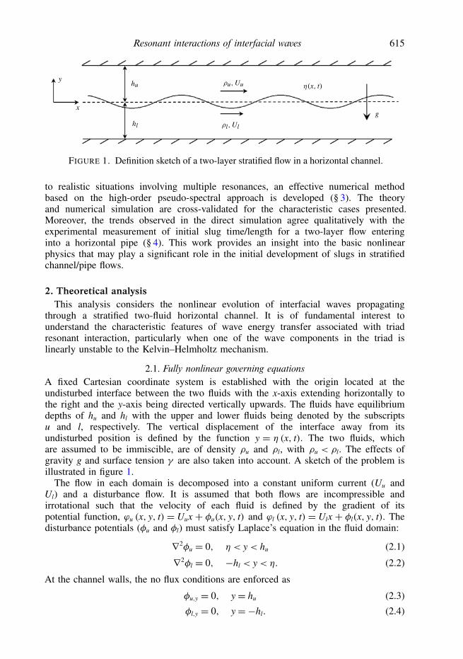
FIGURE 1. Definition sketch of a two-layer stratified flow in a horizontal channel.

to realistic situations involving multiple resonances, an effective numerical methodbased on the high-order pseudo-spectral approach is developed (§ 3). The theoryand numerical simulation are cross-validated for the characteristic cases presented.Moreover, the trends observed in the direct simulation agree qualitatively with theexperimental measurement of initial slug time/length for a two-layer flow enteringinto a horizontal pipe (§ 4). This work provides an insight into the basic nonlinearphysics that may play a significant role in the initial development of slugs in stratifiedchannel/pipe flows.

2. Theoretical analysisThis analysis considers the nonlinear evolution of interfacial waves propagating

through a stratified two-fluid horizontal channel. It is of fundamental interest tounderstand the characteristic features of wave energy transfer associated with triadresonant interaction, particularly when one of the wave components in the triad islinearly unstable to the Kelvin–Helmholtz mechanism.

2.1. Fully nonlinear governing equationsA fixed Cartesian coordinate system is established with the origin located at theundisturbed interface between the two fluids with the x-axis extending horizontally tothe right and the y-axis being directed vertically upwards. The fluids have equilibriumdepths of hu and hl with the upper and lower fluids being denoted by the subscriptsu and l, respectively. The vertical displacement of the interface away from itsundisturbed position is defined by the function y = η (x, t). The two fluids, whichare assumed to be immiscible, are of density ρu and ρl, with ρu < ρl. The effects ofgravity g and surface tension γ are also taken into account. A sketch of the problem isillustrated in figure 1.

The flow in each domain is decomposed into a constant uniform current (Uu andUl) and a disturbance flow. It is assumed that both flows are incompressible andirrotational such that the velocity of each fluid is defined by the gradient of itspotential function, ϕu (x, y, t) = Uux + φu(x, y, t) and ϕl (x, y, t) = Ulx + φl(x, y, t). Thedisturbance potentials (φu and φl) must satisfy Laplace’s equation in the fluid domain:

∇2φu = 0, η < y< hu (2.1)

∇2φl = 0, −hl < y< η. (2.2)

At the channel walls, the no flux conditions are enforced as

φu,y = 0, y= hu (2.3)

φl,y = 0, y=−hl. (2.4)


Requiring that the interface remain material produces

η,t + (Uu + φu,x)η,x = φu,y, y= η (2.5)

η,t + (Ul + φl,x)η,x = φl,y, y= η (2.6)

while the balance of normal stresses at the interface between the two fluids gives

R

[φu,t + 1

2(∇φu)

2+Uuφu,x + η]−[φl,t + 1

2(∇φl)

2+Ulφl,x + η]

=−η,xx

W(1+ η2

,x)−3/2

, y= η (2.7)

where R ≡ ρu/ρl is the density ratio and W ≡L 2gρl/γ is the Weber number. In theabove equations, the quantities are non-dimensionalized in terms of the characteristiclength L and time T = (L /g)1/2. This problem is complete with the specification ofan appropriate set of initial conditions for φu, φl and η.

2.2. Linear theory and the Kelvin–Helmholtz instability

For the purpose of better understanding the nonlinear analysis in the followingsections, it is beneficial to review the key findings from the classical linear theory.The linearization of (2.1)–(2.7) in terms of the small interfacial wave steepness εproduces

∇2φu = 0, 0< y< hu (2.8a)

∇2φl = 0, −hl < y< 0 (2.8b)

φu,y = 0, y= hu (2.8c)

φl,y = 0, y=−hl (2.8d)

η,t + Uuη,x − φu,y = 0, y= 0 (2.8e)

η,t + Ulη,x − φl,y = 0, y= 0 (2.8f )

R(φu,t + Uuφu,x + η)− (φl,t + Ulφl,x + η)+ η,xx

W= 0, y= 0. (2.8g)

A travelling wave solution of (2.8) takes the form

η = ηo

2ei(kx−ωt) + c.c. (2.9a)

φu = ηo−i(Uuk − ω)2k tanh khu

cosh k(y− hu)

cosh khuei(kx−ωt) + c.c. (2.9b)

φl = ηoi(Ulk − ω)2k tanh khl

cosh k(y+ hl)

cosh khlei(kx−ωt) + c.c. (2.9c)

where ηo is the amplitude of the (initial) wave disturbance, k is the wavenumber and ωis the frequency. The symbol ‘c.c.’ represents the complex conjugate of the preceding


term(s). The frequency ω is related to the wavenumber k by the dispersion relation:

ω = k(UuRTl + UlTu)

RTl + Tu± k

[1k

(TuTl

RTl + Tu

)

×(

1−R + k2

W

)− R (Uu − Ul)

2 TuTl

(RTl + Tu)2

]1/2

(2.10)

where Tu/l ≡ tanh khu/l. From (2.10), it is clear that ω is a complex number if|Uu − Ul|> Uc with the critical velocity Uc defined as

Uc(k)≡[(RTl + Tu)

Rk

(1−R + k2

W

)]1/2

. (2.11)

Under this condition, the wave (of wavenumber k) is unstable with its amplitudegrowing exponentially with time by drawing energy from base flows.

Without loss of generality, we assume that Uu > Ul in the following analysis and weconsider the case with Uu − Ul slightly exceeding Uc, i.e. Uu − Ul = Uc(1+∆) where0<∆ 1. In this case, the frequency can be written as

ω ≡ ωR + iωI

= k(UuRTl + UlTu)

RTl + Tu± i[

2kTuTl

RTl + Tu

(1−R + k2

W

)]1/2

∆1/2 + O(∆3/2). (2.12)

Clearly, the growth rate ωI = O(∆1/2) while Uu − Ul − Uc = O(∆).

2.3. Triad resonant wave–wave interactionIn the context of linear theory, waves of different wavelengths (or frequencies) travelindependently in time/space. When nonlinear interactions among them are accountedfor, locked waves are generated. The amplitudes of the locked waves are generallyof higher-order compared with the primary waves. If the frequency and wavenumberof the locked wave satisfy the dispersion relation (2.10), the locked wave becomes afree wave. In this case, the interaction becomes resonant. As a result, the generatedfree wave can grow significantly with its amplitude being comparable to that of theprimary waves. Resonant interactions are known to play a critical role in the evolutionof nonlinear ocean surface waves as they cause energy transfer among different wavecomponents in the wave spectrum (e.g. Phillips 1960).

In this study, we consider a triad resonant interaction in which one of the primarywaves is unstable due to the Kelvin–Helmholtz effect. The focus is on the mechanismof energy transfer from the unstable wave to the stable waves in the triad. Fordefiniteness, we consider a triad consisting of three free waves with wavenumbers k1,k2 and k3. Without loss of generality, we let k3 < k1 < k2 with the k2 wave beingunstable (and k1 and k3 waves being stable). Unlike in the conservative wave systemin which the frequencies of interacting waves involved are all real, the frequencyof the unstable k2 wave is complex in the present case. The multiple-scale analysiscommonly used in the conservative wave system cannot be directly applied here. Theevolution of the amplitudes of interacting waves in the triad is now affected not onlyby the resonant interaction but also by the interfacial instability. The time scales ofthese two processes need to be properly considered in the analysis. To obtain a basicunderstanding of the interaction mechanism of these two processes, we consider the k2

wave to be slightly unstable with Uu − Ul = Uc(1+∆), ∆ 1. In the present analysis,we choose to expand the interaction problem at Uu − Ul = Uc(1 + ∆) with respect to


0

0.2

0.4

0.6

0.8

1.0

5 10 15

(a)

(b)

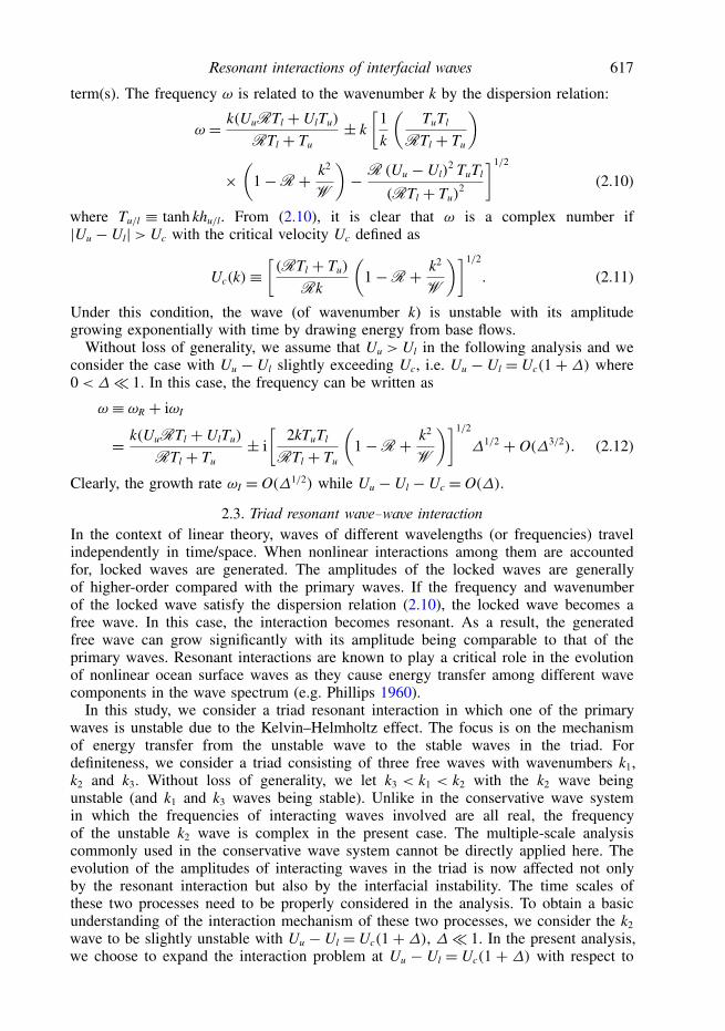
FIGURE 2. (a) Sketch of the neutral stability curve (——) and wavenumbers of the primarywaves forming a resonant triad (k1, k2, k3) along with the second harmonic (2k2) of the k2wave. (b) Normalized wavenumbers k1/k2 (· · ·) and k3/k2 (— · —) in a resonant triad as afunction of the critical velocity Uc(k2). The curve (——) in (b) represents the subharmonicresonance with k1/k2 = k3/k2 = 0.5. The results are obtained with R = 1.23 × 10−3,W ∼= 845.5, H = 1.25, α ≡ hu/H = 0.5 and Ul = 1.13. (With L ∼= 0.08 m and T ∼= 0.09s, as an example, these parameters correspond to an air–water flow in a horizontal channelwith fixed hu = hl = 0.05 m, Ul = 1.0 m s−1 and γ = 0.073 N m−1.)

the marginally stable state at Uu − Ul = Uc in terms of ∆ (Loesch 1974). A sketchof the interacting waves in the plane formed by wavenumber and velocity jump isillustrated in figure 2(a).

At the marginally stable state, the k2 wave is neutrally stable. Following the analysisof Phillips (1960) for conservative resonances, a resonant triad involving k1, k2 and k3

waves are formed under the condition: k2 − k1 = k3 and ω2 − ω1 = ω3, where ω1(k1)

and ω3(k3) are given by (2.10) while for a given k2, the frequency, ω2(k2), is givenby the real part of (2.12). Figure 2(b) shows a typical result of k1 and k3 (normalizedby k2) as a function of Uc(k2). The result shown corresponds to the left branch ofthe neutral stability curve in figure 2(a). For lower Uc, the triad resonance involvinglong and short waves exist. There also exists a subharmonic resonance between k2 andits subharmonic k1 = k3 = 1/2k2. For larger Uc, the triad resonance converges to its


special case of subharmonic resonance. In this work, the analysis is focused on thecase of general triad resonance with k1 6= k3 (at relatively lower Uc). The subharmonicresonance is to be analysed in a separate study.

In the following analysis, for generality, we consider a near-resonance triad in whichthe wavenumbers and frequencies of the interacting waves have the relations

k2 − k1 = k3

ω2 − ω1 = ω3 + σ (2.13)

where σ (with σ ωj, j = 1, 2, 3) represents the frequency detuning. Note thatthe triad resonance condition is satisfied exactly when σ = 0. In addition, forboth simplicity and clarity, the second harmonic of the k2 wave is assumed tobe stable. When this constraint is relived, the analysis procedure is similar, but adifferent combination in the order of magnitudes of the interacting waves needs to beconsidered.

2.4. Multiple-scale analysisIn this section we shall derive the analytic equations governing the time evolutionof the amplitudes of the interacting waves in the triad by use of the method ofmultiple scales which captures the combined effect of the nonlinear Kelvin–Helmholtzinstability and resonant wave–wave interaction.

2.4.1. Perturbation expansionsAs (2.12) indicates, the growth rate of the k2 wave is of O(∆1/2). Thus, there exists

two distinct time scales. One is the fast time t associated with the rapid change of thephases of the waves. The other is the slow time τ associated with the time variation ofthe amplitudes of the waves. Clearly, we have τ = ∆1/2t for the present problem. Forthe perturbation analysis, we assume that the steepness of the interface is small withO(ε) = O(∆1/2). For convenience, we expand the velocity potentials (φu and φl) aswell as the interfacial displacement η in a regular perturbation expansion of the form

φu(x, y, t, τ )=5∑

m=1

∆(m+1)/4φ(m)u (x, y, t, τ )+ O(∆7/4) (2.14a)

φl(x, y, t, τ )=5∑

m=1

∆(m+1)/4φ(m)l (x, y, t, τ )+ O(∆7/4) (2.14b)

η(x, t, τ )=5∑

m=1

∆(m+1)/4η(m)(x, t, τ )+ O(∆7/4) (2.14c)

where φ(m)u , φ(m)l and η(m), m = 1, . . . , 5, are O(1). This expansion is established underthe assumption that the amplitude of the unstable wave (k2) is O(∆1/2) while that ofthe other two stable waves (k1, k3) are O(∆3/4). With this order arrangement, the effectof the cubic self-interaction on the evolution of the k2 wave could be comparable tothat of the quadratic (resonant) interactions of the k1 and k3 waves. Following thestandard procedure of the multiple-scale perturbation analysis, the nonlinear boundary-value problem for φu and φl is decomposed into a sequence of linearized boundary-value problems for φ(m)u and φ

(m)l , m = 1, 2, . . . , 5, which are presented in Appendix.

These problems are then solved sequentially starting from m= 1.


2.4.2. The O(∆1/2) solutionAt this order, the boundary-value problem is identical to that outlined in § 2.2. The

solution for the linearly unstable k2 wave is

φ(1)u =cosh k2(y− hu)

cosh k2hu[P2(τ )eiψ2 + c.c.] + φ(1)u0 (τ ) (2.15a)

φ(1)l =

cosh k2(y+ hl)

cosh k2hl[Q2(τ )eiψ2 + c.c.] + φ(1)l0 (τ ) (2.15b)

η(1) = A2(τ )

2eiψ2 + c.c. (2.15c)

where P2, Q2 and ψ2 are given from the general expressions:

Pj(τ )= −iDujAj(τ )

2kj tanh kjhu, Qj(τ )= iDljAj(τ )

2kj tanh kjhl, ψj = kjx− ωjt (2.16)

and Duj ≡ (Ul + Uc)kj − ωj and Dlj ≡ Ulkj − ωj with the subscript j = 2. Note thatthe boundary-value problem for φ(1)u and φ

(1)l admits space-independent solutions

φ(1)u0 (τ ) and φ(1)l0 (τ ) which will be shown to be important in the higher-order solutions.

The slow-time dependent amplitude, A2(τ ), and potentials, φ(1)u0 (τ ) and φ(1)l0 (τ ), are

governed by the evolution equations to be developed below.

2.4.3. The O(∆3/4) solutionAt this order, the solution represents the (stable) k1 and k3 waves:


cosh k1hu[P1(τ )eiψ1 + c.c.]

+ cosh k3(y− hu)

cosh k3hu[P3(τ )eiψ3 + c.c.] + φ(2)u0 (τ ) (2.17a)

φ(2)l =

cosh k1(y+ hl)

cosh k1hl[Q1(τ )eiψ1

+ c.c.] + cosh k3(y+ hl)

cosh k3hl[Q3(τ )eiψ3 + c.c.] + φ(2)l0 (τ ) (2.17b)

η(2) = A1(τ )

2eiψ1 + A3(τ )

2eiψ3 + c.c. (2.17c)

where P1,3, Q1,3 and ψ1,3 are given from the general expressions (2.16) with thesubscript j = 1 and 3, respectively. Like the m = 1 problem, the boundary-valueproblem at m = 2 also admits space-independent potentials, φ(2)u0 (τ ) and φ(2)l0 (τ ), whichare functions of slow time. The slow-time-dependent amplitudes, A1(τ ) and A3(τ ), aregoverned by the evolution equations to be developed below.

2.4.4. The O(∆) solutionThe inhomogeneous forcing terms at this order are

f (3)1 =− 12 A2eiψ2 + p4A2

2e2iψ2 + c.c. (2.18a)

f (3)2 =− 12 A2eiψ2 + d4A2

2e2iψ2 + c.c. (2.18b)

f (3)3 = f2A2eiψ2 + f7A22e2iψ2 + c.c.+ f8 |A2|2+ φ(1)l0 −Rφ(1)u0 (2.18c)


with the coefficients given by

p4 =−12

ik2Du2Cu2, d4 = 12

ik2Dl2Cl2, (2.19a)

f2 = i2k2

(Dl2Cl2 +RDu2Cu2), f7 =−18[(3− C2

l2)D2l2 −R(3− C2

u2)D2u2], (2.19b)

f8 = 14[(C2

l2 − 1)D2l2 −R(C2

u2 − 1)D2u2] (2.19c)

where Cu/lj ≡ coth(kjhu/l) and the symbol ‘·’ denotes the derivative with respect toslow time τ . There are zeroth, first and second harmonics in the forcing terms.The boundary-value solution associated with the zeroth and second harmonic forcingcan be obtained directly. Since the first harmonic is the homogeneous solution ofthe boundary-value problem, the first harmonic forcing must satisfy the solvabilitycondition, specified by the Fredholm alternative, in order to obtain a non-trivialinhomogeneous solution. By applying Green’s theorem between the O(∆1/2) and O(∆)solutions (for the first harmonic), the solvability condition is found to take the form

iA2

k2

[RDu2

Tu2+ Dl2

Tl2

]= G2

[RD2

u2

k2Tu2+ D2

l2

k2Tl2− 1+R − k2

2

W

](2.20)

where Tu/lj ≡ tanh(kjhu/l) and G2 denotes the half amplitude of the first harmonic(propagating wave) of η(3). Since k2 and ω2 satisfy the dispersion relation, it isstraightforward to show that the terms in the brackets on both sides of (2.20) areidentically zero. Since all of the structure of the propagating k2 wave is contained inthe O(∆1/2) solution, G2 can be set to zero without any loss of generality. The totalsolution for φ(3)u , φ(3)l , and η(3) are then written as


cosh k2hu(α2A2eiψ2 + c.c.)+ cosh 2k2(y− hu)

cosh 2k2hu(α22A2

2e2iψ2 + c.c.) (2.21a)

φ(3)l =

cosh k2(y+ hl)

cosh k2hl(β2A2eiψ2 + c.c.)+ cosh 2k2(y+ hl)

cosh 2k2hl(β22A2

2e2iψ2 + c.c.) (2.21b)

η(3) = ν22(A22ei2ψ2 + c.c.)+ ν0 |A2|2+ φl0 −Rφu0

R − 1(2.21c)

where

ν22 = k2D2

l2

[2Cl4Cl2 − 1

2(3− C2l2)]−RD2

u2

[2Cu4Cu2 − 1

2(3− C2u2)]

8RCu4D2u2 + 8Cl4D2

l2 + 4k2(R − 1− (4k22/W ))

(2.22a)

ν0 = (C2l2 − 1)D2

l2 −R(C2u2 − 1)D2

u2

4(R − 1)(2.22b)

α2 =− 12k2Tu2

, α22 =−iDu2

(k2Cu2 + 4ν22

4k2Tu4

)(2.22c)

β2 = 12k2Tl2

, β22 =−iDl2

(k2Cl2 − 4ν22

4k2Tl4

)(2.22d)

with Cu/l4 = coth(2k2hu/l) and Tu/l4 = tanh(2k2hu/l).One notes that if the two stable waves (k1 and k3) are set to be of O(∆1/2) like the

unstable wave (k2), an unbalanced resonant interaction term would be present in (2.20).


By letting the two stable waves be O(∆1/4) smaller than the unstable k2 wave,the effects of triad resonant interaction and nonlinear Kelvin–Helmholtz instabilitywill converge together correctly in the O(∆3/2) problem without the presence ofsingularities in the lower-order solution.

2.4.5. The O(∆5/4) solutionAt this order, the only terms in f (4)j (j = 1, 2, 3) which produce secular terms are

those with phase ψ1 and ψ3. Upon neglecting the non-secular terms, f (4)j , j = 1, 2 and3, takes the form

f (4)1 =− 12 A1eiψ1 − 1

2 A3eiψ3 + p1A∗1A2ei(ψ2−ψ1) + p3A2A∗3ei(ψ2−ψ3) + c.c. (2.23a)

f (4)2 =− 12 A1eiψ1 − 1

2 A3eiψ3 + d1A∗1A2ei(ψ2−ψ1) + d3A2A∗3ei(ψ2−ψ3) + c.c. (2.23b)

f (4)3 = f1A1eiψ1 + f3A3eiψ3 + f4A∗1A2ei(ψ2−ψ1)

+ f6A2A∗3ei(ψ2−ψ3) + c.c.+ φ(2)l0 −Rφ(2)u0 (2.23c)

where ψ2 − ψ1 = ψ3 − $τ and ψ2 − ψ3 = ψ1 − $τ with $ = σ∆−1/2, and thecoefficients are given by

p1 =−14

ik3(Du1Cu1 + Du2Cu2), p3 =−14

ik1(Du2Cu2 + Du3Cu3) (2.24a)

d1 = 14

ik3(Dl1Cl1 + Dl2Cl2), d3 = 14

ik1(Dl2Cl2 + Dl3Cl3) (2.24b)

f1 = i2k1

(Dl1Cl1 +RDu1Cu1), f3 = i2k3

(Dl3Cl3 +RDu3Cu3) (2.24c)

f4 = 14R[D2

u1 + D2u2 − (1+ Cu1Cu2)Du1Du2] − D2

l1 − D2l2 + (1+ Cl1Cl2)Dl1Dl2 (2.24d)

f6 = 14R[D2

u2 + D2u3 − (1+ Cu2Cu3)Du2Du3] − D2

l2 − D2l3 + (1+ Cl2Cl3)Dl2Dl3. (2.24e)

Upon the use of the solvability conditions which can be realized by applying Green’stheorem to the O(∆3/4) and O(∆5/4) solutions, we obtain the evolution equations forA1 and A3:

A1 = iB23A2A∗3e−i$τ (2.25a)

A3 = iB12A∗1A2e−i$τ (2.25b)

where

B23 = k1

4

[Dl1Cl1(Dl2Cl2 + Dl3Cl3)− D2

l2 − D2l3 + (1+ Cl2Cl3)Dl2Dl3

RDu1Cu1 + Dl1Cl1

]− Rk1

4

[Du1Cu1(Du2Cu2 + Du3Cu3)− D2

u2 − D2u3 + (1+ Cu2Cu3)Du2Du3

RDu1Cu1 + Dl1Cl1

](2.26a)

B12 = k3

4

[Dl3Cl3(Dl1Cl1 + Dl2Cl2)− D2

l1 − D2l2 + (1+ Cl1Cl2)Dl1Dl2

RDu3Cu3 + Dl3Cl3

]− Rk3

4

[Du3Cu3(Du1Cu1 + Du2Cu2)− D2

u1 − D2u2 + (1+ Cu1Cu2)Du1Du2

RDu3Cu3 + Dl3Cl3

]. (2.26b)


These two interaction coefficients, B23 and B12, are the same as those in the case whereall three waves in the resonant triad are linearly stable to the Kelvin–Helmholtz effect,as shown by Campbell (2009).

2.4.6. The O(∆3/2) solutionThe forcing terms f (5)j , j= 1, 2 and 3, are

f (5)1 = (p2A1A3ei$τ + p5 |A2|2 A2 + p6A2(Rφ(1)u0 − φ(1)l0 )+ p7A2 + c.c.)eiψ2

+ Rφ(1)u0 − φ(1)l0

R − 1− ν0

ddτ(|A2|2) (2.27a)

f (5)2 = (d2A1A3ei$τ + d5 |A2|2 A2 + d6A2(Rφ(1)u0 − φ(1)l0 )+ c.c.)eiψ2

+ Rφ(1)u0 − φ(1)l0

R − 1− ν0

ddτ(|A2|2) (2.27b)

f (5)3 = [f5A1A3 + f9A2 + f10A2 + f11 |A2|2 A2 + f13A2(Rφ(1)u0 − φ(1)l0 )+ c.c.]eiψ2

+ f12A2A∗2 + f ∗12A∗2A2 + f14 |A1|2+f15 |A3|2 (2.27c)

where ∗ denotes the complex conjugate and the coefficients are given by

p2 =−14

ik2 (Du1Cu1 + Du3Cu3) (2.28a)

p5 = α22k22 +

12

ik2Du2

[38

k2 − Cu2 (ν22 + ν0)

](2.28b)

p6 =− ik2Du2Cu2

2 (R − 1)(2.28c)

p7 =− iUck2

2(2.28d)

d2 = 14

ik2 (Dl1Cl1 + Dl3Cl3) (2.28e)

d5 = β22k22 +

12

ik2Dl2

[38

k2 + Cl2 (ν22 + ν0)

](2.28f )

d6 = ik2Dl2Cl2

2 (R − 1)(2.28g)

f5 = 14

(Cl1Cl3 − 1)Dl1Dl3 − D2

l1 − D2l3 −R

[(Cu1Cu3 − 1)Du1Du3 − D2

u1 − D2u3

](2.28h)

f9 = β2 −Rα2 (2.28i)

f10 =−12RUcDu2Cu2 (2.28j)

f11 = R

(ik2Du2α22 [Tu4 − Cu2]+ 1

2Du2

[ν0 + ν22 + 5

8k2Cu2

])− 3k4

2

16W

+ 12

D2l2

[58

k2Cl2 − ν0 − ν22

]+ ik2Dl2β22 [Tl4 − Cl2] (2.28k)

f12 = i4

Dl2 − i2

k2β2Dl2Cl2 −R

[i4

Du2 + i2

k2α2Du2Cu2

](2.28l)


f13 = D2l2 −RD2

u2

2(R − 1)(2.28m)

f14 = 14

[D2

l1(C2l1 − 1)−RD2

u1(C2u1 − 1)

](2.28n)

f15 = 14

[D2

l3(C2l3 − 1)−RD2

u3(C2u3 − 1)

]. (2.28o)

In (2.27), the non-relevant terms are not included for clarity.Imposing the solvability condition for the forcing with phase ψ2, we obtain the

evolution equation for A2:

A2 =ΩA2 +N |A2|2 A2 +M A2

(Rφ(1)u0 − φ(1)l0

)+ B13A1A3ei$τ (2.29)

with

Ω = −RUcDu2Cu2

Rα2 − β2(2.30)

N = ik2Rα22Du2[Tu4 − 2Cu2] + β22Dl2[Tl4 − 2Cl2]

Rα2 − β2

+ RD2u2[(ν0 + ν22)(1− C2

u2)+ k2Cu2] + D2l2[(ν0 + ν22)(C2

l2 − 1)+ k2Cl2]2(Rα2 − β2)

− 3k42

16W (Rα2 − β2)(2.31)

M = D2l2(1− C2

l2)+RD2u2(C

2u2 − 1)

2(R − 1)(Rα2 − β2)(2.32)

B13 = (Cl1Cl3 − 1)Dl1Dl3 − D2l1 − D2

l3 −R[(Cu1Cu3 − 1)Du1Du3 − D2u1 − D2

u3]4(Rα2 − β2)

− RDu2Cu2(Du1Cu1 + Du3Cu3)− Dl2Cl2(Dl1Cl1 + Dl3Cl3)

4(Rα2 − β2). (2.33)

Equation (2.29) requires that Rφ(1)u0 − φ(1)l0 be solved for. For the zeroth harmonic, theboundary-value problem for φ(m)u and φ(m)l in (A 2a)–(A 2f ) allows for a solution thatcan be a function of slow time τ only. Thus, the zeroth harmonic forcing in f (5)1 andf (5)2 must vanish, which leads to

Rφ(1)u0 − φ(1)l0 = (R − 1)ν0d

dτ|A2|2 . (2.34)

Integration of this equation with respect to τ gives

Rφ(1)u0 − φ(1)l0 = (R − 1)ν0 |A2|2+C (2.35)

where the integration constant is determined by the initial condition, C = Rφ(1)u0 −φ(1)l0 − (R − 1)ν0 |A2|2 evaluated at τ = 0.The leading-order solution of the mean interface elevation in (2.21c) then becomes

η(3) = ν0 |A2|2−Rφ(1)u0 − φ(1)l0

R − 1= C

1−R. (2.36)


The zeroth harmonic forcing in f (4)3 and f (5)3 gives the higher-order solution:η(4) + η(5) = [φ(2)l0 −Rφ(2)u0 + f12A2A∗2 + f ∗12A∗2A2 + f14 |A1|2+ f15 |A3|2]/(R − 1) where thequantity φ(2)l0 −Rφ(2)u0 needs to be determined in the O(∆7/4) boundary-value problem.

Upon substitution of t = ∆−1/2τ , a2 = ∆1/2A2, a1 = ∆3/4A1, a3 = ∆3/4A3, andσ =$∆−1/2, we rewrite the evolution equations for the amplitudes of the interactingwaves in the triad in the form

d2a2

dt2= Ωa2 + ˆN |a2|2 a2 + B13a1a3eiσ t (2.37a)

da1

dt= iB23a2a∗3e−iσ t (2.37b)

da3

dt= iB12a2a∗1e−iσ t (2.37c)

where Ω = (Ω +M C)∆ and ˆN = N +M (R − 1)ν0. In the right-hand side of(2.37a), the first term represents the linear Kelvin–Helmholtz instability effect, thesecond-term the nonlinear correction (associated with cubic self-interactions) to theKelvin–Helmholtz instability effect and the third term the triad resonant interactioneffect. The effect of the mean interface elevation upon the Kelvin–Helmholtzinstability is also considered with the inclusion of C in Ω .

2.5. Properties of the nonlinear interaction equationsThe analytic solution to (2.37) is, in general, not known and can only be foundthrough numerical integration. In the case of a perfect resonance (σ = 0) or for smalltime, analytical solutions or integral properties can be derived.

2.5.1. Resonant interactions with σ = 0For the perfect resonance case, σ = 0. With the decomposition aj(t) = Rj(t)eiθj(t),

j= 1, 2 and 3, (2.37b) and (2.37c) are separated into real and imaginary parts:

R1 =−B23R2R3 sinΦ (2.38a)

R1θ1 = B23R2R3 cosΦ (2.38b)

R3 =−B12R1R2 sinΦ (2.38c)

R3θ3 = B12R1R2 cosΦ (2.38d)

where Φ = θ2 − θ1 − θ3. Using (2.38a) and (2.38c) and integrating with respect to time,we obtain

B[R21(τ )− R2

1(0)] = [R23(τ )− R2

3(0)] (2.39)

where B = B12/B23. For B < 0, we have from (2.39) that |B|R21(t) + R2

3(t) =|B|R21(0) + R2

3(0). This indicates that for B < 0, the growth of R1 and R3 remainsbounded with their maximum amplitudes being limited by their initial conditions. ForB > 0, (2.39) shows that there is no restriction on how large the two waves can growdue to the resonant interaction with the unstable k2 wave.

2.5.2. Solution at small timeWhen the amplitudes of the interacting modes are small (with k2a2 1 and

a1/a2, a3/a2 1), the nonlinear terms in (2.37a) have a weak secondary effect. Thisleaves the evolution equation of a2 to be dominated by the linear instability. Withthis simplification, the coupled evolution (2.37) can be solved for the (initial) growth


rates of a2, a1 and a3 due to the linear instability and the triad resonant interaction.Evolution at small initial time (with a1/a2, a3/a2 1) is an example of this situation.

In this case, it is straightforward to obtain a2(t) = a2 expΩ1/2t where a2 is theinitial value of a2 at t = 0. By taking the time derivative of (2.37c), we have

a3 = iB12

(a∗1a2 + a∗1a2 − iσa∗1a2

)e−iσ t. (2.40)

Upon substitution of a2(t) and use of (2.37b), we rewrite the above equation as

a3 =(√

Ω − iσ)

a3 + |a2|2 e2√ΩtB12B23a3. (2.41)

Introducing the change of variable ξ = |a2| (B12B23)1/2 expΩ1/2t, we write (2.41) in

the form

ξ 2 d2a3

dξ 2+ iσ√

Ωξ

da3

dξ− ξ

2

Ωa3 = 0 (2.42)

which is a transformed version of the Bessel differential equation. The general solutionof (2.42) takes the form

a3(ξ)= ξ−ν[C(3)

1 Jν

(−iξ√Ω

)+ C(3)

2 Yν

(−iξ√Ω

)](2.43)

where ν = (iσ −√Ω)/(2

√Ω), and Jν and Yν represent the Bessel functions of the

first and second kinds, respectively. The constants C(3)1 and C(3)

2 are determined fromthe initial condition to be

C(3)1 =

ξ ν0 [a3Yν+1(−iξ0/√Ω)+ i

√Ω a∗1a2B12Yν(−iξ0/

√Ω)]

Jν(−iξ0/√Ω)Yν+1(−iξ0/

√Ω)− Jν+1(−iξ0/

√Ω)Yν(−iξ0/

√Ω)

(2.44a)

C(3)2 =−

ξ ν0 [a3Jν+1(−iξ0/√Ω)+ i

√Ω a∗1a2B12Jν(−iξ0/

√Ω)]

Jν(−iξ0/√Ω)Yν+1(−iξ0/

√Ω)− Jν+1(−iξ0/

√Ω)Yν(−iξ0/

√Ω)

(2.44b)

where ξ0 = ξ(t = 0) and a1,3 = a1,3(t = 0). Owing to the symmetry, the solution to a1

can be obtained from that of a3 by switching a3 with a1.To assist in understanding the basic characteristics of the solution for the growth

of a3 (and a1), we consider the nearly perfect resonance case. With σ/ω3 1, themiddle term on the left-hand side of (2.42) can be ignored. The general solution of theresulting equation is given as

a3(ξ)= D1eξ/√Ω + D2e−ξ/

√Ω (2.45)

where the constants D1 and D2 are determined from the initial condition. Dependingon the signs of the interaction coefficients (B12 and B23), the solution in (2.45) showsdifferent characteristic behaviours. When B12 and B23 have the same sign (i.e. B > 0),ξ is purely real and is proportional to exp(Ω1/2t). As a result, a3 ∼ exp[exp(Ω1/2t)]which shows a bi-exponential growth with time. This suggests a highly efficientmechanism for transferring energy to linearly stable wave modes from a linearlyunstable wave mode through triad resonant interaction. In the study of (wind) wavegeneration by a sheared current, Janssen (1987) predicted a similar energy transfermechanism due to the nonlinear coupling between a linearly unstable mode and its


second harmonic. When B12 and B23 have different signs (i.e B < 0), ξ is purelyimaginary. In this case, a3 ∼ exp[i exp(Ω1/2t)] which shows an oscillatory feature intime with a constant amplitude but an exponentially growing frequency. (Note that thisresult is consistent with the finding in the preceding section for the perfect resonancecase with B < 0.)

3. Numerical methodThe theoretical analysis § 2 provides valuable insights into the dynamics of resonant

triad wave interaction coupled with the Kelvin–Helmholtz instability effect for a two-fluid flow in a horizontal channel. To verify the theoretical prediction and deal withthe practical situation involving multiple resonant interactions, we develop an effectivenumerical method that enables direct time simulation of the nonlinear initial boundary-value problem ((2.1)–(2.7)).

3.1. Mathematical formulation of a high-order spectral method

An efficient high-order pseudo-spectral (HOS) method, originally developed byDommermuth & Yue (1987) for the study of nonlinear surface gravity waves, ismodified to simulate the nonlinear interfacial evolution of stratified channel flows. Theextension to nonlinear interactions of internal waves and surface waves over variablebottom topography was achieved by Alam, Liu & Yue (2009). This method solves theprimitive equations of the problem by following the evolution of a large number ofspectral interfacial wave modes and accounts for their interactions up to an arbitrarilyhigh order of nonlinearity using a pseudo-spectral approach.

3.1.1. Time evolution equationsThis process begins with the definition of the potentials at the interface within each

fluid domain

φIu(x, t)= φu(x, η(x, t), t) (3.1a)

φIl (x, t)= φl(x, η(x, t), t). (3.1b)

Applying chain rule to (3.1) allows for the standard derivatives on the interface (y= η)to be written as

∂φ

∂t= ∂φ

I

∂t− ∂φ∂y

∂η

∂t, y= η (3.2a)

∂φ

∂x= ∂φ

I

∂x− ∂φ∂y

∂η

∂x, y= η. (3.2b)

With these new definitions of the potential derivatives, the boundary conditions maybewritten as functions of the interface potentials. The kinematic boundary conditions(2.5) and (2.6) take the form

∂η

∂t=−

[Uu + ∂φ

Iu

∂x

]∂η

∂x+[

1+(∂η

∂x

)2]∂φu

∂y, y= η (3.3)

∂η

∂t=−

[Ul + ∂φ

Il

∂x

]∂η

∂x+[

1+(∂η

∂x

)2]∂φl

∂y, y= η (3.4)


while the dynamic boundary condition, (2.7), is expressed as

∂Ψ I

∂t= 1

2

[1+

(∂η

∂x

)2][(

∂φl

∂y

)2

−R

(∂φu

∂y

)2]+ 1

2

[R

(∂φI

u

∂x

)2

−(∂φI

l

∂x

)2]

+RUu∂φI

u

∂x− Ul

∂φIl

∂x− (1−R)η + 1

W

ηxx(1+ η2

x

)3/2 , y= η (3.5)

where Ψ I(x, t) ≡ φIl (x, t) − RφI

u(x, t). Together, (3.3) (or (3.4)) and (3.5) form aset of interfacial evolution equations that can be integrated in time to obtain thedynamic behaviour of the interface between the two fluids, provided that the interfacevelocities (∂φu/∂y and ∂φl/∂y on y= η) and potentials (φI

u and φIl ) can be solved from

the boundary-value problem.

3.1.2. Perturbation expansionsIf it is assumed that φu, φl and η are O(ε) 1, where ε is a measure of the wave

steepness, then these terms can be expanded in a perturbation series up to order M interms of the small variable ε

φu/l(x, y, t)=M∑

m=1

φ(m)u/l (x, y, t) (3.6)

where φ(m)u and φ(m)l are O (εm). Since this is a free boundary problem, with φu, φl andη being unknown, we expand φu and φl on the interface (y= η) in Taylor series aboutthe mean interface (y= 0):

φu/l(x, η, t)=M∑

m=1

φ(m)u/l (x, η, t)=

M∑m=1

M−m∑k=0

ηk

k!∂k

∂ykφ(m)u/l

∣∣∣∣y=0

. (3.7)

It should be noted that the second summation is evaluated up to M − m in order tomaintain a consistent expansion up to O(εM).

Defining Ψ (x, y, t)≡ φl(x, y, t)−Rφu(x, y, t) and using (3.7) produces

Ψ I(x, t)=M∑

m=1

Ψ (m)(x, η, t)=M∑

m=1

M−m∑k=0

ηk

k!∂k

∂ykΨ (m)

∣∣∣∣y=0

. (3.8)

If all terms of common order in (3.8) are collected, a set of Dirichlet boundaryconditions for each Ψ (m) (≡φ(m)l −Rφ(m)u ) on y= 0 can be obtained as

Ψ (1)(x, 0, t)= ψ I (3.9)

Ψ (m)(x, 0, t)=−m−1∑k=1

ηk

k!∂k

∂ykΨ (m−k)

∣∣∣∣y=0

, m= 2, 3, . . . ,M (3.10)

with Ψ I(x, t) being obtained from the evolution equation (3.5) at any time t.Taking the difference between (2.5) and (2.6) gives a new form of the kinematic

interfacial boundary condition:

Φy = ηx[Φx + (Uu − Ul)], y= η (3.11)


where Φ ≡ φu−φl. Applying the perturbation expansions for φu, φl and then expandingthem in Taylor series about y= 0 yields

Φ(x, η, t)=M∑

m=1

Φ(m)(x, η, t)=M∑

m=1

M−m∑k=0

ηk

k!∂k

∂ykΦ(m)

∣∣∣∣y=0

. (3.12)

Substituting this expansion into (3.11), a set of Neumann boundary conditions can beobtained for each Φ(m)

y on y= 0:

Φ(1)y (x, 0, t)= ηx(Uu − Ul) (3.13)

Φ(m)y (x, 0, t)= ηx

m−1∑k=1

η(k−1)

(k − 1)!∂ (k−1)

∂y(k−1)Φ(m−k)

x

∣∣∣∣y=0

−m−1∑k=1

ηk

k!∂ (k+1)

∂y(k+1)Φ(m−k)

∣∣∣∣y=0

(3.14)

for m= 2, 3, . . . ,M.With these expansions, the nonlinear boundary-value problem for φu, φl is

decomposed into a sequence of linear boundary-value problems for the perturbedpotentials φ(m)u , φ(m)l , m = 1, 2, . . . ,M, which can be solved sequentially starting fromm= 1 up to an arbitrary order M.

3.1.3. Solution of φ(m)u and φ(m)lAssuming a periodic boundary condition in the x direction and choosing a

normalization that makes the length of the computational domain L = 2π, theboundary-value solution at each order m, which satisfies both Laplace’s equation andthe zero-flux condition at the walls, can be written as a truncated Fourier series of theform

φ(m)u (x, y, t)=N∑

n=−N

A(m)n (t)cosh kn(y− hu)

cosh knhueiknx (3.15a)

φ(m)l (x, y, t)=

N∑n=−N

B(m)n (t)cosh kn(y+ hl)

cosh knhleiknx (3.15b)

where the wavenumber of the nth Fourier mode kn = n. From the Dirichlet boundarycondition for Ψ (m) and the Neumann boundary condition for Φ(m), the unknownFourier modal amplitudes (A(m)n and B(m)n ) are determined to be

A(m)n =−Φ(m)

yn + Ψ (m)n kn tanh knhl

kn(tanh knhu +R tanh knhl)(3.16a)

B(m)n =Ψ (m)

n kn tanh knhu −RΦ(m)yn

kn(tanh knhu +R tanh knhl)(3.16b)

for n = −N,−N + 1, . . . ,N but n 6= 0, where Ψ (m)n and Φ(m)

yn are the Fourier modalamplitudes of Ψ (m)(x, 0, t) and Φ(m)

y (x, 0, t), respectively. For the mode of n = 0, the

Dirichlet boundary condition requires that B(m)0 − RA(m)0 = Ψ (m)0 while the Neumann

boundary condition is automatically satisfied. For the complete solution of the problem,the specific values of A(m)0 and B(m)0 are not needed. For convenience in computation,we let A(m)0 = 0 and B(m)0 = Ψ (m)

0 .After the boundary-value solutions of φ(m)u and φ

(m)l are determined up to order

M, the interface potentials φIu and φI

l can be evaluated from (3.7). The interface


velocities, ∂φu/∂y and ∂φl/∂y on y = η, can be evaluated similarly by making Taylorseries expansions about y= 0 and then substituting the solutions of φ(m)u and φ(m)l . Theevolution equations (3.3) (or (3.4)) and (3.5) can be integrated in time (with properlydefined initial conditions) by the use of any high-resolution integration method, suchas the fourth-order Runge–Kutta scheme.

One notes that owing to the use of perturbation expansion (3.6) and spectralexpansion (3.15), the boundary-value solution converges exponentially fast withincreasing the order M and the number of spectral modes N for moderately steepinterfaces. However, as the interface steepness increases, the convergence rate with Mbecomes slower. For steep waves, the present method is invalid because (3.6) will nolonger converge with M. In this case, a fully nonlinear scheme needs to be applied.

This numerical method is designed for efficiently simulating the nonlinear evolutionof an interface composed of broadbanded wave components. It is also equally capableof simulating the nonlinear evolution of a specific discrete set of wave modes. Forthese problems, a simple bandpass filter is applied at each time step to remove allnon-relevant spectral components.

3.2. Validation of the numerical method

As a verification of the numerical method, a relatively simple case of a single triadresonance is considered in which the three interacting waves are all linearly stable. Forthis problem, a closed-form analytic solution is available. The evolution equations forthe amplitudes of the interacting waves take the form (Campbell 2009):

da1

dt= iB23a2a∗3e−iσ t (3.17a)

da2

dt= ib13a1a3eiσ t (3.17b)

da3

dt= iB12a∗1a2e−iσ t (3.17c)

where the interaction coefficient b13 is

b13 = k2

4(RDu2Cu2 + Dl2Cl2)[Dl2Cl2(Dl1Cl1 + Dl3Cl3)−RDu2Cu2(Du1Cu1 + Du3Cu3)

+R(D2u1 + D2

u3)− (D2l1 + D2

l3)− Dl1Dl3(1− Cl1Cl3)

+RDu1Du3(1− Cu1Cu3)] (3.18)

and B12 and B23 are given by (2.26) in § 2.4.5. For perfect resonance (σ = 0), (3.17)can be solved analytically with the solution given in terms of Jacobian ellipticfunctions (e.g. McGoldrick 1965). With initial amplitudes a1(0) = a1, a2(0) = 0 anda3(0)= a3, as an example, the solution takes the form

a1 = a1dn(Ξ |m) (3.19a)

a2 = a3

√b13

B12sn(Ξ |m) (3.19b)

a3 = a3cn (Ξ |m) (3.19c)


(× 103)

0.2

0.6

1.0

1.4

2 4 6 8 10 120 14

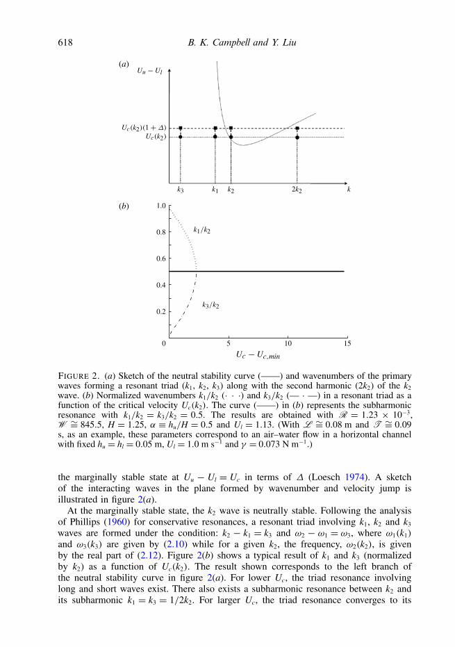
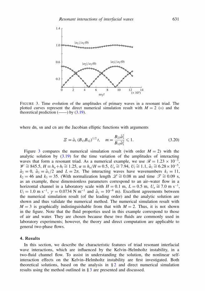
FIGURE 3. Time evolution of the amplitudes of primary waves in a resonant triad. Theplotted curves represent the direct numerical simulation result with M = 2 () and thetheoretical prediction (——) by (3.19).

where dn, sn and cn are the Jacobian elliptic functions with arguments

Ξ = a1 (B13B12)1/2 t, m= B23a2

3

B12a21

6 1. (3.20)

Figure 3 compares the numerical simulation result (with order M = 2) with theanalytic solution by (3.19) for the time variation of the amplitudes of interactingwaves that form a resonant triad. As a numerical example, we use R = 1.23 × 10−3,W ∼= 845.5, H ≡ hu+hl

∼= 1.25, α ≡ hu/H = 0.5, Uu∼= 7.94, Ul

∼= 1.1, a1∼= 6.28×10−5,

a2 = 0, a3 = a1/2 and L = 2π. The interacting waves have wavenumbers k1 = 11,k2 = 46 and k3 = 35. (With normalization length L ∼= 0.08 m and time T ∼= 0.09 s,as an example, these dimensionless parameters correspond to an air–water flow in ahorizontal channel in a laboratory scale with H = 0.1 m, L = 0.5 m, Uu

∼= 7.0 m s−1,Ul = 1.0 m s−1, γ = 0.0734 N m−1 and a1 = 10−6 m). Excellent agreements betweenthe numerical simulation result (of the leading order) and the analytic solution areshown and thus validate the numerical method. The numerical simulation result withM = 3 is graphically indistinguishable from that with M = 2. Thus, it is not shownin the figure. Note that the fluid properties used in this example correspond to thoseof air and water. They are chosen because these two fluids are commonly used inlaboratory experiments; however, the theory and direct computation are applicable togeneral two-phase flows.

4. ResultsIn this section, we describe the characteristic features of triad resonant interfacial

wave interactions, which are influenced by the Kelvin–Helmholtz instability, in atwo-fluid channel flow. To assist in understanding the solution, the nonlinear self-interaction effects on the Kelvin–Helmholtz instability are first investigated. Boththeoretical solutions, based on the analysis in § 2 and direct numerical simulationresults using the method outlined in § 3 are presented and discussed.


(× 102)

10–6

10–4

10–2

100

102

104

0 2 4 6 8 10 12 14

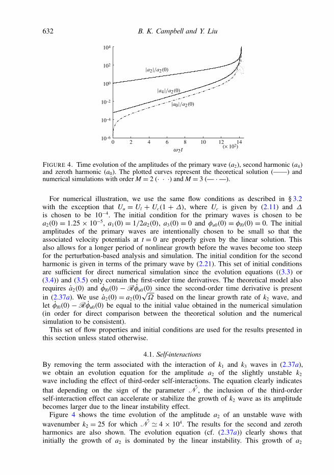
FIGURE 4. Time evolution of the amplitudes of the primary wave (a2), second harmonic (a4)and zeroth harmonic (a0). The plotted curves represent the theoretical solution (——) andnumerical simulations with order M = 2 (· · ·) and M = 3 (— ·—).

For numerical illustration, we use the same flow conditions as described in § 3.2with the exception that Uu = Ul + Uc(1 + ∆), where Uc is given by (2.11) and ∆

is chosen to be 10−4. The initial condition for the primary waves is chosen to bea2(0) = 1.25 × 10−5, a1(0) = 1/2a2(0), a3(0) = 0 and φu0(0) = φl0(0) = 0. The initialamplitudes of the primary waves are intentionally chosen to be small so that theassociated velocity potentials at t = 0 are properly given by the linear solution. Thisalso allows for a longer period of nonlinear growth before the waves become too steepfor the perturbation-based analysis and simulation. The initial condition for the secondharmonic is given in terms of the primary wave by (2.21). This set of initial conditionsare sufficient for direct numerical simulation since the evolution equations ((3.3) or(3.4)) and (3.5) only contain the first-order time derivatives. The theoretical model alsorequires a2(0) and φl0(0) −Rφu0(0) since the second-order time derivative is presentin (2.37a). We use a2(0) = a2(0)

√Ω based on the linear growth rate of k2 wave, and

let φl0(0) −Rφu0(0) be equal to the initial value obtained in the numerical simulation(in order for direct comparison between the theoretical solution and the numericalsimulation to be consistent).

This set of flow properties and initial conditions are used for the results presented inthis section unless stated otherwise.

4.1. Self-interactionsBy removing the term associated with the interaction of k1 and k3 waves in (2.37a),we obtain an evolution equation for the amplitude a2 of the slightly unstable k2

wave including the effect of third-order self-interactions. The equation clearly indicatesthat depending on the sign of the parameter ˆN , the inclusion of the third-orderself-interaction effect can accelerate or stabilize the growth of k2 wave as its amplitudebecomes larger due to the linear instability effect.

Figure 4 shows the time evolution of the amplitude a2 of an unstable wave withwavenumber k2 = 25 for which ˆN ' 4 × 104. The results for the second and zerothharmonics are also shown. The evolution equation (cf. (2.37a)) clearly shows thatinitially the growth of a2 is dominated by the linear instability. This growth of a2


continues according to linear theory until the third-order self-interaction term becomessignificant. Since ˆN > 0, the third-order self-interaction increases the growth rate ofa2 above that of the linear solution. This nonlinear effect is stronger as a2 becomeslarger in the evolution. As time increases, the growth rate continues to increase untilthe amplitude of a2 rapidly becomes unbounded, as shown in figure 4. The secondharmonic is a locked wave that is stable in this case. Thus, it grows at twice the rateof a2. For the zeroth harmonic, the leading-order theoretical solution is a near-zeroconstant. The next order solution is not pursued in this study.

The direct numerical simulation results (M = 2, 3) compare excellently with thetheoretical prediction for both the primary wave and its second harmonic until the verylate stage of evolution when the solution quickly blows up. The numerical solution isconvergent with order M since the solution of M = 2 agrees well with that of M = 3except at the late stage where the third-order effects become apparent. The numericalsimulation also provides a prediction for the zeroth harmonic that is generally aboutone order smaller than the second harmonic except at the late stage of evolutionwhen the solution quickly becomes singular. One notes that as the wave amplitudea2 becomes considerably large at late stage of evolution, higher-order effects areimportant, which are not considered in the theoretical analysis. While the simulationcan include such higher-order effects, it will eventually fail to converge with M aswave steepness continues to increase since the numerical simulation is based on aperturbation approach.

A numerical search over a wide range of flow parameters suggests that the case ofˆN < 0 occurs only when the second harmonic of the k2 wave is also linearly unstable.

The theoretical analysis in § 2 does not apply to this case since the analysis assumes alinearly stable second harmonic. In this case, strong interactions between the primarywave and its second harmonic, called an overtone resonance, can occur. This itself isan interesting topic in nonlinear interfacial wave dynamics and is pursued in a separatestudy.

4.2. Triad resonant interactionsWe now turn to the study of triad resonant interaction that involves one unstable andtwo stable interacting wave components. The discussion in § 2.5 indicates that differentcharacteristic solutions exist depending on the sign of the parameter B ≡ B12/B23.Both cases are considered here.

4.2.1. B < 0For this example the triad resonance consists of the interacting waves with

wavenumbers k1 = 24, k2 = 25 and k3 = 1 which produces ˆN ' 4 × 104 andB ' −0.017. The k2 wave is slightly unstable. The resulting evolution of theamplitudes of these waves, as well as the second harmonic of k2 wave and thezeroth harmonic, is shown in figure 5.

The analytic solution demonstrates that the amplitudes of the k2 wave, itssecond harmonic and the zeroth harmonic behave similarly to the case without theinvolvement of the triad resonance interaction, discussed in § 4.1. The growth of a2

is dominated by the linear instability while the second harmonic, which is locked toa2, grows with twice the linear growth rate of a2. As a2 becomes large, the positivenonlinear self-interaction term causes the growth rate to continuously increase untilthe solution becomes singular. This singularity causes the second harmonic to becomesingular as well. The theoretical solution predicts that the zeroth harmonic maintainsa near-zero constant amplitude during the entire evolution. In this case, the amplitude


(× 102)

10–6

10–4

10–2

100

102

104

0 2 4 6 8 10 12 14

(× 102)

10–6

10–4

10–2

100

102

104

0 2 4 6 8 10 12 14

(a)

(b)

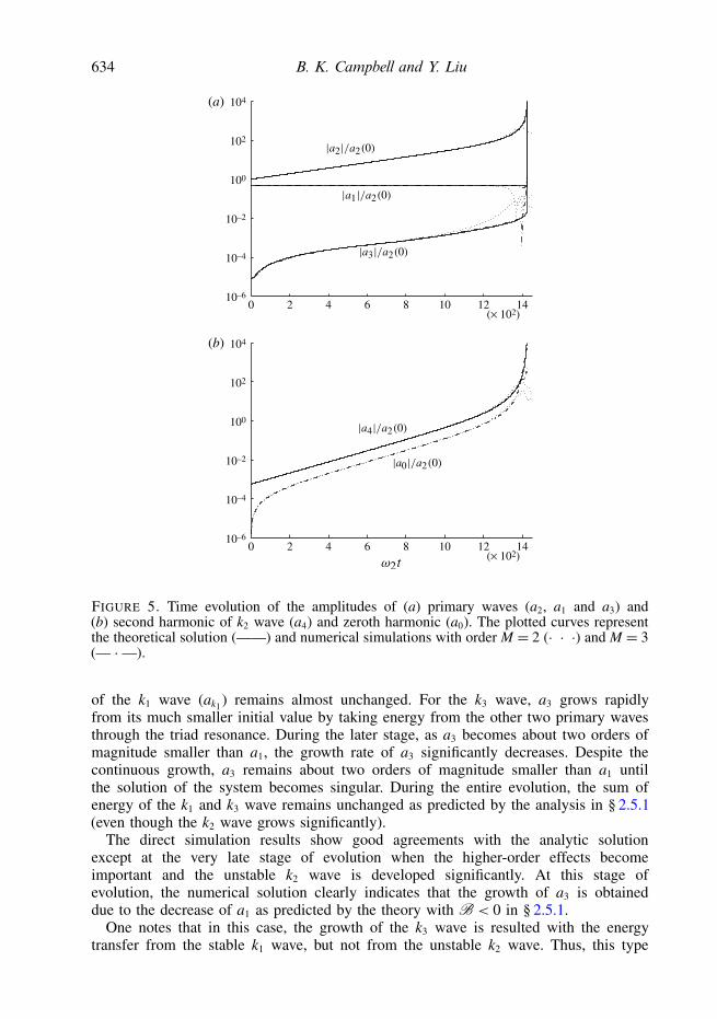
FIGURE 5. Time evolution of the amplitudes of (a) primary waves (a2, a1 and a3) and(b) second harmonic of k2 wave (a4) and zeroth harmonic (a0). The plotted curves representthe theoretical solution (——) and numerical simulations with order M = 2 (· · ·) and M = 3(— ·—).

of the k1 wave (ak1) remains almost unchanged. For the k3 wave, a3 grows rapidlyfrom its much smaller initial value by taking energy from the other two primary wavesthrough the triad resonance. During the later stage, as a3 becomes about two orders ofmagnitude smaller than a1, the growth rate of a3 significantly decreases. Despite thecontinuous growth, a3 remains about two orders of magnitude smaller than a1 untilthe solution of the system becomes singular. During the entire evolution, the sum ofenergy of the k1 and k3 wave remains unchanged as predicted by the analysis in § 2.5.1(even though the k2 wave grows significantly).

The direct simulation results show good agreements with the analytic solutionexcept at the very late stage of evolution when the higher-order effects becomeimportant and the unstable k2 wave is developed significantly. At this stage ofevolution, the numerical solution clearly indicates that the growth of a3 is obtaineddue to the decrease of a1 as predicted by the theory with B < 0 in § 2.5.1.

One notes that in this case, the growth of the k3 wave is resulted with the energytransfer from the stable k1 wave, but not from the unstable k2 wave. Thus, this type


(× 102)

(× 102)

(a)

(b)

10–6

10–4

10–2

100

102

104

0 5 10 15

10–4

10–2

100

102

104

0 2 4 6 8 10 12 14 16 18

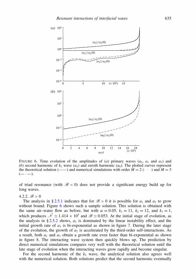
FIGURE 6. Time evolution of the amplitudes of (a) primary waves (a2, a1 and a3) and(b) second harmonic of k2 wave (a4) and zeroth harmonic (a0). The plotted curves representthe theoretical solution (——) and numerical simulations with order M = 2 (· · ·) and M = 3(— ·—).

of triad resonance (with B < 0) does not provide a significant energy build up forlong waves.

4.2.2. B > 0The analysis in § 2.5.1 indicates that for B > 0 it is possible for a1 and a3 to grow

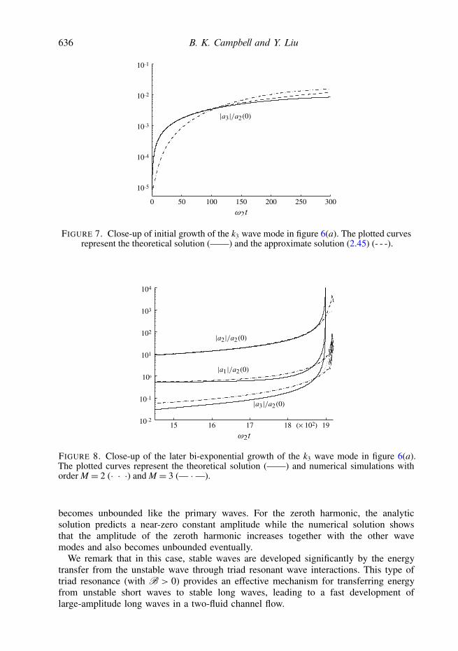
without bound. Figure 6 shows such a sample solution. This solution is obtained withthe same air–water flow as before, but with α = 0.05, k1 = 11, k2 = 12, and k3 = 1,which produces ˆN ' 1.414× 105 and B ' 0.053. At the initial stage of evolution, asthe analysis in § 2.5.2 shows, a2 is dominated by the linear instability effect, and theinitial growth rate of a3 is bi-exponential as shown in figure 7. During the later stageof the evolution, the growth of a2 is accelerated by the third-order self-interactions. Asa result, both a1 and a3 obtain a growth rate even faster than bi-exponential as shownin figure 8. The interacting wave system then quickly blows up. The prediction bydirect numerical simulations compares very well with the theoretical solution until thelate stage of evolution when the interacting waves grow rapidly and become singular.

For the second harmonic of the k2 wave, the analytical solution also agrees wellwith the numerical solution. Both solutions predict that the second harmonic eventually


10–5

10–4

10–3

10–2

10–1

50 100 150 200 2500 300

FIGURE 7. Close-up of initial growth of the k3 wave mode in figure 6(a). The plotted curvesrepresent the theoretical solution (——) and the approximate solution (2.45) (- - -).

104

103

10–2

102

10–1

100

101

15 16 17 18 19(× 102)

FIGURE 8. Close-up of the later bi-exponential growth of the k3 wave mode in figure 6(a).The plotted curves represent the theoretical solution (——) and numerical simulations withorder M = 2 (· · ·) and M = 3 (— ·—).

becomes unbounded like the primary waves. For the zeroth harmonic, the analyticsolution predicts a near-zero constant amplitude while the numerical solution showsthat the amplitude of the zeroth harmonic increases together with the other wavemodes and also becomes unbounded eventually.

We remark that in this case, stable waves are developed significantly by the energytransfer from the unstable wave through triad resonant wave interactions. This type oftriad resonance (with B > 0) provides an effective mechanism for transferring energyfrom unstable short waves to stable long waves, leading to a fast development oflarge-amplitude long waves in a two-fluid channel flow.


4.3. Multiple resonant interactionsRealistic two-fluid flow problems involve a broadbanded spectrum of interfacialwaves that can form multiple coupled triad resonant (and near-resonant) interactions.Moreover, as the interface steepens, higher-order resonant interactions may also play arole. Large-amplitude long waves can be developed due to the combined effects of thelinear instability and multiple resonant interactions. The extension of the theoreticalanalysis in § 2 to include multiple coupled resonant interactions is in principle possible,but not straightforward. The direct numerical simulation developed in § 3 is moreappropriate for these practical cases.

As a numerical example, we consider the growth and time evolution of a large-amplitude long wave that is developed from a smooth interface in a two-phase channelflow. The spectrum shall be broadbanded and contain multiple resonant triads. Thisproblem will approximate the spacial evolution of the first slug developed near theinlet of the two-phase channel flow. While there is a rich collection of laboratoryexperiments in the literature, the vast majority of these tests are carried out usingcylindrical pipe geometries (e.g. Fan et al. 1993). Ideally, comparisons betweennumerical simulations and measurements should be made with identical geometry.However, to obtain an initial estimate, the numerical simulations presented here areperformed using the same flow properties as those in pipe flow experiments.

We choose to compare the direct simulations against the results of Ujang (2003)and Ujang et al. (2006) who carried out experiments of air–water flows througha horizontal 78 mm pipe with different gas/liquid velocities and liquid holdups.We specifically focus on the case of figure 5(c) of Ujang et al. (2006) orfigure 5.3(a) of Ujang (2003) for which the superficial gas and liquid velocitiesUSG ≡ UuAu/Apipe = 4.64 m s−1 and USL ≡ UlAl/Apipe = 0.61 m s−1 with Apipe, Au andAl being the cross-sectional area of the pipe and the areas of the pipe occupied bythe upper and lower fluids, respectively. The gas fraction for the pipe is w 0.4 andthe surface tension coefficient is 0.037 N m−1. In the simulation, the channel depth isset to be equal to the pipe diameter (H = 78 mm) and the void fraction is fixed asα = 0.4. The uniform gas and liquid velocities are Uu = USGApipe/AG = 12.53 m s−1

and Ul = USLApipe/AL = 0.97 m s−1.In the numerical computation, we use L = 0.318 m and T = 0.180 s for

length and time normalization. The length of the (periodic) computational domaincorresponds to a laboratory channel length of 2.0 m. The density ratio is R =1.18× 10−3 and the Weber number is W = 2.67× 104. The simulations are performedwith N = 32 and different orders of nonlinearity (M = 1, 2 and 3). The initialdisturbance on the interface is given by the white noise with a near machine-zeroamplitude of 10−15. We note that in reality, the growth of very short waves arelimited by viscous damping and small-scale wave breaking which are not consideredin the simulation based on the potential flow formulation. Since our purpose is todemonstrate the growth of long waves through multiple/coupled resonant interactionswith short waves, a spectral filtering is applied in the nonlinear simulations (withM = 2 and 3) to limit the maximum steepness of each of the unstable short-wavecomponent (with k > 17) at 0.1 sech(0.05k). This approach was developed by Longuet-Higgins & Cokelet (1976) and Dommermuth & Yue (1987) in the simulation ofnonlinear breaking waves in the ocean.

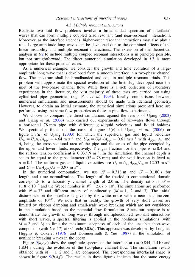
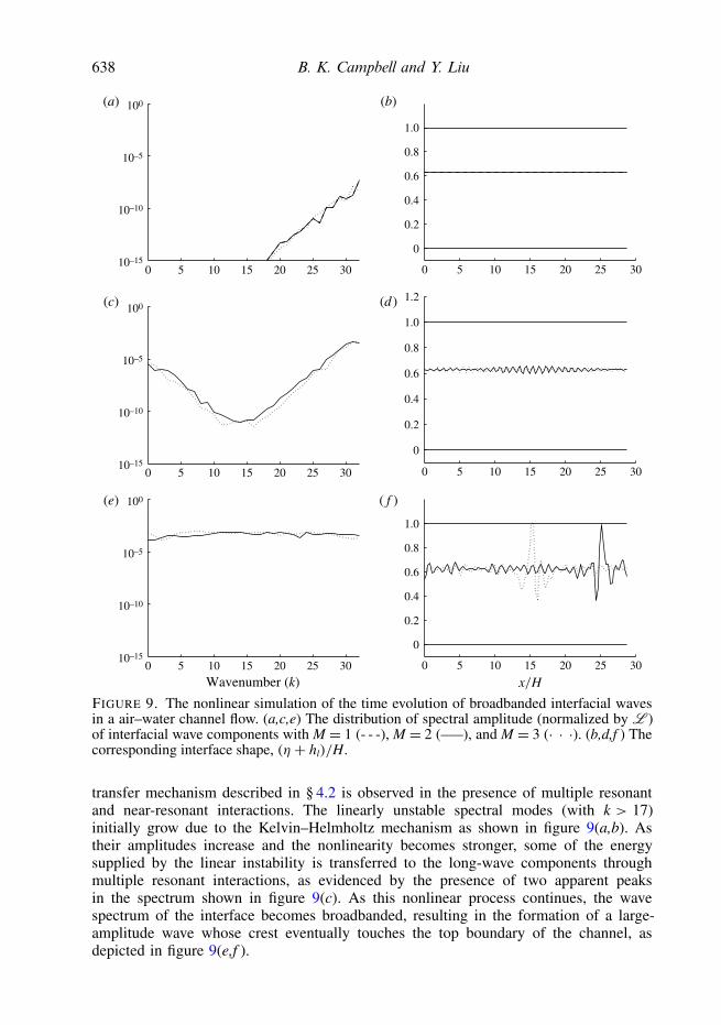
Figure 9(a,c,e) show the amplitude spectra of the interface at t = 0.844, 1.410 and1.834 s during the evolution of the two-phase channel flow. The simulation resultsobtained with M = 1, 2 and 3 are compared. The corresponding interfacial shape isshown in figure 9(b,d,f ). The results in these figures indicate that the same energy


Wavenumber (k)

10–15

10–10

10–5

100

0 5 10 15 20 25 30

10–15

10–10

10–5

100

0 5 10 15 20 25 30

10–15

10–10

10–5

100

0 5 10 15 20 25 30

0 5 10 15 20 25 30

0 5 10 15 20 25 30

5 10 15 20 25

0

0.2

0.4

0.6

0.8

1.0

0

0.2

0.4

0.6

0.8

1.0

1.2

0

0.2

0.4

0.6

0.8

1.0

0 30

(a) (b)

(c) (d )

(e) ( f )

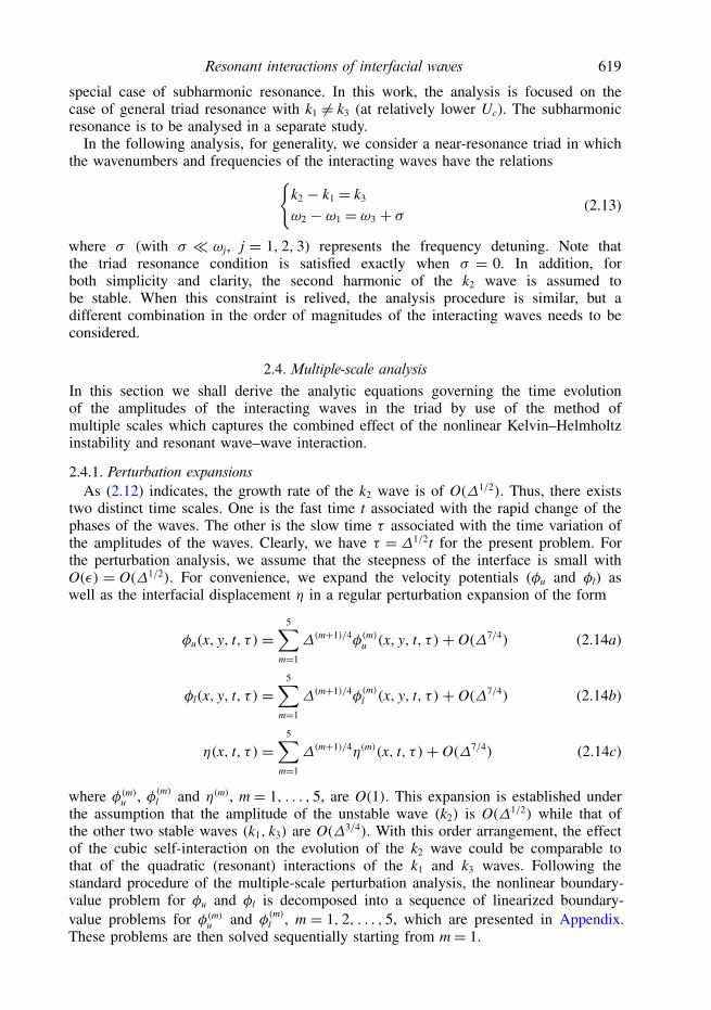
FIGURE 9. The nonlinear simulation of the time evolution of broadbanded interfacial wavesin a air–water channel flow. (a,c,e) The distribution of spectral amplitude (normalized by L )of interfacial wave components with M = 1 (- - -), M = 2 (—–), and M = 3 (· · ·). (b,d,f ) Thecorresponding interface shape, (η + hl)/H.

transfer mechanism described in § 4.2 is observed in the presence of multiple resonantand near-resonant interactions. The linearly unstable spectral modes (with k > 17)initially grow due to the Kelvin–Helmholtz mechanism as shown in figure 9(a,b). Astheir amplitudes increase and the nonlinearity becomes stronger, some of the energysupplied by the linear instability is transferred to the long-wave components throughmultiple resonant interactions, as evidenced by the presence of two apparent peaksin the spectrum shown in figure 9(c). As this nonlinear process continues, the wavespectrum of the interface becomes broadbanded, resulting in the formation of a large-amplitude wave whose crest eventually touches the top boundary of the channel, asdepicted in figure 9(e,f ).


For this case, the interface bridges the channel diameter after t ∼ 1.83 s ofevolution. The width of the large wave disturbance is ∼1.8H. By multiplying this timeby the group velocity of the wave with wavelength of ∼1.8H, where Cg

∼= 1.0 m s−1,we obtain the slug-initiation distance of approximately 1.85 m from the inlet (Gaster1962). The difference in the nonlinear solutions with M = 2 and 3 are small untiltimes just prior to the instant when the long-wave crest touches the top boundary. Thesimulation with M = 1 bridges the channel at much earlier time than the M = 2 and 3cases, thus it is not shown in figure 9(c,f ). This result compares qualitatively well withthe experimental observation of Ujang (2003) who reported that first slugging occurredin the region of 1.46–2.86 m from the inlet. Even though this comparison is only afirst-order estimate, this method appears to consistently reproduce results which havecomparable length and times scales to the cases in figure 5 of Ujang (2003).

5. Conclusions

This paper has considered, both theoretically and computationally, the triad resonantinteractions of interfacial waves, which are influenced by the Kelvin–Helmholtzinterfacial instability, in an inviscid two-fluid incompressible flow through a horizontalchannel. The focus is on the mechanism of energy transfer from unstable shortwaves to stable long waves through nonlinear resonant wave interactions. Based ona multiple-scale analysis, in the context of a potential flow formulation, nonlinearinteraction equations are derived which govern the amplitude evolution of theinteracting waves in a resonant triad, including the effects of interfacial instability.An effective numerical method for direct simulations of nonlinear interfacial waveinteractions is also developed based on a high-order pseudo-spectral approach. Itis used for verification of the theoretical analysis and the examination of practicalapplications involving multiple resonances with a broadbanded spectrum of waves.Cross-validations between the theoretical solutions and direct numerical simulationsare obtained for various characteristic flows considered.

It is found that depending on the flow conditions, there exists an extremely efficientenergy transfer from the base flow to the stable long wave due to the coupled effectsof nonlinear wave resonance and interfacial instability. The growth rate of the longwave can reach up to bi-exponential (or faster). Moreover, in this case, the (linearly)unstable wave can grow unboundedly even when the nonlinear self-interaction effectsare accounted for, as do the stable waves in the resonant triad.

This work shows that the nonlinear coupling of an interfacial instability andnonlinear resonant wave interactions can cause a rapid development of long waves(which are themselves linearly stable). Such a behaviour of long-wave growth bearssimilarities to that of slug formation in stratified channel/pipe flows, as observed inexperiments. This suggests that the nonlinear mechanism found in this study mayplay an important role in slug formation and may improve slug-transition criteria. Asa demonstration, we performed direct numerical simulations of nonlinear two-phasechannel flow evolution involving multiple resonant and near-resonant wave interactions.The predicted slug-initiation length compares qualitatively well with the laboratorymeasurement. The application of the present work to the general multi-phase flowproblem for development of improved slug flow transition criteria, prediction of slugfrequency/length and direct comparisons with experimental measurements is the focusof ongoing research.


AcknowledgementsThis work was financially supported by Chevron Corporation. Their sponsorship is

greatly appreciated. We would also like to thank Dr R. Roberts and Dr K. Hendricksonfor their thoughtful discussions and feedback on the subject.

Appendix. Perturbation equationsBased on the definitions of the two time scales, the differential time operator in

(2.5)–(2.7), ∂/∂t, is replaced by ∂/∂t +∆1/2∂/∂τ , which leads to

∇2φu = 0 (A 1a)

∇2φl = 0 (A 1b)φu,y = 0 (A 1c)

φl,y = 0 (A 1d)

η,t +∆1/2η,τ + [Ul + Uc(1+∆)+ φu,x]η,x − φu,y = 0 (A 1e)

η,t +∆1/2η,τ + (Ul + φl,x)η,x − φl,y = 0 (A 1f )

R

φu,t +∆1/2φu,τ + 1

2φ2

u,x + [Ul + Uc(1+∆)]φu,x + 12φ2

u,y + η

−(φl,t +∆1/2φl,τ + 1

2φ2

u,x + Ulφl,x + 12φ2

l,y + η)+ η,xx (1+ η2

x)−3/2

W= 0. (A 1g)

Expanding (A 1e), (A 1f ) and (A 1g) in Taylor series about the undisturbed interfaceposition and applying (2.14) gives rise to a sequence of governing equations for φ(m)u ,φ(m)l , and η(m), m= 1, . . . , 5:

∇2φ(m)u = 0 (A 2a)

∇2φ(m)l = 0 (A 2b)

φ(m)u,y = 0 (A 2c)

φ(m)l,y = 0 (A 2d)

η(m),t + (Ul + Uc)η(m),x − φ(m)u,y = f (m)1 (A 2e)

η(m),t + Ulη(m),x − φ(m)l,y = f (m)2 (A 2f )

R[φ(m)u,t + (Ul + Uc)φ(m)u,x + η(m)] − [φ(m)l,t + Ulφ

(m)l,x + η(m)] +

η(m),xx

W= f (m)3 . (A 2g)

where f (1)j = 0 and f (2)j = 0, j= 1, 2, 3 and f (m)j for m= 3, 4 and 5 are functions of thelower-order solutions.

The O(∆) problem:

f (3)1 =−η(1),τ − φ(1)u,xη(1),x + η(1)φ(1)u,yy (A 3a)

f (3)2 =−η(1),τ − φ(1)l,x η(1),x + η(1)φ(1)l,yy (A 3b)

f (3)3 = [η(1)φ(1)l,ty + φ(1)l,τ + 12 (φ

(1)l,x )

2+Ulη(1)φ

(1)l,xy + 1

2 (φ(1)l,y )

2]−R[η(1)φ(1)u,ty + φ(1)u,τ + 1

2 (φ(1)u,x)

2+(Ul + Uc)η(1)φ(1)u,xy + 1

2 (φ(1)u,y)

2]. (A 3c)


The O(∆5/4) problem:

f (4)1 =−η(2),τ − η(1),x φ(2)u,x − η(2),x φ(1)u,x + η(1)φ(2)u,yy + η(2)φ(1)u,yy (A 4a)

f (4)2 =−η(2),τ − η(1),x φ(2)l,x − η(2),x φ(1)l,x + η(1)φ(2)l,yy + η(2)φ(1)l,yy (A 4b)

f (4)3 = [η(1)φ(2)l,ty + η(2)φ(1)l,ty + φ(2)l,τ + φ(1)l,x φ(2)l,x + Ul(η

(1)φ(2)l,xy + η(2)φ(1)l,xy)

+φ(1)l,y φ(2)l,y ] −R[η(1)φ(2)u,ty + η(2)φ(1)u,ty + φ(2)u,τ + φ(1)u,xφ

(2)u,x

+ (Ul + Uc)(η(1)φ(2)u,xy + η(2)φ(1)u,xy)+ φ(1)u,yφ

(2)u,y]. (A 4c)

The O(∆3/2) problem:

f (5)1 =−η(3),τ − Ucη(1),x − η(1),x φ(3)u,x − η(3),x φ(1)u,x − η(1)φ(1)u,xyη

(1),x − η(2),x φ(2)u,x

+ η(1)φ(3)u,yy + η(3)φ(1)u,yy + η(2)φ(2)u,yy +12(η(1))

2φ(1)u,yyy (A 5a)

f (5)2 =−η(3),τ − η(1),x φ(3)l,x − η(3),x φ(1)l,x − η(1)φ(1)l,xyη(1),x − η(2),x φ(2)l,x + η(1)φ(3)l,yy

+ η(3)φ(1)l,yy + η(2)φ(2)l,yy +12(η(1))

2φ(1)l,yyy (A 5b)

f (5)3 =[η(1)φ

(3)l,ty + η(3)φ(1)l,ty + η(2)φ(2)l,ty +

12(η(1))

2φ(1)l,tyy + φ(3)l,τ + φ(1)l,x φ

(3)l,x

+ η(1)φ(1)l,x φ(1)l,xy +

12(φ

(2)l,x )

2+Ul

(η(1)φ

(3)l,xy + η(2)φ(2)l,xy + η(3)φ(1)l,xy +

12(η(1))

2φ(1)l,xyy

)+φ(1)l,y φ

(3)l,y + η(1)φ(1)l,y φ

(1)l,yy +

12(φ

(2)l,y )

2]−R

[η(1)φ(3)u,ty + η(3)φ(1)u,ty + η(2)φ(2)u,ty

+ 12(η(1))

2φ(1)u,tyy + φ(3)u,τ + φ(1)u,xφ

(3)u,x + η(1)φ(1)u,xφ

(1)u,xy +

12(φ(2)u,x)

2

+Ucφ(1)u,x(Ul + Uc)(η

(1)φ(3)u,xy + η(2)φ(2)u,xy + η(3)φ(1)u,xy +12(η(1))

2φ(1)u,xyy)+ φ(1)u,yφ

(3)u,y

+ η(1)φ(1)u,yφ(1)u,yy +

12(φ(2)u,y)

2]+ 3

2

(η(1),x )2η(1),xx

W. (A 5c)

R E F E R E N C E S

ALAM, M.-R., LIU, Y. & YUE, D. K. P. 2009 Bragg resonance of waves in a two-layer fluidpropagating over bottom ripples. Part II. Numerical simulation. J. Fluid Mech. 624, 225–253.

BARNEA, D. & TAITEL, Y. 1993 Kelvin–Helmholtz stability-criteria for stratified flow—viscousversus non-viscous (inviscid) approaches. Intl J. Multiphase Flow 19 (4), 639–649.

BENNEY, D. J. 1962 Non-linear gravity wave interactions. J. Fluid Mech. 14 (4), 577–584.BONTOZOGLOU, V. & HANRATTY, T. J. 1990 Capillary gravity Kelvin–Helmholtz waves close to

resonance. J. Fluid Mech. 217, 71–91.CAMPBELL, B. K. 2009 Nonlinear effects on interfacial wave growth into slug flow. Master’s thesis,

Massachusetts Institute of Technology.DOMMERMUTH, D. G. & YUE, D. K. P. 1987 A high-order spectral method for the study of

nonlinear gravity-waves. J. Fluid Mech. 184, 267–288.DRAZIN, P. G. 1970 Kelvin–Helmholtz instability of finite amplitude. J. Fluid Mech. 42, 321–335.FAN, Z., LUSSEYRAN, F. & HANRATTY, T. J. 1993 Initiation of slugs in horizontal gas–liquid

flows. AIChE J. 39 (11), 1741–1753.


FUNADA, T. & JOSEPH, D. D. 2001 Viscous potential flow analysis of Kelvin–Helmholtz instabilityin a channel. J. Fluid Mech. 445, 263–283.

GASTER, M. 1962 A note on the relation between temporally-increasing and spatially-increasingdisturbances in hydrodynamic stability. J. Fluid Mech. 14 (2), 222–224.

JANSSEN, P. 1986 The period-doubling of gravity capillary waves. J. Fluid Mech. 172, 531–545.JANSSEN, P. 1987 The initial evolution of gravity capillary waves. J. Fluid Mech. 184, 581–597.JURMAN, L. A., DEUTSCH, S. E. & MCCREADY, M. J. 1992 Interfacial mode interactions in

horizontal gas–liquid flows. J. Fluid Mech. 238, 187–219.LIN, P. Y. & HANRATTY, T. J. 1986 Prediction of the initiation of slugs with linear-stability theory.

Intl J. Multiphase Flow 12 (1), 79–98.LOESCH, A. Z. 1974 Resonant interactions between unstable and neutral baroclinic waves. 1.

J. Atmos. Sci. 31 (5), 1177–1201.LONGUET-HIGGINS, M. S. 1962 Resonant interactions between two trains of gravity waves. J. Fluid

Mech. 12, 321–332.LONGUET-HIGGINS, M. S. & COKELET, E. E. 1976 The deformation of steep surface waves on

water. I. A numerical method of computation. Proc. R. Soc. Lond. A. 350, 1–26.MANSBRIDGE, J. V. & SMITH, R. K. 1983 On resonant interactions between unstable and neutral

baroclinic waves. J. Atmos. Sci. 40 (2), 378–395.MASLOWE, S. A. & KELLY, R. E. 1970 Finite-amplitude oscillations in a Kelvin–Helmholtz flow.

Intl J. Non-Linear Mech. 5, 427–435.MATA, C., PEREYRA, E., TRALLERO, J. L & JOSEPH, DD 2002 Stability of stratified gas–liquid

flows. Intl J. Multiphase Flow 28 (8), 1249–1268.MCGOLDRICK, L. F. 1965 Resonant interactions among capillary-gravity waves. J. Fluid Mech. 21,

305–331.NAYFEH, A. H. & SARIC, W. S. 1972 Nonlinear waves in a Kelvin–Helmholtz flow. J. Fluid Mech.

55 (SEP26), 311–327.PEDLOSKY, J. 1975 Amplitude of baroclinic wave triads and mesoscale motion in ocean. J. Phys.

Oceanogr. 5 (4), 608–614.PHILLIPS, O. M. 1960 On the dynamics of unsteady gravity waves of finite amplitude. 1. The

elementary interactions. J. Fluid Mech. 9 (2), 193–217.ROMANOVA, N. N. & ANNENKOV, S. Y. 2005 Three-wave resonant interactions in unstable media.

J. Fluid Mech. 539, 57–91.TAITEL, Y. & DUKLER, A. E. 1976 Model for predicting flow regime transitions in horizontal and

near horizontal gas–liquid flow. AIChE J. 22 (1), 47–55.UJANG, P. M. 2003 Studies of slug initiation and development in two-phase gas–liquid pipeline flow.

PhD thesis, University of London.UJANG, P. M., LAWRENCE, C. J., HALE, C. P. & HEWITT, G. F. 2006 Slug initiation and

evolution in two-phase horizontal flow. Intl J. Multiphase Flow 32 (5), 527–552.

Nonlinear resonant interactions of interfacial waves in horizontal stratified channel flows

Documents

Transcript of Nonlinear resonant interactions of interfacial waves in horizontal stratified channel flows