Nordic Concrete Research – Publ. No. NCR 65 – ISSUE 2 / 2021 – Article 4, pp. 63-79

63

© Article authors. This is an open access article distributed under the Creative Commons Attribution-NonCommercial-NoDerivs licens. (http://creaticecommons.org/licenses/by.nc-nd/3.0/).

ISSN online 2545-2819

ISSN print 0800-6377

DOI: 10.2478/ncr-2021-0014

Received: Sept. 10, 2021

Revision received: Nov. 26, 2021

Accepted: Nov. 29, 2021

Nonlinear Analysis of Reinforced Concrete Shear Walls Using Nonlinear Layered Shell Approach

Ali Vatanshenas Doctoral Researcher Faculty of Built Engineering, Tampere University Korkeakoulunkatu 5, 33720, Tampere, Finland ali.vatanshenas@tuni.fi

ABSTRACT This study discusses nonlinear modelling of a reinforced concrete wall utilizing the nonlinear layered shell approach. Rebar, unconfined and confined concrete behaviours are defined nonlinearly using proposed analytical models in the literature. Then, finite element model is validated using experimental results. It is shown that the nonlinear layered shell approach is capable of estimating wall response (i.e., stiffness, ultimate strength, and cracking pattern) with adequate accuracy and low computational effort. Modal analysis is conducted to evaluate the inherent characteristics of the wall to choose a logical loading pattern for the nonlinear static analysis. Moreover, pushover analysis’ outputs are interpreted comprehensibly from cracking of the concrete until reaching the rupture step by step. Key words: Crack, Nonlinear analysis, Pushover analysis, Reinforced concrete wall, Shell.

Nordic Concrete Research – Publ. No. NCR 65 – ISSUE 2 / 2021 – Article 4, pp. 63-79

64

1. INTRODUCTION General-purpose finite element programs like Abaqus, Ansys, etc. try to solve the constitutive relation for each element illustrated in Figure 1 where stresses and strains are related via the stiffness matrix (Equation 1). This approach is complex, time-consuming, and sometimes the results are not as satisfactory as expected. Therefore, a more practical technique like the nonlinear layered shell approach is advantageous.

Figure 1 –3D presentation of stresses acting on a cubic element.

⎣⎢⎢⎢⎢⎡𝜎𝜎11𝜎𝜎22𝜎𝜎33𝜎𝜎23𝜎𝜎13𝜎𝜎12⎦

⎥⎥⎥⎥⎤

�6×1

=

⎣⎢⎢⎢⎢⎡𝐷𝐷11𝐷𝐷21𝐷𝐷31𝐷𝐷41𝐷𝐷51𝐷𝐷61

𝐷𝐷12𝐷𝐷22𝐷𝐷32𝐷𝐷42𝐷𝐷52𝐷𝐷62

𝐷𝐷13𝐷𝐷23𝐷𝐷33𝐷𝐷43𝐷𝐷53𝐷𝐷63

𝐷𝐷14𝐷𝐷24𝐷𝐷34𝐷𝐷44𝐷𝐷54𝐷𝐷64

𝐷𝐷15𝐷𝐷25𝐷𝐷35𝐷𝐷45𝐷𝐷55𝐷𝐷65

𝐷𝐷16𝐷𝐷26𝐷𝐷36𝐷𝐷46𝐷𝐷56𝐷𝐷66⎦

⎥⎥⎥⎥⎤

�������������������������6×6

⎣⎢⎢⎢⎢⎡𝜀𝜀11𝜀𝜀22𝜀𝜀33𝜀𝜀23𝜀𝜀13𝜀𝜀12⎦

⎥⎥⎥⎥⎤

�6×1

(1)

To consider material nonlinearity using the nonlinear layered shell approach, an axial stress-strain backbone curve is required. This curve represents the normal stress-strain relationships in each direction (i.e., σ11-𝜀𝜀 11, σ22-𝜀𝜀 22, and σ33-𝜀𝜀 33). Then, the shear stress-strain curve is obtained automatically using the axial curve assuming that shear behavior is achieved from the compressive and tensile behavior acting at 45° to the material axis Mohr's circle in the plane [1]:

𝜎𝜎𝑖𝑖𝑖𝑖�𝜀𝜀𝑖𝑖𝑖𝑖� = �𝜎𝜎𝑠𝑠ℎ𝑒𝑒𝑒𝑒𝑒𝑒�𝜀𝜀𝑖𝑖𝑖𝑖�, 𝑖𝑖𝑖𝑖 𝜀𝜀𝑖𝑖𝑖𝑖 ≥ 0−𝜎𝜎𝑠𝑠ℎ𝑒𝑒𝑒𝑒𝑒𝑒�−𝜀𝜀𝑖𝑖𝑖𝑖�, 𝑖𝑖𝑖𝑖 𝜀𝜀𝑖𝑖𝑖𝑖 ≤ 0

(2)

𝜎𝜎𝑠𝑠ℎ𝑒𝑒𝑒𝑒𝑒𝑒�𝜀𝜀𝑖𝑖𝑖𝑖� = 0.25[𝜎𝜎𝑡𝑡𝑒𝑒𝑡𝑡𝑠𝑠𝑖𝑖𝑡𝑡𝑡𝑡�𝜀𝜀𝑖𝑖𝑖𝑖� − 𝜎𝜎𝑐𝑐𝑡𝑡𝑐𝑐𝑐𝑐𝑒𝑒𝑒𝑒𝑠𝑠𝑠𝑠𝑖𝑖𝑡𝑡𝑡𝑡�−𝜀𝜀𝑖𝑖𝑖𝑖�], 𝜀𝜀𝑖𝑖𝑖𝑖 = 0.5𝛾𝛾𝑖𝑖𝑖𝑖 ≥ 0, 𝑖𝑖 ≠ 𝑗𝑗 (3)

The axial stress-strain backbone curve which is input can be specified manually based on experiments or from proposed analytical models in the literature. 2. MATERIAL BEHAVIOUR In the following, the formulation of implemented models in this study is presented briefly.

Nordic Concrete Research – Publ. No. NCR 65 – ISSUE 2 / 2021 – Article 4, pp. 63-79

65

2.1 Rebar model Park parametric model is used for estimating the rebars axial stress-strain curve (Figure 2) and is obtained from the following equations.

Figure 2 – Park parametric stress-strain curve [2].

In the elastic domain (ε ≤ εy): 𝑖𝑖 = 𝐸𝐸 𝜀𝜀 (4)

Where E is the modulus of elasticity. In the perfectly plastic domain (εy < ε ≤ εsh): 𝑖𝑖 = 𝑖𝑖𝑦𝑦 (5)

In the strain hardening domain (εsh < ε ≤ εu):

𝑖𝑖 = 𝑖𝑖𝑦𝑦[𝑚𝑚(𝜀𝜀 − 𝜀𝜀𝑠𝑠ℎ) + 260(𝜀𝜀 − 𝜀𝜀𝑠𝑠ℎ) + 2

+(𝜀𝜀 − 𝜀𝜀𝑠𝑠ℎ)(60 −𝑚𝑚)

2(30(𝜀𝜀𝑢𝑢 − 𝜀𝜀𝑠𝑠ℎ) + 1)2] (6)

where m is computed from:

𝑚𝑚 =�𝑖𝑖𝑢𝑢𝑖𝑖𝑦𝑦

� (30(𝜀𝜀𝑢𝑢 − 𝜀𝜀𝑠𝑠ℎ) + 1)2 − 60(𝜀𝜀𝑢𝑢 − 𝜀𝜀𝑠𝑠ℎ) − 1

15(𝜀𝜀𝑢𝑢 − 𝜀𝜀𝑠𝑠ℎ)2 (7)

Nordic Concrete Research – Publ. No. NCR 65 – ISSUE 2 / 2021 – Article 4, pp. 63-79

66

2.2 Concrete model The Mander method is used for approximating concrete’s behavior. The Mander’s model uses two different formulations for confined and unconfined concrete [3].

Unconfined formulation Mander’s unconfined concrete curve is presented in Figure 3. According to this figure, a stress-strain curve is obtained using the equations below.

Figure 3 – Mander’s unconfined parametric stress-strain curve [2].

In the curved domain (ε ≤ 2𝜀𝜀𝑐𝑐′):

𝑖𝑖 =

𝑖𝑖𝑐𝑐′(𝜀𝜀𝜀𝜀𝑐𝑐′

)� 𝐸𝐸

𝐸𝐸 − �𝑖𝑖𝑐𝑐′

𝜀𝜀𝑐𝑐′��

� 𝐸𝐸

𝐸𝐸 − �𝑖𝑖𝑐𝑐′

𝜀𝜀𝑐𝑐′�� − 1 + � 𝜀𝜀𝜀𝜀𝑐𝑐′

�⎝⎜⎛ 𝐸𝐸

𝐸𝐸−�𝑓𝑓𝑐𝑐′

𝜀𝜀𝑐𝑐′�⎠

⎟⎞

(8)

In the linear descending domain (2𝜀𝜀𝑐𝑐′ < ε ≤ εu):

𝑖𝑖 =

2𝑖𝑖𝑐𝑐′ �𝐸𝐸

𝐸𝐸 − �𝑖𝑖𝑐𝑐′

𝜀𝜀𝑐𝑐′�� � 𝜀𝜀𝑢𝑢 − 𝜀𝜀

𝜀𝜀𝑢𝑢 − 2𝜀𝜀𝑐𝑐′�

� 𝐸𝐸

𝐸𝐸 − �𝑖𝑖𝑐𝑐′

𝜀𝜀𝑐𝑐′�� − 1 + 2⎝

⎜⎛ 𝐸𝐸

𝐸𝐸−�𝑓𝑓𝑐𝑐′

𝜀𝜀𝑐𝑐′�⎠

⎟⎞

(9)

Confined formulation Mander’s confined concrete curve is shown in Figure 4. Concerning this figure, a plot is obtained utilizing the equations below.

Nordic Concrete Research – Publ. No. NCR 65 – ISSUE 2 / 2021 – Article 4, pp. 63-79

67

Figure 4 – Mander’s confined parametric stress-strain curve [2].

𝑖𝑖 =𝑖𝑖𝑐𝑐𝑐𝑐′ ( 𝜀𝜀𝜀𝜀𝑐𝑐𝑐𝑐′

) � 𝐸𝐸𝐸𝐸 − 𝐸𝐸𝑠𝑠𝑒𝑒𝑐𝑐

�

� 𝐸𝐸𝐸𝐸 − 𝐸𝐸𝑠𝑠𝑒𝑒𝑐𝑐

� − 1 + ( 𝜀𝜀𝜀𝜀𝑐𝑐𝑐𝑐′)�

𝐸𝐸𝐸𝐸−𝐸𝐸𝑠𝑠𝑠𝑠𝑐𝑐

� (10)

Where 𝜀𝜀𝑐𝑐𝑐𝑐′ is given by:

𝜀𝜀𝑐𝑐𝑐𝑐′ = [5 �𝑓𝑓𝑐𝑐𝑐𝑐′

𝑓𝑓𝑐𝑐′− 1� + 1]𝜀𝜀𝑐𝑐𝑐𝑐′ (11)

All in all, the axial stress-strain curves used for rebar and concrete in this study are presented in Figure 5. As shown in this figure, negligible tensile strength is considered for concrete and strength and ductility of the confined concrete is significantly higher than the unconfined concrete which clarifies the importance of horizontal reinforcements (i.e., ties).

(a) (b)

Nordic Concrete Research – Publ. No. NCR 65 – ISSUE 2 / 2021 – Article 4, pp. 63-79

68

(c)

Figure 5 – Axial stress-strain curves used for a) rebar, b) confined concrete, and c) unconfined concrete.

3. MODELLING In this section, a numerical model of a test conducted by the Institute of Structural Engineering (IBK), ETH Zurich is created based on the results published in the literature. The considered wall in this study is labeled as WSH6 in the literature and has the dimensions of 4560 mm × 2000 mm × 150 mm. A sketch of the test set-up and cross-section configuration is given in Figure 6. The tip of the wall is horizontally pulled and pushed under cyclic static loading conditions. In addition, a vertical load of 1476 kN is applied on top of the wall and kept constant during the test. Further details regarding the test procedure are referred to [4,5].

(a) (b)

Figure 6 – Test specimen’s configuration: a) laboratory test, and b) cross section details (units are in mm) [4].

Nordic Concrete Research – Publ. No. NCR 65 – ISSUE 2 / 2021 – Article 4, pp. 63-79

69

As shown in Figure 7, the model created in this study consists of three rectangular-shaped element mesh parts: Two flange zones and one web zone. Foundation is not modeled, and fixed restraints are assumed at the bottom of the wall. A total number of 648 elements are used where the web and flange zones consist of 360 and 288 elements, respectively. The largest element has the dimensions of 129 mm × 126.7 mm. The flange zones have finer mesh since more critical conditions are expected in those regions. Also, a constant vertical load is divided by the number of joints situated at the top of the model and assigned as point loads.

Figure 7 – Finite element model.

The wall is created as an area section. Area section is decomposable into membrane and plate. Membrane generates in-plane outputs (two translational and one rotational degrees of freedom are involved). Plate simulates out-of-plane response (one translational and two rotational degrees of freedom are involved). The sketch of membrane and plate behaviors is illustrated in Figure 8. Decomposition of the area section into membrane and plate in addition to the understanding of the structural response under a specific loading direction assists us to neglect or simplify the less crucial portions of the area section which end up minimizing the computational effort and time of the analysis. This technique is exploited in the following sections.

Nordic Concrete Research – Publ. No. NCR 65 – ISSUE 2 / 2021 – Article 4, pp. 63-79

70

(a) (b)

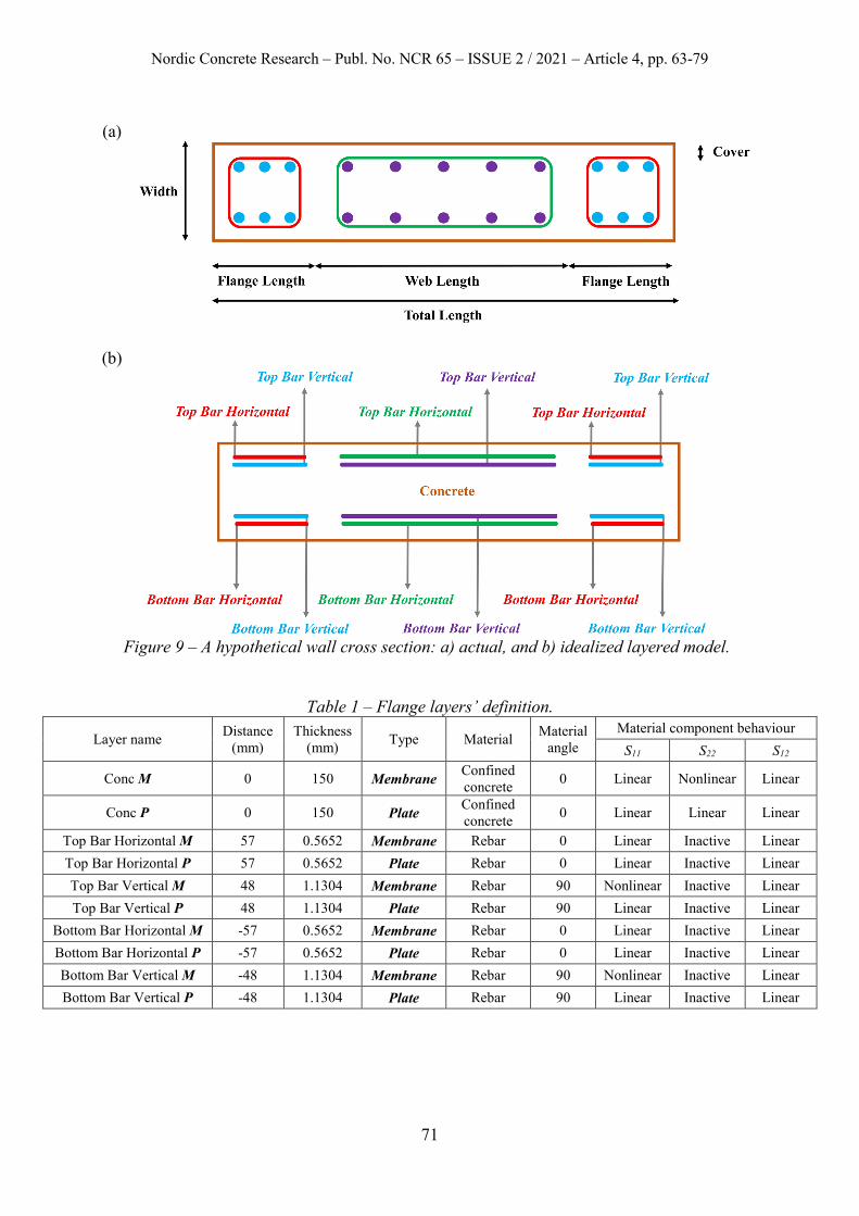
Figure 8 – Area section types’ degrees of freedom: a) membrane, and b) plate. The wall’s heterogeneous section is idealized utilizing a nonlinear layered shell approach. In this method, a hypothetical wall section presented in Figure 9a is idealized by layers corresponding to the area and distance of the elements from the section’s centerline in each portion of the wall section (Figure 9b). The multilayer approach is based on the Timoshenko beam theory assuming small deformations. It considers variation in post-yield bending and the shear via various elements in series. Thorough details and formulation of this method are referenced to [6]. Five layers are considered in the model including top horizontal bars, top vertical bars, concrete, bottom vertical bars, and bottom horizontal bars. According to the wall details given in Figure 6, flange regions provide better confinement for the core concrete, and as a result confined concrete material is only assigned to the flange zones while unconfined concrete material is used for the web section of the wall. It is also possible to add another layer for the cover part of the area sections. However, due to applying less complexity to the model and satisfactory results presented in the next section, this layer is neglected in the modeling. Details regarding layers’ definitions for flange and web area sections are given in Tables 1 and 2, respectively. As shown in the tables, each layer is decomposed into membrane and plate while only membrane parts of the concrete and vertical bars consider material nonlinearity in one direction and other layers are modeled as simplified linear or neglected in the definition. Layers’ definition is achieved based on the direction of loading, engineering judgment, and experience of the designer. If uncertain conditions occur, a fully nonlinear model is recommended. However, it amplifies analysis’ computation effort and duration significantly.

Nordic Concrete Research – Publ. No. NCR 65 – ISSUE 2 / 2021 – Article 4, pp. 63-79

71

(a)

(b)

Figure 9 – A hypothetical wall cross section: a) actual, and b) idealized layered model.

Table 1 – Flange layers’ definition.

Layer name Distance (mm)

Thickness (mm) Type Material Material

angle Material component behaviour

S11 S22 S12

Conc M 0 150 Membrane Confined concrete 0 Linear Nonlinear Linear

Conc P 0 150 Plate Confined concrete 0 Linear Linear Linear

Top Bar Horizontal M 57 0.5652 Membrane Rebar 0 Linear Inactive Linear Top Bar Horizontal P 57 0.5652 Plate Rebar 0 Linear Inactive Linear Top Bar Vertical M 48 1.1304 Membrane Rebar 90 Nonlinear Inactive Linear Top Bar Vertical P 48 1.1304 Plate Rebar 90 Linear Inactive Linear

Bottom Bar Horizontal M -57 0.5652 Membrane Rebar 0 Linear Inactive Linear Bottom Bar Horizontal P -57 0.5652 Plate Rebar 0 Linear Inactive Linear Bottom Bar Vertical M -48 1.1304 Membrane Rebar 90 Nonlinear Inactive Linear Bottom Bar Vertical P -48 1.1304 Plate Rebar 90 Linear Inactive Linear

Nordic Concrete Research – Publ. No. NCR 65 – ISSUE 2 / 2021 – Article 4, pp. 63-79

72

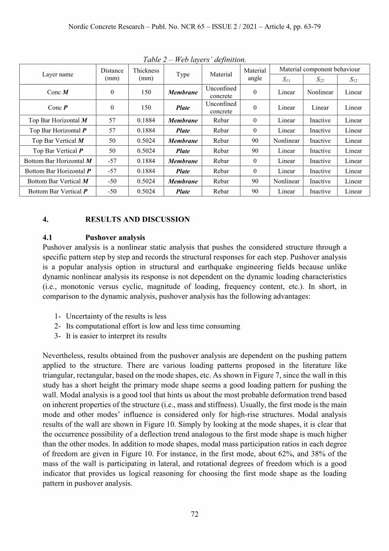
Table 2 – Web layers’ definition.

Layer name Distance (mm)

Thickness (mm) Type Material Material

angle Material component behaviour

S11 S22 S12

Conc M 0 150 Membrane Unconfined concrete 0 Linear Nonlinear Linear

Conc P 0 150 Plate Unconfined concrete 0 Linear Linear Linear

Top Bar Horizontal M 57 0.1884 Membrane Rebar 0 Linear Inactive Linear Top Bar Horizontal P 57 0.1884 Plate Rebar 0 Linear Inactive Linear Top Bar Vertical M 50 0.5024 Membrane Rebar 90 Nonlinear Inactive Linear Top Bar Vertical P 50 0.5024 Plate Rebar 90 Linear Inactive Linear

Bottom Bar Horizontal M -57 0.1884 Membrane Rebar 0 Linear Inactive Linear Bottom Bar Horizontal P -57 0.1884 Plate Rebar 0 Linear Inactive Linear Bottom Bar Vertical M -50 0.5024 Membrane Rebar 90 Nonlinear Inactive Linear Bottom Bar Vertical P -50 0.5024 Plate Rebar 90 Linear Inactive Linear

4. RESULTS AND DISCUSSION 4.1 Pushover analysis Pushover analysis is a nonlinear static analysis that pushes the considered structure through a specific pattern step by step and records the structural responses for each step. Pushover analysis is a popular analysis option in structural and earthquake engineering fields because unlike dynamic nonlinear analysis its response is not dependent on the dynamic loading characteristics (i.e., monotonic versus cyclic, magnitude of loading, frequency content, etc.). In short, in comparison to the dynamic analysis, pushover analysis has the following advantages:

1- Uncertainty of the results is less 2- Its computational effort is low and less time consuming 3- It is easier to interpret its results

Nevertheless, results obtained from the pushover analysis are dependent on the pushing pattern applied to the structure. There are various loading patterns proposed in the literature like triangular, rectangular, based on the mode shapes, etc. As shown in Figure 7, since the wall in this study has a short height the primary mode shape seems a good loading pattern for pushing the wall. Modal analysis is a good tool that hints us about the most probable deformation trend based on inherent properties of the structure (i.e., mass and stiffness). Usually, the first mode is the main mode and other modes’ influence is considered only for high-rise structures. Modal analysis results of the wall are shown in Figure 10. Simply by looking at the mode shapes, it is clear that the occurrence possibility of a deflection trend analogous to the first mode shape is much higher than the other modes. In addition to mode shapes, modal mass participation ratios in each degree of freedom are given in Figure 10. For instance, in the first mode, about 62%, and 38% of the mass of the wall is participating in lateral, and rotational degrees of freedom which is a good indicator that provides us logical reasoning for choosing the first mode shape as the loading pattern in pushover analysis.

Nordic Concrete Research – Publ. No. NCR 65 – ISSUE 2 / 2021 – Article 4, pp. 63-79

73

Mode 1

UX = 0.6246 UZ = 0 Ry = 0.38461

Mode 2 UX = 1.223E-17 UZ = 0.82173 Ry = 3.85E-17

Mode 3 UX = 0.22883 UZ = 1.108E-20 Ry = 0.27262

Mode 4

UX = 0.06217 UZ = 1.094E-16 Ry = 0.10924

Mode 5 UX = 4.007E-17 UZ = 0.09107 Ry = 1.32E-16

Mode 6 UX = 0.01977 UZ = 6.428E-19 Ry = 0.06083

Mode 7

UX = 0.01284 UZ = 1.287E-15 Ry = 0.01849

Mode 8 UX = 4.258E-17 UZ = 9.037E-07 Ry = 5.018E-16

Mode 9 UX = 0.00728 UZ = 8.53E-16 Ry = 0.03452

Figure 10 – Wall mode shapes and their mass participation ratios in X-direction (UX), Z-direction (UZ), and rotation around the out-of-plane axis (Ry).

Nordic Concrete Research – Publ. No. NCR 65 – ISSUE 2 / 2021 – Article 4, pp. 63-79

74

As shown in Figure 11, the moment-displacement curve achieved by the pushover analysis is compared with the test result, and an earlier research [4,7]. The backbone curve of the cyclic test follows a quite similar trend as the estimation graph. Besides, the stiffness and ultimate strength of the wall are approximated properly. However, the model could not estimate the ductility of the wall quite well which might be due to the difference in the type of loading (i.e., cyclic, and monotonic) and simplifications during the modeling (i.e., ignoring bar-slip effects, inactivating some layers, ignoring foundation-wall interaction, etc.).

Figure 11 – comparison of model estimation with test results [4], and previous research

conducted by [7]. In the following, obtained results from the analysis are discussed. Figure 12a presents the same estimation curve as in Figure 11 with the number of steps corresponding to each output. Besides, Figure 12b provides the displacement and input energy mobilization degrees until reaching the last step. As expected, displacement and energy trends increase as the number of steps goes up with a quite similar trend. It is shown that the trend until step 1 has been almost linear. Then, the wall starts showing nonlinear response and reaches its ultimate strength at step 3. Subsequently, softening of the wall starts with a smooth decreasing trend until reaching step 6. Next, a sharp decrease in the strength of the wall is estimated until reaching step 7. Following, a plateau-like path is obtained in the 7-8 loading path. Finally, the wall fails at step 9. Also, note that smaller loading increments are used prior to the abrupt softening behavior (i.e., steps 4,5, and 6).

Nordic Concrete Research – Publ. No. NCR 65 – ISSUE 2 / 2021 – Article 4, pp. 63-79

75

(a) (b)

Figure 12 – Pushover analysis outputs: a) moment-displacement curve including number of steps, and b) normalized displacement and normalized input energy trends obtained from the

pushover analysis. 4.2 Failure sequence An in-depth investigation of the individual layers, failure mechanism, and physical meaning of each step is covered by evaluation of the shell outputs for concrete and rebar layers. Therefore, vertical stresses generated in the concrete and rebar membrane layers are plotted for each step in Figures 13 and 14. By comparing these graphs and stress-strain relations defined in Figure 5 for concrete and rebar, wall response is interpreted step by step:

• Step 1: In this step, both concrete and rebars have not reached their ultimate strengths. However, concrete in the flange region is entered to the nonlinear zone of its stress-strain curve and is expected to crack from the very beginning of the loading. It is obvious from this stage that the most critical zone for concrete and rebars are the lower right and the lower left corners of the model, respectively. Also note that concrete only tolerates negligible tension.

• Step 2: In this step, rebars enter the nonlinear region in tension and concrete keeps cracking. • Step 3: In this step, rebars keep yielding in tension and concrete is very close to failure. This

step is used to compare the crack patterns in the test with the results obtained from the pushover analysis. As shown in Figure 15, the model has been able to simulate the concrete’s crack pattern with adequate accuracy. Note that loading considered in this study is monotonic while it has been cyclic in the experiment. Therefore, the estimation result is comparable to the north direction of the wall in the test.

• Step 4: In this step, concrete in the flange region fails. Consequently, rebars enter the elastoplastic region also in compression.

• Step 5: As shown in Figure 12, this step is located very close to step 4. Therefore, no significant change of behavior in comparison to the previous step is observed.

• Step 6: In this step, rebars reach their ultimate strength in tension and fail. • Steps 7-9: Both concrete and rebars are failed in the critical positions and cannot carry further

loads at those regions. Redistribution of stresses to the adjacent elements is observed. It is fair to say that at these steps, plastic hinges are created, and the structure is laterally unstable. This assumption is observed also in Figure 12, where a sharp decrease in strength and stiffness is obvious after the 6th step. However, the structure might still be capable of carrying a limited vertical load.

Nordic Concrete Research – Publ. No. NCR 65 – ISSUE 2 / 2021 – Article 4, pp. 63-79

76

Step 1 Step 2 Step 3

Step 4 Step 5 Step 6

Step 7 Step 8 Step 9

Figure 13– Stresses generated in the concrete membrane layer in each pushing step (units are in kN/m2).

Nordic Concrete Research – Publ. No. NCR 65 – ISSUE 2 / 2021 – Article 4, pp. 63-79

77

Step 1 Step 2 Step 3

Step 4 Step 5 Step 6

Step 7 Step 8 Step 9

Figure 14– Stresses generated in the top bar’s membrane layer in each pushing step (units are in kN/m2).

Nordic Concrete Research – Publ. No. NCR 65 – ISSUE 2 / 2021 – Article 4, pp. 63-79

78

(a) (b)

Figure 15– Comparison of crack patterns of the considered wall: a) stresses created in the concrete membrane layer in the 3rd step of loading, and b) test results [4].

5. CONCLUSIONS Nonlinear modeling of the structural wall utilizing a nonlinear layered shell approach was conducted in this study. One and two nonlinear materials were defined for the rebars and concrete, respectively. Where confined concrete was only assigned to the flange zones of the wall according to the Mander parametric model. Then, the wall’s heterogenous section was idealized using nonlinear layers. A finite element model was built and validated based on the test available in the literature. The model showed adequate accuracy under static nonlinear (pushover) loading based on the moment-deflection curve and comparison of results with crack pattern in the test. Moreover, interpretation of the failure sequence of the wall was made via evaluation of the stress results of the longitudinal rebars and concrete membrane layers. Progressive failure under the monotonic loading in the horizontal direction is approximated as the following: First, concrete starts cracking from the early stages of loading. Then, rebars yield in tension. Next, concrete in the lower right side of the wall breaks down and rebars start yielding in compression as well. Consequently, rebars in tension lose their strength and the wall becomes horizontally unstable.

Nordic Concrete Research – Publ. No. NCR 65 – ISSUE 2 / 2021 – Article 4, pp. 63-79

79

ACKNOWLEDGEMENT The author acknowledges financial support from Tampere University. REFERENCES 1. Computers and Structures, Inc. (CSI): “Analysis reference manual for SAP2000, ETABS,

and SAFE”. 2016, Berkeley, California, USA. 2. Computers and Structures, Inc. (CSI): “Technical Note Material Stress-strain Curves”.

2008, Berkeley, California, USA. 3. Mander J B, Priestley M J & Park R: “Theoretical stress-strain model for confined

concrete”. Journal of structural engineering, No. 144(8), 1988, pp. 1804-1826. 4. Dazio A, Beyer K & Bachmann H: “Quasi-static cyclic tests and plastic hinge analysis of

RC structural walls”. Engineering Structures, No. 31 (7), 2009, pp. 1556-1571. 5. Dazio A, Wenk T & Bachmann H: “Tests on reinforced concrete structural walls under

cyclic-static impact”. (“Versuche an Stahlbetontragwänden unter zyklisch-statischer Einwirkung”). Birkhäuser (Report), No. 239, 1999. (In German)

6. Belmouden Y & Lestuzzi P: “Analytical model for predicting nonlinear reversed cyclic behaviour of reinforced concrete structural walls”. Engineering Structures, No. 29(7), 2007, pp. 1263-1276.

7. Marzok A, Lavan O & Dancygier A N: “Predictions of moment and deflection capacities of RC shear walls by different analytical models”. Structures, No. 26, 2020, pp. 105-127.