Nonlinear analysis of cantilever shape memory alloy beams of variable cross section

This article has been downloaded from IOPscience. Please scroll down to see the full text article.

2007 Smart Mater. Struct. 16 531

(http://iopscience.iop.org/0964-1726/16/2/035)

Download details:

IP Address: 130.209.6.43

The article was downloaded on 02/12/2009 at 17:44

Please note that terms and conditions apply.

The Table of Contents and more related content is available

HOME | SEARCH | PACS & MSC | JOURNALS | ABOUT | CONTACT US

IOP PUBLISHING SMART MATERIALS AND STRUCTURES

Smart Mater. Struct. 16 (2007) 531–540 doi:10.1088/0964-1726/16/2/035

Nonlinear analysis of cantilever shapememory alloy beams of variable crosssectionMuhammad Ashiqur Rahman1 and Muhammad Arefin Kowser

Department of Mechanical Engineering, Bangladesh University of Engineering andTechnology, Dhaka 1000, Bangladesh

E-mail: ashiq@me.buet.ac.bd

Received 19 June 2006, in final form 12 December 2006Published 5 March 2007Online at stacks.iop.org/SMS/16/531

AbstractCantilever beams, made of shape memory alloy (SMA), undergo much largerdeflection in comparison to those made of other materials. Again, cantileverbeams with reducing cross section along the span show much largerdeflections compared to those of constant cross section beams. Analysis wasconducted for such a cantilever beam with reducing cross-sectional areamade of SMA, taking into account its highly nonlinear stress–strain curves.A computer code in C has been developed using the Runge–Kutta techniquefor the purpose of simulation. For rigorous analysis, the true stress–straincurves in tension as well as in compression have been used for the study.Moment–curvature and reduced modulus–curvature relations are obtainedfrom the nonlinear stress–strain relations for different sections of the beamand used in the simulation. It is seen that load–deflection curves are initiallylinear but nonlinear and convex upward at a high load. Furthermore, thecompressive stress in the beam is significantly higher than the tensile stressbecause of asymmetry. Interestingly, for the different cases considered, it isfound that part of the SMA beam material may remain in the parent austenitephase, mixed phase or in the stress-induced martensitic phase. Importantly, itis found that more material can be removed from an SMA beam of uniformstrength, originally designed without considering geometric nonlinearity andthe effect of end-shortening. Comparison of the numerical results with theavailable theory shows very good agreement, verifying the soundness of theentire numerical simulation scheme.

Nomenclature

b0, b width of the beam at fixed end and at anypoint on its span

E Young’s modulus for the beam materialE ′′ reduced modulus of elasticity for the beam materialh height of the beamh1 distance from the neutral axis to the lower surface

of beamh2 distance from the neutral axis to the upper surface

of beam

1 Author to whom any correspondence should be addressed.

I0, I area moment of inertia at the fixed end and atany point x

L length of the beamM, Mb bending momentsP tip loads curved length of beamx horizontal distance measured from the fixed endX H , X L upper and lower limits of xy elastic curve’s deflectionZ section modulus of beamδ tip deflectionδh end-shorteningε elongation in the fiber

0964-1726/07/020531+10$30.00 © 2007 IOP Publishing Ltd Printed in the UK 531

M A Rahman and M A Kowser

ε1 elongation in the extreme fiber in the convex sideε2 elongation in the extreme fiber in the concave sideρ radius of curvature of elastic curve� |ε1| + |ε2|σ stress

1. Introduction

Studies of modern adaptive structural elements are challengingas they often involve nonlinear (both geometric and material)analysis. This is because such elements (for example, beam orcolumn, especially in adaptive structures) often undergo verylarge deflections during their applications. Again, cantileverbeams are often made lighter by removing extra material fromthem, mainly for economy and space constraints. The mostcommon example is the classical leaf springs that are designedfor uniform strength. Moreover, slots/openings are also madeby removing material from them (Rahman et al 2005a, 2006a).The present study concentrates on the response of such acantilever beam made of shape memory alloy (SMA) withvariable cross-sectional area under a tip load. This studywould be especially important since SMA itself is one ofthe most widely used functional materials in many adaptivestructures as well as in medical and biomedical applications.Superelastic SMAs can recover extremely large strains whenthey are unloaded. They, however, possess highly nonlinearstress–strain relations, with inherent asymmetry in tension andcompression (Rahman 2001, Orgeas and Favier 1995, Rahmanand Tani 2006 and Rahman and Khan 2006).

That the topic of cantilever beams is always interestingcan be seen from the huge number of studies reported in theliterature. Those studies deal mainly with the large deflectionanalysis of cantilever beams made of conventional engineeringmaterials; out of those researches only a few relevant to thepresent study are discussed below followed by discussions onSMA beams and columns.

Bele’ndez et al (2005) carried out numerical simulationusing the Runge–Kutta–Felhberg method to find the tipdeflection of a very slender beam under a combined load. Theauthors studied the large deflections of a uniform cantileverbeam under the action of a combined load consisting ofan external vertical concentrated load at the free end and auniformly distributed load and compared the numerical resultswith the experimental ones. Young’s modulus for the beammaterial was calculated by comparing the numerical resultswith the experimental ones. We took the opportunity to cross-check the soundness of our numerical scheme by comparingthe available experimental results of Bele’ndez et al (2005).

Rahman et al (2006a) carried out extensive numericalsimulations for studying the response of a slender cantileverbeam with an opening of different shapes (circle, ellipse andsquare slots). It was found that the elliptic holes developthe minimum stresses and deflections. Rahman et al (2005a)also performed tests to verify the soundness of the numericalresults obtained considering varying cross sections because ofa circular hole.

Studies on the bending of the SMA beams/columns arealso reported in the literature. Investigations of the bendingproblems of pseudoelastic beams were initiated by Atanakovicand Achenbach (1989), where the explicit analytical moment

0

500500

10001000

15001500

20002000

0 0.05 0.1 0.0.1515 0.0.2TrTrue Strain

Tru

e S

trtres

s ss (

MP

a)

Compression

Tension

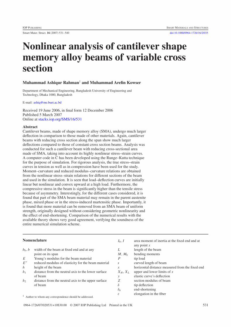
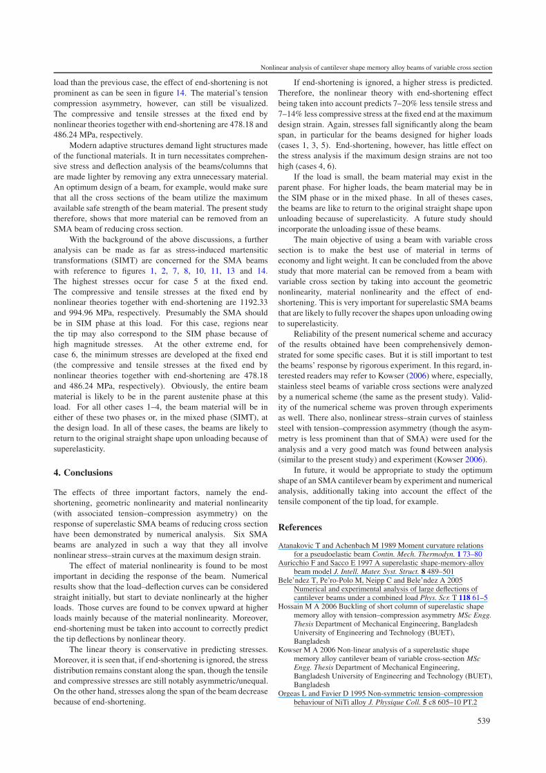
Figure 1. Experimental stress–strain curves for superelastic SMA:experiment done on a 2 mm diameter rod (Rahman 2001).

curvature relation was derived for rectangular beams loaded bya single pulse moment.

Raniecki et al (2001) studied the variation of stress andthe phase content distribution in an arbitrary symmetric crosssection of the beam for a single bending cycle and derivedthe explicit analytical equations for the moment–curvaturehysteresis loop.

By numerical simulation, Auricchio and Sacco (1997)demonstrated that for pure bending of a Nitinol superelasticSMA beam, with different properties in tension andcompression, the axial strain has a non-monotonic responsewith the bending moment during loading and unloading. Thecomplicated movement of the neutral axis of the cross sectionof the beam due to stress-induced martensitic transformation(SIMT) leads to such a peculiar response.

More recent studies regarding the bending of pseudoelas-tic SMA beams are reported by Rejnar et al (2002).

Since SMA is a widely used structural element(column/shaft), the phenomena of buckling of pseudoelasticSMA columns and shafts have also been extensivelydemonstrated by Rahman et al (2001, 2005b, 2006b).Furthermore, Rahman et al (2006c) also studied the bucklingof the stainless steel columns. Experiments were conductedand later a numerical simulation was carried out in orderto analyze the observed buckling and postbuckling behaviorfor the columns. Precise and quantitative analyses of theresults verify the fact that the material’s σ–ε properties, bothin tension and compression, are attributed to the column’sbuckling behavior. Obviously, elastic bending analysis (basedon Hooke’s law) is not sufficient for the SMA beam that hashighly nonlinear σ–ε relations (figure 1). Moreover, for a highintensity load, rigorous σ–ε curves in tension and compressionshould be used for analysis, as pointed by Rahman (2001).Very recently, Hossain (2006) investigated the buckling ofshort SMA columns and compared the results with those fromTimoshenko’s method (Timoshenko and Gere 1981).

It was concluded from our previous studies that thebest results from numerical simulation would be possible,particularly for the short SMA columns, if both the tensileand compressive σ–ε curves can be considered simultaneously(Rahman et al 2005b).

Therefore, the present study is based on simultaneous useof the tension–compression curves of the SMA, as found by

532

Nonlinear analysis of cantilever shape memory alloy beams of variable cross section

Figure 2. Idealized stress–strain diagram of the superelastic SMA.

Rahman (2001) and reproduced in figure 1. The compositionof superelastic SMA rods is as follows: Ti 49.3 at.%,Ni 50.2 at.%, V 0.5 at.%. The diameter of the SMArod is 2 mm and the SMA’s transformation temperaturesare −59 ◦C, −34 ◦C, −27 ◦C and −3 ◦C for the martensitefinish, martensite start, austenite start and austenite finish,respectively. The average measured Young’s modulus for theparent phase was 65 GPa (Rahman 2001).

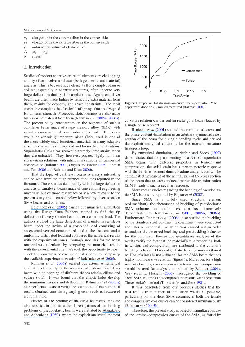
At this point, it is relevant to give a brief description ofsuperelasticity, shown in terms of the σ–ε diagram in figure 2.The phase transformation (from austenite to martensite or viceversa) is typically marked by four transition temperatures,namely martensite finish (Mf), martensite start (Ms), austenitefinish (Af), and austenite start (As). For the SMA used in thisstudy, Mf < Ms < As < Af. For T > Af, the SMA existsin the parent austenite phase. Under mechanical loading thestress-induced martensitic transformation (SIMT) starts whena critical stress is exceeded. When SIMT is over the SMAexists in the stress-induced martensite (SIM) phase. This SIMphase is, however, unstable in the absence of stress at thistemperature. Consequently, during unloading the initiationof reverse phase transformation is marked by another criticalstress. When this reverse SIMT is complete the SMA returnsto its parent austenite phase. The complete loading–unloadingcycle shows a typical hysteresis loop (figure 2) known aspseudoelasticity. It can be noted that the SIMT and the reverseSIMT are marked by a reduction of the material stiffness(figure 2).

In this study simulations were conducted for a cantileverbeam with varying cross-sectional area, made of superelasticSMA. The varying cross section was due to reducing widthwith constant height along the span, in order to make thebeam theoretically of uniform strength. This point wasnot considered in the previous studies by other researchers.Moreover, rigorous stress–strain curves for SMA obtained byuniaxial tension and compression tests have been used, withoutany idealization. Furthermore, since SMA beams can undergovery large deflections, this study also incorporates geometricnonlinearity in the analysis.

2. Mathematical analysis

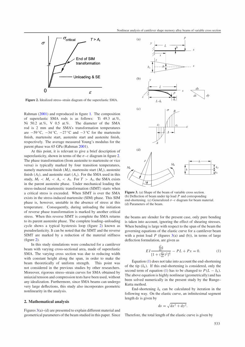
Figures 3(a)–(d) are presented to explain different material andgeometrical parameters of the beam studied in this paper. Since

(c)

(d)

(b)

(a)

Figure 3. (a) Shape of the beam of variable cross section.(b) Deflection of beam under tip load P and correspondingend-shortening. (c) Generalized σ–ε diagram for beam material.(d) Parameters of the beam.

the beams are slender for the present case, only pure bendingis taken into account, ignoring the effect of shearing stresses.When bending is large with respect to the span of the beam thegoverning equations of the elastic curve for a cantilever beamwith a point load P (figures 3(a) and (b)), in terms of largedeflection formulation, are given as

E Id2 ydx2

[1 + (dydx )2] 3

2

− P L + Px = 0. (1)

Equation (1) does not take into account the end-shorteningof the tip (δh). If this end-shortening is considered, only thesecond term of equation (1) has to be changed to P(L − δh).The above equation is highly nonlinear (geometrically) and hasbeen solved numerically in the present study by the Runge–Kutta method.

End-shortening δh can be calculated by iteration in thefollowing way. On the elastic curve, an infinitesimal segmentlength ds is given by

ds = √dx2 + dy2.

Therefore, the total length of the elastic curve is given by

533

M A Rahman and M A Kowser

s =∫ xH

xL

√dx2 + dy2

=∫ xH

xL

√

1 +(

dy

dx

)2

dx (2)

where X H = L − δh and X L = 0.With the assumption of linear elastic behaviour, δh is

calculated numerically by trial. At first, the elastic curve isevaluated from the solution of equation (1) without consideringδh . Next, assuming the value of X H = L − δh , in such away that the integral of equation (2) becomes s ≈ L , it canbe said that δh = L − X H . In this study δh was calculatedwith the following convergence criteria, L � s � 0.998L .Next, putting the value of δh in equation (1) of the elastic curve,deflections at corresponding loads can be found. Alternatively,at first a small value of δh is assumed and equation (1) is solved.Once the elastic curve is known, equation (2) is integratednumerically by Simpson’s 3/8th rule to check whether theassumed value of δh is accurate or needs to be improvedby the next step. Therefore, in order to take into accountthe end-shortening, equations (1) and (2) have to be solvedsimultaneously.

Next, design parameters based on classical linear theory,for the beams of uniform strength, are given by the followingequations

M

Z= 6P L

b0h2= 6P(L − x)

bh2(3)

in which b0 is the width of the beam at the built-in end. Then,

b = b0(L − x)

L. (4)

Since the section modulus (Z) and moment of inertiaof a beam of triangular shape change with x in the sameproportion as the bending moment, the maximum stress andthe curvature remain constant along the beam (figure 3(a)).Therefore, the deflection of the beam at the end, of course,without considering the end-shortening, is

δ = 1

2

P L3

E I0(5)

where, I0 = b0h3

12 represents the moment of inertia of the crosssection at the built-in end.

Though the solution for tip-deflection from equation (5)is exact and readily available, extensive numerical analysisis involved to get the solutions from the highly nonlinearequations (1) and (2). In particular, the end-shortening needsto be calculated by iterations, during numerical simulations.

More importantly, since for the present study the stress isfar beyond the proportional limit and the cross section variesalong the span, the stiffness (E I ) in equation (1) also becomesvariable at the grid points. The following section describes indetail the strategy to tackle the material nonlinearity for purebending of such a beam.

2.1. Analysis of the inelastic deformation of the beam(Timoshenko and Gere 1981)

The theory is based upon the assumption that the crosssection of the beam remains plane during bending and hence

longitudinal strains are proportional to their distance from theneutral surface. Let us assume that the same relation existsbetween stress and strain as represented by the diagram offigure 3(c).

With reference to figure 3(d), the radius of curvature of theneutral surface produced by the bending moment M is equal toρ. In such a case the unit elongation of a fiber at distance yfrom the neutral surface is

ε = y

ρ. (6)

Denoting by h1 and h2 the distance from the neutral axisto the lower and upper surfaces of the beam, respectively, theelongations in the extreme fibers are

ε1 = h1

ρε2 = −h2

ρ. (7)

It is seen that the elongation or contraction of any fiber isreadily obtained provided we know the position of the neutralaxis and the radius of curvature ρ. These two quantities can befound from the following two equations of static equilibrium

∫σ dA = b

∫ h1

−h2

σ dy = 0 (8)

∫σ y dA = b

∫ h1

−h2

σ y dy = Mb. (9)

Equation (8) is now used for determining the position ofthe neutral axis. From equation (6) we have

y = ρε dy = ρ dε. (10)

Substituting into equation (8) we obtain∫ h1

−h2

σ dy = ρ

∫ ε1

ε2

σ dε = 0. (11)

Hence, the position of the neutral axis is such that theintegral vanishes. The integral can be represented by the areaunder the σ–ε diagram (figure 3(c)) from ε2 to ε1. Now wedefine � as the sum of the absolute values of the maximumelongation and maximum contraction, which is

� = ε1 − ε2 =∣∣∣∣h1

ρ

∣∣∣∣ +

∣∣∣∣h2

ρ

∣∣∣∣ = h

ρ. (12)

In calculating the radius of curvature ρ we use equation (9)in the following form

bρ2∫ ε1

ε2

σε dε = Mb. (13)

Next, by observing that ρ = h�

and E ′′ Iρ

= Mb we get

E ′′ = 12

�3

∫ ε1

ε2

σε dε. (14)

The integral in equations (13) and (14) represents themoment of the area under the σ–ε diagram from ε2 to ε1 withrespect to the vertical axis as shown in figure 3(c). Of course,for numerical simulation we used experimental σ–ε curves(figure 1) in place of the fictitious figure 3(c). Once the M–� and E ′′–� curves are known equations (1) and (2) can besolved, replacing the stiffness parameter E I by its appropriatevalues at different grid points.

534

Nonlinear analysis of cantilever shape memory alloy beams of variable cross section

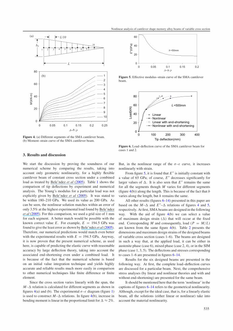
(b)

(a)

Figure 4. (a) Different segments of the SMA cantilever beam.(b) Moment–strain curve of the SMA cantilever beam.

3. Results and discussion

We start the discussion by proving the soundness of ournumerical scheme by comparing the results, taking intoaccount only geometric nonlinearity, for a highly flexiblecantilever beam of constant cross section under a combinedload as treated by Bele’ndez et al (2005). Table 1 shows thecomparison of tip deflections by experiment and numericalanalysis. The Young’s modulus for a particular load was notexplicitly given by Bele’ndez et al (2005). It was stated tobe within 180–210 GPa. We used its value as 200 GPa. Ascan be seen, the nonlinear solution matches within an error ofonly 3.5% at the highest experimental load found by Bele’ndezet al (2005). For this comparison, we used a grid size of 1 mmfor each segment. A better match would be possible with theknown correct value E . For example, E = 194.5 GPa wasfound to give the least error as shown by Bele’ndez et al (2005).Therefore, our numerical predictions would match even betterwith the experimental results with E = 194.5 GPa. Anyway,it is now proven that the present numerical scheme, as usedhere, is capable of predicting the elastic curve with reasonableaccuracy by large deflection theory, taking into account theassociated end-shortening even under a combined load. Itis because of the fact that the numerical scheme is basedon an initial value integration technique and yields highlyaccurate and reliable results much more easily in comparisonto other numerical techniques like finite difference or finiteelement.

Since the cross section varies linearly with the span, theM–� relation is calculated for different segments as shown infigures 4(a) and (b). The experimental σ–ε diagram (figure 1)is used to construct M–� relations. In figure 4(b), increase inbending moment is linear in the proportional limit for � ≈ 2%.

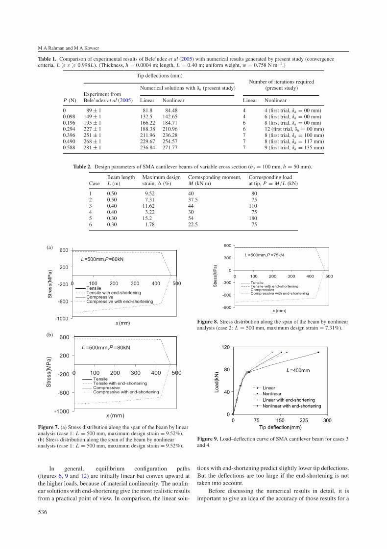
Figure 5. Effective modulus–strain curve of the SMA cantileverbeam.

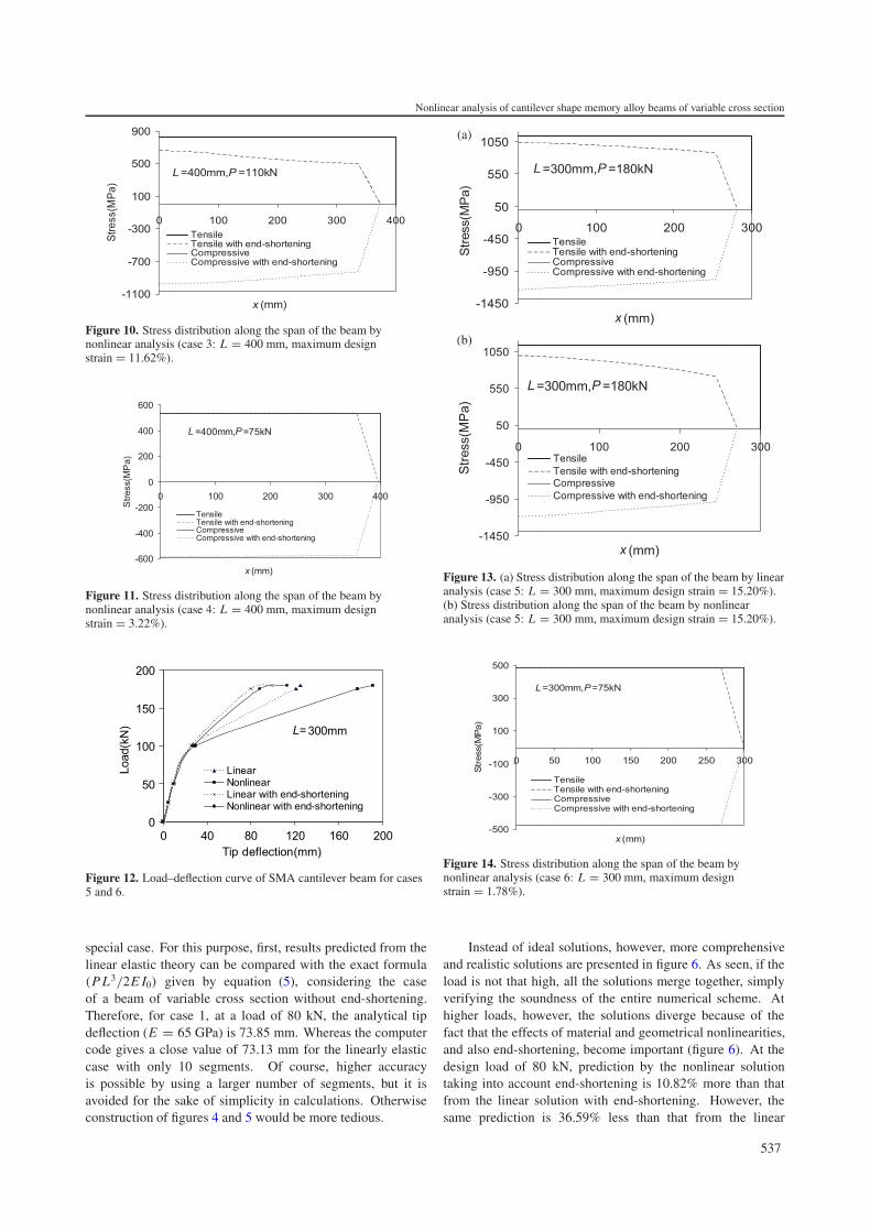
Figure 6. Load–deflection curve of the SMA cantilever beam forcases 1 and 2.

But, in the nonlinear range of the σ–ε curve, it increasesnonlinearly with strain.

From figure 5, it is found that E ′′ is initially constant witha value of 65 GPa; of course, E ′′ decreases significantly forlarger values of �. It is also seen that E ′′ remains the samefor all the segments though M varies for different segments(figure 4(b)) along the length. This is because of the fact that bvaries along the length, but h remains the same.

All other results (figures 6–14) presented in this paper arebased on the M–� and E ′′–� relations of figures 4 and 5,respectively. At first, SMA beams are designed in the followingway. With the aid of figure 4(b) we can select a valueof maximum design strain (�) that will occur at the fixedend. Corresponding M and consequently, load (P = M/L)

are known from the same figure 4(b). Table 2 presents thedimensions and maximum design strains of the designed beamsof variable cross section (cases 1–6). The beams are designedin such a way that, at the applied load, it can be either inaustenite phase (case 6), mixed phase (case 2, 4), or in the SIMphase (case 1, 3, 5). The deflections and stresses correspondingto cases 1–6 are presented in figures 6–14.

Results for the six designed beams are presented in thefollowing way. At first, the complete load–deflection curvesare discussed for a particular beam. Next, the comprehensivestress analyses (by linear and nonlinear theories and with andwithout end-shortening) are presented for the same beam.

It should be mentioned here that the term ‘nonlinear’ in thecaptions of figures 6–14 refers to the geometrical nonlinearity.Although, except for the ideal case, that is, for a linearly elasticbeam, all the solutions (either linear or nonlinear) take intoaccount the material nonlinearity.

535

M A Rahman and M A Kowser

Table 1. Comparison of experimental results of Bele’ndez et al (2005) with numerical results generated by present study (convergencecriteria, L � s � 0.998L). (Thickness, h = 0.0004 m; length, L = 0.40 m; uniform weight, w = 0.758 N m−1.)

Tip deflections (mm)Number of iterations required

Numerical solutions with δh (present study) (present study)Experiment from

P (N) Bele’ndez et al (2005) Linear Nonlinear Linear Nonlinear

0 89 ± 1 81.8 84.48 4 4 (first trial, δh = 00 mm)0.098 149 ± 1 132.5 142.65 4 6 (first trial, δh = 00 mm)0.196 195 ± 1 166.22 184.71 6 8 (first trial, δh = 00 mm)0.294 227 ± 1 188.38 210.96 6 12 (first trial, δh = 00 mm)0.396 251 ± 1 211.96 236.28 7 8 (first trial, δh = 100 mm)0.490 268 ± 1 229.67 254.57 7 8 (first trial, δh = 117 mm)0.588 281 ± 1 236.84 271.77 7 9 (first trial, δh = 135 mm)

Table 2. Design parameters of SMA cantilever beams of variable cross section (b0 = 100 mm, h = 50 mm).

Beam length Maximum design Corresponding moment, Corresponding loadCase L (m) strain, � (%) M (kN m) at tip, P = M/L (kN)

1 0.50 9.52 40 802 0.50 7.31 37.5 753 0.40 11.62 44 1104 0.40 3.22 30 755 0.30 15.2 54 1806 0.30 1.78 22.5 75

(a)

(b)

Figure 7. (a) Stress distribution along the span of the beam by linearanalysis (case 1: L = 500 mm, maximum design strain = 9.52%).(b) Stress distribution along the span of the beam by nonlinearanalysis (case 1: L = 500 mm, maximum design strain = 9.52%).

In general, equilibrium configuration paths(figures 6, 9 and 12) are initially linear but convex upward atthe higher loads, because of material nonlinearity. The nonlin-ear solutions with end-shortening give the most realistic resultsfrom a practical point of view. In comparison, the linear solu-

Figure 8. Stress distribution along the span of the beam by nonlinearanalysis (case 2: L = 500 mm, maximum design strain = 7.31%).

Figure 9. Load–deflection curve of SMA cantilever beam for cases 3and 4.

tions with end-shortening predict slightly lower tip deflections.But the deflections are too large if the end-shortening is nottaken into account.

Before discussing the numerical results in detail, it isimportant to give an idea of the accuracy of those results for a

536

Nonlinear analysis of cantilever shape memory alloy beams of variable cross section

Figure 10. Stress distribution along the span of the beam bynonlinear analysis (case 3: L = 400 mm, maximum designstrain = 11.62%).

Figure 11. Stress distribution along the span of the beam bynonlinear analysis (case 4: L = 400 mm, maximum designstrain = 3.22%).

Figure 12. Load–deflection curve of SMA cantilever beam for cases5 and 6.

special case. For this purpose, first, results predicted from thelinear elastic theory can be compared with the exact formula(P L3/2E I0) given by equation (5), considering the caseof a beam of variable cross section without end-shortening.Therefore, for case 1, at a load of 80 kN, the analytical tipdeflection (E = 65 GPa) is 73.85 mm. Whereas the computercode gives a close value of 73.13 mm for the linearly elasticcase with only 10 segments. Of course, higher accuracyis possible by using a larger number of segments, but it isavoided for the sake of simplicity in calculations. Otherwiseconstruction of figures 4 and 5 would be more tedious.

(a)

(b)

Figure 13. (a) Stress distribution along the span of the beam by linearanalysis (case 5: L = 300 mm, maximum design strain = 15.20%).(b) Stress distribution along the span of the beam by nonlinearanalysis (case 5: L = 300 mm, maximum design strain = 15.20%).

Figure 14. Stress distribution along the span of the beam bynonlinear analysis (case 6: L = 300 mm, maximum designstrain = 1.78%).

Instead of ideal solutions, however, more comprehensiveand realistic solutions are presented in figure 6. As seen, if theload is not that high, all the solutions merge together, simplyverifying the soundness of the entire numerical scheme. Athigher loads, however, the solutions diverge because of thefact that the effects of material and geometrical nonlinearities,and also end-shortening, become important (figure 6). At thedesign load of 80 kN, prediction by the nonlinear solutiontaking into account end-shortening is 10.82% more than thatfrom the linear solution with end-shortening. However, thesame prediction is 36.59% less than that from the linear

537

M A Rahman and M A Kowser

solution and 126.5% less than that from the nonlinear solutionif the effect of end-shortening is ignored.

Regarding the presentation style of the stresses, we preferto use x on the abscissa for figures 7, 8, 10, 11, 13 and 14.x has been defined in figure 3 as the horizontal distance of apoint on the elastic curve, measured from the fixed end. Forclarity, x = X H corresponds to the projection of the deflectedelastic curve’s tip on the x axis. The advantage of stressversus x curve is that one can get an idea of end-shorteningdirectly. Nonlinear stress analyses are presented for all sixcases considered. But, to keep the volume a minimum, linearsolutions of stresses are presented only for case 1 (figures 7(a)and (b)) and case 5 (figures 13(a) and (b)). Interested readersmay refer to Kowser (2006) for the rest of the linear solutions.Generally, tension–compression asymmetry is prominent forall the cases considered: the higher the design strains, themore prominent is the asymmetry. Another distinguishingfeature is the fall of stress along the beam span, the higheststress being at the fixed end; in contrast, a classical leaf springunder ideal conditions should develop uniform stresses alongall its span. Moreover, nonlinear solutions with end-shorteningpredict the stresses that are significantly smaller than thosepredicted without taking into account end-shortening. Linearsolutions slightly over-predict the stresses in comparison to thenonlinear solutions.

It has already been mentioned that for the ideal case, that isfor linear theory, elastic material and ignoring the effect of end-shortening, a beam with linearly reducing cross section shoulddevelop equal stress all along its span. In order to visualizethe real situations, however, figures 7(a) and (b) show thestress distributions for the geometrically linear and nonlinearcases, respectively. First of all it is clear that the tensileand compressive stresses are highly asymmetric (figures 7).Moreover, if end-shortening is ignored, both geometricallylinear and nonlinear cases predict the same solutions of stresses(either tensile or, compressive) for the cantilever beams. Onthe other hand, stress decreases along the span of the beammainly because of end-shortening. It is found that compressivestress falls more significantly than the tensile stress because ofasymmetry in the stress–strain relations.

From linear analysis (figure 7(a)), at fixed end the tensileand compressive stresses without end-shortening are foundto be 601.20 and 947.90 MPa, respectively. But, with end-shortening the tensile and compressive stresses are 558.91 and854.64 MPa, respectively. With end-shortening, at the last gridpoint (x = 425.34 mm) the tensile and compressive stressesare 539.72 and 655.20 MPa, respectively (tensile stress andcompressive stress are 10.23% and 30.84% less, respectively,than the corresponding stresses found without end-shortening).

Again by nonlinear analysis considering end-shortening,tensile and compressive stresses at the fixed end are,respectively, 557.12 and 847.69 MPa as shown in figure 7(b).At the last grid point (at x = 422.19 mm) these tensile andcompressive stresses are 543.26 and 705.18 MPa, respectively.

Figure 8, for case 2, shows the stress distribution alongthe span of the beam at a load of 75 kN. Since the beamparameters are the same as those of case 1 except for the load,the corresponding point (on the equilibrium configuration path)can be located in figure 6. The stress pattern as shown infigure 8 is similar to, but of lower magnitude than, that of case 1

(figure 7). The compressive and tensile stresses at the fixed endby nonlinear theories together with end-shortening are 778.19and 549.21 MPa, respectively.

For case 3, figure 9 shows that at the design loadof 110 kN, if end-shortening is taken into account the tipdeflection predicted by nonlinear solution is 19.32% more thanthat found by linear solution.

Figure 10 shows the stress distribution along the span ofthe beam for case 3 at a load of 110 kN. The compressiveand tensile stresses at the fixed end by nonlinear theoriestogether with end-shortening are 978.55 and 661.48 MPa,respectively. Because of a higher load than those for cases1 and 2, the tension–compression asymmetry of the stressesis quite prominent. Also stresses decrease quite significantlyalong the span.

Figure 11 presents stresses along the beam span for case 4at a load of 75 kN. The compressive and tensile stresses at thefixed end by nonlinear theories together with end-shorteningare 584.04 and 534.31 MPa, respectively. Since the fall ofstress along the span is less prominent in comparison to case3, it appears end-shortening has little effect for case 4 as far asstress analysis is considered.

Figure 12 shows the load–deflection curves obtained forcase 5. Since the highest strains occur in the beams forthis case, therefore, the tension–compression asymmetry andalso the effect of end-shortening should also be the mostprominent. Tip deflection is found to increase substantiallywith an insignificant increase of the loading parameter at thehigher loads. Because of very large strains, the effectivemodulus (E ′′) is small enough, and it appears load–deflectioncurves would become almost flat if further increases are madeat the highest load, as predicted by linear as well as nonlinearsolutions with end-shortening. As can be seen, at a design loadof 180 kN, tip deflection for a nonlinear solution with end-shortening is 12.37% more than that from a linear solution withend-shortening. Of course, this tip deflection is found to beconsiderably larger if end-shortening is ignored.

For case 5, the effect of high load on the beam’sresponse is very clear in terms of stress analysis as shownin figure 13. The maximum stresses at the fixed end, bynonlinear theory, without end-shortening are 1131.70 and1389.20 MPa in tension and compression, respectively. Butwith end-shortening the values are 994.96 and 1192.33 MPain tension and compression, respectively (figure 13(b)). Thecorresponding tensile and compressive strains are 7.47% and5.85%, respectively, their sum being 13.32%. We assume,upon unloading, this SMA beam can fully recover its shapeby virtue of superelasticity. It is interesting to note that themaximum design strain for this case, which is the summationof tensile and compressive strains (but, of course, withoutconsidering geometric nonlinearity and end-shortening) was15.2%, as shown in table 2.

Though the fixed end stresses are quite high, both thetensile and compressive stresses fall remarkably along the spanand their values are 539.72 and 655.20 MPa, respectively, at thelast grid point on the span. It clearly indicates more materialcan be safely removed, particularly near the vicinity of the tip,to make the SMA beam lighter, more economic and of course,theoretically of uniform strength.

Figure 14 shows the stress distribution for case 6 along thebeam span at a load of 75 kN. Because of significantly lower

538

Nonlinear analysis of cantilever shape memory alloy beams of variable cross section

load than the previous case, the effect of end-shortening is notprominent as can be seen in figure 14. The material’s tensioncompression asymmetry, however, can still be visualized.The compressive and tensile stresses at the fixed end bynonlinear theories together with end-shortening are 478.18 and486.24 MPa, respectively.

Modern adaptive structures demand light structures madeof the functional materials. It in turn necessitates comprehen-sive stress and deflection analysis of the beams/columns thatare made lighter by removing any extra unnecessary material.An optimum design of a beam, for example, would make surethat all the cross sections of the beam utilize the maximumavailable safe strength of the beam material. The present studytherefore, shows that more material can be removed from anSMA beam of reducing cross section.

With the background of the above discussions, a furtheranalysis can be made as far as stress-induced martensitictransformations (SIMT) are concerned for the SMA beamswith reference to figures 1, 2, 7, 8, 10, 11, 13 and 14.The highest stresses occur for case 5 at the fixed end.The compressive and tensile stresses at the fixed end bynonlinear theories together with end-shortening are 1192.33and 994.96 MPa, respectively. Presumably the SMA shouldbe in SIM phase at this load. For this case, regions nearthe tip may also correspond to the SIM phase because ofhigh magnitude stresses. At the other extreme end, forcase 6, the minimum stresses are developed at the fixed end(the compressive and tensile stresses at the fixed end bynonlinear theories together with end-shortening are 478.18and 486.24 MPa, respectively). Obviously, the entire beammaterial is likely to be in the parent austenite phase at thisload. For all other cases 1–4, the beam material will be ineither of these two phases or, in the mixed phase (SIMT), atthe design load. In all of these cases, the beams are likely toreturn to the original straight shape upon unloading because ofsuperelasticity.

4. Conclusions

The effects of three important factors, namely the end-shortening, geometric nonlinearity and material nonlinearity(with associated tension–compression asymmetry) on theresponse of superelastic SMA beams of reducing cross sectionhave been demonstrated by numerical analysis. Six SMAbeams are analyzed in such a way that they all involvenonlinear stress–strain curves at the maximum design strain.

The effect of material nonlinearity is found to be mostimportant in deciding the response of the beam. Numericalresults show that the load–deflection curves can be consideredstraight initially, but start to deviate nonlinearly at the higherloads. Those curves are found to be convex upward at higherloads mainly because of the material nonlinearity. Moreover,end-shortening must be taken into account to correctly predictthe tip deflections by nonlinear theory.

The linear theory is conservative in predicting stresses.Moreover, it is seen that, if end-shortening is ignored, the stressdistribution remains constant along the span, though the tensileand compressive stresses are still notably asymmetric/unequal.On the other hand, stresses along the span of the beam decreasebecause of end-shortening.

If end-shortening is ignored, a higher stress is predicted.Therefore, the nonlinear theory with end-shortening effectbeing taken into account predicts 7–20% less tensile stress and7–14% less compressive stress at the fixed end at the maximumdesign strain. Again, stresses fall significantly along the beamspan, in particular for the beams designed for higher loads(cases 1, 3, 5). End-shortening, however, has little effect onthe stress analysis if the maximum design strains are not toohigh (cases 4, 6).

If the load is small, the beam material may exist in theparent phase. For higher loads, the beam material may be inthe SIM phase or in the mixed phase. In all of theses cases,the beams are like to return to the original straight shape uponunloading because of superelasticity. A future study shouldincorporate the unloading issue of these beams.

The main objective of using a beam with variable crosssection is to make the best use of material in terms ofeconomy and light weight. It can be concluded from the abovestudy that more material can be removed from a beam withvariable cross section by taking into account the geometricnonlinearity, material nonlinearity and the effect of end-shortening. This is very important for superelastic SMA beamsthat are likely to fully recover the shapes upon unloading owingto superelasticity.

Reliability of the present numerical scheme and accuracyof the results obtained have been comprehensively demon-strated for some specific cases. But it is still important to testthe beams’ response by rigorous experiment. In this regard, in-terested readers may refer to Kowser (2006) where, especially,stainless steel beams of variable cross sections were analyzedby a numerical scheme (the same as the present study). Valid-ity of the numerical scheme was proven through experimentsas well. There also, nonlinear stress–strain curves of stainlesssteel with tension–compression asymmetry (though the asym-metry is less prominent than that of SMA) were used for theanalysis and a very good match was found between analysis(similar to the present study) and experiment (Kowser 2006).

In future, it would be appropriate to study the optimumshape of an SMA cantilever beam by experiment and numericalanalysis, additionally taking into account the effect of thetensile component of the tip load, for example.

References

Atanakovic T and Achenbach M 1989 Moment curvature relationsfor a pseudoelastic beam Contin. Mech. Thermodyn. 1 73–80

Auricchio F and Sacco E 1997 A superelastic shape-memory-alloybeam model J. Intell. Mater. Syst. Struct. 8 489–501

Bele’ndez T, Pe’ro-Polo M, Neipp C and Bele’ndez A 2005Numerical and experimental analysis of large deflections ofcantilever beams under a combined load Phys. Scr. T 118 61–5

Hossain M A 2006 Buckling of short column of superelastic shapememory alloy with tension–compression asymmetry MSc Engg.Thesis Department of Mechanical Engineering, BangladeshUniversity of Engineering and Technology (BUET),Bangladesh

Kowser M A 2006 Non-linear analysis of a superelastic shapememory alloy cantilever beam of variable cross-section MScEngg. Thesis Department of Mechanical Engineering,Bangladesh University of Engineering and Technology (BUET),Bangladesh

Orgeas L and Favier D 1995 Non-symmetric tension–compressionbehaviour of NiTi alloy J. Physique Coll. 5 c8 605–10 PT.2

539

M A Rahman and M A Kowser

Rahman M A 2001 Behavior of the superelastic shape memory alloycolumns under compression and torsion PhD Thesis TohokuUniversity, Japan

Rahman M A, Chowdhury R K and Ahsan M M R 2005a Responseof a slender cantilever beam with a circular hole—experimentand large deflection analysis JMED 34 46–59

Rahman M A and Khan R M 2006 Unique local deformation of thesuperelastic shape memory alloy rods during relaxation tests fortensile loading–unloading cycles Int. J. Struct. Eng. Mech. 22563–74

Rahman M A, Qiu J and Tani J 2001 Buckling and postbucklingcharacteristics of the superelastic SMA columns Int. J. SolidsStruct. 38 9253–65

Rahman M A, Qiu J and Tani J 2005b Buckling and postbucklingcharacteristics of the superelastic SMA columns—numericalsimulation J. Intell. Mater. Syst. Struct. 16 691–702

Rahman M A, Qiu J and Tani J 2006b Buckling and postbucklingbehavior of solid superelastic shape memory alloy shafts Int. J.Struct. Eng. Mech. 23 339–52

Rahman M A, Rahman S and Hossain A H M Z 2006a Largedeflection analysis of cantilever beams with an opening Int. J.Appl. Mech. Eng. to be published

Rahman M A and Tani J 2006 Local deformation characteristics ofthe shape memory alloy rods during forward and reverse stressinduced martensitic transformations J. Intell. Mater. Syst. Struct.17 959–65

Rahman M A, Tani J and Afsar A M 2006c Postbuckling behaviourof stainless steel (SUS304) columns under loading–unloadingcycles J. Construct. Steel Res. 62 812–9

Raniecki B, Rejzner J and Lexcellent C 2001 Anatomization ofhysteresis loops in pure bending of ideal pseudoelastic SMAbeams Int. J. Mech. Sci. 43 1339–68

Rejnar J, Lexcellent C and Raniecki B 2002 Pseudoelastic behaviourof shape memory alloy beams under pure bending; experimentand modelling Int. J. Mech. Sci. 44 665–86

Timoshenko S and Gere J M 1981 Theory of Elastic Stability(New York: McGraw-Hill)

540