Design of Thick Concrete Beams - DIVA
180
KTH ROYAL INSTITUTE OF TECHNOLOGY SCHOOL OF ARCHITECTURE AND THE BUILT ENVIRONMENT DEGREE PROJECT IN STRUCTURAL ENGINEERING AND BRIDGES SECOND LEVEL STOCKHOLM, SWEDEN 2016 Design of Thick Concrete Beams Using Non-Linear FEM Bennie Hamunzala & Daniel Teklemariam
-
Upload
khangminh22 -
Category
Documents
-
view
7 -
download
0
Transcript of Design of Thick Concrete Beams - DIVA

KTH ROYAL INSTITUTE OF TECHNOLOGY
SCHOOL OF ARCHITECTURE AND THE BUILT ENVIRONMENT
DEGREE PROJECT IN STRUCTURAL ENGINEERING AND BRIDGES SECOND LEVEL
STOCKHOLM, SWEDEN 2016
Design of Thick Concrete Beams
Using Non-Linear FEM
Bennie Hamunzala & Daniel Teklemariam

Design of Thick Concrete Beams
Using Non-Linear FEM
Bennie Hamunzala & Daniel Teklemariam
Master of Science Thesis Stockholm, Sweden 2016

TRITA-BKN. Master Thesis 496, 2016
ISSN 1103-4297
ISRN KTH/BKN/EX--496--SE
KTH School of ABE
SE-100 44 Stockholm
SWEDEN
© Bennie Hamunzala & Daniel Teklemariam 2016 Royal Institute of Technology (KTH) Department of Civil and Architectural Engineering Division of Structural Engineering and Bridges

i
Abstract The experimental studies performed on the behaviour of very thick concrete beams
subjected to static loads have revealed that the shear mechanisms play an important
role in the overall response and failure behaviour.
The aim of this thesis is to recommend suitable design methods for thick concrete beams
subjected to off-centre static concentrated load according Eurocode 2 by using non-linear
finite element analysis (NLFEA). To achieve this task, Abaqus/Explicit has been used
by employing constitutive material models to capture the material non-linearity and
stiffness degradation of concrete. Concrete damaged plasticity model and perfect
plasticity model has been used for concrete and steel respectively. Three dilation angles
(30º, 38º and 45º) and fracture energy from FIB 1990 (76 N/m) and FIB 2010 (142 N/m)
has been used to investigate their influence on the finite element model. The dilation
angle of 38º and FIB 2010 fracture energy was adopted as the suitable choice that
reasonably matched with the experimental results. In verifying and calibrating the finite
element model, the experimental results of the thick reinforced concrete beam conducted
by the American Concrete Institute have been used. Three design approaches in the
ultimate and serviceability limit state according to Eurocode 2 recommendations have
been used namely; the beam method, strut and tie method and shell element method.
Using the reinforcement detailing of the hand calculations of beam method and strut and
tie method and linear finite element analysis of shell element method, non-linear finite
element models have been pre-processed and analysed in Abaqus/Explicit. During the
post-processing, the results have been interpreted and compared between the three
design methods. The results under consideration are hand-calculated load at 0.3 mm
crack width, FE-load at 0.3 mm crack width, amount of reinforcement and FE-failure
load.
The comparison of the results between the three design approaches (beam method, strut
and tie method and shell element method) indicates that strut and tie method is better
design approach, because it is relatively economic with regards to the quantity of
reinforcement bars, has the higher load capacity and has a higher load at crack width of
0.3 mm crack width.
Keywords: Thick concrete beam, Capacity, Non-linear finite element analysis, Crack
width, Load deformation response, Ultimate and Serviceability limit state.

ii
Sammanfattning
De experimentella studier som utförts på tjocka betongbalkar som utsätts för statisk last
har visat att skjuvning spelar en viktig roll i brottmekanismen. Syftet med detta
examensarbete är att rekommendera lämpliga dimensioneringsmetoder för tjock
betongbalkar utsatt for statisk koncentrerad last enligt Eurokod 2 med hjälp av icke-
linjära finita element metod.
Abaqus/Explicit användes genom att utnyttja konstitutiva materialmodeller för att
fånga materialens icke-linjäritet och minskad styvhet. Tre dilatationsvinklar (30°, 38°
och 45°) och två brottenergi från FIB 1990 (76 N/m) och FIB 2010 (142 N/m) tillämpas
för att kontrollera deras inverkan på FE-modellerna. Dilatationsvinkel med 38° och FIB
2010 med högre brottenergi valdes i de icke-linjära finita elementanalyserna. Kontroll av
FE-modellerna är baserad på ”American Concret Institutes” experimentella resultat på
de tjocka betongbalkarna.
Handberäkningar av tjocka betongbalkar har utförts i brott- och bruksgränstillstånd
med tre dimensioneringsmetoder i Eurokod 2 nämligen balk metoden, fackverksmetoden
och linjära-FE skalelementmetoden. Jämförelse har gjorts för de olika
dimensioneringsmetoderna, genom att använda de armeringsdetaljer av
handberäkningar i de verifierade och kalibrerade icke linjära FE-modellerna i
Abaqus/Explicit. Resultaten i fråga är last för 0.3 mm handberäknad sprikvidd, FE-last
för 0.3 mm sprikvidd, armeringsmängd och FE-brottlast.
Jämförelse av resultaten mellan de tre dimensioneringsmetoder (balkmetod,
fackverksmetod och skalelementmetod) visar att fackverksmetod är bättre design
metod, eftersom det är relativt ekonomiskt med avseende på armeringsmängd, har högre
lastkapacitet och last på 0.3 mm sprickvidd.
Nyckelord: Tjocka betongbalkar, Kapacitet, Icke-linjära finita element analys,
Sprikvidd, Deformation, Brott-och bruksgränstillstånd

iii
Preface The research work presented in this master thesis has been conducted at the Division of
Structural Engineering and Bridges, Department of Civil and Architectural Engineering
at the Royal Institute of Technology (KTH) in collaboration with ELU consultant. ELU
consultant is a Swedish engineering company in construction, civil and geotechnical
engineering with headquarters in Stockholm and branch offices
in Gothenburg and Helsingborg. The research has been conducted under the supervision
of Adj. Professor Costin Pascoste and PhD student Christoffer Svedholm.
First of all, we would like to express our sincere gratitude and appreciation to our
supervisors Adj. Professor Costin Pascoste and PhD student Christoffer Svedholm, for
giving us the opportunity to work in this research area and more especially for their
guidance, encouragement and advice.
We also would like to thank Dr. Andreas Andersson, PhD student Abbas Zangeneh
Kamali and PhD student José Javier Veganzones Muñoz for their helpful advice
regarding the numerical modelling of concrete.
Last but not the least, our deepest and warmest gratitude to our families, especially our
parents.
Stockholm, June 2016
Bennie Hamunzala & Daniel Teklemariam

iv
Contents
Abstract ................................................................................................................... i
Sammanfattning ...................................................................................................... ii
Preface ................................................................................................................... iii
1 Introduction ..................................................................................................... 1
1.1 Background ................................................................................................. 1
1.2 Aim and scope ............................................................................................. 1
1.3 Limitations .................................................................................................. 2
1.4 Outline of the thesis .................................................................................... 2
2 Structural behaviour of thick reinforced concrete beams ..................................... 5
2.1 Concrete beams ........................................................................................... 5
2.2 Beam method ............................................................................................ 10
2.2.1 Introduction .................................................................................. 10
2.2.2 Design stages (hand calculation) .................................................... 11
2.3 Strut and tie method ................................................................................. 12
2.3.1 Introduction .................................................................................. 12
2.3.2 Design stages (hand calculation) .................................................... 13
2.4 Shell Element Method (Linear FE Analysis) ............................................. 18
2.4.1 Introduction .................................................................................. 18
2.4.2 Design stages ................................................................................. 19
2.5 Failure modes in RC beams ....................................................................... 19
3 FE modelling of thick reinforced concrete beam ................................................ 21
3.1 Uniaxial behaviour of plain concrete .......................................................... 21
3.1.1 Uniaxial behaviour in compression................................................. 22
3.1.2 Uniaxial behaviour in tension ........................................................ 23
3.2 Concrete damaged plasticity model ........................................................... 25
3.3 Modelling of reinforcement ........................................................................ 26
3.4 Explicit dynamic analysis .......................................................................... 27
3.4.1 Time increment ............................................................................. 28
3.4.2 Mass Scaling and loading rate ........................................................ 29

v
3.4.3 Energy balance .............................................................................. 29
4 Experimental program ..................................................................................... 31
4.1 Description of the experiment .................................................................... 31
4.2 Partially reinforced concrete beam ............................................................ 32
4.2.1 Predictions from Engineers ............................................................ 33
4.3 Fully reinforced concrete beam .................................................................. 37
4.3.1 Predictions from Engineers ............................................................ 39
4.4 Summary of the Results ............................................................................ 40
5 Verification of FE model .................................................................................. 41
5.1 Description of FE model ............................................................................ 41
5.2 Results of partially reinforced beam .......................................................... 45
5.2.1 Load deformation response and crack pattern ................................ 45
5.2.2 Influence of dilation angles ............................................................ 49
5.2.3 Influence of fracture energy (FIB 1990 & FIB 2010) ...................... 50
5.3 Results of fully reinforced beam ................................................................. 50
5.3.1 Load deformation response and crack pattern ................................ 50
5.3.2 Influence of dilation angles ............................................................ 54
5.3.3 Influence of fracture energy (FIB 1990 & FIB 2010) ...................... 54
5.4 Summary of the results .............................................................................. 55
6 Design and Analysis in SLS and ULS ............................................................... 59
6.1 Beam method ............................................................................................ 59
6.1.1 Results for hand calculation ........................................................... 59
6.1.2 Results using non-linear FEM for load case 1 ................................. 60
6.1.3 Non-linear FEM stress at SLS and ULS load case 1 ....................... 62
6.1.4 Results using non-linear FEM for load case 2 ................................. 64
6.1.5 Non-linear FEM stress at SLS and ULS load case 2 ....................... 66
6.1.6 Summary of the results .................................................................. 67
6.2 Strut and tie method ................................................................................. 69
6.2.1 Results for hand calculation ........................................................... 69
6.2.2 Results using non-linear FEM for load case 1 ................................. 71
6.2.3 Non-linear FEM stress at SLS and ULS load case 1 ....................... 72
6.2.4 Results using non-linear FEM for load case 2 ................................. 74
6.2.5 Non-linear FEM stress at SLS and ULS load case 2 ....................... 75

vi
6.2.6 Summary of the results .................................................................. 77
6.3 Shell Element Method (Linear FE Analysis) ............................................. 79
6.3.1 Section forces in the ULS for load case 1 ........................................ 79
6.3.2 Section forces in the ULS for load case 2 ........................................ 80
6.3.3 Results using linear FEM for load case 1 and load case 2 ............... 81
6.3.4 Results using non-linear FEM for load case 1 ................................. 83
6.3.5 Results using non-linear FEM for load case 2 ................................. 84
6.3.6 Summary of the results .................................................................. 84
7 Comparison of results for the three design approaches ....................................... 87
7.1 Hand-calculated load at 0.3 mm crack width ............................................. 87
7.2 FE-load at 0.3 mm crack width ................................................................. 87
7.3 Amount of reinforcement ........................................................................... 88
7.4 Failure FE-load ......................................................................................... 89
8 Conclusion and further research ....................................................................... 91
8.1 Discussion ................................................................................................. 91
8.2 Conclusion ................................................................................................ 92
Bibliography ........................................................................................................... 93
A Input parameters for the verified FE model ...................................................... 97
B Quality assurance of FE model ......................................................................... 99
B.1 Mesh size and element type ............................................................................. 99
B.2 Energy ratio ................................................................................................. 100
C Beam method (hand calculation) ................................................................... 101
D Strut and Tie method (hand calculation) ....................................................... 123
E Shell Element Method (Hand calculation) ...................................................... 145

vii
List of Abbreviations ACI: American Concrete Institute
2D: Two-Dimensional
3D: Three-Dimensional
CDPM: Concrete Damaged Plasticity Model
FE: Finite Element
FEA: Finite Element Analysis
FEM: Finite Element Modelling
LFEM: Linear Finite Element Modelling
NLFEM: Non-Linear Finite Element Modelling
RC: Reinforced Concrete
STM: Strut and Tie Method
BM: Beam Method

viii

1
1
Introduction
1.1 Background
Determining the ultimate strength of very thick beams is always a challenge because the
distributions of local effects are non-linear even in the un-cracked stage. The thick beams
are dominated by the D regions also called disturbed or discontinuity regions where plain
section does not remain plain, hence predicting the ultimate strength for such beams as
stipulated in different design codes such as Eurocode, ACI, MCFT and AASHTO-LRFD
can be different.
The experiment has been performed on the behaviour of partially and fully reinforced
very thick concrete beams subjected to static loads by Collins et al. on behalf of
American Concrete Institute.
Non-linear finite element analysis in Abaqus/Explicit will carried out using concrete
damage plasticity model (CPDM) in order to verify the finite element models based on
the experimental results. Eurocode 2 recommends three design approaches at SLS and
ULS: beam method, strut and tie method and shell element method for a design of a very
thick concrete beams. Those design methods will be compared with the help of non-linear
finite element analysis to suggest the most suitable design approach for the thick
concrete beam subjected to an off centre static load.
1.2 Aim and scope
The aim of this work is study the capacity of thick reinforced concrete beam subjected
to an off center static concentrated load by using non-linear finite element and thereafter
make a recommendation of a suitable design method in Eurocode 2 for this particular
case. To achieve this research task, the following sub tasks will conducted:
Abaqus/Explicit will be used by employing suitable constitutive material models
to capture the material non-linearity of concrete and steel and stiffness
degradation.
Verification of the FE model by using experimental results of the thick
reinforced concrete beam conducted by the ACI.
Chapter hapter

2
CHAPTER 1. INTRODUCTION
Hand calculations and linear finite element analysis of the design of the thick
reinforced concrete beam will be performed in the ultimate and serviceability
limit state using two design methods and one design method respectively
according to Eurocode 2 recommendations.
Numerical simulations of the Eurocode 2 design methods.
Comparison of the results (crack width, crack pattern, load deformation response,
load at crack width of 0.3 mm and failure load) of the numerical simulations with
the hand calculations.
Quantification and comparison of the reinforcements for the three design
approaches.
1.3 Limitations
In the present research, only the effect of the static concentrated load on the static
response of the thick reinforced concrete beam will be considered. Present research is
also limited to conventional reinforced, normal strength concrete and simply supported
structures.
1.4 Outline of the thesis
The contents of the chapters are presented below to give an overview of the structure of
the master thesis.
In chapter 2, a literature review of the structural behaviour of thick reinforced concrete
beams. The chapter begins with description of thick reinforced concrete beams in the
quest to differentiate them from ordinary beams. It then proceeds to describe the failure
modes of thick concrete beams and finally discusses the design approaches in Eurocode
2.
In chapter 3, a literature review of FE modelling of thick reinforced concrete beam.
Uniaxial behaviour in both compression and tension and constitutive model that
captures the material non-linearity of concrete and steel is presented. After this, the
chapter describes the explicit dynamic analysis and some major factors that influence
the analysis.
In chapter 4, the experiment conducted by Collins and colleagues at American Concrete
Institute has been described for the partially and fully reinforced beams and the results
presented for the experiment and the predictions by participating engineers.

3
1.4. OUTLINE OF THE THESIS
In chapter 5, verification of the FE model is studied for partially and fully reinforced
beams. The influences of dilation angles and fracture energies (FIB 1990 and FIB 2010)
response of the thick reinforced concrete beam under a static concentrated load are
investigated. The results are presented in form of crack width, crack pattern and load
deformation response.
In chapter 6, analysis and design of the thick reinforced concrete beam according to
Eurocode 2 was studied for partially and fully reinforced using three design approaches
(beam method, strut and tie and the shell element method). The analysis and design was
done in the ultimate and serviceability limit state using hand calculations and non-linear
finite element method. Detailing of reinforcement, Crack width, load-deformation
response, load at 0.3 mm crack width in FEM, failure load in FEM and crack pattern
was determined and presented.
In chapter 7, the results for the three design approaches were compared. The results
considered are the reinforcement content, hand calculated crack width, hand calculated
load at crack with of 0.3 mm, the load at 0.3 mm crack width in FEM, and the failure
load in FEM.
In chapter 8, the results were discussed, recommendations made and finally conclusion.

4
.

5
2
Structural behaviour of thick
reinforced concrete beams
2.1 Concrete beams
According to the Eurocode 2 (Section 5.3.1(3)), a beam is a member with span not less
than 3 times the overall section depth; otherwise, the member has to be designed as a
deep beam. The experimental concrete beam has a span of 19 m and a depth of 4m,
which gives span to depth ratio of 4.75; therefore, it classified as an ordinary beam.
The main difference between ordinary beam and deep beam are (Kusanale, 2014):
Since it is plate heavily loaded its plane, it is two dimensional action.
Plain section does not remain plain in a deep beam.
Shear deformations cannot be ignored in a deep beam.
Concrete structure can be divided into two regions based on the stress distribution. The
regions where Bernoulli’s hypothesis is valid with linear strain distribution are called B-
regions while discontinuity regions where St. Venant’s principle is applicable with non-
linear strain distribution are called D-regions. Some of the factors that cause the non-
linear distribution of stress are the sudden change of geometry and regions close to the
concentrated forces as described in St. Venant’s principle, refer to Figure 2.1.
Figure 2.1: St. Venant’s principle (Brown, 2006)
Chapter

6
CHAPTER 2. STRUCTURAL BEHAVIOUR OF THICK RC BEAMS
D regions dominate within the deep beam, and hence different approaches are used to
analyse them as opposed to the approaches used in ordinary beams (Schlaich, 1991).
Design Approaches according to Eurocode 2
Three design approaches according to Eurocode 2 were tackled namely beam method,
strut and tie method and shell element method in the ultimate and serviceability limit
state using hand calculation and non-linear finite element analysis. The material
properties presented in Table 2.1 and Table 2.2 were used for the design approaches.
Table 2.1: Material properties for steel
Properties Values
Initial elastic modulus, Ec 30 GPa
Poisson’s ratio, υ 0.2
Density, ρ 2500 kg/m3
Compressive cylinder strength, fcm 40 MPa
Peak compressive strain, εc1 2.2 ‰
Ultimate compressive strain, εu 3.5 ‰
Tensile strength, fctm 3 MPa
Fracture energy (FIB 1990), GF_1990 76 Nm/m2
Fracture energy (FIB 2010), GF_2010 142 Nm/m2
Dilation angle, ψ 38º
Max Aggregate size 14 mm
Rayleigh damping 10 %

7
2.1. CONCRETE BEAMS
Table 2.2: Material properties for steel
Properties Values
Elastic modulus, Es 210 GPa
Poisson’s ratio, υ 0.3
Density, ρ 7850 kg/m3
Yield strength, fy 500 MPa
Yield strain, εsy 2.38 ‰
Ultimate limit state design
Hand calculations were done for beam method and strut & tie method according to the
design recommendations in Eurocode 2. The longitudinal and transverse reinforcement
bars were determined in the ultimate limit state. Thereafter, numerical simulation of the
non-linear FEM in Abaqus was analysed for both the beam method and strut & tie
method to determine the failure load, load deformation response, crack widths and crack
pattern. In the non-linear FEM, 3 node triangular elements were used for discretizing
concrete and 2 node truss elements for discretizing steel. The mesh size used for both
triangular elements and truss elements was 50 mm.
For the third design, the shell element method, a linear FEM model was analysed. The
FE model was composed of plain concrete discretized with 3-node triangular general-
purpose shell elements of 50 mm mesh size. After analysing the model, the in plane
section forces in the transverse and longitudinal direction were extracted and plotted.
The reinforcement areas was calculated based on the assumption that the tensile stress
is the carried by the reinforcement in the ultimate limit state. Using the detailed
reinforcement, a non-linear FEM was analysed to determine the responses as for the
beam method and strut and tie method.
Serviceability limit state design
In serviceability, limit state, the crack width, 𝑤𝑘, for the all the design approaches was
calculated based on Eurocode 2 (Section 7.3.4) by using Eq. 2.1 to Eq. 2.3.

8
CHAPTER 2. STRUCTURAL BEHAVIOUR OF THICK RC BEAMS
𝑤𝑘 = 𝑆𝑟,𝑚𝑎𝑥(𝜀𝑠𝑚 − 𝜀𝑐𝑚) (2.1)
where
𝑆𝑟,𝑚𝑎𝑥 maximum crack spacing
𝜀𝑠𝑚 mean strain in the reinforcement
𝜀𝑐𝑚 mean stain in the concrete between cracks
Eq. 2.2 gives the mean strain difference between steel and concrete. Figure 2.2 indicates
the different ways of calculating the effective bar height, ℎ𝑐,𝑒𝑓𝑓,, which is required to
calculate the area , 𝐴𝑐,𝑒𝑓𝑓 , of tensioned concrete surrounding the reinforcements.
Figure 2.2: Effective tension area (Eurocode2, 2005)

9
2.1. CONCRETE BEAMS
𝜀𝑠𝑚 − 𝜀𝑐𝑚 = 𝐸𝜎𝑠−𝑘𝑡
𝑓𝑐𝑡,𝑒𝑓𝑓
𝜌𝑝,𝑒𝑓𝑓(1+𝛼𝑒𝜌𝑝,𝑒𝑓𝑓)
𝐸𝑠≥ 0.6
𝜎𝑠
𝐸𝑠 (2.2)
where 𝜎𝑠: Stress in the tension reinforcement 𝛼𝑒: Stiffness ratio 𝐸𝑐/𝐸𝑠 𝜌𝑝,𝑒𝑓𝑓: Area ratio 𝐴𝑠/𝐴𝑐,𝑒𝑓𝑓
𝑘𝑡: Time dependent factor
(𝑘𝑡 = 0.6 for short term loading 𝑘𝑡 = 0.4 for long term loading)
The maximum crack spacing is evaluated by using Eq. 2.3.
𝑆𝑟,𝑚𝑎𝑥=𝑘3𝑐 + 𝑘1𝑘2𝑘4∅/𝜌𝑝,𝑒𝑓𝑓 (2.3)
where
∅ Bar diameter
Equivalent diameter ∅𝑒𝑞 for a section with 𝑛1 bars of diameter ∅1 and 𝑛2 bars of diameter
∅2 is estimated by using Eq. 2.4.
∅𝑒𝑞 =𝑛1∅1
2+𝑛2∅22
𝑛1∅1+𝑛2∅2 (2.4)
𝑐: Cover to the longitudinal reinforcement 𝑘1: Coefficient that takes into account bond properties of the bonded reinforcement (𝑘1=0.8 high bond bars and 𝑘1 = 1.6 for plain surface) 𝑘2: Coefficient that takes into account the distribution of strain (𝑘2=0.5 for bending and 𝑘2 = 1 for pure tension) 𝑘3: Recommended value according to Eurocode 2
( 𝑘3 = 3.4)
𝑘4: Recommended value according to Eurocode 2 ( 𝑘4 = 0.425)

10
CHAPTER 2. STRUCTURAL BEHAVIOUR OF THICK RC BEAMS
2.2 Beam method
2.2.1 Introduction
Beam method or as other authors refer to it as standard beam, method is a common
design method where beams are designed by applying the principles of Euler-Bernoulli
beam theory, a simplification of a linear theory of elasticity. The theory is based on the
assumption that the plane cross sections remain plane before and after bending. As a
thumb of the rule, Eurocode 2 defines a concrete beam (reinforced or non-reinforced) as
a structure whose ratio of the span length to overall depth is greater than 3, else it is a
deep beam.
For a rectangular cross section of a concrete beam, Eurocode 2 presents the distribution
of stress block in the ultimate limit state as shown Figure 2.3.
Figure 2.3: Rectangular stress distribution (Eurocode 2)
where
𝜆 = 0.8 for fck ≤ 50 MPa, η = 1.0 for fck ≤ 50 MPa, Fc is the
resultant concrete compression force, Fs is the resultant rebar
tensile force, x is the height from the neutral axis, 𝜆x is the
compressive zone, d is the effective depth, 𝜀𝑠 is the rebar
strain, 𝜀𝑐𝑢3 is concrete strain, As is the area of the rebar, and
Ac is the concrete area of compressive zone.

11
2.2. BEAM METHOD
2.2.2 Design stages (hand calculation)
The following are the design steps according to Eurocode 2, for a detailed calculation
refer to Appendix C.
Step 1: The geometric, load and boundary properties are presented in Figure 2.4 and
Figure 5.1. The material properties are presented in Table 2.1 and Table 2.2. The
structure under consideration is a simply supported beam supported on a hinge on one
end and roller on the other end.
Figure 2.4: Geometric properties of the beam
Step 2: The support reactions, shear force and moment force were determined using laws
of force equilibrium.
Step 3: Classified the beam, according to EN 1992-1-1 cl. 5.3.1(3), whether it is an
ordinary beam or deep beam.
Step 4: Determined the concrete cover according to EN 1992-1-1 equation 4.1 and
assumed the size of the longitudinal and transverse reinforcements to calculate the
effective depth.
Step 5: Determined the normalized bending resistance to check whether there is need of
the compression reinforcement.
Step 6: Determined the tensile longitudinal reinforcements using the maximum design
moment in the beam, yield steel strength and calculated level arm and finally
conducted all the checks as prescribed by Eurocode 2.

12
CHAPTER 2. STRUCTURAL BEHAVIOUR OF THICK RC BEAMS
Step 7: Checked the shear capacity of the beam without reinforcement according to EN
1992-1-1 cl 6.2.2
Step 8: Determined the deflection at serviceability limit state (80 % of the failure load).
Step 9: Determined the crack width according to EN 1992-1-1 cl 7.3.4 at serviceability
limit state (80 % of the failure load).
2.3 Strut and tie method
2.3.1 Introduction
Strut and tie models are suitable to use where non-linear stress distribution occurs in a
concrete structure for instance near supports, concentrated loads and openings. The
typical area of applications of strut and tie models are for designing deep beams, corbels,
pile caps and footing, dapped-end beams and anchorage zones (Martin, 2007). Figure 2.5
shows strut and tie models for designing corbels, pile caps and end blocks.
Figure 2.5: Common strut and tie models (Beton-Verein, 2005)
13
2.3. STRUT AND TIE METHOD
There are mainly three compressive stress field configurations of struts, which are prism-
shaped with constant strut width, bottle-shaped with expansion at the middle and
contraction at the ends of the strut and fan-shaped with varying inclination along the
strut (Martin, 2007).The three geometrical shapes of struts are shown in Figure 2.6.
Figure 2.6: Three types of geometrical shapes of struts (Martin, 2007)
2.3.2 Design stages (hand calculation)
Strut and tie models may be used as a design tool where non-linear strain distribution
occurs according to Eurocode 2(2004). The compression struts in concrete, the tension
ties in the reinforcement and the nodes which connect the struts and ties make up strut-
and tie model. Equilibrium has to be maintained at each node in strut-and-tie model in
order to calculate member forces in the struts and ties. The angle between concrete
compression strut and reinforcement tie, 𝜃, should be limited according to Eq. 2.5 for a
concrete beam.
1≤ 𝑐𝑜𝑡𝜃 ≤ 2.5 (2.5)

14
CHAPTER 2. STRUCTURAL BEHAVIOUR OF THICK RC BEAMS
Design of struts
The design strength of concrete strut with or without transverse compressive stress can
be estimated using Eq. 2.6. Figure 2.7 shows a concrete strut with transverse compressive
stress or zero stress.
Figure 2.7: Concrete strut with transverse compressive stress or zero stress
𝜎𝑅𝑑.𝑚𝑎𝑥 = 𝑓𝑐𝑑 (2.6)
The design strength of concrete struts in a cracked compression zones with transverse
tension as shown in Figure 2.7 can be calculated using equation 2.7. The recommended
value for 𝑣 , can be calculated using Eq. 2.8.
Figure 2.7: Concrete strut with transverse tension
𝜎𝑅𝑑.𝑚𝑎𝑥 = 0.6 𝑣 ,𝑓𝑐𝑑 (2.7)

15
2.3. STRUT AND TIE METHOD
𝑣 , = 1 −𝑓𝑐𝑘
250⁄ (2.8)
Design of ties
The design strength of transverse ties and reinforcement is designed according EC
2(section 3.2 and 3.3). The reinforcement should be anchored into the concentrated
nodes and Eq. 2.9 gives the design strength.
𝑓𝑦𝑑 =𝑓𝑦𝑘
𝛾𝑠⁄ (2.9)
Reinforcement ties required to resist the transverse forces at the nodes may be smeared
over the length of the tension zone caused by the compression trajectories. The tensile
force T for partial discontinuity regions when 𝑏 ≤𝐻
2 and for full discontinuity regions
when 𝑏 >𝐻
2 is estimated by Eq. 2.10 and 2.11 respectively as displayed in Figure 2.8.
Figure 2.8: Partial discontinuity and full discontinuity regions arising from compression stress
(Westberg, 2010)

16
CHAPTER 2. STRUCTURAL BEHAVIOUR OF THICK RC BEAMS
𝑇 =1
4[
(𝑏−𝑎)
𝑏] 𝐹 (2.10)
𝑇 =1
4[1 −
0.7𝑎
ℎ] 𝐹 (2.11)
Design of nodes
The design values for the compressive stresses for compression nodes without ties can be
calculated using Eq. 2.12. The recommended value for 𝑘1 is 1 according to EC 2. Figure
2.9 shows three compressive forces in the struts acting on a single node, which is
commonly named CCC node.
𝜎𝑅𝑑.𝑚𝑎𝑥 = 𝑘1 𝑣 ,𝑓𝐸𝑐𝑑 (2.12)
Figure 2.9: CCC node
17
2.3. STRUT AND TIE METHOD
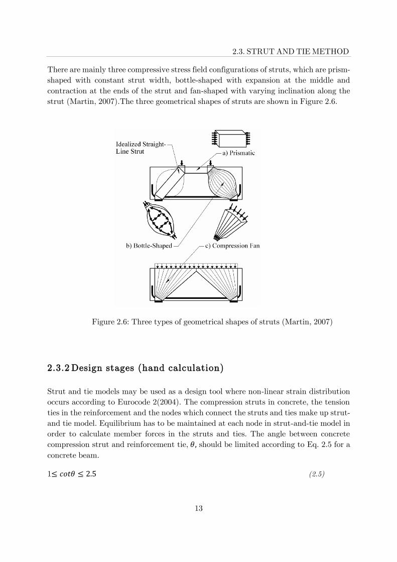
The maximum compressive stresses for compression nodes with ties provided in one
direction can be designed using Eq. 2.13.The recommended value for 𝑘2 is 0.85 according
to EC 2. Two compressive forces in the struts and one tensile force in tie acting on a
single node, which is classified as CCT node and displayed Figure 2.10.
𝜎𝑅𝑑.𝑚𝑎𝑥 = 𝑘2 𝑣 ,𝑓𝐸𝑐𝑑 (2.13)
Figure 2.10: CCT node
The maximum compressive stresses for compression nodes with ties provided in more
than one direction can be designed using Eq. 2.14. The recommended value for 𝑘3 is 0.75
according to EC 2. One compressive force in the strut and two tensile forces in tie
intersecting on a single node, which is traditionally, called CTT node and displayed
Figure 2.11.
𝜎𝑅𝑑.𝑚𝑎𝑥 = 𝑘3 𝑣 ,𝑓𝐸𝑐𝑑 (2.14)

18
CHAPTER 2. STRUCTURAL BEHAVIOUR OF THICK RC BEAMS
Figure 2.11: CTT node
2.4 Shell Element Method (Linear FE Analysis)
2.4.1 Introduction
According to TRVK Bro 11 (B.2.7.1), 3D models capable of capturing the structural
response have to be used in order to describe forces, geometry and deformation properties
fully. The use of 3d-shell elements therefore is becoming more important in designing
structures such as concrete bridges.
Linear FE analysis will be performed using 3d-shell elements in order to get the out of
plane shear components that will be used for calculating the normal forces; consequently,
the amount of reinforcement required can be determined.

19
2.4. SHELL ELEMENT METHOD
2.4.2 Design stages
Concrete shell elements treated in Eurocode 2 Annex LL. The internal forces in a shell
element generally consists of three plane components (𝑛𝐸𝑑𝑥 , 𝑛𝐸𝑑𝑦& 𝑛𝐸𝑑𝑥𝑦 = 𝑛𝐸𝑑𝑦𝑥), three
slab components (𝑚𝐸𝑑𝑥 , 𝑚𝐸𝑑𝑦, 𝑚𝐸𝑑𝑥𝑦 = 𝑚𝐸𝑑𝑦𝑥) and two out of plane shear components
(𝑣𝐸𝑑𝑥 , 𝑣𝐸𝑑𝑦). Figure 2.12 displays a shell element model with a unit dimensions and
internal forces.
The design calculation of the normal forces (𝑛𝑥𝑣 & 𝑛𝑦𝑣) by taking in to consideration the
in plane shear force (𝑛𝑦𝑥) are performed using Eq. 2.15 and Eq. 2.16 in which the tensile
force and the compressive force will have positive and negative sign respectively. The
value of 𝜇 which is used for practical reasons is 1 according to BBK 04 (Section 6.7.3).
𝑛𝑥𝑣 = 𝑛𝑥 + 𝜇|𝑛𝑦𝑥| (2.15)
𝑛𝑦𝑣 = 𝑛𝑦 +1
𝜇 |𝑛𝑦𝑥| (2.16)
Figure 2.12: Shell element model and internal
forces (Eurocode2, 2005)
2.5 Failure modes in RC beams
The first bending cracks develop in the regions where the bending moment is maximum
and the shear forces are small. As a load increases, additional shear cracks will appear
within the

20
CHAPTER 2. STRUCTURAL BEHAVIOUR OF THICK RC BEAMS
regions where shear forces are larger; consequently, shear failure may happen. Shear
cracks normally begins as bending cracks perpendicular to the axis of the beam, but they
incline towards the loading point (Carpinteri, 1992). Figure 2.13 shows typical shear
failure for a concrete beam.
Figure 2.13: Typical shear failure for a concrete
beam (Ibrahim, 2002).
Flexural and shear failure are the two main failure modes in RC beams. The shear failure
is normally brittle than the flexural failure. Concrete failure, steel failure and combined
concrete and steel failure are the three flexural failure mechanisms in RC beams due to
the amount of the reinforcement. In a concrete failure, concrete reaches to its ultimate
strength before steel reaches its yield strength; consequently, the concrete crushes first
without any warning. Concrete failure can be caused by high amount of reinforcement
and when the compressional strength of concrete is lower than the yield strength of the
steel. In steel failure; on the other hand, steel reaches its yield strength before concrete
reaches to its ultimate strength. Steel failure can be induced when amount of
reinforcement is low and the compressional strength of concrete is higher than the yield
strength of the steel and it is favourable compared to the previous failure mode.
Furthermore, a combined concrete and steel failure develops when concrete and steel
reaches yielding simultaneously (Asekeen, 2016). Furthermore, the behaviour of concrete
is different under different magnitudes of hydrostatic pressure, at low pressure the failure
is brittle while at high pressures the failure is ductile (Malm, 2009).

21
3
FE modelling of thick reinforced concrete beam
According to Kmiecik et al. (2011), modelling of reinforced concrete always poses a
challenge because of the non-linear behaviour of concrete from the very start it is loaded
in compression. For the detailed constitutive models of concrete, see [Bangash (2001),
Chen (1982), Chen and Han (1995), Karihaloo (2003), Malm (2006) and Malm (2009)].
Uniaxial behaviour of plain concrete
3.1 Uniaxial behaviour of plain concrete
According to Yu et al. (2010), the nonlinearity of concrete in compression before the
peak stress is due to concrete plasticity and after the peak due to concrete damage.
Plasticity is characterized by uncoverable deformation after all the loads have been
removed and damage is characterized by the reduction of elastic modulus. The non-
linearity of concrete under compression and tensile load can be modelled using plasticity
model, damage model or concrete damaged plasticity model. There are numerous
experiments and studies in uniaxial, biaxial and multiaxial behaviour of concrete under
static and dynamic loading that have been conducted, for details refer to [Zielirtski
(1984), Kotsovos (2015), Hordijk (1992), Hillerborg (1985), Lee at el (2014), Bazant et
al. (1983), Yu et al. (2010), Feensta (1995), Kmiecik et al. 2011, Mier (1984)]
We shall focus the on the recommendations as prescribed by Eurocode 2, FIB 1990 and
FIB 2010 on how to model the stress strain relationship of concrete and steel in both
compression and tensile. The following relations from Eq.3.1 to Eq. 3.8 were used to
describe the material properties of concrete.
𝑓𝑐𝑚 = 𝑓𝑐𝑘 + 8 (𝑀𝑃𝑎) (3.1)
𝑓𝑐𝑡𝑘,0.05 = 0.7𝑓𝑐𝑡𝑚 (3.2)
𝐸𝑐𝑚 = 22 [𝑓𝑐𝑚
10]
0.3 (3.3)
𝜀𝑐1 = 0.7𝑓𝑐𝑡𝑚0.31 ≤ 2.8 ‰ (3.4)
Chapter
22
CHAPTER 3. FE MODELLING OF THICK RC BEAMS
𝐸𝑐 = 𝛼𝑖𝐸𝑐𝑖 (3.5)
𝐸𝑐𝑖 = 𝐸𝑐𝑚 & 𝛼𝑖 = 0.8 + 0.2𝑓𝑐𝑚
88 ≤ 1.0 (3.6)
𝐺𝐹_2010 = 73𝑓𝑐𝑚0.18 (3.7)
𝐺𝐹_1990 = 𝐺𝐹0 [𝑓𝑐𝑚
𝑓𝑐𝑚0]
0.7 (3.8)
𝑓𝑐𝑚0 = 10 𝑀𝑃𝑎, 𝐺𝐹0 = 0.02875 & 𝜀𝑐𝑢1 = 3.5 ‰
where 𝐺𝐹0 base value of the fracture energy
𝐺𝐹 fracture energy
𝑓𝑐𝑚 mean compressive strength
𝑓𝑐𝑘 characteristic compressive strength
𝜀𝑐𝑢1 ultimate compressive strain
𝜀𝑐1 peak compressive strain
𝜀𝑐 compressive strain
𝐸𝑐 initial modulus of elasticity of concrete
𝐸𝑐𝑖 mean modulus of elasticity of concrete
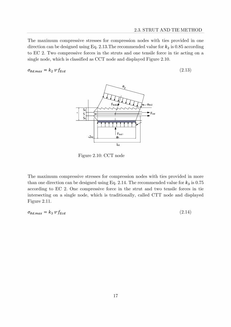
3.1.1 Uniaxial behaviour in compression
The stress strain relationship of concrete can be modelled using the recommendations in
Eurocode 2, FIB 1990 and FIB 2010. According to EN 1992-1-1, cl. 3.1.5 (1) and Figure
3.1, the following are the relations that describe the short-term uniaxial loading
illustrated in Eq. 3.9 to Eq.3.11:
𝜎𝑐
𝑓𝑐𝑚=
𝑘𝜂−𝜂2
1+(𝑘−2)𝜂 (3.9)
𝜂 = 𝜀𝑐
𝜀𝑐1 (3.10)
𝑘 = 1.05𝐸𝑐𝑚|𝜀𝑐1|
𝑓𝑐𝑚 (3.11)
where 0 ≤ |𝜀𝑐| ≤ 𝜀𝑐𝑢1

23
3.1. UNIAXIAL BEHAVIOUR OF PLANE CONCRETE
Figure 3.1:Concrete stress strain relationship (Eurocode2, 2005).
To avoid the numerical issues, stresses in the model should not be decreased to zero
instead, it is recommended to use a slightly higher value.
3.1.2 Uniaxial behaviour in tension
Modelling the uniaxial behaviour in tension is the most problematic. If the model has
large regions without reinforcement, it is recommended to use fracture mechanics based
on fracture energy or crack opening to avoid mesh sensitivity of the analysis. According
to Hillerborg (1985), the stress deformation behaviour of concrete under tensile loading
can be described by means of two curves namely stress strain relation including
unloading branches, refer to Figure 3.2 (a) and stress deformation relation, refer to
Figure 3.2 (b). There are several stress deformation curves available in literature that
define the descending portion of the curve when concrete begins undergo deformation
also called strain softening but the most common are linear, bilinear, and exponential
(Malm, 2015).
Figure 3.2: Tensile behaviour of concrete by means two curves: (a) stress-strain relationship for the undamaged zone, (b) stress-crack opening relationship for the damage zone, source: (Hillerborg, 1985)

24
CHAPTER 3. FE MODELLING OF THICK RC BEAMS
where 𝜎𝑡 concrete tensile stress
𝑓𝑐𝑡𝑚 concrete mean tensile strength
𝐺𝑓 fracture energy
𝑤 crack opening
𝜀 concrete strain
Plain concrete subjected to uniaxial tension is elastic up to the ultimate tensile strength.
At the ultimate tensile strength or the failure stress, micro cracks initiates in the concrete
material and once the failure stress is exceeded, the micro cracks merges to create wide
crack openings and hence the concrete material exhibiting a softening behaviour of the
stress strain response (Abaqus manual 6.14). The uniaxial tension behaviour just before
the ultimate tensile strength of the concrete material is not dependant on the mesh size.
It is the post peak behaviour of concrete in tension that is the most interesting and
challenging. Figure 3.3 (a), Figure 3.3 (b) and Figure 3.3 (c) presents the linear, bilinear
and exponential descending portion of curve respectively, when concrete undergoes
strain softening behaviour. Concrete tensile strength versus crack width in Figure 3.3
(c), according to Hordijk (1992), can be estimated using Eq. 3.12.
Figure 3.3: Tensile stress-crack opening relationships for the damage zone, (a) linear, source:
(Abaqus manual 6.14), (b) bilinear, source: (FIB, 1990), (c) exponential, source: (Hordijk, 1992)
𝜎 𝑓𝑡⁄ = [1+(𝑐1𝑤
𝑤𝑐)3]𝑒
−(𝑐1𝑤
𝑤𝑐)
−𝑤
𝑤𝑐(1 + 𝑐1
3)𝑒−𝑐2 (3.12)
where σ concrete tensile stress
𝑓𝑡 yield tensile strength for concrete
𝑐1 3
𝑐2 6.93
w crack opening
𝑤𝑐 maximum crack opening given in figure 3.3
The linear curve was used in this study where fracture energy (Gf) was directly specified
as the material property in Abaqus.
25
3.2. CONCRETE DAMAGED PLASTICITY MODEL
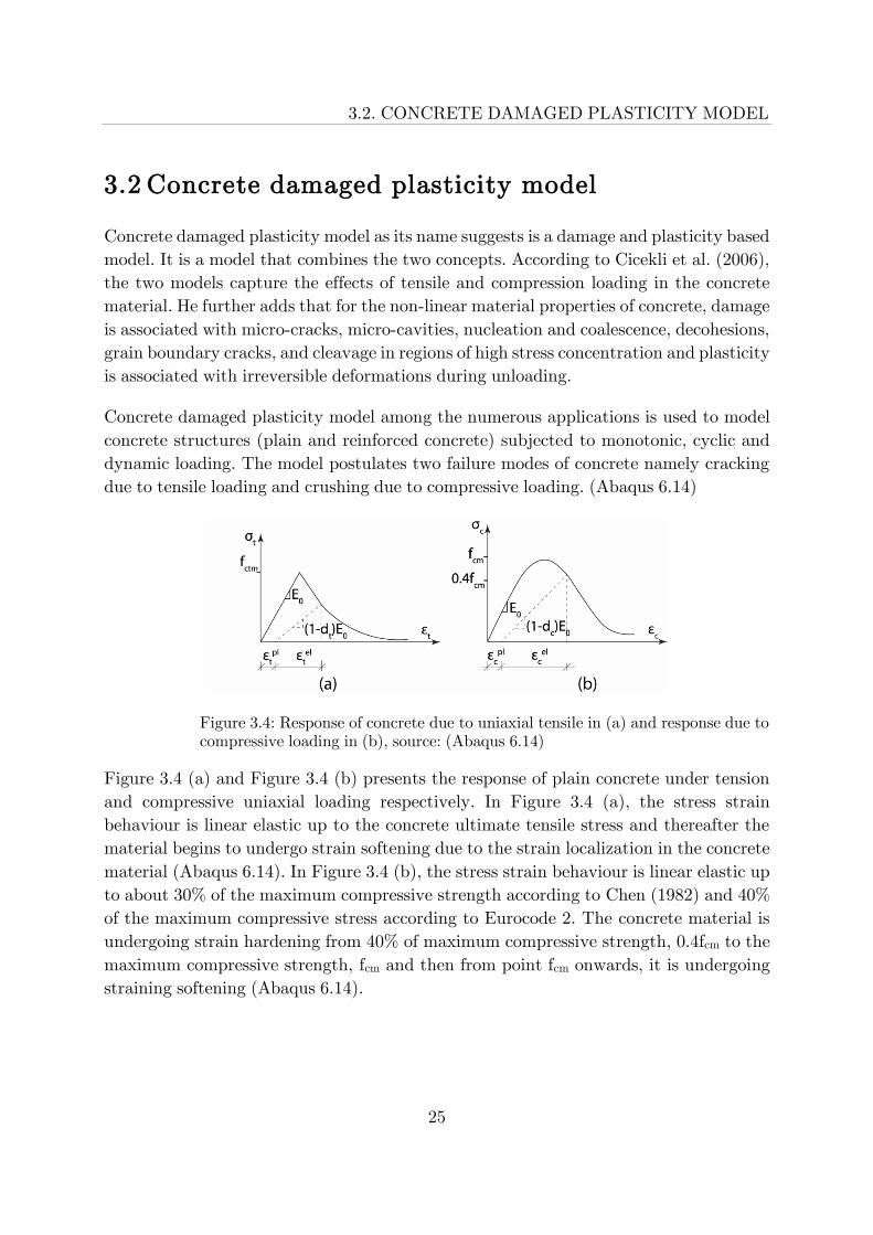
3.2 Concrete damaged plasticity model
Concrete damaged plasticity model as its name suggests is a damage and plasticity based
model. It is a model that combines the two concepts. According to Cicekli et al. (2006),
the two models capture the effects of tensile and compression loading in the concrete
material. He further adds that for the non-linear material properties of concrete, damage
is associated with micro-cracks, micro-cavities, nucleation and coalescence, decohesions,
grain boundary cracks, and cleavage in regions of high stress concentration and plasticity
is associated with irreversible deformations during unloading.
Concrete damaged plasticity model among the numerous applications is used to model
concrete structures (plain and reinforced concrete) subjected to monotonic, cyclic and
dynamic loading. The model postulates two failure modes of concrete namely cracking
due to tensile loading and crushing due to compressive loading. (Abaqus 6.14)
Figure 3.4: Response of concrete due to uniaxial tensile in (a) and response due to compressive loading in (b), source: (Abaqus 6.14)
Figure 3.4 (a) and Figure 3.4 (b) presents the response of plain concrete under tension
and compressive uniaxial loading respectively. In Figure 3.4 (a), the stress strain
behaviour is linear elastic up to the concrete ultimate tensile stress and thereafter the
material begins to undergo strain softening due to the strain localization in the concrete
material (Abaqus 6.14). In Figure 3.4 (b), the stress strain behaviour is linear elastic up
to about 30% of the maximum compressive strength according to Chen (1982) and 40%
of the maximum compressive stress according to Eurocode 2. The concrete material is
undergoing strain hardening from 40% of maximum compressive strength, 0.4fcm to the
maximum compressive strength, fcm and then from point fcm onwards, it is undergoing
straining softening (Abaqus 6.14).

26
CHAPTER 3. FE MODELLING OF THICK RC BEAMS
3.3 Modelling of reinforcement
According to FIB code 2010, reinforcing steel may be bars, wire or welded fabric
characterized by the geometric, mechanical and technological properties. The geometric
properties include the size and the surface characteristics and the mechanical properties
include the yield and ultimate strength, ductility, fatigue behaviour and behaviour under
extreme thermal conditions. Finally, the technological properties include bond
characteristics, bendability, weldability, thermal expansion and durability.
The properties considered in this study are size, yield strength, ductility and thermal
expansion. According to Eurocode 2, the valid specified yield strength is from 400 MPa
to 600MPa. The following idealized model presented in Figure 3.5 was used in this study
(FIB, 1990).
Figure 3.5: Idealized stress strain relation in the steel bar (FIB, 1990).
The reinforcement can be modelled as a one-dimensional bar (truss element) which is
defined singly or embedded in concrete using metal plasticity models. The metal
plasticity models can use Mises or Hill yield surfaces with associated plastic flow for
isotropic and anisotropic yield, respectively, perfect plasticity or isotropic hardening
behaviour, etc. (Abaqus, 6.14)
In this study, perfect plasticity behaviour was used for modelling the steel reinforcement
in Abaqus. Perfect plasticity simply means that stress at the yield point of the material
does not change with plastic strain. In short, the yield stress is constant as the plastic
strain keeps increasing in a material, refer to Figure 3.6.

27
3.3. MODELLING OF REINFORCEMENT
Figure 3.6: Uniaxial stress strain curve for a typical metal (University of Auckland solid mechanics lectures).
3.4 Explicit dynamic analysis
Explicit dynamic analysis is a mathematical method that uses central difference rule or
forward Euler for integrating the equations of motion through time by using known
values to obtain the unknown values. The dynamic equilibrium, presented in Eq. 3.13,
is solved at the beginning of each increment.
𝑀�̈� = 𝑃 − 𝐼 (3.13)
where
M is the nodal mass matrix, �̈� is the nodal accelerations, P is the external
applied force and I is the internal element force.
At the first current time step (t), the nodal acceleration (�̈�) is calculated as presented in
Eq. 3.14 using the lumped mass matrix, M which is a diagonal matrix always used by
the explicit analysis.
�̈� ǀ(𝑡) = (𝑀)−1 (𝑃 − 𝐼) ǀ(𝑡) (3.14)
It is the diagonal mass matrix that makes the calculation of the nodal acceleration trivial
or easier at any given time, t.
The Eq. 3.14 applies to both implicit and explicit analysis. The major difference between
implicit and explicit analysis is the method by which the nodal accelerations are
calculated. Refer to Abaqus manual 6.14 and Chopra (1995) for a detailed explanation
of the two methods of analysis.

28
CHAPTER 3. FE MODELLING OF THICK RC BEAMS
In this study, we used the quasi-static dynamic explicit analysis to avoid convergence
problems and because our model has discontinuities due to the cracks that develop in
the concrete material as soon as material begins to soften due to the localization of strain.
3.4.1 Time increment
The time increment ∆𝑡 must be less than stable time increment, ∆𝑡𝑚𝑖𝑛 to get a bounded solution, otherwise the oscillations and instability related issues would occur in the model response.
The stable time increment is defined as presented in Eq. 3.15.
∆𝑡𝑚𝑖𝑛 ≤ 2
𝜔𝑚𝑎𝑥(√1 + 𝜉2 − 𝜉) (3.15)
where
𝜔𝑚𝑎𝑥 is the highest eigenvalue in the model, and 𝜉 is the damping factor (hence the damping reduces the stable time increment)
The dynamic explicit analysis solves every problem as a wave transmission problem. The
minimum time that the dilatational wave, 𝐶𝑑 takes to travel from one element to another
in a model is called the stable time increment presented in Eq. 3.16.
𝐶𝑑 = √𝐸 𝜌⁄ (3.16)
where
𝐸 is the young’s modulus and 𝜌 is the current material density
Based on the dilatational wave, 𝐶𝑑 the stable time increment is calculated as presented in Eq. 3.17.
∆𝑡 = 𝐿𝑒 𝐶𝑑⁄ (3.17)
where
𝐿𝑒 is the element dimension
When the dilatational wave, 𝐶𝑑 is increased and or element dimension, 𝐿𝑒 decreased, the
stable time increment is reduced.

29
3.4. EXPLICIT DYNAMIC ANALYSIS
3.4.2 Mass Scaling and loading rate
Mass scaling is an artificial technique that increases the density of the material for the
whole model or in the specific elements that are controlling the time step. Mass scaling
and loading rates reduces the running time for the model. However, high values of mass
scaling and excessive loading rates can lead to erroneous solutions due to the inertia
effects.
3.4.3 Energy balance
The energy balance in Abaqus/Explicit is expressed Eq. 3.18:
𝐸𝐼 + 𝐸𝑉𝐷 + 𝐸𝐹𝐷 + 𝐸𝐾𝐸 − 𝐸𝑊 = 𝐸𝑇𝑂𝑇 = constant (3.18)
where
𝐸𝐼 is internal energy (elastic, inelastic, strain energy)
𝐸𝑉𝐷 is energy absorbed by viscous dissipation
𝐸𝐹𝐷 is frictional dissipation energy
𝐸𝐾𝐸 is kinetic energy
𝐸𝑊 is work of external forces
𝐸𝑇𝑂𝑇 is total energy in the system
For quasi-static analysis, the kinetic energy 𝐸𝐾𝐸 should be a small fraction (typically 5%
to 10 %) of the work of externals, 𝐸𝑊 or internal energy, 𝐸𝐼 according to Abaqus manual
6.14.

30

31
4
Experimental program
4.1 Description of the experiment
As a way of developing a reference against which the accuracy of failure prediction design
methods can be compared to, a thick slab specimen of dimension 4m height by 19m
effective length by 250 mm thickness was built by Collins et al. and loaded to failure
under an off center point load. For the detailed description of the specimen and its
material and section properties, refer to Figure 4.1 and Table 4.1.
Figure 4.1:Details of longitudinal and cross-section of the membrane wall, source: Collins et al.(2015)
Table 4.1: Material and section properties, source Collins et al. (2015)
fc = 40 MPa Bar Size Cross section area Steel yield Strength,
fy
b = 250 mm 30M = 29.9 mm2 700 mm2 573 MPa
h = 4000 mm 20M = 19.5 mm2 300 mm2 522 MPa
d = 3840 mm
max aggregate = 14 mm
Chapter

32
CHAPTER 4. EXPERIMENTAL PROGRAM
Before carrying out the experiment (loading to failure the above specimen with an off
center point load), the Engineers from all over the world were invited to predict the
magnitude the of point load P required to cause failure of the specimen, the location
where the first failure would occur and load deformation response for two mutually
exclusive cases.
Case 1: When the minimum shear reinforcement according to ACI is only placed on the
left shear span, refer Figure 1.1.
Case 2: When the minimum shear reinforcement according to ACI is placed on both the
left and the right shear spans, refer Figure 1.1.
In both cases, the considerable self-weight of the specimen was to be considered in the
ultimate strength prediction. 66 Engineers, 33 from the universities and 33 from the
industry, participated in this challenge of predicting the ultimate strength of the thick
slab. After the Engineers predicted the ultimate strength for the two cases and sent their
results consisting of values based on a number of codes of practice, then the experiment
was conducted by loading the specimen to failure and the results recorded at every stage,
in the un-cracked as well as in the cracked stages. The crack widths and crack spacing
were also recorded at every stage. (Collins et al. 2015)
4.2 Partially reinforced concrete beam
Flexural cracking first occurred at when P reached 198 kN with a corresponding
bending moment of 1900 kNm and a tensile stress in concrete of 2.48 MPa. Figure 4.2
(a) shows when P had reached 375 kN, about 7 cracks can be seen in the east span, the
average spacing of these cracks is 724 mm and average crack width is 0.06 mm. Two of
these cracks extend to the mid-depth of the member and the spacing between these
cracks is 2320 mm, which is 0.6d. The cracks near the mid-depth have the width of
about 3 times greater than the average crack width near the flexural tension surface. In
Figure 4.2 (b), P was increased to 625 kN and the crack developed into a potential
flexural tension crack. In Figure 4.2 (c), P was further increased to 685 kN and the
crack propagated towards the point load at 45 degrees from the mid-depth. The crack
width at the mid-depth was up to 3 mm, the crack spacing between the three cracks at
mid depth was 0.6d and 0.68d and the load deflection was 12 mm. In Figure 4.2 (d),
the specimen was reloaded to 433 kN, and the cracks opened up to 35mm. Hence the
maximum serviceability load is 198 kN and the ultimate load is 685 kN, the load
deformation at ultimate is 12 mm and the failure occurred on the east shear span (span
without minimum reinforcement), refer to Figure 4.3 and Figure 4.4. (Collins et al.
2015)

33
4.2. PARTIALLY REINFORCED CONCRETE BEAM
4.2.1 Predictions from Engineers
As earlier on pointed out, the 66 predictions were made by engineers who responded to
the challenge of predicting the shear strength of the thick slab. 26 predictions came from
Europe, 23 from the United States, 14 from Canada, and one each from Australia, Brazil,
and Mexico. The predictions were made based on the six codes of practice. Considering
a large variation of ultimate strength predictions, it is proof enough that predicting the
ultimate strength of a slab or thick concrete beam without reinforcement was a very
challenging task. In Figure 4.3, the upper red zone indicates very un-conservative results
where the ratio of predicted failure to observed ranges from 1.5 to 5.5 and the yellow
band falls in the range ±10% from the observed strength. Only 20% of the entries were
accurate while the 44% of the entries and the two codes (ACI and Eurocode) were in the
red zone.
Engineers were also required to predict the load deformation response of the thick slab
when the load was 25, 50, 75, and 100% of the predicted failure load. A total of 36 entries,
13 from industry and 23 from academia submitted their predictions as shown in Figure
4.4. From the results in Figure 4.4, it can be seen that predicting the load deformation
response of a very thick slab is very challenging. The yellow band in Figure 4.4 indicates
the results that fall within ±20% of the observed results. Five engineers lie within the
yellow zone, 2 lie below the yellow zone which means they underestimated the stiffness
and 18 lie below the yellow zone meaning they overestimated the stiffness, while 11
intersect the zone because the calculated post cracking stiffnesses was very high.
Only three of the load deformation response predictions managed to predict the failure
load within ±10% of the observed or experimental results and four predicted load
deformation within ±20% of the experimental results. These predictions were submitted
by Cervenka and Sajdlova from a consulting firm in Prague, Czech Republic; Conforti
and Facconi of the University of Brescia, Italy; and Bentz from the University of
Toronto. Non-linear finite element models was used for the first two predictions and
sectional analysis program response 2000 was used for the third prediction. Cervenka
and Sajdlova submitted the most accurate prediction with regard to the location of the
failure. (Collins et al. 2015)

34
CHAPTER 4. EXPERIMENTAL PROGRAM
Figure 4.2: Diagonal cracking of east span, source: Collins et al. (2015)

35
4.2. PARTIALLY REINFORCED CONCRETE BEAM
Figure 4.3 : Comparison of predictions with experimental results for case (Collins, 2015

36
CHAPTER 4. EXPERIMENTAL PROGRAM
Figure 4.4: Predicted and observed load-deformation response for initial test-case 1 (failure in east span, Note: 1 kip = 4.45 kN; 1 in. = 25 mm) (Collins, 2015).

37
4.3. FULLY REINFORCED CONCRETE BEAM
4.3 Fully reinforced concrete beam
The same specimen that was used in the partially reinforced beam, it was repaired by
strapping the right shear with four pairs of 36 mm diameter dywidag thread bars and
post-tensioning each bar to about 270 kN. Thereafter it was loaded with an off center
point load at the same location as in the previous case. In Figure 4.5 (a), the point load
reached 1750 kN and the diagonal crack widths was up to 4 mm and when the load was
increased to 2162 kN in Figure 4.5(b), the concrete at the left end of the loading plate
crushed as shown in Figure 4.5. Hence the failure load was 2162 kN on the left shear
span. The load deformation response of the repaired specimen is shown in Figure 4.6.
The maximum deflection at failure was 39.3 mm. (Collins et al., 2015)
Figure 4.5: Diagonal cracking of west span of case 2 (Collins, 2015)

38
CHAPTER 4. EXPERIMENTAL PROGRAM
Figure 4.6: Load-deformation response of repaired specimen (Note: 1 kip = 4.45 kN; 1 in. = 25 mm) (Collins, 2015).

39
4.3. FULLY REINFORCED CONCRETE BEAM
4.3.1 Predictions from Engineers
Figure 4.7 shows the predictions that were made by 44 Engineers (16 from the industry
and 28 from the academia) that participated. The red zone show un-conservative and
the yellow band indicate excellent results within ±10% of the observed results.
Figure 4.7: Comparison of predictions with experimental results for case 2, source: Collins et al. (2015)

40
CHAPTER 4. EXPERIMENTAL PROGRAM
4.4 Summary of the Results
For both cases (partially and fully reinforced), only two entries managed to submit
predictions of the failure load within ±10% of the observed results using their own finite
element programs. Of the two best entries, Cervenka Consulting had predictions of the
load deformation was more accurate and as a result were chosen as the overall winners
of the prediction competition.
Comparing the failure load results in Figure 4.3 and Figure 4.7, from the 66 entries in
partially reinforced , 29 entries were in the red zone (un-conservative zone) while of the
44 entries in the fully reinforced, only 1 was in red zone. For the partially reinforced,
only 24% of the predictions were conservative while for the fully reinforced, 66% of the
predictions were conservative. This is evidence enough that predicting the ultimate
strength of thick slabs was a challenging task and requires more extensive research.
(Collins et al., 2015)

41
5
Verification of FE model
Model verification and validation serves the purpose of making engineering predictions
acquire a certain acceptable level of accuracy and confidence. With regard to finite
element analysis (FEA), verification has to do with ensuring that the process of
developing the FEA model iscorrect while validation ensures that the FEA model
matches with the available experimental results or data to a certain acceptable level of
confidence (Thacker, 2004).
Abaqus/Explicit 6.14 has been used in developing and analysing the reinforced concrete
thick beam FE model subjected to static loading for partially and reinforced concrete.
For testing a reinforced concrete thick beam, the FE model has been verified, calibrated
and validated against the experimental investigation conducted by the American
Concrete Institute (Michael Collins, 2015). In verifying and validating the FE model,
the finite element results were compared to the experimental results, in this case the
results under consideration are the load deformation response and crack width and crack
pattern.
5.1 Description of FE model
The 2D plane stress elements have been used to model the FE model. By plane stress we
mean all the stresses act in plane direction, in-plane displacements, strains and stresses
can be taken be to uniform in the thickness direction and transverse shear stress is
negligible. The FE models have been modelled as a simply supported beam with hinge
and roller on the boundary conditions. The layouts of the longitudinal and shear
reinforcements are shown in Figure 5.1(a) and Figure 5.1(b) for partially and fully
reinforced concrete beams respectively. Figure 5.1 (c) shows the cross section for both
cases.
Chapter

42
CHAPTER 5. VERIFICATION OF FE MODEL
Figure 5.1: Loads, boundary conditions and reinforcements for (a) partially reinforced concrete beam, (b) fully reinforced concrete beam and (c) cross section for both cases.
The longitudinal and shear reinforcement bars were modelled with 2-node linear 2-D
truss element (T2D2) with a mesh size of 50 mm. The concrete region was modelled by
the unstructured 3-node linear plane stress triangle element (CPS3) with a mesh size of
50 mm. The size of the elements was selected based on the convergence of the results as
shown in appendix B.1. Element types and mesh size are displayed for partially and fully
reinforced concrete beams in Figure 5.2 and Figure 5.3 respectively.

43
5.1. DESCRIPTION OF FE MODEL
Figure 5.2: Reinforcement for partially and fully reinforced concrete beams with 2-node
linear truss element (T2D2) with a mesh size of 50 mm.
Figure 5.3: Concrete for partially and fully reinforced concrete beams with 3-node linear
plane stress triangle element (CPS3) with a mesh size of 50 mm.
44
CHAPTER 5. VERIFICATION OF FE MODEL
The advantage of unstructured mesh is that they easily adapt to boundaries of arbitrary
shapes and can be refined locally (R. Marchand, 2007). The experimental crack profile
or path cannot be predicted in the case of structured mesh (Song, 2008). In addition,
structured mesh confines the crack propagation paths around the node points of the
mesh elements and eventually lead to different crack profiles. In the non-linear analysis
of discontinuous structures which involve arbitrary crack growth, the element types
usually used are triangular elements for 2-D and tetrahedral elements for 3-D because
they allow easier and flexible crack propagation when compared to the quadrilateral for
2-D and brick elements for 3-D. In the case of quadrilateral for 2-D and brick elements
for 3-D, the crack profile opens only along either original direction or 90º diversion
(Zhang, 2007).
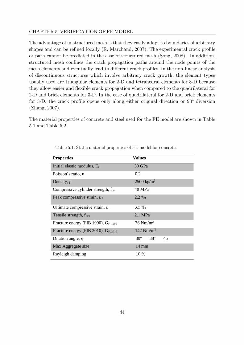
The material properties of concrete and steel used for the FE model are shown in Table
5.1 and Table 5.2.
Table 5.1: Static material properties of FE model for concrete.
Properties Values
Initial elastic modulus, Ec 30 GPa
Poisson’s ratio, υ 0.2
Density, ρ 2500 kg/m3
Compressive cylinder strength, fcm 40 MPa
Peak compressive strain, εc1 2.2 ‰
Ultimate compressive strain, εu 3.5 ‰
Tensile strength, fctm 2.1 MPa
Fracture energy (FIB 1990), GF_1990 76 Nm/m2
Fracture energy (FIB 2010), GF_2010 142 Nm/m2
Dilation angle, ψ 30º 38º 45º
Max Aggregate size 14 mm
Rayleigh damping 10 %
45
5.1. DESCRIPTION OF FE MODEL
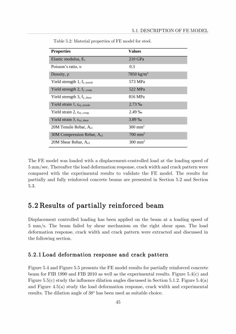
Table 5.2: Material properties of FE model for steel.
Properties Values
Elastic modulus, Es 210 GPa
Poisson’s ratio, υ 0.3
Density, ρ 7850 kg/m3
Yield strength 1, fy_tensile 573 MPa
Yield strength 2, fy_comp 522 MPa
Yield strength 3, fy_shear 816 MPa
Yield strain 1, εsy_tensile 2.73 ‰
Yield strain 2, εsy_comp 2.49 ‰
Yield strain 3, εsy_shear 3.89 ‰
20M Tensile Rebar, As1 300 mm2
30M Compression Rebar, As2 700 mm2
20M Shear Rebar, As3 300 mm2
The FE model was loaded with a displacement-controlled load at the loading speed of
5 mm/sec. Thereafter the load deformation response, crack width and crack pattern were
compared with the experimental results to validate the FE model. The results for
partially and fully reinforced concrete beams are presented in Section 5.2 and Section
5.3.
5.2 Results of partially reinforced beam
Displacement controlled loading has been applied on the beam at a loading speed of
5 mm/s. The beam failed by shear mechanism on the right shear span. The load
deformation response, crack width and crack pattern were extracted and discussed in
the following section.
5.2.1 Load deformation response and crack pattern
Figure 5.4 and Figure 5.5 presents the FE model results for partially reinforced concrete
beam for FIB 1990 and FIB 2010 as well as the experimental results. Figure 5.4(c) and
Figure 5.5(c) study the influence dilation angles discussed in Section 5.1.2. Figure 5.4(a)
and Figure 4.5(a) study the load deformation response, crack width and experimental
results. The dilation angle of 38º has been used as suitable choice.

46
CHAPTER 5. VERIFICATION OF FE MODEL
For FIB 1990 in Figure 5.4(a), the load deformation curve is identified with four critical
points of interest. Point 1 is in stage I when the beam begins to crack with a maximum
crack width of 0.02 mm. At this stage onwards, the beam experiences stiffness
degradation due to the crack openings. At point 2, the beam develops a maximum crack
opening of 2.75 mm close to the mid-depth of the beam. It is at point 2 that the beam
fails because the crack opening is too wide. The crack pattern at point 2 indicates a shear
failure mechanism on the right shear span. Comparing the experimental result with the
FE model results, there is a match in the crack pattern at point 2 as well as the load
deformation response as shown in Figure 5.4(b). Comparing the failure loads in Figure
5.4(b), the FE model results are conservative. There is some crack opening and closing
at point 2 where the beam fails and later the beam finds another path where its capacity
increases to peak capacity at point 3 and finally the capacity drops at point 4. It was
assumed that the crack tensile normal stress and crack tensile normal strain was
maximum when the crack was opening and then suddenly tensile normal stress and crack
tensile normal strain was negligible or zero when the crack was closing. However, the
crack shear stress and crack shear strain did not disappear but was stored upon closing
(Borst, 1987). When the crack was closing, it experienced crack compressive normal
stress and crack compressive normal strain and its elastic behaviour was recovered. Why
this behaviour happened requires extensive research. This crack opening and closing
behaviour at failure was even exhibited for FIB 2010, refer to Figure 5.5. At point 3 and
4, the crack opening widens as shown in Figure 5.5 (a).

47
5.2. RESULTS OF PARTIALLY REINFORCED BEAM
Figure 5.4: (a) Force displacement plot for partially reinforced FE-model FIB 1990 and with a dilation angle of 38º, (b) Force displacement plot for partially reinforced FE-model FIB 1990 with a dilation angle of 38º versus the experimental result and (c) Force displacement plot partially reinforced FE-model FIB 1990 with dilation angles of 30º, 38º and 45º.
48
CHAPTER 5. VERIFICATION OF FE MODEL
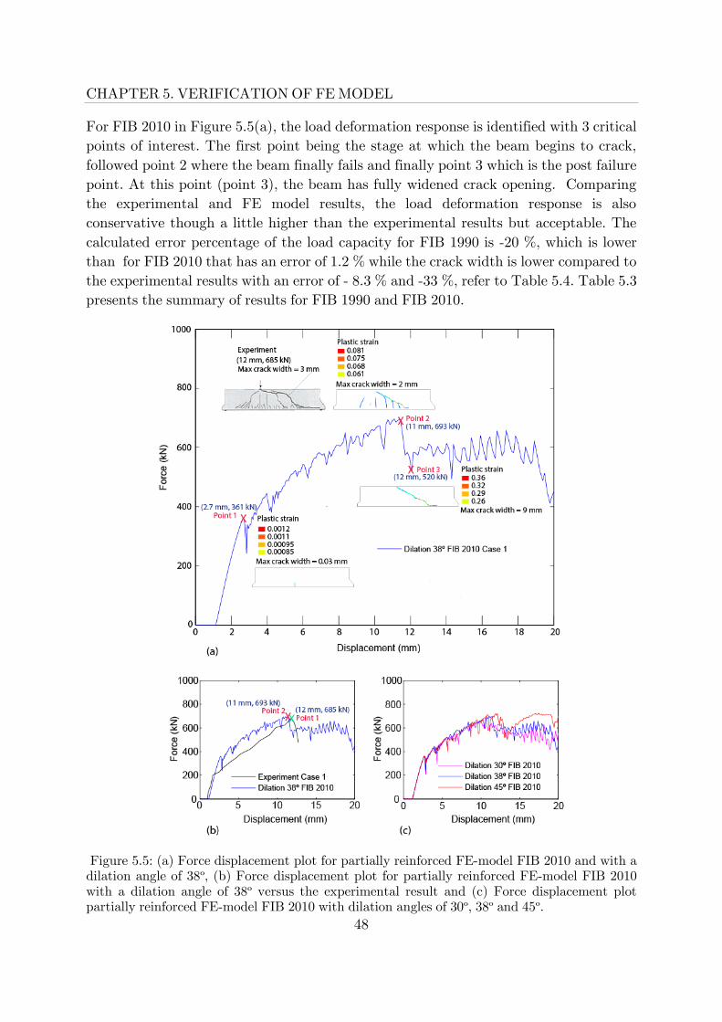
For FIB 2010 in Figure 5.5(a), the load deformation response is identified with 3 critical
points of interest. The first point being the stage at which the beam begins to crack,
followed point 2 where the beam finally fails and finally point 3 which is the post failure
point. At this point (point 3), the beam has fully widened crack opening. Comparing
the experimental and FE model results, the load deformation response is also
conservative though a little higher than the experimental results but acceptable. The
calculated error percentage of the load capacity for FIB 1990 is -20 %, which is lower
than for FIB 2010 that has an error of 1.2 % while the crack width is lower compared to
the experimental results with an error of - 8.3 % and -33 %, refer to Table 5.4. Table 5.3
presents the summary of results for FIB 1990 and FIB 2010.
Figure 5.5: (a) Force displacement plot for partially reinforced FE-model FIB 2010 and with a dilation angle of 38º, (b) Force displacement plot for partially reinforced FE-model FIB 2010 with a dilation angle of 38º versus the experimental result and (c) Force displacement plot partially reinforced FE-model FIB 2010 with dilation angles of 30º, 38º and 45º.

49
5.2. RESULTS OF PARTIALLY REINFORCED BEAM
Table 5.3: Partially reinforced FE model and Experimental results.
Failure load (kN)
Deformation (mm)
Crack width (mm)
Experiment 685 12 3
FIB 1990 551 10 2.75
FIB 2010 693 11 2
Figure 5.6: Comparison between experiment and partially reinforced FE model FIB 1990 and FIB 2010 with a dilation angle of 38o.
5.2.2 Influence of dilation angles
The dilation angle, ψ is a material parameter used in Abaqus finite element commercial
software. Dilation angle is defined as the concrete internal friction angle and usually a
value of ψ = 36º or 40º which is used in simulations (Kmiecik, 2011). Moreover, dilation
angles of 25º to about 40º have been usually used in simulations for normal grade concrete
under biaxial stresses. Brittle behaviour is associated with lower values of dilation angles
while ductile behaviour is associated with higher values of dilation angles (Malm, 2009).

50
CHAPTER 5. VERIFICATION OF FE MODEL
In Figure 5.4(c) for the case FIB 1990, the influence from the point the first crack
develops to the failure point is almost negligible. From the failure point onwards to the
ultimate point, the influence of the dilation angles is distinct and relatively significant.
As can be seen in the Figure 5.4(c), ψ = 30º exhibits some brittle behaviour while ψ =
45º exhibits some ductile behaviour.
5.2.3 Influence of fracture energy (FIB 1990 & FIB 2010)
Fracture energy is the area under the tensile stress versus crack opening curve, refer to
Figure 3.3. Tensile stress and crack opening is directly proportional to the fracture
energy, hence the higher the fracture energy, the higher the capacity of the beam as
evidenced in Figure 5.4(b) and Figure 5.5(b) for partially reinforced concrete beams. The
results for FIB 1990 and FIB 2010 are presented in Figure 5.6 and Table 5.3.
5.3 Results of fully reinforced beam
Displacement controlled loading has been applied on the beam at a loading speed of 5
mm/s. The beam failed by shear mechanism on the left shear span. The load deformation
response, crack width and crack pattern is discussed in the following section. The pre-
stressed thread bars are modelled as a uniform temperature load based on Hooke’s law.
5.3.1 Load deformation response and crack pattern
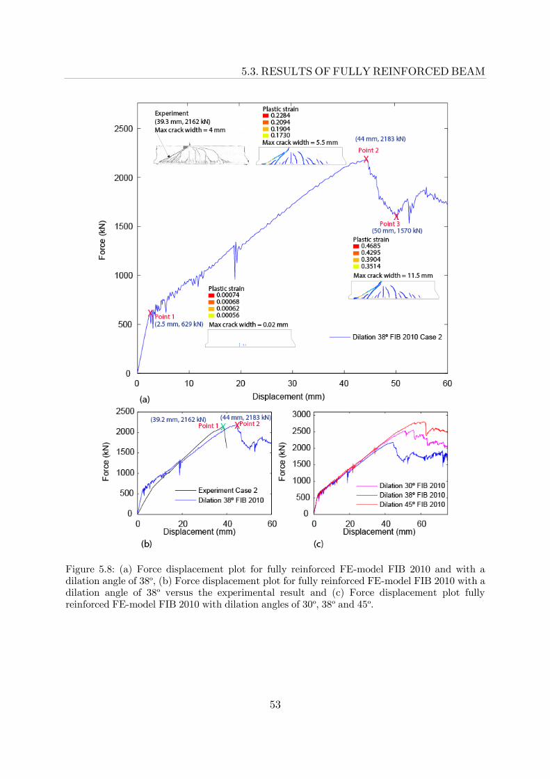
Figure 5.7 and Figure 5.8 present the FE model results for fully reinforced concrete beam
for FIB 1990 and FIB 2010 as well as experimental results. Figure 5.7(c) and 5.8(c)
display the influence of dilation angles. Figure 5.7(a) and Figure 5.8(a) study the load
deformation response, crack width and experimental results. The dilation angle of 38º
has been used as suitable choice.
Figure 4.7(a) of FIB 1990 is identified with 3 critical points of interest. Point 1 is the
point where the beam begins to crack with a maximum crack width of 0.015 mm, the
beam fails at point 2 with a maximum crack width of 5 mm and finally the point 3 the
ultimate point at which the crack width widen with a maximum crack width of 11.5 mm.
Note that, the crack width at point 2 is higher in the current study compared with the
experiment, refer to Figure 5.7(a). However, for the failure load, there is a good match
between numerical and

51
5.3. RESULTS OF FULLY REINFORCED BEAM
experimental results refer to Table 5.4 to check the comparisons. The error percentage
of calculated capacity for FIB 1990 was -8 %, which is lower than FIB 2010 that has an
error of 1 %, refer to Table 5.4.
Figure 5.7: (a) Force displacement plot for fully reinforced FE-model FIB 1990 and with a dilation angle of 38º, (b) Force displacement plot for fully reinforced FE-model FIB 1990 with a dilation angle of 38º versus the experimental result and (c) Force displacement plot fully reinforced FE-model FIB 1990 with dilation angles of 30º, 38º and 45º.

52
CHAPTER 5. VERIFICATION OF FE MODEL
Figure 5.8(a) of FIB 2010 is identified with 2 points of interest. The beam begins to crack
at point 1 with a maximum crack width of 0.015 mm and the failure takes place at point
2 with the maximum crack width 5 mm. The crack widths are very large compared to
the experiment. The calculated error percentage for FIB 1990 was 25 %, which is lower
than FIB 2010 that has an error of 37.5 %, refer to Table 5.4. The beam fails by shear
on the left shear span, which matches with experimental crack pattern, refer to Figure
5.8(a). Comparison between experiment and partially reinforced FE model for FIB 1990
and FIB 2010 with a dilation angle of 38o is displayed in Figure 5.9.
53
5.3. RESULTS OF FULLY REINFORCED BEAM
Figure 5.8: (a) Force displacement plot for fully reinforced FE-model FIB 2010 and with a dilation angle of 38º, (b) Force displacement plot for fully reinforced FE-model FIB 2010 with a dilation angle of 38º versus the experimental result and (c) Force displacement plot fully reinforced FE-model FIB 2010 with dilation angles of 30º, 38º and 45º.

54
CHAPTER 5. VERIFICATION OF FE MODEL
Table 5.4: Fully reinforced FE model and Experimental results.
Failure load (kN)
Deformation (mm)
Crack width (mm)
Experiment 2162 39.3 4
FIB 1990 1989 40 5
FIB 2010 2183 44 5.5
Figure 5.9: Comparison between experiment and fully reinforced FE model FIB
1990 and FIB 2010 with a dilation angle of 38o.
5.3.2 Influence of dilation angles
Dilation angle of ψ = 45º produced a higher capacity for both cases. On the contrary, ψ
= 38º gave lower capacity compared with ψ = 30º as shown in Figure 5.7 and Figure 5.8.
5.3.3 Influence of fracture energy (FIB 1990 & FIB 2010)
The crack width is higher for FIB 2010 compared to the crack width for FIB 1990 as
given in Table 5.4. In addition, the capacity for FIB 2010 is higher when compared to
the capacity for FIB 1990.

55
5.4. SUMMARY OF THE RESULTS
5.4 Summary of the results
The summary of the results for partially and fully reinforced FE-models compared to the
experimental results are presented in Table 5.5. For both cases, FIB 2010 predicts the
failure loads within ± 20 % of the experimental failure loads. The deformation is within
-17 % of the experimental value for partially reinforced and - 12 % of the experimental
value for fully reinforced. The crack width is within - 33 % of the experimental value for
partially reinforced and + 37.5 % of the experimental value for fully reinforced. Figure
5.10 and Figure 5.11 show the error between both cases and the experimental results.
The probable reason why the values of the crack width are higher in fully reinforced is
because the interaction between the concrete and the steel was not modelled in a way to
capture the bond slip behaviour instead it was modelled as fixed reinforced embedded
and fixed to the concrete. The other reason would be the influence of the pre-stressing
force in the shear reinforcement on the right shear span.
The failure mechanism was shear for all cases. The flexural cracks at the tensile face of
the beam surfaced when the tensile strength of concrete was reached. The flexural cracks
propagated from the tensile face of the beam towards the mid depth of the beam. At a
later stage as the load increased, the flexural inclined at 45º towards the loading point.
Finally, another crack near the support, along the tensile reinforcement propagated at
an inclined direction of 45º merging together with the flexural shear cracks towards the
loading point. There was a clear shear action effect in the beam hence a distinct shear
failure mechanism.
The influence of the dilation angles on partially reinforced for both FIB 1990 and FIB
2010 was negligible up to the failure point but the distinct and relatively significant after
the failure point to the ultimate. According to the studies conducted, lower values of
dilation angle produce brittle behaviour while higher values produce ductile behaviour.
This effect was not distinct at failure for partially as well as for fully reinforced because
the dilation angle ψ = 38º gave lower capacity than ψ = 30º. The influence of dilation
angles on fully reinforced was significant at failure for both FIB 1990 and FIB 2010
especially for ψ = 45º, the effect was increased capacity.
The influence of the fracture energy for partially reinforced for both FIB 1990 and FIB
2010 are adequate. Partially reinforced for FIB 2010 has a higher capacity when
compared to the fully reinforced FIB 1990.

56
CHAPTER 5. VERIFICATION OF FE MODEL
Table 5.5:Summary of partially and fully reinforced FE model and Experimental results
Capacity (kN)
Deformation (mm)
Crack width (mm)
Case 1 Experiment 685 12 3
FIB 1990 551 10 2.75
FIB 2010 693 11 2
Failure Mode
Case 1 FIB 1990 – Shear Failure on the right hand shear span
Case 1 FIB 2010 – Shear Failure on the right hand shear span
Case 2 Experiment 2162 39.3 4
FIB 1990 1989 40 5
FIB 2010 2183 44 5.5
Failure Mode
Case 2 FIB 1990 – Shear Failure on the left hand shear span
Case 2 FIB 2010 – Shear Failure on the left hand shear span
Figure 5.10: The Error between partially reinforced FE model and Experimental results.

57
5.4. SUMMARY OF THE RESULTS
Figure 5.11: The Error between fully reinforced FE model and Experimental results.

58

59
6
Design and Analysis in SLS and ULS
Note that, load case 1 and 2 denotes the point loads of 685 kN and 2162 kN respectively.
FIB 1990 and FIB 2010 denotes the fracture energy of 76 N/m and 142 N/m respectively.
These loads and fracture energies were used for the three design approaches.
6.1 Beam method
6.1.1 Results for hand calculation
The calculated transverse and longitudinal reinforcement using the beam method
according to Eurocode 2 in ultimate limit state is presented in Figure 6.1 (a) and Figure
6.1 (b) load case 1 and 2 respectively.
In serviceability limit state, the crack width, 𝑤𝑘 was calculated and presented in Figure
6.1 (a) and 6.1 (b), which was 0.29 mm for both cases. The deformations estimated were
4 mm and 15.4 mm.
Detailed calculation of the reinforcement area, crack width and deformation is presented
in Appendix C. The reinforcement quantities, crack width and deformation for both
cases are summarized in Table 6.1.
Chapter

60
CHAPTER 6. DESIGN AND ANALYSIS IN SLS AND ULS
Figure 6.1: Beam method (hand calculation) results in the ultimate and serviceability limit state for (a) load case 1 and (b) load case 2.
6.1.2 Results using non-linear FEM for load case 1
Using FIB 1990 in Figure 6.2, the beam begins to crack at point 1 with a maximum crack
width of 0.0011 mm. At point 2, the beam fails with a maximum crack width of 4 mm.
After the beam failed, the load found another path where it regained its stiffness until it
reached a

61
6.1. BEAM METHOD
peak capacity at point 3 with a maximum crack width of 5.5 mm and finally the point 4
where the crack width grew to a width of 7.5 mm. This behaviour was observed in the
Section 5.2 and 5.3.
Using FIB 2010 in Figure 6.2, the beam begins to crack at point 1 with a maximum crack
width of 0.005 mm. The beam failed at point 2 with a crack width of 3 mm. It regains
its stiffness to the peak capacity at point 3 with a crack width of 5.5 mm and finally the
ultimate capacity at point 4 where the beams crack width widens to a value of 13 mm.
The load finds another path in the beam, which is stiffer. The reason why the beam
regains its stiffness calls for additional research. The probable reason would be numerical
issues in FEM.
Regarding the results in Figure 6.2, the main action effect was bending which resulted
into the formation of flexural cracks, which propagate more or less vertically from the
tensioned zone to the mid span regions of the beam. This is evidenced in the crack
patterns from point 1 to point 4 in Figure 6.2 for both FIB 1990 and FIB 2010. Therefore,
the failure mechanism for a ductile flexure failure. The load at 0.3 mm crack width is
650 kN for FIB 2010.

62
CHAPTER 6. DESIGN AND ANALYSIS IN SLS AND ULS
Figure 6.2: Load deformation response, crack width and crack pattern load case 1
6.1.3 Non-linear FEM stress at SLS and ULS load case 1
At serviceability limit state (80 % of the failure load = 640 kN), Figure 6.3 presents the
distribution of flexural stresses (σx) for the whole beam for FIB 2010. Few critical points
of interest along path 1 to 4 were plotted to view the distribution of normal stresses
across section depth of the beam presented in Figure 6.3 (a) to figure 6.3 (d). Along path
1 shown in Figure 6.3 (a) and Figure 6.3 (e), the magnitude of the normal stress
distribution is not significant. Along path 2, in Figure 6.3 (b), the flexure stress is almost
linear as the tensile stress increases near the loading point. The distribution of flexure
stress is almost linear along

63
6.1. BEAM METHOD
path 3 as shown in Figure 6.3 (c) and the tensile stress has increased to a value of 2.5
MPa while the concrete tensile strength is 3 MPa. Along path 4 presented in Figure 6.3
(d) at the point of loading, the concrete is fully cracked from 0 m to 3.6 m along the
depth of the beam. The figure indicates that there is no flexure stress in the concrete
from 0 m to 3.6 m, and from 3.6 m to 4 m, the concrete region experiences flexure
compression stress. The compressed zone is roughly about 0.4 m.
Figure 6.3: Flexural stresses at 80 % of the failure load for load case 1 FIB 2010 (SLS)
Along the depth with no stresses, all the flexure tensile stresses have been taken by the
reinforcement bars with stress of 360 MPa, refer to Figure 6.3 (f).
At the ultimate limit state (ultimate failure load of 800 kN), Figure 6.4, presents the
distribution of flexure stresses along the same paths discussed in the previous case. Along
path 1 to path 3 in Figure 6.4 (a) to Figure 6.4 (c) respectively, the flexural compressive
stresses are not very significant except for the flexural tensile stresses along path 2 which
is about 2.8 MPa, a much closer to the tensile strength of concrete (3 MPa). Along path
4 in Figure 6.4 (d) and Figure 6.4 (e), the concrete is fully cracked and hence the concrete
has no stresses from 0 m to 3.7 m. The compressed zone is about 0.3 m.
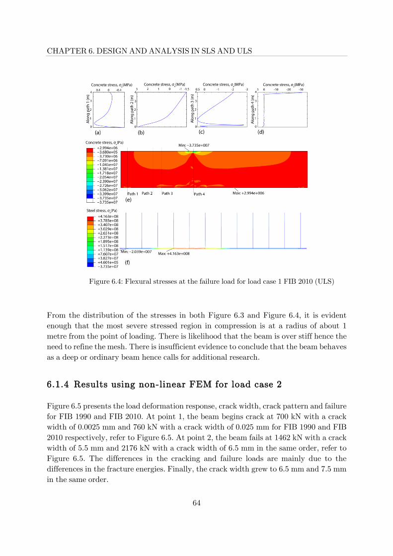
64
CHAPTER 6. DESIGN AND ANALYSIS IN SLS AND ULS
Figure 6.4: Flexural stresses at the failure load for load case 1 FIB 2010 (ULS)
From the distribution of the stresses in both Figure 6.3 and Figure 6.4, it is evident
enough that the most severe stressed region in compression is at a radius of about 1
metre from the point of loading. There is likelihood that the beam is over stiff hence the
need to refine the mesh. There is insufficient evidence to conclude that the beam behaves
as a deep or ordinary beam hence calls for additional research.
6.1.4 Results using non-linear FEM for load case 2
Figure 6.5 presents the load deformation response, crack width, crack pattern and failure
for FIB 1990 and FIB 2010. At point 1, the beam begins crack at 700 kN with a crack
width of 0.0025 mm and 760 kN with a crack width of 0.025 mm for FIB 1990 and FIB
2010 respectively, refer to Figure 6.5. At point 2, the beam fails at 1462 kN with a crack
width of 5.5 mm and 2176 kN with a crack width of 6.5 mm in the same order, refer to
Figure 6.5. The differences in the cracking and failure loads are mainly due to the
differences in the fracture energies. Finally, the crack width grew to 6.5 mm and 7.5 mm
in the same order.

65
6.1. BEAM METHOD
Figure 6.5: Load deformation response, crack width and crack pattern load case 2
For FIB 1990, the propagation of the crack was 45 degrees from near the support to the
loading point, a clear indication that the failure mechanism is shear failure. For FIB
2010, the propagation of the cracks began as a splitting crack in the reinforcement which
later changed direction and inclined at 45 degrees towards the loading point. Before it
reached the loading point at mid depth of the beam, the beam failed and failure
mechanism is a brittle shear failure. The load at 0.3 mm crack width is 820 kN.

66
CHAPTER 6. DESIGN AND ANALYSIS IN SLS AND ULS
6.1.5 Non-linear FEM stress at SLS and ULS load case 2
Figure 6.6 and Figure 6.7 presents the distribution of flexure stresses in concrete and
steel at serviceability limit state (80% of the failure load = 2176 kN) and ultimate limit
state (2176 kN).
Along path 1 to path 2 in Figure 6.6 (a) to Figure 6.6 (b) respectively, the stresses are
not very significant. Along path 3 in Figure 6.6 (c), the concrete is cracked up to the mid
depth of the beam. Along path 4 in Figure 6.6 (d), the concrete is cracked up to the
height of 3.5 m from the bottom edge of the beam so that all the stresses are transferred
to the reinforcement.
Figure 6.6: Flexural stresses at 80 % of the failure load for Case 2 FIB 2010 (SLS)
Along path 1 and path 2 in Figure 6.7 (a) and Figure 6.7 (b) respectively, stresses are
not significant to cause failure in the beam. The propagation of crack along path 3 in
Figure 6.7 (c) extended to about 3.5 m from the bottom edge of the beam height. Along
path 4 in Figure 6.7 (d), the concrete is fully cracked from 0 m to 3.5 m and the rest of
the upper section is under compression stresses.

67
6.1. BEAM METHOD
Figure 6.7: Flexural stresses at the failure load for Case 2 FIB 2010 (ULS)
6.1.6 Summary of the results
From the distribution of the stresses it is not sufficient to make a conclusion whether the
beam behaves as a deep beam or ordinary beam because of the concentration of stresses
around a small region, which may mean that the beam is over stiff, and requires mesh
refinement. The total reinforcement bars for both cases is 1.74 tonnes and the calculated
crack width is 0.29 mm less than the limit (0.3 mm) according to Eurocode 2, refer to
Table 6.1. The calculated deflection for load case 1 and load case 2 is 4 mm and 15.4 mm
respectively which is less than the limit (span length/250 = 76 mm) according to
Eurocode 2, refer to Table 6.1. The failure mechanism for load case 1 FIB 2010 and load
case 2 FIB 2010 is ductile flexure and brittle shear failure respectively.

68
CHAPTER 6. DESIGN AND ANALYSIS IN SLS AND ULS
Table 6.1: Calculated values using beam method (hand calculation)
Total mass of
reinforcement
(tonne)
Crack width
(mm)
Deflection
(mm)
Case 1 0.54 0.29 4
Case 2 1.2 0.29 15.4
Total 1.74
Failure Modes in FE Model
Case 1 FIB 2010 –Ductile Flexure failure
Case 2 FIB 2010 – Brittle Shear failure

69
6.2. STRUT AND TIE METHOD
6.2 Strut and tie method
6.2.1 Results for hand calculation
The calculated stirrups and longitudinal reinforcement using the strut and tie method
according to Eurocode 2 in ultimate limit state is presented in Figure 6.9 (a) and Figure
6.9 (b) for both load case 1 and load case 2. The respective truss models used for design
are displayed in Figure 6.8 (a) and Figure 6.8 (b).
In serviceability limit state, the crack width, 𝑤𝑘 was calculated for 20 mm and 32 mm
diameter longitudinal bars. The crack width, 𝑤𝑘 , for load case 1 and load case 2 is 0.30
mm and 0.29 mm respectively. The deformations estimated; on the other hand, are 5.1
mm and 15.5 mm respectively. Crack width and deformation calculations can be found
in Appendix B.
Figure 6.8: Truss model used for (a) load case 1 (b) and load case 2.

70
CHAPTER 6. DESIGN AND ANALYSIS IN SLS AND ULS
Figure 6.1: Strut and tie method (hand calculation) results in the ultimate and serviceability limit state for (a) load case 1 and (b) load case 2.
71
6.2. STRUT AND TIE METHOD
6.2.2 Results using non-linear FEM for load case 1
For FIB 1990 in Figure 6.10, the maximum crack width at point 1 where the linear
stress/strain ends is 5 mm, while the load reaches 596 kN. The crack width and the force
displacement plot at point 1 indicate a big crack opening and closing. The beam fails at
point 2 with a maximum crack width of 12.5 mm, while the peak load reaches 839 kN.
The failure mechanism when the load reaches a peak value is clearly brittle.
For FIB 2010 in Figure 6.10, the maximum crack width at point 1 where the linear
stress/strain ends is 0.055 mm, while the load reaches 640 kN. The beam fails at point 2
with a maximum crack width of 11.5 mm, while the peak load reaches 850 kN. The failure
mechanism when the load reaches a peak value is ductile.
The failure mechanism for both FIB 1990 and FIB 2010 is flexure shear failure with some
bond-split behaviour. The load at 0.3 mm crack width is 650 kN.

72
CHAPTER 6. DESIGN AND ANALYSIS IN SLS AND ULS
Figure 6.2: Load deformation response, crack width and crack pattern for Strut-and-Tie method (load case 1)
6.2.3 Non-linear FEM stress at SLS and ULS load case 1
For FIB 2010, the distributions of flexural stress (σx) in concrete and reinforcement bars
at SLS (80 % of the failure load = 680 kN) as presented in Figure 6.11 (d) and Figure
6.11 (e). The stress values at three paths plotted to view the distribution of across depth
of the beam are shown in Figure 6.11 (a) to Figure 6.11 (c). The stress distribution along
path 1 shows the

73
6.2. STRUT AND TIE METHOD
compressional stress in the strut is 0.5 MPa. The tensile stress along path 2 is zero, which
indicates that there are cracks in the concrete, while local compression near the loading
point with compressed zone of 0.4 m. The distribution of flexure stress is almost linear
along path 3 with a maximum tensile strength of 2 MPa, while the concrete tensile
strength is 3 MPa. The maximum tensile stress in the reinforcements is 460 MPa.
Figure 6.11: Flexural stresses at 80 % of the failure load for load case 1 FIB 2010 (SLS)
The distributions of flexural stress (σx) for concrete and reinforcement bars at ULS
(failure load = 850 kN) are presented in Figure 6.12 (d) and Figure 6.12 (e). The stress
values at three paths were plotted to view the distribution of stress across the depth of
the beam as shown in Figure 6.12 (a) to Figure 6.12 (c). The stress distribution along
path 1 shows the maximum compressive stress in the strut that is 12 MPa. The tensile
stress along path 2 is zero indicating the presence of cracks in the concrete, while local
compression near the loading point with compressed zone of 0.4 m. The distribution of
flexure stress is almost linear along path 3 with a maximum tensile stress of 2.5 MPa,
while the concrete tensile strength is 3 MPa. The maximum tensile stress in the
reinforcements reached the yield strength of 500 MPa.

74
CHAPTER 6. DESIGN AND ANALYSIS IN SLS AND ULS
Figure 6.12: Flexural stresses of the failure load for Case 1 FIB 2010 (ULS)
6.2.4 Results using non-linear FEM for load case 2
For FIB 1990 in Figure 6.13, the maximum crack width at point 1 where the linear
stress/strain ends is 0.0025 mm, while the load reaches 764 kN. The beam fails at point
2 with a maximum crack width of 5.5 mm, while the peak load reaches 2745 kN. The
failure mechanism when the load reaches a peak value shows some brittle behaviour.
For FIB 2010 in Figure 6.13, the maximum crack width at point 1 where the linear
stress/strain ends is 0.0015 mm, while the load reaches 765 kN. The beam fails at point
2 with a maximum crack width of 3.5 mm while the peak load reaches 2746 kN. The
failure mechanism when the load reaches a peak value is ductile.
The failure mechanism for both FIB 1990 and FIB 2010 is flexure shear failure with some
bond-split behaviour. The results found by the two different fracture energies are almost
similar for load case 2. The load at 0.3 mm crack width is 891 kN.

75
6.2. STRUT AND TIE METHOD
Figure 6.3: Load deformation response, crack width and crack pattern for Strut-and-Tie method (load case 2)
6.2.5 Non-linear FEM stress at SLS and ULS load case 2
The distributions of flexural stress (σx) for concrete and reinforcement bars at SLS (80
% of the failure load = 2197 kN) for FIB 2010 is presented in Figure 6.14 (d) and Figure
6.14 (e).

76
CHAPTER 6. DESIGN AND ANALYSIS IN SLS AND ULS
The stress values at three paths are also plotted to view the distribution of stress across
depth of the beam as shown in Figure 6.14(a) to Figure 6.14 (c). The stress distribution
along path 1 shows the compressive stress in the strut that reached 3 MPa. The tensile
stress along path 2 is zero and it indicates cracks in the concrete, while local compression
near the loading point is 28 MPa with compressed zone of 0.4 m. The distribution of
flexure stress is non-linear along path 3 with a maximum value of tensile strength of 2
MPa. The stress in the reinforcement bars is of 460 MPa.
Figure 6.14: Flexural stresses at 80 % of the failure load for load case 2 FIB 2010 (SLS).
The distributions of flexural stress (σx) for concrete and reinforcement bars at ULS
(failure load = 2746 kN) is presented in Figure 6.15 (d) and Figure 6.15 (e). The stress
values at three paths were plotted to view the distribution of stress across depth of the
beam as shown in Figure 6.15 (a) to Figure 6.15 (c). The stress distribution along

77
6.2. STRUT AND TIE METHOD
path 1 shows the maximum compressive stress in the strut that is 3 MPa. The tensile
stress along path 2 is zero and it indicates cracks in the concrete, while local compression
near the loading point is 33 MPa with compressed zone of 0.4 m. The distribution of
flexure stress along path 3 has a maximum compressional stress of 5 MPa. The
reinforcement bars reached yield stress of 500 MPa.
Figure 6.15: Flexural stresses of the failure load for Case 2 FIB 2010 (ULS)
6.2.6 Summary of the results
From the distribution of the stresses in both load cases for strut and tie method, stress
is localized within a small area, which indicate that the FE model was over stiff. This
could be solved by refining the mesh density to enhance bending in the FE model that
in turn would distribute the stresses across a wider region in the beam. The failure
mechanism for both load cases is flexure shear couple with bond splitting behaviour. The
cracks propagate more or less vertically from the tension area in beam towards the mid

78
CHAPTER 6. DESIGN AND ANALYSIS IN SLS AND ULS
depth of the beam at the point of loading. Other cracks extend vertically from the tension
face towards the mid depth of the beam of the concrete beam and later incline at 45
degrees towards the loading. The vertical cracks, flexure cracks, caused by the tensile
failure in the concrete and the inclined cracks, shear cracks, caused by the compression
failure in the concrete. There was some splitting failure behaviour along the
reinforcement bars, which could have occurred probably due the fact that we did not
model the interface interaction between the concrete element and the reinforcement to
capture the real bond slip behaviour. The rest of the results are summarized in Table
6.2, which includes the reinforcement content, crack width and deformation for the three
design approaches.
Table 6.2: Calculated values using strut and tie method hand calculation.
Total mass of
reinforcement
(tonne)
Crack width
(mm)
Deflection
(mm)
Case 1 0.36 0.30 5.1
Case 2 1.4 0.29 15.5
Total 1.76
Failure Modes in FE Model
Case 1 FIB 2010 – Flexure shear / bond splitting failure
Case 2 FIB 2010 – Flexure shear / bond splitting failure
79
6.3. SHELL ELEMENT METHOD
6.3 Shell Element Method (Linear FE Analysis)
6.3.1 Section forces in the ULS for load case 1
Figure 6.16 presents the distribution of section forces extracted from finite element
analysis by using shell element method. The beam was loaded to 685 kN in linear finite
element analysis. Thereafter the horizontal and vertical section forces extracted at the
point of loading along the beam depth and at the mid depth of the beam along the
longitudinal axis respectively. The horizontal forces extracted are normal force in the x-
direction and the shear force in the xy direction. Figure 6.16 (a) presents the horizontal
section forces at the point of loading and Figure 6.16 (b) presents the summation of
section forces. The normal force in the x-direction was summed up with the absolute
value of the shear force in the xy-direction to obtain the total horizontal design force
presented in Figure 6.16 (b). The same is true for the Figure 6.16 (c) and Figure 6.16
(d). Figure 6.16 (c) presents the vertical section forces extracted along the mid depth of
the beam along the longitudinal span of the beam. Figure 6.16 (c) presents the normal
forces in y-direction and the shear in the xy-direction. Summing up the normal force in
the y-direction and the absolute value of the shear force in the xy-direction produced the
total vertical design force presented in Figure 6.16 (d).
Assuming that in the ultimate limit state all the tensile strength is taken up by the
reinforcement bars, the tensile zone for Figure 6.16 (b) was divided into five segments.
At each segment, the average section force per meter was read out and recorded for the
five segments and later converted to the area of reinforcement required to carry each
respective section force per meter for each segment using the yield strength of steel (fy =
500 MPa), refer to Appendix D for the detailed calculations. The lower segment has the
higher area of reinforcement bars while the upper segment has the lower area of
reinforcement bars, refer to Figure 6.18 (a). The tensile zone in Figure 6.16 (d) was used
to design the shear reinforcement, refer to Figure 6.18 (a) and Appendix D for the
detailed calculation.

80
CHAPTER 6. DESIGN AND ANALYSIS IN SLS AND ULS
Figure 6.16: Distribution of section forces for Case 1-ULS
6.3.2 Section forces in the ULS for load case 2
Figure 6.17 presents the distribution of section forces. The beam was loaded to 2162 kN
and thereafter the section forces extracted and summed up. Figure 6.17 (b) presents the
calculated amount of reinforcement, refer to Appendix D for the detailed calculation.

81
6.3. SHELL ELEMENT METHOD
Figure 6.17: Distribution of section forces for Case 2-ULS
6.3.3 Results using linear FEM for load case 1 and load case 2
The calculated stirrups and longitudinal reinforcement using the shell element method
according to BBK 04 (section 6.7.3) in ultimate limit state is presented in Figure 6.18
(a) and Figure 6.18 (b) for load case 1 and load case 2 respectively.
In serviceability limit state, the crack width, 𝑤𝑘, was calculated for the smeared
longitudinal reinforcements as shown in Figure 6.18 (a) and Figure 6.18 (b). Hand-
calculated loads, which gave the crack width of 0.3 mm are 480 kN and 908 kN for load
case 1 and load case 2 respectively. The deformations estimated are 2.1 mm and 5.8 mm.
Crack width and deformation calculations can be found in Appendix D.

82
CHAPTER 6. DESIGN AND ANALYSIS IN SLS AND ULS
Figure 6.4: Reinforcement detailing, crack width and deformation, (a) load case 1 and (b) load case 2

83
6.3. SHELL ELEMENT METHOD
6.3.4 Results using non-linear FEM for load case 1
For the shell element method for both load case 1 and load case 2, only FIB 1990 fracture
energy (142 N/m) and the dilation angle 38º was used since it was the suitable choice for
the beam method and strut and tie method.
The beam in shell element method in Figure 6.19 began to crack at the load of 570 kN
with a crack width of 0.023 at point 1. It failed at the point 2 at the load of 740 kN with
crack width of 0.63 mm which grew to 3 mm at point 3. The failure mechanism is flexure
since the tensile face is dominated by vertical flexure cracks propagating towards the
mid depth of the beam. The load at 0.3 mm crack width is 586 kN.
Figure 6.19: Load deformation response, crack width and crack pattern for shell element method for load case 1.

84
CHAPTER 6. DESIGN AND ANALYSIS IN SLS AND ULS
6.3.5 Results using non-linear FEM for load case 2
In Figure 6.20, the beam begins to crack at point at the load of 661 kN with a crack
width of 0.07 mm. The flexural crack grew which later inclined at 45º towards the loading
point and finally failed at point 2 at the load of 2495 kN. The failure mechanism is flexure
shear. The load at 0.3 mm crack width is 1055 kN.
Figure 6.20: Load deformation response, crack width and crack pattern for shell element method for load case 2.
6.3.6 Summary of the results
The amount of reinforcement calculated for load case 1 and load case 2 was 0.51 tonnes
and 2.1 tonnes respectively as shown in Table 6.3. The total reinforcement calculated for
both cases was 2.61 tonnes. The calculated crack width was 0.3 mm for both cases. The
deformation evaluated was below the limit value of 76 mm. All calculated values using
shell element method is given in Table 6.3.
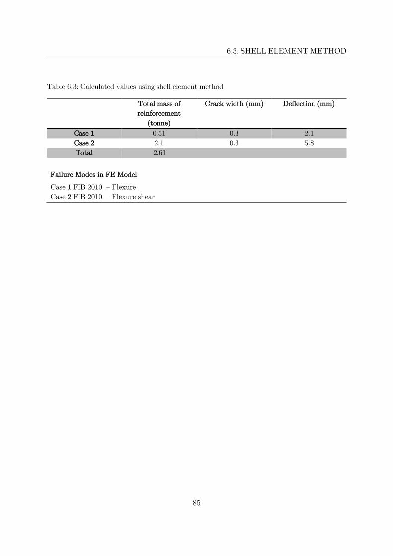
85
6.3. SHELL ELEMENT METHOD
Table 6.3: Calculated values using shell element method
Total mass of
reinforcement
(tonne)
Crack width (mm) Deflection (mm)
Case 1 0.51 0.3 2.1
Case 2 2.1 0.3 5.8
Total 2.61
Failure Modes in FE Model
Case 1 FIB 2010 – Flexure
Case 2 FIB 2010 – Flexure shear

86

87
7
Comparison of results for the three design approaches
7.1 Hand-calculated load at 0.3 mm crack width
Strut and tie method and beam method gave similar results for partially and fully reinforced concrete beams with respect to hand-calculated load at 0.3 mm crack width; while shell element method yielded lower loads. The difference between the results found using shell element method and the other two methods are -12 % and -48 % for partially and fully reinforced concrete beams respectively as shown in Figure 7.1.
Figure 7.1: Comparison between the three design methods for hand-calculated load at 0.3 mm crack width.
7.2 FE-load at 0.3 mm crack width
Strut and tie method gave 9 % higher value compared with beam method for fully reinforced concrete beams with respect to FE-load at 0.3 mm crack width while the results are the same for partially reinforced beams , whereas shell element method gave 29 % higher and 29 %
Chapter

88
CHAPTER 7. COMPARISON OF RESULTS FOR THREE DESIGN APPROACHES
lower FE-load at 0.3 mm crack width for fully and partially reinforced concrete beams respectively. The comparisons are displayed in Figure 7.2.
Figure 7.2: Comparison between the three design methods for FE-load at 0.3 mm crack width.
7.3 Amount of reinforcement
The amount of reinforcement needed using strut and tie method and shell element method were 5 % and 57 % higher respectively compared with beam method for partially and fully reinforced concrete beams added together. The comparison of the amount of reinforcement can be seen in Figure 7.3.

89
7.3. AMOUNT OF REINFORCEMENT
Figure 7.3: Comparison between the three-design methods w.r.t. the total amount of reinforcement.
7.4 Failure FE-load
The failure FE-load estimated using strut and tie method were conservative in comparison with the beam method with 6 % and 26 % for partially and fully reinforced concrete beams respectively. Similarly, shell element method gave higher failure FE-load with 5 % and 15 % compared to the beam method for partially and fully reinforced concrete beams respectively. The comparison of the failure FE-loads can be seen in Figure 7.4.
Figure 7.4: Comparison between the three design methods for failure FE-load.

90

91
8
Conclusion and further research
8.1 Discussion
In verifying and calibrating the FE model, the implicit integration technique was used
in Abaqus. The concrete damaged plasticity model for concrete and perfect plasticity
model for steel was employed. The loading used was a displacement controlled loading
and to avoid the mesh sensitivity issues, the fracture mechanics cracking model by was
employed by using the fracture energy and concrete tensile as one of the material input
parameters in Abaqus. The element type initially employed in the model was the 4 node
bilinear plain stress element for concrete and 2 node truss element for steel. In spite of
these undertakings, there was a number of challenges the major one being the
convergence problem which ultimately consumed part of the working time. Explicit
integration technique was employed, a method that does not require convergence
however the ratio of kinetic energy to internal energy of the model’s response must
always be below 5% to ascertain quality results considering the fact that all other inputs
in the model are correct. A quasi-static analysis using the explicit analysis was adopted.
Since the meshing was structured, the profile of the crack propagation was constrained
to propagate about the nodes to a different crack profile altogether. Replacing the
structured 4 node mesh with the unstructured 3 node mesh, the crack profile propagated
through the right crack profile which matched the experimental results. The size of the
element use for both the 4 node and the 3 node was 50 mm. Running each model
consumed about 8 to 10 hours. The model response had some dynamics effects hence
Raleigh material damping was introduced. The damping factor introduced to the model
was 10 % which reduced dynamic effects in the model response.
Three design approaches according to the recommendations in Eurocode 2 were done,
namely the beam method, strut and tie and shell element method. After having
calculated the reinforcement, the FE model were numerically simulated and the normal
stresses at the ultimate and serviceability limit state extracted for the beam method and
strut and tie method.
The examined stress in the disturbed regions was discovered to be insignificant when
compared to the stresses in the compressed zone. There was a localization of stresses
around a radius of about a meter from the loading point which may have been caused by
the over stiffness of the FE model. One of the probable solutions to reduce the over
stiffness in an FE model is to refine the mesh element. Since the beam regions dominated
Chapter

92
CHAPTER 8. CONCLUSION AND FURTHER RESEARCH
the disturbed regions with regards to the significance of the stresses, we would suggest
that our structure is a beam according to the Eurocode definition. However, this would
be verified even further in the future research when the FE model (beam method and
strut and tie method) mesh is refined.
8.2 Conclusion
1. Non-linear FE model (FIB 2010) using CPDM produced a good approximation within ±12% of the experimental result for failure load, failure mechanism and deformation.
2. FIB 2010 (𝐺𝑓=142 N/m) gave a higher capacity when compared to FIB 1990
(𝐺𝑓=76 N/m).
3. Higher values of dilation angles produce a ductile behavior and higher load capacity while lower values produce a brittle behavior and lower load capacity. This effect was not very distinct and evident for case 1 because the differences between 30º, 38º and 45º were rather small. In case 2, it was distinct and evident but not in the right order probably due to the pre-stressing load.
4. The beam has some disturbed regions near the loading and boundary points and beam regions away from loading and boundary points. The beam can be classified as a beam according to Eurocode 2 because the beam regions dominate with regard to the intensity of the stresses.
5. Dilation angle of 38º produced reliable results within ±20% of the experimental results regarding to failure load, failure mechanism and deformation.
6. With regards to the amount of reinforcement, Strut & Tie method was the most economical design method for case 1 while Beam method was the most economical design method for case 2. Summing up the reinforcements content for both cases, beam method become the most economical design method by ± 2% difference (Beam method has 1.74 Tonnes and Strut & Tie has 1.76 Tonnes).
7. With regard to FE load capacity and FE load at 0.3 mm crack width, strut & tie is higher by 9% and 26% compared to the beam method results respectively, hence making the strut & tie the recommended method of design.
8. Shell element method (linear-FEM) has the highest amount of reinforcement (2.61 Tonnes) , which is 50% of beam method and 48% of strut & tie) and it gave a crack width higher than the limit value 0.3 mm hence requires skin reinforcements to reduce the crack width.
9. Eurocode gives more freedom for designers to choose appropriate truss m

93
Bibliography
Abaqus 6.14 Available at: http://abaqus.software.polimi.it/v6.14/pdf_books/index.pdf
Asekeen, S., 2016. civilengineersforum. [Online] Available at: http://civilengineersforum.com/about-civil-engineers-forum/ [Använd 10 05 2016].
Bangash, M., 2001. Manual of numerical methods in concrete in modelling and application validated by experimental and site monitoring data. London: Thomas Telford.
Bazant, P. Z., 1983. Crack band theory for fracture of concrete. Construction material, 16(No. 93), pp. PP 155 - 177.
Beton-Verein, 2005. Design aids for Eurocode 2, part 1[ENV 1992-1-1]. Second ed. London: E & FN Spon.
Borst, J. G. R. a. R. d., 1987. Analysis of mixed-mode fracture in concrete. Journal of Engineering Mechanics, 113(11), pp. pp.1739-1758.
Brown, M. D., 2006. Design for shear in reinforced concrete using strut-and-tie models, Texas: Texas department of transportation.
Carpinteri, A., 1992. Application of fracture mechanics to reinforced concrete. 1 red. Torino: ELSEVIER SCIENCE PUBLISHERS LTD..
Chen, W. a. H. D., 1988. Plasticity for structural engineers. New York: Springer Verlag Inc..
Chopra, 1995. Dynamics of structures. New Jersey: Prentice Hall.
Collins, P. M. e. a., 2015. The Challenge of predicting the shear strength of very thick slabs. Concrete International, 37(11), pp. PP 29 - 37.
Dominique Chapelle, K.-J. B., 2003. The finite element analysis of shells - fundamentals. Le Chesnay: Springer.
Eurocode2, 2005. Eurocode2. Brussels: u.n.
Feentra, H. P. a. B. R., 1995. Constitutive model for reinforced concrete. Journal of engineering, 121(No. 5), pp. PP 587 - 595.
FIB, 1990. CEB FIB Model Code 1990, London: Thomas Telford.
FIB, 2010. Germany: Federal Republic of Germany.
94
BIBLIOGRAPHY
Hillerborg, A., 1985. The theoretical basis of a method to determine the fracture energy of concrete. Construction materials, 18(106), pp. pp 291-296.
Hordijk, 1992. Tensile and tensile fatigue behaviour of concrete, experiments, modeling and analyses. Heron, 37(1), pp. PP 1 -79.
Ibrahim, A., 2002. www.assakkaf.com. [Online] Available at: http://www.assakkaf.com [Använd 20 05 2016].
Karihaloo, B., 2003. Failure of concrete. Comprehensive structural intergrity, Volym 2.10, pp. PP 475 - 546.
Kmiecik, P., 2011. Modelling of reinforced concrete structures and composite structures with concrete strength degradation taken into consideration. Archives of civil and mechanical engineering, 11(3), pp. pp.1-14.
Kmiecik, P. K. M., 2011. Modelling of reinforced concrete structures and composite structures with concrete strength degradation taken into consideration. ARCHIVES OF CIVIL AND MECHANICAL ENGINEERING, XI(No. 3), pp. 623 - 636.
Kotsovos, D. M., 2015. Finite element modeling of structural concrete-short term static and dynamic loading conditions. London: Taylor and Francis Group.
Kusanale, M. A. A., 2014. Analysis and design of R.C deep beam by finite element method. International journal of emerging engineering research and technology, 2(4), pp. PP166-169.
Lectures, e. s. m., n.d. University of Auckland. [Online] Available at: http://homepages.engineering.auckland.ac.nz/~pkel015/SolidMechanicsBooks/Part_II/index.html
Lee, J. a. L. M., 2014. An experimental study of plain concrete. Concrete structures and materials, 8(No. 2), pp. PP 129 - 139.
Malm, R., 2006. Shear cracks in concrete structures subjected to in plane stresses. Lic. Thesis, Stockholm: Royal Institute of Technology (KTH).
Malm, R., 2009. Predicting shear type crack initiation and growth in concrete with non-linear finite element method, Stockholm: Royal Institute of Technology (KTH).

95
BIBLIOGRAPHY
Malm, R., 2009. Predicting shear type crack initiation and growth in concrete with non-linear finite element method, Stockholm: KTH Royal Institute of Technology.
Malm, R., 2015. Non-linear analyses of concrete beams with Abaqus, Stockholm: Royal Institute of Technology (KTH).
Martin, B. T., 2007. Verification and implementation of strut-and-tie model in LRFD bridge design specifications, New York: American association of state highway and transportation (AASHTO).
Michael Collins, E. B. Q. &. G. P., 2015. The challenge of predicting the shear strength of very thick slabs. Concrete international, 37(11), pp. PP29-37.
Mier, V., 1984. Strain softening of concrete under multiaxial loading conditions, Phd thesis, Netherlands: Delft university of technology.
Mnaour Chouchane, T. F. B. D. A. &. F. C., 2015. Design and Modeling of Mechanical Systems-II. 1 red. Hammamet: Springer.
R. Marchand, J. Y. L. K. K. a. R. R., 2007. Unstructured Meshes and Finite Elements in Space Plasma Modelling:Principles and Applications. TERRAPUB, 1(1), pp. pp.111-143.
Schlaich, P., 1991. Design and detailing of structural concrete using strut-and-tie models. The Structural Engineer, 69(6), p. 15.
Song, J.-H., 2008. Computations of the dynamic fracture of quasi-brittle plane and shell structures by the extended Finite Element Method, ILLINOIS: NORTHWESTERN UNIVERSITY.
Thacker, B. H., 2004. Concepts of model verification and validation, San Antonio, TX: Southwest Research Institute.
Westberg, B., 2010. www.stralsakerhetsmyndigheten.se. [Online] Available at: http://www.stralsakerhetsmyndigheten.se/Global/Publikationer/Rapport/Sakerhet-vid-karnkraftverken/2010/SSM-Rapport-2010-39.pdf [Använd 20 05 2016].
Yu, T. a. T. J., 2010. Finite element modeling of confined concrete-II: Plastic - damage model. Engineering structures, March.pp. PP 680 - 691.
Zhang, Z., 2007. Extrinsic cohesive modeling of dynamic fracture and microbranching instability using a topological data structure, Urbana,Illinois: University of Illinios at Urbana-Champaign.
Zielirtski, A. J., 1984. Concrete strutures under impact loading rate effects , Netherlands: Delft University of Technology.

96
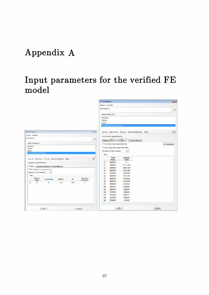
97
A
Input parameters for the verified FE model
Appendix

98
APPENDIX A. INPUT PARAMETERS FOR THE VERIFIED FE MODEL
The input paramters used to model concrete and steel. Concrete damaged plasticity model was used for concerete and perfect plasticitiy model for steel.

99
B
Quality assurance of FE model
B.1 Mesh size and element type
Mesh size control were performed for one of the model verifications of non-linear fem
(FIB 2010 Case 2) in order to find the largest mesh size which gives sufficient results.
Mesh sizes 40 mm and 50 mm were examined and compared with the experimental
results of Case 2 as displayed in the Figure 5.10. The two mesh sizes were chosen for
control based on the largest diameter of pre-stressing thread bars used in the
experimental Case 2 which was 36 mm. The errors for the ultimate loads for 40 mm and
50 mm were -4.6 % and 0.92 % compared with the experimental value respectively;
consequently, mesh size of 50 mm were selected. The 3-node concrete elements (CPS3)
were preferred than 4-node concrete elements (CPS4R) owing to capture localized cracks
of concrete. Moreover the reinforcement was modelled using 2-node truss elements
(T2D2).On the other hand; linear finite element analysis was made using 3-node concrete
triangular thin shell elements (S3R) with mesh size of 50 mm.
Figure B.1 Force-displacement plots for mesh control of 40 mm and 50 mm
Appendix

100
APPENDIX B. QUALITY ASSURANCE OF FE MODEL
B.2 Energy ratio
The results found during dynamic explicit analysis have to be checked by the ratio between kinetic energy (KE) and internal energy (IE) for the sake of assuring accuracy
of the results. The ratio 𝐾𝐸
𝐼𝐸 is supposed to be lower than 5% (Mnaour Chouchane,
2015).The energy ratio for non-linear FEM analysis were checked for all model verifications and design cases .They fulfilled the requirement except some fluctuation at the beginning of the loading. Table 3 shows the investigation made for one of the model verifications (FIB 2010 Case 2).
Figure B.2: Energy ratio percentage between kinetic energy and internal energy of the model FIB 2010 Case 2
-20
0
20
40
60
80
100
120
140
0 2 4 6 8 10 12 14
KE/
IE[%
]
Loading Step

101
C
Appendix
Beam method (hand calculation)

102
APPENDIX C. BEAM METHOD
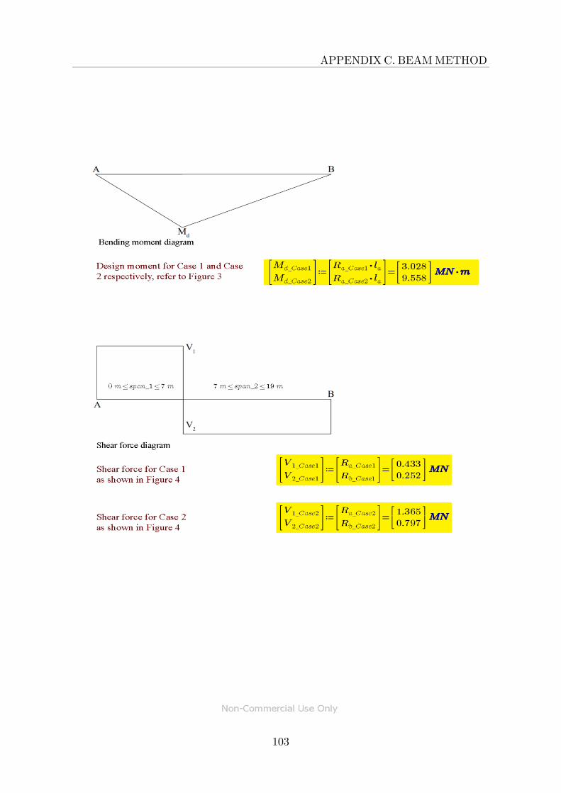
103
APPENDIX C. BEAM METHOD

104
APPENDIX C. BEAM METHOD

105
APPENDIX C. BEAM METHOD

106
APPENDIX C. BEAM METHOD

107
APPENDIX C. BEAM METHOD

108
APPENDIX C. BEAM METHOD

109
APPENDIX C. BEAM METHOD

110
APPENDIX C. BEAM METHOD

111
APPENDIX C. BEAM METHOD

112
APPENDIX C. BEAM METHOD

113
APPENDIX C. BEAM METHOD

114
APPENDIX C. BEAM METHOD

115
APPENDIX C. BEAM METHOD

116
APPENDIX C. BEAM METHOD

117
APPENDIX C. BEAM METHOD

118
APPENDIX C. BEAM METHOD

119
APPENDIX C. BEAM METHOD

120
APPENDIX C. BEAM METHOD

121
APPENDIX C. BEAM METHOD

122

123
D
Appendix
Strut and Tie method (hand calculation)

124
APPENDIX D. STRUT AND TIE METHOD

125
APPENDIX D. STRUT AND TIE METHOD

126
APPENDIX D. STRUT AND TIE METHOD

127
APPENDIX D. STRUT AND TIE METHOD

128
APPENDIX D. STRUT AND TIE METHOD

129
APPENDIX D. STRUT AND TIE METHOD

130
APPENDIX D. STRUT AND TIE METHOD

131
APPENDIX D. STRUT AND TIE METHOD

132
APPENDIX D. STRUT AND TIE METHOD
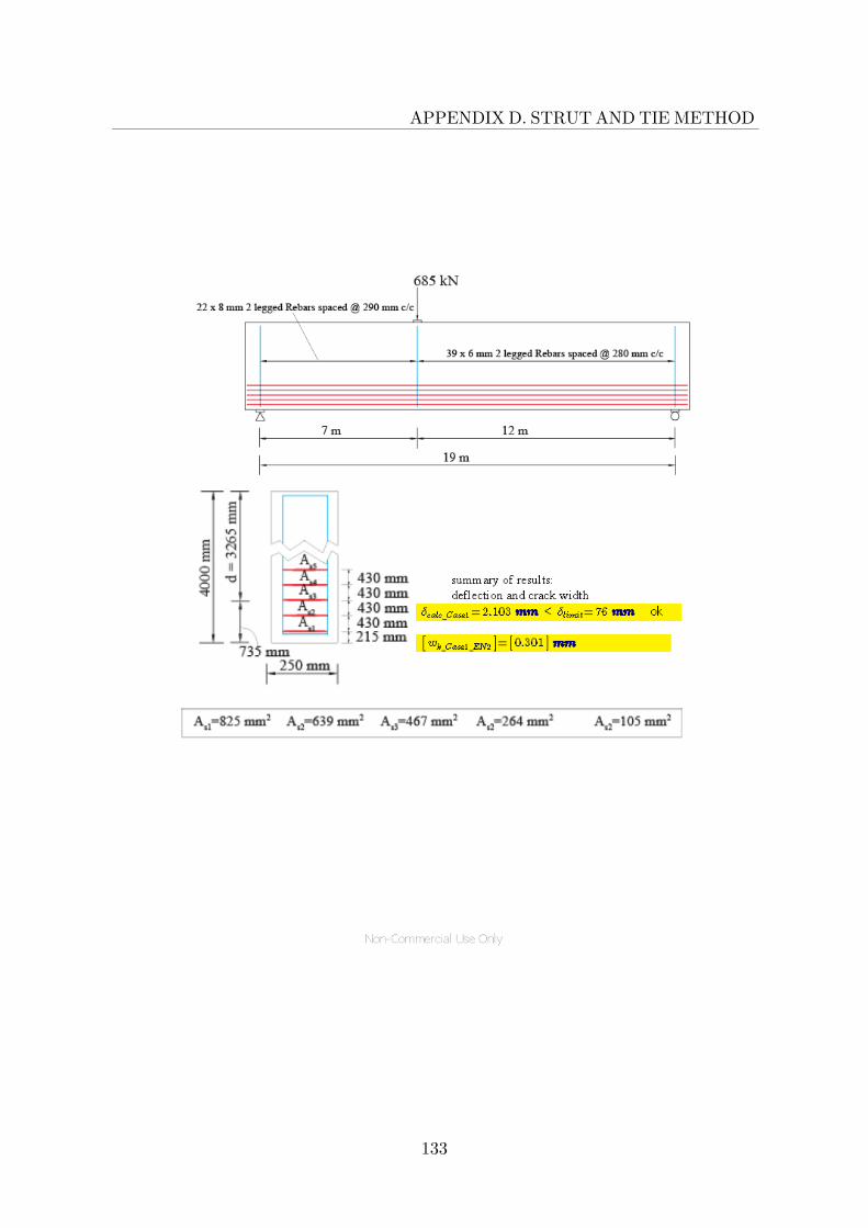
133
APPENDIX D. STRUT AND TIE METHOD

134
APPENDIX D. STRUT AND TIE METHOD

135
APPENDIX D. STRUT AND TIE METHOD
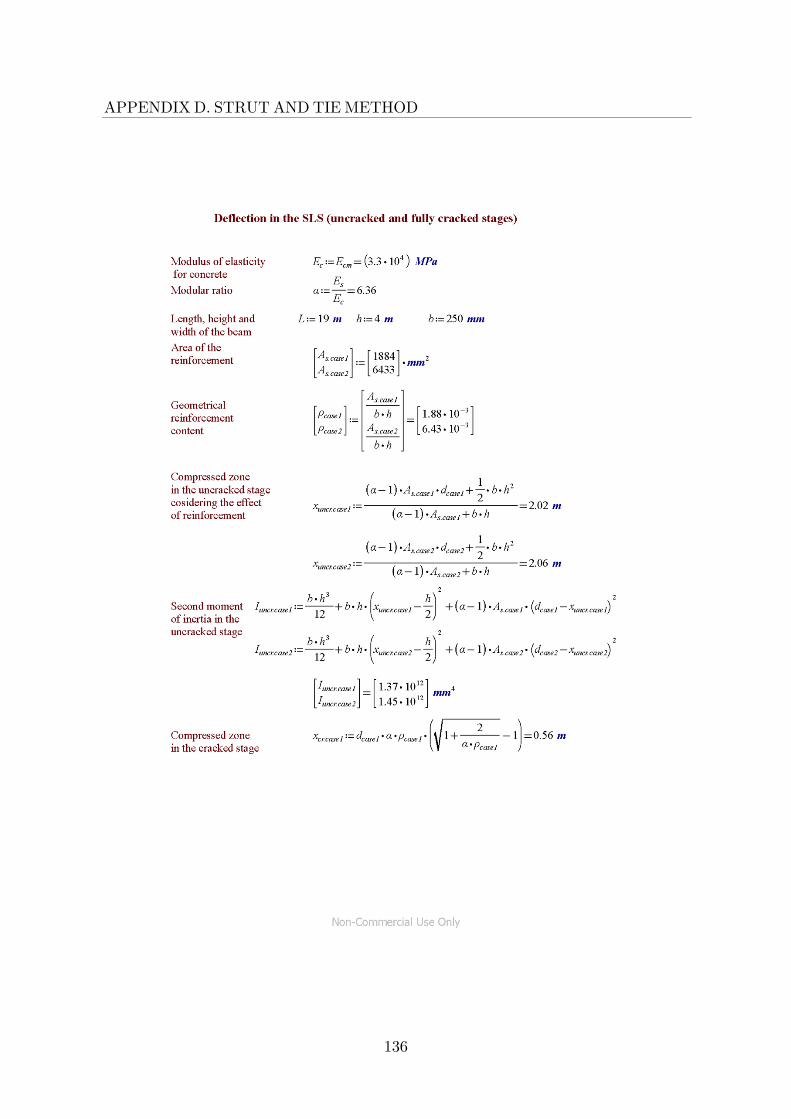
136
APPENDIX D. STRUT AND TIE METHOD

137
APPENDIX D. STRUT AND TIE METHOD

138
APPENDIX D. STRUT AND TIE METHOD

139
APPENDIX D. STRUT AND TIE METHOD

140
APPENDIX D. STRUT AND TIE METHOD

141
APPENDIX D. STRUT AND TIE METHOD

142
APPENDIX D. STRUT AND TIE METHOD

143
APPENDIX D. STRUT AND TIE METHOD

144

145
E
Appendix
Shell Element Method (Hand calculation)

146
APPENDIX E. SHELL ELEMENT METHOD

147
APPENDIX E. SHELL ELEMENT METHOD
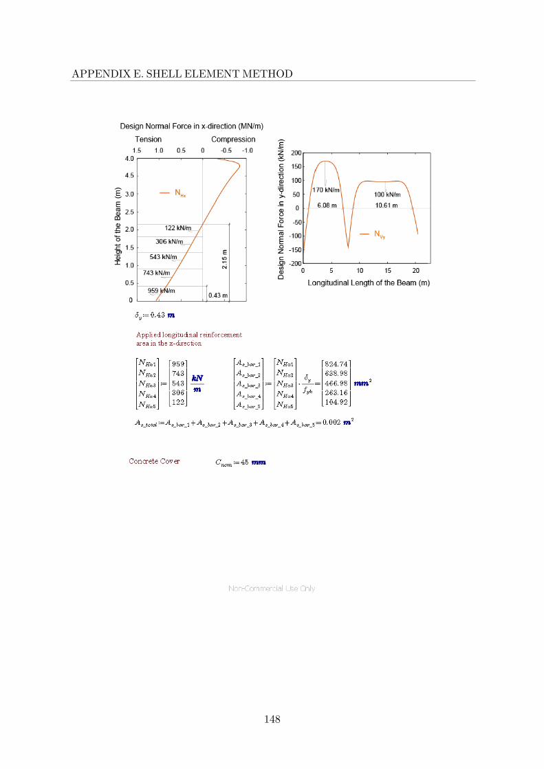
148
APPENDIX E. SHELL ELEMENT METHOD

149
APPENDIX E. SHELL ELEMENT METHOD

150
APPENDIX E. SHELL ELEMENT METHOD

151
APPENDIX E. SHELL ELEMENT METHOD

152
APPENDIX E. SHELL ELEMENT METHOD

153
APPENDIX E. SHELL ELEMENT METHOD

154
APPENDIX E. SHELL ELEMENT METHOD

155
APPENDIX E. SHELL ELEMENT METHOD

156
APPENDIX E. SHELL ELEMENT METHOD
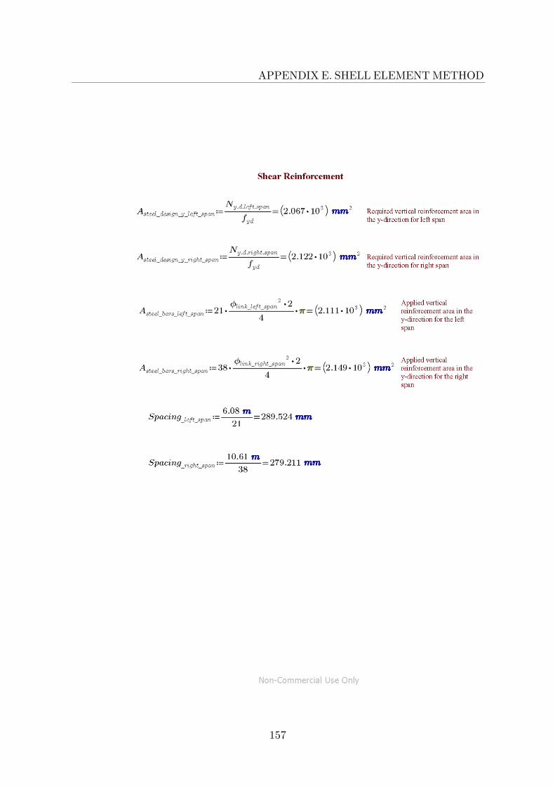
157
APPENDIX E. SHELL ELEMENT METHOD

158
APPENDIX E. SHELL ELEMENT METHOD
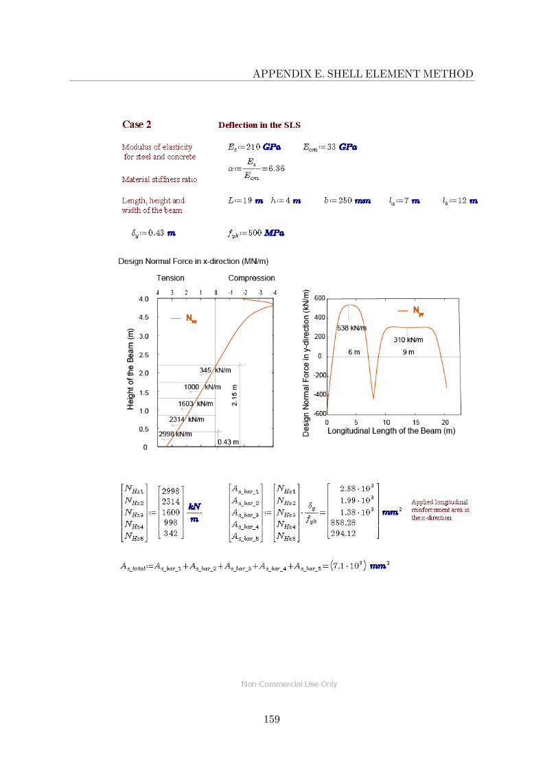
159
APPENDIX E. SHELL ELEMENT METHOD

160
APPENDIX E. SHELL ELEMENT METHOD
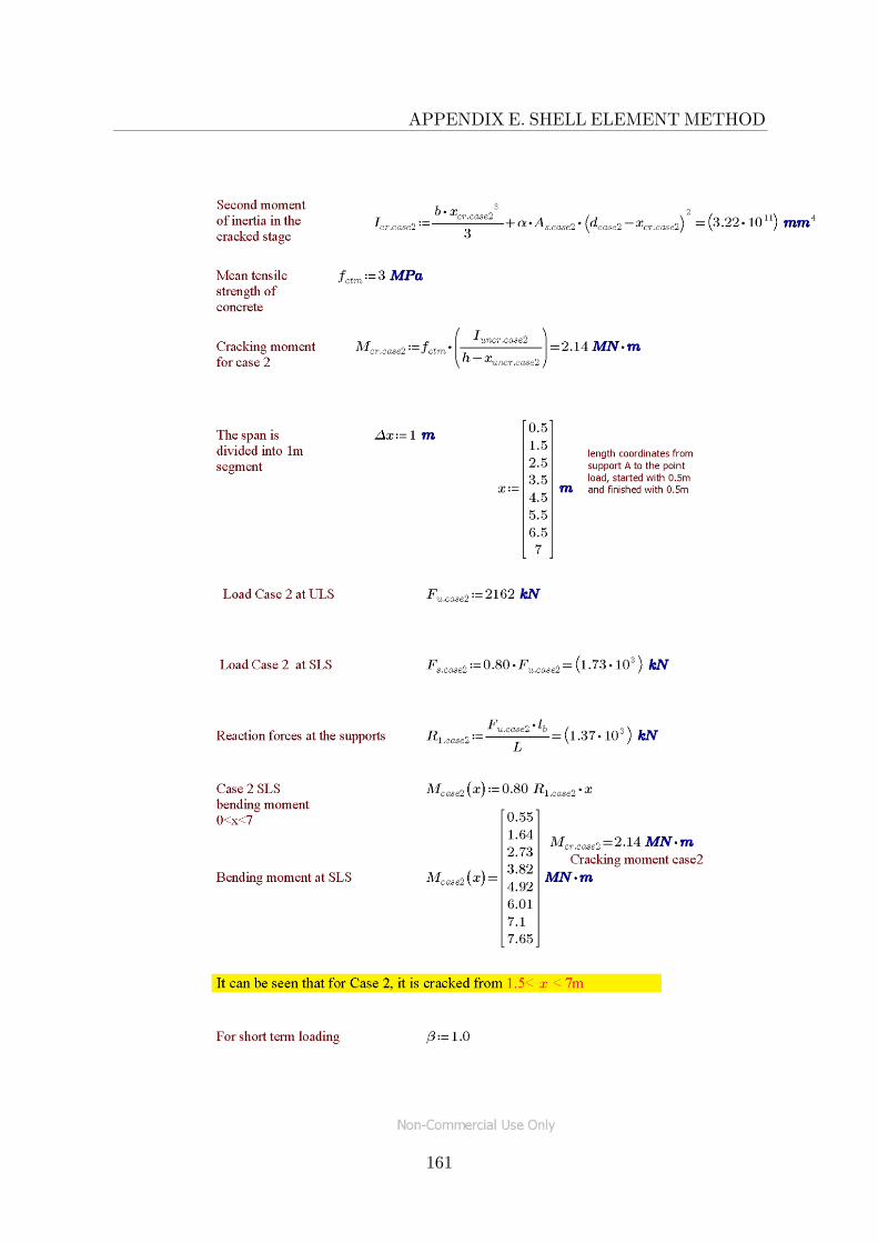
161
APPENDIX E. SHELL ELEMENT METHOD

162
APPENDIX E. SHELL ELEMENT METHOD

163
APPENDIX E. SHELL ELEMENT METHOD

164
APPENDIX E. SHELL ELEMENT METHOD

165
APPENDIX E. SHELL ELEMENT METHOD

166
APPENDIX E. SHELL ELEMENT METHOD

167
APPENDIX E. SHELL ELEMENT METHOD


www.kth.se
TRITA-BKN, MASTER THESIS 496 2016
ISSN 1103-4297
ISRN KTH/BKN/EX-496-SE