
Hybrid representation and simulation of stiff biochemical networks
Nonintrusive and structure preserving multiscale integration
of stiff ODEs, SDEs and Hamiltonian systems with hidden
slow dynamics via flow averaging
Molei Tao1, Houman Owhadi1,2, and Jerrold E. Marsden1
April 14, 2010
Abstract
We introduce a new class of integrators for stiff ODEs as well as SDEs. Examplesof subclasses of systems that we treat are ODEs and SDEs that are sums of twoterms, one of which has large coefficients. These integrators are (i) Multiscale: theyare based on flow averaging and so do not fully resolve the fast variables and have acomputational cost determined by slow variables (ii) Versatile: the method is basedon averaging the flows of the given dynamical system (which may have hidden slowand fast processes) instead of averaging the instantaneous drift of assumed sepa-rated slow and fast processes. This bypasses the need for identifying explicitly (ornumerically) the slow or fast variables (iii) Nonintrusive: A pre-existing numericalscheme resolving the microscopic time scale can be used as a black box and easilyturned into one of the integrators in this paper by turning the large coefficients onover a microscopic timescale and off during a mesoscopic timescale (iv) Convergentover two scales: strongly over slow processes and in the sense of measures over fastones. We introduce the related notion of two-scale flow convergence and analyzethe convergence of these integrators under the induced topology (v) Structure pre-serving: They inherit the structure preserving properties of the legacy integratorsfrom which they are derived. Therefore, for stiff Hamiltonian systems (possiblyon manifolds), they can be made to be symplectic, time-reversible, and symmetrypreserving (symmetries are group actions that leave the system invariant) in allvariables. They are explicit and applicable to arbitrary stiff potentials (that neednot be quadratic). Their application to the Fermi-Pasta-Ulam problems shows ac-curacy and stability over four orders of magnitude of time scales. For stiff Langevinequations, they are symmetry preserving, time-reversible and Boltzmann-Gibbs re-versible, quasi-symplectic on all variables and conformally symplectic with isotropicfriction.
Contents
1 Overview of the integrator on ODEs 3
1California Institute of Technology, Applied & Computational Mathematics, Control & Dynamicalsystems, MC 217-50 Pasadena , CA 91125
1
arX
iv:0
908.
1241
v2 [
mat
h.N
A]
13
Apr
201
0

1.1 FLAVORS . . . . . . . . . . . . . . . . . . . . . . . . . . . . . . . . . . . . 41.2 Two-scale flow convergence . . . . . . . . . . . . . . . . . . . . . . . . . . 61.3 Asymptotic convergence result . . . . . . . . . . . . . . . . . . . . . . . . 61.4 Rationale and mechanism behind FLAVORS . . . . . . . . . . . . . . . . 71.5 Non asymptotic convergence result . . . . . . . . . . . . . . . . . . . . . . 91.6 Natural FLAVORS . . . . . . . . . . . . . . . . . . . . . . . . . . . . . . . 101.7 Related work . . . . . . . . . . . . . . . . . . . . . . . . . . . . . . . . . . 111.8 Limitations of the method . . . . . . . . . . . . . . . . . . . . . . . . . . . 121.9 Generic stiff ODEs . . . . . . . . . . . . . . . . . . . . . . . . . . . . . . . 12
2 Deterministic mechanical systems: Hamiltonian equations 142.1 FLAVORS for mechanical systems on manifolds . . . . . . . . . . . . . . . 15
2.1.1 Structure preserving properties of FLAVORS . . . . . . . . . . . . 162.1.2 An example of a symplectic FLAVOR . . . . . . . . . . . . . . . . 162.1.3 An example of a symplectic and time-reversible FLAVOR . . . . . 172.1.4 An artificial FLAVOR . . . . . . . . . . . . . . . . . . . . . . . . . 17
2.2 Variational derivation of FLAVORS . . . . . . . . . . . . . . . . . . . . . 18
3 SDEs 193.1 Two-scale flow convergence for SDEs . . . . . . . . . . . . . . . . . . . . . 203.2 Non intrusive FLAVORS for SDEs . . . . . . . . . . . . . . . . . . . . . . 213.3 Convergence theorem . . . . . . . . . . . . . . . . . . . . . . . . . . . . . . 213.4 Natural FLAVORS . . . . . . . . . . . . . . . . . . . . . . . . . . . . . . . 223.5 FLAVORS for generic stiff SDEs . . . . . . . . . . . . . . . . . . . . . . . 23
4 Stochastic mechanical systems: Langevin equations 254.1 FLAVORS for stochastic mechanical systems on manifolds . . . . . . . . . 264.2 Structure Preserving properties of FLAVORS for stochastic mechanical
systems on manifolds . . . . . . . . . . . . . . . . . . . . . . . . . . . . . . 264.2.1 Example of quasi-symplectic FLAVORS . . . . . . . . . . . . . . . 274.2.2 Example of quasi-symplectic and time-reversible FLAVORS . . . . 274.2.3 Example of Boltzmann-Gibbs reversible Metropolis-adjusted FLA-
VORS . . . . . . . . . . . . . . . . . . . . . . . . . . . . . . . . . . 27
5 Numerical analysis of FLAVOR based on Variational Euler 285.1 Stability . . . . . . . . . . . . . . . . . . . . . . . . . . . . . . . . . . . . . 285.2 Error analysis . . . . . . . . . . . . . . . . . . . . . . . . . . . . . . . . . . 305.3 Numerical error analysis for nonlinear systems . . . . . . . . . . . . . . . 30
6 Numerical experiments 336.1 Hidden Van der Pol oscillator (ODE) . . . . . . . . . . . . . . . . . . . . . 336.2 Hamiltonian system with nonlinear stiff and soft potentials . . . . . . . . 346.3 Fermi-Pasta-Ulam problem . . . . . . . . . . . . . . . . . . . . . . . . . . 36
6.3.1 On resonances . . . . . . . . . . . . . . . . . . . . . . . . . . . . . 39
2

6.4 Nonlinear 2D primitive molecular dynamics . . . . . . . . . . . . . . . . . 396.5 Nonlinear 2D molecular clipper . . . . . . . . . . . . . . . . . . . . . . . . 416.6 Forced nonautonomous mechanical system: Kapitza’s inverted pendulum 436.7 Nonautonomous SDE system with hidden slow variables . . . . . . . . . . 456.8 Langevin equations with slow noise and friction . . . . . . . . . . . . . . . 466.9 Langevin equations with fast noise and friction . . . . . . . . . . . . . . . 48
7 Appendix 497.1 Proof of theorems 1.1 and 1.2 . . . . . . . . . . . . . . . . . . . . . . . . . 497.2 Proof of Theorem 3.1 . . . . . . . . . . . . . . . . . . . . . . . . . . . . . . 55
Acknowledgements Part of this work has been supported by NSF grant CMMI-092600. We are grateful to C. Lebris, J.M. Sanz-Serna, E. S. Titi, R. Tsai and E.Vanden-Eijnden for useful comments and providing references. We would also like tothank two anonymous referees for precise and detailed comments and suggestions.
1 Overview of the integrator on ODEs
Consider the following ODE on Rd,
uε = G(uε) +1
εF (uε). (1.1)
In Subsections 1.9, 2.1, 3.1, 3.5 and 4.1 we will consider more general ODEs, stiff de-terministic Hamiltonian systems (2.1), SDEs ((3.1) and (3.15)) and Langevin equations((4.1) and (4.2)); however for the sake of clarity, we will start the description of ourmethod with (1.1).
Condition 1.1. Assume that there exists a diffeomorphism η := (ηx, ηy), from Rd ontoRd−p × Rp (with uniformly bounded C1, C2 derivatives), separating slow and fast vari-ables, i.e., such that (for all ε > 0) the process (xεt, y
εt) = (ηx(uεt), η
y(uεt)) satisfies anODE system of the form
xε = g(xε, yε) xε0 = x0
yε = 1εf(xε, yε) yε0 = y0
. (1.2)
Condition 1.2. Assume that the fast variables in (1.2) are locally ergodic with respectto a family of measures µ drifted by slow variables. More precisely, we assume that thereexists a family of probability measures µ(x, dy) on Rp indexed by x ∈ Rd−p and a positivefunction T 7→ E(T ) such that limT→∞E(T ) = 0 and such that for all x0, y0, T and φuniformly bounded and Lipschitz, the solution to
Yt = f(x0, Yt) Y0 = y0 (1.3)
satisfies∣∣∣ 1
T
∫ T
0φ(Ys)ds−
∫Rpφ(y)µ(x0, dy)
∣∣∣ ≤ χ(‖(x0, y0)‖)E(T )(‖φ‖L∞ + ‖∇φ‖L∞) (1.4)
3

where r 7→ χ(r) is bounded on compact sets.
Under conditions 1.1 and 1.2, it is known (we refer for instance to [95] or to Theorem14, Section 3 of Chapter II of [104] or to [88]) that xε converges towards xt defined asthe solution to the ODE
x =
∫g(x, y)µ(x, dy), x|t=0 = x0 (1.5)
where µ(x, dy) is the ergodic measure associated with the solution to the ODE
y = f(x, y) (1.6)
It follows that the slow behavior of solutions of (1.1) can be simulated over coarse timesteps by first identifying the slow process xε and then using numerical approximationsof solutions of (1.2) to approximate xε. Two classes of integrators have been founded onthis observation: The equation free method [64, 65] and the Heterogeneous MultiscaleMethod [36, 40, 35, 5]. One shared characteristic of the original form of those integratorsis, after identification of the slow variables, to use a micro-solver to approximate theeffective drift in (1.5) by averaging the instantaneous drift g with respect to numericalsolutions of (1.6) over a time span larger than the mixing time of the solution to (1.6).
1.1 FLAVORS
In this paper, we propose a new method based on the averaging of the instantaneous flowof the ODE (1.1) with hidden slow and fast variables instead of the instantaneous driftof xε in ODE (1.2) with separated slow and fast variables. We have called the resultingclass of numerical integrators FLow AVeraging integratORS (FLAVORS). SinceFLAVORS are directly applied to (1.1), hidden slow variables do not need to be identi-fied, either explicitly or numerically. Furthermore FLAVORS can be implemented using
an arbitrary legacy integrator Φ1εh for (1.1) in which the parameter 1
ε can be controlled(figure 1). More precisely, assume that there exists a constant h0 > 0 such that Φα
h
satisfies for all h ≤ h0 min( 1α , 1) and u ∈ Rd∣∣Φα
h(u)− u− hG(u)− αhF (u)∣∣ ≤ Ch2(1 + α)2 (1.7)
then FLAVOR can be defined as the algorithm simulating the process
ut =(Φ0δ−τ Φ
1ετ
)k(u0) for kδ ≤ t < (k + 1)δ (1.8)
where τ is a fine time step resolving the fast time scale (τ ε) and δ is a mesoscopictime step independent of the fast time scale satisfying τ ε δ 1 and
(τ
ε)2 δ τ
ε(1.9)
In our numerical experiments, we have used the “rule of thumb” δ ∼ γ τε where γ is asmall parameter (0.1 for instance).
4
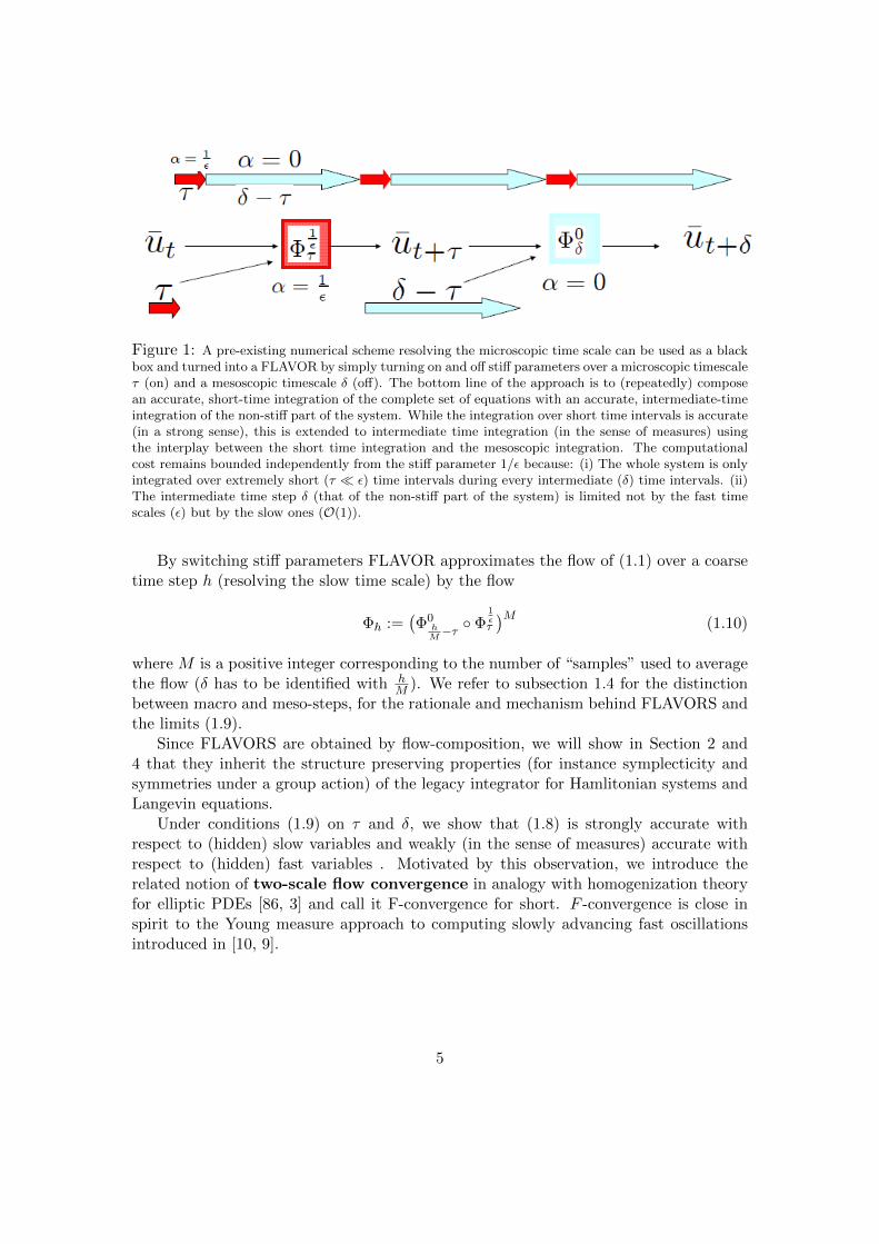
Figure 1: A pre-existing numerical scheme resolving the microscopic time scale can be used as a blackbox and turned into a FLAVOR by simply turning on and off stiff parameters over a microscopic timescaleτ (on) and a mesoscopic timescale δ (off). The bottom line of the approach is to (repeatedly) composean accurate, short-time integration of the complete set of equations with an accurate, intermediate-timeintegration of the non-stiff part of the system. While the integration over short time intervals is accurate(in a strong sense), this is extended to intermediate time integration (in the sense of measures) usingthe interplay between the short time integration and the mesoscopic integration. The computationalcost remains bounded independently from the stiff parameter 1/ε because: (i) The whole system is onlyintegrated over extremely short (τ ε) time intervals during every intermediate (δ) time intervals. (ii)The intermediate time step δ (that of the non-stiff part of the system) is limited not by the fast timescales (ε) but by the slow ones (O(1)).
By switching stiff parameters FLAVOR approximates the flow of (1.1) over a coarsetime step h (resolving the slow time scale) by the flow
Φh :=(Φ0
hM−τ Φ
1ετ
)M(1.10)
where M is a positive integer corresponding to the number of “samples” used to averagethe flow (δ has to be identified with h
M ). We refer to subsection 1.4 for the distinctionbetween macro and meso-steps, for the rationale and mechanism behind FLAVORS andthe limits (1.9).
Since FLAVORS are obtained by flow-composition, we will show in Section 2 and4 that they inherit the structure preserving properties (for instance symplecticity andsymmetries under a group action) of the legacy integrator for Hamlitonian systems andLangevin equations.
Under conditions (1.9) on τ and δ, we show that (1.8) is strongly accurate withrespect to (hidden) slow variables and weakly (in the sense of measures) accurate withrespect to (hidden) fast variables . Motivated by this observation, we introduce therelated notion of two-scale flow convergence in analogy with homogenization theoryfor elliptic PDEs [86, 3] and call it F-convergence for short. F -convergence is close inspirit to the Young measure approach to computing slowly advancing fast oscillationsintroduced in [10, 9].
5

1.2 Two-scale flow convergence
Let (ξεt )t∈R+ be a sequence of processes on Rd (functions from R+ to Rd) indexed byε > 0. Let (Xt)t∈R+ be a process on Rd−p (p ≥ 0). Let x 7→ ν(x, dz) be a function fromRd−p into the space of probability measures on Rd.
Definition 1.1. We say that the process ξεt F-converges to ν(Xt, dz) as ε ↓ 0 and
write ξεtF−−→ε→0
ν(Xt, dz) if and only if for all functions ϕ bounded and uniformly Lipshitz-
continuous on Rd, and for all t > 0,
limh→0
limε→0
1
h
∫ t+h
tϕ(ξεs) ds =
∫Rdϕ(z)ν(Xt, dz) (1.11)
1.3 Asymptotic convergence result
Our convergence theorem requires that uεt and ut do not blow up as ε ↓ 0; more precisely,we will assume that the following conditions are satisfied.
Condition 1.3. Assume that:
1. F and G are Lipschitz continuous.
2. For all u0, T > 0, the trajectories (uεt)0≤t≤T are uniformly bounded in ε.
3. For all u0, T > 0, the trajectories (uεt)0≤t≤T are uniformly bounded in ε, 0 < δ ≤h0, τ ≤ min(τ0ε, δ).
For π, an arbitrary measure on Rd, we define η−1 ∗ π to be the push forward of themeasure π by η−1.
Theorem 1.1. Let uεt be the solution to (1.1) and ut be defined by (1.8). Assume thatequation (1.7) and conditions 1.1, 1.2 and 1.3 are satisfied, then
• uεt F -converges to η−1 ∗(δXt ⊗ µ(Xt, dy)
)as ε ↓ 0 where Xt is the solution to
Xt =
∫g(Xt, y)µ(Xt, dy) X0 = x0. (1.12)
• ut F -converges to η−1 ∗(δXt ⊗ µ(Xt, dy)
)for ε ≤ δ/(−C ln δ), τ
ε ↓ 0, ετ δ ↓ 0 and
( τε )2 1δ ↓ 0.
Remark 1.1. The F -convergence of uεt to η−1 ∗(δXt ⊗ µ(Xt, dy)
)can be restated as
limh→0
limε→0
1
h
∫ t+h
tϕ(uεs) ds =
∫Rpϕ(η−1(Xt, y))µ(Xt, dy) (1.13)
for all functions ϕ bounded and uniformly Lipshitz-continuous on Rd, and for all t > 0.
6

Remark 1.2. Observe that g comes from (1.5). It is not explicitly known and does notneed to be explicitly known for the implementation of the proposed method.
Remark 1.3. The limits on ε, τ and δ are in essence stating that FLAVOR is accurateprovided that τ ε (τ resolves the stiffness of (1.1)) and equation (1.9) is satisfied.
Remark 1.4. Throughout this paper, C will refer to an appropriately large enough con-stant independent from ε, δ, τ . To simplify the presentation of our results, we use thesame letter C for expressions such as 2CeC instead of writing it as a new constant C1
independent from ε, δ, τ .
1.4 Rationale and mechanism behind FLAVORS
We will now explain the rationale and mechanism behind FLAVORS. We refer to Sub-section 7.1 of the appendix for the detailed proof of Theorem 1.1. Let us start byconsidering the case where η is the identity diffeomorphism. Let ϕ
1ε be the flow of (1.2).
Observe that ϕ0 (obtained from ϕ1ε by setting the parameter 1
ε to zero) is the flow of(1.2) with yε frozen, i.e.,
ϕ0(x, y) = (xt, y) where xt solvesdx
dt= g(x, y), x0 = x. (1.14)
The main effect of FLAVORS is to average the flow of (1.2) with respect to fast degreesof freedom via splitting and re-synchronization. By splitting, we refer to the substitution
of the flow ϕ1εδ by composition of ϕ0
δ−τ and ϕ1ετ , and by re-synchronization we refer to
the distinct time-steps δ and τ whose effects are to advance the internal clock of fastvariables by τ every step of length δ. By averaging, we refer to the fact that FLAVORS
approximates the flow ϕ1εh by the flow
ϕh :=(ϕ0
hM−τ ϕ
1ετ
)M(1.15)
where h is a coarse time step resolving the slow time scale associated with xε, M is apositive integer corresponding to the number of samples used to average the flow (δ isidentified with h
M ) and τ is a fine time step resolving the fast time scale, of the order ofε, and associated with yε. In general, analytical formulae are not available for ϕ0 andϕ
1ε and numerical approximations are used instead.
Observe that when FLAVORS are applied to systems with explicitly separated slowand fast processes, they lead to integrators that are locally in the neighborhood ofthose obtained with HMM (or equation free) methods with a reinitialization of the fastvariables at macrotime n by their final value at macrotime step n− 1 and with only onemicrostep per macrostep [37, 39].
We will now consider the situation where η is not the identity diffeomorphism and
7

give the rationale behind the limits (1.9).
unδΦ
1ετ //
η
unδ+τΦ0δ−τ //
η
u(n+1)δ
η
(x, y)nδ
Ψ1ετ //
η−1
OO
(x, y)nδ+τΨ0δ−τ //
η−1
OO
(x, y)(n+1)δ
η−1
OO
As illustrated in the above diagram, since (xt, yt) = η(ut), simulating unδ defined in(1.8) is equivalent to simulating the discrete process
(xnδ, ynδ) :=(Ψ
1εδ−τ Ψ0
τ
)n(x0, y0) (1.16)
whereΨαh := η Φα
h η−1 (1.17)
Observe that the accuracy (in the topology induced by F-convergence) of ut with respectto uεt, solution of (1.1), is equivalent to that of (xt, yt) with respect to (xεt, y
εt) defined by
(1.2). Now, for the clarity of the presentation, assume that
Φαh(u) = u+ hG(u) + αhF (u) (1.18)
Using Taylor’s theorem and (1.18), we obtain that
Ψαh(x, y) = (x, y)+h
(g(x, y), 0
)+αh
(0, f(x, y)
)+
∫ 1
0vT Hess η(u+tv)v(1−t)2 dt (1.19)
withu := η−1(x, y) and v := h(G+ αF ) η−1(x, y) (1.20)
It follows from equations (1.19) and (1.20) that Ψ1εh is a first order accurate integrator
approximating the flow of (1.2) and Ψ0h is a first order accurate integrator approximating
the flow of (1.14). Let h be a coarse time step and δ a mesostep. Since x remains nearlyconstant over the coarse time step, the switching (on and off) of the stiff parameter 1
εaverages the drift g of x with respect to the trajectory of y over h. Since the coarsestep h is composed of h
δ mesosteps, the internal clock of the fast process is advanced byhδ ×
τε . Since h is of the order of one, the trajectory of y is mixing with respect to the
local ergodic measure µ provided that τδε 1, i.e.
δ τ
ε(1.21)
Equation (1.21) corresponds to the right hand side of equation (1.9). If η is a non-lineardiffeomorphism (with non-zero Hessian), it also follows from equations (1.19) and (1.20)
that each invocation of the integrator Ψ1ετ occasions an error (on the accuracy of the
slow process) proportional to ( τε )2. Since during the coarse time step h, Ψ1ετ is solicited
8
hδ -times, it follows that the error accumulation during h is h
δ ×( τε )2. Hence, the accuracyof the integrator requires that 1
δ × ( τε )2 1, i.e.(τε
)2 δ (1.22)
Equation (1.22) corresponds to the left hand side of equation (1.9).Observe that if η is linear, its Hessian is null and the remainder in the right hand
side of (1.19) is zero. It follows that if η is linear, the error accumulation due to finetime steps on slow variables is zero and condition (1.21) is sufficient for the accuracy ofthe integrator.
It has been observed in [38] and in Section 5 of [111] that slow variables do not needto be identified with HMM/averaging type integrators if the relation between originaland slow variables is linear or a permutation and if
∆t
M τ
ε(1.23)
where is M the number of fine-step iterations used by HMM to compute the average thedrift of slow variables and ∆t is the coarse time step (in HMM) along the direction ofthe averaged drift. The analysis of FLAVORS associated with equation (1.19) reaches asimilar conclusion if η is linear in the sense that the error caused by the Hessian of η in(1.19) is zero and in the (sufficient) condition (1.21) is analogous to (1.23) for M = 1. Itis also stated on Page 2 of [38] that “there are counterexamples showing that algorithmsof the same spirit do not work for deterministic ODEs with separated time scales if theslow variables are not explicitly identified and made use of. But in the present context,the slow variables are linear functions of the original variables, and this is the reason whythe seamless algorithm works.” Here, the analysis of FLAVORS associated with equation(1.19) shows an algorithm based on an averaging principle would indeed, in general, notwork if η is nonlinear (and (1.22) not satisfied) due to the error accumulation (on slowvariables) associated with the Hessian of η. However, the above analysis also showsthat if condition (1.22) is satisfied, then, although η may be nonlinear, flow averagingintegrators will always work without identifying slow variables.
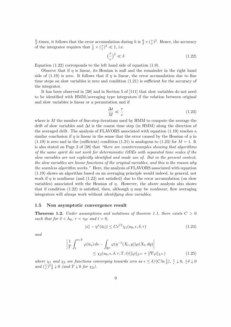
1.5 Non asymptotic convergence result
Theorem 1.2. Under assumptions and notations of theorem 1.1, there exists C > 0such that for δ < h0, τ < τ0ε and t > 0,
|xεt − ηx(ut)| ≤ CeCtχ1(u0, ε, δ, τ) (1.24)
and ∣∣∣∣ 1
T
∫ t+T
tϕ(us) ds−
∫Rpϕ(η−1(Xt, y))µ(Xt, dy)
∣∣∣∣≤ χ2(u0, ε, δ, τ, T, t)(‖ϕ‖L∞ + ‖∇ϕ‖L∞) (1.25)
where χ1 and χ2 are functions converging towards zero as ε ≤ δ/(C ln 1δ ), τ
ε ↓ 0, ετ δ ↓ 0
and ( τε )2 1δ ↓ 0 (and T ↓ 0 for χ2).
9
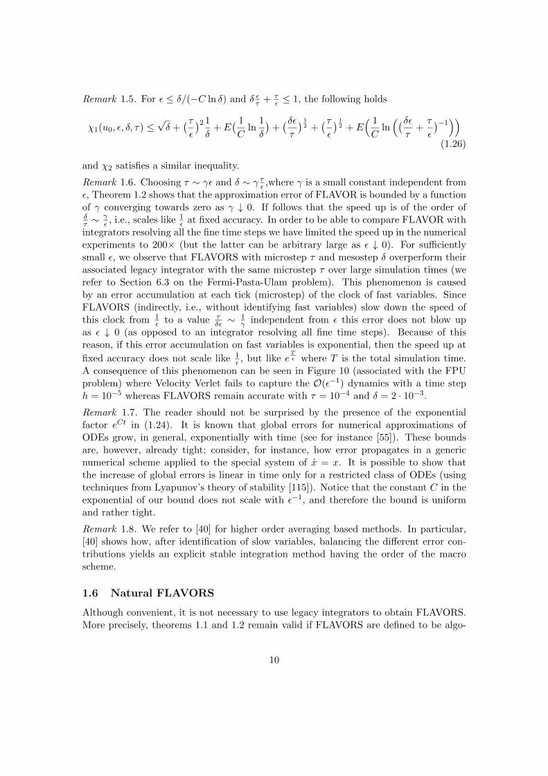
Remark 1.5. For ε ≤ δ/(−C ln δ) and δ ετ + τε ≤ 1, the following holds
χ1(u0, ε, δ, τ) ≤√δ +
(τε
)2 1
δ+ E
( 1
Cln
1
δ
)+(δετ
) 12 +
(τε
) 12 + E
( 1
Cln((δε
τ+τ
ε
)−1))
(1.26)
and χ2 satisfies a similar inequality.
Remark 1.6. Choosing τ ∼ γε and δ ∼ γ τε ,where γ is a small constant independent fromε, Theorem 1.2 shows that the approximation error of FLAVOR is bounded by a functionof γ converging towards zero as γ ↓ 0. If follows that the speed up is of the order ofδτ ∼
γε , i.e., scales like 1
ε at fixed accuracy. In order to be able to compare FLAVOR withintegrators resolving all the fine time steps we have limited the speed up in the numericalexperiments to 200× (but the latter can be arbitrary large as ε ↓ 0). For sufficientlysmall ε, we observe that FLAVORS with microstep τ and mesostep δ overperform theirassociated legacy integrator with the same microstep τ over large simulation times (werefer to Section 6.3 on the Fermi-Pasta-Ulam problem). This phenomenon is causedby an error accumulation at each tick (microstep) of the clock of fast variables. SinceFLAVORS (indirectly, i.e., without identifying fast variables) slow down the speed ofthis clock from 1
ε to a value τδε ∼
1γ independent from ε this error does not blow up
as ε ↓ 0 (as opposed to an integrator resolving all fine time steps). Because of thisreason, if this error accumulation on fast variables is exponential, then the speed up at
fixed accuracy does not scale like 1ε , but like e
Tε where T is the total simulation time.
A consequence of this phenomenon can be seen in Figure 10 (associated with the FPUproblem) where Velocity Verlet fails to capture the O(ε−1) dynamics with a time steph = 10−5 whereas FLAVORS remain accurate with τ = 10−4 and δ = 2 · 10−3.
Remark 1.7. The reader should not be surprised by the presence of the exponentialfactor eCt in (1.24). It is known that global errors for numerical approximations ofODEs grow, in general, exponentially with time (see for instance [55]). These boundsare, however, already tight; consider, for instance, how error propagates in a genericnumerical scheme applied to the special system of x = x. It is possible to show thatthe increase of global errors is linear in time only for a restricted class of ODEs (usingtechniques from Lyapunov’s theory of stability [115]). Notice that the constant C in theexponential of our bound does not scale with ε−1, and therefore the bound is uniformand rather tight.
Remark 1.8. We refer to [40] for higher order averaging based methods. In particular,[40] shows how, after identification of slow variables, balancing the different error con-tributions yields an explicit stable integration method having the order of the macroscheme.
1.6 Natural FLAVORS
Although convenient, it is not necessary to use legacy integrators to obtain FLAVORS.More precisely, theorems 1.1 and 1.2 remain valid if FLAVORS are defined to be algo-
10

rithms simulating the discrete process
ut :=(θGδ−τ θετ
)k(u0) for kδ ≤ t < (k + 1)δ (1.27)
where θετ and θGδ−τ are two mappings from Rd onto Rd (the former approximating the flowof the whole system (1.1) for time τ , and the latter approximating the flow of v = G(v)for time δ − τ), satisfying the following conditions.
Condition 1.4. Assume that:
1. There exists h0, C > 0 such that for h ≤ h0 and any u ∈ Rd,∣∣θGh (u)− u− hG(u)∣∣ ≤ Ch2 (1.28)
2. There exists τ0, C > 0, such that for τε ≤ τ0 and any u ∈ Rd,∣∣∣θετ (u)− u− τG(u)− τ
εF (u)
∣∣∣ ≤ C(τε
)2(1.29)
3. For all u0, T > 0, the discrete trajectories((θGδ−τ θετ
)k(u0)
)0≤k≤T/δ
are uniformly
bounded in ε, 0 < δ ≤ h0, τ ≤ min(τ0ε, δ).
Observe that (1.8) is a particular case of (1.27) in which θε = Φ1ε and the mapping
θG is obtained from the legacy integrator Φα by setting α to zero.
1.7 Related work
Dynamical systems with multiple time scales pose a major problem in simulations becausethe small time steps required for stable integration of the fast motions lead to largenumbers of time steps required for the observation of slow degrees of freedom [109, 54].Traditionally, stiff dynamical systems have been separated into two classes with distinctintegrators: stiff systems with fast transients and stiff systems with rapid oscillations[6, 35, 98]. The former has been solved using implicit schemes [46, 34, 54, 56], Chebyshevmethods [70, 1] or the projective integrator approach [48]. These latter have been solvedusing filtering techniques [45, 66, 100] or Poincare map techniques [47, 90]. We alsorefer to methods based on highly oscillatory quadrature [32, 60, 59], an area that hasundergone significant developments in the last few years [61]. It has been observedthat at the present time, there exists no unified strategy for dealing with both classesof problems [35]. When slow variables can be identified, effective equations can beobtained by averaging the instantaneous drift driving those slow variables [104]. Twoclasses of numerical methods have been built on this observation: The equation-freemethod [64, 65] and the Heterogeneous Multiscale Method [36, 40, 35, 5]. Observe thatFLAVORS apply in a unified way to both stiff systems with fast transients and stiffsystems with rapid oscillations, with or without noise, with a mesoscopic integrationtime step chosen independently from the stiffness.
11

1.8 Limitations of the method
The proof of the accuracy of the method (theorems 1.1 and 1.2) is based on an averagingprinciple; hence, if ε is not small (the stiffness of the ODE is weak), although the methodmay be stable, there is no guarantee of accuracy. More precisely, the global error of themethod is an increasing function of ε, δ, τ
ε , δετ , ( τε )2δ. Writing γ := τ
ε the accuracy
method requires γ2 δ γ. Choosing δ = γ32 , the condition ε δ 1 (related to
computational gain) requires ε23 γ 1 which can be satisfied only if ε is small.
The other limitation of the method lies in the fact that a stiff parameter 1ε needs to
be clearly identified. In many examples of interest (Navier-Stokes equations, Maxwell’sequations,...), stiffness is a result of nonlinearity, initial conditions or boundary condi-tions and not of the existence of a large parameter 1
ε . Molecular dynamics can also createwidely separated time-scales from non-linear effects; we refer, for instance, to [116] andreferences therein.
1.9 Generic stiff ODEs
FLAVORS have a natural generalization to systems of the form
uα,ε = F (uα,ε, α, ε) (1.30)
where u 7→ F (u, α, ε) is Lipshitz continuous.
Condition 1.5. Assume that:
1. ε 7→ F (u, α, ε) is uniformly continuous in the neighborhood of 0.
2. There exists a diffeomorphism η := (ηx, ηy), from Rd onto Rd−p × Rp, indepen-dent from ε, α, with uniformly bounded C1, C2 derivatives, such that the process(xαt , y
αt ) =
(ηx(uα,0t ), ηy(uα,0t )
)satisfies, for all α ≥ 1, the ODE
xα = g(xα, yα) xα0 = x0, (1.31)
where g(x, y) is Lipschitz continuous in x and y on bounded sets.
3. There exists a family of probability measures µ(x, dy) on Rp such that for allx0, y0, T
((x0, y0) := η(u0)
)and ϕ uniformly bounded and Lipschitz
∣∣∣ 1
T
∫ T
0ϕ(yαs ) ds−
∫Rpϕ(y)µ(x0, dy)
∣∣∣ ≤ χ(‖(x0, y0)‖)(E1(T ) + E2(Tαν)
)‖∇ϕ‖L∞
(1.32)where r 7→ χ(r) is bounded on compact sets and E2(r)→ 0 as r →∞ and E1(r)→0 as r → 0.
4. For all u0, T > 0, the trajectories (uα,0t )0≤t≤T are uniformly bounded in α ≥ 1.
12

Remark 1.9. Observe that slow variables are not kept frozen in equation (1.32). Theerror on local invariant measures induced by the (slow) drift of xα is controlled by E2.More precisely, the convergence of the right hand side of (1.32) towards zero requires theconvergence of T towards zero and (at the same time) the divergence of Tαν towardsinfinity.
Assume that we are given a mapping Φα,εh from Rd onto Rd approximating the flow
of (1.30). If the parameter α can be controlled then Φα,εh can be used as a black box for
accelerating the computation of solutions of (1.30).
Condition 1.6. Assume that:
1. There exists a constant h0 > 0 such that Φα,ε satisfies for all h ≤ h0 min( 1αν , 1),
0 < ε ≤ 1 ≤ α ∣∣Φα,εh (u)− u− hF (u, α, ε)
∣∣ ≤ C(u)h2(1 + α2ν) (1.33)
where C(u) is bounded on compact sets.
2. For all u0, T > 0, the discrete trajectories((
Φ0,εδ−τ Φ
1ε,ε
τ
)k(u0)
)0≤k≤T/δ
are uni-
formly bounded in 0 < ε ≤ 1, 0 < δ ≤ h0, τ ≤ min(h0εν , δ).
FLAVOR can be defined as the algorithm given by the process
ut =(Φ0,εδ−τ Φ
1ε,ε
τ
)k(u0) for kδ ≤ t < (k + 1)δ (1.34)
The theorem below shows the accuracy of FLAVORS for δ h0, τ εν and(τεν
)2 δ τ
εν .
Theorem 1.3. Let u1ε,ε
t be the solution to (1.30) with α = 1/ε and ut be defined by(1.34). Assume that Conditions 1.5 and 1.6 are satisfied then
• u1ε,ε
t F -converges towards η−1 ∗(δXt ⊗ µ(Xt, dy)
)as ε ↓ 0 where Xt is the solution
to
Xt =
∫Rpg(Xt, y)µ(Xt, dy) X0 = x0, (1.35)
• As ε ↓ 0, τε−ν ↓ 0, δ εν
τ ↓ 0, τ2
ε2νδ↓ 0, ut F -converges towards η−1∗
(δXt⊗µ(Xt, dy)
)as ε ↓ 0 where Xt is the solution of (1.35).
Proof. The proof of Theorem 1.3 is similar to that of Theorem 1.1 and 3.1. Only the ideaof the proof will be given here. The condition ε 1 is needed for the approximationof uα,ε by uα,0 and for the F -convergence of u
1ε,0. Since yαt = ηy(uα,0t ) the condition
τ εν is used along with equation (1.33) for the accuracy of Φ1ε,ε
τ in (locally) approxi-mating yαt . The condition δ τ
εν allows for the averaging of g to take place prior to a
significant change of xαt ; more precisely, it allows for m 1 iterations of Φ1ε,ε
τ prior to
a significant change of xαt . The condition(τεν
)2 δ is required in order to control the
error accumulated by m iterations of Φ1ε,ε
τ .
13

2 Deterministic mechanical systems: Hamiltonian equa-tions
Since averaging with FLAVORS is obtained by flow composition, FLAVORS have aninherent extension to multiscale structure preserving integrators for stiff Hamiltoniansystems, i.e. ODEs of the form
p = −∂qH(p, q) q = ∂pH(p, q) (2.1)
where the Hamiltonian
H(q, p) :=1
2pTM−1p+ V (q) +
1
εU(q) (2.2)
represents the total energy of a mechanical system with Euclidean phase space Rd ×Rdor a cotangent bundle T ∗M of a configuration manifold M.
Structure preserving numerical methods for Hamiltonian systems have been devel-oped in the framework of geometric numerical integration [54, 72] and variational inte-grators [78, 75]. The subject of geometric numerical integration deals with numericalintegrators that preserve geometric properties of the flow of a differential equation, and itexplains how structure preservation leads to an improved long-time behavior [53]. Vari-ational integration theory derives integrators for mechanical systems from discrete vari-ational principles and are characterized by a discrete Noether theorem. These methodshave excellent energy behavior over long integration runs because they are symplectic,i.e., by backward error analysis, they simulate a nearby mechanical system instead ofnearby differential equations. Furthermore, statistical properties of the dynamics suchas Poincare sections are well preserved even with large time steps [16]. Preservation ofstructures is especially important for long time simulations. Consider integrations of aharmonic oscillator, for example: no matter how small a time step is used, the ampli-tude given by Forward Euler / Backward Euler will increase / decrease unboundedly,whereas the amplitude given by Variational Euler (also known as symplectic Euler) willbe oscillatory with a variance controlled by the step length.
These long term behaviors of structure-preserving numerical integrators motivatedtheir extension to multiscale or stiff Hamiltonian systems. We refer to [31] for a recentreview on numerical integrators for highly oscillatory Hamiltonian systems. Symplecticintegrators are natural for the integration of Hamiltonian systems since they reproduce atthe discrete level an important geometric property of the exact flow [20]. For symplecticintegrators primarily for (but not limited to) stiff quadratic potentials, we refer to theImpulse Method, the Mollified Impulse Method, and their variations [51, 110, 44, 96],which require an explicit form of the flow map of stiff process. In the context of vari-ational integrators, by defining a discrete Lagrangian with an explicit trapezoidal ap-proximation of the soft potential and a midpoint approximation for the fast potential,a symplectic (IMEX—IMplicit–EXplicit) scheme for stiff Hamiltonian systems has beenproposed in [105]. The resulting scheme is explicit for quadratic potentials and implicitfor non quadratic stiff potentials. We also refer to Le Bris and Legoll’s (Hamilton-Jacobi
14

derived) homogenization method [20]. Asynchronous Variational Integrators [74] pro-vide a way to derive conservative symplectic integrators for PDEs where the solutionadvances non-uniformly in time; however, stiff potentials require a fine time step dis-cretization over the whole time evolution. In addition, multiple time-step methods [106]evaluate forces to different extends of accuracies by approximating less important forcesvia Taylor expansions, but it has issues on long time behavior, stability and accuracy, asdescribed in Section 5 of [73]. Fixman froze the fastest bond oscillations in polymers toremove stiffness by adding a log term resemblant of entropy-based free energy to com-pensate [43]. This approach is successful in studying statistics of the system, but doesnot always reconstruct the correct dynamics [91, 89, 14].
Several approaches to the homogenization of Hamiltonian systems (in analogy withclassical homogenization [11, 62]) have been proposed. We refer to M-convergenceintroduced in [101, 15], to the two-scale expansion of solutions of the Hamilton-Jacobiform of Newton’s equations with stiff quadratic potentials [20] and to PDE methods inweak KAM theory [41]. We also refer to [26], [58] and [95].
Obtaining explicit symplectic integrators for Hamiltonian systems with non-quadraticstiff potentials is known to be an important and nontrivial problem. By using Verlet/leap-frog macro-solvers, methods that are symplectic on slow variables (when those variablescan be identified) have been proposed in the framework of HMM (the HeterogeneousMultiscale Method) in [102, 24]. A “reversible averaging” method has been proposedin [71] for mechanical systems with separated fast and slow variables. More recently,a reversible multiscale integration method for mechanical systems was proposed in [6]in the context of HMM. By tracking slow variables, [6] enforces reversibility in all vari-ables as an optimization constraint at each coarse step when minimizing the distancebetween the effective drift obtained from the micro-solver (in the context of HMM) andthe drift of the macro-solver. We are also refer to [99] for HMM symmetric methods formechanical systems with a stiff potentials of the form 1
ε
∑νj=1 gj(q)
2.
2.1 FLAVORS for mechanical systems on manifolds
Assume that we are given a first order accurate legacy integrator for (2.1) in which theparameter 1/ε can be controlled, i.e. a mapping Φα
h acting on the phase space such that
for h ≤ h0 min(1, α−12 )∣∣∣Φα
h(q, p)− (q, p)− h(M−1p,−V (q)− αU(q)
)∣∣∣ ≤ Ch2(1 + α) (2.3)
Write Θδ, the FLAVOR discrete mapping approximating solutions of (2.1) over timesteps δ ε, i.e.
(q(n+1)δ, p(n+1)δ) := Θδ(qnδ, pnδ). (2.4)
FLAVOR can then be defined by
Θδ := Φ0δ−τ Φ
1ετ (2.5)
Theorem 1.3 establishes the accuracy of this integrator under Conditions 1.5 and 1.6provided that τ
√ε δ and τ2
ε δ τ√ε.
15
2.1.1 Structure preserving properties of FLAVORS
We will now show that FLAVORS inherit the structure preserving properties of theirlegacy integrators.
Theorem 2.1. If for all h, ε > 0 Φεh is symmetric under a group action, then Θδ is
symmetric under the same group action.
Theorem 2.2. If Φαh is symplectic on the co-tangent bundle T ∗M of a configuration
manifold M, then Θδ defined by (2.5) is symplectic on the co-tangent bundle T ∗M.
Theorem 2.1 and Theorem 2.2 can be resolved by noting that “the overall method issymplectic - as a composition of symplectic transformations, and it is symmetric - as asymmetric composition of symmetric steps” (see Chapter XIII.1.3 of [54]).
WriteΦ∗h :=
(Φ−h
)−1(2.6)
Let us recall the following definition corresponding to definition 1.4 of the Chapter V of[54]
Definition 2.1. A numerical one-step method Φh is called time-reversible if it satisfiesΦ∗h = Φh.
The following theorem, whose proof is straightforward, shows how to derive a “sym-plectic and symmetric and time-reversible” FLAVOR from a symplectic legacy integratorand its adjoint. Since this derivation applies to manifolds, it also leads to structure-preserving FLAVORS for constrained mechanical systems.
Theorem 2.3. If Φαh is symplectic on the co-tangent bundle T ∗M of a configuration
manifold M, then
Θδ := Φ1ε,∗τ2 Φ0,∗
δ−τ2
Φ0δ−τ2
Φ1ετ2
(2.7)
is symplectic and time-reversible on the co-tangent bundle T ∗M.
Remark 2.1. Observe that (except for the first and last steps) iterating Θδ defined by(2.7) is equivalent to iterating
Θδ := Φ0,∗δ−τ2
Φ0δ−τ2
Φ1ετ2 Φ
1ε,∗τ2
(2.8)
It follows that a symplectic, symmetric and reversible FLAVOR can be obtained in anonintrusive way from a Stormer/Verlet integrator for (2.1) [53, 55, 114].
2.1.2 An example of a symplectic FLAVOR
If the phase space is Rd×Rd, then an example of symplectic FLAVOR is obtained fromTheorem 2.2 by choosing Φα
h to be the symplectic Euler (also known as Variational Euleror VE for short) integrator defined by
Φαh(q, p) =
(qp
)+ h
(M−1
(p− h
(V (q) + αU(q)
))−V (q)− αU(q)
)(2.9)
and letting Θδ be defined by (2.5).
16

2.1.3 An example of a symplectic and time-reversible FLAVOR
If the phase space is the Euclidean space Rd×Rd, then an example of symplectic and time-reversible FLAVOR is obtained by letting Θδ be defined by Equation (2.7) of Theorem2.3 by choosing Φα
h to be the symplectic Euler integrator defined by (2.9) and
Φα,∗h (q, p) =
(qp
)+ h
(M−1p
−V (q + hM−1p)− αU(q + hM−1p)
)(2.10)
2.1.4 An artificial FLAVOR
There is not a unique way of averaging the flows of (2.2). We present below an alternativemethod based on the freezing and unfreezing of degrees of freedom associated with fastpotentials. We have called this method “artificial” because it is intrusive. With thismethod, the discrete flow approximating solutions of (2.1) is given by (2.4) with
Θδ := θtrδ−τ θετ θVδ (2.11)
where θVδ is a symplectic map corresponding to the flow of Hslow(q, p) := V (q), approx-imating the effects of the soft potential on momentum over the mesoscopic time step δand defined by
θVδ(q, p)
=(q, p− δ∇V (q)
). (2.12)
θετ is a symplectic map approximating the flow of Hfast(q, p) := 12pTM−1p+ 1
εU(q) overa microscopic time step τ :
θετ(q, p)
=(q + τM−1p, p− τ
ε∇U(q + tM−1p)
)(2.13)
θtrδ−τ is a map approximating the flow of the Hamiltonian Hfree(q, p) := 12pTM−1p under
holonomic constraints imposing the freezing of stiff variables. Velocities along the direc-tion of constraints have to be stored and set to be 0 before the constrained dynamics,i.e., frozen, and the stored velocities should be restored after the constrained dynamics,i.e., unfrozen; geometrically speaking, one projects to the constrained sub-symplecticmanifold, runs the constrained dynamics, and lifts back to the original full space. Of-tentimes, the exact solution to the constrained dynamics can be found (examples givenin Subsections 5.3, 5.2, 6.2, 6.3 and 6.4).
When the exact solution to the constrained dynamics cannot be easily found, one maywant to employ integrators for constrained dynamics such as SHAKE [94] or RATTLE[4] instead. This has to be done with caution, because symplecticity of the translationalflow may be lost. The composition of projection onto the constrained manifold (freez-ing), evolution on the constrained manifold, and lifting from it to the unconstrainedspace (unfreezing) preserves symplecticity in the unconstrained space only if the evolu-tion on the constrained manifold preserves the inherited symplectic form. A numericalintegration preserves the discrete symplectic form on the constrained manifold, but notnecessarily the projected continuous symplectic form.
17

Remark 2.2. This artificial FLAVOR is locally a perturbation of nonintrusive FLAVORS.By splitting theory [81, 54],
θtrδ−τ θετ θVδ ≈ θtrδ−τ θVδ−τ θετ θVτ ≈ θtrδ−τ θVδ−τ Φ1ετ (2.14)
whereas Φ0δ−τ Φ
1ετ ≈ θfreeδ−τ θ
Vδ−τ Φ
1ετ , where θfree is the flow of Hfree(q, p) under no
constraint. The only difference is that constraints are treated in θtr but not in θfree.
Remark 2.3. This artificial FLAVOR can be formally regarded as Φ∞δ−τ Φ1ετ . In contrast
natural FLAVOR is Φ0δ−τ Φ
1ετ .
The advantage of this artificial FLAVOR lies in the fact that only τ √ε δ
and δ τ√ε
are required for its accuracy (and not τ2
ε δ). We also observe that,
in general, artifical FLAVOR overperforms nonintrusive FLAVOR in FPU long time(O(ω2)) simulations (we refer to Subsection 6.3).
2.2 Variational derivation of FLAVORS
FLAVORS based on variational legacy integrators [78] are variational too. Recall thatdiscrete Lagrangian Ld is an approximation of the integral of the continuous Lagrangianover one time step, and Discrete Euler-Lagrangian equation (DEL) corresponds to thecritical point of the discrete action, which is a sum of the approximated integrals. Thefollowing diagram commutes:
Singlescale LdFLAV ORization //
action principle
Multiscale Ld
action principle
Singlescale DEL
FLAV ORization // Multiscale DEL
For example, recall Variational Euler (i.e. symplectic Euler) for system (2.2) withtime step h
pk+1 = pk − h[∇V (qk) + 1ε∇U(qk)]
qk+1 = qk + hpk+1
(2.15)
can be obtained by applying variational principle to the following discrete Lagrangian
Ld1/εh (qk, qk+1) = h
[1
2
(qk+1 − qk
h
)2
−(V (qk) +
1
εU(qk)
)]. (2.16)
Meanwhile, FLAVORized Variational Euler with smallstep τ and mesostep δp′k = pk − τ [∇V (qk) + 1
ε∇U(qk)]
q′k = qk + τp′kpk+1 = p′k − (δ − τ)∇V (q′k)
qk+1 = q′k + (δ − τ)pk+1
(2.17)
18

can be obtained by applying variational principle to the FLAVORized discrete La-grangian
Ldδ(qk, q′k, qk+1) = Ld
1/ετ (qk, q
′k) + Ld
0δ−τ (q′k, qk+1)
= τ
[1
2
(q′k − qkτ
)2
−(V (qk) +
1
εU(qk)
)]+ (δ − τ)
[1
2
(qk+1 − q′kδ − τ
)2
− V (q′k)
](2.18)
FLAVORizations of other variational integrators such as Velocity Verlet follow sim-ilarly.
3 SDEs
Asymptotic problems for stochastic differential equations arose and were solved simulta-neously with the very beginnings of the theory of such equations [104]. Here, we referto the early work of Gikhman [49], Krylov [67, 68], Bogolyubov [13] and Papanicolaou-Kohler [87]. We refer in particular to Skorokhod’s detailed monograph [104]. As forODEs, effective equations for stiff SDEs can be obtained by averaging the instantaneouscoefficients (drift and the diffusivity matrix squared) with respect to the fast compo-nents; we refer to Chapter II, Section 3 of [104] for a detailed analysis including errorbounds. Numerical methods such as HMM [37] and equation-free methods [7] have beenextended to SDEs based on this averaging principle. Implicit methods in general fail tocapture the effective dynamics of the slow time scale because they cannot correctly cap-ture non-Dirac invariant distributions [76] (we refer to non-Dirac invariant distributionas a measure of probability on the configuration space whose support is not limited toa single point). Another idea is to treat fast variables by conditioning; here, we referto optimal prediction [28, 27, 29] that has also been used for model reduction. We alsorefer to [8, 52, 108, 22, 23, 76, 2].
Since FLAVORS are obtained via flow averaging, they have a natural extension toSDEs developed in this section. As for ODEs, FLAVORS are directly applied to SDEswith mixed (hidden) slow and fast variables without prior (analytical or numerical)identification of slow variables. Furthermore, they can be implemented using a pre-existing scheme by turning on and off the stiff parameters.
For the sake of clarity, we will start the description of with the following SDE on Rd:
duεt =(G(uεt) +
1
εF (uεt)
)dt+
(H(uεt) +
1√εK(uεt)
)dWt, uε0 = u0 (3.1)
where (Wt)t≥0 is a d-dimensional Brownian Motion; F and G are vector fields on Rd; Hand K ared×d matrix fields on Rd. In Subsection 3.5, we will consider the more generalform (3.15).
Condition 3.1. Assume that:
1. F,G,H and K are uniformly bounded and Lipschitz continuous.
19

2. There exists a diffeomorphism η := (ηx, ηy), from Rd onto Rd−p×Rp, independentof ε, with uniformly bounded C1, C2 and C3 derivatives, such that the process(xεt, y
εt) = (ηx(uεt), η
y(uεt)) satisfies the SDEdxε = g(xε, yε) dt+ σ(xε, yε)dWt, xε0 = x0
dyε = 1εf(xε, yε) dt+ 1√
εQ(xε, yε)dWt, yε0 = y0
(3.2)
where g is d − p dimensional vector field; f a p-dimensional vector field; σ is a(d− p)× d-dimensional matrix field; Q a p× d-dimensional matrix field and Wt ad-dimensional Brownian Motion.
3. Let Yt be the solution to
dYt = f(x0, Yt) dt+Q(x0, Yt) dWt Y0 = y0 (3.3)
there exists a family of probability measures µ(x, dy) on Rp indexed by x ∈ Rd−pand a positive function T 7→ E(T ) such that limT→∞E(T ) = 0 and such that forall x0, y0, T and φ with uniformly bounded Cr derivatives for r ≤ 3,∣∣∣ 1
T
∫ T
0E[φ(Ys)
]−∫φ(y)µ(x0, dy)
∣∣∣ ≤ χ(‖(x0, y0)‖)E(T ) max
r≤3‖φ‖Cr (3.4)
where r 7→ χ(r) is bounded on compact sets.
4. For all u0, T > 0, sup0≤t≤T E[χ(‖uεt‖
)]is uniformly bounded in ε.
Remark 3.1. As in the proof of Theorem 1.1 the uniform regularity of F , G, H and Kcan be relaxed to local regularity by adding a control on the rate of escape of the processtowards infinity. To simplify the presentation, we will use the global uniform regularity.
We will now extend the definition of two-scale flow convergence introduced in Sub-section 1.2 to stochastic processes.
3.1 Two-scale flow convergence for SDEs
Let(ξε(t, ω)
)t∈R+,ω∈Ω
be a sequence of stochastic processes on Rd (progressively measur-
able mappings from R+ × Ω to Rd) indexed by ε > 0. Let (Xt)t∈R+ be a (progressivelymeasurable) stochastic process on Rd−p (p ≥ 0). Let x 7→ ν(x, dz) be a function fromRd−p into the space of probability measures on Rd.
Definition 3.1. We say that the process ξεt F-converges to ν(Xt, dz) as ε ↓ 0 and write
ξεtF−−→ε→0
ν(Xt, dz) if and only if for all function ϕ bounded and uniformly Lipshitz-
continuous on Rd, and for all t > 0
limh→0
limε→0
1
h
∫ t+h
tE[ϕ(ξεs)
]ds = E
[ ∫Rdϕ(z)ν(Xt, dz)
](3.5)
20

3.2 Non intrusive FLAVORS for SDEs
Let ω be a random sample from a probability space (Ω,F ,P) and Φαh(, ω) a random
mapping from Rd onto Rd approximating the flow of (3.1) for α = 1/ε. If the parameter αcan be controlled, then Φα
h can be used as a black box for accelerating the computation ofsolutions of (3.1) without prior identification of slow variables. Indeed, assume that thereexists a constant h0 > 0 and a normal random vector ξ(ω) such that for h ≤ h0 min( 1
α , 1)(E[∣∣Φα
h(u, ω)−u−hG(u)−αhF (u)−√hH(u)ξ(ω)−
√αhK(u)ξ(ω)
∣∣2]) 12
≤ Ch32 (1+α)
32
(3.6)then FLAVOR can be defined as the algorithm simulating the stochastic process
u0 = u0
u(k+1)δ = Φ0δ−τ (., ω′k) Φ
1ετ (ukδ, ωk)
ut = ukδ for kδ ≤ t < (k + 1)δ
. (3.7)
where ωk, ω′k are i.i.d. samples from the probability space (Ω,F ,P), δ ≤ h0 and τ ∈ (0, δ)
such that τ ≤ τ0ε. Theorem 3.1 establishes the asymptotic accuracy of FLAVOR forτ ε δ and (τ
ε
) 32 δ τ
ε. (3.8)
3.3 Convergence theorem
Theorem 3.1. Let uε be the solution to (3.1) and ut defined by (3.7). Assume thatequation (3.6) and Conditions 3.1 are satisfied, then
• uεt F -converges towards η−1 ∗(δXt ⊗µ(Xt, dy)
)as ε ↓ 0 where Xt is the solution to
dXt =
∫g(Xt, y)µ(Xt, dy) dt+ σ(Xt) dBt X0 = x0 (3.9)
where σ is a (d− p)× (d− p) matrix field defined by
σσT =
∫σσT (x, y)µ(x, dy) (3.10)
and Bt a (d− p)-dimensional Brownian Motion.
• ut F -converges towards η−1 ∗(δXt ⊗ µ(Xt, dy)
)as ε ↓ 0, τ ≤ δ, τ
ε ↓ 0, δετ ↓ 0 and(
τε
) 32 1δ ↓ 0.
The proof of convergence of SDEs of type (3.2) is classical, and a comprehensivemonograph can be found in Chapter II of [104]. A proof of (mean squared) convergenceof HMM applied to (3.2) (separated slow and fast variables) with σ = 0 has been
21
obtained in [37]. A proof of (mean squared) convergence of the Equation-Free Methodapplied to (3.2) with σ 6= 0 but independent of fast variables has been obtained in [50].Theorem 3.1 proves the convergence in distribution of FLAVOR applied to SDE (3.1)with hidden slow and fast processes. One of the main difficulties of the proof of Theorem3.1 lies in the fact that we are not assuming that the noise on (hidden) slow variablesis null or independent from fast variables. Without this assumption, xεt converges onlyweakly towards Xt, the convergence of uε can only be weak and techniques for strongconvergence can not be used. The proof of Theorem 3.1 relies on a powerful result bySkorokhod (Theorem 1 of Chapter II of [104]) stating that the convergence in distributionof a sequence of stochastic processes is implied by the convergence of their generators.We refer to Subsection 7.2 of the appendix for the detailed proof of Theorem 3.1.
3.4 Natural FLAVORS
As for ODEs, it is not necessary to use legacy integrators to obtain FLAVORS for SDEs.More precisely, Theorem 3.1 remains valid if FLAVORS are defined to be algorithmssimulating the discrete process
u0 = u0
u(k+1)δ = θGδ−τ (., ω′k) θετ (ukδ, ωk)
ut = ukδ for kδ ≤ t < (k + 1)δ
(3.11)
where ωk, ω′k are i.i.d. samples from the probability space (Ω,F ,P) and θετ and θGδ−τ
are two random mappings from Rd onto Rd satisfying following conditions 3.2. Moreprecisely, θετ (., ω) approximates in distribution the flow of (3.1) over time steps τ ε.θGh (., ω) approximates in distribution the flow of
dvεt = G(vεt) dt+H(vεt) dWt (3.12)
over time steps h 1.
Condition 3.2. Assume that:
1. There exists h0, C > 0 and a d-dimensional centered Gaussian vector ξ(ω) withidentity covariance matrix such that for h ≤ h0,(
E[∣∣θGh (u, ω)− u− hG(u)−
√hH(u)ξ(ω)
∣∣2]) 12
≤ Ch32 (3.13)
2. There exists τ0, C > 0 and a d-dimensional centered Gaussian vector ξ(ω) withidentity covariance matrix such that for τ
ε ≤ τ0,(E[∣∣θετ (u, ω)−u− τG(u)− τ
εF (u)−
√τH(u)ξ(ω)−
√τ
εK(u)ξ(ω)
∣∣2]) 12
≤ C(τε
) 32
(3.14)
22
3. For all u0, T > 0, sup0≤n≤T/δ E[χ(‖unδ‖
)]is uniformly bounded in ε, 0 < δ ≤ h0,
τ ≤ min(τ0ε, δ), where u is defined by (3.11).
3.5 FLAVORS for generic stiff SDEs
FLAVORS for stochastic systems have a natural generalization to SDEs on Rd of theform
duα,ε = F (uα,ε, α, ε) dt+K(uα,ε, α, ε) dWt (3.15)
where (Wt)t≥0 is a d-dimensional Brownian Motion, F and K are Lipshitz continuousin u.
Condition 3.3. Assume that:
1. γ 7→ F (u, α, γ) and γ 7→ K(u, α, γ) are uniformly continuous in the neighborhoodof 0.
2. There exists a diffeomorphism η := (ηx, ηy), from Rd onto Rd−p×Rp, independentfrom ε, α, with uniformly bounded C1, C2 and C3 derivatives, and such that thestochastic process (xαt , y
αt ) = (ηx(uα,0t ), ηy(uα,0t )) satisfies for all α ≥ 1 the SDE
dxα = g(xα, yα) dt+ σ(xα, yα) dWt xα0 = x0 (3.16)
where g is d − p dimensional vector field, σ is a (d − p) × d-dimensional matrixfield, g and σ are uniformly bounded and Lipschitz continuous in x and y.
3. There exists a family of probability measures µ(x, dy) on Rp such that for allx0, y0, T
((x0, y0) := η(u0)
)and ϕ with uniformly bounded Cr derivatives for r ≤ 3,∣∣∣ 1
T
∫ T
0E[ϕ(yαs )
]ds−
∫ϕ(y)µ(x0, dy)
∣∣∣ ≤ χ(‖(x0, y0)‖)(E1(T )+E2(Tαν)
)maxr≤3‖ϕ‖Cr
(3.17)where r 7→ χ(r) is bounded on compact sets and E2(r)→ 0 as r →∞ and E1(r)→0 as r → 0.
4. For all u0, T > 0, sup0≤t≤T E[χ(‖uα,0t ‖
)]is uniformly bounded in α ≥ 1.
Remark 3.2. As in the proof of Theorem 1.1, the uniform regularity of g and σ canbe relaxed to local regularity by adding a control on the rate of escape of the processtowards infinity. To simplify the presentation, we have use the global uniform regularity.
Let ω be a random sample from a probability space (Ω,F ,P) and Φα,εh (., ω) a random
mapping from Rd onto Rd approximating in distribution the flow of (3.15) over time stepsτ ε. If the parameter α can be controlled, then Φα,ε
h can be used as a black box foraccelerating the computation of solutions of (3.15). The acceleration is obtained withoutprior identification of the slow variables.
Condition 3.4. Assume that:
23

1. There exists h0, C > 0 and a d-dimensional centered Gaussian vector ξ(ω) withidentity covariance matrix such that for h ≤ h0, 0 < ε ≤ 1 ≤ α and h ≤h0 min( 1
αν , 1)(E[∣∣Φα,ε
h (u)− u− hF (u, α, ε)−√hξ(ω)K(u, α, ε)
∣∣2) 12
≤ Ch32 (1 + α
3ν2 ) (3.18)
2. For all u0, T > 0, sup0≤n≤T/δ E[χ(‖unδ‖
)]is uniformly bounded in ε, 0 < δ ≤ h0,
τ ≤ min(h0εν , δ), where u is defined by (3.19).
FLAVORS Let δ ≤ h0 and τ ∈ (0, δ) such that τ ≤ τ0εν . We define FLAVORS as
the class of algorithms simulating the stochastic process t 7→ ut defined byu0 = u0
u(k+1)δ = Φ0,εδ−τ (., ω′k) Φ
1ε,ε
τ (ukδ, ωk)
ut = ukδ for kδ ≤ t < (k + 1)δ
(3.19)
where ωk, ω′k are i.i.d. samples from the probability space (Ω,F ,P).
Remark 3.3. ωk simulates the randomness of the increment of the Brownian Motionbetween times δk and δk + τ . ω′k simulates the randomness of the increment of theBrownian Motion between times δk+ τ and δ(k+ 1). The independence of ωk and ω′k isreflection of the independence of the increments of a Brownian Motion.
The following theorem shows that the flow averaging integrator is accurate withrespect to F -convergence for τ εν δ and( τ
εν) 3
2 δ τ
εν. (3.20)
Theorem 3.2. Let u1ε,ε
t be the solution to (3.15) with α = 1/ε and ut be defined by(3.19). Assume that Conditions 3.3 and 3.4 are satisfied then
• u1ε,ε
t F -converges towards η−1 ∗(δXt ⊗ µ(Xt, dy)
)as ε ↓ 0 where Xt is the solution
to
dXt =
∫g(Xt, y)µ(Xt, dy) + σ(Xt) dBt X0 = x0 (3.21)
where σ is a (d− p)× (d− p) matrix field defined by
σσT =
∫σσT (x, y)µ(x, dy) (3.22)
and Bt a (d− p)-dimensional Brownian Motion.
• As ε ↓ 0, τε−ν ↓ 0, δ εν
τ ↓ 0,(τεν
) 32 1δ ↓ 0, ut F -converges towards η−1 ∗
(δXt ⊗
µ(Xt, dy))
as ε ↓ 0 where Xt is the solution to (3.21).
24

Proof. The proof of Theorem 3.2 is similar to the proof of Theorem 3.1. The conditionε 1 is needed for the approximation of uα,ε by uα,0 and for the F -convergence of u
1ε,0.
Since yαt = ηy(uα,0t ) the condition τ εν is used along with Equation (3.18) for the
accuracy of Φ1ε,ε
τ in (locally) approximating yαt . The condition δ τεν allows for the
averaging of g and σ to take place prior to a significant change of xαt; more precisely, it
allows for m 1 iterations of Φ1ε,ε
τ prior to a significant change of xαt. The condition(τεν
) 32 δ is required in order to control the error accumulated by m iterations of
Φ1ε,ε
τ .
4 Stochastic mechanical systems: Langevin equations
Since the foundational work of Bismut [12], the field of stochastic geometric mechanicshas grown in response to the demand for tools to analyze the structure of continuousand discrete mechanical systems with uncertainty [103, 57, 112, 30, 82, 83, 85, 69, 77, 18,17, 19]. Like their deterministic counterparts, these integrators are structure preservingin terms of statistical invariants.
In this section, FLAVORS are developed to be structure preserving integrators forstiff stochastic mechanical systems, i.e., stiff Langevin equations of the form
dq = M−1p
dp = −∇V (q) dt− 1ε∇U(q) dt− cp dt+
√2β−1c
12dWt
(4.1)
and of the formdq = M−1p
dp = −∇V (q) dt− 1ε∇U(q) dt− c
εp dt+√
2β−1 c12√εdWt
(4.2)
where c is a positive symmetric d× d matrix.
Remark 4.1. Provided that hidden fast variables remain locally ergodic, one can alsoconsider Hamiltonians with a mixture of both slow and fast noise and friction. For thesake of clarity, we have restricted our presentation to (4.1) and (4.2).
Equations (4.1) and (4.2) model a mechanical system with Hamiltonian
H(q, p) :=1
2pTM−1p+ V (q) +
1
εU(q). (4.3)
The phase space is the Euclidean space Rd × Rd or a cotangent bundle T ∗M of aconfiguration manifold M.
Remark 4.2. If c is not constant and M is not the usual Rd × Rd Euclidean space, oneshould use the Stratonovich integral instead of the Ito integral.
25

4.1 FLAVORS for stochastic mechanical systems on manifolds
As in Section 2, we assume that we are given a mapping Φαh acting on the phase space
such that for h ≤ h0 min(1, α−12 )∣∣∣Φα
h(q, p)− (q, p)− h(M−1p,−V (q)− αU(q)
)∣∣∣ ≤ Ch2(1 + α) (4.4)
Next, consider the following Ornstein-Uhlenbeck equations:
dp = −αcp dt+√α√
2β−1c12dWt (4.5)
The stochastic flow of (4.5) is defined by the following stochastic evolution map:
Ψαt1,t2(q, p) =
(q, e−cα(t2−t1)p+
√2β−1αc
12
∫ t2
t1
e−cα(t2−s)dWs
)(4.6)
Let δ ≤ h0 and τ ∈ (0, δ) such that τ ≤ τ0/√α. FLAVOR for (4.1) can then be defined
by (q0, p0) = (q0, p0)
(q(k+1)δ, p(k+1)δ) = Φ0δ−τ Ψ1
kδ+τ,(k+1)δ Φ1ετ Ψ1
kδ,kδ+τ (qkδ, pkδ)(4.7)
and FLAVOR for (4.2) can be defined by(q0, p0) = (q0, p0)
(q(k+1)δ, p(k+1)δ) = Φ0δ−τ Φ
1ετ Ψ
1εkδ,kδ+τ (qkδ, pkδ)
(4.8)
Theorem 3.2 establishes the accuracy of these integrators under Conditions 3.3 and
3.4 provided that τ √ε δ and
(τ√ε
) 32 δ τ√
ε.
4.2 Structure Preserving properties of FLAVORS for stochastic me-chanical systems on manifolds
First, observe that if Φαh and Ψ
1εh are symmetric under a group action for all ε > 0, then
the resulting FLAVOR, as a symmetric composition of symmetric steps, is symmetricunder the same group action (see comment below Theorem 2.3).
Similarly, the following theorem shows that FLAVORS inherits structure-preservingproperties from those associated with Φα
h (the component approximating the Hamilto-nian part of the flow).
Theorem 4.1.
• If Φαh is symplectic, then the FLAVORS defined by (4.7) and (4.8) are quasi-
symplectic as defined in Conditions RL1 and RL2 of [84] (it degenerates to asymplectic method if friction is set equal to zero and the Jacobian of the flow mapis independent of (q, p)).
26

• If in addition c is isotropic then FLAVOR defined by (4.7) is conformally symplec-tic, i.e., it preserves the precise symplectic area change associated to the flow ofinertial Langevin processes [80].
Proof. Those properties are a consequence of the fact that FLAVORS are splittingschemes. The quasi-symplecticity and symplectic conformallity of GLA has been ob-tained in a similar way in [17].
4.2.1 Example of quasi-symplectic FLAVORS
An example of quasi-symplectic FLAVOR can be obtained by choosing Φαh to be the sym-
plectic Euler integrator defined by (2.9). This integrator is also conformally symplecticif c is isotropic and friction is slow.
4.2.2 Example of quasi-symplectic and time-reversible FLAVORS
Defining Φαh by (2.9) and Φα,∗
h by (2.10), an example of quasi-symplectic and time-reversible FLAVOR can be obtained by using the symmetric Strang splitting:
(q(k+1)δ, p(k+1)δ) = Ψ1kδ+ δ
2,(k+1)δ
Φ1ε,∗τ2 Φ0,∗
δ−τ2
Φ0δ−τ2
Φ1ετ2Ψ1
kδ,kδ+ δ2
(q, p) (4.9)
for (4.1) and
(q(k+1)δ, p(k+1)δ) = Ψ1ε
(k+1)δ− τ2,(k+1)δ Φ
1ε,∗τ2 Φ0,∗
δ−τ2
Φ0δ−τ2
Φ1ετ2Ψ
1ε
kδ,kδ+ τ2(q, p) (4.10)
for (4.2). This integrator is also conformally symplectic if c is isotropic and friction isslow.
4.2.3 Example of Boltzmann-Gibbs reversible Metropolis-adjusted FLA-VORS
Since the probability density of Ψt1,t2 can be explicitly computed, it follows that theprobability densities of (4.9) and (4.10) can be explicitly computed, and these algo-rithms can be metropolized and made reversible with respect to the Gibbs distributionas it has been shown in [19] for the Geometric Langevin Algorithm introduced in [17].This metropolization leads to stochastically stable (and ergodic if the noise appliedon momentum is not degenerate) algorithms. We refer to [19] for details. Observethat if the proposed move is rejected, the momentum has to be flipped and the accep-tance probability involves a momentum flip. It is proven in [19] that GLA [17] remainsstrongly accurate after a metropolization involving local momentum flips. Whether thispreservation of accuracy over trajectories transfers in a weak sense (in distributions) toFLAVORS remains to be investigated.
27

(a) Nonintrusive FLAVOR (b) Artificial FLAVOR
Figure 2: Stability domain of non-intrusive and artificial FLAVOR applied to (5.1) as a function of δand τ/ε. ω = 1/
√ε = 1000.
5 Numerical analysis of FLAVOR based on Variational Eu-ler
5.1 Stability
Consider the following linear Hamiltonian system
H(x, y, px, py) =1
2p2x +
1
2p2y +
1
2x2 +
ω2
2(y − x)2 (5.1)
with ω 1. Here x+y2 is the slow variable and y − x is the fast variable.
It can be shown that, when applied to (5.1), Symplectic Euler (2.9) is stable if andonly if h ≤
√2/ω. Write Θδ,τ the non-intrusive FLAVOR (2.5) obtained by using Sym-
plectic Euler (2.9) as a Legacy integrator. Write Θaδ,τ the artificial FLAVOR described
in Subsection 2.1.4.
Theorem 5.1. The non-intrusive FLAVOR Θδ,τ with 1/√τ ω 1 is stable if and
only if δ ∈ (0, 2).The artificial FLAVOR Θa
δ,τ with 1/τ ω 1 is stable if and only if δ ∈ (0, 2√
2).
Proof. The numerical scheme associated with Θδ,τ can be written asyn+1
xn+1
(py)n+1
(px)n+1
= T
ynxn
(py)n(px)n
(5.2)
28

with
T =
1 0 δ − τ 00 1 0 δ − τ0 0 1 00 0 0 1
1 0 0 00 1 0 0
τ − δ 0 1 00 0 0 1
1 0 τ 00 1 0 τ0 0 1 00 0 0 1
1 0 0 00 1 0 0
−τ(ω2 + 1) τω2 1 0τω2 −τω2 0 1
The characteristic polynomial of T is
λ4 + (−4 + δ2 − δ2τ2 + 2δτ3 − τ4 + 2δτω2 − δ2τ2ω2 + 2δτ3ω2 − τ4ω2)λ3 + (6− 2δ2
+ 2δ2τ2 − 4δτ3 + 2τ4 − 4δτω2 + δ3τω2 + 2δ2τ2ω2 − 4δτ3ω2 − δ3τ3ω2 + 2τ4ω2
+ 2δ2τ4ω2 − δτ5ω2)λ2
+ (−4 + δ2 − δ2τ2 + 2δτ3 − τ4 + 2δτω2 − δ2τ2ω2 + 2δτ3ω2 − τ4ω2)λ+ 1 (5.3)
Since ω 1, τ 1/ω2, as long as δ . 1 roots to the above polynomial are close toroots to the asymptotic polynomial
λ4 + (δ2 − 4)λ3 + (6− 2δ2)λ2 + (δ2 − 4)λ+ 1 (5.4)
which can be shown to be 1 with multiplicity 2 and 12(2− δ2 ± δ
√δ2 − 4). It is easy to
see that all roots are complex numbers with moduli less or equal to one if and only if|δ| ≤ 2.
The numerical scheme associated with Θaδ,τ can be written as in (5.2) with
T =
1 0 δ−τ
2δ−τ
2
0 1 δ−τ2
δ−τ2
0 0 1 00 0 0 1
1 0 0 00 1 0 0−τω2 τω2 1 0τω2 −τω2 0 1
1 0 τ 00 1 0 τ0 0 1 00 0 0 1
1 0 0 00 1 0 0−δ 0 1 00 0 0 1
(5.5)
The characteristic polynomial of T is
2λ4+(4ω2τ2+τδ+δ2−8)λ3+(12−2δ2−2δτ−8τ2ω2+2δ2τ2ω2)λ2+(4ω2τ2+τδ+δ2−8)λ+2(5.6)
Since ω 1, τ 1/ω, as long as δ . 1 roots to the above polynomial are close to rootsto the asymptotic polynomial
2λ4 + (δ2 − 8)λ3 + (12− 2δ2)λ2 + (δ2 − 8)λ+ 1 (5.7)
which can be shown to be 1 with multiplicity 2 and 14(4− δ2 ± δ
√δ2 − 8). All roots are
complex numbers with moduli less or equal to one if and only if |δ| ≤ 2√
2
Figures 2(a) and 2(b) illustrate the domain of stability of nonintrusive FLAVOR(based on symplectic Euler (2.5) and (2.9)) and artificial FLAVOR (2.11) applied to theflow of (5.1), i.e. values of δ and τ/ε ensuring stable numerical integrations. We observethat artificial FLAVOR has a much larger stability domain than nonintrusive FLAVOR.Specifically, for nonintrusive FLAVOR and large values of δ, τ = o(
√ε) is not enough
29

and one needs τ = o(ε) for a stable integration, whereas artificial FLAVOR only requiresτ =
√2ε, a minimum requirement for a stable symplectic Euler integration of the fast
dynamics.Notice that there is no resonance behavior in terms of stability; everything below the
two curves is stable and everything outside is not stable (plots not shown).
5.2 Error analysis
The flow of (5.1) has been explicitly computed and compared with solutions obtainedfrom nonintrusive FLAVOR based on symplectic Euler ((2.5) and (2.9)) and with arti-ficial FLAVOR (2.11).
The total simulation time is T = 10, and absolute errors on the slow variable havebeen computed with respect to the Euclidean norm of the difference in positions betweenanalytical and numerical solutions. Stability is investigated using the same techniqueused in Subsection 5.1. Figures 3(a) and 3(b) illustrate errors as functions of mesostep δand renormalized small step τ/ε. Observe that given δ errors are minimized at specificvalues of τ/ε for both integrators, but the accuracy of nonintrusive FLAVOR is lesssensitive to τ/ε. Figures 3(c) and 3(d) plot the optimal value of τ/ε as a function of δand the associated to error. Observe also that for nonintrusive FLAVOR the dependenceof the optimal value of τ/ε on δ is weak, whereas for artificial FLAVOR the optimal valueof τ/ε roughly scales linearly with δ. Figure 3(e) and 3(f) describe how error changeswith smallstep τ for mesostep δ fixed. Figure 3(e) can be viewed in correspondencewith the condition δ << τ/ε required for accuracy. This requirement, however, is justa sufficient condition to obtain an error bound, as we can see in Figure 3(f). Therethe weak dependence of the error on τ/ε for a fixed δ shows that one does not have tochoose the microstep with too much care or optimize the integrator with respect to itsvalue, if artificial FLAVOR is used. As a matter of fact, all the numerical experimentsillustrated in this paper (except for Figures 3(c) and 3(d)) have been performed withoutany tuning of the value τ/ε. We have simply used the rule of thumb δ ∼ γ τε where γ isa small parameter (0.1 for instance).
Therefore, it appears that the benefits of artificial FLAVORS lie in their superioraccuracy and stability.
Notice that there is no resonant value of δ or τ .
5.3 Numerical error analysis for nonlinear systems
In this subsection, we will consider the nonlinear Hamiltonian system
H(x, y, z, px, py, pz) =1
2p2x +
1
2p2y +
1
2p2z + x4 + ε−1ω1
2(y − x)2 + ε−1ω2
2(z − y)2 (5.8)
Thus, the potential is U = ω12 (y − x)2 + ω2
2 (z − y)2 and V = x4. Here x+y+z3 acts as a
slow degree of freedom and y − x and z − y act as fast degrees of freedom.Figure 4 illustrates t 7→ x(t)+y(t)+z(t)
3 (slow variable, convergent strongly) and t 7→(y(t)− x(t), z(t)− y(t)) (fast variables, convergent in measure) computed with symplec-tic Euler and with the induced symplectic FLAVOR (2.5)). Define q := (x, y, z). To
30

(a) Error of nonintrusive FLAVOR as afunction of δ and τ/
√ε. Notice that not all
pairs of step lengths lead to stable integra-tions.
(b) Error of artificial FLAVOR as a functionof δ and τ/
√ε
(c) Optimal τ/√ε and error of nonintrusive
FLAVOR as functions of δ(d) Optimal τ/
√ε and error of artificial
FLAVOR as functions of δ
(e) Error dependence on τ/√ε for a given δ:
nonintrusive FLAVOR(f) Error dependence on τ/
√ε for a given δ:
artificial FLAVOR
Figure 3: Error analysis of (5.1). Parameters are ω =√ε = 103, x(0) = 0.8 and y(0) = x(0) + 1.1/ω.
31

Figure 4: Comparison between trajectories integrated by Variational Euler and FLAVOR (defined by(2.5) and (2.9)). FLAVOR uses mesostep δ = 0.01 and microstep τ = 0.0005, and Symplectic Euler usestime step τ = 0.0005. Time axes in the right column are zoomed in (by different ratios) to illustrate thefact that fast variables are captured in the sense of measure. FLAVOR accelerated the computation byroughly 20x ( δ = 20τ). In this experiment ε = 10−6, ω1 = 1.1, ω2 = 0.97, x(0) = 0.8, y(0) = 0.811,z(0) = 0.721, px(0) = 0, py(0) = 0 and pz(0) = 0. Simulation time T = 50.
illustrate the F -convergence property of FLAVOR, we fix H = 1, vary the mesostepδ = H/M by changing M and show the Euclidean norm error of the difference between1M
∑M−1i=0 q(T − ih/M) computed with FLAVOR and computed with symplectic Euler
in Figure 5(a). Notice that without an averaging over time length h, the error will be nolonger monotonically but oscillatorily decreasing as δ changes (plots not shown), becausefast variables are captured only in the sense of measure. As shown in Figure 5(a) theerror scales linearly with 1
M for M not too small, and therefore the global error is alinear function of the mesostep δ and the method is first order convergent. Figure 5(b)shows that the error in general grows linearly with the total simulation time, and thislinear growth of the error has been observed for a simulation time larger than ω (ε−1/2).Figure 5(c) shows that the error does not depend on ω ( ε−1/2) for a fixed δ, as long as εis not too large (i.e. ω not too small); the error is instead controlled by M . This is notcaused by reaching the limit of machine accuracy, it is a characteristic of the method:the plateau for large ω corresponds to the complete scale separation regime of FLAVORas a multiscale method.
Notice that there is no resonant value of δ in the sense of convergence.
32

(a) Asymptotically linear er-ror dependence on δ = 1/M
(b) Asymptotically linearerror dependence on totalsimulation time T
(c) Asymptotically indepen-dent of the scaling factor ω
Figure 5: Error dependence on parameters in a FLAVOR simulation of (5.8)
The fact that the error scales linearly with total simulation time is a much stronger(numerical) result than our (theoretical) error analysis for FLAVORS (in which theerror is bounded by a term growing exponentially with the total simulation time). Weconjecture that the linear growth of the error is a consequence of the fact that FLAVORis symplectic and is only true for a subclass of systems, possibly integrable systems. Arigorous analysis of the effects of the structure preservation of FLAVORS on long termbehavior remains to be done.
6 Numerical experiments
6.1 Hidden Van der Pol oscillator (ODE)
Consider the following system ODEsr = 1
ε (r cos θ + r sin θ − 13r
3 cos3 θ) cos θ − ε r cos θ sin θ
θ = −ε cos2θ − 1ε (cos θ + sin θ − 1
3r2 cos3 θ) sin θ
(6.1)
where ε 1. Taking the transformation from polar coordinates to Cartesian coordinatesby [x, y] = [r sin θ, r cos θ] as the local diffeomorphism, we obtained the hidden system:
x = −εyy = 1
ε (x+ y − 13y
3)(6.2)
Taking the second time derivative of y, the system can also be written as the 2nd-orderODE:
y + y =1
ε(1− y2)y. (6.3)
The latter is a classical Van der Pol oscillator [113]. Nonintrusive FLAVOR as defined by(1.34) can be directly applied to (6.1) (with hidden slow and fast processes) by turningon and off the stiff parameter 1
ε . More precisely, defining Φε,α(r, θ) by
Φα,εh (r, θ) :=
(rθ
)+ αh
((r cos θ + r sin θ − 1
3r3 cos3 θ) cos θ
−(cos θ + sin θ − 13r
2 cos3 θ) sin θ
)− εh
(r cos θ sin θcos2θ
)(6.4)
33

Figure 6: Over a timespan of 5/ε (a) Direct Forward Euler simulation of (6.2) with time steps resolvingthe fast time scale (b) (nonintrusive (1.34)) FLAVOR simulation of (6.2) (c) Polar to cartesian imageof the (nonintrusive (1.34)) FLAVOR simulation of (6.1) with hidden slow and fast variables. ForwardEuler uses time step h = 0.05ε = 0.00005. The two FLAVORS simulations use δ = 0.01 and τ = 0.00005.Parameters are 1
ε= 1000, x(0) = 1, y(0) = 1
FLAVOR is defined by (1.34) with u := (r, θ), i.e.,
(rt, θt) =(Φ0,εδ−τ Φ
1ε,ε
τ
)k(r0, θ0) for kδ ≤ t < (k + 1)δ. (6.5)
We refer to Figure 6 for a comparison of integrations by Forward Euler, used as abenchmark, and FLAVORS. FLAVORS gives trajectories close to Forward Euler andcorrectly captures the O(1
ε ) period [113] of the relaxation oscillation. Moreover, a 200xacceleration is achieved using FLAVOR.
6.2 Hamiltonian system with nonlinear stiff and soft potentials
In this subsection, we will apply the Symplectic Euler FLAVOR defined by (2.5) and(2.9) to the mechanical system whose Hamiltonian is
H(y, x, py, px) :=1
2p2y +
1
2p2x + ε−1y6 + (x− y)4 (6.6)
Here, stiff potential ε−1U = ε−1y6 and soft potential V = (x− y)4 are both nonlinear.
34

Figure 7: In this experiment, ε = 10−6, y(0) = 1.1, x(0) = 2.2, py(0) = 0 and px(0) = 0. Simulationtime T = 2. FLAVOR (defined by (2.5) and (2.9)) uses mesostep δ = 10−3 and microstep τ = 10−5,Variational Euler uses small time step τ = 10−5, and IMEX uses mesostep δ = 10−3. Since the fastpotential is nonlinear, IMEX is an implicit method and nonlinear equations have to be solved at everystep, and IMEX turns out to be slower than Variational Euler. FLAVOR is strongly accurate withrespect to slow variables and accurate in the sense of measures with respect to fast variables. Comparingto Symplectic Euler, FLAVOR accelerated the computation by roughly 100x.
Figure 7 illustrates t 7→ y(t) (dominated by a fast process), t 7→ x(t) − y(t) (a slowprocess modulated by a fast process), and t 7→ H(t) computed with: Symplectic Euler,the induced symplectic FLAVOR ((2.5) and (2.9)), and IMEX [105]. Notice that x−y isnot a purely slow variable but contains some fast component, and therefore the FLAVORintegration of it contains a modulation of local oscillations, which could be interpretedas that fast component slowed down by FLAVOR. It’s not easy to find a purely slowvariable or a purely fast variable in the form of (1.2) for this example, but the integratedtrajectory for such a slow variable will not contain these slowed-down local oscillations.
Figure 8: Fermi-Pasta-Ulam problem [42] – 1D chain of alternatively connected harmonic stiff andnon-harmonic soft springs
35

(a) By Variational Euler with smalltime step τ ′ = 5× 10−5 = 0.05/ω. 38 pe-riods in Subplot2 with zoomed-in timeaxis (∼380 in total over the whole sim-ulation span).
(b) By artificial FLAVOR (2.11) withmesostep δ = 0.002 and microstep τ =10−4 = 0.1/ω. 38 periods in Subplot2with zoomed-in time axis (∼380 in totalover the whole simulation span).
Figure 9: Simulations of the FPU problem over T = 2ω. Subplot2 of both figures have zoomed-in timeaxes so that whether phase lag or any other distortion of trajectory exists could be closely investigated.In this experiment m = 3, ω = 103, x(0) = [0.4642,−0.4202, 0.0344, 0.1371, 0.0626, 0.0810] is randomlychosen and y(0) = [0, 0, 0, 0, 0, 0].
6.3 Fermi-Pasta-Ulam problem
In this subsection, we will consider the Fermi-Pasta-Ulam (FPU) Problem [42] illustratedby Figure 8 and associated with the Hamiltonian
H(q, p) :=1
2
m∑i=1
(p22i−1 + p2
2i) +ω2
4
m∑i=1
(q2i − q2i−1)2 +
m∑i=0
(q2i+1 − q2i)4. (6.7)
The FPU problem is a well known benchmark problem [79, 54] for multiscale integratorsbecause it exhibits different behaviors over widely separated timescales. The stiff springsnearly behave like harmonic oscillators with period ∼ O(ω−1). Then, the centers ofmasses linked by stiff springs (i.e., the midpoints of stiff springs) change over a timescaleO(1). The third timescale, O(ω), is associated with the rate of energy exchange betweenstiff springs. The fourth timescale, O(ω2), corresponds to the synchronization of energyexchange between stiff springs. On the other hand, the total energy of the stiff springsbehaves almost like a constant. This wide separation of timescales can be seen in Figure9, 10, and 12, where four subplots address different scales: Subplot1 shows the fastvariables (q2i−q2i−1)/
√2; Subplot2 shows one of the slow variables (q2+q1)/
√2; Subplot3
shows the energy transfer pattern among stiff springs, which is even slower; Subplot4shows the near-constant total energy of three stiff springs. All four subplots are time-series. A comprehensive survey on FPU problem, including discussions on timescalesand numerical recipes, can be found in [54].
Figures 9(a) and 9(b) compare symplectic Euler (with time steps fine enough toresolve FPU over the involved long time scale) and with the artificial FLAVOR (2.11).On a timescale O(ω) (ω 1), FLAVOR captured slow variable’s periodic behavior with
36

the correct period and phase, as well as the slower process of energy transfer. At thesame time, FLAVOR accelerated the computation by roughly 40x (since δ = 40τ ′).
It is not worrisome that artificial FLAVOR produces stiff spring energy trajectorieswith rapid local oscillations, which exhibit in both thicker individual energy curvesand total energy with larger variance. In fact, these local oscillations do not seemto affect the global transfer pattern nor its period and are caused by the numericalerror asociated with microstep τ . This can be inferred by using the artificial FLAVORintroduced in Subsection 2.1.4 with θετ corresponding to the exact flow of Hfast (ratherthan its Variational Euler approximation: this specific artificial Euler resembles theImpulse Method, but the Impulse Method will yield unbounded trajectories if one runseven longer time simulations, whereas FLAVORS do not seem to have an error growingexponentially with the total simulation time). As illustrated in Figure 11, exact flowhelps to obtain thin energy curves of stiff springs with no rapid local oscillations aswell as a total energy with a variance smaller than that given by fine Variational Euler(Figure 9(a)), with the transfer pattern similar to Figure 9(b).
Now, we reach further to O(ω2) total integration time to investigate different inte-grators’ performances in capturing the synchronized energy exchange pattern (Figure10).
There is a significant difference among stiff spring energy transfer patterns producedby Velocity Verlet, FLAVOR, IMEX and the Impulse Method. Here, there is no analyticsolution or provably accurate method for comparison. FLAVOR is the only methodthat shows periodic behavior on the long time scale and convergence tests show thatFLAVOR’s trajectories remain stable under small variations of step sizes. Notice thatmathematically it can be shown that the dynamical system admits periodic orbits (forexample, by Poincare-Bendixson theorem). Furthermore, it is physically intuitive thatthe three stiff springs should alternatively obtain their maximal and minimal energies,and these maximal energies should be of fixed values. In addition, if we change theslow potential to be quadratic the system is still very similar to non-harmonic FPU butnow analytically solvable. There, the energy exchanging pattern (Figure 12) resemblesFLAVORS’ result of the non-harmonic system but not the other integrators’. Notice thatif run on the modified quadratic FPU problem however, FLAVORS, Velocity-Verlet,IMEX and the Impulse Method all obtain perfect results (plots omitted). These arenumerical evidences supporting FLAVOR on the O(ω2) timescale.
It is worth discussing why Velocity-Verlet with a time step much smaller than thecharacteristic length of the fast scale (O(1/ω))is still not satisfactory. Being a secondorder method, it has an error bound of O(eTh2). On the other hand, backward erroranalysis guarantees that the energy of the integrated trajectory oscillates around thetrue conserved energy, hence eliminating the possibility of exponential growth of thenumerical solution. Nevertheless, at this moment there is no result known to the authorsto link these two analytical results to guarantee long term accuracy on the stiff springs’energies. The energy exchange among stiff springs is in fact an delicate phenomenon,and a slight distortion in stiff spring lengths could easily disrupt its period or even itsperiodicity.
37
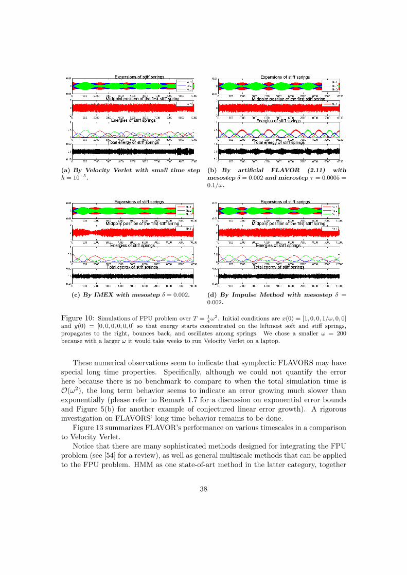
(a) By Velocity Verlet with small time steph = 10−5.
(b) By artificial FLAVOR (2.11) withmesostep δ = 0.002 and microstep τ = 0.0005 =0.1/ω.
(c) By IMEX with mesostep δ = 0.002. (d) By Impulse Method with mesostep δ =0.002.
Figure 10: Simulations of FPU problem over T = 14ω2. Initial conditions are x(0) = [1, 0, 0, 1/ω, 0, 0]
and y(0) = [0, 0, 0, 0, 0, 0] so that energy starts concentrated on the leftmost soft and stiff springs,propagates to the right, bounces back, and oscillates among springs. We chose a smaller ω = 200because with a larger ω it would take weeks to run Velocity Verlet on a laptop.
These numerical observations seem to indicate that symplectic FLAVORS may havespecial long time properties. Specifically, although we could not quantify the errorhere because there is no benchmark to compare to when the total simulation time isO(ω2), the long term behavior seems to indicate an error growing much slower thanexponentially (please refer to Remark 1.7 for a discussion on exponential error boundsand Figure 5(b) for another example of conjectured linear error growth). A rigorousinvestigation on FLAVORS’ long time behavior remains to be done.
Figure 13 summarizes FLAVOR’s performance on various timescales in a comparisonto Velocity Verlet.
Notice that there are many sophisticated methods designed for integrating the FPUproblem (see [54] for a review), as well as general multiscale methods that can be appliedto the FPU problem. HMM as one state-of-art method in the latter category, together
38

Figure 11: By artificial FLAVORS (Subsection2.1.4) based on exact fast flow with mesostep δ =0.002 and microstep τ = 10−4. Less oscillatorystiff spring energies. 38 periods in Subplot2 withzoomed-in time axis (∼380 in total over the wholesimulation span).
Figure 12: Harmonic FPU, T = 50ω, exact solu-tion
with identification of slow variables [5] captured the energy transfer between stiff springsover a time span of the order of ω. Simulations shown here are over a time span of theorder of O(ω2).
6.3.1 On resonances
Multiscale in time integrators are usually plagued by two kinds of resonances.The first kind, called Takens resonance [107], is related to the fact there are no closed
equations on slow variables [15]. FLAVORS avoid Takens resonance because, thanks toF -convergence, the information on the local invariant measure of fast variables is notlost. Observe that the FPU problem has Takens resonance (the eigenfrequencies ofthe strong potential are identical). Nevertheless, FLAVORS still capture the solutiontrajectories given any large value of ω with mesostep δ 1/ω independent of ω.
The second kind [25] is related to instabilities created by interactions between pa-rameters ε, τ and δ. For instance, if ε−1 = ω2 resonance might happen at ωδ or ωτequal to multiples of π/2. The analysis provided in Section 5 shows that such unstableinteraction does not occur, either in the sense of stability or in terms of peaks of errorfunction. This can be intuitively understood by observing that FLAVORS never approx-imate cos(δω), while on the other hand, it does approximate cos(τω) whose resonancefrequency τ = 2π/ω is ruled off by the requirement of τ ε for nonintrusive FLAVORand τ
√ε for artificial FLAVOR.
6.4 Nonlinear 2D primitive molecular dynamics
Now consider a two-dimensional, two degrees of freedom example in which a point massis linked through a spring to a massless fixed hinge at the origin. While the spring as well
39

(a) FLAVOR (b) Velocity Verlet
Figure 13: Quantities of interest in integrations of FPU over different timescales. FLAVOR (2.11)captures the fastest timescale in the sense of measure, while Velocity Verlet cannot accurately capturethe slowest (O(ω2)) timescale despite of the small time step it uses. Here FLAVOR is 200 times fasterthan Velocity Verlet. All parameters are the same as in Figure 10(a) and 10(b), e.g. ω = 200, δ = 0.002,τ = 0.0005 and h = 10−5.
as the point mass are allowed to rotate around the hinge (the spring remains straight),the more the spring-mass tilts away from its equilibrium angle the more restorative forceit will experience. This example is a simplified version of prevailing molecular dynamicsmodels, in which bond lengths and angles between neighboring bonds are both spring-like; other potential energy terms are ignored.
Denote by x and y the Euclidean coordinates of the mass, and px, py correspondingmomentums. Also introduce polar coordinates (r, θ), with x = r cos θ and y = r sin θ.Then the Hamiltonian reads
H =1
2p2x +
1
2p2y +
1
2ω2(r − r0)2 + (cos θ)2
=1
2p2x +
1
2p2y +
1
2ω2(√x2 + y2 − r0)2 +
x2
x2 + y2(6.8)
where r0 is equilibrium bond length parameter and ω is large number denoting bondoscillation frequency.
Remark 6.1. This seemingly trivial example is not easy to integrate.
1. If the system is viewed in Euclidean coordinates (x, y, px, py) it is completely non-linear with a nonpolynomial potential, and hence the Impulse Method or its vari-ations [51, 110, 44, 96], or IMEX [105], or the homogenization method introducedin [20] cannot be applied using a mesostep.
2. If the Hamiltonian is rewritten in generalized coordinates (r, θ, pr, pθ), H = 12p
2r +
12p2θr2
+ 12ω
2(r − r0)2 + 12 cos(θ)2, a fast quadratic potential can be identified.
40

However, the mass matrix
[1 00 r2
]is not constant, but rapidly oscillating, and
hence methods that work for quasi-quadratic fast potentials (i.e. “harmonic oscil-lator” with a slowly changing frequency) ([20] for example) cannot be applied.
Figure 14: Simulation of (6.8). Symplectic Euler uses small time step τ = 0.0002 and the inducedsymplectic FLAVOR ((2.5) and (2.9)) uses mesostep δ = 0.01 and microstep τ = 0.0002. In thissimulation ω = 500, x(0) = 1.1, y(0) = 0.8, px(0) = 0, py(0) = 0 and simulation time T = 100.
Figure 14 compares symplectic Euler with the induced symplectic FLAVOR ((2.5)and (2.9)) applied to (6.8) in Euclidean coordinates.
FLAVOR reproduced the slow θ trajectory while accelerating the simulation time byroughly 50x (since δ = 50τ). It can also be seen from both energy fluctuations and thetrajectory of the fast variable that the fast process’ amplitude is well captured althoughits period has been lengthened.
6.5 Nonlinear 2D molecular clipper
We now consider a united-atom representation of a three atom polymer with two bonds(e.g. propane or water molecule). This is a simplified version of several prevailingmolecular dynamics force fields (for example, CHARMM [21], AMBER [33], or a simplerexample of butane [92, 93]). Using conservation of momentum, we fix the coordinatesystem in the 2D plane defined by the three atoms. Introduce both Cartesian coordinates(x1, y1, x2, y2, x3, y3), as well as generalized coordinates r1 =
√(x2 − x1)2 + (y2 − y1)2
41
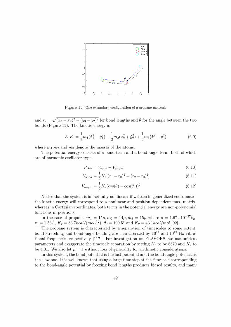
Figure 15: One exemplary configuration of a propane molecule
and r2 =√
(x3 − x2)2 + (y3 − y2)2 for bond lengths and θ for the angle between the twobonds (Figure 15). The kinetic energy is
K.E. =1
2m1(x2
1 + y21) +
1
2m2(x2
2 + y22) +
1
2m3(x2
3 + y23) (6.9)
where m1,m2,and m3 denote the masses of the atoms.The potential energy consists of a bond term and a bond angle term, both of which
are of harmonic oscillator type:
P.E. = Vbond + Vangle (6.10)
Vbond =1
2Kr[(r1 − r0)2 + (r2 − r0)2] (6.11)
Vangle =1
2Kθ(cos(θ)− cos(θ0))2 (6.12)
Notice that the system is in fact fully nonlinear: if written in generalized coordinates,the kinetic energy will correspond to a nonlinear and position dependent mass matrix,whereas in Cartesian coordinates, both terms in the potential energy are non-polynomialfunctions in positions.
In the case of propane, m1 = 15µ,m2 = 14µ,m3 = 15µ where µ = 1.67 · 10−27kg,r0 = 1.53A, Kr = 83.7kcal/(molA2), θ0 = 109.5 and Kθ = 43.1kcal/mol [92].
The propane system is characterized by a separation of timescales to some extent:bond stretching and bond-angle bending are characterized by 1014 and 1013 Hz vibra-tional frequencies respectively [117]. For investigation on FLAVORS, we use unitlessparameters and exaggerate the timescale separation by setting Kr to be 8370 and Kθ tobe 4.31. We also let µ = 1 without loss of generality for arithmetic considerations.
In this system, the bond potential is the fast potential and the bond-angle potential isthe slow one. It is well known that using a large time step at the timescale correspondingto the bond-angle potential by freezing bond lengths produces biased results, and many
42

physics based methods have been proposed to remedy this difficulty (for example by theapproach of Fixman [43]; also see a review in [117]). On the other hand, few multiscalemethods work for this fully nonlinear system.
Figure 16: Simulations of exaggerated propane molecule (Subsection 6.5). Symplectic Eu-ler uses h = 0.01 and the induced symplectic FLAVOR ((2.5) and (2.9)) parameters are δ =0.1 and τ = 0.01. Initial conditions are [x1, y1, x2, y2, x3, y3] = [0, 0, 1.533, 0, 2.6136, 1.0826] and[m1x1,m1y1,m2x2,m2y2,m3x3,m3y3] = [−0.4326,−1.6656, 0.1253, 0.2877,−1.1465, 1.1909].
Figure 16 compares symplectic Euler with the induced symplectic FLAVOR ((2.5)and (2.9)) applied in Euclidean coordinates. 10x acceleration is achieved. A simula-tion movie is also available at http://www.cds.caltech.edu/~mtao/Propane.avi andhttp://www.acm.caltech.edu/~owhadi/.
6.6 Forced nonautonomous mechanical system: Kapitza’s inverted pen-dulum
As the famous Kapitza’s inverted pendulum shows [63] (for recent references see [6]for numerical integration and [97] for generalization to the stochastic setting), the upposition of a single pendulum can be stabilized if the pivot of the pendulum experiencesexternal forcing in the form of vertical oscillation. Specifically, if the position of thepivot is given by y = sin(ωt), the system is governed by
lθ = [g + ω2 sin(2πωt)] sin θ (6.13)
43

where θ denotes the clockwise angle of the pendulum from the positive y direction, l isthe length of the pendulum and g is the gravitational constant. In this case, the rapidvibration causes the pendulum to oscillate slowly around the positive y direction with aO(1) frequency.
Figure 17: Simulations of the inverted pendulum. The integration by Variational Euler +d’Alembert principle uses time step h = 0.2/ω/
√l ≈ 0.000067, while FLAVOR (defined
by (6.15)) uses δ = 0.002 and τ = 0.2/ω/√l. Also, g = 9.8, l = 9, θ(0) = 0.2, θ(0) = 0
and ω = 1000
A single scale integration of this system could be done by Variational Euler withdiscrete d’Alembert principle for external forces [78]
fi = ω2 sin(2πωih)
pi+1 = pi + h[g + fi] sin θi
θi+1 = θi + hpi+1/l
(6.14)
where the time step length h has to be smaller than O(1/ω).FLAVOR is given by
qnδ+τ = qnδ + τpnδ/l
pnδ+τ = pnδ + τg sin(qnδ+τ ) + ω2 sin(2πωnτ)
q(n+1)δ = qnδ+τ + (δ − τ)pnδ+τ/l
p(n+1)δ = pnδ+τ + (δ − τ)g sin(q(n+1)δ)
(6.15)
44
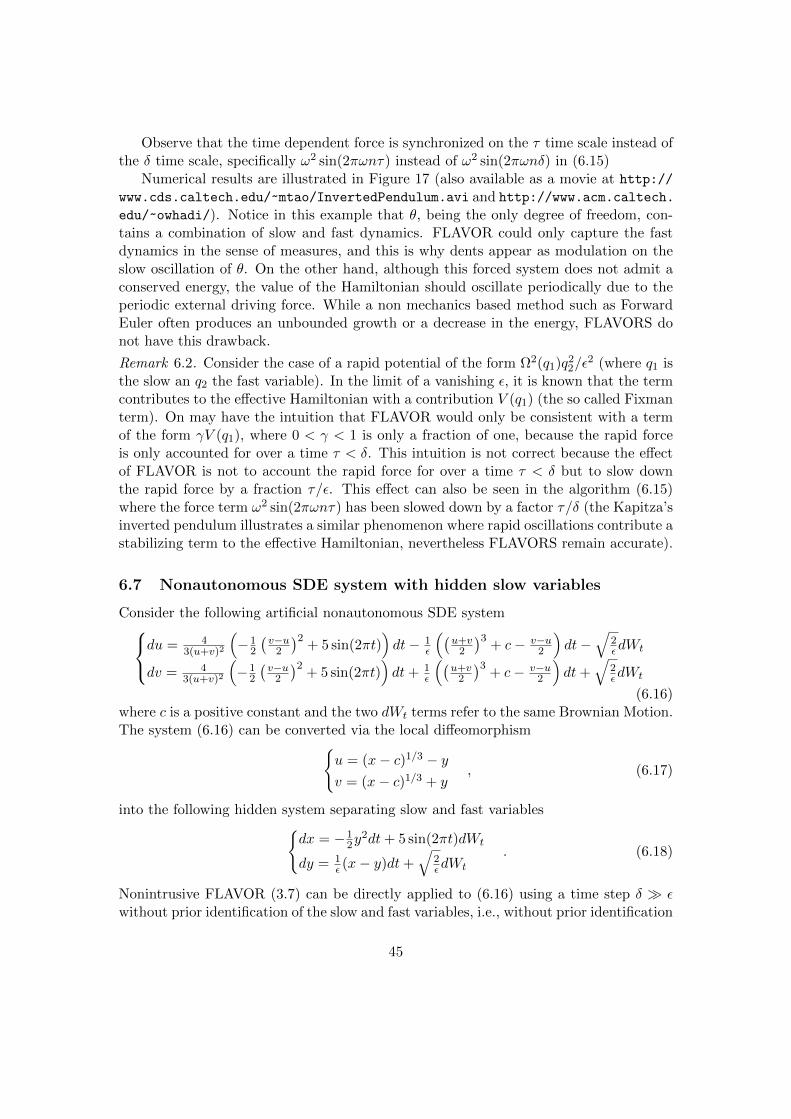
Observe that the time dependent force is synchronized on the τ time scale instead ofthe δ time scale, specifically ω2 sin(2πωnτ) instead of ω2 sin(2πωnδ) in (6.15)
Numerical results are illustrated in Figure 17 (also available as a movie at http://
www.cds.caltech.edu/~mtao/InvertedPendulum.avi and http://www.acm.caltech.
edu/~owhadi/). Notice in this example that θ, being the only degree of freedom, con-tains a combination of slow and fast dynamics. FLAVOR could only capture the fastdynamics in the sense of measures, and this is why dents appear as modulation on theslow oscillation of θ. On the other hand, although this forced system does not admit aconserved energy, the value of the Hamiltonian should oscillate periodically due to theperiodic external driving force. While a non mechanics based method such as ForwardEuler often produces an unbounded growth or a decrease in the energy, FLAVORS donot have this drawback.
Remark 6.2. Consider the case of a rapid potential of the form Ω2(q1)q22/ε
2 (where q1 isthe slow an q2 the fast variable). In the limit of a vanishing ε, it is known that the termcontributes to the effective Hamiltonian with a contribution V (q1) (the so called Fixmanterm). On may have the intuition that FLAVOR would only be consistent with a termof the form γV (q1), where 0 < γ < 1 is only a fraction of one, because the rapid forceis only accounted for over a time τ < δ. This intuition is not correct because the effectof FLAVOR is not to account the rapid force for over a time τ < δ but to slow downthe rapid force by a fraction τ/ε. This effect can also be seen in the algorithm (6.15)where the force term ω2 sin(2πωnτ) has been slowed down by a factor τ/δ (the Kapitza’sinverted pendulum illustrates a similar phenomenon where rapid oscillations contribute astabilizing term to the effective Hamiltonian, nevertheless FLAVORS remain accurate).
6.7 Nonautonomous SDE system with hidden slow variables
Consider the following artificial nonautonomous SDE systemdu = 43(u+v)2
(−1
2
(v−u
2
)2+ 5 sin(2πt)
)dt− 1
ε
((u+v
2
)3+ c− v−u
2
)dt−
√2εdWt
dv = 43(u+v)2
(−1
2
(v−u
2
)2+ 5 sin(2πt)
)dt+ 1
ε
((u+v
2
)3+ c− v−u
2
)dt+
√2εdWt
(6.16)where c is a positive constant and the two dWt terms refer to the same Brownian Motion.The system (6.16) can be converted via the local diffeomorphism
u = (x− c)1/3 − yv = (x− c)1/3 + y
, (6.17)
into the following hidden system separating slow and fast variablesdx = −1
2y2dt+ 5 sin(2πt)dWt
dy = 1ε (x− y)dt+
√2εdWt
. (6.18)
Nonintrusive FLAVOR (3.7) can be directly applied to (6.16) using a time step δ εwithout prior identification of the slow and fast variables, i.e., without prior identification
45

Figure 18: (a) Integration of (6.16) by nonintrusive FLAVOR (3.7) using mesostep step δ = 0.01 (b)Integration of (6.16) by Euler-Maruyama using fine time step h = 10−4 (c) Integration of (6.18) byEuler-Maruyama using the same small step h = 10−4. Expectations of the slow variable (whether or nothidden) are obtained by empirically averaging over an ensemble of 100 independent sample trajectories.ε = 10−4, x(0) = 1 + ε, y(0) = 1, T = 2 (the expectation of the real solution will blow up around T = 3).We have chosen c = 10 so that the transformation is a diffeomorphism.
of the slow variable x or of the system (6.18). The expected values of solutions of (6.16)integrated by FLAVORS with mesostep δ and Euler-Maruyama with a small time stepτ are presented in Figure 18. FLAVOR has accelerated the computation by 100x.
6.8 Langevin equations with slow noise and friction
In this subsection, we consider the one dimensional, two degrees of freedom systemmodeled by the SDEs (now both springs are quartic rather than harmonic):
dy = pydt
dx = pxdt
dpy = −ε−1y3dt− 4(y − x)3dt− cpydt+ σdW 1t
dpx = −4(x− y)3dt− cpxdt+ σdW 2t
. (6.19)
We compare several autocorrelation functions and time-dependent moments of thisstochastic process integrated by quasi-symplectic FLAVOR ((4.7) and (2.9)) and Geo-metric Langevin Algorithm (GLA) [17]. FLAVOR and GLA gave results in agreement
46

Figure 19: SDE (6.19): autocorrelation functions of E[y(t)y(0)] (dominantly fast) andof E[(x(t) − y(t))(x(0) − y(0))] (dominantly slow), empirically obtained by GLA andFLAVORS.
(Figure 19, 20(a), 20(b)). Since GLA is weakly-convergent and Boltzmann-Gibbs pre-serving, this is numerical evidence that quasi-symplectic FLAVOR is also.
Expectations are empirically calculated by averaging over an ensemble of 100 sampletrajectories with T = 30, ε = 10−8, τ = 0.001, δ = 0.01. y(0) = 2.1/ω (with ω := 1/
√ε),
x(0) = y(0) + 1.8, c = 0.1 and σ = 0.5. GLA uses time step h = 0.001. Noise andfriction are slow here in the sense that they are not of the order O(ω) or larger.
As shown in the plots, in the regime dominated by deterministic dynamics (roughlyfrom t = 0 to t = 8) various moments calculated empirically by FLAVORS and GLAare in agreement, indicating that the same rate of convergence towards the Boltzmann-Gibbs distribution is obtained. And in that regime, autocorrelation functions of theslow variables agree, serving as numerical evidence that FLAVORS is weakly convergingtowards the SDE solution, whereas autocorrelation functions of the fast variables agreeonly in the sense of measures (after time averaging over a mesoscopic (o(1)) time span).The fluctuations between FLAVORS and GLA for large time are an effect of the finitenumber of samples (100) used to compute sample averages.
Recall that if the noise is applied to slow variables, FLAVORS do not convergestrongly but only in the sense of distributions.
47

(a) E(x(t)− y(t)
)(b) E
((x(t)− y(t))2
)Figure 20: SDE (6.19): Empirical moments obtained from simulations of ensembles of(6.19) with GLA and quasi-symplectic FLAVOR (Subsection 4.2.1)
6.9 Langevin equations with fast noise and friction
Consider a system with the same configuration as above. The difference is that the softspring oscillates at a frequency nonlinearly dependent on the stiff spring’s length, andthe left mass experiences strong friction and noise while the right mass does not. TheHamiltonian is
H(y, x, py, px) =1
2p2y +
1
2p2x/2 +
1
4ω4y4 + ey(x− y)2, (6.20)
and the governing SDEs are:dy = pydt
dx = pxdt
dpy = −ω4y3dt− (2 + y − x)(y − x)eydt− ω2cpydt+ ωσdW t
dpx = −2(x− y)eydt
. (6.21)
In this system, the deterministic dynamics and the effects of noise and friction bothinvolve a O(1/ω2) timescale. We have implemented the fast noise and friction versionof FLAVORS ((4.8) and (2.9)).
In Figure 21, we have plotted the first and second moments of the dominantly slowvariable x(t) − y(t) as well as the first moment of the dominantly fast variable y(t)as functions of time. Moments of the dominantly slow variable integrated by quasi-symplectic FLAVOR (Subsection 4.2.1) and GLA [17] concur, numerically suggestingweak convergence and preservation of Boltzmann-Gibbs. 100x computational accelera-tion is achieved.
48
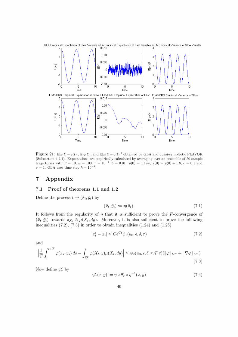
Figure 21: E[x(t)− y(t)], E[y(t)], and E[x(t)− y(t)]2 obtained by GLA and quasi-symplectic FLAVOR(Subsection 4.2.1). Expectations are empirically calculated by averaging over an ensemble of 50 sampletrajectories with T = 10, ω = 100, τ = 10−4, δ = 0.01. y(0) = 1.1/ω, x(0) = y(0) + 1.8, c = 0.1 andσ = 1. GLA uses time step h = 10−4.
7 Appendix
7.1 Proof of theorems 1.1 and 1.2
Define the process t 7→ (xt, yt) by
(xt, yt) := η(ut). (7.1)
It follows from the regularity of η that it is sufficient to prove the F -convergence of(xt, yt) towards δXt ⊗ µ(Xt, dy). Moreover, it is also sufficient to prove the followinginequalities (7.2), (7.3) in order to obtain inequalities (1.24) and (1.25)
|xεt − xt| ≤ CeCtψ1(u0, ε, δ, τ) (7.2)
and∣∣∣ 1
T
∫ t+T
tϕ(xs, ys) ds−
∫Rpϕ(Xt, y)µ(Xt, dy)
∣∣∣ ≤ ψ2(u0, ε, δ, τ, T, t)(‖ϕ‖L∞ + ‖∇ϕ‖L∞)
(7.3)
Now define ψετ byψετ (x, y) := η θετ η−1(x, y) (7.4)
49

Define ψgh byψgh(x, y) := η θGh η−1(x, y) (7.5)
Proposition 7.1. The vector fields f and g associated with the system of Equations(1.2) are Lipschitz continuous. We also have
(xt, yt) =(ψgδ−τ ψ
ετ
)k(x0, y0) for kδ ≤ t < (k + 1)δ. (7.6)
Moreover, there exists C > 0 such that for h ≤ h0 and τε ≤ τ0 we have∣∣ψετ (x, y)− (x, y)− τ
(g(x, y), 0
)− τ
ε
(0, f(x, y)
)∣∣ ≤ C(τε
)2(7.7)
and ∣∣ψgh(x, y)− (x, y)− h(g(x, y), 0
)∣∣ ≤ Ch2. (7.8)
Furthermore, given x0, y0, the trajectories of (xεt, yεt) and (xt, yt) are uniformly bounded
in ε, δ ≤ h0, τ ≤ min(τ0ε, δ).
Proof. Since (x, y) = η(u), we have
x = (G+1
εF )∇ηx η−1(x, y) (7.9)
y = (G+1
εF )∇ηy η−1(x, y). (7.10)
Hence, we deduce from Equation (1.2) of Condition 1.1 that
g(x, y) = G∇ηx η−1(x, y) (7.11)
f(x, y) = F∇ηy η−1(x, y). (7.12)
We deduce the regularity of f and g from the regularity of G, F and η. Equation (7.6)is a direct consequence of the definition of ψετ and ψgh and Equation (1.27) (we write(x0, y0) := η(u0)). Observe that Equation (1.2) of Condition 1.1 also requires that
F∇ηx = 0 G∇ηy = 0. (7.13)
Now observe that
ψετ (x, y)− (x, y)−(g(x, y), 0
)τ −
(0, f(x, y)
)τε
=(η θετ − η − τ
(G∇ηx, 0
)− τ
ε
(0, F∇ηy
)) η−1(x, y).
(7.14)
Using (7.13), (1.29), Taylor expansion and the regularity of η we obtain (7.7). Similarly
ψgh(x, y)− (x, y)− h(g(x, y), 0
):=(η θGh − η(x, y)− h
(G∇ηx, 0
)) η−1(x, y). (7.15)
Using (7.13), (1.28), Taylor expansion and the regularity of η we obtain (7.8). Theuniform bound (depending on x0, y0) on the trajectories of (xεt, y
εt) and (xt, yt) is a
consequence of the uniform bound (given u0) on the trajectories of uεt and ut.
50

It follows from Proposition 7.1 that it is sufficient to prove theorems 1.1 and 1.2 in thesituation where η is the identity diffeomorphism. More precisely, the F -convergence ofut is a consequence of the F -convergence of (xt, yt) and the regularity of η. Furthermore,from the uniform bound (depending on (x0, y0)) on the trajectories of (xεt, y
εt) and (xt, yt)
we deduce that g and f are uniformly bounded and Lipshitz continuous (in ε, δ ≤ h0,τ ≤ min(τ0ε, δ)) over those trajectories.
Define
g :=
∫g(x, y)µ(x, dy)
where µ is the family of measures introduced in Condition 1.2. Let us prove the followinglemma.
Lemma 7.1.
|xεnδ − xnδ| ≤CeCnδ(δ +
(τε
)2 1
δ+ sup
1≤l≤n|J(l)|
)(7.16)
with J(k) = J1(k) + J2(k),
J1(k) :=
k−1∑n=0
( ∫ (n+1)δ
nδg(xεnδ, y
εs) ds− δg(xεnδ
)(7.17)
and
J2(k) :=k−1∑n=0
δ(g(xnδ)− g(xnδ, ynδ)
)(7.18)
Proof. Observe that
xε(n+1)δ = xεnδ +
∫ (n+1)δ
nδg(xεnδ, y
εs) ds+
∫ (n+1)δ
nδ(g(xεs, y
εs)− g(xεnδ, y
εs)) ds (7.19)
Hence,
xε(n+1)δ − x(n+1)δ = xεnδ − xnδ + I1 + I2(n) + I3 + I4(n) + I5 (7.20)
with
I1 :=
∫ (n+1)δ
nδ(g(xεs, y
εs)− g(xεnδ, y
εs))ds (7.21)
I2(n) :=
∫ (n+1)δ
nδg(xεnδ, y
εs) ds− δg(xεnδ) (7.22)
I3 := δ(g(xεnδ)− g(xnδ)
)(7.23)
I4(n) := δ(g(xnδ)− g(xnδ, ynδ)
)(7.24)
I5 := δg(xnδ, ynδ)− (x(n+1)δ − xnδ) (7.25)
51

Now observe that|I1| ≤ ‖∇xg‖L∞δ2 (7.26)
and|I3| ≤ δ‖∇xg‖L∞ |xεnδ − xnδ|. (7.27)
Using (7.7) and (7.8) we obtain that
|I5| ≤ C(δ2 +
(τε
)2)(7.28)
Combining the previous equations, we have obtained that
xε(n+1)δ − x(n+1)δ ≤ xεnδ − xnδ + C(δ2 +
(τε
)2)+ Cδ|xεnδ − xnδ|+ (I2 + I4)(n) (7.29)
and
xε(n+1)δ − x(n+1)δ ≥ xεnδ − xnδ − C(δ2 +
(τε
)2)− Cδ|xεnδ − xnδ|+ (I2 + I4)(n) (7.30)
Write
J(n) :=n−1∑k=0
(I2 + I4)(k) (7.31)
Summing the first n inequalities (7.29) and (7.30)
xεnδ − xnδ ≤ C(δ2 +
(τε
)2)n+ Cδ
n−1∑k=0
|xεkδ − xkδ|+ J(n) (7.32)
xεnδ − xnδ ≥ −C(δ2 +
(τε
)2)n− Cδ
n−1∑k=0
|xεkδ − xkδ|+ J(n) (7.33)
Hence
|xεnδ − xnδ| ≤ C(δ2 +
(τε
)2)n+ Cδ
n−1∑k=0
|xεkδ − xkδ|+ |J(n)| (7.34)
And we obtain by induction
|xεnδ − xnδ| ≤C(δ2 +
(τε
)2)(n+ Cδ
n∑k=1
(n− k)(1 + Cδ)k−1)
|J(n)|+ Cδ
n∑l=2
(1 + Cδ)l−2|J(n− l + 1)|(7.35)
Equation (7.35) concludes the proof of Lemma 7.1.
We now need to control J1(k) and J2(k). First, let us prove the following lemma.
52

Lemma 7.2. For N ∈ N∗ we have
|J1(k)| ≤ (δk)C(δeC
δNε + E
( δNε
))(7.36)
Proof. Define yεt such that yεt = yεt for t = (n+ j/N)δ, j ∈ N∗, and
dyεtdt
=1
εf(xεnδ, y
εt) for (n+ j/N)δ ≤ t < (n+ (j + 1)/N)δ. (7.37)
Using the regularity of f and g we obtain that
|yεt − yεt | ≤ CδeCδNε . (7.38)
First, observe that
1
δ
∫ (n+1)δ
nδg(xεnδ, y
εs) ds− g(xεnδ) = K1 +K2 (7.39)
with
K1 :=1
δ
N−1∑j=0
∫ (n+(j+1)/N)δ
(n+j/N)δ
(g(xεnδ, y
εs)− g(xεnδ, y
εs))ds (7.40)
and
K2 :=1
N
N−1∑j=0
(Nδ
∫ (n+(j+1)/N)δ
(n+j/N)δg(xεnδ, y
εs) ds− g(xεnδ)
). (7.41)
We have
|K1| ≤ ‖∇yg‖L∞1
N
N−1∑j=0
sup(n+j/N)δ≤s≤(n+(j+1)/N)δ
|yεs − yεs|. (7.42)
Hence, we obtain from (7.38) that
|K1| ≤ CδeCδNε (7.43)
Moreover, we obtain from conditions 1.2 and 1.3 that
|K2| ≤ CE( δNε
)(7.44)
This concludes the proof of Lemma 7.2.
Lemma 7.3. We have for m ∈ N∗∣∣J2(k)∣∣ ≤ Cδk(mδ + E(
mτ
ε) +
(τε
+mδ +m(τ
ε)2)eC
mτε
). (7.45)
53

Proof. Let m ∈ N∗. Define (xs, ys) such that for j ∈ N∗, n ∈ N∗,
dxsdt = g(xs, ys) for jmδ ≤ s < (j + 1)mδdysdt = 1
εf(xs, ys) for nδ ≤ s < nδ + τ
ys = ynδ+τ for nδ + τ ≤ s < (n+ 1)δ
y(n+1)δ = ynδ+τ for n+ 1 6= jm
(xjm, yjm) = (xjmδ, yjmδ)
. (7.46)
Define yas by dyatdt = 1
εf(xjmδ, yat ) for jmτ ≤ t < (j + 1)mτ
yajmτ = yjmδ, (7.47)
and define xan byxan = xjmδ for jm ≤ n < (j + 1)m. (7.48)
Observe thatJ2(k) = K3 +K4 +K5 +K6 +K7 (7.49)
with
K3 :=k−1∑n=0
( ∫ (n+1)δ
nδg(xs, ys) ds− δg(xnδ, ynδ)
), (7.50)
K4 :=
k−1∑n=0
δ(1
τ
∫ (n+1)τ
nτg(xan, y
as ) ds− 1
δ
∫ (n+1)δ
nδg(xs, ys) ds
), (7.51)
K5 :=δ
τ
k−1∑n=0
(τ g(xan)−
∫ (n+1)τ
nτg(xan, y
as ) ds
), (7.52)
K6 := δ
k−1∑n=0
(g(xnδ)− g(xan)
). (7.53)
Using the regularity of g we obtain
|K6| ≤ δkCδm. (7.54)
Arranging the right hand side of (7.51) into groups of m terms corresponding to theintervals of (7.47) we obtain, from Condition 1.2 and Condition 1.3, that
|K5| ≤ CkδE(mτ
ε). (7.55)
Using (7.48) and the regularity of f and g we obtain the following inequality
|yaδτt− yt| ≤ CmδeC
mτε . (7.56)
54

It follows that|K4| ≤ CδkmδeC
mτε . (7.57)
Similarly, using (7.7) and (7.8), we obtain the following inequalities
|ynδ − ynδ| ≤ C(τ
ε+mδ +m(
τ
ε)2)
mτ
εeC
mτε , (7.58)
|xnδ − xnδ| ≤ Cm(δ + (
τ
ε)2). (7.59)
It follows that|K3| ≤ Cδk
(τε
+mδ +m(τ
ε)2)eC
mτε . (7.60)
This concludes the proof of Lemma 7.3.
Combining Lemma 7.1, 7.2 and 7.3 we have obtained that
|xεnδ − xnδ| ≤CeCδn(δ +
(τε
)2 1
δ+ δeC
δNε + E
( δNε
)+ E(
mτ
ε)
+(τε
+mδ +m(τ
ε)2)eC
mτε
) (7.61)
Choosing N such that eCδNε ∼ δ−
12 (observe that we need ε ≤ δ/(−C ln δ)) and m such
that mτε e
Cmτε ∼
(δετ + τ
ε
)− 12 we obtain for δε
τ + τε ≤ 1 that
|xεnδ − xnδ| ≤CeCδn(√δ +
(τε
)2 1
δ+ E
( 1
Cln
1
δ
)+(δετ
) 12 +
(τε
) 12 + E
( 1
Cln((δε
τ+τ
ε
)−1))) (7.62)
This concludes the proof of inequality (7.2). The proof of (7.3) is similar and is also aconsequence of (7.2).
7.2 Proof of Theorem 3.1
Define the process t 7→ (xt, yt) by
(xt, yt) := η(ut). (7.63)
It follows from the regularity of η that it is sufficient to prove the F -convergence of(xt, yt) towards δXt ⊗ µ(Xt, dy). Now define ψετ by
ψετ (x, y, ω) := η θετ (., ω) η−1(x, y), (7.64)
Define ψgh byψgh(x, y, ω) := η θGh (., ω) η−1(x, y). (7.65)
55
Proposition 7.2. The vector fields f , g and matrix fields σ, Q associated with thesystem of Equations (3.2) are uniformly bounded and Lipschitz continuous. We alsohave
(x0, y0) = η(u0)
(x(k+1)δ, y(k+1)δ) = ψgδ−τ (., ω′k) ψετ((xkδ, ykδ), ωk
)(xt, yt) = (xkδ, ykδ) for kδ ≤ t < (k + 1)δ
(7.66)
where ωk, ω′k are i.i.d. samples from the probability space (Ω,F ,P). Moreover there
exists C > 0 and and d-dimensional centered Gaussian vectors ξ′(ω), ξ′′(ω) with identitycovariance matrices such that for h ≤ h0 and τ
ε ≤ τ0 we have
(E[∣∣ψgh(x, y, ω)− (x, y)− h
(g(x, y), 0
)−√h(σ(x, y)ξ′(ω), 0
)∣∣2]) 12
≤ Ch32 , (7.67)
(E[∣∣ψετ (x, y, ω)− (x, y)− τ
(g(x, y), 0
)− τ
ε
(0, f(x, y)
)−√τ(σ(x, y)ξ′′(ω), 0
)−√τ
ε
(0, Q(x, y)ξ′′(ω)
)∣∣2]) 12
≤ C(τε
) 32 .
(7.68)
Proof. Since (x, y) = η(u), we obtain from (3.1) and Ito’s formula
dx =((G+
1
εF )∇ηx η−1(x, y)
)dt+
(∇ηx(H +
1√εK)) η−1(x, y) dWt
+1
2
∑ij
∂i∂jηx((H +
1√εK)(H +
1√εK)T
)ijdts
(7.69)
dy =((G+
1
εF )∇ηy η−1(x, y)
)dt+
(∇ηy(H +
1√εK)) η−1(x, y) dWt
+(1
2
∑ij
∂i∂jηy((H +
1√εK)(H +
1√εK)T
)ij
) η−1 dt.
(7.70)
Hence we deduce from Equation (3.2) of Condition 3.1 that
g(x, y) =(G∇ηx +
1
2
∑ij
∂i∂jηx(HHT )ij
) η−1(x, y) (7.71)
σ(x, y) =(∇ηxH
) η−1(x, y) (7.72)
f(x, y) =(F∇ηy +
1
2
∑ij
∂i∂jηy(KKT )ij
) η−1(x, y) (7.73)
Q(x, y) =(∇ηyK
) η−1(x, y). (7.74)
56
Remark 7.1. Observe that Equation (3.2) of Condition 3.1 requires that
F∇ηx = 0 G∇ηy, (7.75)∑ij
∂i∂jηx(KKT
)ij
= 0, (7.76)
∑ij
∂i∂jηy(HHT
)ij
= 0, (7.77)
∑ij
∂i∂jηx(KHT +HKT
)ij
= 0, (7.78)
and ∑ij
∂i∂jηy(KHT +HKT
)ij
= 0. (7.79)
Equations (7.78) and (7.79) are satisfied if KHT is skew-symmetric. One particular casecould be, of course, KHT = 0, which translates into the fact that for all u the ranges ofH(u) and K(u) are orthogonal, i.e., the noise with amplitude 1/
√ε is applied to degrees
of freedom orthogonal to those with O(1) noise.
We deduce the regularity of f , g, σ and Q from the regularity of G, F , H, K andη. Equation (7.6) is a direct consequence of the definition of ψετ and ψgh and Equation(7.66). Now observe that
ψετ (x, y, ω)− (x, y)− τ(g(x, y), 0
)− τ
ε
(0, f(x, y)
)−√τ(σ(x, y)ξ′(ω), 0
)−√τ
ε
(0, Q(x, y)ξ′(ω)
)=(η θετ − η − τ
(G∇ηx +
1
2
∑ij
∂i∂jηx(HHT )ij , 0
)− τ
ε
(0, F∇ηy +
1
2
∑ij
∂i∂jηy(KKT )ij
)−√τ(∇ηxHξ′(ω), 0
)−√τ
ε
(0,∇ηyKξ′(ω)
)) η−1(x, y).
(7.80)
Using Equations (7.75), (7.76), (7.77), (7.78) and (7.79), the Taylor-Ito expansion ofη θετ , the regularity of η, and Setting ξ′ equal to ξ defined in Equation (3.14) we obtainEquation (7.68). The proof of Equation (7.67) is similar.
It follows from Proposition 7.2 that it is sufficient to prove Theorem 3.1 in thesituation where η is the identity diffeomorphism. More precisely the F -convergence ofut is a consequence of the F -convergence of (xt, yt) and the regularity of η.
Let x 7→ ϕ(x) be a function with continuous and bounded derivatives up to order 3.Let us prove the following lemma.
57

Lemma 7.4. We have
E[ϕ(x(n+1)δ)
]− E
[ϕ(xnδ)
]=
δE[g(xnδ, ynδ)∇ϕ(xnδ) + σσT (xnδ, ynδ) : Hessϕ(xnδ)
]+ I0
(7.81)
with
|I0| ≤ C(δ
32 +
(τε
) 32
). (7.82)
Proof. Write (xnδ+τ , ynδ+τ ) := ψετ (xnδ, ynδ, ωn). Using Equation (7.68) we obtain thatthere exists an N (0, 1) random vector ξn independent from (xnδ, ynδ) and such that
xnδ+τ − xnδ = g(xnδ)τ +√τσ(xnδ, ynδ)ξn + I1 (7.83)
with (E[(I1)2]
) 12 ≤ C
(τε
) 32 . (7.84)
Hence ∣∣∣∣∣E[ϕ(xnδ+τ )]− E
[ϕ(xnδ)
]− τE
[g(xnδ, ynδ)∇ϕ(xnδ)
+ σσT (xnδ, ynδ) : Hessϕ(xnδ)]∣∣∣∣∣ ≤ C(τε ) 3
2
(7.85)
Similarly, using Equation (7.67) we obtain that there exists an N (0, 1) random vectorξ′n, independent from (xnδ+τ , ynδ+τ ), and such that
x(n+1)δ − xnδ+τ = g(xnδ+τ , ynδ+τ )(δ − τ) + σ(xnδ+τ , ynδ+τ )√δ − τξ′n + I2 (7.86)
with (E[(I2)2]
) 12 ≤ C(δ − τ)
32 . (7.87)
Whence∣∣∣∣∣E[ϕ(x(n+1)δ)]− E
[ϕ(xnδ+τ )
]− (δ − τ)E
[g(xnδ+τ , ynδ+τ )∇ϕ(xnδ+τ )
+ σσT (xnδ+τ , ynδ+τ ) : Hessϕ(xnδ+τ )]∣∣∣∣∣ ≤ C(δ − τ) 3
2 .
(7.88)
Using the regularity of σ, we obtain that(E[∣∣σ(xnδ+τ , y(n+1)δ)− σ(xnδ, ynδ)
∣∣2]) 12 ≤ C
(δ
12 +
√τ
ε
). (7.89)
The proof of (7.81) follows from (7.68), (7.85), (7.88), (7.89) and the regularity of g andϕ.
58

Lemma 7.5. We have ∣∣∣E[ϕ(xnδ)]− ϕ(x0)
nδ− Lϕ(x0)
∣∣∣ ≤ J5 (7.90)
with (for δ ≤ Cτ/ε)
|J5| ≤ C((δε
τ
) 14 +
(τε
) 32
1
δ+
√τ
ε
)+ CE
( 1
Clnτ
δε
). (7.91)
Proof. Define Bt by B0 = 0 and
Bt − Bnτ = Bnδ+t −Bnδ for nτ ≤ t ≤ (n+ 1)τ. (7.92)
Define ys by y0 = y0 and
dyt =1
εf(x0, yt) dt+
1√εQ(x0, yt)dBt. (7.93)
Write
g(x0) :=
∫g(x0, y)µ(x0, dy). (7.94)
Using Lemma 7.4 we obtain
E[ϕ(xnδ)
]− ϕ(x0)
nδ= Lϕ(x0) + J1 + J2 + J3 + J4, (7.95)
with
Lϕ(x0) := g(x0)∇ϕ(x0) + σσT (x0) : Hessϕ(x0), (7.96)
J1 =1
n
n−1∑k=0
E[g(xkδ, ykδ)∇ϕ(xkδ) + σσT (xkδ, ykδ) : Hessϕ(xkδ)
]− 1
n
n−1∑k=0
E[g(x0, ykδ)∇ϕ(x0) + σσT (x0, ykδ) : Hessϕ(x0)
],
(7.97)
J2 =1
n
n−1∑k=0
(E[g(x0, ykδ)∇ϕ(x0) + σσT (x0, ykδ) : Hessϕ(x0)
]− 1
τ
∫ (k+1)τ
kτE[g(x0, ys)∇ϕ(x0) + σσT (x0, ys) : Hessϕ(x0)
]ds),
(7.98)
J3 =1
nτ
∫ nτ
0E[g(x0, ys)∇ϕ(x0) + σσT (x0, ys) : Hessϕ(x0)
]ds− Lϕ(x0), (7.99)
|J4| ≤ C(δ
12 +
(τε
) 32
1
δ
). (7.100)
59

Using the regularity of σ, g, ϕ, (7.6) and (7.7) we obtain
|J1| ≤ C(
(nδ)12 + nδ + n
(τε
) 32
). (7.101)
Using Property 3 of Condition 3.1 and Property 3 of Condition 3.2 we obtain
|J3| ≤ CE(nτ
ε). (7.102)
Using (7.67) and (7.68), we obtain the following inequality(E[∣∣ynδ − ynτ ∣∣2]) 1
2 ≤ C(√τ
ε+ (nδ)
12 + nδ + n
(τε
) 32
)nτεeC
nτε , (7.103)
which leads to
|J2| ≤ C(√τ
ε+ (nδ)
12 + nδ + n
(τε
) 32
)eC
nτε . (7.104)
Hence, we have obtained ∣∣∣E[ϕ(xnδ)]− ϕ(x0)
nδ− Lϕ(x0)
∣∣∣ ≤ J5, (7.105)
with
|J5| ≤ C(√τ
ε+ (nδ)
12 + nδ + n
(τε
) 32
)eC
nτε + E(
nτ
ε) + C
(τε
) 32
1
δ. (7.106)
Choosing n such that√
nτε e
C nτε ∼
(τεδ
) 14 we obtain (7.91) for δ ≤ Cτ/ε.
We now combine Lemma 7.5 with Theorem 1 of Chapter 2 of [104] which states
that the uniform convergence (in x0, y0) ofE[ϕ(xnδ)
]−ϕ(x0)
nδ to Lϕ(x0) as ε ↓ 0, τ ≤ δ,
τε ↓ 0, δετ ↓ 0 and
(τε
) 32 1δ ↓ 0 implies the convergence in distribution of xnδ to the Markov
process generated by L.The F -convergence of (xt, yt) can be deduced from the convergence in distribution
of xt and Equation (3.4) of Condition 3.1. The proof follows the same lines as above,which will not be repeated here.
References
[1] A. Abdulle, Fourth order Chebyshev methods with recurrence relation, SIAM J.Sci. Comput., 23 (2002), pp. 2041–2054 (electronic).
[2] A. Abdulle and S. Cirilli, S-ROCK: Chebyshev methods for stiff stochasticdifferential equations, SIAM J. Sci. Comput., 30 (2008), pp. 997–1014.
60

[3] G. Allaire, Homogenization and two-scale convergence, SIAM J. Math. Anal.,23 (1992), pp. 1482–1518.
[4] H. Anderson, RATTLE: A velocity version of the SHAKE algorithm for molec-ular dynamics calculations, J. Comput. Phys., 52 (1983), pp. 24–34.
[5] G. Ariel, B. Engquist, and Y.-H. Tsai, A multiscale method for highly oscil-latory ordinary differential equations with resonance, Math. Comput., 78 (2009),p. 929.
[6] , A reversible multiscale integration method, To appear, Comm. Math. Sci.,(2009).
[7] A. Armaou and I. Kevrekidis, Equation-free optimal switching policies forbistable reacting systems, Internat. J. Robust Nonlinear Control, 15 (2005),pp. 713–726.
[8] S. Artem′ev and K. Shurts, Zhestkie sistemy stokhasticheskikh differentsialnykhuravnenii s malym shumom i ikh chislennoe reshenie, vol. 1039, Ross. Akad. NaukSibirsk. Otdel. Vychisl. Tsentr, Novosibirsk, 1995.
[9] Z. Artstein, I. G. Kevrekidis, M. Slemrod, and E. S. Titi, Slow observablesof singularly perturbed differential equations, Nonlinearity, 20 (2007), pp. 2463–2481.
[10] Z. Artstein, J. Linshiz, and E. S. Titi, Young measure approach to computingslowly advancing fast oscillations, Multiscale Model. Simul., 6 (2007), pp. 1085–1097.
[11] A. Bensoussan, J. L. Lions, and G. Papanicolaou, Asymptotic analysis forperiodic structure, North Holland, Amsterdam, 1978.
[12] J. Bismut, Mecanique aleatoire, Springer, 1981.
[13] N. Bogolyubov, Problemy dinamiceskoı teorii v statisticeskoı fizike, Gosudarstv.Izdat. Tehn.-Teor. Lit., Moscow-Leningrad, 1946.
[14] F. A. Bornemann and C. Schutte, A mathematical approach to smoothedmolecular dynamics: Correcting potentials for freezing bond angles. Prprint SC9-30 (Dember 1995), 1995.
[15] , Homogenization of Hamiltonian systems with a strong constraining potential,Phys. D, 102 (1997), pp. 57–77.
[16] N. Bou-Rabee and J. Marsden, Hamilton-Pontryagin integrators on Liegroups. I. Introduction and structure-preserving properties, Found. Comput. Math.,9 (2009), pp. 197–219.
61

[17] N. Bou-Rabee and H. Owhadi, Long-run accuracy of variational integratorsin the stochastic context. arXiv:0712.4123. Accepted for publication in SINUM.,2009.
[18] , Stochastic variational integrators, IMA J. Numer. Anal., 29 (2009), pp. 421–443.
[19] N. Bou-Rabee and E. Vanden-Eijnden, Pathwise accuracy and ergodicity ofmetropolized integrators for SDEs. Submitted, 2009.
[20] C. L. Bris and F. Legoll, Integrators for highly oscillatory Hamiltonian sys-tems: an homogenization approach, Tech. Report 6252, Inria Rapport de recherche,2007.
[21] B. Brooks, R. Bruccoleri, B. Olafson, D. States, S. Swaminathan, andM. Karplus, CHARMM: A program for macromolecular energy, minimization,and dynamics calculations, J Comp. Chem., 4 (1983), pp. 187–217.
[22] K. Burrage and T. Tian, The composite Euler method for stiff stochastic dif-ferential equations, J. Comput. Appl. Math., 131 (2001), pp. 407–426.
[23] , Stiffly accurate Runge-Kutta methods for stiff stochastic differential equa-tions, Comput. Phys. Comm., 142 (2001), pp. 186–190. Computational physics2000. “New challenges for the new millenium” (Gold Coast).
[24] M. Calvo and J. Sanz-Serna, Heterogeneous multiscale methods for mechanicalsystems with vibrations., preprint, (2008).
[25] , Instabilities and inaccuracies in the integration of highly oscillatory problems,SIAM J. Sci. Comput., 31 (2009), pp. 1653–1677.
[26] F. Castella, P. Chartier, and E. Faou, An averaging technique for highly-oscillatory hamiltonian problems, SIAM J. Numer. Anal., 47 (2009), pp. 2808–2837.
[27] A. Chorin, O. Hald, and R. Kupferman, Optimal prediction and the Mori-Zwanzig representation of irreversible processes, Proc. Natl. Acad. Sci. USA, 97(2000), pp. 2968–2973 (electronic).
[28] , Optimal prediction with memory, Phys. D, 166 (2002), pp. 239–257.
[29] A. Chorin, A. Kast, and R. Kupferman, Optimal prediction of underresolveddynamics, Proc. Natl. Acad. Sci. USA, 95 (1998), pp. 4094–4098 (electronic).
[30] G. Ciccotti, T. Lelievre, and E. Vanden-Eijnden, Projections of diffu-sions on submanifolds: Application to mean force computation, CPAM, 61 (2008),pp. 0001–0039.
62

[31] D. Cohen, T. Jahnke, K. Lorenz, and C. Lubich, Numerical integratorsfor highly oscillatory Hamiltonian systems: a review, in Analysis, modeling andsimulation of multiscale problems, Springer, Berlin, 2006, pp. 553–576.
[32] M. Condon, A. Deano, and A. Iserles, On highly oscillatory problems arisingin electronic engineering, M2AN Math. Model. Numer. Anal., 43 (2009), pp. 785–804.
[33] W. Cornell, P. Cieplak, C. Bayly, I. Gould, K. Merz, D. Ferguson,D. Spellmeyer, T. Fox, J. Caldwell, and P. Kollman, A second generationforce field for the simulation of proteins, nucleic acids, and organic molecules, J.Am. Chem. Soc., 117 (1995), pp. 5179–5197.
[34] G. Dahlquist, Convergence and stability in the numerical integration of ordinarydifferential equations, Math. Scand., 4 (1956), pp. 33–53.
[35] W. E, Analysis of the heterogeneous multiscale method for ordinary differentialequations, Commun. Math. Sci., 1 (2003), pp. 423–436.
[36] W. E, B. Engquist, X. Li, W. Ren, and E. Vanden-Eijnden, Heterogeneousmultiscale methods: a review, Commun. Comput. Phys., 2 (2007), pp. 367–450.
[37] W. E, D. Liu, and E. Vanden-Eijnden, Analysis of multiscale methods forstochastic differential equations, Comm. Pure Appl. Math., 58 (2005), pp. 1544–1585.
[38] , Nested stochastic simulation algorithms for chemical kinetic systems withmultiple time scales, J. Comput. Phys., 221 (2007), pp. 158–180.
[39] W. E, W. Ren, and E. Vanden-Eijnden, A general strategy for designingseamless multiscale methods, J. Comput. Phys., 228 (2009), pp. 5437–5453.
[40] B. Engquist and Y.-H. Tsai, Heterogeneous multiscale methods for stiff ordi-nary differential equations, Math. Comp., 74 (2005), pp. 1707–1742 (electronic).
[41] L. Evans, A survey of partial differential equations methods in weak KAM theory,Comm. Pure Appl. Math., 57 (2004), pp. 445–480.
[42] E. Fermi, J. Pasta, and S. Ulam, Studies of nonlinear problems, Tech. ReportLA-1940, Los Alamos Scientific Laboratory, 1955.
[43] M. Fixman, Classical statistical mechanics of constraints: A theorem and appli-cation to polymers, Proc. Nat. Acad. Sci. USA, 71-8 (1974), pp. 3050–3053.
[44] B. Garcıa-Archilla, J. Sanz-Serna, and R. Skeel, Long-time-step methodsfor oscillatory differential equations, SIAM J.Sci.Comput., 20 (3) (1999), pp. 930–963.
63

[45] W. Gautschi, Numerical integration of ordinary differential equations based ontrigonometric polynomials, Numer. Math., 3 (1961), pp. 381–397.
[46] C. Gear, Numerical initial value problems in ordinary differential equations,Prentice-Hall Inc., Englewood Cliffs, N.J., 1971.
[47] C. Gear and K. Gallivan, Automatic methods for highly oscillatory ordinarydifferential equations, in Numerical analysis (Dundee, 1981), vol. 912 of LectureNotes in Math., Springer, Berlin, 1982, pp. 115–124.
[48] C. Gear and I. Kevrekidis, Projective methods for stiff differential equations:problems with gaps in their eigenvalue spectrum, SIAM J. Sci. Comput., 24 (2003),pp. 1091–1106 (electronic).
[49] I. Gihman, On the theory of differential equations of stochastic processes. I, II,Amer. Math. Soc. Transl. (2), 1 (1955), pp. 111–137, 139–161.
[50] D. Givonand, I. G. Kevrekidis, and R. Kupferman, Strong convergence ofprojective integration schemes for singularly perturbed stochastic differential sys-tems, Commun. Math. Sci., 4 (2006), pp. 707–729.
[51] H. Grubmuller, H. Heller, A. Windemuth, and K. Schulten, General-ized Verlet algorithm for efficient molecular dynamics simulations with long-rangeinteractions, Mol. Sim., 6 (1991), pp. 121–142.
[52] S. Gusev, Algoritm peremennogo shaga dlya chislennogo resheniya zhestkikhsistem stokhasticheskikh differentsialnykh uravnenii, vol. 1094, RossiıskayaAkademiya Nauk Sibirskoe Otdelenie, Institut Vychislitel′noı Matematiki i Matem-aticheskoı Geofiziki, Novosibirsk, 1997.
[53] E. Hairer, C. Lubich, and G. Wanner, Geometric numerical integration il-lustrated by the Stormer-Verlet method, Acta Numer., 12 (2003), pp. 399–450.
[54] , Geometric Numerical Integration: Structure-Preserving Algorithms for Or-dinary Differential Equations, Springer, Heidelberg Germany, second ed., 2004.
[55] E. Hairer, S. Nørsett, and G. Wanner, Solving ordinary differential equa-tions. I, vol. 8 of Springer Series in Computational Mathematics, Springer-Verlag,Berlin, second ed., 1993. Nonstiff problems.
[56] E. Hairer and G. Wanner, Solving ordinary differential equations. II, vol. 14of Springer Series in Computational Mathematics, Springer-Verlag, Berlin, sec-ond ed., 1996. Stiff and differential-algebraic problems.
[57] C. Hartmann, An ergodic sampling scheme for constrained Hamiltonian systemswith applications to molecular dynamics, J. Stat. Phys., 130 (2008), pp. 687–711.
[58] A. Iserles, On the global error of discretization methods for highly-oscillatoryordinary differential equations, BIT, 42 (2002), pp. 561–599.
64

[59] , Think globally, act locally: solving highly-oscillatory ordinary differentialequations, Appl. Numer. Math., 43 (2002), pp. 145–160. 19th Dundee BiennialConference on Numerical Analysis (2001).
[60] , On the numerical analysis of rapid oscillation, in Group theory and numer-ical analysis, vol. 39 of CRM Proc. Lecture Notes, Amer. Math. Soc., Providence,RI, 2005, pp. 149–163.
[61] A. Iserles, S. P. Nørsett, and S. Olver, Highly oscillatory quadrature:the story so far, in Numerical mathematics and advanced applications, Springer,Berlin, 2006, pp. 97–118.
[62] V. Jikov, S. Kozlov, and O. Oleinik, Homogenization of Differential Opera-tors and Integral Functionals, Springer-Verlag, 1991.
[63] P. Kapitza, Collected Papers of P.L.Kapitza, Volume II., edited by D. Ter Haar,Pergamon Press, Oxford UK, 1965.
[64] I. Kevrekidis, C. Gear, J. Hyman, P. Kevrekidis, O. Runborg, andC. Theodoropoulos, Equation-free, coarse-grained multiscale computation: en-abling microscopic simulators to perform system-level analysis, Commun. Math.Sci., 1 (2003), pp. 715–762.
[65] I. Kevrekidis and G. Samaey, Equation-free multiscale computation: Algo-rithms and applications, Annual Review of Physical Chemistry, 60 (2009), pp. 321–344. PMID: 19335220.
[66] H.-O. Kreiss, Problems with different time scales, Acta Numer., 1 (1992),pp. 101–139.
[67] B. Kryloff and N. Bogoliouboff, La theorie generale de la mesure dans sonapplication a l’etude des systemes dynamiques de la mecanique non lineaire, Ann.of Math. (2), 38 (1937), pp. 65–113.
[68] N. Kryloff and N. Bogoliouboff, On some problems in the ergodic theory ofstochastic systems, Zap. Kafedr. Mat. Fiz. Inst. Budivel. Mat. Akad. Nauk. Ukrain.SSR, 4 (1939), pp. 243–287.
[69] J.-A. Lazaro-Camı and J. Ortega, Stochastic Hamiltonian dynamical systems,Rep. Math. Phys., 61 (2008), pp. 65–122.
[70] V. Lebedev and S. Finogenov, The use of ordered Cebysev parameters in it-eration methods, Z. Vycisl. Mat. i Mat. Fiz., 16 (1976), pp. 895–907, 1084.
[71] B. Leimkuhler and S. Reich, A reversible averaging integrator for multipletime-scale dynamics, J. Comput. Phys., 171 (2001), pp. 95–114.
65
[72] , Simulating Hamiltonian dynamics, vol. 14 of Cambridge Monographs on Ap-plied and Computational Mathematics, Cambridge University Press, Cambridge,2004.
[73] B. J. Leimkuhler, S. Reich, and R. D. Skeel, Integration methods for molecu-lar dynamics, in Mathematical approaches to biomolecular structure and dynamics(Minneapolis, MN, 1994), vol. 82 of IMA Vol. Math. Appl., Springer, New York,1996, pp. 161–185.
[74] A. Lew, J. Marsden, M. Ortiz, and M. West, Asynchronous variationalintegrators, Arch. Rational Mech. Anal., 167 (2003), pp. 85–145.
[75] , Variational time integrators, Int. J. Numer. Methods Eng., 60 (2004),pp. 153–212.
[76] T. Li, A. Abdulle, and W. E, Effectiveness of implicit methods for stiff stochas-tic differential equations, Commun. Comput. Phys., 3 (2008), pp. 295–307.
[77] S. Malham and A. Wiese, Stochastic Lie group integrators, SIAM J. Sci. Com-put., 30 (2008), pp. 597–617.
[78] J. Marsden and M. West, Discrete mechanics and variational integrators, ActaNumerica, (2001), pp. 357–514.
[79] R. McLachlan and D. OıNeale, Comparison of integrators for the Fermi-Pasta-Ulam problem., preprint NI07052-HOP, Isaac Newton Institute for Mathe-matical Sciences., (2007). http://www.newton.ac.uk/preprints/NI07052.pdf.
[80] R. McLachlan and M. Perlmutter, Conformal Hamiltonian systems, J.Geom. Phys., 39 (2001), pp. 276–300.
[81] R. McLachlan, G. Reinout, and W. Quispel, Splitting methods, Acta Nu-merica, (2002), pp. 341–434.
[82] G. Milstein, Y. Repin, and M. Tretyakov, Symplectic methods for Hamilto-nian systems with additive noise, SIAM J. Num. Anal., 39 (2002), pp. 1–9.
[83] , Symplectic methods for stochastic systems preserving symplectic structure,SIAM J. Num. Anal., 40 (2003), pp. 1–9.
[84] G. Milstein and M. Tretyakov, Quasi-symplectic methods for Langevin-typeequations, IMA J. Numer. Anal., 23 (2003), pp. 593–626.
[85] G. N. Milstein and M. V. Tretyakov, Stochastic Numerics for MathematicalPhysics, Springer, 2004.
[86] G. Nguetseng, A general convergence result for a functional related to the theoryof homogenization, SIAM J. Math. Anal., 20 (1989), pp. 608–623.
66
[87] G. Papanicolaou and W. Kohler, Asymptotic theory of mixing stochastic or-dinary differential equations, Comm. Pure Appl. Math., 27 (1974), pp. 641–668.
[88] G. A. Pavliotis and A. M. Stuart, Multiscale methods, vol. 53 of Texts inApplied Mathematics, Springer, New York, 2008. Averaging and homogenization.
[89] D. Perchak, J. Skolnick, and R. Yaris, Dynamics of rigid and flexible con-straints for polymers. Effect of the Fixman potential, Macromolecules, 18 (1985),pp. 519–525.
[90] L. Petzold, L. Jay, and J. Yen, Problems with different time scales, ActaNumer., 6 (1997), pp. 437–483.
[91] S. Reich, Smoothed langevin dynamics of highly oscillatory systems, Phys. D, 138(2000), pp. 210–224.
[92] R. Rosenberg, B. Berne, and D. Chandler, Isomerization dynamics in liq-uids by molecular dynamics, Chem. Phys. Lett., 75 (1980), p. 162.
[93] J. Ryckaert and A. Bellemans, Molecular dynamics of liquid n-butane nearits boiling point, Chem. Phys. Lett., 30 (1975), p. 123.
[94] J. Ryckaert, G. Ciccotti, and H. Berendsen, Numerical integration of thecartesian equations of motion of a system with constraints: Molecular dynamics ofn-alkanes, J. Comput. Phys., 23 (1977), pp. 327–341.
[95] J. A. Sanders and F. Verhulst, Averaging methods in nonlinear dynamicalsystems, vol. 59 of Applied Mathematical Sciences, Springer-Verlag, New York,1985.
[96] J. Sanz-Serna, Mollified impulse methods for highly oscillatory differential equa-tions, SIAM J. Numer. Anal., 46 (2) (2008), pp. 1040–1059.
[97] , Stabilizing with a hammer, Stoch. Dyn., 8 (2008), pp. 47–57.
[98] , Modulated Fourier expansions and heterogeneous multiscale methods, IMAJ. Numer. Anal., 29 (2009), pp. 595–605.
[99] J. Sanz-Serna, G. Ariel, and Y.-H. Tsai, Multiscale methods for stiff andconstrained mechanical systems., preprint, (2009).
[100] R. Scheid, The accurate numerical solution of highly oscillatory ordinary differ-ential equations, Math. Comp., 41 (1983), pp. 487–509.
[101] C. Schutte and F. A. Bornemann, Homogenization approach to smoothedmolecular dynamics, in Proceedings of the Second World Congress of NonlinearAnalysts, Part 3 (Athens, 1996), vol. 30, 1997, pp. 1805–1814.
67

[102] R. Sharp, Y.-H. Tsai, and B. Engquist, Multiple time scale numerical methodsfor the inverted pendulum problem, in Multiscale methods in science and engineer-ing, vol. 44 of Lect. Notes Comput. Sci. Eng., Springer, Berlin, 2005, pp. 241–261.
[103] R. Skeel and J. Izaguirre, J.a.: An impulse integrator for Langevin dynamics,Mol. Phys, 100 (2002), pp. 3885–3891.
[104] A. Skorokhod, Asymptotic methods in the theory of stochastic differential equa-tions, vol. 78 of Translations of Mathematical Monographs, American Mathemati-cal Society, Providence, RI, 1989. Translated from the Russian by H. H. McFaden.
[105] A. Stern and E. Grinspun, Implicit-explicit variational integration of highlyoscillatory problems, Multiscale Model. Simul., (2009). Accepted, to appear.
[106] W. B. Streett, D. J. Tildesley, and G. Saville, Multiple time-step methodsin molecular dynamics, Molecular Physics, 35 (1978), pp. 639 – 648.
[107] F. Takens, Motion under the influence of a strong constraining force, in GlobalTheory of Dynamical Systems. edited by Z. Nitecki and C. Robinson, Springer-Verlag, Berlin-Heidelberg Germany, 1980.
[108] T. Tian and K. Burrage, Implicit Taylor methods for stiff stochastic differentialequations, Appl. Numer. Math., 38 (2001), pp. 167–185.
[109] M. Tuckerman, B. Berne, and G. Martyna, Reversible multiple time scalemolecular dynamics, J. Chem. Phys., 97 (1992), pp. 1990–2001.
[110] M. Tuckerman, B. J. Berne, and G. J. Martyna, Reversible multiple timescale molecular dynamics, J. Chem. Phys., 97 (1992), pp. 1990–2001.
[111] E. Vanden-Eijnden, On HMM-like integrators and projective integration methodsfor systems with multiple time scales, Commun. Math. Sci., 5 (2007), pp. 495–505.
[112] E. Vanden-Eijnden and G. Ciccotti, Second-order integrators for Langevinequations with holonomic constraints, Chem. Phys. Letters, 429 (2006), pp. 310–316.
[113] F. Verhulst, Nonlinear Differential Equations and Dynamical Systems, Springer,Berlin-Heidelberg Germany, second ed., 1996.
[114] L. Verlet, Computer “experiments” on classical fluids. I. thermodynamical prop-erties of Lennard-Jones molecules, Physical Review, 159 (1967), pp. 98+.
[115] D. Viswanath, Global errors of numerical ODE solvers and Lyapunov’s theoryof stability, IMA J. Numer. Anal., 21 (2001), pp. 387–406.
[116] T. Yanao, W. S. Koon, and J. E. Marsden, Intramolecular energy transferand the driving mechanisms for large-amplitude collective motions of clusters, J.Chem. Phys., (2009), p. 144111.
68

[117] G. Zhang and T. Schlick, LIN: A new algorithm to simulate the dynamicsof biomolecules by combining implicit-integration and normal mode techniques, J.Comp. Chem., 14 (1993), pp. 1212–1233.
69
Copyright © 2022 FDOKUMEN