COMPARATIVE STUDY OF AVERAGING AND DISTRIBUTION BASEDAPPROACHES FOR

UNCERTAIN DATA USING DECISION TREE

CH.RAMADEVI1*, SK ABDUL NABI , B.VIJITHA

1Assistant Professor in Department of CSE, AVNIET, Hyderabad, AP,INDIAProfessor and HOD in Department of CSE, AVNIET, Hyderabad, AP,INDIAAssistant Professor in Department of CSE

ABSTRACT— In spite of the great progress in the data miningfield in recent years, the problem of missing and uncertain datahas remained a great challenge for data mining algorithms. Valueuncertainty arises in many applications during the datacollection process. Example sources of uncertainty includemeasurement/quantization errors, data staleness, and multiplerepeated measurements. With uncertainty, the value of a data itemis often represented not by one single value, but by multiplevalues forming a probability distribution. Rather thanabstracting uncertain data by statistical derivatives (such asmean and median), we discover that the accuracy of a decisiontree classifier can be much improved if the “completeinformation” of a data item (taking into account the probabilitydensity function (pdf)) is utilized. We extend classical decisiontree building algorithms to handle data tuples with uncertainvalues. Extensive experiments have been conducted that show thatthe resulting classifiers are more accurate than those usingvalue averages. Since processing pdf’s is computationally morecostly than processing single values (e.g., averages), decisiontree construction on uncertain data is more CPU demanding thanthat for certain data. To tackle this problem, we propose aseries of pruning techniques that can greatly improveconstruction efficiency.Key words— Uncertain Data, CDTA (Classical Decision TreeAlgorithm), Probability Density Function (PDF) ,Data Mining,Pruning Techniques.

I INTRODUCTION

Data is often associated with uncertainty because of measurementinaccuracy, sampling discrepancy, outdated data sources, or othererrors. This is especially true for applications that requireinteraction with the physical world, such as location-basedservices and sensor monitoring . Decision trees is a simple yetwidely used method for classification and redictivemodeling. A decision tree partitions data into smaller segmentscalled terminal nodes. Each terminal node is assigned a classlabel. The non-terminal nodes, which include the root and otherinternal nodes, contain attribute test conditions to separaterecords that have different characteristics. The partitioningprocess terminates when the subsets cannot be partitioned anyfurther using predefined criteria. Decision trees are used inmany domains. In traditional decision-tree classification, afeature (an attribute) of a tuple is either categorical ornumerical. For the latter, a precise and definite point value isusually assumed. In many applications, however, data uncertaintyis common. The value of a feature/attribute is thus best capturednot by a single point value, but by a range of values giving riseto a probability distribution. A simple way to handle datauncertainty is to abstract probability distributions by summarystatistics suchas means and variances. We call this approach Averaging. Anotherapproach is to consider the complete information carried by theprobability distributions to build a decision tree. We call thisapproach Distribution-based. Our goals are (1) to devise analgorithm for building decision trees from uncertain data usingthe Distribution-based approach; (2) to investigate whether theDistribution-based approach could lead to a higher classificationaccuracy compared with the Averaging approach; and (3) toestablish a theoretical foundation on which pruning techniquesare derived that can significantly improve the computationalefficiency of the Distribution-based algorithms. Data uncertaintyarises naturally in many applications due to various reasons. Webriefly discuss three categories here: measurement errors, datastaleness, and repeated measurements.

A. Measurement Errors

Data obtained from measurements by physical devices are oftenimprecise due to measurement errors. As an example, a tympanic(ear) thermometer measures body temperature by measuring thetemperature of the ear drum via an infrared sensor. A typical earthermometer has a quoted calibration error of ±0.2˚C, which isabout 6.7% of the normal range of operation, noting that thehuman body temperature ranges from 37˚C (normal) and to 40˚C(severe fever). Compound that with other factors such asplacement and technique, measurement error can be very high. Forexample, it is reported that about 24% of measurements are off bymore than 0.5˚C, or about 17% of the operational range. Anothersource of error is quantization errors introduced by thedigitization process. Such errors can be properly handled byassuming an appropriate error model, such as a Gaussian errordistribution for random noise or a uniform error distribution forquantization errors.

B. Data Staleness

In some applications, data values are continuously changing andrecorded information is always stale. One example is location-based tracking system. The where about of a mobile device canonly be approximated by imposing an uncertainty model on its lastreported location. A typical uncertainty model requires knowledgeabout the moving speed of the device and whether its movement isrestricted (such as a car moving on a road network) orunrestricted (such as an animal moving on plains). Typically a 2Dprobability density function is defined over a bounded region tomodel such uncertainty.

C. Repeated Measurements

Perhaps the most common source of uncertainty comes from repeatedmeasurements. For example, a patient’s body temperature could betaken multiple times during a day; an anemometer could recordwind speed once every minute; the space shuttle has a large

number of heat sensors installed all over its surface. When weinquire about a patient’s temperature, or wind speed or thetemperature of a certain section of the shuttle, which valuesshall we use? Or, would it be better to utilize all theinformation by considering the distribution given by thecollected data values? Yet another source of uncertainty comesfrom the limitation of the data collection process. For example,a survey may ask a question like, ―”How many hours of TV do youwatch each week?” A typical respondent would not reply with anexact precise answer. Rather, a range (e.g., ―6–8 hours”) isusually replied, possibly because the respondent is not so sureabout the answer himself. In this example, the survey canrestrict an answer to fall into a few pre-set categories (such as―”2–4 hours”, ―”4–7 hours”, etc.). However, this restrictionunnecessarily limits the respondents’ choices and adds noise tothe data. Also, for preserving privacy, sometimes point datavalues are transformed to ranges on purpose before publication.

Fig. 1. (a) The real-world data are partitioned into threeclusters (a, b, c). (b) The recordedlocations of some objects (shaded) are not the same as their truelocation, thus creating clustersa’, b’, c’ and c’’. (c) When line uncertainty is considered,clusters a’, b’ and c are produced.The clustering result is closer to that of (a) than (b) is.

II. RELATED WORKS

This section formally defines the problem of decision-treeclassification on uncertain data. We first discuss traditionaldecision trees briefly. Then, we discuss how data tuples withuncertainty are handled. A. Traditional Decision Trees

In our model, a dataset consists of d training tuples, {t1, t2,….td}, and k numerical (real-valued) feature attributes, A1,….Ak.The domain of attribute Aj is dom(Aj). Each tuple ti isassociated with a feature vector Vi = (υi,1, υi,2,…. υi,k) and aclass label ci, where υi,j Є dom(Aj) and ci Є C, the set of allclass labels. The classification problem is to construct a modelM that maps each feature vector (vx,1,….. vx,k) to a probabilitydistribution Px on C such that given a test tuple t0 = (υ0,1,…..,υ0,k, c0), P0 = M(υ0,1,…. , υ0,k) predicts the class label c0with high accuracy. We say that P0 predicts c0 if c0 = arg maxcЄCP0(c). In this paper we study binary decision trees with tests onnumerical attributes. Each internal node n of a decision tree isassociated with an attribute Ajn and a split point zn Є dom(Ajn), giving a binary test υ0, jn ≤ zn. An internal node hasexactly 2 children, which are labeled ―”left” and ―”right”,respectively. Each leaf node m in the decision tree is associatedwith a discrete probability distribution Pm over C. For each c ЄC, Pm(c) gives a probability reflecting how likely a tupleassigned to leaf node m would have a class label of c. To determine the class label of a given test tuple t0 = (υ0,1,….. , υ0,k, ?), we traverse the tree starting from the root nodeuntil a leaf node is reached. When we visit an internal node n,we execute the test υ0, jn ≤ Zn and proceed to the left child orthe right child accordingly. Eventually, we reach a leaf node m.The probability distribution Pm associated with m gives theprobabilitiesthat t0 belongs to each class label c Є C. For a single result,we return the class label c Є C that maximizes Pm(c). B. Handling Uncertainty Information Under our uncertainty model, a feature value is represented notby a single value, υi, j, but by a PDF, fi,j . For practicalreasons, we assume that fi, j is non-zero only within a boundedinterval [ai,j , bi,j ]. (We will briefly discuss how our methodscan be extended to handle pdf’s with unbounded domains in) A PDFfi,j could be programmed analytically if it can be specified inclosed form. More typically, it would be implemented numericallyby storing a set of s sample points x Є [ai,j, bi,j] with theassociated value fi,j(x), effectively approximating fi,j by a

discrete distribution with s possible values. We adopt thisnumerical approach for the rest this paper. With thisrepresentation, the amount of information available is explodedby a factor of s. hopefully; the richer information allows us tobuild a better classification model. On the down side, processinglarge numbers of sample points is much more costly. In this paperwe show that accuracy can be improved by considering uncertaintyinformation. We also propose pruning strategies that can greatlyreduce the computational effort. A decision tree under ouruncertainty model resembles that of the point-data model. Thedifference lies in the way the tree is employed to classifyunseen test tuples. Similar to the training tuples, a test tuplet0 contains uncertain attributes. Its feature vector is thus avector of pdf’s (f0,1,…., f0,k). A classification model is thus afunction M that maps such a feature vector to a probabilitydistribution P over C. The probabilities for P are calculated asfollows. During these calculations, we associate eachintermediate tuple tx with a weight wx Є [0, 1]. Further, werecursively define the quantity Øn(c; tx,wx), which can beinterpreted as the conditional probability that tx has classlabel c, when the sub tree rooted at n is used as an uncertaindecision tree to classify tuple tx with weight wx. For eachinternal node n (including the root node), to determine Øn(c; tx,wx), we first check the attribute Ajn and split point zn of noden. Since the PDF of tx under attribute Ajn spans the interval[ax,jn, bx,jn], we compute the ―left‖ probability PL = fx,jn(t)∫dt (or PL = 0 in case zn < ax,jn) and the ―right‖ probability PR= 1 - PL. Then, we split tx into 2 fractional tuples tL and tR.(The concept of fractional tuples is also used in C4.5 forhandling missing values.) Tuples tL and tR inherit the classlabel of tx as well as the pdf’s of tx for all attributes exceptAjn. Tuple tL is assigned a weight of wL = wx .PL and its PDF forAjn is given by fL, jn (x) = fx, zn (x) /wL if x Є [ax, jn, zn] 0 otherwise TupletR is assigned a weight and PDF analogously. We defineØn(c;tx,wx) = PL.ØnL(c;tL,wL)+PR.ØnR(c; tR,wR) where nL and nRare the left child and the right child of node n, respectively.For every leaf node m, recall that it is associated with aprobability distribution Pm over C. We define Øm(c; tx,wx) =

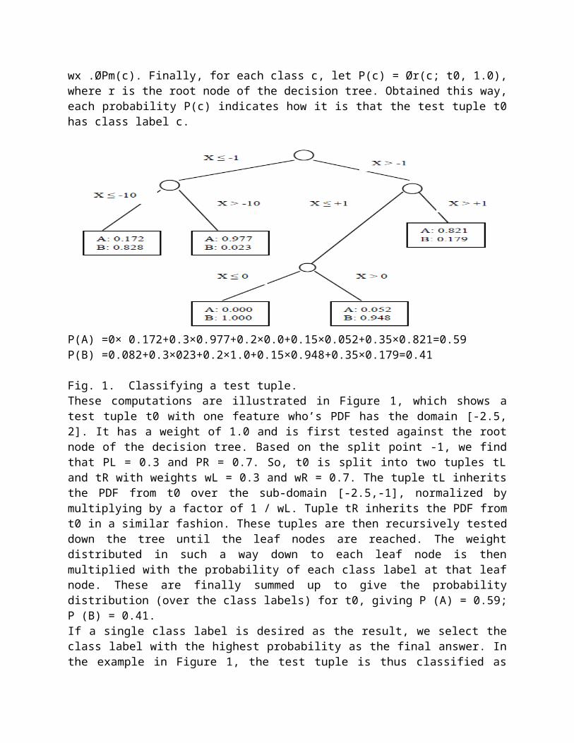
wx .ØPm(c). Finally, for each class c, let P(c) = Ør(c; t0, 1.0),where r is the root node of the decision tree. Obtained this way,each probability P(c) indicates how it is that the test tuple t0has class label c.

P(A) =0× 0.172+0.3×0.977+0.2×0.0+0.15×0.052+0.35×0.821=0.59 P(B) =0.082+0.3×023+0.2×1.0+0.15×0.948+0.35×0.179=0.41

Fig. 1. Classifying a test tuple.These computations are illustrated in Figure 1, which shows atest tuple t0 with one feature who’s PDF has the domain [-2.5,2]. It has a weight of 1.0 and is first tested against the rootnode of the decision tree. Based on the split point -1, we findthat PL = 0.3 and PR = 0.7. So, t0 is split into two tuples tLand tR with weights wL = 0.3 and wR = 0.7. The tuple tL inheritsthe PDF from t0 over the sub-domain [-2.5,-1], normalized bymultiplying by a factor of 1 / wL. Tuple tR inherits the PDF fromt0 in a similar fashion. These tuples are then recursively testeddown the tree until the leaf nodes are reached. The weightdistributed in such a way down to each leaf node is thenmultiplied with the probability of each class label at that leafnode. These are finally summed up to give the probabilitydistribution (over the class labels) for t0, giving P (A) = 0.59;P (B) = 0.41. If a single class label is desired as the result, we select theclass label with the highest probability as the final answer. Inthe example in Figure 1, the test tuple is thus classified as

class ―”A” when a single result is desired. The most challengingtask is to construct a decision tree based on tuples withuncertain values. It involves finding a good testing attributeAjn and a good split point Zn for each internal node n, as wellas an appropriate probability distribution Pm over C for eachleaf node m. We describe algorithms for constructing such treesin the next section.

III ALGORITHEMS

In this section, we discuss two approaches for handling uncertaindata. The first approach, called ―”Averaging”, transforms anuncertain dataset to a point-valued one by replacing each PDFwith its mean value. More specifically, for each tuple ti andattribute Aj, we take the mean value1 υi, j = x fi, j(x) dx as∫its representative value. The feature vector of ti is thustransformed to (υi,1… υi,k). A decision tree can then be built byapplying a traditional tree construction algorithm.

Fig. 2. Decision Tree

To exploit the full information carried by the pdf’s, our second approach, called ―”Distribution-based”, considers all the sample

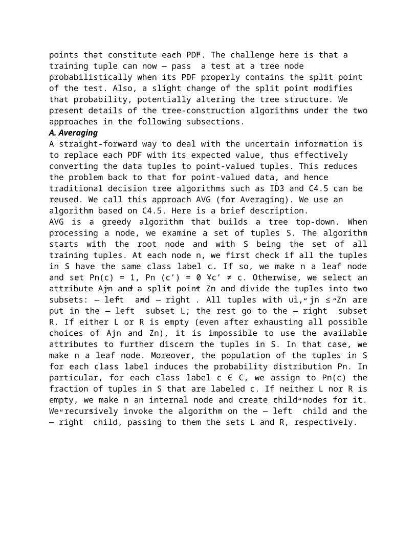
points that constitute each PDF. The challenge here is that a training tuple can now ―”pass” a test at a tree node probabilistically when its PDF properly contains the split point of the test. Also, a slight change of the split point modifies that probability, potentially altering the tree structure. We present details of the tree-construction algorithms under the twoapproaches in the following subsections. A. Averaging A straight-forward way to deal with the uncertain information is to replace each PDF with its expected value, thus effectively converting the data tuples to point-valued tuples. This reduces the problem back to that for point-valued data, and hence traditional decision tree algorithms such as ID3 and C4.5 can be reused. We call this approach AVG (for Averaging). We use an algorithm based on C4.5. Here is a brief description. AVG is a greedy algorithm that builds a tree top-down. Whenprocessing a node, we examine a set of tuples S. The algorithmstarts with the root node and with S being the set of alltraining tuples. At each node n, we first check if all the tuplesin S have the same class label c. If so, we make n a leaf nodeand set Pn(c) = 1, Pn (c’) = 0 Ұc’ ≠ c. Otherwise, we select anattribute Ajn and a split point Zn and divide the tuples into twosubsets: ―”left” and ―”right”. All tuples with υi, jn ≤ Zn areput in the ―”left” subset L; the rest go to the ―”right” subsetR. If either L or R is empty (even after exhausting all possiblechoices of Ajn and Zn), it is impossible to use the availableattributes to further discern the tuples in S. In that case, wemake n a leaf node. Moreover, the population of the tuples in Sfor each class label induces the probability distribution Pn. Inparticular, for each class label c Є C, we assign to Pn(c) thefraction of tuples in S that are labeled c. If neither L nor R isempty, we make n an internal node and create child nodes for it.We recursively invoke the algorithm on the ―”left” child and the―”right” child, passing to them the sets L and R, respectively.

To build a good decision tree, the choice of Ajn and Zn iscrucial. At this point, we may assume that this selection isperformed by a black box algorithm Best Split, which takes a setof tuples as parameter, and returns the best choice of attributeand split point for those tuples. We will examine this black boxin details. Typically, Best Split is designed to select theattribute and split point that minimizes the degree ofdispersion. The degree of dispersion can be measured in manyways, such as entropy (from information theory) or Gini index.The choice of dispersion function affects the structure of theresulting decision tree. In this paper we assume that entropy isused as the measure since it is predominantly used for buildingdecision trees.

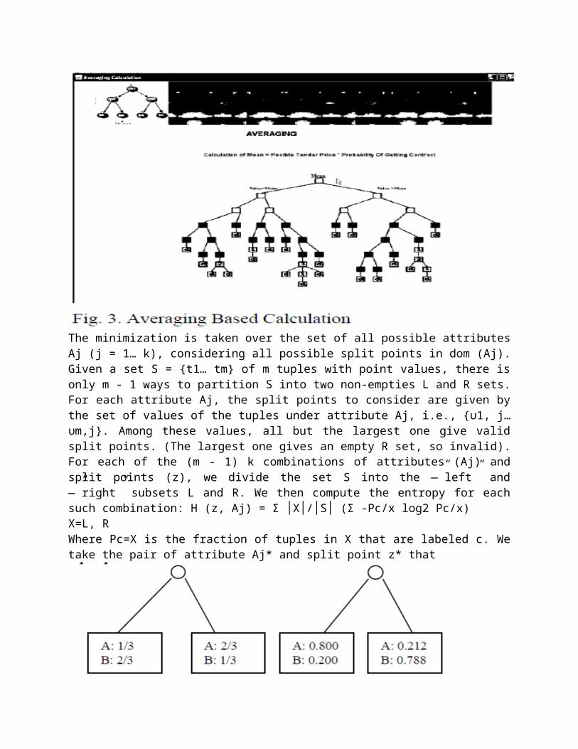
The minimization is taken over the set of all possible attributesAj (j = 1… k), considering all possible split points in dom (Aj).Given a set S = {t1… tm} of m tuples with point values, there isonly m - 1 ways to partition S into two non-empties L and R sets.For each attribute Aj, the split points to consider are given bythe set of values of the tuples under attribute Aj, i.e., {υ1, j…υm,j}. Among these values, all but the largest one give validsplit points. (The largest one gives an empty R set, so invalid).For each of the (m - 1) k combinations of attributes (Aj) andsplit points (z), we divide the set S into the ―”left” and―”right” subsets L and R. We then compute the entropy for eachsuch combination: H (z, Aj) = Σ │X│/│S│ (Σ -Pc/x log2 Pc/x) X=L, R Where Pc=X is the fraction of tuples in X that are labeled c. Wetake the pair of attribute Aj* and split point z* that

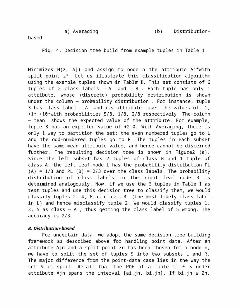
a) Averaging (b) Distribution-based

Fig. 4. Decision tree build from example tuples in Table 1.

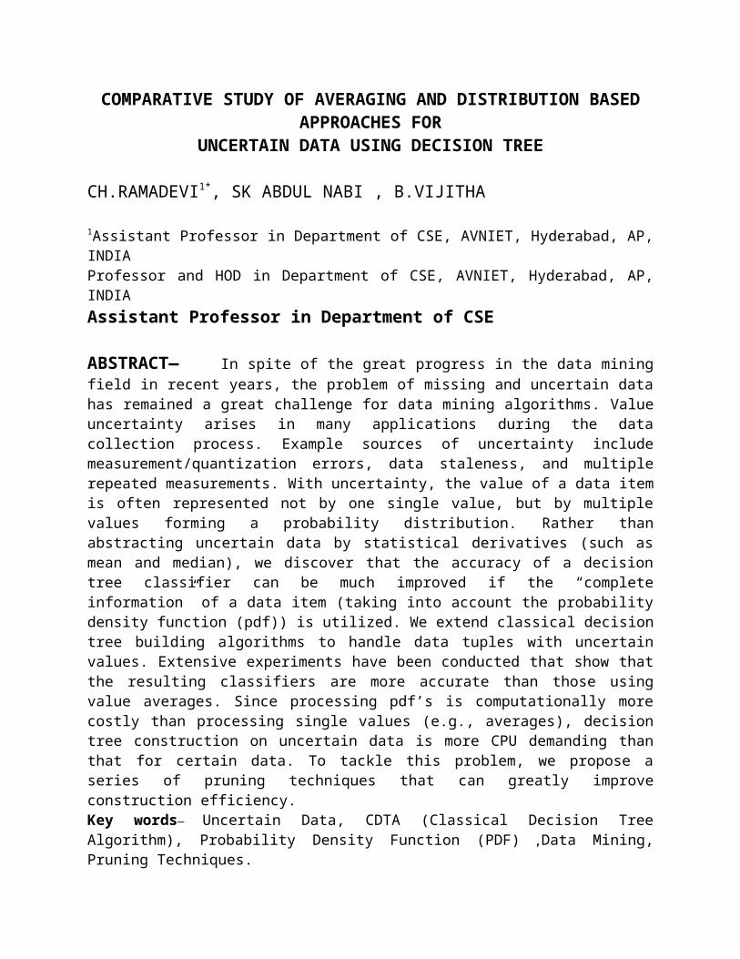
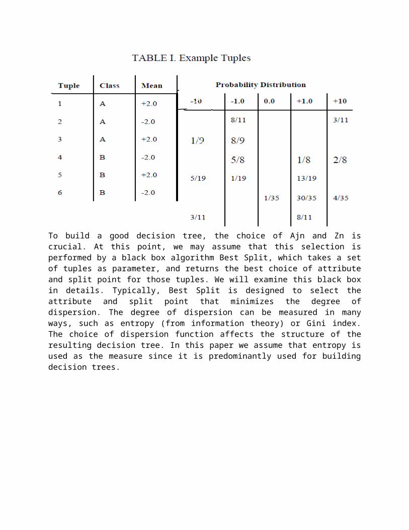
Minimizes H(z, Aj) and assign to node n the attribute Aj*withsplit point z*. Let us illustrate this classification algorithmusing the example tuples shown in Table I. This set consists of 6tuples of 2 class labels ―”A” and ―”B”. Each tuple has only 1attribute, whose (discrete) probability distribution is shownunder the column ―”probability distribution”. For instance, tuple3 has class label ―”A” and its attribute takes the values of -1,+1, +10 with probabilities 5/8, 1/8, 2/8 respectively. The column―”mean” shows the expected value of the attribute. For example,tuple 3 has an expected value of +2.0. With Averaging, there isonly 1 way to partition the set: the even numbered tuples go to Land the odd-numbered tuples go to R. The tuples in each subsethave the same mean attribute value, and hence cannot be discernedfurther. The resulting decision tree is shown in Figure2 (a).Since the left subset has 2 tuples of class B and 1 tuple ofclass A, the left leaf node L has the probability distribution PL(A) = 1/3 and PL (B) = 2/3 over the class labels. The probabilitydistribution of class labels in the right leaf node R isdetermined analogously. Now, if we use the 6 tuples in Table I astest tuples and use this decision tree to classify them, we wouldclassify tuples 2, 4, 6 as class ―B” (the most likely class labelin L) and hence misclassify tuple 2. We would classify tuples 1,3, 5 as class ―”A”, thus getting the class label of 5 wrong. Theaccuracy is 2/3.

B. Distribution-based For uncertain data, we adopt the same decision tree building

framework as described above for handling point data. After anattribute Ajn and a split point Zn has been chosen for a node n,we have to split the set of tuples S into two subsets L and R.The major difference from the point-data case lies in the way theset S is split. Recall that the PDF of a tuple ti Є S underattribute Ajn spans the interval [ai,jn, bi,jn]. If bi,jn ≤ Zn,

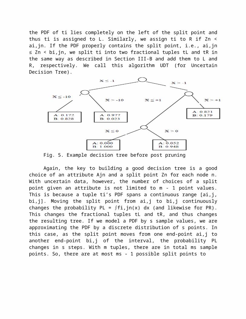
the PDF of ti lies completely on the left of the split point andthus ti is assigned to L. Similarly, we assign ti to R if Zn <ai,jn. If the PDF properly contains the split point, i.e., ai,jn≤ Zn < bi,jn, we split ti into two fractional tuples tL and tR inthe same way as described in Section III-B and add them to L andR, respectively. We call this algorithm UDT (for UncertainDecision Tree).

Fig. 5. Example decision tree before post pruning

Again, the key to building a good decision tree is a goodchoice of an attribute Ajn and a split point Zn for each node n.With uncertain data, however, the number of choices of a splitpoint given an attribute is not limited to m - 1 point values.This is because a tuple ti’s PDF spans a continuous range [ai,j,bi,j]. Moving the split point from ai,j to bi,j continuouslychanges the probability PL = fi,jn(x) dx (and likewise for PR).∫This changes the fractional tuples tL and tR, and thus changesthe resulting tree. If we model a PDF by s sample values, we areapproximating the PDF by a discrete distribution of s points. Inthis case, as the split point moves from one end-point ai,j toanother end-point bi,j of the interval, the probability PLchanges in s steps. With m tuples, there are in total ms samplepoints. So, there are at most ms - 1 possible split points to

Fig.6 Distribution Based Calculation

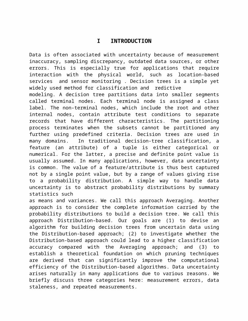
Considering all k attributes, to determine the best (attribute,split-point) pair thus require us to examine k (ms - 1)combinations of attributes and split points. Comparing to AVG,UDT is s time more expensive. Note that splitting a tuple intotwo fractional tuples involves a calculation of the probabilityPL, which requires integration. We remark that by storing the PDFin the form of a cumulative distribution, the integration can bedone by simply subtracting two cumulative probabilities. Let us re-examine the example tuples in Table I to see how thedistribution-based algorithm can improve classification accuracy.By taking into account the probability distribution, UDT buildsthe tree shown in Figure 3 before pre-pruning and post-pruningare applied. This tree is much more elaborate than the tree shownin Figure 2(a), because we are using more information and hencethere are more choices of split points. The tree in Figure 3turns out to have 100% classification accuracy! After post-pruning, we get the tree in Figure 2(b). Now, let us use the 6tuples in Table I as testing tuples to test the tree in Figure2(b). For instance, the classification result of tuple 3 givesP(A) = 5/8× 0.80 + 3/8× 0.212 = 0.5795 and P(B) = 5/8 × 0.20 +3/8 × 0.788 = 0.4205.

Since the probability for ―”A” is higher, we conclude that tuple3 belongs to class ―”A”. All the other tuples are handledsimilarly, using the label of the highest probability as thefinal classification result. It turns out that all 6 tuples areclassified correctly. This hand-crafted example thus illustratesthat by considering probability distributions rather than justexpected values, we can potentially build a more accuratedecision tree.

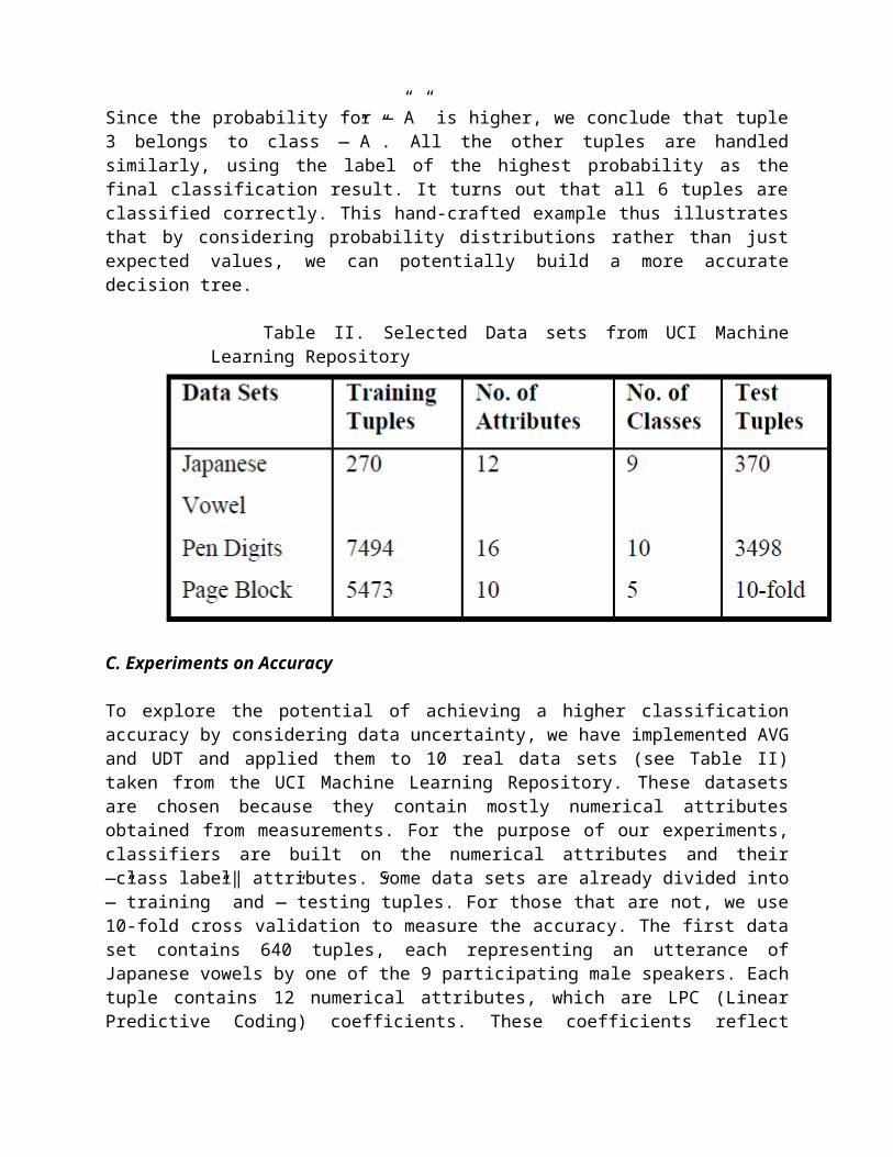
Table II. Selected Data sets from UCI MachineLearning Repository

C. Experiments on Accuracy

To explore the potential of achieving a higher classificationaccuracy by considering data uncertainty, we have implemented AVGand UDT and applied them to 10 real data sets (see Table II)taken from the UCI Machine Learning Repository. These datasetsare chosen because they contain mostly numerical attributesobtained from measurements. For the purpose of our experiments,classifiers are built on the numerical attributes and their―class label‖ attributes. Some data sets are already divided into―”training” and ―”testing”tuples. For those that are not, we use10-fold cross validation to measure the accuracy. The first dataset contains 640 tuples, each representing an utterance ofJapanese vowels by one of the 9 participating male speakers. Eachtuple contains 12 numerical attributes, which are LPC (LinearPredictive Coding) coefficients. These coefficients reflect

important features of speech sound. Each attribute value consistsof 7 – 29 samples of LPC coefficients collected over time. Thesesamples represent uncertain information, and are used to modelthe PDF of the attribute for the tuple. The class label of eachtuple is the speaker id. The classification task is to identifythe speaker when given a test tuple.

The other 9 data sets contain ―”point values” withoutuncertainty. To control the uncertainty for sensitivity studies,we augment these data sets with uncertainty information generatedas follows. We model uncertainty information by fittingappropriate error models on to the point data. For each tuple tiand for each attribute Aj , the point value υi,j reported in adataset is used as the mean of a PDF fi,j , defined over aninterval [ai,j , bi,j ]. The range of values for Aj (over thewhole data set) is noted and the width of [ai,j, bi,j ] is set tow . │Aj│, where │Aj │ denotes the width of the range for Aj and wis a controlled parameter. To generate the PDF fi,j , we considertwo options. The first is uniform distribution, which impliesfi,j(x) = (bi,j - ai,j). The other option is Gaussiandistributions, for which we use 4 (bi,j – ai,j) as the standarddeviation. In both cases, the PDF is generated using s samplepoints in the interval. Using this method (with controllableparameters w and s, and a choice of Gaussian vs. uniformdistribution), we transform a data set with point values into onewith uncertainty. The reason that we choose Gaussian distributionand uniform distribution is that most physical measures involverandom noise whichfollows Gaussian distribution, and that digitization of themeasured values introduces quantization noise that is bestdescribed by a uniform distribution. Of course, most digitizedmeasurements suffer from a combination of both kinds ofuncertainties. For the purpose of illustration, we have onlyconsidered the two extremes of a wide spectrum of possibilities.The results of applying AVG and UDT to the 10 datasets are shownin Table III. As we have explained, under our uncertainty model,classification results are probabilistic. Following, we take theclass label of the highest probability as the final class label.We have also run an experiment using C4.5 with the informationgain criterion. The resulting accuracies are very similar to

those of AVG and are hence omitted. In the experiments, each PDFis represented by 100 sample points (i.e., s = 100), except forthe ―Japanese Vowel” data set. We have repeated the experimentsusing various values for w. For most of the datasets, Gaussiandistribution is assumed as the error model. Since the data sets―”Pen Digits”, ―”Vehicle” and ―”Satellite” have integer domains,we suspected that they are highly influenced by quantizationnoise. So, we have also tried uniform distribution on these threedatasets, in addition to Gaussian.6 For the ―Japanese Vowel” dataset, we use the uncertainty given by the raw data (7 – 29samples) to model the PDF. From the table, we see that UDT buildsmore accurate decision trees than AVG does for differentdistributions over a wide range of w. For the first data set,whose PDF is modeled from the raw data samples, the accuracy isimproved from 81.89% to 87.30%; i.e., the error rate is reducedfrom 18.11% down to 12.70%, which is a very substantialimprovement. Only in a few cases (marked with ―”#” in the table)does UDT give slightly worse accuracies than AVG. To better showthe best potential improvement, we have identified the best cases(marked with ―_”) and repeated them in the third column of thetable. Comparing the second and third columns of Table III, wesee that UDT can potentially build remarkably more accuratedecision trees than AVG. For example, for the ―Iris” data set,the accuracy improves from 94.73% to 96.13%. (Thus, the errorrate is reduced from 5.27% down to 3.87%). Using Gaussiandistribution gives better accuracies in 8 out of the 9 datasetswhere we have modeled the error distributions as described above.This suggests that the effects of random noise dominatequantization noise. The exception is ―”Pen Digits”. As we havepointed out, this dataset contains integral attributes, which islikely subject to quantization noise. By considering a uniformdistribution as the error model, such noise is taken intoconsideration, resulting in high classification accuracy. We have repeated the experiments and varied s, the number ofsample points per PDF, from 50 to 200. There is no significantchange in the accuracies as s varies. This is because we arekeeping the PDF generation method unchanged. Increasing simproves our approximation to the distribution, but does notactually change the distribution. This result, however, does not

mean that it is unimportant to collect measurement values. Inreal applications, collecting more measurement values allow us tohave more information to model the pdf’s more accurately. Thiscan help improve the quality of the PDF models. As shown above,modeling the probability distribution is very important whenapplying the distribution-based approach. So, it is stillimportant to collect information on uncertainty.

D. Effect of Noise Model

How does the modeling of the noise affect the accuracy? In theprevious section, we have seen that by modeling the error, we canbuild decision trees which are more accurate. It is natural tohypothesis that the closer we can model the error, the better theaccuracy will be. We have designed the following experiment toverify this claim. In the experiment above, we have taken datafrom the UCI repository and directly added uncertainty to it soas to test our UDT algorithm. The amount of errors in the data isuncontrolled. So, in the next experiment, we inject someartificial noise into the data in a controlled way. For eachdataset (except ―”Japanese Vowel”), we first take the data fromthe repository. For each tuple ti and for each attribute Aj , thepoint value υi,j is perturbed by adding a Gaussian noise withzero mean and a standard deviation equal to σ = 1 /4 (u .│Aj │),where u is a controllable parameter. So, the perturbed value isυi,j = υi,j + δi,j , where δi,j is a random number which followsN(0,. Finally, on top of this perturbed data, we add uncertaintyas described in the last subsection (with parameters w and s).Then, we run AVG and UDT to obtain the accuracy, for variousvalues u and w (keeping s = 100). If the data from the UCI repository were ideal and 100% error-free, then we should expect to get the highest accuracy wheneveru = w. This is because when u = w, the uncertainty that we usewould perfectly model the perturbation that we have introduced.So, if our hypothesis is correct, UDT would build decision treeswith the higher accuracy. Nevertheless, we cannot assume that thedatasets are error-free. It is likely that some sort ofmeasurement error is incurred in the collection process of thesedatasets. For simplicity of analysis, let us assume that the

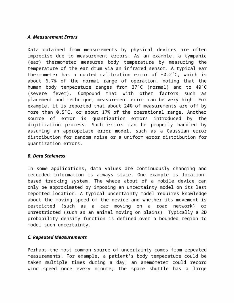
errors are random errors Єi,j following a Gaussian distributionwith zero mean and some unknown variance σ2. So, if ūi,j is thetrue, noise-free (but unknown to us) value for attribute Aj intuple ti, then υi,j = ūi,j + Єi,j . Hence, in the perturbeddataset, we have ūi,j = ūi,j + Єi,j + δi,j . Note that the totalamount of noise in this value is Єi,j +δi,j , which is the sum oftwo Gaussian-distributed random variables. So, the sum itselfalso follows the Gaussian distribution N(0, σ2) where σ2 = σ2 +σ2. If our hypothesis is correct, then UDT should give the bestaccuracy when w matches this σ, i.e., when (w.│Aj│ /4)2 = σ2 + σ2= σ2 + (u.│Aj │ / 4)2, i.e. w2 = (k.σ) 2 + u2 (2) We have carried out this experiment and the results for thedataset ―Segment” is plotted in Figure 4. Each curve (except theone labeled ―model”, explained below) in the diagram correspondsto one value of u, which controls the amount of perturbation thathas been artificially added to the UCI dataset. The x-axiscorresponds to different values of w—the error model that we useas the uncertainty information. The y-axis gives the accuracy ofthe decision tree built by UDT. Note that for points with w = 0,the decision trees are built by AVG. To interpret this figure,let us first examine each curve (i.e., when u is fixed). It isobvious from each curve that UDT i.e., when u is fixed). It isobvious from each curve that UDT gives significantly higheraccuracies than AVG. Furthermore, as w increases from 0, theaccuracy rises quickly to up a plateau, where it remains high(despite minor fluctuations). This is because as w approaches thevalue given by (2), the uncertainty information models the errorbetter and better, yielding more and more accurate decisiontrees. When w continues to increase, the curves eventually dropgradually, showing that as the uncertainty model deviates fromthe error, the accuracy drops. From these observations, we canconclude that UDT can build significantly more accurate decisiontrees than AVG. Moreover, such high accuracy can be achieved overa wide range of w (along the plateau). So, there is a wide error-margin for estimating a good w to use. Next, let us compare the different curves, which correspond todifferent values of u—the artificially controlled perturbation.The trend observed is that as u increases, accuracy decreases.

This agrees with intuition: the greater the degree ofperturbation, the more severely is the data contaminated withnoise. So, the resulting decision trees become less and lessaccurate. Nevertheless, with the help of error models and UDT, weare still able to build decision trees of much higher accuraciesthan AVG. Last but not least, let us see if our hypothesis can be verified.Does a value of w close to that given by yield a high accuracy?To answer this question, we need to estimate the value of k.σ. Wedo this by examining the curve for u = 0. Intuitively, the pointwith the highest w should give a good estimation of k.σ. However,since the curve has a wide plateau, it is not easy to find asingle value of w to estimate the value. We adopt the followingapproach: Along this curve, we use the accuracy values measuredfrom the repeated trials in the experiment to estimate a 95%-confidence interval for each data point, and then find out theset of points whose confidence interval overlaps with that of thepoint of highest accuracy. This set of points then gives a rangeof values of w, within which the accuracy is high. We take themid-point of this range as the estimate for k.σ. Based on thisvalue and, we calculate a value of w for each u, and repeat theexperiments with each such pair of (u, w). The accuracy ismeasured and plotted in the same figure as the curve labeled―model”. From the figure, it can be seen that the points wherethe ―model” curve intersects the other curves lie within theplateau of them. This confirms our claim that when the uncertaininformation models the error closely, we can get high accuracies.

We have repeated this experiment with all the other datasetsshown in Table II (except ―Japanese Vowel”),and the observations are similar. Thus, we conclude that ourhypothesis is confirmed: The closer we can model the error, thebetter will be the accuracy of the decision trees build by UDT.

IV. CONCLUSIONSWe have extended the model of decision-tree classification

to accommodate data tuples having numerical attributes with

uncertainty described by arbitrary pdf’s. We have modifiedclassical decision tree building algorithms (based on theframework of C4.5) to build decision trees for classifying suchdata. We have found empirically that when suitable pdf’s areused, exploiting data uncertainty leads to decision trees withremarkably higher accuracies. We therefore advocate that data becollected and stored with the PDF information intact. Performanceis an issue, though, because of the increased amount ofinformation to be processed, as well as the more complicatedentropy computations involved. Therefore, we have devised aseries of pruning techniques to improve tree constructionefficiency. Our algorithms have been experimentally verified tobe highly effective. Their execution times are of an order ofmagnitude comparable to classical algorithms. Some of thesepruning techniques are generalizations of analogous techniquesfor handling point-valued data. Other techniques, namely pruningby bounding and end-point sampling are novel. Although our noveltechniques are primarily designed to handle uncertain data, theyare also useful for building decision trees using classicalalgorithms when there are tremendous amounts of data tuples.

V REFERENCES

1. Wolfson, O., Sistla, P., Chamberlain, S. and Yesha, Y. “Updating and Querying Databases that Track MobileUnits,” Distributed and Parallel Databases, 7(3), 1999.2. Cheng, R., Kalashnikov, D., and Prabhakar, S. “Evaluating Probabilistic Queries over Imprecise Data,” Proceedings of the ACM SIGMOD International Conference on Management of Data, June 2003.3. R. Agrawal, T. Imielinski, and A. N. Swami, “Database mining: A performance perspective,” IEEE Trans. Knowl. Data Eng., vol. 5,no. 6, pp. 914–925, 1993.4. L. Hawarah, A. Simonet, and M. Simonet, ―”A Probabilistic approach to classify incomplete objects Using decision trees,” inDEXA, ser. Lecture Notes In Computer Science, vol. 3180. Zaragoza, Spain: Springer, 30 Aug.-3 Sep. 2004, pp. 549–558.5. J. R. Quinlan, ―Learning logical definitions from Relations,”Machine Learning, vol. 5, pp. 239–266, 1990.

6. Y. Yuan and M. J. Shaw, ―Induction of fuzzy Decision trees,” Fuzzy Sets Syst., vol. 69, no. 2, pp. 125–139, 1995.7. M. Umanol, H. Okamoto, I. Hatono, H. Tamura, F. Kawachi, S. Umedzu, and J. Kinoshita, ―”Fuzzy Decision trees by fuzzy ID3 algorithm and its Application to diagnosis systems,” in Fuzzy Systems, 1994, vol. 3. IEEE World Congress on Computational Intelligence, 26-29 Jun. 1994, pp. 2113–2118. 8. C. Z. Janikow, ―”Fuzzy decision trees: issues and methods”, IEEE Transactions on Systems, Man, and Cybernetics, Part B, vol. 28, no. 1, pp. 1–14, 1998. 9. C. Olaru and L. Wehenkel, ―”A complete fuzzy Decision tree technique”, Fuzzy Sets and Systems, vol. 138, no. 2, pp. 221–254,2003. 10. T. Elomaa and J. Rousu, ―”General and efficient multisplitting of numerical attributes”, Machine Learning, vol. 36, no. 3, pp. 201–244, 1999. 11. U. M. Fayyad and K. B. Irani, ―”On the handling of Continuous-valued attributes in decision tree Generation”, Machine Learning, vol. 8, pp. 87–102, 1992. 12. T. Elomaa and J. Rousu, ―”Efficient multisplitting Revisited: Optima preserving elimination of Partition Candidates”, Data Mining and Knowledge Discovery, vol. 8, no. 2, pp. 97–126, 2004. 13. L. Breiman, J. H. Friedman, R. A. Olshen, and C. J. Stone, Classification and Regression Trees. Wadsworth, 1984. 14. T. Elomaa and J. Rousu, ―Necessary and sufficient pre-processing in numerical range discretization,‖ Knowledge and Information Systems, vol. 5, no. 2, pp. 162–182, 2003. 15. L. Breiman, ―Technical note: Some properties of Splitting criteria,‖ Machine Learning, vol. 24, no. 1, pp. 41–47, 1996. 16. T. M. Mitchell, Machine Learning. McGraw-Hill, 1997, ISBN 0070428077. 17. A. Asuncion and D. Newman, ―UCI machine Learning repository,‖ 2007. [Online]. Available: http://www.ics.uci.edu/_mlearn/MLRepository.html 18. R. E. Walpole and R. H. Myers, Probability and Statistics for Engineers and Scientists. Macmillan Publishing Company, 1993.

19. S. Tsang, B. Kao, K. Y. Yip, W.-S. Ho, and S. D. Lee, ―Decision trees for uncertain data,‖ in ICDE, Shanghai, China, 29Mar.–4 Apr. 2009, pp. 441– 138